The Temporal Spotlight of Attention - CiteSeerX

THE TEMPORAL SPOTLIGHT OF ATTENTION:COMPUTATIONAL AND ELECTROPHYSIOLOGICAL EXPLORATIONS

a thesis submitted to

The University of Kent at Canterbury

in the subject of computer science

for the degree

of doctor of philosophy

By

Srivas Chennu

December 2009

Contents

List of Tables ix

List of Figures x

Abstract xiii

Acknowledgements xiv

I Background 1

1 Introduction 2

1.1 Overview . . . . . . . . . . . . . . . . . . . . . . . . . . . . . . . . . . . . . . . . . 2

1.1.1 Temporal Attention . . . . . . . . . . . . . . . . . . . . . . . . . . . . . . 2

1.1.2 Human Electrophysiology . . . . . . . . . . . . . . . . . . . . . . . . . . 5

1.1.3 Cognitive Modelling . . . . . . . . . . . . . . . . . . . . . . . . . . . . . . 6

1.2 Central Hypotheses . . . . . . . . . . . . . . . . . . . . . . . . . . . . . . . . . . 7

1.3 Organisation . . . . . . . . . . . . . . . . . . . . . . . . . . . . . . . . . . . . . . . 9

1.4 Collaborations and Publications . . . . . . . . . . . . . . . . . . . . . . . . . . . 12

2 Prior Research 13

2.1 Temporal Attention and TAE . . . . . . . . . . . . . . . . . . . . . . . . . . . . 13

2.2 Rapid Serial Visual Presentation . . . . . . . . . . . . . . . . . . . . . . . . . . . 15

2.3 The Attentional Blink . . . . . . . . . . . . . . . . . . . . . . . . . . . . . . . . . 16

2.3.1 The Task . . . . . . . . . . . . . . . . . . . . . . . . . . . . . . . . . . . . 16

2.3.2 AB Phenomena . . . . . . . . . . . . . . . . . . . . . . . . . . . . . . . . 16

ii

2.4 The Electrophysiology of Attention and Consciousness . . . . . . . . . . . . . 19

2.4.1 Electroencephalography . . . . . . . . . . . . . . . . . . . . . . . . . . . 19

2.4.2 Event-related Potentials . . . . . . . . . . . . . . . . . . . . . . . . . . . 20

2.4.3 ERP Components . . . . . . . . . . . . . . . . . . . . . . . . . . . . . . . 20

2.4.4 ERPimages . . . . . . . . . . . . . . . . . . . . . . . . . . . . . . . . . . . 24

2.5 Feature Binding in Vision . . . . . . . . . . . . . . . . . . . . . . . . . . . . . . . 25

2.5.1 Feature Binding in the Temporal Dimension . . . . . . . . . . . . . . . 28

2.5.2 Modelling Temporal Feature Binding . . . . . . . . . . . . . . . . . . . 33

2.6 Conclusions . . . . . . . . . . . . . . . . . . . . . . . . . . . . . . . . . . . . . . . 40

3 Models of the Temporal Spotlight 41

3.1 The ST2 Model . . . . . . . . . . . . . . . . . . . . . . . . . . . . . . . . . . . . . 41

3.1.1 Types and Tokens . . . . . . . . . . . . . . . . . . . . . . . . . . . . . . . 42

3.1.2 Stage 1 of Neural-ST2 . . . . . . . . . . . . . . . . . . . . . . . . . . . . . 43

3.1.3 Stage 2 of Neural-ST2 . . . . . . . . . . . . . . . . . . . . . . . . . . . . . 44

3.1.4 Transient Attentional Enhancement: the Blaster . . . . . . . . . . . . . 44

3.1.5 How the Model Blinks - Suppression of TAE . . . . . . . . . . . . . . . 45

3.2 The LC-NE Model . . . . . . . . . . . . . . . . . . . . . . . . . . . . . . . . . . . 46

3.2.1 Behavioural Network . . . . . . . . . . . . . . . . . . . . . . . . . . . . . 46

3.2.2 The Locus Coeruleus . . . . . . . . . . . . . . . . . . . . . . . . . . . . . 47

3.2.3 How the Model Blinks - The LC Refractory Period . . . . . . . . . . . 48

3.3 Related Work . . . . . . . . . . . . . . . . . . . . . . . . . . . . . . . . . . . . . . 48

3.3.1 The Global Workspace Model . . . . . . . . . . . . . . . . . . . . . . . . 48

3.3.2 The CODAM Model . . . . . . . . . . . . . . . . . . . . . . . . . . . . . 49

3.3.3 The eSTST Model . . . . . . . . . . . . . . . . . . . . . . . . . . . . . . . 49

3.3.4 The Boost and Bounce Model . . . . . . . . . . . . . . . . . . . . . . . . 50

3.4 Conclusions . . . . . . . . . . . . . . . . . . . . . . . . . . . . . . . . . . . . . . . 50

4 Connecting Modelling and Electrophysiology 51

4.1 Introducing Virtual ERPs . . . . . . . . . . . . . . . . . . . . . . . . . . . . . . . 51

4.2 Generating Virtual ERPs . . . . . . . . . . . . . . . . . . . . . . . . . . . . . . . 53

4.2.1 Grand Average Virtual ERPs . . . . . . . . . . . . . . . . . . . . . . . . 56

iii

4.2.2 Virtual ERPimages . . . . . . . . . . . . . . . . . . . . . . . . . . . . . . 56

4.3 Virtual ERP Components . . . . . . . . . . . . . . . . . . . . . . . . . . . . . . . 57

4.3.1 Early Visual Processing - The Virtual ssVEP . . . . . . . . . . . . . . 57

4.3.2 Transient Attentional Enhancement - The Virtual N2pc . . . . . . . . 58

4.3.3 Working Memory Encoding - The Virtual P3 . . . . . . . . . . . . . . . 59

4.4 Conclusions . . . . . . . . . . . . . . . . . . . . . . . . . . . . . . . . . . . . . . . 59

II Explorations of the Temporal Spotlight 60

5 Comparing the ST2 and the LC-NE models 61

5.1 Introduction . . . . . . . . . . . . . . . . . . . . . . . . . . . . . . . . . . . . . . . 61

5.2 TAE in the ST2 Model: The Blaster . . . . . . . . . . . . . . . . . . . . . . . . 63

5.2.1 Internal Structure . . . . . . . . . . . . . . . . . . . . . . . . . . . . . . . 64

5.3 TAE in the LC-NE Model: The Locus Coeruleus . . . . . . . . . . . . . . . . . 65

5.3.1 The Locus Coeruleus & Norepinephrine . . . . . . . . . . . . . . . . . . 66

5.4 Assessment of Models . . . . . . . . . . . . . . . . . . . . . . . . . . . . . . . . . 68

5.4.1 The ST2 Model . . . . . . . . . . . . . . . . . . . . . . . . . . . . . . . . 69

5.4.2 The LC-NE Model . . . . . . . . . . . . . . . . . . . . . . . . . . . . . . 73

5.4.3 Discussion . . . . . . . . . . . . . . . . . . . . . . . . . . . . . . . . . . . . 77

5.5 Extension of the LC-NE Model . . . . . . . . . . . . . . . . . . . . . . . . . . . 80

5.5.1 Performance of the Extended LC-NE Model . . . . . . . . . . . . . . . 81

5.6 Final Discussion . . . . . . . . . . . . . . . . . . . . . . . . . . . . . . . . . . . . 82

5.6.1 The Blaster and the LC . . . . . . . . . . . . . . . . . . . . . . . . . . . 83

5.6.2 Correlates of the P3 . . . . . . . . . . . . . . . . . . . . . . . . . . . . . . 84

5.7 Conclusions . . . . . . . . . . . . . . . . . . . . . . . . . . . . . . . . . . . . . . . 85

6 Target Discriminability and Temporal Perception 86

6.1 Introduction . . . . . . . . . . . . . . . . . . . . . . . . . . . . . . . . . . . . . . . 86

6.1.1 Motivation and Overview . . . . . . . . . . . . . . . . . . . . . . . . . . 89

6.2 The Single Target Experiment . . . . . . . . . . . . . . . . . . . . . . . . . . . . 89

6.3 Target Processing in Onset Presentation . . . . . . . . . . . . . . . . . . . . . . 90

iv

6.3.1 Behaviour . . . . . . . . . . . . . . . . . . . . . . . . . . . . . . . . . . . . 90

6.3.2 Early Components . . . . . . . . . . . . . . . . . . . . . . . . . . . . . . . 90

6.3.3 The P3 . . . . . . . . . . . . . . . . . . . . . . . . . . . . . . . . . . . . . 91

6.4 Modelling Onset Presentation with the ST2 Model . . . . . . . . . . . . . . . . 92

6.4.1 Step 1: Simulating Early Components . . . . . . . . . . . . . . . . . . . 92

6.4.2 Step 2: Simulating the P3 . . . . . . . . . . . . . . . . . . . . . . . . . . 94

6.4.3 Step 3: Simulating Behavioural Accuracy . . . . . . . . . . . . . . . . . 97

6.5 Discussion . . . . . . . . . . . . . . . . . . . . . . . . . . . . . . . . . . . . . . . . 99

6.5.1 Early Components vs. the ssVEP . . . . . . . . . . . . . . . . . . . . . 99

6.5.2 Lag 1 Sparing and Onset Presentation . . . . . . . . . . . . . . . . . . . 100

6.5.3 Is Onset Presentation an Equal Substitute for RSVP? . . . . . . . . . 101

6.6 Conclusions . . . . . . . . . . . . . . . . . . . . . . . . . . . . . . . . . . . . . . . 102

7 The Temporal Precision of Attention 103

7.1 Introduction . . . . . . . . . . . . . . . . . . . . . . . . . . . . . . . . . . . . . . . 103

7.1.1 Attentional Precision and the ST2 Model . . . . . . . . . . . . . . . . . 104

7.2 The Two Target Experiment . . . . . . . . . . . . . . . . . . . . . . . . . . . . . 105

7.3 Behavioural Analysis . . . . . . . . . . . . . . . . . . . . . . . . . . . . . . . . . . 105

7.4 ERP Analysis . . . . . . . . . . . . . . . . . . . . . . . . . . . . . . . . . . . . . . 106

7.5 Single-Trial Analysis . . . . . . . . . . . . . . . . . . . . . . . . . . . . . . . . . . 110

7.5.1 Analysis of ITC and ERSP . . . . . . . . . . . . . . . . . . . . . . . . . 110

7.5.2 Analysis of ERPimages . . . . . . . . . . . . . . . . . . . . . . . . . . . . 116

7.5.3 Analysis of Phases . . . . . . . . . . . . . . . . . . . . . . . . . . . . . . . 119

7.6 Explaining Temporal Precision using the ST2 Model . . . . . . . . . . . . . . . 125

7.6.1 Simulated Behavioural Accuracy . . . . . . . . . . . . . . . . . . . . . . 125

7.7 Virtual ERPs . . . . . . . . . . . . . . . . . . . . . . . . . . . . . . . . . . . . . . 125

7.7.1 Virtual ERPimages . . . . . . . . . . . . . . . . . . . . . . . . . . . . . . 128

7.8 Discussion . . . . . . . . . . . . . . . . . . . . . . . . . . . . . . . . . . . . . . . . 134

7.9 Related Work . . . . . . . . . . . . . . . . . . . . . . . . . . . . . . . . . . . . . . 136

7.9.1 Chun (1997), Popple and Levi (2007) . . . . . . . . . . . . . . . . . . . 136

7.9.2 Vul, Nieuwenstein and Kanwisher (2008) . . . . . . . . . . . . . . . . . 137

v

7.9.3 Sergent, Baillet and Dehaene (2005) . . . . . . . . . . . . . . . . . . . . 139

7.10 Conclusions . . . . . . . . . . . . . . . . . . . . . . . . . . . . . . . . . . . . . . . 139

8 Attention and Temporal Feature Binding 141

8.1 Introduction . . . . . . . . . . . . . . . . . . . . . . . . . . . . . . . . . . . . . . . 141

8.2 The Two-Feature Extension to ST2: The 2f-ST2 Model . . . . . . . . . . . . . 142

8.2.1 Rationale . . . . . . . . . . . . . . . . . . . . . . . . . . . . . . . . . . . . 142

8.2.2 Architecture . . . . . . . . . . . . . . . . . . . . . . . . . . . . . . . . . . 144

8.2.3 Dynamics . . . . . . . . . . . . . . . . . . . . . . . . . . . . . . . . . . . . 150

8.2.4 Configuration . . . . . . . . . . . . . . . . . . . . . . . . . . . . . . . . . . 152

8.3 Behavioural Predictions of the 2f-ST2 Model . . . . . . . . . . . . . . . . . . . 154

8.3.1 Manipulation of the Key Feature Pathway . . . . . . . . . . . . . . . . 155

8.3.2 Manipulation of the Response Feature Pathway . . . . . . . . . . . . . 159

8.3.3 Summary . . . . . . . . . . . . . . . . . . . . . . . . . . . . . . . . . . . . 162

8.4 Reaction Times for Response Positions . . . . . . . . . . . . . . . . . . . . . . . 162

8.5 The Temporal Binding Experiment . . . . . . . . . . . . . . . . . . . . . . . . . 167

8.6 Conclusions . . . . . . . . . . . . . . . . . . . . . . . . . . . . . . . . . . . . . . . 170

9 Neural Dynamics of Temporal Feature Binding 172

9.1 Virtual ERPs from 2f-ST2 . . . . . . . . . . . . . . . . . . . . . . . . . . . . . . 172

9.2 Determinants of the P3 . . . . . . . . . . . . . . . . . . . . . . . . . . . . . . . . 174

9.3 ERP Predictions of the 2f-ST2 Model . . . . . . . . . . . . . . . . . . . . . . . . 177

9.3.1 Combined Key-locked and Response-locked Averages . . . . . . . . . . 177

9.3.2 Correct Reports, Pre-target Errors and Post-target Errors . . . . . . . 180



9.4 The Temporal Binding Experiment . . . . . . . . . . . . . . . . . . . . . . . . . 191

9.4.1 Combined Key-locked and Response-locked Averages . . . . . . . . . . 191

9.4.2 Correct Reports, Pre-target Errors and Post-target Errors . . . . . . . 193



9.4.5 Summary . . . . . . . . . . . . . . . . . . . . . . . . . . . . . . . . . . . . 203

vi

9.5 Conclusions . . . . . . . . . . . . . . . . . . . . . . . . . . . . . . . . . . . . . . . 204

III Discussion 206

10 Conclusions, Contributions and Outlook 207

10.1 Conclusions . . . . . . . . . . . . . . . . . . . . . . . . . . . . . . . . . . . . . . . 207

10.2 Contributions . . . . . . . . . . . . . . . . . . . . . . . . . . . . . . . . . . . . . . 211

10.3 Future Outlook . . . . . . . . . . . . . . . . . . . . . . . . . . . . . . . . . . . . . 213

10.3.1 Experimental Directions . . . . . . . . . . . . . . . . . . . . . . . . . . . 213

10.3.2 Theoretical Directions . . . . . . . . . . . . . . . . . . . . . . . . . . . . 216

IV Appendix 220

A Computational Methods 221

A.1 The ST2 Model . . . . . . . . . . . . . . . . . . . . . . . . . . . . . . . . . . . . . 221

A.1.1 On-Off Circuits . . . . . . . . . . . . . . . . . . . . . . . . . . . . . . . . 221

A.1.2 Gate-Trace Pair . . . . . . . . . . . . . . . . . . . . . . . . . . . . . . . . 222

A.1.3 Weights and Connectivity . . . . . . . . . . . . . . . . . . . . . . . . . . 224

A.1.4 Model Configuration . . . . . . . . . . . . . . . . . . . . . . . . . . . . . 224

A.2 The Re-implemented LC-NE Model . . . . . . . . . . . . . . . . . . . . . . . . . 225

A.2.1 Simulating Blanks in the LC-NE Model . . . . . . . . . . . . . . . . . . 225

A.3 The Extended LC-NE Model . . . . . . . . . . . . . . . . . . . . . . . . . . . . . 225

A.3.1 Extension Parameters . . . . . . . . . . . . . . . . . . . . . . . . . . . . . 226

A.4 The 2f-ST2 Model . . . . . . . . . . . . . . . . . . . . . . . . . . . . . . . . . . . 227

A.4.1 Architecture . . . . . . . . . . . . . . . . . . . . . . . . . . . . . . . . . . 227

A.4.2 Dynamics . . . . . . . . . . . . . . . . . . . . . . . . . . . . . . . . . . . . 230

A.4.3 General Configuration . . . . . . . . . . . . . . . . . . . . . . . . . . . . 230

A.4.4 Configuration for Behavioural Simulations in Section 8.3 . . . . . . . . 231

B Experimental Methods 233

B.1 Experiment 1 . . . . . . . . . . . . . . . . . . . . . . . . . . . . . . . . . . . . . . 233

B.1.1 Participants . . . . . . . . . . . . . . . . . . . . . . . . . . . . . . . . . . . 233

vii

B.1.2 Stimuli and Apparatus . . . . . . . . . . . . . . . . . . . . . . . . . . . . 233

B.1.3 Procedure . . . . . . . . . . . . . . . . . . . . . . . . . . . . . . . . . . . . 233

B.1.4 EEG Recording and Analysis . . . . . . . . . . . . . . . . . . . . . . . . 235

B.1.5 Computational Modelling . . . . . . . . . . . . . . . . . . . . . . . . . . 237

B.2 Experiment 2 . . . . . . . . . . . . . . . . . . . . . . . . . . . . . . . . . . . . . . 237

B.2.1 Participants . . . . . . . . . . . . . . . . . . . . . . . . . . . . . . . . . . . 237


B.2.3 Procedure . . . . . . . . . . . . . . . . . . . . . . . . . . . . . . . . . . . . 238



B.3 Experiment 3 . . . . . . . . . . . . . . . . . . . . . . . . . . . . . . . . . . . . . . 243

B.3.1 Participants . . . . . . . . . . . . . . . . . . . . . . . . . . . . . . . . . . . 243


B.3.3 Procedure . . . . . . . . . . . . . . . . . . . . . . . . . . . . . . . . . . . . 244



Bibliography 249

viii

List of Tables

1 Connection weights in the ST2 model that were modified in this thesis . . . . 224

2 Leak current values in Stage 1 of the response pathway of the 2f-ST2 model 228

3 Connection weights in Stage 1 of the response pathway of the 2f-ST2 model . 229

4 Connection weights in Stage 2 of the 2f-ST2 model . . . . . . . . . . . . . . . . 229

5 Conditions of interest analysed in Experiment 2 . . . . . . . . . . . . . . . . . 240

6 Conditions of interest analysed in Experiment 3 . . . . . . . . . . . . . . . . . 247

ix

List of Figures

1 RSVP stream similar to that used by Lawrence (1971) . . . . . . . . . . . . . 15

2 Human performance in the AB task, reported by Chun and Potter (1995) (Bow-

man & Wyble, 2007) . . . . . . . . . . . . . . . . . . . . . . . . . . . . . . . . . . 17

3 Generating ERPs from EEG . . . . . . . . . . . . . . . . . . . . . . . . . . . . . 21

4 Examples of ERP components (Woodman & Luck, 2003) . . . . . . . . . . . . 22

5 ERPs vs. ERPimages. . . . . . . . . . . . . . . . . . . . . . . . . . . . . . . . . . 24

6 Visual information processing in the brain . . . . . . . . . . . . . . . . . . . . . 26

7 The binding problem (Wolfe & Bennett, 1997) . . . . . . . . . . . . . . . . . . 27

8 Sample response distributions from temporal binding experiments reported

in Botella, Garcia, and Barriopedro (1992) . . . . . . . . . . . . . . . . . . . . 30

9 Influence of the AB on temporal feature binding (Chun, 1997a; Vul, Nieuwen-

stein, & Kanwisher, 2008) . . . . . . . . . . . . . . . . . . . . . . . . . . . . . . . 32

10 The Botella, Barriopedro, and Suero (2001) model . . . . . . . . . . . . . . . . 35

11 The Neural-ST2 model (Craston, Wyble, Chennu, & Bowman, 2009) . . . . . 42

12 The LC-NE model (Nieuwenhuis, Gilzenrat, Holmes, & Cohen, 2005) . . . . 47

13 The role of virtual ERPs in cognitive science research . . . . . . . . . . . . . . 53

14 Node-level activation dynamics in Neural-ST2 . . . . . . . . . . . . . . . . . . . 54

15 Virtual ERPs from the ST2 model . . . . . . . . . . . . . . . . . . . . . . . . . 57

16 The dynamics and circuitry of the blaster in Neural-ST2 (Bowman & Wyble,

2007) . . . . . . . . . . . . . . . . . . . . . . . . . . . . . . . . . . . . . . . . . . . 64

17 Dynamic behaviour of the LC-NE system . . . . . . . . . . . . . . . . . . . . . 66

18 ST2 model performance in the AB task (Bowman & Wyble, 2007) . . . . . . 69

x

19 T2 consolidation delay by lag for the ST2 model (Bowman, Wyble, Chennu,

& Craston, 2008) . . . . . . . . . . . . . . . . . . . . . . . . . . . . . . . . . . . . 72

20 Standard blink conditions generated from the re-implemented LC-NEmodel (Bow-

man et al., 2008) . . . . . . . . . . . . . . . . . . . . . . . . . . . . . . . . . . . . 74

21 T2 consolidation delay by lag for the LC-NE model (Bowman et al., 2008) . 76

22 The extended LC-NE model (Bowman et al., 2008) . . . . . . . . . . . . . . . 79

23 Standard blink conditions generated from the extended LC-NE model (Bow-

man et al., 2008) . . . . . . . . . . . . . . . . . . . . . . . . . . . . . . . . . . . . 81

24 Behavioural accuracy scores from AB studies using Onset presentation (Ward,

Duncan, & Shapiro, 1997; McLaughlin, Shore, & Klein, 2001; Visser, Bischof,

& Di Lollo, 2004; Rolke, Bausenhart, & Ulrich, 2007) . . . . . . . . . . . . . . 88

25 Fast fourier transforms (FFT) of the ERPs for the RSVP (left) and Onset

(right) conditions (Chennu, Craston, Wyble, & Bowman, 2009b) . . . . . . . 90

26 Human P3 for targets in RSVP and Onset presentation (Chennu et al., 2009b) 91

27 Step 1 of simulating Onset presentation . . . . . . . . . . . . . . . . . . . . . . 92

28 Virtual ssVEP wave for the RSVP and early components for the Onset con-

ditions (Chennu et al., 2009b) . . . . . . . . . . . . . . . . . . . . . . . . . . . . 93

29 Step 2 of simulating Onset presentation (Chennu et al., 2009b) . . . . . . . . 95

30 After Step 2: Virtual P3 for the RSVP and Onset conditions (Chennu et al.,

2009b) . . . . . . . . . . . . . . . . . . . . . . . . . . . . . . . . . . . . . . . . . . 96

31 Step 3 of simulating Onset presentation . . . . . . . . . . . . . . . . . . . . . . 97

32 After Step 3: Virtual P3 for the RSVP and Onset conditions . . . . . . . . . 98

33 Human ERPs for targets presented outside and inside the AB . . . . . . . . . 107

34 Human ERPs for targets seen outside and inside the AB . . . . . . . . . . . . 109

35 ITC evoked by targets inside and outside the AB . . . . . . . . . . . . . . . . . 112

36 ERSP evoked by targets inside and outside the AB . . . . . . . . . . . . . . . 115

37 Human N2pc ERPimages for targets seen outside and inside the AB . . . . . 117

38 Human P3 ERPimages for targets seen outside and inside the AB . . . . . . 118

39 Human P3 ERPimages for the T2 Lag 8 and T1 Lag 3 conditions . . . . . . . 123

40 Virtual ERPs for targets seen outside and inside the AB . . . . . . . . . . . . 126

xi

41 50% area latency-sorted virtual N2pc ERPimages for targets seen outside and

inside the AB . . . . . . . . . . . . . . . . . . . . . . . . . . . . . . . . . . . . . . 129

42 50% area latency-sorted virtual P3 ERPimages for targets outside and targets

inside the AB . . . . . . . . . . . . . . . . . . . . . . . . . . . . . . . . . . . . . . 130

43 The 2f-ST2 model . . . . . . . . . . . . . . . . . . . . . . . . . . . . . . . . . . . 145

44 Temporal feature binding in the 2f-ST2 model . . . . . . . . . . . . . . . . . . 150

45 Key feature manipulation in Botella et al. (2001) simulated by 2f-ST2 . . . . 157

46 Response feature manipulation in Botella et al. (2001) simulated by 2f-ST2 . 160

47 Reaction time data from Botella (1992) explained by the 2f-ST2 model . . . 163

48 Simulation of behavioural data from Experiment 3 by the 2f-ST2 model . . . 168

49 Virtual ERPs from the 2f-ST2 model . . . . . . . . . . . . . . . . . . . . . . . . 174

50 Virtual ERPs from the 2f-ST2 model combining across all response positions,

time-locked to the key feature and response feature in each trial . . . . . . . . 178

51 Key-locked and response-locked virtual ERPs from the 2f-ST2 model for cor-

rect reports, pre-target and post-target errors . . . . . . . . . . . . . . . . . . . 181

52 Early and late key feature conditions from the 2f-ST2 model . . . . . . . . . . 184

53 Early and late response feature conditions from the 2f-ST2 model . . . . . . . 187

54 Behaviour and ERPs from Experiment 3 . . . . . . . . . . . . . . . . . . . . . . 192

55 ERPs evoked by correct reports, pre-target errors and post-target errors . . . 194

56 Behaviour and ERPs for the letter and symbol conditions . . . . . . . . . . . 199

57 An on-off circuit . . . . . . . . . . . . . . . . . . . . . . . . . . . . . . . . . . . . 222

58 A gate-trace pair . . . . . . . . . . . . . . . . . . . . . . . . . . . . . . . . . . . . 223

59 Weight types and connectivity patterns in the ST2 model . . . . . . . . . . . . 223

60 The RSVP and Onset presentation paradigms . . . . . . . . . . . . . . . . . . 234

61 The two-target bilateral RSVP paradigm used in Experiment 2 (Craston et

al., 2009) . . . . . . . . . . . . . . . . . . . . . . . . . . . . . . . . . . . . . . . . . 238

62 The single-target coloured bilateral RSVP paradigm used in Experiment 3 . 244

xii

Abstract

The study of attention aims to understand how the visual system focuses its resources on

salient targets presented amongst competing distractors. In a continuously changing envi-

ronment, temporal attention must pick out targets presented in between spatially coincident

distractors that are offset in time. Cognitive theories have proposed that this task is medi-

ated by a temporal ‘spotlight’ of attention. This thesis combines evidence from behaviour

and electrophysiology (EEG) with theoretical insights from neural network modelling to

investigate the interplay between this spotlight and conscious perception.

The experiments described in this thesis investigate the electrophysiology of temporal

visual perception using the Rapid Serial Visual Presentation (RSVP) paradigm. Building

upon behavioural research, we use EEG to investigate the influence of target discriminability,

the Attentional Blink (AB) and feature integration on the temporal dynamics of visual per-

ception. These findings characterise the influence of pre-attentional processes on attentional

deployment, and the subsequent influence of this deployment on perception and behaviour.

In addition, they provide the basis for a complementary computational elucidation.

The theoretical component of this thesis is based on the ST2 neural network model.

The notion of Transient Attentional Enhancement (TAE) embodied therein is the computa-

tional equivalent of the temporal spotlight. Its function is evaluated within the ST2 model

and in relation to other modelling approaches. In addition, human ERP (Event-Related

Potential) data from the experiments are compared with the model’s equivalent activation

traces, termed Virtual ERPs. This combination of theory and experiment broadens our un-

derstanding of temporal visual perception, and in conjunction, highlights the role of neural

modelling in informing EEG research.

xiii

Acknowledgements

My first foray into the topic of human cognition, consciousness, and ‘all that’ began with

a reading of Phantoms in the Brain by Vilayanur S. Ramachandran. For handing me a

well-worn copy of that book, I have only my mother Devaki and brother Arjun to thank.

However, my nascent interest in the topic would not have gotten very far if not for

the enthusiasm displayed by Howard Bowman in taking me on as a student. He has been

a most supportive and meticulous adviser all through my PhD, guiding my research with

characteristically gentle persuasion. In same breath, I thank Brad Wyble for his convoluted

code and straight answers. Owing to Brad and the continuing comradeship of Patrick

Craston, I got my research off to a running start for which I will always be grateful. In

addition, I was lucky to receive advice and support from Dinkar Sharma, Rosie Cowell,

Dominique Chu and Alex Freitas at the University of Kent. Thanks are also due to Dinkar

and John Duncan from the MRC Cognition and Brain Sciences Unit at Cambridge for

agreeing to examine this thesis.

More heartfelt thanks go to Damian Dimmich, Poul Henriksen, Katherine Johnson,

Sabrina Panëels, Tara Puri, Edward Suvanaphen and Bryony Worthington, for being great

company during the highs and lows of my charmed life as a PhD student.

Lastly, I should be remiss not to thank the School of Computing at the University of

Kent for their support, in the form of a research scholarship and the concomitant peace of

mind with which to pursue my research to fruition.

xiv

Part I

Background

1

Chapter 1

Introduction

We introduce this thesis with an overview of the three overarching themes which form the

basis of the research described here, namely temporal attention, human electrophysiology

and cognitive modelling. Following that, we outline the general organisation of its contents

into parts and chapters. In the last section of this chapter, we highlight the strongly collab-

orative aspect of this thesis and list the publications that have resulted from the research

leading up to it.

1.1 Overview

1.1.1 Temporal Attention

Within the science of cognitive psychology, the study of attention is targeted at understand-

ing how the mind focuses its processing resources on information that is contextually salient

in its environment, while suppressing irrelevant distracting information (Driver, 2001). In

the context of the visual system, this filtering mechanism is essential to its information

processing hierarchy (Hochstein & Ahissar, 2002). It enables the system to select a com-

paratively small amount of task-relevant information from a large quantity of sensory data.

The nature of attention, especially within the research into visual awareness, is one of the

most studied and debated aspects of human cognition, both as a conduit to the conscious

mind (James, 1890; Broadbent, 1958; Kahneman, 1973; Pashler, 1996) and as a metaphor

2

for the underlying neural dynamics (Wurtz, Goldberg, & Robinson, 1980; Posner & Peter-

son, 1990; Luck, 1998).

Visual attention has been extensively investigated in the spatial domain, i.e., in which

stimuli are presented simultaneously but are spatially offset in the visual field. This is

a situation quite common in everyday circumstances. Consequently, the role of spatial

attention in selectively enhancing task-relevant stimuli in the visual field, especially in visual

search paradigms, has been explored in much breadth and depth (Broadbent, 1958; Deutsch

& Deutsch, 1963; Duncan, 1980, 1981; Treisman & Gelade, 1980; Desimone & Duncan, 1995;

Luck, Chelazzi, Hillyard, & Desimone, 1997; Treisman, 1998). In this context, attention has

been popularly thought of as a ‘spotlight’ that highlights a specific location of the visual

field for further processing, while suppressing irrelevant surrounding information (Sperling,

1960; Averbach & Coriell, 1961; Posner, Snyder, & Davidson, 1980; Winer & Cottrell, 1996).

Studies that have characterised this spatial spotlight have found that it can ‘illuminate’

regions of varying size (C. W. Eriksen & St James, 1986), has limits to the spatial resolution

within its central focus (Bouma, 1970; B. A. Eriksen & Eriksen, 1974; J. Miller, 1991; He,

Cavanagh, & Intriligator, 1996), and degrades in efficiency with increasing distance from

this centre (C. W. Eriksen & Yeh, 1985; Downing & Pinker, 1985).

Based on a large body of evidence, researchers have debated the extent to which the

spotlight metaphor is applicable for spatial attention (see Cave & Bichot, 1999). This is

because experiments have found that humans can divide their attention between multiple

tasks (Corbetta, Miezin, Dobmeyer, Shulman, & Petersen, 1991; Bichot & Schall, 1999;

though see Castiello & Umiltà, 1992; McCormick, Klein, & Johnston, 1998), and track the

movement of multiple objects in their visual field (Pylyshyn & Storm, 1988; Pylyshyn, 1989;

though see Yantis, 1992). In addition, it has been proposed that attention can operate at the

level of objects rather than location (Duncan, 1984; Kanwisher & Driver, 1992). Such object-

based selective attention is influenced by perceptual grouping of visual features (Driver &

Baylis, 1989; Behrmann, Zemel, & Mozer, 1998; Cave & Bichot, 1999), and is thought to

be achieved using internal mental representations referred to as ‘object files’ (Kahneman &

Treisman, 1984; Kahneman, Treisman, & Gibbs, 1992; Chun, 1997b; Kanwisher & Driver,

1992).

On the other hand, temporal attention, relating to how salient stimuli are selected in

3

time, when presented with competing stimuli occupying the same spatial location but offset

in time, is relatively less well understood. For the most part, this is because humans have

been found to be extremely good at quickly extracting meaning from rapidly changing

visual information (Sperling, Budiansky, Spivak, & Johnson, 1971; Lawrence, 1971; Potter,

1975; Reeves & Sperling, 1986; Weichselgartner & Sperling, 1987). As a result, the limits

of temporal attention do not become evident in most everyday circumstances. However,

with the progressively ubiquitous use of technology in our daily environment, the pace of

human life is continually increasing. We are being exposed to real-life situations in which the

temporal limits of our perceptual abilities are often reached. Common examples are scenarios

involving automobile drivers and pilots, who have to selectively respond and act according

to fleeting stimuli from numerous sources of information if they are to avoid potentially

disastrous consequences. As a result, now more than ever, it has become important to

understand and characterise the temporal capacity limits of human attention and vision.

Therefore, fundamental research in this direction would be very beneficial, and could have

significant implications for the design of the next generation of human-computer interface

technologies (Su, Bowman, Barnard, & Wyble, 2008; Bowman, Su, Wyble, & Barnard, 2009;

Makeig, 2009).

This thesis works towards addressing this gap in knowledge, and focuses on the empirical

and theoretical study of temporal attention and perception. In this context, the temporal

spotlight of attention, or more accurately, Transient Attentional Enhancement (TAE), de-

scribes the cognitive mechanism that provides a short-lived burst of enhancement to fleeting

visual targets. Thus, the temporal spotlight highlights a brief window of time at a partic-

ular spatial location. In this sense, it is effectively spatially and temporally specific1. The

temporal spotlight plays a crucial role in ensuring that briefly presented stimuli generate

enough neural activation to reach the level of conscious awareness. In this thesis, temporal

perception refers to the temporal dynamics of visual perception that result from the action

of this spotlight. In the following sections, we highlight the two main techniques that we will

use to investigate the mechanisms of temporal attention and perception: electrophysiology

(EEG) and cognitive modelling.

1In comparison, the spatial spotlight discussed previously highlights regions of space (or objects withinthem) for sustained periods of time.

4

1.1.2 Human Electrophysiology

Experimental psychology since the ‘cognitive revolution’ (Broadbent, 1958; Neisser, 1967)

has relied on behavioural metrics to characterise the unseen but indirectly observable pro-

cesses underlying human cognition. Though behavioural psychology has been very suc-

cessful in adding to our understanding of the mind, it is limited in its ability to directly

study cognitive processes. In many situations, like in the case of attention, the processes

being studied come into play at a very early stage after the visual onset of information, and

are far removed from the eventual behavioural outcome. More recently, the field of cogni-

tive neuroscience has attempted to bring the power of neuroimaging technologies to bear

upon this problem (Gazzaniga, Ivry, & Mangun, 2002). Techniques like fMRI (functional

Magnetic Resonance Imaging), EEG (Electroencephalography), MEG (Magnetoencephalog-

raphy) and PET (Positron Emission Tomography) are attempting to directly capture the

brain in action as it is processing information and executing behaviour. Using these tools,

cognitive neuroscientists aim to discover the neural substrates and mechanisms in the brain

that support the complex machinery of the mind.

For the purposes of studying temporal perception in humans, non-invasive, scalp-recorded

electrical activity (EEG) (and increasingly, MEG) is a particularly useful tool. This is mainly

because it is a moment-by-moment electrical signature of neural dynamics, which provides

researchers with markers of short-lived brain events occurring very soon after the visual on-

set of stimuli. In particular, within a controlled laboratory setting, changes in ongoing EEG

activity have been shown to be reproducibly time-locked to the occurrence of task-relevant

stimuli. Such event-related EEG dynamics are thought to reliably reflect temporal charac-

teristics of the pre-conscious neural processing of such stimuli (Hillyard & Picton, 1987; Luck

& Hillyard, 1990; Hillyard & Anllo-Vento, 1998; Luck, 1998). Hence, in conjunction with be-

havioural techniques, event-related EEG has become a part of a methodology that provides

the fine-grained resolution essential for empirical study of temporal attention (Luck, 2005;

Makeig, Debener, Onton, & Delorme, 2004; Makeig & Onton, 2009). In this thesis, we will

employ a combination of behavioural and EEG data to investigate temporal attention and

perception. The findings therefrom will be an important source of empirical information to

constrain and inform our theoretical explorations of the temporal spotlight of attention.

5

1.1.3 Cognitive Modelling

Theoretical descriptions have a long-standing tradition in cognitive psychology, and aim

to consolidate and explain the variety of observable human behaviour within broad-based

explanations focused on fundamental principles. Cognitive models can be thought of as com-

putationally explicit manifestations of theoretical hypotheses, and encapsulate our knowl-

edge of some aspect of behaviour. In addition to explaining known patterns of behaviour,

a cognitive model allows researchers to generate new predictions about as yet unknown

behaviour, and thus generate unambiguous and therefore falsifiable tests of the theory un-

derlying the model. The empirical verification of these predictions serves to validate some

theories and refute competing ones, thereby advancing our understanding and completing

the cycle of theory and experiment.

Cognitive models can be broadly classed into symbolic and sub-symbolic, based on the

level of explanation they adhere to. Symbolic, or computationalist models view the mind as

a information processing system in which mental states are symbolic representations that

are operated upon by mental processes (Turing, 1937; Newell & Simon, 1976; Fodor, 1975;

Pylyshyn, 1984). In this view, the functioning of cognition can be thought of as ‘symbol ma-

nipulation’, beginning with input symbols that are successively processed and transformed

into output symbols. Consequently, symbolic models focus on explanations of human cog-

nition at this level, describing it in terms of symbolic information processing. Sub-symbolic

models, on the other hand, view cognition as being embodied in multi-layered, flexible neu-

ral networks in the brain (Turing, 1948; Hebb, 1949; Rosenblatt, 1958). In recent times,

concomitant with the development of cognitive neuroscience, connectionist approaches to

sub-symbolic modelling have gained popularity as a means of bridging the ‘brain-mind bar-

rier’. They attempt to explain how symbolic mental concepts are implemented by the inter-

actions within and between brain networks (Marr, 1982). Connectionism aims to explain the

complexities of cognition and behaviour as emerging out of the parallel, distributed interac-

tions of a large number of relatively simple and uniform units of computation (Rumelhart,

McClelland, & the PDP Research Group, 1986; Chalmers, 1990; Elman, 1991). Connec-

tionist models are typically implemented as neural networks consisting of interconnected

artificial neurons, wired up in architectures inspired by our understanding of brain anatomy

6

and function. Effectively, by remaining faithful to the forms of computation known to be

possible in the brain, such cognitive neural networks attempt to understand how mental

processes are embodied in their neural substrate.

As part of the theoretical component of this thesis, we will focus on cognitive mod-

elling that draws upon these different approaches, to embody high-level cognitive constructs

in functional neural network descriptions. In doing so, we show that such modelling ap-

proaches can provide an important complement to empirical research in cognitive neuro-

science. Specifically, modern neuroimaging techniques are capable of generating large quan-

tities of data about brain dynamics, which can be difficult to interpret without a priori

hypotheses. Connectionist models of cognition can fill this need, as they generate hy-

potheses at multiple levels of explanation. This is because, in addition to making testable

predictions about behaviour, sub-symbolic descriptions also make predictions about the un-

derlying neural dynamics that produce it. Hence, behavioural and neuroimaging research

can be combined with such models to explain patterns of effect in data from these disparate

sources within a common explanatory framework. In this thesis, we will mostly employ

and extend the Simultaneous Type, Serial Token (ST2) model (Bowman & Wyble, 2007),

a neural network model of temporal attention and working memory. We will apply a novel

methodology for generating virtual activation traces from the model that are comparable to

human EEG. In conjunction with generating hypotheses about behaviour, this will enable

us to make predictions about the electrophysiology of temporal attention and perception.

1.2 Central Hypotheses

The research presented in this thesis investigates a set of inter-related hypotheses about the

nature of transient attentional enhancement and its role in human visual cognition. These

are described below in turn.

The Existence of TAE

We propose that there exists in the human cognitive architecture a mechanism that provides

a transient attentional enhancement to visual stimuli. It generates a short-lived burst of

excitation, intended to benefit the representations of task-relevant stimuli and aid their

7

consolidation into working memory. In this sense, TAE functions like an attentional gate,

which briefly opens to allow important information to be made available for conscious access.

It performs this function by highlighting a short window of time and a region of space around

the presentation of a task-relevant stimulus. The ST2 neural network model implements the

mechanism of TAE as conceptualised here. It forms the basis of the theoretical explorations

of TAE described in this thesis. Chapter 5 evaluates the implementation of TAE in ST2,

highlighting how its characteristics explain human behaviour in the context of temporal

visual perception.

The Task Relevance of Stimuli and TAE

Transient attentional enhancement is triggered by the presentation of task-relevant stimuli

to the visual system. Specifically, we suggest that it is selectively activated by the detection

of task relevance. This detection can happen earlier or later in the sequence of visual infor-

mation processing, effectively altering the time at which TAE is triggered. In chapter 6, we

will investigate the influence of target discriminability on the latency of conscious percep-

tion as measured by EEG. We then interpret our findings as an outcome of variation in the

triggering latency of TAE in the ST2 model.

Once activated, TAE provides a burst of excitation that is temporally and spatially

specific, but is not feature specific. To elaborate, though TAE is triggered by the detection

of task-relevant stimulus features, its benefit is not restricted to the stimulus that triggered

it. Rather, it enhances the mental representations of all stimuli that happen to be active.

Suppression of TAE by Working Memory Encoding

Once TAE initiates the process of consolidating a stimulus into working memory, it is

actively suppressed by this very process. Hence, it is prevented from being triggered again

for subsequent stimuli, until the consolidation of the first stimulus has been completed. The

duration of this suppression depends on the time taken for consolidation. In turn, this time

is influenced by the strengths of the mental representations generated by the stimulus. In

chapter 5, we describe how the ST2 model characterises this temporal relationship. Further,

we comparatively evaluate it against other modelling approaches to TAE.

8

The Influence of TAE on the Temporal Precision of Perception

We hypothesise that TAE provides visual perception with temporal precision. The unim-

paired availability of TAE ensures that the amount of time taken to consolidate a stimulus

into working memory is relatively stable, depending only on its strength. When TAE is

impaired, the temporal acuity of perception is adversely affected. In particular, this results

in increased variability and reduced accuracy in the temporal dynamics of visual percep-

tion. This role of TAE is the topic of chapter 7. Therein, we mine EEG data to uncover

differences in temporal precision produced by the impairment of TAE. Further, we inform

these findings in light of predictions drawing upon its dynamics in ST2.

The Role of TAE in Temporal Feature Binding

We consider transient attentional enhancement to play a pivotal role in the efficient com-

bination of stimulus features in time. This function becomes important in scenarios where

the visual system is presented with stimuli comprising multiple task-relevant features. Such

features of briefly presented stimuli are likely to generate concurrently active, temporally

overlapping mental representations. In this context, we suggest that TAE mediates the

binding of the target’s features into working memory. It determines the temporal dynamics

of this process, in which task-relevant features benefit from its enhancement and get bound

together into conscious perception. Chapters 8 and 9 describe an extension to ST2, termed

the 2f-ST2 model, which simulates the temporal binding of pairs of stimulus features, and

the role of TAE therein. In these chapters, we will also present results from behavioural

and EEG data that test and verify the functional role of TAE in temporal feature binding.

1.3 Organisation

The contents of this thesis are organised into three parts. Part I provides the required

background, beginning with this introductory chapter. Chapter 2 follows on and serves as

a review of the previous research relevant to the topic of temporal attention. It discusses

commonly used experimental techniques employed to study the Attentional Blink (AB)

phenomenon. It also describes previous research in the area of temporal feature binding,

and introduces the terminology that will be referred to in later chapters.

9

Chapter 3 continues the literature review, and focuses on two computationally explicit

models that have described the role of the temporal spotlight of attention in visual infor-

mation processing: the ST2 and the LC-NE models. The ST2 model in particular, forms

the basis of the theoretical component of this thesis. Also, this description is revisited in

Chapter 5, which conducts a comparative assessment of these models and the mechanism

of Transient Attentional Enhancement (TAE) embodied in them.

Chapter 4 concludes Part I with an introduction to virtual ERPs (Event-Related Po-

tentials) from the ST2 model. There, we provide a rationale for the use of virtual ERPs in

extending the flow of ideas between empirical and theoretical research with the aid of EEG

data. In addition, we describe the methodology for generating specific virtual ERPs from

the ST2 model, which are qualitatively comparable to human ERPs, both at the level of

grand averages and single trial dynamics.

Part II forms the main body of this thesis, and describes a collection of explorations of

the temporal spotlight of attention. It begins with a comparative evaluation of the ST2 and

LC-NE models in chapter 5. Starting with a description of TAE as embodied in these two

models, we conduct a detailed assessment of how both models fare in terms of explaining the

main phenomena that characterise the AB. We also introduce a potential extension to the

LC-NE model, borrowing concepts from ST2 to bridge the levels of explanation encompassed

by the two models.

In chapter 6, we explore the question of how the discriminability of targets from dis-

tractors affects the temporal dynamics of visual perception. This issue is explored using

evidence from EEG data, and complemented by neural network modelling using the ST2

model. In particular, we compare two contrasting conditions, one in which targets are dis-

cernible by their visual onset, and another in which a categorical discrimination must be

made to distinguish targets. We then examine the effect of this difference on EEG activity,

and investigate the observed pattern of changes using simulations from the ST2 model. In

doing so, we perform a sequence of justifiable alterations to the model, which affect the way

in which TAE is triggered by the occurrence of targets. By generating virtual ERPs that

have differences similar to their human counterparts, we propose an explanation for how

target discriminability influences the deployment of the temporal spotlight of attention.

Chapter 7 continues our exploration of the temporal spotlight, and investigates its role

10

in providing perception with temporal precision. Using the Attentional Blink (AB) as a

modulatory mechanism and EEG as an index of neural dynamics, we show how impairing

the temporal spotlight adversely affects conscious perception. We go beyond traditional

ERPs to investigate single-trial dynamics using time-frequency analysis of data from an

EEG experiment, and compare the temporal precision of perception outside and inside the

AB window. We then interpret our findings using virtual ERPs from the ST2 model, to

propose a theoretical explanation of the influence of the AB on the precision of temporal

attention and perception.

Chapter 8 extends beyond the visual processing of targets with single features, and

investigates the role of the temporal spotlight in feature binding. We introduce the 2f-

ST2 model, an extension to ST2 that enables it to simulate the binding of features of

items presented in rapid succession. Starting with a rationale for the development of the

2f-ST2 model, we describe its neural network architecture, and how it provides a sub-

symbolic description of the binding of visual features in time. We then generate behavioural

predictions from the model about the effect of systematic experimental manipulations, and

validate them using existing and new data.

In chapter 9, the last one in Part II, we take the 2f-ST2 model further, and employ

it to make a range of testable predictions about EEG responses evoked during temporal

feature binding. We also present new EEG data describing the neural dynamics of temporal

binding. We use this data to verify some of the main ERP predictions from the 2f-ST2

model and comparatively evaluate it against previous modelling approaches.

Part III concludes this thesis, combining its main conclusions, contributions and future

directions in chapter 10. Therein, we return to the central hypotheses outlined in section 1.2

and highlight how the research described in Part II has addressed each one of them. We then

discuss the main contributions of this thesis to current research. Finally, we look forward

to suggest potential experimental and theoretical directions in which the research themes

explored in this thesis could be advanced.

11

1.4 Collaborations and Publications

The research described in the main body of this thesis has benefited significantly from

intensive collaboration with Patrick Craston (PC), Brad Wyble (BW) and Howard Bowman

(HB). In addition, most of this research has been published in peer-reviewed journals and

conferences.

The ST2 model, which forms the basis of most of the theoretical explorations herein,

was previously developed by HB and BW (Bowman & Wyble, 2007). As a part of his

thesis, PC developed a general methodology for the generation of virtual ERPs from the

model (Craston, 2009). For the research leading up to this thesis, I applied the virtual ERP

methodology to generate virtual N2pc traces.

For the research described in chapter 5, I re-implemented the LC-NE model published

by Nieuwenhuis, Gilzenrat, et al. (2005). With this re-implementation, I performed a

comparative assessment of the ST2 and LC-NE models, and then developed an extension

to the LC-NE model. This work was conducted in collaboration with HB, with input from

BW and PC. It has been published in the journal Brain Research (Bowman et al., 2008).

Experiment 1, the data from which is used to study the influence of target discriminabil-

ity on temporal perception in chapter 6, was originally designed by PC and BW, with input

from HB. It was conducted by PC and me. Consequently, PC and I performed the data

analysis and computational modelling presented in chapter 6. This work has been published

in the Proceedings of the 31st Annual Conference of the Cognitive Science Society (Chennu

et al., 2009b).

Experiment 2 was designed by PC and BW with input from HB, and conducted by PC

and me. I performed the data analysis and computational modelling presented in chapter 7

in collaboration with PC, with input from BW and HB. This work has been published in

the journal PLoS Computational Biology (Chennu, Craston, Wyble, & Bowman, 2009a).

For the research described in chapters 8 and 9, I developed the 2f-ST2 model and per-

formed the computational modelling described therein. In particular, I extended the virtual

ERP methodology to generate virtual N2pc and P3 traces from 2f-ST2. In addition, I

designed, conducted and analysed data from Experiment 3. This work benefited from dis-

cussions with HB, BW and PC.

12

Chapter 2

Prior Research

This chapter provides an overview of the previous research relevant to the topic of temporal

attention. We begin by discussing the experimental techniques conventionally employed

in this regard, focusing in particular on the Attentional Blink (AB) phenomenon. We

then move on to a brief introduction to human electrophysiology (EEG) and the principles

involved in EEG data analysis. In the final section, we review experimental research in the

area of temporal feature binding, and introduce the related terms, concepts and modelling

work that we will will revisit later in this thesis.

2.1 Temporal Attention and TAE

The study of temporal attention for the purposes of this thesis refers to the exploration

of how salient visual information is selected for further processing when presented with

competing information occupying the same spatial location but offset in time. In this

context, a temporal spotlight of attention is hypothesised to selectively highlight and enhance

processing of salient information, thereby increasing the chances that this information gets

successfully encoded into working memory (WM).

In the real world, most visual stimuli are available long enough to generate sufficient

sensory activation to ensure their successful encoding. The Rapid Serial Visual Presentation

(RSVP) paradigm, on the other hand, is designed to test the limits of temporal perception

by presenting the visual system with a stream of fleeting stimuli at high rates such that they

generate very little sensory activation, and hence are unlikely to reach conscious perception.

13

The Attentional Blink (AB) is a phenomenon commonly observed in RSVP (Chun & Potter,

1995; Raymond, Shapiro, & Arnell, 1992) tasks in which two targets are embedded in the

sequence of stimuli constituting an RSVP stream. It has been found that if the first target

(T1) is correctly reported, performance on the second target (T2) is impaired when it

appears within 200 to 500ms of the onset of the first target. In such circumstances, the key

role of this temporal spotlight of attention in visual perception can be studied in detail. A

transient attentional enhancement (TAE) is hypothesised to provide additional activation to

a salient stimulus in an RSVP stream, significantly increasing its chances of being consciously

perceived.

This notion of the temporal spotlight is supported by experimental findings, in particu-

lar by one of the trademarks of the Attentional Blink, lag 1 sparing (Potter, Chun, Banks,

& Muckenhoupt, 1998). The fact that a T2 occurring immediately after T1 is reported at

baseline levels suggests that it gets the benefit of the attentional enhancement triggered by

T1. The role of TAE is also supported by previous research. Drawing upon their exper-

imental data, Weichselgartner and Sperling (1987) referred to a first attentional ‘glimpse’

triggered by cued targets. Later, Nakayama and Mackeben (1989) described two forms of

covert visuospatial attention: one sustained component that was slow to deploy, and the

other a transient component with behavioural effects that began 50ms after a task rele-

vant cue, but then fading within 150ms. In addition, Müller and Rabbitt (1989) reported

improved performance when cues preceded a fleeting target by 100 or 175ms. They found

the same pattern as Nakayama and Mackeben (1989); that is, peripheral cues first evoked a

transient pattern of improved accuracy, which then fell to a baseline defined by the sustained

component of attention. Recent work exploring transient attention has identified similar ef-

fects (Kristjansson, Mackeben, & Nakayama, 2001; Kristjansson & Nakayama, 2003). In

general, the transient component appears to be triggered exogenously, by the occurrence of

a salient stimulus (Posner et al., 1980). However, it is regulated by endogenously configured

task goals (Yantis, 1998). This notion of transient attentional enhancement has been pre-

viously studied in different paradigms, and has informed the explorations reported in this

thesis. The following sections describe the relevant paradigms and phenomena in greater

detail, before providing an overview of the current research and methodologies in this field.

14

card

bite

SLOW

seat

paper

-2

-1

0

+1

+2

Time

~100ms

. . .

. . .

Figure 1 RSVP stream similar to that used by Lawrence (1971). Participants were requiredto identify the only word in uppercase, embedded in a stream of lowercase distractor words.

2.2 Rapid Serial Visual Presentation

In the study of temporal attention and conscious perception, the Rapid Serial Visual Presen-

tation (RSVP) paradigm has a long history (Broadbent & Broadbent, 1987; Lawrence, 1971)

as a means to enforce tight temporal constraints on visual information processing. In a typ-

ical RSVP experiment, visual stimuli are presented in rapid succession at the same spatial

location on a screen, with each stimulus staying on for a very short period of time, approx-

imately 100ms. This rate of presentation is called the Stimulus Onset Asynchrony (SOA).

Embedded in such a stream of task-irrelevant stimuli, called distractors, are task-relevant

targets that have been deemed to be salient, depending on the experimental instructions.

As an early example, figure 1 shows a sample sequence of stimuli similar to those used

by Lawrence (1971).

At the speeds of presentation common in RSVP, the early visual system is able to form

only fleeting mental representations of items before they are overwritten by following items.

Further, in the early stages of the visual processing pathway, the traces of successive items

overlap in time. RSVP hence makes the task of temporal selection and perception harder

than in everyday circumstances, bringing down performance from ceiling levels and inducing

participants to make errors in perception. Thus, RSVP allows experimenters to study the

dynamics of selective attention in time, in addition to the influence of distractor processing

and the nature of visual masking.

15

2.3 The Attentional Blink

2.3.1 The Task

As introduced previously, the Attentional Blink (AB), often referred to as ‘the blink’ in this

thesis, is a phenomenon commonly observed in RSVP (Chun & Potter, 1995; Raymond et

al., 1992) tasks in which two targets are embedded in the sequence of stimuli constituting

an RSVP stream. It has been found that if the first target (T1) is correctly reported,

performance on the second target (T2) is impaired when it appears within 200 to 500ms

of the onset of the first target. This behavioural impairment is termed the Attentional

Blink, and has been shown to occur with a variety of visual stimuli, including alphanumeric

stimuli (Craston et al., 2009; Chun & Potter, 1995), words (Luck, Vogel, & Shapiro, 1996),

faces (Fox, Russo, & Georgiou, 2005) and pictures (Trippe, Hewig, Heydel, Hecht, & Miltner,

2007). In this thesis, most of the focus will be on the ‘letters-in-digits’ task (with letter

targets and digit distractors) used by Chun and Potter (1995). This variant of the AB task

can be considered to be a pure test involving categorical discrimination between targets and

distractors. Furthermore, it avoids introducing a task switch between T1 and T2, which has

been argued to introduce a potential confound (Chun & Potter, 2000).

2.3.2 AB Phenomena

A large amount of research literature has identified a variety of phenomena that charac-

terise the AB, discussed below in turn. Though the occurrences of these phenomena vary

depending on the actual RSVP task and the stimuli therein, they serve to inform theoretical

understanding of the AB effect, and constrain computational accounts of it.

The Basic Blink

A typical AB serial-position curve, arising from the letters-in-digits task (Chun & Potter,

1995), describes the Basic Blink condition in figure 2. As is evident, the AB is a 200-500ms

(approx) interval post-T1 onset in which performance on T2, conditional on correct report

of T1, (i.e. T2ST1) is significantly reduced. Also, generally the blink has a sharper onset

than offset. Finally, if T2 immediately follows T1 it is reported at baseline levels, which is

described as lag 1 sparing.

16

!

"!

#!

$!

%!

&!!

& " ' # ( $ )

*&

+,-./

!

"!

#!

$!

%!

&!!

& " ' # ( $ )

0-/12304156

*"375839:3+;<=->

*&?&304-56!

"!

#!

$!

%!

&!!

& " ' # ( $ )

0-/12304156

*"375839:3+;<=->

*&?&304-56

!

"!

#!

$!

%!

&!!

& " ' # ( $ )

*&

+,-./

b) Human: T2|T1

d) Human: Inversions & T1 Accuracy(Basic Blink Condition)

a) Model: T2|T1

c) Model: Inversions & T1 Accuracy(Basic Blink Condition)

The ST2 model’s performance (a, c) compared to human data (b, d). In all cases, a letters-in-digits task was considered with a 100ms SOA. T2 performance (a, b) represents the accuracy in reporting T2 on trials in which T1 was reported. In c and d, the lines at the top of the graph show T1 accuracy, while the lines at the bottom denote the percent chance for the reported order of T1 and T2 to be inverted. Human data are from (Chun & Potter, 1995) except the T2 end of stream data, which is from (Giesbrecht & Di Lollo, 1998). Horizontal axes represent lag, while vertical axes denote accuracy. In the T1+1 blank condition there is no lag-1 case, since that slot is blank. Model data reproduced from (Bowman & Wyble, 2007). This diagram is reproduced from (Bowman & Wyble, 2007).

FIGURE 3

T2 LagT2

| T1

% A

ccur

acy

Figure 2 Human performance in the AB task, reported by Chun and Potter (1995). X-axis denotes lag position of T2, while Y-axis denotes percentage accuracy of T2 report, conditionalon the correct report of T1. Note that in the T1+1 Blank condition, there is no lag 1, as that slotis blank. Reproduced from Bowman and Wyble (2007).

Increased Processing of T1+1 Slot

There is a good deal of evidence that the item (whether it be a distractor or a target)

immediately after the first target in a dual target RSVP stream is particularly deeply pro-

cessed. For example, in a letter detection AB paradigm (Chua, Goh, & Hon, 2001) found

that a distractor immediately following a T1 primes a later T2 more than it would at other

positions relative to T1. This finding suggests that the T1 opens up a short window of

transient attentional enhancement, which includes the following distractor. Furthermore,

lag 1 sparing suggests increased processing when the T1+1 item is a target. Indeed, T2 at

lag 1 can even have better accuracy than the T1 preceding it (Craston et al., 2009). Thus,

it seems clear that the occurrence of the T1 initiates a brief window of generalised enhance-

ment. Furthermore, there is evidence that this window has a fixed minimal extent; that is,

it lasts at least 120ms (Potter, Staub, & O’Connor, 2002; Wyble, Bowman, & Nieuwenstein,

2009; Bowman & Wyble, 2007; Nieuwenhuis, Gilzenrat, et al., 2005). The emphasis here is

on ‘minimal extent’, as there is evidence that the window can be extended when a sequence

of target items is presented, as described in section 2.3.2.

Spatial Specificity of Lag 1 Enhancement

As previously discussed, the lag 1 attentional enhancement is generalised, in the sense that

an enhancement is observed whatever the lag 1 item. However, there is evidence that the

enhancement is not spatially generalised. In particular, Visser, Bischof, and Di Lollo (1999)

17

have shown that there is no sparing if a lag 1 T2 appears in a different spatial location to

T1, suggesting that the enhancement is restricted to the location of the initiating stimulus.

This finding has been generalised to a spatial cueing setting (Wyble, Bowman, & Potter,

2009).

T1-T2 Costs at Lag 1

Lag 1 sparing does not come free of cost. Initial evidence for this perspective is that

T1 performance is reduced at lag 1, suggesting competition between T1 and T2 at this

lag (Potter et al., 2002; Craston et al., 2009). Further evidence of lag 1 costs arises from

data on temporal order confusion; that is, situations in which T1 and T2 are both identified,

but are ‘perceived’ in the wrong order. Data from Chun and Potter (1995) suggests that

participants are only about 70% accurate at reporting the temporal order of targets. This

deficit in order report disappears rapidly as the two targets are moved apart, reaching 95%

by lag 3.

Blink Attenuation with T1+1 Blank

The blink is attenuated if a blank is placed in the T1+1 position, but not if the blank is

placed at T1+2, as can be inferred from figure 2. This suggests that when T1 is easier to

perceive, T2 is also more easily perceived 1.


In the same spirit, the strength of the T2 trace also affects blink depth. Although empirical

studies have not directly assessed this fact, it has been shown that the blink is absent if T2 is

the last item in the stream (Giesbrecht & Di Lollo, 1998), where it is effectively unmasked,

see figure 2. This finding has been confirmed by Vogel and Luck (2002). Thus, on the whole,

ease of target processing modulates blink depth. However, it is possible that this apparent

blink attenuation is partly also due to the ceiling effect in T2’s performance, caused by its

unmasking.

1However, findings by Chua (2005) suggest a more complicated relationship between T1 luminance andT2 performance.

18

Delayed T2 Consolidation

In typical AB studies, the blink is not total; that is, T2 performance is never zero at

any lag. This raises the question of the fate of T2s seen during the blink. There are

two extreme positions; that seen T2s ‘break-through’ or ‘outlive’ the blink. Here, the

break-through scenario describes a T2 that is seen during the blink because it manages to

override the impairment of attention. In contrast, the outliving scenario suggests that the T2

waits and hence survives the impairment of attention until T1 processing is completed. T2

manipulations that attenuate the blink (e.g. increasing the personal or emotional salience of

the T2 (Anderson, 2005) are sometimes described as T2 break-through effects. On the other

hand, ERP studies also suggest that T2 consolidation is delayed during the blink (Martens,

Munneke, Smid, & Johnson, 2006; Vogel & Luck, 2002), arguing in favour of T2 outliving

the AB. Indeed, it might be that some mixture of these two scenarios is occurring from one

trial to the next in an AB experiment.

Spreading the Sparing

There is recent evidence that the blink is not absolute, in the sense that the sparing window

can be extended beyond lag 1 if a continuous stream of targets is presented (Di Lollo,

Ghorashi, & Enns, 2005; Olivers, Stigchel, & Hulleman, 2005). Spreading the sparing is in

fact suggested by the finding of spared performance at lag 2 in the T1+1 blank condition

in figure 2.

2.4 The Electrophysiology of Attention and Consciousness

This section shifts focus to introduce the key ideas in human electroencephalography (EEG)

relevant to this thesis. Beginning with a general description of research methods and analysis

techniques, it reviews the literature on the EEG components focused on in later chapters.

2.4.1 Electroencephalography

The neurophysiological measurement of electrical brain activity on the scalp is known as

electroencephalography. Richard Caton, an English physician in the late 19th century dis-

covered that electrical currents were generated inside the brain (Swartz, 1988) in correlation

19

with neural activity. This finding laid the groundwork for later work by the German neu-

rologist Hans Berger, who in 1924, found that electrical currents could also be recorded

non-invasively using sensitive electrodes placed on the scalp (Berger, 1929). Since then,

EEG research has made significant progress in the collection and analysis of the raw EEG

time series data recorded off the scalp. In particular, researchers have discovered many EEG

“correlates” of different aspects of cognitive processing. The following sections introduce the

correlates that are relevant to this thesis, and the methodologies used to extract and analyse

them.

2.4.2 Event-related Potentials

In modern EEG experiments, participants perform cognitive tasks while their EEG is

recorded continuously from multiple electrodes near their scalp. The large amount of raw

EEG data thus generated is reduced in its dimensionality to extract Event-related Potentials

(ERP) (also called Evoked Potentials), which represent the average response of the brain to

a cognitive event of interest in the context of the experiment. The steps in this process are

illustrated in figure 3. Raw EEG recorded at an electrode is represented as time series data,

and segmented into chunks time-locked to the occurrence of externally generated cognitive

events. These chunks are then averaged together to generate the ERP. The averaging pro-

cess increases the signal-to-noise ratio by attenuating EEG activity that is not time-locked

to the cognitive event. The resulting ERP waveform contains a number of positive and neg-

ative deflections evoked by the event, which are referred to as ERP components. A number

of these ERP components have been associated with key cognitive processes occurring in the

brain. Researchers correlate ERP evidence across multiple experiments to infer the nature

and dynamics of neural processing occurring in response to stimuli, and they predict the

consequences of experimental manipulations on this processing, as reflected by EEG data.

2.4.3 ERP Components

We now focus on ERP components that are relevant to this thesis. These components will

be generated and analysed using data from the experiments discussed later, and used to

inform theoretical hypotheses about attention and conscious perception.

20

+...

+

=

Segment 1

Segment 2

Segment n

Grand Average ERP

+

Raw EEG

Segmentation

Averaging

Figure 3 Generating ERPs from EEG. The process of averaging segments of raw EEG toextract event-related potentials. Positive is plotted upwards.

21

-4

0

4

8

12

-200 0 200 400 600 800

ms

!V

P1

P3

N1

-0.50

0.00

0.50

1.00

1.50

2.00

0 200 400 600 800

ms

!V

A: Early Components and P3

B: ssVEP

C: Calculation of the N2pc

Figure 4 Examples of ERP components. Panel A: A sample ERP showing the P1, N1 andP3 ERP components. Positive is plotted upwards. Panel B: A sample ssVEP wave oscillating at10Hz. Positive is plotted upwards. Panel C: An illustration of how to extract a lateralised ERPcomponent, such as the N2pc. Negative is plotted upwards. Reproduced from Woodman and Luck(2003).

22

Early sensory processing When individual stimuli are presented to the visual system,

initial positive and negative deflections in the ERP, called the P1 and N1 (Figure 4A),

are elicited. They typically occur around 100-200ms after stimulus presentation, and are

commonly associated with early sensory processing (Hillyard & Anllo-Vento, 1998) in the

occipital visual cortex, where these components are strongest.

On the other hand, when a sequence of items are presented in rapid sequence, like in

RSVP, the steady-state Visually Evoked Potential (ssVEP) is elicited (Figure 4B). This

is a wave, also strongly centred around the occipital electrodes, oscillating at the same

frequency as the presentation rate of the items (Mueller & Hubner, 2002; Mueller et al.,

1998; Di Russo, Teder-Sälejärvi, & Hillyard, 2003).

Attentional selection The N2pc ERP component has been described as a correlate of

attentional selection when subjects are required to detect task-relevant targets among irrel-

evant distractor items (Luck & Hillyard, 1994; Eimer, 1996; Hopf et al., 2000). Importantly,

previous research has shown that the N2pc reflects an endogenous attentional response selec-

tive to the presentation of task-relevant information (Kiss, Jolicoeur, Dell’Acqua, & Eimer,

2008). In contrast to early visual components, task relevance rather than psychophysical

characteristics of stimuli are known to module it. The N2pc occurs around 150-300ms post-

stimulus presentation and is a lateralised negative deflection of the ERP. In order to elicit an

N2pc, participants are instructed to selectively attend to stimuli presented laterally relative

to a central fixation point. This results in the attended stimulus being more extensively pro-

cessed in the contralateral hemisphere of the brain. Consequently, as illustrated in figure 4C,

the N2pc is usually observed at parietal and occipital electrodes, in the difference waveform

calculated by subtracting the ipsilateral waveform from the contralateral waveform.

Working memory consolidation The distinctive P3 (or P300) is the third positive

peak of the ERP, usually centred at parietal electrodes and occurring between 300 and

600ms post-stimulus presentation (Figure 4A). The P3 is one of the most widely studied

ERP components elicited in a variety of experimental settings. The exact cognitive pro-

cesses underlying the P3 have been subject to much debate (see Donchin & Coles, 1988

and Verleger, 1988 for details). However, for the purposes of this thesis, the P3 component

is considered to be a correlate of the consolidation of targets into working memory (Donchin,

1981; Vogel, Luck, & Shapiro, 1998). This assumption is supported by a considerable body

23

30µV

-30µV

0

Subj

ect n

umbe

r

3

6

9

12

1

A: ERP B: ERPimage

Figure 5 ERPs vs. ERPimages. Panel A: ERP with time plotted on the x-axis and averageamplitude variation on the y-axis. Positive is plotted upwards. Panel B: ERPimage correspondingto the ERP in Panel A. Time is plotted on the x-axis, and individual EEG trials are plotted ina stacked fashion along the y-axis. Amplitude variation is displayed using a colour scale, visualsmoothing is applied across trials to reduce noise and aid interpretation.

of prior research, which has found that the occurrence of a P3 is strongly correlated with cor-

rectly reported targets. Conversely, targets that are missed do not elicit a P3 (Kranczioch,

Debener, & Engel, 2003; Vogel et al., 1998).

2.4.4 ERPimages

ERP analysis is a powerful tool for experimental research in cognitive psychology. However,

when generating an ERP average (Figure 5A), multi-dimensional raw EEG data is reduced

to a one-dimensional dataset displaying a sequence of voltage fluctuations over time. The

averaging process extracts EEG activity that is consistently time-locked to the stimulus,

whereas the rest of the signal is treated as irrelevant background noise. The problem with

this approach (which is common to the averaging process in general) is that although it

extracts the overall trends present in the data, information that is specific to individual

observations - but not present in a temporally consistent fashion throughout the data - is

lost. Average ERPs capture general trends in the data, but do not provide any measure

of the variance of the underlying distribution of trials, a potentially important source of

information about neural processing. ERPimages (Makeig, Debener, et al., 2004; Delorme

& Makeig, 2004) provide one way to address this issue, by allowing researchers to visualise

patterns in single-trial EEG data, make observations, and draw conclusions from patterns

of inter-trial variation.

As an example, figure 5B depicts the ERPimage corresponding to the grand average ERP

24

in Figure 5A. It displays the raw EEG trials stacked on top of each other. Voltage values

per timepoint are expressed by means of a colour scale in which blue indicates negative and

red indicates positive values. The individual trials comprising the grand average are stacked

vertically along the y-axis. The trials making up the ERPimage can be sorted by a number

of criteria, including subject number (as in Figure 5B), amplitude, temporal latency of a

cognitive event, oscillatory phase at a given frequency Makeig, Delorme, et al. (2004), etc.

In order to reduce visual noise and aid interpretation, ERPimages are usually smoothed

by averaging over small subsets of trials using a sliding smoothing window. ERPimages

thus generated can be used to investigate inter-trial variability not visible in the grand

average. Furthermore, as will be demonstrated in later chapters, they can be used to

compare differences in the dynamics of neural processing across experimental conditions, at

a level of detail that conventional ERP analyses cannot achieve.

2.5 Feature Binding in Vision

This section introduces another focus of this thesis: the role of temporal attention in visual

feature binding. It introduces the key concepts and terminology that forms the basis of the

research described in later chapters, and reviews previous literature in this context.

The ventral visual processing pathway in the human brain progressively integrates the

large quantities of information received from the eyes. A conceptual view of this processing

hierarchy is depicted in figure 6A, and figure 6B highlights the location of these constituent

processing layers within the brain. The earliest layer, V1 represents basic constituent fea-

tures of objects in the visual field, like orientation, colour, etc. in specialised neuronal

maps. Successive layers progressively integrate information from previous ones, represent-

ing increasingly complex information about the visual input.

But in addition to this bottom-up processing hierarchy, top-down, goal-driven atten-

tion plays a key role in the process of feature binding in vision: the process by which

featural information represented in the hierarchy is selectively enhanced and integrated, or

‘bound’ together to create coherent representations in working memory (Treisman & Gelade,

1980; Wolford, 1975; Prinzmetal, 1981). In this context, how the brain solves the binding

25

!"#"$"%"&"'"(")"*""+","-"#".","'"#"."/"

012"3()4()*"5.#-62$"!"#$ %&'(&')$ *+,%-#.$ +#/#+0$ 1,$ ",2$ 1"#$ %+3&'$ *+#4

5,'05&,60-7$ 5,.%&'#0$ 8&063-$ /#316+#09$ -&:#$ 5,-,6+$ 3'($

0"3*#$&'$1"#$#;3.*-#$%#-,29$1,$5+#31#$5,"#+#'1$.#'13-$

#<6&83-#'10=$

>+&830$?"#''69$@"A$>16(#'19$B'&8#+0&17$,/$C#'1$

D.3&-E$0+&830F).3&-=5,.$

G#%E$"11*EHH222=50=:#'1=35=6:HI05JKL$

012"7''2)'(#),6"8%#'6(*1'"M1$ &0$ ,6+$ 3%&-&17$ 1,$ 0#-#51&8#-7$ /,560$ 0*31&3-$ 311#'1&,'$ 1"31$

3--,20$ 60$ 1,$ %&'($ /#316+#0$ 1,)#1"#+$ &'1,$ 2#--4(#/&'#($

.#'13-$ +#*+#0#'131&,'0=$ !"&0$ +,-#$ ,/$ 1"#$ !""#$"%&$!'(

)*&"'%+,"(%#5,.#0$#8&(#'1$&'$8&063-$0#3+5"$#;*#+&.#'10=$

N&'(&')$ 3$ ,((-7$ ,+&#'1#($ %3+$ &'$ 1"#$ -#/1$ 3++37$ %#-,2$ &0$

3-.,01$ &'013'13'#,60$ 3'($ #//,+1-#009$ 2"#+#30$ /&'(&')$ 3$

+#($8#+1&53-$%3+$&'$1"#$+&)"1$3++37$13:#0$.65"$.,+#$2,+:=$

!"&0$ &0$ %#5360#$ 311#'1&,'$ &0$ +#<6&+#($ 1,$ %&'($ 1,)#1"#+$

0*31&3-$/#316+#0$,'-7$&'$1"#$-311#+$530#=$

G#$ 016(7$ ",2$ 311#'1&,'$ &0$ (#*-,7#($ &'$ 1&.#$ 1,$ 5,++#51-7$

%&'($ /-##1&')$ 01&.6-&9$ 60&')$ +3*&(-7$ *+#0#'1#($ 01+#3.0$ ,/$

01&.6-&$ -&:#$ &'$ 1"#$ #;3.*-#$ %#-,2=$ O#+#9$ 2"#'$ 30:#($ 1,$

&(#'1&/7$1"#$+#($13+)#1$-#11#+$P9Q9$*#,*-#$,/1#'$.3:#$#++,+0$

3'($+#*,+1$-#11#+0$3+,6'($1"#$13+)#1=$R'3-7S&')$1"#$*311#+'$

,/$1"#0#$#++,+0$1#--0$60$0,.#1"&')$3%,61$1"#$1#.*,+3-$+,-#$

,/$311#'1&,'$&'$/#316+#$%&'(&')=$

G#$(&+#51-7$,%0#+8#$%&'(&')$ &'$351&,'$%7$+#5,+(&')$DDT9$

3-0,$53--#($-.,()":,;2<=$!"#0#$#-#51+&53-$0&)'3-0$5,'13&'$

0701#.31&5$ /-651631&,'0$ +#/-#51&')$ '#6+3-$ *+,5#00#0=$ N,+$

#;3.*-#9$ 1"#$5=>>$ &'$ 1"#$ /&)6+#$%#-,2$ &0$#8,:#($%7$ 1"#$

%&'(&')$,/$1"#$13+)#1$9?"R'3-70&0$,/$DDT$(313$3--,20$60$1,$

&'8#01&)31#$",2$1"#$%+3&'$0,-8#0$1"#$%&'(&')$*+,%-#.=$

012"@(<&,6"8/<'2$"!,$ 0,-8#$ 1"#$ %&'(&')$ *+,%-#.9$ 1"#$ %+3&'$ .601$ 5,.%&'#$

8&063-$/#316+#0$*+,5#00#($&'$(&0*3+31#$%+3&'$+#)&,'0$P0##$

%#-,2Q$%7$3$"&#+3+5"7$,/$*+,5#00&')$-37#+0=$

R/1#+$G,-/#$#1$3-=$PKUUUQ$

R0$ &'$ 1"#$ /&)6+#$%#-,29$ -,2#+$ -37#+0$ &'$ 1"#$"&#+3+5"7$3+#$

,+)3'&S#($ 30$ 0*31&3-$.3*0$ ,/$ 8&063-$ /#316+#0$ -&:#$ 5,-,6+$

3'($ ,+&#'131&,'=$ B**#+$ -37#+0$ +#*+#0#'1$ *+,)+#00&8#-7$

.,+#$5,.*-#;$,%V#510$3'($01+6516+#0=$

W&'(&')$ &0$ 3$ *+,%-#.$ /,+$ 1"#$ %+3&'$ (#0*&1#$ &10$

0##.&')-7$ #//,+1-#00$ +#0,-61&,'$ &'$ (3&-7$ -&/#=$

B'(#+013'(&')$ ",2$ 1"#$ %+3&'$ 0,-8#0$ &1$ )&8#0$ 60$

&'0&)"10$&'1,$1"#$'#6+3-$5,++#-31#0$,/$5,'05&,60'#00=$

M'$1"#$#;3.*-#$3%,8#9$2"#'$*+#0#'1#($2&1"$3$+#($0<63+#$

3'($3$%-6#$5&+5-#9$",2$(,#0$ 1"#$%+3&'$300,5&31#$+#('#00$

2&1"$0<63+#'#00$3'($%-6#'#00$2&1"$5&+5-#'#00X$

!!

"!

"! !"#"$"%"&"'"(")"*""+","-"#".","'"#"."/"

012"3()4()*"5.#-62$"!"#$ %&'(&')$ *+,%-#.$ +#/#+0$ 1,$ ",2$ 1"#$ %+3&'$ *+#4

5,'05&,60-7$ 5,.%&'#0$ 8&063-$ /#316+#09$ -&:#$ 5,-,6+$ 3'($

0"3*#$&'$1"#$#;3.*-#$%#-,29$1,$5+#31#$5,"#+#'1$.#'13-$

#<6&83-#'10=$

>+&830$?"#''69$@"A$>16(#'19$B'&8#+0&17$,/$C#'1$

D.3&-E$0+&830F).3&-=5,.$

G#%E$"11*EHH222=50=:#'1=35=6:HI05JKL$

012"7''2)'(#),6"8%#'6(*1'"M1$ &0$ ,6+$ 3%&-&17$ 1,$ 0#-#51&8#-7$ /,560$ 0*31&3-$ 311#'1&,'$ 1"31$

3--,20$ 60$ 1,$ %&'($ /#316+#0$ 1,)#1"#+$ &'1,$ 2#--4(#/&'#($

.#'13-$ +#*+#0#'131&,'0=$ !"&0$ +,-#$ ,/$ 1"#$ !""#$"%&$!'(

)*&"'%+,"(%#5,.#0$#8&(#'1$&'$8&063-$0#3+5"$#;*#+&.#'10=$

N&'(&')$ 3$ ,((-7$ ,+&#'1#($ %3+$ &'$ 1"#$ -#/1$ 3++37$ %#-,2$ &0$

3-.,01$ &'013'13'#,60$ 3'($ #//,+1-#009$ 2"#+#30$ /&'(&')$ 3$

+#($8#+1&53-$%3+$&'$1"#$+&)"1$3++37$13:#0$.65"$.,+#$2,+:=$

!"&0$ &0$ %#5360#$ 311#'1&,'$ &0$ +#<6&+#($ 1,$ %&'($ 1,)#1"#+$

0*31&3-$/#316+#0$,'-7$&'$1"#$-311#+$530#=$

G#$ 016(7$ ",2$ 311#'1&,'$ &0$ (#*-,7#($ &'$ 1&.#$ 1,$ 5,++#51-7$

%&'($ /-##1&')$ 01&.6-&9$ 60&')$ +3*&(-7$ *+#0#'1#($ 01+#3.0$ ,/$

01&.6-&$ -&:#$ &'$ 1"#$ #;3.*-#$ %#-,2=$ O#+#9$ 2"#'$ 30:#($ 1,$

&(#'1&/7$1"#$+#($13+)#1$-#11#+$P9Q9$*#,*-#$,/1#'$.3:#$#++,+0$

3'($+#*,+1$-#11#+0$3+,6'($1"#$13+)#1=$R'3-7S&')$1"#$*311#+'$

,/$1"#0#$#++,+0$1#--0$60$0,.#1"&')$3%,61$1"#$1#.*,+3-$+,-#$

,/$311#'1&,'$&'$/#316+#$%&'(&')=$

G#$(&+#51-7$,%0#+8#$%&'(&')$ &'$351&,'$%7$+#5,+(&')$DDT9$

3-0,$53--#($-.,()":,;2<=$!"#0#$#-#51+&53-$0&)'3-0$5,'13&'$

0701#.31&5$ /-651631&,'0$ +#/-#51&')$ '#6+3-$ *+,5#00#0=$ N,+$

#;3.*-#9$ 1"#$5=>>$ &'$ 1"#$ /&)6+#$%#-,2$ &0$#8,:#($%7$ 1"#$

%&'(&')$,/$1"#$13+)#1$9?"R'3-70&0$,/$DDT$(313$3--,20$60$1,$

&'8#01&)31#$",2$1"#$%+3&'$0,-8#0$1"#$%&'(&')$*+,%-#.=$

012"@(<&,6"8/<'2$"!,$ 0,-8#$ 1"#$ %&'(&')$ *+,%-#.9$ 1"#$ %+3&'$ .601$ 5,.%&'#$

8&063-$/#316+#0$*+,5#00#($&'$(&0*3+31#$%+3&'$+#)&,'0$P0##$

%#-,2Q$%7$3$"&#+3+5"7$,/$*+,5#00&')$-37#+0=$

R/1#+$G,-/#$#1$3-=$PKUUUQ$

R0$ &'$ 1"#$ /&)6+#$%#-,29$ -,2#+$ -37#+0$ &'$ 1"#$"&#+3+5"7$3+#$

,+)3'&S#($ 30$ 0*31&3-$.3*0$ ,/$ 8&063-$ /#316+#0$ -&:#$ 5,-,6+$

3'($ ,+&#'131&,'=$ B**#+$ -37#+0$ +#*+#0#'1$ *+,)+#00&8#-7$

.,+#$5,.*-#;$,%V#510$3'($01+6516+#0=$

W&'(&')$ &0$ 3$ *+,%-#.$ /,+$ 1"#$ %+3&'$ (#0*&1#$ &10$

0##.&')-7$ #//,+1-#00$ +#0,-61&,'$ &'$ (3&-7$ -&/#=$

B'(#+013'(&')$ ",2$ 1"#$ %+3&'$ 0,-8#0$ &1$ )&8#0$ 60$

&'0&)"10$&'1,$1"#$'#6+3-$5,++#-31#0$,/$5,'05&,60'#00=$

M'$1"#$#;3.*-#$3%,8#9$2"#'$*+#0#'1#($2&1"$3$+#($0<63+#$

3'($3$%-6#$5&+5-#9$",2$(,#0$ 1"#$%+3&'$300,5&31#$+#('#00$

2&1"$0<63+#'#00$3'($%-6#'#00$2&1"$5&+5-#'#00X$

!!

"!

"!

A B

Figure 6 Visual information processing in the brain. Panel A: The ventral visual processinghierarchy. Successive layers integrate progressively more complex information. Panel B: The earlylayers of the ventral visual processing hierarchy highlighted in a sagittal view of the brain.

problem refers to the cognitive and neural mechanisms by which feature binding is accom-

plished (Treisman, 1996; Wolfe & Cave, 1999). The essence of the hypothesised binding

problem is depicted in figure 7A: when presented with a red square and a blue triangle,

how does the visual system correctly associate “redness” with “squareness”, and “blueness”

with “triangleness”, instead of the other way around? The assumption that feature binding

is indeed a problem (which the brain normally solves quite efficiently) derives from mul-

tiple arguments (Wolfe & Cave, 1999). Firstly, referring back to figure 6, our knowledge

of neuroanatomy suggests that basic features like colour and shape are represented in dif-

ferent regions of the primary visual cortex (V1), and must be combined at a later stage

of processing. Secondly, visual search experiments have shown that searching for feature

conjunctions is much harder than searching for single features. For example, in figure 7B,

finding a oddly-oriented bar in the search display on the left is relatively easy and almost

instantaneous, as the target item has a unique discriminating characteristic, namely orien-

tation. In comparison, finding a red vertical bar in the display on the right is much more

difficult and effortful, as the discriminating characteristic of the target item is a combination

26

A B

!"#"$"%"&"'"(")"*""+","-"#".","'"#"."/"

012"3()4()*"5.#-62$"!"#$ %&'(&')$ *+,%-#.$ +#/#+0$ 1,$ ",2$ 1"#$ %+3&'$ *+#4

5,'05&,60-7$ 5,.%&'#0$ 8&063-$ /#316+#09$ -&:#$ 5,-,6+$ 3'($

0"3*#$&'$1"#$#;3.*-#$%#-,29$1,$5+#31#$5,"#+#'1$.#'13-$

#<6&83-#'10=$

>+&830$?"#''69$@"A$>16(#'19$B'&8#+0&17$,/$C#'1$

D.3&-E$0+&830F).3&-=5,.$

G#%E$"11*EHH222=50=:#'1=35=6:HI05JKL$

012"7''2)'(#),6"8%#'6(*1'"M1$ &0$ ,6+$ 3%&-&17$ 1,$ 0#-#51&8#-7$ /,560$ 0*31&3-$ 311#'1&,'$ 1"31$

3--,20$ 60$ 1,$ %&'($ /#316+#0$ 1,)#1"#+$ &'1,$ 2#--4(#/&'#($

.#'13-$ +#*+#0#'131&,'0=$ !"&0$ +,-#$ ,/$ 1"#$ !""#$"%&$!'(

)*&"'%+,"(%#5,.#0$#8&(#'1$&'$8&063-$0#3+5"$#;*#+&.#'10=$

N&'(&')$ 3$ ,((-7$ ,+&#'1#($ %3+$ &'$ 1"#$ -#/1$ 3++37$ %#-,2$ &0$

3-.,01$ &'013'13'#,60$ 3'($ #//,+1-#009$ 2"#+#30$ /&'(&')$ 3$

+#($8#+1&53-$%3+$&'$1"#$+&)"1$3++37$13:#0$.65"$.,+#$2,+:=$

!"&0$ &0$ %#5360#$ 311#'1&,'$ &0$ +#<6&+#($ 1,$ %&'($ 1,)#1"#+$

0*31&3-$/#316+#0$,'-7$&'$1"#$-311#+$530#=$

G#$ 016(7$ ",2$ 311#'1&,'$ &0$ (#*-,7#($ &'$ 1&.#$ 1,$ 5,++#51-7$

%&'($ /-##1&')$ 01&.6-&9$ 60&')$ +3*&(-7$ *+#0#'1#($ 01+#3.0$ ,/$

01&.6-&$ -&:#$ &'$ 1"#$ #;3.*-#$ %#-,2=$ O#+#9$ 2"#'$ 30:#($ 1,$

&(#'1&/7$1"#$+#($13+)#1$-#11#+$P9Q9$*#,*-#$,/1#'$.3:#$#++,+0$

3'($+#*,+1$-#11#+0$3+,6'($1"#$13+)#1=$R'3-7S&')$1"#$*311#+'$

,/$1"#0#$#++,+0$1#--0$60$0,.#1"&')$3%,61$1"#$1#.*,+3-$+,-#$

,/$311#'1&,'$&'$/#316+#$%&'(&')=$

G#$(&+#51-7$,%0#+8#$%&'(&')$ &'$351&,'$%7$+#5,+(&')$DDT9$

3-0,$53--#($-.,()":,;2<=$!"#0#$#-#51+&53-$0&)'3-0$5,'13&'$

0701#.31&5$ /-651631&,'0$ +#/-#51&')$ '#6+3-$ *+,5#00#0=$ N,+$

#;3.*-#9$ 1"#$5=>>$ &'$ 1"#$ /&)6+#$%#-,2$ &0$#8,:#($%7$ 1"#$

%&'(&')$,/$1"#$13+)#1$9?"R'3-70&0$,/$DDT$(313$3--,20$60$1,$

&'8#01&)31#$",2$1"#$%+3&'$0,-8#0$1"#$%&'(&')$*+,%-#.=$

012"@(<&,6"8/<'2$"!,$ 0,-8#$ 1"#$ %&'(&')$ *+,%-#.9$ 1"#$ %+3&'$ .601$ 5,.%&'#$

8&063-$/#316+#0$*+,5#00#($&'$(&0*3+31#$%+3&'$+#)&,'0$P0##$

%#-,2Q$%7$3$"&#+3+5"7$,/$*+,5#00&')$-37#+0=$

R/1#+$G,-/#$#1$3-=$PKUUUQ$

R0$ &'$ 1"#$ /&)6+#$%#-,29$ -,2#+$ -37#+0$ &'$ 1"#$"&#+3+5"7$3+#$

,+)3'&S#($ 30$ 0*31&3-$.3*0$ ,/$ 8&063-$ /#316+#0$ -&:#$ 5,-,6+$

3'($ ,+&#'131&,'=$ B**#+$ -37#+0$ +#*+#0#'1$ *+,)+#00&8#-7$

.,+#$5,.*-#;$,%V#510$3'($01+6516+#0=$

W&'(&')$ &0$ 3$ *+,%-#.$ /,+$ 1"#$ %+3&'$ (#0*&1#$ &10$

0##.&')-7$ #//,+1-#00$ +#0,-61&,'$ &'$ (3&-7$ -&/#=$

B'(#+013'(&')$ ",2$ 1"#$ %+3&'$ 0,-8#0$ &1$ )&8#0$ 60$

&'0&)"10$&'1,$1"#$'#6+3-$5,++#-31#0$,/$5,'05&,60'#00=$

M'$1"#$#;3.*-#$3%,8#9$2"#'$*+#0#'1#($2&1"$3$+#($0<63+#$

3'($3$%-6#$5&+5-#9$",2$(,#0$ 1"#$%+3&'$300,5&31#$+#('#00$

2&1"$0<63+#'#00$3'($%-6#'#00$2&1"$5&+5-#'#00X$

!!

"!

"!

!

"

"

Figure 7 The binding problem. Panel A: The essence of the binding problem. The brain mustcorrectly combine “squareness” and “triangleness” with “redness and “blueness”, respectively. PanelB: A demonstration of the fact that binding is indeed a problem. Finding a oddly-oriented bar inthe display on the left is easy, because of the unique target-discriminating characteristic (orienta-tion). Finding a red vertical bar in the display on the right is difficult, because the discriminatingcharacteristic is a combination of two basic features (orientation and colour). Adapted from Wolfeand Bennett (1997).

of two basic features, namely orientation and colour. The factors that influence this appar-

ent difference in the difficulty and efficiency of visual search have been extensively explored

and debated (see Wolfe, 1998 for a review. Also see Duncan & Humphreys, 1989; Treisman,

1991; Duncan & Humphreys, 1992). In a similar vein, researchers have found that under

experimental conditions that impede the focusing of attention on specific objects, partic-

ipants can be induced to produce errors in binding, generally referred to as conjunction

errors. Under such circumstances, they often consciously perceive illusory conjunctions of

visual features, which are defined as ‘miscombination of features actually presented in a

single display’ (Treisman & Gelade, 1980).

Since the pioneering work by Treisman and Wolford, the various aspects of feature

binding in space have been extensively explored in numerous experiments over the past

two decades (Ivry & Prinzmetal, 1991; Cohen & Ivry, 1989; Treisman & Schmidt, 1982)

(see Prinzmetal (1995) for a review). On the empirical front, the nature and verity of illusory

conjunctions in this context has been debated (Donk, 1999; Prinzmetal, Diedrichsen, & Ivry,

2001; Donk, 2001). On the theoretical front, various models have been proposed to explain

the cognitive mechanisms that subserve spatial feature binding (Ashby, Prinzmetal, Ivry, &

Maddox, 1996; Wolfe, 1994; Treisman & Gormican, 1988; Treisman & Gelade, 1980). But

in comparison, much less research has been devoted to feature binding and the formation of

illusory conjunctions in time. In an attempt to address this gap in knowledge, later chapters

27

of this thesis focus on the experimental and theoretical study of temporal feature binding.

The following sections now lay the foundation for the research described in those chapters.

2.5.1 Feature Binding in the Temporal Dimension

Temporal feature binding refers to combination of features of objects presented one after

the other, in the same spatial location. In this context, illusory conjunctions are made up

of features that were not presented simultaneously, but in sequence. Experiments involving

feature binding in time usually employ the RSVP paradigm, where a stream of stimuli is

presented in rapid succession, whose features evoke short-lived activation in the early visual

system. The earliest report of the occurrence of temporal illusory conjunctions came from

experiments conducted by Lawrence (1971). Figure 1 depicts the kind of RSVP streams

used therein. When asked to identify the only uppercase word in a rapidly presented stream

of lowercase words, participants often made mistakes, and reported words occurring in tem-

poral positions around the correct target position. Under such demanding experimental

conditions, successive stimuli overwrite the activation generated by items presented before,

leading to the possibility of the formation of illusory conjunctions. This highlights an impor-

tant distinction between feature binding in space and time: features of items simultaneously

presented in different spatial locations are thought to have some amount of location infor-

mation associated with them (Wolfe & Cave, 1999). However, features of items presented in

rapid succession at the same spatial location lack such distinction. Hence, in this context,

the visual system has the task of solving the binding problem in time: it must pick out the

features of targets in the RSVP stream, amongst multiple, temporally overlapping features

of distractors.

Before going further, we now list some relevant terms and definitions, previously used

by Botella et al. (2001). These are applicable across experiments involving temporal binding,

and are useful in the theoretical elucidation of the data generated therefrom.

RSVP streams like that depicted in figure 1 contain sequences of items, consisting of

targets embedded within distractors. Each such item is set up to have featural properties

that vary along orthogonal and independent feature dimensions. In this context, it is im-

portant to note that the term feature, as used here and later in this thesis, is defined in a

relatively general sense. In this context, it refers to any task-relevant categorical property

28

of a stimulus. Hence, psychophysical characteristics like colour, orientation, etc., as well as

more high-level characteristics, like semantic identity, case and frequency of alphanumeric

symbols and words are considered to be ‘features’. This definition subsumes and extends

beyond the traditional definition of features as basic visual properties of stimuli that are

processed in the primary visual cortex.

In a typical temporal feature binding experiment, each item in the RSVP stream has a

constituent pair of features relevant to the task, which we refer to as the key and response

feature of the item.

Amongst these, the features relevant in the context of temporal feature binding in RSVP

are the following:

Key feature is the task-defining feature that is present only in a target item. Typically,

this is the feature that participants are asked to look for.

Response feature is the feature of the target item that is asked to be identified and

reported. Importantly, every item in the RSVP stream will have a reportable response

feature.

Referring to the example of the Lawrence (1971) experiment, the key feature would be

“uppercaseness”, and the response feature would be word identity. In this context, partici-

pants can produce one of three possible responses:

Correct reports are responses where the response feature reported matches that of the

target item(s).

Feature errors occur when participants report a response feature that was not presented

in temporal proximity to the target item, or one that was not presented at all.

Conjunction errors occur when participants report a response feature from an item pre-

sented in close temporal proximity to the target, either before or after it.

Conjunction errors as described above can be further classified into one of the following

types.

Pre-target Errors also called a pre-target intrusion, occur when the response feature re-

ported is from an item presented before the target in the RSVP stream.

29

A: Post-Intrusion Pattern B: Pre-intrusion Pattern

Figure 8 Sample response distributions from temporal binding experiments reportedin Botella et al. (1992). Panel A: A post-intrusion pattern with API 0.53. The key feature is“uppercaseness” and the response feature is word colour. Panel B: A pre-intrusion pattern with API-0.11. The key feature is “uppercaseness” and the response feature is word identity.

Post-target Errors also called a post-target intrusion, occur when the response feature

reported is from an item presented after the target in the RSVP stream.

Over a large number of trials in a typical experiment, participants produce a distri-

bution of responses, which can be plotted as a histogram of positional frequencies. These

histograms, also called intrusion patterns, plot the frequency of responses from each position

around and including the target item. Sample response distributions from results reported

in Botella et al. (1992) are shown in figure 8. The x-axis in these histograms denotes the

position of the intrusion relative to the target’s position, and the y-axis the number of re-

sponses from that position. Specifically, the bar at -1 (-2) indicates the number of pre-target

errors where the response feature reported occurred one position (two positions) before the

target’s position. The interpretation of +1 and +2 errors is similar. For each such response

distribution, we can calculate a real scalar value called the Average Position of Intrusions

(API). The API represents the ‘centre of mass’ of the response distribution, and is very

useful in characterising it. It is calculated as

API in

Qin, ix0

i ni

Pinin, ix0 ni

, (1)

where n,n is the range of response positions around the target (i.e., response posi-

tions n items away from the target position) classified as conjunction errors, and ni is the

30

absolute frequency of responses from position i. As an example, the API values of the his-

tograms in figure 8 are 0.53 and -0.11, respectively. By comparing API values across related

experimental conditions generated by a manipulation, we can quantitatively measure the

pre- or post-target shift between the distributions resulting from that manipulation.

Given an API for a distribution, we can classify the distribution as one of the following

types:

Post-intrusion pattern is a response distribution with an API A 0 (figure 8A).

Symmetric pattern is a response distribution with an API = 0.

Pre-intrusion pattern is a response distribution with an API @ 0 (figure 8B).

Based on this distinction, the response distribution in figure 8A can be classified as a

post-intrusion pattern, while that in figure 8B as a pre-intrusion pattern.

With this terminological framework, a large body of behavioural research on temporal

binding can be comparatively analysed. Since the early work by Lawrence, many exper-

iments have shown that conjunction errors in time can also be produced using a variety

of visual features, including colour, shape and semantic category (Botella & Eriksen, 1992;

Botella et al., 1992; Botella, 1992; Botella & Eriksen, 1991; Kikuchi, 1996; Keele, Cohen,

Ivry, Liotti, & Yee, 1988; Gathercole & Broadbent, 1984; McLean, Broadbent, & Broadbent,

1983; Broadbent, 1977a). The API values of the response distributions produced in these

experiments vary across the spectrum from pre to post. Further, manipulations involving

either the key or response feature have produced systematic and predictable shifts in the

response distributions (Botella et al., 2001).

The Influence of the Attentional Blink on Temporal Binding

The AB, as introduced in section 2.3, describes the reduction in the ability to perceive a

second target (T2) in RSVP, if it is presented 100-500ms after a correctly reported first target

(T1). Experiments that have combined the AB with temporal feature binding have found

that the response distribution for the T2 is modulated during the AB time window (Vul et

al., 2008; Popple & Levi, 2007; Chun, 1997a). Chun (1997a) employed an RSVP paradigm

where the key feature was colour and the response feature was letter identity, and found that

31

1196 CHUN

15.39, p < .001], and there was a significant interactionof condition ! lag [F(6,114) = 12.99, p < .001]. In sum,a sharp increase in posttarget intrusions was obtained atthe AB lags. One exception is the symmetrical to pretar-get intrusion pattern at Lags 1 and 2. This was due to thelarge increase in intrusions from T1 and its neighboringpositions. A large proportion of these intrusions includedtrials in which T1 was reported as T2. These inversion er-rors occur frequently in RSVP tasks (Reeves & Sperling,1986), and their proportion is always highest at Lag 1,typically diminishing by Lag 3 (Chun and Potter, 1995).Although these represent true errors in the order of re-port of the two targets, it is unclear how to classify them,since in many cases, typically the order and not the iden-tity of the two targets is misreported. Attentional alloca-tion to T1 also appears to enhance its immediately neigh-boring items, increasing the likelihood of pretargetintrusions on T2’s appearing at Lags 1 and 2. As noted inthe introduction, the processing of T1 and its neighboringevents (Lag 1) represents a singularity in the AB function.Lags 1 and 2 aside, the dominant pattern in the presentresults is a dramatic increase of posttarget intrusions atAB lags.

An ANOVA was performed on the intrusion errors,with condition (single target, dual target), lag, intrusiontype (pretarget intrusions vs. posttarget intrusions) and

relative serial position (1–3) as factors. There was a maineffect of condition [F(1,19) = 33.76, p < .001], confirmingthat an increase in attentional load produces a higherproportion of intrusion errors. Overall, a symmetricalpattern of intrusions was observed, as is indicated by thelack of a main effect of type [F(1,19) < 1]. Of focal inter-est is the significant interaction of condition ! type[F(1,19) = 29.80, p < .001], consistent with the hypothesisthat there would be an increase of posttarget intrusions inthe dual-target condition. Most importantly, as shown inTable 1 and Figure 2, this increase of posttarget intrusionsin the dual-target condition was dependent on lag, assupported by a significant three-way interaction of condi-tion ! intrusion type ! lag [F(6,114) = 10.76, p < .001].

The overall proportion of intrusion errors decreased asa function of lag [F(6,114) = 21.30, p < .001]. The effectof lag on intrusion errors was greater in the dual-targetcondition, as is indicated by the significant interactionof condition ! lag [F(6,114) = 8.99, p < .001]. The in-teraction of lag ! type of intrusion errors was also sig-nificant [F(6,114) = 13.11, p < .001].

Most of the intrusions were of nontarget items that ap-peared immediately before or after the cued target item,replicating previous findings (Botella & Eriksen, 1991,1992; Gathercole & Broadbent, 1984; Lawrence, 1971;McLean et al., 1983). Thus, a plot of the distribution ofresponses for each RSVP target as a function of relativeserial position followed a bell-shaped curve, with thehighest proportion of responses (in most cases) being thecorrect target item, and with intrusion errors from neigh-boring items predominantly drawn from Relative SerialPositions "1 and +1. There was a main effect of relativeserial position [F(2,38) = 458.71, p < .001]. Relative se-rial position interacted with lag [F(12,228) = 1.92, p <.05] as well as intrusion type [F(2,38) = 4.92, p < .05].The interaction of condition ! relative serial positionwas not significant [F(2,38) = 1.04, p > .36]. There weresignificant three-way interactions of relative serial posi-tion ! condition ! lag [F(12,228) = 3.46, p < .001], rel-ative serial position ! condition ! intrusion type [F(2,38)= 44.94, p < .001], and relative serial position ! lag !intrusion type [F(12,228) = 12.99, p < .001]. The four-way interaction of relative serial position ! condition !lag ! intrusion type was also significant [F(12,228) =5.10, p < .001].

Overall, the requirement to report T1 produced an ABinterference effect on detection and recall of T2, result-ing in lower accuracy than in the single-target conditionat Lags 1–4. As predicted, the effects on T2 accuracy,misses, and intrusion error types all showed gradual re-covery to baseline performance for single targets, as thelag increased.

T1 Report and Intrusion ErrorsAs is shown in Table 1, having to report both targets in

the dual-target condition also affected performance on T1.T1 was correctly reported on 68.2% of the trials in thedual-target condition and on 74.5% of the trials in thesingle-target condition [F(1,19) = 20.94, p < .001]. There

Figure 2. Intrusion index scores for T2 as a function of lag andcondition. Positive scores indicate posttarget intrusion patterns;negative scores indicate prepatterns. Error bars represent thestandard error of the mean.

A

API

T1T2

during the AB, not only T2 itself, but also other items around T2,

are less likely to be seen and reported. The AB is not causedsimply by elevated levels of posttarget intrusions, because even

those intrusions are less frequent during the AB than at SOAsoutside the range of the AB. Instead, selection is less effective

during the blink. An attempt to select letters from the RSVPstream yields fewer educated guesses: Selection is suppressed,and subjects resort to greater levels of random guessing.

The second relevant metric of temporal selection is its latency,which we estimated as the center of mass of reports in the win-

dow around a given target. This measure (originally employed byChun, 1997a) corresponds to the average reported serial posi-

tion, relative to the target (see the appendix), and is independentof both the efficacy and the precision of selection. Nonzerovalues of the center of mass correspond to systematic inaccu-

racies of selection: A positive center of mass means subjects

were more likely to report items that followed the target than

items preceding the target, whereas a negative center of massmeans subjects were more likely to report items preceding the

target than those following the target. If the center of mass ismore positive for T2 than T1, this indicates that selection is

delayed for T2, relative to T1.Figure 4b plots this measure of delay for T1 and T2 reports as

functions of SOA. At short SOAs (83, 167ms), the center of mass

for T2 reports was negative, indicating that items before thetarget were reported more often than items after the target; this

may have occurred because items between T1 and T2 benefitfrom the imprecise selection of both targets and are thus re-

ported more often than other items. The negative center of massfor T2 reports at short SOAs became a delay (relative to thecenter of mass for T1 reports) at SOAs greater than 250 ms. This

result indicates a substantial shift to a pattern of posttarget in-trusions. The delay of selection persisted longer than the sup-

pression of selection, as themeasure of delay did not return to T1levels in any of the SOAs we investigated (up to 833 ms). At thelong SOAs, we found a slowly decaying exponential trend, ex-

trapolation of which suggests that subtle traces of delay may lastas long as 2 s. Given that items were separated by 83.3 ms, we

were able to compute the delay of the center of mass in time.These calculations revealed that selection was delayed by

roughly 75 ms at an SOA of 417 ms and was still delayed byabout 30 ms at the longest SOA we measured (833 ms).A third metric of selection is the precision of selection around

the center of mass. This can be measured by the variance of thecenter of mass of reported items (see the appendix). Figure 4c

displays this measure as a function of SOA for T1 and T2 report.The time course of the variance in the position of T2 report wasdifferent from that for both delay and suppression: Variance was

much greater for T2 than for T1 at SOAs of 167, 250, and 333ms,but this difference was gone by 417 ms. Because in the limit,

suppression and diffusion yield identical distributions of report,we checked that our measure of diffusion does not merely reflect

a side effect of suppression. By estimating the level of randomguessing (i.e., the probability of reporting items from serialpositions distant from the target), we could correct for the effects

of suppression; this correction resulted in no qualitative changesto the reported results.

To assess whether the three measures of selection followdifferent time courses, we first conducted an analysis of variance

with the factors of SOA (1–10 items), measure (efficacy, latency,or precision), and target (1 or 2). All effects and interactionswere significant at a p value of .0001; most important, the three-way interaction was highly significant, F(18, 660)5 16.31, p<.00001. Of course, the three-way linear interaction is not the

most rigorous test of the claim that the three effects followdifferent time courses, because relationships between measuresare not expected to be linear. The essence of our hypothesis is

that each of the three measures takes a different amount of time(in terms of SOA) to return to T1 levels. Thus, we could rigor-

Fig. 4. Results for the three selection-window measures: (a) averageprobability of reporting an item within the seven-item selection windowaround the target (suppression), (b) center of mass of reports in thewindow around the target (delay), and (c) variance of the center of massin the window around the target (diffusion). Each measure is shown as afunction of stimulus onset asynchrony (SOA) between the two targets. Allerror bars correspond to 1 SEM.

Volume 19—Number 1 59

Edward Vul, Mark Nieuwenstein, and Nancy Kanwisher

B

during the AB, not only T2 itself, but also other items around T2,

are less likely to be seen and reported. The AB is not causedsimply by elevated levels of posttarget intrusions, because even

those intrusions are less frequent during the AB than at SOAsoutside the range of the AB. Instead, selection is less effective

during the blink. An attempt to select letters from the RSVPstream yields fewer educated guesses: Selection is suppressed,and subjects resort to greater levels of random guessing.

The second relevant metric of temporal selection is its latency,which we estimated as the center of mass of reports in the win-

dow around a given target. This measure (originally employed byChun, 1997a) corresponds to the average reported serial posi-

tion, relative to the target (see the appendix), and is independentof both the efficacy and the precision of selection. Nonzerovalues of the center of mass correspond to systematic inaccu-

racies of selection: A positive center of mass means subjects

were more likely to report items that followed the target than

items preceding the target, whereas a negative center of massmeans subjects were more likely to report items preceding the

target than those following the target. If the center of mass ismore positive for T2 than T1, this indicates that selection is

delayed for T2, relative to T1.Figure 4b plots this measure of delay for T1 and T2 reports as

functions of SOA. At short SOAs (83, 167ms), the center of mass

for T2 reports was negative, indicating that items before thetarget were reported more often than items after the target; this

may have occurred because items between T1 and T2 benefitfrom the imprecise selection of both targets and are thus re-

ported more often than other items. The negative center of massfor T2 reports at short SOAs became a delay (relative to thecenter of mass for T1 reports) at SOAs greater than 250 ms. This

result indicates a substantial shift to a pattern of posttarget in-trusions. The delay of selection persisted longer than the sup-

pression of selection, as themeasure of delay did not return to T1levels in any of the SOAs we investigated (up to 833 ms). At thelong SOAs, we found a slowly decaying exponential trend, ex-

trapolation of which suggests that subtle traces of delay may lastas long as 2 s. Given that items were separated by 83.3 ms, we

were able to compute the delay of the center of mass in time.These calculations revealed that selection was delayed by

roughly 75 ms at an SOA of 417 ms and was still delayed byabout 30 ms at the longest SOA we measured (833 ms).A third metric of selection is the precision of selection around

the center of mass. This can be measured by the variance of thecenter of mass of reported items (see the appendix). Figure 4c

displays this measure as a function of SOA for T1 and T2 report.The time course of the variance in the position of T2 report wasdifferent from that for both delay and suppression: Variance was

much greater for T2 than for T1 at SOAs of 167, 250, and 333ms,but this difference was gone by 417 ms. Because in the limit,

suppression and diffusion yield identical distributions of report,we checked that our measure of diffusion does not merely reflect

a side effect of suppression. By estimating the level of randomguessing (i.e., the probability of reporting items from serialpositions distant from the target), we could correct for the effects

of suppression; this correction resulted in no qualitative changesto the reported results.

To assess whether the three measures of selection followdifferent time courses, we first conducted an analysis of variance

with the factors of SOA (1–10 items), measure (efficacy, latency,or precision), and target (1 or 2). All effects and interactionswere significant at a p value of .0001; most important, the three-way interaction was highly significant, F(18, 660)5 16.31, p<.00001. Of course, the three-way linear interaction is not the

most rigorous test of the claim that the three effects followdifferent time courses, because relationships between measuresare not expected to be linear. The essence of our hypothesis is

that each of the three measures takes a different amount of time(in terms of SOA) to return to T1 levels. Thus, we could rigor-

Fig. 4. Results for the three selection-window measures: (a) averageprobability of reporting an item within the seven-item selection windowaround the target (suppression), (b) center of mass of reports in thewindow around the target (delay), and (c) variance of the center of massin the window around the target (diffusion). Each measure is shown as afunction of stimulus onset asynchrony (SOA) between the two targets. Allerror bars correspond to 1 SEM.

Volume 19—Number 1 59

Edward Vul, Mark Nieuwenstein, and Nancy Kanwisher

T2T1

Figure 9 Influence of the AB on temporal feature binding. Panel A: Post-pattern shift inthe API of T2’s response distribution during the AB window. Reproduced from Chun (1997a). PanelB: Increased variance in T2’s response distribution during the AB window. Reproduced from Vulet al. (2008).

the response distribution for the T2 had a later API as compared to that for the T1. This is

demonstrated in figure 9A. During the window of the AB deficit (from lags 3 to 6), there is

a significant post-pattern shift in the API of responses for the T2. However, the post-target

shift is absent when a single target (T1) is presented by itself. In another AB experiment, Vul

et al. (2008) employ annular rings for the key feature and letter identity for the response.

They too find a post-pattern shift in the response distribution for the T2 when presented

within the AB window. During this window, they also find a concomitant increase in the

variance of T2’s response distribution. As can be seen in figure 9B, participants in Vul et al.

(2008) are more likely to select a response feature for the T2 from the distractors surrounding

it, when T2 is presented at lags where the AB effect is maximally influential. Further, there

are differences in the time-course of these observed effects on temporal binding, potentially

deriving from differences in experimental settings like SOA, response settings, etc.

In summary, behavioural research into temporal feature binding has uncovered patterns

of data that constrain and inform our theoretical understanding of the underlying mecha-

nisms, and have led to the development of the cognitive modelling work focused on in the

32

next section.

2.5.2 Modelling Temporal Feature Binding

Since the discovery of the existence of temporal illusory conjunctions in the 70s, many

attempts have been made to explain the observed patterns of data. Early theories were

proposed by Lawrence (1971), Broadbent (1977b), McLean et al. (1983) and Gathercole

and Broadbent (1984). These proposals were based on two-stage serialised mechanisms of

perception, where the occurrence of the key feature in the first stage triggered its further

processing of response features in a second stage. This theoretical construct was able to

explain, to some extent, the occurrence of post-target errors due to occasional processing

delays in the first stage. But later findings of large numbers of pre-target errors (Kikuchi,

1996; Botella & Eriksen, 1992; Kanwisher, 1991) are difficult to explain in a serial model.

This is because it posited that response features of items in the stream are not analysed till

the occurrence of the key feature, precluding the possibility of pre-target errors. In addition,

related research found that features processed in parallel can independently drive response

selection and decision making (Fournier, Eriksen, & Bowd, 1998; Fournier & Eriksen, 1991).

Considered together, these findings provided compelling evidence against serial models of

temporal binding.

Consequently, later theoretical explorations of temporal binding have favoured parallel

processing of multiple features in early stages of visual processing (Chun & Potter, 1995;

Keele & Neill, 1978; Kanwisher, 1991). In these models, collections of features or types

are extracted in parallel in an early pre-attentional stage of visual processing. Of these

types, those that are deemed relevant for the task being performed are selectively enhanced

by top-down attention. Transient attentional enhancement, the exploration of which forms

the main focus of this thesis, facilitates response selection and/or the combination of the

extracted features into working memory. Further, these theories have proposed that under

difficult experimental settings like in RSVP, the fleeting nature of the representations in the

early stages leads to confusion in the binding process, resulting in the observed errors in

behaviour and the formation of illusory conjunctions.

33

The Botella et al. (2001) Model

We now focus our attention on a recent cognitive model of temporal feature binding, pro-

posed by Botella et al. (2001). This two-stage model is an abstract, descriptive one with a

formalised mathematical implementation. It draws upon previous models of temporal per-

ception (Chun, 1997b; Chun & Potter, 1995; Shapiro & Raymond, 1994; Kanwisher, 1991;

Reeves & Sperling, 1986; Keele & Neill, 1978), and attempts to capture theoretical under-

standing of temporal visual processing in a high-level yet concrete description. Furthermore,

it embodies assumptions about the cognitive architecture and information flow underlying

temporal perception. The authors use the model to make behavioural predictions about

variations in the response distributions arising from manipulations in temporal binding ex-

periments. Before listing its key predictions, we first briefly summarise the architecture of

the model.

As illustrated in figure 10, the model has multiple elements, each of which represents

an aspect of processing evoked by items in an RSVP stream. Each element is implemented

by a module, the processing within which is computing using formal, parametric equations.

The following are the 4 main elements of the model:

Parallel Module K labelled (1) in figure 10, continually processes the key feature di-

mension of items in the RSVP stream, as and when they are presented to the system. It is

capable of processing multiple items at the same time. Importantly, for a given experimental

setting, it is configured to recognise the occurrence of the target-defining key feature when

it comes along. When this occurs at a critical time denoted by tc, it triggers the Attentional

Focusing module after a certain amount of processing delay dependant on the task setting.

Parallel Module R labelled (2) in figure 10, processes the response feature dimension of

items, in a manner similar to Module K. Importantly, it starts processing successive response

features in the stream before the target-defining key feature has been detected by Module

K. Thus, at any given time during the presentation of an RSVP stream, there are likely

to be multiple response features being concurrently processed by Module R. Thus, Module

K and Module R operate in parallel, with the amount of cognitive resources being made

available to each of them being variable across, but constant within, experimental settings.

34

1456 BOTELLA, BARRIOPEDRO, AND SUERO

RSVP STREAM FILLER (+2)

FILLER (+1)

TARGET

FILLER (-1)

FILLER (-2)

FILLER (-3)

MODULE K

EXTRACT KEY DIMENSION FEATURES

DETECT TARGET DEFINING FEATURE

MODULE R

EXTRACT & BRIEFLY RETAIN

RESPONSE FEATURES

ACCESS

RESPONSE

FEATURES

FOCUSING

MECHANISM

ACTIVATE

ATTENT1ONAL

PROCESSING

SOPHISTICATED GUESSING

MECHANISM

SELECT A RESPONSE FEATURE

NO (1-P)

YES (P)

IDENTIFY

TARGET

CORRECT

RESPONSE

Figure 3. Flowchart showing how the model works. RSVP = Rapid serial visual presentation; P = Probability

of a successful focusing; 1 - P = Probability of a failure in focusing.

other, which we refer to as Module R, processes the response

dimension. When the presentation of the series begins, and with

the appearance of each additional element, a process begins in each

module: one is devoted to processing the key dimension and the

other to processing the response dimension. The mechanisms

responsible for each of these processes are multientry and mul-

tiexit; they are capable of working with different elements from the

list at the same time, and processing them independently. How-

ever, their way of functioning is sensitive to the processing re-

sources assigned to them. Participants will assign different levels

of resources to the modules according to the perceived difficulty of

processing the two dimensions (Kahneman, 1973), although the

assignment is basically stable for a specific experimental

condition.

The third mechanism is that of attentional focusing; we assume

that its activity begins when Module K detects the feature that

defines the target, a kind of conditional triggering present in

several similar models (Chun & Potter, 1995; Kanwisher, 1991;

Weichselgartner & Sperling, 1987). The time taken for focusing is

variable and, therefore, the probability that it is completed before

the target disappears from the screen (or, more probably, from

short-term visual memory; Chun & Potter, 1995) is greater, the

(1)

(2)

(3)

(4)

Figure 10 The Botella et al. (2001) model. (1) Module K processes key features in parallel.(2) Module R processes response features in parallel. (3) The deterministic attentional focusingpathway. (4) The probabilistic sophisticated guessing pathway. Reproduced from Botella et al.(2001).

35

Binding Route 1: attentional focusing labelled (3) in figure 10, is triggered after

the target is detected by Module K. In everyday circumstances, where stimuli are usually

available for around a second or more, this module is triggered when the target is still present

in the visual field. But in RSVP, the very short presentation times imply that, contingent on

the processing times in Module K, the target might already have been replaced by successive

items by the time the Attentional Focusing module is triggered. Thus, depending on the

timing of cognitive events, the attentional focusing is successful with a probability of p, in

which case it manages to select from Module R the correct response feature belonging to

the target. In RSVP trials in which this happens, feature binding is error-free, this first,

deterministic binding route is taken and the target is correctly bound and reported.

Binding Route 2: sophisticated guessing labelled (4) in figure 10, is the alternative

binding route adopted when the Attentional Focusing module fails to get triggered in time to

unambiguously identify the target’s response feature. When this happens (with a probability

of 1 p), the sophisticated guessing mechanism selects one of many response features co-

active at time tc. These are most likely to be response features of items presented both before

and after the target, including that of the target itself. The choice is made probabilistically,

with the probability that a particular response feature is chosen being proportional to its

level of activation at time tc. Thus, over a large number of RSVP trials comprising targets

and neighbouring items of varying feature strengths, the outcome of this choice process will

be a distribution of probabilities of response feature selection centred around the target

position, and including both pre- and post-target errors.

Based on this architecture, the authors of the Botella et al. (2001) model make testable

behavioural predictions. It is important to note that the model does not predict any specific

response distribution for a given combination of key and response features. Instead, it only

predicts changes in the number of correct reports and shifts in the API of response distri-

butions across isolated manipulations of the main elements of the model. These predictions

are now summarised below.

Manipulation of processing time in Module K In a pair of experimental conditions

A and B, differing only in the processing delay associated with the key feature of items in

36

Module K (with B having a greater delay than A), the model predicts the following two

effects:

1. The number of correct reports will decrease. This is because the probability p with

which attentional focusing succeeds (and the first binding route is taken) in condition B

will decrease. This, in turn, happens because the SOA remains the same, but the critical

time tc at which focusing begins, is delayed. Consequently, it is less likely that the target is

still present when attentional focusing finishes and response selection begins.

2. There will be a post-target shift in the responses. In other words, the API of the

response distribution for condition B will become more positive. This is because the mean

time at which response selection happens is increased, and consequently, response features of

items presented after the target are more likely to be selected by the sophisticated guessing

mechanism.

Manipulation of processing time in Module R In this scenario, the processing delay

in Module R is manipulated across a pair of conditions A and B, with B having increased

delay compared to A. In this case, the Botella et al. (2001) model predicts the following:

1. The number of correct reports will not decrease. The model predicts this because

neither the SOA nor the mean processing time in Module K has changed. Consequently,

the probability p of choosing one of the two binding routes remains the same.

2. There will be a pre-target shift in the responses. For condition B, there will be

a relative increase in the number of pre-target errors. In other words, the API of the

response distribution for this condition will be more negative. This is because, amongst

the trials that take the sophisticated guessing route, there will be a greater probability that

response features of items presented before the target are still being processed at the time

the sophisticated guessing mechanism makes a probabilistic choice.

Manipulation of probability of successful focusing In this manipulation, the proba-

bility p of successful focusing in the Attentional Focusing module is reduced across a pair of

conditions A and B, with B having a lower value for p than A. Relating to this manipulation,

the Botella et al. (2001) model has the following predictions:

1. The number of correct reports will decrease. This prediction follows directly from the

37

reduction of p, as it implies that the number of correct reports via the successful focusing

route will decrease.

2. There will be no shift in the response distribution. This is because the average time

elapsed from target onset till critical time tc remains the same across the experimental

manipulation. Thus, though the total number of conjunction errors will increase, there will

be no pre- or post-target shift in the relative probabilities with which response features

are selected. In other words, the model predicts no change in the API of the response

distribution.

Of the above predictions, those relating to manipulations of processing times in Modules

K and R agree with results form previous temporal binding experiments that separately

vary delays in key feature processing (Chun, 1997a; Botella, 1992) and response feature

processing (Boucart, Moroni, Fuentes, & Belin, 1998; Kikuchi, 1996). In addition, the

authors of Botella et al. (2001) themselves present results from their own experiments

(Experiments 1A and 1B for key feature manipulation and Experiment 2 for response feature

manipulation), which are also in keeping with these predictions. However, they do not

present any results or suggest any experimental techniques that could be used as a test of

their predictions relating to the manipulation of the probability of successful focusing.

Discussion On the whole, the Botella et al. (2001) model is one of the first concrete,

comprehensive attempts at a mechanistic explanation of temporal feature binding. It brings

together ideas from many existing theories, and is able to replicate data from and predict

variations in response distributions in a large number of behavioural experiments. Neverthe-

less, it is a “box-and-arrow” model of architecture and dynamics. This limits its descriptive

ability, in particular to explain causation by linking cognitive mechanisms to underlying

functional neural dynamics.

An important theoretical issue with the Botella et al. (2001) model that we will return to

in later chapters of this thesis relates to the existence of two distinct mechanisms for temporal

feature binding, implemented by the attentional focusing and the sophisticated guessing

routes. Note that these two binding routes are additional to the two parallel pathways

posited for processing key and response features, in Module K and Module R, respectively.

According to Botella et al. (2001), the adoption of this dual-route approach is necessitated

38

by a combination of factors. They cite theoretical considerations (Treisman & Gelade, 1980;

Treisman & Schmidt, 1982; Prinzmetal, Henderson, & Ivry, 1995; Ashby et al., 1996) which

lead them to suggest that the probability of successful attentional focusing depends on

exposure time of the target (i.e., SOA). When successful, attentional focusing is thought to

lead to a qualitatively and quantitatively distinct outcome, necessitating the existence of a

binding route different from that which produces conjunction errors. In addition, they point

to complexities in previous behavioural evidence in Botella and Eriksen (1992) and Botella

(1992) to argue for a dual-route approach. In particular, reaction time data from Botella

(1992) suggests that most correct reports are processed earlier than conjunction errors. To

explain this pattern of data, the Botella et al. (2001) model proposes that most correct

reports are processed by the deterministic attentional focusing route, which is faster and

more efficient than the probabilistic sophisticated guessing route. Conjunction errors, on the

other hand, are produced exclusively by the latter binding route, and therefore are slower

than correct reports. However, the model leaves unexplained the mechanistic basis for the

probabilistic choice of binding route. In other words, in a given trial, it seems to ‘know’

which of the two routes to follow, depending on the SOA and the time taken for processing

the target’s key feature. In addition, the model does not specify how the attention focusing

route manages to select the correct response feature to bind to the target’s key feature. This

is because, as can be seen in figure 10, the attentional focusing route does not receive any

input from Module R, which is responsible for the processing of all response features.

On the experimental front, the authors do not suggest an empirical test that could be

used to manipulate the probability with which one of these binding routes is chosen during

temporal feature binding. Further, they leave open the issue of if and how the two routes

might be realised neurally, in particular as to whether they might be more parsimoniously

implemented at the level of neural dynamics. Finally, at its current level of abstraction,

the model is limited to predictions about behavioural data. Later chapters of this thesis

describe the 2f-ST2 model (an extension to the ST2 model introduced in the next chapter),

which improves upon the Botella et al. (2001) model. The 2f-ST2 model simulates temporal

feature binding using only a single processing route in a neural network architecture. As

discussed therein, we show that this single binding route postulated by 2f-ST2 can more

parsimoniously explain data relating to the generation of correct reports and conjunction

39

errors.

2.6 Conclusions

In this chapter, we have provided a broad overview of the important research techniques,

concepts and methodologies relevant to the experimental and theoretical study of temporal

attention. The literature discussed here will form the starting point for much of the empirical

research described in this thesis. The next chapter continues the review of previous work

in the field of temporal attention, but focuses specifically on previous models of temporal

attention that have informed and guided the theoretical component of this thesis.

40

Chapter 3

Models of the Temporal Spotlight

This chapter focuses on two computationally explicit models that describe the role of the

temporal spotlight of attention in visual information processing. We begin with a descrip-

tion of the ST2 model of temporal attention and working memory, and move on to the

neurocomputational LC-NE model. Both these models attempt to provide a theoretical

interpretation of the phenomena associated with the Attentional Blink (AB), and form the

basis of the research described in this thesis. In later chapters, we will investigate extensions

and explorations involving these models, with the aim of expanding our understanding of

temporal attention and its role in conscious perception.

3.1 The ST2 Model

The Simultaneous Type, Serial Token (ST2) model of temporal attention, described in detail

in Bowman and Wyble (2007), is an abstract neural model of episodic attentional processing.

The model incorporates constituent processes of these episodes, which segment and make

sense of the continuously evolving visual world along the temporal dimension. These include

early visual processing, item identification, attentional selection and encoding into working

memory. ST2 theory as described in Bowman and Wyble (2007) is targeted at modelling the

letters-in-digits RSVP task (Chun & Potter, 1995). The model particularly encapsulates the

episodic distinctiveness hypothesis, suggesting that the AB reflects a system attempting to

allocate unique episodic contexts to the target stimuli. The overall architecture of the ST2

model, or strictly speaking, its neural implementation Neural-ST2, is shown in figure 11.

41

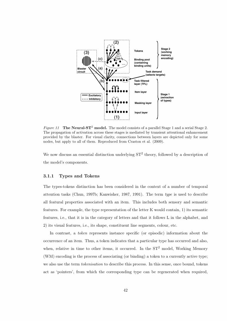
Input layer

Masking layer

Item layer

Task filtered layer (TFL)

...Binding pool(containing binding units)

Tokens

Blaster circuit

ExcitatoryInhibitory

(1)

(2)

(3)

Task demand(selects targets)

Stage 2(workingmemoryencoding)

Stage 1(extractionof types)

(a)

(b)

(c)

Figure 11 The Neural-ST2 model. The model consists of a parallel Stage 1 and a serial Stage 2.The propagation of activation across these stages is mediated by transient attentional enhancementprovided by the blaster. For visual clarity, connections between layers are depicted only for somenodes, but apply to all of them. Reproduced from Craston et al. (2009).

We now discuss an essential distinction underlying ST2 theory, followed by a description of

the model’s components.

3.1.1 Types and Tokens

The types-tokens distinction has been considered in the context of a number of temporal

attention tasks (Chun, 1997b; Kanwisher, 1987, 1991). The term type is used to describe

all featural properties associated with an item. This includes both sensory and semantic

features. For example, the type representation of the letter K would contain, 1) its semantic

features, i.e., that it is in the category of letters and that it follows L in the alphabet, and

2) its visual features, i.e., its shape, constituent line segments, colour, etc.

In contrast, a token represents instance specific (or episodic) information about the

occurrence of an item. Thus, a token indicates that a particular type has occurred and also,

when, relative in time to other items, it occurred. In the ST2 model, Working Memory

(WM) encoding is the process of associating (or binding) a token to a currently active type;

we also use the term tokenisation to describe this process. In this sense, once bound, tokens

act as ‘pointers’, from which the corresponding type can be regenerated when required,

42

e.g. at retrieval. A token-like mechanism in the brain is likely to be localised in the

frontal areas associated with WM (E. K. Miller, Erickson, & Desimone, 1996; Desimone,

1996; Passingham & Sakai, 2004), where neurons have been found to maintain sustained

activity following the perception of targets (Marois, Yi, & Chun, 2004; Kranczioch, Debener,

Schwarzbach, Goebel, & Engel, 2005).

3.1.2 Stage 1 of Neural-ST2

Stage 1 of the ST2 model simulates the functional aspects of cascaded, parallel processing

in the ventral visual processing pathway (Rousselet, Thorpe, & Fabre-Thorpe, 2004). Ac-

tivation fed into the ST2 model at the Input layer propagates through a sequence of layers

that abstractly represent the functional steps of visual processing. The Masking layer rep-

resents inhibitory interactions that generate forward and backward masking effects (Seiffert

& Di Lollo, 1997). The transience of item representations arises from these interactions and

determines bottom-up trace strength. Thus, activation traces are greatly weaker for stimuli

that are followed by another stimulus, as opposed to stimuli followed by a blank (Bowman

& Wyble, 2007). Such traces are differentiated by describing them as either strong (followed

by a blank) or weak (followed by a stimulus). The simulation of masking in ST2 is consis-

tent with findings from neurophysiology (Keysers & Perrett, 2002; Rolls, Tovée, & Panzeri,

1999; Kovács, Vogels, & Orban, 1995). Single cell recordings in this context have found

clear reductions in the firing rates of neurons in the temporal cortex as a result of masking.

Activation from early visual processing layers in the model feeds into layers that ab-

stractly represent type-oriented processing. The Item layer supports temporally sustained

but decaying representations of items in the RSVP stream. At this layer, targets and dis-

tractors are treated identically. Also, semantic and conceptual features of these items are

extracted (Potter, 1993), and priming effects are implemented. The ‘output’ of Stage 1 is

the Task Filtered Layer (TFL). Each node in the TFL represents the type of an item in the

RSVP stream. Such type nodes correspond to neurons at the late stages of ventral visual

processing in the IT cortex (E. K. Miller et al., 1996). At the TFL, a Task Demand mecha-

nism selectively emphasises processing in nodes corresponding to targets. fMRI studies have

found that the ventrolateral prefrontal cortex (VLPFC) performs a similar role within the

fronto-parietal network in the brain (Duncan, 2001; E. K. Miller & Cohen, 2001). Neurons

43

in this region have been found to rapidly adapt and selectively respond only to task-relevant

items (Hampshire, Duncan, & Owen, 2007; Hampshire, Thompson, Duncan, & Owen, 2009).

In the ST2 model, task demand effectively filters the items that receive attentional enhance-

ment and proceed to Stage 2.

3.1.3 Stage 2 of Neural-ST2

Stage 1 of the ST2 model yields a decaying trace of the visual and semantic features of target

items within the TFL. It is parallel in the sense that different items can be simultaneously

active at the TFL. In contrast, Stage 2 implements sequential encoding of these items into

WM, with this sequentiality emerging from mechanisms that attempt to ensure that items

are discretely and unambiguously bound into WM. Types and tokens are bound via a pattern

of sustained activation in a set of nodes comprising the Binding Pool. In particular, there is

no synaptic change involved in this binding mechanism. Further, the binding pool contains

one binding node for each combination of type and token (see figure 59B for a pictorial

description). In other words, the binding pool is a localist (see O’Reilly & Munakata, 2000

for a definition) activation based memory for type-token associations1. The projections into

and out of the pool are arranged such that each type-token association is represented by

a portion of the pool. Inhibition between tokens ensures only one token is active at any

one time, thus enforcing a serialisation of working memory encoding. Effectively, an item is

encoded into working memory by connecting its type node in Stage 1 to a working memory

token in Stage 2. This process is referred to as tokenisation. If at the end of a trial, the

type node of a target has a valid connection to a token, the target is successfully ‘reported’

by the ST2 model.

3.1.4 Transient Attentional Enhancement: the Blaster

ST2 suggests that when the visual system detects an item that may be task relevant, a

Transient Attentional Enhancement (TAE) occurs, which is directed at the location at which

that item appears. For a weak (masked) item, the contribution of this enhancement is critical

1This localist implementation of the binding pool in 2f-ST2 is not intended to be scalable to the levelof complexity represented in the brain. In section 10.3, we will discuss how the binding pool could beimplemented with a more neurophysiologically realistic, distributed architecture.

44

in enabling it to activate a token and thereby be encoded. The TAE is implemented by a

mechanism called the blaster (described in greater detail in section 5.2). Above threshold

activity in any node of the TFL (which will only happen for targets, because of the task

demand filter) excites the blaster through the projection marked (a) in figure 11. The blaster

sends a powerful excitatory projection to type nodes in Stage 1 (through the projections

marked (b) in figure 11). This causes a generalised, but short lived, feedback excitation

of layers in the later part of Stage 1. In the brain, such an attentional mechanism might

correspond to the function of the temporo-parietal junction (TPJ) and the ventral frontal

cortex (Corbetta & Shulman, 2002; Serences et al., 2005). Further, it might be that that

these cortical structures interact with subcortical regions in the thalamus, including the

locus coeruleus ( Aston-Jones, Rajkowski, & Cohen, 2000; discussed further in section 3.2)

and the pulvinar (Arend et al., 2008; Grieve, Acuña, & Cudeiro, 2000).

3.1.5 How the Model Blinks - Suppression of TAE

The cause of the blink is inhibition through the projection marked (c) in figure 11. This

link ensures that, while binding pool nodes are being allocated, the blaster is held offline.

Importantly, this inhibition is not active while an existing encoding is being maintained.

As binding pool nodes are in fact gate-trace micro-circuits (see appendix A.1.2), the gate is

only active during an allocation period; it is the gate of each binding pool node that has an

inhibitory projection to the blaster (more details later in section 5.2). Therefore, the general

behaviour of the blaster is a brief spike of excitation followed by a period of inactivity until

the completion of the current token binding. This is the mechanism by which the model

exhibits an AB: unavailability of the blaster protects the integrity of the T1 binding by

limiting attentional resources that could cause binding intrusions. This is consistent with

our central theoretical position that the blink is the marker of a system that is attempting

to allocate distinct episodic contexts. Thus, it ‘deliberately’ sacrifices T2s in order to ensure

the episodic integrity of T1, i.e., that it is unambiguously tokenised.

45

3.2 The LC-NE Model

The LC-NE model proposed by Nieuwenhuis, Gilzenrat, et al. (2005) makes an important

contribution to understanding the AB; a strength being that the model is framed within the

context of a broad neurophysiological theory of attentional function (Aston-Jones & Cohen,

2005; Aston-Jones et al., 2000; Usher, Cohen, Servan-Schreiber, Rajkowski, & Aston-Jones,

1999), based on the function of the Locus Coeruleus (LC) brain-stem nucleus, and the neu-

rotransmitter Norepinephrine (NE) released by it. Perhaps of most importance, the LC-NE

theory proposes a specific neurophysiological underpinning to the P3 (Nieuwenhuis, Aston-

Jones, & Cohen, 2005), which is being extensively used as an ERP correlate of attentional

processing in the AB context (Kranczioch et al., 2003; Luck et al., 1996; Martens, Munneke,

et al., 2006; Vogel & Luck, 2002; Vogel et al., 1998). On the whole, the LC-NE theory pro-

poses a unified explanation of temporal attention, which reconciles the AB phenomenon,

neurophysiology, electrophysiology (in respect of the P3) and neural modelling.

To explain the AB, the LC-NE model depicted in figure 12 is configured such that only

task-relevant targets generate a phasic LC response. LC innervation of the cortex ensures

that the excitatory response of cortical neurons is amplified. In a visual discrimination

task, monkey LC neurons are activated with a temporal profile that seems to match the

AB curve, prompting the development of the model. It consists of two main components:

the behavioural network and the LC. We discuss these in turn, before considering how the

model generates an AB.

3.2.1 Behavioural Network

The behavioural network is a simple feed-forward system, with major inter-layer connections

being one-to-one. The network comprises three layers: Input, Decision and Detection. In

the AB context, a sequence of stimuli is presented at the input layer to simulate the RSVP

stream.

The decision layer implements an ongoing competition between three alternatives: the

two targets and a single unit abstractly modelling all distractors. Nodes in the decision layer

compete through lateral inhibition. Crosstalk connections are also included between input

and decision nodes, reflecting feature similarity between stimuli. The decision layer projects

46

Figure 12 The LC-NE model. Crosstalk connections between T1 and D are not shown for visualclarity. Point sizes of arrows indicates weight strength. Reproduced from Nieuwenhuis, Gilzenrat,et al. (2005).

in one-to-one fashion to the detection layer, which serves as the output from the model.

On the assumption that only targets are reported, the detection layer does not represent

distractors. Finally, excitatory self-loops are included to sustain activation at decision and

detection nodes. However, these loops are not strong enough to yield an active memory.

3.2.2 The Locus Coeruleus

The Locus Coeruleus (LC) is a minute brain-stem structure (German et al., 1988) that

projects widely to the cortex, with a special emphasis on areas involved in attentional pro-

cessing (Aston-Jones et al., 2000). In the LC-NE model, the LC modulates activity in the

behavioural network. Specifically, the LC is excited by detection of a salient stimulus. In

the context of the behavioural network, this means that targets fire the LC, as reflected by

the fact that target nodes in the decision layer have excitatory projections to the LC. LC

activity has a modulatory effect on the behavioural network, by simulating the release of

the neurotransmitter Norepinephrine (NE). This release multiplicatively scales the afferent

signals to network units, transiently adjusting their gain. Amplification of the multiplica-

tive gain ‘sharpens’ the sigmoidal transfer functions (Aston-Jones & Cohen, 2005) making

decision and detection layer units temporarily more responsive.

47

3.2.3 How the Model Blinks - The LC Refractory Period

Following a firing of the LC and the subsequent release of NE, it enters a refractory period.

This arises because, while NE enhances processing in cortical areas, local NE release within

the LC is believed to be autoinhibitory. Thus, following a phasic response, this autoinhibi-

tion generates an LC refractory period, during which further LC phasic response is rare. In

the LC-NE model, it is unavailability of the LC during its refractory period that causes the

blink. That is, the model blinks as a result of the following sequence of events. Firstly, the

T1 fires the LC, which provides a window of enhancement lasting around 150ms. Secondly,

following this T1-induced firing, the LC enters its refractory period. Thirdly, T2s arriving

during this period are unable to immediately re-fire the LC and, consequently, do not benefit

from a timely (NE-induced) increase in gain. This leaves T2s arriving during the refractory

period at a disadvantage, ensuring that only particularly strong T2s get reported. Blink

recovery happens because, if the T2 follows the T1 after a sufficient time interval, the LC

will have recovered from its refractory period and the T2 will be able to fire it in short order.

Indeed, the LC-NE model suggests that the AB profile will exactly follow the profile of the

LC refractory period.

3.3 Related Work

In this section, we briefly discuss some other models that simulate the Attentional Blink.

In particular, we highlight the mechanisms used in these models to implement the temporal

spotlight of attention, and comparatively evaluate them against the blaster and the LC.

3.3.1 The Global Workspace Model

The global workspace model (Dehaene, Sergent, & Changeux, 2003) is a general, biologically

detailed architecture of neural information processing. It begins at early sensory stages and

leads up to a central, global workspace of attentional control and consciousness. In the

model, stimuli compete for access to this global workspace and benefit from enhancement

due to attentional feedback. In particular, it explains the AB by proposing that when T2 is

presented shortly after T1, it fails to enter the global workspace, which is occupied by the

processing of T1. However, the model does not explain many of the other findings related

48

to the AB, including spreading the sparing (see Bowman & Wyble, 2007 for a detailed

comparison to the ST2 model).

3.3.2 The CODAM Model

The Corollary Discharge of Attention Movement (CODAM) model is a broad-based mech-

anism of attentional control, with many links to neurobiology (Taylor & Rogers, 2002). It

consists of a bottom-up pathway along which stimuli have to pass, in order to have access

to working memory. Importantly, items processed in this pathway require the benefit of an

attentional enhancement signal provided by a module called the ‘inverse model controller’

(IMC) to successfully progress into working memory. Fragopanagos, Kockelkoren, and Tay-

lor (2005) simulate the model in an AB setting, in which this attentional control signal is

withheld from the T2 when presented in close succession to T1, to ensure that T2 does not

interfere with T1 encoding. Though the CODAM model simulates the basic AB curve, it

does not generate as broad a range of data as the ST2 model, and also does not simulate

spreading the sparing (see Bowman & Wyble, 2007 for further analysis).

3.3.3 The eSTST Model

The eSTST model (Wyble, Bowman, & Nieuwenstein, 2009) is a revision of the ST2 model

that enables it simulate spreading the sparing (Di Lollo et al., 2005; Olivers et al., 2005). As

mentioned in section 2.3.2, spreading the sparing is a recent finding that suggests the lag 1

sparing window can be extended to multiple targets, if they are presented in rapid succession

after the T1. The eSTST model retains many of the structural aspects of ST2; in particular

it too has a blaster that is responsible for providing transient attentional enhancement

to targets. However, the important difference with respect to ST2 is that the blaster in

eSTST does not have an innate refractory period. Instead, its deployment is controlled

by competing inhibitory and excitatory connections from WM encoding and target input,

respectively (Wyble, Bowman, & Nieuwenstein, 2009). This implementation allows each

target in a string of consecutive targets to generate a recurrent, extended enhancement of

attention.

49

3.3.4 The Boost and Bounce Model

The Boost and Bounce model of temporal attention (Olivers & Meeter, 2008) is another

recent computational model, which, like the eSTST model explains the AB and spreading

the sparing within a common framework. In contrast to the eSTST model however, the

Boost and Bounce model emphasises the role of distractor suppression in producing the

AB (Raymond et al., 1992). In the model, an attentional ‘gating’ mechanism ‘boosts’ targets

and ‘bounces’ (i.e., suppresses) distractors, effectively serving as the temporal spotlight.

Once opened by a target, this gate stays open as long as more targets are presented in

succession. But a distractor following a target inadvertently benefits from the attentional

boost and provokes a prolonged inhibitory bounce response that results in an AB effect.

3.4 Conclusions

This chapter has focused on two neural models of temporal visual processing and the AB.

These models form the basis of the theoretical explorations in later chapters of this thesis.

In particular, the ST2 model will provide the main modelling platform based on which the

experimental results presented in this thesis are interpreted. The characteristics of this

model will be comparatively evaluated against the LC-NE model, and a potential extension

to the LC-NE model that incorporates concepts from ST2. In addition, later chapters of this

thesis also elaborate on an extension to the ST2 model, to enable it to simulate temporal

feature binding in vision. The next chapter delves deeper into the mechanisms of the ST2

model, to elaborate on the methodologies that will be used in this thesis to connect modelling

and electrophysiological data.

50

Chapter 4

Connecting Modelling and

Electrophysiology

The previous chapters have provided an overview of the experimental and theoretical back-

ground related to the research presented in this thesis. Following on from there, a key idea

explored in this thesis is how the connection between experiment and theory can be en-

hanced by EEG data. Here, we provide an overview of the generation of virtual ERPs from

the ST2 model. Beginning with an introduction to the concept, we provide a rationale for

the use of virtual ERPs in extending the flow of ideas between models and data. We then go

on to describe the methodology for generating specific virtual ERPs from subcomponents

of the ST2 model, which are qualitatively comparable to human ERPs, both at the level of

grand averages and single trial dynamics.

4.1 Introducing Virtual ERPs

Computational modelling of cognition is commonly focused on the replication of behavioural

data. In this regard, they have provided concrete frameworks for expressing and instantiat-

ing cognitive theories. These models can then be used to generate experimental predictions.

Testing these predictions then feeds back into further refinement of the models they are

derived from, thus completing the cycle of theory and experiment.

51

Within the domain of cognitive models, neural network models of cognition, in addi-

tion to replicating behavioural data, embody a hypothesis about underlying structure and

function. These models attempt to ‘explain’ behaviour as emerging naturally out of func-

tional structures in the brain and the neural dynamics that these structures support. Often,

these structures are inspired by and justified based on research into neural physiology and

anatomy. In doing so, neural network modellers hope to understand how specific aspects of

cognition are embodied in the brain.

On the empirical front, cognitive science is no longer limited to behavioural research.

Recent advances in brain imaging technology allow researchers to monitor the participant’s

behaviour at a certain task, and in addition, record ongoing brain activity that is correlated

with a particular behaviour. Among the different imaging techniques, EEG provides partic-

ularly high temporal resolution, and is well suited to studying the millisecond-scale temporal

dynamics of conscious perception. Researchers have been successful in mining EEG data

to infer aspects of both subconscious and conscious neural processing. The convergence of

behavioural and neuro-imaging research is rapidly changing the insights that can be gained

about the neural architecture and processing that underlie behaviour.

Given this background, the natural question that arises is how these two approaches to

understand cognition at the neural level can be beneficially combined. A significant part

of this thesis has been devoted to this question, previously investigated in Craston et al.

(2009) and Craston (2009). Specifically, we are interested in using the Neural-ST2 model

to validate human EEG data. This is possible because cognitive neural networks consist

of nodes, which derive from the functional characteristics of real neurons. The activation

of nodes in a model can be interpreted as the analogue of the activation of an assembly

of neurons in the brain. Consequently, activation traces in a model are comparable to

aggregate neural activity expressed in EEG data.

Figure 13 summarises the rationale behind the concept of virtual ERPs, and their rela-

tionship to human ERPs. As depicted in the illustration, behavioural data for the particu-

lar set of experimental observations constrain the development of a neural network model.

Drawing on a broad set of behavioural data related to the AB, repetition blindness and

RSVP in general, Bowman and Wyble (2007) proposed the ST2 model, which embodied a

two-stage theory of temporal visual processing. As discussed previously in section 3.1, the

52

Configure the ST2 model to replicate the

behavioural data

Generate virtual ERPs from model

neurons

Behavioural data

from humansERP data

from humans

What do virtual ERPs tell us about

human ERPs?

Figure 13 The role of virtual ERPs in cognitive science research. Behavioural data is usedto constrain the ST2 model, virtual ERPs from which are then evaluated against human ERPs.

ST2 model simulates human behavioural accuracy using its neural network implementation.

In parallel, a large amount of electrophysiological data has been collected in the context

of the previously stated phenomena. The relevant question explored in this thesis is thus:

do virtual activation traces generated from the neural network model represent meaningful

patterns that mirror human EEG data, allowing us to replicate, interpret and make pre-

dictions about human EEG data in a way similar to that previously used with behavioural

data? The rest of this chapter sets down the foundation for this exploration. First, the

methodology used to generate virtual ERPs from the model is discussed. This is followed

by an overview of the key ERP components that are the focus of study and replication in

this thesis.

4.2 Generating Virtual ERPs

As illustrated in figure 11, the ST2 model consists of a number of layers, each containing

several nodes. Nodes of one layer are connected to nodes in other layers via excitatory and

inhibitory connections. In order to describe the activation dynamics at the individual node

level, figure 14 focuses on a single connection between a pair of nodes. The two nodes de-

picted represent a typical ST2 node pair in two neighbouring layers. Nodes in the ST2 model

53

Membrane potential

Membrane potential

Presynaptic activation

Postsynaptic activation

x Weight (synaptic projection)

Out

put

func

tion

Node B

Node A

Figure 14 Node-level activation dynamics in Neural-ST2. A typical pair of neural networknodes situated in two neighbouring connected layers of the ST2 model. As shown in the figure, wecan extract the membrane potential, presynaptic activation and postsynaptic activation for eachnode of the Neural-ST2 model.

receive input from other layers via weighted connections and update their membrane poten-

tial according to shunting equations derived from the Hodgkin-Huxley approach (Hodgkin

& Huxley, 1952). Once the membrane potential reaches a given threshold, they produce

output according to a rate-coding X-over-X+1 function (O’Reilly & Munakata, 2000). In

figure 14, the membrane potential describes the activation within the node. The weighted

connections between the nodes are assumed to correspond to major synaptic projections

in the brain. Within the context of a given weighted synaptic projection outgoing from a

node, activation output produced by the node is referred to as presynaptic activation. This

activation, when multiplied by the corresponding synaptic weight results in a postsynaptic

activation that feeds into the node at which the synaptic projection ends.

In the human brain, the difference in electric charge between the dendrite and the

postsynaptic cell body of an active neuron creates an electric dipole. To generate a signal

that is strong enough to be registered by the EEG, a population of neurons has to be active

together and spatially aligned, which causes the individual dipoles to summate. In our

understanding of neural electrophysiology, cortical pyramidal neurons are known to have

long-range connections and are aligned perpendicular to the cortex, and are assumed to

be a major contributor to EEG activity (Baillet, Mosher, & Leahy, 2001; Luck, 2005). In

54

addition, pyramidal neurons release glutamate as their neurotransmitter, and therefore have

an excitatory effect on networks they participate in.

For generating virtual ERPs, we attempt to keep the methodology as simple as possible,

while at the same time approximating the mechanisms that are assumed to occur in the

brain. Virtual ERPs are generated by summing over postsynaptic activation values (see

figure 14), the rationale being that it is postsynaptic potentials between the dendrite and

the cell body that primarily generate the EEG signal recorded at the scalp. In line with

pyramidal neurons forming excitatory connections in the brain, the virtual ERP consists of

postsynaptic activation values from excitatory connections only. Note that only activation

traces from connections between layers (and not self-loops that connect nodes within a layer)

are included in the virtual ERP, as these are assumed to be an analogue of the long-range

connections from pyramidal neurons that contribute towards the signal measured in the

human ERP.

It is obvious that virtual ERPs remain a coarse approximation of the human ERP.

Many factors, such as the distortion of the signal by the scalp, are not addressed1. In

this context, it is important to note that the approach to simulating ERPs employed here is

philosophically distinct: in particular, the ST2 model is not expressly configured to generate

virtual ERPs that fit their human counterparts. Rather, the model is first matched to

human behavioural data, and the virtual ERPs generated in this configuration are verified

for comparability with human ERPs. Consequently, due to these limitations of the virtual

ERP technique, one can only expect to obtain a qualitative rather than a quantitative

match to the data. Nevertheless, this process allows us to provide a common explanation

for a pattern of behavioural and ERP effects, in addition to verifying the internal dynamics

of model’s architecture. Further, as we shall see in later chapters, virtual ERPs allow

us to make qualitative predictions about the pattern of changes in human ERPs across

experimental conditions of interest.

1For an example of an approach to modelling ERPs that is based on a neurobiologically constrainedsource reconstruction, see the Dynamic Causal Modelling (DCM) technique (David, Harrison, & Friston,2005; David, Kilner, & Friston, 2006).

55

4.2.1 Grand Average Virtual ERPs

Grand average virtual ERPs, comparable to their human equivalents previously introduced

in section 2.4.3, allow for qualitative comparison of traditional ERP components commonly

investigated in EEG research. To generate virtual ERPs from a simulated trial, we adopt

the straightforward approach and sum over all nodes of a relevant subset of layers from

the ST2 model. In addition, neurophysiological evidence suggests that there is a delay of

around 70ms for neural activation related to visual processing to travel from the retina

to occipital areas (Schmolesky et al., 1998). ST2 does not model this aspect of visual

processing, and hence to account for this delay, virtual ERPs generated by the model are

shifted by 70ms. Finally, to generate the grand average virtual ERP corresponding to an

experimental condition, we average across the simulated trials making up that condition.

4.2.2 Virtual ERPimages

When generating ERP averages, raw EEG data is collapsed to a one dimensional dataset

displaying a sequence of voltage fluctuations over time. The averaging process extracts

EEG activity that is time-locked to the stimulus, whereas the rest of the signal is treated

as irrelevant background noise. As previously pointed out in section 2.4.4, the problem

with this approach is that information that is specific to individual observations is lost.

Consequently, ERPimages (Makeig, Debener, et al., 2004; Delorme & Makeig, 2004) have

been proposed as a means for visualising single-trial dynamics in EEG data.

This shortcoming of the averaging process also applies to virtual ERPs. A simulation

run of the ST2 model contains a number of trials encompassing a range of target strength

values. A grand average virtual ERP illustrates the general time course of activation in

chosen layers in the model, but is blind to inter-trial variation that occur because of varying

strength values. To address this problem, we generate virtual ERPimages from the ST2

model, using visualisation techniques similar to those used to generate human ERPimages.

As we shall see, virtual ERPimages bring out patterns of variation that are not evident

in the grand average virtual ERP, and depict the dynamics of the model across individual

trials of a simulation run.

56

...


Stage 1

Stage 2

Blaster

Virtual P3

Virtual ssVEP orVirtual P1-N1

Σ

ΣVirtual N2pc

Figure 15 Virtual ERPs from the ST2 model. The virtual ssVEP is generated from the inputand masking layers. The virtual P3 is generated from the item, TFL, binding pool and token layers.The virtual N2pc is generated from blaster activation.

4.3 Virtual ERP Components

This section focuses on the specific virtual ERP components that are generated from the

ST2 model and compared with human ERP components. A human ERP component is

typically recorded from a particular set of electrodes and associated with certain cognitive

processes. In the ST2 model, different layers of the model were designed to correspond to

various stages of cognitive processing in the brain. As shown in figure 15, by summing over

neural network activation from nodes within specific layers of the ST2 model, we can extract

virtual ERPs related to particular stages of cognitive processing.

4.3.1 Early Visual Processing - The Virtual ssVEP

Correlates of early visual processing in the human ERP are observed at occipital elec-

trode sites. A target presented on its own evokes the well-known N1 and P1 ERP early

components, reflecting early perceptual processing of the visual features of the target (see

57

figure 4A). However, in the context of RSVP, successive items in the stream evoke a sus-

tained ssVEP wave (Di Russo et al., 2003), which oscillates at a frequency equal to the

presentation rate of items in the stream (see figure 4B).

In the ST2 model, targets and distractors in the RSVP stream are ‘presented’ to the

input layer. The input layer thus corresponds to very early stages of processing in the

brain. At the masking layer, each item is subject to competition from temporally adjacent

items in the stream, thus simulating forward and backward masking at early vision. The

amount of masking is determined by the bottom-up strength of the neighbouring items.

Together, the input and masking layer reflect perceptual processing of stimuli, and thus

most closely resemble neural processing in the early visual cortex. Consequently, as in

figure 15, activation at these layers is summated to generate the virtual ERP corresponding

to early visual processing, and in particular, the virtual ssVEP. In chapter 6, we will modify

the ST2 model to simulate the processing of a single target on its own, and generate virtual

early P1 and N1 components from it.

4.3.2 Transient Attentional Enhancement - The Virtual N2pc

The N2pc ERP component has been associated with attentional selection (Luck & Hillyard,

1994; Eimer, 1996; Hopf et al., 2000) (see figure 4C). It has been observed whenever attention

is directed toward a visual stimulus. In the ST2 model, attention is modelled by the blaster,

which is triggered only by targets at the TFL, and provides them with a transient burst

of excitation to facilitate working memory encoding. Hence, in order to generate a virtual

ERP component that reflects the selective attentional response in the ST2 model, we average

activation from the blaster’s output across multiple trials to generate the virtual N2pc for

a particular condition. (see figure 15). However, it should be noted that, unlike the human

N2pc, the virtual N2pc is not a lateralised component. This is because the ST2 model

does not simulate hemispheric differences in attentional responses. Further, the virtual

N2pc is a positive activation trace from the blaster. In comparison, the human N2pc is a

negative-going electrical potential difference. This arises from complexities relating to the

neural generators of the human N2pc, and their projections onto the scalp, which are not

simulated by the ST2 model. Despite these differences, variations in blaster activity across

conditions of interest are qualitatively comparable to those in the human N2pc.

58

4.3.3 Working Memory Encoding - The Virtual P3

The human P3 ERP component is a broad ERP component spread across a large area of

the scalp, most prominent at parietal electrode sites (see figure 4A). It is thought to reflect

a global event in the brain, involving interaction between multiple cortical regions. The

meaning of the P3 and the cognitive processes that it reflects have been the subject of much

debate (see Donchin & Coles, 1988; Verleger, 1988 for an extensive discussion). In almost

all RSVP experiments, the P3 is observed to be correlated with conscious perception and

working memory consolidation of targets (Donchin, 1981; Vogel et al., 1998; Kranczioch

et al., 2003; Sergent, Baillet, & Dehaene, 2005). This notion is supported by the related

finding that the P3 is absent for missed targets in RSVP (Kranczioch et al., 2003).

In the ST2 model, working memory encoding occurs by creating a binding link between

types from Stage 1 and tokens from Stage 2, a process referred to as tokenisation (see

section 3.1). Tokenisation is initiated by the arrival of a target at the TFL, which triggers

the blaster (see figure 11). The blaster responds by generating a transient attentional

enhancement, providing a burst of excitation to the item and TFL layers. TFL nodes

project to the binding pool, which in turn are connected to the tokens in Stage 2 (see

figure 59B). Tokenisation completes when a token node gets bound to the target’s type in

the TFL via intermediate nodes in the binding pool. Hence, on the whole, the item and TFL

layers, the binding pool and the tokens are all involved in encoding an item into working

memory. Consequently, as depicted in figure 15, these layers contribute towards the virtual

P3 component, which is generated by summating the activation across all constituent nodes.

4.4 Conclusions

This chapter has outlined the concept of virtual ERPs, focusing on highlighting the rationale

behind virtual ERPs and the general methodology for generating them. In particular, virtual

ERPs provide a two-fold benefit: firstly, we can use them to interpret behavioural and ERP

data within a common explanatory framework. Secondly, we can use the comparisons

between human and virtual ERPs to verify the internal mechanisms of the ST2 model. The

general introduction provided here will be elucidated when specific virtual ERPs from the

model are generated and compared to human ERPs across conditions of interest.

59

Part II

Explorations of the Temporal

Spotlight

60

Chapter 5

Comparing the ST2 and the LC-NE

models

We begin the main body of this thesis with a theoretical exploration of the ST2 and LC-NE

models. This work comparatively evaluates two complementary neural network models that

describe the role of the temporal spotlight in temporal perception and the Attentional Blink.

First, we comparatively describe the inner workings of Transient Attentional Enhancement

(TAE) as embodied in these two models. This followed by a detailed assessment of how

both models fare in terms of explaining the main phenomena that characterise the AB, as

previously listed in section 2.3.2. In final section of this chapter, based on our insights into

the two models, we introduce a potential extension to the LC-NE model. This extension

borrows concepts from ST2 to expand the explanatory power of the LC-NE model and

bridge the levels of explanation they encompass.

5.1 Introduction

In addition to the large body of behavioural research relating to the AB described previously

in section 2.3, there has been considerable recent interest in identifying neural correlates of

the underlying mechanisms (Craston et al., 2009; Martens, Munneke, et al., 2006; Marois,

Chun, & Gore, 2000; Rolke, Heil, Streb, & Hennighausen, 2001; Marois et al., 2000; Vogel

& Luck, 2002; Vogel et al., 1998). To complement this line of enquiry, there has been

61

work on developing neurally explicit computational explanations (Bowman & Wyble, 2007;

Fragopanagos et al., 2005; Nieuwenhuis, Gilzenrat, et al., 2005; Chartier, Cousineau, &

Charbonneau, 2004; Battye, 2003; Dehaene et al., 2003). Amongst these, the ST2 (Bowman

& Wyble, 2007) and the LC-NE (Nieuwenhuis, Gilzenrat, et al., 2005) models, previously

introduced in chapter 3, are notable approaches. This is because the former reproduces

a broad spectrum of AB phenomena and the latter ties into a concrete neurophysiological

substrate. In a sense, the ST2 model works down from the behavioural data, while the

LC-NE model works up from the neurophysiology. Thus, an important research question

concerns how these two models relate to one another. In particular, to what extent can

the neurophysiological mechanisms highlighted in the LC-NE model be reconciled with the

cognitive-level mechanisms inherent in the ST2 model? This chapter focuses on such issues,

and comparatively evaluates the computational implementations of the temporal spotlight

in the two models. In this context, we have re-implemented the LC-NE model to better

understand the role of attention therein. Additionally, we have worked on extending the

model using mechanisms inspired by the ST2 model to enable it to reproduce a broader

spectrum of behavioural data pertaining to the AB. The research in this chapter builds

upon the introduction to the ST2 and LC-NE models provided in chapter 3, and mutually

informs the mechanisms that implement the temporal spotlight of attention therein.

A similarity between the LC-NE and ST2 approaches is that they both assume temporal

spotlights that are triggered by detection of a salient stimulus (e.g. a target stimulus) and

are short-lived. In ST2, the enhancement is the Transient Attentional Enhancement (TAE),

which is realised by the blaster, while in the LC-NE model the enhancement arises from

the Locus Coeruleus itself. That said, the two enhancements do have somewhat different

purposes. ST2’s blaster aids detection and WM encoding of weak items, while the LC is

assumed to have its affect on decision and response systems, where it optimizes processing

in multilayer decision systems (Aston-Jones & Cohen, 2005). However, both approaches

assume that it is unavailability of this attentional resource (blaster and LC respectively)

that is the direct cause of the blink. The mechanism that causes this unavailability is,

though, very different in the two cases. In ST2, the blaster is held offline by ongoing

working memory encoding. This preserves the integrity of such encoding by preventing a

second item from corrupting the episodic integrity of a first item. In the LC-NE model, after

62

firing, the LC enters an intrinsic refractory period in which it is difficult to refire. It is this

conceptual difference between the temporal spotlights that is at the heart of the comparison

in this chapter.

5.2 TAE in the ST2 Model: The Blaster

In the ST2 model introduced in section 3.1, the blaster implements transient attentional

enhancement. In this role, it mediates the establishment of type-token bindings across a

parallel Stage 1 and a serial Stage 2. An item passing the salience filter in the final layer

of Stage 1 of the ST2 model in a strongly active form initiates the blaster, which elevates

activation across the later levels of Stage 1. This mechanism is exogenous in character, being

triggered externally by the occurrence of a salient stimulus, and highlights a very brief

window of time and space that is particularly salient. Specifically, the blaster enhances

the activation level of salient items, aiding their encoding into WM. This is particularly

important when considering demanding stimulus environments (such as RSVP), as unaided,

fleeting representations have insufficient bottom-up activation to facilitate encoding. In this

regard, the blaster plays a key role in facilitating type-token binding. The blaster has the

following important characteristics:

Y Firstly, it is a brief pulse of a fixed duration (around 100ms), irrespective of the

exogenous strength of the salient stimulus.

Y Secondly, it only fires once per tokenisation. Once a target (T1) triggers the blaster

and the process of binding is initiated, it is held offline by inhibition from the binding

pool till the process is complete. This inhibition attempts to associate distinct episodic

contexts to targets, and prevents a second target (T2) in close temporal proximity to T1

from interfering with its tokenisation. T2 occurring within 200-500ms of T1 must “wait”

till the T1 tokenisation is complete for the blaster to fire again. This implies that only T2s

with strong bottom up strength have enough activation to “outlive” T1 tokenisation. It is

this mechanism, embodying the episodic distinctiveness hypothesis, that enables the ST2

model to simulate the attentional blink.

Y Thirdly, the blaster is spatially specific, but is not featurally selective in its enhance-

ment. That is, it is initiated by detection of features characterising the task set but the

63

0 200 400 600 800 1000

0.2

0

0.2

0.4

0.6

0.8

1

Time from target onset (ms equivalent)

Activ

atio

n

TFLBlasterBinding Pool

A: Blaster Dynamics

!"#$%&'

()%*)%+,(-.

!"#$%&'

()%*)%

,(//.

!"#$%&'+

01*)%

,(-.2

3

!"#$%&'+01*)%+,(//.

45/6

0%&7

6#8&'

!91:91;

<=="

!"#

!$#

!%#

!&#

>?@9%#%='8

01A9B9%='8

C""+%=+(1&+*'=D&@%9=1+,&?@9%#%='8.

(1&+%=+C""+*'=D&@%9=1+,&?@9%#%='8.

!"#$%&'()

B: Blaster Circuit

Figure 16 The dynamics and circuitry of the blaster in Neural-ST2. Panel A: Dynamics ofthe blaster as regulated by the TFL and the binding pool. Panel B: Internal circuitry of the blaster.Output connection thresholds emanating from the blaster output on neuron are denoted 1, 2 and 3,with 1 less than 2 less than 3. Reproduced from Bowman and Wyble (2007).

effect of the blaster is not restricted to those features.

Figure 16A depicts the activation dynamics of the blaster and its relationship to input

from TFL and inhibition from the binding pool. The presentation of a single target in RSVP

excites its corresponding node in TFL, which in turn feeds input to the blaster. Due to the

way its internal circuit is configured, the blaster produces a ballistic response to excitation

from TFL. This response gets fed back to the TFL, boosting the activation of the target’s

TFL node to a value high enough to initiate tokenisation. During tokenisation, the binding

pool node connecting the target’s TFL node to the currently active token is excited. As

previously described, this excitation is set up to inhibit the blaster. This produces the

prolonged suppression in the blaster’s activation seen in figure 16A, preventing it from

firing again till tokenisation is complete. Its activation eventually returns to baseline once

tokenisation is completed and suppression from the binding pool dies down.

5.2.1 Internal Structure

Though not essential for understanding the role of the blaster in the ST2 model, it is infor-

mative to examine the internal circuitry that produces the response characteristics observed

in figure 16A. This circuitry is depicted in figure 16B. As all connections in the blaster circuit

saturate at a very low level, the nodes making up this circuit display ballistic dynamics. In

64

other words, when their activation crosses a certain threshold, the output of the nodes very

quickly reaches a maximum value, and remains mostly unchanged with further increase in

activation. The blaster’s implementation comprises two on-off circuits (see section A.1.1),

distinguished as blaster input, which governs initiation of the blaster, and blaster output,

which governs the blaster’s output effect. Thus, the blaster is initiated by TFL excitation

of the blaster input on neuron (via projection (a)). However, the resulting activation is

short lived and rapidly curtailed when the blaster input on neuron feeds inhibition back

onto the blaster input on neuron (generating the blaster refractory period). Furthermore,

this suppression is maintained by ongoing binding, via the projection marked (c)1. The

resulting brief on neuron activation of the blaster input circuit has the role of instigating

blaster output activation through the link marked (d). This Output circuit generates a tem-

porally fixed output to the TFL and Item layer (via the projection marked (b)). This effect

is obtained through the blaster output on neuron having different thresholds for outputting

along different connections, where threshold (1) is less than (2) is less than (3). When the

blaster output on neuron is excited, it begins its self-excitatory cycle with a low threshold

(1), causing it to ramp up with a predictable time course. When activation crosses threshold

(2), it begins outputting at a fixed level over projection (b). On crossing the third threshold

(3), it strongly excites the blaster output on neuron, which in turn inhibits it, ending the

blaster’s output at the appropriate time.

5.3 TAE in the LC-NE Model: The Locus Coeruleus

The LC-NE model (Nieuwenhuis, Gilzenrat, et al., 2005) is inspired by a broad neurophys-

iologically grounded theory (Gilzenrat, Holmes, Rajkowski, Aston-Jones, & Cohen, 2002;

Aston-Jones & Cohen, 2005; Aston-Jones et al., 2000; Nieuwenhuis, Aston-Jones, & Cohen,

2005; Usher et al., 1999) about the function of the Locus Coeruleus nucleus as a modulator

of attentional control. As introduced in section 3.2, the LC-NE theory proposes a unified

explanation of temporal attention, which reconciles the AB phenomenon, neurophysiology,

1Note that this projection is depicted as inhibitory in figure 11. But, in fact, it is realised as an excitatoryprojection onto the blaster input off neuron, which generates an inhibitory effect of the binding pool ontothe blaster input on neuron.

65

0 200 400 600 8000.2

0

0.2

0.4

0.6

0.8


Activ

atio

n

LCNE

Figure 17 Dynamic behaviour of the LC-NE system. Activation traces plot the response ofthe LC and NE components of the re-implemented LC-NE model to the presentation of a singletarget in RSVP.

electrophysiology (with respect to the P3) and neural modelling. The model can be di-

vided into two components: the behavioural network and the LC-NE system. The model

hypothesises the LC-NE system to be the component providing the transient attentional

enhancement in response to the presentation of task-relevant stimuli to the behavioural

network.

As a part of the research leading up to this thesis, the LC-NE model of the AB, as

described in Nieuwenhuis, Gilzenrat, et al. (2005) was re-implemented to explore the inner

workings of the LC-NE system, and to explore the model’s behaviour with regard to the

AB phenomena described in section 2.3.2. This work eventually led to the development

of extensions to the LC-NE model, described later in this chapter. The details of this

re-implemented LC-NE model are described in appendix A.2. We now draw upon simula-

tions conducted with the re-implemented model to provide an in-depth description of the

behaviour and internal details of the LC-NE system.

5.3.1 The Locus Coeruleus & Norepinephrine

The LC-NE model explains the AB in terms of the functioning of the Locus Coeruleus

(LC) (Nieuwenhuis, Gilzenrat, et al., 2005), a minute brain-stem structure (German et

66

al., 1988) that projects widely to the cortex, with a special emphasis on areas involved in

attentional processing (Aston-Jones et al., 2000). The LC is known to have two modes

of operation: in its phasic mode, it produces a sharp response to the presentation of a

target, but has a low ambient firing rate of 1-2Hz when it is presented with distractors. In

the tonic mode, it has a higher ambient firing rate of 2-4Hz for distractors, and produces

a shallow response to targets (Gilzenrat et al., 2002). In the phasic mode of operation,

strong LC innervation of the cortex with the neurotransmitter Norepinephrine (NE) ensures

that the excitatory response of cortical neurons is amplified. In a visual discrimination

task, LC neurons in monkeys are activated with a temporal profile that seems to match

the AB (Aston-Jones et al., 2000). This observation of phasic LC function prompted its

application to the AB in the form the LC-NE model previously introduced in section 3.2

and depicted in figure 12 (Nieuwenhuis, Gilzenrat, et al., 2005).

Figure 17 depicts the temporal dynamics of the LC-NE system in its phasic mode of

operation. As previously described in section 3.2, this LC component is excited by the

detection of task-relevant targets in the decision layer of the behavioural network. Figure 17

depicts how, when perturbed enough from its baseline level because of this excitation, LC

activity rapidly increases, producing a characteristic ballistic response to the target. This

response causes a much slower increase in the amount of NE produced by the LC. This release

of NE has a feedback modulatory effect on the behavioural network of the LC-NE model, as

it multiplicatively scales the afferent signals to network units in the decision and detection

layers, transiently adjusting their gain and making them more responsive to the activation

generated by the target (see section 3.2). However, after firing, the LC enters a refractory

period evident in figure 17. This arises as, while NE enhances processing in cortical areas,

local NE release within the LC is known to be autoinhibitory. Thus, following the excitation

of the LC by the decision layer and subsequent release of NE, this autoinhibition generates

an LC refractory period, during which further excitation is suppressed by NE release.

Internal Structure

We now describe how the characteristic dynamics of the LC-NE system observed in fig-

ure 17 are implemented in the model, though this is not a requirement for understanding its

67

behaviour. The LC-NE system is realised using an adaptation of the FitzHugh-Nagumo sys-

tem of equations (Gilzenrat et al., 2002; Fitzhugh, 1969; Nagumo, Arimoto, & Yoshizawa,

1964), which governs the interactions between a pair of coupled activity variables, one sim-

ulating the LC and other simulating NE. The FitzHugh-Nagumo system was originally used

as simplification of the Hodgkin-Huxley equations for modelling action potentials in indi-

vidual neurons. It characterises the LC-NE system as a dynamical system controlled by

two temporal variables: the first variable, vt, represents LC activity, and is excited by

target-related activation in the behavioural network and inhibited by the second variable

ut. ut represents NE output, and is influenced by the current level of LC activity. In its

standard formulation, the FitzHugh-Nagumo system relates these two variables by a pair of

ordinary differential equations (ODE), as described below:

τvdv

dt Avv a1 v u (2)

τudu

dt v γu (3)

where τv and τu are time constants such that τv P τu, and A A 0,0 @ a @ 1 and γ A 0.

Importantly, the time constant associated with LC activity (τv) is much smaller than

the time constant associated with NE output (τu). It is this difference that sets up the

dynamics illustrated in figure 17, where LC activity, which is very sensitive to excitatory

input, rises rapidly in response to target presentation. In contrast, NE output rises much

slower in response to LC activity. But once it does, it has a strong inhibitory effect on the

LC, driving it down into the refractory period, from which it recovers only as NE output

slowly returns back to baseline.

5.4 Assessment of Models

We now assess the ST2 and LC-NE models against the empirical phenomena relating to the

AB, previously discussed in section 2.3.2. This general comparison of the models aims to

bring out their similarities as well as their differences, and feeds into the topic of the next

section, which discusses a potential extension to the LC-NE model that combines ideas from

68

T2 Lag

T2 |

T1 %

Acc

urac

y

blinks as a result of the following sequence of events. Firstly,the T1 fires the LC, which provides a window of enhancementlasting around 150 ms. Secondly, following this T1-inducedfiring, the LC enters its refractory period. Thirdly, T2s arrivingduring this period are unable to immediately re-fire the LCand, consequently, do not benefit from a timely (NE-induced)increase in gain. This leaves T2s arriving during the refractoryperiod at a disadvantage, ensuring that only particularlystrong T2s get reported.

Blink recovery arises since, if the T2 follows the T1 after asufficient time interval, the LC will have recovered from itsrefractory period and the T2 will be able to fire it. Indeed, theLC–NE model suggests that the AB profile will exactly followthe profile of the LC refractory period.

4. Assessment of models

We assess the two models against the empirical phenomenapreviously highlighted. We start with ST2.

4.1. The ST2 model

4.1.1. The basic blinkThe ST2 model generates a blink because the blaster issuppressed by ongoing T1 tokenization. T2s at lags 2 and 3

fall at the point of maximum impairment (see Fig. 3(a)), due tothe length of time they have to wait for the blaster to comeback on line. The impairment decreases monotonicallythrough lags 4, 5 and 6, as it becomes more likely thattokenization of the T1 finishes before T2 has decayed.

However, at lag-1, T2 is close enough in time to T1 to takeadvantage of the (T1-initiated) blaster firing. Thus, the modeldemonstrates lag-1 sparing (see Fig. 3(a)). However, althoughT2 is typically encoded at lag-1, invariably, this only occursinto the first token, alongside T1.

4.1.2. Increased processing of T1+1 slotST2’s TAE provides an enhancement that begins shortly afteran initiating item (the T1 in an AB setting) and is very brief(lasting around 50 ms). Thus, in an AB setting, the blasterenhances the T1 and T1+1 slots. There are a number ofphenomena that this mechanism enables the model toexhibit. Firstly, as just discussed, the model generates lag-1sparing. Secondly, in fact the model’s lag-1 performance hasa tendency to be elevated above baseline (i.e. post recoveryand single target performance); see Fig. 3(a) and the 50 msSOA data in Fig. 19 of Bowman and Wyble (2007). (Asdiscussed in Section 2.2.2, this is also found in humans.)Thirdly, in Bowman and Wyble (2007) we reproduced Chuaet al.’s (2001) finding that a distractor is a more effectiveprime of a T2 if it is preceded by a T1. Finally, although we

Fig. 3 – The ST2 model's performance (a, c) compared to human data (b, d). In all cases, a letters-in-digits task was consideredwith a 100ms SOA. T2 performance (a, b) represents the accuracy in reporting T2 on trials in which T1was reported. In panels cand d, the lines at the top of the graph show T1 accuracy, while the lines at the bottom denote the percent chance for thereported order of T1 and T2 to be inverted. Human data are fromChun and Potter (1995) except the T2 end of streamdata, whichis from Giesbrecht and Di Lollo (1998). Horizontal axes represent lag, while vertical axes denote accuracy. In the T1+1 blankcondition there is no lag-1 case, since that slot is blank.Model data reproduced fromBowman andWyble (2007). This diagram isreproduced from Bowman and Wyble (2007).

32 B R A I N R E S E A R C H 1 2 0 2 ( 2 0 0 8 ) 2 5 – 4 2

Figure 18 ST2 model performance in the AB task. X-axis denotes lag position of T2, whileY-axis denotes percentage accuracy of T2 report, conditional on the correct report of T1. Notethat in the T1+1 Blank condition, there is no lag 1, as that slot is the blank one. Reproducedfrom Bowman and Wyble (2007).

both approaches.

5.4.1 The ST2 Model

The Basic Blink

The ST2 model generates a blink because the blaster is suppressed by ongoing T1 tokeni-

sation. T2s at lags 2 and 3 fall at the point of maximum impairment (see figure 18), due to

the length of time they have to wait for the blaster to come back online. The impairment

decreases monotonically through lags 4, 5 and 6, as it becomes more likely that tokenisation

of the T1 finishes before T2 has decayed.

However, at lag 1, the T2 is close enough in time to T1 to take advantage of the

(T1-initiated) blaster firing. Thus, the model demonstrates lag 1 sparing (see figure 18).

However, although the T2 is typically encoded at lag 1, invariably, this only occurs into the

first token, alongside T1.

Increased Processing of T1+1 slot

ST2’s TAE provides an enhancement that begins shortly after an initiating item (the T1

in an AB setting) and is very brief (lasting around 50ms). Thus, the blaster enhances the

69

T1 and T1+1 slots. There are a number of phenomena that this mechanism enables the

model to exhibit. Firstly, as just discussed, the model generates lag 1 sparing. Secondly,

the model’s lag 1 T2 performance has a tendency to be elevated above baseline (i.e. post

recovery and single target performance; see Bowman & Wyble, 2007), consistent with find-

ings from Craston et al. (2009). Thirdly, Bowman and Wyble (2007) reproduce the finding

by Chua et al. (2001), that a distractor is a more effective prime of a T2 if it is preceded

by a T1. Finally, the model is consistent with the finding of labile attention at short T1-T2

SOAs (Potter et al., 2002), in that it allows for a second salient stimulus, T2, to attract

processing resources that have already been allocated to an earlier stimulus, T1.


Although the model has not yet been used to simulate spatial phenomena, from a theoret-

ical perspective, the ST2 blaster is spatially specific. This is consistent with the previous

research into this mechanism, viz, transient spatial attention, as identified by Nakayama and

Mackeben (1989). As previously discussed, this spatial specificity is consistent with findings

in RSVP presentation settings (Visser et al., 1999; Wyble, Bowman, & Potter, 2009).


ST2 exhibits T1-T2 costs at lag 1 (see Craston et al., 2009; figure 5B). The loss in T1

accuracy at lag 1 arises because, when T2 is very strong and T1 weak, binding can complete

before T1 is strongly active, yielding a successful binding from token 1 to T2 and no binding

to T1. Moreover, at lag 1, the model is inaccurate at determining the order of the two targets.

At lag 1, often, both T1 and T2 are bound to the first token. This reflects a loss of episodic

information: due to the temporal proximity of T1 and T2, the model has failed to allocate

discrete episodic contexts for the two targets. These findings of costs at lag 1 are supported

by human data (see section 2.3.2).


The model demonstrates the key finding that inserting a blank in the T1+1 slot attenuates

the blink. The sequence of events that generates this phenomenon is as follows. Firstly, an

70

unmasked item yields a strong activation trace. Thus, a T1 followed by a blank generates

a higher amplitude trace at the TFL. Secondly, and this is the critical step, tokenisation,

both in the sense of binding pool node and token allocation, completes more quickly. This

is because, through the gate-trace mechanism (see appendix A.1.2), the model turns acti-

vation strength into time to encode, on the principle that stronger evidence for an item (as

encapsulated by activation strength) leads to more rapid encoding into WM. Thus, placing

a blank after a T1 greatly shortens its tokenisation. Thirdly, tokenisation will be more likely

to have finished before the T2 has decayed at the TFL, increasing the probability that the

T2 will fire the blaster2.

Here, the key principle that blink attenuation with T1+1 blank reflects is that there is a

reciprocal relationship between bottom-up trace strength and blink depth. This is obtained

in ST2 by tying tokenisation time to trace strength.


We compare the model to data from Giesbrecht and Di Lollo (1998), who examined the effect

of placing T2 at the end of the stream (see figure 18). As required, the blink is obliterated.

However, the ST2 model obtains attenuation of the blink with T2 unmasking in a different

manner to attenuation with T1 unmasking. Specifically, a T2+1 blank produces strong T2

traces that are more likely to outlive the blink. That is, T2 unmasking does not affect how

long the blaster is held offline by T1 tokenisation, but it does make the T2 more ‘resilient’

to this blaster unavailability.


Following on from above, T2s encoded by ST2 during the blink typically possess strong

activation traces. Variation in activation strength could reflect spontaneous noise or inherent

2One subtlety of the T1+1 blank data is that performance is particularly elevated at lag 2. The ST2

model obtains a qualitatively similar pattern at lag 2, as it is the only data point in which T2 is not stronglyforward masked. (Although backward masking is far stronger, weak forward masking is also included inST2.) Absence of forward masking increases the bottom-up trace strength of the T2, which gives it a smalladvantage according to the principles we discuss in the next section. However, it could be that lag 2 sparingin the T1+1 blank condition is actually a reflection of a form of spreading the sparing (see section 2.3.2),because a sequence consisting of a T1 followed by a blank at lag 1 and a T2 at lag 2 is akin to presentingthree targets in a row. Consequently, this would explain the quantitatively smaller effect of lag 2 sparingthat the ST2 model currently obtains, as it does not explain spreading the sparing.

71

T2 consolidation delay by lag for the ST2 and LC-NE models. For ST2, consolidation delay was measured as the time from target onset to peak amplitude of the TFL unit for that target. For LC-NE, consolidation delay was measured as the time from target onset to peak amplitude of the detection layer unit for that target. At each lag we averaged across all seen T2 trials. All ST2 parameter settings were as presented in (Bowman & Wyble, 2007).Note though that even though the qualitative match between these two sets of data is very good, quantitatively they are very different, as reflected by them being presented on very different scales.

FIGURE 4

(a) ST2 Model

200

250

300

350

400

450

500

550

1 2 3 4 5 6 7 8

T1 to T2 Lag

T2

Co

ns

oli

da

tio

n D

ela

y (

ms

)

(b) LC-NE Model

155

160

165

170

175

180

1 2 3 4 5 6 7 8

T1 to T2 Lag

T2

Co

ns

oli

da

tio

n D

ela

y (

ms

)

Figure 19 T2 consolidation delay by lag for the ST2 model. Consolidation delay is measuredas the time from target onset to peak amplitude of the TFL unit for that target. At each lag, allseen T2 trials are averaged together. Reproduced from Bowman et al. (2008).

differences in how particular targets stand out (Wyble & Bowman, 2005). Consequently,

T2s are often seen during the blink because they outlive blaster unavailability. As a result,

in the average, T2s are consolidated later during the blink. Figure 19 shows data from the

ST2 model that encapsulates this effect. T2 consolidation delay qualitatively mirrors the

blink curve: T2 consolidation is most delayed when the blink is deepest and un-delayed (i.e.

at baseline) post blink recovery. Interestingly, the model suggests that T2 consolidation at

lag 1 is accelerated, relative to post recovery baseline, which is consistent with the previously

discussed increased processing of the T1+1 slot.

Although a human study that explores the full spectrum of lags is not available, there is

considerable evidence from electrophysiology, for delayed T2 P3s during the blink (Martens,

Elmallah, London, & Johnson, 2006; Vogel & Luck, 2002) (see section 2.3.2). This provides

important support for the ST2 model.


In respect of the parameter settings used in Bowman and Wyble (2007), the ST2 model does

not replicate spreading the sparing. The inhibitory projection from the binding pool to the

blaster (marked (c) in figure 11) is sufficiently strong that ongoing tokenisation renders

72

the blaster unavailable soon after T1 starts to be encoded. Thus, the model exhibits lag

1 sparing, but, in the context of a continuous sequence of targets and a standard SOA of

around 100ms, it does not exhibit lag 2 or 3 sparing. This is because, whether interleaved

with distractors or not, any target appearing in the 200 to 500ms interval post T1 onset,

will not be able to fire the blaster immediately.

A revision of the ST2 model, in which suppression of the blaster is not absolute and a

somewhat more sophisticated token system is used, is described in Wyble, Bowman, and

Nieuwenstein (2009). In this revised model, a continuous stream of target-related activity

can repeatedly refire the blaster, but at the expense of loss of episodic distinctiveness, e.g.

order and repetition blindness errors. This revised model also replicates the finding that the

blink can be reversed, in the sense that, although a T2 in the sequence T1 D T2 T3 would

be blinked, the T3 would not be (Olivers et al., 2005). This is because the T2 overcomes

blaster suppression; however, because of the difficulty of refiring the blaster, T2 misses this

benefit, which falls on the T3.

5.4.2 The LC-NE Model

We now move to an assessment of the LC-NE model. The simulation results that we present

are based upon the equations and parameter settings presented in Nieuwenhuis, Gilzenrat,

et al. (2005), which was re-implemented for the research described in this chapter. Evidence

that we have faithfully replicated the LC-NE model is given by the fact that we generate a

blink curve consistent with that found in Nieuwenhuis, Gilzenrat, et al. (2005). (To maintain

consistency with the presentation of the ST2 model and indeed the human behavioural

data, we use the conditional measure: T2ST1, instead of the T2 % accuracy measure used

by Nieuwenhuis, Gilzenrat, et al. (2005). This change has no qualitative effect on the shape

of the basic blink curve.)

The Basic Blink

The LC-NE model generates a blink curve with lag 1 sparing, as depicted in figure 20. As

previously suggested, the blink obtained follows the profile of the LC refractory period and

lag 1 is spared, as it benefits from the NE release arising from the T1-induced LC firing.

73

Standard blink conditions generated from the reprogrammed LC-NE model. Accuracy is T2 | T1 for all conditions except T1. For T1+1, lag-1 is not a valid data point, since it contains the blank. For full details of conditions see main text.

FIGURE 5

!

"!

#!

$!

%!

&!!

& " ' # ( $ ) %

*+,-./0123-4-25

6778,.790.30:";:&

<.3-70</-5=

:&

:&>&0</.5=

:"0?5@02A0*4,+.B

Figure 20 Standard blink conditions generated from the re-implemented LC-NE model.Accuracy is T2ST1 for all conditions except T1. X-axis denotes lag, while Y-axis denotes percentageaccuracy of target report. Note that in the T1+1 Blank condition, there is no lag 1, as that slot isthe blank one. Reproduced from Bowman et al. (2008).

Increased Processing of T1+1 Slot

The T1-induced LC firing benefits the T1+1 slot. Furthermore, the enhancement is item

non-specific, in the sense that it would also benefit a distractor in the T1+1 slot. Thus, the

model should be viewed as consistent with the finding of increased priming from distractors

following T1s (Chua et al., 2001). The LC-NE model is also consistent with a temporal,

rather than sequential (by-item) interpretation of blink onset. That is, it suggests that the

T1-induced enhancement has a minimal extent, which is broadly fixed and is not regulated

by intervening distractors. This is supported by a number of findings (see section 2.3.2).


The LC-NE enhancement is assumed to be completely generalised, both featurally and

spatially. That is, any item, whatever its features or spatial location, would be enhanced.

In other words, the LC-NE system provides a purely temporal filter. As acknowledged

by Nieuwenhuis, Gilzenrat, et al. (2005), this means that the LC-NE model cannot explain

the spatial specificity of lag 1 sparing without assuming a further mechanism.

74


The LC-NE model does not generate T1-T2 costs at lag 1. Firstly, as can be seen in

figure 20, there is no decrement in T1 performance at lag 1. In addition, the model does not

encode order information. Thus, the finding of increased order inversions at lag 1 cannot

be investigated.


In the LC-NE model, the length of the LC refractory period is not fixed. Rather, stronger

LC firings yield a longer refractory period. This raises a problem, as strength of LC firing

is determined by the strength of the target that drives it. Thus, greater bottom-up trace

strength leads to a longer refractory period. This facet of the model has the consequence

that unmasking T1s (i.e., the T1+1 blank condition) deepens and lengthens the blink.

This issue was explored further in simulation runs. As acknowledged by the authors,

the LC-NE simulation presented in Nieuwenhuis, Gilzenrat, et al. (2005) does not model

masking. Thus, the effects of following a T1 by a 100ms blank instead of a distractor were

modelled indirectly. Specifically, an RSVP sequence containing a T1 followed by a blank is

modelled as D T1 T1 D , where a standard (non-blank) T1 is modelled as D T1 D

D (Ds denote arbitrary distractors. See section 5.5 for discussion of the technical issues

associated with this manipulation). This approach is consistent with the observation that

the after-image of a visual stimulus remains for some hundreds of milliseconds if a masking

item does not follow, inferring from the literature on iconic memory (Coltheart, 1983; Sper-

ling, 1960) or single cell recordings of persistence in the visual processing pathway (Keysers

& Perrett, 2002; Keysers, Xiao, Földiák, & Perrett, 2005). The results of our simulation of

the T1+1 blank condition are shown in figure 20. As predicted, the model shows a deeper

and longer blink for this condition, and this is indeed because stronger LC firing (arising

from stronger T1s) leads to a longer refractory period. This weakness of the model was

acknowledged in Nieuwenhuis, Gilzenrat, et al. (2005).

75

T2 consolidation delay by lag for the ST2 and LC-NE models. For ST2, consolidation delay was measured as the time from target onset to peak amplitude of the TFL unit for that target. For LC-NE, consolidation delay was measured as the time from target onset to peak amplitude of the detection layer unit for that target. At each lag we averaged across all seen T2 trials. All ST2 parameter settings were as presented in (Bowman & Wyble, 2007).Note though that even though the qualitative match between these two sets of data is very good, quantitatively they are very different, as reflected by them being presented on very different scales.

FIGURE 4

(a) ST2 Model

200

250

300

350

400

450

500

550

1 2 3 4 5 6 7 8

T1 to T2 Lag

T2

Co

ns

oli

da

tio

n D

ela

y (

ms

)

(b) LC-NE Model

155

160

165

170

175

180

1 2 3 4 5 6 7 8

T1 to T2 Lag

T2

Co

ns

oli

da

tio

n D

ela

y (

ms

)

Figure 21 T2 consolidation delay by lag for the LC-NE model. Consolidation delay wasmeasured as the time from target onset to peak amplitude of the detection layer unit for that target.At each lag, all seen T2 trials are averaged together. Reproduced from Bowman et al. (2008).


The LC-NE model does generate blink attenuation with a T2+1 blank. In order to match

T2 end of stream data, a similar manipulation to that just discussed was investigated, but

now for T2. Specifically, sequences of the form D T1 D D T2 D (basic blink, lag 3) were

compared with those of the form D T1 D D T2 T2 (T2 End of Stream, lag 3). As with

humans (see figure 2), the model exhibited ceiling performance (see figure 20). Also, as was

the case with the ST2 model, the blink is removed with T2 unmasking, as high amplitude

T2s benefit from higher intrinsic strength and a greater ability to outlive the LC refractory

period.


T2 consolidation latencies are indeed delayed during the blink. This can be seen in figure 21,

which shows the results of generating T2 consolidation latencies from our re-implemented

LC-NE model. Furthermore, as was the case for ST2, the LC-NE model generates accel-

erated P3 consolidation latencies (relative to recovery baseline) at lag 1. This is again

because the lag 1 item benefits from the T1-induced enhancement, which here amounts to

NE release generated by the T1-induced LC firing. In fact, the LC-NE model generates the

76

same qualitative pattern of T2 consolidation latencies by lag as the ST2 model, which gives

strong credence to this particular theoretical prediction. In comparing the T2 consolida-

tion delay produced by the ST2 and LC-NE models, it should be noted that even though

the qualitative match between these two sets of data is very good, quantitatively they are

very different, as reflected by them being presented on very different scales (see figures 19

and 21).


The LC-NE model does not generate spreading the sparing. This is evident in the lag 2

data point of the T1+1 blank condition, see figure 20. As previously discussed, this data

point is modelled as a stream of distractors containing the subsequence T1 T1 T2, i.e. a

continuous sequence of targets. For this data point, the model performs below the basic

blink curve (see figure 20), while humans are almost at baseline performance (see figure 2).

Because of the nature of the LC refractory period, the LC-NE model fails to spread the

sparing. This is because, firstly, if a T1 fires the LC, it will go into a refractory period (in

this sense it is ballistic) and, secondly, ongoing bottom-up activation to the LC (as generated

by a continuous stream of targets) cannot overcome the refractory period. Investigations

with the LC-NE model suggest that a continuous stream of particularly strong targets can

change the shape of the refractory period, preventing it from being so deep. However, (with

the current parameter settings) the length of the refractory period is not shortened by this

manipulation. Thus, once it starts, the refractory period has to run to completion.

5.4.3 Discussion

Beyond the realm of specific behavioural phenomena, there are a number of other important

differences between the ST2 and LC-NE approaches. Firstly, ST2’s TAE, i.e., the blaster is

an additive enhancement, while the LC enhances by increasing the gain of the activation

function. Thus, the mechanism in Nieuwenhuis, Gilzenrat, et al. (2005) is multiplicative,

which yields a gating aspect that is not present in the blaster. ST2’s additive enhancement

has the virtue of simplicity; in particular, it does not require any mechanisms that are

not present in standard neural network frameworks. However, although the additive bias

approach works well in the ST2 context, in which the enhancement is very brief, we have

77

had trouble modelling spreading the sparing with this mechanism. Spreading the sparing

suggests a more sustained amplification or, at least, a rapid series of pulses of transient

attention. In this context, an additive bias is susceptible to pushing even stimuli never

presented over threshold, due to the accumulation over time of additive excitation. As a

result, our revision of the ST2 framework to handle spreading the sparing, has moved to a

multiplicative gain in further work (Wyble, Bowman, & Nieuwenstein, 2009), which avoids

this problem. Thus, in this respect, the ST2 and LC-NE frameworks seem to be coming

together.

Secondly, as acknowledged by the authors (Nieuwenhuis, Gilzenrat, et al., 2005), their

approach does not sustain a memory trace to the end of a trial. That is, T1 and T2 acti-

vations rise and fall at the detection layer with a time-course in the range of a few hundred

milliseconds of simulated time. WM maintenance is viewed as a separate mechanism that

is beyond the scope of the LC-NE model. In contrast, the ST2 model incorporates to-

ken micro-circuits that implement durable, activation-based WM maintenance of encoded

targets and support their association with types.

Thus far, this chapter has demonstrated that both the ST2 and LC-NE models generate

a number of the key empirical phenomena. However, both have difficulty with spreading

the sparing and the LC-NE model additionally has difficulties with blink attenuation with

T1+1 blank, T1-T2 costs at lag 1 and requires the assumption of an additional mechanism

to explain the spatial specificity of the lag 1 enhancement. A full elaboration on how

these models could be extended to explain all these phenomena is beyond the scope of

this exploration. Nevertheless, the next section focuses on how the LC-NE model could be

extended in order to model an important aspect of the human data, namely the reciprocal

relationship between bottom-up trace strength and the AB bottleneck. This extension

will provide the additional benefit of adding a WM maintenance mechanism to the model.

Furthermore, the implications of such additions for LC neurophysiology are discussed.

78

Figure 22 The extended LC-NE model. Crosstalk connections between T1 and D are notshown for visual clarity. Point sizes of arrows indicates weight strength. Interface nodes connectthe gate-trace system with the LC, ensuring gradual interactions between them. Reproduced fromBowman et al. (2008).

79

5.5 Extension of the LC-NE Model

This section considers a possible extension of the LC-NE model that would enable it to

simulate blink attenuation with T1+1 blank and maintain items in WM beyond encod-

ing. The intent here is not to develop a fully formed alternative AB model. Rather, this

section simply considers a possible extension of the LC-NE model that would enable it to

simulate blink attenuation with T1+1 blank and maintain items in WM beyond encoding.

The mechanisms that considered here are inspired by those already present in ST2. This is

undertaken as an exploratory exercise that, in particular, could inform further neurophysi-

ological explorations of the LC-NE system, especially of the major projections between the

cortex and LC. It thus also clarifies the neurophysiological implications of the cognitive-level

mechanisms proposed by ST2.

In the LC-NE network, transient representations of decision results arise at the detection

layer, which is where the model finishes. However, one could also imagine a WM encoding

system that ‘reads out’ from these detection layer activations. Such a system could be based

upon the gate-trace mechanisms from the ST2 context (see appendix A.1.2). This possibility

is explored in the context of the LC-NE model. However, it is important to note that in

this exploration, the basic LC-NE model remains unchanged; thus, the changes discussed

here are a strict extension of the LC-NE model published in Nieuwenhuis, Gilzenrat, et

al. (2005). The structure of the extended system is shown in figure 22. Please refer to

appendix A.3 for more details on the implementation of the extended LC-NE model.

As is inherent in the gate-trace approach, the trace neurons maintain items in WM, while

gate neurons enable items to be encoded into WM, i.e. they gate access to trace neurons.

The gate-trace extension to the LC-NE model behaves as follows. Firstly, activation onset

of gate neurons mirrors detection node activations, subject to a small time delay. Secondly,

active gate neurons drive their corresponding trace neuron until it crosses threshold, at

which point encoding is deemed to have completed. As a result, the trace neuron rapidly

suppresses its gate and enters a self-sustaining attractor state at which point the target has

been successfully encoded into WM.

Thus, the gate-trace extension adds the capacity to hold items in WM once they have

been successfully encoded. However, in addition, the extension ties LC suppression to

80

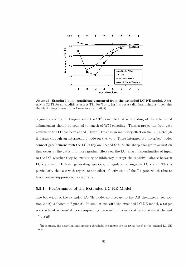
Figure 23 Standard blink conditions generated from the extended LC-NE model. Accu-racy is T2ST1 for all conditions except T1. For T1+1, lag 1 is not a valid data point, as it containsthe blank. Reproduced from Bowman et al. (2008).

ongoing encoding, in keeping with the ST2 principle that withholding of the attentional

enhancement should be coupled to length of WM encoding. Thus, a projection from gate

neurons to the LC has been added. Overall, this has an inhibitory effect on the LC, although

it passes through an intermediate node on the way. These intermediate ‘interface’ nodes

connect gate neurons with the LC. They are needed to turn the sharp changes in activation

that occur at the gates into more gradual effects on the LC. Sharp discontinuities of input

to the LC, whether they be excitatory or inhibitory, disrupt the sensitive balance between

LC state and NE level, generating spurious, unregulated changes in LC state. This is

particularly the case with regard to the offset of activation of the T1 gate, which (due to

trace neuron suppression) is very rapid.

5.5.1 Performance of the Extended LC-NE Model

The behaviour of the extended LC-NE model with regard to key AB phenomena (see sec-

tion 2.3.2) is shown in figure 23. In simulations with the extended LC-NE model, a target

is considered as ‘seen’ if its corresponding trace neuron is in its attractor state at the end

of a trial3.

3In contrast, the detection unit crossing threshold designates the target as ‘seen’ in the original LC-NEmodel.

81

The extended LC-NE model generates an interesting profile of data. Firstly, it generates

a longer basic blink curve, which is more consistent with human data. Secondly, attenuation

of the blink with T2+1 is preserved. Thirdly, as anticipated, the model obtains blink

attenuation with T1+1 blank. The lag 2 data point remains a difficulty with the LC-NE

model, as performance can only recover, at best, to the level defined by the refractory period,

no matter how rapidly the T1 is encoded. This difficulty would be partially offset by an

implementation of weak forward masking, as implemented in the ST2 model. Furthermore,

as suggested previously, the good human performance observed at lag 2 in the T1+1 blank

condition could be attributed to a spreading the sparing-like effect. This is because the T1+1

blank is akin to sustaining an iconic representation of T1, yielding a continuous sequence of

target-related activity. This effect is not explained by the extended LC-NE model.

Finally, there is the issue of what the neurophysiological implications are for the ex-

tensions introduced to the LC-NE model. Firstly, there is nothing controversial about

gate-trace circuits, as inhibitory inter-neurons are common-place in the brain (O’Reilly &

Munakata, 2000). The central point of uncertainty is the suggested projection from WM

encoding areas to the LC, which are posited to have an inhibitory effect. Although it is

known that there are major projections from frontal areas (especially orbital frontal cortex

and the anterior cingulate) to the LC (Aston-Jones & Cohen, 2005), whether these have the

required characteristics to support the extended LC system remains to be answered. For an

approach such as that suggested in this section to obtain greater credence, projections such

as these would need to be identified in the primate brain.

5.6 Final Discussion

The ST2 model provides a concrete and broad scope theory of the AB, which matches a

large spectrum of empirical phenomena. In particular, the model generates a blink curve

with lag 1 sparing, increased processing of the T1+1 slot, blink attenuation with T1+1

blank, blink attenuation with T2+1 blank, delayed consolidation for T2s seen during the

blink and T1-T2 costs at lag 1. In addition, the mechanisms postulated are consistent with

the known spatial specificity of the lag 1 enhancement and a late stage blink bottleneck.

On the other hand, the LC-NE model suggests a compelling theory for the cause of the

82

AB based on a neurophysiologically prescribed theory of attentional function. The model

also generates a number of the key AB phenomena; for example, it generates a blink curve

with lag 1 sparing, increased processing of the T1+1 slot, blink attenuation with T2+1

blank and delayed consolidation for T2s seen during the blink. It is also broadly consistent

with a late stage bottleneck. However, it does not generate blink attenuation with T1+1

blank, T1-T2 costs at lag 1, and the LC theory does not suggest a spatially specific lag 1

enhancement.

While the ST2 model is neurophysiologically plausible, in the sense that it is formu-

lated using known neurobiological mechanisms, there is uncertainty concerning the exact

localisation of some of ST2’s components. Thus, an exploration of the relationship between

the LC-NE model’s brain-level proposal and the ST2 model’s cognitive-level proposal is

potentially valuable, and has been the focus of this chapter. Although it should also be

acknowledged that, when comparing the two models, they have somewhat different intent

and scope. ST2 is a more elaborate model than the LC-NE model, containing more layers

and components. This reflects ST2’s intent to be a relatively broad scope model of temporal

attention and WM encoding and maintenance. In contrast, the LC-NE model, as presented

in Nieuwenhuis, Gilzenrat, et al. (2005), does not claim to model WM, rather its value lies

with the fact that a blink effect is obtained despite only adding a minimal set of additional

assumptions to those included in previous LC-NE simulations (Gilzenrat et al., 2002).

5.6.1 The Blaster and the LC

The LC enhancement and ST2’s blaster have a number of similarities, e.g. both are initiated

by detection of a salient stimulus, they are type non-specific and their temporal profiles are

similar. However, there are important differences between the two.

Firstly, the blaster is postulated to have its effect on stimulus representations relatively

early in the processing pathway, certainly no later than inferotemporal cortex and perhaps

actually in visual cortex (Bowman & Wyble, 2007). The hypothesis being that ‘blasted’

types obtain greater bottom-up trace strength, giving them a tokenisation advantage. Thus,

in ST2, the attentional gate works by regulating bottom-up trace strength. In contrast, the

LC is suggested to have its main effect on decision and response systems (Aston-Jones

& Cohen, 2005). Furthermore, LC innervation is not dense in visual cortex (especially

83

primary visual cortex) (Nieuwenhuis, Aston-Jones, & Cohen, 2005) and LC innervation of

the temporal lobes is more focused on the superior temporal gyrus (especially, the Temporo-

parietal Junction (TPJ)) than the inferior temporal gyrus.

Secondly, the blaster is assumed to be spatially specific; however, the LC enhancement

would be expected to be spatially general, as suggested by neuroanatomical studies of the

pattern of noradrenergic projections (Nieuwenhuis, Aston-Jones, & Cohen, 2005). The LC-

NE approach cannot resolve this difficulty without introducing a further mechanism that

enhances specific locations, and that mechanism is likely to be similar to ST2’s blaster. One

speculative (and perhaps less than parsimonious) explanation could be that the LC provides

the temporal profile of a transient form of attention, such as produced by the blaster. One of

the candidate areas for locating the blaster is the TPJ (Bowman & Wyble, 2007; Corbetta

& Shulman, 2002; Serences et al., 2005) and the LC is known to strongly innervate the TPJ.

If one assumed a spatially specific amplifier at the TPJ, then the LC could be ‘amplifying

the amplifier’ in a transient fashion.

5.6.2 Correlates of the P3

An important question is how to relate models to the P3. The LC-NE theory suggests

a specific neural substrate for the P3 (Nieuwenhuis, Aston-Jones, & Cohen, 2005). The

link from activation traces in the LC-NE model to the P3 though is not as clear cut. In

particular, all the target-induced activations in the LC-NE model peak and indeed finish a

good deal earlier than the known time-course of the P3, as is evident in figure 21. Thus, these

target-induced activations are not direct analogues of the P3. This leaves the possibility

that the P3 is an indirect (delayed) consequence of these target-induced activations; that is,

that there is a latency offset between model activation traces and what is observed as the

P3. However, a judgement of the validity of this explanation awaits a concrete proposal for

the mechanics of this further latency offset. Although not perfect, the time-course of ST2

target activation (especially at the TFL) is more consistent with that of the P3, which, in

an RSVP setting, peaks between 400 and 450ms after the onset of the eliciting stimulus.

Indeed, as introduced in chapter 4 and discussed in later chapters, the ST2 model has been

successfully used to generate virtual ERP components, which are compared with human

ERPs (Craston et al., 2009; Chennu, Craston, Wyble, & Bowman, 2008), including the P3.

84

5.7 Conclusions

The comparatively evaluation of the ST2 and LC-NE models in this chapter has described

the implementation of TAE in both models, and assessed their ability to explain the main

AB phenomena. In doing so, we have gained key insights into how the behaviour and

neurophysiology of temporal attention and the AB could be related. In addition, the pro-

posed extension to the LC-NE model has attempted to combine ideas from both models

and bridge across their levels of explanation. The following chapter shifts focus to explore

a different aspect of the temporal spotlight, namely the influence of target discriminability

on its temporal dynamics.

85

Chapter 6

Target Discriminability and Temporal

Perception

How does the discriminability of targets from distractors affect the temporal dynamics of

visual perception? This is the question investigated in this chapter. This issue is explored

using evidence from EEG data, and complementary neural network modelling. Specifically,

we describe an experiment that manipulates the discriminability of targets in RSVP between

two contrasting conditions, one in which targets are discernible by their visual onset, and

another in which a categorical discrimination must be made to distinguish targets. We then

examine the effect of this on the evoked EEG activity, and attempt to explain the pattern

of changes by simulations involving the ST2 model. As we shall see, this exercise adds

to our understanding of how the process of target discrimination influences the latency of

attentional deployment, in addition to informing issues related to the equivalence of previous

AB experiments.

6.1 Introduction

The deployment of endogenous attention allows the visual system to selectively enhance the

neural representations of task-relevant features in the environment. Our understanding of

the neurophysiology of vision in monkeys suggests that focal attention can modulate neural

activity very early in the visual processing pathway. Studies of neural firing patterns in

86

spatial selection tasks report correlates of endogenous attention in the extrastriate visual

cortex, when a salient feature must be discriminated and selectively enhanced in the presence

of competing spatial distractors (Reynolds, Chelazzi, & Desimone, 1999; Luck et al., 1997;

Chelazzi, Miller, Duncan, & Desimone, 2001). In humans, ERP studies of selective spatial

attention have found that stimulus features at attended locations are enhanced as early as 70-

80ms after onset (Hillyard & Anllo-Vento, 1998). But how does selective attention operate

in time? Specifically, when the visual system is rapidly presented with successive fleeting

stimuli at an already attended spatial location, how quickly can it discriminate a target

embedded in a sequence of distractors, and generate a transient attentional enhancement?

In this regard, previous behavioural research has found that the extent to which irrelevant

distractors temporally interfere with target processing critically depends on how effectively

the visual system is configured to distinguish between featural characteristics of targets and

distractors (Visser et al., 2004).

Visser et al. (2004) use two variants of a sequential stimulus presentation paradigm,

previously used by Ward et al. (1997) to study the Attentional Blink. In the typical RSVP

variant, targets are inserted in a sequential stream of distractors presented at the same

spatial location. In the second variation, referred to in this chapter as Onset (termed the

‘Skeletal’ task by Ward et al. (1997)), no stream of distractors is used. Instead, targets are

briefly presented and are followed by a backward visual mask. See figure 60 in appendix B.2

for samples streams from the Onset and RSVP conditions.

The Attentional Blink deficit is found in many previous studies employing Onset presen-

tation (Ward et al., 1997; McLaughlin et al., 2001; Visser et al., 2004; Rolke et al., 2007).

The AB curves obtained therein are shown in figure 24. However, Visser et al. (2004)

have found that the presence of distractors in RSVP nevertheless influences the difficulty

of target selection during the AB. In addition to the reduction in behavioural accuracy,

another common finding observed with RSVP is lag 1 sparing, which is missing with Onset

presentation1.

1An exception to this pattern is data reported by Visser et al. (2004) (see figure 24C), which suggests asmall amount of lag 1 sparing even with Onset presentation.

87

186 MCLAUGHLIN, SHORE, KLEIN

Comparison of the two paradigms

In examining the stream task and the TM±TM task, the ®rst thing that becomes

apparent is that whereas T1 performance is comparable across the two paradigms, T2

accuracy is much higher in the stream task (compare Figures 4 and 5). Whereas T2

performance (i.e., the group mean for any one lag) never goes below 52% in the stream

task, it falls as low as 11% in the TM±TM task. This pattern might be explained as

follows. In the TM±TM paradigm there is only 45 ms of uninterrupted time to process

T1, whereas in the stream paradigm there is 90 ms. All other things being equal, one

might therefore expect T1 performance to be worse in the TM±TM paradigm. However,

because the two paradigms were blocked subjects could try to optimize their resource

allocation to identify T1. For this purpose, the TM±TM paradigm provides an oppor-

tunity to aim resources at the perceptual moment of T1 because it is the ®rst item

presented. Such effective ``aiming’’ of resource allocation would not be possible in the

stream paradigm because the ®rst item is never T1 and the position of T1 within the

stream is randomized. Therefore, with attention more tightly focused and more intensely

allocated toward T1 in the TM±TM paradigm, the performance disadvantage that one

might have expected for T1 is counteracted and, following the well-accepted notion that

increased attention to T1 will result in an increased blink, that is precise ly what we ®nd

when comparing the two paradigms.

Figure 5. Results from Experiment 3, target mask±target mask task. Target 1 (T1) accuracy and conditional

Target 2 (T2|T1) accuracy at ®ve levels of lag (corresponding to T1±T2 SOA). Error bars represent the

between-observer standard error of the mean.

TEMPORAL DISCRIMINATION WITHIN THE ATTENTIONAL BLINK 1299

which depicts percent correct T2 discrimination and mean RT as a function of task and SOA. Discrimination perfor-mance increased with increasing SOA [F(2,30) 25.8, p .001]. As expected, discrimination performance of the Landolt-squares’ gap was better in the single-task than in the dual-task condition [F(1,15) 31.3, p .001]. Most important, however, this task effect was clearly in-fluenced by SOA [F(2,30) 12.7, p .001]. As SOA increased, discrimination performance of the tasks con-verged to the same performance level. This interaction also mirrors the different effects of SOA in the two task conditions. There was a stronger influence of SOA in the dual-task [F(2,30) 23.8, p .001] than in the single-task [F(2,30) 12.4, p .001] condition. The interaction between task and SOA is consistent with previous stud-ies (e.g., McLaughlin et al., 2001; Ward et al., 1997) and strongly suggests that an AB occurred for the spatial dis-crimination task within the skeletal presentation stream.

An ANOVA on RT supports this conclusion. Due to higher task demands, mean RT was slower in the dual-task than in the single-task condition [F(1,15) 30.2, p .001]. Moreover, mean RT decreased with increasing SOA [F(2,30) 54.5, p .001], and this SOA effect was more pronounced in the dual-task than in the single-task condition [F(2,30) 26.3, p .001]. This interaction most probably illustrates the time demands to process and consolidate T1 into a stable short-term memory repre-sentation. During this time interval, the processing of T2 is postponed and has to wait until attentional capacity is free for the second task. Since the participants were in-structed to react as correctly and as fast as possible, one might argue they have strategically traded speed against accuracy. However, the present pattern of results—that is, slower RTs, together with an impaired discrimination per-formance for T2 at short SOA—excludes such a speed–accuracy trade-off account.

In summary, the present results confirm the well-known AB effect for a spatial task. If participants have to process two rapidly presented targets which are subject to subsequent masking, the second target suffers from the attentional processing of T1. It is important to mention, however, that the processing deficit for T2 in the dual-task condition does not result from low-level masking. This conclusion is supported by the fact that T2 processing in the single-task condition stayed relatively constant across SOA. Taken together, the results of Experiment 1 are in line with several other studies showing an AB for different nontemporal stimuli (e.g., Chun & Potter, 1995; Raymond et al., 1992).

EXPERIMENT 2

In this experiment, we embedded a temporal gap dis-crimination task (Yeshurun & Levy, 2003) as T2 task within the RSVP to investigate the influence of attention on temporal discrimination performance.1

MethodParticipants. A fresh sample of twenty-seven 19–43-year-old

adults served as paid participants. As in Experiment 1, participants

they had recognized. For this task, they responded by keypresses with their middle and index fingers. In the single-task condition, no question mark appeared. Participants initiated the next trial by pressing one of the response keys. A single session lasted about 1.5 h and consisted of 14 blocks of 24 trials each. The single-task and dual-task conditions were blocked and the order of conditions was counterbalanced across participants. The first two blocks of each condition were considered practice and discarded from data analy-sis. After each block, participants received feedback concerning the percentage of correct responses. The experiment factorially com-bined task (single-task vs. dual-task), SOA (183, 366, or 733 msec), and gap position (left vs. right).

Data analysis. Separate two-way ANOVAs with factors task and SOA were performed on percent correct discrimination performance of T2 and on mean RT of correct T2 responses (given correctly iden-tified T1 in the dual-task condition). To assess possible interference effects of T2 processing on the processing of T1, we conducted an additional ANOVA with factor SOA on percent correct recognition performance of T1 in the dual task condition. Whenever appropriate, p values were adjusted for violations of the sphericity assumption using the Huynh–Feldt correction. RTs shorter than 150 or greater than 1,500 msec were considered outliers and their corresponding trials were discarded (1.9%).

Results and DiscussionThe overall recognition performance of T1 (89.4%) was

not influenced by SOA (F 1), indicating that T2 pre-sentation did not affect T1 processing. The results for the spatial discrimination task are summarized in Figure 2,

T2 D

iscr

imin

atio

n (%

Cor

rect

)

50

75

80

85

90

95

100

SOA (msec)

183 366 733

RT T

2 (m

sec)

0

300

400

500

600

700

800

900

1,000

Dual taskSingle task

Figure 2. Results of Experiment 1 (spatial task). Percentage of correct T2 discrimination and mean RT as a function of task and SOA. The standard error was computed from the pooled error terms of the corresponding ANOVA according to a suggestion made by Loftus (2002).

TEMPORAL DISCRIMINATION WITHIN THE ATTENTIONAL BLINK 1299

which depicts percent correct T2 discrimination and mean RT as a function of task and SOA. Discrimination perfor-mance increased with increasing SOA [F(2,30) 25.8, p .001]. As expected, discrimination performance of the Landolt-squares’ gap was better in the single-task than in the dual-task condition [F(1,15) 31.3, p .001]. Most important, however, this task effect was clearly in-fluenced by SOA [F(2,30) 12.7, p .001]. As SOA increased, discrimination performance of the tasks con-verged to the same performance level. This interaction also mirrors the different effects of SOA in the two task conditions. There was a stronger influence of SOA in the dual-task [F(2,30) 23.8, p .001] than in the single-task [F(2,30) 12.4, p .001] condition. The interaction between task and SOA is consistent with previous stud-ies (e.g., McLaughlin et al., 2001; Ward et al., 1997) and strongly suggests that an AB occurred for the spatial dis-crimination task within the skeletal presentation stream.

An ANOVA on RT supports this conclusion. Due to higher task demands, mean RT was slower in the dual-task than in the single-task condition [F(1,15) 30.2, p .001]. Moreover, mean RT decreased with increasing SOA [F(2,30) 54.5, p .001], and this SOA effect was more pronounced in the dual-task than in the single-task condition [F(2,30) 26.3, p .001]. This interaction most probably illustrates the time demands to process and consolidate T1 into a stable short-term memory repre-sentation. During this time interval, the processing of T2 is postponed and has to wait until attentional capacity is free for the second task. Since the participants were in-structed to react as correctly and as fast as possible, one might argue they have strategically traded speed against accuracy. However, the present pattern of results—that is, slower RTs, together with an impaired discrimination per-formance for T2 at short SOA—excludes such a speed–accuracy trade-off account.

In summary, the present results confirm the well-known AB effect for a spatial task. If participants have to process two rapidly presented targets which are subject to subsequent masking, the second target suffers from the attentional processing of T1. It is important to mention, however, that the processing deficit for T2 in the dual-task condition does not result from low-level masking. This conclusion is supported by the fact that T2 processing in the single-task condition stayed relatively constant across SOA. Taken together, the results of Experiment 1 are in line with several other studies showing an AB for different nontemporal stimuli (e.g., Chun & Potter, 1995; Raymond et al., 1992).

EXPERIMENT 2

In this experiment, we embedded a temporal gap dis-crimination task (Yeshurun & Levy, 2003) as T2 task within the RSVP to investigate the influence of attention on temporal discrimination performance.1

MethodParticipants. A fresh sample of twenty-seven 19–43-year-old

adults served as paid participants. As in Experiment 1, participants

they had recognized. For this task, they responded by keypresses with their middle and index fingers. In the single-task condition, no question mark appeared. Participants initiated the next trial by pressing one of the response keys. A single session lasted about 1.5 h and consisted of 14 blocks of 24 trials each. The single-task and dual-task conditions were blocked and the order of conditions was counterbalanced across participants. The first two blocks of each condition were considered practice and discarded from data analy-sis. After each block, participants received feedback concerning the percentage of correct responses. The experiment factorially com-bined task (single-task vs. dual-task), SOA (183, 366, or 733 msec), and gap position (left vs. right).

Data analysis. Separate two-way ANOVAs with factors task and SOA were performed on percent correct discrimination performance of T2 and on mean RT of correct T2 responses (given correctly iden-tified T1 in the dual-task condition). To assess possible interference effects of T2 processing on the processing of T1, we conducted an additional ANOVA with factor SOA on percent correct recognition performance of T1 in the dual task condition. Whenever appropriate, p values were adjusted for violations of the sphericity assumption using the Huynh–Feldt correction. RTs shorter than 150 or greater than 1,500 msec were considered outliers and their corresponding trials were discarded (1.9%).

Results and DiscussionThe overall recognition performance of T1 (89.4%) was

not influenced by SOA (F 1), indicating that T2 pre-sentation did not affect T1 processing. The results for the spatial discrimination task are summarized in Figure 2,

T2 D

iscr

imin

atio

n (%

Cor

rect

)

50

75

80

85

90

95

100

SOA (msec)

183 366 733

RT T

2 (m

sec)

0

300

400

500

600

700

800

900

1,000

Dual taskSingle task

Figure 2. Results of Experiment 1 (spatial task). Percentage of correct T2 discrimination and mean RT as a function of task and SOA. The standard error was computed from the pooled error terms of the corresponding ANOVA according to a suggestion made by Loftus (2002).

B

Contingent capture in the AB 47

T1 - T2 lag (ms)

Percen

tage co

rrect respo

nses (T

2 | T

1)

0

20

40

60

80

100

100 300 700

Figure 3

NO RSVP

RSVP

A

C

ATTENTIONAL BLINK AND DWELL TIME 595

were the same only for the T2 X present trials. T1 and T2 werenever the same on the T2 X absent trials.) The attention factor de-termined the task for subjects. In both attend and ignore T1 condi-tions, subjects were asked to determine whether or not T2 was anX. In the attend T1 conditions, subjects were also asked to report inwhich of two sizes T1 appeared; in this case, the T1 task was stressedover the T2 task. The T2 X presence and SOA factors controlled theidentity and onset of T2. On X present trials, T2 was a black letterX; on X absent trials, T2 was randomly a black H, K, or Y. T2 ap-peared in any one of eight temporal positions, with the SOA fol-lowing T1 ranging from 180 to 810 msec, in 90-msec intervals.

There were three possible sizes for the T2 item: at a viewing dis-tance of approximately 60 cm, small letters subtended approxi-mately .24º ! .48º, medium letters .32º ! .64º, and large letters.48º x .96º. The T1 item was of either small or medium size. Patternmasks following T1 and T2 (illustrated in Figure 1) were 1.17º !1.33º.

All factors were varied within subjects. Each block contained192 trials, 12 trials for each combination of T2 X presence and SOAfactors. Within the experimental session, there were four blocks oftrials, one for each combination of attention and similarity factors.Order of block presentation was counterbalanced between subjects.

Procedure. Each trial proceeded as follows. A fixation dot waspresent in the center of the display before the trial began. Subjectsinitiated the trial by pressing the computer mouse button. At thistime, the immediate offset of the fixation dot was accompanied bya 240-msec auditory signal. There was a random delay of 360–630 msec from fixation offset until the presentation of the RSVP se-quence. In attend T1 blocks, subjects were asked to identify the sizeof the white item (T1), as well as determine whether the seconditem (T2) was the letter X . Subjects were instructed to make thesize discrimination their first priority. In the ignore T1 blocks, sub-jects were asked only to determine whether the second item was theletter X. After the sequence was over, the fixation dot appeared againin the center of the display, and subjects made reports verbally. Inattend T1 blocks, the T1 report was made first (“small” or “large”).The T2 report was always “absent” or “present.” The experimenterentered responses immediately on a computer keyboard.

Before each block of trials began, subjects were given roughly 20trials of practice, mainly to provide familiarity with the T1 dis-crimination required in that block. No feedback was provided dur-ing the experiment.

Stimuli were presented on an Apple Hi-Res 13-in. color monitorcontrolled by an Apple Macintosh IIci running custom software.

Results and DiscussionAnalyses were performed using data from all T2 X

present trials. Accuracy on T2 X absent trials was at ceil-ing (98.7% over all conditions) and showed no effect ofany experimental manipulation. Accuracy on T1 sizejudgments averaged 79.6% correct over all conditions,and we obtained the same pattern of T2 performance re-gardless of whether the analysis was conditionalized onT1 accuracy.

Figure 2 presents T2 accuracy over time, as a functionof attention to T1 and similarity between T1 and T2. Twomain effects are apparent. First, T2 accuracy is higher inthe ignore T1 than the attend T1 conditions, averaging90.2% and 81.25%, respectively [F(1,7) " 11.03, p ".013]. Second, there is a main effect of SOA, such that laterpositions are more accurate than early ones [F(7,49) "10.21, p < .0005]. These two factors also produced a re-liable interaction [F(7,49) " 3.66, p " .003], such thataccuracy in the attend conditions is initially lower but re-covers with time to approximately the same asymptoticlevels as in the ignore conditions. These statistics simplyconfirm the general impression from the figure that at-tention to T1 results in extended interference in process-ing a subsequent T2.

To estimate the duration of interference from T1 pro-cessing on T2, we compared accuracy at each SOA in at-tend and ignore T1 conditions. T2 accuracy was reliablylower for attend than ignore conditions at SOAs of450 msec and below [3.32 > t(7) > 1.90, .005 < p < .05,one-tailed]. At SOAs greater than 450 msec, these differ-ences were not reliable [t(7) < 1.55, p > .05, one-tailed].Interference from an attended object on a subsequent ob-ject in the present study is sustained for approximately400–500 msec, roughly the same duration as found in

15 msec

180 - 810 msec

90 msec

•

360-630 msec

Fixation T1 T2Mask Mask

Figure 1. Schematic of a trial in Experiment 1. All items ap-peared in the center of the display screen. The stimuli depicted(all items shown to scale) are a small T1 and a large T2. Targetsand masks were presented for 15 msec. Mask latency was90 msec. Onset asynchrony between T1 and T2 varied from 180to 810 msec. Following trial initiation and fixation offset was arandom delay between 360 and 630 msec.

0

20

40

60

80

100

100 200 300 400 500 600 700 800 900

T2 A

ccur

acy

(% H

its)

SOA (msec)

Ignore/Different

Attend/Different

Ignore/Identical

Attend/Identical

Figure 2. T2 detection accuracy in Experiment 1, no nontar-gets. Accuracy on T2 X present trials plotted as a function ofT1–T2 SOA. In the ignore T1 conditions (open symbols), only Xpresence or absence for T2 was reported; in attend T1 conditions(filled symbols), the size of T1 was reported in addition to X pres-ence or absence for T2. In different conditions (square symbols),T1 was a white outline box; in identical conditions (cross sym-bols), T1 was a white X.

D

Figure 24 Behavioural accuracy scores from AB studies using Onset presentation. PanelA: Reproduced from Ward et al. (1997). The ‘Attend/Different’ and ’Attend/Identical’ condi-tions represent Onset presentation with two different and identical targets, respectively. The ‘Ig-nore/Different’ and ’Ignore/Identical’ conditions were similar, but participants were required toignore the first target. Panel B: Reproduced from McLaughlin et al. (2001). White squares showT1 accuracy per lag. Black squares indicate T2 accuracy per lag conditional on T1 being correct.Panel C: Reproduced from Visser et al. (2004). The ‘No RSVP’ condition represents Onset presen-tation. Panel D: Reproduced from Rolke et al. (2007). White circles (Single task) show T2 accuracyper lag when subjects were instructed to ignore T1 and report T2. Black circles (Dual task) showT2 accuracy per lag when subjects were instructed to report both T1 and T2 per lag.

88

6.1.1 Motivation and Overview

Taken together, previous behavioural research clearly shows that when distractors are fea-

turally similar to targets, accuracy of target identification is reduced. This chapter builds

upon this finding, and investigates how the time course of target processing is affected by

target discriminability. Adapting an experimental paradigm similar to that used by Visser

et al. (2004), we record EEG data in an experiment that aims to compare the temporal

dynamics of the underlying neural processing evoked by a single target presented in the On-

set and RSVP conditions. We choose a simple one-target setup for our experiment to keep

its design simple, to avoid potential confounds arising from multiple targets, and to allow

us to focus on specific questions relating to EEG dynamics. Importantly, we complement

the analysis of the data from our experiment with a theoretical exploration. Specifically,

we compare the differences in the ERP signatures evoked by targets presented in the above

conditions, and propose an explanation of these differences within the context of the ST2

model. To this end, we take the ST2 model as described in section 3.1, and by performing

a sequence of theoretically sound changes to its configuration, we enable it to simulate the

Onset condition. The modifications are validated by comparing virtual ERP traces gener-

ated from the model to human ERP traces. As we shall see, the model provides a convincing

explanation of the pattern of experimental results, in addition to informing questions about

the cognitive equivalence of target processing in masking and RSVP experiments.

6.2 The Single Target Experiment

This chapter analyses behavioural and EEG data from Experiment 1, which employed a

blocked design with two conditions of interest: trials in the RSVP condition had single letter

targets embedded within a centrally presented RSVP stream of digit distractors presented

at a rate of 47.1ms. In comparison, the Onset condition consisted of single letter targets

presented on their own, and followed by a digit mask immediately after, both presented for

47.1ms. Participants were required to report the identity of the letter at the end of each

trial. The P3 ERPs analysed below were recorded at the P7 and P8 electrodes. Please refer

to appendix B.1 for a detailed overview of the experimental method.

89

10 20 30 400

0.005

0.01

Frequency (Hz)

Pow

er

10 20 30 400

0.005

0.01

Frequency (Hz)

Pow

er

Figure 25 Fast fourier transforms (FFT) of the ERPs for the RSVP (left) and Onset(right) conditions. The ERPs are averaged across the P7 and P8 electrode locations. The RSVPcondition shows a peak in the FFT plot at the frequency of target presentation (approx. 21Hz),which is not present for Onset presentation. Reproduced from Chennu et al. (2009b).

6.3 Target Processing in Onset Presentation

We first present the behavioural and electrophysiological results for targets in Onset pre-

sentation and targets in RSVP. Following this, we elaborate on how the ST2 model can be

modified in order to simulate Onset presentation and conclude this section with a theoretical

discussion.

6.3.1 Behaviour

Overall, when compared to RSVP, Onset presentation makes targets easier to detect. Par-

ticipants report 76% of targets correctly if they are embedded in a regular RSVP stream,

whereas in the Onset condition target accuracy is 86%. This difference is statistically sig-

nificant: F(1,16) = 7.87, MSE @ 0.01, p = 0.01, and corroborates a similar finding by Visser

et al. (2004).

6.3.2 Early Components

Whether a target is presented in Onset presentation or RSVP has a strong effect on early

processing. Figure 26 illustrates a highly significant difference in the P1 and N1 ERP early

components between targets in RSVP and Onset presentation. The mean absolute value in

the area from 0-200ms after target presentation is 3.3µV for targets in Onset streams and

90

T

Figure 26 Human P3 for targets in RSVP and Onset presentation. The ERPs are averagedacross the P7 and P8 electrode locations. ERPs are time-locked to target presentation time ‘T’.Reproduced from Chennu et al. (2009b).

1.02µV for targets in RSVP (F(1,16) = 91.93, MSE = 0.479, p @ 0.001).

Instead of evoking the P1/N1 complex of early components, RSVP targets produce an

ssVEP (steady state Visual Evoked Potential) wave (Di Russo et al., 2003) oscillating at the

same frequency as the presentation rate of items in the RSVP stream. As seen in Figure 25,

each item is presented for 47.1ms (corresponding to the RSVP rate of roughly 20 items per

second), resulting in a peak at approx. 21Hz in the FFT plot for the RSVP condition.

6.3.3 The P3

The P3 component, which is depicted in Figure 26, temporally overlaps with the ssVEP

evoked by the sequence of distractors preceding and following the target, and shows a

different profile for Onset compared to RSVP targets. The 50% area latency (Luck &

Hillyard, 1990) of the P3 in the 200-800ms window is shorter for Onset (mean 452.59) than

RSVP targets (mean 518.53ms). This difference is marginally significant; F(1,16) = 4.16,

MSE = 8885.97, p = 0.06. However, the difference in the mean or peak amplitude of the

P3 in the 200-800ms window is not significant.

91

Blastercircuit

Input layer

Masking layer

Item layer

Task filtered layer

Task Demand

Blasterin

Blasteroutput

Stage 1

Input array forRSVPOnset

Stage 2


... D D T D D ...

... _ _ T D _ ...

Figure 27 Step 1 of simulating Onset presentation. As indicated in the figure, the inputarray to the model is modified by removing distractors.

6.4 Modelling Onset Presentation with the ST2 Model

The ST2 model as published in Bowman and Wyble (2007) and described in Section 3.1

cannot simulate Onset presentation. In the following, we will show how, by making a number

of theoretically justified changes to the architecture of the model, we can replicate our

experimental results with respect to Onset presentation, with respect to both behavioural

and EEG data. Please refer to appendix B.1 for more details of the model configuration.

6.4.1 Step 1: Simulating Early Components

Manipulation

In Onset presentation, the stream contains just the target and the distractor following the

target. All other distractors are replaced by blank intervals. In order to simulate such a

stream in the ST2 model, we modify the array of values that serve as input to the model.

As depicted in figure 27, all distractors - except the one following the target - are set to a

value of zero, equivalent to no activation.

92

.000

.010

.020

.030

.040

.050

.060

.070

-200 0 200 400 600 800 1000 1200

Activation

ms equivalent

RSVP

Onset

T

Figure 28 Virtual ssVEP wave for the RSVP and early components for the Onsetconditions. The virtual ERPs are recorded from the input and masking layers of the ST2 model.‘T’ indicates the presentation of the target. ERPs are time-locked to presentation of the target.Reproduced from Chennu et al. (2009b).

Results

The modification of the input array has a strong effect on virtual ERP traces resembling

early visual processing. For targets in RSVP, the model shows a continuous virtual ssVEP

wave oscillating at the frequency of target presentation (figure 28), replicating the pattern

of human data observed in figure 25. The first item of the RSVP stream causes an increase

of activation in early layers of the model, and subsequent stimuli excite early layers and

suppress previous stimuli due to masking, producing a sustained oscillation that lasts until

the end of the RSVP stream. In effect, the cumulative effect of early visual processing

in the model manifests as the virtual ssVEP, instead of as distinctive early virtual ERP

components. Note that the average activation in the virtual ssVEP in figure 28 is constantly

above zero, because of continual input from the RSVP stream. However, the actual value

of this activation has no particular significance. In human EEG data, baseline corrections

ensure that the mean amplitude over time of the human ssVEP is close to zero.

In contrast, in Onset presentation, there are no distractors and hence there is no acti-

vation preceding the target. Presentation of the target creates a strong burst of activation

at early layers of the ST2 model. As there is no forward masking, the activation evoked by

93

the Onset target at early layers is higher than in regular RSVP. The distractor following

the target in Onset presentation then produces a second large burst of activation, as it is

not constrained by backward masking. All of this activation at early layers occurs between

the model equivalent of 100 and 200ms following target presentation.

Overall, there is a general qualitative match between the observed changes in the virtual

ERPs (figure 28) and the human early ERP components (figure 26), comparing across the

RSVP and Onset conditions. Virtual ERP activation associated with early visual processing

shows a distinct activation for Onset targets and an oscillatory pattern for RSVP targets.

However, it is evident that there are considerable differences between the virtual ERP for

the Onset condition and the P1/N1 complex observed in the human ERP. This is because

the ST2 model does not incorporate much of the complexity of early visual processing that

underlies this complex. Furthermore, many factors, such as the distortion of the signal by

the scalp, are not simulated2. Nevertheless, by matching the model to human behaviour

and comparing the consequently generated virtual ERPs again their human counterparts, we

have attempted to provide an common explanation for patterns of change in the behavioural

and EEG data.

6.4.2 Step 2: Simulating the P3

Manipulation

Replication of behavioural accuracy and the virtual P3 component requires theoretically

justified changes to the architecture of the ST2 model. Onset targets appear on a previously

blank screen, whereas in RSVP, the target has to be selected from a continuous stream of

distractors. In terms of the ST2 model, we hypothesise that the difference between target

detection in these conditions influences the way in which the blaster is triggered:

Y In RSVP, the system cannot distinguish targets from distractors until they have

reached the TFL. There, the task demand mechanism acts as a filter, selectively enhancing

targets and inhibiting distractors.

Y In Onset presentation, there are no distractors preceding the target, hence, the system

2See the Dynamic Causal Modelling (DCM) technique (David et al., 2005, 2006) for an example of anapproach to modelling ERPs that is based on a neurobiologically constrained source reconstruction.

94

Blastercircuit

Input layer

Masking layer

Item layer

Task filtered layer

Task Demand

Blasterin

Blasteroutput

Stage 1

Blaster 'trigger' forRSVPOnset

weight0.02003

weight0.015

Stage 2


Figure 29 Step 2 of simulating Onset presentation. The connection from Stage 1 that triggersthe blaster is moved from the task filtered layer to the masking layer. Reproduced from Chennu etal. (2009b).

can assume that the first item that is ‘presented’ to the input layer is the target. Accordingly

and as seen in Figure 29, we propose that in Onset presentation, the blaster is triggered

as soon as activation reaches the masking layer3. Moving this connection from the TFL to

the masking layer also requires a modification of the weight value of that connection (see

Figure 29), because activation levels in the TFL and masking layers differ4.

Results

Activation propagates through the ST2 model with a temporal lag from one layer to the

next. Hence, if the blaster is triggered from the masking layer, the blaster fires at an earlier

timepoint relative to target onset than if activation has to propagate to the TFL before

the blaster can be triggered. Consequently, the blaster’s output is also shifted earlier in

3For the purpose of simulating Onset presentation, our manipulation produces the desired effect. How-ever, our modification of the model architecture would have to be reconsidered in order to simulate a slightlydifferent stream setup, for instance, if the target was also preceded by distractor items (e.g. a stream of thetype ‘D D T D’). Under these circumstances, the distractors can potentially also fire the blaster, as taskdemand does not operate until the TFL and, hence, the system cannot distinguish targets from distractorsat the masking layer. Note, however, that although distractors can fire the blaster in Onset presentation,task demand at the TFL will prevent distractors from being tokenised.

4Compared to the TFL, activation values at the masking layer are higher in absolute terms. Hence,we reduce the weight values between masking layer and blaster, to prevent the blaster circuit from beingovercharged by the input from the masking layer.

95

.000

.050

.100

.150

.200

-200 0 200 400 600 800 1000 1200

Activation

ms equivalent

RSVP

Onset

T

Figure 30 After Step 2: Virtual P3 for the RSVP and Onset conditions. The RSVP virtualERP is baseline corrected to -200 to 0ms with respect to target onset to account for distractor relatedactivity, which is absent in the Onset condition. ERPs are time-locked to target presentation time‘T’. Reproduced from Chennu et al. (2009b).

time. The first consequence of this change is a shift in latency of the virtual P3 for Onset

compared to RSVP targets, as seen in Figure 30. With the change in model architecture

to reflect processing of Onset targets, the blaster is triggered earlier, and thus initiates the

target’s tokenisation and virtual P3 earlier than in the RSVP condition.

The change in model architecture means that the blaster now fires for all Onset targets.

This correctly increases the accuracy of the ST2 model at encoding Onset targets relative to

RSVP targets (100% vs 77%). Furthermore, the same change in the model that simulated

the behavioural effect also produces a latency difference in the virtual P3: the 50% area

latency of the virtual P3 in the 200-600ms window is shorter for Onset (365ms) than for

RSVP targets (430ms). This pattern replicates the significant latency difference observed

in human P3 data.

Although behavioural accuracy in the Onset condition should indeed be above RSVP

accuracy, this is not a very good replication of the human behavioural performance for

detecting Onset targets, which is below ceiling. A further modification of the weight value

between masking layer and blaster does not have the desired effect on simulated accuracy

96

Blastercircuit

Input layer

Masking layer

Item layer

Task filtered layer (TFL)

Task demand

Blasterin

Blasteroutput

Stage 1

Stage 2

Reduce weightby 0.92%

STEP 3


Figure 31 Step 3 of simulating Onset presentation. The weight of the connection from taskdemand to target nodes in the TFL is reduced by 0.92%.

and virtual P3 for Onset targets. This is due to the blaster ‘trigger’ functioning in an ‘all-

or-none’ fashion, hence, the weight value would have to be reduced to close to zero before

there is any further effect on the target’s tokenisation process. Reducing the weight to

close to zero, however, has a counterproductive effect as, in this case, the blaster can only

be triggered by those targets with the highest strength values. Consequently, only a few

targets are tokenised and all other targets are not ‘detected’ by the model. This reduces

the simulated accuracy in the Onset condition to below that for RSVP targets, which is

obviously not a desirable replication of the human data either. Consequently, we need to

perform one additional modification to the architecture of the ST2 model, as described in

the next section, in order to accurately simulate Onset presentation.

6.4.3 Step 3: Simulating Behavioural Accuracy

Manipulation

An RSVP stream consists of one or more targets embedded in a stream of distractors. In

Onset presentation, however, the stream contains only the target and the following distrac-

tor. When an RSVP target arrives at the TFL, the task demand mechanism plays a vital

role in selecting the target from simultaneously active distractors. In Onset presentation,

97

.000

.050

.100

.150

.200

-200 0 200 400 600 800 1000 1200

Activation

ms equivalent

RSVP

Onset

T

Figure 32 After Step 3: Virtual P3 for the RSVP and Onset conditions. The RSVP virtualERP is baseline corrected to -200 to 0ms with respect to target onset to account for distractor relatedactivity, which is absent in the Onset condition. ‘T’ indicates the presentation of the target andERPs time-locked to presentation of the target.

however, the target competes with only one other distractor at the TFL and hence there

is no need for the task demand mechanism to be as strong. Conceptually, in Onset pre-

sentation, the focus of selection moves earlier and reducing the strength of the task filter

reflects this adjustment of focus. In other words, as the system can select earlier with Onset

presentation, its later selection mechanism (at the TFL) can be more liberal. Consequently,

we reduce the weight from task demand to target nodes in the TFL by 0.92% of the original

value (see Figure 31).

Results

The reduction in task demand for Onset presentation means that target nodes have less

activation at the TFL. Relatively strong targets can nevertheless initiate a tokenisation

process despite lower activation levels. Weak targets, however, fail to overcome the threshold

for tokenisation and cannot proceed into Stage 2 for working memory encoding. After

this modification to the model’s architecture, weak Onset targets have too little activation

for tokenisation and are ‘missed’. The ST2 model now generates a simulated accuracy of

85% for Onset targets, which replicates the human behavioural accuracy for Onset targets.

98

Simulated RSVP accuracy from the model obviously remains unchanged at 77%.

The deceased task demand also causes a change in the virtual P3 evoked in the Onset

condition. As can be seen in figure 32, there is a reduction in its mean amplitude compared

to the RSVP condition. This reduction is in addition to the latency shift produced in it

after Step 2 (figure 30), and is produced because the reduction in task demand means that

target nodes in the TFL receive less positive bias. Consequently, in comparison to the

RSVP condition, target nodes in the Onset condition have relatively lesser activation going

into Stage 2 and evoke a weaker virtual P3 during the tokenisation process. This pattern of

differences between the virtual P3s bears qualitative correspondence to the visual differences

observed in the human P3s in figure 26. As can be seen therein, the human P3 for the RSVP

condition has a higher grand average peak amplitude in the RSVP condition than in the

Onset condition, though this could not be verified statistically.

6.5 Discussion

After making the described changes to the ST2 model, we have enabled it to simulate

the Onset condition in terms of its qualitative relationships to the RSVP condition, with

respect to both behavioural and EEG data. Comparing these to the simulation of target

presentation in RSVP provides us a potential explanation of the mechanisms underlying the

observed differences in behavioural and EEG data.

6.5.1 Early Components vs. the ssVEP

Consistent with previous findings, individually presented items in Onset presentation pro-

duce the P1/N1 complex, whereas repeatedly presented items in RSVP evoke an ssVEP

wave oscillating at the frequency of stimulus presentation (Mueller & Hillyard, 2000). In

RSVP, the virtual ssVEP oscillation is caused by the stream of distractors and targets feed-

ing into the model. Each item is presented at the input layer and propagates to the masking

layer where the item experiences weak inhibition from previous items (forward masking).

The item generates a short-lived peak of activation in the virtual ssVEP, before it is subject

to stronger suppression from the following item in the RSVP stream (backward masking).

This process repeats itself for each item in the RSVP stream and causes the oscillatory

99

pattern that can be observed in the virtual ssVEP wave.

In Onset presentation, the target is not forward masked, hence its activation at early

layers of the ST2 model is immediately larger than the activation of a target in RSVP. The

following distractor inhibits the target, which causes a very transient reduction in activation.

Following this, the distractor’s activation causes a large spike in the virtual ERP, as it is not

backward masked. Although visually quite different to the P1/N1 complex in the human

ERP, the virtual ERP representing early processing in the ST2 model has a corresponding

time course and is a qualitative fit to the human data.

6.5.2 Lag 1 Sparing and Onset Presentation

After modifying the ST2 model, we are able to simulate Onset presentation and can qual-

itatively replicate the human data in our single target paradigm in terms of behavioural

accuracy and virtual ERPs. Our change to the model architecture also suggests a predic-

tion about lag 1 sparing in two target paradigms investigating the AB.

In the regular RSVP, targets are embedded in a continuous stream of distractors. If two

targets are presented in immediate succession, and they are backward masked by at least

one distractor, T2 accuracy is quite high. In fact, T2 accuracy is often higher than that

of single target detection. This is the lag 1 sparing effect (see section 2.3.2). In an AB

experiment using Onset presentation, however, we would expect there to be no such second

target advantage.

According to the ST2 model, this is because in a regular RSVP stream, T1 triggers the

blaster when it reaches the TFL. However, there is some temporal delay between the blaster

being triggered and the timepoint of its full effect on the item layer and the TFL. In regular

RSVP, this means that a T2 appearing at the TFL shortly after T1 will get much of the

benefit of T1’s blaster response. This results in the increased accuracy at detecting T2,

manifesting as lag 1 sparing.

In Onset presentation however, T1 triggers the blaster at an earlier timepoint, i.e. as

soon as T1 reaches the masking layer. Despite there being some temporal delay until the

blaster becomes fully active, the blaster will have its major effect by the time T1’s activation

has reached the item layer and the TFL. As Onset presentation causes the whole activation

profile of the blaster to be earlier in time, the blaster is no longer active when T2 arrives,

100

as it is already being suppressed by T1’s tokenisation. Hence, the ST2 model predicts low

accuracy for T2 at lag 1 in Onset presentation.

Turning to the evidence from human data, we know that in the regular RSVP condition,

if T2 is presented immediately following T1, its accuracy is high, i.e. we observe clear lag

1 sparing (see section 2.3.2). In comparison, behavioural data from AB studies employing

Onset presentation (see figure 24) suggest that the evidence for lag 1 sparing is weak. Indeed,

with the exception of findings by Visser et al. (2004), most of the previous studies employing

Onset presentation (Ward et al., 1997; McLaughlin et al., 2001; Rolke et al., 2007) find that

T2 accuracy is lowest at lag 1.

6.5.3 Is Onset Presentation an Equal Substitute for RSVP?

Despite its common application in experiments designed to study temporal visual processing,

the RSVP paradigm has a number of practical disadvantages. Due to the fast presentation

rate, RSVP streams contain a large number of distractors, and have a typical duration of

2-3 seconds. Furthermore, the rapid presentation of items is often taxing for participants,

especially in long experiments. This situation arises when conducting EEG or Magnetoen-

cephalography (MEG) experiments, where, in order to increase the signal-to-noise ratio by

averaging, each condition is presented several times. Hence, as experimental time in an

EEG/MEG laboratory is costly, there is a major incentive to minimise the duration of the

experiment.

In comparison, the Onset task ‘minimises demands both on selective attentional process-

ing and on location switching mechanisms’ (Ward et al., 1997), while nevertheless seeming

to reveal the attentional limitations underlying the AB. Thus, due to simpler and shorter

experiments, the Onset condition seems ideal for studies employing MEG or EEG to study

the AB. Indeed, as a previous study investigating the AB by means of MEG and the Onset

condition states: ‘an AB effect is observed whether targets are embedded in a 20-item RSVP

stream or just presented on their own followed by masks. In order to save measurement time,

we decided to employ this abbreviated version for our study’ (Kessler et al., 2005). However,

from the results presented in this chapter, we argue that there are considerable differences in

target processing between Onset presentation and RSVP. Though our experiment employed

only a single target, we believe that these results inform and are directly relevant to dual

101

target RSVP studies. Consequently, direct comparisons between EEG/MEG data collected

using these two paradigms should be interpreted with caution.

6.6 Conclusions

This chapter has investigated the influence of target discriminability on temporal dynamics

of visual perception using electrophysiology. In addition, by making systematic and jus-

tifiable changes to the ST2 model, we have enabled it to simulate Onset presentation of

targets. The comparison between the performance of this modified version to the original

one has allowed us to propose an explanation to the observed differences in the human EEG

between the RSVP and Onset conditions, on the basis of how target discriminability affects

the latency of attentional deployment. Further, this exercise has informed questions about

the experimental equivalence of these paradigms, at the level of neural dynamics, for the

study of the Attentional Blink phenomenon.

102

Chapter 7

The Temporal Precision of Attention

In this chapter, we continue our exploration of the temporal spotlight, and investigate its

role in providing perception with temporal precision. Using the Attentional Blink (AB) as

a modulatory mechanism and EEG as an index of temporal dynamics, we will show how

impairing the temporal spotlight adversely affects conscious perception. We describe data

from an EEG experiment, which is used to compare the temporal precision of perception

outside and inside the AB window. In this process, we begin with an analysis of average

ERPs, and then delve deeper into time-frequency analysis of single trial EEG data to provide

a more fine-grained test of our hypothesis. We then interpret our findings from this analysis

using virtual ERP simulations from the ST2 model, to propose an explanation based on

variation in the temporal precision of attention.

7.1 Introduction

This chapter investigates the hypothesis that diminished attentional control increases the

temporal jitter in the latency of a target’s working memory consolidation. The Attentional

Blink (AB) provides us with a suitable phenomenon with which to test our hypothesis: we

propose that the reduced availability of attention during the AB increases the temporal

noise in visual attention. To investigate this issue, we compare the ERPs evoked by targets

outside vs. inside the AB. In doing so, we determine whether there is an increase in the inter-

trial variability of the latency of target consolidation inside the AB. EEG has the advantage

of excellent temporal resolution, allowing us to study short-lived cognitive events that evoke

103

changes in ongoing EEG activity. To test for increased temporal jitter, we analyse the N2pc

and P3 ERP components, commonly associated with selective attention (Eimer, 1996) and

working memory (Kok, 2001; Vogel et al., 1998), respectively.

In addition to presenting and analysing human EEG data, we use the ST2 model’s

neural network implementation to generate virtual ERPs (see chapter 4). For each of the

experimental conditions, virtual ERPs are contrasted with human ERPs, both at the level

of grand averages and single trials. This comparative evaluation allows us to validate the

ST2 model and propose explanations for the human ERP effects.

7.1.1 Attentional Precision and the ST2 Model

Before delving into the EEG data, we summarise the predictions of the ST2 model about

temporal variability in target processing. The model suggests that working memory en-

coding involves creating a binding between the type of a stimulus (which can include its

visual features and semantic attributes) and a token (an episodic representation specific to

a particular occurrence of an item) (Kanwisher, 1987; Mozer, 1989). In the ST2 model,

a Transient Attentional Enhancement (TAE) from the blaster amplifies the type represen-

tation of a salient (i.e., task relevant) stimulus to assist in its binding to a token, in a

process referred to as tokenisation. This TAE can serve as an attentional gate, which can

be temporarily deactivated to allow one target encoding to be completed before a second is

begun.

From the perspective of the ST2 model, the AB is an artefact of the visual system

attempting to assign unique tokens to targets (Wyble, Bowman, & Nieuwenstein, 2009)1.

More specifically, the process of encoding T1 into working memory is triggered by TAE,

and TAE itself is subsequently suppressed until T1 encoding has completed. The period

of TAE unavailability varies from trial to trial depending on how long it takes to tokenise

T1, which in turn depends on its bottom-up strength. As pointed out previously in this

thesis, the ST2 model suggests that there is a reciprocal relationship between T1 strength

and the duration of its tokenisation process (see chapter 5 and Bowman et al., 2008). Thus,

1In order to explain findings relating to the AB, the definition of an episode is extended in Wyble,Bowman, and Nieuwenstein (2009) to include multiple tokens. Nevertheless, for the purposes of this chapter,each token corresponds to an episodic context in working memory.

104

in an RSVP stream, if a T2 is presented 100-600ms after a perceived T1 (as is the case

during the AB), its processing outcome depends on multiple factors. T2’s own strength

determines its dependence on TAE, as highly salient T2s might potentially ‘break-through’

the AB (Anderson, 2005) and get encoded relatively early. T2s with strength values slightly

lower in the range ‘outlive’ the AB (and thus the unavailability of TAE), and hence are

indirectly influenced by T1 strength. Overall, the variability in the temporal dynamics of

T2’s encoding process is influenced both by T1 and T2 strengths. Hence, over all possible

strengths, the ST2 model proposes that there should be increased variance in processing

latency for targets seen during the AB. With this initial prediction from the ST2 model, we

now proceed to describe results from an EEG experiment that serves to test it.

7.2 The Two Target Experiment

This chapter analyses behavioural and EEG data from Experiment 2. The experiment

consisted of RSVP trials with two bilateral streams, presented at a rate of 105.9ms per

item. Each trial had two letter targets, T1 and T2, embedded among digit distractors. T2

was presented at lags 1, 3 and 8 following the T1. EEG was recorded from participants while

the streams were being presented, and later correlated with their behavioural responses. The

N2pc ERPs analysed in this section were recorded at the P7, P8, O1 and O2 electrodes,

while the P3 ERP was recorded at the Pz electrode. Please refer to appendix B.2 for a

detailed overview of the experimental method.

7.3 Behavioural Analysis

The mean human accuracy for T1 identification in Experiment 2 is 82%. The accuracy of

T2 identification (conditional on correct report of T1) is 83% at lag 1, 54% at lag 3, and

74% at lag 8. There is a significant effect of lag on accuracy (F(1.48,12.58) = 15.58, MSE =

0.03, p @ 0.001, after applying a Greenhouse-Geisser correction on the degrees of freedom).

Additionally, in pairwise comparisons, T2 accuracy is significantly lower at lag 3 compared

to lag 8 (F(1,17) = 11.66, MSE = .03, p @ 0.01) and lag 1 (F(1,17) = 60.88, MSE = 0.01,

p @ 0.001). Consequently, the paradigm employed evokes a reliable AB effect.

105

7.4 ERP Analysis

Figure 33A depicts the grand average human N2pc ERPs evoked by targets presented outside

(all T1s followed by T2s at lag 8 ) and inside (all T2s at lag 3 following a seen T1 ) the

AB. A standard one-way repeated measures ANOVA reveals that there is no significant

difference across subjects, in the mean/peak amplitude of the N2pc ERPs within the 130-

260ms window indicated in the figure (F @ 1). Further, analysis of the onset latency of the

N2pc using jackknife analysis (with an onset criterion of 50% of peak amplitude; see J. Miller,

Patterson, & Ulrich, 1998) did not find any differences (t @ 1). The lack of any difference in

mean N2pc amplitude stands in contrast to results reported by Jolicoeur, Sessa, Dell’Acqua,

and Robitaille (2006), who found that the N2pc evoked by targets presented inside the AB

was significantly smaller than that evoked by targets presented outside it (see Jolicoeur et

al., 2006; figure 3). In our data, as evident in figure 33A, we find that the N2pc evoked by

targets presented inside the AB has a comparatively less well-defined onset and offset, and

increased horizontal spread2.

The human P3 ERPs for targets presented outside and inside the AB is depicted in

figure 33B. As suggested by the large reduction of amplitude in the figure, there is a sig-

nificant reduction in P3 amplitude for targets inside the AB within the 300-700ms window

indicated therein: targets presented outside the AB have a mean P3 amplitude of 3.68µV,

while targets presented inside the AB have a mean amplitude of 2.22µV (F(1,17) = 11.61,

MSE = 1.65, p @ 0.01). However, there is no suggestion of a latency difference between the

P3s, as measured by subject-wise 50% area latency analysis (Luck & Hillyard, 1990) (F @

1).

The comparative analysis of ERPs performed above is confounded by the variation in

behavioural accuracy across the conditions, occurring as a natural consequence of the AB

effect. In other words, the ERPs for targets presented inside the AB include a much greater

number of trials in which targets were completely missed or partially processed, but failed to

2Findings by Jolicoeur et al. (2006) also suggest that the N2pcs for seen T2s at lag 3 might be temporallycoincident with the Sustained Posterior Contralateral Negativity (SPCN) component evoked by the seenT1 preceding it. This is because, in their data, the SPCN component occurred in the 300-500ms windowfollowing target onset (Jolicoeur et al., 2006; figure 3). However, no such component is evident in our data,either for targets presented outside or inside the AB. Specifically, in figure 33A, there is no statisticallysignificant negativity in the 300-500ms window following target onset.

106

200 100 0 100 200 300 400 500 600 7002.5

2

1.5

1

0.5

0

0.5

1

1.5

2

Time from target onset (ms)

Am

plitu

de (u

V)

Targets Presented Outside the ABTargets Presented Inside the AB

A: N2pc

B: P3

200 0 200 400 600 8004

2

0

2

4

6

8

10

12

14


Am

plitu

de (u

V)

Targets Presented Outside the ABTargets Presented Inside the AB

Figure 33 Human ERPs for targets presented outside and inside the AB. Panel A: Grandaverage N2pc. Panel B: Grand average P3. Dashed lines indicate the window used for statisticalanalysis.

107

be correctly reported. Such targets are unlikely to evoke a clear P3, as has been previously

reported (Kranczioch et al., 2003; Vogel et al., 1998). Consequently, the process of averaging

over trials with varying behavioural responses in the above conditions could have resulted in

a differential attenuation of the ERPs for targets presented inside the AB. To address this

issue, we investigate the N2pc and P3 evoked only by correctly reported or seen targets,

and evaluate our EEG data against our hypothesis of increased temporal variability.

Figure 34A depicts the N2pc evoked by targets seen outside (T1 Lag 8: seen T1s followed

by T2s at lag 8 ) and inside (T2 Lag 3: seen T2s at lag 3 following a seen T1 ) the AB. The

pattern of variation observed here is similar to that in figure 33A: the N2pc evoked by targets

seen inside the AB appears to be more attenuated and spread out in the grand average. But

as before, there is no statistically significant difference between the N2pc ERPs in terms

of mean/peak amplitude (F @ 1) within the 130-260ms window indicated in the figure. A

comparison of jackknife latency (with an onset criterion of 50% of peak amplitude) suggests

a small difference: the N2pc for targets seen inside the AB is later (195.12ms) than that for

targets seen outside the AB (164.68ms). However, this difference does not reach significance

(t(1,17) = 1.19, p = 0.13).

With the P3, as before, we observe significant differences (figure 34B), with targets seen

inside the AB evoking an attenuated P3 in the 300-700ms window: targets seen outside

the AB have a mean amplitude of 4.08µV, while targets seen inside the AB have a mean

amplitude of 2.69µV (F(1,17) = 9.09, MSE = 1.92, p @ 0.01). In addition, a 50% area

latency analysis reveals that targets seen inside the AB evoke a significantly delayed P3

(483.78ms) compared to targets seen outside the AB (455.78ms): F(1,17) = 6.33, MSE =

1115.31, p = 0.02. This finding agrees with results reported by Martens, Elmallah, et al.

(2006) and Vogel and Luck (2002), who have found that target consolidation is delayed

during the AB.

On the whole, these findings suggest that, even for targets that are seen inside the AB,

there might exist key differences in the dynamics of temporal visual processing, as compared

to targets seen outside the AB. Indeed, as is evident in figure 34A (and in figure 33A), the

N2pc ERPs evoked by targets outside and inside the AB appear to have very different

temporal profiles. However, these differences are not very well suited to the application of

the average ERP analysis techniques we have employed in this section. In particular, the

108

200 100 0 100 200 300 400 500 600 7002.5

2

1.5

1

0.5

0

0.5

1

1.5

2


Am

plitu

de (u

V)

Targets Seen Outside the ABTargets Seen Inside the AB

A: N2pc

B: P3

200 0 200 400 600 8004

2

0

2

4

6

8

10

12

14


Am

plitu

de (u

V)

Targets Seen Outside the ABTargets Seen Inside the AB

Figure 34 Human ERPs for targets seen outside and inside the AB. Panel A: Grandaverage N2pc. Panel B: Grand average P3. Dashed lines indicate the window used for statisticalanalysis.

109

statistical results produced by mean/peak amplitude analysis, jackknife analysis, etc. are

sensitive to the choice of the time window used to define the ERP component. Owing to

the temporal characteristics of the N2pc evoked by targets inside the AB, the appropriate

choice of this window is difficult, and has to be based on unreliable visual estimates. In the

next section, we circumvent these problems and go beyond the analysis of average ERPs.

Instead, we enquire into differences in the temporal dynamics of target processing outside

and inside the AB at the level of single EEG trials.

7.5 Single-Trial Analysis

We now go beyond an analysis of averaged ERP components, as such methods cannot di-

rectly inform our hypothesis of reduced attentional precision during the AB. This is because

the averaging collapses across and hence discards information about temporal fluctuations

in the individual EEG trials contributing to the ERP. Given a set of trials that are averaged

together, both decreases in amplitude and increases in latency variation within that set will

attenuate the mean amplitude of the ERP. Hence, examining the average does not directly

provide the necessary information to decide which of the two sources of variation in the

individual trials (amplitude or latency) caused the reduction in ERP amplitude. Further,

measures like 50% area latency analysis (Luck & Hillyard, 1990) cannot be used to measure

latencies in single trials, due to the levels of irrelevant noise activity. Consequently, we

employ time-frequency analysis techniques that provide alternative measures to investigate

single trial dynamics underlying grand average ERPs. These methods enable us to perform

a more fine-grained analysis of EEG data, and test our hypothesis using both qualitative

and quantitative means.

7.5.1 Analysis of ITC and ERSP

To begin our investigation of the single-trial dynamics latent in the N2pc and the P3 ERPs,

we characterise their time-frequency signatures by calculating Inter-Trial phase Coherence

analysis (ITC) and Event-Related Spectral Perturbation (ERSP) (Delorme & Makeig, 2004;

Tallon-Baudry, Bertrand, Delpuech, & Pernier, 1996). ITC provides an index of the amount

of inter-trial variability in the latency of EEG activity. Here, latency is estimated by the

110

phase of the EEG signal, calculated using wavelet-based time-frequency analysis (see ap-

pendix B.2 for details). From these phase values, ITC is calculated as a dimensionless

scalar normalised to a value between 0 and 1. It measures the extent to which the phase of

stimulus-locked EEG activity at a particular frequency is correlated across a set of trials.

Time-frequency maps of ITC values allow us to visualise the amount of phase synchronisa-

tion in different time windows and frequency bands. The other measure we are interested

in, ERSP, estimates stimulus-related power changes, measured in decibels. In parallel with

ITC, ERSP time-frequency plots depict how the stimulus-related power fluctuates over time

and across frequencies.

In the following analysis, we are interested in investigating the ITC underlying the

N2pc and P3 ERP components. Consequently, we measure and comparatively evaluate the

temporal variation in ITC within the time and frequency windows where the power of these

ERP components is located. At a given time-frequency point, an ITC value of 0 indicates

a complete lack of phase coherence across the set of trials being analysed, whereas an ITC

value of 1 signifies that the phase is perfectly time-locked to the stimulus. ITC values

can hence be visualised in a time-frequency colourmap with time relative to stimulus onset

along one dimension, and frequency along another. Each data point in the plot is coloured

according to the amount of ITC observed at a particular time and frequency across all trials

in an experimental condition. Please refer to appendix B.2 for further details about the ITC

analysis parameters.

Figure 35 shows the ITC plots for the N2pc and P3 components. Each of the time-

frequency plots in the figure is a colour map depicting ITC effects time-locked to the pre-

sentation of the target, which occurs at timepoint zero. As indicated by the colour scale to

the right, increased ‘redness’ represents a larger ITC value, and thus more phase synchro-

nisation across the trials making up the corresponding grand averages in figure 34. ITC

significance for each data point in these plots is calculated using a two-tailed bootstrap sig-

nificance test with a significance criterion of 0.01 (Delorme & Makeig, 2004). Non-significant

data points are coloured green. In this regard, it is important to note that bootstrap anal-

ysis does not correct for multiple comparisons at the time-frequency data points. However,

in practice, neighbouring data points calculated by time-frequency decomposition are not

111


Freq

uenc

y (H

z)

0 100 200 300 400 5001

2

3

4

5ITC

0

0.05

0.1

0.15

0.2

0.25


Freq

uenc

y (H

z)

0 200 400 6001

2

3

4

5ITC

0

0.1

0.2

0.3

0.4

0.5


Freq

uenc

y (H

z)

0 100 200 300 400 5001

2

3

4

5ITC

0

0.05

0.1

0.15

0.2

0.25


Freq

uenc

y (H

z)

0 200 400 6001

2

3

4

5ITC

0

0.1

0.2

0.3

0.4

0.5


Freq

uenc

y (H

z)

0 100 200 300 400 5001

2

3

4

5ITC

0.15

0.1

0.05

0

0.05

0.1

0.15


Freq

uenc

y (H

z)

0 200 400 6001

2

3

4

5ITC

0.5

0

0.5

Targ

ets

outs

ide

the

ABN2pc ITC P3 ITCA B

Targ

ets

insi

de th

e AB

C D

Diff

eren

ce

E F

Figure 35 Inter-trial Coherence produced in the N2pc and the P3 evoked by targetsinside and outside the AB. The left column shows ITC time-frequency plots for the N2pc, whilethe right column shows those for the P3. Targets outside the AB are plotted on the first row, andtargets inside the AB on the second row. The final row contains a difference plot between the twoconditions. Dashed lines indicate time window of interest for the ERP in question.

112

independent, and are highly correlated3. We avoid the multiple comparisons problem by

basing our analysis on an a priori hypothesis of expected differences in ITC. Specifically, we

compare the ITC evoked by targets outside and inside the AB only within the time windows

defined by the grand average ERPs in figure 34 (130-260ms for the N2pc and 300-700ms

for the P3). The corresponding windows are indicated by dashed lines in the ITC plots in

figure 35. Further, we focus only on the 1-5Hz frequency window, where the power of the

N2pc and P3 are located. According to our hypothesis, the relative decrease in temporal

precision for targets inside the AB should produce a corresponding reduction in ITC evoked

by the N2pc/P3 within this time-frequency window. Hence, a smaller ITC value for targets

inside the AB (compared to targets outside the AB) would argue for increased temporal

jitter across the single-trial ERPs evoked in this condition.

In figure 35, the first row depicts ITC effects for targets outside the AB and the second

row depicts the ITC for targets inside the AB. The third row shows differences in ITC

between the previous two plots. As apparent from the altered colour scale for these difference

plots, a positive data point coloured red indicates a significantly greater ITC in the former

(target outside the AB) condition, whereas a negative data point coloured blue indicates a

significantly greater ITC in the latter (target inside the AB) condition.

The left column of figure 35 depicts the ITC plots of EEG activity underlying the N2pc

ERP component. A visual comparison of the relevant time windows within the plots in

figures 35A and 35C suggests that the N2pc for targets inside the AB does indeed produce

lesser ITC than targets outside the AB. The difference plot in figure 35E corroborates this,

as it registers an increased amount of ITC in figure 35A than in figure 35C, within the N2pc

time window.

Turning to the P3 ITC plots in the right column, it is evident that the P3 evoked by

targets inside the AB produces much lesser ITC than targets outside the AB (figures 35B

and 35D). Further, the large positive region within the P3 time window in the difference

plot in figure 35F, along with its wider colour scale, clearly shows that there is much more

ITC in figure 35B than in figure 35D.

3Consequently, the standard bonferroni correction for multiple comparisons is too conservative in this con-text, and more specialised correction methods are required (Tanji, Suzuki, Delorme, Shamoto, & Nakasato,2005).

113

The ITC differences in figures 35E and 35F are located in a single cluster of data points

within the expected time-frequency window. They agree with our previously stated hypoth-

esis, and make it highly improbable that these differences were produced by random effects.

However, in the comparisons of the ITC difference plots, it is clear that the P3 registers

much larger differences in temporal variability than the N2pc. This is most likely due to

relatively small N2pc amplitudes at the single trial level. Nevertheless, the qualitative sim-

ilarity of the pattern observed in the ITC plots for the N2pc and the P3 suggest that the

AB affects both ERP components in the same way, albeit with differences in the measurable

strength of the effect.

To complement the ITC plots, figure 36 plots event-related power changes, or Event-

Related Spectral Perturbation (ERSP; Delorme & Makeig, 2004) for the same 6 conditions.

Each of the time-frequency plots in figure 36 is a colour map depicting power fluctuations

time-locked to the target, in the trials making up the corresponding grand averages in fig-

ure 34. Importantly, these fluctuations are measured relative to a spectral baseline window

of -500ms to -300ms preceding target presentation. Consequently, as indicated by the colour

scale to the right, ‘redness’ implies increase in power, while ‘blueness’ reflects decrease, rel-

ative to the mean power in this baseline window. As with the ITC plots, ERSP significance

for each data point is calculated using a two-tailed bootstrap significance test with a sig-

nificance criterion of 0.01. Non-significant data points are coloured green. Please refer to

appendix B.2 for further details about the ERSP analysis parameters.

As can be seen by comparing the difference plots in figures 35E and 35F with those in

figures 36E and 36F, it is evident that the changes in ITC are concomitant with changes

in ERSP. Specifically, the reduced ITC evoked by targets inside the AB is associated with

a reduction in the amount of ERSP associated with the ERPs. This highlights a potential

confound in the ITC analysis: it is possible (though unlikely) that the observed reduction

in ITC could be solely explained by the reduction in ERSP, rather than by any underlying

reduction in temporal precision. This confound arises because the relative reduction in

power could have diminished the accuracy of ITC calculation. In a later section, we solve

this problem by directly analysing the phase distributions underlying the ITC analysis after

correcting for the influence of changes in ERP power during the AB.

To reiterate our central hypothesis in this chapter, if there is indeed a reduction in the

114


Freq

uenc

y (H

z)

0 100 200 300 400 5001

2

3

4

5ERSP(dB)

1.5

1

0.5

0

0.5

1

1.5


Freq

uenc

y (H

z)

0 200 400 6001

2

3

4

5ERSP(dB)

4

2

0

2

4


Freq

uenc

y (H

z)

0 100 200 300 400 5001

2

3

4

5ERSP(dB)

1.5

1

0.5

0

0.5

1

1.5


Freq

uenc

y (H

z)

0 200 400 6001

2

3

4

5ERSP(dB)

4

2

0

2

4


Freq

uenc

y (H

z)

0 100 200 300 400 5001

2

3

4

5ERSP(dB)

1.5

1

0.5

0

0.5

1

1.5


Freq

uenc

y (H

z)

0 200 400 6001

2

3

4

5ERSP(dB)

5

0

5

Targ

ets

outs

ide

the

ABN2pc ERSP P3 ERSPA B

Targ

ets

insi

de th

e AB

C D

Diff

eren

ce

E F

Figure 36 Event-related Spectral Perturbation produced in the N2pc and the P3 evokedby targets inside and outside the AB. The left column shows ERSP time-frequency plots forthe N2pc, while the right column shows those for the P3. Targets outside the AB are plotted onthe first row, and targets inside the AB on the second row. The final row contains a difference plotbetween the two conditions. Dashed lines indicate time window of interest for the ERP in question.

115

precision of the deployment of attention in response to targets during the AB, we would

expect this to indirectly affect the temporal variability of the related ERP components. The

ITC analysis above provides support for our hypothesis. However, there exist an important

problem with the interpretation of the ITC plots. This is the potential confound that the

observed ITC changes could be explained by the ERSP changes. In the next sections, we

address this issue by directly visualising and analysing the phase distributions of the ERPs.

7.5.2 Analysis of ERPimages

The ERPimages (Delorme & Makeig, 2004) in figures 37 and 38 compare the N2pc and

the P3, respectively, evoked by targets seen outside and inside the AB. They allow us to

visualise the EEG trials underlying the grand average ERPs (figures 34A and 34B). These

ERPimages represent time with respect to target onset along the X-axis, individual trials

along the Y-axis, and the single-trial EEG amplitude using a colour scale. The trials in

these images are time-locked to the onset of the corresponding target. Further, they have

been sorted from bottom to top by descending order of the phase angle of the single-trial

N2pc/P3 at the timepoint indicated by the dashed line, which is set to the peak latency of

the corresponding grand average N2pc/P3. This phase-sorting method effectively attempts

to order the trials according to the approximate latency of the phasic N2pc/P3 response

to a target. Here again, single-trial ERP latency is estimated by EEG phase, calculated

using a wavelet-based analysis similar to that employed for calculating ITC and ERSP (see

appendix B.2 for more details). Further, the frequency at which these N2pc/P3 phase angles

are estimated is that at which the corresponding ITC is maximally different between the

conditions of interest. This choice of frequency aims to maximise the observable difference

in the phase distributions of the N2pc/P3 between targets outside and inside the AB. This

frequency, identified by the peaks of the difference plots within the time windows indicated

in figures 35E and 35F, is 2.45Hz for the N2pc and 1.53Hz for the P3, respectively. Phase-

sorted ERPimages are then plotted for each condition, with trials having longer latency

N2pc/P3 being placed at the bottom, and trials with shorter latency N2pc/P3 at the top.

These ERPimages have been vertically smoothed to improve visual clarity, using a sliding

window of 50 trials. Following from our hypothesis, for targets inside the AB, we expect

to observe an increased “slope” in the blue “smear” representing the N2pc, and/or the red

116

6

3

0

3

6

Phas

eso

rted

Tria

ls

100

200

300

400

500

600

700

800

200 100 0 100 200 300 400 500 600 700 800Time from target onset (ms)

2

2

µV

6

3

0

3

6

Phas

eso

rted

Tria

ls

200

400

600

800

1000

1200

1400

200 100 0 100 200 300 400 500 600 700 800Time from target onset (ms)

2

2

µV

A: Targets outside the AB

B: Targets inside the AB

µV

µV

µV

µV

Figure 37 Human N2pc ERPimages for targets seen outside and inside the AB. TheERPimages are time-locked to target presentation. Trials are sorted by phase at the peak latencyof the grand average N2pc (indicated by the dashed line). The diagonal solid line running acrossthe ERPimage illustrates the variation in phase, and is plotted by mapping the circular range ofphase values onto the linear range of timepoints encompassed by the wavelet. Dashed-dotted linesindicate the time window used to measure subject-wise peak latencies.

117

15

7.5

0

7.5

15

Phas

eso

rted

Tria

ls

100

200

300

400

500

600

700

800

200 0 200 400 600 800Time from target onset (ms)

15

15

µV

15

7.5

0

7.5

15

Phas

eso

rted

Tria

ls

200

400

600

800

1000

1200

1400


15

15

µV



µV

µV

µV

µV

Figure 38 Human P3 ERPimages for targets seen outside and inside the AB. The ER-Pimages are time-locked to target presentation. Trials are sorted by phase at the peak latency ofthe grand average P3 (indicated by the dashed line). The diagonal solid line running across theERPimage illustrates the variation in phase, and is plotted by mapping the circular range of phasevalues onto the linear range of timepoints encompassed by the wavelet. Dashed-dotted lines indicatethe time window used to measure subject-wise peak latencies.

118

“smear” representing the P3. This would indicate that these targets suffer greater temporal

variance compared to targets outside the AB.

Comparing the human N2pc ERPimages in figure 37, there is a weak suggestion of

increased inter-trial temporal variance for targets inside the AB. This lack of a strong

difference is possibly because the N2pc is a relatively small fluctuation in single trials, and

does not produce a large amount of measurable latency variation. In comparison, the human

P3 ERPimages in figure 38 suggest much more strongly, that the P3 for targets inside the AB

suffers from increased temporal jitter: in comparison to the P3 evoked by targets outside the

AB, the P3 evoked by targets inside the AB seems to exhibit increased inter-trial variance

in latency around the peak of the corresponding grand average. This is because the P3 has

a relatively large amplitude at the single trial level, and mirrors the larger differences in

P3-related ITC in the previous section. It is relevant in this context to note that we did not

find a correlation in the phase of the N2pc and the P3 from trial to trial, either for targets

seen outside or inside the AB. This might possibly be due to the fact that latency variation

in the single-trial N2pc is smaller compared to the P3, and is affected by higher levels of

noise. Consequently, the ability of phase analysis to accurately estimate the latency of the

single-trial N2pc could be diminished, effectively obscuring a weak correlation. Later in this

chapter, we will discuss this issue with respect to predictions from the ST2 model.

7.5.3 Analysis of Phases

In this section, we back up the comparisons from previous sections and directly analyse the

phase estimates generated by time-frequency decomposition of ERP data. This method of

analysing phase distributions allows us to statistically test whether the observed reduction

in temporal precision during the AB is consistent across subjects. It delves deeper than

the ITC analysis in section 7.5.1, and provides a more specific estimate of the magnitude

of the difference in the temporal precision of the N2pc/P3. In addition, as we shall see,

this method of phase analysis allows us to correct for the potential power-related confound

highlighted in the previous section.

In the previous section, we used the phase values estimated at the peak latency of grand

average ERPs to sort the trials plotted in the ERPimages. Here, we adapt this technique to

subject-wise analysis of phases. We group the trials in each condition by subject. For each

119

group, we select the phase angles estimated at the peak latency of the individual subject

averages4. However, the frequencies used to estimate these phase angles remain the same

as those used in the previous section. The time windows within which the peak latencies of

the subject averages are measured are based on the maximal temporal extents of the phase-

sorted single-trial ERPs seen in the ERPimages. As indicated in figures 37 and 38, the time

windows used are 100-400ms for the N2pc and 300-700ms for the P3. The phase angles

thus selected form a circular distribution (Mardia & Jupp, 2000) of angular data values

that effectively represent the temporal latency of the single trial ERP. By comparing across

subjects the variance in the distributions of phase angles for targets outside and inside the

AB, we can test whether the visual differences observed in the ERPimages are statistically

significant.

To calculate variance, the subject-wise N2pc/P3 phase distributions are modelled as von

Mises distributions (Mardia & Jupp, 2000). For each of them, a concentration parameter

κ is calculated using maximum likelihood estimation. The κ parameter of a distribution

is a measure of its density around its mean value, and is an analogue of the inverse of its

variance. The larger the κ value of a circular distribution, the more concentrated it is around

the mean. Importantly, κ is a linear parameter, and can be compared using conventional

statistical tools. Hence, in order to test whether targets inside the AB suffer from increased

temporal jitter, we compare κ values of subject-wise N2pc/P3 phase distributions evoked by

targets outside and inside the AB, using a standard one-way repeated-measures ANOVA.

The results of the ANOVA validate what the visual differences observed in the ERPimages

clearly indicate: the κ of the phase distribution for the N2pc for targets outside the AB is

statistically larger than that for targets inside the AB: mean κ for targets outside the AB

is 0.46, whereas mean κ for targets inside the AB is 0.32 (F(1,17) = 6.14, MSE = 0.03, p =

0.02). The κ values of the phase distributions for the P3 show a similar pattern: mean κ for

targets outside the AB is 0.98, whereas mean κ for targets inside the AB is 0.56 (F(1,17)

= 13.09, MSE = 0.12, p @ 0.01). Hence, both the N2pc and the P3 have reduced temporal

precision during the AB. However, as is evident from the magnitude of the mean κ values

and the results of the ANOVAs, the effect is stronger in the P3.

4Note that the phase angles used to sort the ERPimages in the previous section were estimated at peaklatency of the grand average.

120

The Potential Confound of Reduced Amplitude

A potential confound in our time-frequency analysis arises from a comparative reduction in

the amplitude of the N2pc/P3 during the AB. This reduction can be observed in the grand

average ERPs in figure 34. This also agrees with previous reports of reduced amplitude

of the N2pc (Jolicoeur et al., 2006)and P3 (Craston et al., 2009; Sessa, Luria, Verleger, &

Dell’Acqua, 2006; Kranczioch et al., 2003; Vogel et al., 1998) for targets presented during the

AB. In addition, as pointed out previously with ITC-ERSP analysis, the ERSP difference

plots in figures 36E and 36F highlight the reduction in stimulus-related power during the AB.

It could hence be argued that the increased variation in the onset latency of the ERPs for

targets inside the AB is due to its reduced amplitude. This issue arises because the reduction

in power can effectively diminish the ability of the time-frequency analysis to calculate the

phase of the single-trial ERP. In other words, given a pair of N2pc/P3 datasets, one with

reduced power compared to the other, the counter-argument to our interpretation would

have claimed to explain the statistical differences in the phase distributions by a reduction

in power during the AB.

To address this claim, we discount the influence of differences in power by redoing our

statistical comparison of N2pc/P3 phase angles for targets outside and inside the AB. But

this time, before comparing the phase distributions, we first reject trials from the outside

the AB condition with the highest power, within the 100-400ms window for the N2pc and

the 300-700ms window for the P3. This has the effect of reducing the mean power of

the N2pc/P3 for targets outside the AB, now consisting only of the remaining trials. In

performing this step, we discount any influence of the amplitude of the N2pc/P3 on the

phase calculations. Indeed, we reject a sufficiently large number of trials so as to reduce

the mean power for targets outside the AB to a value significantly smaller than that of the

mean power for targets inside the AB. Specifically, before trial rejection (i.e., including all

trials in the condition) the mean N2pc power for targets outside the AB is 3.98dB5. This

value is statistically greater than the mean N2pc power for targets inside the AB: 3.63dB

5ERP power is estimated using a procedure different from that used to estimate ERSP. Consequently,the actual power values reported here differ from corresponding ERSP values in figure 36. However, thequalitative relationship between ERP power for targets outside and inside the AB is the same as thatobserved in the ERSP.

121

(F(1,17) = 17.19, MSE = 0.06, p @ 0.001). After rejecting 223 trials with the highest N2pc

power, the mean N2pc power for targets outside the AB is reduced to 3.50dB over 1358

trials. This diminished power is now statistically lesser than that for targets inside the AB

(F(1,17) = 5.49, MSE = 0.01, p = 0.03). But in confirmation of our hypothesis, we find that

the difference between the κ values of the subject-wise N2pc phase distributions for targets

outside the AB after trial rejection and targets inside the AB is still marginally significant:

mean κ for targets outside the AB after trial rejection is reduced to 0.44; mean κ for targets

inside the AB remains unchanged at 0.32 (F(1,17) = 4.35, MSE = 0.03, p = 0.05).

The above procedure produces similar results with the P3. Before trial rejection, mean

P3 power for targets outside the AB is 8.42dB. This value is statistically greater than the

mean P3 power for targets inside the AB: 6.65dB (F(1,17) = 38.51, MSE = 0.73, p @ 0.001).

After rejecting 598 trials with the highest P3 power, the mean P3 power for targets outside

the AB is reduced to 6.39dB over 983 trials. This diminished power is statistically lesser

than that for targets inside the AB (F(1,17) = 6.91, MSE = 0.089, p = 0.02). However, the

difference in the κ values of the P3 phase distributions for targets outside the AB after trial

rejection and targets inside the AB is still significantly different: mean κ for targets outside

the AB after trial rejection is reduced to 0.80; mean κ for targets inside the AB remains

unchanged at 0.53 (F(1,17) = 7.37, MSE = 0.07, p = 0.01).

These results address the potential confound associated with the reduction in power

during the AB. Specifically, they confirm that the differences observed in the N2pc/P3

phase distributions reflect underlying differences in the corresponding temporal dynamics,

which cannot be explained away by differences in amplitude or power.

Phase distributions for T2s at Lag 8 and T1s at Lag 3

In order to further elucidate the statistical comparisons presented above, we extend them to

include two complementary conditions: T2 Lag 8 (seen T2s at lag 8 following a seen T1 ),

and T1 Lag 3 (seen T1s followed by seen T2s at lag 3 ). For the sake of brevity, we restrict

ourselves to the analysis of the P3 data. As observed in the previous analyses, the pattern

of differences produced by the AB in the N2pc and P3 ERPs are qualitatively similar, and

the P3 registers a much stronger effect that is easier to measure. We compare the P3 phase

distributions for the T2 Lag 8 and T1 Lag 3 conditions with those for targets seen outside

122

15

7.5

0

7.5

15

Phas

eso

rted

Tria

ls

100

200

300

400

500

600

700

800


15

15

µV

15

7.5

0

7.5

15Ph

ase

sorte

d Tr

ials

200

400

600

800

1000

1200


15

15

µV

A: T2 Lag 8

B: T1 Lag 3

µV

µV

µV

µV

Figure 39 Human P3 ERPimages for the T2 Lag 8 and T1 Lag 3 conditions. Trials aresorted by phase at the peak latency of the grand average P3 (indicated by the dashed line). Thediagonal solid line running across the ERPimage illustrates the variation in phase, and is plotted bymapping the circular range of phase values onto the linear range of timepoints encompassed by thewavelet.

123

(T1 Lag 8: seen T1s followed by T2s at lag 8 ) and inside (T2 Lag 3: seen T2s at lag 3

following a seen T1 ) the AB. The ERPimages in figure 39 depict the phase-sorted P3s for

these two conditions6.

First, in order to confirm the methodological validity of our time-frequency analysis,

we check for whether the proximity of the T1 and T2 P3s at lag 3 adversely affects the

estimation of phases. Specifically, it could be that the preceding T1 P3 interferes with the

wavelet analysis of the T2 P3 (despite the short wavelet length) and artificially increases

the variance of its phase distribution7. To test for this, we compare the subject-wise phase

distributions for the T1 Lag 8 P3 (figure 38A) and the T1 Lag 3 P3 (figure 39B) conditions8.

If the wavelet analysis is indeed confounded, we would expect a comparative increase in the

variance of the phase distribution (and concomitant decrease in κ) of the T1 Lag 3 P3. But

instead, we find that the T1 Lag 3 P3 has a slightly higher mean κ of 1.01 than the T1

Lag 8 P3 with a mean κ of 0.98. This difference is not significant. (F @ 1). Thus, the T1

Lag 3 P3 has a relatively high κ value despite its proximity to the T2 Lag 3 P3. Overall,

this suggests that the wavelet analysis is not confounded by this proximity, and is indeed

capturing the EEG activity associated with the P3 being analysed.

The finding of increased temporal variance in T2 processing during the AB leads us to

the question of the influence of variance in T1 processing thereupon. Towards answering

this question, we compare the differential effect of T1 on T2, across its presentation outside

and inside the AB. We find that there are no visual differences apparent in the temporal

variability of the T1 Lag 8 P3 (figure 38A) and the T2 Lag 8 P3 (figure 39A). In keeping

with this observation, the κ values of the corresponding phase distributions, 0.98 for the T1

Lag 8 P3 and 0.89 for the T2 Lag 8 P3, are not statistically distinguishable (F @ 1). In

contrast, the visual comparison between the T1 Lag 3 P3 (figure 39B) and the T2 Lag 3

P3 (figure 38B) suggests that the former has higher temporal precision. Also, the κ of the

phase distribution for the T1 Lag 3 P3 (κ = 1.01) is statistically greater than that for the

6The phase angles used to sort these ERPimages are estimated at the peak latencies of the correspondinggrand averages, and at the frequencies at which the ITC values for the corresponding conditions are maximal(1.27Hz for both T2 Lag 8 and T1 Lag 3).

7Note that this question does not arise with the N2pc, as the T1 Lag 3 and T2 Lag 3 N2pc ERPs aretemporally disjoint (see figure 37).

8The phase angles used for the statistical comparisons in this section are estimated at the peak latenciesof the subject-wise grand averages for each condition, and at the frequencies at which the ITC values forthe corresponding conditions are maximal.

124

T2 Lag 3 P3 (κ = 0.55): F(1,17) = 12.67, MSE = 0.15, p @ 0.01. Taken together, these

findings lead to an important conclusion: T1’s influence on T2 jitter is temporally limited,

i.e., T1 significantly increases T2 jitter only when T2 is presented within the AB window.

Following on from these findings, we are interested in whether there exist a direct rela-

tionship between the latencies of individual T1 and T2 P3s during the AB, as reflected by

their phase values. However, a trial-by-trial circular correlation of phase values of the T1

and T2 P3s at lag 3 fails to find any relationship between the phases. This lack of an effect

agrees with visual inferences from figure 38B, which suggest that sorting by the phase of the

T2 Lag 3 P3 does not result in any evident sorting of the T1 P3 preceding it. In the same

vein, sorting by the phase of the T1 Lag 3 P3 in figure 39B does not produce any sorting of

the T2 P3 following it. Later in this chapter, we will look at implications of this finding for

the ST2 model, and suggest a possible explanation for it within our experimental context.

7.6 Explaining Temporal Precision using the ST2 Model

In order to validate the ST2 model, we now use it to generate virtual ERPs. In analogy to

human ERP components, we can generate virtual ERP components for targets outside and

inside the AB. This approach, in addition to allowing us to validate the internal dynamics

of the ST2 model, provides theoretical explanations for the human EEG effects observed in

the previous section. Please refer to appendix B.2 for more details on how virtual ERPs

and ERPimages specific to this analysis are generated.

7.6.1 Simulated Behavioural Accuracy

The simulated behavioural accuracy from the ST2 model is 85% for targets outside the AB

and 31% for targets inside the AB. The ST2 model thus qualitatively replicates the human

behavioural data.

7.7 Virtual ERPs

Human ERPs and ERPimages unavoidably include inter-subject variability, occurring nat-

urally in the neural dynamics across the subject pool. Hence, in this section, in order to

125

100 0 100 200 300 400 500 600 700 8000

1

2

3

4

5

6

7


Post

syna

ptic

Act

ivat

ion

Targets seen outside the ABTargets seen inside the AB

A: N2pc

B: P3

0 200 400 600 800 1000 12000

0.05

0.1

0.15

0.2


Post

syna

ptic

Act

ivat

ion

Targets seen outside the ABTargets seen inside the AB

ST2

Figure 40 Virtual ERPs for targets seen outside and inside the AB. Panel A: The virtualN2pc. Panel B: The virtual P3. The virtual P3s only depict simulated activity evoked by the targetin question.

126

generate comparable virtual ERPs and ERPimages, we simulate inter-subject variability by

introducing a small, random subject-wise delay in the processing of all stimuli in the model

(see appendix B.2 for more details). For each such ‘simulated’ subject with a particular

delay value, we execute a complete run of the model. This procedure is then repeated as

many times as there are experimental subjects. In this way, we generate multiple datasets

of simulated trials, one per subject and condition, which can then be statistically analysed.

Further, by combining trials across all simulated subjects, we generate virtual ERPs and

ERPimages that capture some of the complexity present in their human counterparts.

Figure 40 depicts the average virtual N2pc and P3 ERPs evoked by targets seen outside

(seen T1s followed by T2s at lag 8 ) and inside (seen T2s at lag 3 following a seen T1 ) the

AB. Note that in contrast to the human P3 ERPs in figure 34B, the corresponding virtual

P3 ERPs in figure 40B only depict simulated activity evoked by the target in question.

This has been done for visual clarity, and is possible because we can isolate and selectively

plot the dynamics associated with the consolidation of a specific target in the ST2 model.

However, this is not possible with the virtual N2pc, as it only consists of activation from

the blaster.

Comparing figures 40A and 34A, it is obvious that there exist many differences be-

tween the virtual and human N2pc ERPs. As pointed out earlier in section 4.3, the visual

differences between the virtual and human N2pc arise due to neurophysiological factors.

However, more importantly, the virtual N2pc is considerably delayed for targets inside the

AB. This prediction could not be fully confirmed in the human N2pc ERPs (figure 34A);

but as pointed out in section 7.4, there is a suggestion of a latency difference that is weakly

significant. Thus, there might indeed be a small delay in the latency of the human N2pc

for targets inside the AB, which is obscured by the effect of noise. In figure 40A, the model

also predicts that the virtual N2pc for targets inside the AB is comparatively attenuated.

In addition, there is also a relative increase in its temporal ‘spread’, though this is not

easily discernible in the average. In the next section, we will elaborate on and explore the

underlying causes of these differences by analysing single-trial virtual ERPs.

Turning to the virtual P3 ERPs in figure 40B, it is evident that the model exaggerates

the delay of the virtual P3 for targets inside the AB. Nevertheless, this predicted increase

in latency with respect to the virtual P3 for targets outside the AB agrees with similar

127

differences in the human P3s (figure 34B). As pointed out in section 7.4, there is a significant

increase in the 50% area latency of the human P3 during the AB. This replication of the

human ERP data by the model effectively follows from the delayed consolidation of targets

during the AB. However, as can be seen in figure 40B, the model also predicts that the

virtual P3 is relatively attenuated and more temporally spread out during the AB. We will

explore these differences further in the next section, using virtual ERPimages.

This section has highlighted the main qualitative similarities between the virtual and hu-

man ERPs evoked by targets outside and inside the AB. However, there are many differences

between the virtual and human N2pc/P3, in terms of shape and temporal characteristics.

This is a consequence of the fact that virtual ERPs do not represent much of the complex

neural dynamics underlying the human ERPs. Hence, any comparison between the human

and virtual ERPs should be considered at a level of abstraction that the ST2 is capable

of. Hence, the focus of the evaluation of model vs. data in this context is on the relative

variation in these ERPs across conditions of interest. Importantly, the virtual N2pc/P3 for

targets inside the AB show a comparative attenuation, increase in overall latency and hor-

izontal spread, similar to their human counterparts. Following on from these observations,

we delve further into the underlying causes of the observed variation in the virtual ERPs,

at the level of single trials.

7.7.1 Virtual ERPimages

As with the analysis of human ERPs, grand average virtual ERPs are ‘blind’ to underlying

trial-by-trial fluctuations, and cannot be used to dissociate potential sources of aggregate

effects. Hence we investigate the correspondence between model and human ERP data at

the level of individual trials. This is done by generating virtual ERPimages from the ST2

model. Similar to their human counterparts, virtual ERPimages illustrate the activation

profiles of simulated trials making up a particular condition of interest.

Figures 41 and 42 depict the virtual N2pc and P3 ERPimages for targets seen outside and

inside the AB. Trials in these ERPimages are sorted by 50% area latency (Luck & Hillyard,

1990) within the windows indicated in the figures9. In addition, these virtual ERPimages

9Note that, unlike with human ERPs, we can use the 50% area latency measure with single virtual ERPtraces, as they are free from noise.

128

15

7.5

0

7.5

15

Tria

ls

100

200

300

400

500

600

700

100 0 100 200 300 400 500 600 700 800Time from target onset (ms)

7.9

7.9

Activ

atio

n

15

7.5

0

7.5

15

Tria

ls

200

400

600

800

1000

1200

1400

1600

1800

2000

100 0 100 200 300 400 500 600 700 800Time from target onset (ms)

7.9

7.9

Activ

atio

n



ST2

ST2

50%

Are

a La

tenc

y-so

rted

Tria

ls50

% A

rea

Late

ncy-

sorte

d Tr

ials

Figure 41 50% area latency-sorted virtual N2pc ERPimages for targets seen outsideand inside the AB. The virtual ERPimages are time-locked to presentation of the target ofinterest, and are plotted with respect to model time equivalent to milliseconds. The dashed linesindicate the window within which the 50% area latency of the virtual N2pc was identified. The solidline indicates the 50% area latency of the virtual N2pc in each trial.

129

0.25

0.13

0

0.13

0.25

Tria

ls

100

200

300

400

500

600

700

0 200 400 600 800 1000 1200Time from target onset (ms)

0.2

0.2

Activ

atio

n

0.25

0.13

0

0.13

0.25

Tria

ls

200

400

600

800

1000

1200

1400

1600

1800

2000

0 200 400 600 800 1000 1200Time from target onset (ms)

0.2

0.2

Activ

atio

n



ST2

ST2

50%

Are

a La

tenc

y-so

rted

Tria

ls50

% A

rea

Late

ncy-

sorte

d Tr

ials

Figure 42 50% area latency-sorted virtual P3 ERPimages for targets outside and tar-gets inside the AB. The virtual ERPimages are time-locked to presentation of the target ofinterest, and are plotted with respect to model time equivalent to milliseconds. The dashed linesindicate the window within which the 50% area latency of the virtual P3 was identified. The solidline indicates the 50% area latency of the virtual P3 in each trial. They only depict simulatedactivity evoked by the target in question.

130

have been vertically smoothed to improve visual clarity, using a sliding window of 10 trials.

Note that in contrast to the human ERPimages in figure 38, the corresponding virtual

ERPimages in figure 42 only depict simulated activity evoked by the target in question. As

in figure 40B, this has been done for visual clarity, and is possible because we can isolate

and selectively plot the dynamics associated with the consolidation of a specific target in

the ST2 model. However, this is not possible with the virtual N2pc ERPimages in figure 41,

as they only depict activation from the blaster.

In the next sections, we compare the virtual ERPimages to their human counterparts

using qualitative and quantitative methods. As we shall see, this process sheds light on

the dynamics of the model at the single-trial level, and provides an in-depth explanation of

increased temporal variability during the AB.

Qualitative Comparisons to Human ERPimages

The virtual ERPimages in figure 41 depict the single-trial virtual N2pcs evoked by targets

seen outside and inside the AB. These are the same trials that went into the grand averages

plotted in figure 40A. Trials in these virtual ERPimages have been sorted by 50% area

latency (Luck & Hillyard, 1990) of the appropriate virtual N2pc within 200-750ms after

target onset (indicated by dashed lines) in each trial.

As can be seen in figure 41A, a strong virtual N2pc is evoked by all targets seen outside

the AB. The latency of the virtual N2pc in this condition is influenced only by variation in

T1 strength. For targets inside the AB (figure 41B), the single-trial virtual N2pcs appears

to be relatively weaker. This is because, trials in figure 41B fall into one of two types.

There are trials in which T2 is strong enough to ‘break-through’ the AB, and gets encoded

early despite getting no enhancement from the blaster. Consequently, there is no virtual

N2pc in such trials. However, there are many trials in which T2 is not quite strong enough

to break-through, but manages to ‘outlive’ the suppression of the blaster and get encoded

relatively late. In these trials, the blaster does fire for the T2 after T1 tokenisation is

complete, producing a late virtual N2pc. Further, in such trials, the firing latency of the

blaster varies more from trial to trial than it does for targets outside the AB, because of the

combined influence of variation in T1 and T2 strengths. As a consequence, the virtual N2pc

evoked by targets inside the AB has slightly more temporal variability in its latency. This is

131

not immediately evident in comparing virtual N2pc ERPimages. In the next section we will

demonstrate this difference using a quantitative comparison. In figure 41B, this mixture of

‘break-through’ and ‘outlive’ trials, along with vertical smoothing in the ERPimage, reduces

the apparent amplitude of the single-trial N2pc. As a result, the corresponding average in

figure 40A is relatively delayed and attenuated. This is because though it averages over

both types of trials, only ‘outlive’ trials evoke a visible virtual N2pc. Furthermore, as can

be inferred from figure 41B, the mixture of these two trial types means that the model does

not predict a strong correlation between the latency of the virtual N2pc evoked by a T2

seen during the AB and the T1 preceding it.

The difference between the virtual N2pc ERPimages qualitatively matches the pattern

of differences in the human N2pc ERPimages (figure 37). Specifically, as will be shown

quantitatively in the next section, the virtual N2pc for targets inside the AB, when it is

evoked, has increased temporal variability than the virtual N2pc for targets outside the AB.

In addition, the model suggests that the human N2pc might consist of a mixture of ‘break-

through’ and ‘outlive’ scenarios, across which its amplitude is very different. However, as

with the virtual N2pc ERPimage (figure 41B), these two types of trials might be intermixed

in the human ERPimage (figure 37B). This is because the phase-sorting of human ERPim-

ages in section 7.5.2 does not separate trials based on the amplitude of the N2pc. Hence, it

is difficult to definitively determine the existence of these two types of trials in the human

N2pc for targets inside the AB. Nevertheless, the relative attenuation, increase in latency

and temporal spread observed in both the virtual (figure 40A) and human (figure 34A)

average N2pc for targets inside the AB lend support to the model’s interpretation of the

data.

Figure 42 depicts the single-trial virtual P3s evoked by targets seen outside and inside

the AB. These are the same trials that went into the grand averages plotted in figure 40B.

Also, trials in these virtual ERPimages have been sorted by 50% area latency of the virtual

P3 within 200-1100ms after target onset.

The ERPimages for the virtual P3 show that the simulated EEG activity for targets

outside the AB (figure 42A) is relatively more well aligned with target onset. In comparison,

the virtual P3s for targets inside the AB (figure 42A) have visibly more inter-trial temporal

variability. As with the virtual N2pc, this is because the virtual P3 is only influenced by T1

132

strength variation. In comparison, the virtual P3 for targets inside the AB (figure 42B) has

a wider range of latencies. This increase in variation arises due to the combination of effects

influencing T2’s encoding process. Very strong T2s break-through the AB and produce an

early virtual P3. T2s with mid-range strengths outlive the AB, and evoke a late virtual

P3 whose dynamics depend on both T1 and T2 strengths. Consequently, its latency varies

considerably from trial to trial. Taken together, the combination of these effects produces

comparatively increased temporal jitter in the virtual P3 for targets inside the AB, as seen in

the virtual P3 ERPimage (figure 42B). Also, it explains the relative attenuation, increased

delay and temporal spread in the virtual P3 average for targets inside the AB, in figure 40B.

Further, it also implies that the model does not predict a strong correlation between the

latency of the virtual P3 for a T2 seen inside the AB and the T1 preceding it.

On the whole, the differences between the virtual P3 ERPimages for targets outside

and inside the AB are a qualitative replication of those in the corresponding human P3

ERPimages (figure 38). The increased temporal variability in the P3 during the AB, evident

in both the human and virtual ERPimages, is explained by the model as arising due to

the combined influence of target strengths. In the next section, we extend our analysis of

single-trial virtual ERPs, and verify the qualitative differences depicted here using statistical

analysis of latencies across simulated subjects.

Quantitative Comparisons to Human ERPimages

We now quantitatively test the observed differences in the virtual ERPimages, by comparing

across simulated subjects the latencies of the virtual N2pc and P3. To do so, the 50% area

latency values that were used to sort the virtual ERPimages in the previous section are

grouped by subject. The subject-wise distributions thus generated are then compared using

conventional statistical methods. This analysis follows on from the qualitative comparison

of the virtual ERPimages, and mirrors the statistical analysis of the human N2pc and P3

phase distributions.

We find that the virtual N2pc evoked by targets outside the AB has a significantly earlier

mean 50% area latency (329.82ms) than targets inside the AB (624.44ms)10: (F(1,17) A 100,

10For targets seen inside the AB, only trials that evoked a virtual N2pc were included in the analysis.

133

MSE @ 0.001, p @ 0.001). Importantly, the latency of the virtual N2pc evoked by targets

outside the AB has a smaller standard deviation (SD): mean SD values for virtual N2pc

latency are 6.98ms and 17.57ms outside and inside the AB, respectively. This difference is

highly significant (F(1,17) A 100, MSE @ 0.001, p @ 0.001). This result provides confirmation

that the virtual N2pc does indeed suffer from comparatively increased temporal variability

during the AB, as suggested by the virtual ERPimage in figure 41B.

We obtain similar results when analysing the virtual P3. Targets outside the AB have sig-

nificantly earlier mean 50% area latency (514.20ms) than targets inside the AB (635.44ms):

F(1,17) A 100, MSE = 6.69, p @ 0.001. Further, virtual P3s evoked by targets outside the AB

have much smaller standard deviation in their latencies (mean SD = 45.56ms) than those

evoked by targets inside the AB (mean SD = 94.54ms). This difference is highly significant:

F(1,17) A 100, MSE = 0.052, p @ 0.001. Again, this result agrees with the qualitative dif-

ferences in the virtual ERPimages, demonstrating that the P3 evoked by targets inside the

AB is more temporally jittered.

On the whole, the results in this section argue that the effect of increased temporal

jitter for targets inside the AB is statistically significant across simulated subjects, and

affects both the virtual N2pc and P3. Indeed, to some extent, the differences reported here

are entirely expected. This is because the model does not incorporate any noise at the

single-trial level, and hence inter-trial differences are necessarily significant. However, the

statistical comparisons performed here ensure that these differences are not affected by the

addition of inter-subject variability.

7.8 Discussion

Our qualitative and quantitative comparisons of human ERPimages support the notion of

increased temporal variance in target processing during the AB. Further, we have shown that

the observed differences in the phase distributions of targets seen outside and inside the AB

are indeed real, and cannot be explained by differences in amplitude or any methodological

limitations. Finally, our analysis also suggests that T1 processing significantly influences

the variance in T2 processing during the AB window, though this could not be confirmed

by a trial-by-trial correlation of T1 and T2 phases. At the end of this section, we interpret

134

this finding in relation to predictions from the ST2 model.

The virtual ERPs and ERPimages have provided a means for visualising the theory

underlying the ST2 model, at a fine-grained level of detail. Using this novel methodology

of comparing model and data both at the level of averages and single-trials, we have shown

that, in line with the ST2 model’s hypothesis, activation traces of attentional response and

consequent working memory encoding show decreased temporal precision for targets inside

the AB compared to targets outside it. However, it is clear from the virtual ERPimages

that the virtual N2pc/P3 for targets inside the AB is exaggerated in terms of its delay

and duration. This is because the model overemphasises the duration of TAE suppression

during T1 encoding. But it does not affect the qualitative comparisons with the human

ERPimages, or the conclusions we have drawn therefrom.

To explicate the causes of temporal variability in the ST2 model, we now summarise the

underlying mechanisms that produce it. In the model, transient attentional enhancement

(TAE) is evoked by detection of a target, and this attention triggers the encoding of that

target into working memory by binding its type representation to a working memory token,

which results in this target being correctly reported at the end of the trial. For targets

presented outside the AB, the TAE mechanism (i.e. the blaster circuit) is readily available.

It fires as soon as an item is classified as a target, and encoding is thus tightly time-locked

to the target onset. Thus, there is relatively lesser variation in the tokenisation delay and

consequently the latency of the virtual N2pc and P3. Also, because attention is immediately

deployed, the model’s behavioural accuracy at detecting targets outside the AB is high.

However, as described previously, the processing of a target presented during the AB

is complicated by multiple factors. Firstly, T1’s strength determines the period of unavail-

ability of the blaster, because of the reciprocal relationship between T1 strength and the

duration of its tokenisation process. In addition, T2’s own strength determines its depen-

dence on the blaster, as highly salient T2s (at upper end of the range of target strength) can

break-through the AB and get encoded early. T2s with slightly lower strength values can

outlive the AB, but require the blaster’s enhancement. Quite a few T2s, however, have in-

sufficient strength to survive the delay in the blaster response and are missed, producing an

AB. This complex relationship between T1 and T2 at lag 3 increases temporal variability in

the latency of T2’s virtual N2pc/P3. Also, as pointed out earlier, it implies that the model

135

does not predict a strong, direct correlation between the N2pc/P3 latencies of targets seen

outside vs. inside the AB. A possible reason for the lack of any such correlation between

the corresponding human N2pc/P3 phase distributions could be insufficient variation in T1

strength in Experiment 2, combined with noise obscuring a weak effect. With sufficient

variation in T1 strength (for example, when comparing across T1 masked vs. unmasked)

the dynamics of the ST2 model propose a stronger relationship between the duration of the

T1 P3 and the latency of the T2 N2pc/P3 during the AB. Indeed, as pointed out before, the

model suggests that there should be a reciprocal influence of T1 strength on its encoding

duration (Bowman et al., 2008), which would in turn have implications for T2 N2pc/P3

latency. Testing for such a relationship would be informative, but a detailed exploration of

this topic is beyond the scope of this thesis (see section 10.3 for a discussion). However,

the ST2 model does predict that there should be a strong correlation between the latency

of the N2pc and P3 evoked by a particular target, whether it is seen outside or inside the

AB. However, no clear correlation was found in the human data. As pointed out previously,

this might possibly be due to the fact that latency variation in the single-trial N2pc is rela-

tively small compared to the P3, and is affected by higher levels of noise. Consequently, the

ability of phase analysis to accurately estimate the latency of the single-trial N2pc might

be relatively diminished, effectively obscuring a weak correlation.

7.9 Related Work

Our experimental results and theoretical explorations complement and inform previous re-

search on temporal selection and the AB. We now discuss these findings and propose inter-

pretations in terms of the ST2 model.

7.9.1 Chun (1997), Popple and Levi (2007)

Chun (1997a) provides initial evidence regarding the effect of the AB on temporal binding.

Employing an RSVP paradigm consisting of letters enclosed in coloured boxes and target

letters marked by a distinctively coloured box, he investigates the distribution of responses

made by participants when either one or two targets are presented. He calculates the centre

of mass of this distribution for targets outside and inside the AB, and finds that for targets

136

outside the AB, the distribution is roughly symmetrical around the target position. But for

targets inside the AB, he observes a significant shift in the response distribution toward items

presented after the target. In addition, behavioural data presented in Chun (1997a) shows

that the variance of the response distribution for T2 report increases when it is presented

inside the AB. Popple and Levi (2007) present additional behavioural evidence consistent

with findings from Chun (1997a). Using a colour-marked RSVP paradigm where each item

had two features (colour and identity), they find that incorrect reports mostly come from

the distractor items that are presented close to, and generally following the T2. In addition,

they observe that this distribution of responses for T2 shows a pronounced increase in its

spread compared to T1.

These findings are well explained by the ST2 model. In ST2, the inhibition of the

blaster delays the deployment of attention to a T2 presented during the AB. Consequently,

distractors presented right after the T2 are more likely to be tokenised when the second

stage becomes available, resulting in the observed shift in the response distribution. Also,

as explained in the previous section, due to a combination of factors influenced by T1 and

T2 strengths, there is increased temporal variability in T2’s encoding process. This in turn

leads to increased variation in the behavioural response for T2s presented inside the AB.

7.9.2 Vul, Nieuwenstein and Kanwisher (2008)

Vul et al. (2008) propose that temporal selection is modulated along multiple dimensions

by the AB. They employ an RSVP paradigm consisting of letters, with targets delineated

by simultaneously presented annular cues. Their behavioural analysis suggests that target

selection is affected by the AB in one or more of three externally dissociable dimensions dis-

cussed below: suppression, delay, diffusion. However, with the ST2 model, we demonstrate

that all three can result from the suppression of attention.

Y Suppression refers to the reduction in the effectiveness of temporal selection during the

AB, and a concomitant increase in random guesses. Vul et al. (2008) measured this effect

in the form of a decrease in the mean probability of selecting a proximal response (from

3 item positions) around the target, when it occurs during the AB. In contrast to results

in Popple and Levi (2007), they find a significant decrease in this value for T2s during the

AB. In the ST2 model, suppression can be explained by a reduction in the probability of

137

a target triggering the blaster. During the AB, a relatively large percentage of T2s fail to

fire the blaster and do not have enough bottom-up strength to be tokenised. The model

would hence predict the suppression observed by Vul et al. (2008), because the percentage

of trials in which the blaster fires in response to a T2 would be reduced during the AB.

Furthermore, as participants are forced to indicate a response for both targets in Vul et al.

(2008), this reduction would translate to an increase in the number of random guesses for

the T2. Finally, as one would expect, the time course of suppression follows the time course

of the AB as simulated by the ST2 model.

Y Delay refers to a systematic post-target shift in the locus of responses chosen for

T2 when compared to T1. Vul et al. (2008) quantified delay as the centre of mass of the

distribution of responses for each target, calculated similarly to the API (Average Position of

Intrusions) measure in Botella et al. (2001) and the intrusion index score in Chun (1997a).

This notion of an increase in the latency of attentional selection is reflected in the ST2

model. Specifically, suppression of the blaster during T1 encoding results in an increase

in the latency of its response to a T2 during the AB (see Bowman et al., 2008 for more

details on delayed T2 consolidation in the ST2 model). As a result, in an RSVP paradigm

like that used by Vul et al. (2008), items presented after T2 are more likely to get the

benefit of the blaster and get chosen as responses, resulting in the observed shift in the

response distribution. However, this shift in the locus of responses observed by Vul et al.

(2008) seems to persist at late T2 lag positions well beyond the duration of the AB, and

is somewhat more puzzling. This finding could perhaps be attributed to the cognitive load

associated with holding T1 in working memory.

Y Diffusion refers to a decrease in the precision of temporal selection, corresponding

to an increase in the overall spread in the distribution of responses during the AB. Vul

et al. (2008) estimate diffusion by comparing the variance around the centre of mass of

the response distributions for T1 and T2, and find that it is significantly increased for T2s

during the AB. This observation is explained by the ST2 model as follows: in the context

of the paradigm in Vul et al. (2008), there would be increased temporal variation in T2

encoding because of the influence of T1 processing. Hence, due to the influence of both T1

and T2 strengths on response selection, erroneous responses further away from the target

position would get selected for tokenisation, producing increased variance in the distribution

138

of responses. Again, the time course of diffusion is similar to that of suppression, and is in

keeping with the window of the AB predicted by the ST2 model.

In summary, we think that a single underlying mechanism of variation in the temporal

dynamics of attention from trial to trial could potentially explain the three effects observed

in Vul et al. (2008). An explicit computational account of these three dimensions in terms

of the ST2 model is beyond the scope of this thesis. Nevertheless, the explanation proposed

above highlights the role that the temporal dynamics of transient attention would play in

explaining these effects.

7.9.3 Sergent, Baillet and Dehaene (2005)

Sergent et al. (2005) combine behaviour and EEG to investigate the timing of brain events

underlying access to consciousness during the AB. They analyse early and late ERP compo-

nents evoked by a pair of targets, a T1 followed by a T2 either at a short lag (equivalent to

our inside the AB condition) or at a long lag (equivalent to our outside the AB condition).

They plot unsorted ERPimages to visualise the inter-trial variation in the EEG activity, and

find that when T2 is presented within the AB, T1’s P3 influences the temporal dynamics of

the ERP components correlated with conscious access to T2. In particular, the ERPimage

depicting their T1 and T2 P3s clearly shows that even when T2 is seen during the AB

window, it evokes a more ‘smeared out’ P3 as compared to the T1. However, the analysis

of single-trial data in Sergent et al. (2005) presents ERPimages that are not sorted (unlike

the phase sorting we have performed in this chapter), thus limiting their interpretation.

Further, they do not compare temporal variability of targets seen outside and inside the

AB. Despite these differences, their data agrees with ours, and supports our hypothesis of

reduced temporal precision during the AB. This is because we would expect increased inter-

trial variability in the P3 evoked by a T2 inside the AB to result in a ‘smearing out’ effect

in its ERPimage, when trials are plotted after smoothing, but without sorting by phase.

7.10 Conclusions

In this chapter, we have presented human ERP evidence in favour of a reduction in the

temporal precision of transient attention during the AB. The AB provides us with a suitable

139

phenomenon with which to investigate the interplay between attention and perception. The

interplay between these tightly linked cognitive processes is adversely affected during the

AB, producing the reduction in precision observed in behavioural and EEG data.

Using ERPimages, we have provided qualitative evidence for differences in temporal

variability in the N2pc and P3 evoked by targets seen outside vs. inside the AB. This ev-

idence is supported quantitatively, by a combination of ITC analysis and direct statistical

comparison of phase distributions. These analyses suggest that there is significantly in-

creased temporal jitter in the ERP activity evoked by targets inside the AB. This finding is

consistent with the theoretical framework of the ST2 model. Specifically, we have used the

ST2 model’s neural implementation to generate both virtual ERPs and ERPimages, which

we have then compared to their human counterparts. We believe that correlating model

and electrophysiological data in this way provides a two-fold benefit. Firstly, it has provided

a sufficient explanation for the modulatory effects of the AB on the temporal precision of

visual processing. Secondly, it has allowed us to instantiate and test the model at the level

of single-trial dynamics. In doing so, we have shown that the theoretical assumptions about

the nature of temporal visual processing embodied in ST2 can be validated using EEG data.

We believe that the combination of experimental and theoretical analyses presented in this

chapter contributes to converging evidence for the notion that the AB results in a reduction

in the temporal acuity of selective attention.

The last chapter of this thesis will return to the general idea of comparing human and

virtual ERPs. But before that, the next chapter shifts focus to discuss a significant extension

to the ST2 model, which extends its capabilities to the domain of feature binding in time.

140

Chapter 8

Attention and Temporal Feature

Binding

In this chapter, we describe the 2f-ST2 neural network model of temporal feature binding.

Beginning with a rationale for its development, we describe its neural network architec-

ture and dynamics. We then generate behavioural predictions from the model relating to

experimental manipulations, and validate them using data from previous studies. In this

process, we will highlight how the 2f-ST2 model improves over the Botella et al. (2001)

model, and provides a more parsimonious description of temporal binding. Following on

from this, we describe behavioural data from our temporal binding experiment. This data

refutes a prediction of the Botella et al. (2001) model and confirms an alternative one by

the 2f-ST2 model, demonstrating that 2f-ST2 can explain a potentially broader set of data.

8.1 Introduction

The empirical and theoretical work discussed thus far in this thesis has investigated various

aspects of the temporal visual processing where targets had only one task-relevant feature

dimension. In other words, in such experimental contexts, a target is distinguishable from

distractors based on a distinguishing characteristic that participants are asked to detect,

identify and later report. In conjunction, the original ST2 model described in section 3.1 and

published in Bowman and Wyble (2007) simulates the temporal processing of targets with a

141

single feature dimension, i.e., semantic identity, and the subsequent encoding of this identity

into working memory. The research in this chapter extends beyond such paradigms, and

investigates the binding of arbitrarily selected pairs of feature dimensions in time, referred to

in this thesis as temporal feature binding1. This is the process by which arbitrarily specified

categories of visual/semantic features are ‘bound’ together into working memory, under tight

temporal constraints. We present the 2f-ST2 model of temporal feature binding and the role

of the temporal spotlight therein. This theoretical research draws upon and extends beyond

the ST2 and Botella et al. (2001) models, in addition to previous behavioural research into

temporal feature binding (see section 2.5 for a detailed introduction).

8.2 The Two-Feature Extension to ST2: The 2f-ST2 Model

The 2f-ST2 model has been designed to simulate temporal feature binding in RSVP ex-

periments. In the kind of paradigms we will refer to in this and the next chapter, RSVP

streams contain sequences of target items and distractor items. Each such item has a con-

stituent pair of features relevant to the task, which we refer to as the key and response

feature of the item. Over the items in the stream, these features vary along orthogonal and

independent dimensions (see section 2.5 for formal definitions of these terms). The 2f-ST2

model simulates the initial parallel processing of these features and the detection of a target

item defined by its task-relevant key feature. Further, it highlights the role of the temporal

spotlight in binding a pair of concurrent key and response features into working memory.

In the sections below, we highlight the rationale behind the development of this model, and

describe its neural network architecture in detail.

8.2.1 Rationale

The main proposal of the 2f-ST2 model is a neurophysiologically inspired mechanism describ-

ing the process of temporal feature binding in vision. It draws upon previous models (Keele

& Neill, 1978; Chun & Potter, 1995; Botella et al., 2001), and provides a deeper level of

elucidation of the experimental findings. and in particular, improves upon the high level

1As pointed out in section 2.5, the term ‘feature’ here (and in the literature) is used in a general sense,to include both basic visual features and high-level semantic representations.

142

model proposed by Botella et al. (2001) (see section 2.5.2). Highlighted below are the main

advantages of the 2f-ST2 model, which we will revisit later in this and the next chapter.

Depth As 2f-ST2 is a neural network model, it explains the causation of behavioural

outcomes and cognitive events at the level of neural dynamics. In this sense, the model

allows for a level of explanation that is lower than that provided by Botella et al. (2001),

whose ‘box-and-arrow’ model is limited to a description of abstract information processing

constructs.

Breadth Another key theoretical advantage of the 2f-ST2 model is that its explanatory

powers extend beyond behavioural research relating to temporal feature binding. As it is

based on the original ST2 model, it preserves the ability to explain behavioural and EEG

findings relating to other phenomena like Attentional Blink, Repetition Blindness, etc. 2f-

ST2 subsumes these phenomena within a relatively broad framework describing temporal

visual processing. In comparison, Botella et al. (2001) restrict themselves to an explanation

of correct reports and the formation of illusory conjunctions in temporal feature binding.

Parsimony In their model, Botella et al. (2001) propose two distinct mechanisms for

temporal feature binding, implemented by the attentional focusing and sophisticated guess-

ing routes. Their arguments for the existence of two different binding routes are based on

theoretical and empirical grounds (please refer to the discussion in section 2.5.2 for details).

However, the Botella et al. (2001) model leaves unclear the mechanistic basis upon which

one of the two hypothesised routes is chosen in a given situation. Critically, the model

hypothesises an unspecified mechanism by which it knows how to switch between the atten-

tional focusing route (and bind the correct response feature) and the sophisticated guessing

route (and probabilistically select a response feature). In this sense, the Botella et al. (2001)

model is non-parsimonious in its proposition.

In contrast, as we shall see, the 2f-ST2 model explains how common underlying neural

network constructs could lead to different dynamics and consequent processing outcomes at

the behavioural level. Importantly, the process of temporal feature binding in 2f-ST2 does

not have any knowledge of the ‘correct’ response feature. Rather, correct responses and

conjunction errors are all generated by the same underlying architecture, due to variation

143

in activation dynamics from trial to trial. Importantly, this common architecture explains

previous reaction time data (Botella, 1992) that led Botella et al. (2001) to propose a

dual-route approach in their model (see the discussion in section 2.5.2 for more details).

Thus, the 2f-ST2 model is more parsimonious in its assumption of required mechanisms,

and provides a common framework for interpreting qualitative differences in behaviour. As

described in the next section, the 2f-ST2 model includes two parallel pathways for processing

key and response features of items, but only one common binding mechanism for binding

a pair of such features into working memory. In contrast, the Botella et al. (2001) model,

in addition to having two parallel modules (Module K and R) to process key and response

features, also suggests that there are two distinct routes for completing feature binding.

Verification As we have shown in previous chapters, the ST2 model has been used to

generate virtual ERPs, which have been beneficially compared to human ERPs from different

experiments studying temporal perception. The 2f-ST2 model provides the same benefit in

the context of temporal feature binding. The generation of virtual ERPs from the 2f-ST2

model, and the evaluation of these predictions in the light of human ERPs relating to

temporal binding form the basis of the next chapter. In this regard, 2f-ST2 extends beyond

the Botella et al. (2001) model in two ways: firstly, it allows for interpretation of ERP data,

in addition to explaining behaviour using a common theoretical framework. Secondly, ERP

data can then also be used as an additional source of informing and constraining the model

(see chapter 4 for a general introduction to model-data comparisons at the level of ERPs).

8.2.2 Architecture

Figure 43 depicts the neural architecture of the 2f-ST2 model. As is evident from the

comparison to the architecture of the original ST2 model in figure 11, 2f-ST2 borrows from

and extends beyond it, introducing some important additions described below. For technical

details on the configuration of the 2f-ST2 model, please refer to appendix A.4.

Broadly speaking, the architecture of the 2f-ST2 model can be divided into two stages

of processing. Stage 1 is responsible for the processing of the features of items, and building

their type representations. 2f-ST2 proposes that, in Stage 1, the key and response features

(see section 2.5) of items in RSVP are processed separately and concurrently, within two

144

Input layers

Masking layers

Item layers

Type layers

... Binding pool(containing binding units)

Tokens

Blaster circuit


Key



Response

...(a)

(b)

(d) (e)

(h)(g)

(f)

(c)

Figure 43 The 2f-ST2 model. Task demand is indicated by the dashed ellipse around the target’skey pathway type node. In comparison to ST2, 2f-ST2 includes a parallel response feature processingpathway in Stage 1, in addition to an extended binding pool and token mechanism in Stage 2.

distinct, parallel pathways. To some extent, these two pathways share functional similarity

with Module K and Module R of the Botella et al. (2001) model. In 2f-ST2, the key feature

processing pathway and the response feature processing pathway, each consist of 4 layers,

namely Input, Masking, Item and Type. Thus, for each item in an RSVP stream, each layer

in the key/response pathway has a node responsible for processing the corresponding feature

of the item. Functionally speaking, these layers in the key and response pathways of 2f-ST2

have roles similar to their counterparts in the original ST2 model, but with some important

technical and conceptual differences, discussed further in the sections below.

Stage 2 of the 2f-ST2 model consists of the binding pool and a set of tokens. The

binding pool mediates the establishment of an association between a pair of type nodes in

the Type layers of the two pathways in Stage 1 with a working memory token. Tokens

create in the model a notion of serial order, and provide it with an episodic memory of

previous bindings. In order to create and maintain such bindings between a pair of key and

response types with a token, the binding pool contains multiple nodes that are selectively

activated during the binding process. Importantly, this binding process is supported by the

deployment of Transient Attentional Enhancement (TAE) from the blaster. This positive

145

feedback from the blaster ensures that the key and response features to be bound have

enough activation strength to get consolidated into a token via the binding pool. On the

whole, feature binding in 2f-ST2 involves the temporal interplay between concurrently active

key and response types, the blaster and the binding pool.

The Key Feature Processing Pathway

As defined previously in section 2.5, the key feature dimension of RSVP items in temporal

binding experiments is that which participants are required to monitor for the occurrence

of the target item. Thus, the key feature dimension could be a basic visual property of the

items, like colour, shape, orientation, etc., or a semantic property, like identity. The target

item in the stream is defined by its unique key feature, which participants are required to

detect. In 2f-ST2, the constituent key features of items in RSVP are processed in the key

feature processing pathway. In terms of its architecture and internal connectivity between

layers, the key feature processing pathway of 2f-ST2 is effectively the same as the processing

pathway in Stage 1 of the original ST2 model (see section 3.1). Hence, the key pathway

is responsible for processing key features of items in a cascaded fashion, and eventually

generating type representations at its Type layer.

At the Type layer of the key pathway, a task demand mechanism operates to enhance

type representations of key features belonging to a target, and suppress those belonging to

distractors. Hence, by definition, distractors are RSVP items that do not have the target-

defining key feature. The role of the task demand here, similar to that in ST2, is to ensure

that only the activation of key features of a target at the key pathway Type layer can trigger

the blaster, through the connection labelled (a) in figure 43.

The Blaster

The blaster in 2f-ST2 is internally implemented identically to that in the ST2 model. How-

ever, here it is only triggered by activation feeding in from target type nodes at the Type

layer in the key pathway. Once activated, the blaster produces its characteristic ballistic

response, to provide a non-specific, short-lived burst of attentional enhancement to all Item

and Type layer nodes in both key and response pathways, through the connections marked

(b) and (c) in figure 43. This boost provides the maximally active key and response types

146

enough activation to initiate a combined binding process in the binding pool. As we shall see

later, the temporal relationship of the blaster’s firing to feature processing times effectively

determines the dynamics and behaviour of 2f-ST2.

The Response Feature Processing Pathway

As pointed out earlier, RSVP items in temporal feature binding experiments typically have a

pair of orthogonal and independent feature dimensions (see section 2.5 for an introduction).

The key feature dimension identifies a target in the stream, while the response feature

dimension specifies features that are available to be bound to the key feature of the target

for later report. Within Stage 1 of 2f-ST2, response features of successive items in RSVP

are processed independently of their key features, in a separate, parallel response feature

processing pathway. This response pathway has a hierarchy of layers similar to the key

pathway described earlier. However, there are some important differences in its architecture

and connectivity, as described below.

Task Demand In 2f-ST2, the task demand mechanism does not operate at the Type layer

of the response pathway. This is because, by definition, a target in RSVP is differentiated

and selectively enhanced due to its unique key feature. Hence, task demand operates, as

with the ST2 model, at the Type layer of the key pathway, selectively emphasising the

type node of the target and suppressing those of distractors. However, at the Type layer

of the response pathway, there is no task demand mechanism. In other words, all response

features, including that of the target, are treated equally. In contrast to the Botella et

al. (2001) model (specifically, the attentional focusing route therein), the 2f-ST2 model

does not have any knowledge of the ‘correct’ response feature. At the response pathway

Type layer, response types of distractors presented in temporally proximal (i.e., -2, -1, +1

and +2) positions relative to target can be co-active with the response type of the target.

Hence, any of these response types can be bound with the key type of the target. But in

order to generate a binding, the potential conflict between multiple co-active response type

nodes needs to be resolved. This requirement leads to the second important difference in

the response pathway, lateral inhibition, described next.

147

Response Competition Type representations of co-active response features compete

with each other, because of the weak lateral inhibition that is introduced between type

nodes in the response pathway Type layer. This ensures that, under normal circumstances,

only strongly active response types can initiate the feature binding process. During the to-

kenisation of a target, depending on the relative timing of the blaster firing and the strengths

of the co-active response types, the response type of the target or a temporally proximal

distractor can win this competition. This competitive interaction between type nodes in

the response pathway Type layer hence produces different possible binding outcomes and

eventual behavioural responses, including correct reports and conjunction errors. In addi-

tion, the lateral inhibition also makes it unlikely that multiple response types have enough

strength to get bound simultaneously with the same key type.

The Binding Pool

The binding pool in 2f-ST2 maintains associations between tokens and key and response

types at the corresponding Type layers in the two pathways in Stage 1. It consists of a set

of nodes, which are implemented identically to those in the binding pool of the ST2 model. In

the current localist implementation2 of the binding pool in 2f-ST2, its nodes can be grouped

into two disjoint subsets. The first subset is responsible for maintaining associations between

key types and the tokens. Hence, it has one node for each combination of key type and

token3. Consequently, these binding pool nodes receive activation from their corresponding

target type nodes in the key pathway Type layer, via the connection labelled (d) in figure 43.

Internally, this connectivity is implemented like in the ST2 model (see figure 59B). The

second subset of binding pool nodes maintains associations between response types and the

tokens, and has one binding pool node for each combination of response type and token.

Thus, nodes in this subset receive activation from their corresponding type nodes in the

response pathway Type layer, via the connection labelled (e) in figure 43.

Given this architecture, for a target with a pair of (key and response) features, creating a

2This localist implementation of the binding pool in 2f-ST2 is not intended to be scalable to the levelof complexity represented in the brain. In chapter 10.3, we will discuss how the binding pool could beimplemented with a more neurophysiologically realistic, distributed architecture.

3Note that key type nodes of distractors are suppressed at the Type layer by the task demand mechanism,and do not participate in binding.

148

successful binding involves two binding pool nodes, one in each of the above subsets. Because

of activation feeding in from the two pathways, these nodes are activated to associate a

token with two type nodes, one in the key pathway Type layer and the other in the response

pathway Type layer4.

An important consequence of this combined binding pool is the resulting functional

distinction between the 2f-ST2 model and the Botella et al. (2001) model. The latter

model proposes two distinct binding routes for temporal feature binding, where most correct

reports come from the attentional focusing route, while conjunction errors occur in the

sophisticated guessing route. The 2f-ST2 model suggests a mechanism where these different

kinds of responses lie on the same spectrum of possible binding outcomes, despite qualitative

differences in behaviour. Here, the binding of both correct reports and conjunction errors

proceeds through the same processing sequence over a common neural network architecture.

However, differences in the temporal dynamics lead to different behavioural outcomes. Later

in this chapter, by simulating reaction times with the 2f-ST2 model, we will describe how

this single mechanism could potentially explain previous data that was used to justify the

dual-route approach adopted in the Botella et al. (2001) model.

Tokens

The 2f-ST2 model has a set of tokens that provide it an episodic memory of previous

bindings. Tokens in 2f-ST2 have an internal architecture like those in the ST2 model.

They are activated in serial order, and the currently active token inhibits all binding pool

nodes of other tokens via the connection labelled (g) in figure 43. However, during binding

in 2f-ST2, a token receives activation from a pair of binding pool nodes, via the connection

labelled (h) in figure 43. These binding pool nodes are in turn excited by a pair of type

nodes, one in the key pathway Type layer and the other in the response pathway Type

layer. Thus, the successful completion of the binding process results in an association being

established between the active token, a pair of binding pool nodes, a key type and a response

type. Later, the model can retrieve a previously established binding recorded in a token,

4Under occasional circumstances, if multiple response type nodes have enough activation in the responsepathway Type layer, they can both activate their corresponding binding pool nodes and get bound with akey type into the same token. However, the probability of such ‘multiple bindings’ is low, and is specifiedfor specific simulation configurations in the appendix.

149

TG

RA

C

TG

RA

C+2

+10

-1-2 Task: What is the identity of the letter in RED?

Key Feature PathwayTarget feature to be detected

Response Feature PathwayTarget feature to be reported

Early visual processing creates fleeting feature representations

0

15

30

45

60

-2 -1 0 1 2

Perc

enta

ge o

f Res

pons

es

Response Position

TG

R

A

C

Pre-Target Intrusions

Post-Target Intrusions

Blaster (TAE)enhances co-active response features

combines key and response features into

durable WM tokens

Stage 1

Stage 2

Binding Pool

Behavioural Response Distribution

Task Demand

Figure 44 Temporal feature binding in the 2f-ST2 model. Key and response features ofsuccessive items in an RSVP stream are processed in parallel, and get bound together into tokens viathe extended binding pool. The range of different possible binding outcomes produces a behaviouralresponse distribution shown at the bottom.

by following in reverse the path of activation used to establish it, to identify the key and

response types that are bound to it via the binding pool.

8.2.3 Dynamics

We now describe how the architecture of the 2f-ST2 model simulates the temporal binding

of key and response features in a typical RSVP setting. At a conceptual level, figure 44

illustrates the process by which this happens in the model, using the example of an RSVP

paradigm consisting of coloured letters. A typical task instruction in such an experimental

context would be “Identify the letter presented in the colour Red” (the letter ‘R’ in the sample

trial shown in figure 44). The key and response features (colour and identity, respectively,

in the example paradigm) of successive items in the RSVP stream are processed in parallel,

within the corresponding pathways in Stage 1. Importantly, response features of items are

processed all the way up to the Type layer, well before the target item actually occurs

150

within the stream. The occurrence of the target is detected by the appropriately tuned task

demand filter in the key pathway at the end of Stage 1. In this example paradigm, the task

demand is tuned to look for the colour red. Upon the activation of the corresponding type

node, it triggers the blaster.

The feedback enhancement provided by the blaster in 2f-ST2 is non-specific, and provides

a short-lived burst of enhancement to all nodes in the Item and Type layers in both pathways.

At the key pathway Type layer, only the key feature of the target derives practical benefit

from this enhancement, as key features of distractors are suppressed by the task demand

mechanism. In case of the example in figure 44, the target’s key feature is the colour red.

Hence, as with single target encoding in the ST2 model, the corresponding key pathway

Type layer node is the only one that has enough activation to feed into a binding pool

node. However, in the response pathway, there is no such suppression in operation. Thus,

any response features currently active at the time of the blaster firing benefit from its

enhancement. In everyday circumstances, this would typically be the response feature of

the target. But in an RSVP setting, where featural representations of items in the stream

are fleeting and overlap in time, multiple response features (letter identities in the example)

are likely to be co-active at any given time. Further, these co-active responses compete with

each other, due to the lateral inhibition at the response Type layer. Because of the blaster’s

enhancement, the maximally active response has enough strength to feed activation into a

binding pool node. This then initiates the chain of events to trigger its binding into the token

that is being bound in parallel with the key feature. At end of a typical binding process, a

token in WM is bound to a pair of type nodes, one in each of the Type layers of the two

pathways, through a pair of binding pool nodes. In effect, it is the temporally concurrent

activation of a pair of (key and response) features that results in them being bound together.

Further, this mechanism is common to all the possible behavioural outcomes the model

can produce, including correct reports, pre-target and post-target errors. Also, it is this

mechanism that is the major point of contrast between 2f-ST2 and the Botella et al. (2001)

model, which proposes two conceptually different binding routes for correct reports and

conjunction errors. In particular, the (Botella et al., 2001) model leaves unspecified how

the choice between its two binding routes is implemented. The dynamics outlined above

describe how the need for choosing between different behavioural outcomes is unnecessary

151

in the 2f-ST2 model. Here, these apparently different binding routes are parsimoniously

realised by a single underlying mechanism.

As can be inferred from this description of 2f-ST2 dynamics, the relative times for fea-

ture processing in the two pathways plays an important role in determining the pattern of

bindings produced over a range of key and response feature strengths. This is because, in

any given trial, the relative amounts of time taken to process key and response features of

items determines which response feature benefits most from the blaster’s enhancement and

gets encoded. This in turn depends not only on the strengths of the features themselves

(which vary from trial to trial), but also on the configuration of processing times in the

two pathways. Over a large number of simulated trials encompassing a variety of feature

strengths, the model produces a range of binding outcomes, making up a response distribu-

tion, depicted as a histogram at the bottom of figure 44. This histogram plots the relative

probabilities with which the model produces correct reports, pre-target and post-target er-

rors. In a majority of trials with normal model configuration, the response feature of the

target is the maximally active one at the time of blaster firing. Hence it receives most of the

TAE, and successfully gets bound into a token. But on quite a few trials, response features

of items before (in the -1 or -2 positions) or after (in the +1 or +2 positions) the target can

be more active at the time of blaster firing, and subsequently get encoded. This can happen

due to a combination of factors, including systematic variation in feature strengths, random

trial-to-trial variation in processing delay in the pathways, and additive systematic manip-

ulations of this delay (described further in the next section). In such circumstances, the

model produces a conjunction error or an illusory conjunction, in the form of a pre-target or

a post-target intrusion (see section 2.5 for formal definitions of these terms). Of course, the

relative probability of occurrence of these different responses depends on the specific con-

figuration of the model. As we shall see in the next section, systematic manipulations in its

configuration allow the 2f-ST2 model to simulate different response distributions observed

in previous behavioural experiments.

8.2.4 Configuration

As a neural network model, the 2f-ST2 model has many parameters that control its operation

(see appendix A.4 for details). These include local parameters that affect the dynamics in

152

a particular layer, and global parameters that affect the model as a whole. However, for all

the simulations described in this and the next chapter, the model’s configuration as defined

by these parameters is kept mostly unchanged. In these simulations, the parameters of

interest are the following:

τD is a random, variable +ve/-ve delay added to the processing of features in both pathways,

within a trial. Importantly, τD is repeatedly sampled within each trial run, once

per item in the stream, from a gaussian distribution with mean of 0 and standard

deviation of 15ms, and is added to both key and response pathways5. For a particular

item in a trial, the value of τD introduced in the processing of its key and response

features is the same. However, the bottom-up input strengths of these features are

varied independently from trial to trial (see appendix A.4). Consequently, the parallel

processing of these features in Stage 1 is not perfectly synchronous. The addition of

τD effectively introduces temporal noise in this processing, and allows the model to

generate larger numbers of conjunction errors and broader response distributions.

τK adds a fixed +ve/-ve delay to the processing of all features in the key pathway. Note

that, unlike τD, τK is not sampled from a gaussian distribution. Rather, it is kept

the same for all trials within a complete simulation run. In this thesis, τK is altered

across a pair of simulation runs, to model experimental conditions involving systematic

manipulations of key feature processing.

τR is similar to τK , except that it adds a fixed +ve/-ve delay to the processing of all features

in the response pathway instead. In this thesis, τR is altered across a pair of simulation

runs, to model experimental conditions involving systematic manipulations of response

feature processing.

With this understanding of the 2f-ST2 model’s architecture, dynamics and configura-

tion, we now proceed to generate predictions from it. These predictions are generated by

reconfiguring the τK and τR parameters described above, while keeping all other parameters

unchanged.

5These settings for τD are kept the same in all the simulations described in this thesis.

153

8.3 Behavioural Predictions of the 2f-ST2 Model

Behavioural research has investigated isolated manipulations in the times of feature pro-

cessing in the key or response pathway, and measured the subsequent effect on the pattern

of responses (Botella et al., 2001; Botella, 1992; Kikuchi, 1996; Boucart et al., 1998). These

manipulations have involved changes to a variety of different stimulus characteristics, from

low-level psychophysical aspects (like colour) to high-level lexical contexts (like word fre-

quency). Behaviourally, the main consequence of these manipulations is a measurable change

in the number of correct reports, and a shift in the locus of responses relative to the target.

This shift is visible in the response distribution, and can be quantified and statistically

compared using metrics like the Average Position of Intrusions (API) ( Botella et al., 2001;

also see section 2.5).

The 2f-ST2 model described above is capable of simulating the generation of correct

reports, pre-target and post-target errors in temporal binding tasks. Further, it can simulate

the effect of manipulations in the relative processing delays of features in the key or response

pathway. Specifically, as pointed out in the previous section, the model has a parameter for

each pathway, which, for all trials within a complete simulation run, adds a fixed delay in the

processing of all features in that pathway. This delay parameter is referred to as τK in the

key feature pathway and τR in the response feature pathway. In the ‘default’ configuration

of the model, τK and τR are set to 0. This setting effectively means that there is no overall

difference in the processing times of features in the two pathways. In order to simulate an

isolated increase in the processing time in one pathway, the corresponding delay parameter,

τK or τR, is set appropriately. With this fixed delay, and with all other parameters remaining

unchanged, a complete simulation run of the model is executed, encompassing multiple trials

over a range of feature strength combinations in both pathways (See appendix A.4 for details

of strength variation in the model). The simulated trials thus generated are used to plot

response distributions and virtual ERPs.

This method for simulating the effect of key and response feature manipulations ab-

stracts away from the particulars of the experimental techniques used in previous studies

to create similar manipulations. The advantage offered by this method is that it involves

the reconfiguration of a single generic parameter (either τK or τR) in the model. With

154

this change, the model can simulate data from a potentially large number of studies, which

produce shifts in the response distributions, albeit using different experimental techniques.

Like the Botella et al. (2001) model, 2f-ST2 does not make any quantitative predictions

about the response distribution produce in an experimental condition. Rather, it makes

qualitative predictions about shifts in the response distributions produced in experimental

conditions that differ only in the relative processing times of either the key or the response

feature. Consequently, the value of the delay introduced in a pathway to simulate a partic-

ular condition is arbitrarily chosen. But the direction of the difference between the delay

values required to simulate a pair of conditions is significant. In the same sense, the ac-

tual API values and correct report percentages generated by the model are not matched

to behavioural data. Instead, the direction of the change in these values across a pair of

simulated conditions is compared with human data.

8.3.1 Manipulation of the Key Feature Pathway

According to the 2f-ST2 model, increasing the processing delay in the key pathway, while

keeping all other model settings constant, should increase the relative proportion of post-

target errors. In other words, given a pair of conditions A and B, where B has a greater

τK than A, the response distribution for condition B should have a more positive API.

This is because an isolated increase in the processing delay in the key pathway implies that

activation reaches the key Type layer later in condition B, in turn delaying the firing of

the blaster. It is thus more probable that response features of items presented after the

target in the RSVP stream are more active at the time of blaster firing. They consequently

benefit more from its enhancement and get bound to the key feature. Over the entire range

of target strengths, the competitive interactions of response features with different target

strengths produce a response distribution with a range of different outcomes. Across all

trials, the distribution for condition B will consist of more post-target errors than that for

condition A.

Conceptually speaking, this manipulation is, in part, similarly described by the 2f-ST2

and Botella et al. (2001) models. The Botella et al. (2001) model also predicts a post-target

shift in the response distribution if the mean processing time in Module K is increased in

isolation. However, an important distinction between the two models relates to correct

155

reports. The Botella et al. (2001) model predicts that the number of correct reports

will always decrease along with an increase in the API of the response distribution (see

section 2.5.2). This seemingly implausible prediction arises because their model posits a

dual-route binding mechanism, where increasing the processing delay in Module K results

in fewer trials binding via the attentional focusing route, and consequently reduced accuracy.

Indeed, to quote Botella et al. (2001),

If we make an experimental manipulation involving an increase in mean pro-

cessing time per element in Module K while the other mechanisms of the model

are held constant, two things will occur. The first is that the number of correct

responses produced through successful attentional focusing will decrease. The rea-

son is that SOA is held constant and the moment at which the focusing process

begins is delayed, the probability of completing it in time decreases. The second

is that the response features selected will tend to come from elements presented

later, given that the mean time elapsed before the triggering of the selection

mechanism will be greater in the condition with longer processing time. Thus,

on increasing mean processing time in Module K we can predict a reduction in

the number of correct responses and a later API.

In contrast, the 2f-ST2 model does not mandate a reduction in the number of correct

reports alongside a post-target shift. Whether the number of correct reports increases, de-

creases or remains unchanged along with a post-target shift depends on the pair of conditions

being compared. Going from a condition with a strongly pre-target response distribution

to one with a relatively more symmetric distribution, 2f-ST2 predicts that the number of

correct reports should increase. However, going from a condition with a relatively symmet-

ric response distribution to one with a strongly post-target distribution, the model predicts

that the number of correct reports should decrease. These predictions arise because binding

in 2f-ST2 occurs over the same architecture for all responses. In other words, correct reports

and conjunction errors are qualitatively similar in terms of the neural dynamics leading up

to them. Thus, depending on the model’s configuration for a pair of conditions, the number

of correct reports can either increase, decrease or remain unchanged along with a post-target

shift. Later in this chapter, we will present behavioural data from our experiment, which

156

High or low frequency animal word

0

20

40

60

Pre-target Post-target

% F

requ

ency

High frequencyLow frequency

0

20

40

60


% F

requ

ency

truckbeach

dog

potatoglass

-2-1

0

+1+2

iguanaOr

Task: What is the colour of the only animal word in the list?

Human

A B C

Model

2f-ST2

beach

dog

potato

iguana

High LowWord Frequency

Or

...

...

...

...

...

...Or

TAE TAE

Figure 45 Key feature manipulation in Botella et al. (2001) simulated by the 2f-ST2

model. Panel A: Pair of task conditions in Experiment 1A of Botella et al. (2001). Panel B:Variation in 2f-ST2 model dynamics across the task conditions. Panel C: Response distributionsgenerated by humans and the 2f-ST2 model in the task conditions.

validates the 2f-ST2 model and refutes the Botella et al. (2001) model.

To test these predictions from the 2f-ST2 model, we focus on Experiment 1A from Botella

et al. (2001), as it provides an isolated manipulation of key feature processing time in an

RSVP task. In this experiment, participants viewed a sequence of coloured words presented

in an RSVP setting, and were asked to identify the colour of the only animal word in an

RSVP stream of coloured words. Hence word identity was the key feature, and colour the

response feature. Figure 45A depicts an example trial from the experiment. The processing

delay for the key feature was manipulated by altering the frequency of the word in language

use: high-frequency words corresponded to key features that could be processed quickly

(i.e., with lesser delay) than low frequency words. As in the example, the animal word

could either be a high-frequency animal word (say, ‘dog’) or a low-frequency animal word

(say, ‘iguana’). In confirmation of the assumption that low-frequency word identities are

processed slower, Botella et al. (2001) report a significant post-target shift in the response

distribution for low-frequency words in comparison to high-frequency words. This shift is

evident in the histogram plotted at the top of figure 45C, which depicts the relative percent-

ages of pre-target and post-target errors reported in the two conditions from Experiment

157

1A 6. Further, it is supported by a significantly later API for the low frequency condition

(API = .043) than the high frequency condition (API = -0.306): t(1,12) = 4.18, p @ 0.001.

In addition, Botella et al. (2001) also find a significant reduction in the number of correct

reports, going from the high-frequency word condition with 77.6% correct reports, to the

low-frequency word condition with 29.2% correct reports: t(1,12) = 15.697, p @ 0.001 7.

Figure 45B conceptually illustrates how the 2f-ST2 model simulates this pattern of data.

The τK parameter is set to 0ms and 40ms for the high-frequency and low-frequency word

conditions, respectively8. This difference reflects the fact that key feature processing is

presumed to take longer in the low-frequency word condition. All other model parameters

are kept constant (see appendix A.4 for more details). This manipulation effectively delays

the average blaster firing latency for the low frequency condition, leading to a increased

probability that it enhances response features following the target. Across an entire simu-

lation run involving a range of key and response feature strengths, it eventually produces

a distribution of responses that has a later (i.e., more positive) API in the low-frequency

word condition.

The lower histogram in Figure 45C depicts the relative percentages of pre-target and

post-target errors produced by the 2f-ST2 model for the τK values corresponding to the high-

frequency and low-frequency word conditions. A clear post-target shift can be seen therein,

and is mirrored by the corresponding simulated API values of -0.11 and 0.78 for the high-

frequency and low-frequency word conditions, respectively. In addition, the model generates

more (62%) correct reports in the high-frequency condition, compared to that (55%) in the

low-frequency condition. Taken together, the post-target shift and the reduction in the

number of correct reports produced by the 2f-ST2 model are a replication of the pattern

seen in the human data in Experiment 1A from Botella et al. (2001). It is important to

note that the actual API and accuracy values generated by the model are not important.

Rather, it is the relative change in the values across the high-frequency and low-frequency

word conditions that demonstrates the model’s replication of the data.

6The histograms in figure 45C only compare pre-target errors to post-target errors, as Botella et al.(2001) do not report separate values for error rates at individual response positions.

7All values reported are from Botella et al. (2001).8Note that for the high-frequency condition, the model is effectively in its default configuration.

158

8.3.2 Manipulation of the Response Feature Pathway

The complementary manipulation to that described in the previous section involves changing

the processing delay in the response pathway of the 2f-ST2 model. For a pair of conditions

A and B, with B having a greater value for τR than A, the response distribution for con-

dition B should have an earlier, more negative API. This is because an isolated increase

in the processing delay in the response pathway means that response features are slower

to get processed. Hence, all else being equal, in condition B, at the time the target’s key

feature reaches the key pathway’s Type layer, response features from items presented before

the target are more likely to be getting processed at the response pathway’s Type layer.

Consequently, they benefit more often from the blaster’s enhancement and get bound to

a token, producing an overall response distribution with a greater proportion of pre-target

errors.

The above prediction of the 2f-ST2 model is similar to that from the Botella et al. (2001)

model. But as in the previous section, the two models differ in terms of their prediction

regarding changes in the number of correct reports. The Botella et al. (2001) model places

a restriction on the number of correct reports, and predicts that they remain unchanged

when the response pathway is manipulated, as the relative proportion of trials processed

via the attentional focusing and the sophisticated guessing pathways remains the same. As

per Botella et al. (2001),

Suppose now that we experimentally manipulate the mean processing time in

Module R, maintaining constant the other mechanisms of the model. Because

neither SOA nor mean processing time in Module K are altered, the proportion

of trials completed by means of focusing will not change. In contrast, in the trials

completed through the sophisticated guessing mechanism, there will be changes

in the intrusion pattern. In the condition with greater mean processing time in

Module R, the API will be earlier because the development of the representations

is more incipient. The balance between pre- and posttarget intrusions will be more

favorable for the pretarget intrusions as the average processing time increases in

Module R. This could also lead to a small change in the correct response rate

because, although correct responses produced by the focusing system will remain

159

0

20

40

60


% F

requ

ency

High frequencyLow frequency

0

20

40

60


% F

requ

ency

Task: Which is the only word in UPPER case?

cardbite

SLOWseat

paper

-2-1

0+1

+2

maudlinirrupt

PRATEcraven

elysian

-2-1

0+1

+2

High frequency words list

Low frequency word list

Or

Human

A B C

High Low

lowerUPPER

lower

biteslow

seat

irruptprate

craven

lowerUPPER

lower

Word Frequency

... ...

... ...

...

...

...

...

Or

Or

TAE TAE

Model

2f-ST2

Figure 46 Response feature manipulation in Botella et al. (2001) simulated by the2f-ST2 model. Panel A: Pair of task conditions in Experiment 2 of Botella et al. (2001). PanelB: Variation in 2f-ST2 model dynamics across the task conditions. Panel C: Response distributionsgenerated by humans and the 2f-ST2 model in the task conditions.

the same, there can be changes in the frequency of fortunate conjunctions.

The 2f-ST2 model, however, does not require that correct reports remain the same or

change only by a small amount. The rationale for this is similar to that pointed out in the

previous section: in contrast to the Botella et al. (2001) model, all correct reports and con-

junction errors are processed by the same neural network hierarchy in 2f-ST2. Consequently,

the model predicts that sufficiently large manipulations in the response pathway will pro-

duce a significant change (either increase or decrease, depending on the configuration) in

the number of correct reports, in conjunction with pre-target shifts.

Experiment 2 from Botella et al. (2001) provides behavioural data to test these predic-

tions from the 2f-ST2 model. It describes an isolated response feature manipulation involving

words, where target words were presented in uppercase, amongst an RSVP stream of dis-

tractor words in lowercase. This experimental design, a sample trial from which is shown

in figure 46A, is based on initial experiments by Lawrence (1971). Participants were asked

to identify the only word in uppercase. Thus, “uppercaseness” was the key feature to be de-

tected, and word identity was the response feature to be reported. An isolated manipulation

of the processing delay of the response features of items was obtained by using low or high

frequency words. With the assumption that low frequency word identities (e.g., ‘PRATE’)

160

were associated with a relative increase in processing time in the response pathway, they

were expected to produce more pre-target errors than high-frequency word identities (e.g.,

’SLOW’). The upper histogram in figure 46C illustrates the observed shift in the relative

distribution of pre-target and post-target errors in the two conditions 9. In confirmation

of their expectations, Botella et al. (2001) report a pre-target shift in the response distri-

bution, going from the high-frequency word condition to the low-frequency word condition.

This was concomitant with a relatively small but significant API shift from 0.131 for high-

frequency words to -0.034 for low frequency words: t(1,9) = 2.763, p @ 0.03. However, no

significant change was found in the number of correct reports, which were 30.7% and 31.5%

for the high and low frequency conditions, respectively (t(1,9) = 0.556, p @ 0.6) 10.

As shown in figure 46B, the 2f-ST2 model simulates this pattern of data using a method

similar to that employed in the previous section. τR, the parameter controlling the fixed

amount of processing delay in the response pathway is set to a higher value (10ms) in the

low-frequency word condition as compared to the high-frequency word condition (0ms)11.

This choice is based on the same logic as that applied in the previous section: low-frequency

words take longer to get processed in the response pathway compared to high-frequency

words. All other model parameters are kept constant (see appendix A.4 for more details).

Consequently, response features of items take longer to reach the Type layer in the low-

frequency condition, and those of distractors presented before the target are more likely

to have higher activation at the moment the blaster is triggered by the occurrence of the

target-defining feature in the key pathway. Hence, over a complete simulation run, the

larger τR value produces a distribution of responses that has a earlier (i.e., more negative)

API in the low-frequency word condition.

The lower histogram in Figure 46C depicts the relative percentages of pre-target and

post-target errors produced by the 2f-ST2 model for the τR values corresponding to the high-

frequency and low-frequency word conditions. A pre-target shift can be seen therein, and is

mirrored by the corresponding simulated API values of -0.11 and -0.31 for the high-frequency

and low-frequency word conditions, respectively. In addition, the model produces the same

9The histograms in figure 46C only compare pre-target errors to post-target errors, as Botella et al.(2001) do not report separate values for error rates at individual response positions.

10All values reported are from Botella et al. (2001).11Note that for the high-frequency condition, the model is effectively in its default configuration.

161

number of correct reports (62%) in the two conditions. Taken together, these results from

the model are a replication of findings in Experiment 2 from Botella et al. (2001). Firstly,

the API shift produced by the model is in keeping with the weakly significant pre-target

shift seen in the human response distributions. Secondly, the constancy in the number of

correct reports agrees with the similar lack of a significant difference in the human data.

However, it should be noted that this constancy in the number of correct reports predicted

by the 2f-ST2 model arises due to the relatively small change in τR. With a big enough

manipulation in the response feature pathway, the model would predict a larger pre-target

shift, accompanied by a significant change in the number of correct reports.

8.3.3 Summary

The previous two sections have described how the 2f-ST2 model simulates behavioural data

relating to temporal feature binding, involving a representative set of experimental con-

ditions. By following a method of model reconfiguration based on only single parame-

ter changes, we have enabled it to simulate the effects observed in a pair of experiments

from Botella et al. (2001), involving systematic, isolated manipulations of key and response

feature processing times. Importantly, the method employed for simulating these manipu-

lations abstracts away from the specifics of the experimental configuration being simulated.

This gives the 2f-ST2 model a broad applicability and explanatory power that is extensible

to many other behavioural studies that investigate temporal feature binding (Botella, 1992;

Kikuchi, 1996; Boucart et al., 1998). This is because, though these studies have used a

variety of techniques for producing key and response feature manipulations, they effectively

generate shifts in response distributions and changes in the number of correct reports similar

to those seen in the previous sections. Indeed, later in this chapter, we will apply the 2f-ST2

model and the reconfiguration method used above to interpret new behavioural data from

our own experiment.

8.4 Reaction Times for Response Positions

In the previous section, we have used the 2f-ST2 model to replicate response distributions

from Botella et al. (2001). The model proposed by Botella et al. (2001) also explains these

162

Correct Pre target Post target500

550

600

Response Position

2fST

2 reac

tion

time

(ms

equi

vale

nt)

375

400

425

Bote

lla (1

992)

reac

tion

time

(ms)

Botella (1992)2f ST2 Model

A

B

0.07

0.035

0

0.035

0.07

Time (ms)100 0 100 200 300 400 500 600 700 800 900 1000

100

200

300

400

500

600

700

800

900

1000

1100


Tria

ls s

orte

d by

reac

tion

time

(ms

equi

vale

nt)

Cor

rect

repo

rtsP

re-ta

rget

Pos

t-tar

get

Correct reportsPre-target errors

Post-target errors

Figure 47 Reaction time data from Botella (1992) explained by the 2f-ST2 model. PanelA: Average reaction times from Botella (1992) and the 2f-ST2 model for the three response positions.Panel B: Virtual ERPimage depicting the activation dynamics of token trace neurons, grouped byresponse position and sorted by reaction time within each group. Dashed lines indicate the meanreaction time for each response position.

163

distributions; but we argue that it proposes a non-parsimonious dual-route approach to do

so. As pointed out in section 2.5.2, Botella et al. (2001) proposed two distinct binding routes

for producing correct reports and conjunction errors, partly in order to explain reaction time

data from Botella (1992). In this section, we generate reaction times from the 2f-ST2 model

and show that it can replicate this data using its common binding mechanism, thereby

removing the need for a dual-route approach.

In Botella (1992), participants were required to detect the colour of a digit target embed-

ded in an RSVP sequence of coloured letters, and make a speeded response to this detection.

Trials belonged to one of two conditions: in the target-specified condition, the identity of

the digit was pre-specified, whereas in the target-categorised condition, participants only

knew that the target could be any digit. Botella (1992) measured reaction times of par-

ticipants when they produced correct reports and conjunction errors, and found the same

pattern in both conditions: correct reports were associated with the earliest reaction times,

followed by pre-target errors and post-target errors. This can be seen in figure 47A, which

plots reaction times for the three response positions, averaged across the target-specified

and target-categorised conditions. Further, according to Botella et al. (2001), there was

large variability in the reaction times for correct reports. Specifically, correct report trials

were made up of two types, ‘fast’ ones with short reaction times, and ‘slow’ ones with rela-

tively longer reaction times. Combining these patterns in the reaction time data, Botella et

al. (2001) justified the existence of two binding routes: the fast, deterministic attentional

focusing route and the slower, probabilistic sophisticated guessing route. They hypothesised

that ‘fast’ correct reports take the attentional focusing route, while ‘slow’ correct reports,

along with pre-target and post-target errors, take the sophisticated guessing route.

In 2f-ST2, reaction times are modelled by the time at which the token completes binding

to a pair of key and response pathway Type layer nodes. This event is indexed by the trace

neuron12 of the active token reaching 75% of its maximal postsynaptic activation13. In the

model, this threshold marks the completion of target consolidation into WM, and its earliest

availability for conscious report. Hence, in each trial, we define the reaction time measure

produced by the model as the simulation time at which this threshold is reached by the

12Tokens are made up of gate-trace pairs (see appendix A.1.2).13In both the ST2 and 2f-ST2 models, tokenisation proceeds to completion if this threshold is reached.

164

token trace neuron. To generate reaction time distributions comparable to human data,

trials from a complete simulation run of the model in its default configuration (τK = 0 and

τR = 0) are grouped according to response position (i.e., correct reports, pre-target or post-

target errors). Within each group, reaction times measured as above are averaged together.

These average reaction times for the three response positions are plotted in figure 47A. As

can be seen, the model produces the same pattern of data as reported by Botella (1992).

However, it is evident from comparing the scales on the y-axis that the model overestimates

the actual reaction time values. Nevertheless, it replicates the relative qualitative differences

between the reaction times observed in the human data.

To understand and further explore the pattern of reaction times produced by the 2f-ST2

model, it is useful to examine the activation dynamics of the trace neuron of the active

token in each trial. Figure 47B plots these dynamics as a virtual ERPimage, grouping trials

based on the response position. Within each group, trials have been sorted by the reaction

time measured as described above. The dashed lines indicate the mean reaction time for

each response position. As can be seen, correct reports have the earliest mean, followed by

pre-target and post-target errors, in that order. However, there is also considerable variation

and overlap in the distributions of reaction times for these response positions. This gaussian

variation arises naturally due to the inter-trial variability set up in the 2f-ST2 model (see

section 8.2.4 and appendix A.4). We explain how this variation influences the distributions,

by first focusing on the reaction times for correct reports. As can be seen at the bottom

of figure 47B, there are some correct reports that complete tokenisation earlier than any

errors; but many others are tokenised later than the mean reaction times for pre-target and

post-target errors. For the early correct reports, the blaster fires early. Further, it fires

temporally close to the peak of the activation of a strongly active response type node. This

is because an early blaster firing for a strong target key type node, produced by a negative

τD value for the target item, will be correlated with a correspondingly early and strong

target response type node. In this situation, this node maximally benefits from the blaster’s

enhancement, quickly wins the competition between co-active response types, and hence

initiates tokenisation relatively early. For the late correct reports with a more positive value

of τD, the blaster fires later, and enhances the activation of a less strong response type. In

such situations, it takes longer for the response type to overcome the lateral inhibition and

165

initiate tokenisation. Together, these trials make up the variation in the simulated reaction

times for correctly reported targets. This variation in 2f-ST2 dynamics explains similar

observations of ‘fast’ and ‘slow’ correct reports in the human data (Botella et al., 2001).

Conjunction errors occur in trials in which the target’s key and response features are

relatively weak and occur later (due to a more positive τD). Because of this, the blaster

fires relatively later. Among such trials, there are those in which the response feature of

a proximal distractor before the target is relatively stronger. The corresponding response

type node hence benefits more from the blaster’s enhancement and wins the competition,

producing a pre-target error. In other trials, a stronger response feature of a proximal

distractor after the target is enhanced by the blaster, resulting in a post-target error. For

both types of conjunction errors, the blaster’s enhancement occurs temporally further away

from the peak of the activation of the response type node that eventually gets bound. These

type nodes take longer to overcome the lateral inhibition at the Type layer of the response

pathway. As a result, tokenisation takes longer on average, and contributes to the increases

in mean reaction times for conjunction errors. Further, this mean is naturally later for post-

target errors than for pre-target errors. This is because post-target errors are correlated

with late blaster firing and delayed activation of the response type that benefits from it.

In addition, as can be seen in figure 47B, there is increased inter-trial variability in the

tokenisation time for conjunction errors. This is because, overall, they are associated with

an increased amount of variation in feature strength and τD.

The dynamics described above produce the pattern of reaction time data depicted in

figure 47. Importantly, using a common binding mechanism for correct reports and con-

junction errors, the 2f-ST2 model replicates human reaction time data reported by Botella

(1992). In doing so, it provides a more parsimonious and in-depth explanation of the tem-

poral dynamics of feature binding than the Botella et al. (2001) model. In the next section,

we go further, and demonstrate that the 2f-ST2 model also explains a wider range of data

than the Botella et al. (2001) model.

166

8.5 The Temporal Binding Experiment

In this section, we describe and analyse behavioural data from an EEG experiment that

investigates the neural dynamics of temporal binding. This data refutes a prediction from

the Botella et al. (2001) model, relating to the influence of an isolated key feature manip-

ulation on the number of correct reports. Further, we demonstrate that the 2f-ST2 model

can be configured to replicate this data.

The analysis below focuses on behavioural data from Experiment 3. It consisted of

coloured letter and symbol targets embedded within bilateral RSVP streams of digit dis-

tractors presented at a rate of 94ms per item. The key feature in the blocked design was

target identity (letter or symbol), and the response feature was colour. Please refer to

appendix B.3 for a detailed description of the experimental method.

Figure 56A depicts the response distributions generated by the letter and symbol target

conditions in Experiment 3. As is evident, due to the high presentation rate, participants

produced a large number of errors in both conditions, centred around the relative position

of the target in the RSVP stream. We calculate the API of these distributions to provide

a scalar estimate of mean location of the responses in the two conditions. The API value

for letter targets is 0.18, and that for symbol targets is 0.31. This difference is significant

(F(1,13) = 9.7, MSE = 0.01, p @ 0.01). In addition, the number of correct reports (i.e.,

at position ‘0’) varies significantly across the two conditions: 29% for letter and 35% for

symbols, with a marginally significant difference (F(1,13) = 3.24, MSE = 65.9, p = 0.09).

Based on these results, the letter and symbol target conditions can be considered as an

isolated experimental manipulation of key feature processing. This is because, across these

two conditions, only the average delay involved in the processing of the target-defining key

feature, i.e., its identity, is varied. The average delay in the processing of the response

feature (i.e., colour) remains the same. Further, going from the letter condition to the

symbol condition, the delay in the processing of key features increases. This is corroborated

by the fact that there is a post-target shift in the response distributions, as characterised

by their API values.

The interesting finding in this data is that the post-target shift is concomitant with an

increase in the number of correct reports, even if this increase is only marginally significant.

167

2 1 0 1 20

10

20

30

40

50

Response Position

% F

requ

ency

LetterSymbol

AHuman

2f-

Model

ST2 B

2 1 0 1 20

10

20

30

40

50

60

70

Response position relative to target

% F

requ

ency

Early key featureLate key feature

Figure 48 Simulation of behavioural data from Experiment 3 by the 2f-ST2 model.Panel A: Response distributions for the letter (API = 0.18) and symbol (API = 0.31) conditions.Panel B: Response distributions for the early key feature (API = -0.86) and late key feature (API= -0.11) conditions.

168

This directly contradicts the prediction of the Botella et al. (2001) model (see section 2.5.2).

Contrary to the pattern in the data, it posits that post-target shifts in response distributions

induced by an isolated manipulation of the key feature are associated with a decrease in

the number of correct reports14. This prediction derives from the dual-route approach to

temporal binding in the model. Hence, our data casts doubt on this aspect of Botella et al.

(2001) model, and the mechanisms in the model that lead to this falsified prediction.

We now test whether the 2f-ST2 model can replicate this pattern of data. In order to

generate a pair of conditions involving an isolated manipulation of the key pathway, we

execute two complete simulation runs of the model, differing only in the amount of fixed

additional delay τK introduced in the processing of all features in the key pathway for one

condition. This technique is similar to that used to simulate the response distribution shifts

in section 8.3.1. Here, we employ it to generate a pair of conditions, early key feature and

late key feature, with τK values of -40ms and 0ms, respectively, while keeping all other model

parameters constant (see appendix B.3 for details)15.

Figure 48B depicts the response distributions generated by the 2f-ST2 model in the early

and late key feature conditions. The early key feature condition has an API of -0.86, while

the late key feature condition has an API of -0.11. Also, the number of correct reports

increases from 54% to 62%. The increase in API between the two conditions corresponds

to the large post-target shift seen in the response distributions. Importantly, this post-

target shift is associated with an increase in the number of correct reports. It is worth

noting that this prediction of an increase is different from the prediction in section 8.3.1.

Therein, owing to a different configuration of τK , the model had predicted a decrease in

the number of correct reports alongside a post-target shift. This change in the model’s

prediction reiterates the point previously highlighted in that section: as all behavioural

outcomes share a common binding mechanism, correct reports can increase or decrease in

the model along with pre-target or post-target shifts, depending on the actual values of τK

and τR.

The pattern of changes going from the early key feature to the late key feature condition

14Note that even if the statistical difference between the number of correct reports in the letter and symbolconditions is taken to be insignificant, it still contradicts the prediction from Botella et al. (2001).

15Note that for the late key feature condition, the model is effectively in its default configuration.

169

are qualitatively equivalent with those observed in the human data, going from the letter to

the symbol condition (figure 48A). There are, of course, many differences between model and

data in this regard, in terms of the actual API values and the number of correct reports.

However, as pointed out earlier, the focus of the comparisons here is the ability of the

model to replicate patterns in the human data using a systematic manipulation of a single

parameter.

In this section, we have explained new behavioural data relating to temporal feature

binding using the 2f-ST2 model. Importantly, we have shown that this data verifies the

earlier prediction from the model, that the number of correct reports can increase (or stay

the same), along with a post-target shift in the response distribution. This data is in

opposition to the predictions of the Botella et al. (2001) model, which always predicts a

reduction in the number of correct reports. The falsification of this prediction brings into

question the underlying mechanisms in the model, and in particular existence of two distinct

routes for temporal feature binding in the brain. In contrast, the ability of the 2f-ST2 model

to explain this data provides support for its assumption of a common binding mechanism

for correct reports and conjunction errors.

8.6 Conclusions

The 2f-ST2 model has been the main focus of this chapter. Starting with a justification for

building it, we have described its neural network architecture and unified binding mecha-

nism. Following that, we have conducted a series of explorations with the model. Overall,

these explorations, in addition to highlighting the capabilities of the 2f-ST2 model, have

also critiqued many aspects of the Botella et al. (2001) model. We have shown that though

the 2f-ST2 model draws upon aspects of the high-level structure of the Botella et al. (2001)

model, it makes some important new contributions, mainly in terms of depth, breadth and

parsimony.

Firstly, the model provides an in-depth explanation of temporal feature binding and the

role of attentional enhancement therein. The sub-symbolic level of description afforded by

2f-ST2 goes beyond the symbolic level of explanation afforded by the Botella et al. (2001)

model. This is because, using a neurophysiologically inspired architecture, it is possible

170

to describe how cognitive differences in the binding process might be realised using neural

network dynamics. Further, as we shall see in the next chapter, the 2f-ST2 model allows us

to make predictions about the electrophysiology of temporal feature binding.

Secondly, using 2f-ST2, we have described a generic methodology for simulating exper-

imental manipulations of key and response feature processing. Further, we have used the

model to generate specific, testable predictions relating to such manipulations. These pre-

dictions have been comparatively evaluated against those from the Botella et al. (2001)

model, and consequently verified using previous behavioural data. Further, new data from

our experiment has generated evidence that confirms predictions from 2f-ST2, and refutes

those from the Botella et al. (2001) model. This comparative evaluation has demonstrated

that the 2f-ST2 model has greater explanatory breadth than the Botella et al. (2001) model.

Finally, in addition to simulating response distributions, we have employed the 2f-ST2

model in this chapter to model behavioural reaction times. With this ability, we have

shown that the model can more parsimoniously explain previous data about reaction times

associated with correct reports and conjunction errors. This effort has provided support

for the common binding mechanism employed in 2f-ST2 for generating correct reports and

conjunction errors, and effectively argued against the dual-route approach proposed by

the Botella et al. (2001) model.

In the next chapter, we continue further with explorations using the 2f-ST2 model.

Therein, we tap into the capabilities of the model’s neural network implementation and

generate ERP predictions from it. In conjunction, we describe new ERP data from Experi-

ment 3 and compare them to virtual ERPs from the 2f-ST2 model.

171

Chapter 9

Neural Dynamics of Temporal

Feature Binding

In the previous chapter, we have described and modelled behavioural data relating to tem-

poral feature binding. Specifically, previous experiments have investigated how participants

respond in RSVP tasks involving the temporal binding of pairs of features, and characterised

their response distributions under different conditions. In this context, we have introduced

the 2f-ST2 neural network model of temporal binding, and shown that it can explain be-

havioural data from a variety of previous experiments. In this chapter, we take the model

further, and employ it to make a range of testable predictions about the EEG responses

evoked during temporal binding in RSVP. We then describe results from our EEG exper-

iment into temporal feature binding. To our knowledge, this experiment is the first EEG

study of temporal feature binding in RSVP. We have used the behavioural data from this

experiment in the previous chapter to verify predictions from the 2f-ST2 model. Here, we

use the EEG data therefrom to test some of the main ERP predictions of the 2f-ST2 model.

9.1 Virtual ERPs from 2f-ST2

The neural network architecture of the 2f-ST2 model allows us to make qualitative predic-

tions of systematic patterns of change in ERPs reflecting temporal feature binding. Indeed,

172

this ability of the model is one of its important strengths, as it allows us to connect be-

haviour and EEG data within one explanatory framework. However, it is important to note

that the 2f-ST2 model is not explicitly reconfigured to generate virtual ERPs that fit their

human counterparts. Rather, the model is first qualitatively matched to human behavioural

data, and the virtual ERPs generated in this configuration are verified for comparability

with human ERPs. In this sense, the process of generating virtual ERPs from 2f-ST2 is

similar to that used with the ST2 model (see chapter 4). Consequently, one can only expect

to obtain a qualitative match to the data. Nevertheless, this process allows us to provide a

common explanation for a pattern of behavioural and ERP effects, in addition to verifying

the internal dynamics of the model’s architecture.

Following from the behavioural predictions generated in the previous chapter, we will

focus on ERP predictions relating to effects of manipulations of processing time in the key

and response feature pathways. Some of these will later be tested using human EEG data

from our experiment. But first, we describe the virtual ERP components that serve to

explicate the predictions from the 2f-ST2 model (please see chapter 4 for an introduction to

the virtual ERP technique).

The two main virtual ERPs we are interested in generating from the 2f-ST2 model and

comparing with their human counterparts are the virtual N2pc and virtual P3.

The Virtual N2pc is essentially the same as in the original ST2 model, and is introduced

in section 4.3. As shown in figure 49, it is generated by averaging the activation traces from

the blaster in the 2f-ST2 model over the simulated trials comprising a condition of interest.

The Virtual P3 is enlarged in its definition compared to the ST2 model, to now summate

over the Item and Type layers of both key and response feature pathways, in addition to

the extended binding pool and the tokens (see figure 49). This is because, in the 2f-ST2

model, the process of binding a pair of key and response features into a WM token involves

activation of all these layers. Consequently, their combined activation is considered to

represent the process of target consolidation.

173

Input layers

Masking layers

Item layers

Type layers

... Binding pool(containing binding units)

Tokens

Blaster circuit


Key



Response

...

Virtual P3Σ

Virtual N2pc

Figure 49 Virtual ERPs from the 2f-ST2 model. The virtual P3 is generated from the item,Type, binding pool and token layers of both key and response feature pathways. The virtual N2pcis generated from blaster activation.

9.2 Determinants of the P3

Previous empirical research has investigated the influence of stimulus processing and re-

sponse generation on the human P3 (Verleger, Jaskowski, & Wascher, 2005; Falkenstein,

Hohnsbein, & Hoormann, 1994; Falkenstein, Hohnsbein, Hoormann, & Blanke, 1991). In

these experiments, participants are typically required to detect the occurrence of a task-

relevant stimulus and also respond to it in a speeded fashion. It has been found that the P3

reflects a combination of influences from both stimulus and response related processing. In

other words, the temporal dynamics of the P3 depend in part, on the updating of cognitive

context by the target, and on the preparation of a response to it (‘stimulus updating’ and

‘response updating’; see Rösler, Borgstedt, & Sojka, 1985). In particular, Verleger et al.

(2005) argued that the P3 in their task was influenced by stimulus and response in equal

measure. To do so, they produced two P3 averages, one time-locked to the presentation

of the target stimulus (stimulus-locked), and the other time-locked to the production of an

overt response to it (response-locked). To them, the finding that the amplitude of the P3

was reliably equal in both these averages suggested that the P3 was influenced similarly

174

by stimulus and response related processes. Verleger et al. (2005) based this conclusion on

the hypothesis that if the P3 was more influenced by temporal characteristics of stimulus

processing, it would have a relatively higher amplitude in the stimulus-locked average. Con-

versely, if the P3 were more influenced by the temporal characteristics of response processing,

this would show up as a higher amplitude in the response-locked average.

In this chapter, we inform and extend this empirical research into the nature of the

P3, by combining theoretical explorations using the 2f-ST2 model with analysis of human

EEG data. The virtual P3 in the model is produced by a combination of dynamics of key

and response feature processing, in addition to the binding pool and the tokens. Hence

an interesting question that we explore here is how the processing in the key and response

pathways determines the dynamics of the virtual P3. A related question also addressed

in this context is how the virtual P3 is affected by systematic manipulations of processing

delay in these pathways, similar to those performed in the previous chapter.

Despite the conceptual similarities between our analysis and that conducted by Verleger

et al. (2005), it is important to note that there are some important differences. Firstly, there

is a fundamental distinction between their notion of ‘stimulus’ and ‘response’ processing and

our definition of ‘key’ and ‘response’ feature processing. A potential source of confusion here

relates to the common use of the term ‘response’, which in the context of Verleger et al.

(2005) means the production of a speeded response to a stimulus. In contrast, in the 2f-

ST2 setting, ‘response’ refers to the processing of response features of stimuli presented in

RSVP, which are concurrently processed with key features and eventually integrated with

the target’s key feature into WM tokens during the binding process. Hence, for each trial

in which a token is bound to a pair of feature types, we generate virtual ERPs time-locked

to presentation of the key and the response feature in that trial. These are referred to as

key-locked and response-locked virtual ERPs, respectively.

Another crucial divergence between the analysis in Verleger et al. (2005) and the analysis

here relates to the issue of temporal variability: as acknowledged by Verleger et al. (2005),

an important assumption in their analysis is that there is no appreciable difference in the

relative amounts of temporal variability in the dynamics of stimulus and response processing

contributing to the P3. With this assumption, they view differences between the stimulus-

locked and response-locked averages as indicative of the relative extent to which the P3 is

175

driven by these two processes. In contrast, we do not assume that the effective amounts of

temporal variability in key and response feature processing reflected in the virtual P3 are

equal. In the absence of this assumption, differences in our key-locked and response-locked

averages could be explained by differences in the relative amounts of temporal variability

manifested in the key and response pathways. For example, higher virtual P3 amplitude

in the key-locked average compared to the response-locked average could mean that the

amount of temporal variability in key feature processing is lower than that in response

feature processing. This is likely to be the case in 2f-ST2: over a complete simulation

run, temporal variability in activation dynamics at the Type layer of the key pathway is

determined by τD and the strength of the target’s key feature. The key feature strengths

of distractors are kept constant (see appendix A.4 for details). However, in the response

pathway, in addition to τD, the strengths of pairs of response features are varied over

all possible combinations. This sets up competition between the corresponding types at

the Type layer of the response pathway. Consequently, the effective amount of temporal

variability in the activation dynamics within the response pathway is greater. Indeed, it is

this variability that allows the model to simulate different behavioural outcomes, including

correct reports, pre-target and post-target errors.

In this chapter, we extend the analysis of the determinants of the P3 beyond that

conducted by Verleger et al. (2005). This is because by examining P3 differences produced

by time-locking, Verleger et al. (2005) could only make claims about synchronicity of the

P3 to stimulus or response processing. To elaborate, by finding that the P3 had equal

amplitude in the stimulus-locked and response-locked averages, they effectively showed that

it was equally synchronised to the onset time of the stimulus and the response. However,

this synchronicity reflects an extrinsic property of the P3 relating to time-locking, and does

not fully address the issue of what intrinsic effect the temporal dynamics of stimulus and

response processing have on the P3.

Towards informing this issue, we employ the 2f-ST2 model to ‘look inside’, at the intrinsic

determinants of the virtual N2pc/P3. In the following sections, we use key-locked and

response-locked averages to show that the N2pc/P3 is determined by feature processing

in two ways: it is intrinsically driven by (or caused by) activation dynamics in the key

pathway, but is also sensitive to (or correlated with) the behavioural outcome of competitive

176

processing in the response pathway. In this regard, our claim that the P3 is driven by key

feature processing is stronger than the claim by Verleger et al. (2005) that the P3 is

synchronised to stimulus processing. This is because the former demonstrates causation,

while the latter only demonstrates a temporal correlation. As we shall see, these theoretical

explorations provide us with a deeper understanding of the temporal dynamics of 2f-ST2,

and the determinants of the N2pc/P3. In addition, we complement these explorations with

empirical analysis to test the model’s predictions. To do so, we comparatively evaluate our

virtual ERPs against human ERPs from Experiment 3.

9.3 ERP Predictions of the 2f-ST2 Model

9.3.1 Combined Key-locked and Response-locked Averages

We begin our explorations of ERP predictions from the 2f-ST2 model with an investigation

of integrative aspects of processing reflected in key-locked and response-locked virtual ERPs.

From the description of the 2f-ST2 model in the previous chapter (see section 8.2.3), it is

clear that it is the occurrence of the target’s key feature in the key pathway Type layer

that triggers the blaster’s attentional response and the consequent binding process. The

aggregate dynamics of these processes drive the virtual N2pc and P3, respectively. Further,

as pointed out in the previous section, there is effectively more temporal variability in

the response pathway than the key pathway. In this scenario, we expect that response-

locking (as compared to key-locking) would produce relatively more temporal variance in

the single-trial virtual ERP. In turn, this implies that the response-locked average virtual

ERP is expected to be broader and have a lower amplitude. This is because the response-

locked average combines trials across all response positions (i.e., correct reports, pre-target

and post-target errors). Effectively, it averages over the temporal variability in the response

pathway that produces these different behavioural outcomes.

To test this intuition, we compare the virtual ERPs produced by the 2f-ST2 model in

its default configuration. With τK and τR both set to zero, a complete simulation run of

the model is executed. This produces the response distribution plotted in figure 50A, which

allows us to group trials based on behavioural outcome. We then plot the mean virtual N2pc

and P3, averaged across all trials in which a successful binding was completed. Figures 50B

177

200 0 200 400 600 800 10000

0.1

0.2

0.3

0.4

0.5

0.6


Post

syna

ptic

act

ivat

ion

Key feature lockedResponse feature locked

C: Virtual P3

200 100 0 100 200 300 400 500 600 700 8000

5

10

15

20

25


Post

syna

ptic

act

ivat

ion


B: Virtual N2pc

2 1 0 1 20

10

20

30

40

50

60

70


% F

requ

ency

A: Response Distribution

Figure 50 Virtual ERPs from the 2f-ST2 model combining across all response positions,time-locked to the key feature and response feature in each trial. Panel A: The responsedistribution produced by the 2f-ST2 model in its default configuration. Panel B: Average key-lockedand response-locked virtual N2pc generated by the model in its default configuration. Panel C: Av-erage key-locked and response-locked virtual P3 generated by the model in its default configuration.Dashed lines indicate the window used for measuring peak activation and 50% area latency.

178

and 50C depict these average virtual ERPs. In both figures, the trials comprising the

averages plotted with solid lines are key-locked, i.e, time-locked to the time of presentation

of the target’s key feature. In other words, timepoint ‘0’ represents the time at which the

target’s key feature was presented at the input layer of the key pathway in the model. The

trials in the averages plotted with dashed lines are response-locked, i.e., time-locked to the

time of presentation of the target’s response feature. In these trials, timepoint ‘0’ represents

the time at which the response feature that eventually got bound with the target’s key

feature was initially presented at the input layer of the response pathway.

It is evident from comparing the virtual N2pc ERPs in figure 50B that the peak am-

plitude decreases and the temporal ‘spread’ increases, going from the key-locked to the

response-locked average. Specifically, the peak postsynaptic activation of the virtual N2pc

within the 100-600ms window is 8.71 in the key-locked average, and 6.58 in the response-

locked average. Also, there is a difference in the 50% area latency (Luck & Hillyard, 1990)

between the two averages, which is 346.97ms and 350.98ms in the key-locked and response-

locked averages, respectively. A similar pattern of reduction in peak amplitude and increase

in temporal spread emerges with the virtual P3 ERPs in figure 50C. The peak postsynaptic

activation within the 200-800ms window is 0.44 and 0.39 in the key-locked and response-

locked averages, respectively. In addition, there is a relatively small shift, from 466.59ms

(key-locked) to 470.03ms (response-locked), in 50% area latency.

The comparisons between the key-locked and response-locked ERPs support our intu-

ition that there is more temporal variability in the activation dynamics of the response

pathway. However, it does not fully answer the question of exactly how this variability

affects the virtual N2pc and P3. Specifically, the averages plotted in figure 50B and 50C

combine across behavioural responses (i.e., correct reports, pre-target and post-target er-

rors). Consequently, they do not allow us to visualise in what way the virtual ERPs are

sensitive to the behavioural outcome of competitive processing in the response pathway. To

elaborate, though the virtual N2pc and P3 are strongly driven by the key pathway1, it is not

fully clear in what way they are sensitive to the temporal variability in the response pathway

that produces different behavioural responses. To address these issues, in the next section

1Indeed, as the blaster’s firing depends only on key feature processing, the virtual N2pc is driven entirelyby the key pathway.

179

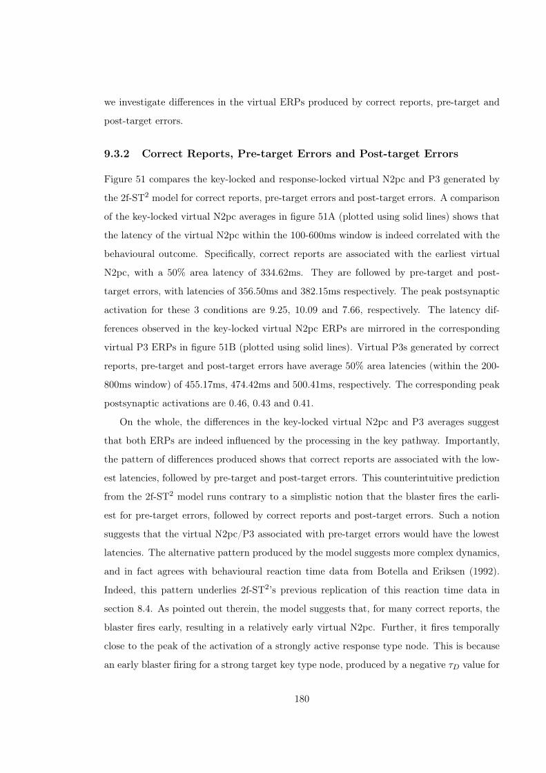
we investigate differences in the virtual ERPs produced by correct reports, pre-target and

post-target errors.

9.3.2 Correct Reports, Pre-target Errors and Post-target Errors

Figure 51 compares the key-locked and response-locked virtual N2pc and P3 generated by

the 2f-ST2 model for correct reports, pre-target errors and post-target errors. A comparison

of the key-locked virtual N2pc averages in figure 51A (plotted using solid lines) shows that

the latency of the virtual N2pc within the 100-600ms window is indeed correlated with the

behavioural outcome. Specifically, correct reports are associated with the earliest virtual

N2pc, with a 50% area latency of 334.62ms. They are followed by pre-target and post-

target errors, with latencies of 356.50ms and 382.15ms respectively. The peak postsynaptic

activation for these 3 conditions are 9.25, 10.09 and 7.66, respectively. The latency dif-

ferences observed in the key-locked virtual N2pc ERPs are mirrored in the corresponding

virtual P3 ERPs in figure 51B (plotted using solid lines). Virtual P3s generated by correct

reports, pre-target and post-target errors have average 50% area latencies (within the 200-

800ms window) of 455.17ms, 474.42ms and 500.41ms, respectively. The corresponding peak

postsynaptic activations are 0.46, 0.43 and 0.41.

On the whole, the differences in the key-locked virtual N2pc and P3 averages suggest

that both ERPs are indeed influenced by the processing in the key pathway. Importantly,

the pattern of differences produced shows that correct reports are associated with the low-

est latencies, followed by pre-target and post-target errors. This counterintuitive prediction

from the 2f-ST2 model runs contrary to a simplistic notion that the blaster fires the earli-

est for pre-target errors, followed by correct reports and post-target errors. Such a notion

suggests that the virtual N2pc/P3 associated with pre-target errors would have the lowest

latencies. The alternative pattern produced by the model suggests more complex dynamics,

and in fact agrees with behavioural reaction time data from Botella and Eriksen (1992).

Indeed, this pattern underlies 2f-ST2’s previous replication of this reaction time data in

section 8.4. As pointed out therein, the model suggests that, for many correct reports, the

blaster fires early, resulting in a relatively early virtual N2pc. Further, it fires temporally

close to the peak of the activation of a strongly active response type node. This is because

an early blaster firing for a strong target key type node, produced by a negative τD value for

180

200 100 0 100 200 300 400 500 600 700 8000

5

10

15

20

25


Post

syna

ptic

act

ivat

ion

Correct: key lockedPre target: key lockedPre target: response lockedPost target: key lockedPost target: response locked

200 0 200 400 600 800 10000

0.1

0.2

0.3

0.4

0.5

0.6


Post

syna

ptic

act

ivat

ion


A: Virtual N2pc

B: Virtual P3

Figure 51 Key-locked and response-locked virtual ERPs from the 2f-ST2 model forcorrect reports, pre-target and post-target errors. Panel A: Virtual N2pc. Panel B: VirtualP3. Note that the response-locked virtual ERP averages for correct reports are the same as thekey-locked averages. Dashed lines indicate the window used for measuring peak activation and 50%area latency.

181

the target item, will be correlated with a correspondingly early and strong target response

type node. In this situation, this response type node maximally benefits from the blaster’s

enhancement, and quickly wins the competition between co-active response types. Conse-

quently, tokenisation is initiated relatively early, producing an early virtual P3. Conjunction

errors, on the other hand, occur in trials in which the target’s key and response features

are relatively weak and are activated later (due to a more positive τD). In this situation,

the blaster fires relatively later on average, producing a later virtual N2pc. Among such

trials, there are those in which the response feature of a proximal distractor before/after

the target is relatively stronger, producing a pre-target/post-target error. For both types of

conjunction errors, the blaster’s enhancement occurs temporally further away from the peak

of the activation of the response type node that eventually gets bound. These type nodes

take longer to overcome the lateral inhibition at the Type layer of the response pathway.

As a result, tokenisation takes longer on average for conjunction errors, and produces later

virtual P3s. Further, this mean is naturally later for post-target errors than for pre-target

errors. This is because post-target errors are correlated with late blaster firing and delayed

activation of the response type that benefits from it.

Turning to the response-locked averages in figure 51 (plotted using dashed lines), we

see that the virtual N2pc/P3 for pre-target errors are shifted later in time, whereas those

for post-target errors are shifted earlier in time2. Furthermore, the latency differences

between the response-locked averages are much larger than those between the key-locked

averages. These shifts demonstrate that the response-locked virtual ERPs are correlated

with differences in processing outcomes in the response pathway. In other words, though

the virtual N2pc/P3 is driven by the key pathway, it is sensitive to the effectively greater

temporal variability in the response pathway that produces different behavioural outcomes

(i.e. correct reports, pre-target and post-target errors). The consequently large variation

in the latencies of the response-locked virtual ERPs in figures 51A and 51B produces the

reduction in amplitude and increased temporal spread seen in the corresponding combined

response-locked averages (see figures 50B and 50C).

2Note that, as would be expected, the response-locked ERP average for correct reports is the same asthe key-locked average.

182


In this section, we look at the ERP predictions of the 2f-ST2 model in the context of

manipulation in processing delay in the key pathway. In order to compare virtual ERPs

across a pair of conditions involving an isolated manipulation of the key pathway, we execute

two complete simulation runs of the model. These conditions differ only in the amount of

fixed additional delay τK introduced in the processing of all features in the key pathway

for one condition. In the previous chapter, we used such a manipulation to replicate shifts

in response distributions in data from Botella et al. (2001) (see section 8.3.1) and from

Experiment 3 (see section 8.5). Here, we employ the pair of conditions, early key feature

and late key feature (with τK values of -40ms and 0ms, respectively), the same as the

ones previously generated in section 8.53 (see appendix B.3 for details). In that section,

this configuration of the model allowed us to simulate response distributions that were

comparable to behavioural data from Experiment 3. Here, we investigate the virtual ERPs

for the same pair of conditions. Later in this chapter, we will compare them to their human

counterparts, using the EEG data from the same experiment.

Figure 52 depicts the behavioural and virtual ERP output of the model for the early and

late key feature conditions. As is evident from the distributions in figure 52A, the model

produces a post-target shift in the responses, reflected by an increase in the API across the

early (API = -0.86) and late key feature (API = -0.11) conditions. In conjunction with this

post-target shift, we intuitively expect a concomitant increase in the latency of the key-

locked virtual ERPs. This is because the increase in τK used to produce this shift would

effectively delay the activation of the target’s key type node. In turn, this would increase

the average latency of blaster firing in the late key feature condition, producing a relatively

later virtual N2pc and P3.

The key-locked (plotted using solid lines) and response-locked (plotted using dashed

lines) virtual N2pc and P3 averages evoked in the early and late key feature conditions

are shown in figures 52B and 52C . For each condition, these averages include all trials

in which a token was bound, combining across all response positions (i.e., correct reports,

pre-target and post-target errors). In keeping with intuition, the key-locked virtual N2pc is

3Note that for the late key feature condition, the model is effectively in its default configuration.

183

200 0 200 400 600 800 10000

0.1

0.2

0.3

0.4

0.5

0.6


Post

syna

ptic

act

ivat

ion

Early key feature: key lockedEarly key feature: response lockedLate key feature: key lockedLate key feature: response locked

C: Virtual P3

200 100 0 100 200 300 400 500 600 700 8000

5

10

15

20

25


Post

syna

ptic

act

ivat

ion

Early key feature: key lockedEarly key feature: response lockedLate key feature: key lockedLate key feature: response locked

B: Virtual N2pc

2 1 0 1 20

10

20

30

40

50

60

70


% F

requ

ency

Early key featureLate key feature


Figure 52 Early and late key feature conditions from the 2f-ST2 model. Panel A: Be-havioural response distributions. Panel B: Key-locked and response-locked virtual N2pc averages.Panel C: Key-locked and response-locked virtual P3 averages. Dashed lines indicate the windowused for measuring peak activation and 50% area latency.

184

later in the late key feature condition. The visual difference is confirmed by the mean 50%

area latencies (Luck & Hillyard, 1990) within the 100-600ms window in the two conditions:

307.18ms in the early key feature condition and 346.97ms in the late key feature condition.

In comparison, there is not much difference in their peak postsynaptic activations, which

are 8.82 and 8.71 respectively. The key-locked virtual P3 in figure 52C (plotted using solid

lines) is also relatively later in the late key feature condition: the 50% area latencies of the

virtual P3 (within the 200-800ms window) in the early and late key feature conditions are

437.62ms and 466.59ms, respectively. The peak activation is the same (0.44) in both cases.

On the whole, the latency shifts observed in the key-locked virtual N2pc and P3 ERPs

follow naturally from the increase in processing delay in the key pathway. However, these

key-locked ERPs are in contrast to their response-locked counterparts. As can be seen in

figure 52B, the peak activations of the response-locked virtual N2pc ERPs are markedly

lower than those of the corresponding key-locked averages. Specifically, the peak activation

of the response-locked virtual N2pc is 5.51 in the early key feature condition and 6.58 in the

late key feature condition. Similarly, the peak activation of the virtual P3 is also reduced in

the response locked averages in figure 52C: 0.38 and 0.39 in the early and late key feature

conditions, respectively. This decrease in peak activation of the response-locked averages is

similar to that seen in figure 50, and is explained by the fact that there is effectively more

temporal variability in the response pathway. Hence, response-locking increases the latency

differences in the virtual ERPs associated with correct reports, pre-target and post-target

errors (see figure 51). This increase in turn reduces the peak activation and increases the

breadth of the combined response-locked average.

Finally, in comparing the virtual ERPs in figures 52B and 52C, it is interesting to note

that the clear latency shift in the key-locked ERP averages are reduced by response locking.

Indeed, the 50% area latencies of the response-locked virtual N2pc ERPs in figure 52B are

similar: 347.25ms and 350.98ms in the early and late key feature conditions, respectively.

The corresponding latencies of response-locked virtual P3 ERPs in figure 52C are also sim-

ilar (467.51ms and 470.03ms). This absence of a latency difference in the response-locked

averages reflects the fact that the response pathway is not affected by the manipulation of

processing delay in the key pathway. Response locking produces a compensatory effect that

cancels out the latency differences seen in the key-locked averages. To elaborate, in both

185

the early and late key feature conditions, the response-locked average for correct reports

has the same latency as the corresponding key-locked average. However, the latency of the

response-locked average for pre-target errors in the early key feature condition is later than

the corresponding average in the late key feature condition. This is because, in the early

key feature condition, there are more trials that result in pre-target errors. Across these

trials, the relatively earlier firing of the blaster in the key-locked average is compensated

for in the response-locked average, by the earlier presentation of the response feature that

gets bound. Consequently, in the early key feature condition, the response-locked virtual

N2pc/P3 for pre-target errors is more delayed with respect to the presentation time of the

response feature being time-locked to4. Following an analogous logic, the response-locked

average for post-target errors in the late key feature condition is earlier than the correspond-

ing average in the early key feature condition. Here again, there is a compensatory effect

of increased number of post-target error trials in the late key feature condition. Hence,

the response-locked virtual N2pc/P3 in these trials is advanced with respect to the rela-

tively later presentation time of the response feature that gets bound therein. This pair of

effects produced by response locking means that the latency difference between the com-

bined key-locked averages in the early and late key feature conditions is cancelled out in the

response-locked averages.


In this section, we shift focus to a comparative evaluation of virtual ERPs generated by the

model across a pair of conditions involving a manipulation in the response pathway of the 2f-

ST2 model. This exploration complements and contrasts that in the previous section, which

focused on a manipulation in the key pathway. Therein, we established that an increase

in processing delay in the key pathway was associated with a concomitant increase in the

latency of the key-locked virtual N2pc and P3. This is in agreement with the architecture

and dynamics of temporal feature binding in 2f-ST2, which is strongly influenced by the key

pathway. However, we have also previously shown in section 9.3.2 that the virtual N2pc/P3

are sensitive to response feature processing, in terms of the latency differences between

4These delayed virtual N2pcs for pre-target errors in the early key feature condition produce the second,late peak in the corresponding response-locked average plotted in figure 52B.

186

200 0 200 400 600 800 10000

0.1

0.2

0.3

0.4

0.5

0.6


Post

syna

ptic

act

ivat

ion

Early response feature: key lockedEarly response feature: response lockedLate response feature: key lockedLate response feature: response locked

200 100 0 100 200 300 400 500 600 700 8000

5

10

15

20

25


Post

syna

ptic

act

ivat

ion

Early response feature: key lockedEarly response feature: response lockedLate response feature: key lockedLate response feature: response locked

2 1 0 1 20

10

20

30

40

50

60

70


% F

requ

ency

Early response featureLate response feature

C: Virtual P3

B: Virtual N2pc


Figure 53 Early and late response feature conditions from the 2f-ST2 model. Panel A:Behavioural response distributions. Panel B: Key-locked and response-locked virtual N2pc averages.Panel C: Key-locked and response-locked virtual P3 averages. Dashed lines indicate the window usedfor measuring peak activation and 50% area latency.

187

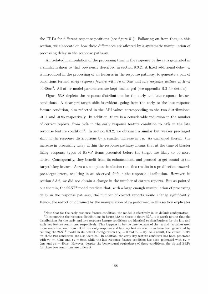
the ERPs for different response positions (see figure 51). Following on from that, in this

section, we elaborate on how these differences are affected by a systematic manipulation of

processing delay in the response pathway.

An isolated manipulation of the processing time in the response pathway is generated in

a similar fashion to that previously described in section 8.3.2. A fixed additional delay τR

is introduced in the processing of all features in the response pathway, to generate a pair of

conditions termed early response feature with τR of 0ms and late response feature with τR

of 40ms5. All other model parameters are kept unchanged (see appendix B.3 for details).

Figure 53A depicts the response distributions for the early and late response feature

conditions. A clear pre-target shift is evident, going from the early to the late response

feature condition, also reflected in the API values corresponding to the two distributions:

-0.11 and -0.86 respectively. In addition, there is a considerable reduction in the number

of correct reports, from 62% in the early response feature condition to 54% in the late

response feature condition6. In section 8.3.2, we obtained a similar but weaker pre-target

shift in the response distributions by a smaller increase in τR. As explained therein, the

increase in processing delay within the response pathway means that at the time of blaster

firing, response types of RSVP items presented before the target are likely to be more

active. Consequently, they benefit from its enhancement, and proceed to get bound to the

target’s key feature. Across a complete simulation run, this results in a predilection towards

pre-target errors, resulting in an observed shift in the response distribution. However, in

section 8.3.2, we did not obtain a change in the number of correct reports. But as pointed

out therein, the 2f-ST2 model predicts that, with a large enough manipulation of processing

delay in the response pathway, the number of correct reports would change significantly.

Hence, the reduction obtained by the manipulation of τR performed in this section explicates

5Note that for the early response feature condition, the model is effectively in its default configuration.6In comparing the response distributions in figure 53A to those in figure 52A, it is worth noting that the

distributions for the early and late response feature conditions are identical to distributions for the late andearly key feature conditions, respectively. This happens to be the case because of the τK and τR values usedto generate the conditions. Both the early response and late key feature conditions have been generated byrunning the 2f-ST2 model in its default configuration (τK = 0 and τR = 0). As a result, the virtual ERPsfor these two conditions are also identical. In addition, the early key feature condition has been generatedwith τK = -40ms and τR = 0ms, while the late response feature condition has been generated with τK =0ms and τR = 40ms. However, despite the behavioural equivalence of these conditions, the virtual ERPsfor these two conditions are different.

188

that prediction.

Figure 53B and 53C depict the key-locked (plotted using solid lines) and response-locked

(plotted using dashed lines) virtual N2pc and P3 averages for the early and late response

feature conditions. For each condition, these averages include all trials in which a token was

bound, combining across all response positions (i.e., correct reports, pre-target and post-

target errors). As is evident, there is no difference in either pair of key-locked averages across

the two conditions. For the key-locked virtual N2pc, the 50% area latencies are 346.97ms

and 347.18ms, and the peak activations are 8.71 and 8.82 (within the 100-600ms window)

in the early and late response feature conditions, respectively. For the key-locked virtual

P3, the 50% area latencies (466.59ms) and peak activations (0.48) within the 200-800ms

window are the same in both conditions.

In the previous section, an increase in the processing delay within the key pathway

produced concomitant increases in latency of the key-locked virtual ERPs. In contrast, an

increase in processing delay within the response pathway produces no such latency differ-

ences in the key-locked virtual ERPs. In case of the virtual N2pc, this is because it is

entirely driven by blaster firing, which in turn depends on processing in the key feature

pathway. As the processing delay in the key pathway remains unchanged, the activation of

the target’s key type node has the same average latency across the early and late response

feature conditions. This translates into identical firing times for the blaster, reflected in the

virtual N2pc. In addition, the virtual P3 reflects the fact that, irrespective of the response

type that gets bound to the target’s key type, the binding process has the same temporal

profile in both conditions. However, the pre-target shift in the response distribution arises

because, in the late response feature condition, the blaster’s enhancement more frequently

benefits response types active before that of the target. Thus, though the key-locked vir-

tual ERP averages do not change in any way, the relative proportion of correct reports,

pre-target errors and post-target errors making up these averages differ considerably.

Turning to the response-locked averages in figures 53B and 53C, a clear increase is evident

in the latency of the virtual ERPs in the late response condition. Further, the response-

locked virtual N2pc and P3 have lower peak activation in both conditions, compared to their

key-locked counterparts. Specifically, the 50% area latencies of the response-locked virtual

189

N2pc are 350.98ms and 387.22ms in the early and late response feature conditions, respec-

tively. The corresponding peak activations are 6.58 and 5.51. Also, the 50% area latencies

of the response-locked virtual P3 are 470.03ms and 496.05ms, and the peak activations are

0.39 and 0.38, in the early and late response feature conditions, respectively.

The relative increase in the latency of the response-locked virtual ERPs in the late

response feature condition derives from underlying shifts in the latencies of pre-target and

post-target errors. Specifically, there are more pre-target errors in the late response feature

condition (see figure 53A). Hence, the response-locked ERP for such errors in this condition

constitutes relatively more trials time-locked to a timepoint well in advance of target onset.

As the virtual N2pc and P3 are driven by the key pathway but are sensitive to the response

pathway, this relatively earlier time-locking delays them in the response-locked average for

pre-target errors7. Alongside, there are more post-target errors in the early response feature

condition (see figure 53A). As a result, the response-locked ERP for such errors in this

condition includes relatively more trials time-locked to a timepoint well after target onset.

Again, as the virtual N2pc and P3 are driven by the key pathway, this relatively later

time-locking effectively produces an earlier virtual ERP in the response-locked average for

post-target errors in the early response feature condition. In other words, the corresponding

average is earlier in the late response feature condition. On the whole, a combination of

delayed pre-target errors in the late response feature condition and advanced post-target

errors in the early response feature condition produce the relative shift in the combined

response-locked averages, as seen in figures 53B and 53C8.

The above sections have discussed a series of explorations with the 2f-ST2 model. In

these explorations, we have explicated a series of qualitative predictions, generated using

conditions simulated with the model. These predictions specify the pattern of changes we

expect to see in human ERPs for corresponding experimental conditions. In the following

section, we turn to new EEG data from Experiment 3, which allows us to test many of these

predictions.

7These delayed virtual N2pcs for pre-target errors in the late response feature condition produce thesecond, late peak in the corresponding response-locked average plotted in figure 53B.

8Taken together, the pattern of differences between the key-locked and response-locked virtual ERPs forthe early and late response feature conditions can be seen as inversion of the pattern observed with thevirtual ERPs for the early and late key feature conditions (see figures 52B and 52C). This is effectivelybecause, as pointed out earlier, these conditions are simulated by an inversion of the τK and τR parameters.

190

9.4 The Temporal Binding Experiment

In this section we shift focus to an analysis of EEG data from Experiment 3. In the

previous chapter, we analysed the behavioural data from this experiment (see section 8.5).

As pointed out therein, it consisted of coloured letter and symbol targets embedded within

bilateral RSVP streams of digit distractors presented at a rate of 94ms per item. The key

feature in the blocked design was target identity (letter or symbol), and the response feature

was colour. Also, EEG was recorded at the P7, P8, O1 and O2 electrodes for the N2pc

and at the Pz electrode for the P3. This data was later correlated with the behavioural

responses of the participants. Please refer to appendix B.3 for a detailed description of the

experimental method.

9.4.1 Combined Key-locked and Response-locked Averages

In line with the sequence of explorations conducted with the 2f-ST2 model, we begin our

analysis of the ERP data by comparing the key-locked and response-locked averages of the

human N2pc and P3. To generate these averages, we combine trials across the letter and

symbol conditions, selecting trials in which participants made a correct report, pre-target

or post-target error. The overall response distribution produced is shown in figure 54A. The

API of this distribution is 0.25.

Figures 54B and 54C depict the key-locked (plotted using solid lines) and response-locked

(plotted using dashed lines) N2pc and P3 grand average ERPs. These averages combine

the same correct report, pre-target and post-target error trials across the letter and symbol

conditions. The only difference between the averages is in terms of time-locking. The key-

locked averages are time-locked to the presentation time of the target’s key feature in each

trial. In contrast, the response-locked averages are time-locked to the presentation time of

the response feature that was eventually reported in that trial.

From the figures, it is evident that response locking reduces the amplitude of both the

N2pc and the P3. The peak amplitude of the key-locked N2pc within the 130-330ms window

is -1.3µV, while that of the response-locked N2pc is -0.99µV. This difference is marginally

significant across subjects: F(1,13) = 3.83, MSE = 0.17, p = 0.07. In addition, there is

a small but significant difference in the jackknife latency (with an onset criterion of 50%

191

200 0 200 400 600 8002

0

2

4

6

8

10

12


Ampl

itude

(uV)

Key feature lockedResponse feature locked C: P3

200 100 0 100 200 300 400 5002

1.5

1

0.5

0

0.5

1

1.5

2


Ampl

itude

(uV)


B: N2pc

2 1 0 1 20

10

20

30

40

50

Response Position

% F

requ

ency


Figure 54 Behaviour and ERPs from Experiment 3. Panel A: Response distribution. PanelB: Key-locked and response-locked N2pc grand average ERPs. Panel C: Key-locked and response-locked P3 grand average ERPs. Dashed lines in the ERP plots indicate the window used forstatistical analysis. All figures combine trials across the letter and symbol conditions.

192

of peak amplitude; see J. Miller et al., 1998) between the two averages: 193.89ms in the

key-locked average and 172.52ms in the response locked average (t(1,13) = 2.4, p @ 0.05).

The difference in peak amplitude between the key-locked and response-locked P3s in fig-

ure 54C exhibits a similar pattern to the N2pcs. The peak amplitudes of the key-locked and

response-locked averages are 10.07µV and 8.94µV respectively. This difference is significant:

F(1,13) = 13.92, MSE = 0.65, p @ 0.01. In addition, there is a significant difference in the

50% area latencies between the two averages: 498.57ms and 590.43ms in the key-locked and

response-locked average, respectively (F(1,13) = 8.66, MSE = 95.3, p @ 0.05).

The peak amplitude differences between the key-locked and response-locked N2pc and P3

averages in figures 54B and 54C match the peak activation differences predicted in the virtual

ERPs generated by the 2f-ST2 model (see figures 50B and 50C). Specifically, as there is less

temporal variability in the key pathway than the response pathway, the model predicted

that the key-locked average N2pc/P3 would have a larger peak activation than the response-

locked averages (see section 9.3.1). This prediction is validated by the corresponding human

ERPs. In addition, the latency difference predicted between the key-locked and response-

locked virtual P3 is also in agreement with the human P3 ERPs in figure 54C. However, in

case of the human N2pc, the direction of the small latency shift across the two averages in

figure 54B is opposite to that predicted by the model. This difference is possibly because the

N2pc is a relatively small ERP component, and is considerably attenuated in the response-

locked average. As with the virtual N2pc, this is due to increased temporal variation in the

response-locked ERPs. As a result, correct estimation of latency is difficult. In contrast,

the P3 is a much larger component, and allows for a more reliable calculation of 50% area

latency.

9.4.2 Correct Reports, Pre-target Errors and Post-target Errors

Following on from the comparison between combined key-locked and response-locked av-

erages, we now investigate differences between the ERPs associated with correct reports,

pre-target and post-target errors. This investigation parallels the comparison between cor-

responding virtual ERPs in section 9.3.2. Therein, we had found that even though the

virtual N2pc and P3 were driven by the key pathway, they were sensitive to the tempo-

ral variability in the response pathway that produced behavioural differences. Specifically,

193

200 100 0 100 200 300 400 5002

1.5

1

0.5

0

0.5

1

1.5

2


Ampl

itude

(uV)


200 0 200 400 600 8002

0

2

4

6

8

10

12


Ampl

itude

(uV)


A: N2pc

B: P3

Figure 55 ERPs evoked by correct reports, pre-target errors and post-target errors.Panel A: Key-locked and response-locked N2pc grand average ERPs. Panel B: Key-locked andresponse-locked P3 grand average ERPs. Note that the response-locked ERP averages for correctreports are the same as the key-locked averages. Dashed lines indicate the window used for statisticalanalysis.

194

correct reports had the earliest key-locked virtual N2pc and P3 latencies, followed by pre-

target and post-target errors. In addition, we found that with the response-locked ERPs,

the order of latencies was markedly different: post-target errors were the earliest, followed

by correct reports and pre-target errors (see figure 9.3.2). This was explained by reason-

ing that, though the virtual ERPs were driven by the key pathway, they were sensitive

to the temporal variability in the response pathway that eventually produced behavioural

differences. Consequently, the response-locked ERPs for pre-target errors were delayed and

those for post-target errors were advanced, relative to the presentation time of the erroneous

response feature that got bound.

Figure 55 depicts the key-locked (plotted using solid lines) and response-locked (plotted

using dashed lines) grand average N2pc and P3 ERPs evoked by the three response positions,

combining trials across the letter and symbol conditions. As can be seen in figure 55A,

the key-locked N2pc for correct reports and post-target errors are identical, while that

for pre-target errors appears to be affected by a slight baseline shift relative to the other

two conditions. However, pairwise comparisons between the conditions did not yield any

significant differences in peak amplitude (F @ 1) or jackknife (with an onset criterion of

50% of peak amplitude) latency (t < 1) within the 130-330ms window. This lack of any

differences between the N2pc is consistent with the pattern seen in the key-locked P3 ERPs.

As can be seen in figure 55B, the key-locked P3 evoked by correct reports, pre-target and

post-target errors are effectively identical, with no suggestion of any visual differences. In

keeping with this, a pairwise statistical comparison within the 300-700ms window did not

reveal any variation in 50% latency (F @ 1) or peak amplitude (F @ 1) across the three

response positions.

Turning to the response-locked N2pc and P3 ERPs in figure 55, clear differences are

visible when comparing them to their key-locked counterparts9. First, we compare the

response-locked N2pc for correct reports and pre-target errors: we find that correct re-

ports have an earlier jackknife (with an onset criterion of 50% of peak amplitude) latency

(179.28ms) than pre-target errors (286.9ms). This difference is not significant (t(1,13) =

1.39, p = 0.09). This lack of an effect is due to the obvious attenuation of the response-locked

9Note that, as would be expected, the response-locked ERP for correct reports is the same as the key-locked ERP.

195

ERP (see figure 55A). In turn, this is because the N2pc is a relatively small component, and

the increased latency variation between the response-locked ERPs for the -1 and -2 positions

greatly reduces the amplitude of the pre-target error average ERP, which combines trials

from these two positions. This attenuation is confirmed by a significant difference in the

peak amplitude (F(1,13) = 7.61, MSE = 1.09, p = 0.01) between the response-locked N2pc

for correct reports (-2.28µV) and pre-target errors (-1.15µV). The next comparison of inter-

est is between the response-locked N2pc for correct reports and post-target errors. There is

a visual suggestion of a latency difference between the ERPs, confirmed by an estimation

of their jackknife latencies (with an onset criterion of 50% of peak amplitude): post-target

errors have a slightly earlier latency (164.73ms) than correct reports (194.8ms), but this

difference is not significant (t < 1). Again, this lack of an effect is most likely due to the

attenuation of the N2pc average caused by response locking, which combines ERPs across

the +1 and +2 positions. Because of this attenuation, the peak amplitude for post-target

errors (-1.48µV) is marginally lower than that for correct reports (-2.28µV) (F = 4.16, MSE

= 1.01, p = 0.06).

The pattern of differences between the response-locked ERPs are clearer in the P3 aver-

ages in figure 55B, due to the relatively large amplitude of the P3. The first comparison is

between the response-locked P3s for correct reports and pre-target errors. As is clearly evi-

dent, the P3 for pre-target errors is significantly later than that for correct reports. This is

supported by a highly significant difference in 50% area latency of the P3, which is 504.92ms

for correct reports and 567.69ms for pre-target errors (F(1,13) = 48.83, MSE = 524.52, p @

0.001). Also, there is a small, expected reduction in peak amplitude between the averages

(which is not significant): 11.23µV for correct reports and 10.04µV for pre-target errors

(F(1,13) = 1.98, MSE = 4.67, p = 0.2). The next comparison, between the response-locked

P3s for correct reports and post-target errors, also suggests a latency difference: the 50%

area latency of the P3 evoked by post-target errors is earlier (486.15ms) than that evoked by

correct reports (504.92ms). This difference is not significant: F(1,13) = 1.8, MSE = 1295.17,

p = 0.2. However, a jackknife analysis (with an onset criterion of 50% of peak amplitude)

of P3 latencies within the 250-700ms window suggests a weakly significant effect (t(1,13)

= 2.08, p = 0.03), with post-target errors having an earlier latency (298.5ms) than correct

reports (337.91ms). There is no suggestion of a difference in peak amplitude between the

196

two P3s (F @ 1).

The differences between the key-locked and response-locked human ERPs are worth

comparing to the corresponding virtual ERPs. The key-locked virtual ERPs in figure 51

show small but clear differences in latency and amplitude. In particular, the model predicts

that correct reports are associated with the earliest key-locked ERPs, followed by those for

pre-target errors and post-target errors (see section 9.3.2). However, the statistical tests

performed above on the key-locked human N2pc and P3 ERPs in figure 55 do not suggest

any differences in latency or amplitude. This finding is in contradiction to the predictions

of the 2f-ST2 model10. This divergence between model and data could be due to implicit

assumptions in our simulations with the 2f-ST2 model, which might not be valid in our

experiment. In particular, for simplicity, we assume that the amount of random delay in-

troduced to the processing of items, as controlled by the τD parameter (see section 8.2.4),

is the same in the key and response pathways. It is possible that in our experiment, the

temporal variability in the processing of key (letter, digits and symbols) and response fea-

tures (colours) are markedly different. Indeed, to test this possibility, we conducted further

simulations with the model, with reduced temporal variability in the key pathway relative

to the response pathway. To do so, for all trials in a simulation run, the τD parameter was

fixed at 0ms in the key pathway (i.e., key features of items were not randomly delayed or

advanced). In the response pathway, as before, τD was randomly sampled for each item in

a trial, from a gaussian distribution with a mean of 0ms and a standard deviation of 15ms.

All other model parameters were the same as in its default configuration. We found that, in

this altered configuration of the model, the latency and amplitude differences between the

key-locked averages for correct reports, pre-target and post-target errors (figure 51) were

eliminated. However, the latency differences between the corresponding response-locked av-

erages remained qualitatively unchanged. Thus, the model produced a pattern of virtual

ERPs similar to their human counterparts in figure 55. Based on this simulation, we pro-

pose that in our setup in Experiment 3, there might be much less temporal variability in

the processing of key features.

10In fact, the lack of any difference in the latencies of the key-locked ERPs for correct reports, pre-target and post-target errors also contradicts reaction time data reported by Botella (1992). However, thisdifference might be due to the fact that our experimental setup did not involve a speeded reaction time task.

197

The differences between the response-locked virtual ERPs in figure 51 show a clear

correspondence with the human ERPs in figure 55. As there is more temporal variability in

the response pathway, response locking increases the amount of latency variation between

the virtual N2pc and P3 associated with correct reports, pre-target and post-target errors.

Specifically, the model predicts that post-target errors have the earliest response-locked

virtual ERPs, followed by correct reports and pre-target errors. The statistical differences

between the response-locked human ERPs corroborate this ERP prediction from the model,

though the effects are weak with the human N2pc in particular. Nevertheless, the qualitative

pattern of differences between the response-locked human ERPs are similar to those between

the virtual ERPs from the 2f-ST2 model. This similarity lends support to the dynamics in

the model that produce these differences. Further, it suggests that the human N2pc/P3,

though driven by key feature processing, is sensitive to temporal variability in the temporal

dynamics of response feature processing.


In this section, we focus on the influence of an isolated manipulation of key feature processing

on the human N2pc and P3 ERPs. As pointed out previously in section 8.5, the letter and

symbol conditions in Experiment 3 constitute a pair of conditions involving a relative delay

in the processing of key features (in the symbol condition). This is seen in the post-target

shift between the response distributions for the two conditions, plotted in figure 56A. The

API of the distribution for the letter condition is 0.18, and that for the symbol condition is

0.31. Further, this difference is significant (F(1,13) = 9.7, MSE = 0.01, p @ 0.01). Following

on from this behavioural difference, we now compare the N2pc and P3 ERPs evoked by

letter and symbol targets.

Figures 56B and 56C depict the key-locked (plotted using solid lines) and response-

locked (plotted using dashed lines) N2pc and P3 ERPs evoked by letter and symbol targets.

Each of these ERPs include all trials in which the key feature of the target was correctly

reported, and average across all response positions (i.e., correct reports, pre-target and post-

target errors). The first comparison is between the key-locked N2pc evoked by letter and

symbol targets. As can be seen in figure 56B, symbol targets evoke a later key-locked N2pc.

Statistically, a jackknife analysis (with an onset criterion of 50% of peak amplitude) of the

198

200 0 200 400 600 8002

0

2

4

6

8

10

12


Ampl

itude

(uV)

Letter: key lockedLetter: response lockedSymbol: key lockedSymbol: response locked

C: P3

200 100 0 100 200 300 400 5002

1.5

1

0.5

0

0.5

1

1.5

2


Ampl

itude

(uV)

Letter: key lockedLetter: response lockedSymbol: key lockedSymbol: response locked

B: N2pc

2 1 0 1 20

10

20

30

40

50

Response Position

% F

requ

ency

LetterSymbol


Figure 56 Behaviour and ERPs for the letter and symbol conditions. Panel A: Responsedistributions. Panel B: Key-locked and response-locked N2pc grand average ERPs. Panel C: Key-locked and response-locked P3 grand average ERPs. Dashed lines in the ERP plots indicate thewindow used for statistical analysis.

199

visual difference in latency (within the 130-330ms window) shows a significant effect: letter

targets have a mean jackknife latency of 147.56ms, whereas symbol targets have a latency

of 197.92ms. (t(1,13) = 6.26, p @ 0.001). However, there is no evidence for a difference in

peak amplitude (F @ 1). Next, we compare the key-locked P3 for letter and symbol targets,

shown in figure 56C. The main visual difference between the key-locked P3 ERPs is their

amplitude. The peak amplitude of the P3 within the 300-700ms window is 9.41µV for letter

targets and 11.44µV for symbol targets. This difference is significant: F(1,13) = 6.68, MSE

= 4.3, p = 0.02. However, though the peak latencies of the key-locked grand average P3s

differ considerably (456ms for letter targets and 524ms for symbol targets), this difference

is not statistically significant across subjects (F @ 1). Similarly, there is no indication of

a significant difference in the 50% area latencies (Luck & Hillyard, 1990) across the two

conditions (F @ 1).

We now move to comparisons between the response-locked ERPs in figure 56. A com-

parison of the response-locked N2pc ERPs for letter and symbol targets in figure 56B to

their key-locked counterparts shows that they are relatively attenuated by the process of

response locking. This pattern, essentially the same as that described in section 9.4.1 (see

figure 54B), arises because of the significant latency variation between the response-locked

N2pcs for the different response positions. This in turn reduces the amplitude of the com-

bined average. With a small ERP component like the N2pc, this attenuation considerably

obscures the component in the grand average. We find that there is no statistical difference

between the peak amplitudes of the response-locked N2pc ERPs for letter and symbol tar-

gets (F @ 1). Also, a jackknife analysis (with an onset criterion of 50% of peak amplitude)

of the latencies of these response-locked N2pc ERPs fails to find a statistical difference.

Finally, we compare the response-locked P3 ERPs evoked by letter and symbol targets

in figure 56C. There is no significant difference in the 50% area latencies (F @ 1). The peak

amplitudes of the response-locked P3 for letter and symbol targets are 8.6µV and 10.02µV

respectively. This difference is not significant: F(1,13) = 3.0, MSE = 4.67, p = 0.1. As

with the N2pc, the response locking clearly reduces the peak amplitude of the P3, due to

reasons previously highlighted in section 9.4.1 (see figure 54C).

The ERP results presented above exhibit a complex pattern of effects in terms of changes

200

in amplitude and latency across the conditions of interest. The 2f-ST2 model offers a qual-

itative explanation for some important effects, with the aid of the virtual ERPs described

earlier in section 9.3.3. Therein, we compared the key-locked and response-locked virtual

ERPs generated by the model in the early and late key feature conditions. As established in

the previous chapter (see section 8.5), these two conditions in the model are behaviourally

comparable to the letter and symbol conditions, respectively. Following on from that, we

can compare the virtual ERPs in figure 52 to those described in this section. However, it is

worth noting that, as can be seen in the response distributions in figure 56A, the number of

post-target errors does not change much between the letter and symbol conditions. Conse-

quently, the magnitude of the differences between the human ERPs for these conditions are

likely to be smaller than those between the corresponding virtual ERPs for the early and

late key feature conditions.

In particular, the key-locked human N2pc ERP in figure 56B shows a shift in latency

between letter and symbol target conditions, which is consistent with the latency shift

between the virtual N2pc for early and late key feature conditions (see figure 52B). In

addition, a similar shift is also evident in the key-locked virtual P3 generated by the model

for these two conditions (see figure 52C). This derives directly from the fact that target

consolidation in 2f-ST2, as reflected by the virtual P3, is driven strongly by the blaster

activity reflected in the virtual N2pc. However, this prediction from the model could not

be verified in the key-locked human P3 ERPs (figure 56C). This could possibly be due to a

weak effect obscured by noise. Also, the main effect observed in the human P3 (in both the

key-locked and response-locked averages), i.e., the reduction in amplitude of the letter P3,

could potentially be due to aspects of the experimental design. Previous research has shown

that the P3 is sensitive to a variety of experimental factors (see Kok (2001) for a review). It

has been found that changes in task difficulty interact with changes in processing strategy

and stimulus characteristics across experimental blocks to affect the size of the P3. As a

consequence, it is possible that the relatively large difference in P3 amplitude produced by

the blocking of letter and symbol targets obscured smaller differences in P3 latency predicted

by the 2f-ST2 model.

In the context of differences between key-locked P3s, it is interesting to note that the

201

latency shift predicted by the model (across a pair of conditions involving an isolated ma-

nipulation of the key feature) is indeed observed in previous ERP data reported by Polich

and Donchin (1988). In their lexical decision experiment, Polich and Donchin (1988) found

that low-frequency words (equivalent to the late key feature condition) evoked P3s that

were generally later than those evoked by high-frequency words (equivalent to the early

key feature condition)11. Importantly, in their experiment, trials were not blocked by word

frequency, i.e., participants did not know whether the target in a given trial would be a

low-frequency or high-frequency word. This is in contrast to the design in Experiment 3,

where letter and symbol targets were presented in separate blocks. Consequently, partic-

ipants knew beforehand as to whether the target would be a letter or a symbol. For this

reason, it could be that our P3 data was additionally influenced by differences associated

with ‘cognitive effort’ employed by the participants in the two blocks. This potential con-

found did not exist in the experimental setup employed by Polich and Donchin (1988). As

a result, their data provides us with a clearer test of the 2f-ST2 model’s predictions, which

are indeed confirmed by the pattern of P3 latency differences reported by them.

As pointed out previously in section 9.4.1, the response-locked N2pc and P3 in the

human data suffer an attenuation similar to that observed in the response-locked virtual

ERPs in figure 52. In the case of the model, this attenuation derives from the increased

latency variation in the response pathway. Hence, we see a qualitative equivalence of the

response-locked human ERPs to their model equivalents, for both the letter and symbol

conditions. This corroboration provides important empirical support for the architecture

and dynamics of the 2f-ST2 model.


In section 9.3.4, we discussed the ERP predictions from the 2f-ST2 model relating to a

manipulation of processing delay in the response pathway (see figure 53. However, these

predictions could not be directly tested with human EEG data from Experiment 3. This was

because Experiment 3 did not incorporate a manipulation of response feature processing,

either a priori or post-hoc. As a result, the ERP predictions of the model relating to an

11See figures 1 and 2 in Polich and Donchin (1988).

202

isolated response feature manipulation could not be directly tested. However, as pointed

out in section 9.3.4, the late key feature and the early response feature conditions are the

same, in that they both represent the output of the 2f-ST2 model simulated in its default

configuration. Further, the early key feature and late response feature conditions are mutual

inversions, as the former is simulated with τK = -40ms and τR = 0ms, while the latter is

simulated with τK = 0ms and τR = 40ms.

In the previous section, we have used the human EEG data to test the model’s ERP

predictions for the early and late key feature conditions. Hence, due to the correspondence

between the early/late key feature and the late/early response feature conditions, respec-

tively, we have indirectly tested the model’s predictions for the latter pair of conditions.

Indeed, this equivalence does not obviate the need for direct verification of the model’s

predictions in the early and late response feature conditions. Nevertheless, it mitigates the

seriousness of the limitation imposed by the unavailability of comparable human EEG data.

9.4.5 Summary

We now summarise the outcomes of the comparisons between the virtual ERPs from the

2f-ST2 model and the human ERPs from Experiment 3. In section 9.4.1, we began with a

comparison of key-locked and response-locked ERPs combining across the letter and symbol

conditions, and across all response positions. The main prediction of the model in this

regard was that the amplitude of the response-locked average would be lower than the key-

locked average (figure 50). This prediction was confirmed in the corresponding human ERPs

(figure 54).

Next, in section 9.4.2, we separated the key-locked and response-locked human ERPs

for correct reports, pre-target and post-target errors. For the key-locked ERPs, the 2f-ST2

model predicted a pattern where correct reports had the earliest latency, followed by pre-

target and post-target errors (figure 51). However, we found that there was no difference in

the latency or amplitude of the corresponding human ERPs (figure 55). As discussed therein,

with a further reduction in the amount of effective temporal variability in the key pathway,

the model was better able to predict the pattern observed in the key-locked human ERPs.

Alongside, the model was able to qualitatively replicate the pattern of latency differences

observed in the response-locked ERPs for the three response positions. It predicted that

203

the response-locked ERPs for post-target errors would be the earliest, followed by correct

reports and pre-target errors (figure 51). This pattern was also seen in the human data,

though it was not significant in the N2pc due to its diminished amplitude (figure 55).

Finally, in section 9.4.3, we analysed the key-locked and response-locked ERPs for the let-

ter and symbol conditions. As highlighted in section 8.5, these conditions were behaviourally

equivalent to the early and late key feature conditions simulated by the 2f-ST2 model. The

model predicted that, concomitant with the post-target shift in the response distributions,

symbol targets should produce key-locked ERPs that were later than those produced by

letter targets (figure 52). Though this pattern was verified in the key-locked human N2pc

ERPs, it was not seen in the P3 ERPs (figure 56). As discussed in section 9.4.3, this might

have been due to methodological confounds in our experimental setup, which produced

other systematic differences in the key-locked human P3s. Further, we pointed out that P3

data from Polich and Donchin (1988) provides a clearer test of the model’s predictions in

this regard, and is in agreement with them. As for the response-locked virtual ERPs, the

model predicted a relative attenuation due to response locking (figure 52). This attenuation

was confirmed in the response-locked human N2pc and P3 for both the letter and symbol

conditions (figure 56).

9.5 Conclusions

This chapter has extended the capabilities of the 2f-ST2 model beyond the behavioural

domain, and highlighted its ability to make testable predictions relating to human ERPs.

This is an important strength of the model, as it allows us to interpret behavioural and

EEG data using a common explanatory framework. We began the chapter with a series

of explorations that explicated the ERP predictions from the model. Exploring the 2f-ST2

model at this greater level of detail has allowed us to provide in-depth explanations of how

it simulates high-level behaviour, building up from the level of neural network dynamics.

In particular, we have described how the model produces a counterintuitive pattern that

replicates reaction time data reported by Botella and Eriksen (1992). In addition, the

explorations have drawn upon results from current empirical research into the influence

204

of stimulus and response related processing on the P3. The comparisons between key-

locked and response-locked averages in these explorations have informed this research, and

highlighted the model’s predictions in each case.

In addition, we have used EEG data from our temporal binding experiment to verify some

of the main ERP predictions from the model. In particular, we have compared key-locked

and response-locked averages in our EEG data and compared them with virtual ERPs from

the 2f-ST2 model. Further, we have described in our data a pair of experimental conditions

involving a systematic manipulation of delay in key feature processing. The ERPs generated

in these conditions have also been tested against virtual ERPs from the model. However, as

pointed out previously in chapter 4, limitations in the virtual ERP technique imply that the

match between human and virtual ERPs can only be qualitative. In addition, limitations

deriving from experimental methodology have meant that not all the predictions from the

model could be fully tested with our EEG data. Nevertheless, the comparative evaluations

conducted here have allowed us to verify important internal mechanisms implemented in the

2f-ST2 model. In summary, this combination of theory and experiment has contributed to

our understanding of the temporal dynamics of feature binding and the role of the temporal

spotlight therein.

205

Part III

Discussion

206

Chapter 10

Conclusions, Contributions and

Outlook

Over the previous chapters, we have described research involving a collection of theoretical

and experimental explorations into the dynamics of temporal attention and perception. In

this chapter, we take stock, to bring together the ideas explored therein and highlight how

they have addressed the central hypotheses of this thesis. Following that, we discuss how

this work informs the current state of research in its field, and directions in which it could

be taken forward.

10.1 Conclusions

In this section, we return to the central hypotheses of this thesis, outlined in section 1.2.

We highlight how the research described in this thesis has addressed the proposals made

therein, and discuss issues that remain to be resolved.

The Existence of TAE

We hypothesised in section 1.2 that there exists in human cognition a mechanism that pro-

vides transient attentional enhancement (TAE), thereby functioning like a temporal spot-

light. In this thesis, we have highlighted a large body of experimental research that points

to the existence of such a mechanism. The evidence therefrom, drawing on both behaviour

207

and electrophysiology, suggests this TAE functions like an attentional gate, providing an en-

hancement that is short-lived and non-specific. Further, the incorporation of such a TAE in

the ST2, 2f-ST2 and other cognitive models, as described in chapters 5 and 8, have enabled

them to sufficiently explain a broad spectrum of empirical evidence. In particular, the pro-

file of blaster unavailability during ongoing encoding explains the temporal characteristics

of the Attentional Blink (AB) deficit. In addition, the finding of lag 1 sparing agrees with

the time course and generality of the blaster’s enhancement. Further, as demonstrated in

chapters 7 and 9, the human N2pc, thought to reflect attentional selection, shows a qual-

itative correspondence to the blaster’s activation reflected in the virtual N2pc. Together,

these sources of evidence provide support for the notion that a TAE-like mechanism might

indeed exist in the brain.

However, though we have speculated on the neurophysiological underpinnings of TAE,

this line of investigation has not been focused on here. It might be that TAE is actually

a emergent product of the collective interaction of many different brain regions and sys-

tems. Further research in this direction might shed more light on the inter-connectivity

and dynamics of these systems. Indeed, this knowledge would inform our interpretation

of existing behavioural and EEG data, and the architectural assumptions of the ST2 and

2f-ST2 models.

The Task Relevance of Stimuli and TAE

Another hypothesis in section 1.2 was that the detection of task relevant stimuli selectively

activates TAE, and that this can happen earlier or later in time relative to stimulus presenta-

tion. In chapter 6 we focused on this issue, and explored how the discriminability of targets

from distractors affects temporal perception. The chapter described results from our EEG

experiment that directly investigated how the neural dynamics of perception varied across

a pair of conditions that differed maximally in the discriminability of targets. In particular,

we compared changes in early visual processing and the P3 ERP across this manipulation.

Therein, we showed that the latency of the P3 was clearly affected by how quickly targets

could be identified. Furthermore, we followed up this empirical research with a theoretical

elucidation based on the ST2 model. By making a sequence of justifiable changes to its

architecture, we enabled the model to replicate the pattern of effects observed in our data.

208

With this exploration, we explained how target discriminability might be influencing the

deployment latency of TAE, thereby producing observable changes in temporal perception

and consequent behaviour.

Suppression of TAE by Working Memory Encoding

Next, we suggested that TAE is suppressed by ongoing consolidation. Further, the duration

of this suppression is dependant on the strength of the mental representations generated by

the target. To support this claim, in chapter 5 we pointed to behavioural evidence relating

to the AB, which suggests that the AB is attenuated when T1 strength is increased (for

example, by presenting a blank after it). In addition, we demonstrated how the recipro-

cal relationship between target strength and AB duration implemented by the ST2 model

explains this pattern of data. As described in chapter 3, the ST2 model implements the

suppression of TAE during binding. Because of the reciprocal relationship, stronger targets

produce shorter windows of TAE suppression, thereby producing the observed attenuation of

the AB. Further, chapter 5 also focused on the neurophysiologically inspired LC-NE model

of temporal attention. We pointed out that, in its published form, it could not explain

the behavioural evidence for the reciprocal relationship. However, we proposed and imple-

mented an extension to the LC-NE model based on ST2 concepts. This extension enabled

it to replicate the reciprocal relationship between target strength and the suppression of the

LC-NE system.

The Influence of TAE on the Temporal Precision of Perception

In section 1.2, we proposed that the unimpaired availability of TAE ensures the temporal

precision of perception. In contrast, impairment of TAE results in increased temporal un-

certainty and error rates. This proposal was focused on in chapter 7, using a combination

of experimental and theoretical techniques. For the experimental aspect, we employed data

from our experiment that recorded EEG activity evoked by target processing outside and

inside the AB window. With this data, we applied a methodology that used ERPimages

and time-frequency analysis of single-trial N2pc and P3 responses to test the hypothesis

that the neural dynamics of target perception inside the AB were more temporally variable.

209

Based on this methodology, a combination of qualitative and quantitative techniques was

employed to show that impairment of TAE (during the AB window) temporally ‘jittered’

the processing reflected by the ERPs. To complement this empirical approach, we employed

the ST2 model to interpret our data at the level of single-trial dynamics. Using complemen-

tary virtual ERPs and ERPimages, we showed that T1 processing affected the precision of

TAE deployment for T2, thereby adversely affecting its consolidation into working memory.

Correlating data and model at this level not only allowed us to propose a sufficient expla-

nation for the pattern of EEG data, but also to validate the architecture and dynamics of

the ST2 model in greater detail. Finally, we tied in our research with existing literature,

and interpreted reports of increased binding errors and temporal inaccuracy during the AB

in terms of our hypothesis.

The Role of TAE in Temporal Feature Binding

The last hypothesis in section 1.2 was that TAE plays an important role in the process of

temporal feature binding. We suggested that TAE determines the dynamics of the process

by which concurrently active mental representations of task-relevant features are bound

into working memory. Chapters 8 and 9 instantiated this hypothesis in the form of the

2f-ST2 model. In chapter 8, we described how 2f-ST2 provides a sub-symbolic description

of the role of TAE in binding co-active stimulus features into working memory. We gener-

ated behavioural predictions from the model, which were verified using data from previous

experiments, in addition to our own. In particular, it showed how the dynamics of TAE de-

ployment affected behavioural outcomes (i.e., correct reports and illusory conjunctions) and

associated reaction times, producing patterns of variation that agreed with behavioural data.

This validation demonstrated that 2f-ST2 improves upon previous modelling approaches, by

providing a description of temporal feature binding that is more in-depth, broad-based and

parsimonious.

The research in chapter 8 laid the groundwork for generating EEG predictions from

2f-ST2 in chapter 9. There, we focused on virtual ERPs from the model, to gain deeper

insights into the temporal dynamics of attention and perception embodied therein. Over a

sequence of explorations, we generated virtual N2pc and P3 traces from 2f-ST2 to provide

predictions about human EEG data relating to temporal feature binding. Specifically, these

210

predictions embodied the model’s claims about the interaction between TAE, temporal

perception and behavioural outcomes. To test these claims, we turned to EEG data from our

experiment. The findings therefrom successfully verified some of the main ERP predictions

of the model. In particular, we demonstrated that, as predicted by 2f-ST2, the dynamics

of TAE deployment and temporal perception were driven by key feature processing. These

dynamics formed the basis of the model’s ability to replicate a counterintuitive pattern of

reaction time data. However, not all the ERP predictions from 2f-ST2 could be verified, due

to limitations of experimental methodology and theoretical assumptions. Nevertheless, the

comparative evaluations between model and data allowed us to validate the model’s main

internal mechanisms. Finally, to return to our hypothesis, this combination of theory and

experiment elucidated the influence of TAE in mediating temporal feature binding.

10.2 Contributions

This section broadens the scope of the discussion to highlight the main contributions of this

thesis to current research. We touch upon a methodological contribution before discussing

how we inform current understanding of feature binding and visual perception.

Combining Modelling and Electrophysiology

A common theme in most of this thesis has been the attempt to apply neural network mod-

elling to make predictions about human electrophysiology. This novel technique, previously

proposed in Craston (2009), embodies connectionist thinking in its approach to verifying

high-level behaviour by simulating functional neural dynamics. It has enabled us to extend

cognitive modelling beyond the explanation of behaviour. We have used neural models

to interpret the preceding dynamics that produce the behaviour. In turn, we have also

validated many of the mechanisms that simulate these dynamics. Owing to the nature of

our methodology, the match between simulated and real dynamics has only been qualita-

tive. Nevertheless, interpreting behavioural and EEG data within a common explanatory

framework has provided us deeper insights into temporal attention and perception.

211

The Temporal Spotlight and Feature Binding

The 2f-ST2 model described in this thesis proposes a functional neural architecture for

implementing feature binding in temporal perception. In particular, it hypothesises a crucial

role for the temporal spotlight of attention therein, as the intermediary between two stages

of information processing. Over the research described in this thesis, we have emphasised

the distinction between this temporal spotlight and its spatial counterpart. Alongside, we

have established that, though the processes of feature binding in space and time share

fundamental properties, there are also important distinctions. With the 2f-ST2 model, we

have demonstrated how the temporal spotlight provides transient attentional enhancement

to establish a binding between temporally overlapping featural representations of stimuli

(presented in succession at a particular spatial location). This functional description of

temporal feature binding at the level of neural network dynamics improves upon previous

modelling efforts, and feeds into current research into the binding problem in general.

In this regard, it is important to note that the description of temporal feature binding

provided by 2f-ST2 does not necessarily conflict with proposals based on temporal syn-

chrony (Gray, 1999). Indeed, it is possible that temporal correlations between oscillatory

patterns in neuronal populations might be employed in conjunction with attentional en-

hancement (Singer, 1999). At its level of abstraction, the 2f-ST2 model describes how such

concurrent patterns of activity might be functionally influenced by the temporal spotlight.

Further, it proposes a consequent architecture for maintaining multiple such bindings in

a token-based working memory, once they have been established. In doing so, the model

reaches up to the level of behaviour, explaining the formation of correct reports and illusory

conjunctions in the temporal domain.

The Episodic Nature of Consciousness

As pointed out in chapter 3, the ST2 model embodies the notion of episodic distinctiveness

in temporal perception. The 2f-ST2 model remains faithful to this idea and extends it to

temporal feature binding. Generally speaking, it proposes that the cognitive architecture

involved in temporal perception aims to provide conscious awareness with a coherent picture

of an ever-changing reality. To elaborate, at the level of raw visual input, the real world

212

presents a continuously changing environment, where events take place in uninterrupted

succession. However, for us to make sense of it, this input needs to be transformed into

distinct, episodic memories that occur in a particular temporal order. According to the 2f-

ST2 model, the temporal spotlight mediates this transformation, effectively by enabling the

visual system to take ‘snapshots’ of specific segments of time, in response to the occurrence

of salient events (Wyble, Bowman, & Nieuwenstein, 2009). These snapshots ‘capture’ groups

of featural representations that are conjoined into working memory. Each such snapshot,

represented by a token in the model, is intended to be a separate, discrete episode accessible

to conscious awareness. The model suggests that many related behavioural phenomena

manifest because of the temporal limitations in a system that is attempting to create such

episodic representations of reality. In particular, the AB is caused by the suppression of the

temporal spotlight during the ongoing creation of an episode. Similarly, illusory conjunctions

occur when the temporal spotlight highlights an incorrect group of visual representations to

be combined into an episode. Over the course of this thesis, we have studied this system as

implemented in the ST2 and 2f-ST2 models, and characterised the role of temporal spotlight

in shaping conscious experience.

10.3 Future Outlook

In this final section, we look at potential directions in which the research described in this

thesis could be taken further. In the course of this research, we have combined computational

modelling with EEG experimentation to study temporal attention. Consequently, in the

following sections, we speculate on future lines of enquiry that could be pursued along these

two directions.

10.3.1 Experimental Directions

At many points in this thesis, we have highlighted interesting predictions from the ST2

and 2f-ST2 models that could not be tested with the empirical data collected herein. This

section returns to these predictions, and discusses potential experimental ideas that could

serve to verify the models and inform their further development.

213

Connecting T1 Duration with T2 Latency

In chapter 7, we measured the single-trial latencies of P3s (as estimated by their phases)

evoked in the T1 Lag 3 and T2 Lag 3 conditions (see section 7.5.3). In the discussion

section therein, we discussed potential reasons for why we did not observe a direct trial-by-

trial correlation between these P3 latencies. As pointed out there, Experiment 2 was not

designed to generate much variation in T1 strength, and consequently, a weak correlation

between the P3 latencies could have been obscured by noise. With sufficient variation in

T1 strength, the dynamics of the ST2 model propose a stronger relationship between the

duration of the T1 Lag 3 P3 and the latency of the T2 Lag 3 P3. Indeed, the model suggests

that there should be a reciprocal influence of T1 strength on its encoding duration (Bowman

et al., 2008), which would in turn have implications for T2 P3 latency.

One possible method to test this prediction from the ST2 model is to devise an ex-

periment that incorporates a stronger variation in T1 strength, and then investigate the

correlation between T1 and T2 P3 latencies across this variation, in addition to across T2’s

presentation outside and inside the AB window. This is because the ST2 model suggests

that, within the appropriate range, T1 P3 duration is driven by its bottom-up strength.

An experiment that builds on the sort of designs we have described in this thesis could

incorporate a strong variation in T1 strength produced by explicitly manipulating its psy-

chophysical characteristics. This could be done by varying the backward masking of the T1

item in RSVP, i.e., by replacing the distractor following the T1 with a blank screen. Going

further, a more fine-grained modulation of T1 strength could be achieved by varying the

relationship between its presentation duration and that of the blank following it, thereby

introducing a variable inter-stimulus interval following the T1. Such an experimental config-

uration would allow us to gradually increase T1 strength along a linear scale, and measure

the consequent effect on the duration of its P3 and the latency of T2’s P3.

Two-Feature AB with EEG

Chapter 7 highlighted results from previous research (Chun, 1997a; Popple & Levi, 2007;

Vul et al., 2008) involving experiments where items with pairs of features were presented in

RSVP. In these studies, participants were required to detect the occurrence of two targets

214

(T1 and T2) with unique key features within the RSVP stream, and identify the associated

response features. They all reported finding an AB effect for T2 in this context. In addition,

they also reported specific changes in the response distributions for the T2 when it was

presented during the AB (see section 7.9. Therein, we connected their findings with our

hypothesis of reduced temporal precision during the AB, and showed that the ST2 model

could explain the pattern of behavioural effects observed in these studies. In this regard,

it would be informative to conduct a study that extends the experimental paradigm used

in these previous ones, by recording EEG in conjunction with behavioural responses. The

data generated therefrom would inform our understanding of the influence of the AB on the

neural dynamics of temporal feature binding, and guide theoretical research in this regard.

In particular, as discussed later in this chapter, EEG data from the proposed ‘two-feature

AB’ study would directly inform the further development of the 2f-ST2 model, to enable it

to explicitly simulate influence of the AB on feature binding in time.

Response Feature Manipulation with EEG

In chapter 8 we showed how the 2f-ST2 model can simulate behavioural effects produced

by experimental manipulations of key and response processing times. In particular, we

described results from a pair of experiments conducted by Botella et al. (2001), one involving

a key feature manipulation and another involving a response feature manipulation. As

described in section 8.3, the 2f-ST2 model was able to simulate the behavioural effects of

both manipulations. Then, in chapter 9, we went further and generated ERP predictions

from the 2f-ST2 model about the effects of such systematic manipulations on the N2pc

and P3 (see section 9.3). Using EEG data from Experiment 3, we compared the virtual

ERPs generated by 2f-ST2 to human ERP data across a pair of conditions involving a

manipulation of key feature processing time. However, as pointed out in the discussion

section in chapter 9, Experiment 3 did not incorporate a complementary response feature

manipulation. Hence, an appropriate EEG study consisting of a pair of conditions differing

only in response processing times would provide data that could be used as an additional test

of the ERP predictions from 2f-ST2. As an example, the design of such a study could invert

the task from Experiment 3, by presenting coloured easy/hard alphanumeric/symbol stimuli

in RSVP, and requiring participants to identify the item presented in a particular unique

215

colour. This would produce a pair of conditions across which the average processing time for

the key feature (colour) remained the same, while that for the response feature (identity)

varied depending on whether the target item was an easy or hard alphanumeric/symbol

stimulus. N2pc and P3 data from this study could be compared with virtual ERPs from

figure 53. This comparative evaluation would help further validate 2f-ST2’s mechanisms,

and add to our understanding of the interplay between temporal attention and binding.

10.3.2 Theoretical Directions

We now turn to directions in which the modelling work on the 2f-ST2 model introduced in

this thesis could be continued. These directions aim not only to broaden the explanatory

scope of the model, but also to explore more neurocomputationally viable implementations.

Modelling Two-feature AB with 2f-ST2

As pointed out earlier in this chapter, a ‘two-feature AB’ EEG study extending from be-

havioural studies (Chun, 1997a; Popple & Levi, 2007; Vul et al., 2008) would generate new

data to inform further development of the 2f-ST2 model. In parallel, the extension of the 2f-

ST2 model to explicitly simulate the influence of the AB on temporal feature binding would

generate testable ERP predictions that could be verified with this data. In this thesis, the

2f-ST2 model has been used to simulate the binding of pairs of features in RSVP streams

consisting of a single target. In this scenario, we have manipulated the feature processing

time in the key and response pathways and shown that some of the main behavioural and

ERP predictions from the 2f-ST2 model about the effect of such manipulations are validated

by empirical data. The model could be further extended to explicitly simulate the influence

of the AB additional to these manipulations. To do so, it would need to simulate the feature

binding of two targets, T1 and T2, presented in an RSVP stream consisting of items with

pairs of features, in close succession so as to produce an AB effect for T2. This addition

would naturally increase the computational complexity of the model, and further optimisa-

tions might be required in order to keep simulation time within feasible limits. Overall, this

combination of theoretical and experimental enquiry would significantly add to the 2f-ST2

model’s capabilities as a broad-based description of temporal visual processing.

216

Distributed Representations in the Binding Pool

The binding pool in the 2f-ST2 model implements an activation based memory for type-

token associations. In other words, the binding pool remembers which types were associated

with which tokens during binding, thereby providing the model with a way to later recall

the types of seen targets. For this purpose, the binding pool contains one binding node for

each combination of type node and token, which gets turned on only if the type and token

are associated during binding. Such a representation, also referred to as localist (O’Reilly

& Munakata, 2000), allows for simple and sufficient implementation of the binding pool in

the model, where only a few types are represented. However, the binding pool is likely to be

implemented in a distributed fashion in the brain. This is because a localist representation

does not scale well when considering all the possible types of items the brain can represent.

Hence, mandating a unique cortical micro-circuit for each combination of type and token

would require an unreasonable number of neurons dedicated to the task of maintaining

bindings. For such problems, distributed representations (Rumelhart et al., 1986) have

been proposed as a neurophysiologically feasible alternative. Indeed, in many cases, the

brain appears to rely on distributed activation patterns over neuronal cell assemblies to

store mappings1 (Haxby et al., 2001; Ishai, Ungerleider, Martin, Schouten, & Haxby, 1999;

also see Desimone & Ungerleider, 1989; Tanaka, 1996 for reviews). Another unrealistic

aspect of a localist binding pool is that it would allow for perfectly accurate retrievals of

previously stored associations, and have theoretically unbounded capacity. This follows from

the fact that there is a unique binding pool node whose state of activation unambiguously

determines whether an association was created between the corresponding type and token

during binding. As there is no theoretical limit on the number of binding pool nodes, an

unbounded number of associations can be stored and correctly retrieved. Again, this notion

is unrealistic, and is refuted by previous cognitive and neurophysiological research into the

limitations of human working memory (Luck & Vogel, 1997; Alvarez & Cavanagh, 2004;

Callicott et al., 1999; also see Cowan, 2001 for a review). It has been found that there is a

limit to the number of type-token associations that humans can store in working memory,

1In reality, it might be that a combination of localist and distributed representations is implemented inthe brain (Page, 2001).

217

and that the decreasing probability of correct retrieval gradually is modulated by the number

and complexity of previously stored associations. On the whole, these arguments make a

convincing case for investigating a distributed binding pool implementation in the 2f-ST2

model. However, in this context, it is important to note that we are not proposing that

all neural constructs in the model might be implemented in a distributed fashion. For

example, it is likely that token-like mechanisms are more suited to localist representations

in the brain (Page, 2001).

As pointed out earlier in this chapter, from a neurophysiological perspective, binding

is a complex phenomenon, thought to tap into temporal correlations in the firing patterns

of many neuronal cell assemblies (Milner, 1974; Gray, 1999; Koch, 2004). However, within

the context of the 2f-ST2 model, it is interesting to investigate the implementation of a

distributed binding pool that functionally approximates this complexity2. In a distributed

binding pool, nodes are not specific to a combination of type and token. Rather, the process

of binding involves creating a type-token association that activates a randomly chosen subset

of binding pool nodes to different degrees. In other words, a binding is stored in a distributed

fashion, as a ‘spread of activation’ over a group of binding pool nodes. Importantly, a given

binding pool node can be involved in multiple type-token associations. Conversely, the sets

of binding pool nodes used by different type-token associations can overlap, i.e., have nodes

in common between them. In order to retrieve a stored association in such a distributed

memory, activation is fed ‘backwards’ from the active token, via the binding pool nodes

that were randomly chosen during binding, to ‘re-activate’ the associated type node. In

contrast to a localist binding pool, this retrieval process in a distributed binding pool is not

deterministic, i.e., there is a certain probability with which the correct type node associated

with an active token can be re-activated. This probability is a function of many parameters,

including the total number of nodes available in the distributed binding pool, the number

of types and tokens, etc. In particular, as the number of stored associations increases, the

average amount of overlap in a binding pool of a given size also increases. Consequently,

the probability of correct retrieval degrades gracefully with increasing overlap, imposing a

natural limit on the number of associations that can be stored while keeping this probability

2Preliminary modelling work with the ST2 model suggests that a relatively small distributed bindingpool could store mappings involving a large number of types (Wyble, Bowman, & Nieuwenstein, 2009).

218

above chance level.

A move to a distributed binding pool implementation would not produce significant

changes in the overall behaviour and dynamics in the model, at least within the context of

the simulations we have conducted in this thesis. This is because, in our simulation of RSVP

streams, only a few types and tokens are involved in the binding process. Consequently,

retrieval accuracy will be relatively high, even with a distributed implementation. Nev-

ertheless, adding this implementation would make the model more neurocomputationally

feasible, i.e., more in-line with what is known about how the brain processes and stores in-

formation across patterns of activation over groups of neuronal assemblies. The distributed

binding pool in itself could then be employed in simulations to test the limits of its per-

formance, and its dependence on the main parameters controlling its implementation. A

better knowledge of these parameters could be used to inform our understanding of working

memory performance in humans, and allow us to make predictions about the nature and

functioning of binding pool-like mechanisms in the brain.

219

Part IV

Appendix

220

Appendix A

Computational Methods

A.1 The ST2 Model

The ST2 model (Bowman & Wyble, 2007) is a neural-network model of temporal attention

and working memory. Neurons in the ST2 model are implemented using the O’Reilly and

Munakata (2000) model of rate-coded neurons. The mechanisms operating in these neuro-

physiologically plausible abstractions of real neurons are based on the Hodgkin and Huxley

(1952) equations (Koch, 1998). The following sections outline some of the common neural

constructs employed in the model.

A.1.1 On-Off Circuits

Individual nodes in the Item and TFL layers, and the Blaster Input and Blaster Output are

implemented as on-off micro-circuits, each consisting of a pair of such neurons. As shown

in figure 57, the circuit consists of a self-sustaining on neuron that excites an inhibitory off

neuron. The on neuron is activated by incoming input, and due to its self-loop, temporally

sustains its activation for a while, even after the input has been removed. During this

time, the off neuron also builds up excitation, and once it crosses its output threshold, it

strongly suppresses the on neuron. This interaction emulates the behaviour of excitatory

and inhibitory interneuron cell assemblies in the brain (see Bowman & Wyble, 2007 for more

details).

221

On

OffExcitatoryInhibitory

A B

0 200 400 600 800 1000

0

0.1

0.2

0.3

0.4

0.5


Activ

atio

n

OnOff

Figure 57 An on-off circuit. Nodes in the Item and TFL layers, and the Blaster Input andBlaster Output in the ST2 model have this internal structure.

A.1.2 Gate-Trace Pair

A gate-trace pair (Bowman et al., 2008; Bowman &Wyble, 2007) is an inhibitory interneuron

circuit, involving an excitatory gate neuron and a self-sustaining inhibitory trace neuron.

Each token in figure 11 has this internal structure, depicted in figure 58A. The gate neuron

is so named because it acts as a gate to the trace neuron. That is, activation of the trace

neuron (which is in a closed circuit with the gate) follows activation of and is driven by

the gate. The trace neuron is so named because, once activated above threshold, it will self

sustain; i.e., it maintains the trace of an item in WM. However, once over threshold, the

trace neuron will also suppress the gate neuron. This interplay between the gate and trace

neurons of a token can be seen in the membrane potentials plotted in figure 58B. A single

target presented in an RSVP stream excites the gate neuron of the currently active token.

This increased activation gradually feeds into the trace neuron, which eventually enters an

attractor due to the excitatory self-loop. Once in the stable attractor, the trace neuron

strongly suppresses the gate neuron and prevents it from being activated again.

Importantly, when gate neurons are placed in an inhibitory competition, as is the case

with tokens in the ST2 model, a receptive competitive active memory is obtained. Because

trace neurons maintain representations and gates are removed from the competition once

their traces have been allocated, the layer can engage in a series of (competitive) encoding

episodes. Gate-trace circuits have the further benefit that encoding time is inversely related

222

Gate

TraceExcitatoryInhibitory

A

0 200 400 600 800 10001

0.5

0

0.5

1

1.5

2

2.5

3


Activ

atio

n

GateTrace

B

Figure 58 A gate-trace pair. Binding pool nodes and tokens in the ST2 model have this internalstructure.

A B

Figure 59 Weight types and connectivity patterns in the ST2 model. Panel A: Differentconnection types between layers. Panel B: Connectivity into and out of the binding pool. For visualclarity, connectivity is shown only for one neuron in each layer. Solid connections are excitatory,and dashed connections are inhibitory.

to activation strength. The time to encode a stimulus using a gate-trace pair is the interval

from when the gate starts to be active to when its corresponding trace neuron crosses

threshold. Importantly, this time will be shorter the stronger the extrinsic (bottom-up)

activation of the gate. Because of this property of gate-trace pairs, they naturally yield

a reciprocal relationship between bottom-up trace strength and encoding time, a property

which underlies the depth of the AB in ST2 (Bowman et al., 2008).

223

From Layer To Layer SOA (ms) New Weight Old WeightInput Masking 100 .023 0.022Input Masking 50 .058 0.05TFL Blaster input on 100, 50 .02003 0.018Blaster input off Blaster input off 100, 50 .0112 0.01

Table 1 Connection weights in the ST2 model that were modified in this thesis.

A.1.3 Weights and Connectivity

Connections between layers in the ST2 model are one of three types, as shown in figure 59A.

One-to-one connections link corresponding nodes in the source and destination layers (e.g.,

feedforward excitatory connections from Item to TFL). One-to-all connections link each

individual node in the source layer to all nodes in the destination layer (e.g., feedback exci-

tatory connections from Blaster output to TFL). One-to-all-lateral connections are identical

to one-to-all connections, except for the one-to-one connection between corresponding nodes

in the source and destination layers (e.g., feedforward inhibitory connections from Input to

Masking). Figure 59B depicts the pattern of fan-out and fan-in connectivity in the binding

pool, using an example scenario with 2 TFL type nodes and 3 tokens. This configuration

requires 6 binding pool nodes to maintain associations between each combination of type

and token. As can be seen, a TFL type is connected to only those binding pool nodes that

associate it with each token. Further, a token inhibits other tokens, and the binding pool

nodes associated with them.

A.1.4 Model Configuration

For all the simulations of the ST2 model in this thesis, the model was configured with as few

parameter changes as possible compared to the version published in Bowman and Wyble

(2007). Table 1 contains a list of the neural network weight values that were modified.

Note that, despite these changes, the model still reproduced all behavioural data published

in Bowman and Wyble (2007). In addition, the number of distractor nodes in Stage 1 were

increased from 10 to 15 nodes. This had no effect on behavioural accuracy, but was required

to generate virtual ERP traces at 50ms SOA.

224

A.2 The Re-implemented LC-NE Model

The original LC-NE model described in Nieuwenhuis, Gilzenrat, et al. (2005) was re-

implemented as a part of the research leading up to this thesis. In this re-implementation,

the equations and parameters governing the LC-NE system and the behavioural network

remained exactly the same as that in the original model. The only exception was the num-

ber of iterations comprising a simulation trial, which was increased from 2200 to 2400 to

extend the trial over 48 units of model time and incorporate 8 lag positions for T2.

A.2.1 Simulating Blanks in the LC-NE Model

Consideration of the T1+1 blank condition in the LC-NE model was confused by the fact

that placing an actual blank after the T1, i.e. presenting D T1 _ D to the model,

obliterated the blink. However, this was not due to absence of backward masking, and indeed

would have been inconsistent with the afterimage persistence of visual stimuli (Keysers &

Perrett, 2002; Keysers et al., 2005). The blink was attenuated with D T1 _ D because

the T2 benefits from reduced inhibitory competition. The blank interval in the T1+1

position allowed the activation level of the distractor node to fall to nearly resting level. In

the LC-NE model, a T in a sequence D _ T D D (or, indeed, D _ D T D , etc)

always had an advantage over a T in a sequence not containing a blank (e.g . D D T D

D ). Thus, blanks placed anywhere in the stream generated a forward going (in the sense

of the stream) competitive advantage. However, there were a number of reasons why this

could not have served as an explanation of AB attenuation with T1+1 blank. For example,

if the LC-NE decision layer set-up had been taken as a model of target-blank effects in the

AB, it would have predicted that T1-1 blank should massively improve T1 performance

and attenuate the blink, which it does not (Breitmeyer, Ehrenstein, Pritchard, Hiscock, &

Crisan, 1999).

A.3 The Extended LC-NE Model

The re-implemented LC-NE model (see appendix A.2) was extended using constructs from

the ST2 model, as a part of the comparative evaluation of the two models. In this extension,

225

pairs of gate-trace neurons (see section 3.1) for each target stimulus, connected to their

corresponding detection layer nodes, formed the “read out” system for WM encoding. In

addition, interface nodes translate gate neuron activation into inhibition of the LC-NE

system. The parameters and simulation procedure for the extensions to the LC-NE model

are described in the following sections.

A.3.1 Extension Parameters

In the extended LC-NE model, the state Z of a node is updated once every iteration, by

numerically integrating the ordinary differential equation for that node using a simple Euler

method and then computing the activity of the node, using its sigmoidal activation function

fZ, which is defined as,

fZ 1

1 egZb(4)

where g is the multiplicative gain and b is the tonic bias input.

The differential equation for computing the state of a gate neuron G is given by

dXG

dt XG wGT fXT θ wGRfXR (5)

where XG is the state of G, wGT (4) is the weight of the connection from the detection

layer node T to G, wGR (-10) is the weight of the connection from G’s trace neuron R to

G, θ (0.532) is the baseline activity level of T and x maxx,0. The equation above is

used to compute the state of G only after fXT crosses the threshold of 0.67 used in the

original LC-NE model. The activation function for XG, i.e. fXG, uses a gain (g) of 1 and

a bias (b) of 1.

The equation for computing the state of a trace neuron R is given by:

dXR

dt XR wRGfXG wRRfXR (6)

226

where XR is the state of R, wGR (0.2) is the weight of the connection from the gate

neuron G to R and wRR (3) is the weight of the self-loop on R. The activation function for

XR , i.e. fXR, uses a gain (g) of 20 and a bias (b) of 0.3.

The equation for computing the state of an interface node I is given by:

τIdXI

dt XI wIG minfXG, µ (7)

where XI is the state of I, wIG (20) is the weight of the connection from the gate neuron

G to I, τI (10) is the time constant of XI and µ (0.8) is an upper threshold on the activity

level of G that is received by I. The activation function for XI , i.e. fXI, uses a gain (g)

of 4 and a bias (b) of 1.4.

In the extended model, the LC-NE system receives inhibitory input from the interface

nodes. Consequently, the equation modelling the LC state variable v is modified to:

τvdv

dt wvXfXT1 fXT2

wvI fXI1 ρ fXI2 ρ

va vv 1 u (8)

where wvI (-0.4) represents the weights of the inhibitory connections from the interface

nodes I1 and I2 with activities fXI1 and fXI2, respectively, and ρ (0.8) represents a

lower threshold on the activity of the interface nodes. wvX (0.3) is the link weight from

decision layer to LC, and XT1 and XT2 are the states of the decision units.

A.4 The 2f-ST2 Model

A.4.1 Architecture

The 2f-ST2 model is an extension of the ST2 model as described in Bowman and Wyble

(2007), and later modified as outlined in section A.1. However, in order to integrate the

extension with the original ST2 model into a coherent architecture that could replicate the

227

Layer LeakInput .07Masking .01Item on .04Item off .02Type on .07Type off .02

Table 2 Leak current values in Stage 1 of the response pathway of the 2f-ST2 model.

behavioural data related to temporal feature binding, some of its parameters had to be

modified. These are detailed in the following sections.

Stage 1

The 4 layers in Stage 1 of the original ST2 model became the key feature pathway in the

2f-ST2 model. The parallel response feature pathway was added by replicating these layers,

namely Input, Masking, Item and Type. For each replicated layer, the number of nodes in

it was the same as that in its counterpart in the existing key pathway. However, there were

differences in many parameters in the two pathways, as described below.

Key Pathway The following changes were made to the configuration of the Stage 1 layers

in the original ST2 model to convert them into the key feature pathway of the 2f-ST2 model.

1. The weights of the connections from the Item layer to the Type layer were reduced

from 0.015 to 0.013, to decrease activation strengths at the Type layer. In addition, the

strength of the leak current at the Type layer was increased from 0.07 to 0.0715.

2. The weights of the connections from the off neurons to the on neurons of the Type

layer micro-circuits were increased from -0.12 to -0.15, to ensure that the on neurons were

suppressed at the correct times.

3. The weight of the connection from the Type layer to the blaster Input was increased

from 0.02003 to 0.02803, so that the blaster received more of the activation generated by

target type nodes.

Response Pathway Table 2 lists the leak current settings for the layers in Stage 1 of the

response pathway, and table 3 lists the weights of the connections between the layers. An

228

From Layer To Layer Type WeightInput Masking 1 .023Input Masking 3 -.105Masking Masking 3 -.06Masking Item on 1 .014Item on Type on 1 .015Item on Item off 1 .02Item on Item on 1 .0095Item off Item on 1 -.15Item off Item off 1 .0095Type on Type on 1 .022Type on Type on 3 -.05Type on Type off 1 .01Type off Type on 1 -.5Type off Type off 1 .01Blaster out on Item on 2 .3Blaster out on Type on 2 .8

Table 3 Connection weights in Stage 1 of the response pathway of the 2f-ST2 model.Connection type (column 3) specifies the whether the connection was a one-to-one (1), one-to-all(2) or one-to-all lateral (3). See figure 59 for a pictorial description of these connection types.

From Layer To Layer Weight RemarksType on Binding pool gate .1 (1)Binding pool gate Token gate .01 (2)Token gate binding pool gate -4.5 (3)

Table 4 Connection weights in Stage 2 of the 2f-ST2 model. (1) Excitatory weight fromType layer nodes to associated binding pool gates. (2) Excitatory weight from binding pool gatesto associated tokens (3) Inhibitory weight from token to binding pool gates not associated with it.

important addition was the weak lateral inhibition between Type layer nodes, indicated by

the small negative weight between Type layer on neurons. In addition, activity in the Item

and Type layers did not influence the blaster. However, the blaster provided enhancement

to the Item and Type layers. Finally, task demand did not operate at the response pathway

Type layer.

Stage 2

The binding pool in Stage 2 of the ST2 model was expanded to include nodes that repre-

sented associations between response pathway type nodes and tokens. To this end, a total

of 100 binding pool nodes were added, one for each combination of 4 tokens and 25 response

229

types (including all targets and distractors). The extension of the ST2 model resulted in the

alteration of its activation dynamics, which needed to be compensated for to ensure that

the model’s behaviour remained within bounds. Importantly, the tokens were now receiving

double the input (from two binding pool nodes compared to one in the original model).

Table 4 lists the Stage 2 weights that were adjusted to account for this alteration.

A.4.2 Dynamics

A typical simulation run of the 2f-ST2 model consisted of multiple trials. Across these trials,

the strength of key feature of the target was varied across a range, while the strengths of the

key features of distractor items were kept constant. However, in the response pathway, in

order to simulate the generation of correct reports and conjunction errors, the strengths of

the response features of the target as well as distractors around the target had to be varied.

In order to keep the simulation time within feasible limits, only the strengths of response

features of proximal (-1, -2, +1 and +2) distractors were varied, in addition to that of the

target’s response feature. The strengths of all other distractor response features were kept

constant across all trials.

Additional reductions in simulation times were obtained by minimising the number of

strength combinations simulated in the response pathway. Specifically, strengths of the

target’s response feature and one of the proximal distractors were varied in a pair-wise

fashion, while the strengths of the other proximal distractors were kept constant. By doing

so, we produced a set of trials that simulated competitive interactions between the response

features of the target and a particular proximal distractor, over all possible response feature

strengths. In effect, this set comprised a representative (but not an exhaustive) subset of

all the possible outcomes that could be generated by the 2f-ST2 model.

A.4.3 General Configuration

During the simulation of each trial in the 2f-ST2 model, a randomly selected +ve/-ve delay

τD was added to the processing of all features in both pathways. τD was repeatedly sampled

within each trial run, once per item in the stream, from a gaussian distribution with mean of

0 and standard deviation of 15ms. This effectively introduced temporal noise in the model’s

230

dynamics, and allowed for the simulation of a larger number of conjunction errors and

broader response distributions. Further, isolated manipulations of the feature processing

time in the key or the response pathway were simulated. To do so, for all trials within

a simulation run, a fixed additional +ve/-ve delay was introduced in the processing of all

features in the desired pathway. This delay parameter was referred to as τK in the key

pathway and τR in the response pathway. In the default configuration of the 2f-ST2 model,

both τK and τR were set to 0. To simulate a particular key (response) feature manipulation,

τK (τR) was appropriately set at the beginning of a complete simulation run, and stayed

the same for all trials within that run.

In all simulations of the 2f-ST2 model described in this thesis, the input RSVP streams

presented to it were comprised of 25 items presented for 20 time steps each, equivalent to

100ms in model. The target item was presented at position 10 in the stream. Each item

presented to the model had a pair of strength values, one in the key pathway and another

in the response pathway. Distractors had constant key feature strength of 0.526. The key

feature and response feature strengths of targets were independently iterated from 0.442

to 0.61 in steps of 0.028. For each response feature strength value of the target, that of a

proximal distractor (i.e., in the -1, -2, +1 or +2 positions) was in turn iterated from 0.442

to 0.61 in steps of 0.028. During each such iteration, the response feature strength of all

other proximal distractors was kept constant at 0.526. This iterative sequence was repeated

for each proximal distractor. On the whole, this process generated a total of 1372 trials

comprising a complete simulation run of the 2f-ST2 model.

A.4.4 Configuration for Behavioural Simulations in Section 8.3

The previous sections have described the general configuration of the 2f-ST2 model used

for all the conditions simulated below. Only the τK and τR parameters that controlled the

processing delays in the key and response pathways were changed according to the condition

being simulated.

Key Feature Manipulation

To simulate the behavioural key feature manipulation from Experiment 1A in Botella et al.

(2001) described in chapter 8, the high-frequency word condition was simulated by running

231

the 2f-ST2 model in its default configuration (i.e., τK = 0ms and τR = 0ms). Of the total

of 1372 trials making up a complete simulation in this configuration, a token was bound to

a pair of features in 1122 trials. In 113 of these trials, two response features were bound

to the same key feature, in which case one of them was randomly selected for behavioural

report.

The low-frequency word condition was simulated by introducing a delay of 40ms (i.e.,

τK = 40ms and τR = 0ms) in the processing of all features in the key pathway in each trial.

Of the total of 1372 trials making up a complete simulation in this configuration, a token

was bound to a pair of features in 1117 trials. In 120 of these trials, two response features

were bound to the same key feature, in which case one of them was randomly selected for

behavioural report.

Response Feature Manipulation

To simulate the behavioural response feature manipulation from Experiment 2 in Botella

et al. (2001) described in chapter 8, the high-frequency word condition was simulated by

running the 2f-ST2 model in its default configuration (see above for details).

The low-frequency word condition was simulated by introducing a delay of 10ms (i.e., τK

= 0ms and τR = 10ms) in the processing of all features in the response pathway in each trial.




behavioural report.

232

Appendix B

Experimental Methods

B.1 Experiment 1

B.1.1 Participants

Twenty-two university students were paid 10 GBP to participate in the experiment. Two

were excluded due to an excessive number of EEG artefacts, and a further three were

excluded because of insufficient number of trials in the Onset condition, leaving 17 partic-

ipants for the behavioural and EEG analysis (mean age 22.2; SD 3.3). Participants were

free from neurological disorders and had normal or corrected-to-normal vision. The study

was approved by the local ethics committee.

B.1.2 Stimuli and Apparatus

We presented alphanumeric characters in black, against a white background, on a 21" CRT

computer screen (1024x768 @ 85Hz) placed at a distance of at a distance of 100cm from

the viewer. All stimuli were presented using the Psychophysics toolbox version 2 (Brainard,

1997) running on MATLAB version 6.5 under Microsoft Windows XP. Stimuli were in Arial

font and had an average size of 2.1X x 3.4X visual angle.

B.1.3 Procedure

Participants viewed four blocks (3 RSVP/1 Onset, counterbalanced between subjects) of

100 trials each. Within each block, there were 96 trials containing a single target, and 4

233

A

97...4

U8...3

+

...4C

...+

BFigure 60 The RSVP and Onset presentation paradigms. Panel A: A regular RSVP streamwhere a target letter is embedded in a stream of digit distractors. Panel B: The Onset presentationparadigm, which contains only the target letter and the following digit distractor as its mask.

trials consisting only of distractors. Five practice trials preceded the first block in both the

RSVP and Onset conditions, and were not included in the final analysis. The underlying

structure and timing of RSVP and Onset streams were the same. However, in the RSVP

condition, the target was embedded in a continuous stream of distractors. In comparison,

Onset streams contained only the target and a following distractor that served as a backward

mask. The target for each trial was chosen at random from a list of 14 capital letters (B, C,

D, E, F, G, J, K, L, P, R, T, U, V); distractors could be any digit except 1 or 0. The target

item’s position in the stream varied between positions 10 and 54. The ‘distractor only’ trials

were randomly inserted to make the occurrence of the target less predictable. Trials were

randomly ordered and 50% of targets were followed by a blank in both RSVP and Onset

trials to equate patterns within blocks. However, the data from the Onset unmasked and

RSVP unmasked conditions (streams where the target was not followed by a distractor)

condition were not analysed. Figure 60 depicts the conditions (Panel A: regular RSVP,

Panel B: Onset presentation) that were analysed from Experiment 1. Figure 60A depicts

a single target embedded in a regular RSVP stream. Figure 60B shows a Onset stream

consisting solely of the target and the following distractor. Although some studies (Ward

et al., 1997) employ patterns instead of digits to mask the targets, the important difference

with respect to RSVP is that all other distractor items are omitted.

234

A fixation cross presented for 500ms preceded the first item of each stream. Items were

presented at the unconventionally fast rate of approx. 20 items per second (item duration

47.1ms; no inter-stimulus interval) to ensure participants’ detection accuracy was not at

ceiling in this relatively easy single target detection task.

An RSVP stream consisted of 70 items (total stream length 3.3 seconds) to allow a

sufficient amount of time between target presentation and the end of the stream. The

Onset condition contained a blank screen for 471ms to 2.5 seconds (depending on the target

position), then the target (and its mask in the masked condition) for 47.1ms each, followed

by another 706ms to 2.8 seconds of blank screen. The relatively long time period between the

presentation of the target and the end of the stream ensured that the subject’s behavioural

response did not interfere with the EEG signal evoked by the target. Each stream ended

with a dot or a comma presented for 47.1ms. Following stream presentation, participants

were asked ‘Was the final item a comma or a dot?’ and in the following screen ‘If you saw a

letter, type it. If not, press Space.’. Participants entered their responses using a computer

keyboard. The dot-comma task was included to ensure that participants maintained their

attention on the stream after the target had passed.

B.1.4 EEG Recording and Analysis

EEG activity was recorded from Ag/Ag-Cl electrodes mounted on an electrode cap (FMS,

Munich, Germany) using a high input impedance amplifier (1000MΩ, BrainProducts, Mu-

nich, Germany) with a 22-bit analogue-to-digital converter. Electrode impedance was re-

duced to less than 25 kΩ before data acquisition (Ferree, Luu, Russell, & Tucker, 2001).

EEG amplifier and electrodes employed actiShield technology (BrainProducts, Munich, Ger-

many) for noise and artefact reduction.

EEG data was recorded using Vision Recorder (BrainProducts, Munich, Germany), The

sampling rate was 2000Hz (digitally reduced to 1000Hz at a later stage) and the data was

digitally filtered at low-pass 85Hz and high-pass 0.5Hz during recording. 22 electrodes

were placed at the following standard locations according to the international 10/20 sys-

tem (Jasper, 1958): Fp1, Fp2, Fz, F3, F4, F7, F8, Cz, C3, C4, C7, C8, Pz, P3, P4, P7, P8,

Oz, O1, O2, T7 and T8. In addition, a pair of electrodes recorded activity from both ear-

lobes, which were used to re-reference the data offline. Electrooculographic (EOG) activity

235

was bipolarly recorded from below and to the right side of the right eye.

The EEG data was analysed using Vision Analyzer (BrainProducts, Munich, Germany),

in conjunction with EEGLAB 6.01b (Delorme & Makeig, 2004) and custom MATLAB

scripts. The data was referenced to a common average online and re-referenced to linked

earlobes offline. Left mastoid acted as ground. Signal deviations in the EOG channel of

more than 50µV within an interval of 100ms were identified as eye blink and movement

artefacts. These were removed by rejecting data in the window of 200ms before and after an

eye artefact. To verify that these trials were accurately identified by the algorithm, we per-

formed a manual inspection after the algorithm had been applied. ERPs were time-locked

to the onset of the target and extracted from -200ms to 1200ms with respect to target

onset. After segmentation, direct current drift artefacts were removed using a DC detrend

procedure employing the average activity of the first and last 100ms of a segment as starting

and end point, respectively. Following this, the baseline was corrected to the prestimulus

interval (-200ms to timepoint 0) and segments were averaged to create ERPs.

ERP component amplitudes were derived from mean amplitude values within a certain

window. ERP component latencies were calculated using 50% area latency analysis (Luck

& Hillyard, 1990). Amplitude and latency values from subject averages were submitted

to MATLAB scripts (Trujillo-Ortiz, Hernandez-Walls, & Trujillo-Perez, 2004) to perform

repeated measures Analysis of Variance (ANOVA). After all statistical analyses, a 25Hz low

pass filter was applied to enhance visualisation of ERP components.

We analysed EEG data from occipital-parietal scalp locations, more precisely, the P7 and

P8 electrode sites. We averaged across these two sites as we were not interested in lateralised

effects, but rather on ERP components that were not specific to one of the hemispheres.

The analysis also focused on early visual processing, and the ERP trace averaged across the

P7 and P8 electrodes contained both the P3 component and ERP components associated

with early visual processing.

All ERPs contained only those trials in which the target was correctly identified. After

artefact rejection, there were a total of 1517 trials left where the target was seen in the RSVP

condition (with an average of 89 trials per subject, and the smallest trial count being 52),

and 560 trials where the target was seen in the Onset condition (with an average of 33 trials

per subject, and the smallest trial count being 19). We verified that this large difference,

236

due effectively to the experimental design, did not influence the statistical results. For each

statistical comparison, this was done by redoing the statistical tests after randomly sampling

trials from the RSVP condition for each subject, equal in number to Onset condition, and

ensuring that the results did not change qualitatively.

B.1.5 Computational Modelling

In order to simulate single target RSVP streams with 50ms presentation rate, the input

stream presented to the ST2 model contained 40 items, with the single target appearing at

position 14 of the stream. Each item was presented for 10 timesteps, equivalent to 50ms in

model time. Each item presented to the model had a certain strength value. Distractors

had a constant value of 0.526. The strength of the single target was varied from 0.442 to

0.61 in steps of 0.014, resulting in a total of 13 trials making up a complete simulation run.

All other model parameters and settings were as described in section A.1.

Virtual ERPs

To simulate data from Experiment 1, we focused on the virtual ssVEP and P3 ERPs, which

were compared with the human ssVEP and P3 for the Onset and RSVP conditions. The

virtual ssVEP was generated by recording activation from the Input and Masking layers,

and the virtual P3 was generated by summating activation across the Item, TFL, binding

pool and token layers (see chapter 4).

B.2 Experiment 2

B.2.1 Participants

We recruited 20 new under- and postgraduate university students (mean age 23.1, SD 3.2;

10 female; 18 right-handed) who provided written consent and received 10 GBP for partic-

ipation. Two participants were excluded from the analysis. The first one seemed to be a

non-blinker (Martens, Munneke, et al., 2006), as his performance was at ceiling across all

three lags. The second participant was excluded due to persistently high oscillations in the

alpha band throughout the experiment. Hence, 18 participants remained for behavioural

237

39

...7K

5D

<

,

+

T1

T2

...2

83

...57

34...

92.6°2.6° 105

.9ms

Figure 61 The two-target bilateral RSVP paradigm used in Experiment 2. A typicaltrial began with a central fixation cross that turned into an arrow pointing toward the stream inwhich two letter targets would appear amongst digit distractors in RSVP sequence. At the end ofthe trial, the arrow turned into a dot or a comma. Reproduced from Craston et al. (2009).

and EEG analysis (mean age 22.5, SD 2.7; 9 female; 18 right-handed). Participants were

free from neurological disorders and had normal or corrected-to-normal vision. The study

was approved by the local ethics committee.


Stimulus presentation settings were the same as that in Experiment 1, except for a reduction

in average stimulus size (1.03X x 0.69X visual angle) to ensure that the paradigm produced

a reliable AB effect.

B.2.3 Procedure

Participants viewed four blocks of 100 trials. Before starting the experiment, participants

were asked to make 5 eye blinks and 5 horizontal eye movements to record the typical

pattern of EOG activity. This was used to configure the algorithm for eye blink artefact

rejection. Participants performed 8 practice trials, which were not included in the analysis.

As shown in figure 61, RSVP streams were preceded by a fixation cross in the centre of the

screen. After 400ms, the cross turned into an arrow indicating the side at which the targets

would be presented. After 200ms, two streams of digits were simultaneously presented at

an equal distance of 2.6X visual angle to the left and right of fixation. The RSVP stream

238

consisted of 35 items presented for 105.9ms each with no inter-stimulus interval. For 84%

of trials in a block, the stream on the side indicated by the arrow contained 2 targets (T1

& T2), in 16% of trials both streams were made up of distractor digits only. The ‘distractor

only’ trials were randomly inserted to make the occurrence of targets less predictable. In a

trial, T1 and T2 were selected from a list of 18 possible targets (A, B, C, D, E, F, G, H,

J, K, L, N, P, R, T, U, V, Y); distractors could be any digit except 1 or 0. T1 appeared

between position 5 and 17; T2 followed T1 at position 1 (no intervening distractors - lag 1),

position 3 (2 intervening distractors - lag 3) or position 8 (7 intervening distractors - lag 8).

The arrow remained in the centre of the screen until the streams were over and then turned

into either a dot or a comma.

Before the experiment started, participants were told to keep their eyes fixated on the

centre of the screen from presentation of the cross until the dot/comma, as trials with eye

movements would be identified in the EOG and excluded from the analysis. Participants

were told to direct their covert attention towards the indicated stream, search for the two

target letters and remember whether the last item was a dot or a comma. They were

also informed that streams could contain either two or zero targets. Following stream

presentation, participants were presented with the message ‘If you saw letters - type them

in order, then dot or comma for the final item’ and entered their response without time

pressure using a computer keyboard. The dot-comma task was included to ensure that

participants kept their eyes fixated on the centre of the screen throughout the duration of

the RSVP stream.


EEG recording hardware was identical to that employed for Experiment 1. EEG data was

recorded using Vision Recorder (BrainProducts, Munich, Germany), at a sampling rate of

1000Hz. The left mastoid acted as ground. Online referencing to the average of all channels

and filtering at 80Hz low-pass and 0.25Hz high-pass were applied. 20 electrodes were placed

at the following standard locations according to the international 10/20 system (Jasper,

1958): Fp1, Fp2, Fz, F3, F4, F7, F8, Cz, C3, C4, Pz, P3, P4, P7, P8, Oz, O1, O2, T7

and T8. In addition, a pair of electrodes recorded activity from both earlobes, which were

used to re-reference the data offline. Horizontal eye movements, recorded from a bipolar

239

Condition TrialsTargets Presented Outside the AB 1873Targets Presented Inside the AB 1561Targets Seen Outside the AB (T1 Lag 8) 1581Targets Seen Inside the AB (T2 Lag 3) 859T2 Lag 8 1208T1 Lag 3 851

Table 5 Conditions of interest analysed in Experiment 2. The second column lists thenumber of trials in each condition after artefact rejection.

EOG channel placed below and to the left of the participant’s left eye, and indicated that

participants had moved their eyes away from fixation and towards one of the RSVP streams.

EEG data was analysed using Vision Analyzer (BrainProducts, Munich, Germany), in

conjunction with EEGLAB 6.01b (Delorme & Makeig, 2004) and custom MATLAB scripts.

Signal deviations in the EOG channel of more than 50µV within an interval of 100ms were

identified as eye blinks and movement artefacts, and a window of 200ms before and after an

artefact were marked for rejection. To verify that these artefacts were accurately identified

by the algorithm, we performed a manual inspection after the algorithm had been applied.

ERP component amplitudes were derived from mean amplitude values within a cer-

tain window. ERP latencies were calculated using jackknife analysis (with an onset cri-

terion of 50% of peak amplitude; see J. Miller et al., 1998) for the N2pc and 50% area

latency analysis (Luck & Hillyard, 1990) for the P3. Amplitude and latency values from

subject averages were submitted to MATLAB scripts (Trujillo-Ortiz, Hernandez-Walls, &

Trujillo-Perez, 2004; Trujillo-Ortiz, Hernandez-Walls, & Trujillo-Perez., 2004; Trujillo-Ortiz,

Hernandez-Walls, Castro-Perez, & Barba-Rojo, 2006) to perform repeated measures Anal-

ysis of Variance (ANOVA). Where appropriate, p-values were adjusted using Greenhouse-

Geisser correction.

We analysed EEG data from parietal-occipital electrode sites. Specifically, to localise

the N2pc ERP component, we used the P7, P8, O1 and O2 electrode sites. To localise

the P3 ERP component, we used the Pz electrode. The continuous EEG data from each

participant was loaded into MATLAB and low-pass filtered at 25Hz. The data was then

segmented into trials, by extracting a time window of -500ms to 1000ms around the target

onset times for the conditions of interest listed in table 5.

240

Trials marked as containing artefacts by the procedure defined above were excluded from

further analysis. After artefact rejection, the total number of trials in the above conditions

of interest are listed in table 5. A linear detrend function was applied to all retained trials.

Each such trial was then baselined to the -200ms to 0ms window before presentation of the

target to which it was time-locked. The only exceptions were the trials comprising the N2pc

ERPs evoked by targets presented and seen inside the AB, which were baselined to the -500

to -300ms window before T2 presentation to ensure that there was no T1-related activity

in the baseline window.

ITC-ERSP Analysis

For the analysis of ITC and ERSP, continuous EEG data was segmented into trials by

extracting time windows from -1000ms to 1000ms around target onset. After rejecting

artefacts, this produced 1519 and 836 trials in the targets seen outside and inside the AB

conditions, respectively. The ERSP and ITC evoked by the N2pc and the P3 in these two

conditions were estimated with the EEGLAB v6.01b newtimef function. For both conditions

and ERPs, the time-frequency analysis performed by newtimef used half-cycle Morlet-like

wavelets of discrete frequencies between 1 and 5Hz, a spectral baseline window of -500ms

to -300ms, and a padding ratio of 16. A bootstrap method (Delorme & Makeig, 2004)

was used to construct a surrogate distribution for each time-frequency estimate by repeated

temporal shuffling and accumulation that was repeated 200 times. The significance of each

time-frequency estimate was then tested against its surrogate distribution at a significance

level of 0.01. All other parameters were set to newtimef defaults. Please refer to EEGLAB

documentation for more details on these parameters.

ERPimage Analysis

To plot the ERPimages, trials were vertically sorted by phase angle, calculated using wavelet-

based time-frequency analysis performed separately for each trial. For the time-frequency

analysis, half-cycle Morlet-like wavelets (Delorme & Makeig, 2004) at 2.45Hz and 1.53Hz

were used as templates for the N2pc and P3, respectively. These frequencies were selected

by identifying the peaks of the ITC difference plots in figures 35E and 35F, within the time

window of interest for the ERP in question. The time-frequency analysis returned a pair

241

of two-dimensional matrices, indexed by trial number and timepoint, and consisting of the

power and phase values calculated at the specified frequency. The phases of the N2pc/P3

across all trials in a condition were selected at the peak of the corresponding grand average

for that condition. For targets seen outside the AB, this peak occurred at 204ms and 428ms,

respectively, for the N2pc and the P3. For targets seen inside the AB, the corresponding

peaks occurred at 252ms and 496ms, respectively. For the T2 Lag 8 and T1 Lag 3 conditions,

the peaks of the P3s occurred at 444ms and 424ms, respectively. ERPimages were plotted

for each condition by sorting the trials based on their corresponding phase values. Trials

were vertically smoothed using sliding window of 50 trials to improve visual clarity.

Phase Analysis

Single N2pc/P3 trials for each condition were grouped by subject. For each trial in each

group, phase values estimated at the frequencies mentioned above were selected at the peak

latencies of the subject-wise average ERPs. For each subject and condition, this produced

a circular distribution (Mardia & Jupp, 2000) of phase values within the range π,π. A

concentration parameter κ was estimated for each of these subject-wise phase distributions,

using maximum likelihood estimation in the R statistical package (R Development Core

Team, 2008). The κ values were then statistically compared outside and inside the AB by

feeding them into a standard one-way repeated measures ANOVA in MATLAB (Trujillo-

Ortiz, Hernandez-Walls, & Trujillo-Perez, 2004).


In order to simulate the two-target paradigm in the ST2 model, the input RSVP streams

presented to it were comprised of 25 items presented for 20 time steps each, equivalent

to 100ms in model. T1 appeared at position 7 in the stream and T2 followed T1 after 0

to 7 (lags 1 - 8) intervening distractors. Each item presented to the model had a certain

strength value. Distractors had a constant value of 0.526. Strength values for T1 and T2

were iterated from 0.442 to 0.61 in steps of 0.014. Hence, the model simulated a total of 169

target strength combinations at each lag position. All other model parameters and settings

were as described in section A.1.

242

Virtual ERPs

To generate virtual ERPs and ERPimages comparable to their human counterparts in Ex-

periment 2, we combined simulated trials across multiple complete runs of the model. For

each of the 18 subjects in the human data, a complete simulation run of the ST2 model was

executed once, over all combinations of T1 and T2 strengths. For all trials in each such run,

a small delay (fixed per subject) was introduced in the processing of all stimuli presented

to the model. This delay was a positive or a negative integer value, randomly sampled once

per run, from a normal distribution with a mean of 0ms and a standard deviation of 50ms.

To simulate ERP data from Experiment 2, we focused on generating virtual N2pc and P3

ERPs for targets outside and inside the AB. The virtual N2pc was generated by recording

activation from the blaster, and the virtual P3 was generated by summating activation

across the item, TFL, binding pool and token layers (see chapter 4).

Virtual ERPimages

To generate the virtual ERPimage for a particular condition, the corresponding trials from

all the runs were collected together, sorted by 50% area latency (Luck & Hillyard, 1990)

within the 200-1100ms window in each trial, and plotted as a colour-map with a vertical

smoothing window of 10 trials to improve visual clarity.

B.3 Experiment 3

B.3.1 Participants

We recruited 14 new under- and postgraduate university students (mean age 22.3, SD 5.7;

9 female; 12 right-handed) who provided written consent and received 10 GBP for partici-

pation. Participants were free from neurological disorders and had normal or corrected-to-

normal vision. The study was approved by the local ethics committee.


We presented dark grey (RGB value of [64, 64, 64]) alphanumeric characters and sym-

bols surrounded by coloured squares. The squares themselves were presented on a dark

243

3 8... ...97

K5

6

<

+

X

...2

35

#3

4...92.7°2.7°

94ms

Figure 62 The single-target coloured bilateral RSVP paradigm used in Experiment 3.A typical trial began with a central fixation cross that turned into an arrow pointing to the stream inwhich the target letter or symbol would appear amongst digit distractors. All items were presentedagainst a coloured background square. At the end of the trial, the arrow turned into a ‘+’ or an ‘=’sign.

grey (RGB value of [64, 64, 64]) background on a 21" CRT computer screen (1024x768 @

85Hz) placed at a distance of 100cm from the viewer. All stimuli were presented using the

Psychophysics toolbox version 3 (Brainard, 1997) running on MATLAB version 7.6 under

Microsoft Windows XP. All stimuli were in Arial font. The characters and symbols sub-

tended a maximal visual angle of 1.2X x 1.2X, while the coloured squares surrounding them

subtended a maximal visual angle of 1.36X x 1.36X.

B.3.3 Procedure

Participants viewed two blocks of 180 trials each. A block began with a task instruction

indicating that the target item within all trials in the block would be either a letter or

a symbol. The ordering of ‘letter’ blocks and ‘symbol’ blocks was counterbalanced across

participants. Trials in both blocks had the structure depicted in figure 62. A trial began

with a white fixation cross in the centre of the screen. After 500ms, the cross turned into

a white arrow indicating the side at which a target would be presented. After 200ms, two

streams of 16 items were simultaneously presented at an equal distance of 2.7X visual angle

244

to the left and right of fixation, at a rate of 94ms per item with no inter-stimulus interval.

Colours for the squares surrounding items were sampled from a set of 5 values (Red: [255,

0, 0], Green: [0, 255, 0], Blue: [0, 0, 255], Yellow: [255, 255, 0], Cyan: [0, 255, 255]).

Both streams began with digits that were randomly sampled from a set of 8 possible

values (2, 3, 4, 5, 6, 7, 8, 9) such that there were no repetitions of identity or colour

within 3 consecutive positions. The target item was presented on one side of fixation chosen

randomly with counterbalancing across trials within a block, at a random position between

6 and 12 in the stream. Targets were letters or symbols (depending on the block), randomly

chosen from sets of 8 items: (D, E, G, K, L, T, U, V) for letters and (#, %, £, ¥, P,

, Þ, ) for symbols. Colours for the target and the proximal distractors (i.e., distractors

in -1, -2, +1 and +2 positions relative to the target) in its stream were assigned using a

random permutation of the above five colours listed above. This random permutation was

counterbalanced across trials within a block. In a particular block, if letters were designated

as targets, the item on the opposite side of the target in every trial within that block (i.e.,

in the same relative position but in the other stream) would be a symbol, and vice versa.

The combinatorial pairing of a target item with a corresponding item in the opposite stream

was counterbalanced across trials within a block. The colour of this item was always the

same as that of the target. Further, the colours of the proximal distractors surrounding this

item in its stream were the same as the colours of the corresponding proximal distractors

surrounding the target. Effectively, this design ensured that the overall psychophysical

structure of the blocks and the trials within them remained relatively invariant, and only

the task relevance of letters and symbols as targets varied according to the task instruction

for the block.

The arrow indicating the lateral position of the target remained in the centre of the

screen until both streams were over, and then turned into either a ‘+’ sign or an ‘=’ sign

(see figure 62). At the beginning of a block, participants were told to keep their eyes fixated

on the centre of the screen from the time the cross was presented, until the +/= sign

indicated the end of the streams. In addition, they were told to direct their covert attention

towards the stream indicated by the arrow, and search for the target item, note its identity

and the colour of the square surrounding it. In addition, they were asked to remember

whether the last item was a + sign or an = sign. This final +/= task was included to

245

ensure that participants kept their eyes fixated on the centre of the screen throughout the

duration of the trial.

At the end of a trial, participants were asked 3 questions. For each question, they were

presented with a response menu with multiple options in a list. They were instructed to

navigate the list using the up and down arrows, and select an option using the enter key of a

standard UK keyboard. In the first menu, they were asked to select the last item that they

saw, and were given 3 options: ‘+’, ‘=’ and ‘None of the above’. Following that, they were

presented with a second response menu where they were asked to select the identity of the

target item, and were given 6 options. The first 5 consisted of the target item plus 4 other

items, randomly chosen without repetition from the target set (i.e., letters or symbols) for

the block. The order of these 5 items in the menu were randomised. The final option in

the menu was the ‘None of the above’ option. This identity question effectively ensured

that participants could not perform the task of identifying the target’s colour by attending

to the item opposite to the target in the other stream. The third response menu asked

participants to select the colour of the square surrounding the target, and were again given

6 options. The first 5 options consisted of a random permutation of the 5 colours used in the

experiment, and the last option was ‘None of the above’. In all 3 menus, participants were

instructed to use the last ’None of the above’ option only if they were completely uncertain

about all of the other five responses.


EEG recording hardware was identical to that employed for Experiment 1. EEG data was

recorded using Vision Recorder (BrainProducts, Munich, Germany), at a sampling rate of

1000Hz. Electrode channel locations used were identical to that used in Experiment 2.

Online referencing to the average of all channels, de-trending and filtering at 80Hz low-pass

and 0.25Hz high-pass were applied.

EEG data was analysed using EEGLAB 7 (Delorme & Makeig, 2004) and custom MAT-

LAB scripts. The raw data was filtered at 25Hz. Following that, signal deviations in the

EOG channel of more than 50µV within an interval of 100ms were identified as eye blinks

and movement artefacts, and a window of 200ms before and after an artefact were marked

for rejection. Later, segmented trials containing such marked regions were excluded from

246

Condition N2pc Trials P3 TrialsLetter+Symbol 3417 3017Letter 1629 1435Symbol 1788 1582Correct reports 1117 956Pre-target errors 881 801Post-target errors 1417 1258

Table 6 Conditions of interest analysed in Experiment 3. Columns 2 and 3 list the totalnumber of trials that were retained for N2pc and P3 plotting and analysis after artefact rejection.

further analysis. The data was then re-referenced to the earlobe channels and down-sampled

to 250Hz.

Trials for conditions of interest were extracted from the raw EEG data, by segmenting

the data into windows of -200 to 800ms around target onset for N2pc analysis and -200

to 1000ms for P3 analysis. For all conditions, the trials containing artefacts were rejected,

and were further restricted to those in which the last item question and the target identity

question had been correctly answered. The number of retained trials in each condition

are listed in table 6. These trials were baselined to the -200 to 0ms window preceding

target onset. ERP amplitudes for a condition were derived from mean voltage values within

a window identified by examining the grand average for that condition. ERP latencies

were calculated using jackknife analysis (with an onset criterion of 50% of peak amplitude;

see J. Miller et al., 1998) for the N2pc and 50% area latency analysis (Luck & Hillyard,

1990) for the P3. Amplitude and latency values from subject-wise averages were submitted

to MATLAB scripts (Trujillo-Ortiz, Hernandez-Walls, & Trujillo-Perez, 2004) to perform

repeated measures Analysis of Variance (ANOVA).


Section A.4 describes the general configuration of the 2f-ST2 model used for all the conditions

simulated below. Only the τK and τR parameters that controlled the processing delays in

the key and response pathways were changed according to the condition being simulated.

247

Key Feature Manipulation

The early key feature condition was simulated by introducing a delay of -40ms (i.e., τK =

-40ms and τR = 0ms) in the processing of all features in the key pathway in each trial.




behavioural report.

The late key feature condition was simulated by running the 2f-ST2 model in its default

configuration (i.e., τK = 0ms and τR = 0ms). Of the total of 1372 trials making up a

complete simulation in this configuration, a token was bound to a pair of features in 1122

trials. In 113 of these trials, two response features were bound to the same key feature, in

which case one of them was randomly selected for behavioural report.

Response Feature Manipulation

The early response feature condition was simulated by running the 2f-ST2 model in its

default configuration (see above for details).

The late response feature condition was simulated by introducing a delay of 40ms (i.e.,

τK = 0ms and τR = 40ms) in the processing of all features in the response pathway in each

trial. Of the total of 1372 trials making up a complete simulation in this configuration, a

token was bound to a pair of features in 1123 trials. In 164 of these trials, two response

features were bound to the same key feature, in which case one of them was randomly

selected for behavioural report.

Virtual ERPs

To simulate ERP data from Experiment 3, we focused on the virtual N2pc and P3 ERPs.

The virtual N2pc was generated by recording activation from the blaster, and the virtual

P3 was generated by summating activation across the item, Type, binding pool and token

layers in both key and response pathways (see figure 49).

248

Bibliography

Alvarez, G. A., & Cavanagh, P. (2004). The Capacity of Visual Short-Term Memory Is Set

Both by Visual Information Load and by Number of Objects. Psychological Science,

15 (2), 106-111.

Anderson, A. K. (2005). Affective Influences on the Attentional Dynamics Supporting

Awareness. Journal of Experimental Psychology: General, 134 (2), 258-281.

Arend, I., Machado, L., Ward, R., McGrath, M., Ro, T., & Rafal, R. D. (2008). The role

of the human pulvinar in visual attention and action: evidence from temporal-order

judgment, saccade decision, and antisaccade tasks. In C. Kennard & R. J. Leigh (Eds.),

Using Eye Movements as an Experimental Probe of Brain function - A Symposium in

Honor of Jean Büttner-ennever (Vol. 171, p. 475-483). Elsevier.

Ashby, F. G., Prinzmetal, W., Ivry, R., & Maddox, W. T. (1996). A formal theory of feature

binding in object perception. Psychological Review, 103 (1), 165-192.

Aston-Jones, G., & Cohen, J. D. (2005). An Integrative Theory of Locus Coeruleus-

Norepinephrine Function: Adaptive Gain and Optimal Performance. Annual Review

of Neuroscience, 28 (1), 403-450.

Aston-Jones, G., Rajkowski, J., & Cohen, J. (2000). Locus coeruleus and regulation of

behavioral flexibility and attention. Progress in Brain Research, 126, 165-182.

Averbach, E., & Coriell, A. S. (1961). Short-term memory in vision. Bell System Technical

Journal, 40, 309-328.

Baillet, S., Mosher, J., & Leahy, R. (2001). Electromagnetic brain mapping. IEEE Signal

Processing Magazine, 18 (6), 14-30.

Battye, G. (2003). Connectionist Modelling of Attention and Anxiety. Unpublished doc-

toral dissertation, The Medical Research Council’s Cognition and Brain Sciences unit,

249

Cambridge.

Behrmann, M., Zemel, R. S., & Mozer, M. C. (1998). Object-based attention and oc-

clusion: Evidence from normal participants and a computational model. Journal of

Experimental Psychology: Human Perception and Performance, 24 (4), 1011-1036.

Berger, H. (1929). Uber das Elektroencephalogramm des Menschen. Arch. Psychiatr.

Nervenkr., 87, 527-570.

Bichot, N. P., & Schall, J. D. (1999). Effects of similarity and history on neural mechanisms

of visual selection. Nat Neurosci, 2 (6), 549-554.

Botella, J. (1992). Target-specified and target-categorized conditions in RSVP tasks as

reflected by detection time. Bulletin of the Psychonomic Society, 30 (3), 197-200.

Botella, J., Barriopedro, M. I., & Suero, M. (2001). A Model of the Formation of Illusory

Conjunctions in the Time Domain. Journal of Experimental Psychology: Human

Perception and Performance, 27 (6), 1452-1467.

Botella, J., & Eriksen, C. (1992). Filtering versus parallel processing in RSVP tasks.

Perception & Psychophysics, 51 (4), 334-343.

Botella, J., & Eriksen, C. W. (1991). Pattern changes in rapid serial visual presentation

tasks without strategic shifts. Bulletin of the Psychonomic Society, 29 (2), 105-108.

Botella, J., Garcia, M. L., & Barriopedro, M. (1992). Intrusion patterns in rapid serial

visual presentation tasks with two response dimensions. Perception & Psychophysics,

52 (5), 547-552.

Boucart, M., Moroni, C., Fuentes, L. J., & Belin, C. (1998). Variations of attentional blink

as a function of task and semantic similarity. Abstracts of the Psychonomic Society,

3, 685.

Bouma, H. (1970). Interaction Effects in Parafoveal Letter Recognition. Nature, 226 (5241),

177-178.

Bowman, H., Su, L., Wyble, B., & Barnard, P. (2009). Salience Sensitive Control, Temporal

Attention and Stimulus-Rich Reactive Interfaces. In C. Roda (Ed.), Human Attention

in Digital Environments. Cambridge University Press.

Bowman, H., & Wyble, B. (2007). The Simultaneous Type, Serial Token Model of Temporal

Attention and Working Memory. Psychological Review, 114 (1), 38-70.

Bowman, H., Wyble, B., Chennu, S., & Craston, P. (2008). A Reciprocal Relationship

250

Between Bottom-up Trace Strength and the Attentional Blink Bottleneck: Relating

the LC-NE and ST2 Models. Brain Research, 1202, 25-42.

Brainard, D. H. (1997). The Psychophysics Toolbox. Spatial Vision, 10, 433-436.

Breitmeyer, B. G., Ehrenstein, A., Pritchard, K., Hiscock, M., & Crisan, J. (1999). The roles

of location specificity and masking mechanisms in the attentional blink. Perception &

Psychophysics, 61 (5), 179-809.

Broadbent, D. E. (1958). Perception and Communication. London: Pergamon Press.

Broadbent, D. E. (1977a). Colour, localisation and perceptual selection. In Psychologie

Experimental et Comparee (p. 95-98). Paris: Presses Universitaires de France.

Broadbent, D. E. (1977b). The hidden preattentive process. American Psychologist, 32,

109-118.

Broadbent, D. E., & Broadbent, M. H. P. (1987). From Detection to Identification: Response

to Multiple Targets in a Rapid Serial Visual Presentation. Perception & Psychophysics,

42, 105-113.

Callicott, J. H., Mattay, V. S., Bertolino, A., Finn, K., Coppola, R., Frank, J. A., et al.

(1999). Physiological Characteristics of Capacity Constraints in Working Memory as

Revealed by Functional MRI. Cerebral Cortex, 9 (1), 20-26.

Castiello, U., & Umiltà, C. (1992). Splitting focal attention. Journal of Experimental

Psychology: Human Perception and Performance, 18 (3), 837-848.

Cave, K. R., & Bichot, N. P. (1999). Visuospatial attention: beyond a spotlight model.

Psychonomic bulletin & review, 6 (2), 204-223.

Chalmers, D. (1990). Syntactic Transformations on Distributed Representations. Connec-

tion Science, 2, 53-62.

Chartier, S., Cousineau, D., & Charbonneau, D. (2004). A Connectionist Model of the At-

tentional Blink Effect During a Rapid Serial Visual Presentation Task. In L. Earlbaum

(Ed.), Sith International Conference on Cognitive Modeling (p. 64-69).

Chelazzi, L., Miller, E. K., Duncan, J., & Desimone, R. (2001). Responses of Neurons

in Macaque Area V4 During Memory-guided Visual Search. Cereb. Cortex, 11 (8),

761-772.

Chennu, S., Craston, P., Wyble, B., & Bowman, H. (2008). Transient Attentional Enhance-

ment during the Attentional Blink: ERP correlates of the ST2 models. In R. M. French

251

& E. Thomas (Eds.), FROM ASSOCIATIONS TO RULES: Connectionist Models of

Behavior and Cognition (Vol. 17, p. 236). 5 Toh Tuck Link, SINGAPORE 596224:

World Scientific.

Chennu, S., Craston, P., Wyble, B., & Bowman, H. (2009a). Attention Increases the

Temporal Precision of Conscious Perception: Verifying the Neural-ST2 Model. PLoS

Computational Biology, 5 (11), e1000576.

Chennu, S., Craston, P., Wyble, B., & Bowman, H. (2009b). The influence of target

discriminability on the time course of attentional selection. In N. A. Taatgen & H. van

Rijn (Eds.), Proceedings of the 31st Annual Conference of the Cognitive Science Society

(p. 1506-1511). Austin, TX: Cognitive Science Society.

Chua, F. (2005). The effect of target contrast on the attentional blink. Perception &


Chua, F., Goh, J., & Hon, N. (2001). Nature of Codes Extracted During the Attentional

Blink. Journal of Experimental Psychology: Human Perception and Performance,

27 (5), 1229-1242.

Chun, M. (1997a). Temporal binding errors are redistributed by the attentional blink.


Chun, M. (1997b). Types and Tokens in Visual Processing: A Double Dissociation Between

the Attentional Blink and Repetition Blindness. Journal of Experimental Psychology:

Human Perception and Performance, 23 (3), 738-755.

Chun, M., & Potter, M. (1995). A Two-Stage Model for Multiple Target Detection in Rapid

Serial Visual Presentation. Journal of Experimental Psychology: Human Perception

and Performance, 21 (1), 109-127.

Chun, M., & Potter, M. (2000). The attentional blink and task switching within and

across modalities. In K. Shapiro (Ed.), Temporal constraints on human information

processing (p. 20-35). Oxford: Oxford University Press.

Cohen, A., & Ivry, R. (1989). Illusory conjunctions inside and outside the focus of attention.

Journal of Experimental Psychology: Human Perception and Performance, 15 (4), 650-

663.

Coltheart, M. (1983). Iconic memory. Philosophical Transactions of the Royal Society B:

Biological Sciences, 302 (1110), 283-94.

252

Corbetta, M., Miezin, F., Dobmeyer, S., Shulman, G., & Petersen, S. (1991). Selective and

divided attention during visual discriminations of shape, color, and speed: functional

anatomy by positron emission tomography. J. Neurosci., 11 (8), 2383-2402.

Corbetta, M., & Shulman, G. L. (2002). Control of goal-directed and stimulus-driven

attention in the brain. Nat Rev Neurosci, 3 (3), 201-215.

Cowan, N. (2001). The magical number 4 in short-term memory: A reconsideration of

mental storage capacity. Behavioral and Brain Sciences, 24 (1), 87-114.

Craston, P. (2009). Applying cognitive electrophysiology to neural modelling of the attentional

blink. Unpublished doctoral dissertation, University of Kent.

Craston, P., Wyble, B., Chennu, S., & Bowman, H. (2009). The attentional blink re-

veals serial working memory encoding: Evidence from virtual & human event-related

potentials. Journal of Cognitive Neuroscience, 21 (3), 550-566.

David, O., Harrison, L., & Friston, K. J. (2005). Modelling event-related responses in the

brain. NeuroImage, 25 (3), 756-770.

David, O., Kilner, J. M., & Friston, K. J. (2006). Mechanisms of evoked and induced

responses in MEG/EEG. NeuroImage, 31 (4), 1580-1591.

Dehaene, S., Sergent, C., & Changeux, J.-P. (2003). A Neuronal Network Model linking

Subjective Reports and Objective Physiological Data during Conscious Perception.

Proceedings National Academie of Sciences, 100 (14), 8520-8525.

Delorme, A., & Makeig, S. (2004). EEGLAB: an open source toolbox for analysis of

single-trial EEG dynamics including independent component analysis. Journal of

Neuroscience Methods, 134 (1), 9-21.

Desimone, R. (1996). Neural mechanisms for visual memory and their role inâ€%attention.

Proceedings of the National Academy of Sciences of the United States of America,

93 (24), 13494-13499.

Desimone, R., & Duncan, J. (1995). Neural Mechanisms of Selective Visual Attention.

Annual Review of Neuroscience, 18, 193-222.

Desimone, R., & Ungerleider, L. G. (1989). Handbook of Neuropsychology. In F. Boller &

J. Grafman (Eds.), (Vol. 2, p. 267-299). New York: Elsevier.

Deutsch, J. A., & Deutsch, D. (1963). Attention: Some theoretical considerations. Psycho-

logical Review, 70, 80-90.

253

Di Lollo, J., V.and Kawahara, Ghorashi, S., & Enns, J. (2005). The Attentional Blink:

Resource depletion or temporary loss of control? Psychological Research, 69 (3), 191-

200.

Di Russo, F., Teder-Sälejärvi, W., & Hillyard, S. (2003). Steady-state VEP and attentional

visual processing. In A. Z. . A. Proverbio (Ed.), The Cognitive Electrophysiology of

Mind and Brain (p. 259-274). San Diego: Academic Press.

Donchin, E. (1981). Surprise! . . . Surprise? Psychophysiology, 18, 493-513.

Donchin, E., & Coles, M. (1988). Is the P300 component a manifestation of context

updating? Behavioral and Brain Sciences, 11, 357-374.

Donk, M. (1999). Illusory Conjunctions Are an Illusion: The Effects of Target-Nontarget

Similarity on Conjunction and Feature Errors. Journal of Experimental Psychology:

Human Perception and Performance, 25 (5), 1207-1233.

Donk, M. (2001). Illusory conjunctions die hard: A reply to Prinzmetal, Diedrichsen,

and Irvy (2001). Journal of Experimental Psychology: Human Perception and Perfor-

mance, 27 (3), 542-546.

Downing, C. J., & Pinker, S. (1985). Attention and Performance XI. In M. I. Posner &

O. S. M. Marin (Eds.), (chap. The spatial structure of visual attention). Hillsdale,

NJ: Erlbaum.

Driver, J. (2001). A selective review of selective attention research from the past century.

British Journal of Psychology, 92, 53-78(26).

Driver, J., & Baylis, G. C. (1989). Movement and visual attention: The spotlight metaphor

breaks down. Journal of Experimental Psychology: Human Perception and Perfor-

mance, 15 (3), 448-456.

Duncan, J. (1980). The locus of interference in the perception of simultaneous stimuli.

Psychological Review, 87, 272-300.

Duncan, J. (1981). Directing attention in the visual field. Perception and Psychophysics,

30 (1), 90-93.

Duncan, J. (1984). Selective attention and the organization of visual information. Journal

of Experimental Psychology: General, 113, 501-517.

Duncan, J. (2001). An adaptive coding model of neural function in prefrontal cortex. Nat

Rev Neurosci, 2 (11), 820-829.

254

Duncan, J., & Humphreys, G. (1992). Beyond the search surface: Visual search and

attentional engagement. Journal of Experimental Psychology: Human Perception and

Performance, 18 (2), 578-588.

Duncan, J., & Humphreys, G. W. (1989). Visual search and stimulus similarity. Psycho-

logical Review, 96 (3), 433-458.

Eimer, M. (1996). The N2pc component as an indicator of attentional selectivity. Elec-

troencephalography and Clinical Neurophysiology, 99 (3), 225-234.

Elman, J. L. (1991). Distributed representations, simple recurrent networks, and grammat-

ical structure. Machine Learning, 7 (2), 195-225.

Eriksen, B. A., & Eriksen, C. W. (1974). Effects of noise letters upon the identification of

a target letter in a nonsearch task. Perception & Psychophysics, 16, 143-149.

Eriksen, C. W., & St James, J. D. (1986). Visual attention within and around the field of

focal attention: a zoom lens model. Perception and Psychophysics, 40 (4), 225-240.

Eriksen, C. W., & Yeh, Y.-y. (1985). Allocation of attention in the visual field. Journal of


Falkenstein, M., Hohnsbein, J., & Hoormann, J. (1994). Time pressure effects on late

components of the event-related potential (ERP). Journal of Psychophysiology, 8 (1),

22-30.

Falkenstein, M., Hohnsbein, J., Hoormann, J., & Blanke, L. (1991). Effects of crossmodal

divided attention on late ERP components. II. Error processing in choice reaction

tasks. Electroencephalography and Clinical Neurophysiology, 78 (6), 447-455.

Ferree, T. C., Luu, P., Russell, G. S., & Tucker, D. M. (2001). Scalp electrode impedance,

infection risk, and EEG data quality. Clinical Neurophysiology, 112 (3), 536-544.

Fitzhugh, R. (1969). Biological Engineering. In H. P. Schwan (Ed.), (p. 1-85). McGraw-Hill

Book Company.

Fodor, J. A. (1975). The Language of Thought. Crowell Press.

Fournier, L. R., & Eriksen, C. W. (1991). All-or-none versus a graded process concep-

tion of attention. In Thirty-second Annual Meeting of the Psychonomic Society. San

Francisco, CA.

Fournier, L. R., Eriksen, C. W., & Bowd, C. (1998). Multiple-feature discrimination

255

faster than single-feature discrimination within the same object? Perception & Psy-

chophysics, 60 (8), 1384-1405.

Fox, E., Russo, R., & Georgiou, G. A. (2005). Anxiety modulates the degree of atten-

tive resources required to process emotional faces. Cognitive, Affective, & Behavioral

Neuroscience, 5 (4), 396-404.

Fragopanagos, N., Kockelkoren, S., & Taylor, J. G. (2005). A neurodynamic model of the

attentional blink. Cognitive Brain Research, 24 (3), 568-586.

Gathercole, S. E., & Broadbent, D. E. (1984). Combining attributes in specified and cate-

gorized target search: further evidence for strategic differences. Memory & cognition,

12 (4), 329-337.

Gazzaniga, M. S., Ivry, R., & Mangun, G. R. (2002). Cognitive Neuroscience: The Biology

of the Mind (2nd ed.). New York, NY: W. W. Norton and Company.

German, D., Walker, B., Manaye, K., Smith, W., Woodward, D., & North, A. (1988). The

human locus coeruleus: computer reconstruction of cellular distribution. J. Neurosci.,

8 (5), 1776-1788.

Giesbrecht, B., & Di Lollo, V. (1998). Beyond the Attentional Blink: Visual Masking

by Object Substitution. Journal of Experimental Psychology: Human Perception and

Performance, 24 (5), 1454-1466.

Gilzenrat, M. S., Holmes, B. D., Rajkowski, J., Aston-Jones, G., & Cohen, J. D. (2002).

Simplified dynamics in a model of noradrenergic modulation of cognitive performance.

Neural Networks, 15 (4-6), 647-663.

Gray, C. M. (1999). The Temporal Correlation Hypothesis of Visual Feature Integration:

Still Alive and Well. Neuron, 24 (1), 31-47.

Grieve, K. L., Acuña, C., & Cudeiro, J. (2000). The primate pulvinar nuclei: Vision and

action. Trends in Neurosciences, 23 (1), 35-39.

Hampshire, A., Duncan, J., & Owen, A. M. (2007). Selective Tuning of the Blood Oxygena-

tion Level-Dependent Response during Simple Target Detection Dissociates Human

Frontoparietal Subregions. J. Neurosci., 27 (23), 6219-6223.

Hampshire, A., Thompson, R., Duncan, J., & Owen, A. M. (2009). Selective tuning of the

right inferior frontal gyrus during target detection. Cognitive, Affective, & Behavioral

Neuroscience, 9 (1), 103-112.

256

Haxby, J. V., Gobbini, M. I., Furey, M. L., Ishai, A., Schouten, J. L., & Pietrini, P. (2001).

Distributed and Overlapping Representations of Faces and Objects in Ventral Tem-

poral Cortex. Science, 293 (5539), 2425-2430.

He, S., Cavanagh, P., & Intriligator, J. (1996). Attentional resolution and the locus of visual

awareness. Nature, 383 (6598), 334-337.

Hebb, D. O. (1949). The Organization of Behaviour. New York: John Wiley and Sons.

Hillyard, S. A., & Anllo-Vento, L. (1998). Event-related brain potentials in the study of

visual selective attention. Proceedings of the National Academy of Sciences of the

United States of America, 95 (3), 781-787.

Hillyard, S. A., & Picton, T. W. (1987). Handbook of Physiology. In F. Plum (Ed.), (Vol. 5,

p. 519-584). Bethesda, MD: American Physiological Society.

Hochstein, S., & Ahissar, M. (2002). View from the Top: Hierarchies and Reverse Hierarchies

in the Visual System. Neuron, 36 (5), 791-804.

Hodgkin, A. L., & Huxley, A. F. (1952). A quantitative description of membrane current

and its application to conduction and excitation in nerve. The Journal of Physiology,

117 (4), 500-544.

Hopf, J.-M., Luck, S. J., Girelli, M., Hagner, T., Mangun, G. R., Scheich, H., et al. (2000).

Neural Sources of Focused Attention in Visual Search. Cereb. Cortex, 10 (12), 1233-

1241.

Ishai, A., Ungerleider, L. G., Martin, A., Schouten, J. L., & Haxby, J. V. (1999). Distributed

representation of objects in the human ventral visual pathway. Proceedings of the

National Academy of Sciences of the United States of America, 96 (16), 9379-9384.

Ivry, R. B., & Prinzmetal, W. (1991). Effect of feature similarity on illusory conjunctions.


James, W. (1890). The Principles of Psychology (Vol. 1). New York: Holt.

Jasper, H. H. (1958). The ten-twenty electrode system of the International Federation.

Electroencephalography & Clinical Neurophysiology, 10, 371-375.

Jolicoeur, P., Sessa, P., Dell’Acqua, R., & Robitaille, N. (2006). Attentional control and

capture in the attentional blink paradigm: Evidence from human electrophysiology.

European Journal of Cognitive Psychology, 18 (4), 560-578.

Kahneman, D. (1973). Attention and Effort. Englewood Cliffs, NJ: Prentice Hall.

257

Kahneman, D., & Treisman, A. (1984). Varieties of Attention. In R. Parasuraman &

R. Davies (Eds.), (p. 29-61). New York: Academic Press.

Kahneman, D., Treisman, A., & Gibbs, B. J. (1992). The reviewing of object files: Object-

specific integration of information. Cognitive Psychology, 24, 175-219.

Kanwisher, N. (1987). Repetition Blindness: Type recognition without token individuation.

Cognition, 27, 117-143.

Kanwisher, N. (1991). Repetition Blindness and Illusory Conjunctions : Errors in Bind-

ing Visual Types With Visual Tokens. Journal of Experimental Psychology: Human


Kanwisher, N., & Driver, J. (1992). Objects, Attributes, and Visual Attention: Which,

What, and Where. Current Directions in Psychological Science, 1 (1), 26-31.

Keele, S. W., Cohen, A., Ivry, R., Liotti, M., & Yee, P. (1988). Tests of a temporal theory

of attentional binding. Journal of Experimental Psychology: Human Perception and

Performance, 14 (3), 444-452.

Keele, S. W., & Neill, W. T. (1978). Handbook of Perception. In E. C. Carterette & M. P.

Friedman (Eds.), (Vol. 9, p. 3-47). New York: Academic Press.

Kessler, K., Schmitz, F., Gross, J., Hommel, B., Shapiro, K., & Schnitzler, A. (2005).

Target consolidation under high temporal processing demands as revealed by MEG.

NeuroImage, 26 (4), 1030-1041.

Keysers, C., & Perrett, D. I. (2002). Visual masking and RSVP reveal neural competition.

Trends in Cognitive Sciences, 6 (3), 120-125.

Keysers, C., Xiao, D. K., Földiák, P., & Perrett, D. I. (2005). Out of sight but not out of

mind: the neurophysiology of iconic memory in the superior temporal sulcus. Cognitive

Neuropsychology, 22 (3), 316-332.

Kikuchi, T. (1996). Detection of Kanji words in a rapid serial visual presentation task.

Journal of Experimental Psychology: Human Perception and Performance, 22 (2),

p332-341.

Kiss, M., Jolicoeur, P., Dell’Acqua, R., & Eimer, M. (2008). Attentional capture by visual

singletons is mediated by top-down task set: New evidence from the N2pc component.

Psychophysiology, 45, 1013-1024(12).

Koch, C. (1998). Biophysics of Computation: Information Processing in Single Neurons

258

(Computational Neuroscience) (1 ed.). Oxford University Press, USA.

Koch, C. (2004). The Quest for Consciousness: A Neurobiological Approach. Englewood,

CO: Roberts & Company Publishers.

Kok, A. (2001). On the utility of P3 amplitude as a measure of processing capacity.

Psychophysiology, 38 (3), 557-577.

Kovács, G., Vogels, R., & Orban, G. A. (1995). Cortical correlate of pattern backward

masking. Proceedings of the National Academy of Sciences of the United States of

America, 92 (12), 5587-5591.

Kranczioch, C., Debener, S., & Engel, A. K. (2003). Event-Related Potential Correlates of

the Attentional Blink Phenomenon. Cognitive Brain Research, 17 (1), 177-187.

Kranczioch, C., Debener, S., Schwarzbach, J., Goebel, R., & Engel, A. K. (2005). Neural

Correlates of Conscious Perception in the Attentional Blink. NeuroImage, 24 (3), 704-

714.

Kristjansson, A., Mackeben, M., & Nakayama, K. (2001). Rapid, object-based learning in

the deployment of transient attention. Perception, 30 (11), 1375-1387.

Kristjansson, A., & Nakayama, K. (2003). A primitive memory system for the deployment

of transient attention. Perception & Psychophysics, 65, 711-724(14).

Lawrence, D. (1971). Two studies of visual search for word targets with controlled rates of

presentation. Perception and Psychophysics, 10, 85-89.

Luck, S. J. (1998). Attention. In H. Pashler (Ed.), (p. 257-295). London, UK: University

College London Press.

Luck, S. J. (2005). An Introduction to the Event-Related Potential Technique. MIT Press,

Cambridge, MA.

Luck, S. J., Chelazzi, L., Hillyard, S. A., & Desimone, R. (1997). Neural Mechanisms of

Spatial Selective Attention in Areas V1, V2, and V4 of Macaque Visual Cortex. J

Neurophysiol, 77 (1), 24-42.

Luck, S. J., & Hillyard, S. A. (1990). Electrophysiological evidence for parallel and serial

processing during visual search. Perception & Psychophysics, 48, 603-617.

Luck, S. J., & Hillyard, S. A. (1994). Spatial Filtering During Visual Search: Evidence From

Human Electrophysiology. Journal of Experimental Psychology: Human Perception


259

Luck, S. J., & Vogel, E. K. (1997). The capacity of visual working memory for features and

conjunctions. Nature, 390, 279-281.

Luck, S. J., Vogel, E. K., & Shapiro, K. L. (1996). Word meanings can be accessed but not

reported during the attentional blink. Nature, 383 (6601), 616-618.

Makeig, S. (2009). Foundations of Augmented Cognition. Neuroergonomics and Operational

Neuroscience. In (Vol. 5638, p. 749-758). Berlin, Germany: Springer.

Makeig, S., Debener, S., Onton, J., & Delorme, A. (2004). Mining event-related brain

dynamics. Trends in Cognitive Sciences, 8 (5), 204-210.

Makeig, S., Delorme, A., Westerfield, M., Jung, T., Townsend, J., Courchesne, E., et al.

(2004). Electroencephalographic Brain Dynamics Following Manually Responded Vi-

sual Targets. PLoS Biology, 2 (6), e176.

Makeig, S., & Onton, J. (2009). Oxford Handbook of Event-Related Potential Components.

In S. Luck & E. Kappenman (Eds.), (chap. ERP Features and EEG Dynamics: An

ICA Perspective). Oxford University Press.

Mardia, K. V., & Jupp, P. E. (2000). Directional statistics. Chichester; New York: J. Wiley.

Marois, R., Chun, M., & Gore, J. (2000). Neural Correlates of the Attentional Blink.

Neuron, 29, 229-308.

Marois, R., Yi, D., & Chun, M. (2004). The Neural Fate of Consciously Perceived and

Missed Events in the Attentional Blink. Neuron, 41, 465-472.

Marr, D. C. (1982). Vision: A Computational Investigation into the Human Representation

and Processing of Visual Information. New York, NY: W.H. Freeman and Company.

Martens, S., Elmallah, K., London, R., & Johnson, A. (2006). Cuing and stimulus proba-

bility effects on the P3 and the AB. Acta Psychologica, 123 (3), 204-218.

Martens, S., Munneke, J., Smid, H., & Johnson, A. (2006). Quick Minds Don’t Blink: Elec-

trophysiological Correlates of Individual Differences in Attentional Selection. Journal

of Cognitive Neuroscience, 18 (9), 1423-1438.

McCormick, P., Klein, R., & Johnston, S. (1998). Splitting versus sharing focal attention:

comment on Castiello and Umiltà (1992). Journal of Experimental Psychology: Human


McLaughlin, E., Shore, D., & Klein, R. (2001). The attentional blink is immune to masking-

induced data limits. The Quarterly Journal of Experimental Psychology: Section A,

260

54 (1), 169-196.

McLean, J. P., Broadbent, D. E., & Broadbent, M. H. (1983). Combining attributes in

rapid serial visual presentation tasks. Quarterly Journal of Experimental Psychology

(A), 35 (1), 171-186.

Miller, E. K., & Cohen, J. D. (2001). An integrative theory of prefrontal cortex function.

Annual Review of Neuroscience, 24 (1), 167-202.

Miller, E. K., Erickson, C. A., & Desimone, R. (1996). Neural Mechanisms of Visual Working

Memory in Prefrontal Cortex of the Macaque. J. Neurosci., 16 (16), 5154-5167.

Miller, J. (1991). The flanker compatibility effect as a function of visual angle, atten-

tional focus, visual transients, and perceptual load: A search for boundary conditions.


Miller, J., Patterson, T., & Ulrich, R. (1998). Jackknife-based method for measuring LRP

onset latency differences. Psychophysiology, 35 (1), 99-115.

Milner, P. M. (1974). A model for visual shape recognition. Psychological review, 81 (6),

521-535.

Mozer, M. (1989). Types and Tokens in Visual Letter Perception. Journal of Experimental


Mueller, M. M., & Hillyard, S. (2000). Concurrent recording of steady-state and tran-

sient event-related potentials as indices of visual-spatial selective attention. Clinical

Neurophysiology, 111 (9), 1544-1552.

Mueller, M. M., & Hubner, R. (2002). Can the Spotlight of Attention be Shaped Like A

Doughnut? Psychological Science, 13 (2), 119-124.

Mueller, M. M., Picton, T. W., Valdes-Sosa, P., Riera, J., Teder-Salejarvi, W. A., & Hillyard,

S. A. (1998). Effects of spatial selective attention on the steady-state visual evoked

potential in the 20-28 Hz range. Cognitive Brain Research, 6 (4), 249-261.

Müller, H. J., & Rabbitt, P. M. (1989). Reflexive and voluntary orienting of visual attention:

Time course of activation and resistance to interruption. Journal of Experimental


Nagumo, J., Arimoto, S., & Yoshizawa, S. (1964). An active pulse transmission line sim-

ulating nerve axon. In Proceedings of the Institute of Radio Engineers (Vol. 50, p.

2061-2070).

261

Nakayama, K., & Mackeben, M. (1989). Sustained and transient components of focal visual

attention. Vision Research, 29 (11), 1631-1647.

Neisser, U. (1967). Cogntive Psychology. Appleton-Century-Crofts.

Newell, A., & Simon, H. A. (1976). Computer science as empirical inquiry: symbols and

search. Communications of the ACM, 19 (3), 113-126.

Nieuwenhuis, S., Aston-Jones, G., & Cohen, J. (2005). Decision Making, the P3, and the

Locus Coeruleus-Norepinephrine System. Psychological Bulletin, 131 (4), 510-532.

Nieuwenhuis, S., Gilzenrat, M., Holmes, B., & Cohen, J. (2005). The role of the locus

coeruleus in mediating the attentional blink: A neurocomputational theory. Journal

of Experimental Psychology: General, 134 (3), 291-307.

Olivers, C. N. L., & Meeter, M. (2008). A boost and bounce theory of temporal attention.

Psychological review, 115 (4), 836-863.

Olivers, C. N. L., Stigchel, S. van der, & Hulleman, J. (2005). Spreading the sparing:

against a limited-capacity account of the attentional blink. Psychological Research, 1,

1-14.

O’Reilly, R., & Munakata, Y. (2000). Computational Explorations in Cognitive Neuro-

science. MIT Press.

Page, M. (2001). Connectionist modelling in psychology: A localist manifesto. Behavioral

and Brain Sciences, 23 (04), 443-467.

Pashler, H. (1996). The Psychology of Attention. Cambridge, MA: MIT Press.

Passingham, D., & Sakai, K. (2004). The prefrontal cortex and working memory: physiology

and brain imaging. Current Opinion in Neurobiology, 14 (2), 163-168.

Polich, J., & Donchin, E. (1988). P300 and the word frequency effect. Electroencephalography

and Clinical Neurophysiology, 70 (1), 33-45.

Popple, A. V., & Levi, D. M. (2007). Attentional blinks as errors in temporal binding.

Vision Research, 47 (23), 2973-2981.

Posner, M. I., & Peterson, S. E. (1990). The attention system of the human brain. Annual

Review of Neuroscience, 13, 25-42.

Posner, M. I., Snyder, C. R., & Davidson, B. J. (1980). Attention and the detection of

signals. Journal of Experimental Psychology: General, 109 (2), 160-174.

Potter, M. C. (1975). Meaning in visual search. Science, 187, 965-966.

262

Potter, M. C. (1993). Very short-term conceptual memory. Memory & Cognition, 21 (2),

156-161.

Potter, M. C., Chun, M., Banks, B., & Muckenhoupt, M. (1998). Two Attentional Deficits

in Serial Target Search: The Visual Attentional Blink and an Amodal Task-Switch

Deficit. Journal of Experimental Psychology: Human Perception and Performance,

24 (4), 979-992.

Potter, M. C., Staub, A., & O’Connor, D. (2002). The Time Course of Competition for

Attention: Attention Is Initially Labile. Journal of Experimental Psychology: Human


Prinzmetal, W. (1981). Principles of feature integration in visual perception. Perception &


Prinzmetal, W. (1995). Visual feature integration in a world of objects. Current Directions

in Psychological Science, 4, 90-94.

Prinzmetal, W., Diedrichsen, J., & Ivry, R. B. (2001). Illusory Conjunctions Are Alive

and Well: A Reply to Donk (1999). Journal of Experimental Psychology: Human


Prinzmetal, W., Henderson, D., & Ivry, R. (1995). Loosening the constraints on illusory

conjunctions: Assessing the roles of exposure duration and attention. Journal of


Pylyshyn, Z. W. (1984). Computation and Cognition. Cambridge, MA: MIT Press.

Pylyshyn, Z. W. (1989). The role of location indexes in spatial perception: a sketch of the

FINST spatial-index model. Cognition, 32 (1), 65-97.

Pylyshyn, Z. W., & Storm, R. W. (1988). Tracking multiple independent targets: Evidence

for a parallel tracking mechanism. Spatial Vision, 3, 179-197.

R Development Core Team. (2008). R: A Language and Environment for Statistical Com-

puting. Vienna, Austria.

Raymond, J., Shapiro, K., & Arnell, K. (1992). Temporary Suppression of Visual Processing

in an RSVP Task: An Attentional Blink? Journal of Experimental Psychology: Human


Reeves, A., & Sperling, G. (1986). Attention Gating in Short-term Visual Memory. Psy-

chological Review, 93 (2), 180-206.

263

Reynolds, J. H., Chelazzi, L., & Desimone, R. (1999). Competitive Mechanisms Subserve

Attention in Macaque Areas V2 and V4. J. Neurosci., 19 (5), 1736-1753.

Rolke, B., Bausenhart, K. M., & Ulrich, R. (2007). Impaired temporal discrimination within

the attentional blink. Perception and Psychophysics, 69, 1295-1304(10).

Rolke, B., Heil, M., Streb, J., & Hennighausen, E. (2001). Missed Prime Words within

the Attentional Blink evoke an N400 Semantic Priming Effect. Psychophysiology, 38,

165-174.

Rolls, E. T., Tovée, M. J., & Panzeri, S. (1999). The Neurophysiology of Backward Visual

Masking: Information Analysis. Journal of Cognitive Neuroscience, 11 (3), 300-311.

Rosenblatt, F. (1958). The Perceptron: A Probabilistic Model for Information Storage and

Organization in the Brain. Psychological Review, 65, 386-408.

Rösler, F., Borgstedt, J., & Sojka, B. (1985). When perceptual or motor sets are changed:

Effects of updating demands on structure and energy of P300. Acta Psychologica,

60 (2-3), 293-321.

Rousselet, G. A., Thorpe, S. J., & Fabre-Thorpe, M. (2004). How parallel is visual processing

in the ventral pathway? Trends in Cognitive Sciences, 8 (8), 363-370.

Rumelhart, D. E., McClelland, J. L., & the PDP Research Group. (1986). Parallel Dis-

tributed Processing (Vol. 1:Foundations). Cambridge, MA: MIT Press.

Schmolesky, M. T., Wang, Y., Hanes, D. P., Thompson, K. G., Leutgeb, S., Schall, J. D., et

al. (1998). Signal Timing Across the Macaque Visual System. J Neurophysiol, 79 (6),

3272-3278.

Seiffert, A., & Di Lollo, V. (1997). Low-Level Masking in the Attentional Blink. Journal of


Serences, J. T., Shomstein, S., Leber, A. B., Golay, X., Egeth, H. E., & Yantis, S. (2005).

Coordination of Voluntary and Stimulus-Driven Attentional Control in Human Cortex.

Psychological Science, 16 (2), 114-122.

Sergent, C., Baillet, S., & Dehaene, S. (2005). Timing of the brain events underlying access

to consciousness during the attentional blink. Nature Neuroscience, 10 (10), 1391-1400.

Sessa, P., Luria, R., Verleger, R., & Dell’Acqua, R. (2006). P3 latency shifts in the at-

tentional blink: Further evidence for second target processing postponement. Brain

Research, 1137, 131-139.

264

Shapiro, K. L., & Raymond, J. E. (1994). Temporal allocation of visual attention: Inhibition

or interference? In D. Dagenbach & T. H. Carr (Eds.), Inhibitory processes in attention,

memory, and language. (p. 151-188). Academic Press: San Diego.

Singer, W. (1999). Neuronal Synchrony: A Versatile Code for the Definition of Relations?

Neuron, 24 (1), 49-65.

Sperling, G. (1960). The information available in brief visual presentations. Psychological

monographs: General and Applied, 74 (11), 1-29.

Sperling, G., Budiansky, J., Spivak, J. G., & Johnson, M. C. (1971). Extremely rapid visual

search: The maximum rate of scanning letters for the presence of a numeral. Science,

174, 307-311.

Su, L., Bowman, H., Barnard, P., & Wyble, B. (2008). Process Algebraic Modelling of

Attentional Capture and Human Electrophysiology in Interactive Systems. Formal

Aspects of Computing, 21, 513-539.

Swartz, B. (1988). Timeline of the history of EEG and associated fields. Electroencephalog-

raphy & Clinical Neurophysiology, 106, 173-176.

Tallon-Baudry, C., Bertrand, O., Delpuech, C., & Pernier, J. (1996). Stimulus Specificity of

Phase-Locked and Non-Phase-Locked 40Hz Visual Responses in Human. J. Neurosci.,

16 (13), 4240-4249.

Tanaka, K. (1996). Inferotemporal Cortex and Object Vision. Annual Review of Neuro-

science, 19 (1), 109-139.

Tanji, K., Suzuki, K., Delorme, A., Shamoto, H., & Nakasato, N. (2005). High-Frequency

gamma-Band Activity in the Basal Temporal Cortex during Picture-Naming and

Lexical-Decision Tasks. J. Neurosci., 25 (13), 3287-3293.

Taylor, J. G., & Rogers, M. (2002). A control model of the movement of attention. Neural

Networks, 15 (3), 309-326.

Treisman, A. (1991). Search, similarity, and integration of features between and within di-

mensions. Journal of Experimental Psychology: Human Perception and Performance,

17 (3), 652-676.

Treisman, A. (1996). The binding problem. Current Opinion in Neurobiology, 6 (2), 171-178.

Treisman, A. (1998). Feature Binding, Attention and Object Perception. Philosophical

Transactions: Biological Sciences, 353 (1373), 1295-1306.

265

Treisman, A., & Gelade, G. (1980). A feature-integration theory of attention. Cognitive

Psychology, 12 (1), 97-136.

Treisman, A., & Gormican, S. (1988). Feature analysis in early vision: Evidence from search

asymmetries. Psychological Review, 95 (1), 15-48.

Treisman, A., & Schmidt, H. (1982). Illusory conjunctions in the perception of objects.

Cognitive Psychology, 14 (1), 107-141.

Trippe, R. H., Hewig, J., Heydel, C., Hecht, H., & Miltner, W. H. (2007). Attentional

Blink to emotional and threatening pictures in spider phobics: Electrophysiology and

behavior. Brain Research, 1148, 149-160.

Trujillo-Ortiz, A., Hernandez-Walls, R., Castro-Perez, A., & Barba-Rojo, K. (2006).

epsGG: Greenhouse-Geisser epsilon. A MATLAB file. (Available at http://www.

mathworks.com/matlabcentral/fileexchange/loadFile.do?objectId=12839. Re-

trieved on 27/11/2009.)

Trujillo-Ortiz, A., Hernandez-Walls, R., & Trujillo-Perez, R. (2004). RMAOV1: One-way

repeated measures ANOVA. A MATLAB file. (Available at http://www.mathworks.

com/matlabcentral/fileexchange/5576. Retrieved on 27/11/2009.)

Trujillo-Ortiz, A., Hernandez-Walls, R., & Trujillo-Perez., R. (2004). RMAOV2: Two-way

repeated measures ANOVA. A MATLAB file. (Available at http://www.mathworks.

com/matlabcentral/fileexchange/5578. Retrieved on 27/11/2009.)

Turing, A. M. (1937). On Computable Numbers, with an Application to the Entschei-

dungsproblem. Proc. London Math. Soc., s2-42 (1), 230-265.

Turing, A. M. (1948). Turing, A. M., Intelligent machinery. In D. C. Ince (Ed.), Col-

lected Works of A.M. Turing: Mechanical Intelligence. Amsterdam: Elsevier Science

Publishers, 1992.

Usher, M., Cohen, J. D., Servan-Schreiber, D., Rajkowski, J., & Aston-Jones, G. (1999).

The Role of Locus Coeruleus in the Regulation of Cognitive Performance. Science,

283 (5401), 549-554.

Verleger, R. (1988). Event-related potentials and cognition: A critique of the context

updating hypothesis and an alternative interpretation of P3. Behavioral Brain Science,

11, 343-427.

Verleger, R., Jaskowski, P., & Wascher, E. (2005). Evidence for an Integrative Role of P3b

266

in Linking Reaction to Perception. Journal of Psychophysiology, 19, 165-181.

Visser, T., Bischof, W., & Di Lollo, V. (2004). Rapid serial visual distraction: Task-

irrelevant items can produce an attentional blink. Perception & Psychophysics, 66,

1418-32.

Visser, T., Bischof, W. F., & Di Lollo, V. (1999). Attentional switching in spatial and non-

spatial domains: Evidence from the attentional blink. Psychological Bulletin, 125 (4),

458-469.

Vogel, E., & Luck, S. (2002). Delayed Working Memory Consolidation during the Atten-

tional Blink. Psychonomic Bulletin & Review, 9 (4), 739-743.

Vogel, E., Luck, S., & Shapiro, K. (1998). Electrophysiological Evidence for a Postper-

ceptual Locus of Suppression During the Attentional Blink. Journal of Experimental


Vul, E., Nieuwenstein, M., & Kanwisher, N. (2008). Temporal Selection Is Suppressed,

Delayed, and Diffused During the Attentional Blink. Psychological Science, 19 (1),

55-61.

Ward, R., Duncan, J., & Shapiro, K. (1997). Effects of similarity, difficulty, and nontarget

presentation on the time course of visual attention. Perception & Psychophysics, 59 (4),

593-600.

Weichselgartner, E., & Sperling, G. (1987). Dynamics of automatic and controlled visual

attention. Science, 238 (4828), 778-780.

Winer, G. A., & Cottrell, J. E. (1996). Does anything leave the eye when we see? Ex-

tramission beliefs of children and adults. Current Directions in Psychological Science,

5 (5), 137-142.

Wolfe, J. M. (1994). Guided Search 2.0: A revised model of visual search. Psychonomic

Bulletin and Review, 1 (2), 202-238.

Wolfe, J. M. (1998). Attention. In H. Pashler (Ed.), (p. 13-73). London, UK: University


Wolfe, J. M., & Bennett, S. C. (1997). Preattentive Object Files: Shapeless Bundles of

Basic Features. Vision Research, 37 (1), 25-43.

Wolfe, J. M., & Cave, K. R. (1999). The Psychophysical Evidence for a Binding Problem

in Human Vision. Neuron, 24 (1), 11-17.

267

Wolford, G. (1975). Perturbation model for letter identification. Psychological Review, 82,

184-199.

Woodman, G. F., & Luck, S. J. (2003). Serial deployment of attention during visual

search. Journal of Experimental Psychology: Human Perception and Performance,

29 (1), 121-138.

Wurtz, R., Goldberg, M., & Robinson, D. (1980). Behavioral modulation of visual re-

sponses in the monkey: Stimulus selection for attention and movement. Progress in

Psychobiology and Physiological Psychology, 9, 43-83.

Wyble, B., & Bowman, H. (2005). Computational and Experimental Evaluation of the

Attentional Blink: Testing The Simultaneous Type Serial Token Model. In B. Bara,

L. Barsalou, & M. Bucciarelli (Eds.), CogSci 2005, XXVII Annual Conference of the

Cognitive Science Society (p. 2371-2376). Cognitive Science Society.

Wyble, B., Bowman, H., & Nieuwenstein, M. (2009). The attentional blink provides episodic

distinctiveness: Sparing at a cost. Journal of Experimental Psychology: Human Per-

ception and Performance, 35 (3), 787-807.

Wyble, B., Bowman, H., & Potter, M. C. (2009). Categorically defined targets trigger spa-

tiotemporal visual attention. Journal of Experimental Psychology: Human Perception


Yantis, S. (1992). Multielement visual tracking: attention and perceptual organization.

Cognit Psychol, 24 (3), 295-340.

Yantis, S. (1998). Attention. In H. Pashler (Ed.), (p. 223-256). London, UK: University


268

The Temporal Spotlight of Attention - CiteSeerX

Documents

Transcript of The Temporal Spotlight of Attention - CiteSeerX