GPS Data Analytics in Football: A Spotlight on Deceleration

Author

Newans, Timothy Jamie

Published

2018-06

Thesis Type

Thesis (Masters)

School

School of Medical Science

DOI

https://doi.org/10.25904/1912/2640

Copyright Statement

The author owns the copyright in this thesis, unless stated otherwise.

Downloaded from

http://hdl.handle.net/10072/381390

Griffith Research Online

https://research-repository.griffith.edu.au

1

GPS Data Analytics in Football: A Spotlight on Deceleration

Mr Timothy Jamie Newans

B. Exercise Science

Griffith Health

Griffith University

Submitted in fulfilment of the requirements of the

Master of Medical Research degree.

June 2018

2

Abstract

Background: As technology has improved, the ability to gain data from player monitoring

devices has become more prevalent in sport science, especially with the introduction of Global

Positioning System (GPS) technology. We know that the ability to rapidly increase velocity is

a key element of field-based sports such as football, which require repeated sprint efforts

throughout a game. What is less intuitive is the importance of negative acceleration or

“deceleration” to team-sport performance. Deceleration is important because it affords players

the ability to change direction and avoid collisions. Furthermore, deceleration may be a

significant contributor to muscle fatigue and damage, which is an important consideration for

performance and recovery. The two predominant metrics used to describe deceleration profiles

are the frequency of deceleration efforts and the distance covered whilst decelerating; however,

there are flaws with both metrics when considering the deceleration movement. Similarly, as

deceleration is a secondary movement to a preceding acceleration, deceleration is opportunistic

and cannot be analysed in isolation.

Methods: Activity profiles were collected from twenty male football players competing in the

Australian Hyundai A-League during 58 matches throughout two seasons (N = 368

observations). Match data were organised into ten 9-minute periods (i.e., P1: 0 - 9 min) and the

time spent accelerating at moderate (1 to 2 m·s−2) and high (> 2 m·s−2) acceleration (ACCM and

ACCH, respectively) and the time spent decelerating at moderate (-1 to -2 m·s−2) and high (< -

2 m·s−2) deceleration (DECM and DECH, respectively) were quantified. Additionally,

deceleration:acceleration and deceleration:high-velocity running ratios were also quantified to

interrogate the opportunistic nature of deceleration activity throughout match play. A linear

mixed model was used to determine the effects of time on the duration spent accelerating and

3

decelerating, as well as the effect of position and formation on the duration spent accelerating

and decelerating.

Results: All four acceleration and deceleration metrics decreased between 23 – 26% from the

first 9-min interval to the last 9-min interval. There was a significant effect of time on each

metric and each displayed negative logarithmic curves within both halves of football match

play. When examining the ratios of deceleration to acceleration and high-velocity running,

there was no change in the ratio between DECH duration and total acceleration duration (ACCH

+ ACCM), while the ratios between DECM duration and total acceleration duration, DECM

duration and high-velocity running distance (> 14.4 km·h1), and DECH duration and high-

velocity running distance increased as the match progressed.

Discussion: Using negative logarithmic curves to illustrate the acceleration and deceleration

decay provides a novel methodological approach to quantify the high-intensity actions during

football match play. The decrease in the duration of deceleration efforts throughout match play

could simply be attributed to a lack of opportunity, as evident by the increase in the ratio of

deceleration:acceleration and deceleration:high-velocity running. This conflicts with the

conclusions of previous studies which suggest that deceleration ability is compromised in the

latter periods of match play.

Practical Applications: Researchers and practitioners should consider the frequency and

intensity of deceleration before making inferences regarding a decrease in a player’s ability to

decelerate. By utilising negative logarithmic curves, practitioners can model the decay in

acceleration and decelerations profiles. Finally, researchers and practitioners must be aware of

the opportunistic nature of deceleration and monitor changes in the ratios of

deceleration:acceleration and deceleration:high-velocity running, rather than relying on

deceleration values in isolation.

4

Statement of Originality

This work has not previously been submitted for a degree or diploma in any university. To the best of

my knowledge and belief, the thesis contains no material previously published or written by another

person except where due reference is made in the thesis itself.

_____________________________

Timothy Jamie Newans

5

Table of Contents

Abstract .................................................................................................................................................. 2

Statement of Originality ....................................................................................................................... 4

Publications arising from candidature ................................................................................................ 7

Chapter 1 - Introduction ................................................................................................................... 10

Chapter 2 – Review of the literature ................................................................................................ 14

2.1 - The use of data in sports ............................................................................................................... 15

2.2 - Player monitoring ......................................................................................................................... 15

2.2.1 - Internal Load .............................................................................................................................. 17

2.2.2 - External Load ............................................................................................................................ 17

2.2.3 - Match analysis techniques in sport ............................................................................................ 18

2.3 - The global positioning system (GPS) ........................................................................................... 19

2.3.1 - GPS as a player tracking tool..................................................................................................... 20

2.3.2 - Validity and reliability of GPS .................................................................................................. 21

2.3.3 - Applications of GPS technology to team sports ........................................................................ 23

2.4 - Application of GPS in football ...................................................................................................... 24

2.4.1 - Measures of physical performance ............................................................................................ 25

2.4.2 - Movement classifications .......................................................................................................... 26

2.4.3 - Positional differences in the activity profiles of football players .............................................. 27

2.4.4 - The importance of deceleration during football ........................................................................ 27

2.5 - Methodological approaches to quantifying deceleration ............................................................. 30

2.5.1 - Modelling Techniques ............................................................................................................... 33

2.5.2 - Novel metrics ............................................................................................................................. 34

2.6 – Aims and Hypotheses ................................................................................................................... 35

Chapter 3 – Methods ......................................................................................................................... 37

3.1 - Subject Description ....................................................................................................................... 38

3.2 - Experiment Design ....................................................................................................................... 38

3.3 - Equipment ..................................................................................................................................... 40

3.4 - Data Collection ............................................................................................................................. 40

3.5 - Data Analysis ................................................................................................................................ 45

3.5.1 - Opportunistic Nature of Deceleration ........................................................................................ 46

3.6 - Statistical Analysis ........................................................................................................................ 47

Chapter 4 – Results ............................................................................................................................ 51

4.1 - Effect of time on acceleration and deceleration metrics .............................................................. 52

4.2 - Effect of time on deceleration to acceleration ratio ..................................................................... 56

4.3 - Effect of time on deceleration to high velocity ratio ..................................................................... 57

6

Chapter 5 – Discussion ...................................................................................................................... 59

5.1 - Novel Findings .............................................................................................................................. 60

5.1.1 - Quantifying the duration spent accelerating and decelerating ................................................... 60

5.1.2 - Modelling acceleration and deceleration ................................................................................... 61

5.1.3 - Ratios of deceleration to acceleration and deceleration to high-velocity running ..................... 62

5.2 - Limitations of Research ................................................................................................................ 64

5.3 - Practical Applications .................................................................................................................. 65

5.4 - Future Research ........................................................................................................................... 66

Chapter 6 – Conclusion ..................................................................................................................... 69

Chapter 7 – References ...................................................................................................................... 72

Chapter 8 – Submitted Manuscript .................................................................................................. 83

8.1 - Statement of contribution to co-authored published paper .......................................................... 84

7

Publications arising from candidature

Section 9.1 of the Griffith University Code for the Responsible Conduct of Research (“Criteria for

Authorship”), in accordance with Section 5 of the Australian Code for the Responsible Conduct of

Research, states:

To be named as an author, a researcher must have made a substantial scholarly contribution

to the creative or scholarly work that constitutes the research output, and be able to take

public responsibility for at least that part of the work they contributed. Attribution of

authorship depends to some extent on the discipline and publisher policies, but in all cases,

authorship must be based on substantial contributions in a combination of one or more of:

Conception and design of the research project

Analysis and interpretation of research data

Drafting or making significant parts of the creative or scholarly work or critically

revising it so as to contribute significantly to the final output.

Section 9.3 of the Griffith University Code (“Responsibilities of Researchers”), in accordance with

Section 5 of the Australian Code, states:

Researchers are expected to:

Offer authorship to all people, including research trainees, who meet the criteria for

authorship listed above, but only those people.

Accept or decline offers of authorship promptly in writing.

Include in the list of authors only those who have accepted authorship

Appoint one author to be the executive author to record authorship and manage

correspondence about the work with the publisher and other interested parties.

Acknowledge all those who have contributed to the research, facilities or materials

but who do not qualify as authors, such as research assistants, technical staff, and

8

advisors on cultural or community knowledge. Obtain written consent to name

individuals.

Included in this thesis is a paper in Chapter 8.0 which is co-authored with other researchers. My

contribution to this paper is outlined at the front of the relevant chapter. The bibliographic details for

this paper including all authors, is:

Chapter 8.0:

Under Revision: Newans, T., Bellinger, P., Dodd, K., & Minahan, C. (2018). Modelling the

acceleration and deceleration profile of elite-level football players. Int J Sports Physiol Perform.

Appropriate acknowledgements of those who contributed to the research but did not qualify as authors

are included in the paper.

(Signed) _________________________________ (Date)______________

Timothy Jamie Newans

(Countersigned) ___________________________ (Date)______________

Supervisor: Associate Professor Clare Minahan

9

GPS Data Analytics in Football:

A Spotlight on Deceleration

10

Chapter 1 -

Introduction

11

Google searches of the words “data analytics” has increased by over 400% in the past five

years (Google, 2018). Indeed, universities are tailoring Bachelor and Master degrees

specifically in the study of data analytics (Australian National University, 2018; Deakin

University, 2018; Griffith University, 2018). While banking, communications, government,

and manufacturing have been the traditional consumers of data analytics, its application in

other industries such as education, healthcare, and transportation is becoming commonplace.

One such consumer that is increasingly using data to monitor the health and performance of

their athletes is the sports industry, with many professional sporting clubs employing data

analysts to gain an advantage over their competitors. However, for data analysts to gain any

insight, valid and useful data needs to be collected to make valuable inferences.

With the increase in quality of wearable technology in elite sports, the ability to collect

informative and valid data has become more efficient (Delaney, Cummins, Thornton, &

Duthie, 2017). Global Positioning System (GPS) technology has enabled sport scientists to

gather data on the movement patterns of elite-level athletes, with meaningful data available

both live and immediately post-session. GPS has also been applied to detect the fatigue level

of players during matches (Randers, 2010), identify periods of most intense match play and

establish the differences in activity profiles by position, competition level, and sport (Delaney,

Thornton, et al., 2017; Vigh-Larsen, Dalgas, & Andersen, 2018). As a result, there has been a

growth in both the refinement and improvement of old measures of physical performance, as

well as the development of new measures to progress sport science.

When describing the movement patterns of football match play, previous research has typically

assessed the total distance covered, distances covered within various velocity thresholds, and

the frequency of acceleration efforts (Sweeting, Cormack, Morgan, & Aughey, 2017).

However, one movement pattern that is commonly overlooked is deceleration; the movement

required to decrease a body’s kinetic energy or velocity (Andrews, McLeod, Ward, & Howard,

12

1977). Deceleration is an important movement to consider because the ability to decrease

velocity rapidly is a key element of field-based sports such as football, which require repeated

high-intensity changes of direction. Football players perform, on average, 430 decelerations

per match (Mara, Thompson, Pumpa, & Morgan, 2017). Furthermore, the magnitude of

deceleration activity in team-sport athletes during match play has been associated with elevated

circulating creatine kinase (CK) concentration, which is an estimate of the degree of muscle

damage (Young, Hepner, & Robbins, 2012). Due to both the prevalence of deceleration in

football match play as well as the muscle-damaging induced effects of deceleration, it is

essential to interrogate the deceleration when assessing movement patterns.

When assessing deceleration, there are multiple measures to consider. The frequency of

deceleration efforts gives a quick and easily interpretable measure of the amount of efforts;

however, it does not describe the magnitude of the deceleration. Meanwhile, the distance

covered whilst decelerating is also commonly used (Sweeting et al., 2017) due to its ability to

assess the magnitude of a deceleration based on how far a player covered whilst deceleration.

However, it is also inappropriate to use as it would be more beneficial for players to cover less

distance while decelerating at a higher magnitude, allowing the player to turn more quickly and

accelerate in the opposite direction. To decelerate, a player must have been in motion to have

the opportunity to slow down. If the player had not started running, the player has no

opportunity to decelerate. Therefore, when analysing the deceleration profile of a player, it

must not only consider just the deceleration efforts, but also the events signifying the beginning

of a sprint (i.e. acceleration and high-speed running). By developing ratios of the deceleration

efforts to the acceleration efforts, these ratios demonstrate the dependency of deceleration on

acceleration, and also show that the decline in deceleration could simply be attributed to a lack

of opportunity.

13

Deceleration has only recently become a focus of analysis and therefore this thesis aimed to

gain a deeper understanding of deceleration, outline the implications that deceleration

monitoring can provide for clubs, and develop new metrics to analyse the data currently

collected by GPS technology to provide practical applications for clubs to monitor players’

performance. The focus of this thesis is on the application of GPS data in football; specifically,

quantifying the deceleration profiles of elite-level male football players during match play.

Therefore, the experimental study emanating from this thesis aimed to identify a metric that

could be used to describe deceleration profiles considering both the magnitude and frequency

of the deceleration action.

14

Chapter 2 –

Review of the literature

15

2.1 - The use of data in sports

There are a plethora of technologies used within sport science, with devices yielding large

datasets that provide great insight and understanding regarding a player’s wellbeing and

movement patterns. In each data entry, limited information can be inferred or extrapolated, but

collectively, across all interactions, and with the increased processing power of computers, the

analysis of data has become even more powerful. However, despite the increase in the amount

of data and statistical tests available, the ability to draw meaningful conclusions has been

limited by the ability of sport scientists to appropriately analyse these datasets (Finch &

Marshall, 2015). Paraag Marathe, president of the San Francisco 49ers, stated that “if [data] is

not synthesised in a way that a QB [player] or coach can use it, then it's useless" (Brousell,

2014). In Australia, the Australian Football League is the most advanced in terms of data

collection, having collected extensive data over the past 30 years (Howes, 2017); although

Darren O’Shaughnessy of Ranking Software says “proper analytics have really only taken off

in the past two” (Howes, 2017). Therefore, the need for appropriate analysis, not just the

collection, of data is paramount within sport science in order to make meaningful inferences,

with player monitoring as the main source of data within elite sports.

2.2 - Player monitoring

Player monitoring can used for the minimization of fatigue and the prevention of non-

functional overreaching, illness, and/or injury (Taylor, Chapman, Cronin, Newton, & Gill,

2012). Fatigue is clearly multifactorial (Halson, 2014) and has a number of mechanisms and is

appropriately described as “the failure to maintain the required or expected force (or power

output)” (Edwards, 1983). From physical, psychological, mental, social or spiritual factors, a

player can become “fatigued” which results in a player being unable to perform to the best of

their ability during a match or training. Fatigue is typically associated with a decline in either

fitness or wellbeing. If players are healthy, injury free and have low levels of fatigue, a more

16

consistent squad can be maintained for team selection. Furthermore, if player availability is

maximised and the players in a squad are consistent, there is a higher chance of them winning

against a less consistent squad (Hägglund et al., 2013). Similarly, players that complete greater

than 80% of planned training weeks are seven times more likely to achieve individual

performance goals (Raysmith & Drew, 2016). As a result, player monitoring is important

element of sport science and conditioning within team sports.

When monitoring a player’s fitness and wellbeing, the monitoring tools fall under two broad

categories: external and internal load monitors. The external load is an objective measure of

the work performed by an athlete, independent of their characteristics (Wallace, Slattery, &

Coutts, 2009). The internal load of a player shows the effect that the external work done has

had on an athlete, whether physiological, neurological or psychological. Due to the high

variability in response to exercise between players, it is not possible to understand the stress

on a given player when examining the external load alone (Desgorces, Senegas, Garcia,

Decker, & Noirez, 2007). Impellizzeri et al. (2004) found that when the same external load

(i.e., high-speed running distances and sprinting distances) are matched by two players, the

internal load differs between the players (Impellizzeri, Rampinini, Coutts, Sassi, & Marcora,

2004). Similarly, by prescribing exercise at a given intensity, the physiological response will

be different among players even with the same aerobic capacity (Abt & Lovell, 2009; Bouchard

& Rankinen, 2001) which could lead to some players not gaining sufficient conditioning within

training sessions. Therefore, by analysing a player’s internal and external load, two conclusions

can be drawn: a player’s total load (sums of internal and external loads) (Esposito et al., 2004),

and a measure of fatigue (ratio between internal and external load) (Halson, 2014).

17

2.2.1 - Internal Load

Within internal load there are two branches: physiological load and perceptual load. Heart rate

(HR) is one of the most commonly tracked metrics within sport science, and can be used to

derive physiological internal load monitors (Halson, 2014; Hopkins, 1991) due to its linear

relationship during steady-state exercise with the rate of oxygen consumption (Hopkins, 1991).

As a result, HR can be used to categorise and prescribe exercise intensities (Borresen &

Lambert, 2008). In recent years, HR-derived metrics have been developed, such as HR

Variability (Buchheit, 2014) and HR Recovery (Buchheit, 2014; Daanen, Lamberts, Kallen,

Jin, & Van Meeteren, 2012), to quantify aspects of the internal physiological load of a player.

When comparing perceptual internal load monitors, Rate of Perceived Exertion (RPE) is one

of the more readily-used monitors due to its simplicity and cost-effectiveness. Though not

entirely valid (Chen, Fan, & Moe, 2002), when RPE is used in conjunction with other measures

such as Heart Rate (HR) and lactate, RPE can be a useful measure of internal load (Buchheit

et al., 2013; Halson, 2014). Similarly, athlete self-reported measures (Saw, Main, & Gastin,

2016) are also commonly used perceptual internal monitoring metrics used to assess the

wellbeing of a player by asking athletes to rate their mood, sleep, stress, and other wellbeing

markers. Questionnaires such as the Profile of Mood States (Morgan, Brown, Raglin,

O'Connor, & Ellickson, 1987), Daily Analysis of Life Demands for Athletes (Rushall, 1990),

and Total Recovery Scale (Kentta & Hassmen, 1998) all provide useful subjective information

to understand the wellbeing of a player (Halson, 2014).

2.2.2 - External Load

In the past, many techniques have been used to analyse the external load of players in team

sports. Halson (2014) identified three subcategories: i) power output-measuring devices, ii)

time-motion analysis, and iii) neuromuscular function measures, for quantifying the external

18

load on a player (Halson, 2014). This thesis will specifically focus on the use of time-motion

analysis to quantify the acceleration and deceleration contributions to the external load of

football players during match play.

2.2.3 - Match analysis techniques in sport

Two important factors when assessing the usefulness of a player monitoring tool are cost of

equipment and manpower. Notational analysis, where an individual scribes every event in a

match, requires minimal cost outlay but is very time consuming. Each game is subjectively

coded into locomotor categories (Spencer et al., 2004), but requires many hours of manpower

just to scribe a single match. Similarly, manual video analysis requires minimal cost outlay,

while only one individual is required to analyse game footage. As a result, companies have

developed programs to automate these processes.

Computer-based tracking systems and semi-automated tracking systems have been developed

which can detect player movements and positions and produce reports like those produced via

notational and manual video analysis. While products such as Prozone (Valter, Adam, Barry,

& Marco, 2017) and Amisco (Castellano, Alvarez-Pastor, & Bradley, 2014) drastically reduce

the manpower hours required to produce reports and meaningful data, it comes at a significant

outlay of which most clubs cannot justify affording. As a result, most clubs typically revert to

using notational and video analysis by establishing student placements and unpaid internships

as a form of gaining these manpower hours required to gain the necessary data. However,

subjective analysis during notational and manual video analysis is limited by the observer’s

ability to categorise high-speed movements as they are of short duration and the precision with

which these are recorded is compromised. For example, an observer may categorise a sprint as

when the player begins to accelerate as opposed to when they obtain a sprinting speed.

19

When analysing the movement patterns of athletes in field-based sports, either video-based

tracking systems like the ZXY system (Bendiksen et al., 2013; Ingebrigtsen, Dalen, Hjelde,

Drust, & Wisloff, 2015) or device-based tracking systems such as GPS technology are typically

used. The data retrieved from GPS technology, as well as motion capture vision such as VICON

can help quantify a player’s external load (Halson, 2014). Video-based tracking systems

typically required larger financial outlay, as well as the requirement of setting up cameras to

monitor the activity. Meanwhile GPS technology has a considerably lower financial investment

and is more portable; however, requires the athlete to wear the unit.

2.3 - The global positioning system (GPS)

GPS units typically contain a GNSS receiver, an accelerometer, a gyroscope, and a

magnetometer, providing a multitude of data points. GPS units contain a receiver that

communicates with orbiting satellites to pinpoint the unit’s location with respect to each

satellite. An accurate location for the GPS can be established if at least four satellites are in

communication with the receiver (Larsson, 2003). GPS were originally designed for military

use and are typically used for location purposes, with a wide variety of uses from soldiers, to

vehicles, and even animals. Most commercially-available GPS technology used in sports

sample at 10 Hz, resulting in 10 incoming signals each second determining the location of the

unit (Cummins, Orr, O'Connor, & West, 2013). From the location signals, technology

companies develop complex algorithms to derive speed and acceleration metrics based on the

rate of change in 10 Hz signal (Terrier & Schutz, 2005). The speed is calculated by ‘Doppler

shift’, which is the changes in satellite signal frequency due to receiver movement (Schutz &

Herren, 2000). After calculating the speed, higher derivatives such as accelerations and

decelerations can be calculated from the rate of change of velocity. The inbuilt accelerometer

is also used by companies to develop impact-based metrics through deriving the delta

accelerometer value. Similar algorithms can also be used to determine the frequency of jumps

20

and dives, with some companies now developing GPS technology for specific positions in

sports such as goalkeepers to measure position-specific metrics (i.e., imbalance in jump power,

recovery time from dives etc.).

2.3.1 - GPS as a player tracking tool

In 1997, GPS devices were first used to detect human movement and physical activity (Schutz

& Chambaz, 1997). Since then, GPS are commonly used in team sports to quantify the

movement patterns of athletes during training and competition. When analysing a player’s

external load, the distance covered and time spent in velocity thresholds such as jogging

(approximately 7-15 km·h-1), running (approximately 15-20 km·h-1), high-speed running

(approximately 20-25 km·h-1) and sprinting (> 25 km·h-1) has been predominantly employed

(Bradley et al., 2009). The distance covered within these zones gives insight into the external

load applied through constant and varied running; however, fails to address the changing of

direction and halting, two manoeuvres that are regularly used in field-based sports. With the

increase in sampling rate of GPS technologies, more appropriate measures for quantifying the

load of these manoeuvres are accelerations and decelerations (Hewit, Cronin, Button, & Hume,

2011; Young et al., 2012) and therefore should be considered when measuring the external load

of a player.

GPS technology has been integrated into sports due to its ability to quantify the type, duration,

and frequency of discrete movements making up the intermittent-activity patterns in team

sports. GPS technology can trace the movements of a player around the field and can be used

to detect fatigue (Randers, 2010), identify periods of most intense play (Delaney, Thornton, et

al., 2017), differentiate between activity profiles by position, competition level, and sport

(Vigh-Larsen et al., 2018), and more recently to derive tactical or strategic information during

match play (Aughey, 2011). Furthermore, coaches and sport scientists can periodise training

21

sessions from the external load performed by a player. GPS data measuring the movement

patterns of match play can be used to develop sport-specific conditioning drills for training

involving the movement activity, durations of movement, and rest periods that replicate the

most intense periods of match play.

2.3.2 - Validity and reliability of GPS

The validity and reliability of technology is paramount when assessing whether technology can

be applied for player monitoring. The first validation study with GPS technology by Edgecomb

and Norton (2006) compared the total distance recorded by a 1 Hz GPS unit to the distance

recorded by a trundle wheel. While the trundle wheel distance was significantly correlated to

the GPS-measured distance, there was a mean error of 4.8 ± 7.2% (Edgecomb & Norton, 2006).

Since this first validation study, the sampling rate of GPS technology has quickly improved,

with typical commercially-available GPS technology sampling at 10 Hz. As more devices have

been developed, as well as more rigorous and more complex algorithms for refining the GPS

signal, the number of validation and reliability studies have increased (Aughey, 2011;

Castellano, Casamichana, Calleja-Gonzalez, Roman, & Ostojic, 2011; Cummins et al., 2013;

Varley, Fairweather, & Aughey, 2012). Varley et al. (2012) reported 10 Hz MiniMaxX units

(Catapult Sports, Melbourne, Australia) were 2-3 times more accurate at detecting changes in

velocity in comparison to 5 Hz units (Varley, Fairweather, et al., 2012). However, both the 10

Hz and 5 Hz GPS units still underestimated instantaneous velocity when compared to a 50 Hz

laser (Varley, Fairweather, et al., 2012). Castellano et al. (2011) also examined the accuracy of

10 Hz MiniMaxX units and found 10 Hz units were more accurate over longer distances in

comparison to previous 5 Hz GPS units (Castellano et al., 2011). A comparison study between

the 10 Hz MiniMaxX units and the 15 Hz GPSports unit (GPSports, Canberra, Australia)

displayed an increase in validity and inter-unit reliability in comparison to 1 Hz and 5 Hz units,

and that the 10 Hz MiniMaxX unit seemed to be superior at measuring athlete movements.

22

However, both units are still incapable of accurately measuring movement patterns above 20

km·h-1 (Johnston, Watsford, Kelly, Pine, & Spurrs, 2014). Taken together, these findings

suggest that an increase in sampling rate has led to an increase in validity, accuracy, and

reliability of GPS units (Duffield, Reid, Baker, & Spratford, 2010; Johnston et al., 2012;

Petersen, Pyne, Portus, & Dawson, 2009).

When assessing the validity and reliability of GPS technology for quantifying the acceleration

and deceleration activity, Akenhead et al. (2014) established an acceleration dependent validity

and reliability for 10 Hz MiniMaxX units, whereby velocity reliability and accuracy is

inversely related to acceleration. Accelerations over 4 m·s-2 have diminished accuracy and

therefore may not be appropriate in sports where athletes are regularly exceeding 4 m·s-2

(Akenhead, French, Thompson, & Hayes, 2014). Buchheit et al. (2014) warned against using

the frequency of acceleration and deceleration efforts as some units reported up to 56%

variation between units for decelerations at < -4 m·s-2 (Buchheit, Al Haddad, et al., 2014).

However, the authors employed 15 Hz GPSports GPS units where the 15 Hz is calculated by

supplementing a 10 Hz GPS receiver with accelerometer data (Aughey, 2011), with an

interpolated 5 Hz summing the total 15 Hz. While this has led to some practitioners refraining

from using acceleration-derived metrics from GPS technology, it should be noted that validity

and reliability studies should only be applied to the brands that are being used within the

respective studies (Akenhead et al., 2014). Currently, Catapult Sports seem to be the most

appropriate brand for collection due to the number of validation studies on their predecessor

models (Akenhead et al., 2014; Varley, Fairweather, et al., 2012), as well as the comparisons

between brands (Delaney, Cummins, et al., 2017; Johnston et al., 2014).

Delaney et al. (2017) produced a study analysing the inter-unit reliability of commonly-used

acceleration and deceleration metrics, as well as the interchangeability of units across brands

of GPS units (Delaney, Cummins, et al., 2017). The coefficient of variation (CV) of the number

23

of acceleration and deceleration efforts for the 10 Hz Catapult S5 units varied from 3.3% for

low deceleration efforts to 5.9% for high acceleration efforts. The CV of the duration spent

accelerating and decelerating varied from 1.6% for low deceleration to 11.8% for high

deceleration, while the distance covered whilst accelerating and decelerating had a CV varying

from 1.8% for low deceleration to 11.1% for high deceleration. When assessing the

interchangeability between the 10 Hz Catapult S5 unit and the 5 Hz GPSports HPU unit, large

differences were apparent for the number, duration and distance covered whilst accelerating,

while moderate differences were evident in the number of decelerations. Finally, very large

differences were reported for the duration and distance covered whilst decelerating (Delaney,

Cummins, et al., 2017), which suggests that acceleration and deceleration data across different

GPS brands may be comparable, but it is certainly not interchangeable.

Currently, 10 Hz is becoming the minimum sampling rate required to produce acceptable data

in terms of precision and reliability with regard to total distance, distance covered in various

velocity thresholds and accelerations and decelerations (Delaney, Cummins, et al., 2017).

However, with the rapid development of new models and new algorithms, the rate of validity

and reliability studies for each combination has not been commensurate with the recent uptake.

Therefore, researchers and practitioners occasionally trust the technology that previously has

been validated and found to be reliable as updates and changes to the GPS software have been

implemented (Buchheit, Al Haddad, et al., 2014).

2.3.3 - Applications of GPS technology to team sports

In a similar way that coaches can utilise GPS technology for individual player monitoring, the

technology can also be applied in a team context to identify styles of match play. When GPS

data are aligned with notational and video analysis, coaches can identify the movement patterns

as a result of differing tactics (Buchheit, Allen, et al., 2014). Coaches can identify the activity

24

profile both when in attack and defence, as well as where they are located on the field (i.e.,

front, middle, or back third). A greater understanding of the activity profile of matches and

training also allows the tailoring of training to adapt players to the activity profiles required in

matches. Finally, GPS technology in team sports can also be applicable for media-related

purposes. By providing live data on the activity profile of players, broadcasters can create a

more engaging product, enabling comparisons between players available mid-match.

2.4 - Application of GPS in football

Previously in football, GPS technology was not permitted to be worn by players in competition.

As a result, the only way to describe the efforts of match was to classify the frequency of

actions performed. In a typical football match, a player performs between 1000-1400 short

activities in a match, requiring the player to make decisions whether to sprint, change direction,

pass, or tackle every four to six seconds (Bangsbo, Norregaard, & Thorso, 1991; Mohr,

Krustrup, & Bangsbo, 2003; Rienzi, Drust, Reilly, Carter, & Martin, 2000). From this

information we can deduce that in a typical match, players will have 50 involvements with the

ball, 30 passes, 15 tackles, and 10 headers, all of which are performed between periods of

changing direction, sprinting, and monitoring team formation structure (Mohr et al., 2003).

However, more recently, players are now permitted to wear GPS technology in all levels of

competition (The International Football Association Board, 2015). In the 2014 FIFA World

Cup in Brazil, 905 observations of 340 players were taken across the seven rounds of the

tournament (Chmura et al., 2017). A mean total distance of 10.07 ± 0.96 km per match was

recorded across all players, with 8.83 ± 2.11% of the total distance covered above 19.9 km·h-

1. When comparing the level of competition, the total distance, percentage of total distance at

high intensity, and total number of sprints were all significantly higher in semi-finals and finals

in comparison to earlier matches in the knockout tournament (Chmura et al., 2017). As such,

25

the introduction of GPS technology has opened the scope from just classifying movements

within football, to developing more specific measures of physical performance within matches.

Over time, more metrics have been developed to better understand GPS data in football.

2.4.1 - Measures of physical performance

As GPS technology can quantify the type, duration, and frequency of discrete movements in

team sports, researchers are constantly seeking new measures of physical performance that can

be derived from this data. The total distance covered is one of the most common metrics used

to quantify the external load of athletes (Sweeting et al., 2017). In football, outfield players

cover between 10-12 km per match (Stolen, Chamari, Castagna, & Wisloff, 2005); however,

this does not provide an appropriate representation of the match intensity. More appropriately,

the distances covered within certain speed thresholds are quantified to determine the intensity

of football match play (Bradley et al., 2009; Carling, Bradley, McCall, & Dupont, 2016).

However, recent studies have suggested that quantifying the acceleration and deceleration

profile during matches are more sensitive to fatigue than the running distance covered at

different speeds (Akenhead, Hayes, Thompson, & French, 2013). Furthermore, solely

quantifying the distances covered within certain speed thresholds fails to capture the moments

in a match that use the most energy in a sport such as football where frequent changes of

direction are prevalent (Chaouachi et al., 2012). Therefore, the quantification of an athlete’s

ability to accelerate, decelerate and change direction quickly and efficiently may be more

important for successful football-specific physical performance (Akenhead et al., 2013;

Lockie, Murphy, Knight, & Janse de Jonge, 2011). In match play, players cover 2282 ± 120 m,

448 ± 68 m, 128 ± 29 m and 50 ± 16 m at low (0 to -1 m.s-2), intermediate (-1 to -2 m·s-2), high

(-2 to -3 m·s-2), and maximal (< -3 m·s-2) deceleration intensities respectively (Osgnach, Poser,

Bernardini, Rinaldo, & di Prampero, 2010). Although these values provide preliminary

26

information regarding the deceleration profiles of all players, these values do not consider the

positional demands on deceleration frequency, distance and duration.

2.4.2 - Movement classifications

Despite the increase in studies investigating activity profiles of football players, a recent review

article by Sweeting et al. (2017) outlined the need for standardisation in the classification of

velocity and acceleration thresholds. As GPS technologies typically come with manufacturer-

designed velocity and acceleration thresholds, many coaches are disconcerted when adjusting

these values (Cunniffe, Proctor, Baker, & Davies, 2009). As a result, there is a myriad of

different thresholds used to determine the velocity threshold in which an athlete is running. For

example, between 0 and 5.40 m·s-1 has previously been classified as ‘low velocity’ (Varley,

Gabbett, & Aughey, 2014), yet in the same sport anything greater than 4.00 m·s-1 has been

classified as high-speed running (Sullivan et al., 2014). As such, comparison of studies that

only present values within thresholds is limited unless the boundaries are aligned.

Another approach is to set thresholds as a percentage of maximal speed. For example, when

setting an athlete’s maximal speed at 30 km·h-1, efforts between 0 – 20% (0 – 6 km·h-1) would

be deemed walking, 20 – 40% (6 – 12 km·h-1) would be deemed jogging, 40 – 60% (12 – 18

km·h-1) would be deemed running, 60 – 80% (18 – 24 km·h-1) would be deemed high-speed

running, and 80 – 100% (24 – 30 km·h-1) would be deemed sprinting. By setting thresholds in

relation to an individual’s anaerobic threshold, running speed that coincides with attainment of

maximal oxygen uptake, and maximal sprinting speed, individualisation of velocity thresholds

becomes much simpler for calculations, and can account for differences in physical capacity

between players (Sweeting et al., 2017).

27

2.4.3 - Positional differences in the activity profiles of football players

As well as the need for standardisation of velocity and accelerations, the position and formation

of a team can also affect the activity profiles of football players. When assessing the difference

in total distance covered between positions, midfielders cover significantly higher distances

than forwards or defenders (Di Salvo et al., 2007), with no significant difference between

forwards and defenders. However, attackers and midfielders spend more time at high velocities

than defenders (Bloomfield, Polman, & O'Donoghue, 2007). Centre midfielders (CM) cover

the greatest distances in a match due to their location on the field averaging greater than 12 km

per match. Meanwhile, wide players (e.g., fullbacks and wide midfielders) and forwards cover

on average 11 km, while centre backs covered the smallest distance with approximately 10 km.

However, these demands on positions change when assessing different speed thresholds. When

examining distance covered at speeds over 19.8 km/h, wide midfielders cover the highest

distance with approximately 1 km, while fullbacks, centre midfielders, and forwards cover

similar distances (approximately 930 m), with central defenders significantly lower again, only

covering approximately 680 m per game. With respect to acceleration and deceleration, central

defenders recorded the lowest frequency of accelerations and decelerations (129 ± 6 per game)

(Vigh-Larsen et al., 2018), while wide defenders and midfielders recorded the largest

frequencies (180 ± 12 and 190 ± 8 per game respectively).

2.4.4 - The importance of deceleration during football

Deceleration is a crucial movement within football. Deceleration is the act of slowing down

from a velocity. As with many field-based sports (hockey, rugby league etc.) the ability to slow

down in football is imperative to success in the sport. In attack a player needs to evade

opponents, avoid contact, and stay within bounds. In defence, a player needs to respond quickly

to an opposition, whether that be by marking a player or engaging in contact to dispossess the

28

opposition. These movement patterns all require change of direction and, as such, require the

athlete to decelerate quickly.

Deceleration is required to decrease a body’s kinetic energy (1/2 m·v2). Through deceleration,

a player can halt movement or change direction. For a player to decelerate, the individual’s

centre of mass (COM) needs to be posterior to their point of contact with the ground, the

stiffness of joints is decreased, the flight time is minimised and the landing distance is

maximised (Andrews et al., 1977). During deceleration, muscular contractions are

predominantly eccentric, with contractions of the hip flexors, knee extensors and plantar

flexors undergoing the most contraction (Andrews et al., 1977). It has been proposed that the

eccentric contractions of the hip flexors, knee extensors and plantar flexors, during deceleration

is associated with muscle damage (Andrews et al., 1977). For example, Newham et al. (1986)

reported that downhill walking, which requires eccentric contractions by deceleration, is

associated with significantly higher levels of plasma CK concentration, which is a marker that

has been associated with muscle damage. (Newham, Jones, & Edwards, 1986). A cross-over

study was performed with a 5-wk washout period, whereby participants either walked uphill

(predominantly concentric contractions) or downhill (predominantly eccentric contractions) for

one hour. In both conditions, heart rate, CK concentration, and the participant’s perception of

pain was measured. Heart rate was significantly higher in the uphill condition, while CK

concentration and perception of pain were significantly higher following the downhill

condition. Even though participants felt downhill walking was virtually effortless, they were

barely able to stand on their toes due to the muscle soreness and damage in the calf muscles

(Newham et al., 1986). While this study was able to demonstrate that deceleration is associated

with CK concentration, a more recent study reported that post-exercise CK concentration was

associated with the magnitude of deceleration activity in team sport athletes (Young et al.,

2012). In 2012, Young and colleagues reported that the distances covered while performing

29

moderate accelerations, moderate decelerations, and high decelerations during an Australian-

rules football match were significantly greater for the group of players with higher post-match

CK concentrations. It was found that of all commonly used GPS metrics, the distance covered

below the high deceleration threshold (< -3 m·s-2) was the most highly correlated with post-

match CK concentration. The results of this study (Young et al., 2012) suggest that high-

intensity running movements in Australian-rules football match play, in particular deceleration,

is a relatively large contributor to muscle damage. Given that deceleration activity is also highly

prevalent in football match play (Akenhead et al., 2013; Mara et al., 2017; Russell et al., 2016;

Vigh-Larsen et al., 2018), the findings from Young et al. (Young et al., 2012) also has

implications for the muscle damage consequences of decelerating during football match play.

Despite the strong association between the magnitude of deceleration activity and muscle

damage, deceleration is one of the least energetically-expensive movement in football

(Osgnach et al., 2010). Osgnach and colleagues studied the metabolic cost of deceleration

during football match play (Osgnach et al., 2010) and established that the metabolic demand at

a given running speed was dependent upon the acceleration or deceleration magnitude. The

least energetically-demanding deceleration magnitude was -2 m·s-2, suggesting that

decelerating at greater or less than -2 m·s-2 is more energetically demanding for all given

running velocities. Therefore, an odd conundrum has been established whereby decelerating at

the relatively low intensity of -2 m·s-2 (considered a moderate intensity deceleration) is the

least energetically demanding, yet prolonged periods of decelerating is conducive to muscle

damage. Due to the association between the magnitude of deceleration and a marker of muscle

damage (Young et al., 2012) and the importance of a player’s ability to decelerate and change

direction quickly (Akenhead et al., 2013; Lockie et al., 2011), it is necessary to explore

deceleration as a physical performance measure within football.

30

2.5 - Methodological approaches to quantifying deceleration

The most widely used technology to quantify deceleration activity is GPS, due to the simplicity

and ease of which the data can be acquired. As GPS technology is commercially sold and

requires complex algorithms to calculate the data recorded, companies typically allow the user

to set various velocity and acceleration thresholds so the intensity of each sprint, acceleration,

and deceleration can be categorised (Witte & Wilson, 2004). Though the best practice for

analysing GPS data is to preserve the continuous nature of each variable (Altman & Royston,

2006), due to the manufacturer’s software, GPS analysis is typically used with discretised zones

when analysing velocities and accelerations.

Because of this discretisation, a wide variety of thresholds have been established in an attempt

to categorise movements. Recently, Sweeting et al. (2017) conducted a narrative review to

examine the varying velocity and acceleration thresholds employed to analyse team-sport

athlete external load. (Sweeting et al., 2017). It was established that “there was no consensus

on the definition of a sprint or acceleration, even within a single sport” (Sweeting et al., 2017).

For instance, the low deceleration threshold in various sports has been described as between 0

to -1 m·s-2 (Osgnach et al., 2010), between -0.65 to -1.47 m·s-2 (Johnston, Watsford, Austin,

Pine, & Spurrs, 2015), between -1 to -2 m·s-2 (Akenhead et al., 2013) and between -1.5 to -3

m·s-2 (Buchheit, Al Haddad, et al., 2014).

Given that deceleration is the least-energetically demanding activity, requiring less energy than

constant running, and is associated with muscle damage, the quantification of deceleration

activity is considered important when quantifying the athlete external load. Currently, four

studies (Akenhead et al., 2013; Mara et al., 2017; Russell et al., 2016; Vigh-Larsen et al., 2018)

have aimed to identify the deceleration patterns of athletes in football. These four papers are

illustrated in Table 1. Akenhead et al. (2013) were the first to quantify the deceleration output

31

of football players within time intervals across a match (Akenhead et al., 2013). The authors

quantified the distance covered accelerating across four thresholds (TACC, > 1 m·s−2; LACC, 1–

2 m·s−2; MACC, 2–3 m·s−2; HACC, > 3 m·s−2) and four levels of deceleration (TDEC, < −1 m·s−2,

LDEC, −1 to −2 m·s−2; MDEC, −2 to −3 m·s−2; HDEC, < −3 m·s−2).

Typically, three measures are quantified by GPS manufacturers when measuring deceleration

activity: frequency, distance and duration (Cummins et al., 2013). First, the frequency of

deceleration efforts illustrates the quantity of decelerations performed in a given time-period.

The frequency was first reported by Russell et al. (2016) who established that there were 321

± 38 and 291 ± 21 total decelerations (< -0.5 m·s-2) in the first and second halves, respectively,

in addition to 24 ± 7 and 19 ± 6 high-intensity decelerations (< -3 m·s-2), respectively.

Table 1. Review of studies analysing the transient pattern of deceleration in elite-level football

Author Year Participants Device Measure Time periods

Akenhead et al. 2013 36 Male players

from Newcastle

United (UK)

10 Hz MiniMaxX

GPS units

(Catapult)

- Distance covered at

various deceleration

thresholds

Six 15-min

periods

Russell et al. 2016 11 Under-21 from

Swansea City FC

(UK)

10 Hz Viper Pod

GPS units

(STATSports)

- Frequency of

deceleration efforts

Six 15-min

periods

Two halves

Mara et al. 2017 12 Female players

from Canberra

United FC

(Australia)

8 HD video

cameras imported

into Optical Player

Tracking System

software

- Time between

deceleration efforts

- Frequency of

deceleration efforts

Six 15-min

periods

Vigh-Larsen et

al.

2018 14 Adult Male

players and 13 U19

Male players from

FC Midtjylland

(Denmark)

ZXY tracking

system

- Frequency of

deceleration efforts

Six 15-min

periods

32

Furthermore, when examining by 15-min intervals, 116 ± 16 and 9 ± 3 total and high-intensity

decelerations were reported in the first 15-min interval compared with 91 ± 10 and 6 ± 2 high-

intensity decelerations (< -3 m·s-2) in the final 15-min of a match. Delaney et al. (2017) also

found that, in rugby league, the frequency of high acceleration and deceleration efforts had the

lowest association with perceived muscle soreness (Delaney, Cummins, et al., 2017) in

comparison to the duration spent whilst decelerating. The frequency of efforts provide an

indication of how often players are required to decelerate during football match play; however,

it provides limited information on the magnitude of the deceleration efforts and the external

load of each deceleration effort. Therefore, the frequency of these efforts may be inadequate to

have practical implications for player monitoring. Furthermore, the act of classifying

continuous data into discrete bands is both inappropriate and imprecise due to constraints

applied by the GPS manufacturer (Altman & Royston, 2006).

Secondly, the distance covered whilst decelerating at a given intensity is another metric that

can help to establish the deceleration activity profile. Osgnach et al. (2010) reported that

football players ran 3821 ± 335 m, 1176 ± 206 m, 411 ± 98 m and 188 ± 65 m at low (0 to -1

m·s-2), intermediate (-1 to -2 m·s-2), high (-2 to -3 m·s-2) and maximal (< -3 m·s-2) deceleration

intensities (Osgnach et al., 2010), which equates to 16% of total distance covered whilst

decelerating at < -1 m·s-2. These findings are similar to that of Akenhead et al. (2013), who

reported that 18% of total distance is spent accelerating or decelerating (Akenhead et al., 2013).

Akenhead et al. (2013) were the first to demonstrate between-half reductions in acceleration

and deceleration performance, reporting significant reductions in the total deceleration distance

(466 ± 42 m and 434 ± 46 m), low intensity deceleration distance (191 ± 30 m and 175 ± 29

m) moderate intensity deceleration distance (108 ± 13 m and 102 ±14 m) and high intensity

deceleration distance (84 ± 17 m and 78 ± 15 m). By reporting the distance covered in each

deceleration threshold, the decrease in deceleration capacity throughout a match is more

33

evident compared to the quantification of the frequency of deceleration efforts (Akenhead et

al., 2013). However, the suggestion that the reduction in the distance covered decelerating is

synonymous with a reduction in the capacity to decelerate (Akenhead et al., 2013) is not

appropriate. The act of decelerating is opportunistic in nature, that is, a deceleration requires a

prior acceleration and it may be that a hampered ability to accelerate, or reach peak velocity,

could be masking the reduction in the distance covered while decelerating (Akenhead et al.,

2013). Furthermore, the measurement of the distance covered while decelerating is counter-

intuitive as it would be preferable for a player to cover a shorter amount of distance while

decelerating, as it enables the player to change their direction and run in the opposite direction

more easily.

Finally, the duration of time spent decelerating is another metric that can quantify the

deceleration profile of an individual during match play. As GPS technology only provides the

amount of time spent in discretised thresholds, the duration in each threshold provides the most

appropriate measurement of deceleration (Delaney, Cummins, et al., 2017). Due to the

discretised thresholds, it must be assumed that all deceleration efforts are at the lowest intensity

in the given deceleration threshold (i.e., anything < -2 m·s-2 must be assumed that it is -2 m·s-2

as there is no way of differentiating between deceleration intensities within thresholds). As a

result, a player will have accomplished a greater deceleration magnitude by spending longer

decelerating at that given intensity. Given the rationale for the use of this deceleration metric,

it is surprising that no previous study has reported the duration spent decelerating at various

intensities as a measure of deceleration capacity.

2.5.1 - Modelling Techniques

While reporting absolute values of external load output is common within sports science

literature, these values are rarely modelled to describe the changes in external load within a

34

match. When examining the decline in acceleration and deceleration in previous studies

(Akenhead et al., 2013; Mara et al., 2017; Russell et al., 2016; Vigh-Larsen et al., 2018), it was

apparent that there was a non-linear decline. As a result, a log or power analysis would be

appropriate to model the decline during a match. Katz and Katz (1994) first proposed the use

of log and power analyses in sports when assessing the relationship between the distance of

running events and the world-record time to complete each event (Katz & Katz, 1994). From

this, Delaney et al. (2017) expanded on the power law relationship to assess whether this

relationship still applied to running intensity and duration of play in team sports (Delaney,

Thornton, et al., 2017). It was determined that as the duration of the most intense period of

football match play lengthen, the intensity of the period declines exponentially. It was also

found that the rate of decline across all positions was similar, however there was positional

differences in the peak running capacities achieved (Delaney, Thornton, et al., 2017).

Therefore, it is reasonable to suggest that a model like that of Delaney et al. (2017) could be

employed to describe the decay in high-intensity efforts (i.e., accelerations, decelerations, and

high-speed running).

2.5.2 - Novel metrics

One novel metric that has been developed recently is the average acceleration metric (Delaney,

Cummins, et al., 2017). This metric considers the absolute value of all acceleration and

deceleration magnitudes and calculates their mean across a given period. By calculating the

mean, this can be used as an indication of the intensity of the time period, of which has been

found to have greater reliability between units than other threshold-based metrics (i.e., distance

covered whilst accelerating or frequency of efforts) (Delaney, Cummins, et al., 2017).

Similarly, an average deceleration metric could also be derived in a similar fashion only taking

into consideration the deceleration magnitudes which would have the scope to further

understand deceleration and acceleration profiles.

35

One aspect of deceleration that has never been explored is the opportunistic nature of

deceleration. It is often overlooked, but it is necessary to examine as the opportunity to

decelerate is complementary to high-intensity precedents (i.e., accelerating and high-speed

running). That is, a deceleration can only follow from a given rate of velocity. As a result,

decrements in the frequency, distance, and the duration of deceleration efforts could occur

indirectly as a result of a decrease in the opportunity to decelerate and not necessarily a

compromised ability to decelerate. Indeed, the reduction in the distance covered and frequency

of deceleration efforts have also been accompanied with reductions in acceleration capacity

and high-speed running (Vigh-Larsen et al., 2018). Furthermore, Mara et al. (2017) reported

that the mean time between acceleration and deceleration efforts increased from the first half

to the second half. These findings suggest that the apparent reductions in distance and

magnitude of deceleration efforts (Akenhead et al., 2013; Mara et al., 2017; Russell et al., 2016;

Vigh-Larsen et al., 2018) does not necessarily give causality to a compromised ability to

decelerate, rather, a lack of opportunity to decelerate.

Therefore, attempts to quantify the deceleration capacity, are required to quantify the

deceleration profile in relation to movements that signify the preceding actions required to

create the opportunity to decelerate. Two essential metrics that should be considered in unison

are the acceleration magnitude (i.e., frequency, distance, or duration) and the high-intensity

velocity threshold (i.e., distance covered above a given high velocity). As a result, the

development of a metric that quantifies the deceleration profile, while also accounting for the

quantity of preceding high-intensity efforts the player has performed appears warranted.

2.6 – Aims and Hypotheses

The first aim of the study within this thesis is to quantify the duration spent accelerating and

decelerating in elite-level football. Previous studies have quantified the frequency of

36

accelerations and decelerations (Mara et al., 2017; Russell et al., 2016; Vigh-Larsen et al.,

2018) and the distances covered whilst accelerating and decelerating (Akenhead et al., 2013);

however, no study has assessed the duration spent accelerating and decelerating. It is

hypothesised that the duration spent accelerating and decelerating will more closely reflect the

distances covered rather than the frequency of acceleration and deceleration efforts. From this,

the second aim is to model the acceleration and deceleration profiles of elite-level male football

players. As seen in the aforementioned studies (Akenhead et al., 2013; Mara et al., 2018), it is

hypothesised that the time spent accelerating and decelerating will decrease as the match

progresses, with an increase in activity immediately following the half-time interval. Finally,

this thesis aims to establish a new metric that enhances our understanding of deceleration as an

external load marker that encompasses the opportunistic nature of deceleration. Ratios of

deceleration to both acceleration and high-velocity running will be established to identify

whether deceleration ability is indeed compromised (Akenhead, 2013) or whether there is

simply less opportunity to decelerate. It is hypothesised that there will be no change in the

ratios and that a decrease in deceleration can be attributed to a lack of opportunity.

37

Chapter 3 –

Methods

38

3.1 - Subject Description

Thirty-two elite male football players registered to the same team playing in the Australian A-

League participated in the study. Data was collected during the 2015/16 and 2016/17 A-League

seasons. Ethics was sought from the club and approved by the Griffith University Ethics

Committee (Griffith Human Research Ethics Number 2017/369). To determine the eligibility

for inclusion of each player, the following criteria were satisfied: i) was aged between 18 and

40 yr, ii) had started in at least twenty matches to ensure the player is at an elite-level, and iii)

had played the full 90 minutes in the match, with no injury reported before, or as a result of,

the match. This excluded twelve players, with twenty players deemed eligible. The team played

with three formations: 4-2-3-1, 4-2-2-2 and 4-3-3. Therefore, the players were divided into six

positional groups: centre-backs (CB), fullbacks (FB), centre defensive midfielders (CDM),

wingers (W), and strikers (ST). Goalkeepers were excluded from analysis as their movement

demands were significantly different to the rest of the squad (data unpublished).

3.2 - Experiment Design

10 Hz Catapult X4 and S5 units (Catapult Sports) recorded the player movements of elite-level

male football players across the duration of the 2015/16 and 2016/17 Australian A-League

Football, FFA Cup, and Asian Champions League seasons. Twelve units were used altogether

(nine X4 units and three S5 units). Due to financial constraints, the club were not able to

purchase the same model of units for all of their players. Similarly, as the data was collected

retrospectively, the information regarding when hardware and software updates were installed

is unavailable. While this would drastically affect the effects of analysing results between

players (Buchheit, Al Haddad, et al., 2014; Delaney, Cummins, et al., 2017; Thornton et al.,

2018), this study aimed to investigate the within-match match change in decelerations and

accelerations. Therefore, by comparing the relative change in acceleration and deceleration

with respect to the first period of match play, every file has been calibrated to it’s own

39

hardware, software, filters, processing, and environmental conditions (i.e. satellite availability,

cloud cover, stadium height etc.). While ideally the same model of unit, hardware update, and

software update would be synonymous across all files, it was determined that using the delta

change rather than the absolute change in acceleration and deceleration would minimise the

variability associated with different hardware, software, and processing.

The units were secured in a harness, allowing the unit to sit between the scapulae of the players.

The players wore the harness throughout all training sessions and therefore were familiar with

the apparatus. No discomfort was reported by any athlete throughout the duration of the

recording. The units were turned on and inserted into the harness of each athlete prior to the

standardised warm-up before the match, allowing adequate time before the start of first half,

where the pertinent data was to be recorded from. Where possible, the same unit was used for

the same player each week to minimize error. The Head of High Performance monitored this

process to ensure consistency in recording protocol; however, when the Head of High

Performance was unable to monitor, the second most skilled worker in using GPS technology

facilitated this process. The receiver for the Catapult GPS units was connected to a laptop

(Asus, Beitou District, Taipei, Taiwan), and was situated just above ground level in the

stadium, as per the manufacturer’s instruction. After the completion of the match, the Head of

High Performance turned off all units, and uploaded the data to the laptop via a charge case

(Catapult Sports). The Head of High Performance or a trained assistant coded each match in

Openfield (Catapult Sports) into sections (i.e., warm-up, first half, second half, extra time if

applicable), and ensured the data was coded correctly to each player. Finally, the data was

uploaded to Openfield (Catapult Sports), Catapult’s encrypted storage cloud.

Consent to use the relevant data was sought from the Football Operations Manager at the

Football Club. As part of the player’s contract, the club may act on behalf of the player for

improvements to the player’s performance if it is delivered in a safe and effective manner. Few

40

risks were identified that come as a direct result of this study, however privacy of athlete’s data

needed to be maintained, and therefore all data that was analysed was de-identified, with all

identifiable data remaining in the Openfield software (Catapult Sports).

3.3 - Equipment

The Catapult X4 and S5 units (Catapult Sports) contained a GNSS receiver, an accelerometer

and a gyroscope (Thornton, Nelson, Delaney, Serpiello, & Duthie, 2018). The GNSS receiver

sampled at 10 Hz to provide location information via orbiting satellite, whilst the accelerometer

and gyroscope sampled at 100 Hz to provide acceleration and inertial movement data.

Distances covered at various accelerations were derived from the GNSS and accelerometer

components. As the X4 and S5 units (96 x 52 x 14 mm) were only recently released before data

collection, only one validity study has been published which assessed the inter-unit reliability

of maximal speed during straight-line running (Delaney, Cummins, et al., 2017). However,

previous studies have demonstrated the accuracy and reliability of their predecessors for the

measurement of the distance covered during acceleration efforts (mean bias = −0.01 ± 0.43 m)

and velocities during deceleration (mean bias = 8.9%, Pearson correlation = 0.98) (Varley,

Fairweather, et al., 2012).

3.4 - Data Collection

The data for the 2015/16 and 2016/17 Hyundai A-League, FFA Cup and Asian Champions

League seasons was retrieved retrospectively from Openfield (Catapult Sports). Each game file

was opened consecutively and by examining the movement of players on-screen, the point of

kick-off was established at the point of first player movement from the set formation for a kick-

off. Similarly, the end of the half was determined by the point at which no players were deemed

to be displaying actions that indicated play was continuing (i.e., pressing for the ball, moving

into passing lanes etc.). While this may not be entirely accurate and congruent with the match

41

clock, as the analysis later to be performed only required the first 45 min of each half (i.e., no

additional time), it was not deemed necessary to have the exact time of the conclusion of the

half. The time of these intervals were recorded into an Excel spreadsheet for later reference

when determining the intervals of each time-period. Once the playing time for each half was

established, each half was broken into 9-min intervals (5 intervals + 1 for additional time each

half) using the in-built function in Openfield by assigning blocks of 540 s to each half.

The following thresholds were set for accelerations:

1. A5 Acceleration containing accelerations greater than 2.0 m·s−2

2. A4 Acceleration containing accelerations from 1.0 m·s−2 to 2.0 m·s−2

3. A3 Acceleration containing decelerations and accelerations from -1.0 m·s−2 to 1.0 m·s−2

4. A2 Acceleration containing decelerations from -1.0 m·s−2 to -2.0 m·s−2

5. A1 Acceleration containing decelerations less than -2.0 m·s−2

A comma-separated value (CSV)-format export was generated for each half with all recorded

data for analysis and housed in folders according to the season and round in which the half took

place.

The identity of the players who started and their playing position was established by a game

log which was built in Microsoft Excel. All formation, minutes and position information were

retrieved from Goal.com, Fox Sports, and Hyundai A-League website. If discrepancies

occurred, the HHP determined the correct information. For this log, the starting eleven players

were recorded, with the following information:

- Player ID: This column had a numeric value assigned for each player to de-identify the

data.

- Season: This column indicated the season the match was played in (2015/16 or 2016/17)

42

- Competition: This column indicated the competition the match was played in (Hyundai

A-League, FFA Cup, or Asian Champions League)

- Round: This column indicated the round of the competition the match was played in

(Round 1-27, Semi-final, or Preliminary Final in HAL, Round of 32 in FFA, and

Qualifier or Group match in ACL)

- Match: This column contained a unique identifier for each match that was played

- Date: This column indicated the date in which the match took place.

- Position: This was broken into seven categories: Forward (FW), Winger (W), Centre

Attacking Midfielder (CAM) Centre Midfielder (CM), Centre Defensive Midfielder

(CDM), Fullback (FB), and Centre Back (CB).

- Formation: There were three formations used throughout the two years:

o 4-2-2-2 (two FB, two CB, two CDM, two W, and two FW)

o 4-2-3-1 (two FB, two CB, two CDM, one CAM, two W, and one FW)

o 4-3-3 Defence (two FB, two CB, two CDM, one CM, two W, and one FW)

- Side of Field: To differentiate between W, CDM, FB, and FW (only in 4-2-2-2

formation), this column indicated the side (left or right). CAM, CM, and CB were

deemed to play in the middle.

- Minutes: This column indicated the number of minutes played by each player if they

were substituted before the conclusion of the game.

- Full Game: This column, with reference to the minutes that were played by each player,

determined whether the player completed the match.

- Location: This column indicated whether the match was held at a Home, Away, or

Neutral ground.

- Opponent: This column indicated the opponent in the match.

43

- Result: This indicated whether the team Won, Lost, Drew, Won in Extra Time (if

applicable), or Lost in Extra Time (if applicable).

In total, 726 player entries were entered into the log from 66 matches.

The game log and the CSV exports from Openfield for each half were merged and an

intermediate database was built, combining all the CSV imports into one larger dataframe. To

do so, a customised Python script was developed. The following steps outline the process to

construct the dataframe. Please see the end of this Methods chapter for the full Python script.

1. Create a list containing the name of every CSV’s absolute path (seen in Script 1 at

end of Methods chapter).

2. Establish the Season, Round and Half for each CSV from the folder the CSV files

were located in (see Script 2).

3. Set formula to attach the Season, Round and Half to the CSV files (see Script 3).

4. Compile all CSV files into one main data frame (see Script 4).

5. Once the data frame of all the CSV files was compiled, a merge between the game

log and the main data frame was required (see Script 5). In Catapult software, the first

interval is denoted as “0”. Script 5 was used and replicated with ‘2nd Half’ inserted in

the second iteration.

Following the establishment of a CSV file containing all movement data for every match entry

had been established, filtering needed to occur to only house the pertinent data for the present

study.

1. Full Game: Firstly, only games where the player played the full duration of the 90-minute

regular time were included in the analysis. Therefore, all players who were substituted off

44

at some point were excluded. This was achieved by filtering out those deemed ‘Not Full

Game’ in the ‘Full Game’ column.

2. Goalkeepers: Due to the vastly different positional demands, all goalkeeper entries were

excluded from analysis.

3. Competition: Due to insufficient data to determine whether the competition of play was

a confounding factor, only Hyundai A-League matches (the standard weekly competition)

were included in the analysis.

4. Selected Metrics: While the CSV exports contained every available metric in the

Catapult software, we chose to interrogate the duration spent accelerating/decelerating

given the importance of these variables for the accurate quantification of football-specific

physical performance. Five metrics were examined for analysis:

1. A5 Acceleration Duration (> 2.0 m·s−2) coded as ACCH

2. A4 Acceleration Duration (1.0 m·s−2 to 2.0 m·s−2) coded as ACCM

3. A2 Acceleration Duration (-1.0 m·s−2 to -2.0 m·s−2) coded as DECM

4. A1 Acceleration Duration (< -2.0 m·s−2) coded as DECH

5. High Velocity (> 14.4 km·h−1) coded as HV (used for developing ratios)

5. Extreme Outliers: To determine extreme outliers within the dataset, box-and whisker

plots were first generated to visually inspect for any obvious outliers. Erroneous values can

be recorded due to lost GPS signal, and therefore the values for some metrics can become

extraordinarily high, these values were to be excluded from analysis. The acceleration and

deceleration data from each match were assessed for erroneous values, and any data points

that lied more than four standard deviations from the local mean were removed. Of the

14,720 data points, 80 (0.54%) were deemed outliers and were excluded. Once these were

45

excluded, histograms and Q-Q plots were built to examine for any further abnormalities in

distribution.

3.5 - Data Analysis

To visualise the data from the de-identified database, means plots were generated in Microsoft

Excel 2016 (Microsoft) and SPSS V25 (IBM, Armonk, New York, United States) to illustrate

the change in the duration of acceleration/decelerations throughout the 10 time-periods. These

means plots highlighted a few key characteristics:

- The highest duration recorded for all four acceleration/deceleration measures was found

in P1 (0:00 to 9:00 min)

- A substantial decline was seen from P1 to P2 and P3 (9:01 to 18:00 min and 18:01 to

27:00 min, respectively)

- A less severe decline/plateau was evident in P4 and P5 (27:01 to 36:00 min and 36:01

to 45:00 min respectively)

- A rapid increase was seen between P5 and P6 (45:01 to 54:00 min)

- A substantial decline from P6 to P7 and P8 (54:01 to 63:00 min and 63:01 to 72:00 min

respectively)

- A less severe decline/plateau was also evident in P9 and P10 (72:01 to 81:00 min and

81:01 to 90:00 min respectively)

Due to these characteristics, it was determined that the most appropriate method to model the

decay was to model the two halves independently to minimise the residuals identified in the

rise between P5 and P6. Similarly, due to the sharp drops immediately after P1 and P6, and the

shallower drops around P4 and P9, it was determined that linear regressions were not evident,

and that either negative exponential or negative logarithmic curves more closely represented

the data.

46

After assessing the correlation with linear, logarithmic, and exponential functions in Microsoft

Excel, it was determined that negative logarithmic curves would be used to model the data due

to a higher coefficient of determination. As a result, eight curves were generated for the

acceleration and deceleration metrics, with two curves for each of the four metrics (one curve

for each half). With these curves, two important values were quantified: a coefficient and an

intercept. The coefficient was always negative to provide the decay of the curve, while the

intercept was always positive to show the origin of the curve (as duration could not be

negative). A more negative coefficient would indicate a sharper decay, while a less negative

coefficient would indicate a less severe decay. Conversely, an intercept of a greater magnitude

would indicate a larger duration to begin each half, while an intercept of a lower magnitude

would indicate a smaller duration to begin each half. The coefficient of variation (CV) for each

metric was calculated by dividing the average of all player means by the standard deviation of

all players’ means.

As the duration values were extracted from 9-min periods of match play, pilot experimentation

determined that setting the curves to bisect each 9-min period would provide the most accurate

curve. Therefore, P1 was set at 4:30 min, P2 at 13:30 min, P3 at 22:50, and so forth.

3.5.1 - Opportunistic Nature of Deceleration

To determine the most appropriate metric to examine the opportunistic nature of deceleration,

a ratio of deceleration to acceleration was generated as well as a ratio of deceleration to high

velocity. To generate the total acceleration, the duration of high acceleration and moderate

acceleration were summed to create a total acceleration metric (> 1.0 m·s−2) for each time

period. This signified the amount of time used in that period to generate speed, and thus

requiring deceleration to slow down from. Four separate ratios were constructed:

1. High deceleration duration to total acceleration duration ratio (D:AH)

47

2. Moderate deceleration duration to total acceleration duration ratio (D:AM)

3. High deceleration duration to total distance covered at high velocity (D:HVH)

4. Moderate deceleration duration to total distance covered at high velocity (D:HVM)

These metrics were calculated in SPSS (IBM) by dividing the duration of high and moderate

deceleration durations in each 9-min period respectively by the total acceleration duration and

high velocity in each 9-min period that was previously calculated.

A means plot was generated to visualise the ratios. Similar to the acceleration and deceleration

metrics, these ratios were tested for normality in each time period and match through visually

inspecting histograms, boxplots and Q-Q plots.

3.6 - Statistical Analysis

The de-identified database was analysed using SPSS software v25 (IBM) and R Studio

software (V 1.1.442). Due to functionality and ease of use, SPSS was used to generate

descriptive statistics and assumption testing. For more complex modelling, R was used to

develop linear mixed models (LMM) to analyse the data. Due to the dependency both within

player (i.e., multiple games from the same player), as well as the dependency within game (i.e.,

multiple time points from the same game), it was deemed that a LMM would be the most

appropriate statistical analysis test (Hopkins, Marshall, Batterham, & Hanin, 2009; Piepho,

Buchse, & Richter, 2004). In the LMMs, random effects were assigned to both player and

match, while fixed effects were assigned to position, formation, and interval within the match.

This allowed all data points to be retained, especially when players played in different positions

in different matches. Significance testing was assessed using the “stargazer” package in R

software (Hlavac, 2018). Due to the rise across the half-time interval, the model was broken

into three: first half, second half, and a comparison across the half-time interval.

48

As a result, of the 32 players, there were 20 eligible players across the following positions:

4 Centre Backs

5 Centre-Defensive Midfielders

2 Centre Midfielders

3 Full Backs

2 Forward

4 Wingers

Using the 20 eligible players, LMMs were used to test the following effects:

1. Effect of time on acceleration and deceleration metrics:

Independent Variable (IV): Interval

Dependent Variable (DV): ACCH, ACCM, DECM, and DECH

Random Effect: Player and Match

2. Effect of time, position, and formation on acceleration and deceleration metrics:

IV: Interval

Fixed Factors: Position and Formation

DV: ACCH, ACCM, DECM, and DECH

Random Effect: Player and Match

3. Effect of time on ratio metrics:

IV: Interval

DV: D:AH, D:AM, D:HVH and D:HVM

Random Effect: Player and Match

The results of the LMMs were processed in Microsoft Excel for graphing and tablature.

49

Script 1:

Script 2:

Script 3:

Script 4:

Filenames = []

import os

for dirpath, dirnames, filenames in os.walk('~/ ***/'):

for file in filenames:

if os.path.join(os.path.relpath(dirpath, ''~/ ***/'), file).endswith('.csv'):

Filenames.append(os.path.join(os.path.relpath(dirpath, ‘'~/ ***/’), file))

rootDataFrame = pd.read_csv("~/***/df.csv ")

def appendCSV (file_path):

global rootDataFrame

[year, whichRound, half] = getPartsFromFilePath(file_path)

dataFrame = pd.read_csv(file_path,skiprows = 5, header=0)

dataFrame["Year"] = year

dataFrame["Round"] = whichRound

dataFrame["Half"] = half

rootDataFrame = rootDataFrame.append(dataFrame)

def getPartsFromFilePath(filePath):

parts = filePath.split('\\')

parts[9] = parts[9][:-4]

return parts[7:]

for dirpath, dirnames, filenames in os.walk(‘’~/***/’’):

for file in filenames:

if file.endswith('.csv'):

appendCSV(os.path.join(os.path.abspath(dirpath),file))

50

Script 5:

j = 0

for j in Intervals:

maskHalf = rootDataFrame["Half"] == '1st Half'

maskInterval = rootDataFrame["Interval"] == j

fullmask = rootDataFrame[maskHalf & maskInterval]

df = df.merge(fullmask,how='left',left_on=["Player","Round","Year"],right_on=["Last

Name","Round","Year"])

j = j+1

df.to_csv(‘finaldf.csv')

51

Chapter 4 –

Results

52

Table 2 displays the physical performance variables to illustrate values like those previously

found in literature.

Table 2. Performance variables (mean ± SD) between first and second halves of football match

play.

1st Half 2nd Half Full Match

95% CI

Difference

(H1 – H2)

Total Distance

(m) 5652.3 ± 625.9 5245.3 ± 703.7* 10904.0 ± 1137.8 333.4 to 483.4

V4-6 (m) 811.9 ± 253.6 722.6 ± 242.3* 1530.6 ± 459.0 72.8 to 111.5

V4 (m) 506.5 ± 167.0 443.4 ± 159.1* 947.1 ± 303.7 53.2 to 77.2

V5 (m) 246.9 ± 95.3 224.4 ± 87.8* 469.9 ± 162.7 14.2 to 32.4

V6 (m) 58.5 ± 44.0 54.8 ± 43.1 113.6 ± 71.7 -1.6 to 8.9

DECH (n) 19.2 ± 7.6 17.0 ± 7.0* 36.2 ± 13.0 1.5 to 2.9

DECM (n) 72.8 ± 22.4 63.2 ± 20.5* 135.9 ± 40.5 8.1 to 11.1

ACCM (n) 105.2 ± 30.9 91.9 ± 28.3* 197.1 ± 56.0 11.4 to 15.3

ACCH (n) 21.0 ± 7.8 12.0 ± 5.4* 33.0 ± 11.6 8.4 to 9.8

N.B. V4 = 14.7 to 19.7 km·h-1, V5 = 19.7 to 25.1 km·h-1, V6 = > 25.1 km·h-1, DECH = < -2 m·s-2,

DECM = -1 to -2 m·s-2, ACCM = 1 to 2 m·s-2, ACCH = > 2 m·s-2, * indicates sig. different from first

half (p < 0.05)

The values for all metrics except distance covered in V6 (> 25 km·h-1) were significantly lower

in the second half compared to the first half.

4.1 - Effect of time on acceleration and deceleration metrics

There was a significant effect of time on DECH (Χ2(9) = 273.02, p < 0.001), DECM (Χ2(9) =

736.27, p < 0.001), ACCM (Χ2 (9) = 952.86, p < 0.001) and ACCH (Χ2 (9) = 171.33, p < 0.001).

Figure 1 illustrates the decay in the duration spent accelerating and decelerating throughout

match play. There was a 27% decline in DECH from P1 to P10, a 26% decline in DECM, a 27%

decline in ACCM, and a 26% decline in ACCH. In P1, players spent on average 6.7 sec (95%

53

CI: 5.6 to 7.9) in ACCH, 38.9 sec (32.8 to 44.9) in ACCM, 33.4 sec (29.2 to 37.6) in DECM, and

8.1 sec (6.5 to 9.6) in DECH.

54

Figure 1. Total duration of high (top panel) and moderate (bottom panel) acceleration and

deceleration efforts (ACC and DEC, respectively) during football match play. Values are mean

± 95% CI. * indicates sig. different from P1, † indicates sig. different from P5, and ^ indicates

sig. different from P6.

Players spent the most time accelerating and decelerating during P1. P1 was significantly

higher (p < 0.05) than all other periods in all four measures. Similarly, there was an increase

following the half-time break of 8% and 6% for ACCH and ACCM, respectively, a 6% increase

for DECH, while there was no significant change in DECM. P6 was significantly higher (p <

0.01) than P7-P10 for all measures.

When assessing the formational influence on the duration spent accelerating and decelerating,

the 4-3-3 formation recorded significantly higher acceleration and deceleration values than the

4-2-3-1 formation, with no significant differences between the 4-2-2-2 and either 4-3-3 or 4-2-

3-1 formation. The difference between formations is displayed in Table 3.

Table 3. Formational effect on acceleration and deceleration metrics in elite-level football

Measure Formation Difference in Mean 95% CI

ACCH

4-2-2-2 0.302 (-0.278 to 0.882)

4-3-3 0.592* (0.214 to 0.970)

DECH

4-2-2-2 0.446 (-0.150 to 1.041)

4-3-3 0.442* (0.033 to 0.810)

ACCM

4-2-2-2 1.430 (-0.497 to 3.357)

4-3-3 1.872* (0.631 to 3.113)

DECM

4-2-2-2 1.359 (-0.581 to 3.299)

4-3-3 1.717* (0.468 to 2.966)

N.B. Reference category = 4-2-3-1 formation, * indicates significantly different from

reference formation

55

When assessing the positional influence on the duration spent accelerating and decelerating,

fullbacks spent the least duration in ACCH with forwards and wingers recording significantly

higher ACCH values. Centre backs were significantly lower in DECH and DECM than all other

positions except for wingers in DECM. Centre backs also recorded the lowest ACCM values,

while CDM was significantly higher than all other position except for fullbacks in ACCM.

Table 4 contains the positional differences across all four measures.

Table 4. Positional effect on acceleration and deceleration metrics in elite-level football

Measure Position Difference in Mean 95% CI

ACCH

CDM 0.363 (-0.374 to 1.100)

CM 0.005 (-0.824 to 0.834)

FB -0.138 (-0.836 to 0.560)

FW 0.861σ (-0.041 to 1.763)

W 0.715σ (-0.118 to 1.548)

DECH

CDM 1.977* (1.215 to 2.749)

CM 1.429* (0.563 to 2.295)

FB 1.466* (0.737 to 2.195)

FW 1.582* (0.639 to 2.525)

W 2.150*^ (1.273 to 3.026)

ACCM

CDM 3.481* (0.902 to 6.060)

CM 1.212† (-1.620 to 4.044)

FB 2.371* (0.203 to 4.359)

FW 1.083† (-1.971 to 4.137)

W 0.439† (-2.638 to 3.516)

DECM

CDM 4.915* (2.375 to 7.455)

CM 3.860* (1.077 to 6.643)

FB 2.476*† (0.345 to 4.607)

FW 3.493* (0.492 to 6.494)

W 1.769†^ (-1.251 to 4.789)

N.B. Reference category = Centre Back, * indicates sig. different from CB, † indicates sig.

different from CDM, ̂ indicates sig. different from CM, σ indicated sig. different from FB, CDM

= centre defensive midfielder, CM = centre midfielder, FB = fullback, FW = forward, W = winger

56

From the negative logarithmic curves, a coefficient and an intercept were calculated for each

measure. Table 5 displays the coefficients, intercepts, R2, and coefficients of variation (CV) of

the logarithmic curves.

The coefficients were all lower in the second half compared to the first half; however, the

intercept was of a lower magnitude. The deceleration intercepts were higher than the

acceleration intercepts in the high domain, while the deceleration intercepts were lower in the

moderate domain.

4.2 - Effect of time on deceleration to acceleration ratio

Examination of the ratios of deceleration:acceleration identified a significant increase

throughout each half for D:AM (Χ2(9) = 48.03, p < 0.001), while there was no significant

difference in D:AH (Χ2(9) = 8.739, p = 0.462). The ratios for each time-period are shown in

Figure 2.

No significant differences were evident in D:AH, while D:AM increased from P1 to P2 with no

significant change from P2 to P5. There was a significant decrease following the half-time

Table 5. Coefficients and intercepts for the duration of acceleration and deceleration

models.

1st Half 2nd Half CV

(%) Coefficient Intercept R2 Coefficient Intercept R2

ACCH -0.48 6.39 0.89 -0.52 5.84 0.95 13.3%

DECH -0.56 7.68 0.96 -0.65 6.88 0.99 12.1%

ACCM -2.83 36.48 0.91 -2.83 32.54 0.99 6.6%

DECM -1.99 31.88 0.92 -2.08 28.15 >0.99 7.2%

N.B. ACCH = High Acceleration, DECH = High Deceleration, ACCM = Moderate

Acceleration, DECM = Moderate Deceleration, and CV = Coefficient of Variation.

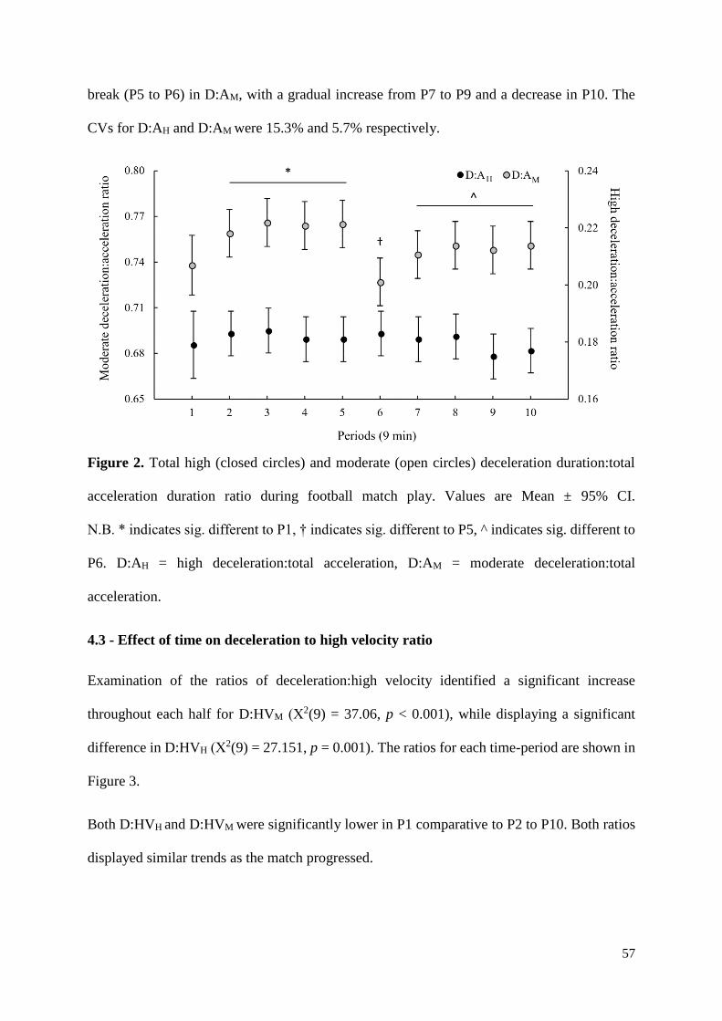
57

break (P5 to P6) in D:AM, with a gradual increase from P7 to P9 and a decrease in P10. The

CVs for D:AH and D:AM were 15.3% and 5.7% respectively.

Figure 2. Total high (closed circles) and moderate (open circles) deceleration duration:total

acceleration duration ratio during football match play. Values are Mean ± 95% CI.

N.B. * indicates sig. different to P1, † indicates sig. different to P5, ^ indicates sig. different to

P6. D:AH = high deceleration:total acceleration, D:AM = moderate deceleration:total

acceleration.

4.3 - Effect of time on deceleration to high velocity ratio

Examination of the ratios of deceleration:high velocity identified a significant increase

throughout each half for D:HVM (Χ2(9) = 37.06, p < 0.001), while displaying a significant

difference in D:HVH (Χ2(9) = 27.151, p = 0.001). The ratios for each time-period are shown in

Figure 3.

Both D:HVH and D:HVM were significantly lower in P1 comparative to P2 to P10. Both ratios

displayed similar trends as the match progressed.

58

Figure 3. Total high (closed circles) and moderate (open circles) deceleration duration:high

velocity distance ratio during football match play. Values are Mean ± 95% CI.

N.B. * indicates sig. different to P1. D:HVH = high deceleration:high velocity, D:AM =

moderate deceleration:high velocity.

59

Chapter 5 –

Discussion

60

The aims of this thesis were three-fold. Firstly, to quantify the duration spent accelerating and

decelerating in elite-level football, secondly to model the acceleration and deceleration profiles

of elite-level male football players, and finally to establish a new metric that enhances our

understanding of deceleration as an external load marker that encompasses the opportunistic

nature of deceleration.

5.1 - Novel Findings

5.1.1 - Quantifying the duration spent accelerating and decelerating

The present study was the first to use the duration of acceleration and deceleration efforts to

describe these temporal patterns of elite-level football match play. Although the previous

studies assessing the deceleration profiles of football players have provided important

information regarding the deceleration output in match play, the interpretation of this data is

limited due to the type of deceleration metric reported (i.e., the distance covered and frequency

of acceleration and deceleration efforts). In the present study, there was an approximate 25%

decline in the duration spent in all four acceleration and deceleration thresholds (DECH, DECM,

ACCM, and ACCH) from P1 to P10. When segmented into halves, there was between 15 - 19%

decline from P1 to P5 (first half), between 18 - 24% decline from P6 to P10 (second half), and

between 2 - 8% increase from P5 to P6 (across the half-time interval) for all four metrics. The

decline in deceleration duration is closely mirrored by the decline in acceleration, and therefore

the two metrics need to be considered in tandem. Therefore, by modelling the decline in

acceleration and deceleration, the synonymous values should be reflected in the decay curves.

In contrast to the previous studies, the duration spent in each deceleration band illustrates the

frequency of efforts (i.e., more efforts would result in more duration spent decelerating) as well

as the magnitude of deceleration effort (i.e., a deceleration from a high velocity would take

longer to perform and therefore an increase in duration spent decelerating). When assessing the

61

distance covered whilst decelerating, ideally a player should aim to cover less distance whilst

decelerating rather than more distance, as it enables a player to turn more quickly and sprint

again in the opposite direction, thus increasing their chances of reaching the ball before their

opponent. As such, the distance covered decelerating, should not be used as a measure of

deceleration activity as it would be more beneficial for a player to cover less distance whilst

decelerating. Similarly, when considering the frequency of deceleration efforts, the magnitude

of these efforts is unclear, and therefore are not appropriate to identify the true deceleration

profile of match play. Finally, the duration between deceleration efforts (Mara et al., 2017)

fails to capture both the magnitude of each deceleration efforts, as well as the opportunistic

nature of deceleration. Therefore, the duration spent decelerating is the most appropriate metric

to employ.

5.1.2 - Modelling acceleration and deceleration

The second aim of this study was to use statistical modelling to illustrate the decay in a player’s

ability to accelerate and decelerate within a match. Due to the half-time interval, the match was

split into two negative logarithmic decay curves for all four measures (DECH, DECM, ACCH,

and ACCM). These curves were characterised by a steep drop from P1 to P2 in the first half (P6

to P7 in second half), followed by a less severe decline from P2 to P5 (P7 to P10 in second

half). Also arising from the negative logarithmic decay curves, were the coefficients and

intercepts from the function of each curve. The intercept, or constant, in the decay curve

illustrates the maximum capacity of the athletes for a given metric. For instance, an intercept

of 7.58 in the first half for DECH compared to an intercept of 6.71 in the second half illustrates

that the overall magnitude of deceleration output is lower in the second half comparative to the

first half. This represents a 13% decline in duration spent in DECH during the second half in

comparison to the first half. Meanwhile, the coefficient, or decay rate, illustrates the rate at

which each metric declines throughout each half. A coefficient of zero would indicate no

62

decline at all throughout the half. This coefficient is analogous to a decrement score or a fatigue

index, where the function considers the delta value from the initial time-point. For instance, in

DECH, the coefficient for the first half (-0.564) and the coefficient for the second half of -0.563

are essentially equal. This means that although the intercept is considerably lower in the second

half compared to the first half, the rate at which DECH declines across each half is comparative.

These coefficients and intercepts can be used as a method of comparing the relative acceleration

and deceleration profiles of individual players and positions. Future research may obtain

sufficient data for each player/position to generate valid curves and make it possible to make

inferences based upon these measures to determine the capabilities of different players, and the

positional demands of different formations.

5.1.3 - Ratios of deceleration to acceleration and deceleration to high-velocity running

In the present study, the novel methodology of expressing the ratios of deceleration to

acceleration and ratios of deceleration to high velocity distance aimed to examine the

opportunistic nature of deceleration. The DECH decayed at an equal rate to the total

accelerations as evident by the D:AH which did not change throughout the match. Meanwhile,

the ability to decelerate in the moderate domain was better maintained despite a decay in

duration spent accelerating and high velocity distance, resulting in an increase in D:AM and

D:HVM. We interpret these findings to indicate that the decline in deceleration efforts evident

throughout match play could be attributed to a lack of opportunity, rather than an impaired

deceleration ability. This is in opposition to the findings that suggest the ability to decelerate

is hampered in the late stages of football match play (Akenhead et al., 2013; Mara et al., 2017;

Russell et al., 2016; Vigh-Larsen et al., 2018). Akenhead reported reductions in the distances

covered whilst accelerating and decelerating, suggesting that acceleration and deceleration

capability are acutely compromised during match play (Akenhead et al., 2013). Initially, this

seems valid, however there is a methodological flaw in assuming that acceleration and

63

deceleration are independent of each other. As deceleration requires a preceding acceleration,

the ability to decelerate is heavily dependent on acceleration which makes the isolation of the

deceleration profile of match play logistically challenging to determine whether deceleration

capacity is compromised. Although methodologically-flawed, the three subsequent studies

assessing the deceleration profile of football match play (Mara et al., 2017; Russell et al., 2016;

Vigh-Larsen et al., 2018) have all held this same assumption. The frequency of deceleration

efforts does not capture the intensity of each effort (Russell et al., 2016; Vigh-Larsen et al.,

2018), the duration between efforts does not capture the opportunistic nature of deceleration

(Mara et al., 2017), and finally the distance covered whilst decelerating is counter-intuitive as

it is more beneficial to cover less distance while decelerating, enabling a player to change

direction more rapidly. This is unlike the time spent decelerating as, due to the discretised

bands, the more time spent decelerating must correspond to a greater deceleration output.

Therefore, the distance covered whilst decelerating, the frequency of deceleration efforts, and

the duration between deceleration efforts all fail to capture elements of the deceleration profile.

In congruence with the data provided in the four previously mentioned studies examining the

deceleration profile of football match play (Akenhead et al., 2013; Mara et al., 2017; Russell

et al., 2016; Vigh-Larsen et al., 2018), it was apparent that all displayed similar trends between

acceleration and deceleration. The reduction in the distance covered while decelerating

throughout the match in the Akenhead et al. (2013) study is a close reflection of the change in

distance covered while accelerating, which would presumably display no change in the ratio

between deceleration and acceleration. The symmetry in the duration between deceleration

efforts and the duration between acceleration efforts evident in the study of Mara et al. (2017)

would also ostensibly be reflected in a constant ratio between deceleration and acceleration.

Russell et al. (2016) compared the frequency of acceleration and deceleration efforts and

showed the effect of time on acceleration and deceleration efforts were near identical, as seen

64

by partial η2 of 0.601 and 0.603 respectively. Finally, Vigh-Larsen et al. (2018) plotted the

frequency of acceleration and deceleration efforts but reported a slight increase in deceleration

efforts compared to accelerations in the second 15-min interval of the match, compounding the

inference that changes in deceleration values can be attributed to a lack of opportunity.

The increase in D:AM and constant D:AH could also be due to the differing energetic demands

of different magnitudes of acceleration and deceleration. Moderate decelerations require the

least energy of all acceleration magnitudes (Osgnach et al., 2010) and it is therefore reasonable

to suggest that the least energetically-demanding movements are impacted the least throughout

the duration of a match. As such, it is remiss to ignore both the magnitude of each deceleration

effort (as illustrated by the duration of deceleration efforts) and the opportunistic nature of

deceleration which can be identified by the ratio of deceleration to acceleration.

5.2 - Limitations of Research

This study reinforces the need to further interrogate the deceleration profile and explore

different methodological approaches to understand the origin of the altered deceleration profile

throughout match play. Due to varying match conditions and tactics, interpretations of the

alterations in physical performance metrics should only be made on a longitudinal basis (Paul,

Bradley, & Nassis, 2015). If matches are taken as standalone values, acceleration and

deceleration profiles will more likely reflect the style of play in one match and are likely

influenced by strategies such as athlete pacing (Paul et al., 2015), rather than a player’s

impairment in a given physical performance metric. This is reflected by the coefficient of

variation (CV) for each metric, with a mean CV between 6 and 14% across the four metrics.

As longitudinal data is required for inferences, outputs from an individual match should not be

used to draw conclusions. It should also be noted that strategies could change in the later stages

65

of a match due to the match scenario, with teams needing to either protect a lead, or push for a

result, which could significantly impact on the transient patterns of their activity.

One limitation of the present study is the accuracy and reliability of quantifying the acceleration

and deceleration output from commercially available GPS technology (Buchheit, Al Haddad,

et al., 2014). Caution needs to be taken when reporting acceleration and deceleration values

due to the variability between units (Buchheit, Al Haddad, et al., 2014). To minimize the

variability associated with quantifying metrics of acceleration, we quantified the relative

values. By measuring changes in value, rather than absolute values, the variance attributed to

the unit is reduced, thus decreasing the overall uncertainty. If the raw data was also able to be

retrieved, an analysis of the exact magnitude of each deceleration effort may provide a more

precise understanding of the transient nature of deceleration output. A further limitation of the

present study relates to the sample size (n = 16) which was due to the stringent inclusion criteria

and single pool of players (i.e., from the same team). As such, it was not feasible to generate

position-specific curves. It is noted however that the acceleration and deceleration profiles may

vary according to player position with wide players recording significantly more efforts than

central players (Vigh-Larsen et al., 2018).

5.3 - Practical Applications

Due to the muscle damage-inducing nature of the deceleration action (Newham et al., 1986;

Young et al., 2012), deceleration needs to be considered as an important part of a training

program, especially where the ability to increase and decrease velocity very rapidly is a key

element of performance. Modelling the decay of GPS metrics can provide practitioners with

coefficients and intercepts from the negative logarithmic curves to quantify a player’s capacity

and decay and can use these as markers of better conditioning. Practitioners should not view

magnitude of deceleration efforts in isolation; rather, with respect to the preceding acceleration

66

and high-velocity running. Similarly, a ratio between deceleration and acceleration may

represent a more appropriate measurement to assess the deceleration profile, as it accounts for

the opportunistic nature of deceleration output during match play.

5.4 - Future Research

When exploring the deceleration profile in future studies, it is pertinent to recognise the

secondary and opportunistic nature of deceleration. If the deceleration output is quantified

using discretised thresholds, as seen by the typical outputs of GPS manufacturers, the duration

spent in each threshold should be used, rather than the frequency of efforts or the distance

covered while decelerating. If the raw GPS data is accessible, the amplitude of each

deceleration effort can also facilitate an understanding of the absolute deceleration values.

When considering the change in deceleration capacity, two methods can be used. Firstly, if the

discretised thresholds are quantified, values must be compared to actions signifying the start

of running (i.e., an acceleration or high-speed distance). If the raw GPS data is accessible, then

the change in the magnitude of decelerations throughout the duration of a match can also be

used to make inferences regarding the temporal change in deceleration capacity.

In the current study, due to the limited number of players, there was not sufficient data to

identify position-specific decay models. To develop position-specific models, a larger sample

population would be required (n > 10 for each position) to better estimate the variance

attributed to position rather than simply player variance. Similarly, having footballers play

multiple positions may assist in minimising the individual variance, and increase the

confidence in the position specific model of the given physical performance variable (i.e.,

deceleration profile). Furthermore, as this study only compared three different formations,

formation-specific decay curves could also be created to highlight the highest- and lowest-

acceleration and deceleration demanding formations. For instance, a 4-2-1-2 narrow formation

67

may demand a higher level of moderate acceleration and decelerations given the central

tendency of play, whereas a 5-4-1 wide formation may enforce more high acceleration and

deceleration efforts. Once ample coefficients and intercepts are quantified across various teams

and quality of competition, benchmarks can also be set for players to achieve appropriate player

conditioning during training, ensuring their performances are not hampered in the later stages

of a match.

Additional insights into the whole-game temporal patterns can be achieved by dividing the

periods of match play into smaller intervals. If data were divided into periods of 5 min, there

would be 18 periods throughout a match, which could identify trends that were not visible in

the 9-min intervals. For example, due to large variance there is no statistically significant

decline from P2 to P5, and from P7 to P10. Therefore, if more segmentation was used, the

difference between the 10-15 min interval and 40-45 min interval may be substantial. However,

this method may dampen the most intense period of match play as the most active period of a

match may not fall completely within one of these predefined blocks, and; therefore, the

temporal periods of match play may underestimate the activity profile of competition. The

transient changes in the deceleration profile may be more appropriately studied by employing

the use of rolling epochs (Delaney, Thornton, et al., 2017; Howe, Aughey, Hopkins, Stewart,

& Cavanagh, 2017; Varley, Elias, & Aughey, 2012) rather than discrete time periods. By using

a rolling epoch approach, the position- and duration-specific transient decay could be illustrated

for all 90 min of the match, using a moving average method.

The establishment of the coefficients and intercepts to describe the deceleration profile of

football match play is a novel approach. As a result, this could be applied to other metrics

commonly used in GPS data analysis. I would hypothesise that total distance and distance

covered within different velocity thresholds would follow a similar trend, and that if

coefficients and intercepts could be generated for each threshold, useful practical information

68

could be synthesised to improve conditioning and tactical training exercises. For example, if a

player has a low decay rate for velocities less than 16 km·h−1 but has a high decay rate for

velocities more than 16 km·h−1, then more specific conditioning drills (i.e., running volume

performed at velocity above 16 km·h−1) can be prescribed to target the relevant deficiency.

69

Chapter 6 –

Conclusion

70

This thesis aimed to understand how GPS data has been applied in sport science, identify areas

that have rarely been explored, and then translate this information into valid and meaningful

metrics for player monitoring. Specifically, this thesis focused on deceleration due to the

prevalence within football match play, the mechanism of the movement (i.e., muscle-damaging

eccentric contractions), and the energetic demands of the movement. Three main outcomes

were established: a valid metric for deceleration, a model of decay throughout football match

play, and a metric to encompass the opportunistic nature of deceleration.

The duration spent whilst decelerating in discretised thresholds is available in commercially-

available GPS software; however, it is rarely used. From the findings arising from this thesis,

We suggest that this metric should be used to quantify the external load performed via

deceleration, rather than the more commonly-used metrics such as the frequency of

deceleration efforts or the total distance covered whilst decelerating.

When assessing the decay in external workload, negative logarithmic curves can be used to

describe the decay, as it can be presented with a coefficient and an intercept. These decay

curves, while currently only used for deceleration, can also be applied to other metrics used to

quantify the external load within match play (e.g., high-speed running and metres per minute).

We/I suggest that utilising a rolling epoch while calculating these values would also result in

more accurate curves.

It should be known that deceleration cannot be examined independently as the action is

secondary to a preceding acceleration/running velocity. Therefore, when evaluating whether

an individual’s deceleration ability has been compromised, the duration spent decelerating

should be compared to a primary action (e.g., the frequency and magnitude of accelerations or

high-speed running). Of the data within this thesis, the rate of decay in deceleration was less

71

than or equal to the rate of decay in acceleration and therefore we are unable to infer that the

ability to decelerate during football match play is compromised.

72

Chapter 7 –

References

73

Abt, G., & Lovell, R. (2009). The use of individualized speed and intensity thresholds for

determining the distance run at high-intensity in professional soccer. J Sports Sci, 27(9),

893-898.

Akenhead, R., French, D., Thompson, K. G., & Hayes, P. R. (2014). The acceleration

dependent validity and reliability of 10 Hz GPS. J Sci Med Sport, 17(5), 562-566.

Akenhead, R., Hayes, P. R., Thompson, K. G., & French, D. (2013). Diminutions of

acceleration and deceleration output during professional football match play. J Sci Med

Sport, 16(6), 556-561.

Altman, D. G., & Royston, P. (2006). The cost of dichotomising continuous variables. Br Med

J, 332(7549), 1080.

Andrews, J. R., McLeod, W. D., Ward, T., & Howard, K. (1977). The cutting mechanism. Am

J Sports Med, 5(3), 111-121.

Aughey, R. J. (2011). Applications of GPS technologies to field sports. Int J Sports Physiol

Perform, 6(3), 295-310.

Australian National University. (2018). Bachelor of Applied Data Analytics. Retrieved from

https://programsandcourses.anu.edu.au/program/BADAN

Bangsbo, J., Norregaard, L., & Thorso, F. (1991). Activity profile of competition soccer. Can

J Sport Sci, 16(2), 110-116.

Bendiksen, M., Pettersen, S. A., Ingebrigtsen, J., Randers, M. B., Brito, J., Mohr, M., . . .

Krustrup, P. (2013). Application of the Copenhagen soccer test in high-level women

players–locomotor activities, physiological response and sprint performance. Hum Mov

Sci, 32(6), 1430-1442.

Bloomfield, J., Polman, R., & O'Donoghue, P. (2007). Physical demands of different positions

in FA Premier League soccer. J Sports Sci Med, 6(1), 63-70.

74

Borresen, J., & Lambert, M. I. (2008). Quantifying training load: A comparison of subjective

and objective methods. Int J Sports Physiol Perform, 3(1), 16-30.

Bouchard, C., & Rankinen, T. (2001). Individual differences in response to regular physical

activity. Med Sci Sports Exerc, 33(6 Suppl), S446-451; discussion S452-443.

Boyd, L. J., Ball, K., & Aughey, R. J. (2011). The reliability of MiniMaxX accelerometers for

measuring physical activity in Australian Football. Int J Sports Physiol Perform, 6(3),

311-321.

Bradley, P. S., Sheldon, W., Wooster, B., Olsen, P., Boanas, P., & Krustrup, P. (2009). High-

intensity running in English FA Premier League soccer matches. J Sports Sci, 27(2),

159-168.

Brousell, L. (2014, March 11). 8 ways big data and analytics will change sports. CIO. Retrieved

from https://www.cio.com/

Buchheit, M. (2014). Monitoring training status with HR measures: Do all roads lead to Rome?

Front Physiol, 5(73).

Buchheit, M., Al Haddad, H., Simpson, B. M., Palazzi, D., Bourdon, P. C., Di Salvo, V., &

Mendez-Villanueva, A. (2014). Monitoring accelerations with GPS in football: Time

to slow down? Int J Sports Physiol Perform, 9(3), 442-445.

Buchheit, M., Allen, A., Poon, T. K., Modonutti, M., Gregson, W., & Di Salvo, V. (2014).

Integrating different tracking systems in football: Multiple camera semi-automatic

system, local position measurement and GPS technologies. J Sports Sci, 32(20), 1844-

1857.

Buchheit, M., Racinais, S., Bilsborough, J. C., Bourdon, P. C., Voss, S. C., Hocking, J., . . .

Coutts, A. J. (2013). Monitoring fitness, fatigue and running performance during a pre-

season training camp in elite football players. J Sci Med Sport, 16(6), 550-555.

75

Carling, C., Bradley, P., McCall, A., & Dupont, G. (2016). Match-to-match variability in high-

speed running activity in a professional soccer team. J Sports Sci, 34(24), 2215-2223.

Castellano, J., Alvarez-Pastor, D., & Bradley, P. S. (2014). Evaluation of research using

computerised tracking systems (Amisco and Prozone) to analyse physical performance

in elite soccer: A systematic review. Sports Med, 44(5), 701-712.

Castellano, J., Casamichana, D., Calleja-Gonzalez, J., Roman, J. S., & Ostojic, S. M. (2011).

Reliability and accuracy of 10 hz GPS devices for short-distance exercise. J Sports Sci

Med, 10(1), 233-234.

Chaouachi, A., Manzi, V., Chaalali, A., Wong del, P., Chamari, K., & Castagna, C. (2012).

Determinants analysis of change-of-direction ability in elite soccer players. J Strength

Cond Res, 26(10), 2667-2676.

Chen, M. J., Fan, X., & Moe, S. T. (2002). Criterion-related validity of the Borg ratings of

perceived exertion scale in healthy individuals: A meta-analysis. J Sports Sci, 20(11),

873-899.

Chmura, P., Andrzejewski, M., Konefal, M., Mroczek, D., Rokita, A., & Chmura, J. (2017).

Analysis of motor activities of professional soccer players during the 2014 World Cup

in Brazil. J Hum Kinet, 56, 187-195.

Cummins, C., Orr, R., O'Connor, H., & West, C. (2013). Global positioning systems (GPS)

and microtechnology sensors in team sports: A systematic review. Sports Med, 43(10),

1025-1042.

Cunniffe, B., Proctor, W., Baker, J. S., & Davies, B. (2009). An evaluation of the physiological

demands of elite rugby union using global positioning system tracking software. J

Strength Cond Res, 23(4), 1195-1203.

76

Daanen, H. A., Lamberts, R. P., Kallen, V. L., Jin, A., & Van Meeteren, N. L. (2012). A

systematic review on heart-rate recovery to monitor changes in training status in

athletes. Int J Sports Physiol Perform, 7(3), 251-260.

Deakin University. (2018). Master of Data Analytics. Retrieved from

http://www.deakin.edu.au/course/master-data-analytics

Delaney, J. A., Cummins, C. J., Thornton, H. R., & Duthie, G. M. (2017). Importance,

reliability and usefulness of acceleration measures in team sports. J Strength Cond Res.

Delaney, J. A., Thornton, H. R., Rowell, A. E., Dascombe, B. J., Aughey, R. J., & Duthie, G.

M. (2017). Modelling the decrement in running intensity within professional soccer

players. J Sci Med Football, 2(2), 86-92.

Desgorces, F. D., Senegas, X., Garcia, J., Decker, L., & Noirez, P. (2007). Methods to quantify

intermittent exercises. Appl Physiol Nutr Metab, 32(4), 762-769.

Di Salvo, V., Baron, R., Tschan, H., Calderon Montero, F. J., Bachl, N., & Pigozzi, F. (2007).

Performance characteristics according to playing position in elite soccer. Int J Sports

Med, 28(3), 222-227.

Duffield, R., Reid, M., Baker, J., & Spratford, W. (2010). Accuracy and reliability of GPS

devices for measurement of movement patterns in confined spaces for court-based

sports. J Sci Med Sport, 13(5), 523-525.

Edgecomb, S. J., & Norton, K. I. (2006). Comparison of global positioning and computer-based

tracking systems for measuring player movement distance during australian football. J

Sci Med Sport, 9(1-2), 25-32.

Edwards, R. H. (1983). Biochemical bases of fatigue in exercise performance: Catastrophe

theory of muscular fatigue. In Biochemistry of exercise (Vol. 13, pp. 3-28). Champaign,

IL: Human Kinetics Publishers.

77

Esposito, F., Impellizzeri, F. M., Margonato, V., Vanni, R., Pizzini, G., & Veicsteinas, A.

(2004). Validity of heart rate as an indicator of aerobic demand during soccer activities

in amateur soccer players. Eur J Appl Physiol, 93(1-2), 167-172.

Google. (2018). Explore Search Interest for Data + Analytics by Time, Location and

Popularity on Google Trends. Retrieved from

https://trends.google.com/trends/explore?q=data%20analytics&geo=US

Griffith University. (2018). Bachelor of Computer Science. Retrieved from

https://degrees.griffith.edu.au/Program/1534/

Hägglund, M., Waldén, M., Magnusson, H., Kristenson, K., Bengtsson, H., & Ekstrand, J.

(2013). Injuries affect team performance negatively in professional football: An 11-

year follow-up of the UEFA Champions League injury study. Br J Sports Med, 47, 738-

742.

Halson, S. L. (2014). Monitoring training load to understand fatigue in athletes. Sports Med,

44 Suppl 2, S139-147.

Hewit, J., Cronin, J., Button, C., & Hume, P. (2011). Understanding deceleration in sport.

Strength and Conditioning Journal, 33(1), 47-52.

Hopkins, W. G. (1991). Quantification of training in competitive sports. Methods and

applications. Sports Med, 12(3), 161-183.

Hopkins, W. G., Marshall, S. W., Batterham, A. M., & Hanin, J. (2009). Progressive statistics

for studies in sports medicine and exercise science. Med Sci Sports Exerc, 41(1), 3-13.

Howe, S. T., Aughey, R. J., Hopkins, W. G., Stewart, A. M., & Cavanagh, B. P. (2017).

Quantifying important differences in athlete movement during collision-based team

sports: Accelerometers outperform global positioning systems. Paper presented at the

IEEE International Symposium on Inertial Sensors and Systems (INERTIAL).

78

Howes, J. (2017, September 15). Sports analytics on the rise as Australia plays catch up with

the rest of world. The Guardian. Retrieved from https://www.theguardian.com/sport/

Hlavac, M (2018). stargazer: Well-formatted regression and summary statistics Tables. R

package version 5.2.1. Retrieved from https://CRAN.R-project.org/package=stargazer

Impellizzeri, F. M., Rampinini, E., Coutts, A. J., Sassi, A., & Marcora, S. M. (2004). Use of

RPE-based training load in soccer. Med Sci Sports Exerc, 36(6), 1042-1047.

Ingebrigtsen, J., Dalen, T., Hjelde, G. H., Drust, B., & Wisloff, U. (2015). Acceleration and

sprint profiles of a professional elite football team in match play. Eur J Sport Sci, 15(2),

101-110.

Johnston, R. J., Watsford, M. L., Austin, D. J., Pine, M. J., & Spurrs, R. W. (2015). An

examination of the relationship between movement demands and rating of perceived

exertion in australian footballers. J Strength Cond Res, 29(7), 2026-2033.

Johnston, R. J., Watsford, M. L., Kelly, S. J., Pine, M. J., & Spurrs, R. W. (2014). Validity and

interunit reliability of 10 Hz and 15 Hz GPS units for assessing athlete movement

demands. J Strength Cond Res, 28(6), 1649-1655.

Johnston, R. J., Watsford, M. L., Pine, M. J., Spurrs, R. W., Murphy, A. J., & Pruyn, E. C.

(2012). The validity and reliability of 5 Hz global positioning system units to measure

team sport movement demands. J Strength Cond Res, 26(3), 758-765.

Katz, L., & Katz, J. S. (1994). Fractal (power law) analysis of athletic performance. Sports Med

Training Rehab, 5(2), 95-105.

Kentta, G., & Hassmen, P. (1998). Overtraining and recovery. A conceptual model. Sports

Med, 26(1), 1-16.

Larsson, P. (2003). Global positioning system and sport-specific testing. Sports Med, 33(15),

1093-1101.

79

Lockie, R. G., Murphy, A. J., Knight, T. J., & Janse de Jonge, X. A. (2011). Factors that

differentiate acceleration ability in field sport athletes. J Strength Cond Res, 25(10),

2704-2714.

Mara, J. K., Thompson, K. G., Pumpa, K. L., & Morgan, S. (2017). The acceleration and

deceleration profiles of elite female soccer players during competitive matches. J Sci

Med Sport, 20(9), 867-872.

Mohr, M., Krustrup, P., & Bangsbo, J. (2003). Match performance of high-standard soccer

players with special reference to development of fatigue. J Sports Sci, 21(7), 519-528.

Morgan, W. P., Brown, D. R., Raglin, J. S., O'Connor, P. J., & Ellickson, K. A. (1987).

Psychological monitoring of overtraining and staleness. Br J Sports Med, 21(3), 107-

114.

Newham, D. J., Jones, D. A., & Edwards, R. H. (1986). Plasma creatine kinase changes after

eccentric and concentric contractions. Muscle Nerve, 9(1), 59-63.

Osgnach, C., Poser, S., Bernardini, R., Rinaldo, R., & di Prampero, P. E. (2010). Energy cost

and metabolic power in elite soccer: A new match analysis approach. Med Sci Sports

Exerc, 42(1), 170-178.

Paul, D. J., Bradley, P. S., & Nassis, G. P. (2015). Factors affecting match running performance

of elite soccer players: Shedding some light on the complexity. Int J Sports Physiol

Perform, 10(4), 516-519.

Petersen, C., Pyne, D., Portus, M., & Dawson, B. (2009). Validity and reliability of GPS units

to monitor cricket-specific movement patterns. Int J Sports Physiol Perform, 4(3), 381-

393.

Piepho, H. P., Buchse, A., & Richter, C. (2004). A mixed modelling approach for randomized

experiments with repeated measures. J Agron Crop Sci, 190(4), 230-247.

80

Raysmith, B. P., & Drew, M. K. (2016). Performance success or failure is influenced by weeks

lost to injury and illness in elite australian track and field athletes: A 5-year prospective

study. J Sci Med Sport, 19(10), 778-783.

Rienzi, E., Drust, B., Reilly, T., Carter, J. E., & Martin, A. (2000). Investigation of

anthropometric and work-rate profiles of elite south american international soccer

players. J Sports Med Phys Fitness, 40(2), 162-169.

Rushall, B. S. (1990). A tool for measuring stress tolerance in elite athletes. J Appl Sport

Psychol, 2(1), 51-66.

Russell, M., Sparkes, W., Northeast, J., Cook, C. J., Love, T. D., Bracken, R. M., & Kilduff,

L. P. (2016). Changes in acceleration and deceleration capacity throughout professional

soccer match-play. J Strength Cond Res, 30(10), 2839-2844.

Saw, A. E., Main, L. C., & Gastin, P. B. (2016). Monitoring the athlete training response:

Subjective self-reported measures trump commonly used objective measures: A

systematic review. Br J Sports Med, 50, 281-291.

Schutz, Y., & Chambaz, A. (1997). Could a satellite-based navigation system (GPS) be used

to assess the physical activity of individuals on earth? Eur J Clin Nutr, 51(5), 338.

Schutz, Y., & Herren, R. (2000). Assessment of speed of human locomotion using a differential

satellite global positioning system. Med Sci Sports Exerc, 32(3), 642-646.

Spencer, M., Lawrence, S., Rechichi, C., Bishop, D., Dawson, B., & Goodman, C. (2004).

Time-motion analysis of elite field hockey, with special reference to repeated-sprint

activity. J Sports Sci, 22(9), 843-850.

Stolen, T., Chamari, K., Castagna, C., & Wisloff, U. (2005). Physiology of soccer: An update.

Sports Med, 35(6), 501-536.

81

Sullivan, C., Bilsborough, J. C., Cianciosi, M., Hocking, J., Cordy, J., & Coutts, A. J. (2014).

Match score affects activity profile and skill performance in professional australian

football players. J Sci Med Sport, 17(3), 326-331.

Sweeting, A. J., Cormack, S. J., Morgan, S., & Aughey, R. J. (2017). When is a sprint a sprint?

A review of the analysis of team-sport athlete activity profile. Front Physiol, 8(432).

Taylor, K., Chapman, D., Cronin, J., Newton, M. J., & Gill, N. (2012). Fatigue monitoring in

high performance sport: A survey of current trends. J Aust Strength Cond, 20(1), 12-

23.

Terrier, P., & Schutz, Y. (2005). How useful is satellite positioning system (GPS) to track gait

parameters? A review. J Neuroeng Rehabil, 2(1), 28.

The International Football Association Board. (2015). Amendments to the laws of the game –

2015/2016 and information on the completed reform of the International Football

Association Board. Retrieved from https://resources.fifa.com/

Thornton, H. R., Nelson, A. R., Delaney, J. A., Serpiello, F. R., & Duthie, G. M. (2018). Inter-

unit reliability and effect of data processing methods of global positioning systems. Int

J Sports Physiol Perform, 1-24.

Valter, D. S., Adam, C., Barry, M., & Marco, C. (2017). Validation of Prozone ®: A new

video-based performance analysis system. Int J Perform Anal Sport, 6(1), 108-119.

Varley, M. C., Elias, G. P., & Aughey, R. J. (2012). Current match-analysis techniques'

underestimation of intense periods of high-velocity running. Int J Sports Physiol

Perform, 7(2), 183-185.

Varley, M. C., Fairweather, I. H., & Aughey, R. J. (2012). Validity and reliability of GPS for

measuring instantaneous velocity during acceleration, deceleration, and constant

motion. J Sports Sci, 30(2), 121-127.

82

Varley, M. C., Gabbett, T., & Aughey, R. J. (2014). Activity profiles of professional soccer,

rugby league and Australian Football match play. J Sports Sci, 32(20), 1858-1866.

Vigh-Larsen, J. F., Dalgas, U., & Andersen, T. B. (2018). Position-specific acceleration and

deceleration profiles in elite youth and senior soccer players. J Strength Cond Res,

32(4), 1114-1122.

Wallace, L. K., Slattery, K. M., & Coutts, A. J. (2009). The ecological validity and application

of the session-RPE method for quantifying training loads in swimming. J Strength Cond

Res, 23(1), 33-38.

Witte, T. H., & Wilson, A. M. (2004). Accuracy of non-differential gps for the determination

of speed over ground. J Biomech, 37(12), 1891-1898.

Young, W. B., Hepner, J., & Robbins, D. W. (2012). Movement demands in Australian Rules

football as indicators of muscle damage. J Strength Cond Res, 26(2), 492-496.

83

Chapter 8 –

Submitted Manuscript

84

8.1 - Statement of contribution to co-authored published paper

This chapter includes a co-authored paper. The status of the co-authored paper, including all

authors, is:

Under Revision: Newans, T., Bellinger, P., Dodd, K., & Minahan, C. (2018). Modelling the

acceleration and deceleration profile of elite-level football players. Int J Sports Physiol

Perform.

The contributions to the paper involved:

Timothy Newans: Idea Formation, Experimental Design, Data Analysis, Manuscript

Preparation and Revisions

Phillip Bellinger: Experimental Design, Manuscript Preparation, and Revisions

Karl Dodd: Data Collection, Manuscript Preparation

Clare Minahan: Idea Formation, Experimental Design, Manuscript Preparation, and

Revisions

(Signed) _________________________________ (Date)______________

Timothy Newans

(Countersigned) ___________________________ (Date)______________

Co-author of paper: Dr Phillip Bellinger

(Countersigned) ___________________________ (Date)______________

Supervisor: Associate Professor Clare Minahan

85

Modelling the acceleration and deceleration profile of elite-level football players

86

Abstract

Purpose: The ability to increase and decrease velocity very rapidly is a key element of field-based

sports such as football, which require repeated high-intensity changes of direction. The purpose of the

present study was to develop a new methodological approach to quantify the acceleration and

deceleration profiles of elite-level male football players during competitive match play.

Methods: Global positioning system (GPS) technology measures were collected from 20 male football

players competing in the Australian Hyundai A-League during 58 matches throughout two seasons (N

= 368 observations). Match data were organized into ten 9-minute periods (i.e., P1: 0 - 9 min) and the

time spent accelerating at moderate (1–2 m·s−2) and high (>2 m·s−2) acceleration (ACCM and ACCH,

respectively) and deceleration (DECM and DECH, respectively) were quantified. Additionally,

deceleration:acceleration ratios were also quantified to identify the transient nature of deceleration

activity throughout match play.

Results: All acceleration and deceleration metrics displayed significant negative logarithmic curves

within each half of football match play, while a partial recovery was evident directly following the half-

time period. There was no change in the ratio of high deceleration:acceleration; however, a significant

increase in the ratio of moderate deceleration:acceleration was evident as each half progressed.

Conclusions: Using negative logarithmic curves to illustrate the acceleration and deceleration decay

provides a novel methodological approach to quantify the high-intensity actions during football match

play. A decrease in the duration of deceleration efforts throughout a match may be attributed to a lack

of opportunity, evidenced by the increase in the ratio of deceleration:acceleration as a result of a

decrease in the number of high-intensity efforts. However, improving the ability to decelerate rapidly

may be an important aspect of football-specific physical performance due to the repeated high-intensity

changes of direction during football match play.

Key words: GPS, player load, movement patterns, soccer

87

Introduction

Characterizing movement patterns and understanding the physical demands of team sports are crucial

for the construction of training drills, match simulations and team strategy1, 2. Global Positioning System

(GPS) technology can be used to quantify the type, duration, and frequency of discrete movements

making up the intermittent-activity patterns in team sports3, 4. Solely quantifying the distances covered

within certain speed thresholds fails to capture the moments of sports, such as football, where frequent

changes of direction are prevalent5, 6. Recent studies have suggested that quantifying the acceleration

and deceleration profile during matches are more sensitive to fatigue than the running distance covered

at different speeds7-10 which are most commonly used11-13. Therefore, the quantification of an athlete’s

ability to accelerate and decelerate may be more important for the accurate quantification of football-

specific physical performance7, 14.

Despite the recent focus on the importance and usefulness of quantifying the acceleration profile in

team-sport athletes, one metric that has been commonly overlooked is the ability to decelerate11. Indeed,

decelerations are just as common as accelerations in football6 and will also contribute significantly to

the players’ external load during match play. Furthermore, as decelerations are a key element in the

ability to change direction5 it is vital that the deceleration profile is considered when assessing the

external load of a player throughout a match. This reinforces the need to identify the typical deceleration

profile during match play as a marker of physical performance for football players.

There are numerous accelerometer and GPS derived deceleration-based variables that have been

used to quantify the deceleration profile of professional football match play7-10. For example, Akenhead

et al. (2013) first reported time-dependent reductions in the total distance covered whilst decelerating7,

while other research has quantified the total number of acceleration and deceleration efforts8-10.

Alternatively, Mara et al. (2017) reported that the mean time between acceleration and deceleration

efforts increased from the first half to the second half. Collectively, these studies7-10 have suggested that

the capability to decelerate is acutely compromised during match play; however, the interpretation of

some data is limited because the magnitude of the intensity of each deceleration effort was unknown in

these studies8-10. Furthermore, the quantification of the distance covered whilst decelerating and the

88

number of deceleration efforts do not take into consideration whether a player has had the opportunity

to decelerate7-10. As a player’s top speed and ability to maintain speed decreases throughout a match15,

the opportunities to decelerate also decrease and therefore doesn’t necessarily give causality to a

compromised ability to decelerate, rather, a lack of opportunity to decelerate. To consider the

opportunistic nature of deceleration, the values must also be compared to a value that signifies the

initiation of a sprint. Due to commercial GPS units only providing discretized values for deceleration

zones3, an appropriate alternative method to describe the deceleration profile is the duration spent in

each deceleration zone. With a discretized value, it must be assumed that the value is at the lowest end

of the zone (i.e., exactly -2.0 m·s-2 for anything <-2.0 m·s-2). As a result, a player will have accomplished

a greater deceleration magnitude by spending longer decelerating at that given intensity.

The present study established a ratio of deceleration:acceleration to identify the transient nature of

deceleration during football match play. An increase in this ratio would imply that a player’s

deceleration ability is being impeded more than their acceleration ability, whilst a decrease in this ratio

would imply the opposite. Therefore, the aim of this study is to characterize the acceleration and

deceleration profiles of elite footballers by quantifying the time spent in each acceleration and

deceleration zone and develop a new methodological approach to minimize the bias within metrics of

deceleration.

Methods

Subjects

Twenty elite male football players (age: 28.1 ± 5.3 yr, stature: 179.0 ± 7.3 cm, body mass: 74.0 ± 6.4

kg) registered to play for the same team playing in the Australian A-League were included in this study.

The study was approved by the Griffith University Human Research Ethics Committee and consent was

sought from the Football club to obtain the data.

Design

89

The present study used a longitudinal, observational study design utilizing data collected from 58

matches throughout the 2015/16 and 2016/17 Australia A-League seasons. For a match to be included

in analysis, the football player must have played the full 90 min of the match.

Methodology

A total of 368 game entries were eligible (six forwards, seven midfielders and seven defenders),

with a median number of games per player of 14 (Range: 5-47 matches). During each match, players

wore a GPS unit which sampled at a rate of 10 Hz (Catapult X4 or S5 unit) which was turned on prior

to the commencement of the warm-up (~45min prior to kick-off). Immediately prior to the warm-up

each starting player was fitted with a customized harness, allowing the GPS unit to sit between the

player’s scapulae. Where possible, the same unit was used for the same player each week to minimize

error.

The deceleration bands were set as <-2.0 m·s−2 for a high deceleration (DECH) and between -1.0

and -2.0 m·s−2 for a moderate deceleration (DECM), values between -1.0 and +1.0 m·s−2 were deemed

negligible efforts and were discounted. Similarly, values between +1.0 and +2.0 m·s−2 was deemed a

moderate acceleration (ACCM) and values greater than +2.0 m·s−2 was deemed a high acceleration

(ACCH). These thresholds were chosen as they have been defined as moderate intensity in previous

research7-9, thus, allowing a comparison between studies.

Data from each match was retrieved retrospectively from Catapult’s Openfield software and split

into ten 9-min periods (P1 = 0-9:00 min, P2 = 9:01-18:00 min and so forth) and exported to comma-

separated value format. Any additional time at the end of the regulation 45-min half was excluded from

analysis for standardization. Nine minute intervals were chosen to allow each block to represent 10%

worth of the match.

To analyze the data, an average duration for each acceleration and deceleration band was calculated

for each player in each period to create the acceleration and deceleration profile for that player. The

mean was then taken for all players for each period, from which the decay curves could be fitted. Due

to the shape of decay, logarithmic functions were deemed most appropriate to estimate the decay in

90

each half. For each function, a coefficient and intercept were calculated. The coefficient would indicate

the rate of decay for the player, of which a value of zero would indicate no decay at all. Meanwhile, the

intercept would indicate the total acceleration or deceleration capacity of a player, with a higher

intercept being desirable.

In order to calculate the ratio of deceleration:acceleration, the duration of DECH and DECM were

divided by the total amount of time spent accelerating (ACCH + ACCM) in each period to generate a

ratio of high deceleration:acceleration (D:AH) and a ratio of moderate deceleration:acceleration (D:AM).

Similarly, the individual mean for each player in each period was calculated to quantify each player’s

deceleration ratio. By calculating the mean of all players, an overall deceleration ratio was calculated

for each period.

Statistical Analysis

The data was analyzed using SPSS V25 (IBM, Armonk, New York, United States) and using

customized software (R, v 3.5.0). For statistical analysis, a linear mixed model was used to determine

the effect of time on the acceleration, deceleration, and ratio measures. Chi-squared statistics and the

degrees of freedom are reported in the results. The coefficient of variation (CV) for each metric was

calculated by dividing the average of all player means by the standard deviation of all players’ means.

Results

There was a significant effect of time on DECH (Χ2(9) = 273.02, p < 0.001), DECM (Χ2(9) =

736.27, p < 0.001), ACCM (Χ2(9) = 952.86, p < 0.001) and ACCH (Χ2(9) = 171.33, p < 0.001). Figure

1 illustrates the decay in the duration spent accelerating and decelerating throughout match play, while

Table 1 displays the coefficients, intercepts, R2, and coefficients of variation (CV) of the logarithmic

curves.

Players spent the most time accelerating and decelerating during P1. P1 was significantly higher

than all other periods in the first half for all four measures. There was an increase following the half-

91

time break of 8% and 6% for ACCH and ACCM, respectively, while there was no significant change in

deceleration. P6 was significantly higher than P7-P10 for all measures.

The coefficients were all lower in the second half compared to the first half; however, the

intercept was of a lower magnitude. The deceleration intercepts were higher than the acceleration

intercepts in the high domain, while the deceleration intercepts were lower in the moderate domain.

Examination of the ratios of deceleration:acceleration identified a significant increase

throughout each half for D:AM (Χ2(9) = 48.03, p < 0.001), while there was no significant difference in

D:AH (Χ2(9) = 8.739, p = 0.462). The ratios for each time-period are shown in Figure 2.

No significant differences were evident in D:AH, while D:AM increased from P1 to P2 with no

significant change from P2 to P5. There was a significant decrease following the half-time break (P5 to

P6) in D:AM, with a gradual increase from P7 to P9 and a decrease in P10. The CVs for D:AH and D:AM

were 15.3% and 5.7% respectively.

Discussion

In the present study, we identified that at both moderate and high thresholds, the time spent accelerating

and decelerating displayed a negative logarithmic decay curve. The decay DECH, DECM, ACCM, and

ACCH was similar to that of previous research7-10 with large decreases from P1 to P2 and from P6 to P7

while there was a partial recovery from P5 to P6 across the half-time interval. Furthermore, there were

was no change in D:AH throughout match play, while D:AM increased significantly throughout each

half. Collectively, these findings may indicate that the decay in deceleration may be due to a lack of

opportunity rather than a compromised ability to decelerate.

The results demonstrated that after modelling the deceleration and acceleration durations, the

coefficients and intercepts from the curves can appropriately quantify the decay in the durations. For

instance, in ACCH, the coefficients are approximately equal (-0.48 and -0.52) for the first and second

half respectively), indicating that players decay at the same rate throughout the first and second half.

92

Although the decay rate for ACCH was equal throughout halves, the magnitude that the curve originated

from was lower (6.39 and 5.84 for the first and second half respectively). This indicates that despite an

equal decay rate, a lower magnitude of ACCH was evident throughout the entire second half

comparatively. By segmenting the matches into smaller periods (i.e., ten periods rather than six that has

previously been applied7-10), the shape of the decay curve becomes more apparent. This may be due to

the heightened motivation or strategy in P1 and P6, representing the most intense periods of match play.

This could also be due to tactics17, which may mask the underlying reasons attributable to the changes

in deceleration output.

In the present study, the novel methodology of expressing the ratios of deceleration to

acceleration was designed to examine the opportunistic nature of deceleration. As decelerating requires

a prior acceleration, it is imperative to consider deceleration in relation to acceleration. The high

decelerations decayed at an equal rate to the total accelerations as seen in D:AH. Meanwhile, the ability

to decelerate in the moderate domain was maintained despite a decay in accelerating resulting in an

increase in D:AM. We interpret these findings to indicate that the decline in the deceleration duration

throughout match play could be attributed to a lack of opportunity, rather than an impaired deceleration

ability. This is in opposition to the findings that suggest the ability to decelerate is hampered in the late

stages of football match play7-10.

When comparing the findings of the present study with comparative literature7-10, there is

disagreement regarding the magnitude of the discrete bands employed to quantify the acceleration and

deceleration output11. Two studies set >2 m·s−2 and <2 m·s−2 as their only acceleration and deceleration

bands respectively8, 9, another study set >3 m·s−2 and <3 m·s−2 as their high acceleration and deceleration

bands10, and Akenhead et al. (2013) set six bands (three accelerations and three decelerations).

Furthermore, there is currently no consensus regarding the definition of an acceleration effort which

makes the comparison between studies problematic11. Therefore, due to the differences in the movement

definitions and analysis techniques used in these studies11, the comparison of our research with others

is difficult and should be examined with caution. Although previous studies7-10 have provided important

information regarding the deceleration profile of football match play, the interpretation of their data is

93

limited. For instance, ideally a player should aim to cover less distance whilst decelerating rather than

more distance, as it enables a player to turn more quickly and sprint again in the opposite direction, thus

increasing their chances of reaching the ball before their opponent. As a result, the distance covered

whilst decelerating may not accurately reflect changes in deceleration capacity during a match.

Similarly, the frequency of deceleration efforts8-10 and the duration between deceleration efforts8 have

failed to capture the magnitude of these efforts and therefore are not appropriate to identify the

deceleration profile of match play. Therefore, future research should utilize the duration of acceleration

and deceleration efforts rather than the frequency8-10 or distance7 of these efforts. Furthermore, reporting

the ratio of deceleration to acceleration can account for the opportunistic nature of deceleration.

In the present study, the D:AM increased while there was no change in the D:AH. One possible

reason for these findings may relate to the energetic cost of acceleration and deceleration. Previous

reports examining the energetic demands of acceleration and deceleration6 have suggested that

moderate decelerations between -1.5 to -2.0 m·s−2 require the least energy of any acceleration or

deceleration magnitude6. As such, it is reasonable to suggest that the least energetically-demanding

movements are affected the least throughout the duration of football match play which would explain

the increase in D:AM. Similarly, when the deceleration intensity decreases below -2 m·s−2, the associated

energetic cost increases, reaching similar magnitudes compared to acceleration6. Therefore, we suggest

that the high duration of deceleration and total duration of accelerations would decay at a similar rate,

resulting in no change to D:AH. As such, it is remiss to ignore the opportunistic nature of deceleration.

The present study reinforces the need to further interrogate the deceleration profile and explore

different methodological approaches to understand the origin of the altered deceleration profile

throughout match play, in particular, the varied responses in D:AH and D:AM. Due to varying match

conditions and tactics, interpretations resulting from physical performance metrics should only be made

on a longitudinal basis17. If single matches are taken as standalone values, curves will more likely reflect

the style of play in one match which are likely influenced by strategies such as athlete pacing17, rather

than a player’s impairment in match activity. This is reflected by the mean CV for DECH, DECM, ACCM,

and ACCH, which ranged between 12 and 17% across the four metrics. As such, we suggest that

94

longitudinal data (i.e., a full season of matches) is required to be able to make confident inferences

about the quantification of football-specific physical performance.

One limitation of the present study relates to the accuracy and reliability of the quantification of the

acceleration and deceleration output from commercially available GPS units. We used the duration of

acceleration and deceleration after reviewing reliability studies as caution needs to be taken when

reporting the frequency of acceleration and deceleration efforts due to the variability between units18.

To minimize the variability associated with quantifying metrics of acceleration, we quantified the

longitudinal means and compared relative values. By measuring the delta value, rather than absolute

value, the variance attributed to the unit is reduced, thus decreasing the overall uncertainty. A further

limitation of the present study relates to the sample size (n = 20) which was due to the stringent inclusion

criteria and single pool of players (i.e., from the same team). As such, it was not feasible to generate

position-specific decay curves. However, we do acknowledge that the acceleration and deceleration

profiles may vary according to player position with wide players recording significantly more efforts

than central players9. Further research with a larger sample size may identify position- or formation-

specific decay models. Further segmentation and employing decay curves across more physical

performance metrics could also add value to the GPS-derived quantification of match activity profiles.

Practical Applications

Deceleration needs to be considered as an important part of a training program, especially where the

ability to increase and decrease velocity very rapidly is a key element of performance. Decay

coefficients and intercepts from the negative logarithmic curves can be used to quantify a player’s

deceleration and acceleration ability and can be implemented into current GPS analysis techniques.

Similarly, a ratio between deceleration and acceleration may represent a more appropriate measurement

to assess the deceleration profile, as it accounts for the opportunistic nature of deceleration output during

match play.

95

Conclusions

The present study investigated the decline in deceleration and acceleration ability throughout the

duration of elite-level football match play. The decay in deceleration and acceleration were mirrored

across the high and moderate thresholds. Furthermore, there were was no change in D:AH throughout

match play, while D:AM increased significantly throughout each half. We interpret these findings to

suggest that a lack of opportunity to decelerate during match play is evident, rather than a decline in

deceleration ability. The decay curves presented in the current study, along with the associated

coefficients and intercepts, may be used to accurately interpret a player’s acceleration- and deceleration-

specific fatigue index and avoids the bias of overestimation of the effect of fatigue on the ability to

decelerate.

96

REFERENCES

1. Stolen T, Chamari K, Castagna C, Wisloff U. Physiology of soccer: an update. Sports Med

2005; 35(6):501-536.

2. Chmura P, Andrzejewski M, Konefal M, Mroczek D, Rokita A, Chmura J. Analysis of motor

activities of professional soccer players during the 2014 World Cup in Brazil. J Hum Kinet

2017; 56:187-195.

3. Cummins C, Orr R, O'Connor H, West C. Global positioning systems (GPS) and

microtechnology sensors in team sports: a systematic review. Sports Med 2013; 43(10):1025-

1042.

4. Aughey RJ. Applications of GPS technologies to field sports. Int J Sports Physiol Perform

2011; 6(3):295-310.

5. Chaouachi A, Manzi V, Chaalali A, Wong del P, Chamari K, Castagna C. Determinants

analysis of change-of-direction ability in elite soccer players. J Strength Cond Res 2012;

26(10):2667-2676.

6. Osgnach C, Poser S, Bernardini R, Rinaldo R, di Prampero PE. Energy cost and metabolic

power in elite soccer: a new match analysis approach. Med Sci Sports Exerc 2010; 42(1):170-

178.

7. Akenhead R, Hayes PR, Thompson KG, French D. Diminutions of acceleration and

deceleration output during professional football match play. J Sci Med Sport 2013; 16(6):556-

561.

8. Mara JK, Thompson KG, Pumpa KL, Morgan S. The acceleration and deceleration profiles of

elite female soccer players during competitive matches. J Sci Med Sport 2017; 20(9):867-872.

9. Vigh-Larsen JF, Dalgas U, Andersen TB. Position specific acceleration and deceleration

profiles in elite youth and senior soccer players. J Strength Cond Res 2017; doi:

10.1519/JSC.0000000000001918

97

10. Russell M, Sparkes W, Northeast J, Cook CJ, Love TD, Bracken RM, et al. Changes in

acceleration and deceleration capacity throughout professional soccer match-play. J Strength

Cond Res 2016; 30(10):2839-2844.

11. Sweeting AJ, Cormack SJ, Morgan S, Aughey RJ. When is a sprint a sprint? A review of the

analysis of team-sport athlete activity profile. Front Physiol 2017; 8:432.

12. Carling C, Bradley P, McCall A, Dupont G. Match-to-match variability in high-speed running

activity in a professional soccer team. J Sports Sci 2016; 34(24):2215-2223.

13. Bradley PS, Sheldon W, Wooster B, Olsen P, Boanas P, Krustrup P. High-intensity running in

English FA Premier League soccer matches. J Sports Sci 2009; 27(2):159-168.

14. Lockie RG, Murphy AJ, Knight TJ, Janse de Jonge XA. Factors that differentiate acceleration

ability in field sport athletes. J Strength Cond Res 2011; 25(10):2704-2714.

15. Delaney JA, Thornton HR, Rowell AE, Dascombe BJ, Aughey RJ, Duthie GM. Modelling the

decrement in running intensity within professional soccer players. Sci Med Footb 2017; 1-7.

16. Mohr M, Krustrup P, Bangsbo J. Match performance of high-standard soccer players with

special reference to development of fatigue. J Sports Sci 2003; 21(7):519-528.

17. Paul DJ, Bradley PS, Nassis GP. Factors affecting match running performance of elite soccer

players: shedding some light on the complexity. Int J Sports Physiol Perform 2015; 10(4):516-

519.

18. Buchheit M, Al Haddad H, Simpson BM, Palazzi D, Bourdon PC, Di Salvo V, Mendez-

Villanueva A. Monitoring accelerations with GPS in football: time to slow down? Int J Sports

Physiol Perform 2014; 9(3):442-445.