WORKING PAPER SERIES

The Temporal Pattern of Trading Rule Returns and Central BankIntervention: Intervention Does Not Generate Technical

Trading Rule Profits

Christopher J. Neely

Working Paper 2000-018Bhttp://research.stlouisfed.org/wp/2000/200-018.pdf

FEDERAL RESERVE BANK OF ST. LOUISResearch Division411 Locust Street

St. Louis, MO 63102

______________________________________________________________________________________

The views expressed are those of the individual authors and do not necessarily reflect official positions ofthe Federal Reserve Bank of St. Louis, the Federal Reserve System, or the Board of Governors.

Federal Reserve Bank of St. Louis Working Papers are preliminary materials circulated to stimulatediscussion and critical comment. References in publications to Federal Reserve Bank of St. Louis WorkingPapers (other than an acknowledgment that the writer has had access to unpublished material) should becleared with the author or authors.

Photo courtesy of The Gateway Arch, St. Louis, MO. www.gatewayarch.com

The Temporal Pattern of Trading Rule Returns and Central Bank Intervention:Intervention Does Not Generate Technical Trading Rule Profits

Christopher J. Neely*

November 30, 2000

Abstract: This paper characterizes the temporal pattern of trading rule returns and officialintervention for Australian, German, Swiss and U.S. data to investigate whether interventiongenerates technical trading rule profits. High frequency data show that abnormally high tradingrule returns precede German, Swiss and U.S. intervention, disproving the hypothesis thatintervention generates inefficiencies from which technical rules profit. Australian interventionprecedes high trading rule returns, but trading/intervention patterns make it implausible thatintervention actually generates those returns. Rather, intervention responds to exchange ratetrends from which trading rules have recently profited.

* Senior Economist, Research Department411 Locust St.Federal Reserve Bank of St. LouisSt. Louis, MO 63102(314) 444-8568 (o), (314) 444-8731 (f), neely@stls.frb.org

Primary Subject Code: G0 - Financial EconomicsSecondary Subject Code: G14 - Information and Market EfficiencyKeywords: technical analysis, trading rules, intervention, exchange rates

The views expressed are those of the author and do not necessarily reflect official positions ofthe Federal Reserve Bank of St. Louis, or the Federal Reserve System. The author thanks theFederal Reserve Bank of New York, the Board of Governors of the Federal Reserve, the ReserveBank of Australia, the Bundesbank, the Swiss National Bank, the Bank of England and theReserve Bank of New Zealand for assistance in obtaining data. The author also thanks BlakeLeBaron, Suk-Joong Kim, Carol Osler, Paul Weller and Jeffrey Wrase for helpful comments andMrinalini Lhila for research assistance.

1

Evidence has accumulated in recent years that technical analysis—the use of past price

behavior to determine trading decisions—can be useful in the foreign exchange market (Sweeney

(1986), Levich and Thomas (1993), Neely, Weller and Dittmar (1997)). This finding has

challenged the efficient markets hypothesis, which holds that exchange rates reflect information

to the point where the potential excess returns do not exceed the transactions costs of acting

(trading) on that information (Jensen (1978)).

Researchers have been less successful in explaining why excess returns accrue to technical

rules to than in documenting those returns. The literature has focused on three hypotheses: 1) the

return to technical trading rule strategies compensates traders for bearing risk (Kho (1996)); 2)

the apparent success of technical trading can be explained by data snooping (Ready (1998),

Sullivan, Timmermann and White (1999)); and 3) official intervention in foreign exchange

markets generate inefficiencies from which technical rules profit.

Many authors have speculated that intervention by monetary authorities is the source of

technical trading rule profitability (Friedman (1953), Dooley and Shafer (1983), Corrado and

Taylor (1986), Sweeney (1986), and Kritzman (1989)). The fact that technical rules seem to be

less useful in equity and commodity markets—where there is no intervention—buttressed the

argument (Silber (1994)). More recently, a seminal paper by LeBaron (1999) found a

remarkable correlation between daily U.S. official intervention and returns to a typical moving

average rule.1 These findings further convinced many researchers that technical trading rule

returns were generated by official intervention.

Further research confirmed and extended LeBaron’s (1999) results. Szakmary and Mathur

(1997) found that monthly trading rule returns were correlated with changes in reserves—a

proxy for official intervention. Neely (1998) reconciled LeBaron’s results on the profitability of

2

trading against U.S. intervention with Leahy’s (1995) results on the positive profits of U.S.

intervention. Saacke (1999) extended LeBaron’s results using Bundesbank data and examined

the profitability of intervention for both the U.S. and Germany. Sapp (1999) used U.S. and

Bundesbank data and explored whether other macroeconomic and financial variables help

explain technical trading rule profits. Other studies have looked at the effects of actual or

reported intervention with higher frequency data (e.g., Goodhart and Hesse (1993), Peiers

(1997), Chang and Taylor (1998), Fischer and Zurlinden (1999), and Beattie and Fillion (1999)).

No paper, however, has carefully considered the timing of the correlation between

intervention and the daily trading rule returns found by LeBaron (1999).2 This study uses high-

frequency trading rule returns and five intervention series from four central banks to investigate

whether intervention generates trading rule profits. The data indicate that trading rule returns

precede U.S., German and Swiss intervention, casting doubt on the hypothesis that intervention

generates technical trading rule profits for these cases. On the other hand, trading rule returns in

the AUD/USD do appear to lag Australian intervention. The direction and timing of intervention

and trading rule signals makes it implausible that intervention generates trading rule returns even

for the AUD/USD, however. Rather, intervention is correlated with trading rule returns because

monetary authorities intervene in response to stem short-term trends from which trading rules

have recently profited.3

1 Davutyan and Pippenger (1989) explored similar issues with Canadian data from the 1950s.2 The basic result in this paper—that trading rule returns precede intervention—was mentioned briefly in Neely(1998) and Neely and Weller (2000) but not fully documented in either paper.3 This does not, of course, mean that monetary authorities seek to minimize technical trading profits. Instead,authorities might simply dislike the trends themselves.

3

2. THE DATA

2.1. Intervention Data

This analysis uses five intervention series from four monetary authorities—Australia,

Germany, Switzerland and the United States. The Australian intervention data pertain to the

Australian dollar/U.S. dollar (AUD/USD) market from 3/4/85 to 6/30/99. The German

interventions were conducted in the deutschemark/U.S. dollar (DEM/USD) market from 7/1/83

to 12/31/98. The Swiss intervention was in the Swiss franc/U.S. dollar (CHF/USD) market;

these data start on 1/1/86 and end on 12/29/95.4 Finally, the U.S. intervention data involves in-

market transactions in the DEM/USD and Japanese yen/U.S. dollar (JPY/USD) markets from

7/1/83 to 12/31/98.5 In each case, the starting and ending dates were chosen to maximize the

sample size for which intervention data and intraday exchange rates were available.

Table 1 displays the summary statistics in millions of U.S. dollars for the five intervention

series. As these intervention series have been described in previous papers, I will note only three

points. Panel A of Table 1 shows that almost all intervention series are positively serially

correlated. That is, purchases of dollars tend to be followed by purchases of dollars. Panel B

shows that the unconditional probability of intervention varies from 43 percent for the Australian

series to less than four percent for Swiss intervention. Interventions also tend to cluster together

in time. The conditional probability of intervention on day t, given intervention at t-1, varies

from 27 percent for Swiss intervention to 75 percent for Australian intervention.

One fact that stands out is that all the purchases are small compared with the $1.5 trillion

daily turnover in all currencies in the global foreign exchange market (Bank for International

4 Many results were also computed for Swiss intervention in the DEM/USD and JPY/USD markets. As there wereonly four and eight observations for these series, the results have been omitted for the sake of brevity.5 This study follows LeBaron (1999) in using in-market interventions, which are explicitly designed to change theexchange rate.

4

Settlements (1999)). The maximum transaction among the five series is a $950 million sale of

dollars by the Bundesbank. Skeptics of the effectiveness of foreign exchange intervention have

long cited the small size of intervention, relative to the flow of foreign exchange (Edison

(1993)). To the extent that this argument is correct, it argues against the hypothesis that

intervention could generate trading rule returns.6

2.2. Daily exchange rates and interest rates

To correspond with the U.S., German and Swiss intervention series, this paper uses the noon

New York (1700 Greenwich Mean Time (GMT)) buying rates for the USD against the DEM,

JPY, and CHF from the H.10 Federal Reserve Statistical Release.7 The daily exchange rate

corresponding to the Australian intervention data was the AUD/USD exchange rate collected by

the Reserve Bank of Australia at 4:00 p.m. Eastern Australian Time, 0600 GMT.

Daily interest rate data are from the Bank for International Settlements (BIS), collected at

0900 GMT. Australian interest rate data were unavailable over an extended sample so returns

for this exchange rate were calculated exclusive of interest differentials. These exchange rate

and interest rate series have been described in Neely, Weller and Dittmar (1997) and Neely and

Weller (2000); summary statistics are omitted for brevity.

2.3. Intraday exchange rates

The use of daily exchange rates almost inevitably leaves some ambiguity about the timing of

6 Bhattacharya and Weller (1997) counter this argument with a model in which small amounts of intervention canreveal central bank information to private parties, influencing the exchange rate.7 Intraday exchange rate collection times will be presented in Greenwich Mean Time (GMT)—also called UniversalTime (UT). Table 2 translates GMT into the local time of the location of the intervening monetary authorities. TheH.10 data are used for the DEM, JPY and CHF exchange rates, rather than the Data Resources Incorporated (DRI)data used by LeBaron (1999), because the time of collection of the DRI data changes in mid-sample. The DRI datawere collected at the New York open (9:00 am New York time) prior to October 8, 1986, and at 11:00 am NewYork time (the London close) after October 8, 1986. Because most U.S. intervention occurs during the New York

5

returns and intervention. To address the timing question, four sets of intraday exchange rates

have been assembled from daily exchange rates series observed at different times during the day.

Data availability necessitated slight differences among the four sets of intraday data. In choosing

daily series for inclusion in the intraday data set, a tradeoff was made between maximizing the

number of observations per day and retaining the possible greatest time period for the intraday

data. This strategy permitted six observations per day for the DEM/USD and CHF/USD, at

0600, 1000, 1400, 1600, 1700 and 2200 GMT. The JPY/USD had one more observation per day,

at 0800 GMT. The Australian data were limited to three observations per day, at 2300, 0600,

and 1600 GMT.8 For each intervention series, a maximum sample in which the intervention

series, the daily exchange rate and the intraday exchange rates all exist was selected. Thus, the

samples varied for each intervention series. Time spans ranged from 10 years for the Swiss

intervention in CHF/USD to 15 years, 6 months for the U.S. and German cases.

The data were filtered mechanically to remove obvious outliers—characterized by

consecutive six-or-more standard deviation changes in opposite directions—and then rechecked

visually. The largest number of outliers was four, for the JPY/USD series. The Data Appendix

describes the sources of the intraday data more fully.

Table 3 shows the summary statistics on the log changes in percentage terms. Note that in

the computation of the summary statistics, if the observation at t+1 was missing, the return at t

was calculated as the return from t to t+2. The series with the highest percentage of missing

observations was the AUD/USD data collected at 2300, which had six percent fewer

morning, the break in the timing of collection of DRI data creates special problems in determining the temporalordering of returns and intervention.8 Describing the time of collection of the intraday exchange rate data in GMT is an approximation. The data werecollected during specified local times, which were then translated into GMT without allowance for daylight savingstime changes. Thus, actual times of collection in GMT could vary by an hour from those described. For purposes ofthis paper, the approximation is not important.

6

observations than the AUD/USD series collected at 1600.

Despite the irregular nature of the intraday data, the return statistics were grossly similar for

each series within an exchange rate set. Most of the mean changes are less than one basis point.

There does seem to be some tendency for “overnight” returns—those from 1600 or 1700 GMT to

2200 or 2300 GMT, when European markets are closed—to be slightly larger than other mean

returns. The Newey-West−corrected t statistics, with a five-period window, suggest that

although these overnight returns are generally very small—in the 1 to 2 basis point range—they

are still statistically different from zero. These small overnight returns might simply be

compensation for interest differentials rather than anomalies, however. The fact that the

DEM/USD, JPY/USD and CHF/USD overnight changes are negative while the AUD/USD

changes are positive supports this explanation; the dollar would be expected to depreciate against

the relatively low interest DEM, JPY and CHF but appreciate against the high interest AUD. The

largest daily seasonality found is in the JPY/USD series; returns from 0800 to 1000 are about 2

basis points while those from 1000 to 1400 are almost −4 basis points. All the results would be

robust to the exclusion of the JPY/USD series collected at 1000. The small mean returns imply

that the irregular nature of the data does not introduce any seasonality that would be significant

for this paper’s results.

3. DAILY RETURNS AND INTERVENTION

3.1. Daily Return Results

Before exploring the temporal pattern of trading rule returns with intraday data, let us first

review the results with daily returns and intervention for this sample. For continuity with the

previous literature, this paper will follow LeBaron’s (1999) lead and examine signals from an

7

MA 150 technical trading rule.9 The rule prescribes:

,150

1 if USDsell and ,150

1 if Buy USD149

0

149

0��==

<≥i

t-iti

t-it SSSS (1)

where St is the spot foreign exchange price of USD at time t.10

Excess returns to the rule are calculated under the assumption that a trader holds an amount

of money in a margin account that collects the U.S. interest rate. The trader then borrows against

that margin to either invest in the foreign currency (short the USD) or to invest in USD assets

(short the foreign currency). The continuously compounded (log) excess return to switching

back and forth between fully margined long and short positions in the foreign currency is

approximated by ztrt. The variable zt takes the values of +1 for a long position in USD and -1 for

a short position, and rt is defined as11

)1ln()1ln(lnln *1 ttttt iiSSr +++−−= + . (2)

The variables it* and it denote the daily interest rates on foreign and U.S. investments,

respectively. The total excess return, r, for a trading rule during the period from time zero to

time T is the sum of the signed daily returns:

�−

=

=1

0

T

ttt rzr . (3)

Panel A of Table 4 shows the mean annual return, standard deviation, t-statistic, Sharpe ratio

and trades-per-year from using an MA 150 trading rule on each of the five samples. The rule

makes positive returns in all five samples, ranging from 8.72 percent per annum for the

9 Sapp (1999) has shown that intervention/return results are not overly sensitive to the length of the moving averageemployed in the technical trading rule.10 The signals generated by the moving average rule could depend on whether the exchange rate is defined as dollarsper unit of foreign currency or units of foreign currency per dollar. In practice, however, the correlation in thesignals generated by the two methods exceeds 99 percent, and the returns are nearly identical. Neely (1998) providesmore details on the derivation of the equations for excess returns.11 This definition of rt introduces a very small approximation error in the case of a short position. Note that thesecalculations include no adjustment for transactions costs. Given that transactions costs for a change of position

8

JPY/USD from July 1983 to December 1998 to 2.44 percent for the AUD/USD from March

1985 through June 1999. The row labeled p-value shows the chance that such returns would be

produced by chance under the null hypothesis of a zero mean return. The only case in which the

p-value is greater than 0.05 is that of AUD/USD, for which it is 0.14.

3.2. Removing Periods of Official Intervention

Panel B of Table 4 shows the results from LeBaron's (1999) procedure that removes returns

from t-1 to t when there is intervention at t.12 LeBaron’s (1999) sample comprised in-market U.S.

intervention in the DEM/USD and JPY/USD markets from 1979 through 1992. Panel B

confirms LeBaron’s results for other series and different samples to a remarkable degree, with

only minor discrepancies. For example, even after removing U.S. intervention in the JPY/USD

market from July 1983 through 1998, the annual return is still a healthy and statistically

significant 4.5 percent (from 8.7 percent).

The row labeled Markov p-value shows the chance that randomly removing returns—

assuming that intervention follows a Markov process—would lower the return as much as

removing actual intervention observations, assuming that intervention follows a Markov process.

The only case in which the Markov p-value indicates an insignificant relation between returns

and intervention is that of the Swiss intervention in the CHF/USD market: it has a 4.4 percent

annual return after removing intervention and a Markov p-value of 0.29. The sign of the relation

is consistent with other results, however, and the failure to obtain a statistically significant fall in

return might simply reflect the poor power of the test statistic in the presence of relatively sparse

probably do not much exceed 5 basis points for a large institutional trader and that the rules trade from five to eighttimes a year, the annual returns net of transactions costs would be 25-40 basis points lower, still well above zero.12 Note that the timing of the daily data (1700 GMT for the DEM/USD, JPY/USD and CHF/USD, 0600 for theAUD/USD) includes all Australian, German and Swiss business hours in the return from observation t-1 to t, butonly half of the U.S. business day.

9

Swiss intervention and a shorter sample.

Some of the strongest results are in the AUD/USD market, which has not been previously

studied in this context. Removing Australian intervention periods from March 1985 through

June 1999 reduces the annual return from 2.44 percent to –2.27 percent. Other strong results are

generated by removing Bundesbank intervention in the DEM/USD market from July 1983

through December 1998. This procedure, which reduces the annual return from 6.03 percent to

only 1.28 percent, confirms the results of Saacke (1999) and Sapp (1999) using Bundesbank

intervention data over other samples.

Figure 1 illustrates predicted daily trading rule returns around periods of intervention.

Predicted returns were constructed by regressing daily trading rule returns on leads and lags of

an indicator variable for non-zero intervention:

�−=

−+−− ++=2

21011

jtjtjtt Ibarz ε (4)

where It+j is an indicator variable taking the value one if there is any intervention on day t+j. The

resulting regression coefficients ({a0+bj}j=-22) are the predicted returns in the 2 days prior to, on

the day of and in the 2-days after intervention. The horizontal axis of Figure 1 is labeled in hours

from the beginning of the intervention day in GMT; the dating convention has made the returns

backward looking in the figure. For example, because the USD, DEM and JPY daily data were

collected at 1700 GMT, the predicted return from t-1 to t coincides with the label 1700 for those

cases. Similarly, the predicted return from t to t+1 coincides with the label 41 and the return

from t+1 to t+2 is labeled 65.13 The vertical lines in each panel denote the business hours of the

day for each of the four intervening countries. U.S. business hours are from 1300 to 2100 hours

13 24 hours after 1700 would be 41 in the notation of the figure.

10

GMT; German and Swiss business hours are 0600-1400 GMT; Australian business hours occur

during –0200 to 0600 GMT.

On the whole, Table 4 and Figure 1 confirm LeBaron's (1999) finding that high technical

trading rule returns tend to be correlated with periods of intervention. The results—using a

broader sample of intervention series and different time periods—are similar to those found by

LeBaron (1999) in U.S. data, Szakmary and Mathur (1997) in multinational monthly data or by

Saacke (1999) and Sapp (1999) in U.S. and German data.14

Figure 1 clearly illustrates the correlation between days of intervention and technical trading

rule returns. The coarseness of the daily data makes it difficult to draw firm conclusions

regarding temporal patterns in the data, however. For example, because the U.S. returns both

from t-1 to t and from t to t+1 could be influenced by intervention at t, these daily data cannot

tell us the temporal ordering of the high returns and the intervention.

4. INTRADAY RESULTS

4.1. Definition of returns with intraday results

Intraday returns are calculated as the log change from one intraday price to the next, but

exclusive of overnight interest differentials. That is, the ith return on day t is calculated as:

tititi SSr ,,1, lnln −= + (5)

where Si,t is the ith observation on day t of the foreign exchange price of USD. Intraday returns

whose initial observation occurred at or after the time of daily exchange rate collection day t but

before the collection time on day t+1 are signed with the day t signal from the MA 150 rule.15

14 Szakmary and Mathur (1997) found that—in monthly data—the results for the CAD/USD were not nearly asstrong as for other dollar exchange rates, the DEM/USD, JPY/USD, GBP/USD and CHF/USD.15 Recall that the daily DEM/USD, JPY/USD and CHF/USD exchange rates were collected at 1700 GMT while thedaily AUD/USD exchange rate was collected at 0600 GMT. One could permit trade at hours other than noon,

11

Returns to a trading rule over a sample are the sum of signed intraday returns. It should be

emphasized that these are intraday returns—several hours long—not simply daily returns

recorded at different times of the day.

4.2. Tabular results with intraday data

Table 5 displays the annualized trading rule statistics from signed daily returns, constructed

from intraday exchange rates.16 Comparing Table 5 with Table 4 shows that including or

excluding interest differentials makes little difference to results from the data used here. All of

the annualized intraday returns excluding interest rate differentials are within 75 basis points of

the interest-adjusted daily results in Table 4. The p-values for the null of zero return are only

slightly higher than those in Table 4. The largest such statistics are 0.07 and 0.17 for the Swiss

and Australian cases, respectively. The similarity between Tables 4 and 5 is consistent with

LeBaron’s (1999) finding that the correlation between trading rule returns and intervention is

robust to the inclusion or exclusion of interest income. It is also consistent with other research

that suggests that interest rate differentials are approximately orthogonal to exchange rate returns

(Engel (1996)).

As in Table 4, removing daily returns from t-1 to t when there is intervention at t reduces the

mean annual return in every case, though again, the size of the reduction varies. Removing

Swiss intervention from the CHF/USD return series leaves a still substantial 5.21 percent annual

return, whereas removing days of Australian intervention from the AUD/USD series reduces the

annualized return to -2.27 percent. The only Markov p-value greater than 0.05 was 0.32, for the

Swiss case. In other words—except for the Swiss case—we can reject the null hypothesis that

however, given the low frequency of trading for the MA 150 rule, this would not make much difference in theperformance of the rule.16 Calculations with daily exchange rates—exclusive of interest rates—produce very similar results, of course.

12

randomly removing returns would lower the mean as much as removing actual intervention.

4.3. The Temporal pattern of returns and intervention

The coarseness of the daily data—collected at noon on day t—left the sequence of returns

and intervention unclear. Does intervention precede high trading rule returns, suggesting that the

returns are caused by intervention? Or, do high returns precede intervention, indicating that

monetary authorities react to predictable trends by "leaning against the wind?" Or, are the

returns truly coincident with intervention? The use of intraday exchange rate data provides

greater power to distinguish among these three cases.

A procedure similar to that used in Figure 1 is used to characterize the temporal pattern of

trading rule returns and intervention. Intraday trading rule returns—where the periods are in

hours rather than in business days—are regressed on leads and lags of intervention signals. That

is, returns around intervention are predicted by fitted values from the following regression:

tij

jtjiititi Ibarz ,

2

2,0,,, ε++= �

−=+ (6)

where zi,t is the {-1,1} signal from the MA 150 rule associated with the ith period on day t, ri,t is

the intraday return from period i to i+1 on day t and It-j is the jth lag of the indicator variable for

non-zero intervention at t.

The top panel (Panel A) of Figure 2 displays the resulting coefficients (({ai,0+bi,j}j=-22) as the

backward-looking predicted intraday returns in the 5 business days around intervention.17 The

estimated ai,0 coefficients were very small, consistent with the summary statistics in Table 3. To

facilitate the discernment of patterns in the somewhat noisy predicted return data, the lower

panel (Panel B) of Figure 2 shows smoothed predicted returns, a backward-looking 24-hour

moving average of the predicted returns. The horizontal axes of the figures are labeled in hours

13

from the beginning of the intervention day in GMT. For example, in panel B, an observation

labeled –5 would denote the moving average of the returns from 1900 GMT two days prior to

intervention to 1900 GMT on the day prior to intervention. The vertical lines in each panel again

denote the business hours of the day for the location of each of the intervening monetary

authorities.

Business hours are significant because one might reasonably assume that most intervention

transactions take place during those hours. Although the U.S. authorities do not publicly release

the times of intervention, Goodhart and Hesse (1993) and Humpage (1998) report that it

generally occurs before the close of the London markets, at 1600 GMT. There is more

information about the timing of Swiss intervention, which is publicly announced. Generally, the

Swiss National Bank intervened for the first time at 1400 GMT during joint intervention with the

Federal Reserve.18 As these joint interventions often also involve the Bundesbank, one might

surmise that most Bundesbank intervention in the DEM/USD markets occurs contemporaneously

with SNB intervention—during the European afternoon or U.S. morning.19 The timing of

Reserve Bank of Australia operations is less certain; the RBA specifically states that intervention

may occur during non-business hours (Rankin (1998)).

Figure 2 is consistent with Figure 1 and Tables 4 and 5 in that the backward-looking trading

rule returns are usually high from –1700 to 1700 GMT on the day of interventions for the U.S.,

Swiss and German cases. Figure 2 also reveals patterns that were not apparent from the tables,

however. Most importantly, it is clear that the highest U.S., Swiss, and German excess returns

17 Although daily seasonality was a real possibility given the heterogeneity of the intraday data series, examinationof the constants showed no evidence that this affected the conclusions drawn from Figure 2.18 The author thanks Andreas Fischer of the Swiss National Bank for private communications regarding the timingof Swiss intervention.19 The correlations between signed indicators of U.S., Swiss and German intervention range from 0.55 to 0.62during the 1986-1995 sample.

14

precede the business hours during which intervention would be carried out. Most of the high

returns are finished by 0800 GMT for the U.S. and German cases and by 1000 GMT for the

Swiss case. This timing indicates that, for the German, Swiss and U.S. cases, intervention is

probably reacting to predictable short-run changes in exchange rates. In other words, the

apparent coincidence of intervention and trading rule returns might result from leaning-against-

the-wind behavior.20

4.4 Morning-to-morning and business day results

We can quantify how much of the abnormal returns in Figure 2 could have preceded

intervention by computing the daily returns from intraday returns from early morning to early

morning—prior to the business day, instead of noon-to-noon as in Table 5. Panel A of Table 6

shows that the unconditional results for early-morning to early-morning returns for each of the

five cases are very similar—not surprisingly—to the noon-to-noon cases presented in Table 5.

Panel B shows that removing observations in the 24 hours prior to the beginning of the

intervention day reduces the mean returns substantially. But, these high returns precede

intervention and therefore could not plausibly have been caused by intervention. In contrast,

Panel C removes returns in the 24 hours after the beginning of the intervention day. Intervention

might have preceded—and therefore plausibly caused—these returns. But, removing these

returns that follow intervention still leaves significant technical trading rule mean returns. The

U.S. and Swiss cases still have high mean returns (4.23 and 6.04 percent) that are statistically

significant at the 10 percent level. These results are consistent with the hypothesis that

intervention responds to strong short-term trends in the market but does not generate technical

20 As a check on the robustness of the methodology, the same figure was created for isolated interventions—thosefor which there was no other intervention within two days of another intervention. With 70-95 percent fewer

15

trading rule returns.

The German intraday results from Panel C of Table 6 show that removing returns during the

24 hours after the start of the day of intervention does reduce the return on the DEM/USD

trading rule to 2.18 percent. However, Figure 2 suggests that part of this reduction is caused by

high returns after the business day of intervention. One can argue that such post-business returns

should be excluded from the calculations because they are less likely to have been caused by

intervention. Neely (2000) provides some evidence from a survey of central bankers themselves

to support this proposition: 61 percent of respondents believe that the full effect of intervention is

felt in a few hours or less. Panels D and E show the results of excluding returns on the business

day prior to and the business day of intervention.21 Excluding returns on the business day of

intervention (Panel E) generally leaves the return to the trading rule at significant (or nearly

significant) levels for the U.S., Swiss and German cases. For example, the annualized return to

the trading rule, after excluding the business day of U.S. intervention, is a hefty 6.99 percent.

In contrast to the U.S., Swiss and German cases, both Figure 2 and Table 6 show that returns

are high during and after Australian interventions. For the Australian case, it appears that the

timing of returns and intervention alone cannot rule out the hypothesis that intervention might

help generate technical trading returns. Inferring causality from such timing is highly

speculative, of course. The next section examines evidence on whether the timing and direction

of trading and intervention supports such speculation.

observations, results for the U.S. and Swiss cases were consistent with Figure 2; those for Germany showed no clearpattern and those for Australia were inconsistent with results shown in Figure 2.21 The notes to Table 6 provide the business hours excluded in each case. Business hours were about 12 hours long.

16

4.5 How might intervention contribute to technical trading profits?22

Although the mechanism is not often fully developed in the literature, one can reason out

how intervention might generate profits to trend-following trading rules. If one rules out

systematically perverse effects of intervention—e.g., USD purchases leading to depreciation of

the USD—two stories seem possible. First, intervention to buy dollars might generate a

sustained appreciation in the value of the dollar. This would require intervention to precede the

sustained appreciation and for intervention to trade in the same direction as the trading rule.

That is, when the central bank is buying dollars, the trading rule should also be buying dollars.

The second story is that intervention might temporarily delay a change in the exchange rate,

permitting trading rules time to switch positions and profit by trading against the central bank.

That is, a central bank might sell dollars as the dollar is appreciating, temporarily depressing the

price and allowing traders to buy dollars cheaply and profit on the resumption of the trend. Of

course, this assumes that the trading rule switches positions during or shortly after the

intervention. If the trading rule does not switch positions during intervention, it can’t take

advantage of a delayed movement.

The first story requires traders to trade with central banks. The second story requires traders

to switch positions to trade against central banks. Neither story fits the facts. Table 7 shows that

the MA 150 rule is usually (typically more than 80 percent of the time) trading against the

position taken by central banks in periods around intervention. It appears that intervention is not

likely to cause technical trading rule returns in a structural sense for any of the cases.

Table 7 is consistent with the alternate explanation that central bank intervention is a

response to strong trends in exchange rates. Because the MA 150 rule is a trend-following rule,

22 This discussion will ignore the important question of why such profits are not arbitraged away and concentrateinstead on characterizing possible combinations of intervention, technical positions and exchange rate returns that

17

the fact that central banks generally intervene against the position taken by the rule indicates that

they intervene contrary to recent exchange rate changes.

Finally, one might ask if it is possible that intervention is predictable, rationally anticipated,

and therefore might follow the trends (and profits) it creates. Because intervention leans against

the wind, such an expectations-based story would require that expectations of intervention create

systematically perverse effects. That is, expectations of official dollar purchases would have to

generate a trend depreciation of the dollar, for example. This story seems implausible.

4.6 Under what conditions do these monetary authorities intervene?

The finding that intervention is correlated with returns to trading rules but apparently does

not cause those returns raises the issue of what conditions prompt monetary authorities to

intervene. The fact that the technical trading rules trade against intervention—that is, the rules

are buying dollars when the central banks are selling dollars and vice versa—implies that central

banks intervene to lean against the wind, to counter recent short-term trends in exchange rates.

Such a finding would be consistent with empirical research on intervention (Almekinders and

Eijffinger (1996)), results of a survey on intervention practices (Neely (2000)) and the public

pronouncements of monetary authorities (Board of Governors (1994, p. 64) or Rankin (1998)).

To test the proposition that intervention is a reaction to exchange rate changes, one would

like to use the most recent exchange rate changes that are unlikely to be contemporaneous with

intervention. For each of the five intervention series, the nearest 24 hours of intraday returns just

prior to the business day of intervention are aggregated into the first lag of returns; the 24 hours

of returns prior to that are aggregated into the second lag of returns and so on. For the U.S.

intervention in DEM and JPY, the last returns used to predict day t intervention end at 1000

might generate technical profits.

18

GMT; for German and Swiss intervention, the last such returns end at 0600; and for Australian

intervention the last returns used end at 1600 GMT on day t-1. Note that it is necessary to use

Australian returns data from day t-1 as the Australian business day on day t begins at 2200 GMT

of day t-1.

Intervention might also be used to signal to the market that exchange rates are misaligned

with their fundamental determinants. Neely (2000) finds that 66.7 percent of responding

authorities stated that a desire to return exchange rates to fundamental values sometimes or

always motivated intervention. A simple measure of a monthly purchasing-power-parity

exchange rate is constructed with the following regression:

tttt tPPS εβµ ++=+− )ln()ln()ln( * (7)

where St is the foreign exchange price of dollars, Pt* and Pt are the foreign and U.S. price levels,

and t denotes a time trend. The fitted values for ln(St) are linearly interpolated to business day

frequency. The deviations of the actual exchange rate from its fitted values measure the

misalignment from what the monetary authorities might regard as long-run fundamentals.

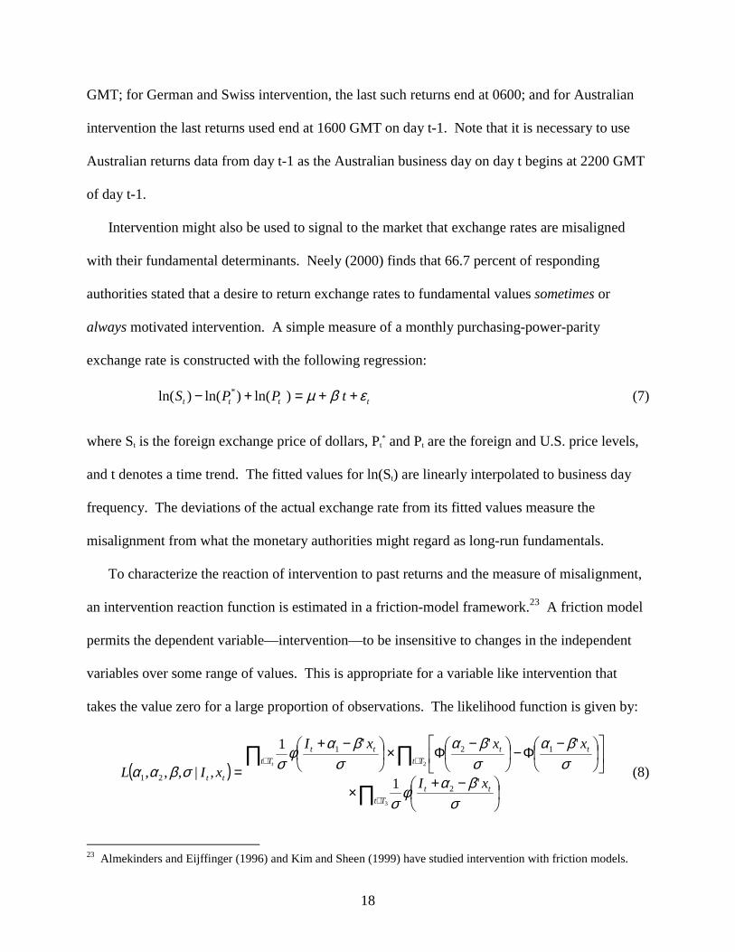
To characterize the reaction of intervention to past returns and the measure of misalignment,

an intervention reaction function is estimated in a friction-model framework.23 A friction model

permits the dependent variable—intervention—to be insensitive to changes in the independent

variables over some range of values. This is appropriate for a variable like intervention that

takes the value zero for a large proportion of observations. The likelihood function is given by:

( )∏

∏ ∏

∈

∈ ∈

��

���

� −+×

��

�

���

���

� −Φ−�

�

���

� −Φ×�

�

���

� −+

=

3

2

'1

'''1

,|,,,2

121

21

Tttt

Tt Tttttt

tt xI

xxxI

xILt

σβαφ

σ

σβα

σβα

σβαφ

σσβαα (8)

23 Almekinders and Eijffinger (1996) and Kim and Sheen (1999) have studied intervention with friction models.

19

where It is intervention at time t, α1 (< 0) is the lower bound on insensitivity for changes in the

linear combination of explanatory variables (β’xt) to affect It, α2 (> 0) is the corresponding upper

bound, {φ, Φ} denote the normal density and cumulative normal density, respectively, and T1, T2

and T3 denote the sets of observations for which It is negative, zero and positive, respectively.

Up to five lags of intervention, up to five lags of 24-hour cumulated returns and the deviation

of the exchange rate were permitted for each intervention series and the models were estimated

by maximum likelihood, subject to the constraint that the estimated model be stationary.24 The

best model was selected by the Schwarz criterion (SC).

Table 8 displays the coefficients from the best models as well as the results of two likelihood

ratio tests. Consistent with the autocorrelation found in the summary statistics, the coefficients

on lagged intervention are generally positive. Coefficients on lagged returns are negative—

indicating leaning-against-the-wind behavior. The coefficient on the exchange rate deviation is

also negative in each case, meaning that monetary authorities tend to buy dollars when the value

of the dollar is below its purchasing-power-parity fundamental measure and sell dollars when the

dollar is above that measure. It is difficult to assess the economic plausibility of the ranges of

inaction {α1,α2}, because they apply to a linear combination of independent variables. It is

reassuring, however, that the range of inaction is smaller for Australia, which intervened more

frequently than the other authorities. The first hypothesis tested by likelihood ratio is that the

coefficient(s) on the lag(s) of the exchange rate return are jointly zero. This restriction is

overwhelmingly rejected in each case. The second hypothesis is that the coefficient on the

exchange rate deviation is zero. The only case for which we fail to reject this restriction is that

of the AUD/USD, for which the coefficient is of the correct sign but insignificant. Intervention

20

tends to lean against the wind and to be in the correct direction to reduce misalignment.

A common problem in estimating time series relations, such as reaction functions, is

structural instability. To test for structural stability in a model at a known break point, T0, one

can estimate the model before and after T0 and use the resulting parameter estimates, �θ1 and �θ 2 ,

and their covariance matrices, V1 and V2, to compute a Wald test statistic (Hamilton (1994)):

( ) [ ] ( )211

2121ˆˆ'ˆˆ θθθθλ −+−= −VV . (9)

Under the null hypothesis of no structural break at T0, the test statistic is distributed as a chi-

square random variable with degrees of freedom equal to the number of parameters being tested.

The null of no structural break at T0 is rejected for sufficiently high values of λ.

Wald tests for structural breaks in the middle of each sample failed to reject structural

stability in every case, except that of the AUD/USD.25 Even in this case, the qualitative

inference on the coefficients over each subsample was the same as that drawn from the whole

sample: Intervention is negatively related to recent trends in exchange rates and to deviations

from the purchasing-power-parity fundamental means. Thus, the determinants of central bank

intervention appear structurally stable. Full results are omitted for brevity.

5. CONCLUSION

During the last 15 years, researchers have accumulated evidence that technical trading rules

can produce excess returns in foreign exchange markets. These returns cannot be readily

explained by reasonable transactions costs, conventional measures of risk or data mining. For a

long time, some have speculated that these trading rule returns result from official intervention.

24 There was great difficulty fitting the models for U.S. intervention with more than three intervention lags, so thoseresults were not considered.

21

Many have interpreted recent research as confirming this suspicion. LeBaron (1999), Saacke

(1999) and Sapp (1999) found strong correlations between periods of U.S. and German

intervention and high trading rule returns. Szakmary and Mathur (1997) extended this research

to multinational monthly data.

The primary contribution of this paper is to show that the high frequency evidence disproves

the hypothesis that intervention generates trading rule profits. Instead, intervention reacts to the

same strong short-run trends from which the trading rules have recently profited.

In addition to showing that intervention does not generate trading rule profits, this paper

characterizes the temporal patterns of high frequency trading rule returns and intervention for

Australian, German, Swiss and U.S. intervention. Positive correlations found in German and

U.S. data are also present—with minor variations—in longer samples and in Australian and

Swiss data. For the U.S., German and Swiss cases, the highest returns probably precede

intervention by less than 24 hours. For Australia, the highest returns appear to be coincident

with or follow the likely hours of intervention. However, examination of the direction of trading

signals and intervention make it implausible that intervention is actually generating those returns.

25 The finding of instability in the RBA’s reaction function might not surprise those who have read Rankin (1998),who describes five distinct periods of intervention behavior by the RBA during this sample.

22

Data Appendix

Collection Time (GMT) Date 1 Date 2 Source Type of PriceDEM/USD 6 19830701 19981231 Reserve Bank of Australia triangular arbitrage on mid points

10 19830701 19981231 Swiss National Bank triangular arbitrage on bid rates14 19830701 19981231 Federal Reserve Bank of New York mid point of bid and ask16 19830701 19981231 Bank of England triangular arbitrage, unspecified17 19830701 19981231 Federal Reserve Bank of New York mid point of bid and ask22 19830701 19981231 Federal Reserve Bank of New York mid point of bid and ask

JPY/USD 6 19830701 19981230 Reserve Bank of Australia triangular arbitrage on mid points8 19830701 19981230 Bank of Japan unspecified, representative10 19830701 19981230 Swiss National Bank Triangular arbitrage on bid rates14 19830701 19981230 Federal Reserve Bank of New York Mid point of bid and ask16 19830701 19981230 Bank of England Triangular arbitrage, unspecified17 19830701 19981230 Federal Reserve Bank of New York Mid point of bid and ask22 19830701 19981230 Federal Reserve Bank of New York Mid point of bid and ask

CHF/USD 6 19860103 19951229 Reserve Bank of Australia Triangular arbitrage on mid points10 19860103 19951229 Swiss National Bank bid rates14 19860103 19951229 Federal Reserve Bank of New York mid point of bid and ask16 19860103 19951229 Bank of England triangular arbitrage, unspecified17 19860103 19951229 Federal Reserve Bank of New York mid point of bid and ask22 19860103 19951229 Federal Reserve Bank of New York mid point of bid and ask

AUD/USD 23 (t-1) 19850303 19990629 Reserve Bank of New Zealand triangular arbitrage on mid points6 19850304 19990630 Reserve Bank of Australia mid point of bid and ask16 19850304 19990630 Bank of England triangular arbitrage, unspecified

Notes: The table describes the sources and collection times of the intraday exchange rates used in the paper. Column 1 provides theexchange rate while column 2 shows the collection time in GMT. Columns 3 and 4 show the beginning and ending dates of thesample in YYYYMMDD format. The fifth column shows the source of the data while the sixth displays any available details on thetype of price or how the exchange rate was calculated.

23

References

Almekinders, G. and S.C.W. Eijffinger, 1996, A friction model of daily Bundesbank and Federal

Reserve intervention, Journal of Banking and Finance 20, 1365-1380.

Bank for International Settlements, 1999, Central bank survey of foreign exchange and

derivatives market activity 1998 (Basle, Switzerland).

Beattie, N. and J-F. Fillion, 1999, An Intraday Analysis of the Effectiveness of Foreign

Exchange Intervention, Bank of Canada Working Paper 99-4, February.

Bhattacharya, U. and P. Weller, 1997, The advantage to hiding one's hand: speculation and

central bank intervention in the foreign exchange market. Journal of Monetary

Economics 39, 251-277.

Board of Governors of the Federal Reserve System, 1994, The Federal Reserve System:

Purposes and Functions (Washington, DC).

Chang, Y. and S. J. Taylor, 1998, Intraday Effects of Foreign Exchange Intervention by the Bank

of Japan, Journal of International Money and Finance 17, 191-210.

Corrado, C. and D. Taylor, 1986, The cost of a central bank leaning against a random walk,

Journal of International Money and Finance 5, 303-314.

Davutyan, N. and J. Pippenger, 1989, Excess returns and official intervention: Canada 1952-

1960, Economic Inquiry 27, 489-500.

Dooley, M. and J. Shafer, 1983, Analysis of short-run exchange rate behavior: March 1973 to

November 1981 in: D. Bigman and T. Taya, eds., Exchange rate and trade instability:

causes, consequences, and remedies (Ballinger, Cambridge, MA) .

24

Edison, H., 1993, The effectiveness of central-bank intervention: a survey of the literature after

1982, Princeton University, Department of Economics, Special Papers in International

Economics, No. 18.

Engel, C., 1996, The forward discount anomaly and the risk premium: a survey of recent

evidence, Journal of Empirical Finance 3, 123-192.

Fischer, A. M. and M. Zurlinden, 1999, Exchange rate effects of central bank interventions: an

analysis of transaction prices, Economic Journal 109, 662-676.

Friedman, M., 1953, The case for flexible exchange rates, essays in positive economics

(University of Chicago Press, Chicago).

Goodhart, C. A. E., and T. Hesse., 1993, Central bank forex intervention assessed in continuous

time, Journal of International Money and Finance 12, 368-389.

Hamilton, J., 1994, Time Series Analysis, (Princeton University Press, Princeton).

Humpage, O., 1998, U.S. Intervention: assessing the probability of success, Federal Reserve

Bank of Cleveland Working Paper 9608.

Jensen, M., 1978, Some anomalous evidence regarding market efficiency, Journal of Financial

Economics 6, 95-101.

Kho, B-C., 1996, Time-varying risk premia, volatility, and technical trading rule profits:

evidence from foreign currency futures markets, Journal of Financial Economics 41, 249-

290.

Kim, S. and J. Sheen, 1999, The determinants of foreign exchange intervention by central banks:

evidence from Australia, The University of New South Wales, unpublished manuscript.

Kritzman, M., 1989, Serial dependence in currency returns: investment implications, Journal of

Portfolio Management 16, 96-102.

25

Leahy, M., 1995, The profitability of US intervention in the foreign exchange markets, Journal

of International Money and Finance 14, 823-844.

LeBaron, B., 1999, Technical trading rule profitability and foreign exchange intervention,

Journal of International Economics 49, 125-143.

Levich, R. and L. Thomas, 1993, The significance of technical trading rule profits in the foreign

exchange market: a bootstrap approach, Journal of International Money and Finance 12,

451-474.

Neely, C., 2000, The practice of central bank intervention: looking under the hood, Central

Banking 11, 24-37.

Neely, C., 1998, Technical analysis and the profitability of US foreign exchange intervention,

Federal Reserve Bank of St. Louis Review, 3-17.

Neely, C, and P. Weller, 2000, Technical analysis and central bank intervention, Federal Reserve

Bank of St. Louis Working Paper 97-002C, Forthcoming in the Journal of International

Money and Finance.

Neely C., P. Weller and R. Dittmar, 1997, Is technical analysis in the foreign exchange market

profitable? A genetic programming approach, Journal of Financial and Quantitative

Analysis 32, 405-426.

Peiers, Bettina, 1997, Informed traders, intervention and price leadership: a deeper view of the

microstructure of the foreign exchange market, Journal of Finance 52, 1589-1614.

Rankin, B., 1998, The exchange rate and the reserve bank's role in the foreign exchange market,

http://www.rba.gov.au/publ/pu_teach_98_2.html.

Ready, M., 1998, Profits from technical trading rules, University of Wisconsin, unpublished

manuscript.

26

Saacke, P., 1999, Technical analysis and the effectiveness of central bank intervention,

University of Hamburg, unpublished manuscript.

Sapp, S., 1999, The role of central bank intervention in the profitability of technical analysis in

the foreign exchange market, Ivey School of Business, University of Western Ontario,

unpublished manuscript.

Silber, W., 1994, Technical trading: when it works and when it doesn’t, Journal of Derivatives 1,

39-44.

Sullivan, R., A. Timmermann and H. White, 1999, Data-snooping, technical trading rule

performance, and the bootstrap, Journal of Finance 54, 1647-1691.

Sweeney, R., 1986, Beating the foreign exchange market, Journal of Finance 41, 163-182.

Szakmary, A. and I. Mathur, 1997, Central bank intervention and trading rule profits in foreign

exchange markets, Journal of International Money and Finance 16, 513-535.

27

Table 1: Summary statistics on central bank intervention

Panel A: Unconditional StatisticsMonetary Authority Exchange Rate Date1 Date2 Obs µ |µ| σ min max ρ1 ρ2 ρ3 ρ4 ρ5

United States DEM/USD 19830701 19981231 4043 -1.27 8.82 52.89 -797.0 950.0 0.30 0.23 0.19 0.16 0.15Germany DEM/USD 19830701 19981231 3777 -6.04 11.12 52.72 -950.8 722.0 0.36 0.30 0.20 0.23 0.17United States JPY/USD 19830701 19981230 4042 0.14 7.89 49.48 -833.0 800.0 0.38 0.28 0.28 0.26 0.20Switzerland CHF/USD 19860103 19951229 2606 -0.90 2.46 19.02 -545.0 150.0 0.07 0.06 0.14 0.05 0.05Australia AUD/USD 19850304 19990630 3630 4.50 19.37 57.99 -933.7 437.3 0.48 0.26 0.19 0.18 0.18

Panel B: Statistics conditional on interventionMonetary Authority Exchange Rate Date1 Date2 Obs µ |µ| σ P(It ≠ 0) P(It ≠ 0 | It-1 = 0) P(It ≠ 0 | It-1 ≠ 0)United States DEM/USD 19830701 19981231 228 -22.52 156.43 222.10 0.06 0.03 0.49Germany DEM/USD 19830701 19981231 474 -48.12 88.61 141.99 0.13 0.05 0.65United States JPY/USD 19830701 19981230 197 2.93 161.90 224.65 0.05 0.03 0.50Switzerland CHF/USD 19860103 19951229 101 -23.12 63.51 94.39 0.04 0.03 0.27Australia AUD/USD 19850304 19990630 1549 10.54 45.39 88.43 0.43 0.19 0.75

Notes: The table shows summary statistics on intervention by four central banks in four exchange rates. All figures show USDpurchases in millions of USD. The top panel shows the unconditional statistics while the bottom panel shows statistics conditional onintervention. µ is the mean of the series, |µ| is the mean of the absolute value of the series, σ is the standard deviation of the series,min and max are the extrema, while ρ1, ρ2, ρ3, ρ4 and ρ5 are the first five autocorrelations. In the bottom panel: P(It ≠ 0 ) is theunconditional probability of intervention. P( It ≠ 0 | It-1 = 0 ) is the probability of a non-zero intervention at t, conditional on nointervention at t-1. P( It ≠ 0 | It-1 ≠ 0 ) is the probability of a non-zero intervention at t, conditional on non-zero intervention at t-1. Allstatistics are calculated on the basis of business days, not calendar days.

28

Table 2: Time Zones of Intervention vs. Greenwich Mean Time

EasternAustralia

Frankfurtand Zurich

GreenwichMean Time

New York

10 1 0 1911 2 1 2012 3 2 2113 4 3 2214 5 4 2315 6 5 016 7 6 117 8 7 218 9 8 319 10 9 420 11 10 521 12 11 622 13 12 723 14 13 8

0 15 14 91 16 15 102 17 16 113 18 17 124 19 18 135 20 19 146 21 20 157 22 21 168 23 22 179 0 23 18

Notes: The table translates Greenwich Mean Time in local standard times for the interveningmonetary authorities.

29

Table 3: Summary statistics on intraday exchange rate changes

Time1 Time2 Date1 Date2 Obs µ |µ| σ t-stat min max ρ1 ρ2 ρ3 ρ4 ρ5

DEM/USD 6 10 19830701 19981231 3929 0.009 0.17 0.24 2.34 -1.58 1.55 0.00 -0.03 0.02 0.01 -0.03Changes 10 14 19830701 19981231 3914 -0.006 0.22 0.33 -1.05 -2.66 2.63 -0.01 0.02 0.05 -0.01 0.00

14 16 19830701 19981231 3911 -0.004 0.21 0.28 -0.82 -1.90 2.16 -0.05 0.04 -0.01 0.01 0.0216 17 19830701 19981231 3939 0.000 0.15 0.22 -0.10 -1.70 1.60 -0.01 0.04 0.02 0.00 0.0017 22 19830701 19981231 3867 -0.013 0.21 0.28 -2.99 -2.05 2.10 -0.05 0.00 0.00 -0.02 0.0122 6 19830701 19981231 3904 0.003 0.20 0.29 0.76 -2.49 3.46 -0.03 -0.02 -0.01 0.00 -0.02

JPY/USD 6 8 19830701 19981230 3928 -0.002 0.10 0.17 -0.62 -1.85 1.37 -0.02 0.00 -0.02 -0.01 0.05Changes 8 10 19830701 19981230 3843 0.023 0.13 0.18 7.93 -1.09 1.65 -0.02 -0.05 0.03 -0.02 0.00

10 14 19830701 19981230 3913 -0.038 0.19 0.34 -7.13 -4.47 3.50 0.05 0.03 0.05 0.03 0.0414 16 19830701 19981230 3906 0.005 0.17 0.28 1.16 -2.51 2.44 0.04 0.06 0.00 0.01 0.0216 17 19830701 19981230 3938 0.004 0.12 0.18 1.44 -2.25 1.50 -0.01 0.01 0.03 -0.01 0.0017 22 19830701 19981230 3870 -0.007 0.18 0.27 -1.75 -2.84 2.23 -0.03 -0.02 0.01 0.02 0.0122 6 19830701 19981230 3903 -0.003 0.25 0.35 -0.46 -2.88 2.85 -0.02 -0.02 -0.03 -0.02 0.03

CHF/USD 6 10 19860103 19951229 2534 -0.011 0.20 0.28 -1.91 -1.67 1.62 0.02 -0.03 0.02 0.02 -0.02Changes 10 14 19860103 19951229 2525 0.010 0.25 0.38 1.35 -1.76 2.94 -0.01 0.03 0.04 0.01 0.00

14 16 19860103 19951229 2505 0.003 0.25 0.33 0.41 -2.25 2.42 -0.06 0.07 -0.03 0.01 0.0116 17 19860103 19951229 2540 -0.003 0.18 0.25 -0.64 -1.82 1.44 -0.04 0.04 0.01 -0.02 0.0217 22 19860103 19951229 2497 -0.019 0.23 0.32 -2.96 -2.22 1.91 -0.02 0.00 0.01 -0.03 -0.0122 6 19860103 19951229 2502 -0.002 0.23 0.33 -0.37 -2.53 2.79 0.00 -0.01 0.00 -0.01 -0.01

AUD/USD -1 6 19850304 19990630 3422 -0.009 0.19 0.32 -1.66 -2.52 3.53 0.05 0.03 -0.03 0.01 0.02Changes 6 16 19850304 19990630 3630 -0.013 0.27 0.44 -1.80 -3.35 3.25 0.09 0.02 0.03 0.02 0.00

16 23 19850304 19990630 3636 0.024 0.26 0.40 3.66 -3.67 3.14 -0.01 -0.01 -0.02 0.00 0.06Notes: The table presents summary statistics on the intraday percentage log changes in exchange rates. The four panels show thestatistics for the DEM/USD, JPY/USD, CHF/USD and AUD/USD respectively. The columns labeled Time1 and Time2 show the time(in GMT) of the initial and final price in the return calculation. The DEM/USD row labeled {6,10} for example, shows summarystatistics for log returns from 0600 to 1000 GMT. The first observation for the AUD/USD begins one hour before midnight of day t.Starting and ending dates for the data are shown in the columns labeled Date1 and Date2. t-stat denotes the Newey-West corrected t-statistic for the null hypothesis that the mean return is equal to zero. See the notes to Table 1 for descriptions of Obs, µ, |µ|, σ, min,max, ρ1, ρ2, ρ3, ρ4 and ρ5.

30

Table 4: Daily trading rule returns conditional on removing periods of intervention

Monetary Authority United States Germany United States Switzerland AustraliaExchange Rate DEM/USD DEM/USD JPY/USD CHF/USD AUD/USDPanel A: All observations

obs 3892 3892 3891 2512 3629mean 6.03 6.03 8.72 5.10 2.44std 0.69 0.69 0.68 0.79 0.62t-stat 2.17 2.17 3.17 1.28 0.93sharpe 0.55 0.55 0.80 0.41 0.25ntrades 7.55 7.55 5.23 6.41 8.17p-value 0.01 0.00 0.00 0.05 0.14

Panel B: Remove p(t)/p(t-1) when I(t) /= 0obs 3661 3302 3692 2410 2080mean 2.61 1.28 4.50 4.44 -2.27std 0.67 0.67 0.66 0.78 0.55t-stat 0.99 0.51 1.74 1.16 -1.30sharpe 0.25 0.13 0.44 0.37 -0.34ntrades 7.42 7.29 5.23 6.21 5.52p-value 0.13 0.40 0.02 0.11 0.86Markov-p 0.00 0.00 0.00 0.29 0.00date 1 19830701 19830701 19830701 19860103 19850304date 2 19981231 19981231 19981230 19951229 19990630

Notes: The table shows the results of an MA 150 rule on daily foreign exchange rate data withinterest rates in the return calculations, except for the AUD/USD. Panel A shows the results forall observations. Panel B excludes return observations from t-1 to t for which there was non-zerointervention at t. obs is the number of observations in each sample. mean is the meanannualized return to the rule in percentage terms. std is the standard deviation of the dailyreturns in percentage terms. t-stat is the t-statistic for the null hypothesis that the mean annualreturn is zero. sharpe is the annualized Sharpe ratio for the rule. ntrades is the number of tradesper year. p-value is the p-value for the test of the null that the mean return is zero. Low p-valuesreject the null hypothesis. In panel B, Markov-p shows the simulated p-value for the test of thenull that the change in the mean annual return from Panel A to Panel B would have been as greatby randomly removing returns. Date 1 and date 2 are the beginning and ends of the samples inyyyymmdd format.

31

Table 5: Trading rule returns with intraday data, conditional on removing periods of intervention

Monetary Authority United States Germany United States Switzerland AustraliaExchange Rate DEM/USD DEM/USD JPY/USD CHF/USD AUD/USDPanel A: All observations

obs 3892 3892 3891 2512 3629mean 5.98 5.98 8.29 5.84 2.44std 0.69 0.69 0.68 0.79 0.62tstat 2.15 2.15 3.01 1.47 0.93sharpe 0.55 0.55 0.76 0.47 0.25ntrades 7.55 7.55 5.23 6.41 8.17p-value 0.02 0.02 0.00 0.07 0.17

Panel B: Remove p(t)/p(t-1) when I(t) /= 0obs 3661 3302 3692 2410 2080mean 2.59 1.47 4.20 5.21 -2.27std 0.67 0.67 0.66 0.78 0.55tstat 0.99 0.59 1.62 1.37 -1.30sharpe 0.25 0.15 0.41 0.43 -0.34ntrades 7.42 7.29 5.23 6.21 5.52p-value 0.19 0.32 0.05 0.12 0.91Markov-p 0.00 0.00 0.00 0.32 0.00date 1 19830701 19830701 19830701 19860103 19850304date 2 19981231 19981231 19981230 19951229 19990630

Notes: See the notes to Table 4.

32

Table 6: Morning to morning returns with and without days and business days of intervention.

Monetary Authority United States Germany United States Switzerland AustraliaExchange Rate DEM/USD DEM/USD JPY/USD CHF/USD AUD/USDPanel A: All observations

obs 3891 3891 3890 2511 3628mean 5.87 5.89 8.28 5.91 2.40tstat 1.99 1.97 2.95 1.43 0.90p-value 0.02 0.01 0.01 0.05 0.20

Panel B: Remove p(t)/p(t-1) when I(t) /= 0obs 3660 3301 3691 2409 2080mean 2.28 0.05 3.69 2.95 -0.65tstat 0.82 0.02 1.38 0.74 -0.35p-value 0.18 0.49 0.07 0.19 0.61Markov-p 0.00 0.00 0.00 0.00 0.05

Panel C: Remove p(t+1)/p(t) when I(t) /= 0obs 3661 3302 3692 2410 2080mean 4.23 2.18 6.02 6.04 -2.65tstat 1.50 0.79 2.28 1.52 -1.46p-value 0.07 0.22 0.00 0.09 0.86Markov-p 0.00 0.00 0.00 0.67 0.01

Panel D: Remove business hour returns prior to the day of interventionobs 3775.00 3620.04 3790.00 2463.71 3111.33mean 3.32 1.95 5.75 3.56 1.32tstat 1.21 0.75 2.16 0.89 0.70p-value 0.11 0.28 0.03 0.24 0.29Markov-p 0.00 0.00 0.00 0.00 0.35

Panel E: Remove business hour returns on the day of interventionobs 3776.00 3621.04 3791.00 2464.71 3112.00mean 3.90 3.31 6.99 5.91 -0.30tstat 1.41 1.26 2.66 1.50 -0.16p-value 0.10 0.11 0.02 0.05 0.57Markov-p 0.00 0.02 0.04 0.52 0.11date 1 19830701 19830701 19830701 19860103 19850304date 2 19981231 19981231 19981230 19951229 19990630

Notes: The table provides statistics on returns calculated from morning to morning, startingprior to the business day in each intervening country. The hours over which the returns arecalculated for the five cases are 1000, 0600, 1000, 0600, and 1600 (of t-1) GMT. In local times,these would be 0500, 0700, 0500, 0700 and 0200, respectively. See the notes to Table 4 fordefinitions of obs, mean, tstat, p-value, and Markov-p. Panel A shows the results for allobservations. Panel B removes the returns in the 24 hours prior to the beginning of the morningobservation when there is intervention. Panel C removes the returns in the 24 hours after themorning observation when there is intervention. Panel D removes the returns during thebusiness day prior to the day of intervention. Panel E removes the returns during the businessday of intervention. Business day hours are calculated as 1000-2200, 0600-1700, 1000-2200,0600-1700, and 1600 (day t-1) to 0600 GMT for each of the five cases, respectively. Thenumber of observations in Panels C and D refers to the number of 24-hour periods and so neednot be an integer value.

33

Table 7: Do the technical traders trade with or against central banks?

Authority United States Germany United States Switzerland AustraliaRate DEM/USD DEM/USD JPY/USD CHF/USD AUD/USD

-2 0.05 0.06 0.06 0.05 0.19-1 0.06 0.07 0.07 0.04 0.190 0.15 0.12 0.13 0.13 0.281 0.06 0.07 0.07 0.04 0.202 0.04 0.06 0.06 0.05 0.20

Notes: The table shows the proportion of the time that the MA 150 trader and the monetaryauthority were on the same side of the market from two days prior to intervention to two daysafter intervention. For example, the third row, second column shows that MA 150 traders werepurchasing (selling) dollars only 5 percent of the time before U.S. authorities purchased (sold)dollars. The timing convention is that intervention at t is contemporaneous with the tradingposition from t-1 to t.

34

Table 8: Under what conditions do monetary authorities intervene?

UnitedStates

Germany UnitedStates

Switzerland Australia

DEM/USD DEM/USD JPY/USD CHF/USD AUD/USDI1 (s.e.) 0.95 (0.00) 0.60 (0.06) 0.95 (0.00) 0.95 (0.00) 0.74 NAI2 (s.e.) 0.33 (0.05) -0.09 NAI3 (s.e.) 0.13 NAR1 (s.e.) -6.95 (1.26) -4.40 (0.62) -6.63 (1.28) -3.40 (0.90) -0.52 NAR2 (s.e.) -2.75 (0.61) -2.85 (0.89) -0.27 NAR3 (s.e.) -3.31 (0.62) -3.11 (0.92)R4 (s.e.) -2.58 (0.93)XRD (s.e.) -0.41 (0.06) -0.51 (0.03) -0.63 (0.08) -0.88 (0.12) -0.16 NAσ (s.e.) 0.31 (0.02) 0.17 (0.01) 0.29 (0.02) 0.16 (0.01) 0.08 NAα1 (s.e.) -0.59 (0.03) -0.28 (0.01) -0.59 (0.04) -0.29 (0.03) -0.11 NAα2 (s.e.) 0.65 (0.04) 0.40 (0.02) 0.64 (0.04) 0.49 (0.04) 0.06 NALR test, p-value 52.50 (0.00) 433.61 (0.00) 83.00 (0.00) 88.15 (0.00) 153.52 (0.00)LR test, p-value 33.33 (0.00) 101.03 (0.00) 28.77 (0.00) 47.10 (0.00) 3.45 (0.18)

Notes: The table shows the results from a friction model estimating monetary authority reaction functions. Equation (8) in the textshows the likelihood function. The best models were selected from maximal lag lengths of 5 lags of intervention and 5 lags of returnsby the Schwarz criterion. The top panel shows the coefficient estimates and standard errors. The coefficients on lags of interventionare labeled I1 to I5, that on the lagged return variable as R1 and the coefficient on the exchange rate deviation as XRD. The bottompanel shows the results of likelihood ratio tests for two hypotheses: 1) that the coefficients on lagged returns are zero—that theauthority doesn’t lean against the wind; 2) that the coefficient on the deviation from purchasing power parity is zero—that theauthority does not intervene to correct misalignments. NA indicates that standard errors were unavailable as the Hessian was nearsingular.

35

Figure 1: Daily trading rule returns around periods of intervention

Notes: The figure depicts predicted daily backward-looking returns to an MA 150 rule aroundperiods of intervention—obtained by regressing trading rule returns on leads and lags ofintervention. The vertical lines depict the business day of intervention in the interveningcountry. Australian business hours are –0200 to 0600 GMT; German and Swiss business hoursare 0600 to 1400 GMT; U.S. business hours are 1300 to 2100 hours GMT. The horizontal axisshows hours before (negative) and after (positive) midnight on the day of intervention in GMT.

36

Figure 2: Intraday trading rule returns around periods of intervention

Notes: The figure depicts predicted backward-looking intraday returns to an MA 150 rulearound periods of intervention—obtained by regressing intraday trading rule returns on leads andlags of intervention. The top panel depicts annualized intraday returns while the bottom paneldepicts the 24-hour backward-looking moving average of those returns. The vertical lines depictthe business day of intervention in the intervening country. The horizontal axis shows hoursbefore (negative) and after (positive) midnight on the day of intervention in GMT.