The systems engineering of automated fire assay laboratories ...
295
THE SYSTEMS ENGINEERING OF AUTOMATED FIRE ASSAY LABORATORIES FOR THE ANALYSIS OF THE PRECIOUS METALS by Keith Shearer McIntosh Dissertation presented for the Degree of DOCTOR OF PHILOSOPHY (Extractive Metallurgical Engineering Science) in the Department of Process Engineering at the University of Stellenbosch Promoters Dr. J.J. Eksteen Prof. L. Lorenzen Prof. K.R. Koch STELLENBOSCH December 2004
-
Upload
khangminh22 -
Category
Documents
-
view
3 -
download
0
Transcript of The systems engineering of automated fire assay laboratories ...

THE SYSTEMS ENGINEERING OF AUTOMATED FIRE ASSAY LABORATORIES FOR THE ANALYSIS OF THE PRECIOUS METALS
by
Keith Shearer McIntosh
Dissertation presented for the Degree
of
DOCTOR OF PHILOSOPHY (Extractive Metallurgical Engineering Science)
in the Department of Process Engineering
at the University of Stellenbosch
Promoters Dr. J.J. Eksteen
Prof. L. Lorenzen Prof. K.R. Koch
STELLENBOSCH
December 2004

ii
DDEECCLLAARRAATTIIOONN
I hereby certify that this dissertation is my own original work, except where specifically acknowledged in the text. Neither the present dissertation, nor any part thereof has previously been submitted for a degree at any university.
_________________
K.S. McIntosh
June 2004

iii
SSYYNNOOPPSSIISS
The objective of this work was to achieve a completely automated fire assay system for the analysis of process control samples on a flotation plant in less than 120 minutes. With this in mind, a systems engineering approach was undertaken. The physical and chemical characteristics of the technology for each subsystem were investigated in turn and the critical factors that influenced accuracy, precision and analysis time were identified and optimised.
Some of the key developments achieved during this work were:
• Existing technology for the sampling, filtering, drying and grinding of flotation plant samples were evaluated and where necessary, modified for this application.
• The fusion system was totally re-designed with a bottom-loading configuration called FIFA (Fast In-line Fire Assay) to make automation with a central robot possible. With the fast fusing flux developed, a quantitative collection of the platinum group elements with a fifteen-minute fusion was achieved compared to an hour for the classical method.
• A robust automated separator system was developed to isolate the lead collector from the fusion in the molten state thereby separating it quantitatively from the slag. This allowed the automation of the entire fire assay process.
• Methods to prepare lead standards for calibration were developed. These were used to optimise analytical protocols for the analysis of platinum group elements in lead using a spark optical emission spectrometer. This made it possible to accurately determine the quantities of platinum group elements in lead samples prepared by the automated fire assay system.
• A fully automated system was developed that could meet the accuracy and precision requirements for the analysis of tailings and feed grade samples in concentrator slurry streams in less than one hour compared with the 24-72 hours required when using classical methods.
The new fire assay technology including flux, FIFA system, oxygen lance and separator were all patented along with the automation vendor. This technology has made the first fully automated fire assay system a reality.

iv
OOPPSSOOMMMMIINNGG
Die hoofoogmerk van die studie was om ‘n totale geoutomatiseerde vuuressaieering stelsel te ontwerp vir die ontleding van prosesbeheermonsters van ‘n flotasieaanleg in ‘n bestek van 120 minute. Gedurende die ontwerp is ‘n ingeneursstelselbenadering gebruik. Die fisiese en chemiese kenmerke van elke deel van die tegnologie is eers afsonderlik en dan as ‘n geheel ondersoek. Die bepalende faktore wat akkuraatheid, presisie en ontledingstyd beinvloed het was geidentifiseer en geoptimeer.
Die hoofpunte van die werk behels onder andere die volgende:
• Bestaande tegnologie vir monsterneming, filtrasie, droging en vermaling van flotasiemonsters was ondersoek en is, waar nodig, aangepas vir die finale stelsel.
• Die smeltingsisteem was in geheel herontwerp om monsters van onder in die FIFA (Fast In-line Fire Assay) sisteem te laai en sodoende die outomatisering met ‘n sentrale robot te vergemaklik. ‘n Vinnig smeltende vloeimiddel was ontwikkel wat ‘n kwantitatiewe versameling van die platinum groep elemente binne ‘n tydsduur van vyftien minute moontlik gemaak het, in vergelyke met die oorspronklike duur van die klassieke smelt metode van een uur.
• ‘n Outomatiese skeier was ontwikkel waarmee die gesmelte loodversamelaar geskei kon word van die slakfase. Met die nuwe stelsel kon die hele vuuressaieerproses outomaties verloop.
• Metodes is ontwikkel om loodstandaarde vir kalibrasie doeleindes te berei. Die standaarde is op hulle beurt weer gebruik om ‘n ontleding protokol daar te stel vir die analiese van die platinum groep elemente in lood, met behulp van ‘n vonkontlading-optiese-uitstraling-spektrometriese instrument. Ten einde was dit moontlik om outomaties klein hoeveelhede van die platinum groep elemente in monsters akkuraat te bepaal, na voorbereiding met behulp van die geoutomatiseerde vuuressaieering stelsel.
• Die volle geoutimatiseerde stelsel was ontwikkel wat aan die akkurate en noukeurige vereistes voldoen het vir die ontleding van flotasie-uitskot-en-voergraad monsters van die konsentraataanleg binne die bestek van ‘n uur.
Die nuwe vuuressaieer tegnologie, insluitend die vinnig smeltende vloeimiddel, FIFA en skeier stelsels, asook die suurstof lanset is gepatenteer met die vervaardiger. Die studie het gelei tot die eerste volle geoutomatiseerde vuuressaieering stelsel wat tans gebruik word in die industrie.

v
DDEEDDIICCAATTIIOONN
This thesis is dedicated to my wife Lillian, my daughter Timarah and my son Christopher who give me much inspiration, support and are such a joy.
AACCKKNNOOWWLLEEDDGGEEMMEENNTTSS
No work on this thesis could have happened without the support of the entire team at the Anglo Platinum Research Centre. Whether the contribution was large or small a great thank you is extended to the entire staff and Management.
• First and foremost to Neville Randolph, the Consulting Chemist who identified the need to research fire assay. His original drive gave me a job as a newly graduated chemist and helped progress the project to the point where significant improvements were achieved and a difficult method automated.
• Thank you to Martin Wright and Alan Buck without whom the original project would not have been approved.
• My mentor and promoter at Stellenbosch, Jacques Eksteen who unfailingly took on the project and whose commitment made a difficult task all the easier.
• Derek Auer as my boss and mentor at the research centre without his dedication and drive the thesis would never have been written up. A big thank you for reading the manuscript tirelessly.
• Innovative Met Products, Boyne Hohenstein, George Cowan and Pierre Hofmeyr my co-collaborators in a difficult task. Their innovation, knowledge and experience in the field of automation made the theory provided by my fire assay research, a workable solution.
•• I would also like to thank the following people at the research centre; Johan,Willy, Lesley, Veronica, Eunice, Margaret, Mzwakhe and Martin for their assistance during the project.

vi
TTAABBLLEE OOFF CCOONNTTEENNTTSS
CHAPTER 1 ........................................................................................................................1
1 INTRODUCTION ..........................................................................................................1
1.1 AN OVERVIEW OF ANGLO PLATINUM...............................................................3
1.2 ANALYTICAL REQUIREMENTS AT ANGLO PLATINUM.....................................6
1.3 MINERALOGY OF THE BUSHVELD COMPLEX..................................................9
1.4 HEALTH AND SAFETY.......................................................................................13
1.5 WASTE DISPOSAL.............................................................................................14
1.6 ANALYTICAL RESEARCH OBJECTIVES ..........................................................14
1.7 OVERVIEW OF PROCEEDING CHAPTERS......................................................15
CHAPTER 2 ......................................................................................................................17
2 FIRE ASSAY THEORY AND METHODS ...................................................................17
2.1 INTRODUCTION.................................................................................................17
2.2 HISTORY OF FIRE ASSAY.................................................................................19
2.3 FIRE ASSAY CHEMISTRY AND THEORY.........................................................20
2.3.1 OXIDES, SLAG STRUCTURE AND CHEMISTRY.......................................20
2.3.2 CLASSIFICATION OF SILICATES AND BORATES ....................................25
2.3.3 THERMODYNAMICS ...................................................................................26
2.3.4 SLAG COMPOSITIONS ...............................................................................27
2.3.5 SURFACE AND INTERFACIAL TENSION...................................................28
2.3.6 VISCOSITY...................................................................................................31
2.3.7 DENSITY ......................................................................................................34
2.3.8 SEPARATION OF COLLECTOR AND SLAG...............................................35
2.4 FIRE ASSAY FUSION.........................................................................................36
2.4.1 THE COLLECTOR........................................................................................39
vii
2.4.2 SLAG............................................................................................................41
2.4.3 CHROMITE SAMPLES.................................................................................42
2.4.4 FLUX COMPOSITIONS................................................................................44
2.5 CUPELLATION....................................................................................................46
2.6 LEAD FIRE ASSAY METHODS - A REVIEW......................................................48
2.6.1 4E GRAVIMETRIC ANALYSIS.....................................................................50
2.6.2 SILVER PRILL METHOD .............................................................................52
2.6.3 PALLADIUM PRILL METHOD......................................................................55
2.6.4 GOLD PRILL METHOD ................................................................................56
2.6.5 DISSOLUTION OF LEAD ............................................................................57
2.6.6 NICKEL SULPHIDE......................................................................................59
2.6.7 OVERVIEW OF METHODS .........................................................................61
2.7 DISCUSSION ......................................................................................................63
CHAPTER 3 ......................................................................................................................64
3 SAMPLE PREPARATION ..........................................................................................64
3.1 PRINCIPLES OF SAMPLE PREPARATION .......................................................64
3.2 BULK SAMPLES .................................................................................................66
3.3 DRYING ..............................................................................................................66
3.4 PULVERISING ....................................................................................................67
3.4.1 VERTICAL SPINDLE PULVERISER ............................................................67
3.4.2 SWING MILL.................................................................................................68
3.4.3 SIZING..........................................................................................................69
3.5 SUB SAMPLING..................................................................................................71
3.5.1 ROTARY SPLITTING ...................................................................................71
3.5.2 DIPPING.......................................................................................................74

viii
3.6 HOMOGENEITY TESTING .................................................................................75
3.6.1 STATISTICAL EVALUATION .......................................................................76
3.6.2 SUMMARY OF HOMOGENEITY TESTING .................................................79
3.7 DISCUSSION ......................................................................................................80
CHAPTER 4 ......................................................................................................................82
4 BASELINE ANALYSIS USING CLASSICAL METHODS............................................82
4.1 ANALYSIS OF COPPER, NICKEL, BISMUTH AND SULPHUR .........................83
4.2 LEAD DISSOLUTION METHOD .........................................................................84
4.2.1 EFFECT OF SAMPLE SIZE ON UG2 ANALYSIS ........................................85
4.2.2 PGE RESULTS FOR THE LEAD DISSOLUTION METHOD........................87
4.2.3 EXAMINATION OF CLASSICAL LEAD FIRE ASSAY SLAG .......................89
4.2.4 IMPURITIES IN THE LEAD COLLECTOR ...................................................92
4.3 NICKEL SULPHIDE.............................................................................................93
4.3.1 PGE RESULTS FOR NICKEL SULPHIDE ...................................................95
4.3.2 SLAG EXAMINATION OF THE CLASSICAL NICKEL SULPHIDE METHOD .. .....................................................................................................................96
4.4 COMPARISON OF LEAD AND NICKEL SULPHIDE METHODS........................98
4.4.1 COMPARISON WITH CERTIFIED REFERENCE MATERIALS.................101
4.4.2 ANALYTICAL PRECISION .........................................................................103
4.5 QC VALUES AND LIMITS.................................................................................104
4.6 DISCUSSION ....................................................................................................106
CHAPTER 5 ....................................................................................................................108
5 AUTOMATION TECHNOLOGY................................................................................108
5.1 AUTOMATION OF FIRE ASSAY FOR PROCESS CONTROL .........................111
5.2 EXISTING AUTOMATION TECHNOLOGIES....................................................114

ix
5.2.1 SAMPLING .................................................................................................114
5.2.2 FILTRATION...............................................................................................116
5.2.3 DRYING......................................................................................................117
5.2.4 GRINDING..................................................................................................118
5.2.5 FLUXING ....................................................................................................119
5.3 FUSION TECHNOLOGY AND DEVELOPMENT ..............................................120
5.3.1 FUSION USING INDUCTIVE HEATING.....................................................120
5.3.2 FUSION WITH RESISTIVELY HEATED FURNACES................................126
5.3.3 FUSION CRUCIBLES.................................................................................129
5.4 SLAG SEPARATION TECHNOLOGY AND DEVELOPMENT ..........................130
5.4.1 DECANTING...............................................................................................130
5.4.2 VOLUMETRIC SLAG SEPARATION..........................................................130
5.4.3 COWAN SEPARATOR...............................................................................132
5.5 FLUX DEVELOPMENT FOR AUTOMATION....................................................135
5.5.1 PGE ANALYTICAL RESULTS FOR FUSION WITH THE AUTOMATED FLUX ..........................................................................................................141
5.5.2 IMPURITIES IN THE LEAD COLLECTOR .................................................144
5.5.3 EXAMINATION OF LEAD SLAG FOR AUTOMATION FLUX.....................145
5.6 OXIDATION OF SAMPLES DURING AUTOMATED FIRE ASSAY ..................149
5.6.1 LANCE FACTORIAL DESIGNED EXPERIMENT.......................................151
5.6.2 OXIDATIVE FLUX FACTORIAL DESIGNED EXPERIMENT......................156
5.6.3 SUMMARY OF OXIDATIVE TEST WORK .................................................158
5.7 DISCUSSION OF AUTOMATION DEVELOPMENT WORK .............................159

x
CHAPTER 6 ....................................................................................................................161
6 SPARK OPTICAL EMISSION ANALYSIS ................................................................161
6.1 STANDARDS PREPARATION EQUIPMENT AND METHODS ........................161
6.1.1 EQUIPMENT FOR THE PREPARATION OF STANDARDS ......................162
6.1.2 CHEMICALS AND REAGENTS..................................................................165
6.1.3 PREPARATION OF LEAD STANDARDS...................................................166
6.2 CHEMICALLY ANALYSED LEAD STANDARDS ..............................................167
6.3 SYNTHETIC STANDARDS ...............................................................................169
6.3.1 LEAD STANDARDS CONTAINING SILVER, BISMUTH, NICKEL, COPPER AND SULPHUR..........................................................................................169
6.3.2 LEAD STANDARDS CONTAINING IRON, COBALT, ARSENIC, ANTIMONY AND OTHER IMPURITY ANALYTES.........................................................171
6.3.3 LEAD STANDARDS PREPARED FROM PGE SOLUTIONS.....................172
6.3.4 LEAD STANDARDS PREPARED WITH SOLID PGE SPONGES..............173
6.4 ANALYSIS OF LEAD USING SPARK OPTICAL EMISSION SPECTROMETRY.... ..........................................................................................................................174
6.4.1 INTRODUCTION TO SPARK OPTICAL EMISSION SPECTROMETRY....175
6.4.2 SPARK GENERATION...............................................................................176
6.4.3 OPTICAL SYSTEM OF THE ARL 4460 INSTRUMENT .............................181
6.4.4 TIME RESOLVED OPTICAL EMISSION SPECTROSCOPY .....................185
6.5 CALIBRATION OF THE ARL 4460 INSTRUMENT ...........................................185
6.5.1 INSTRUMENT STANDARDISATION .........................................................187
6.5.2 ANALYTICAL CONDITIONS ......................................................................189
6.5.3 TIME RESOLVED SPECTROSCOPY WINDOW .......................................192
6.5.4 CALIBRATION RESULTS ..........................................................................194

xi
6.5.5 PRECISION OF SPARK OPTICAL EMISSION ANALYSIS OF LEAD .......202
6.6 ANALYTICAL RESULTS ...................................................................................203
6.6.1 ANALYSIS OF GEOLOGICAL SAMPLES..................................................203
6.6.2 ANALYSIS OF CERTIFIED REFERENCE MATERIALS............................208
6.7 DISCUSSION OF SPARK OPTICAL EMISSION ..............................................209
CHAPTER 7 ....................................................................................................................211
7 AUTOMATED PROCESS CONTROL LABORATORY.............................................211
7.1 ANALYTICAL PROCESS ..................................................................................211
7.2 LABORATORY DESIGN ...................................................................................214
7.2.1 SOFTWARE ...............................................................................................216
7.3 FILTRATION......................................................................................................216
7.4 MICROWAVE DRYING .....................................................................................217
7.5 GRINDING.........................................................................................................218
7.5.1 INPUT AND DISCHARGE PARAMETERS ................................................218
7.5.2 GRINDING PARAMETERS ........................................................................221
7.5.3 MILL DISCHARGE HOMOGENEITY..........................................................223
7.5.4 MILL CONTAMINATION AND CLEANING.................................................224
7.5.5 FINAL GRINDING TESTS ..........................................................................228
7.6 AUTOMATED FLUXING ...................................................................................230
7.7 AUTOMATED FIRE ASSAY PREPARATION ...................................................231
7.7.1 FUSION FACTORIAL EXPERIMENT.........................................................232
7.8 SLAG SEPARATION.........................................................................................234
7.9 LEAD BUTTON PREPARATION.......................................................................235
7.9.1 ISO-PROPANOL COOLING.......................................................................235
7.9.2 LEAD MILLING OPTIMISATION ................................................................235

xii
7.10 ANALYTICAL PERFORMANCE OF THE AUTOMATED SYSTEM...................238
7.11 COMPARISON WITH CLASSICAL METHODS ................................................240
7.11.1 TURNAROUND TIME.................................................................................240
7.11.2 COST..........................................................................................................244
7.11.3 SAFETY......................................................................................................245
7.11.4 WASTE.......................................................................................................246
7.12 DISCUSSION AND CONCLUSION ON AUTOMATED FIRE ASSAY LABORATORIES ..............................................................................................246
CHAPTER 8 ....................................................................................................................250
8 OVERALL CONCLUSIONS......................................................................................250
8.1 HISTORICAL DEVELOPMENT.........................................................................250
8.2 HIGHLIGHTS OF THE DEVELOPMENT WORK ..............................................252
8.3 A LOOK INTO THE FUTURE............................................................................253
REFERENCES ................................................................................................................255

xiii
LLIISSTT OOFF TTAABBLLEESS
Table 1.1 Summary of the composition of the Merensky and UG2 reefs...........................11
Table 1.2 Summary of PGE minerals for the Merensky and UG2 reefs.............................12
Table 2.1 Classification of borates.....................................................................................25
Table 2.2 Classification of silicates ....................................................................................26
Table 2.3 Thermodynamic data for the reaction of sodium carbonate and silica ...............27
Table 2.4 Lead fire assay slag compositions for Merensky and UG2 samples ..................28
Table 2.5 Surface tension estimates of lead and slag at 1200°C.......................................30
Table 2.6 Viscosity calculated lead and slag at 1200°C ....................................................32
Table 2.7 Density calculated at 1200°C.............................................................................34
Table 2.8 Effect of lead droplet size, slag viscosity and density on settling time ...............35
Table 2.9 Thermodynamic data for the reduction of lead oxide .........................................39
Table 2.10 Thermodynamic data for the decomposition of sulphides ................................40
Table 2.11 Thermodynamic data for the decomposition of oxides.....................................41
Table 2.12 Flux compositions used for classical lead fire assay........................................44
Table 2.13 Flux compositions for classical nickel sulphide fire assay................................45
Table 2.14 Thermodynamic data for the oxidation of metals during cupellation ................47
Table 2.15 Summary of fire assay methods.......................................................................62
Table 3.1 Summary of particle size distributions for the prepared QC samples.................70
Table 3.2 Summary of splitting precisions during sample preparation...............................73
Table 3.3 Results for the XRF measurement of the Merensky tailings splits .....................76
Table 3.4 Analysis of variance for the XRF measurement made on two days ...................77
Table 3.5 Analysis of variance summary for the evaluation of splitting..............................77
Table 3.6 Comparison of data before and after outlier deletion .........................................79
Table 3.7 Sample XRF homogeneity testing......................................................................80

xiv
Table 4.1 List of Certified Reference Materials used .........................................................82
Table 4.2 Results for copper, nickel, bismuth and sulphur on feeds and tailings...............83
Table 4.3 Results for copper, nickel, bismuth and sulphur on concentrate........................83
Table 4.4 Analytical parameters for the lead dissolution method.......................................84
Table 4.5 Comparison of SARM 65 (UG2 ore) analyses with different sample masses using a single tailed t-test assuming unequal variances ..................................86
Table 4.6 Results for the single tailed t-test assuming unequal variances for the comparison between small and large samples used for the analysis of the UG2 feed and tailings QCs .............................................................................86
Table 4.7 Outliers for the PGE analysis of the QCs and CRMs with the lead dissolution method..............................................................................................................88
Table 4.8 Summary of PGE results for classical lead fire assay........................................88
Table 4.9 Examination of fire assay slag for lead inclusions using the SEM .....................89
Table 4.10 Chromite in classical lead fire assay slags.......................................................90
Table 4.11 Concentrations of copper, nickel, sulphur and bismuth measured in the lead collector after fire assay ..................................................................................92
Table 4.12 Recovery of copper, nickel and sulphur from the sample in the lead collector.93
Table 4.13 Analytical parameters for the nickel sulphide method ......................................94
Table 4.14 PGE results for classical nickel sulphide fire assay .........................................95
Table 4.15 Single tailed paired t- test for the comparison of the lead and nickel sulphide methods..........................................................................................................99
Table 4.16 Regression data for the comparison of the lead and nickel sulphide methods......................................................................................................................100
Table 4.17 Comparison of the analysed values for the CRM to the certified values ........102
Table 4.18 %RSD calculated for the lead and nickel sulphide methods ..........................104
Table 4.19 QC values with 95% confidence limits and analytical range ..........................105
Table 5.1 Thermodynamic data for the decomposition of boron nitride ...........................124
Table 5.2 Slag formation with different sodium compounds.............................................137

xv
Table 5.3 Flux compositions for FIFA ..............................................................................140
Table 5.4 Analytical conditions used for FIFA fusions .....................................................141
Table 5.5 Comparison of FIFA PGE results to the QC values .........................................141
Table 5.6 Statistical results for the FIFA values on the QCs............................................142
Table 5.7 Regression data for FIFA fusion method on the QCs ......................................142
Table 5.8 Concentrations of copper, nickel, sulphur and bismuth measured in the lead collector after FIFA fusion..............................................................................144
Table 5.9 Recovery of copper, nickel and sulphur from the sample into the lead collector with the FIFA fusion ........................................................................................145
Table 5.10 SEM examination of FIFA slags for lead inclusions .......................................146
Table 5.11 SEM examination of FIFA slags for chromite.................................................147
Table 5.12 Slag composition for FIFA slags ....................................................................149
Table 5.13 Factors for the 3-level lance factorial experiment...........................................151
Table 5.14 Measurement of the flow rate for the fire assay lance....................................152
Table 5.15 Results from the lance factorial experiment ...................................................152
Table 5.16 Comparison of the behaviour of different sample types when using the oxygen lance on the melt after FIFA fusion ...............................................................154
Table 5.17 Thermodynamic data for the fire assay lance ................................................155
Table 5.18 Comparison of oxidants used in the oxidative flux factorial experiment .........156
Table 5.19 Factors for the flux factorial experiment .........................................................156
Table 5.20 Results for the flux factorial experiment .........................................................157
Table 5.21 Effects of oxidant on the copper, nickel, sulphur and bismuth in lead after fusion ...........................................................................................................158
Table 6.1 Analysis of lead/concentrate QC samples .......................................................168
Table 6.2 Reduction of oxides during lead standard preparation.....................................171
Table 6.3 Compounds used for the preparation of lead standards ..................................172

xvi
Table 6.4 Calibrations of Pt 299.8x2nm line for the ARL 4460 and Spectro M instruments........................................................................................................................175
Table 6.5 Spark analytical conditions for the ARL 4460 instrument.................................194
Table 6.6 Comparison between synthetic lead PGE standards .......................................195
Table 6.7 Calibration results for the important analytical elements..................................198
Table 6.8 Summary of interferences used in the calibration ............................................200
Table 6.9 Regression analysis of the chemically analysed standards .............................200
Table 6.10 Summary of geological samples ....................................................................207
Table 6.11 Comparison of the Spark-OES analysis with the assigned values for the CRMs......................................................................................................................208
Table 7.1 Equipment requirements and throughput.........................................................213
Table 7.2 Filtration test results on UG2 flotation samples................................................216
Table 7.3 Microwave drying test results on UG2 flotation samples..................................217
Table 7.4 Effect of speed and time on HP1500 mill discharge.........................................219
Table 7.5 Effect of speed oscillations during mill discharge.............................................220
Table 7.6 Factors for the grinding factorial experiment....................................................221
Table 7.7 Results of the grinding factorial experiment .....................................................222
Table 7.8 Relation between fineness and sample retention in the large mill....................223
Table 7.9 XRF homogeneity measurements....................................................................224
Table 7.10 Carryover measurements for the large mill ....................................................225
Table 7.11 Sample carryover measurements ..................................................................227
Table 7.12 Global grinding program for the Herzog HP1500 mill.....................................228
Table 7.13 Final grinding results......................................................................................229
Table 7.14 Results for the grinding tests on UG2 flotation samples ................................230
Table 7.15 Examination of fusion parameters..................................................................231
Table 7.16 Factors for the fusion factorial experiment .....................................................232

xvii
Table 7.17 Fusion factorial results ...................................................................................233
Table 7.18 Factors for the HN-FF milling factorial experiment.........................................236
Table 7.19 Results for the lead milling factorial experiment.............................................236
Table 7.20 Performance of the HN-FF milling machine ...................................................237
Table 7.21 Automated preparation parameters for the analysis of UG2 feed and tailings......................................................................................................................238
Table 7.22 Analytical results for UG2 feed and tail QC....................................................239
Table 7.23 Turnaround times for classical and automated fire assay ..............................241
Table 7.24 Efficiency of the various fire assay methods ..................................................243
Table 7.25 Cost comparison of the classical fire assay methods to the automated FIFA analysis.........................................................................................................244

xviii
LLIISSTT OOFF FFIIGGUURREESS
Figure 1.1 The Anglo Platinum process flow chart...............................................................4
Figure 1.2 Location of the Bushveld Complex in South Africa ...........................................10
Figure 2.1 Cations and oxygen atoms in a slag structure ..................................................21
Figure 2.2 Schematic of crystalline silica (A), glassy silica (B), sodium silicate glass (C) .22
Figure 2.3 Phase diagrams of Na2O-SiO2 and Na2O-B2O3 systems..................................23
Figure 2.4 Ternary phase diagrams for the Na2O-B2O3-SiO2 system ................................24
Figure 2.5 Effect of temperature and Na2O concentration on surface tension for the Na2O-SiO2 system .....................................................................................................30
Figure 2.6 Effect of B2O3 concentration on surface tension for the Al2O3-CaO system .....31
Figure 2.7 Effect of slag composition on viscosity .............................................................33
Figure 2.8 A time line schematic of fire assay fusion process............................................37
Figure 2.9 Lead losses to the slag for the fusion of chromite samples ..............................43
Figure 2.10 Schematic time line of the cupellation process ...............................................47
Figure 2.11 Schematic of fire assay methods ....................................................................50
Figure 2.12 Photographs and SEM image of 4E prills .......................................................52
Figure 2.13 Photographs and BSE image of silver prills ....................................................53
Figure 2.14 Illustration of proposed passivation with silver prills........................................54
Figure 2.15 Photograph and BSE image of palladium prills...............................................55
Figure 2.16 A photograph and BSE image of gold prills ....................................................56
Figure 2.17 Insoluble platinum/rhodium alloys from gold prills...........................................57
Figure 3.1 Particle size distribution of the UG2 tail sample................................................70
Figure 3.2 Feed and tailings splitting scheme....................................................................72
Figure 3.3 Concentrate splitting scheme............................................................................72
Figure 3.4 Scatter plot of the individual analytical results ..................................................78

xix
Figure 4.1 Back Scattered Electron images of lead fire assay slags .................................91
Figure 4.2 Back scattered electron images of nickel sulphide slags ..................................96
Figure 4.3 Back Scattered Electron images of chromites in the nickel sulphide slags.......97
Figure 4.4 Comparison of the Lead and Nickel Sulphide methods ....................................98
Figure 4.5 Pictorial summary of classical fire assay ........................................................107
Figure 5.1 The analytical process ....................................................................................109
Figure 5.2 Schematic of automation ................................................................................111
Figure 5.3 Schematic of the proposed automation route .................................................113
Figure 5.4 Operation of the Herzog automated filter press ..............................................116
Figure 5.5 Second generation induction furnace .............................................................123
Figure 5.6 Back Scattered Electron images of induction furnace lead fire assay slags ...125
Figure 5.7 Schematic of the FIFA furnace design............................................................128
Figure 5.8 Comparison of crucible designs......................................................................129
Figure 5.9 Operation of the volumetric slag separator .....................................................131
Figure 5.10 Melting head and separator combination......................................................131
Figure 5.11 The original ceramic cone separator.............................................................133
Figure 5.12 Final separator design ..................................................................................134
Figure 5.13 Heat capacity calculations for various alkali compounds ..............................138
Figure 5.14 Proposed reaction mechanism for the FIFA flux...........................................139
Figure 5.15 Comparison of the FIFA fusion with the QC values ......................................143
Figure 5.16 Back Scattered Electron images of automated lead fire assay slags............148
Figure 5.17 Schematic of the oxygen lance.....................................................................150
Figure 5.18 The effects on base metals in lead for the lance...........................................153
Figure 5.19 Pictorial summary of the automation development work...............................160
Figure 6.1 Copper mould for the casting of lead standards .............................................164

xx
Figure 6.2 Lead standards preparation equipment and layout.........................................165
Figure 6.3 Phase diagram of the lead-sulphur binary system..........................................170
Figure 6.4 Spark generator circuit with external ignition. .................................................177
Figure 6.5 Shape of the spark discharge .........................................................................179
Figure 6.6 Diagram of the spark stand of the ARL 4460 instrument. ...............................180
Figure 6.7 Spectrometer optical system on the 4460.......................................................182
Figure 6.8 Behaviour of palladium analysis with time on the ARL 4460 instrument.........189
Figure 6.9 Effect of integration time on Spark analysis with the ARL 4460......................191
Figure 6.10 Effect of integration time on the precision of Spark measurement on the ARL 4460 ............................................................................................................192
Figure 6.11 Effect of TRS windowing on Spark-OES analysis on the ARL 4460 .............193
Figure 6.12 Comparison of platinum calibrations for synthetic standards........................195
Figure 6.13 Interference of sulphur, copper and nickel on iridium (351.4nm) ..................199
Figure 6.14 Measurement of the chemically analysed standards on the ARL 4460 ........201
Figure 6.15 The dependence of precision on grade on the ARL 4460.............................202
Figure 6.16 Platinum and palladium analyses for geological samples using FIFA preparation and Spark-OES .....................................................................205
Figure 6.17 Gold and rhodium analyses for the geological samples using FIFA preparation and Spark-OES............................................................................................206
Figure 7.1 Analytical process for an automated process control laboratory.....................212
Figure 7.2 Layout of the fire assay preparation and analysis circuits for the Modikwa process control laboratory.............................................................................214
Figure 7.3 Three dimensional layout of the fire assay preparation circuits for the Modikwa process control laboratory .............................................................................215
Figure 7.4 Effect of mill discharge speed with time..........................................................220
Figure 7.5 The effect of air cleaning on contamination for the Herzog large mill .............225
Figure 7.6 The effect of multiple cleaning cycles on contamination .................................226

xxi
Figure 7.7 Retention in the large mill with varying sample mass .....................................229
Figure 7.8 Correlation of grade with lead recovery ..........................................................233
Figure 7.9 Comparison of analysis time for the fire assay methods.................................242
Figure 7.10 Photographs of the large grinding mills, fluxing machine and FIFA furnaces for the automated laboratory .............................................................................248
Figure 7.11 Photographs of the slag separator and automated spark analysis technology....................................................................................................................249

xxii
GGLLOOSSSSAARRYY %RSD Percentage Relative Standard Deviation, a measure of repeatability
(precision).
4E An assay of the sum of the platinum, palladium, gold and rhodium content of a sample. It is an approximate estimate of the grade. Also called a gravimetric PGE result.
AAS Atomic Absorption Spectrometry
ACP Anglo Platinum Converter Process
ANOVA Analysis of variance, a statistical test to determine differences between sets of data where a systematic change was performed.
Aqua regia A powerful oxidising acid mixture using 3 parts hydrochloric and 1 part nitric acid. This acid dissolves most metals.
BEC Background Equivalent Concentration, this is the effective concentration of the analyte calculated using the intensity measured in the blank. The lower the BEC the more sensitive the analysis.
BEE Black Empowerment Enterprise
Block cupel A porous block of magnesia with hollows used for polishing PGE alloy prills.
BMR Base Metal Refinery
Borax Strictly this is sodium tetraborate decahydrate Na2B4O7.10H2O, however, it often is used in reference of the anhydrous form that is used almost exclusively for fire assay, also known as borax glass.
BSE Back Scattered Electrons, these electrons generated in a scanning electron microscope allow for imaging of samples.
Buttons A common name for the solid collector phase formed during fire assay.
CCD Charge Coupled Device, a photosensitive microchip that is used to detect light in modern spectrometers and digital cameras.
CCS Current Controlled Source, a highly reproducible digitally controlled system for generating electrical sparks.
Chromitite A layer of rock in which chromite (FeCr2O4) dominates the composition.
CI Confidence Interval, this refers to the certainty associated with a statistical test.
Carius tube A glass tube that is sealed for pressure dissolution of samples at elevated temperatures and pressure.

xxiii
CNOPS Specialised optical emission analysis for carbon, nitrogen, oxygen, phosphorus and sulphur, usually in steel.
Co-collector An alloying element that is added to aid collection of PGE during cupellation.
CRM Certified Reference Material, a well prepared and analysed sample. Analysis is done by many international laboratories in a round robin.
Crucible A fire clay pot used to perform fire assay fusions.
Cupel A porous magnesia receptacle used for cupellation.
Cupellation An oxidative fusion for the treatment of lead alloys to separate PGE.
De-slagging The mechanical removal of slag from the lead collector in fire assay.
ED-XRF Energy dispersive X-ray fluorescence spectrometry.
df Degrees of freedom
FAAS Flame Atomic Absorption Spectrometry
FIC Final Insoluble Concentrate – the transfer material between the Base Metal and Precious Metal Refinery.
FIFA Fast In-line Fire Assay
Fluorspar Calcium fluorite (CaF2) the most commonly used fluidiser for fire assay.
Fluxing The mixing of flux with a weighed sample.
FREML Functional Relationship Estimation by Maximum Likelihood
FWHM Full width at half maximum, the measurement made to define spectral band pass for spectrometers and is related to optical resolution.
Gangue The components of an ore that do not have any value, like the aluminosilicate components.
GFAAS Graphite Furnace Atomic Absorption Spectrometry
Green house gases
Gases such as carbon monoxide, carbon dioxide and nitrous oxides that contribute to global warming.
HEPS High Energy Pre-Spark – a moderate spark that is used to prepare the analytical surface before the analytical spark is made.
HT Cupellation
A high temperature cupellation step used to remove the final lead impurities from prills typically at 1300°C
ICP-MS Inductively Coupled Plasma-Mass Spectrometry
ICP-OES Inductively Coupled Plasma-Optical Emission Spectrometry
Immafuse A dedicated induction fusion machine for fire assay sample preparation

xxiv
JV Joint Venture
kcps Kilo counts per second, the measurement of intensity for XRF and Spark
Litharge Lead oxide, PbO, a yellow solid, the most common fire assay lead source, available in large quantities and is PGE free
LOD Limit of Detection, this is the minimum concentration that can be measured in a sample using the analytical instrument.
Mafic Layered igneous rocks
Matte A copper, nickel iron sulphide material of variable composition containing the PGEs after smelting
Modikwa Platinum Mine
Anglo Platinum’s latest joint venture partnership where the first fully automated fire assay system was installed for process control on the flotation concentrator plant.
Ore Any natural mineral substance from which a metal, alloy or metallic compound can be extracted for a profit
oz Ounces troy – the standard measurement unit for precious metals (31.1035g per ounce)
P Probability, expressed as a fraction for statistical tests.
PCL Process Control Laboratory
PDC Process Design Criteria, a document generated to conceptualise the requirements for design of a plant or laboratory.
PGE Platinum Group Elements (platinum, palladium, rhodium, ruthenium, iridium and osmium)
PGM Platinum Group Minerals
PMR Precious Metal Refinery
PPE Personal Protective Equipment
Prill A metallic alloy bead of PGE and gold formed after cupellation
Profiling The adjustment positioning of the spectrum for maximum intensity with the optical emission spectrometer.
QC Quality control, samples for monitoring accuracy
R2 Co-efficient of variation for a line the closer to 1 the value the better the
agreement between two data sets. ( 2R = r, the correlation co-efficient )
RLC An electrical circuit containing the three components of resistance (R), inductance (L) and capacitance (C)
rpm Revolutions per minute

xxv
SAFT Spark Analysis For Traces
SARM South African Reference Material
Scoria A solid precipitate of base metal oxides that form during cupellation these can trap lead and cause PGE losses during assay.
SD Standard Deviation
SEM Scanning Electron Microscope
SMS Sample Manipulation System for the ARL 4460 instrument
Spark-OES Spark-Optical Emission Spectrometry
SUS Set Up Sample, these are samples that are used to standardise the spark instrument to maintain the accuracy of the calibration.
TRS Time Resolved Spectroscopy, a windowing technique used to measure the spectrum at a defined time interval.
t-test A statistical test to determine whether there is a significant difference between two data sets.
VUV Vacuum Ultra Violet, highly energetic ultra violet radiation in the range from 160-190nm associated with the analysis of carbon, nitrogen, oxygen, phosphorus and sulphur. Analysis requires specialised optics.
XRD X-ray Diffraction
XRF X-ray Fluorescence

THE SYSTEMS ENGINEERING OF AUTOMATED FIRE ASSAY LABORATORIES FOR THE ANALYSIS OF THE PRECIOUS
METALS

1
CCHHAAPPTTEERR 11
1 INTRODUCTION
The beautiful metal, platinum, is a highly coveted commodity. The metal is tough, abrasion resistant, has a bright metallic lustre and does not tarnish. Its unique properties make it useful in a number of applications:
• Jewellery
• Industrial catalysis, refining and catalytic converters in automobiles
• Electronic components and computer hard drives
• Medicine, chemotherapy drugs, biosensors and pacemakers
• Vessels for speciality glass manufacture
• Laboratory crucibles, electrodes and thermocouples
• Fuel cell technology
The history of platinum takes us back to 700 BC, a brief chronology of platinum is given below [1, 2].
700 BC Platinum is used by the Egyptians to make a document casket
1590 Platinum is discovered by the Spanish Conquistadors in the rivers of Ecuador and given the name “platina del pinto” meaning “little silver”
1795 With the introduction of the metric system, the first 1 metre length and 1 kilogram mass are made from platinum because of its durability
1824-1846
The first substantial deposits of platinum are discovered in the Ural mountains of Russia. Coins are minted and become legal tender
1924 The largest deposits of platinum in the world are discovered in South Africa by Dr. Hans Merensky
1970 Platinum is used in automobile catalytic converters for pollution control
1970-present
Platinum is used in a multitude of high technology applications such as electronics, catalysis and medicine to name a few
The demand for platinum is steadily increasing [3]. Jewellery and investment remain important uses for platinum. Up to 50% of the world production of platinum was used for jewellery during 2002 and the market in China is on the increase. Platinum coins for collectors and investors alike are minted in Australia, USA, Canada and Russia [4].

Chapter 1 Introduction
2
Possibly the most well known application is in the catalytic converters for automobile exhaust systems [5]. Since anti-pollution legislation was introduced in the USA, Europe and Japan, the demand has grown. Legislation, such as the Clean Air Act (CAA) [6] in the United States in 1970, was to reduce harmful gas emissions. These gases such as hydrocarbons, carbon monoxide and nitrous oxides contribute to global warming, smog and acid rain. The use of a catalyst on a car exhaust system converts these hazardous gases into less harmful ones. Emissions of these gases from cars in the USA have been reduced by 60-80% compared with 1960s.
Automotive catalysts usually use platinum, palladium and rhodium in various compositions. With more diesel engines being sold, particularly in Europe, the demand for platinum has increased, as this is the only metal used for this application. With tighter control limits expected in the future, there should be increased loading of platinum on these catalysts and therefore a steady increase in demand for the near future is expected [3].
New applications such as fuel cell technologies use platinum electrodes for the generation of electricity from hydrogen and oxygen. These “clean” technologies, because of their high efficiencies and low emissions of green house gasses have attracted a high profile and thus made platinum the metal of the future.
The demand for platinum grew by 5% during 2002 up to 6,540,000 ounces but there was still a shortfall of 560,000 ounces as only 5,970,000 was produced. This resulted in a steady increase in the platinum price. The metal traded at between US$ 481 – 607 per ounce during 2002 with an average price for the year of US$ 539, up by 2% from the previous year. By contrast the prices of all the other PGE (platinum group elements) fell by more than 29% over the same period, mostly due to an oversupply contributed by the increased production for platinum (these metals all occur together in nature).
The South African producers provided 4,450,000 ounces, which was 75% of the world’s production. Of the South African producers, Anglo Platinum was the largest, contributing 2,250,000 million ounces during 2002. This was just over half the South African production and 38% of the world’s supply.
PGE in South Africa are mined primarily from three reefs of the Bushveld Complex. These are the Merensky, Platreef and UG2 reefs and are the largest known PGE resources in the world.
The second largest PGE deposit can be found at the Great Dyke in Zimbabwe although that country is a relatively small producer on the global scale [7]. Platinum is also mined at the Stillwater Complex, Montana in the USA. They are also economically exploited at Sudbury, Ontario in Canada and there are large deposits at Norilsk in

Chapter 1 Introduction
3
Russia although most of these deposits contain palladium as the primary PGE. A review of the various deposits and their exploitation can be found in Vermaak [8].
In view of the future prospects of platinum, Anglo Platinum has taken the lead to increase its production to meet global demands. With its expansion program, the analytical demands of the group are expected to increase. New technologies, needed to meet these analytical demands were investigated in this dissertation.
1.1 AN OVERVIEW OF ANGLO PLATINUM
In the Western Bushveld, the Merensky reef was discovered on the farm Elandsfontein, near Brits in June 1925 and a mine that later became Anglo Platinum’s Rustenburg Platinum Mine began production 45km to the east of where the discovery of the reef was made at the end of 1929 on the farm Waterval by Potgietersrus Platinum Limited. This was the first major platinum producer in South Africa.
Production stopped in 1931 due to a serious depression of the platinum price. Full production only resumed in 1933 with the amalgamation of the Rustenburg sections and the formation of Rustenburg Platinum Mines. The platinum business has been an erratic one ever since, with booms and slumps in the platinum price, due to supply and demand of the metal. The erratic behaviour of the platinum market and the danger of serious periodic surpluses and shortages resulted in the secrecy and caution around the industry in South Africa noted by Viljoen [9].
From those humble beginnings came Anglo Platinum, the world’s largest primary supplier of platinum. Production reached a record high of 2,250,000 ounces of platinum in 2002. The company has undertaken to increase its production to 3,500,000 ounces by 2006 to meet the future demands for platinum [10, 11, 12]. This ambitious plan was spurred by new government policies involving land reform and the review of mineral rights in the Mineral and Petroleum Resources Development Act, 2002 [13].
Existing mines are the Rustenburg Platinum Mine, Union Section, Amandelbult Section, Lebowa Platinum Mine and Potgietersrus Platinum Limited. Several new joint venture mines have come on line, the Bafokeng-Rasimone Platinum Mine near Rustenburg started production in 1999 and more recently the Modikwa Platinum Mine near Burgersfort in Mpumalanga began operations in 2002.
An overview of the production flow is given in Figure 1.1.

Chapter 1 Introduction
4
Figure 1.1 The Anglo Platinum process flow chart1
Most of the mines are underground operations using decline and vertical shafts, the exception is Potgietersrus Platinum Limited which is an open pit operation [14]. Several other mines are planned for the near future such as Twickenham and Der Brochen [10]. The total grade for run of mine ore is usually less than 10g.ton-1 2.
The mined ore is milled and subjected to flotation. During this hydrometallurgical process the base metal sulphides and platiniferous minerals are floated and separated from the gangue silicate and chromite portions of the ore [15]. The PGE enriched flotation concentrate is filtered and transported by road to one of Anglo Platinum’s smelters for further processing. Total PGE grades for flotation concentrate are typically less than 300g.ton-1. Typically 200-400,000 tons of ore are treated per month in the more modern flotation plants.
The flotation concentrate is dried and then smelted with suitable fluxes in an electric resistance furnace to produce a furnace matte. Anglo Platinum has three smelters, the
1 The grades given are the approximate maximum grade and are by no means accurate, the intention is to demonstrate roughly how the material is upgraded to yield the final metal products.
2 Grams of precious metal per ton of ore
Mining
ConcentratorPlant
(Flotation)
Tailings (1g.ton-1)
Smelter Converter
Concentrate (300g.ton-1)
Furnace Matte (0.1%)
Waste overburden
Magnetic
Separation
Base MetalRefinery
(Leaching,Processing andElectro winning)
Non-magnetic Ni-Cu Matte
(2%)
Precious MetalRefinery
(Distillation, solvent extraction)
Magnetic Alloy (50%)
Final Insoluble Concentrate
(40%)
Pt Pd Au Rh Ru Ir
Ni
Cu
Co
Converter Matte (0.2%)
Slag (1g.ton-1)
Ore feed (10g.ton-1)
Slag (1g.ton-1)

Chapter 1 Introduction
5
largest is at Waterval near Rustenburg where converting is also performed. The smelter at Union section produces only furnace matte. The Polokwane Smelter, which is part of the expansion program, began production during 2002/3 and also produces furnace matte.
The matte collects the PGE and separates from the iron silicate slag with further benefaction of the PGE. Furnace matte is typically less than 1000g.ton-1 in total PGE grade with percentage levels of base metals. The furnace matte is transported to the Waterval facility where conversion is done. The furnace matte contains up to 40% iron, during converting the iron is oxidised and the converter matte is further enriched with copper, nickel and the PGE. After conversion the nickel copper converter matte is cast into ingots that are slow cooled, a process unique to Anglo Platinum [16, 17]. During slow cooling, alloy phases rich in platinum and palladium are formed.
To increase the converting capacity a new converter called the ACP (Anglo Platinum Converter Process) was built at Waterval and began smelting in 2001. This new technology using an oxygen lance retains the sulphur dioxide gas formed and converts it to sulphuric acid in an acid plant alongside the converter. This plant was built so that fugitive gas emissions could be reduced, a problem often associated with conventional Pierce-Smith Converters used at Waterval. The ACP technology will alleviate pollution problems in the future and improve the matte quality due to better control [18].
The converter matte is then pulverised and undergoes magnetic separation to remove the alloy. This alloy, due to its high percentage levels of PGE content, is routed directly to the Precious Metal Refinery (PMR) in Rustenburg. The non-magnetic matte with low percentage levels of PGE and high percentages of nickel, copper and cobalt is routed to the Base Metal Refinery (BMR) also in Rustenburg. The matte is leached using sulphuric acid and the copper, nickel and cobalt are separated by solvent extraction. The final nickel and copper are recovered electrolytically and cathodes are produced. The cobalt is crystallised and isolated as cobalt sulphate. After leaching, the final insoluble concentrate (FIC) has percentage levels of PGE and is transported to the PMR where it is refined.
In the PMR process, FIC is pressure leached with hydrochloric acid and chlorine. Once dissolved, the PGE are extracted by various processes such as solvent extraction, distillation, ion exchange and selective precipitation. The PMR is being expanded to increase its capacity to meet the demands of Anglo Platinum in the future. The final metals are produced as sponges some of which are melted and cast into ingots.
This is a simple overview of the process and is by no means comprehensive. The one thing that becomes apparent is that the process is complex and costly. This in conjunction with their low grade in the ground and the rarity of these elements contribute to their high price.
Chapter 1 Introduction
6
1.2 ANALYTICAL REQUIREMENTS AT ANGLO PLATINUM
Each and every step in the process where there is a transfer of material requires it to be evaluated for metal accounting and process control. Thus the material needs to be sampled and accurately analysed. The methods involved are numerous and many different analytical techniques are used.
The largest number of samples are analysed by fire assay techniques. These are used for low-grade materials such as ore, flotation tailings and concentrate. For higher grades and base metals, XRF (X-ray Fluorescence) is used. While for very high-grade materials often wet chemical digestion with measurement by ICP-OES (Inductively Coupled Plasma-Optical Emission Spectrometry) is the most common. The final metals are analysed using Spark-OES (Spark-Optical Emission Spectrometry).
The majority of analysis is done at five fire assay laboratories at the various mining sites. The largest laboratory is the PF Retief laboratory in Rustenburg that analyses samples from the four concentrators, the smelter in Rustenburg and Bafokeng-Rasimone. The other four fire assay labs are at Union, Amandelbult, Potgietersrus and Lebowa. There are also laboratories at the refineries. In the past each mine has had its own laboratory for mining/exploration, process control and metal accounting analysis. The high cost of these laboratories and the rapid expansion of Anglo Platinum has resulted in samples from some sites being diverted to existing laboratories.
The last laboratory is at the Anglo Platinum Research Centre (ARC) where specialised analyses to service the research efforts at the centre are performed. The research centre is also involved with method development work and is where the research on fire assay and automation was carried out.
Analysis requirements at Anglo Platinum can be broadly categorised in three:
• Mining and exploration
• Metal accounting
• Process control
For metal accounting the highest accuracy and precision is required. Whether it is mining, flotation, smelting or refining, the analysis is used to calculate the metal produced and determines the profitability of the Business Unit within Anglo Platinum.
These have very serious financial implications. As an example, if a flotation plant were to produce 20,000 tons of concentrate in a month with a platinum grade of 100g.ton-1 and the uncertainty of the analysis was 2%, the financial risk of the analysis would be

Chapter 1 Introduction
7
R5,500,0003. Anglo Platinum would be at risk of losing over five million Rand worth of platinum based on the uncertainty of the analysis. With metal accounting, only the most accurate and precise analytical methods are used, unfortunately these are costly. A typical nickel sulphide analysis done externally4 may cost R750 per sample [19]. With up to 500 flotation concentrate samples being analysed monthly this is a cost of R375,000.
Normally with transfers within the Group, analytical uncertainty would not result in an actual financial loss. But, the newest mines like Bafokeng-Rasimone and Modikwa (and others to come) are all joint venture (JV) partnerships to meet government requirements for Black Empowerment Enterprise (BEE) [20]. In a joint venture Anglo Platinum enters into a 50% partnership with other companies. The PGE containing concentrate produced from the concentrator plant needs to be analysed and there is financial settlement done based on the value calculated from the analysis. This is no longer an internal stock transfer as a payment is made to a second party. The analysis of the samples poses a financial risk to the company and the accuracy and precision requirements for metal accounting analysis have increased.
The mined ore is also subject to analysis and because of joint ventures; the sampling campaigns are more stringent resulting in increased numbers of samples. With the on-going expansion program, to understand the ore body, more exploration samples are being produced by drilling bore holes and taking samples. The problem that has arisen is that no new laboratory facilities have been built to handle this increased workload and these analyses are being outsourced to external laboratories. There are significant cost implications to the analysis as the cost can be estimated at about R300 per sample and if a conservative estimate of 20,000 exploration and mining samples per month is used, there is a cost of R6,000,000 spent on analysis every month.
These geological and mining samples are also considered metal accounting samples and need to be analysed reasonably accurately. The results are used to calculate ore reserves and again this has financial implications in the planning and production of a mine. These figures appear in the financial report every year as a “built up” head grade as well as reserves in ounces of platinum [21].
Process control analysis requirements are quite different in that although accurate and precise analyses are required, this is not the overriding requirement. Since flotation is a time dependent process, analysis is required at regular time intervals to monitor the process. If the efficiency of the process drops and the grade for the tailings from a
3 Based on US$500 per oz of platinum and an exchange of 1US$=8ZAR
4 An external cost is used because internal costs often do not reflect overheads taken by other sections in the larger corporate company. An external cost is a more reliable estimate of the true cost of analysis.

Chapter 1 Introduction
8
bank of cells increases, adjustments can be made to stabilise the process. In theory this is all very well, but because of the low grade and complexity of the ore, the only available analytical route has been fire assay. Unfortunately, the traditional fire assay procedure is a lengthy process.
In process control a timely assay of reasonable accuracy and precision is more useful than a highly accurate analysis after a long time. Timing is important as PGE will already be lost to the tailings dam, without the chance of recovery, if the analysis is received too late. An ideal situation would be to get an assay within 2 hours as this is the approximate retention time of a bank of flotation cells. If an analysis is received within this time, losses can be potentially avoided by adjusting the process to recover the PGE.
For process control, the sample is removed as slurry by a mechanical cross-stream sampler. It is then filtered, dried and transported to the laboratory for analysis. At the laboratory the sample has to be pulverised, weighed and mixed with flux. The fluxed sample is then fused and cast while molten. Once the melt has cooled and solidified the lead collector is then mechanically separated and cupelled. During the oxidative fusion the lead is oxidised and the molten oxide is absorbed into the porous cupel. After cupellation a PGE bead called a prill remains.
The prill is removed from the cupel and placed in a block cupel and subjected to another high temperature polishing step to remove any remaining lead impurities. The final prill is removed from the block cupel and flattened to remove cupel residue and finally weighed on a microbalance. This result is reported as a 4E grade for the sample. It has been convention to correct this figure with a factor due to losses in cupellation. This factor is calculated by comparison to quantitative chemical analysis methods. This is not an ideal solution to the problem as the accuracy of the factors used is often in question.
Then the result is finally reported to the plant. This procedure is called the gravimetric or 4E method, a name derived from the fact that the prill contains the sum of the platinum, palladium, rhodium and gold from the sample.
The only reason that this method is still used is due to its historical setting, its fast turnaround time and the fact that it is relatively inexpensive. Methods using wet chemical preparation and spectroscopic analysis would take longer and be considerably more expensive. An analysis performed in triplicate in our laboratories costs around R55 [22].
With one sample being taken every shift about 1400 samples would be analysed monthly at a cost of R77,000. The turn around in analysis could be a minimum of 8 hours, however, this is not achievable in practice and typically a result will take 24 to 72 hours to be reported. The reason for this is that flotation plants work 24 hours a

Chapter 1 Introduction
9
day, 7 days a week, while laboratories work a 12 hour day with a staggered shift and only 5½ days a week. Samples taken on a Saturday afternoon are only reported by Tuesday morning while most other samples are reported the day after they are taken. The net result of this is that true process control is not done on these plants but rather historical plant monitoring is achieved.
Some new innovations such as XRF slurry analysers [23, 24] have been implemented on some plants. These are capable of giving rapid turnaround analysis of only a few minutes of some higher-grade streams within the plant. This has given a modicum of process control – but ideally it is necessary to quickly analyse low grade feed and tailing streams to get true process control. With good process control it is possible to improve recovery of the concentrator plant and increase platinum production. With the saving of metal any potential process control laboratory would pay for itself in a short time.
1.3 MINERALOGY OF THE BUSHVELD COMPLEX
The mineralogy of the three main reef types of the Bushveld Complex is discussed briefly as it has a significant role in the pyrometallurgical fire assay methods used to treat and analyse the materials. A schematic of the location of the Bushveld Complex is shown in Figure 1.2.
There are three reefs of economic value for the exploitation of their PGE, these are the Merensky [25], Platreef and UG2 (Upper Group 2) reefs. The reefs occur in the mafic portion of the Bushveld Complex and are the most important source of PGE in the world.
The Merensky reef is coarse grained to pegmatoidal pyroxenite (silicates) with one or two layers of chromitite.
The Platreef is also a silicate and is an altered form of the Merensky reef. It is composed of a complex sequence of medium to coarse-grained pyroxenites, melanorite and norites. In places these are pegmatoidal and serpentinised (enriched with magnesium) [26].
The UG2 layer consists of primarily chromite (60-90% by volume), orthopyroxene and plagioclase. The chromite is a solid solution of spinel 98% (FeCr2O4) and ulvospinel 2% (MgAl2O4). It is developed between 15 and 370m below the Merensky reef [27].

Chapter 1 Introduction
10
Figure 1.2 Location of the Bushveld Complex in South Africa5
The base metal sulphides pyrrhotite, pentlandite, chalcopyrite and pyrite are the main sulphide phases in the Merensky and Platreef. These sulphides occur as interstitial blebs to the silicate and chromite. In the silicate part of the Merensky and Platreef, the sulphides can be 20x10mm and larger. While in the chromite layers of the Merensky reef they are restricted to 2x2mm. Most of the PGE are associated with the base metal sulphides. The PGE may also occur as discrete mineral phases and many phases have been identified. These PGE minerals can often be tellurides, bismithides, antimonides and arsenides [28, 29].
For the UG2 layer, most of the PGE are also associated with the base metal sulphides, pentlandite, chalcopyrite, pyrrhotite, cobaltian pentlandite, millerite, and pyrite. The mineral sizes of the sulphides are relatively small, typically less than 40µm, with an average of about 6µm. PGE minerals are ten times smaller.
The composition of the various sample types are summarised in Table 1.1 [30, 31, 32 and 33].
5 Reproduced from Johnson Matthey’s “Platinum 2003”

Chapter 1 Introduction
11
Table 1.1 Summary of the composition of the Merensky and UG2 reefs
Abundance
/ Volume %
Mineral Composition Merensky UG2
Enstatite (Mg, Fe)SiO3 55-60 15-20
Feldspar (Ca, Na)(Al, Si)2O3 35-40 3-5
Chlorite (Mg, Fe, Al)6(Si, Al)4O10(OH)8 ≈1 <1
Talc Mg3Si4O10(OH)2 2-3 1-2
Tremolite Ca2Mg5Si8O22(OH)2 1
Serpentine (Mg, Fe, Ni)3Si2O5(OH)4 <1 <1
Silicates and oxides
Chromite (Fe, Mg)(Cr, Al, Fe)2O4 1 70-75
Sulphides:
Pyrrhotite
Pentlandite
Chalcopyrite
Pyrite
Fe1-xS (x≤0.2),
(Ni, Fe)9S8
CuFeS2
FeS2
Total
≈1
Total
<0.1
The biggest differences are in the chromite and silicate compositions. Merensky/Platreef are high in silicate minerals and low in chromite and the opposite is true of UG2. The other difference is in the sulphide content; the Merensky/Platreef sample types have at least ten times higher sulphide content.
From the diversity of minerals alone, the prospect of obtaining accurate analysis of a sample would seem to be a big task. Not only does the sample vary from one reef to next, but within the various reefs the composition varies in vertical distribution as well as from area to area.
With the PGE minerals the variation from site to site is even more drastic with some sites having high abundance of a particular phase compared to others. For example at Rustenburg Platinum Mine about 10% of the PGE by volume occurs as ferroplatinum while at Union, by comparison, this value is 83% [34]. The overall data is summarised in Table 1.2.

Chapter 1 Introduction
12
Table 1.2 Summary of PGE minerals for the Merensky and UG2 reefs
Abundance
/ Volume%
Class Minerals/composition examples Merensky UG2
PGE alloys Ferroplatinum (Pt3Fe), Palladium alloy (Pd, Cu), Electrum (Au, Ag)
29.1 21.2
Arsenides Sperrylite (PtAs2) 17.2
PGE sulphides Braggite (Pt, Pd)NiS, Cooperite (PtS), Malanite (Pt, Pd, Rh, Cu)S
25.4 45.5
Laurite (Ru, Os, Ir)S2 9.8 29.8
Tellurides Moncheite (PtTe2), Merenskyite (PdTe2) 16.8
Others 0.1 3.5
Occurrence with:
Sulphides 67 53
Silicates 32 20
Chromite <1 3
Liberated PGE 24
By grinding, the aggregates become smaller and there is less risk of bias when removing a sample. The use of a larger sample will also be more representative because the compositions of individual grains become less significant. Two different metallic alloys occur in larger proportions of the PGE minerals and these are ferroplatinum and electrum. Metallic particles tend to deform without a significant decrease in particle size and therefore these minerals will be less homogeneously distributed within the sample. From this discussion the two elements most likely to show imprecision in analysis shall be gold and platinum.
The UG2 reef has a higher overall PGE content due to the higher ratios of rhodium, ruthenium and iridium [35]. The higher chromitite content of the UG2 reef also makes it more difficult to analyse as the sample is highly refractory. With the smaller size of sulphide and PGE minerals the UG2 sample material will be more homogenous than Merensky or Platreef.

Chapter 1 Introduction
13
1.4 HEALTH AND SAFETY
The health and safety of all employees is important, and none more so than those exposed to hazardous materials. The fire assay process is particularly difficult in this regard as employees are exposed to heat, dust and toxic chemicals. Fire assay furnace rooms typically operate at between 30-50ºC. Personnel are exposed to toxic lead compounds, the most common being lead oxide that is a component of the flux and a by-product of the fusion and cupellation processes. There is exposure to environmental dust both of fine sample materials – silicates and chromites and also to the powdered flux. These are all regulated by the Occupational Safety and Health (OSH) Act [36].
Exposure to all of these hazards requires environmental control. Where possible, heat is reduced by good ventilation and efficient down-draft extraction. The extraction system requires a filter system to remove 99% of particles less than 1µm in size. This is because the air that is removed from the furnace room contains lead that precipitates as a yellow/white solid lead oxide that needs to be properly contained. Lead exposure limits of less than 1µg per cubic meter of air are required. These levels are decreasing all the time and the laboratory needs to ensure that the regulations are being met.
Prolonged exposure to heat tires employees and they are required, by law, to rest 15 minutes every 2 hours. They are also required to drink 650mL of water per hour. Protective equipment that is needed for these conditions are: thermal clothing, a tinted face shield, thermal gloves, an overall and safety boots. The overalls need to be laundered every day and employees are not permitted to wear their own clothes while working. Change house facilities are needed with a locker room. The employees also need to shower after working with lead and change clothes. The contaminated clothing needs to be kept separately and sent to the laundry. At lunch and tea times the employee needs to get out of the contaminated clothing and change so that other employees are not exposed. These factors affect the work efficiency of the labour force and require more people to be employed and to work in split shifts.
Additional personal protective equipment required: vinyl/latex disposable gloves, a dust mask and a disposable plastic apron. Safety glasses and leather gloves are required for handling the glass slag.
In addition to all the preventative measures, pre-employment baseline screening is performed. During employment, environmental monitoring to measure exposure levels is required biannually and blood tests to measure individual exposure of employees. Employees with high lead in blood levels need to be removed from the area. Pregnant women are not permitted to work in lead areas and need to inform the company in the

Chapter 1 Introduction
14
event of pregnancy. In the past, fire assay has been the exclusive domain of men but this is no longer the case.
The hazards of fire assay are numerous, but can be managed effectively. The possibility of automation would dramatically improve the negative health and safety aspects of fire assay. This is a sound and justifiable motive albeit with limited financial benefits.
1.5 WASTE DISPOSAL
The greatest concern with fire assay is the large volumes of waste that it produces. For example each lead fire assay analysis produces approximately 160g of lead-cupel waste containing approximately 50% lead by mass. The method also produces about 300g of glass slag and 200g of crucible waste per assay, but fortunately the lead content of these is typically less than 5%.
The lead-cupel waste for approximately 20 000 geological samples (in duplicate) and 1 500 process control samples per concentrator (also in duplicate) amounts to 25 tons of lead-cupel waste per month. The problem of this is that the magnesite cupels are highly refractory and it is not commercially viable to recycle them. For the majority of laboratories this waste needs to be removed in a large skip for disposal. This is done in only one registered landfill site in South Africa at a considerable cost (about R1.60 a sample).
1.6 ANALYTICAL RESEARCH OBJECTIVES
It was undertaken in 1996 to begin research into the fire assay process. At the time the primary focus was the development of metal accounting methods for the accurate analysis of samples for the PGE. The objectives were to develop accurate and robust methods in order to reduce inter-laboratory bias and reduce financial risk within the company.
After some investigation it was concluded that with the limitations of existing fire assay methods, research into better ways to perform the analysis was required with new direction and focus. To this end automation was investigated with the following intentions:
• Improve turnaround analysis on low-grade plant streams to within 2 hours on the plant itself. i.e. reduce the requirement for expensive fire assay laboratories.
• Improve accuracy and precision on feed grade steams of Pt >2g.ton-1 to within 5% and to within 10% for tailings streams with Pt <2g.ton-1.
• Remove the requirement and dependence on 4E gravimetric correction factors.

Chapter 1 Introduction
15
• Reduce operator dependence and provide 24 hour analysis on samples taken every 2 hours, an improvement of the sampling interval of 4 times.
• Minimise the cost of analysis.
• Improve health and safety aspects of the fire assay method especially with regard to the exposure of operators to high environmental temperatures and toxic lead containing compounds.
• Increase the capacity for analysis to accommodate future analytical requirements for the analysis of large volumes of mining (underground) and exploration (bore hole) samples.
• Develop some fundamental understanding of the fire assay process with a view of improving method development.
• Reduce the quantity and toxicity of waste produced.
1.7 OVERVIEW OF PROCEEDING CHAPTERS
This thesis is presented on the development done on a team-based project. A question may arise as to whether the award of a doctorate to an individual within that project is merited? What is new and innovative that is contributed by that person? I have attempted to answer that question.
I have contributed the philosophy of fire assay project in terms of automated fusion followed by separation and direct spark analysis. Although portions of this idea have been proposed, or even tried in the past, the idea of using them as an integrated entity is claimed to be new and innovative. All the theory, thermodynamics, chemistry and mechanistic data proposed for this system, I have contributed. The result is the new flux that was developed. The entire analytical method of spark analysis has been realised from this work, which has involved the preparation of new calibration materials and method optimisation. I have certified the accuracy of the system through the analysis of reference materials and compared the new method with existing classical methods.
My involvement has also been to critically evaluate all the various options for automation in a structured and scientific way. I facilitated the process of conception for the basic automation concept between numerous role-players from many different backgrounds. For this I was acknowledged as an inventor of this fire assay process on the automation vendor’s patent application [37]. Even once the designs were complete, the re-evaluation and feedback loop was closed by my input to further refine and improve the designs. Without the continuity and motivation that I provided to the project as a whole, it is doubtful that it would have been as successful as it was.

Chapter 1 Introduction
16
Many inventions in science are as a result of a combined team effort. I have been fortunate to be in the right place at the right time and have made the most of the opportunity presented. Therefore, the remainder of the thesis is presented as a team project and acknowledgement made to all who made a significant contribution. For more details on the historical time line of this project and the specific contributions from other individuals and companies please refer to Appendix F.
Returning to the chapter overviews, the importance of the research project has been discussed is this first chapter and the main objective is to improve the fire assay process by automation. To achieve this, some basic understanding of the concepts of fire assay are needed and this is covered in Chapter 2. It will cover the manual analytical methods that are currently being used and serve as a baseline for comparison to the newer techniques.
In Chapter 3 the preparation of samples for this work will be discussed along with the equipment and methods used. The certified reference materials (CRMs) used as quality control (QC) samples will also be presented.
Sample and QC analysis will be covered in Chapter 4 and this will include the most accurate fire assay techniques; direct lead dissolution and nickel sulphide. The analysis of slag by scanning electron microscope (SEM) and the analysis techniques for copper, nickel, bismuth and sulphur will also be presented.
The core of the automation technologies will be presented in Chapter 5 where the sample preparation equipment is presented. Special equipment for automating fire assay fusion and separation, such as furnaces and crucibles will be demonstrated. The test work done with flux for the fusion of samples with the automated furnaces will also be presented. Lastly the use of a lance for lead matrix clean up and pre-concentration of the lead collector is presented.
Chapter 6 focuses on the analytical technique used for automated analysis and that is Spark-OES using current controlled source (CCS) and time resolved spectroscopy (TRS). It is this newly perfected technique that makes the accurate determination of PGE in the lead disc possible.
The integrated automation for a process control laboratory is presented in Chapter 7 where conventional fire assay is compared to the automated technique. The entire work is summarised and conclusions are drawn in Chapter 8.

17
CCHHAAPPTTEERR 22
2 FIRE ASSAY THEORY AND METHODS
Fire assay is the most popular method for preparing low-grade samples for the analysis of PGE and gold. It is often applied without truly understanding the principles and theory. In this chapter a review of the theory is given and its application in practice. It is only by understanding the theory of fire assay that it can be successfully applied to automation technology that is to be presented later.
2.1 INTRODUCTION
The South African platinum ores consist predominantly of silicates and chromites that are interspersed with low levels of base metal sulphides and trace levels of Platinum Group Minerals (PGM). The latter can be sulphides, tellurides, arsenides and metal alloys of various compositions. Most of the sulphides and some of the PGM may be soluble with oxidising acid digestion.
One of the most common methods of analysis is to perform an aqua regia dissolution [38]. Most simple wet chemical methods will dissolve the soluble portion leaving most of the sample untouched and the analyte is analysed in a simplified matrix. The PGE metallic alloys, depending on their composition, may not dissolve in any acid mixture at standard laboratory temperature and pressure. The insoluble gangue silicate and chromite minerals may occlude some of the soluble minerals. Recoveries in the region of 20-70% are typically found for South African ores [39, 40, 41]. These methods can be suitable for quick trend or screening analysis where an accurate result is not necessary, they are not suitable for accurate quantitative analysis.
Silicates and chromites are insoluble in most acids. Mixtures with hydrofluoric acid are needed to treat silicates. Chromites can be dissolved with mixtures of phosphoric and perchloric acids [42]. The problem is that even if the matrix is completely dissolved, there is usually a large dilution involved. This makes the analysis of the PGE at low levels difficult, even with sensitive techniques like ICP-MS (Inductively Coupled Plasma Mass Spectrometry). An additional challenge for these methods is that many of the matrix elements such as nickel, silicon, iron, chromium and copper all cause interference with the measurement techniques.

Chapter 2 Fire Assay Theory and Methods
18
Ion exchange can be used to remove interfering cations or because the PGE occur as halide-complex anions, an anion exchanger can be used to isolate them [43, 44, 45, 46]. These multi-step analyses become extremely complicated. They are only suitable for small sample throughputs by highly experienced and skilled analysts.
A problem with most wet chemical techniques is that often a small sample is analysed and the methods, because of the natural inhomogeneity of the sample have poor precision compared to fire assay.
A better method of dissolving resistant samples requires specialised high-pressure equipment, the Carius tube method [47]. The sample is put into a thick walled glass tube, hydrochloric acid is added along with a small quantity of nitric acid. The tube is sealed with a torch and placed into a steel jacket. They are heated in an oven at around 240°C. Once cool, the tube is opened, the liquid diluted and analysed. There are still limitations to this method particularly with high silicate samples as a gelatinous precipitate forms. The matrix can also cause interference problems with the analytical technique.
Another method requires the ability to handle reactive and toxic gases such as chlorine [48, 49]. With these chlorination techniques, the sample is mixed with sodium chloride in a ceramic boat. This is put into a tube furnace that is heated and purged with chlorine gas. The sample is converted to soluble sodium/chloride salts that are leached with water and acidified. The technique can treat fairly big samples provided the tube furnace is large enough. The introduction of large quantities of sodium can cause problems with instrumental analysis.
The entire matrix can be dissolved using an alkali fusion. The most robust of these is sodium peroxide that can fuse samples at temperatures of 700-850°C. Other fluxes such as sodium hydroxide, sodium carbonate and lithium tetraborate are used to name but a few [50, 51]. The final solutions contain considerable quantities of sodium and need to be diluted for suitable measurement. The dilution and matrix cause analytical problems. Methods to isolate the PGE from the alkali solution have been moderately successful but are not precise or accurate [52].
There is no doubt that classical wet chemical techniques can be applied to low-grade samples, but are complex, time consuming and costly. By contrast a large sample can be analysed using fire assay. With sufficient labour and relatively cheap resources in the form of flux reagents and high temperature furnaces, this can conveniently be done in batch processes handling large sample volume.
The fire assay technique is the core analytical technique for many gold and precious metal producers. It is a well-used technique that has a long and distinguished history over several centuries.

Chapter 2 Fire Assay Theory and Methods
19
A quote from Beamish [53] is appropriate “During forty years of research in this field the senior author has not experienced a single example of failure of the classical assays to find a paying ore” emphasising the reliability and trust that people have perceived in the fire assay technique over the years. With this in mind, one of the most difficult things to achieve is to introduce new or complementary techniques.
The major advantage of fire assay is the complete elimination of associated mineral substances by using the crucible fusion. The matrix of the sample is destroyed and replaced by a relatively simple metallic matrix that can be treated further. Metallic lead is by far the most commonly used metal for this purpose because the PGE and gold can be easily isolated using cupellation.
2.2 HISTORY OF FIRE ASSAY
It is estimated that the beginnings of fire assay originate in the first half of the third millennium B.C. and was most likely discovered during the refining of galena to produce lead in Asia Minor. The first physical evidence of fire assay, was the discovery of refined silver of considerable purity from lead ores in a process very much like cupellation [54].
There are biblical references to fire assay, the earliest can be found from the prophet Moses (at around 1300 B.C.) in the Old Testament. Where in Numbers 31:22, 23 [55] he says: “Only the gold, and the silver, the brass, the iron, the tin, and the lead, everything that may abide the fire ye shall make it go through the fire, and it shall be clean”. There are other references in the Bible to alloys, silver, gold, dross, furnaces, “fining” pots (cupels), and clay crucibles. There is little doubt that in fire assay is the beginnings of analytical chemistry and it is the oldest analytical technique [56].
The Romans were able to de-silver their lead down to as low as 0.001% and this was used in the manufacture of lead pipes. They also made use of amalgamation for purification. The ore was alloyed by heating it with mercury, salt and copper sulphate to form a silver amalgam. The alloy was then distilled to recover mercury in the distillate and the silver was recovered as the residue. These fundamental techniques are the beginnings of early pyrometallurgy [54].
The Romans also used a similar amalgamation on the treatment of gold ores. Mercury was used to dissolve the gold within the ore and was separated from the gangue by filtering it through leather. The mercury was then heated and the precious metal recovered in the residue while the mercury was recovered as the distillate. This is analogous to the crucible fusion and cupellation used in modern fire assay. The basic principles are identical: a metal is employed as a collector and is then separated from the PGE.

Chapter 2 Fire Assay Theory and Methods
20
There was renewed interest in fire assay again in the middle ages after a long period of stagnation. The first scientific documentation of fire assay was in the sixteenth century by Agricola in his book “De Re Metallica” [57] and “Pyrotechnia” by Biringuccio [58]. Agricola summarised assaying: “The method of assaying ore used by mining people, differs from smelting only by the small amount of material used. Inasmuch as, by smelting a small quantity, they learn whether the smelting of a large quantity will compensate them for their expenditure”. It is clear that assaying was not only a method of determining the quantity of metal in an ore but also a chemical analysis of its behaviour to examine how it was best refined.
With renewed interest in the precious metals in the 19th and 20th centuries, fire assay has flourished and there have been many new publications. The text by Bugbee from 1922 combined the principles of pyrometallurgy with assaying. It has remained a valuable reference to fire assay and has been revised and re-printed four times, the last in 1981 [59]. Some of the better ways to become acquainted with the literature is to read the reviews that appear periodically such as by Van Loon [60], Kallmann [61], Barefoot [62] and Rao [63].
2.3 FIRE ASSAY CHEMISTRY AND THEORY
The theory of fire assay is related to the topic of pyrometallurgy. Chemists are often intimidated about the idea of high temperature systems because they deviate from the familiar solution chemistry at room temperature. But to understand the mechanisms that take place during this pyrometallurgical process one must become familiar with some of the basic concepts such as oxide slags, viscosity, thermodynamics and surface tension. These would not be part of the reading diet of an analytical chemist and therefore requires some diversity into pyrometallurgy.
2.3.1 OXIDES, SLAG STRUCTURE AND CHEMISTRY
Acids and bases in fire chemistry do not behave the same as those commonly found in wet chemistry. One property is analogous; acid and basic oxides react to form “salts” similar to classical wet chemistry.
An example may be the neutralisation of an acid with a carbonate:
Na2CO3 + H2SO4 → Na2SO4 + CO2(g) + H2O 2.1
Similarly the reaction with an acid oxide:
Na2CO3 + SiO2 → Na2SiO3 + CO2(g) 2.2
In the wet chemical reaction, 2.1, the sodium sulphate formed is a “salt” while in fire chemistry the sodium silicate that forms, 2.2, is termed a slag (assuming all is molten).

Chapter 2 Fire Assay Theory and Methods
21
The similarity is that usually the substance that acts as a base in aqueous chemistry, is usually also a base in high temperature pyrometallurgy. Most bases are oxides of alkaline, alkaline earth and lower valence states of the transition metals (FeO is a basic oxide while Fe2O3 is more amphoteric to acidic in character).
Acidic oxides include silica (SiO2) that is by far the most important, followed by borate (B2O3), phosphate (P2O5) and others in decreasing order of importance (As2O5, Sb2O5, WO3, V2O3, SO3 and TiO2). Only the non-volatile acid anhydrides are of importance in fire chemistry.
Some oxides of aluminium, zinc, lead, bismuth, tin and a few heavy metals are amphoteric in nature and can act both as a base and acid, depending on the circumstance. The best example of an amphoteric oxide is that of aluminium, in the mineral kaolinite (Al2O3.2SiO2) alumina acts as a base while in spinel (MgO.Al2O3) the alumina plays the role of an acid.
There are two different theories that can be used to describe slags, that of molecular theory and the other as ionic [64]. In molecular theory it is assumed that the slag consists of individual oxides such as SiO2 and CaO as an example, these can then “react” or associate to form SiO2.CaO. This is very useful for predicting the effects of additions of the CaO on the SiO2 based on the activities of the individual oxides.
Figure 2.1 Cations and oxygen atoms in a slag structure6
It has been shown that the conduction mechanism in liquid slags is ionic in nature and that electronic conduction (based on covalent molecules) only becomes important for
6 Reproduced from the “Slag Atlas”, Verein Deutscher Eisenhüttenleute, 1995.
Bridging oxygen
Non-bridging oxygen
Tetrahedral (network-forming) cation
Network modifying cation

Chapter 2 Fire Assay Theory and Methods
22
slags that have >70% FeO or MnO in their composition [64]. It can be concluded that most molten slags are predominantly ionic in character. The slag consists of ions such as the cations Fe2+, Ca2+ and Na+ and anions O2-, F- S2- and anion complexes such as SiO4
4-, PO43- and AlO3
3-.
The structure of the slag determines its physical properties such as density and viscosity, and is affected by how the SiO4
4- tetrahedra combine in 3 dimensional space. The complex silicate anions (SiO4
4-) can polymerise to form Si2O76-, Si3O10
8- etc. by means of bridging oxygen atoms to form 3 dimensional structures, 2 dimensional sheets and chains. Cations break the bonded oxygen to form non-bonded oxygen, O- and O2- anions. The various types of cations and bridging/non-bridging oxygen are shown in Figure 2.1.
The nature of the cation affects the proportions of the various anionic species in the melt, smaller more highly charged cations result in more of the extreme SiO2 and SiO4
4- species, Mg>Ca>Sr>Li>Na>K. Silica and silicates are by far the most important network formers, but other cations can also form coordinated anionic species such as TiO4
4-, PO43-, AlO4
5- and FeO45-.
Another way to differentiate between acidic and basic oxides is to classify them as network formers or network breakers/terminators. Silica or quartz is the ultimate acidic oxide formed by a continuous network of SiO4
4- tetrahedra. These tetrahedra are joined via covalent bonds between the oxygen atoms to the central silicon atom with each oxygen atom being shared between two tetrahedra.
Figure 2.2 Schematic of crystalline silica (A), glassy silica (B), sodium silicate glass (C) 7
7 Reproduced from the “Slag Atlas”, Verein Deutscher Eisenhüttenleute, 1995.
Silicon Oxygen
Sodium
A. B. C.

Chapter 2 Fire Assay Theory and Methods
23
The basic oxides such as soda (Na2O) and lime (CaO) act as matrix modifiers and are more ionic in nature in their interaction with the oxygen atoms of the SiO4
4- tetrahedral matrix. These metal atoms bond with the oxygen atoms on the tetrahedra terminating the network structure, the effect of these matrix modifiers on the structure can be seen in Figure 2.2.
Within the molten state as the number of basic oxides increases, the melting point decreases along with an increase in fluidity. On cooling, these melts of intermediate composition can be quenched to form glass. This is best shown with the aid of a phase diagram [65], Figure 2.3.
Fire assay flux converts compounds infusible at a certain temperature into new compounds that melt at a desired lower temperature. In the case of the phase diagram between SiO2-Na2O, if the liquidus is traced from the right hand side, pure silica melts at 1700°C as the mass of Na2O added increases the melting point decreases until it reaches a minimum of 790°C with a composition containing 75mol% SiO2 and 25mol% Na2O. This is the eutectic for the SiO2-Na2O system.
Figure 2.3 Phase diagrams of Na2O-SiO2 and Na2O-B2O3 systems8
8 Reproduced from “Phase Diagrams for Ceramicists”, Levine, 1966.

Chapter 2 Fire Assay Theory and Methods
24
With the soda/borate system in Figure 2.3, the melting point from the compound sodium metaborate at 968°C steadily decreases until the composition of sodium tetraborate is reached and the melting point is at about 743°C. Similar behaviour can be demonstrated with other base/acid oxide combinations such as CaO-SiO2, Na2O-Al2O3 and FeO-SiO2. Although a similar effect to SiO2-Na2O is seen in the phase diagram for Na2O-B2O3, unlike SiO2, B2O3 has a very low melting point. The combining of B2O3 with Na2O decreases the melting point of the lower borate containing compounds. What is not clear from a phase diagram is the effect on viscosity or interfacial tension.
Figure 2.4 Ternary phase diagrams for the Na2O-B2O3-SiO2 system9
9 Reproduced from “Phase Diagrams for Ceramicists”, Levin, 1966.

Chapter 2 Fire Assay Theory and Methods
25
Borate and high borate compounds, although they melt at lower temperatures are polymeric melts with high viscosity. By adding a base such as sodium, although the melting point of the slag may increase, improves the fluidity.
The primary effect of adding borax/high borate compounds is to decrease the melting point of the slag further than can be achieved by using alkali fluxes only. This is best shown in a ternary phase diagram, Figure 2.4. For simplicity the sodium and borate oxides are combined in a single phase namely sodium metaborate that is used as a common flux and is plotted with silica in a conventional two phase, phase diagram. The latter is derived from the line between SiO2 and Na2O.B2O3 on the ternary phase diagram.
With the addition of up to 50mol% SiO2 the melting point of the slag of composition Na2O.B2O3.2SiO2 is 540°C. Adding soda and borate to a silicate sample will be very effective in lowering the melting point of the sample to produce a good slag at conventional fire assay temperatures.
2.3.2 CLASSIFICATION OF SILICATES AND BORATES
The classification of borates and silicates are done based on the acid/base oxygen ratios and is given in Table 2.1 and Table 2.2. This is done by counting the number of oxygen atoms in the basic oxides in proportion to the number of oxygen atoms in the acidic oxides.
Table 2.1 Classification of borates
Name Oxygen ratio
Acid to base
Formula
R= bivalent base
Orthoborate 1:1 3RO.B2O3
Pyroborate 1.5:1 2RO.B2O3
Sesquiborate 2:1 3RO.2B2O3
Metaborate 3:1 RO.B2O3
Biborate 6:1 RO.2B2O3
From Table 2.1 with an acid base ratio of 1:1, the orthoborate would be considered to be neutral while all the others would be increasingly acidic. Usually the highly acidic borates form very viscous melts even though they melt at lower temperatures. This is due to the network interactions within the melt. Borax glass or anhydrous sodium tetraborate as it is commonly called, Na2B4O7, is actually a biborate Na2O.2B2O3 with an acid to base oxygen ratio of 6:1, it begins to melt at around 740ºC (in Figure 2.3) and forms a very viscous melt. Even though the viscosity may increase, it performs the important function of lowering the melting point of the slag. The pyroborate

Chapter 2 Fire Assay Theory and Methods
26
composition for borates produces a fluid melt. Therefore, borax glass is a very useful component for the fusion of basic metal oxides.
Table 2.2 Classification of silicates
Name Oxygen ratio
Acid to base
Formula
R= bivalent base
Subsilicate 0.5:1 4RO.SiO2
Mono/singulosilicate 1:1 2RO. SiO2
Sesquisilicate 1.5:1 4RO.3SiO2
Bisilicate 2:1 RO.SiO2
Trisilicate 3:1 2RO.3SiO2
The classification of silicates is given in Table 2.2. The silicates of lead and the alkali metals are fusible in all the silicate classifications. The silicates of iron and manganese fuse with difficulty in the range above normal fire assay temperatures while the oxides of aluminium, calcium and magnesium are infusible.
The bi and trisilicate compositions of slag will have little effect on the assay crucible while slags with the subsilicate composition will aggressively attack the crucible to satisfy the affinity of the basic oxides for silica.
The basics of fire assay are that acid components of a sample may be fused with the aid of a basic oxide, usually sodium carbonate, litharge, limestone, or iron oxide. For basic sample constituents an acid such as silica or borax is used. Fire assay is about balancing the properties of the sample with those of the flux.
2.3.3 THERMODYNAMICS
Thermodynamics is one of the tools that is used for pyrometallurgy [66, 67]. It can be used to predict whether a reaction is likely to occur or not. In this way the correct flux component that is needed to fuse a particular component of the sample can be predicted. For example:
Na2CO3 + SiO2 → Na2O.SiO2(l) + CO2(g) 2.3
Some thermodynamic values calculated for the above reaction 2.3 are given in Table 2.3.
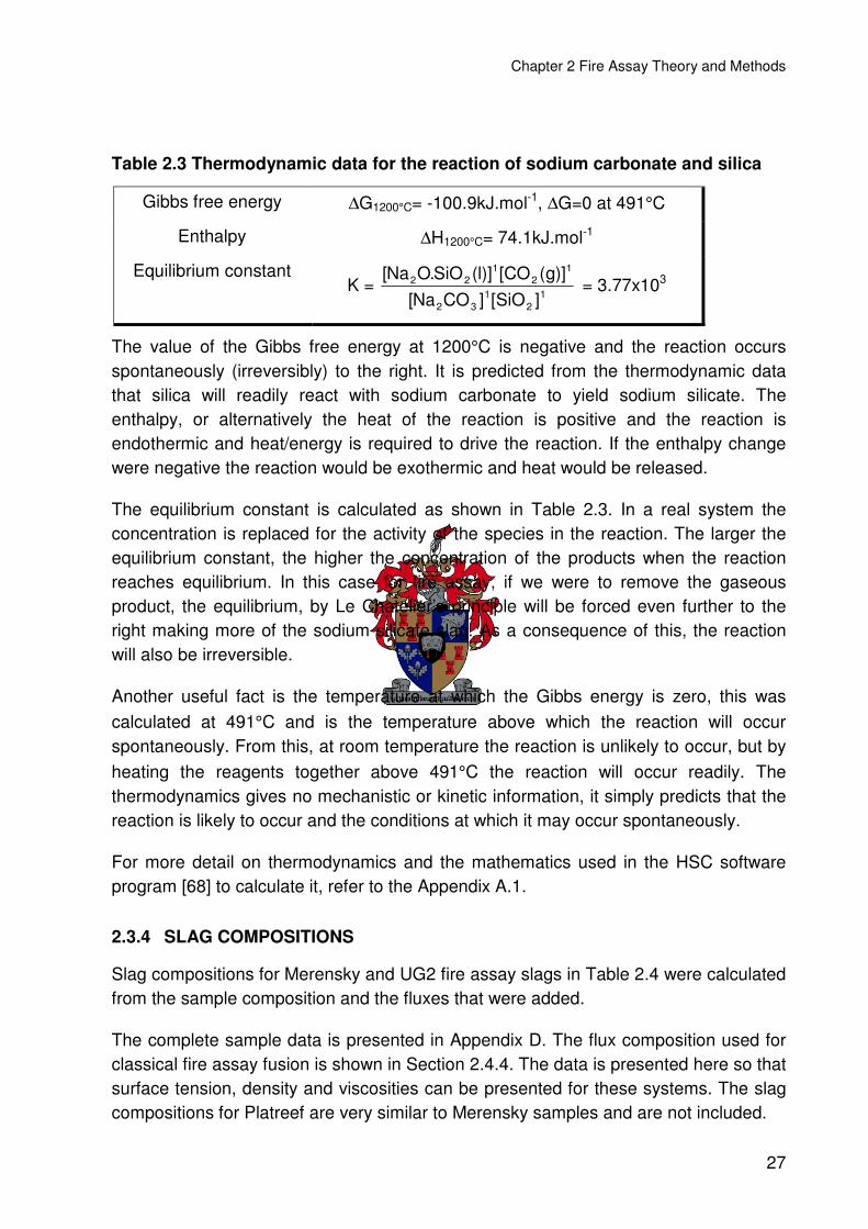
Chapter 2 Fire Assay Theory and Methods
27
Table 2.3 Thermodynamic data for the reaction of sodium carbonate and silica
Gibbs free energy ∆G1200°C= -100.9kJ.mol-1, ∆G=0 at 491°C
Enthalpy ∆H1200°C= 74.1kJ.mol-1
Equilibrium constant K =
12
132
12
122
]SiO[]CONa[)]g(CO[)]l(SiO.ONa[
= 3.77x10³
The value of the Gibbs free energy at 1200°C is negative and the reaction occurs spontaneously (irreversibly) to the right. It is predicted from the thermodynamic data that silica will readily react with sodium carbonate to yield sodium silicate. The enthalpy, or alternatively the heat of the reaction is positive and the reaction is endothermic and heat/energy is required to drive the reaction. If the enthalpy change were negative the reaction would be exothermic and heat would be released.
The equilibrium constant is calculated as shown in Table 2.3. In a real system the concentration is replaced for the activity of the species in the reaction. The larger the equilibrium constant, the higher the concentration of the products when the reaction reaches equilibrium. In this case for fire assay, if we were to remove the gaseous product, the equilibrium, by Le Chatelier’s principle will be forced even further to the right making more of the sodium silicate slag. As a consequence of this, the reaction will also be irreversible.
Another useful fact is the temperature at which the Gibbs energy is zero, this was calculated at 491°C and is the temperature above which the reaction will occur spontaneously. From this, at room temperature the reaction is unlikely to occur, but by heating the reagents together above 491°C the reaction will occur readily. The thermodynamics gives no mechanistic or kinetic information, it simply predicts that the reaction is likely to occur and the conditions at which it may occur spontaneously.
For more detail on thermodynamics and the mathematics used in the HSC software program [68] to calculate it, refer to the Appendix A.1.
2.3.4 SLAG COMPOSITIONS
Slag compositions for Merensky and UG2 fire assay slags in Table 2.4 were calculated from the sample composition and the fluxes that were added.
The complete sample data is presented in Appendix D. The flux composition used for classical fire assay fusion is shown in Section 2.4.4. The data is presented here so that surface tension, density and viscosities can be presented for these systems. The slag compositions for Platreef are very similar to Merensky samples and are not included.
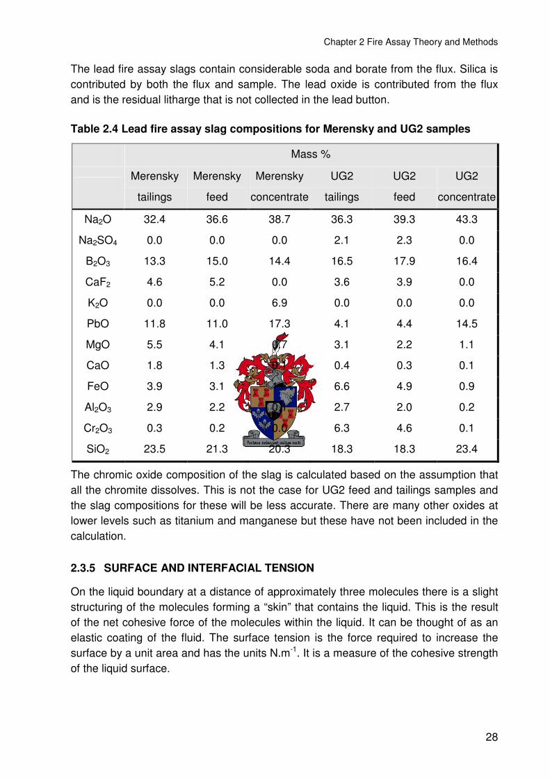
Chapter 2 Fire Assay Theory and Methods
28
The lead fire assay slags contain considerable soda and borate from the flux. Silica is contributed by both the flux and sample. The lead oxide is contributed from the flux and is the residual litharge that is not collected in the lead button.
Table 2.4 Lead fire assay slag compositions for Merensky and UG2 samples
Mass %
Merensky
tailings
Merensky
feed
Merensky
concentrate
UG2
tailings
UG2
feed
UG2
concentrate
Na2O 32.4 36.6 38.7 36.3 39.3 43.3
Na2SO4 0.0 0.0 0.0 2.1 2.3 0.0
B2O3 13.3 15.0 14.4 16.5 17.9 16.4
CaF2 4.6 5.2 0.0 3.6 3.9 0.0
K2O 0.0 0.0 6.9 0.0 0.0 0.0
PbO 11.8 11.0 17.3 4.1 4.4 14.5
MgO 5.5 4.1 0.7 3.1 2.2 1.1
CaO 1.8 1.3 0.1 0.4 0.3 0.1
FeO 3.9 3.1 1.3 6.6 4.9 0.9
Al2O3 2.9 2.2 0.1 2.7 2.0 0.2
Cr2O3 0.3 0.2 0.0 6.3 4.6 0.1
SiO2 23.5 21.3 20.3 18.3 18.3 23.4
The chromic oxide composition of the slag is calculated based on the assumption that all the chromite dissolves. This is not the case for UG2 feed and tailings samples and the slag compositions for these will be less accurate. There are many other oxides at lower levels such as titanium and manganese but these have not been included in the calculation.
2.3.5 SURFACE AND INTERFACIAL TENSION
On the liquid boundary at a distance of approximately three molecules there is a slight structuring of the molecules forming a “skin” that contains the liquid. This is the result of the net cohesive force of the molecules within the liquid. It can be thought of as an elastic coating of the fluid. The surface tension is the force required to increase the surface by a unit area and has the units N.m-1. It is a measure of the cohesive strength of the liquid surface.

Chapter 2 Fire Assay Theory and Methods
29
This surface interacts with the environment around it. The interaction of the fluid with air or a gas usually is referred to as surface tension, it will result in the formation of a meniscus. The interactions between two liquids or a liquid and a solid are referred to as interfacial tension.
The reason that interfacial tension is important is that it determines adhesion, spreading, wetting and in slag/metal (or matte) systems the droplet size. The higher the interfacial tension, the larger the droplets in the slag. It also means that the slag will be less adhesive to the metal. Lower interfacial tension will result in wetting and spread of the liquid. This may affect corrosion of the crucible and slag creep over the sides.
Surface tension is dependent on temperature and generally decreases with increasing temperature. It approaches zero at the boiling point of a liquid. It is also dependent on agitation. In highly agitated melts where there is considerable mixing, the surface tension of a collector phase may approach zero. As the melt settles and the phases separate the surface tension of the metal will increase retaining it into a single phase.
Surface tension is also dependent on composition. These need to be found in appropriate references, particularly for slag systems. Surface tension of pure metals, like lead is calculated as shown in Equation 2.1, [69]. The surface tension data for various liquids can be compared to give an idea of interfacial tension between them.
( )( )dTdTT 00 γ−+γ=γ Equation 2.1
Where:
γ Surface tension (mN.m-1)
γ0 Surface tension at temperature T0 (mN.m-1), from reference table
T Temperature (K)
T0 Reference temperature in (K) (usually the melting point)
dγ/dT Rate change of surface tension with temperature (mN.m-1.K-1)
For the slags the surface tension needs to be estimated from the available data. In Figure 2.5 a slag containing about 36mol% Na2O with SiO2 will have a surface tension of 285mN.m-1. The addition of 15mass% of B2O3 reduces the surface tension by 75mN.m-1 for the oxide slag system in Figure 2.6. From this data the surface tension of the slag was estimated.
The effect of oxygen and sulphur on the surface tension of a metallic liquid is to lower it considerably. The effect of the sulphide is greater than the oxide. From the data for PbS, [70] the approximate value for PbO is estimated. All the surface tension data is shown in Table 2.5.

Chapter 2 Fire Assay Theory and Methods
30
Table 2.5 Surface tension estimates of lead and slag at 1200°°°°C
Surface tension (γ)
/mN.m-1
Slag PbS PbO Pb
≈210 200 ≈250 355
From the surface tension data it is predicted that mattes will have lower surface tension than metals and will form smaller droplets in the slag. This will play a role in settling of the collector phase during fusion.
The data also indicates that liquid metal oxides will wet ceramic materials more readily than metals. These are important because they will allow the lead metal to be separated from lead oxide during cupellation purely from its ability to wet solid ceramic materials.
Figure 2.5 Effect of temperature and Na2O concentration on surface tension for the Na2O-SiO2 system10
10 Reproduced from the “Slag Atlas”, Verein Deutscher Eisenhüttenleute, 1995.
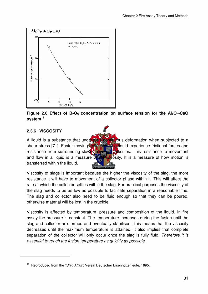
Chapter 2 Fire Assay Theory and Methods
31
Figure 2.6 Effect of B2O3 concentration on surface tension for the Al2O3-CaO system11
2.3.6 VISCOSITY
A liquid is a substance that undergoes continuous deformation when subjected to a shear stress [71]. Faster moving molecules in a liquid experience frictional forces and resistance from surrounding slower moving molecules. This resistance to movement and flow in a liquid is a measure of its viscosity. It is a measure of how motion is transferred within the liquid.
Viscosity of slags is important because the higher the viscosity of the slag, the more resistance it will have to movement of a collector phase within it. This will affect the rate at which the collector settles within the slag. For practical purposes the viscosity of the slag needs to be as low as possible to facilitate separation in a reasonable time. The slag and collector also need to be fluid enough so that they can be poured, otherwise material will be lost in the crucible.
Viscosity is affected by temperature, pressure and composition of the liquid. In fire assay the pressure is constant. The temperature increases during the fusion until the slag and collector are formed and eventually stabilises. This means that the viscosity decreases until the maximum temperature is attained. It also implies that complete separation of the collector will only occur once the slag is fully fluid. Therefore it is essential to reach the fusion temperature as quickly as possible.
11 Reproduced from the “Slag Atlas”, Verein Deutscher Eisenhüttenleute, 1995.

Chapter 2 Fire Assay Theory and Methods
32
With fire assay, the slag composition will have the overriding effect on the viscosity thereof because the fusion temperature is constant.
For metals the viscosity at a temperature below the boiling point can be calculated from Equation 2.2 [69].
( )RTEexp0η=η Equation 2.2
Where:
η Dynamic viscosity (mNs.m-2=10-2 poise)
η0 Standard viscosity (mNs.m-2), from reference table
T Temperature (K)
E Activation energy (kJ.mol-1), from reference table
R Gas constant (8.3144 J.K-1.mol-1)
For slags the viscosity can also be approximately calculated using the Riboud model, [72]. This may not be suitable for fire assay slags and needs to be verified from other data.
( )TBexpAT = Equation 2.3
Where:
η Dynamic viscosity (poise=10-1Ns.m-2)
A exp(-17.51+1.73XCaO + 5.82XCaF2 + 7.02XNa2O – 33.76XAl2O3
)
B +31140 – 23896XCaO – 46356XCaF2 – 39159XNa2O + 68833XAl2O3
T Temperature (K)
XCaO = XCaO + XMgO + XFeO1.5 + XMnO + XBO1.5
(molar fractions)
XNa2O = XNa2O + XK2O (molar fractions)
Table 2.6 Viscosity calculated lead and slag at 1200°°°°C
Viscosity (η)
/poise
Slag min Slag max Pb
0.08 0.19 0.0094
The viscosity of the lead collector is much lower than that of the slag and will flow more easily. The highest viscosity was calculated for the largest silicate sample fused for

Chapter 2 Fire Assay Theory and Methods
33
Merensky tailings while the lowest viscosity was calculated for the Merensky concentrate.
The slag viscosities calculated seem reasonable when compared to the graph shown in Figure 2.7. As the ratio of silicon to boron increases and the slag is more acidic, the more viscous it is. When the basic oxide Na2O is added to the slag there is a drastic drop in the viscosity. A Na2O addition of 10mol% drops the viscosity 3 orders of magnitude. This is the reason that basic slags are often used for lead fire assay. The fire assay slags calculated in Section 2.3.4 have compositions of Na2O in the range of 35-44mol%, B2O3 in the range from 13-18mol% and SiO2 in the range from 20-27mol% (Si:B ratios of 0.6-1.0). This unfortunately, falls outside the range in the graph. The increased SiO2 content would increase the viscosity but be countered by the higher Na2O content. The viscosity is estimated to be in the range of 0.1poise and there is sufficient agreement with the Riboud model.
Figure 2.7 Effect of slag composition on viscosity12
12 Reproduced from the “Slag Atlas”, Verein Deutscher Eisenhüttenleute, 1995.

Chapter 2 Fire Assay Theory and Methods
34
2.3.7 DENSITY
Density is defined as the mass of an object divided by its volume and is usually expressed in g.cm-3. The density difference between the slag and the collector is essential to ensure good separation, provided the two liquids are immiscible.
For the lead the density can be calculated from Equation 2.4 [69].
( )( )dTdTT 00 ρ−+ρ=ρ Equation 2.4
Where:
ρ Density (g.cm-3)
ρ0 Density at temperature T0 (g.cm-3), from reference table
T Temperature (K)
T0 Reference temperature in (K) (melting point)
dρ/dT Rate change of density with temperature (g.cm-3.K-1)
For the slag, the density can be calculated from the partial molar volume with Equation 2.5. The partial molar volume data for some oxides was available from the “Slag Atlas”, [73], the partial molar volume for B2O3 was taken from Riebling, [74].
...VxVxVxV 332211 +++= Equation 2.5
Where:
V Molar volume (cm3.mol-1)
1V Partial molar volume of component 1 (cm3.mol-1), from reference table at a given temperature
x1 Mole fraction of component 1
The results from the calculations are summarised in Table 2.7. The slag concentration did not play a large role in the density of the slag and the differences were less than 10% for the entire composition range.
Table 2.7 Density calculated at 1200°°°°C
Density (ρ)
/g.cm-3
Slag min Slag max NiS Pb
2.4 2.6 5.0 9.5

Chapter 2 Fire Assay Theory and Methods
35
With the density of lead at 25°C being 10.7g.cm-3 compared with 9.5 g.cm-3 at 1200°C, the lead collector will contract by 12%. This is evident from depressions often observed on the lead button after casting.
2.3.8 SEPARATION OF COLLECTOR AND SLAG
The separation of two liquids is given by the Stokes equation, Equation 2.6:
( )µ
ρ−ρ=∞ 18
gdV sc
2
Equation 2.6
Where:
V Maximum limiting velocity (m.s-1) d Diameter of collector sphere (m)
µ Viscosity (poise) g Gravitational constant = 9.8m.s-2
ρc Density of collector (kg.m-3)
ρs Density of slag (kg.m-3)
From the equation the settling velocity is dependent on the difference between the density of the metal/collector and the slag. It is also dependent on the size of the collector droplet in the slag. The larger the droplet, the higher the settling velocity. The droplet size will be a function of the interfacial tension between the slag and collector phases as well as the agitation between them. The liberation of carbon dioxide and other gases during the formation of the lead collector phase in fire assay will contribute to this.
Table 2.8 Effect of lead droplet size, slag viscosity and density on settling time
Droplet Size /µm
Slag Viscosity /Ns.m-2
Slag Density /g.cm-3
Time /s
Time /min
100 0.008 2.4 10.3 00:10
0.019 2.4 24.6 00:25
0.008 2.6 10.6 00:10
0.019 2.6 25.2 00:25
10 0.008 2.4 1035 17:15
0.019 2.4 2458 40:58
0.008 2.6 1067 17:47
0.019 2.6 2529 42:09

Chapter 2 Fire Assay Theory and Methods
36
For all the metal to be collected from the slag the droplets need to fall a distance of 5cm within the fusion time of 60minutes, this is a settling velocity of 1.4x10⁻⁵m.s-1. With this velocity, particles of the 5-8µm range will not settle in time for a classical fire assay fusion. Of course this does not take into account the coalescence of the droplets when the melt is agitated. Droplets of 100µm will settle out in 10-25 seconds while droplets of 10µm will take up to approximately 40 minutes to settle, the comparisons can be seen in Table 2.8.
To assist with settling, the viscosity of the slag needs to be made as low as possible and the fusion temperature as high as possible. A higher concentration of lead in the slag will also be more likely to coalesce and settle quicker, it is predicted that there will be an optimum lead to slag ratio that will result in a quantitative collection of the lead phase.
2.4 FIRE ASSAY FUSION
Lead fire assay fluxes usually have five main components these are litharge, maize meal/flour (or any other suitable carbon source), sodium carbonate, borax and silica. For nickel sulphide there is usually also five components, nickel, sulphur, sodium carbonate, borax and silica. In general the composition of the flux has been determined experimentally.
Any fire assay flux has two functions, firstly to form a suitable collector to pre-concentrate the analyte and secondly to form a suitable slag to retain the gangue from the sample. The collector should be immiscible in the slag and the two phases should be easily separated.
The principle is relatively simple, two phases form during the fusion, the metallic/matte collector, and the molten oxide slag. During the fusion there is constant evolution of carbon dioxide, carbon monoxide, sulphur dioxide and other gases. This causes vigorous agitation and mixing of the chemicals and sample.
The first important factor is the fineness of the sample itself, from the literature a particle size of less than 100mesh is stipulated and this correlates to approximately 85% passing 150µm [54]. For the flux components, the most critical will be litharge and carbon these need to be intimately mixed with the sample as these are responsible for the formation of the collector and need to be in situ with the sample when the PGE are liberated so that they can be collected.
Finally the collector needs to separate from the slag so that it can be treated further. This is where the choice of flux reagents is important for the fusion process. One such example would be the introduction of soda into the charge. Sodium oxide is an unstable compound and cannot be stored or easily produced and needs to be formed during the fusion process. This can be achieved with a number of compounds such as

Chapter 2 Fire Assay Theory and Methods
37
sodium carbonate (Na2CO3), sodium hydroxide (NaOH) and sodium bicarbonate (NaHCO3). All three of these compounds will generate gas during the fusion process (water vapour and carbon dioxide). The gas that is evolved causes the agitation of the melt during the fusion process and assists in the mixing of the charge. To moderate the agitation, these components need to be controlled so that the charge does not splash over.
The mixing ensures good contact between the slag and the collector. The collection of the PGE requires a high or preferential solubility in the collector and a low solubility in the oxide melt. In general most of the PGE are regarded to be collected into a lead alloy. The literature suggests that iridium and osmium may be collected as a fine suspension as they do not alloy readily with lead [50].
The collector is immiscible with the oxide slag and due to a difference in density, the lead separates to the bottom of the melt. The fusion principle is displayed graphically in Figure 2.8, [75].
Figure 2.8 A time line schematic of fire assay fusion process
Initially the dry powdered flux and sample are inert. Once they are placed into a furnace and the temperature is raised they begin to react.
After only 10 minutes there is still a substantial quantity of unreacted sample/flux mixture in the centre of the pot. On the sides molten slag is circulated and vigorously agitated by gas evolved during the fusion.
Droplets of molten lead are observed to circulate in an agitated melt and others are observed to form on top of the unreacted solid sample/flux. From this it is concluded
Fire clay crucible
60 min 30 min 15min 0 min
Dry sample/flux
powder
Molten slag
Lead
Gas bubbles

Chapter 2 Fire Assay Theory and Methods
38
that very little heating is done from the exposed top of the flux. Instead the heating takes place from heat transfer of the pot walls to the sample/flux contacting it.
With approximately 15 minutes of fusion time, a small island of the solid unreacted sample/flux remains floating on top of the vigorously agitated slag. Flames and smoke caused by the combustion of the flour are also observed.
The entire charge becomes molten after 25-30 minutes of fusion and the charge continuously generates bubbles of gas. A convection current is seen to circulate within the molten slag. The current moves inwards from the sides of the crucible and sinks down at the centre. This also indicates that the sides of the pot provide heat to the charge and it moves upward along the sides. It then circulates toward the centre where it cools and sinks. Within the convection currents of the slag, small droplets of molten lead are circulated, they eventually coalesce with others becoming heavier and sink to the bottom of the pot.
This observed mechanism is in contrast to the lead rain theory that has been proposed for this collection technique [76]. The lead rain theory suggests that a rain of lead droplets fall through the molten slag collecting the PGE on the way. This would imply that there is only a single chance to collect the PGE before the lead collects at the bottom of the crucible. This appears to be a simplistic model. The true fire assay mechanism is more dynamic with lead droplets circulating within the slag and there is a much greater likelihood of collecting all the PGE in a single fusion.
The lead fire assay technique is more like a high temperature liquid/liquid extraction system. The slag produced by the flux needs to act as a solvent for the gangue minerals leaching and destroying them to liberate the PGE. The lead liquid then acts to retrieve the PGE and concentrate them in the collector phase. This means that the volume of the lead collector, the volume of slag and the solubility of the PGE in the collector phase are important for a quantitative collection of the PGE.
In the time from 30–60 minutes the circulation of the molten slag slows as less gas is evolved. The slag becomes more viscous as the melt equilibrates and the slag dissolves some of the crucible. Eventually the convection begins to move in the opposite direction were slag moves from the bottom up to the centre of the crucible and out to the sides. This is an indication that the fusion is complete.
What was found during this time line is that the button mass peaks at 30-40 minutes and then diminishes in mass as the fusion progresses to 60 minutes. This may be due to the introduction of more silicates from the crucible into the slag. This imbalance is corrected in the slag by the oxidation of the lead collector and the litharge formed reports to the slag. The equilibrium in the fire assay fusion shifts with time. In conventional fire assay the fusion is usually performed for 60 minutes, as this is a practical time required for the fusion furnace to re-attain its temperature.

Chapter 2 Fire Assay Theory and Methods
39
From the time line data a fusion time of 30-40 minutes is required to attain complete collection using classical fire assay.
2.4.1 THE COLLECTOR
Litharge, (lead oxide, PbO) is the source of metallic lead in lead fire assay. It is reduced to form the collector. The reductant used can be any oxidisable carbon source, usually maize meal, flour or activated carbon.
The initial reduction of litharge is performed by means of a gaseous intermediate, namely carbon monoxide (CO(g)). The direct carbothermic reduction only becomes spontaneous above 300°C. The early reduction of litharge requires the availability of oxygen and is dependent on the oxidising conditions within the furnace. The thermodynamic data is all tabulated in Table 2.9.
A draft through the fusion furnace is required for successful fusion as it is essential to remove the gasses generated in the fusion away from the charge.
Another useful reductant is metallic iron and is usually added in the form of iron nails. This plays an important role in the nail assay that is used to assay high sulphide and antimonide samples [59]. Other metals can be used as reductants such as aluminium, however care must be taken as the oxide that forms can be refractory and difficult to fuse as in the case of aluminium – alumina forms.
Table 2.9 Thermodynamic data for the reduction of lead oxide
Reaction ∆G1200°C
/kJ.mol-1
∆H
/kJ.mol-1 Log[K]
T∆G=0
/°C
2C + O2(g) → 2CO(g) -482.5 -230.0 17.1 <0
CO(g) + 0.5O2(g) → CO2(g) -154.6 -280.5 5.5 <0
PbO + CO(g) → Pb + CO2(g) ↑ -73.8 -95.9 2.6 <0
PbO + C → Pb + CO(g) ↑ -160.5 69.6 5.7 300
PbO + 0.5C → Pb + 0.5CO2(g)↑ -117.1 -13.2 4.2 <0
Fe + PbO → FeO + Pb -86.9 -79.4 3.1 <0
2Al + 3PbO → Al2O3 + 3Pb -961 -1134 34.1 <0
Litharge also acts as an oxidant and can decompose sulphides within the sample. Thus it can play an important role in the liberation of PGE within the fusion. In addition to litharge and a reducing agent, an oxidant such as potassium nitrate may be required. This is often the case where a sample contains a high proportion of sulphide such as in Merensky concentrate samples. The oxidising agent ensures the fusion of
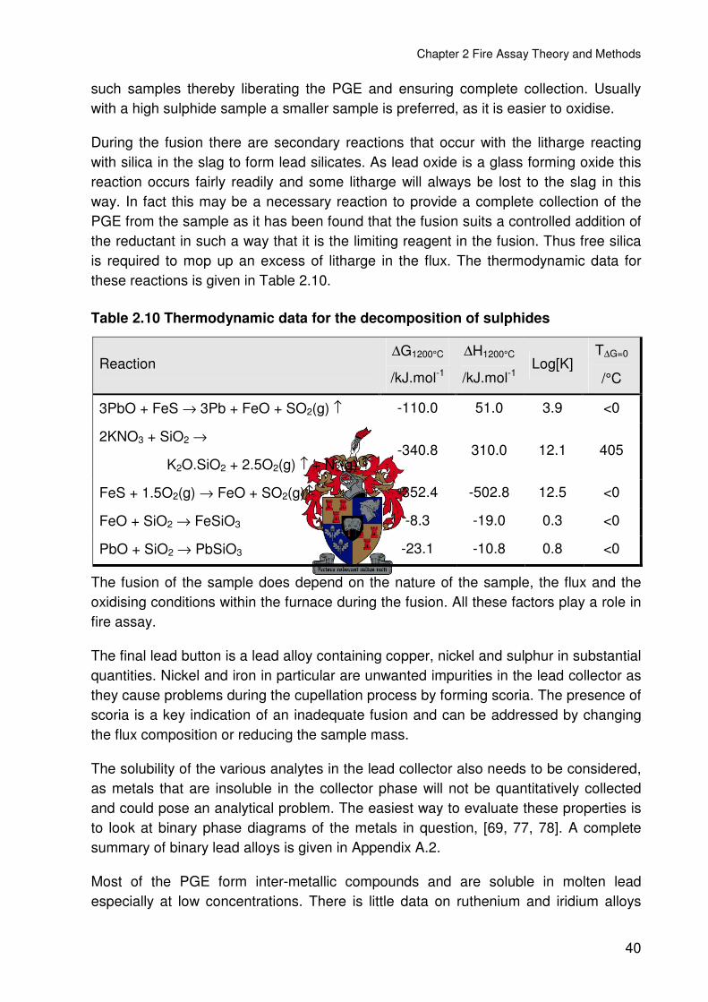
Chapter 2 Fire Assay Theory and Methods
40
such samples thereby liberating the PGE and ensuring complete collection. Usually with a high sulphide sample a smaller sample is preferred, as it is easier to oxidise.
During the fusion there are secondary reactions that occur with the litharge reacting with silica in the slag to form lead silicates. As lead oxide is a glass forming oxide this reaction occurs fairly readily and some litharge will always be lost to the slag in this way. In fact this may be a necessary reaction to provide a complete collection of the PGE from the sample as it has been found that the fusion suits a controlled addition of the reductant in such a way that it is the limiting reagent in the fusion. Thus free silica is required to mop up an excess of litharge in the flux. The thermodynamic data for these reactions is given in Table 2.10.
Table 2.10 Thermodynamic data for the decomposition of sulphides
Reaction ∆G1200°C
/kJ.mol-1
∆H1200°C
/kJ.mol-1 Log[K]
T∆G=0
/°C
3PbO + FeS → 3Pb + FeO + SO2(g) ↑ -110.0 51.0 3.9 <0
2KNO3 + SiO2 →
K2O.SiO2 + 2.5O2(g) ↑ + N2(g) ↑ -340.8 310.0 12.1 405
FeS + 1.5O2(g) → FeO + SO2(g)↑ -352.4 -502.8 12.5 <0
FeO + SiO2 → FeSiO3 -8.3 -19.0 0.3 <0
PbO + SiO2 → PbSiO3 -23.1 -10.8 0.8 <0
The fusion of the sample does depend on the nature of the sample, the flux and the oxidising conditions within the furnace during the fusion. All these factors play a role in fire assay.
The final lead button is a lead alloy containing copper, nickel and sulphur in substantial quantities. Nickel and iron in particular are unwanted impurities in the lead collector as they cause problems during the cupellation process by forming scoria. The presence of scoria is a key indication of an inadequate fusion and can be addressed by changing the flux composition or reducing the sample mass.
The solubility of the various analytes in the lead collector also needs to be considered, as metals that are insoluble in the collector phase will not be quantitatively collected and could pose an analytical problem. The easiest way to evaluate these properties is to look at binary phase diagrams of the metals in question, [69, 77, 78]. A complete summary of binary lead alloys is given in Appendix A.2.
Most of the PGE form inter-metallic compounds and are soluble in molten lead especially at low concentrations. There is little data on ruthenium and iridium alloys

Chapter 2 Fire Assay Theory and Methods
41
with lead. Some problems can arise with copper and nickel as there are immiscibility gaps in the composition range of these binary alloys. In the immiscibility gap two liquids will form and there will be a partition of the PGE between the metallic phases. This could cause severe problems in the efficient collection of the PGE and needs to be avoided. Samples with high sulphide content need to be oxidised so that copper and nickel are reported to the slag and not to the collector. At low concentrations below 3%, nickel and copper will dissolve in metallic lead and will be collected in the lead button.
2.4.2 SLAG
The slag is formed from three components: sodium carbonate, borax and silica. The primary function of these three components is to form a low melting point and fluid slag with the gangue components of the sample.
Sodium carbonate decomposes by action on acid oxides at temperatures higher than 400°C to form sodium slags, it is the source of soda (Na2O).
The anhydrous borax (Na2B4O7) added introduces the borate (B2O3) and additional soda. The borate is used to decompose the refractory basic oxides like calcium and magnesium oxide.
The addition of silica is to moderate the reaction of the soda and borate oxides on the crucible. It is also an acidic flux for basic oxides like iron and ensures that they report to the slag. It also scavenges excess litharge from the flux. The reactions are summarised in Table 2.9.
Table 2.11 Thermodynamic data for the decomposition of oxides
Reaction ∆G1200°
/kJ.mol-1
∆H1200°C
/kJ.mol-1
Log[K] T∆G=0
/°C
Na2CO3 + SiO2 → Na2O.SiO2(l) + CO2(g) -100.9 74.1 3.6 491
Na2CO3 + Al2O3 → Na2O.Al2O3 + CO2(g) -59.0 71.6 2.1 662
B2O3 + CaO → CaO.B2O3 -113.0 -81.2 4.0
Silica also ensures the formation of a homogeneous slag. But, the quantity of silica added must be controlled because it increases the melting point and can make the slag viscous.
The overall picture is that the silicates, aluminates and basic metal oxides from the sample become dissolved in a liquid oxide matrix. These solidify on cooling to form an amorphous sodium borosilicate glass. The fire assay fusion relies on the stability of the metal oxides and their solubility in the slag.

Chapter 2 Fire Assay Theory and Methods
42
In fire assay the slag forming fluxes are generally added in excess of what is required. A mass balance of the flux and sample is not done. This is to make the flux more versatile to tolerate variations in sample composition. It also ensures dissolution of the sample so that the fusion can be quantitative. This is essential for accurate analysis.
2.4.3 CHROMITE SAMPLES
Problems are noted in the fusion of chromite samples, the chromite spinel is highly refractory and is resistant to chemical attack. In addition chromic oxide has a limited solubility in sodium borosilicate slag. The measured solubility using standardless energy dispersive XRF analysis during the examination of the slag using the SEM, Section 4.2.3, has been found to be 2-3% and as a result of this, large chromite samples cannot be adequately dissolved with conventional fire assay fluxes [79, 80]. The insolubility of chromite can be solved with the fusion of small samples. The subsequent analyses of such fusions are more difficult due to the low concentrations of PGE present. With a modern analytical technique such as ICP-MS, these analytical problems can also be solved.
Undissolved chromite particulates can cause entrainment of lead in the slag. In addition it causes cohesion of the slag to the lead button. After casting of chromite fire assay melts (from UG2 samples), the cooling lead contracts forming a hollow layer just below the surface. When separating the button and slag a thin lead foil breaks away with the slag and is usually lost. This is shown in A. of Figure 2.9, other entrainment losses are shown in B. and C.
These physical losses of lead cause losses of PGE. They can be minimised by the addition of sodium sulphate to the flux. The sulphates are reduced to form lead sulphide that is collected in the lead collector. Between 1000-2000ppm of sulphur is measured in the collector with the addition of sodium sulphate to the flux. This raises the melting point and hardens the lead, making the collector more robust. The sulphate also reduces the adhesion of the chromite/slag on the button and avoids physical loss. The sodium sulphate may also affect the surface tension properties of both the slag and collector phase to reduce adhesion.
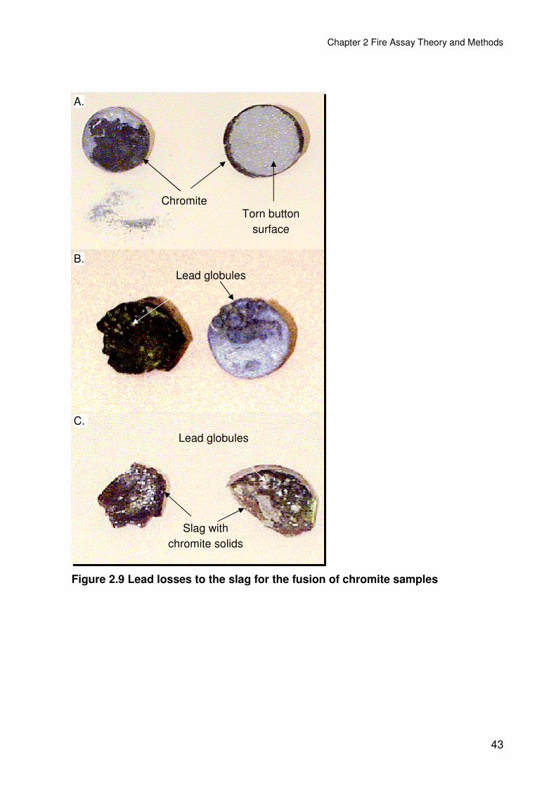
Chapter 2 Fire Assay Theory and Methods
43
Figure 2.9 Lead losses to the slag for the fusion of chromite samples
Chromite
A.
B.
C.
Lead globules
Lead globules
Torn button surface
Slag with chromite solids

Chapter 2 Fire Assay Theory and Methods
44
2.4.4 FLUX COMPOSITIONS
The fluxes for classical lead fire assay were determined experimentally. Some of the basic principles used will be discussed.
Table 2.12 Flux compositions used for classical lead fire assay
Mass /g
Merensky feed
and tailings
UG2 feed
and tailings
Merensky
concentrate
UG2
concentrate
Na2CO3 118.2 166 132.2 130.2
Na2B4O7 50 80 50 50
SiO2 25 48 45 45
PbO 90 100 90 90
C 3.3 4.5 3.6 3.3
KNO3 17.7
CaF2 12 12
Na2SO4 7
Paraffin 1.5 1.5 1.5 1.5
Total 300 420 340 320
Sample 50-75 50-75 10-20 10-20
With the flux an excess of litharge is added with the activated carbon being the limiting agent. The extra litharge is to be used as a de-sulphurising agent. Sodium carbonate and borax are both added to form a suitable solvent for the sample.
Fluorspar is added as a fluidising agent. Experimentally it is found to improve the settling of the lead collector. Small additions to the flux result in an increase in the button size. The addition of fluorspar also makes the flux more versatile as the flux can be used on larger sample masses without modification, with only a small sacrifice in fluidity. Larger additions of fluorspar are ineffective due to excessive corrosion to the crucible during fusion.
Potassium nitrate is added as an oxidant and de-sulphurising agent. It is necessary for the decomposition of high sulphide samples that are characteristic of Merensky flotation concentrate. The amount of the reductant (sulphides from the sample or activated carbon from the flux) is important to yield a large enough lead button. From experiments it is found that the button mass should exceed 35g otherwise the fusion is only semi-quantitative. Concentrate samples need additional silica to dissolve the

Chapter 2 Fire Assay Theory and Methods
45
copper and nickel oxides contributed from the sulphides in the sample. No fluorspar additions are necessary for concentrates because of the small sample masses.
With UG2 feeds and tailings a larger lead button is aimed for, so that losses to the slag would be less significant. The fusion of chromites is assisted by the addition of sodium sulphate as explained in Section 2.4.3.
The addition of paraffin is to act as a wetting agent in order to reduce dusting of the powdered flux. It is quickly volatilised during the fusion and does not contribute significantly as a reductant.
The nickel sulphide fluxes used are tabulated in Table 2.13. The difference from the lead flux lies in the use of nickel, copper and sulphur to form the matte collector. An excess of sulphur is added and acts as a wetting agent during the early stage of the fusion as it has a low melting point. Later in the fusion the potassium nitrate is used to oxidise the excess sulphur.
Table 2.13 Flux compositions for classical nickel sulphide fire assay
Mass /g
Merensky feed
and tailings
UG2 feed
and tailings
Merensky/UG2
concentrate
Na2CO3 60 61 45.0
Na2B4O7 166.9 140.0 127.0
SiO2 13.1 30.0 30.0
Ni 16.0 16.0 14.7
Cu 0.9 0.9 0.8
Fe 18
S 15.8 15.8 14.5
KNO3 13.1 22.0 12.0
CaF2 13.1 20.0 5.0
Na2SO4 15
Paraffin 1.1 1.3 1.0
Total 300 330 250
Sample 50-75 50-75 10-40

Chapter 2 Fire Assay Theory and Methods
46
The UG2 feed and tailings flux also incorporates iron as a reagent. The metallic iron is oxidised with potassium nitrate and forms part of the slag. The iron rich silicate slag improves the separation of the matte for chromite rich samples.
2.5 CUPELLATION
The cupellation process is applied as a second pre-concentration/separation step to lead fire assay. The core of the technology lies with the cupel. The cupel is made from magnesium oxide. The manufacturing process involves the shaping of a cupel from wet clay. The ‘green’ cupel is made with a sedimentary process. After drying, the particulates of magnesium oxide are bound together to form a porous cupel.
For the cupellation process, the cupel is placed into a muffle furnace at 1000-1100°C. The initial preheating step takes 10 to 15 minutes and is used to dry the cupel and heat it up to the cupellation temperature. The clean lead button is placed into the cupel with a pair of tongs. Some laboratories forgo the pre-heating step and load buttons on cold cupels that are then loaded into the furnace. The lead alloy collector melts and at the elevated temperatures is oxidised with air.
If the collector contains nickel, it is oxidised first and precipitates. It floats on the lead bath and due to its high melting point of 1985°C, it deposits on the upper surface of the cupel. This ring structure is called a scoria.
The lead that is oxidised forms a thin liquid layer on top of the molten lead. The lead oxide is drawn into the porous cupel. The lead oxide with its lower interfacial tension wets the cupel and is absorbed by capillary action. The lead has a higher interfacial tension and sits above the surface. Copper oxides, provided the concentration is low enough, diffuse along with the lead oxide into the cupel. Sulphur in the lead collector is oxidised and volatilised as sulphur dioxide. Sulphur can affect the surface tension properties of the lead melt and can cause diffusion of the alloy into the cupel. Ideally the lead should be free of both nickel and sulphur. Cupellation can tolerate moderate quantities of copper. Copper sulphate is often used as a flux additive to colour the cupel green. In this way the assays can have a unique marking pattern to trace errors during preparation.
Thermodynamic data for the reactions during cupellation are summarised in Table 2.14.
The lead becomes enriched with the PGE that are resistant to oxidation and eventually the liquid freezes forming a PGE prill. The shape of the prill is dependent on the rate at which the lead is absorbed in the final stages of the cupellation process.

Chapter 2 Fire Assay Theory and Methods
47
Table 2.14 Thermodynamic data for the oxidation of metals during cupellation
Oxide melting point /°C
∆H1100°C
/ kJ.mol-1
∆G1100°C
/ kJ.mol-1 Log(K)
Pb(l) + 0.5O2(g) → PbO(l) 886 -186.4 -87.9 3.4
Ni + 0.5O2(g) → NiO(s) 1985 -233.5 -117.4 4.5
2Cu + 0.5O2(g) → Cu2O (s) 1235 -191.4 -68.5 2.7
Pb(g) + 0.5O2(g) → PbO(s)↓ 886 -368.0 -145.4 5.5
A graphical representation of the cupellation process can be seen in Figure 2.10.
Of the PGE, platinum, palladium, gold and silver are resistant to oxidation at the cupellation temperatures of 1000-1100°C and remain as metallic prill residue. All the osmium and most of the ruthenium are volatilised as their stable oxides. In addition iridium is lost, this may occur by the volatilisation of the iridium oxide, IrO2 in the presence of platinum [77]. This phenomenon primarily occurs over 1200°C and iridium losses may occur during the high temperature cupellation step.
Figure 2.10 Schematic time line of the cupellation process
Most of the losses of the cupellation process occur during the formation of the prill. If the prill freezes quickly and does not coalesce properly, fragments of PGE can be found at the bottom of the cupel.
X-ray Diffraction (XRD) analyses of the cupels before and after cupellation show that the original magnesium oxide phase, periclase, in the cupels is chemically unaltered.
60 min 20 min 15min 0 min 50 min
Cupel (MgO)
Lead button
Molten lead
Lead oxide
PGE prill

Chapter 2 Fire Assay Theory and Methods
48
The lead oxide phase, massicot, is absorbed into the cupel. Cupellation is a physical separation process similar to filtration.
If the temperature is too low, i.e. below the melting point of lead oxide at 886°C, the cupellation process will not occur. This causes “freezing” of the lead button in the cupel as it becomes encased in a solid oxide layer. This phenomenon can damage the cupel and cause additional losses during cupellation. The various oxides and their physical properties can be found in Appendix A.3.
The lead button prior to cupellation should be as clean as possible. There should be no slag attached to the lead as this can cause additional scoria with the introduction of iron from the slag. The borate present in the slag can react with the magnesia of the cupel causing pitting of the surface. These can cause additional physical losses during cupellation, as lead is held up on the uneven surface and does not coalesce at the bottom of the cupel.
There is considerable volatilisation of lead during the cupellation procedure. The volatilisation of lead and the formation of lead oxide have negative health and safety aspects and good ventilation is essential. The lead oxide is a reactive flux and can damage the refractories of the furnace. Fire assay furnaces, especially muffle furnaces for cupellation, need constant maintenance.
Co-collectors may be added to the fusion. These metals are usually chosen for their ability to alloy with the PGE during cupellation. Silver is by far the most popular choice. A co-collector reduces the effects of physical losses during cupellation. Other choices are gold and palladium. The alloying information of the various co-collectors is summarised in appendices A.4, A.5, A.6 and A.7.
It is apparent that there is much opportunity for things to go wrong during classical lead fire assay.
2.6 LEAD FIRE ASSAY METHODS - A REVIEW
Classical lead fire assay methods have traditionally used weighing to determine the final grade. This has always been an attractive prospect because the end result is a tangible metal fragment that can be seen and assessed. The problem is that they are inaccurate. These traditional methods have been supplemented with more modern instrumental techniques. The fire assay preparation methods remain the same, with the fusion and cupellation, but the final analysis is carried out by wet chemical preparation and instrumental analysis. The most popular being Flame Atomic Absorption Spectrometry (FAAS) and Inductively Coupled Plasma Optical Emission Spectrometry (ICP-OES), but Graphite Furnace Atomic Absorption Spectrometry (GFAAS) and Inductively Coupled Plasma Mass Spectrometry (ICP-MS) are also used.

Chapter 2 Fire Assay Theory and Methods
49
The basic fire assay technique takes a weighed portion of a prepared sample adds a suitable powdered flux and the mixture is blended (fluxing). The mixture is transferred into an alumina/silicate fire clay crucible and is fused in an electric hearth furnace for 60-90 minutes at 1100-1200°C (fusion). The melt is cast and the collector is mechanically separated from the slag (de-slagging).
The clean lead button is placed into a preheated cupel at 950-1100°C inside an electric muffle furnace, the low temperature cupellation step. The lead is oxidised and removed by diffusion into the cupel over a 45-60 minute period. The metal prill residue that remains is transferred to a block cupel. The cupel and prills are ignited at 1300°C in an electric high temperature furnace for 60 minutes to volatilise the impurities in the high temperature cupellation step. The final prill is flattened to remove adhering cupel residue. The prill is weighed and the 4E gravimetric grade determined. This is called gravimetric fire assay or commonly referred to as a 4E assay where a sum of the platinum, palladium, rhodium and gold content is reported.
Other fire assay variations are also used. The most common is nickel sulphide where a nickel-based flux is used to fuse the sample. It is a more modern fire assay technique and makes use of nickel sulphide as a collector specifically for the analysis of platinum, palladium, rhodium, ruthenium and iridium [81]. The latter two cannot be analysed conveniently using any other technique. With the application of a distillation technique the osmium content can also be reported. A good comparison of the various methods is given by Juvonen, [82].
For the nickel sulphide method, the fire assay step is used for pre-concentration followed with a wet chemical analysis. The sample and flux mixture are fused at 1200°C for 90 minutes and the melt is cast into an iron mould. The nickel sulphide collector containing the PGE is mechanically separated from the oxide slag.
The buttons are crushed and pulverised in preparation for wet chemical treatment. The base metal sulphides are leached using hydrochloric acid. The PGE sulphide residue that precipitates is filtered and then dissolved using aqua regia. The PGE content is measured using an instrumental technique.
In many commercial laboratories the addition of co-collectors are common practice. Silver is used as an alloying co-collector to collect platinum, palladium and gold. Palladium and gold are used to collect primarily rhodium, though they can also be used for the analysis of platinum. The prills with their co-collector cannot be separated using the high temperature cupellation step and instead are analysed by wet chemical dissolution and an instrumental technique. These methods are run in tandem so that a quantitative analysis of the platinum, palladium, rhodium and gold can be determined. These “standard” methods are covered in a number of texts, [38, 53, 83]

Chapter 2 Fire Assay Theory and Methods
50
The various fire assay methods that can be used are summarised in the schematic diagram, Figure 2.11.
Figure 2.11 Schematic of fire assay methods
2.6.1 4E GRAVIMETRIC ANALYSIS
The gravimetric analysis is still used due to its fast turnaround time and simplicity. However it is known that losses occur with the technique [76]. The method is not widely used for research purposes due to its known inaccuracy and experimenters use more quantitative methods of analysis.
To supplement existing knowledge on the gravimetric technique an internal research project was carried out. The aim was to further understanding and improve the technique to make it more quantitative. A number of experiments were performed to identify where losses during cupellation occur. Variables examined in the experiments included temperature, time and airflow (draft) in the cupellation furnace [84]. Recoveries from a known PGE spike were examined.
Co-collector
Sample Preparation
Fluxing
Flux
Fusion
De-slagging
Button Preparation
LT Cupellation
Chemical Preparation
HT Cupellation Chemical Preparation
Instrumental Analysis
(Lead dissolution)
(Nickel Sulphide)
Instrumental Analysis
(Lead dissolution)
(Nickel Sulphide)
Instrumental Analysis
(Silver prill)
(Palladium prill )
Instrumental Analysis
(Silver prill)
(Palladium prill )
Gravimetric Analysis
(4E prill )
Gravimetric Analysis
(4E prill )

Chapter 2 Fire Assay Theory and Methods
51
There were significant effects of temperature and time on the outcome of the results. Generally higher cupellation temperature and longer time resulted in better removal of lead and impurities from the prill. Measurable quantities of lead and ruthenium still remained after low temperature cupellation. The PGE prills with higher ratios of rhodium retained more lead.
The platinum recovered in the prill was not affected by any of the cupellation variables.
The palladium recovered was affected by both temperature and time. Higher temperatures and longer cupellation time resulted in losses of palladium. Gold displayed similar behaviour to palladium. The losses of palladium and gold appear to be caused by volatilisation.
The rhodium behaved differently to the other elements. The analysis showed lower recovery with lower temperatures and shorter times. The losses were as a result of the oxidation of some of the rhodium at lower temperatures. Rhodium oxide (Rh2O3) is thermodynamically stable to 1150°C and is insoluble in aqua regia, therefore it was not dissolved during the wet chemical preparation. Using pressure dissolution with a Carius tube it was possible to dissolve the entire prill and obtain better recoveries.
The effect of the prill mass on the recovery and grade was also studied [85]. The losses of PGE were found to increase as the prill mass decreased. This was caused by physical losses to the cupel during cupellation and subsequent handling. Secondly, losses by volatilisation of the more volatile PGE that increased as the prill mass decreased.
The impurity levels also increased with prill mass. The main impurities were lead and magnesium from the block cupel. Ruthenium found in the prill after low temperature cupellation was removed during the high temperature cupellation. As the size and surface area of the prill increased the quantity of adhering cupel residue also increased thereby introducing more magnesium.
The problems inherent in the cupellation process is probably best summarised by the photographs in Figure 2.12. In the first picture, A, there is clearly a PGE residue in the cupel in the top right hand corner of the photograph. In the photograph, B, when flattening the 4E prill, the cupel residue did not break off entirely but was pressed into the metal at the centre.

Chapter 2 Fire Assay Theory and Methods
52
Figure 2.12 Photographs and SEM image of 4E prills
A better idea of the 4E prill was obtained by preparing a polished section and examining it with the SEM. The back scattered electron (BSE) image of the prill is shown in C. The electrons produce XRF emissions that are analysed using energy dispersive (ED) analysis. It was discovered that the prill was extremely inhomogeneous with many phases of varying composition. The prills were also full of holes where metal had been volatilised during the high temperature cupellation.
These experiments highlighted the problems with the low temperature cupellation step. The losses are variable being affected by both temperature, time, PGE ratio/composition and prill size that is dependent on grade and sample mass. This is not the only problem however, Bugbee [59] reports that cupel quality, size and shape all affect the low temperature cupellation.
The gravimetric 4E method is not suitable for highly accurate analysis. Due to the inconsistent nature of the losses, correction will also be unreliable.
2.6.2 SILVER PRILL METHOD
The silver prill technique is similar to the 4E technique, the difference being the addition of a silver nitrate solution to the charge just prior to fusion. During the cupellation process silver is resistant to oxidation, although it may contain some dissolved oxygen within the alloy [77]. During the final stages of the cupellation process a silver prill forms. This silver prill contains quantitatively the platinum, palladium and gold from the sample. For most applications of low-grade feeds and tailings samples 10mg of silver will form a molten silver prill with a ratio of >20:1 of silver to total PGE and a minimum platinum to silver ratio of 8:1 [38]. For flotation concentrate samples with higher quantities of PGE, the mass of silver added needs to be increased to 20mg to ensure a soluble alloy.
A. B. C. Fragment
Magnesite

Chapter 2 Fire Assay Theory and Methods
53
The prill is usually spherical and properly formed. Rhodium does not alloy readily with silver and is not soluble in molten silver. As a consequence the rhodium is deposited in the cupel and is lost. This was confirmed by drilling out the base of the cupel after removal of the silver prill and pressure dissolving the residue in a Carius pressure tube. The final solution was measured by ICP-MS [84]. Using this technique 8-25% of the rhodium from a sample was analysed from the cupel residue. Using pressure dissolution on silver prills a 60-70% recovery of rhodium from a sample was obtained. Analysis of the same samples using conventional wet chemical preparation, only a 2-3% recovery of rhodium was obtained. This confirmed the theory that rhodium losses for the silver prill method are due to the formation of rhodium oxide that does not dissolve with conventional digestion. It also confirmed physical losses to the cupel.
An example of a silver prill in a shown in, A, Figure 2.13. Surprisingly the silver prills are not homogenous solid solutions as was anticipated. SEM analysis [86] of polished sections found discrete PGE phases like Pb>Ru>Bi and Rh>Pt>Ir. These are the lighter portions in the image, C, of Figure 2.13. These may also result in poor dissolution that was observed for high PGE:Ag ratios. It is essential that sufficient silver is added to alloy with the PGE.
Another problem that can occur with silver prills is vegetation. This occurs when a prill bursts or fragments on cooling, a picture of this is shown in B of Figure 2.13. This is caused when dissolved oxygen in the molten silver is rapidly expelled from the silver as it freezes. At 1000°C the solubility of oxygen in silver is about 0.25-0.35%. This can cause severe physical losses. The addition of copper to the lead causes a trace quantity to be collected in the silver. This reduces the quantity of oxygen that can dissolve in the silver and minimises vegetation.
Figure 2.13 Photographs and BSE image of silver prills
Physical losses do still occur with the silver prill method. This occurs at the interface of the cupel and the silver prill and often an irregular interface can be observed.
Silver prills can be dissolved with a microwave digestion system. The prills are placed into plastic dissolution tubes with lids. Nitric acid is added, the prills are dissolved/parted with the first microwave-heating step. Hydrochloric acid is then added
A. B. C. Vegetation

Chapter 2 Fire Assay Theory and Methods
54
to form aqua regia and a second microwave dissolution step is performed. Once the prills are completely dissolved the solution can be analysed with an appropriate analytical technique [87].
One of the biggest problems with the silver prill technique is that during the dissolution an insoluble silver chloride precipitate forms. Thus care must be taken when measuring silver prill solutions otherwise the tubing of the sample introduction systems for the analytical instrument may become blocked. Ideally these solutions should be filtered, in practice however the solution is allowed to settle and is decanted.
The manual dissolution technique where larger acid volumes were used has been shown to be quantitative. UG2 samples analysed by the silver prill method dissolve in nitric acid and leave a black particulate residue in the beaker (more noticeable for higher-grade samples). When adding sufficient hydrochloric acid the silver chloride precipitate is dissolved. This prevents interference of the silver chloride during the dissolution of the residue by aqua regia.
Figure 2.14 Illustration of proposed passivation with silver prills
In the microwave method, when smaller acid volumes were used, the dissolution of UG2 type samples was not always quantitative. This was influenced by the precipitation of the silver chloride. With the particulate residue after the parting of UG2 silver prills, it is possible that the residue may act as a nucleation site for the recrystallisation of silver chloride from solution. This may cause a “passivation” effect and prevent the dissolution of the PGE as illustrated in Figure 2.14.
The microwave dissolution technique is quite elegant as it facilitates easier handling of large sample loads. Combined with ICP-OES analysis, this makes a powerful analytical tool. However, the technique needs to be operated with care to obtain a quantitative dissolution of the silver prill.
Ag Alloy PGE
Alloy PGE Residue
HNO3 HCl
PGE residue AgCl

Chapter 2 Fire Assay Theory and Methods
55
2.6.3 PALLADIUM PRILL METHOD
For the efficient collection of rhodium, palladium is added as a co-collector. Palladium is reported to quantitatively collect platinum, gold and rhodium [83].
An interesting note is that palladium and rhodium are immiscible at lower temperatures (below the melting point of palladium at 1547°C) [69]. The collection of rhodium by palladium may be a mechanical one. It is interesting that this technique is used routinely for the analysis of rhodium, as this would not have been predicted from the metallurgy.
For the routine method between 1 and 10mg of palladium is added as a solution to the charge prior to the fusion. An example of a palladium prill in a cupel is shown in, A, Figure 2.15.
Figure 2.15 Photograph and BSE image of palladium prills
A BSE image of a palladium prill is shown in B, Figure 2.15. The palladium and 4E prills are similar in structure, both were very inhomogeneous and often have holes. These may be where lead volatilised during cupellation. Alternatively dissolved gasses may precipitate during solidification to form gas pockets. The prills appear agglomerate in nature. These have various PGE containing phases. The palladium prills using 1mg and cupelled at 1000°C contained 22-29% by mass of lead.
The co-collector prills are removed after the low temperature cupellation step and are analysed by wet chemical dissolution similar to the silver prill method. Both hydrochloric and nitric acids are added together and a single step dissolution is performed. The solution is made to volume and then measured, usually with FAAS using uranium as a releasing agent.
Co-collectors effectively minimise physical losses that may occur during the formation of the prill. Some losses may still occur at the interface between the prill and the cupel. For robustness it is best to use 10mg of palladium as a co-collector as this gives quantitative recoveries for rhodium, platinum and gold. While with smaller masses of the co-collector sporadic uncontrolled losses may occur.
A. B.

Chapter 2 Fire Assay Theory and Methods
56
It was found that if pressure dissolution in a Carius tube was used to dissolve palladium prills that quantitative analysis of iridium could be obtained. Ruthenium recoveries were poor with only 20-30% of this metal being recovered. The addition of palladium as a co-collector was unable to prevent the volatilisation of ruthenium tetroxide.
The palladium prill method is typically used to supplement the silver prill method by providing a rhodium grade.
2.6.4 GOLD PRILL METHOD
The metallurgy of gold/PGE alloys was initially considered [77, 78]. Platinum, palladium and silver form solid solutions with gold when solidified from the molten state making gold a perfect collector for these elements. Rhodium in small quantities can be dissolved by molten gold. The solubility was estimated to be 3.5% at 1100°C [77]. It is possible that gold would be a suitable collector of rhodium provided the cupellation temperature and mass of co-collector is correct. It is calculated that between 10 and 30mg of gold is required for feed and concentrate samples respectively.
The solid solubility of iridium and ruthenium in gold is small. Should collection of these metals occur, it is predicted that it would be via mechanical collection within the gold matrix. A photograph of a gold prill is shown in A of Figure 2.16 and BSE image in B.
Figure 2.16 A photograph and BSE image of gold prills
The gold prill was found to be the most homogenous of the all the co-collector types when analysed on the SEM. Small discrete phases containing (Rh>Pt>Pd>Pb>Os)Bi were identified. Small platelets containing Ru>Ir at the core and Ru>Rh>Pt>Ir at the rim were also found. The formation of these various phases within the gold prill appears to be caused by the presence of ruthenium, iridium and osmium. These cause crystallisation of discrete phases within the matrix and may contain some of the other PGE. These phases are more resistant to chemical attack and result in poor dissolution of the prills.
A. B.

Chapter 2 Fire Assay Theory and Methods
57
The insoluble residue after an aqua regia leach of the gold prill was found to contain star-like crystals that were enriched with platinum and rhodium, Figure 2.17. These elements were semi-quantitatively analysed by the ED-XRF on the electron microscope and contained mostly Rh>Pt alloys [88].
Conventional dissolution techniques could not be used for the dissolution of these platinum rhodium alloys. Pressure dissolution of the prills produced quantitative analysis for platinum, palladium, rhodium and iridium. The recovery of ruthenium in the gold prill was around 70%, the remainder may have been volatilised.
Figure 2.17 Insoluble platinum/rhodium alloys from gold prills
Gold appears to be the best lead fire assay co-collector, provided pressure dissolution is performed on the prills.
2.6.5 DISSOLUTION OF LEAD
With all the associated problems of the cupellation process (with and without co-collectors) it was decided to investigate the direct analysis of the lead collector for PGE after the fusion [89]. The literature has a reference to the method by Diamantatos [90]. With this analysis technique perchloric acid was used to dissolve the lead collector. The PGE were precipitated using formic acid and the residue was collected by filtration, dissolved and analysed. The method was tested but deemed too dangerous for routine analysis.
The preparation of lead from fire assay is important prior to dissolution. Conventional mechanical removal of the slag is not suitable as a gelatinous silicate residue forms after the leach and the solution cannot be filtered. For this type of analysis the bulk of the slag is removed from the button. The slag on the button surface is then cracked by gentle tapping with a spatula. The slag is then leached from the button using a 10% v/v solution of hydrochloric acid. With gentle heating the slag begins to dissolve and loosens from the button. The button is then rinsed with water and buffed with paper. The lead is flattened to a sheet 1mm in thickness, cut into strips and placed in a glass beaker for leaching.

Chapter 2 Fire Assay Theory and Methods
58
It was found that hydrobromic acid could be used to dissolve lead [91], although the dissolution is slow. By adding bromine the dissolution of lead is extremely rapid. With a little experimentation a solution of concentrated hydrobromic acid with 80mL of bromine per litre was found to be optimal for the dissolution. The dissolution of lead with this acid mixture is exothermic and self-propagating. The lead is allowed to react until bromine fumes are no longer generated. This procedure is carried out in a fume cupboard. The beaker is then placed onto a warm hotplate to complete the dissolution. Once dissolved, the excess bromine is boiled off leaving a solution of hydrobromic acid containing lead.
The largest problem with this type of solution is that lead bromide can precipitate. This occurs when the solution is diluted, becomes too cold, or if the volume decreases too much during dissolution. For most purposes 3mL of the acid mixture per gram of lead is sufficient to dissolve the lead and retain it in solution.
The next task is to isolate the PGE from the solution. A reference was found to the precipitation/stripping of PGE from solution using sodium borohydride [92]. This extremely strong reductant reduces the PGE to the metal. Testing a 10% m/v solution of sodium borohydride on a dissolved lead button in hydrobromic acid it was found that the PGE were precipitated first, followed by large lead agglomerates.
By using 1-2mL of a 10% m/v solution of sodium borohydride it is possible to selectively precipitate the PGE. An XRF scan of the precipitate indicated the presence of platinum, palladium, gold, rhodium, ruthenium and iridium. However, when dissolving the precipitate with aqua regia, only quantitative analysis of platinum, palladium, gold and rhodium is achieved. The ruthenium and iridium are both resistant to dissolution using aqua regia and the residue had to be fused with sodium peroxide to obtain quantitative analyses. The analyses of iridium and ruthenium are not routinely performed for the lead dissolution technique.
The method is further improved by using ascorbic acid to the cold leach solution as a bromine scavenger. This improves the reproducibility of the precipitation step. Ascorbic acid acts as a mild reductant and reduces the solution lightening it until a light straw-coloured solution is formed. This takes several minutes to react. The ascorbic acid is sensitive to heat in the acid media and needs to be added to a cool solution at around room temperature otherwise it decomposes and carbon is precipitated in solution. Volumes of 2-4mL of a 20% m/v solution of ascorbic acid in water are found to be sufficient for the removal of excess bromine from the solution.
Tellurium is also added as a co-precipitant, this makes it easier to identify when the precipitation is complete. The borohydride solution is added while stirring with a magnetic stirrer. This agitation allows the volatilisation of gas from the addition of the borohydride solution.

Chapter 2 Fire Assay Theory and Methods
59
In all cases extremely concentrated solutions of sodium borohydride and ascorbic acid are used in order to minimise the volume of water added so as not to dilute the acid. All the glassware is rinsed with 1:1 hydrobromic acid solution to prevent precipitation of lead bromide.
The lead dissolution method is used to analyse platinum, palladium, rhodium and gold in a variety of samples and is used extensively for development work. The method is designed to evaluate lead fire assay fluxes and to verify the complete collection of PGE by comparison to the nickel sulphide procedure.
The final solution is a clean matrix containing predominantly PGE and can be measured by FAAS, GFAAS, ICP-OES and ICP-MS. All of these techniques have been successfully applied.
The method was found to be superior to the standard nickel sulphide method for the analysis of feed and tailings samples. In particular the analysis of UG2 chromite samples is highly improved using this technique with smaller samples and instrumental analysis by ICP-MS or GFAAS.
Similar results to nickel sulphide were obtained for the analysis of concentrate samples with the lead method. The analysis of larger concentrate sample masses is better using the nickel sulphide procedure. This is due to limitations in the dissolution of sulphide materials using lead fluxes.
The major disadvantage of the method is the large amount of lead waste in a hydrobromic acid medium that is to be disposed of. Comparatively, acidic nickel waste can be recycled at the Base Metal Refinery.
2.6.6 NICKEL SULPHIDE
The first application of the nickel sulphide technique was performed for the analysis of osmiridium in Witwatersrand gold ores in 1965 [93]. By comparison to lead fire assay technique, nickel sulphide is very modern. With nickel sulphide the PGE are not collected in a metallic alloy but rather within a nickel matte.
Much of the early development of the method for the analysis of PGE was done at Mintek during the late 1960s and early 1970s [94, 95, 96]. These methods used nickel carbonate that decomposes with heat to form nickel oxide that in turn reacts with sulphur in the flux to produce the nickel matte. Similarly to lead fire assay the nickel matte has a higher density and is immiscible with the oxide slag and so the collector separates gravimetrically [97]. The fusion reactions forming the slag are analogous to lead fire assay.
The PGE are collected as solid solutions within the matte. The first fusion in earlier work was not completely efficient and approximately 2-7% of the PGE were not

Chapter 2 Fire Assay Theory and Methods
60
collected. This was due to the lower density of the matte compared to the lead metal collector in conventional fire assy. A second wash fusion was performed to collect the PGE. This was necessary because of small droplets of the collector being left behind in the slag and only being collected the second time around.
More recent methods use metallic nickel powder to make the nickel sulphide collector and with flux modifications have proven to collect the PGE quantitatively with a single fusion [98, 99]. A number of methods have been published with improved instrumental techniques such as ICP-MS [100, 101]. The nickel sulphide/ICP-MS technique is a very powerful analytical tool and with its low detection limit is suitable for almost any sample.
The nickel sulphide technique with flux modifications such as the use of sodium hydroxide and lithium tetraborate have been applied to the analysis of chromite samples, with varying degrees of success [99, 102]. An interesting approach was taken by Puakert et al [103]. The nickel sulphide technique is similar in some ways to solvent extraction. They studied the effects of the ratios of the flux and sample to the mass of the collector. They also studied the effect of the sulphur content of the flux. Since they used small masses of the collector they found that the sample composition affected the results. Higher quantities of copper and iron in the button caused problems when dissolving the matte with hydrochloric acid. The use of fluorspar (CaF2) in the flux increases the fluidity [70]. It causes corrosion of the crucible, but improves the settling of the collector making a single pass collection possible.
Unlike lead fire assay, the nickel sulphide matte separates cleanly and easily from the slag. This is achieved when the flux composition is correct with a sodium carbonate to borax ratio of 1:2 – an acidic slag is required. Basic slags result in poor nickel sulphide collection as the matte becomes soluble in the slag and does not separate. This is because basic slags have higher sulphide capacity [104].
The button is crushed and pulverised for the wet chemical preparation. The matte should be about 100 mesh (100% passing 150µm) for efficient leaching otherwise matte remains in the filtrate and causes base metal contamination of the final analytical solution. The nickel sulphide is leached using hydrochloric acid and the PGE are liberated. During the leaching of the matte, hydrogen sulphide is generated and precipitates the PGE as a sulphide. The insoluble PGE sulphide residue is then separated by filtration. A tellurium collection is performed with stannous chloride as a reductant to precipitate any partially dissolved PGE, notably palladium [105]. The precipitate is dissolved using aqua regia and the PGE content is measured using an instrumental technique.
Nickel sulphide has one very distinct advantage and that is the analysis of all the PGE simultaneously. The disadvantages are the complexity, extremely long analysis time, expense and it is labour intensive. Sulphur dioxide is generated as a by-product of the

Chapter 2 Fire Assay Theory and Methods
61
fusion. The dissolution of the matte generates hydrogen sulphide along with arsenides and selenium compounds that are present as impurities from the sample. These are poisonous and therefore leaching must be done in a fume cupboard. Large volumes of nickel waste are generated.
All the disadvantages aside, the nickel sulphide method is considered the most definitive method for the accurate determination of PGE in low-grade samples. The nickel sulphide technique is used for the metal accounting analysis of feed and tailings samples both Merensky and UG2. These analyses are used to calculate correction factors for gravimetric lead fire assay. The analysis of flotation concentrate, both UG2 and Merensky is also performed by nickel sulphide and is done on every truck of concentrate that is transported from the flotation plants to the Smelter at Anglo Platinum. The technique is also applied to furnace matte as well as furnace slag and again for accurate metal accounting analysis. Financial settlement and production calculations are done on these analyses and the method needs to be both accurate and precise.
2.6.7 OVERVIEW OF METHODS
All the methods in fire assay have their advantages and also their disadvantages these are summarised in Table 2.15.
The best method is clearly nickel sulphide as with a single fusion the analysis of five precious metals and gold can be routinely done. The method is however extremely costly and is applied to important metal accounting samples.
The second best method is the lead dissolution technique as it can be used to analyse for platinum, palladium, rhodium and gold – all the economically important metals. Alternatively an alkali fusion can be applied to the residue or pressure dissolution to the precipitate for the analysis of iridium and ruthenium. Due to the low solubility of lead in hydrobromic acid and the possible formation of lead bromide precipitate, the method is not applied routinely. It is employed as a comparative analytical technique for the assignment of consensus values to QC samples and as a development tool for fire assay research.
The main advantages of using a co-collector are that the precision is increased because physical losses during cupellation are minimized. Co-collectors yield a more reliable analysis and are much easier to handle. The final solution has a relatively simple matrix and should be easily and reliably analysed.
The fact that a more precise analysis is achieved means that the co-collector methods are suitable for process control such as in a concentrator plant. There is a lower detection limit and better analysis of tails may be achieved. The one disadvantage is that the methods are more complex and the simplicity of the gravimetric method is lost.

Chapter 2 Fire Assay Theory and Methods
62
Table 2.15 Summary of fire assay methods
Method Advantages Disadvantages
Nickel sulphide • Six element method
• Accurate and precise
• International standard method
• Complexity
• Long leach time
• Time consuming
• Large volume of nickel waste
• Base metal (nickel) contamination in final solution
Lead dissolution • Fast dissolution
• Accurate and precise
• No cupellation
• Long button preparation time
• Complexity
• Time consuming
• Hydrobromic acid-lead waste
• Only four elements routinely analysed
• Lead contamination in final solution
Silver prill • Simple wet chemical dissolution
• Fast analysis
• Precise elemental analysis
• Physical losses are minimised
• Cupellation
• Silver chloride precipitate
• Only three elements analysed
• Lead cupel waste
Palladium prill • Simple wet chemical dissolution
• Fast analysis
• Precise elemental analysis
• Physical losses are minimised
• Cupellation
• Palladium matrix in solution
• Only one element analysed routinely
• Lead cupel waste
4E gravimetric • Fast analysis
• Simple technique
• Easy operation
• Inaccurate, imprecise
• Requires correction factors
• Variable losses
• Cupellation
• Non elemental analysis
• Lead cupel waste

Chapter 2 Fire Assay Theory and Methods
63
The silver prill method is applied routinely for the analysis of geological bore core samples. The method is used to analyse for platinum, palladium and gold and if applied correctly can be used for the quantitative analyses of these elements. Its biggest disadvantage is the inability to analyse for rhodium. For the latter, samples with a platinum grade of greater than 1g.ton-1 are re-fused using palladium as a co-collector for the analysis of rhodium. This poses a problem, as the silver prill analyses have to be completed before the palladium prill analysis can begin. This doubles the turnaround time for the analysis and is considerably wasteful in terms of consumable resources such as flux, time and labour. A notable omission is the gold co-collector method, it is excluded as the method is not used routinely.
The 4E gravimetric method is applied to process control samples that are corrected against the nickel sulphide method. The method is inaccurate but provides cheap analysis in the shortest possible time. It also does not require specialised instrumentation such as FAAS or ICP-OES as a microbalance is used. This is relatively simple to operate and is easy to train personnel that do not have a formal tertiary qualification.
2.7 DISCUSSION
The basic theory on slag chemistry has been presented. This is applicable to automation as much as it is to classical fire assay. No matter how the technology changes, the chemistry and physiochemical effects during the fusion remain the same.
When pushing the envelope in trying to reduce the analysis time with automation it is essential that there is a sound understanding of the underlying chemistry. This allows the prediction of methods that will work with a substantially better chance of success. This foundation will stand in good stead both for Chapter 4 where the baseline analysis using classical methods are discussed as well as in Chapter 5 where the key automation technologies are presented.
The classical methods have been presented along with information from the literature. The advantages and disadvantages of the various methods have been discussed. Only the most accurate methods, those of the lead dissolution method and nickel sulphide are to be used for the analysis of QC materials during this work.
In Chapter 3 manual methods for the preparation of the QC samples for this work is presented. These QC samples are to be used to give the baseline for the classical methods. The baseline is to be used to perform development and validation of the automation methodologies. The manual methods also provide the basic principles of sample preparation that are equally applicable to the automation technologies.

64
CCHHAAPPTTEERR 33
3 SAMPLE PREPARATION
When performing research on an analytical method, the sample preparation needs to be done with the best possible methods so that sampling variation does not falsely affect the outcome of the research. Simply put, analysis is dependent on the weakest link, whether the error is as a result of the sampling or on the measurement of the final solid or solution, the total accuracy is dependent on the sum of all the individual errors [106]. Taking a good sample is essential for accurate analysis and is dependent on how well the sample is prepared.
The concept of error addition is mathematically expressed below in Equation 3.1; the total variance of the method is the sum of the variances of the individual steps. Most analytical techniques can be divided into three general steps those of sampling, sample preparation and finally measurement.
σ2(total) = σ2(sampling) + σ2(sample preparation) + σ2(measurement) Equation 3.1
One way to assess an analytical method is to use well-analysed CRMs. These well-prepared samples can be used to validate the sample preparation and analytical method. Ideally the CRM should be similar to the sample type analysed. Since this is often not possible, the preparation of in-house QC materials is required. It should also be understood that the age of the CRM might be important because analytical methods change with time and often get more accurate.
CRMs are also costly and therefore are usually used sparingly. Suitable QC materials can be used for development and optimisation work. This chapter focuses on the preparation of such QC materials.
3.1 PRINCIPLES OF SAMPLE PREPARATION
There are numerous texts that examine the principle of sampling. These focus on the statistical modelling of the effects of sampling. The texts by Pitard [107, 108] are good in the practical application of sampling by means of mechanical samplers be they cross-stream cutters, pipe samplers or augers, all of which are used at Anglo Platinum. Some of these sampling concepts with regard to mining and financial risk are discussed by Bartlett [109].

Chapter 3 Sample Preparation
65
One of the more important concepts that is applicable to assaying and analysis is the effect of particle size on the variance of sampling. Pitard shows that the sampling variance is proportional to the diameter of the largest particle size fraction (of the valuable portion of the sample) to the third power divided by the sample mass, this is shown mathematically in Equation 3.2.
( )s
32
MCd
sampling = Equation 3.2
Where:
σ2(sampling) The fundamental error of sampling (variance, ppm2)
C The sampling constant. It is dependent on the sample itself and how it is sampled and needs to be determined experimentally (ppm2.g.m-3)
d The diameter of the largest valuable particle size fraction in the lot to be sampled (m)
Ms The mass of sample taken (g)
From Equation 3.2 it can be seen that there are two ways to reduce sampling errors. The first is to reduce the particle size and the second is to increase the sample mass.
With this in mind, the first task for any analysis is to grind the samples as finely as is practically possible. The accuracy of a sample is determined by its richest and coarsest particles as these are the ones that have the potential to bias the sample. This is called the “nugget” effect and is common for gold samples.
In PGM ores it can also occur and is related to mineralogy. Gold occurs as a native metal alloy with silver and is resistant to grinding. Many of the PGMs occur as sulphides and these minerals can be ground.
The nugget effect arises when a relatively large particle of an element occurs in the assay sample causing the result to be unnaturally high. As an example a single particle of 80 to 100µm is found where the average is usually 5 to 10µm. In some of the data searched in the mineralogy database at the Research Centre [110], some electrum particles with an averaged diameter of 80µm have been identified. If one of these particles were to be assayed in a single 50g assay aliquot, the “nugget” of 80µm13 would raise the grade from 0.20g.ton-1 to 0.30g.ton-1, a difference of 50%. This is caused by the occurrence of gold in a metallic form at low concentration.
13 Gold density 19.3g.cm-3

Chapter 3 Sample Preparation
66
A similar effect may occur for platinum because of the occurrence of the metallic alloy ferroplatinum. Particles of up to 300µm in diameter have been found [111]. Using these numbers and the density/composition data from Cabri14 [32], if one particle of ferroplatinum of this size was to occur in a 50g sample containing 3g.ton-1 platinum, the overall grade would increase to 7.3g.ton-1. It is a known fact that gold nuggets usually do not grind but the same cannot be said for ferroplatinum.
The purpose of the calculation was to examine the effect of PGE rich minerals on the analysis. The above example shows that it is essential to grind the sample as fine as possible. In doing so, sampling effects will have less effect on the outcome of the final result. An additional benefit is that a smaller mass is required for a representative sample. In short, the finer the top size the more homogeneous the sample.
3.2 BULK SAMPLES
Bulk samples were obtained from two sites; Amandelbult and Potgietersrus and came from the Merensky, UG2 and Platreef. The samples were from the various flotation plants and included 30kg of feed and tailings and 10kg of the flotation concentrate. The samples were from several batches of samples over an extended period. They were filtered, dried and sent to the Research Centre for further processing.
3.3 DRYING
The bulk sample was split by hand into 2kg portions and placed into stainless steel drying pans. The samples were dried overnight (a minimum of 14 hours) at 105°C in a standard convection oven. The pans were removed and allowed to cool. All analyses are reported based on a dry mass basis. The material is not significantly hygroscopic and can be stored for extended periods in closed containers without the necessity of re-drying the sample.
The dried material was then passed through a 2mm screen and combined in a 25L plastic drum. The coarse residue such as wood chips, paper, steel cable, plastic, insects and the like, were discarded.
An inversion mixer was used to blend the sample. The drum was about three quarters full and was ideal for mixing as there was sufficient space for the material to move inside. The opening of the drum was covered with glazed brown paper and the plastic lid was clamped in place. The drum was strapped onto a steel roller frame, inclined at 30° to the horizontal. The frame was rotated by a set of motorised rollers and this
14 Ferroplatinum alloy Pt0.80Fe0.16Cu0.03Pd0.01 with density 19.13g.cm-3

Chapter 3 Sample Preparation
67
inverted the drum. The material within the drum cascaded and was tumble mixed in this fashion for one hour.
3.4 PULVERISING
The dry material still contained small agglomerates of up to 2mm in size and needed to be pulverised. A vertical spindle pulveriser was used to prepare the bulk feed and tailings material. Disc pulverisers are one of the most common methods of preparation and have been used in the South African mining industry since the 1920’s and are documented in texts by Moir (1923) [112], Dillon (1955) [113] and more recently by Lenahan (1986) [83]. In the latter, assay sample size requirements are quoted as 85% less than 150µm.
For the concentrate sample the possibility of cross-contamination from the vertical spindle pulveriser becomes too great due to the higher grade of the material. The preparation of the concentrate was done with a swing mill and gives a suitably fine grind. It is more time consuming and labour intensive than the vertical spindle pulveriser.
3.4.1 VERTICAL SPINDLE PULVERISER
The vertical spindle pulveriser is a common piece of laboratory equipment used in mining industry particularly for the fast throughput of bulky mining and ore samples.
The machine works with a stationary bottom disc with a second rotating disc above it. The distance between the discs is mechanically controlled and the sample is fed through a hole in the centre of the top disc. The sample at the centre of the disc is flung outwards by the centrifugal force of the rotating disc and ground between the two steel discs. It emerges from between the discs and is funnelled into a cup below.
The discs are adjusted manually after every sample of 500g. The adjustment is subject to experience, but the basics are that the discs are adjusted together until they touch and briefly stop moving. The gap is then widened slightly to allow the discs to move freely. The gap will be typically less than 0.1mm. If the gap is too close the sample will choke and not feed properly through the discs. After the sample has passed through, the discs are pneumatically raised and the sample is blown down with jets of compressed air and collected in the sample cup.
The feed and tailings samples were fairly bulky but the pulveriser was convenient as the sample can be passed in batches of 500g taking approximately 3 minutes each. The continuous preparation allowed the 30kg of material to be pulverised in 3-4 hours.

Chapter 3 Sample Preparation
68
The pulveriser can handle fairly coarse sample up to 10mm in diameter. Larger samples, rocks and cores need to be crushed prior to pulverising. The most common method is to use a jaw crusher, but this technique was not needed.
The vertical spindle pulveriser can retain sample and needs to be carefully cleaned before another sample is processed. For bulk samples this is not a problem and the sample can be passed continuously through the machine after adjusting the discs. The discs do steadily wear and the sample will contain small steel particles from the grinding media.
The pulveriser has dust extraction but care needs to be taken with setting the extraction as it can act as a cyclone by removing the finest portion of the sample. This needs to be checked and monitored as it can potentially bias the sample. If the machine is setup and operated correctly it can be a reliable sample preparation tool.
When the sample was changed the pulveriser was flushed clean with compressed air. Coarse quartz was pulverised and the mill cleaned with air again.
The pulverised sample was recombined into a clean 25L plastic drum and mixed, as before, using an inversion mixer.
3.4.2 SWING MILL
The swing mill produces a fine grind and is an extremely aggressive method of pulverising analytical samples. Variations on the swing mill are used for both semi and fully automated sample preparation for analysis. The preparation of the concentrate samples was performed using a manually operated swing mill.
The mill has a central motor with an acentric weight that is rotated. When the motor is started the rotation of the weight swings the platform of the mill outward. The platform is then retained with a set of springs. A counterweight at the bottom of the motor determines the amplitude of the swing. The grinding is performed with the vibratory action of the platform.
The grinding is performed within a cylindrical bowl. Depending on the size of the bowl used it may contain a cylindrical puck and rings. The sample is ground by the action of the puck and rings against the base and sides of the bowl. The bowls can be made from various materials like mild steel, chrome steel and tungsten carbide. The bowls have three typical sizes; 100mm, with a single 50mm diameter puck (25cc), 200mm bowl with a 50mm puck and 100mm ring (100cc) and a 300mm diameter bowl with a 100mm puck (250cc), 150mm and 200mm rings. The selection of the bowl depends on the mass of material to be prepared. The swing mill is very versatile and the bowls, pucks and rings are easily cleaned with soap and water thereby reducing

Chapter 3 Sample Preparation
69
contamination. The feed to the mill should typically be less than 2mm to produce a reasonable grind.
For the preparation of the concentrate material a 300mm diameter bowl of hardened chrome steel was used. Approximately 250g of sample material was scooped into the bowl and ground for 2 minutes. The preparation of 10kg concentrate material took 2-3 hours. The pulverised material was recombined in a 25L plastic drum and mixed for one hour with an inversion mixer.
3.4.3 SIZING
Sizing can be done in a variety of ways that include dry screening and wet screening. The wet screening technique is usually considered the most reliable as it is not subject to the physical loss of fine material. The only problem being that the wet sample needs to be dried before being weighed [83]. For very fine samples the formation of slimes can prevent good screening analysis and other methods are required. One of the more popular techniques is the use of diffraction by coherent laser light [114]. The extent of the diffraction is proportional to the size of the particles in the sample. With laser sizing very fine sample material can be reliably analysed. The method is quick and convenient and is often used for fast sizing analysis. For details of the sizing analysis refer to Appendix B.5.
The laser requires the sample to be dispersed within water using rapid stirring and the diffraction is measured. In this way the sample is diluted considerably as the technique is extremely sensitive. The analysis is reported as a volume passing a particular size and a pareto chart is plotted of the data, see Figure 3.1. The volume sizing is related to the screening method by the density of the sample material.
The sizing was done to determine how finely prepared the samples were after routine preparation. The sizing analysis is summarised in Table 3.1. It is clear that the concentrate samples were finer than the feed and tailings samples. This is as a consequence of the grinding technique. The swing mill is shown to produce a more consistent and fine grind. The feed and tailing samples met the desired specification of 85% passing 150µm.
It is noted that from the D10 value 10% of the volume for all the samples are less than 1µm, while for the feed and tailings there is a larger distribution of particle sizes. In this manner there is not an even distribution of particles but rather a bimodal distribution of fine and coarse particles, this can be clearly seen in Figure 3.1. The implication of this is that the material is likely to segregate on standing with the finer particles separating from the coarser particles.
For flotation, ores are ground to liberate the PGM and sulphide minerals, this is necessary so that the liberated particles can be separated. The implications of this are

Chapter 3 Sample Preparation
70
that the finer portion of the sample may be enriched in base metal sulphides and PGE. The sample needs to be properly mixed prior to the assay sample being taken. Dusting losses of the sample need to be avoided, large dust (fines) losses could potentially bias the sample.
Table 3.1 Summary of particle size distributions for the prepared QC samples
D10 /µm
D50 /µm
D90 /µm %<74µm %<150µm
Maximum size /µm
UG2 Tailings 0.8 48.0 163.3 63.4 87.6 355
Feed 0.5 40.0 164.7 65.2 87.3 355
Concentrate 0.9 16.1 74.1 90.0 99.2 212
Merensky Tailings 0.5 23.1 173.0 70.6 86.8 425
Feed 0.7 30.6 161.0 69.2 88.3 355
Concentrate 0.6 9.1 48.9 95.9 99.4 355
Platreef Tailings 0.5 16.7 79.4 88.2 99.2 212
Feed 0.5 18.4 154.0 74.2 89.4 425
Concentrate 0.5 7.6 47.2 96.4 99.6 300
Figure 3.1 Particle size distribution of the UG2 tail sample

Chapter 3 Sample Preparation
71
3.5 SUB SAMPLING
When a very bulky sample arrives in the laboratory, the entire sample cannot be analysed and needs to be reduced in size. This needs to be done in a way that the analytical sample is representative of the bulk. Once the material has been pulverised this can be done more reliably. Splitting is usually done using a riffle, of which there are numerous kinds, and the mechanical rotary riffler is the most reliable. If this is to be done manually the technique of cone and quartering can be used [83].
3.5.1 ROTARY SPLITTING
The bulk sample was once again mixed using the inversion mixer. The sample was then split into smaller aliquots. For this a mechanical 10 way rotary splitter was used. The splitter was disassembled, washed, dried and then reassembled prior to operation.
The sample was scooped into a funnel above a vibratory hopper. The height above the base of the hopper to the funnel was fixed at approximately 3-5mm. The sample was fed along the hopper into the first cup, the hopper was then stopped and the material transferred back to the funnel. The motor was started and the carousel with the ten steel cups was rotated at a constant speed. The hopper was restarted and began to cut small portions of the falling stream into the cups.
The material in the funnel was replenished until the cups were full. The splits were then randomly recombined into five, 5L plastic containers. The entire bulk material was split in this fashion to produce five secondary splits. Each of the splits was then mixed using the inversion mixer and split in the same way to produce ten tertiary splits. The remaining four secondary splits were split in the same fashion to produce a total of fifty splits.
The final splits were placed into new 1L plastic screw cap jars. The jars were all labelled with a printed self adhesive label and the mass of the split and the container were recorded. This was done for all the Merensky, Platreef and UG2 feed and tailings samples. The UG2 samples, due to their higher density, were placed in 500mL plastic jars. A schematic for the low grade splitting regimen is shown in Figure 3.2.

Chapter 3 Sample Preparation
72
Figure 3.2 Feed and tailings splitting scheme
Figure 3.3 Concentrate splitting scheme
Bulk Sample
1 2 3 4 5 6 7 8 9 10
1 2 3 4 5
Primary split
Secondary split
Tertiary split
321
45
678
910 3
21
45
678
910 3
21
45
678
910 3
21
45
678
910 3
21
45
678
910
Bulk Sample
1 2 3 4 5 6 7 8 9 101 2 3 4 5 6 7 8 9 10
1 2 3 4 51 2 3 4 5
Primary split
Secondary split
Tertiary split
321
45
678
910 3
21
45
678
910 3
21
45
678
910 3
21
45
678
910 3
21
45
678
9103
21
45
678
910 3
21
45
678
910 3
21
45
678
910 3
21
45
678
910 3
21
45
678
910 3
21
45
678
910 3
21
45
678
910 3
21
45
678
910 3
21
45
678
910
Bulk Sample
1 2 3 4 5 6 7 8 9 10
1 2 3 4 5
Primary split
Secondary split
Tertiary split
5
21
43 5
21
43 5
21
43 5
21
43 5
21
43 Quaternary split
1 2 3 4 5
Bulk Sample
1 2 3 4 5 6 7 8 9 101 2 3 4 5 6 7 8 9 10
1 2 3 4 51 2 3 4 5
Primary split
Secondary split
Tertiary split
5
21
435
21
43 5
21
43 5
21
43 5
21
43 5
21
435
21
435
21
43 5
21
435
21
43 5
21
435
21
43 5
21
435
21
43 Quaternary split
1 2 3 4 51 2 3 4 5

Chapter 3 Sample Preparation
73
The concentrate samples were prepared in a similar way, during the primary split the splits were randomly recombined into five primary splits that were then further split in 10. Two of the tertiary splits were then randomly recombined to make a total of 25 quaternary splits, the splitting scheme is shown in Figure 3.3.
The masses of the final splits were examined and the relative standard deviation (RSD) of the splits calculated. These were all found to be less than 3% RSD and because of the random re-combinations were considered fit for purpose. The randomisation reduces the possible systematic error that may be introduced by the splitting technique. The overall preparation is presented in Table 3.2.
Table 3.2 Summary of splitting precisions during sample preparation
%RSD on splitting masses
Primary Secondary Tertiary Quaternary
UG2 Tailings 2.5 1.1 2.4
Feed 2.2 1.0 2.6
Concentrate 1.9 0.9 1.9 1.6
Merensky Tailings 2.9 0.8 2.2
Feed 1.9 1.0 2.5
Concentrate 2.1 0.4 2.7 2.0
Platreef Tailings 2.4 1.2 2.4
Feed 1.9 0.3 2.3
Concentrate 2.9 1.7 2.3 2.3
Physical losses during splitting were monitored and throughout the splitting process the mass difference was less than 5g in total. With a QC mass of around 30kg, the physical losses during splitting were insignificant.
The splitter was operated at 30rpm and it took approximately 2 hours to split the five secondary splits on the feed and tail samples, meaning that each recombined split contained about 720 cuts of approximately 8g each. The final splits contained a further 70 cuts of the secondary splits.

Chapter 3 Sample Preparation
74
For all practical purposes the samples that were taken were representative of the bulk material and complied with the sampling theory found in Pitard [108].
• All the sectors in the riffle were identical in size.
• The feed rate was constant.
• The rotating speed of the carousel was constant.
• The speed of the carousel was adjusted so that the sample was not deflected out of the cup during the cutting of the sample.
• The cutter was aligned radially to the stream.
• Dust losses were minimised.
The rotary splitter produced a layered sample that needed to be mixed. The individual splits were placed into a 25L plastic drum and mixed with the inversion mixer. The samples were individually re-mixed using a small laboratory scale turbular mixer prior to taking a sample. The sealed plastic jar was clamped into the mixer using rubber bands. The container was then inverted and rotated inside the mixer. Due to the possibility of segregation this was always done just prior to taking a sample. Approximately 15 minutes of mixing was found to be adequate.
3.5.2 DIPPING
Any analytical samples from the individual splits were taken by dipping. In this procedure the entire sample was emptied onto a 400x400mm square piece of glazed brown paper. The sample was slowly roll mixed by drawing one corner of the paper horizontally over the sample. The paper lifts the sample and tumble mixes it, and by alternating the corners a sample can be efficiently mixed.
The sample was then flattened out on the paper with a spatula and a cross drawn across the sample to divide it into quarters. The assay aliquot was then dipped in small quantities from alternate quarters of the sample until there was sufficient mass. Usually 12-20 dips are taken depending on the aliquot required.
This dipping technique should provide the best possible analytical sample and was done to reduce sampling errors.

Chapter 3 Sample Preparation
75
3.6 HOMOGENEITY TESTING
Homogeneity testing was required to ascertain whether or not the sample preparation was adequate. Although this cannot be done for conventional routine assay samples, it is a useful technique to evaluate the preparation of bulk QC samples. This poses a problem because with the imprecision of fire assay it is difficult to evaluate the precision of the sample preparation. Therefore other more precise analytical techniques are required. One of the most reliably precise analytical techniques is XRF.
The XRF cannot detect PGE reliably below about 100ppm. This means that other elements at higher concentration that may behave similarly, or are associated with the PGE are analysed instead. The choice is the copper and nickel sulphides that are associated with the PGE in nature and hence in the sample. By evaluating the homogeneity of copper and nickel within the sample splits it was possible to draw conclusions on the homogeneity of the sample and this should apply to the PGE as well.
For the feed and tailings samples 10 samples of the splits were randomly chosen and represented 20% of the samples. For the concentrates 5 samples of the 25 were selected and also represented 20% of the total.
Samples were prepared for XRF using the pressed pellet technique. Two aliquots of 16g each were dipped and mixed with 1g of EMU15 binder. The mixture was then ground for 3 minutes in a 100cc bowl using a six-pot swing mill. The direction of grinding was changed every 30 seconds. The ground material was transferred out into an aluminium cup. The cup was gently tapped on a flat surface to settle the material and it was then pressed in a hydraulic XRF press with 40mm dies at 20 tonnes of pressure for 30 seconds.
The final pellets were inspected for cracks or any surface imperfections; defective pellets were broken down mixed with an agate mortar and pestle and repressed. Fortunately there were few defective pellets. The pellets were then measured using a Philips PW 2400 Spectrometer. The Kα lines for copper, nickel, iron, cobalt and chromium were measured and the counts recorded. The measurements were made for all the pellets and were repeated a second day. Since the samples were prepared in duplicate it was possible to estimate the precision of the preparation technique and with the sample being measured on two different days it was possible to estimate the precision of the XRF measurement. Finally the comparison of the precision of the various splits can be compared by an analysis of variance (ANOVA).
15 EMU is a styrene derivative polymer that is a popular choice due to its excellent binding properties. Other choices could have been sodium stearate or cellulose.

Chapter 3 Sample Preparation
76
3.6.1 STATISTICAL EVALUATION
An ANOVA was performed on the data, the mathematical calculation resolves the random experimental/determination errors from a known change or factor - a deliberate action performed by the experiment, in this case the splitting of the sample. The basic statistics can be obtained from any number of textbooks, two good examples used are Chatfield [115] and Miller [116].
The counts for the metals, copper, nickel, iron, cobalt and chromium were measured in the samples on two different days and reported. With this experiment there are actually two variables – the day and the splits. These need to be analysed independently. First the variation of the XRF measurement from one day to the next was examined, Table 3.3 shows only the nickel data for the Merensky tailings as a worked example, the remaining data for all the samples are summarised later.
Table 3.3 Results for the XRF measurement of the Merensky tailings splits
Ni day 1
/kcps Ni day 2
/kcps
Split/Sample Disc A Disc B Disc A Disc B
Merensky tailings 1 24.77 24.83 24.81 24.87
Merensky tailings 2 24.80 24.79 24.87 24.74
Merensky tailings 3 24.77 24.76 24.77 24.81
Merensky tailings 4 24.80 24.84 24.87 24.88
Merensky tailings 5 24.78 24.84 24.85 24.88
Merensky tailings 6 24.81 24.64 24.78 24.75
Merensky tailings 7 24.83 24.78 24.88 24.86
Merensky tailings 8 24.84 24.92 24.83 24.91
Merensky tailings 9 24.85 24.77 24.90 24.83
Merensky tailings 10 24.78 24.83 24.83 24.88
Average 24.80 24.84
Using the macro from Microsoft Excel, a single factor ANOVA was performed. For details of the ANOVA refer to Appendix C.1. An Alpha of 0.05 was used and this determines the value for which the F becomes significant. With a smaller value of alpha, the test is more tolerant and the critical value of F is larger. If the value calculated for F, for our experiment, is larger than F-critical then the test is significant at the desired confidence interval. In this case with a probability (P) of 0.05 (alpha) it refers to a 95% confidence interval (CI). This means that it is 95% certain that the test

Chapter 3 Sample Preparation
77
is positive and that there is a statistically significant difference in the variation caused by the factor.
Table 3.4 Analysis of variance for the XRF measurement made on two days
Source of Variation SS df16 F P F critical
Between Groups 0.014 1 5.23 0.03 4.10
Within Groups 0.103 38
Total 0.117 39
The first observation, from Table 3.3, is that the measurement for nickel on the second day was slightly higher than on the first.
From Table 3.4, the variation within groups - the measurements themselves within the day were higher than the variation from day to day. This can be seen from the column SS (Sum of the Squares) which calculates the variance.
Looking at the F value it was higher than the F-critical value and the P-value (the probability) was less than 0.05 - therefore the result was marginally significant.
The measurement on day 2 was higher than on day 1 and the difference is larger than what can be expected from normal random experimental error associated with the preparation of the materials for measurement. There was a definite difference in the measurement by the XRF from one day to the next. This is largely due to the good precision with which the XRF measurements are made that such a small difference would be statistically significant.
The data for the day-to-day measurements was then averaged. A one factor ANOVA was performed on the data to examine the splitting.
Table 3.5 Analysis of variance summary for the evaluation of splitting
Source of Variation SS df F P F critical
Between Groups 0.026 9 1.50 0.27 3.02
Within Groups 0.019 10
Total 0.044 19
The value of F statistic calculated, in Table 3.5, was less than F critical meaning the probability that the value occurs by random variation was high. The variation for splits
16 df – degrees of freedom

Chapter 3 Sample Preparation
78
was within the error for the analysis thereof (taking into account the preparation and measurement error). The conclusion being that there were no systematic errors introduced by the splitting of the samples and the splits can be considered identical.
Another consideration was to look for possible outliers. The easiest way was to make a scatter plot of the data. Looking at the graph, Figure 3.4, a single determination was highlighted with a circle. There appears to be a problem with sample 6b. Indeed when this sample was re-measured on the second day a higher result was obtained, confirming a measurement error on day 1.
Figure 3.4 Scatter plot of the individual analytical results
This is a topic of outlier deletion. With small data sets like the ones above it becomes extremely difficult to correctly identify and omit outliers. Often the experience of a chemical analyst is required and a chemical reason for the rejection can be found, for example a chemical interference, a physical loss and others. Provided a legitimate reason can be given, a result can be rejected but this must be reported when the results are presented.
The data was further examined with a simple comparison, shown in Table 3.6. The difference between the highest and lowest nickel measurement is about 1%. With the omission of the outlier this becomes 0.7%. The splitting limit for the samples was set at 1% as an acceptable and realistic target and clearly from Table 3.6 this was obtained. This may not be true for other elements and will be dependent on the accuracy and
Plot of Ni XRF measurement for Merensky tailings splits
24.60
24.70
24.80
24.90
25.00
1a 1b 2a 2b 3a 3b 4a 4b 5a 5b 6a 6b 7a 7b 8a 8b 9a 9b 10a
10b
Sample
Ni /
kcps
Ni day 1
Ni day 2
Plot of Ni XRF measurement for Merensky tailings splits
24.60
24.70
24.80
24.90
25.00
1a 1b 2a 2b 3a 3b 4a 4b 5a 5b 6a 6b 7a 7b 8a 8b 9a 9b 10a
10b
Sample
Ni /
kcps
Ni day 1
Ni day 2

Chapter 3 Sample Preparation
79
precision of the preparation and XRF analysis of those elements. Homogeneity testing was a useful technique for screening the preparation of the QC material and could quickly identify a problem in the splitting before time and money was spent on PGE analysis.
Table 3.6 Comparison of data before and after outlier deletion
Unaltered data Outlier removed
Ni day 1 Ni day 2 Ni day 1 Ni day 2
Average / kcps 24.80 24.84 24.81 24.84
Difference / kcps 0.04 0.03
%Difference 0.15 0.12
Maximum / kcps 24.920 24.920
Minimum / kcps 24.639 24.741
Difference 0.281 0.179
%Difference 1.14 0.72
The data could also be generated using a two-way ANOVA in Microsoft Excel. However, the calculations used were not robust and could not calculate the statistics with missing data and outliers became a problem. With the scheme used above, where the day 1 and day 2 measurements were averaged, there was no problem with omitting a data point. Both calculations gave identical results with complete data sets.
3.6.2 SUMMARY OF HOMOGENEITY TESTING
The data for all the statistical analysis of the homogeneity testing are presented in Table 3.7. For simplicity only the probability (P) values were tabulated, as all the other statistical numbers were not necessary for the interpretation. Any P number less than 0.05 was considered marginally significant and values below 0.01 were significant, values less than 0.0001 were considered highly significant.
Out of the 45 statistical tests only 1 was significant and 3 were marginally significant. The data were sporadic, the testing regimen was designed to look for systematic splitting errors where there would be consistent splitting differences; this was not seen for any of the QCs prepared.
The calculated splitting limits were typically less than 2%. The largest limit that was calculated was for UG2 tailings, this was not surprising since the copper and nickel in this sample type were extremely low in concentration.
The QCs prepared were considered suitable for accurate development work.

Chapter 3 Sample Preparation
80
Table 3.7 Sample XRF homogeneity testing
P Split
Cu Ni Co Fe Cr ± %
UG2 tailings 0.261 0.796 0.457 0.492 0.589 2.88
Merensky tailings 0.735 0.267 0.006 0.081 0.032 0.69
Platreef tailings 0.516 0.501 0.480 0.702 0.740 0.85
UG2 feed 0.054 0.106 0.178 0.068 0.755 1.22
Merensky feed 0.255 0.044 0.535 0.206 0.062 1.26
Platreef feed 0.262 0.483 0.412 0.113 0.328 1.37
UG2 concentrate 0.610 0.981 0.972 0.278 0.147 0.79
Merensky concentrate 0.433 0.775 0.472 0.328 0.988 0.62
Platreef concentrate 0.014 0.318 0.452 0.555 0.632 0.54
3.7 DISCUSSION
The entire preparation of the QC materials was done manually. The reason for this was that at the time there was no automated equipment at Anglo Platinum for this purpose. It also served as a suitable baseline and some of the findings are summarised:
• The manual methods were time consuming.
• Considerable care had to be taken to prevent cross-contamination.
• The methods were labour intensive.
• Preparation quality may be impaired as the operator tired during a shift and quality of the preparation was operator dependent.
• Training and experience were prerequisites to good preparation.
The feed and tailings samples prepared with the vertical spindle pulveriser were considerably coarser than the concentrates. This was a limitation of the grinding technique and the swing mill was far superior.
The concentrate samples could be used as they were. For feed and tailings samples some additional pulverising could be required, depending on the analytical technique.

Chapter 3 Sample Preparation
81
With fire assay, using large samples, the feed and tailings samples were also adequate.
With suitable QC materials prepared, a baseline for classical fire assay methods is to be established in the next Chapter. The baseline values provide the backbone to evaluate the technology for automation in Chapter 5. This is to be followed by the spark analytical technique in Chapter 6 and the design of a fully automated fire assay laboratory in Chapter 7.

82
CCHHAAPPTTEERR 44
4 BASELINE ANALYSIS USING CLASSICAL METHODS
Classical fire assay methods were used to analyse the QC materials that were prepared as described in Chapter 3. The methods selected for the baseline analysis were those that give the most accurate results. Classical lead fire assay preparation followed by chemical analysis of the lead collector – the lead dissolution method. This was followed by analysis using the nickel sulphide method. These two methods will give the most accurate and reliable analysis for low-grade samples.
The baseline analysis was to be done to establish suitable values for the QC materials. CRMs were analysed at the same time to establish the accuracy of these classical methods so that the QCs could be validated.
Table 4.1 List of Certified Reference Materials used
SARM 7 Merensky ore [117, 118]
SARM 7B Merensky ore [119]
SARM 64 UG2 tailings [120]
SARM 65 UG2 ore [121]
SARM 66 UG2 concentrate (preliminary values)
SARM7 and 7B were from the same material. SARM 7B was “re-certified” some 25 years after the first CRM was prepared. There were no other Merensky reference materials available. The more recent CRMs from Mintek were derived from the UG2 reef. For SARM 64 and 65 there were certified values, but for SARM 66 there were only preliminary values. There were no CRMs from the Platreef available.
There were a number of other CRMs from various sources such as the Canadian Certified Reference Material Project (CCRMP) [122] where Canadian ores were used for the preparation. Other ores and concentrates from Russia were also found. None of these matched the Bushveld Complex and the cost was prohibitive. A quotation [123] indicated that for 70-400g of material would cost R2,500-R4,500. Considering fire assay used 30-100g a time and that these materials had not been analysed before, this did not make economic sense.

Chapter 4 Baseline Analysis Using Classical Methods
83
4.1 ANALYSIS OF COPPER, NICKEL, BISMUTH AND SULPHUR
The sample materials were analysed for copper, nickel, iron, chrome, silicon, titanium, calcium, aluminium and magnesium using a fusion with sodium peroxide. For this analysis 0.5g was fused using 5g of sodium peroxide in a 30mL zirconium crucible with a muffle furnace at 800°C for 4 minutes. Once the crucible was cold the alkali residue was leached with water and acidified with hydrochloric acid. Yttrium was added as an internal standard and the solution was diluted to 500mL in a volumetric flask that resulted in a 20% v/v hydrochloric acid matrix. The final solution was analysed by ICP-OES.
The amphoterics; arsenic, antimony, tellurium, tin and the heavy metals bismuth and lead were analysed in the samples using the Carius tube method presented earlier in Section 2.2. These solutions were diluted and measured by ICP-MS.
Sulphur determination was also performed using a dedicated analyser. For details of the analytical techniques used refer to the Appendix B. The results for some of the more important elements can be seen in Table 4.2 and Table 4.3, the remaining elements and data can be found in Appendix D.
Table 4.2 Results for copper, nickel, bismuth and sulphur on feeds and tailings
UG2
tailings Merensky
tailings Platreef tailings
UG2 feed
Merensky feed
Platreef feed
Bi /ppm <0.5 <0.5 0.6 <0.5 <0.5 0.9
Cu /ppm <50 62 211 <50 666 839
Ni /ppm 963 867 480 1056 1693 1440
S /ppm 178 611 833 377 3024 3762
Table 4.3 Results for copper, nickel, bismuth and sulphur on concentrate
UG2
concentrate Merensky
concentrate Platreef
concentrate
Bi /ppm 3 8 13
Cu /% 0.773 2.02 1.46
Ni /% 1.39 3.53 2.65
S /% 3.28 8.65 6.71

Chapter 4 Baseline Analysis Using Classical Methods
84
The sulphur, nickel and copper content of the Merensky and Platreef samples were higher than for UG2. This was in agreement with the mineralogy presented in Section 1.3.
The very low levels of bismuth in the sample materials meant that the contribution from the sample to the lead collector would be small for this element.
4.2 LEAD DISSOLUTION METHOD
For the analysis of the PGE a classical lead fire assay preparation was performed using conventional fluxes, crucibles and furnaces followed by the lead dissolution method. The wet chemical preparation and analysis was all carried out as presented in Section 2.6. A portion of the lead was retained for further analysis by spark.
A summary of the analytical parameters is given in Table 4.4.
Table 4.4 Analytical parameters for the lead dissolution method
Tailings and Feed Concentrate
UG2
Merensky and Platreef
UG2 Merensky
and Platreef
Sample mass 10 & 50-75g 50-100g 10g 10-12g
Flux mass 340 & 420g 300g 300g 350g
Fusion temperature Set point at 1200°C, furnace temperature 1130-1200°C
Fusion time 60 minutes
Casting Poured manually in iron moulds and cooled
Slag Separation Mechanical, followed by leaching with 10% v/v HCl
Button preparation Buffed, mechanically flattened and cut in strips
Leaching 60-150mL (80mL.L-1 HBr/Br2)
Precipitation 2mg Te and 2ml 10% m/v NaBH4 in H2O
Filtration 0.4µm, 40mm diameter polycarbonate filter membranes
Dissolution Aqua regia; 40mL (30mL HCl and 10mL HNO3)
Measurement techniques
ICP-OES, ICP-MS, FAAS and GFAAS
ICP-OES, FAAS and ICP-MS
For the lead dissolution method there were five different fluxes used, the details of the fluxes were summarised in Section 2.4.4.

Chapter 4 Baseline Analysis Using Classical Methods
85
The following procedures were used during test work to ensure quality analysis:
• The analytical balance was checked with calibrated masses.
• An instrument QC was measured before, during and after the analysis to check the validity of the calibration.
• Multiple dilutions for samples measured by ICP-MS were done due to its large dynamic range. The averages of 2-3 dilutions were reported for ICP-MS.
• Internal standards were used for all solutions measured.
• Drift correction was performed for ICP-OES.
• Blanks were carefully prepared and analysed. For techniques on low-grade samples measured by ICP-MS, the blanks were subtracted.
The calculation given in Equation 4.1 was used to determine the grade in the sample:
S
FSFS
LA
LB
MVC
MM
Grade×
×= Equation 4.1
Where:
Grade (g.ton-1 ≡ µg.g-1 ≡ ppm) MS Mass of sample (g)
MLB Lead Button mass (g) CFS Concentration, final solution (µg.mL-1)
MLA Lead Mass Analysed (g) VFS Volume, final solution (mL)
4.2.1 EFFECT OF SAMPLE SIZE ON UG2 ANALYSIS
For the lead dissolution method, trials on UG2 feeds and tailings were done with 10g and repeated with 50/75g sample masses. The data were compared to determine whether or not there was a difference in the analytical result by changing the sample mass. This was important because with a smaller sample it was completely dissolved in the slag and there was no hindrance in the collection of the PGE. In theory, if the sample was not dissolved, perhaps there was incomplete collection of the PGE. This was tested on the data.
The first test that was done was a one-tailed t-test assuming unequal variances. A single tailed test was performed to test whether the result for the small sample mass was higher than for the large sample mass. Refer to Appendix C for details on the calculation. The reason that this test was chosen was that the sample size should affect the precision of the analysis and hence the variance. The analysis of SARM 65 is given as an example in Table 4.5. There was no significant difference in the analysis using different masses.

Chapter 4 Baseline Analysis Using Classical Methods
86
Table 4.5 Comparison of SARM 65 (UG2 ore) analyses with different sample masses using a single tailed t-test assuming unequal variances
Sample mass /g
Pt /g.ton-1
Pd /g.ton-1
Au /g.ton-1
Rh /g.ton-1
SARM 65 10 2.877 1.326 0.032 0.582
10 2.889 1.318 0.031 0.575
10 2.780 1.271 0.026 0.558
10 2.888 1.308 0.031 0.579
50 2.891 1.313 0.032 0.601
50 2.657 1.255 0.095 0.552
50 2.702 1.261 0.032 0.566
50 2.928 1.308 0.037 0.607
t-test (P) 0.43 0.31 0.18 0.61
Significant No No No No
It was observed that if the blanks were not subtracted that the analysis using a smaller sample would be biased high. It was imperative to analyse the blanks as accurately as possible. The data is summarised in Table 4.6.
Table 4.6 Results for the single tailed t-test assuming unequal variances for the comparison between small and large samples used for the analysis of the UG2 feed and tailings QCs
Pt Pd Au Rh
UG2 Tailings t-test (P) 0.36 0.44 0.46 0.37
Significant No No No No
UG2 Feed t-test (P) 0.27 0.14 0.06 0.49
Significant No No No No
Overall there was no sign of a consistently higher result by using a smaller sample. In fact there were a number of samples that showed a higher result when fusing a larger sample – this was observed on the tailings sample for platinum and palladium. The larger sample yielded a higher concentration in the final solution that could be more accurately determined.

Chapter 4 Baseline Analysis Using Classical Methods
87
It appeared that the fire assay fusion extracted the PGE from the sample even though the chromites were not completely dissolved. This was clearly seen on the chromite grains that were studied with the SEM. Dendritic erosion patterns within the chromite grains were observed indicating that the chromite had been “leached” with the slag, Figure 4.1. This clearly showed that it was not a prerequisite for quantitative analysis to dissolve the entire UG2 sample during the fire assay fusion.
4.2.2 PGE RESULTS FOR THE LEAD DISSOLUTION METHOD
The data from the samples were tabulated together and crosschecked for errors. Some of the known errors that occurred during the analytical preparation such as spills, leaks during filtration and other miscellaneous handling errors were eliminated.
Looking at the data, the platinum and gold results sometimes showed occasional high results where the value would increase by 20-30% for a single replicate. Normally common sense would dictate that the point should be deleted possibly due to cross-contamination. This assumption could be incorrect, as the mineralogical character of these PGE ores for these two elements lends itself to the “nugget effect” examined earlier in Section 1.3. These data points were retained even though they worsen the precision of the analysis.
Possible outliers were examined using the Dixon’s Q test [124]. This is a useful test where there are small data sets. The test is very tolerant and values will not be unnecessarily excluded. The statistical calculation and worked examples are given in Appendix C.2.
The Dixon’s Q test is limited in its application as it cannot correctly identify more than one outlier in a data set, and Q-tests should not be done sequentially. Specialised tests with different Q values can be done to identify more than one outlier at a time. There are a number of other outlier tests with their own strengths and weaknesses and this is a statistical topic all of its own [125].
The outliers found in this work for the lead dissolution method are summarised in Table 4.7. Only 2% of the data points were found to be genuine outliers for platinum, palladium and rhodium. There was a 4% rejection for gold, possibly attributable to the nugget effect. Outliers exclude samples that were removed for a physical or chemical reason during the analysis. There were few outliers in the data set.
It was imperative to observe and delete samples that had a true physical reason for rejection. This is not applicable if you have not done the work yourself, then a statistical test is required.

Chapter 4 Baseline Analysis Using Classical Methods
88
The Dixon’s Q test could identify gross outliers, for example on gold. This created another dilemma, with the known mineralogical nature of gold in these ores, could this be a genuine value? Common sense prevailed if for example the result was ten times higher than the other values as this would seriously skew the average and affect the precision of the analysis. From the mineralogical data, a nugget effect could have caused differences by a factor of only 2 in the analysis as was shown in Section 1.3. Such extraordinarily high analyses were excluded.
Table 4.7 Outliers for the PGE analysis of the QCs and CRMs with the lead dissolution method
Pt Pd Au Rh
Total analyses 103 104 100 98
Total outliers 2 2 4 2
Rejection rate /% 1.9 1.9 4.0 2.0
The final analytical results for the lead fire assay method are shown in Table 4.8.
Table 4.8 Summary of PGE results for classical lead fire assay
Pt
/g.ton-1
Pd
/g.ton-1
Au
/g.ton-1
Rh
/g.ton-1
UG2 tailings 0.794 0.426 0.019 0.154
Merensky tailings 0.422 0.200 0.065 0.031
Platreef tailings 0.359 0.342 0.060 0.021
UG2 feed 2.53 1.20 0.038 0.514
Merensky feed 3.91 1.65 0.268 0.284
Platreef feed 2.32 2.22 0.293 0.176
UG2 concentrate 84.9 45.2 1.82 15.6
Merensky concentrate 84.1 54.5 4.40 11.6
Platreef concentrate 58.5 66.0 6.12 5.39
SARM 7 3.77 1.58 0.35 0.25
SARM 7B 3.75 1.47 0.37 0.25
SARM 64 0.503 0.201 0.013 0.083
SARM 65 2.70 1.31 0.033 0.58
SARM 66 91.1 49.0 1.12 17.5

Chapter 4 Baseline Analysis Using Classical Methods
89
4.2.3 EXAMINATION OF CLASSICAL LEAD FIRE ASSAY SLAG
To check whether or not all the lead had been quantitatively collected the slags were submitted to the Mineralogy Department at the Research Centre. Sections of slag were taken and mounted in resin. The slags were then polished to obtain a flat surface. Since the slags were hygroscopic, polishing had to be done with paraffin and the samples were stored in a desiccator. Prior to analysis they were coated with carbon and analysed using a SEM.
A summary of the findings [126] is shown in Table 4.9.
Table 4.9 Examination of fire assay slag for lead inclusions using the SEM
Slag sample Mode of occurrence Abundance Size
Range
UG2 tailings (10g) Lead enrichment around slag cracks Very low
UG2 tailings (75g) None Absent
UG2 tailings (SARM 64) Spherical inclusions Very low <1µm
Merensky tailings Spherical inclusions Very low 1-2µm
Merensky tailings Lead enrichment on surface Medium
Platreef tailings None Absent
Platreef tailings Lead enrichment on surface Low
UG2 feed (10g) None Absent
UG2 feed (50g) Inclusions associated with chromite Very low 2µm
UG2 feed (SARM 65) None Absent
Merensky feed Inclusions associated with chromite Very low 1-2µm
Merensky feed (SARM 7) Spherical inclusions near edge Localised 1-5µm
Platreef feed Spherical inclusion (one) Very low 15µm
Merensky concentrate Lead enrichment on surface Very low
UG2 concentrate None Absent
Platreef concentrate None Absent
UG2 concentrate (SARM66) None Absent
The occurrence of spherical lead inclusions was rare and these inclusions were small in size. Lead was found enriched on surfaces and localized at cracks in the slag. These were found to be caused by undissolved litharge – the yellow lead oxide that had separated out of the slag and were of little concern. The slags were clean of the collector phase and it was reasonable to say that the classical fire assay fusion yielded a quantitative collection of the lead collector phase.

Chapter 4 Baseline Analysis Using Classical Methods
90
The larger inclusion, such as the 15µm sphere, may have resulted from the casting procedure where the lead was poured through the slag. It was possible that lead droplets separated from the collector and became entrained in the slag. Fortunately these losses were not significant. In one case an enrichment of lead occurred at the edge of a piece of slag where a thin piece of lead had torn off from the lead button.
The occurrence of chromite phases were also studied during the examination of the slag since these can cause lead entrainment and increased viscosity. It was necessary to determine whether or not the chromite was affecting the collection of the lead collector. From Table 4.10 there were some inclusions of lead associated with the undissolved chromites and these were associated with higher sample masses. There were no bulk losses of lead.
Table 4.10 Chromite in classical lead fire assay slags
Sample Chromite form Abundance
UG2 tailings (10g) Extensively altered to recrystallised Low
UG2 tailings (50g) Unaltered to slightly altered with Cr-rich rims High
UG2 tailings (SARM 64) Slightly altered to recrystallised High
Merensky tailings Unaltered to altered at edges. Medium
Merensky tailings Slightly altered to recrystallised. Associated surface growth
Low
Platreef tailings Not detected Absent
Platreef tailings Not detected Absent
UG2 feed (10g) Extensively altered to recrystallised High
UG2 feed Unaltered to slightly altered at rim with pitting High
UG2 feed (SARM 65) Unaltered to slightly altered Medium
Merensky feed Slightly altered Low
Merensky feed (SARM 7) Not detected Absent
Platreef feed Not detected Absent
Merensky concentrate Not detected Absent
UG2 concentrate Not detected Absent
Platreef concentrate Not detected Absent
UG2 concentrate (SARM 66) Not detected Absent
What was seen from the SEM was that low sample masses of chromite material were almost completely dissolved in the slag. Some of the chrome then precipitated out forming enriched chromic oxide needles these can be seen in picture D of Figure 4.1.

Chapter 4 Baseline Analysis Using Classical Methods
91
Chr
slag
500 µm
A. A concentration of apparently unaltered chromite (bright - Chr) at the edge of UG2 tailings slag (75g). Back scattered electron (BSE) image – the black area is resin.
Chr
slag
10 µm
B. A rounded chromite (Chr) with crinkled appearance, surrounded by slag for Merensky tailings. BSE image.
Chr
Chr
slag
10 µm
C. BSE image of chromite (Chr) particles in UG2 tailings slag (75g). These have altered and show pitting and/or Cr-enriched rims.
Chr
slag
10 µm
D. This chromite particle has altered to form recrystallised chromite (Chr) and Cr2O3 needles (arrowed) in UG2 tailings slag. BSE image.
Figure 4.1 Back Scattered Electron images of lead fire assay slags

Chapter 4 Baseline Analysis Using Classical Methods
92
With higher sample loading of chromite material there was enriched chromite grains in zones of the slag indicating that the material had settled during the fusion. This is responsible for the viscous sludge that can form in the fusion. Fortunately with the flux composition used, this did not seriously affect the collection.
The fusions for the lead collection methods were considered to be good and no problems with the preparation were encountered.
4.2.4 IMPURITIES IN THE LEAD COLLECTOR
The impurities were analysed in the lead collector using Spark-OES. This is a fast and convenient way of doing this. Four major impurities were identified, copper, nickel sulphur and bismuth. The nickel, copper and sulphur impurities were from the sample with small contributions from the flux. The bismuth impurity was almost entirely from the flux and was consistent in concentration irrespective of sample type. The concentrations for the major impurities in the lead collector are presented in Table 4.11.
Table 4.11 Concentrations of copper, nickel, sulphur and bismuth measured in the lead collector after fire assay
Concentration in lead collector
Cu
/ppm
Ni
/ppm
S
/ppm
Bi
/ppm
Blank 13 21 50 270-410
Tailings 12-240 36-330 22-2500
Feed 16-530 44-770 23-1700
Concentrate 400-1600 380-1400 200-2100
Many other elements were measured including arsenic, tellurium, antimony, iron and cobalt. These minor impurities were measured typically in the range less than 10ppm and did not contribute significantly to the matrix. It should be noted that care was taken in the removal of slag from the sample, especially where the sample was re-melted. If the slag was not efficiently removed, iron impurities in the collector became significant.
Fluxing in fire assay was aimed at the removal of impurities from the lead collector. Clearly from the impurity levels measured it was not a totally efficient process. The quantities of elements that reported to the lead collector were calculated as a percentage from the sample that was fused. This was a measure of the efficiency of the collection and is given in Table 4.12.

Chapter 4 Baseline Analysis Using Classical Methods
93
Table 4.12 Recovery of copper, nickel and sulphur from the sample in the lead collector
% Recovery from sample
Cu Ni S
UG2 tailings 51.0 12.7 1448.8
UG2 tailings (small sample) 15.8 12.1 23.8
Merensky tailings 97.7 20.5 3.4
Platreef tailings 68.3 28.0 13.2
UG2 Feed 119.3 16.6 564.5
UG2 Feed (small sample) 77.3 15.3 0
Merensky Feed 85.0 36.8 22.8
Platreef Feed 82.1 49.0 30.3
UG2 Concentrate 74.7 67.5 44.0
Merensky Concentrate 34.5 17.0 2.6
Platreef Concentrate 37.8 13.7 1.1
The recoveries of copper were generally higher than for nickel or sulphur. This indicated that copper was more difficult to extract from the lead into the slag during fusion. The high recoveries of sulphur for the UG2 feed and tailings sample was due to the flux. The use of sodium sulphate in the flux contributed 2000ppm sulphur to the lead button. Where no sodium sulphate was used (for small UG2 samples) showed low recoveries for sulphur. This confirmed that the contribution of sulphur from the sodium sulphate flux was significant.
In general the sulphur and nickel was efficiently removed with low recovery in the lead. The oxidation of the sulphur and nickel with the concentrate flux was efficient using potassium nitrate. This could be seen with the low recoveries for the Merensky and Platreef concentrate samples. Recoveries for the UG2 concentrate were higher as it was fluxed without an oxidant.
4.3 NICKEL SULPHIDE
The nickel sulphide fire assay method was performed on the same set of samples and CRMs. The method was carried out as described in Section 2.6.6. A summary of the parameters for the nickel sulphide method is given in Table 4.13.
It is worthwhile to comment that blank measurements for the nickel sulphide methods were essential as PGE are often low-level contaminants in nickel and other metals.
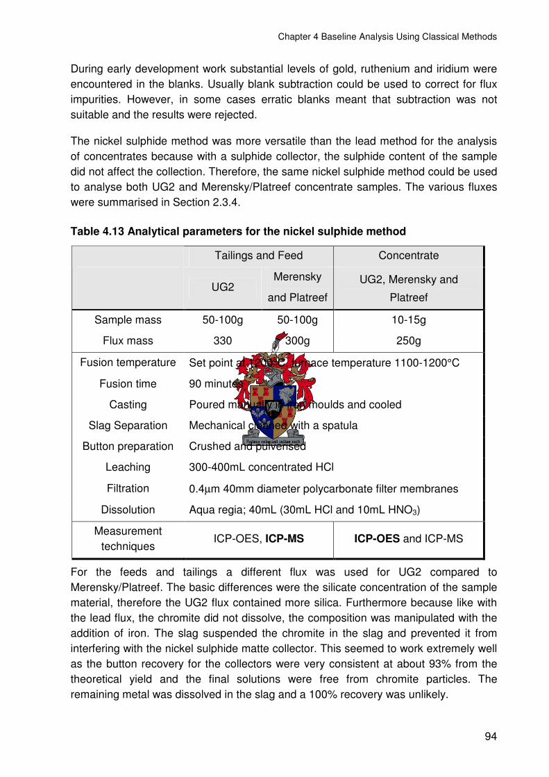
Chapter 4 Baseline Analysis Using Classical Methods
94
During early development work substantial levels of gold, ruthenium and iridium were encountered in the blanks. Usually blank subtraction could be used to correct for flux impurities. However, in some cases erratic blanks meant that subtraction was not suitable and the results were rejected.
The nickel sulphide method was more versatile than the lead method for the analysis of concentrates because with a sulphide collector, the sulphide content of the sample did not affect the collection. Therefore, the same nickel sulphide method could be used to analyse both UG2 and Merensky/Platreef concentrate samples. The various fluxes were summarised in Section 2.3.4.
Table 4.13 Analytical parameters for the nickel sulphide method
Tailings and Feed Concentrate
UG2
Merensky
and Platreef
UG2, Merensky and
Platreef
Sample mass 50-100g 50-100g 10-15g
Flux mass 330 300g 250g
Fusion temperature Set point at 1200°C, furnace temperature 1100-1200°C
Fusion time 90 minutes
Casting Poured manually in iron moulds and cooled
Slag Separation Mechanical cleaned with a spatula
Button preparation Crushed and pulverised
Leaching 300-400mL concentrated HCl
Filtration 0.4µm 40mm diameter polycarbonate filter membranes
Dissolution Aqua regia; 40mL (30mL HCl and 10mL HNO3)
Measurement techniques
ICP-OES, ICP-MS ICP-OES and ICP-MS
For the feeds and tailings a different flux was used for UG2 compared to Merensky/Platreef. The basic differences were the silicate concentration of the sample material, therefore the UG2 flux contained more silica. Furthermore because like with the lead flux, the chromite did not dissolve, the composition was manipulated with the addition of iron. The slag suspended the chromite in the slag and prevented it from interfering with the nickel sulphide matte collector. This seemed to work extremely well as the button recovery for the collectors were very consistent at about 93% from the theoretical yield and the final solutions were free from chromite particles. The remaining metal was dissolved in the slag and a 100% recovery was unlikely.
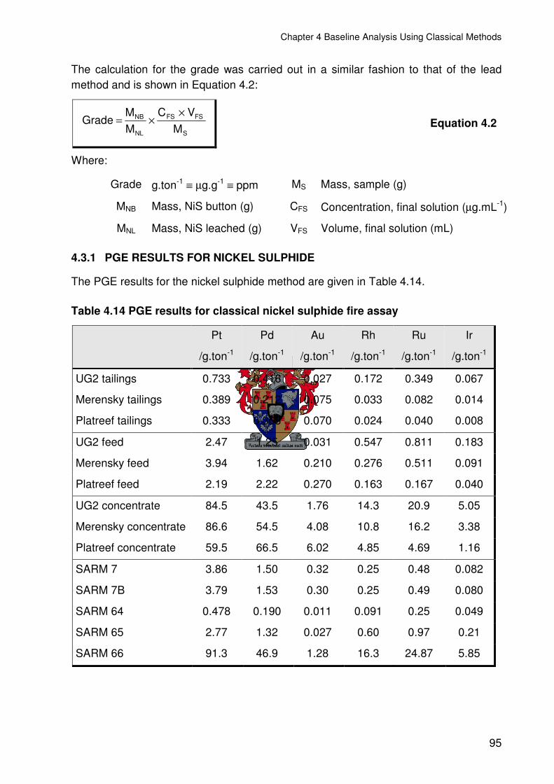
Chapter 4 Baseline Analysis Using Classical Methods
95
The calculation for the grade was carried out in a similar fashion to that of the lead method and is shown in Equation 4.2:
S
FSFS
NL
NB
MVC
MM
Grade×
×= Equation 4.2
Where:
Grade g.ton-1 ≡ µg.g-1 ≡ ppm MS Mass, sample (g)
MNB Mass, NiS button (g) CFS Concentration, final solution (µg.mL-1)
MNL Mass, NiS leached (g) VFS Volume, final solution (mL)
4.3.1 PGE RESULTS FOR NICKEL SULPHIDE
The PGE results for the nickel sulphide method are given in Table 4.14.
Table 4.14 PGE results for classical nickel sulphide fire assay
Pt
/g.ton-1
Pd
/g.ton-1
Au
/g.ton-1
Rh
/g.ton-1
Ru
/g.ton-1
Ir
/g.ton-1
UG2 tailings 0.733 0.416 0.027 0.172 0.349 0.067
Merensky tailings 0.389 0.212 0.075 0.033 0.082 0.014
Platreef tailings 0.333 0.363 0.070 0.024 0.040 0.008
UG2 feed 2.47 1.25 0.031 0.547 0.811 0.183
Merensky feed 3.94 1.62 0.210 0.276 0.511 0.091
Platreef feed 2.19 2.22 0.270 0.163 0.167 0.040
UG2 concentrate 84.5 43.5 1.76 14.3 20.9 5.05
Merensky concentrate 86.6 54.5 4.08 10.8 16.2 3.38
Platreef concentrate 59.5 66.5 6.02 4.85 4.69 1.16
SARM 7 3.86 1.50 0.32 0.25 0.48 0.082
SARM 7B 3.79 1.53 0.30 0.25 0.49 0.080
SARM 64 0.478 0.190 0.011 0.091 0.25 0.049
SARM 65 2.77 1.32 0.027 0.60 0.97 0.21
SARM 66 91.3 46.9 1.28 16.3 24.87 5.85

Chapter 4 Baseline Analysis Using Classical Methods
96
4.3.2 SLAG EXAMINATION OF THE CLASSICAL NICKEL SULPHIDE METHOD
The slags for the nickel sulphide collection were also examined by the Mineralogy Department [127, 128].
For the concentrate samples only trace quantities of nickel sulphide inclusions were found most of which were in the sub-micron range and are shown in Figure 4.2.
10 µm
A. The largest sulphide inclusion that was encountered in concentrate slag samples. The image shows the main Ni3S2 area (medium) with darker veining, possibly NiS, and the brighter Cu2S phase at the side. The dark surrounding area is slag.
10 µm
B. The only other evidence of sulphide inclusions were these submicron Ni>Cu sulphides (arrowed) that occurred across a 50 µm band in a piece of concentrate slag.
Figure 4.2 Back scattered electron images of nickel sulphide slags
Only trace occurrences of nickel sulphide inclusions were found for the feed and tailings samples, these were typically less than 20µm in size. These in general were larger than was observed for the lead collection. This was not surprising as with the lower density of the nickel sulphide matte it would take longer to settle, Section 2.3.8. With the UG2 samples the occurrence of these inclusions were even fewer. This could mean that for the silicate samples, the increase of viscosity caused more physical losses to the slag. This would make sense because the settling rate would be slower for a more viscous slag.
The slags were clean as there were no large losses of nickel sulphide to the slag. The nickel sulphide collection was considered quantitative.
The chromites within the UG2 slags were also examined, where an interesting discovery was made. It was found that unlike the comparative lead fire assay slag the

Chapter 4 Baseline Analysis Using Classical Methods
97
chromite particles were evenly distributed throughout the slag and had not settled as they had in the lead fire assay slag.
Like the lead fire assay slags, only small quantities of the chromites were dissolved and once the concentration reached saturation, the dissolved chromium was observed to crystallise as chromic oxide. The rims of the chromite grains were modified and the interior leached but most of the chromite grain remained unaltered. These are clearly shown in Figure 4.3.
A. 35x magnification of a UG2 feed slag. Take note of the even distribution of the chromite grains
B. Recrystallised chromite in the UG2 slag.
Figure 4.3 Back Scattered Electron images of chromites in the nickel sulphide slags
This microscopic examination correlated to the macroscopic properties of the slag. The UG2 fusions for the nickel sulphide method were poured smoothly without the appearance of the chromite sludge that was seen for the lead fusions. This was due to the modification of the slag composition of the UG2 fusion and proved to be successful in preventing large physical losses and collection of chromite in the collector that has been reported by Parry [99] and others [97] in the literature.

Chapter 4 Baseline Analysis Using Classical Methods
98
4.4 COMPARISON OF LEAD AND NICKEL SULPHIDE METHODS
Visually the data was examined and the averages were found to be within one standard deviation of each other. A linear regression was performed on the data and is shown in Figure 4.4. The graphical representation was the simplest way to compare the two data sets. Clearly the analytical results lay in a tight cluster about the 1:1 correlation line. The gold with the lowest concentration showed the largest deviation from the line but overall followed the trend.
Figure 4.4 Comparison of the Lead and Nickel Sulphide methods
To verify the close agreement, a paired t-test was applied to the data, for details on the paired t-test refer to Appendix C.3. The paired t-test compared the averages of the two paired data sets to determine whether or not the average of the differences for the pairs differs from zero. If one method was higher than the other there would be a consistent difference between the sample pairs. The paired t-test determined whether that difference was significant. A two-tailed test was performed to determine whether there was any significant difference irrespective of whether or not the difference was higher or lower. The results from the test are shown in Table 4.15. Overall there was
Comparison of Nickel Sulphide and Lead Methods
0.01
0.10
1.00
10.00
100.00
0.01 0.10 1.00 10.00 100.00
Lead dissolution /µµµµg.g-1
Nic
kel S
ulph
ide
/ µµ µµg.
g-1
Pt
Pd
Au
Rh
Comparison of Nickel Sulphide and Lead Methods
0.01
0.10
1.00
10.00
100.00
0.01 0.10 1.00 10.00 100.00
Lead dissolution /µµµµg.g-1
Nic
kel S
ulph
ide
/ µµ µµg.
g-1
Pt
Pd
Au
Rh

Chapter 4 Baseline Analysis Using Classical Methods
99
no significant difference between the methods. Neither of the methods showed a consistent bias on any of the elements analysed.
Table 4.15 Single tailed paired t- test for the comparison of the lead and nickel sulphide methods
Probability (P)
Pt Pd Au Rh
All data 0.25 0.24 0.22 0.06
Tailings only 0.02 0.70 0.11 0.12
Feed only 0.86 0.88 0.03 0.44
Concentrate only 0.27 0.28 0.48 0.01
Possibly the best method to check for bias was to perform a linear regression on the data for each element. The best way to fit the data was using a technique called Functional Relationship Estimation by Maximum Likelihood (FREML). This was a complicated technique and used an iterative process to solve the line between the data. The key feature was that it used a weighing scheme where data points were weighted according to their precision of analysis. This type of curve fitting was good for the comparison of two methods as it took into account the precision of the two techniques. The same line was achieved irrespective of which results were plotted on the X-axis [129]. The data that was output also had a standard error estimate for the slope and intercept. These were checked to determine whether they deviated from 1 and 0 respectively using a t-test. The t-test that was used was for the comparison with a known value and the formula can be found in Appendix C.3.
Calculations using the FREML technique were done with a Microsoft Excel add in provided by the Royal Society of Chemistry and was available from their website [130].
Conventional least squares linear fitting was limited in that one of the variables was considered “error free” (the independent variable). With normal regression analysis a different line can be obtained depending on which method was assigned as the independent variable. This could result in misinterpretation of the data.
The data were all plotted with the lead fire assay value on the X-axis so that the following relation, Equation 4.3, holds:
NiS grade = slope x Pb grade Equation 4.3
For the analysis the lines were constrained to pass through the origin as both sets of data had reliable blanks and were blank corrected.
For perfect agreement between the methods the slope calculated should be unity.

Chapter 4 Baseline Analysis Using Classical Methods
100
A summary of the regression data is given in Table 4.16.
Table 4.16 Regression data for the comparison of the lead and nickel sulphide methods
Slope Std error R2 t-test
Significant
All Elements 0.978 0.006 0.999 Yes
Pt 0.997 0.012 1.000 No
Pd 0.986 0.010 0.999 Yes
Au 0.967 0.044 0.998 No
Rh 0.958 0.010 1.000 Yes
The regression analysis was more sensitive to small changes than a paired t-test. The slope was checked to determine whether the slope deviated significantly from one.
Overall the correlation between the nickel sulphide and lead methods were good being close to unity both for the correlation co-efficient (R2) and for the slope. The lead dissolution method was on average 0-4% higher than the nickel sulphide method depending on element and grade.
The methods were similar for platinum and palladium as the slopes implied that the difference between the methods was about 1% overall.
With the two metals at lower concentration, the agreement was still good considering that many of the samples were at the low and sub ppm range. An overall difference of 4% on rhodium was predicted. Although, when looking at the data the lead method was not always higher.
There was no significant difference between the methods on gold even though the difference was around 3%.
If the results were examined critically, the feeds and tailings were measured at one time with the same calibration for the lead method using ICP-MS, the same was done for nickel sulphide some time later. A similar procedure was used for concentrates using ICP-OES. Therefore, small differences in the calibration would result in a bias.
For ICP-OES the instrument QC was required to be within ±1%. This could have still given a maximum difference of 2% even if the QC checks passed. With ICP-MS, the measurement was less imprecise, so the instrument QC was required to be within ±3%, this could give a maximum difference of 6%.

Chapter 4 Baseline Analysis Using Classical Methods
101
The differences were within these limitations of the instrumental uncertainty and the agreement was good considering the low grade.
4.4.1 COMPARISON WITH CERTIFIED REFERENCE MATERIALS
The supplier of CRMs issued a certificate of analysis that gave the preferred values and 95% confidence intervals (CI). It was often mistakenly interpreted that the analysis of the CRM should fall within the CI. If a very large set of samples was analysed, for the average, this may be true, however in practice when analysing a small number of replicates the average may not fall within the CI as there would be experimental error associated with the determination. The CI does not take into account the precision of the analytical method [131].
When the supplier gave a standard deviation and the number of determinations in the average for the values of the CRM, a significance test was performed. This test was very similar to a t-test assuming equal variance and the mathematics are covered in Appendix C.3.4. The test compared the two means and determined whether there was a significant difference based on the variance in the analysis and the variance in the assignment of the reference value. A worked example for analysis of SARM 7 by nickel sulphide is shown in Appendix C.3.4.
For values where there was no additional statistical data, another t-test was performed to determine whether the difference between the averages was greater than zero. For this t-test an average for an experimentally determined result was compared with a known/certified value. The calculation took into account only the variance of the method used to analyse the CRM and no provision was made for variance of the assigned value. The mathematical details can be found in Appendix C.3.5 with a worked example. The lead and nickel sulphide results for the CRM were combined and compared to the recommended values. The overall findings are listed in Table 4.17.
The platinum and palladium showed good correlation with the certified values and there was agreement within the limits of the precision of the analysis. Two of the QCs had significantly different values for gold. The first, SARM7B, was a result of the re-assigned values, if the comparison was made to the original analysis this would not be significant. The analysis of gold for SARM7 and 7B were identical, and therefore there was some doubt as the validity of the newly assigned value. The second was SARM 66, there was a large difference compared with the “preliminary certified values” for gold. The analysis of the nickel sulphide and lead methods closely agreed and it was likely that the “preliminary certified values” were incorrect.

Chapter 4 Baseline Analysis Using Classical Methods
102
Table 4.17 Comparison of the analysed values for the CRM to the certified values
Pt Pd Au Rh Ru Ir
SARM 7 Average /g.ton-1 3.791 1.560 0.340 0.247 0.485 0.082
Certified /g.ton-1 3.74
±0.045 1.53
±0.032 0.31
±0.015 0.24
±0.013 0.43
±0.057 0.074
±0.012
within 95% CI No Yes No Yes Yes Yes
t-test Significant? No No No No No No
SARM 7B Ave. /g.ton-1 3.771 1.503 0.331 0.249 0.487 0.080
Certified /g.ton-1 3.74
±0.045 1.53
±0.032 0.31
±0.015 0.24
±0.013 0.43
±0.057 0.074
±0.012
within 95% CI Yes No No Yes Yes Yes
t-test Significant? No No Yes No No No
SARM 64 Ave /g.ton-1 0.496 0.198 0.013 0.086 0.249 0.049
Certified /g.ton-1 0.475
±0.013 0.21
±0.015 0.018
±0.003 0.08
±0.005 0.24
±0.015 0.052
±0.005
within 95% CI No Yes No No Yes Yes
t-test Significant? No No No No No No
SARM 65 Ave /g.ton-1 2.716 1.316 0.031 0.581 0.969 0.208
Certified /g.ton-1 2.64
±0.05 1.28
±0.04 0.034
±0.005 0.522
±0.018 0.853
±0.038 0.183 ±0.01
within 95% CI No Yes Yes No No No
t-test Significant? No Not Not Yes Yes Yes
SARM 66 Ave /g.ton-1 91.32 46.90 1.28 16.33 24.87 5.85
Certified /g.ton-1 91.2 ±3.1
51.1 ±4.7
0.66 ±0.03
17.5 ±1.8
26.5 ±1.5
7.10 ±2.2
within 95% CI Yes Yes No Yes No Yes
t-test Significant? No Yes Yes No Yes Yes
With SARM 66, ruthenium was outside the limits; this is again expected to be due to the fact that these are only “preliminary certified values”.
SARM 65 was identified as a “problem sample” because there was poor agreement for the three elements; rhodium, ruthenium and iridium. The rhodium analysis was

Chapter 4 Baseline Analysis Using Classical Methods
103
confirmed for our data by the lead method. Ruthenium and iridium were only done by nickel sulphide. Our values were higher than the certified values, if this difference were to be predicted, from the problems of entrainment of the collector during the fusion for nickel sulphide it would be predicted that other laboratories that do not use a modified UG2 flux for nickel sulphide would tend to be low. Other methods using co-collectors for rhodium collection may also be biased low, Section 2.6.3.
Almost all of the analyses agreed with the certified values for the CRMs, therefore the methods were accurate and the values quoted for the QCs are also accurate.
4.4.2 ANALYTICAL PRECISION
The precision or % repeatability is defined as follows in Equation 4.4 [132]:
rs22r = x
s22r% r= ≡ 2.83 x %RSD Equation 4.4
Where:
r Repeatability
%r % repeatability (precision)
sr Standard deviation of replicate measurements
x Average
This range covers the typical analyses expected for the sample for this type of analysis. It gives a meaningful range for comparison when doing small numbers of samples during test work. Each individual analysis should fall within this range. However for simplicity the %RSD was used for comparison.
It was quite noticeable that the relative standard deviation for the tailings samples were much higher than for the concentrate samples, Table 4.18. There is a relationship between grade and analytical precision and it is described by Boyer [133]. This relation can be used to compare the precision achieved with the analysis.
%RSD = 21-0.5logC Equation 4.5
Where:
%RSD Percentage relative standard deviation
C Concentration expressed as a fraction (1ppm = 10-6)
For feed and tailings with a platinum grade at around 1ppm a %RSD of 16% is anticipated from the model, while for concentrate at 80ppm the %RSD should be 8%.

Chapter 4 Baseline Analysis Using Classical Methods
104
The overall precision should improve by a factor of 2 for the analysis of concentrate samples.
Table 4.18 %RSD calculated for the lead and nickel sulphide methods
%RSD
Pt Pd Au Rh Ru Ir
Feed +tailings 6.0 4.7 21.9 4.3 Lead method Concentrate 1.3 1.3 7.1 0.7
Feed +tailings 4.2 6.8 22.7 5.3 8.0 7.1 NiS method
Concentrate 2.7 2.1 10.0 2.8 2.6 5.8
Feed +tailings 5.1 5.7 22.3 4.8 8.0 6.9 Combined
Concentrate 2.0 1.7 8.6 1.7 2.6 5.8
The %RSD obtained for the methods was better than predicted by the Boyer model by a factor of 4. In general the elements gave similar %RSD with the exception of gold that showed considerably more variation than the others. This would be attributable to the nugget effect that has been proposed in Section 1.3.
In general there was an improvement of the precision by a factor of 2-3 (as predicted by the Boyer model) between the low grade and the high-grade samples. The analysis for gold on all samples irrespective of grade was worse than the other elements.
4.5 QC VALUES AND LIMITS
Usually with a QC sample a 95% confidence interval is calculated for the average. A 95% confidence interval is a normalised range applied to an average and is based on the number of results in the statistical population used to determine the average. The 95% CI is the range in which it is 95% certain that the true value for the analysed sample lies. The larger the number of replicates the better the statistical calculation for the standard deviation becomes and therefore the better the statistical comparison.
Important for the 95% CI is the studentised t value. These are values generated from a normal Gaussian distribution and are available in any statistics textbook. The value is higher for fewer measurements as the uncertainty is larger. For an infinite population the t value is 1.96 for a 95% CI. For more than 30 replicates, the t-value can be taken as 2. For measurements with less than 30 replicates the value of t needs to be looked up so that an accurate value can be obtained, as this will affect the 95% CI reported.
The 95% CI is calculated by multiplying the standard deviation by the value of t (2 for larger populations) and dividing this by the square root of the number of replicates (count). The t value is taken on the table for n-1 degrees of freedom.

Chapter 4 Baseline Analysis Using Classical Methods
105
ns t CI 95% ∗= Equation 4.6
Where:
t t value (from table)
s Standard deviation
n number of individual replicates
The 95% confidence limit for the averages on all the prepared QC materials were calculated and are tabulated in Table 4.19.
Table 4.19 QC values with 95% confidence limits and analytical range (in parentheses)
Pt
/g.ton-1
Pd
/g.ton-1
Au
/g.ton-1
Rh
/g.ton-1
Ru
/g.ton-1
Ir
/g.ton-1
UG2 tailings 0.770±0.022
(0.060) 0.422±0.018
(0.075) 0.022±0.006
(0.022) 0.161±0.007
(0.020) 0.349±0.032
(0.072) 0.067±0.002
(0.004)
Merensky tailings
0.408±0.015 (0.048)
0.205±0.012 (0.057)
0.069±0.008 (0.039)
0.032±0.002 (0.008)
0.082±0.019 (0.042)
0.014±0.001 (0.002)
Platreef tailings
0.349±0.017 (0.067)
0.35±0.022 (0.095)
0.064±0.005 (0.018)
0.022±0.001 (0.004)
0.04±0.009 (0.020)
0.008±0.001 (0.003)
UG2 feed 2.493±0.037
(0.24) 1.233±0.027
(0.17) 0.036±0.008
(0.018) 0.535±0.013
(0.058) 0.811±0.041
(0.092) 0.183±0.007
(0.015)
Merensky feed
3.93±0.11 (0.55)
1.628±0.036 (0.15)
0.227±0.039 (0.22)
0.278±0.006 (0.018)
0.511±0.021 (0.083)
0.086±0.005 (0.046)
Platreef feed 2.20±0.17
(0.82) 2.218±0.086
(0.34) 0.277±0.028
(0.14) 0.168±0.010
(0.039) 0.167±0.012
(0.043) 0.039±0.002
(0.008)
UG2 concentrate
84.6±1.3 (3.9)
43.90±0.73 (2.2)
1.78±0.11 (0.48)
14.63±0.44 (0.79)
20.92±0.47 (1.7)
5.05±0.18 (0.67)
Merensky concentrate
86.17±0.81 (4.0)
54.50±0.38 (2.1)
4.13±0.11 (0.65)
10.95±0.15 (0.51)
16.19±0.16 (1.0)
3.38±0.06 (0.35)
Platreef concentrate
59.16±0.92 (4.0)
66.35±0.76 (3.8)
6.06±0.23 (1.2)
5.02±0.17 (0.20)
4.69±0.12 (0.44)
1.16±0.11 (0.40)

Chapter 4 Baseline Analysis Using Classical Methods
106
In Table 4.19 there is no attempt to report any value below the 1ng.g-1 (ppb) level, otherwise 3 significant figures are shown.
What was also included in Table 4.19 was the analytical range which was based on 2.83 times the standard deviation as was discussed in Section 4.4.2. This gave the typical analytical range in which the replicate analyses lay for the classical methods. It was an important number for comparisons when doing development work where often only a few replicates were performed. If the replicates were close to the consensus value and were within the confidence interval that was great, however it was probable that when only a few replicates were analysed they were more likely to lie in the range that was characterised by the analytical method. Therefore, concern should only be raised when analysis lay outside the typical analytical range that was defined for the classical methods. This range also too the results k into account the homogeneity of the sample and sampling practice.
4.6 DISCUSSION
Once values of the QC materials were established, they could be used for the development work on automation.
The test work also performed another very valuable function in that it provided a baseline for the comparison of automated fire assay work. A summary of the classical fire assay methods is shown photographically in Figure 4.5, this is to give an idea of the equipment and methods used.
Work done in automation can be compared directly with the classical fire assay methods on the same samples. Comparisons of not only the analytical result but also other physical comparisons, for example, with slags will prove useful especially with the recognised need to improve turnaround time. This requires that the analytical method is shortened, for example, by reducing the fusion time and it will be useful to compare the two methods.
The next chapter introduces the technologies that are required for an automated process. The special requirements of equipment to be automated are discussed and how these technologies were developed. The development of suitable fluxes for automation is also discussed and comparisons to the classical method are made.

Chapter 4 Baseline Analysis Using Classical Methods
107
A. For classical fire assay batches of samples are prepared in trays of crucibles
B. Crucibles containing sample and flux are loaded into the furnace using a pneumatic fork.
C. Crucibles with the fused sample are removed from the furnace with a pair of tongs and manually cast into an iron mould, where they are cooled.
D. Once cold the slag is mechanically separated from the button and is hammered into a cube.
E. Cupels are loaded with a fork in preparation for cupellation. Once hot, the lead buttons are placed into the cupels.
F. The de-slagged buttons are loaded into hot cupels and oxidised. The lead oxide is absorbed and gives the cupel a characteristic yellow colour. The prill is removed from the base of the cupel.
Figure 4.5 Pictorial summary of classical fire assay
Crucibles A.
Flux
Fusion Furnace B.
Pneumatic Loading Fork
Iron Moulds
C.
Furnace Tongs
Cupellation Furnace
E. Hood
Loading Fork
Cupels
De-slagged buttons
Cupels Containing Lead Oxide
F.
PGE Prills
Lead Buttons
Slag
Used crucibles
D.

108
CCHHAAPPTTEERR 55
5 AUTOMATION TECHNOLOGY
Automation is not simply replacing a person with a robot. There is considerable instrumentation and machinery required to automate a process. It is always wise to start with steps or processes that have already been automated and refine the process to define high risk items that have not been automated before and that require development work. From there an automated process can be built by putting the basic automation building blocks together.
There are a number of types of automation and can vary from the simple probe to a complex automated laboratory. These are discussed below:
• On-line process analysers: These types of analysers are usually probes that are inserted into the process stream and are dedicated measuring instruments that make a measurement of the process, they are also called in-stream analysers. An example would be XRF process analysers, such as the Thermo Gamma-Metrics AnStat XRF probe [23], and gas analysers. Typical measurement intervals can be a few seconds to several minutes. Other analysers require a sample to be extracted from the process and could be treated before being analysed. Examples would be the Malvern [134] particle size analyser and the Courier 30XP XRF analyser [24]. Analysis cycle times are usually in the order of several minutes, measurements are automatically updated in the control system and real time process control is done.
• Instrument autosamplers: These came to the fore in the 1970s when GFAAS was introduced and were the first instruments to be automated. The sampler was found to improve both the precision and accuracy of the analysis. Autosamplers for ICP-OES and ICP-MS are now commonplace. Autosamplers improve productivity by releasing the operator from the mundane measurement of samples.
• Dedicated automation: These custom machines are designed for a specific task. They may have robotics, and are usually aimed at large scale sample preparation such as crushing, grinding and sub sampling. This option is usually very costly and needs to be carefully considered because should the process or plant change, the equipment may need to the drastically modified at considerable cost. The benefit is improved turnaround time for physically demanding sample preparation tasks.

Chapter 5 Automation Technology
109
• Versatile modular robotics: This is the most popular type of automation being installed. These use modular machines designed to perform preparation of one kind or another. Sample manipulation is done using a central robot that moves the sample from one step to the next. These systems are versatile because modules can be added or removed at a later stage should the process or analytical procedure change.
The basic analytical process is common to any analytical measurement whether it is in the analytical laboratory, on-line XRF analyser, wet chemical process analyser and multi-million rand automated robot laboratory. It is the methodologies as to how these steps are achieved that changes between the systems. A schematic of the analytical process is given in Figure 5.1.
Figure 5.1 The analytical process
The need for accurate and precise analytical data is obvious, but high productivity, fast sample turnaround and cost-effectiveness are equally important. Unfortunately manual sample preparation procedures limit achievement of this goal since they are:
• A major source of errors as they are subject to human variability.
• Labour intensive and therefore expensive.
• Time-consuming leading to slow sample turnaround time.
• Disconnected from the automatic flow of information.
• Expose people to hazardous environments and chemicals.
Most laboratories have more work than they have time available to do it, and important but lower priority samples may not be analysed within a reasonable period of time.
Sample Acquisition
Sample Preparation
Analytical Measurement
Data Processing Reporting
Sample Acquisition
Sample Preparation
Analytical Measurement
Data Processing Reporting
Sample Acquisition
Sample Preparation
Analytical Measurement
Data Processing Reporting

Chapter 5 Automation Technology
110
High analytical workloads have detrimental effects on quality as the sample preparation concerns expressed earlier in Chapter 3 feature prominently.
Laboratory automation, the “economic alternative to manual operation”, is therefore best justified when it strives to address sample preparation. Automated laboratories regularly feature the following benefits:
• High levels of productivity and equipment utilisation.
• Faster turnaround times.
• Improved quality of sample preparation and ultimately results.
• Significant reduction in operating costs.
• Ensured health and safety of personnel.
• Reliable documentation and data audit trails.
• Improved job satisfaction, as personnel are not used to execute boring work.
Even with these measurable benefits, the automation of an existing or new laboratory is an expensive exercise - which automation system to acquire is therefore most important. Figure 5.2 depicts the relationship between the number of samples per day, the complexity of the analysis and the domain of manual, flexible and dedicated automation.
For low sample quantities or extremely complex analysis, manual procedures are usually the best approach. Very high sample loads require dedicated equipment automation (e.g. clinical laboratories) or, when complexity increases, dedicated robot automations as found within the automobile industry (e.g. welding joints). Flexible robot automation fits between the extremes. It is primarily associated with the “automation” of the operator. Laboratories of this nature are characterised by ease of reprogramming, multiple task capability and flexibility for the future. These flexible robot automations are what was considered to be the most viable for fire assay automation due to the complexity of the analytical process.

Chapter 5 Automation Technology
111
Figure 5.2 Schematic of automation
The flexible robot automation alternative was considered due to these benefits:
• Fully automated sample preparation and analysis using industrial robots.
• Unattended, 24 hours per day operation.
• Achieve better precision and, potentially, better accuracy.
• Provide faster sample turnaround.
• Flexibility to change should new technology become available.
• Eliminate operator errors and thereby save costs.
5.1 AUTOMATION OF FIRE ASSAY FOR PROCESS CONTROL
Anglo Platinum was fortunate to be in an expansion phase with a number of sites being developed. A site being developed on the farm Maandagshoek was identified as a suitable place for a mine with a concentrator plant. The site would later develop into the Modikwa Platinum Mine.
The remote location lent itself to automation because of the lack of skilled labour in the area and there were no nearby laboratories where samples could be sent. A new laboratory had to be built and a fast turnaround laboratory on the concentrator was deemed a good solution rather than a conventional fire assay laboratory. The mine samples that required analysis did not have the same time dependence as those for process control and could be outsourced to a central analytical facility.
Dedicated equipmentautomation
Dedicated robotautomation
Sam
ples
per
day
Flexible robot automation
Manual
high
med
low
low med high
Complexity of Sample Preparation
Dedicated equipmentautomation
Dedicated robotautomation
Sam
ples
per
day
Flexible robot automation
Manual
high
med
low
low med high
Complexity of Sample Preparation
Dedicated equipmentautomation
Dedicated equipmentautomation
Dedicated robotautomation
Dedicated robotautomation
Sam
ples
per
day
Flexible robot automation
Flexible robot automation
ManualManual
high
med
low
high
med
low
low med highlow med high
Complexity of Sample Preparation

Chapter 5 Automation Technology
112
One of the biggest benefits to automating the fire assay process would be the possibility of improving turnaround time. This would have a significant effect on process control for flotation plants where long lead-time in analysis has a large cost implication. Valuable material may be lost if process refinements are not made in time. So there were two fundamental challenges to automating the fire assay process:
• How to automate the entire analytical process, particularly with regard to those steps that had not been automated before.
• Reduce analysis time.
At this point the realms of analytical science become blurred with automation engineering science. Both fields have information required by the other. Automation engineers provide information on machines, transport devices, proximity sensors etc.− the tools that make automation possible. What these engineers lack is the chemical knowledge and the analytical know-how. These two fields need to be combined with a suitable partnership.
Anglo Platinum had the chemical knowledge with fire assay experience, a little automation experience and had dealt with a number of automation vendors. IMP was new to the fire assay field and a good working relationship was established where IMP [135], the local agent for Herzog [136], could apply their specialist automation knowledge and experience. Extensive collaborative work was carried out between IMP and Anglo Platinum and it was possible to marry automation and analytical science. A joint patent for the new fire assay procedure was proposed and eventually registered by IMP [37].
The first step was to examine the existing methods of analysis. There were a number of steps that had been automated before and these included grinding, fluxing, filtration and drying, but needed to be evaluated for the application on PGE ores. With minor modification they were expected to be applied without any significant problems.
Some of the challenges to automation that were identified are:
• Sampling: most systems fail because an adequate sample cannot be delivered to the analytical process in a reliable automated fashion and usually require manual intervention.
• The fusion process: Conventional fire assay furnaces would not be suitable for automation due to the heat involved. Specialised grippers would be required and issues such as reach versus load come into play as a crucible can weigh as much as 2kg when fully laden with flux and sample.
• Cupellation: This was a problem again due to furnace design, heat and corrosive chemicals such as litharge. The process of removing a tiny prill from the cupel was especially challenging.
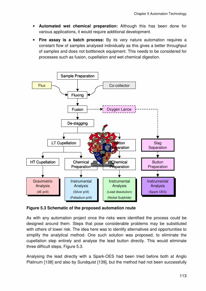
Chapter 5 Automation Technology
113
• Automated wet chemical preparation: Although this has been done for various applications, it would require additional development.
• Fire assay is a batch process: By its very nature automation requires a constant flow of samples analysed individually as this gives a better throughput of samples and does not bottleneck equipment. This needs to be considered for processes such as fusion, cupellation and wet chemical digestion.
Figure 5.3 Schematic of the proposed automation route
As with any automation project once the risks were identified the process could be designed around them. Steps that pose considerable problems may be substituted with others of lower risk. The idea here was to identify alternatives and opportunities to simplify the analytical method. One such solution was proposed, to eliminate the cupellation step entirely and analyse the lead button directly. This would eliminate three difficult steps, Figure 5.3.
Analysing the lead directly with a Spark-OES had been tried before both at Anglo Platinum [138] and also by Sundquist [139], but the method had not been successfully
Co-collector
Sample Preparation
Fluxing
Flux
Fusion
De-slagging
Button Preparation
LT Cupellation
Chemical Preparation
HT Cupellation Chemical Preparation
Instrumental Analysis
(Lead dissolution)
(Nickel Sulphide)
Instrumental Analysis
(Lead dissolution)
(Nickel Sulphide)
Instrumental Analysis
(Silver prill)
(Palladium prill)
Instrumental Analysis
(Silver prill)
(Palladium prill)
Gravimetric Analysis(4E prill)
Gravimetric Analysis(4E prill)
Instrumental Analysis
(Spark OES)
Instrumental Analysis
(Spark OES)
Button Preparation
Oxygen Lance
Slag Separation

Chapter 5 Automation Technology
114
implemented. This was deemed high risk, as a new analytical method including calibration would have to be developed. The entire topic on this analytical method is outlined in Chapter 6.
To make the spark analysis of the lead button a possibility requires the slag to be separated from the lead and quenched in some sort of mould. Although the separation of the lead and slag had not been automated, a number of techniques were available and the spark analysis route was a serious contender. The risk was associated with the automation of a manual slag separator system that would take considerable development work.
In her work, Sundquist concluded the analysis of platinum, palladium and rhodium could not be reliably performed using the Spark Analysis For Traces (SAFT) technique. This was due to changes in the matrix from the type of sample and variations in the fire assay process. To improve the method she recommended that other fusion methods be investigated to reduce the uptake of base metals in the lead collector and secondly to automate the fusion process to provide better control.
Some of the other limitations in the work by Sundquist were:
• Lack of reliable calibration standards, the lead could not be analysed directly and standards were prepared from samples analysed by nickel sulphide.
• Poor slag removal contributed to the matrix problems.
The possibility of cleaning the matrix of the lead collector was also identified as a requirement to reduce the problems associated with the direct analysis of the lead button using Spark-OES. For this purpose an oxygen lance was proposed to remove nickel, again this was a high risk item, as it had never been used for fire assay before.
5.2 EXISTING AUTOMATION TECHNOLOGIES
The existing automation technologies were tested for compatibility for PGE ores at various sites. Some of the technologies were already being used at Anglo Platinum and were assessed for future improvements.
5.2.1 SAMPLING
Sampling of slurry streams at Anglo Platinum concentrators were done using a cross-stream cutter. These cross-stream cutters were used to sample the flowing stream across a launder at appropriate sites in the concentrator plant. From the cutter the sampled stream was then sub-sampled using an intermediate hopper and rotating vezin sampler. These samplers were not reliable and would often be choked. The intermediate hopper holds the stream and drains slowly with the rotating vezin taking enough cuts to ensure a representative sample.

Chapter 5 Automation Technology
115
These often did not work well with too few cuts being taken. Each site had their own specification and samplers were all custom built. These samplers had no communication or control electronics other than a simple timer and were not suitable for automation.
The Thermo Gamma-Metrics Sampling Stations (SamStats) were investigated and found to meet sampling requirements for slurry streams [140], even for “bimodal” streams as found in UG2 plants. These were first installed at Lebowa Platinum on their UG2 concentrator and operated successfully [141]. The SamStats were initially designed to sub-sample slurry streams to be analysed by an XRF probe and in these cases were called AnStats (Analytical Station).
The sampler was a stationary riffler that cut the moving slurry stream. The moving slurry was forced under a baffle plate and emerged as a highly turbulent stream that then passed through a stationary set of cutters. The slurry sample stream could then be reduced further with more similar sampling stages. The samplers could be designed to permit full flow of stream (up to 70 m3.hr-1 for a tank 600mm wide). The tanks, agitators and riffler blades of the SamStats were all either plastic or rubberised to reduce abrasion.
For the final stage of sampling, a cross-stream cutter was used to take the analytical sample. The sample at this stage was mixed with an impeller prior to the cut being taken.
The sampler needed to be interfaced to the laboratory sample preparation system that could give signals to it. It was important that the laboratory could control the sampler and sampling interval to ensure that the correct quantity of slurry was delivered to the laboratory.
These sampling requirements meant that the SamStats had to be located in a group above the laboratory and the sample gravity fed to the filter unit. The design of the concentrator plant was centred around the laboratory. This was a new concept in design as sampling and analysis was usually considered after the plant was built.
The sample delivery to the process control laboratory (PCL) also had to be controlled by the software. Multiplexers were required with a sample flopper to deviate the stream to waste during periods where no sample was being taken. The multiplexers were also to be equipped with screens to remove contaminants such as plastic, wire and wood chips from the sample stream as these could cause blockages in the piping. The sample from the sampler was stored in an intermediate holding tank below the multiplexer. Once there was sufficient sample after a prescribed sampling period the sample was to be released to the filter unit in the laboratory.

Chapter 5 Automation Technology
116
This sophisticated sampling system was required to ensure that the correct sample size was delivered to the laboratory. The holding tanks were to be fitted with level indicators so that the cutting rate of the sampler could be adjusted to deliver 1L of sample to the laboratory after 2 hours. With the high density of chromite, the slurry had to be constantly agitated to ensure that a representative sample was taken.
5.2.2 FILTRATION
The automation of filtration was achieved by IMP and Herzog and was implemented at a phosphate producer Foskor in Palaborwa [142].
The system used a filter press to remove water from the sample and had a rotating cup design. The perforated base of the cup was detachable and held the filter cloth. The upper section comprised of two metal plates on either side of a rubber tube. The tubing could be expanded or compressed by applying either air pressure or a vacuum to close or open the filter cup, respectively.
The filter press opened and rotated to an angle of 45° to receive a sample. It then moved back to an upright position and was closed for filtering. Air pressure was applied by a bellows to the filter press and the water was forced out through the base. A schematic of the filter operation is shown in Figure 5.4.
Figure 5.4 Operation of the Herzog automated filter press
After filtering the cup was opened and inverted. The press was re-sealed and the sample filter cake was dislodged with air pressure into a bowl. The filter was then automatically cleaned with water prior to the next cycle.
Vacuum
Filter cup
Filter cloth
Slurry
Cake
Inflatabletube
Air
Rotate
Vacuum
Filter cup
Filter cloth
Slurry
Cake
Inflatabletube
Air
Rotate
VacuumVacuum
Filter cup
Filter cloth
Slurry
Cake
Inflatabletube
Filter cup
Filter cloth
Slurry
Cake
Inflatabletube
Air
Rotate
Air
Rotate
Vacuum
Filter cup
Filter cloth
Slurry
Cake
Inflatabletube
Air
Rotate
Vacuum
Filter cup
Filter cloth
Slurry
Cake
Inflatabletube
Air
Rotate
VacuumVacuum
Filter cup
Filter cloth
Slurry
Cake
Inflatabletube
Filter cup
Filter cloth
Slurry
Cake
Inflatabletube
Air
Rotate
Air
Rotate

Chapter 5 Automation Technology
117
It was found that the standard cloth size of 100µm was not suitable as there was loss of fines. A 10µm filter cloth was used on top of the coarse 100µm cloth. With the 10µm cloth and the use of a flocculent as a filtration aid, clear filtrates without the loss of fines were obtained.
Filter times of 5-300s were found and were dependent on the fineness of the material and the mass of sample, without flocculent filter times of up to 15 minutes were required. Small quantities of flocculent were required and only 5mL of a 1g.L-1 solution of Magnafloc 341, a polyacrilamide flocculent, was need. For this reason, the filter system required a flocculent dosing system. The filter cakes produced by the system contained 3-22% moisture after filtration and were solid masses suitable for further drying.
It was concluded that the automated filter press system could be optimised to work with PGE ore types.
5.2.3 DRYING
There are a number of ways that a filter cake can be dried and these include conventional drying ovens, infrared heaters, vacuum ovens and microwaves. For process control purposes the drying time needed to be as short as possible. With this in mind conventional drying in an oven typically took between 60-120 minutes and was not always reliable, as PGE ore filter cakes tended to form a crust that prevented diffusion of moisture from the centre of the cake. Infrared drying had similar problems. An alternative was to use microwave drying. This had not been applied to PGE ores and required testing. This test work was performed on equipment at Foskor.
The Herzog system used an industrial microwave with a power output of 1.2 kW at 2,450 MHz supplied by Puschner [143]. The microwave used custom-made PTFE (polytetrafluoroethylene) sample bowls for drying. The microwave had a centrally located sample pedestal that was mounted on a load cell. The mass of the sample was monitored during drying and it was possible to dry to a constant mass. This was important functionality for automation as the sample material was dried for the shortest possible time, an important factor for fast turnaround.
Water was added to dry samples and these were dried in the microwave. The microwave was found to efficiently dry samples in 5-9 minutes with a mass range from 100-400g and moisture contents from 5-20%. Residual moisture after drying was found to be less than 0.1% and was comparable to conventional oven drying methods. Some problems with the PTFE bowls were experienced as many were melted or damaged where the microwaves had heated metal wire contaminants from the sample stream and this posed a fire risk. The heat of the sample material also deformed the shape of the bowl. Since the bowl remained cool compared to the sample, moisture was found to condense on the upper walls.
Chapter 5 Automation Technology
118
Test work on filter cakes produced by the filter press revealed problems with the fast drying of the cake. The moisture was found to rapidly volatilise causing the cake to burst and caused physical loss of the sample.
Another problem was that the PGE ore and concentrate samples coupled with the microwaves and heated up. Some of the samples began to fuse in localised hotspots on the sample surface. Mineralogical analyses of these samples showed that some of the sulphide minerals in the Merensky concentrate had melted and recrystallised, bonding the silicates together. In a UG2 feed sample the silicate minerals had melted bonding the chromites with a slag-like glass [144]. Fortunately chemical analysis of the fused materials showed that there was no significant change in the sulphur and PGE content of the samples.
Some recommendations were made to improve the drying technique to be incorporated for the drying of PGE flotation products:
• The filter cake needed to be broken up prior to drying.
• The microwaves be diffused and spread out over the sample either by using a multiple beam, an additional mode stirrer or rotating the sample.
• Temperature measurement and control with the use of an optical pyrometer within the microwave oven chamber.
• The PTFE bowls should be replaced with glass.
It was concluded that microwaves could be applied to the drying of PGE ores and concentrate.
5.2.4 GRINDING
The dry filter cake material produced by the microwave oven was found to be extremely hard. A normal paddle mixer had been used in the Foskor system to break up the cake for transportation to the robot circle. This was not suitable for PGE ores and concentrate and a more robust system would be required.
For this purpose a cone/mortar crusher device was proposed. Such a device had been developed for the Potgietersrus laboratory by Dickie and Stockler [145] for crushing hard concentrate filter cakes. The mortar crusher used a rotating cone to break the cake that fell into a cup below. The mortar crusher was able to quickly reduce a hard, coarse cake into a loose powder with a few agglomerates of less than 5mm in diameter.
Herzog manufactured a range of vibratory mills for grinding. These were automated versions of the manual swing mill discussed in the preparation of the QC material,

Chapter 5 Automation Technology
119
Section 3.4.2. Some of these automated mills had already been successfully installed at Anglo Platinum’s first Robolab at the ACP [146].
The problem was that standard mills on offer by Herzog had small capacity of less than 500g. Some of the predicted sample masses were in excess of 1kg and the sample material would have had to be split, milled in batches, recombined and blended prior to further preparation. This would have required more equipment, cost more and taken longer. There were other suppliers in the market with large capacity puck mills such as the LM2 mills [147] that were in operation at the PF Retief laboratory and had a 1.8kg capacity.
Herzog/IMP undertook the development of a large 1.5L capacity mill.
5.2.5 FLUXING
Fluxing required the weighing of sample material and flux followed by mixing and dosing of the mixture into a crucible. A fluxing machine had been developed by Herzog for Newmont Gold [148] in the United States and with several years of operation was considered reliable. The basic difference was that the flux was not weighed, and it was not in the configuration required. A modified machine had to be designed and built for Anglo Platinum.
The proposed equipment made use of a screw feeder to dose flux to a minimum mass. Samples were to be dosed with a vibratory hopper using a slider system to dispense volumetric cuts. The samples were then to be weighed. The flux and sample mixed and finally the mixture dispensed into a hot crucible prior to fusion.
Unfortunately there were no locally available examples of these machines to test. The first time they were examined was during the factory acceptance tests of the equipment and were extensively modified for the Modikwa plant. A new design is now available that addressed some of the problems with the choking of hoppers and sample dosing systems.
The fluxing of samples could be reliably achieved with the Herzog technology.

Chapter 5 Automation Technology
120
5.3 FUSION TECHNOLOGY AND DEVELOPMENT
The steps that were not previously automated were piloted at IMP and test work for Anglo Platinum was carried out on these prototypes. Wherever possible input was provided to IMP on the design and materials of manufacture relating to fire assay theory – this offered a good balance between theory, design and engineering. These included the fusion process, slag separation and oxygen lance technology.
5.3.1 FUSION USING INDUCTIVE HEATING
Early development work with fire assay involved the investigation of induction heating. In this application a graphite crucible was used to perform the fusion. With an induction generator it was possible to heat the crucible and perform a conventional fire assay fusion. This fire assay innovation was pioneered by Mr. Willie Brits, a former chief chemist at Anglo Platinum’s Potgietersrus laboratory, who later patented the process [149]. Considerable development work was done in conjunction with Mr. Brits [150].
There were two basic designs for induction furnaces [151]:
• Ajax-Wyatt (cored type)
• Leeds-Northrup furnace (uncored type)
The induction heating for fire assay applications was best performed with the second type of furnace. In that design the crucible was located inside a water-cooled induction coil. Eddy currents were induced in the conductive crucible to heat it. Essentially the inductive heating was a special form of resistive heating.
The heat generated in the conductor is proportional to its resistance and to the square of the current induced. This is given in Equation 5.1
c212
22 RRP Ι=Ι= Equation 5.1
The currents 1Ι and 2Ι are the currents in the primary and secondary circuits. Similarly
the R2 is the resistance in the secondary circuit and Rc is the effective coupled resistance the load causes in the primary circuit. With some mathematical manipulation, Equation 5.2 is derived.

Chapter 5 Automation Technology
121
( )ρµΙπ= flnr4P 20
21
2 Equation 5.2
Where:
P Power (W) µ Effective permeability of charge (Ω.cm.Hz-1)
r0 Radius of cylindrical charge (cm) n Turns of coil per cm (cm-1)
f Supply frequency (Hz) l Length of charge (cm)
ρ Resistivity of charge (Ω.cm-1×10⁻⁹) Ι Current (A)
The basic formula and its derivation are not important but the concepts denoted by it are. The induction of a current in the charge/conductor is dependent on the geometry and the material of the charge. It also depends on the geometry of the induction coil itself.
About 90% of the heat is generated within a thin layer on the surface of the conductor, the rest of the charge is heated by conduction. The depth at which the heat is generated is dependent on the frequency used, the higher the frequency the thinner the layer. Also the layer will be thinner for ferromagnetic materials that have a high effective permeability and thick for non-magnetic materials. The induction depth is also dependent on the resistivity. Resistivity changes with temperature and typically for a conductor like iron, the resistivity will increase with temperature and hence the inductive depth will increase. An induction furnace must be built for a specific purpose with regard to size, geometry and the type of load that will be used.
The first trials with an induction furnace, a high frequency generator operated at 6.5kHz with a maximum power output of 10kW was used. It had a cylindrical induction coil 15cm tall, 15cm in diameter with 6 turns. The coil was encased within a ceramic insulator to protect it from mechanical wear. During operation the coil was cooled with continuously flowing water at about 5-10L per minute supplied with an evaporative cooler.
The induction furnace was used to heat a conductive graphite crucible. The crucible then provided heat for a fire assay fusion.
The initial test work involved a conventional fire assay flux without a reductant, and the pot provided the carbon necessary to reduce the litharge. Due to the fact that there was only one crucible, the test work was performed with a preheated crucible. The crucible was simply loaded with the charge from the top in situ. The loose flux mixture was either poured into the pot or alternatively introduced inside a thin polyethylene plastic bag.

Chapter 5 Automation Technology
122
The fusion was visually inspected from above and the fusion took between 15 to 25 minutes to get to a quiescent state. This initial observation agreed with the time line that was shown in Section 2.4 where the first 20-30 minutes of a standard fire assay fusion was required to get the crucible and charge up to the fusion temperature. Therefore, by using a pre-heated crucible the fusion time could be considerably reduced.
Once the fusion was complete, the carbon pot was raised with a lever system and removed with a pair of tongs. The melt was poured into a conventional iron mould. The slag was manually removed and the buttons were analysed using cupellation or lead dissolution methods.
Some of the key findings in this early work were:
• The addition of the charge to a preheated crucible could reduce the fusion time by a half or more with a standard fire assay flux.
• Removing the crucible from the top reduced heat exposure of the operator.
• There was a small amount of spitting and physical loss of the charge.
• Degradation of the carbon crucible caused graphite particles in the slag with subsequent losses of lead collector droplets due to entrainment.
• Results were reasonably accurate and precise and the method showed promise.
Further development of the induction heating method involved more sophisticated and dedicated fusion machines. The initial prototype was a mechanical piston type machine that simply loaded and unloaded the induction furnace.
The machine used a conventional induction generator at 13kHz with a maximum power output of 10kW. There was a similar coil construction to what was used in the manual operation. The coil was in a fixed position approximately 1.2m from the ground.
The mechanical system operated with a crankshaft that was used to raise and lower the carbon pot. The entire assembly was rotated for loading and pouring of the melt. A ceramic sheath was cast around the carbon pot. This had a dual function, firstly to protect the outside of the pot from oxidation in air and secondly to give the pot better mechanical resistance. The instrument poured into a standard cast iron mould.
The second generation of induction machines were manufactured locally by a company Hiprom [152] under licence from Mr. Brits. The basic principle remained the same but the entire fusion head with the crucible was turned to cast the melt. A diagram of the second induction furnace melting head is given in Figure 5.5.

Chapter 5 Automation Technology
123
For automation purposes the flux was put into a plastic “pop-top” container where the sample could be weighed into the flux and the container sealed. The container could then be placed directly into the melting head. The problem was that the plastic produced residual carbon after combustion. This caused entrainment problems of the lead collector in the slag. Changes to the plastic by using calcium carbonate as a filler, proved ineffective in controlling the carbon particles in the slag.
A significant development was the use of a secondary slag separator. This volumetric separator worked reasonably well and is discussed a little later in Section 5.4.2. This first machine was purchased by Anglo Platinum and tested extensively. There were some significant flux developments and again these will be discussed separately Section 5.5.
Yet the technology turned out to be premature. The materials of design and engineering were inadequate. The machine could not be reliably operated for long enough periods to evaluate it properly. Many of the failures were associated with the furnace on the slag separator.
Figure 5.5 Second generation induction furnace
The induction furnace concept was licensed to Spectro Analytical Instruments who developed the third generation machine called the Immafuse [153].
The volumetric slag separator was incorporated within the fusion head. The melting pot design was improved and boron nitride inserts were placed into the carbon pot for better chemical resistance.
Sample container
Suction cup and loading arm
Furnace retainer lid
Carbon pot
Induction coil
Insulation
Thermocouple
Furnace lid
Scraper
Lid arm (pneumatic system)
Sample container
Suction cup and loading arm
Furnace retainer lid
Carbon pot
Induction coil
Insulation
Thermocouple
Furnace lid
Scraper
Lid arm (pneumatic system)
Sample container
Suction cup and loading arm
Furnace retainer lid
Carbon pot
Induction coil
Insulation
Thermocouple
Furnace lid
Scraper
Lid arm (pneumatic system)
Sample container
Suction cup and loading arm
Furnace retainer lid
Carbon pot
Induction coil
Insulation
Thermocouple
Furnace lid
Scraper
Lid arm (pneumatic system)
Sample container
Suction cup and loading arm
Furnace retainer lid
Carbon pot
Induction coil
Insulation
Thermocouple
Furnace lid
Scraper
Lid arm (pneumatic system)
Sample container
Suction cup and loading arm
Furnace retainer lid
Carbon pot
Induction coil
Insulation
Thermocouple
Furnace lid
Scraper
Lid arm (pneumatic system)

Chapter 5 Automation Technology
124
Some concerns were raised as it was predicted that boron nitride would be ineffective, as it would be dissolved by action of the flux, see Table 5.1.
Table 5.1 Thermodynamic data for the decomposition of boron nitride
∆G1200°C
/kJ Log K
2BN + 2.5O2(g) → B2O3(l) + 2NO(g)↑ -531.2 18.8
2B2O3 + 2NaOH → Na2B4O7 + H2O(g) -216.7 7.7
Nevertheless the machine was built and was superior to any of the predecessors. A solid state RF generator was used that was silent in operation. The engineering was much more sturdy and robust, but the basic concepts were much the same as the previous instrument. The core technology was the melting head design. The melting head was high tech but also extremely costly with prices being quoted at US$1,000 with a “guaranteed” 100 fusion/separations with their patented flux.
The system was tested at the Spectro premises in South Africa [154, 155]. This new design melting head was a little bit more effective than the simple carbon pot but the action of the flux dissolved away the boron nitride (as predicted) causing premature failure of the crucible.
The fusions were tested and the analyses were lower than the recommended values on QC samples. There was considerable cross-contamination from one sample to the next and was particularly noticeable for concentrate samples on tailings. Only 25 fusions were achieved with a single crucible. Mineralogical examination of the slags revealed that the fusion was not complete even though the fusion had been lengthened to 7 minutes from a recommended setting of 2 minutes. The slag also contained considerable quantities of lead droplets [156]. These were responsible for the low results and contamination. They are shown in Figure 5.6.
The work on the induction furnace was discontinued because the technology was considered inadequate. It is estimated that another few years of development with an experienced automation vendor will be required to develop induction furnace technology to a saleable product for fire assay.
In conclusion the findings with the induction furnace were:
• A fusion system cannot be developed without a suitable fluxing regime, as the two are inter-related.
• Radically new technology took considerable development time.
• The experience of a knowledgeable automation vendor was essential for the successful application of new technology to automation.

Chapter 5 Automation Technology
125
The induction furnace was the first foray into the automation of fire assay and is credited as the catalyst that encouraged other developers to seriously consider the possibility of automating fire assay.
A. Undissolved chromite (Chr) and tiny bright lead inclusions surrounded by slag in the Merensky tailings slag.
B. Dark areas of sodium oxide or borate are inter-grown with the more normal brighter slag from the fusion of a Merensky feed. The tiny bright specks are lead. This indicates incomplete fusion.
C. A slag inhomogeneity in slag sample from a Merensky concentrate fusion. The bright area contains swarms of tiny lead inclusions.
D. Reaction rims are visible around chromite and swarms of tiny lead inclusions are present. This is a slag from the fusion of a UG2 feed sample.
Figure 5.6 Back Scattered Electron images of induction furnace lead fire assay slags
10 µm500 µm
100 µm
Chr
50 µm

Chapter 5 Automation Technology
126
5.3.2 FUSION WITH RESISTIVELY HEATED FURNACES
The key problem with the fusion in a conventional furnace was the heat and reach issues involved. A normal furnace had doors that open from the front through which crucibles were loaded and removed. In manual preparation the operator was exposed to considerable heat and needed protective equipment and long tongs to manipulate the crucible. Even though the doors could be automated it was not desirable to expose the robot to the heat of the furnace due to its sensitive electronic components.
One method to reduce the exposure was to load the furnace from the top as was done in the original induction furnace. An alternative was to load and unload the furnace from below. Once the crucible was removed from the furnace it could be manipulated more easily without exposure to heat from the furnace itself.
Electrical furnaces are resistively heated using high resistance elements. The heat generated in the furnace is given by Equation 5.3 [151]:
RtE 2Ι= Equation 5.3
Where:
E Energy (J) R Resistance (Ω)
Ι Current (A) t Time (s)
The heat from the elements emitted by radiation and assuming a “black body” i.e. a perfect radiator is given by Stefan’s law, Equation 5.4:
H = σT4 Equation 5.4
Where:
H Heat radiated (J.m-2.s-1)
T Surface temperature of the black body (K)
σ Constant (5.73x10⁻⁸J.m-2.s-1.K-4)

Chapter 5 Automation Technology
127
For the elements to radiatively heat the furnace Equation 5.5 must hold:
( )442FE TTAR −σ=Ι Equation 5.5
Where:
Ι Current (A) TF Furnace temperature (K)
R Resistance (Ω) TE Element temperature (K)
A Effective radiating area (m2) σ Constant (5.73x10⁻⁸J.m-2.s-1.K-4)
The derivation of the above equations are not important but the concepts provided are. The first requirement of a heating element is that its resistance should be high so that the current provided need not be too high. The maximum operating temperature of the element will determine the temperature that the furnace attains. At equilibrium the heat lost by the furnace will be proportional to ( )4
F4E TTA −σ where TF will be the operating
temperature for the furnace.
The operating temperature of the elements must be sufficiently high enough to compensate for heat losses of the furnace and will be above the operating temperature of the furnace. This should be considered in the design of the furnace. With the coiled wire elements part of the heat is absorbed. The elements run at a higher temperature and consequently less power is consumed. While the furnace attains temperature the power drawn is constant and the temperature of the element rises along with the furnace temperature.
The first prototype furnace was built by the South African furnace company Ultrafurn [157]. The furnace was a basic rectangular steel structure with insulating bricks. A drawing of the furnace concept is shown in Figure 5.7.
The top of the furnace was hinged and could be opened for maintenance. In the base of the furnace there were five holes. The furnace was mounted on a steel frame with five pneumatic cylinders mounted directly below the holes. On top of the piston was mounted a pedestal with ceramic insulation rings. The rings protected the pedestal and piston from the heat in the furnace. The furnace was arranged in a straight line and the name FIFA (Fast In-line Fire Assay) was coined.
The elements for fire assay furnaces also need to have oxidation resistance. For this application the most suitable elements were Kanthal (nickel chromium), super Kanthal (molybdenum silicide) and silicon carbide. In the prototype, Kanthal wire elements were located on the sidewall. Normal resistive wire elements were chosen, as the furnace was small and well contained. These elements were cheaper and easy to maintain compared to the silicon carbide glowbars used in conventional fusion

Chapter 5 Automation Technology
128
furnaces. The power supply for the Kanthal wire elements was simpler than for silicon carbide glow bars, as the latter required a step transformer.
Figure 5.7 Schematic of the FIFA furnace design
The FIFA design was compact and efficient with controllable airflow around each crucible. Every position in the FIFA furnace was equally heated as the crucibles were equidistant from the heating elements. With slag containment rings and accurate positioning, the fusions in the FIFA system gave more reproducible fusion conditions. The elements were located within 10cm from the crucible and were heated by radiant heat from the elements. An added advantage of the FIFA was that it was made with standard well-understood technologies and used standard, freely available crucibles. This fusion system was much cheaper than the inductive heating used for the Immafuse.
Testing of normal fusions was carried out with the FIFA furnace that used conventional fire assay crucibles and fluxes. There were no problems with the automation of the FIFA furnace and this was carried out with a small, articulated laboratory robot, CRS F3 [158], to test the concept. Once this was proven the automation of the fire assay fusion became a low risk item.
Chimney
Off gas
Containment ring
CrucibleInsulation
Insulation rings
Pedestal with alumina supportAir
Pneumatic piston
Chimney
Off gas
Containment ring
CrucibleInsulation
Insulation rings
Pedestal with alumina supportAir
Pneumatic piston
Chimney
Off gas
Containment ring
CrucibleInsulation
Insulation rings
Pedestal with alumina supportAir
Pneumatic piston
Chimney
Off gas
Containment ring
CrucibleInsulation
Insulation rings
Pedestal with alumina supportAir
Pneumatic piston

Chapter 5 Automation Technology
129
5.3.3 FUSION CRUCIBLES
While it may be easy to say that a “standard” fire assay fusion crucible was used, there were some important criteria for the selection of an appropriate supplier. The first thing that came to mind was the shape of the crucible. Since the central robot needed to handle the crucible with its gripper, the size and shape of the crucible needed to be consistent. Problems were experienced with conventional crucibles as they were found to be oval and varied in dimension.
Figure 5.8 Comparison of crucible designs
The “Robolab crucible” in Figure 5.8 was developed in conjunction with Terra Nova Ceramics [159]. The crucible was specifically designed to be more stable in the furnace and prevent pot turnovers – a common problem with conventional crucibles. The crucible had a broader base and the blunt shape gave the crucible a larger volume. The molten charge remained in the bottom half of the crucible. The low centre of gravity was important during the early part of the fusion where the charge boiled vigorously and rose in the crucible. The crucible could become top heavy and topple over.
The crucible casing was improved with time to give a more consistent shape – not an easy task for clay materials as they contracted when they were fired. Consistency in these disposable ceramic components was essential for successful automation. Considerable collaboration between the manufacturer and the automation vendor was needed to fulfil the requirements for automation.
Robolab crucible
Conventional crucible
Slag volume
level
Robolab crucible
Conventional crucible
Slag volume
level
Robolab crucible
Conventional crucible
Slag volume
level
Robolab crucible
Conventional crucible
Slag volume
level

Chapter 5 Automation Technology
130
5.4 SLAG SEPARATION TECHNOLOGY AND DEVELOPMENT
To make a fire assay method totally automated required a method of automatically separating the lead collector and slag. Particularly for spark analysis the lead button produced needed to be completely slag free and rapidly cooled during casting to ensure homogeneity.
5.4.1 DECANTING
The first slag separation was performed manually. The operator would carefully pour the slag out of the crucible. Once the slag had drained, the lead left in the base could be rapidly poured into a mould. This was fairly successful but had some serious flaws:
• The method was operator dependent and not easily automated.
• The lead collector rapidly oxidised once the slag was removed.
• Residual slag always remained in the crucible and sometimes reported with the lead.
5.4.2 VOLUMETRIC SLAG SEPARATION
The volumetric separator was a more controlled form of decanting. With the higher density of lead it settled and displaced slag. It was possible, if the volume of lead was known, to pour the melt across a receptacle that would fill with the lead while the slag was decanted away. By inverting the receptacle the lead could then be drained and selectively cast. The first volumetric slag separator was manufactured by Hiprom in the prototype Immafuse machine discussed earlier in Section 5.3.1. The operation of this slag separator is shown Figure 5.9.
Some of the issues with slag separation using this method were that the separator needed to be heated to retain the fluidity of the slag so that it could be decanted. So the separator needed to be contained in a furnace of some sort and rotated. This was extremely difficult as the elements in the furnace embrittled and broke easily when the furnace was moved. The slag was corrosive and highly conductive, this caused numerous separator failures. The separator needed to be replaced regularly.

Chapter 5 Automation Technology
131
Figure 5.9 Operation of the volumetric slag separator
This slag separator was combined with the melting head for the first production Immafuse induction fusion machine. This was a novel idea as it eliminated the requirement of two separate devices and is shown in Figure 5.10.
Figure 5.10 Melting head and separator combination
Fusion Slag removal Lead casting
Slag
Lead
Lead
Fusion Slag removal Lead casting
Slag
Lead
Lead
Fusion Slag removal Lead casting
Slag
Lead
Lead
Fusion Slag removal Lead casting
Slag
Lead
Lead
Fusion Slag removal Lead casting
Slag
Lead
Lead
Fusion Slag removal Lead casting
Slag
Lead
Lead
Stainless steel casing
Resistive heating elements
Cast ceramic
Thermocouple
Ceramic lid and separator pot
Slag
Lead
Chilled mould with ejector
Stainless steel casing
Resistive heating elements
Cast ceramic
Thermocouple
Ceramic lid and separator pot
Slag
Lead
Chilled mould with ejector
Stainless steel casing
Resistive heating elements
Cast ceramic
Thermocouple
Ceramic lid and separator pot
Slag
Lead
Chilled mould with ejector
Stainless steel casing
Resistive heating elements
Cast ceramic
Thermocouple
Ceramic lid and separator pot
Slag
Lead
Chilled mould with ejector

Chapter 5 Automation Technology
132
The disadvantages of the volumetric separator were similar to manual decanting:
• The lead collector rapidly oxidised once the slag was removed.
• The molten lead oxide that formed was highly reactive and corrosive causing the separator to deteriorate rapidly.
• Lead losses were common as the lead was highly fluid and easily spilled, especially if the separator was moved too quickly.
• Residual slag always remained in the crucible and sometimes reported with the lead. This effect worsened as the separator deteriorated.
5.4.3 COWAN SEPARATOR
The Cowan Separator was developed by Mr. George Cowan in collaboration with Anglo Platinum in the early stages and then later with IMP.
The original idea that was proposed to Mr. Cowan was a method to flatten lead buttons into strips that would be suitable for digestion using the lead dissolution technique. Initial efforts involved the flattening of lead with a hydraulic press, though this required mechanical flattening first. Later the re-melting and centrifugal casting of the lead was investigated. This did not work too well as it resulted in lead leaks but what was significant was the separation of the lead from the slag during casting.
The Cowan separator was born by drilling a hole into the base of a standard cast iron mould and casting the lead into the mould directly. The lead was able to exit through the hole before the slag, but with a cold mould the lead had a tendency to freeze. This required the separator to be heated and a cast iron mould no longer became feasible and a ceramic cone was used as shown in Figure 5.11.
The cone separator made use of the difference in density between the slag and lead. The lead sank to the base of the cone displacing the slag above it and rapidly drained through the hole. Once the lead passed through, the slag with its higher viscosity would slowly move through the hole. With its lower surface tension compared to the slag it wetted the cone and collected along the base. By adjusting the diameter of the hole in the base, the rate at which the slag drained could be controlled. The optimum hole diameter was between 0.8-1.2mm as this allowed a 3-5s delay for the slag to drain after the lead. This was sufficient time to remove the mould before it was contaminated with slag.
The original design was entirely manually operated and the cones were loaded in the furnace during the fusion. Prior to the casting the cone was removed and placed in a holder above the mould. The cone was allowed to cool slightly to a dull orange colour and the melt was then cast and the cone moved away from the mould once the lead had passed through. The operation was slow and operator dependent but worked fairly

Chapter 5 Automation Technology
133
reliably. The cone was used only once and was disposed of. The drainage time for the lead was 15-30s. Its biggest problem was the oxidation of the fine stream of lead during casting.
Figure 5.11 The original ceramic cone separator
To automate this concept required the cone to be heated in a furnace under controlled conditions. A small furnace was built to enclose a cone that was loaded in the top. The furnace maintained the temperature of the separator at 900-1100°C. The furnace was stationary and the melt was cast into the separator.
The next incremental improvement was to purge the furnace with nitrogen. This was effective in preventing oxidation of the lead during casting. The lead was cast into a steel water-cooled mould with a graphite pad. The graphite was eventually substituted with copper for more efficient cooling.
The first designs used cones with drains made from alumina tube to remove the slag so that they could be re-used. These cones were affectionately called sputniks and were difficult to make. One of the key developments was that multiple holes were used at the base for fast drainage of the lead and this shortened the separation time.
Once the principle of re-using the separator cone several times proved successful the shape was changed to be similar to a conventional crucible so that the robot could manipulate it. The upper walls were extended and given a lip so that it could be inserted into a furnace.
Lead
Slag
Ceramic Cone
MouldSlag adheres
to cone
Lead
Slag
Ceramic Cone
MouldSlag adheres
to cone
Lead
Slag
Ceramic Cone
MouldSlag adheres
to cone
Lead
Slag
Ceramic Cone
MouldSlag adheres
to cone

Chapter 5 Automation Technology
134
Considerable work was done on the base of the crucible. The shape was changed to control the direction of slag drainage. The final optimisation was done at Anglo Platinum during hot commissioning trials.
The separator crucible was a critical component for the system and it requires some detail. The size and shape of the crucible had to be consistent as this could affect the alignment and loading thereof. The key points to this technology are highlighted in Figure 5.12. The support rim had to be whole and undamaged. It also had to be a consistent thickness and the vertical height from the base of the rim to the bottom of the crucible had to be within 5mm.
In the older design labelled A in Figure 5.12, the slag was drained from the side. The hole was quite large and slag drained quickly. The slag ran down the side of the crucible and due to the angle, inertia and viscosity of the slag was deviated inwards into the mould. Unfortunately physical limitations in the automated system prevented the mould from being located closer to the separator. The problem had to be resolved by changing the initial design of the separator.
Figure 5.12 Final separator design
Casing
Support rim
Weir
Old drain hole φ8mm
New drain hole φ4mm
Separator insert
Hole φ0.8mm
Alumina
A
B
C D
Mould
Fusion pour
Casing
Support rim
Weir
Old drain hole φ8mm
New drain hole φ4mm
Separator insert
Hole φ0.8mm
Alumina
A
B
C D
Mould
Fusion pour
Casing
Support rim
Weir
Old drain hole φ8mm
New drain hole φ4mm
Separator insert
Hole φ0.8mm
Alumina
AA
BB
CC DD
Mould
Fusion pour
Fusion pour
Casing
Support rim
Weir
Old drain hole φ8mm
New drain hole φ4mm
Separator insert
Hole φ0.8mm
Alumina
A
B
C D
Mould
Fusion pour
Casing
Support rim
Weir
Old drain hole φ8mm
New drain hole φ4mm
Separator insert
Hole φ0.8mm
Alumina
A
B
C D
Mould
Fusion pour
Casing
Support rim
Weir
Old drain hole φ8mm
New drain hole φ4mm
Separator insert
Hole φ0.8mm
Alumina
AA
BB
CC DD
Mould
Fusion pour
Fusion pour

Chapter 5 Automation Technology
135
The other problem with this older separator design was that a large quantity of slag was retained. This large head of slag created extra pressure forcing it through the insert. The reactive slag also caused the separator to deteriorate.
The final design (B in Figure 5.12) used a smaller drain hole of only 4mm in diameter. The hole allowed the slag to fill the crucible and broke the fall of the lead during casting. The lead with its higher density sank through the melt and collected in the weir. The slag ran slowly out through the drain hole. This left a large head of slag to apply pressure to the lead collector and it was forced quickly through the ceramic insert.
The lead, due to its high fluidity and high interfacial tension flowed directly out of the separator insert and fell into the mould (labelled D). The insert was concave at the top and this allowed the lead to drain more evenly.
Once the lead was through, the slag continued to drain until only a small quantity remained. The slag, due to its higher viscosity, slowly flowed out of the holes in the insert. Due to its lower interfacial tension it wetted and adhered to the separator crucible. It ran down the concave sides of the separator at the base and fell past the mould into the slag bin (C in Figure 5.12).
Advantages of the Cowan separator:
• A static separator, no moving during casting.
• Cheap and disposable.
• Compatible with automation and robot gripper.
• Nitrogen purge of lead during casting prevented oxidation of lead.
• Fast separation.
5.5 FLUX DEVELOPMENT FOR AUTOMATION
The flux for the automated system needed development work so that it could be added to a hot crucible reliably. The second objective was to reduce the fusion time as much as possible.
During the early work, when adding flux to a heated crucible, spitting of the charge resulted. This caused a small physical loss of the sample/flux mixture before the charge melted. Often this would occur immediately or would be delayed by up to 30 seconds after loading.
This spitting of the charge was initially thought to be caused by the rapid decomposition of sodium carbonate. However, when the thermodynamics were considered it was discovered that sodium carbonate was a stable compound and only

Chapter 5 Automation Technology
136
began to melt at temperatures above 858°C. It gave up its carbon dioxide by the reaction with silica in the sample or flux.
When it was examined again, it was reasoned that the flux was very fine and therefore contained considerable air. When adding the charge to the heated crucible the air expanded rapidly causing the spitting observed. The first attempt to control the spitting was to use a flux wetting agent to bind it. To this end a mixture of a paraffin wax and a high-density polyethylene polymer material were added. The low melting point of the wax of less than 70°C meant that the wax instantaneously melted and the liquid wetted the flux and bound it together. The wax volatilised and above 120°C the polymer would melt and perform a similar function. A 5-8g addition of a 1:1 mixture of polymer and wax worked reasonably well as a wetting agent for a charge of 250-300g.
Although the addition of a wetting agent helped with the physical loss of the charge during loading it did nothing to improve the fusion times. The fusion time was up to 25 minutes for a conventional flux with a pre-heated crucible.
It was observed that the reaction time of fire assay fluxes was limited by the decomposition of the sodium carbonate component as this required time to react with the substrate and melted at a high temperature. The evolution of carbon dioxide gas resulted in thorough mixing of the melt, it also caused the loss of heat and poor conduction of the melt thereby limiting the fusion time.
To speed up the reaction time it was concluded that two things could be done:
• Pre-react the sodium carbonate to eliminate the evolution of carbon dioxide.
• Substitute some of the sodium carbonate for another low melting point sodium salt so that the melt would be more conductive for heat transfer.
For the first flux, the sodium carbonate, borax and silica were pre-reacted by fusing the material at 1200°C for 45 minutes to form a sodium borosilicate glass. This material was cast, crushed and pulverised to form a glass flux. The glass flux was substituted for the silica, sodium carbonate and borax in a standard fire assay flux. The second flux was prepared by substituting half the amount of sodium carbonate with an equivalent amount of sodium hydroxide. The thermodynamics of these fluxes are considered in Table 5.2.
From the thermodynamic data it was predicted that the use of sodium hydroxide would react faster than sodium carbonate. The reaction was exothermic while that for sodium carbonate was endothermic requiring heat to drive the reaction. There would be a delay in the reaction of sodium carbonate and silica as the reaction only became spontaneous above 322°C.

Chapter 5 Automation Technology
137
Table 5.2 Slag formation with different sodium compounds
∆H1200°C /kJ.mol-1
∆G1200°C
/kJ.mol-1 Log[K] T∆G=0
/°C
Na2CO3 + SiO2 → Na2SiO3 + CO2(g) 74.1 -100.9 3.6 322
Na2CO3 + ∆ → Na2O + CO2(g) 316.7 124.1 -4.4 >1200
2NaHCO3 + SiO2
→ Na2SiO3 + H2O(g) + 2CO2(g) 142.9 -438.4 15.5 185
2NaHCO3 → Na2O + H2O(g) + 2CO2(g) 385.7 -213.4 7.7 682
2NaOH + SiO2 → Na2SiO3 + H2O -51.6 -159.6 5.7 <0
2KOH + SiO2 → K2SiO3 + H2O -43.7 -156.9 5.6 <0
The heat capacity of sodium hydroxide and sodium carbonate were also compared. These were calculated from equations in the HSC database [68]. The data was plotted over a temperature range that would occur during the fusion. From Figure 5.13 it could be seen that the heat capacity of sodium hydroxide was almost half that of sodium carbonate over the entire temperature range. Less energy was required to heat up the sodium hydroxide and the temperature of a charge with more sodium hydroxide would rise faster under constant heating conditions.
From the thermodynamic data potassium hydroxide would also react in a similar manner to sodium hydroxide and could also be used to substitute for sodium carbonate.
Then the fluxes were fused in a preheated alumina crucible using a standard muffle furnace at 1200°C. The flux with sodium hydroxide was found to react completely within 10 minutes. The other with sodium borosilicate glass reacted faster than the conventional flux and was fluid after about 12 minutes.
What also became apparent was that the heating source was not critical to fire assay as it was limited by the heat capacity of the crucible and the flux itself and not to the heat source. The fusion time could be shortened by using different flux components without affecting the slag composition.
The pre-reacted glass that was manufactured was considerably coarser than the traditional flux components as the glass was abrasive and not easily pulverised. It was observed that the bulk density of the flux/sample mixture was increased when adding this component. The volume of the charge was decreased by 20-30%. When the charge was melted there was no spitting of the charge as the coarse particles allowed better diffusion of the gasses generated during the fusion. This gave a more even and consistent fusion. To this end, the borax glass that was normally <75µm (200 mesh)

Chapter 5 Automation Technology
138
and very fine was substituted with anhydrous borax. This borax product was coarser and typically <2mm (10 mesh) and gave the desired increase in bulk density.
Figure 5.13 Heat capacity calculations for various alkali compounds
It was concluded that to react fluxes quickly and thereby to reduce the fusion time required that:
• At least one component should melt quickly for fast heat transfer.
• The evolution of gas in the reaction mixture should be easily diffused.
Due to availability, and the fact that the fusion was faster, the flux optimisation was focused on sodium hydroxide and the pre-reacted glass was not used. The problem with sodium hydroxide was that it was extremely hygroscopic and was therefore seldom used in conventional fire assay. Provided the flux was properly contained this should not pose an insurmountable problem.
The low melting point of sodium hydroxide allowed it to melt and wet the flux, this allowed rapid conduction of heat from the crucible through the molten ionic salt into the sample and charge. The slag composition could remain the same as used in conventional fire assay but with a faster fusion mechanism. The air in the finely powdered flux in conventional fire assay (and to some extent the FIFA flux) acted as an insulator preventing conduction of heat into the flux/sample. The addition of a readily fusible and conductive flux overcame the heat transfer delay.
The proposed fusion mechanism of the automated fusion is shown in Figure 5.14.
Comparison of the heat capacities for various alkali compounds
0
50
100
150
200
250
0 200 400 600 800 1000 1200
Temperature / oC
Cp
/J.K
-1.m
ol-1
Na2CO3
NaOH
KOH
Na2CO3
Comparison of the heat capacities for various alkali compounds
0
50
100
150
200
250
0 200 400 600 800 1000 1200
Temperature / oC
Cp
/J.K
-1.m
ol-1
Na2CO3
NaOH
KOH
Na2CO3

Chapter 5 Automation Technology
139
Figure 5.14 Proposed reaction mechanism for the FIFA flux
With the FIFA furnace, because the crucible was pre-heated the heat was immediately available for the reactions to begin. Thus the FIFA furnace simply maintained the temperature of the crucible. While in the conventional fusion, the furnace had to heat the crucible before the flux began to react and delayed the fusion as was discovered in the early time line experiment, Section 2.4.
During the first trials the normal charge with 80-90g of litharge was used. This had to be reduced to 60g of litharge because the excess had a negative effect on the separator. The separator insert was made of alumina and litharge at elevated temperature dissolves alumina. The excess litharge in the flux caused the holes in the insert to broaden and the result was slag leaking into the lead collector. The litharge was also reduced to lower the mass of the lead collector so that the PGE were concentrated in the collector so that it was easier to measure by Spark-OES.
Similarly the conventional fluidiser for fire assay was fluorspar, this corrosive chemical dissolved the alumina insert with a similar result to the free litharge. Care also needed to be taken with adding too much sodium hydroxide because this reacted too quickly and generated considerable gas in the early part of the fusion. This caused the slag to froth and boil over. Therefore, the addition of some sodium carbonate moderated the fusion sufficiently to prevent the charge boiling over. The flux compositions are tabulated in Table 5.3.
Alumina crucible
Dry sample/flux
powder
Heat
FIFA fusion
Molten flux
Heat Heat
Conventional fusion
Heat
Alumina crucible
Dry sample/flux
powder
Heat
FIFA fusion
Molten flux
Heat Heat
Conventional fusion
Heat
Alumina crucible
Dry sample/flux
powder
Heat
FIFA fusion
Molten flux
Heat Heat
Conventional fusion
Heat
Alumina crucible
Dry sample/flux
powder
Heat
FIFA fusion
Molten flux
Heat Heat
Conventional fusion
Heat

Chapter 5 Automation Technology
140
Table 5.3 Flux compositions for FIFA
Mass /g
Component Feed and tailings
Concentrate
Na2CO3 15 13.4
NaOH 51.8 35.4
KOH (12) 10.6
Na2B4O7 49.6 48
SiO2 20 40
PbO 61.2 50.8
C 2.4 1.8
Total 200 200
Sample 50 5
The silica, like in classical fire assay, was added to moderate the corrosion of the slag on the crucible. For feeds and tailings, initially 12g of potassium hydroxide was substituted for the equivalent mass of sodium hydroxide. With its lower molar mass the sodium hydroxide would make the slag slightly more basic, but since an excess of alkali was added anyway, it had very little effect on the overall fusion. The fusions were identical, and due to the availability of sodium hydroxide as fine prills, the composition using only sodium hydroxide was then used exclusively.
The lowest mass of flux was used, as less heat was needed and this was better for a fast fusion. For the fusion of concentrate, the flux contained additional silica and there was a small excess of litharge to decompose the sulphides. The flux for the FIFA system was evaluated by fusing the sample manually. The melt was poured into a cast iron mould as per classical fire assay. The slag was retained and analysed using the SEM. The lead button from the process was analysed for its PGE content using the classical lead dissolution method as was described in Section 2.6.5. The analytical parameters used for the FIFA fusion procedure is summarised in Table 5.4. The separator was not used in this trial so that the slag could be retained.
The fusion of silicate samples was good with the formation of a clear homogenous slag. The fusions of chromite samples were similar to conventional fire assay with a two phase slag consisting of a glassy portion and a more viscous chromite slurry. The separation of the two phases for UG2 were not as pronounced as for the conventional fire assay and probably related to the shorter settling time. As a result, the chromite remained more evenly distributed throughout the slag.

Chapter 5 Automation Technology
141
Table 5.4 Analytical conditions used for FIFA fusions
Tailings and Feed Concentrate
UG2
Merensky and Platreef
UG2, Merensky and Platreef
Sample mass 30-50g 50g 5g
Flux mass 200g 200g 200g
Fusion temperature Set point at 1200°C, furnace temperature 1200-1240°C
Fusion time 15 minutes
Casting Poured manually in iron moulds and cooled
Slag Separation Mechanical, followed by leaching in 10%v/v HCl
Button preparation Buffed, mechanically flattened and cut in strips
Leaching 60-150mL (140mL.L-1 HBr/Br2)
Precipitation 2mg Te and 2ml 10%m/v NaBH4 in H2O
Filtration 0.4µm 40mm diameter polycarbonate filter membranes
Dissolution Aqua regia; 40mL (30mL HCl and 10mL HNO3)
Measurement ICP-MS ICP-MS
5.5.1 PGE ANALYTICAL RESULTS FOR FUSION WITH THE AUTOMATED FLUX
The data from the FIFA fusion experiments the analytical results are summarised in Table 5.5.
Table 5.5 Comparison of FIFA PGE results to the QC values
FIFA fusion QC value
Sample Pt Pd Au Rh Pt Pd Au Rh
UG2 tailings 0.784 0.436 0.027 0.163 0.770 0.422 0.022 0.161
Merensky tailings 0.451 0.204 0.065 0.032 0.408 0.205 0.069 0.032
Platreef tailings 0.348 0.337 0.064 0.022 0.349 0.350 0.064 0.022
UG2 feed 2.52 1.21 0.031 0.540 2.49 1.23 0.036 0.535
Merensky feed 4.14 1.67 0.239 0.311 3.93 1.63 0.227 0.278
Platreef feed 2.19 2.37 0.269 0.184 2.20 2.22 0.277 0.168
UG2 conc. 85.8 45.13 1.91 14.9 84.6 43.9 1.78 14.6
Merensky conc. 87.3 56.7 4.83 11.1 86.2 54.5 4.13 10.9
Platreef conc. 59.8 68.6 5.98 5.22 59.2 66.3 6.06 5.02

Chapter 5 Automation Technology
142
The data for the FIFA fusion showed good agreement with the consensus values for the QCs. The data were further examined with the use of a t-test as outlined in Appendix C.3, the statistical test data is summarised in Table 5.6.
Table 5.6 Statistical results for the FIFA values on the QCs
Significance
Pt Pd Au Rh
UG2 tailings No No No No Merensky tailings Yes No No No Platreef tailings No No No No
UG2 feed No No Yes No Merensky feed No No No No Platreef feed No No No Yes
UG2 concentrate No No No No Merensky concentrate No No No No Platreef concentrate No No No No
The t-tests showed a statistically significant difference on only 3 analyses. The differences were not consistent for a particular element or any particular sample. Overall there was no consistent difference between the analysis using the FIFA fusion method compared to the QC value. The method gave the same analysis as the classical fire assay methods used to assign the QC value.
The data were also analysed using linear regression. The correlation co-efficient was close to 1 indicating a linear correlation between the two sets of data. The lines were constrained to pass through the origin and the slope expressed the relationship between the two methods, i.e. FIFA result = slope x QC value. From the slope in Table 5.7, the FIFA fusion method resulted on average a 3% higher result.
Table 5.7 Regression data for FIFA fusion method on the QCs
Slope Standard
error R2 Significant
All Elements 1.029 0.010 1.000 Yes

Chapter 5 Automation Technology
143
Figure 5.15 Comparison of the FIFA fusion with the QC values
The difference predicted was within the magnitude of the difference that can be expected by ICP-MS using a fairly large dilution (±3%). Considering that for most samples only 4 replicates were analysed the comparison was extremely good. The good correlation of the data was emphasised with the graphical plot shown in Figure 5.15, where a tight spread was seen around the 1:1 correlation line.
From the statistical tests and linear regression analysis, it was clear that the FIFA fusion method yielded the same analytical result that could be achieved using classical lead collection and nickel sulphide methods. With the close correlation of the data it was concluded that the fluxes developed for the FIFA system resulted in a quantitative collection of the PGE with a fusion time of only 15 minutes at a fusion temperature of 1200-1250°C.
Comparison of FIFA fusion to the QC values
0.01
0.10
1.00
10.00
100.00
0.01 0.10 1.00 10.00 100.00
QC value /µµµµg.g-1
FIFA
fusi
on /
µµ µµg.g
-1
Pt
Pd
Au
Rh
Comparison of FIFA fusion to the QC values
0.01
0.10
1.00
10.00
100.00
0.01 0.10 1.00 10.00 100.00
QC value /µµµµg.g-1
FIFA
fusi
on /
µµ µµg.g
-1
Pt
Pd
Au
Rh

Chapter 5 Automation Technology
144
The fusion system was adequate for highly reproducible analysis required for process control. The analysis using the lead dissolution method was also accurate enough for metal accounting analysis required for boreholes and geological samples.
5.5.2 IMPURITIES IN THE LEAD COLLECTOR
The concentrations of copper, nickel, sulphur and bismuth were measured in the lead collector after FIFA fusion. This was done using Spark-OES. The results are tabulated in Table 5.8. In general the base metal concentrations after FIFA collection were higher compared to those for the classical fire assay methods and were as a result of the reduced mass of the lead collector. (The results are compared with Table 4.12 in Chapter 4.) The blank impurity levels were similar to the classical method and this was expected because similar flux components were used. Again the bismuth impurity was contributed from the litharge in the flux.
What was more important was the recovery of these elements in the collector compared to the original quantity in the sample. This was a measure of the efficiency of the fusion process and the results are tabulated in Table 5.9. These automated FIFA flux compositions were similar in efficiency for the removal of nickel and sulphur for feed and tailings samples. The FIFA flux was more efficient in the selective removal of copper and the recoveries were lower than for the classical method and may have been as a consequence of the shortened fusion time.
The flux for the high sulphide concentrates, Merensky and Platreef were much less efficient, with high recoveries for nickel and sulphur. This was because the flux did not contain an oxidant. This will be addressed later in Section 5.6 with the discussion of oxidation.
Compromise fluxing conditions were required to enhance fusion speed with a sacrifice in selectivity.
Table 5.8 Concentrations of copper, nickel, sulphur and bismuth measured in the lead collector after FIFA fusion
Concentration in lead collector
/ppm
Cu Ni S Bi
Blank 13 17 40 260-370
Tails 25-260 120-400 26-2700
Feed 40-710 100-1000 32-3300
Concentrate 800-1500 1000-3200 2500-6600

Chapter 5 Automation Technology
145
Table 5.9 Recovery of copper, nickel and sulphur from the sample into the lead collector with the FIFA fusion
% Recovery from sample
Cu Ni S
UG2 tailings 41.4 14.0 0.0
Merensky tailings 103.6 24.2 10.4
Platreef tailings 66.5 28.5 17.8
UG2 feed 100.6 18.5 0.0
Merensky feed 79.7 45.8 26.8
Platreef feed 74.4 61.1 31.9
UG2 concentrate 74.5 53.6 56.2
Merensky concentrate 58.1 69.5 60.1
Platreef concentrate 67.0 57.5 53.4
5.5.3 EXAMINATION OF LEAD SLAG FOR AUTOMATION FLUX
The slag was analysed using the SEM in a similar regime as was used to evaluate the classical lead collection method. The data are summarised in Table 5.10.
The lead inclusions found in the FIFA slag were more abundant and larger in size compared with the classical lead fire assay slags. The difference was most likely as a result of the shortened fusion time during the FIFA collection.
Where there was a medium to higher abundance of lead that was associated with lead enrichment around cracks due to unreacted litharge in the slag – this was of no concern for the collection of the PGE. Another contributing factor was the lead observed at the sample edge and this was where small pieces of foil that broke off with the slag after casting. These losses were observed to be small as the lead foil sizes were seldom larger than 2-4mm2 in area and weighed less than 0.1g with a button mass of 45g this was a loss of less than 0.2%.
The reason that the slag adhered to the lead button was due to the high silicate content of the slag contributed by the sample because the polymeric slag was quite adhesive. This was not a problem for the automation as the slag was to be separated in the molten state and the SEM examination was to focus on the spherical inclusions.
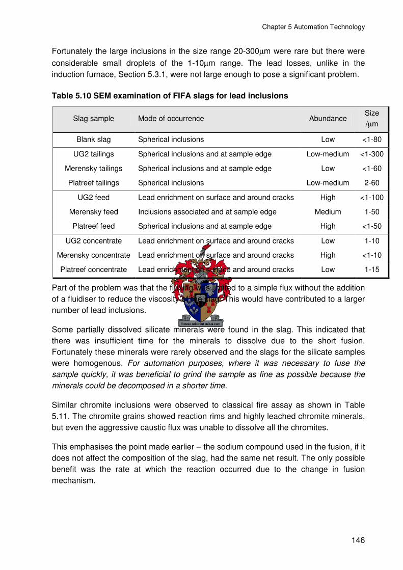
Chapter 5 Automation Technology
146
Fortunately the large inclusions in the size range 20-300µm were rare but there were considerable small droplets of the 1-10µm range. The lead losses, unlike in the induction furnace, Section 5.3.1, were not large enough to pose a significant problem.
Table 5.10 SEM examination of FIFA slags for lead inclusions
Slag sample Mode of occurrence Abundance Size /µm
Blank slag Spherical inclusions Low <1-80
UG2 tailings Spherical inclusions and at sample edge Low-medium <1-300
Merensky tailings Spherical inclusions and at sample edge Low <1-60
Platreef tailings Spherical inclusions Low-medium 2-60
UG2 feed Lead enrichment on surface and around cracks High <1-100
Merensky feed Inclusions associated and at sample edge Medium 1-50
Platreef feed Spherical inclusions and at sample edge High <1-50
UG2 concentrate Lead enrichment on surface and around cracks Low 1-10
Merensky concentrate Lead enrichment on surface and around cracks High <1-10
Platreef concentrate Lead enrichment on surface and around cracks Low 1-15
Part of the problem was that the fluxing was limited to a simple flux without the addition of a fluidiser to reduce the viscosity of the slag. This would have contributed to a larger number of lead inclusions.
Some partially dissolved silicate minerals were found in the slag. This indicated that there was insufficient time for the minerals to dissolve due to the short fusion. Fortunately these minerals were rarely observed and the slags for the silicate samples were homogenous. For automation purposes, where it was necessary to fuse the sample quickly, it was beneficial to grind the sample as fine as possible because the minerals could be decomposed in a shorter time.
Similar chromite inclusions were observed to classical fire assay as shown in Table 5.11. The chromite grains showed reaction rims and highly leached chromite minerals, but even the aggressive caustic flux was unable to dissolve all the chromites.
This emphasises the point made earlier – the sodium compound used in the fusion, if it does not affect the composition of the slag, had the same net result. The only possible benefit was the rate at which the reaction occurred due to the change in fusion mechanism.

Chapter 5 Automation Technology
147
Table 5.11 SEM examination of FIFA slags for chromite
Slag sample Mode of occurrence Abundance
Blank FIFA slag Not detected
UG2 tailings (50g) Unaltered to slightly altered High
Merensky tailings (50g) Rounded and crinkled appearance Low
Platreef tailings (50g) Not detected
UG2 feed (30g) Unaltered to slightly altered High
Merensky feed (50g) Rounded, some with crinkled appearance Medium
Platreef feed (50g) Not detected
UG2 concentrate (5g) Not detected
Merensky concentrate (5g) Not detected
Platreef concentrate (5g) Not detected
The slag composition was calculated from the flux composition, sample composition and sample mass used in the fusion. The compositions of the silicate feed and tailings samples (Merensky and Platreef) were very similar due to the same sample mass being used. Similarly the chromite UG2 samples were also similar. The slag compositions for concentrate samples were all similar due to the small sample mass used. An average composition for each of the three major slag types is presented in Table 5.12.
These can be compared to the classical fire assay slag compositions presented in Section 2.3.4. The notable differences were that there was no fluidiser, CaF2, as this was detrimental to the separator. The UG2 modifier Na2SO4 was also not added as the large quantity of sulphur introduced into the lead collector was not good for sample homogeneity when analysing using the Spark-OES.
The compositions were similar to the classical fire assay slags. The FIFA silicate slags had less PbO while the chromite slags contained more than the classical slags. The B2O3 content was on average slightly higher because no CaF2 was added and the larger addition of borax aided with fluidity. This made the slag more acidic than the classical slags. It may explain why the slags were more adhesive to the lead when casting into an iron mould. This adhesion does not affect the slag separator and it should be remembered that the slag system was designed for automated fusion and separation, not the classical casting procedure.

Chapter 5 Automation Technology
148
A. Undissolved chromite (Chr) with a tiny bright lead particle attached.
B. An inhomogeneity in Merensky tailings slag. The core is composed mainly of Ca-Al silicate and the rim is of Na-K-Al silicate.
C. Brighter areas are lead-rich at the edge of
the slag, as are the tiny specks within the slag.
D. Spherical lead inclusions (Pb) in a FIFA,
Platreef feed slag. BSE image
Figure 5.16 Back Scattered Electron images of automated lead fire assay slags
Chr
50 µm 10 µm
100 µm
Pb
Pb
50 µm
slag

Chapter 5 Automation Technology
149
Table 5.12 Slag composition for FIFA slags
Mass %
UG2 feed/tailings
Silicate feed/tailings
Concentrate
Na2O 35 34.7 34.6
B2O3 18.7 18.5 23
K2O 6.2
PbO 6.9 9.8 5.3
MgO 3.8 5.2 0.7
CaO 0.5 2.5 0.1
FeO 8.1 3.4 0.9
Al2O3 3.4 2.2 0.1
Cr2O3 7.8 0.2 0.1
SiO2 15.8 23.5 29.0
5.6 OXIDATION OF SAMPLES DURING AUTOMATED FIRE ASSAY
The selective oxidation of the lead collector was undertaken to determine whether or not the lead matrix could be cleaned up. One of the problematic elements on the Spark-OES measurement reportedly was nickel [139]. To minimise the risk for a fully automated system, matrix cleanup was investigated to reduce interference levels.
Looking at an Ellingham diagram in Gilchrist [66] it was predicted that nickel could be more easily oxidised than lead, it made the selective removal of nickel from lead feasible.
There were two ways that oxidation could be carried out during fire assy. The first was simply by using a suitable oxidising flux, the most popular being potassium nitrate. The second method was the use of the patented oxygen lance [137].
There were a number of early versions of the lance designed by IMP. The problem with the lance was that it was heavily corroded by the action of the molten slag. The lance failed quickly if the tip was inserted into the lead metal. Therefore the lance needed to be positioned above the collector with the purge gas impinging on the lead. The lance was also prone to blockage from the slag.

Chapter 5 Automation Technology
150
The fire assay lance was manufactured from stainless steel, it had an inner tube through which the oxygen passed. The outer tube was air-cooled and the cooling air was vented to atmosphere. The air-cooling of the lance was essential as when the lance was inserted into the molten slag the slag froze on the surface and protected it from excessive corrosion by the molten slag. The basic operation of the lance is shown in Figure 5.17
Figure 5.17 Schematic of the oxygen lance
After a standard FIFA fusion the crucible could be removed from the FIFA furnace and placed onto a ceramic pad. A pneumatic pedestal stand similar to the FIFA furnace was used to drive the crucible up towards the lance at a fixed height. The height was manually adjusted from the base of the pedestal and locked into position. The lance height above the lead collector was dependent on the thickness of the base of the pot.
The oxygen and nitrogen flow to the lance was controlled using pneumatic valves. Prior to and after lancing, nitrogen was continuously purged through the lance to keep the airway open and prevented slag from freezing in the tube. During the oxidation cycle, the gas was switched by computer control to supply oxygen and the gas was bubbled through the melt. Once the timer had counted down, the computer drove the pneumatic cylinder down and changed over the gas flow to nitrogen. After lancing, the melt was allowed to settle for 15-30s and separated in the Cowan separator.
Molten slag
LeadGas bubbles
O2(g)Air-cooling
Lead settles
Molten slag
LeadGas bubbles
O2(g)Air-cooling
Lead settles
Molten slag
LeadGas bubbles
O2(g)Air-cooling
Lead settles
Molten slag
LeadGas bubbles
O2(g)Air-cooling
Lead settles

Chapter 5 Automation Technology
151
5.6.1 LANCE FACTORIAL DESIGNED EXPERIMENT
A factorial designed experiment was performed on a Merensky feed sample. A factorial experiment allowed the examination of critical variables for an experimental system. The mathematics allows for the resolution of effects from the variables and their interactions to be modelled and statistically evaluated. This was done with the aid of Design Expert software [160]. For more information on experimental design refer to Appendix C.3.6. A three level factorial was designed with duplication on two factors, the centre point was repeated a further 3 times, a total of 2x32 + 3 = 21. A set of 3 control samples was also performed without any oxidation after fusion. There were a total of 24 fusions done.
The factors that were to be examined were the oxygen flow rate for 2.5, 3 and 3.5 on the flow meter and the lance blow time of 7, 12 and 17 seconds. The times took into account a 2 second lag required to drive the pot up to the lance. The actual blow times were 5, 10 and 15 seconds. A summary of the experimental design is given in Table 5.13. The high flow rate of 3.5 and using blow times of 0 (control), 12 and 17 seconds were repeated in duplicate for UG2 and Platreef samples. These were for direct comparison with the Merensky samples.
Table 5.13 Factors for the 3-level lance factorial experiment
Factor label
Factor Lower level
Centre level
Upper level
A Flow rate 2.5 3 3.5
B Time /s 5 10 15
The lance height was fixed at 30mm from the base of the pedestal. The thickness of the crucible bases were measured and found to be between 12-16mm. There was a maximum of 4mm deviation in the lance height.
A sample mass of 75g was used throughout the trials. To the samples, 250g of FIFA flux was weighed in a plastic container. The container was closed and the sample and flux were thoroughly mixed together by shaking the container vigorously. The container was then opened and the mixture was transferred to a stainless steel cup.
The samples were fused using the FIFA system. This was done manually by lowering the crucible from the furnace taking the crucible in a pair of tongs and pouring the flux/sample mixture into the crucible. The crucible was returned to the pedestal and lifted into the furnace. The fusion was performed for 15 minutes. The crucible was manually removed and placed onto the lance pedestal.
The lance cycle was then activated on the computer. Once the lance action was completed the crucible was removed from the lance pedestal and placed alongside the
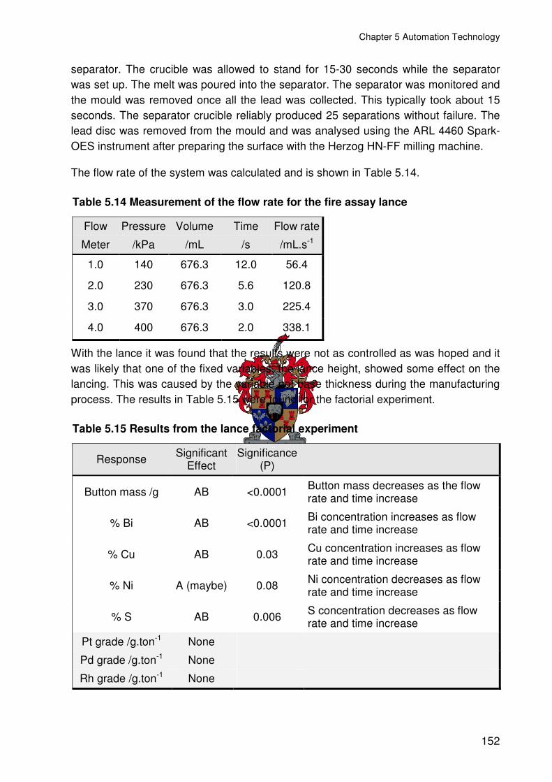
Chapter 5 Automation Technology
152
separator. The crucible was allowed to stand for 15-30 seconds while the separator was set up. The melt was poured into the separator. The separator was monitored and the mould was removed once all the lead was collected. This typically took about 15 seconds. The separator crucible reliably produced 25 separations without failure. The lead disc was removed from the mould and was analysed using the ARL 4460 Spark-OES instrument after preparing the surface with the Herzog HN-FF milling machine.
The flow rate of the system was calculated and is shown in Table 5.14.
Table 5.14 Measurement of the flow rate for the fire assay lance
Flow
Meter
Pressure
/kPa
Volume
/mL
Time
/s
Flow rate
/mL.s-1
1.0 140 676.3 12.0 56.4
2.0 230 676.3 5.6 120.8
3.0 370 676.3 3.0 225.4
4.0 400 676.3 2.0 338.1
With the lance it was found that the results were not as controlled as was hoped and it was likely that one of the fixed variables, the lance height, showed some effect on the lancing. This was caused by the variable pot base thickness during the manufacturing process. The results in Table 5.15 were found for the factorial experiment.
Table 5.15 Results from the lance factorial experiment
Response Significant Effect
Significance (P)
Button mass /g AB <0.0001 Button mass decreases as the flow rate and time increase
% Bi AB <0.0001 Bi concentration increases as flow rate and time increase
% Cu AB 0.03 Cu concentration increases as flow rate and time increase
% Ni A (maybe) 0.08 Ni concentration decreases as flow rate and time increase
% S AB 0.006 S concentration decreases as flow rate and time increase
Pt grade /g.ton-1 None
Pd grade /g.ton-1 None
Rh grade /g.ton-1 None

Chapter 5 Automation Technology
153
Any effect with a probability (P) of less than 0.05 was considered significant. The effect AB was the interaction of flow rate and time and meant that the combined effect of the two factors together was more significant than the effects of the factors alone. There was an “interaction” of the factors.
The only data that was unsatisfactory was that of the nickel concentration and this was seriously hampered by poor reproducibility on the spark instrument caused by sample inhomogeneity particularly for higher nickel concentrations.
The data can be grouped in three: Firstly, the bismuth and copper where the concentration increased as the button got smaller (caused by the higher oxygen flow rate and longer exposure time). The second, the nickel and sulphur where the concentration decreased as the mass of lead decreased. The third and last was the PGE where the grade calculated for the sample was unaffected by the oxidation of the lead. The bismuth was a known impurity in the fire assay reagents while the copper, nickel and sulphur were contributed from the sample. The correlation of the button mass and base metal content is best summarised in the graph shown in Figure 5.18.
Figure 5.18 The effects on base metals in lead for the lance
Both the copper and bismuth showed linear trends with a tight spread around the line. This was due to homogeneity in the sample and the accuracy of the measurement.
The sulphur and nickel showed considerable spread of the data related to sample inhomogeneity and poor precision in the measurement. The sulphur concentration decreased rapidly and approached zero for a button mass of 35g. The decrease in
Correlation of base metal concentration with button mass
0.00
0.04
0.08
0.12
0.16
35.0 40.0 45.0 50.0 55.0 60.0
Button mass /g
% C
on
cen
trat
ion
Bi
Cu
Ni
S
Correlation of base metal concentration with button mass
0.00
0.04
0.08
0.12
0.16
35.0 40.0 45.0 50.0 55.0 60.0
Button mass /g
% C
on
cen
trat
ion
Bi
Cu
Ni
S

Chapter 5 Automation Technology
154
nickel was linear and from the trend line the nickel concentration approached zero for a button mass of 9g.
This phenomenon was related to the oxidation rate of the various metals from the lead bath. The sulphur and nickel were oxidised more rapidly than the lead while the bismuth and copper were oxidised more slowly. The PGE were not oxidised and remained in the lead collector where they were quantitatively concentrated.
Table 5.16 Comparison of the behaviour of different sample types when using the oxygen lance on the melt after FIFA fusion
O2 (g) Flow
/mL.s-1
Time
/s
Button mass
/g
Bi
/ppm
Cu
/ppm
Ni
/ppm
S
/ppm
Pt
/g.ton-1
Pd
/g.ton-1
Rh
/g.ton-1
Merensky feed
QC value 3.93 1.63 0.28
0 0 53.2 378 751 725 1040 4.00 1.86 0.29
280 7 48.9 406 762 567 486 3.83 1.86 0.29
280 12 47.3 413 762 636 487 3.98 1.87 0.30
280 17 40.8 478 763 445 33 4.13 1.84 0.29
Change -23% +27% +2% -39% -97%
UG2 feed
QC value 2.49 1.23 0.54
0 0 54.7 349 47 74 52 2.47 1.28 0.53
280 12 41.9 428 44 49 0 2.41 1.26 0.52
280 17 36.0 509 45 42 0 2.40 1.28 0.52
Change -34% +46% -5% -44% -100%
Platreef feed
QC value 2.20 2.22 0.17
0 0 53.1 370 861 619 1015 2.12 2.54 0.17
280 12 45.1 433 866 366 79 2.22 2.47 0.17
280 17 37.9 514 859 351 20 2.12 2.40 0.17
Change -29% +39% 0% -43% -98%
After the factorial experiment was completed, the lance was tested on Platreef and UG2 feed samples to compare them to what was obtained for the Merensky feed. In

Chapter 5 Automation Technology
155
this way the performance of the lance on other sample types could be predicted without the requirement of performing extensive test work.
There was a substantial decrease in the button mass with the use of the oxygen lance. The buttons with an initially higher sulphur and nickel content, the Merensky and Platreef samples were oxidised more slowly than for example the UG2 that had comparatively lower copper, nickel and sulphur concentration. The quantity of lead oxidised was dependant on the copper, nickel and sulphur content of the button.
The PGE values for platinum and rhodium were within an acceptable range based on the QC values on these materials. There was a large positive bias on the palladium measured.
This test work confirmed the factorial data shown earlier, the oxidation of lead occurred at a slower rate than the oxidation and removal of the nickel and sulphur. While the oxidation of both copper and bismuth occurred more slowly and therefore these two elements become more concentrated in the lead. Some thermodynamic data is presented in Table 5.17.
The data predicts that the nickel and sulphur would be more easily oxidised than lead and have a more negative Gibbs function value (∆G). The corresponding equilibrium constant value log(K) was also more positive and the equilibrium would tend more to the oxide for these elements. The reverse was true of both bismuth and copper. No consideration was given to the fact that the lead bath was a mixture/solution of these elements and their activities would be dependent on concentration. It was a useful guide as to the order of oxidation.
Table 5.17 Thermodynamic data for the fire assay lance
∆H1200°C
/kJ.mol-1
∆G1200°C
/kJ.mol-1
Log (K)
2Pb + O2(g) → 2PbO -369.2 -161.6 5.7
2Bi + O2(g) → 2BiO -424.2 -122.8 4.4
2Ni + O2(g) → 2NiO -466.1 -217.9 7.7
2Cu + O2(g) → 2CuO -319.4 -52.2 1.5
S + O2(g) → SO2(g) -347.2 -283.4 10.1
From the first tests done to define the experimental operating parameters it was found that the lancing became uncontrollable as the button mass decreased and there was a chance of oxidising the entire button and losing the assay. In addition, the automated Spark-OES system could not handle a button mass of less than 36g as the button became too small for the Sample Manipulation System (SMS) robot to handle. The risk of small physical losses during the separation affecting the assay became more

Chapter 5 Automation Technology
156
significant as the collector mass decreased. The compromise conditions used for the factorial suited all sample types well without fear of losing the collector. Although, it may be possible to optimise the system for better nickel removal in the future.
5.6.2 OXIDATIVE FLUX FACTORIAL DESIGNED EXPERIMENT
For the flux test work the Merensky feed QC material was used. In this experiment, two oxidants, potassium nitrate and sodium nitrate, were used in an attempt to oxidise nickel and sulphur from the lead collector. In addition silver was added to the charge as it could have been useful in assisting with the base metal removal from the lead collector without excessive oxidation thereof. The silver was added using 2mm thick wire.
The reason that two different oxidants were used was because they began to react at different temperatures. It was hoped that this would allow the oxidation to be more selective by oxidising only the sulphides of the sample as shown in Table 5.18.
Table 5.18 Comparison of oxidants used in the oxidative flux factorial experiment
Reaction ∆H1200°C /kJ.mol-1
∆G1200°C /kJ.mol-1
Log[K] T∆G=0 /°C
2NaNO3 + SiO2 →
Na2SiO3 + 2.5O2(g) + N2(g) 192.8 -367.5 13.0 215
2KNO3 + SiO2 →
K2SiO3 + 2.5O2(g) + N2(g) 310.0 -340.8 12.1 401
The difference in the reaction points should have differing effects on the oxidation of the sample or reductant. In saying this, with the automated system the flux was added to a pre-heated crucible and the addition of sodium hydroxide to the flux accelerated the fusion process. The effect could be less pronounced than it would be if the charge were to be more slowly heated as in conventional fire assay.
A standard two level factorial was designed using the set points in Table 5.19.
Table 5.19 Factors for the flux factorial experiment
Factor label
Factor Lower limit
/g
Centre point
/g
Upper limit
/g
A KNO3 0.0 1.5 3.0
B NaNO3 0.0 1.5 3.0
C Ag 0.0 0.25 0.50

Chapter 5 Automation Technology
157
The sample and components were weighed into a 100ml glass Schott bottle. The sample and components were transferred into a plastic container with 250g of FIFA feed flux. The sample and flux were thoroughly mixed and then transferred into a stainless steel cup. The samples were fused for 15 minutes and separated with a Cowan separator.
The results of the factorial are summarised in Table 5.20. The first observation was that both of the oxidants will decrease the button mass obtained and their effects were additive and independent. In general, the sodium nitrate had a larger effect mostly because it had a smaller molar mass and therefore on a mass/mass comparison had a larger molar effect.
The oxidants generally were good for the removal of nickel as an impurity from the buttons. Although the sulphur concentration decreased as well, the effect was not statistically significant. This was related to the inhomogeneity of the sample and the inaccurate measurement of the sulphur in the buttons.
Table 5.20 Results for the flux factorial experiment
Response Significant Effects
Significance (P)
Button mass /g A
B
<0.0001
<0.0001
Button mass decreased as the mass of KNO3 or NaNO3 increased the effects were additive and there was no interaction
% Bi A
B
<0.0001
<0.0001
%Bi increased as the mass of KNO3 or NaNO3 increased, the effects were additive and there was no interaction
% Cu B 0.02 %Cu increased as the mass of NaNO3 increased
% Ni A
B
0.01
0.006
%Ni decreased as the mass of KNO3 or NaNO3 increased, the effects were additive and there was no interaction
% S B 0.08
%S concentration decreased as NaNO3 mass increased the effect was not significant and there was no effect of KNO3 (related to poor precision).
Pt grade /g.ton-1 None
A problem was found with the effect of silver on the palladium and rhodium measurement as the calculated grades increased as the silver addition increased. This was found to be due to PGE impurities in the silver wire used, fortunately the platinum was unaffected.

Chapter 5 Automation Technology
158
Since the effects of the oxidants were additive the data was combined and summarised in Table 5.21. The oxidants were quite useful in decreasing the nickel and sulphur concentration in the collector by around 40% while only decreasing the button mass by about 20%. The copper concentration was only slightly higher when using the oxidant while the bismuth was substantially increased, but in saying this, the bismuth was contributed by the flux and varied from batch to batch.
Table 5.21 Effects of oxidant on the copper, nickel, sulphur and bismuth in lead after fusion
Oxidant
/mol
Button mass
/g
Bi
/ppm
Cu
/ppm
Ni
/ppm
S
/ppm
Pt
/g.ton-1
QC value for Merensky feed 3.93
0.000 53.15 379 763 762 1243 4.23
0.030 47.64 427 778 573 992 4.12
0.032 47.19 430 782 678 1269 4.36
0.033 45.96 444 797 585 1009 4.35
0.035 46.12 441 785 558 921 4.16
0.065 41.64 501 802 457 811 4.40
% change -22 32 5 -40 -35
By comparison to the oxygen lance for the same sample, the lance was able to achieve a 97% reduction in the sulphur concentration with a similar button mass reduction. The effectiveness of the nickel removal was approximately the same with around 39% reduction in concentration.
5.6.3 SUMMARY OF OXIDATIVE TEST WORK
The test work revealed that it was possible to clean up the lead matrix with the removal of the problem elements; sulphur and nickel. Oxidants like potassium nitrate worked well for the removal of nickel and sulphur impurities in the lead button.
The oxygen lance was found to be much more effective in the removal of sulphur from the lead matrix. The added benefit was that the sample homogeneity and the precision of sparks on the lead discs with low sulphur content were much better than those with higher sulphur content.
The oxygen lance could be applied equally well to Merensky, Platreef and UG2 samples without any detrimental effects. This made the application of an oxygen lance

Chapter 5 Automation Technology
159
to geological samples very useful as the sample matrix would have less of an effect on the final analysis.
Both the flux additions and the lance had the ability to clean the matrix of nickel and sulphur. With nickel causing interference on the Spark-OES, by removing some of this element errors associated with inter-element corrections would be reduced.
The reduction in the lead button mass had the additional benefit of concentrating the PGE and the increase in the analytical signal in conjunction with the reduction of the interfering elements would improve both the accuracy and precision of the analysis.
5.7 DISCUSSION OF AUTOMATION DEVELOPMENT WORK
The key components for a fully automated fire assay system were successfully developed. Existing automated technology were successfully evaluated for their application on PGE material.
Development work with IMP and other suppliers yielded:
• A fully automated and versatile sampling system.
• A fully automated filter for water removal.
• Microwave drying to constant mass.
• Sample size reduction and grinding
• Sample weighing, flux dosing and mixing.
• Automated fusion using the new FIFA technology.
• Fast quantitative fusion using the flux developed.
• Automated slag separation using the Cowan separator.
The only missing link in the chain was the direct analysis of the lead collector using Spark-OES. The preparation of suitable standards and the development of an analytical program for Spark-OES analysis are covered in the next chapter. Even though all the key components and technology have been tested individually they need to be integrated into a complete working system. Versatile robotics systems need to incorporate these machines in a unified working laboratory. The system needs to be designed and modelled before being built and is covered in Chapter 7. A pictorial review of the automation development is given in Figure 5.19.

Chapter 5 Automation Technology
160
A. Manual loading of the bottom loading FIFA furnace during flux trials.
B. Manual unloading of a crucible with fused sample from the FIFA furnace during flux trials.
C. Handling of the hot crucible with a central CRS F3 articulated robot during fusion trials.
D. Casting of the fusion into the slag separator using the CRS F3 robot during fusion trials.
E. Water cooled mould with lead button after separation. The button is ejected from below and is taken out the top.
F. Fire assay oxygen lance for impurity removal from the lead collector.
Figure 5.19 Pictorial summary of the automation development work
FIFA Furnace
Pneumatic Cylinders
Crucible With
Molten Sample
B.
Ceramic Insulation
FIFA Furnace
Pneumatic Pedestal
Crucible Loading
A.
Central Robot
Separator
Lance
C. Robot Gripper
Separator furnace
Separator Crucible
D.
Crucible
Slag
Lead Button
Separator furnace
E.
Water-cooled Mould
F.
Oxygen lance
Crucible Pedestal
Hood
Extraction
Height Adjustment

161
CCHHAAPPTTEERR 66
6 SPARK OPTICAL EMISSION ANALYSIS
“Atomic Emission Spectrometry is today the backbone of chemical analysis for the identification, specification and process control in virtually all branches of the metallurgical industry” Slickers [161]. This statement is certainly true of the platinum industry where our key analyses are done using ICP-OES. Since emission spectroscopy has such a strong foothold in our current analysis it is relatively easy to motivate the analysis of lead by Spark-OES, since the concepts used in ICP-OES remain the same, the largest difference being the source of the atomic spectrum.
The direct spectrochemical analysis of the lead button after lead collection fire assay is an essential component for the automation of fire assay. A fast and accurate analysis is required that can also be easily automated. For this purpose new standards and analytical protocols are presented in this Chapter.
6.1 STANDARDS PREPARATION EQUIPMENT AND METHODS
The key to any type of surface analysis is highly dependent on the preparation and presentation of an appropriate sample. The requirements for accurate and precise analysis are:
• The lead sample is homogenous with a uniform analyte distribution.
• The sample is free from slag and other inclusions.
• The surface is flat and free from holes or surface imperfections.
• The analyte is in sufficient concentration to generate an analytical signal above the background.
In classical fire assay during casting the lead collector sinks to the base of the melt. The slag then begins to solidify; it hardens at 650-850°C depending on the composition. Since the slag is less thermally conductive than the metal collector, it keeps the collector warm. With its low melting point of 327°C the melt equilibrates and is annealed.

Chapter 6 Spark Optical Emission Analysis
162
The result is that when the lead finally solidifies it is inhomogeneous and contains a slag coating that is not easily separated. To perform spark analysis on a homogenous sample, lead from classical fire assay requires a second re-melt and casting of the metal to quench it.
With the casting of molten samples it is often found that the surface varies in composition due to interaction of the metal surface with the atmosphere. To prevent any analytical bias, the sample surface needs to be prepared for analysis. For hard samples such as steel, the sample can be ground, polished or milled. For soft materials such as lead, grinding or sanding of the surface are usually unsuitable as the metal can retain particles of the grinding media. This could bias the sample and introduce unnecessary contamination, thus the lead surface needs to be prepared with an appropriate milling technique.
The lead collector after fire assay is coated with slag and traditional mechanical slag removal is ineffective as slag is driven into the metal. With slag in the metal and some lead oxidation during re-melting, the slag oxide phases become more soluble in lead, introducing unwanted contaminants. Iron and chromium can be introduced into the lead in this way. Under normal reducing conditions iron and chromium are virtually insoluble in lead [69].
Another method of preparing slag free buttons is to perform a selective leach. The sodium borosilicate slag is soluble in dilute hydrochloric acid while the lead collector is largely insoluble. Once the slag is removed the lead can be re-melted and cast without contamination of the collector with slag.
It is best to separate the liquids after the fusion as is done with the automated Cowan separator. This allows the lead to be simultaneously separated from the slag and rapidly quenched without a second re-melting step.
6.1.1 EQUIPMENT FOR THE PREPARATION OF STANDARDS
The preparation of lead standards was initially done with a graphite crucible in a muffle furnace set at 800-850°C. The melt was then poured into a graphite water-cooled mould. Graphite materials were used so that the metal would not adhere to the surface of the crucible or mould. The water was held in a plastic bucket and reticulated with a submersible pump. The biggest problem with this technique was the oxidation of the lead during casting. The samples with higher nickel, copper and sulphur content that were prepared, were found to be inhomogeneous. Nickel in high concentration in particular, posed a problem with the precipitation of visible green/black nickel oxide in the lead during casting.

Chapter 6 Spark Optical Emission Analysis
163
To improve the preparation technique the following were addressed:
• Higher re-melt temperatures.
• Casting should be done anaerobically.
• Faster quenching of the lead.
The temperature was considered important as the solubility of the analyte elements change with temperature, a fact that is used in the refining of lead [162]. To retain the analytes collected by lead from fire assay, the re-melt had to be performed at similar temperatures to the fusion. For this purpose a kettle furnace was used.
The furnace supplied by Ultrafurn [157] used a graphite crucible. The kettle furnace was a cylindrical top-loading furnace and held a single crucible with a maximum operating temperature of 1150°C, for specifications check Appendix B.8. The temperature of the crucible was measured with an optical pyrometer once the furnace had attained temperature and confirmed that it was accurate. The kettle furnace was found to be compact, convenient for ease of handling with good heat containment and low heat exposure for the operator. The size lent itself to be put inside a glovebox, for use under inert atmospheres.
To prevent the oxidation of the molten lead during casting, it was done under a nitrogen atmosphere inside a glovebox [163]. The glovebox was custom made for this purpose and was large enough to hold the furnace and the equipment for the preparation of standards. The glovebox was equipped with inlet and outlet nozzles for cooling water. A transfer hatch was located on the side. The glovebox had two 220mm diameter openings in the front for the gloves and was equipped with bungs to close the holes. For details on the specifications of the glovebox refer to Appendix B.8.
To cool the standards rapidly during casting, water-cooled copper moulds were made. A refrigerated water bath was sourced from Labcon [164], specifications are given in Appendix B.8. The bath contained an externally reticulated water pump so that water could be circulated in the copper mould. The waterbath was used to provide cooling water at between 5 and 10°C for effective cooling at a flow rate of 9L.min-1.
The moulds were manufactured from copper as this material has the best heat conduction properties for this purpose [71]. The melting point of copper was only 1083°C and when molten lead at a temperature above the melting point of copper was cast in the mould, it was possible for the lead to alloy with the copper and bond on the surface. The key was to cool the lead so quickly that this could not happen. With this in mind the copper mould was made oversize so that the mass of the mould was larger than the lead standard and acted as a heat sink to rapidly draw the heat away from the sample.

Chapter 6 Spark Optical Emission Analysis
164
The mould shape was tapered at 1° to help with the removal of the solid sample. The base of the mould was 25mm in diameter to prepare appropriately sized standards and samples. This was compatible with the production samples in the automated system. The mould was 50mm in depth and lead standards up to 140g were prepared. A second mould was also manufactured with a diameter of 40mm to prepare 500g set up samples (SUS) required for automation. A diagram of the mould design is shown in Figure 6.1.
Figure 6.1 Copper mould for the casting of lead standards
The inlet was placed at the bottom of the recess and the outlet at the top. The inlet and outlet were separated horizontally by an angle of 30°. This was so that the water would not “short circuit” the mould and would circulate from below, fill the mould and flow out the top, to ensure efficient cooling.
The moulds were constantly maintained as the surface tarnished with time. Prior to use the moulds were lightly sanded with fine P1200 emery paper and buffed with paper. A dirty mould caused the lead to adhere to the surface. The entire preparation setup is shown schematically in Figure 6.2.
Side view Top view
Copper
Steel jacket
O-ring
30°
Inlet
Outlet
Mould
Side view Top view
Copper
Steel jacket
O-ring
30°
Inlet
Outlet
Mould
Side view Top view
Copper
Steel jacket
O-ring
30°
Inlet
Outlet
Mould
Side view Top view
Copper
Steel jacket
O-ring
30°
Inlet
Outlet
Mould
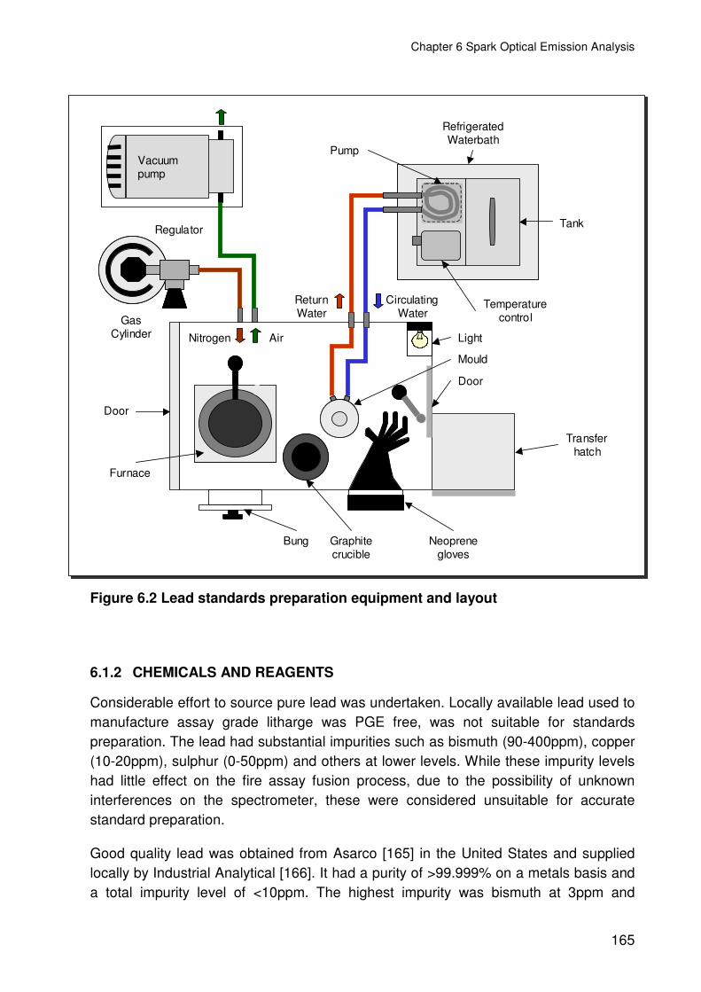
Chapter 6 Spark Optical Emission Analysis
165
Figure 6.2 Lead standards preparation equipment and layout
6.1.2 CHEMICALS AND REAGENTS
Considerable effort to source pure lead was undertaken. Locally available lead used to manufacture assay grade litharge was PGE free, was not suitable for standards preparation. The lead had substantial impurities such as bismuth (90-400ppm), copper (10-20ppm), sulphur (0-50ppm) and others at lower levels. While these impurity levels had little effect on the fire assay fusion process, due to the possibility of unknown interferences on the spectrometer, these were considered unsuitable for accurate standard preparation.
Good quality lead was obtained from Asarco [165] in the United States and supplied locally by Industrial Analytical [166]. It had a purity of >99.999% on a metals basis and a total impurity level of <10ppm. The highest impurity was bismuth at 3ppm and
Vacuum pump
Gas Cylinder Air
Return Water
Circulating Water
Regulator
Nitrogen
Mould
Furnace
Door
Light
Refrigerated Waterbath
Tank
Temperature control
Pump
Transfer hatch
Bung Neoprene gloves
Door
Graphite crucible
Vacuum pump
Gas Cylinder Air
Return Water
Circulating Water
Regulator
Nitrogen
Mould
Furnace
Door
Light
Refrigerated Waterbath
Tank
Temperature control
Pump
Transfer hatch
Bung Neoprene gloves
Door
Graphite crucible
Vacuum pump
Gas Cylinder Air
Return Water
Circulating Water
Regulator
Nitrogen
Mould
Furnace
Door
Light
Refrigerated Waterbath
Tank
Temperature control
Pump
Transfer hatch
Bung Neoprene gloves
Door
Graphite crucible
Vacuum pump
Gas Cylinder Air
Return Water
Circulating Water
Regulator
Nitrogen
Mould
Furnace
Door
Light
Refrigerated Waterbath
Tank
Temperature control
Pump
Transfer hatch
Bung Neoprene gloves
Door
Graphite crucible

Chapter 6 Spark Optical Emission Analysis
166
cadmium at 2ppm. The lead was available in 1kg ingots and <2mm (10 mesh) granules, convenient for the preparation of lead standards. The lead was chemically analysed using the lead dissolution method and was PGE free.
Copper and nickel metal powder of high purity were obtained from OM Group [167] and were supplied by Protea Industrial Chemicals [168]. The sulphur was AnalAR reagent from BDH [169]. The nickel, copper and sulphur were analysed for their PGE contents using a blank nickel sulphide fusion and were found to be PGE free.
Other analytes were added as oxides like bismuth oxide (Bi2O3) and arsenic trioxide (As2O3). Spectrographically pure compounds from Johnson Matthey [170] were used.
6.1.3 PREPARATION OF LEAD STANDARDS
The metallic lead and analyte compounds were weighed and placed into a glass container. The containers were labelled and put into the transfer hatch of the glovebox. The transfer hatch was purged and the container was moved into the purged chamber. The crucible was removed from the furnace and the material was transferred into it. With the more volatile elements, the material was transferred into a cold crucible. It was returned to the furnace and heated at 1150°C for a minimum of 20 minutes. Larger samples were melted for longer (60 minutes maximum).
Just prior to casting the copper mould was wiped with paper towel to dry condensate from the surfaces. It was essential that it was completely dry as moisture in the mould caused spattering of the molten metal during casting. After the re-melt the lid of the furnace was opened. The crucible was removed and the metal was immediately cast in one continuous motion into the mould.
For most standards, the 25mm mould quenched 120g of molten lead at 1150°C in 1-2s. With the 40mm mould, 500g of lead was quenched in approximately 5s. The disc was allowed to cool completely for 1 minute before the mould was inverted and the disc removed.
Physical losses during the re-melt procedure were found to be small, 0.1% being the average. Physical losses were caused by small droplets remaining inside the crucible and were easily removed by inverting and gently tapping the crucible on a ceramic plate.

Chapter 6 Spark Optical Emission Analysis
167
6.2 CHEMICALLY ANALYSED LEAD STANDARDS
Matched matrix standards were prepared from lead derived from sample material. First a standard fire assay fusion was performed using a large sample to collect PGE, copper, nickel, sulphur and other contaminants in the lead collector. For this purpose Merensky concentrate and UG2 concentrate materials were fused. The individual samples were fused using 20g per fusion.
The melts were poured into cast iron moulds. Once cool, the lead collector was mechanically separated from the bulk of the slag. The lead button with adhering slag was retained without any further mechanical treatment and the slag was discarded.
The lead buttons for each sample type were placed into a new fire clay crucible. They were covered with approximately 100g of borax and the crucible was re-heated at a temperature of 1200°C. The molten mixture was poured through a preheated ceramic separator (Cowan cone, Section 5.4.3) above a 25L drum of water. The separator allowed the molten lead to pass through the hole in the base of the cone and the lead was granulated into lead pellets of approximately 2-3mm in diameter. The borax was retained in the ceramic cone and contained the residual slag from the lead buttons. The lead granules were dried overnight in a drying oven at 60°C to prevent oxidation of the lead (at higher temperature). The standards were wet chemically prepared and analysed for their impurities and PGE content.
In the first method, for the determination of the nickel, copper and bismuth, the samples were digested using 1:1 v/v nitric acid. The solution was then diluted and made to volume. The solutions were analysed by ICP-MS. The PGE content for the lead was also measured using this technique. Due to the high dilution required to reduce the total dissolved solids to below 0.2% for the ICP-MS, the results for PGE tended to be imprecise and inaccurate.
For the second technique the lead sample was dissolved in a minimum of nitric acid. After digestion at a low heat, the lead was precipitated as a chloride using hydrochloric acid. The lead chloride was filtered off and the filtrate was collected and boiled down. More chloride salts were removed after a second addition of hydrochloric acid. The second filtrate was then boiled down and transferred to a volumetric flask. Yttrium was used as an internal standard and the samples were measured by ICP-OES. The same samples were then diluted and re-measured by ICP-MS.
The sulphur content of the lead samples was determined using a sulphur analyser (refer to the Appendix B.6 for details). With this technique the metal sample was placed inside an alumina boat and pushed into a tube furnace at 1350°C. The metal was oxidised with an oxygen purge and the off gas analysed by absorption using an infrared sensor for its SO2(g) content. The concentration of sulphur in the sample was

Chapter 6 Spark Optical Emission Analysis
168
then calculated. The values for the bulk standards were calculated from all the analytical methods.
The lead standards were analysed for their PGE content using the classical lead dissolution technique as outlined in Section 2.6.5. The final solutions were measured by ICP-MS and ICP-OES for the PGE. The PGE values for the two bulk standards are reported in Table 6.1.
Table 6.1 Analysis of lead/concentrate QC samples
Pt /µg.g-1
Pd /µg.g-1
Au /µg.g-1
Rh /µg.g-1
Average 20.71 12.71 1.31 2.07
n 7 7 7 7
SD 0.45 0.36 0.06 0.10
Merensky concentrate
QC
95% CI 0.42 0.34 0.06 0.09
Relative uncertainty range 2.0% 2.6% 4.3% 4.3%
Average 19.35 8.83 0.18 3.59
n 5 7 7 7
SD 0.08 0.11 0.01 0.06
UG2 concentrate
QC
95% CI 0.11 0.12 0.01 0.07
Relative uncertainty range 0.6% 1.3% 4.5% 1.9%
A set of standards was prepared by dilution of the bulk lead standards. For this method a mass of the bulk standard was weighed out along with the required mass of blank lead. A calibration range containing 0.5-20ppm platinum was prepared for the Merensky and 0.5-18ppm for the UG2. Another set of “mixed” standards was prepared by changing various ratios of the bulk UG2 and Merensky lead alloys.
The standards and the concentrations can be found in Appendix E.1.
The disadvantages of these chemically analysed standards were:
• Calibration was limited to the accuracy and precision of the original chemical analysis.
• Some differences existed with the copper and nickel determinations and it could not be determined which methods were correct.
• No analysis was available for ruthenium and iridium in the standards.
• Impurities such as arsenic, tellurium and antimony could not be accurately determined at the levels found in the bulk lead standard alloys.

Chapter 6 Spark Optical Emission Analysis
169
• The matrix range and ratios were limited to the original sample and the lead alloys formed from them.
• Flotation plants commonly blend ore from various sources and can combine UG2, Merensky, oxidised ore etc.
• Geological ores can vary to the extremes and may not match the Merensky or UG2 calibrations with regard nickel, copper, sulphur or PGE ratio and composition.
6.3 SYNTHETIC STANDARDS
From some of the early spark work the matrix of the lead buttons was found to contain:
• 2-400ppm bismuth (flux impurity)
• 50-5000 nickel, copper and sulphur (from flux and sample)
• <20ppm of other impurities such as iron, arsenic, antimony, tin, zinc and others
• <50ppm of the required analytes, platinum, palladium, gold, rhodium, ruthenium and iridium
It was decided that the matrix was simple enough to prepare matrix matched synthetic standards. It was also proposed that inter-element corrections be done to correct for interferences wherever applicable. With this in mind binary and ternary lead standards were prepared for interference investigation. The overlap/interference investigations were to be limited to the four primary impurities, nickel, copper, sulphur and bismuth as it was expected that with their higher concentrations these would be the most likely sources of interference.
6.3.1 LEAD STANDARDS CONTAINING SILVER, BISMUTH, NICKEL, COPPER AND SULPHUR
Lead foil was shaped into a boat and the powdered elements or oxides were weighed into it. The boat was then folded closed and transferred to a graphite crucible along with a weighed portion of blank lead. The standards were prepared in the manner described earlier in Section 6.1.3.
With sulphur, the lead boat was added to a cold crucible and the heating was performed slowly. The temperature was raised to 400°C, just above the melting point of lead, and held there for 10 minutes to allow the lead to react with the sulphur. This was to prevent the volatilisation of sulphur. Otherwise the procedure was the same as for the other standards.
Sulphur/lead alloys were the most difficult to prepare as the standards were often not homogenous. This behaviour could be explained by examining the phase diagram for the lead/sulphur system in Figure 6.3 [77]. The addition of sulphur rapidly increased the melting point of lead alloy; this could be seen with the liquidus increasing from the
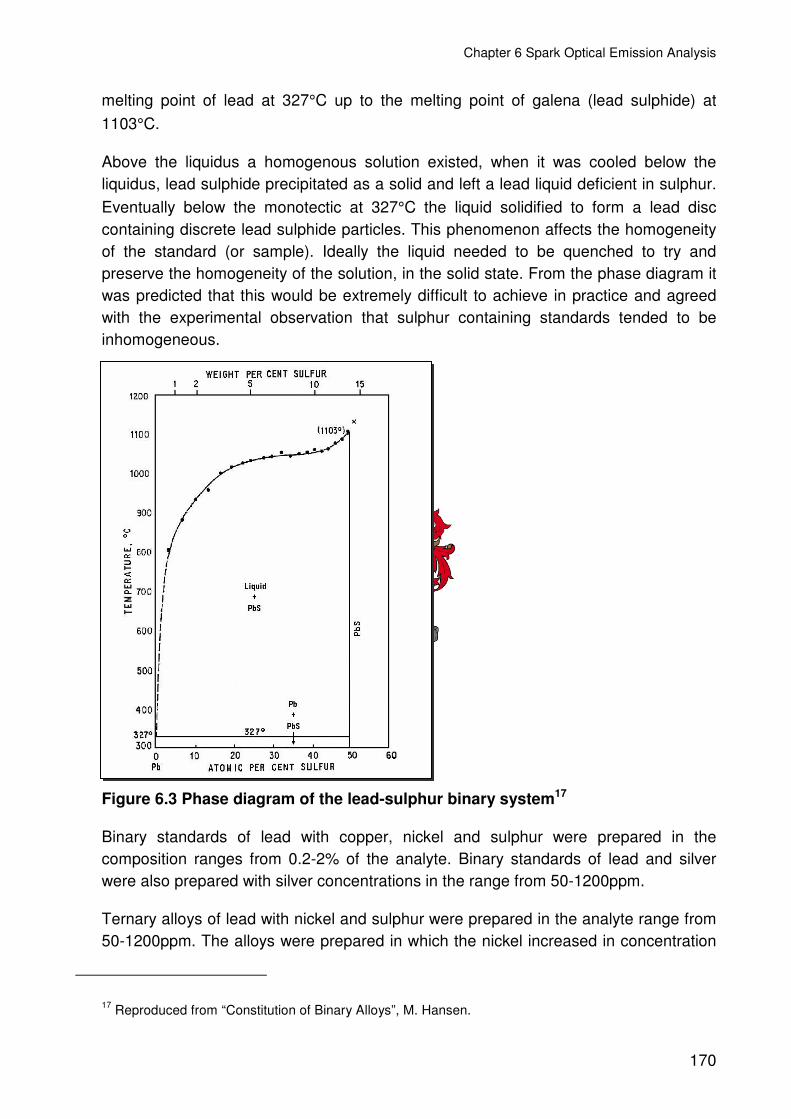
Chapter 6 Spark Optical Emission Analysis
170
melting point of lead at 327°C up to the melting point of galena (lead sulphide) at 1103°C.
Above the liquidus a homogenous solution existed, when it was cooled below the liquidus, lead sulphide precipitated as a solid and left a lead liquid deficient in sulphur. Eventually below the monotectic at 327°C the liquid solidified to form a lead disc containing discrete lead sulphide particles. This phenomenon affects the homogeneity of the standard (or sample). Ideally the liquid needed to be quenched to try and preserve the homogeneity of the solution, in the solid state. From the phase diagram it was predicted that this would be extremely difficult to achieve in practice and agreed with the experimental observation that sulphur containing standards tended to be inhomogeneous.
Figure 6.3 Phase diagram of the lead-sulphur binary system17
Binary standards of lead with copper, nickel and sulphur were prepared in the composition ranges from 0.2-2% of the analyte. Binary standards of lead and silver were also prepared with silver concentrations in the range from 50-1200ppm.
Ternary alloys of lead with nickel and sulphur were prepared in the analyte range from 50-1200ppm. The alloys were prepared in which the nickel increased in concentration
17 Reproduced from “Constitution of Binary Alloys”, M. Hansen.

Chapter 6 Spark Optical Emission Analysis
171
as the sulphur decreased, this kept the concentration of the matrix element approximately constant. Similar ternary alloys were also prepared for lead with copper and bismuth.
All the standards and their concentrations can be found in Appendix E.3.
6.3.2 LEAD STANDARDS CONTAINING IRON, COBALT, ARSENIC, ANTIMONY AND OTHER IMPURITY ANALYTES
The standards were prepared from a variety of standard materials and included powdered metal and oxides. It was expected that the oxides given in Table 6.3 were reduced in the graphite crucible and alloyed with the lead. Some oxides such as tellurium dioxide were reduced by the lead itself. These reactions are summarised in Table 6.2.
Table 6.2 Reduction of oxides during lead standard preparation
Reaction ∆H1150°C /kJ.mol-1
∆G1150°C /kJ.mol-1
Log[K] T∆G=0 /°C
As2O3 + 1.5C → 2As + 1.5CO2(g) 292.3 -379.8 13.9 340
TeO2 + 2Pb → Te + 2PbO(l) -81.9 -95.8 3.5 <0
PbO(l) + C → Pb(l) + CO(g) 70.8 -152.6 5.6 300
The final products were homogenous metallic alloys and a graphite crucible is a good choice for the preparation of metallic lead standards (as it does not dissolve). The only disadvantage was the inclusion of solid graphite in the final standard. The graphite floated on top of the molten lead and after casting it remained on the top of the disc. The carbon was removed when the lead was prepared for analysis and was not a required analyte. A bulk standard with the analytes in Table 6.3 was prepared first.
The bulk standard was prepared so that most of the analytes had a nominal concentration of 500ppm. Iron and cobalt had poor solubility in lead and the bulk standard had a concentration of 50ppm. The bulk standard was prepared like the sulphur standards presented earlier but was not cast in a mould but granulated in water under anaerobic conditions. After filtration the granules were dried in a porcelain bowl using a low temperature (<60°C) on a hotplate.
The standards and concentrations prepared can be found in Appendix E.3.

Chapter 6 Spark Optical Emission Analysis
172
Table 6.3 Compounds used for the preparation of lead standards
Analyte Compound Melting Point /°C
As As2O3 817
Co Co 1495
Fe Fe 1538
Sb Sb2O4 631
Se SeO2 220
Sn SnO2 232
Te TeO2 449.5
Tl Tl2O3 304
Zn Zn 420
6.3.3 LEAD STANDARDS PREPARED FROM PGE SOLUTIONS
This method was one of the original techniques used to prepare synthetic PGE standards. The early work was carried out by spiking flux with a PGE solution and collecting them in lead by fire assay fusion. The method was found to be inaccurate, as the final lead mass could not be predicted, although corrections could be made for the lead recovered. The lead also had to be de-slagged and impurities of unknown concentration were introduced into the lead. This was discontinued, but provided standards that could be used to evaluate various suppliers and instruments.
A better method to prepare these standards was to make a cylindrical lead ingot. This was done by weighing a portion of blank lead, re-melting and casting it in the copper mould. A 12mm diameter hole was drilled into the ingot to make a receptacle for PGE stock solutions. Attempts to make a lead foil boat to hold the solution failed due to leaks caused from the corrosive hydrochloric acid.
A mixed PGE stock solution was prepared from pure single element solutions. The density of the stock was recorded on preparation and it was stored in a sealed Schott bottle. A ten times dilution of the stock was also prepared. A volume of solution was dispensed into the ingot using a Gilson syringe pump [171] and the mass was

Chapter 6 Spark Optical Emission Analysis
173
recorded. In this way a mass correction was made for small differences in the volume dispensed.
The ingot was placed onto a hotplate at a low temperature to evaporate the solvent. This was done slowly without boiling to avoid physical losses.
The ingot mass was supplemented with lead granules to make up the difference to the desired mass. The ingot was placed into a cold crucible and prepared as outlined in Section 6.1.3.
The standards and their concentrations that were prepared are in Appendix E.3.
6.3.4 LEAD STANDARDS PREPARED WITH SOLID PGE SPONGES
The use of pure PGE metal sponges was investigated as it was convenient to not have to dissolve metal to make stock solutions. An added advantage was that unlike the chloro-species, the metals were stable and only volatilised at very high temperature. Therefore, the loss of metal during the re-melt was less likely than the method used for the preparation using solutions.
With the low concentrations of the PGE required for the lead alloys an intermediate bulk standard had to be prepared, as the masses of the sponges required were too small to be reliably weighed. With the bulk standard the PGE were weighed into a lead foil boat using a microbalance with a precision of 0.1µg. The boat was folded carefully to preserve the metal inside. It was combined with lead granules to prepare a 100g lead standard and was melted and cast in the usual way.
The lead ingot was flattened on an anvil using a 2-pound hammer to form a 1mm thick flat plate. The lead was then cut into strips with a pair of scissors.
The lead standards were prepared by dilution. Appropriate masses of the bulk lead/PGE standard were combined with blank lead and re-melted and cast as previously described in Section 6.1.3.
The concentrations for the lead standards prepared can be found in Appendix E.3.

Chapter 6 Spark Optical Emission Analysis
174
6.4 ANALYSIS OF LEAD USING SPARK OPTICAL EMISSION SPECTROMETRY
Instrumentation that is already automated is always considered first for new automation projects. The two most commonly automated instrumental techniques are XRF and Spark-OES.
With the high density and electron count of lead, it is a heavy absorber for X-rays. Secondary X-rays generated by the analyte would be absorbed by the sample itself. It is expected that analysis of trace elements in lead would be insensitive and XRF is not suitable for the analysis of lead materials.
All the local lead suppliers in South Africa used Spark-OES for the analysis of their final lead products. Two such suppliers that were visited included Fry’s Metals [172] who used a Belec instrument and Lead Processing [173] who used an ARL 4460 instrument.
For Spark-OES instrumentation a number of suppliers were approached and included Spectro Analytical Instruments [174], ThermoARL [175], OBLF [176], Leeman [177] and Belec [178]. Belec and OBLF indicated that the detection limits required were too low for any of their instrumentation.
Both Spectro and ThermoARL had instruments that would be suitable for the job. Spectro supply the Spectro M (now the Spectrolux) spectrometer that was deemed suitable and developed their PGE Detector to go with their Immafuse machine. ThermoARL proposed their 4460 instrument for the job. The system from Leeman used Glow Discharge Atomic Absorption Spectrometry. It was also considered as it could be automated much like Spark-OES instrumentation.
A preliminary set of standards was prepared by fusion as outlined in Section 6.3.3. Samples from classical fire assay were re-melted and cast. Sets were submitted to Spectro, ThermoARL and Leeman.
Leeman generated linear calibration curves for the pure lead/PGE standards that were supplied but were unable to detect PGE in samples containing nickel and sulphur impurities.
The data from Spectro and ARL were reprocessed manually and calibrations, Background Equivalent Concentration (BEC) and Limit of Detection (LOD) were calculated. This allowed for objective comparison as the software and calculations done by the two manufacturers were a little different. Both instruments gave almost identical calibrations, BEC and LOD data when the same analytical lines were chosen. Such a comparison is given for platinum in Table 6.4:

Chapter 6 Spark Optical Emission Analysis
175
Table 6.4 Calibrations of Pt 299.8x2nm line for the ARL 4460 and Spectro M instruments
BEC /ppm
DL /ppm
Correlation Coefficient
R2
Curve type
Spectro 6.0 0.2 0.9995 Linear
ARL 6.1 0.2 0.9987 Linear
Based on the data for these early trials it was clear that either the Spectro M or the ARL 4460 would be suitable as intensities were good and calibrations were achieved. The previous work done by Sundquist [139] on the analysis of PGE in lead was done with Spectro and it was very tempting to settle for a Spectro instrument.
When examining the samples after sparking, the Spectro M instrument had been operated to ablate an area of 5x5mm and created a deep divot in the analytical surface about 0.5mm in depth. By contrast the ARL 4460 was a much more moderate attack, a 2x2mm area was ablated, less than 0.1mm was removed from the surface and still a similar analytical performance was achieved. It was concluded that the Spectro instrument was ablating much more of the sample to get the same sensitivity as the ARL instrument. It was likely that the ARL could be optimised further to improve the analysis while the Spectro M was probably at the limit of its performance boundaries.
Although the predicted performance was similar based on the calibration data, the ARL instrument gave better agreement with the in-house QC samples and was typically within 1 standard deviation thereof [179].
With the time available to prove the technology it was not possible to evaluate the two systems exhaustively. All the development and research work was reported for the ARL 4460 that was purchased for the Research Centre to do the development work, although it should be equally applicable to the Spectro M.
6.4.1 INTRODUCTION TO SPARK OPTICAL EMISSION SPECTROMETRY
There are a number of different electrical discharges used for analysis [180]. These are differentiated by the current density during the discharge and in increasing order of current density are; Townsend discharge, glow discharge, arc and spark discharges. An arc is a continuous and stable electrical discharge and can be maintained for long periods. A spark is a transient discharge and occurs over a short period of time and is associated with a high current.

Chapter 6 Spark Optical Emission Analysis
176
Arc discharges are associated traditionally with low detection limits, 0.1-1µg.g-1 but poor precision with %RSD of around 5% [180]. Arc discharges generate lower temperatures and melt more of the sample surface. Therefore for analysis, arcs have lower background and higher sensitivity. Sparks have traditionally had higher detection limits 10-100µg.g-1 but better precision 1-2% RSD [180]. With the high temperatures generated by sparks they are less prone to matrix, sample composition and structural effects. Many modern instruments make use of ‘hybrid sparks’ that are somewhere in between these extremes and are possible due to newer technology.
Irrespective of how the discharge is generated, electrons are accelerated from the electrode towards the sample. When the electrons collide with the sample they are rapidly decelerated and release energy into the sample surface and heat it. This ablates material from the surface and ionises the chamber gas. A transient high temperature plasma is generated that contains atoms, ions, electrons and high-energy molecules. These excited species emit characteristic radiation.
Radiation from the spark stand is diverted through a light guide into the spectrometer where it is dispersed into its characteristic wavelengths. The light is then measured using a detection system and converted through an electronic system into a count rate. With the aid of a computer system the numbers generated by the electronics are used to calculate a calibration from known standards. Samples are then determined by comparison to the calibration.
6.4.2 SPARK GENERATION
The spark is generated with an electric circuit that includes the sample. This is called a point to plane discharge where the “point” is the electrode tip and the plane is the sample surface. The gap between the electrode and spark is effectively a capacitance of the circuit. The circuit contains a resistor, inductor and capacitor. These components in the circuit determine the shape and period of the spark that is generated. A diagram of a spark generator circuit is shown in Figure 6.4.

Chapter 6 Spark Optical Emission Analysis
177
Figure 6.4 Spark generator circuit with external ignition18.
Where:
U1 Applied voltage U2 Applied voltage SP Sample plane
S Switch CE Counter electrode
RL Charging resistor RZ Ignition resistor AG Analytical gap
RB Discharge resistor AxG Auxiliary gap
RM Measuring resistor
CL Capacitor CZ Ignition capacitor
L Inductance SZ Ignition, Tesla coil
The basic principles of the spark generation can be discussed with this circuit. The capacitor CL is charged with a voltage U1. The discharge is triggered with an ignition coil, where the circuit setup is much the same as for the spark generator. What it does is make the analytical gap (AG) conductive by ionising some of the gas in the chamber. At this point the capacitor CL discharges through RB and L across AG and through the sample.
The value RM is the measurement resistor and is a low resistance resistor that is used to measure the current in the circuit with an oscilloscope, it usually has a resistance of around 0.1Ω.
18 Reproduced from “Automatic Atomic Emission Spectroscopy” by Slickers
RZ
CZ U2
AxG
CE
L
RM
SPAG
S
RL
U1
+
_
CL
SZ
RB
RZ
CZ U2
AxG
CE
L
RM
SPAG
S
RL
U1
+
_
CL
SZ
RB

Chapter 6 Spark Optical Emission Analysis
178
The supply voltage U2 and the values of CL, RB, L, determine the nature of the discharge. The lower the values of L and RB the higher the current density and the “harder” the spark. These discharges can be up to 250A. While with higher values of RB and L the “softer” the spark, it is more diffuse and arc-like in character.
The circuit can be oscillating (the current oscillates after the initial discharge) or aperiodically dampened (a single half periodic oscillation after the initial discharge). High voltage sparks tend to be oscillating due to limitations in the circuit components. The type of circuit is defined by Equation 6.1:
LC CLR 2= Equation 6.1
If RB<RC (RC is the critical resistance) then an oscillating circuit results and when RB=RC the circuit is critically dampened. While if RB>RC then the spark is over critically dampened. Usually the limit of critical damping is aimed for. Basically this means that the size of the capacitor and the inductance control the shape of the current discharge.
Typically values of CL are 1-20µF and L at 10µH, but will depend entirely on the application. High voltage (>1000V) discharges usually last for the interval of 10-100µs while lower voltage (<1000V) sparks take 100-1000µs.
With the resistors being in series, the resistance of the sample contributes to the circuit and when the composition, dimensions or temperature of the sample changes, so can its resistance. Generally metals that have low vaporisation points and whose thermal conductivity is highly temperature dependent, such as lead, will be affected by temperature changes in the sample. For this reason the spark stand on the ARL 4460 was equipped with water-cooling that was reticulated with a pump to maintain the temperature of the stand and sample.
In the more modern instruments such as the ARL 4460 a digitally controlled spark generator circuit was used. During the spark the discharge was monitored electronically and was adjusted during sparking to keep the current discharge constant. New fast electronics made this possible and is what ThermoARL call a current controlled source (CCS). The spark generation here was much more complex than the simple RLC circuit presented in Figure 6.4. The basic principles of combining resistance, capacitance and inductance were still valid except that it was done electronically with a complex circuit. The power board that generates the power at 80V and 100kHz supplies the CCS board that generates the spark.

Chapter 6 Spark Optical Emission Analysis
179
Figure 6.5 Shape of the spark discharge
It was no longer possible for the operator of the instrument to adjust the circuit by changing the various components. This was done electronically and was set with a number in the software. The manufacturer has the tools to optimise the spark and this was done by ARL. A spark with suitable ablation properties was designed and was fairly gentle, just ablating the surface. Lead has a low melting point and was easily ablated. The sparks were generated at a frequency of 600Hz. The entire spark takes P=1/f, therefore a spark was triggered every 1666µs using an ignition coil.
The spark for the analysis of lead on the ARL 4460 was examined with an oscilloscope the current measured peaked at 38A then rapidly diminished over a 40µs time period. The current was held constant at around 8A where the analytical measurement was made as shown in Figure 6.5.
Spark discharge current
0
5
10
15
20
25
30
35
40
45
0 40 80 120 160 200
Time /µµµµs
Cur
rent
/A
Spark discharge current
0
5
10
15
20
25
30
35
40
45
0 40 80 120 160 200
Time /µµµµs
Cur
rent
/A

Chapter 6 Spark Optical Emission Analysis
180
A high energy pre-spark (HEPS) is also often used to homogenise the analytical zone. The HEPS is modified by changing CL, which is increased by 5 times, and RL is adjusted to equal RC, in the circuit shown in Figure 6.4 and Equation 6.1. This results in a higher energy but more diffuse spark covering almost twice the area of the analytical spark. The discharge heats a thin layer of the surface that melts. The surface solidifies and then undergoes ablation from the analytical spark. This generates a more homogenous surface for analysis.
Figure 6.6 Diagram of the spark stand of the ARL 4460 instrument.19
The spark was generated inside the spark stand of the analysis table and is shown in Figure 6.6. The electrode was contained within a non-conductive PTFE cylinder and was insulated from the metal base block and analysis table with a glass insulator cup. The insulator cup was removable so that volatilised metal that condensed on it could be cleaned. The cup was opaque, black quartz glass to prevent unwanted reflected light. Only the light generated by the emission during the spark was admitted along the optical path to the spectrometer.
Argon gas was used to purge the spark chamber and flowed counter current to the direction of the light emitted from the electrode. This was to force the volatilised metal and gasses towards the exhaust. This prevented deposition of metal on the optical components of the spectrometer – namely the primary lens. The optical path further on had a shutter that could be closed during high intensity pre-spark. Light was only admitted to the spectrometer during analysis. The gas seal of the spark chamber was
19 Reproduced from the Operator manual for the 4460
Argon Exhaust
Analysis table
Tungsten disc
Spark chamberSampleOptical path
Argon Inlet
Argon Inlet Base block (water cooled)
Glass Insulator cup
Tungsten electrode
PTFE Cylinder
Argon Exhaust
Analysis table
Tungsten disc
Spark chamberSampleOptical path
Argon Inlet
Argon Inlet Base block (water cooled)
Glass Insulator cup
Tungsten electrode
PTFE Cylinder

Chapter 6 Spark Optical Emission Analysis
181
important and needed to be covered by the sample. This was to prevent the ingress of air into the system. Oxygen could cause unwanted absorption of light and may enhance the background, as well as the formation of refractory oxides with some elements.
The exhaust gas from the spark stand flowed through an oil filter where metal particles were collected. The gas then flowed through a final air filter before being vented to atmosphere.
6.4.3 OPTICAL SYSTEM OF THE ARL 4460 INSTRUMENT
The ARL 4460 instrument was a Paschen Runge mount, vacuum polychromator with a Rowland circle configuration [180]. The spectrometer light box itself was made from aged cast iron, and weighed around 700kg. This was for mechanical stability of the system. This spectrometer case was evacuated with a pumping system. The entire spectrometer was contained within an oven at 38°C using 3 elements with circuiting fans. The temperature control was good, typically within ±0.1°C. This was to prevent changes in the spectrometer due to thermal expansion and contraction.
Light from the stand passed through a collimator that contained the shutter and was collected with the primary lens. The lens was electrically heated to prevent a temperature gradient between the stand and spectrometer. It was a VUV (Vacuum Ultra Violet) lens that was made from calcium fluoride and was also transparent to radiation in the region of 160-190nm. This system was specifically designed for the measurement of carbon, nitrogen, oxygen, phosphorus and sulphur, the CNOPS analyses [181]. It was not essential, but with sulphur being measured at 180.73nm was still preferred for our application. For the same reasons, the grating was coated with magnesium fluoride and the entrance windows for the phototubes were also magnesium fluoride.
To get sufficient transparency a high vacuum was required in the spectrometer. This was achieved on the ARL 4460 instrument with a dual pumping system. The main vacuum down to 20mbar was achieved with a dual head diaphragm pump. This was a dry membrane pump and did not introduce hydrocarbons from the lubricants into the spectrometer – an old problem with vacuum spectrometers. These hydrocarbons could deposit on the optics, reducing the analytical signal with time. The second stage to achieve the high vacuum was done with a high-speed (27 000 rpm) molecular drag pump and the final vacuum that was achieved was better than 10-4mbar.
The primary lens focused the light from the stand on the primary slit of the spectrometer. For the ARL 4460 instrument this was a 20µm slit and acted as the objective for the spectrometer.

Chapter 6 Spark Optical Emission Analysis
182
The light was then dispersed with the aid of a concave diffraction grating mirror with 1080grooves/mm. The geometry of the spectrometer was based on the Rowland circle principle. The light entered the spectrometer through the primary slit on the circumference of the Rowland circle. This light fell on the concave grating on the other side of the circle. The light was then dispersed and reflected where it focused on the secondary slits, again on the Rowland circle. The ARL 4460 instrument had a 1m focal length. This is best illustrated with a diagram shown in Figure 6.7.
Figure 6.7 Spectrometer optical system on the 446020
Adjustment of the spectrum in the spectrometer was achieved by moving the position of the primary slit on the Rowland circle. This adjusted all the positions on the secondary slits. It was required that the secondary slits were all correctly aligned and is done at the factory. The analyte intensity can be adjusted with a micrometer screw gauge for maximum and this was called profiling. What can be seen from Bragg’s law, Equation 6.2 was that sinθ was proportional to λ and the angle of diffraction increased as the wavelength increased. The spectrum became dispersed over an arc on the Rowland circle.
Rowland circle
Concave grating and mounting
Primary slit
Secondary slit
Mirror and filter
Phototube
Spectrometer
Mirror rack/s
Primary lens
Source
Profile adjustment
Rowland circle
Concave grating and mounting
Primary slit
Secondary slit
Mirror and filter
Phototube
Spectrometer
Mirror rack/s
Primary lens
Source
Profile adjustment
Rowland circle
Concave grating and mounting
Primary slit
Secondary slit
Mirror and filter
Phototube
Spectrometer
Mirror rack/s
Primary lens
Source
Profile adjustment
Rowland circle
Concave grating and mounting
Primary slit
Secondary slit
Mirror and filter
Phototube
Spectrometer
Mirror rack/s
Primary lens
Source
Profile adjustment

Chapter 6 Spark Optical Emission Analysis
183
The dispersion of the light is given by Bragg’s law, Equation 6.2:
θ=λ sindn 2 Equation 6.2
Where:
n Order of diffraction d Spacing of the grooves e.g. 1080lines/mm d=1/1080 = 925.9nm
λ Wavelength (nm) θ Angle of diffraction (°)
Light of the desired wavelength corresponding to the analyte required was then isolated from the spectrum by positioning a secondary slit at the correct position on the Rowland circle. The secondary slits on the 4460 varied from 20-75µm depending on the adjacent lines.
What also can be seen from the Bragg’s law equation was that higher order reflections would also occur. These could potentially interfere with the measured analytical lines. For higher dispersion on the 4460, usually the second order reflections were measured, but were less intense. To isolate the desired wavelength, for example if we wanted to measure at 300nm we could position the phototube at an equivalent wavelength of 2x300nm = 600nm to measure the same light in the second order. To remove the interferences from possible first order lines a filter was needed.
mλ=2dn Equation 6.3
Where:
λ Wavelength (nm) m Order
d Optical layer thickness (nm) n Refraction index
There were two different kinds of filters – the first was a transmission filter – simply this was coloured glass that would transmit the desired wavelength while absorbing the others. The spectral band pass FWHM (full width at half maximum) of these was usually 30-40nm. Another type of filter was an interference filter using the Fabry-Perot etalon, Equation 6.3. In the interference filter light was reflected between two partially reflective mirrors that were separated by a thin layer. The interference of the radiation will allow only certain wavelengths to be transmitted.
Therefore with an optical spacing of 600nm the maximum intensity of transmitted light from the filter would be, 1200nm (first order), 600nm in the second order, 300nm in the third order at that position. In this way a first order wavelength can be separated from a
20 Reproduced (with modifications) from “Automatic Atomic Emission Spectroscopy” by Slickers

Chapter 6 Spark Optical Emission Analysis
184
second order wavelength at the same position. These interference filters had a spectral band path of 5nm. Interference filters were used on the 4460 for the analytical lines that are interfered from lower or higher order reflections.
With the configuration used in the ARL 4460 instrument most of the analytical lines were measured in the second order, there were some analytical lines that were measured in the first, third and even forth order. All were dependent on the spectral resolution required and were balanced against physical spacing constraints on the circle and the desired intensity/sensitivity.
The light from the filter then fell on a concave mirror that focused it from the horizontal plane either up or down into the side entrance window of the phototube. The phototube may also have had a mask that covered the window slightly, this allowed light to enter only from the analytical mirror. It was sometimes necessary to add a mask to prevent stray light from adjacent tubes, mirrors or screws from reflecting light into the phototube.
The light fell onto the target of the phototube that amplified the light signal converting it into an electronic pulse. The instrument electronics then recorded the pulses. The phototubes in the ARL 4460 instrument were generally 10 stage phototubes, 28mm in diameter with quartz or glass sheath side entrance windows, different tubes were used for the various analyte lines. The lines below 190nm had magnesium fluoride windows. There was a minimum energy and hence maximum wavelength above which the photoelectric effect would no longer occur for a particular surface and is called the work function of the target element, it is given by Equation 6.4 [182].
maxmin
chE
λ= Equation 6.4
Where:
Emin Minimum energy to eject an electron (eV) λmax The maximum wavelength (m)
h Planck’s constant, (4.136x10⁻¹⁵eV.s-1) c Speed of light (2.998x10⁸m.s-1)
The cathode of the phototube was coated with a metal and was called a photocathode. The tube was evacuated and a voltage was applied to the cathode and the dynodes of the phototube all connected with various voltages. When light was shone on the surface of the photocathode, its energy was absorbed and it emitted an electron. This electron was accelerated under voltage and struck the first dynode releasing more electrons and so forth for as many amplification stages as was required.
There were two limiting factors for phototubes; firstly the construction material of the photocathode – different materials had different λmax. This would limit the maximum wavelengths that could be detected by a particular phototube. Secondly, the bottom

Chapter 6 Spark Optical Emission Analysis
185
boundary λmin would be set by the entrance window of the phototube and whether or not it was transparent to the lower wavelengths or if they would be absorbed. Various sensitivities could be used for phototubes and depended on the number of dynodes in the tube.
The final signal from the phototube was measured when a current flows. This was converted into a pulse or count, which, was then recorded with electronics of the system and eventually with a computer. The computer and software were then used to calculate the function between intensity and concentration for the calibration of the instrument.
6.4.4 TIME RESOLVED OPTICAL EMISSION SPECTROSCOPY
This optical setup described in the previous section was very similar to that used in classical ICP-OES. In many ways it is now considered an old fashioned technique due to the emergence of new simultaneous Echelle optical systems. These new systems use a CCD (Charge Coupled Device) to detect the light in the spectrometer. They are beginning to replace the conventional ICP polychromator, because the spectrometer is smaller and cheaper. There is also a spark instrument available from both ARL and Spectro that uses this CCD technology. The limitation is that the CCD needs to store the signal for a prolonged time before it can be counted. This excludes the possibility of using a windowing technique to measure the spectrum.
With the spark technique using the classical polychromator and phototube arrangement it was possible to do time resolved spectroscopy (TRS). This technique used the principle that the transient atomic analyte signal in the afterglow of a spark, decayed in an argon atmosphere at a slower rate than the ionic, molecular and background spectra. It was therefore possible by using TRS to optimise the measuring window to retain the analyte signal while the background/interfering signals had virtually decayed. In this way it was possible to maximise the analyte to background light intensity ratio and thereby reduce the detection limit of the spark technique.
The TRS technique was highly sensitive and could improve the LOD ten-fold. This made it highly suitable for the measurement of traces in a solid matrix.
6.5 CALIBRATION OF THE ARL 4460 INSTRUMENT
As with any instrument the ARL 4460 needed to be calibrated and there were a number of different ways that this could be done. The software was quite flexible and therefore the various options need to be examined.
The basic choices were whether or not the analysis was performed by ratioing the intensities of the analyte and matrix. The common practice was to ratio to the matrix element so that small differences in the ablation rate could be accounted for [180]. This

Chapter 6 Spark Optical Emission Analysis
186
assumed that the analyte ablated at the same rate as the matrix. This may not always true, particularly where there were precipitates in the metal sample such as sulphur in steel. For such examples a burn-off curve would be required where the sample was ablated for increasing time until a steady state was achieved. Usually there would initially be an increase in the analyte signal followed by an asymptotic decrease. This was important if reproducible analysis was required and once the steady state prevailed the ratioing of the analyte to matrix intensity would be more valid.
A preliminary experiment was done to measure the raw intensity of a sample. The %RSD was calculated based on the raw intensity and then compared to the %RSD for intensity ratios. It was found that the %RSD improved by a factor of two by using ratios. What was also observed was that the %RSD did not improve for analyte elements that were inhomogeneously distributed in the sample. Analysis for PGE in lead should be done using analyte:matrix intensity ratios for the best precision.
The next decision was whether or not the concentration should be ratioed to the matrix. Since a solid sample was being analysed and there was a considerable variation in the concentration of some of the analyte elements such as copper, nickel and sulphur, the concentration of the matrix itself would change. Therefore it was necessary to correct for the effect of the matrix concentration on the intensity that was used to ratio to the analyte.
As an example if an analyte were measured in a binary alloy at a concentration of 100ppm, the matrix concentration would be 99.99%. If the same analyte concentration were measured in another sample but with other analytes that contributed to a total of 1% of the matrix, the matrix concentration would be only about 99%. The intensity of the matrix signal would be reduced by 1% due to dilution. This would result in the concentration being overstated by about 1% based on the calibration using intensity ratios. It was essential to correct for the matrix concentration when using intensity ratios for calibration. The best way to do this was to use the analyte:matrix concentration ratio for the calibration, as this was what the intensity ratio represented. The analyte:matrix concentration ratio that would be determined from the calibration would be normalised to the matrix concentration and could be used to correct for differences in the matrix concentration.
The matrix could be calculated from Equation 6.5.

Chapter 6 Spark Optical Emission Analysis
187
+=
1C100
Cratio
matrix Equation 6.5
Where:
Cmatrix Concentration of matrix (%)
ratioC The sum of analyte:matrix concentration ratios
From the example Cmatrix = 100/((1/99 + 0.01/99) +1) = 98.99%.
The absolute concentration could then be calculated from Equation 6.6:
matrixration CCC ×= Equation 6.6
Where:
Cn Absolute concentration of the analyte (%)
Cmatrix Concentration of matrix (%)
Cratio The analyte:matrix concentration ratio
In the example, the analyte was calculated (0.01/99*98.99)= 0.0100% or 100ppm.
For the determination of the PGE in lead where the highest accuracy was required and where the matrix could vary the analyte:matrix concentration ratio method was best.
6.5.1 INSTRUMENT STANDARDISATION
The instrument response changed with time. Examples could be fouling of optics, small changes in the sensitivity of components like phototubes etc. This was called drift and to correct for these time dependent changes, standardisation was done. The first requirement of standardisation was to have low and high concentration set up samples (SUS). The values of the SUS do not need to be accurately known but the low point, usually the blank and the high point had to have a significantly different analyte concentration. Usually the top standard would be about the same, or slightly above the concentration range for the calibration. The SUS had to be as homogenous as physically possible, as corrections were done with the measurement of the analyte and needed to be done reproducibly so that drift could be detected with some certainty.
The SUS were measured on the instrument just prior to calibration; these values were then recorded as the nominal values. Standardisation was used to correct the measured intensities back to the nominal vales so that the measured intensities correlated to the response of the spectrometer when it was calibrated.

Chapter 6 Spark Optical Emission Analysis
188
There were two types of drift, the first was translational drift were for example the measured values of the high and low SUS were higher or lower by the same value. This could be caused by something like fouling of the instrument optics. This could be corrected by using Equation 6.7 (all quantities I were intensities in counts). In some ways this could be thought of as a blank correction.
Icorrected = Imeasured + (Inominal low – Imeasured low) Equation 6.7
The next type of drift was rotational drift where the low SUS measured the same but the high SUS was either higher or lower than the nominal value. Changes in the response of the phototube due to small changes in the electronics may have caused this type of drift. This can be corrected by using Equation 6.8.
Icorrected = Imeasured × (Inominal high / Imeasured high) Equation 6.8
So the full correction given by the translational and rotational corrections is given by:
Icorrected = (α × Imeasured) + β Equation 6.9
Where:
low measuredhigh measured
low nominalhigh nominal
II
II
−−
=α
)I(I high measuredhigh nominal ×α−=β
This drift correction corrected the intensities before they were used to calculate the concentration from the calibration curve and it made no difference whether the curve was linear, quadratic or even cubic.
Drift correction could be thought of as calibration maintenance. If the instrument underwent repairs or any other physical changes that could affect the performance thereof it should then ideally be re-calibrated. However, for day-to-day variations like changes in gas, cleaning of the instrument and profile adjustments, standardisation could correct for these subtle differences and maintain the accuracy of the instrument calibration. This had been shown to be reliable for more than six months of continuous operation and time will tell how long it will last in practice before re-calibration is required.

Chapter 6 Spark Optical Emission Analysis
189
6.5.2 ANALYTICAL CONDITIONS
There were various options in the software to customise the analytical condition. There was an argon purge that allowed gas to circulate for a fixed time before analysis took place. This ensured that there was no air in the sparking chamber after the sample was placed on the analysis table. A purge time of around 2s was adequate due to the design and flow of argon in the spark stand itself.
There was an option for a pre-spark and for the analysis of lead sparking condition 19 was used. This pre-spark was generated at 600Hz with 1000V and had a discharge current of around 20A. Pre-spark testing was done for between 1-20s, there was no significant improvement in the homogeneity of the sample as the %RSD on the inhomogeneous analytes nickel and sulphur did not improve significantly. A consistent decline in intensity as the pre-spark time increased was noticed. This could affect the sensitivity of the analysis, particularly at lower levels near the detection limit. As a precautionary step a 2s pre-spark was performed to treat the sample surface. This would remove any small inhomogeneities and dirt on the surface before analysis.
Figure 6.8 Behaviour of palladium analysis with time on the ARL 4460 instrument
There was also an option to use a pre-integration time. This was where the analytical spark was used to ablate the surface and the measurement was delayed for a certain time before measurement. Usually this was a delay to allow the spark condition to stabilise before measurement was made. Although it was initially thought not to be
Analysis of Pd in Pb with time
2.50
3.00
3.50
4.00
4.50
0 25 50 75 100 125 150 175 200
Analyses
Pd
/ µµ µµg.
g-1
Pd
UCL
LCL
A B C2 hours 240 hours 400 hours
Analysis of Pd in Pb with time
2.50
3.00
3.50
4.00
4.50
0 25 50 75 100 125 150 175 200
Analyses
Pd
/ µµ µµg.
g-1
Pd
UCL
LCL
A B C2 hours 240 hours 400 hours

Chapter 6 Spark Optical Emission Analysis
190
necessary – certainly it made little difference on a freshly prepared surface, when measuring a monitor sample over an extended time anomalous behaviour on the analysis of palladium was discovered, this is shown in Figure 6.8. No such effect was observed for platinum, rhodium or any other analyte.
In the period labelled “A” the control limits of the instrument were established by measuring the control sample 20 consecutive times. This was the short-term precision of the instrument on a newly prepared analytical surface. The analytical measurement was very reproducible over this time. The instrument with its SMS was then setup to measure the sample every 4 hours. Once the sample surface was completely analysed the surface was automatically re-prepared and the process continued. Periodic spikes were observed in the analysis. The analytical measurement would increase and once the sample surface was re-prepared would fall back within the correct limits for the sample. As the sample aged over a 48-hour period the apparent palladium content would increase.
To rectify this situation an integration delay time of 2s was introduced into the analysis during the period “C” and this reduced the periodicity of the palladium analysis into more acceptable limits. The delay time allowed a small amount of the sample surface to be ablated before an analytical measurement was taken. It appeared from this that there was an enrichment of palladium at the surface of the sample that increased with time.
This phenomenon was time dependent and fortunately with a fully automated system, analysis would be done directly on a sample with a freshly prepared surface. This was shown to have no effect on the analysis of production samples. It did pose a problem with the continuous measurement of control samples and therefore a pre-integration time was introduced. Also it meant that control limits needed to be determined over an extended time period of 48 hours and not after 20 consecutive measurements, as this would allow for some time dependent variation.
The analytical intensity measured increased with integration time and the relationship was highly linear (R2 >0.999) and predictable. The intensities measured on the lines for platinum (299.8nm) and lead (matrix, 322.1nm) are shown in Figure 6.9 as these had similar intensities. For analytical purposes the intensity ratio was used and after 10s integration the ratio levelled off and could be seen for platinum (299.8nm), palladium (340.5nm) and rhodium (343.5nm).
The reproducibility from one spark to the next also needed to be considered and is shown in Figure 6.10. From the %RSD with three sparks it was predicted that the precision between spark measurements improved as the integration time was increased. There was a large change initially as the integration time was increased from 5 to 10s. Then the improvement was smaller as the integration was increased to 20s. This meant that for homogenous samples a longer integration time of 20s with

Chapter 6 Spark Optical Emission Analysis
191
fewer sparks (2) would yield the best results. For inhomogeneous samples where accuracy was important, it was better to integrate for a shorter time (10s) and perform more sparks (4).
Figure 6.9 Effect of integration time on Spark analysis with the ARL 4460
The samples would take the same total analysis time but the analysis would be better tailored for the kind of sample and analytical requirements. If the sample was less homogenous and there was a large %RSD between replicate sparks, it was best to measure more sparks over the entire analytical surface, the average result would then be more representative. This was also applicable when trying to measure close to the detection limit, as this would cause more variability in the analysis. The analytical measurement on the spark instrument could be tailored to the analytical requirements.
Effect of integration time on analysis
0
100
200
300
400
0 5 10 15 20
Integration time /s
inte
nsity
/kcp
s
0.40
0.43
0.46
0.49
0.52
Rat
io
Pb (matrix)
Pt
Ratio Pt/Pb
Ratio Pd/Pb
Ratio Rh/Pb
Effect of integration time on analysis
0
100
200
300
400
0 5 10 15 20
Integration time /s
inte
nsity
/kcp
s
0.40
0.43
0.46
0.49
0.52
Rat
io
Pb (matrix)
Pt
Ratio Pt/Pb
Ratio Pd/Pb
Ratio Rh/Pb

Chapter 6 Spark Optical Emission Analysis
192
Figure 6.10 Effect of integration time on the precision of Spark measurement on the ARL 4460
6.5.3 TIME RESOLVED SPECTROSCOPY WINDOW
The analytical window was one of the more important instrumental optimisations necessary for the analysis, as it would have a direct influence on the LOD. This was best evaluated by measuring the peak to background ratio. To do this with a fixed channel instrument was difficult because unless the background positions were included in the instrument, they could not be measured simultaneously. Instead the background was measured for a blank sample at the analytical position.
Effect of integration time on precision
0.0
0.4
0.8
1.2
1.6
2.0
4 6 8 10 12 14 16 18 20 22
Integration time /s
%R
SD
Pt
Pd
Rh
Pb
Average
Effect of integration time on precision
0.0
0.4
0.8
1.2
1.6
2.0
4 6 8 10 12 14 16 18 20 22
Integration time /s
%R
SD
Pt
Pd
Rh
Pb
Average

Chapter 6 Spark Optical Emission Analysis
193
The assumption here was that the blank did not contain PGE; for the lead materials used this was true since they were wet chemically analysed.
Figure 6.11 Effect of TRS windowing on Spark-OES analysis on the ARL 4460
In order to measure the peak to background ratio, the window of the analytical measurement was varied between 0 and 160µs after the initiation of the spark. The window was held open for 180µs before being closed; this was only a fraction of the total spark time of 1666µs. The intensities measured and the peak to background ratios for the measurement of platinum (299.8nm) are plotted in Figure 6.11.
A notable trend from the graph was that there was a very large increase in the analytical signal by using a windowing technique. The first point on the graph represented by 0µs had no windowing and the intensity was integrated for the entire spark. From the intensities it was found that almost the entire analytical signal was generated in the first 120µs of the spark after which the intensity fell away to zero. Integrating for longer than 160-180µs had no benefit to the analysis and reduced the average intensity.
The analytical signal peaked with a TRS window opening of 5-20µs and then began to fall off. The background intensity also dropped off at 20µs and fell at a faster rate than the analytical signal. This increased the peak to background ratio and it levelled off at 40-60µs.
Intensities measured with TRS windowing
0
30
60
90
120
0 20 40 60 80 100 120 140 160
Window open /µµµµs
Inte
nsit
y /k
cps
Pt
Pt Bk
Peak/Bk ratio
Intensities measured with TRS windowing
0
30
60
90
120
0 20 40 60 80 100 120 140 160
Window open /µµµµs
Inte
nsit
y /k
cps
Pt
Pt Bk
Peak/Bk ratio

Chapter 6 Spark Optical Emission Analysis
194
Opening the TRS window at 40µs maximised the peak to background ratio while retaining as much of the analyte signal as possible. All the PGE analytes showed a similar effect with an optimum at 40-60µs. So even though it was possible to set a unique window for every element, all the analytes were measured with a TRS window of opening at 40µs and closing after 180µs.
6.5.4 CALIBRATION RESULTS
Calibration was done using the following optimal analytical conditions in Table 6.5:
Table 6.5 Spark analytical conditions for the ARL 4460 instrument
Analytical parameter Time /s Analytical parameter Value
Flush time 3 TRS Window open 40µs
Post flush 3 Window close 180µs
Pre-spark time 1 Argon Analysis 5L.min-1
Pre integration time 1 Standby 1.5L.min-1
Integration 15 Spark Pre-spark condition 19
Total time 23 Spark condition 26
Calibration was done using analyte:matrix intensity ratios and analyte:matrix concentration ratio.
These analytical conditions were chosen to make the analysis as robust as possible. They could be customised depending on the application.
The first thing that was done was to compare the two sets of synthetic calibrations against each other to determine whether or not there were any differences as a result of the method in which the synthetic standards were prepared.
The two sets of PGE standards – the one prepared by using mixed stock solutions and the other using PGE sponges yielded identical calibration graphs. The differences between the calibrations on platinum were less than 0.09%, based on the slope of the calibration graph shown in Figure 6.12. The data for all the PGE are compared in Table 6.6.

Chapter 6 Spark Optical Emission Analysis
195
Table 6.6 Comparison between synthetic lead PGE standards
Pt Pd Au Rh Ru Ir
% Difference 0.09 0.39 -1.25 0.05 -1.93 -3.18
The two elements with the poorest sensitivity were gold and iridium, the “sponge standards” prepared using solid sponges had a higher calibration range and the calibration was more reliable as the standards were not measured so close to the detection limits. For ruthenium the set of “sponge standards” showed some variability in the sample homogeneity at higher concentrations. The calibration range may have been too high in concentration for ruthenium to prepare homogeneous standards.
Figure 6.12 Comparison of platinum calibrations for synthetic standards
The set of “sponge standards” covered the widest range of concentrations and was used for the final calibrations for the PGE. Both methods of preparing standards were suitable for the preparation of accurate calibration standards.
Most of the PGE analyses were linear for the low range with the first five standards, but as the concentration increased the calibration became more curved and in general a quadratic fit produced the best correlation.
Comparison of synthetic PGM standards for Pt
0.000
0.025
0.050
0.075
0.100
0.125
0.0 10.0 20.0 30.0 40.0 50.0
Pt concentration /µµµµg.g-1
Rat
io in
tens
ity
Sponge stds
Solution stds
Comparison of synthetic PGM standards for Pt
0.000
0.025
0.050
0.075
0.100
0.125
0.0 10.0 20.0 30.0 40.0 50.0
Pt concentration /µµµµg.g-1
Rat
io in
tens
ity
Sponge stds
Solution stds
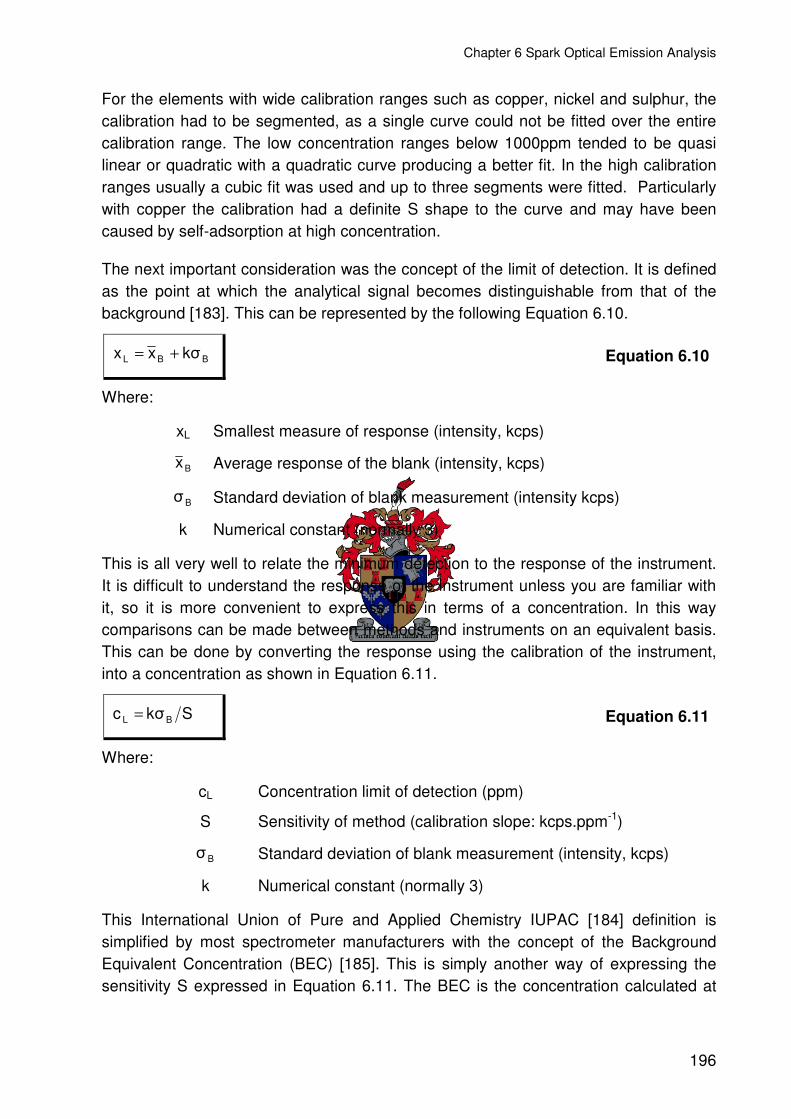
Chapter 6 Spark Optical Emission Analysis
196
For the elements with wide calibration ranges such as copper, nickel and sulphur, the calibration had to be segmented, as a single curve could not be fitted over the entire calibration range. The low concentration ranges below 1000ppm tended to be quasi linear or quadratic with a quadratic curve producing a better fit. In the high calibration ranges usually a cubic fit was used and up to three segments were fitted. Particularly with copper the calibration had a definite S shape to the curve and may have been caused by self-adsorption at high concentration.
The next important consideration was the concept of the limit of detection. It is defined as the point at which the analytical signal becomes distinguishable from that of the background [183]. This can be represented by the following Equation 6.10.
BBL kxx += Equation 6.10
Where:
xL Smallest measure of response (intensity, kcps)
Bx Average response of the blank (intensity, kcps)
B Standard deviation of blank measurement (intensity kcps)
k Numerical constant (normally 3)
This is all very well to relate the minimum detection to the response of the instrument. It is difficult to understand the response of the instrument unless you are familiar with it, so it is more convenient to express this in terms of a concentration. In this way comparisons can be made between methods and instruments on an equivalent basis. This can be done by converting the response using the calibration of the instrument, into a concentration as shown in Equation 6.11.
Skc BL = Equation 6.11
Where:
cL Concentration limit of detection (ppm)
S Sensitivity of method (calibration slope: kcps.ppm-1)
B Standard deviation of blank measurement (intensity, kcps)
k Numerical constant (normally 3)
This International Union of Pure and Applied Chemistry IUPAC [184] definition is simplified by most spectrometer manufacturers with the concept of the Background Equivalent Concentration (BEC) [185]. This is simply another way of expressing the sensitivity S expressed in Equation 6.11. The BEC is the concentration calculated at

Chapter 6 Spark Optical Emission Analysis
197
an intensity of two times the background/blank intensity and is directly proportional to the slope.
Sx2BEC B= Equation 6.12
Where:
BEC Background Equivalent Concentration (ppm)
S Sensitivity of method (calibration slope: kcps.ppm-1)
Bx Average response of the blank (intensity, kcps)
The BEC gives a measure of the sensitivity of the analytical line. The lower the BEC the more sensitive the line and the easier it is to resolve the analytical signal above the background. This is one of the more important parameters used to evaluate spectrometer performance.
With the BEC data, the limit of detection (LOD) can then be calculated as defined as follows [185].
BECxk
LODB
B ×= Equation 6.13
Where:
k Numerical constant for LOD, k=3
σB Standard deviation of the pure matrix intensity (kcps)
Bx Average intensity of the pure matrix/blank (kcps)
BEC Background Equivalent Concentration (ppm)
There are two primary components that will determine the LOD of an instrument – the first is the reproducibility of the analytical measurement and the second is the sensitivity as determined by the BEC. The calibration data for the more important analytes is summarised in Table 6.7.
With the LOD, this was the minimum concentration in the lead that could be reliably measured. Below this value the measurement would be imprecise and may give a concentration value that is negative as it would then statistically possible to get a measurement that was lower than the average reported for the blank. Data near or below the LOD were imprecise and less reliable. This brings us to the concept of the limit of quantification (LOQ); this is the limit at which is considered that an analyte can be determined accurately with good precision. This limit is also defined with Equation 6.13, where k=10 and is 3 times above the LOD.
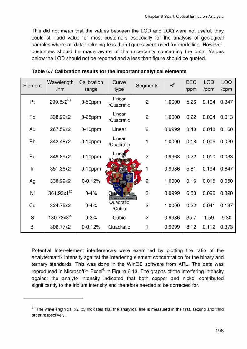
Chapter 6 Spark Optical Emission Analysis
198
This did not mean that the values between the LOD and LOQ were not useful, they could still add value for most customers especially for the analysis of geological samples where all data including less than figures were used for modelling. However, customers should be made aware of the uncertainty concerning the data. Values below the LOD should not be reported and a less than figure should be quoted.
Table 6.7 Calibration results for the important analytical elements
Element Wavelength
/nm Calibration
range Curve type
Segments R2 BEC /ppm
LOD /ppm
LOQ /ppm
Pt 299.8x221 0-50ppm Linear
/Quadratic 2 1.0000 5.26 0.104 0.347
Pd 338.29x2 0-25ppm Linear
/Quadratic 2 1.0000 0.22 0.004 0.013
Au 267.59x2 0-10ppm Linear 2 0.9999 8.40 0.048 0.160
Rh 343.48x2 0-10ppm Linear
/Quadratic 1 1.0000 0.18 0.006 0.020
Ru 349.89x2 0-10ppm Linear
/Quadratic 2 0.9968 0.22 0.010 0.033
Ir 351.36x2 0-10ppm Linear 1 0.9986 5.81 0.194 0.647
Ag 338.29x2 0-0.12% Quadratic
/cubic 2 1.0000 0.16 0.015 0.050
Ni 361.93x120 0-4% Quadratic 3 0.9999 6.50 0.096 0.320
Cu 324.75x2 0-4% Quadratic
/Cubic 3 1.0000 0.22 0.041 0.137
S 180.73x320 0-3% Cubic 2 0.9986 35.7 1.59 5.30
Bi 306.77x2 0-0.12% Quadratic 1 0.9999 8.12 0.112 0.373
Potential Inter-element interferences were examined by plotting the ratio of the analyte:matrix intensity against the interfering element concentration for the binary and ternary standards. This was done in the WinOE software from ARL. The data was reproduced in Microsoft Excel® in Figure 6.13. The graphs of the interfering intensity against the analyte intensity indicated that both copper and nickel contributed significantly to the iridium intensity and therefore needed to be corrected for.
21 The wavelength x1, x2, x3 indicates that the analytical line is measured in the first, second and third order respectively.

Chapter 6 Spark Optical Emission Analysis
199
A concentration of 0.3% nickel gave the same intensity as though there was 10ppm of iridium in the sample. For copper the interference was less but 1.8% copper contributed an iridium intensity equivalent to 10ppm. Sulphur had the opposite effect on the analysis and depresses the iridium signal. This was a matrix effect related to the melting point and volatilisation of the sample due to its sulphur content.
Iridium was by far the worst analyte for interference and this was aggravated by the fact that the emission intensity was low. Unfortunately there was a limited choice of analytical lines and inter-element correction needed to be applied for measurement of iridium, but due to the very large interference it was unlikely that iridium would be reliably analysed in lead samples containing large quantities of copper and nickel.
Figure 6.13 Interference of sulphur, copper and nickel on iridium (351.4nm)
Inter-element correction was done using the following calculations, Equation 6.14:
×+= )Ck(CC nnduncorrectecorrected Equation 6.14
Where:
Cn Concentration (absolute or ratioed) of interfering analyte (ppm)
kn Correction co-efficient
In the typical sample range where copper, nickel and sulphur were analysed at 0-0.2% in concentration it was found that the interferences from the various matrix elements
Interference Investigation for Iridium
0.0
1.0
2.0
3.0
4.0
5.0
0 0.03 0.06 0.09 0.12
Ir analyte intensity ratio
Inte
rfer
ent
conc
ence
ntat
ion
/%
%Ni%Cu%SIr 10ppmBlank
Interference Investigation for Iridium
0.0
1.0
2.0
3.0
4.0
5.0
0 0.03 0.06 0.09 0.12
Ir analyte intensity ratio
Inte
rfer
ent
conc
ence
ntat
ion
/%
%Ni%Cu%SIr 10ppmBlank

Chapter 6 Spark Optical Emission Analysis
200
were small. It was best to use as few corrections as possible as this was another source of error and corrections were applied only where entirely necessary as was shown for iridium. Generally where nickel and copper would enhance the analytical signal, sulphur would depress it. These matrix effects largely cancelled out and were small enough to ignore. The full table of the interference factors from the investigation are appended in E.5 and a summary table is given in Table 6.8.
Table 6.8 Summary of interferences used in the calibration
Analyte Wavelength /nm
Interfering element
k Factor
Pt 299.79x2 None
Pd 340.45x2 None
Au 267.59x2 None
Rh 343.48x2 None
Ru 349.89x2 None
Ir 351.36x2 Cu -5.47e-4
Ni -2.40e-3
S 3.23e-5
To test the accuracy of the calibration obtained by using synthetic lead/PGE standards, the chemically analysed standards from the Merensky, UG2 and mixed Merensky/UG2 sets were analysed.
Table 6.9 Regression analysis of the chemically analysed standards
Slope Standard error
R2 df t-test significant
All 0.986 0.002 1.00 59 Yes
Pt 0.987 0.002 1.00 19 Yes
Pd 0.969 0.007 1.00 19 Yes
Rh 0.995 0.007 1.00 19 Yes
The comparison is shown graphically in Figure 6.14. The data was analysed using linear regression with the FREML technique discussed in Section 4.4. This was to determine whether or not there was a difference between the spark analysis and the chemically analysed values. The analysed values and uncertainty for the bulk lead/concentrate samples were given earlier in Table 6.1. The results of the regression

Chapter 6 Spark Optical Emission Analysis
201
analysis are tabulated in Table 6.9. A t-test was done on the slope to determine whether the difference was statistically significant.
Figure 6.14 Measurement of the chemically analysed standards on the ARL 4460
The slope of the regression analysis for all the analytes differs from unity and the differences were statistically significant. This meant that a bias existed between the chemically analysed values and spark analysis, with the spark analysis producing a lower result (spark result = slope x chemical analysis). The coefficients of variation, R2, were close to unity and indicated that the data were highly correlated and that the differences were consistent throughout.
The statistics do not reveal which value was correct, only that the spark result was slightly lower, with the biggest difference being 3% on palladium. Good agreement was obtained for rhodium with the difference being 0.5%, platinum was 1.3% lower.
The differences can be as a result of two things, either the calibration using the synthetic lead/PGE standards were slightly low or the average for the lead/concentrate QC materials was slightly overstated. The latter was the most likely because if the uncertainty in the chemical analysis was considered, Table 6.1, the 95% uncertainty limits were typically in the order of ±2% and from the regression analysis the overall agreement was within 1.5%.
The analyses agreed within the uncertainty of the chemical analysis used to assign the original lead/concentrate QC values for the preparation of the chemically analysed
Measurement of wet chemically analysed standards
0.0
5.0
10.0
15.0
20.0
0.0 5.0 10.0 15.0 20.0
Chemical analysis /µµµµg.g-1
Spa
rk a
naly
sis
/ µµ µµg.
g-1
Pt
Pd
Rh
X=Y
Measurement of wet chemically analysed standards
0.0
5.0
10.0
15.0
20.0
0.0 5.0 10.0 15.0 20.0
Chemical analysis /µµµµg.g-1
Spa
rk a
naly
sis
/ µµ µµg.
g-1
Pt
Pd
Rh
X=Y

Chapter 6 Spark Optical Emission Analysis
202
standards. This further illustrated the problems associated with chemically analysed standards and secondary calibration, there was a larger uncertainty in the calibration and this was the reason that synthetically prepared calibration standards were used.
The data also indicated that samples measured with the chemically analysed standards would be overstated by 1-2%. This was important for the comparisons in the next section.
6.5.5 PRECISION OF SPARK OPTICAL EMISSION ANALYSIS OF LEAD
Like with most analytical techniques, Spark-OES precision should improve as the analyte concentration (signal) increases. This should be true, provided that the sample remains homogenous, the relationship is shown in Figure 6.15.
Figure 6.15 The dependence of precision on grade on the ARL 4460
The samples were not always homogeneous and the homogeneity was dependent on composition. For example the lead samples derived from the Merensky reef contained more sulphur and nickel and as these increased in concentration the inhomogeneity of the sample also increased.
The overall trend can be seen in the graph and generally the platinum and rhodium were more precisely determined than the palladium. The trend lines indicated that below 0.5ppm the %RSD increased to 8%. At 2-5ppm the %RSD normally reduced to less than 2%.
Dependence of precision on analyte concentration
0.0
2.0
4.0
6.0
8.0
10.0
0.0 5.0 10.0 15.0 20.0
Concentration /µµµµg.g-1
%R
SD
on
Spa
rk O
ES
ana
lysi
s
Pt
Pd
Rh
Dependence of precision on analyte concentration
0.0
2.0
4.0
6.0
8.0
10.0
0.0 5.0 10.0 15.0 20.0
Concentration /µµµµg.g-1
%R
SD
on
Spa
rk O
ES
ana
lysi
s
Pt
Pd
Rh

Chapter 6 Spark Optical Emission Analysis
203
6.6 ANALYTICAL RESULTS
The early evaluation of the spark analysis was done on geological samples using standards made from the chemically analysed lead/concentrate QC materials that were discussed earlier in Section 6.2. Although reasonable values were obtained it was not entirely satisfactory. With the development of the synthetic calibration standards the instrument was recalibrated as discussed in Section 6.5.4. The synthetic standard calibration was used to evaluate the accuracy of the analytical method with suitable QC materials.
6.6.1 ANALYSIS OF GEOLOGICAL SAMPLES
Exploration bore hole samples from the Merensky and UG2 reefs were obtained. The samples included hanging wall and footwall samples along with samples across the reef. A total of 20 “barren” samples with a grade of less than 1.5g.ton-1 and 40 reef samples with grades above 1.5g.ton-1 were obtained. These were typical of the requirements for geological analysis.
The borehole samples were prepared by an independent commercial laboratory and analysed using the silver prill method for platinum, palladium and gold. Samples with a grade of greater than 1.5g.ton-1 from the silver prill analysis (Section 2.6.2) were repeated and re-analysed using the palladium prill method (Section 2.6.3) to get a rhodium value. Samples were all analysed in duplicate.
These prepared samples were analysed using the prototype Fast In-line Fire Assay (FIFA) system as presented in detail in Section 5.5. The FIFA system was manually operated with an operator manipulating the sample between each piece of equipment.
The samples were manually weighed and flux added. The flux/sample mixture was then charged into the hot crucible that was loaded into the FIFA furnace to fuse. The crucible was removed and the melt poured into the separator and the lead button was collected from the mould.
The lead buttons obtained were milled with a Herzog HN-FF and sparked for analysis. The ARL 4460 instrument was calibrated with the chemically analysed standards both for the UG2 and Merensky sample types. An analytical selection program was implemented and the choice was based on the nickel concentration of the analysis. Samples with nickel concentration greater than 1000ppm (0.1%) were recalculated using the Merensky calibration.
The lead discs from the FIFA, after they were sparked were also chemically analysed using the lead dissolution method as presented in Section 2.6.5. The lead sample was chemically prepared and measured by ICP-OES. This was to provide a definitive comparison for the spark method.

Chapter 6 Spark Optical Emission Analysis
204
Once the concentration of the analyte was determined from the calibration, the grade in the sample was calculated with Equation 6.15.
S
LBLB
MCM
Grade×
= Equation 6.15
Where:
Grade (g.ton-1 ≡ µg.g-1 ≡ ppm) MS Mass, sample (g)
MLB Mass, Lead Button (g) CLB Concentration, Lead button (µg.g-1)
The results for the platinum and palladium are graphically shown in Figure 6.16. From the graph there was a positive deviation of the “spark” results compared to the lead dissolution results. The platinum results reported from the silver prill method were lower and more erratic compared to the lead dissolution results. In general the comparison of the chemical analysis and the spark were good because exactly same lead disc was analysed. Moreover, several samples were mislabelled by the commercial laboratory and did not correspond to the grade; this was where a sample that was analysed as a reef sample had no grade. This was a common problem with manual methods.
The palladium analyses show better agreement between the silver prill method and the spark analysis. Similar to the platinum results, the palladium for the silver prill method showed erratic results. The results from the spark on palladium were slightly higher than those reported by the wet chemical method.
The gold and rhodium analysis is shown in Figure 6.17. For gold there was poor precision with all three methods. The spark analysis was also close to the detection limit for the ARL 4460 instrument. This was clear on the graph for the spark analysis as the comparison became completely flat at around 0.1g.ton-1. This was a concentration of 0.12ppm in the lead matrix and compared well with the observed detection limit.
Rhodium was another important element but for classical fire assay required another fire assay preparation with palladium as a co-collector. For the wet chemical and spark analysis there was good agreement. However the results from the palladium prill method were considerably lower and erratic.

Chapter 6 Spark Optical Emission Analysis
205
Figure 6.16 Platinum and palladium analyses for geological samples using FIFA preparation and Spark-OES
Comparison of platinum analyses
0.0
2.0
4.0
6.0
8.0
10.0
0.0 2.0 4.0 6.0 8.0 10.0
Pt (Pb wet chem) /g.ton-1
Pt c
ompa
rativ
e an
alys
is /g
.ton
-1
Pt Ag PrillPt SparkX=Y
Comparison of platinum analyses
0.0
2.0
4.0
6.0
8.0
10.0
0.0 2.0 4.0 6.0 8.0 10.0
Pt (Pb wet chem) /g.ton-1
Pt c
ompa
rativ
e an
alys
is /g
.ton
-1
Pt Ag PrillPt SparkX=Y
Comparison of palladium analyses
0.0
2.0
4.0
6.0
8.0
0.0 2.0 4.0 6.0 8.0
Pd (Pb wet chem) /g.ton-1
Pd
com
para
tive
anal
ysis
/g.to
n-1
Pd Ag prillPd SparkX=Y
Comparison of palladium analyses
0.0
2.0
4.0
6.0
8.0
0.0 2.0 4.0 6.0 8.0
Pd (Pb wet chem) /g.ton-1
Pd
com
para
tive
anal
ysis
/g.to
n-1
Pd Ag prillPd SparkX=Y

Chapter 6 Spark Optical Emission Analysis
206
Figure 6.17 Gold and rhodium analyses for the geological samples using FIFA preparation and Spark-OES
Comparison of gold analyses
0.0
0.4
0.8
1.2
1.6
2.0
0.0 0.4 0.8 1.2 1.6 2.0
Au (Pb wet chem) /g.ton-1
Au
com
para
tive
anal
ysis
/g.to
n-1
Au Ag prillAu SparkX=Y
Comparison of gold analyses
0.0
0.4
0.8
1.2
1.6
2.0
0.0 0.4 0.8 1.2 1.6 2.0
Au (Pb wet chem) /g.ton-1
Au
com
para
tive
anal
ysis
/g.to
n-1
Au Ag prillAu SparkX=Y
Comparison of rhodium analyses
0.0
0.4
0.8
1.2
1.6
2.0
0.0 0.4 0.8 1.2 1.6 2.0
Rh (Pb wet chem) /g.ton-1
Rh
com
para
tive
anal
ysis
/g.to
n-1
Rh (Pd prill)Rh (Spark)X=Y
Comparison of rhodium analyses
0.0
0.4
0.8
1.2
1.6
2.0
0.0 0.4 0.8 1.2 1.6 2.0
Rh (Pb wet chem) /g.ton-1
Rh
com
para
tive
anal
ysis
/g.to
n-1
Rh (Pd prill)Rh (Spark)X=Y

Chapter 6 Spark Optical Emission Analysis
207
Regression analysis was done for all the elements using the FREML technique as outlined in Section 4.4. The results are tabulated in Table 6.10. From the slopes of the regressions, the spark analysis was on average 3-4% higher for the elements platinum, palladium and rhodium. The regression coefficients for these three elements showed a very good linear relationship being close to unity. The differences between the methods were statistically significant as confirmed with a paired t-test.
This indicated that there was a consistent bias between the analysis using the spark and lead dissolution method. For the spark analysis the accuracy was dependent on the original calibration standards. The analysed, matrix matched standards were found to be understated by 2% compared to synthetically prepared standards in Section 6.3.4. This would result in 2% higher analysis of the samples with these standards and was in agreement with the bias observed on the geological samples.
The data for gold was too imprecise to draw adequate conclusions other than to say that a “similar” trend was found in the gold analysis between the methods.
Table 6.10 Summary of geological samples
Pt Pd Au Rh
Slope Spark 1.040 1.029 1.045 1.029
Ag/Pd prill 0.914 0.992 0.920 0.828
R2 Spark 0.998 0.998 0.820 0.997
Ag/Pd prill 0.961 0.963 0.758 0.925
Spark <0.0001 <0.0001 0.17 0.002 t-test (P)
Ag/Pd prill 0.0003 0.33 0.88 <0.0001
The analysis with the silver prill method for platinum was low by 8.6% and this difference was statistically significant. The analysis of palladium was in good agreement with the wet chemical analysis of the lead. Therefore, the silver prill method resulted in a lower platinum analysis. This was been seen before and arose where there was poor dissolution of PGE rich alloy phases in the silver prill, this was discussed earlier in Section 2.6.2.
The accuracy of the spark method was typically better than 3% compared with the wet chemical analysis using the lead dissolution method. This was adequate for process control purposes. It was also shown that the FIFA/Spark-OES gave better agreement with the lead dissolution method than the silver prill and palladium prill methods. It was also suitable for the accurate analysis of geological exploration samples. The limitation was the accuracy of the standards used for calibration and there was room for improvement.

Chapter 6 Spark Optical Emission Analysis
208
6.6.2 ANALYSIS OF CERTIFIED REFERENCE MATERIALS
Weighted composites of the lead samples prepared from the CRMs using classical fire assay were prepared. The lead was re-melted and cast as was outlined for the lead standards in Section 6.1.3. The surface was milled and they were analysed using the ARL 4460 Spark-OES using the synthetic calibration standards. This was done to evaluate whether the calibration could produce values that were accurate enough for certification. Significance tests as outlined in Appendix C.3. were performed to determine whether there was a significant difference between the analysed value and the assigned reference values, the results are summarised in Table 6.11.
Table 6.11 Comparison of the Spark-OES analysis with the assigned values for the CRMs
Pt Pd Au Rh Ru Ir
SARM 7B Ave. /g.ton-1 3.83 1.58 0.371 0.262 0.449 <0.13
Certified /g.ton-1 3.74
±0.045 1.54
±0.032 0.27
±0.015 0.24
±0.013 0.46
±0.057 0.074
±0.012
Within 95% CI Yes No No Yes Yes N/A
t-test Significant? No No Yes No No
SARM 64 Ave /g.ton-1 0.446 0.189 <0.07 0.084 0.299 <0.14
Certified /g.ton-1 0.475
±0.013 0.21
±0.015 0.018
±0.003 0.08
±0.005 0.24
±0.015 0.052
±0.005
Within 95% CI No No N/A Yes No N/A
t-test Significant? No No No No
SARM 65 Ave /g.ton-1 2.76 1.32 <0.06 0.551 0.870 <0.12
Certified /g.ton-1 2.64
±0.05 1.28
±0.04 0.034
±0.005 0.522
±0.018 0.853
±0.038 0.183 ±0.01
Within 95% CI No Yes N/A No Yes N/A
t-test Significant? No No No No
SARM 66 Ave /g.ton-1 90.2 48.5 1.26 16.3 22.3 5.35
Certified /g.ton-1 91.2 ±3.1
51.1 ±4.7
0.66 ±0.03
17.5 ±1.8
26.5 ±1.5
7.10 ±2.2
Within 95% CI Yes Yes No Yes No Yes
t-test Significant? No No Yes No Yes Yes
Chapter 6 Spark Optical Emission Analysis
209
The analysis of iridium with the spark was plagued with interference problems. However, when the concentration was high enough like for the UG2 concentrate, SARM 66, reasonable values were obtained. The analysis of gold was below the detection limit on two of the four samples. On SARM 7B and SARM 66 there was sufficient gold in the lead for quantitative analysis. Even though the gold results were higher than the assigned values they were in good agreement with the analysis previously presented for lead dissolution, Section 4.2 and nickel sulphide, Section 4.3. As was discussed in those sections there was some doubt as to the accuracy of those assigned values for gold.
The values for ruthenium showed reasonable agreement with the assigned values. This was a pleasant surprise as there was little data in the literature with regard to the ability of lead to collect both ruthenium and iridium. These elements were traditionally analysed by the nickel sulphide method for accurate analysis. Certainly for the three low-grade samples SARM 7B, SARM 64 and SARM 65 the agreement was acceptable. The result for the concentrate SARM 66 was lower than the assigned value. The lead collection fusion may have played a role in the loss of ruthenium and more work may be required to determine the nature of the loss.
For the analytically important elements, platinum, palladium and rhodium the agreement with the assigned values was good using Spark-OES with the calibration using synthetic standards.
6.7 DISCUSSION OF SPARK OPTICAL EMISSION
First and foremost the development of methods to prepare good calibration materials was paramount to the success of spark analysis. Good standards allowed the assessment of suitable instrumentation for the purpose of direct analysis of PGE in lead. The key in the preparation was to quench the molten lead quickly under anaerobic conditions.
The development of chemically analysed standards allowed the first evaluation of the potential of the technique for accurate routine analysis that was performed on geological materials of varying matrix. It also demonstrated that the technique provided acceptably precise analysis for process control samples.
Further development of synthetic lead PGE and impurity analyte standards allowed for the investigation of matrix and inter-element effects. This allowed the analytical protocol to be optimised.
The spark analysis could produce accurate results for the analysis of tailings, feed and concentrate samples on platinum, palladium and rhodium. Depending on the grade, accurate analysis of gold, ruthenium and iridium was also achieved. The Spark-OES technique could be improved by pre-concentrating the PGE in the lead sample during
Chapter 6 Spark Optical Emission Analysis
210
the fire assay preparation. With such improvements for the automated and classical systems, the accuracy and limits of detection can still be improved.
The spark produced both accurate and precise analysis that was equally suitable for process control and also for the accurate analysis of geological samples for metal accounting purposes. The spark exceeded the initial expectations of only producing reproducible analysis for process control. The spark analysis should be suitable for any fire assay analysis including the analysis of low-grade tailings samples.
The ARL 4460 Spark-OES instrument was proven to be a robust and stable spectrometer. It maintained its accuracy and stability over long periods of time with only routine maintenance. The time resolved spectroscopy technique reduced the detection limits considerably by lowering the peak to background ratio by a factor of 6. This instrument allowed for the first time, the accurate spark-OES analysis of PGE in the lead matrix.
The ARL WinOE software was highly customisable and was used to produce accurate and reliable analysis tailored to particular analytical requirements. Another advantage of the instrument was that it had a standard SMS that could be interfaced directly to an automation system. The fact that this was a standard option meant that additional work was not required to interface the instrument and lowered the risk to automaton considerably. The SMS could be set up to analyse SUS to maintain the accuracy of the calibration. Monitor samples were used to assess the accuracy and stability of the analysis. This allowed the best quality data to be reported.
The next chapter involves the combining of all the new technology into an integrated and fully automated process control laboratory.

211
CCHHAAPPTTEERR 77
7 AUTOMATED PROCESS CONTROL LABORATORY
There were many automated systems to choose from and the choice was often not a trivial matter. From the two basic approaches, dedicated automation and modular automation with robotics. Modular instruments and a robot allowed more flexibility i.e. modules could be upgraded or replaced with others. It was the preferred route compared to large custom-built machines. Since these systems were so flexible and there were so many options and variations, these systems needed to be modelled to facilitate the best choice.
After the technology for the automation process were developed and tested a laboratory to perform process control on the Modikwa flotation plant was designed. While the development work was fairly broad to evaluate any number of alternatives, the final research was focused on the analysis of UG2 feed and tailings samples for process control analysis. The requirements were to produce an analytical result within 120 minutes of taking a sample. The analysis of low-grade tailings samples of less than 2g.ton-1 was required to be within 10% with an RSD of 10%. For feed grade samples of greater than 2g.ton-1 the accuracy was to be within 5% and an RSD of 5%.
The design of the laboratory had to be fully automated to facilitate closed loop process control.
7.1 ANALYTICAL PROCESS
The design of the laboratory needed to be evaluated for each step. Since the laboratory was costly, the process needed to be thoroughly planned. The first step was to create a process flow diagram as shown in Figure 7.1. In the flow diagram such eventualities as solid powdered waste, hazardous lead waste, slurry and sample waste needed to be considered. Although at a high level, specifics were not essential yet. There was no effort to provide completely detailed design data as this was best performed by the automation vendor. What was important was to examine the process flow to determine whether or not the basic design could handle the sample load and that it agreed with the vendor’s design.
The process time for each step in the analytical process needed to be evaluated to determine the rate determining steps. In this way the process flow through the laboratory could be examined. Timing for each step was examined to determine bottlenecks in the flow and adding more equipment could ease these.

Chapter 7 Automated Process Control Laboratory
212
Equipment that needed to be routinely maintained required redundancy so that the laboratory could continue to operate while maintenance was carried out.
Cost also played a role in the design, as some equipment was too costly to introduce redundancy. This therefore needed to be weighed against the cost due to loss of production.
Figure 7.1 Analytical process for an automated process control laboratory
The analytical process was broken up into four circuits. The first was the sampling and transfer of the sample to the laboratory as a slurry. The second was the mechanical preparation circuit where the sample was filtered, dried, ground and fluxed. The third was the fire assay preparation and finally the analytical circuit where the sample surface was prepared and analysed.
The laboratory needed to analyse 11 slurry streams every 2 hours. For the preparation circuit the samples needed to be processed every 11 minutes to keep with the sample load. For the fire assay and spark analysis circuit, analysis was to be performed in duplicate and an additional 10% QC samples needed to be analysed. This amounted to a sample load of 11x2 + 10% = 24 samples every 2 hours. The throughput of samples in the fire assay and analytical circuits needed to be less than 5 minutes to maintain the workload.
Microwavedrying
Slurry, water(return to process)
Grinding
De-dusting(return to process)
Weighing, fluxing
De-dustingLead waste (Disposal)
Fusion
Separation
Lead button
Weigh, mill surface
Spark analysis
Composite
Sampling
Slurry transfer
Filter
Lead waste (Recycle)
Calculate, report
1
2
3
4
Slag waste
(Disposal)

Chapter 7 Automated Process Control Laboratory
213
By examining the sample processing rate the number of equipment required to perform the job in the allotted time could be predicted. For this the process time for each piece of equipment needed to be conservatively estimated. Robot handling time was included for the process time for the equipment and was not examined independently. This may not be true for other processes where the handling of the robot does need to be calculated. The sample processing rate was then given by the process time divided by the number of instruments or samples that could be processed simultaneously. The calculations are summarised in Table 7.1.
Table 7.1 Equipment requirements and throughput
Duration /minutes
No. of instruments
Redundancy Sample Throughput
/m:s
Sampling 120 11 No
Filtering 20 12 Yes (1) 1:50
Drying 20 3 Yes (1) 6:40
Mixing and splitting 5 2 Yes (1) 2:50
Milling 8 3 Yes (2) 2:40
Weighing and fluxing 5 2 Yes (1) 2:30
Fusion 20 6 Yes (2) 3:20
Casting and separation 4 2 Yes (1) 2:00
Surface Milling 4 1 No 4:00
Measurement Spark-OES 4 1 No 4:00
Total (excl. sampling) 90
With the sampling circuit each stream required its own sampler. For each stream its own filter unit was required to reduce the possibility of contamination, even though the units were automatically cleaned after every cycle. This provision also allowed all the sample streams to be sampled and filtered simultaneously.
For the mechanical preparation circuit the rate-limiting step was the microwave drying. With three microwaves, strictly, there was one redundant oven but it was required to reduce the throughput and all the samples would be processed in 6:40x11=73:20. In the fire assay circuit the fusion step was rate determining. Even though there were only two FIFA furnaces six samples could be processed independently. The total load of 24 fusions would be processed in 80 minutes. Finally in the analytical circuit, the spark would be the rate-limiting step and the 24 samples would be analysed in 96 minutes.
There were some implications if all the samples were to be taken simultaneously, the first sample would be reported after 94 minutes and the final sample 20x4=80 minutes later. The total lag time would be 174 minutes after the time the samples were taken.

Chapter 7 Automated Process Control Laboratory
214
ARL 4460 Spark-OES Instrument
ARL Sample Manipulation
System (SMS)
HN-FF milling
machine
Fluxing Machine
Slag Separator
Fast In-line Fire Assay Furnace Crucible
and Separator Carousel
Central Robot
Large Grinding
Mill
Waste Skip and
Chute
Conveyer Belt
This snapshot approach that was normally used for plant control was not suitable for an automated laboratory. Instead if the sampling rate were staggered by 10 minutes every sample would be reported 94 minutes after the sample was taken. This laboratory design would then meet the specification of 120 minutes and optimise the utilisation of the equipment.
To analyse all the samples within 120 minutes when taking samples simultaneously would require as a minimum, an additional microwave drying oven, another FIFA furnace as well as a milling machine and another spark. This would significantly increase the cost of the laboratory in terms of equipment and also size, as it would no longer be possible to use a single robot circle due to space constraints.
7.2 LABORATORY DESIGN
The laboratory design started with a process design criteria (PDC) document [186] where the basic operating requirements for the process control laboratory were stipulated. This was a valuable source of information for the vendor as it stipulated the basic parameters of the design.
Figure 7.2 Layout of the fire assay preparation and analysis circuits for the Modikwa Process control laboratory

Chapter 7 Automated Process Control Laboratory
215
The next phase was the basic design. This was done with the automation vendor (IMP) and the manufacturer (Herzog). The design of the fire assay and analytical circuits are shown in Figure 7.2. The three dimensional layout of the fire assay circuit is also given in Figure 7.3.
Figure 7.3 Three dimensional layout of the fire assay preparation circuits for the Modikwa Process control laboratory
The laboratory had three logical systems, the filter/dryer, fire assay robot circle and a spark robot circuit. Samples were transferred between these systems using conveyer belts.
The filter dryer consisted of 12 automatic filter units, a manual filter unit (for ad hoc slurry samples), a pin punch, 3 automatic microwave ovens and two mixers/cone crusher machines. Manipulation within the circuit was performed using a linear robot.
The fire assay robot circle had 3 large mills, 2 fluxer/dosing machines, 2 FIFA furnaces (3-position) and 2 slag separators (2-position). Samples were manipulated within the robot circle with a large central robot.
The spark robot circle consisted of an HN-FF milling machine and an ARL 4460 Spark-OES instrument. Manipulation within the circuit was handled by the SMS with a small laboratory scale articulated robot.

Chapter 7 Automated Process Control Laboratory
216
7.2.1 SOFTWARE
The operating software for the automated laboratory was essential for success. The Herzog system used software called PrepMaster. It was user friendly and easy to operate. The software also had various access levels that allowed the software to be protected from modification by unauthorised personnel.
The software allowed the system to be correctly setup and operated. Every analytical sample type could be analysed with its own analytical conditions and could be customised to suit the analytical requirements. This was important functionality because of the complexity of these modular robotic systems.
It was necessary to look after and maintain the analytical programs, as it was no use having the best possible analytical equipment if it was not operated correctly.
7.3 FILTRATION
The operation of the Herzog FP filter unit was tested on ten representative flotation products. These materials had different particle size, grades and different compositions that were typical of UG2 flotation plants. The filtration character of these materials varied widely and the results are reported in Table 7.2. The filter time was recorded once water stopped draining from the unit, as there was no automatic method to detect the filter time.
Table 7.2 Filtration test results on UG2 flotation samples
Sample Type Sample mass
/g
Filter time
/s
% Moisture
% Loss of cake
Rougher Cleaner Tailings 400 45 21.9 -1.0
Scavenger Feed 400 45 7.9 2.5
Rougher Feed 400 3 4.1 -0.5
Flash Float Tailings 400 5 6.0 -8.0
Natural Fines Tailings 400 5 - -10
Rougher Tailings 400 10 5.3 -1.5
Flash Feed 400 3 3.0 -12
Natural Fines Feed 400 10 6.0 -0.5
Final Tailings 400 10 4.9 1.0
Scavenger Cleaner Tailings 400 180 10.2 -1.5

Chapter 7 Automated Process Control Laboratory
217
A 10µm filter cloth above a 100µm backing cloth was used inside the cup as a filtration medium. A volume of 10-30mL of a 10g.L-1 solution of Magnafloc 541 was used as a filtration aid. The test work showed filter times of three minutes or less. Clear filtrates were obtained when the filter aid was used and the equipment worked extremely efficiently. Unfortunately the filter presses had no mechanism to detect when the filtration was complete and therefore filtration needed to be done for a fixed time. To ensure that the sample was properly filtered a longer time was allowed and filtration was typically set for 600s.
There were some problems with physical loss of the cake where a piece broke off and fell down the side of the bowl. This was a case where the cake did not come out of the filter cup straight. With minor adjustments this was fixed but small losses of a few grams were unavoidable. The moisture content of the filter cake was dependent on the nature of the sample material.
7.4 MICROWAVE DRYING
Filter cakes were dried in the Puchner Microwave drying oven after being punctured by a pin punch. The microwave had an optical pyrometer and the temperature was controlled to below 140°C during drying. The drying was done in Pyrex bowls made for the system, all the changes proposed from the early work in Section 5.2.3 were successfully implemented. The results for the drying of the flotation samples are reported in Table 7.3.
Table 7.3 Microwave drying test results on UG2 flotation samples
Sample Type Filter Cake
/g % Moisture
Drying time /min
Maximum temperature
/°C
Rougher Cleaner Tailings 396 21.9 10 125
Scavenger Feed 410 7.9 6 138
Rougher Feed 398 4.1 - 150
Flash Float Tailings 368 6 10 142
Natural Fines Tailings 360 - - -
Rougher Tailings 394 5.3 5 146
Flash Feed 352 3 6 120
Natural Fines Feed 398 6 8 134
Final Tailings 404 4.9 5 150
Scavenger Cleaner Tailings 394 10.2 10 150
Chapter 7 Automated Process Control Laboratory
218
The microwave drying was effective for all the different flotation samples. All samples were dried to constant mass and therefore the minimum drying time was used, this was an ideal way to save analysis time for the automated system. The filter cakes were efficiently dried. After passing through the cone crusher the sample was less than 5mm with dry agglomerates and mostly powdered material.
7.5 GRINDING
The large grinding mill was a new design of vibratory swing mill. This large mill had a grinding capacity of 1.5L and was capable of grinding up to 1kg of sample. The machine used a cylindrical cavity in which there was two grinding discs placed one on top of the other. The lower grinding disc moved along the base of the grinding vessel and had a hole through the centre of the disc with an opening to the perimeter. The top disc also had a hole through the centre and a spine on top of the disc across the opening. The spine scraped material from the top of the grinding chamber and re-circulated it during grinding.
Sample was introduced from the top of the grinding chamber and entered through the grinding discs. The bottom disc displaced the sample and the centrifugal force of the swinging mill forced the sample out from the hole in the side of the bottom disc against the side of the grinding vessel where it was crushed and pulverised by the swinging disc. The hardened chrome steel discs were likely to require annual replacement.
7.5.1 INPUT AND DISCHARGE PARAMETERS
The basic operating parameters of the mill were fully customisable and the effectiveness of the mill was dependent on these parameters.
The mill had a variable speed drive and the grinding speed could be changed. The input time, discharge time and the discharge speeds could all be changed. The input time was of no real concern – this was simply the time that the mill allowed for the sample to fall into the mill before it began the grinding cycle. Coarse material required a short time of 10-20s to fall into the mill. Fine bulky material took longer. Since the inlet of the mill remained open inside the grinding chamber, excess material could fall into the mill while it was in operation and an input time of 10s was sufficient. The speed of the mill during sample input was best set at 800rpm, as at higher speeds coarse material was forced back up the inlet pipe. To save time on the sample input a short pre-grind could be used at 800rpm to continue introducing material into the mill after it was closed. This principle could be used to shorten the grinding program.
The discharge of the mill was investigated. The effects of time and speed of the mill on discharge were examined. For the experiment a 700g sample was loaded into the mill and ground for 30s. The sample was then discharged at various mill speeds and time.

Chapter 7 Automated Process Control Laboratory
219
The goal of the experiment was to see how much sample could be discharged from the mill. The findings are summarised in Table 7.4 and Figure 7.4.
The test work showed that the discharge rate of the mill was noticeably faster with a discharge speed of 1000rpm. The mill discharge also tapered off at 40-80s where there was no further sample being discharged from the mill, this can be clearly seen in Figure 7.4. There was sample material retained within the mill and was removed during the cleaning cycle.
Table 7.4 Effect of speed and time on HP1500 mill discharge
Sample discharge mass
/g Discharge time
/s Speed 650rpm
Speed 800rpm
Speed 1000rpm
10 378.7 331.6 397.1
20 547.8 544.1 647.8
40 649.7 651.2 667.1
80 647.3 668.9 671.7
120 646.7 675.8 674.6
Minimum retention /g
50.3 24.2 25.4
Maximum discharge rate /g.s-1
27.4 27.2 32.4
The effect of changing the mill speed during the discharge was also examined. There were four discharge cycles that could be changed between fast and slow. The order of the oscillation was also changed starting with the mill remaining at 1000rpm and then changing to 500rpm, the second trial was done with the mill slowing to 500rpm before speeding up again. The results for the trial are tabulated in Table 7.5. It was clearly shown that by slowing the mill immediately during the discharge assisted in discharging more of the sample.

Chapter 7 Automated Process Control Laboratory
220
Figure 7.4 Effect of mill discharge speed with time
Table 7.5 Effect of speed oscillations during mill discharge
Sample retention /g % Sample retention
Sample
/g Fast/Slow Slow/Fast Fast/Slow Slow/Fast
200 21.0 17.3 10.5 8.7
500 34.7 28.7 6.9 5.7
700 39.4 33.0 5.6 4.7
At the slower speed the discs in the mill slowed down and began to bump against the side, causing the mill to “knock”. The total discharge time was set at 60s with each of the 4 cycles taking approximately 15s each. This was the minimum setting if all possible sample material was to be discharged. The system could also be optimised to discharge only the quantity of sample needed for an assay with the remainder flushed to waste.
When grinding sample material, it was found that the minimum speed to prevent the knocking of the mill was 750-800rpm. It was best for the long term running of the mill to avoid knocking of the discs inside the mill as this would have caused unnecessary damage over time. Therefore the oscillations during discharge were set with a minimum speed of 800rpm and a maximum speed of 1000rpm.
Effect of mill discharge speed and time
200
300
400
500
600
700
0 25 50 75 100 125
Discharge time /s
Dis
char
ge m
ass
/g
650rpm
800rpm
1000rpm
Effect of mill discharge speed and time
200
300
400
500
600
700
0 25 50 75 100 125
Discharge time /s
Dis
char
ge m
ass
/g
650rpm
800rpm
1000rpm
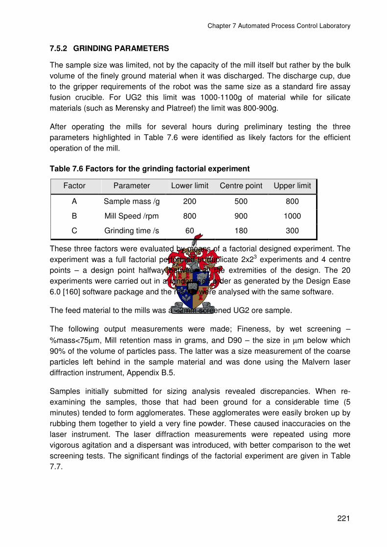
Chapter 7 Automated Process Control Laboratory
221
7.5.2 GRINDING PARAMETERS
The sample size was limited, not by the capacity of the mill itself but rather by the bulk volume of the finely ground material when it was discharged. The discharge cup, due to the gripper requirements of the robot was the same size as a standard fire assay fusion crucible. For UG2 this limit was 1000-1100g of material while for silicate materials (such as Merensky and Platreef) the limit was 800-900g.
After operating the mills for several hours during preliminary testing the three parameters highlighted in Table 7.6 were identified as likely factors for the efficient operation of the mill.
Table 7.6 Factors for the grinding factorial experiment
Factor Parameter Lower limit Centre point Upper limit
A Sample mass /g 200 500 800
B Mill Speed /rpm 800 900 1000
C Grinding time /s 60 180 300
These three factors were evaluated by means of a factorial designed experiment. The experiment was a full factorial performed in duplicate 2x23 experiments and 4 centre points – a design point halfway between all the extremities of the design. The 20 experiments were carried out in a randomised order as generated by the Design Ease 6.0 [160] software package and the results were analysed with the same software.
The feed material to the mills was a <2mm screened UG2 ore sample.
The following output measurements were made; Fineness, by wet screening – %mass<75µm, Mill retention mass in grams, and D90 – the size in µm below which 90% of the volume of particles pass. The latter was a size measurement of the coarse particles left behind in the sample material and was done using the Malvern laser diffraction instrument, Appendix B.5.
Samples initially submitted for sizing analysis revealed discrepancies. When re-examining the samples, those that had been ground for a considerable time (5 minutes) tended to form agglomerates. These agglomerates were easily broken up by rubbing them together to yield a very fine powder. These caused inaccuracies on the laser instrument. The laser diffraction measurements were repeated using more vigorous agitation and a dispersant was introduced, with better comparison to the wet screening tests. The significant findings of the factorial experiment are given in Table 7.7.

Chapter 7 Automated Process Control Laboratory
222
Table 7.7 Results of the grinding factorial experiment
Measurement Significant
Effects Significance
(P)
A 0.0002 Fineness decreased with increasing sample
B 0.02 Fineness increased with higher speed Fineness
C 0.0003 Fineness increased with longer time
C 0.0004 Retention increased with longer grinding time
Mill retention AB 0.005
Retention increased with an increasing sample mass and faster grinding speed
A 0.03 D90 size increased with increasing sample
B 0.058 D90 size decreased with faster milling D90
C 0.008 D90 size decreased with longer milling time
From the results of the factorial experiment both the fineness and the D90 results produced similar data.
To obtain a suitably fine sample material required the grinding to be done at high speed, for a longer time using less sample mass. Using the factorial data it was possible to build a model to predict the mill performance.
Fineness = 57.2 - 0.0182 x Sample mass + 0.0294 x Speed + 0.0444 x Time
With this formula one could calculate the grinding time required to get a 500g sample with a fineness of 85% passing 75µm using a grinding speed of 1000rpm. Solving for the equation, the grinding time required would be 169s.
There were limitations to the model as it was bounded by the design factors originally used. It was also limited to the feed that was used which was relatively coarse. With a finer feed, the model would shift to greater fineness. The last factor was that it was limited to UG2 materials.
The second response examined was the retention within the mill. Preferably this needed to be a minimum as this limited the possibility of sample carry over during grinding. It was not as important as the fineness, which was a critical requirement for the fire assay process. The data showed the importance of the grinding time, as well as the interaction between sample size and time. All these factors indicated that the retention within the mill was dependent on the fineness of the mill product that was discharged.

Chapter 7 Automated Process Control Laboratory
223
To validate this claim the factorial data was re-examined. The milling test work done with 800g of sample showed a reasonable range. This data was reprocessed to examine the correlation of fineness and sample retention and is presented in Table 7.8.
Table 7.8 Relation between fineness and sample retention in the large mill
Retention /g
Fineness
(%mass <75µm)
12.2 71.9
20.9 89.3
16.1 78.4
22.5 94.8
This data indicated that the retention in the mill increased with increasing sample fineness.
This was a physical effect as more of the fine material coated the surfaces of the mill and was retained. This may relate to the static adhesion properties of this fine material, as was noted earlier, this fine material tended to agglomerate. The net result was that finely ground material was more easily retained.
The mill needed to be thoroughly cleaned between samples. It was also predicted that a short grinding cycle with coarse sand would be more effective in flushing the mill than to grind the material for any extended time, as there would be less possibility of retaining the cleaning materials within the mill.
7.5.3 MILL DISCHARGE HOMOGENEITY
A sample was generated by weighing 450g of coarse 2mm graded quartz and weighing 50g of AR grade copper sulphate on top. This sample was extremely inhomogeneous with the bright blue crystals on top of the light brown quartz grains.
This mixture was introduced into the mill and ground. The mill discharge was then examined to be a fine grey powder without any visible signs of segregation. This was a worst-case scenario with materials of extremely different composition and grinding characteristics. The quartz was very coarse (1-2mm) and hard while the copper sulphate crystals were smaller (0.5-1mm) and extremely friable.
The sample was dipped from the top, middle and bottom of the discharge cup to check for homogeneity. The samples were measured by XRF using a loose powder technique in a De Katt sample cup. In addition two more samples were prepared in the

Chapter 7 Automated Process Control Laboratory
224
same way and mixed prior to a dip sample being drawn. The results for the homogeneity testing are shown in Table 7.9 below.
Table 7.9 XRF homogeneity measurements
XRF Cu Kα
/kcps
Average /kcps
Standard deviation
%RSD
Sample 1 2163
Sample 2 2095
Sample 3 top 2103 2114 31 1.5
Sample 3 middle 2149
Sample 3 bottom 2090
All 5 samples 2120 34 1.6
The results from the homogeneity testing were encouraging. Within the limitations of the loose powder technique and the reproducibility of making these samples, the mill discharge was homogeneous.
7.5.4 MILL CONTAMINATION AND CLEANING
The large mills retained sample material and needed to be cleaned out before the next sample was prepared. The mills had an air cleaning cycle with blow-down from the sample input chute and were tested for effectiveness. In addition the mill had quartz dosing to perform flushing of the mills. With the design of the laboratory, there were also 3 mills included, through which different grade materials could be passed to reduce the possibility of cross contamination. This initial work was to examine whether or not this was necessary.
A contamination mixture was made by grinding quartz and copper sulphate together inside the mill. The mill was then put through its cleaning cycle and the residual sample was collected with a 50g quartz sample to examine the contamination within the mill. Measurement of the final sample was done by XRF for the copper content. With this, the contamination of blank samples was measured. From this data the carry over from one sample to the next was calculated.

Chapter 7 Automated Process Control Laboratory
225
A comparison of the contamination of a blank after cleaning the mill with and without air is shown in Figure 7.5.
Figure 7.5 The effect of air cleaning on contamination for the Herzog large mill
Table 7.10 Carryover measurements for the large mill
%Cu
Test 1 (coarse) (no air)
Test 2 (coarse)
Test 3 (fine)
Cu2SO4/SiO2 mixture 3.42 3.42 3.42
Flush 1, 50g quartz 0.653 0.429 0.409
Flush 2, 50g quartz 0.094 0.092 0.081
Flush 3, 50g quartz 0.028 0.029 0.027
Flush 4, 50g quartz 0.013 0.015 0.016
Flush 5, 50g quartz 0.009
The air cleaning cycle of the large mill aided in reducing cross contamination, as the copper Kα peak in Figure 7.5 for the blank quartz after air cleaning was significantly lower than without. It must be noted that the scale was logarithmic and the net counts in the 50g sample without cleaning was 414kcps while with air cleaning this was
Comparison of mill cleaning programs
1
10
100
1000
10000
43.0 44.0 45.0 46.0 47.0 48.0
°2θθθθ
Cu
Kαα αα
/kcp
s (l
og s
cale
)
Quartz blank
Copper sulphate mix
Quartz flush (no air)
Quartz flush (after air)
Comparison of mill cleaning programs
1
10
100
1000
10000
43.0 44.0 45.0 46.0 47.0 48.0
°2θθθθ
Cu
Kαα αα
/kcp
s (l
og s
cale
)
Quartz blank
Copper sulphate mix
Quartz flush (no air)
Quartz flush (after air)

Chapter 7 Automated Process Control Laboratory
226
reduced to 264kcps. Thus air cleaning reduced the contamination by 36%. It was clear that there was measurable carry over after air cleaning of the mill.
From the data of the sequential flushing steps it was noticeable that sequential quartz dosing was effective in flushing the mill, as can be seen in Table 7.10. Particularly a second and third quartz dose reduced carry over from the original sample. It also highlighted the effectiveness of the air cleaning. For test 1 the first flush stage, the air cleaning was omitted and the measured copper in the blank flush was much higher. With the subsequent flushes the air cleaning was turned back on and the contamination was reduced to a similar level to the other tests.
The reduction in contamination is also clearly shown with the XRF plots in Figure 7.6 where sequential quartz flushing reduced the copper signal systematically.
The use of a finer quartz sand of around 0.5-1mm was more effective initially than the very coarse quartz of 3-4 mm used in test 2. This could be related to the bulk volume as there would be more contact of the finer quartz with the mill surfaces prior to milling and it would help to flush the inlet systems. Very fine quartz was of little use as it clogged the inlet systems.
The milling time for the quartz flush was minimised to 20s to avoid the quartz being retained in the mill and contaminating subsequent samples too.
Figure 7.6 The effect of multiple cleaning cycles on contamination
Cleaning of the large mill
1
10
100
1000
10000
43 44 45 46 47 48
°2θθθθ
Cu
Kαα αα
/kcp
s (l
og s
cale
)
Quartz blank
Copper sulphate mix
Quartz flush 1
Quartz flush 2
Quartz flush 3
Quartz flush 4
Quartz flush 5
Cleaning of the large mill
1
10
100
1000
10000
43 44 45 46 47 48
°2θθθθ
Cu
Kαα αα
/kcp
s (l
og s
cale
)
Quartz blank
Copper sulphate mix
Quartz flush 1
Quartz flush 2
Quartz flush 3
Quartz flush 4
Quartz flush 5

Chapter 7 Automated Process Control Laboratory
227
To measure the physical carry over of the original sample into subsequent samples required the calculation of the mass of the original sample needed to produce the copper concentration measured. This equation can be derived to calculate the mass carryover and is shown in Equation 7.1.
10050
M0.0685Cu CO
Quartz ××=%
100 0.0685Cu 50
M QuartzCO ×
×=
% Equation 7.1
Where:
%CuQuartz The copper concentration measured in the quartz blank sample
50 50g Quartz blank sample
6.85 %Cu in the original sample used to contaminate the mill
MCO Mass carry over from the original sample
(excluding any dilution during the cleaning cycle)
The results for the mass carryover calculations are tabulated in Table 7.11.
Table 7.11 Sample carryover measurements
Quartz for cleaning
/g
%Cu in 50g quartz
blank
Mass carryover
/g
% Carry- over in 500g
50.0 0.274 2.00 0.40
100.0 0.246 1.79 0.36
200.0 0.184 1.34 0.27
Using this data, for example if the mill was to prepare a 500g natural fines sample with a platinum grade of 15g.ton-1 and then to prepare a 500g final tail sample with a grade of 0.5g.ton-1. The net contamination of the final tail would change from 0.5g.ton-1 to 0.56g.ton-1 due to the carry over from the high-grade sample.
This was an unacceptable situation and it meant that high-grade samples should be dedicated to their own mill. What could also be done was to flush with sand more than once as this was proven to be very effective in the first tests. Two or three quartz cleaning cycles with 50g each was more effective than one cycle of 100-200g. It could be clearly seen that by adding more quartz simply diluted the effect of the contamination and reduced it proportionally, this can be seen in Table 7.11.

Chapter 7 Automated Process Control Laboratory
228
By contrast multiple cleaning reduced the contaminant concentration by a factor of 5-15 times. Another choice would be to dilute the high-grade sample with quartz before grinding.
7.5.5 FINAL GRINDING TESTS
For the final testing of the mill a global program was set up and tested with varying sample masses on each of the three mills, the grinding program is summarised in Table 7.12. Samples were analysed using laser diffraction for particle size. The trials showed that there were similar results for all three mills and the data was averaged in Table 7.13.
The milling program was tested with up to 800g of feed material and produced a mill discharge that was safely above the specification of 85% passing 150µm. A tighter specification was set for automation of 85% passing 75µm to help ensure homogeneity of the sample for volumetric dosing.
It was noticeable that there were considerably more coarse particles when the mill was fed with a larger mass of sample. This could have been improved by increasing the grinding time. The system could be customised in the future to suit the feed material using an appropriate grinding program that can be specified in the method using the PrepMaster software. The global program was suitable for the grinding of all Modikwa samples irrespective of the masses provided.
Table 7.12 Global grinding program for the Herzog HP1500 mill
Grinding Cleaning
Parameter Setting Parameter Setting
Material input time 10s Air cleaning cycles 3x21s
Material input speed 800rpm Sand dosing time 7s
Grinding time 1 30s Input time 10s
Grinding speed 1 800rpm Sand input speed 800rpm
Grinding time 2 150s Sand grinding time 20s
Grinding speed 2 1000rpm Sand grinding speed 1000rpm
Sample discharge time 20s Sand discharge time 20s
Discharge speed 1000rpm Sand discharge speed 1000rpm
Total time 330

Chapter 7 Automated Process Control Laboratory
229
Table 7.13 Final grinding results
Sample
/g
Sample retention
/g
% Sample retained
Particle size %vol
<75µm
D 10 /µm
D 50 /µm
D 90 /µm
200 16.1 8.1 99.05 0.29 3.45 29.87
500 21.9 4.4 97.03 0.30 4.17 41.89
800 28.3 3.5 90.71 0.32 6.59 70.77
It was observed that the relative retention decreased as the feed mass increased. This tied in with the factorial experiment, where the retention was dependent on the fineness of the discharge and therefore the more finely ground the material (at a fixed mass) the more was retained. In this case, because only the mass was varied, the retention was dependent on the sample mass fed to the mill. The relative retention in the mill increased as the mass decreased because the fineness of the discharge increased with smaller masses.
The large mills were tested on a selection of the UG2 flotation samples a few coarse Platreef feed samples were also passed through the mill to examine whether or not the mill could handle large particle sizes. All samples irrespective of particle size or mass were milled using the global program. The results are shown in Table 7.14.
Figure 7.7 Retention in the large mill with varying sample mass
Sample retained in the Herzog HP 1500 mill
10.0
15.0
20.0
25.0
30.0
0 200 400 600 800 1000
Sample mass /g
Sam
ple
reta
ined
/g
2.0
4.0
6.0
8.0
10.0
% S
ampl
e re
tain
ed
Sample retention /g
% Sample retained
Sample retained in the Herzog HP 1500 mill
10.0
15.0
20.0
25.0
30.0
0 200 400 600 800 1000
Sample mass /g
Sam
ple
reta
ined
/g
2.0
4.0
6.0
8.0
10.0
% S
ampl
e re
tain
ed
Sample retention /g
% Sample retained

Chapter 7 Automated Process Control Laboratory
230
Table 7.14 Results for the grinding tests on UG2 flotation samples
Sample Type Sample Mass
/g
Sample retained
/g
% Sample retention
Before milling
(% volume <75µm)
After milling
(% volume <75µm)
Flash Float tailings 500 22 4.4 - 98.5
Rougher feed 500 16 3.2 27.0 97.4
Scavenger feed 500 30 6.0 79.2 98.1
Rougher cleaner tailings 500 16 3.2 92.2 98.8
Rougher feed 502 24 4.8 27.0 97.5
PPL feed (<10mm) 504 20 4.0 - 91.5
Final tailings 500 24 4.8 41.6 98.2
Final tailings 1000 36 3.6 41.6 93.3
The large mill comfortably achieved the classical specification of 80% passing 150µm in size. The samples prepared were much finer than was achievable using the vertical spindle pulveriser and were similar to the manually operated swing mill as discussed in Section 3.4. This automated design however was much easier to operate and was more consistent since it was not operator dependent.
7.6 AUTOMATED FLUXING
The Herzog automated fluxing machine was a complex piece of equipment. Not a lot of work was done in optimising it, as this was a relatively simple physical process. The accuracy of the volumetric dosing was monitored and optimised to give consistent cuts, adjustments had to be made to the vibratory feeder and the hopper system to achieve consistency. The number of cuts to yield the desired mass of 40g for all three of the dosing systems was determined (each machine had 2 QC slider-dosers and 1 sample slider-doser). The mixing of the sample and flux was examined to determine whether or not the material was adequately mixed. This was achieved with a wire whisk that was rotated and moved up and down inside the internal cup of the machine. It was an efficient process without retaining flux or sample on the wire.
The efficiency of the cleaning cycle was the most important. The internal cup in the machine was examined and found to be efficiently cleaned during the air cleaning cycle. A problem was encountered when there was power failure or other miscellaneous stops during the fluxer operation. This was caused by the hygroscopic

Chapter 7 Automated Process Control Laboratory
231
nature of the sodium hydroxide flux that picked up moisture and agglomerated the flux and sample. This had to be thoroughly cleaned before continuing the operation.
What was done was to check for possible cross-contamination in the equipment. For this a UG2 feed grade material was fluxed and followed by blank silica. The procedure was repeated several times. No significant contamination of the blank material was measured after the flux was fused, separated and analysed on the Spark-OES.
What was apparent was that due to the hygroscopic nature of the flux, problems were encountered with physical loss of the flux/sample if the material stood too long in the machine. Paraffin was added to the flux to reduce the uptake of moisture and worked reasonably well although it did not eliminate the problem. Constant preventative maintenance of the equipment was required for both flux feeding and the internal cup where the material was mixed. The fluxers have redundancy and one could be maintained while the other was in operation.
A number of changes were proposed for future generations of fluxing machines, a number of which were implemented in other Herzog fluxers. Additional work to eliminate the use of sodium hydroxide in the flux is also proposed.
7.7 AUTOMATED FIRE ASSAY PREPARATION
The fusion parameters needed to be tested for the automated system, as there were delays with the loading and unloading of the FIFA furnace using the robot. This allowed the crucible to cool during the process. Even though the parameters were tested manually, they had to be re-examined for the automated system.
The fusion was tested manually first. This was done to check for the lower design limit for a factorial experiment. The results of the preliminary tests are shown in Table 7.15.
Table 7.15 Examination of fusion parameters
Flux /g
Sample /g
Fusion time /min
Fusion Temp.
/°C Description
200 49.5 10 1158 Some un-reacted flux and lead shot in the slag
200 50.0 15 1158 A few lead drops in a viscous slag
200 50.0 20 1160 Complete
The estimated minimum parameter for the fusion was a mass of 50g of UG2 feed material fused with 200g of flux for 12 minutes. It was a deliberate choice to use this parameter, as it was useful to test the boundaries of the fusion.

Chapter 7 Automated Process Control Laboratory
232
7.7.1 FUSION FACTORIAL EXPERIMENT
There was a reasonable amount of confidence that the fusion parameters were close to an optimum at 50g sample, 250g flux, fusing at 1200°C for 15 minutes. To test this, a three level factorial experiment was designed using the Design Expert software [160]. The reason that this choice was made over a conventional 2 level factorial was due to the fact that a three level design gives better resolution of the design space and allows for the evaluation of curvature. It was also better for modelling the optima of the design. With a 3 level design there were no centre points, and there were three factors, a total of 33=27 experiments, some were duplicated and a total of 39 trials were performed. A summary of the factors and design parameters are given in Table 7.16.
The data was analysed for the lead recovery from the flux, palladium grade and rhodium grade. These were the critical parameters. A problem was experienced with the measurement of platinum with the Spark-OES and was discovered to be an interference of bismuth on the platinum 304.3nm line. Since the original result was averaged with the platinum 299.8nm line, the result had a positive bias and therefore had to be ignored.
Table 7.16 Factors for the fusion factorial experiment
Factor Lower level
Middle Level
Upper level
Sample /g 40 40 40
A Flux /g 200 250 300
B Time /min 12 16 20
C Temperature /°C 1150 1200 1250
The points generated in the factorial were of course not exactly at the set point. In performing the factorial analysis, the actual measured values were used to replace all the set point values. This improved the modelling of the data, the results of which are shown in Table 7.17.
The data in Figure 7.8 shows a correlation between button recovery and the palladium or rhodium grade.
The lead recovery calculation was based on the ideal composition of the flux and may have been inaccurate depending on the flux homogeneity and exact fusion conditions. What was interesting was the similarity in the structure of the graphs, where there was a low recovery and a lower palladium grade there was a similar low rhodium point. This indicated an error common to both elements, namely where there was a physical loss of the collector.
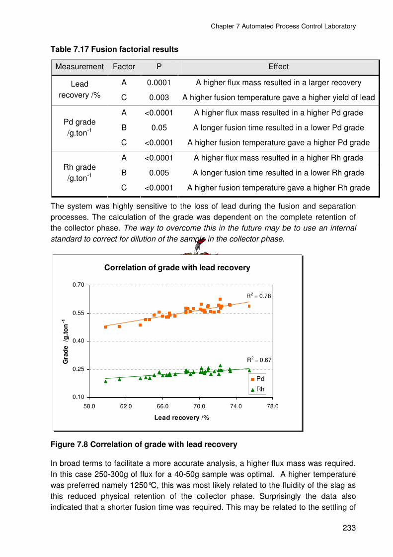
Chapter 7 Automated Process Control Laboratory
233
Table 7.17 Fusion factorial results
Measurement Factor P Effect
A 0.0001 A higher flux mass resulted in a larger recovery Lead recovery /% C 0.003 A higher fusion temperature gave a higher yield of lead
A <0.0001 A higher flux mass resulted in a higher Pd grade
B 0.05 A longer fusion time resulted in a lower Pd grade Pd grade /g.ton-1
C <0.0001 A higher fusion temperature gave a higher Pd grade
A <0.0001 A higher flux mass resulted in a higher Rh grade
B 0.005 A longer fusion time resulted in a lower Rh grade Rh grade /g.ton-1
C <0.0001 A higher fusion temperature gave a higher Rh grade
The system was highly sensitive to the loss of lead during the fusion and separation processes. The calculation of the grade was dependent on the complete retention of the collector phase. The way to overcome this in the future may be to use an internal standard to correct for dilution of the sample in the collector phase.
Figure 7.8 Correlation of grade with lead recovery
In broad terms to facilitate a more accurate analysis, a higher flux mass was required. In this case 250-300g of flux for a 40-50g sample was optimal. A higher temperature was preferred namely 1250°C, this was most likely related to the fluidity of the slag as this reduced physical retention of the collector phase. Surprisingly the data also indicated that a shorter fusion time was required. This may be related to the settling of
Correlation of grade with lead recovery
R2 = 0.78
R2 = 0.67
0.10
0.25
0.40
0.55
0.70
58.0 62.0 66.0 70.0 74.0 78.0
Lead recovery /%
Gra
de /
g.to
n-1
Pd
Rh
Correlation of grade with lead recovery
R2 = 0.78
R2 = 0.67
0.10
0.25
0.40
0.55
0.70
58.0 62.0 66.0 70.0 74.0 78.0
Lead recovery /%
Gra
de /
g.to
n-1
Pd
Rh

Chapter 7 Automated Process Control Laboratory
234
chromite from the UG2 sample in the fusion, as this was also a potential cause of physical loss of the collector.
7.8 SLAG SEPARATION
The automated separator system was designed using an open furnace with a closing lid. The mould was located from the bottom where swung in and up underneath the Cowan separator crucible. The furnace had a hole though the centre in which the crucible was located with the robot. A sleeve protected the furnace from exposure to lead or slag. This system was different to the one used for the development work on the separator crucible presented in Section 5.4. The open design, required for automation, meant that considerable heat was lost from the separator crucible and the furnace temperature needed to be optimised.
A minimum pre-heating time of 20 minutes was required to heat the crucible up to operating temperature. The furnace temperature was increased with 50° intervals from 950°C up to 1200°C. Blockage of the separator occurred with the furnace temperature below 1100°C. The optimum furnace operating temperature was found to be 1150°C and produced a temperature of 900-950°C at the bottom of the separator at the alumina insert, this was critical for efficient separation.
The nitrogen purge on the system was inefficient, although the nitrogen tended to reduce the oxidation of lead it was not sufficient to eliminate it. When the purge flow rate was increased, the oxidation worsened with air being drawn into the hot zone below the separator crucible. Future designs of the furnace and purge systems have been proposed but were not been tested.
Cold water to the mould was supplied using a refrigerated chiller. The cooling of the system was optimised and a temperature of 10°C was found to be optimal. At this temperature there was not too much condensate on the surface of the mould and it could be evaporated from the surface when the mould went into the furnace. The mould had to be inserted 5s before casting to ensure that it was dry.
A number of changes were implemented to the system after it was delivered. For example the mould shape was changed to a tapered design so that the mould could get closer to the separator crucible. Another problem with the slag run off was experienced where slag would stick to the mould arm and jam the mechanism. This problem was solved by introducing a water-cooled deflector plate to rapidly cool the slag. The slag would then break free and fall into the slag bin.
The separator system for the Modikwa process control laboratory worked reliably but needed constant maintenance during operation. Fortunately the system had redundancy and maintenance could be carried out on one separator while the other was in operation without affecting the production of the laboratory. This emphasised

Chapter 7 Automated Process Control Laboratory
235
the importance of having redundancy for equipment that required constant maintenance.
7.9 LEAD BUTTON PREPARATION
The surface of the lead disc needed to be properly prepared for accurate analysis. It was dependent on the quality of the lead discs obtained from separator and the mould. These should not have any holes or slag in them. Preparation of the lead discs was done with a Herzog Non-Ferrous Fine (HN-FF) milling machine.
7.9.1 ISO-PROPANOL COOLING
The spraying of iso-propanol onto the sample during milling was tested. This was done by operating the HN-FF machine in manual mode and spraying the coolant through the nozzle onto the sample. The flow was adjusted to a minimum and was only slightly visible. This was done to conserve the coolant consumption and reduce vapour. It was also necessary for evaporation of the iso-propanol to cool the sample and therefore a thin coating on the surface was beneficial.
7.9.2 LEAD MILLING OPTIMISATION
A factorial experiment was designed using the Design Expert software [160] to optimise the milling of lead buttons with the HN-FF milling machine. The main requirements of the milling stage was to produce a clean, polished and burr free analytical surface. The reason for this was that when the sample was placed on the stand of the spark instrument, a good gas seal was required. The problem with the burr was that it could get trapped beneath the lead disc and cause gas leaks, resulting in poor sparks.
The experiment was designed with three numerical factors and one categorical factor. The latter being the coolant that was either on or off. Each of the data points were performed singly and the centre point was done in triplicate, although with the categorical factor the “centre” point was replicated with both iterations of the factor making it 6 “centre” points in total. A total of 24+2x3=22 experiments were performed. The factors and experimental parameters used in the experiment are summarised in Table 7.18.

Chapter 7 Automated Process Control Laboratory
236
Table 7.18 Factors for the HN-FF milling factorial experiment
Factor Parameter Lower limit Centre point Upper limit
A Cut depth /mm 0.5 1.0 1.5
B Arm Speed /mm.min-1 800 900 1000
C Spindle speed /rpm 60 180 300
D Coolant Off On/off On
With the experiments only the final cutting of the surface of the lead disc was considered, as the HN-NF was setup with two spindles. The first provided a rough cut and was mechanically setup to be 1.5mm below the first. Therefore when more than 1.5mm was to be removed from the disc, the excess was cut off with a coarse cut followed with the polishing cut of the final spindle. The height of 1.5mm was therefore the upper limit for the HN-FF instrument. The summarised results for the experiment are given in Table 7.19.
The lead discs were selected and ranged in mass from 36-42g. The height, diameter and mass of each button were recorded both before and after milling. Other measurements that were made were the number of smear marks, the length of the smear marks, the mass of the burr, and the angle of the arc that the burr occupied on the edge of the disc.
Table 7.19 Results for the lead milling factorial experiment
Measurement Significant Effect
Significance (P)
Burr arc /° B 0.001 Arc decreased with increasing arm speed
BD 0.0002 The number of smears was at a minimum for a slower arm speed with the coolant on.
Smears CD 0.0002
The number of smears decreased with the coolant on and the number of smears was also reduced with the coolant off when a
higher spindle speed was used.
Smear length /mm D <0.0001 The length of the smears decreased when the
coolant was on
Burr mass 22 A <0.0001 The mass/size of the burr increased the more sample material was removed (cut depth).
22 Note: This data was obtained by reprocessing the 4 level factorial into a 3 level factorial by ignoring the effects of the coolant.

Chapter 7 Automated Process Control Laboratory
237
The surface imperfections, like smear marks were highly dependent on whether or not the coolant was on. With the iso-propanol cooling on, the surfaces were cleaner with a more polished finish. The coolant was the overriding effect particularly with the length of the smear marks. It was also found that by reducing the speed of the arm and increasing the spindle speed in conjunction with the use of the coolant prevented smears during milling. The arm speed also affected the length of the burr with a smaller arc being covered with a higher arm speed.
The mass of the burr removed from the edge was dependent primarily on the cut depth. The more material that was removed from the surface the larger the burr. This could clearly be seen as a thin foil on the side of the disc approximately the same width as the depth that was removed, i.e. cut depth 1.5mm≈1.5mm wide burr.
Examining the data showed that the coolant had very little effect on the burr formation but a very significant effect on the polished finish of the analytical surface. For the best finish on the lead disc with the smallest burr, the HN-FF had to operate with the highest spindle speed of 5000rpm for fine milling, an arm speed of 150-200mm.min-1 with the coolant on.
The accuracy of the cutting was examined and summarised in Table 7.20.
Table 7.20 Performance of the HN-FF milling machine
Set point /mm
Average cut
/mm
%RSD Mass removed
/g
0.5 0.43 29.7 2.4
1.0 1.03 7.3 5.8
1.5 1.45 7.6 8.3
The machine operated quite accurately to the set points being on average within 0.07mm of the set point and was within the tolerance of 0.1mm for the machine. However, the repeatability could be poor when the cutting depth was small.
Using a diamond-milling tip was recommended by Herzog to aid with burr removal. Experimentation with a diamond tip was done and had no significant improvement with removing the burr on the edge or the quality of the analytical surface (without coolant). This was because the tungsten carbide tips were new and sharp. It was discovered that the diamond tip remained sharp and resulted in a better sample surface over a prolonged period. In this way it prevented burr formation and was beneficial to the lead sample preparation.

Chapter 7 Automated Process Control Laboratory
238
Two-sided milling was employed and worked well. The two sided milling effectively reduced the cutting depth by lifting and cutting the surface in two directions. It was effective in burr removal, although in saying this it was found to be impossible to remove the burr entirely and instead, the two-sided milling smeared the burr up the side of the lead disc and prevented it from interfering with the analytical surface. The disadvantage with two-sided milling was that it increased the sample preparation time by 30s.
The preparation of standards was required to remove old spark burn marks and a minimum of the sample was to be removed. For this purpose a simple preparation program was used with a cut depth of 0.2mm. If the minimum cutting height of 0.1mm was used then the burn marks were not completely removed. For standards re-preparation, because such a small cutting depth was used there was no burr to speak of and two-sided milling was not required. Two programs were used, one for routine sample preparation and another for SUS and calibration standards re-preparation.
7.10 ANALYTICAL PERFORMANCE OF THE AUTOMATED SYSTEM
The performance of the automated system was checked by introducing QC samples at the fluxing machine. These samples were then analysed automatically by the system. Since the equipment was to be used at the Modikwa plant it was tested using the UG2 feed and tailings QCs, the analytical parameters used are given in Table 7.21.
Table 7.21 Automated preparation parameters for the analysis of UG2 feed and tailings
UG2 Feed and Tailings
Sample mass Volumetrically dosed and weighed, 35-45g
Flux mass Screw fed and weighed, 245-250g (FIFA flux)
Fusion temperature Set point at 1250°C, furnace temperature 1240-1250°C
Fusion time 15 minutes
Casting Poured automatically with the central robot
Slag Separation Automatic with the Cowan separator (at 1150°C)
Button preparation Automatically milled, 1.2mm removed from surface
Measurement SMS with automated Spark-OES
The analytical results from the automated system are tabulated in Table 7.22. The UG2 QC results were extremely good with the analysed value being within two standard deviations of the consensus values. This gave confidence in the automated fire assay preparation and analysis. For Modikwa’s process control requirements the

Chapter 7 Automated Process Control Laboratory
239
intention was to ensure that the results were within 10% relative of the consensus value for representative QCs at tailings levels and 5% for feed grade.
Table 7.22 Analytical results for UG2 feed and tail QC
Pt grade /g.ton-1
Pd grade /g.ton-1
Rh grade /g.ton-1
UG2 Tailings Average 0.82 0.46 0.17
SD 0.07 0.02 0.01
%RSD 8.2 3.9 3.6
Consensus 0.770 ±0.022
0.422 ±0.018
0.161 ±0.007
% Difference 6.5 9.0 5.6
UG2 Feed Average 2.53 1.26 0.48
SD 0.09 0.02 0.01
%RSD 3.4 1.4 2.2
Consensus 2.493 ±0.037
1.233 ±0.027
0.535 ±0.013
% Difference 1.5 2.2 10.2
The tailings values were within 10% for both the %RSD and the relative difference and met the analytical requirements for the tailings sample. For the UG2 feed both the platinum and palladium met the analytical requirement of being within 5% RSD and also within 5% on the consensus values. The rhodium was noticeably lower. The precision of the rhodium determination was good and comparable with classical methods.
The accurate determination of platinum and palladium indicated a quantitative recovery from the automated fire assay system. The reason for the bias on rhodium resulted from problems with standardisation and calibration as this was done during factory acceptance testing with a new factory calibrated ARL 4460 Spark-OES instrument. The instrument was recalibrated at the Modikwa site.
The new automated technology provided an accurate and fully automated analysis with acceptable precision.

Chapter 7 Automated Process Control Laboratory
240
7.11 COMPARISON WITH CLASSICAL METHODS
It was inevitable that comparisons needed to be drawn with the classical methods. The accuracy and precision of the fully automated system was good. The FIFA system was superior to the 4E gravimetric fire assay method, as no correction factors were required. The results were also shown to be more reliable than the silver and palladium prill methods due to inherent problems with the solubility of the prill alloys.
The lead dissolution and nickel sulphide methods remained at the top of the list. In the hands of an experienced chemist they produced the most accurate and reliable analysis but with considerable cost. These manual methods were lengthy and this was where the FIFA system came into its own, it had unparalleled turnaround times of analysis that could not be achieved with conventional methods. This gave the system a much better sample analysis rate.
7.11.1 TURNAROUND TIME
The FIFA system could return an analytical result from the introduction of a dry sample in 38 minutes, after which an analysis could then be received every 3 minutes thereafter. There was no other fire assay, wet chemical or instrumental method that could compare with this at the low grades analysed.
The estimations of minimum turnaround times are shown in Table 7.23. A constraint in the calculation was a minimum step time of 5 minutes. This was a serious handicap for the automated FIFA system since some preparation steps were less than 2 minutes. However this limitation was adequate for this comparison.
The minimum turnaround times for the other classical methods were between 4 and 7 times longer.

Chapter 7 Automated Process Control Laboratory
241
Table 7.23 Turnaround times for classical and automated fire assay
Time /minutes
Analytical steps
Nickel sulphide
Lead dissolution
Ag & Pd Prill
4E FIFA
Filter 10 10 10 10 5
Dry 60 60 60 60 5
Sample Prep
Pulverise 10 10 10 10 10
Fluxing 5 5 5 5 5
Fusion 90 60 60 60 15
Cast 5 5 5 5 5
Slag separation 5 30 5 5 5
Fire Assay
Button preparation 10 5 0 0 5
LT Cupellation 0 0 65 65 0 Cupel
HT Cupellation 0 0 0 60 0
Leach 120 60 30 0 0
Precipitate 10 10 0 0 0
Dissolve 60 60 30 0 0
Wet chemistry
Liquid handling 30 30 30 0 0
Calibrate 10 10 10 0 0 Analysis
Measure 5 5 5 5 5
Minimum turnaround time /min 430 360 325 285 60
Typical laboratory turnaround time /days
2-5 2-5 3-14 1-5
The reason for the fast turnaround time for the FIFA system is best illustrated in the graph shown in Figure 7.9. Substantial time was saved by eliminating the requirement of cupellation or wet chemical steps.

Chapter 7 Automated Process Control Laboratory
242
Time with the FIFA system was also saved during the sample preparation and fusion steps because of optimisation using automation. Instrumental analysis time was also shorter as unlike the instrumental techniques used for the classical methods the spark calibration was continuously maintained and the sample was measured immediately.
Figure 7.9 Comparison of analysis time for the fire assay methods
Another useful comparison to make was the throughput of samples with the number of people required. It was a difficult task to make a useful comparison because the very nature of the classical fire assay was a batch process and there was usually additional capacity for the manual methods. The data is shown in Table 7.24. The table shows the analytical efficiency for the various systems. During operation the FIFA system had the highest efficiency of 5 samples per employee per hour as there were only 2 employees on shift at any one time, when considering an entire 24 hour day the fact that a total of 6 operators were required dropped the efficiency to 1.67 samples per employee per hour. The employees for the Robolab needed only have limited skills (once the laboratory was commissioned) and provided a monitoring and maintenance function to keep the laboratory running
The classical methods required more people due to the larger number of steps in the processes and as the complexity increased the number of employees increased proportionately. The nickel sulphide and lead dissolution methods had the slowest sample throughput and this was one of the reasons for the high cost of these methods. Manual labour as well as highly skilled wet chemical technicians and instrumental technicians were required for those methods. Consumables also contributed a
Comparison of analysis time for classical and automated methods
0
60
120
180
240
Sam
ple
prep
arat
ion
Fire
ass
aypr
epar
atio
n
Cup
ella
tion
Wet
chem
istry
Ana
lysi
s
Tim
e /m
in
Nickel sulphide
Lead dissolution
Ag/Pd Prill
4E
FIFA
Comparison of analysis time for classical and automated methods
0
60
120
180
240
Sam
ple
prep
arat
ion
Fire
ass
aypr
epar
atio
n
Cup
ella
tion
Wet
chem
istry
Ana
lysi
s
Tim
e /m
in
Nickel sulphide
Lead dissolution
Ag/Pd Prill
4E
FIFA

Chapter 7 Automated Process Control Laboratory
243
significant cost to these methods as costly specialised equipment and chemicals were required.
The 4E method was fairly efficient; it also did not require specialist technical labour. This was why it was such an attractive method and has had such a strong foothold in the industry.
The silver and palladium prill methods were halfway between the 4E and nickel sulphide methods. They offered a compromise in accuracy and precision compared with throughput and cost. It must be noted that the efficiency was fairly good if the silver prill method was done alone at around 1.46 samples per employee per hour. However when a rhodium analysis was required the entire process had to be repeated and halved the number of batches analysed and this made the method less efficient. It also had a seriously negative effect on the turnaround for the laboratory as the data had to be collated, repeats had to be done, and this resulted in delays of up to 2 weeks!
Table 7.24 Efficiency of the various fire assay methods
Nickel
sulphide Lead
dissolution Ag & Pd
Prill 4E FIFA
Batch size /samples 10 10 24 24 1
Working day /hours 12 12 12 12 24
Batch time /hours 2.3 2 1.5 1.5 0.1
Batches /per day 5 6 8 (4) 8 240
Total samples 50 60 192 192 240
Samples /hour 4.2 5.0 16.0 16.0 10.0
Employees 11 11 11 8 6 (2)
Analysis rate
/samples per employee per hour 0.38 0.45
1.46 (0.73)23
2.00 1.67
(5.00)24
This simple comparison assumed one piece of equipment to perform each of the steps in the manual methods, it assumed no redundancy and no additional equipment to improve throughput in bottlenecked steps. Laboratories could be specifically modified and improved to handle a specific method, but this was a fair comparison.
23 The analysis rate is halved if a Rh result is required as the sample needs to be repeated
24 The FIFA system is highly efficient on a shiftly basis but when an entire day is considered due to the increase in the number of employees the overall efficiency drops

Chapter 7 Automated Process Control Laboratory
244
7.11.2 COST
The comparison of analysis cost for various methods was difficult because there were so many different variables to consider. For simplicity the analysis of geological materials was considered for the analysis of platinum, palladium and rhodium (as the primary analytes) in duplicate. The analysis costs for the Ag/Pd prill method were averaged from three commercial South African laboratories. The nickel sulphide cost was averaged from two commercial laboratories one South African and the other Australian. The 4E cost was obtained from Anglo Platinum’s Potgietersrus laboratory and due to the variability of the 4E method analysis was always done in triplicate. The cost of the automated FIFA system was a conservative budgetary estimate obtained during the design and was reasonably accurate. The cost comparison is summarised in Table 7.25.
Table 7.25 Cost comparison of the classical fire assay methods to the automated FIFA analysis.
Method Analysis Cost
Elements analysed
Total analytes
Cost per analyte
Additional value
Nickel Sulphide (duplicate)
R750 Pt, Pd, Rh, Au, Ru, Ir
12 R62.50 R0
Ag/Pd Prill (duplicate)
R210 Pt, Pd, Au, Rh 8 R26.30 R0
4E prill (triplicate)
R55 Sum of Pt, Pd, Au and Rh
3 R18.30 R0
Automated FIFA (duplicate)
R40 Pt, Pd, Rh, (Au), (Ru), (Ir)
6 R6.70 R10.00 (R20.10)
The automated FIFA analysis gave the greatest value in terms of cost per analysis. The primary analytes of platinum, palladium and rhodium were analysed routinely. In addition analysis of gold, ruthenium and iridium were achieved as well. Gold and iridium were limited due to their low concentration, but for sufficient concentration an accurate analysis was achieved. Ruthenium was also analysed but had a limited accuracy and certainly the nickel sulphide method was the preferred analysis route. These additional analytes gave a potential added value of R20.10 with the FIFA system, as a concentration below the detection limit in itself was useful information that can be used for geological modelling purposes.
The cost per analyte for nickel sulphide was extremely high but with this additional cost came the most accurate and precise analysis available for the PGE. The Ag/Pd prill method was the next most expensive method, although in routine practice to lower the

Chapter 7 Automated Process Control Laboratory
245
costs, only 33% of the samples are repeated for rhodium analysis using the Pd prill method. This reduced the cost from R210 to R185 per analysis.
The 4E method was cheaper than the nickel sulphide and Ag/Pd prill methods but because only a 4E grade was obtained there was no elemental analysis. This reduced the real value of the method and was compounded by the inaccuracy thereof.
There was little doubt that the automated FIFA analysis system gave good value for the cost of analysis.
7.11.3 SAFETY
Automation has several health and safety consequences. All automated systems are designed to minimise the requirement of an operator. Automated equipment, such as mechanical robots, operate blind on a pre-determined path and can be extremely dangerous. They are designed with torque monitors and would stop if something unexpected were to occur. Considerable damage or injury can occur before the system comes to a halt and it is essential to keep people safe.
To make these systems safe, a “robot circle” was designed. This circle was contained within Perspex safety barriers with interlocks. Should someone open the door and enter the robot circle, the entire system would stop automatically.
Traditional fire assay methods for the analysis for PGE exposes people to hazardous and toxic lead compounds, dust and heat.
The automated FIFA system reduced exposure to heat and the toxic lead fumes from the fusion. All these systems were contained with extraction systems. The system did not use cupellation and as this was the most harmful step due to the generation of lead fumes the requirement for PPE (Personal Protective Equipment) was reduced. This was in line with legislation of the OSH Act [36] where the exposure of people to hazardous materials should be approached in the following manner: eliminate, mitigate and control. The first principle to eliminate can include using automation to avoid exposing people to hazardous materials. Mitigate, implies the use of engineering controls to minimise exposure. These include ventilation and extraction as is done as a standard in fire assay laboratories where lead fluxes are used. These measures reduce the last requirement of the Act, to control the exposure through the wearing of PPE.
However, as with any laboratory equipment, these instruments needed to be maintained and serviced. Under those circumstances the exposure to toxic chemicals could not be completely avoided and the wearing of mandatory PPE such as dust masks, safety glasses, gloves and appropriate clothing was required.

Chapter 7 Automated Process Control Laboratory
246
7.11.4 WASTE
One of the largest sources of waste in the traditional fire assay method was cupel waste that could contain up to 50% lead by mass. The cupels were refractory and secondary lead refiners would not attempt them for recycling. This waste had been disposed off with a waste management company at a designated landfill site.
The largest waste produced by the FIFA system was lead bullion. This was easily recycled and could be considered a minor commodity to recover some assay costs. It was unfeasible to attempt to recycle the PGE as typical values in the lead ranged from 0.5-10ppm.
The automated system reused fusion crucibles up to 10 times before they were discarded. This was possible due to the lowered corrosion on the crucible because of the shortened fusion time. There was also less thermal shock because the crucible remained hot. In routine laboratories crucibles were re-used 3-5 times before they are discarded. For nickel sulphide and lead dissolution method, crucibles were only used once. The automated system reduced cupel waste by 100%. There was additional slag separator waste, but these were re-used 20 times and the total crucible and separator waste was still 10-20% less than the classical methods.
Slag waste for the automated system was about 10% less than the classical lead fire assay methods as the flux masses used were smaller due to optimisation of the fusion.
Unlike the lead dissolution and nickel sulphide methods there was no liquid base metal or acid waste generated by the system, therefore there were no concerns regarding effluent waste.
Fine sample dust and lead flue dust were contained and disposed of in the same manner as conventional fire assay. This was also diminished because there was no cupellation.
All round the automated system was superior in waste management than the classical methods.
7.12 DISCUSSION AND CONCLUSION ON AUTOMATED FIRE ASSAY LABORATORIES
There was little doubt that the automated FIFA system was highly efficient. It gave good accuracy and precision. It optimised equipment use and labour. The method was cost effective because it required less labour. Consumable costs were reduced because the method reused crucibles, separators and was optimised in terms of flux requirements. It produced less waste and some costs were recovered by the recycling of lead.

Chapter 7 Automated Process Control Laboratory
247
It could also produced an analytical result for process control purposes in under an hour and for the first time made real closed loop process control on a PGE concentrator possible.
The entire laboratory was evaluated with each system and piece of equipment independently. The equipment was optimised for the application at each step such as grinding and fusion. The systems were then integrated to a unified whole.
The objectives of the research and development were met:
• The turnaround analysis on low-grade plant streams was within 2 hours with the laboratory located on the plant itself. Traditional fire assay laboratories are no longer needed.
• The accuracy and precision on feed grade steams on Pt >2g.ton-1 were within 5% and were within 10% for tailings streams with Pt <2g.ton-1.
• Quantitative chemical analysis was achieved and correction factors like for the 4E gravimetric method are not needed.
• The number of operators and the required skill level were reduced. The laboratory provides 24-hour analysis on 11 sample streams taken 10 minutes apart and repeated every 2 hours.
• The cost of analysis was reduced with added value.
• The laboratory was well contained and minimised operator exposure to high temperature and toxic lead containing compounds. The automated laboratory improved the health and safety aspects of the fire assay method.
• The automated method was efficient and the laboratories with this design will have increased capacity. This was essential for Anglo Platinum’s expansion program and the projected sample load of mining (underground) and exploration (bore hole) samples.
• Less waste was produced from the laboratory and a significant portion was generated as recyclable metallic lead.
• The automated fire assay process was patented and was a significant development in technology.
Although the Modikwa process control laboratory was the first fully automated fire assay laboratory in the world, two other laboratories have been built and should be commissioned during 2004. This gives confidence that the technology has been embraced and should flourish. A pictorial summary of the automated technology for the laboratory is shown in Figure 7.10 and Figure 7.11.

Chapter 7 Automated Process Control Laboratory
248
A. Robot charging the mill for grinding. B. The interior of the mill with motor and retaining springs
C. A view inside the grinding vessel showing the grinding disks and the lid.
D. Dosing of flux into the internal cup within the fluxer. E. QC sample dosing inside the fluxer.
F. Sample and flux are mixed with a stirrer using a wire whisk. G. Flux mixture is dosed through a funnel into a hot crucible.
H. Loading of crucible with flux/sample charge into the FIFA furnace to perform the fusion.
I. FIFA furnace removed from beneath the hood and opened for maintenance. J. Interior of the furnace revealing the heating elements and refractories.
Figure 7.10 Photographs of the large grinding mills, fluxing machine and FIFA furnaces for the automated laboratory
A. B.
Motor
Counter weight
Grinding Vessel
Springs
C.
Grinding Vessel
Grinding Disks
Lid
Sample Inlet
D. E.
Sample Dosing Internal
Cup Balance
Vibrator
QC Hopper
F.
FIFA Furnace
Hot Crucible
G.
Stirrer
FIFA Pedestal
Robot
Fluxing Machine
H.
FIFA Furnace
Extraction Hood I.
J.
Chimney
Heating Elements
Refractory Ceramics
Bottom Furnace
Entry

Chapter 7 Automated Process Control Laboratory
249
A. Robot retrieves a crucible containing a molten charge from the FIFA furnace after fusion.
B. The robot casts the molten fire assay fusion from the crucible into the slag separator unit.
C. View of slag draining from the slag separator crucible.
D. The robot removes a used separator crucible. E. The alumina sleeve protects the separator furnace from slag. The cutout allows heat (and nitrogen) to the critical zone of the separator.
F. The chute and bin for the disposal of used crucibles. G. The slag bin located below the furnace in the slag separator unit.
H. Automatic analysis on the ARL 4460 Spark-OES instrument with the SMS robot.
Figure 7.11 Photographs of the slag separator and automated spark analysis technology
A. B.
Separator Furnace
Furnace Lid
Separator Crucible
C.
Slag Drain
Furnace Lid
Separator Crucible
Empty Crucible
D.
Furnace Refractories
Used Separator Crucible
Cut-out
Alumina Sleeve
F. Separator Furnace
Crucible Bin
Chute
G
Slag Bin
Slag

250
CCHHAAPPTTEERR 88
8 OVERALL CONCLUSIONS
This thesis delineates a systems engineering approach to develop a fully automated fire assay laboratory for fast process control analysis at a flotation concentrator plant. The physical and chemical characteristics and technology of each subsystem were investigated in turn and the critical factors that influence accuracy, precision and analysis time were identified and optimised.
The thesis therefore has two major components:
• Method development and design: A scientific investigation of how the fundamental operating, physical and chemical characteristics could be selected for optimal accuracy, precision and minimise analysis time. This was done on the sub-systems individually.
• Systems integration for automation: The selection of the methods and technology for automation to form a robust integrated system. The optimisation and interdependence of subsystems were considered. By optimising for example the grinding, the effect of contamination of subsequent steps was eliminated.
8.1 HISTORICAL DEVELOPMENT
Research started with a simple idea that was uncovered by observation in the first lead fire assay time line experiment in 1997 where it was identified that the fusion time could be significantly reduced. This observation encouraged Mr. W. Brits to initiate his research into the use of inductive heating for a dedicated fire assay fusion machine. An assay process that was later patented. The investigation of inductive heating and classical fire assay led to flux development in the fire assay field which gave a better fundamental understanding of the process and promoted alternative components on fluxing that led to faster fusion.
The lead dissolution method was developed between 1998-1999 due to inherent problems associated with classical fire assay using cupellation. Once cupellation was conclusively identified as the major problem area, significant advances on the other aspects of fire assay could be made. The lead dissolution method allowed for accurate assessment of the lead fire assay fusion. For the first time fusion research was divorced from the inherent inaccuracy of cupellation. The lead dissolution method allowed the preparation of matched lead fire assay standards for spark analysis, a key component of automated fire assay.

Chapter 8 Overall Conclusions
251
Early exploration of dedicated fire assay fusion machines using the induction principle provided key fundamental information for the fusion process using automation. Although unsuccessful, it provided a catalyst for more in-depth research by specialised automation vendors.
Development with IMP from 2000-2004 showed that a team of diverse individuals was needed to breakthrough on novel technologies. The fire assay method patent was definitive of this achievement. Objective views and teamwork were essential for success. Affiliations with specialist automation companies were required as this was a highly specialised field, cross-pollination of ideas and information sharing were essential when the method was automated. The importance of experience could not be overlooked.
It was also shown that it was useful to keep to tried and trusted technology and re-design to meet automation requirements. Radically new technology should only be resorted to when existing technology could not fulfil the requirements of automation. This reduced the risk and significantly decreased the development time. One such example was the use of microwave drying for the filter cake. The fact that samples could be dried to constant mass without wasting time was important and could not be easily achieved with conventional heating. The Fast In-line Fire Assay (FIFA) fusion was an example of using existing technology by re-designing it. By bottom loading a conventional furnace made automation of the fusion step possible. The development time for the FIFA system was in the order of 6 months compared to the incomplete development of the induction furnace that took in excess of 4 years.
The work was culminated in May of 2003 with the installation of a fully automated laboratory at the flotation plant at the Modikwa Platinum Mine.
The automation supplier and vendor could build reliable equipment, but the customer needed to refine and optimise the system to his requirements. The equipment was highly sophisticated and needed to be properly optimised for best results. Therefore the commissioning of these systems took a considerable amount of time. One of the biggest problems with the automation system was that it was perceived to be “plug and play: it arrives, you switch it on and you get results”. This was not the case: the system was installed, commissioned, optimised and finally produced results. To the uninformed this process of installation would have been unacceptable. The system was fully commissioned and operational by October of 2003.
Another misconception was that the automated system did not require people to operate it and that that job losses would result. Nothing could be farther from the truth, the Robolab needed people to look after and maintain it. The laboratory needed different skills and was more like a production plant. Where before an analytical chemist would be hired, a suitable high school graduate was employed and trained.

Chapter 8 Overall Conclusions
252
The skills required were less specialised for routine operation and was a considerable advantage due to the remote location. However for commissioning and support, particularly during installation, highly specialised personnel were required and support from the automation vendor was essential. Training played a significant role in the operation of the laboratory. Since the technology was radically new in-house training with the vendor was undertaken and was largely focused on preventative maintenance and replenishment of consumables. The laboratory was highly efficient and used its resources well. The Robolab created new jobs in a place were no conventional laboratory could survive, or never before would have been considered.
With these humble beginnings of a process control laboratory in a plant at a remote site, there is little doubt that fire assay and the assaying profession is changed forever. It is likely that in the next 20 years that there will be fewer and fewer manual fire assay laboratories because of advantages of cost, speed, accuracy and safety of these automated systems. A point is that the first large production laboratory using this technology for the accurate analysis of geological, mining and exploration samples has been designed and built. The laboratory will eventually have a capacity of 60 000 samples a month and is to come into operation during 2004. This provides the much needed momentum to move this technology from the prototype phase into the real world.
8.2 HIGHLIGHTS OF THE DEVELOPMENT WORK
Some of the key developments achieved during this work both with the automation vendor, instrument developer and the Anglo Platinum Research Centre were:
• Existing technology for the sampling, filtering, drying and grinding of flotation plant samples were evaluated and where necessary, modified for this application.
• The fusion system was re-designed to a bottom-loading configuration called FIFA (Fast In-line Fire Assay) to make automation with a central robot possible. With automation, a pre-heated fusion crucible was used to save time, an option not available for manually operated systems.
• A fast fusing flux was developed for automation that provided a quantitative collection of PGE in 15 minutes compared to classical fusion techniques that took 60 minutes.
• A fire assay oxygen lance was developed to selectively oxidise nickel and sulphur from the lead collector. This technology allowed for less matrix problems for the determination of the PGE in the lead collector directly using spark optical emission spectrometry.

Chapter 8 Overall Conclusions
253
• A robust automated separator system was developed to isolate the lead collector from the fusion in the molten state. This allowed the automation of the entire fire assay process.
• Methods to prepare lead standards for the calibration of spark optical emission spectrometers were undertaken as these alloys were not commercially available. This made the accurate and precise determination of PGE in the lead collector phase possible. It was also a key component for a fully automated system.
• Analytical protocols were developed and optimised for the analysis of PGE in lead using an ARL 4460 spark optical emission spectrometer.
• A fully automated system was developed that could meet the accuracy and precision requirements of tailings and feed grade samples.
The new fire assay technology and flux development that included the FIFA system, oxygen lance and separator were all patented in conjunction with the automation vendor. This technology made the first fully automated fire assay system a reality.
There were significant cost savings associated with automation. The speed of analysis was significantly improved, that was not achievable with classical fire assay methods. The analysis was both accurate and precise without the high repeat rate and mix-ups that were common with manual methods. The accuracy was shown to be within 10% for tailings samples of less than 2g.ton-1 and within 5% for feed grade of greater than 2g.ton-1 on platinum, the key process control element. The precision was within 10% RSD for tailings and 5% RSD for feed on platinum. Accurate analysis was also obtained for palladium and rhodium. The Robolab was able to exceed its design in many areas, the most significant being the turnaround time for a sample analysed in duplicate of 38 minutes compared to the initial design of 120 minutes.
8.3 A LOOK INTO THE FUTURE
With the improved sample preparation that automation offers, it may be possible to miniaturise the fire assay process and this may have more significant cost savings in the future. The oxygen lance is expected to play a larger role in the future as people push to further reduce the detection limits and improve accuracy.
Flux development will probably continue in the effort to fuse chromite samples. It is predicted that other slag systems such as phosphates may significantly improve the dissolution of chromite. The use of sodium hydroxide in the flux is problematic due to the hygroscopic nature of the compound and alternatives are likely to be investigated. Other collectors that may be used could include copper, bismuth, silver and perhaps even nickel sulphide.

Chapter 8 Overall Conclusions
254
Optimisation of the fusion process may improve the detection limit of this technology by a factor of 3-10 times in the near future by reducing the mass of the collector phase.
Instrumentation may improve and other vendors may compete to supply instruments for the analytical measurement. It is likely that a fire assay machine using inductive heating may be brought to the market in the next few years. Other heating sources such as microwaves and gas could also be used for the fusion.
It is foreseen that fire assay albeit in an automated form will continue to provide the backbone of PGE analysis of low-grade materials in the precious metal industry.

255
RREEFFEERREENNCCEESS
1. McDonald, D.; “A History Of Platinum”, Johnson Matthey and Co., 254 pages, 1960.
2. Chronology of platinum: available on the internet: http://www.myplatinum.co.uk, December 2003.
3. Kendall, T.; “Platinum 2003”, Johnson Matthey Report, available on the internet: http://www.platinum.matthey.com, May 2003.
4. Platinum coins: Internet: http://www.certifiedmint.com, December 2003.
5. Bloomfield, L.A.; “Catalytic Converter”, Scientific American, February 21, 2000. Internet: http://www.scientificamerican.com
6. Clean Air Act, USA: Internet: http://www.epa.gov - Plain English Guide to the Clean Air Act, 1970, December 2003.
7. Oberthur, T.; Cabri, L. J.; Weiser, T.; McMahon, G.; Muller, P.; “Pt, Pd And Other Trace Elements In Sulphides Of The Main Sulphide Zone, Great Dyke, Zimbabwe – A Reconnaissance Study”, Can. Min, vol. 35, p 567-609, 1997.
8. Vermaak, C.F.; “The Platinum Group Metals: A Global Perspective”, Mintek, Private Bag X3015, Randburg, 2195, South Africa. 247 pages, 1995.
9. Viljoen, M.J.; Hieber, R.; “The Rustenburg Section Of Rustenburg Platinum Mines Limited, With Reference To The Merensky Reef” extracted from Anhaeusser, C.R.; and Maske, S.; “Mineral deposits of Southern Africa”, Volumes I and II, Geol. Soc. S. Afr., xxx pages, xxxx.
10. Anglo Platinum’s expansion program: available on the internet: http://www.angloplatinum.com, select → Our Operations → Expansion Projects → Overview, December 2003.
11. Spicer, D.; “Platinum Group’s Capex Surges…”, Mining Weekly, p. 4, August 30-September 5, 2002.
12. Creamer, T.; “…Strategic Review Of Projects Under Way”, Mining Weekly, p. 5, August 30-September 5, 2002.
13. Mbeki, T. (President); Mineral and Petroleum Resources Development Act, 3 October 2002: On the internet: http://www.acts.co.za/mprd_act/index.htm, December 2003.

256
14. Anonymous, “A Basket Full Of Minerals”, SA Mining, Coal, Gold & Base Minerals, p. 14, September 1997.
15. Aplan, F.F.; “Flotation”, Kirk-Othmer Encyclopedia of Chemical Technology, 3rd Edition, Vol. 10, p. 523-547, 1980.
16. Lanam, R.D.; Zysk, E.D. “Platinum-Group Metals”, Kirk-Othmer Encyclopedia of Chemical Technology, 3rd Edition, Vol. 18, p. 228-253, 1980.
17. Hochreiter, R.C.; Kennedy, D.C.; Muir, W.; Wood, A.I.; “Platinum In South Africa”, J. S. Afr. Inst. Min. Metall., Vol. 85, no. 6, p. 165-185, June 1985.
18. “Anglo Platinum”, review by SA Mining, August 2002.
19. Personal communication: Visser, M.; Assistant Chief Chemist, Anglo Platinum Research Centre, quotation from SGS Lakefield Laboratory, 58 Melvill Str., Booysens, South Africa, nickel sulphide cost estimate of R750 for analysis done in duplicate, 23 December 2003.
20. Anglo Platinum’s Black Empowerment Enterprise (BEE), available on the internet: http://angloplatinum.com, select → Sustainable Development → Economic Impacts → BEE/HDSA, March 2004.
21. Davison, B. (CEO); “Anglo American Platinum Corporation Limited, Annual Report 2002”, 2003.
22. Personal communication with Hepburn, J.; Assistant Chief Chemist, PPRus Laboratory, January 2004.
23. “Amdel” In-stream XRF analyser, Thermo Gamma-Metrics Pty. Ltd., P.O. Box 292, Torrensville Plaza, 5031, Australia. On the internet: http://www.thermogammametrics.com.au
24. Courier XRF analyser, Outokumpu, South Africa: Outokumpu Technology Pty. Ltd. (Market Area Africa) P.O. Box 4197, Halfway House, 1685, South Africa. On the internet: http://www.outokumpu.fi.
25. Mostert, A.B.; Hofmeyr, P.K.; Potgieter, G.A.; “The Platinum-Group Mineralogy Of The Merensky Reef At The Impala Platinum Mines, Bophuthatswana”, Economic Geology, Vol. 77, p. 1385-1394, 1982.

257
26. Gain, S.B.; Mostert, A.B.; “The Geological Setting Of The Platinoid And Base Metal Sulphide Mineralisation Of The Bushveld Complex In Drenthe, North Of Potgiertersrus”, Economic Geology, Vol. 77, p. 1395-1404, 1982.
27. McLaren, C.H.; De Villiers, J.P.R.; “The Platinum-Group Chemistry And Mineralogy Of The UG2 Chromitite Layer Of The Bushveld Complex”, Economic Geology, Vol. 77, p. 1348-1366, 1982.
28. Kinloch, E. D.; “Regional Trends In The Platinum-Group Mineralogy Of The Critical Zone Of The Bushveld Complex, South Africa”, Economic Geology, Vol. 77, p. 1328-1347, 1982.
29. Kingston, G.A.; El-Dosuky, B.T.; “A Contribution On The Platinum-Group Mineralogy Of The Merensky Reef At The Rustenburg Platinum Mine”, Economic Geology, Vol. 77, p. 1367-1384, 1982.
30. Personal communication: Schouwstra, R.; Head of the Mineralogy Department at the Anglo Platinum Research Centre, November 2003.
31. Hurlbut Jr., C.S.; Klein, C.; “Manual Of Mineraology (After J. D. Dana)”, 19th Edition, 352 pages, 1977.
32. Cabri, L.J.; “Platinum-Group Elements: Mineralogy, Geology, Recovery”, The Canadian Institute of Mining and Metallurgy, Special Volume 23, 267 pages, 1981.
33. Blackburn, W.H.; Dennen, W.H.; “Encyclopaedia Of Mineral Names”, The Canadian Mineralogist, Special Publication 1, 360 pages, 1997.
34. Schouwstra, R.P.; Kinloch, E.D.; Lee, C.A.; “A Short Geological Review Of The Bushveld Complex”, Platinum Metals Rev., Vol. 44, No. 1, p. 33-39, 2000.
35. Liddell, K.S.; McRae, L.B.; and R.C. Dunne, “Process Routes For The Benefaction Of Noble Metals From Merensky And UG2 Ores”, Mintek Review No. 4, 1986.
36. De Klerk, F.W. (president); Occupational Health and Safety (OSH) Act, 1993, of interest are the General Safety Regulations, 1993; Hazardous Chemical Substances Regulations, 1995; Lead Regulations, 2001; Noise-induced hearing loss Regulations, 2003; available online on the internet: http://www.acts.co.za, March 2004.
37. Cowan, G.M.; Hohenstein, B.F.; McIntosh, K.S.; Hofmeyr, P.K.; Patent P21402PC00, “Assaying Method”, patented by Innovative Met Products (Pty) Ltd., Corner Commissioner and Christopher Streets, Boksburg East Industrial Township, Boksburg, 1459, South Africa. March 2001.

258
38. Van Loon, J.C.; Barefoot, R.R.; “Determination of the Precious Metals: Selected Instrumental Methods”, John Wiley and Sons, 276 pages, 1991.
39. Gowing, C.J.B.; Potts, P.J.; “Evaluation Of A Rapid Technique For The Determination Of Precious Metals In Geological Samples Based On Selective Aqua Regia Leach”, Analyst , Vol. 116, p. 773-779, 1991.
40. Reddi, G.S.; Ganesh, S.; Rao, C.R.M.; Ramanan, V.; “Determination Of Gold In Geological Materials By Atomic Absorption Spectrometry After Bromine And Hydrochloric Acid Extraction At Room Temperature”, Analytica Chimica Acta, Vol. 260, p. 131-134,1992.
41. Palmer, I.; Palmer, R.; Steele, T.W.; “The Separation Of Platinum, Palladium, Rhodium And Gold From Ores And Concentrates By Aqua Regia Extraction And By High-Temperature Chlorination Followed By Acid Leaching”, Journal of the South African Chemical Institute, Vol. 25, p. 190-197, 1972.
42. Khvostova, V.P.; Golovnya, S.V.; “Chemical Methods Of Breaking Down Platinum-Containing Ores And Rocks”, Industrial Laboratory, Vol. 48, No. 7, p.631-636,1982.
43. Al-Bazi, A.J.; Chow, A.; “Platinum Metals-Solution Chemistry And Separation Methods (Ion-Exchange And Solvent Extraction)”, Talanta, Vol. 31, No. 10A, p. 815-836, 1984.
44. Rehkamper, M.; Halliday, A.N.; “Development Of New Ion-Exchange Techniques For The Separation Of The Platinum Group And Other Siderophile Elements From Geological Samples”, Talanta, Vol. 44, p. 663-672, 1997.
45. Makishima, A.; Nakanishi, M.; Nakamura, E.; “A Group Separation Method For Ruthenium, Palladium, Rhenium, Osmium, Iridium And Platinum Using Their Bromo Complexes And An Anion Exchange Resin”, Analytical Chemistry, Vol. 73, p. 5240-5246, 2001.
46. Chen, Z.; Fryer, B.J.; Longerich, P.; Jackson, S.E.; “Determination Of The Precious Metals In Milligram Samples Of Sulphides And Oxides Using Inductively Coupled Plasma Mass Spectrometetry After Ion Exchange Preconcentration”, Journal Of Analytical Atomic Spectrometry, Vol. 11, p. 805-809, 1996.
47. Rehkamper, M.; Halliday, A.N.; Wentz, R.F.; “Low-Blank Digestion Of Geological Samples For Platinum-Group Element Analysis Using A Modified Carius Tube Design”, Fresenius J. Anal. Chem., Vol. 361, p. 217-219, 1998.

259
48. Perry, B.J.; Speller; D.V.; Barefoot, R.R.; Van Loon, J.C.; “A Large Sample, Dry Chlorination, ICP-MS Analytical Method For The Determination Of Platinum Group Elements And Gold In Rocks”, Canadian Journal of Applied Spectroscopy, Vol. 38, No. 5, p. 131-136, 1993.
49. Van Loon, J.C.; Szeto, M.S.; Howson, W.W.; Levin, I.A.; “A Chlorination-Atomic Spectrometry Method For The Analysis Of Precious Metal Samples”, Atomic Spectroscopy, Vol. 5, No. 2, p. 43-45, 1984.
50. Kallmann, S.; Maul, C.; “Referee Analysis Of Precious Metal Sweeps And Related Materials”, Talanta, Vol. 30, No. 1, p. 21-38, 1983.
51. Bettinelli, M.; ”Determination Of Trace Metals In Siliceous Standard Reference Materials By Electrothermal Atomic Absorption Spectrometry After Lithium Tetraborate Fusion”, Analytica Chimica Acta, Vol. 148, p.193-201, 1983.
52. Jin, X.; Zhu, H.; “Determination Of Platinum Group Elements And Gold In Geological Samples With ICP-MS Using A Sodium Peroxide Fusion And Tellurium Co-Precipitation”, Journal of analytical atomic spectrometry, Vol. 15, p. 747-751, 2000.
53. Beamish, F.E.; Van Loon, J. C.; “Recent Advances In The Analytical Chemistry Of The Noble Metals”, Pergamon Press, 1972.
54. Haffty, J.; Riley, L.B.; Goss, W.D.; “A Manual On Fire Assaying And Determination Of The Noble Metals In Geological Materials”, Geological Survey Bulletin 1445, 1977.
55. The Holy Bible, King James Version translated in 1611.
56. Coulson, R.E.; “The Origins Of Quantitative Inorganic Analysis”, Talanta, Vol. 1, p. 256-262,1958.
57. Agricola, G.; ”De Re Metallica”,1556. English translation by Hoover, H.C.; Hoover, L.H.; 1912, Dover Publications, unabridged reprint, 638 pages, 1986.
58. Biringuccio, V.; ”Pirotechnia”,1540. English translation by Smith, C.S.; Gnudi, M.T.; 1942, Dover Publications, revised reprint, 476 pages, 1990.
59. Bugbee, E.E.; “A textbook of fire assaying”, Colorado School of Mines, 1922, 3rd edition, 314 pages, 1981.
60. Von Loon, J.C.; “Accurate Determination Of The Noble Metals. I. Sample Decomposition And Methods Of Separation”, Trends in analytical chemistry, Vol. 3, No. 10, p. 272-275,1984.

260
61. Kallmann, S.; “A Survey Of The Determination Of The Platinum Group Elements”, Talanta, Vol. 34, No. 8, p.677-698, 1987.
62. Barefoot, R.R.; Von Loon, J.C.; “Recent Advances In The Determination Of The Platinum Group Elements And Gold”, Talanta, Vol. 49, p. 1-14, 1999.
63. Rao, C.R.M.; Reddi, G.S.; ”Platinum Group Metals (PGM); Occurrence, Use And Recent Trends In Their Determination”, Trends in analytical chemistry, Vol. 19, No. 9, p. 565-586, 2000.
64. Mills, K.C; “Structure Of Liquid Slags”, Chapter 1, “Slag Atlas”, 2nd Edition, edited by Verein Deutscher Eisenhüttenleute, p1-8, 1995.
65. Levin, E.M.; Robbins, C.R.; McMurdie, H.F.; ”Phase Diagrams For Ceramicists”, American Ceramic Society ,1966.
66. Gilchrist, J.D.; “Extraction Metallurgy”, Pergamon Press, xxx pages, 1967.
67. Gaskell, D.R.; “Introduction To The Thermodynamics Of Materials”, 3rd Edition, Taylor & Francis, 568 pages, 1995.
68. HSC Chemistry for Windows, version 4.1, available from Outokumpu Research Oy, Information service, P. O. Box 60, FIN – 28101 Pori Finland.
69. Smithells, C.J.; “Metals Reference Book”, 5th Edition, Butterworths, 1566 pages, 1978.
70. Richardson, R.F.; “Physical Chemistry Of Melts In Metallurgy, Volume 2”, Academic Press, 1974.
71. Perry, R.H.; Chilton, C.H.; “Chemical Engineer’s Handbook”, 5th Edition, Mcgraw-Hill, 1973.
72. Mills, K.C; “Viscosities Of Molten Slags”, Chapter 9, “Slag Atlas”, 2nd Edition, edited by Verein Deutscher Eisenhüttenleute, p. 349-402, 1995.
73. Keene, B.J.; Mills, K.C; “Densities Of Molten Slags”, Chapter 8, “Slag Atlas”, 2nd Edition, edited by Verein Deutscher Eisenhüttenleute, p. 313-348, 1995.
74. Riebling, E.F.; “Volume Relations In Na2O.B2O3 And Na2O. SiO2.B2O3 Melts at 1300°C”, Journal of the American Ceramic Society, Vol. 50, p.46-54, 1967.
75. Auer, D.; McIntosh, K.S.; Anglo Platinum Internal Research Report, “Interim Report: Fundamentals Of Fire Assay” Project reference RPMC00.C9195, 1997.

261
76. van Wyk, E.; Dixon, K.; “The Recovery Of Platinum-Group Metals And Gold By The Lead-Collection Step Of The Fire-Assay Procedure”, South African Institute for Mining and Metallurgy (Mintek), Report, No. M88, 1983.
77. Hansen, M.; “Constitution Of Binary Alloys”, McGraw-Hill, 1305 pages, 1958.
78. Elliott, R.P.; “Constitution Of Binary Alloys, First Supplement”, McGraw-Hill, 877 pages, 1965.
79. Steele, T.W.; Robert, R.V.D; van Wyk, E.; Ellis, P.J.; “An Examination Of Fire-Assay Techniques As Applied To Chromite-Bearing Materials”, South African Institute for Mining and Metallurgy (Mintek), Report, No. 1905, 1977.
80. Robert, R.V.D.; Nell, J.; Vine, R.L.; “An Investigation Into Some Aspects Of The Fire-Assay Procedure With Lead As A Collector For The Noble Metals”, South African Institute for Mining and Metallurgy (Mintek), Report No. M412, 1997.
81. Yali, S.; Xiyun, G.; Andao, D.; “Determination Of Platinum Group Elements By Inductively Coupled Plasma-Mass Spectrometry Combined With Nickel Sulphide Fire Assay And Tellurium Ocprecipitation”, Spectrochimica Acta, Part B No. 53, p. 1463-1467, 1998.
82. Juvonen, R.; Kallio, E.; Lakomaa, T.; “Determination Of Precious Metals In Rocks By Inductively Coupled Plasma Mass Spectrometry Using Nickel Sulphide Concentration. Comparison With Other Pre-Treatment Methods”, Analyst, Vol. 119, p. 617-621, 1994.
83. Lenahan; W.C.; de L. Murry-Smith, R.; “Assay And Analytical Practice In the South African Mining Industry”, 640 pages, 1986.
84. McIntosh, K.S.; Anglo Platinum Internal Research Report, “The Analysis Of UG2 Chromite Samples By Lead Collection Fire Assay. Report 3: The Cupellation Of Chromite And Merensky Samples.” Project reference RPMC00.C9197, 1999.
85. McIntosh, K.S.; Vermeulen, J.M.; Anglo Platinum Internal Research Report, “An Investigation Of The Lead Collection Fire Assay Technique”, Project Reference: RPMC00.C8197, 1999.
86. Andrews, L.; Mineralogy: Anglo Platinum Research Centre, Memorandum (M/00/65), “Scanning Electron Microscope Examination Of Prills And Cupel Scrappings”, 2000.
87. McIntosh, K.S; Auer, D.; Anglo Platinum Internal Research Report, “The Silver Prill Method Revisited”, Project Reference: M/RD/CP/01/A403/A, 2001.

262
88. Andrews, L.; Mineralogy: Anglo Platinum Research Centre, Memorandum (M/00/62), “Scanning Electron Microscope Investigation Of A PGM Residue”, 2000.
89. McIntosh, K.S.; Vermeulen, J.M.; Anglo Platinum Internal Research Report, “The Lead Button Dissolution Method”, Project Reference: RPMC00.C8197, 1998.
90. Diamantatos, A.; “Accurate Determination Of Platinum, Palladium, Gold And Silver In Ores And Concentrates By Wet Chemical Analysis Of The Lead Assay Button”, Analyst, Vol. 111, p. 213-215, 1986.
91. Hobart, E.W.; Kallmann, S.; “Hydrobromic Acid Dissolution Of Lead Buttons For PGM Analysis”, Ledoux and Company, 359 Alfred Ave., Teaneck, New Jersey 07666, USA, 1990.
92. Jackwerth, E; Hohn, R; Musaick, K.; “Preconcentration Of Traces Of Ag, Au, Bi, Cu, And Pd, From Pure Lead By Partial Precipitation Of The Matrix With NaBH4 As A Reducing Agent”, Fresenius Z. Anal. Chem., Vol. 299, p. 362-367, 1979.
93. Williamson, J.E.; Savage, J.A.; “The Determination Of Osmiridium In Witwatersrand Ores”, Journal of the South African Institute of Mining and Metallurgy, January 1965.
94. Steele, T. W.; Robért, R.V.D; van Wyk, E.; Palmer, R.; “Concentration Of The Noble Metals By A Fire Assay Technique Using Nickel Sulphide As A Collector”, National Institute for Metallurgy (Mintek), Report No. 1371, 1971.
95. Robért, R.V.D; van Wyk, E.; Palmer, R.; “The Development Of A Fire Assay Procedure Using Nickel Sulphide As The Collector For The Noble Metals”, Bulletin of the South African Institute of Assayers and Analysts, No. 16, 1972.
96. Steele, T.W.; Dixon, K.; Jones, E.A.; Rasmussen, S.; Robért, R.V.D.; “The Efficiency Of The Fire Assay Procedure With Nickel Sulphide As The Collector In The Determination Of Platinum, Silver, Gold, And Iridium”, National Institute for Metallurgy, Report No. 1714, 1975.
97. Hoffman, E. L.; Naldrett, A. J.; van Loon, J. C.; Hancock, R. G. V.; Manson, A.; “The Determination Of All The Platinum Group Elements And Gold In Rocks And Ore By Neutron Activation Analysis After Preconcentration By A Nickel Sulphide Fire-Assay Technique On Large Samples”, Analytica Chimica Acta, No. 102, p. 157-166, 1978.
98. McDonald, I.; Hart, R.J.; Tredoux, M.; “Determination Of The Platinum-Group Elements In South African Kimberlites By Nickel Sulphide Fire-Assay And Neutron Activation Analysis”, Analytica Chimica Acta, No. 289, p. 237-247, 1994.

263
99. Parry, S.J.; Asif, M.; Sinclair, I.W.; “Radiochemical Fire Assay For The Determination Of The Platinum Group Elements”, Journal of Radioanalytical and Nuclear Chemistry Articles, Vol. 123, No. 2, p. 593-606, 1988.
100. Date, A.R.; Davis, A.E.; Cheung, Y.Y.; “The Potential Of Fire Assay And Inductively Coupled Plasma Source Mass Spectrometry For The Determination Of Platinum Group Elements In Geological Materials”, Analyst, Vol. 112, 1987.
101. Asif, M.; Parry, S. J.; “Elimination Of Reagent Blank Problems In The Fire Assay Pre-Concentration Of The Platinum Group Elements And Gold With A Nickel Sulphide Bead Of Less Than One Gram Mass”, Analyst, Vol. 114, 1989.
102. Zereini, F.; Skerstupp, B.; Urban, H.; “Comparison Between The Use Of Sodium Tetraborate And Lithium Tetraborate In Platinum Group Element Determination By Nickel Sulphide Fire Assay”, Geostandards Newsletter, Vol. 18, No. 1, p.105-109, 1994.
103. Paukert, T.; Rubeska, I.; “Effects Of Fusion Charge Composition On The Determination Of Platinum Group Elements Using Collection Into A Minimised Nickel Sulphide Button”, Analytica Chimica Acta, Vol. 278, p. 125-136, 1993.
104. Gaye, H.; Lehmann; “Slag Capacities”, Chapter 6, “Slag Atlas”, 2nd Edition, edited by Verein Deutscher Eisenhüttenleute, p. 257-282, 1995.
105. Sun, M.; Jain, J.; Zhou, M.; Kerrich, R.; “A Procedural Modification For Enhanced Recovery Of Precious Metals (Au, PGE) Following Nickel Sulphide Fire Assay And Tellurium Co-Precipitation: Applications For Analysis Of Geological Samples By Inductively Coupled Plasma Mass Spectrometry”, Canadian Journal of Applied Spectroscopy, Vol. 38, No. 4, 1993.
106. Settle, F.A.; Pleva, M.; “The Weakest Link Exercise”, Analytical Chemistry News and Features, p. 538-540, August 1999.
107. Pitard, F.F.; “Pierre Gy’s Sampling Theory And Practice: Volume I Heterogeneity And Sampling”, CRS Press, 1989.
108. Pitard, F.F.; “Pierre Gy’s Sampling Theory And Practice: Volume II Sampling Correctness And Sampling Practice”, CRS Press, 1989.
109. Bartlett, H.E.; “The Quality Of Sampling And Chemical Analysis”, Analytica, Vol. 3., No. 1, 1995.

264
110. Personal communication: Hey, P.; Chief Mineralogist, Anglo Platinum Research Centre, 1999.
111. Personal communication: Hey, P.; Chief Mineralogist, Anglo Platinum Research Centre, November 2003.
112. Moir, J.; Stanley, G.H.; “Rand Assay Practice”, 1923.
113. Dillon, V.S.; “Assay Practice On The Witwatersrand”, 603 pages, 1955.
114. Particle size analysis, Malvern Laser Diffraction instruments: Internet: http://www.malvern.co.uk , March 2004.
115. Chatfield, C.; “Statistics For Technology: A Course In Applied Statistics”, 3rd Edition revised, Chapman & Hall, 381 pages, 1983.
116. Miller, J.C.; Miller, J.N.; “Statistics for Analytical Chemistry”, 2nd Edition, Ellis Horwood, 227 pages, 1988.
117. Steele, T.W.; Levin, J.; Copelowitz, I.; “Preparation And Certification Of A Reference Sample Of A Precious Metal Ore”, National Institute for Metallurgy (Mintek), Report No. 1696, 1975.
118. Steele, T.W.; “Certificate Of Analysis Platinum Ore SARM 7”, distributed by the SA Bureau of Standards, P/Bag X191, Pretoria 0001, South Africa. Prepared by Mintek, P/Bag X3015, Randburg 2125, South Africa, 1975.
119. Murugan, S.; “Certificate Of Analysis Platinum Ore SARM 7B”, Prepared and Distributed by Mintek, P/Bag X3015, Randburg 2125, Republic of South Africa. Telephone: +27 11 792-4047, Telefax: +27 11 792-6650 Email: [email protected], 2003.
120. Groot, D.; “Certificate Of Analysis Chromite (UG2) Platinum Ore Tailings SARM 64”, prepared and distributed by Mintek, P/Bag X3015, Randburg 2125, Republic of South Africa. Telephone: +27 11 792-4047, Telefax: +27 11 792-6650 Email: [email protected], 2001.
121. Groot, D.; “Certificate Of Analysis Chromite (UG2) Platinum Ore SARM 65”, Prepared and Distributed by Mintek, P/Bag X3015, Randburg 2125, Republic of South Africa. Telephone: +27 11 792-4047, Telefax: +27 11 792-6650 Email: [email protected], 2001.
122. CCRMP, “Canadian Certified Reference Material Project”, Natural Resources Canada, 555 Booth Street, Ottawa, ON K1A 0G1.

265
123. Quotation from: Industrial Analytical, P. O. Box 12897, Vorna Valley, 1688, South Africa, tel. +27 11 486-4321, 2003.
124. Rouessac, F.; Rouessac, A.; “Chemical Analysis: Modern Instrumentation Methods And Techniques”, John Wiley & Sons, 445 pages, 2000.
125. Hawkins, D.M.; “Identification Of Outliers”, Chapman and Hall, 188 pages, 1980.
126. Andrews, L.; “Mineralogy Of Fire Assay Slag Samples”, Mineralogy Anglo Platinum Research Centre, report reference M/02/42, 2003.
127. Andrews, L.; “Mineralogy Of PN Fire Assay Slag Samples”, Mineralogy Anglo Platinum Research Centre, report reference M/02/21, 2002.
128. Roberts, J.R. de R; “Mineralogical examination of eleven fire assay slag samples”, Mineralogy Anglo Platinum Research Centre, report reference number M/03/55, 2003.
129. Ripley, B.D.; Thompson, M.; “Regression Techniques For The Detection Of Analytical Bias”, Analyst, Vol. 112, 1987.
130. Analytical Methods Committee (AMC), FREML software: available from the Royal Society of Chemistry, Internet:http://www.rsc.org/lap/rsccom/amc/amc_software, March 2004.
131. Bloom, L.; Leaver, M.; “Using The Correct Control Limits”, Explore, No. 115, p. 3-4, 1996.
132. Feinberg, M.; “Basics Of Interlaboratory Studies: Trends In The New ISO 5725 Standard Edition”, Trends in Analytical Chemistry, vol. 14, no. 9, p450-457, 1995.
133. Boyer, K.W.; Horwitz, W.; Albert, R.; “Interlaboratory Variability In Trace Element Analysis”, Analytical Chemistry, Vol. 57, p. 454-459, 1985.
134. Malvern Particle Size Analysers, Micron Scientific (South African Agents), P.O.Box, 14100, Farremere, 1518, Gauteng, South Africa.
135. Innovative Met Products (Pty) Ltd, Corner Commissioner and Christopher Streets, Boksburg East Industrial Township, Boksburg, 1459, South Africa, tel. +27 (0)11 914-4500. Internet http://imp.co.za
136. Herzog Maschinenfabrik GmbH +Co, Auf dem Gehren 1, 49086, Osnabruk, Germany. Internet: http://www.herzog-maschinenfabrik.de

266
138. Bartlett, H.E.; Anglo Platinum Internal Report, “SAFT Its Potential Use For Plant Process Control”, 1995.
139. Sundquist, L.P.; “Analysis Of Platinum, Palladium And Rhodium At Trace Concentration In Lead Using Time Resolved Spark Emission Technique Called SAFT”, Master of Science Thesis, University of Cape Town, March 2000.
140. Pitard, F.F.; “Review Of A New Simplified And Easy To Maintain Sampling Stream For Large Flow Slurry Streams In Mineral Processing Plants”, Francis Pitard Sampling Consultants, Report prepared for Amdel Limited Instrumentation Division, 20th March 1999.
141. McIntosh, K; Memorandum: “ANSTAT Samplers At Lebowa”, 22nd November 2000.
142. Phalaborwa Mine (phosphate producer), Foskor Ltd, P.O.Box 1, Phalaborwa, 1390, South Africa.
143. Puschner, Microwave drying systems, Telephone + 49 (0) 421 68853-0, Fax + 49 (0)42168853-10, Internet http://www.pueschner.com
144. Andrews, L.; Anglo Platinum Research Centre, Mineralogy Department, Communication: “Microwaved Samples KMB1 And KMC1”, 25 July 2000.
145. Motar/cone crusher from: Dickie and Stockler, +27 (0)11 493-1604.
146. Anglo Platinum Catalyst Magazine, “Robolab - A Process Control Breakthrough”, p. 6, August 2003.
147. LM2 puck mills, Labtech Essa Pty. Ltd. (Labtechnics Australia), 8 Yelland Way, Bassendean, WA 6054, Australia. Internet: http:/www1.labtechessa.com.au, December 2003.
148. Newmont Mining Company, Internet: http:/www.newmont.com, December 2003.
149. Brits, W.H.; “Assaying”, International Publication No. WO 00/26664, 11 May 2000.
150. McIntosh, K.S.; Internal Anglo Platinum Research Report, “Preliminary Investigation For The Automation Of Lead Fire Assay Using Inductive Heating”, Project reference: RPMC0.C9196, 24 November 1999.
151. Gilchrist, J.D.; “Fuels, Furnaces and Refractories”, Permagon, 353 pages, 1977.
152. Hiprom (Pty) Ltd, P.O.Box 732, Pinegowrie, 2123, +27 (0)11 787-4458, 1999.

267
153. Immafuse Machine, information available from Spectro Analytical Instruments. Internet: http://www.spectroai.com, December 2003.
154. McIntosh, K.S.; Auer, D.; Internal Anglo Platinum Research Report, “The Immafuse Alternative”, Analytical Technology Research, Report No.16, 15 June 2001.
155. Spectro Analytical Instruments (South Africa), Freight City, Pomona Rd. Kempton Park, Gauteng, South Africa.
156. Andrews, L.; Anglo Platinum Research Centre, Mineralogy Department, Memorandum, Reference M/01/22, “Homogeneity Of Immafuse Slags”, 4 June 2001.
157. Furnace manufacturers, Ultra-furn cc., 20 Lantern Rd., Wadeville, tel. +27 (0)11 824-3762
158. CRS F3 “human scale” laboratory articulated robot: Thermo CRS Ltd, 5344 John Lucas drive, Burlington, ON L7L 6A6, Canada. Internet: http://www.thermo.com
159. Crucible manufacturers, Terra Nova Ceramics, P.O.Box 748, Meyerton, 1960, tel. +27 (0)16 362-1179.
160. Design Expert 6.0.3 from Stat Ease, 2021 East Hennepin Ave. Suite 191, Minneapolis, MN, 55413, USA. Available in South Africa from Chempute Software P.O. Box 856 Kloof 3640, Tel. +27 (0)31 764-6840.
161. Slickers, K.A.; “Spectrochemical Analysis In The Metallurgical Industry”, Pure & Appl. Chem., Vol. 65, No. 12, p2443-2452, 1993.
162. Alcock, C.B.; “Principles Of Pyrometallurgy”, Academic Press, 348 pages, 1976.
163. Glove box, Laboratory and Air Purification Systems cc., P.O. Box 5811, Halfway House, 1685. Telephone: +27 (0)11 312-0484.
164. Refrigerated water bath, Labcon, South African suppliers Labex(Pty) Ltd. P.O. Box 46009, Orange Grove, 2119. Telephone: +27 (0)11 483-1643.
165. Lead suppliers, Asarco, 495 East 51st Avenue, Denver, CO 80216, United States. Internet: http://www.asarco.com/, November 2003.
166. Industrial Analytical, Industrial Analytical House, 4 Indianapolis Rd., Kyalami Business Park. Telephone +27 (0)11 466-4321. Internet: http://www.industrialanalytical.co.za/, November 2003.

268
167. Copper and nickel suppliers, OM Group Inc, 50 Public Square, Suite 3500, Cleveland, OH 44113. Internet: http://www.omgi.com/, November 2003.
168. Chemical suppliers, Protea Industrial Chemicals, 1 Berrange Road, Wadeville Ext 1, Germiston, Private Bag 14195, Wadeville 1422, South Africa. Telephone: (011) 821-3300. Internet: http://proteachem.co.za/, November 2003.
169. Chemical suppliers, BDH, supplied in South Africa by Merck, Merck (Pty) Ltd - South Africa, 1 Friesland Dr., Longmeadow Business Estate South, Modderfontein, 1645, PO Box 1998, Halfway House 1685. Telephone: +27 (0)11 372-5000. Internet: http://www.bdh.com/ and http://merck.co.za, November 2003.
170. Specpure reagents: Johnson Matthey, Internet http://www.chemicals.matthey.com
171. Gilson dilutor, Labotec, P.O. Box 6553, Halfway House, 1685. telephone: +27 (0)11 315-5434. Internet: http://www.labotec.co.za, November 2003.
172. Lead recycler/refinery, Fry's Metals (Pty) Limited, Osborne Road, Wadeville, PO Box 519, Germiston, 1400 South Africa. Telephone: +27 (0)11 827 5413. Internet: http://www.frys.co.za/, November 2003.
173. Lead recycler/refinery, Lead Processing, 93 Neutron, Vulcania, Brakpan, South Africa. Telephone: +27 (0)11 817-2461.
174. SPECTRO Analytical Instruments GmbH & Co. KG, Boschstr. 10, 47533, Kleve, Germany. SPECTRO Analytical Instruments (South Africa), Freight City, Pomona Rd., Kempton Park. Tel +27 (0)11 979-4241. Internet: http://www.spectro-ai.com/, November 2003.
175 ThermoARL, En Vallaire Quest C, Case Postale, CH-1024, Ecublens Switzerland. South African Supplier: ThermoArlabs, Mars Street, Rhodesfield, Kempton Park, PO Box 557, Kempton Park, 1620, South Africa. Telephone: +27 (0)11 570-1840. Internet: http://www.thermoarlabs.co.za/ and http://www.thermoarl.com/, November 2003.
176. OBLF Society For Electronics and Fine Mechanics Ltd, Salinger field 44, 58454, Witten, Germany. Internet: http://oblf-spektrometrie.bei.t-online.de/, November 2003.
177. Leeman Labs, Inc., 6 Wentworth Drive, Hudson, NH 03051 U.S.A. Internet: http://www.leemanlabs.com/, November 2003.
178. Belec SpeKtrometrie Opto-electronik, Hamburger Strasse 12, D-49124 Georgsmarienhütte, Germany. South African agents: IMP Scientific & Precision

269
Equipment, P.O.Box 1110, Boksburg, 1460. Internet: http://www.belec.de/english/, November 2003.
179. McIntosh, K.; Auer, D; Internal Anglo Platinum Report, “The Preparation Of Lead Spectrographic Standards And Samples”, Analytical Technology Research Report No. 23, Project Ref. M/RD/CP/01/A402/A, 12 October 2001.
180. Slickers, K; “Automatic Atomic Emission Spectroscopy”, Second edition, Bruhlsche Universitatsdruckerei, 539 pages, 1993.
181. Muller, E.; Cassagne, P.; “Improved C, N, O, P, S Determination In Steel With An ARL 4460”, ICP Information Newsletter, Vol. 27, No. 3, p. 220-225, 2001.
182. Beiser, A; “Concepts Of Modern Physics”, 4th Edition, McGraw-Hill, p50 and p526, 1987.
183. Analytical Methods Committee, “Recommendations For The Definition, Estimation And Use Of The Detection Limit”, Analyst, Vol. 112,p. 199-204,1987.
184. International Union of Pure and Applied Chemistry (IUPAC), Internet: http://www.iupac.org, March 2004.
185. ThermoARL Configuration Manual for WinOE 3.0-1 software, Ref. No. AA83497-01, February 2001.
186. Auer, D; McIntosh, K.; “Process Design Criteria: Concentrator Process Control Laboratory, Eastern Bushveld Maandagshoek UG2 Plant”, Revision 0, 28 September 2000.