
The State of the Region - Old Dominion University
156
The State of the Region HAMPTON ROADS 2010 REGIONAL STUDIES INSTITUTE | OLD DOMINION UNIVERSITY
-
Upload
khangminh22 -
Category
Documents
-
view
3 -
download
0
Transcript of The State of the Region - Old Dominion University

The State of the RegionHAMPTON ROADS 2010
REGIONAL STUDIES INSTITUTE | OLD DOMINION UNIVERSITY

168
134
264
264
664
295
464
64
64
64
64
64
95
95
85
258
258
58
17
17
17460
13
13
HREDA_11x8.5_Map.indd 1 8/30/10 3:29:32 PM
October 2010
Dear Reader:
This is Old Dominion University’s 11th annual State of the Region report. While it represents the work of many people connected in various ways to the university,
the report does not constitute an official viewpoint of Old Dominion, or its president, John R. Broderick. The State of the Region reports maintain the goal of
stimulating thought and discussion that ultimately will make Hampton Roads an even better place to live. We are proud of our region’s many successes, but realize
it is possible to improve our performance. In order to do so, we must have accurate information about “where we are” and a sound understanding of the policy
options available to us.
The 2010 report is divided into nine parts:
The Hampton Roads Economy: Where We’ve Been, Where We’re Going: We are slowly recovering from the worldwide recession. However, both the port and tourism are sputtering and defense spending may decelerate in the future.
Feeling Pain: Regional Markets for Office and Industrial Space: Vacancy rates are high, especially for industrial space, and lease rates have fallen. Times are tough and may remain so for the foreseeable future.
Sizing Up the Competition: Hampton Roads Versus Other East Coast Container Ports: Over the past decade, the Port of Virginia has slipped to third place on the East Coast behind Savannah, Ga. Perhaps we can reverse this by means of Norfolk Southern Corp.’s Heartland Corridor and the recent lease acquisition of the APM Maersk facility in Portsmouth.
Light Rail: The Experience of Other Cities and Implications for Hampton Roads: Building The Tide hasn’t bankrupted Norfolk because of significant federal funding. Paying to operate The Tide, however, could be quite painful if the experience of other regions provides a clue.
The Chrysler Museum of Art: A Longer Look: All things considered, our regional cultural treasure is doing well as it adjusts to new financial and cultural realities.
Destination of Choice: The Virginia Aquarium & Marine Science Center: Despite attracting 700,000 visitors annually, the Aquarium is not familiar to many people. We examine the Aquarium and outline its role in the economic development of a key area of Virginia Beach.
Cinema in Hampton Roads: History and Prospects: The “movies” have been turned upside down over the past half century by television, the Internet, movie rentals and changing customer tastes. We explore what has happened in Hampton Roads and speculate about the future. Partisan Politics in Hampton Roads: Color Us Purple: Once dominated by Democrats and more recently by Republicans, Hampton Roads has become a swing region politically. Currently, we are disadvantaged by an absence of legislator seniority in Richmond and Washington. How Are We Doing? The Dashboard Indicators of Vision Hampton Roads: Vision Hampton Roads provides a “dashboard” of critical performance variables that helps us determine how we really are doing in areas such as education and the economy. Our report card is mixed.
THE STATE OF THE REGION | HAMPTON ROADS 2010 i

Old Dominion University, via the president’s and provost’s offices, and the College of Business and Public Administration, via the dean’s office, continue to provide support for this report. However, it would not appear without the vital backing of the private donors whose names appear below. They believe in Hampton Roads and in the power of rational discussion to improve our circumstances, but are not responsible for the views expressed in the report.
The Aimee and Frank Batten Jr. Foundation Hampton Roads Chamber of Commerce
R. Bruce Bradley Kaufman and Canoles
Ramon W. Breeden Jr. Thomas Lyons
Arthur A. Diamonstein Patricia W. and J. Douglas Perry
George Dragas Jr. Anne B. Shumadine
The following individuals were instrumental in the research, writing, editing, design and dissemination of the report:
Vinod Agarwal Vicky Curtis Feng Lian Ken Plum
Linda Candler Steve Daniel Sharon Lomax Wayne Talley
Lynn Clements Susan Hughes Linda McGreevy Ayush Toolsidass
Chris Colburn Elizabeth Janik Janet Molinaro Gilbert Yochum
Special recognition is due Vinod Agarwal and Gilbert Yochum of the Old Dominion University Economic Forecasting Project, which Professor Yochum directs. Their penetrating analyses of the regional and Commonwealth economies are by consensus the baseline by which numerous economic activities are measured.
My hope is that you, the reader, will be stimulated by the report and will use it as a vehicle to promote productive discussions about our future. Please contact me at [email protected] or 757-683-3458 should you have questions.
All 11 of the State of the Region reports may be found at www.odu.edu/forecasting and www.jamesvkoch.com. Single paper copies may be purchased at my website for $25 (discounts for bulk purchases).
Sincerely,
James V. Koch
Board of Visitors Professor of Economics and President Emeritus
THE STATE OF THE REGION | HAMPTON ROADS 2010ii

The Hampton Roads Economy

THE STATE OF THE REGION | HAMPTON ROADS 20104
THE HAMPTON ROADS ECONOMY: WHERE WE’VE BEEN, WHERE WE’RE GOING
The worldwide recession punished Hampton Roads in 2009. Fortunately, in 2010 both the nation and region began to
recover. As expected, Department of Defense spending cushioned the area’s economic downturn. Military spending within
the region grew by an estimated 3.1 percent in 2010, but this was the lowest rate of increase since 2000. Further, residual
problems from the recession, particularly in the housing and banking industries, have not disappeared and have acted as a
drag on regional growth.
The prospective closure of the Joint Forces Command (JFCOM) constitutes an ominous storm cloud on the economic horizon. Further, defense-related spending in Hampton Roads also would decline significantly if yet another aircraft carrier task force is moved outside of the region. Meanwhile, there is increasing concern that rising sea levels will impose costs on the region. Taking all of these factors into account, it is fair to say that the economic outlook for our region during this decade is mediocre.
This recession will go into the record books as unusual. Despite rising income and expenditures in Hampton Roads in 2010, employment growth has been quite modest. Regional firms appear to have learned how to do more with less. The result has been rising labor productivity, which eventually will pay off for Hampton Roads in terms of more jobs and higher wage rates. In the short run, however, it has provided cautious firms with another reason not to hire more employees.
In order to get a sense of how economic events will unfold in Hampton Roads during 2011, we will explore the region’s basic economic data, giving special attention to housing markets.
Taking the Measure of the Region’s Economic ActivityReCessIOn anD ReCOveRy
The 2010 growth rate of the Hampton Roads economy will be very close to 2.4 percent, the highest regional rate since 2006, but still substantially below the area’s 3.2 percent average annual growth over the last 40 years. Our gross output is expected to reach $81.1 billion in 2010, making the Hampton Roads economy comparable in size to those in other metropolitan areas such as nashville, new Orleans, Hartford and austin.
Table 1 reveals that the region’s economic growth rate has tapered off significantly in the latter part of the recent decade. Most of this slow growth can be attributed to the national recession rather than to any current structural problems within the Hampton Roads economy.
During the early part of the decade, seen in Graph 1, the region’s economy grew much faster than the national economy. This growth was directly attributable to the rapid increase in Department of Defense spending from 2000 to 2004. substantial, but slower rates of regional growth in subsequent years were strongly related to slowdowns in Department of Defense spending within Hampton Roads. From 2000 to 2010, our estimated total output grew considerably faster than

THE HAMPTON ROADS ECONOMY 5
that of the nation. The region’s real gross domestic product grew at a rate of 31.8 percent over the decade, while real national GDP growth was 18.9 percent.
Rising unemployment rates inevitably accompany slow economic growth. as seen in Graph 2, the region’s unemployment rate rose rapidly during the recession and will average 7.6 percent in 2010. This is the highest rate in more than 20 years. nevertheless, on a more upbeat note, Graph 3 reports that total unemployment insurance claims in our region have begun to recede, declining nearly 10 percent from May 2009 to May 2010. However, even with rising regional output and declining unemployment claims, our unemployment rate is not likely to diminish substantially over the next year because unemployed people who had previously been discouraged from seeking a job because of the shrinking economy may choose to re-enter the labor force. These are the “discouraged workers” that unemployment rates ordinarily do not capture.
small consolation though it may be, Hampton Roads’ unemployment rate over the past two years has tracked about two percentage points lower than that of the nation. Once again, rising defense spending within the region helped to moderate the effects of the national recession. That economic engine now appears to be sputtering.
Graph 4 reveals that Department of Defense spending in Hampton Roads continued to increase in 2010 to an estimated $20 billion annually. It has roughly doubled from 2000 to 2010, growing at an average annual rate of nearly 7 percent per year. This externally originated infusion of direct spending into the Hampton Roads economy has had a powerful expansionary effect on economic activity. The Old Dominion University economic Forecasting Project estimates that increases in defense spending since 2000 accounted for more than three-quarters of the region’s growth during the first decade of the millennium.
alas, this may come to an end. secretary of Defense Robert Gates, obviously speaking for President Barack Obama, has signaled that defense spending may not increase as much as the rate of inflation in the next few years. Major weapons systems acquisitions and ship construction are scheduled to decline. and, secretary Gates has indicated that he intends to close JFCOM, which in
a worst-case scenario would cost the region about 10,000 jobs and $1 billion in lost income after all economic ripple effects are taken into account. yes, 10,000 is a small proportion of the approximately 100,000 full-time military and civilian employees in the region, but it will cast a pall over the region’s economic growth if even one-half of this comes to pass.
TAblE 1
EsTiMATED HAMpTon RoADs GRoss REGionAl pRoDucT (GRp), noMinAl AnD REAl (pRicE ADjusTED), 2000 To 2010
YEARnominal GRp
billions$
Real GRp (2005=100)
billions$
Real GRp Growth Rate
percent2000 49.23 55.54 3.3
2001 52.48 57.89 4.2
2002 56.06 60.85 5.1
2003 60.64 64.44 5.9
2004 64.20 66.35 3.0
2005 68.43 68.43 3.1
2006 72.37 70.09 2.4
2007 76.06 71.61 2.2
2008 78.09 71.98 0.5
2009 78.43 71.44 -0.7
2010 81.14 73.18 2.4source: Old Dominion University economic Forecasting Project. Data incorporate U.s. Department of Commerce personal income revisions through May 2010.
ReTaIl sales anD new CaR ReGIsTRaTIOns
Hampton Roads taxable sales, a term that excludes new automobile registrations, fell by 1.2 percent during 2009 and continued to decline slightly through the first quarter of 2010 (see Graph 5). However, the Old Dominion University economic Forecasting Project estimates that retail sales are recovering and we will see an overall annual increase in taxable sales of 1.9 percent in

THE STATE OF THE REGION | HAMPTON ROADS 20106
2010. Meanwhile, spurred by the “cash for clunkers” federal tax credit, new automobile registrations climbed more than 25 percent.
Based on national data, household consumption and saving patterns appear to have stabilized after being severely stressed by the recession and a dramatic tightening in credit. Graph 6 discloses that the net worth of regional households is again increasing after a 20 percent decline in 2008. However, as Graph 7 indicates, households have yet to work out all of their financial kinks. Bankruptcies within the region have increased nearly threefold over the past four years. even so, the total numbers remain relatively small, at least as compared to those in locations such as Florida and California.
new automobile sales, measured by registrations, suffered a serious decline in 2009, falling by 37.5 percent. auto sales recovered substantially in the first quarter of 2010 (see Graph 5), and are likely to remain at a much higher level than 2009, given sales incentives, pent-up demand, a leveling off of tightened credit standards and rising regional income.
PORT aCTIvITy anD TOURIsM
as part of the down cycle in international trade created by the recent recession, the Port of Hampton Roads experienced a decline in general cargo tonnage of 16.4 percent in 2009 (see Graph 8). The steepness of the recent general cargo decline relative to past recessions reflects the international character of the recent economic downturn.
simultaneous with the recovery of the global and national economies, more global trade is expected; this will increase general cargo tonnage at the Port of Hampton Roads by an estimated 6.3 percent in 2010. The port will benefit in the future from two new developments. First, norfolk southern Corp.’s new Heartland Corridor is scheduled to become fully operational in september 2010. The new rail corridor will decrease intermodal travel distance from the Port of Hampton Roads to Chicago by approximately 250 miles and therefore will make the region much more competitive when it vies for Midwest ocean cargo.
This will happen slowly, however, for it takes a long time for shipping lines to adjust their scheduling. second, the leasing of the Portsmouth aPM terminal by the virginia Port authority is likely to result in a substantial diversion of port general cargo away from existing facilities to the new terminal. The new terminal is roughly 10 percent more efficient in cargo movement than the older terminals and this will improve the port’s competitive position, especially relative to its east Coast rivals.
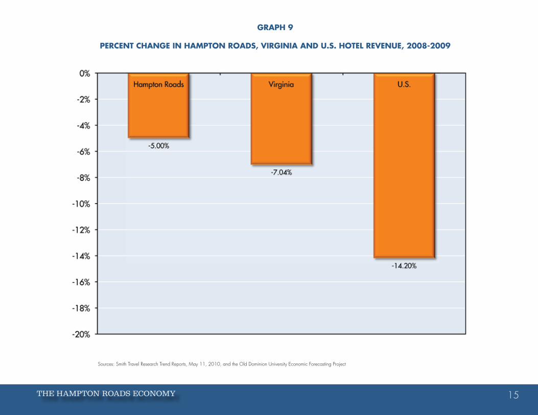
Unsurprisingly, the recession has had a particularly negative effect on travel and tourism as businesses and households adjust to adverse conditions. Graph 9 discloses that it was a tough year for tourism in Hampton Roads in 2009, though not quite as bad as it was for hotels in virginia and the United states.
The decline in regional tourism was not evenly distributed across the region. Graph 10 illustrates the reality that williamsburg’s hotel industry was particularly hard hit by the recession. To lesser degrees, so were norfolk and Portsmouth. This is not due to overbuilding of hotel rooms. each city’s supply has remained relatively constant; it is falling demand that is the culprit. The result has been falling occupancy and room rates. This has dealt a blow to tax collections in many cities.
williamsburg’s tourism market share declined from 30.6 percent in 1999 to 17.6 percent in 2009 (see Graph 11). The Historic Triangle (of which williamsburg is the key) faces significant challenges in marketing itself to a changing demographic of guests that apparently has less affinity for things historic. The winners in the rearrangement of regional tourism market shares have been Chesapeake/suffolk, Hampton/newport news and virginia Beach. The latter provides classic beach tourism plus other attractive amenities, while the former two have focused primarily on serving business travelers.

THE HAMPTON ROADS ECONOMY 7
GRApH 1
RATE oF GRoWTH oF GDp (u.s.) AnD GRp (HAMpTon RoADs)
source: Old Dominion University economic Forecasting Project

THE STATE OF THE REGION | HAMPTON ROADS 20108
GRApH 2
HAMpTon RoADs AnD u.s. AnnuAl unEMploYMEnT RATE (2001-2010)
sources: U.s. Department of labor and the Old Dominion University economic Forecasting Project

THE HAMPTON ROADS ECONOMY 9
GRApH 3
ToTAl unEMploYMEnT insuRAncE clAiMs in HAMpTon RoADs
jAnuARY 2003 To ApRil 2010
sources: virginia employment Commission and the Old Dominion University economic Forecasting Project

THE STATE OF THE REGION | HAMPTON ROADS 201010
GRApH 4
EsTiMATED DiREcT DoD spEnDinG in HAMpTon RoADs*
(2000-2010)
source: Old Dominion University economic Forecasting Project *Includes federal civilian and military personnel and procurement

THE HAMPTON ROADS ECONOMY 11
GRApH 5
HAMpTon RoADs AnnuAl pERcEnT cHAnGE in TAXAblE sAlEs AnD nEW AuToMobilE REGisTRATions
(1sT QuARTER 2009 To 1sT QuARTER 2010)
source: Old Dominion University economic Forecasting Project

THE STATE OF THE REGION | HAMPTON ROADS 201012
GRApH 6
EsTiMATED HousEHolD nET WoRTH in HAMpTon RoADs
(2000-2009; billions oF $)*
source: Old Dominion University economic Forecasting Project *Fourth quarter of each year

THE HAMPTON ROADS ECONOMY 13
GRApH 7
HAMpTon RoADs bAnKRupTciEs*
(2006-2010)
source: Old Dominion University economic Forecasting Project *Includes total new petitions filed and reopened cases, chapters 7 through 15

THE STATE OF THE REGION | HAMPTON ROADS 201014
GRApH 8
GEnERAl cARGo TonnAGE AT THE poRT oF HAMpTon RoADs, 1991-2010
sources: virginia Port authority and the Old Dominion University economic Forecasting Project
THE HAMPTON ROADS ECONOMY 15
GRApH 9
pERcEnT cHAnGE in HAMpTon RoADs, ViRGiniA AnD u.s. HoTEl REVEnuE, 2008-2009
sources: smith Travel Research Trend Reports, May 11, 2010, and the Old Dominion University economic Forecasting Project

THE STATE OF THE REGION | HAMPTON ROADS 201016
GRApH 10
pERcEnT cHAnGE in HoTEl REVEnuE
VARious HAMpTon RoADs ciTiEs, 2008-2009
sources: smith Travel Research, Jan. 20, 2010, and the Old Dominion University economic Forecasting Project

THE HAMPTON ROADS ECONOMY 17
GRApH 11
EsTiMATED MARKET sHAREs oF HAMpTon RoADs
HoTEl inDusTRY As MEAsuRED bY HoTEl REVEnuE
sources: smith Travel Research Trend Reports, Dec. 27, 2007, Dec. 22, 2008, Dec. 23, 2009, and the Old Dominion University economic Forecasting Project

THE STATE OF THE REGION | HAMPTON ROADS 201018
The Hampton Roads job MarketIn the recent recession the annual level of job losses within Hampton Roads bottomed in 2009, as shown in Graph 12. between 2000 and 2007, an average of 8,800 net new jobs was added annually. Things have changed. Graph 12 reports that the region lost approximately 37,000 jobs from 2008 to 2010. nevertheless, Graph 13 illustrates that we have turned the corner and in the second half of 2010, have been adding jobs.
job growth is likely to continue to be slow. First, the value of commercial real estate has fallen 42 percent since 2007 and this has had a profoundly discouraging impact on a variety of business firms. second, financial credit has been quite tight and firms that wish to borrow funds to expand often have found it impossible. banks are attempting to straighten out their balance sheets to cope with delinquent borrowers and frequently decline to make new commitments. Third, a variety of tax increases and a 41 percent increase in the minimum wage have diminished the desire of some firms to add workers.
If there is any joy in all of this, it is that despite our woes, we are doing better than comparable metropolitan regions in the southeast (see Graph 14). Hampton Roads’ job losses were slightly smaller (proportionately) than those of Raleigh and much smaller than those of Charlotte, Jacksonville and the United states.
HIGH-PROFIle JOB lOsses
More than most others, this recession has been characterized by highly visible job losses at firms that either have contracted their operations or closed their doors. Table 2 reports our estimates of the total jobs lost within Hampton Roads attributable to some of the area’s companies. (These data include multiplier effects estimated from the U.s. Department of Commerce RIMs II economic model.)
at this date, the precise economic impact of the JFCOM closure is unknown and therefore smithfield Foods leads the list of firms whose downsizing has had a ripple effect on the regional economy. However, the list is spread over a wide range of industries. The city of Franklin actually is not part of the defined virginia Beach-norfolk-newport news Msa (Hampton Roads), but some of its job losses nevertheless have occurred within our region.
TAblE 2
EsTiMATED ToTAl* jobs losT To THE HAMpTon RoADs EconoMY REsulTinG FRoM sElEcTED coMpAnY
DoWnsizinG oR sHuTDoWn
company Estimated jobs lost
JFCOM? 5,000-10,000?
smithfield Foods 2,318
verizon wireless 1,465
Cooper vision 1,413
International Paper 1,156
Usaa 1,083
alcoa Howmet 595
U.s. Food service 373
Dean Foods/Pet Dairy 368
advanced services 282
Capital Group Companies 277sources: Old Dominion University economic Forecasting Project and the U.s. Department of Commerce RIMs II economic modeling system. Based upon direct job losses reported by The virginian-Pilot on Dec. 29, 2009. *Total includes direct, indirect and induced job losses.
The jobs losses displayed in Table 2 accounted for slightly more than a third of the area’s estimated job losses in 2009 and 2010. The economic effects of plant closings typically are transmitted throughout all the cities of Hampton Roads. It’s also true that the shuttering of some firms located just outside of the region (such as International Paper) also can have a major negative impact upon our region.

THE HAMPTON ROADS ECONOMY 19
eMPlOyMenT, waGes anD InCOMe, 2000-2010
The United states lost an estimated 7.7 million jobs during the economic recession and in 2010 actually had 1.1 percent fewer jobs than it had in 2000. Here in Hampton Roads, we lost approximately 37,000 jobs during the recession, but experienced a 2.4 percent overall gain in employment for the decade. still, 2000-2010 was a difficult period for Hampton Roads; new civilian employment in the region rose by a meager 17,600 jobs. compare this to the 1990s when we gained more than 112,000 new jobs.
Compensation, however, is a different thing. as seen in Graph 15, the estimated total earnings of local private-sector employees grew substantially faster than those of private-sector employees nationally. However, it is the estimated total earnings for Hampton Roads military personnel that is the eye-catcher. The earnings of military personnel rose at a rate that was more than double that of the national average for private-sector employees as the Department of Defense, which no longer can depend upon a military draft, moved to attract and retain its soldiers and civilians.
Graph 16 reveals that average private-sector wages in Hampton Roads exceeded the national average in 2009. Much of this can be attributed to the economic ripples created by the decade-long increases in defense spending within the region. Rapidly rising labor productivity in Hampton Roads bodes to continue this trend in 2011.
The relatively strong wage performance of the private sector, along with the rapid decade-long increase in the earnings of military personnel, led both to rising household income and an increase in the spread between the median income of Hampton Roads households and that of households across the nation (see Graph 17). in 2000, regional median household income was 4.3 percent greater than that of households nationally. by the end of 2010, we believe this gap will have widened to 13.1 percent. it didn’t used to be this way. in the 1990s, median household income in Hampton Roads trailed national averages. Our improved relative standing largely reflects our superior
economic performance during the economic recession, which in turn reflects the magnificent cushion provided the region by defense spending.
What the lord giveth, however, the lord also taketh away. if increases in defense spending in Hampton Roads taper off (this seems likely), or jFcoM is phased down or shuttered, or additional aircraft carrier groups leave the region, or new classes of ships are homeported elsewhere, or the mix of defense spending changes in favor of “boots on the ground” rather than naval expenditures, then Hampton Roads could be hurt economically even if overall national defense spending continues to increase.
Did all industries share equally in the region’s recent gains and losses? no. Graph 18 displays the decade’s five largest industry gainers and losers with respect to job growth. The expansion of the health care and social assistance segment of the economy led the way in job growth from 2000 to 2010, creating fully 80 percent more jobs than the next leading industry, leisure and hospitality. Other services, which include such varied activities as auto repair, electronics and appliance repair, and a host of small businesses such as auto body shops and beauty parlors, followed the leisure sector, but still created only about 30 percent of the jobs generated by health care and social assistance.
Interestingly, local government was fourth on the list of growth industries, as governments spent generous increases in tax revenues earlier in the decade. This performance seems unlikely to continue because of falling tax revenues and diminished state subsidies.
Manufacturing led the way among the job losers, giving up more than twice the number of jobs as lost in retail and wholesale trade. Manufacturing employment declined by an estimated 13.6 percent in Hampton Roads between 2000 and 2010. However, manufacturing employment in the United states as a whole declined 33.4 percent. nevertheless, it is important to keep in mind that the value of manufacturing output rose almost 10 percent in the United states during the same time period. in Hampton Roads, the value of output generated by manufacturing increased by 25.7 percent between 2000 and 2010. Hence, fewer people are producing

THE STATE OF THE REGION | HAMPTON ROADS 201020
more valuable manufactured goods. neither Hampton Roads nor the united states is getting out of the business of manufacturing goods. increasingly, however, we are getting by with fewer workers.
note once again that the absolute number of uniformed military personnel in our region declined over this period. and keep in mind that military earnings rose very rapidly during the decade despite this loss of personnel, resulting in a significant earnings boost on a per-person basis.
Graph 19 provides an “economic glide path” for employment changes in Hampton Roads between 2000 and 2010. These glide paths smooth out ups and downs along the way and are primarily useful to illuminate long-term trends.
Conspicuously absent from the slate of employment growth industries in Graph 19 are any industry sectors that would be affected by port activity. This is peculiar since at its height port general cargo rose by almost a third (review Graph 8) over the course of the decade. However, transportation and warehousing, an industry closely aligned with port activity, experienced a secular decline through the decade. These data suggest that productivity increases in intermodal shipping, occasioned by such examples as scale economies of larger vessels, improved rail service, more efficient cranes for loading/unloading vessels, computer control of warehouse cargo and a whole host of other new cargo movement efficiencies, have served to substitute for labor (employment) in this highly competitive industry. simply put, despite the growth of cargo throughput, the port lost jobs overall because of increasingly efficient operations.

THE HAMPTON ROADS ECONOMY 21
GRApH 12
nET nEW ciViliAn WAGE AnD sAlARY jobs cREATED in HAMpTon RoADs (2000-2010)
sources: U.s. Department of labor and the Old Dominion University economic Forecasting Project

THE STATE OF THE REGION | HAMPTON ROADS 201022
GRApH 13
ciViliAn EMploYMEnT in HAMpTon RoADs (THousAnDs oF jobs, 2000-2010)
source: Old Dominion University economic Forecasting Project

THE HAMPTON ROADS ECONOMY 23
GRApH 14
ciViliAn EMploYMEnT GRoWTH RATE in sElEcTED MsAs AnD THE u.s., ApRil 2008-ApRil 2010
sources: U.s. Department of labor, June 8, 2010, and the Old Dominion University economic Forecasting Project (not seasonally adjusted)

THE STATE OF THE REGION | HAMPTON ROADS 201024
GRApH 15
EsTiMATED pERcEnTAGE incREAsE in ToTAl EARninGs (WAGEs, sAlARiEs AnD FRinGE bEnEFiTs) sElEcTED cATEGoRiEs (2000-2009)
sources: U.s. Department of Commerce, U.s. Bureau of labor statistics and the Old Dominion University economic Forecasting Project

THE HAMPTON ROADS ECONOMY 25
GRApH 16
HAMpTon RoADs AnD u.s. MEAn pRiVATE-sEcToR HouRlY EARninGs (2007-2010)
sources: U.s. Department of labor Ces wages and the Old Dominion University economic Forecasting Project

THE STATE OF THE REGION | HAMPTON ROADS 201026
GRApH 17
coMpARison oF MEDiAn HousEHolD incoME: HAMpTon RoADs AnD THE u.s., 1998-2010
sources: U.s. Census Bureau and the Old Dominion University economic Forecasting Project

THE HAMPTON ROADS ECONOMY 27
GRApH 18
EMploYMEnT GAins AnD lossEs in HAMpTon RoADs, 2000-2010
sources: U.s. Census Bureau and the Old Dominion University economic Forecasting Project sources: U.s. Department of labor, U.s. Department of Commerce and the Old Dominion University economic Forecasting Project

THE STATE OF THE REGION | HAMPTON ROADS 201028
GRApH 19
coMpARATiVE TREnD GRoWTH RATEs FoR HAMpTon RoADs’ lEADinG EMploYMEnT GRoWTH AnD conTRAcTion inDusTRiEs
source: Old Dominion University economic Forecasting Project

THE HAMPTON ROADS ECONOMY 29
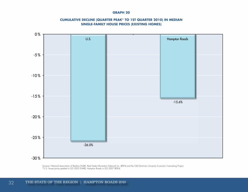
Residential Housing: Anatomy of a struggling MarketThe Hampton Roads housing market continued to experience declining median home prices and homeowner equity, while foreclosures and for-sale home inventory rose. as seen in Graph 20, median single-family home prices have fallen by more than 15 percent since their peak in the third quarter of 2007. The rate of decline nationally has been nearly double that of the region. we believe that housing prices, adjusted for seller concessions, are likely to continue to decline, albeit at very modest rates.
The collapse of housing prices reported in Graph 20 has been the most important contributor, both nationally and regionally, to the decline in the proportion of homeowners relative to renters, as well as to the falling proportion of positive equity that homeowners maintain in their houses. Graph 21 provides an interesting perspective on these developments. Three variables are reported here – current homeownership rates, peak homeownership rates and the percentage of homes that have positive equity (the value of a property exceeds the value of its mortgage, if any). Taking Hampton Roads as an example, the current homeownership rate is about 64 percent; this is down from a peak of about 79 percent. Approximately 79 percent of homes in Hampton Roads have positive equity; another way of saying this is that only 21 percent of homeowners in our region are “under water” and owe more in their mortgage than their home is worth. This number is likely to increase if home prices continue to decline, but one can see in Graph 21 that Hampton Roads is well below the U.s. average and dramatically better off than locations such as los angeles and Miami.
HOUsInG InvenTORy: THe sUPPly OF HOMes On THe MaRkeT
Foreclosures in Hampton Roads have risen steadily since 2006 (see Graph 22). estimated regional foreclosure filings increased by a factor of more than 12 over the period 2006-10 and are, or will eventually appear as, part of the
inventory of unsold homes in the area. While the overall rate of home foreclosures in Hampton Roads is below the national average, our rate of increase in foreclosures between 2006 and 2010 has been more than double that of the nation.
The total residential inventory of unsold Hampton Roads homes, which includes both new and existing houses (see Graph 23) has also been on the rise. From a low point of 3,311 homes in 2004, the regional inventory rose to an estimated 15,261 homes in 2010 – a nearly fivefold increase.
HOMe sales
between 2006 and 2008, total home sales in Hampton Roads fell by nearly one-third (see Table 3). Even so, sales of homes did increase between 2008 and 2009, though that still left them about 70 percent below their 2006 peak. However, fully 18 percent of these home sales were “distressed” properties that had to be sold because of foreclosures and similar reasons. One can see in Table 3 that non-distressed home sales have declined every year since 2006.
TAblE 3
DisTREssED* AnD non-DisTREssED REsiDEnTiAl HoMEs solD in HAMpTon RoADs: 2006-2009
Year All salesDistressed
sales
non-Distressed
sales
percent Distressed
sales2006 22,407 59 22,348 0.26
2007 19,154 262 18,892 1.37
2008 15,048 1,049 13,999 6.97
2009 15,852 2,869 12,983 18.10sources: Real estate Information network and the Old Dominion University economic Forecasting Project. Information deemed reliable but not guaranteed. *Distressed sales represent bank-owned homes and short sales.

THE STATE OF THE REGION | HAMPTON ROADS 201030
Complicating the interpretation of a turnaround in the annual number of regional home sales is the role played by the federal government’s program to boost housing sales through the use of tax credits. The program, initiated in late February 2009, gave as much as $8,000 to homebuyers who closed on their home by nov. 30, 2009. although the program was eventually extended into 2010, the extension was not passed until the initial credit was set to expire, leaving potential homebuyers who considered purchasing a home prior to november 2009 uncertain as to whether they would be able to access the credit if they waited past that date.
It appears likely that the small increase in our region’s home sales between 2008 and 2009 can be attributed largely to tax incentives, which de facto reduced the buyer’s purchasing price. This invites the possibility that the removal of the tax incentive in May 2010 will cause a downward shift in regional housing sales. There already are signs that this is occurring. like the tax incentive provided for automobiles (“cash for clunkers”), the one-time tax incentive for home buying may simply have moved forward the date when people were likely to make that purchase anyway. after all the smoke has cleared, it is not certain that these incentives will have engineered significant increases in the total number of units sold. The incentives were designed to provide a short-term economic stimulus and it appears they have done so. Their long-run economic impact, however, may be minimal.
The rising inventory of homes available for sale in Hampton Roads has tripled the time it takes to sell a house compared to 2005 (see Graph 24). Between 1995 and 2010, new homes on average accounted for 28 percent of the proportion of total unsold homes in the regional housing inventory. In 2010, however, new homes account for only 19 percent of total unsold inventory. This reflects dramatic reductions in new home construction. Between 2006, which represents the height of the regional residential real estate bubble, and 2010, the average annual inventory of new homes in Hampton Roads ballooned to 2,819, which was 1,338 more than the average of the preceding decade. This excess inventory has put a considerable dent in new home construction.
new ResIDenTIal COnsTRUCTIOn
Graph 25 reveals that home construction fell by more than half between its recent 2005 peak and its 2009 trough. nevertheless, this adjustment has been much less wrenching than that which occurred in the mid-1980s when new construction fell from an annual high of about 23,000 houses in 1986 to only about 7,000 in 1991. That housing contraction was the most difficult in the region’s recorded history.
Graph 25 is especially useful because it relates new home construction to total employment in the region. One need not be a nobel Prize winner to see that new home construction closely tracks regional employment. Indeed, the causation runs from employment to home building. The closing of JFCOM, however, could strangle our regional economic recovery and consequently depress our housing market.
CleanInG UP THe HOUsInG InvenTORy BUBBle: RelaTIve PRICe
CHanGes, aFFORDaBIlITy anD Real HOUse PRICes
Market forces already are at work that will reduce the oversupply of houses in our region, though the JFCOM closure could complicate matters. Table 4 computes the relative price of renting and owning in Hampton Roads. Between 2000 and 2010, monthly rental rates for a three-bedroom home rose by an estimated 47.4 percent, while the monthly payment (principal plus interest) for owning a similar house increased by only 34.5 percent. This was a dramatic turnaround from earlier in the decade (2000 to 2007) when the principal and interest required of home buyers increased by 75.1 percent, while the median rent for a similar structure increased by only 41.4 percent over the same period. since 2007, the principal and interest required of the owner of a median-priced home has declined from $1,495 monthly to $1,149 (30 percent).
what this means is that for many people, it now is cheaper to own a home than to rent the same structure. The ratio of monthly principal and interest to monthly rent has declined from 1.25 in 2006 to only .88 in 2010. Graph 26 places this in the context of the 1979-2010 time period and compares Hampton Roads

THE HAMPTON ROADS ECONOMY 31
to the United states. Relatively speaking, this is one of the best times in recent history to purchase a home in our region, if you have the ability to do so.
If Hampton Roads houses are historically affordable and it now is relatively cheaper to own than to rent, then why aren’t houses selling like hot cakes and prices rising? The answer to this question lies in the region’s supply and demand for housing. after adjusting for inflation, housing prices can be expected to rise when there are fewer houses on the market than people want to buy at prevailing prices. economists label this “excess demand.” On the other hand, housing prices can be expected to fall when there are more houses on the market than people want to buy at prevailing prices. This is “excess supply.”
TAblE 4
EsTiMATED HousE REnTAl AnD pRincipAl AnD inTEREsT FoR A HousE pAYMEnT in HAMpTon RoADs (2000-2010)
Median Monthly Rent for a Three-
bedroom House
p&i Monthly for a Median-priced House
Ratio of Monthly p&i
to Rent
2000 $882 $854 0.97
2001 911 809 0.89
2002 1,037 827 0.80
2003 1,044 779 0.75
2004 1,087 971 0.89
2005 1,118 1,202 1.08
2006 1,164 1,459 1.25
2007 1,247 1,495 1.19
2008 1,236 1,447 1.17
2009 1,277 1,190 0.93
2010 1,300 1,149 0.88sources: U.s. Department of Housing and Urban Development and the Old Dominion University economic Forecasting Project
Graph 27 depicts the relation of excess demand and excess supply of housing to the direction and value of change in housing prices. The left-hand scale measures the number of homes that have been in excess supply or excess demand in a given year. For example, in 1996, the excess supply of homes was approximately 2,400, while in 2004, during the housing boom, the excess demand for homes was about 5,000. One can see that currently we have a record level of excess supply of homes (about 7,000).
The right-hand scale of Graph 27 records what was happening to housing prices in each of these years. Between 2000 and 2005, when there was excess demand for housing, prices rose rapidly (almost 20 percent in 2005). This was not sustainable and housing prices began to taper off; by 2008, prices actually were declining. This was coincident with a rising excess supply of homes.
The Graph 27 data lead almost inevitably to the conclusion that housing prices in Hampton Roads have declined in 2010 and are apt to decline further in 2011. We believe the 2010 decline in prices will be about 5 percent, but that the 2011 decline will be more modest. The historical affordability and the relative price of owning versus renting notwithstanding, given the large volume of foreclosures likely in the region’s housing market over the course of 2010 and the lack of employment growth in Hampton Roads, it is difficult to envision how our region will quickly be able to “work off” the huge excess supply of housing that currently exists. economic recovery, however, can work wonders and that is the primary key to a regional housing revival (from the standpoint of sellers).
THE STATE OF THE REGION | HAMPTON ROADS 201032
GRApH 20
cuMulATiVE DEclinE (QuARTER pEAK* To 1sT QuARTER 2010) in MEDiAn sinGlE-FAMilY HousE pRicEs (EXisTinG HoMEs)
sources: national association of Realtors (naR), Real estate Information network Inc. (ReIn) and the Old Dominion University economic Forecasting Project *U.s. house prices peaked in Q3 2005 (naR); Hampton Roads in Q3 2007 (ReIn).

THE HAMPTON ROADS ECONOMY 33
GRApH 21
EsTiMATED HoMEoWnER EQuiTY AnD oWnERsHip RATEs: HAMpTon RoADs, u.s. AnD sElEcTED METRopoliTAn HousinG MARKETs
sources: las vegas, los angeles, Miami and san Diego: Federal Reserve Bank of new york, U.s. Census Bureau, lPs analytics and The wall street Journal. Hampton Roads and the U.s.: U.s. Census Bureau, First america Core logic and The virginian-Pilot. Data are for fourth quarter, 2009.

THE STATE OF THE REGION | HAMPTON ROADS 201034
GRApH 22
HAMpTon RoADs REsiDEnTiAl FoREclosuRE FilinGs, 2006-2010
sources: Realty Trac and the Old Dominion University economic Forecasting Project

THE HAMPTON ROADS ECONOMY 35
GRApH 23
EsTiMATED inVEnToRY oF ToTAl (nEW consTRucTion AnD EXisTinG) REsiDEnTiAl HoMEs in HAMpTon RoADs As MEAsuRED bY AcTiVE lisTinG on ApRil 30 oF EAcH YEAR
(1995-2010)
sources: Real estate Information network Inc. and the Old Dominion University economic Forecasting Project. Information deemed reliable but not guaranteed.

THE STATE OF THE REGION | HAMPTON ROADS 201036
GRApH 24
HAMpTon RoADs EXisTinG REsiDEnTiAl HoMEs solD AnD AVERAGE nuMbER oF DAYs on THE MARKET (2000-2009)
sources: Real estate Information network Inc. and the Old Dominion University economic Forecasting Project. Information deemed reliable but not guaranteed. Days on market are calculated from the date listed to the date under contract for existing homes sold.

THE HAMPTON ROADS ECONOMY 37
GRApH 25
AnnuAl cHAnGE in ToTAl EMploYMEnT AnD ToTAl (sinGlE AnD MulTi-uniT) nEW HousinG pERMiTs in HAMpTon RoADs, 1980-2010
sources: U.s. Census Bureau, U.s. Department of Commerce and the Old Dominion University economic Forecasting Project

THE STATE OF THE REGION | HAMPTON ROADS 201038
GRApH 26
HousinG AFFoRDAbiliTY: MonTHlY pAYMEnT FoR A MEDiAn-pRicED REsAlE HousE As A pERcEnTAGE oF MEDiAn HousEHolD MonTHlY incoME in HAMpTon RoADs AnD THE u.s. (1979 To 2010)
source: Old Dominion University economic Forecasting Project (assumes 4.9 percent mean mortgage rate in 2010)

THE HAMPTON ROADS ECONOMY 39
GRApH 27
EsTiMATED EXcEss supplY/EXcEss DEMAnD oF HousEs in THE HAMpTon RoADs sinGlE-FAMilY HousinG MARKET (RiGHT scAlE) RElATiVE To THE AnnuAl cHAnGE in REAl HousE pRicEs (lEFT scAlE)
source: Old Dominion University economic Forecasting Project

THE STATE OF THE REGION | HAMPTON ROADS 201040
summaryThis year has been one of recovery for the Hampton Roads economy. after two years of decline, the region’s economy will expand at a rate of 2.4 percent in 2010. However, this is not likely to be accompanied by strong employment growth, and the region has experienced a net migration outflow.
approximately three-quarters of all economic expansion in Hampton Roads in recent years has come from defense spending, which now accounts for approximately 45 percent of total economic activity in our region, directly and indirectly. Two other economic pillars, tourism and the port, contracted during the recession and are slowly working their way back to more accustomed levels of activity.
2011 should be a better year for Hampton Roads, economically speaking. nevertheless, our extreme dependence upon defense spending places us in a highly vulnerable position. Changes in the level of defense spending, or the closure of JFCOM, or the movement of aircraft carrier groups away from the region, or changes in the mix of defense spending, could severely disadvantage us in the future. It seems likely that defense spending in Hampton Roads will decelerate over the coming decade.
Further, because of our peculiar topography, we are highly dependent upon a road transportation system that features four tunnels and numerous choke points. Unless improved, this system will impose increasingly higher costs on many of the region’s citizens over the next few years. There also is the prospect of higher costs due to rising sea levels and increasingly common flooding.
Taken together, the factors noted here (plus other influences) suggest a subtle deterioration in the long-term outlook for economic growth in Hampton Roads. Whatever one thinks about the time period 2000-05, these years may in fact turn out to be the good old days that we remember fondly.

THE HAMPTON ROADS ECONOMY 41
? MilEs

Regional Markets for Office and Industrial Space

THE STATE OF THE REGION | HAMPTON ROADS 201044
FEELING PAIN: REGIONAL MARKETS FOR OFFICE AND INDUSTRIAL SPACE
I’ve never seen anything like this in 36 years. – Sharon Ryals-Taylor, Thalhimer Commercial Real Estate
Real estate professionals usually divide the commercial real estate market into five sub-markets: (1) multifamily housing; (2) office; (3) industrial; (4) retail; and
(5) hotels and casinos. Last year, we examined the hotel market. This year, we focus on the office and industrial space market segments, which have been
going through difficult times.
Our primary data source for the office space and industrial space markets is CoStar Group Inc., the most prominent provider of information, marketing and analytic services to commercial real estate professionals. CoStar offers its customers online access to the most comprehensive database of commercial real estate information in the United States, as well as the United Kingdom and France. Founded in 1987 and headquartered in Bethesda, Md., CoStar employs 1,400 people and has what is believed to be the largest professional research organization in the industry. Its national database includes records on approximately 2.8 million properties containing 69.1 billion square feet of space.
Our focus here is on the existing inventory of space (supply), occupied space (demand), property availability rates and quoted monthly rental/lease rates for office and industrial space, all between 2005 and 2009. Note that quoted monthly rental/lease rates do not include any concessions offered to tenants. Such information would be very interesting, but is not available. We compare Hampton Roads to Charlotte, Raleigh-Durham, Jacksonville, Richmond and Savannah. Our choice of the time period 2005 to 2009 primarily reflects the availability of data, though it also very nicely spans years when the market was booming to recent years when the market has been depressed.
Some words of caution are in order. Data reported here are from the fourth quarter of the year and were extracted from CoStar’s database on May 14, 2010. The numbers shown here are subject to change because CoStar’s database is live, dynamic and constantly being revised. CoStar Market Reports are best viewed as a snapshot taken at a point in time; this picture will be different over time. For example, when buildings are added to the database, or delivery dates on buildings change, this alters CoStar’s data set.
CB Richard Ellis and CoStar are the two major providers of historical information on office and industrial markets, and their data definitions differ slightly. We rely upon CoStar’s definitions here.
Employment is a very rough thermometer of the health of the commercial real estate market, since firms that have no employees do not need commercial real estate space. Here, we examine office employment in our six comparable metropolitan regions. (Employment in manufacturing, trade, transportation and utilities is included in industrial employment.)
Table 1 reports employment levels and growth trends in three areas: non-farm employment, industrial employment and office employment. We focus on our six regions from 2005-07 and 2007-09. One can see in Table 1 that all of the other markets saw larger increases in non-farm

REGIONAL MARKETS FOR OFFICE AND INDUSTRIAL SPACE 45
employment, industrial employment and office employment than Hampton Roads between 2005 and 2007. However, the onset of the recession produced negative employment growth in all three categories for 2007-09. Indeed, in the industrial employment category, losses were particularly severe and wiped out all the gains observed from 2005 to 2007. In several cities, this also was true for office employment.
What is the absolute size of the commercial real estate markets in the six metropolitan areas? Table 2 provides some notion of relative size in 2007, which was the historical peak. Now, in 2010, employment levels are below those of three years ago.
TABLE 1
CHANGES IN TOTAL NON-FARM, INDUSTRIAL AND OFFICE EMPLOYMENT, 2005 to 2009
Percent Growth in Total Non-Farm Employment
Percent Growth in Industrial Employment
Percent Growth in Office Employment
2005-07 2007-09 2005-07 2007-09 2005-07 2007-09
U.S. 2.91 -4.85 0.81 -9.08 3.93 -7.28
Charlotte 8.68 -5.78 4.18 -9.43 11.01 -7.25
Raleigh-Durham
9.21 -2.38 5.18 -8.76 10.15 -4.20
Hampton Roads
1.91 -4.63 0.00 -9.24 2.17 -6.19
Jacksonville 4.99 -7.57 3.31 -9.20 3.33 -10.02
Richmond 2.86 -4.61 1.32 -9.71 3.65 -6.59
Savannah 7.74 -6.20 4.32 -7.89 12.30 -16.25Sources: Bureau of Labor Statistics, U.S. Department of Labor and the Old Dominion University Economic Forecasting Project
TABLE 2
NON-FARM, INDUSTRIAL AND OFFICE EMPLOYMENT IN SELECTED MARKETS, 2007
Total Non-Farm Employment
Industrial Employment Office Employment
Rank Rank Rank
Charlotte 859,900 1 261,800 1 233,000 1
Raleigh-Durham
803,000 2 203,200 2 185,500 2
Hampton Roads
775,300 3 201,200 3 159,900 4
Jacksonville 633,800 4 171,800 4 164,600 3
Richmond 633,300 5 160,700 5 156,200 5
Savannah 161,400 6 50,700 6 28,300 6Sources: Bureau of Labor Statistics, U.S. Department of Labor and the Old Dominion University Economic Forecasting Project

THE STATE OF THE REGION | HAMPTON ROADS 201046
The Office MarketGraph 1 displays the supply of available office space as measured by existing inventory in square feet, 2005-2009, for our six chosen markets. The Charlotte and Raleigh-Durham office markets are the largest and the Savannah market is the smallest. Note that the supply of office space trended modestly upward in all six markets through 2009 despite the cooling of the economy. It’s little wonder, then, that problems have emerged in these markets and rental rates have begun to fall.
Graph 2 displays “availability rates” for office space in the six markets. Availability rates are not the same as vacancy rates because they take into account space that might currently be occupied, but shortly will become available, as well as new space that shortly will become available and therefore can be rented. Vacancy rates, on the other hand, trace only space that is unoccupied and do not address space that is “available” for rental or lease.
Availability rates are preferred because they are slightly more sensitive measures than vacancy rates of what is actually going on in commercial real estate markets. Note that availability rates ordinarily will be higher than the vacancy rates. In 2006, availability rates began to climb in all six markets and by 2009 vastly exceeded those in 2005. Savannah’s availability rate in 2009 (19.97 percent) was particularly elevated and was substantially higher than that in Hampton Roads (14.68 percent), even though the growth of Savannah’s port traffic outstripped Hampton Roads from 2005 to 2009.
What impact did these rising availability rates have upon rental rates for office space? Graph 3 provides quoted “full-service rental rates” for each of the six metropolitan area office markets between 2005 and 2009. Full-service rental rates are inclusive of all operating expenses such as utilities, electricity, janitorial services, taxes and insurance. One can see that these rates increased in every market from 2005 to 2008, but declined in 2009 in every market except Jacksonville. Quoted rents are lowest in Richmond and generally highest in Charlotte and Raleigh-Durham. Through 2007, Hampton Roads had the second-lowest rental rates among the six regions, but beginning in 2008, the glut of available space in Savannah pushed rates there below those in Hampton Roads.
Table 3 brings together several important measures of office space activity. Included in the table are changes that have occurred in the existing inventory of office space, office space actually occupied and quoted rental rates for office space in the six metropolitan regions between 2005 and 2009. Because of the recession, we have divided the time period into two segments, 2005-07 and 2007-09. We can summarize these data as follows:
• The supply of office space increased in each of the six markets from 2005 to 2009 and by fully 12.46 percent in Hampton Roads.
• Office space actually occupied by tenants increased in every market, 2005-09, but declined in three of the six markets, 2007-09. In Hampton Roads, occupied space increased only .7 percent between 2007 and 2009.
• Quoted rental rates for office space rose in all markets, 2005-09, and increased by 10.75 percent in Hampton Roads. This rate tapered off to 3.23 percent in Hampton Roads from 2007 to 2009. Note, however, that in Graph 3, we found that between 2008 and 2009, quoted rental rates declined in five of six markets. Hence, supply and demand were strongly out of balance by 2009 and landlords dealt with this by reducing their rates. In Hampton Roads, the average per-square-foot full-service rental rate declined from $18.40 in 2008 to $18.23 in 2009. This sharp reversal from previous years’ increases underlines that by 2009, the office space market in our region had transitioned from high levels of occupancy and rising rates to much less bountiful times for landlords and more attractive times for renters.

REGIONAL MARKETS FOR OFFICE AND INDUSTRIAL SPACE 47
TABLE 3
CHANGES IN SUPPLY, DEMAND AND QUOTED RENTAL RATES FOR OFFICE SPACE, 2005-2009
Percent Growth in Existing Inventory
Percent Growth in Occupied Space
Percent Growth in Average Quoted Rental Rate
2009 Existing Inventory in Square Feet
Rank by SF
2005-09 2005-07 2007-09 2005-09 2005-07 2007-09 2005-09 2005-07 2007-09Charlotte 10.36 4.91 5.20 8.10 6.88 1.14 7.52 4.09 3.29 89,213,662 1
Raleigh-Durham
12.48 5.54 6.58 11.04 6.79 3.98 8.88 10.34 -1.42 80,998,667 2
Jacksonville 9.20 5.86 3.15 6.50 7.70 -1.12 12.19 9.04 2.89 58,446,708 3
Richmond 6.56 4.17 2.29 3.53 5.61 -1.97 7.41 5.37 1.94 58,253,821 4
Hampton Roads
12.46 7.29 4.83 5.78 5.05 0.70 10.75 7.29 3.23 44,750,034 5
Savannah N/A N/A 3.91 N/A N/A -0.58 N/A N/A -3.15 5,980,608 6Sources: CoStar Group Inc. and the Old Dominion University Economic Forecasting Project

THE STATE OF THE REGION | HAMPTON ROADS 201048
GRAPH 1
SUPPLY OF OFFICE SPACE MEASURED BY EXISTING INVENTORY (SQUARE FEET), SIX METRO AREAS, 2005-2009
Sources: CoStar Group Inc. and the Old Dominion University Economic Forecasting Project

REGIONAL MARKETS FOR OFFICE AND INDUSTRIAL SPACE 49
GRAPH 2
AVAILABILITY RATES FOR OFFICE SPACE, SIX METRO AREAS, 2005-2009
Sources: CoStar Group Inc. and the Old Dominion University Economic Forecasting Project

THE STATE OF THE REGION | HAMPTON ROADS 201050
GRAPH 3
AVERAGE QUOTED FULL-SERVICE RENTAL RATE OF OFFICE SPACE, SIX METRO AREAS, 2005-2009
Sources: CoStar Group Inc. and the Old Dominion University Economic Forecasting Project

REGIONAL MARKETS FOR OFFICE AND INDUSTRIAL SPACE 51
The Industrial MarketWhat about industrial commercial real estate space? Graph 4 displays the supply of available industrial space from 2005 to 2009 as measured by existing inventory. Because the Charlotte industrial market is more than twice as large as any of the other markets, its supply is not shown here. The supply of industrial space increased in all the six markets, 2005-09, though sometimes only modestly. In Hampton Roads, for example, the supply of industrial space increased by 8.1 percent from 2005 to 2009, while the comparable growth rate in Charlotte was only 3.6 percent.
Graph 5 gives availability rates for industrial space in these markets. Except for Hampton Roads, availability rates declined in the metropolitan areas between 2005 and 2007. Thereafter, availability rates increased, usually substantially (to more than 41 percent in Savannah in 2009). Hampton Roads, however, is the outlier in this arrangement. The availability rates for our industrial space never declined in the boom years from 2005 to 2007 and actually rose every year from 2005 to 2009. In our region, then, the market for industrial space has been glutted and suffering for at least half a decade.
Graph 6 provides information on average quoted “triple net lease” rates for industrial space in the six markets, 2005-09. In a triple net lease, each tenant is responsible for her proportionate share of property taxes, property insurance, common operating expenses and common area utilities related to the property in which they are located. Tenants are further responsible for all costs associated with their own occupancy, including personal property taxes, janitorial services and all utility costs. In all six markets, triple net lease rates increased from 2005 to 2006, but then began to decline in most of the markets. By 2009, rates were declining in every market and many were below the 2005 level. In Hampton Roads, for example, triple net lease rates in 2009 had fallen to $4.88 per square foot, 11.5 percent below the 2005 level.
Table 4 brings together data for the industrial space markets in the six metropolitan areas. Included here are changes in existing inventory (supply),
occupied space (demand) and quoted lease rates, all for 2005 through 2009. One can summarize these results as follows:
• The supply of industrial space grew in each of the six markets (Charlotte, Jacksonville, Richmond, Hampton Roads, Raleigh-Durham and Savannah) between 1.57 percent and 8.05 percent.
• The supply of industrial space grew most rapidly in Hampton Roads (8.05 percent).
• Space actually occupied, however, declined in one of the six markets between 2005 and 2009 and in five of the six markets between 2007 and 2009.
• Occupied industrial space grew in Hampton Roads by .78 percent from 2007 to 2009, but as noted below, this required significantly lower rental rates.
• Quoted triple net lease rental rates declined in one of the six markets between 2005 and 2009, but in all six markets between 2007 and 2009.
• Hampton Roads experienced the greatest decline in triple net lease rates, -10.29 percent from 2005 to 2009 and -13.63 percent from 2007 to 2009. It is apparent that the significant increase in the supply of industrial space in our region required landlords to offer substantially lower rental rates. Only Savannah, among the other metropolitan regions, has faced similar circumstances.

THE STATE OF THE REGION | HAMPTON ROADS 201052
TABLE 4
CHANGES IN SUPPLY, DEMAND AND QUOTED LEASE RATES FOR INDUSTRIAL SPACE, SIX METRO AREAS, 2005-2009
Percent Growth in Existing Inventory
Percent Growth in Occupied Space
Percent Growth in Average Quoted Rental Rate
2009 Existing Inventory in Square Feet
Rank by SF
2005-09 2005-07 2007-09 2005-09 2005-07 2007-09 2005-09 2005-07 2007-09Charlotte 3.59 2.24 1.31 2.54 3.31 -0.75 3.76 11.29 -6.76 276,233,005 1
Jacksonville 7.55 2.02 5.42 2.73 3.13 -0.38 10.71 21.17 -8.63 117,173,443 2
Richmond 1.57 0.49 1.07 -2.20 1.39 -3.54 3.21 7.80 -4.26 113,807,016 3
Hampton Roads
8.05 4.67 3.23 0.50 -0.28 0.78 -10.29 3.86 -13.63 103,305,791 4
Raleigh-Durham
2.50 1.93 0.56 1.89 6.36 -4.20 0.00 12.26 -10.92 95,847,164 5
Savannah N/A N/A 19.80 N/A N/A -8.52 N/A N/A -3.86 27,419.765 6Sources: CoStar Group Inc. and the Old Dominion University Economic Forecasting Project

REGIONAL MARKETS FOR OFFICE AND INDUSTRIAL SPACE 53
GRAPH 4
SUPPLY OF INDUSTRIAL SPACE (SQUARE FEET), FIVE METRO AREAS, 2005-2009
Sources: CoStar Group Inc. and the Old Dominion University Economic Forecasting Project

THE STATE OF THE REGION | HAMPTON ROADS 201054
GRAPH 5
AVAILABILITY RATES FOR INDUSTRIAL SPACE, SIX METRO AREAS, 2005-2009
Sources: CoStar Group Inc. and the Old Dominion University Economic Forecasting Project

REGIONAL MARKETS FOR OFFICE AND INDUSTRIAL SPACE 55
GRAPH 6
AVERAGE QUOTED TRIPLE NET LEASE RATES FOR INDUSTRIAL SPACE, SIX METRO AREAS, 2005-2009
Sources: CoStar Group Inc. and the Old Dominion University Economic Forecasting Project

THE STATE OF THE REGION | HAMPTON ROADS 201056
Summing It UpIn this chapter, we have examined the markets for two types of commercial real estate – office space and industrial space – and have done so by comparing Hampton Roads to five other roughly similar southeastern U.S. metropolitan areas. It is fair to say that the shine has come off both the office space and industrial space markets, but the industrial space market has endured the most difficult times. This is true in each of the six regions – Charlotte, Raleigh-Durham, Jacksonville, Richmond, Hampton Roads and Savannah.
Here in Hampton Roads, availability rates for office space have increased every year since 2005, at least partially because additional space has become available. In simple terms, the supply of office space is outstripping the demand for it, and this stimulated a decline in office rental rates between 2008 and 2009 after several years of healthy growth.
The market for industrial space has been disrupted substantially in Hampton Roads. The availability rate of industrial space within our region has increased every year since 2005, a direct implication of additional space coming online in a time of economic recession. The pain of adjustments in the regional industrial space market has been more severe than in the office space market. Between 2007 and 2009, triple net lease rates fell 13.63 percent in Hampton Roads, a sign of a glutted market in which supply and demand are well out of balance. Triple net lease rates in our region fell to only $4.88 per square foot in 2009, well below the $5.44 rate that reigned in 2005, and it seems likely that further declines are in store. It is a good time to be a lessee and a bad time to be a lessor.
How long will this last? Much depends upon the speed of national economic recovery. An expanding national economy would be quite helpful to regional commercial real estate markets. However, while necessary, this may not be sufficient. Hampton Roads is heavily dependent upon Department of Defense spending; approximately 45 percent of our regional economic activity relates directly and indirectly to defense spending. If this spending decelerates, or
aircraft carrier groups are moved out of the region or the mix of defense spending changes to the detriment of the U.S. Navy, then the regional economy could remain in a torpor for years to come. Transportation problems and water inundation challenges will only exacerbate the situation.
It is fair to say that the market for office space in Hampton Roads is closer to recovery and equilibrium than the market for industrial space. Seasoned commercial real estate professionals label this the most severe contraction since the Great Depression of the 1930s. We can only hope that our experience over the next decade does not imitate that period in history because then it took more than 15 years for the commercial real estate markets to show substantial recovery.

REGIONAL MARKETS FOR OFFICE AND INDUSTRIAL SPACE 57
Appendix: Some Definitions
Office Space: The CoStar Office Report, unless specifically
stated otherwise, calculates office statistics using CoStar
Group’s entire database of existing and under-construction
office buildings in each metropolitan area. Included are office,
office condominium, office loft, office medical, all classes and
all sizes, and both multi-tenant and single-tenant buildings,
including owner-occupied buildings. Excluded is office space
on federal government properties (e.g., military installations)
and at other governmental facilities (e.g., Norfolk International
Terminals, Newport News Marine Terminal and Portsmouth
Marine Terminal). All rental rates reported in the CoStar
Office Report have been converted to full-service-equivalent
rental rates. Office space data used in this report include all
types of space: Class A, Class B and Class C.
Industrial Space: The CoStar Industrial Report calculates
statistics using CoStar Group’s database of existing, under-
construction and under-renovation industrial buildings in
each given metropolitan area. All industrial building types
are represented regardless of size, including warehouse, flex,
research and development, distribution, manufacturing,
industrial showroom and service buildings. The report also
gives statistics for both single-tenant and multi-tenant
buildings, including owner-occupied buildings. A flex building is
designed to be versatile, and may be used in combination with
office (corporate headquarters), research and development,
quasi-retail sales and, including, but not limited to, industrial,
warehouse and distribution uses. At least half of the rentable
area of the building must be used as office space. Flex buildings
typically have ceiling heights under 18 feet, and are zoned as
light industrial.
However, the data exclude industrial areas such as airports,
airplane hangars, auto salvage facilities, cement/gravel plants,
chemical/oil refineries, contractor storage yards, landfills,
lumberyards, railroad yards, self-storage, shipyards, flex
telecom hotel/data hosting, industrial telecom hotel/data
hosting, utility substations and water treatment facilities.
Also excluded are industrial facilities on federal government
properties and at other governmental facilities. All rental rates
reported in the CoStar Industrial Report are calculated using
the quoted triple net (NNN) rental rate for each property.
Existing Inventory: To be included, buildings must have
received a certificate of occupancy and be able to be occupied
by tenants. Generally, this measure includes a percentage of
common areas including all hallways, main lobbies, bathrooms
and telephone closets. It does not include space in buildings that
are either planned, under construction or under renovation.
Vacant Space: This is defined as space that is not currently
occupied by a tenant, regardless of any lease obligation that
may exist. Vacant space could be space that either is available,
or not available. For example, sublease space that is currently
being paid for by a tenant, but not occupied by that tenant,
would be considered vacant space.

THE STATE OF THE REGION | HAMPTON ROADS 201058
Occupied Space: This represents the difference between
existing inventory and vacant space.
Available Space: This is the total amount of space that is
marketed as available for lease in a given time period. It includes
any space that is available, regardless of whether the space is
vacant, occupied, available for sublease or available at a future
date.
Availability Rate: This is the ratio of available space to total
rentable space, calculated by dividing the total available square
feet by the total rentable square feet, as measured by existing
inventory.
Vacancy Rate: This measurement is expressed as a percentage
of the total amount of physically vacant space divided by the
total amount of existing inventory.
Full Service Rental Rate: This is a measure of rental rates
for space reported to be office space, including all operating
expenses such as utilities, electricity, janitorial services, taxes
and insurance.
Industrial Building: This is a type of building adapted for such
uses as the assemblage, processing and/or manufacturing of
products from raw materials or fabricated parts. Additional uses
include warehousing, distribution and maintenance facilities.
The primary purpose of the space is for storing, producing,
assembling or distributing a product.
Triple Net Lease (NNN): In a triple net lease, tenants are
responsible for their proportionate share of property taxes,
property insurance, common operating expenses and common
area utilities. Tenants are further responsible for all costs
associated with their occupancy, including personal property
taxes, janitorial services and all utility costs.

REGIONAL MARKETS FOR OFFICE AND INDUSTRIAL SPACE 59

Hampton Roads Versus Other East Coast Container Ports

THE STATE OF THE REGION | HAMPTON ROADS 201062
Sizing Up the Competition: hampton RoadS VeRSUS otheR eaSt CoaSt ContaineR poRtS
To reach a port we must sail, sometimes with the wind, and sometimes against it. But we must not drift or lie at anchor. – Oliver Wendell Holmes, 1809-1894
More than 90 percent of the world’s international trade flows through ports such as the Port of Hampton Roads. Depending upon who is doing
the counting, the Port of Hampton Roads is responsible for 7 percent to 12 percent of our regional economic activity.
When our port prospers, Hampton Roads thrives; when it languishes, we visibly weaken.
This strong connection to our regional welfare provokes an obvious question. How are we (and the port) situated with respect to future developments? Will we benefit from the refashioning of the Panama Canal? Can we compete capably with other East Coast ports? Are there alternate strategies we should pursue? These are the topics we address in this chapter.
A Bit of BackgroundIn the past half-century, the nature of the commercial cargo transportation across the oceans has changed dramatically. Until the 1950s, general cargo (a term that excludes bulk cargo such as coal, liquids and grain) was handled as “break-bulk” cargo – it was placed on pallets and loaded/unloaded to and from ships by means of on-board cranes. This was a slow, expensive, item-by-item, labor-intensive process. Individual boxes containing everything from clothing to radios were unloaded, one by one.
All this changed when Malcolm McLean, believing that individual pieces of general cargo needed to be handled only twice – at their origin when stored
in a standardized container box and at their final customer destination when unloaded – purchased a small tanker company, renamed it Sealand and cleverly adapted its ships to transport truck trailers. McLean’s efforts met with great success when several major port organizations such as the U.S. Maritime Association, the Federal Maritime Board and the International Standards Organization spearheaded a worldwide compromise that standardized container sizes and characteristics. Truck trailers soon were replaced by trailers without wheels and general cargo rapidly began to be stored in standardized containers, generally 20 feet or 40 feet in length, without wheels. These became known as TEUs (20-foot equivalent units) and FEUs (40-foot equivalent units).
On April 26, 1956, the first voyage of a Sealand containership occurred when a vessel left Newark, N.J., for Puerto Rico. And in 1966, the first containerization of international trade began with the voyage of a Sealand ship from the United States to the Netherlands.
The advent of containerization demanded the redesign of ships and ports. Ships transporting containers were redesigned without cranes aboard. Below decks, cargo space was divided into cells to enhance the loading and unloading of containers. Without cranes taking up room, the deck space now could be used

HAMPTON ROADS VERSUS OTHER EAST COAST CONTAINER PORTS 63
to stack containers five high. This increased the container carrying capacity of these ships by approximately 30 percent.
These developments required ports to invest in dockside cranes, various types of infrastructure and mobile capital. Berths were redesigned so that containerships could dock parallel to them for easier loading and unloading by dockside cranes. Warehouses were removed and land was cleared for outdoor storage of containers. Containers were stored on truck chassis or stacked on land one upon another, several units high, depending upon available space of land and the port’s style of operation.
Hampton Roads and Other U.S. Container PortsThe 10 top-ranked container ports in the United States, ranked by TEU throughput, are shown in Graph 1. Imported TEUs arrive by ship and leave a port for an American location by means of truck, rail or barge. Alternatively, exported TEUs arrive by truck, rail or barge and leave a port by ship for another destination.
The two largest U.S. container ports are the West Coast ports of Los Angeles and Long Beach (located very close to each other, but separate organizations), with 23.4 percent and 19.4 percent, respectively, of the TEU throughput of the 10 top-ranked U.S. container ports. Together, these two ports handle a whopping 42.8 percent of the total TEU throughput at the major U.S. container ports. Most of these TEUs are related to Asian trade. Many of the containerships calling at these two ports are “Post-Panamax” ships, exceeding 5,000 TEUs in size, and are too large to transit the Panama Canal as it currently is configured. Consequently, TEUs from Post-Panamax ships that dock on the American West Coast, but have cargo destined for the eastern region of the United States, are placed on double-stack railroad cars at the ports and sent across country.
The third- and fourth-largest U.S. container ports are the ports of New York/New Jersey and Savannah, with 15.6 percent and 7.8 percent, respectively, of the TEU throughput of the 10 top-ranked U.S. container ports.
The Port of Hampton Roads is the sixth-largest U.S. container port (but the third-largest East Coast container port) with 6.2 percent of the TEU throughput of the country’s major U.S. container ports. The container ports of Miami, Jacksonville and Baltimore (not shown in Graph 1) were the fifth-, sixth- and seventh-largest East Coast container ports in 2008.
Relative port market shares have changed substantially over the past decade. Table 1 reports growth rates in TEUs handled at the largest American ports between 1998 and 2008. Among East Coast ports, New York/New Jersey grew 113.5 percent over that time period, while

THE STATE OF THE REGION | HAMPTON ROADS 201064
Savannah grew an amazing 258.1 percent and in the process passed Hampton Roads. At the other end of the spectrum, Charleston, Port Everglades, Miami, Jacksonville and Baltimore grew much more slowly than TEU traffic nationally. They rank among the losers in the rigorous competition for TEU cargoes over the past decade. (Baltimore, however, has profitably focused its attention on automobiles and roll-on, roll-off traffic, neither of which count as TEUs.) Hampton Roads grew (66.4 percent), but this was only slightly more than the national average (63.7 percent).
The 10 top-ranked U.S. container ports with respect to market share, (expressed as a percentage) of TEUs imported from and exported to Asia only, appear in Graph 2. The ports of Los Angeles and Long Beach are ranked first and second in market share of imports from (at 30.9 percent and 23.4 percent, respectively) and exports to Asia (at 24.7 percent and 21.1 percent, respectively) among U.S. container ports. The two largest East Coast container ports, New York/New Jersey and Savannah, are ranked third and fourth, respectively, in market share (at 12 percent and 6.7 percent, respectively) of imports from Asia. The third- and fourth-largest East Coast container ports, Hampton Roads and Charleston, are ranked eighth and ninth, respectively, among U.S. container ports for imports to (at 3.6 percent and 2.6 percent, respectively) and exports from (at 6 percent and 2.1 percent, respectively) Asia.
TABLE 1
HOT AND COLD: RANkiNg U.S. PORTS BY SizE (TEUs, 2008)
PortContainer TEUs 2008
Percent growth Rate, 1998-2008
Los Angeles 7,849,985 132.4
Long Beach 6,350,125 55.0
New York/New Jersey 5,265,058 113.5
Savannah 2,616,126 258.1
Oakland 2.236.244 42.0
Hampton Roads 2,003,278 66.4
Tacoma 1,861,352 161.0
Houston 1,794,309 87.1
Seattle 1,704,492 10.4
San Juan 1,684,883 -15.4
Charleston 1,635,534 28.0
Port Everglades 985,095 39.9
Miami 828,349 1.7
Jacksonville 697,494 -8.0
Baltimore 612,887 25.9
U.S. 42,827,594 63.7Sources: American Association of Port Authorities and the Old Dominion University Economic Forecasting Project

HAMPTON ROADS VERSUS OTHER EAST COAST CONTAINER PORTS 65
gRAPH 1
TEN TOP-RANkED U.S. CONTAiNER PORTS (TEU THROUgHPUT iN 1,000s) iN 2008
Source: Containerisation International, March 2009

THE STATE OF THE REGION | HAMPTON ROADS 201066
gRAPH 2
U.S. CONTAiNER PORT MARkET SHARE Of TEUs fROM AND TO ASiA (2008)
Source: B. Mongelluzo, “Looking Past the Downturn,” Journal of Commerce, March 2, 2009

HAMPTON ROADS VERSUS OTHER EAST COAST CONTAINER PORTS 67
The Challenges facing East Coast Container PortsTHE MATTER OF SIzE
Since 1996, the size of the largest containership in worldwide service has more than doubled. Fourteen years ago, the largest containership available was the Regina Maersk, with a carrying capacity of 6,000 TEUs. By 2005, Hapag-Lloyd’s Colombo Express’ carrying capacity was 8,750 TEUs. And by 2007, the Emma Maersk had a carrying capacity of 13,000 TEUs.
Let’s provide some perspective. The Emma Maersk is 1,302 feet long and 184 feet wide, with a draft of more than 50 feet. By comparison, the U.S. Navy’s largest aircraft carrier is only 1,220 feet long and 132 feet wide, with a draft of 39 feet. Today’s containerships are giants and those now on order will be able to carry more than 14,000 TEUs. By 2012, only 30 percent of containerships will account for 64 percent of the TEU carrying capacity of all containerships in world service. Hence, there are tremendous economies of scale with respect to ship size, where container traffic is concerned. Simply put, it is more cost-effective to operate huge TEU-bearing ships.
The dramatically increased size of containerships in worldwide service places pressure on ports to increase: 1) water depths in entrance channels and alongside berths; 2) channel widths that provide sufficient ship turning circles; 3) the use of larger-sized dockside container cranes, with a longer outreach, loading capacity and lift height; 4) terminal storage capacity; and 5) truck and railroad facilities that service the larger ships. However, it is fair to say that the capacities of most East Coast container ports have lagged behind the increase in the size of containerships.
THE NEED TO IMPROvE OPERATIONAL EFFICIENCY
Larger containerships also place pressure on ports to become more efficient in their operations – i.e., to provide faster ship turnaround times (for example, by increasing the number of container moves per hour to and from a berthed containership by a ship-to-shore crane). While huge ships may be more cost-
effective in transporting TEUs across the oceans, the reverse often can be true once the vessels reach a port. Simply put, it is difficult for any port to handle 13,000 TEUs quickly. More cranes are required to work larger-sized ships, and there are physical and planning challenges associated with serving larger ships that are not present with smaller ships.
The goal is to minimize “in port” time so that the larger ships can spend more time at sea and take advantage of their efficiency there. Hence, there is great pressure to increase the number of containers moved per hour to reduce labor costs (usually based on hours rather than the number of TEUs moved) and equipment costs.
PANAMA CANAL ExPANSION
In 2006, the voters of Panama approved a $5.25 billion plan to expand and modernize the Panama Canal, with an expected completion date of 2014. Two new lock facilities are being constructed, one on the Atlantic Ocean side and the other on the Pacific Ocean side of the canal. Also, navigational channels are being widened to at least 280 meters in their straight sections and 366 meters in their turns. This will allow previously impossible channel passings between Post-Panamax ships moving in opposite directions. Further, the canal is being dredged to accommodate ship drafts of up to 50 feet. The expansion will allow Post-Panamax containerships up to 12,500 TEUs in size to pass through the canal.
The Panama Canal expansion will benefit East Coast ports at the expense of West Coast ports. Post-Panamax containerships that previously called at West Coast ports (since they were too large to transit the Panama Canal) now will be able to transit the expanded canal and call at East Coast ports. Forecasts by the Panama Canal Authority predict that the percentage of containerized cargo from Northeast Asia passing through the canal destined for East Coast ports will increase with (or decrease without) the expansion from 38 percent in 2005 to 44 (36) percent, 46 (29) percent and 49 (23) percent in 2015, 2020 and 2025, respectively.

THE STATE OF THE REGION | HAMPTON ROADS 201068
However, these forecasts do not take into account possible increases in canal tolls. Panama will have to pass on the cost of its canal expansion, and if its rate increases turn out to be significant, a large share of the cost savings from using the all-water Panama Canal service rather than the more expensive intermodal rail service from California ports to the U.S. East Coast will be lost. Currently, a Panamax ship carrying 2,000 TEUs pays a toll of $250,000 simply to transit the canal. It remains to be seen how much this will increase.
ADAPTING TO ALL-WATER SUEz CANAL SERvICES
An alternate way to ship cargo from North Asia to the U.S. East Coast is via the Suez Canal, which joins the Mediterranean Sea and the Gulf of Suez. However, this route takes a week longer than going through the Panama Canal. Further, because of the greater distance involved, container shipping lines that wish to exercise this option must deploy a greater number of ships to maintain weekly service through the Suez Canal. Ten containerships may be needed for a weekly service from Asia via the Suez Canal, versus only eight ships via the Panama Canal. Nevertheless, if Panama Canal rates rise too much, shipping companies will shift to the Suez Canal route, provided political instability in the Middle East does not discourage such a development.
Meanwhile, containership lines (especially those calling at U.S. West Coast ports) have been re-evaluating their services and have introduced “port-to-port” rate structures for their customers. This means that shippers are responsible for the inland transportation of international cargo rather than the “door-to-door” rates that apply when shipping lines such as Maersk are responsible for inland transportation of international cargo.
A Closer Look at the CompetitionHow do the major East Coast ports compare in terms of the terminals they have available to serve ships coming to and going from the United States? Table 2
provides that information, which we will now utilize to focus upon the competitive positions of each of these ports.
PORT OF NEW YORk AND NEW JERSEY
The Port of New York and New Jersey, which has grown much more rapidly than the U.S. average over the past decade, has six marine terminals – three that handle only containers and three that handle containers as well as other commodities (see Table 2). More than 75 percent of the cargo in the Port of New York and New Jersey emanates from, or is distributed to, locations within a 200-mile radius of the port.
TABLE 2
THE MARiNE TERMiNALS Of EAST COAST PORTS
Port ContainersContainers/
OtherOther
New York & New Jersey
3 3 ---
Savannah 1 --- 1
Hampton Roads 3 1 ---
Charleston 2 1 2
Baltimore 1 1 2
The Port of New York and New Jersey has a channel depth of 45 feet, soon to be dredged to 50 feet (see Graph 3). There is on-dock rail service at multiple piers. An express rail facility allows railroads to combine railcars from all the port’s on-dock rail facilities to form lengthy trains. The express rail service also allows the port to compete for cargo in Midwest markets, against Halifax and Montreal in Canada and East Coast container ports as far south as the Port of Savannah.
New York/New Jersey’s ability to compete with other East Coast container ports will be enhanced upon the completion of Norfolk Southern’s “Crescent Corridor” intermodal rail route, which will provide larger rail tunnels that offer more direct double-stack container rail service between New York/New Jersey and

HAMPTON ROADS VERSUS OTHER EAST COAST CONTAINER PORTS 69
Memphis. New York/New Jersey is fortunate to be served by three railroads – Norfolk Southern, CSx and Canadian-Pacific Railway.
One of New York/New Jersey’s major advantages is its location. Of the large U.S. East Coast ports, it is the closest, in terms of distance, to Western and Northern European ports such as Hamburg, Antwerp and London. Hence, it will always have a cost advantage over other East Coast ports with respect to Western and Northern European cargoes, at least in terms of time and distance. What happens to such cargoes on land, of course, is a different matter, and some of New York/New Jersey’s advantage is dissipated by the port itself.
An important disadvantage of the Port of New York and New Jersey is the Bayonne Bridge, under which nearly all traffic into the port must travel. The bridge has only a 151-foot vertical clearance above waterline. This poses an obstacle for larger-sized Post-Panamax containerships moving to and from the port. Also, labor relations within the Port of New York and New Jersey occasionally have been tense, and this port faces significant restrictions on its ability to hire new and replacement International Longshoremen’s Association (ILA) dockworkers.
PORT OF SAvANNAH
The Port of Savannah boasts only one container terminal, the Garden City Terminal, but its 1,200 acres make it the largest container terminal in North America. It also has a non-container terminal, the Ocean Terminal, that handles break-bulk and roll-on, roll-off cargo. However, it has a channel depth of only 42 feet, though the channel soon will be dredged to 48 feet. It is the largest port near Atlanta. Twenty percent of its throughput is handled by rail and it has close access to Interstate highways 16 and 95.
Savannah is a relatively efficient port. One critical measure of operational efficiency is the average number of containers a port moves to and from ships per hour. Savannah’s ship-to-shore cranes average 37 container moves per hour (see Graph 4). This is a rate about 20 percent higher than that of the Port of Hampton Roads.
Like virginia, Georgia is a right-to-work state. As a result, non-unionized state employees operate ship-to-shore cranes and interchange gates (as opposed to
unionized ILA dockworkers). This reduces the labor costs incurred by the Port of Savannah in providing services to shipping lines and shippers.
Container marine terminals often exhibit economies of scale – that is, the average cost per container handling by a terminal declines as the number of containers increases. Thus, Savannah’s large Garden City Terminal incurs lower unit costs per TEU handled than smaller-sized terminals at other East Coast ports. Presumably, this enables Savannah to underprice unionized competitors such as Hampton Roads, Baltimore and New York/New Jersey.
The Bayonne Bridge Problem: Ships seeking to call at
the Port of New York and New Jersey must pass under
the Bayonne Bridge, which at lowest water level is only
151 feet above the surface. Larger ships today often tower
175 feet above waterline. Hence, in order to pass under
the Bayonne Bridge today, these larger ships either must
fold down their antenna masts, take on ballast or wait
for a low tide. Ships reaching 225 feet above waterline
are on the horizon and the “new” Panama Canal, with its
ability to accommodate much larger ships, is scheduled
for completion in 2014. This presents the Port of New
York and New Jersey with an existential challenge. If it
replaces the bridge, this could take more than 10 years;
if it jacks up the bridge, this could take seven or eight
years; if it constructs a tunnel, this could take 15 years.
Any of these remedies will cost billions. By comparison,
any problems at the Port of Hampton Roads seem minor.

THE STATE OF THE REGION | HAMPTON ROADS 201070
gRAPH 3
CHANNEL DEPTHS Of U.S. EAST COAST CONTAiNER PORTS (iN fEET)
Source: Websites for various ports *Planned depth for Charleston: N/A

HAMPTON ROADS VERSUS OTHER EAST COAST CONTAINER PORTS 71
gRAPH 4
SHiP-TO-SHORE CRANE AvERAgE CONTAiNER MOvES PER HOUR
Sources: B. Mongelluzo, “Winner and Losers,” Journal of Commerce, Feb. 2, 2009, and interviews
* Average of the container moves per hour of 32, 28 and 35 for Norfolk International Terminals, Portsmouth Marine Terminal and APM Terminal of virginia, respectively ** New York & New Jersey: NA

THE STATE OF THE REGION | HAMPTON ROADS 201072
Savannah led all U.S. ports in TEU growth between 1998 and 2008. Without question, this has been good for Savannah and the state of Georgia. However, we must note that moving TEUs is not the only way a port can prosper. On the East Coast, Baltimore has performed reasonably well despite some locational disadvantages by focusing upon non-TEU traffic such as imported automobiles. Other ports have done well by concentrating upon attracting related manufacturing and distribution facilities.
There are three reasons for Savannah’s ascendancy. First, it has demonstrated its ability to attract large retail shippers that have invested in regional distribution centers (RDCs) close to the port. Frankie Lau of the Orient Overseas Container Line, quoted in The virginian-Pilot on May 2, 2010, noted, “It is not a decision by the shipping line as to where we want to route this cargo. It’s basically the customer’s choice.” And, the customers in question here are large retail shippers such as Walmart, Target and Home Depot, which Savannah has successfully courted.
Second, the unbundling of containers (loading containers with a variety of commodities from import containers for direct delivery to retail stores) in RDCs close to Savannah has provided transportation cost savings to large retail shippers. Savannah has demonstrated the ability to mix and match different types of cargo efficiently.
Third, Savannah has good rail connections from the port to the Norfolk Southern North/South Trunk Line, the Heartland Corridor and the East-West Land Bridge that carries cargo to and from Los Angeles. Savannah has little or no cost disadvantage compared to Hampton Roads in terms of cargoes destined for Chicago, and its connections to the West Coast are superior to Hampton Roads (and most other East Coast ports).
Looking forward, the Port of Savannah will benefit from the opening of the “new” Panama Canal in 2014. it is the closest large port to the canal and seems poised to reduce Hampton Roads to a distant third place among East Coast ports.
The Port of Savannah’s “focus on retail” approach to increasing its cargo throughput began with the Savannah Economic Development Authority’s development of the Crossroads Industrial Park about five miles from the port’s
Garden City Terminal. The presence of Home Depot and Pier 1 Imports near the port at that time was a catalyst for other large retailers to locate RDCs near Savannah. More than 220 RDCs now exist that handle containers relating to the Port of Savannah. This reflects strong collaboration among the Georgia Port Authority (GPA), the state of Georgia, economic development agencies within the state and retailers. The state of Georgia has provided economic incentives to Interstate16 corridor counties for the establishment of RDCs. Further, a GPA Client Relations Center that was created in 2001 offers a single contact for shippers utilizing the port; it receives 600 phone calls each day from port shippers.
it is not by accident that the Port of Savannah has grown approximately four times as fast as the Port of Hampton Roads over the past decade. Unless Hampton Roads improves its competitive position, this trend is destined to continue.
PORT OF HAMPTON ROADS
The Port of Hampton Roads consists of the three state marine terminals of the Port of virginia – Norfolk International Terminals (NIT), Portsmouth Marine Terminal (PMT) and Newport News Marine Terminal (NNMT) – plus the privately owned APM Terminal of virginia (APM). NIT and PMT are dedicated to handling containers, while NNMT handles break-bulk, roll-on, roll-off and bulk cargoes. APM is a modern, technologically sophisticated container terminal located in Portsmouth.
In summer 2010, the virginia Port Authority signed an agreement to lease APM’s Portsmouth terminal for 20 years at a cost that likely will approach $1.4 billion. The terminal handled 427,000 TEUs in 2009, but is capable of much higher rates of activity.
In addition, a new Craney island Marine Terminal (CiMT) may be constructed in three phases over the next 20-25 years at a cost of $2.2 billion. The first phase could begin in 2011. When all phases are completed, CiMT will have a capacity of 2.5 million TEUs. (The Port of Hampton Roads’ total throughput now is slightly less than this.)

HAMPTON ROADS VERSUS OTHER EAST COAST CONTAINER PORTS 73
gRAPH 5
This map is published with the kind permission of Professor Jean-Paul Rodrigue, Department of Global Studies and Geography, Hofstra University.

THE STATE OF THE REGION | HAMPTON ROADS 201074
With a channel depth of 50 feet, our port is the deepest of any East Coast container ports and will be dredged to 55 feet. Any additional dredging beyond 55 feet is questionable because of the tunnels that transverse Hampton Roads.
Unlike the Port of New York and New Jersey, the Port of Hampton Roads is not restricted by bridge heights. Thirty percent of its throughput is handled by rail. It has on-dock rail service at the NIT and APM terminals. The port is served by two railroads, Norfolk Southern and CSx.
Hampton Roads seeks to handle discretionary cargo destined for the country’s Northeast and Midwest regions and it has promoted improvements in rail service from the port to these areas. In particular, it has championed the Heartland Rail Corridor project (expected completion in 2010), a Norfolk Southern intermodal rail route that will reduce the distance to Chicago from 1,264 miles to 1,031 miles. This route, which heads west via Columbus, Ohio, requires that 28 rail tunnels in virginia, West virginia and kentucky be heightened so that the route can handle double-stack container rail cars.
Some believe the Heartland Corridor will be a “game changer” for Hampton Roads. Jon DeCesare, of World Class Logistics Consulting, asserts, “if you look at the East Coast, Norfolk’s in the strongest position” (The virginian-Pilot, May 2, 2010). if he is correct, this bodes well for Hampton Roads and the Commonwealth of virginia. However, given Savannah’s distance advantage to the Panama Canal, its primo location at one end of the East-West Land Bridge, and its well-developed relationships with RDC customers such as Walmart, this is hardly a foregone conclusion.
The Port of Hampton Roads also may benefit from the National Gateway intermodal rail route that is being developed by CSx. This project, a public-private partnership, will develop the Interstate 81, Interstate 70 and Interstate 76 (Pennsylvania Turnpike) corridors between virginia, Washington, D.C., Pennsylvania and northwest Ohio.
On the negative side of the ledger, ship-to-shore cranes in the Port of Hampton Roads average only between 28 and 35 container moves per hour, making it less efficient than a port such as Savannah. However, the APM Terminal facility
the virginia Port Authority recently leased is much more efficient and might be capable of serving 40 containers per hour. Even so, this will reduce cargo going through terminals such as the PMT and currently it is doubtful that increased break-bulk and roll-on/roll-off cargo will substitute for container traffic there.
While 80 RDCs throughout virginia are affiliated with the Port of Hampton Roads, this is many fewer than the comparable 220 for Savannah. Nevertheless, a positive note was sounded in this regard recently when CenterPoint Properties announced it will construct a warehouse in Suffolk, 20 miles from NiT.
PORT OF CHARLESTON
The Port of Charleston, whose TEU throughput stagnated and increased at less than one-half the national rate between 1998 and 2008, has five marine terminals. Two are dedicated to handling containers (North Charleston Terminal and the Wando Welch Terminal), one to handling containers and break-bulk cargoes (Columbus Street Terminal), and two (Union Pier Terminal and the veterans Terminal) to handling cargoes other than containers. The Union Pier Terminal handles break-bulk and roll-on/roll-off cargoes, while the veterans Terminal handles bulk, break-bulk and roll-on/roll-off cargoes. The Port of Charleston is developing a new container terminal on a former U.S. Navy base that will have a capacity of 1.4 million TEUs when completed in 2014.
The Port of Charleston has a channel depth of 45 feet and benefits from close access to Interstate 95. State employees (as in the case of Port of Savannah) operate ship-to-shore cranes and interchange gates rather than ILA dockworkers, thus reducing costs and making the port more price-competitive to users. Its ship-to-shore cranes average 40 container moves per hour, the highest rate among large East Coast ports.
Unlike the Port of Savannah, the Port of Charleston has more than one marine terminal in which containers are handled. However, like New York/ New Jersey, Charleston has a bridge under which ships must pass. Charleston’s Ravenel Bridge has a 186-foot vertical clearance and this does not pose an obstacle for larger-sized Post-Panamax containerships, unlike the 151-foot clearance of the

HAMPTON ROADS VERSUS OTHER EAST COAST CONTAINER PORTS 75
Bayonne Bridge at the Port of New York and New Jersey. However, larger ships now on the drawing boards will not be able to pass under this span.
PORT OF BALTIMORE
The Port of Baltimore has four marine terminals – the MIT Seagirt, dedicated to handling only containers; the Dundalk Marine Terminal, handling containers, roll-on, roll-off and break-bulk cargoes; the North Locust Point Marine Terminal, handling grain cargoes; and the South Locust Point Marine Terminal, handling cruise passengers. TEU throughput via these terminals, however, expanded at only about 40 percent of the national rate between 1998 and 2008. Slowly, inexorably, the Port of Baltimore appears to be losing the competitive TEU battle against other East Coast ports. However, as noted above, it has nonetheless performed reasonably well by focusing its attention on non-TEU cargoes such as automobiles imported into the United States.
The port has a channel depth of 45 feet (as do the Port of New York and New Jersey and the Port of Charleston), but is scheduled to be dredged to 50 feet. Unlike the Port of Hampton Roads, the Port of Baltimore handles relatively little discretionary cargo. The port’s ship-to-shore cranes average 36 container moves per hour. Like the Port of New York and New Jersey and the Port of Savannah, Baltimore is near large consumer markets – the third-largest U.S. consumer market when one includes the Baltimore, Philadelphia and Washington, D.C., metro areas. This is advantageous and can help overcome cost disadvantages.
Nevertheless, the Port of Baltimore suffers from three disadvantages relative to the Port of Hampton Roads. first, the ships it serves must pass by the Port of Hampton Roads; Baltimore is an additional 250-mile, 10-hour trek up the Chesapeake Bay. Second, even though Baltimore is served both by Norfolk Southern and CSx railroads, the rail links to the port have double-stack rail restrictions that obviate the possibility of certain shipments and cargoes being moved via rail. Third, Baltimore’s labor relations and bureaucratic structure sometimes have been problematic.
fluctuations in Port ThroughputThere are three key actors connected to cargoes moving in and out of any port: (1) transportation carriers such as shipping lines and railroads; (2) shippers who want to move goods; and (3) the port itself. Let’s focus on the port. Ports are vitally interested in increasing their cargo throughput and/or reducing fluctuations in their throughput. Two obvious ways to address these desires involve increasing the number of port calls made by carrier ships and vehicles (carrying cargo) and increasing the amount of cargo that shippers transport in and out of the port.
To these ends, ports can enter into long-term contracts with carriers to call at the port (the “carrier customer” approach) and/or provide incentives for large retail container shippers to build distribution centers in the vicinity of the port (the “shipper customer” approach). In the carrier customer approach, the carrier determines the ports where its ships and vehicles will call. The focus of a port here is upon influencing carriers such as Maersk. Under the shipper customer approach, the shipper determines the ports where carrier ships and vehicles transporting its cargo will call. The focus of a port here is upon shippers and retailers such as Walmart.
virginia international Terminals (viT), which operates the Port of virginia’s marine terminals of the Port of Hampton Roads, has focused on the carrier customer approach to increasing its TEU throughput and reducing fluctuations in its TEU throughput over time. viT has entered into 10-year contracts with a number of shipping lines to call at the port and provide a minimum number of containers per time period. By contrast, the Port of Savannah has focused on the shipper customer approach. The Port of Savannah has 220 regional distribution centers compared to 80 RDCs for the Port of Hampton Roads.
When a port focuses on the carrier customer approach, it becomes highly sensitive to the wishes of carriers. For example, if carriers choose larger-sized ships that require ports with deeper channel drafts, such ports will be receptive

THE STATE OF THE REGION | HAMPTON ROADS 201076
to providing deep drafts to accommodate these ships. Because the Port of Hampton Roads has the deepest channel draft (50 feet) of any port on the East Coast, it is not surprising that it has tended to focus on the carrier customer approach to business. Alternatively, it is not surprising that the Port of Savannah has focused on the shipper customer approach because it has the smallest channel draft (42 feet) of any of the East Coast ports we depicted in Graph 3.
The carrier customer approach to increasing TEU throughput and reducing fluctuations in TEU throughput over time for a port has the advantage of generating discretionary cargo that could travel via several different ports. However, this means that such a port is more dependent on efficient intermodal transportation service in moving discretionary cargo to and from distant inland markets. In the case of Hampton Roads, these inland markets range from Pittsburgh, Cleveland, Indianapolis and Chicago to Raleigh-Durham, Memphis and St. Louis.
The Heartland Corridor intermodal rail route advantageously addresses some of these concerns for the Port of Hampton Roads. However, the absence of a “third crossing,” the two-lane nature of the Midtown and Downtown tunnels, the two-lane nature of i-64 in the direction of Richmond and the failure of the Commonwealth to upgrade Route 460 south of the James River can only be recorded as disadvantages.
Alternatively, under the shipper customer approach, a port where big retailer shippers have constructed near-port RDCs (as is true for the Port of Savannah), an efficient intermodal transportation service for moving cargo to and from distant inland markets is relatively less important. Cargoes travel much shorter distances and often not via rail. Only 18 percent of the port throughput for the Port of Savannah is handled by rail versus 30 percent for the Port of Hampton Roads.
Private vs. Public Operation? The nation’s largest ports
(New York/New Jersey, Los Angeles and Long Beach) largely
are operated by private, profit-making concerns, an option
now being considered in Virginia. Many of the smaller ports,
such as Savannah, are operated by public organizations. The
Port of Virginia is operated on an interesting and oft-praised
hybrid basis that combines aspects of private and public
operation. Which is the preferred way to go? That’s not clear,
but it is a hotly debated topic in Virginia and elsewhere, as
the 2005-06 controversy over Dubai Ports World revealed.
Regardless, more than 80 percent of all ports in the United
States currently are managed by foreign operators.

HAMPTON ROADS VERSUS OTHER EAST COAST CONTAINER PORTS 77
final ThoughtsOver the past decade, it appears that two West Coast container locations have emerged from the pack and now dominate TEU activity – Los Angeles/Long Beach and Tacoma. Other West Coast ports have been left in their dust.
On the East Coast, New York/New Jersey and Savannah have begun to put significant distance between them and other ports, including Hampton Roads, at least where TEUs are concerned. While the game is far from decided, it appears that Hampton Roads will earn the bronze medal (third place) in the East Coast TEU port competition. Both New York/New Jersey and Savannah boast advantages over Hampton Roads that have led to TEU traffic moving in their directions.
It is difficult to say whether a carrier-oriented customer approach or a shipper-oriented customer approach would generate greater throughput and stability for a port. Much depends upon the size of the inland markets for carrier customer ports versus the number and size of RDCs at shipper customer ports. These in turn reflect incentives provided by states and regions, as well as investments made by them in port and transportation infrastructure. The Port of Hampton Roads fortuitously benefits from a naturally deepwater channel, but there are very few other free lunches to be had in the competition among ports.
Since it appears that the strong promotion of one approach will not be to the detriment of the strong promotion of the other (assuming sufficient resources are available), a container port can thus generate a great amount of throughput by being a strong promoter of both approaches. One of several avenues to stimulate this development in virginia would be to establish a vPA Client Relations Center similar to that of the Georgia Port Authority to offer a single contact to shipper customers of the port.
further, in order for the Port of Hampton Roads to become a strong promoter of the shipper customer approach for increasing its throughput, the Commonwealth of virginia must be willing to provide greater economic incentives (at the levels provided by the state of georgia to the Port of Savannah) to
attract a greater number of RDCs, especially in the vicinity of the Port of Hampton Roads. For example, state economic incentives would encourage the establishment of RDCs in cities and counties directly adjacent to the interstate highways that surround the port. And, as noted above, it is essential that the transportation infrastructure within Hampton Roads be improved.
The Port of Hampton Roads already is an important economic engine for the region. This role could become even more important if the region and the Commonwealth are willing to make critical, timely investments relating to the port. Coincidentally, these investments also would make the region more attractive to a Department of Defense that appears to be giving increasing thought to moving assets elsewhere. A variety of private businesses that are disadvantaged by the region’s cul-de-sac location also would benefit. Promotion of the Port of Hampton Roads and enhancement of the regional infrastructure, then, are not the parochial ventures that some critics have attempted to argue.

Light Rail

THE STATE OF THE REGION | HAMPTON ROADS 201080
LIGHT RAIL: THE EXPERIENCE OF OTHER CITIES AND IMPLICATIONS FOR HAMPTON ROADS
With Modest Expectations, __________ Opens Rail Line After Years of Delays – www.thetransportpolitic.com, March 22, 2010
Which American city best fits into the blank above? Charlotte, Seattle, or perhaps Denver? Norfolk in 2011? All of those are possibilities, but the
actual city in question is Austin, Texas. The headline is from a blog discussing urban transportation. Austin is the central city in a region that just this
year passed Hampton Roads in population. It now has a light rail system that was much delayed and rather more expensive than planned. What
can we learn from Austin’s experience and, for that matter, the experiences of other cities?
Light Rail Facts and BackgroundIn 2007, there were 33 operating light rail systems in the United States. These systems generally use electric cars and operate on dedicated tracks. They are capital-intensive and require large up-front investments. Honesty requires us to report that construction delays and cost overruns are endemic. Economic geographer and urban planner Bent Flyvbjerg found that, on average, recent urban rail projects ended up running about 40 percent over budget (Journal of the American Planning Association, summer 2002).
Nevertheless, the share of light rail in U.S. transit ridership has been rising over time. In 2007, light rail trips represented 4.1 percent of total trips, up from 3.2 percent in 1995. Further, total public transit usage in general is on the rise. Approximately 5 percent of all workers commute daily via some sort of public transportation. This share was last reached in 1956. The primary reason we use mass transit is to go to work. Approximately 60 percent of all transit trips are for
going to and from work. More than 30 percent of these commuters use transit five days a week.
Speed is an important consideration in commuting decisions. For relatively short trips (less than 10 miles), passengers on light rail trains travel about 15 miles per hour, while heavy rail trains travel about 20 miles per hour. (An example of heavy rail is the Washington, D.C., region’s Metro system). These speeds often do not represent an improvement over automobile transportation times.
Light rail is usually more cost-effective than all other mass transit modes in terms of operating expenses. The primary reason for this is that with the exception of a few diesel versions, light rail trains are powered by electricity. Table 1 reports 2003 operating costs per passenger mile for urban transportation systems that operate both light rail systems and bus systems. The data support the following generalizations:
• The bus systems in these locations account for four times as many passenger miles as the light rail systems.

LIGHT RAIL 81
TABLE 1
OPERATING EXPENSES PER PASSENGER MILE: LIGHT RAIL VERSUS BUS, 2003
Location
Light Rail Annual
Passenger Miles (Millions)
Light Rail Annual
Operating Expenses (Millions)
Light Rail Operating Costs Per
Passenger Mile
Bus Annual Passenger
Miles (Millions)
Bus Annual Operating Expenses (Millions)
Bus Operating Costs Per
Passenger Mile
Annual Light Rail Operating
Savings (Millions)
Baltimore 48.554 $34.502 $0.71 333.545 $209.831 $0.63 -$3.96
Buffalo 14.444 $17.046 $1.18 73.395 $78.754 $1.07 -$1.55
Dallas 120.674 $57.543 $0.48 248.024 $202.334 $0.82 $40.90
Denver 45.495 $20.068 $0.44 325.031 $217.440 $0.67 $10.37
Hudson-Bergen 25.885 $48.483 $1.87 921.989 $550.537 $0.60 -$33.03
Los Angeles 225.712 $86.200 $0.38 1440.547 $744.313 $0.52 $30.42
Portland 169.572 $55.296 $0.33 237.345 $171.402 $0.72 $67.16
Sacramento 47.465 $30.375 $0.64 75.326 $68.385 $0.91 $12.63
Salt Lake City 55.206 $19.926 $0.36 91.173 $83.820 $0.92 $30.83
San Diego 159.356 $38.986 $0.24 121.935 $66.839 $0.55 $48.37
Santa Clara-San Jose 26.815 $50.943 $1.90 153.531 $213.693 $1.39 -$13.62
St. Louis 124.973 $36.707 $0.29 122.166 $107.046 $0.88 $72.80
Averages 88.679 $41.340 $0.74 345.334 $226.200 $0.81 $21.78Source: Sudhakar Raju, Journal of Public Transportation (April 2008)
• Both light rail and bus operating costs per passenger mile are highly variable, but the light rail average cost per passenger mile is about 10 percent lower than that for buses. More recent evidence, however, from the 2006 National Transit Profile indicates that this gap has widened to about 30 percent, or approximately 20 cents per mile. Few would contest the conclusion that light rail systems can be operated at a lower per passenger cost than “bus only” systems.
• In eight of the 12 cities/regions, the light rail systems save money by being more efficient than the accompanying bus systems.
Light Rail in NorfolkWere one to ask Norfolk’s older residents about light rail and The Tide, they likely would note that light rail really is not new to the city. Electric trolley cars provided public transportation from the late 19th century until the late 1940s. In fact, more than 100 years ago, light rail provided one of the first true examples of regional cooperation in Hampton Roads. Peggy Haile McPhillips, Norfolk city historian with the Norfolk Public Library, talks about a horse-drawn trolley transit system that started in 1870 and traveled along Church Street (http://www.npl.lib.va.us/history/history6.html). Notably, if the horses were sick, human beings would pull the trolley!

THE STATE OF THE REGION | HAMPTON ROADS 201082
In 1894, electric trolley cars appeared and connected areas in Portsmouth and South Norfolk to downtown Norfolk. However, by 1925, buses began to replace the electric trolley system and by 1948, the electric system had disappeared.
According to its website, Norfolk’s light rail system, The Tide, “will extend 7.4 miles on an east to west alignment from the Eastern Virginia Medical Center through downtown Norfolk, continuing along the Norfolk Southern right-of-way, adjacent to I-264, to Newtown Road. Eleven stations will be constructed along the route with four park and ride locations that provide access to major areas such as Norfolk State University, Tidewater Community College (Norfolk Campus), Harbor Park, City Hall, MacArthur Center, and the Sentara Norfolk General Hospital.”
The Tide is under construction and is scheduled to open in 2011. It will run almost parallel to Virginia Beach Boulevard from the Newtown Road area to downtown Norfolk. Then, via several links, it will move west and terminate at the Sentara Norfolk General/Eastern Virginia Medical School medical complex. Along its Virginia Beach Boulevard path, The Tide will follow what is currently the
HRT’s (Hampton Roads Transit’s) Bus Route 20, which begins at the oceanfront in Virginia Beach and heads west. Route 20 is one of HRT’s most productive routes and more people ride it than any other HRT route. In January 2010, approximately 84,000 passengers used Route 20. Average weekday ridership is approximately 4,000 passengers, according to a memo from Phillip Shucet, president and CEO of the Transportation District Commission of Hampton Roads, on Feb. 18, 2010.
Data from the Virginia Department of Rail and Public Transportation’s 2009 Comprehensive Operations Analysis indicate that Route 20 serves an average of 29 passengers per revenue hour, or about one-third more than the system average of 22 passengers per hour. The Fare Box Recovery Ratio (fare revenue divided by operating costs) for Route 20 is about 24 percent as compared to a system-wide average of only 17.3 percent. This means that the subsidy supporting Route 20 is approximately 76 percent of its operating costs, or about $1.90 per passenger. By comparison, on its typical bus line, the HRT system subsidizes 83 percent of the operating costs, which equates to $3.18 per passenger.
Hampton Roads Transit (HRT) provides public
transportation within seven cities in Hampton
Roads: Chesapeake, Hampton, Newport News,
Norfolk, Portsmouth, Suffolk and Virginia Beach. It
was formed in 1999 after a merger between Pentran
(Peninsula) and TRT (Southside). HRT funding
comes from the following sources:
• Federal Funding: 32%
• Local Funding: 31%
• Passenger Revenue: 21%
• State Revenue: 16%

LIGHT RAIL 83
Such subsidies are not unusual. For example, fare revenue covers only 28.2 percent of operating costs in St. Louis, 19.4 percent in Baltimore and 21.4 percent in Buffalo (Molly D. Castelazo and Thomas A. Garrett, “Light Rail: Boon or Boondoggle?” The Regional Economist, July 2004). Nationally, annual light rail system operating costs vastly exceed light rail revenues. The same is true for bus systems. Taxpayers fill in the balance. The result is a redistribution of income from taxpayers to those who choose to ride light rail.
Should HRT decide to close the portion of Bus Route 20 from Newtown Road to downtown Norfolk, it will force former bus passengers to travel via light rail to and from the city. HRT is aware of this. Table 3 in the publication “Comprehensive Operations Analysis for Hampton Roads Transit,” produced by the Virginia Department of Rail and Public Transportation, discusses “Recommended Services Changes” for our region. One of the recommendations is that HRT “Implement bus preemption along Virginia Beach Blvd. Connect route with Newington Station when LRT complete.”
The views of the Commonwealth’s Department of Rail and Public Transportation do not determine official policy for HRT. Nevertheless, its recommendation with respect to closing portions of Route 20 recognizes the possibility of “channel conflict” – when the expansion of one arm of a business cannibalizes another arm. The department would wade in and deal with this problem by wiping out the competitive bus line. It is not clear what HRT will do; however, it appears that such action may be necessary if The Tide is to reduce congestion, lower energy consumption and diminish carbon emissions. HRT cannot reach those goals for The Tide if it runs competitive light rail and bus lines simultaneously over closely aligned routes.
Comparing Norfolk to Other Light Rail CitiesIt is difficult to evaluate The Tide without reference to light rail systems that exist in other cities. We can see in column 3 of Table 2 that half of the light rail systems in comparable cities have only one line and that all of these one-line
systems are relatively new. In general, the longer a system has existed, the greater the number of lines and the larger the number of riders. The very new Seattle and Charlotte light rail systems do not yet have large riderships. To some observers, the ridership numbers in column 2 provide evidence in favor of the “If you build it, they will come” hypothesis.
TABLE 2
COMPARING CITY LIGHT RAIL SYSTEMS
City/Region Ridership Lines StationsYear
OpenedLength In Miles
Baltimore 34,700 3 33 1992 30
Charlotte 20,000 1 15 2007 9.6
Dallas 70,000 3 38 1996 48.6
Denver 70,400 5 36 1994 39.4
Houston 45,000 1 16 2004 7.5
Minneapolis- St. Paul
32,500 1 19 2004 12.3
Phoenix 43,509 1 32 2008 20
Pittsburgh 4 66 1987 25
Portland 107,600 4 84 1986 53
Sacramento 110,600 2 45 1987 37.4
Salt Lake City 53,100 3 28 1999 19
Seattle 16,120 1 13 2009 15.6
Norfolk 1 11 2011 7.4Sources: “Light Rail Transit,” Encyclopædia Britannica, 2010; Encyclopædia Britannica Online, May 5, 2010, http://www.britannica.com/EBchecked/topic/340676/light-rail-transit; www.wikipedia.com; city Internet websites
Of the light rail systems described in Table 2, Charlotte’s appears to be closest to The Tide. The Charlotte light rail system (the Lynx) has one line, approximately the same number of stops as is contemplated for The Tide, and is about the same length. Early returns on the Lynx are mixed. Ridership is greater than expected, but these passengers appear to have been taken from existing bus

THE STATE OF THE REGION | HAMPTON ROADS 201084
routes. Thus, it is not clear that congestion has been improved due to this channel conflict.
In addition, transportation planners in Charlotte recently have struggled with lower than expected sales tax revenue. This has forced them to reconsider a planned connection of a streetcar line to the Lynx. Further, like most central cities, Charlotte is interested in getting financial buy-in from its suburbs, but this has been largely unsuccessful because suburbanites view the Lynx as primarily benefiting central city residents.
Table 3 presents additional data for other cities/regions that have light rail systems. The focus of this table is the ranking of light rail and bus use relative to
city and regional population rankings. Both the light rail and the bus rankings are for metropolitan regions. The rankings are by number of unlinked passenger trips.
By comparing the population rankings to the usage rankings, we can obtain a rough idea of what Norfolk might expect with respect to transit usage. Dallas, for example, is the eighth-largest city in the country and is located within the fourth-largest metropolitan area. Nevertheless, in terms of total miles traveled, Dallas ranks 10th in light rail trips, but only 23rd in bus trips. Dallas, then, is an “auto city” that does not rely heavily on public transportation. Phoenix, which does have a light rail system, also follows in this vein and its residents favor automobiles over public transportation.
In Baltimore, however, citizens use both bus and light rail relatively more than one might expect. The same is true for the citizens of Salt Lake City.
The number of bus trips in Hampton Roads is lower than expected for a region of 1.6 million people, but the miles traveled on buses are about what is expected. Our bus riders take longer trips.
Of course, we do not know what light rail ridership in Norfolk will be, but if the annual ridership of 4.5 million forecast by HRT turns out to be accurate, then The Tide will rank between the 18th and the 19th most traveled light rail systems in terms of passenger trips. This would place us between Buffalo and Cleveland.
Light rail Lynx train in station. Charlotte, N.C.

LIGHT RAIL 85
The Tide website cites these benefits of light rail:Reduces Traffic Congestion: Light rail can move as many people as
four to six lanes of interstate highway.
Positive Economic Impact: A report commissioned by the Federal
Transit Administration to understand the economic impact of public
transportation found that there was a significant positive economic
impact on jobs and business revenues. The study found that in the
year following the transit investment, 314 jobs are created for each
$10 million invested in transit capital funding. In addition, transit
operations spending provides for a direct infusion to the local economy
with more than 570 jobs created for each $10 million invested in the
short term.
Business Attractor: Almost half of the nation’s Fortune 500
companies, representing over $2 trillion in annual revenues, are
headquartered in America’s transit-intensive metropolitan areas.
Business Sales Gains: Businesses would realize a gain in sales of three
times the public sector investment in transit capital - a $10 million
investment results in a $30 million gain in sales. Regarding transit
operations spending, businesses would see a $32 million increase in
business sales for each $10 million in transit operations spending.
Economic Development Generator: Rail lines are fixed, high-value
assets. Developers are more comfortable investing capital into a
system that will continue. Since 1977, when the first Metrorail station
opened in Virginia, Metrorail has generated substantial economic
benefits for the Commonwealth. By 2010, Metrorail will generate: $2.1
billion in additional Commonwealth revenues and net revenues of $1.2
billion (in excess of the Commonwealth contributions to Metrorail).
Every taxpayer dollar invested in public transportation generates
about $4 to $9 in economic returns, according to the American Public
Transportation Association.
Cheaper than Roadways: New urban highways cost as much as $100
million per mile, whereas the Norfolk light rail line costs about $45.6
million a mile.
Saves You Money on Gas: Public transportation saves more than 855
million gallons of gasoline, or 45 million barrels of oil, a year – enough
to heat and cool one-fourth of American homes annually, according to
the Center of Transportation Excellence.
Better for the Environment: Public transportation generates, per
passenger mile, 95 percent less carbon monoxide and 92 percent less
volatile organic compounds than passenger vehicles – and about half as
much carbon dioxide and nitrogen oxide.
Traffic Congestion Costs Money, Transit Saves Money: Without
transit, the nation’s $40 billion in annual traffic congestion losses
would be $15 billion higher. In fact, if all the Americans who take
transit to work decided to drive, their cars would circle the Earth with
a line of traffic 23,000 miles long. Americans lose more than 1.6 million
hours a day stuck in traffic.
Transit Increases Family Spending Budget: Transportation accounts
for approximately 17 percent of our Gross Domestic Product, which
means transportation is critical to business and personal economic
security. For American families, transportation represents 18 percent
of household spending, the second largest expenditure after housing.
Americans living in transit intensive metropolitan areas save $22
billion per year in transportation related expenses. The annual cost
of driving a single-occupant vehicle is $4,800 to $9,700, depending on
mileage. The annual average cost for public transportation for one
adult is $200 to $2,000, depending on services used, according to the
Center for Transportation Excellence.
Increases Property Value: Properties located within a quarter-mile
radius of a light rail station increase in value by up to 25 percent more
than other properties, according to studies conducted by the Urban
Land Institute. There are some exceptions, the studies show, such as
properties next to Park and Ride lots.

THE STATE OF THE REGION | HAMPTON ROADS 201086
TABLE 3
ADDITIONAL COMPARISONS OF LIGHT RAIL SYSTEMS
City Or Region
Metropolitan Population
Rankings, U.S.
Top 50 Light Rail Rankings,
U.S.
Top 50 Bus Rankings, U.S.
Region City Trips Miles Trips MilesBaltimore 20 20 17 15 13 11
Charlotte 33 18 NA NA 46 47
Dallas 4 8 10 5 23 17
Denver 21 24 9 7 14 10
Houston 6 4 13 17 11 5
Minneapolis- St. Paul
16 47 15 14 18 13
Phoenix 12 5 NA NA 24 28
Pittsburgh 22 60 16 16 22 15
Portland 23 29 NA NA 20 20
Sacramento 25 37 50 ≥ 51 12 11
Salt Lake City 48 126 11 10 42 32
Seattle 15 25 22 22 19 7
Hampton Roads 36 80 NA NA 48 43Source: 2009 Public Transportation Fact Book, 60th Edition, April 2009, American Public Transportation Association
Table 4 supplies data from the American Community Survey on how people travel to work. Column 2 notes the percentage of a region’s workers who do not have an automobile available to them. One can see that automobiles are less likely to be owned in Baltimore and Pittsburgh in the East and Portland and Seattle in the West. We suspect that this is for different reasons. Baltimore and Pittsburgh have large numbers of lower-income households, while Seattle and Portland claim relatively more people who choose not to have cars because of their support for environmental causes. Both factors tend to increase citizen support for large public transit systems, which all four regions boast.
TABLE 4
TRAVEL TO WORK CHARACTERISTICS
City/RegionPercent
No Vehicle Available
Percent Drive Alone
Percent Carpool
Percent Public
Transportation
Mean Travel Time
Baltimore 5.1 75.96 9.75 6.43 29.2
Charlotte 2.6 79.49 11.65 1.95 25.1
Dallas 2.2 79.94 11.50 1.64 26.8
Denver 3.0 75.29 10.05 4.72 26.7
Houston 2.9 78.12 12.57 2.65 28.5
Minneapolis- St. Paul
2.7 78.48 8.71 4.33 24.1
Phoenix 2.9 74.96 13.70 2.40 26.5
Pittsburgh 3.9 77.17 9.35 5.72 25.2
Portland 3.5 71.57 10.74 6.10 24.9
Sacramento 2.1 75.14 12.28 2.66 25.8
Salt Lake City 2.1 75.35 12.70 3.46 22.1
Seattle 3.1 70.03 11.72 7.82 27.9
Hampton Roads 2.7 80.36 9.94 1.80 23.4Source: 2006-2008 American Community Survey 3-Year Estimates, U.S. Census Bureau, http://factfinder.census.gov/
By contrast, Hampton Roads is an area where a large majority of people drive to work; only 2.7 percent of households don’t have access to an automobile and column 4 reveals that more than 80 percent of all workers drive alone to their workplace. This could mean that light rail will be a tough sell in Norfolk. However, it also means there is greater than usual potential for The Tide to garner riders. “Ride The Tide” eventually could turn out to be a popular alternative to solo drives to work.
Column 6 of Table 4 tells us that relative to the regions that have light rail, commuters in Hampton Roads do not spend as much time traveling as the others – the single exception being the Salt Lake City metropolitan area – though the

LIGHT RAIL 87
variance from highest to lowest is only about seven minutes. Interestingly, there is no correlation in this sample of regions between commuting time and the percentage of drivers that use public transportation. One might have expected to see long commute times stimulate use of public transportation. Not so.
Finally, it is striking how similar the Hampton Roads region is to Charlotte in terms of how workers choose to get to work. The drivers in both regions turn their noses up at public transportation as a means to get to their jobs and are less likely to carpool.
The Cost of The TideVirtually every light rail system constructed in the United States has been afflicted with cost overruns. The Tide has been no different. The Tide’s website informs us:
• “The Tide has experienced two significant public episodes of cost overruns. The first, reported in the fall of 2008, made it clear that the original projected cost of the project – $232 million – was low. Unfortunately, the assessment that produced the new cost – $288 million – lacked the rigor necessary to determine a reliable estimate.
• “In August and September of 2009, an internal HRT assessment looked at a more reasonable cost-to-complete. This work was compiled in an October 2009 report, and put the project cost at $324 million. The October 2009 report was not made public. The report’s author suggested that her work be reviewed by an independent entity. The October 2009 HRT assessment served as the foundation for the AECOM report issued on January 27, 2010. AECOM’s estimate of a cost-to-complete was $335 million based on the limited time and material they had on hand to review.”
While the ultimate construction cost of The Tide will not be known until it is completed, if the AECOM Technology Corp. assessment is on target, then the cost overrun will be 51 percent, or $103 million. This does not qualify as pocket change, but as
we will see, the high level of subsidy provided by the U.S. government for the construction of The Tide dramatically reduces the financial obligation of Norfolk.
Benefits and Costs: What Does Experience Tell Us?Todd Litman of the Victoria Transport Policy Institute (Canada) has been an influential evaluator of light rail systems. He concludes that high-quality public transportation systems require $268 in additional annual subsidies per capita and $104 in additional annual fares paid by riders per capita. However, he estimates the annual per capita benefits to be at least $1,040. Note that Litman’s analysis compares ordinary public transportation systems to those that are of “high quality.” This is not necessarily the same as light rail, though most light rail systems are included in the “high quality” category. (Litman’s work is found in “Raise My Taxes, Please! Evaluating Household Savings from High Quality Public Transit Service,” Victoria Transport Policy Institute, 2010).
Another of Litman’s papers, “Rail Transit in America: A Comprehensive Evaluation of Benefits” (Victoria Transportation Policy Institute, 2009), discusses light rail systems similar to The Tide. The most often cited benefit of light rail systems is reduced traffic congestion. Litman cites research indicating that congestion is reduced as rail transit mileage increases, but increases as bus transit mileage rises. Thus, he concludes that rail systems often are efficient substitutes for bus systems.
Litman also reports research that the savings realized because of reduced congestion exceed the subsidies required for rail construction. He further notes, however, that the savings are greatest for large rail systems. Even so, for small rail systems similar to The Tide, he concludes that congestion cost savings are larger than for “bus only” systems.
Litman’s research suggests small rail systems yield about $40 in annual congestion-reducing benefits per capita compared to bus-only systems. If we consider only the residents of Norfolk in this equation, then Litman predicts the annual benefit from the reduction in

THE STATE OF THE REGION | HAMPTON ROADS 201088
congestion in Norfolk will be approximately 234,220 x $40 = $9,368,800. These savings are primarily a product of reduced travel times, which presumably are valued at the prevailing hourly wage rate of commuters.
There also could be computable financial benefits associated with reduced energy usage, diminished pollutants and carbon emissions, increased economic activity, diminished fatal automobile accidents, etc. As we will soon see, however, the reductions in energy consumption, pollutants and carbon emissions are largely illusory. Indeed, a case can be made that automobiles are more energy efficient and environmentally friendly than light rail systems.
The $9.37 million estimate of annual congestion savings in Norfolk is more than sufficient to catch one’s attention, although it would take almost 36 years of such savings to pay for the estimated $335 million construction cost of The Tide. Further, this is without discounting the savings to reflect the fact that the $335 million could have been used for other purposes. If we discount these future congestion benefits at 5 percent (a conservative assumption), and assume that the congestion savings grow at 2.5 percent per year, then it would take 76 years (the year 2087) for the congestion savings to pay for the construction costs. Unfortunately, the tracks now being constructed will have worn out long before 2087.
Hence, taken by itself, and setting aside other benefits and costs, Norfolk’s initiative would not be regarded in conventional financial circles as an attractive investment relative to alternatives. Nevertheless, as one astute observer put it to us, “If you’re playing with someone else’s money, that really does change everything.” As we will see in a section below, approximately half of the cost of The Tide will be paid for by non-Norfolkians, primarily taxpayers from other states. This makes a tremendous difference, at least from the standpoint of the taxpayers of the city of Norfolk.
Since reduction in congestion is one of the chief benefits delivered by light rail, let’s focus on driving congestion in Norfolk compared to other regions. The Texas Transportation Institute reports congestion data for the Hampton Roads region rather than for Norfolk. Column 2 of Table 5 reports the percentage of peak period travel in each region that is considered to be congested – that is, afflicted by extensive driving delays. The higher the congestion percentage in column 2, the more likely it is that light rail would deliver congestion-reducing benefits.
TABLE 5
REGIONAL CONGESTION DATA
Congested Travel Congestion Costs
City/RegionPercent of
Peak
Delays Per Peak Traveler
Dollar Costs
Per Peak Traveler
Rank
Baltimore 69 44 $982 13
Charlotte 60 40 $876 23
Dallas 66 53 $1,077 9
Denver 67 45 $913 21
Houston 73 56 $1,112 5
Minneapolis- St. Paul
58 39 $812 26
Phoenix 68 44 $1,034 11
Pittsburgh 24 15 $300 72
Portland 68 37 $765 34
Sacramento 76 39 $805 28
Salt Lake City 54 27 $535 48
Seattle 66 43 $938 17
Hampton Roads
51 29 $579 42
Source: Texas Transportation Institute, http://mobility.tamu.edu/ums/
For Hampton Roads, the data indicate that during peak times our major roadways are congested 51 percent of the time. Only Pittsburgh has a lower value in this regard. Houston and Sacramento suffer from the most congestion. Though not reported in Table 5, Los Angeles (86 percent) and Chicago (79 percent) have the greatest peak travel time congestion in the United States.
Column 3 of Table 5 reports driver delays per peak travel trip, measured in hours for 2007. Only Pittsburgh and Salt Lake City have lower total delay hours than

LIGHT RAIL 89
Hampton Roads. Charlotte’s number of hours delayed is 30 percent higher than that of Hampton Roads.
Column 4 supplies the Texas Transportation Institute’s estimate of the average annual dollar value of congestion cost per traveler. This estimate reflects the average wages rate of commuters in each region and presumes that time wasted sitting in traffic jams is worth money. This number translates to the annual average congestion cost per peak traveler. Once again, only Pittsburgh and Salt Lake City had lower congestion costs than Hampton Roads.
Column 5 ranks Hampton Roads relative to other regions with respect to its congestion costs per traveler. Only the 100 largest regions are considered. The higher the number, the lower the congestion costs. Hampton Roads’ ranking (42nd) indicates that the cost of traffic congestion here is less than in Charlotte (23rd), a region with which we are often compared, but higher than Salt Lake City (48th) and Pittsburgh (72nd).
A second benefit associated with light rail systems is a probable reduction in costs associated with road maintenance (fixing potholes and the like), while a third benefit is savings associated with commuters not having to pay for parking. To the extent that an individual can utilize light rail to avoid owning an automobile at all, there could be a fourth class of benefits. This, however, would appear to apply more to metropolitan areas such as New York City rather than to Norfolk.
A fifth possible benefit associated with light rail systems is that they may enable citizens to spend a smaller share of their incomes on transportation, thus increasing their disposable incomes and allowing them to spend more money on other things. In this regard, there is some evidence that lower-income residents often benefit the most from the introduction of mass transit systems. It’s not clear this would be true in Norfolk given the path of The Tide; however, it is a topic worthy of further investigation once the system is in operation.
Data from other cities and regions indicate that total consumer spending on “small rail” transportation actually is about $150 per person, per year, higher than is true for “bus only” systems. This translates to 15.8 percent of one’s expenditures, versus only 14.9 percent for bus-only regions. The major expenditure gains from mass transit
systems appear to accrue to large rail systems (for example, the New York City subway system). Citizens in New York City spend about $500 less annually for transportation than they would in the absence of the subway system.
A sixth benefit associated with light rail relates to a reduction in traffic deaths, which are lower in small-rail cities than in bus-only cities. Specifically, cities with small-rail systems have 9.9 traffic-related deaths per 100,000 citizens annually, compared to 11.7 for bus-only cities. How much is this worth? The U.S. government conventionally places a value of about $3 million on a life when it makes decisions concerning transportation, health and safety expenditures. This means that a small-rail system would save a predicted 1.8 x 2.3422 = 4.22 lives annually.1 These 4.22 lives are worth 4.22 x $3 million = $12.66 million annually, which is about one-quarter larger than the predicted congestion-reducing benefits of light rail.
We assure the squeamish reader that placing financial values on life is a conventional decision technique used by federal agencies. We also wish to note that the “saved lives” benefit easily is the largest documentable benefit associated with the introduction of The Tide.
A seventh argued benefit of light rail systems relates to a reduction in energy usage and pollution emissions. The data in Table 6 allow us to shed a bit of light on the degree to which light rail diminishes energy use and pollution in the regions we have been considering. Columns 2 and 4 report, respectively, the total energy usage of a transportation system measured in British Thermal Units (BTUs) and the carbon dioxide (CO2) emitted by that system. Columns 3 and 5 measure the same variables, but do so for light rail systems specifically. Each of the numbers in columns 2 through 5 is per passenger mile.
Randal O’Toole, author of “Gridlock: Why We’re Stuck in Traffic and What to Do About It” (Cato Institute, 2009), notes that in the United States, the average BTUs of energy consumption per passenger mile (about 3,700) is just about the same for passenger cars and light rail. Other studies have estimated the BTU energy consumption of automobiles per mile to be in the range of
1 1.8 = 11.7 – 9.9, and is the additional number of lives per 100,000 citizens saved annually by small rail.

THE STATE OF THE REGION | HAMPTON ROADS 201090
4,400 (David S. Lawyer, “Does Mass Transit Save Energy?” http://www.lafn.org/~dave/trans/energy/does_mt_saveE.html).
If we accept 3,700 to 4,400 BTUs per passenger mile as the appropriate range for automobile travel, then the data in Table 6 reveal that bus-only transit systems and light rail systems often are less energy efficient than automobiles. Further, as automobiles become more fuel efficient (the “fleet average” miles per gallon of automobiles produced by U.S. manufacturers will rise from about 25 mpg today to more than 35 mpg in 2016, a 40 percent improvement), automobiles will in most cases be more energy efficient per passenger mile than either bus-only or light rail transit systems.
The story is a bit different when we examine carbon emissions. Passenger cars on average emit 50 percent more pounds of carbon dioxide per passenger mile than light rail. It is not clear if the enhanced mpg standards will alter this relationship.
Whatever conclusion we might seek to reach about the energy consumption of a light rail system such as The Tide becomes more complicated if we take into account the energy source of the electricity used to power the system. Electricity generated by coal will in general create more carbon dioxide than electricity generated by solar/wind/nuclear means. Hence, regions will differ with regard to how much light rail will improve pollution. Some of the energy impact of The Tide therefore depends upon how Dominion Virginia Power chooses to generate its electricity. This is not something HRT can control.
The data in Table 6 indicate that in Baltimore, Denver and Pittsburgh, light rail actually increases energy consumption and worsens pollution. Hence, it is not as efficient as the other modes of public transit. Indeed, if the average passenger automobile utilizes about 3,700 BTUs per passenger mile, then only four of the 12 transit systems in our sample are more energy efficient than this. If the higher-end automobile BTU estimate per passenger mile of 4,400 is used, then six of the 12 transit systems are more energy efficient than automobiles, but only four of nine light rail systems meet the same standard.
While we have no direct way to do so, we also should take into account the energy and environmental costs connected to the construction of a light rail
system. Both appear to be large, but no reliable data are available that measure these costs. We should add that the congestion costs (increases, not reductions) associated with The Tide construction have been legendarily large in size.
The light rail city located closest to Hampton Roads for which we have data is Baltimore. The energy use and pollution numbers for light rail in Baltimore are discouraging because they are much higher than for the bus portions of its public transportation system and actually are noticeably inferior to ordinary automobile transportation. Baltimore’s light rail system may appear to be green, but it is not. However, Baltimore operates one of the nation’s older light rail systems and no doubt the technology being adopted by the HRT will involve more adept, fuel-efficient, clean vehicles. Even so, it is worth noting that in the early 1960s, many mass transit authorities argued that buses were cheaper to operate and more flexible than streetcar systems. In Baltimore, at least, it appears they are correct.
It would be hazardous to make too much of the energy and pollution data reported in Table 6. In the language of economists, ceteris paribus (other things held constant) may well have been violated. That is, there are many other relevant variables not considered in Table 6 that may well account for the differences we observe. For example, it seems likely that topography and atmospheric conditions in these regions and the sources of the energy they utilize for mass transit make a difference. What we may be observing in Table 6, then, is not the relative inefficiency of mass transit or light rail systems, but the influence of other factors not included in the data.
Nevertheless, the data in Table 6 should stimulate a degree of caution among those who boldly proclaim that mass transit systems in general, and light rail in particular, save energy and reduce pollution. The evidence is much more nuanced than many suppose.
An eighth and final benefit often cited by proponents of light rail is that the introduction of a light rail system increases property values along the system. This, they argue, is good not only for the private property owners involved, but also it generates higher property tax collections for local governments. Thus, the economic boost a light rail system provides to a city could pay for part of its construction cost.

LIGHT RAIL 91
TABLE 6
POLLUTION EMISSION AND MASS TRANSIT SYSTEMS, 2006Urban Area Transit
Energy Consumption, Per Passenger Mile
Carbon Dioxide Emissions, Per Passenger Mile
RegionBTUs-Total
Transit System
BTUs-Light Rail
CO2-Total Transit System
CO2-Light Rail
Baltimore 4,497 8,128 .67 1.09
Charlotte 4,488 NA .72 NA
Dallas 5,414 4,466 .85 .60
Denver 3,596 4,400 .59 .78
Houston 3,528 2,849 .57 .39
Minneapolis- St. Paul
3,722 2,498 .56 .35
Phoenix NA NA NA NA
Pittsburgh 5,357 9,265 .82 1.18
Portland 3,008 2,482 .36 .08
Sacramento 5,613 4,821 .69 .29
Salt Lake City 3,241 2,830 .54 .56
Seattle NA NA NA NA
Norfolk 4,133 .66Sources: Randal O’Toole, “Gridlock: Why We’re Stuck in Traffic and What to Do About It” (Cato Institute Press, 2009). Original data are from the 2006 National Transit Data Base, Federal Transit Administration.
In a 2007 article in the journal Urban Studies, Daniel Hess and Tangerine Almeida reviewed empirical research in this area. Most studies do find that light rail increases property values, but those increases typically are focused on the properties closest to the light rail stations. For example, Hess and Almeida found in Buffalo, N.Y., that every foot a home was closer to a light rail station increased average property values between 99 cents and $2.31, or between $1,300 and $3,000 per home. These average effects, however, did not apply to all areas.
Benefits are positive near stations in high-income areas, but negative near stations in low-income areas. Further, some properties literally can be too close to a station; noise, vibration, clutter and increased traffic apparently cause decreases in some property values. Nationally, this latter phenomenon appears to apply primarily to older rail systems.
It is difficult to predict exactly what will happen when The Tide begins operation. However, we expect some businesses to increase in value, particularly those in Norfolk’s downtown area and some near Norfolk State University, if the now-vacant land near NSU’s McDemmond Center for Applied Research is capably developed. In their article “Light Rail – Boon or Boondoggle?” Molly Castelazo and Thomas Garrett, economists at the St. Louis Federal Reserve Bank, argue that the costs of light rail are spread among almost all citizens, but that a specific individual’s share of the cost is sufficiently low so that relatively few people are disadvantaged enough to complain. However, the benefits, they argue, are concentrated among a much more limited group of people. Property owners near a light rail line, engineering and architectural firms that work on light rail systems, workers who build the light rail and some elected officials tend to benefit from the introduction of a light rail system. They are intensely interested in the system and are willing to expend time, energy and funds to make it happen. This description may or may not apply to light rail development in Norfolk, but it constitutes a classic argument why incremental government activity occurs.
An oft-cited critic of light rail systems is James DeLong of the libertarian Reason Foundation. In his now somewhat dated “Myths of Light-Rail Transit” (Reason Public Policy Institute, Policy Study #244, September 1998), DeLong takes issue with many of the argued benefits advanced by supporters of light rail. For example, he contends that light rail actually is not really rapid transit because it takes travelers time to get to the station, engage in transfers and utilize linkages that may not be as convenient as buses. DeLong also notes that demand forecasts for light rail usually have exaggerated actual ridership. He believes this is true because many trips taken by individuals do not involve commuting and take place at off-peak times. He asserts that as much as 60 percent of afternoon travel has nothing to do with work (running errands, picking up children, etc.) and will not involve use of light rail. Further, such trips can be flexibly scheduled at off-peak times. DeLong references a study that found, of all the cities that

THE STATE OF THE REGION | HAMPTON ROADS 201092
started light rail systems in the 1970s and 1980s, only San Diego experienced an increase in the share of commuters using public transportation between 1980 and 1990.
The Question of Who PaysCONSTRUCTION
A rational person might conclude that the costs of constructing a light rail system exceed the benefits for Norfolk, but still be in favor of building and expanding the system if: (1) someone else is going to bear the cost; and (2) the light rail system is more efficient than the bus system it will at least partially replace. The Hampton Roads Planning District Commission (HRPDC) revealed that $167 million of the original $222 million cost (or 75 percent) of the Norfolk light rail was to be paid for by funds coming from outside the city. There are not many projects that any city can undertake in which three-fourths of the cost is transferred to citizens outside the city. Economists refer to such shifting of costs as “tax exporting.”
The same HRPDC study indicated that HRT was planning over time to purchase $318 million worth of new buses, of which only $121 million, or 38 percent, would come from external sources. It is easy to see that it might well be wise for Norfolk to forge ahead with light rail and to eschew buses, given the different sizes of the subsidies for each. After all, the average cost to a citizen of Norfolk is approximately twice as high if bus transportation is expanded and improved compared to developing light rail.
Cost overruns for The Tide have diminished the relative size of the subsidy for light rail. However, even if The Tide turns out to cost $335 million (a pricey, but not surprising, $45 million per mile) and all of the cost overruns must be paid by the citizens of Norfolk, the $167 million in external funds still represents a 50 percent subsidy to Norfolk by taxpayers located around the nation. Hence, cost overruns or not, the proportional subsidy of outsiders for light rail in Norfolk exceeds the proportional subsidy for buses. And, if the city of Norfolk is able
to convince the Commonwealth or the U.S. government to pay for some of the current cost overruns, then light rail becomes even more attractive to Norfolk taxpayers relative to expanding the HRT bus system.
We would be negligent if we did not take note of one particular class of people who have borne implicit costs associated with the construction of The Tide. These are the business owners who have suffered financial losses because of the construction, drivers who have experienced sometimes-unpredictable delays because of construction, and citizens who have had to come to terms with dusty air and dirty surfaces. We do not have a number to place upon these costs; we do know they are non-negligible.
Ultimately, despite the good fortune of Norfolk, taxpayers should bear in mind the case of the St. Louis MetroLink light rail system. Two Federal Reserve economists (Castelazo and Garrett, cited above) found that annual taxpayer subsidies for light rail in St. Louis were so large that they “could instead be used to buy an environmentally friendly hybrid Toyota Prius every five years for each poor rider and even to pay annual maintenance costs of $6,000. Increases in pollution would be minimal with the hybrid vehicle, and 7,700 new vehicles on the roadway would result in only a 0.5 percent increase in traffic congestion. And there would still be funds left over – about $49 million per year. These funds could be given to all other MetroLink riders (amounting to roughly $1,045 per person per year) and be used for cab fare, bus fare, etc.”
It is fortuitous that Norfolk has “sugar daddies” (the Commonwealth and the U.S. government) that will pay approximately half of the costs of constructing The Tide, even after inclusion of the estimated 44 percent cost overrun. If the experience of Norfolk is similar to that of other cities with light rail, in financial terms, this will turn out to be a good investment for Norfolkians, assuming it can break even financially on the operation of The Tide. Norfolk will recoup its investment as soon as 2019 if its experience mirrors other light rail communities in terms of reductions in congestion and fewer

LIGHT RAIL 93
traffic fatalities. However, this assumes there will be no annual operational financial losses on The Tide.
As good as this result could be for Norfolkians, it does not mean that the construction of light rail in Norfolk is an intelligent investment for society as a whole, for taxpayers across the nation must pay the construction subsidies. It is difficult to mount a strong argument why taxpayers in, say, Gallup, N.M., or Bangor, Maine, should subsidize light rail travel in Norfolk.
OPERATIONAL COSTS
Accumulated evidence suggests not only that light rail in Norfolk will require significant annual operational subsidies, but also that it represents a redistribution of income from all taxpayers to those who choose to ride light rail. Every mile traveled, every passenger carried, likely will require a financial subsidy. HRT currently collects about 20 percent of its revenue from passenger fares. Let’s do a bit of modeling to provide some basis for this conclusion.
Table 1 revealed that the cost per passenger mile in 12 light rail cities ranged between 29 cents (St. Louis) and $1.90 (Santa Clara-San Jose) in 2003. The average cost per passenger mile for light rail in the 12 cities was 74 cents. More recent data from the 2006 National Transit Data Base of the Federal Transit Administration found an average operating cost per passenger mile of 57 cents for light rail and 77 cents for buses. If we take the intermediate value of 67 cents per passenger mile and update it to 2011, then an estimate of 75 cents per passenger mile seems reasonable.
The Tide will be 7.4 miles in length. Let’s assume that the average passenger rides four miles per trip. Then, the average operating cost of a round-trip ride to The Tide will be 4 x 2 x $.75 = $6. Can The Tide successfully charge $6 per trip and coax drivers out of their cars and riders out of their Route 20 buses? We believe this would be a stretch. The not-yet-open 27-mile Heartland Light Rail System in Kansas City, Mo., has bandied about a $4 round-trip fare, but
that would generate only about 40 percent of projected operating costs in that system’s first year. In our hypothetical example, a $4 round-trip fare for The Tide would generate only two-thirds of anticipated operating costs per fare mile.
In the absence of a thorough, well-grounded economic study of the demand for rides on The Tide at various price levels, it is difficult to predict precisely how large the annual operating losses will be. However, it would be nothing short of astonishing if The Tide were able to break even financially. In the usual situation nationally, fare collections from passengers seldom exceed one-third of operating costs.
Taxpayer subsidies for The Tide almost certainly are going to be required. The HRT will find itself between the proverbial rock and hard place here, however. A high subsidy will enable lower fares and attract more passengers, but will require taxpayers to make a larger contribution. A low subsidy, on the other hand, while reducing the burden on taxpayers, would increase fares and discourage ridership.
It seems inevitable that some combination of taxpayers is going to subsidize those who ride The Tide. This is hardly unprecedented; taxpayers already subsidize about three-quarters of the cost of transporting riders on HRT buses. Further, since light rail subsidies per passenger mile typically are lower than those for buses, it could well be the case that The Tide actually will reduce the existing redistributional burden on taxpayers.
Final ObservationsPerhaps it really doesn’t make much difference what previous empirical studies tell us about the performance and efficiency of light rail systems because The Tide is under construction and will begin operation in 2011. It is fair to say that evidence concerning the overall efficacy of light rail is mixed at best, but this evidence is not necessarily relevant to The Tide because of the $167 million subsidy the city of Norfolk is receiving for the project.

THE STATE OF THE REGION | HAMPTON ROADS 201094
Nevertheless, it is worth noting what we have found:
• Reductions in congestion due to light rail often are small because the appearance of light rail does not always convince people to abandon automobiles and buses.
• If reduced congestion were the only benefit derived from The Tide, and the system costs $335 million, then it would be 2087 before the current value of this benefit would exceed the construction cost.
• The lifesaving benefits from light rail typically are $12.66 million annually for a city the size of Norfolk and reflect the likelihood that there will be fewer fatal traffic accidents because of The Tide. These lifesaving benefits exceed the congestion-reducing benefits of light rail (which we estimate to be $9.37 million in 2011).
• If one adds the lifesaving benefits to the congestion-reducing benefits of The Tide, then the sum of these annual benefits is $12.66 million + $9.37 million = $22.03 million. Thus, in 2030, the current value of these benefits will exceed construction costs for the citizens of the United States collectively. However, since Norfolk is paying only about half of those costs, it will recoup the value of its investment by 2019. This assumes a discount rate of 5 percent with respect to future benefits and ignores subsequent subsidies that could well be required to operate The Tide. That is, this particular projection assumes that The Tide can break even financially on its operations.
• Ridership sometimes has been disappointing when new light rail systems have opened, though ridership tends to grow over time. “If you build it, they will come” does appear to apply to some (though not all) light rail systems.
• Ridership will grow much more rapidly if American gasoline prices rise toward the levels one sees in Western Europe. Oil priced at $150 per barrel might be bad news to most Americans, but it would be good news for The Tide.
• Ridership will grow much more rapidly if the light rail system is expanded to cover major population concentrations and travel paths (for example, Naval
Station Norfolk, Old Dominion University, the oceanfront and perhaps Norfolk International Airport, Regent University/CBN and Greenbrier). However, in the absence of major construction and operational subsidies, these additional sites may not be financially feasible. Hard analysis is required.
• Nationally, light rail systems typically generate only one-quarter to one-third of their operation expenses from fares. Significant operation subsidies are required. If The Tide imitates past experience, then some combination of taxpayers will be asked to foot this bill. This represents a subsidy from all taxpayers to those who choose to ride light rail. A wide range of different income classes typically shares these subsidies.
• Mitigating the anticipated subsidy, however, will be the economic value of reduced congestion and fewer deaths because of decreased automobile and bus travel.
• Energy consumption and pollution emissions are just about as likely to increase as they are to decrease when light rail systems are introduced. Light rail appears to use just about as much energy per passenger mile as automobile travel. Significant planned increases by 2016 in automobile mileage per gallon may make automobiles visibly more energy efficient than most light rail systems.
• The source of energy used to generate the electricity that powers a light rail system, along with regional topography and atmospheric conditions are important variables that help determine whether a system is able to improve energy consumption and pollution emission performance over an existing bus-only system.
• Typically, there is a positive economic impact enjoyed by some of the businesses and residences located near light rail stations, though the economic benefits generated by these systems are not widely shared by others who live in regions that have them. Higher-income property owners tend to capture most of these locational benefits.

LIGHT RAIL 95
Source: Hampton Roads Transit website

The Chrysler Museum of Art

THE STATE OF THE REGION | HAMPTON ROADS 201098
THE CHRYSLER MUSEUM OF ART: A LONGER LOOK
We remain true to our mission of being a catalyst, bringing art and people together to enrich and transform lives.– From the Chrysler Museum of Art’s “Vision for 2015”
Last year’s State of the Region report examined the Chrysler Museum of Art and we noted that the museum has gained a reputation as “a repository of acclaimed
masterworks in all genres and periods that has become an educational and aesthetic hub on the Atlantic Coast.” At the same time, however, we noted that “the
Chrysler and its director, William Hennessey, have been vexed by declining state support, tight budgets and deteriorating economic conditions.” Further, this
has occurred at a time when the very role of art museums has been changing in the United States. In this chapter, we examine many of the Chrysler’s innovative
responses to these new and very challenging circumstances.
Visitor Satisfaction and Attendance The Chrysler Museum of Art’s 2006-09 strategic plan states that the institution’s “primary measure of success is the enthusiasm with which visitors recommend the Museum to others.” Indeed, since 2007 the Chrysler has regularly surveyed its visitors on this specific consideration.1 Asked the likelihood (on a scale of 1 to 10) that they would recommend the museum to others, most visitors respond affirmatively. Since introducing the survey, the Chrysler has consistently demonstrated desirable Net Promoter Scores ranging from 87 percent to 93 percent. The museum’s score for the first eight months of the 2009-10 fiscal year was 90.54 percent (see Table 1).
Visitor answers to the survey question “What did you enjoy most?” varied widely, suggesting a broad level of satisfaction with the museum’s offerings. According to
1 This strategy for assessing customer satisfaction was introduced by Frederick F. Reichheld in a well-known Harvard Business Review article from December 2003, “The One Number You Need to Grow.”
the director of visitor services, Colleen Higginbotham, survey respondents often single out the museum’s special exhibitions, as well as its collections of glass and European paintings.
These survey data, collected on a random basis by museum staffers, are buttressed by overall attendance figures. As Table 2 reveals, the number of visitors to the Chrysler has grown 56 percent since 2007. Moreover, the museum’s success in attracting 183,690 visitors in 2009 stands out favorably when compared to national statistics. The most recent National Endowment for the Arts Survey of Public Participation in the Arts indicates that attendance at art museums and galleries decreased from 27 percent of all adult Americans in 2002, to 23 percent in 2008.2 Intriguingly, there is anecdotal evidence to suggest that the subsequent economic recession may be reversing this downward trend. The Art Newspaper and The New York Times reported strong attendance at some of the country’s best-known art institutions in 2009, possibly due to “the relative bargain of a museum ticket” compared to
2 National Endowment for the Arts, 2008 Survey of Public Participation in the Arts (November 2009), available at: http://arts.endow.gov/research/2008-SPPA.pdf

THE CHRYSLER MUSEUM OF ART 99
other forms of entertainment.3 Increased attendance at the Chrysler in the past year may reflect these developments.
TAbLE 1
“NET ProMoTEr” DATA, SEPTEMbEr 2009 - FEbruAry 2010
On a scale of 1 to 10, how likely is it that you would recommend the Chrysler to a friend?”
(1 = Would not recommend; 10 = Would definitely recommend)
Score # of Responses % of Responses
1* 1 0.13%
2* 0 0.00%
3* 1 0.13%
4* 1 0.13%
5* 1 0.13%
6* 4 0.51%
7** 16 2.05%
8** 42 5.37%
9*** 33 4.22%
10*** 683 87.34%(Net Promoter Score = Promoters - Detractors)
782 90.54%
Source: Chrysler Museum of Art *1.02% (Answers 1-6 = Detractors) **(Answers 7-8 = Passively Neutral, not counted) *** 91.56% (Answers 9-10 = Promoters)
3 Andrew Goldstein, “Museum attendance rises as the economy tumbles,” The Art Newspaper (Dec. 9, 2009), at: http://www.theartnewspaper.com/articles/Museum-attendance-rises-as-the-economy-tumbles/19840. See also Damien Cave, “In Recession, Americans Doing More, Buying Less,” The New York Times (Jan. 2, 2010), at: http://www.nytimes.com/2010/01/03/business/economy/03experience.html.
TAbLE 2
ATTENDANCE by MoNTh, JANuAry 2006 - FEbruAry 2010
2010 2009 2008 2007 2006January 12,056 21,468 9,799 10,028 9,028
February 9,554 16,324 12,377 11,534 12,148
March 9,701 11,931 11,408 10,151
April 15,409 12,240 11,541 14,498
May 16,170 11,082 11,343 14,213
June 11,973 8,787 9,757 8,665
July 15,253 10,124 7,382 8,081
August 9,203 9,562 7,391 7,306
September 14,492 8,949 7,720 9,185
October 22,567 14,659 10,513 11,822
November 15,855 14,008 10,106 14,169
December 15,275 14,300 9,130 11,269
yearly Totals 183,690 137,818 117,853 130,535Percent increase
in attendance Special Exhibitions
2006-07 -9.72%10/14/09 - 1/3/10
To Live Forever: Egyptian Treasures from the Brooklyn Museum
2007-08 16.94%4/8/09 - 7/19/09
Art of Glass 2
2008-09 33.28%11/12/08 - 2/1/09
American Chronicles: The Art of Norman Rockwell
2006-09 40.72%5/15/08 - 8/17/08
Rembrandt’s Etchings: The Embrace of Darkness and Light
3/11/07 - 6/10/07
From Goya to Sorolla: Masterpieces from the Hispanic Society of America
10/20/06 - 1/7/07
A Century of Great Photography from The Virginian-Pilot
Source: William Hennessey
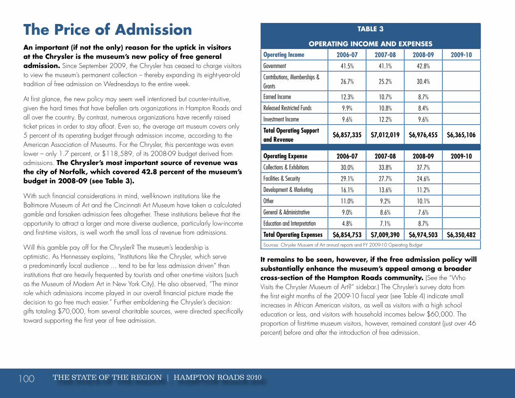
THE STATE OF THE REGION | HAMPTON ROADS 2010100
The Price of AdmissionAn important (if not the only) reason for the uptick in visitors at the Chrysler is the museum’s new policy of free general admission. Since September 2009, the Chrysler has ceased to charge visitors to view the museum’s permanent collection – thereby expanding its eight-year-old tradition of free admission on Wednesdays to the entire week.
At first glance, the new policy may seem well intentioned but counter-intuitive, given the hard times that have befallen arts organizations in Hampton Roads and all over the country. By contrast, numerous organizations have recently raised ticket prices in order to stay afloat. Even so, the average art museum covers only 5 percent of its operating budget through admission income, according to the American Association of Museums. For the Chrysler, this percentage was even lower – only 1.7 percent, or $118,589, of its 2008-09 budget derived from admissions. The Chrysler’s most important source of revenue was the city of Norfolk, which covered 42.8 percent of the museum’s budget in 2008-09 (see Table 3).
With such financial considerations in mind, well-known institutions like the Baltimore Museum of Art and the Cincinnati Art Museum have taken a calculated gamble and forsaken admission fees altogether. These institutions believe that the opportunity to attract a larger and more diverse audience, particularly low-income and first-time visitors, is well worth the small loss of revenue from admissions.
Will this gamble pay off for the Chrysler? The museum’s leadership is optimistic. As Hennessey explains, “Institutions like the Chrysler, which serve a predominantly local audience ... tend to be far less admission driven” than institutions that are heavily frequented by tourists and other one-time visitors (such as the Museum of Modern Art in New York City). He also observed, “The minor role which admissions income played in our overall financial picture made the decision to go free much easier.” Further emboldening the Chrysler’s decision: gifts totaling $70,000, from several charitable sources, were directed specifically toward supporting the first year of free admission.
TAbLE 3
oPErATiNg iNCoME AND ExPENSESOperating Income 2006-07 2007-08 2008-09 2009-10
Government 41.5% 41.1% 42.8%
Contributions, Memberships & Grants
26.7% 25.2% 30.4%
Earned Income 12.3% 10.7% 8.7%
Released Restricted Funds 9.9% 10.8% 8.4%
Investment Income 9.6% 12.2% 9.6%
Total Operating Support and Revenue
$6,857,335 $7,012,019 $6,976,455 $6,365,106
Operating Expense 2006-07 2007-08 2008-09 2009-10
Collections & Exhibitions 30.0% 33.8% 37.7%
Facilities & Security 29.1% 27.7% 24.6%
Development & Marketing 16.1% 13.6% 11.2%
Other 11.0% 9.2% 10.1%
General & Administrative 9.0% 8.6% 7.6%
Education and Interpretation 4.8% 7.1% 8.7%
Total Operating Expenses $6,854,753 $7,009,390 $6,974,503 $6,350,482Sources: Chrysler Musuem of Art annual reports and FY 2009-10 Operating Budget
it remains to be seen, however, if the free admission policy will substantially enhance the museum’s appeal among a broader cross-section of the hampton roads community. (See the “Who Visits the Chrysler Museum of Art?” sidebar.) The Chrysler’s survey data from the first eight months of the 2009-10 fiscal year (see Table 4) indicate small increases in African American visitors, as well as visitors with a high school education or less, and visitors with household incomes below $60,000. The proportion of first-time museum visitors, however, remained constant (just over 46 percent) before and after the introduction of free admission.

THE CHRYSLER MUSEUM OF ART 101
To be sure, the data in Table 4 derive from a small sample of Chrysler patrons over a short period of time; the full consequences of the new admission policy are not yet apparent. What does seem clear, however, is that free admission alone is not a magic recipe for bringing residents of Hampton Roads (or any other community) through the doors of their local museum. The keys to a thriving and well-attended art museum include not only affordability, but also a record of high-quality exhibitions and public programs, as well as the active cultivation of a loyal membership base. The Chrysler has done quite well here.
Who Visits the Chrysler Museum of Art?
The people of Hampton Roads are the Chrysler Museum’s
most important audience. According to Director William
Hennessey, the museum’s investigations have consistently
shown that 83 percent to 87 percent of its visitors live
within a 50-mile radius. As set out in a recent vision
statement, the Chrysler’s staff and board of trustees
intend to “continue to focus our efforts on serving the
people of southeastern Virginia,” as well as to expand the
size and diversity of the museum’s audience “to mirror
the demographics of Hampton Roads” by the year 2015.
The Chrysler’s audience is not yet a perfect reflection of
the entire regional population, but it is not far off. Art
museum visitors throughout the country tend to be
whiter, more affluent and better educated than the
population as a whole. The same trends are apparent
among respondents of the Chrysler Museum’s visitor
survey. However, African American visitors appear
to be less underrepresented at the Chrysler than at
other U.S. art museums. African Americans comprise
31 percent of the Hampton Roads population, while 23
percent of visitors surveyed at the Chrysler in 2009-10
identified themselves as African American. By contrast,
African Americans comprise 12.1 percent of the U.S.
population, but represent only 5.9 percent of all U.S. art
museum visitors, according to the National Endowment
for the Arts.

THE STATE OF THE REGION | HAMPTON ROADS 2010102
TAbLE 4
DEMogrAPhiCS oF ViSiTorS
hampton roads Population (2008)**
Chrysler Museum Visitors (2009-10)
Chrysler Museum Visitors (2008-09)
Changeu.S.
Population (2008)**
Demographic Distribution of u.S. Art
Museum Visitors (2008)*race/Ethnicity
African American 31.0% 22.99% 18.72% 4.27% 12.1% 5.9%
American Indian 0.3% 1.17% 0.00% 1.17% 0.7% N/A
Asian/Indian 3.1% 4.69% 3.83% 0.86% 4.4% N/A
Caucasian 58.9% 69.40% 73.62% -4.22% 65.4% 78.9%
Hispanic/Latino 4.3% 1.76% 2.13% -0.37% 15.4% 8.6%
Other 2.3% 0.00% 1.70% -1.70% 2.0% 6.6%
Education
Elementary school 2.9% 0.14% 0.00% 0.14% 6.4% 0.8%
Some high school 8.1% 3.57% 2.29% 1.28% 8.7% 4.0%
High school 26.9% 17.99% 7.29% 10.70% 28.5% 12.8%
Some college 26.0% 19.78% 31.14% -11.36% 21.3% 28.5%
College graduate 25.7% 28.85% 29.86% -1.01% 25.0% 32.8%
Graduate/professional degree
10.4% 29.67% 29.43% 0.24% 10.2% 21.1%
household incomeUnder $20,000 14.6% 3.03% 1.74% 1.29% 17.8% 6.5%
$20,000 - $39,999 19.0% 7.49% 3.47% 4.02% 20.7% 13.7%
$40,000 - $59,000 18.7% 10.87% 5.79% 5.08% 17.6% 8.0% ($40-50K)
$60,000 - $79,000 $60-75K 11.5% 8.56% 10.42% -1.86% 10.5% 20.6% ($50-75K)Sources: Chrysler Museum of Art, 2008 American Community Survey (1-year estimates), at: http://factfinder.census.gov, and the National Endowment for the Arts, 2008 Survey of Public Participation in the Arts, at: http://arts.endow.gov/research/2008-SPPA.pdf
** Note that the race and income categories for U.S. art museum visitors used by the NEA differ slightly from those used by the Chrysler Museum ** Note that the income categories used by the American Community Survey differ slightly from those used by the Chrysler Museum

THE CHRYSLER MUSEUM OF ART 103
TAbLE 4
DEMogrAPhiCS oF ViSiTorS
household income
$80,000 - $99,999 $75-100K 14.6% 9.09% 6.95% 2.14% 12.4% 18.0% ($75-100K)
$100,000 + 21.6% 15.51% 13.32% 2.19% 21.0% 33.2%
NA / Student N/A 25.31% 27.80% -2.49% N/A N/A
Retired N/A 20.14% 30.50% -10.36% N/A N/A
is this your first visit to the Chrysler Museum?
Yes 46.67% 46.51% 0.16%
No 53.23% 53.49% -0.26%
Approximately how much time did you spend in the museum today?
In hours 1.85 2.13 -28.00%Sources: Chrysler Museum of Art, 2008 American Community Survey (1-year estimates), at: http://factfinder.census.gov, and the National Endowment for the Arts, 2008 Survey of Public Participation in the Arts, at: http://arts.endow.gov/research/2008-SPPA.pdf
** Note that the race and income categories for U.S. art museum visitors used by the NEA differ slightly from those used by the Chrysler Museum ** Note that the income categories used by the American Community Survey differ slightly from those used by the Chrysler Museum

THE STATE OF THE REGION | HAMPTON ROADS 2010104
Membership and Special Exhibitions“Museums that do not charge a general admission fee usually have much smaller membership programs,” asserted a 2007 article in the journal Museum News.4 These are words of caution for the Chrysler, which depends upon its members for a critical backbone of community and financial support. Membership accounted for 11.8 percent, or $800,000, of the Chrysler’s budget in 2008-09. In return, members enjoyed perks such as museum shop discounts, subscriptions to The Chrysler Magazine, invitations to members-only events and free admission. Thus, a substantial risk of ceasing to charge for general admission is eliminating one of the museum’s most attractive incentives for membership.
Happily, the Chrysler seems to have averted this risk. At the end of February 2010, the museum boasted 4,089 active memberships, a 12 percent increase over the previous year (see Table 5). The overwhelming majority of new members joined at the household level of $75 per year ($65 for seniors, active-duty military and teachers). The most significant recent decline has come in corporate memberships at the $500 and $1,000 levels, presumably the result of a difficult economy. However, the museum’s most dedicated supporters ($3,000-plus per year) remained roughly constant. year-to-date membership revenue at the end of February 2010 totaled $662,650 (8 percent more than the previous year), placing the museum on track to fulfill or exceed its $860,000 membership goal for 2009-10.
The data in Table 5 speak well of the Chrysler’s support across the breadth of Hampton Roads. Both large donors and “average” residents of the Hampton Roads community are represented. The gratifying increase in household memberships perhaps is a positive charitable response to the new policy of free general admission. Another factor may be the museum’s special exhibitions, which continue to carry a modest admission charge for all nonmembers. Free admission to the museum’s special exhibitions and their accompanying programs continues to provide a strong incentive for membership.
4 Gypsy McFelter, “The Cost of ‘Free’: Admission Fees at American Art Museums,” Museum News (January/February 2007), available at: http://www.aam-us.org/pubs/mn/MN_JF07_cost-free.cfm
TAbLE 5
ChrySLEr MuSEuM MEMbErShiPTotal
Memberships as of 2/28/09
Total Memberships as
of 2/28/10
Existing Members
Renewal Rate
New Memberships as
of 2/28/10
Individual Memberships
MPS Benefactor ($10,000)
8 8 71% 1
MPS Patron ($5,000)
47 50 98% 0
MPS Sponsor ($3,000)
112 105 86% 2
Director’s Circle ($1,000)
68 62 84% 1
Patron ($500) 62 56 85% 0
Friend ($250) 176 161 80% 3
Associate ($150) 277 282 80% 14
Household ($75/$65*)
1,683 2,123 45% 475
Individual ($55/$45*)
1,148 1,139 57% 178
Student ($25) 33 77 5% 27
Corporate Memberships
BEC ($5,000) 22 20 82% 2
Benefactor ($2500) 2 2 10% 0
Director’s Circle ($1,000)
12 3 0% 0
Patron ($500) 8 1 0% 0
Totals 3,658 4,089 703Source: Chrysler Museum of Art * Discounted memberships are for seniors age 65 or older, teachers and active-duty military.

THE CHRYSLER MUSEUM OF ART 105
Between Oct. 14, 2009, and Jan. 3, 2010, the Chrysler hosted “To Live Forever: Egyptian Treasures from the Brooklyn Museum,” its first-ever special exhibition of ancient Egyptian art. Egyptian relics are a popular attraction for museumgoers everywhere. Table 6 records that “To Live Forever” was one of the best-visited special exhibitions in the Chrysler’s recent history, exceeded only by “American Chronicles: The Art of Norman Rockwell” in average daily attendance. Special events associated with the exhibition included showings of Egypt-themed movies, an overnight “Sleep with the Mummies” activity for families with children ages 6-12, and a dance and preview weekend for members only. on display for only 53 days, “To Live Forever” helped to bring in more membership and admissions revenue ($30,494 and $48,800, respectively) than did other special exhibitions of longer duration. Museum shop sales during the Egyptian exhibition ($107,148) were also robust.
A successful special exhibition brings “glamour and novelty” to a familiar museum, Hennessey noted in the January/February 2010 issue of The Chrysler Magazine. “Experience has shown us that it is borrowed treasures that most effectively capture the public’s imagination and draw them through our doors.”
Special exhibitions clearly attract new visitors (and their dollars), but the associated costs of these exhibitions can be considerable. The budgeted cost of “To Live Forever” was $325,000, a figure that does not include the substantial hours spent by Chrysler staff on installation, interpretation, marketing and the like. According to hennessey, the division of resources between special exhibitions and an institution’s permanent collection is “one of the most perennially vexing balancing acts facing museums today.” Thus, the Chrysler seeks to balance high-profile, though costly, loan exhibitions like “To Live Forever” with shows of local interest that can be organized by the museum itself, such as a planned “hampton roads Collects” exhibition that will borrow from private collections throughout the region. “Women of the Chrysler: A 400-Year Celebration of the Arts,” presented between March 24 and July 18, 2010, was an innovative presentation of works by women artists drawn entirely from the museum’s permanent collection.

THE STATE OF THE REGION | HAMPTON ROADS 2010106
TAbLE 6
SPECiAL ExhibiTioN CoMPAriSoNTo Live Forever
Art of glass 2
Norman rockwell
rembrandt’s Etchings
goya to Sorolla
Virginian-Pilot Photos
AttendancePaid admissions 9,414 6,457 8,532 4,271 4,295 4,291
Members 3,322 2,844 2,865 1,536 1,483 1,768
Wednesday - day N/A 6,718 6,622 5,425 4,426 3,313
Wednesday - night N/A 3,214 2,151 3,225 2,798 2,176
Other free admissions 2,506 8,990 10,400 4,423 3,942 3,354
General admissions 6,677 N/A N/A N/A N/A N/A
Business entry 3,290 3,666 2,857 2,692 3,580 2,831
Tours 8,297 3,672 7,096 1,644 4,628 6,049
Special events 8,337 13,799 6,794 5,811 8,505 9,310
Historic houses 666 1,053 1,217 1,901 1,294 995
Exhibition totals 42,509 50,413 48,534 30,928 34,951 34,087Days open 53 75 57 68 65 70
Average daily attendance (excluding special events and historic houses)
506 474 711 341 387 340
Front of house revenueAdmissions $48,800 $36,900 $48,663 $24,792 $18,154 $23,277
Donation box $3,532 $13,860 $13,334 $11,637 $7,813 $5,510
Museum shop sales $107,148 $114,579 $95,155 $64,951 $62,787 $63,470
Membership $30,494 $17,670 $10,306 $10,163 $10,860 $8,053
Exhibition totals $189,974 $183,009 $167,458 $111,543 $99,614 $100,310Source: Chrysler Museum of Art

THE CHRYSLER MUSEUM OF ART 107
Education and Public ProgramsA review of Table 3 indicates that “Education and Interpretation” represents a small but growing portion of the Chrysler’s operating expenses. Between 2006-07 and 2008-09, the proportion of the museum’s budget devoted to education rose from 4.8 percent to 8.7 percent, proportionally the largest increase in any category throughout this two-year time span. The museum’s Department of Education and Public Programs oversees a diverse array of activities, including the operation of the Jean Outland Chrysler Library, tours for students and teachers (more than 19,000 in 2008-09); development of an e-museum that will provide online access to the 35,000 objects in the Chrysler’s collection; gallery talks, lectures, concerts and children’s activities; and even programs such as “Yoga for Art Lovers” and “The Fine Art of Wine.”
The breadth of these public programs, including a few that are only tangentially related to the Chrysler’s collections and exhibitions, reveal much about the changing role of museums in American society. In decades past, art museums often resembled a treasure house or temple. The architecture of the Chrysler Museum itself, constructed in the 1930s as the Norfolk Museum of Arts and Sciences, was directly inspired by palaces of the Italian Renaissance. Nineteenth- and early 20th-century museums preserved works of art so that they could be appreciated in an appropriately reverential setting. The function of museums as “protectors of culture” carries on today, but their institutional atmosphere is typically more casual, interactive and socially inclusive than in the past. Even the definition of “art” has expanded – as demonstrated, for example, by the Chrysler’s hosting of special exhibitions on Ferrari automobiles (2003) and news photography from The Virginian-Pilot (2006). Public and private funding sources expect museums to promote diversity and engage in community outreach.
For these reasons, a successful museum of the 21st century must do much more than display works of art. hennessey says that he likes “the idea that museums can be forums – places where the entire community gathers to celebrate shared events and
values, to exchange and explore ideas, for social interaction, perhaps for a meal or some shopping.” As the mission of the Chrysler has expanded and evolved, so too has its Department of Education and Public Programs (and its Department of Visitor Services, founded in 2007). The allocation of a museum’s finite resources among its various branches represents another delicate balancing act for a museum director, particularly in lean economic times. For every enthusiast of the Yoga for Art Lovers class or the “Women of the Chrysler” interactive website (http://www.womenofthechrysler.org), there is apt to be someone else who considers these initiatives a distraction from core museum responsibilities such as acquisitions and conservation. Indeed, the Chrysler Museum currently employs only two full-time curators, though the creation of a new position in photography and contemporary art is planned through the establishment of a future endowment.

THE STATE OF THE REGION | HAMPTON ROADS 2010108
Plans for the FutureA new curatorship is just a small part of the Chrysler’s designs for the future. in March 2010, the board of trustees approved a new plan for the renovation and expansion of the museum’s main building, as well as for the conversion of the former Wachovia bank building (located nearby at the corner of grace and Duke streets) into a glassmaking studio. The overall project cost is estimated at $18 million, $2 million of which has already been received in the form of a challenge grant from a private donor. An upcoming capital campaign will seek to raise the remaining funds necessary for construction, as well as increase the museum’s endowment for operation funds.
A prime motivation for the main building’s renovation is to create 8,000 square feet of new gallery space, thereby allowing more works in the permanent collection to be placed on display. Plans call for 2,500 new square feet of the new space to be dedicated to the glass collection, expanding the current display space by one-third. Additional improvements will enhance the building’s accessibility for visitors and staff. The museum’s restaurant and catering facilities will move to a more central location; guests with wheelchairs (or with strollers) will no longer be asked to enter the building through a side door. The expansion will take the form of two wings flanking the main entry; both new wings are designed to integrate smoothly with the Chrysler’s existing architecture. “The resulting building,” promises a recent development plan, “will look to the passerby almost identical to the current structure.”
The second component of the Chrysler’s expansion project is the construction of a glass studio (or “hot shop”) that will allow museum visitors to experience the glassmaking process live. Of the four U.S. museums most recognized for their collections of historical and contemporary glass (including the Corning Museum of Glass in New York, the Toledo Museum of Art and the Museum of Glass in Tacoma, Wash.), only the Chrysler does not operate its own glassmaking furnace. A hot shop would add an appealing new attraction for visitors, and also allow the Chrysler “to partner with local schools like Tidewater Community
College (where a small glassblowing program has already been established) and the Governor’s School for the Arts,” according to the museum. With a high-quality studio, the Chrysler could invite accomplished glassblowers to hold demonstrations in conjunction with special exhibitions (like the recent “Art of Glass 2”), or even to serve as artists in residence for a longer duration.
Final ThoughtsThe advantages of the Chrysler Museum of Art’s planned renovation and expansion are many – including the enhancement of its nationally recognized specialty in art glass, as well as the opportunity to improve the main building’s design for visitors and staff alike. As the museum’s leadership is certainly aware, however, raising $16 million in the current economic climate is a formidable challenge. Like other arts organizations in hampton roads, the Chrysler has faced some unpleasant fiscal realities in recent months. The museum’s budgeted operating revenue for the 2009-10 fiscal year was $6,365,106 – 6.5 percent less than the previous year. This downward trend may continue, as the Chrysler’s funding through the city of Norfolk and the Virginia Commission for the Arts is expected to decline in 2010-11. For the foreseeable future, the museum’s budget is likely to remain lean, despite positive increases in membership and visitor traffic.
With shrinking resources at its disposal, the Chrysler Museum must perform more services and appeal to a broader audience than in generations past. This calls not only for financial discipline, but also for creative and flexible management. In our view, the Chrysler has risen admirably to the challenge. The year 2009 was called an “annus horribilis” for U.S. art museums.5 in response to the sudden decline of their endowments and gifts from private donors, well-known institutions canceled exhibitions, imposed pay furloughs or turned to other drastic measures in order to make ends meet. by contrast, the Chrysler introduced a new
5 Javier Pes and Helen Stoilas, The Art Newspaper (Jan. 28, 2010), at: http://www.theartnewspaper.com/articles/Recovery-after-annus-horribilis/20186

THE CHRYSLER MUSEUM OF ART 109
policy of free general admission, increased its visitor numbers, hosted well-received special exhibitions and moved forward with an ambitious proposal for renovation and expansion. These are no small accomplishments in a year marked by the sharpest economic contraction since the great Depression. Residents of Hampton Roads can be proud of their region’s flagship institution for the visual arts.

The Virginia Aquarium & Marine Science Center

THE STATE OF THE REGION | HAMPTON ROADS 2010112
DESTINATION OF CHOICE: THE VIRGINIA AQUARIUM & MARINE SCIENCE CENTER
Which tourist and scientific center in Hampton Roads has attracted 11 million guests (including 1 million students) since opening in 1986? What
is the Commonwealth’s most popular non-historical, nonprofit tourist attraction? Unless tutored, many might be inclined to answer the Nauticus/
USS Wisconsin complex in Norfolk to both questions. The correct answer, however, is the Virginia Aquarium & Marine Science Center in Virginia
Beach.
The 11 million visitors have been treated to unique and educational experiences with live animal displays, interactive science exhibits, and both in-house and outreach natural history programs. In addition, the Virginia Aquarium’s Research and Conservation division has made major contributions to the scientific understanding of marine mammals and sea turtles in the mid-Atlantic region. The Aquarium employs 142 people throughout the year and utilizes an amazing 1,000 volunteers and numerous student interns in a variety of support roles.
Whether or not one is interested in the attractive exhibits and programs the Aquarium has to offer, it should be of interest that the facility forms the foundation stone for the strategic development and enhancement of a large section of Virginia Beach, which stretches from Rudee Inlet in the north to Oceana Naval Air Station in the south. Over the next few decades, this plan is anticipated to reshape this section of the city.
From Idea to AquariumSoon to celebrate its 25th anniversary, the Virginia Aquarium & Marine Science Center started as an idea in 1973, when C. Mac Rawls, a science supervisor for Virginia Beach Public Schools, was asked to head a panel to study the school board’s suggestion for a science resource room. After two years of study
and discussion, the panel recommended a marine science museum devoted to educating the public about Virginia’s marine environment, and suggested the city hire an expert to review the committee’s plan and offer further recommendations. The project became known as the Virginia Beach Marine Science Museum and, in 1979, the city of Virginia Beach donated a 9-acre site between Owl Creek and General Booth Boulevard for the facility. Rawls was named director of the museum.
A year later, the City Council appointed three task forces to aid in the development of the Virginia Marine Science Museum, whose first task was to rename the yet-to-be-built facility the Virginia Museum of Marine Sciences. Shortly thereafter, the 10-member Museum Foundation Task Force officially formed the Virginia Marine Science Museum Foundation Inc., which was – and still is – the Aquarium’s nonprofit fundraising body. In 1983, the foundation, as well as other museum supporters, successfully lobbied to persuade the Virginia General Assembly to appropriate $2 million for construction of the museum. The city of Virginia Beach added $3.5 million, and the project was soon under way.
Meanwhile, the foundation conducted a $2 million capital campaign to pay for the museum’s exhibits, while other related happenings were taking place. Rawls and his staff of six moved from their office on Arctic Avenue to their new quarters at Camp Pendleton, and Harold, a 17-pound lobster caught by Hagan Seafood Corp., was donated to the museum as its first live animal exhibit.

THE VIRGINIA AQUARIUM & MARINE SCIENCE CENTER 113
On June 14, 1986, the 41,500-square-foot facility officially opened to the public, but not before undergoing another name change, back to the Virginia Marine Science Museum. Attendance that summer exceeded projections by about 45 percent, as more than 109,000 visitors entered the doors in the first three months.
Conservation Leads the WayIn the late 1980s, the museum took its conservation-through-education mission to the next level, and a team of expert staff and volunteers, funded by the foundation, began responding to stranded marine mammals and sea turtles that washed up sick, injured or dead along Virginia’s shores. The new stranding program provided the impetus for numerous research projects on seals, dolphins, right whales and endangered sea turtles, leading to millions of dollars in conservation research grants and positioning the staff as experts in those fields. Today, the Aquarium’s right whale expert teaches staff at other institutions on the East Coast about the biology and behavior of these animals and is frequently called upon to participate in a stranding event or necropsy (animal autopsy) of this species. And because of the 2009 acquisition of a pair of critically endangered tomistoma crocodiles – one of only seven pairs in the United States – the Aquarium’s reptile curator has traveled to Thailand and Borneo to both study the animals in the wild and consult on in situ research projects. And research begets research: the Aquarium’s academic, government and non-government partnerships resulted recently in the awarding of an estimated $4.5 million National Oceanic and Atmospheric Administration grant for sea turtle research.
Also during this year, the foundation funded the development of an outreach program that has evolved into the present-day Ocean in Motion traveling aquarium program. Today, Ocean in Motion travels as far away as Bristol, Staunton and Danville, bringing marine education, along with a host of saltwater critters, to more than 25,000 schoolchildren annually.
Expanding and AttractingBy the early 1990s, plans were in place for a second phase of the Virginia Marine Science Museum that would triple its size to 120,000 square feet, and add more than 45 acres of land, two buildings and a connecting nature trail over the Owl Creek marsh. Virginia Beach City Council approved $32.8 million from the Tourism Growth Investment Fund (a direct funding stream from the city’s hospitality industry) for the expansion.
As an additional source of revenue, the museum introduced winter whale watching trips, developing an off-season tourism industry for the city. In 2009, this venture resulted in an estimated $611,000 in direct spending to local hotels, restaurants and shops. The foundation raised another $5 million for the expansion’s exhibits, and phase II opened in 1996 with an attendance increase that surpassed projections. The two years following the expansion saw an unprecedented period of growth for the facility, with annual attendance approaching 700,000 in 1997, then settling around the 600,000 level by 1999, where it remained for the next decade.
Competition for tourist dollars is intense and sites that are perceived to be old or unchanged often experience a drop in attendance. Such perceptions make it more difficult to attract both new visitors in search of a novel experience and repeat visitors. It appears that this has been responsible for the facility’s stagnant and falling attendance rates during the past decade. The foundation responded to this circumstance with a set of attractive new exhibits, but they took time to develop and construct and in the short-turn probably reduced rather than increased attendance. However, these innovations have been successful. Graph 1 reveals that attendance at the Virginia Aquarium & Marine Science Center (so named on July 1, 2004) was projected to reach 647,000 in fiscal year 2010, and 700,000 in fiscal year 2011 because of the new exhibits.

THE STATE OF THE REGION | HAMPTON ROADS 2010114
GRAPH 1
VISITOR ATTENDANCE AT THE VIRGINIA AQUARIUM

THE VIRGINIA AQUARIUM & MARINE SCIENCE CENTER 115
Visitors do much more than see fish when they come to the Virginia Aquarium. Per capita spending has increased from $9.35 in FY 1999 to $14.16 in FY 2010. In addition to Aquarium admission, guests purchase IMAX film tickets, gift shop souvenirs and Aquarium-themed photos. They also dine in the café, cruise the creek on a pontoon boat and opt to get wet in animal encounter programs like the in-the-water Seal Splash. The Aquarium’s effort to increase earned income has created spinoff revenue in the form of taxes for the city of Virginia Beach as well as the Commonwealth of Virginia. Admission and sales/meal taxes generated as a result of Aquarium operations grew from $396,000 in FY 1999 to $774,000 in FY 2010, a 95 percent increase.
When out-of-town visitors come to Virginia Beach and visit the Aquarium, they also tend to spend more and stay longer (see Table 1). What is not clear is whether the facility per se attracts higher-spending and longer-staying visitors, or whether such individuals simply discover and take advantage of the Aquarium after they come to Virginia Beach. There is no dispute, however, that the Aquarium forms an important part of a complex of tourist attractions that make Hampton Roads in general, and Virginia Beach in particular, more appealing.
The path to the current enterprise known as the Virginia Aquarium & Marine Science Center was not without pitfalls, however. In 1998, the facility had a new project on the drawing board that would include a 100,000-square-foot building housing a 1.6 million-gallon Atlantic Coast habitat, two indoor aviaries, a new classroom, hands-on interactive exhibits, a marine animal stranding and research center, and a new store. The signature animal species proposed for the new exhibition building was the bottlenose dolphin. Animal-rights activists threatened to protest and disrupt the city of Virginia Beach and the facility’s operations, however, over their objection to dolphins in captivity. As a result of both the opposition and the commitment of funds for the proposed new convention center, city leaders decided not to approve funding for the project at that time.
TABLE 1
VIRGINIA BEACH VISITORS CHARACTERISTICS: SPENDING AND LENGTH OF STAY
CharacteristicsOver
$1,000$500-$1,000
$250- $499
Less than $250
Nights stayed 5.6 2.8 2.0 2.0
Party size 4.3 3.2 2.8 3.0
Stayed in hotel 71% 84% 77% 33%
Visited Busch Gardens or Williamsburg
26% 17% 9% 9%
Sports (golf, fishing) 19% 8% 9% 5%
Visited Aquarium 32% 16% 23% 5%Source: Gilbert Yochum and Vinod Agarwal, Virginia Beach 2009 Boardwalk Overnight Visitor Survey
The Virginia Marine Science Museum (as it was known then) subsequently opened a teaching facility, Bay Lab, at First Landing State Park in 1999. This hands-on educational laboratory, filled with aquariums, touch tanks and microscopes, offers programs focusing on various Chesapeake Bay topics, and serves more than 1,400 students and families each year. However, the Aquarium’s research interests these days reach far beyond Hampton Roads’ waterways: it has hosted summits on alternative energy, provided ship speed studies that have international whale protection implications, mapped port traffic for use in wind farm planning and, in partnerships with local and national universities, is developing research projects that will help this area and other shoreline communities predict and prepare for sea level rise as a result of global warming. A 40-foot research vessel, the Ocean Explorer, was christened in 2009 as part of a joint venture with Virginia Wesleyan College. The college will use the vessel for its marine biology and environmental curricula, while the Aquarium will be able to conduct on-the-water research and, in rare cases, large marine mammal interventions during beaching or entanglement. These partnerships provide a model for other nonprofits, bringing an entrepreneurial focus to what are largely public funds, whether through dedicated tax streams or grants.

THE STATE OF THE REGION | HAMPTON ROADS 2010116
Following Rawls’ retirement in 2001, Lynn Clements, former deputy director and interim director, was named the executive director of the Virginia Marine Science Museum and the city of Virginia Beach director of the Department of Museums and Cultural Arts.
The Virginia Beach City Council endorsed the facility’s name change to the Virginia Aquarium & Marine Science Center in 2004, accompanied by a branding campaign launched by the ad agency BCF. While still embracing its core mission of conservation through education, the Aquarium, in concert with the foundation’s board of trustees and city leaders, cast an eye toward long-term fiscal sustainability. Cultural Arts became a separate entity with the completion of the Sandler Center for the Performing Arts in 2007, with Clements continuing to oversee the Aquarium and the city-owned historic houses: Francis Land House, Lynnhaven House and Adam Thoroughgood House. This is a somewhat unusual arrangement, but one that has worked well.
Funding and FundraisingToday’s Virginia Aquarium relies upon an interesting and flexible public/private partnerships structure that may well represent the future for the majority of tourist and scientific installations and organizations in Hampton Roads. Aquarium partnerships exist between the city of Virginia Beach and the Aquarium’s foundation, and appear to succeed because each entity has distinct and separate areas of authority, control and responsibility, though common goals. The city owns the Aquarium buildings and grounds, and provides utilities, building maintenance and landscape services. The Aquarium’s budget must be approved by City Council through the annual budget process or by agenda request. All revenues earned through admissions, memberships and Aquarium store sales are deposited into the city’s general fund and designated for the facility’s operations.
In contrast to many other facilities, the Aquarium earns 94 percent of the funds necessary to finance its annual operating budget. The city of Virginia Beach provides between $300,000 and $400,000 annually of the Aquarium’s $11
million budget (see Table 2), which includes general operating expenditures of $3.6 million and a payroll of $5.4 million. Any net revenues at year’s end are deposited into a Replacement and Renewal Capital Improvement Program Fund, to be used for purchasing items such as pumps, filters and computer equipment on an as-needed basis. This fund has provided $568,000 for these capital items since its inception in FY 2003.
As the fundraising component of the partnership, the Aquarium Foundation owns the exhibits and the animals, and conducts educational programming in support of the Aquarium’s conservation-through-education mission, reaching nearly half a million children and adults in FY 2009. The foundation’s annual operating budget of approximately $2 million is funded through donations, grants, philanthropic-level and corporate memberships, sponsorships and educational program fees, such as those for boat trips and the Seal Splash experience. Foundation fundraising efforts also support temporary exhibits, research and conservation activities. Scientific study of marine animals through stranding response, rehabilitation, field research and conservation programs is a major focus of the foundation.
TABLE 2
COMBINED FINANCIAL RESULTS: THE AQUARIUM AND ITS FOUNDATION
Fiscal Year Revenues Percent ChangeFY 2005 $8,221,601
FY 2006 $9,607,546 16.86%
FY 2007 $9,342,398 -2.76%
FY 2008 $8,960,116 -4.09%
FY 2009 $8,284,984 -7.53%
FY 2010 $9,406,557 13.54%
FY 2011 $11,055,950 17.53%

THE VIRGINIA AQUARIUM & MARINE SCIENCE CENTER 117
The foundation’s volunteer board of directors willingly provides many hours of their time in support of the Virginia Aquarium’s mission. They work closely with staff members, providing legal and business guidance as well as budgetary approval and oversight of the foundation’s annual budget. To ensure commonality of mission and purpose, the Aquarium’s director serves as CEO of both the Aquarium and the foundation. This organizational structure combines the stability of the city’s support for operations with the flexibility of a private foundation that can raise funds and set an entrepreneurial course for the facility.
Aquarium and foundation operations and partnerships generated $672,414 in direct tax revenue to the city and the Commonwealth of Virginia through admissions and sales/meal taxes in fiscal year 2009; $620,057 of that remained in the city of Virginia Beach and $52,357 in sales tax was paid to the Commonwealth. An attendance boost is projected for FY 2011, the first full year of operation of Restless Planet, the facility’s newest series of exhibits. This, coupled with increased admission prices, is projected to grow Aquarium revenues and expand the taxes generated by its operations to $774,609.
Aquarium management has brought in temporary exhibits and launched new programs in an effort to keep up public interest, maintain attendance and thereby maintain revenue levels. Attendance and revenue declined between FY 2007 and FY 2009, primarily due to construction of new exhibits, but rebounded very nicely in FY 2010 and is projected to set a record in FY 2011.
The Aquarium also works closely with the Virginia Beach Convention & Visitors Bureau to entice a quarter of the city’s overnight visitors to the facility, making it Virginia Beach’s most-visited attraction. In FY 2011, the facility expects to host some 700,000 visitors, surpassing Colonial Williamsburg and making the Aquarium the Commonwealth’s most popular non-historical destination.

THE STATE OF THE REGION | HAMPTON ROADS 2010118
Restless Planet In 2003, the Virginia Marine Science Museum, as it was still known, recognized the need to renovate its 17-year-old exhibits. Not only was the science outdated, but also exhibit technology had changed drastically since the 1980s. Long gone were traditional, static exhibits. According to the minutes of the foundation’s Exhibits Committee, the stated objectives of the project were as follows:
• Create a project exciting enough to increase visitation/attendance
• Maintain Virginia theme while incorporating novel ideas for educational exhibits that meet our conservation-through-education mission
• Maintain those aspects of the current Aquarium exhibits that make our facility unique (e.g., the mix of live animals/interactive exhibits)
• Create a balance between education and entertainment.
Because many people learn kinesthetically, the area would be modernized with immersive habitats that mimic the temperature, flora and fauna of the real-life areas they represent. More than 30 hands-on interactive exhibits that challenge visitors to test their skills and knowledge about salinity, gravity, volcanism, seismology and other sciences would be added to the facility’s 300 existing interactive exhibits.
The largest project since the addition of a second building and nature trail in 1996, Restless Planet, which opened Nov. 21, 2009, comprises four immersive habitats, dozens of new hands-on interactive exhibits and 110,000 gallons of new aquariums showing the forces that shaped Virginia hundreds of millions of years ago. A project of this magnitude required considerable funding through a capital campaign and strategic partnerships. The Commonwealth of Virginia, the city of Virginia Beach and its citizens stepped up to the challenge.
In early 2008, six months before the scheduled conclusion of its $27.8 million capital campaign, the Virginia Aquarium & Marine Science Center Foundation announced that it had already exceeded its campaign goal. Included in the total was $14.4 million from the city of Virginia Beach to cover infrastructure
construction of the Restless Planet project. The Commonwealth of Virginia also appropriated $2 million. As a result of meeting the goal, the Aquarium received a $650,000 challenge grant from the Kresge Foundation of Troy, Mich.
The Aquarium’s fiscal year 2008 operations provided $662,749 to the city’s net direct revenue return from tourism. However, a major improvement to the existing facility, in the form of the Restless Planet, would enable the Aquarium to attract more visitors each year and additional earned revenues of just under $2 million, with a projected $200,000 in admissions tax revenues to the city during the first year. The foundation, on the other hand, continues to fund education, research, exhibit development and maintenance, and animal acquisition and care.
Despite its relative independence, the Aquarium is feeling the impact of Virginia Beach’s 2011 budget shortfall. To meet the required cuts in city-supported general operating expenses, the Aquarium has consolidated some programming and staff positions, reduced the number and cost of its IMAX offerings, expanded the hours of its more than 800 volunteers, and encouraged its members to “go green” by receiving their member newsletter and other materials via e-mail (an estimated savings of $20,000 in printing costs alone). But budget cuts can only go so deep when your assets have an appetite. “No matter what happens, the animals still have to eat,” said Executive Director Clements, referring to the expanded collection of 12,000 animals.
In addition to tax revenues, the Aquarium supports the local economy in other ways. Its recent $25 million Restless Planet addition provided badly needed jobs for contractors, suppliers and subcontractors. Its 142 employees pay taxes, buy homes and otherwise contribute to the local economy each year through direct and indirect spending. This doesn’t even take into account the overall impact of tourism, which pumps $78.4 million a year into Virginia Beach tax revenues alone. With the exception of Colonial Williamsburg, the Virginia Aquarium led local attractions in both operating budget and visitation in 2008 (see Table 3).
During its first six weeks, Restless Planet saw a 54 percent increase in visitation over the same period in 2008. These increased admissions generated more than $40,000 in tax revenue to the city of Virginia Beach. The Aquarium also is

THE VIRGINIA AQUARIUM & MARINE SCIENCE CENTER 119
one of the higher-priced local attractions: after a five-year moratorium on ticket price increases, partly due to the three-year construction process, the Aquarium raised its price from $11.95 to $17 for an adult admission, compared to the Virginia Living Museum’s $17 and Nauticus’ $11.95. But the Aquarium’s price of admission is still well below Colonial Williamsburg’s $36 one-day ticket in 2010.
TABLE 3
LOCAL HAMPTON ROADS ATTRACTIONS: 2008Attraction Governance Employees Budget Attendance Ticket Price
Va. Living Museum
Private nonprofit 90 $4.25m 215,000 $17/$13
Va. Zoo City/nonprofit 76 $3.5m 316,000 $8/$6
Nauticus City/advisory 51 $6m 400,000 $11.95/$9.50
Colonial Williamsburg
Private nonprofit 4,000 est. $249m 660,000 $36/$18
Va. Aquarium City/nonprofit 142 $11m 600,000 $17/$12Source: Association of Zoos & Aquariums Member Directory 2009
Graph 2 illustrates the gap between the Aquarium and four well-known, major aquariums in the country in terms of annual attendance and operating budgets. The differences hinge on several factors. The “Big Four” (the Monterey in California, the Shedd in Chicago, the Georgia in Atlanta and the National in Baltimore) enjoy much larger regional population bases, available land for physical plant expansion and operating budgets that average about three times that of the Virginia Aquarium. Not coincidentally, all but the National Aquarium are based on multimillion-dollar endowments from benefactors such as Hewlett-Packard and Home Depot.
The Virginia Aquarium may not yet be comparable to the Big Four in terms of attendance and budget, but it remains a viable contributor to the local economy and continues to attract a nearly equal mix of Virginia and out-of-state visitors (see Graph 3). The recently opened Restless Planet has resulted in gratifying increases in attendance and membership; however, the Aquarium must rely on an ever-changing blend of films, new temporary exhibits, programs and experiences to cater to audiences hungry not just for education, but for entertainment as well. It will take an innovative approach to bring 750,000 visitors annually to the Aquarium until the next major expansion allows it to reach the 1 million-visitor threshold that, for many, signifies the “big time” insofar as tourist and scientific sites are concerned.

THE STATE OF THE REGION | HAMPTON ROADS 2010120
GRAPH 2
THE BIG FOUR U.S. AQUARIUMS
Source: Association of Zoos & Aquariums Member Directory 2009

THE VIRGINIA AQUARIUM & MARINE SCIENCE CENTER 121
GRAPH 3
WHERE VIRGINIA AQUARIUM VISITORS COME FROM
Source: Clarity oms, Virginia Aquarium Visitor Intercept Study, September 2006

THE STATE OF THE REGION | HAMPTON ROADS 2010122
The Virginia Aquarium and the Larger Virginia Beach Development PictureIf the Virginia Aquarium’s goal is to attract attendance and funding similar to the “Big Four” depicted in Graph 2, then this is unlikely to be realized in the near future despite the very nice upsurge in attendance because of its newer attractions. However, farsighted planners such as Ned Williams, local commercial real estate broker and chairman of the Aquarium Foundation’s board of trustees, believe that such a goal can be realized if it is integrated within a well-designed plan that not only includes the Aquarium, but also nearby attractions and amenities. As such, the Aquarium’s development would anchor the development and enhancement of a major section of Virginia Beach.
Williams is spearheading the Aquarium/Owl Creek District Plan (ADP), a 20-year vision for the retail, cultural, maritime and natural environment of the area within Virginia Beach that stretches roughly from the Rudee Inlet bridge to Oceana. In addition to the Aquarium, the district encompasses a public boat ramp, residential area, state military reservation, Navy property and facility, the city’s dredge operations facility, Department of Parks and Recreation open-space property, a tennis facility, public schools and the privately owned/operated Ocean Breeze Waterpark and Motor World.
In a recently published request for proposals for planning services for the ADP, the following priorities were addressed:
Recreation: Plans for human scale, pedestrian-friendly experiences incorporating existing and planned shared-use pathways; highlights open space preservation areas; … and provides a harmonic link between the oceanfront and the District, all while complementing the surrounding physical environment as well as providing a platform for a several-day-visit experience
Research & Technology: Lays the foundation for marine research facilities in partnership with higher education; recognizes the planned Aquarium Marine
Animal Care Center as an exhibit support facility for future exhibit buildings that also contain research aspects
Education: Creates a stimulating framework for a life-long learning community, potentially including a children’s environmental activity center and/or high school honors marine science summer resident program; environmental learning opportunities through outdoor, hands-on learning for all ages
Entertainment: Examines current nearby offerings, including the motor park and water park. Proposes locations, types and scale of additional family-friendly entertainment opportunities which complement similar facilities existing and planned within Virginia Beach and the region
Economic Development Opportunities: Offers opportunities for location of alternative energy and green businesses
Exhibits: Identifies location and scale for another exhibit building in order for the Virginia Aquarium to reach the national benchmark of 1 million annual guests.
A steering committee of Aquarium, foundation and city staff and leadership, local business leaders, academicians and military liaisons exists, and subcommittees have been established to oversee each of the six priorities. A $200,000 planning budget, funded equally by the city of Virginia Beach (Open Space Funding CIP 3-148, Aquarium & Owl Creek Master Plan) and the Virginia Aquarium & Marine Science Center Foundation, will result in a plan that provides “a graphic vision of the District with recommended location and scale of existing and proposed land uses,” including design guidelines directed toward achievement of that vision and strategies necessary to implement the plan.
The goal, explains Williams, is to create a nationally recognized center of excellence for programs relating to the coastal and marine environment through a process that will become a national model for land use development. This organic process will study and plan for the melding of the available property with the future needs of residents and tourists, combining military activity, ecotourism, recreation, scientific research, commerce and education in an authentic way to produce a viable plan for the next two decades and beyond. This plan builds on Virginia Beach’s 2009 Resort Area Master Plan and is designed to serve as an economic engine for the region and state.

THE VIRGINIA AQUARIUM & MARINE SCIENCE CENTER 123

Cinema in Hampton Roads

THE STATE OF THE REGION | HAMPTON ROADS 2010126
CINEMA IN HAMPTON ROADS: HISTORY AND PROSPECTS
A good film is when the price of the dinner, the theatre admission and the babysitter were worth it.– Alfred Hitchcock, 1899-1980
Film lovers in Hampton Roads historically have demanded choice. This reflects America’s long-standing love affair with the movies – one of the few constants in
our culture over the past century. Ever since motion picture technology debuted at the end of the 19th century, its trajectory has been attached as much to the
business of filmmaking as it has been to the development of its storytelling artistry.
Ambitious immigrant entrepreneurs moved the early studios from the East Coast to the West, avoiding the fractious battles over patents while seeking favorable year-round conditions for their emergent stars and crews. Cheap land and abundant sunshine brought them to Los Angeles by the 1910s, and studio heads with their eyes ever on the bottom line controlled their fiefdoms for decades, occasionally consuming each other in a tightening system. Metro-Goldwyn-Mayer, consolidated in 1925, was associated with major productions and glamorous actors (“more stars than there are in heaven”). Warner Brothers, first to establish the viability of “talkies,” focused on gritty social dramas and crime stories that enjoyed a boom during the Depression. Paramount produced sophisticated films with a European flavor, employing many of the émigrés fleeing Nazi oppression.
Earlier, in 1919, United Artists was formed by a quartet of powerful figures on both sides of the camera – Chaplin, Fairbanks, Pickford and Griffith – who had become frustrated by the strictures of studio contracts. RKO emerged as a “mini-major,” eventually creating a home for “independent” filmmaker Orson Welles in the ’40s. Perhaps more importantly, this studio followed the interests in the female anatomy of its eventual owner, Howard Hughes, and would challenge the restrictive censorship in effect since the early ’30s. The production of films like “The Outlaw” led postwar efforts to abolish the production code, but these soon took a backseat to the search for solutions to television’s growing threat.
By its nature, the film business is driven as much by evolving technology as by narrative development. At the turn of the 20th century, stories of all types were available for production, but the mechanics were more tentative, slower to emerge. Content was well in advance of technology. Once multi-reel narratives replaced early documentary one-reelers, story development propelled successive innovations in delivery: sound at the end of the 1920s; the three-strip Technicolor process in the mid-1930s; increased screen size and the introduction of 3-D projection in the 1950s; and, most recently, computer-generated imagery (CGI) that has changed the industry in almost every sense, from acting to exhibition.
While change has been constant in the film industry, there are several periods when the studios were required to alter their practices, lest they lose their leading position in entertainment. One such period came during the Great Depression, when Americans flocked to movie theaters in search of relief from economic woes. Many of these theaters, particularly those connected to the major studios, were so elaborate that the term “picture palaces” was coined to describe their gilded foyers and plush interiors. Hours could be spent in the silvery light of the screens, which were always singular or, in industry terminology, “four-wall,” even in the most elaborate houses. Neighborhood theaters – the “nabes” – proliferated in every city and town, offering “dish nights,” talent contests and other events, often staged with studio aid to draw customers and extract the nickels and dimes from their pockets.

CINEMA IN HAMPTON ROADS 127
The Development of the Movies in Hampton RoadsDuring the 1930s, the city of Norfolk was the theater capital of the region, serving its population of about 130,000 with 15 four-wall theaters. Downtown, on Granby Street, Loew’s State, with 3,200 seats, captured many big releases for the area, while the nearby Wells offered 1,300 seats. The Strand and the Granby each had 1,000 seats and the Norva was one-half larger at 1,500.
In these days of segregation, African Americans patronized theaters around Church Street, notably the Booker T, which offered 1,200 seats. Typically, neighborhood theaters were situated closer to trolley-car lines, like those surrounding the 35th Street corridor’s Newport (700 seats) and Byrd (500 seats). These were customary sizes for smaller theaters, which often screened second-run features.
Portsmouth boasted five smaller theaters, most of which were clustered on High Street. Together, they provided a total of 2,906 seats for their patrons. Far smaller than its Norfolk counterpart, Portsmouth’s 450-seat Booker T movie theater focused on the African American community, while the Colony and the Gates, each with more than 700 seats, provided even more ample room for their moviegoers. The communities of Virginia Beach and Suffolk each had two theaters, totaling 1,719 and 1,600 seats, respectively. In western Hampton Roads, the town of Franklin, whose population stood at only 2,930, had a single theater, the Franklin.
On the Peninsula, Hampton enjoyed two movie theaters – the Lyric (300 seats) and the Langley (850 seats). Newport News, a far larger city with 34,417 inhabitants, relied upon five theaters, two with 900-seat houses: the Paramount and the James. The Warwick was almost as large with 800 seats, followed by the Palace (776 seats) and the Dixie (550 seats).
Williamsburg, just then beginning the reconstruction of its Colonial center, was still a village-sized community of 3,778 residents. The Williamsburg Theater had recently been built on Duke Street in the midst of the redevelopment area, with 800 seats. Two other houses, the Imperial and the New Theater, could seat 1,250 between them.
The Challenge of TelevisionMany movie theaters had been built and programmed by the Hollywood studios. However, that lucrative revenue stream for the studios disappeared after 1948, when the industry was forced to divest its theater holdings after federal antitrust proceedings. Even so, a much bigger threat – television – was lurking over the horizon.
Television’s post-World War II challenge threatened to keep entire families glued to home screens by offering a variety of programming that no movie studio could match. In 1955, an estimated 45.63 million American homes already had television sets and 20,000 to 50,000 of those were in color. Almost 84 percent of households had a television in living rooms or dens.
Three major television networks produced their own dramatic series, comedy revues inspired by vaudeville and hosted by the likes of Milton Berle and Ed Sullivan, and comedy series such as “The Honeymooners” and “I Love Lucy.” Nightly television news programs hastened the demise of movie theater newsreels, and their providers – Fox Movietone, Hearst Metrotone, Pathé and the news sections incorporated into Universal and Paramount studios – bit the dust by the mid-1950s. Cartoons were no longer produced for the big screen, but tailored and simplified for the kiddies on Saturday mornings, notably by Hanna-Barbera Inc., founded in 1957.
The unavoidable question was: What could the studios do that would lure their audiences back to the public, big-screen experience? The truth was that regional movie theaters could not do much on their own to stem this adverse tide. However, several responded by introducing larger screens. They also imitated many other movie theaters nationally by expanding the “academy ratio” (essentially a 4:3 format used from the beginning in all American film

THE STATE OF THE REGION | HAMPTON ROADS 2010128
production) to wider sizes. Older readers may remember Cinemascope, Todd-AO 2.1 and Vistavision, trademarked formats that eventually would be joined in specialty houses by Cinerama, the forerunner of today’s 70-foot IMAX system.
These big-screen innovations provided 1950s and ’60s movie audiences in Hampton Roads with what occasionally was almost a sensually overwhelming experience. Patrons were swept majestically across Arabian deserts in “Lawrence of Arabia” (1962) and Russian steppes in “Dr. Zhivago” (1965), both of which delivered stories that punched every emotional button. Regional theaters capitalized on the interest in such extravaganzas by increasing their ticket prices for these showings.
In the 1956 edition of the annual Yearbook of the Motion Picture, Robert W. Coyne, co-chairman of the Governing Committee of the Council of Motion Picture Organizations, addressed the coming years with optimism, noting that audiences would likely expand as war and postwar babies reached maturity. “Our problem,” he said, “is to create the movie-going habit in this new generation and to reawaken the interest of those of the present generation who have been diverted … to other forms of entertainment.” Perhaps exaggerating the financial distress the hated admission tax apparently was causing theater owners, Coyne failed to identify emerging trends in film content, such as the rise of genres directed toward a younger market and the influence of foreign titles beginning to be shown in a few first-run houses.
It was – and still is – difficult to adjust the intimate close-ups expected in screen love affairs to the wide-screen format, but it was done, if usually not well. And if that vast landscape of larger-than-life screen icons paired off in prolonged embraces didn’t satisfy audiences, there was now a sure draw for adolescents – 3-D. In the early ’50s, for the first time in cinema history, viewers were required to don a pair of paper glasses, and watch as three-dimensional swords and sorcerers worked magic seemingly two inches in front of their eyes.
Diversions like these could be expensive in both production and exhibition, but studios discovered another tactic that was both inexpensive and seductive: their infiltration into the new and voracious television medium. Even though it had not
yet advanced to round-the-clock broadcasting, television had difficulty filling the pre-midnight hours with its own product, so many studios were called upon to lease their older film catalogs to television distributors, thereby creating a fresh revenue stream along with a new audience for classic films.
These trends, however, also signaled the breakup of the studio system. When Howard Hughes sold RKO to General Tire and Rubber in 1955 for $25 million, he sold that studio to a corporation with no prior experience in film production. This was the first in a dizzying series of sales and restructurings that stretch to the present day. A chill wind was blowing through Hollywood’s top offices. If they could lose their hold on theaters and suffer the closing of an entire studio, then what would be the future of production and exhibition? Theater owners in our region, buffeted on all sides by change, no longer were securely under the studios’ financial protection. Many were loathe to embrace the more expensive large-screen technologies in their single-screen houses because most of the movies they were showing hardly were in the class of “Lawrence of Arabia.”
The next obvious step for struggling Hollywood studios was television production, a direction heralded by Desilu Studios, which heavily invested in the “I Love Lucy” series. The Disney studio achieved success with children’s programming and soon extended this innovation to large-screen films and spin-offs such as “The Mickey Mouse Club” and the Fess Parker “Davy Crockett” television/film packages. Who among the more mature cannot remember Fess Parker (who only recently died) and his raccoon tail hat, imitations of which appeared on the heads of hundreds of youngsters in Hampton Roads in the 1950s?
In the 1956 Yearbook of Motion Pictures, many of the full-page advertisements for actors noted their appearances on television and in film. New York-based actors like James Dean commonly came to Hollywood after apprenticing on stage and in live television broadcasts. In the early years of the motion picture, stage actors had disdained film, coming to it only after its economic success had made them stars. Now actors would increasingly appear in all three mediums.
The quirky 3-D process, with its requirements for expensive projection equipment, failed to attract regional movie audiences in sufficient numbers to quell television’s incursions. Over the next three decades, innovation was confined to the content of films, influenced by an efflorescence of foreign films, whose titles crept

CINEMA IN HAMPTON ROADS 129
onto American screens, often bringing with them a sophisticated sensibility, a combination of gritty realism and philosophical ambiguity – not to mention a mature sexuality – that fostered an independent film culture in the United States that was beyond studio control. State censorship boards, active since the 1930s, began to disappear. Indeed, Virginia’s did not survive the ’50s.
The listing of movie theaters in our region, published in the 1956 Yearbook, remained substantial, though population shifts reflecting the growth of Virginia Beach and other suburban areas were apparent. There were 21 movie houses in Norfolk, still the region’s largest population center with 313,513 residents. The 685-seat Riverview on Granby Street was designated an “art theater,” showing foreign titles to a select audience. A local family managed the Rosna, the Rosele and the Memrose, later to be joined in the 1960s by the Colley, subsequently rechristened as the Naro. Portsmouth, whose population in 1955 numbered 80,000, was movie theater-rich and its Commodore, built at the end of the war years, offered 1,008 seats. Virginia Beach, still in the early stages of growth,
had the beachfront 850-seat Bayne and the Roland, another small house.
Drive-in theaters, exhibitors’ newest outdoor venues, which lured families and teens, had become a national phenomenon in the post-war years, and the area boasted eight: Norfolk had three, Portsmouth and Suffolk two each, and the Beach just one. However, the Virginia Beach theater survived into the ’70s, closing after the advent of video-rental stores.
Hampton still had the Lyric and the Langley in 1956, plus an additional three movie theaters added since the end of World War II. These new entrants included the Rex, a 412-seat house on Queen Street near the Lyric, the Center Theater with 500 seats and the Wythe, a venue of approximately the same size. Newport News had grown considerably in the wake of the war, and now boasted 11 theaters for its 42,358 residents, up from five only 20 years earlier. Those five – the Warwick, the Dixie, the Paramount, the James and the Palace – were still in operation in 1956, but now had been joined by the Jefferson, the Wythe and the Moton, with seating for just over 500 patrons in each. Two others, the Pix and the Stuart, existed, but no seating charts exist for them.
Population growth on the Peninsula certainly helped this mini-boom in movie theaters after World War II, but this was not uniform across cities. Williamsburg’s four theaters decreased to a single house, the Williamsburg, on Duke of Gloucester Street. By contrast, Franklin, now with a population of 4,670, enjoyed two houses – the Lyons State, with 672 seats, and the older Franklin, once its sole theater.
As the ’60s began, studios maintained their reliance on stars, melodramas and the search for blockbusters, yet none of which could assure profits. Huge, budget-busting films like “Cleopatra” (1963) threatened to wreak financial havoc on studios already downsizing. The studios began to sell off assets such as back lots and warehouses full of props and costumes. Stars began to break contracts, negotiating their own careers outside major studios, new indications of a fading system beset by corporate takeovers.
Sony’s consumer-friendly VCR (video cassette recorder) represented a major breakthrough in technology, though it was regarded with great suspicion by the

THE STATE OF THE REGION | HAMPTON ROADS 2010130
movie studios and remained expensive for home consumption. VCRs appeared commercially in 1975 when Sony rolled out its Betamax standard for VCRs, but the next year JVC introduced its VHS system, and it eventually won the market. Betamax offered superior picture quality, but a mere hour’s worth of recording capacity. The VHS tape’s extended play was successful in home marketing, and by the 1980s, as prices for the systems fell, Betamax disappeared. This established a typical pattern: many new technologies would initially offer several competing formats, but because of pervasive economies of scale and price competition, only one format would survive.
Because of VCRs, new films, after a reasonable wait – initially up to 12 months from their theatrical openings – could be re-released on video, creating the possibility of additional profit. However, movie studios had to be dragged to that recognition because they believed that VCRs would drive them out of business. The studios attempted to suppress the sale of VCRs, alleging copyright violations. The Motion Picture Association of America’s Jack Valenti deplored the “savagery and the ravages of this machine” (the VCR) and compared it to the Boston Strangler! However, the U.S. Supreme Court did not accept this reading of the evidence and ruled in Sony Corp. of America v. Universal City Studios Inc. (1984) that VCRs were permissible in private use.
The Sony decision proved a lifesaving loss for the studios, which ultimately would earn more revenue from VCRs and related sales than they would from ticket sales at movie theaters. It was not such good news, however, for regional theaters, which could not claim any of this revenue stream. Hence, as VHS movie tapes proliferated, local movie theaters suffered and this accelerated an already noticeable trend of closures. Boarded-up movie theaters became commonplace in Hampton Roads in the 1980s and ’90s.
In the late 1970s, responding to a new and ever-expanding wealth of titles, video-rental stores began to open nationwide, initially providing both tapes and playback systems for rent to a growing pool of customers. While many of these were established by independent entrepreneurs with single locations, one individual (Wayne Huizenga, who first made his fortune hauling garbage and selling automobiles) recognized a greater potential in the young business and, in
1987, founded Blockbuster. This movie-rental firm eventually expanded to 3,700 outlets in 11 countries, including more than one dozen in Hampton Roads. Less than a decade later, Huizenga sold Blockbuster to media conglomerate Viacom, which owns CBS and MTV. Viacom used the income from Blockbuster to acquire Paramount Pictures, establishing a triple presence for itself in entertainment production.
Nothing is forever, however; today Blockbuster is losing money and its stock has fallen to less than 5 percent of its peak value. New entrants such as Netflix and the ability of individuals to download movies via the Internet have taken most of the air out of Blockbuster’s business model.
Amidst all this, however, movie theaters still had audiences, though their demographics had trended downward in age for most Hollywood productions. They often featured “tent-pole” films that could establish a series of lucrative sequels. Pitched to the teenagers who continued to go out to movies, these ranged from the “Star Wars,” “Star Trek” (evolved from the wildly popular television series) and “Indiana Jones” cycles to exploitative moneymakers like the “American Pie” franchise.

CINEMA IN HAMPTON ROADS 131
During the last two decades of the 20th century and the first decade of the 21st, independent and foreign films relied upon the major metropolitan areas and film festivals like those in Telluride, Col., Tribeca, N.Y., and Toronto, as well as the important Sundance festival organized by actor-director Robert Redford in Park City, Utah, to excite film lovers. Boutique films played briefly, if at all, in the smaller houses of megaplex theaters, which had sprung up in suburban shopping malls across the country, or in the rare independent theater like Norfolk’s Naro or Portsmouth’s Commodore.
The National Association of Theater Owners reports that there were 36,448 indoor theater screens and 683 drive-in screens in the country in 1989. A decade later, those numbers were 38,605 and 628, respectively. The increasing number of screens supported larger ticket sales. Theaters in the United States and Canada sold l.26 billion tickets in 1989 and 1.44 billion in 1999. However, by 2009, ticket sales had tailed off to only 1.41 billion despite considerable population growth.
The recent advent of digital projection, which has established a new standard in the industry, has forced theaters large and small to install entirely new systems at significant expense. This may be as important a transition as the introduction of sound in the early 1930s. Digital projection is computer-based and offers state-of-the-art sound and picture quality, rendering obsolete celluloid film stock, which is invariably scratched each time it is projected. The digital format requires refitting each projection room with new equipment, which most movie houses can afford only if the studios provide upfront financial aid. Further, though maintenance of celluloid film projection costs exhibitors $1,000 to $2,000 a year per auditorium, digital systems are still far more expensive to mount and maintain, with annual costs in the $5,000 to $10,000 range.
Digital movies have been embraced by the dominant theater chains, including some in Hampton Roads, though this has happened incrementally. In 2003, Regal Entertainment established Regal CineMedia, introducing digital “pre-shows,” industry terminology for the local advertising slides that utilized a now archaic projection system. Within four years, Regal First-Look became the standard format for this lucrative revenue source, one that favored regional businesses in its lineup, playing before trailers and corporate advertising that hold patrons in their seats until showtime. Since
2007, when Regal opened its first all-digital theater in Henderson, Nev., this new and certainly improved process has become the norm. It is likely that theatrical exhibitors, most of whom are corporate, will keep abreast of the technology. Most of them already have accommodated the systems in most of their houses, and have added a specialized house for 3-D projection, which has re-entered the entertainment arena with renewed vigor.
Today, Hampton Roads has a substantial number of movie screens, most of them in the multiplexes operated by the national chains Regal Entertainment Group and Cinemark. Regal, established in 1989, now has locations in 39 states. With 6,775 screens and 548 locations, it has aggressively acquired smaller chains such as United Artists Theaters, Cobb RC Theaters and the National Group. UA went bankrupt in 2000 at the end of a building binge for multiplexes that heralded the consolidation of the theatrical system with giants like Regal, which has been successful in maintaining its market value in the first decade of the new century. In 2008, Regal reported revenues of $2.66 billion, with a net income of $363 million.
As might be expected, Regal’s local footprint is by far the area’s largest, with 18 screens at the region’s newest mall, Norfolk’s MacArthur Center, as well as 13 at Greenbrier Mall in Chesapeake and 16 at Harbour View Grande Stadium in rapidly growing Suffolk.
On the Peninsula, Regal operates the Regal Newtown Cinemas 12 and Newport News’ Regal Kiln Creek Cinema 20, each with a dedicated 3-D screen. The AMC Hampton 24 at Town Center has two 3-D screens, one capable of screening in the IMAX format.
Cinemark operates theaters in Military Circle Mall in Norfolk and Chesapeake Square Mall in Portsmouth/Chesapeake, each with 10 screens. Naval Station Norfolk has its own theater complex, the 10-screen Main Gate, but none of these screens has been upgraded to digital. In addition, Main Gate has not fitted any of its screens for 3-D. All of the other megaplexes not only have gone digital, but also have devoted at least one screen to the renascent 3-D process.

THE STATE OF THE REGION | HAMPTON ROADS 2010132
In the face of these developments, it cannot be surprising that the older movie theaters mentioned earlier have all but disappeared. However, three independent theaters (Norfolk’s Naro Expanded Cinema, the Commodore in Portsmouth and the Kimball in Williamsburg) plus a group of watch-and-dine Cinema Cafés do offer alternatives to the movie theater megaplexes.
Between the extremes denoted by the independent movie houses and the megaplexes, a few alternatives exist. For example, there is a three-screen theater in Franklin – the Armory Drive Cinema – that is praised for its reasonable, $5.50 ticket price (with seniors and children paying $3.75).
On the subject of pricing, the cost of installing new movie theater systems, acquiring the films that are rented to theaters week by week, and other expenses have caused prices at most megaplexes to rise substantially. Regal ticket prices in 2010 ordinarily find adults paying about $10 for evening screenings and $7.50 for matinees. An additional $3.50 may be required for 3-D movies (though IMAX, shown only in Hampton’s Air and Space Museum, runs $5 above the regular price). Today, seniors, members of the military and students ordinarily pay $7.50, and children’s tickets are $3.50. This is a far cry from matinee movies that cost only a dime or a quarter during the Great Depression.
The Naro, Kimball and Commodore: Oddballs or Models for the Future?In 1977, Thom Vourlas and Tench Phillips teamed up to open the Naro Expanded Cinema on Colley Avenue in Norfolk’s Ghent section, debuting with an Ingmar Bergman festival. This was two years before the first multiplex opened at Military Circle Mall, and there was as yet no cable television in the area. Video-rental stores were still in their infancy, television channels devoted entirely to classic films had yet to appear, and studios and distributors were more inclined to rent big titles to independents like Arf Inc., the pair’s corporate name.
Within the decade, the Naro had hit a comfortable stride, often screening the top foreign, independent and studio titles to more than 400 patrons per night. On weekends after the last feature, they kept the lights on past midnight for the perennially popular “Rocky Horror Picture Show,” which attracted crowds dressed as their favorite characters from the movie. Their bottom line was enhanced by sophisticated calendars, ably designed by Phillips, with movie synopses written by local film critics and packed with advertising from area restaurants, retail businesses and hot spots. The Naro quickly became a magnet for development on Colley Avenue, helping to make Ghent a destination for the area’s more hip citizens.
The Naro’s pricing for single tickets remains lower than that of the national chains, and the purchase of a 10-ticket book reduces the single admission from $9 to $6.30. With a distinctive concession stand offering popcorn, candy and freshly brewed coffee right inside its small foyer, the theater’s average total cost for two for a movie is less than $19. This compares quite favorably to the Regal MacArthur Center, where an evening for two would likely top $33. Vourlas admits that in every theater, it’s the concession stand that makes the money, not the ticket sales, since the distributors have a graduated scale for each week a film is booked. “In the ‘old days,’” says Phillips, “with a first-run American film, given eight weeks as a standard booking, we would have to pay 70 percent of our gross the first week.” Now, according to Vourlas, “We’re doing an aggregate form. No matter how long we play the film (and it’s seldom for eight weeks), we pay 50 percent of our gross.” This kind of scheduling is now the norm for the Naro, which also has begun multiple and overlapping shows.
There is an additional wrinkle, however, that constrains what movies the Naro can show. In addition to distributors’ demands for lengthy bookings for first-run American films, they also have a “two-and-a-half mile” rule, which dictates the number of screens that may show a film in a nearby area. Regal Cinema’s MacArthur Center location is within that 2.5-mile distance and consequently many new films screened at MacArthur cannot be shown at the Naro. Nonetheless, Vourlas and Phillips manage to book the independent, foreign and documentary films its audience wants, and with a demographic that trends older, they know that many will wait to see new releases in second-run at their favorite theater. In the 2010 post-Oscar rerun marathon, “Crazy Heart,” whose star Jeff Bridges won the Best Actor award, gave the theater its most profitable weekend in months.

CINEMA IN HAMPTON ROADS 133
The Naro finds smaller film distributors like Fox Searchlight, Focus Features, Roadside Attractions and Apparition Films easy to work with because they permit staggered showings and aggregate booking. Vourlas and Phillips continue to innovate and their community activism leads them to book popular documentary series on ecological and spiritual topics, complete with speakers drawn from the region, throughout the year. They also run summer festivals of older films hosted by local critic Mal Vincent, whose star-studded firsthand stories attract patrons.
The close association of the two Naros – Cinema and Video (the latter moved next door to the former on Colley Avenue in 2000) – has created a synergistic film focus in Ghent. The cinema, long considered the “centerpiece of Ghent” and ground zero for the neighborhood’s reputation as a local Greenwich Village, underwent an upgrade in early 2001 with new roofing, new screen and seats, and, most importantly, a full digital package for its projection room. Approximately $70,000 in gifts from the city of Norfolk and the community, along with $150,000 from the Clarence Foundation, created by Vourlas and Phillips, enabled the Naro
to remodel and modernize. Absent these funds, the Naro Expanded Cinema might have folded at the beginning of the new century. Even so, like the Naro Expanded Video, one of the last of the older independent film-rental stores on the East Coast, it remains among the last of the breed; single-screen houses now account for less than 4 percent of theaters in the country.
The only other “movie art house” in our region is associated with Colonial Williamsburg. The Kimball, which was once the Williamsburg Theater, now shows foreign, documentary and independent films, but also works closely with Colonial Williamsburg to offer plays, performances and other events relevant to that organization’s mission. This keeps the theater, which is located in the midst of the shopping district within the old city limits, open in its original state. But its film programs are not its chief focus.
In Portsmouth, a distinctive situation unfolded at the Commodore, a theater built on High Street at the end of World War II. After much of the city’s population began to shift to the suburbs, its audiences declined, and when the theater closed in 1975, it had been reduced to screening porn films. Shuttered for years thereafter, it was bought by a church, but demands that the church renovate the site led to a seven-year battle, culminating in threats of condemnation. In 1987, Fred Schoenfeld, who had worked from his teen years for local movie houses, learning the business when 90 percent of theaters in the country were four-walled, stepped in with the idea of offering full food service along with showing movies. Schoenfeld’s family now runs the refurbished four-wall, complete with its original balcony for those who do not want the full-service menu offered on the floor. The Schoenfelds initially sank three times the budget they anticipated to reopen the theater, but since the advent in 1990 of food and drink, they’re now seemingly comfortable with a “$10K business.”
Playing first-run films continuously most of the year (“Titanic” played for 21 straight weeks), the Commodore also has featured a live bluegrass concert each year since it reopened. However, Schoenfeld takes pains not to compete with the Naro Expanded Cinema’s festivals. The combination of a comfortable, well-equipped theater, first-run films and a varied menu prepared on-site has

THE STATE OF THE REGION | HAMPTON ROADS 2010134
made the Commodore Theater a distinctive (though unknown to many) movie destination.
The Commodore, however, was not the first film-and-food venue in the region. The Cinema Café, which opened in a Virginia Beach strip mall more than 20 years ago, is the “pioneer cinema eatery” in Hampton Roads, boasting three screens. CEO John Walker and his partners now have four locations, three of them devoted to second-run features – the original triple-screen theater in the Pembroke area, a second location in Virginia Beach’s Kempsville neighborhood, another in Chesapeake’s Greenbrier section, and a newly built first-run 12-plex in Hampton. The latter features stadium seating equipped with counters in each row that enable patrons to summon the waitstaff.
More ambitious than either the Naro’s owners or Schoenfeld, Walker sees financial opportunity in opening the doors for family celebrations and business meetings in his refurbished theaters. His second-run houses cater to a different market than any of the multiplexes. Since films now appear on DVD within four or five months of their theatrical debut and can be streamed via computer and cable systems directly to home viewing often within six weeks (and sometimes on pay-per-view even the same day as the DVD release), booking for the original Cinema Cafés is more difficult. Cox Communications, Comcast and Verizon offer attractive movie menus and have deep pockets.
Nevertheless, special pricing by the Cinema Cafés helps bring audiences in throughout the week. This spring, for example, the Pembroke and Greenbrier houses charged only $1 on “Twisted Tuesdays,” $2.75 less than the normal $3.75 ticket price. And on “Wacky Wednesdays” at the Kempsville location, patrons could purchase a ticket for $3.50, a dip from the normal $4.75 price the rest of the week. Walker sees interest in the food/film model growing. Regal Entertainment has opened a number of Cinebars around the country, an experiment joined by the AMC chain’s Fork and Spoon theaters. It appears that Walker’s innovation may help the bottom line for theater conglomerates that are struggling to retain business lost to developments in home delivery.
In fact, one chain has opened more than 20 such venues around the country: Movie Tavern. The only one in Hampton Roads is in Williamsburg, competing with the Regal Newtown for clients. With two screens, one accommodating 3-D films, this Movie Tavern is an “original” location, which indicates that its food is ordered in the lobby and delivered to the seats, all of which have convenient tables in front of them. More elaborate Taverns include the kind of service offered by the Commodore and Walker’s theaters. All early shows at the Tavern cost $6, and tickets never go above $8.50 on weekend nights, which is appealing to students and local residents.
Also on the Peninsula, Cobb Theatres’ eight-screen CinéBistro opened June 25, 2010, at Hampton’s Town Center. According to its website, this upscale theater “allows its customers to enjoy the splendor of watching a movie in their own specially reserved, ultra-luxurious high back leather rocking chair, eat a sumptuous gourmet meal served in their seat, sip premium cocktails and fine wine, and then retire to the terrace for delicious coffee and dessert.” One of only five such theaters in the country, the Hampton location is also the only one that has a bowling alley.
The Video Store AlternativeThroughout the 1980s and early ’90s, as video stores and cable access proliferated, the Naro Cinema held its own, even leasing its name and logo to a single-store video outlet, located nearby on Spotswood Avenue. Naro Expanded Video, which opened in 1989, joined four other stores in the mid-Atlantic region owned and operated by Barry Solan and four partners. Ideally, one of these partners was intended to manage the Norfolk site, but after a few years, the store failed to realize Solan’s hopes and was sold to Tim Cooper and Linda McGreevy in 1996. Cooper, whose weekly columns of film criticism had been appearing since 1983 in Portfolio Magazine, the region’s now defunct alternative newspaper, revived the business with tactics that have kept Naro Expanded Video afloat to the present day.
Recognizing that Blockbuster and other movie-rental chains then in operation would have far more copy depth for current releases, Naro Expanded Video

CINEMA IN HAMPTON ROADS 135
focused on acquiring films in all areas, creating a growing archive of films in every possible category save one: hard-core erotica. The German release “Taxi zum Klo,” which had once provoked a police raid when it was shown at Naro Expanded Cinema, was an early acquisition, but its presence for home consumption failed to draw a similar response from the city, and the film remains in the store’s popular LGBT (Lesbian-Gay-Bisexual-Transexual) section. Cooper hired knowledgeable staff and helped McGreevy organize the offerings into easily accessible categories. The acquisition of vintage posters, photographs and movie memorabilia enhanced the atmosphere for their targeted membership of film buffs and connoisseurs, creating an ambience unparalleled in the region.
Like the Naro Expanded Cinema, which has always offered ticket books at a discounted price, the video store’s thrifty members can keep on file prepaid cards, which give them a discount from the rental price of a single DVD. Over the past decade, the store has adapted to industry standards, and now has 35,000 titles on disc. Those movies not yet transferred to DVD and Blu-ray remain in reserve on VHS videotape. Pricing has risen only slightly over the years, standing at $4 for a single rental, including new releases. There are various prices for multiple rentals and multi-disc sets of contemporary American and British TV series, which are enjoyed by a growing percentage of the store’s membership.
The video store business has been forced to innovate as well. When Cooper acquired Naro Expanded Video in 1996, the store’s rivals included two independents in Norfolk, as well as numerous chains, notably Dallas-based Blockbuster, the industry leader. In the 14 years since Cooper first stocked the shelves with videotapes, other local independents have vanished and chains have alternatively proliferated, consolidated and closed in turn. The prognosis for “brick-and-mortar” video stores appears to be grim in light of increased availability of top-flight movies via broadband cable and satellite sources such as Direct TV and the Dish Network, the emergence of hybrid competitors such as Netflix, the ability of individuals to download movies via the Internet and new kiosk competitors such as Redbox. Even so, Cooper understands the value of a well-stocked and organized venue with knowledgeable film buffs behind the counter.
Cooper’s niche business, which peaked at just under $400,000 in annual revenue a few years ago, has stayed afloat in the face of seemingly steep odds. “We’re committed to our members’ love of good – and even bad – films and want to offer the kind of experience that film lovers have always savored. Every kind of film can be found in our ‘archive,’ and though we don’t have the ability to keep up with the copy depth for current releases the chains offer, we have so much more of everything from the history of film that we can satisfy almost any customer,” says Cooper. Both individuals seeking a particular film that piques their interest and film buffs find Naro Expanded Video to be an attractive oasis. Those behind the counter actually know what they are doing.
While no one can say what will happen to stores that have established such a niche, the chain video stores are undoubtedly facing challenging times. Blockbuster’s fortunes have plummeted since Viacom divested it in 2004. Blockbuster always has focused on new releases and rapidly moves older titles from the shelves to sale racks (ironically, a practice that has helped Cooper increase his inventory). Blockbuster has copy depth, but it no longer has much breadth and its holdings seldom include foreign films or independent gems. Further, much like the fast-food chains, the young clerks Blockbuster employs come and go, and seldom have any historical sense of films more than a year old. Another bit of instability has been added by highly variable late-fee charges, which even disappeared for a short period in 2008.
At times, Blockbuster’s attempts to capture consumers’ wallets have seemed clueless. The announcement of grand schemes like in-store cross-retail with Radio Shack, the acquisition of huge stocks of games and their players, and more recent forays into video-on-demand and online rentals paired with in-store returns have failed to improve the chain’s bottom line. When the DVD format first appeared, Blockbuster promoted sales over rentals, but competition from giant retailers like Walmart, Circuit City and Best Buy defeated such efforts. Customer and stockholder satisfaction plunged as the first decade of the century waned. In late March 2010, Blockbuster stock had plummeted to 25 cents a share. The bottom line is that Blockbuster is losing money and in a little over a year will have closed more than 3,000 stores nationally and inside the region. That said, in early 2010, there were still more than two dozen Blockbuster stores in Hampton Roads.

THE STATE OF THE REGION | HAMPTON ROADS 2010136
Kiosk vendors like Coinstar’s Redbox (which both sells and rents its stock) have provided stiff competition for everyone through bargain pricing (rentals at $1 per night), convenient locations near exit doors in grocery stores, outside convenience stores, on college campuses and at gas stations. Redbox reported 1 million rentals per day in 2009. But customer satisfaction is mixed. Redbox titles are more likely than not recent releases provided in multiple copies, much like the chain brick-and-mortars, but no one checks returns on the rentals, and consequently some discs in the machines are scratched or cracked, rendering them useless.
Netflix, the most successful of current online venues, sends discs by mail to its 12.3 million subscribers. It appears to be prospering and announced a 36 percent jump in its fourth-quarter earnings for 2009. Boasting an increase of 1 million members last year and a “churn” (subscriber loss) of only 4.2 percent for the quarter, it predicts it will have 16 million subscribers at the end of 2010. Since its founding in 1997, Netflix has adeptly pursued the market for online video retailing, partnering with major studios and capturing exclusive deals for films like the 1998 neo-noir style “Croupier,” which was unavailable elsewhere for months after its release. Sony recently announced that it is rolling out a $200 Internet-enabled media player exclusively for Netflix customers. With 58 distribution centers around the country, Netflix has earned the right to call itself “the world’s largest subscription service for online rental.” Now, driven by its ability to stream movies, television programs and games over the Internet, Netflix appears to be well positioned for the future.
But not everyone is content with Netflix’s service. As its subscriber pool has jumped, the company has struggled to provide DVDs to satisfy increased demand, and at present, it can be three or four weeks before a customer can receive the newest releases. Early in 2010, Netflix added an “Expected Availability” notification in its online queue, where customers list the films they want sent, many of which now have a “very long wait” until shipment. Subscribers have also been bothered by defective discs, incorrect mailings and indifferent responses to their complaints. Some have begun to return to traditional brick-and-mortar stores like Naro Expanded Video or have taken their chances with Redbox. One disgruntled customer recently told us, “I was asked to wait
several weeks for ‘Sherlock Holmes,’ so I dropped Netflix and went to the Naro Video. I got a copy that night.”
The Bottom Line for Cinema and Movie DevoteesThe outlook for film lovers in Hampton Roads remains upbeat. Movie aficionados have unprecedented access to the cinema. Films big and small continue to arrive at the first-run houses, cycle through second-run venues and appear on DVD and online within four to five months. No matter what happens to the national chains such as Blockbuster, Redbox or Netflix, our region’s independent film theaters (the Naro and the Kimball) and its sole stand-alone independent video store (Naro Expanded Video) seem well positioned to continue to serve discerning movie lovers. Improved offerings by regional cable providers such as Cox Communications, Comcast and Verizon also have made significant improvements in the choices available to film viewers.
It always has been perilous to attempt to predict the future paths that technological change will carve out for Americans. It is neither easy to anticipate innovations such as the Kindle and the I-Pad, nor to predict how well they will be received. Nevertheless, a constant, at least for now, is the love that millions of Americans have for movies, whether enjoyed in movie houses or at home. It may not necessarily be a good time to be in the movie house business, but it is a superb time to watch an unprecedented variety of movies.

CINEMA IN HAMPTON ROADS 137

Partisan Politics in Hampton Roads

THE STATE OF THE REGION | HAMPTON ROADS 2010140
Partisan Politics in HamPton roads: color Us PUrPle
For nearly a century after Reconstruction ended, Virginia was reliably a “blue” Democratic state. For much of that time, all of the state’s regions, including
Hampton Roads, could be expected to follow the lead of its long-time political boss, U.S. Sen. Harry F. Byrd, who served in Congress from 1933 to 1965.
This meant, with few exceptions, that they should vote for the Democratic presidential candidate and, with even fewer exceptions, for the Byrd machine-selected
candidates for governor, the state legislature and local offices.
All that certainty changed in the last half of the 20th century when the pendulum of political influence clearly swung in the other direction. Election results during the last couple of decades could lead one to conclude that Virginia has become a “red” Republican state and Hampton Roads a reliably Republican region. But just as the predictability and orderliness of Virginia’s politics under the Byrd machine eventually became unraveled, recent election results suggest that Republicans should not take the Old Dominion or Hampton Roads for granted.
National PoliticsLed by Sen. Byrd, Virginians moved away from the national Democratic Party as it got too liberal for them, with big government and spending under President Franklin Roosevelt and the New Deal. The civil rights movement, embraced by many national Democratic leaders, may have put the final nail in the coffin of dependable Virginia Democratic political participation. Virginians voted for Harry Truman, but not John F. Kennedy, but then for Lyndon Johnson, for president. However, the Commonwealth did not vote for another Democratic presidential candidate for 44 years, when Barack Obama received its support in 2008.
Table 1 depicts the strength of the Obama/Biden ticket relative to the McCain/Palin ticket in Hampton Roads. Voters in our region contributed mightily to the president’s historic win in the Commonwealth. Approximately 70 percent of voters in Hampton, Newport News, Norfolk and Portsmouth put their X in the Obama/Biden box. Nevertheless, it is far from clear whether the
November 2008 support for Obama represents the beginning of a new trend among voters in the region, or is simply an aberration reflecting this particular election.
Hampton Roads voters joined the rest of the state in replacing Republican Sen. George Allen with Democrat Jim Webb in 2006. Webb did not receive over 50 percent of the vote in his win, but came away with a more than 21,000-vote lead in Hampton Roads that proved to be his margin of victory statewide. In the second Senate race of the decade, Virginia voters in 2008 chose former Democratic Gov. Mark Warner over former Republican Gov. Jim Gilmore as Virginia’s junior senator to succeed retiring Republican Sen. John Warner. The 69-31 ratio numbers depicting Warner votes to those of Gilmore reflect the approximate approval rating each had when leaving the governor’s office. While Webb’s race was a squeaker, Warner won in a landslide. In the space of two years Virginia had gone from Republican to Democratic representation in the U.S. Senate. Hampton Roads voters contributed to both victories, as can be seen in Table 2.
At the congressional level, few shifts in power have occurred in the region during the last decade, but there have been some changes in those who represent the region in Washington, D.C. Four congressional districts encompass all or parts of Hampton Roads: the 1st, 2nd, 3rd and 4th. The past decade started with two Republicans and two Democrats representing the region and ended with the same ratio, but with some personnel and district changes.

PARTISAN POLITICS IN HAMPTON ROADS 141
Table 1
PresideNTial elecTiON - 2008 resulTs - HamPTON rOads JurisdicTiONs
Jurisdiction Obama/biden mccain/PalinTotal Votes
% VotesTotal Votes
% Votes
countiesAccomack 7,607 48.69 7,833 50.13
Isle of Wight 8,573 42.87 11,258 56.29
Northampton 3,800 57.69 2,713 41.19
Surry 2,626 60.71 1,663 38.45
York 13,700 40.41 19,833 58.5
citiesChesapeake 53,994 50.21 52,625 48.94
Franklin 2,819 63.67 1,576 35.59
Hampton 46,917 69.05 20,476 30.13
Newport News 51,972 63.93 28,667 35.26
Norfolk 62,819 71.02 24,814 28.05
Poquoson 1,748 24.74 5,229 74.01
Portsmouth 33,327 69.27 13,984 29.96
Suffolk 22,446 56.24 17,165 43.01
Virginia Beach 98,885 49.13 100,319 49.84
Williamsburg 4,328 63.76 2,353 34.16
Hampton roads 415,561 56.31 310,508 43.68statewide 1,959,532 52.62 1,725,005 46.33Source: Virginia State Board of Elections *Percentages do not add to 100 because third-party candidates and write-in votes are not included.
The 1st District remained firmly under conservative Republican control when Robert J. Wittman succeeded Rep. Jo Ann Davis, who died after representing the district for most of the decade.
The 2nd District seat was won in 2008 by moderate Democrat Glenn Nye after being controlled by Republicans for most of the decade. Republican Rep. E.L. Schrock, a retired Naval officer, left office under a whiff of misconduct and was replaced by Republican Thelma Drake, who in turn was defeated by Nye.
The 3rd District, a majority-minority district, remains strongly in the hands of Congressman Bobby Scott, a veteran, eloquent and liberal African American Democrat from Newport News.
The 4th District shifted power following the death of Democratic Rep. Norman Sisisky and the election in 2002 of conservative Republican Randy Forbes of Chesapeake, who continues to represent the district.
Three of the four congressional races in Hampton Roads are not expected to be competitive in 2010. The exception is the 2nd District, where Republican Scott Rigell, a successful businessman, will mount a strong and well-financed challenge to first-term Rep. Nye. Nye, who voted against several Obama administration priorities, has alienated some members of his own party for that reason, though these votes generally played well in the region. In any case, many Republicans view this seat as “theirs.” A shift here would give Republicans a 3-to-1 majority in the region’s Congressional delegation for the first time since 2002.

THE STATE OF THE REGION | HAMPTON ROADS 2010142
Table 2
VirgiNia seNaTOrial elecTiONs, 2006 aNd 2008 HamPTON rOads resulTs
2006 2008Jim Webb george allen mark Warner Jim gilmore
Jurisdiction Votes Percent Votes Percent Votes Percent Votes PercentcountiesAccomack 4,704 47.51 5,059 51.10 9,594 63.11 5,379 35.38
Isle of Wight 5,126 41.35 7,105 57.32 11,579 58.87 7,849 39.90
Northampton 2,302 54.64 1,860 44.15 4,803 74.17 1,583 24.44
Surry 1,534 56.36 1,162 42.69 2,732 71.83 1,029 27.05
York 9,370 40.98 13,222 57.83 18,389 55.05 14,599 43.71
citiesChesapeake 30,761 47.09 33,772 51.70 65,527 62.48 38,304 36.52
Franklin 1,300 52.91 1,131 46.03 3,217 76.23 958 22.70
Hampton 24,325 61.70 14,541 36.89 51,193 77.31 14,149 21.36
Newport News 25,242 55.19 19,851 43.40 57,654 72.82 20,469 25.85
Norfolk 31,909 64.48 16,879 34.11 69,102 79.58 16,660 19.18
Poquoson 1,569 29.77 3,640 69.07 3,324 47.66 3,562 51.08
Portsmouth 17,453 68.83 9,527 34.85 35,371 77.68 9,597 21.07
Suffolk 11,810 49.85 11,638 49.12 24,069 65.44 12,260 33.33
Virginia Beach 57,657 46.48 64,852 52.28 124,517 63.85 67,886 34.81
Williamsburg 2,066 59.35 1,375 39.50 4,875 73.02 1,630 24.41
Hampton roads 227,128 52.48 205,614 47.51 485,946 69.24 215,914 30.76statewide 1,175,606 49.59 1,166,277 49.20 2,369,327 65.03 1,228,830 33.72Source: Virginia State Board of Elections *Percentages do not add to 100 because third-party candidates and write-in votes are not included.

PARTISAN POLITICS IN HAMPTON ROADS 143
state PoliticsParalleling the state’s switch from blue to red at the national level has been the change from Democratic to Republican dominance at the state and local levels. Over the years, the relative liberalism of Democratic candidates at the national level has caused many Virginia leaders and voters to reject them. At the same time, the failure of the Byrd political machine at the state and local levels to adequately fund schools, colleges, mental health services and other programs, plus its conservatism on social issues, pushed many moderates into Republican ranks.
One of Byrd’s young lieutenants, Mills Godwin from Suffolk, led the “Young Turks” in the Virginia Senate to provide more money for state programs. Although Godwin, likewise a Democrat, was more moderate than Byrd, he was able to keep Byrd’s support and was elected governor in 1966. After being out of office for one term, he ran a second time and was elected governor as a Republican. His reason for running again (after switching political parties) was to prevent the much more liberal (in a national sense) Democrat Henry Howell of Norfolk from being elected governor. Apparently it was all right for the political pendulum to swing toward the center in the state in the 1970s, but not too far to the left.
Hampton Roads citizens during the past decade voted for two winning Democratic and one winning Republican governors just as voters throughout the Commonwealth did. Table 3 shows the vote by Hampton Roads jurisdictions for successful candidates Mark Warner, Tim Kaine and Bob McDonnell, and their opponents, in the 2001, 2005 and 2009 races, respectively. Previous to 2001, Republicans had won two straight races for governor, George Allen in 1997 and Jim Gilmore in 1993. Yet, those are the same two individuals whom voters rejected in 2006 and 2008 for the U.S. Senate. Times change.
Graphs 1 and 2 illustrate the steady decline of the Democratic Party’s dominance of the House of Delegates and the state Senate, 1975-2000. Eventually, in 1995, the Democrats lost their majority in the Senate and likewise their majority in the House in 1999. Only recently have Democrats become competitive in the Senate, where they hold a thin majority going into the 2011
elections. Republicans in the House of Delegates came close to a super majority in 2003 and currently hold about 60 seats there.
Republicans had an almost 2-to-1 margin in the Hampton Roads House of Delegates delegation at the beginning of the last decade. By last year, that advantage had dwindled to almost parity with the Democrats. In Senate districts fully or partially in Hampton Roads, Republicans boasted seven state senators to four Democrats in 1999. By 2007, when senators were last up for election, the advantage had declined to six Republicans to five Democrats in the region’s delegation at the same time the Democrats were taking control of the Senate. The changing partisan representation in the House of Delegates and the Senate for districts fully or partially in Hampton Roads is shown in Tables 4 and 5.

THE STATE OF THE REGION | HAMPTON ROADS 2010144
Table 3
elecTiON OF gOVerNOr OF VirgiNia - 2001, 2005 aNd 20092001 2005 2009
Jurisdiction Mark Warner Mark Earley Tim Kaine Jerry Kilgore Bob McDonnell Creigh Deeds
Counties Total % Votes Total % Votes Total % Votes Total % Votes Total % Votes Total % Votes
Accomack 3,710 50.21 3,575 48.48 3,860 49.84 3,754 48.47 5,400 62.42 3,249 37.56
Isle of Wight 4,727 49.91 4,708 49.71 4,664 45.66 5,262 51.51 7,684 65.83 3,981 34.1
Northampton 2,316 64.16 1,236 34.24 2,058 60.76 1,256 37.08 1,976 51.03 1,892 48.86
Surry 1,550 65.54 801 33.87 1,480 60.68 919 37.68 1,105 46.18 1,283 53.61
York 7,530 45.04 9,083 54.33 8,142 44.39 9,565 52.15 13,420 69.6 5,839 30.28
Cities
Chesapeake 24,087 45.76 28,328 53.82 26,612 50.32 24,885 47.05 32,518 60.29 21,376 39.63
Franklin 1,434 65.54 781 35.15 1,394 57.53 988 40.78 1,013 45.43 1,216 54.53
Hampton 20,627 63.68 11,592 35.79 20,961 63.75 11,078 33.69 13,559 41.98 18,696 57.88
Newport News 21,318 56.97 15,920 42.54 21,743 57.41 15,095 39.86 18,401 49.93 18,415 49.96
Norfolk 28,244 65.24 14,741 34.05 27,791 66.12 12,899 30.69 15,913 39.79 24,025 60.08
Poquoson 1,489 35.7 2,656 63.68 1,383 34.2 2,515 62.19 3,737 80.16 922 19.78
Portsmouth 17,336 65.73 8,922 33.83 16,314 65.74 7,926 31.94 8,824 40.18 13,124 59.76
Suffolk 9,124 53.11 7,996 46.54 10,480 53.72 8,561 43.88 11,095 55.73 8,798 44.2
Virginia Beach 43,495 46.33 49,800 53.04 47,120 48.63 46,471 47.96 63,964 63.73 36,303 36.17
Williamsburg 1,475 57.48 1,067 41.58 1,782 60.53 1,081 36.72 1,579 45.26 1,905 54.6
Hampton Roads
188,462 52.9 161,206 47.24 195,784 55.42 152,255 44.57 200,188 56.4 161,024 43.59
Statewide 984,177 52.16 887,234 47.03 1,025,942 51.72 912,327 45.99 1,163,523 58.62 818,909 41.26Source: Virginia State Board of Elections *Percentages do not add to 100 because third-party candidates and write-in votes are not included.

PARTISAN POLITICS IN HAMPTON ROADS 145
graPH 1
POliTical ParTies iN THe HOuse OF delegaTes

THE STATE OF THE REGION | HAMPTON ROADS 2010146
graPH 2
POliTical ParTies iN THe seNaTe

PARTISAN POLITICS IN HAMPTON ROADS 147
Table 4
VirgiNia HOuse OF delegaTes HOuse disTricTs iN WHOle Or iN ParT iN
HamPTON rOads—ParTy aFFiliaTiON OF members, 2001 TO 2009
district 2001 2003 2005 2007 2009Whole
21 R R R D R
76 R R R R R
77 D D D D D
78 R R R R R
79 D D D D D
80 D D D D D
81 R R R R R
82 R R R R R
83 R R R D R
84 R R R R R
85 R R R R R
87 R R R R R
89 D D D D D
90 R D D D D
91 R R R R R
92 D D D D D
94 R R R R R
95 D D D D D
100 R D D D D
Part64 D D D D D
75 D D D D D
93 R R R R D
96 R R R R R
Table 5
VirgiNia sTaTe seNaTe seNaTe disTricTs iN WHOle Or iN ParT iN
HamPTON rOads—ParTy aFFiliaTiON OF members, 1999 TO 2007
district 1999 2003 2007
1 R R D
2 D D D
3 R R R
5 D D D
6 R R D
7 R R R
8 R R R
13 R R R
14 R R R
15 D R R
18 D D D

THE STATE OF THE REGION | HAMPTON ROADS 2010148
Political cloutVoters in Hampton roads consistently have been in the mainstream with state and national voters as of late, as indicated by their strong support both for President barack Obama and gov. bob mcdonnell (who earned 64 percent of the vote in his home city of Virginia beach). Hampton Roads voters joined other Commonwealth voters in rejecting an incumbent Republican U.S. senator in 2006 and replacing him with Democrat Jim Webb, who had never before held elective office, but had served as secretary of the Navy under President Ronald Reagan. In 2008, our region joined the rest of Virginia in pulling a “Warner for Warner” substitution by electing businessman and former Virginia Gov. Mark Warner, a Democrat, to replace retiring powerful Republican Sen. John Warner. Even as Democratic gubernatorial candidate Creigh Deeds was getting roundly defeated statewide, he still won with respectable numbers in Hampton Roads’ older cities.
Meanwhile, the region’s congressional delegation has been reasonably stable and has preserved a split between the two major political parties. While it contains one clearly liberal member and two clearly conservative members, they unite on the issues that define the region. Hampton Roads has self-evident interest in federal issues, especially defense spending and technology development. Both of its current senators are viewed as being exceptionally well versed on those issues.
some assessments of Hampton roads politics speak of the region as though it has been monolithically conservative in its choice of candidates. as we have seen, this is not true. What is true is that the older cities of Hampton, Newport News, Norfolk and Portsmouth (all of which have significant African American populations) vote more strongly Democratic than the region as a whole. President Obama carried these cities with nearly 70 percent of the vote. However, he lost Virginia Beach, the most populous city in Virginia, and nearly all of the smaller towns and counties in the region.
When Jim Webb was edging out incumbent George Allen, he was helped by a strong vote in Hampton, Newport News, Norfolk and Portsmouth. For various
reasons, Mark Warner faced a much weaker opponent in Jim Gilmore, and as a consequence he garnered more than three-fourths of the votes in the older cities of the region.
Hampton Roads, then, is not uniformly red or blue in its politics and frequently switches sides from one election to another. The region’s electorate may lean slightly Republican when no scandals, major issues or exceptionally charismatic candidates are present. Nevertheless, we have become a swing region that either party can hope to win, depending upon the particular characteristics of the election in question.
DECLINING INFLUENCE?
it is generally agreed that our region’s political influence has declined in recent years, both at the state and federal levels. At the state level, “Hampton Roads shoots itself in the foot by defeating its most senior, influential legislators” (the observation of a legislator from outside the area). Setting politics and parties aside, seniority clearly counts in the Virginia General Assembly. Old hands oftentimes evaluate a legislator’s influence by the number on his/her automobile license plate. The lower the number (indicating lengthier service) – 1 through 100 in the House of Delegates and 1 through 40 in the Senate – the more power and influence a legislator is likely to be able to wield.
Movement of Hampton Roads state legislators into positions of influence in Richmond has been thwarted by voter and individual actions. Sen. Marty Williams, of Newport News, who chaired the Senate Transportation Committee and showed strong leadership in attempting to resolve the region’s transportation challenges, was defeated in a Republican primary by an individual who went on to lose the general election. Delegate Leo Wardrup, of Virginia Beach, a capable and sometimes combative legislator who chaired the House Transportation Committee, typically evinced much less willingness to consider taxes as a solution to the region’s transportation challenges. When he retired, he was replaced by a Democrat (Joe Bouchard, the respected former commander of Naval Base Norfolk) who held the seat for a single term before being voted out of office decisively.

PARTISAN POLITICS IN HAMPTON ROADS 149
Delegate Phil Hamilton chaired a committee and was vice chair of the House Appropriations Committee. Despite his key position and heretofore good reputation, he lost his seat in 2009 amid allegations that he had arranged an appropriation for a position to be filled by him at Old Dominion University. Hamilton was replaced by a Democrat. Also in the House, Delegate Terrie Suit, of Virginia Beach, showed leadership potential and was building seniority before deciding not to run for re-election. She later took a senior position in Gov. McDonnell’s administration.
In the state Senate, Democrats Yvonne Miller, Mamie Locke and Louise Lucas chair the committees on Transportation, General Laws and Technology, and Local Government, respectively. They occupy relatively safe seats and hold key positions that could be very valuable to the region in the long run if they are united in approach and are able to find ways to work with the Republican-controlled House of Delegates.
The challenge and disappointments of working with a state legislature that is divided in its control – a Republican majority in the House of Delegates and a Democratic majority in the Senate – are not unique to Hampton Roads. Many Virginia regions have experienced success for their legislative agendas in one house, only to see those items defeated in the other house. increasingly sharp partisanship in Virginia politics has hollowed out the political center and it is increasingly difficult to build bipartisan coalitions on many issues. it seems unlikely that redistricting after the 2010 u.s. census will change this situation, which is at least partially a function of noncompetitive districts, politically speaking.
Ideally, most items that appear on locally developed legislative wish lists will not be seen as partisan. For example, appropriations for Old Dominion University or Christopher Newport University have no intrinsic partisan character. The trick for local officials and community leaders is to get buy-in from all segments of their delegation to support their agenda above state partisan interests.
The ultimate weapon of enforcement in favor of any regional agenda is the ballot box. Legislators who adhere to statewide political ideology above taking care of the people back home, in theory, can be held accountable at election
time. A “no tax pledge,” for example, may please state and national political leaders and in fact be a key to election, but at the same time may well be inconsistent with a regional agenda that includes improving the area’s tunnels. Yet, it is not hard to understand why wizened legislators would take such a pledge. If they don’t, they may be punished both by local voters and the state party. They may encounter well-financed primary opposition and receive inferior committee assignments if they survive.
schizophrenic voters, who don’t like taxes but do like services and good roads, are left to sort out their often contradictory impulses at the ballot box. Thus, we see some legislators biting the dust because they have advocated increased taxes, even while others are elected because they support increased provision of services and larger investments in transportation. Voters frequently do attempt to have the best of both worlds, however impossible that might actually be.
Another factor that will influence Hampton Roads’ political clout in the state in the future is the decline in our regional population as a percentage of the state’s population. as indicated in Table 6, our region is projected to grow through 2030, but not as fast as the rest of Virginia (or, more specifically, Northern Virginia). This will ultimately decrease Hampton roads’ share of the state’s population, from nearly 23 percent in 1990 to about 19 percent in 2030. each percentage decline will represent the loss of another state delegate seat to Northern Virginia; each 2 1/2 percent decline represents the loss of a state senate seat. at the federal level, the region also will share its congressional representation with areas outside Hampton roads.
Local residents understandably took offense at a local newspaper headline earlier this year that read: “Old, slow and not too bright. Welcome to Hampton Roads?” But it is important to look carefully at the Brookings Institute study to which the newspaper article referred. It lumped Hampton Roads into a group of “the most demographically disadvantaged” of the nation’s 100 largest metropolitan areas. The Brookings report, “State of Metropolitan America,” found that Hampton Roads, the nation’s 35th-largest metro area, has a slow-

THE STATE OF THE REGION | HAMPTON ROADS 2010150
growing, aging population with less education and diversity than the national average. Of particular concern was the conclusion that the region has a below-average population growth rate and an aging population.
Table 6
POPulaTiON PrOJecTiONs: 2010, 2020, 2030
Locality1990
Population2000
Population2010 Est. Population
2020 Est. Population
2030 Est. Population
Cities
Chesapeake 151,982 199,184 236,683 272,381 308,736
Franklin 8,392 8,346 8,809 9,348 9,930
Hampton 133,773 146,437 144,803 144,655 144,650
Newport News 171,477 180,150 181,601 182,415 183,372
Norfolk 261,250 234,403 236,338 237,448 238,927
Poquoson 11,005 11,566 11,921 12,281 12,782
Portsmouth 103,910 100,565 99,919 100,429 101,071
Suffolk 52,143 63,677 93,830 122,482 151,427
Virginia Beach 393,089 425,257 447,836 470,288 493,095
Williamsburg 11,600 11,998 13,707 13,866 14,159
Counties
Accomack 31,703 38,305 40,245 42,185 44,249
Isle of Wight 25,053 29,728 37,067 44,083 51,629
Northampton 13,061 13,093 13,990 14,932 15,931
Surry 6,145 6,829 7,210 7,585 8,156
York 42,434 56,297 66,569 76,376 86,823
Hampton Roads
1,417,017 1,525,835 1,640,528 1,750,754 1,864,937
Statewide 6,189,197 7,078,515 8,010,239 8,917,396 9,825,019
HR as % of State
22.89% 21.56% 20.48% 19.63% 18.98%
Source: U.S. Census Bureau
The inability of the region to come to an agreement on the resolution of major issues affects its political clout at all levels of government. The polls and surveys over many years have clearly established that transportation is considered by everyone to be the major issue in Hampton roads. yet, agreed-upon solutions have been as scarce as the polls and surveys have been numerous. A well-publicized effort to invest additional funds in regional transportation led by former state Sen. Marty Williams resulted in a referendum in 2002 that was soundly defeated. And, as we already have noted, so was Sen. Williams. The region was strong in its rejection of the proposal, voting 61.75 percent “no” to 38.25 percent “yes.” While one might seek to attribute the decisiveness of this defeat to the form of taxation proposed or the projects listed, since then no one has come forth with another proposal or solution. Hence, the region’s transportation needs (at least as some see them) largely have gone unaddressed. To have clout in Richmond or Washington, Hampton Roads must express clearly what it actually will support, just as it did when it emphatically revealed via referendum what it would not support.
A second initiative in the General Assembly with Hampton Roads legislator support would have shifted the responsibility for raising funds for transportation from the state legislature to an appointed body. In the instance of our region, it would have allowed the Hampton Roads Transportation Commission to raise taxes to finance transportation projects. Several local governments in Hampton Roads objected, and a lawsuit was brought in Northern Virginia. Eventually, the state Supreme Court ruled the notion was unconstitutional. Those observing these attempts by the state legislature to side-step responsibility viewed the initiative as an incredible display of a lack of leadership and statesmanship. Perhaps, but the ultimate sanction upon legislators is to defeat them at the polls, and that has happened most often to those who have proposed tax increases, however clothed.
Prior to the introduction of effective two-party politics in the 1970s, a single party (the Democrats) eventually would have proffered some solution to the region’s transportation challenges, whether or not the proposal was well crafted, and it would have passed. The absence of effective competition from Republicans would have insulated supportive Democrats from defeat if a tax increase were involved, and hence such initiatives usually passed, though frequently after long

PARTISAN POLITICS IN HAMPTON ROADS 151
delays. Those days are long gone, however, and the robust two-party character of Hampton Roads’ legislative delegation today often diffuses the region’s focus and putative unity. This observation does not constitute a hagiographic view of Virginia’s one-party dominance by Democrats; it does reflect the reality that one party held the keys to progress, or lack thereof, on many issues ranging from transportation to civil rights for slightly more than a century. Viewed historically, this was both good and bad.
conclusionThe last time partisan politics in Hampton Roads was considered in The State of the Region report was 2001. The report at that time “confirmed the recent decline in the political power of the region.” It offered this explanation: “For a variety of reasons, including lower than average regional population growth and the retirement or defeat of senior regional legislators, Hampton Roads’ political power has been on the wane. … One can sugarcoat this result in various ways, but it is undeniable that the region’s political clout in the legislative halls of Richmond has declined significantly since the mid-1990s.” Clearly the region has not regained what the 2001 report described as the “obvious power that the Moss-Diamonstein-Walker-Andrews quartet enjoyed in the days of yore.”
it is fair to say that the region continues to lack political clout. This not only is true in richmond, but also in Washington, where two talented, but relatively junior senators have taken the place of powerful sen. John Warner and sen. george allen, whose influence was growing significantly until he stumbled verbally in his re-election bid.
The State Board of Elections reports that at the time of the 2008 election, 82.8 percent of the estimated voting-age population in Hampton Roads was registered to vote. That number is third highest in the Commonwealth, where the statewide average is 82.2 percent. The Hampton Roads Center for Civic Engagement conducted a civic capital assessment of the region in 2009. The interviews and surveys conducted were designed to assess our civic capital: i.e., the “civic values, skills and infrastructure needed for citizens to work
together to define and shape the region’s quality of life.” When asked the most important public issue, respondents listed transportation, regionalism and the economy. Of these three issues, elected officials and other area leaders ranked transportation the highest of the three. At the same time, regionalism was not ranked important by elected officials.
It should come as little surprise that survey participants gave their lowest grade (D) on this regional report card to the question: How would you grade overall civic engagement in regional issues? When asked to rank certain institutions on a scale of trust from 1 to 10, with 10 being the highest level, local government employees had the greatest level of trust at 6.5, while local elected officials at 5.65 and elected state representatives at 5.63 had the lowest levels of trust among respondents.
In political theory, competition between two political parties should result in more and better solutions, but that is most likely to happen if there are vigorous political campaigns on issues for which the outcome for a jurisdiction is otherwise fairly predictable. Such issue-oriented campaigns really have not occurred in the region, with few exceptions. We know with some predictability those cities and counties that are likely to be red or blue. While that mix within the region may give an overall hue of purple, Hampton Roads voters may want to create a stronger color of purple by holding elected officials to a higher level of accountability than they have in the past, and by sending home in electoral defeat some of the reds and blues who have not been performing at an acceptable level on behalf of the region. However, since many districts in Hampton Roads are not really competitive, that is unlikely to occur in many cases. We are poorer for this.

Dashboard Indicators of Vision Hampton Roads

THE STATE OF THE REGION | HAMPTON ROADS 2010154
HOW ARE WE DOING? THE DASHBOARD INDICATORS OF VISION HAMPTON ROADS
Ed Koch, the mayor of New York City from 1978 to 1989, became famous for continuously asking New Yorkers, “How am I doing?” The voluble mayor,
who also served as a congressman and as a judge on the television show “The People’s Court,” and still is an active commentator on public issues, seemed
genuinely interested in knowing what people thought about his performance and how his city was doing.
Mayor Koch’s constant performance checkups have much to commend to Virginians in general and residents of Hampton Roads in particular. How are we doing? As a region, are we making progress, or are we falling behind?
Vision Hampton Roads, which in essence is an economic strategic plan for the region, comes into the picture at this point. Vision provides a “dashboard” of critical performance variables that help us determine how we really are doing. The dashboard is part of a region-wide five-year economic development strategy for Hampton Roads created with input from business, academia, nonprofits, government, military and citizens. (More information can be found at http://visionhamptonroads.org.)
The planning for Vision was led by the Hampton Roads Partnership and the Hampton Roads Planning District Commission in a process consistent with the U.S. Department of Commerce Economic Development Administration’s Comprehensive Economic Development Strategy (CEDS) program, which is used to qualify regions for federal funding. The final product took nearly a year of work and involved more than 150 community volunteers in planning and 500 citizens via a public survey.
Vision initially adopted 10 dashboard variables as measures of progress and success. These can be followed in real time on Hampton Roads Performs, the region’s website for tracking quality of life performance measures (http://hamptonroadsperforms.org). The variables are:
1. Business Start-ups
2. Employment Growth
3. Modeling & Simulation
4. Net Migration
5. Personal Income
6. Port/Maritime
7. Poverty
8. Research & Technology
9. Unemployment
10. Workforce Quality
Data relating to all of these variables (with the exception of the modeling and simulation measure) are presented below, along with the assessment of Vision Hampton Roads about where the region stands and how it has progressed or fallen behind in recent years. The State of the Region report has added its own commentary and some additional data to provide perspective.

THE DASHBOARD INDICATORS OF VISION HAMPTON ROADS 155
Personal IncomeVision Hampton Roads Goal: Improve the growth of per capita personal income, resulting in a higher standard of living. The measurement is mean per capita income measured in constant 2008 dollars. The data come from the Bureau of Economic Analysis, U.S. Department of Commerce.
Vision Hampton Roads Grade: Improving
State of the Region Commentary: The worldwide recession that put a crimp in economic activity affected Hampton Roads as well. However, cushioned by defense expenditures, we did not experience as large a decline in per capita income as occurred in the Commonwealth and nationally. One reason is that the compensation of active-duty and civilian personnel employed by the Department of Defense increased more rapidly than private-sector pay in recent years. Nevertheless, between 2000 and 2009, the number of active-duty and civilian-defense employees in the region actually fell by about 9,000. The result has been a smaller number of more highly compensated individuals. “Improving” probably is a generous grade in light of recent declines in per capita income, though it would be fair to say that we have been hurt less than other regions by the recession.
Hampton Roads
Annual% Change
VirginiaAnnual
% ChangeU.S.
Annual% Change
2009 $39,066 -0.76% $43,742 0.76% $39,560 -1.28%
2008 $39,364 -0.74% $44,075 -1.65% $40,166 -1.80%
2007 $39,659 +2.09% $44,815 +1.69% $40,904 +1.60%
2006 $38,849 +3.18% $44,072 +2.79% $40,260 +3.09%
2005 $37,649 $42,875 $39,052

THE STATE OF THE REGION | HAMPTON ROADS 2010156
The PORT/TEUsVision Hampton Roads Goal: Improve total TEUs (20-foot equivalent units) shipped through the Port of Virginia. Track Hampton Roads relative to other East Coast ports such as Savannah, which has passed us to become the second largest port on the East Coast. The data source is the American Association of Port Authorities.
Vision Hampton Roads Grade: Improving
State of the Region Commentary: In another chapter of this report, we point out that Savannah has eclipsed the Port of Virginia in terms of TEU traffic. In the space of five years, Savannah bolted past the Port of Virginia and now holds a 26 percent TEU lead over us. There are many other valuable types of port activity that are not measured by TEU traffic, but much of the future of our port is tied to standardized TEU traffic. “Improving” appears to be an overly generous grade and does not accurately reflect what has been going on with respect to East Coast port traffic. Improved railroad connections to the Midwest have the potential to improve our position, as does the refashioning of the Panama Canal.
Hampton Roads
Annual % Change
SavannahAnnual % Change
2008 2,083,278 -0.76% 2,616,126 + 0.45%
2007 2,128,366 -0.74% 2,604,302 +20.56%
2006 2,046,285 +2.09% 2,160,16 +13.60%
2005 1,981,955 +3.18% 1,901,520 +14.44%
2004 1,808,933 1,662,021

THE DASHBOARD INDICATORS OF VISION HAMPTON ROADS 157
Poverty RateVision Hampton Roads Goal: Increase the number of households above the poverty level. The data source is the U.S. Census Bureau.
Vision Hampton Roads Grade: Maintaining
State of the Region Commentary: “Maintaining” seems the appropriate grade. The recession has pushed up poverty rates across the country and Hampton Roads is no exception. In the short term, there is little we can do about this, as national and international economic conditions call the tune to which we must dance. In the long run, however, factors such as the quality of our workforce, the adequacy of our transportation system, research and development expenditures, etc., do make a difference. Unfortunately, these are very difficult variables to manipulate in the short run.
Hampton Roads
Virginia U.S.
2008 11.0% 10.2% 13.2%
2007 10.8% 9.9% 13.0%
2006 10.2% 9.6% 13.3%
2005 10.9% 10.0% 13.3%
2004 11.0% 9.5% 12.7%

THE STATE OF THE REGION | HAMPTON ROADS 2010158
Research & Technology Vision Hampton Roads Goal: Improve expenditures in active research and technology. The data source is the National Science Foundation and the dollars are expressed in thousands.
Vision Hampton Roads Grade: Improving
State of the Region Commentary: Research and development (R&D) expenditures can be highly variable, as the data below demonstrate. Nevertheless, the federal R&D expenditures coming into the area’s colleges and universities declined by 9.6 percent between 2005 and 2008. Were it not for a significant increase in funded R&D at Old Dominion University, the region’s performance in this area would be truly deficient. “Falling behind” may be too tough a grade in light of the variability of R&D expenditures; however, these data provide us with relatively little to crow about as a region.
Old Dominion
William & Mary EVMS Hampton Norfolk
State CNU All
2008 $66,538 $55,090 $30,777 $21,089 $7,893 $ 805 $182,192
2005 $51,820 $55,282 $37,175 $47,370 $7,450 $2,140 $201,237
% Change, 2005-2008
+28.4% -.45% -17.2% -55.5% +5.9% -62.4% -9.5%
National Rank
156 169 206 234 300 544 N.A.

THE DASHBOARD INDICATORS OF VISION HAMPTON ROADS 159
UnemploymentVision Hampton Roads Goal: Improve the number of people actively employed. The data come from the Bureau of Labor Statistics, U.S. Department of Labor.
Vision Hampton Roads Grade: Worsening
State of the Region Commentary: The discussion above relative to poverty rates also applies here. The economic recession put a dent in Hampton Roads. However, perhaps we can be permitted a bit of Schadenfreude with respect to the rest of the country, which has suffered much higher rates of unemployment than we have. Once again, however, there’s not much we can do about this in the short run. We have little to say about the major determinants of our fate – the volume of defense expenditures (which account for about 45 percent of our regional economic activity), President Obama’s stimulus package or the actions of the Federal Reserve. The “worsening” grade is appropriate, but not one we can do much about immediately.
Hampton Roads
Virginia U.S.
2009 6.83% 6.65% 9.30%
2008 4.17% 3.93% 5.78%
2007 3.17% 3.00% 4.62%
2006 3.33% 3.02% 4.62%
2005 3.93% 3.52% 5.08%

THE STATE OF THE REGION | HAMPTON ROADS 2010160
Workforce QualityVision Hampton Roads Goal: Improve the number of citizens with college degrees (measured by percentage of the adult population holding an advanced degree). The data come from the U.S. Census Bureau.
Vision Hampton Roads Grade: Improving
State of the Region Commentary: Yes, we have improved our performance in this relatively narrow category, but so also have Virginia and the United States. In particular, we continue to lag the Commonwealth (and most especially Northern Virginia) in terms of the percentage of our adults who have earned an advanced degree. Interestingly, it is not commonly recognized that Hampton Roads is somewhat of a college town, in the sense that it hosts approximately 100,000 college students. Unfortunately, these individuals tend to earn their degrees and then often move elsewhere. Since the most respected quality of life ratings systems tend to give Hampton Roads well above average grades, it is difficult to avoid the conclusion that our college graduates move because of more attractive job opportunities elsewhere.
Hampton Roads
Virginia U.S.
2008 10.4% 13.8% 10.2%
2007 9.9% 13.7% 10.1%
2006 9.8% 13.2% 9.9%
2005 9.8% 13.4% 10.0%

THE DASHBOARD INDICATORS OF VISION HAMPTON ROADS 161
Employment GrowthVision Hampton Roads Goal: Speed the rate at which the economy creates and fills new jobs. The data measure the overall growth rate in employment (the number of jobs filled) and they come from the Bureau of Economic Analysis, U.S. Department of Commerce.
Vision Hampton Roads Grade: Maintaining
State of the Region Commentary: Job growth in Hampton Roads exceeded the Virginia and national averages between 2000 and 2005. Since then, we have fallen behind. This is reflected in net out-migration of people from Hampton Roads since 2005. Typically, jobs act as a magnet that attracts people more so than people attracting jobs. Our job growth has been mediocre and hence more than a few of our citizens have been leaving. “Maintaining” appears to be a generous grade.
Hampton Roads
Virginia U.S.
2008 0.39% 1.04% 1.05%
2007 1.40% 1.96% 2.13%
2006 1.22% 1.68% 2.07%
2005 1.51% 2.59% 2.09%
2004 2.26% 2.75% 1.81%

THE STATE OF THE REGION | HAMPTON ROADS 2010162
Business Start-UpsVision Hampton Roads Goal: Improve the number of new businesses relative to the size of the population; this is perceived to be a measure of economic expansion and entrepreneurism. The data show the rate per 10,000 people and come from the Virginia Employment Commission.
Vision Hampton Roads Grade: Maintaining
State of the Region Commentary: Like R&D activity, the volume of business start-ups tends to fluctuate from year to year. Nevertheless, the data below demonstrate that our region trails the rest of the Commonwealth by significant margins where business start-ups are concerned. We may be maintaining our start-up rate, but that rate is deficient. This is yet another reflection of tepid job growth and the departure of college graduates.
Hampton Roads
VirginiaNorthern Virginia
Central Virginia
2008 7.41 10.41 13.76 10.90
2007 10.99 14.91 18.03 16.73
2006 8.10 10.36 14.59 10.81
2005 10.24 12.51 17.80 12.59
2004 6.09 8.25 11.64 9.09

THE DASHBOARD INDICATORS OF VISION HAMPTON ROADS 163
Net MigrationVision Hampton Roads Goal: Increase the flow of people moving into the region and remaining here – a measure of the region’s overall attractiveness. The data measure the annual net change in population and come from the U.S. Census Bureau.
Vision Hampton Roads Grade: Worsening
State of the Region Commentary: Data supplied by Vision Hampton Roads confirm that our region has been suffering from out-migration for half a decade. Indeed, Census data reveal that the population of Hampton Roads grew only 6.2 percent between April 2000 and July 2009, while Virginia grew 11.4 percent and the United States grew 9.1 percent during the same time period. Further, as a region, we grew more slowly during this period than Charleston, Charlotte, Durham, Jacksonville, Raleigh, Richmond and Savannah (all roughly comparable Southeast regions). Our lagging population growth is a crude thermometer telling us that we are not producing enough jobs to attract and retain people.
Hampton Roads
Virginia Jacksonville Savannah
2009 -7,185 39,166 3,518 6,166
2008 -14,947 24,768 7,109 2,624
2007 -14,711 20,156 13,113 5,729
2006 -96 35,901 23,115 5,242
2005 -4,481 50,938 19,497 2.030
2004 7,995 52,110 22,905 3,753