THE STATE OF TEXAS I

BEFORE THE PUBLIC UTILITIES COMMISSION

RE: The Economic Viability |

of Unit 2 of the | DOCKET No.

South Texas Electric |

Generating Station |

TESTIMONY OF PAUL CHERNICK

ON BEHALF OF

THE COMMITTEE FOR CONSUMER RATE RELIEF

August 12, 1987

. 1

. 1

, 4

, 5

, 7

, 9

9

14

21

25

29

38

43

45

60

64

67

67

67

67

Table of Contents

1 INTRODUCTION AND QUALIFICATIONS

1.1 Qualifications

1.2 The Purpose and Structure of this

Testimony

1.3 A Short History of PVNGS

2 OPERATING COST INPUTS

2.1 Capacity Factor

2.1.1 Measuring and Comparing Capacity

Factors

2.1.2 Projecting STNP2 Capacity Factors

2.2 Non-Fuel Station O&M

2.3 Capital Additions

2.4 The Cost of Decommissioning

2.5 The Useful Life of STNP 2

2.6 Overheads

3 STNP 2 CONSTRUCTION COST AND SCHEDULE . . . .

4 POTENTIAL FOR CONSERVATION

5 BIBLIOGRAPHY

6 TABLES AND GRAPHS

7 APPENDICES

7.1 A: RESUME OF PAUL CHERNICK

7.2 B: CAPACITY FACTOR DATA

i

/

/

7.3 C: NUCLEAR CONSTRUCTION COST AND SCHEDULE

DATA 67

7.4 D: OPERATIONS AND MAINTENANCE AND CAPITAL

ADDITIONS DATA 67

7.5 E: CAPACITY FACTOR ANALYSIS 67

7.6 F: CAPITAL ADDITIONS ANALYSIS 67

7.7 G: OPERATIONS AND MAINTENANCE ANALYSIS . 67

ii

TESTIMONY OF PAUL CHERNICK

1 INTRODUCTION AND QUALIFICATIONS

Q: Mr. Chernick, would you state your name, occupation and

business address?

A: My name is Paul L. Chernick. I am President of PLC,

Incorporated, 10 Post Office Square, Suite 950, Boston,

Massachusetts.

1.1 Qualifications

Q: Mr. Chernick, would you please briefly summarize your

professional education and experience?

A: I received a S.B. degree from the Massachusetts Institute of

Technology in June, 1974 from the Civil Engineering

Department, and a S.M. degree from the Massachusetts

Institute of Technology in February, 1978 in Technology and

Policy. I have been elected to membership in the civil

engineering honorary society Chi Epsilon, and the engineering

honor society Tau Beta Pi, and to associate membership in the

research honorary society Sigma Xi.

I was a Utility Analyst for the Massachusetts Attorney

General for over three years, and was involved in numerous

aspects of utility rate design, costing, load forecasting,

and evaluation of power supply options. My work has

considered, among other things, the effects of rate design

and cost allocations on conservation, efficiency, and eguity.

At Analysis & Inference and in my current position, I have

advised a variety of clients on utility matters. My resume

is attached to this testimony as Appendix A.

Q: Mr. Chernick, have you testified previously in utility

proceedings?

A: Yes. I have testified approximately forty times on utility

issues before various agencies including the Massachusetts

Department of Public Utilities, the Massachusetts Energy

Facilities Siting Council, the New Mexico Public Service

Commission, the Illinois Commerce Commission, the District of

Columbia Public Service Commission, the New Hampshire Public

Utilities Commission, the Connecticut Department of Public

Utility Control, the Michigan Public Service Commission, the

Maine Public Utilities Commission, the Vermont Public Service

Board, the Pennsylvania Public Utilities Commission, the

Federal Energy Regulatory Commission, and the Atomic Safety

and Licensing Board of the U.S. Nuclear Regulatory

Commission. A detailed list of my previous testimony is

contained in my resume. Subjects I have testified on include

cost allocation, rate design, long range energy and demand

forecasts, costs of nuclear power, conservation costs and

potential effectiveness, generation system reliability, fuel

- 2 -

efficiency standards, and ratemaking for utility production

investments and conservation programs.

Q: Have you testified previously before this commission?

A: Yes. I testified on inter-class cost allocations in Docket

3298, regarding Gulf States Utilities.

Q: Have you authored any publications on electric utility

planning and ratemaking issues?

A: Yes. I have authored several papers and reports in those

areas. These publications are listed in my resume.

- 3 -

1.2 The Purpose and Structure of this Testimony

Q: What is the purpose of your testimony?

A: It is my understanding that this case was docketed to evaluate

the economic viability of STNP 2. During Phase l of the

case, a financial model was developed for the purpose of this

evaluation. My testimony will estimate future costs of STNP

and alternatives for use in the financial model.

Q: How is your testimony structured?

A: The last portion of this first Section provides a brief

summary of the history of STNP 2, as a background for the

discussion of events and decision points in the remainder of

the testimony.

Section 2 provides the derivation of my estimates of the

likely operating costs and capacity factor for STNP 2, which

are the inputs to the financial model. Section 3 presents my

estimates of likely costs and in-service dates for STNP2.

Finally, Section 4 dicusses the potential of conservation in

the service territories of the STNP2 owners.

The Appendices to this testimony provide more detailed

explanations of various topics considered in the text.

Appendix A is my resume, as referenced in the discussion of

my qualifications, Section 1.1.

- 4 -

1.3 A Short History of STNP 2

Q: Please describe Unit 2 of the South Texas Nuclear

Project.

A: The South Texas Nuclear Project is located in Palacios,

Texas. The project is managed and operated by Houston

Lighting and Power, but ownership is divided among four

participants, of which HL&P currently owns 30.8%.1 The

project includes two units, each a Westinghouse Pressurized

Water Reactor (PWR), with a Westinghouse turbine and a rated

capacity of 1250 megawatts. Thus, HL&P's share of STNP 2 is

385 MW. Bechtel is the architect-engineer for the project,

and Ebasco is the constructor. Both roles were held by Brown

& Root prior to February 1982.

The owners' projections of cost and operating parameters will

be attributed to HL&P throughout this testimony, although

some of the projections may originate with Bechtel or Touche

Ross, a consultant to the utilities in this proceeding.

The utilities currently project that STNP 1 will enter

commercial operation in December 1987,2 at a direct cost

1. The other participants are Central Power and Light (25.2%), the City of Austin (16%), and the City of San Antonio (28%).

2. This target is quite optimistic, since STNP 1 does not yet have a low power operating license, or even a license to load fuel. As shown in Section 3, nuclear plants typically require

- 5 -

(excluding AFUDC) of $3.55 billion, and that STNP 2 will

reach commercial operation in June 1989, at a direct cost of

$1,427 billion.3 Including AFUDC (at HL&P rates), the

estimated costs are $5,138 billion for Unit 1 and $2,146

billion for STNP2.

a year or so to reach commercial operation following receipt of their first operating license.

STEGS Capital Cost Data, 6/26/87.

- 6 -

2 OPERATING COST INPUTS

Q: What operating parameters have you examined for STNP2?

A: I have attempted to determine realistic estimates for the

capacity factor of STNP2 and for the various costs of running

the unit, including non-fuel O&M and capital additions. I

have also reviewed HL&P projections for decommissioning costs

and for the useful life of STNP2. Based upon analyses of

historical performance and trends:

1. While HL&P projects a constant "nominal" capacity

factor of 65% for STNP2, the capacity factors (based on

design rating) will more likely average about 53% in

the first five years, 56% in the mature years, and 52%

after 12 years.

2. Non-fuel O&M has been escalating much faster than

general inflation, at about 12-14% in real terms, while

HL&P is projecting essentially no real increases. This

trend has persisted for many years and may well

continue. Including operating expenses which are

accounted for separately from the station operating

expenses, STNP2 O&M might reasonably be expected to

start at about $95 million annually (about 34% higher

than HL&P's estimate), doubling in real terms by early

in the next century, and more than doubling again by

the year 2020.

- 7 -

3. If historical rates of additions apply to STNP2, the

capital cost of the plant will also increase

significantly during its lifetime. HL&P's projection

that capital costs will increase by $13.1 million

annually in 1990 dollars should be increased by about

50%.

4. Decommissioning also must be expected to cost more than

HL&P currently estimates.

5. HL&P appears to assume that STNP2 will operate for 35

years. This projection is not supported by experience

to date.

Detailed analyses of these cost components are presented

below, including comparisons of my estimates to those of

HL&P.

- 8 -

2.1 Capacity Factor

2.1.1 Measuring and Comparing Capacity Factors

Q: How can the annual kilowatt-hours output of electricity from

each kilowatt of STNP2 capacity be estimated?

A: The average output of a nuclear plant is less than its

capacity for several reasons, including refueling, other

scheduled outages, unscheduled outages, and power reductions.

Predictions of annual output are generally based on estimates

of capacity factors. Since the capacity factor projections

used by HL&P are rather optimistic, it may be helpful to

consider the role of capacity factors in determining the cost

of STNP2 power, before estimating those factors.4

The capacity factor of a plant is the ratio of its average

output to its rated capacity. In other words

CF = Output/(RC x hours)

where CF = capacity factor, and

RC = rated capacity.

4. This portion of my testimony will also discuss some common errors in utility treatment of nuclear capacity factors, and some of the justifications which utilities have offered in previous proceedings for projecting capacity factors which exceed historical experience.

- 9 -

In this case, it is necessary to estimate STNP2's capacity

factor, so that annual output, and hence cost per kWh, can be

estimated.

On the other hand, an availability factor is the ratio of the

number of hours in which some power could be produced to the

total number of hours.

The difference between capacity factor and availability

factor is illustrated in Figure 2.1. The capacity factor is

the ratio of the shaded area in regions A and B to the area

of the rectangle, while the availability factor is the sum of

the width of regions A, B, and C. Clearly, if the rated

capacity is actually the maximum capacity of the unit, the

availability factor will always be at least as large as the

capacity factor and will generally be larger. Specifically,

the availability factor includes the un shaded portion of

region B, and all of region C, which are not included in the

capacity factor.

Capacity factors are also often compared with equivalent

availability factors (EAFs). EAF is a subjective measure,

reported by the operating utility and representing only the

utility's opinion of what the unit might have done, if not

for factors which the utility may wish to consider to be

"economic". These "economic" factors include, for example,

reductions in output to delay a refueling outage until other

nuclear units have completed maintenance or repair

procedures. Furthermore, the calculation of EAF assumes that

- 10 -

the unit would have run perfectly if not for the "economic"

limitation. Utilities frequently assume that new units will

have capacity factor similar to historical EAFs, rather than

historical CFs. Under the best of conditions, EAF is a

performance measure of limited usefulness, due to its

subjective nature.

Even if EAF were not such a flawed measure, there is little

reason to believe that historical EAFs would provide as

accurate predictors of STNP2 CF than would historical CFs.

While utility terminology often suggests that EAFs differ

from CFs only because of "load following" and "load

leveling", essentially all nuclear units in the US are base-

loaded, and the difference between EAF and CF is rarely due

to load following, per se.

Table 2.1 compares the EAFs to the CFs of 10 Westinghouse

reactors in areas of large amounts of oil and gas generation

the Northeast, Florida, and California. The differences

between EAF and CF are sizable for these nuclear units,

despite baseload operation. It is clear from Table 2.1 that

EAFs are useless for predicting CFs for nuclear plants.

Q: What is the appropriate measure of "rated capacity" for

determining historical capacity factors to be used in

forecasting STNP2 power costs?

A: The three most common measures of capacity are

Maximum Dependable Capacity (MDC);

- 11 -

Design Electric Rating (DER); and

Installed or Maximum Generator Nameplate rating (IGN or MGN).

The first two ratings are used by the NRC, and the third by

FERC.

The MDC is the utility's statement of the unit's "dependable"

capacity (however that is defined) at a particular time.

Early in a plant's life, its MDC tends to be low until

technical and regulatory constraints are relaxed, as "bugs"

are worked out and systems are tested at higher and higher

power levels. During this period, the MDC capacity factor

will generally be larger than the capacity factor calculated

on the basis of DER or MGN, which are fixed at the time the

plant is designed and built. Furthermore, many plants' MDCs

have never reached their DERs or MGNs.

Humboldt Bay has been retired after fourteen years, and

Dresden 1 after 18 years, without getting their MDCs up to

their DERs. Connecticut Yankee has not done it in 16 years;

nor Big Rock Point in 19 years; nor many other units which

have operated for more than a decade, including Dresden units

2 and 3, and Oyster Creek. For only about one nuclear plant

in five does MDC equal DER, and in only one case (Pilgrim)

does the MDC exceed the DER. Therefore, capacity factors

based on MDC will generally continue to be greater than those

based on DERs, throughout the unit's life.

- 12 -

The use of MDC capacity factors in forecasting STNP2 power

cost would present no problem if the MDCs for STNP2 were

known for each year of its life. Unfortunately, these

capacities will not be known until STNP2 actually operates

and its various problems and limitations appear. All that is

known now is an initial estimate of the DER, which is 1250

MW.5 Since it is impossible to project output without

consistent definitions of Capacity Factor and Rated Capacity,

only DER and MGN capacity factors are useful for planning

purposes. I use DER capacity factors in my analysis.

Actually, DER designations have also changed for some plants.

The new, and often lower, DERs will produce different

observed capacity factors than the original DERs. For

example, Komanoff (1978) reports that Pilgrim's original DER

was 670 MW, equal to its current MDC, not the 655 MW value

now reported for DER. Therefore, in studying historical

capacity factors for forecasting the performance of new

reactors, it is appropriate to use the original DER ratings,

which would seem to be the capacity measure most consistent

with the 1250 MW expectation for STNP2. This problem can

also be avoided through the use of the MGN ratings, although

MGN ratings tend to be nominal, with limited relation to

actual capability.

HL&P may also have published an estimate of the MGN capacity of the unit, but I have not seen it. In general, MGN ratings average about 4% higher than DER ratings, so I will assume a 1300 MW MGN for STNP2.

- 13 -

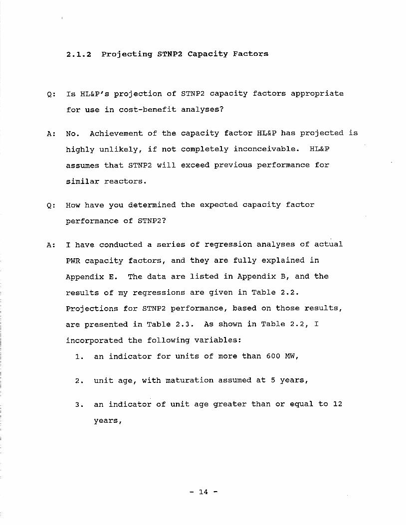
2.1.2 Projecting STNP2 Capacity Factors

Q: Is HL&P's projection of STNP2 capacity factors appropriate

for use in cost-benefit analyses?

A: No. Achievement of the capacity factor HL&P has projected is

highly unlikely, if not completely inconceivable. HL&P

assumes that STNP2 will exceed previous performance for

similar reactors.

Q: How have you determined the expected capacity factor

performance of STNP2?

A: I have conducted a series of regression analyses of actual

PWR capacity factors, and they are fully explained in

Appendix E. The data are listed in Appendix B, and the

results of my regressions are given in Table 2.2.

Projections for STNP2 performance, based on those results,

are presented in Table 2.3. As shown in Table 2.2, I

incorporated the following variables:

1. an indicator for units of more than 600 MW,

2. unit age, with maturation assumed at 5 years,

3. an indicator of unit age greater than or equal to 12

years,

- 14 -

4. the portion of a refueling or other major outage which

occurred in the year, usually taking the values of 0 or

1,

5. an indicator for the period 1979-1983, and

6. indicators for large Westinghouse turbines and

Combustion Engineering reactors.

Data were available for 447 full calendar years of operation

at all PWRs from 1973 to 1985. A small amount of pre-1973

operating experience could not be used for lack of refueling

data. Equation 1 is based on all available data, while

Equation 2 excludes data from Palisades and San Onofre 1

(leaving 421 unit-years).

Equation 1 presents results which project a low PWR

performance, by analyzing the historic experience of all

PWRs. Equation 2 presents alternative results by excluding

San Onofre 1 and Palisades and analyzing some different

variables. San Onofre 1 had particularly bad experience

after its twelfth year in operation, so once it is removed

from the database, the aging problem is not as evident.

Furthermore, Palisades is the only plant with a Combustion

Engineering reactor and outstandingly low reliability: when

Palisades is removed from the database, Combustion

Engineering units demonstrate higher capacity factors than

other PWRs. Finally, the capacity factor of plants with

Westinghouse 44" turbines is not significantly less than

other plants once those two plants are removed.

- 15 -

Both equations demonstrate that PWR performance from 1979 to

1983 was lower (by about 7%) than the pre-1979 period. In

both regressions,

large PWRs had capacity factors 11-15 points lower than

small (400-600) units,

- maturation increased capacity factors by about two

points annually until age five, and

refueling decreased capacity factor by about 10%.

Table 2.3 provides the projections of Equations 1 and 2 for

STNP2, under two sets of assumptions: first, that it

operates at the levels demonstrated in the pre-1979 period

(and 1984-85), and second, that it operates only as well as

the average of PWR performance in the 1979-83 period.6

Depending on the period used as a basis for extrapolation,

the mature capacity factor before age 12 ranges from 53% to

60%. The "old age" capacity factor, after year 12, ranges

from 45% to 60%. These are average results derived from the

regression analysis of the historical record. There is a

great deal of variation from the average, however; the

regressions typically explain less than a third of the

variation in the data, and Easterling (1979) derived 95%

prediction intervals of about 8% for years 2 to 10 at 1100 MW

For simplicity, I have treated STNP2 as if it will enter service on 1/1/90. This is more pessimistic than HL&P's projection, and more optimistic than historical experience would suggest.

- 16 -

PWRs. Actually, the variation would be somewhat larger, due

to the greater variation in the first partial year and the

first full year.7

Predicting the future effects of regulation, of safety

issues, and of aging is difficult at best. Projecting STNP2

performance based on the variables used in my equations

raises such difficult questions as:

Does a plant's performance really stabilize after year

five, and then begin deteriorating after age 12, as

represented by AGE5 and AGE_12? What will be the long-

term deterioration in capacity factor after age 12?

Did 1984 mark a recovery from the deterioration in

performance seen during the previous five years, will

performance continue at average 1980s levels, or will

it settle at some intermediate level?

For the purposes of this analysis, I have assumed that long-

run PWR performance will fall between pre-1979 and 1979-83

levels.

Thus, I have based my projections on an average of the

results of Equations 1 and 2, evaluated at pre-1979 and then

1979-83 conditions. Since the AGE_12 variable is excluded

from Equation 2, I have implicitly included only half of the

observed aging effect for older units. I have also assumed

On the other hand, some of the apparent variation would tend to average out for any individual unit.

- 17 -

that STNP2 will refuel in every year except the first.8

Thus, I believe the best current estimates for STNP2 are 56%,

48%, 51%, 53% and 55% in years one to five, respectively

(averaging 53%), an average of 56% in years six to eleven,

and an average of 52% thereafter. This calculation is shown

in Column [5] of Table 2.3.

Are HL&P's projections for STNP2 capacity factor reasonable?

No. To compare the accuracy of the capacity factors I

derived above, and HL&P's projections, to actual results, I

have performed the calculations presented in Table 2.4. For

the ten PWRs over 1000 MW which had entered service by 1983,

the average capacity factor as of September 1986 was 55.1%.

The capacity factor estimates which I derived in Table 2.3

predict an average of 54.5%, while HL&P would predict an

average of 64.7% for the "nominal" case and 71.2% for the

"target" case.9 Clearly, HL&P's expectations are highly

optimistic.

The actual ten-unit average will vary with refueling

schedules, and has much less data than I used in my

regressions. The actual data strongly supports the

conclusion that HL&P's projections significantly overstate

the capacity factors of large PWRs. On the other hand, my

HL&P assumes that STNP2 will refuel in every year, including its first.

It is not at all clear what HL&P actually predicts for STNP2 performance.

- 18 -

results closely approximate actual capacity factors for

similar plants.

Q: Have you performed any analyses on the data from these large

PWRs, on an annual basis?

A: Yes. Table 2.5 presents the annual capacity factors for the

units used in the previous analysis, through December 1984.

No other large (over 1000 MW) PWRs had completed a full year

of commercial operation as of the end of 1985. I have

assumed that the very low capacity factors for Trojan, and

for Salem 1 and Salem 2 in their second operating years are

not generated by the same sort of random process which

accounts for the other variation in nuclear capacity

factor.10 However, there is no reason to believe that some

comparable (if not exactly identical) problem can not occur

for STNP2. Hence, I delete these three observations from the

individual year calculations, and instead reflect the

probability of a major problem by computing the average

effect. Compared to the results for all the other plants,

these events reduced capacity factors by a total of 127.6

percentage points from average second year performance, in 70

unit-years of experience, for a 1.8% reduction in all

capacity factors. The average capacity factor which results

from this analysis is about 56.5% for the first four years,

with a mature capacity factor (from year five) of 55.6%.

10. This calculation recognizes that some of the other units do not have Westinghouse turbines, which caused the problems at Salem. STNP does use Westinghouse turbines.

- 19 -

This analysis also indicates that HL&P's projections for

STNP2 capacity factor are much higher than the actual

performance of large PWRs, even without adjusting for the

turbine-related differences.11

Q: Is it appropriate to include the period since 1979, when the

TMI accident and subsequent regulatory actions affected

nuclear plant operation, in the analysis of nuclear capacity

factors?

A: I believe that it is. Several more major nuclear accidents

or near-misses are likely to occur before the scheduled end

of STNP2 operation. Various recent estimates of major

accident probabilities range from 1/200 to 1/1000 per reactor

year (See Chernick, et al., 1981; Minarick and Kukielka,

1982). These estimates are based both on the implicit

probability assessments of nuclear insurers, who must

actually bet their own money on being correct, and on

engineering models of actual reactor performance. Thus,

major accidents can be expected every two to ten years once

100 reactors are operating. If anything, the 1968-85 period

has been relatively favorable for nuclear operations.

11. Through the first 11 months of 1986, the 10 units in Table 2.5 averaged a 50.7% capacity factor. The six younger 1000+ MW Westinghouse units which had completed their first fuel cycle (LaSalle 1&2, Catawba 1, McGuire 2, Callaway, and WPPSS2) averaged 50.2%, even though Catawba and Callaway have GE turbines. Thus, 1986 was not shaping up as a good year for nuclear plants comparable to STNP.

- 20 -

2.2 Non-Fuel Station O&M

Q: How have you estimated non-fuel O&M expense for STNP2?

A: I have examined the available historical data on nuclear O&M

for domestic nuclear plants. Appendix D lists the non-fuel

O&M for each U.S. nuclear plant for each full operating year

from 1968 to the most recent available data. Plants were

excluded from the analysis for years in which new nuclear

units were added, so each observation represents a full

year's O&M for a clearly defined number of units and of

megawatts.

Table 2.6 presents the results of three regressions on all of

the data in Appendix D for light water reactors, a total of

535 observations. Table 2.7 presents the results of the same

three regressions using only the data for plants of more than

300 MW, from Appendix D. All costs are stated in 1983

dollars, deflated at the GNP deflator. A total of 457

observations were available for Table 2.7.

The equations in Table 2.6 indicate that real O&M costs for

all plants have increased at about 12% annually, and that the

economies-of-scale factor for nuclear O&M is about 0.50, so

doubling the size of a plant (in Equation 1) or of a unit (in

Equations 2 and 3) increases the O&M cost by about 44%.

Equation 1 indicates that, once total plant size has been

- 21 -

accounted for, the number of units is inconsequential, and

the effect on O&M expense is statistically insignificant.

Equations 2 and 3 both measure size as MW per unit, and they

both find that the effect of adding a second identical unit

is about the same as the effect of doubling the size of the

first unit: 44% for Equation 2 and 40% for Equation 3.

Equation 3 tests for extra costs in the Northeast, which are

commonly found in studies of nuclear plant construction and

operating costs, but is otherwise identical to Equation 2.

Indeed, there is a highly significant differential:

Northeast plants cost 32% more to operate than other plants

(using the definition of North Atlantic from the Handy-

Whitman index). I will use this Equation 3 as the basis of

my projection.

The results with the data set which excludes the smaller

plants (Table 2.7) are quite similar: the most important

difference is that the annual growth rate in large plant O&M

is significantly higher than that of the overall data set.

This effect would produce much larger O&M projections, if it

were extrapolated out into the next century. O&M also rises

faster as a function of plant size in Table 2.3. There is no

clear basis for choosing between the two data sets.

What O&M projections would your regression results predict

for STNP2?

- 22 -

A: Table 2.8 extrapolates the results for Equation 3 for plants

of one and two units, each of 1300 MW MGN,12 and displays the

annual nominal O&M cost implied for STNP2 over the period

1990 - 2024, which is HL&P's projection of the unit's useful

life. Results are shown for both datasets. The same Table

presents alternative projections from the historical data,

assuming that the annual O&M expense increases linearly in

real terms, at the real increment projected by Equation 3

between 1990 and 1991. Finally, Table 2.8 compares these

results with HL&P's current projections: the "Tentative

Assumptions" from July 1986 were a bit higher.

Q: Are HL&P's O&M projections reasonable?

A: Based on the historical data, HL&P's projections for STNP2

O&M are reasonable in the first year or two.13 Since HL&P

assumes that the persistent real escalation in nuclear O&M

will abruptly drop to about 1% annually, even the most

favorable projection I present (linear escalation,.based on

all plants) is twice HL&P's projection by the turn of the

century, and over four times as large by 2024. Thus, HL&P's

long-term projection of STNP2 station O&M costs is

inconsistent with historical experience, and is extremely

optimistic.

12. In general, MGN ratings average about 4% greater than DER ratings.

13. HL&P's O&M projections are not reasonable if they are intended to include non-station expenses, as discussed below.

- 23 -

Protracted geometric growth in real O&M cost at historical

rates would probably lead to retirement of this plant (and

most nuclear plants) fairly early in the century, as it would

then be prohibitively expensive to operate (unless the

alternatives were even more expensive than HL&P predicts).

High costs of O&M and necessary capital additions were

responsible for the retirement (formal or de facto) of Indian

Point 1, Humboldt Bay, and Dresden 1, after only 12, 13, and

18 years of operation, respectively. Thus, rising costs

caught up to most of the small pre-1965 reactors during the

1970's: only Big Rock Point and Yankee Rowe remain from that

cohort.

On the other hand, our experience with nuclear O&M escalation

stretches over only 17 years (1968-1984), so projecting

continued constant real escalation past the year 2000

(another 16 years into the future) is rather speculative. It

is more likely that the actual outcome will fall somewhere

around the moderate real growth implied by my linear

projections.

- 24 -

2.3 Capital Additions

Q: Is HL&P's estimate of capital additions to STNP2 reasonable?

A: Not currently. The Touche-Ross Tentative Assumptions (July

1986) projected annual capital additions (or interim

replacements) of $23 million in 1990 dollars, which is fairly

representative of historical patterns. The "STPEGS Capital

Cost Data" projections of HL&P (6/26/87) lists much more

optimistic additions of just $13.1 million in 1990 dollars,

starting in 1991, with somewhat lower additions in earlier

years. These lower levels are not supported by experience to

date.

Q: How did you estimate capital additions?

A: Appendix D lists annual capital additions for all plants for

which cost data was available, from FERC Form 1 and DOE

compilations of FERC Form 1 data (now reported on p. 403),

through 1984. Each plant is included for all years in which

no units were added or deleted, and for which the data were

not clearly in error. The available experience totaled 520

plant-years of operation, and the average annual capital

addition in the database was $20.7/kW expressed in MGN terms,

- 25 -

or about $26.9 million annually for STNP2 in 1983 dollars.14

The capital additions are deflated at the appropriate

regional Handy-Whitman index for nuclear construction, which

has itself increased at 1.4% above the GNP inflation rate.15

The July 1984 Handy-Whitman index was estimated by escalating

the July 1983 index at the growth rate of the January index

from 1983 to 1984.

Capital additions vary with a number of factors, and vary

greatly from year to year, complicating statistical analyses.

Review of the data indicates that:

large plants have lower capital additions per kilowatt-

year than do small plants,

- multi-unit plants have lower capital additions per

kilowatt-year than do single-unit plants,

- Northeastern plants have higher capital additions than

those in other parts of the country, and

capital additions per kilowatt-year have generally been

rising over time, despite the greater prevalence of

large and multi-unit plants in the later data.

14. The STNP2 capacity used in these calculations was 1300 MW, 4% higher than the unit's DER, representing my estimate of the MGN rating.

15. From 1970 to 1983, the GNP deflator rose from 91.45 to 215.63, for an annual rate of 6.8%. In the same period, the July Handy-Whitman nuclear index for Region 1 rose from 81 to 227, an annual increase of 8.2%.

- 26 -

Figure 2.2 and Table 2.9 show the average capital additions

for each year since 1972, for all plants, and for large

single units. Levels of capital additions for both groups

have increased over time, at least since the mid-1970's.16

Over the last seven years, the average for all plants was

$27.7/kW-yr: over the last five years, the average has been

$32.3/kW-yr. The rate of capital additions may have

stabilized in the 1980's, or it may be increasing at about

$4/kW-yr/yr. If capital additions continue at $32.3/kW-yr in

1983 Handy-Whitman dollars, and if the nuclear Handy-Whitman

index continues to run 1.4 points above the GNP deflation

(for which I use the Touche-Ross projections of 5.25% from

1990 on, and assume 4% until 1990), the annual capital

additions for STNP2 would be as shown in Column 2 of Table

2.11; Column 1 of that table shows HL&P's projections of

capital additions.

Some of the recent trend in the data may result from plant

aging, and another portion is undoubtedly related to TMI-

inspired regulatory changes, so extrapolating the trend out

is somewhat speculative. Thus, I have used a recent average,

rather than continuing the increases. However, there is some

evidence of an overall upward trend in the period 1972-78, as

well, so any TMI-related effect constitutes a continuation of

the historical conditions, rather than a unique event.

The data for large single units in the early 1970's is from a very small sample.

- 27 -

Q: Did you perform a regression analysis on capital additions

data?

A: Yes. Appendix F contains a detailed description of the

regression analysis and an interpretation of the results,

which are summarized in Table 2.10. The significance of the

resulting regression equations is better than I had expected,

and yields reasonable projections, also shown in Table 2.11.

Q: What are your recommendations with regard to projections of

STNP2 capital additions?

A: I believe that it is prudent to assume that capital additions

at STNP2 will continue at recent levels, starting at $19.24

million in 1990 and rising at 6.65% thereafter.

In comparison, HL&P assumes annual capital additions of $13.1

million in 1990 dollars, rising at 5.25%. HL&P also assumes

slightly lower additions in 1990.

- 28 -

2.4 The Cost of Decommissioning

Q: What is meant by "decommissioning**?

A: The decommissioning of a retired nuclear power plant involves

the transition of the plant from a nuclear facility, subject

to attendant health and safety regulations, to a non-nuclear

facility, posing no radiation-related risks to human health

or to the general environment. Current NRC policy envisions

the use of any of three approaches to decommissioning:

1. DECON: The prompt decontamination and dismantlement of

the plant.

2. SAFSTOR: The mothballing of the plant under continuing

surveillance, until decontamination and dismantlement.

3. ENTOMB: The enclosure of all radioactive portions of

the plant within a secure entombment structure, until

decontamination and dismantlement.

Of these three approaches, only DECON is considered to be a

permanent solution to isolation of the plant's accumulated

radiation burden from the environment. It is generally

assumed that plants will be dismantled promptly upon

retirement.

- 29 -

Q: What is the basis of HL&P's estimate of the cost of

decommissioning STNP 2?

A: HL&P apparently relies on a conventional engineering estimate

of the cost of decommissioning through the prompt dismantling

(DECON) method. The source of the estimate is not yet clear.

Q: What is HL&P's estimate of the cost of decommissioning

STNP 2?

A: The cost estimate is $168,115,000 for the entire unit, stated

in 1990 dollars. I derived this value by adding the Touche-

Ross assumptions (from July 11, 1986) for the four

participants.

Q: Are these values consistent with other recent estimates

for nuclear decommissioning costs?

A: The STNP 2 assumptions appear to be considerably lower than

recent estimates for other units. Table 2.12 lists the

decommissioning costs estimated for other nuclear units by

TLG Engineering personnel.17 The values are shown as

reported by TLG, and restated in 1990 dollars, assuming

inflation at GNP levels to 1986, and 4% thereafter. The STNP

2 estimates are about 39% less than other recent (1985/86)

estimates, which range from $206 to $315 million per unit in

1990 dollars, for units over 1000 MW.

17. These estimates were prepared for the various utilities. I have not been able to obtain similar data from and other decommissioning cost consultant to the utility industry.

- 30 -

Q: How much experience is available in the prompt

dismantling (DECON) process for nuclear power plant

decommissioning?

A: There is very little direct experience. The only nuclear

power plant to have been dismantled was Elk River, which was

decommissioned in 1974.18 As can be seen in Table 2.12,

estimated DECON costs have doubled in real terms since 1975:

the Elk River experience is clearly out of date.

As significant as the lack of experience is the apparent

reluctance of utilities to undertake the DECON process.

Table 2.13 lists retired nuclear power plants, with their

dates of operation. Some of the units have been placed in a

"safe storage" mode, but dismantlement has not started at any

of them.19

Q: Does a delay in decommissioning, following retirement,

allow the size of the decommissioning fund to grow?

A: The fund would tend to grow, due to the accumulation of

investment income. However, the cost of the original

18. Portions of the technology have been demonstrated in various capital additions, such as the replacement of steam generators.

19. Perhaps the best example of this reluctance is the Department of Energy's decision to float the reactor pressure vessel of the retired Shippingport unit on a barge, down the Ohio and Mississippi Rivers; through the Gulf of Mexico, the Caribbean and the Panama Canal; along the Pacific Coast to the Columbia River; and finally up the Columbia to DOE's Hanford Reservation. The vessel will then be buried intact. This procedure would not be undertaken for commercial-scale units, whose pressure vessels will be disassembled on site.

- 31 -

decommissioning tasks would also increase, due to inflation.

In addition, the decommissioning fund would be reduced by the

cost of the preparations for the delay, such as sealing

structures, securing equipment, and cleaning and drying

surfaces which should not deteriorate during the delay, and

by the continuing maintenance and surveillance expenses.

These costs would reduce the level of the fund during the

delay, and so would reduce the rate at which the investment

income would accumulate. It is not clear whether a

significant delay in decommissioning would result in the fund

rising faster than the decommissioning expense.

A delay in initiating DECON would tend to make the

decommissioning process more nearly resemble SAFSTOR or

ENTOMB, which are generally estimated to be more expensive

(even in constant dollars) than DECON.

Q: Do you consider the current STNP 2 decommissioning cost

estimates to be reliable?

A: No. It is clear from Table 2.12 that estimated costs of

nuclear decommissioning have been increasing rapidly. Table

2.14 displays the results of a regression analysis on the

data from Table 2.12: the coefficient of the YEAR variable

indicates that TLG cost estimates have been increasing at the

rate of e0,174 annually, or a compound growth rate of 19% in

real terms.20 The data from Table 2.12 and the regression

20. All of the coefficients are highly statistically significant, except for the TWIN coefficient.

- 32 -

results from Table 2.14 (using average values for the set of

plants estimated in each year) are graphed in Figure 2.3.

The pattern of increases in the estimated cost of

decommissioning raises considerable question about the

validity of the current estimates.

Of course, the current estimates could represent the final

set of increases in decommissioning cost estimates, and

actual decommissioning costs could turn out to be similar to

those estimates.21 However, experience with other nuclear

power costs suggests that the industry is characterized more

by persistent cost growth than by cost stability. Virtually

all nuclear cost components have been increasing for most of

the history of the commercial nuclear power industry:

The estimated and actual costs of constructing nuclear

power plants have been increasing consistently since

the late 1960s. Typically, cost estimates for

completed plants have increased about 10% annually in

real terms (excluding inflation due to schedule

slippage) from the issuance of the construction permit

to commercial operation.

Nuclear non-fuel operating and maintenance costs have

been increasing (and exceeding expectations) since the

early 1970s. Through 1984, the average annual rate of

increase was approximately 12-14%.

21. In any case, the STNP 2 decommissioning estimate is quite low for a contemporary estimate.

- 33 -

- Capital additions to nuclear power plants in commercial

operation, generally ignored in cost projections into

the early 1980s, were significant cost elements in the

1970s: since the Three Mile Island accident capital

additions have increased dramatically.

These patterns of cost increases are documented elsewhere in

this testimony.

The pattern of increases in decommissioning cost estimates,

combined with the persistent increases in projected and

actual costs for those nuclear cost components with which we

have greater experience, strongly suggests that

decommissioning costs will exceed current estimates.

Q: What is the relationship between the pattern of cost

increases in other nuclear cost components, and the

increases in cost estimates for decommissioning?

A: Decommissioning cost estimates have increased for reasons

similar to those which have produced large and persistent

increases in other nuclear cost components. The earlier

estimates have been determined to have underestimated the

complexity (and hence the cost) of such problems as disposal

of radioactive wastes, and the supervision of workers in

radioactive areas. In general, the problems with estimates

of other nuclear cost components can be attributed to similar

underestimation of the problems inherent in operations as

complex as nuclear power production, and the failure to

- 34 -

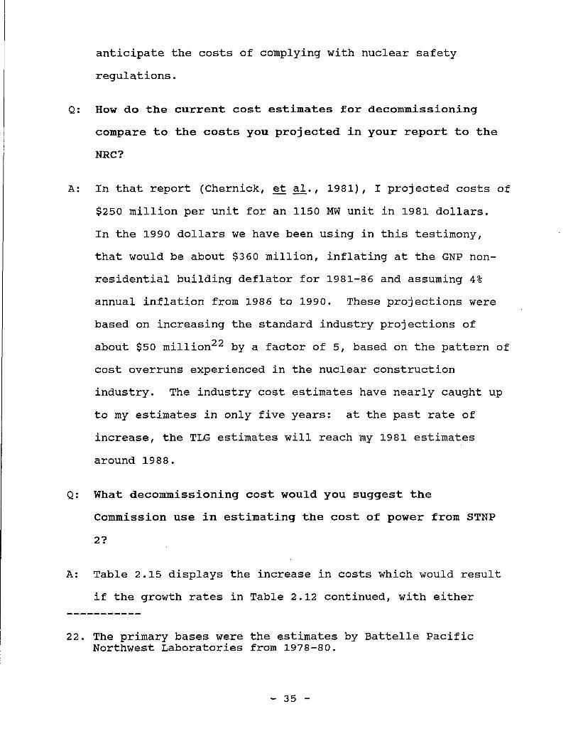
anticipate the costs of complying with nuclear safety

regulations.

Q: How do the current cost estimates for decommissioning

compare to the costs you projected in your report to the

NRC?

A: In that report (Chernick, et al., 1981), I projected costs of

$250 million per unit for an 1150 MW unit in 1981 dollars.

In the 1990 dollars we have been using in this testimony,

that would be about $360 million, inflating at the GNP non­

residential building deflator for 1981-86 and assuming 4%

annual inflation from 1986 to 1990. These projections were

based on increasing the standard industry projections of

about $50 million22 by a factor of 5, based on the pattern of

cost overruns experienced in the nuclear construction

industry. The industry cost estimates have nearly caught up

to my estimates in only five years: at the past rate of

increase, the TLG estimates will reach my 1981 estimates

around 1988.

Q: What decommissioning cost would you suggest the

Commission use in estimating the cost of power from STNP

2?

A: Table 2.15 displays the increase in costs which would result

if the growth rates in Table 2.12 continued, with either

22. The primary bases were the estimates by Battelle Pacific Northwest Laboratories from 1978-80.

- 35 -

linear or compound growth after 1986. If the TLG

decommissioning cost estimate trends (based on data spanning

8 years) continue for just another 8 years, the cost estimate

will rise another 150% to 300%.

Overall, I would suggest that the Commission base its

decommissioning cost estimate for STNP 2 on the assumption

that the cost will exceed current estimates by at least 150%

in constant dollars.23 Thus, the review of STNP 2 should

assume a final cost for decommissioning of at least $600

million in 1990 dollars.

Q: Should the same value be used for to establish the level

of contributions to the decommissioning funds for STNP 1,

for the owners who are regulated by the PUCT?

A: I believe that would be reasonable, but it is not necessary.

Decommissioning funding can start with a smaller, more

optimistic figure. If future developments indicate that the

final costs are likely to be different than that initial

target, accumulation of the decommissioning fund can be

accelerated or delayed, to aim for a larger or smaller final

fund balance. Given experience to date, it is likely that an

increase in funding would be required, if the inital target

is much lower than the $600 million level.

23. In selecting this relatively modest increase (by past standards), I have taken into account the inclusion in most estimates of a 25% contingency.

- 36 -

While many decisions regarding the STNP 1 decommissioning

fund can be delayed for several years, decisions must be made

today regarding the fate of STNP 2. For that purpose, I

would recommend that the Commission assume a moderate

continuation of the historical experience in decommissioning

cost estimation.

- 37 -

2.5 The Useful Life of STNP 2

Q: How long does HL&P expect each STNP 2 unit to be in

commercial operation?

A: The projected life of each unit is 35 years.

Q: Is this a reasonable projection for the purpose of

designing a nuclear decommissioning fund?

A: No, for two reasons. First, there has been very little

experience with the longevity of nuclear power plants, and

second, what little experience is available suggests that the

useful lives of nuclear units may be much shorter than 39

years.

Q: What experience is available regarding the longevity of

nuclear power plants?

A: The five small plants which entered commercial service in the

early 19607s would be 20-26 years old today, if all had

survived.24 Of this cohort, Indian Point 1, Humboldt Bay,

and Dresden 1 have been retired (formally or de facto), after

24. This group excludes the exotic demonstration reactors, some of which used liquid metal coolant, organic moderation, and other technologies very different than the light water reactors which have prevailed in US nuclear power plant design. I have also excluded some very small demonstration reactors which operated for only a few years.

- 38 -

only 12, 13, and 18 years of operation, respectively. Only

Big Rock Point and Yankee Rowe remain from that cohort. Even

the older and larger of the survivors, Yankee Rowe, has been

in service only since 1961, and is thus only 26.25 LaCrosse,

a 50MW unit which entered service in November 1969, was

retired in April 1987, after 17.5 years of operation.

The first units of more than 300 MW went commercial in

January 1968: they have just reached age 19. The only clear

retirement among this group is Three Mile Island 2, which

operated for only a few months prior to its accident.

Various nuclear units which are currently on protracted

shutdowns due to safety and design problems (such as Pilgrim)

may never reopen, but such units may be shut down for an

extended period before it becomes clear that they have

reached the end of their useful lives.

To summarize, HL&P is projecting that STNP 2 will survive

twice as long as has the oldest domestic unit over 300 MW,

and 50% longer than the oldest domestic commercial power

reactor of any size. Basing cost-benefit on this projection

would be unwise.

Q: How do the design differences between STNP 2 and older

units affect the likely useful lives of STNP 2?

A: There is simply no way to know. The measures taken at STNP 2

to correct safety, maintenance, and reliability problems at

25. It is also only a 175 MW unit.

- 39 -

other plants may be successful, and may result in STNP 2

operating longer than will older nuclear power plants.

Alternatively, the added equipment at STNP 2 may result in

additional problems, rendering STNP 2 uneconomic to operate

at an earlier age than the retirement ages of the older

units. Also, it is important to remember that STNP 2 is

starting life at a time when nuclea*r O&M expenses are

already quite high: if historic trends continue, STNP 2 will

become uneconomic at about the same date as older units, and

thus at a much earlier age.

Given the limited experience and uncertainties, what do

the data suggest about the useful life of nuclear power

plants?

In the decommissioning insurance study (NUREG/CR-2370), I

found that the available data suggested a median useful life

of approximately 20 years. Michael B. Meyer (1986), one of

my co-authors on NUREG/CR-2370, updated the analysis of the

operating life of nuclear power plants contained in the NRC

report.26 Depending on the data set utilized, the median

useful life of nuclear power plants would appear to be 20 to

35 years. Unfortunately, the data, no matter how defined,

are quite sparse.

Are the same forces which resulted in the early

retirement of older units still in operation?

This analysis does not include the Lacrosse retirement.

- 40 -

A: Yes. High costs of O&M and necessary capital additions,

mostly driven by regulatory considerations, were responsible

for the retirement of most of the small pre-1965 reactors

during the 1970s and of Lacrosse. O&M expenses have

continued to grow much faster than inflation, and capital

additions have been much higher in the 1980s than in the

1970s.

Large nuclear power units, such as the STNP units, show

considerable economies of scale in O&M. Multiple unit sites,

such as STNP 2, also show strong economies of duplication:

two nuclear units can be operated for less (and require less

additions) than twice the cost of one unit. Thus, STNP 2

will be less vulnerable to the operating cost economics than

were the small (and often single) units built in the 1960s.

Nevertheless, protracted growth in real O&M costs at

historical rates, especially combined with the continuation

of recent rates of capital additions, could prompt retirement

of STNP 2 (and most nuclear plants) fairly early in the next

century, as it would then be prohibitively expensive to

operate.

Q: What useful life would you recommend the Commission use

for STNP 2 in this proceeding?

A: While all parties certainly hope that STNP 2 (if it is*

completed and enters commercial operation), and other nuclear

units, remain economical and in operation for 35 years or

more, we must accept the very real possibility that they will

- 41 -

not survive for more than 25 or 30 years. I would therefore

recommend that the Commission evaluate the economics of STNP

2 based on no more than 30 years of operation. Given the

historical trends in nuclear plant operating costs, 25 years

would be a more prudent assumption.

Q: Should the depreciation rates for the STNP units be based on

25 year expected lives?

A: That would be reasonable from a technical viewpoint, but it

is not necessary. Given the large rate increases likely to

be associated with placing the units in ratebase, the

Commission may initially prefer to use a longer expected

life, producing lower depreciation rates. Depreciation rates

can be increased later in the units' lives, if continued

experience supports my projections. This approach would

accomplish some of the goals of a phase-in of STNP costs,

without formally deferring recovery.

I

- 42 -

2.6 Overheads

Q: Are all of the expenses associated with operating a

nuclear power plant recorded as plant O&M costs in the

FERC form?

A: No. Some of the costs related to owning and operating a

nuclear power plant are recorded in other accounts. This is

true for such costs as legal and regulatory expenses,

insurance, payroll taxes, and employee benefits.

Collectively, these expenses may be considered overhead

costs.

Q: How did you estimate these overheads?

A: Table 2.16 displays the overhead expenses for Yankee Atomic,

Connecticut Yankee, Vermont Yankee, and Maine Yankee during

1984 and 1985. The Yankee companies were chosen for this

analysis because they have no other utility plant or

operations besides the nuclear power plants. For other

utilities, it would be very difficult to determine the

portion of overheads attributable to the nuclear plant.

Line 7 of Table 2.16 shows the overhead expenses for each

Yankee plant expressed as a percentage of total station non-

fuel O&M. The percentages vary from 11.9% for Connecticut

Yankee in 1984 to 57.6% for Maine Yankee in 1984. The

average overhead expense for the four plants in this period

- 43 -

was 27%. Thus, it is appropriate to add 27% to the STNP2

station O&M projection to reflect overheads. Table 2.17

shows the most optimistic O&M projection from historical

results in Table 2.8 (column 13), grossed up for overheads.

- 44 -

3 STNP 2 CONSTRUCTION COST AND SCHEDULE

Are the current cost and schedule estimates for STNP 2

likely to be achieved?

No. Nuclear cost and schedule estimates, including those

prepared by Bechtel, have been notoriously unreliable and

over-optimistic. In addition, the period allowed for the

startup of STNP 2 (from fuel load to commercial operation) is

much shorter than would be indicated by historical

experience.

Please describe the historical reliability of nuclear

power plant cost and schedule estimates.

Appendix C summarizes the data available regarding the cost

and schedule histories of the nuclear power plants which had

entered commercial service by 1984. I have excluded from the

cost analysis the turnkey plants, for which the manufacturers

provided at least partial cost caps, and the reactors for

which the federal government provided cost sharing. In

addition, I have no detailed cost estimate data for either

San Onofre 1 or Connecticut Yankee, and at the time this

analysis was prepared, I had no information on the final cost

of a few units which went commercial in 1984. For each

available estimate, Appendix C lists the actual commercial

operation date (COD), the actual construction cost, the date

of the cost estimate and the estimated cost and COD for that

estimate. The cost and schedule history data in Appendix C

- 45 -

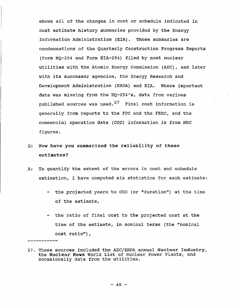
shows all of the changes in cost or schedule indicated in

cost estimate history summaries provided by the Energy

Information Administration (EIA). Those summaries are

condensations of the Quarterly Construction Progress Reports

(Form HQ-254 and Form EIA-254) filed by most nuclear

utilities with the Atomic Energy Commission (AEC), and later

with its successor agencies, the Energy Research and

Development Administration (ERDA) and EIA. Where important

data was missing from the HQ-254's, data from various • 9 7* • « • published sources was used. ' Final cost information is

generally from reports to the FPC and the FERC, and the

commercial operation date (COD) information is from NRC

figures.

Q: How have you summarized the reliability of these

estimates?

A: To quantify the extent of the errors in cost and schedule

estimation, I have computed six statistics for each estimate:

the projected years to COD (or "duration") at the time

of the estimate,

the ratio of final cost to the projected cost at the

time of the estimate, in nominal terms (the "nominal

cost ratio"),

27. These sources included the AEC/ERDA annual Nuclear Industry, the Nuclear News World List of Nuclear Power Plants, and occasionally data from the utilities.

- 46 -

the cost ratio expressed as a growth rate, annualized

by the estimated time to completion, in nominal terms

(the "nominal myopia factor"),

- the ratio of the initial cost estimate to the final

cost, with the latter restated in the dollars of the

initial COD estimate, to remove schedule-related

inflation and AFUDC,

the real cost ratio annualized by the actual duration,

and the ratio of the actual remaining time until

commercial operation to the projected time (the

"duration ratio").

These terms are all fairly self-explanatory, except for

myopia. The myopia factor is a measure of the widespread

shortsightedness demonstrated by the nuclear industry in

estimating construction costs. As the commercial operation

dates for nuclear plants are pushed further into the future,

utilities have more severely underestimated the cost of their

construction. I have measured this effect with the following

formula:

(cost ratio)(1/estimated duration)

Table 3.1 summarizes the average values of each of these

statistics, disaggregated by the estimated duration at the

time of the cost estimate. . For the 3-4 year estimated

duration interval corresponding to the November 1985 estimate

of a June 1989 in-service date for STNP 2 (an estimated

- 47 -

duration of 3.58 years), the average myopia indicates that

the actual cost of these units was typically 27% greater than

the estimate, for each year that construction was expected to

take. The average nominal cost ratio demonstrates that the

average plant cost 2.39 times as much to complete as

initially estimated, while the duration ratio indicates that

the plants took almost twice (1.97 times) as long as was

projected. In real terms, the average cost ratio was 1.84,

and the average myopia was 18%.

Q: What are the implications of these results for STNP 2?

A: Unless there is some concrete reason to believe that the

nuclear industry's ability to forecast costs has improved, it

would be appropriate to apply the results of Table 3.1 to the

most recent cost and schedule estimates of STNP 2 to produce

revised or corrected estimates. Applying the historical

experience to STNP 2 yields the following results:

If the duration ratio for STNP 2 is 1.97, it would

require 7.06 years to be completed, from November 1985,

or until December 1992.

If the nominal myopia factor is 27%, the final cost

will be 2.35 times the November 1985 forecast, or $5.0

billion.

If the nominal cost ratio is 2.39, the final cost will

be 2.39 times the November 1985 forecast, $5.1 billion.

- 48 -

If the real myopia factor is 18%, the final cost will

be 1.81 times the November 1985 estimate, plus

inflation during the schedule slippage. For inflation

at 5.25%, 3.58 years of slippage would increase the

cost 20.1%, bringing the total cost to 2.17 times the

11/85 estimate, or $4.7 billion.

If the real cost ratio is 1.84, and the schedule

slippage adds another 20.1% to the cost, the total cost

would be 2.21 times the 11/85 estimate, or $4.7

billion.

Q: These results are based on data through 1984. How do you

expect that they would change if they were updated?

A: The results for plants completed between 1984 and the present

would probably be worse than the earlier data: the cost

overruns would be higher and the schedule slippages would be

greater. In general, the relatively trouble-free units were

completed and placed in service early, with much smaller

schedule slippages and cost overruns than were experienced by

the units of the same vintage which entered service more

recently, or are still under construction. For example, the

1984-87 data would include such problem plants as Diablo

Canyon, Grand Gulf, and River Bend. Future data bases will

include Shoreham, Seabrook, Watts Bar, and Nine Mile Point 2,

assuming that all these units finally go commercial. None of

these analyses would ever include the worst disasters of

- 49 -

nuclear construction, the cancelled units such as WPPSS 4 and

5, Zimmer, Midland, and Marble Hill.

Q: Does the fact that STNP 2 is a second unit offer any hope

that its cost and schedule performance will be better

than average?

A: Yes, to some extent. Second units which significantly trail

the first unit at a plant have often (but not always)

encountered lower schedule slippage and lower cost escalation

after the in-service date of the first unit. Therefore, it

is reasonable to hope that the cost and schedule for STNP 2

will increase significantly near the commercial operation

date (COD) of STNP 1 (an event which may occur late this year

or early next year), and then increase relatively little in

the remaining years of construction. If STNP 1 actually

enters service in December 1987, as scheduled, and a new (and

more reliable) estimate for STNP 2 appears at that time, 2.08

years of the 11/85 schedule would be subject to the higher

slippage rates expected prior to the STNP 1 COD, and the

remaining 1.5 years would be subject to whatever favorable

effects the completion of STNP 1 would imply. If the 9 o slippage after STNP 1 COD is only 20% of the average, ° the

total slippage in STNP 2 cost and schedule might be expected

to be about as much as would occur over 2.38 years (or about

66% of the estimated duration for STNP 2 at the time of the

28. Note that the averages presented in Table 3.1 include the more favorable results of the lagging second units in the database.

- 50 -

11/85 estimate) for a unit without any trailing-unit

advantages.

Applying the historical schedule overrun of 97% for 2.38

years worth of exposure produces 2.31 years (28 months) of

slippage, bringing the expected STNP 2 COD to March of 1991.

If the real cost overrun is equivalent to 2.38 years of

myopia at 18%, the cost would increase 48%, plus delay-

related inflation of 12.5%, for a total increase of 67%, to

$3.6 billion.

Q: One important consideration in determining the cost of

completing STNP 2 is the federal income tax treatment of

the unit, which depends on its in-service date. Based on

historical experience, what is the likelihood that STNP 2

can be in service prior to December 1990?

A: The chances are not very good. Table 3.2 displays all of the

estimates in the 3-4 year duration range from Appendix C,

sorted in order of the schedule overruns. Figure 3.1 shows

the breakdown of overruns by interval, and Figure 3.2 shows

the cumulative distribution of the overruns.

If the duration ratio for the 11/85 STNP 2 estimate exceeds

44%, the in-service date would slide past the end of 1990,

and the favorable tax treatment under the transition rules of

the Tax Reform Act of 1986 would be lost. In the historical

data, 78.6% of the estimates showed slippage of more than

44%. Even if the slippage at STNP 2 is one third less than

historical results, so that the critical figure for

- 51 -

comparison is a 66% schedule overrun, 58.3% of the historical

data shows duration ratios in excess of that figure.29

Q: Have the STNP cost and schedule estimates been more

stable than the industry average since the first estimate

by Bechtel in August 1982?

A: Yes. In that period, the direct cost estimate has remained

constant, aided by the decline in inflation rates, and by the

reduction of contingency. The STNP 1 schedule has slipped

only six months,30 and the STNP 2 schedule has not been

changed. Total cost estimates for the plant would presumably

be somewhat higher, due to the additional AFUDC on STNP 1.

If the slippage remains at these low levels, STNP 2 would

enter service prior to the December 1990 deadline, and at a

cost closer to HL&P's estimate than to mine.

Q: Do the relative levels of the estimated costs for STNP 1

and STNP 2 shed any light on the reliability of the STNP

2 cost estimate?

29. This analysis double-counts the advantages of trailing second units. The 58.3% figure is the fraction of estimates which showed schedule overruns of more than 66%, on the assumption that the status of STNP 2 as a trailing second unit will allow it to do a third better, and thus have only a 44% overrun if conditions were otherwise comparable to units without the trailing-second unit advantage. However, the data set for Table 3.2 includes trailing second units, such as TMI 2 and Hatch 2, and several of the estimates which fall under the 66% cut-off are for these trailing units.

30. Given the absence of an operating license in August 1987, four months prior to the scheduled commercial operation date, further slippage is very likely.

- 52 -

A: Yes. The cost estimate for STNP 2 is extremely low relative

to that for STNP 1. Table 3.3 lists the relative direct

costs (or cost estimates) for all the multiple units for

which the TVA reports separate values, along with the

temporal spacing between units. STNP 2 is projected to cost

only 42% of the cost of STNP 1. This ratio is tied for

lowest with Peach Bottom, where both units entered service in

the same year. The next lowest value is 66%, and the average

for units with 1-2 years separating is 91%. This fact

certainly raises greater questions about the reliability of

the STNP 2 cost estimate.

Q: Have your myopia techniques been employed successfully in

previous situations?

A: Yes. In January 1980, PSNH estimated that Seabrook 1 and 2

would cost a total of $2.8 billion. A previous version of my

myopia analysis predicted a cost of $5.9-11.5 billion. The

last A/E estimate for the twin plant (prior to cancellation

of Unit 2 in 1984) was for $10.1 billion. My numerous other

predictions for Seabrook have also generally been borne out.

For example, in 1984, PSNH predicted a COD of 8/86 for Unit

1, while I predicted 11/88. PSNH has now acknowledged that

the plant is unlikely to be in operation by 7/88.

Myopia analysis was also the basis for my projecting in 1979

that the cost of Pilgrim 2 (then estimated by Boston Edison

at $1,895 billion) would rise to $3.8-4.9 billion. In

- 53 -

September 1981, Edison announced a cost estimate of $4

billion, and cancelled the unit.

In October 1982, Commonwealth Edison predicted that the

Braidwood plant would cost $2.74 billion. I predicted a cost

of $4.78 to $5.45 billion, plus delay-related inflation. The

final results are not yet in, since the two units are

scheduled for operation later this year and in 9/88, but the

utility estimate now stands at $5.05 billion, with a 21 month

delay.

Myopia has also allowed me to produce (after the fact, but

only using data available at the time) corrected versions of

previous estimates for several nuclear plants, which were

more accurate than the utilities' estimates at the time. On

the other hand, these techniques did not anticipate the

stability in the cost and schedule estimates for Millstone 3

(a unit at which construction was intentionally slowed down

for a few years), after 1982.

Q: Please expand on your previous statement that the period

allowed for the start-up of STNP 2 (from fuel load to

commercial operation) is much shorter than would be

indicated by historical experience.

A: Table 3.4 lists the startup intervals for all units in

commercial operation which received their operating licenses

- 54 -

since the beginning of 1978.31 The shortest start-up period,

4 months, was that of St. Lucie 2, generally regarded as one

of the great success stories of post-TMI nuclear

construction. The intervals for the other units range up to

43 months, with a 34-plant average of 13 months.

Table 3.5 lists the dates of operating license issuance for

units which are still in start-up. Perry, Fermi, and

Shoreham will certainly increase the average start-up

interval when they enter service.32 All 6 units in Table 3.5

already have start-up periods in excess of six months.

Q: What is HL&P's projection of the STNP 2 start-up

interval?

A: HL&P is currently projecting a start-up period of six months

for each STNP unit, from fuel load to COD. Fuel load

generally occurs immediately following the issuance of an

operating license. This projection is considerably more

optimistic than would be suggested by the historical

experience. Only two of the units in Table 3.4 have beaten

this projection, and five have tied it, out of the 34 units.

If HL&P's projection of the fuel load date were correct, but

31. Some utilities have reported different COD's for ratemaking and for other purposes. Whenever possible, I use the COD reported to the NRC.

32. Nine Mile Point 2 is scheduled for commercial operation in "early 88" according to the 8/3/87 Central Hudson quarterly report: if this estimate is correct, startup of Nine Mile Point 2 will require 15 months, further raising the average.

- 55 -

start-up required the 13 month average from Table 3.4, STNP 2

would go commercial in January 1990.

Q: Why have nuclear cost and schedule estimates been subject

to such persistent and significant overruns?

A: Recent acknowledgements by the utilities themselves explain

why the estimates have been incorrect. Many nuclear cost

estimates were never intended to be predictions of the final

cost of the plant: they were budget targets and cost-control

documents. In the rapidly changing environment of nuclear

construction, utilities and architect/engineers (A/Es) chose

not to incorporate best estimates of the effects of evolving

regulations. This issue is discussed at some length in Meyer

(1984). Employees of Management Analysis Corporation (MAC),

in testimony filed by Central Maine Power and Maine Public

Service in their 1984 rate cases, summarize this practice

with respect to Seabrook:

PSNH established schedules that required superior effort. This strategy is generally appropriate because it demands the best possible performance from contractors. (Dittmar and Ward, 1984, page 25)

The MAC analysis further considered the tradeoffs between

conservative and optimistic estimates, and explained the

construction management advantages of intentionally

optimistic estimates:

If a budget is based on an overly conservative (high) estimate which establishes easily attained goals, a project's cost is likely to rise to fulfill the prediction. The use of aggressive targets is a management approach which, when reasonably applied, provides incentive for improving performance. If unrealistic cost or

- 56 -

schedule targets are maintained too long, a project can be affected adversely. In such situations, it is difficult to hold people accountable for goals that they know are unrealistic. Morale problems may occur which could reduce productivity, cause delays or increase cost. A more serious consequence of managing to unrealistically aggressive targets may occur if activities are improperly sequenced such that work cannot be accomplished efficiently because of artificially induced constraints. (Ibid, page IV-6)

Southern California Edison, lead participant in the San

Onofre plant, has reported that it actually kept two sets of

cost estimates during much of the construction of San Onofre

2 and 3. One set was used for discussions with contractors

and for other public purposes, while a higher set of

estimates was used for top-level management purposes. The

higher set included estimates of "possible future growth,"

because

In late 1974, Edison project management recognized that due to the constantly changing nuclear industry regulatory and economic environment, in addition to the exposures due to specifically identifiable causes, the project costs would likely be impacted by many other unknowns. (Perla, et al., 1985)

In January 1975, when San Onofre 2 and 3 were scheduled to be

complete in 5.5 and 6.75 years, respectively, SCE included

"possible future growth" of about 50% of the total budget, in

addition to conventional contingencies of about 8% in the

public budget.

United Illuminating, a participant in both the Seabrook and

Millstone 3 projects, has also acknowledged this practice, as

demonstrated by the testimony of its President and other

- 57 -

officials before the Connecticut Public Utilities Control

Authority, filed 8/1/84:

The project management estimate, used by the project manager to control construction of the facility, should be established as a challenging but achievable goal. Depending upon the degree of challenge desired, the project management estimate should have a probability of 10% to 30% of not being exceeded . . . [T]he project management estimate serves the need to maintain tight project controls . . .

Unfortunately, much less than 10% of nuclear cost estimates

have been achieved, so the cost control function seems to

have been overdone. It also appears that nuclear cost

estimates routinely exclude effects of future, pending, and

newly effective regulations which have not yet been reflected

in the plant drawings, and of the other complications of

building a nuclear plant.

Similar objectives and approaches have been apparent in the

cost estimation procedures of other plants I have reviewed,

including Midland, Marble Hill, and the WPPSS units.

It is important to remember that, throughout the period that

utilities and A/Es were intentionally understating their

estimates of the costs and construction schedules of nuclear

units, they were describing those estimates to regulators,

investors, and even other utilities as reliable, achievable

predictions. It was common to see extensive discussions of

why a new estimate was more reliable than previous estimates,

- 58 -

and why the new estimate could be (and would be) achieved.33

Therefore, assertions by HL&P and Bechtel that this estimate

is correct should not be given particularly great weight.

Q: How do the cost overruns you have estimated translate to

annual construction costs?

A: Results comparable to a 67% increase in total costs, with the

commercial operation date delayed to early 1991, can be

derived through any of a number of changes in the cash flows.

Table 3.6 provides one such cash flow, based on scaling up

HL&P's costs to the entire unit.

33. By definition, each estimate occurs when design and construction are further advanced, and when more experience with nuclear construction is available. Nonetheless, there is no learning curve evident in the cost estimate histories of most units (normalized for projected time to completion), or of the industry as a whole.

- 59 -

4 POTENTIAL FOR CONSERVATION

Q: What was your basis for estimaing the potential for

conservation of electricity in the service territories of

the STNP owners?

A: I started with detailed estimates of the conservation

potential for the Austin Electric Utility Department, as

derived by a consultant to the Department. The report of the

consultant, Rocky Mountain Institute (Lovins 1986), or RMI,

provides the following estimated savings by customer class for

technically and economically feasible improvements in electric

energy use efficiency in existing facilities:

residential: 79%

commercial: 73%

large power: 51%

miscellaneous: 25%

Peak savings would be about the same, with commercial savings

somewhat higher (due to the large savings available in cooling

and in lighting, which is a major contributor to peak cooling

loads) and residential savings somewhat lower. Savings in new

construction were conservatively assumed to be the same as in

existing buildings, except that a 90% reduction in energy usage

was found to be feasible in new residential construction. A

further 3% improvement in transmission and distribution

efficiency was estimated.

- 60 -

These savings were very inexpensive, averaging less than one

cent/kWh in 1986 dollars. They were also six times the size of

the projected savings from Austin's existing conservation

programs. Additional savings may become available as further

technologies mature, and/or at higher prices.

Q: How have you extrapolated the Austin results to the other

STNP particiapants?

A: Table 4.1 gives a disaggregation of the 1985 retail sales of

the four participants into rate classes roughly comparable to

those used in the Austin study. Table 4.2 shows the savings

which would be achieved if each of the utilities experienced

the same percentage savings by class as was estimated for

Austin.

The Large Power class in Austin is primarily composed of

electronics plants, which have different load characteristics

than heavy process industries, such as oil refineries and

chemicals. The Austin industrials have more of the loads

typical of commercial customers, such as lighting and space

conditioning, and less of the process drives (large electric

motors) typical of industrial customers. Therefore, the Austin

industrial conservation potential estimate is included as a

"high" case, and an estimate by the same consultant (Lovins

1985) for a pulp-and-paper plant is included as a "low" case.34

34. The percentage of savings given for the low case is the middle of the range presented in the conclusions to Lovins (1985). The range of savings estimates (17% to 36%) results largely from the mill's lack of detailed knowledge of the condition (or even the number) of motors in the plant.

- 61 -

Table 4.2 computes the total savings potential in each customer

class for each utility, and then adds up the savings by class,

by utility, and overall. Line 4 shows the ratio of the

potential savings in 1985 to actual sales, and line 5 computes

the number of years of growth at 4% which could be offset by

savings of the estimated magnitude. Depending on the utility

and the industrial savings fraction assumed, 18 to 33 years of

load growth could be displaced by conservation.

Q: Why did you compare the savings to load growth at 4%?

A: I do not have load forecasts for the individual utilities.

Overall, the ERCOT utilities project that their energy loads

will to grow at 4% annually over the next decade.35

Q: Is it reasonable to extrapolate Austin's conservation

potential to the other STNP owners?

A: It is quite reasonable. Each utility will have a different

mix of conservation opportunities, depending on details of the

building stock, end uses, and so on, but the total potential

savings by class should not vary dramatically. For the class

with the greatest heterogeneity, the industrials, I have

included a range of estimates. In many cases, the values used

in the Austin study would be conservative, either for such

interior locations as Austin and San Antonio, or for the humid

coastal cities served by CP&L and HL&P. Some of the values

used by RMI were averages of Austin and coastal conditions,

35. See NERC 1986.

- 62 -

while others were estimated directly for Austin and would show

larger conservation potential in more humid conditions. There

are obvious uncertainites in the extrapolations, but many of

the variations tend to balance out (for example, evaporative

cooling works better in Austin, but dehumidification saves more

in cooling costs in Houston). The greatest uncertainties lie

in categories of savings not included in RMI study, such as

site-specific opportunities (such as shading, or industrial

process changes) and in the development of new conservation

technologies; therefore, the total conservation potential is

likely to be higher than indicated in Table 4.2, rather than

lower.

Of course, the estimates from the Austin study are not as

useful to the other utilities in terms of conservation program

design, and Table 4.2 is not a real substitute for detailed

analysis of conservation potential by each utility. The

Commission should be very wary of supporting any utility's

power supply construction projects until the utility has

completed an efficiency potential study equivalent in scope to

the RMI study.

Q: Does this conclude your initial direct testimony?

A: Yes.

- 63 -

5 BIBLIOGRAPHY

1. Atomic Energy Commission, The Nuclear Industry, annual, 1966-74 (published by ERDA in 1974).

2. Calderone JW, "Millstone Point Unit 3 Capacity Factor Projections," Northeast Utilities, Reliability Engineering Department, October 4, 1982.

3. Chernick, P., Fairley, W., Meyer, M., and Scharff, L., Design, Costs and Acceptability of an Electric Utility-Self-Insurance Pool for Assuring the Adequacy of Funds for Nuclear Power Plant Decommissioning Expense (NUREG/CR-2370), U.S. Nuclear Regulatory Commission, December, 1981.

4. Chernick, P. and Meyer, M., "Capacity/Energy Classifications and Allocations for Generation and Transmission Plant," in Award Papers in Public Utility Economics and Regulation, Institute of Public Utilities, Michigan State University, 1982.

5. Chernoff, H., "Individual Purchase Criteria for Energy-Related Durables: The Misuse of Life Cycle Cost," in The Energy Journal, October 1983.

6. Dittmar JE, and Ward LA, Testimony on Behalf of Central Maine Power Company (Maine PUC 84-120) and on Behalf of Maine Public Service (Maine PUC 84-80), filed August 31, 1984.

7. Easterling, RG, Statistical Analysis of Power Plant Capacity Factors, (Albuquerque, NM: Sandia Laboratories) 1979.

8. Easterling RG, Statistical Analysis of Power Plant Capacity Factors Through 1979, (Albuquerque, NM: Sandia Laboratories), April, 1981.

9. Energy Information Administration (previously Federal Power Commission), Historical Plant Cost and Production Expenses (previously titled Steam-Electric Plant and Production Expenses and Thermal-Electric Plant and Production Expenses), 1960-1983.

10. Energy Systems Research Group, "Approaches to the Development of Generating Plant Performance Standards for Palo Verde," February 1986.

11. Federal Energy Regulatory Commission (previously Federal Power Commission), Annual Reports by Class A and B Electric Utilities (Form No. 1), 1984 and various.

- 64 -

12

13

14

15

16

17

18

19

20

21

22

23

24

25

26

Federal Power Commission, Steam-Electric Plant Construction Cost and Annual Production Expenses, annual to 1974.

Hausman, J, "Individual Discount Rates and the Purchase and Utilization of Energy-Saving Durables," Bell Journal of Economics, Spring 1979, pages 33-54.

Komanoff C, Nuclear Plant Performance, Council on Economic Priorities, November 1976.

Komanoff C, Nuclear Plant Performance Update, Council on Economic Priorities, May 1977.

Komanoff C, Nuclear Plant Performance, Update 2, (New York, NY: Komanoff Energy Associates), 1978.

Komanoff C, Power Plant Cost Escalation, (New York, NY: Komanoff Energy Associates), 1981.

Lovins, AB, "Scoping Calculation of Elecrrical Savings in a Pulp-and-Paper Mill," Rocky Mountain Institute, June 18, 1985.

Lovins, AB, "Advanced Electricity-Saving Technologies and the South Texas Project," report to the City of Austin Electric Utility Department, Rocky Mountain Institute, December 31, 1986.

Meyer MB, "Nuclear Power Plant Cost Underestimation: Mechanisms and Corrections," Public Utilities Fortnightly, February 16, 1984.

Meyer MB, "Depreciating Nuclear Power Plants," in Proceedings of the Fifth NARUC Biennial Regulatory Information Conference, National Regulatory Research Institute, September 3-5, 1986, pp. 223-232.

Minarick, J.W. and Kukielka, C.A., "Precursors to Potential Severe Core Damage Accidents 1969-79," NUREG/CR-2497, 1982.

Mooz WE, Cost Analysis of Light Water Reactor Power Plants, RAND Corporation for DOE, R-2304-DOE, June 1978.

Mooz WE, A Second Cost Analysis of Light Water Reactor Power Plants, Rand Corporation Report R-2504-RC, December, 1979.

North American Electric Reliability Council (NERC), "1986 Reliability Review," 1986.

Nuclear Regulatory Commission, Licensed Operating Reactors: Status Summary Report (the "Gray Books"), NUREG-0020, monthly.

- 65 -

27. Nuclear Regulatory Commission, Nuclear Power Plant Operating Experience (the "Green Books"), various years, 1974-82.

28. Perl LJ,"Estimated Costs of Coal and Nuclear Generation", National Economic Research Associates, December 1978.

29. Perla HF, et al., "Cost and Controls Study of San Onofre Units 2 and 3," Pickard, Lowe and Garrick, Inc., March 1985.

30. United Illuminating Company, "Joint Testimony of JF Cobey, JF Crowe, RL Fiscus, and RJ Grossi", Connecticut Department of Public Utility Control, Docket No. 84-06-17, August 1, 1984, page 3.

- 66 -

' TABLES AND FIGURES

TABLE 2.1; COMPARISON OF EQUIVALENT AVAILABILITY FACTORS TO CAPACITY FACTORS

Calendar Year 1 2 3 4 J 6 7 8 9 10 11 12 13

San Onofre 1 EAF CF

EAF-CF

33.3 On n UUi 0 0.0

69.3 69.3 0.0

81.0 81.0 0.0

87.5 87.5 0.0

74.6 74.6 0.0

60.3 60.3 0.0

83.5 83.5 0.0

86.2 86.2 0.0

69.0 65.6 3.4

62.1 62.1 0.0

78.4 71.2 7.2

89.1 89.1 0.0

21.6 21.6 0.0

Connecticut Yankee EAF CF

EAF-CF

73.8 73.8 0.0

84.5 76.1 8.4

70.4 70.2 0.2

84.1 83.1 1.0

85.4 85.1 0.3

48.2 48.2 0.0

86.4 86.4 0.0

82.3 81.9 0.4

79.8 79.3 0.0

79.8 79.7 0.1

93,5 93.5 0.0

81.8 81.8 0.0

70,6 70.6 0.0

Ginna EAF CF

EAF-CF

64.9 64.9 0.0

82.0 82,0 0.0

56.0 55,9 0.1

59.5 59,5 0.0

66.9 65.9 0.0

56.5 56.5 0,0

64.9 64.9 0.0

66.5 66.6 0.0

69.1 68.7 0.4

81.5 80.9 0.6

72.6 72.5 0.0

60.8 50.7 0.1

66.0 66.0 0.0

Turkey Point 3 EAF CF

EAF-CF

57.2 54.5 2.7

59.7 59.7 0.0

72.0 72.0 0.0

71.1 71.0 0.1

73.8 73.7 0.1

74.2 74.2 0.0

47.5 47.5 0.0

72.2 72,2 0.0

15.4 15.4 0.0

62.1 52.1 0.0

Turkey Point 4 EAF CF

EAF-CF

64.7 64.7 0.0

62.8 62. S 0.0

72.3 72.3 0.0

53.7 53.7 0.0

70.4 67.2 3.2

65.2 58.0 7.2

74.7 74.7 0.0

73.0 73.0 0.0

71.5 71.5 0.0

9.2 9.2 0.0

Indian Point 2 EAF CF

EAF-CF

63.8 63.8 0.0

51.5 51.6 0.0

43.4 43.4 0.0

53.9 53.9 0.0

79.9 79.8 0.1

52.9 52.9 0.0

30.4 30.4 0.0

76.3 76.3 0.0

34,5 31.2 3.3

Indian Point 3 EAF CF

EAF-CF

75.7 75.7 0.0

47.1 46.9 0.2

03.8 84.0 4,8

30.1 29.5 0.5

35.9 35.9 0.0

26.4 26.5 -0.1

0.0 0.0 0.0

Beaver Valley 1 EAF CF

EAF-CF

50.2 50.2 0.0

29.9 29.3 0.1

26.8 14.3 12.0

11.9 11.9 0.0

57.7 54.8 2.9

44.1 43.4 0.7

Sales) 1 EAF CF

EAF-CF

39.1 39.1 0.0

52.0 51,7 0.3

42,5 42.5 0.0

47.8 43.4 4.4

57.3 54.8 3.0

52.8 52.8 0.0

Salera 2 EAF CF

EAF-CF

82.1 82.1 0.0

74.1 70.5 3.6

Source: Electric Power Research Institute, Nuclear Unit Operating Experience: 1980-1982 Update; April 1984, Appendix F (EPRI NP-34B0)

CCRRT201/07-Apr-87

TABLE 2.2: PHR CAPACITY FACTOR REGRESSIONS

Equation i Equation 2

Coef t-stat Coef t-stat

CONSTANT 73.197. 0.2 72.827 24.5

HW600 [13 -11.417. -5.0 -14.727 -8.0

AGE5 123 2,317 3.8 2.317. 4.2

AGE.12 [33 -10.897. -3.2 -- —

OUT [43 -10.017. -5.2 -9.557. -5.2

W44 [53 -3.597. -1.9 — —

YR79.S3C7I -7.167 -4.2 -7.037 -4.4

CE £81 — — 7.437. 3.7

ADJUSTED R-SG 0.176 0.228

F STATISTIC 16.9 25.8

OBSERVATIONS [83 447 421

Notes: III MH600 = i, if Design Electrical Rating (DER) > 600 UN; 0 otherwise. 12] AGES = minimus of AGE (years from COD to middle of current year), and 5. E33 AGE.12 = 1, if AGE >= 12; 0 otherwise. [41 OUT = number of refuelings in year, including other single outages

lasting more than 3 months (OUT usually equals 0 or i). 151 044 = i, if unit contains Westinghouse 44" turbine; 0 otherwise. C63 Indicator = i in this year; 0 otherwise. [73 YR79-83 = 1, if between 1978 and 1984; 0 otherwise. [33 CE=1, if Combustion Engineering is the NSSS; 0 otherwise. [93 Full calender years of PHR operation, 1973-85.

CCRRT202/06-Apr-87

TABLE 2.3: PHR CAPACITY FACTOR PROJECTIONS FOR STNP2

Equation 1 Equation 2

Value of YEAR REFUEL

Value of AGE5

Value of A6E.12

Pre-1979 Conds.

Avg. 1979-84 Conds.

Pre-1979 Conds.

Avg. 1979-84 Conds.

Average of four cases

1990 0 0.5 0 Cll

59.351 [21 52.191

C3J 59.251

[4] 52.231

[5] 55.751

1991 1 1.5 0 51.651 44.491 52.021 44.991 48.281

1992 1 2.5 0 53.961 46.801 54.331 47.301 50.591

1993 1 3.5 0 56.271 49.111 56.631 49.601 52.901

1994 1 4.5 0 58.581 51.421 58.941 51.921 55.211

1995-2001 1 5 0 59.731 52.571 60.101 53.071 56.371

2002-2024 [61 1 5 1 48.841 41.681 60.101 53.071 50.921

Average 1990-2024 52.031 44.871 59.551 52.521

General note: All coefficients are froa equations in Table 6.2. Calculated for a 1250 HH unit with a Hestinghouse turbine, and a COD of 12/31/89.

Coluan notes: 111,131 Assuaes pre-1979 conditions exist in the projection years; therefore, all

YR79_83 variable is set equal to 0.

121,[41 Adjusts the projected capacity factor by the coefficient of the YR79.83 variable.

CCRRT202/11-Aug-87

TABLE 2.4; COMPARISON OF CAPACITY FACTOR PREDICTIONS

Capacity Factor Predictions Calendar Years of Experience

1 -m-

2 3 4 5 6 7-11 12 +

PLC £21 55.8Z 48.31 50.6Z 52.9Z 55.22 56.4Z 56.4Z 51.82

HHP Nominal £31 58.7Z 65.0Z 65.0Z 65.0Z 65.0Z 65.0Z 65.0Z 65.0Z

HL4P Target £31 70.5X 70.52 70.5Z 70,52 71.62 71.62 71.62 71.62

Predicted Capacity Factors As of: 30-NOV-86

COD Unit Years of Experience in each Calendar Year Actual

£41 HLAP

Nominal HL&P

Target PLC £51

Salem 1 30-Jun 77 0.51 1.00 1.00 1.00 1.00 1.00 3.93 52.6Z 64.72 71.22 54.4Z

Zion 1 31-Dec 73 0.00 1.00 1.00 1.00 1.00 1.00 5.00 2.94 56.62 65.0Z 71.3Z 53.92

Zion 2 17-Sep 74 0.29 1.00 1.00 1.00 1.00 1.00 5.00 1.92 60.3Z 64.92 71.32 54.1Z

Cook 1 27-Aug 75 0.35 1.00 1.00 1.00 1.00 1.00 5.00 0.93 59.3Z 64.81 71.3Z 56.1Z

Cook 2 01-Jul 78 0.50 1.00 1.00 1.00 1.00 1.00 2.92 60.0Z 64.62 71.1Z 55.9Z

Trojan 20-Hay 76 0.62 1.00 1.00 1.00 1.00 1.00 4.93 53.5Z 64.6Z 71.2Z 56.4Z

Sequoyah 1 01-Jul 81 0.50 1.00 1.00 1.00 1.00 0.91 45.7Z 64.4Z 70.9Z 52.9Z

Sequoyah 2 01-Jun 82 0.59 1.00 1.00 1.00 0.91 49.8Z 64.2Z 70.7Z 52.22

HcSuire I 01-Dec 81 0.08 1.00 1.00 1.00 1.00 0.91 51.2Z 64.9Z 70.9Z 52.7Z

Salem 2 13-0ct 81 0.22 1.00 1.00 1.00 1.00 0.91 47.4Z 64.7Z 70.9Z 52.7Z

Average £61 ~557IX ~64~7Z ~71~2Z ~54i5Z

Notes: Til First partial year. No refueling assumed for PLC assumption. £21 Projections from column £51 of Table 2-3. £31 From -STPE6S Data', Revision 0, 6/26/87. £41 Cumulative Net Elec. Energy/Cumulative Report Period Hours/DER; From NRC 6ray Book,

November 30, 19B6. £51 Cook 1 and 2, and Trojan do not have Uestinghouse 44'

turbines. Therefore, the value of the U44 coefficient is subtracted from the projected capacity factor for these plants, so they are 1.8Z higher than otherwise.

£61 Weighted by experience.

CCRRT204/11-Aug-87

TABLE 2.5: HISTORICAL CAPACITY FACTORS (DER), UNITS SIMILAR TO STNP2

ON IT

ZION i

ZION 2

COOK i

TROJAN

SALEM 1

COOK 2

SEQUOYAH I

SALEM 2

NCSUIRE 1

SEQUOYAH 2

DER first NET m year

1050

1050

1090

1130

1090

1100

1148

1115

1180

1140

74

75

78

77

73

79

82

82

82

83

AVERAGES; ALL UNITS 13] 1106

CAPACITY FACTOR BY CALENDAR YEAR 123

1 2 3 4 5 6 7 8 9 10 11 12

37,8/1 53,4% 51.6% 54.7% 73.67 £0,2% 70.67 67.37 51.07 43.77 61.77 52.37

52,57 50.37 68.27 73.27 51.87 57.27 57.27 56.17 67.27 64.97 55.67

71.17 50.17 65.87 59,37 67.57 71.07. 56.17 55.47 78.97 22.27

65.67 16.87 53.27 61.27 64.97 48.57 41.27 47.77 69,87 65,77

47,47 21,47 59.47 64.87 42.97 56.37 22.27 94,37

61,87 69.37 66.37 72,67 72.87 55.57 59.07

48.87 73.07 60.57 40.47

81.37 7.57 32,77 51.47

41.67 44.87 61,97 65,67

66.57 63.57 55,87

57,47 57.87 57.57 60.47 62.27 58,17 51,07 64,27 66,77 49,17 58.77 52.37

ADJUSTMENT FOR DEVIATIONS AT SALEM 1 AND TROJAN ALL UNITS: Salea/Trojan deviation 143 127.67

unit-years C53 70 deviation/unit-year 1,37

ADJUSTED AVERAGE (all units) 55.67 56.07 55.77 58,57 60.47 56.37 49.27 62,37 64,97 47,37 56,87 50,57

all years >5 years

56,57 55,67

Notes: 1. Original reported value, 2. Computed from NRC-reported net output and original DER; Grey Boot, 1/85, various years, 3. Values for year 2 for Trojan, Salem 1, and Sal en 2 are excluded from averages. 4. 3 $ 57,87 - 16.87 - 21,47 - 7.57. 5. Total number of full unit-years for these ten units, through 1985.

CCRRT205/06-Aug-87

TABLE 2.6: RESULTS OF REGRESSIONS ON O&M DATA (All plants in dataset)

Equation 1 Equation 2 Equation 3

Coef t-stat Coef t-stat Coef t-stat

CONSTANT -2.12 -7.94 -2.12 -7.94 -2.19 -8.77

ln(MH) 121 0.53 21.15 — — — --

In(UNITS) 0.03 0.56 0.55 12.27 0.70 15.34

YEAR [31 0.11 28.62 0.11 28.62 0.11 31.24

ln(HW/unit) — — 0.53 21.15 0.48 20.23

NE [4] — — — — 0.28 8.78

Adjusted R-sq. 0.85 0.85 0.87

F statistic 1032.2 1032.2 904.3

Notes: Cil The dependent variable in each equation is ln(non-fuel OLM in 1983$)

[21 MW = number of HegaHatt in NGN. [31 YEAR = Calendar Year - 1900; e.g., 1985 = 85, [41 NE is a dummy variable which measures whether the plant is

located in the Northeast Region (defined as Handy Whitman's North Atlantic Region). NE = 1 if located in Northeast Region, 0 if elsewhere.

CCRRT208/06-Apr-87

TABLE 2.7: RESULTS QE REGRESSIONS ON O&H DATA (All plants > 300 MU)

Equation 1 Equation 2 Equation 3

Coef t-stat Coef t-stat Coef t-stat

CONSTANT -4.38 -9.43 -4.33 -3.43 -4.46 -10.30

ln(NW) C21 0.62 10.13

In(UNITS) -0.07 -0.85 0.55 12.33 0.67 15.88

YEAR 131 0.13 28.31 0.13 28.31 0.13 30.73

1 n(MH/uni t) -- - 0.62 10.13 0.59 10.34

NE C41 -- -- - - 0.26 8.31

Adjusted R-sq. 0.77 0.77 0.80

F statistic 519.4 519,4 465.4

Notes: [13 The dependent variable in each equation is in(non-fuel OfcM in 1983$)

[23 MN = number of KegaWatt in MGN. [33 YEAR = Calendar Year - 1900; e.g., 1985 = 85. [43 NE is a dummy variable which measures whether the plant is

located in the Northeast Region (defined as Handy Whitman's North Atlantic Region). NE = 1 if located in Northeast Region, 0 if elsewhere.

CCRRT208/06-Apr-87

TABLE 2.8: PROJECTIONS OF ANNUAL NON-FUEL Q&H EXPENSE FOR STNP2 ($ Million)

Year HL&P Fro* Equation 13 (Table 2.7) CA1 Fro* Equation 13 (Table 2.6) CB1

Compound Real Srowth ($1983) Linear Real Growth Coapound Real Growth ($1983) Linear Real Growth

$1983 $1983 Difference $1983 $1983 Difference Noainal (2 Units) (1 Unit) (Unit 2) Noainal 1983$ Noainal (2 Units)(1 Unit) (Unit 2) Noainal 1983$ Noainal

11] 12] 13] 14] 15] 16] 17] 18] 19] 110] 111] 112] 113]

1990 $71 $196 $123 $73 $94 $73 $94 $152 $94 $58 $75 $58 $75 1991 $75 $224 $140 $83 $113 $83 $113 $170 $105 $65 $88 $65 $88 1992 $80 $255 $160 $95 $136 $94 $134 $190 $117 $73 $104 $72 $103 1993 $84 $292 $183 $109 $163 $104 $157 $213 $131 $82 $123 $79 $119 1994 $89 $333 $209 $124 $196 $115 $181 $238 $147 $91 $145 $86 $136 1995 $95 $380 $238 $142 $236 $125 $208 $267 $165 $102 $ 170 $93 $155 1996 $100 $434 $272 $162 $284 $135 $237 $299 $184 $115 $201 $100 $175 1997 $106 $496 $311 $185 $341 $146 $269 $335 $206 $128 $237 $107 $197 1998 $113 $566 $355 $211 $410 $156 $303 $375 $231 $144 $279 $114 $221 1999 $120 $646 $405 $241 $492 $166 $340 $420 $259 $161 $329 $121 $247 2000 $127 $737 $462 $275 $591 $177 $380 $470 $290 $180 $387 $128 $275 2001 $134 $842 $528 $314 $711 $187 $423 $526 $325 $202 $456 $135 $305 2002 $142 $961 $603 $359 $854 $197 $470 $589 $363 $226 $538 $142 $337 2003 $151 $1,097 $688 $409 $1,026 $208 $521 $660 $407 $253 $634 $149 $373 2004 $160 $1,253 $786 $467 $1,233 $218 $576 $738 $456 $283 $747 $156 $410 2005 $170 $1,431 $897 $534 $1,482 $228 $635 $827 $510 $317 $880 $162 $451 2006 $180 $1,633 $1,024 $609 $1,781 $239 $698 $926 $571 $355 $1,037 $169 $495 2007 $191 $1,865 $1,169 $695 $2,140 $249 $767 $1,037 $639 $397 $1,222 $176 $543 2008 $202 $2,129 $1,335 $794 $2,571 $260 $840 $1,161 $716 $445 $1,440 $183 $594 2009 $214 $2,431 $1,524 $907 $3,090 $270 $920 $1,300 $802 $498 $1,697 $190 $649 2010 $227 $2,775 $1,740 $1,035 $3,713 $280 $1,005 $1,455 $898 $558 $2,000 $197 $708 2011 $241 $3,168 $1,987 $1,182 $4,461 $291 $1,097 $1,629 $1,005 $624 $2,357 $204 $771 2012 $255 $3,617 $2,268 $1,349 $5,361 $301 $1,196 $1,824 $1,125 $699 $2,778 $211 $839 2013 $270 $4,130 $2,590 $1,540 $6,442 $311 $1,302 $2,043 $1,260 $783 $3,273 $218 $912 2014 $287 $4,715 $2,956 $1,759 $7,741 $322 $1,416 $2,287 $1,411 $876 $3,858 $225 $991 2015 $304 $5,383 $3,375 $2,008 $9,302 $332 $1,538 $2,561 $1,580 $981 $4,546 $232 $1,075 2016 $322 $6,146 $3,854 $2,292 $11,178 $342 $1,670 $2,867 $1,769 $1,099 $5,357 $239 $1,165 2017 $341 $7,017 $4,400 $2,617 $13,432 $353 $1,810 $3,211 $1,980 $1,230 $6,314 $246 $1,262 2018 $362 $8,011 $5,023 $2,988 $16,140 $363 $1,961 $3,595 $2,217 $1,377 $7,440 $253 $1,366 2019 $383 $9,146 $5,735 $3,411 $19,395 $373 $2,123 $4,025 $2,483 $1,542 $8,768 $260 $1,477 2020 $406 $10,443 $6,548 $3,895 $23,305 $384 $2,297 $4,507 $2,780 $1,727 $10,333 $267 $1,597 2021 $431 $11,922 $7,476 $4,447 $28,005 $394 $2,482 $5,046 $3,113 $1,933 $12,177 $274 $1,724 2022 $457 $13,612 $8,535 $5,077 $33,652 $405 $2,681 $5,650 $3,485 $2,165 $14,350 $281 $1,861 2023 $484 $15,541 $9,745 $5,796 $40,437 $415 $2,895 $6,326 $3,902 $2,424 $16,912 $288 $2,007 2024 $513 $17,743 $11,125 $6,617 $48,591 $425 $3,123 $7,084 $4,370 $2,714 $19,930 $295 $2,164 2025 $544 $20,257 $12,702 $7,555 $58,389 $436 $3,367 $7,931 $4,892 $3,039 $23,486 $302 $2,331

Notessll] Fro. STPEGS Capital Cost Data, 2/28/87. Inflated at 6Z annually. 121 ,161 HIM250 $ 1.04, UNITS =2, NE=0. [31, 151, C71, C91 Inflation rates are assuaed to be 4X, 1986-90, 5.25X fro. 1990-2025.

Froa Tentative Assuaptions. 141,18] Froa 1992 on, projections increase by the difference between the 1990 fc 1991 projections. CA1 Regressions originally perforaed on data froa all plants > than 300 HU. IB! Regressions originally perforaed on data froa all plants in database.

CCRRT208/12-Aug-87

TABLE 2.3; NUCLEAR CAPITAL ADDITIONS, 1972-1304

All years before and including;

Overall Average: (I of obs.)

1978-1984 Average; (i of obs.)

Averages by Year (in $/kv-yr)

Single units, Year All plants > 800 HH

1972 $1.43 1973 $10.87 $38.90 1974 $11.07 $26.82 1975 $8.71 $19.72 1976 $15.07 $2.98 1977 $19.91 $12.78 1978 $17.77 $25.94 1979 $14.82 $16.75 1930 $27.73 $27.97 i 901 $31.65 $28.33 1932 $29.06 $24.30 1983 $29.78 $26.42 1984 $42.88 $34.45

$20.74 $23.37 520 127

$27.69 $26.49 314 97

1980-1984 Average; (I of obs.)

$32.29 224

$28.80 67

TABLE 2.10s PROJECTIONS OF ANNUAL CAPITAL ADDITIONS PER UNIT, FOR STNP2 ($ Thousand)

Regression Equation for Capital Additions per Unit

Nominal Cost Projections (Incremental)

Year 1st Unit 2nd Unit Total Constant

ln(HU per unit)

ln(Units)

-31905

6777

-12690

Real Cost Projections (1983 $) for STNP2

1 UNIT 2 UNITS

Per Unit $31,163 $22,366

Total $31,163 $44,733

Incremental $31,163 $13,570

If 80 11221 ====

If 81 13131 If 82 11667 1990 $44,188 $19,242 $63,430 If 83 13508 1991 $47,126 $20,522 $67,648 If 84 22861 1992 $50,260 $21,887 $72,146

1993 $53,602 $23,342 $76,944 1980-84 14478 1994 $57,167 $24,894 $82,061

1995 $60,968 $26,550 $87,518 1996 $65,023 $28,315 $93,338 1997 $69,347 $30,198 $99,545 1998 $73,958 $32,206 $106,165 1999 $78,876 $34,348 $113,225 2000 $84,122 $36,632 $120,754 2001 $89,716 $39,068 $128,784 2002 $95,682 $41,666 $137,348 2003 $102,045 $44,437 $146,482 2004 $108,831 $47,392 $156,223 2005 $116,068 $50,544 $166,612 2006 $123,786 $53,905 $177,691 2007 $132,018 $57,490 $189,508 2008 $140,797 $61,313 $202,110 2009 $150,161 $65,390 $215,551 2010 $160,146 $69,738 $229,885 2011 $170,796 $74,376 $245,172 2012 $182,154 $79,322 $261,476 2013 $194,267 $84,597 $278,864 2014 $207,186 $90,223 $297,409 2015 $220,964 $96,222 $317,186 2016 $235,658 $102,621 $338,279 2017 $251,329 $109,446 $360,775 2018 $268,042 $116,724 $384,766 2019 $285,867 $124,486 $410,353 2020 $304,877 $132,764 $437,642 2021 $325,152 $141,593 $466,745 2022 $346,774 $151,009 $497,783 2023 $369,835 $161,051 $530,886 2024 $394,429 $171,761 $566,190

Notes: til Real cost projections froa the regression equation assume HM per unit =1250*1.04. [2] Noainal Cost projections are calculated 1.41 above the GNP Inflator through 1986, and escalated by

5.4% froa 1987-1990, and 6.65Z thereafter. 13] Regressions originally performed on data froa all plants in database.

TABLE 2.11: PROJECTIONS OF CAPITAL ADDITIONS COSTS FOR STNP2 ($ Million)

HL&P Capital Extrapolation of Projections froa Additions Recent Historical Regression

Year Budget Average Analysis E23

int in 1983 $ • $41.98 $13.57

1990 $9.15 $59.52 $19.24 1991 $13.00 $63.48 $20.52 1992 $14.51 $67.70 $21.89 1993 $15.27 $72.20 $23.34 1994 $16.08 $77.01 $24.89 1995 $16.92 $82.13 $26.55 1996 $17.81 $87.59 $28.32 1997 $18.74 $93.41 $30.20 199B $19.73 $99.62 $32.21 1999 $20.76 $106.25 $34.35 2000 $21.85 $113.31 $36.63 2001 $23.00 $120.85 $39.07 2002 $24.21 $128.89 $41.67 2003 $25.48 $137.46 $44.44 2004 $26.82 $146.60 $47.39 2005 $28.22 $156.35 $50.54 2006 $29.70 $166.74 $53.90 2007 $31.26 $177.83 $57.49 2008 $32.91 $189.66 $61.31 2009 $34.63 $202.27 $65.39 2010 $36.45 $215.72 $69.74 2011 $38.37 $230.07 $74.38 2012 $40.38 $245.37 $79.32 2013 $42.50 $261.68 $84.60 2014 $44.73 $279.09 $90.22 2015 $47.08 $297.65 $96.22 2016 $49.55 $317.44 $102.52 2017 $52.15 $338.55 $109.45 2018 $54.89 $361.06 $116.72 2019 $57.77 $385.07 $124.49 2020 $60.80 $410.68 $132.76 2021 $64.00 $437.99 $141.59 2022 $67.36 $467.12 $151.01 2023 $70.89 $498.18 $161.05 2024 $74.61 $531.31 $171.76

NOTES for Table 2.11: HI $13.1 ($1990) beginning in 1992, lillion escalated at 5.25Z froa 1991 through 2024. Froa STPE6S Capital Cost Data, 6/26/87, p 8.

121 $32.29/kw escalated at 1.4Z above the 8NP inflator froa 1983 to 1986, by S.4I froa 1986 to 1990, and at 6.65Z froa 1991 through 2024.

131 Projections froa regression analysis on capital additions, which is fully

TABLE 2.12: TL8 DECOMMISSIONING ESTIMATES, CONSTANT DOLLARS

Estimated Estimated Cost/Unit Cost/Unit

Base (Base Year ($1990, Plant/Station Year Dollars) Hill ions)C2] HW F'WR [31

Fermi 2 1378 67 126 1056 0 Monti cello 1979 44 76 536 0 Prairie Island 10.2 1979 33 57 520 1 Brunswick 1 1979 48 83 790 0 Brunswick 2 1379 37 64 790 0 Robinson 1379 28 48 565 1 Summer 1381 52 75 900 1 Sinna 1902 108 146 490 1 Shoreham 1982 123 167 819 0 Ca!I away 1983 128 167 1150 f i Maine Yankee 1983 126 165 825 1 1 North Anna 112 1983 110 154 850 1 Spurry 102 1983 104 136 775 1 Wolf Creek 1983 109 142 1150 i Water ford 3 1984 114 144 1104 1 Beaver Valley 1984 139 17b 833 i Kewaunee 1984 114 144 535 4 1 Davis Besse 1984 138 174 906 1 Diablo Canyon 1 1985 215 262 1084 1 Diablo Canyon 2 1985 256 311 1105 1 Shippingport 1985 98 119 150 I Perry 1 1985 253 315 1205 0 Duane Arnold 1385 154 187 538 0 River Bend 1 1985 201 245 940 o Chrystal River 3 1985 177 215 825 1 Nine Mile 2 198S 264 309 1085 0 Vogtle 1 1986 215 252 1100 1 Vogtle 2 1986 176 206 1100 4 1 Seabrook 1 1986 221 259 1150 1 Nine Mile I 1986 212 248 610 o

Notes: £ 1] From Response to Interrogatory IA6-4-23, NHPSC 2004. [21 Inflated at GNP, £31 PHR = 1 if PHR. [41 TWIN = i if cheaper twin, .5 if pair of units.

£43

0 0

0.5 0 1 0 0 0 0 0 0

0.5 0.5 0 0 0 0 0 ! 0 0 0 0 0 0 0

TABLE 2.13s REACTOR YEARS OF EXPERIENCE

Retired Units in Order of First Generation;;

:i. s t £ 1 e C t r i c B h u td o w n Unit Years Generate Date

Dresden 1 1S„54 15 Apr GO 31— Oct-- 7 8 Indian Point 1 12,, 12 IS—Sep G2 31—Oct 74 l-lumtaoldt Bay 13„21 IS Apr G3 02-Jul 76 Hal lam 1»26 23 Nay 63 Ol Sep 64 Elk River 4„44 24 Aug-S3 01-Feb-68 P i cj u a 21S 0 4 -- N o v G 3 01 J a n—G G CvTR 3„04 IS Dec-63 01 Jan 67 Bonus 3 „ S 14 A i.g fo 4 01 J u n 68 P a t h f i n d e r 1» 1 9 25 J u 1 — G 6 01 — 0 c t 6 7 F e r m :i. J. S,, 32 05—A u g G G 2 9—N o v 72 P e a c In B o 11 o rn 1 7„ 7 G 2 7 J a n—G 7 01 Nov 7 4 Three Mile Island 0,. 93 21~-Apr™7f3 28--Mar-79

Other Early Units;;

Yankee- R o we 26-76 10—N o v •- G 0 Big R oc k Po i n t 24„6S 08—Dec 62

Sources NRC Grey book,, II III Years from first generation to shutdown - longer than

c:o m mere i al 1 i fe« [21! To 0G Aug 87 -

TABLE 2.14: REGRESSION RESULTS, TLG DECOMMISSIONING ESTIMATES

Regression Output: Constant -11.7049 Std Err Of Y Est 0.198324 R Squared 0.871725 No. of Observations 30 Degrees of Freedom 25

Y b c d f LN(COST) ($1986) LN(MW) Year PWR T

X Coefficient(s) 0.3409 0.173984 -0.2110 -0.121 Std Err of Coef. 0.0894 0.015074 0.07932 0.1151

LN(COST) = a + b(In(MW) + c(Year) + d(PWR) + f(T)

Cost = eAa * MWAb * (eAc)AYear * (eAd)APWR * (eAf)ATwin

Cost = 8.25E-06 * MWA.3409 * 1.19AYear * ,7987APWR * .8917ATwin, where Year = Base Year minus 1900.

Cost in millions of 1986 dollars. To convert to 1990 dollars, inflate at 4% annually.

TABLE 2.15: EXTRAPOLATION OF TRENDS IN DECOMMISSIONING COST ESTIMATES, TOTAL STNP2 ESTIMATE ($ 1990)

Years Since Constant Linear 1986 I Growth Growth

—I13-- —£21— 1987 1 $200 $200 1988 2 $238 $233 1989 3 $283 $265 1990 4 $337 $297 1991 5 $401 $329 1992 6 $477 $362 1993 7 $568 $394 1994 8 $676 $426 1995 9 $805 $459 1996 10 $958 $491 1997 11 $1,140 $523 1998 12 $1,356 $555 1999 13 $1,614 $588 2000 14 $1,921 $620 2001 15 $2,285 $652 2002 16 $2,720 $685 2003 17 $3,237 $717 2004 18 $3,852 $749 2005 19 $4,584 $781 2006 20 $5,455 $814 2007 21 $6,491 $846 2008 22 $7,725 $878 2009 23 $9,193 $910 2010 24 $10,940 $943 2011 25 $13,019 $975

Notes: III Growth at exponent of .1758, or 19.2X annually, fro* Table 2.2. (21 Linear growth at 19.2Z of 1986 value.

1986 value fro* Econoaic Viability Study, Touche Ross Tentative Inputs.

TABLE 2=IS: ANALYSIS OF OVERHEAD EXPENSE FOR YANKEE PLANTS ($ THOUSANDS)

Connecticut Yankee Atomic Yankee Vermont Yankee Maine Yankee

1984 1985 1934 1385 1984 1985 1984 I QQS I JUd

1. Other QM1 •-> CM Cjwuw 2,871 6,370 6,776 3,777 10,226 17,934 i Q 9QO

2, Employment Taxes:

FICA Fed Uneap.

State Uneap.

1,462 38 70

1,462 38 78

686 16 •in •j-J

686 16 •J-J

724 45 48

724 45 40

705 19 63

705 19 CQ

3, Total Other A i 0; 7, iul 4,448 7.106 I - " ~ 7,512 9,594 11,044 18,722 20;077

4. Station Q&H 38,113 43,895 86,320 86,492 64,652 67,187 67,574 71,454

5. Fuel 11,691 7,301 26,432 40,941 21,449 20,771 35,079 ac r a 4 OJ,Q

E. Non-fuel Station O&N 26,422 36,595 59,889 45,550 43,203 46,416 32,495 35,760

7, Other as a 7 of Non-fuel Station O&H 15.537 12.167. 11.877 16.497 •v"i •- < y 23.797 57.617 56.147

Source: 1985 FERC Foras of Yankee Atomic, Main e Yankee, , Vermont Yankee, a ,.nd Connect i cut Yank

Average;

TABLE 2.17: PROJECTION OF TOTAL 04N EXPENSE

Station Total Year 04H 04N

m [2]

1990 $75 $95 1991 $88 $112 1992 $103 $131 1993 $119 $151 1994 $136 $173 1995 $155 $196 1996 $175 $222 1997 $197 $250 1998 $221 $281 1999 $247 $313 2000 $275 $349 2001 $305 $387 2002 $337 $428 2003 $373 $473 2004 $410 $521 2005 $451 $573 2006 $495 $629 2007 $543 $689 2008 $594 $754 2009 $649 $824 2010 $708 $899 2011 $771 $979 2012 $839 $1,066 2013 $912 $1,159 2014 $991 $1,258 2015 $1,075 $1,365 2016 $1,165 $1,480 2017 $1,262 $1,603 2018 $1,366 $1,735 2019 $1,477 $1,876 2020 $1,597 $2,028 2021 $1,724 $2,190 2022 $1,861 $2,363 2023 $2,007 $2,549 2024 $2,164 $2,748 2025 $2,331 $2,960

Notes: [II Froi Table 2.8, Coluan 13. 121 Coluan 1 aultiplied by 1.27 (overhead

percentage calculated in Table 2.16).

TABLE 3.1, PART 2: NOMINAL COSTOVERRUNS AMD MYOPIA FACTORS

Est i mated Time to

Comp1et i on

( y e a r s ) 1 — 1•99

2 - 2. 99

O _ O Ci Ci vJ m Z) J

4 — 4 >99

5 +

Number of Estimates

188

167

91

61

82

Average Cost

Rat i o

1 3 9

2, 02

2, 39

2. 78

O CO •uJ m O \-J

Aver age Myopi a

257

327.

277.

247

l£. 7

TABLE 3.1: HISTORICAL NUCLEAR DURATION MYOPIA

Estimated Time to

Complet i on

(years) 1 — 1. . 99

2 - 2.99

3 - 3.99

4 - 4.99

5 +

Number of Estimates

218

175

103

S3

82

Average Pro­jected Time to Complete

Average Durat i on

Ratio

1.41

2. 40

3. 44

4. 40

5.77

2.05

2. 13

1 . 97

1.76

1 . 6 1

TABLE 3.1, PART 3s REAL COST OVERRUNS AND MYOPIA FACTORS

Esti mated T i me t o

CompIet i on

(years) 1 - .1. . 99

2 - 2.99

3 - 3.99

A ~ A a 99

5 +

Number of Estimates

188

167

91

61

82

Average Cost

Rat i o

1. 25

1.64

1. 84

2. 15

2. 69

Average Myop .i a

197.

'227.

187.

187.

177.

TABLE 3,2; COMPARISON OF ACTUAL TO ESTIMATED DURATION Page

Percentage Actual Date of Estimated Years to COD Entering

Unit COD Estimate COD Estimated Actual Ratio Service —£13— — [23— —[33— ---[43— — [51 — -[63- -—[73—

Hatch 2 -Sep-79 Sep-75 Apr-79 3.58 4.00 1.12 1,0% Maine Yankee Dec-72 Sep-68 May-72 3.66 4,25 1,16 1.97, Three Mile Island 2 Dec-78 Sep-74 May-78 3.66 4,25 1.16 2.3% Prairie Island 2 Dec-74 Sep-70 Hay-74 3.66 4,25 1.16 3.97, Point Beach 1 Dec-70 Jun-66 Apr-70 3.83 4.50 1,17 4=97 Point Beach 1 Dec-70 Sep-66 Apr-70 3.58 4.25 1.19 5.87 Robinson 2 Mar-71 Jun-65 May-70 3.92 4,75 1,2! 6,87 Peach Bottom 3 Dec-74 Mar-71 Apr-74 3.09 3.75 1.22 7.87 Honticeilo Jun-7! Jun-66 May-70 3.92 5.00 1,28 8=77 Ginna Jul-70 Dec-65 Jun-59 3.50 4.58 1,31 9.77 Sinna Jul-70 Mar-66 Jun-69 3=25 4.33 1.33 10.77 Trojan Dec-75 Mar-71 Sep-74 3,50 4.75 1,36 11,77 Surry 2 May-73 Dec-68 Mar-72 3.25 4.41 1.36 12,67 Three Mile Point 1 Dec-59 Sep-64 Jul-68 3.83 5.25 1.37 13,67 Pilgrim I Dec-72 Jun-68 Sep-71 3,25 4.50 1 = 39 14,67 Duane Arnold Feb-75 Dec-70 Dec-73 3,00 4.17 1.39 15,57 Hatch 2 Sep-79 Sep-74 Apr-78 3.58 5.00 1,40 15,57 Oconne 3 Dec-74 Sep-6';' Jun-73 3,75 5,25 1.40 17,57 Three Mile Island 2 Dec-7B Jun-73 Hay-77 3.92 5,50 1,40 18,47 Brunswick i Mar-77 Dec-72 Dec-75 3.00 4,25 1.42 19,47 Fort Calhoun i Sep-73 Mar-59 May-72 3,17 4.50 1.42 20,47 Millstone 1 Mar-71 Dec-65 Aug-69 3.67 5,25 1,43 21,47 Dresden 3 Nov-71 Mar-66 Feb-70 n

Ot 3L 5,67 1.45 22,37 Millstone 2 Dec-75 Dec-70 Apr-74 3,33 5.00 1.50 23,37 Peach Bottom 3 Dec-74 Sep-69 Mar-73 3,50 5.25 1.50 24,37 Brunswick 2 Nov-75 Dec-70 Mar-74 3.25 4,92 1.51 25,27 Arkansas I Dec-74 Mar-69 Dec-72 3.75 5.75 1.53 26,27 Brunswick I Mar-77 Jun-71 Mar-75 3.75 5.75 1.53 27,27 Surry I Dec-72 Dec-67 Mar-71 3,25 5,00 1,54 28.27 Peach Boilers 3 Dec-74 Dec-69 Mar-73 3.25 5.00 1.54 29,17 Zion i Oec-73 Mar-59 Apr-72 3,09 4,75 1,54 30,17 Oconee 1 Jul-73 Jun-67 Hay-71 3=92 6,08 1.55 31.17 Arkansas 1 Dec-74 Jun-59 Dec-72 3,50 5.50 1.57 32,07 St. Lucie 1 Jun-76 Dec-70 Jun-74 3.50 5.50 1,57 33,07 Quad Cities 2 Mar-73 Sap—£7 Mar-71 3,50 5,50 1,57 34,07 Peach Bottom 3 Dec-74 Mar-70 Mar-73 3.00 4=75 1,58 35,07 Oconee 1 Jul-73 Sep-67 May-71 3.66 5,83 1.59 35,97 Calvert Cliffs 1 Hay-75 Mar-69 Jan-73 ? 0.4

•j • QH 6.17 1,6! 36.97 Kewaunee Jun-74 Mar-69 Jun-72 3.25 5.25 1.61 37,97 Brunswick 1 Mar-77 Dec-71 Mar-75 3.25 5.25 1.62 38.87 Fort Calhoun 1 Sep-73 Sap—£7 May-71 3.66 6.00 1,64 39.87 Oyster Creek 1 Dec-69 Jun-64 Oct-67 3.33 5.50 1,65 40,87 Susquehanna 1 Jun-83 Dec-76 Nov-80 3.92 6.50 1.66 41,77 St. Lucie 1 Jun-76 Jun-71 Jun-74 3.00 5,00 1.67 42,77 Farley 2 Jul-Bi Dec-75 Apr-79 3.33 5,58 1,68 43.77 Three Mile Island 2 Dec-73 Aug-72 May-76 3.75 6.33 1.69 44,77 Susquehanna 1 Jun-83 Mar-77 Nov-80 3.57 6,25 1.70 45,67 Oconee 2 Sep-74 Mar-69 May-72 3.17 5.50 1.74 46,57 Farley 1 Dec-77 Sep-71 Apr-75 3.58 6.25 1,75 47.62 Hatch 1 Dec-75 Mar-70 Jun-73 O *lC •J • 5.75 1.77 48,57 Quad Cities 1 Feb-73 Jun-66 Mar-70 3.75 6,67 1.78 49.57 Hatch 1 Dec-75 Jun-70 Jun-73 3.00 5.50 1.83 50,57

TABLE 3,2; COMPARISON OF ACTUAL TO ESTIMATED DURATION

Percentage Actual Date of Estimated Years to C :0D Entering

Unit COD Estimate COD Estimated Actual Ratio Service — -[13-- —121— —133— —143 -C53— -C6J- —-C71—

St. Lucie i Jun-75 Sep—59 Hay-73 3,66 6,75 1 = 84 51,57 Three Mile Island 1 Sep-"4 Jun-67 Hay-71 3,92 7,25 !,G5 52,47 Sal eas 1 Jun-77 Sep—71 Oct-74 3,08 5,75 1,87 53.47 Cook 1 Aug-75 Jun-69 Sep-72 3.25 6.17 1.90 54.47 Beaver Valley 1 Oct-76 Dec-69 Jun-73 3,50 6.83 1,95 55.37 Peach Bottom 2 Jul-74 Sep-67 Mar-71 3,50 6,33 1,95 56.37 Calvert Cliffs 2 Apr-77 Sep-70 Jan-74 3,33 6,58 1.97 57,37 Three Nile Island 1 Sep-74 Dec-67 Hay-71 3,4! 6,75 1,98 58,37 Three Nile Island 2 Dec-78 Sep-71 Hay-75 3,66 7,25 1.98 59,27 Arkansas 2 Mar-80 Sep-73 Dec-76 3,25 6,50 2.00 60.27 Brown's Ferry 1 Aug-74 Dec-66 Oct-70 3.83 7,67 2,00 61,27 Browns Ferry 1 Aug-74 Sep-56 Aug-70 3.92 7,92 2.02 62,17 Arkansas 2 Har-SO Jun-73 Oct—76 3.33 6,75 2,02 53,17 Summer i Jan-94 Dec-/fa May-80 3.41 7,08 2.07 64,17 Arkansas 2 Mar-30 Dec-73 Dec-76 3,00 6,25 2,08 65,07 Browns Ferry 3 Har-77 Sep-70 Oct-73 3,08 6,50 2.11 66.07 Peach Bottom 2 Jul-74 Mar-68 Mar-71 3,00 6,33 2.11 67,07, Arkansas 2 Mar-80 Dec-71 Oct-75 3.83 8.25 2,15 68,07 McGuire 1 Dec-81 Sep-74 Jan-78 3,33 7,25 2.17 68,97 Lasalle 1 Oct-82 Sep-75 Dec-78 3,25 7,08 2=18 69,97 Cook 2 Jul-70 Sep-70 Mar-74 3,50 7.83 2,24 70,97 Browns Ferry i Aug-74 Sep-67 0ct-70 3.08 6,92 2,24 71,87 Three Nile Island 2 Dec-78 Sep-70 May-74 3,66 8,25 2,25 72,07 Farley 2 Jul-81 Jun-73 Jan-77 3.59 8.08 2.25 73,87 HcSuire 1 Dec-81 Dec-74 Jan-78 3,09 1 •*,

! J «.• 74,57 Chrystal River 3 Mar-77 Jun-68 Apr-72 3,83 8,75 2,28 75,77 Indian Point 3 Aug-76 Sep-67 Jul-71 3.83 8,32 2,33 76,77, Indian Point 2 Aug-73 Jun-66 Jun-69 3.00 7,17 2,39 77,77 Farley 2 Jul-81 Dec-73 Jan-77 3.09 7.58 2.46 78,67 North Anna 2 Dec-80 Sep-71 Jun-75 3=75 3,25 2,47 79,67 Salem 1 Jun-77 Jun-67 Hay-71 3,92 10,00 2,55 80,67 North Anna 2 Dec-30 Dec-71 Jun-75 3,50 9,00 2,57 81,67 Sequoyah 2 Jun-82 Sep-74 Sep-77 3.00 7,75 2.58 82,57 McGuire 1 Dec-31 Sep-73 Nov-76 3.17 0 -~C

Q i u-J 2,60 83.57 North Anna 2 Dec-80 Mar-72 Jul-75 3,33 8,75 2,53 04,57 Summer 1 Jan-84 Jun-74 Jan-78 3,59 3,59 2,67 85,47, Sequoyah 2 Jun-82 Dec-73 Feb-77 3,17 8,50 2,60 86.47 Sales 2 Oct-81 Dec-72 Mar-76 3,25 8,03 2,72 87.47 Salem 2 Oct-81 Sep-71 Hay-75 3.66 10.08 2,75 88,37 McGuire i Dec-81 Dec-72 Mar-76 3,25 9,00 2,77 89,37 Cook 2 Jul-78 Jun-69 Sep-72 3,25 9=08 2,79 90,37 Sequoyah 2 Jun-82 Jun-73. Aug-76 3,17 9,00 2.84 91.37 Sequoyah 1 Jul-31 Jun-70 Apr-74 3.83 11,08 2,89 92,27 Salem 2 Oct-81 Jun-71 Dec-74 3,50 10,34 2.95 93,27 Seqouyah 2 Jun-82 Jun-70 Apr-74 3.83 12,00 3.13 94.27 Sequoyah 2 Jufr82 Dec-72 Dec-75 3.00 3.50 3,17 95.17 Sequoyah 2 Jun-82 Dec-71 Har-75 3,25 10,50 3.23 96.17 Sequoyah 2 Jun-82 Jun-72 Jul-75 3,08 10,00 3,25 97,17 Sequoyah 1 Jul-81 Mar-71 Apr-74 3,09 10.34 3,35 98.17 Salem 2 Oct-81 Mar-71 Apr-74 3.09 10,59 3.43 99,07 Sales 2 Oct-Sl Mar-70 Jul-73 3.33 11,59 3.47 100.07

TABLE 3.2; COMPARISON OF ACTUAL TO ESTIMATED DURATION Page 3

Percentage Actual Date of Estimated Years to COD Entering

Unit COD Estimate COD Estimated Actual Ratio Service --111 121— —[31— —[41 C51— -Cfaj- C71—

Notes; 111, 123, and 133 From AppendiC. [43 [33 - [23. [53 til - [23. [63 C53/L43. [73 Percentage of units with duration ratios less than or

equal to Column [63.

TABLE 3.3: RATIO OF SECOND UNIT DIRECT COST TO FIRST UNIT DIRECT COST

Cost Excluding AFUDC

Plant Name Unit : Unit 2

DRESDEN 213 1128 $131 TURKEY POINT 314 $146 $124 QUAD CITIES IK 1152 $132 OCONEE IK $135 $140 PEACH BOTTOM 2K $537 $226 151 SALEM IK $671 $570 POINT BEACH IK $137 $151 CALVERT CLIFFS IK $415 $280 ZION IK $283 $186 BEAVER VALLEY IK $611 $3,295 LIMERICK IK $2,275 $1,800 NORTH ANNA IK $638 $405 BRUNSWICK IK $418 $333 [61 FARLEY IK $706 $770 SUSQUEHANNA IK $1,298 $1,350 SOUTH TEXAS IK $2,306 $1,175

Average:

Ratio of Cofflfflercial Operation Bate Unit 2

r,;, ynjt. |

Unit 1 Unit 2 ^ Cost

Aug-70 Nov-71 1027 Dec-72 Sep-73 85% Feb-73 Nar-73 87% Jul-73 Sep-74 104% Jul-74 Dec-74 42% Jun-77 Oct-81 85% Dec-70 Apr-73 1107. May-75 Apr-77 677. Oct-73 Seo-74 667 Apr-77 Nov-87 [31 5397 Feb-86 Nov-90 t43 797 Jun-78 Nov-80 fabX Hov-75 Har-77 807 Dec-78 Jul-Sl 1097 Jun-83 Feb-85 1057 Dec-07 Jun-89 427.

1157

Source: Cost and COD data is from U.S. Nuclear Plants Cost Per Kilowatt Report, TVA, March, 1987.

Notes: 111 Unit 2 Cost divided by Unit 1 Cost. C23 Unit 2 COD minus Unit 1 COD. [31 Unit 2 listed as "late 87"; Unit 1 cost includes AFUDC. C43 Unit 2 listed as "late 90", C53 Costs include AFUDC. 161 Unit 2 preceded Unit 1. 171 Averages exclude STNP IK,

Years Between

CODs — 1 2 ] —

1.25 0.75 0,08 1.17 0.42 4.33 2,33 1,92 0,92 10.58 4.75 2.42 1.33 2,58 1.67 1,50

2.43

TABLE 3.4: RECENT EXPERIENCE IN START-UP INTERVALS

Bate of Issuance, First Operating

Unit License 113

Commercial Start-up Operation Interval

Date (Months) —C23— —C33—

SHEARON HARRIS 1 Oct-36 Hay-87 8 HOPE CREEK 1 Apr-86 Dec—86 8 CATAWBA 2 Feb-OS Aug-86 6 DIABLO CANYON 2 Apr-85 Mar-8b 11 MILLSTONE 3 Nov-85 Apr-86 5 PALO VERDE 2 Dec-85 Sep-86 9 RIVER BEND 1 Aug-85 Jun-86 9 WOLF CREEK Mar-85 Sep-35 6 BYRON 1 Oct-84 Sep-85 11 CALLAWAY 1 Jun-84 Dec-84 b CATAWBA 1 Dec-34 Jun-85 6 LIMERICK 1 Oct-84 Feb-86 15 PALO VERDE 1 Dec-84 Feb-86 14 SUSQUEHANNA 2 Har-84 Feb-85 11 WATERFORD 3 Dec-84 Sep-85 9 LASALLE 2 Dec-83 Oct-84 10 WM MCSUIRE 2 Mar-83 Mar-84 11 ST LUCIE 2 Apr-83 Aug-83 4 WPPSS 2 Dec-83 Dec-84 12 GRAND GULF 1 Jun-82 Jul-85 36 LASALLE 1 Apr-32 Jan-84 21 SAN QNOFRE 2 Feb-82 Aug-83 17 SAN ONOFRE 3 Nov-B2 Apr-84 16 SUMMER 1 Aug-82 Jan-84 16 SUSQUEHANNA 1 JuI-82 Jun-83 11 DIABLO CANYON 1 Sep-81 May-85 43 UN MCGUIRE 1 Jan-Si Dec-81 10 SEQUOYAH 2 Jun-81 Jun-82 11 JM FARLEY 2 0ct-80 Jul-81 9 NORTH ANNA 2 Apr-80 Dec-80 8 SALEM 2 Apr-80 Oct-81 18 SEQUOYAH 1 Feb-80 Jul-81 16 ARKANSAS 2 Sep-7S Mar-BO 18 EDWIN I HATCH 2 Jun-78 Sep-79 14

Average:

Notes: Ell From Atomic Industrial Forum, January, 1987. C23 From Nuclear News, February, 1987 and NRC. 131 Column E2I - Column C3].

TABLE 3.5: UNITS IN STARTUP, JULY 1987

First Full Months from Operating Power First License

Unit License License to July 1987 —ill — --[23-

Byron 2 Nov-86 Jan-87 8 Nine Nile Point 2 Oct-86 Jul-87 8 Clinton 1 Sep-86 Apr-87 10 Perry 1 Mar-86 Nov-86 16 Fermi 2 Mar-85 Jul-85 23 Shor ehafii Dec-84 31

Notes; III From Atomic Industrial Forum, January, 1987. C2I Frore NRC, Data as of July, 1987.

TABLE 3.6: CONVERSION OF 671 COST OVERRUN TO ANNUAL CASH FLOWS

Direct PTax S&UTax AFUDC B&R Sett. Total Cuaulative &PC

HL&P Share: HL&P Forecast (11

pre-87 361.7 7.0 1.3 103.1 1 cO O

CO

CO

•

394.1 87 78.4 2.2 0.6 41.5 122.7 516.8 88 69.8 2.9 0.5 50.6 123.8 640.6 89 1.4 6.0 28.6 36.0 676.6

HL&P Share: Revised Forecast 121

pre-87 361.7 7.0 1.3 103.1 -79.0 394.1 394.1 87 85.0 2.2 0.7 41.5 129.4 523.5 88 120.0 2.9 0.9 51.3 175.0 698.5 89 110.0 6.5 0.8 69.8 187.2 885.7 90 100.0 8.3 0.7 88.6 197.6 1083.3 91 10.0 2.5 27.1 39.6 1122.9

Total Plant: Revised Forecast (31

87 276.0 88 389.6 09 357.1 90 324.7 91 32.5

7.1 2.1 9.5 2.8

21.2 2.6 26.9 2.3 8.2

Notes: (11 Costs fro* STPE6S Capital Cost Data, 6/26/87, pp 10-18. 121 Direct selected so that 141 = 1.66.

PTax and AFUDC scaled on previous year's emulative Total. SteUTax scaled on Direct. AFUDC assuaed to be 10Z in 1990 and 1991. PTax uses 1989 rate in 1990 and 1991. 1991 costs for 3 aonths.

(31 HLItP share divided by 30.8Z. [41 Ratio of Cuaulative Total to HL&P Cuaulative Total.

TABLE 4.1: HE6AHATTH0UR SALES

Houston Central Sales L&P PltL Austin San Antonio

Residential 14,981,112 4,469,884 2,171,000 3,491,415

Connercial 11,490,874 3,664,447 2,517,000 1,735,893

Industrial 27,418,046 5,985,326 452,000 3,617,943

Other Retail 103,808 346,524 144,000 75,565

Total Retail 53,993,840 14,466,181 5,284,000 8,920,816

Source: Financial Statistics of Selected Electric Utilities, 1985. Lovins (1986).

TABLE 4.2: EFFICIENCY POTENTIAL

Fraction 19B5 Sales Hith Efficiency 13] Efficiency Left After

Class Savings Function

Efficiency Iaproveaents HLiP CP&L Austin

San Antonio Total

Residual [11

79X [21

21X 3,146,034 938,676 455,910 733,197 5,273,816

Coaaercial 73X 27X 3,102,536 989,401 679,590 468,691 5,240,218

Industrial Lou High

25X 50X

75X 50X

20,563,535 13,709,023

4,488,995 2,992,663

339,000 226,000

2,713,458 1,808,972

28,104,987 18,736,658

Other 25X 75X 77,856 259,893 108,000 56,674 502,423

Total Lou High

26,889,960 20,035,449

6,676,964 5,180,632

1,582,500 1,469,500

3,972,020 3,067,534

39,121,444 29,753,115

X savings (41 Lou High

50.2X 62.9 X

53.8X 64.2 X

70. IX 12.21

55.5X 65.6X

Years of Srouth [51 Deferred at 4X

Lou High

17.8 25.3

19.7 26.2

30.7 32.6

20.6 27.2

Notes: [11 Froa Lovins (1986), except "lou industrial " froa Lovins (1985). 12] I - 111. (31 121 x 1985 Sales froa Table 4.1. [41 1 - Total / (Table 4.1 Total). [51 In (l/d-X savings)/ln(1.04) = -ln(l-X savings)/ln(1.04).

FIGURE 2.1: DIAGRAMMATIC DESCRIPTION OF AVAILABILITY FACTOR AND CAPACITY FACTOR

Region:

100

OUTPUT as I of rated capacity

Unit operates at full rated capacity

! Unit operates at ! less than full ! rated capacity

c a Unit not opera-! Unit Is ting, though I not it could be 'operable

\\WAWA\VA\VA\\i\ WAVAWWAWAVA.'tt WUWWVAWWWVAIW WWUWAWVAVAWiVA I \VASVA\YA\\\VA\V.\VA 1 WWSVAWAWttUUiUW \\YA\\\\\\VA\\\\\\!VA\\ SWWWWWWWWWMWWW NWWWWWWWWWMWWW VA\\\\\\\\VA\\\\\\!VAVA\\ UVAWWUWVAWW! WWWW I WAYAWUWWWWUNWWWW I

\\ YAYAW WVAWSW! \N YAVAVA I \VAVA YAWWVAYA! VAWAYAS UUttUUNYAWWUlVAWAYAU \N\YAYAVA\VAVA\iYA\YAYAVA AYAYAWYAW YAW! WYAYAW YA\ \\\\N\\\\\N\\\\\\\\\!\\\\\\\\\VA\\\ WVAYAYAWAYAWiYAWWWWWUU WYAWWAWWYAWlWWVAYAYAYAWW

0 ! of HOURS in period

100

1. CRPflCITY FRCTDJ = BUEEHSE OUTPUT t RATED CBPBQTY (Shaded Brea I Area of Rectangle)

2. BUHILEBILnY FACTOR » POSSIBLE HOURS QT PRQDUaiOH / TOTAL HOURS (Sun of uidths fl,0,C & 0)

FIGURE 2.2: CAPITAL ADDITIONS (yaarly avgs. In 1983 $/MW—yr)

Y «a rs • All plants + All 1-units >800 MW

i '

i

(

250

260

240

220

200

150

1 60

140

120

ICO

50

60

40

FIGURE 2.3: DECOMMISSIONING COSTS Estimates Performed by TLG

• • •

•

S

•

•

/ .-•"D

/

/

• i

• •

/

O

•

•

50 51 54

Tear

FIGURE 3.1: DURATION RATIOS DISTRIBUTED BY INTERVALS

0<=R<.5 .5<=R<1 1<=R<1.5 1.5<=R<2 2<=R<2.5 2.5<=R<3 3<=R<3.5

R = Duration Ratio

FIGURE 3.2: CUMULATIVE DISTRIBUTION OF DURATION RATIOS

APPENDIX B:

CAPACITY FACTOR DATA

APPENDIX 3: PVR Capacity Factor Data

Coon. Op. Data Reactor T-G

MU Data CF «

Unit Mama ID# <DER) year m y GUH GUH/DER/3.76 AGE CE B8U W40" U44" REFUEL OUTAGE

San Onofra 1 1 450 63 1 63 1262 0.319 0.50 0 0 1 0 e 0.000 San Onofre 1 t 450 69 1 63 2607 0.661 1.50 0 0 1 0 « 0.000 San Onofre 1 1 450 70 1 63 3059 0.776 2.50 0 0 1 0 e 0.000 San Onofra 1 1 450 71 1 63 3303 0.838 3.50 0 0 1 0 e 0.000 San Onofra 1 1 450 72 1 68 2312 0.711 4.50 0 0 1 0 e 0.000 San Onofra 1 1 450 '73 1 63 2267 0.575 5.50 0 0 1 0 1.000 0.000 San Onofra 1 1 450 74 1 68 3145 0.798 6.50 0 0 1 0 0.000 0.000 San Onofra 1 1 450 73 1 68 3245 0.323 7.50 0 0 1 0 1.000 0.000 San Onofra 1 1 450 76 1 63 2473 0.626 3.50 0 0 1 0 0.430 0.000 San Onofra 1 1 450 77 1 68 2333 0.592 9.50 0 0 1 0 0.520 0.000 San Onofra 1 1 450 78 1 63 2679 0.630 10.50 0 0 1 0 1.000 0.000 San Onofra 1 1 450 79 1 63 3356 0.351 11.50 0 0 1 0 0.000 0.000 San Onofra 1 1 450 30 1 63 817 0.207 12.50 0 0 1 0 1.000 0.000 San Onofra 1 1 450 81 1 63 779 0.198 13.50 0 0 1 0 0.000 1.000 San Onofra 1 1 450 82 1 63 510 0.129 14.50 0 0 1 0 0.000 1.000 San Onofra 1 450 S3 1 63 *11.3 -0.003 15.50 0 0 1 0 0.000 1.000 San Onofra 1 1 450 84 1 63 262.6 0.067 16.50 0 0 1 0 0.000 1.000 San Onofra 1 1 450 83 1 63 2453 0.624 17.50 0 0 1 0 0.177 0.000

Com Yankee 2 573 63 1 63 2995 0.593 0.50 0 0 0 1 • 0.000

Com Yankee 2 573 69 1 68 3639 0.722 1.50 0 0 0 1 0 0.000

Com Yankee 2 573 70 1 63 3533 0.702 2.50 0 0 0 1 0 0.000

Com Yankae 2 573 71 1 68 4187 0.831 3.50 0 0 0 1 0 0.000

Com Yankee 2 573 72 1 63 4300 0.351 4.50 0 0 0 1 0 •0.000

—CflmJfankee. 2 573 73 1 63 242S • 0.431 5.50 0 0 0 1 1.000 0.000

Com Yankee 2 573 74 1 63 4351 0.364 6.50 0 0 0 1 0.000 0.000

Com Yankee 2 573 73 1 63 4121 0.313 7.50 0 0 0 1 1.000 0.000

Com Yankee 2 573 76 1 63 4028 •0.797 3.50 0 0 0 1 1.000 0.000

Com Yankee 2 573 77 1 63 4013 0.797 9.50 0 0 . 0 1 1.000 0.000

Com Yankee 2 573 78 1 63 4708 0.935 10.50 0 0 0 1 0.000 0.000

Com Yankee 2 573 . 79 1 68 4116 0.817 11.50 0 0 0 1.000 0.000

Com Yankee 2 573 80 1 68 3563 0.705 12.50 0 0 0 1.000 0.000

Com Yankee 2 573 31 1 63 4063 0.307 13.50 0 0 0 1 1.000 0.000

Com Yankee 2 573 32 1 68 4533 0.901 14.50 0 0 0 1 0.000 0.000

Com Yankee 2 573 33 1 63 3731 0.751 15.50 0 0 0 1 1.000 0.000

Com Yankee 2 573 84 1 63 3362 0.667 16.50 0 0 a 1 1.000 0.000

Com Yankee 2 573 83 1 63 4633 0.921 17.50 0 0 0 1 0.000 0.000

Gima 3 490 71 7 70 2705 0.630 1.00 0 0 1 0 . 0.000

Gfma 3 490 72 7 70 2356 0.547 2.00 0 0 1 0 . 0.000

Gima 3 490 73 7 70 3396 0.791 3.00 0 0 1 0 0.000 0.000

Gima 3 490 74 7 70 2097 0.439 4.00 0 0 1 0 1.000 0.000

Ginna 3 490 73 7 70 3041 0.708 5.00 0 0 1 0 1.000 0.000

Gima 3 490 76 7 70 2061 0.479 6.00 0 0 1 0 1.000 0.000

Gima 3 490 77 7 70 3028 0.705 7.00 0 0 1 0 1.000 0.000

Gima 3 490 73 7 70 3219 0.750 8.00 0 0 0 1.000 0.000

Gima 3 490 79 7 70 2961 0.690 9.00 0 0 1 0 1.000 0.000

Gima 3 490 80 7 70 3094 0.719 * 10.00 0 0 1 0 1.000 0.000

Gima 3 490 81 7 70 3323 0.774 11.00 0 0 1 0 1.000 0.000

Gima 3 490 82 7 70 2403 0.561 12.00 0 0 1 0 1.000 0.000

Gima 3 490 83 7 70 3040 0.703 13.00 0 0 1 0 1.000 0.000

Gima 3 490 34 7 70 3157 0.735 14.00 0 0 1 0 1.000 0.000

PVRCF8TG/11-Apr-86

APPENDIX 3: PUR Capacity Factor Data Page 2

Cam. Op. Date ' Reactor T-G MU Data CF •

Unit Nana ID# (DER) year mn yr GUN GUH/DER/8.74 AGS CE 32U U40" W44" REFUEL OUTAGE

Gima 3 490 85 7 70 3420 0.843 15.00 0 0 1 0 1.000 0.000 Point Seech 1 A 497 71 12 70 3274 0.752 0.53 0 0 1 0 e 0.000 Point Seech 1 4 497 72 12 70 2925 0.470 1.53 0 0 1 0 e 0.000 Point Seech 1 4 497 73 12 70 2743 0.430 2.58 0 0 1 0 1.000 0.000 Point Seach 1 4 497 74 12 70 3142 0.722 3.53 0 0 1 0 1.000 0.000 Point Seach 1 4 497 75 12 70 2922 0.471 4.53 0 0 1 0 1.000 0.000 Point Seech 1 4 497 74 12 70 3404 0.780 5.53 0 0 1 0 1.000 0.000 Point Seech 1 4 497 77 12 70 3487 0.847 . 4.53 0 0 1 0 1.000 0.000 Point Seach 1 4 497 78 12 70 3795 0.872 7.53 0 0 1 0 0.000 0.000 Point Seach 1 4 497 79 12 70 3055 0.702 3.53 0 0 1 0 1.000 0.000 Point Seach 1 4 497 80 12 70 2477 0.547 9.58 0 0 1 0 1.000 0.000 Point Seach 1 4 497 81 12 70 2415 0.401 10.58 0 0 1 0 1.000 0.000 Point Seach 1 4' 497 82 12 70 2702 0.421 11.58 0 0 1 0 1.000 0.000 Point Seach 1 4 497 S3 12 70 2384 0.548 12.53 0 0 1 0 0.431 0.000 Point Seech 1 4 497 84 12 70 3109 0.714 13.53 0 0 1 0 0.519 O.QCQ Point Seech 1 4 497 85 12 70 3354 0.770 14.53 0 0 0 1.000 0.Q00 Robinson 2 5 707 72 3 71 4829 0.778 1.33 0 0 0 1 0.000 Robinson 2 3 707 . 73 3 71 3744 0.408 2.33 0 0 0 1 1.000 0.000 Robinson 2 5 707 74 3 71 4813 0.777 3.33 0 0 0 1 1.000 0.000 Robinson 2 S 707 75 3 71 4171 0.473 4.33 0 0 0 1 1.000 0.000 Robinson 2 5 707 74 3 71 4874 0.785 5.33 0 0 0 1 1.000 0.000 Robinson 2 S 707 77 3 71 4230 0.483 4.33 0 0 0 1 0.000 0.000 Robinson 2 5 707 78 3 71 3980 . 0.443 7.33- 0 0 0 1 1.000 0.000 Robinson 2 5 707 79 ' 3 71 4005 0.447 8.33 0 0 0 1 1.000 0.000 Robinson 2 5 707 80 3 71 3211 0.517 9.33 0 0 . 0 1 1.000 0.Q0Q Robinson 2 5 707 81 3 71 3504 0.544 10.33 0 0 0 o.ooo 0.000 Robinson 2 5 707 82 3 71 2252 0.344 11.33 0 0 0 1 ' .000 0.000 Robinson 2 S 707 83 3 71 3347 '• 0.540 12.33 0 o • 0 1 o.ooo 0.000 Robinson 2 5 707 84 3 71 190 0.031 13.33 0 0 0 1 0.977 0.000 Robinson 2 5 707 85 3 71 5240 0.844 14.33 0 0 - 0 0.023 0.000 Palisades 6 821 72 12 71 1745 0.245 0.58 1 0 0 e 0.000 Palisades 4 821 73 12 71 2411 0.335 1.53 1 0 0 1 0.201 0.000 Palisades 4 821 74 12 71 78 0.011 2.53 1 0 0 1 1.000 0.000 Palisades 4 821 75 12 71 2428 0.338 3.53 1 0 0 1 0.140 0.000 Palisades 4 821 74 12 71 2847 0.395 4.53 1 0 0 1 0.340 0.Q00 Palisades 4 821 77 12 71 5085 0.707 5.53 1 0 0 1 0.000 0.000 Palisades 4 821 78 12 71 2424 0.345 4.53 1 0 0 1 1.000 0.000 Palisades 4 821 79 12 71 3433 0.477 7.58 1 0 < 0 1 0.437 0.000

Palisades 4 821 80 12 71 2380 0.330 8.53 1 0 0 1 0.543 O.QOO Palisades 4 821 81 12 71 3443 . 0.482 9.53 1 0 0 1 1.000 0.000

Palisades 4 821 82 12 71 3345 0.445 10.58 1 0 0 1 0.000 0.000

Palisades 4 821 83 12 71 3749 0.524 11.53 1 0 0 1 0.400 0.000

Palisades 4 821 84 12 71 811.5 0.113 12.58 1 0 0 1 0.400 0.000

Palisades 4 821 85 12 71 5302 0.737 13.53 1 0 0 1 0.435 0.000

Point Seach 2 7 497 73 10 72 3004 0.490 0.75 0 0 1 0 0.000 0.000

Point Seach 2 7 497 74 10 72 3178 0.730 1.75 0 0 1 0 1.000 0.000

Point Beach 2 7 497 75 10 72 3741 0.859 2.75 0 0 1 0 0.000 0.000

Point 3each 2 7 497 74 10 72 3742 0.342 3.75 0 0 1. 0 1.000 0.000

Point Beach 2 7 497 77 10 72 3422 0.332 4.75 0 0 1 0 1.000 0.000

Point Seach 2 7 497 78 10 72 3859 0.884 5.75 0 0 1 0 0.000 0.000

PURCF8TG/11-Apr*84

APPENDIX 3: PUR Capacity Factor Data

Cam. Op. Data MW Data -

Unit Nam 10# (OER) year en yr

Point Beach 2 7 497 79 10 72 Point Seadi 2 7 497 80 10 72 Point Beach 2 7 497 81 10 72 Point 3each 2 7 497 82 10 72 Point Saach 2 7 497 83 10 72 Point Saach 2 7 497 34 10 72 Point Saach 2 7 497 85 10 72 Surry 1 3 323 73 12 72 Surry 1 3 823 74 12 72 Surry 1 3 823 75 12 72 Surry 1 3 823 73 12 72 Surry 1 3 823 77 12 72 Surry 1 3 823 73 12 72 Surry 1 3 823 79 12 72 Surry 1 3 823 80 12 72 Surry 1 3 823 81 12 72 Surry 1 3 823 32 12 72 Surry 1 3 823 S3 12 72 Surry 1 3 823' 84 12 72 Surry 1 3 823 85 12 72 Turkey Point 3 9 745 73 12 72 Turkey Point 3 9 745 74 12 72 Turkey Point 3 9 745 75 12 72 Turkey Point 3- 9 745 76 12 72 Turkey Point 3 9 745 77 12 72 Turkey Point 3 9 745 73 12 72 Turkey Point 3 9 745 79 12 72 Turkey Point 3 9 745 80 12 72 Turkey Point 3 9 745 81 12 72 Turkey Point 3 9 745 82 12 72 Turkey Point 3 9 745 83 12 72 Turkey Point 3 9 745 84 12 72 Turkey Point 3 9 745 85 12 72 Maine Yankee 10 790 73 12 72 Maine Yankee 10 790 74 12 72 Maine Yankee 10 790 75 12 72 Maine Yankee 10 790 76 12 72 Maine Yankee 10 790 77 12 72 Maine Yankee 10 790 73 12 72 Maine Yankee 10 790 79 12 72 Maine Yankee 10 790 80 12 72 Maine Yankee 10 790 81 12 72 Maine Yankee 10 790 82 12 72 Maine Yankee 10 790 S3 12 72 Maine Yankee 10 790 34 12 72 Maine Yankee 10 790 85 12 72 Surry 2 11 823 74 5 73 Surry 2 11 823 75 5 73 Surry 2 11 823 76 5 73 Surry 2 11 323 77 5 73

Page 3

Reactor T-G

CF » GUM GWH/DER/3.76 AGE CS SAW U40" U44» REFUEL OUTAGE

3707 0.851 6.75 0 0 1 0 1.000 0.000 3583 0.822 7.75 0 0 1 0 1.000 0.000 3720 0.854 8.75 0 0 1 0 1.000 0.000 3606 0.828 9.75 0 0 1 0 1.000 o.ooo 3016 0.693 10.75 0 0 1 0 1.000 0.000 3512 0.307 11.75 0 0 1 0 1.000 0.000 3603 0.823 12.75 0 0 1 0 1.000 0.000 3461 0.480 0.5S 0 0 0 1 0.000 0.000 3313 0.460 1.58 0 0 0 1 0.678 o.ooo 3917 0.543 2.58 0 0 0 1 0.322 0.000 4397 0.603 3.58 0 0 0 1 0.767 0.000 5024 0.697 4.58 0 0 0 1 0.233 0.000 4704 0.652 5.58 0 0 0 1 1.000 0.000 2255 0.313 6.58 0 0 0 0.000 1.000 2473 0.342 7.58 0 0 0 1 0.000 1.000 2377 0.330 8.53 0 0 0 1 0.000 1.000 5433 0.761 9.58 0 0 0 1 0.000 0.000 4086 0.567 10.58 0 0 0 1 1.000 0.000 3334 0.462 11.58 0 "o 0 1 1.000 0.000 5613 0.779 12.58 0 0 0 1 o.ooo 0.000 3323 0.510 0.58 0 0 0 1 O.OOQ o.ooo 3624 0.555 1.58 0 0 0 1 1.000 o.ooo 4375 0.670 2.58 0 0 0 1 1.000 0.000 4320 0.660 3.58 0 0 o. 1 .0.722 0.000 4471 0.685 4.58 0 0 0 1 0.721 0.000 4501 0.690 5.58 0 0 0 1 0.557 0.000 2875 0.441 6.58 0 0 0 1 0.453 0.000 4387 0.670 7.58 0 0 0 1 0.542 0.000 912 0.140 3.58 0 0 0 1 1.000 0.000 3766 0.577 9.58 0 0 0 1 0.000 0.000 4325 0.663 10.58 0 0 0 0.930 0.000 4784 0.733 11.58 0 0 0 0.070 0.000 3412 0.523 12.58 0 0 0 1 1.000 0.000 3351 0.484 0.58 1 0 0 1 0.000 0.000 3574 0.516 1.58 1 0 0 1 1.000 0.000

4502 0.651 2.58 1 0 0 1 1.000 0.000

5929 0.354 3.58 1 0 0 1 O.OOO 0.000 5145 0.743 4.53 1 0 0 1 1.000 0.000 5355 0.774 5.58 1 0 0 1 1.000 0.000

4539 0.656 6.53 1 0 0 1 0.000 0.000 4404 0.635 . 7.53 1 0 0 1 1.000 0.000 5212 0.753 8.58 1 0 0 1 1.000 0.000 4524 0.654 9.53 1 0 0 1 1.000 0.000 4634 0.670 10.58 1 0 0 1 1.000 0.000 5134 0.742 11.53 1 0 0 1 1.000 0.000 5354 0.774 12.58 1 0 0 1 1.000 0.000 2635 0.365 1.17 0 0 0 1 0.000 1.000 5053 0.701 2.17 0 0 0 1 1.000 0.000 3343 0.462 3.17 0 0 0 1 1.000 0.000 4457 0.618 4.17 0 0 0 1 1.000 0.000

PVRCF8TG/11-Apr-86

APPENDIX 3: PVR Capacity Factor Data Page 4

Coon. Op. Date Reactor T-G HU Data CF •

Unit Mam ID* (DER) year an yr GVH GUH/DER/3.76 AGE CS 3&U W40" U44" REFUEL OUTAGE

Surry 2 11 323 78 5 73 5372 0.745 5.17 0 0 0 1 0.000 0.000 Surry 2 11 823 79 5 73 612 0.085 6.17 0 0 0 1 0.846 0.000 Surry 2 11 823 80 5 73 2242 0.310 7.17 0 0 0 1 0.154 0.000 Surry 2 n 823 81 5 73 5150 0.714 8.17 0 0 0 1 1.000 0.000 Surry 2 11 823 82 5 73 5492 0.762 9.17 0 0 0 1 0.000 0.000 Surry 2 11 823 83 5 73 4086 0.567 10.17 0 0 0 1 1.000 0.000 Surry 2 11 823 34 5 73 5209 0.723 11.17 0 0 0 1 0.000 0.000 Surry 2 11 823 85 5 73 4072 0.565 12.17 0 0 0 1 1.000 0.000 Oconea 1 12 886 74 7 73 3998 0.515 1.00 0 1 0 0 0.702 0.000 Oconea 1 12 886 75 7 73 5286 0.681 2.00 0 1 0 0 0.298 0.000 Oconea 1 12 886 76 7 73 3994 0.513 3.00 0 1 0 Q 1.000 0.000 Oconea 1 12 886 77 7 73 3944 0.503 4.00 0 1 0 a 1.000 0.000 Oconea 1 12 886 78 7 73 5054 0.651 5.00 0 1 0 0 1.000 0.000 Oconea 1 12 886 79 7 73 5000 0.644 6.00 0 1 0 0 0.720 0.000 Oconea 1 12 886 88 7 73 5117 0.657 7.00 0 1 0 0 0.280 0.000 Oconea 1 12 886 81 7 73 2996 0.386 8.00 0 1 0 0 1.000 o.ooo Oecnaa 1 12 886 82 7 73 5153 0.664 9.00 0 1 0 0 0.000 0.000 Oconea 1 12 886 83 7 73 5141 0.662 10.00 0 1 0 0 1.000 0.000 Oconea 1 12 886 84 7 73 6167 0.795 11.00 0 1 0 0 1.000 0.000 Oconea 1 12 886 85 7 73 7066 0.910 12.00 0 1 0 0 0.000 0.000 Indian Point 2 13 873 74 8 73 3324 0.435 0.92 0 0 0 1 0.000 o.ooo Indian Point 2 13 873 75 a 73 4885 0.639 1.92 0 0 0 1 0.000 0.000 Indian Point 2 13 873 76. 8 73 2268 0.296 2.92 0 • 0 ' 0 1 1.000 0.000_ Indian Point 2 13 873 77 a 73 5210 0.681 3.92 0 0 0 1 0.000 0.000 Indian Point 2 13 873 78 8 ' 73 4369 . 0.571 4.92 0 0. 0 1 1.000 o.ooo Indian Point 2 13 873 79 8 73 4805 0.628 5.92 0 0 0 1 1.000 o.ooo Indian Point 2 13 873 80 8 73 4264 0.556 6.92 0 0 0 1 0.332 o.aaa Indian Point 2 13 873 81 8 73 3055 0.399 7.92 0 0 0. 1 0.668 o.ooo Indian Point 2 13 873 82 8 73 4447 0.581 8.92 0 0 0 1 1.000 0.000 Indian Point 2 13 873 83 8 73 60.73 0.008 9.92 0 0 0 0.427 o.ooo Indian Point 2 13 873 84 8 73 2887 0.378 10.92 0 0 0 1 0.573 0.000 Indian Point 2 13 873 85 8 73 6665 0.372 11.92 0 0 0 1 0.000 0.000 Turkey Point 4 14 745 74 9 73 4293 0.658 0.83 0 0 0 1 0.000 0.000 Turkey Point 4 14 745 75 9 73 3990 0.611 1.83 0 0 0 1 1.000 0.000 Turkey Point 4 14 745 76 9 73 3772 0.576 2.83 0 0 0 1 1.000 0.000 Turkey Point 4 14 745 77 9 73 3666 0.562 3.83 0 0 0 1 1.000 0.000 Turkey Point 4 14 745 78 9 73 3788 0.580 4.83 0 0 0 1 1.000 0.000 Turkey Point 4 14 745 79 9 73 3845 0.589 5.83 0 0 0 1 1.000 0.000 Turkey Point 4 14 745 80 9 73 3854 0.589 6.83 0 0 0 1 0.797 0.000 Turkey Point 4 14 745 81 9 73 4505 0.690 7.a3 0 0 0 1 0.203 0.000 Turkey Point 4 14 745 82 9 73 3845 0.589 8.83 0 0 0 1 0.000 0.000 .Turkey Point 4 14 745 83 9 73 2973 0.456 9.83 0 0 0 1 1.000 0.000 Turkey Point 4 14 745 84 9 73 3079 0.472 10.83 0 0 0 1 1.000 o.ooo Turkey Point 4 14 745 85 9 73 5178 0.793 11.83 0 0 0 1 0.000 0.000 Fort Calhoun 15 457 74 9 73 2416 0.603 0.83 1 0 0 0 0.000 0.000 Fort Calhoun 15 457 75 9 73 2081 0.520 1.83 1 0 0 0 1.000 0.000 Fort Calhoun 15 457 76 9 73 2195 0.547 2.33 1 0 0 0 1.000 0.000 Fort Ca I how 15 457 77 9 73 2993 0.743 3.83 1 0 0 0 1.000 o.ooo Fort Calhow 15 457 78 9 73 2849 0.712 4.83 1 0 0 0 1.000 0.000 Fort Calhow 15 457 79 9 73 3666 0.916 5.83 1 0 0 0 0.000 0.000

PVRCF8TG/11-Apr-86

APPENDIX 3: PUR Capacity Factor Data Page 5

Coon. Op. Data Reactor T-Q

MW Data CP •

Unit Man ID* <DER) year an yr GUH SUH/OER/8.76 ACS CE BiU U40" W44" REFUEL OUTAGE

Fort Calhoun 15 457 80 9 73 2011 0.501 6.33 1 0 0 0 1.000 0.000 Fort Calhoun 15 457 81 9 73 2150 0.537 7.33 1 0 0 0 1.000 0.000 Fort Calhoun 15 457 82 9 73 3482 0.370 3.33 1 a 0 0 0.209 a.ooo Fort Calhoun 15 457 83 9 73 0.07 0.000 9.33 1 0 0 0 0.791 0.000 Fort Calhoun 15 457 84 9 73 2332 0.583 10.83 1 0 0 0 1.000 0.000 Fort Calhoun 15 457 85 9 73 3066 0.766 11.33 1 0 0 0 0.753 0.000 Prairie Island 1 16 530 74 12 73 1433 0.309 0.53 0 a 1 0 0.000 0.000 Prairie Island 1 16 530 75 12 73 3694 0.796 1.58 0 0 1 0 1.000 o.oao Prairie Island 1 16 530 76 12 73 3269 0.702 2.53 0 0 1 0 1.000 0.000 Prairie Island 1 16 530 77 12 73 3715 0.800 3.58 0 0 1 0 1.000 o.oao Prairie Island 1 16 530 78 12 73 3811 0.321 4.58 0 0 1 a 1.000 0.000 Prairie Island 1 16 530 79 12 73 2911 0.627 5.58 0 0 1 0 1.000 0.000 Prairie Island 1 16 530 80 12 73 3106 0.667 6.53 0 0 1 0 1.000 0.000 Prairie Island 1 16 530 81 12 73 3839 0.327 7.58 0 0 1 0 1.000 a.ooo Prairie Island 1 16 530 82 12 73 3918 0.344 8.58 0 0 1 0 1.000 a.ooo Prairie Island 1 16 530 83 12 73 3888 0.337 9.58 0 0 1 0 0.916 o.oao Prairie Island 1 16 530 84 12 73 4159 0.396 10.58 0 0 1 0 0.084 0.000 Prairie Island t 16 530 85 12 73 3677 0.792 11.53 0 0 1 0 1.000 0.000 2 ion 1 17 1050 74 12 73 3478 CC.378 0.58 0 0 0 1 0.000 1.000 Zion 1 17 1050 75 12 73 4909 0.534 1.58 0 0 a 1 0.000 0.000 Zion 1 17 1050 76 12 73 4757 0.516 2.53 0 0 0 1 1.000 o.oao Zion 1 17 1050 77 12 73 5034 0.547 3.58 0 0 0 1 1.000 0.000 Zion t 17 1050 78 12 73 6770 0.736 4.53 0 0 0 1 1.000 0.000 Zion 1 17 1050 79 12 73 5537 ' 0.602 5.53 0 0 0 1 1.000 0.000 Zion 1 17 1050 80 12 73 6515 0.706 6.53 0 0 0 1 a.ooo 0.000 Zion 1 17 1050 81 12 73 6193 0.673 7.53 0 0 0 1 1.000 0.000 Zion 1 17 1050 82 12 73 4695 0.510 3.58 0 0 0 1 1.000 o.ooa Zion I 17 1050 83 12 73 4016 0.437 9.58 0 0 0 0.355 a.ooo Zion 1 17 1050 84 12 73 5692 0.619 10.58 0 0 0 0.145 0.000 Zion 1 17 1050 85 12 73 4814 0.523 11.58 0 0 0 1.000 0.000 Kewaunee 18 560 75 . 6 74 3341 0.681 1.08 0 0 1 ' 0 o.ooa 0.000 Kewaunee 18 560 76 6 74 3383 0.688 2.08 0 0 1 0 1.000 0.000 Kewaunee 18 560 77 6 74 3546 0.723 3.08 0 0 1 0 1.000 0.000 Kewaunee 18 560 78 6 74 3890 0.793 4.08 0 0 1 0 1.000 0.000 Kewaunee 18 560 79 6 74 3439 0.701 5.08 0 0 1 0 1.000 0.000 Kewaunee 18 560 80 6 74 3632 0.738 6.08 0 0 0 1.000 0.000 Keweunee 18 560 81 6 74 3769 0.768 7.08 0 0 1 0 1.000 0.000 Kewaunee 1S 560 82 6 74 3825 0.780 3.08 0 0 1 0 1.000 0.000 Kewaunee 18 560 83 6 74 3706 0.755 9.08 0 0 1 0 1.000 0.000 Kewaunee 18 560 84 6 74 3810 0.777 10.08 0 0 1 0 1.000 o.oao Kewaunee 18 .560 85 6 74 3699 0.754 11.08 . 0 0 1 0 1.000 0.000 Oconee 2 19 886 75 9 74 4968 0.640 0.33 0 1 0 0 u.oao o.oao Oconee 2 19 886 76 9 74 4229 0.543 1.33 0 1 0 0 1.000 0.000 Oconee 2 19 886 77 9 74 3825 0.493 2.33 0 1 0 0 1.000 0.000 Oconee 2 19 886 78 9 74 4786 0.617 3.83 0 1 0 0 1.000 0.000 Oconee 2 19 886 79 9 74 5968 0.769 4.33 0 1 0 0 0.000 o.ooa Oconee 2 19 886 80 9 74 3879 0.498 5.33 0 1 0 0 1.000 0.000 Oconee 2 19 886 81 . 9 74 5190 0.669 6.33 0 1 0 0 0.045 0.000 Oconee 2 19 886 82 9 74 3437 0.443 7.33 0 1 0 0 0.955 0.000 Oconee 2 19 886 83 9 74 5141 0.662 8.83 0 1 0 0 1.000 0.000

PURCF8TG/11-Apr-86

APPENDIX 3: PVR Capacity Factor Data Page 6

Com. Cp. Data Reactor T-G MM Data Cf •

Unit Name 10* CDER) year m yr GUM GUH/DER/3.76 AGE CE B&U U40" U44" REFUEL OUTAGE

Oconaa 2 19 826 84 9 74 7298 0.940 9.83 0 1 0 0 0.000 0.000 Oconaa 2 19 386 85 9 74 5058 0.652 10.33 0 1 0 0 1.000 0.000 TMI 1 20 819 75 9 74 5542 0.772 0.83 0 1 0 0 0.000 0.000 TMI 1 20 819 76 9 74 4336 0.603 1.83 0 1 0 0 1.000 0.000 TMI 1 20 819 77 9 74 5463 0.761 2.83 0 1 0 0 1.000 0.000 TMI 1 20 819 78 9 74 3674 0.791 3.83 0 1 0 0 1.000 0.000 Zion 2 21 1030 75 9 74 4829 0.525 0.83 0 0 0 1 0.000 0.000 Zion 2 21 1030 76 9 74 4641 0.503 1.83 0 0 0 1 0.000 O.OOO Zion 2 21 1030 77 9 74 6275 0.682 2.83 0 0 0 1 1.000 0.000 Zion 2 21 1050 78 9 74 6732 0.732 3.83 0 0 0 1 1.0QQ 0.000 Zion 2 21 1030 79 9 74 4760 0.518 4.83 0 0 0 1 1.000 0.000 Zion 2 21 1050 80 9 74 5279 0.572 5.83 0 0 0 1 1.000 0.000 Zion 2 21 1050 81 9 74 5257 0.572 6.33 0 0 0 1 1.000 0.000 Zion 2 21 1030 82 9 74 5158 0.561 7.83 0 0 0 1 0.000 0.000 Zion 2 21 1050 83 9 74 6181 0.672 8.83 0 0 0 1 1.000 0.000 Zion 2 21 1050 84 9 74 5986 0.651 9.83 0 0 0 1 1.000 0.000 Zion 2 21 1050 85 9 74 5114 0.556 10.33 0 0 0 1 0.394 0.000 Oconaa 3 22 986 75 12 74 5037 0.583 • 0.58 0 1 0 0 0.000 0.000 Oconaa 3 22 986 76 12 74 4755 0.549 1.58 0 1 0 0 1.000 0.000 Oconaa 3 22 986 77 12 74 5239 0.607 2.58 0 1 0 0 1.000 0.000 Oconaa 3 22 986 78 12 74 6064 0.702 3.58 0 1 0 0 1.000 0.000 Oconaa 3 22 986 79 12 74 3260 0.377 4.58 0 1 0 0 1.000 0.000 Oconaa 3 22 986 80 12 74' 5218 0.602 5.58 0 1 0 0. 0.264 0.000 Ocsoft# 3 22 886 81 12 74 n -nt (1 _ 0. . . 0_ n 7TA . n nnn

Oconaa 3 22 986 82 12 74 2117 0.245 7.58 0 1 0 0 1.000 0.000 Oconaa 3 22 986 83 12 74 7099 0.322 8.53 a 1 0 0 O.QOQ 0.000 Oconaa 3 22 986 84 12 74 5354 0.620 9.58 0 1 0 0 1.000 0.000 Oconaa 3 22 986 85 12 74 4853 0.562 10.58 0 '1 0 0 1.000 0.000 Arkansas 1 23 850 75 12 74 4880 0.655 C.58 0 1 0 1 O.OOO 0.000 Arkansas 1 23 850 76 12 74 3888 0.521 1.58 0 1 0 1 0.000 0.000 Arkansas 1 23 850 77 12 74 5103 0.685 2.58 0 1 0 1.000 0.000

Arkansas 1 23 850 78 12 74 5250 0.705 3.58 0 1 0 1 1.000 0.000

Arkansas 1 23 850 79 12 74 3323 0.446 4.53 0 1 0 1 1.000 0.000

Arkansas 1 23 850 80 12 74 3782 0.507 5.58 0 1 0 1 0.000 0.000

Arkansas 1 Z3 850 81 12 74 4901 0.653 6.53 0 1 0 1 1.000 0.000

Arkansas 1 23 850 82 12 74 3721 0.500 7.53 0 0 1 0.369 0.000

Arkansas 1 23 850 S3 12 74 3220 0.432 8.58 0 0 1 0.631 0.000 Arkansas 1 23 850 84 12 74 4604 0.618 9.53 a 1 0 1 0.763 o.aaa Arkansas 1 23 850 85 12 74 5190 0.697 10.58 0 1 0 1 0.237 0.000 Prairia Island 2 24 530 75 12 74 3176 0.684 0.58 0 0. 1 0 0.000 0.000 Prairia Island 2 24 530 76 12 74 2661 0.572 1.58 0 0" 1 0 1.000 0.000 Prairia Island 2 24 530 77 12 74 3882 0.836 2.58 0 0 1 0 1.000 0.000 Prairia Island 2 24 530 78 12 74 3924 0.845 3.58 0 0 1 0 1.000 0.000 Prairia Island 2 24 530 79 12 74 4193 0.903 4.58 0 0 1 0 0.000 0.000 Prairia Island 2 24 530 80 12 74 3469 0.745 5.53 0 0 1 0 1.000 0.000 Prairia Island 2 24 530 81 12 74 3093 ' 0.666 6.58 0 0 1 0 1.000 0.000 Prairia Island 2 24 530 82 12 74 3858 0.331 7.58 0 0 1 0 1.000 0.000 Prairia Island 2 24 530 83 12 74 3716 0.300 8.58 0 0 1 0 1.000 0.000 Prairia Island 2 24 530 84 . 12 74 3906 0.841 9.58 0 0 1 0 1.000 0.000 Prairia Island 2 24 530 85 12 74 3608 0.777 10.58 0 0 1 0 1.000 0.000

PVRCF8TG/11>Apr-36

APPENDIX S: PVR Capacity Factor Data Page 7

Coma. Op. Data Reactor T-G

MW Data CP * Unit Na ID* (DER) year an y GUH GUH/DER/3.76 AGE C£ B4U U4Q" W44" REFUEL OUTAGE

Randio Saca 25 913 76 4 75 2205 0.275 1.25 0 1 0 1 0.000 1.000 Randio Saco 25 913 77 4 75 5880 0.735 2.25 0 1 0 1 1.000 0.000 Randio Saco 25 913 78 4 75 4988 0.624 3.25 0 1 0 1 1.000 0.000 Randio Seco 25 913 79 4 75 5712 0.714 4.25 0 1 0 1 0.000 0.000 Randio Saco 25 913 80 4 75 4415 0.551 5.25 0 1 0 1 1.000 0.000 Rancho Saco 25 913 81 4 75 2631 0.329 6.25 0 1 0 1 1.000 0.000 Randio Saca 25 913 82 4 75 3367 0.421 7.25 0 1 0 1 0.000 0.000 Randio Seea 25 913 83 4 75 2820 0.356 8.25 0 1 0 1 1.000 0.000 Randio Saco 25 913 84 4 75 3768 0.471 9.25 0 1 0 1 0.000 0.000 Randio Saco 25 913 85 4 75 1936 0.242 10.25 0 1 0 1 1.000 0.000 Calvert Cliff 1 26 845 76 5 75 6304 0.849 1.17 1 0 0 0 0.001 0.00Q Calvert Cliff 1 26 845 77 5 75 4882 0.660 2.17 1 0 0 0 0.999 0.000 Calvert Cliff 1 26 845 78 5 75 4676 0.632 3.17 1 0 0 0 1.000 0.000 Calvert Cliff 1 26 845 79 5 75 4194 0.567 4.17 1 0 0 0 1.000 0.000 Calvert Cliff 1 26 845' 80 5 75 4534 0.611 5.17 1 0 0 0 0.000 0.000 Calvert CHff 1 26 845 at 5 75 6110 0.825 6.17 1 0 0 0 1.000 0.000 Calvert Cliff 1 26 845 82 3 75 5362 0.724 7.17 1 0 0 0 1.000 0.000 Calvert Cliff 1 26 845 83 5 75 5570 0.752 8.17 1 0 0 0 1.000 0.000 Calvert Cliff 1 26 845 84 5 75 6222 0.841 9.17 1 0 0 0 0.000 0.000 Calvert Cliff 1 26 845 85 5 75 4360 0.589 10.17 1 0 0 0 1.000 0.000 Cooic 1 27 1090 76 8 75 6805 0.711 0.92 0 0 0 0 0.130 0.000 Cook 1 27 1090 77 8 75 4736 0.501 1.92 0 0 0 0 0.370 0.000 Cook 1 27 1090 78 8 75 6287 0.658 2.92 0 0 0 0 1.000 0.000 Cook 1 27 1090 79 8 75 5660 0.593 3.92 0 0 0 0 1.000 0.000 Cook 1 27 1090 80. a 75 6462 0.675 4.92 0 0 0 0 1.000 0.000 Cook 1 27 1090 81 8 75 6732 0.710 5.92 0 0 0 0 1.000 0.000 Cook 1 27 1090 82 8 75 5353 0.561 6.92 0 0 0 0 1.000 0.000 Cook 1 27 1090 83 a 75 5286 0.554 7.92 0 0 0 0 ' 1.000 0.000 Cook 1 27 1090 84 8 7!i 7551 0.791 8.92 0 0 0 0 0.000 o.ooo Cook 1 27 1090 85 8 75 2116 0.222 9.92 0 0 0 0 1.000 0.000 Millstone 2 28 828 76 12 75 4539 0.624 0.53 1 0 0 0 0.000 o.ooo Millstone 2 28 828 77 12 75 4343 0.599 1.58 1 0 0 0 0.326 0.000 Millstone 2 28 828 78 12 . 75 4500 0.620 2.53 1 0 0 0 0.674 0.000 Millstone 2 23 823 79 12 75 4364 0.602 3.53 1 0 0 0 1.000 0.000 Millstone 2 28 828 80 12 75 4882 0.671 4.53 1 0 0 0 1.000 0.000 Millstone 2 28 828 81 12 75 6092 0.340 5.58 1 0 0 0 0.267 0.000 Millstone 2 28 828 82 12 75 5009 '0.691 6.53 1 0 0 0 0.733 0.000 Millstone 2 28 828 83 12 75 2453 0.333 7.58 1 0 0 0 0.954 0.000 Millstone 2 28 828 84 12 • 75 6608 0.911 3.53 1 0 0 0 0.046 0.000 Millstone 2 28 828 85 12 75- 3498 0.482 9.58 1 0 0 0 1.000 0.000 Trojan 29 1130 77 5 76 6492 0.656 1.17 0 0 0 0 0.000 0.000 Trojan 29 1130 78 5 76 1666 0.168 2.17 0 0 0 0 1.000 0.000 Trojan 29 1130 79 5 76 5267 0.532 3.17 0 0 0 0 0.000 0.000 Trojan 29 1130 80 5 76 6073 0.612 4.17 0 . 0 0 0 1.000 0.000 Trojan 29 1130 81 5 76 6424 0.649 5.17 0 0 0 0 1.000 0.000 Trojan 29 1130 82 5 76 4802 0.485 6.17 0 0 0 0 1.000 0.000 Trojan 29 1130 83 5 76 4081 0.412 7.17 0 0 0 0 1.000 0.000 Trojan 29 1130 84 5 76 4736 0.473 8.17 0 0 0 0 1.000 0.000 Trojan 29 1130 85 5 76 6911 0.693 9.17 0 0 0 0 1.000 0.000 Indian Point 3 30 873 77 8 76 5518 0.722 0.92 0 0 0 1 0.000 0.000

PVRCF8TG/11-Apr* 86

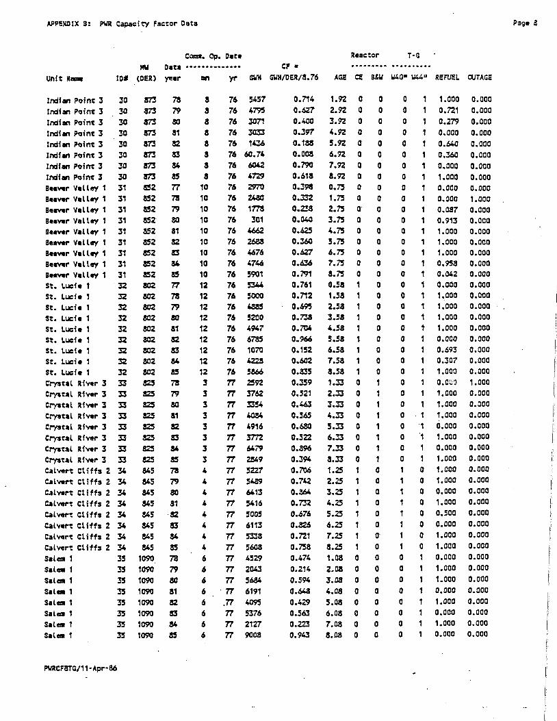
APPENDIX B: PUR Capacity Factor Data Page 3

Coon. Op. Date Reactor T-G

MU Data CP «

Unit Nana ID# (DERI year on yr GUH GUH/DER/8.76 AGE cs 3&U W40" W44u REFUEL OUTAGE

Indian Point 3 30 873 78 8 76 5457 0.714 1.92 0 0 0 1 1.000 0.Q00

Indian Point 3 30 873 79 a 76 4795 0.627 2.92 0 0 0 1 0.721 O.QOO

Indian Point 3 30 873 80 a 76 3071 0.400 3.92 0 0 0 1 0.279 0.000 Indian Point 3 30 873 81 8 76 3033 0.397 4.92 0 0 0 1 0.000 0.000 Indian Point 3 30 873 82 8 76 1436 0.188 5.92 0 0 0 1 0.640 0.000 Indian Point 3 30 873 83 8 76 60.74 0.008 6.92 0 0 0 1 0.360 0.000 Indian Point 3 30 873 34 8 76 6042 0.790 7.92 0 0 0 1 0.000 O.QOO Indian Point 3 30 873 85 8 76 4729 0.618 8.92 0 0 0 1 1.000 O.QOO Beaver Valley 1 31 852 77 10 76 2970 0.398 0.75 0 0 0 1 0.000 o.ooo Beaver Valley 1 31 852 78 10 76 2480 0.332 1.75 0 0 0 1 0.000 1.000 Beaver Valley 1 31 852 79 10 76 1778 0.238 2.75 0 0 0 1 0.087 0.000 Beaver Valley 1 31 852 80 10 76 301 0.040 3.75 0 0 0 1 0.913 O.QOO Beaver Valley 1 31 352 31 10 76 4662 0.625 4.75 0 0 Q 1 1.000 O.QOO Beaver Valley 1 31 852 82 10 76 2688 0.360 5.75 0 0 0 1 1.000 O.QOO Beaver Valley 1 31 852 83 10 76 4676 0.627 6.75 0 0 0 1 1.000 O.QOO Beaver Valley 1 31 852 84 10 76 4746 0.636 7.75 0 0 0 1 0.958 O.QOO Beaver Valley 1 31 852 85 10 76 5901 0.791 8.75 0 0 0 1 0.042 0.000 St. Lucie 1 32 802 77 12 76 5344 0.761 0.58 1 0 0 1 0.000 O.QOO St. Lucie 1 32 802 78 12 76 5000 0.712 1.58 1 0 0 1 1.000 O.OOO St. Lucie 1 32 802 79 12 76 4885 0.695 2.58 1 0 0 1 1.000 o.ooo

St. Lucie 1 32 802 80 12 76 5200 0.738 3.58 1 0 0 1 1.000 o.ooo

St. Lucie I 32 802 81 12 76 4947 0.704 4.58 1 0 0 t 1.000 o.ooo St. Lucie 1 32 802 82 12 76 6785 0.966 5.53 1 0 0 1 0.000 0.000 St. Lucie 1 32 802 S3 12 76 1070 0.152 6.53 1 0 0 1 0.693 0.000 St. Lucie 1 32 802 84 12 76 4228 0.602 7.53 1 0 0 1 0.307 0.000 St. Lucie 1 32 802 85 12 76 5866 0.835 8.53 1 0 0 1 1.000 0.000 Crystal River 3 33 825 78 3 77 2592 0.359 1.33 0 1 0 1 0.000 1.000 Crystal River 3 33 825 79 3 77 3762 0.521 2.33 0 1 0 1 1.000 0.000 Crystal River 3 33 825 80 3 77 3354 0.463 3.33 0 1 0 1 1.000 0.000 Crystal River 3 33 825 81 3 77 4084 0.565 4.33 0 1 0 1.000 0.000

Crystal River 3 33 825 82 3 77 4916 0.680 5.33 0 1 0 0.000 0.000

Crystal River 3 33 825 83 3 77 3772 0.522 6.33 0 1 0 1 1.000 0.000

Crystal River 3 33 825 84 3 77 6479 0.396 7.33 0 1 0 1 0.000 0.000

Crystal River 3 33 825 85 3 77 2849 0.394 8.33 0 1 0 1 1.000 o.ooo

Calvert Cliffs 2 34 845 78 4 77 5227 0.706 1.25 1 0 1 0 1.000 0.000

Calvert Cliffs 2 34 845 79 4 77 5489 0.742 2.25 1 0 1 0 1.000 0.000

Calvert Cliffs 2 34 845 80 4 77 6413 0.364 3.25 1 0 1 0 o.ooo 0.000

Calvert Cliffs 2 34 845 81 4 77 5416 0.732 4.25 1 0 1 0 1.000 0.000

Calvert Cliffs 2 34 845 82 4 77 5005 0.676 5.25 1 0 1 0 0.500 0.000

Calvert Cliffs 2 34 845 83 4 77 6113 0.326 6.25 1 0 1 0 0.000 0.000

Calvert Cliffs 2 34 845 84 4 77 5338 0.721 7.25 1 0- 1 0 1.000 0.000

Calvert Cliffs 2 34 845 85 4 77 5608 0.758 8.25 1 0 1 0 1.000 0.000

Salem 1 35 1090 78 6 77 4529 0.474 1.08 0 0 0 1 0.000 O.QOO

Sal as 1 35 1090 79 6 77 2043 0.214 2.08 0 0 0 1 1.000 0.000

Sale* 1 35 1090 80 6 77 5684 0.594 3.08 0 0 0 1 1.000 0.000

Salaa 1 35 1090 81 6 77 6191 0.648 4.08 0 0 0 1 0.000 0.000

Salem 1 35 1090 82 6 .77 4095 0.429 5.08 0 0 0 1 1.000 0.000 Salem 1 35 1090 83 6 77 5376 0.563 6.08 0 0 0 1 o.ooo 0.000 Salem 1 35 1090 84 3 77 2127 0.223 7.08 0 0 0 1 1.000 0.000

Salem 1 35 1090 85 8 77 9008 0.943 8.08 0 0 0 1 o.ooo 0.000

PVRCF3TG/11-Apr-86

APPENDIX 3: PVR Capacity Factor Data Page

Conn. Op. Date Reactor T-G MU Data CP

Unit Nana ID# <DER) year nr> y SUN GUH/DER/8.76 AGE C£ 3&U U40» W44" REFUEL OUTAGE

Oavis-Sesse 1 36 906 7a 11 77 2612 0.329 0.67 0 1 0 0 0.000 0.000 0avis*3ease 1 36 906 79 11 77 3129 0.394 1.47 0 1 0 0 0.000 0.000 Davis*Sessa 1 36 906 80 11 77 2094 0.263 2.67 0 1 0 0 1.000 0.000 Davis*3asa« 1 36 906 81 11 77 4363 0.550 3.67 0 1 0 0 0.000 0.000 Davis*Sessa 1 36 906 82 11 77 3218 0.405 4.67 0 1 0 0 1.000 0.000 Davis-Sessa 1 36 906 83 11 77 4833 0.415 5.67 0 1 0 0 1.000 0.000 Davis*Sessa 1 36 906 34 11 . 77 4292 0.541 6.47 0 1 0 0 0.357 0.000 Davis-Sessa 1 36 906 85 11 77 1943 0.245 7.47 0 1 0 0 0.143 O.OQO Fartay 1 37 829 78 12 77 5920 0.815 0.53 0 0 0 1 0.000 0.000 Fartey 1 37 829 79 12 77 1744 0.240 1.58 0 0 0 1 1.000 O.OQO Fartey 1 37 829 80 12 77 4604 0.632 2.58 0 0 0 1 0.392 o.ooo Farley 1 37 829 81 12 77 2616 0.360 3.53 0 0 0 1 1.234 0.000 Farley 1 37 829 82 12 77 5216 0.718 4.53 0 0 0 1 0.374 0.000 Farley 1 37 829 83 12 77 5983 0.324 5.53 0 0 0 1 1.000 O.OQO Farley 1 37 829 84 12 77 5428 0.747 6.53 0 0'- 0 1 1.000 O.OQO Farley t 37 829 85 12 77 5869 0.308 7.53 0 0 0 1 1.000 0.000 Cook 2 38 1100 79 3 78 5953 0.613 1.33 0 0 0 0 0.789 O.OQO Cook 2 38 1100 80 3 78 6692 0.693 2.33 0 0 0 0 0.211 0.000 Cook 2 38 1100 81 3 78 6385 0.663 3.33 0 0 0 0 1.000 0.000 Cook 2 38 1100 82 3 78 AjOGJL UV7V 0.726 4.33 0 0 0 0 0.649 0.000 Cook 2 38 1100 83 3 78 7013 0.728 5.33 0 0 0 0 0.351 o.ooo Cook 2 38 1100 84 3 78 5364 0.557 6.33 0 0 0 0 1.000 0.000 Cook 2 38 1100 85 3 78 5684 0.590 7.33 0 0 0 0 0.000 0.000 North Ama 1 39 907 79 6 78 4189 ' 0.527 1.08 0 0 0 1 0.321 O.OQO North Ama 1 39 907 80 6 78 5632 0.707 2.03 0 0 0 1 0.179 0.000 North Ama 1 39 907 81 6 78 4638 0.534 3.08 0 0 0 1 0.029 o.oao North Ama 1 39 907 82 6 78 2398 0.302 4.08 0 0 0 1 0.971 o.ooo North Ama 1 39 907 33 6 78 5310 0.668 5.08 0 0 0 1 0.000 0.000 North Ama 1 •39 907 84 6 78 3735 0.476 6.08 0 0 0 1 1.000 0.000 North Ama 1 39 907 85 6 78 5799 0.730 7.08 0 0 0 1 1.000 0.000 Arkansas 2 44 912 81 3 80 4324 0.541 1.33 1 0 0 1 1.000 o.oao Arkansas 2 40 912 82 3 80 3807 0.477 2.33 1 0 0 1.000 0.000 Arkansas 2 40 912 83 3 80 4427 0.554 3.33 1 0 0 1 0.736 0.000 Arkansas 2 40 912 84 3 80 6204 0.777 4.33 1 0 0 1 0.264 0.000 Arkansas 2 40 912 85 3 80 4699 0.588 5.33 1 0 0 1 1.000 o.ooo North Ama 2 41 907 81 12 80 5653 0.711 0.53 0- 0 0 1 0.000 0.000 North Ama 2 41 907 82 12 80 4047 0.509 1.58 0 0 0 1 1.000 0.000 North Ama 2 41 907 S3 12 80 5802 0.730 2.58 0 0 0 1 1.000 0.000 North Ama 2 41 907 34 12 80 4717 0.594 3.53 0 0 0 1 1.000 0.000 North Anna 2 41 907 85 12 80 6814 0.358 4.58 0 0 0 1 0.000 0.000 Sequoyah 1 43 1128 82 7 81 4909 0.497 1.00 0 0 0 1 1.000 0.000 Sequoyah 1 43 1128 83 7 81 7340 0.743 2.00 0 0 0 1 1.000 0.000 Sequoyah 1 43 1128 84 7 81 6105 0.618 3.00 0 0 0 1 1.000 0.000 Sequoyah 1 43 1128 85 7 81 4061 0.411 4.00 0 0 0 1 1.000 0.000 Sat eat 2 44 1115 82 10 81 7942 0.313 0.75 0 0 0 1 0.000 0.000 Salea 2 44 1115 83 10 81 743.6 0.076 1.75 0 0 0 1 1.000 0.000 Salem 2 44 1115 84 10 81 3201 0.328 2.75 0 0 0 1 0.000 1.000 Salem 2 44 1115 as 10 81 5017 0.514 3.75 0 0 0 1 0.000 1.000 McGuire t 45 1180 82 12 81 4302 0.416 0.58 0 0 0 1 o.oao 0.000 HeCuire 1 45 1180 83 12 81 4634 0.448 1.58 0 0 0 1 0.000 0.000

PVRCF8TG/11-Apr-86

APPENDIX 3: PUR Capacity Factor Data Page 10

Conn. Op. Date MU Data •'

Unit Nana ID* (DER) year mn yr

HcGuire 1 45 1180 84 12 81 Mefiuire 1 45 1130 85 12 81 Sequoyah 2 46 1148 83 6 82 Sequoyah 2 46 1143 84 6 82 Sequoyah 2 46 1148 as 6 82 Suaaer 1 46 900 84 1 84 Sumer 1 46 900 85 1 84 San Onofre 2 47 1070 84 8 83 San 0no*re 2 47 1070 85 3 83 St. Lucie 2 48 804 84 8 83 St. Lueie 2 48 804 85 8 83 San Choire 3 49 1080 85 4 84 Callaway 1 50 1171 85 12 84

Reactor T-G

ER/8.76 AGE C£ 3&U U40" W44" REFUEL OUTAGE

0.621 2.58 0 0 0 1 1.000 0.000 0.656 3.58 0 0 0 1 1.000 0.000 0.665 1.08 0 0 0 1 1.000 0.000 0.637 2.08 0 0 0 1 1.000 0.000 0.558 3.08 0 0 0 1 0.000 0.000 0.532 0.50 0 0 0 0 1.000 0.0QQ 0.663 1.50 0 0 0 0 1.000 0.000 0.562 0.92 1 0 0 0 0.404 0.000 0.550 1.92 1 0 0 0 0.596 0.000 0.790 0.92 1 0 0 1 1.000 0.000 0.367 1.92 1 0 0 1 0.000 o.ooo 0.392 1.25 1 0 0 0 0.900 0.000 0.784 0.58 0 0 0 0 0.000 0.000

GUH

6419 6777 6691 6403 5611 4197 5231 5267 5154 5565 6109 3707 8046

APPENDIX C:

NUCLEAR CONSTRUCTION COST AND SCHEDULE DATA

RLC0N2A - Myopia 41

Unit Hase

Hine (tile Point Nine Nile Point Surry 2 Kewaunee Kewaunee Kewaunee Peach Bottca 3 Arkansas 1 Fitzpatrick St, Lucie 1 Beaver Valley 1 Beaver Valley 1 Crystal River 3 Farley 1 North Anna 2 Lasalle 1 Susser 1 Turkey Point 4 Turkey Point 4 Prairie Isl 1 Browns Ferry 3 Farley 2 Sequoyah 1 Lasalle 1 Lasalle 1 Prairie Isl 1 Cooper Arkansas 1 Rancho Seco Trojan Indian Point 3 Beaver Valley 1 Sequoyah 1 Susser 1 Browns Ferry 1 Brunswick 2 Browns Ferry 3 North Anna 1 Nine Nile Point Calvert Cliffs i Three Nile I. 1 Zion 2 Beaver Valley 1 Sales 2 Surry 1 Zion 1 Browns Ferry 1 NcSuire 1 Surry 2 Peach Bott03 3 Brunswick 2 Brunswick 1

Actuals Cost COD

Act.Cost Date of 1972$ Estisate

Estisated Cost COD

st.Cost Est. 1972$ Tears

to COD

NOMINAL Cost Myopia Ratio Factor

REAL Duration Cost Myopia . Ratio Ratio Factor

162 162 155 203 203 203 223 239 419 486 599 599 419 727 542 1367 1233 127 127 233 334 750 934 1367 1367 233 269 239 344 452 570 599 934 1233 276 389 334 7B2 162 335 401 292 599 820 247 276 276 906 155 223 389 313

Dec-69 Dec-69 May-73 Jun-74 Jun-74 Jun-74 Dec-74 Dec-74 Jul-75 dun-76 Oct-76 Qct-76 Mar-77 Dec-77 Dec-80 Oct-32 Jan-84 Sep-73 Sep-73 Dec-73 Har-77 Jul-31 Jul-31 0ct-S2 Oct-32 Dec-73 Jul-74 Dec-74 Apr-75 Oec-75 Auq-76 Oct-76 Jul-31 Jan-84 Aug-74 Nov-75 Mar-77 Jun-73 Dec-69 Apr-77 Sep-74 Sep-74 Oct-76 Oct-Sl Dec-72 Dec-73 Aug-74 Dec-31 May-73 Dec-74 Nov-75 Mar-77

186.9 186.9 146.9 176.7 176.7 176.7 194.1 207.5 333.1 367.4 452.4 452.4 299.2 519.4 303.8 660.3 579.4 119.9 119.9 220.5 233.2 334.3 504.0 660.3 660.8 220.5 234.0 207.5 273.2 359.3 430.7 452.4 504.0 579.4 240.0 309.3 233.2 519.7 186.9 239.4 343.4 253.7 452.4 420.2 246.7 261.0 240.0 464.1 146.9 194.1 309.3 227.4

Jun-68 Dec-63 Nar-72 Nar-72 Jun-72 Sep-72 Dec-73 Nar-73 Jun-73 Dec-74 Jun-74 Dec-74 Mar-74 Jun-76 Nar-78 Jun-80 Jun-32 Jun-71 Dec-7! Dec-71 Jun-75 Sep-79 Jun-79 Nar-79 Dec-79 Sep-72 Jun-72 Sep-72 Sep-73 Sep-74 Sep-73 Sep-74 Sep-73 Sep-32 Sep-71 Dec-73 Dec-74 Mar-76 Dec-67 Dec-75 Jun-73 Mar-72 Mar-74 Mar-73 Dec-70 Jun-71 Mar-71 Dec-78 Dec-71 Sep-73 Sep-73 Dec-75

134 134 147 134 158 163 284 200 301 401 419 451 283 614 467 1107 1174 96

126 190 246 634 632 308 1003

210 207 185 328 366 400 451 632 1174 185 339 149 567 134 251 393 235 419 619 189 232 185 549 145 316 309 329

Jun-69 Dec-69 Nar-73 Nar-73 Jun-73 Sep-73 Dec-74 Mar-74 Jun-74 Dec-75 Jun-75 Dec-75 Nar-75 Jun-77 Nar-79 Jun-81 Jun-83 Jun-72 Dec-72 Dec-72 Jun-76 Sep-30 Jun-80 Mar-80 Dec-SO Qct-73 Jul-73 Qct-73 Oct-74 Oct-75 Oct-74 Qct-75 Oct-79 Oct-83 Oct-72 Jan-75 Jan-76 Apr-77 Jan-69 Jan-77 Aug-74 May-73 Nay-75 Nay-79 Feb-72 Aug-72 May-72 Feh-80 Mar—73 Dec-74 Dec-74 Mar-77

154.4 1 154.4 1 139.0 1 126.7 1 149.4 1 154.1 1 246.8 1 173.8 1 261.6 1 318.8 1 333.1 1 358.5 1 225.0 1 438.4 1 285.8 1 567.3 1 544.5 1 96.0 1

126.0 1 190.5 1 185.9 1 383.4 1 354.2 1 452.9 1 562.2 1 198.9 1 195.7 1 174.9 1 285.0 1 291.0 1 347.6 1 353.5 1 336.7 1 544.5 1 135.1 1 269.5 1 112.6 1 404.9 1 154.4 1 179.2 1 341.5 1 222.2 1 333.1 1 378.3 1 189.0 1 232.0 1 185.1 1 307.7 1 137.1 1 274.6 1 263.5 1 234.9 1

00 00 00 00 00 00 00 00 00 00 00 00 00 00 00 00 00 00 00 00 00 00 00 00 00 08 08 08 08 08 08 08 08 08 08 08 08

25 25 25

1.21 1.21 1.06 1.52 1.29 1.25 0.79 1.19 1.39 1.21 1,43 1.33 1.48 1.18 1.16 1.23 1.09 1.32 1.01 1.22 1,36 1.10 1.56 1.69 1.36 1.11 1.30 1,29 1.05 1.23 1.43 1.33 1.56 1.09 1.49 1.15 2.24 1.33 1.21 1.34 1.02 1.24 1.43 1.32 1.31 1.19 1.49 1.65 1.07 0.71 1.26 0.97

1.211 1.211

1.057 1.518 1.287 1.243 0.736 1.194 1.392 1.213 1.429 1.328 1.481 1.185 1.161 1.235 1.093 1.320 1,006 1.224 1.355 1.096 1,555 1.690 1.362 1.100 1.275 1.266 1.044 1.235 1.337 1.300 1.505 1.086 1.447 1.136 2.102 1.345 1.192 1.305 1.017 1.205 1.358 1.273 1.256 1.160 1.408 1.534 1.057 0.757 1.203 0.974

1.21 1.21 1.06 1.39 1.18 1.15 0.79 1.19 1.27 1.15 1.36 1.26 1.33 1.18 1.06 1.16 1.06 1.25 0.95 1.16 1.28 1.00 1.42 1.46 1.18 1.11 1.20 1.19 0.96 1.23 1.24 1.26 1.30 1.06 1.30 1.15 2.11 1.23 1.21 1.34 1.02 1.14 1.36 1.11 1.31 1.12 1.30 1.51 1.07 0.71 1.15 0.97

1.213 1.211

1.057 1.395 1.183 1.147 0.786 1.194 1.274 1.153 1.358 1.262 3.330 1.185 1.063 1.165 1.064 1.248 0.952 1.158 1.281 1.003 1.422 1.458 1.175 1.100

1.179 1.171 0.961 1.235 1.219 1.240 1.278 1.059 1.271 1,136 1.995 1.259 1.192 1.305 1.017 1,120 1.300 1.093 1.256 1.106 1.249 1.421

'1.057 0.757 i.120 0.974

1.50 1.00 1.17 2.25 2.00 1.75 1.00 1.75 2.08 1.50 2.34 1.84 3.00 1.50 2.76 2.33 1.59 2.25 1.75 .2.00 1.75 1.83 2.08 3.53 2.33 1.15 1.92 2.08 1.46 1.15 2.73 1.93 2.62 1.23 2.69 1.77 2.07 2.08 1.84 1.23 1.07 2.15 2.22 3.08 1.71 2.14 2.93 2.57 1.13 1.00

•11.73 a.00

RLC0N2A - Hyopia 41 Page -2

Actuals Act.Cost Date of Esti aated Est.Cost Est. N0H1NAL REAL Duration Unit Naae Cost COD 19725 Estiaate Cost COD 19724 Years Cost Hyopia Cost Hyopia Ratio

to COD Ratio Factor Ratio Factor Brunswick 1 313 Har-77 227.4 Dec-74 281 Nar-76 212.3 1.25 1.13 1.105 1.07 1.056 1.80 DaYis-Besse 1 672 Nov-77 480.2 Dec-75 533 Har-77 380.6 1.25 1.26 1.205 1.26 1.205 • 1.54 Suaser 1 1283 Jan-84 579.4 Sep-80 827 Dec-81 423.8 1.25 1.55 1.422 1.37 1.285 2.67 Turkey Point 3 109 Dec-72 108.7 Har-70 111 Jun-71 115.6 1.25 0.98 0.983 0.94 0.952 2.20 Surry 2 155 Hay-73 146.9 Sep-71 141 Dec-72 141.0 1.25 1.10 1.081 1.04 1.034 1.33 Prairie Isl 1 233 Dec-73 220.5 Sep-71 148 Dec-72 147.8 1.25 1.58 1.440 1.49 1.377 1.80 Kewaunee 203 Jun-74 176.7 Sep-71 134 Dec-72 134.0 1.25 1.52 1.396 1.32 1.248 2.20 Peach Bottoa 2 531 Jul-74 461.1 Jun-72 352 Sep-73 332.9 1.25 1.51 1.338 1.39 1.298 1.66 Oconee 3 160 Dec-74 139.4 Har-73 137 Jun-74 119.0 1.25 1.17 1.134 1.17 1.134 1.40 Rancho Seco 344 Apr-75 273.2 Har-73 327 Jun-74 284,2 1.25 1.05 1.040 0.96 0.969 1.67 San Onotre 2 2502 Aug-33 1160.3 Har-81 2010 Jun-82 971.6 1.25 1.24 1.191 1.19 1.152 1.93 Suaaer 1 1233 Jan-84 579.4 Har-SO 827 Jun-81 423.3 1.25 1.55 1.420 1.37 1.284 3.07 Turkey Point 4 127 Cop—73 119.9 Har-71 83 Jun-72 83.0 1.25 1.53 1.402 1.44 1.341 2.00 Crystal River 3 419 Har-77 299.2 Jun-75 420 Sep-76 317.4 1.25 1.00 0.998 0.94 0.954 1.40 Brunswick 1 313 Har-77 227.4 Har-75 281 Jun-76 212.3 1.25 1.13 1.105 1.07 1.056 1.60 Davis-Besse 1 672 Nov-77 480.2 Jun-75 461 Sep-76 348.3 1.25 1.46 1.35! 1.38 1.292 1.93 Farley 2 750 Jui-81 384.3 Jun-79 687 Sep-80 385.0 1.25 1.09 1.072 1.00 0.999 1.66 Cook 1 545 Aug-75 433.0 Dec-73 427 Apr-75 339.5 1.33 1.28 1.201 1.28 1.201 1.25 Hatch 1 390 Dec-75 310.4 Dec-72 282 Apr-74 245.0 1.33 1.38 1.277 1.27 1.194 2.25 Lasalle 1 1367 Gct-82 660.8 Dec-80 1184 Apr-82 572.3 1.33 1.15 1.114 1.15 1.114 1.38 Veraont Yankee 184 Nov-72 184.5 Har-70 133 Jul-71 133.5 1.33 1.39 1.278 1.33 1.240 2.00 Surry 1 247 Dec-72 246.7 Jun-70 189 Oct-71 196.9 1.33 1.31 1.221 1.25 1.184 1.88 Three Mi 1e !. 1 401 Sep-74 348.4 Har-73 373 Jui-74 324.1 1.33 1.07 1.056 1.07 1.056 1.13 Duane Arnold 280 Feb-75 222.5 Sep-72 192 Jan-74 166.8 1.33 1.46 1.327 1.33 1.24! 1.81 Browne Ferry 2 276 Har-75 219.6 Har-73 149 Jul-74 129.5 1.33 1.35 1.588 1.69 1.486 1.50 Rancho Seco 344 Apr-75 273.2 Jun-72 264 Oct-73 249.6 1.33 1.30 1.219 1.09 1.070 2.12 Calvert Cliffs 1 431 Hay-75 342.4 Jun-72 250 Oct-73 236.4 1.33 1.72 1.504 1.45 1.320 2.18 Fihpatrick 419 Jul-75 333.1 Jun-72 301 Oct-73 284.6 1,33 1.39 1.282 1.17 1.125 2.31 Cook 1 545 Aug-75 433.0 Jun-72 416 Oct-73 393.4 1.33 1.31 1.224 1.10 1.075 2.37 Cook 1 545 Aug-75 433.0 Jun-73 427 Oci-74 371.0 1.33 1.28 1.200 1.17 1.123 1.62 Indian Point 3 570 Aug-76 430.7 Har-73 317 Jul-74 275.5 1.33 1.30 1.553 1.56 1.398 2.60 8rowns Ferry 3 334 Har-77 233.2 Jun-69 149 0ct-70 163.0 1.33 2.24 1.830 1.46 1.329 5.81 North Anna 1 782 Jun-73 519.7 Dec-75 536 Apr-77 382.7 1.33 1.46 1.327 1.36 1.258 1.87 Sequoyah 1 984 Jul-3! 504.0 Har-70 535 Jul-79 327.1 1.33 1.34 1,580 1.54 1.383 2.50 HcSuire 1 906 Dec-81 464.1 Har-78 549 Jul-79 335.9 1 ^ 1.65 1.456 1.38 1.274 ? 3?

Susquehanna 1 1947 Jun-83 902.9 Con-an wv 184! Jan-02 889.7 1.33 1.06 1.043 1.0! 1.011 2.06 Surry 2 155 Hay-73 146.9 Jun-7! 139 Oct-72 139.0 1.34 1.12 1.087 1.06 1.042 1.43 Farley 1 727 Dec-77 519.4 Jun-75 487 Oct-76 363.0 1.34 1.49 1.350 1.4! 1.294 1.37 fliil stone 2 426 Dec-75 338.9 Dec-73 380 Hay-75 302.1 1.41 1.12 1.085 1.12 1.085 1.41 Susquehanna 1 1947 Jun-33 902.9 Dec-31 2292 Hay-83 1062.9 1.41 0.85 0.89! 0.35 0.891 1.06 Fort Calhoun 1 . 176 Sep-73 166.2 Dec-71 159 Hay-73 150.4 1.42 1.11 1.074 1.11 1.074 1.24 2i on 1 276 Dec-73 261.0 Dec-70 232 Hay-72 232.0 1.42 1.19 1.131 1.12 1.087 2.12 Palisades 147 Dec-71 152.3 Har-69 110 Aug-70 120.3 1.42 1.33 1.225 1.27 1.184 1.94 Three Nile I. 1 401 Sep-74 348.4 Jun-72 328 Nov-73 310.2 1.42 1.22 1.152 1.12 1.085 1.59 Rancho Seco 344 Apr-75 273.2 Sep-72 300 Feh-74 260.7 1.42 1.15 1.100 1.05 1.034 1.82 Calvert Cliffs 1 431 Hay-75 342.4 Sep-72 250 Feb-74 217.2 1.42 1.72 1.467 1.53 1.378 1.88 Farley 1 727 Dec-77 519.4 Sep-74 456 Feb-76 344.6 1.42 1.60 1.390 1.51 1.336 2.29 North Anna 2 542 Dec-80 303.3 Har-77 426 Aug-78 283.2 1.42 1.27 1.185 1.07 1.051 2.65 Oconee 2 160 Sep-74 139.4 Sep-71 137 Feb-73 129.6 1.42 1.17 1.117 1.08 1.053 2.11 Hatch 1 390 Dec-75 310.4 Sep-72 184 Har-74 159.9 1.49 2.12 1.654 1.94 1.558 2.17 North Anna 2 542 Dec-80 303.3 Sep-77 426 Har-79 260.7 1.49 1.27 1.175 1.17 1.108 2.17 Surry 1 247 Dec-72 246.7 Dec-69 189 Jun-71 196.9 1.50 1.31 1.195 1.25 1.163 2.00 Cook 1 545 Aug-75 433.0 Dec-72 427 Jun-74 371.0 1.50 1.28 1.176 1.17 _i.109 1.78

RLC0M2A - Myopia 41

Unit Naee

CookT : Susaer 1 Turkey Point 4 Calvert Cliffs 1 St. Lucie 1 Crystal River 3 Calvert Cliffs 2 Farley 1 Arkansas 1 Browns Ferry 3 Calvert Cliffs 2 Sequoyah 1 Lasalle 1 Sales 1 Davis-Sesse 1 Sequoyah 2 Millstone 2 Browns Ferry 3 Sequoyah 2 Farley 1 Farley 2 Browns Ferry 2 Rancho Seco Calvert Cliffs 1 Surry 2 Ocones i Three Mile 1. 1 Beaver Valley 1 North Anna 2 Sequoyah 1 Pilgris 1 Surry 2 Fort Calhoun 1 Calvert Cliffs 2 North Anna 2 Versont Yankee Three Mile i. 1 Farley 1 North Anna 2 Three Mile 1. 1 Susquehanna 1 Turkey Point 3 Surry 1 Calvert Cliffs 2 Three Mile 1. 2 Peach Bottoa 2 Cook 1 Brunswick 1 Sales 1 Davis-Besse 1 Sequoyah 2 Sequoyah 2 Duane Arnold

Actuals Act.Cost Date of Cost COD 1972$ Estiaate

Estisated Est.Cost Cost COD 1972$

452 12S3 127 431 488 419 335 727 239 334 335 984 1387 850 872 823 428 334 823 727 750 278 344 431 155 158 401 599 542 984 239 155 178 335 542 134 40! 727 542 401 1947 109 247 335 715 531 545 313 850 872 823 823 280

Jul-73 Jan-84 Sep-73 May-75 Jun-78 Mar-77 Apt—77 Dec-77 Dec-74 Mar-77 Apr-77 Jul-3! Oct-32 Jun-77 Nov-77 Jun-32 Dec-75 Mar-77 Jun-82 Dec-77 Jul-31 Mar-75 Apr-75 May-75 May-73 Jul-73 Sep-74 Oct-78 Dec-80 Jul-81 Dec-72 May-73 Sgn-73

Apr-77 Dec-30 Nov-72 Sep-74 Dec-77 Dec-80 Sep-74 Jun-83 Dec-72 Dec-72 Apr-77 Dec-73 Jul-74 Aug-75 Mar-77 Jun-77 Nov-77 Jun-32 Jun-82 Feb-75

300.2 579.4 119.9 342.4 387.4 299.2 239.4 519.4 207.5 238.2 239.4 504.0 880.3 807.2 480.2 301.3 333.9 238.2 301.3 519.4 384.3 219.8 273.2 342.4 148.9 147.1 348.4 452.4 303.3 504.0 239.3 148.9 188.2 239.4 303.3 134.5 348.4 519.4 303.3 348.4 902.9 108.7 248.7 239.4 475.8 481.1 433.0 227.4 807.2 480.2 301.3 301.3 222.5

Dec-78 Dec-80 Dec-70 Dec-71 Jun-74 Jun-73 Jun-74 Dec-75 Mar-72 Mar-74 Mar-74 Mar-77 Jun-79 Mar-75' Mar-75 Mar-79 Sep-72 Sep-73 Dec-80 Dec-74 Sep-78 Jun-72 Mar-72 Mar-72 Mar-7! Sep-89 Sep-72 Sep-73 Sep-78 Sep-78 Jan-70 Sep-70 Sep-7! Dec-73 Dec-78 Jul-70 Mar-72 Jun-74 Mar-78 Mar-71 Jun-79 Sep-89 Sep-89 Sep-73 Aug-78 Jun-71 Jun-71 Jun-75 Dec-73 Sep-74 Sep-78 Sep-7? Mar-72

437 1032

81 210 388 233 273 589 175 149 273 475 918

'878 434 832 282 149 1094 458 852 149 215 210 133 109 383 409

Jun-78 Jun-82 Jun-72 Jun-73 Dec-75 Dec-74 Dec-75 Jun-77 Sep-73 Sep-75 Sep-75 Con—73

Dec-80 Sep-78 Sep-78 Sep-80 Apr-74 Apr-75 Jul-82 Jul-78 Apr-80 Jan-74 Oct-73 Oct-73 Qct-72 May-71 May-74 May-75

383 .May-78 475 May-78

Sep-71 153 133 125 243 331 154 208 415 311 281 1285 99 185 243 837 288 358 328 497 434 832 442 177

May-72 May-73 Aug-75 Aug-78 Mar-72 Nov-73 Feh-78 Noy-77 NOV-72 Feb-31 Jun-7! Jun-71 Jun-75 May-78 Mar-73 Mar-73 Mar-77 Sep-75 Jun-78 Jun-80 Jun-81 Dec-73

290.5 498.3

81.0 198.8 291.0 245.9 217,0 420.8 185.5 118.5 217.0 315,5 514.5 512.3 327.9 354.2 245.0 118.5 528.8 344.8 385.4 129.5 203.3 198.8 138.0 113.3 315.4 325.1 241.3 315.5 159.8 133.0 118.2 193.2 253.3 154.0 194,3 313.8 222.1 281.0 858.3 103.1 171.9 193.2 423.5 272.3 338.8 234.2 394.7 327.9 354.2 228.5 187.4

Est. Years

to COD 1.50 1.50 1.50 1.50 1,50 1.50 1.50 1.50 1.50 1.50 1.50 1.50 1.50 1.51 1.51 1.51 1.58 1.58 1.53 1.53 1.53 1.59 1.59 1.59 1.59 1.88 1.88 1.88 1.88 1.88 1.88 1.88 1.88 1,88 1.88 1.87 1.87 1.87 1.87 1.87 1.87 1.75 1.75 1.75 1.75 1.75 1.75 1.75 1.75 1.75 1.75 1.75 1.75

NOMINAL Cost Myopia

Factor 1.022

REAL

Ratio 1.03 .24 .57 .05 .33 .48 ,23 .24 .38 .24 r*

*

.07

.49

.99

.51

.24

.57

.80

.15

.85

.80

.05

.13

.42 .10 .48 .49 .07 .58 .13 .41 .38 .42 .20 .95 .75 .74 .54 .52 .10 .50 .38 .12 .84 .53 0.97 .71 .55 .99 .41 .58

1.158 1.34S 1.814 1.208 1.299 1.147 1.15! 1.230 1.709 1.147 1.824 1.303 1.182 1.337 0.991 1.299 1.885 0.700 1.343 1.093 1.478 1.344 1.573 1.078 1.237 1.082 1.258 1.273 1.551 1.307 1.074 1.227 1.213 1.238 1.114 1.490 1.399 1.395 1.293 1.282

1.259 1.202 1.089 1.418 1.275 0.983 1.380 1.234 0.992 1.217 1.299

Cost Ratio 1.03 1.18 1.48 1.72 1.28 1.22 1.10 1.24 1.25 2.01 1.10 1.80 1.28 1.19 1.48 0.85 1.38 2 . 01 '

0.57 1.51 1.05 1.89 1.34 1.72 1.08 1.29 1.10 1.39 1.28 1.80 1.50 1.08 1.41 1.24 1.20 1.20 1.79 1.88 1.37 1.33 1.37 1.05 1.44 1.24 1.12 1.89 1.29 0.97 1.54 1.48 0.35 1.33

Myopia Factor

1.022 1.105 1.299 1.438 1.188 1.140 1.088 1.15! 1.182 1.59! 1.088 11366 1.181 1.119 1.288 0.393 1.223 1.558 0.700 1.298 1.032 1.395 1,205 1.410 1.040 1.187 1.082 1.220 1.149 1.328 1.278 1,038 1.227 1.138 1.115 1.114 1.418 1.353 1.208 1.138 1.208 1.03! 1.230 1.131 1.089 1.351 1.155 0.933 1.279 1.243 0.912 1.177 1.177

Duration Ratio

1.05 . 2,08 1.83 2.23 1.33 2.50 1.89 1.33 1.83 2.00 2.05 2.88 2.22 1.50 1.77 2.18 2.08 2.21 0.95 1.90 1.79 1.73 1.94 2.00 1.37 2.30 1.20 1.88 2.58 2.9! 1.75 1.80 1.20 2.00 2.40 1.40 1.50 2.10 2.85 2.09 2.39 1.88 1.88 2.05 1.32 1.78 2.38 1.00 2.00 1.31 2.14 1.57 1.87

RLCQM2A - Myopia 41 Page 4

Actuals Act.Cost Date of Estiaated Est,Cost Est. NOMINAL REAL' Duration Unit Naae Cost COD 1972$ Esti aate Cost COD 1972$ Years Cost Myopia Cost Myopia Ratio

to COD Ratio Factor Ratio Factor Millstone 2 m Dec-75 333.9 Mar-73 341 Dec-74 296.3 1.75 1.25 1.136 1.14 1.080 1.57 Crystal River 3 419 Nar-77 299.2 Dec-74 375 Sep-76 283.4 1,75 1.12 1.065 1.06 1.032 . 1.28 Brows Ferry 3 334 Mar-77 238.2 Mar-73 149 Dec-74 129.5 1,75 2.24 1.584 1.84 1.416 2.28 Sequoyah I 984 Jul-81 504.0 Dec-75 364 Sep-77 259.6 1.75 2.71 1.765 1,94 1.460 3.19 San Onofre 2 2502 Aug-33 1160.3 Mar-80 1824 Dec-81 934.7 1.75 1.37 1.198 1.24 1.131 1.95 Oconee 2 160 Sep-74 139.4 Mar-71 109 Dec-72 109.0 1.75 1.47 1.246 1.28 1.150 2.00 Suaser 1 1283 Jan-84 579.4 Mar-79 756 Dec-80 423.7 1.75 1.70 1.352 1.37 1.195 2.76 Veraont Yankee 184 Nov-72 184.5 Sep-69 120 Jul-71 125.0 1.83 1.54 1.265 1.48 1.237 1.73 Trojan 452 Dec-75 359.3 Sep-73 334 Jul-75 265.5 1.83 1.35 1,180 1.35 1.180 1.23 McSuire 1 906 Dec-91 464.1 Sep-77 466 Jul-79 285.2 1.33 1.94 1.433 1.63 1.305 2.32 Surry 1 247 Dec-72 246.7 Jun-69 165 Apr-71 171.9 1.83 1.50 1.246 1.44 1.218 1.91 Qconee 2 160 Sep-74 139.4 Sep-70 109 Jul-72 109.0 1.83 1.47 1.235 1.28 1.144 2.18 Brows Ferry 2 276 Mar-75 219.6 Sep-7! 149 Jul-73 141.0 1.83 1.85 1.400 1.56 1.274 1,91 Beaver Valley 1 599 Oct-76 452.4 Dec-72 340 0ct-74 295.4 1.83 1.76 1.362 1.53 1.262 2.09 Zion 1 276 Dec-73 261.0 Jun-70 232 Apr-72 232.0 1.83 1.19 1.099 1.12 1.066 1.91 Brows Ferry 1 276 Auq-74 240.0 Jun-70 149 Apr-72 149.1 1.83 1.85 1.400 1.61 1.296 2.27 Three Mile I. 1 401 Sep-74 348.4 Dec-70 262 Qct-72 262.0 1.83 1.53 1.261 1.33 1.168 2.04 Brows Ferry 2 276 Mar-75 219.6 Jun-70 149 Apr-72 149.1 1.83 1.85 1.400 1.47 1.235 2.59 Brows Ferry 3 334 Nar-77 238.2 Jun-70 149 Apr-72 149.1 1.83 2.24 1.551 1.60 1.291 3.68 San Onofre 2 2502 Aug-83 1160.3 Dec-79 1740 Oct-81 891.7 1.83 1.44 1.219 1.30 1,154 2.00 McSuire 1 906 Dec-31 464.1 Nar-77 466 Jan-79 285.2 1.84 1.94 1.436 1.63 1.304 2.59 Calvert Cliffs 2 335 Apr-77 239.4 Mar-75 253 Jan-77 180.6 1.84 1.33 1.165 1.33 1.165 1.13 North Anna 1 782 Jun-78 519.7 Mar-75 536 Jan-77 382.7 1,84 1,46 1.228 1.36 1.181 1.77 Fort Calhoun 1 176 Sep-73 166.2 Jun-69 92 May-71 95.3 1.91 1.91 1.403 1.73 1.334 2 2' Sequoyah 1 984 Jul -81 504.0 Jun-?6 364 May-78 241.7 1.9! 2.71 1.682 2,09 1.468 2.66 McSuire 1 906 Dec-31 464.1 Jun-76 384 May-78 255.3 1.91 2.36 1.566 1,82 1.367 2.87 Ranchc Seco 344 Apr-75 273.2 Jun-7! 215 May-73 203,3 1.92 1.60 1.277 1,34 1,167 2.00 Crystal River 3 419 Nar-77 299.2 Dec-72 283 Nov-74 245.9 1.92 1.48 1.227 1.22 1.103 2.22 North Anna 1 782 Jun-78 519.7 Dec-73 431 Nov-75 342.6 1.92 1.81 1.364 1.52 1.243 2.35 Fort Calhoun 1 176 Sep-73 166.2 Dec-70 125 Noy-72 125.0 1.92 1.41 1.194 1.33 1.160 1.43 North Anna 2 542 Dec-80 303.3 Dec-75 301 Xov-77 214.9 1.92 1.80 1.359 1.41 1.198 2.6! Calvert Cliffs 2 335 Apr-77 239.4 Mar-73 204 Feb-75 162.2 1,92 1.64 1.295 1.48 1.225 2.13

Millstone I 97 Mar-71 Mar-69 Mar-70 1.00 2.000 Point Beach 1 74 Dec-70 Dec-69 Dec-70 1.00 1.000 Point Beach 2 71 Qct-72 Sep-70 Sep-7! 1.00 2,035 Indian Point 2 206 Aug-73 Dec-70 Dec-71 1.00 2.663 Sinna 83 Jul-70 Qon-Afl ww Oct—59 1.08 1.691 Millstone 1 97 Mar-71 Sep-69 Dct-70 1.08 1.382 Quad Cities 1 100 Feb-73 Jun-70 Jul-71 1.08 2.47! Dresden 2 83 Jul-70 Dec-63 Jan-70 1.08 1.457 11stone i 97 Mar-71 Dec-68 Jan-70 1.08 2.07!

Oyster Creek 1 90 Dec-69 Mar-67 Apr-68 1.09 2.534 Insian Point 2 206 Aug-73 M3r-69 May-70 1.17 3.789 Ouad Cities 2 100 Mar-73 Mar-71 May-72 1.17 1.712 Dresden 3 104 Nov-71 Mar-70 Jun-71 1.25 1.335 Oyster Creek 1 90 Dec-69 Sep-66 Jan-68 1.33 2.437 Indian Point 2 206 Aug-73 Jun-69 0ct-70 1.33 3.125 Quad Cities 1 100 Feb-73 Mar-70 Jul-71 1.33 2.193 Indian Point 2 206 Aug-73 Dec-69 May-71 1.41 2.595 Dresden 3 104 Nov-71 Mar-69 Aug-70 1.42 1.882 Point Beach 1 74 Dec-70 Mar-69 Aug-70 1.42 1.236 Point Beach 2 71 Oct-72 Mar-70 Aug-71 1.42 1.824

RLCQM2A - Myopia 41 Pag? -5

Actuals Act.Cost Date of Estiaated Est.Cost Est. Unit Nase Cost COD 1972$ Estisate Cost COD 1972$ Years

to COD Oyster Creek 1 90 Dec-69 Jun-66 Dec-67 1.50 Dresden 3 104 Noy-71 Jun-69 Dec-70 1.50 Indian Point 2 206 Aug-73 Sep-63 Apr-70 1.58 Dresden 2 83 Jul-70 Sep-67 Apr-69 1.53 Quad Cities 1 100 Feb-73 Jun-69 Jan-71 1.59 Dresden 3 104 Noy-71 Dec-63 Aug-70 1.66 Oyster Creek 1 90 Dec-69 Mar-66 Dec-67 1.75 Quad Cities 1 100 Feb-73 Dec-68 0ct-70 1.83 Point Beach 2 71 Oct-72 Sep-69 Aug-71 1.91 Millstone 1 97 Mar-71 Sep-67 Aug-69 1.92

NOMINAL REAL

Ratio Factor Ratio Factor

Duration Ratio

2.334 1.611 3.111 1.739 2.316 1.752 2.142 2.277 1.611 1.324

For: 1 <= t < 2 No. of data points: Average Standard Deviation:

Fort Calhoun 1 176 Brunswick 2 389 Trojan 452 St. Lucie 1 486 Brunswick 1 318 Browns Ferry 3 334 Calvert Cliffs 2 77C

Farley 1 727 North Anna 1 782 Lasalle 1 1387 Kewaunee 203 Kewaunee 203 Peach Bottoa 2 531 Peach Bottoa 2 531 Crystal River 3 419 Sequoyah 1 984 Sequoyah 2 623 Browns Ferry 1 276 Prairie Isl 2 177 Browns Ferry 2 276 Beaver Valley 1 599 Browns Ferry 3 334 Browns Ferry 3 334 Prairie Isl 1 233 Three Mile I. 1 401 Three Mile I. 1 401 Cook 1 545 Farley 1 727 North Anna 1 782 Farley 2 750 Surry 2 155 Browns Ferry 2 276 Calvert Cliffs 2 335 North Anna 1 782

Sep-73 166.2 Sep-69 Nov-75 309.3 Dec-72 Dec-75 359.3 Ssp-72 Jun-76 367.4 Dec-73 Mar-77 227.4 Dec-73 Mar-77 233.2 Auq-72 Apr-77 239.4 Jun-72 Dec-77 519.4 Dec-73 Jun-73 519,7 Dec-72 Oct-82 660.8 Sep-77 Jun-74 176.7 Jup.-70 Jun-74 176.7 Sep-70 Jul-74 461.1 Mar-71 Jul-74 461.1 Dec-70 Mar-77 299.2 Sep-71 Jul-91 504.0 Sep-75 Jun-82 301.3 Mar-73 Aug-74 240.0 Sep-69 Dec-74 153.8 Sep-72 Mar-75 219,6 Sep-69 Oct-76 452.4 Sep-72 Mar-77 23S.2 Sep-72 Mar-77 233.2 Sep-69 Dec-73 220.5 Sep-70 Sep-74 343.4 Jun-70 Sep-74 348.4 Sep-70 Aug—75 433.0 Sep-71 Dec-77 519.4 Mar-73 Jun-73 519.7 Mar-73 Jul-81 334.3 Mar-77 May-73 146.9 Har-70 Har-75 219.6 Mar-71 Apr-77 239.4 Dec-71 Jun-73 519.7 Dec-74

92 Sep-71 95.3 256 Dec-74 222.5 243 Sep-74 211.2 318 Dec-75 252.3 269 Dec-75 213.8 149 Aug-74 129.5 204 Jun-74 177.3 395 Dec-75 314.0 407 Dec-74 353.7 675 Sep-79 413.0 123 Jun-72 123.0 123 Sep-72 123.0 277 Mar-73 261.9 230 Dec-72 230.0 190 Sep-73 179.7 324 Sep-77 231.3 535 «ar-S0 299.6 149 Qct-71 155.3 160 0ct-74 138.7 149 Qct-71 155.3 342 Oct-74 297.2 149 Qct-74 129.5 149 Oct-71 155.3 148 Oct-72 147.3 184 Jul-72 184.0 197 Oct-72 197.0 356 Oct-73 336.6 294 Apr-75 233.7 407 Apr-75 , 323.6 689 Apr-79 421.6 138 Apr-72 138.0 149 Apr-73 141.0 168 Jan-74 146.0 504 Jan-77 359.9

220 190 190 .417 1.423 1.271 .238 0.343 0.194

2.00 1.91 1.383 2.00 1.52 1.233 2,00 1.86 1.364 2.00 1,53 1.237 2.00 1.13 1.038 2.00 2.24 1.496 2.00 1.64 1.282 2.00 1.34 1.357 2.00 1.92 1.336 2.00 2.03 1.423 2.00 1.65 1.236 2.00 1.65 1.236 2.00 1.92 1.334 2.00 2.31 1.519 2.00 2.21 1.435 2.00 3.04 1.742 2.00 1.17 1.080 2.08 1.35 1.345 2.08 1.11 1.051 2.03 1.85 1.345 2.03 1.75 1.309 2.08 2.24 1.473 2.03 2.24 1.473 2.08 1.53 1.245 2.08 2.18 1.453 2.08 2.04 1.406 2.08 1.53 1.226 2.08 2.47 1.545 2.08 1.92 1.368 2.08 1.09 1.042 2.09 1.13 1.059 2.09 1.85 1.344 2.09 2.00 1.393 2.09 1.55 1.234

190 190 220 .293 1.190 1.983 .248 0.154 0.592

1.73 1.317 2.00 1.39 1.179 1.46 1.70 1,305 1.62 1.45 1.206 1.25 1.06 1.031 1.62 1.84 1.356 2.29 1.35 1.162 2,42 1.65 1.286 2.00 1.47 1.212 2.75 1.60 1.265 2.54 1,44 1.199 2.00 1.44 1.199 1.87 1.76 1.327 1.67 2.00 1.416 1.79 1.67 1.290 2.75 2.13 1.476 2.91 1.01 1.003 2.12 1.55 1.233 2.36 1.11 1.051 1.08 1.41 1.181 2.64 1.52 1.224 1.96 1.84 1.340 2.16 1,53 1.223 3.60 1.49 1.212 1.56 1.89 1.359 2.04 1.77 1.315 1.92 1.29 1.128 1.88 2.22 1.467 2.28 1.61 1.255 2.52 0.91 0.957 2.08 1.06 1.031 1.52 1.56 1.237 1.92 1.64 1.268 2.56 1.44 1.193 1.68

RLC0H2A - Myopia 41 Pace >6

Unit Naae

Sequoyah 1 Farley 2 Palisades Beayer Valley 1 North Anna 1 Sequoyah 2 Susquehanna 1 Maine Yankee Peach Bottoa 2 Three Mile I, 1 Three Mile I. 1 Oconee 3 North Anna 1 Sequoyah 1 McSuire 1 Suaaer 1 Surry 1 Sales 1 Surry 2 Peach Bottos 2 Brunswick 2 Brunswick 1 North Anna 1 Arkansas 2 Thrss I. 1 Peach Bottoa 3 St. Lucie 1 St. Lucie 1 Beaver Valley 1 Calvert Cliffs 2 Sales 1 S U 5 5 6 r i Fort Calhoun 1 Turkey Point 4 Kewaunee Afk2nt53c 2 Farley 2 Sequoyah 1 Farley 2 Sequoyah 1 Coouer Beaver Valley 1 Calvert Cliffs 2 Sales 1 Farley 2 Browns Ferry 2 Calvert Cliffs 1 Indian Point 3 Calvert Cliffs 2 Arkansas 2 Arkansas 2 Sequoyah 1 Farley 2

Actuals Act.Cost Date of Cost COD 1972$ Estiaate

Estiaated Cost COD

Est.Cost 1972$

984 750 147 599 782 623 1947 219 531 401 40! 160 782 984 906 1283 247 850 155 531 309 318 782 640 401 223 486 486 599 335 850

1283 176 127 203 640 750 984 750 984 269 599 335 850 750 276 431 570 335 640 640 984 750

Jul-81 Jul-81 Dec-71 Oct-76 Jun-78 Jun-82 Jun-83 Dec-72 Jul-74 Sep-74 Sep-74 Dec-74 Jun-78 Jul-81 Dec-81 Jan-84 Dec-72 Jun-77 May-73 Jul-74 Nov-75 M3r-77 Jun-78 Mar-SO Sep-74 Dec-74 Jun-76 Jun-76 0ct-76 Apr-77 Jun-77 Jan-84 Sep-73 Sep-73 Jun-74 Mar-80 Jul-31 Jul-81 Jul-3! Jul-81 Jul-74 Oct-76 Apr-77 Jun-77 Jul-81 Mar-75 May-75 Aug-76 Apr-77 Mar—80 Nar-30 Jul-81 Jul-81

504.0 384.3 152.3 452.4 519.7 301.3 902.9 219.2 461.1 348.4 348.4 139.4 519.7 504.0 464.1 579,4 246.7 607.2 146.9 461.1 309.3 227.4 519.7 358.7 348.4 194.1 367.4 367.4 452.4 239.4 607.2 579.4 166.2 119.9 176.7 353.7 384.3 504.0 334.3 504.0 234.0 452.4 239.4 607.2 384.3 219.6 342.4 430.7 239.4 358.7 358.7 504.0 384.3

Dec-74 Mar-78 Mar-63 Mar-73 Sep-73 Mar-77 Mar-81 Mar-70 Mar-70 Sep-71 Mar-70 Sep-71 Mar-74 Jun-74 Dec-76 Mar-78 Dec-68 Dec-72 Dec-69 Dec-69 Dec-7! Sep-73 Sep-72 Bec-75 Jun-69 Jun-72 Mar-72 Mar-73 Sep-71 Mar-72 Sep-74 Sep-78 Mar-70 Mar-70 Mar-70 Mar-75 Jun-75 Mar-74 Dec-76 Dec-72 Dec-70 Jun-72 Sep-72 Dec-70 Dec-77 Sep-70 Sep-70 Har-71 Sep-74 Jun-75 Sep-75 Sep-74 Sep-74

324 635 89

340 407 475 2276 131 230 296 184 137 446 313 334 675 165 425 133 218 210 251 360 393 162 316 235 313 286 168 678 675 125 80 12! 339 365 313 572 095 207 311 204 237 662 149 170 256 256 339 369 313 363

Jan-77 Apr-80 May-70 May-75 Nov-75 May-79 May-83 May-72 May-72 Nov-73 May-72 Nov-73 May-76 Aug-76 Feb-79 May-80 Mar-71 Mar-75 Mar-72 Mar-72 Mar-74 Dec-75 Dec-74 Mar-73 Sep-71 Sep-74 Jun-74 Jun-75 Dec-73 Jun-74 Dec-76 Dec-80 Jun-72 Jun-72 Jun-72 Jun-77 Sep-77 Jun-76 Apr-79 Apr-75 Apr-73 Oct-74 Jan-75 Apr-73 Apr-80 Jan-73 Jan-73 Jul-73 Jan-77 Oct-77 Jan-78 Jan-77 Jan-77

231.3 355.9 97.3

270.3 323.6 290.4 1055.3 131.0 230.0 279.9 184.0 129.6 337.0 236.1 235.0 373.3 171.9 337.9 138.0 218.0 182.5 199.5 312.3 261.3 163.7 274.6 204.2 252.3 270.4 146.0 512.3 378.3 125.0 80.0

121.0 242.1 260.6 236.1 350.0 178.5 195.7 270.2 162.2 224.1 371.0 141.0 160.3 242.1 182.3 242.1 245.3 223.1 259.2

Est. Years

to COD 2.09 2.09 2.17 2.17 2.17 2.17 2.17 2.17 2.17 2.17 2.17 2.17 2.17 2.17 2.17 2.17 2.25 2.25 2.25 2.25 2.25

NOMINAL Cost Myopia

Factor 1.703

? os 2.25 2.25 2.25 2.75

9,2s 2.2* 2.25 2.25 ")

2.25 2.25 2.33 2.33 2.33

2.ou

2.33 2.34 2.34 2.34 2.34 2.34 2.34 2.34 2.34

Ratio 3.04 1.18 1.65 1.76 1.92 1.31 0.36 1.21 2.31 1.35 2.18 1.17 1.75 3.15 2.36 1.90 1.50 2.00" 1.13 2.43 1.35 1.27 2.17 1.63 2.47 0.7! 2.07 1.53 2.09 2.00 1.25 1.90 1.41 1.53 1.68 1.39 2.05 3.15 1.31 4.38 1.30 1.93 1.64 3.59 1.13 1.35 2.53 2.23 1.31 1.89 1.73 3.15 2.07

REAL Cost Myopia

Factor 1.452

1.083 1.260 1.299 1.352 1.134 0.931 1.092 1.470 1.150 1,432 1.075 1.295 1.697 1.485 1.345 1.196 1.362 1.054 1.486 1.316 1.112 1.412 1.242 1.496 0.857 1.38! 1.208 1.339 1.359 1.106 1.330 1.163 1.227 1.259 1.326 1.377 1.663 1.123 1.885 1.119 1.324 1.237 1.729 1.055 1.302 1.439 1.409 1.123 1.313 1.266 1.634 1.364

Ratio 2.18 1.08 1.57 1.67 1.61 1.04 0.86 1.2! 2.00 1.24 1,39 1.08 1.54 2.13 1.97 1.53 1.44 1.80 1.06 2.12 1.70 1.14 1.66 1.37 2.06 0.71 1.30 1.45 1.67 1.64 1.1.9 1.53 1.33 1.50 1.46 1.48 1.47 2.13 1.10 2.82 1.20 1.67 1.43 2.7! 1.04 1.56 2.13 1.78 1.31 1.48 1.46 2.26 1.48

1.038 1.232 1.269 1.245 1.017 0.931 1.092 1.378 1.106 1.342 1.034 1.221 1.419 1.369 1.217 1.175 1.298 1.028 1.396 1.265 1.060 1.253 1.151 1.380 0.857 1.298 1.181 1.257 1.246 1.078 1.208 1.135 1,197 1.183 1.19! 1.188 1.400 1.041 1.561 1.080 1.247 1.182 1.533 1.015 1.209 1.382 1.230 1.123 1.183 1.177 1,418

'17184

Duration Ratio

3.15 1.60 1.73 1.66 2.19 2,42 1.04 1.27 2.00 1.33 2.08 1.50 1.96

2.69 1.78 2.00 1.52 2.04 1.74 1.56 2.56 1.89 2.tt 1.1! 1.39 1.45 2.26 2.26 1." 2.37 1.56 1,56 1.89 2.22 2.70 3.26 1.97 3.68 1.54 1.36 1.96 2.79 1.54 1.92 2.00 2.34 1.11 2.03 1.93 2.92 2.92

RLC0N2A - Myopia 41

Unit Naae

Susquehanna 1 St. Lucie 1 Davis-Besse 1 Three Mile I. 1 Prairie Isl 2 Davis-Besse I Sequoyah 1 Nine Nile Point Browns Ferry 2 Browns Ferry 3 Susquehanna 1 Peach Bottcs 2 Cook 1 St. Lucie 1 Beaver Valley 1 Davis-Besse 1 Farley 1 North Anna 1 Sequoyah 1 Sequoyah 1 Farley 2 Trojan Beaver Val1ey 1 Sales 1 North Anna 2 Sales 2 Trojan North Anna 2 Farley 2 Hi 11 stone 2 Hatch 1 Cook 2 Sequoyah 1 Browns Ferry 2 Beaver Valley 1 Browns Ferry 3 Sales ! North Anna 2 Sequoyah 2 Farley 2 Fort Calhoun 1 Lasalle 1 Three Nile I. 1 Oconee 2 North Anna 2 Sequoyah 2 Arkansas 2 North Anna 2 Turkey Point 4 Three Nile I. 1 Beaver Valley 1 North Anna 1 North Anna 1

Actuals Act.Cost Date of Estisated Est.Cost Cost COD 1972$ Estiaate Cost COD 1972$

1947 486 672 401 177 672 984 162 276 334 1947 531 545 486 599 672 727 782 984 984 750 452 599 850 542 820 452 542 750 426 390 452 984 276 599 334 850 542 623 750 176 1367 401 160 542 623 640 542 127 401 599 782 782

Jun-83 Jun-76 Nov-77 Sep-74 Dec-74 Nov-77 Jul-81 Dec-69 Nar-75 Kar-77 Jun-83 Jul-74 Aug-75 Jun-76 Oct-76 Nov-77 Dec-77 Jun-73 Jul-81 Jul-31 Jul-81 Dec-75 flct-76 Jun-77 Dec-30 Qct-81 Dec-75 Dec-80 Jul-81 Dec-75 Dec-75 Jui-78 Jul-81 Nar-75 Qct-76 Har-77 Jun-77 Dec-30 Jun-82 Jul-81 Sep-73 Oct-82 Sep-74 Sep-74 Dec-80 Jun-82 ttar-SO Dec-80 Sep-73 Sep-74 Oct-76 Jun-78 Jun-78

902.9 367.4 480.2 348.4 153.3 480.2 504.0 186.9 219.6 233.2 902.9 461.1 433.0 367.4 452.4 480.2 519.4 519.7 504,0 504.0 334.3 359.3 452.4 607.2 303.3 420.2 359.3 303.3 384.3 338.9 310.4 300.2 504.0 219.6 452.4 238.2 607.2 303.3 301.3 384.3 166.2 660.3 343.4 139.4 303.3 301.3 358.7 303.3 119.9 348.4 452.4 519.7 519.7

Sep-79 Dec-72 Dec-72 Dec-69 Dec-71 Sep-73 Jun-72 Jun-66 Sep-67 Sep-71 Sep-78 Sep-69 Sep-70 Dec-71 Dec-71 Jun-72 Jun-73 Dec-71 Jun-73 Dec-73 Dec-74 Nar-72 Jun-71 Jun-71 Nar-75 Har-74 Dec-72 Dec-72 Sep-76 Sep-71 Sep-70 Sep-75 Dec-71 Nar-68 Nar-72 Har-63 Nar-72 Nar-73 Jun-76 Jun-74 Sep-68 Sep-76 Sep-69 Sep-69 Sep-73 Sep-75 Jun-74 Har-74 Sep-69 Dec-68 Sep-70 Sep-71 Jun-71

1607 318 349 180 145 409 213 83

124 149

1293 206 339 218 286 304 294 344 225 225 363 233 219 237 301 496 284 227 499 252 184 437 213 124 309 124 336 227 364 338 92 585 162 109 227 324 313 240 41 150 219 310 308

Jan-82 Nay-75 Hay-75 Nay-72 Hay-74 Feb-76 Nov-74 Nov-68 Feh-70 Feb-74 Feb-81 Nar-72 Nar-73 Jun-74 Jun-74 Dec-74 Dec-75 Jun-74 Dec-75 Jun-76 Jun-77 Sep-74 Dec-73 Dec-73 Sep-77 Sep-76 Jul-75 Jul-75 Apr-79 Apr-74 Apr-73 Apr-78 Jul-74 0ct-70 Oct-74 Oct-70 0ct-74 Oct-75 Jan-79 Jan-77 Nay-71 Nay-79 Nay-72 Nay-72 May-76 Nay-78 Feb-77 Nov-76 Jun-72 Sep-71 Jun-73 Jun-74 Har-74

776.7 252.3 277.4 180.0 125.6 309.1 184.7 106.6 136.0 129.5 662.5 206.0 320.6 189.4 248.5 264.2 233.7 298.9 178.5 169.6 259.2 202.5 207.1 224.1 214.9 374.3 225.3 180.5 305.3 219.0 174.0 290.5 184.7 136.0 268.5 136.0 291.5 180.5 222.4 241.3 95.3 358.0 162.0 109.2 171.5 215.4 227.1 181.4 .41.0 156.2 207.1 269.4 267.6

Est. Years to COD 2.34 2.41 2.41 2.41 2.41 2.42 2.42 2.42 2.42 2.42 2,42 2.50 2.50 2.50 2.50 2.50 2.50 2.50 2.50 2.50 2.50 2.50 2.50 2.50 2.51 2.51 2.58 2.58 2.58 2.58 2.53 2.53 2.58 2.58 2.58 2.53 2.58 2.53 2.58 2.59 2.66 2,66 2.66 2.66 2.66 2.66 2.67 2.67 2.75 2.75 2.75 2.75 2.75

NOMINAL Cost Nycpia

Factor

REAL Duration

Ratio 1.21 1.53 1.93 2.23 1.22 1.64 4.63 1.84 2.22 2.24 1.51 2.58 1.61 2.23 2.09 2.21 2.47 2.27 4.38 4.38 2.07 1.94 2.73 3.59 1.80 1.65 1.59 2.39 1.50 1.69 2.12 1.03 4.63 2.22 1.94 2.68 2.53 2.39 1.71 7 77 1.91 2.34 2.47 1.47 2.39 1.92 2.01 2.26 3.09 2.67 2.73 2.52 2.54

1.086 1.192 1.312 1.393 1.087 1.228 1.885 1.288 1.390 1.395 1.184 1.461 1.209 1.378 1.344 1.374 1.437 1.389 1.806 1.806 1.337 1.303 1.495 1.666 1.265 1.222 1.197 1.401 1.171 1.226 1.338 1.013 1.810 1.362 1.292 1.465 1.433 1.400 1.232 1.361 1.275 1.376 1.405 1.155 1.386 1.278 1.299 1.356 1.508 1.430 1.442 1.400 1.403

Cost Nyopia Ratio Ratio Factor 1.16 1.067 1.60 1.45 1.168 1.45 1.73 1.255 2.04 1.94 1.315 1.97 1.22 1.087 1.24 1.55 1.200 1.72 2.73 1.515 3.76 1.75 1.261 1.45 1.61 1.219 3.10 1.84 1.286 2.27 1.36 1.136 1.96 2.24 1.381 1.93 1.35 1.128 1.97 1.94 1.303 1.80 1.32 1.271 1.93 1.82 1.270 2.17 2.22 1.376 1.80 1.74 1.248 2.60 2.82 1.515 3.23

. 2.97 1.546 3.03 1.48 1.171 2.63 1.77 1.258 1.50 2.18 1.367 2.13 2.71 1.489 2.40 1.41 1.148 2.30 1.12 1.047 3,03 1.59 1.197 1.16 1.63 1.224 3.10 1.26 1.093 1.37 1.55 1.184 1.65 1.78 1.251 2.03 1.03 1.013 1.10 2.73' 1.475 3.71 1.61 1.204 2,71 1.68 1.224 1.77 1.75 1.242 3.43 2.03 1.329 2.03 1.68 1.223 3.00 1.35 1.125 2.32 1.59 1.197 2.74 1.73 1.230 1.88 1.85 1.259 2.28 2.15 1.333 1.38 1.28 1.096 1.83 1.77 1.239 2.72 1.40 1.134 2.53 1.58 1.187 2.15 1.68 1.213 2.53 2.92 1.478 1.46 2.23 1.339 2.09 2.18 1.329 2.21 1.93 1.270 2.46 1.94 ... 1.273 2.55

RLCQH2A - Myopia 41 Paps

Actuals Act.Cost Date of Estiaated Est.Cost Unit Naae Cost COD 1972$ Estiaate Cast COD 1972$

Arkansas 2 440 Mar-80 358.7 Sep-74 318 Jun-77 227.1 Lasalle 1 1347 Oct-82 440.8 Dec-74 585 Sep-79 358.0 North Anna 1 782 Jun-78 519.7 Mar-72 344 Dec-74 298.9 North Anna 2 542 Dec-80 303.8 Dec-74 244 Sep-77 188.5 Salea 2 820 Oct-81 420.2 Dec-73 497 Sep-74 375.2 Salea 1 850 Jun-77 407.2 Mar-70 237 Dec-72 237.0 Indian Point 3 570 Aug-74 430.7 Sep-43 154 Jul-71 142.5 North Anna 2 542 Dec-80 303.8 Sep-72 208 Jul-75 145.4 Oconee 3 140 Dec-74 139.4 Sep-70 109 Jul-73 103.1 Indian Point 3 570 Aug-74 430.7 Sep-49 154 Jul-72 154.0 Indian Point 3 570 Aug-74 430.7 Sep-70 213 Jul-73 204.1 Hatch 2 515 Sep-79 315.1 Jun-74. 512 Apr-79 313.3 Peach Bottoa 3 223 Dec-74 194.1 Dec-70 221 Oct-73 209.0 Crystal River 3 419 Mar-77 299.2 Jun-49 148 Apr-72 148.0 North Anna 2 542 Dec-80 303.3 Jun-73 227 Apr-74 171.5 Farley 2 750 Jul-81 384.3 Jun-77 489 Apr-30 384.2 McSuire 1 904 Dec-31 444.1 Jun-74 220 Apr-77 157.1 Sequoyah 2 423 Jun-32 301.3 Jun-74 313 Apr-77 223.1 Browns Ferry 3 334 Mar-77 238.2 Mar-71 149 Jan-74 129.5 St, Lucie 1 484 Jun-74 347.4 Jun-72 249 May-75 213.3 St. Lucie 2 1430 Aug-83 443.2 Jun-80 1100 May-83 510.1 Suaaer 1 1233 Jan-84 579.4 Jun-74 493 May-79 301.7 Zion 2 092 Sep-74 253.7 Jun-70 213 May-73 201.4 Three Mile I. 2 715 Dec-78 475.4 Jun-75 430 May-73 418.8 Browns Ferry 2 274 Mar-75 219.4 Mar-47 117 Feh-70 128.3 Arkansas 2 440 Mar-80 353.7 Har-74 273 Feb-77 194.9 Susquehanna 1 1947 Jun-83 902.9 Mar-73 1195 Feb-81 412.4

Point Beach 2 7! Oct-72 Dec-49 Dec-71 Oyster Creek 1 90 Dec-69 Sep-45 Nov-47 Quad Cities 2 100 Mar-73 Mar-70 May-72 Quad Cities 2 100 Har-73 Dec-48 Apr-71 Millstone 1 97 Mar-71 Mar-47 Aug-49 Quad Cities 1 100 Feb-73 Sep-47 Mar-70 Quad Cities 2 100 Mar-73 Jun-49 Jan-72 Dresden 2 83 Jul-70 Mar-44 Feb-49

Est. Years

to COD 2.75 2.75 2.75 2.75 2.75 2.75 2.83 2.33 2.83 2.83 2.83 2.33 2.83 2.83 2.33 2.83 2.83 2.83 2.84 2.91 2,91 2.91 2.92 2.92 2.92 2.92 2.92

2,00 2.17 2.17 2.33 2.42 2.50 2.58 2.92

NOMINAL Cost Myopia

Factor 1.290

Ratio 2.01 2.34 2.27 2.05 1.45 3.59 3.85 2.4! 1.47 3.45 2.4! 1.01 1.01 2.83 2.39 1.09 4.12 1.99 2.24 1.8! 1.30 2.40 1.37 1.14 2.35 2.34 1.43

REAL Cost Myopia

Factor 1.181

1.342. 1.348 1.299 1.200 1.590 1.581 1.403 1.144 1.580 1.404 1.002 1.004 1.444 1.340 1.030 1.448 1.274 1.328 1.225 1.094 1.389 1.114 1.045 1.340 1.338 1.182

Ratio 1.58 1.85 1.74 1.41 1.12 2.54 2.45 1.84 1.35 2.74 2.09 1.01 0.93 2.02 1.77 1.00 2,95 1.35 1.84 1.72 1.30 1.92 1.24 1.14 1.7! 1.34 1.47

1.250 1.223 1.189 1.042 1.407 1.412 1.240 1.113 1.432 1.297 1.002 0.974 1.282 1.223 0.998 1.444 1.112 1.239 1.204 1.094 1.251 1.082 1.045 1.202 1. ?32 1.142

Duration Ratio

2.00 2.12 2.27 2.18 2.85 2.43 2.81 2.92 1.50 2.44 2.10 1.15 1.41 2.73 2.45 1.44 2.45 2.82 2.11 1.37 1.09 2.40 1.44 1.19 2.74 2.05 1.80

1.413 1.942 1.384 1.823 1.453 2.171 1.450 1.482

For: 2 <= t < 3 Ho, of dat3 points: 175 147 147 147 147 175 ftver3ge 2.397 2.055 1.331 1.449 1.223 2.100 Standard Deviation: 0.279 0.734 0.183 0.449 0.1o2 0.585

RLCQH28 - Myopia 41

Actuals Act.Cost Date at Estiaated Est.Cost Unit Naae Cost COD 19724 Estiaate Cost COD 1972$

Peach Bottoa 2 531 Jul-74 461.1 Mar-68 163 Mar-71 169.8 Brunswick 1 313 Har-77 227.4 Dec-72 214 Dec-75 170.1 Sequoyah 2 623 Jun-82 301.3 Dec-72 225 Dec-75 173.5 Peach Bottoa 3 223 Dec-74 194.1 Mai—70 221 Mar-73 209.0 Duane Arnold 280 Feb-75 222.5 Dec-70 148 Dec-73 140.0 Hatch 1 390 Dec-75 310.4 Jun-70 184 Jun-73 174.0 St. Lucie 1 486 Jun-76 367.4 Jun-71 203 Jun-74 176.4 Arkansas 2 640 Mar-80 358.7 Dec-73 273 Dec-76 206.3 Sequoyah 2 623 Jun-82 301.3 Sep-74 313 Sep-77 223.1 Sequoyah 2 623 Jun-S2 301.3 Jun-72 213 Jul-75 168.9 Browns Ferry I 276 Aug-74 240.0 Sep-67 124 0ct-70 136.0 Browns Ferry 3 334 Har-77 238.2 Sep-70 149 Oct-73 141.0 Salea 1 350 Jun-77 607.2 Sep-71 308 Oct-74 267.6 Zion 1 276 Dec-73 261.0 Mar-69 205 Apr-72 205.0 Peach Bottoa 3 223 Dec-74 194.1 Mar-7! 263 Apr-74 223.5 Farley 2 750 Jul-SI 384.3 Dec-73 329 Jan-77 234.9 Sequoyah 1 984 Jul-SI 504.0 Mar-71- 213 Apr-74 184.7 Salea 2 820 Oct-31 420.2 Mar-71 237 . Apr-74 205.9 McSuire 1 906 Dec-81 464.1 Dec-74 384 Jan-78 255.3 Fort Calhoun 1 176 Sep-73 166.2 Mar-69 92 May-72 92.0 Oconee 2 160 Sep-74 139.4 Mar-69 93 May-72 92.6 McSuire 1 906 Dec-81 464.1 Sep-73 220 Nov-76 166.2 Sequoyah 2 623 Jun-82 301.3 Jun-73 225 Auq-76 169.6 SfiQuoysh 2 623 Jun-82 301.3 Dec-73 2?s Feb-77 160.3 Surry 1 247 Bec-72 246.7 Dec-67 144 Mar-71 150.0 Surry 2 ) 55 May-73 146.9 0or-AQ 123 Mar-72 123.0 Peach Bottoa 3 223 Dec-74 194.1 Dec-69 203 Mar-73 192.0 Brunswick 2 389 Nov-75 309.3 Dec-70 195 Mar-74 169.4 Brunswick 1 318 Mar-77 227.4 Dec-71 181 Mar-75 143.9 Salea 2 820 Qct-8! 420.2 Dec-72 425 Mar-76 321.1 McSuire 1 906 Dec-31 464.1 Dec-72 220 Mar-76 166.2 Sscjoyah 2 623 Jun-82 301.3 Dec-71 223 Mar-75 168.9 Piiqria 1 239 Dec-72 239.3 Jun-63 12? Sep-?! 127.4 Arkansas 2 640 Mar-80 358.7 Sep-73 275 nsc-7£ 207.8 Lasalle 1 1367 Oct-32 660.3 Sep-75 498 .Dec-78' 331.1 Vowsnnoo 203 Jun-74 176.7 Mar-69 109 Jun-72 109,0 Cook 1 545 Auo-75 " 433.0 Jun-69 235 Con-79 » a. 235.0 Hatch 1 390 Dec-75 310.4 Mar-70 185 Jun-73 174.9 Cook 2 452 Jul-78 300.2 Jun-69 235 Sep-72 235.0 Millstone 2 426 Dec-75 338.9 Dec-70 239 Apr-74 207.7 North Anna 2 542 Dec-BQ 303.3 Mar-72 198 Jul-75 157.4 Farley 2 750 Jul-31 334.3 Dec-75 477 Apr-79 291.9 Calvert Cliffs 2 335 Apr—77 239.4 Sep-70 128 Jan-74 111.2 Arkansas 2 640 Mar-80 358.7 Jun-73 275 Oct-76 207.3 Salea 2 820 Oct-81 420.2 Mar-70 237 Jul-73 224.1 McSuire 1 906 Dec-81 464.1 Sep-74 365 Jan-78 242.7 Three Mile I. 1 401 Sep-74 343.4 Dec-67 124 May-71 129.2 Suaaer 1 1233 Jan-84 579.4 Dec-76 635 M.ay-80 355.9 Peach Bottoa 2 531 Jul-74 461.1 Sep-67 163 Mar-71 169.8 Peach Bottoa 3 223 Dec-74 194.1 Sep-69 193 Mar-73 182.5 Cook 2 452 Jul-78 300.2 Sep-70 339 Mar-74 294.6 St. Lucie I 486 Jun-76 367.4 Dec-70 200 Jun-74 173.8 Beaver Valley 1 599 Oct-76 452.4 Dec-69 192 Jun-73 181.6

Est. Years

to CQD 3.00 3.00 3.00 3.00 3.00 3.00 3.00 3.00 3.00 3.08 3.08 3.08 3.08 3.09 3.09 3.09 3.09 3.09 3.09 3.17 3.17 3.17 3.

NOMINAL Cast Myopia

Ratio

17 3.17 3.25 3.25 3.25 3.25

3,25 3.25 3.25 3.

7 n*.

j. jj 3.33 3.33 3.33 3.33 3.33 3.33 3.41 3.41 3.50 3.50 3.50 3.50 3.50

3.26 1.49 2.78 1.01 1.89 2.12 2.40 2.34 1.99 2.93 2.22 2.24 2.74 1.35 0.85 2.28 4. A3 3.46 2.36 1.91 1.73 4.12 2.78 2.78 1.7! 1.26 1.10 2.00 1.76 1.93 4.12 2.93 1.96 2.33 2.74 1.87 2.32 2.11 1.92 1.78 2.74 1.57 2,62 2.33 3.46 2.48 3.23 2.02 3.26 1.16 1.33 2.43 3.12

1.482 1.142 1.406 1.003 1.237 1.285 1.333 1.328 1.259 1.418 1.295 1.299 1.390 1.101 0.948 1.306 1.643 1.495 1.321 1.227 1.189 1.563 1.380 1.330 1.180 1.075 1.030 1.237 1.190 1.224 1.546 1.393 1.229 1.297 1.364 1.21! 1.295 1.253 1.222 1.190 1.353 1.145 { "7TC 1. JOJ 1.288 1.451 1.313 1.410 1.229 1.402 1.043 1.085 1.289 1.384

REAL Cost Myopia

Ratio 2.72 1.34 1.69 0.93 1.59 1.78 2.08 1.74 1.35 1.78 1.76 1.69 2.27 1.27 0.85 1.64 2.73 2.04 1.82 1.8! 1.51 2.79 1.78 1.88 1.64 1.19 1.01 1.83 1.53 1.31 2.79 1.78 1.38 1.73 2.00 1.62 1.84 1.77 1.28 1.63 1.93 1.32 2.15 1.73 1.87 1.91 2.70 1.63 2.72 1.06 1.02 2.11 2.49

Duration Ratio

.396

.102

.191 0.976 .167 .213 .277 .202 .105 .207 .202 . 186 .304 .08! .948 .173 .385 .260 .214 .205 .133 .383, .199 .220 .166 .056 .003 .204 .151 .086 .372 .195 .214 .183 .237 .160 .207 .193 .073 .158 .213 .086 .253 .173 .207 .215 .337 .153 .331 .018 .005 .239 .298

RLC0H2B - Hyopia 41 Page 1

Actuals Act.Cost Date of Estiaated Est.Cost Est. NOMINAL REAL Duration Unit Haae Cost COD 1972$ Estisate Cost COD 1972$ Years Cost Hyopia Cost Hyopia Ratio

to COD Ratio Ratio North Anna 2 542 Dec-30 303. a Dec-71 198 Jun-75 157.4 3.50 2.74 1.333 1.93 1.207 2.57 Arkansas 1 239 Dec-74 207.5 Jun-69 132 Dec-72 132.0 3.50 1.81 1.184 1.57 1.138 1.57 Saiea 2 820 Oct-31 420.2 Jun-71 237 Dec-74 205.9 3.50 3.46 1.425 2.04 1.226 2.95 Trojan 452 Dec-75 359.3 Har-71 228 Sep-74 198.1 3.50 1.98 1.216 1.81 1.185 1.36 Farley 1 727 Dec-77 519.4 Sep-71 259 Apr-75 205.9 3.58 2.81 1.334 2.52 1.295 1.75 Hatch 2 515 Sep-79 315.1 Sep-75 513 Apr-79 313.9 3.58 1.00 1.001 1.00 1.00! 1.12 Hatch 2 515 Sep-79 315.1 Sep-74 513 Apr-78 341.0 3.58 1.00 1.001 0.92 0.978 1.40 Farley 2 750 Jul-91 334.3 Jun-73 268 Jan-77 191.4 3.59 2.80 1.332 2.01 1.215 2.25 Susser 1 1283 Jan-84 579.4 Jun-74 355 Jan-78 236.0 3.59 3.61 1.43! 2.45 1.285 2.67 Heine Yankee 219 Dec-72 219.2 Sep-63 131 Nay-72 131.0 3.66 1.67 1.15! 1.67 1.151 1.16 Qccns? 1 158 Jul-73 147.1 Sep-67 93 Hay-71 96.5 3.66 1.68 1.152 1.53 1.122 1.59 Fort Calhoun 1 176 Sep-73 166.2 Sep-67 70 Nay-71 72.9 3.66 2,51 1.286 2.28 1.252 1.64 Prairie Isl 2 177 Dec-74 153.3 Sep-70 112 Hay-74 97.5 3.66 1.58 1.133 1.58 1.133 1.16 St. Lucie 1 486 Jun-76 367.4 Sep-69 123 Nay-73 116.3 3.66 3.95 1.455 3.16 1.369 1.84 Three Nile I. 2 715 Dec-78 475.6 Sep-70 285 Hay-74 247.7 3,66 2.51 1.286 1.92 1.195 2.24 Three Nile 1. 2 715 Dec-78 475.6 Sep-7! 345 Hay-75 274.3 3.66 2.07 1.220 1.73 1.162 . 1.97 Three Nile I. 2 715 Dec-78 475.8 Sep-74 580 Hay-78 385.6 3.66 1.23 1.059 1.23 1.059 1.15 Sales 2 320 Oct-81 420.2 Sep-71 308 Hay-75 244.9 3.66 2.66 1.306 1.72 1.159 . 2.75 Susquehanna 1 1947 Jun-83 902.9 Nar-77 1097 Nov-80 615.0 3.67 1.77 1.169 1.47 1.110 1.70 Oconee 3 160 Dec-74 139.4 Sep-69 109 Jun-73 103.3 3.75 1.47 1.108 1.35 1.083 1.40 Brunswick 1 318 Nar-77 227.4 Jun-71 182 Har-75 144.7 3.75 1.75 1.161 1.57 1.123 1.53 Three Nile 1. 2 715 Dec-78 475.6 Aug-72 465 Hay-76 351.4 3.75 1.54 1.122 1.35 1.084 1.68 North Anna 2 542 Dec-SO 303.8 Sep-7! 19! Jun-75 151.8 f 7* 4. / J 2.84 1.321 2.00 1,203 2.47 Arkansas 1 239 Dec-?4 207.5 Nar-69 138 Dec-72 138,0 y nc 0. / J 1.73 1.157 1.50 1.115 1.53 Nine Nile Point 1 162 Dec-69 186.9 Sep-64 68 Jul-68 82.4 3.83 2.39 1.255 2.27 1.239 1.37 Indian Point 3 570 Auq-76 430.7 Sep-67 154 Jul-71 160,4 3.83 3.70 1.407 2.69 1.294 2.34 Browns Ferry 1 276 Aug-74 240.0 Dec-66 117 Oct-70 123.3 3.83 2.35 1.250 1.87 1.178 2.00 Crystal River 3 419 Nar-77 299.2 Jun-69 113 Apr-72 113.0 3.33 3.71 1.408 2,65 1.289 2.28 Arkansas 2 840 Nar-80 358,7 Dec-71 200 Oct-75 159.0 3.83 3.20 1.355 2.26 1.236 2.15 Sequoyah 1 984 Jul-91 504.0 Jun-70 187 Apr-74 162.1 3.83 5.27 1.543 3.11 1.344 2.39 Sequoyah 2 623 Jun-82 301.3 Jun-70 187 Apr-74 162.1 3.33 3.34 1.370 1.86 1.176 3.13 Calvert Cliffs 1 431 Hay-75 342.4 Har-69 124 Jan-73 117.3 3.84 3.47 1.383 2,92 1.322 1.61 Qccfiss i 156 Jul-73 147.1 Ju.n-87 86 Hay-71 89.3 3.92 1.8! 1.164 1.65 1.136 1.55 Browns Ferry 1 276 Aug-74 240.0 Sep-66 117 Aug-70 123.3 3.92 2.35 1.244 1.87 1.174 2.02 Three Nile 1. 1 401 Qon-74 ^ 348.4 Jun-67 106 Hay-71 110.4 3.92 3.78 1.405 3.16 1.34! 1.85 Sales 1 850 Jun-77 607,2 Jun-67 149 Hay-71 155,2 3.92 5.7! 1.560 3.91 1.417 2.55 Three Nile I. 2 715 Dec-78 475.6 Jun-73 525 Nay-77 374.9 3.92 1.36 1.082 1.27 1.063 1.40 Susquehanna 1 1947 Jun-83 902.9 Dec-76 1032 Nov-80 578.2 3.92 1.39 1.176 1.56 1.12! 1.66

Indian Point 2 206 Aug-73 Jun-66 Jun-69 3.00 2.389 Si.nna 83 Jul-70 Har-66 Jun-69 3.25 1.332 Oyster Creek 1 90 Dec-69 Jun-64 Oct-67 3.33 1.651 Suad Cities 2 100 Har-73 Sep-67 Har-71 3.50 1.572 Sinna 83 Jul-70 Dec-65 Jun-69 3.50 1.309 Point Beach 1 74 Dec-70 Sep-66 Apr-70 3.58 1.137 Nil 1stone 1 97 Har-71 Dec-65 Aug-69 3.67 1.431 Suad Cities 1 100 Feb-73 Jun-66 Har-70 3.75 1.780 Point Beach 1 74 Dec-70 Jun-66 Apr-70 3.83 1.174 Nonticello 105 Jun-71 Jun-66 Hay-70 3.92 1.277 Robinson 2 78 Har-71 Jun-66 Hay-70 3.92 1.213 Dresden 3 104 Nov-71 Har-66 Feb-70 3.92 1.445

RLC0H2B - flycpi a 41 Page 12

Actual 5 Act.Cost Date of Estisated Est.Cost Est. NOMINAL REAL Duration Unit Nase Cost COD 1972$ Estisate Cost COD 1972$ Years Cost Myopia Cost Myopia Ratio

to COD Ratio Ratio Myopia

Sales 2 820 Oct-81 420.2 Sep-74 496 May-79 303.5 4.66 1.65 1.114 1.38 1.072 1.52 St. Lucie 2 1430 Aug-83 663.2 Sep-78 845 Hay-33 391.9 4.66 1.69 1.119 1.69 1.119 1.05 Maine Yankee 219 Dec-72 219.2 Sep-67 100 Hay-72 100.0 4.67 2.19 1.183 2.19 1.133 1.13 Nine Nile Point 1 162 Oec-6? 186.9 Har-64 68 Nov-68 82.4 4.67 2.39 1.205 2.27 1.192 1.23 Susquehanna 1 1947 Jun-83 902.9 Har-76 1047 Nov-80 586.8 4.67 1.86 1.142 1.54 1.097 1.55 Sales 1 850 Jun-77 607.2 Sep-66 139 Hay-71 144.8 4.70 6.12 1.470 4.19 1.356 2.29 Three Nile I. 2 715 Dec-78 475.6 Aug-69 214 Hay-74 186.0 4.75 3.34 1.289 2.56 1.219 1.96 Trojan 452 Dec-75 359.3 Dec-69 227 Sep-74 197.3 4.75 1.99 1.156 1.82 1.135 1.26 Farley 1 727 Dec-77 519.4 Jun-70 203 Apr-75 161.4 4.83 3.58 1.302 3.22 1.274 1.55 Arkansas 2 640 Har-80 358.7 Dec-70 183 Oct-75 145.5 4.83 3.50 1.296 2.47 1.205 1.91 Sequoyah 2 623 Jun-82 301.3 Dec-68 161 Oct-73 152.2 4.83 3.87 1.323 1.98 1.152 2.79 Peach Bottos 3 223 Dec-74 194.1 Har-68 145 Jan-73 137.1 4.34 1.54 1.093 1.42 1.074 1.40 Calvert Cliffs 1 431 Hay-75 342.4 Har-68 125 Jan-73 118.2 4.84 3.45 1.291 2.90 1.246 1.48 Calvert Cliffs 2 335 Apr-77 239.4 Har-69 105 Jan-74 91.2 4.84 3.19 1.271 2.62 1.221 1.67 Oconee 2 160 Sep-74 139,4 Jun-67 86 Hay-72 85.8 4.92 1.87 1.136 1.63 1.104 1.47

Point Beach 2 71 Oct-72 Har-67 Apr-71 4.08 1.368 Ouad Cities 2 100 Mar-73 Sep-66 Har-71 4.50 1.445

Fori 4 <= t < 5 No. of data point; 63 61 61 61 61 63 Average 4.398 2.827 1.251 2.193 1,186 1.752 Standard Deviation,' 0.256 1.186 0.117 0.715 0.085 0.481

Oconee 3 160 Duane Arnold 2S0 Hatch 1 390 North Anna 1 7S2 St. Lucie 2 1430 Arkansas 1 23? St. Lucie 2 1430 Sequoyah 1 984 Zion 1 276 Calvert Cliffs 1 431 Crystal Riyer 3 41? Fitcpatri'ck 41? HcSuire 1 908 Lasalle 1 1387 Prairie Isl 1 233 Surry 2 155 Brunswick 1 310 Davis-Besse 1 872 Sales 2 820 Lasalle 1 1387 Lasalle 1 1387 Beaver Valley 1 59? San Onofre 2 2502 St. Lucie 2 1430 Millstone 2 428 Hatch 2 515

Dec-74 Feb-75 Oec-75 Jun-78 Auq-33 Dec-74 Aug-S3 Jul-81 Dec-73 Hay-75 Bar-77 Jul-75 Dec-Si flct-82 Dec-73 Hay-73 Nar-77 Nov-77 Oct-81 Oct-32 Qct-82 Qct-78 Aug-83 Aug-93 Dec-75 Sep-79

139.4 222.5 310.4 519.7 683.2 207.5 663.2 504.0 261.0

„ 342.4 299.2 333.1 464.1 660.3 220.5 146.9 227.4 480.2 420.2 660.8 660.3 452.4 1160.3 663.2 338.9 315.1

Jun-68 88 Jun-73 83.1 5.00 1.83 1.128 1.68 1.109 1.30 Dec-63 107 Dec-73 101.2 5.00 2.62 1.212 2.20 1.171 1.23 Jun-68 160 Jun-73 151.3 5.00 2.44 1.195 2.05 1.155 1.50 Har-69 185 Har-74 160.8 5.00 4.23 1.334 • 3.23 1.265 1.85 Dec-74 537 Dec-79 328.6 5.00 2.36 1.216 2.02 1.151 1.73 Dec-67 132 Dec-72 132,0 5.00 1.81 1.126 1.57 1.095 1.40 Dec-75 620 Dec-80 347.5 5.00 2.31 1.182 1.91 1.133 1.53 Sep-68 161 Qct-73 152.2 5.08 6.11 1.428 3.31 1.266 2« Mar-67 164 Apr-72 164.0 5.0? 1.63 1.108 1.59 1.096 1.33 Dsc~w7 123 Jan-73 116.3 5.09 3.50 1.279 2.94 1.236 1,46 Mar-67 110 Apr-72 110.0 5.09 3.81 1.301 2.72 1.217 1.97 Har-68 224 Hay-73 211.3 5.17 1.87 1.129 1.57 1.092 1.42 Sep-70 17? Nov-75 142.3 5.17 5.06 1.369 3.26 1.257 2.18 Mar-73 407 Hay-78 270.6 5.17 3.36 1.264 2.44 1.189 1.36 Mar-67 100 Hay-72 100.0 5.17 2,33 1.178 2,21 1.165 1.31 Dec-66 108 Mar-72 108.0 5.25 1.44 1.072 1.36 1.060 1.22 Dec-70 194 Nar-76 146.6 5.25 1.64 1.099 1.55 1.087 1.19 Sep-6? 201 Dec-74 174.7 5.25 3.35 1.25? 2.75 1.212 1.56 Dec-67 128 Mar-73 121.0 5.25 6.41 1.425 3.47 1.268 2.64 Sep-72 407 Dec-77 290.6 5.25 3.36 1.260 2.27 1.16? 1.92 Sep-73 430 Dec-73 285.9 5.25 3.18 1.247 2.31 1.173 1.73 Har-68 150 Jun-73 141.8 5.25 3.99 1.302 3.19 1.247 1.64 Har-74 655 Jun-79 400.3 5.25 3.82 1.291 2.89 1.224 1.79 Sep-75 537 Dec-30 301.0 5.25 2.66 1.205 2.20 1.162 1.51 Dec-68 179 Apr-74 155.5 5.33 2.38 1.177 2.18 1.157 1.31 Dec-72 330 Apr-73 219.4 5.33 1.56 1.087 1.44 -1.070 1.27

RLCGH2B - «yopi a 41 Page 1

Actuals Act,Cost Date of Estiaated Est.Cost Unit Haae

Lasalle 1 Lasalle 1 San Onofre 2 Peach Bottoa 3 Rancho Seco Oconee 3 Duane Arnold St. Lucie 2 Trojan Farley 1 Beaver Valley 1 Farley 2 Calvert Cliffs 1 Susquehanna 1 Oconee 2 Sales 2 Lasalle I Trojan St. Lucie 2 Calvert Cliffs 2 Suaaer I Hatch 2 St. Lucie 2 Zion 2 Susquehanna 1 Pilgria 1 Davis-Besse 1 Susquehanna 1 San Qnofre 2 St. Lucie 2 Oconee 3 Lasalle 1 San Onofre 2 hill stone 2 San Qnofre 2 Peach Bottoa 3 Calvert Cliffs 2 Susquehanna 1 St. Lucie 2 San Onofre 2 Hi 11 stone 2 San Onofre 2 Susquehanna 1 Prairie Isl 2 San Qnofre 2 Farley 2 San Onofre 2 Calvert Cliffs 2 Susquehanna 1 San Onofre 2 St. Lucie 2 St. Lucie 2 Susquehanna 1

C05t CQD 1972$ Estiaate Cost CQD 1972$

1367 Oct-82 660.8 Jun-73 407 0ct-78 270.6 1367 Oct-82 660.8 Jun-70 360 Qct-75 286.2 2502 Aug-33 1160.3 Jun-76 1210 0ct-31 620.1 223 Dec-74 194.1 Sep-67 145 Jan-73 137.1 344 Apr-75 273.2 Dec-67 134 Hay-73 126.7 160 Dec-74 139.4 Dec-67 93 Jun-73 87.6 280 Feb-75 222.5 Jun-68 103 Dec-73 97.4

1430 Aug-83 6au. 2 Jun-74 360 Dec-79 220.3. 452 Dec-75 359.3 Mar-69 197 Sep-74 171.2 727 Dec-77 519.4 Sep-69 164 Apr-75 130.4 599 Oct-76 452.4 Dec-67 150 Jul-73 141.3 750 Jul-81 384,3 Sep-71 233 Apr-77 166.4 431 Hay-75 342,4 Jun-67 118 Jan-73 111.6 1947 Jun-83 902.9 Sep-73 830 May-79 495.7 160 Sep-74 139.4 Sep-66 75 May-72 75.4 820 Oct-31 420.2 Sep-67 128 Hay-73 121.0 1367 Oct-82 660.3 Sep-71 360 Hay-77 257.1 452 Dec-75 359.3 Dec-68 196 Sep-74 170.3 1430 Aug-83 663.2 Dec-72 360 0ct-78 239.3 335 Apr-77 239.4 Har-68 106 Jan-74 92.1 1283 Jan-34 579.4 Mar-71 234 Jan-77 167.1 515 Sep-79 315.1 Jun-70 189 Apr-76 142.8 1430 Aug-83 663.2 Jun-77 850 May-33 394.2 292 Sep-74 253.7 Jun-67 153 Hay-73 144.7 1947 Jun-83 902.9 Dec-74 945 Nov-30 529.6 239 Dec-72 239.3 Jul-65 70 Jul-71 72.9 672 Nov-77 480.2 Dec-68 180 Dec-74 156.4 1947 Jun-83 902.9 Jun-69 150 27560 119,2 2502 Aug-83 1160.3 Jun-73 655 Jun-79 400.3 1430 Aug-83 663.2 Dec-76 850 Dec-82 410.9 160 Dec-74 139.4 Jun-67 92 Jun-73 87.1

1367 Oct-82 660.3 Dec-71 360 Dec-77 257.1 2502 Aug-83 1160.3 Jun-70 213 Jun-76 160.9 426 Dec-75 338.9 Har-68 146 Apr-74 126.9 2502 Aug-33 1160.3 Sep-75 1142 0ct-81 585.2 223 Dec-74 194.1 Dec-66 125 Jan-73 118.2 335 Apr-77 239.4 Dec-67 107 Jan-74 93.0

1947 Jun-83 902.9 Sep-74 810 Hov-SO 454.0 1430 Aug-83 663.2 Sep-76 620 Dec-82 299.7 2502 Aug-83 1160.3 Mar-70 189 Jun-76 142.3 426 Dec-75 338.9 Dec-67 150 Apr-74 130.3

2502 Aug-83 1160.3 Har-75 1142 Jul-81 585.2 1947 Jun-83 902.9 Dec-72 703 Hay-79 430.2 177 Dec-74 153.3 Dec-67 80 May-74 69.3 2502 Aug-83 1160.3 Dec-71 409 Jun-78 271.9 750 Jul-31 384.3 Sep-70 183 Apr-77 130.7 2502 Aug-83 1160.3 Dec-74 893 Jul-81 457.6 335 Apr-77 239.4 Jun-67 105 Jan-74 91.2 1947 Jun-83 902.9 Sep-69 150 Jun-76 113.3 2502 Aug-83 1160.3 Sep-71 363 Jun-78 241.3 1430 Aug-83 663.2 Har-73 360 Dec-79 220.3 1430 Aug-83 663.2 Mar-74 360 Dec-80 201.8 1947 Jun-83 902.9 Jun-71 373 Jun-78 247.9

Est. Years

to COD 5.33 5.33 5.33 5.34 5.42 5.50 5.50 5.50 5.50 5.53 5.53 5.53 5.5? 5.66 5.66 5.66 5.66 5.75 5.33 5.34 5.34 5.88 5.91 5.92 5.92 6.00 6.00 6.00 6.00 6.00 6.00 6.00 6.00 6.03 6.08 6.09 6,09 6.17 6.25 6.25 6.33 6.34 6.41 6.41 6.50 6.53 6.53 6.59 6.75 6.75 6.75 6.75 7.00

NOMINAL Cost Myopia

Ratio 3.36 3.80 2.07 1.54 2.56 1.73 2.72 3.97 2.2? 4.44 3.9? 3.22 3.65 2.40 2.13 6.41 3.80 2.31 3.97 3.16 5.48 2.72 1.68 1.91 2.06 3.42 3.74 12.93 3.82 I .68 1.74 3.30 II.75 2.92 2.19 1.7? 3.13 2.40 2.31

13.24 2.34 2.19 2.77 2.22 6.12 4.10 2.30 3.19 12.98 6.89 3.97 3.97 5.22

1.255 1.234 1.146 1.084 1.190 1.105 1.199 1.235 1.163 1.306 1.281 1.233 1.261 1.168 1.143 1.388 1.266 1.156 1.267 1.218 1.338 1.186 1,092 1.115 1.130 1.227 1.246 1.533 1.250 1.091 1.097 1.249 1.508 1.193 1.133 1.100 1.206 1.153 1.143 1.511 1.179 1.132 1.172 1.132 1.321 1.239 1.169 1.193 1.462 1.331 1.227 1.227 1.266

REAL Cost Myopia

Ratio 2.44 2.31 1.87 1.42 2.16 1.59 2.28 3.01 2.10 3.98 3.19 2.31 3.07 1.82 1.35 3.47 2.57 2.11 2.77 2.60 3.47 2.21 1.68 1.75 1.70 3.28 3.07 7.57 2.89 1.61 1.60 2157 7.21 2.67 1.98 1.64 2.58 1.99 2.21 8.12 2.60 1.98 2.10 2.22 4.27 2.94 2.54 2.62 7.97 4.81 3.01 3.29 3.64..

1.182 1.170 1.125 1.067 1.152 1.088 1.162 1.222 1.144 1.281 1.231 1.162 1.222 1.112 1.115 1.246 1.181

1.139 1.191 1.178 1.237 1.144 1.092 1.100 1.094 1.219 1.206 1.401 1.194 1.083 1.082

.1.170 .1.390 1.175 1.119 1.085 1.168 1.118 1.136 1.398 1.163 1.114 1.123 1.132 1.250 1.178 1.152 1.158 1.360 1.262 1.177 1.193

. 1.203

Duration Ratio

1.75 2.31 1.34 1.36 1.35 1.27 1.21 1.67 1.23 1.48 1.58 1.76 1.42 1.72 1.41 2.49 1.96 1.22 1.83 1.56 2.20 1.57 1.04 1.23 1.44 1.24 1.49 2.33 1.69 1.11

1.25 1.81 2.19 1.27 1.30 1.3! 1.53 1.42 1.11 2.15 1.26 1.33 1.64 1.09 1.79 1.65 1.32 1.49 2.04 1.77 1.54 1.39 1.71

RLCQM23 - Hycpi a 41

Actuals Act.Cost Date of Estiaated Est.Cost Unit Naae Cost COD 1972$ Estisate Cost COD 1972*

Susquehanna 1 1947 Jun-83 902.9 Har-72 645 May-79 394.4 Susquehanna 1 1947 Jun-33 902.9 Dec-71 526 May-79 322.1 Susquehanna 1 1947 Jun-83 902.9 Dec-70 250 Jun-78 166.2

For: 5 <= t No. of data points: Average Standard Deviation:

Est. NOMINAL REAL Duration Years Cost Myopia Cost Myopia Ratio to COD Ratio Ratio 7.16 3.02 1.167 2.29 1.123 1.57 7.41 3.70 1.193 2.80 1.149 1.55 7.50 7.79 1.315 5.43 1.253 1.67

82 82 82 82 82 82 5.773 3.676 1.226 2.751 1.176 1.532 0.607 2.441 0.102 1.357 0.073 0.350

APPENDIX D:

OPERATIONS AND MAINTENANCE

AND

CAPITAL ADDITIONS DATA

RPTCiOH 3: QUt and Ca«tal Millions Data

Total Cost 1983 ow- OM -fuel Plant Yr Sating Cost Increase t • Tuel 1983 1 /tC-yr

Manias I 74 302 233027 • • • t •

Mamas J 75 902- 233751 5721 10107 1103 7034 11.64 Mamas ! 76 302 212201 3153 5962 5015 3787 6.51 Mamas I 77 302 217069 1865 7997 8379 12383 3.37 Mamas 1 78 302 253591 6925 10259 12125 17353 11.37 Manas 1 78 302 268130 11136 18611 18323 21335 20.67 Manias 1 80 HA HA • • • « »

Mamas 112 31 1845 316557 • • • « . Mamas 112 32 1815 9Z7111 11574 11031 51498 56538 5.33 Mamas 112 S3 1815 935327 96SS 3686 66173 66173 4.71 Mamas 112 84 1815 1017607 81730 80031 75818 73030 13.11 Beaver Valley 7S 323 533637 , • « t »

Beaver Valley 77 323 538716 -931 -1525 11692 22550 -1.65 Bauer Valley 78 323 582103 -16358 -23883 22681 3Z470 -25.38 Saver Valley 78 323 575357 -6011 -8067 22307 30185 -8.71 Beaver Valley 30 3Z3 547575 71203 B7819 31771 11366 35.18 Sever Valley 31 324 571233 23708 26903 35533 39155 29.12 Beaver Valley 32 323 718515 77232 80751 19111 $1030 87.63 Beaver 'Valley 33 90S 323685 81170 81170 68156 63156 39.69 Beaver Valley 84 321 878814 131 S3 17214 71835 69213 51.12 Big fact Pout S3 SI 11112 * > • • •

Big Bock Pout S4 51 14349 -63 -221 666 1971 H.10 Big Back Paint S3 75 13750 -553 -2106 715 am -28.07 Big Bock Point SB 75 13733 43 11? 763 2110 1.99 Big Bock Point 87 75 13837- 11 116 1086 2358 1.91 Big Bock Point 68 75 13325 as 287 865 2257 3.82 Big Bock Pout 6B 75 13353 32 36 333 Z31S 1.29 Big Bock Pout 70 75 11324 366 1022 1062 2581 13.64 Big Bock Point 71 75 11554 220 533 1266 2810 7.31 Big Bock Point 72 75 11731 177 132 1112 3011 5.75 Big.Beck Point 73 75 14315 81 195 15SS 3230 2.60 8ig Bock Point 74 75 16012 1137 2115 2263 4235 32.20 Big Bock Point 75 75 16537 575 1031 2584 1121 13.79 Big Bock Point 76 75 22307 6320 10702 3183 5173 142.70 Big Bock Point 77 75 23371 1064 1668 SI 25 7880 22.24 Big Bock Point 78 75 21409 438 639 3615 5213 3.52 Big Bock Point 78 75 27814 2605 3473 9232 12165 46.31 Big Bock Point 30 75 27282 218 304 8103 10149 4.06 Big Bock Point 31 75 33355 6031 6863 12370 14279 91.51 Big Bock Point 82 75 37068 3712 3862 15513 16103 61.49 Big Bock Point 83 75 39382 2314 2311 16561 16561 30.85 Big Bock Point 81 75 10105 723 701 12218 11805 9.35 Brums Terry 112 75 2304 512553 • • • • , Brows Terry 112 75 2304 552357 33701 66719 15104 26204 2B.97 Brows Terry 1,2, ,3 77 3156 353325 • « • » «

Brows Terry 1,2, ,3 78 3456 985991 32666 17072 15921 65710 13.62 Brows Terry 1,2, ,3 78 3155 983350 2359 3092 55588 73219 0.89 Brows Terry 1,2,3 80 345S 830123 2078 2185 66369 8Q8Z7 0.72 Brows Terry 1,2,3 31 3156 892715 2237 2503 85169' 91095 0.72 Brows Terry 1,2,3 92 34E5 315514 22733 23101 92271 95813 6.77 8rouns Tern; 1,2,3 33 3155 323430 13376 13376 108916 ' 108916 4.04 Brows Terry 1,2, ,3 31 3455 1037733 108300 106119 129936 125317 30.30 Bninsuick 2 75 ess 382216 • • • # a

lo/

0HBPM/Q7-fKHS

ItfPEJHlia O: oan awi Capital Additions data

Iota! Cost 19B3 0W- BI1-fuel I of Plant Vr Sating Cost Increase t fuel 19831 Ati-yr Segion Units

Sruosuidi Z 76 366 339113 6872 11553 10518 17115 13.34 Srunsuck 21 77 1733 70250 . • • • t Brunsuiok 21 2 1733 714923 7383 10617 26633 38128 5.13 Sramcic 21 73 1733 20823 35300 47055 34205 45074 27.15 Brasuick 21 SO 1733 776989 26161 31285 57516 63418 18.25 Srunswd 21 11 1733 26546 23050 73150 80S3Z 16.76 Brunsuid 21 32 1755 305771 2235 2295 112235 116543 1.31 8nsauick 21 83 1733 393322 37551 87551 109814 109814 50.82 Brunsuid 21 34 1733 1020910 127588 125407 103362 99642 72.26 Caluert Cliffs 1 75 318 423747 » • • • •

Calvert Cliffs 1 76 718 430674 1927 3216 8984 14613 3.50 Calvert Cliffs 1U 77 1823 765355 • • • • •

Caluert Cliffs UZ 78- 1823 ' 777711 11716 1713 25397 37217 9.39 Calvert Cliffs 112 73 1823 20095 2384 3133 36397 47961 1.74 Calvert Cliffs 112 30 1323 790983 10893 13439 41623 50242 7.35 Caivert Cliffs 112 31 1823 320215 23227 33173 50409 55496 18,15 Calvert Cliffs 112 32 1323 352313 32098 33577 61969 64348 18.37 Calvert Cliffs 112 33 1823 903368 SI5S 51555 52772' 52772 23,28 Calvert Cliffs 112 34 1823 942111 33243 36753 62343 60099 20.11

B 1

•S 1 63 600 91801 • • 2047 5340 •

Connecticut Vansee S3 600 91341 40 121 2067 5129 0.20 Connecticut Yankee 70 600 93516 1675 4694- 4473 10547 7.32 Connecticut Vankee 71 600 93663 153 335 3279 7354 0.56 Connecticut Vankee 72 600 93814 145 346 3749 8073 0.53 Connecticut Vankee 73 600 94016 202 453 •6352 12935 0.75 Connecticut Vankee 74 600 106212 12196 24235 4935 9234 40.18 Connecticut Vankee 75 600 108921 2709 4842 9381 16059 8.07 Connecticut Vankee 76 600 114503 5532 9317 9419 15326 15.53 Connecticut Vankee 77 600 117Z33 2735 4252 9448 14527 7.09 Connecticut Vankee 73 600 121288 4050 5931 8736 12506 9.39 Connecticut Vankee 2 600 123037 1749 2335 189Z3 24935 3.39 Connecticut Vankee 30 600 137544 14607 18021 35155 42430 30.03 Connecticut Vankee 31 60Q 1S255Z 14908 16921 37488 41271 28.20 Connecticut Yankee 32 600 16782 15328 16032 35723 37094 26.72 Connecticut Vankee 33 600 182739 14861 14861 48672 48872 24.77 Connecticut Vankee 34 50Q 191277 3538 9206 59889 57733 13.58 Cook 1 2 1089 538611 •' • • 0 3 Cook 1 76 1089 544650 6039 10227 7047 11467 " 9.39 3 Cook 1 77 1039 552233 7588 11835 10012 15394 10.92 3 Cook 112 2 zzoa 996177 • • » « 3 Cook 112 2 2235 1025329 29652 39535 26750 35249 17.30 3 Cook t!2 80 2250 1074584 48755 S3B47 32409 39115 25.60 3 Cook 112 31 Z23S 1096310 21725 24468 37957 41799 10.71 3 Cook 112 32 2235 1118610 22300 23200 50853 52811 10.15 3 Cook 112 33 2235 1145590 26380 26380 59519 59519 11.31 3 Cook 112 34 2235 t169784 24194 23470 80435 77540 10.27 J Cooper 74 835 246263 • • • • , 3 Cooger 2 835 263237 23013 41339 7386 12644 49.53 3 Cooper 76 835 259287 0 0 10211 16615 0.00 3 Cocoer 77 335 302332 33095 51879 10213 15711 62.13 I Cooper 2 336 384630 82248 128810 8305 11891 143.55 3 Coooer 2 336 384570 -60 -80 10232 13483 -0.10 3 Cooper 30 836 384553 -1 -1 19004 22935 O.OQ 3

®8PSHT.'27-fiiH6

fiPOTUX 5: OStt and Capital Additions Data

Total Cost 1S83 out - 0S11-fuel lof Plant Yr Bating Cast Increase 1 fuel 1933 J /TU-yr legion Units

CdfipCT 31 773 333748 -821 -925 20455 ZZSlf -f',19 I Caoper 32 335 334353 610 535 23432 24333 0.75 1 Cacper 33 335 333559 -749 -743 30893 30893 -0.50 1 Cooper 84 335 383311 -98 • -95 25539 24774 -111 1 Crystal liver 77 an 355535' • t • • 1 Crystal liver 73 830 415173 49533 71523 15613 22351 80.37 1 Crystal liver 75 839 419131 3353 5133 23392 31614 S.8T f Crystal h per 3D 333 421155 1324 2301 33341 4S0S 2.59 1 Crystal liver 31 301 384011 -37D44 -40533 42313 46533 -50.SI 1 Crystal liver 82 301 335753 1748 1734 46736 48S92 2.24 1 Crystal liver 33 801 336SZ0 10351 10351 67548 67548 13.53 1 Crystal Huer 84 350 452274 55554 54703 34631 31633 61.43 1 Qauis-Sesse 77 350 557366 • • • • • 1 Baois-Oesse 78 505 53147 77181 11261? 14096 20130 124.30 1 Bavis-Oesse 73 905 571149 35393 47391 21737 28643 52.37 1 0avis-3esse 39 962 738544 67404 82733 44630 53355 86.31 1 Bavis-Oesse 31 952 7SS437 47833 53333 41413 45592 56.0? 1 Bauis-tese 32 952 345126 59559 62033 59955 52256 a 55 1 Davis-Jesse 83 962 36337 35337 49323 49323 37.33 1 Davis-Jesse M 963 1003254 120731 117119 51BQZ 55614 121.57 1 Dresden 1 82 203 34180 • . • « • , 1 Dresden 1 S3 203 34442 262 921 1266 3804 4.43 1 Dresden 1 54 203 34463 26 91 1071 3169 0.44 1 Dresden 1 55 203 34451 -1? -50' 1254 3560 -0.29 1 Bresden ! 55. 209 34352 -93 -343 1153 3253 -1.55 1 Bresden 1 57 203 34366 14 46 1912 5208 0.22 1 Dresden ! 53 208 33467 -533 -2397 1573 4365 -13.93 1 Bresden 1 S3 208 33368 501 1510 1788 4435 7.26 1 Dresden 142 70 1019 115559 • • • • • 2. Dresden 1,2,3 71 1323 220330 • « • * • 3 Dresden 1,2,3 72 1365 241473 21093 51525 9142 19586 27.63 3 Brescen 1,2,3 73 1365 23533? -6082 -14110 9050 18429 -7.57 3 Dresden 1,2,3 74 1355 Z37303 1906 3845 16731 31307 LOS 3 Dresden 1,2,3 75 1865 249177 11874 21355 32895 55313 11.45 3 Dresden 1,2,3 75 1865 2SS493 7315 12339 30092 48355 5.64 3 Dresden 1,2,3 77 1865 253522 2023 3181 25999 41513 1.71 3 Dresden 1,2,3 73 1865 278387 13365 26737 33932 48577 14.37 3 Dresden t,2,3 73 1355 290785 13399 13531 44579 SB74Z 3.94 3 Dresden 1,2,3 89 1355 303201 12418 15241 33130 46020 8.17 3 Dresden 1,2,3 31 1365 307054 3SS3 4339 40361 44434 L33 ' 3 Bresden 1,2,3 32 1855 331590 24535 25525 43740 45419 13.53 3 Dresden 1,2,3 33 1365 240159 3579 8579 47134 47134 4.50 3 Dresden 1,2,3 34 1855 472533 132359 123409 55921 65543 68.05 3 Ouane Arnold 74 555 238821 • • • , 1 Ouane Arnold 75 555 Z73730 -9091 -16350 3839 5572 -23.94 1 Ouane Arnold 76 555 279523 199 335 7050 11472 0.59 1 Diane Arnold 77 555 287551 7633 11956 7508 11544 21.18 1 Duane Arnold 73 597 282345 -5215 -7611 11915 17059 -1L75 1 Diane Arnold 73 597 306753 24423 32564 9522 I2S55 54.55 1 Ouane Arnold 30 537 324186 17415 21331 18393 222BS 35.31 1 Ouane Arnold •81 537 333463 IS274 17202 21956 24172 28.31 1 Duane Arnold 32 597 365399 2SB49 26892 29239 3036! 45.05 Ouane Arnold 33 537 337117 31303 31303 45949 45949 53.23 i l

Umr/Q7-f:iHS

BPPOfllK ft QUI and Capital Additions Data

Total Cost 1983 OUt - QW -fuel laf Plant Yr fating Cost Increase $ fuei 1983 1 /ftl-yr fagion (kits

Duane Arnold M 537 112135 15313 14860 31537 33342 24.39 Farley 1 77 888 72742S • • • • •

Farley 1 78 888 734519 7093 10221 12207 17175 11.51 farley 1 79 888 751834 mis 22133 22515 29708 25.25 Farley 1 aa 388 781329 3695 11594 2S731 31059 13.06 Farley 112 31 177S 1541981 • • » • •

Farley 132 82 1777 1611172 69191 71023 52188 51503 39.97' Farley 112 S3 1777 1S42S59 31697 31697 60275 60275 17.31 Farley 112 84 1777 16S1849 21980 21604 7S222 74057 12.15 Fifepatnd 75 349 Wt • • • • •

Fitepatriri 7S 849 Hfl • • 10700- 17111 Fitzpatridc 77 819 H8 • • 17383 26723 •

rttzpatridt 78 883 H8 • 19015 27255 •

Fitzpatridt 79 883 M • 9 25131 33115 •

Fifcpatrici 88 383 HA • « 33313 10194 «

Fitzpatridt SI 883 357741 « , 35673 10388 •

Fitzpatridt 32 383 341537 -22511 -23533 31504 32713 -25.71 Hfapairidt 33 883 373395 23719 28719 43170 13170 32.55 Fitpatridt 84 383 129919 56602 51397 53796 51860 51.60 Fort Calhoun 73 181 173870 • • • • •

Fort Calhoun 71 181 175300 1930 3894 3413 5335 8.09 Fort Calhoun 75 181 178572 2772 4985 S96Z 10205 10,26. Fort Calhoun 75 181 1780% 321 519 7419 12121 1.14 Fort Calhoun 77 181 173991 1099 1721 8193 13059 3.53 Fort Calhoun' 73 181 180323 334 187 3116 11519 1.01 Fort Calhoun 79 18t 180320 £02 669 8501 11205 1.39 Fort Calhoun 30 181 192700 11870 11571 14332 17298 13.2? Fort Calhoan 31 181 198511 5341 6532 11172 12530 13.68 Fort Calhoun 82 181 211011 12197 13001 18934 19651 27.23 Fort Calhoun 83 181 221511 10173 10173 23860 23850 21.77 Fart Calhoun 84 532 230353 8811 8530 25239 21331 17.0! Sinna 70 577 83I7S • • • • •

Sinna 71 517 83075 -100 -253 1391 9819 -0.50 Sinna 72 517 83982 907. 2167 1082 8790 1.19 Sinna 73 517 8SQQ1 1022 2320 353S 7200 1.49 Sinna 74 517 87663 2661 5305 5331 10038 10.26 Sinna 75 517 89750 2022 3721 6597 11293 7.20 Sinna 7S 517 93303 3553 5939 7355 11969 11.49 Sinna 77 517 111141 20833 32391 mi 12212 52.65 Sinna 78 517 121360 7719 11305 3819 1KE7 21.37 Sinna 79 517 123112 72S2 9681 12319 15892 18.73 Sinna 80 517' 136133 7026 3668 18921 22810 16.77 Sinna 81 517 153487 23319 26501 22182 21751 51.25 Sinna •82 517 182754 23257 21359 29570 30705 17.08 6inna 83 517 211985 32231 32231 Z5955 25956 . 52.33 Sinna 84 517 226071 21086 20251 32679 31503 39.19 Hatch 1 76 350 330333 • •

Hatch 1 77 350 336739 6405 9812 ' 9799 15065 11.53 Hatch 1 78 850 109113 12314 17711 12258 17553 20.38 Hatch 112 79 1702 970179 •

Hatch 112 80 1700 917117 28723 34355 38186 16150 20.21 Hatch 112 81 1701 969365 22213 21314 62010 68263 14.27 Hatch 112 82 701 001921 35159 36400 67589 70237 21.36

OftSFHHf/flT-T eh-35

RPPOOIH 9: 03ft and Capital Additions Cata

Total Cost 1983 08ft - 05ft -fuel t of Plant Yr Hating Coat Incrase t fuel 1983 7 /W-yr Hegion Units

Hatch 112 33 1701 1131115 129231 129291 107302 107802 75.03 2 2 Hatch 1SZ M 1731 1250053 125937 123735 139787 131755 72.73 2 2 Hunooldt 33 50 21171 • • « 9 5 1 Duwaldt SI 53 23735 -635 -2555 525 1551 -12.77 5 1 Hunooldt ss 50 21175 390 m 629 1822 21.35 6 1 Hunooldt si £3 22221 -1952 -7101 552 1577 -118.35 5 I Hwboldt . 57 S3 22180 255 392 630 1716 11.37 5 1 Hunooldt Si 63 22519 139 165 532 1513 7.75 6 1 Hunaldt 89 63 22533. 69 222 616 1503 3.70 6 1 Hunooldt 73 53 22751 75 230 619 1153 3.33 6 1 Htrbaldt 7! sa 22850 35 213 925 2077 1.01 5 1 Hunooldt 72. 53 22317 37 255 897 1932 1.27 6 1 Hunooldt 73 55 22998 51 123 915 1853 1.97 5 1 Hunooldt 71- e 23171 173 381 1070 2002 5.86 5 t Bvnaldt 75 ss ZHJ31 350 1618 1221 2090 25.35 5 1 Hunooldt 75 55 21513 512 90S 1980 3222 13.32 6 1 Hunooldt 77 S 25725 2183 3533 3081 1737 51.39 5 1 Hmool dt 73 55 23505 1730 2575 1535 2311 11.15 5 1 Hunooldt 73 55 22557 51 33 1185 1957 1.27 6 1 Indian Ttzint 1 S3 275 I2S213 « • 9 t 9 1 1 Indian Point t SI 275 128255 37 131 2891 8551 0.98 1 1 Indian Point t 55 275 125330 75 256 2525 '7605 0.97 1 1 Indian Point 1 55 275 12889T 2551 8303 2923 3217 32.03 1 1 Indian Paint ! 57 275 128821 -70 -230 3181 3572 -0.31 1 Indian Point t 58 275 123813 -3 -10 2331 7306 -0.03 t 1 Indian Point 1 S3 275 127911 -901 -2736 2713 5731 -9.35 1 1 Indian Point 1 73 275 123083 169 171 3198 8237 1.72 1 1 Indian Point 1 71 275 123175 92 237 3962 3836 0.36 1 1 Indian Point 1 72 275 128933 •753 1823 6953 11965 5.53 1 1 Indian Point 152 73 1233 331953 • , • • 1 2 Indian Point 152 71 1233 310183 5225 10KH 12737 23331 8.08 1 2 Indian Point 152 75 1233 318213 3030 11353 13195 22539 11.19 1 2 Indian Point 112 75 1233 359110 11192 18531 18235 29753 19.30 1 2 Indiaa Point 152 77 1233 370537 11227 17155 15525 25909 13.55 1 2 Indian Point 192 73 1233 377573 6935 10153 23167 10321 7.39 1 Z Indian Point 1&2 79 1238 379955 2393 3195 3ZS13 13011 2.98 1 2 Indian Point 2 90 1013 329HS « • , < 1 1 Indian Paint 2 31 1013 398037 55592 77852 51505 50007 78.35 1 1 Indian Point 2 32 1013 151Q10 52973 65375 68651 713QQ 55.03 1 1 Indiaa Point 2 33 1013 177118 tsms 16108 19910 . 19910 16.20 1 I Indiaa Point 2 81 1013 503352 26131 25101 96839 93351 25.08 1 1 Indian Point J 7S 1125 m • 9 * • 1 1 Indian Point J 77 1125 m • 12551 19157 • 1 1 Indian Point 3 73 1053 Hft • 23318 33382 • 1 1 Indian Point 3 79 1053 H8 9 28881 38051 #' 1 1 Indian Point 3 30 1013 HR 9 50357 50777 • 1 1 Indian Point 3 31 1013 193018 58171 61015 • 1- 1 Indian Point 3 32 t0!3 522350 29332 30681 32512 85710 30.23 1 1 Indian Point 3 33 1013 533919 15539 16599 18682 10582 15.39 1 1 Indian Point 3 31 1013 560398 21119 20613 S598Z 53557 20.35 1 1 Keuaunee 71 535 202193 9 • « 3 t Kewaunee 75 535 203339 1195 2151 8915 15313 9.02 3 1 Kaaunee - 75 535 205351 1962 3323 10727 17155 6.2! 3 1

QW8PRHI/07-f eb-9fi

RPPQOIX ft OSfl and Capital Mditiona Oata

Total Cost 1983 oan- oan -fuel Plant Yr Hating Cost Increase S fuei 1393 J /WJ-yr Hegaon

Haaunte 77 535 205832 511 318 10924 1673? 1.S9 3 Keuaunee 73 535 203718 3355 5525 I043IJ 14931 10.52 3 Keuaunee 73 535 213233 3541 4721 11323 14920 8.32 3 teaunee 33 535 24536 1407 1727 14843 17914 3.23 3 fcuaunee 31 535 227413 12717 14322 19334 21235 25,77 3 Kaiaunee 82 53 3087 3154 21973 22322 17.57 3 Keuaunee 83 53 252151 15351 15951 23325 23325 23.31 3 Kauunee W 53 253757 7305 7087 27323 25327 13.25 3 LaSalle 32 1073 13351 3 • • • » • 3 LaSalle 33 1170 1344053 7887 7887 35373 35379 5.71 3 LaSalle 112 W 2341 2117511 • • • • # 3 Lacrosse 73 50 22331 • • • • , 3 Lacrosse 79 3 23132 111 138 3041 4007 3.75 3 Laatisse 89 3 25387 2355 3505 3313 4005 70.09 3 Lacrosse 31 S3 26237 250 232 3955 4354 5.53 3 Lacrosse 32 « • • , • # • 3 Lacrosse 33 • • » • • • 3 Lacrosse 34 • « • • • • * 3 feme Yankee 73 330 215225 • • • • • 1 feine Yankee 74 333 221074 1813 3532 5232 9730 1.44 1 tlslRe Yankee 75 330 233710 12535 2ZS3S 530! 10737 27.21 1 feine Yanxee 75 330 235253 1359 2253 5251 8551 2.73 1 Itaine Yankee 77 e 235154 1385 2153 3418 12343 2.59 1 •feine Yankee 73 354 237310 1355 1935 10317 15486 2.20 1 feme Yankee 73 354 233337 2177 2907 9371 13133 126 1 ttaine Yankee 33 354 216347 5360 8163 14023 16931 9.30 1 Seine Yankee 31 354 252210 15333 17171 20575 22653 20.22 1 feme Yankee 32 864' 253733 7199 7344 23554 23650 9.03 1 feine Yankee 33 354 275713. 5375 5375 21557 21557 5.32 1 feme Yankee 84 854 235412 ' 19539 18932 32195 31325 21.9! 1 ItcSuire 1 31 1220 305501 « • » 1 Scfiuire I 32 1220 309145 3545 3703 37253 33633 3.04 .1-IteSwre ! 33 1220 303347 -5739 -5733 55030 56038 -4.75 1 OeSuire 112 . 34 2441 1935253 • • • • 1 Ittilstone 1 71 551 36819 * 4 • , 1 Ittilstone ! 72 651 97343 521 1252 7677 15532 1.33 1 Ittilstone 1 73 551 38837 1194 3391 7535 15547 5.13 1 Ittilstone I 74 66! 39745 -9? -183 9300 18353 -0.23 1 Ittilstone 1 75 55! 99214 199 892 12055 20654 1.25 1 Ittilstone 1 75 31 125141 25337 43225 1HH0 22346 65.25 Ittilstone 1 77 3! 127175 2335 3630 12537 13431 5.19 1 Ittilstone 1 78 31 133793 12307 18024 16449 23517 27.27 1 Ittilstone 1 73 31 153135 13352 17323 23050 30386 28.97 1 Ittilstone 1 30 31 167133 14303 17545 24734 23912 25.70 1 Ittilstone 1 31 31 217250 73812 90537 33270 36523 137.04 1 Ittilstone 1 32 661 275630 23530 23949 33465 31750 45.21 1 Ittilstone t 33 32 282531 6651 6651 43559 13553 10.05 1 Ittilstone I 84 652 300213 17717 17027 36867 35540 25.71 1 Ittilstone 2 75 303 118372 • • • t Ittilstone 2 75 303 4ZSZ71 7899 13134 10923 17783 11.50 1 Ittilstone 2 77 303 118751 22480 34952 17377 25719 38.45 1 Ittilstone 2 78 303 163533 11887 21802 22238 31907 22.99 1 Ittilstone 2 73 303 164571 1036 1393 21931 23399 1.52 1

(!t8PRHT/37-r efa-36

flPPDiO 3: GUI and Capital Rdditicni Oata

Total Cast 1393 QSK - 08rt -fuel I of Plant Yr Eating Coat Increase $ fuel t9831 /Til-jr Segion Units

milstsne Z 30 303 177526 12912 15929 30163 36405 17.52 1 Itillstone 2 St 903 •195510 18024 20457 22877 31791 22.51 1 Ittilstone 2 92 903 529017 33507 34946 '45213 46985 33.44 1 milstone 2 33 903 557377 23960 28960 56452 56452 31.36 1 Rillstsne Z 34 910 3533 3213 19539 47755 9.07 1 Honticello 7! 553 105011 « • e • • 3 Hon ti cello 72 563 104937 -71 -131 2567 5523 -0.32 3 Honti cello 73 563 106269 1932 4482 5006 10194 7.39 3 Honti cello 74 560 117996 11127 22448 5179 9691 39.52 3 Hanticella 7S 550 122106 4110 7392 8729 14943 13.01 3 Itentieeilo 7S 560 123262 1256 2127 6609 10754 3.74 3 Honticello 77 560 121390 1023 1611 11109 17081 2.34 3 Hooticeilo 73 563 126460 2093 3061 9136 13079 5.39 3 Honticello 73 560 134937 8449 11265 10584 13947 19.33 3 ItMiiceilo at 563 133725 4730 5377 21113 2S344 10.35 3 Honticello at 56a 150407 10632 12030 18261 20104 21.13 3 Itonticello 32 563 171425 21018 21366 30799 31981 33.50 3 Honticello 33 563 227698 56273 56Z73 22629 22523 98.93 3 Honticello 31 569 254921 127223 123417 43203 11648 216.98 3 Nine (tile Point 70 620 162235 « • • • • t (fine (tile Point 71 511 164492 2257 5822 2759 6138 9.08 1 Nine (tile Point 72 611 162116 -2076 -4961 3575 7698 -7.74 1 Nine Hile Point 73 511 163212 796 1807 4524 9212 2.32 1 Sine (tile Point 71 541 .163339 177 352 625! 11697 0.55 1 (tine (tile Point 75 641 164189 . 800 1430 5310 TjiQ 2.23 1 (tine (tile Point 75 541 131200 17011 23333 5330 8673 44.30 .1 Ifine Hile Point 77 641 182037 6837 10703 9743 11981 16.70 1 dine (tile Point 73 641 137026 •1001 -1466 6332 9136 -2.29 1 • (tine (tile Point 73 641 201020 16394 22592 11663 15368 35.40 1 Ifine Itile Point 30 641 217371 13231 16397 329S4 39785 25.53 1 Ifine (tile Point St 542 265015 47544 54075 28744 29443 84.23 1 (fine (tile Point 32 620 231922 16507 17586 21180 22304 28.53 1 (fine (tile Point 33 542 267716 85324 35324 25517 25517 133.68 I Sine Hile Point 31 542 160273 92527 38922 26788 25121 133.51 1 ffcrth tons 1 73 973 781739 • • « • • L North Nina 1 73 373 733864 213 2735 19519 25720 2.35 2 North Dm 112 30 1959 1315369 • • • • « L 2 Horth tea l&Z 31 1953 1368195 SZ32S 57262 28857 31763 29.23 2 2 North ftraa 112 32 1959 1416217 48022 49Z97 13493 45162 25.16 2 2 North Nona 112 33 1959 1302075 •114142 -111112 40110 10110 -58.27 2 I North Hima 112 31 1959 1312555 10480 10301 59187 57055 5.26 Z I Oconee t 73 385 155612 • • • 4 1 Oconee 1,2,3 71 2660 476443 • * • • • 4 3 Oconee 1,2,2 75 2660 476631 218 446 12449 21311 0.17 2 3 Oconee 1,2,3 76 2660 478793 2102 3534 16735 27231 1.33 2 3 Oconee 1,2,3 77 2660 490721 11931 18331 25033 38198 6.39 2 3 Oconee 1,2,3 73 2661 492639 1965 2332 29600 12375 1.06 2 3 Oconee 1,2,3 73 2661 198935 6216 8187 10177 52942 3.-08 Z 3 Oconee 1,2,3 30 2661 509433 10503 >2563 52003 62764 4.72 2 3 Oconee 1,2,2 81 2666 520036 10538 11538 58733 61722 4.35 2 3 Oconee 1,2,2 32 2566 532160 12132 12454 88016 91394 4.67 2 3 Oconee 1,2,3 33 Z667 533959 7791 7791 82851 3285? 2.92 2 3 Oconee 1,2,3 81 2667 559053 19094 18763 93024 89675 7.01 2 3

0R8PPHT/O7-r«H6

ftfPDHJIJ! 3: OStl and Coital Mditimw Oata rags a

Tatal Coat 1903 DM - OW -fuel I of Plant Vr Sating Cost Increase t fuel 1933 J /tll-yr Seglon Units

Oyster Creek 70 550 89eS3 «- % • •

Oyster Creek 71 550 92121 2223 5773 3097 6916 10.50 Oyster Creek 72 50 92337 516 1233 3377 3319 2.21 Oyster Creek 73 50 9275 129 293 6311 12351 0.53 Oyster Creek 71 550 92193 -533 -1131 10673 19931 -2.05 Oyster Creek 75 50 J71S1 1953 88S3 12210 21073 16.10 Oyster Creek 7S 50 108515 11391 13018 10399 16921 31.68 Oyster Creek 77 50 112533 1033 . 6273 11833 22307 11.42 Oyster Creek 73 50 150159 37375 55170 15393 22759 100.35 Oyster Creek 79 50 161715 11236 15070 13055 17203 27.10 Oyster Creek SO 50 200255 31510 17510 37520 15235 86.33 Oyster Creek 31 50 222953 22703 25771 15254 19321 16.36 Oyster Creek 32 '50 255107 33111 31985 60312 631 IS 65.61 Oyster Creek- 33 50 331 HI 75031 75031 7321S 73215 136.13 Oyster Creek 31 50 393315 31 TIE 53193 33739 80771 103.17 Palisades 72 311 113637 • • • • •

Palisades 73 311 160231 13597 31515 3160 6435 33.50 Palisades 71 811 180063 19779 39902 11773 22039 19.21 Palisades 75 .311 182237 2221 1018 9601 15436 1.95 Palisades 7S 311 185272 2975 5033 9813 15024 6.21 Palisades 77 311 182033 -3201 -5022 3563 10100 -6.19 Palisades 73 811 199313 17575 2SSH '15393 22035 31.62 Palisades 79 311 191651 -m -6356. 26311 34714 -8.21 Palisades 91 311 mas 16851 20639 19251 23235 25.51 Palisades 31 311 255191 13983- 19523 ma 48535 61.03 Palisades 32 811 282337 27175 23273 28152 39923 31.36 Palisades 33 312 375573 92953 92303 57020 57030 111.46 Palisades 31 312 393731 18203 17363 51563 19712 21.76 Peach 3ottan 2,1 71 2331 712153 • • • « •

Peach Button 2,2 75 2301 753981 11323 21122 12619 21502 9.17 Peach 3otton 2,2 75 2301 731722 7711 12921 30601 49793 5. SI Peach Soticn 2,2 77 2301 791091 . 32272 50322 16671 71756 21.85 Peach Sotton 2,2 73 2301 8Q719S 13102 19627 39308 56270 8.52 Peach Sottcn 2,3 79 2301 313792 6293 • 8107 HJ001 . 52714 3.65 Peach 3ottcm 2,2 80 2301 836703 22916 28271 55375 60544 12.27 Peach 8atta 2,3. 81 2301 902139 65161 71298 72315 79913 32.25 Peach Sottcn 2,2 32 2201 953100 51221 53532 81669 31301 23.25 Peach 3otton 2,2 33 2301 993310 39910 33910 105231 '105231 17.32 Peach 2,3 81 2301 1017193 • 51186 52075 105533 101715 22. SO Pilgrin 72 55 221510 • • • • •

Pilgnn 73 55 239329 • , » •

Pilgrin 71 55 235982 -3397 -6665 9527 17827 -10.18 Pilgrin 75 55 238161 182 862 7310 12565 1.32 Pilgnn 76 55 211110 1976 3306 16633 27065 12.58 Pilgnn 77 55 257579 16139 25093 15320 23556 38.31 Pilgnn 73 63? 231758 1179 6120 11187 20310 8.91 Pilgnn 79 687 270123 8670 11577 13337 21223 16.85 Pilgnn 30 57 337936 57553 83316 27735 33534 121.32 Pilgnn 31 687 358630 20591 23183 31991 38526 34.19 Pilgrin 32 57 130711 72031 75350 12127 44065 109.53 Pilgnn 33 57 172831 12123 12120 17276 47276 61.31 Pilgnn 81 587 639225 166331 159911 S7351 SS772 23Z.77 Point Beach 1 71 523 73959 • • • • •

artspRHr/07-feb-es

SPPOifllH D: OSfl and Capital Additions Qata rage j

Plant Yr Pating Totai Cost

[ Cost Increase 1933

t fflfl -fuel

M -fuel 1983 1 <tU-yr Region

Paint 8ead 112 72 1017 195598 • • • • 9 3 Paint 3ead 112 73 1017 161632 16231 37779 3647 7125 36.38 3 Point 3ead 112 71 1017 161938 -198 -395 522 9735 -0.2 3 Paint Acaca 112 75 1017 169229 2783 £014 5153 10511 1.73 3 Point 3eed 112 75 1017 167125 2901 49t3 6532 10726 1.59 3 Point 3eaca 112 77 1017 1675S9 571 900 8014 12322 3.36 J V Point Sad 112 78 1017 171139 3190 5093 295 10537 1.38 3 ton Seed 112 7? 1017 170653 -5ZJ -555 12981 18120 -0.68 3 Point Seed 112 30 1017 172972 1801 2214 17901 21609 2.12 3 Point Sead 112 31 1017 188995 16023 18095 26320 2527 17.21 3 Point 3eed 112 32 1017 192297 3302 39S 31951 2177 3.78 3 Point 9tad 112 33 1018 199910 213 213 36587 2557 2.99 J Point Sad 112 W 1018 229698 2738 2397 42051 40540 27.51 3 Prairie III. 1 73 593 233231 • • • • » 3 Prairie Isi. 112 71 1188 105379 • t • • • 3 Prairie IsL 112 75 1138 110207 1333 3692 72J 12133 7.33 3 Prairie Lai. 112 78 1138 913037 230 4877 15571 2312 1.11 3 Prairie IsL 112 77 1138 923965 10879 17051 17090 2277 11.33 3 Prairie Isl. 112 78 1138 925132 1218 1771 11211 20319 i.a 3 Prairie Isi. 112 79 1138 933553 8177 11303 IS346 20222 9.53 3 Prairie Isi. 112 30 1138 999765 11107 221 212 27971 11.50 3 Prairie Isi. 112 31 1138 95703Z 12316 13370 2791 2195 11.70 3 Prairie Isi. 112 32 1188 473633 21606 22178 2169 2250 18.95 3 Prairie Isi. 112 33 1138 999313 21160 21160 31251 3121 17.31 3 Prairie Isi. 112 31 1188 539237 • 39339 2211 223 32100 32.21 . 3 Quad Cities 112 72 165S 200119 » t • • • 3 SUM Cilia 112 73 1855 211539 11390 292 6290 12808 15.98 3 Quad Citin 112 71 1555 223382 1213 21901 9210 1721 15.01 3 Quad Cities 112 75 1855 237227 1215 29000 11777 25297 11.49 3 Quad Cilia 112 78 1855 211180 9253 7202 16723 27211 ' 4.35 3 Quad Citia 112 77 1855 247191 5714 8957 17755 27302 5.41 _ 3 Quad Citia 112 • 78 1855 252951 5757 3900 22153 31735 5.07 3 Quad Ciiia 112 79 1655 263711 10790 14337 2120 30361 8.69 3 Quad Citia 112 38 1855 273075 921 11957 2636 96691 5.92 3 Quad Cities 112 31 1855 273524 5999 6137 37272 41033 3.71 3 Quad Cities 112 32 1855 311157 252 2950 92185 13305 20.50 3 Quad Citia 112 33 1857 32712 1S9S8 15963 99990 11990 9.54 3 Quad Citia 112 31 1858 314163 -1257 -1253 512 51-255 -7.53 3 Panda Sees 75 923 393520 • « » , 5 Panda Sea 78 923 343433 -182 -322 7793 11701 -0.2 6 Panda Seen 77 923 336050 -7388 -11964 19000 2152 -12.39 6 Panda Sees 78 928 333792 2712 4121' 11834 16911 4.44 6' Pando Aeon 79 928 335553 796 1012 13720 t8Q79 1.09 6 Panda Aeca 30 928 23574 19036 17991 2908 31235 18.79 6 Panda Aeca 31 923 365551 t2077 '13716 2542 39129 14.78 6 Pando Sees 32 923 36922 271 3722 2330 37721 4.01 6 Pancno Sees 33 929 372191 219 219 52538 52533 3.14 6 Panda Sea 31 923 917331 75137 73115 57961 5532 78.75 6 Pobinson 71 763 77753 • • • « • 2 Pobinson 72 763 81999 424S 10353 1780 3333 13.50 2 Robinson 73 783 82113 114 24 4609 9385 0.34 2 Pobinson 71 763 83272 1159 259 4730 8911 3.07 2 Pobinson 75 768 81982 1710 302 6360 10883 4.00 2

OtSPSMr/07-Teb-36

Plant

SPPOiDIX Qe 08)1 an

— — — — rnrnmmm^ — m

7 S 7 M - . 1 ' . - • 7 7 . 7 6 3 ' / 8 s 3 g £ S B ! 3 f«5'7 .51/$2"; 1' > .'L

73 -7» '«3E .i3.3 :3=J 1 .»; 39 '768 ' HSEs^T - gsr - "§222£ft*- "J. — si 7S3" ts^^^^^;^?3s&!la8r^:-'8.i^"_;.t 02 • J69F.t3sc£®raS! ,'..fafiifcv..«*£* if» _iir i._-. >• -83 • T83*:l58«S5^6a ltsic'31 .?: :ai7^7 -itt- i'-': 1- ~ •• 93' • :j.' i >< 77 1 -

Page 10

Eohinaan 2aoinson Joflinsoa tohiiuoa Oobinsoa PnhinsM Osbinsan Wanson Eoalnson Sales 1 Sales 1 Sales 1 Sales ! Sales 182 Sales 182 Sales 182

82 383 MDfiai aa' BH.>iS65Sb<..U2S2 :3liJ3-i,Z

Sales 182 .88 Z33tf !?iiSrfp :l|f T337r ^?S02§- gS ' ^11 £ :--SM Ono/re 1 68 -8ST,'-S303E?IS»J'-%. '?• 1 1 : '" - i-SaaOnofrel 53 aSSS>. W7%^E1 &t* -; • ._ Sm flwfre I 70 • •:«Sr 3® te 2p 2Z3t5p 5265 35T-'ffii »' '" r * •„ SM Oarfre 1 71 85B jEH fe %'U8T ..2f1Zj '.S310 -f ~tlO", 3tV.l - - " San flrerfre 1 72 *3t Ef7^3T^^7t \'.-3518s???* 7575 ' .'t£- t. £• -:" • San Omrfre 1 72 858SBt SSi... fcS- rV-:-San flmrfre I 78 ISO'£ *?^ ;5?3Sx S iSJOJO"3 * 1 -?i i- • Sao-Oarfrel 75- 48^WBrSwfciaS -ffif;.» 1 ;, ---.. -/ Sm Onaire 1 76 «gT.5t |=2Sfc a lOtSt 1 ' .~T^~' San forfre 1 77 «J§':-S^£|5 |#8S £-.|p?»S 2&3S**i 5,3 '7. 3 ! ?-SM Snofre 1 73 SJT%6f., 1 = '• SM Omrfre t ~ 73 S.«2S:416SB H'-rzf i 3 J >-' 3-. ~ S M Omrfrs 1 - 8 0 r S B C ^ n Q a T ' F " ' " " • • — San flmrfre t 81 85av^4 f3 r 8 ;23 - 683rm 7.5 V\ ' ~'" SM flmrfre 1 82 • 858, 1 '3®t'r'1032!3,-,. < S ,"\ 1 •..; ; -' _ SM flmrfre 182 '3 1577^5-'.- 1" •• - ; -„' SM Omrfre 1 £3 33 • 27M> fvtt' f|§j5& Sequoyah J , 81 ''1220' ' ± J -:r- fT-i rlr "J _'•'•"•'• Sequoyah 182"" '* 82 7W iaSS^ :'5^3^5j- | •S- r•"' ' ,-Sequoyah 182 fef-I SBS .iiai. 2 , i . •" t Sequoyah 182 • 88.aCil!E3 iS75P lff - V' St. Lucie 1 ,76' -iik fZ '.t --SL Lucie 1 77'. '8S£:r =J!S 8Sy:?SEi'- ? l & n.-"r -. St Lucie 1 73 St Lucie 1 73 .JSJ. lS&'--f8S€f 3jS:?. 1 $j±l St Lucie 1 .80 450! ^"1 - ; €- ,r£_ St line 1 81. ^8SJ ;'Sn5?£-fef5TflrZ2|l I?'" 1 . > " v St Lucie 1 8ZL.8SO iS2!!#y jl ^SSg7? ag 'tlW&fr •''&&-&• T' - 1 t ? St Lucie 182 8TilS73 •'2 IZ. . -"J St Lucie 182 8871S7T 188^^6732^163 _ &Tt — S ..:.482.'0Sg*- 2-Sumerl ' 83 S35~ 'f .- '-- rl Surry 1 72 887 ** Z 7 -:" '. ; "I •

Surry 182 ' 71: 7655 -'iljgf •7 • Surry 182 75-"l635 "8l«S?yp^37/-J^ Strry 182

(H8PRHT/(I7-r eH6

76 16S

flPPEUIH 5: 0811 and Capital Additions Oata Page II

Total Cost 1983 0811- 0811 -fuel I of Plant Yr Eating Cost Increase * fuei 1383 t /flU-yr Eegiofl Units

Surry 182 77 1595 112235 3720 5715 15977 21565 3.37 • 2 2 Surry 182 78 1695 119952 7716 11119 1933 2653 ' 5.56 2 2 Surry 182 79 1695 109703 -1021! -13131 3313 30720 -7.53 2 2 Surry 182 30 1535 555033 116380 I7SE2 23153 35551 103.23 2 2 Sirry 182 31 1695 750969 1910S 213271 3118S 31332 12.32 2 2 Surry 182 32 1695 785058 32239 32911 33883 31353 19.13 2 2 Surry 112 33 1595 805393 2Z335 22335 S7153 57153 13.13 2 2 Surry 112 31 t6S5 822239 15815 16553 59116 57017 9.2 Z 2 Susquehanna I 31 1037 1771653 • • • « • 2 1 Ilirte Bile Isl. 1 71 871 398357 • • # • • 1 1 Ihree Bile Isi. 1 75 371 KJ0923 2591 1531 11225 21351 5,2 1 1 Three Bile Isl. I 76 371 399125 -1503 -2509 17310 29029 -2.38 1 1 Three Bile Isl. I 77 371 398895 •m -821 13237 20130 -0.95 1 1 Ihree Bile Isl. 1 73 371 351902 -35993 -51177 17951 25703 -62.20 1 1 Three Bile Isl. I 79 871 107935 16031 51163 11812 15501 70.57 1 1 Three Bile Isi. I 30 m M • • Hfl m • 1 1 Ihree Bile Isl. I 31 870 111536 • • 51018 53503 • 1 1 Trajan 75 1215 151973 • • • • « 6 1 Trojan 77 !Z!6 160565 8588 11053 13623 20951 11.2 6 1 Trojan 78 1215 •165119 5753 8617 15201 21785 7.11 6 1 Trojan 79 1215 185705 20235 2753 16957 2311 2.63 6 1 Trajan 30 1216 503279 16571 2DS99 25790 31127 16.31 6 I Trojan 31 1215 S137S5 15186 51661 32205 35155 12.18 6 1 Trojan 32 1215 565575 16811 17509 30629 31805 11.10 6 1 Trojan 33 1236 573S91 3313 3318 30315 30315 6.31 5 I Trojan 81 1215 581233 7389 7185 16089 11130 5.51 6 1 Turtey Point 3 72 750 103709 • • • 2 1 Turkey Point Sit 73 1519 231239 • • • • I 2 Turtey Paint 31 71 1519 235196 1257 3653 9660 18078 5.70 .2 2 Turtey Point 31 75 1519 211255 8760 15751 15193 2652 10.37 2 2 Turtey Paint 31 75 1513 2S573S ttH9 19213 18602 302S3 12.67 2 2 Turtey Paint 31 77 1513 257598 11913 18350' 15109 222 12.03 2 2 Turtey Paint 31 73 1519 273111 5793 3318 18602 26630 5.60 2 2 Turtey Paint 31 79 1519 231131 10990 11105 22511 29663 9.19 2 2 Turtey Paint 31 30 1513 293559 92Z3 11030 30830 37210 7.25 2 2 Turtey Point 31 31 1519 305503 11819 12357 30271 33329 8.51 2 Turtey Paint 31 32 1519 117221 111721 111687 32055 33297 2.50 2 2 Turtey Paint 31 33 IS20 527221 110800 110000 17775 17775 72.2 2 Turtey Paint 31 81 1520 585301 53080 57087 S0051 57392 2.56 2 2 tenant Yankee 72 511 172012 , • • • 1 I tenant Yankee 73 553 181181 12139 2837 1957 10091 50.15 1 1 tenant Yankee 71 S53 185158 677 1318 5592 10651 2.39 1 1 tenant Yankee 75 553 185739 531 I038 7682 13151 1.31 1 1 tenant Yankee 75 553 193336 8117 13598 7912 12871 21.15 1 1 tenant Yankee 77 553 196331 2115 3801 9775 15030 6.2 1 1 tenant Yankee 73 553 198837 2506 3670 11191 1602! ' 6.2 1 1 tenant Yankee 79 563 200335 1998 2668 11208 1872 1.71 1 1 tenant Yankee 88 553 217575 I67W 20652 2585 2260 36.58 J 1 tenant Yankee 31 563 225115 3510 9693 25795 29199 17.2 1 1 tenant Yankee 32 553 231880 5755 6031 33761 35060 10.71 1 1 tenant Yankee 83 563 255209 23329 3329 16312 16312 11. U 1 I tenant Yankee 81 553 259855 1617 U6S 13203 11618 7.33 1 1 Yankee-Poue 52 152 38162 • « t • • 1 1

«8P8HT/07-feH6

HPPDiDIX Ds OlUt and Capital Wditions Data Page 12

Total Cost 1983 OBI - OBI -fuel t of Plant Yr Satin? Cost Increase $ fuel m t /flU-yr Region Units

Yankee-Sew 63 185 33393 Z2S 837 1312 3912 4.52 1 1 Yankee-Sow 64 185 38622 221 795 1121 3317 4.23 1 1 Yankee-Sow SS tss 33756 m 511 1103 HJ53 2.75 1 1 Yankee-Sow 66 185 39390 621 ZJ1S 1505 1222 11.50 1 1 Yankee-Sow 67 185 39560 178 53 1307 550 3.02 1 1 Yankee-Sow 63 185 33572 12 5 1501 3915 0.21 1 J Yankee-Sow 63 185 336Z3 51 151 1602 3975 0.33 1 1 Yankee-Sow 70 185 33535 13 5 1553 3553 0.20 1 1. Yankee-Sow 71 tss UE71 65 165 1715 3311 8.35 1 1 Yankee-Sow 72 185 ASM 1223 Z337 2312 5271 15.37 1 1 Yankee-Sow 73 185 12507 1007 ZZS5 2137 1952 12.38 1 1 Yankee-Sow 71 185 mn 1955 3315 550 7331 21.16 1 J Yankee-Sow 75 185 *101 1623 2910 1557 7301 15.73 1 1 Yankee-Sow 75 185 15566 165 775 1375 8037 4.20 1 1 Yankee-Sow 77 18S 18332 1756 Z715 6356 10711 14.34 1 1 Yankee-Sow 73 185 18312 530 819 7653 10355 4.53 1 I Yankee-Sow 73 185 52192 3230 150 10159 13375 • 23.57 1 1 Yankee-Sow SO 165 55225 3093 516 22250 2551 2153 1 Yankee-Sow 31 185 53717 3132 9570 22059 21235 51.73 1 1 Yankee-Sow 82 !8S 72119 8132 8821 21320 25253 47.58 J 1 Yankee-Sow S3 185 72533 51 51 18987 18387 1.31 1 1 Yankee-Sow 81 185 7551 ' 3051 235 25122 2547! 15.35 1 ' 1 Zion t 73 1098 275983 • • t • 3 1 uon 112 71 2195 565219 • « • • 3 2 Zion 112 75 2195 567987 2168 599 1275 21801 1.73 3 2 Zion 112 75 2195 571752 3775 6333 18263 29725 2.51 3 2 Zion 112 77 2196 577903 5H1 9626 18101 27337 4.33 3 2 Zion 112 73 2195 SH6395 8193 12332 20333 23180 5.54 3 2 Zion 112 73 2195 591911 8515 1135 26551 5518 5.19 3 2 Zion 112 80 2196 625738 30817 37BSS 565 15117 17.21 3 2 Zion 112 31 2195 533723 1335 15631 11861 13332 7.15 3 2 Zion 112 32 2195 650175 10152 10871 52517 51537 4.35 3 2 Zion 112 33 2195 630259 30081 30081 18570 48570 13.70 3 2 Zion 112 31 2195 689803 511 3Z59 55850 54811 4.22 3 2

i ii n

i

owraHi/w-FeHS

APPENDIX E:

CAPACITY FACTOR ANALYSIS

REGRESSION ANALYSIS OF PWR CAPACITY FACTORS

MAY 1986

By Anne Edwards and Paul Chernick

Table of Contents

1 Introduction . 1

2 Data and Sources i

3 Preliminary Analyses ... 3

4 Regressions 7

4.1 Outage Effects 7

4.2 Age Effects 8

4.3 Turbine Effects ' 8

4.4 Year Effects ........ 10

4.5 Size Effects • • • 11

4.6 More Age Effects 12

4.7 More Turbine Effects .......... 13

5 Results 13

6 Regressions on Reduced Dataset ....... 14

i

1 Introduction

This analysis builds on previous work, which was based on

data through 1983. Since then, the database regarding capacity

factors of PWR nuclear power plants has grown a great deal with

the addition of data through 1984 and again with data through

1985. With the increased number of observations, a better

representation of nuclear power plant experience, we can be more

confident about the results which are generated by our analyses.

The analysis which is described here includes plots,

correlations, and regressions, and results in an equation for

predicting capacity factors into the future.

2 Data and Sources

The variables in Table 1 were originally entered into or

calculated within the capacity factor database. The database has

a separate observation for each unit of each plant, because there

are no economies of scale in capacity factors. The printout of

the complete database is included as Appendix B.

TABLE 1: Variables used in Regression Analysis of PWR Capacity Factors

Variable Description Source

NAME

ID

MW

YEAR

COD

GWH

CF

AGE

CE

BW

W40

W44

REFUEL

Separate name for each unit [11

Identification number for each unit; index based on chronological order of commercial operation date

Design Electrical Rating (DER) £1]

Datapoint year [i]

Month and year of commercial operation II] date

Annual Net Electric Energy output [11 (MWH), divided by 1000.

CF - Capacity Factor » MWH/DER/3760

Years from commercial operation to middle of current year

Dummy variable indicating NSSS is Combustion Engineering

Dummy variable indicating NSSS is Babcock and Wilcox

Dummy variable indicating unit con­tains Westinghouse turbine generator with 40" blade

Dummy variable indicating unit con­tains Westinghouse turbine generator with 44" blade

Number of full refuelings which occurred during the year. Usually 0 or 1, but may be partial or slightly greater than one if the unit was out over the new year.

Calculated

Calculated

12] '

C21

[2,31

[2,31

[11

- 2 -

Table 1 Sources:

[1] NRC "Green Books," Nuclear Power Plant Operating Experience* NUREG/CR-3430, for data 1973-1982. NRC •Gray Books," Licensed Operating Reactors. Status .gum-marv Reoort. NUREG-0020, up to September 1985.

[2] Electrical World. "Annual Generation Construction Surveys," annual.

[31 Electric Power Research Institute, Nuclear Unit Operating Experience: 1980 Through 1982 Update. (EPRI NP—3430), April 1984, Appendix C. Westinghouse turbines entering service after 1978 assumed to have 44" blade.

Other variables were created during the course of our analyses,

but they are defined in the text which follows. To complete the

list of all variables used in this analysis, the new variables

are: AFT78, YR79_83, OCT, AGE5, and AGE_12.

3 Preliminary Analyses

Before running regressions, it may be helpful to see what

the data looks like in its simplest form. Plots of the raw data,

and correlations between the variables, are helpful in

determining the variables which have a strong effect on capacity

factors. This is easily done by plotting capacity factors on

other variables, one at a time. If there is a clear trend in any

one plot, then that variable may explain some part of the

variability. Attachment 1 contains all of the plots run for this

analysis.

The first three plots display all capacity factor data

plotted first on AGE, then on MW, then on YEAR. When compared

with AGE, capacity factors do appear to increase in the first few

years. The existence of very low capacity factors in later years

- 3 -

suggests not only that capacity factors level off after five

years, but also that they appear to decrease as age increases

past ten or twelve years. It is not clear from the plot whether

the low capacity factors in later years will be explained by

variables other than age.

At first sight, there appears to be a strong negative trend

when capacity factor is compared to MW. However, the

distribution of datapo.ints on size leads one to visually separate

the units into groups. There is a gap around 600-700 MW, to the

left of which the capacity factors are higher. Once the small

plants are distinguished from the larger plants, the size trend

does not appear to be smooth at all, but rather there appears .to

be a sharp drop which occurs at the 600-700 MW gap.

When compared with YEAH,, capacity far-hnrg An 0n

average, and the majority of seriously low capacity factors occur

after 1378. The plot of CF on YEAR suggests that the regulatory

reaction to the TMI accident in 1979 had a profound effect on the

performance of nuclear power plants. To test this, we created a

variable called AFT78, (APT78 * 1 if 1979 or later, and 0

otherwise) , and looked at plots of all data where AFT78=».t, and

then where APT78=»0, separately."'- These plots are included in

Attachment 1, with the plots of earlier data first.

1. Note that the dataset was once divided at the end of 1979, but the division at the beginning of 1979 has more significance.

The age effect, when we compare the plots from the two time

periods, is more strongly positive before. 1979 than after. The

size effect (MW) is strongly negative before 1979, but in the .

later years the negative trend is more.vague and could be

considered to be positive. Because the difference in time

periods does influence the relationship between other variables,

we decided to include the AFT78 variable in our regressions.

The effect of refuelings appears to be negative in both time

periods. The plots of CP on REFUEL show extremely low capacity

factors in years with no refuelings. Further research indicated

that many of those low capacity factors were caused by extended

outages for reasons other than refueling. We created another

variable called OUTAGE to indicate each plant-year during which

the NRC reports a single-purpose, non-refueling outage lasting .

more than three months. The value of OUTAGE, like REFUEL, is

usually and in this case always equal to 0 or 1. Table 2 below

is a list of observations for which OUTAGE - 1.

All further analyses used OUT in place of REFUEL, where

OUT - REFUEL + OUTAGE. 1

TABLE 2: Major Outages Other Than Refuelings

Portion of outage Plant name . Year within ye

Surry 2 1974 1.00 Zion 1 1974 1.00 Rancho Seco 1975 1.00 Beaver Valley 1 1978 1.00 Crystal River 3 1978 1.00 Surry 1 1979 1.00 Surry 1 1980 1.00 San Onofre 1 1981 1.00 Surry 1 1981 1.00 San Onofre 1 1982 1.00 San Onofre 1 1983 1.00 San Onofre 1 1984 1.00 Salem 2 1984 1.00

Sources NEC "Green Books," Nuclear Power Plant Operating Experience, NUREG/CR-3430, for data 1973-1382. NRC "Gray•Boc*s," Licensed Operating Reactors, Status Summary Report# NUREG-0Q2Q, up to September 1985.

Por comparison, plots of CP on.REFUEL and CP on OUT are

included in Attachment 1, for both time periods. Note that when

each plot of CP on REPUEL is compared with the plot of CP on OUT

for the same time period, the low capacity factors at REFUEL=0

have shifted to 0UT=1. As would be expected, major outages do on

average cause lower annual capacity factors.

Another helpful step in determining which variables to

include in the regressions is a correlation matrix. Each

correlation in the matrix demonstrates the relationship between

two variables in the dataset (see page 1 of Attachment 2). When

two variables are highly correlated, due to factors other than

the effect we are trying to measure, the correlation can confound

the results of a regression which includes both variables. Por

example, YEAR and AGE are highly correlated because age increases

- 6 -

with time directly. We must expect that the effects of these two

variables will be difficult to distinguish in the regression

equations. The calculated effect of one could hide the true

effect of the other. Likewise, problems may arise from using the

Westinghouse turbine variables in a regression with MW, because

of the fact that Westinghouse 44" turbines were generally

installed in later, larger plants, while Westinghouse 40"

turbines were installed in the smallest units.

The second page of Attachment 2 is the correlation matrix

which includes most of the variables which were ultimately used

in our analyses. This was a helpful reference tool when

specifying the regression equations.

4 Regressions

Our first regressions duplicate those which appeared in an

early A&I PWR capacity factor analysis, using data through 1982

(Tables 3.16 and 3.17, Testimony of Paul Chernick, State of New

Hampshire before the Public Utilities Commission,. Docket

*84-200). These are simple regressions, but they indicate the

bottom line effects of age and size on capacity factors. With

the added data for 1983 through 1985, the size trend has not

changed much at all, and the age effect has decreased. (See also

Attachment 3, pp. 1-2)

- 7 -

4.1 Outage Effects

The outage indicator, as we have already seen, is an

extremely important explanatory variable. OUT is included for

all but the simplest regressions in this analysis, and remains

significant throughout.

4.2 Age Effects

First in the simple regressions, and then in all regressions

that followed, we included AGES, which is the minimum value of

AGE and 5. This version of the age variable represents the fact

that the typical unit's performance improves over the first five

years of it3 life (more or less), and then levels off. Other

analyses have also indicated that there is a maturation level at

the age of 5 (see Easterling, Statistical Analysis of Power Plant

Capacity Factors through 1979. NUREG/CE-1881). We tested other

ages as level-off points, but reconfirmed that the upward trend

continues most notably until age 5, and loses significance when

the level-off age is later. (See Attachment 3, pp. 3-4)

4,3 Turbine Effects

The nest variables added to the regression were the

Westinghouse turbine indicators, W4Q and W44. These seemed to

improve the equations (see Attachment 3, pp. 4-6), but two things

indicated that the coefficients were not representing their true

effects. Pirst of all, the Westinghouse 44" turbine appeared to

have a negative effect, while the 40" turbine had an even

stronger positive effect. Other sources on past experience

indicate that the opposite is trues 44" turbines have actually

performed better than 40" turbines, and neither should, have a

positive effect on capacity factors (see Attachment 4).2

' It is likely' that the turbine-variables-axe- picking up the—

size effect in the regression. When MW is introduced into the

equation which contains turbine variables, it is not significant.

However, when MWis in the equation without turbine variables, as

we have seen, it is very significant (Attachment 3, pp. 6-7)•

The size effect is better established than the turbine effect,

and demonstrates the expected sign, so we chose to omit the

Westinghouse variable from the estimation equation at this point.

2. All of the units in our database have either Westinghouse or General Electric turbines, with the two exceptions of Cook 2 which has a Brown-Boveri turbine, and San Onofre 2 which has a GEO turbine (General Electric Company, D.X.) .

4 . 4 Year Effects

The transformation of the age variable to AG25 leaves it

less correlated with time, which allows us greater flexibility in

introducing time-related variables into the equation. As we

learned from our preliminary analyses, the YEAR variable is

highly correlated with other variables in its raw form. With

data through 1984 in our earlier regresssions, the variable AFT73 .

explained a large part of the variability in the data. With the

addition of 1985 data, AFT73 explains less of the variability,

suggesting that nuclear power plant performance has improved over

the last couple of years.

—i To-determine-.a more detailed- time pattern of PWR performance

in the post-TMI period, we created a dummy variable for each

year, 1979 and after. The separate year dummies are not highly

correlated with age variables (see page 2 of Attachment 2),•

presumably because in any one year there is a large variety of

ages among the plants. For that reason, we could add them to our

regressions without the fear of confounding the results we had

already discovered.

The results on the separate year variables including 1985,

begin on page 14 of Attachment 3, and indicate the definite

improvement in performance in 1984 and 1985. Some years, namely

1981, 1984, and 1985, do not have a significant effect, so the

overall equation loses some significance when the separate year

- 10 -

dummies are used (see Attachment 3, pp. 14, 15, and

intermittently thereafter).

For our latest analysis we introduced one more variable

(YR79_83) to distinguish the post-TMI years from pre-1979 and

post-1983 time periods, The significant results of equations

including this variable (Attachment 3, pages 15+), indicate that

the years 1979-33 were distinctly worse than other years.

Whether this is a cyclical change or a one-time event has yet to

be determined.

4.5 Size Effects

Previous analyses of PWR capacity factors have consistently

indicated strong negative correlations between size and capacity

factor. Consistent with common practice, we have previously

represented si2e with the continuous variable MW, assuming that

the size effect is roughly linear over the range of interest

(400-1200- MW) . However, inspection of the plots in Attachment 2,

and the regressions in Attachment 3, page 8,' indicates that

increased size beyond 600 MW has little, if any, effect on

capacity factors. The trend which had been detected in the size

effect may be better modeled as a downward shift at MW=600.3 The

new variable MW600, a dummy variable to indicate plants larger

3. No units have original DER's between 575 MW and 707 MW.

- 11

than 600 MW, was created and added to our regressions. (See

Attachment 3, pp. 11+)

4.6 More Age Effects

Once we had a good regression (Attachment 3, page 8,

bottom), we plotted the residuals on size (MW) and age (AGE) to

see if there was remaining variability which could be attributed

to either of those variables (Attachment 3, pp. 9 and 10).

Indeed, we discovered that although we had adequately modelled

the trend in the maturation years with AGES, there also exists a

downward trend in the later years of a unit's life. At first we

defined a variable which, in effect, was the opposite of AGE5.

AGE_12 equaled the maximum value of AGE and 12. This variable

was a significant addition to the regression, but indicated a

very rapid downward trend. A.more appropriate definition, given

the small amount of datapoints for plants greater than 12 years

old, was to make AGE_12 a dummy variable (AGE_12 =» 1 if AGE is

greater than or equal to 12, and 0 otherwise). The coefficient

then indicates the inefficiency of a plant 12 or more year3 old

(Attachment 4, pp. 11+).

For the sake of completeness, we also tried AGE__10 and

AGE__11 dummy variables in the equation. AGE—12 was the most

significant break-off point (Attachment 3, pp. 11-12).

- 12

4.7 More Turbine Effects

The last variable to be added, or rather added again, was

W44. The correlation between W44 and'MW600 is still high (see

page 2 of Attachment 2) , which is one reason for the lower F-

statistic when W44 is added. However, it is an additional

variable which explains some variability, so the adjusted R2

increases, and the coefficient is significant (Attachment 3,

pages 13 and 17).

5 Results

The results from our "best* regression on the full database

(Attachment 3,'page 17) are recorded as Equation 1 in Table 6.2,

and projections from that equation are calculated in Table 6.3.

Three things should be noted when considering these results.

First, all results reported here are based on data from 1973 to .

1985. We have data for the majority of the variables back to

1968, but we have no source of refueling data before 1973.

Therefore, because REFUEL and OUT are missing for all

observations before 1973, those observations are excluded when a

regression is run. In order to be able to include those

observations, we tried to assign average values for the years

1973-1978, to the earlier years. When the regressions were run

on this hypothetical data, however, none of the effects were

particular strengthened. In any case, there are only 16 of those

- 13 -

"missing* observations, and they represent the experience of only

the earliest and smallest plants (only Robinson 2 and Palisades,

which both entered' commercial operation in 1372, are larger than

600 MW).

Second, the second unit of the Parley nuclear plant was

inadvertantly left out of the database. It has only been

operating since 1381, and would not be expected to change the

results.

Finally, the DER of Sequoyah 1 is incorrectly reported in

Appendix B, the capacity factor database, as 1128 MW. The DER is

actually 1148, which means that the capacity factors for Sequoyah

1 are calculated to be slightly lower than the true capacity

factors.

6 Regressions on Reduced Dataset

32 observations were deleted from the database in order to

test a couple of hypotheses of particular interest to Palo Verde.

First, San Onofre 1 was deleted, because it is a unit which has

performed extremely poorly since its twelfth year in operation.

Second, Palisades was deleted, because it is the only Combustion

Engineering plant which has had particularly low capacity

factors.

After running various regressions on this dataset, beginning

with Equation 1, the preferred composition of the equation

changed. Once San Onofre is removed, the AGE_12 variable loses

its significance (Attachment 3, page 18), and is taken out. When

- 14 -

Palisades is removed, the dummy variable CE is added to the

equation and found to be significant (Attachment 3, page 19).

Combustion Engineering units have generally had good experience,

with the exception of Palisades, which is unusual in several

respects. Palo Verde is a Combustion Engineering plant, so a

positive coefficient on the CE variable increases the capacity

factors projected for Palo Verde.

Finally, during the course of these changes, the W44

variable loses significance and is removed. The best results

from this reduced dataset (Attachment 3, page 23) are reported as

Equation 2 in Table 6.2, and projections from that equation are

calculated in Table 6.3.

- 15 -

(list C/ cf alJC ICQZid' 3*1 Cii. b " . wumt Etc.

ATTACHMENT 1 Page 1 All data

a a 3.3 a a a a a a

3 a a a a a a a a C3 b a aa aa a a a a

aa a a aa a b da b aa a a 0.3 a a a aaa a a a baa a a ab a

aa a a a a a ab a a 3 3 a 3 b a b aa a aa a a a a a ab a aa a a a

a aaaa a a aa tab a a ab a a a a b a 0.7 aaaa a baac b cab b a b a a a aa aa a a

a b b a ba a a ac baa aba b aa to ab a a aa a a ba aa a a b a a a a a a a a a a a d bb a a a b a a aa a a b a a

0.0 aa ab aa a s aa aaba a a a a a a a a a aa aa aa aaa a a b 3333 a

a stab 3a aba a aa b aa aa a aa aab aa aa aa a a 3 3 3 b a

0.5 a a aaa a b aa a a a b a a a a ba a a 3 b 33

h a a a a a a a 3 3 a aa

0.3 a a a b w * tf to a aa a 3 a a a a 3

3 b a b a b aa a a a b

3.2 a 3

a a a

a a a a

a

b a s a

« i a a a

aa

1 2 3 t S S 7 3 J ID 11 12 13 H 15 16 17 13 19 23 2

a?!

n IJ ie

Si

piit sf rf"yaar

c# *

ISsii thisr--" aoru

lagan id: a 1 1 cbs, b •> Z cbi, etc

year All data

sas IS.'J? (huro&y, april a, 1S2£ 2

i zi*ru legends a »1 cbs, b12 ebs, etc.

4 a a 4 a b

.2* * a b

b a a

b a a

a a

* b a : e a a a a b. a * a d e •c a b b a a

.8* a a a A m a c % a aa a a a a 4 aa a b a s « b 33 a a 3 4 a a a a e a s b aca s a 4 b: a a a aba : ba bb k V b

a de a bb b e a: ab b a a b a a 4 3 b a 4 a a b d a b aa a c aa c 3 3 a 4 a v w k w s a ab a g a k k , WW 4 4 k 14 a b a a ca ad c a aa a a a 3 a

.5 » a a a a 4 a' aa b 3a k w a b a a 4 a a a a 4 W d a b a a k u a A a k n w 4 a w a a a be k w A k % 4 b a 4 b a 3 a ab 3 b aa t a 3

5 4 4

a a a .. a

a a b

b a :a

s a

: a 3b

a

k W a a 1 k 4 M

a

aa

a 3 aa aa aa u.

a

a a

a a a

a aa a a a

a

Kffi «2 502 550 £22 650 702 qcn U00 1150

ru the prwadurs plot used 2.12 seconds and 55% ad printed pages 1 ta o.

JL Qa

1S:57 tkrsday, aprii 138$ 2

pisi sf rf*year legends 3 11 obs, b •« 2 oba, etc

3.? a a c a a b a a b

a a a c a a b b a b c a b b b a a b c d b

0.3 a a a a b b a a e 4 a a a a h w a a b a b t

a 4 b a c a b d b b a b e e a a c e b e b

3.7 a a a • b e e » 4 d d a h w b a f e a d d c e a a

a a d a b d i a c a b a u u a a b a i d b a a k w 4 t k t*

3.3 a a a a b s d . e a a b 5 a a b b a b d b c a a

a a a e .b .b b e 4 s c b e e d a a b a c

0.3 a a a c e d e a a a a a e d a

a a b a b a a e b

3.3 a a a a b a a * to b a a a a . a

a a a a a ' b 3 a b a a b a

3.3 a a a a a a

a b a b a • a a

3.2 a a a a

a a a a

3.1 a a a

a a

3.3 a • d

S3 S3 73 71 72 73 71 75 7S 77 73 73 S3 81 32 82 81 oe

year

1S:27 thuTabaVt april

1 — 4 , • • ) i ~ 2 s i s s i ™ . • Vahtf to ' to WM«I« biW.

421 proc plot; piat cf»ege cf*reruei afteu; rrs-j.j 11

as 13:08 tueidey, January 21, 1985

plot of ef* 9 g t legends a * 1 obs, b * Z obs, etc.

cf

0.9

0 . 3

0 . 7

0.5

o.s

0.1

0.3

0.2

0.1

0.0

a a a a a a a

a a h a a a a a h

a a a a a a a a a a a a a h

b a a a a b h a

b a a a a a a a a a a a a b a a b a

a a a a a b a a a b a a a a a a a a a a a

a a a a a a a a a a a a a

a a a a a a a a a a a a a a

a a b a a a a a

a a a b a a a a a a a

b a a a a a a

a

a a a

a a a a a a

a a a a

a

a

Q 1 Z 3 4 S 5 7 8 J 1 0 " 1 2

a g e

sas U.-08 '.uessay, January 21, 1335 5

plot of of*ref.'jl legend* a * I a as, b » 2 abs, •

notii 16 obs had nissing values

refuel Pre-1979

sas 13:68 tuesday, January 21, 1SS6 7

plot of si*m legends a • 1 abs, b « 2 obs, etc.

b b b a

a b b a a a a a a a a b a b a a a e a a

a s a a a a a a , a b

a t a a a a h a b a a a a a b a a a

a b a b . b b a a a a a b a a a a a a

a a a a a a a • t a e a a aa • • 'a a ab a a a b a a

b a a a a a b a a a a b b

b a a b a a a a

b a

a a , a

a b b a

a a a a

a

0.0 •

KJO 150 SO SO 600 650 700 750 800 850 900 S53 1000 1053 1100 115

nu notes the procedure plot used 0.Q9 seconds and 546 and printed pages 5 to 7.

125 _ proe reg: rodei cfege b» ce u10 uH veer vui:

age Pre-1979

as 13s US tutsday, January 21, 1385

plat of t1*rztot1 legaidj a » 1 ofa, b « 2 obs, etc.

c f * a <k

8.3* ' b * e * a * a

5 . 3 * *a * a ' a * a »

8.7 (b a » ' J a a * e a • b 'a 5 »

8 . 5 •« a a a *a A * a a *« a

8 . S * a a

* a 8 . 3 » ®

* a

8.2 •

t •

3.8 •

•c -• c * a a

8.8 •» ' a * b * a a a

8.8 8 J 8.2 8.3 8.3 B.S 8.6 8.7 8.3 8.3 1.3

r e f u e i

ratei 16 a b a h a d russiraj 'values

121 proc plat: plot ci'aut; av au«t: Pre-19 79

s u 1 0 * 0 2 u a f l / i M d a y , f e o r x i a r y 1 3 , 1 3 2 6 1

aft7W

p l o t o f c / * o u t k g e n d : a * 1 o b a . b * 2 a b a , e t c .

c a a d

e t

a d a b a f a a e

a a g d a a g s a s

e a a a d a a a a c

e b

a a d e a d a a b t e

a a a

a a a e

a a a a a a

a

a.a a.i 02 0.3 o.< a.s a.s a.? o.s o.s_

out

1.0

not:: 16 oo: had nusina oaiusj

fist sf sf*aq: legends 3 1 1 sis, i ' 2 sis, its.

a a

a a a

a a a a a a a

a a a a a a a a a a a a a a

a b ba b aa a a a 3 aaa a ah a

a 33 aa a 3 a a b . a a a a a a a b 3 a a 3 a a

a b a a a a a t a a a a b a a a a a a a a b a a a a a a 3 3

a a a a b a a b a t a a b aa a a b a 3 a aaa a

a b b a b a a a a a b a a a b aa aaha a aa 3 a a a a a a a a a b a a a a a

a a a a a a a a b a a a a a a a a a a a a a a 3 a b a

a a 3a a a a 3 3 a a a a a b a a '

a a a a a a a a a a a

a a b a a a a a a a a a

3 a b 3 3 a a b

a a a

a a b a a a a

a a a

aa

1979 and after

age

as

plst si si'rzi'ssl legends a * 1 sis, b - 2 sis, stc.

3.3 'a

3.3 3.; —+— 0.2

a a i —

3.1 3.S

rsfud

su

plsi if :1*?w legsnsi: a * 1 sis, b * 2 ofcs, etc.

0.3 0.2 2.3 1.1 1.2

19 79 and after

17.in tk.~»j... t ? taoc r 4l«*W il.Ui UfM .If d

0.3 • A a

b a b a a

a a

*

A

a a b s

b e a

a a a a a b

a a a

3.2 • A

*

*

a a

a a

b a

b a a e a : a

a

a

a a a a a b a ba a

2

a a a a

a ba

a

a k u

3.7 • bb a a k * w u

a

a w *

b a a A k • v * *

b a

k

baa •

w

k w

3

a a a a a a a

*

0.5 • a a a a ad a a a a a a *

0.5 • a a a b aa a a b a a A a a a a d a a a b a A a a a •1 ka

4 w% a b b k ^ * W

* a a a aft aa k w . a a

0.5 • *

a 3

& eb

a a aft

a ' . . a b

a

a

aa

fa a •sk

a a

a a a a

a a aa

aa

132 153 502 550 600 550 702 750 202 252 902 950 1002 1252 1102 1150

ags 19 79 and af ter

as 17sl3 thursday, cipril 7, 12SS <

plst it cf*rtfusl Irgsris a « 1 cfcs, b 5 Z s&s, etc.

ti' *

*

1.1 •

1.3 • *3 *b M. *

0.3 »d a a *b *e a to

0.2 >5 a *e *b 'b a

0.7 M>

IS »e 'a to

*v to 3.2 -a

a •i.

a aa a

a a

a a

a

a a

a a a a. a a

a a

0.4 *i

a e i 3 3 n h j k i

a k J J 3 h e h

a : a d

0.3 •

0.2 »a

3.1 •

0.3 n o 1.1 1.2

? 1Q0£ C */«*to hliwt toto* •* *«toto to

sas

aft73=l

plat of rf*oot legend: a » 1 abs, b * 2 ohs, etc.

ef *

1979 and after

1.1»

1.3 • *a *b

3.3 +d a a

*e a •e

3.3 *c a *s *b *b a

3.? *e a *b 4

0.1 »c 'c a 4c

. *S 0.5 *a

*b *a *b

3.1 *b

a a a aa a

a a

a

a a a

a a

a a a a

a a

a e i 9 3 n h 1 k 4

a k j j 3 h ! h

a c a d e

a e j

a a

0.1 •

0.2 0.2 0.2 0.1 0.S 0.5 0.7 0.3 0.3 1.0 1.1 1.2

out note: the procedure plat used 3.09 oecands and 554k and printed pages 1 ta S. note: sas used 11£5k nenor/.

note: as institute inc. •sas circle po has 3000 C3rV, »• 2 1

prw csrr; var ct age m u1Q u44 ta c; year cat;

ATTACHMENT 2 as

uariabla a % man ltd day 5Urt ftimnun narinun

et 461 3.6103 3.1267 231.6 • -3.3033 3.965 age 461 5.9261 3.7594 2731.9 0.5023 17.523 nu 461 799.2234 231.3743 364204.3 453.0022 1123.300 u43 453 0JZ33 3.1173 133.2 0.2202 1.222 u44 463 0.5373 0.4992 247.3 3.2023 1.022 h» 461 0.1627 8 «« 75.2 0.0223 1.003 OS 461 0.1366 0.5900 86.3 0.0223 1.000 yaar 461 79.3265 3.7255 36303.3 63.0023 85.003 out 445 0.5313 3.1241 307.9 3.2200 1.234

psarson caniatiai caiildtnis / prcfc > V undar h2:rho-0 / nurisr at

et aga ,-v u43 a44 ta ea

Page 1 11:10 frtday,.april 1, 1926 1

out

et 1.20202 3.26100-2.23339 0.2S993 -0.20454 -0.39754 0.02737 -2.017.6 -2.13333 0.0022 2.1731 3.2221 3.2021 3.022! 2.0363 3.3373 0.7133 0.2013

461 461 461 460 460 461 461 461 445

aga 3.06422 1.30222 -0.22425 2.13433 -2.22935 -0.0637? -3.03712 3.62133 3.09073 3.1701 2.2222 3.382! 3.0209 2.S2S? 3.17.7 3-223 3.2221 3.0337

161 461 461 462 463 - 461 161 461 443

.« WM .ft WJC 1 .ft £0*0? It ft 1104* .ft ftl CT? ft •><JT?4 Jt 11Cn? im v -i--* r-* V*«WWI«k W.WAWt V.MIWI V »**wW4» n ftftm ft ww it ivwrt ft ftmtt it mwi ft mim ft rm ft nnm n iwc? U.U1JUX u .uTf V.IMM W.WWV* V«MM« V. WW* V* * W M.WW* W*W4«4»

461 461 461 462 462 461 461 461 443

u40 3.23992 2JS433 -3.69527 1.02222 -3.37342 -0.33727 -3.IS0S7 -0.13362 0.15233 3.2221 0.2201 2.221 3.2022 3.0021 3.0001 0.2012 3.0209 3.2012

463 462. 462 460 462 462 462 450 444

«44 -0.32434 -3.02966 3.22273 -43.37342 1.20022 -0.13323 -2.03334 3.24560 -3.110ZS 0.2201 3.3237 3.2001 0.20C1 3.0002 3.2043 3.4470 3.3291 0.0201

460 462 • 462 462 462 462 462 460 444

la -3.09734 -3.05377 3.21242 -3.23727 -0.12233 1.00220 -3.21109 0.03122 -3.04090 3.2363 0.1717 2.1221 3.009! 3.0243 3.0220 3.2001 0.4636 3.2394

461 46! 461 462 462 461 461 451 445

•• (i «nn ji (tew ji nicr? ji icmr? j\ rncrt ~n mim i nmvin n nac: ji 111771 WW WaVWWt VtlWI IW JtiWMt t keWUWW M.HKIWU

3.5573 3.2126 2.7227 3.0212 2.9473 3.2021 3.0002 3.1655 3.7731 461 461 461 460 463 461 461 461 445

year -0.2175 3.52153 3.29734 -3.15560 0.3456a' 0.03122 0.26462 1.022O2 3.25553 3.753 3.000! 3.000! 0.0009 3.3291 0.4656 3.1656 3.0000 3.2415

461 461 461 460 460 461 461 461 ' 145

out -3.15559 3.59073 -3.11502 0.15223 -3,11225 -3.04020 -0.0127 2.05562 1.02023 3.0212 2.055? 0.0152 0.0213 2.2221 3.2394 8.771 0.2115 3.0009

445 146 445 444 444 445 145 445 445 nolo: tfta proiorfure oorr used 0.10 oeecssc and 3546 and prir.tod page 1.

475 pro: r;;; .-radai ct age ta: 476 - * Sinsis 'agraissr. Jl:

as

pearecn correlation coefficients / proi > *r* under hflsrfio^O / nurcer of olaeratisns

ef • a/t73 ageS 392,12 out «£03 if?? i/S3

ef 1.32220 "3.39357 3 J38M -3.033% -0.15533 -3.22027 -0.23454 -3.31813 -3.38425 -3.00370 -3.34724 -3.U5S3 0.21S37 • 0.3000 ' 0.3447 0.3199 0.1239 0.3013 0.3001 0.3001 0.2021 0.1833 0.3521 0.2115 0.3122 0.7189

461 181 181 481 445 481 ISO 461 481 481 461 481 481

aftTS -0.39357 1.00203 0.81817 0.19805 0.33550 0.17389 0.04827 0.22272 0.22272 0.22205 0.22234 0.21132 0.24710 0.2447 0.0222 0.2221 0.3001 0.4532 0.0001 0.3212 0.3201 8.8001 0.3001 0.3201 0.3001 0.3001

461 481 451 481 445 481 460 481 481 481 481 451 481

agrf 0.10844 0.51517 1.30009 0.12225 0i?1Z2 -0.11453 -0.21222 3.22597 0.11157 0.13732 0.13124 0.15213 0.14137 0.0199 0.2201 0.2002 3.3221 0.2222 3.0123 0.8310 0.8835 0.0185 0.3232 0.3217 3.3210 3.3222

4 6 1 4 6 1 4 6 1 4 8 1 4 4 5 4 8 1 4 8 0 4 6 1 1 6 1 4 8 1 1 5 1 4 8 1 4 8 1

' age,12 -0.03S26 3.19835 3.19398 1.30020 3.C09S2 -0.23473 -0.01553 -0.37533 -0.01512 -0.01231 3.33813 3.38255 3.33322 0.4029 0.3221 0.2021 0.3200 0.233? 0.3201 0.8754 0.0229 0.7481 0.8288 0.2951 0.1705 0.3534

481 481 481 451 145 481 480 481 461 481 461 461 481

out -0.15533 3.03530 0.17422 0.02983 1.32KB-0.11322 -0.11225 0.31122 3.31171 0.38522 -9.38211 3.K4S2 -3.32147 0.3213 0.4522 0.0022 0.3337 3.3003 8.0816 0.321 0.2133 3.21E5 8.178S 3.2058 3.2135' 2.5250

445 445 445 445 445 ' 445 444 445 445 445 145 445 145

nuSOO -0.25027 0.17389 -0.11453 -3.22473 -3.14330 1.00220 0.43129 3.02312 0.02312 3.03200 0.04182 0.01387 0.05854 0.002! 0.0001 0.3132 0.3221 0.3318 0.3220 0.3201 0.2204 0.8201 0.4331 3.3391 0-2371 0.2258

481 .451 4£1 4SI 445 461 480 481 481 481 481 451 481

nil -0.20454 0.04807 -0.31322 -0.01953 -0.1123 0.48139 1.00009 -O.OOS49 -0.00840 0.0230? 0.02362 0.22382 0.01389 0.2001 0.2242 0.8310 0.8754 0.0221' 3.0001 0.2222 0.2911 0.3911 0.3825 0.3424 0.5404 0.8281

462 480 460 482 444 182 450 480 460 182 160 180 ISO

if?3 -0.04813 0.22272 3.02897 -0.07923 0.21122 0.0223 -O.20S43 1.00200 -0.08383 -0.09339 -9.0JSI3 -0.09735 -0.09973 0.2021 0.2021 0.3835 0.0399 2.3133 0.8224 0.3911 0.2002 0.K33 0.0174 0.2391 0.0385 0.0322

461 481 48! 481 445 461 463 481 481 481 481 ! 481 481

ifSO -0.28498 0.22272 321187 -0.21512 0.01171 3.02313 -0.02840 -0.03983 1.00002 -O.Q9239 -0.29813 -O.0973S -0.23979 0.1833 0.2001 0.3185 8.7181 0.S355 0.8224 0.8911 0.0539 0.2002 0.2474 0.0391 0.2385 0.2322

4 5 l 4 £ i 4 £ l 4 6 i 4 4 5 1 8 l 4 6 f l 4 8 i 4 5 i 4 8 l 4 £ l 4 8 l 4 £ l

ifSi -0.02372 0.22905 0.13700 -0.01321 0.38523 0.03223 0.22307 -0.09239 -0.09239 1.02202 -0.09338 -0.12013 -2.12282 0.3521 0.2001 0.0232 0.8385 0-17S 0.4931 0.2823 0.0171 0.0471 0.0202 0.0333 0.0318 0.0278

461 481 481 ^ 481 445 481 480 481 461 461 461 481 161

if82 -0.24721 0.23334 3.13124 0.00810 -0.05211 0.04482 0.02882 -0.05813 -0.09813 -0.29838 1.22030 -0.10410 -0.10873 0.3115 0.0221 0.0247 0.8951 0.2058 0.3391 0.5404 0.0391 0.0331 0.0338 0.2022 0.0253 0.2218

481 481 481 481 445 481 482 481 481 481 481 461 461

1/83 -O.I1658 0.21138 3.1528 3.08335 0.S482 0.0198? 0.02882 -0.09738 -0.09738 -0.10213 -0.10413 1.00020 -3.10815 0.0122 0.2021 0.2210 0.1705 0.2185 0.2971 0.5401 0.0388 0.038s 0.0318 3.2253 Q.OOOO 0.0222

461 481 481 461 415 461 480 481 461 161 461 161 461

if91 0.21507 3.24740 0.11187 3.08322 -0.02417 0.05854 0.01239 -0.29979 -0.G9973 -0.10282 -0.12873 -0.10215 1.20200 0.7469 0.220! 0.2023 3.0534 8.9250 0.2258 0.8881 8.2322 0.0322 0.2278 0.0218 0.0202 0.2020

461 481 481 461 445 161 460 461 461 181 161 461 161 note: the procedure ccrr used 0.11 seconds and 5548 and printed.pages 1 to 2.

478 ?rcc plot: plot :f*oui:

1/slS thursday, april 3, 1986 2

• Page 2

if91 i/82 if83 if84

ATTACHMENT 3

Regression Results for

PWR Capacity Factor Analysis

- 14 -

sas 11:42 friday, april 4, 1385

dtp variable! of analysis of variance

ran of squares

~j-I 7 t trxifrx? ntowAA fc AeWewwww »_* in u accrual yiit iw *7.V«ww*«W4

e tsiai 453 15.0322244

next square

0.E322S2Z1 3 «7C«T7

f value

1C 47*3

jsrsblf

Ortftftf

rest nse 3.1227122 dep nean 2.5122415 c.v. 3.5223

pararaier estinatrs

paraneter variasie df estinate

r-square 0.0671 ad] r-sq 2.0521

standard t for hfis error parareter l proa J *t*

tnterse? I 0.22571442 0.2415531? age 1 -3.002512222 0.022227552 m 1 -2.252242772 3.252042541 ante: the precesure reg used 2.2? acsndi and 7S2i and printed page 2.

12.411 -3.222 J CCS

3.0221 3.2217 N (WMI

47? pres reg; nsdei cf-ngeS w 473 * Single Segressicr, J2;

as

dep variable: of analysis at esnar

11.in two-,. —i taoc i 4*' '« ** U+rt *4 *f 4

«W< V* nean 3SSTC2 if square f value prahJf

IMMW 2 1 14TOfe9 A .* <«*«AWV (i C77eirw» V.VI M >«*H4 17.517 8.2521 l#W VI 1 M iCQ 1 w }4 OOITTWC A 1 .Wl W»VV ft iwcncw V<WWA««#W» • 4«*4»2 W IMUM 4£ft tC .17WJ44 AW > l

1 WWI .ntt 0.1S02?2? 3.0711 dep seas ft Cfft04ie V.MtfV UW ad] r-s; it n«7j

C.v. ClCifl

VWTIOma1 df

4IUM 4

ages 1 nu 1

U4NM

ft TTQaCiOl 4>t*4JMW IV • ft W)0?703t0 <*• VWWWAV

-3.020223554

WUHHMt V

tmr

ft rurmci W.M (VI V* V* 3.055551532 0.022242222

» <— LA. K i w */v»

parsnete.—2

1.171 -5.125'

rod ) *t*

3.C021 0.1412 0.0001

sate: the procedure reg uses 0.07 seconds and 763k and printed page 2.

prsc reg; .-.odd :f-*agi£ ,•* aft?3;

11:42 friaay, ssni 4. 1235

sas Page 3

16:34 thursday, april 3, 1986 1

dtp variable: cf analysis of variance

sut of nan sorts df squares square t value prcb)f

nodel 3 1J2S58Q81 0.37519360 11.481 0.1 error 441 11.41223774 9.03268881 e total 444 1S.S37318S5

root nse 0.1807723 dep nean 0.6089253 c.v. 25.68807

rsquare 0.1724 adj r-sq 0.0661

paraneter estmaies

paraneter standard t for hfl: variable df estimate error parantter*0 proh > *t*

iatercep 1 0.55759219 0.02669007 22.394 0.0001 itm 1 -0.07732379 0.02092970 -3.534 9.0QQ2 ageS 1 0J33S2S96 9.006315964 4.478 0.0001 out 1 -0.08387789 0.020S7770 -4.075 i.offin note: the procedure reg used 9.03 seconds and 7681 and printed page 1.

47? proc reg; nodel cf-aft73 age7 out;

sas 16*34-thursday april J, 1986-

dep variable: e1 analysis of variance

sui of nean source df squares square f value prob)f

nodel 3 1.01091233 0.23657078 10320 o.oom error 441 11.52690622 0.03254883 c total 444 15.53781255

root nse 0.1811561 r-sqare 0.0651 dep nean 0.6089258 adj r-sq 0.0587 c.v. 29.80594

paraneter estimates

paraneter standard t far hfl: variable df estinate error paraneteHl prob ) *t*

intercep 1 0.821081S2 0.02355181 26.056 o.oom aft73 1 -0.07883543 0.02171973 -3.625 0.0003 age? t 0.01870108 0.004616220 1.051 0.0001 out 1 -0.07855751 0.02051140 -3.830 0.0001 note: the procedure reg used 0.07 seconds and 768k and printed page 2.

478 proc reg; nodel cf*3ft?8 age9 out; 479

»•- (hursday, apnl 3f 1986 ,3

533 16:34 thursday, april 3, 1986

dtp variable: cf analysis of variance

sun of nean source df squares square f value prob)f

bodel 3 1-12EEH0S1 0.37519350 11.481 Q.Q001 error 441 14.41223774 8.03268081 e total 444 15.53731365

root nse 8.1807733 r-square 8.3724 dep nean 8.5089253 ad] nq 8.0661 e.u. 23.

paraneter estimates

paraneter standard t for hOi valahle df estirete error pararwteHJ prob) *t*

inters 1 3.59759219 3.82559007 22.394 0.8021 aft73 1 -0.07732373 3.82892978 • -3.534 0.0802 age5 1 8JE0S239S O.OOS31S3S4 4.478 0.0221 out 1 -8.03337739 8.82E7770 -4.875 0.8831 note* Use procedure res used 8.02 seconds and 758k and printed pagt 1.

477 pros rtq; nodal cf*aft?3 age? out;

sas — 16*34- thursdapr-apr.l 3, 1986.

dep 'variable: cf analysis of variance

source df sit of

squares

Bodel 3 1.81091233 error 441 14.52590522 e total 444 15.53731355

root ret 8.1314951 dep Bean 8.5889253 o.v. 23.30534

paraneter estimates

(teas square

0.33597073 3.03294083

r-square ad] r-sq

variable df

intercep 1 aft73 1 age? I out 1

f value

13-238

8.0551 8.0537

paraneter estimate

0.52408152 -0.07883343 0.01370103

-8.8735577!

prob)f

8.0881

standard error

8.02395134 0.82174973

8.834515223 0.02051148

t for h8: paraneter*0

25.055 -3.525 4.051

-3.330

prob ) *t*

8.8001 0.0003 ft nnm

8.3001 note: the procedure rtg used 2.07 seconds and 768k and printed page 2.

473 proc reg; nodal cf»aft73 age9 out: 479

sac [£-*] thursdav, apr-.l 3, 1925 ' 3

sas

dtp variable! cf analysis d variance

an d ntan sum df squares square f value prublf

nodel ' 3 0.37325115 3.32543133 3.333 3.QC31 error 441 14.55346740 8.0330210 e total 444 15.33731855

root use 0J21S931 r-square 1.0533 dtp nest 0.503S2S3 adj r-sq 0.SS57 c.u. 23.3333

I5s34 thursday^apni 3, 1384 a

pararteter esti-stes

paraneter standard t for hQ: variable df estinate error paraneteHl prod > *f

interoep 1 0.53531334 0.02257773 23.042 0.0021 a#t78 1 -0.07805142 0.02135045 "-3.570 0.0(814 agd 1 0.2411233 0.003333713 2J27 0.0221 out 1 -0.0752152 0.02247445 -3.723 0.0202 notes the procedure rtg used 0.07 stands and 7SSk and printed paps 3.

480 pros rtg; node! ageS out u40 u44;

sas —lCell IhursdayraprtHrlOSfr 4

dtp variables d analysis d variance

sin d MSS sorts if squares square f value problf

node! 5 2.2111373 0.4522275 15.20 0.0021 error 438 13.22254837 0.02013075 e total 442 15.53455715

rest nse 0.1737543 > f-equare 0.1488 dtp rseao 0.5087335 adj req 0.132 c.v, 28.54(57

paranetr estiiatss

' paraneter standard t for hOs ' variable df estinate error paraneteHl prcb >

Intereep 1 B critincn 0.02231707 a.£55 0.2221 aftTS 1 -0.0520212 0.02043548 -3.025 0.0225 ages 1 0.0252425 0.005734731 3.203 0.22(12 out 1 -0.10114233 0.0133732 •5 ac? 0.0221 u40 1 0.03133733 0.02505311 2.25 0.0202 u44 I -0.04132441 0.02025313 -2.034 0.0277 net:: the procedure reg used 0.03 secsnds and ?S8k and pnnted page 4.

481 pros reg; nodel cf*aft;S ageS out u:

1C-71 J ? 4flOt C 23C IsS-V? Ji**-—•« ***** •• . •

analysis of variance

source it sin a i

squares

Page 5 nean

square

mid 1 115547213 2.25123954 error 139 11.25912929 9.23273131 6 total 113 15.53456713

root nse 01S991S3 r-square lie? nean 0.3037555 adj r-sj c.v. 25.272

paraneter estinates

1 value

8.232

2.2733 0.0365

prob>f

9.2201

parameter standard t for h9r variable df estimate error parameter**] prob > *t*

intercep 1 2.30011523 2.02573751 29113 0.M aft73 1 -9.03911271 9.3212033 -3.791 9.0092 ages 1 9.0232193 9.003931517 1135 9.0001 sat 1 -9.03520753 9.22032797 HJ2 9.0091 u 1 -9.20S315971 2.22001795 -9.317 9.7259 notee the procedure reg used 2.23 seconds and 7581 and printed page 3. -

132 proc reg; ncdel ef*t£79 ifSQ lf91 if32 if33 ifW ageS wt «49 nth 133

535 1S«31 thursday, april I, 1923 3

dtg variahlet ci analysis of variance

sui of nean source H squares snare i value proh)f

node! 19 2.7112S7SE 0.Z7912S77 9.273 O.OM error 133 12.79339951 2.22951593 e total 112 15.5316323

root nse 01718891 r-cqtare 01765 . * dep nean 0.6037995 adj r-sq 0.1571 c.v. 23.23115

paraneter estinates

parofwtcr standard t for hfl« variable 4* MWIMU error paraneteHl prob ) T

intercep 1 0.31335273 9.2225H755 2.535 9.0001 if79 1 -9.2712222 2.03972923 -2.27 9.020 i«S2 I -9.09272323 2.02127532 -2.357 0.0222 i»21 1 -0.35133323 9.03033333 -1.535 9.0953 ifSZ 1 -9.2231223 0.02397357' -2.271 0.0012 if33 1 -9.11357727 0.92013323 -2.92 0.0091 if81 1 -9.01320723 0.0292131 -1.179 9.1299 ageS 1 0.02597925 0.203235117 1.153 9.0001 cut 1 -n ixmuti 1 iwt 2.2932131 -5.029 9.0001 u10 1 JT MIt»70C 9.0215II02 3.315 9.0002 uU i * *3.(232^3 9.2331253 -2.010 0.0150 notes the procedure re; used 9. 03 seconds 3nd 7331 and printed page 5.

iCd ZTZZ •"I"! ft72 aoe£ out vl 0 u41 :SK

dep variable: cf analysis of variance Page 6

sun of nean source df squares square f value prob)f

nodel 5 2.35333095 0.3322233 13.001 0.0001 error 137 13222752 0.0301520 c total 113 15.5315526

root nse 02735753 r-sqare 0225 dep nean 3.5037955 adj r-sq 02398 o.v. 23.5275

paraneter st MMW*

phMwaMtotZT ... « /— in. W 1M* t«W«

JJ wtlTawtr ZTTZm pMMMt **m* + |M Ml t W

1 44lbM <9*0 * 3.5322155 0.05535851 10.12 0.322 a/tTS 1 -3.05373515 0.0253531 -2.185 0.0133 ageS 1 3.02230353 fl.07122255 3215 0.021 out 1 -020053132 3.2397532 -5.235 Q.0Q2 utt 1 0.05733353 0.03252535 ' 2.370" 0.0330 u11 1 -0.DH38S87 3.3ZE7SH -2.223 0.0233 m 1 -0.000071025 3.0QQCSZ531 -1231 0232 natet tbe procedure reg used 3.37 sessnds and 7S5k and printed page 7.

185 proc reg; nodel cf*aft?S ages out nw

as > 15« 34 thunday, april 1, 1725 8

dep variable: of analysis of variance

set of neat source if squares spare t value problf

nodel 1 1.75315503 0.H2112 error HQ 13.7773522 0.0313123 s total W 15.53731855

root roe 0.1753525 dep nean 0.5333253 o.v. 29.05373

11.OSS 3.0031

r-square 02133 adj r-sq OiOS2

« ' J

paraneier estimates

paraneter standard t for hQ: variable df estinate error paraneteH prob > *t*

internes t 0.73328022 0.05063733 15.550 0.0001 aftTS 1 -0.31305257 0.3225185 -1.370 0.0135 aged 1 0.287002 0.307153511 2.503 0.0031 out 1 -fl nrntnic^ 3.0227353 -1.133 0.0001 (V 1 -0.00020033 0.200015615 -1.503 0.002 notes the procedure reg used 3.03 seconds and ?68k and printed page 3.

2 sas<r> lag os as 5.03 vs2/nvs job «t73731 step 15:31 tfcursdav, apnl 3, 1335

Page 7

Z' sastr; lag ss as S.ua vsz/rvs joo extranet step

185 proc rtp; nodel c/*i/79 ifSO if91 ifS2 ifS3 i/S9 agsS out m; '

lam tnursay, apru un

S3

dtp ariahiei c/ analysis of variance

source df SU1 of smarts

nodei 9 2-17385554 error 125 12.25535221 c total 144 15.53731255

l£iit thursday, april 3, 1935 9

ntatt scpare

8.29122729 0.320732

i value

7.353

prob)f

a.aoQi

root nse 3.17S29S3 r-square 8-1357 dep nan 0.5839253 adj raj 8.1219 e.u. 23.73771

paraater estimates

paranettr standard t for hfli variable df estimate • error' par3teter*9 proi > 't* >w-v- C.C ill -fy?*! e?.<XC-( ifrterttp i 4 0.73997128 0:09922791 15.395 0.0081 i/75 1 -0.05950827 0.02113128 -2.(52 0.2983 ifS2 1 -9.0S27S2S3 0.92222318 -2.515 0.2892 itai 1 -9.01292217 0.021:2231 -1.238 8 »«? 1982 1 -9.37927221 0.02032222 -2.913 0.2159 if22 1 -9.1811299 0.22272222 -2.237 0.0811 1/89 1 -9.02122719 0.02312227 -1.290 2-23S5 agoS 1 9.320223 0.083291122 3J99 0.0813

Ou-r -4.V1U .jXC( '1 „ ^ Y>

dcp nana o.s023zs3 "•j ?s w?l to.lt. kK.IWtll

ndj r~sb u .idd

paraneirr estiratas

paranetar standard t far h3:

variable df estimate error paraneter^O prcb > 'f

iniercep I 0.73317123 0.01925711 15.995 0.3331

lfTJ 1 -0.06162037 0.03113133 -2.352 0.3103

ifffl 1 -0.22375353 0.02222210 -2.515 0.0092

ifU 1 -0.01332217 0.03152591 -1.293 0.1652

ifC 1 -0.07127521 0.(72225.375 -2.413 0.0151

ifS3 1 -0.10112531 0.03075303 -2.227 0.0011

ifS1 1 -0.033715 0.33012237 -1.310 0.2289

ages 1 0.22055535 0.005541122 3.1H 0.0313

out 1 -0.03321013 0.02237223 •-1.23S 0.3001

nu 1 -0.220225112 0.000011571 -1.531 0.001

note: the procedure reg aed 3.39 seconds and 763k and printed page 1.

its tit

prsc reg: nsdel cf^aft72 ages out nu: output sui*t» rresid;

as

i; voriohlss sf analyse 5i vanance

30utc2 sun st

squares next

square

nsdd 1 1.7SSHSS22 8.41211131 errcr 112 12.T773SZS2 B.E3I29 e total m 15.53731255

rest we 0.1759525 • de; nean 0.SG392S3 ... je nco?o C.».

paranetar esiinates

paranetar variable if estimate

r-square adj r-35

f value

11.25

«tit? ¥••*«** 0.1252

probOf

0.0001

standard t fsr hS: errcr paranetenO prsb > *t*

intarcip 1 0.7322322 aftTS 1 -0.3422525? irt-c i (i nirwwin flljtoto . 4 tf>lMVIV«M

1 -3.02913152

0.25253733 15.553 0.2231 0.0212S1SS -1.370 3.JHSS

0.027159511 2.S23 0.2233 ii nifti-mr? _i fl nmi • v*»w«.w«w to.tofetoAWtoto l.ito* OiWNi

sta: thx data at ucrk.tus has 321 observations and 22 variables. 101 cbs/tric u 1 -0.203210322 0.30321S545 -1.503 0.2001 eta: the prsccdure rig used 0.12 seconds and 7521 and printed page 2.

177 pros sari; by vriQ *f1 years

eta: data set vork.ius has 151 observations and 22 variables. 121 obsdtrk. eta: the procedure sort used 0-.12 seconds and 1155k.

173 proa ntans: uar resid: by utO ull;

sss

var standard nimnun na'tire

472 prcc plat: plat rtsidtu*- rentage,'*'; 482

S33 17:13 tluraday, april 3, 19HS

plat ai rtsid*w jynbal uad is

0.3

-0.5

-O.S

-3.7

> ft ft ft » «* # ft

• ft ft

1.2 * ft t « »* » ft ft # « * * ft** ft ft ft ft ft * » # ft » »» « ft ft* ft ft ft ft ft

» » » » ft« ** #* « ft ft ft ft ft ft 8.1 # * # *« ft ft#* #• * ft ft ft

» * • » * » > » # ft ft ft ft * ft

« » » t * » f* ** ***** ft ft ft ft ft » • * # * » « f* » * ft* ft ft ft ft

0.2 » # * » ft* » ft ft ft* ft ft » « » « * * ft* ft ft ft ft ft » # > * ft « » » ft * ft ft ft

» ft » ft ft ft ft ft ft -3.1 »* » » * ## ft ft ft ft#

r »* » * » # ft ft e »* » » « > *• » ft ft ft 3 ** * * ft

i -3.2* * » H ft V* d * ft ft ft ft u ft ft* ft ft* ft 3 ft* ft ft 1 -3.2 ft ft ft s ft ft

» ft * ft ft

-3,1 ft ft

» ft

»»

4£0 £02 22 £22 ££2 722 7SO 822 8SD 502 9SQ 1020 12S2 1102 11E2 1222

rC ihm k«i< 'jslll?* tc? olf* '«{

Page 1U sas

plat af resides svrisl ussd is *

17:13 thsrsiy, april 3, 19SS £

0.3

U

0.1

0.0

e s i -0.2 i u a 1 -0.3 s

-0.3

-0.5

3.a

_il 7

m * i * » «

• * • • m • I I I * i « I

• t f # ft ft ft# ft ft ft# ft* ft | iff ff | f HH I ft*## If MM « #1 f I I H ff M iff H H I I H H ff f f f f f f f f M M i f f ffffiiff ff# f ffffffff ff fftffi ff# ff ff f t * # » » » # » » f f f f M » » f f

III ff I f# I I iff# M# » #Mft#» ffffffff « t*m — MM M MM UMSKAa MMMM A MM A ^Hr ww w ww *•••••• iwww www w ww 9

m iff* ff iff »**# ff**# ff ff ff • « ff ff t iff# »# »«•# m # # m ff # ffff ff»

i * *« ff m ff * ffff ff ff » f f » • » f f f f » • § • f f »

ff ff

»Mffff ffff tfffff f f f t # # • «

ffff ft m ft ffffffff ffff M ffff -ffff ffff# ft ffffft ft# ftfti

ft » ft ft ft ft ft- ft

ft ft ft

ft # ff ff

ff ft' ft

ff ft ft ft ft

ft ft

3 t i i i c c i ft ® trt it iff t? 14 • tc \c t? in ifl m ?i it ?? n « * fc * 1 * » » V J AM 1* kM *W * • AW *W * » AM ** MM fc* aw

ruts: IS ohs had nzsnng values S5 cfes redden octet the procedure plat used 0.3? seconds and !54k and printed pages t tc

^81 data three: set one: ttz ace

(0 tn rtf

u» oi c>

% ii VI a

i 9 p *3 r"

51

r»

35

Zi >:? g; t-» •»« S* i<t n* 5> «•- *»• *.« t* rtj «.< r-. mI •»-f) ui r-i M ir»

" 5: 5?

A l l

us 2 2

u> e;

I ¥

I g MS ?- Ij rl «J»

51 h b

8 I l i s

t m i H U M

t o o o «

ft 8* PI w $ g! IJL ii ei 0 0

v*> £5 «a>

El IJL ii ei 0 0

5'! I S I! 8 5j Si Si ][ h X w r m t *p t

*p " v ? t

i h i l

1 s-

3 1

]! *

1 * •t*

I «>

1 • • £

C) -•« •• « I rj

a k

( N 1 li

U»

n 9

ij ii p;

-*i "** d vt

i & *1

9 ml *3 2

li

,9

Ii|! U ii « c>

ij Ij I! hi v»> Ol

m\ ii m m bl in u) y s:

•a s 3 i s *

t«- 0t |j si

II > •»* «-i

?! Ii a U 5)

a a 9 *- nJ o

I

t

9.1

r h ii -** if

|b

• h) ; k;

w & Kl 01 «»•» f M*

ij §j || a e> * c»

Ul ut 5: PI C7> D) CI

ii &

a -tar w

*- tt • fl

r n si

,.i In -4 u :i «i • in r> s

51 PI El s? g! g? VI > .4 _

f? S; Ii Ii e, «p

a

I? Ii ii *-4 r. IT es f-hi > s?

i ? ? ?

h ?« ut 4' W 1: v w

* a it _n

w' 4# ?? .a

C]

1

g! «•* •v ip

e a a

I?

dtp uarianlt: sf analysis if variance

Page 12

sat if W3n source A* Ul squares square f vaiut pre: uf w« 1

ftsdsl 5 2.37201325 Q 47322233 15.312 8.2 fWH error 441 • 1* 17 rcrttn/t?

AW*4W*«*W 1 «*W A /TXJor:n7

c total 432 15.24113233

rent est J 1W«I7 r-squart 0.1529 dtp r.tan ft cftw<? • t adj r-sq 01333 s.u. 22t77£3a

pararwttr tsiinatts

parenttsr stan^rd 1 u>. V 1 «M raw*

vanatlt df tstinait trrcr parantttHj pr*>

intsrrep » *

n -rurun 8 nT>c7ccg lilWWMl 'M.J 22.254 P-58S1 aft72 1 -fl flKOTK 0 22223752 -1.732 ft r*m

W a IWWi li

agrf 1 ! 02222213 0 20572222 7 /m W.WwW

ft nnnc »>**><

out t * —2*2552 n ftiorrrv

ValM.'IWI • -3.972 ft ftftm UtWWA

m£03 1 -2.12234422 3.02232402 -5.333 ft IHW W.WWWA

ayt.12 1 JI iwt'yyw4 w.www# w» 4» ft rt740ft1fW -2.739 0.0052

nstt: tha prccsdurs rtg usai &.0? secssds and 7£2k and printtd pagt 5.

2 saitr) Icy w as 5.03 wi'nss jet crt?3703 stsp

<29 pre: nq; nndtl cf-^ftTS zqtS cat nu&SO ayt.lO 352." oga_12;

U: <1 tuss&v, april 3, 1295

as

dtp uariabltt cf analysis if variar«

sun nean scares it squares S^TS f ualut prst)f

ftcdci 1 1 9 .42512253 ft 7ionir>? W *w "*** a ww 11 CCO A* • WWW 0.0001 trrcr 423 12. 10507345 2.2235211 c tstai uc

t IW te AW . WttQflOO • W UtaUWU

11:31 tussiay, apnl 3, 152£ i

rest Rat dtp ntan C.I.

3.17..... 3 £222717 ta 7*ccr .....

r-cqsrt adj r-sq

0.1352 0.132

parawttr astaaias

variati: parentis tstinai

standard trrcr

t fir h3s paranettreO prci •t*

intaretp t * 3.72232342 ft Aramo W.wwwwvwAw 22.202 0.0052 a«78 1 * -0.223EHI24 ft fttitcrci W.WWWA WW WA -J 071 A|V) * ft nc?n ageS 1 * ft rtmosftcj W.W*W* IkM 1 ft rtftift01rt?4 K.wmwiy*v«* ? or? fc.avt 0.0225 cut 1 -3.09595557 3 22372722 -4 an? f wvr ft ftftm V.VWi nu£00 1 •ft l711CftftlA W .AWWW 4 t >A 0.22105354 -5.203 ft ftftftt Uiuwv* agtJO t «j> nfloowit U . «vv/.<«tv 2 02553125 -9.233 ft OrtftO W.WWtw ass.ll 1 ft Q£7^72E5 ft gcrrnocc 1 1C7 A .WWW 2 ftftft? -im* f ** Uyw_»*. t -5.1-20127 /j 2^77^77 -•? OOft . . VVl ft ftft4l

drp variable: if analysis of variant: Page 13

SSI of nean scarce df squares square f value prob)f

ncdai 5 i 1041ierr to- »y uwyyy (J 11C£ 1441 14 ft10 4 «.y*y 8.0SS1 error iin i <y I2.21732H il iwrw y . iMixvwy

c trial 44£ 1C C4110008 iy.y

rest nse S.1721325 r-eqsart BJSSS de? man ft CJW0747 Vtywyyi <• adj rst 3if53 c.v. 22.22W

parameter sstinaies

paraneter standard t ! — Wily ui 1N*«

variable df estt-aie error paraneter*! proi > *t*

inters:? 1 0.722S597S » irrfenio y.yy*y«4<v 22.272 8.8281 aftTS 1 ^i Mnnin y .y immnu ft ftinoocao Ip.yjyyyyyy -1.31S 3.2K2 3prf 1 2 02157221 0.225722792 3.222 8.8811 oat 1 -ft trvwiico lliivvy >4«« 3.31363113 -5.2£3 3.0221 858,12 1 Ji ftWITCfi y.yyiyyi h-y ft fl740C«7 U .yy uyyyy -2.421 8.E3S -.cnn nfciyyy 1 A -ft 11ftft7C77 y.iiiniyiy 3 22352137 -4.£52 3.0201 «« 1 -ft rtTomwo y.yyyyyyty 3.21551163 J Ml ft f144C Twn» « .y itoto

note: the procedure rtg used 3.23 seconds and ?SSs and printed pape 7.

191 r' = neaas: var aft?2 a^eS sat ape. .12 m£0C utt iffl U211121 If22 447

as

variable noc standard deviation

mrarun value

nannw value

ltd error zf nean

11.it ..-il 0 tone 4 I* hv+uimiyf jyf+ + yj *yw y

sun variKM

WA70 V4 W» W

35l£ oat 332.12 ..inn

if? IIM

i£7 <47 i •• tt? IWW «7

4£7

«2 462 uv jww i£7 IMW

1£2 4*7 IM AC?

ft <4C70074 y ,y i«i ***** t

1 3SS6S2Z? ft <»VK107 y •

Jj AC47Q407

n 732321S2 u« if?9 tfsa .401 *<«« <407 *» **. ifS2 <404 ifSS note*, the procedure mans used 2.11 seconds and SEtk and printed page 3

II (10WTJ17 y ^ t<*

0.02227333 Q.22£22222 2.332ST25? 3 29S2Z213 ft tfttffttM 4 l«M> »*«MO ft tncanr:

2 4WJ1JJ 1 cft~*xm A•««<vwiIk ft 41447000 V« Ito <«l yyy

3,2!512272 Q 4444231? 3J3231330 ft 77*77744

Birireis 0.2212^752 2 2®E£771

3 33333330 Q.EQ33S32 Q 38333333 3 00303300

t ftftoftrtftftft 1 >w«Wvtw

3 ft 7ft?OCACf V.»«*to

ft ftonwiftftft H.nwwuvw

0 32300033

5

1 (1 mtflnniwn ft /WftWWWl y • yyKMW>M4 G.OQffiM ft onmwm y .iimiwmxmw

3.20200003

fwrnnnnn WMXVWWW

jwmwftflft nrwflftnftft ygyyUWwy nnnnrtnftft WMMMWIM IWWHVKW UWMMWWtf innnnnmj

0.22221131 Q.07S27TS2 ft ninnocc? UiMWWVtfWi

0.011^5255 3.2206E121 ft (17710771 U .K»«*VI > * ft rtir'caoi y <y«*»4 «v«* ft nine 051 tf.MWUVVi

ft flf?ft7ft<0 y •««««•

ft <1177070?

ft ftt?C4?Cfl y itftaW |«VM ft rti4ftcnrH y <ua ft rtt47tf<5T l>»Wto IW44I4I

259-2220002 two CTflflffilft Itii lOKuwyW 7ftO OCftftftflft wvw.vwttvwvy 7ft ftrtftrtfhlft yy««4W«ww*g

778 rtftflftflrtft .y.yvMwyy

22.0003333 78*ftftftflftftft yy.vuwwwyw

ft 1?814ft00 IWttM 7 17777141 b.*ty( y* i« ft 10(1777.10 V<4V«1MWM4 ft rtCftWCt y .wwwj ».4 MA ft 107C1CC? ft 14W4TH y .4- iyy l.Ato ft A777CIKC U.UI1*WU ly ft A7CTftft4C W .Ml yyuw iy

4ft nftfwftftft ft iv?ai cm 7 ly.yyyyyyij y.w»v*wy*i

47 nflcnccft ft c«44?8ci ly.vyywuwW y.yy<<*.-«/•

H.EBGQGG 0.02512739 47 rtfWftcnft ft ftoi AC4C4 71 .yvvyiiyv W.yy* <y >y «

13.3333033 G;29122SG5

78 707

Cft 3^8 V w . y » /

o? 131 774 ?Qft 774*70(1

302.3

ion oo<

407 < yy

131 4QC

prse rep; node! stiff! if22 if21 if22 if" if2- ifSS apes out age.12 nuaflO «44; output surifour rresad;

!33 11:41 tueadav, apr.l 2, I92S

^ J « » .4 wto+y vt»

4q7 w

sas

pro: reg; nsasi :rvu i;;; r*res:d;

dep variable: zt analyses variance

source

node! error e tatai

sun at it sports

nan spar:

12

tffi

root nse dip nean o.o.

7 fiinirji* n J.W«V«Vi It i? idorratci ft iwwtf 4*« Y«V*V» .«• li

15.54113293

r-spsrt adj r-s?

s.1s35321 (i own 7 tf.MtWt •<

f value

9.203

01SE3 0.1735

prstOf

3.oan

paraatir estimates

parsnetir variable it esiinate

<t»iyf4«| 1 3 73322323 At < V 1 -0.23333103 lf20 1 Jl (W15AIOO V.MtA* » 1 W

ifa 1 -0.22333332 1132 i -0.23133337 irtJ 1 -0.03213322 1133 t JJ (vwmeaTM ifSS 1 ft rt4£K0^4i V.V IVWt 1 •

age£ 1 3.22237543 out 1 JI fttnoowc V.UVt «<V IW

352.12 1 _j 2,2225337 wsOO 1 Jl 1^40004 v.4*v tvw'

notes the data at usrt./oar utt 1 JI nrrsrw It.MKti Wt/ W

standard t f-v kil* « IM IIV*

error paraiieterO

a nrmif) v.Mwai ifc 2.52

S.232 27573 .1 «« i .Mi

3.23275432 -2.12

ft A77444C4 • 1 IV * -0.210

ft V.W4I AAV I

. .1 a«a 1 . IV

0 23222237 -2.524 0.2522123 -9.030

ft 23222252 1.S5

0.225575543 3.IZ7 2.22352422 J (17.

3 0223352 -5.333

ft WTTOCW -5.252

has t£3 observations 0.21273735

0.13 seconds and 7525 note: the procedure ,15 used

^a+'s j/ v»m|« wd«« '*V«» <>£* I W* 7 it M 4y

and 22 variables. -1.795

and printed page

prd> *r

a. VWM v .ww*

0.0S77 ft ftTftrt

0.2531 2 ^ j ft ftim V.MVVM

0.7923 2.1255 2.0313 3.0301 3.2233 0.2221 02 ohs/trt. 3.0732

a

we

nctss data sat art.flue has 73 observations and 03'variables. 23 obs/trk. note: the lata statenent used 2.23 seconds and 133k.

Page 14

11H1 tuesdav, apr.l 3, 1235 ?

pro: pint: plot resid^tar5'*';

*as It.iY i.-^.1 O tOOC tft

plot it resid»pear syrhci used is *

mat ,-ou dep fttan (1.E083747 adj rsq 0.1539 r> = „ i e e.v. 27.39053 Page 13

paraneter estimates

parsneter standard t far hfl: oariahle if estimate errcr paraneter*d prod > «t*

taiercep 1 0.72317217 0.22135590 y» mo n mwi *4 iVKIM jr73.32 1 -0.07055191 0.21710300 -9.129 0.CS2I aceS 1 9.022232/0 0.205027037 2.715 0.3232 out 1 -0233529025 0.01392102 -4.539 0.3001 nu£0Q 1 -0J253927S 0.01375202 -5.375 0.3021 age_12 1 -U1S2S3S3 0.02230721 -2.927 0.3007 note* the procedure rtg used 0.! 3 seconds end 750k and printed page 3.

S32 proe rtg; nodel cfrifTO if30 if91 ifSZ if83 i/89 ifffi 3geS out ag«_L2 nu50Q;

sas 12:17 ttasday, april 3, 1535 9

dep uariadle: of analysis si variance

wrf £0ua"tloki x snurte si squares square f value pradlf

node" 11 2.3220225 0.25225021 9.25 0.3001 error 925 12.53055552 0.02259932 c total 995 1S.S9115S98

root nse 0.1731213 . r-square 0.1352 dep nean 0.50SS797 adj r-sq 0.1552 e.v. 27.592

paraeter estimates

parawter standard t for hfl: variable df estinate error parweter'O prod > *t*

intereep 1 0.72221223 0.32225530 22.525 0.0001 if79 1 -0.35534212 0.B2132577 -1.799 0.3310 JiW 1 -0.35725139 (i irwnioe -2.070 11 9799

ifSl 1 -0.32554129 0.32293732 -0.321 0:9122 i/32 1 -0.35338351 0.32175335 -1.357 0.3590 ifSJ 1 -0.37552553 0.32135555 -2.999 0.0123 ifS4 1 -0.309555555 0.32135171 -0.197 0.2229 ifSS 1 0.35923910 (1 9J1TJ9C1 w • wm* »WMi i Tin *•1 **i 0.3379 age£ 1 0.31331053 0.8O5555Z3S 2.972 0.3031 out 1 -0.35529350 0.31555305 -9.923 0.0001 age.12 1 -0.12309227 0.02553399 -2.525 0.0003 rueOO 1 -0.19123557 0.02055225 -5.370 0.0001 nets: the procedure rtg used 3.33 seconds and 7201 and printed page 9. nots: as used ?S0k nenary.

note: as institute inc. as circle pa box 3000 oar;, n.o. 27511-3002

»ga ,t w« t

*.»« &«* ASQXUp U** >*-* *3!ss:or. coats: 52.31,10.30

analysis of variance

sun of neon Page 16 source df square square f value prafc>f

node! 1 2.12772503 0.50214523 23.23 0.0031 errcr HZ 12.13341232 0.32251573 e total HS 15.51112223

root noe 3.1721731 mqaars 0.123 dtp man 3.233717 adj req 0.1192

' c.u. 22.27329

pararteier estimates

paraater stan&rd I fcr hOc variable df estimate error parasisrO prd > *1*

intercep 1 3.71923701 0.02221212 22.232 0.3001 yr79,33 1 -3.03553122 0.01727728 -3.83 3.3001 ages 1 0.31339130 3.303011771 3.112 0.0013 out 1 -3.09230825 3.31332212 -1.751 0.3001 nuaOO 1 -3.12025353 0.31315353 -4.132 3.0001 notes tie procedure re? used 0.33 seconds and 730k and printsd page 7.

521 pre reg; node! cf*yr?9,32 3geS cut wuflfl age, 12:

sas 12j1? tueiday, aprli 2, 13SS 3

dap variables :f analysis af varsanse

source d# sun of square

man square

nodel 5 2.77772531 3.S5551S15 error HI 12.73217313 3.32351212 e total 115 15.51113333

root nse 0J731Z23 r-square dtp nean 3.33S8717 adj req e.u. 27.31033

f value

13.135

011737 0.1531

problf

0.2051

to j

parameter estimates

paraneter standard t far hlls variable df estinat: error paraieteHJ prcb > *t*

intercep 1 3.72317217 0 31135510 r> <mo 0.2001 ,~1B M 1 r •i -0.07023111 n aifiMwi -4.121 0.2031 age£ 1 0.02223270 0.305027037 2.716 3.0022 out 1 -0.03331025 3.01312102 -1.334 3.2301 nusOO 1 -0.12531273 3.31975002 -4.875 3.0021 age_!2 1 -0.11535230 0.22330721 -2.127 0.3007' note: the prcetdure reg used 3.33 seconds and 720k and printed page 9.

532 proc re; nodel :fnf73 :fS0 ifSl :fS2 :f32 ifSI if85 ageS cut age.12 nu£00;

sas 12:17 tuessay, ap."l 2, 1325 3

dep car:ails: :f ' anaivsss of var.ance

analysis of variance

source ia sir of

squares nean

square

nadel 6 error MO c total MS

root nse daj neaa e.i».

Z.2063335S 0.18133891 12.53186533 0.02371550 15.51112898

3.1631563 0.5083717 27.33111

r-square adj req-

f value

16.353

0.1370 0.17S3

prnb>f

0.0001

paraneter estimates

paraneta- standard t for hOt variable df estimate error paraneter*3 prcb ) *1*

intercep 1 0.73137725 3.03135057 22.973 O.OOOl yr79.33 1 -0.07159S21 0.0170M12 -1201 0.0001 age5 1 0.02213512 0.205013570 3.317 3.0001 out 1 .-0-10012290 0.0121112S -5.153 0.0001 nvSOO 1 -011437733 0.02257435 -5.031 0.0001 age.12 1 -3JQ8855SZ 0.033B92M -3.21Z 0.0011 uM 1 -0.03537917 0.01055533 -1.922 0.0552 1

£

l

£

•* 8 0.07 seconds and 75Sk and printed page 1.

180 proc reg: nodei cf*lf79 i/80 ifSl if82 if83 if81 i/85 sgei out age. 181 woOO u11; 182

sas

dep variables cf analysis of variance

SUB Of neao •

source df squares square f value prob)f

nodel 12 3.07188253 0.25599021 8.910 0.0001 error 131 12.16931611 0.02373111 c total M6 15.51119898

root use 0.1S95S2S r-spare 0-1977 dep nean 0.5083717 adj r-sq 0.17S5 e.v. 27.33867

paraneter estimates

paraneter standard t for hOr variable df estlnate error paraneter*! prob > *t*

intercea 1 0.73571795 0.03230559 22.775 3.0001 if79 1 -3.05325619 0.03183987 -1.830 0.0679 ifSO 1 -3.07115639 3.03272633 -2.175 0.0302 if81 1 -3.02221721 3.03213835 -3.202 0.3673 if32 1 -3.06151001 0.03167219 -1.913 3.0527 if33 1 -3.08183273 0.03177182 -2.S7S 0.0103 if81 1' -3.007829391 0.03099735 -3.253 0.8007 ifSS 1 0.05101866 0.03175901 1.607 0.1087 ageS 1 0.02087819 0.006665221 3.132 0.0019 out 1 -3.10301819 0.01950963 -5.123 0.0001 ageJZ 1 -3.12115015 0.0357999? -3.392 0.0008

t~\ i i

E Q U A T I O N 1

Page 17

13»46 friday, aprll 11, 1986 2

A W

dtp variable* cf analysis ai variance i «=:s .-v j__

sun of nean source df squares square f value problf

nodel 5 3.01970889 0.50823180 19.533 o.ooin error 127 11.10857113 0.02501533 c total 133 11.15827331

Page 18

mot rue 0.1512323 r-sqtare 0.2151 dep nean 3.6128022 adj r-sq 0.2Qtt e.u. 25.3152

paraneter estinates

paraneter standard t for MJ» variable df estinate error paraneter^) prob ) T

Intercep '1 0.71585232 0.03957203 21.317 8.0001 'yr?9_33 1 -0.06135318 0.01651259 -3.391 0.0001 ages 1 0.02211583 0.005771125 3.832 0.0001 out 1 -0.09105119 0.01877317 -5.009 0.8801 nu60D 1 -022651695 0.02133399 -5.751 0.0001 age_12 1 -0.01153551 0.03552299 -0.325 0.71SQ uU 1 -0.01730812 0.01781615 -2.551 0.0033 note* the procedure reg used 9.38 seconds and 76Sk and printed page 3.

185 proc reg; nodal cf*if79 ii88 if81 if82 ifSS if81 tfSS agei out age.12 186 flwoq wh; 187

sas 13i4S friday, april 11, 1386 1

dep variables cf analysis of 'variance

source df sun of squares

titan square f value

v • ••• \ • .r; x-< X

prob)f

nodel 12 3.1SH6355 9.25287195 error 12! 11.08281633 8.02612733 c total 133 11.15827391

10.057 3.0001

root nse dep nean-e.u.

0.1615791 0.5123032 25.37781

r-equare adj r-sq

0.2223 8.2006

paraneter estinates

paraneter standard t tor hfli variable df estinaie error paraneter-9 prob > *t*

intercep 1 0.71785110 0.03109162 21.053 0.0001 if79 1 -0.0638180Q 0.03088633 -Z.066 0.0391 if SO 1 -9.06811058 0.03173599 -2.155 0.0317 if81 1 -0.02553540 0.03111598 . -9.813 0.1168 ifSZ I -9.05850233 0.03069323 -1.906 0.0573 if83 1 -9.08189055 0.03073303 -2.561 0.0080 if81 1. -9.009918020 0.02996781 -9.332 0.7101 if 85 1 0.02595919 0.03073071 0.377 0.3803 ages I 0.021098Z9 0.006113897 3.271 0.0011 out I -0.0913559" 0.01352236 -1.987 0.0003

wofl 0 1 -0.12915711 0.02232555 -5 .W u.uuui uH 1 -0.0153671Q 0.01739969 -Z.S54 0.0110 notes the procedure reg used 0.08 seconds and 768k and printed page 1.

Page 19

2 sas<r) log nsn 5.08 vsl'nvs job ext73704 step 13siS friday, april 11, 1385

188 data four; set tuo; 189 if iiW then delete;

notei data set uork.four has 199 observations and 29 variables. 37 obs/trk. note: the data statement used 0.05 seconds and 138k.

190 prcc reg; nodel cf*vr7?_33 age5 out »60fl age_12 w94 ce;

as I3s16 friday, april 11, 1385 5

dep variables of analysis of variance r—pv , .

"no ivuift sun of neen

source df squares square f value prchlf

nodel 7 3.05315731 0.13705533 15.270 0.0001 irror 125 11.19357559 0.02585285 c total S3 11.50503288

root nse 0.1633383 dep mean 0.5113993 c.v. • 25.55213

r-square OHIO adj r-sq 0J380

parameter estimates

parameter standard t for h0« variable df estimate error parameter**} prob > T

intercep 1 0.71890739 0.03129083 22.395 0.0001 yr79.33 1 -0.07732333 0.01571333 -9.625. 0.0001 age5 1 0.02951759 0.005377362 9.171 0.3001 out 1 -0.10291199 0.01302920 -5.910 0.0001 nu500 1 -0.12101969 0.02225759 -5.138 0.0001 398.12 1 -0.09959335 0.03397719 -2.333 0.0035 «99 1 *0.01611172 0,01815225 -0.873 0.2831 ee 1 0.07333213 0.02161250 3.338 0.0008 notes the procedure reg used 0.07 seconds and 758k and printed page 5.

191 pros reg; nodel ef*yr79J3 age5 out nuSOO age_12 ee;

sas

dep variablet cf analysis of variance

13:15 friday, april 11, 1985 6

n c "p..a - -

sun of mean source df squares square f value •prob)f

nodel 6 3.03897636 0.50695615 18.355 0.0001 error 127 11.16105532 0.02689731 c total 133 19.50303238

m«9 n tcsocs? n ?noc

Page 20 e.». 2S.S4501

paraneter estimtes

paraneter standard t tor hfli variable df utinaie error paraneteHl prob > 't*

intercep 1 8.71707807 8.03119500 22.987 0.0001 yr79.33 1 -0.07714964 8.01570755 -<.518 8.0001 age5 1 0.02932730 0.005372232 <.1<3 0.0001 out 1 -0.10291636 0.01901035 -5.237 3.0001 nu6Qfl 1 HI .13075522 0.01925309 -6.737 0.0001 age.12 1 -0.10251517 8.03379725 -3.036 0.0025 ce 1 8.07553857 0.02131273 3.599 a.oofl< note* the procedure reg used 0.07 seconds and 768k awl printed page 6.

<92 proc reg; nodel cf»if79 ifStJ if81 if82 if83 if84 if8S ageS out age_12 <93 nwflfl u44 ce:

sas

dep variable: «f analysis af variance

5U1 Of nean source df squares square f value prob)f

nodel 13 3.15322750 0.24375536- 9.033 • 0.0001 11 774?nr7i9 ft

c total <33 K. 50303238

root nse 8.1642798 r-square Oil 35 dep nean B.5K9993 adj r-sq 0.1943 C.V. 25.71355

paraneter estinates

paraneter standard t for hOi wriable df • estinate error paraneterHJ prob > *t*

intereep 1 8.71774553 0.03132775 22.551 0.0001 if79 1 -8.07193065 0.03135072 -2.294 3.8222 ifSO 1 -8.08435547 • 0.03229313 -2.512 0.0093 if81 1 -8.04858714 3.03199538 -1.519 0.1296 if8Z 1 -8.07931065 0.031Z71S5 -2.535 0.0116 m 1 -8.10321012 8.03140873 -3.236 0.0011 if84 • 1 -8.02350915 0.03054515 -0.770 0.4420 IfSS 1 8.02049023 8.03132303 0.654 3.5134 age5 1 0.02480373 0.806534621 3.767 0.0002 out 1 -8.10299240 0.01915115 -5.378 0.0001 age_!2 1 -8.10121523 0.03592131 -2.818 0.0051 nu500 1 -0.12118553 8.02333592 -5.193 . 8.0001 u<9 1 -8.01535443 0.01854507 -8.828 0.4079 ce 1 0.07296955 8.02173808 3.399 0.0009 note: the procedure reg used 0.09 seconds and 758k and printed page 7.

<9< proc reg; nodel cf"if7! if 80 if81 i#82 if83 if84 if85 age5 out age_I2 <95 ' nu680 ce: <95

13:<6 fnday, april 11, 1985 7

k; c ^" c<-' 1 **

ijj 1%

nwouu WW'

Page 21

533

dep ijarlailst ef analysis of variance

sun of nean source df squares square f value problf

nodel 12 315030123 0 7577535 9.735 0.0001 error 121 11.35272865 0.02696610 c total 133 11.50303288

root nse 0.1642125 r-square 8-2172 dap nean 0.6119993 adj r-sq 0.1949 c.v. 2S.7B36

paraneter estimates

paraneter standard t for hfl: variable df estinate error paraneteH) prod > 4t*

intercep 1 0.71672113 0.03179197 22.514 0.0001 if7J 1 -0.07105570 0.03133125 -2.263 0.0233 ifSQ 1 -0.0331S913 0.03221832 -2.579 0.0103 if81 1 -0.01769983 0.03196653 -1.192 01359 iflZ 1 -0.07860857 0.03121813 -2.515 0.0123 if83 1 -010219011 0.G3138SQ5 -3166 0.0012 if81 t -0.02253139 -0.03051212 -0.739 0.1606 i f S S 1 0.0222962! 0.03121016 0.719 0.1758 ages 1' 0.02117166 0.006569962 3.725 0.8082 out 1 -010218186 0.01913123 -5.356 0.3002 age_12 1 -0.10163513 0.03567019 -2.333 0.0035 rwoOQ 1 -0.13077831 0.02025193 -6.157 0.3081 ce 1 • 0.07591878 0.02198123 3.535 O.QOQ5 notes the procedure reg used 0.08 seconds and 763k and printed page 3.

997 data five: set three: 998 if id*6 then deiete;

notes data set writ.five has 131 observations and 29 variables. 97 obs/trk. notes the data siatenent used 3.05 seconds and 138k.

199 proc regp nodel cf*vr?9_83 age5 out nueflfl age_I2 irH ce:

sas

dep 'variables cf analysis of variance

sut of nean source df squares square f value prob>l

ricdel 7 3.16127757 0.15203355 18.795 0.Q001 error 913 9.93322708 0.02105110 c total 120 13.09750165

13*46 friday, april 11, 1986 8

O ""PCLA, < O A 0 A

13:16 friday, apnl 11, 1986 9

- •' jj % «•:

root rrst dep nean c.v.

0.1550851 0.6192393 25.01212

r-square adj r-uj

0.2116 0.2287

analysis of variance

sin of. wan source df squares square f value problf

nodel 7 3.16427757 0.15203965 • 18.795 0.0001 error 413 9.93322703 0.02105110 e total 420 13.09730465

root nse 0.1550851 r-square 0.2416 dap nean 0.5192393 adj r-sq 0.2237 c.v. 25.04242

paraneter estimates

paraneter standard t for Wh variable df estinate error paranatal) prod ) *t*

intercap 1 0.73117695 0.02991773 24.440 O.OflOl yr79.33 1 -0.07060874 0.01612150 -4.380 0.0031 age5 1 0.0Z346429 0.005606709 4J8S 0.0001 out 1 -0.09645443 0.01830140 -5270 O.OOOl nu600 1 -033071865 0.02141151 -6.106 0.0301 age_!2 1 0.005373720 0.03574602 0.150 0.3806 u44 1 -0.02837535 0.01754759 -1.617 0.1065 ca 1 0.05833153 0.02050689 3.335 ' 0.0009 note: the procedure reg used 0.£ 19 seconds and 768k and printed paga 9.

SOU pros rwj; nodal cf*yr79_83 age5 out rudGO u44 ce;

sas

dap variables of analysis of variance

sun of nean source df squares square f value prob)f

nodel 6 3.16373402 0.52723900 a.975 0.0001 error 414 9.93377062 0.02399462 c total 420 13.09750465

root nse 0.154902 r-square 0.2416 dep nean 0.6192898 adj r-sq 0.2306 c.y. 25.01234

paraneter sstinates

paraieter standard t for hfli variable df estinate error paraneteH) prob ) *t*

intercap 1 0.73154766 0.02978071 24.564 0.0001 yr?9_83 1 -0.07080823 0.01504781 -4.412 0.0001 ages 1 0.02359949 0.005527571 4.269 0.0001 out 1 -0.09662865 0.01824309 -5.297 ' 0.0001 nuOCO 1 -0J3119B51 0.02081361 -6.317 0.0001 u44 1 -0.02804765 0.01739027 -1.613 0.1075 ce 1 0.06023203 0.02047139 3.335 0.0QQ9 note: the procedure reg used 0.07 seconds and 763k and printed page 10.

soi proc reg; nodal cf"yr?9_33 ageS out mi60Q ca:

521 pros ng; nodel cf*yr79_33 ages out nufiOO cs; Page 23

sas

dep variable* ci analysis of variance

sw of •nean source df squares square f value problf

nodel 5 3.10131825 0.62026365 25.751 0.0001 error 415 9.99618639 0.02408720 c total 420 13.09750465

root nse 8JS5Z00S r-square- 3.2368 dtp nean 0.6132398 adj r-sq 0.2275 c.v. 2S.06HS

13s46 friday, april 11, 1986 11

i\' ""t5 \ ' j\ >- \ o-' ' 1'."'

1

£Q.UATlOhJ 2.

paraneter estihates

paraneter stamard t far hfls variable df esiinate error paraneter*0 prob >"T

intercep 1 0.72823617 0.02976711 24.464 0.0001 yr79.33 1 -0.07031363 0.01607531 -4.374 0.0001 age5 1 0.02307775 0.005528733 4.174 O.OflOl out 1 -0.09548502 0.01826447 -5.223 0.0001 nuOQ 1 -0.14715355 0.01844335 -7.973 0.0001 ce 1 0.07425277 0.02017229 ' 3.681 0.0003 natet the procedure reg used 0.07 seconds and 7S8k and pnnted page 11.

502 proe rsgj nodal cf*if79 if80 ifSl if82 if83 if84. i/85 ageS out ageJZ 503 wfiuO «44 c«

13«4S friday, april 11, 1986 12

den variables cf analysis of variance

sun of nean source df squares square f value problf

nodei 13 3.25143825 0.25011448 10.339 o.oom error 407 9.84601639 0.02419169 c total 420 13.09750465

root rise 0J 555368 r-square 0.2483 dep nean 0.5192898 adj r-sq 0.2242 c.v. 25.11535

paraneter estiraies

paraneter standard t for hfl: variable df estinate error paraneter*0 prob > At"

intercep 1 0.72390575 0.03040728 23.971 0.0001 1179 1 -O.0779474S 0.03021552 -2.580 0.0102 ifSQ 1 -0.08152511 0.03109863 -2.622 0.0091 if81 1 -0.04484847 0.03080032 -1.456 0.1461 ifBZ 1 -0.07552222 0.03008893 -2.543 0.0114

.'c? < .: i— none

Nuclear and Large Fossil Unit Operating Experience

nf-1191 Research Project 771-4

• Final Report, September 1979

Prepared by

THE S. Mi. S7CLLER CORPORATION Suite 800, Colorado Building

1919 14th Street Boulder, Colorado 30302

Principal Investigators R. H. Koppe EA.J. Olson

Prepared for

Electric Power Research Institute 3412 Hillview Avenue

Palo Alto, California 943C4

EPRI Project Manager W. L Lavaitee

Nuclear Power Division

Turbine Blades

Blade failures have been the most consequential turbine problem in terms of unit Availability and Capacity Factor losses. The impact of these problems, however, have varied for the different types of turbines. Turbine manufacturers for the units comprising this report's data base are as follows:

Westinghouse Turbines

40Inch Blades Calvert Cliffs 2 Ginna Kewaunee 1 Point Beach 1 and 2 Prairie Island 1 and 2

44 Inch Blades - Generation 1 Coooer 1 Indian Point 2 and 3 Maine Yankee Palisades Robinson 2 Salem 1 Surry 1 and 2 Turkey Point 3 and 4

44 Inch 31ades - Generation 2 Arkansas 1 Beaver Valley 1 Crystal River 3 Farley 1 Rancho Seco St. Lucie 1 lion 1 and 2

General Electric Turbines

Browns Ferry 1, 2, and 3 Brunswick 1 and 2 Calvert Cliffs 1 O.C. Cook 1 Davis Besse 1 Dresden 2 and 3 Ouane Arnold Fi tzpa trick" Fort Calhoun 1 Hatch 1 Millstone Point 1 and 2 Monti cello• Oconee 1,2, and 3 Peach Bottom 2 and 3 Pilgrim 1 Quad Cities 1 and 1 Three ftile Island 1 Trojan Vermont Yankee

It is apparent from the data given in the preceding section of this resort that units with Westinghouse turbines have encountered more freouent and much more lengthy outages caused by turbine blade problems than have units with GE turbines. These outages have averaged 536.7 EFPHs lost per outage at units with Westinghouse turbines and only 79.7 EFPHs lost per outage at units with GE turbines. The maj­ority of outages reported as GE turbine blade problems have been relatively brief shutdowns for vibration problems or balancing. GE turbines in this report's data base have experienced only one blade failure that resulted in a lengthy outage. Westinghouse turbines, however, have had many, lengthy blade failures. Losses caus­ed by those blade problems are plotted in Figures 7-31 and 7-32, and a sumnary of the turbine blade failures for the different types of turbines follows:

7-66

•: U

r-

.T-

i-

: d

«/» in a as o o <

u < <

10.0-

9.0*

3.0 ~

q.0fc 1" '~ -"-ri " ' . f a ~ * * * — — r 12 3 4 5 6 7 8

COMMERCIAL AGE (YEARS)

Westinghouse Blade Problems

40" Turbines 44" Gen. 1 Turbines - -44" Gen. 2 Turbines ...

t)oac_ o~nl_ sru_i o-vsj- l- v i *? 7" *3 j

h g " vl-_. v<vj. s w^-s. >-ccs

•"pii; 5VrY\<2 C^. re <2.cVC^ V^^5>-Vv.

<iH ' tu-/ vjuvj.*!

NOTE: A Because of limited data for this

year, the losses are weight-averaged 'with the adjacent years.

</1 to o • os o

o < CL <

— A1 1 =; — '' Er Plants ;-;T

--••

-

0.0 * 1 2 3 4 5 6 7

COMMERCIAL AGE (YEARS) 2 3 4 5 6 7

COMMERCIAL AGE (YEARS)

FIGURE 7-31: LOSSES FROM TURBINE BLADE PR0SLS1S

(Including vibration and balancing)

7-67

t/1 t/i c

<

a. < u

13. q

16.Q

14.0

12.0

10.0

3.0

= !!;•#

~ 6.0

4.0

»i

70 71 72 73 74 75 75 77 CALENDAR YEAR

Westinghause Blade Problems

40" Turbines 44" Gen. V Turbines - -44" Gen. 2 Turbines ...

NOTE: Losses incurred during refueling outages are included in this data.

»_3?

fa

•JSjI

.is^: .. '.rae-r' •-

x V> vi a es a u «c

a. <

70 71 72 73 74 75 76 77 78 CALENDAR YEAR

72 73 74 75 / o CALENDAR YEAR

TT r

FIGURE 7-32: LOSSES FROM TURBINE 3LA0E PROBLEMS

(Including vibration and balancing)

7-63

Nuclear Unit Operating Experience 1980 Through 1982 Update

NP-34S0 Research Project 2183-4

Final Report, April. 1984

Prepared by

THE a M. STOLLER CORPORATION 1919 14th Street Suite sCQ Boulder, Colorado 80202

Principal Investigators R. H. Kcppe E A. J. Olson D. W. LeShay

Prepared for

Electric Power Research Institute 3412 Hillview Avenue

Paio Alto, California 943Q4

EPRI Project Manager P. E Geihaus

System Performance Program Nuclear Power Division

0

tours 4-13 turbine 3l30e3 and rotors 8t vendor

capacity fncror loss ar calendar tear

c 3 p a c i t r r a c t 0 r l 2-0 3 3 i-

ff.4 —t" 7z 88 89

—r-70 71 73 74- 75 78

calendar tear 77 78 79 80 81

—r 82

leceno: 'larts oe west

lo «.st\ —a- v\

f_f ^ '/v-')-^ • ^cx-s u •< • rt.ii c~v~>

£ c — • " k ^ c . f • • " h — i " ' - ' v j l - y

4-33

TABU 6.2: PWt CAPACITY FACTC* SEG2ES5ICW

Equation 1

Coaf Mar

CONSTANT 73.19S 25.3

MU600 [12 -11.41X -5.3 . -14.723 -3.3

AGS3 m 2.31" 3.3 2.31" 6.2

AG2J2 02 • -10.393 -3.2

CUT (41 • 10.31" -5.2 -9.233 -5.2

U44 01 -3.293 -1.9

TR7933 (71 -7.162 -4.2 -7.033 -4.4

C 2 C 3 1 . . . . 7 . 4 3 3 3 . 7

A0JUSTH3 B-SQ 0.176 0.223

F STATISTIC 16.9 2373

C3SS3VATICN3 C33 ' W7 421

Notts: Equation 1 was run on all data. Equation 2 axcludas data frat Palisadas and San Cnofrs 1.

(12 MU6CQ > 1, If Ossign Slaetrical Bating (0EH1 > 600 NW; 3 othsrai'so. C21 ACS * ninimm of ACZ (yaarj frat CCD to middls of currant ysar), and Ol AG2_12 ' 1, If ACZ >« 12; 0 othsraiss. (41 CUT a nuBtr of rafual fnga In yasr, Including othsr singla outagts

lasting nor* than 3 months (CUT usually equals 3 or 11. (31 U44- a t, ff unit contains Utstingnousa 44* turn ins; 0 otharaiss. (61 Indicator » 1 in this yaar; 0 otharaiss. [71 YR79-33 « 1, If bstastn 1978 and 1984; 0 othsraiss. • [31 CS * 1, ff Ctseustion Snginsaring is ths NSSS; 0 athsraiss. (91 Full eslanaar yaars of PW* opsration, 1973-35.

APPENDIX F:

CAPITAL ADDITIONS ANALYSIS

CAPITAL ADDITIONS ANALYSIS

Paul Chernick Joanna Wroblewska

Candae Wills

APPENDIX F: CAPITA!, ADDITIONS ANALYSIS

INTRODUCTION

Capital Additions expenditures have always been difficult to

analyze because of the large amount of annual variability in the

historical data. For this reason, regression analysis has seemed

inappropriate for the estimation of future capital additions.

Our first approach to this problem was to calculate yearly

averages of the capital additions data, which indicated a general

time trend. By narrowing the comparison group of plants to those

which had similar experiences to the plant in question, it was

possible to project the recant experience of the comparison group

into the future. Table 1 displays the results of these

calculations.

We wera recently asked to project the capital additions

expenditures of one plant in particular, Palo Verde Nuclear

Generating Station. FVNGS will eventually have three units, each

sharing a common plant and each with the same size of 1270 MW.

This is the largest plant ever to be built, which makes it

difficult to choose a cohort with which to compare it. Only

three plants have been completed with three units: Browns Ferry,

Dresden, and Oconee. To use only this small group for comparison

would be unwise. In addition, one of the Dresden units is very

old and small. The other two Dresden units and all three Oconee

units are only two-thirds as large as the PVNGS units. As an

Appendix F 1-

alternative, we determined that it is reasonable to look at the

entire dataset for comparable experience, as long as certain

variables were identified. We decided that the best method for

making projections for an extreme plant such as PVNGS is to find

a regression equation which represents the effects of various

variables on capital additions costs.

var1a3lzs

Total Capital Additions, our dependent variable, have been

estimated as the change in book plant cost from the FERC Form 1

or comparable sources. All available capital additions data were

converted to 1383 dollars-.

In designing our regression equation, we decided it was

essential to include the following independent variables:

1) Size (MW): We suspected that economies of scale exist in

capital additions expenditures. As the size of a plant increases

in MW, the capital additions for the plant would be expected to

increase, but at a decreasing rate.

2) Units: We also suspected that economies of duplication

exist in capital additions expenditures. As the number of units

increases, capital additions should also increase, again, at a

decreasing rata.

3) Year; We predicted that the amount of capital additions

would rise significantly following the Three Mile Island accident

in 1979. To measure this effect, we created dummy variables for

each year following the TMI accident.

Appendix F -2-

Table 2 lists all variables used in our regression

equations.

. Regressions •

We began our regression analysis of capital additions with a

linear model, using size # (MW), units, and year indicators as

the independent variables. Our first step was to find the years

which significantly affected capital additions expenditures. We

initially included A7T73 in our equation, a dummy variable for

all years after and including the year of the TMI accident.

However,, an examination of the individual years after 1973

indicated that capital additions increased following the TMI

accident, but that the magnitude of the increase was not constant

over time. Aftar eliminating all insignificant year variables

from our model, we were left with the years 1930, 1981, 1982,

1983, and 1934. These are represented in our equations as IPSO,

1731, 1732, 1733, and 1734.

Our next step was -to examine the size variables, MW and

units. With size # (MW), unit, and 1730-34 as the independent

variables in a linear model, all variables were significant,

except for units. The coefficient for units was actually

negative, indicating that additional units reduced the amount of

capital additions (see Equation 1, Table 3). This was apparently

a spurious result of the small amount of data for plants with

three units in our database. In an attempt to eliminate this

counter-intuitive effect, we normalized our equations by dividing

capital additions and size # (MW) by the number of units. Our

Appendix P -3-

independent variables became MW/unit, units, and IF80-84, with

capital additions/unit as the dependent variable. The results of

our regressions with normalized equations (Equation 2) indicate

that all variables were significant. However, the r-squared

value was quite low for this model.

In addition to the low r-squared value in this model, we

were equally dissatisfied with the theoretical explanation

offered by a linear model. For example, the coefficient for

MW/TJnit indicates that each additional MW causes capital

additions expenditures/unit to rise by $15.66 thousand, while the

coefficient for units indicates that capital additions/unit

decreases by $7,913 thousand with each additional unit. The

coefficients remain the same for plants of large MW size and for

plants with many units.. These numbers suggest that a 12 unit

plant with 600 MW/Unit would have negative capital additions

expenditures, which is a rediculous assumption. However, as

discussed earlier, we suspected that capital additions

expenditures/unit increase with each additional MW, but at a

decreasing rata, and that capital additions/unit decrease with

each additional unit, also at a decreasing rate. Therefore, our

model would not adequately explain the effects of economies of

scale and duplication in capital additions expenditures. To

improve the theoretical explanation in our model, we experimented .

with a series of log and semi-log models.

To capture the effect of economies of scale and duplication,

we first ram a regression using the log of capital additions/unit

Appendix F -4-

as the dependent variable and the log of MW/Unit and the log of

units as the independent variables (Equation 3). This linear log

model specification would produce constant economies of scale,

but the significance and explanitory power of the results were

very poor.

To capture some non-linearities in economies of scale and

duplication and avoid the problems of a linear log model, we

tried a semi-log model, in which we regressed capital

additions/unit on the log of MW/unit, with units and year

indicators as additional independent variables (Equation 4). The

results were consistant with our expectations and slightly

improved from the linear model. We tried a second semi-log

model, in which we regressed capital additions/unit on the log of

units, MW/Unit, and the year indicators (Equation 5). This model

was equally significant and consistant with our predictions. 'Our

final model regressed capital additions/unit on the log of

MW/Unit, the log of units, and the year indicators (Equation 6).

Based on t-statistics and the value of r-squared, the semi­

log model in Equation 6 appears to be the best model. More

importantly, the model in Equation 6 is most consistant with our

theoretical assumptions of the effects of size and units on

capital additions expenditures. For these reasons, we have

chosen Equation 6 to forecast capital additions expenditures for

FVNGS.

Appendix F -5-

Table 1: Yearly Average Capital Additions by

Number of Units

ALL DATA

Capital Additions per HW (19833) Capital Additions per unit (1983S)

All years before

arid including:

1 unit 2 units 3 units 1 unit 2 units 3 units

72 1.00 27.63 879 17175

73 9.96 26.02 •7.57 5853 16051 •4703

74 12.92 6.95 2.06 6452 5423 1282

73 9.23 7.96 5.31 5323 6283 3634

76 18.07 8.88 3.99 8137 8029 2654

77 24.00 9.49 4.30 12978 8024 3535

73 22.31 6.11 9.63 15461 5234 8522

79 18.48 6.97 4.64 12830 6306 3312

80 32.30 21.16 4.54 22171 19020 3365

81 38.03 24.63 2.47 23305 21773 2049

82 35.53 20.68 8.38 23479 18322 6320

83 40.17 19.72 3.36 27252 17843 3372

84 58.33 20.54 35.56 42104 16100 28131

ALL PLANTS > SCO MW PER UNIT

All years before

and including:

Capital Additions per MW (19833)

1 unit 2 units 3 units

72

73 33.90 15.96

74 26.32 10.66

75 19.72 7.50 0.17

76 5.31 8.79 1.33

77 12.78 8.75 6.39

78 . 25.94 6.38 7.34

79 16.75 7.97 1.99

80 27.97 26.49 2.72

81 28.33 28.67 2.54

82 24.30 17.66 5.72

83 28.37 19.02 3.43

84 39.87 16.14 18.92

Capital Additions per unit (19833)

1 unit 2 units 3 units

31545 13213

21792 8889

16603 7099 149

4062 9681 1178

11504 9329 6110

22679 6609 8317

16409 7895 1880

26990 24473 2508

28014 26537 2350

23641 17022 5976

25877 18418 3628

37044 13735 20870

TABLE 2: VARIABLES USED FOR ANALYSIS OF CAPITAL ADDITIONS EXPENDITURES

Variable Description Source

UNITS Number of units in the same plant [1]

MV Maximum Generator Nameplate [1]

MWPUN MW/UNITS; MW per unit Calculated

YEAR Calendar Year [1]

AFT78 Dummy variable indicating whether [1] datapoint occurs after 1978

IF8# Dummy variable indicating whether [1] datapoint is from given year(80-84 only)

CA83 Capital additions in 1983 dollars [1»2]

CA83PUN CA83/UNITS; Capital Additions per unit Calculated

Sources;

[1] Energy Information Administration, Historical Plant Cost and Annual Production Expenses for Selected Electric Plants, DOE/EIA-0455, annual to 1983, 1984 data from FERC Forms No. 1 for individual utilities.

[2] Handy Whitman Index of Public Utility Construction Costs.

TABLE 3: REGRESSION EQUATIONS FOR PREDICTING CAPITAL ADDITIONS ($1983 THOUSAND)

Equation CA83

Equation 2 CA83PUN

Equati CA83 ?UN

m 3 Equation 4 CAB3PUN

Equation 5 CA83PUN

Equation 6 ln(CA83PUN)

Coeff. t-stat Coeff. t-stat Coeff. t+stat j

Coeff. t-stat Coeff. t-stat Coeff. t-stat

Intercept 9215 2.6 8324 2.9 10.92 0l 216 -23622 -2.8 311 0.1 -3.7 MW 10.58 3

ln(MW) MWPUN 15.66 4.4 16.02 4.4

ln(HWPUN) 0.058 0.035 6671.3 4.8 6776.7 4.8 UNITS -6754 -1.6 -7918 -4.5 -7743 -4.5

In(UNITS) -0.166 0.07 -13039 -4.6 -12960 -4.5 IF80 14081 3 11098 3 0.131 0.09 11201 3.1 11106 3 11221 3.1 IF81 16756 3.6 13025 3.6 0.141 0.09 13085 3.6 13061 3.6 13131 3.6 IF82 15397 3.4 11474 3.3 0.143 0.09 11585 3.3 11540 3.3 11667 3.4 IF83 16893 3.7 13210 3.8 0.135 0.09 13383 3.8 13320 3.8 13508 3.9 IF84 28836 6.3 22574 6.4 0.002 0.09 22730 6.5 22692 6.4 22861 6.5

Adjusted R-sq, . 0.142 0.158 0.0139 0.164 0.159 -

F-Statistic 13.2 14.9 2.05 15.5 15

TABLE 4s CAPITAL ADOITIONS PROJECTIONS

LINEAR (CAPITAL ADDITIONS/UNIT) LN(MW/UNIT)

Constant: MW/UNITS: Units: Avg 30-34:

3323.73 15.66

•7913.21 14276

Unit 1 Unit 2 Unit 3

Per Unit 534,570 526,652 513,733

PVNGS Total 534,570 553,303 556,200

Incremental 534,570 513,733 52,397

Constant: -23621.3 MWAINITS: 6671.36 Units: -7743.18 Avg 30-34:14396.57

Unit 1 Unit 2 Unit 3

Per Unit 530,714 522,971 515,227

PVNGS Total 530,714 545,941 545,632

Incremental 530,714 515,227 (5259)

Per Unit

PVNGS Total

Incremental

UKUN1TS)

Constant: 31.1.29 MW/UNITS: 16.02 Units: • -13033.6 Avg 30-34: 14343.92

Unit 1 Unit 2 Unit 3

535,001 525,963 520,676

535,001 551,926 562,023

535,001 516,925 510,103

LN(UNITS) and LN(MW

Constant: -31904.6 MW/UNITS: 6776.63 Units: -12690.1 Avg 30-84:14477.57

Unit 1 Unit 2 Unit 3

Per Unit 531,004 522,208 517,063

PVNGS Total 531,004 544,416 551,133

Incremental 531,004 513,412 56,772

Unit 1

Per Unit: 534,291

PVNGS Total: 534,29T

Increamntal: 534,291

LN(UNITS)

Constant? 9215.37 MU/UN1TS: 10.53 Units: -6753.65 Avg 30-34 13392.5

Unit 2 Unit 3

520,437 515,386

540,974 547,657

56,633 56,633

TABLE 5: Comparison of Predictions with Actuals for Existing 3-Unit Plants

Plant Year MW

Browns Ferry 1&2 75 2304 Browns Ferry 1&2 76 2304 Browns Ferry 1,2,3 77 3456 Browns Ferry 1,2,3 78 3456 Browns Ferry 1,2,3 79 3456 Browns Ferry 1,2,3 80 3456 Browns Ferry 1,2,3 81 3456 Browns Ferry 1,2,3 82 3456 Browns Ferry 1,2,3 83 ' 3456 Browns Ferry 1,2,3 84 3456

Oconee Oconee Oconee Oconee Oconee Oconee ;onee

uconee Oconee Oconee Oconee Oconee

1 1,2,3 1,2,3 1,2,3 1,2,3 1,2,3 1,2,3 1,2,3 1,2,3 1,2,3 1,2,3 1,2,3

73 74 75 76 77 73 79 80 81 82 83 '84

886 2660 2660 2660 2660 2661 266i 2661 26 66 2666 2667 2667

Predicted Predicted , Add's Cap. Add's # of Cap. Add's minus 1983 $ per unit Units per unit Actual

66749 33374 2 2 7070 -26305

47072 15691 J 3 1924 -13766

3092 1031 3 1924 894 2485 828 3 13146 12317 2503 834 3 15055 14221

23404 7801 3 13591 .5790 13976 4659 3 15432 10774

106449 35433 3 24785 -10698

Average Residual: -847

446 149

1 3 3 150 2

3534 1178 3 150 -1028 18331 6110 3 150 -5960 2832 944 3 153 -791

• 8187 2729 3 • 153 . -2576 12560 4187 3 11374 7187 11598 3866 3 13297 9431 12454 4151 3 11332 7631 7791 2597 3 13675 11078

18763 6256 . 3 23028 16772

Average Residual: 4180

aus. agssu a • l as? a • i ass, «a.

it

« 4

4 4

4

4 4

4

aa 4 4

4

a a

; 4 a

4 34 4

3 f t 4 a 3 f t 4

4 4 . 3 f t 4 3 f t

ft 43 33 4 f t 3 f t a

4 3 3 8 4 C

4 '8 443ft 4 8 3ft 3ft 4 3

4 aaftsaaa aha a aa a

nun* *3 * 4 3s 3 8 3 334 *va :cs a 3C 4

4 3 ssa 3fic34 g 3bcs ct23 8 efei t 3 fa 3

; a ajar scad rewrti act

3434 baa a 'a

4

4 4

4

4 4

lssh2

APPENDIX G:

OPERATIONS AND MAINTENANCE ANALYSIS

OPERATIONS & MAINTENANCE ANALYSIS

Paul Chernick Joanna Wroblewska

Candae Wills

APPENDIX Gr'S O&H REGRESSION ANALYSIS

This appendix summarizes the results of our statistical analysis

of operation and maintanca (O&H) expenditures at domestic nuclear

power plants. The purpose of our analysis is prediction of

future- O&H expenditures at new and existing units, from

regression estimates based on historical data.

The non-fuel O&H expenditures were assembled for all commercial

light water reactors operating since 1963. Data is available

through 1984. Years in which new nuclear units were added were

excluded from the analysis, so each observation represents a full

year's O&H. The total number of observations is 535. This data

was converted to 1933 dollars by inflating (or deflating) with

the implicit GNP deflator.

VARIABLES

Our dependent variable was O&H expenditures in 1983 GNP dollars.

The following variables were expected; to affect O&H and thus

ought to be included in the model:

Size -- Thera is a wide range of sizes of nuclear plants.

Individual units in our database-range from 50 MW to 3456

HW. A positive relationship between O&H expenditures and MW

would be expected both from past observations and from first

principle: larger units (or plants) have more and larger

components, which should cost mora to maintain and operate.

As the size of a plant or a unit increases, so do the

expenditures (see Plot 1, Attachment 1) . However, there

should also be some economies of scale: O&M should increase

less rapidly than size.

Units — Most plants consist of 1 or 2 units: only three plants

have had 3 operating units, and 3-unit plants constitute

only 23 observations. Including in the model the number of

units per plant allows us to determine whether a change in

MW caused by am increase in the number of units has the same

cost implications as the same MW change due to the size of

the units in the plant. We suspected that two small units

would require mora O&M than one large unit, of equal total MW

size, but our prior beliefs were not strong.

Year -- Nuclear O&M expenditures have been increasing rapidly

over time, so the variable YEAR was included in the model to

capture the effect of time on O&M. A positive relationship

between YEAR and O&M i3 visible in Plot 3 in Attachment 1.

Table E-l lists all the variables used in our regressions.

REGRESSION SPECIEICATION

We expected a non-linear relationship between the size of a plant

(or of a unit if size is measured in MW/unit) and O&M

expenditures, and between a number of units and O&M. O&M

expenditures (and most other costs) are not directly proportional

to the size of a plant. Increasing size by a constant amount

(say 100 MW) is not likely to increase the O&M expenditures by a

- 2 -

constant dollar amount each time. Instead, it is reasonable to

assume a constant elasticity of O&M expenditures with respect to

size. In other words, increasing the size of a plant (or a unit)

by a certain percentage will change the expenditures by a

constant percentage'each time. This is the standard assumption

of constant economies of scale, which implies a linear

relationship between the logs of the variables. The assumption

can be verified by comparing plots 1 and 2 in Attachment 1. The

former is the plot of 0&H per unit against MW per unit. The

relationship is positive, but non-linear. Plotting In(O&M per

unit) against 1n(MW per unit) shows a positive and linear

relationship, which confirms our expectation.

Similarly, the relationship between the number of units and the

O&H expenditures is not likely to be linear.. Increasing the

number of units from 1 to 2 and from 2 to 3 will probably not

produce the same absoluta increments in the O&M expenditures. It

seems reasonable to suspect that each additional unit will

increase O&M by a smaller amount.

The above effacts are best captured by a log-linear model: we

estimated coefficients for three versions, the results of which

are listed in Attachment 2. Coefficients- in a regression of

In (O&M) on ln(MW) and In(UNITS) represent the constant

elasticities of O&H with respect to MW and UNITS, i.e. the

percentage changes in O&H with a percentage change in MW and

UNITS, respectively. When both ln(MW) and In(UNITS) are included

in the equation (see Equation 1 in Table G-2) as explanatory

variables, tbe latter is insignificant. Once the number of

megawatts is accounted for, the number of units makes little

difference. In other words, the coefficient of MW captures most

of the effect of the number of units.

In order to estimate the separata effects, we used ln(MW/unit)

instead of ln(MW) in Equations 2 and 3. In both equations

In(UNITS) had a positive coefficient, and the variable was

significant.

The variable YEAR was included in the model in a linear form,

which assumes that there has been a constant growth rata rather

than a constant elasticity of O&H over time.1 YEAR was

significant in all the equations. Our assumption can be verified

by plotting YEAR against 0&M7 as in Plot 3. O&M expenditures

(even after inflation is removed).evidently increase with time,

and the increments increase over the year. A plot of year

against In (053!), Plot 4, looks linear, implying a constant rate

of growth of 0&H over time. . To test the constancy of the growth

rata over time, we ran an equation with dummy variables for each

year from 1969 to 1984n. The estimated coefficients at the

dummies were then plotted against the respective years (see Plot

5 in Attachment 1). The graph shows clearly that not only do O&M

costs rise every year, but the increments lie on an almost

straight line from 1971 to 1984.

1. A constant elasticity of O&M with respect to time is not a natural concept. Since time has no -obvious zero point, it is not clear what a "percentage increase in time" would mean.

Equation 3 also tests for a separata effect of a plant's

location. Previous studies have found that nuclear plants

located in the Northeast cost more to build and to operate than

other plants. A Northeast dummy variable (NE) was included in

the model. NE equals 1 if a plant is located in the Northeast

and 0 otherwise. Although other coefficients did not change very

much, the variable is- highly significant.

The value of R-squared in Equation 3 is relatively high,

indicating that most of the variation in O&M is explained by the

explanatory variables. All the variables are highly significant,

both separately and jointly, as indicated by the F-statistic.

TABLE 6-1S VARIABLES USED IN REGRESSION ANALYSIS OF NON-FUEL O&M

Variable Description

O&M operation and maintenance expenditures in 1983 dollars.

MW number of megawatts in Design Electrical Rating.

UNITS number of units in a plant.

YEAR calendar year - 1900.

NE a dummy variable measuring whether the plant is located in the Northeast region. NE-1 if located in the Northeast, NE-0 otherwise.

636 637

pros plot: piot crtouwnuuii.

as

plot at orouwwiun legend: 3*1 abs, b * Z obs, etc.

78883 • a * A

a a a

k a a a k a

68883 * a b * a a a a k a aa a k aa a a k a b a

58888 • a a a a a a k a a b b , a k aaa a a a k aaa a a a k bb a b

10083 : a a e b a * b a a a aa a a a * a b a aa ba b * a aa a ab b a a a k a a bdb ba b

33883 : a aa c a bdb a a k aa a aa badb a b a k c a b a b a abaah a c k a aab b ba b b k ifaaflh a a b

Z80G3 • aa aaa aca b aa a ba a k a aa cabaab a fbcb a a 4 h a dabdec : bote a a a

'* 3 a a aa d debb s ebb a c a ' b bd cacd e a dcaaa a

18883 • a b aa c edac Miahaaa a a * 3 c g a ca b b a b aa 4 b aa a ba dabeba aa 4 cf * jl

3 •

b b a

11:10 tuesdau, July 1, 1986 Z

Pi^TCLcU w\ €,IA 1 £,

? LOT ±

a zeo ids see m ioco izco has hob icgc zoos zzoo zioc zeoo zeos zees

nuoun

note: 8Z a63 had .luang values note: the procedure plot used 8.118 seconds and 7181s and printed page Z. note: sas used 7121; nenoru.

-r -• .titer

sas 11:18 tuesdau, .julv 1, IS86 1

plat of lnsroun<lrnuoun legend: a * 1 abs, b * Z obs, etc.

lncRoun LI. 5

11.3

10.5

13.3

J.S

3.3

3.3

7.5 a b s

a a c e

a a e

a

b

b a

a a

a b

f b b a b

a a a

a a

a a a aa b aaa

a b a a a a a a c

a a a a a a a ab

a aa b a aa a ba b aba aba abaa

a a aaa aba a caa a b

a abac dc b b ad b dec a ad a

b c b t t a a aa e aaa

a a b e b a a a e aa a

a a a a a aa a

a aaa b c a a a a a

b b a a

a a a aa aa a a b b b ababa a aa e acaa b a

a a a a a a a e s c a

a aaabb a bab aced a cab

aa cbge a a b a bbcb a bd b aeaab bb abecsb a aa e b ebb a e a e ab aa b bet a a b eaaa b fab

c aa

a f a b a a aa a e : a

b

ba

P L O T £

3.3 1.1 1.2 1.5 1.7 1.3 5.1 5.2 5.5 5.7 5.3 6.1 6.2 6.5 6.7 6.3 7.1 7.3 7.5 7.7 7.3

Innuoun

rote: 32 ob3 bad nissing values note: the procedure pist used 3.33 seconds and 713k and printed page 1.

626 prut slot: plot amuimoun: 637

onSo

180000

1S0Q0Q

140000

120000

100080

PLOT 5

a a

c a

b a a a

a b a

b b

A a a a b a b * b a d a * a a b c b

60000 • a a b b b * a a a a e d h A b b b b c A b a a d- d b i b * a b e b e d b

40000 • b b a" d 3 c • b e • a c e c e b a A a a e f e 0 3 e d A b 3 e d d e e b a a A b c e f f e e 3 e d d

20000 > a a d e e f e b b a b A b a b e i ft i 3 c a a a

a f d i b k f 3 a a a * a a a a a a a e f e 3 d e a a

b b e 0 e e e e d e b b b b a b a a a 0 + b a a a a a a a a a

62 63 64 65 66 67 68 63 70 71 72 73 74 75 76 77 78 73 90 31 32 33 34

year

note: 32 ohs had russing values nottt the proeecure plot used 0.07 seconds and 718k and printed page 10.

644 data tuo: set one; if nuisflO:

notes data set work.tuo has S23 observations and 12 variables. 171 obs/trk. note: the data statenent used 0.04 seconds and 532k.

645 proc .-eg; node! InonoS^ne Innuoun lnunit3 year;

plot of lnort83»year legend* a • 1 ahs, b • Z obs, etc.

lnan£

12.5

12.0

11.5

11.0

10.5

10.0

3.5

3.0

8.5

7.5

7.0

TLOT L\

a c a b b

b a

b b a a

d e a a d e b e

a a a

a f e a

9 c a e e b b

a a

d d e c b t t e c

a a

a b b e d b f d e c b e b a

a a

a c b b f e e c e a e a e

b c b b e f d c e a e a

a a

a a e

c e d

9 b 1 3 b b c a

a a d e d

J e e c a c b a a

c a f a i

9 b d a d a d

62 63 53 65 55 67 68 59 70 71 72 73 73 75 75 77 73 73 80 81 32 83 83

year

note: 32 obs had mssing values note: the procedure plot used 0.08 seconds and 713k and printed page 5.

633 ~ prnc plat: plot ond3«ne:

PLOT YEAR DUMMIES' COEFFICIENTS

Yaar

533 534

proc rag; model lnom83=»ne Inmwpun inunits year;

saa 14:35 tuesday, June 10, 1935

dep variable: l.nom83 analysis of variance

source

model error c total

df

4 533 534

root mse dep mean c. v.

sum of squares

410.43423 53.1953^135 473.53053

3.3370134-9.959911 3.333533

mean square

102.53857 0.11357800

i—square adj r-sq

parameter estimates

variable df

mxarcep ne lnmuoun Inunits year

parameter estimate

-2.13723329 0.23001397 0.43331595 0.53455923 0.11312143

f value

903.419

0.3721 0.3711

prob> f

0.3001

standard error

0.24945307 0.03199335 0.02335104 0.04S47S4S

0.303525158

t for H0! parameter^

-8.908 3.752

20.173 15.272 31.204

prop > *t*

0 . 0 0 0 1 0.0001 0.0001 0.0001 0.0001

TABLE 3-2: RESULTS OF REGRESSIONS ON OS* DATA (All plants in dataset)

Equation 2 Equation 3

Coef t-stat Coaf t-stat Coaf t-stat

CONSTANT • -2.12 -7.94 -2-12 -7.94 -2.19 -3.77

tn(NW) [23 0.53 21.15

In(UNITS) 0.03 0.56 0.56 12.27 0.70 15.34

TEAR [33 0.11 28.62 0.11 28.42 0.11 31.24

UNITS

ln(MU/unit) -- -- 0.53 21.15 0.48 20.23

NE [43 -- -- - - 0.28 3.78

Adjusted R-sq. 0.35 0.35 0.37

F statistic 1032.2 1032.2 904.3

Notes: [13 The dependant variable in each equation

is ln<non-fuel OS* in 1983S) . [23 HU • rxmtmr of HegaUatt in Design Electrical Rating (DER) [33 YEAR • Calendar Tear • 1900; e*.g., 1985 » 35.

[4] NE is a duoey variable Wiich Measure* Aether the plant is

located in the Northeast Region (defined as Handy Whitman's

North Atlantic Region), where Susquehame 2 is located.

NE « 1 if located in Northeast Region, 0 if elsewhere.

THE STATE OF TEXAS

BEFORE THE PUBLIC UTILITIES COMMISSION

3^7 £

RE: The Economic Viability

of Unit 2 of the

South Texas Electric

Generating Station

SUPPLEMENTARY TESTIMONY OF PAUL CHERNICK

ON BEHALF OF

THE COMMITTEE FOR CONSUMER RATE RELIEF

September 14, 1987

Q: Please identify yourself.

A: My name is Paul Chernick. I am President of PLC, Inc., 10

Post Office Square, Boston MA.

Q: Are you the same Paul Chernick who submitted direct

testimony in this docket?

A: Yes.

Q: What is the subject of your supplementary testimony?

A: I will discuss the appropriate discount rates to use in

this docket.

Q: Why are discount rates significant in this proceeding?

A: Economic cost-benefit analyses use discount rates, because

in general costs (or benefits) are more important if they

occur sooner, rather than later. Individuals and other

economic entities would usually prefer to receive benefits

early, and pay the costs late.1 The discount rate is

intended to approximate this time preference: if the

consumer considers $1 this year to be as valuable as $1.15

next year, the appropriate annual discount rate is 15%.

The appropriate discount rates for investment decisions

vary. First, different entities have different discount

rates, since the short-term sacrifices they would have to

make for long-term benefits will differ. A rich person, a

1 Hence the attraction of "Fly now, pay later." Unfortunately, STNP (and many other investments) require us to "Pay now, fly later." In the case of STNP, the situation may be "Pay now, and someone else will get to fly in twenty years."

2

poor person, a non-profit organization, a start-up high­

tech firm, the local branch of an international

conglomerate, and the State of Texas will find different

ways of raising funds to pay an additional cost, such as

increased electric bills to pay for STNP2. The rich

person may put less in his mutual fund, the poor person

may do without dinner, and the start-up firm may cut back

on the research program which would have made it a market

leader. Thus, the discount rate chosen for an evaluation

should reflect the time preferences of the entities which

will be paying the bills and receiving the benefits.2

Second, not all investments carry the same risks.

Investors require a higher expected return from equity

holdings in high-risk start up ventures than from risk-

free Treasury securities, for example. The discount rate

used should therefore reflect the degree of risk involved

in the projected stream of costs and benefits.

Q: What discount rates do the utilities propose?

A: The discount rates sponsored by Mr. Lattner are 9.91% for

CP&L, 9.95% for HL&P, and 6.12% for the municipals.

Q: Are these reasonable values?

A: No. The discount rates in Mr. Lattner's testimony are far

too low. The Commission should be using an estimate of

It is meaningless to apply discount rates to anything other than cash, such as depreciation, AFUDC, or other non-cash accounting concepts.

3

customer discount rates, rather than estimates of the

utility's discount rates. The discount rates are being

used to discount cash costs and benefits to customers, not

utility cash outlays, and should therefore reflect the

time and risk preferences of the customers, rather than of

utility shareholders or bondholders.

The proposed 6-10% discount rates are not reasonable

approximations of customers' discount rates. If STNP2

just broke even for the customers (had a 0 net present

value) at 6%, for example, it would be equivalent to a

return of 6%, roughly equivalent to a 17 year payback.3

When electric ratepayers have the opportunity to make

conservation investments, even ones much less risky than

STNP2, they generally appear to require returns well in

excess of 6% or even 10%. From the ratepayer's point of

view, STNP2 is an up-front investment which reduces future

electricity bills, just as a more efficient refrigerator

or reflective windows would.

Commercial firms and institutions (e.g., colleges and

hospitals) generally report required paybacks on the order

of 2 to 5 years: it is rare to find such an enterprise

using a discount rate of less than 20%. Industrial firms

3 This simplification would be correct if the benefits to the ratepayers were very long-lived and constant, which they are not. Since traditional ratemaking front-loads the costs of new plants, and since the benefits of STNP2 grow over its lifetime, the payback would be later than 17 years.

4

will also rarely make non-productive investments with

expected paybacks of more than four years, and for some

firms (especially those in the least secure financial

situations) this target is less than one year. Similarly,

Hausman (1979) found that residential consumers used real

discount rates of 15-25% in comparing appliances of

differing efficiencies. Chernoff (1983) surveyed several

studies, all of which found that consumer discount rates

exceed 20% and in some cases exceeded 50%. Ruderman, et

al., found consumer discount rates of about 20% for air

conditioner purchases, with discount rates for other

appliances varying from 40% to over 800%. These discount

rates had increased, or decreased only slightly, from 1972

through 1980. These high discount rates indicate that

most consumers would not be willing to pay the costs of

STNP2, if they could expect a return of only 10% (let

alone 6%), even if STNP2 were only as risky as typical

conservation investments.

Furthermore, STNP2 is not a typical investment in

terms of risk. The risky aspects of PVNGS include its

capacity factor, operating costs, capital additions,

decommissioning costs, useful life, and the chance of an

accident at the plant. STNP2 must be much riskier than

HL&P's or CP&L's business risk, for their distribution,

transmission, and even fossil generation, and also must be

much riskier than the typical investment in customer

5

conservation. STNP2 is obviously very much riskier than

the average risk of default to holders of Austin or San

Antonio bonds.4

For an investment with the risk characteristics of

STNP, 10% is an implausibly low target return. This is

roughly the return on would expect from an investment in

risk-free Treasury securities, which are currently

yielding about 9.8%. I do not believe that any reasonable

person would suggest that STNP2 is as safe an investment

as government bonds.

For the cost-benefit analyses'of STNP, given the

considerations outlined above, I would recommend 15% as a

minimum reasonable discount rate, and value of 20% should

be used as a proxy for an all-customer average.

Q: How should the Commission determine whether to use utility

discount rates or customer discount rates, in evaluating

investment decision?

A: It is necessary to look at the nature of the costs and

benefits being discounted. If the Commission is analyzing

the utility cash flow stream, the utility discount rate is

appropriate. If the Commission is analyzing the customer

cash flow stream, as utility costs are passed on through

Short of default, the city's ratepayers and taxpayers assume all the risks associated with municipal financing. The bond rates are therefore irrelevant as measures of STNP risks.

6

depreciation, return, deferred tax accounting, and so on,

the customer discount rate is appropriate. It is my

understanding that the financial model adopted for this

proceeding assumes that the utilities will be allowed a

fair return: this case is thus primarily concerned with

the costs to rate payers. The financial model generates

those ratepayer costs, not utility costs, and the results

should thus be analyzed with an appropriate estimate of an

average ratepayer discount rate.

Q: What is the "entity making the investment", for the

purpose of selecting a discount rate in this proceeding?

A: The ratepayers are making the "investment" analyzed in the

financial model. Ratepayers will pay higher bills for

many years, while STNP2 is hot heavily depreciated and

while the avoided replacement costs are low. In exchange

for this investment, ratepayers (many of them different

from the ratepayers who made the investment) are likely to

eventually pay lower bills for a subsequent period of

years. Thus, it is ratepayer costs which must be compared

over time, and a ratepayer discount rate which is relevant

to the comparison.

Q: Would a utility discount rate ever be relevant for this

proceeding?

A: Only if the utility offered to defer recovery of all STNP2

costs in excess of the unit's annual benefits, until such

time as annual benefits exceed annual costs, and further

7

to take all risks related to STNP2 which might cause the

costs to permanently exceed the benefits. In that

situation, the utility finance cost and discount rate

would be available to ratepayers, to shift STNP2 costs

into the same time period as the benefits.5 If the

utilities are unwilling to make such commitments, the

ratepayer discount rate (for which I suggest a 20% proxy

value) must be used.

Q: Does this conclude your supplementary testimony?

A: Yes.

The municipal utilities cannot absorb these risks, so HL&P and CP&L would have to make this guarantee.

8

Bibliography

Chernoff, H, "Individual Purchase Criteria for Energy-Related Durables: The Misuse of Life Cycle Cost," Energy Journal, October 1983.

Hausman, J, " Individual Discount Rates and the Purchase and Utilization of Energy-Saving Durables," Bell Journal of Economics, Spring 1979, pages 33-54.

Ruderman, H, Levine, MD, and McMahon, JE, "The Behavior of the Market for Energy Efficiency in Residential Appliances including Heating and Cooling Equipment," Energy Journal, January 1987, pp. 101-124.

9

THE STATE OF TEXAS

BEFORE THE PUBLIC UTILITIES COMMISSION

RE: The Economic Viability

of Unit 2 of the

South Texas Electric

Generating Station

SUPPLEMENTARY TESTIMONY OF PAUL CHERNICK

ON BEHALF OF

THE COMMITTEE FOR CONSUMER RATE RELIEF

September 14, 1987

Q: Please identify yourself.

A: My name is Paul Chernick. I am President of PLC, Inc., 10

Post Office Square, Boston MA.

Q: Are you the same Paul Chernick who submitted direct

testimony in this docket?

A: Yes.

Q: What is the subject of your supplementary testimony?

A: I will discuss the appropriate discount rates to use in

this docket.

Q: Why are discount rates significant in this proceeding?

A: Economic cost-benefit analyses use discount rates, because

in general costs (or benefits) are more important if they

occur sooner, rather than later. Individuals and other

economic entities would usually prefer to receive benefits

early, and pay the costs late.1 The discount rate is

intended to approximate this time preference: if the

consumer considers $1 this year to be as valuable as $1.15

next year, the appropriate annual discount rate is 15%.

The appropriate discount rates for investment decisions

vary. First, different entities have different discount

rates, since the short-term sacrifices they would have to

make for long-term benefits will differ. A rich person, a

1 Hence the attraction of "Fly now, pay later." Unfortunately, STNP (and many other investments) require us to "Pay now, fly later." In the case of STNP, the situation may be "Pay now, and someone else will get to fly in twenty years."

2

poor person, a non-profit organization, a start-up high­

tech firm, the local branch of an international

conglomerate, and the State of Texas will find different

ways of raising funds to pay an additional cost, such as

increased electric bills to pay for STNP2. The rich

person may put less in his mutual fund, the poor person

may do without dinner, and the start-up firm may cut back

on the research program which would have made it a market

leader. Thus, the discount rate chosen for an evaluation

should reflect the time preferences of the entities which

will be paying the bills and receiving the benefits.2

Second, not all investments carry the same risks.

Investors require a higher expected return from equity

holdings in high-risk start up ventures than from risk-

free Treasury securities, for example. The discount rate

used should therefore reflect the degree of risk involved

in the projected stream of costs and benefits.

Q: What discount rates do the utilities propose?

A: The discount rates sponsored by Mr. Lattner are 9.91% for

CP&L, 9.95% for HL&P, and 6.12% for the municipals.

Q: Are these reasonable values?

A: No. The discount rates in Mr. Lattner's testimony are far

too low. The Commission should be using an estimate of

It is meaningless to apply discount rates to anything other than cash, such as depreciation, AFUDC, or other non-cash accounting concepts.

3

customer discount rates, rather than estimates of the

utility's discount rates. The discount rates are being

used to discount cash costs and benefits to customers. not

utility cash outlays, and should therefore reflect the

time and risk preferences of the customers, rather than of

utility shareholders or bondholders.

The proposed 6-10% discount rates are not reasonable

approximations of customers' discount rates. If STNP2

just broke even for the customers (had a 0 net present

value) at 6%, for example, it would be equivalent to a

return of 6%, roughly equivalent to a 17 year payback.3

When electric ratepayers have the opportunity to make

conservation investments, even ones much less risky than

STNP2, they generally appear to require returns well in

excess of 6% or even 10%. From the ratepayer's point of

view, STNP2 is an up-front investment which reduces future

electricity bills, just as a more efficient refrigerator

or reflective windows would.

Commercial firms and institutions (e.g., colleges and

hospitals) generally report required paybacks on the order

of 2 to 5 years: it is rare to find such an enterprise

using a discount rate of less than 20%. Industrial firms

3 This simplification would be correct if the benefits to the ratepayers were very long-lived and constant, which they are not. Since traditional ratemaking front-loads the costs of new plants, and since the benefits of STNP2 grow over its lifetime, the payback would be later than 17 years.

4

will also rarely make non-productive investments with

expected paybacks of more than four years, and for some

firms (especially those in the least secure financial

situations) this target is less than one year. Similarly,

Hausman (1979) found that residential consumers used real

discount rates of 15-25% in comparing appliances of

differing efficiencies. Chernoff (1983) surveyed several

studies, all of which found that consumer discount rates

exceed 20% and in some cases exceeded 50%. Ruderman, et

al., found consumer discount rates of about 20% for air

conditioner purchases, with discount rates for other

appliances varying from 40% to over 800%. These discount

rates had increased, or decreased only slightly, from 1972

through 1980. These high discount rates indicate that

most consumers would not be willing to pay the costs of

STNP2, if they could expect a return of only 10% (let

alone 6%), even if STNP2 were only as risky as typical

conservation investments.

Furthermore, STNP2 is not a typical investment in

terms of risk. The risky aspects of PVNGS include its

capacity factor, operating costs, capital additions,

decommissioning costs, useful life, and the chance of an

accident at the plant. STNP2 must be much riskier than

HL&P's or CP&L's business risk, for their distribution,

transmission, and even fossil generation, and also must be

much riskier than the typical investment in customer

5

conservation. STNP2 is obviously very much riskier than

the average risk of default to holders of Austin or San

Antonio bonds.4

For an investment with the risk characteristics of

STNP, 10% is an implausibly low target return. This is

roughly the return on would expect from an investment in

risk-free Treasury securities, which are currently

yielding about 9.8%. I do not believe that any reasonable

person would suggest that STNP2 is as safe an investment

as government bonds.

For the cost-benefit analyses of STNP, given the

considerations outlined above, I would recommend 15% as a

minimum reasonable discount rate, and value of 20% should

be used as a proxy for an all-customer average.

Q: How should the Commission determine whether to use utility

discount rates or customer discount rates, in evaluating

investment decision?

A: It is necessary to look at the nature of the costs and

benefits being discounted. If the Commission is analyzing

the utility cash flow stream, the utility discount rate is

appropriate. If the Commission is analyzing the customer

cash flow stream, as utility costs are passed on through

Short of default, the city's ratepayers and taxpayers assume all the risks associated with municipal financing. The bond rates are therefore irrelevant as measures of STNP risks.

6

depreciation, return, deferred tax accounting, and so on,

the customer discount rate is appropriate. It is my

understanding that the financial model adopted for this

proceeding assumes that the utilities will be allowed a

fair return: this case is thus primarily concerned with

the costs to rate payers. The financial model generates

those ratepayer costs, not utility costs, and the results

should thus be analyzed with an appropriate estimate of an

average ratepayer discount rate.

Q: What is the "entity making the investment", for the

purpose of selecting a discount rate in this proceeding?

A: The ratepayers are making the "investment" analyzed in the

financial model. Ratepayers will pay higher bills for

many years, while STNP2 is hot heavily depreciated and

while the avoided replacement costs are low. In exchange

for this investment, ratepayers (many of them different

from the ratepayers who made the investment) are likely to

eventually pay lower bills for a subsequent period of

years. Thus, it is ratepayer costs which must be compared

over time, and a ratepayer discount rate which is relevant

to the comparison.

Q: Would a utility discount rate ever be relevant for this

proceeding?

A: Only if the utility offered to defer recovery of all STNP2

costs in excess of the unit's annual benefits, until such

time as annual benefits exceed annual costs, and further

7

to take all risks related to STNP2 which might cause the

costs to permanently exceed the benefits. In that

situation, the utility finance cost and discount rate

would be available to ratepayers, to shift STNP2 costs

into the same time period as the benefits.5 If the

utilities are unwilling to make such commitments, the

ratepayer discount rate (for which I suggest a 20% proxy

value) must be used.

Q: Does this conclude your supplementary testimony?

A: Yes.

The municipal utilities cannot absorb these risks, so HL&P and CP&L would have to make this guarantee.

8

Bibliography

Chernoff, H, "Individual Purchase Criteria for Energy-Related Durables: The Misuse of Life Cycle Cost," Energy Journal, October 1983.

Hausman, J, " Individual Discount Rates and the Purchase and Utilization of Energy-Saving Durables," Bell Journal of Economics, Spring 1979, pages 33-54.

Ruderman, H, Levine, MD, and McMahon, JE, "The Behavior of the Market for Energy Efficiency in Residential Appliances including Heating and Cooling Equipment," Energy Journal, January 1987, pp. 101-124.

9