arX

iv:1

101.

4021

v2 [

astr

o-ph

.CO

] 1

4 M

ar 2

011

Astronomy & Astrophysics manuscript no. paper2 c© ESO 2013December 16, 2013

The star cluster - field star connection in nearby spiral galaxies.

II. Field star and cluster formation histories and their relation.⋆

E. Silva-Villa and S. S. Larsen

Astronomical Institute, University of Utrecht, Princetonplein 5, 3584 CC, Utrecht, The Netherlandse-mail: [e.silvavilla,s.s.larsen]@uu.nl

Preprint online version: December 16, 2013

ABSTRACT

Context. Recent studies have started to cast doubt on the assumption that most stars are formed in clusters.Observational studies of field stars and star cluster systems in nearby galaxies can lead to better constraints on thefraction of stars forming in clusters. Ultimately this may lead to a better understanding of star formation in galaxies,and galaxy evolution in general.Aims. We aim to constrain the amount of star formation happening in long-lived clusters for four galaxies through thehomogeneous, simultaneous study of field stars and star clusters.Methods. Using HST/ACS and HST/WFPC2 images of the galaxies NGC 45, NGC 1313, NGC 5236, and NGC 7793,we estimate star formation histories by means of the synthetic CMD method. Masses and ages of star clusters areestimated using simple stellar population model fitting. Comparing observed and modeled luminosity functions, weestimate cluster formation rates. By randomly sampling the stellar initial mass function (SIMF), we construct artificialstar clusters and quantify how stochastic effects influence cluster detection, integrated colors, and age estimates.Results. Star formation rates appear to be constant over the past 107 − 108 years within the fields covered by ourobservations. The number of clusters identified per galaxy varies, with a few detected massive clusters (M ≥ 105 M⊙)and a few older than 1 Gyr. Among our sample of galaxies, NGC 5236 and NGC 1313 show high star and clusterformation rates, while NGC 7793 and NGC 45 show lower values. We find that stochastic sampling of the SIMF has astrong impact on the estimation of ages, colors, and completeness for clusters with masses ≤ 103 − 104 M⊙, while theeffect is less pronounced for high masses. Stochasticity also makes size measurements highly uncertain at young ages(τ . 108 yr), making it difficult to distinguish between clusters and stars based on sizes.Conclusions. The ratio of star formation happening in clusters (Γ) compared to the global star formation appears tovary for different galaxies. We find similar values to previous studies (Γ ≈ 2%–10%), but we find no obvious relationbetween Γ and the star formation rate density (ΣSFR) within the range probed here (ΣSFR ∼ 10−3 − 10−2M⊙ yr−1

kpc−2). The Γ values do, however, appear to correlate with the specific U-band luminosity (TL(U), the fraction of totallight coming from clusters compared to the total U-band light of the galaxy).

Key words. galaxies: Individual – NGC 5236 galaxies: Individual – NGC 7793 galaxies: Individual – NGC 1313 galaxies:Individual – NGC 45 galaxies: Star clusters – galaxies: Star formation – galaxies: Photometry

1. Introduction

It is often assumed that stars can be formed either in thefield of a galaxy as single stars or in a group of stars (cluster)that formed from the same molecular cloud at the sametime. However this view has been recently questioned byBressert et al. (2010), who challenged the idea that fieldand cluster formation are actually distinct modes of starformation.

Owing to dynamical and stellar evolution clusters dis-rupt (Spitzer 1987) and the stars become members of thefield stellar population. While it is commonly assumed thatmost (if not all) stars formed in clusters (e.g. Lada & Lada2003; Porras et al. 2003, in the solar neighborhood), theamount of star formation happening in those clusters thatremain bound beyond the embedded phase is still uncer-tain. In any case, if clusters are to be used as tracers of

⋆ Table 10 is only available in electronic form at the CDSvia anonymous ftp to cdsarc.u-strasbg.fr (130.79.128.5) or viahttp://cdsweb.u-strasbg.fr/cgi-bin/qcat?J/A+A/

galactic star formation histories, it is of key importance tounderstand what fraction of star formation is happening inlong-lived clusters and whether or not this fraction corre-lates with other host galaxy parameters. Following Bastian(2008), we refer to this fraction as Γ.

Estimating Γ is not straightforward. Apart from dif-ferences arising at the time of formation, cluster disrup-tion will also affect the detected number of clusters ofa given age (τ). Lada & Lada (2003) estimate that be-tween 70% to 90% of the stars in the solar neighborhoodform in embedded star clusters, while only 4–7% of theseclusters survive for more than about 100 Myr. Similarly,Lamers & Gieles (2008) estimate an “infant mortality” rateof 50% to 95%, based on a comparison of the surface den-sity of open clusters and the star formation rate near theSun. By studying the UV flux in and out of clusters in thegalaxy NGC 1313, Pellerin et al. (2007) suggest that over75% (between 75% and 90%) of the flux is produced bystars in the field, concluding that the large number of B-type stars in the field of the galaxy could be a consequence

1

E. Silva-Villa and S. S. Larsen: The star cluster - field star connection in nearby spiral galaxies.

of the (high) infant mortality of clusters. For the SmallMagellanic Cloud, Gieles & Bastian (2008) estimate thatoptically visible, bound clusters account for 2%-4% of thestar formation, while Gieles (2010) estimates this fractionto be in the range 5%–18% for the spiral galaxies M74, M51,and M101. However, most of these studies could not distin-guish between scenarios in which a large fraction of starsinitially form in clusters that rapidly dissolve or whetherthere is a genuine “field” mode of star formation. Studyingthe Antennae galaxy, Fall (2004) estimates that 20% (andpossibly all) stars were formed in clusters. Using a largersample of galaxies, Goddard et al. (2010) find a power-lawrelation (Γ ∝ Σα

SFR) between the fraction of stars formingin clusters that survive long enough to be optically visibleand the star formation rate density of the galaxy (ΣSFR).Their data set covers different types of galaxies, from ir-regulars (i.e. LMC, SMC, and NGC 1569) to grand designspirals (i.e. NGC 5236). The ΣSFR of these galaxies varyfrom 7× 10−3 to ∼ 700× 10−3 M⊙yr

−1Kpc−2. Their Γ vs.ΣSFR relation, however, is based on somewhat heteroge-nous data with different mass- and age ranges, which donot come from the same observations (see details in Sect. 4of Goddard et al. 2010), although the authors do attemptto homogenize the sample by normalizing the cluster sam-ples to a common mass limit.

The actual definition of the phase called infant mortalityis somewhat ambiguous in the literature. Early disruptiondue to rapid gas expulsion may only take a few Myrs, butthe term has also been used to describe mass-independentdisruption, meaning that clusters lifetime is independentof mass over a much longer time span. In the latter case,the “infant mortality rate” (IMR) refers to the fraction ofclusters that are disrupted per decade of age. We prefer tosimply use the term “mass-independent” disruption (MID)in this case. For MID, the IMR is related to the slope a ofthe age distribution, dN/dτ ∝ τa of a mass limited clus-ter sample as a = log(1 − IMR) (Whitmore et al. 2007).For example, de Grijs & Goodwin (2008) found that forthe SMC the IMR is close to 30% (between 3-160 Myr),while the logarithmic age distribution of clusters in theAntennae galaxies is about flat (a ≈ −1), indicating anIMR close to 90% (Fall 2004), assuming that the star for-mation rate has been about constant over the past few 108

years. On theoretical grounds, the time scale for the (grad-ual) cluster disruption is expected to be mass-dependent,owing to tidal shocks and evaporation that follows earlygas expulsion (e.g. Gieles et al. 2006), assuming there is nostrong relation between cluster mass and radius. In thisdescription, the dissolution time tdis of a cluster scaleswith cluster mass as tdis = t4(M/104M⊙)

γ , where t4 isthe lifetime of a 104 M⊙ cluster (see Boutloukos & Lamers2003; Lamers et al. 2005). The time scale on which clus-ters dissolve may also depend on external factors, suchas the tidal field strength, density of molecular gas, pas-sages near/through giant molecular clouds, or through spi-ral arms, etc. (see e.g. Gieles et al. 2006, 2007). This sce-nario attempts to compile in one single formula all the pos-sible processes that affect cluster disruption. See Lamers(2009) for a description of the different models for clusterdissolution.

Determining the extent to which cluster dissolution isa mass-dependent process has turned out to be difficult.Estimations of cluster parameters based on observationsare affected by stochastic effects, degeneracies, and obser-

Fig. 1. Galaxies studied in this paper. Top left: NGC 5236;top right: NGC 7793; bottom left: NGC 1313; and bottomright: NGC 45. Red lines represent the pointings coveredby the HST/ACS, while the blue lines represent the point-ings of the HST/WFPC2. Images were taken from the DSSarchive using Aladin software.

vational uncertainties. For example, Maız Apellaniz (2009)used Monte Carlo simulations to estimate how stochasticeffects coming from the random sampling of the stellarinitial mass function influence the determination of agesand masses, which are derived from broadband photome-try. Piskunov et al. (2009) show how the consideration ofthe discreteness of the stellar initial mass function (IMF)can explain features observed in the color-age relation andcan improve the fit between models and observations. Theyconclude that the large number of red outliers can be ex-plained as a systematic offset coming from the difference be-tween discrete- and continuous-IMF at low masses (Mc=102

M⊙) and young ages (log(τ)[yr] ∼7), reaching up to ∼0.5magnitudes, and decreases down to ∼0.04 magnitudes athigher masses (Mc=106 M⊙).

To estimate field star formation histories, a differ-ent approach is needed than for clusters, because agescannot in general be determined directly for individualstars. Tosi et al. (1991) presented a method that takesincompleteness, resolution, depth, and observational er-rors (among other parameters) into account to constructa synthetic color-magnitude diagram (CMD), which canbe used to estimate the star formation history by com-parison with observations . This method has been de-veloped further by other authors in the past years, e.g.Dolphin (1997) and Harris & Zaritsky (2001), and hasbeen used for a large number of galaxies, e.g. SMC, LMC(Harris & Zaritsky 2004, 2009), M31 (Brown et al. 2008),NGC 1313 (Larsen et al. 2007). In this series of papers, wemake use of this method to estimate the field star forma-tion rates of our target galaxies, which we then comparewith cluster formation rates to estimate Γ.

In Silva-Villa & Larsen (2010, hereafter Paper I), wepresented the tools needed to study and constrain the Γ

2

E. Silva-Villa and S. S. Larsen: The star cluster - field star connection in nearby spiral galaxies.

value of our set of galaxies, and used NGC 4395 as a testbedgalaxy. As the second paper in a series, this paper aims toestimate Γ in different environments and compare it withprevious work (e.g. Gieles 2010; Goddard et al. 2010), us-ing the complete set of galaxies. To this end, we took ad-vantage of the superb spatial resolution of the Hubble SpaceTelescope (HST) and used images of the galaxies NGC 5236,NGC 7793, NGC 1313, and NGC 45, which are nearby, face-on spiral galaxies that differ in their current star formationrates and morphology. These galaxies are near enough (≈ 4Mpc) to allow us to disentangle the cluster system from thefield stars, making it possible to estimate cluster and starformation histories separately and simultaneously from thesame data.

The paper is structured as follows. In Sect. 2, we presenta short overview of previous work on our target galaxies,related to the present study. The basic reduction and char-acteristics of the observations are described in Sect. 3. InSect. 4 we present the photometry procedures applied tothe data and describe how completeness tests were carriedout. We also discuss the effect of stochastic sampling of thestellar IMF on integrated cluster properties. In Sect. 5 wepresent the results of the estimation of ages and masses ofclusters, as well as the field star formation histories. Wealso estimate the cluster formation rates and use these todetermine Γ values. In Sect. 6 we discuss our results andfinally, we summarize and conclude our work in Sect. 7.

2. Dataset overview

In this paper we describe results for the remaining fourgalaxies in our HST/ACS sample: NGC 5236, NGC 7793,NGC 1313, and NGC 45. These four galaxies share theproperties of being face-on, nearby spirals; however, theydiffer in their morphology, star, and cluster formation his-tories. We present the basic properties of each galaxy inTable 1.

Larsen & Richtler (1999) studied cluster populations ina set of 21 galaxies, including the four included here. Usingground-based multiband (UBV RI and Hα) observationsthey estimated the total number of young massive clustersin each galaxy, using a magnitude limit of MV ≤ −8.5.In a further work, Larsen & Richtler (2000) estimated thestar formation rate density (ΣSFR) and the specific U -bandluminosity, TL(U) = 100×L(clusters,U)/L(galaxy,U), foreach galaxy. The TL(U) was found to correlate with ΣSFR.Taking TL(U) as a proxy for the cluster formation efficiency,these data thus suggested an increase in the cluster forma-tion efficiency with ΣSFR. It is worth noting here that theΣSFR values were derived by normalizing the total star for-mation rates, obtained from IRAS far-infrared fluxes, tothe optical galaxy diameters obtained from the RC3 cata-log. Therefore, while these numbers were useful for studyingtrends and correlations, they should not be taken as reliableabsolute values.

More recent estimates of ΣSFR have been madeby Chandar et al. (2010b) for the galaxies NGC 5236and NGC 7793, where they found similar values toLarsen & Richtler (2000). Harris et al. (2001) present aphotometric observation of clusters in the center (inner 300pc.) of NGC 5236. Harris et al. find a large number of youngand massive clusters, consistent with a burst of star forma-tion that began around 10 Myr ago, but note that the ap-parent absence of older clusters might also be due to rapid

disruption. Chandar et al. (2010c) used the newWide FieldCamera 3 (WFC3) on HST to analyze the cluster system ofNGC 5236. They find that luminosity functions and age dis-tributions are consistent with previous work on galaxies ofdifferent morphological types (e.g. Fall 2004). Mora et al.(2007, 2009) studied the cluster system for the same setof galaxies used in this work, based on the same HST im-ages. They present detailed estimates of the sizes, ages, andmasses for the clusters detected. Mora et al. conclude thatthe age distributions are consistent with a ∼80% MID perdecade in age up to 1 Gyr, but could not make a distinctionbetween different models (MDD vs. MID) of cluster disrup-tion. In the galaxy NGC 45 they found a large number ofold globular clusters, of which 8 were spectroscopically con-firmed to be ancient and metal-poor (Mora et al. 2008).

3. Observation and data reduction

The five galaxies studied in this series of papers wereselected for detailed observations with the AdvancedCamera for Surveys (ACS) and Wide Field PlanetaryCamera 2 (WPFC2) onboard HST from the work ofLarsen & Richtler (1999, 2000). The two instruments havea resolution of 0.′′05 and 0.′′046, 0.′′1 for ACS and WFPC2(PC,WFs), respectively. At the distance of our galaxies(∼ 4 Mpc) the ACS pixel scale corresponds to ∼ 1 pc.

Besides NGC 1313, which has three different fields ob-served, the rest of the galaxies were covered using twopointings (see Fig. 1). The bands used for the observa-tions were F336W(∼ U), F435W(∼ B), F555W(∼ V ), andF814W(∼ I), with the exposure times listed in Table 2.The standard STScI pipeline was used for the initial dataprocessing. ACS images were drizzled using the multidriz-zle task (Koekemoer et al. 2002) in the STSDAS packagein IRAF using the default parameters, but disabling theautomatic sky subtraction. WFPC2 images were combinedand corrected for cosmic rays using the crrej task using thedefault parameters.

Object detection for field stars and star clusters wasperformed on an average B, V, and I image, usingdaofind in IRAF for the stars and SExtractor V2.5.0(Bertin & Arnouts 1996) for the clusters. Coordinate trans-formations between ACS and WFPC2 used IRAF. For de-tails we refer to Paper I.

4. Photometry

We review here the procedures for carrying out photometryon our data, however, for details, we refer to Paper I. Due tothe crowding we performed PSF photometry for field stars,while we used aperture photometry for the star clusters.

4.1. Field stars

With a set of bona-fide stars visually selected in our im-ages, measuring their FWHM with imexam, we constructedour point-spread function (PSF) using the PSF task inDAOPHOT. This procedure was followed in the same man-ner for each band (i.e., B,V, and I). The PSF stars were se-lected individually in each band, in order to appear brightand isolated. PSF photometry was done with DAOPHOTin IRAF.

3

E. Silva-Villa and S. S. Larsen: The star cluster - field star connection in nearby spiral galaxies.

Table 1. Galaxy parameters.

Galaxy Type† (m−M)‡ AaB Z 12 + log(O/H)

NGC 5236 SAB(s)c 27.84 0.29 0.008,0.0191 8.2-8.61

NGC 7793 SA(s)d 27.6 0.08 0.008,0.0192 8.575

NGC 1313 SB(s)d 28.2 0.47 0.004,0.0083 8.335

NGC 45 SA(s)dm 28.42 0.09 0.004,0.0084 —

† NASA/IPAC Extragalactic Database (NED); ‡ Mora et al. (2009) and references therein; a Schlegel et al. (1998); 1

Bresolin et al. (2009); 2 Chandar et al. (2010b);3 Walsh & Roy (1997); Larsen et al. (2007); 4 Mora et al. (2007); and5Zaritsky et al. (1994) at r = 3 Kpc.

Table 2. Journal of the observations.

Galaxy Number F336W(U) F435W(B) F555W(V) F814W(I) RA. DEC. Dateof field sec. sec. sec. S (J2000) (J2000)

NGC 5236 1 2400 680 680 430 13:37:00 -29:49:38 2004.07.282 2400 680 680 430 13:37:06 -29:55:28 2004.08.07

NGC 7793 1 2400 680 680 430 23:57:41 -32:35:20 2003.12.102 2400 680 680 430 23:58:04 -32:36:10 2003.12.10

NGC 1313 1 2800 680 680 676 03:18:04 -66:28:23 2004.07.172 2800 680 680 676 03:18:17 -66:31:50 2004.12.183 2800 680 680 676 03:17:43 -66:30:40 2004.05.27

NGC 45 1 2400 680 680 430 00:14:14 -23:12:29 2004.07.052 2400 680 680 430 00:14:00 -23:10:04 2004.06.01

HST zeropoints1 were applied to the PSF magnitudesafter applying aperture corrections (see Sect. 4.3). The zero-points used in this work are ZPB = 25.767, ZPV = 25.727and ZPI = 25.520 magnitudes. Typical errors of our pho-tometry do not change dramatically from the ones in PaperI (see its Fig. 2).

Having magnitudes for our field stars, Hess diagramswere constructed and are depicted in Fig. 2 (each panelpresents all fields combined for each galaxy). The totalnumber of stars varies among the galaxies, all having sometens of thousands. Various phases of stellar evolution canbe identified in the Hess diagrams:

– main sequence and possible blue He-core burning starsat V − I ∼ 0 and −2 ≤ V ≤ −8;

– red He core burning stars at 1.2 ≤ V − I ≤ 2.5 and−2.5 ≤ V ≤ −6.5;

– RGB/AGB stars, near the detection limit at 1 ≤ V−I ≤3 and −0.5 ≤ V ≤ −2.5.

The same features were observed for NGC 4395 in PaperI.

Overplotted in Fig. 2 are the 50% completeness lines(see Sect. 4.5 for details of the completeness analysis). Also,red lines enclose the fitted areas that will be used in Sect.5 to estimate the star formation histories of the galaxies.These areas were selected to cover regions that were clearlyover the 50% completeness and represent stars in differentstages of evolution (e.g. main sequence, red He core burn-ing).

4.2. Star clusters

To detect the cluster candidates we used SExtractor with adetection criterion of six connected pixels and a thresholdof 10 sigma above the background level. The total numbers

1 www.stsci.edu/hst/acs/analisys/zeropints/#tablestart

Fig. 2. Hess diagram for the field stars of the observedgalaxies. The dashed white line represents the 50% com-pleteness curve. Red lines enclose the fitted areas used toestimate the SFH (see Sect. 5).

of objects detected in each galaxy are listed in the second

4

E. Silva-Villa and S. S. Larsen: The star cluster - field star connection in nearby spiral galaxies.

column of Table 3. For these objects aperture photometrywas performed using an aperture radius of six pixels on ourACS pointings, corresponding to about two half-light radiifor a typical star cluster. We used a sky annulus with fivepixels width and an inner radius of eight pixels. For theWFPC2 images, the apertures used cover the same area.There is a possibility of having close-neighbor objects thatcontaminate the photometry, whether inside either of theaperture radii or the sky annulus. Sizes were measured usingthe ISHAPE task in the BAOLAB package (Larsen 1999).

As mentioned in Paper I, three criteria were used toproduce catalogs of cluster candidates from the initialSExtractor output.

1. Size: Candidates must satisfy FWHMSExtractor ≥ 2.7pixels and FWHMishape ≥ 0.7 pixels. These are ratherconservative size cuts that may eliminate some of themost compact clusters, but reduce the risk of contami-nation from other sources.

2. Color: Candidates must satisfy V − I ≤ 1.5.3. Magnitude: Candidates must be brighter than mV =

23 (MV brighter than −4.6 to −5.4, depending on thegalaxy distance).

Since the WFPC2 fields only cover about half the areaof the ACS fields, some objects will only have three-bandphotometry (BV I), while others will have all four colors.Objects that satisfy the three criteria listed above are con-sidered as star cluster candidates in the rest of the paper.However, as found in many previous studies, there is nounique combination of objective criteria that can lead toa successful detection of bona-fide clusters and no falsedetections. Our cluster candidates were therefore visuallyinspected to determine whether they resemble star clus-ters. Based on this, we classified the cluster candidatesinto three categories: Accepted, Suspected, and Rejected.Figure 3 presents some examples of each category. In thisfigure, the first row presents the Accepted objects, whichare clearly extended objects with normal measured sizesand magnitudes. The second row presents the Suspectedobjects, where the size/magnitude measurements may beaffected by crowding, where the shape appears irregular, orwhere the contrast against the background is not strong.The last (third) row presents examples of the Rejected ob-jects.

Table 3 summarizes the total number of objects de-tected that have size measurements (2nd column), the totalnumber of objects with three-band photometry and havesizes over the limits imposed (3rd column), the total num-ber of accepted objects with three- and four band photom-etry (4th and 5th columns), the total number of suspectedobjects with three- and four band photometry (6th and 7th

columns), and the total number of rejected objects (8th col-umn). Shaded areas are the total numbers per galaxy.

Figure 4 shows two-color diagrams for accepted plus sus-pected clusters with four band photometry (all the fieldscombined per galaxy), corrected for foreground extinctionwith the values presented in Table 1. Overplotted is a the-oretical track that a cluster will follow between 4 Myr and1 Gyr using Galev models (Anders & Fritze-v. Alvensleben2003), assuming LMC metallicity and no extinction. We seethat the clusters generally tend to align with the model se-quence, but with significant scatter around it. Below weinvestigate to what extent this scatter may come from

Fig. 3. Examples of objects that were accepted (first row),suspected (second row), and rejected (third row) after vi-sual inspection. Stamps are from the first field observed inNGC 7793 and have sizes of 100×100 pixels.

stochastic color variations due to random sampling of thestellar IMF.

4.3. Completeness

Completeness analysis was carried out separately for fieldstars and star clusters to account for both populations.

4.3.1. Field stars

As in Paper I, we created artificial stars using the PSFobtained in Sect. 4.1. In the magnitude range between 20to 28, every 0.5 magnitudes, we generated 5 images andpassed each one through the photometry procedures, us-ing the exact same parameters as are used for the originalphotometry. A total of 528 stars were added to each image,with a separation of 100 pixels (we did not take subpixelsshifts into account). The images were created usingmksynthin BAOLab (Larsen 1999) and added to the science imagesusing imarith in IRAF. To quantify the dependency of com-pleteness functions on color, we made use of the near 1:1relation between the B − V and V − I colors of stars (seePaper I for details).

Based on our analysis, we found 50% completeness lim-its for each galaxy and for each band, as shown in Table4.

4.3.2. Star clusters

In order to quantify completeness limits we added artifi-cial clusters of different ages and masses to our images.We created artificial clusters using a stochastic approach.

5

E. Silva-Villa and S. S. Larsen: The star cluster - field star connection in nearby spiral galaxies.

Table 3. Number of clusters detected per field, per galaxy. Clusters with measured sizes (2nd column), total of objectswith three band photometry(3rd column), accepted (4th and 5th columns), suspected (6th and 7th columns), and totalrejected (8th column). Subscripts 3B and 4B represent three and four band photometry. Shaded areas indicate the totalper galaxy.

Galaxy F Ishape T3B A3B A4B S3B S4B Rtotal

NGC 5236 F1 9788 1027 286 117 519 255 222NGC 5236 F2 7290 758 274 85 326 123 158NGC 5236 17078 1785 560 202 845 378 380

NGC 7793 F1 12095 521 83 41 308 150 130NGC 7793 F2 13597 274 72 34 95 24 107NGC 7793 25692 795 155 75 403 174 237

NGC 1313 F1 19925 1033 184 70 288 79 561NGC 1313 F2 13153 751 164 52 115 15 472NGC 1313 F3 12287 133 57 28 7 2 69NGC 1313 45365 1917 405 150 410 96 1102NGC 45 F1 3760 46 22 12 2 1 22NGC 45 F2 4634 92 45 23 11 5 36NGC 45 8394 138 67 35 13 6 58

Fig. 4. Two-color diagrams for the clusters with four bandphotometry. The red line represents the theoretical path acluster will follow using GALEV models, assuming LMCmetallicity and no extinction. Accepted+ Suspected clus-ters are presented.

Assuming a Kroupa IMF (Kroupa 2002) in the mass range0.01 to 100 M⊙, a total cluster mass of M = [103, 104, 105]M⊙, and a cluster age range between τ = [107, 109.5] yr(with 0.5 dex steps), we randomly sampled stars from theIMF until the total mass of the stars reached the totalmass assumed for the cluster. Positions were assigned byrandomly sampling a King profile (King 1962). There is a

Table 4. 50 % completeness limits for field stars.

Galaxy Field F435W(B) F555W(V) F814W(I)NGC 5236 1 26.12 26.10 25.10NGC 5236 2 26.48 26.35 25.48NGC 7793 1 26.60 26.52 25.25NGC 7793 2 26.91 26.78 26.03NGC 1313 1 26.64 26.66 26.15NGC 1313 2 26.65 26.55 26.14NGC 1313 3 26.79 26.78 26.41NGC 45 1 26.77 26.74 26.28NGC 45 2 26.67 26.60 26.08

possible pitfall regarding the mass of the last star sampled,because it could overcome the total input (assumed) mass.We kept the last star, even if the total mass is higher thanassumed. This problem affects low-mass clusters more thanhigh-mass clusters. With the ages and masses for the stars,we then interpolated in isochrones (of LMC-like metallicity)from the Padova group (Marigo et al. 2008) and assignedmagnitudes to each star. For all the artificial clusters, anFWHM = 2.7 pixels was assumed (corresponding to aReff ≈ 4 pc). Figure 5 shows stamps of artificial clusters ofdifferent ages and masses, using an average (B, V, and I)image of the galaxy NGC 7793 as an example.

For each combination of age and mass, a total of 100randomly generated clusters were added to the science im-ages using a square grid. The artificial images with clus-ters were created using mksynth in BAOLab (Larsen 1999)and added to the science images using imarith in IRAF.Following the same procedure used for the cluster pho-tometry, an average BV I image was created for each field.SExtractor was then run on this average image, using thesame parameters as in Sect. 4.2. SExtractor returns a filewith coordinates, measured FWHM and other information.To save computational time, owing to the large amount ofobjects that SExtractor could detect, we removed all theoriginal objects (science objects detected previously) fromthe list and kept the ones that are not in the original image.This new coordinate file was passed to ishape in BAOLab tocompute PSF-corrected sizes. We used the coordinate fileto run photometry, again with the same procedures andparameters as for the science photometry. Having B, V, Iphotometry done, size cuts were applied and the output

6

E. Silva-Villa and S. S. Larsen: The star cluster - field star connection in nearby spiral galaxies.

Log(M)=3;Log(T)=7 Log(M)=3;Log(T)=8 Log(M)=3;Log(T)=9

Log(M)=4;Log(T)=7 Log(M)=4;Log(T)=8 Log(M)=4;Log(T)=9

Log(M)=5;Log(T)=7 Log(M)=5;Log(T)=8 Log(M)=5;Log(T)=9

Fig. 5. Stochastic clusters created to estimate the com-pleteness in NGC 7793 (average B, V, and I image, firstfield). From top to bottom, rows represent masses oflog(M)[M⊙]=[3,4,5]. From left to right, columns repre-sent ages of log(τ)[yr]=[7,8,9]. Each images has a size of100× 100 pixels.

file was matched with the input coordinate file to evalu-ate how many of the added artificial objects were recoveredsuccessfully.

Figure 6 shows the output (mV ) average magnitude ofthe recovered clusters versus the fraction recovered for thethree masses and six ages assumed in each galaxy. For themasses log(M)[M⊙]=[3,4,5] as an illustrative example, Fig.6 shows the total number of objects detected applying threedifferent size criteria: (1.) FWHMishape > 0, i.e. no sizecut used to select the clusters; (2.) FWHMishape ≥ 0.2,same size cut used by Mora et al. (2007, 2009); and (3.)FWHMishape ≥ 0.7, the size cut used in this paper. Eachline is for a given cluster mass, while each symbol be-longing to a line represents the time steps assumed, i.e.,τ = [107, 109.5] yr (with 0.5 dex step). From this test weconclude that

1. High-mass clusters (log(M)[M⊙]=5), at any age, are eas-ily recognized by our procedures, regardless of the sizecriteria used.

2. For decreasing cluster mass, clusters of old ages drop outof the sample, and for log(τ)[yr]≥8.5 our completenessis less than 50% for masses below log(M)[M⊙]=4.

3. The completeness depends on the mass, on the size usedto classify an object as extended or not extended, andon age. Decreasing the size threshold would increase the

Fig. 6. Completeness curves for stochastic clusterswith ages log(τ)[yr]=[7,7.5,8,8.5,9,9.5] and masses oflog(M)[M⊙]=[3,4,5] for the four galaxies. All clusters havean input FWHM=2.7 pixels. Red lines represent the num-ber of detections without applying any size criteria (rightcolumn). Blue lines are the number of detections after ap-plying the size criteria of FWHMishape ≥ 0.2 pixels, usedin Mora et al. (2007, 2009) (middle column). Black linesare the number of detections after applying the size cri-teria used in this work (FWHMishape ≥ 0.7 pixels) (leftcolumn). The legend is in units of solar masses (M⊙). Thesymbols over the lines represent an age step (i.e. 0.5 dex)starting from the left.

completeness somewhat for low-mass, young objects,but could introduce additional contamination.

4. Stochasticity affects young star clusters (log(τ)[yr]≤7.5)more dramatically.

At the very young ages in Fig. 6 the completeness dropsbelow 100% at all masses. This can be understood from Fig.7, which shows the histograms for the FWHM of the de-tected objects measured with ishape for log(M)[M⊙]=[3,4,5]and log(τ)[yr]=[7,8,9], using the results from NGC 7793 asan example. The figure shows that at high masses and oldages, the recovered sizes are on average similar to the in-put values, with some spread. However, at younger agesand/or lower masses, the measured sizes are systematicallyless than the input values. In these cases, the light profilescan be dominated by a single or a few bright stars, whilefor high masses and/or old ages, the light profiles are muchsmoother and better fit by the assumed analytic profiles.At young ages and low masses, this bias in the size mea-

7

E. Silva-Villa and S. S. Larsen: The star cluster - field star connection in nearby spiral galaxies.

Fig. 7. Histograms of measured FWHMs for the stochas-tic clusters in NGC 7793 created for the completenessanalysis. From top to bottom, rows represent masses oflog(M)[M⊙]=[3,4,5]. From left to right, columns repre-sent ages of log(τ)[yr]=[7,8,9]. Legends are in logarithmicmass and age units. The red dashed line represents anFWHM=0.7 pixels, as assumed in Sect. 4.3.2, while the bluedash-dotted line represents the input FWHM=2.7 pixels.

surements leads to a decrease in the completeness fractionas more clusters fall below the size cut.

4.4. Aperture corrections

Aperture corrections were estimated separately for star andclusters. We applied the same procedures as in Paper I. Forfield stars, our PSF-fitting magnitudes were corrected to anominal aperture radius of 0.′′5, following standard proce-dures. From this nominal value to infinity, we applied thecorrections in Sirianni et al. (2005).

For star clusters, aperture corrections were applied fol-lowing the equations in Mora et al. (2009), which give arelation between the FWHM of the objects and the aper-ture corrections. The photometric parameters (and dataset) used in our work are the same as the ones used byMora et al. (2009), allowing us to use their equations. Thisset of equations apply corrections to a nominal radius of1.′′45. We adopted the values in Sirianni et al. (2005) tocorrect from there on, although the corrections to infinityare minor (∼ 97% of the total energy is encircled within1.′′5).

4.5. How do stochastic effects influence star clusterphotometry?

The classical approach used to estimate masses and ages ofunresolved star clusters in the extragalactic field is based onthe use of multi-band integrated colors and comparison ofthese with SSP models. Anders et al. (2004) show that it isnecessary to have at least four-band photometry to be ableto break degeneracies (e.g. age-metallicity). However, stan-dard SSP models assume a continuously populated stellarinitial mass function (SIMF), while clusters consist of a fi-nite number of stars. For unresolved clusters, the randomsampling of the SIMF can strongly affect integrated prop-erties such as cluster colors, magnitudes, and parameters(ages, masses) derived from them (Cervino & Luridiana2006; Maız Apellaniz 2009; Popescu & Hanson 2010a,b). Apromising attempt to take the stochastic color fluctuationsinto account when deriving ages and masses has been madeby Fouesneau & Lancon (2010), based on a Bayesian ap-proach.

Here we do not attempt to offer any solution to theSIMF sampling problem, but we quantify its effects thatare related to our study. To that aim, we created clusters byrandomly sampling the SIMF and assigning magnitudes toindividual stars in the same bands used for our photometry(i.e. U, B, V, and I). In addition to its impact on clusterdetection and classification, as described in the previoussection, we also investigated how stochastic SIMF samplingaffects the two-color diagrams and ages.

We used the same recipe as in Sect. 4.3.2 to create arti-ficial clusters. Assuming a range of ages between 106.6 Myrand 109.5 yr and total masses of M=[102, 103, 104, 105, 106]M⊙, we created 100 clusters every 0.1 dex in age. The toprow in Fig. 8 shows the two-color diagrams for each one ofthe total masses, together with an solar-metallicity PadovaSSP model (Marigo et al. 2008). The evolution of the colorsU-B and V-I with time are shown in the second and thirdrows, and the comparison of input (assumed) and output(estimated) ages using AnalySED (Anders et al. 2004) arein the bottom row. The colors indicate the input ages.

Many features are observed here. (1.) For high masses(log(Mass)[M⊙]=[5,6]), the stochastically sampled clustersform narrow sequences in the color-color and color-age dia-grams, in agreement with Cervino & Luridiana (2006). (2.)At intermediate masses, i.e., log(Mass)[M⊙]=[3,4], whichare typical of the cluster masses observed in extragalacticworks, the scatter increases strongly. The scatter observedin the two-color diagrams for this mass range is similarto what is seen in our observed two-color diagrams. (3.)For very low masses (log(Mass)[M⊙]=[2]), the scatter againdecreases but the model colors now deviate strongly fromthe SSP colors. This is because such clusters have a verylow probability of hosting a luminous (but rare and short-lived) post-main sequence star, while the SSP models as-sume that the colors are an average over all stages of stellarevolution (see Piskunov et al. 2009). (4.) For ages log(τ). 8and intermediate masses (log(Mass)[M⊙]=[3,4]), the colordistribution actually becomes bimodal, as observed byPopescu & Hanson (2010a,b). The blue “peak” in the colordistribution is due to clusters without red supergiants,while the presence of even a single red supergiant shiftsthe colors into the other peak. (5.) The bottom row showsthat age estimates are completely dominated by stochas-tic effects for low-mass clusters (log(Mass)[M⊙]=[2,3]). For

8

E. Silva-Villa and S. S. Larsen: The star cluster - field star connection in nearby spiral galaxies.

Fig. 8. Stochastic effects on colors and ages of clusters. First row:Two color diagrams for a stochastic sample of clusterswith different masses and different ages. The dashed line represents Padova 2008 SSP models of solar-like metallicity.Second row: U-B color evolution. Third row: V-I color evolution. Fourth row: Density plot to make a comparison betweeninput and output ages. The red line represents the 1:1 relation, not a fit to the data.

9

E. Silva-Villa and S. S. Larsen: The star cluster - field star connection in nearby spiral galaxies.

higher masses the ages are more accurately recovered, evenif a small scatter is observed compared to the 1:1 relation,especially at ages of a few tens of Myr where the light isstrongly dominated by red supergiant stars.

Based on these results it is clear that photometry andthe ages estimated from broad band photometry can beheavily affected by the stochastic effects introduced bySIMF sampling, as also shown by Maız Apellaniz (2009).We conclude that low-mass clusters (M ≤ 103M⊙) are verystrongly affected, reaching age differences up to log(agein)-log(ageout) ≈ 2.5 dex, for clusters with log(τ)[yr]≤ 8.5,while for high-mass clusters (M ≥ 104M⊙), this effect grad-ually diminishes, an effect that is clearly visible as gaps inFig. 8 (last row). Another important effect is observed asa deviation from the 1:1 red line observed for the low-massclusters, which indicate that the estimated age (Ageout) isagain wrongly recovered, even at old ages (1 Gyr). Oneshould be aware of the risk that low-mass, young clustersmay erroneously be assigned old ages. When using SSPmodels to convert their luminosities to masses, based onsuch wrong age estimates, such objects might be assignederroneously high masses, thus making it into an observedsample (e.g. Popescu & Hanson 2010b).

It is important to mention that the SSP modelsused do not take the binarity or rotation of mas-sive stars into account (see e.g. Maeder & Meynet 2008;Eldridge & Stanway 2009). Also, different isochrone as-sumptions and the techniques used to perform the fit tothe ages and masses can be affecting the results (see e.gScheepmaker et al. 2009; de Grijs et al. 2005). The testspresented in this paper are only intended to address thestochastic sampling effects, and we only rely on Padovaisochrones. A more detailed study must be made to betteraccount for other effects (e.g. by binaries, rotation, etc).

5. Results

In the next sections we estimate the field star formationhistories (SFHs) for each galaxy and determine the agesand masses of the cluster candidates. We then estimate thecluster formation efficiencies, Γ.

5.1. Field star formation histories

To estimate the SFHs, we used the synthetic CMD method.We implemented this method using an IDL-based programthat was introduced and tested in Paper I. For a descriptionof the program we refer the reader to that paper, but herewe summarize the basic functionality.

The synthetic CMD method (Tosi et al. 1991) takes ad-vantage of the power supplied by the CMDs. The methoduses a group of isochrones, together with assumptions aboutthe SIMF, metallicity, distance, extinction, and binarity, toreproduce an observed CMD. Photometric errors and com-pleteness functions (both being treated as magnitude de-pendent parameters by our program) are also taken intoaccount. The program searches for the combination ofisochrones that best matches the observed CMD, therebyestimating the SFH.

The parameters used to estimate the SFH of the galaxiesare: a Hess diagram with a resolution of 200× 200 pixels iscreated, using a Gaussian kernel with a standard deviationof 0.02 magnitudes along the color axis. The matching is

Fig. 9. Fitted Hess diagrams for the sample studied. Redlines are the boxes used for the fit and the 50% complete-ness, same as Fig. 2.

done within the rectangular boxes depicted in Fig. 2, usingthe V-I vs. V color combination, Padova 2008 isochrones(Marigo et al. 2008) and a Kroupa (2002) IMF in the massrange 0.1 to 100 M⊙. The assumed distance moduli, fore-ground extinctions, and metallicities are given in Table 1,while the photometric errors and completeness for eachgalaxy were determined in Sect. 4. The program also in-cludes a simplified treatment of binaries, in which binaryevolution is ignored, but the effect of unresolved binarieson the CMD are modeled. To account for binarity we usedthree different assumptions for the binary fraction (f) andmass ratio (q): (1.) f = 0.0 and q = 0.0, (2.) f = 0.5 andq = [0.1, 0.9] (assuming a flat distribution), and (3.) f = 1and q = 1. These three assumptions are the same ones asused in Paper I.

Figures 9 shows the best-fit Hess diagrams. Comparingwith the observed Hess diagrams (Fig. 2), we see that thefits are far from perfect. In particular, all the model Hessdiagrams show a clear separation between the blue core Heburning (“blue loop”) stars and the main sequence, whilethis is not obvious in most of the observed diagrams. Thismight be partly due to some variation in the internal ex-tinction, which has not been included in our modeling. Toinfer the SFHs of our sample, we combined all the fields(per galaxy) and passed to our program. The star formationrates, normalized to unit area, are shown in Figure 10 andthe average values are listed in Table 5 for ages between 10and 100 Myrs. In this age range, our data are less affectedby incompleteness. Previous estimates of the ΣSFR done by

10

E. Silva-Villa and S. S. Larsen: The star cluster - field star connection in nearby spiral galaxies.

Fig. 10. Star formation rate densities for the data set. Eachline represent an assumption for the binarity (see text fordetails).

Larsen & Richtler (2000) and Chandar et al. (2010b) areincluded in table 5. We see that NGC 5236 and NGC 1313have higher ΣSFR values than NGC 7793 and NGC 45, inagreement with the previous estimates. Within the uncer-tainties (see Paper I), we do not see any significant trends inthe SFRs between 107 and 108 years. While our estimateof ΣSFR agrees very well with the others for NGC 5236,there are significant differences for some of the other galax-ies, most notably for NGC 4395. It should be kept in mindthat the ΣSFR values derived here are for our specific ACSfields, while the others are averages over whole galaxies overa rather large outer diameter. It is therefore not very sur-prising that our new estimates tend to be higher.

5.2. Cluster ages and masses

To determine the ages and masses of the clusters weused the program AnalySED (Anders et al. 2004). UsingGALEV SSP models (Schulz et al. 2002), AnalySED com-pares the observed spectral energy distributions with a li-brary of models to find the best fit. We used GALEV mod-els based on a Kroupa IMF (Kroupa 2002) in the mass range0.1 to 100 M⊙, Padova isochrones (Girardi et al. 2002), anddifferent metallicities, depending on the galaxy.

Based on our analysis of uncertainties due to stochas-ticity, we applied a mass criterion to the cluster samplesin addition to the three selection criteria defined in Sect.4. We require clusters in our sample to be more massive

Fig. 11. Age-mass distributions for the cluster systems.Blue dashed lines represent the magnitude cut at mv = 23.Red boxes will be used to create the age and mass distribu-tions. Left column present the distribution for the Acceptedsample, while the right column present the suspected sam-ple of clusters (see Sect. 4.2). Red dash-dotted line in theright column denotes the mass 104 M⊙ for comparison.

than 1000 M⊙; however, we remind the reader that agesare only reliable for masses greater than 104 M⊙ (for agesτ ≤1 Gyr). The magnitude limit, MV ∼ −5, is generallybelow our 50% detection limit based on the stochasticitytest.

Figure 11 shows the age-mass diagrams for clusters thatsatisfy the four criteria for the accepted and suspected sam-ples separated. Overall, we observe that the suspected clus-ters are below 104 M⊙ (right column in the figure). We seethat the number of clusters in NGC 45 is small, comparedwith the other three galaxies. To first order, this appearsto be consistent with the overall low star formation ratederived for this galaxy. Clusters in all four galaxies displaya range in age and mass, but most are younger than 1 Gyrand have masses below 105 M⊙, with few exceptions. Wecannot exclude, however, that the sample contains someolder clusters that have been assigned too young ages. Inparticular, relatively metal-poor old globulars would not befit well by the models used here. Our sample includes two ofthe eight spectroscopically confirmed old globular clustersin NGC 45 fromMora et al. (2008). From these we find agesof 0.04 and 0.8 Gyr, while Mora et al. find spectroscopic av-erage ages of 4.5 and 6.5 Gyr but consistent with ages asold as 10 Gyr. This confirms the suspicion that some of the

11

E. Silva-Villa and S. S. Larsen: The star cluster - field star connection in nearby spiral galaxies.

Table 5. Estimates of the star formation rates.

Galaxy SFR† Areas† Σ†sfr Σ‡

sfr Σasfr

[M⊙yr−1] [Kpc2] [M⊙yr−1Kpc−2] [M⊙yr−1Kpc−2] [M⊙yr−1Kpc−2]NGC5236 0.39 28.71 13.43 × 10−3 13.8× 10−3 16.8 × 10−3

NGC7793 0.15 23.05 6.43× 10−3 2.12× 10−3 2.8× 10−3

NGC1313 0.68 60 11.26 × 10−3 4.04× 10−3 —NGC45 0.05 48.99 1.01× 10−3 0.23× 10−3 —

NGC4395b 0.17 36.48 4.66× 10−3 0.25× 10−3 —

†estimated in this paper; ‡Larsen & Richtler (2000); aChandar et al. (2010b); b values from Paper I.

clusters in our sample might be older, metal-poor globularswith misassigned ages.

Our catalogs of the cluster candidates are available on-line. Table 10 shows a few example lines to illustrate theformat and the information contained in the catalogs.

5.3. Cluster disruption and formation efficiencies

Although we have derived masses and ages for our clustercandidates, some additional steps are necessary before wecan use this information to derive cluster formation rates.In Paper I we used a Schechter (Schechter 1976) mass func-tion (M⋆ = 2 × 105 M⊙) to extrapolate below the (age-dependent) mass limit and in this way we estimated thetotal mass in clusters with ages between 107 and 108 yearsfor NGC 4395. This approach ignores any effects of disrup-tion but is still useful for relative comparisons. We thereforefirst apply the same approach to the four galaxies in thispaper. Completeness limits were estimated by plotting theluminosity functions and identifying the point where theystart to deviate significantly from a smooth power law. Thisoccurs at the following absolute magnitudes: MV = −6.2for NGC 5236, MV = −5.7 for NGC 7793, MV = −6.8 forNGC 1313, and MV = −5.9 for NGC 45. After estimatingthe mass in clusters with 107 < τ/yr < 108 down to a limitof 10 M⊙ and dividing by the age interval (see Paper I fordetails), the resulting CFRs were normalized to the area ofthe full ACS fields (a factor of ∼ 2.27 more) for comparisonwith the field star formation rates. The resulting CFRs arelisted in the second column of Table 8 (CFRP1).

Especially for NGC 45, the CFRs derived in this wayare highly uncertain owing to the small number of clustersthat have four-band photometry. Better statistics can beobtained by only using the three-band photometry in theACS frames, but at the cost of having no age information forindividual clusters. However, CFRs may still be estimatedby comparing the observed luminosity functions (LFs) withscaled model LFs (Gieles 2010). If the CFR is assumedconstant and assumptions made about the initial clustermass function (Ψ) and disruption parameters, the LF canbe modeled as follows (Eq. 7 in Larsen 2009):

dN

dL=

∫ τmax

τmin

Ψi[Mi(L, τ)]×dMi

dMc

×Υc(τ) × CFR

×fsurv(τ) dτ , (1)

where Ψi[Mi(L, τ)] is the initial mass function; Υc(τ) is themass-to-light ratio, which is only dependent on time in or-der to be able to compute it from classical SSP models; CFRis assumed constant over time; and fsurv(τ) is the number

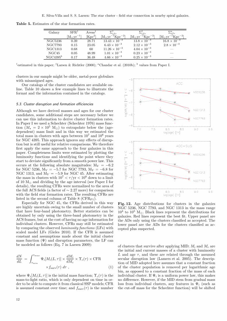
Fig. 12. Age distributions for clusters in the galaxiesNGC 5236, NGC 7793, and NGC 1313 in the mass range104 to 105 M⊙. Black lines represent the distributions forgalaxies. Red lines represent the best fit. Upper panel arethe ADs only using the clusters classified as accepted. Thelower panel are the ADs for the clusters classified as ac-cepted plus suspected.

of clusters that survive after applying MID; Mi and Mc arethe initial and current masses of a cluster with luminosityL and age τ , and these are related through the assumedsecular disruption law (Lamers et al. 2005). The descrip-tion of MID adopted here assumes that a constant fractionof the cluster population is removed per logarithmic agebin, as opposed to a constant fraction of the mass of eachindividual cluster. If Ψi is a uniform power law, this makesno difference. However, if the MID stem from gradual massloss from individual clusters, any features in Ψi (such asthe cut-off mass for the Schechter function) will be shifted

12

E. Silva-Villa and S. S. Larsen: The star cluster - field star connection in nearby spiral galaxies.

Table 6. Slopes for the age distributions for the acceptedand the accepted+suspected samples.

Mass [M⊙] NGC 5236 NGC 7793 NGC 1313Accepted

104 − 105 -0.23±0.1 -0.72±0.27 -0.63±0.12Accepted+Suspected

104 − 105 -0.26±0.08 -0.42±0.19 -0.57±0.11

downwards with time, whereas only the normalization ofΨi will change with time for constant number loss.

In order to apply Eq. (1), some constraints on clus-ter disruption are necessary. Models and empirical con-straints on cluster disruption have been discussed in re-cent years by different authors (e.g. Boutloukos & Lamers2003; Lamers et al. 2005; Whitmore et al. 2007; Larsen2009; Zhang & Fall 1999; Fall 2004, among others), andFall et al. (2009) for different types of galaxies such as theLMC, SMC, Milky Way, M83, or Antennae. Given that itis currently uncertain to what extent MID or MDD domi-nates the cluster disruption, we carried out our analysis forboth scenarios.

Figure 12 shows the age distributions (ADs) for clus-ters with masses between 104 and 105 M⊙ for the galaxiesNGC 1313, NGC 5236, and NGC 7793. NGC 45 has toofew clusters to derive meaningful ADs. We show fits forboth the Accepted and Accepted+Suspected samples. Theslopes of the age distributions, obtained by carrying outfits of the form log(dN/dt) = a × log(τ) + b to the datain Fig. 12, are given in Table 6. There are no large dif-ferences between the slopes derived for the Accepted andAccepted+Suspected sample. Figure 11 shows that most ofthe clusters in the suspected sample have masses below ourlimit of log(M) [M⊙] = 4.0, explaining the similarity of theage distributions above this limit.

As a consistency check for the slope of the age distribu-tions, we performed a maximum likelihood fit to the data,assuming a power-law relation and using the power-law in-dex as a free parameter. Using the accepted and acceptedplus suspected sample of clusters, we estimated the slope ofthe age distributions using the same age and mass rangesas shown in Fig. 12 (i.e. ages between 4 Myrs up to 1 Gyrand masses between 104 and 105 M⊙). The results obtainedare presented in Table 7. The derived slopes agree very wellwith those in table 6, within the errors.

Using clusters with ages between 106.6 ≤ τ ≤ 108 yrand a mass 104 ≤ M ≤ 105 M⊙ we checked for (possible)variations over the slope of the age distributions. The bestfit for these slopes in the new age interval are −0.17± 0.39,−0.38 ± 2.34, and 0.78 ± 0.43 using the accepted sample,and −0.39 ± 0.31, 0.05 ± 0.91, and 0.59 ± 0.91 using theaccepted plus suspected sample, for the galaxies NGC 5236,NGC 7793, and NGC 1313 respectively. The new slopesare to be flatter than the values for the whole age range,showing even positive values; however, in most of the cases,the error is larger than the estimation itself. The possibilityof having shallower slopes indicate that there is a possiblecurvature of the age distribution of star cluster systems,which is not consistent with a (simple) power law.

The slopes found here are, however, somewhat shallowerthan the value of a = −0.9 ± 0.2 found for NGC 5236 byChandar et al. (2010c). If interpreted within the MID sce-

Table 7. Slopes for the age distributions for the acceptedand the accepted+suspected samples based on the maxi-mum likelihood fit.

Mass [M⊙] NGC 5236 NGC 7793 NGC 1313Accepted

104 − 105 -0.27±0.11 -0.48±0.32 -0.63±0.10Accepted+Suspected

104 − 105 -0.31±0.09 -0.30±0.21 -0.60±0.09

nario, the slopes derived here correspond to MID disruptionrates of 41%, 81%, and 77% per decade in age if we use theaccepted sample, and 45%, 62%, and 73% if we use thesample of accepted plus suspected objects, for the galax-ies NGC 5236, NGC 7793, and NGC 1313, respectively. Aweighted average of the slopes for the Accepted samplesleads to a mean slope of 〈a〉 = −0.42 ± 0.07 and an MIDdisruption rate of (62 ± 6)% per decade in age. We usethis mean weighted value for all the galaxies in our sample,including NGC 45 and NGC 4395 where the numbers ofdetected clusters are too low to allow us to estimate theslopes of the age distributions independently.

It is worth comparing our age distributions with those ofMora et al. (2009). Their slopes were considerably steeperthan those found here, but this is partly because Mora et al.worked with magnitude-limited samples, while our age dis-tributions are for mass-limited samples. When taking thisinto account, Mora et al. found that their data were consis-tent with MID disruption rates of 75%–85% per dex, stillsomewhat higher than the values found here. We note thatthe stochastic effects, combined with our relatively conser-vative size cuts, likely cause us to underestimate the num-ber of objects in the youngest bins. This might accountfor some of the flattening of the age distributions in theyoungest bins that is also seen in Fig. 12 for NGC 1313and NGC 5236. For this reason our estimates of the slopesand disruption rates might also be considered lower limits.The less strict size cut used by Mora et al. (FWHM=0.2pixels instead of our 0.7 pixels) would cause them to detectmore compact, young objects, but also possibly ones withincreased contamination. Finally, since visual selection waspart of the sample selection in both our work and the oneof Mora et al., this will also lead to differences in the finalsamples.

A key difference between the MID and MDD models isthat, while the former predicts no change in the shape ofthe mass distribution with age, the latter predicts a flat-tening at low masses. In order to test whether we can dis-tinguish between the two scenarios, model mass distribu-tions (MD, number of objects, per mass bin, per linearage bin) were computed for different age intervals usinga relation analogous to Eq. 1, but integrating over τ forfixed M rather than fixed L. These model MDs were thencompared with the observed MDs in the same age inter-vals. For the MDD scenario we assumed γ = 0.62 and adisruption time of t4 = 1 × 109 yr (Lamers et al. 2005).No infant mortality was included in the MDD models (i.e.fsurv = 1 at all ages). The MID models used the IMR ob-tained above (62%), which is active in the age range 5 Myrsto 1 Gyr, and t4 was set to infinity, making the models in-dependent of mass. We compared the model MDs with ourobservations, dividing our cluster samples into the follow-

13

E. Silva-Villa and S. S. Larsen: The star cluster - field star connection in nearby spiral galaxies.

Fig. 13. Mass-independent models. Left column: MDs ob-served (black symbols) and predicted models (red lines).Right column: Luminosity function observed (black hori-zontal lines), predicted models (red horizontal lines), andtheoretical model (dash-dotted line). Vertical straight linesrepresent the limits used for the fit of the LFs.

ing age and mass bins: log(M)[M⊙]=[3.0,3.5,4.0,4.5,5.0] andlog(τ)[yr]=[6.6,7.5,8.0,8.5,9.0] (shown in Fig. 11).

In Figs. 13 and 14 we compare the observed and pre-dicted MD and LF for MID and MDD models. The bestfits were defined by scaling the model LFs to match theobserved ones, where the observed LFs were created usingvariable binning with ten objects per bin for NGC 1313and NGC 5236 (following Maız Apellaniz (2009)) and fiveobjects per bin for NGC 45, NGC 4395, and NGC 7793.Errors were assumed to be Poissonian. Also shown is thereduced χ2 for each galaxy. Based on these figures, it is dif-ficult to distinguish between the MID and MDD scenarios,mostly because of the limited dynamical range of the dataand the poor statistics.

Our final estimates of the CFRs come from the LFsfor clusters with 3-band photometry in all five galaxies inour sample, using model LFs computed for both MDD andMID disruption. The observed LFs were created in the sameway as described above, using variable binning. We usedthe magnitude ranges up to the brightest cluster in thesample and the lower limit was set at the completenesslimits estimated above (see vertical lines in Fig. 15). TheCFRs are listed in Table 7 for the 4- and 3 band photometry.The CFRs for the four-band photometry have been scaledto the size of the ACS fields. The observed LFs and the best-fitting models are shown in Fig. 15, where MID and MDD

Fig. 14. Mass-dependent models. Left column: MDs ob-served (black symbols) and predicted models (red lines).Right column: Luminosity function observed (black hori-zontal lines), predicted models (red horizontal lines), andtheoretical model (dash-dotted line). Vertical straight linesrepresent the limits used for the fit of the LFs.

models have been tested for the five galaxies in our sample.The CFRs inferred from the fits in Fig 15 only includethe accepted clusters. If we include the “suspected” objectsthen the CFRs increase by 52%, 62%, 30%, 4%, and 25% forNGC 5236, NGC 7793, NGC 1313, NGC 45 and NGC4395,respectively, for the MDD scenario. Similar changes occurfor MID. Furthermore, if we exclude the known ancient GCsin NGC 45 (Mora et al. 2008) from the sample, the Γ valuefor this galaxy decreases by ∼ 20%. Taken together, thisthen makes NGC 45 less of an outlier in Fig. 16 and ingeneral shifts the data points upwards.

Having estimated the SFRs and CFRs, we are now ableto calculate Γ. Table 9 lists the Γ values corresponding tothe different estimates of the CFR. As an additional con-sistency check, we also include a direct comparison of thefraction of light coming from clusters and from field stars,using the magnitude range between mV = 23 and mV = 18.This is not a direct measure of Γ, but is still useful for check-ing any trends. The Γ values derived from the LF fittingare generally a few percent, with the values derived fromMDD models about 48% smaller (or less) than those de-rived for the MID models. We computed the mean valuefor each model and the respective standard error of themean (columns 5th and 8th in Table 9).

14

E. Silva-Villa and S. S. Larsen: The star cluster - field star connection in nearby spiral galaxies.

Table 8. Estimates of the cluster formation rates. Subscript P1 refers to estimations made following Paper I. Disruptionmodels are labeled as MDD and MID. Number of bands used for the estimation are labeled as 3B and 4B.

Galaxy CFRP1 CFR3BMDD CFR4B

MDD CFR3BMID CFR4B

MID

[M⊙yr−1] [M⊙yr−1] [M⊙yr−1] [M⊙yr−1] [M⊙yr−1]

NGC5236 37.7×10−3 23.0×10−3 19.9×10−3 41.0×10−3 36.6×10−3

NGC7793 14.5×10−3 4.0×10−3 3.4×10−3 6.8×10−3 6.6×10−3

NGC1313 60.7×10−3 23.0×10−3 19.7×10−3 44.0×10−3 38.6×10−3

NGC45 8.6×10−3 2.5×10−3 2.7×10−3 4.4×10−3 3.6×10−3

NGC4395 4.5×10−3 2.4×10−3 1.0×10−3 4.0×10−3 1.6×10−3

Table 9. Estimations of Γ and comparison with Goddard et al. (2010) results.

Galaxy ΓP1 Γ3BMDD Γ4B

MDD ΓMDD ± σMDD Γ3BMID Γ4B

MID ΓMID ± σMID Γ† TL(U)† LCL/LFS

[%] [%] [%] [%] [%] [%] [%] [%] [%]NGC5236 9.8 5.9 5.2 5.6±0.6 10.5 9.4 10.0±0.9 10.3 2.36±0.31 9.0NGC7793 9.8 2.6 2.3 2.5±0.3 4.5 4.5 4.5±0.1 8.6 1.15±0.32 3.4NGC1313 9.0 3.3 2.9 3.2±0.2 6.4 5.7 6.1±0.6 9.9 1.49±0.44 11.7NGC45 17.3 5.0 5.4 5.2±0.3 8.8 7.2 8.0±1.1 2.2 0.24±0.17 6.1

NGC4395 2.6 1.4 0.6 1.0±0.6 2.3 0.9 1.6±0.1 8 0.07±0.05 1.7

†Larsen & Richtler (2000). Super and sub-indices for Γ are the same as Table 8. Columns 5 and 8 are the mean and standarderror for each model. Column 9 values using Goddard et al. with our ΣSFR. Column 11 is the fraction between the light fromclusters and the light from field stars in the magnitude range 18 to 23 using MV .

6. Discussion

In Fig. 16 we compare our Γ vs. ΣSFR measurements withthe data in Goddard et al. (2010) (rhombs). We cannot con-firm whether a correlation is present within the range ofΣSFR values probed by our data, but overall our Γ valuesare similar to those found by Goddard et al. in this rangeof ΣSFR or slightly lower. However, following the methodsof Goddard et al., Adamo et al. (2011) estimated values forΓ in the two blue compact galaxies ESO 185 and Haro 11.The results from Adamo et al. are in good agreement withthe power law proposed by Goddard et al. (2010).

According to Larsen & Richtler (2000), the five galax-ies span a significant range in specific U -band luminosity.From Table 9 and Fig. 17, we see that galaxies with high Γvalues generally tend to also have high TL(U) values. Oneexception to this is NGC 45, which has a rather high Γfor its TL(U). The TL(U) value for this galaxy is, however,based on only two clusters, hence subject to very large un-certainty. Nevertheless, the high Γ value for NGC 45 is alsosomewhat puzzling given that it has the lowest ΣSFR. Thismay suggest that there is not a simple relation between Γand ΣSFR. In this context, it is also interesting that thisgalaxy has a large number of ancient GCs for its lumi-nosity, yielding an unusually high globular cluster specificfrequency for a late-type (Sd) galaxy (Mora et al. 2009).

Our measurements of Γ values in the range ∼2–10%are consistent with other recent estimates of the fractionof stars forming in bound clusters. It should be kept inmind that this number is not necessarily an indicator of“clustered” vs. “isolated” star formation, since some starsmay form in embedded clusters that dissolve or expand onshort enough time scales to drop out of our sample.

There is a correlation between TL(U) and Γ, as shownin Fig. 17. We estimated values for Γ using the ac-cepted+suspected samples for the three-band photometryand for MDD and MID models as presented in the figure.

The galaxy NGC 45 deviates from the apparent relation.Two things must be noted. (1) The inclusion of the sus-pected sample does not change the trend observed dramat-ically, although the increases in the CFRs is reflected inthe new Γ estimations, and (2) CFR estimates based ondifferent disruption models follow the same trend.

Estimates of the actual “infant mortality rate” arehard to make unless the embedded phase is probed di-rectly, something which is difficult in external galaxies. ForNGC 1313, Pellerin et al. (2007) find that the IMR is avery efficient process for the dissolution of star clustersin this galaxy (IMR = 90%) based on UV fluxes in andout of clusters. Our estimate of a Γ value of 3%–5% forNGC 1313 indicates that >∼ 95% of star formation in thisgalaxy happens outside clusters that are detected in oursample, in reasonable agreement with the Pellerin et al. es-timate. However, it is also clear that cluster dissolution isa continuous process, and systems that are probed at olderages are generally expected to show a lower fraction of starsin clusters.

A proper account of dissolution effects could, in prin-ciple, be used to correct measurements of Γ at differentages to a common reference (say, 10 Myr), but current un-certainties in the disruption process makes this difficultto apply in practice. As a case in point, Chandar et al.(2010a) estimate a mass-independent disruption rate of80%–90% per decade in age for NGC 5236, a value thatis significantly higher than our estimate ∼ 40% (∼ 62%is our estimated weighted average). These differences un-derscore that the definition of cluster samples (especiallyin star-forming galaxies) is subject to strong selection ef-fects, many of which are age dependent and thus likely toaffect the age distributions. One example is the size cuts,which can easily cause a bias against young objects wherestochastic SIMF sampling leads to underestimated sizeseven for masses of ∼ 104M⊙. Furthermore, there may alsobe a physical relation between cluster size and age (e.g.

15

E. Silva-Villa and S. S. Larsen: The star cluster - field star connection in nearby spiral galaxies.

Fig. 15. LFs for the five galaxies in our sample. We usedMDD andMID theoretical models in left and right columns,respectively. Vertical lines are the limits of the fit. Red hor-izontal lines represent the binned theoretical values, whileblack horizontal lines represent observations. Errors arePoissoninan. Dashed-dotted line is the theoretical LF notbinned.

Fig. 16. Relation between Γ and ΣSFR using average valuesof Γ for the models MDD and MID. Rhombs symbols andline represents the Goddard et al. (2010) data and blackstar symbols represent our set of galaxies.

Elson et al. 1989; Barmby et al. 2009; Mackey & Gilmore2003a,b), compounding this problem.

Fig. 17. Relation between TL(U) and Γ using themodels MDD and MID. The values for Γ using theAccepted+Suspected sample are also included.

When using young clusters (τ less than 100 Myr) we ob-served that the slope of the age distribution gets shallower,indicating a possible curvature or deviation from a power-law relation and showing values for the age distributionsdifferent from previous estimations. However, these resultsare based on a sample that is strongly affected by very fewof clusters.

7. Summary and conclusions

Using HST observations of the galaxies NGC 45, NGC 1313,NGC 4395, NGC 5236, and NGC 7793, we studied theirpopulations of star clusters and field stars separately withthe aim of constraining the quantity Γ, i.e. the ratio ofstars forming in bound clusters and the “field”. We havebeen following the basic approach described in Paper I,i.e. comparing synthetic and observed color-magnitude di-agrams (for the field stars) and SED model fitting (for thestar clusters), to get the formation histories of stars andclusters.

We tested how stochastic effects induced by the SIMFinfluence photometry and the estimation of ages and howthe completeness limits are affected. We conclude that mas-sive clusters (log(Mass)[M⊙] ≥ 5]) are easily detected (withthe parameters used in this work) at any age, while thedetection of clusters with masses below ∼ 104M⊙ can bestrongly affected by stochasticity. Our tests thus show thatcompleteness functions do not just depend on magnitude,but also on age and size. It would be desirable to find betterclassification methods than a simple size cut to determinewhat is, and what is not, a cluster.

We estimated star formation histories and found thatNGC 5236 and NGC 1313 have the highest star formationrates, while NGC 7793, NGC 4395, and NGC 45 have lowerSFRs. Within the uncertainties, we do not see significantvariations within the past 100 Myr.

Comparing observed and modeled mass- and and lu-minosity distributions for the cluster populations in differ-ent galaxies, we find that we cannot distinguish betweendifferent disruption models (mass dependent vs. mass in-dependent). We compared model luminosity functions foreach disruption scenario with observed LFs and derivedCFRs for the cluster systems. From our measurements of

16

E. Silva-Villa and S. S. Larsen: The star cluster - field star connection in nearby spiral galaxies.

the CFRs and SFRs we derived the ratio of the two, Γ, asan indication of the formation efficiency of clusters that re-main identifiable until at least 107 years. We find Γ valuesin the range ∼2–10%, with no clear correlation with ΣSFR

within the (limited) range probed by our data. However,our measurements are roughly consistent with those ofGoddard et al. (2010), who find a relation between ΣSFR

and Γ for a sample of galaxies spanning a wider range inΣSFR (but more heterogeneous data).

A general difficulty in this type of work is to identifya reliable sample of bona-fide clusters. Comparison withprevious work suggests that the cluster samples, althoughcovering the same galaxies, are significantly affected by thecriteria used to classify clusters over the images. This re-sults in different estimates of cluster system parameters,such as those related to the disruption law. Accurate esti-mates of these parameters are also hampered by the rela-tively poor statistics that result from having only patchycoverage of large, nearby galaxies in typical HST imagingprograms.

Acknowledgements. We would like to thank the referee for commentsthat helped to improve this article. We would like to thank MorganFouesneau for catching an error in Fig. 8. This work was supportedby an NWO VIDI grant to SL.

References

Adamo, A., Ostlin, G., Zackrisson, E., & Hayes, M. 2011, ArXiv e-prints

Anders, P., Bissantz, N., Fritze-v. Alvensleben, U., & de Grijs, R.2004, MNRAS, 347, 196

Anders, P. & Fritze-v. Alvensleben, U. 2003, A&A, 401, 1063Barmby, P., Perina, S., Bellazzini, M., et al. 2009, AJ, 138, 1667Bastian, N. 2008, MNRAS, 390, 759Bertin, E. & Arnouts, S. 1996, A&AS, 117, 393Boutloukos, S. G. & Lamers, H. J. G. L. M. 2003, MNRAS, 338, 717Bresolin, F., Ryan-Weber, E., Kennicutt, R. C., & Goddard, Q. 2009,

ApJ, 695, 580Bressert, E., Bastian, N., Gutermuth, R., et al. 2010, ArXiv e-printsBrown, T. M., Beaton, R., Chiba, M., et al. 2008, ApJ, 685, L121Cervino, M. & Luridiana, V. 2006, A&A, 451, 475Chandar, R., Fall, S. M., & Whitmore, B. C. 2010a, ApJ, 711, 1263Chandar, R., Whitmore, B. C., Kim, H., et al. 2010b, ApJ, 719, 966Chandar, R., Whitmore, B. C., Kim, H., et al. 2010c, ApJ, 719, 966de Grijs, R., Anders, P., Lamers, H. J. G. L. M., et al. 2005, MNRAS,

359, 874de Grijs, R. & Goodwin, S. P. 2008, MNRAS, 383, 1000Dolphin, A. 1997, New Astronomy, 2, 397Eldridge, J. J. & Stanway, E. R. 2009, MNRAS, 400, 1019Elson, R. A. W., Freeman, K. C., & Lauer, T. R. 1989, ApJ, 347, L69Fall, S. M. 2004, in Astronomical Society of the Pacific Conference

Series, Vol. 322, The Formation and Evolution of Massive YoungStar Clusters, ed. H. J. G. L. M. Lamers, L. J. Smith, & A. Nota,399–+

Fall, S. M., Chandar, R., & Whitmore, B. C. 2009, ApJ, 704, 453Fouesneau, M. & Lancon, A. 2010, A&A, 521, A22+Gieles, M. 2010, in Astronomical Society of the Pacific Conference

Series, Vol. 423, Astronomical Society of the Pacific ConferenceSeries, ed. B. Smith, J. Higdon, S. Higdon, & N. Bastian, 123–+

Gieles, M., Athanassoula, E., & Portegies Zwart, S. F. 2007, MNRAS,376, 809

Gieles, M. & Bastian, N. 2008, A&A, 482, 165Gieles, M., Portegies Zwart, S. F., Baumgardt, H., et al. 2006,

MNRAS, 371, 793Girardi, L., Bertelli, G., Bressan, A., et al. 2002, A&A, 391, 195Goddard, Q. E., Bastian, N., & Kennicutt, R. C. 2010, ArXiv e-printsHarris, J., Calzetti, D., Gallagher, III, J. S., Conselice, C. J., & Smith,

D. A. 2001, AJ, 122, 3046Harris, J. & Zaritsky, D. 2001, ApJS, 136, 25Harris, J. & Zaritsky, D. 2004, AJ, 127, 1531Harris, J. & Zaritsky, D. 2009, AJ, 138, 1243King, I. 1962, AJ, 67, 471

Koekemoer, A. M., Fruchter, A. S., Hook, R. N., & Hack, W. 2002, inThe 2002 HST CalibrationWorkshop : Hubble after the Installationof the ACS and the NICMOS Cooling System, ed. S. Arribas,A. Koekemoer, & B. Whitmore, 337

Kroupa, P. 2002, Science, 295, 82Lada, C. J. & Lada, E. A. 2003, ARA&A, 41, 57Lamers, H. J. G. L. M. 2009, Ap&SS, 132Lamers, H. J. G. L. M. & Gieles, M. 2008, in Astronomical Society of

the Pacific Conference Series, Vol. 388, Mass Loss from Stars andthe Evolution of Stellar Clusters, ed. A. de Koter, L. J. Smith, &L. B. F. M. Waters, 367

Lamers, H. J. G. L. M., Gieles, M., Bastian, N., et al. 2005, A&A,441, 117

Larsen, S. S. 1999, A&AS, 139, 393Larsen, S. S. 2009, A&A, 503, 467Larsen, S. S., Mora, M. D., Brodie, J. P., & Richtler, T. 2007, in

IAU Symposium, Vol. 241, IAU Symposium, ed. A. Vazdekis &R. F. Peletier, 435–439

Larsen, S. S. & Richtler, T. 1999, A&A, 345, 59Larsen, S. S. & Richtler, T. 2000, A&A, 354, 836Mackey, A. D. & Gilmore, G. F. 2003a, MNRAS, 338, 120Mackey, A. D. & Gilmore, G. F. 2003b, MNRAS, 338, 85Maeder, A. & Meynet, G. 2008, in Astronomical Society of the

Pacific Conference Series, Vol. 388, Mass Loss from Stars and theEvolution of Stellar Clusters, ed. A. de Koter, L. J. Smith, &L. B. F. M. Waters, 3–+

Maız Apellaniz, J. 2009, ApJ, 699, 1938Marigo, P., Girardi, L., Bressan, A., et al. 2008, A&A, 482, 883Mora, M. D., Larsen, S. S., & Kissler-Patig, M. 2007, A&A, 464, 495Mora, M. D., Larsen, S. S., & Kissler-Patig, M. 2008, A&A, 489, 1065Mora, M. D., Larsen, S. S., Kissler-Patig, M., Brodie, J. P., & Richtler,

T. 2009, A&A, 501, 949Pellerin, A., Meyer, M., Harris, J., & Calzetti, D. 2007, ApJ, 658, L87Piskunov, A. E., Kharchenko, N. V., Schilbach, E., et al. 2009, A&A,

507, L5Popescu, B. & Hanson, M. M. 2010a, ArXiv e-printsPopescu, B. & Hanson, M. M. 2010b, ApJ, 713, L21Porras, A., Christopher, M., Allen, L., et al. 2003, AJ, 126, 1916Schechter, P. 1976, ApJ, 203, 297Scheepmaker, R. A., Lamers, H. J. G. L. M., Anders, P., & Larsen,

S. S. 2009, A&A, 494, 81Schlegel, D. J., Finkbeiner, D. P., & Davis, M. 1998, ApJ, 500, 525Schulz, J., Fritze-v. Alvensleben, U., Moller, C. S., & Fricke, K. J.

2002, A&A, 392, 1Silva-Villa, E. & Larsen, S. S. 2010, A&A, 516, A10+Sirianni, M., Jee, M. J., Benıtez, N., et al. 2005, PASP, 117, 1049Spitzer, L. 1987, Dynamical evolution of globular clusters, ed.

L. SpitzerTosi, M., Greggio, L., Marconi, G., & Focardi, P. 1991, AJ, 102, 951Walsh, J. R. & Roy, J. 1997, MNRAS, 288, 726Whitmore, B. C., Chandar, R., & Fall, S. M. 2007, AJ, 133, 1067Zaritsky, D., Kennicutt, Jr., R. C., & Huchra, J. P. 1994, ApJ, 420,

87Zhang, Q. & Fall, S. M. 1999, ApJ, 527, L81

17

E.Silva

-Villa

andS.S.Larsen

:Thesta

rclu

ster-field

starconnectio

nin

nearbyspira

lgalaxies.

Table 10. Online material. The rows presented in this table illustrate what the online material will look like. Column 1st: Name of the galaxy, field observed andcluster number. Column 2nd: ID classification .Columns 3rd and 4th: X and Y coordinates of the clusters over the images. Columns 5th and 6th: Right ascensionand declination (J2000). Columns 7th-14th: U, B, V, and I magnitudes and their respective errors. Column 15th: Age estimated for LMC-like metallicity. Column16th: Mass estimated for LMC-like metallicity. Column 17th and 18th: Sizes measured with SExtractor and Ishape, respectively. Column 19th: Flag for acceptedand suspected objects.

Galaxy Field # ID X Y RA DEC U Ue B Be V Ve I Ie[PIX] [PIX] [J2000] [J2000] [Mag] [Mag] [Mag] [Mag] [Mag] [Mag] [Mag] [Mag]

NGC5236 1 1 5214 245 2539. 13:36:58.81 -29:51:13.94 21.08 0.10 20.89 0.01 20.86 0.01 20.57 0.03NGC5236 1 2 5238 340 2549. 13:36:58.99 -29:51:09.77 22.90 0.21 22.27 0.02 21.66 0.02 20.64 0.02NGC5236 1 3 4360 596 2225. 13:36:58.23 -29:50:51.62 22.55 0.15 22.32 0.02 21.90 0.02 21.09 0.02NGC5236 1 4 5454 614 2609. 13:36:59.62 -29:50:58.36 20.73 0.04 20.64 0.01 20.54 0.01 20.14 0.01NGC5236 1 5 3919 621 1928. 13:36:57.22 -29:50:44.62 21.46 0.07 21.79 0.02 21.76 0.02 21.24 0.03NGC5236 2 1 6116 574. 2690. 13:37:05.64 -29:56:51.97 22.07 0.08 22.15 0.01 22.04 0.01 21.61 0.02NGC5236 2 2 5845 655. 2423. 13:37:04.84 -29:56:42.65 22.05 0.13 21.65 0.02 21.40 0.01 20.71 0.02NGC5236 2 3 5690 719. 2180. 13:37:04.10 -29:56:34.62 22.29 0.12 22.57 0.02 22.28 0.02 21.62 0.02NGC5236 2 4 5859 746. 2461. 13:37:05.12 -29:56:39.33 21.72 0.08 21.35 0.01 21.17 0.01 20.71 0.01NGC5236 2 5 5773 821. 2297. 13:37:04.67 -29:56:32.47 21.87 0.08 21.97 0.01 21.74 0.01 21.23 0.02

Table 11. Continuation Table 10.

Galaxy Field # Log(τ ) Log(M) FWHMSEx FWHMIsha Flag[Yr] [M⊙] [Pix] [Pix]

NGC5236 1 1 8.00 3.86 7.35 2.91 acptNGC5236 1 2 8.87 4.43 5.84 0.74 acptNGC5236 1 3 8.92 4.08 3.81 1.30 acptNGC5236 1 4 8.39 4.20 4.80 1.93 acptNGC5236 1 5 8.05 3.53 6.16 1.63 acptNGC5236 2 1 8.00 3.48 3.89 0.95 acptNGC5236 2 2 8.78 4.16 7.37 3.67 acptNGC5236 2 3 7.81 3.48 3.91 1.35 acptNGC5236 2 4 8.70 4.18 6.79 2.79 acptNGC5236 2 5 8.39 3.73 4.39 1.84 acpt

18