The formation of very wide binaries during the star cluster ...

Mon. Not. R. Astron. Soc. 404, 1835–1848 (2010) doi:10.1111/j.1365-2966.2010.16399.x

The formation of very wide binaries during the star cluster dissolutionphase

M. B. N. Kouwenhoven,1,2�† S. P. Goodwin,2� Richard J. Parker,2� M. B. Davies,3�

D. Malmberg3� and P. Kroupa4�1Kavli Institute for Astronomy and Astrophysics at Peking University, Yi He Yuan Lu 5, Hai Dian District, Beijing 100871, China2University of Sheffield, Hicks Building, Hounsfield Road, Sheffield S3 7RH3Lund Observatory, Box 43, SE-221 00 Lund, Sweden4Argelander Institute for Astronomy, University of Bonn, Auf dem Hugel 71, 53121 Bonn, Germany

Accepted 2010 January 20. Received 2010 January 19; in original form 2009 December 11

ABSTRACTOver the past few decades, numerous wide (>103 au) binaries in the Galactic field and halohave been discovered. Their existence cannot be explained by the process of star formation orby dynamical interactions in the field, and their origin has long been a mystery. We explainthe origin of these wide binaries by formation during the dissolution phase of young starclusters: an initially unbound pair of stars may form a binary when their distance in phasespace is small. Using N-body simulations, we find that the resulting wide binary fraction in thesemimajor axis range 103 au < a < 0.1 pc for individual clusters is 1–30 per cent, dependingon the initial conditions. The existence of numerous wide binaries in the field is consistentwith observational evidence that most clusters start out with a large degree of substructure. Thewide binary fraction decreases strongly with increasing cluster mass, and the semimajor axisof the newly formed binaries is determined by the initial cluster size. The resulting eccentricitydistribution is thermal, and the mass ratio distribution is consistent with gravitationally focusedrandom pairing. As a large fraction of the stars forms in primordial binaries, we predict thata large number of the observed ‘wide binaries’ are in fact triple or quadruple systems. Byintegrating over the initial cluster mass distribution, we predict a binary fraction of a few percent in the semimajor axis range 103 au < a < 0.1 pc in the Galactic field, which is smallerthan the observed wide binary fraction. However, this discrepancy may be solved when weconsider a broad range of cluster morphologies.

Key words: methods: N-body simulations – binaries: general – galaxies: star clusters.

1 IN T RO D U C T I O N

A significant fraction of stars in the Galactic field are in binary andmultiple systems (e.g. Duquennoy & Mayor 1991; Fischer & Marcy1992; Mason et al. 1998; Shatsky & Tokovinin 2002; Goodwin& Kroupa 2005; Kouwenhoven et al. 2005; Lada 2006; Goodwinet al. 2007; Kobulnicky & Fryer 2007; Kouwenhoven et al. 2007;Zinnecker & Yorke 2007). It is also thought that the majority ofstars are born in star clusters (Lada & Lada 2003). Therefore the

�E-mail: [email protected] (MBNK); [email protected] (SPG); [email protected] (RJP); [email protected] (MBD);[email protected] (DM); [email protected] (PK)†Peter and Patricia Gruber Foundation Fellow.

majority of binaries1 in the field population presumably originatefrom clustered star formation.

It is well known that binaries are dynamically processed in starclusters with wider and less bound systems tending to be destroyedby encounters (Heggie 1975; Hills 1975). Therefore, the field bi-nary population is dynamically processed with respect to the birthpopulation of binaries (Kroupa 1995; Parker et al. 2009). The originof most field binaries can be understood as a mixture of differentlyprocessed initial populations (Goodwin 2009).

However, a significant number of very wide (a > 103 au) bi-naries have been observed in the field (see Section 2). As suchwide binaries are extremely sensitive to destruction they have been

1For brevity we will use ‘binaries’ to mean ‘multiples’ of any multiplicity forthe remainder of this paper, only drawing a distinction where it is necessary.

C© 2010 The Authors. Journal compilation C© 2010 RAS

Dow

nloaded from https://academ

ic.oup.com/m

nras/article/404/4/1835/1083026 by guest on 29 January 2022

1836 M. B. N. Kouwenhoven et al.

used to constrain the properties of the Milky Way. Wide binariesin the Galactic disc and halo have been used to place limits on thedensity of MACHOs and other unseen material (e.g. Bahcall, Hut& Tremaine 1985; Quinn et al. 2009) to constrain the formationhistory of the Galaxy (e.g. Allen, Poveda & Hernandez-Alcantara2007a), and to test the dark matter hypothesis (e.g. Hernandez & Lee2008). But the extreme sensitivity to destruction makes the survival(and even formation) of such binaries in a cluster something of amystery.

Many very wide binaries have separations comparable to theaverage interstellar separation in clusters (typically a few times 103

au), and the very widest binaries have separations of the order of thesize of a young cluster core (typically a few times 104 au). Giventhis, it is difficult to see how they could even form, let alone survive,in a cluster (see e.g. Scally, Clarke & McCaughrean 1999; Parkeret al. 2009). Even in an isolated star-forming region the typical sizeof a star-forming core is only 104 au (Ward-Thompson et al. 2007)which presumably sets the very maximum size of a (primordial)binary system.

It is possible that a wide binary forms via dynamical interactionsin the Galactic field (the capture mechanism). A prerequisite forthis mechanism to work is that a significant amount of kinetic en-ergy is dissipated. This energy dissipation can occur due to tidalfriction and due to three-body interaction. Tidal friction occurs inthe rare event of two stars nearly colliding in a close encounter. Inthe vast majority of the cases this results in a merger or a fly-by,and only in a small number of cases does this lead to the for-mation of a binary system. However, all binaries resulting fromcapture by tidal friction are very tight, with orbital period of severaldays.

Another possible mechanism is three-body interactions. In thiscase the third star acts as the energy sink, and is generally ejectedwith high velocity. However, the stellar density in the field is low,of the order of 0.1 M� pc−3, so that three-body encounters are rare,and capture by dynamical friction rarely occurs. Goodman & Hut(1993) find that the creation rate NB for binaries per unit volumecan be approximated by

NB = 0.75G5M5n3

σ 9v

, (1)

where M is the typical mass of a star in the field, n is the num-ber density of stars, σ v is the velocity dispersion and G is thegravitational constant. In the solar neighbourhood M ≈ 0.3 M�,n ≈ 0.03 pc−3 and σ v ≈ 50 km s−1. For the field therefore,NB ≈ 4 × 10−21 pc−3 Gyr−1. This shows that the formation of bina-ries in the field is extremely rare. Note that in dense star clusters thestellar density is high and the velocity dispersion modest, such thatthe number of binaries formed via three-body interactions (equa-tion 1) may be substantial. However, wide binaries, which havesemimajor axes comparable to the size of these clusters, are notformed, as they simply do not fit in these star clusters. Furthermore,N-body simulations by Kroupa & Burkert (2001) have shown thatthe observed broad period distribution of binaries in the field cannotbe produced by dynamically modifying a tighter period distributionin a star cluster.

A third possibility for the origin of wide binaries is formationduring cluster dissolution, which is the mechanism we propose inthis paper. In an evolving star cluster, stars that are initially un-bound, may become bound to each other as the cluster expands,i.e. if the gravitational influence of the other cluster members

decreases.2 In order to form a binary pair in this way, (i) the twostars need to be sufficiently close together, (ii) the two stars needto have a sufficiently small velocity difference and (iii) the newlyformed binary should not be destroyed by gravitational interactionwith the remaining cluster stars or field stars. The possibility ofwide binary formation was previously proposed by Theuns (1992),and the simulations of Moeckel & Bate (2010) also show that awide binary system can form during the early phase of star clusterevolution.

Throughout this paper we refer to binaries with 103 au < a <

0.1 pc as the wide binary population. The paper is organized asfollows. In Section 2 we briefly discuss surveys of wide binary sys-tems and the corresponding observational techniques. In Section 3we explain our technique and assumptions. In Section 4 we pro-vide analytical and Monte Carlo estimates for the resulting widebinary population, and in Section 5 we present estimates based onN-body simulations of evolving star clusters. Finally, in Section 6we present and discuss our conclusions.

2 O BSERVATI ONS OF WI DE BI NARI ES

Observations have indicated that binaries as wide as 1 pc existin the halo, while in the Galactic disc the widest binaries haveseparations of the order of 0.1 pc (e.g. Close, Richer & Crabtree1990; Chaname & Gould 2004). Wider binaries are rare, althoughsome authors claim evidence for binary and higher order multiplesystems wider than 0.1 pc (e.g. Scholz et al. 2008; Caballero 2009;Mamajek et al. 2010).

Statistical properties of a wide binary population are often recov-ered using the angular two-point correlation function (e.g. Bahcall& Soneira 1981; Garnavich 1988; Gould et al. 1995, Longhitano &Binggeli, 2010). The most prominent disadvantages of this methodare the inability to identity individual wide binaries and the needfor a good model for the stellar population that is studied.

Individual wide binary candidates are often identified bytheir common proper motion on the sky (e.g. Wasserman &Weinberg 1991; Chaname & Gould 2004; Lepine & Bongiorno2007; Makarov, Zacharias & Hennessy 2008, and numerous others).Many wide binaries were found by Hipparcos (ESA 1997) as well;see also Soderhjelm (2007). Their nature can then be further con-strained by measuring the parallax and radial velocity (e.g. Lathamet al. 1984; Hartigan, Strom & Strom 1994; Quinn et al. 2009).

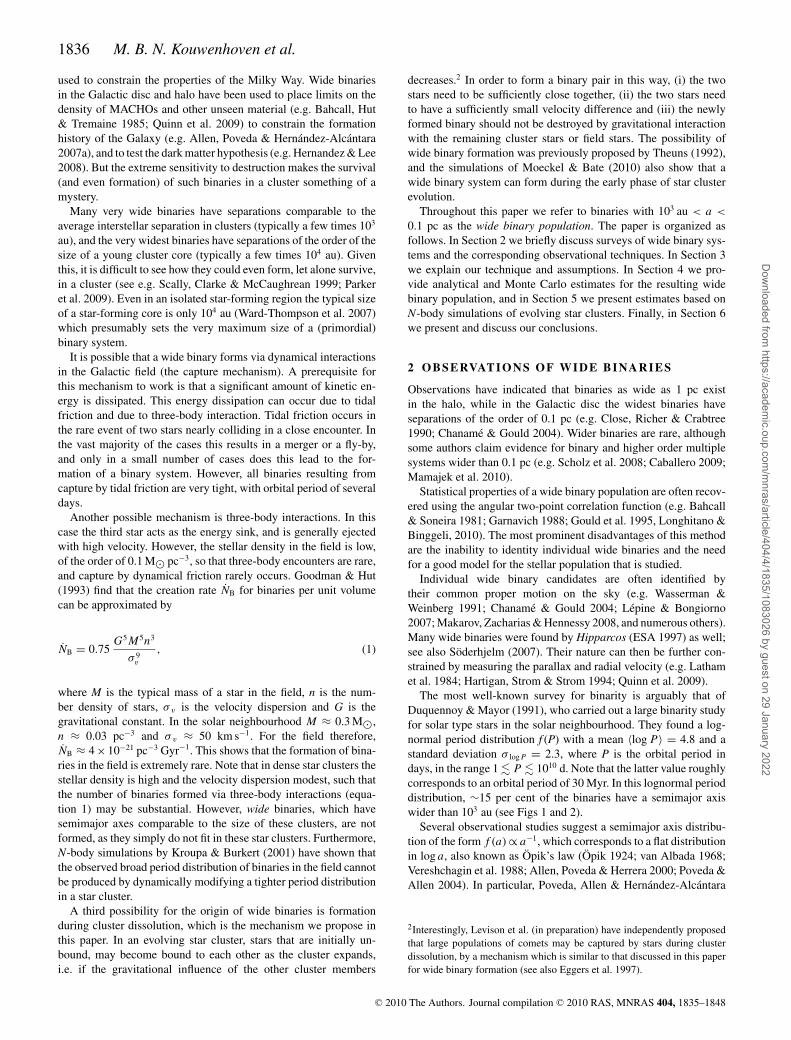
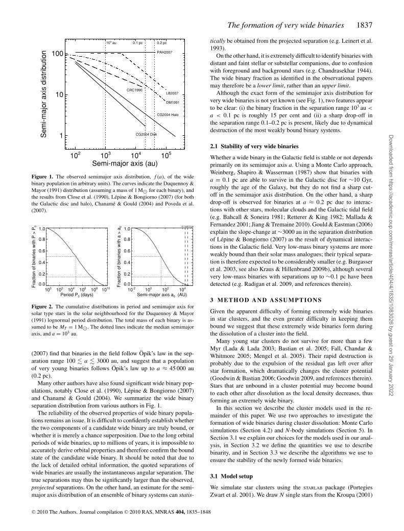
The most well-known survey for binarity is arguably that ofDuquennoy & Mayor (1991), who carried out a large binarity studyfor solar type stars in the solar neighbourhood. They found a log-normal period distribution f (P) with a mean 〈log P 〉 = 4.8 and astandard deviation σ log P = 2.3, where P is the orbital period indays, in the range 1 � P � 1010 d. Note that the latter value roughlycorresponds to an orbital period of 30 Myr. In this lognormal perioddistribution, ∼15 per cent of the binaries have a semimajor axiswider than 103 au (see Figs 1 and 2).

Several observational studies suggest a semimajor axis distribu-tion of the form f (a) ∝ a−1, which corresponds to a flat distributionin log a, also known as Opik’s law (Opik 1924; van Albada 1968;Vereshchagin et al. 1988; Allen, Poveda & Herrera 2000; Poveda &Allen 2004). In particular, Poveda, Allen & Hernandez-Alcantara

2Interestingly, Levison et al. (in preparation) have independently proposedthat large populations of comets may be captured by stars during clusterdissolution, by a mechanism which is similar to that discussed in this paperfor wide binary formation (see also Eggers et al. 1997).

C© 2010 The Authors. Journal compilation C© 2010 RAS, MNRAS 404, 1835–1848

Dow


ic.oup.com/m


The formation of very wide binaries 1837

Figure 1. The observed semimajor axis distribution, f (a), of the widebinary population (in arbitrary units). The curves indicate the Duquennoy &Mayor (1991) distribution (assuming a mass of 1 M� for each binary), andthe results from Close et al. (1990), Lepine & Bongiorno (2007) (for boththe Galactic disc and halo), Chaname & Gould (2004) and Poveda et al.(2007).

Figure 2. The cumulative distributions in period and semimajor axis forsolar type stars in the solar neighbourhood for the Duquennoy & Mayor(1991) lognormal period distribution. The total mass of each binary is as-sumed to be MT = 1 M�. The dotted lines indicate the median semimajoraxis, and a = 103 au.

(2007) find that binaries in the field follow Opik’s law in the sep-aration range 100 � a � 3000 au, and suggest that a populationof very young binaries follows Opik’s law up to a ≈ 45 000 au(0.2 pc).

Many other authors have also found significant wide binary pop-ulations, notably Close et al. (1990), Lepine & Bongiorno (2007)and Chaname & Gould (2004). We summarize the wide binaryseparation distribution from various authors in Fig. 1.

The reliability of the observed properties of wide binary popula-tions remains an issue. It is difficult to confidently establish whetherthe two components of a candidate wide binary are truly bound, orwhether it is merely a chance superposition. Due to the long orbitalperiods of wide binaries, up to millions of years, it is impossible toaccurately derive orbital properties and therefore confirm the boundstate of the candidate wide binary. It should be noted that due tothe lack of detailed orbital information, the quoted separations ofwide binaries are usually the instantaneous angular separation. Thetrue separations may thus be significantly larger than the observed,projected separations. On the other hand, an estimate for the semi-major axis distribution of an ensemble of binary systems can statis-

tically be obtained from the projected separation (e.g. Leinert et al.1993).

On the other hand, it is extremely difficult to identify binaries withdistant and faint stellar or substellar companions, due to confusionwith foreground and background stars (e.g. Chandrasekhar 1944).The wide binary fraction as identified in the observational papersmay therefore be a lower limit, rather than an upper limit.

Although the exact form of the semimajor axis distribution forvery wide binaries is not yet known (see Fig. 1), two features appearto be clear: (i) the binary fraction in the separation range 103 au <

a < 0.1 pc is roughly 15 per cent and (ii) a sharp drop-off inthe separation range 0.1–0.2 pc is present, likely due to dynamicaldestruction of the most weakly bound binary systems.

2.1 Stability of very wide binaries

Whether a wide binary in the Galactic field is stable or not dependsprimarily on its semimajor axis a. Using a Monte Carlo approach,Weinberg, Shapiro & Wasserman (1987) show that binaries witha = 0.1 pc are able to survive in the Galactic disc for ∼10 Gyr,roughly the age of the Galaxy, but they do not find a sharp cut-off in the semimajor axis distribution. On the other hand, a sharpdrop-off is observed for binaries at a ≈ 0.2 pc due to interac-tions with other stars, molecular clouds and the Galactic tidal field(e.g. Bahcall & Soneira 1981; Retterer & King 1982; Mallada &Fernandez 2001; Jiang & Tremaine 2010). Gould & Eastman (2006)explain the slope-change at ∼3000 au in the separation distributionof Lepine & Bongiorno (2007) as the result of dynamical interac-tions in the Galactic field. Very low-mass binary systems are moreweakly bound than their solar mass analogues; their typical separa-tion is therefore expected to be considerably smaller (e.g. Burgasseret al. 2003, see also Kraus & Hillenbrand 2009b), although severalvery low-mass binaries with separations up to ∼0.1 pc have beendetected (e.g. Radigan et al. 2009, and references therein).

3 ME T H O D A N D A S S U M P T I O N S

Given the apparent difficulty of forming extremely wide binariesin star clusters, and the even greater difficulty in keeping thembound we suggest that these extremely wide binaries form duringthe dissolution of a cluster into the field.

Many young star clusters do not survive for more than a fewMyr (Lada & Lada 2003; Bastian et al. 2005; Fall, Chandar &Whitmore 2005; Mengel et al. 2005). Their rapid destruction isprobably due to the expulsion of the residual gas left over afterstar formation, which dramatically changes the cluster potential(Goodwin & Bastian 2006; Goodwin 2009, and references therein).Stars that are unbound in a cluster potential may become boundto each other after dissolution as the local density decreases, thusforming an extremely wide binary.

In this section we describe the cluster models used in the re-mainder of this paper. We use two approaches to investigate theformation of wide binaries during cluster dissolution: Monte Carlosimulations (Section 4.2) and N-body simulations (Section 5). InSection 3.1 we explain our choices for the models used in our anal-ysis, in Section 3.2 we define the quantities we use to describebinarity, and in Section 3.3 we describe the algorithms we use toensure the stability of the newly formed wide binaries.

3.1 Model setup

We simulate star clusters using the STARLAB package (PortegiesZwart et al. 2001). We draw N single stars from the Kroupa (2001)


Dow


ic.oup.com/m



Table 1. Properties of the models used in this paper. The quantity R de-scribes the virial radii of models P1 and P2, while it describes the radius ofthe sphere that includes the fractal structure for models F1 and F2.

Model Structure R (pc) N Q

P1v Plummer 0.1 ≤ R ≤ 1 10 1/2P1e Plummer 0.1 ≤ R ≤ 1 10 3/2P2v Plummer 0.1 10 ≤ N ≤ 1000 1/2P2e Plummer 0.1 10 ≤ N ≤ 1000 3/2

F1v Fractal, α = 1.5 0.1 ≤ R ≤ 1 10 1/2F1e Fractal, α = 1.5 0.1 ≤ R ≤ 1 10 3/2F2v Fractal, α = 1.5 0.1 10 ≤ N ≤ 1000 1/2F2e Fractal, α = 1.5 0.1 10 ≤ N ≤ 1000 3/2

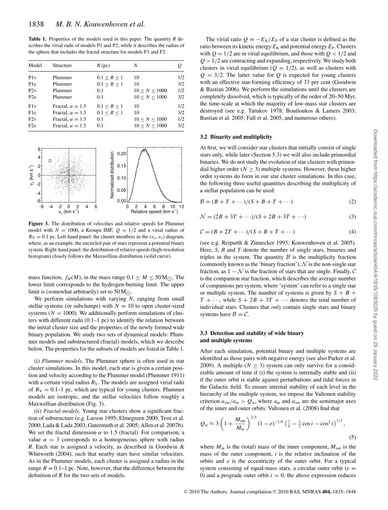
Figure 3. The distribution of velocities and relative speeds for Plummermodel with N = 1000, a Kroupa IMF, Q = 1/2 and a virial radius ofRV = 0.1 pc. Left-hand panel: the cluster members in the (vx, vy) diagram,where, as an example, the encircled pair of stars represent a potential binarysystem. Right-hand panel: the distribution of relative speeds (high-resolutionhistogram) closely follows the Maxwellian distribution (solid curve).

mass function, fM(M), in the mass range 0.1 ≤ M ≤ 50 M�. Thelower limit corresponds to the hydrogen-burning limit. The upperlimit is (somewhat arbitrarily) set to 50 M�.

We perform simulations with varying N, ranging from smallstellar systems (or subclumps) with N = 10 to open cluster-sizedsystems (N = 1000). We additionally perform simulations of clus-ters with different radii (0.1–1 pc) to identify the relation betweenthe initial cluster size and the properties of the newly formed widebinary population. We study two sets of dynamical models: Plum-mer models and substructured (fractal) models, which we describebelow. The properties for the subsets of models are listed in Table 1.

(i) Plummer models. The Plummer sphere is often used in starcluster simulations. In this model, each star is given a certain posi-tion and velocity according to the Plummer model (Plummer 1911)with a certain virial radius RV. The models are assigned virial radiiof RV = 0.1–1 pc, which are typical for young clusters. Plummermodels are isotropic, and the stellar velocities follow roughly aMaxwellian distribution (Fig. 3).

(ii) Fractal models. Young star clusters show a significant frac-tion of substructure (e.g. Larson 1995; Elmegreen 2000; Testi et al.2000; Lada & Lada 2003; Gutermuth et al. 2005; Allen et al. 2007b).We set the fractal dimension α to 1.5 (fractal). For comparison, avalue α = 3 corresponds to a homogeneous sphere with radiusR. Each star is assigned a velocity, as described in Goodwin &Whitworth (2004), such that nearby stars have similar velocities.As in the Plummer models, each cluster is assigned a radius in therange R = 0.1–1 pc. Note, however, that the difference between thedefinition of R for the two sets of models.

The virial ratio Q ≡ −EK/EP of a star cluster is defined as theratio between its kinetic energy EK and potential energy EP. Clusterswith Q = 1/2 are in virial equilibrium, and those with Q < 1/2 andQ > 1/2 are contracting and expanding, respectively. We study bothclusters in virial equilibrium (Q = 1/2), as well as clusters withQ = 3/2. The latter value for Q is expected for young clusterswith an effective star-forming efficiency of 33 per cent (Goodwin& Bastian 2006). We perform the simulations until the clusters arecompletely dissolved, which is typically of the order of 20–50 Myr,the time-scale at which the majority of low-mass star clusters aredestroyed (see e.g. Tutukov 1978; Boutloukos & Lamers 2003;Bastian et al. 2005; Fall et al. 2005, and numerous others).

3.2 Binarity and multiplicity

At first, we will consider star clusters that initially consist of singlestars only, while later (Section 5.3) we will also include primordialbinaries. We do not study the evolution of star clusters with primor-dial higher order (N ≥ 3) multiple systems. However, these higherorder systems do form in our star cluster simulations. In this case,the following three useful quantities describing the multiplicity ofa stellar population can be used:

B = (B + T + · · ·)/(S + B + T + · · ·) (2)

N = (2B + 3T + · · ·)/(S + 2B + 3T + · · ·) (3)

C = (B + 2T + · · ·)/(S + B + T + · · ·) (4)

(see e.g. Reipurth & Zinnecker 1993; Kouwenhoven et al. 2005).Here, S, B and T denote the number of single stars, binaries andtriples in the system. The quantity B is the multiplicity fraction(commonly known as the ‘binary fraction’).N is the non-single starfraction, as 1 − N is the fraction of stars that are single. Finally, Cis the companion star fraction, which describes the average numberof companions per system, where ‘system’ can refer to a single staror multiple system. The number of systems is given by S + B +T + · · ·, while S + 2B + 3T + · · · denotes the total number ofindividual stars. Clusters that only contain single stars and binarysystems have B = C.

3.3 Detection and stability of wide binaryand multiple systems

After each simulation, potential binary and multiple systems areidentified as those pairs with negative energy (see also Parker et al.2009). A multiple (N ≥ 3) system can only survive for a consid-erable amount of time if (i) the system is internally stable and (ii)if the outer orbit is stable against perturbations and tidal forces inthe Galactic field. To ensure internal stability of each level in thehierarchy of the multiple system, we impose the Valtonen stabilitycriterion aout/ain > Qst, where ain and aout are the semimajor axesof the inner and outer orbits. Valtonen et al. (2008) find that

Qst ≈ 3

(1 + Mout

Min

)2/3

(1 − e)−1/6(

74 − 1

2 cos i − cos2 i)1/3

,

(5)

where Min is the (total) mass of the inner component, Mout is themass of the outer component, i is the relative inclination of theorbits and e is the eccentricity of the outer orbit. For a typicalsystem consisting of equal-mass stars, a circular outer orbit (e =0) and a prograde outer orbit i = 0, the above expression reduces


Dow


ic.oup.com/m



to Qst ≈ 3.7. Systems with aout/ain > Qst are internally stable forat least 104 revolutions of the outer component. For wide binaries,with orbital periods of ∼500 000 yr (aout ≈ 104 au), this correspondsto an internally stable period of at least 2 Gyr.

Wide orbits may additionally be unstable against the tidal forcesin the Galactic field and interactions with other single stars andbinaries. We therefore additionally impose a maximum semimajoraxis of 0.1 pc on the outermost orbit of a binary or multiple, moti-vated by the observed wide binary population (see Section 2). Thestability of wider binaries is difficult to assess. As several binarieswider than 0.1 pc are known, our predictions may slightly underes-timate the wide binary fraction. The properties of the wide binarypopulations described in this paper therefore pertain to binaries inthe separation range 103 au < a < 0.1 pc. Note that these binarysystems fall well in the category ‘extremely wide binaries’ in theZinnecker (1984) classification of orbital separations.

4 A NA LY TIC AND NUMERICAL ESTIMATES

Before proceeding to the N-body simulations in Section 5, it is use-ful to first obtain some analytical approximations for the prevalenceof wide binaries that form during cluster dissolution as well as theirorbital characteristics. To this end, we first obtain rough estimatesusing an analytical approach (Section 4.1), and subsequently usinga Monte Carlo approach (Section 4.2).

4.1 Binary formation in Maxwellian velocity space

Wide binaries may form during the dissociation of a cluster if therelative velocity between two stars is sufficiently small that theybecome bound once the perturbing cluster potential is removed.Here we assume that a wide binary will form if the relative velocityis smaller than or roughly equal to the orbital velocity of a star ina wide binary system. For two stars with masses M1 and M2 in acircular binary orbit with semimajor axis a, the velocities of theindividual stars are given by

v1 = M2

√G

a(M1 + M2)and v2 = v1q

−1, (6)

where G is the gravitational constant and q ≡ M2/M1 is the massratio of the binary system. When adopting, for simplicity, q = 1,the above expression reduces to

vorb ≈ 30 km s−1

(M1 + M2

M�

)−1/2 ( a

au

)−1/2, (7)

where vorb is the velocity of either of the components. In order tobe able to form a binary with semimajor axis a, we require velocitydifferences to be smaller than the critical velocity

v � 2vorb ≡ vcrit. (8)

For our choice of the initial mass function (IMF), the total mass of abinary system is of the order of 1 M�. Binaries with a = 3.6 × 105,9 × 104 and 4 × 104 au thus typically require velocity differencesof v � vcrit = 0.1, 0.2 and 0.3 km s−1, respectively.

If the velocity distribution of the stars in a given star clusterfollows a Maxwell-Boltzmann distribution, then so does also thedistribution of relative speeds between the stars. We define therelative velocity V = vi − vj, with components (Vx, Vy, V z) andmagnitude V = |V |. The distribution over relative speeds is thengiven by

fV (V ) dV = 1

2√

πσ 3exp

(− V 2

4σ 2

)V 2dV (9)

(Binney & Tremaine 1987, p. 485), where σ is the one-dimensionalvelocity dispersion. In the Plummer model σ is given by

σ 2Q=1/2(r) = 16GMcl

18πRV

[1 +

(16r

3πRV

)2]−1/2

(10)

(Heggie & Hut 2003) for a cluster in virial equilibrium (i.e.Q = 1/2). Here, Mcl is the total mass of the cluster and r is thedistance to the cluster centre. We can rewrite equation (10) in unitsmore suitable for the clusters considered in this paper. First, we setMcl = N〈m〉, where N is the number of stars in the cluster and 〈m〉 istheir average mass. Using the Kroupa (2001) IMF, 〈m〉 = 0.55 M�.Evaluating the velocity dispersion at the (intrinsic) half-mass radius,r = Rhm ≈ 0.769 RV of the cluster, we find

σQ=1/2 = 0.64

(0.1 pc

RV

)1/2(N

100 stars

)1/2

km s−1. (11)

The kinetic energy for a star cluster with Q = 3/2 is three times thatof a cluster with Q = 1/2, and therefore the corresponding velocitydispersion is

σQ=3/2 =√

3 σQ=1/2. (12)

As an example, Fig. 3 shows the distribution of velocities (vx, vy)for a Plummer model with N = 1000 stars, a virial radius RV =0.1 pc and Q = 1/2. The distribution of relative speeds betweenrandom pairs of stars in the cluster is shown in the right-hand panel.The latter distribution is well approximated by equation (9) withσ = 1.9 km s−1, the velocity dispersion at the half-mass radius isgiven by equation (11).

To find the relative fraction Fb of pairs in a given star clusterwhich has a relative speed such that they may become bound whenthe cluster disperses, we integrate equation (9) between v = 0 andv = vcrit, where vcrit is the critical velocity difference (equation 8),below which we assume that two stars may become bound aftercluster dissolution:

Fb =∫ vcrit

0 P (V )dV∫ ∞0 P (V )dV

=∫ vcrit

0 exp[−V 2/(4σ 2)]V 2dV∫ ∞0 exp[−V 2/(4σ 2)]V 2dV

, (13)

where we normalized the fraction to unity by dividing by the integralof equation (9) between 0 and ∞. To find the number of pairs withrelative speed less than vcrit we multiply Fb by N − 1. Hence

Nneigh = (N − 1) Fb. (14)

If Nneigh is smaller than unity one might expect that the binaryfraction is proportional to Nneigh. In situations where Nneigh is larger(i.e. larger than unity) and hence many stars are close to each other invelocity space, we might expect to have some competition betweenthe stars to stay bound.

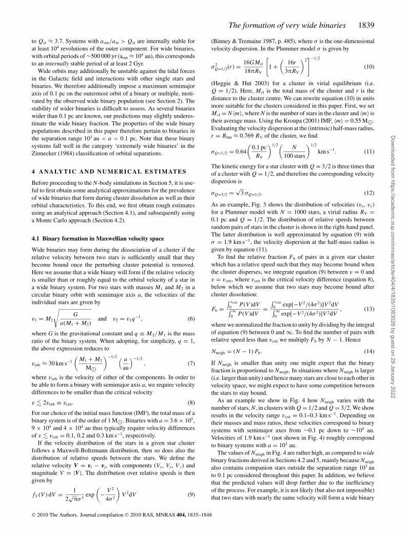
As an example we show in Fig. 4 how Nneigh varies with thenumber of stars, N, in clusters with Q = 1/2 and Q = 3/2. We showresults in the velocity range vcrit = 0.1–0.3 km s−1. Depending ontheir masses and mass ratios, these velocities correspond to binarysystems with semimajor axes from ∼0.1 pc down to ∼104 au.Velocities of 1.9 km s−1 (not shown in Fig. 4) roughly correspondto binary systems with a = 103 au.

The values of Nneigh in Fig. 4 are rather high, as compared to widebinary fractions derived in Sections 4.2 and 5, mainly because Nneigh

also contains companion stars outside the separation range 103 auto 0.1 pc considered throughout this paper. In addition, we believethat the predicted values will drop further due to the inefficiencyof the process. For example, it is not likely (but also not impossible)that two stars with nearly the same velocity will form a wide binary


Dow


ic.oup.com/m



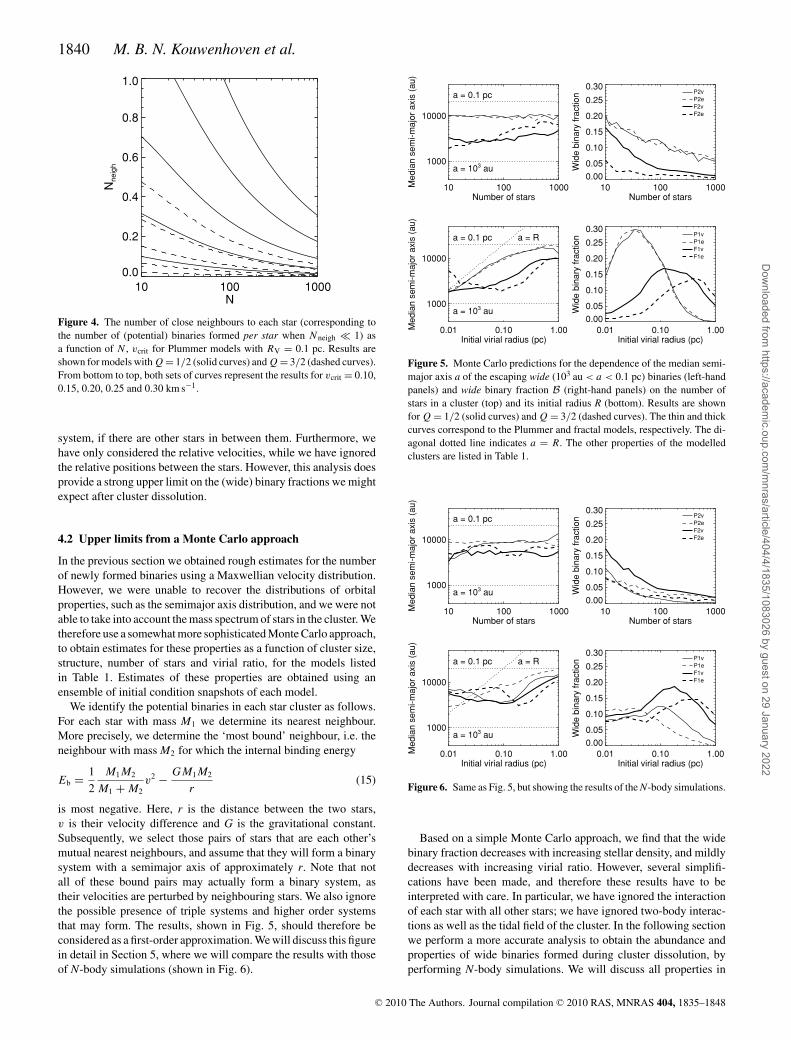
Figure 4. The number of close neighbours to each star (corresponding tothe number of (potential) binaries formed per star when Nneigh � 1) asa function of N , vcrit for Plummer models with RV = 0.1 pc. Results areshown for models with Q = 1/2 (solid curves) and Q = 3/2 (dashed curves).From bottom to top, both sets of curves represent the results for vcrit = 0.10,0.15, 0.20, 0.25 and 0.30 km s−1.

system, if there are other stars in between them. Furthermore, wehave only considered the relative velocities, while we have ignoredthe relative positions between the stars. However, this analysis doesprovide a strong upper limit on the (wide) binary fractions we mightexpect after cluster dissolution.

4.2 Upper limits from a Monte Carlo approach

In the previous section we obtained rough estimates for the numberof newly formed binaries using a Maxwellian velocity distribution.However, we were unable to recover the distributions of orbitalproperties, such as the semimajor axis distribution, and we were notable to take into account the mass spectrum of stars in the cluster. Wetherefore use a somewhat more sophisticated Monte Carlo approach,to obtain estimates for these properties as a function of cluster size,structure, number of stars and virial ratio, for the models listedin Table 1. Estimates of these properties are obtained using anensemble of initial condition snapshots of each model.

We identify the potential binaries in each star cluster as follows.For each star with mass M1 we determine its nearest neighbour.More precisely, we determine the ‘most bound’ neighbour, i.e. theneighbour with mass M2 for which the internal binding energy

Eb = 1

2

M1M2

M1 + M2v2 − GM1M2

r(15)

is most negative. Here, r is the distance between the two stars,v is their velocity difference and G is the gravitational constant.Subsequently, we select those pairs of stars that are each other’smutual nearest neighbours, and assume that they will form a binarysystem with a semimajor axis of approximately r. Note that notall of these bound pairs may actually form a binary system, astheir velocities are perturbed by neighbouring stars. We also ignorethe possible presence of triple systems and higher order systemsthat may form. The results, shown in Fig. 5, should therefore beconsidered as a first-order approximation. We will discuss this figurein detail in Section 5, where we will compare the results with thoseof N-body simulations (shown in Fig. 6).

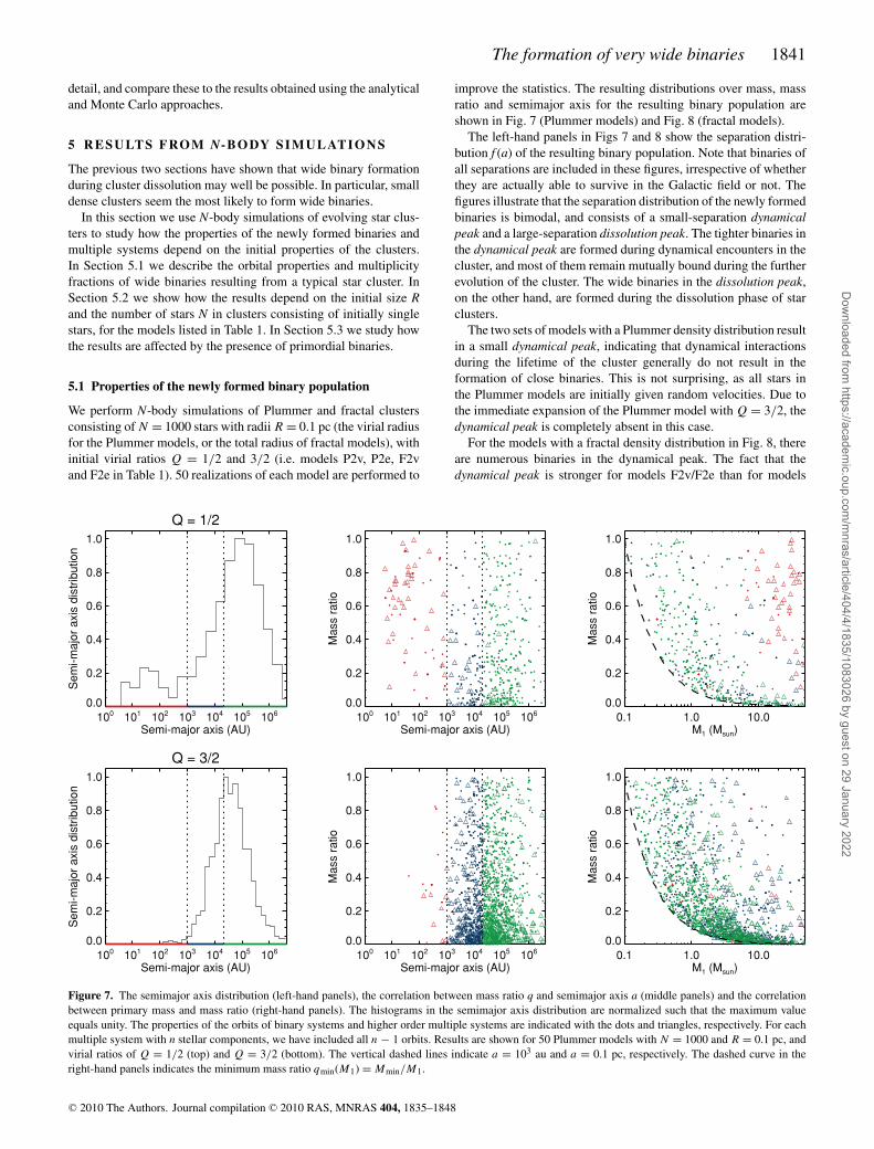
Figure 5. Monte Carlo predictions for the dependence of the median semi-major axis a of the escaping wide (103 au < a < 0.1 pc) binaries (left-handpanels) and wide binary fraction B (right-hand panels) on the number ofstars in a cluster (top) and its initial radius R (bottom). Results are shownfor Q = 1/2 (solid curves) and Q = 3/2 (dashed curves). The thin and thickcurves correspond to the Plummer and fractal models, respectively. The di-agonal dotted line indicates a = R. The other properties of the modelledclusters are listed in Table 1.

Figure 6. Same as Fig. 5, but showing the results of the N-body simulations.

Based on a simple Monte Carlo approach, we find that the widebinary fraction decreases with increasing stellar density, and mildlydecreases with increasing virial ratio. However, several simplifi-cations have been made, and therefore these results have to beinterpreted with care. In particular, we have ignored the interactionof each star with all other stars; we have ignored two-body interac-tions as well as the tidal field of the cluster. In the following sectionwe perform a more accurate analysis to obtain the abundance andproperties of wide binaries formed during cluster dissolution, byperforming N-body simulations. We will discuss all properties in


Dow


ic.oup.com/m



detail, and compare these to the results obtained using the analyticaland Monte Carlo approaches.

5 R ESULTS FROM N- B O DY SI M U L AT I O N S

The previous two sections have shown that wide binary formationduring cluster dissolution may well be possible. In particular, smalldense clusters seem the most likely to form wide binaries.

In this section we use N-body simulations of evolving star clus-ters to study how the properties of the newly formed binaries andmultiple systems depend on the initial properties of the clusters.In Section 5.1 we describe the orbital properties and multiplicityfractions of wide binaries resulting from a typical star cluster. InSection 5.2 we show how the results depend on the initial size Rand the number of stars N in clusters consisting of initially singlestars, for the models listed in Table 1. In Section 5.3 we study howthe results are affected by the presence of primordial binaries.

5.1 Properties of the newly formed binary population

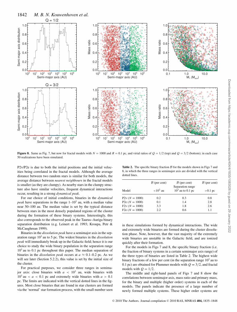
We perform N-body simulations of Plummer and fractal clustersconsisting of N = 1000 stars with radii R = 0.1 pc (the virial radiusfor the Plummer models, or the total radius of fractal models), withinitial virial ratios Q = 1/2 and 3/2 (i.e. models P2v, P2e, F2vand F2e in Table 1). 50 realizations of each model are performed to

improve the statistics. The resulting distributions over mass, massratio and semimajor axis for the resulting binary population areshown in Fig. 7 (Plummer models) and Fig. 8 (fractal models).

The left-hand panels in Figs 7 and 8 show the separation distri-bution f (a) of the resulting binary population. Note that binaries ofall separations are included in these figures, irrespective of whetherthey are actually able to survive in the Galactic field or not. Thefigures illustrate that the separation distribution of the newly formedbinaries is bimodal, and consists of a small-separation dynamicalpeak and a large-separation dissolution peak. The tighter binaries inthe dynamical peak are formed during dynamical encounters in thecluster, and most of them remain mutually bound during the furtherevolution of the cluster. The wide binaries in the dissolution peak,on the other hand, are formed during the dissolution phase of starclusters.

The two sets of models with a Plummer density distribution resultin a small dynamical peak, indicating that dynamical interactionsduring the lifetime of the cluster generally do not result in theformation of close binaries. This is not surprising, as all stars inthe Plummer models are initially given random velocities. Due tothe immediate expansion of the Plummer model with Q = 3/2, thedynamical peak is completely absent in this case.

For the models with a fractal density distribution in Fig. 8, thereare numerous binaries in the dynamical peak. The fact that thedynamical peak is stronger for models F2v/F2e than for models

Figure 7. The semimajor axis distribution (left-hand panels), the correlation between mass ratio q and semimajor axis a (middle panels) and the correlationbetween primary mass and mass ratio (right-hand panels). The histograms in the semimajor axis distribution are normalized such that the maximum valueequals unity. The properties of the orbits of binary systems and higher order multiple systems are indicated with the dots and triangles, respectively. For eachmultiple system with n stellar components, we have included all n − 1 orbits. Results are shown for 50 Plummer models with N = 1000 and R = 0.1 pc, andvirial ratios of Q = 1/2 (top) and Q = 3/2 (bottom). The vertical dashed lines indicate a = 103 au and a = 0.1 pc, respectively. The dashed curve in theright-hand panels indicates the minimum mass ratio qmin(M1) = Mmin/M1.


Dow


ic.oup.com/m



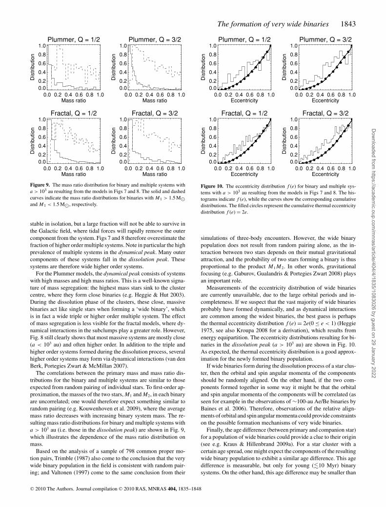
Figure 8. Same as Fig. 7, but now for fractal models with N = 1000 and R = 0.1 pc, and virial ratios of Q = 1/2 (top) and Q = 3/2 (bottom); in each case50 realizations have been simulated.

P2v/P2e is due to both the initial positions and the initial veloc-ities being correlated in the fractal models. Although the averagedistance between two random stars is similar for both models, theaverage distance between nearest neighbours in the fractal modelsis smaller (as they are clumpy). As nearby stars in the clumpy struc-ture also have similar velocities, frequent dynamical interactionsoccur, resulting in a strong dynamical peak.

For our choice of initial conditions, binaries in the dynamicalpeak have separations in the range 1–103 au, with a median valuenear 50–100 au. The median value is set by the typical distancebetween stars in the most densely populated regions of the clusterduring the formation of these binary systems. Interestingly, thisalso corresponds to the observed peak in the Taurus–Auriga binaryseparation distribution (e.g. Leinert et al. 1993; Kroupa, Petr &McCaughrean 1999).

Binaries in the dissolution peak have a semimajor axis in the sep-aration range 103 au to 5 pc. The widest binaries in the dissolutionpeak will immediately break up in the Galactic field; hence it is ourchoice to study the wide binary population in the separation range103 au to 0.1 pc throughout this paper. The median separation ofbinaries in the dissolution peak occurs at a ≈ 0.1–0.2 pc. As wewill see later (Section 5.2.2), this value is set by the initial size ofthe cluster.

For practical purposes, we consider three ranges in semima-jor axis: close binaries with a < 103 au, wide binaries with103 au < a < 0.1 pc and extremely wide binaries with a > 0.1pc. The limits are indicated with the vertical dotted lines in the fig-ures. Most close binaries that are found in star clusters are formedvia the ‘normal’ star formation process, with the small number seen

Table 2. The specific binary fraction B for the models shown in Figs 7 and8, in which the three ranges in semimajor axis are divided with the verticaldotted lines.

B (per cent) B (per cent) B (per cent)Separation range

Model <103 au 103 au to 0.1 pc >0.1 pc

P2v (N = 1000) 0.2 0.3 0.8P2e (N = 1000) 0.1 1.4 2.8F2v (N = 1000) 3.3 1.8 2.6F2e (N = 1000) 2.2 0.6 1.1

in these simulations formed by dynamical interactions. The wideand extremely wide binaries are formed during the cluster dissolu-tion phase. Note, however, that the vast majority of the extremelywide binaries are unstable in the Galactic field, and are ionizedquickly after their formation.

For the models in Figs 7 and 8, the specific binary fraction (i.e.the fraction of binary systems in a certain semimajor axis range) ofthe three types of binaries are listed in Table 2. The highest widebinary fractions of a few per cent (in the separation range 103 au to0.1 pc) are obtained for Plummer models with Q = 3/2, and fractalmodels with Q = 1/2.

The middle and right-hand panels of Figs 7 and 8 show thecorrelations between semimajor axis, mass ratio and primary mass,for the binary and multiple (higher order) systems in each of themodels. The panels indicate the presence of a large number ofnewly formed multiple systems. These higher order systems are


Dow


ic.oup.com/m



Figure 9. The mass ratio distribution for binary and multiple systems witha > 103 au resulting from the models in Figs 7 and 8. The solid and dashedcurves indicate the mass ratio distributions for binaries with M1 > 1.5 M�and M1 < 1.5 M�, respectively.

stable in isolation, but a large fraction will not be able to survive inthe Galactic field, where tidal forces will rapidly remove the outercomponent from the system. Figs 7 and 8 therefore overestimate thefraction of higher order multiple systems. Note in particular the highprevalence of multiple systems in the dynamical peak. Many outercomponents of these systems fall in the dissolution peak. Thesesystems are therefore wide higher order systems.

For the Plummer models, the dynamical peak consists of systemswith high masses and high mass ratios. This is a well-known signa-ture of mass segregation: the highest mass stars sink to the clustercentre, where they form close binaries (e.g. Heggie & Hut 2003).During the dissolution phase of the clusters, these close, massivebinaries act like single stars when forming a ‘wide binary’, whichis in fact a wide triple or higher order multiple system. The effectof mass segregation is less visible for the fractal models, where dy-namical interactions in the subclumps play a greater role. However,Fig. 8 still clearly shows that most massive systems are mostly close(a < 103 au) and often higher order. In addition to the triple andhigher order systems formed during the dissolution process, severalhigher order systems may form via dynamical interactions (van denBerk, Portegies Zwart & McMillan 2007).

The correlations between the primary mass and mass ratio dis-tributions for the binary and multiple systems are similar to thoseexpected from random pairing of individual stars. To first-order ap-proximation, the masses of the two stars, M1 and M2, in each binaryare uncorrelated; one would therefore expect something similar torandom pairing (e.g. Kouwenhoven et al. 2009), where the averagemass ratio decreases with increasing binary system mass. The re-sulting mass ratio distributions for binary and multiple systems witha > 103 au (i.e. those in the dissolution peak) are shown in Fig. 9,which illustrates the dependence of the mass ratio distribution onmass.

Based on the analysis of a sample of 798 common proper mo-tion pairs, Trimble (1987) also come to the conclusion that the verywide binary population in the field is consistent with random pair-ing; and Valtonen (1997) come to the same conclusion from their

Figure 10. The eccentricity distribution f (e) for binary and multiple sys-tems with a > 103 au resulting from the models in Figs 7 and 8. The his-tograms indicate f (e), while the curves show the corresponding cumulativedistributions. The filled circles represent the cumulative thermal eccentricitydistribution f (e) = 2e.

simulations of three-body encounters. However, the wide binarypopulation does not result from random pairing alone, as the in-teraction between two stars depends on their mutual gravitationalattraction, and the probability of two stars forming a binary is thusproportional to the product M1M2. In other words, gravitationalfocusing (e.g. Gaburov, Gualandris & Portegies Zwart 2008) playsan important role.

Measurements of the eccentricity distribution of wide binariesare currently unavailable, due to the large orbital periods and in-completeness. If we suspect that the vast majority of wide binariesprobably have formed dynamically, and as dynamical interactionsare common among the widest binaries, the best guess is perhapsthe thermal eccentricity distribution f (e) = 2e(0 ≤ e < 1) (Heggie1975, see also Kroupa 2008 for a derivation), which results fromenergy equipartition. The eccentricity distributions resulting for bi-naries in the dissolution peak (a > 103 au) are shown in Fig. 10.As expected, the thermal eccentricity distribution is a good approx-imation for the newly formed binary population.

If wide binaries form during the dissolution process of a star clus-ter, then the orbital and spin angular momenta of the componentsshould be randomly aligned. On the other hand, if the two com-ponents formed together in some way it might be that the orbitaland spin angular momenta of the components will be correlated (asseen for example in the observations of ∼100-au Ae/Be binaries byBaines et al. 2006). Therefore, observations of the relative align-ments of orbital and spin angular momenta could provide constraintson the possible formation mechanisms of very wide binaries.

Finally, the age difference (between primary and companion star)for a population of wide binaries could provide a clue to their origin(see e.g. Kraus & Hillenbrand 2009a). For a star cluster with acertain age spread, one might expect the components of the resultingwide binary population to exhibit a similar age difference. This agedifference is measurable, but only for young (�10 Myr) binarysystems. On the other hand, this age difference may be smaller than


Dow


ic.oup.com/m



expected from random pairing, if an initial correlation betweenposition and velocity exists.

5.2 Dependence on cluster properties

In this section we describe how the properties of the wide binarypopulation depend on the initial conditions we assign to a starcluster, in particular its size R, number of stars N, virial ratio Qand morphology (Plummer sphere or fractal structure). We adoptthe cluster properties listed in Table 1. We compare the results thatwe derived earlier using Monte Carlo simulations (Fig. 5), with theresults of N-body simulations, shown in Fig. 6.

5.2.1 Dependence on the initial cluster mass

The top panels of Fig. 6 show the median semimajor axis amed andthe binary fraction B of wide binaries (103 au < a < 0.1 pc) as afunction of the number of stars N in a cluster. For both the Plummermodels and the fractal models, amed does not vary significantly withN and the virial ratio Q. The reason for this is that all these modelshave an identical size R. Since R is the most important size scaleimposed on the modelled star clusters, it determines the size scaling(i.e. semimajor axis distribution) of the newly formed binaries.

The dependence of B on N and Q is qualitatively the same asthe analytical predictions shown in Fig. 4 and the Monte Carlo ap-proximation shown in Fig. 5. The wide binary fraction B decreaseswith increasing N because the stars are further apart in velocityspace (cf. Fig. 3), i.e. the velocity dispersion is larger, and hencetwo neighbouring stars are less likely to form a bound system.

For the N-body simulations we find that the fractal model withQ = 1/2 provides the highest wide binary fractions, although thedifference between models is fairly small (especially when com-pared to the difference with increasing N). Models with Q = 3/2generally result in a smaller wide binary fraction than those withQ = 1/2, due to the larger distance between the stars in velocityspace (see equations 11 and 12). The curves for the fractal models inFigs 5 and 6 are almost the same, indicating that the Monte Carlo ap-proach provides a good estimate of the wide binary population. Forthe Plummer models, the Monte Carlo approach predicts a binaryfraction that is too high, which is due to the fact that the positionsand velocities of stars in the Plummer models as we initialize themare uncorrelated.

5.2.2 Dependence on the initial cluster size

The bottom panels of Fig. 6 shows the dependence of amed and B onthe initial size R of the clusters. Again, these values are only for widebinaries with 103 au < a < 0.1 pc. Note the different definitions ofR: for the Plummer models R represents the virial radius, while forthe fractal models R represents the radius of the sphere enclosing thewhole system. Note again the similarity between the Monte Carloapproximation shown in Fig. 5 and the N-body models.

As discussed above, the initial cluster size R determines thelength-scale in each model, and therefore the size scaling of thesemimajor axis distribution of the newly formed binaries. For ex-ample, changing the initial size of the clusters shown in Figs 7and 8 would simply result in the semimajor axis distribution in theleft-hand panels being shifted to smaller or larger values of a.

This direct dependence of f (a) on R is not seen directly in Fig. 5because we only show the results for wide binaries in the separationrange 103 au < a < 0.1 pc, and because f (a) is bimodal. However,

the R-dependent median semimajor axis and binary fraction canbe explained by the dynamical peak and dissolution peak shiftingthrough the range 103 au < a < 0.1 pc whilst varying R.

The highest B is found when either the dynamical peak, or thedissolution peak, is centred in the separation range 103 au < a <

0.1 pc. For our choice of the initial conditions, this peak occurs atR = 0.025 pc for the Plummer models, when the dissolution peakis centred in the range 103 au to 0.1 pc. The peak in B occurs at R ≈0.15 pc for the fractal models with Q = 1/2 and at R ≈ 0.6 pc forfractal models with Q = 3/2, when the dynamical peak is centredin the range 103 au to 0.1 pc.

Given our set of initial conditions, compact clusters result in awide binary fraction of 8–12 per cent, irrespective of virial ratioand morphology. For more extended clusters, those with a Plummerstructure and those with a higher virial ratio result in a smaller binaryfraction. The difference between the Plummer and fractal modelscan be explained by (i) the difference in the definition of R forthe two sets of models and (ii) by the different intrinsic separationdistribution (see the left-hand panels in Figs 7 and 8).

The cluster size R determines the length-scale of the system,and therefore determines the typical semimajor axis of the newlyformed wide binaries. Other, less important length-scales in thesystem are the mean distance between two stars, which dependson the parameters R, N and the stellar density distribution (seeSection 5.2.1), as well as the typical semimajor axis of primordialbinary systems (see Section 5.3).

5.3 Effects of primordial binarity

In the analysis above we have considered star clusters that initiallyconsist of single stars only. The results for star clusters with anon-zero primordial binary fraction are very similar to the resultsdescribed above, with the difference that the components of the wide‘binary’ are now in many cases primordial binaries. In other words,the majority of the wide ‘binaries’ that formed in the simulationsdescribed in the previous sections actually describe the outer orbitsof wide triple and quadruple systems.

We predict the properties of these wide triple and quadruple sys-tems by performing N-body simulations of the Plummer modelslisted in Table 1, but now we include a non-zero primordial bi-nary fraction. We perform the simulations with primordial binaryfractions B0 ranging from 0 to 100 per cent. We adopt the Kroupa(1995) birth period distribution. This distribution is derived from adetailed analysis of observed stellar populations, and has the form

fP(P ) = 2.5(log P − log Pmin)

45 + (log P − log Pmin)2 (16)

for P min ≤ P ≤ P max, where log P min = 1, log P max = 8.43 and Pis the period in days. We adopt a thermal eccentricity distributionf (e) = 2e (0 ≤ e < 1). We adopt a flat mass ratio distributionf (q) = 1 with 0 < q ≡ M2/M1 < 1 (i.e. we apply pairing functionPCP-I; see Kouwenhoven et al. 2009). Subsequently, we gener-ate an initial population from this birth population, by applyingeigenevolution as described in Kroupa (1995). All binaries are as-signed random orientations and orbital phases at the beginning ofthe simulations.

Due to the inclusion of binary components, the total mass ofeach cluster increases slightly (up to a maximum of 50 per cent fora primordial binary fraction of 100 per cent), although the numberof ‘systems’, N = S + B remains constant. Strictly speaking, it isthus not appropriate to directly compare clusters with and withoutbinaries, as we have changed more than one parameter: binarity and


Dow


ic.oup.com/m



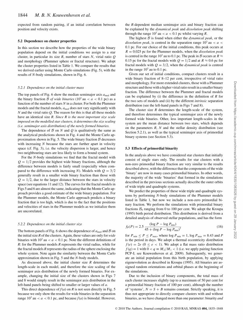
Figure 11. The effect of primordial binarity on the formation of wide bi-naries, for Plummer models with N = 10 and R = 0.1 pc. The solid anddashed curves in each panel indicate the results for Q = 1/2 and 3/2, re-spectively. Top: the effect of a variable primordial binary fraction B0. Thebottom horizontal dotted line indicates a = 18.2 au, the median semimajoraxis for primordial binaries. Bottom: the effect of the semimajor axis a0 formodels with a primordial binary frequency B0 = 50 per cent in which eachbinary has a semimajor axis a = a0. The dash–dotted lines indicate a =18.2 au, the median semimajor axis of binary systems in the Galactic field.The vertical dotted line indicates a = 103 au, beyond which all primordialbinaries are classified as wide binaries.

cluster mass (see e.g. Kouwenhoven & de Grijs 2008). However, asthe increase in cluster mass due to adding the companions is rathersmall, we will ignore this issue.

The results for clusters with a varying primordial binary fractionB0 is shown in the top panels of Fig. 11. For small binary fractions,the results are very similar to those of clusters without primordialbinaries. The properties of the resulting wide binary populationdepend mildly on Q. An increasing Q results in, on average, widerbinaries, hence in a larger fraction of binaries with a > 0.1 pc,and therefore in a slightly smaller wide binary fraction. Note thatB decreases slightly with increasing B0. A larger primordial binaryfraction results in a smaller wide binary fraction, possibly becauseof the destruction of newly formed wide binaries by primordialbinaries (which have a significantly larger collisional cross-sectionthan single stars).

Whether or not primordial binarity affects the formation of widebinaries depends not only on the primordial binary fraction, but alsoon the properties of these binaries: the semimajor axis (or period)distribution, the eccentricity distribution and the mass ratio distribu-tion. The most important of these is the semimajor axis distributionf (a), as it determines the internal binding energy of a binary andthe cross-section for gravitational interactions between binaries andother binaries or single stars. In order to extract the dependence onf (a), we simulate clusters in which all binaries have a single valuefor a = a0. We vary a0 in each cluster, and determine the numberof newly formed binaries. In all simulations we adopt a primordialbinary fraction of 50 per cent, a flat mass ratio distribution and athermal eccentricity distribution.

The results of these simulations are shown in the bottom panelsof Fig. 11. For models with a0 < 103 au, most primordial binariessurvive, while additional wide binary, triple and quadruple systems

are formed. In fact, the resulting wide binary fraction is practicallyindependent of the primordial binary fraction B0. For models witha0 > 103 au, all primordial binary systems are classified as widebinaries. For these models we therefore have B ≈ B0 and a mediansemimajor axis equal to a0, which results in the glitches at a =103 au in Fig. 11.

The wide orbits are part of systems with two, three and fourcomponents. They are formed by randomly pairing single starsand primordial binary systems together. The number of multiplesystems of each degree can thus be estimated by simply calculatingthe probability of randomly drawing a single–single, single–binaryand binary–binary pair. When assuming a primordial binary fractionB0, the multiplicity distribution of the resulting wide population canbe estimated as follows:

Wide binary fraction = B(1 − B0)2, (17)

Wide triple fraction = 2BB0(1 − B0), (18)

Wide quadruple fraction = BB20, (19)

where we have made the assumption that none of the primordialbinary systems has broken up.

All models shown in Fig. 11 result in wide binary fractionsB ≈ 8per cent that are more or less independent of B0 and a0. The valueof B is therefore primarily determined by the initial values of thenumber of system N in the cluster, and its initial size R.

If we assume that the wide orbits in the bottom panels of Fig. 11(where B0 = 50 per cent) are formed of randomly paired com-ponents (i.e. single stars or primordial binaries), we can calcu-late the fraction of higher order multiple systems among the B =8 per cent wide binaries. Among these, we predict that 25, 50 and25 per cent are binary, triple and quadruple systems, respectively.In this example, we thus expect 75 per cent of the ‘wide binaries’to be higher order multiple systems. Due to the random process, theouter orbits of these systems are expected to be uncorrelated withthe inner orbits or stellar spin axes.

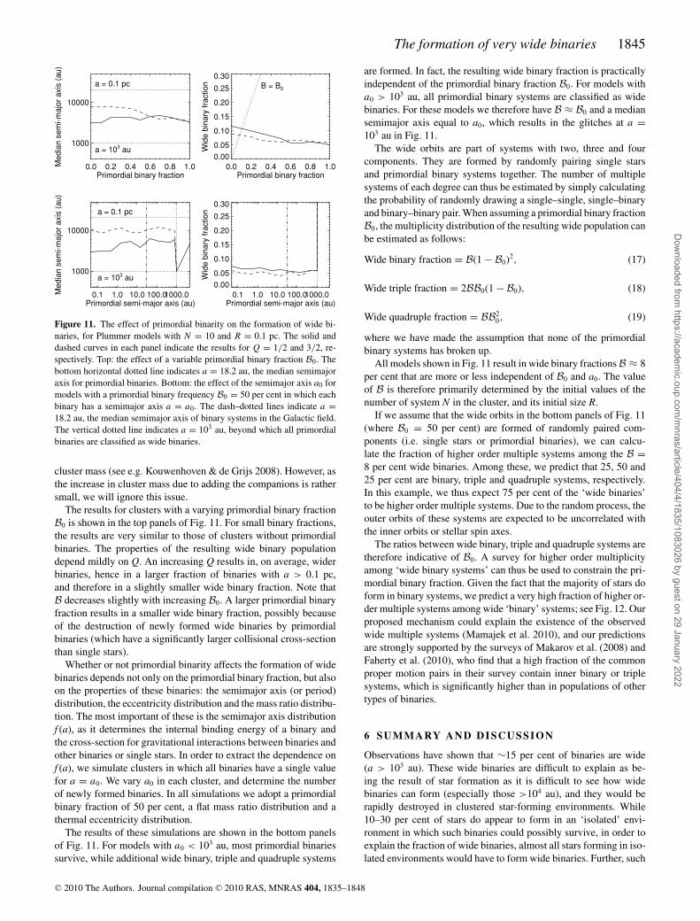
The ratios between wide binary, triple and quadruple systems aretherefore indicative of B0. A survey for higher order multiplicityamong ‘wide binary systems’ can thus be used to constrain the pri-mordial binary fraction. Given the fact that the majority of stars doform in binary systems, we predict a very high fraction of higher or-der multiple systems among wide ‘binary’ systems; see Fig. 12. Ourproposed mechanism could explain the existence of the observedwide multiple systems (Mamajek et al. 2010), and our predictionsare strongly supported by the surveys of Makarov et al. (2008) andFaherty et al. (2010), who find that a high fraction of the commonproper motion pairs in their survey contain inner binary or triplesystems, which is significantly higher than in populations of othertypes of binaries.

6 SUMMARY AND DI SCUSSI ON

Observations have shown that ∼15 per cent of binaries are wide(a > 103 au). These wide binaries are difficult to explain as be-ing the result of star formation as it is difficult to see how widebinaries can form (especially those >104 au), and they would berapidly destroyed in clustered star-forming environments. While10–30 per cent of stars do appear to form in an ‘isolated’ envi-ronment in which such binaries could possibly survive, in order toexplain the fraction of wide binaries, almost all stars forming in iso-lated environments would have to form wide binaries. Further, such


Dow


ic.oup.com/m



Figure 12. Given the fact that most stars form in binary systems, it isexpected that the majority of the wide ‘binary’ systems are in fact part of atriple or quadruple system.

wide binaries cannot be formed later in any significant numbers bydynamical interactions in the Galactic field.

In this paper we study the possibility of wide binary formationduring the dissolution phase of star clusters, in particular, duringthe rapid expansion of clusters after gas expulsion. We study thispossibility using (1) an analytical approach in an idealized situation,(2) a Monte Carlo approach and (3) detailed N-body simulations.Our main conclusions are as follows.

(i) The wide binary fraction B among the dissolved stellar pop-ulation ranges between 1 and 30 per cent, depending on the clusterproperties.

(ii) More massive star clusters result in a smaller wide B thanlow-mass clusters. Clusters with a spherical, smooth stellar densitydistribution form fewer wide binaries than substructured clustersof the same size and mass. This is due to the fact that the averagedistance between nearest neighbours is smaller for substructuredclusters. Expanding (post-gas expulsion) star clusters produce alarger B than those starting out of equilibrium.

(iii) The typical semimajor axis a of the newly formed binariesis similar to the initial size R of the star cluster from which theywere born. The resulting semimajor axis distribution is generally bi-modal, consisting of a dynamical peak with binary systems formedby dynamical interactions, and a dissolution peak with binary sys-tems formed during the cluster dissolution phase.

(iv) The formation of wide binaries during the star cluster disso-lution phase is a random process, resulting in the following orbitalproperties. The eccentricity distribution of the wide binaries is ap-proximately thermal: f (e) ≈ 2e for 0 ≤ e < 1. The mass ratiodistribution of the wide binaries is the result of gravitationally fo-cused random pairing. In a wide binary, the orbital and spin angularmomenta are uncorrelated.

(v) Star clusters with a non-zero primordial binary populationform wide triple and quadruple systems, i.e. the components of anewly formed wide ‘binary’ can themselves be close primordialbinaries, rather than single stars. The ratio of triple to quadruplesystems among very wide orbits is therefore indicative of the pri-mordial binary fraction B0. Given that B0 is large, we predict a high

frequency of triple and quadruple systems among the known wide‘binary’ systems, which is supported by existing surveys for higherorder multiplicity among wide binary systems.

Throughout this paper we have made predictions of the proper-ties of the wide binary population resulting from the dissolution ofindividual clusters. In order to compare our results with observa-tions, we should therefore take into account the fact that the fieldstar population is made up of the stars resulting from an ensembleof clusters of different sizes and masses. The initial cluster massdistribution may be approximated by f (M) ∝ M−γ with γ ≈ 2 (seee.g. Zhang & Fall 1999; Ashman & Zepf 2001; Bik et al. 2003;Hunter et al. 2003). Given the number of stars N = Mcl/〈m〉, where〈m〉 is the average mass of a star, this distribution is equivalent tof (N ) ∝ N−γ . Oey, King & Parker (2004) suggest that the above ex-pression can be extrapolated down to Nmin = 1. The upper limit forthe initial cluster mass distribution is Mmax ≈ 106 M� (e.g. de Grijs& Parmentier 2007, and references therein). The resulting binaryfraction Bf for the ensemble of stars (i.e. the field star population)is then given by

Bf =∫ Nmax

NminB(Ncl)Nf (Ncl)dNcl∫ Nmax

Nminf (Ncl)NdNcl

, (20)

where B(Ncl) is the cluster mass dependent wide binary fraction.The numerator in the above expression is proportional to the numberof binaries, and the denominator is proportional to the total numberof stars in the ensemble of clusters. In addition, the size and disso-lution time of a star cluster, and therefore the wide binary fraction,may also depend on its Galactic location (e.g. Baumgardt & Makino2003). An inspection of Fig. 6 shows that an extrapolation to N ≈106 results in a wide binary fraction of several per cent; smaller thanthe observed 15 per cent, irrespective of the choices for R, Q and themorphology of the cluster. Although we predict rather small values,our back-of-the-envelope calculation does result in the right orderof magnitude for the wide binary fraction in the Galactic field. It isclear, however, that a deeper investigation is required to accuratelyrecover the properties of the wide binary population in the field.In particular, a wider range of star cluster morphologies has to beconsidered, by varying the fractal dimension and position–velocitycorrelations of individual star clusters.

Our proposed formation mechanism for very wide binaries pre-dicts at least several common proper motion pairs in and arounddissolving star clusters and moving groups. For example, the mech-anism may well explain the presence of the three common propermotion pairs in the moving groups studied by Clarke et al. (2010).The future prospects in wide binary research are bright: an enor-mous number of wide binaries are expected to be found withthe GAIA mission3 (Perryman et al. 2001; Turon, O’Flaherty &Perryman 2005) and LAMOST4 (Chu 1998; Stone 2008). Thesedata sets should help determine the true fraction of wide binariesand their orbital parameters.

AC K N OW L E D G M E N T S

We would like to thank Anthony Whitworth (our referee) and SimonPortegies Zwart for a useful discussion on this topic. MBNK wassupported by the Peter and Patricia Gruber Foundation through thePPGF fellowship, the Peking University One Hundred Talent Fund

3See the web site http://www.esa.int/science/gaia.4See the web site http://www.lamost.org.


Dow


ic.oup.com/m



(985), and by PPARC/STFC (grant PP/D002036/1). We would liketo acknowledge CICS for the provision of research computing facili-ties through the White Rose Grid. We acknowledge research supportfrom and hospitality at the International Space Science Institute inBern (Switzerland), as part of an International Team Programme.The authors acknowledge the Sheffield–Bonn Royal Society Inter-national Joint Project grant, which provided financial support andthe collaborative opportunities for this work. The calculations per-formed by DM were carried out on computer hardware purchasedfrom the Royal Physiographic Society in Lund. RJP acknowledgesfinancial support from STFC.

RE FERENCES

Allen C., Poveda A., Herrera M. A., 2000, A&A, 356, 529Allen C., Poveda A., Hernandez-Alcantara A., 2007a, in Hartkopf W. I.,

Guinan E. F., Harmanec P., eds, Proc. IAU Symp. 240, Binary Starsas Critical Tools and Tests in Contemporary Astrophysics. CambridgeUniv. Press, Cambridge, p. 405

Allen L. et al., 2007b, in Reipurth B., Jewitt D., Keil K., eds, Protostars andPlanets V The Structure and Evolution of Young Stellar Clusters. Univ.Arizona Press, Tucson, p. 361

Ashman K. M., Zepf S. E., 2001, AJ, 122, 1888Bahcall J. N., Soneira R. M., 1981, ApJ, 246, 122Bahcall J. N., Hut P., Tremaine S., 1985, ApJ, 290, 15Baines D., Oudmaijer R. D., Porter J. M., Pozzo M., 2006, MNRAS, 367,

737Bastian N., Gieles M., Lamers H. J. G. L. M., Scheepmaker R. A., de Grijs

R., 2005, A&A, 431, 905Baumgardt H., Makino J., 2003, MNRAS, 340, 227Bik A., Lamers H. J. G. L. M., Bastian N., Panagia N., Romaniello M.,

2003, A&A, 397, 473Binney J., Tremaine S., 1987, Galactic Dynamics. Princeton Univ. Press,

Princeton, NJBoutloukos S. G., Lamers H. J. G. L. M., 2003, MNRAS, 338, 717Burgasser A. J., Kirkpatrick J. D., Reid I. N., Brown M. E., Miskey C. L.,

Gizis J. E., 2003, ApJ, 586, 512Caballero J. A., 2009, A&A, 507, 251Chaname J., Gould A., 2004, ApJ, 601, 289Chandrasekhar S., 1944, ApJ, 99, 54Chu Y., 1998, Highlights Astron., 11, 493Clarke J. R. A., Pinfeld D. J., Galvez-Ortz M. C., Jenkins J. S., Burningham

B., Deacon N. R., Jones H. R. A., Pokorny R. S., Barnes J. R., Day-JonesA. C., 2010, MNRAS, 402, 575

Close L. M., Richer H. B., Crabtree D. R., 1990, AJ, 100, 1968de Grijs R., Parmentier G., 2007, Chinese J. Astron. Astrophys., 7, 155Duquennoy A., Mayor M., 1991, A&A, 248, 485Eggers S., Keller H. U., Kroupa P., Markiewicz W. J., 1997, Planet. Space

Sci., 45, 1099Elmegreen B. G., 2000, ApJ, 530, 277ESA 1997, VizieR Online Data Catalog, 1239Faherty J. K., Burgasser A. J., West A. A., Bochanski J. J., Cruz K. L., Shara

M. M., Walter F. M., 2010, AJ, 139, 176Fall S. M., Chandar R., Whitmore B. C., 2005, ApJ, 631, L133Fischer D. A., Marcy G. W., 1992, ApJ, 396, 178Gaburov E., Gualandris A., Portegies Zwart S., 2008, MNRAS, 384, 376Garnavich P. M., 1988, ApJ, 335, L47Goodman J., Hut P., 1993, ApJ, 403, 271Goodwin S. P., 2009, preprint (arXiv:0911.0795)Goodwin S. P., Bastian N., 2006, MNRAS, 373, 752Goodwin S. P., Kroupa P., 2005, A&A, 439, 565Goodwin S. P., Whitworth A. P., 2004, A&A, 413, 929Goodwin S. P., Kroupa P., Goodman A., Burkert A., 2007, in Reipurth B.,

Jewitt D., Keil K., eds, Protostars and Planets V The Fragmentation ofCores and the Initial Binary Population. Univ. Arizona Press, Tucson,p. 133

Gould A., Eastman J., 2006, preprint (astro-ph/0610799)Gould A., Bahcall J. N., Maoz D., Yanny B., 1995, ApJ, 441, 200Gutermuth R. A., Megeath S. T., Pipher J. L., Williams J. P., Allen L. E.,

Myers P. C., Raines S. N., 2005, ApJ, 632, 397Hartigan P., Strom K. M., Strom S. E., 1994, ApJ, 427, 961Heggie D. C., 1975, MNRAS, 173, 729Heggie D., Hut P., 2003, The Gravitational Million-Body Problem: A Multi-

disciplinary Approach to Star Cluster Dynamics. Cambridge Univ. Press,Cambridge

Hernandez X., Lee W. H., 2008, MNRAS, 387, 1727Hills J. G., 1975, AJ, 80, 809Hunter D. A., Elmegreen B. G., Dupuy T. J., Mortonson M., 2003, AJ, 126,

1836Jiang Y., Tremaine S., 2010, MNRAS, 401, 977Kobulnicky H. A., Fryer C. L., 2007, ApJ, 670, 747Kouwenhoven M. B. N., de Grijs R., 2008, A&A, 480, 103Kouwenhoven M. B. N., Brown A. G. A., Zinnecker H., Kaper L., Portegies

Zwart S. F., 2005, A&A, 430, 137Kouwenhoven M. B. N., Brown A. G. A., Portegies Zwart S. F., Kaper L.,

2007, A&A, 474, 77Kouwenhoven M. B. N., Brown A. G. A., Goodwin S. P., Portegies Zwart

S. F., Kaper L., 2009, A&A, 493, 979Kraus A. L., Hillenbrand L. A., 2009a, ApJ, 704, 531Kraus A. L., Hillenbrand L. A., 2009b, ApJ, 703, 1511Kroupa P., 1995, MNRAS, 277, 1507Kroupa P., 2001, MNRAS, 322, 231Kroupa P., 2008, in Aarseth S. J., Tout C. A., Mardling R. A. eds, Lecture

Notes in Physics Vol. 760, Initial Conditions for Star Clusters. Springer-Verlag, Berlin, p. 181

Kroupa P., Burkert A., 2001, ApJ, 555, 945Kroupa P., Petr M. G., McCaughrean M. J., 1999, New Astron., 4, 495Lada C. J., 2006, ApJ, 640, L63Lada C. J., Lada E. A., 2003, ARA&A, 41, 57Larson R. B., 1995, MNRAS, 272, 213Latham D. W., Schechter P., Tonry J., Bahcall J. N., Soneira R. M., 1984,

ApJ, 281, L41Leinert C., Zinnecker H., Weitzel N., Christou J., Ridgway S. T., Jameson

R., Haas M., Lenzen R., 1993, A&A, 278, 129Lepine S., Bongiorno B., 2007, AJ, 133, 889Longhitano M., Binggeli B., 2010, A&A, 509, 46Makarov V. V., Zacharias N., Hennessy G. S., 2008, ApJ, 687, 566Mallada E., Fernandez J. A., 2001, Revista Mexicana Astron. Astrofisica

Conf. Ser., 11, 27Mamajek E. E., Kenworthy M. A., Hinz P. M., Meyer M. R., 2010, AJ, 139,

919Mason B. D., Gies D. R., Hartkopf W. I., Bagnuolo W. G., Jr, ten Brummelaar

T., McAlister H. A., 1998, AJ, 115, 821Mengel S., Lehnert M. D., Thatte N., Genzel R., 2005, A&A, 443, 41Moeckel N., Bate M. R., 2010, MNRAS, in press (arXiv:1001.3417)Oey M. S., King N. L., Parker J. W., 2004, AJ, 127, 1632Opik E., 1924, Tartu Obser. Publ., 25Parker R. J., Goodwin S. P., Kroupa P., Kouwenhoven M. B. N., 2009,

MNRAS, 397, 1577Perryman M. A. C. et al., 2001, A&A, 369, 339Plummer H. C., 1911, MNRAS, 71, 460Portegies Zwart S. F., McMillan S. L. W., Hut P., Makino J., 2001, MNRAS,

321, 199Poveda A., Allen C., 2004, in Allen C., Scarfe C., eds, Revista Mexicana

Astron. Astrofisica Conf. Ser., 21, 49Poveda A., Allen C., Hernandez-Alcantara A., 2007, in Hartkopf W. I.,

Guinan E. F., Harmanec P., eds, Proc. IAU Symp. 240, Binary Starsas Critical Tools and Tests in Contemporary Astrophysics. CambridgeUniv. Press, Cambridge, p. 417

Quinn D. P., Wilkinson M. I., Irwin M. J., Marshall J., Koch A., BelokurovV., 2009, MNRAS, 396, L11

Radigan J., Lafreniere D., Jayawardhana R., Doyon R., 2009, ApJ, 698, 405Reipurth B., Zinnecker H., 1993, A&A, 278, 81Retterer J. M., King I. R., 1982, ApJ, 254, 214


Dow


ic.oup.com/m



Scally A., Clarke C., McCaughrean M. J., 1999, MNRAS, 306, 253Scholz R.-D., Kharchenko N. V., Lodieu N., McCaughrean M. J., 2008,

A&A, 487, 595Shatsky N., Tokovinin A., 2002, A&A, 382, 92Soderhjelm S., 2007, A&A, 463, 683Stone R., 2008, Sci, 320, 34Testi L., Sargent A. I., Olmi L., Onello J. S., 2000, ApJ, 540, L53Theuns T., 1992, A&A, 259, 493Trimble V., 1987, Astron. Nachr., 308, 343Turon C., O’Flaherty K. S., Perryman M. A. C., eds, 2005, ESA Special

Publication Vol. 576, The Three-Dimensional Universe with Gaia. ESA,Noordwijk

Tutukov A. V., 1978, A&A, 70, 57Valtonen M. J., 1997, ApJ, 485, 785Valtonen M., Myllari A., Orlov V., Rubinov A., 2008, in Vesperini E.,

Giersz M., Sills A., eds, IAU Symp. Vol. 246, The Problem of ThreeStars: Stability Limit. Cambridge Univ. Press, Cambridge, p. 209

van Albada T. S., 1968, Bull. Astron. Inst. Netherlands, 20, 47van den Berk J., Portegies Zwart S. F., McMillan S. L. W., 2007, MNRAS,

379, 111Vereshchagin S., Tutukov A., Iungelson L., Kraicheva Z., Popova E., 1988,

Ap&SS, 142, 245Ward-Thompson D., Andre P., Crutcher R., Johnstone D., Onishi T., Wilson

C., 2007, in Reipurth B., Jewitt D., Keil K. eds, Protostars and Planets VAn Observational Perspective of Low-Mass Dense Cores II: EvolutionToward the Initial Mass Function. Univ. Arizona Press, Tucson, p. 33

Wasserman I., Weinberg M. D., 1991, ApJ, 382, 149Weinberg M. D., Shapiro S. L., Wasserman I., 1987, ApJ, 312, 367Zhang Q., Fall S. M., 1999, ApJ, 527, L81Zinnecker H., 1984, Ap&SS, 99, 41Zinnecker H., Yorke H. W., 2007, ARA&A, 45, 481

This paper has been typeset from a TEX/LATEX file prepared by the author.


Dow


ic.oup.com/m


The formation of very wide binaries during the star cluster ...

Documents

Transcript of The formation of very wide binaries during the star cluster ...