
The Stability of the Czech Banking Sector Phenomenon in the ...
356
8 th International Scientific Conference Managing and Modelling of Financial Risks Ostrava VŠB-TU of Ostrava, Faculty of Economics, Department of Finance 5 th – 6 th September 2016 379 The Stability of the Czech Banking Sector Phenomenon in the Company Interest Rate Risk Management František KALOUDA 1 Abstract The aim of this paper is to describe and assess the impact of the Czech banking sector stability to control the cost of capital by the central bank. Methodological basis of the paper is statistical and cybernetic perception and evaluation of the banking system stability. It in this case means the cost of capital management stability, in terms of commercial rates management. The novelty of the paper is in the application of the cybernetic approaches for evaluating stability of the Czech banking sector and in confrontation results of these approaches with statistical approches as well. The expected results of the paper are firs of all the evidence that cybernetic approaches are in this area (stability of the Czech banking sector with special focus to the cost of capital management processes) beneficial. Key words CZ banking system, stability, interes rate risk JEL Classification: C67, G21, G238 1. Úvod Stále platí, že si bankovní úvěr zachovává významné místo ve financování současného podniku. Z pohledu podnikových finančních a speciálně úrokových rizik tato skutečnost znamená, že je stále aktuální usilovat o řízení těchto rizik s cílem jejich minimalizace. V širším kontextu je úsilí o řízení úrokových rizik spojeno s procesy řízení ceny kapitálu na úrovni komerční sazby (též tržní úroková míra) centrální bankou, v čemž hraje rozhodující roli diskontní sazba. Příspěvek je proto věnován zkoumání stability bankovní soustavy ČR, což vede k formulaci závěrů o časovém vývoji komerční sazby. Fenomén stability bankovní soustavy se projevuje v podobě stability komerční sazby, respektive v podobě procesu její stabilizace v průběhu času. Tato problematika byla až dosud v domácích pramenech řešena s využitím více či méně sofistikovaných statistických nástrojů. Přínos příspěvku spočívá především v aplikaci přístupů ekonomické kybernetiky k danému účelu a následně i v konfrontaci takto nově získaných výsledků s tradičními poznatky. 2. Cíl a metodologie Cílem příspěvku je přispět k poznání procesů stanovování ceny kapitálu v podobě vazby komerční sazby na sazbu diskontní a s využitím znalosti logiky tohoto procesu řídit podnikové úrokové riziko. 1 František KALOUDA, Ing., CSc., M.B.A., Masaryk University, Faculty of Economics and Administration, Department of Finance, Lipová 41a, 602 00 Brno, Czech Republic, E-mail: [email protected].
-
Upload
khangminh22 -
Category
Documents
-
view
0 -
download
0
Transcript of The Stability of the Czech Banking Sector Phenomenon in the ...

8th International Scientific Conference Managing and Modelling of Financial Risks Ostrava
VŠB-TU of Ostrava, Faculty of Economics, Department of Finance 5th – 6th September 2016
379
The Stability of the Czech Banking Sector Phenomenon in the Company Interest Rate Risk
Management
František KALOUDA 1
Abstract
The aim of this paper is to describe and assess the impact of the Czech banking sector stability
to control the cost of capital by the central bank. Methodological basis of the paper is statistical
and cybernetic perception and evaluation of the banking system stability. It in this case means
the cost of capital management stability, in terms of commercial rates management.
The novelty of the paper is in the application of the cybernetic approaches for evaluating
stability of the Czech banking sector and in confrontation results of these approaches with
statistical approches as well. The expected results of the paper are firs of all the evidence that
cybernetic approaches are in this area (stability of the Czech banking sector with special focus
to the cost of capital management processes) beneficial.
Key words
CZ banking system, stability, interes rate risk
JEL Classification: C67, G21, G238
1. Úvod
Stále platí, že si bankovní úvěr zachovává významné místo ve financování současného
podniku. Z pohledu podnikových finančních a speciálně úrokových rizik tato skutečnost
znamená, že je stále aktuální usilovat o řízení těchto rizik s cílem jejich minimalizace.
V širším kontextu je úsilí o řízení úrokových rizik spojeno s procesy řízení ceny kapitálu na
úrovni komerční sazby (též tržní úroková míra) centrální bankou, v čemž hraje rozhodující
roli diskontní sazba. Příspěvek je proto věnován zkoumání stability bankovní soustavy ČR,
což vede k formulaci závěrů o časovém vývoji komerční sazby.
Fenomén stability bankovní soustavy se projevuje v podobě stability komerční sazby,
respektive v podobě procesu její stabilizace v průběhu času.
Tato problematika byla až dosud v domácích pramenech řešena s využitím více či méně
sofistikovaných statistických nástrojů.
Přínos příspěvku spočívá především v aplikaci přístupů ekonomické kybernetiky k danému
účelu a následně i v konfrontaci takto nově získaných výsledků s tradičními poznatky.
2. Cíl a metodologie
Cílem příspěvku je přispět k poznání procesů stanovování ceny kapitálu v podobě vazby
komerční sazby na sazbu diskontní a s využitím znalosti logiky tohoto procesu řídit podnikové
úrokové riziko.
1 František KALOUDA, Ing., CSc., M.B.A., Masaryk University, Faculty of Economics and
Administration, Department of Finance, Lipová 41a, 602 00 Brno, Czech Republic, E-mail:

8th International Scientific Conference Managing and Modelling of Financial Risks Ostrava
VŠB-TU of Ostrava, Faculty of Economics, Department of Finance 5th – 6th September 2016
380
Ze statistických nástrojů využívá příspěvek především regresní a korelační analýzu - viz
(Arlt a Altová, 2009), (Hindls, Hronová a Novák, 2007) a (Blatná, 2009) - včetně zdánlivých a
zpožděných (opožděných) korelací (Hindls, Hronová a Novák, 2007) resp. (Blatná, 2009).
Příspěvek využívá literární rešerše, popisu a analyticko-syntetických postupů.
Z instrumentária ekonomické kybernetiky je aplikována teorie statických a přechodových
charakteristik (Fikar a Mikleš, 1999), (Švarc, 2002) a teorie optimální regulace (Švarc, 2003).
Modelově postihnujeme tu část bankovní soustavy ČR, která se týká vztahů diskontní a
komerční sazby. Model je presentován jak v podobě charakteristik systému (statická a
přechodová), viz (Fikar a Mikleš, 1999), tak v podobě algoritmů korelace a regrese.
Modelové uspořádání v zásadě vychází ze splnění požadavku linearity (či linearizace)
modelovaných procesů (Švarc a kol., 2011).
3. Data
Příspěvek vychází z dat, která poskytuje na svých internetových stránkách ČNB. Konkrétně
jde o pramen ARAD – Systém časových řad – ČNB, viz též odkaz v References.
Konkrétní data jsou uváděna v těch případech, kdy to poslouží větší průkaznosti výsledků.
3.1 Korelace dat základního souboru
Základní přehled o vztahu výchozích dat podává obrázek Figure 1, který poskytuje na první
pohled přesvědčivý názor na závislost sledovaných ukazatelů. K tomuto dojmu přispívá i
vypočtený korelační koeficient, přesně řečeno „Pearsonův korelační koeficient“ (Řezanková a
Löster, 2013, str. 48)) r, viz Figure 1.
Figure 1: Časový průběh diskontní a komerční sazby
Pramen: Práce autora, s využitím dat z ARAD – Systém časových řad – ČNB. online] Dostupné na:
<http://www.cnb.cz/cnb/STAT.ARADY_PKG.STROM_DRILL?p_strid=0&p_lang=CS>
Přístup 26.11.2013].
Representativnější představu o podstatě vazeb mezi sazbami poskytne další text.
3.2 Statická charakteristika dat základního souboru
Statickou charakteristiku dat základního souboru uvádí Figure 2. Tamtéž jsou obsaženy i
základní charakteristiky vyrovnání dané časové řady lineární funkcí.
Lineární vyrovnávací funkci používáme z dobrého důvodu. Pokud je totiž jako vyrovnávací
funkce přijatelná právě přímka, pak je zřejmé, že analyzujeme lineární prvek systému (Švarc,
2002). A můžeme tedy pro jeho řešení (v kybernetickém smyslu slova) “použít efektivních
metod teorie lineárních regulačních obvodů … .” (Balátě, 2004, str. 48). Což činíme.

8th International Scientific Conference Managing and Modelling of Financial Risks Ostrava
VŠB-TU of Ostrava, Faculty of Economics, Department of Finance 5th – 6th September 2016
381
Figure 2: Statická charakteristika - data základního souboru
Pramen: Práce autora, s využitím dat z ARAD – Systém časových řad – ČNB. online] Dostupné na:
<http://www.cnb.cz/cnb/STAT.ARADY_PKG.STROM_DRILL?p_strid=0&p_lang=CS>
Přístup 26.11.2013].
Figure 1 je zřejmé, že podle těchto výsledků by bylo bankovní soustavu ČR možné
považovat za lineární systém pouze s výhradami.
Ekonomická teorie ovšem připouští možnosti linearizace a to i modelů v podstatě
nelineárních. „V ekonomických modelech se musí objevit nelineární prvky; ... . Jednou
z možných metod je navrhnout základní model v lineárním tvaru …. a pak jej používat za
obecnějších podmínek, přičemž je možno zavádět nelineární prvky .. .“ (Allen, 1971, str. 289).
Teorie automatického řízení rovněž připouští možnost linearizace řešeného problému:
„Většina systémů je nelineárních. Zabýváme se ale rozborem, zda nelinearita je odstranitelná,
tj. zda systém lze popsat lineárním matematickým modelem a pro řešení použít efektivních
metod teorie lineárních regulačních obvodů …. .“ (Balátě, 2004, str. 48). Tuto možnost –
usilování o odstranitelnost případných nelinearit – v příspěvku využíváme.
4. Výsledky a diskuse
K významu diskontní sazby pro řízení ceny kapitálu v podobě komerční sazby zaujímají
prameny hlavního proudu jednoznačná stanoviska. Pokud je shrneme, lze konstatovat, že
centrální banka pomocí diskontní sazby řídí cenu kapitálu v podobě komerční sazby
(Revenda, 1999, Mankiw, 2000). A to i v případě těch komerčních bank, které úvěr od
centrální banky nečerpají a diskontní sazba by je tedy neměla ovlivňovat (Dvořák, 1999).
Výsledky dosud provedených dílčích analýz (Kalouda, 2014a, Kalouda, 2014b, resp.
Kalouda, 2015), však toto vnímání regulačního potenciálu diskontní sazby ve významné míře
zpochybňují. V zásadě v teoretické rovině potvrzují to, k čemu dospěla současná praxe –
diskontní sazba je jako nástroj efektivního řízení komerční sazby prakticky nepoužitelná.
Toto stanovisko na první pohled podporuje i podle Figure 2 nejednoznačná a nelineární
závislost komerční sazby na sazbě diskontní. Možnostmi linearizace této závislosti se tedy
budeme v příspěvku zabývat v první řadě.
V dalším se budeme věnovat zjišťování časového intervalu, s jakým se průběh komerční
sazby opožďuje za komerční sazbou (jak dlouho trvá stabilizace komerční sazby, po jaké době
je možné považovat komerční sazbu za neměnnou).
4.1 Linearizace statické charakteristiky
Nejednoznačná závislost mezi diskontní a komerční sazbou je důsledkem ignorování
důležitého předpokladu konstrukce charakteristik tohoto typu. Podle pramene (Švarc, 2002,
str. 35) totiž platí, že „Statické vlastnosti regulačních členů se nejčastěji vyjadřují statickou
charakteristikou, což je závislost mezi výstupní a vstupní veličinou v ustáleném stavu ..… .“

8th International Scientific Conference Managing and Modelling of Financial Risks Ostrava
VŠB-TU of Ostrava, Faculty of Economics, Department of Finance 5th – 6th September 2016
382
Ustálenost obou sledovaných veličin jsme sice až dosud předpokládali, avšak bez důkazu.
Stejně tak nebyl až dosud blíže definován pojem „ustálení“.
Právě citovaný zdroj definuje „ustálení“ jako dosažení stabilní hodnoty, když konstatuje, že
„ … ustálení znamená, že musí proběhnout přechodový děj a pak teprve odečteme příslušnou
hodnotu vstupní nebo výstupní veličiny … .„ (tamtéž).
K diskusi však zůstává, kdy je již přechodový děj ukončen. V tomto příspěvku bereme
primárně za doby stabilizace expertní soudy (Kalouda 2014a, Kalouda 2014b a Kalouda 2015)
- pohybují se na úrovni čtyř a více měsíců.
Pak dostáváme stabilizované hodnoty diskontní i komerční sazby podle Table 1.
Table 1: Stabilizované (“ustálené”) hodnoty statické charakteristiky
stabilizační období diskontní sazba (%) komerční sazba (%)
31. 7.2004 – 31.12.2004 1,5 3,87
30. 9.2005 – 30. 6.2006 1,25 3,52
31. 8.2006 – 30. 4.2007 1,5 3,8
31. 7.2007 – 31.10.2007 2,25 4,66
31.12.2007 – 30. 6.2008 2,75 5,25 Pramen: ARAD – Systém časových řad – ČNB. online] Dostupné na:
<http://www.cnb.cz/cnb/STAT.ARADY_PKG.STROM_DRILL?p_strid=0&p_lang=CS>
Přístup 26.11.2013].
Grafické znázornění stabilizovaných hodnot statické charakteristiky se nachází ve Figure 3.
Figure 3: Statická charakteristika – stabilizovaná data
Pramen: Práce autora, s využitím dat z ARAD – Systém časových řad – ČNB. online] Dostupné na:
<http://www.cnb.cz/cnb/STAT.ARADY_PKG.STROM_DRILL?p_strid=0&p_lang=CS>
Přístup 26.11.2013].
4.2 Určení doby stabilizace modelu – statistické přístupy
nalost doby, nezbytné pro stabilizaci hodnoty řízené proměnné (komerční sazby) je pro
podnikovou sféru kriticky významné. Poskytuje totiž zprostředkovaně informaci o míře rizika
možné budoucí nepříznivé změny komerční sazby.
I ekonomická teorie považuje za prokázané, že „Zjišťování délky zpoždění, s jakým se
měnlivost v jedné ekonomické časové řadě odráží v měnlivosti řady druhé je velmi důležitou
praktickou úlohou.“ (Arlt a Radkovský, 2001, str. 14). Informace tohoto typu lze získat,
dvěma způsoby. „ … zdrojem může …. být věcný ekonomický rozbor dané problematiky,
který je založen na ekonomické teorii a logice ekonomické úvahy. …. důležitým zdrojem ….
je však také empirická analýza, spočívající v ekonometrickém posouzení vztahů časových
řad.“ (Artl a Radkovský, 2001, str. 1). Obě možnosti příspěvek využívá.

8th International Scientific Conference Managing and Modelling of Financial Risks Ostrava
VŠB-TU of Ostrava, Faculty of Economics, Department of Finance 5th – 6th September 2016
383
4.2.1 Definice doby stabilizace s využitím elementárních statistických nástrojů
Vycházíme z pramene (Šerý 2010), který doporučuje považovat za správnou dobu reakce
komerčních bank na změnu diskontní sazby dva až tři měsíce. K tomuto závěru se dostává s
využitím zpožděné (opožděné) korelace.
Pro srovnání zpracujeme v duchu stejné logiky i náš základní soubor dat. Získané výsledky
obsahuje Table 2, jejich grafickou podobu pak Figure 4. Shoda výsledků příspěvku s výsledky
pramene Šerý (2010) je zřejmá. Otázkou zůstává, do jaké míra je tato shoda průkazná.
Table 2: Základní a zpožděné korelace základního souboru
zpoždění (měsíce) symbolické označení koeficient korelace r
0 t 0,86639
1 t-1 0,89032
2 t-2 0,89339
3 t-3 0,89279
4 t-4 0,88176
5 t-5 0,85885
6 t-6 0,83809
7 t-7 0,81546
8 t-8 0,78619
9 t-9 0,76171
10 t-10 0,73569 Pramen: Práce autora, s využitím dat z ARAD – Systém časových řad – ČNB. online] Dostupné na:
<http://www.cnb.cz/cnb/STAT.ARADY_PKG.STROM_DRILL?p_strid=0&p_lang=CS>
Přístup 26.11.2013].
Figure 4: Základní a zpožděné korelace základního souboru
Pramen: Práce autora, s využitím dat z ARAD – Systém časových řad – ČNB. online] Dostupné na:
<http://www.cnb.cz/cnb/STAT.ARADY_PKG.STROM_DRILL?p_strid=0&p_lang=CS>
Přístup 26.11.2013].
4.2.2 Definice doby stabilizace s využitím sofistikovanějších statistických nástrojů
Sofistikovanější metodické instrumentárium pro zkoumání vztahu diskontní a komerční
sazby volil pramen (Artl a Radkovský, 2001).
To je zřejmé zvláště v případě diskuse transformací základní časové řady, což může být
podmínkou vytvoření nejvhodnějšího hledaného lineárního modelu. Citovaného pramen sice
prokázal, že diskutované transformace nemají v daném případě kritický význam, to však není
obecně platný závěr.
Mimo teoretické kvality prokazuje citovaný pramen i schopnost formulovat závěry velmi
praktické povahy, viz konstatování, že „při praktické analýze zpoždění českých ekonomických
časových řad není možné očekávat konstantní charakteristiky zpoždění za celé analyzované
období … .“.

8th International Scientific Conference Managing and Modelling of Financial Risks Ostrava
VŠB-TU of Ostrava, Faculty of Economics, Department of Finance 5th – 6th September 2016
384
Pokud jde o adekvátní dobu reakce komerčních bank na změnu diskontní sazby,
doporučuje tento pramen hodnotu přibližně tří měsíců (Artl a Radkovský, 2001). Pozoruhodná
je shoda s výsledky mnohem jednodušší metodiky, presentované v předcházející subkapitole
4.2.1, problém průkaznosti této shody však zůstává.
4.3 Trvání přechodových jevů (doba stabilizace) - přístup ekonomické kybernetiky
S využitím metod ekonomické kybernetiky zde ověříme:
1) v subkapitole 4.2.2 zmíněnou tezi o tom, že „při praktické analýze zpoždění českých
ekonomických časových řad není možné očekávat konstantní charakteristiky zpoždění
za celé analyzované období … .“ (Artl a Radkovský, 2001, str. 15), a rovněž
2) tamtéž presentované stanovisko, že se jako vhodná doba reakce komerčních bank na
změnu diskontní sazby, doporučuje hodnota přibližně tří měsíců, což lze s jistou mírou
tolerance přičíst oběma zde citovaným pramenům.
Pro testování shody uvažovaného zpoždění využijeme teorii přechodové charakteristiky
(Švarc, 2003). Z teorie zde presentujeme jen to nejdůležitější, což je „ ….. doba regulace TR
,
která se rovná době, za kterou trvale klesne odchylka regulované veličiny y pod 5% (někdy se
udává pod 1%) její ustálené hodnoty.” (Švarc, 2002, str. 40).
Vyhodnocování jednotlivých přechodových charakteristik je náročné, proto v příspěvku
presentujeme pouze jeho výsledky.
4.3.1 Rozdílnost charakteristik zpoždění reakce komerční sazby proti diskontní sazbě
V tomto paragrafu dokazujeme platnost teze ad 1) ze subkapitoly 4.3 o obtížně udržitelném
předpokladu konstantních charakteristik zpoždění v celém analyzovaném období.
Individuální přechodové charakteristiky odpovídají časovým intervalům uvedeným v Table
1. Jejich podoba je zachycena ve Figure 5.
Již odtud je zřejmé, že předpoklad konstantních charakteristik zpoždění v celém
analyzovaném období je skutečně neudržitelný.
To ještě nemusí znamenat nic špatného pokud jde o kvalitu řízení komerční sazby sazbou
diskontní. O tom přijmeme pracovní závěr v následujícím paragrafu.
4.3.2 Postačující doba stabilizace komerční sazby
Věnujeme se diskusi druhé teze ze subkapitoly 4.3, která jako dobu adekvátní pro ustálení
řízené veličiny (komerční sazby) předpokládá interval tří měsíců (přibližně). I v tomto případě
k danému účelu vystačíme s informacemi, které obsahuje Figure 5.
Jejich podrobná analýza vede k závěru – který je ostatně možné zformulovat s jistou mírou
nepřesnosti i pouhým odhadem – že s výjimkou 2. intervalu (a s výhradami i 3. intervalu)
nelze vůbec hovořit o ustálených hodnotách komerční sazby.
Důvody pro tento stav jsou v zásadě dva:
a) příliš krátká doba, kterou měl sektor komerčních bank k disposici pro stabilizaci názoru
o výši komerční sazby (viz 1. a hlavně 4. interval) a
b) zřetelné tendence bankovní soustavy ČR přecházet do nestabilního (netlumeně
kmitavého) stavu, což prozrazují v největší míře trajektorie 3. a hlavně 5. intervalu.

8th International Scientific Conference Managing and Modelling of Financial Risks Ostrava
VŠB-TU of Ostrava, Faculty of Economics, Department of Finance 5th – 6th September 2016
385
Figure 5: Přechodové charakteristiky sledovaných období
Pramen: Práce autora, s využitím dat z ARAD – Systém časových řad – ČNB. online] Dostupné na:
<http://www.cnb.cz/cnb/STAT.ARADY_PKG.STROM_DRILL?p_strid=0&p_lang=CS>
Přístup 26.11.2013].
5. Závěr
Z presentovaných dat a z výsledků jejich zpracování je možné formulovat následující
pracovní závěry o bankovním sektoru ČR:
a) pokud jsou závěry o míře stabilizovanosti sledované veličiny formulovány na základě
statistického zpracování dostupných dat, je třeba k nim přistupovat s velkou mírou
obezřetnosti (až dosud se ukazuje, že jde o výsledky příliš optimistické),
b) je možné považovat za prokázané, že charakteristiky zpoždění nebudou konstantní v
celém analyzovaném období,
c) pokud je možné použít pro analýzu charakteristik analyzovaných zpoždění jak
statistické metody, tak i metody ekonomické kybernetiky, je minimálně vhodné dávat
přednost druhým z uvedených,
d) v procesech řízení úrokového rizika podniku nelze důvodně předpokládat, že
segment komerčních bank bude schopen stabilizovat komerční sazbu za období kratší
než čtyři měsíce, z čehož plyne že
e) pokud centrální banka zvedá diskontní sazbu, lze očekávat růst komerční sazby
v horizontu 1 až 1,5 měsíce (pro příliš vysoké hodnoty diskontní sazby se však
v tomtéž časovém horizontu může paradoxně objevit pokles komerční sazby).
References
[1] Allen, R.G. (1971). Matematická ekonomie. Praha: ACADEMIA.

8th International Scientific Conference Managing and Modelling of Financial Risks Ostrava
VŠB-TU of Ostrava, Faculty of Economics, Department of Finance 5th – 6th September 2016
386
[2] ARAD – Systém časových řad – ČNB. online] Dostupné na:
<http://www.cnb.cz/cnb/STAT.ARADY_PKG.STROM_DRILL?p_strid=0&p_lang=CS>
Přístup 26.11.2013].
[3] Arlt, J. and Arltová, M. (2009). Ekonomické časové řady. Praha: Professional Publishing.
[4] Arlt, J., Radkovský, Š. (2001). ANALÝZA ZPOŽDĚNÍ PŘI MODELOVÁNÍ VZTAHŮ MEZI
ČASOVÝMI ŘADAMI. Politická ekonomie 49(1), pp. 58-73. (Rukopis). online] Dostupné
na: <http://nb.vse.cz/~arlt/publik/AR_AZMVMCR_01.pdf> [Přístup 5.8.2016]
[5] Blatná, D. (2009). Metody statistické analýzy. 4. vydání. Praha: BIVŠ
[6] Dvořák, P. (1999). Komerční bankovnictví pro bankéře a klienty. Praha: Linde.
[7] Fikar, M. and Mikleš, J. (1999). Identifikácia systémov. Bratislava: STU. online]
Dostupné na: http://www.kirp.chtf.stuba.sk/ fikar/research/ident/identif.htm
[Přístup 10.6.2016]
[8] Hindls, R., Hronová. S. and Novák, I. (2007). Kvantitativní metody a informační
technologie. Praha: ISU.
[9] Kalouda, F. (2014a). Cost of capital management by central bank like the cybernetic
model. In: Jedlička, M., ed., Hradecké ekonomické dny 2014. Hradec Králové, ČR, 4. a ř.
února 2014. Hradec Králové: Gaudeamus, Univerzita Hradec králové, pp. 428-434.
[10] Kalouda, F. (2014b). The Impact of Discount Rate on Commercial Rates in the Czech
Republic: The Cybernetic Approach. In: Deev, O., Kajurová, V., Krajíček, J., ed.,
European Financial System 2014. Lednice, ČR, 12-13 June, 2014. Brno: Masaryk
University, pp. 307-313.
[11] Kalouda, F. (2015). The Banking System of the Czech Republic as a Cybernetic System
– a Unit Step Response Analysis. In: Kajurová, V., Krajíček, J., ed., European Financial
System 2015. Brno, ČR, 18-19 June 2015. Brno: Masaryk University, pp. 253-261.
[12] Mankiw, N.G. (2000). Zásady ekonomie. Praha: Grada Publishing.
[13] Revenda, Z. (1999). Centrální bankovnictví. Praha: MANAGEMENT PRESS.
[14] Řezanková, H. and Löster, T. (2013). Základy statistiky. Praha: Economica.
[15] Šerý, M. (2010). Vliv diskontní sazby na úrokové sazby komerčních bank v České
Republice. Bc. Mendelova univerzita v Brně. online] Dostupné na:
<http://www.google.cz/url?sa=t&rct=j&q=&esrc=s&source=web&cd=1&ved=0ahUKEwivos
mQtazOAhXKtBQKHe92B-
0QFggbMAA&url=http%3A%2F%2Fis.mendelu.cz%2Fzp%2Fportal_zp.pl%3Fprehled%3D
vyhledavani%3Bpodrobnosti%3D32518%3Bdownload_prace%3D1&usg=AFQjCNGK4NVk
JXeHzaan8BQm0F2OX6Fvnw&bvm=bv.129391328,d.bGs>
[Přístup 10.6.2016]
[16] Švarc, I. (2002). Základy automatizace. Brno: FS VUT.
[17] Švarc, I. (2003). Teorie automatického řízení. Brno: FS VUT.
[18] Švarc, I., Matoušek, R., Šeda, M. and Vítečková, M. (2011). AUTOMATICKÉ ŘÍZENÍ.
2. vydání. Brno: CERM.

8th International Scientific Conference Managing and Modelling of Financial Risks Ostrava
VŠB-TU of Ostrava, Faculty of Economics, Department of Finance 5th – 6th September 2016
387
Transfer of Intellectual Property and Transfer Pricing
Peter Kardoš 1, Miroslav Uhliar 2
Abstract
The matters of the transfer of intellectual property and its transfer pricing have been becoming
more important lately, mostly in relation to the correct taxation process and reluctance to
transfer profits to tax heavens. This paper analyzes the situation in the transfer and transfer
pricing of the intellectual property rights. There are more methods for the calculation of the
correct value of the transfer price between related entities. It is possible to use several methods
defined not only in literature, but also by tax authorities in selected countries. However these
methods are often only theoretical; their real applicability is very problematic and questionable
in practice. The problem resides in little availability of the history of transactions and the legal
regulation level.
Key words
Intellectual Property, Transfer, Pricing, Transfer Pricing Methods
JEL Classification: M21, O30, O31, O34, O38
1 The Core of the Intellectual Property
Intellectual Property includes all the intangible property which is a result of a person’s
intellectual activities and these can be inventions, industrial design, literary work,
architectural work, trademarks, computer games, final theses, a creation of a garden or
interior architecture, a photography, know-how, etc.
The Intellectual Property Rights include all the rights of a person to the results of
intellectual activities. Usually they grant exclusive rights to the authors to use their creations
or inventions during a certain period of time (WTO, 2015). The Intellectual Property consists
of products, work or processes which were made by the mankind and which provide a
competitive advantage. Therefore, the intellectual property rights belong to the creator/author
who can use them in different ways.
The Intellectual Property Rights are made of two basic groups or areas:
I. Author’s Rights
a. Author’s Rights
b. Rights of Executive Artists (related to the Author’s Rights)
c. The Rights of the Producers of Audio and Audio-video Records and the Rights of
Broadcasters (rights related to the Author’s Rights)
II. Industrial Property Rights
a. Industrial Rights:
1 Doc. Ing. Peter Kardoš, PhD., University of Economics in Bratislava, Faculty of Business
Management, Department of Enterprise Economy, [email protected] 2 Ing Miroslav Uhliar, PhD., University of Economics in Bratislava, Faculty of Business Management,
Department of Enterprise Economy, [email protected]

8th International Scientific Conference Managing and Modelling of Financial Risks Ostrava
VŠB-TU of Ostrava, Faculty of Economics, Department of Finance 5th – 6th September 2016
388
Industrial Rights for the results of creative intellectual activities: Patent Rights
(rights of inventors); Rights for (Industrial) Design; Rights for Utility Models;
Rights for the Topography of Semi-conducting Products; Rights for New Plant
Varieties and New Animal Breeds
Industrial Rights for Denomination: Trademark Rights; Rights for Products’
Denomination of Origin and Geographical Indication; Rights for Business Names
b. Rights analogical to Industrial Rights:
Rights for Innovations (rights of innovative proposals); Rights for New Methods
of Prevention, Diagnosis and Medical Treatment of People and Animals and
Protection of Plants against Vermin and Disease; Know-how Rights; Rights for
Logos; Rights for Domain Names; Rights for Name Protection and Good
Reputation of Legal Entities.
The elements of the Intellectual Property are often transferred between different subjects.
They can move through one country or among more countries. There are companies which
evaluate different types of their property or even rent the intangible assets (especially patents,
trademarks and know-how) with the objective of moving their profits into tax havens. Many
countries are trying to stop this profit loss provoked by lower taxation in tax havens. It is also
necessary to ensure correct appreciation of intangible assets in case it is being transferred from
a research facility to join venture or spin-off companies. As the number of mentioned cases
grows, also the importance of intellectual property transfer and transfer pricing matters
increases.
2 Transfer of the Intellectual Property
Once an inventor has obtained a patent, the next question is how to commercialize the
invention. The inventors may retain the patent and proceed to commercialize the invention
themselves. This process, however, requires the inventors to invest capital to produce and
distribute the new product and to have the time and expertise for commercialization. It also
requires the inventors to consider the risk of the invention not being a commercial success.
Many inventors are unable, or unwilling, to make these investments or take these risks. In
such situations, the inventor may look to transfer all or a part of their interest in the patent to
another party (Jakubec 2016).
The transfer of the intellectual property can be seen as a complex process of applying the
objects of the intellectual property while obtaining financial gain (Adamová, Klinka,
Müllerová, 2012). These are the most common forms of the transfer:
Sales – this is a permanent change of the subject, which owns the rights to the intellectual
property. The payment for the rights transfer is usually a single-shot.
Providing a license – the owner of the rights permits another person or entity to use the
object of the intellectual property according to defined conditions, while paying license fees.
Establishing spin-off companies – this form of the intellectual property transfer is usually
chosen in order to use the objects and develop new ones with one’s own resources. This form
is used by academic and research facilities for the purpose of finishing the product or service
in order to succeed on the market. The intellectual property is obtained through the license
contract or rights transfer, while the facility can gain a property share in the spin-off.
In Slovakia, the intellectual property transfer is mostly presented as transfer evaluation and
transfer pricing, however, the matter is much broader than that. It is necessary to understand
where the intellectual property originates, where it comes to the transfer and what is the
reason to use the transfer pricing. Usually the intellectual property itself comes up at
universities and research facilities or in enterprises, but it can also be created by a natural

8th International Scientific Conference Managing and Modelling of Financial Risks Ostrava
VŠB-TU of Ostrava, Faculty of Economics, Department of Finance 5th – 6th September 2016
389
person through their activities. Therefore, it is not possible to localize precisely the space and
subjects, where the intellectual property is being created. The basic way to gain intellectual
property rights is to get a license; the rights transfer itself is less common (Svačina, 2010).
The transfer usually happens through these channels:
1. Transfer of intellectual property from research facilities and universities to legal
entities, which can use the mentioned intellectual property for their business
activities – this is the so-called commercialization of the intellectual property created
at universities and research facilities through their investigation and is put into use by
the business subjects in order to generate cash;
2. Transfer of the intellectual property from a natural person to legal entities – these
are the cases of different inventions, design creations and such, while the main
objective is once again to use the intellectual property more effectively and gain
profit through its use;
3. Transfer of the intellectual property between legal entities – here we have to
determine whether it is a transfer between subjects without any connection and the
price is generated by the market, or the entities are linked and therefore the price has
to be comparable to the price generated by the market.
The first two cases usually include transfers between entities which have no connection
whatsoever and the price is generated as a result of mutual agreement, or similar transactions
of different subjects, which were made in the past. The price should be convenient for all
parties and it should ensure profits from the transfer itself. Even though the entities are not
linked (these are usually subjects managing public resources), the price is mostly set by an
expert estimation – i.e. an appraiser’s statement in order to avoid any future disputes about the
correct value of the recompense for the intellectual property or the correct value of the license
for its use.
3 Transfer Pricing of Intellectual Property
Transfer pricing can be defined as a method of calculating the prices of controlled
transactions between linked companies or persons while the prices take into account the
conditions of an independent relationship between the subjects. We assume that importance of
the transfer pricing will grow significantly in the near future, especially in the area of the
intellectual property rights. The supervision is maintained firstly on the audit level, secondly
on the level of tax offices. The existing licenses provided to third parties (outside the group)
serve as the first basis for retrieving information. These can define the benchmark, which may
later be used for other transactions within the given group. (Parr 2007).
There is a growing number of transactions within the transnational groups, which overpass
the state boundaries, and these types of transactions are supervised not only in the payee’s
country, but also in the beneficiary’s country. Currently it is very popular to transfer the
intellectual property rights (especially trademarks) into tax havens, where there are licensed to
the controlling company and actually to the entities within the defined group. The national tax
offices pay a lot of attention to these transactions. The audits will probably get even tougher
after the exposal of the Panama Papers scandal. The following figure shows the complexity of
a typical transfer pricing transaction:

8th International Scientific Conference Managing and Modelling of Financial Risks Ostrava
VŠB-TU of Ostrava, Faculty of Economics, Department of Finance 5th – 6th September 2016
390
Figure 1: Example of a typical transfer pricing transaction
Source: own processing, data extracted (Smith and Parr, 2004)
The example is showing typical reasons for the transfer pricing. The entities A, B and C are
three different branches of the same international group. The entity A represents the
headquarters, where the research and development is being carried out and at the same time it
is the owner of the intellectual property rights. The production is located in the entity A’s
premises and the partially finished goods are transported to the entity B, where they are
finished and later transported to the entity C in order to be distributed. The entity A also
provides engineering and design services to the entity B and at the same time it grants a
license for a certain production know-how to the mentioned entity B. The entity A provides
the rights to use its trademarks to the entity C. The payments for these products, services and
intellectual property rights flow back through the suppliers’ chain, while they cross the
boundaries of different countries. The entity D does not belong to the group, however, its
transactions are important because they can be presented as market transactions outside of the
group.
The figure above illustrates a situation which is not rare at all. There is a huge number of
goods, services and intellectual property rights (as well as payments for them) which cross the
boundaries and are supervised by tax inspectors from other countries who may have diverse
opinions on fairness and market suitability of these transactions.
The tax offices use two basic principles for transfer pricing of the intellectual property:
the principle of independent market prices and the principle of comparability.
I. The Principle of Independent Market prices
This principle is based on the fact that legal entities apply the same profit as in case of
uncontrolled companies when the real tax profit of a controlled subject is being calculated. In
other words, this principle considers the product’s price per unit, while this product is
supplied within the same group and it belongs to the same type of products which are supplied
to a third-party out of the group. If there is a difference in pricing, the reasons are studied and
in such case the official profit is the one coming from the business made with the third-party
(company outside the group).

8th International Scientific Conference Managing and Modelling of Financial Risks Ostrava
VŠB-TU of Ostrava, Faculty of Economics, Department of Finance 5th – 6th September 2016
391
II. The Principle of Comparability
The comparability is standardly discussed with the employees of tax offices. It is essential
to ensure the comparability of the goods and services in order to use the principle of
independent market prices. So if a company states that the goods, services or rights supplied
to entities within its group are different from those supplied to the companies outside of the
group, it is necessary to investigate the reasons. The comparability is examined mostly in the
area of functionality, contractual due dates, risks, economic conditions and goods and services
comparison. As to the transfer pricing of the intellectual property, we can proclaim that a
transfer of certain objects of intellectual property to third-parties outside the group is less
common. These objects are mostly know-how, some types of patents, trademarks and business
secrets. In these cases, it is practically impossible to ensure the comparability. Even the
companies which prepare the transfer documents for their clients find these transactions
difficult.
3.1 Methods for defining the transfer pricing of intellectual property
According to the rules used for transfer pricing, the price for the intellectual property
transfer has to be comparable to the profit generated by the intellectual property and it should
be calculated with one of the following methods (Smith and Parr, 2004):
- comparable uncontrolled price method;
- method of comparable profits;
- the transactional profit split method;
- other non-specified methods.
3.1.1 Comparable uncontrolled price method (CUP method)
This method is based on the principle that there is a transaction which is not controlled on
the market (a transaction between unlinked companies) and it has already generated a certain
price. The transaction should include the same or at least similar intangible property while
applying similar conditions. It would be too idealistic to suppose that a company would be
able to find the same transaction in the same economic sector related to the same object of
intellectual property (e.g. business secret, know-how, etc.) in the market and at the same time
gain enough details concerning this transaction, comparable profits, transfer conditions, etc.
Thus this method is mostly working in theory as its practicability is a matter of discussion
with certain types of intangible assets. We assume that this method can be used for more
frequent types of intangible assets which are objects of transactions – trademarks, patents,
utility models, etc.
3.1.2 Method of Comparable Profits
This method of comparable profits considers the comparability of profits between unrelated
companies, which own intangible assets similar to those of the tested company. Therefore, if
we compare the profitability of the tested company and the unrelated company and this
profitability is similar, we can assume that the transfer price for the intellectual property,
which has been a matter of transfer, was appropriate and market-related. Once again we
encounter a situation similar to the one described with the previous method – which is limited
awareness of the unrelated company, while the company can only use international databases
of intellectual property transfers which don’t contain any details about the structure and
volume of intellectual property of unrelated companies. We suppose that this method can be
used in cases when the company owns only a few types of intangible assets – a key patent, a

8th International Scientific Conference Managing and Modelling of Financial Risks Ostrava
VŠB-TU of Ostrava, Faculty of Economics, Department of Finance 5th – 6th September 2016
392
key right for a trademark – and thus it would be possible to identify how the intangible assets
contribute to the company’s profit.
3.1.3 The Transactional Profit Split Method
This method is more complicated than the previous ones, but it is also more realistic. It is
based on calculating the value of intangible active capital and functions, which are the result
of transactions for both parties. It also considers the expectations of the involved parties and
risks, which both subjects have to take. If one party provides the intellectual property, while
the other party has to test it, commercialize it, create a market and ensure the product’s
profitability, it is understandable that the second party of the transaction has to take much
higher risks of failure. Therefore, the profit should be distributed in a way when the party,
which needs to commercialize the intellectual property, gains more profit.
The tax offices in the US are strongly against the use of this method, because the answer to
these questions depends on the tax payees and market information. From the international
point of view, this method has obtained certain popularity. Japanese tax offices, for example,
consider it a key method because a high number of transactions include different types of
intangible capital or intellectual property which makes the use of other methods difficult.
An example of a non-specified method can be a transfer of duties to another subject, e.g. an
expert who will provide an assessment. Based on that, the related companies can calculate the
price. This method can be risky as well, because the expert may not have the necessary skill or
they don’t have access to databases, which would help prove the correct price. This method is
normally used by research facilities which are defined by the law, and also by a chosen group
of legal entities.
Conclusion The matters of the transfer of intellectual property and its transfer pricing have been
becoming more important lately, mostly in relation to the correct taxation process and
reluctance to transfer profits to tax havens. We assume that this trend will be applied more
often to smaller clients as well. Slovak law valid from 2015 is a proof to that. In order to
calculate the correct value of the transfer price between related entities it is possible to use
several methods defined not only in literature, but also by tax authorities in selected countries.
However, these methods are often only theoretical; their real applicability is problematic and
questionable in practice. The most effective method would be the evaluation of splitting the
profit for two parties, which took part in the transaction, but it is a complicated process with
unclear results. It is very probable that the number of profits being transferred to tax havens
will decrease and as a result, the requirements for the transfer documents and higher education
of tax controllers will get tougher through time.
Acknowledgement
This paper is an outcome of the research project: “Transfer of intellectual property through
licensing agreements and other instruments of transfer,” VEGA no. 1/0264/15 - project share
is 100%.
References
[1] Adamová, A., Klinka T., Müllerová, K., Duševné vlastníctvo a transfer technológií 1.
Bratislava. Centrum vedecko-technických informácií, 2012. 1. vydanie, 72 p.

8th International Scientific Conference Managing and Modelling of Financial Risks Ostrava
VŠB-TU of Ostrava, Faculty of Economics, Department of Finance 5th – 6th September 2016
393
[2] Jakubec, M. Transfering patent rights. In Aktuálne problémy podnikovej sféry 2016.
Bratislava: Vydavateľstvo EKONÓM, 2016. ISBN 978-80-225-4245-6, p. 394-400
[3] Jakubec, M., 2014. Metóda licenčnej analógie a hodnota ochrannej známky: Royalty
method and value of the trade mark. In Aktuálne problémy podnikovej sféry 2014 :
[recenzovaný] zborník vedeckých prác, pp.146-152.
[4] Jakubec, M., Kardoš, P., 2012. Ekonomické znalectvo – vybrané problémy. Bratislava:
Iura Edition, 2012. ISBN 978-80-8078-663-2.
[5] Kardoš, P., 2016. Transfer pricing in intellectual property: Transferové oceňovanie pri
duševnom vlastníctve. In Aktuálne problémy podnikovej sféry 2016 : [recenzovaný]
zborník vedeckých prác : medzinárodná vedecká konferencia, Bratislava, 5.-6.5.2016,
pp.427-432.
[6] OECD (2010), OECD Transfer Pricing Guidelines for Multinational Enterprises and
Tax Administrations 2010, OECD Publishing, Paris. 2010. ISBN 9789264090187, p. 372
[7] Parr, L. R., 2007. Royalty Rates for Licensing Intellectual Property. New Jersey: John
Wiley & Sons, 2007. ISBN 978-0-470-06928-8.
[8] Smith, G. V. - Parr, L. R., 2005. Intellectual Property – Valuation, Exploitation and
Infringement Damages. New Jersey: John Wiley & Sons, 2005. ISBN 978-0-471-68323-
0.
[9] Svačina, P., 2010. Oceňování nehmotných aktiv. Praha: Ekopress, 2010. ISBN 978-80-
86929-62-0
[10] Uhliar, M., 2015. Duševné vlastníctvo a jeho aplikácia v stavebníctve: Intellectual
property and its application in construction industry. In Aktuálne problémy podnikovej
sféry 2015 : [recenzovaný] zborník vedeckých prác, pp.743-748.
[11] WTO, What are intellectual property rights? [online]
<https://www.wto.org/english/tratop_e/trips_e/intel1_e.htm>

8th International Scientific Conference Managing and Modelling of Financial Risks Ostrava
VŠB-TU of Ostrava, Faculty of Economics, Department of Finance 5th – 6th September 2016
394
Using MADM Methods for Employees’ Training and Development
Kateřina Kashi 1
Abstract
Human resources management is one of the most important parts of any company and should be
included in the company’s decision making. Human Resources management includes several
activities which are important for company’s operation, such as: hiring and retaining
employees, employees’ training and development, remuneration, talent management, etc. Also,
many companies today use competency modelling for various human resources tasks. This
paper introduces a new, innovative way how human resources activities can be executed by
using the multiple attribute decision making methods, i.e. AHP, TOPSIS, and WINGS. The
methods are used to find key competencies for various positions in the company and to create a
competency model that could serve the HR for hiring employees, performance management and
training and development. The paper provides a methodology and practical example.
Key words
Human resources management, competencies, AHP, TOPSIS, WINGS
JEL Classification: C02, C49, M05, M12, M51
1. Introduction
The activity of training and development does not represent only to manage some course or
training, it is much more. Before the training it is necessary to take certain steps, to consult
proposal of training with employees and at the end of training cycle it is necessary to evaluate
it. The process also includes the discussions with supervisors about the training necessity and
justification for these training programs and also their financial demands. The most important
part of training and development is the person who is being trained. Since, if our employees
will be trained and developed towards something they do not really want or need, the training
and development will not provide required results.
However, most of the companies exercise the training and development system where the
training activities are based on the needs of employees, either based on needed development
or according to their development objectives determined at their annual appraisal.
In order to determine and provide needed activity which enables the employees to be more
productive the author will use quantitative methods of economic analysis – methodology will
be described in sixth chapter, to determine core competencies of key employees and then
create a proposal for training and development program for the company. Key role will be
played by the decomposition methods AHP (analytic hierarchy process) – to rank key
competencies, WINGS – method for finding causal relations among criteria and TOPSIS –
this method will be used for evaluating employees.
1 Ing. Kateřina Kashi, VŠB – TU Ostrava, Faculty of Economics, [email protected].

8th International Scientific Conference Managing and Modelling of Financial Risks Ostrava
VŠB-TU of Ostrava, Faculty of Economics, Department of Finance 5th – 6th September 2016
395
2. Employees’ Training and Development
Employees training and development is very important part of human resources
management. Every company that wants to keep competent and capable employees, and by
this sustain competitiveness at the market, should deal with training and developing their
employees. Competitive pressure that is facing the companies today require that staff
members’ knowledge and ideas be current and that they have the skills and abilities that can
deliver results. As any company competes and changes in order to increase company’s
performance, training and development of employees and managers becomes even more
critical than before. Employees must adapt to many changes facing the company and must be
trained continually in order to maintain and update their capabilities. Managers must also have
training and development in order to enhance their managerial and leadership skills and
abilities. Furthermore, effective training is a crucial component of HR management, (Mathis,
Jackson, 2012).
Training is the process by which people acquire capabilities to perform jobs. Training
provides employees with specific, identifiable knowledge and skills for use in their current
jobs. Companies’ usage of training may include the “hard” skills such as teaching sales
representatives how to use the intranet resources, a branch manager how to review an income
statement, or a worker how to set up a machine. “Soft” skills are critical in many instances
and can be taught as well. They may include communication skills, mentoring, managing a
meeting, presentation skills or team work.
3. Competence and Competency Model
Boyatzis, 2009 defines competency as a capability or ability. According to Veteška and
Tureckiová (2008), the term competence can be defined also as a unique human ability to
successfully act and further develop his/her potential on the basis of integrated set of own
sources, that is in the specific context of various tasks and life situations connected with the
possibility and willingness (motivation) to decide and take the responsibility for own
decisions. Page and Wilson (1994) defined competencies as the skills, abilities, personal
characteristics required by and “effective” or “good” manager. Vazirani, 2010 states that
competencies can be divided to observable and testable competencies such as knowledge and
skills, and less accessable competencie related to personal characteristics or personal
competencies. Tureckiová, 2004 states that competencies can be classified by several ways,
i.e. there is an American concept that is aimed at individual characteristics of the job bearer,
i.e. personal characteristics, or behavioral characteristics; British concept which is aimed
especially at the outcomes deriving from the working position, i.e. determined competencies
have to be compliant with the defined professional standards. Competence can be divided to
“soft” and “hard” skills. Hard skills can usually include technical knowledge, skills, abilities,
talent and attitude, which pertain to the technological, financial, economic and procedural
aspects of work. On the other hand, soft skills include the area of behavior and ability to deal
with people that includes everything pertaining to the work with people, that influence
communication and dealing with individuals and groups. (Prokopenko, Kubr et al., 1996).
A competency model is a framework, which lists the competencies required for effective
performance in a specific job or group of jobs. When developing the competency model, the
goal should be to identify the competencies, which are required for superior performance, not
average or poor performance. Completed competency model should include a list of
competencies that are divided into groups by the type, (such as personal, technical, managerial

8th International Scientific Conference Managing and Modelling of Financial Risks Ostrava
VŠB-TU of Ostrava, Faculty of Economics, Department of Finance 5th – 6th September 2016
396
etc.) with a definition and several examples of behavior for each competency. (Marelli,
Tondora, Hoge 2005).
4. Methodology
The research presented in this paper is based on three methods, i.e. AHP, TOPSIS and
WINGS. These methods can be also used in comparison of regions or in finance. (Zmeškal,
Dluhošová, 2015 or Minarčíková, 2015). Analytic hierarchy process is a framework of logic
and problem solving that spans from the spectrum from instant awareness to fully integrated
consciousness by organizing perception, judgments and feelings into hierarchy of forces
which influence decision results. The method is based on innate human ability to utilize
information and experience to estimate relative magnitudes through paired comparison. The
hierarchy represents a complex problem in a multilevel structure, where the first level is the
goal followed by levels of factors, criteria and subcriteria. It can decompose a complex
problem in search of cause-effect explanations in steps which form a linear chain. For detailed
description of AHP, see Kashi, Friedrich (2013).
4.1 TOPSIS Method
TOPSIS method is one of the methods which uses the calculation of distance from the ideal
variant for criteria’s evaluation. For the calculation it is necessary that all criteria are
maximization type, therefore all criteria are modified based on relation ij ijy y . The
calculation procedure can be summarized into following steps. Conversion of minimization
criteria to maximization ones,
1/ 2
2
1
i j
ijp
ij
j
yr
y
, i = 1, 2,…p, j = 1, 2,…, k,
(4.1)
where jvis the weight of jth criteria. The columns in this matrix are after transformation
created by vectors of unitary length based on Euclid’s metrics. Consequently, it is necessary to
find weighted criteria matrix W so that every j-th column of normalized criteria matrix R is
multiplied by relevant weight jv
11 12 1 1 11 2 12 1
21 22 2 1 21 2 22 2
1 2 1 1 2 2
... ...
... ...
.................... ..........................
... ...
k k k
k k k
p p pk p p k pk
w w w v r v r v r
w w w v r v r v rW
w w w w r w r w r
.
(4.2)
Next step is to determine ideal variants 1 2, ,..., kH H H H
and basal variant
1 2, ,..., kD D D Dregarding to values in weighted criteria matrix, where:
max , 1,2,..., ,
min , 1,2,..., .
j iji
j iji
H w j k
D w j k
(4.3)
It follows with calculating the distance of variant from the ideal variant.

8th International Scientific Conference Managing and Modelling of Financial Risks Ostrava
VŠB-TU of Ostrava, Faculty of Economics, Department of Finance 5th – 6th September 2016
397
1/ 2
2
1
, 1,2,..., ,k
i ij j
j
d w H i p
(4.4)
and distance of individual variants from basal variant.
1/ 2
2
1
, 1,2,..., .k
i ij j
j
d w D i p
(4.5)
In both of these cases, Euclid’s range of distance is used. Second to last step is to find the
relative indicator of the variant’s distance from the basal variant.
, 1,2,... ,ii
i i
dc i p
d d
.
(4.6)
where for values icis considered:
1 2
1 2
0 1,
0 , ,... ,
1 , ,... .
i
i j k
i j k
c
c a D D D
c a H H H
(4.7)
By ranking the variants based on descended values iccomplete ranking of all variants is
obtained and there is the possibility to determine the best variant, Fiala, Jablonsky, Manas,
(1994).
4.2 WINGS Method
The WINGS method (Weighted Influence Non-linear Gauge System) has been published
recently (Michnik, 2013) and it is not widely known yet. That's why we shortly describe all
steps of WINGS procedure during the process of solution of the model (the full description of
the method and its theoretical background can be found in (Michnik, 2013). The basic input in
WINGS comprises two features of the studied system's components: internal strength of each
component and influence that one component exerts on another one.
The following scale for the influence evaluations has been chosen: 0 no influence, 1 low
influence, 2 medium influence, 3 high influence, 4 very high influence. Similarly the
evaluations for internal strength (importance) of system components span from no strength (0)
to very high (4) with values computed from the initial AHP weights, that were acquired
before. The strength (importance) dimension in WINGS can have different meanings, thus it
is possible to use AHP estimated priorities converted into WINGS scale. The preferences of
importance are a result of Saaty pairwise comparison instead of direct input made by decision
makers suggested in the original WINGS procedure as of Michnik (2013). Following
description of WINGS is composed of following steps.
All evaluations are inserted into a square matrix D called the direct strength-influence
matrix. This matrix is a n n type with components dij. Values that represent the strength
(importance) of components are inserted on the main diagonal ie. dii= importance of the
component i. Values representing influences are inserted into the matrix so that i j
, dij=
influence of the component i on the component j.
Matrix D is then calibrated according to the formula

8th International Scientific Conference Managing and Modelling of Financial Risks Ostrava
VŠB-TU of Ostrava, Faculty of Economics, Department of Finance 5th – 6th September 2016
398
1C= D
s ,
(4.8)
where calibrating factor s is defined as a sum of all elements of matrix D, ie.
1 1
n n
ij
i j
s d
.
(4.9)
The calibration ensures the existence on total strength-influence matrix T defined in (3) if
there exist at least two positive elements in the matrix D and both are not in the same row.
Opposite situation can be excluded from the analysis, because it does not represent any
system. As well as in the DEMATEL it will ensure that the results are stable according to
homothetic transformation ' , 0,ij ij ijd d d
for , 1,..., .i j n
In the next step the total
strength-influence matrix T is calculated:
2 3 ...
CT C C C
I C
(4.10)
The way of calibration ensures that the series in above equation converge, and consequently
the total strength-influence matrix T exists in almost all cases besides some exotic ones that
can be excluded from the consideration. Then, for each element in the system the row sum ri
and column sum cj of the matrix T are calculated:
1 1
, ,
n n
i ij j ij
j i
r t c t
(4.11)
where tij are elements of the matrix T.
The ri and ci represent the total impact and the total receptivity of component. Finally, for each
element in the system i ir c and i ir c
are calculated. i ir c shows the total engagement of
the component in the system; i ir c indicates the net position (role) of the component in the
system: its positive sign means the component belongs to the influencing (cause) group,
negative sign means that the component belongs to the influenced (result) group. Therefore,
we can create a graph XY ( i ir c and i ir c ), that it is called engagement-position map, that
together with a numerical output helps with the analysis and discussion.
5. Results
Based on the results from the research executed by the author in 2014, where employees of
one manufacturing company located in the Czech Republic were asked about the satisfaction
with the performance appraisal system and the choice of evaluated competencies, the
following competencies were mentioned the most often: work with information, problem
solving, leadership, change management, effective communication, active listening,
negotiating, team cooperation, motivating others, relevant professional knowledge, business
knowledge, strategic thinking, analytical thinking, proactivity, creativity, mental agility and
emotional resilience. To be able to identify key competencies, one position (the top manager –
8th International Scientific Conference Managing and Modelling of Financial Risks Ostrava
VŠB-TU of Ostrava, Faculty of Economics, Department of Finance 5th – 6th September 2016
399
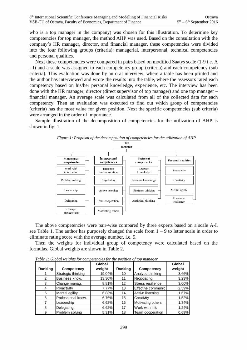
who is a top manager in the company) was chosen for this illustration. To determine key
competencies for top manager, the method AHP was used. Based on the consultation with the
company’s HR manager, director, and financial manager, these competencies were divided
into the four following groups (criteria): managerial, interpersonal, technical competencies
and personal qualities.
Next these competencies were compared in pairs based on modified Saatys scale (1-9 i.e. A
- I) and a scale was assigned to each competency group (criteria) and each competency (sub
criteria). This evaluation was done by an oral interview, where a table has been printed and
the author has interviewed and wrote the results into the table, where the assessors rated each
competency based on his/her personal knowledge, experience, etc. The interview has been
done with the HR manager, director (direct supervisor of top manager) and one top manager –
financial manager. An average scale was calculated from all of the collected data for each
competency. Then an evaluation was executed to find out which group of competencies
(criteria) has the most value for given position. Next the specific competencies (sub criteria)
were arranged in the order of importance.
Sample illustration of the decomposition of competencies for the utilization of AHP is
shown in fig. 1.
Figure 1: Proposal of the decomposition of competencies for the utilization of AHP
The above competencies were pair-wise compared by three experts based on a scale A-I,
see Table 1. The author has purposely changed the scale from 1 – 9 to letter scale in order to
eliminate rating score with the average number, i.e. 5.
Then the weights for individual group of competency were calculated based on the
formulas. Global weights are shown in Table 2.
Table 1: Global weights for competencies for the position of top manager
Ranking Competency
Global
weight Ranking Competency
Global
weight
1 Strategic thinking 19.04% 10 Analytic thinking 3.66%
2 Business know. 13.30% 11 Negotiating 3.23%
3 Change manag. 8.81% 12 Stress resilience 3.00%
4 Proactivity 7.77% 13 Effective communic. 2.59%
5 Mental agility 6.83% 14 Active listening 1.67%
6 Professional know. 6.76% 15 Creativity 1.52%
7 Leadership 6.62% 16 Motivating others 1.34%
8 Delegating 6.62% 17 Work with info 1.24%
9 Problem solving 5.31% 18 Team cooperation 0.69%

8th International Scientific Conference Managing and Modelling of Financial Risks Ostrava
VŠB-TU of Ostrava, Faculty of Economics, Department of Finance 5th – 6th September 2016
400
Utilization of WINGS method for the Determination of Necessary Training
The existing WINGS model of interrelationships and influences was used as a starting
point and importance measure was added to the matrix as characterized by (1). Then the
following sequence of (2) to (4) was used to determine the total strength-influence matrix T.
Then values of i ir c and i ir c were calculated to draw the engagement-position maps for
each of the levels of the model.
Figure 2: Engagement-position map for top level competencies
As can be seen from Figure 2 the personal and interpersonal competencies highly affect the
managerial competencies, so it means that the attention should be paid to the development of
these competencies, i.e. the personal and interpersonal competencies should be developed the
most, since they affect the most the other ones. Technical competencies are independent, and
they are neither affected nor affecting any other competencies and should be developed as
well.
Utilization of TOPSIS method for Employees’ Evaluation
Next, first seven core competencies were selected for the yearly appraisal of the employees.
The employees were evaluated on all the competencies; however the most important
competencies (seven first) i.e. professional knowledge, analytic thinking, proactivity, mental
agility, team cooperation, effective communication and stress resilience will be linked to the
employees’ total reward. The TOPSIS method was used to find out (according to employees
score in each key competency – see table 2) what the ranking of the employees are see table
7.6.
Table 2: Evaluation of employees according to TOPSIS for top manager
Alternative Strategic
thinking
Business
knowledge
Change
management Proactivity
Mental
agility
Professional
knowledge Leadership
Employee 1 87 64 87 74 68 65 63
Employee 2 95 75 88 75 65 58 68
Employee 3 88 78 67 66 70 67 58
Employee 4 75 68 71 73 68 60 56
Employee 5 78 55 72 68 58 65 78

8th International Scientific Conference Managing and Modelling of Financial Risks Ostrava
VŠB-TU of Ostrava, Faculty of Economics, Department of Finance 5th – 6th September 2016
401
The data in table 2 show what evaluation employee 1 - 5 received for the core (first seven)
competencies. The applicant’s ranking is, within the TOPSIS method, determined based on
value ci, since it deals with distance minimization from the ideal variant, whereas the values
are in descending order. The results of employees’ rankings are shown in table 3.
Table 3: Ranking of employees according to TOPSIS for position top manager
Ranking Employees Evaluation
1 Employee 2 0.88
2 Employee 1 0.60
3 Employee 3 0.57
4 Employee 4 0.31
5 Employee 5 0.19
From the table above it is evident that employee 2 is the closest to the ideal variant,
followed by employee 1 and employee 3. Employee 5 has received the worst evaluation with
0.19 which is very far from 1 – the ideal variant.
6. Conclusion
This work briefly describes the competency models, its development and utilization. It also
deals with the description of WINGS method and its utilization in competency modeling. The
results from WINGS imply that among the employees’ interpersonal, personal and managerial
competencies are cause and effect relationships that show how those competencies are
interrelated. This insight should help the company’s management to concentrate on improving
particular competencies that are most influential to the others. The technical competencies
were found to be not affecting nor affected by other competencies. When comparing results
from AHP and WINGS we have to look for an intersection. The most important competency
according to prioritization using AHP is professional knowledge followed by analytic
thinking. Using WINGS, it was found that these competencies are independent to other
competencies and are interrelated only within technical competencies themselves. This means
that company HRM will not be able to influence them by enhancing other competencies and
also that better technical competencies shall not be influential to for example managerial ones.
Since the technical competencies are important the employees selected for the position have to
have these competencies at higher level than the others that can be somehow influenced and
steadily improved. AHP method helped to scale down the number of measures and helped to
determine the most important competencies which lead to the achievement of firm’s strategic
goals. Because of the inherently inter-related nature of the attributes, the determination
process of priorities can be quite complex. According to study’s findings, one may use the
AHP and the WINGS to study the design of competency models as a HR strategic
management system.
Another intersection is among AHP and TOPSIS methods that can be used for more
transparent employee appraisal. Additionally the appraisal priorities can be changed according
to current company situation, strategy and goals. This can be helpful for implementation of
managerial concepts that require continual monitoring of personal or organizational targets.
TOPSIS method uses comparison and ranking to given quantitative values and its properties
can be set to represent chosen evaluation purpose (compromise solution).
The work presented an example that revealed fundamental benefits of MCDM approach
towards competency modeling. AHP method helped to scale down the number of measures
and helped to determine the most important competencies which lead to the achievement of

8th International Scientific Conference Managing and Modelling of Financial Risks Ostrava
VŠB-TU of Ostrava, Faculty of Economics, Department of Finance 5th – 6th September 2016
402
firm’s strategic goals. Because of the inherently inter-related nature of the attributes, the
determination process of priorities can be quite complex. According to study’s findings, one
may use the AHP and the WINGS to study the design of competency models as a HR strategic
management system. AHP and WINGS methods easily handle qualitative and quantitative
metrics simultaneously while incorporating subjective elements of the choice process that may
perhaps be so deeply latent to the respondents’ underlying thought processes that the
respondents are unable to articulate. The AHP and WINGS are also able to neatly capture the
consensus of a potentially divergent group of managers and can be quickly and easily updated
as desired.
References
[1] Barett, A. & O’Connell P.J. Does the training generally work? The returns to in company
training. Industrial and Labor Relations Review, 2001, 54 (3): 647-662.
[2] Bartoňková, H. Firemní vzdělávání. Praha: Grada, 2010. ISBN 978-80-247-2914-5.
[3] Boyatzis, R. E. Competencies in the 21st Century. Journal of Management Development.
Vol. 27 No. 1 (2008), emerald Group Publishing, pp. 5-12.
[4] Boyatzis, R. E. Competencies as a Behavioral Approach to Emotional Intelligence.Journal
of Management Development, Vol. 28 No. 9, pp. 749-770.FORREST, Steven P. and
Tim O. Peterson, E. (2006). It’s called andragogy. Academy of Management Learning &
Education, 5, 113-122.
[5] Kashi, K. & Friedrich V. Manager’s Core Competencies: Applying the Analytic
Hierarchy Process Method in Human Resources. In: Proceedings of the 9th European
Conference on Management Leadership and Governance. Maria Th. Semmelrock-Picej
a Ales Novak. 1. vyd. Reading: Academic Conferences and Publishing International
Limited, 2013.(pp. 384-393).
[6] Kashi, K., & Franek, J. (2014). MADM Methods: Applying Practical Decision Making in
Business Processes. In 13th European Conference on Research Methodology for
Business and Management Studies, City University London, 16-17 June 2014 (pp. 416-
424). Reading: ACPI.
[7] Michnik, Jerzy. (2013) „Weighted Influence Non-linear Gauge System (WINGS) – An
analysis method for the systems of interrelated components“. European Journal of
Operational Research. Vol. 228, No. 3, pp. 536-544.
[8] Minarčíková, E. (2015). Evaluation of Regional Disparities in Visegrad Four based on
Selected MCDM Methods. In 9th International Days of Statistics and Economics
Conference Proceedings (pp. 1128-1137). Prague: Melandrium.
[9] Prokopenko, Joseph and Milan Kubr et al. Vzdělávání a rozvoj manažerů. Praha: Grada,
1996. ISBN 80-7169-250-6.
[10] Sanghi, Seema. The Handbook of Competency Mapping. London: Sage, 2007. ISBN
978-0-7619-3598.
[11] Veteška, Jaroslav and Michaela Tureckiová. Kompetence ve vzdělávání. Praha: Grada,
2008. ISBN 978-80-247-1770-8.
[12] Zmeškal Z., & Dluhošová, D. (2015). Application of the advanced multi-attribute
nonadditive methods in finance distribution. In 10th International Scientific Conference

8th International Scientific Conference Managing and Modelling of Financial Risks Ostrava
VŠB-TU of Ostrava, Faculty of Economics, Department of Finance 5th – 6th September 2016
403
Financial management of Firms and Financial Institutions Ostrava, (pp. 1439-1449).
Ostrava: VŠB-TU Ostrava.
Acknowledgement
This paper is supported by the Student Grant Competition of the Faculty of Economics,
VSB-Technical University of Ostrava, project registration number SP2016/123 and by the
Education for Competitiveness Operational Programme, project registration number
CZ.1.07/2.3.00/20.0296. All support is greatly acknowledged and appreciated.
8th International Scientific Conference Managing and Modelling of Financial Risks Ostrava
VŠB-TU of Ostrava, Faculty of Economics, Department of Finance 5th – 6th September 2016
404
The sense of Real options for valuation
Jakub Kintler 1
Abstract
Real options which are formed on the basis of fixed assets allow the company to minimize risks
associated with investing. We can point that real options represent a contract based on an
underlying asset, which allows the investor to create variant possibilities of the future
development of investment and gives him the opportunity to make decisions in order to stabilize
revenue from this investment. This paper points to the possibility and sense of using real options
for valuation.
Key words
Valuation, real options, personal options
JEL Classification: G32, D46
1. Úvod
Neistota vývoja trhu a podnikateľského prostredia, ktorá je charakteristická pre pokrízový
vývoj v západnej časti sveta, kladie na firmy v záujme zachovania ich konkurencieschopnosti
požiadavku flexibilnosti, ktorá neustále rastie. Požiadavka flexibility sa týka hlavne eliminácie
rizík spojených so zmenami v spotrebiteľských preferenciách, kvalite výrobných vstupov
a materiálov, v znižovaní nákladov, pri zavádzaní nových technológií a produktov na trh.
Reálne opcie predstavujú efektívny nástroj eliminácie rizík spojených s investičnou činnosťou
podniku. Predmetom tohto článku je poukázať na význam využitia reálnych opcií pre znaleckú
činnosť a proces ohodnotenia podniku. V nasledujúcom texte sa budeme zaoberať
predovšetkým rizikami spojenými s investíciami do ľudského kapitálu podniku.
2. Reálne opcie
Reálne opcie sa bežne využívajú pri posudzovaní návratnosti a výhodnosti investícií,
stavieb, PPP projektov, investícií do technológií a pod.. Ich podstata je v tom, že znejú na
konkrétne stále aktívum firmy. V tomto zmysle sú identické s finančnými aktívami, pretože
rovnako generujú výnosy, sú merateľné, vyžadujú finančné krytie, nesú v sebe riziko straty
(zníženia) hodnoty, prípadne rastu hodnoty. Miernou odlišnosťou je merateľnosť nárastu
hodnoty pre nehmotné aktíva firmy akými sú: know-how, goodwill a pod.. Je však potrebné
uviesť, že existujú rozdiely medzi reálnymi a finančnými opciami, ktoré sú zásadné:[1]
obchodovateľnosť – pre reálne opcie zatiaľ neexistuje dostatočne rozvinutý trh,
taktiež sa prejavujú určité asymetrie trhu,
merateľnosť – problematické stanovenie hodnoty nehmotných zložiek aktív
dátum exspirácie opcie – pri reálnych opciách nie je tento dátum presne
stanovený
1 Ing. Jakub Kintler, PhD., Článok je výstupom projektu MŠ SR VEGA číslo 1/0857/16 pod názvom:
Zvyšovanie konkurencieschopnosti malých a stredných podnikov prostredníctvom zavádzania inovácií
v globálnom hospodárskom prostredí, zodpovedný riešiteľ prof. Ing. Helena Majdúchová, CSc., e-mail.:

8th International Scientific Conference Managing and Modelling of Financial Risks Ostrava
VŠB-TU of Ostrava, Faculty of Economics, Department of Finance 5th – 6th September 2016
405
spôsob uzatvorenia kontraktu a podmienok jeho uplatnenia.
Napriek týmto obmedzeniam sa použitie reálnych opcií pri vyhodnocovaní návratnosti
investičných projektov stále viac používa, pretože firme umožňuje v závislosti od
obmedzujúcich podmienok relatívne presne vypočítať hodnotu investície v budúcnosti. Reálne
opcie umožňujú firme minimalizovať nasledovné druhy rizík a neistôt spojených
s investovaním do stálych aktív:[2]
neistota návratnosti – vyplýva z neočakávaného poklesu hodnoty a tým straty
kapitálu
neistota objemu – závisí od sezónnych výkyvov produkovaného množstva,
v závislosti od neočakávaných zmien v dopyte,
neistota nákladov a kvality – závisí od kvality používaných vstupov
a sortimentnej skladby výstupu firmy.
Ľudský kapitál predstavuje vo firme zložku intelektuálneho kapitálu, ktorý je nositeľom
tvorivej činnosti a z hľadiska na jeho nazeranie ho môžeme považovať za strategický nástroj
budovania budúcej ekonomickej sily každého podniku. Kvalifikovaný, správne motivovaný
a tvorivý personál predstavuje v súčasných trhových podmienkach komparatívnu
podnikateľskú výhodu, ktorá nepriamo ovplyvňuje rast hodnoty podniku. Je preto nevyhnutné
poznať riziká spojené s investíciami do ľudského kapitálu firmy, ako aj možnosti ich eliminácie
alebo zabezpečenia. Ľudský kapitál rovnako ako iné zložky kapitálu podniku je nevyhnutné
vnímať ako aktívum, ktoré je merateľné, vyžadujúce investície a súčasne predstavuje riziko
zníženia alebo zvýšenia hodnoty podniku. Rovnako je nutné uviesť aj tú skutočnosť, že ľudský
kapitál rovnako ako stále aktíva generuje nielen súčasné, ale aj budúce výnosy firmy. Riziko
spojené s investíciou do ľudského kapitálu firmy je spojené s nasledovnými druhmi neurčitosti,
ktoré sa prejavujú ako volatilita plánovaných firemných veličín budúcnosti:[3]
neistota výnosu a výkonnosti
neistota množstva
neistota nákladov
Neistota výnosu a výkonnosti je spojená s problematikou zastarania ľudského kapitálu
podniku a rastom fluktuácie. Neistota zastaranosti ľudského kapitálu sa viaže na zastaranie
mentálnych schopností a neochoty, prípadne neschopnosti pracovníkov učiť sa využívať nové
technológie. Fluktuácia predstavuje druhú oblasť neistoty spojenú s výkonnosťou firmy.
Rastúca fluktuácia spôsobuje znižovanie produktivity práce, zvyšovanie nákladov spojených
s náhradou zamestnancov na uvoľnených pracovných pozíciách a súčasne znižuje zisk, ktorý
by vytvorili odchádzajúci pracovníci. Tento druh neistoty je ešte významnejší, ak z firmy
odchádzajú kľúčoví zamestnanci (nositelia firemného know-how a tvorcovia pokračujúcej
hodnoty firmy).
Neistota množstva je spojená so sezónnosťou a kolísaním dopytu. Tomuto druhu rizika
musia čeliť najmä firmy, ktoré sa zaoberajú výrobou sezónneho tovaru alebo poskytujú služby,
ktorých objem je naviazaný na sezónne výkyvy v dopyte. Ide napr. o firmy poskytujúce
ubytovacie a reštauračné služby. Neistota množstva môže byť spojená s rastúcim dopytom po
určitom výrobku alebo službe. Môže ísť napríklad o situáciu, kedy firma nebude schopná
v plnej miere uspokojiť dopytu po svojich produktoch, v dôsledku čoho jej môžu vzniknúť
náklady spojené s neplnením dohodnutých výkonov alebo dodávok. V prostredí pracovnej
legislatívy Slovenska existuje legálny nástroj na elimináciu rizika v dôsledku kolísania dopytu,
ktorým je konto pracovného času.
Neistota nákladov je spojená s nákladmi na zamestnancov. Najväčšiu časť nákladov
spojených s pracovnými silami tvoria mzdové náklady. Ak by sme rozdelili personálne náklady
na variabilné a fixné, potom zmluvné mzdy predstavujú fixnú časť nákladov. Riziko nákladov
je spojené predovšetkým s fixnými nákladmi na zamestnancov. Fixnými nákladmi na
zamestnancov budeme rozumieť základné mzdy kmeňových pracovníkov zamestnaných na

8th International Scientific Conference Managing and Modelling of Financial Risks Ostrava
VŠB-TU of Ostrava, Faculty of Economics, Department of Finance 5th – 6th September 2016
406
trvalý pracovný pomer. Súčasťou tejto problematiky je aj realokácia zamestnancov prípadne
ich znalostí v kontexte kvantitatívnych a kvalitatívnych zmien v dopyte a ponuke.
Riziká uvedené v tomto článku, ktoré sa viažu k ľudskému kapitálu nepredstavujú všetky
riziká spojené s týmto investovaním, uviedli sme len niektoré z nich, aby sme preukázali ich
podobnosť s rizikami, ktoré zvažuje každá firma pri rozhodovaní sa o investičných aktivitách.
3. Porovnanie reálnych a personálnych opcií
Využívanie personálnych nástrojov získavania, udržovania a motivovania pracovných síl
firmy predstavujú prostriedky, pomocou ktorých firma investuje do ľudského kapitálu. Na
základe uvedenej vedomosti môžeme nástroje využívané v personalistike prirovnať k reálnym
opciám, pretože ich cieľom je minimalizovať riziko neúspechu firmy na jej trhovom segmente
a zároveň maximalizovať jej podnikateľskú aktivitu. Porovnateľnosť reálnych opcií
a personálnych nástrojov možno rozvinúť na týchto predpokladoch: sú podložené hmotnými
alebo nehmotnými aktívami firmy, hodnota podkladového aktíva sa mení v čase, sú zmluvne
uzatvárané a poskytujú investorovi variabilitu riešenia v závislosti na okolnostiach. V tabuľke
nižšie uvádzame porovnanie finančných, reálnych a personálnych opcií.
Tabuľka 1: Porovnanie jednotlivých druhov opcií[4]
Kategória Finančné opcie Reálne opcie Personálne opcie
opcia znejúca na finančný derivát hmotné a nehmotné
aktívum
znalosti, zručnosti a správanie sa
zamestnancov
hodnota
podkladového
aktíva
má vlastnú hodnotu má vlastnú hodnotu
zamestnanci generujú hodnotu
použitím znalostí, schopností a
vzorcov správania
variabilita aktíva hodnota finančného
derivátu kolíše v čase
hodnota aktíva kolíše
v čase
využiteľnosť znalostí, schopností a
správania zamestnancov kolíšu v čase
funkcia opcie udáva rozsah budúcich
investícií
udáva rozsah budúcich
investícií
udáva budúcu schopnosť prispôsobenia
sa zamestnancov
cieľ opcie špekulatívny burzový
nástroj
špekulatívny nástroj
investovania
investícia do budúcich schopností a
foriem správania sa zamestnancov
typ opcie kúpna, predajná partnerstvo,
joint- venture
kombinácia nástrojov používaných v
personalistike
právo spojené s
vlastníctvom opcie
predaj alebo kúpa za
vopred stanovenú cenu
v budúcnosti
právo uskutočňovať,
zanechať alebo zmeniť
projekt
rozsah zmeny používaných
personálnych nástrojov vzhľadom na
budúce potreby
opčná prémia právo na finančnú
kompenzáciu
umožňuje čiastočné
investovanie môže zvyšovať aktuálne náklady
Na základe porovnania jednotlivých druhov opcií v tabuľke vyššie môžeme konštatovať ich
vzájomnú podobnosť, preto sa v ďalšom texte budeme zaoberať, akým spôsobom môžu
personálne opcie prispieť k eliminácii rizika neurčitosti z investovania finančných prostriedkov
do ľudského kapitálu podniku. Pracujeme pritom s predpokladom, že niektoré používané
nástroje v personalistike vytvárajú pre firmu možnosti pre minimalizáciu budúcich strát
a súčasne generujú dostatok budúcich možností pre rast a zvyšovanie ziskovosti podnikania.
Pre analýzu investícií do personálnych zdrojov sa budeme zaoberať nasledovnými druhmi
personálnych opcií: opcie na elimináciu neurčitosti návratnosti, opcie na elimináciu neurčitosti
objemu a opcie na elimináciu neurčitosti nákladov.
Personálne opcie ako nástroj eliminácie neurčitosti návratnosti sú orientované na
znižovanie rizika spojeného so zastaraním ľudského kapitálu. Súčasťou uvedeného druhu opcií
je aj eliminácia rizika spojeného s finančnými stratami a nákladmi na zdokonaľovanie
a získavanie nových zručností zamestnancov. Je nutné povedať, že zastaranie ľudského kapitálu

8th International Scientific Conference Managing and Modelling of Financial Risks Ostrava
VŠB-TU of Ostrava, Faculty of Economics, Department of Finance 5th – 6th September 2016
407
sa nedeje plošne, existujú určité schopnosti, zručnosti zamestnancov, ktoré zastarávajú
rýchlejšie ako iné napr. schopnosť viesť motorové vozidlo a dokonale ovládať najmodernejšie
informačné technológie. Eliminovať zastaranie ľudského kapitálu sa uskutočňuje
prostredníctvom tréningu, školení prípadne náborom nových zamestnancov alebo personálnym
lízingom. Napríklad pri získavaní nových zamestnancov si firma stanoví vyššie požiadavky na
vzdelanie, bude uprednostňovať uchádzačov so schopnosťou kreatívneho a analytického
myslenia, alebo uprednostní pracovníkov so široko orientovanými schopnosťami pred
špecializovanými. Následne je možné utvoriť rastúce opcie na základe zvyšovania kvalifikácie
a zlepšovania schopností zamestnancov. Druhou oblasťou problematiky tejto skupiny rizík je
fluktuácia. Rozdiel medzi personálnymi aktívami podniku a jeho stálymi aktívami je v tom, že
ľudí nemožno v plnej miere vlastniť. Zamestnanci môžu odísť z firmy podľa svojho vlastného
uváženia a v čase kedy im to práve vyhovuje. Z uvedeného hľadiska fluktuácia zamestnancov
predstavuje jednu z veľmi významných rizík investícií do ľudského kapitálu podniku.
Odchodom kľúčových zamestnancov firma stráca výkonnosť a títo zamestnanci si so sebou
odnášajú aj svoje jedinečné schopnosti a často aj know-how, ktoré do firmy priniesli, alebo ho
nadobudli. Zamestnanci najčastejšie opúšťajú firmu z dôvodu nespokojnosti s: pracovným
prostredím, ohodnotením pracovného výkonu, nedostatočnou motiváciou, zlou komunikáciu
s nadriadeným, nedostatočnými kompetenciami a pod.. Firmy sa snažia tento negatívny jav
eliminovať týmito prostriedkami: rastom miezd, participáciou na výsledkoch podniku,
ponúkaním rôznych benefitov, školení a iných programov v záujme zníženia fluktuácie kriticky
významných zamestnancov firmy. Firmy s vysokou mierou fluktuácie budú vytvárať viacero
rôznych konkurenčne atraktívnych personálnych opcií v záujme stabilizácie svojich
zamestnancov.
Personálne opcie ako nástroj eliminácie neurčitosti množstva vychádzajú z potreby
zabezpečiť v podniku v rôznom čase rozličné množstvo pracovníkov. Z hľadiska dopytu po
pracovnom kapitále hovoríme o volatilite s ohľadom na sezónnosť, kontrakty, projekty,
brigádnickú prácu, prácu na čiastočný úväzok a prácu na trvalý pracovný pomer. Ak firma
pôsobí v prostredí, kde jej odbyt závisí od aktuálneho vývoja dopytu na trhu, bude vytvárať
personálne rastúce opcie a personálne opcie na čas. Personálne rastúce opcie umožňujú získať
firme potrebný ľudský kapitál bez toho, aby sa nositelia uvedeného kapitálu stali jej kmeňovými
zamestnancami v aktuálnom čase, alebo aby mohli byť internovaní v čase, keď sa ich
schopnosti stanú pre firmu potrebnými. Pre tieto účely firmy využívajú personálny lízing.
Personálne opcie na čas predstavujú všetky formy pracovného pomeru s výnimkou trvalého
pracovného pomeru.[5]
Personálne opcie ako nástroj eliminácie neurčitosti nákladov sú spojené s fluktuáciou
zamestnancov a fixnými nákladmi na zamestnancov. Fixnými nákladmi v tomto prípade
chápeme základné mzdy kmeňových zamestnancov. V prípade vysokých fixných nákladov
firma riskuje straty v dôsledku poklesu tržieb. Mzdy zamestnancov tvoria vo väčšine podnikov
najvyššiu nákladovú položku a zároveň vytvárajú aj najväčší tlak na tok hotovosti. Preto firmy
v záujme eliminácie uvedeného balíka rizík vytvárajú personálne opcie na znižovanie nákladov.
Takýmito opciami môžu byť napríklad znižovanie podielu fixných zložiek mzdy smerom
k variabilným. Variabilnými zložkami miezd sú podiely na zisku, na znížení nákladov, na
tržbách a iné. Je nutné povedať, že nie je možné v legislatívnych podmienkach Slovenska
zaviesť plne variabilné mzdy z dôvodu zákonom stanovenej minimálnej mzdy, čo môžeme pre
podnikanie vnímať ako fixnú mzdu. Napriek preukázaným empirickým výsledkom o miere
zainteresovanosti zamestnanca na výkone firmy, ktorá je priamo úmerná k jeho osobnej
angažovanosti na eliminácii nákladov a raste ziskovosti.

8th International Scientific Conference Managing and Modelling of Financial Risks Ostrava
VŠB-TU of Ostrava, Faculty of Economics, Department of Finance 5th – 6th September 2016
408
4. Význam personálnych opcií pre proces ohodnotenia podniku
Proces ohodnotenia podniku predstavuje postupnosť krokov realizovaných prostredníctvom
zodpovedajúcich metód a techník, ktorých cieľom je určiť najpravdepodobnejšiu cenu v danom
čase a priestore, za ktorú by bolo možné podnik predať pri zodpovedajúcej miere
informovanosti predávajúceho a kupujúceho. Základnými metódami stanovenia všeobecnej
hodnoty podniku v legislatívnom prostredí Slovenskej republiky sú statické a dynamické
metódy ohodnotenia. Medzi statické metódy zaraďujeme metódy vychádzajúce z ohodnotenia
jednotlivých zložiek majetku a zdrojov jeho krytia. Podkladom pre stanovenie všeobecnej
hodnoty podniku sú predovšetkým účtovné a finančné výkazy minulého obdobia, ktoré sú
procesom objektivizácie upravené pre potreby ohodnotenia k stanovenému dátum. Pokiaľ je
dňom ohodnotenia konkrétny dátum v minulosti, objektivizujeme jednotlivé zložky majetku
podniku a zdrojov jeho krytia k uvedenému dátumu, pretože z účtovných a finančných výkazov
vieme relatívne presne určiť výkonnosť a úspešnosť podnikania ohodnocovaného podniku na
základe súboru nástrojov finančno-ekonomickej analýzy. Medzi dynamické metódy stanovenia
všeobecnej hodnoty podniku zaraďujeme predovšetkým výnosové metódy, ktoré anticipujú
budúci vývoj a podnikateľskú úspešnosť ohodnocovaného subjektu. V uvedenom prípade
analyzujeme budúci potenciál podniku na trhu. Teda pracujeme s určitou anticipáciou
podnikateľskej aktivity a stability rozvoja podniku v budúcnosti. Z tohto hľadiska sa v procese
objektivizácie, na základe poskytnutých interných materiálov podniku snažíme predpokladať
budúce výnosy a náklady podniku. Z nich následne počítame zisk a schopnosť podniku
generovať odčerpateľné zdroje, ktoré následne prepočítavame na súčasnú hodnotu. Všeobecnú
hodnotu podniku podnikateľskou metódou pri neobmedzenej životnosti vypočítame
nasledovne: [6]
𝑉Š𝐻𝑃 = 𝐻𝑂𝑍 + 𝐻𝑃 =∑𝑂𝑍𝑡
(1 + 𝑖)𝑡+ (
𝑂𝑍𝑛+1𝑖 − 𝑔
∗1
(1 + 𝑖)𝑛)
𝑛
𝑡−1
za predpokladu 𝑖 > 𝑔
kde:
HOZ – všeobecná hodnota odčerpateľných zdrojov počas hodnoteného obdobia,
OZt – odčerpateľné zdroje počas hodnoteného obdobia,
HP – hodnota pokračujúca,
i – vypočítaná miera kapitalizácie v percentách odrážajúca mieru rizika, priemernú
nákladovosť kapitálu a štruktúru využívaného kapitálu,
OZn+1 – objem odčerpateľných zdrojov v roku nasledujúcom po sledovanom období,
g – trvale udržateľná miera rastu odčerpateľných zdrojov v percentách,
n – dĺžka sledovaného obdobia.
Všeobecnú hodnotu podniku vypočítanú podnikateľskou metódou významným spôsobom
ovplyvňujú dve premenné a to miera kapitalizácie (i) a trvale udržateľná miera rastu (g).
[7]Trvalo udržateľnú mieru rastu podniku zásadným, okrem iných faktorov ovplyvňuje aj
ľudský kapitál, teda personálne zdroje podniku. Napriek skutočnosti, že nie je samostatnou
zložkou majetku vykazovanou v účtovnej a finančnej evidencii, rozhodujúcou mierou
ovplyvňuje budúcu aktivitu, stabilitu, výnosovosť a potenciálny rozvoj podnikateľskej aktivity,
preto je nevyhnutné jeho hodnotu inkorporovať do stanovenia všeobecnej hodnoty podniku.
Jedným z možných prístupov, ako to realizovať je zvýšiť hodnotu trvale udržateľnej miery rastu
na základe analýzy výnosového potenciálu ľudského kapitálu podniku, prostredníctvom
uplatnenia výnosových metód ohodnotenia ľudského kapitálu, ako napríklad HEVA alebo
HCROI.[8]

8th International Scientific Conference Managing and Modelling of Financial Risks Ostrava
VŠB-TU of Ostrava, Faculty of Economics, Department of Finance 5th – 6th September 2016
409
5. Záver
Súčasné ekonomické prostredie, ktoré je charakteristické prehlbujúcou sa geopolitickou
nestabilitou kladie čoraz väčší dôraz na schopnosť prispôsobiť sa novým zmeneným
podmienkam. Nositeľmi schopnosti prispôsobiť sa a zaujať relevantný postoj, ktorý zabezpečí
podnikateľskému subjektu stabilitu a predpoklad na budúci rozvoj sú zamestnanci, nositelia
know-how podniku. Aj na základe uvedeného poznania je potrebné vnímať zamestnancov vo
svojej podstate ako kapitál podniku, do ktorého je potrebné investovať a tak prispievať k jeho
stabilizácii a rozvoju. Každé investičné rozhodnutie vo svojej podstate znamená určitú mieru
neistoty a rizika s ňou spojenú. Je preto logické, že sa podniky snažia toto riziko eliminovať.
Rovnako aj investície do zamestnancov-ľudského kapitálu podniku predstavujú isté riziká,
pretože zamestnancov, teda ľudí nie je možné v plnej miere vlastniť a rozhodovať o nich.
Zamestnanci sú vo svojom rozhodovaní v podstate nezávislí. Investície do ľudského kapitálu
podniku sú teda spojené predovšetkým s rizikom fluktuácie, zastarania, prípadne rastu
nákladovosti. Pre elimináciu týchto rizík môžeme využiť reálne opcie. Pre elimináciu rizík
spojených s investovaním do ľudského kapitálu možno použiť personálne opcie, ktoré svojou
podstatou a významom pre podnik kopírujú reálne opcie. Cieľom personálnych opcií je
zabezpečiť podnikateľskému subjektu investičnú stabilitu a návratnosť vložených investícií do
podnikania.
References
[1] Grisáková, N., 2015. Binomické stromové modely ako nástroj na riešenie reálnych opcií:
Binomial models as a tool for solving real option models. Aktuálne problémy podnikovej
sféry 2015 : [recenzovaný] zborník vedeckých prác, pp.158-166.
[2] Kintler, J., 2013. Eliminácia rizík spojených s investovaním do ľudského kapitálu podniku:
Elimination of the risks associated with the investment in human capital of enterprises.
Personálny marketing a personálny manažment v organizácii : recenzovaný zborník
vedeckých prác, pp.54-65.
[3] Majdúchová, H., Rybárová, D., 2014. Qualitative vs. quantitative risk analysis. Managing
and modelling of financial risks : proceedings : 7th international scientific conference :
8th - 9th september 2014, Ostrava, Czech Republic, pp.455-461.
[4] Bhattacharya, M., Wright, P.: Recognizing Risk in Human Capital Investments : A Real
Options Approach to Strategic Human Resource Management. New York: CAHRS, 2000,
dostupné na internete 30.10.2013
[5] Štetka, P., Rybárová, D., 2014. Vnímané riziko a nákupná konformita. Trendy v podnikání
2014 : recenzovaný sborník příspěvků mezinárodní vědecké konference : Plzeň, 13. - 14.
listopadu 2014, pp.1-7.
[6] Vyhláška Ministerstva spravodlivosti SR číslo 492/2004 Z.z., v platnom znení, ktorou sa
vykonáva zákon č. 382/2004 Z.z., Zákon o znalcoch, tlmočníkoch a prekladateľoch a o
zmene a doplnení niektorých zákonov v znení neskorších zmien.
[7] Rybárová, D., 2014. Výpočet rizika pri stanovení všeobecnej hodnoty majetku: Risk
calculation by the valuation of company´s assets. Znalectvo : v ekonomických odboroch a
stavebníctve, 18(1), pp.14-17.
[8] Pallavi, A.K., Neeraja, R.: A Study on Human Cupital Valuation and Management. In:
IOSR Journal of Business and Management (IOSRJBM) ISSN: 2278-487X Volume 1,
Issue 2 (May-June 2012), dostupné na internete 30.10.2013

8th International Scientific Conference Managing and Modelling of Financial Risks Ostrava
VŠB-TU of Ostrava, Faculty of Economics, Department of Finance 5th – 6th September 2016
410
Back-testing the effectiveness of selected indicators technical analysis of the currency pair using digital
options
Andrea Kolková 1
Abstract
Digital (binary) options are a new instrument of the financial market. History trading on the
OTC market dates from 2008. They are considered very risk investments, therefore no relevant
prediction of the underlying asset, these investments are ineffective. By means of technical
analysis the development of underlying asset can be predicted to some extent and thus digital
options can be put into very attractive investments. The aim of this paper is back-testing the
effectiveness of selected indicators technical analysis of the currency pair with the application
digital options. For this post we are chosen technical analysis indicators mainly based on
moving averages. Testing will be done on a five-minute, hourly, daily, weekly and monthly
charts. The test will be subjected to each of the selected time frame of 65 000 the fair value of
the course, in the course of the currency pair EUR/USD. Effectiveness analysis of indicators
will be made just using digital (binary) options.
Key words
Digital option, technical analysis, forex, simple moving average, exponencial moving average,
MACD
JEL Classification: G10
1. Úvod
V současné době jsou finanční trhy velmi dynamickou veličinou. Technická analýza sama
nabízí velké množství možností, jak reagovat na měnící se situaci na trzích. Při svém
průzkumu Taylor a Allen (1992) zjistil, že na britském trhu nejméně 90% respondetů využívá
technickou analýzu při rozhodování o jejich portfoliích. Camphbell (1997, str. 27) dokonce
považuje možnosti předpovídání cen finančních aktiv za hlavní otázku finanční ekonometrie.
Ve studii Oberlechnera (2001) lze vyčíst i používání technické analýzy v porovnání s
fundamentální. Obelechner (2001) se zaměřil pouze na obchodování s měnovými páry a
dokonce obchodníky rozdělil dle časového horizontu obchodování a dle logiky technickou
analýzu ve větší míře používají obchodníci intradenní a to 65,3%, naopak obchodníci s dobou
držení měny déle než 1 rok se z 67,9% zaměřují spíše na fundamentální analýzu.
2. Teoretické východiska
Technická analýza předpovídá budoucí pohyb kurzů na základě analýzy minulých cen za
využití kvalitativních metod, jako například grafická analýza, ale i kvantitativních metod, jako
je klouzavý průměr, exponenciální klouzavý průměr, anebo využívá kombinaci obojího. V
souladu se základní definicí Murphy (1999, str. 3) jsou základními předpoklady technické
1 Ing. Andrea Kolková, Ph.D., Vysoká škola podnikání a práva, a.s., [email protected].

8th International Scientific Conference Managing and Modelling of Financial Risks Ostrava
VŠB-TU of Ostrava, Faculty of Economics, Department of Finance 5th – 6th September 2016
411
analýzy ceny odrážející všechny tržní události, kurzy se měnící v trendech a historické ceny
mající tendenci se opakovat.
Technická analýza se snaží předpovědět budoucí vývoj ceny na základě analýzy jejího
minulého vývoje (Murphy 1999), k tomu lze použít velmi rozmanité metody. Základem je
však vždy matematická statistika (Kaufman, 2013). Možnosti technické analýzy je vhodné
rozdělit do dvou skupin a to technické indikátory a price action.
Systémy založené na price action jsou známy dokonce již z 18. století, kdy Japonci na své
obchody s rýží aplikovali první svíčkové grafy. Dnes jsou publikovány o něco méně než
technické indikátory například K.H. Lee, G.S. Jo (1999), a jsou předmětem výzkumu spíše na
bázi programování jako například Izumi at all (2006).
Technických indikátorů je celá řada. Některé jsou tradiční a jsou známy již desetiletí. Již v
roce 1988 vydal Colby encyklopedii technických tržních indikátorů (Colby, 1988). George
Lane již před více než třemi desetiletími publikoval svůj Lane’s stochastic oscillator (Lane,
1984), nebo dokonce v 70.tých letech vznikl The relative strength (RS) rozvinutý Wilderem
(1978). V 80.-90. letech 20. století zveřejnil například indikátor Bollinger Bands John
Bollinger (Bollinger, 1992), tento patří do skupiny kanálových systémů, které popsal už
Kaufman (1987) a tím výčet indikátorů zdaleka nekončí.
Z novějších je znám například Chaikin oscillator (Achelis, 2001), či dnes velmi používaný
indikátor MACD představený Appel (2005). V roce 2007 (Cheung & Kaymak, 2007) byl
představen koncept kombinující technické indikátory a fuzzy logiku. Abbasi a Abouec
využitli i systém odvozený od neuro-fuzzy logiky (Abbasi, Abouec, 2008). V roce 2009
Chavarnakul & Enke, (2009) vyvinul hybridní model obchodování na burze za použití Neuro-
fuzzy konceptu nazvaný Genetic Algorithm (NF-GA). V roce 2015 pak technické indikátory
(konkrétně MACD a méně známý indikátor Gann-Hilo) a fuzzy logicku použili znovu
(Chourmouziadis a Chatzoglou, 2015). V současné době dochází ke konstrukci stále nových
indikátorů jako například Rubell at all (2016) založených jak na fuzzy modelování, tak na
kombinaci jednotlivých statisticko-matematických indikátorů. Stávající jsou pak podrobovány
nejrůznějším testům (da Costa, 2015).
Technickou analýzu lze aplikovat jak na trhy akciové, komoditní, tak měnové. A to jak na
akcie přímo, tak na CFD, tak na derivátové produkty nejrůznějšího typu (opce, futures,
swapy). Například opce ještě nabízejí další možnosti. Jedním z nich jdou kombinace opcí
tvořících nejrůznější opční strategie (Kolková, 2006). Dalšími jsou různé exotické opce, jako
například digitální neboli binární, o kterých hovoří například Rick Thachuk (2010), Jaworsky
(2006), Jurník (2013) nebo Cánfas (2013). Použití technické analýzy na tyto nové finanční
produkty je dosud málo publikováno. Případně pokud ano, směřuje pozornost téměř výhradně
na oceňování opcí jako například Hong joong y and Kyoung-sook Moonz (2011), Zmeskal
(2010), Thavaneswarana at all. (2013) nebo Miyake (2016).
Foreing rate exchange (dále jen forex) je největší finanční trh na světě s denním objemem
transakcí převyšující 5 bilionu dolarů. Je to decentralizovaný trh a proto na rozdíl od jiných
aktiv je možno s měnami obchodovat 24 hodin denně.
Riziko představuje trvalý prvek v každé investiční aktivitě, a tedy i na forexovém trhu.
Technická analýza dle Hada a Adamuta (2015) hraje v prevenci tohoto rizika významnou roli
a představuje klíčový bod pro zajištění rizika při obchodech s měnovými páry. Protože
zejména forexové obchody jsou vysoce rizikové, navíc ve spojení s digitálními opcemi, je
vhodné použít i technickou analýzu pro předvídání budoucích změn.

8th International Scientific Conference Managing and Modelling of Financial Risks Ostrava
VŠB-TU of Ostrava, Faculty of Economics, Department of Finance 5th – 6th September 2016
412
3. Výzkumné metody
Realizace technické analýzy na konkrétním trhu se opírá o důkladné sestavení obchodnícho
systému, tento můžeme dle Costa (2015) popsat jako soubor pravidel, která definují podmínky
k zahájení či ukončení obchodování. V tomto příspěvku bude obchodní systém sestaven na
základě technických indikátorů na bázi klouzavých průměrů.
3.1 Klouzavé průměry
Klouzavé průměry vyčíslují průměrnou hodnotu údajů v šíři svého časového rámce.
Například 7 denní klouzavý průměr značí průměrnou hodntou za poslední týden, 14 denní za
poslední dva týdny. Po spojení klouzavých průměrů všech dnů pak vytvoříme křivku
klouzavého průměru. Platformy umožňující obchody na forexu ve většině případů obsahují
možnosti automatického znázornění klouzavý průměry, proto jsou tradery velmi využívaným
nástrojem, bez znalosti jejich principů jsou ovšem pomůckou bezcenou.
3.1.1 Jednoduchý klouzavý průměr
Jednoduchý klouzavý průměr, anglicky Simple Moving Average (dále jen SMA) je možno
definovat vztahem,
N
PSMA
N
i 1 , kde
P je kurz měnového páru a N je počet dní, za který je SMA vyčíslován. Při testování bude
využita strategie křížení klouzavého průměru s aktuálním kurzem. V případě křížení shora to
bude implikovat signál k prodeji v opačném případě signál k nákupu. Zásadním problémem u
volby tohoto indikátoru je definování počtu dní, za který je SMA počítán, v tomto příspěvku
je použita 9 denní SMA.
3.1.2 Exponenciální klouzavé průměry (EMA)
Exponenciální klouzavý průměr neboli Exponencial Moving Average (dále jen EMA) je
považován za lepší nástroj než SMA (Elder, 2006), protože přikládá větší váhu aktuálním
datům a na změny ceny odpovídá rychleji než jednoduchý. Je možno jej vyjádřit vztahem,
)1(01 KEMAKPEMA , kde
1
2
NK , kde
N je počet dnů k vyčíslení EMA, 1P je dnešní kurz a 0EMA je včerejší hodnota EMA.
V tomto příspěvku je opět aplikován obchodní systém na bázi křížení EMA s aktuálním
kurzem, kdy křížení shora je signálem k prodeji a křížení opačné k nákupu. EMA je použita
12 denní a 9 denní.
3.1.3 Klouzavý průměr konvergence divergence
Klouzavý průměr konvergence divergence respektive Moving Average
Convergence/Divergence (dále jen MACD) je jedním z nejpoužívanějších indikátorů vůbec.
V základní verzi, která je použita i v tomto příspěvku se jedná o rozdíl mezi 26 denním a 12
denním indikátorem EMA. Spolu s takto získanou křivkou MACD křivkou je ještě nutno
zakreslit křivku 9 denní EMA, která je nazývána signalizační křivkou. Zde zvolený obchodní
systém se pak opírá o křížení signalizační křivky s MACD křivkou. Protne-li MACD signální
křivku zespoda je to signál k nákupu EURUSD, pokud je to naopak pak k prodeji.

8th International Scientific Conference Managing and Modelling of Financial Risks Ostrava
VŠB-TU of Ostrava, Faculty of Economics, Department of Finance 5th – 6th September 2016
413
3.2 Metodika hodnocení výkonnosti obchodních systémů
Pro analýzu byly využity kurzy měnového páru EURUSD. Pro získávání dat byl využit
program Metatrader4 a analýze byly podrobeny data s časovým rámcem pětiminutovým,
patnáctiminutový, hodinovým, denním, týdenním a měsíčním. Pro data pětiminutová bylo
analyzováno 65 000 hodnot kurzů, v časovém období od 3.6. 2015 do 19.4. 2016. Kurzů
s patnáctiminutovým časovým rámcem bylo použito taktéž 65 000, časové období se
pochopitelně prodloužilo na období od 6.11 2013 do 19.4 2016. Hodinová data byla získána
taktéž v počtu 65 000, časové období pak začínalo už 11.10.2005. Kurzy denní byly již
z pochopitelných důvodu pouze v počtu 4 535 od období 1.1. 1999. Kurzů týdenních je pak
možno získat 912 a měsíčních 209.
Dle obchodních systémů definovaných v kapitolách 3.1.1 – 3.1.3 byly vyhledány obchodní
signály a to jak k nákupu, tak k prodeji. Na tyto signály byly aplikovány digitální opce
s trojnásobnou expirací, a to s následující logikou: digitální opce up na signály k nákupu a
digitální opce down na signály k prodeji. Digitální opce mají v aktuálním období míru
návratnosti 85,01% (například broker XTB na účtu Basic). Na základě této míry pak jsou
vyčísleny celkové zisky z obchodního systému. Všechny výpočty jsou realizovány v programu
Excel.
4. Výsledky
V tabulce 1 jsou zachyceny výsledky zpětného testování obchodních systémů na EURUSD
s pětiminutovým časovým rámcem. Z těchto systémů se jeví jako nejvhodnější použití SMA 9
denní. Indikátor MACD neposkytuje na daném time frame zisk.
Table 1: Testování EURUSD s pětiminutovým time frame
IndikátorCelkový počet
signálů
Počet signálů
generujících zisk
Procento ziskových
signálů
Zisk při použití
digitálních opcí
SMA 9 13033 10578 81% 19%
EMA 9 13950 10770 77% 16%
EMA 12 12078 9456 78% 16%
MACD 5162 3093 59% 0%
V tabulce 2 jsou vyčísleny výsledky strategií za použití 15 minutového časového rámce.
Z těchto výsledků opět je patrný nejlepší ziskový výsledek z indikátoru SMA. Je nutno
podotknout, že tento indikátor také poskytuje nejvíce možných signálů. Obchodní systém
založený na MACD je zcela nevhodný.
Table 2: Testování EURUSD s patnáctiminutovým time frame
IndikátorCelkový počet
signálů
Počet signálů
generujících zisk
Procento ziskových
signálů
Zisk při použití
digitálních opcí
SMA 9 13112 10596 80% 18%
EMA 9 13879 10704 77% 16%
EMA 12 11839 9265 78% 16%
MACD 4881 2895 59% 0%
Při testování EURUSD na hodinovém časovém rámci jsou výsledky obdobné, opět
nejvýhodněji vychází SMA a indikátor MACD je nevhodný.

8th International Scientific Conference Managing and Modelling of Financial Risks Ostrava
VŠB-TU of Ostrava, Faculty of Economics, Department of Finance 5th – 6th September 2016
414
Table 3: Testování EURUSD s hodinovým time frame
IndikátorCelkový počet
signálů
Počet signálů
generujících zisk
Procento ziskových
signálů
Zisk při použití
digitálních opcí
SMA 12469 10180 81% 19%
EMA 9 12816 9997 78% 16%
EMA 10654 8393 79% 17%
MACD 4792 2838 59% 0%
Na delších time frime se situace mění. Na jednodenním časovém rámci se do popředí
zájmu dostává indikátor MACD, který poskytuje nejméně signálů, ovšem nejvíce ziskových.
Indikátor EMA také zlepšuje svou výkonnost se vzrůstajícím počtem dnů, na který je
vypočítáván.
Table 4: Testování EURUSD s jednodenním time frame
IndikátorCelkový počet
signálů
Počet signálů
generujících zisk
Procento ziskových
signálů
Zisk při použití
digitálních opcí
SMA 9 812 651 80% 18%
EMA 9 891 678 76% 15%
EMA 12 717 562 78% 17%
MACD 370 337 91% 27%
U jednotýdenních grafů je situace podobná opět je nejvýhodnější strategie založená na
MACD, která zde dokonce poskytuje 92% ziskových signálů.
Table 5: Testování EURUSD s jednotýdenním time frame
IndikátorCelkový počet
signálů
Počet signálů
generujících zisk
Procento ziskových
signálů
Zisk při použití
digitálních opcí
SMA 9 166 127 77% 15%
EMA 9 185 144 78% 16%
EMA 12 167 127 76% 15%
MACD 60 55 92% 28%
V případě posledního a to měsíčního time frame je situace obdobná a zcela nejvýhodnější
se jeví MACD. Také EMA při zvýšení dnů výpočtu je jednoznačně ziskovější strategií.
Table 6: Testování EURUSD s jednoměsíčním time frame
IndikátorCelkový počet
signálů
Počet signálů
generujících zisk
Procento ziskových
signálů
Zisk při použití
digitálních opcí
SMA 9 36 28 78% 16%
EMA 9 31 20 65% 5%
EMA 12 25 18 72% 11%
MACD 15 14 93% 29%
5. Závěr
Z výsledků práce vyplývá, že délka časového rámce je velmi důležitá při rozhodování o
indikátoru, který bude pro technickou analýzu využit. Analýza jednoznačně dokládá fakt, že

8th International Scientific Conference Managing and Modelling of Financial Risks Ostrava
VŠB-TU of Ostrava, Faculty of Economics, Department of Finance 5th – 6th September 2016
415
na dlouhé časové rámce je vhodnější použití indikátoru MACD na krátké časové rámce jsou
vhodnější SMA nebo EMA. Nebylo také prokázáno, že by indikátor EMA byl pro technickou
analýzu na měnový pár EURUSD lepší nástroj než jednoduchý vážený průměr. Naopak je
zřejmé, že indikátor EMA je přesnější pro delší počet dní ve výpočtu. Testování probíhalo na
digitálních opcích, které na měnovém páru EURUSD generují v aktuálním období míru
návratnosti 85,01%. V posledním sloupci tabulek výsledků je tedy konečný zisk po započtení
míry návratnosti garantované brokerem.
Předmětem dalšího testování mohou být další strategie na bázi průměrů například křížení
klouzavých průměrů, nebo řazení klouzavých průměrů, či kombinace indikátorů na bázi
průměrů s jinými například oscillátory a momentové indikátory, indikátory volatility, nebo
indikátory supportů a resistencí. Případně dalším zkoumáním je možno podrobit i jiné měnové
páry, komodity, indexy nebo akcie.
References
[1] Achelis, S. B. (2001). Technical analysis from A to Z. McGraw Hill New York.
[2] Abbasi, E., & Abouec, A. (2008). Stock price forecast by using neuro-fuzzy inference
system. In Proceedings of the world academy of science, engineering and technology: 36
(pp. 320–323).
[3] Appel, G. (2005). Technical analysis: power tools for active investors. FT Press.
[4] Bollinger, John.(1992) Using bollinger bands. Stocks & Commodities, 10.2: 47-51.
[5] Colby, R. W., & Meyers, T. A. (1988). The encyclopedia of technical market indicators .
Irwin New York.
[6] da Costa, T. R. C. C., Nazário, R. T., Bergo, G. S. Z., Sobreiro, V. A., & Kimura, H.
(2015). Trading system based on the use of technical analysis: A computational
experiment. Journal of Behavioral and Experimental Finance, 6, 42–55.
[7] Chavarnakul, T., & Enke, D. (2009). A hybrid stock trading system for intelligent
technical analysis-based equivolume charting. Neurocomputing, 72 (16), 3517–3528.
[8] Cheung, W. M., & Kaymak, U. (2007). A fuzzy logic based trading system. In
Proceedings of the third european symposium on nature inspired smart information
systems, 07 . St. Julians, Malta.
[9] Chourmouziadis, K., & Chatzoglou, P. D. (2015). An intelligent short term stock trading
fuzzy system for assisting investors in portfolio management. Expert Systems with
Applications .doi: 10.1016/j.eswa.2015.07.063.
[10] Jaworski, A. (2006) CBOT Launches Binary Options. Securities Industry News. 18, 27,
11, 24.7., 2006. ISSN: 10896333.
[11] Jurník, D. (2013) Co jsou to binární opce a jak to funguje. http://www.binarni-
opce.com/manual-binarnich-opci/co-jsou-to-binarni-opce-a-jak-to-funguje Consulted: 8.
4 2013
[12] Kaufman, P.J., (1987). The New Commodity Trading Systems and Methods. New York:
John Wiley and Sons. ISBN 978-1-118-0-4356-1

8th International Scientific Conference Managing and Modelling of Financial Risks Ostrava
VŠB-TU of Ostrava, Faculty of Economics, Department of Finance 5th – 6th September 2016
416
[13] Kim, Hong-Joong; Moon, Kyoung-Sook. (2011) Variable time-stepping hybrid finite
difference methods for pricing binary options. Bulletin of the Korean Mathematical
Society. Volume 48, Issue 2, 2011, pp.413-426, Publisher : The Korean Mathematical
Society
[14] Lane, G. C. (1984). Lane’s stochastics. Technical Analysis of Stocks and Commodities,
2 (3), 80.
[15] Lee, K., & Jo, G. (1999). Expert system for predicting stock market timing using a can-
dlestick chart. Expert Systems with Applications, 16 (4), 357–364.
[16] Miyake, M, Inoue, H, Shi, J, & Shimokawa, (2014), 'A Binary Option Pricing Based on
Fuzziness', International Journal Of Information Technology & Decision Making, 13, 6,
pp. 1211-1227, Business Source Premier, EBSCOhost, viewed 26. 4. 2016.
[17] Rick Thachuk (2010) Binary options - the next big retail investing boom?. FOW
[online]. 2010. ISSN 14629658.
[18] Thavaneswarana, A. Appadoob, S.S. Frank, J (2013) Binary option pricing using fuzzy
numbers. Applied Mathematics Letters, Volume 26, Issue 1, January 2013, Pages 65–72
[19] Wilder, J. W. (1978). New concepts in technical trading systems. Trend Research
Greens-boro, NC.
[20] Zmeskal, Z. (2012) Generalized soft binomial American real option model (fuzzy–
stochastic approach). European Journal of Operational Research, 207, pp. 1096–1103

8th International Scientific Conference Managing and Modelling of Financial Risks Ostrava
VŠB-TU of Ostrava, Faculty of Economics, Department of Finance 5th – 6th September 2016
417
Stochastic dominance enhanced portfolios - empirical evidence
Miloš Kopa 1
Abstract
Stochastic dominance is a relation between two random variables allowing to compare random
returns of two portfolios. Based on the type of stochastic dominance, a decision maker can use
the first-order, the second-order, the third-order stochastic dominance criteria or some more
general rules. In this paper, we analyze the optimal portfolios of stochastic dominance
constrained problems for maximizing mean returns objective and various types of stochastic
dominance relations (the first-order, the second-order, the third-order). Especially, we focus on
the risk-reward in-sample performance of the portfolio returns. We consider monthly returns of
25 Fama-French portfolios (base assets) from two periods: during crises period (2007-2010) and
after crises period (2011-2014). We compare the results of the during crises period with that of
the after crises period.
Key words
Portfolio selection, stochastic dominance, reward-risk performance
JEL Classification: D81, G11
1. Introduction
Mean return maximization is one of the basic goals of a portfolio manager. Starting from a
seminal paper of Markowitz (1952), a risk measuring and controlling has become another
important feature of the portfolio selection. The risk of the investment can be modelled using
risk measures, deviation functionals, etc. Indirectly, the risk attitude of the decision maker can
be captured by a utility function. If so, it leads to maximizing expected utility problem.
However, if the utility function of the decision maker is not know, the maximizing expected
utility problem can not be solved. In this case, the decision maker can circumvent it
considering a set of utility functions. If only a partial knowledge about the utility function is
available (for example concavity) then stochastic dominance (SD) is a useful approach to
decision making.
Stochastic dominance is, in general, a relation between two random variables. This relation
allows for comparison of random returns of losses of the investments. The most popular
stochastic dominance relations are so called the first-order (FSD), the second-order (SSD) and
the third-order (TSD) stochastic dominance. A random variable X dominates a random
variable Y with respect to the N-th order stochastic dominance, 𝑁 = 1, 2, 3 if
𝔼𝑢(𝑋) ≥ 𝔼𝑢(𝑌) for all 𝑢 ∈ 𝑈𝑁
where the set of admissible utility functions for the 𝑁-th order stochastic dominance is
defined as follows:
1 doc. RNDr. Ing. Miloš Kopa, Ph.D., Charles University in Prague, Faculty of Mathematics and
Physics, Department of Probability and Mathematical Statistics, Sokolovská 83, 186 75 Prague, Czech
Republic, e-mail: [email protected]

8th International Scientific Conference Managing and Modelling of Financial Risks Ostrava
VŠB-TU of Ostrava, Faculty of Economics, Department of Finance 5th – 6th September 2016
418
𝑈𝑁 = {𝑢(𝑥) ∈ 𝐷𝑁: (−1)𝑘𝑢(𝑘) ≤ 0, ∀𝑥, 𝑘 = 1, . . . , 𝑁}.
The basics of stochastic dominance go back to 1960th, see Quirk and Saposnik (1962),
Hadar and Russell (1969), Hanoch and Levy (1969), Rothschild and Stiglitz (1970) and
Whitmore (1970). In these papers, several sufficient and necessary conditions for the 𝑁-th
order stochastic dominance, 𝑁 = 1,2,3, were derived. For example, a random variable 𝑋
dominates a random variable 𝑌 with respect to the 𝑁-th order stochastic dominance, 𝑁 = 1,2
if and only if
𝐹𝑋(𝑁)
(𝑧) ≤ 𝐹𝑌(𝑁)
(𝑧) ∀𝑧 ∈ ℝ
where 𝐹𝑋(1)
(𝑧) is a cumulative distribution function of 𝑋 and
𝐹𝑋(2)
(𝑧) = ∫𝑧
−∞𝐹𝑋
(1)(𝑡)𝑑𝑡.
See [13] for more details.
In last years, a substantial development of the stochastic dominance applications in finance
was realized; for example in the following directions:
• portfolio efficiency with respect to stochastic dominance criteria was analyzed, see e.g.
Post and Kopa (2013), Grechuk (2014), Kopa and Post (2015) or Post, Fang and Kopa (2015).
• more robust version of stochastic dominance relations and stochastic dominance
efficiency tests, see e.g. Dentcheva and Ruszczynski (2010), Kopa (2010), Dupačová and
Kopa (2012, 2014).
• more general stochastic dominance (ordering) rules, see e.g. Ortobelli et al. (2013,
2016) and references therein, or Post (2016).
• portfolio enhancement using stochastic dominance rules, mainly the second-order
stochastic dominance criterion, see e.g. Roman, Mitra and Zverovich (2013), Hodder,
Jackwerth and Kolokolova (2015), Post and Kopa (2016).
• Data Envelopment Analysis equivalent models in the sense that a portfolio is classified
efficient with respect to a stochastic dominance relation if and only if it is efficient with
respect to a particular Data Envelopment Analysis model, see Branda and Kopa (2012, 2014,
2016) for more details.
In this paper we focus on the portfolio selection problems which maximize expected return
under stochastic dominance constraints. We consider three models, one with the first-order
stochastic dominance relation, another one with the second-order stochastic dominance
relation and the last one with the third-order stochastic dominance relation. In all models, the
relations are applied to compare the portfolio random return to the random return of a
benchmark. We provide the empirical analysis using monthly data (returns) of 25 Fama
French representative portfolios. The analysis uses two sets of historical data 2007 – 2010 and
2011 - 2014 from the Kenneth French library. We consider the US market index proxied by
CRSP as the benchmark. The goal of the analysis is to compare the risk-reward performance
of the optimal (solution) portfolio for various orders of stochastic dominance and for the two
considered data sets.
The remainder of this paper is structured as follows. Section 2 presents a basic properties
of the SSD relations as well as of the TSD relations. It is followed by a summary of portfolio
selection models with FSD, SSD and TSD constraints in Section 3. These models assume an
empirical distribution of the returns. Section 4 shows the results of the numerical study. The
paper is summarized and concluded in Section 5.

8th International Scientific Conference Managing and Modelling of Financial Risks Ostrava
VŠB-TU of Ostrava, Faculty of Economics, Department of Finance 5th – 6th September 2016
419
2. Stochastic dominance criteria
We consider a random vector r = (r1, r2, . . . , rN)′ of returns of N assets in T equiprobable
scenarios. The returns of the assets for the various scenarios are collected in matrix:
X = (
x1
x2
⋮xT
)
where xt = (x1t , x2
t , … , xNt ) is the t-th row of matrix X. A vector of portfolio weights is
denoted by λ = (λ1, λ2, . . . , λN)′ and the portfolio possibilities are described by
Λ = {λ ∈ RN|1′λ = 1, λn ≥ 0, = 1,2, … , N}.
Let Fr′λ(1)
(x) denote the cumulative probability distribution function of returns of portfolio λ.
The twice cumulative probability distribution function of returns of portfolio λ is given by:
Fr′λ(2)
(t) = ∫t
−∞Fr′λ
(1)(x)dx (1)
and the three times cumulative probability distribution function of returns of portfolio λ is
similarly defined as:
Fr′λ(3)
(y) = ∫y
−∞Fr′λ
(2)(t)dt. (2)
Portfolio λ ∈ Λ dominates portfolio τ ∈ Λ by the first-order stochastic dominance
(r′λ ≻FSD r′τ) if and only if
Fr′λ(1)
(t) ≤ Fr′τ(1)
(t) ∀t ∈ ℝ.
Similarly, portfolio λ ∈ Λ dominates portfolio τ ∈ Λ by the second-order stochastic
dominance (r′λ ≻SSD r′τ) if and only if
Fr′λ(2)
(t) ≤ Fr′τ(2)
(t) ∀t ∈ ℝ.
Finally, portfolio λ ∈ Λ dominates portfolio τ ∈ Λ by the third order stochastic dominance
(r′λ ≻TSD r′τ) if and only if
Fr′λ(3)
(t) ≤ Fr′τ(3)
(t) ∀t ∈ ℝ
and 𝔼(r′λ) ≥ 𝔼(r′τ). See more details in Levy (2016). One could similarly formulate the
necessary and sufficient condition for the general N-th order stochastic dominance in terms of
the N-times integrated distribution functions. However, we are not going to apply these
relations to the portfolio optimization.

8th International Scientific Conference Managing and Modelling of Financial Risks Ostrava
VŠB-TU of Ostrava, Faculty of Economics, Department of Finance 5th – 6th September 2016
420
3. Portfolio selection with stochastic dominance constraints
The optimization models with stochastic dominance constraints were firstly proposed in
Dentcheva and Ruszczynski (2003) for the second-order stochastic dominance relation. Later
on, it was applied to portfolio enhancing in e.g. Roman, Mitra and Zverovich (2013).
Similarly, Hodder, Jackwerth and Kolokolova (2015) applied Kopa and Post (2015) model for
the portfolio enhancement based on the second-order stochastic dominance. In this paper, we
follow these papers and consider the following three models:
max 𝔼(r′λ) (3) s. t. r′λ ≻𝐹𝑆𝐷 r′τ
λ ∈ Λ
max 𝔼(r′λ) (4) s. t. r′λ ≻𝑆SD r′τ
λ ∈ Λ
max 𝔼(r′λ) (5) s. t. r′λ ≻𝑇SD r′τ
λ ∈ Λ
where 𝝉 is a given benchmark (reference) portfolio. Since we consider a discrete distribution
of returns with equiprobable scenarios we can follow Kuosmanen (2004) and reformulate (3)
as a linear mixed integer programming problem:
max𝑝𝑖,𝑗,𝝀
1
𝑇∑𝑇
𝑡=1 𝐱𝑡𝝀 (6)
s.t. 𝑋λ ≥ 𝑃𝑋τ
𝑃 = {𝑝𝑖,𝑗}𝑖,𝑗=1𝑇 , ∑ 𝑝𝑖,𝑗 = ∑ 𝑝𝑖,𝑗 =
𝑇
𝑗=1
𝑇
𝑖=1
1
𝑝𝑖,𝑗 ∈ {0,1}, 𝑖, 𝑗 = 1, … , 𝑇
λ ∈ Λ.
Similarly, following Kopa and Post (2015) or Hodder, Jackwerth and Kolokolova (2015)
problem (4) can be reformulated as follows:
max𝑑𝑠,𝑣𝑡,𝑠,𝝀
1
𝑇∑𝑇
𝑡=1 𝐱𝑡𝝀 (7)
s. t. – 𝑇−1𝐱𝑡𝝀 +1
𝑠𝑑𝑠 − 𝑣𝑡,𝑠 +
1
𝑠∑
𝑇
𝑘=1
𝑣𝑘,𝑠 ≤ −1
𝑇𝑠∑
𝑠
𝑘=1
𝐱𝑘𝝉, 𝑡, 𝑠 = 1,2, … , 𝑇
𝑑𝑠, 𝑣𝑡,𝑠 ≥ 0, 𝑡, 𝑠 = 1,2, … , 𝑇
λ ∈ Λ
Assuming a partition (𝑧1, . . . . , 𝑧𝐾) such that 𝑧1 ≤ 𝐱𝑡𝝉 and 𝑧𝐾 ≥ 𝐱𝑡𝝉 for all 𝑡 = 1,2, . . . , 𝑇,
Post and Kopa (2016) proposed a SCTSD model with a tight sufficient condition for
𝐫′𝝀 ≻𝑇𝑆𝐷 𝐫′𝝉:
max𝜃𝑘,𝑡,𝝀
1
𝑇∑𝑇
𝑡=1 𝐱𝑡𝝀 (8)

8th International Scientific Conference Managing and Modelling of Financial Risks Ostrava
VŠB-TU of Ostrava, Faculty of Economics, Department of Finance 5th – 6th September 2016
421
s. t. 1+𝑒𝑘
2𝑇∑𝑇
𝑡=1 𝜃𝑘,𝑡2 ≤ 𝐹𝐫′𝝉
(3)(𝑧𝑘), 𝑘 = 1, . . . , 𝐾
𝜃𝑘,𝑡 ≥ 𝑧𝑘 − 𝐱𝑡𝝀 𝑘 = 1, . . . , 𝐾, 𝑡 = 1, . . . , 𝑇
1
𝑇∑𝑇
𝑡=1 𝐱𝑡𝝀 ≥1
𝑇∑𝑇
𝑡=1 𝐱𝑡𝝉
𝝀 ∈ Λ
𝜃𝑘,𝑡 ≥ 0, 𝑘 = 1, . . . , 𝐾, 𝑡 = 1, . . . , 𝑇
where 𝑒1 = 𝑒2 = 0 and
𝑒𝑘 =𝐹𝐫′𝝉
(3)(𝑧𝑘)
𝐹𝐫′𝝉(3)
(𝑧𝑘−1)+𝐹𝐫′𝝉(2)
(𝑧𝑘−1)(𝑧𝑘−𝑧𝑘−1)− 1, 𝑘 = 3, . . . , 𝐾.
In this paper, we consider K=100 equidistant partition points. Alternatively, one could
consider, for example: K=T
4. Numerical study
In this section we apply problems (6)-(8) to monthly returns of 25 Fama-French portfolios
(base assets) formed on size and book-to-market, such that the portfolios are the intersections
of 5 portfolios formed on size (market equity, ME) and 5 portfolios formed on the ratio of
book equity to market equity (BE/ME). Moreover we include returns of one-year US tbill as
the risk free returns. The reference (benchmark) portfolio τ is the market US portfolio,
proxied by the CRSP index. We take two data sets: one from the during crisis period 2007-
2010 and the other one from the after crisis period 2011-2014. (each period consists of 240
scenarios of returns).
The following tables summarize the results in terms of means and variances of optimal
solutions. To be able to compare it with the benchmark, we also present a mean-standard
deviation profile of the benchmark in each period.
Table 1: Risk-reward profile of solution portfolios – during crisis period
Portfolio Mean Standard deviation
Benchmark 0.1846 5.7801
FSD solution portfolio 0.1846 5.7801
SSD solution portfolio 0.8963 6.1931
TSD solution portfolio 0.9216 6.4098
Table 2: Risk-reward profile of solution portfolios – after crisis period
Portfolio Mean Standard deviation
Benchmark 1.2463 3.4017
FSD solution portfolio 1.2463 3.4017
SSD solution portfolio 1.3333 3.3271
TSD solution portfolio 1.3501 3.5879
5. Conclusion
In this paper we analyzed the optimal solutions and the risk-reward (mean-variance) profile
of the mean maximizing portfolio selection problem with the first-order, second-order and
third-order stochastic dominance constrains. These constraints guarantee that the solution
portfolio is preferred to the US market portfolio (benchmark) by all investors obeying the
particular stochastic dominance rules. We compared the results of all three models among

8th International Scientific Conference Managing and Modelling of Financial Risks Ostrava
VŠB-TU of Ostrava, Faculty of Economics, Department of Finance 5th – 6th September 2016
422
each other considering two different data sets: one from the during crisis period (2007-2010)
and the other one from the after crisis period. We found that during crisis optimal portfolios
have smaller mean returns and higher standard deviations comparing to the correspondent
after crisis optimal portfolios. Since the first-order stochastic dominance implies the second-
order and it implies the third-order stochastic dominance, the solution portfolio of the third-
order stochastic dominance constrained problems had the highest mean return. However, it is
at the costs of the highest standard deviation. The first-order stochastic dominance is so strong
relation that the solution portfolio is the benchmark, that is, there is no other FSD dominating
portfolio (neither in the first period data nor in the second one). In the after crisis period,
moving to the second-order stochastic dominance constraints leads to portfolio with higher
mean return and smaller standard deviation. However, this is not observed in the during crisis
period. Finally, moving from the second-order to the third-order stochastic dominance
constraints gives a solution portfolio with higher mean returns and higher standard deviations
of returns in both considered periods.
For future research, this study can be improved in various ways. For example, longer
historical data can be used or different frequency data can be considered (mainly with daily
returns). In addition, one can consider the stochastic dominance relations in a more robust
way as it was done in Kopa (2010) or Dupačová and Kopa (2012, 2014) for the first and the
second-order stochastic dominance, using contamination techniques and the worst-case
approach. Alternatively, one can compare the results also with the case when the DARA
(decreasing absolute risk aversion) stochastic dominance is used, see Post, Fang and Kopa
(2015) for more details. Unfortunately, all these improvements would lead to much more
computationally demanding optimization problems.
Acknowledgement: The research was supported by the Czech Science Foundation (GAČR)
under the project No. 15-02938S.
References
[1] Branda, M., and Kopa, M.: DEA-risk Efficiency and Stochastic Dominance Efficiency
of Stock Indices. Czech Journal of Economics and Finance 62, 2 (2012), 106–124.
[2] Branda, M., and Kopa, M.: On relations between DEA-risk models and stochastic
dominance efficiency tests. Central European Journal of Operations Research 22, 1
(2014), 13–35.
[3] Branda, M., and Kopa, M.: DEA models equivalent to general 𝑁-th order stochastic
dominance efficiency tests. Operations Research Letters 44 (2016), 285–289.
[4] Dentcheva, D., and Ruszczynski, A.: Optimization with stochastic dominance
constraints, SIAM Journal on Optimization 14 (2003), 548–566.
[5] Dentcheva, D., and Ruszczynski, A.: Robust stochastic dominance and its application to
risk-averse optimization. Mathematical Programming, Series B 123 (2010), 85–100.
[6] Dupačová, J. and Kopa, M.: Robustness in stochastic programs with risk constraints.
Annals of Operations Research 200, 1 (2012), 55–74.
[7] Dupačová, J. and Kopa, M.: Robustness of optimal portfolios under risk and stochastic
dominance constraints. European Journal of Operational Research 234, 2 (2014), 434–
441.
[8] Grechuk, B.: A simple SSD-efficiency test. Optimization Letters 8, 7 (2014), 2135 –
2143.

8th International Scientific Conference Managing and Modelling of Financial Risks Ostrava
VŠB-TU of Ostrava, Faculty of Economics, Department of Finance 5th – 6th September 2016
423
[9] Hadar, J. and Russell, W. R.: Rules for Ordering Uncertain Prospects. American
Economic Review 59, 1 (1969), 25–34.
[10] Hanoch, G. and Levy, H.: The efficiency analysis of choices involving risk. Review of
Economic Studies 36 (1969), 335–346.
[11] Kopa, M.: Measuring of second-order stochastic dominance portfolio efficiency.
Kybernetika 46, 2 (2010), 488–500.
[12] Kopa, M. and Post, T.: A general test for SSD portfolio efficiency, OR Spectrum 37, 3
(2015), 703 – 734.
[13] Kuosmanen, T.: Efficient diversification according to stochastic dominance criteria.
Management Science 50, 10 (2004), 1390–1406.
[14] Levy, H.: Stochastic dominance: Investment decision making under uncertainty. Third
edition. New York, Springer, 2016.
[15] Markowitz, H. M.: Portfolio Selection. The Journal of Finance 7, 1 (1952), 77–91.
[16] Ortobelli, S., Lando, T., Petronio, F., and Tichy, T.: Asymptotic stochastic dominance
rules for sums of i.i.d. random variables. Journal of computational and applied
mathematics 300 (2016), 432–448.
[17] Ortobelli, S., Shalit, H., and Fabozzi, F.: Portfolio selection problems consistent with
given preference orderings. International Journal of Theoretical and Applied Finance
16 (2013), 38p.
[18] Post, T.: Standard Stochastic Dominance. European Journal of Operational Research
248 (2016), 1009–1020.
[19] Post, T., Fang Y. and Kopa, M.: Linear Tests for DARA Stochastic Dominance.
Management Science 61, 7 (2015), 1615 – 1629.
[20] Post, T. and Kopa, M.: General Linear Formulations of Stochastic Dominance Criteria.
European Journal of Operational Research 230, 2 (2013), 321–332.
[21] Post, T., and Kopa, M.: Portfolio Choice based on Third-degree Stochastic Dominance.
Forthcoming in Management Science. http://dx.doi.org/10.1287/mnsc.2016.2506
[22] Quirk, J. P., and Saposnik, R.: Admissibility and Measurable Utility Functions. Review
of Economic Studies 29 (1962), 140–146.
[23] Roman, D., Mitra, G., and Zverovich, V.: Enhanced indexation based on second-order
stochastic dominance. European Journal of Operational Research 228 (2013), 273–281.
[24] Rothschild, M., and Stiglitz, J.E.: Increasing risk: I. A definition. Journal of Economic
Theory 2 (1970), 225–243.
[25] Whitmore, G.A.: Third-degree Stochastic Dominance. American Economic Review 60
(1970), 457–459.

8th International Scientific Conference Managing and Modelling of Financial Risks Ostrava
VŠB-TU of Ostrava, Faculty of Economics, Department of Finance 5th – 6th September 2016
424
Risks of Investor Bias
Kateřina Kořená1
Abstract
This paper focuses on the risks connected with the decision-making of investors and explains
their most important biases – loss aversion, mental accounting, herding and anchoring. The
aim of this paper is to describe these psychological biases connected with money and
investing and to explain the main risks investors face in relation to these issues. These biases
are often connected with emotions, representing a significant risk. Loss aversion and herding,
in particular, are the most common biases for many investors, posing an important threat not
only for individual investors but for whole financial markets.
Key words
Risks, investors, biases, behavioral finance, financial markets.
JEL Classification: G02, G11
1. Introduction
It is now assumed that many of the mistakes investors make in financial markets are not
caused by their ignorance of financial instruments but by their behavior. These mistakes are
influenced by emotions and are often involuntary and unintentional (Montier, 2010). This
connection between financial markets and psychology is very important and there is a specific
field of study devoted to it: behavioral finance. Behavioral finance has increasingly become
part of mainstream finance, providing explanations for people’s economic decisions by
combining behavioral psychological theory and conventional finance (Baker and Nofsinger,
2010).
Traditionally, economists concluded that people behave in order to maximize the expected
value of their utility. Behavioral finance has challenged these utility maximization
assumptions as inconsistent with ordinary human behavior (Burton and Shah, 2013).
Behavioral finance studies the effects of emotional factors on the economic decisions of
individuals and the consequences they have for financial markets. Behavioral finance is a field
of study that offers explanations for these irrational individuals’ investment decisions as well
as financial market outcomes.
The aim of this paper is to describe the main psychological biases connected with money
and investing and to explain the main risks investors face in relation to these issues.
2. Loss Aversion
Loss aversion bias marked the very beginning of behavioral finance, as first described in
1979 in the paper “Prospect Theory: An Analysis of Decision under Risk” by Daniel
Kahneman and Amos Tversky.
1 Ing. Kateřina Kořená, Ph.D., VŠB – Technical University of Ostrava, Faculty of Economics.
[email protected]. This paper was supported by the SGS Project VŠB – TU Ostrava 2016/54.

8th International Scientific Conference Managing and Modelling of Financial Risks Ostrava
VŠB-TU of Ostrava, Faculty of Economics, Department of Finance 5th – 6th September 2016
425
Kahneman and Tversky researched human risk-aversion and found that people’s attitudes
associated with gains are different from those concerning losses. This means that homo
economicus and the idea of the rationally acting human are challenged by risk aversion. The
authors proved that the same amount of loss brings more pain in comparison with gain and
joy. Prospect theory formalizes the decision process in a way that corresponds more closely to
how people behave than the utility approach of traditional economics (Burton and Shah,
2013).
Graph 1: Prospect Theory
Source: Investopedia.com
Let us consider a typical example of this type of bias. In the final round of a competition,
contestants are asked a question but face the prospect of losing all their money if they answer
incorrectly. However, the majority of the contestants will choose not to answer even though
they stand to double their money if they answer correctly. The example shows that generally
people do not like risk because they are afraid of making too big a loss. Most people think
receiving less or nothing is a more acceptable result.
In the investment process this bias represents a situation in which investors resist investing
in riskier instruments, e.g. stocks, because of their likelihood to be risky. This bias is
especially typical for conservative investors and can result in a disproportionate portfolio
created by overly conservative financial instruments. A portfolio created in such a way is
ultimately susceptible to inflation.
Table 1: Structure of Savings among Czech Households (in %, 2013)
Current Accounts 40.5%
Term Accounts 10.3%
Foreign Currency Accounts 2.4%
Building Savings 16.4%
Pension Funds 10.8%
Insurance Funds 10.9%
Investment Funds 8.8% Source: Czech National Bank, Ministry of Finance, AKAT
Czech investors are prime examples of conservative investors and typically hold more than
50% of their savings in different types of bank accounts, with the largest share deposited in
current accounts. And since they eschew riskier financial instruments their investments fail to
bring higher yields. This situation is partly explained by the low financial literacy of investors
8th International Scientific Conference Managing and Modelling of Financial Risks Ostrava
VŠB-TU of Ostrava, Faculty of Economics, Department of Finance 5th – 6th September 2016
426
and partly by the bad experience of investing in privatization funds, as evidenced during
voucher privatization in the Czech Republic. However, the result is the same in both cases.
Because the investor is not emotionally prepared for more volatile/riskier investing, the
gamble is avoided.
2.1 Disposition Effect and Regret Theory
These biases are closely connected with loss aversion. The disposition effect relates to the
tendency of investors to sell assets whose price has increased but retain assets that have
decreased in value. This allows investors to enjoy the feeling of winning faster and delaying
the pain of loss. It is also known as the “too proud to sell” phenomenon.
Regret theory is the theory that fear of regret can motivate decision-making (Havlíček and
Stupavský, 2013). According to this theory, investors may avoid investment decisions because
they are afraid of a scenario in which their investments will decrease. The opposite situation is
where investors feel the need to invest because of the fear of missing out on an opportunity. In
the first example the fear lies in regretting the decline in value of their investments, while in
the second example the fear lies in regretting an increase in value as a result of a missed
opportunity. Consequently, people anticipate regret if they make a wrong choice, and take this
anticipation into consideration when making decisions. Major financial decisions appear to be
potentially affected by this feeling of regret.
3. Mental Accounting
This bias pertains to the direct relationship we have with money based on emotions. It is
based on the concept that we form behavioral attachments to money according to our feelings
(Belsky and Gilovich, 2003). People have different mental accounts for the same kind of
resource. For example, people distinguish the way in which income is received. The less
probable your source of income the faster you will spend it. When money is won in a lottery
or an unexpected bonus is received, in such cases people will spend faster than if they were to
receive their regular salary. Another example of mental accounting concerns payment. When
people use payment cards they are likely to buy more goods than if they were to pay in cash.
In simple terms, when you pay with a card it hurts you less because you don’t see the money
vanishing before your eyes.
Mental accounting also affects investors, who are often prepared to lose money on the
financial markets. In other words, investors apportion money they can afford to lose as “play
money”, which they are ready to spend even through speculation. This behavior is of course
irrational, since investing money in financial instruments that are likely to be lost is an evident
example of emotional decision-making.
3.1 Ignoring the Importance of Small Amounts
This bias is demonstrated in situations where relatively small amounts of money are
ignored because the importance of such small amounts cannot be appreciated as having an
impact over the long term (Belsky and Gilovich, 2003). Investors are often persuaded that
such investing is futile and unimportant. But if a person were to invest in an equity fund from
the age of 25 to the age of 65, for example 160 CZK, that person would pocket more than 1
million CZK after 40 years (1,011,853 CZK, a historical average yield of 10% in equity
funds). Take the person who spends 50 CZK every day on buying a cup of coffee. That works
out at approximately 1,000 CZK that could be invested every month. Over the course of a 40-
year working life that person would lose more than 6 million CZK (6,324,080 CZK, a
historical average yield of 10% in equity funds). Similarly, those who invest in financial

8th International Scientific Conference Managing and Modelling of Financial Risks Ostrava
VŠB-TU of Ostrava, Faculty of Economics, Department of Finance 5th – 6th September 2016
427
instruments take little stock of the fees charged for these financial instruments because the
fees are seen as negligible at the time.
4. Herding
The herd effect is the tendency for individuals to mimic the actions of a larger group.
Herding often involves a strong herd mentality, which can affect the ways in which
investments are made in financial markets. This bias is also connected with loss aversion bias.
An example of this bias was seen in global financial markets in 2015/2016 where higher
volatility was observed in the stock market, which in turn affected the types of investments
being placed in investment funds.
Graph 2: Stock Market Development
Source: Fichtner Investment Advisors
During this investment period, investors became wary of investing in equity funds due to
this increased volatility and began to withdraw their money from these funds. This decision-
making was influenced by fear and the behavior of other investors.
Graph 3: Equity Funds Net Sales (in millions of USD to 12/10/2016)
Source: Fichtner Investment Advisors

8th International Scientific Conference Managing and Modelling of Financial Risks Ostrava
VŠB-TU of Ostrava, Faculty of Economics, Department of Finance 5th – 6th September 2016
428
Graph 4: Bond Funds Net Sales (in millions of USD to 12/10/2016)
Source: Fichtner Investment Advisors
In contrast, net sales in bond funds increased due to lower volatility and high profits.
However it must be noted that due to long-term low interest rates, larger investments in these
funds are currently not recommended. This decision-making on the part of investors was
influenced by greed and the behavior of other investors.
In general terms, this type of bias is one of the most dangerous for investors. Indeed, a
strong herd mentality can even affect financial professionals, as was the case in the “dot-com
bubble” of 2000 when herd investors were persuaded that internet stocks were the best
investments. And more recently in 2016 there was panic in the financial markets as a result of
the Brexit decision.
5. Anchoring
Anchoring is a perception bias. Everybody has their own anchor, or conviction, as to what
the right number or situation is any given context. Such anchors can affect investors’ frames
of reference. The most typical situation involves attempting to guess something about which
you have limited information (Burton and Shah, 2013). Anchoring also refers to situations
where investors are persuaded from previous experience that, for example, interest rates are,
as a rule, high which means the relevant contemporary information is not sought. They have
their own strong anchoring belief in the interest rate level, which can affect their decision-
making when it comes to investing. Such investors tend to invest very conservatively because
they feel there is no need to run a risk. For example, if your belief is that interest rates are
prohibitively high, your money will remain in your current account.
This anchor is very common among Czech investors, whose perceptions of interest rates
are connected with a situation that occurred between the years 1990 and 1998 when current
account interest rates soared to just above 8%.2 The result of such thinking prompted Czech
investors to pump more than 50% of their savings into bank accounts (see Table 1).
2 In the Czech Republic the highest discount rate was 13%. In 1997, the highest two-week repo rate
was 39%.
8th International Scientific Conference Managing and Modelling of Financial Risks Ostrava
VŠB-TU of Ostrava, Faculty of Economics, Department of Finance 5th – 6th September 2016
429
Unfortunately, the contemporary situation is completely different in that current account
interest rates are now very low, often even lower than 0.01%.
Also common investment anchors can take the form of investment indices (DJIA, S&P
500) such as TV, Internet, other financial advisors, neighbours, relatives and co-workers. For
the vast majority of investors they are very difficult to avoid.
6. Conclusion
This paper introduces the most typical investment biases of investors. These biases are
often connected with emotions, representing a significant risk. Crucially, these psychological
risks can influence the whole investment and decision-making process. Loss aversion and
herding, in particular, are the most common biases for many investors, posing an important
threat not only for individual investors but for whole financial markets.
References
[1] Baker, H.K. and Nofsinger, J.R. (2010) Behavioral Finance. Investors, Corporations and
Markets. New Jersey: Wiley.
[2] Belsky, H. and Gilovich, T. (2003). Proč chytří lidé dělají hloupé chyby, když jde o
peníze. Praha: Práh.
[3] Burton, E.T. and Shah, S.N. (2013). Behavioral Finance. New Jersey: Wiley.
[4] Havlíček, D. and Stupavský, M. Investor 21. století. (2013). Praha: CFA Society Czech
Republic, Plot.
[5] Montier, J. (2010). The Little Book of Behavioral Investing. New Jersey: Wiley.
[6] Fichtner Investment Advisors. Finanční webinář, říjen 2016.
[7] www.investopedia.com

8th International Scientific Conference Managing and Modelling of Financial Risks Ostrava
VŠB-TU of Ostrava, Faculty of Economics, Department of Finance 5th – 6th September 2016
430
Reward and Risk in the Italian Fixed Income Market
Noureddine Kouaissah 1 Sergio Ortobelli 2 Tomas Tichy 3
Abstract
In this paper, we discuss and examine the portfolio optimization problems in the Italian fixed
income market considering two main sources of risk: prices risk and market risk. To achieve
this aim, we propose a two-step optimization problem for two types of bonds. In particular, we
manage the price risk implementing the classical immunization method and then, using the ex-
post results from the optimal immunization problem, we are able to deal with market risk
maximizing the portfolio wealth in a reward-risk framework. Adopting this approach, the paper
then explores empirical applications on the Italian fixed income market using data for the
period 2005-2015. Empirical results shows that the two-step optimization build efficient
portfolios that minimize the price risk and the market risk. This ex-post analysis indicates the
usefulness of the proposed methodology, maximizing the investor’s wealth and understanding
the dynamics of the bonds.
Key words
Portfolio selection, bond market, immunization, reward-risk measure
JEL Classification: G11, G12
1. Introduction
The risk reward measures have a central role in the portfolio theory ever since the
pioneering work of Markowitz (1952). It follows that many portfolio optimization models
based on reward risk measures have been developed for asset allocation, see Farinelli et al.
(2008). In addition, for a survey of recent contributions from operation research and finance to
the theory of portfolio selection see Fabozzi et al. (2010). Different from portfolio strategies in
the stock market, the portfolios of fixed income securities are classically managed using the
concepts of duration, convexity, modified duration (which consider the so-called
immunization) and future wealth. In particular, the main target of every portfolio manager is
to maximize the future wealth computed as the total rate of return. In this context, the total
rate of return maximization is typically solved using risk factor models.
The classical theory of immunization introduced by Redington (1952) and Fisher and
Weil (1971) defines the conditions under which the value of fixed income portfolio is
protected against changes in the level of interest rates. Thus, portfolio managers reduce the
interest rate risk by using the principles of immunization (see, e.g., Vasicek (1977) and Munk
(2011)). The main result of this theory is that immunization is achieved if the duration of the
portfolio is equal to the length of the horizon, and for this reason, the duration matching
constraints usually increases the value of future portfolios. Unfortunately, this approach
presents some limitations since the portfolio is protected only against the assumed risk and
1 Kouaissah, N., University of Bergamo & VSB-TU of Ostrava, [email protected] 2 Ortobelli, S., University of Bergamo & VSB-TU of Ostrava, [email protected] 3 Tichy, T., VSB-TU of Ostrava, [email protected]
The research was supported through the Czech Science Foundation (GACR) under project 15-23699S,
by VSB-TU Ostrava under the SGS project SP2016/11.

8th International Scientific Conference Managing and Modelling of Financial Risks Ostrava
VŠB-TU of Ostrava, Faculty of Economics, Department of Finance 5th – 6th September 2016
431
does not consider the historical behaviour of the assets. In a more recent development,
Ortobelli et al. (2016) consider this aspect and propose a new typology of immunization for
bond portfolios with respect to average term structure changes (called immunization on
average).
As in Ortobelli et al. (2016), we will consider the issue of maximizing the future portfolio
wealth through a two-step optimization problem. In particular, we first maximize the yield to
maturity of a portfolio with constant immunization risk, thus, we create optimal baskets of
bonds. Then, we optimize one performance measure (the Sharpe Ratio, see Sharpe (1994)) of
these funds of bonds. In essence, we manage the price risk implementing the classical
immunization method and then, using the ex-post results from the optimal immunization
problem, we are able to deal with market risk maximizing the portfolio wealth in a reward-
risk framework. Finally, we empirically analyse two kind of bonds traded on the Italian fixed-
income market during the period 2005-2015.
The rest of this paper is organized as follows. Section 2 presents the suggested portfolio
selection methodology, discussing the two steps and different risk measures. Section 3 shows
an implementation of the portfolio selection model applied to two types of bonds (from the
Italian fixed income market). In Section 4 we summarize the results.
2. The portfolio selection problem
In the following section, we present and discuss the two portfolio optimization steps
adopted to solve the optimal investment in the fixed income market.
2.1 The first optimization step with immunization measures
The traditional theory of immunization has a central role in the fixed income portfolio ever
since the seminal paper of Redington (1952) and pioneering work by Fisher and Weil (1971).
In the simplest case, immunization can be defined as follows. Investors wish to construct a
portfolio such that, irrespective of rise or a fall in the interest rate, the value of the portfolio at
the horizon will be at least as large as the liability. Commonly, to achieve this aim, portfolio
managers match asset and liability streams to make them equally sensitive to interest rate
changes.
Duration and convexity quantify the variability of prices linked to the changes in the
interest rate. Theoretically, the price of a bond is a function of the promised payments and the
market rate of return. Assume for simplicity that is a fixed rate of return, then today's price,
of bond i with n coupon payments at times , , is as follows
. (1)
In this representation, is the yield to maturity (in literature also known as internal rate)
which is generally not fixed over time.
In the financial literature, immunization theorems have a theoretical justification from
Taylor's polynomial approximation. Thus, the return from a change in the interest rate can be
approximated by the expression:
Theoretically, there are an infinite number of orders in this expression. If only the first two
terms are considered, the second degree polynomial gives the best approximation of the
return. Duration is defined as the coefficient of the first order approximation multiplied by
minus one, i.e.
(2)

8th International Scientific Conference Managing and Modelling of Financial Risks Ostrava
VŠB-TU of Ostrava, Faculty of Economics, Department of Finance 5th – 6th September 2016
432
In this paper, following Ortobelli et al. (2016) we call modified duration even it is
known in literature as duration, while we call the Macaulay duration (see
Macaulay (1951) and Weil (1973)).
While convexity is the coefficient of the second-order approximation:
. (3)
Modified duration and convexity are useful tools to approximate changes in bond prices.
For a small change in the interest rate, modified durations considered as close approximation
to the actual change in the bond price. However, since the price of a bond is not a linear
function to the interest rate, then convexity term gives a closer approximation. Thus, the
return from a change in the interest rate is usually approximated by the following relation.
. (4)
In practice, there exist several formulas for approximating the convexity. In this paper, we
approximate the convexity with the following formula (as suggested by DataStream) based on
the Macaulay duration and the yield to maturity , i.e.
, (5)
where represents the yield of bond i plus one basis point (0:01%) and the yield minus
one basis point (see Fabozzi ( 2005) and references therein).
2.1.1 The classical immunization approach
In an important article in 1952, Redington proposes immunization concept for infinitesimal
shifts in the interest rate, matching the durations of assets and liabilities. For ease of
exposition, we refer to this approach as the Redington model. Fisher and Weil (1971)
introduce immunization for additive shifts in the yield curve, rather than infinitesimal rate
changes, matching the portfolio duration with the maturity of a single liability. Several authors
provide different perspective in their reviews of the development of immunization principles
(see among others, Fong and Vasicek 1984, Ortobelli et al. 2016 and literature therein).
As in Ortobelli et al. (2016), we formulate the Redington model as follows. Consider
the vector of the yields to maturity of the bonds, the
vector of the modified durations, the vector of the convexities, and
is the vector of the wealth’s invested in the bonds, i.e. , where is
the number of the ith bond we invest in and its price. Furthermore, in the empirical
analysis, we suppose that short sales are not allowed and that ,
where is the interested wealth.
In line with Redington model (1952), we also consider the convexity constraint. Generally,
the main goal of any portfolio investor is to maximize the expected future wealth. In this case,
we measure the future wealth as , i.e. the sum of capitalized wealth
invested in each asset. Then, consistent with the classical portfolio immunization approach,
we suggest a reward/risk portfolio analysis using the expected future wealth as a
return measure and the portfolio modified duration as an immunization risk measure.
Thus, for some fixed modified duration d and an initial wealth W, investors want to maximize
their final wealth according to this approach, by choosing a solution to the following
optimization problem:
(6)
s.t.

8th International Scientific Conference Managing and Modelling of Financial Risks Ostrava
VŠB-TU of Ostrava, Faculty of Economics, Department of Finance 5th – 6th September 2016
433
; ; ;
where is the vector of the wealth invested in the bonds at time t, is the price of the
ith bond at time t, is the vector of modified durations at time t and is the vector of
convexities at time t. In particular, we force the convexity at time t, given by , to be
greater than that at the previous time . Observe that in this first step we do not need
historical observations of bond returns to estimate the risk and return measures, and
optimization problem (6) is a linear programming problem.
2.2 The second optimization step with performance measure
The portfolio selection problem, in the equity market, is generally examined in a reward–risk
framework, according to which, the portfolio choice is made with respect to two criteria – the
expected portfolio return and portfolio risk. In particular, a portfolio is preferred to another
one if it has higher reward and lower risk. Markowitz (1952) introduced the first rigorous
approximating model to the portfolio selection problem, where the return and risk are
modeled in terms of portfolio mean and variance. However, different generalization has been
proposed in the literature (see, among others, Bilgova et al. 2004, Rachev et al. 2008 and the
reference therein). Let us briefly formalize the portfolio performance measure (Sharpe ratio)
that is used in the empirical analysis section.
Sharpe ratio (1994). The Sharpe ratio is used to characterize how well the return of an asset
compensates the investor for the risk taken. The Sharpe ratio computes the price for unity of
risk, and calculated by subtracting the risk-free rate from the rate of return of the portfolio and
then divide the result by the standard deviation of the portfolio returns. Formally:
0
'z
( 'z)( 'z)
x
E x zSR x
, (7)
where, is the portfolio expected returns, is the risk-free return and is the
portfolio standard deviation.
3. Ex-post empirical analysis
In this section, we apply the multi-step methodology using two types of bonds traded on
the Italian fixed income market. In particular, we discuss the results of the two-step approach
to manage immunization risk (Section 3.1) and market risk (Section 3.2).
3.1 Immunization risk management
According to Section 2.2, we control the immunization risk by measuring the sensitivity of
bond prices to changes in interest rates. For this aim, we optimize the portfolio yield to
maturity for some immunization risk measures and requiring a greater or equal convexity. In
this optimization, we consider two different kinds of bonds including Government bonds and
corporate bonds. For each type of bonds we obtain a dataset contained in Thomson Reuters
DataStream as follows: period July 2005 through June 2015 for Government bonds, period
December 2008 through April 2015 for corporate bonds.

8th International Scientific Conference Managing and Modelling of Financial Risks Ostrava
VŠB-TU of Ostrava, Faculty of Economics, Department of Finance 5th – 6th September 2016
434
For portfolio immunization purpose we determine the modified duration, which we
recalibrate every 20 trading days for each type of bonds in order to maintain updated the
wealth level, as follows:
Government bonds: initial duration of 8 years with increasing passes of 0.6 to reach 10
years duration (2005-2015).
Corporate bonds: initial duration of 5.5 years with increasing passes of 0.375 to reach
7 years duration (2008-2015).
We use a moving average window of 125 working days for the computation of each optimal
portfolio and we recalibrate the modified duration every 20 days. We assume that no short
sales are allowed and that it not possible to invest more than 90% in any unique asset
( ). We solve the portfolio optimization problem weekly and then we consider the
sample path of the final wealth obtained by solving (6). We assume proportional transaction
costs of 20 basis points.
In this empirical analysis, for each category of bonds, we have to compute the optimal
portfolio composition every month (twenty trading days). Therefore, at the k-th optimization,
three steps are performed to compute the ex-post final wealth.
Step 1 Preselect all the liquid and active assets in the last 6 months (125 trading days) for a
given dataset. The moving window of 6 months is used to compute the average yield to
maturity of each asset for the portfolio problem (6).
Step 2 Determine the optimal portfolio y that maximizes the final wealth for a fixed
immunization risk measure (i.e. a solution of the optimization problems (6)).
Optimization problems (6) is a linear programming problem and can be solved in a very
efficient way.
Step 3 Compute the ex-post final wealth taking into account 20 basis points as proportional
transaction costs.
We apply the three steps for each category of bonds until the observations are available.
The results of this analysis are reported in Figures 1 and 2 for Government bonds and
corporate bonds respectively.
Figure 1: Ex-post wealth obtained in the first step with the Redington model using Government bonds
Figure 1 shows the classical results of immunization approach when we use the Italian
Government bonds. Generally, we observe that the wealth evolution of Italian sovereign
bonds increases expect the impact of subprime crisis where we see some losses. Clearly, for
short period we denote more or less a constant evolution of the wealth, which increases
slightly in 2008 due to the rise of bond returns. Moreover, as was expected, the higher

8th International Scientific Conference Managing and Modelling of Financial Risks Ostrava
VŠB-TU of Ostrava, Faculty of Economics, Department of Finance 5th – 6th September 2016
435
modified durations provide the best performance in terms of ex-post wealth, which is
increased four times initial wealth, but with a significant immunization risk exposure.
Figure 2 Ex-post wealth obtained in the first step with the Redington model using corporate bonds.
Figure 2 reports the classical results of immunization methodology when we use the
corporate bonds for the period December 2008 through April 2015. As it can be seen from the
Figure 2, this type of bond presents a fluctuating evolution of the wealth. Indeed we observe
that the wealth increases continuously and constantly for the first four years. Then, in the
medium term, we denote a massive losses accompanied by a decrease in duration. This results
could be explained by the fact that most corporate bonds loses values and liquidity during last
crisis that hits the entire financial system. However, at the end of this financial turmoil, we
observe an increasing wealth for all durations considered; the wealth passes in short period
from 0.8 to reach 1.4.
3.2 Market risk management
After the immunization risk reduction obtained in the previous section, we maximize a
performance for each category of bonds, as suggested in the portfolio problems of section 2.2.
This step of optimization consider as assets the 20 funds obtained in the immunization risk
management step (2.3). Therefore, we proceed with the second optimization model to
maximize Sharpe ratio on the 20 historical wealth funds obtained with the Redington model.
The portfolio was recalibrated on weekly basis (every five trading days) using a rolling
moving windows of 6 months of historical observations (125 trading days).
In the empirical analysis, for each category of bonds, we have to compute the optimal
portfolio composition every week (five trading days). Therefore, at the k-th optimization, two
steps are performed to compute the ex-post final wealth.
Step 1. Determine the market portfolio ( )kMx that maximizes the performance ratio
applied to the optimal 20 funds:
(14)
s.t. ,
Here the performance measure is the Sharpe ratio (7). The maximization of the Sharpe
Ratio can be solved as a quadratic-type problem and then it possesses a unique solution.
Step 2. Compute the ex-post final wealth (without transaction costs). We apply these two
steps until the observations are available for every performance measure and for each type of
bonds. The results of this analysis are reported in Figures 3 and 4 for Government bonds and
corporate bonds respectively.

8th International Scientific Conference Managing and Modelling of Financial Risks Ostrava
VŠB-TU of Ostrava, Faculty of Economics, Department of Finance 5th – 6th September 2016
436
Figure 3: Ex-post wealth obtained in the second step maximizing Sharpe Ratio considering the 20 optimal funds
of the Government bonds obtained with the classical immunization problem.
Figure 3 reports the results from the second step optimization on Italian Government bonds.
We observe, in short period between 2006 and 2008, a fluctuating lower level of the wealth.
While, for the period 2008-2010, we not a significant increase that reaches 1.43 due to the
rises of Italian Government yields. Unfortunately, with European credit crisis that hits Italy in
2011, we observe a substantial losses. Then, from 2012 we observe a progressive increases of
the ex-post wealth. Generally, sovereign debts include a wide range of bonds according to
Government needs, for example Italian Government issues the following bonds: BTP, CCT,
CTZ and BOT (all considered in this empirical analysis). According to Bertocchi et al (2013),
the sovereign issuance segment is still the most important segment of the bond market in the
EU representing in September 2012 46% of the total Euro-denominated debt.
Figure 4: Ex-post wealth obtained in the second step maximizing Sharpe Ratio considering the 20 optimal funds
of the corporate bonds obtained with the classical immunization problem.
Figure 4 reports the results from the second step optimization on corporate bonds. We
observe that for the first two years the wealth fluctuates around 0.97. Then from 2011 we note
a substantial losses in this category of bonds, which suffers significantly from European crisis.
However, by end of 2013 we observe a progressive upturns.
4. Conclusion
In this paper, we examine and study the portfolio optimization problems in the Italian fixed
income market considering two main sources of risk (i.e. prices risk and market risk). In
particular, we use two-step optimization problem for two different types of bonds (i.e.
Governement and corporate bonds). Essentially, we manage the price risk implementing the
classical immunization method and then, using the ex-post results from the optimal
immunization problem, we are able to deal with market risk maximizing the portfolio wealth

8th International Scientific Conference Managing and Modelling of Financial Risks Ostrava
VŠB-TU of Ostrava, Faculty of Economics, Department of Finance 5th – 6th September 2016
437
in a reward-risk framework. We evaluate the effectiveness of the proposed approach by an
empirical analysis on the Italian fixed income market using data for the period 2000-2015.
Empirical results shows that the two-step optimization build efficient portfolios that minimize
the price risk and the market risk. This ex-post analysis indicates the usefulness of the
proposed methodology, maximizing the investor’s wealth and understanding the dynamics of
the bonds. Future reasearch will investigate more sophisticated immunization methods and
best performance measures.
References
[1] Bertocchi, M., Consigli, G., D’Ecclesia, R., Giacometti, R., Moriggia, V., & Ortobelli,
L. S. (2013). Euro bonds: Markets, infrastructure and trends. Singapore: World
Scientific.
[2] Biglova, A., Ortobelli, S., Rachev, S. T., & Stoyanov, S. (2004). Different approaches to
risk estimation in portfolio theory. The Journal of Portfolio Management, 31(1), 103–
112.
[3] Christensen, P. O., & Sørensen, B. G. (1994). Duration, convexity, and time value. The
Journal of Portfolio Management, 20(2), 51–60.
[4] Consigli, G. (2013).Market bond products. In M. Bertocchi, et al. (Eds.), Euro bonds:
Markets, infrastructure and trends (pp. 171–222). Singapore: World Scientific.
[5] Ederington, L., Guan, W. & Yan, L.Z. (2015). Bond market event study methods.
Journal of Banking & Finance, 58, 281-293.
[6] Fabozzi, F. J. (2005). The handbook of fixed income securities (Vol. 6). New York:
McGraw-Hill.
[7] Fabozzi, F. J., Dashan, H., & Guofu, Z. (2010). Robust portfolios: Contributions from
operations research and finance. Annals of Operations Research, 176(1), 191–220.
[8] Fisher, L., & Weil, R. L. (1971). Coping with the risk of interest-rate fluctuations:
Returns to bondholders from naive and optimal strategies. The Journal of Business,
44(4), 408–431.
[9] Fong, H. G., & Vasicek, O. A. (1984). A risk minimizing strategy for portfolio
immunization. The Journal of Finance, 39(5), 1541–1546.
[10] Macaulay, F. R. (1951). Short selling on the New York stock exchange. New York:
Twentieth Century Fund.
[11] Munk, C. (2011). Fixed income modelling. Oxford: Oxford University Press.
[12] Ortobelli, S., Vitali, S., Cassader, M. & Tichý, T. (2016) Portfolio selection strategy for
fixed income markets with immunization on average. Annals of Operations Research,
1–21.
[13] Rachev, S., Ortobelli, S., Stoyanov, S., Fabozzi, F. J. & Biglova, A. (2008). Desirable
properties of an ideal risk measure in portfolio theory. International Journal of
Theoretical and Applied Finance, 11(01), 19–54.
[14] Redington, F. M. (1952). Review of the principles of life-office valuations. Journal of
the Institute of Actuaries, 78(3), 286–340.
[15] Sharpe, W. F. (1994). The Sharpe ratio. The Journal of Portfolio Management, 21(1),
49–58.

8th International Scientific Conference Managing and Modelling of Financial Risks Ostrava
VŠB-TU of Ostrava, Faculty of Economics, Department of Finance 5th – 6th September 2016
438
[16] Vasicek, O. (1977). An equilibrium characterization of the term structure. Journal of
Financial Economics, 5(2), 177–188.
[17] Weil, R. L. (1973). Macaulay’s duration: An appreciation. The Journal of Business,
46(4), 589–592.

8th International Scientific Conference Managing and Modelling of Financial Risks Ostrava
VŠB-TU of Ostrava, Faculty of Economics, Department of Finance 5th – 6th September 2016
439
Conflicts of interests in the are of transfer pricing - selected issues
Danuta Kozłowska-Makóś 1
Abstract
Companies included in the complex capital structures often contain transactions which would
not be concluded by an independent company. The result is the emergence of new strategies
related to the revenue and profits transfer to the selected groups of stakeholders. Transfer prices
are one of the instruments for the management of capital group, through which income shifting
occurs within the group. Managers of business centers aim at determining such a transfer price
which will enable them to achieve own benefits, which often leads to conflict of interests and
individual aims with aims of whole complex capital structure. Aim of this article is to present
some selected issues in the scope of transfer pricing from the viewpoint of business centers’
aims as well as whole capital group.
Key words
Conflicts of interest, transfer pricing, capital groups, business centers
JEL Classification: G320
1. Classification of decision-making rights in complex capital
structures
Each economic structure functions thanks to interconnections between its members. In the
capital group, consisting of legally and organizationally independent enterprises,
organizational links are not elements of its structure. They are replaced by capital links and
their decision-making entitlements. Because of that a complex capital structure can be named
as “[…] organizational form of legally individual business units (mostly capital companies),
at the basis of which are internal links (especially capital), enabling the parent company to
impact (influence) and control or co-control over subsidiaries, leading to achieve common
economic goals”.
Thus, a compound of at least two legal and business entities, one of which (the parent,
controlling entity) acquires shares in another economic entity (subordinated, controlled entity)
is understood as the capital group. The relation of subordination and domination between the
parent company and subsidiaries, forms mainly on the basis of stock/share purchase
agreement between these companies. One should, however, pay attention to the fact that the
entire capital group does not have a legal status. The legal persons are particular entities
included which are formally separate and fully independent, despite the obvious capital links.
They may, however, have different influence (impact) on each other.
The main problem of managing complex capital structure is to extract the managing center
and the scope of its activity. It can be managed when this center managing complex capital
structure has the ability to make decisions in the scope of creating the components of the
capital group (Kozłowska-Makóś, 2014, p. 75).
1 Danuta Kozłowska-Makóś, Ph.D., University of Economics in Katowice, danuta.kozlowska-

8th International Scientific Conference Managing and Modelling of Financial Risks Ostrava
VŠB-TU of Ostrava, Faculty of Economics, Department of Finance 5th – 6th September 2016
440
Generally speaking, the parent company deals with capital group management in two
dimensions: subjective and objective. Subjective capital group management is the managing
of the companies forming the group, and objective management is decision-making in the
scope group products (Falencikowski, 2008, p. 166). Thus, area of decision-making can be
understood as an objective or subjective scope of discretion, which may result from the
entitlements conferred.
One should also take into account executive bodies in the capital companies and the scale
of their participation in the ruling (Falencikowski, 2008, p. 146.). Location of decision-
making entitlements at the level of the parent company will point to centralization, while
ceding these entitlements at the level of subsidiaries is seen as decentralization. In contrast,
localization of decision-making entitlements in only one company indicates the concentration
(concentration of decision-making), while the distribution of powers in many companies
means a de-concentration of decision-making (dispersion of decision-making),
(Falencikowski, 2008, p. 146-148).
In general, the decentralization of decision-making requires the need to isolate
responsibility centers within complex capital structures.
Responsibility center can be defined as a separate area of the complex capital structure
with certain costs, results and resources, which the responsibility for the implementation
of the tasks assigned to the relevant entities, or a group of managers, can be joined.
In complex capital structures can be distinguished five types of responsibility centers:
centers of responsibility for the costs, spending limit, revenue, profit and investment. In these
responsibility centers, management has decision-making powers in the area (Sołtys, 1995, pp.
82).
In cost centers the manager has the decision-making discretion, which results in incurred
costs. He is assessed for implementation of the costs budget.
Revenue centers’ manager is responsible only for the achieving of planned revenues and
has no impact on the price formation and cost of a separate unit (Sojak, 2003, pp. 646-647).
In the responsibility centers for spending limit – spending limit is determined, which
overrun does not always indicate the detriment of the center, and vice versa (Sierpińska,
Niedbała, 2003, pp. 94).
In the profit centers manager is responsible for both revenues and expenses. Profit centers
should have adequate autonomy for the scope of choice of recipients and pricing on products
or services sold. The same autonomy should be applied to the costs formatting or in the
opposite case, the profit center cannot function properly.
Investment centers are such units in which managers are responsible for revenue,
planning and cost control, and have the powers to shape the production capacity through
investment decisions on the purchase of new fixed assets (Sojak, 2003, p. 646-647).
In these relations the difficulty of the competency division between the centers is
important: what is owned by one center, and what is owned by other center. It is not possible
to create such a system, in which no central management would interfere.
After isolating the responsibility centers for the results and costs of the enterprise,
problems of proper relations between them arise. They come down to:
- correct pricing of products and services transferred between centers, so as to
best reflect the effects of centers and motivate managers to act;
- maintaining maximum autonomy of the individual centers in fixing pricing at
which they will transfer goods or services to other centers;
- keeping compliance objectives of the particular responsibility centers with the
group objectives;

8th International Scientific Conference Managing and Modelling of Financial Risks Ostrava
VŠB-TU of Ostrava, Faculty of Economics, Department of Finance 5th – 6th September 2016
441
- ensuring correct transfer pricing flexibility, which is the optimum level which
will be dependent on changes in the external environment and the company's
environment. They must be adapted to the situation, so as to best ensure a balance
between compliance of the objectives and autonomy of individuals, and the
maximization of profit capital group in the long term (Sierpińska, Niedbała, 2003,
p. 253 – 255).
It follows that the parent company deals mainly with strategic and investment activities
and coordination of each subsidiary activities. Subsidiaries which are profit centers implement
operational activities. Managers of these centers, at a disposal of certain resources, make
decisions on revenues and costs. They control them using different instruments.
Individualization of solutions impose necessity to take into account the specificity of
capital structures. However, even a good knowledge of these factors does not prevent interest
conflicts between current and long-term objectives of the company, or conflicts arising from
the interrelations between co-operating centers for transferring products and services to each
other. It may even come to the action of the center to the detriment of the whole group. In
short periods it is not harmful, but rather teaches co-responsibility for the results of the entire
complex capital structure, for the increase of its value (Kozłowska-Makóś, 2014, p. 177).
2. Transfer pricing as an element of internal financial links in
complex capital structures
The price level between the trade participants can be formed by objective market factors,
such as the interaction of supply and demand. Prices can be also shaped by subjective
elements, such as, for example, the imposed or established conditions in the business relations
between the parent company and its subsidiary. First of all, the purpose of transfer pricing was
and is to minimize the tax burden of the whole capital group. The result of this can be an
expectation that one of the company would show no income or would show it lower than what
would be expected if those links would not occur (Helin, Szymański, 2005, p. 652). The
measure to achieve these goals has become a transfer pricing strategy.
One of the basic classification criteria of transfer pricing is the basis for their valuation.
Transfer pricing rules do not differ in principle from the methods presented in the general
theory of prices. Capital groups as well as individual companies can use commonly accepted
(theoretical) pricing methods (Sulik-Górecka, Katowice 2010, p. 21). From this point of view,
the transfer prices can be divided into:
- prices based on market prices – they can be prices that unit reaches by the external
sales of its products or market prices used by other companies,
- prices based on costs - they can be real, planned or standard manufacturing costs
at the level of variable costs, full costs or price of “cost…plus margin”,
- contract (negotiated) prices - they are formed as a result of negotiations between
the independent units (Sojak, 2001, p. 69-70).
Prices in the “given" time and in the "given" place (the market) are constantly changing.
This means that prices are characterized by some flexibility. This does not mean, that the
transfer price can be fixed at any height. All of them must comply with the following
assumptions:
- maximum transfer price should not be higher than the lowest market price at which
a buying entity may purchase products or services in the external market,
- minimum transfer price should not be lower than the sum of the marginal costs of
a selling unit’s production, including the opportunity costs (Sojak, 2003, pp. 675-
676).

8th International Scientific Conference Managing and Modelling of Financial Risks Ostrava
VŠB-TU of Ostrava, Faculty of Economics, Department of Finance 5th – 6th September 2016
442
Thus, the control of internal prices within a capital group can be directed to:
- overestimation of transfer pricing in order to show the low profitability
of the subsidiary to reduce tax payments or show a negative financial result of this
unit; individual seller can thus achieve higher profitability;
- overestimation of the transfer price of materials, products or services sold by a
parent company to foreign unit in order to transfer profits abroad in the form of
dividends;
- the manipulation of transfer price in order to, depending on the needs of the profit
of the parent company or subsidiary, ensure a low-interest credit, getting attractive
contracts, acquiring new investors and entering other beneficial agreements
(Toborek – Mazur, 2005, p. 107-108).
It is therefore apparent that there is no single optimal transfer price for all situations.
However, the use of such practices ("non-market" prices) is considered in the world to be
contrary to the provisions of the antitrust laws.
3. Optimal transfer pricing in the internal decision-making centers of
complex capital structures
A major problem in the framework of the internal decision-making centers is transfer
pricing optimization. In the internal transactions responsibility centers appear as internal
supplier and recipient. Because of the responsibility for the results obtained, the managers of
individual centers will try to act in the internal transactions as independent units would do.
Fixed price for the transaction affects the costs incurred by the internal recipient, and internal
revenues generated by the internal supplier. The aim of the managers running individual
responsibility centers is to maximize their own profits to be assessed. Managers
of responsibility centers will therefore seek to establish such a transfer price which will be
optimal from the point of view of their realization purpose. The result of the negotiations
between the managers of responsibility centers may be decisions that are not always good
for both parties and for the capital group as a whole. Fixed price may differ from the optimum
price from the point of view of the whole capital group. This raises the conclusion
that the optimal transfer price, in the Pareto meaning, should take into account
the interests of both responsibility centers which are parties in internal transaction
and the entire complex capital structure. In other words, internal prices are used in order to
optimize the allocation of resources and their use in the whole capital group, without
undermining the autonomy of individuals, neither contributing to unfair or discouraging
distribution of profits between them (Sulik-Górecka, 2010, p. 29).
Thus, due to the achieved objectives and the internal organizational structure, the attempt
to designate a universal optimal transfer price is not an easy task. The choice of a specific
formula for settling the transfer price is determined by many factors. In particular, it requires
the evaluation of the method choice in the context of achieving objectives compliance of the
various responsibility centers and the entire capital group.
First, let’s consider the situation if the targets are compatible between the responsibility
centers and the whole capital group, assuming that the transfer price for the parent unit will be
set at the market price. In turns out that related party (the seller) will be happy to sell the
product at a such fixed price. While for a captive company that is a purchasing party, the price
is far too high. The question therefore arises what should be done in such a situation?
Let us, therefore, consider the transfer price at the level of floating costs. In this case, the
situation is profitable for the captive unit (buyer). On the other hand, the profitability for the
parent company (seller) complicates.

8th International Scientific Conference Managing and Modelling of Financial Risks Ostrava
VŠB-TU of Ostrava, Faculty of Economics, Department of Finance 5th – 6th September 2016
443
So is there such a situation, in which the fixed transfer price would be optimal, that is
acceptable to both responsibility centers? The approach as a result of which the contract
price would be determined, and therefore one that would be acceptable to the two
responsibility centers and at the same time would be beneficial from the point of view of the
whole capital group, seems to be appropriate. Therefore, in order to encourage an entity to
purchase on the internal market and not from another company, this price must be lower than
the market price. On the other hand, it should be the price, which will provide adequate
margin for the seller, so that it is worth to sell within the capital group, and not to the outside.
The price must therefore be higher than the floating costs. Thus, the transfer price may be
lower than the market price by the sales floating costs.
Negotiated prices are applied when the market for the products is not perfectly competitive.
Typically, the negotiations are based on market prices, and the price negotiated depends on the
negotiating skills of managers. It should be emphasized that this price can be used, when there
is a discretionary power of transaction parties, and when the managers have the information
about the range of prices choice. As a result, the autonomy of the responsibility centers and
achievement of compliance the whole capital group objectives strengthens, because the
managers have to cooperate in order to determine the optimal transfer price.
On the other hand, the lack of agreement in regard to this may lead to unnecessary
conflicts. In such situations the board interventions are necessary, as the decisions of
managers of individual centers may lead to lowering profits across the capital group. As a
result, such interference limits the autonomy of responsibility centers (Sojak, 2003, pp. 680 –
685).
4. The impact of corporate income tax for transfer pricing
In the valuation of transfers between related entities there is still one very important
aspect, namely a differentiated tax system in the countries in which the various responsibility
centers of a capital group are located.
Complex capital structures take appropriate policy of price transfer, depending on
whether they are an international group, which has subordinate companies located in countries
with different tax rates. Tax effect in this case of differentiated prices in the international
groups is best demonstrated by the same transfer using so-called high and low transfer price.
In the country of the company-supplier, where is a higher rate of income tax it pays to fix the
transfer price at a lower level. Lower transfer price means that we pay less corporate income
tax. We obtain the lower profit after taxation. However, in the country of the company-
recipient, where is a lower tax rate, the low transfer price means that we pay more income tax.
In the end we get a higher taxable income. Graphically, this situation is shown in figure 1.

8th International Scientific Conference Managing and Modelling of Financial Risks Ostrava
VŠB-TU of Ostrava, Faculty of Economics, Department of Finance 5th – 6th September 2016
444
Figure 1. Preferences of transfer pricing in the international group
Source: Sojak 2003, 721
It can be argued that the phenomena involving the income shifting between companies
lying in the different countries of the same capital group to reduce tax liabilities will remain a
problem on a global scale. Due to the fact that the unification of tax rates around the world is
impossible, in order to minimize this phenomenon it is required international consensus on tax
law concerning related entities, which at present is imperfect and raises important issues
between the taxpayer and tax administration.
5. Conclusion
The above considerations indicate that there is a situation in which there is an agreement of
the interests of all responsibility centers. Mutual financing of current and investment activity
of entities belonging to a complex capital structure affects in different ways on their financial
results and settlements of accounts of income tax. The selection of specific internal transfer
pricing methods depends on whether the entity is the buying or selling party. Therefore, there
can be different various transfer prices with certain consequences for various purposes. The
study also showed that the transfer price reaches a different level in the centers located in the
country than abroad. Thus the conditions of internal financial transactions may differ
significantly from the market, and also be part of a global strategy for financial management
of complex capital structures. The tax authorities of all countries try to prevent the tax
avoidance by capital groups, through the use arm’s lenght principle to estimate their income.
References
[1] Arnold G. (2005). Handbook of Corporate Finance. A business companion to financial
markets, decisions and techniques. Harlow: Pearson Education.
[2] Atan R. et al. (2010). Annual Risk Reporting of Listed Companies in Malaysia. Journal
of Modern Accounting and Auditing; 6 (8), (serial no. 63).
INTERNATIONAL GROUP
A country with a high
tax rate
A country with a low
rate of tax
Business center B Business center A
The low transfer price
The high transfer price

8th International Scientific Conference Managing and Modelling of Financial Risks Ostrava
VŠB-TU of Ostrava, Faculty of Economics, Department of Finance 5th – 6th September 2016
445
[3] Deumes R. (2008). Corporate Risk Reporting. A Content Analysis of Narrative Risk
Disclosures in Prospectuses. Journal of Business Communication, 45(2).
[4] Ehrhardt M.C. and Brigham E.F. (2009). Corporate Finance. South-Western: Mason.
[5] Falencikowski T. (2008). Fuzje i przejęcia przedsiębiorstw. Warszawa: PWE.
[6] Ferraro O. (2011). Comprehensive income in Italy: Reporting preferences and its effects
on performance indicators”. Journal of Modern Accounting and Auditing, Vol. 7, No, 12.
[7] Hangren C. T. et al. (1997). Cost accounting. A managerial emphasis. London: Prentice-
Hall.
[8] Hart M. A. et al.(2006). Mergers & acquisitions from A to Z..New York: AMACOM
New York, cop.
[9] Helin A. and Szymański K. G. (2005). Rachunkowość i opodatkowanie spółek
kapitałowych. Warszawa: Wydawnictwo C. H. Beck.
[10] Kozłowska-Makóś, D. (2014). Transfer pricing optimization in complex capital
structures. Journal of Economics & Management, (2014) 18.
[11] Maruszewska E. W. (2012). Implementation of enterprise resource planning system and
change in accountant’s role – Polish perspective. Management Systems in Production
Engineering, No 2.
[12] Picot G. (2002). Handbook of international mergers andd acquisitions: preparation,
implementation and integration. Basingstoke: Palgrave, cop.
[13] Schreier M. (2012). Qualitative Content Analysis in Practice. London: SAGE
Publications.
[14] Sierpińska M. and Niedbała B. (2003). Controlling operacyjny w przedsiębiorstwie.
Warszawa: PWN.
[15] Slorach S. (2003). Corporate finance, mergers and acquisitions. Oxford University
Press.
[16] Sojak S. (2001). Ceny transferowe. Teoria i praktyka. Warszawa: Wydawnictwo
Naukowe PWN.
[17] Sojak S. (2003). Rachunkowość zarządcza. Toruń: Dom Organizatora.
[18] Sołtys D. (1995). Ceny rozliczeniowe w controllingu operatywnym (wybrane problemy).
Prace Naukowe AE, No. 698.
[19] Sulik-Górecka A. (2010). Wycena transakcji pomiędzy podmiotami powiązanymi. Ceny
transferowe. Katowice: Wydawnictwo Uniwersytetu Ekonomicznego w Katowicach.
[20] Very P. (2004). The management of mergers and acquisitions. Chichester: John Wiley &
Sons, cop.
[21] Weston J. Fred et al.:(2004). Takeovers, restructuring, and corporate governance. Upper
Saddle River: Pearson Hall, cop.
[22] Woods M. (2011). Risk Management in Organisations. An Integrated Case Study
Approach. Oxon: Routledge.

8th International Scientific Conference Managing and Modelling of Financial Risks Ostrava
VŠB-TU of Ostrava, Faculty of Economics, Department of Finance 5th – 6th September 2016
446
[23] Ordinance of Minister of Finance of 10 September, 2009 on the Mode and Procedure of
Determining Legal Persons’ Income by Estimation and Mode and Procedure of
Elimination of Double Taxation of Legal Persons in Case of Adjustment of Profits of
Associated Enterprises, Journal of Laws of 2009, No. 160, item 1268, with amendments.
[24] Act of 15 February 1992 on Legal Persons Income Tax, Journal of Laws of 2011, No. 74,
item 397.
[25] WSA in Lublin of 24 February 2010, I SA/Lu 834/09.

8th International Scientific Conference Managing and Modelling of Financial Risks Ostrava
VŠB-TU of Ostrava, Faculty of Economics, Department of Finance 5th – 6th September 2016
447
Interest rates and risk in the banking sector
Jan Krajíček, Bohuslava Doláková1
Abstract
Changes in banks' clients, is reflected on the one hand to the increase in deposits and the other in
increased demand for financing. The banking sector in recent years a high increase in client deposits,
which is connected a significant decline in deposit interest rates. Banks also declining revenues from
traditional banking charges. The increase in client deposits at low interest rates, forcing banks to seek
new ways to provide credits and loans when falling aversion to credit risk. Risk aversion expressed by
the ratio loans in default on average assets is dependent on the size of banks, particularly their client
orientation.
Key words
Bank, Deposits, Loans, Revenue, Risk
JEL Classification: C15, E37, E42, G20, G21
1. Introduction
Asset and liability management form the crux of bank management and is an essential part
of the financial management of the bank. It's a way of managing the balance sheet structure of
the bank, which is an overview of the bank's assets and sources of its financing (Krajicek
2016).
Management of assets and liabilities refers to the bank as a whole. Bank to manage bank
risk diversification, risk limitation specifying upper and lower volumes borders, while
respecting the criteria of profitability and bank profitability. During Management assets and
liabilities of the bank always acts in the space defined by the central bank, and must respect its
actions in terms of prudent banking and monetary policy.
Interest of the shareholders who have put the bank capital is the bank to achieve maximum
profit rate, while increasing the market value of the bank. On the other side is the client,
represented by the Central Bank as a regulator, whose main aim is stability, liquidity and
solvency of the bank. Art of managing a bank then means to satisfy shareholders on the one
hand, requiring the greatest profitability of invested funds, while meeting the requirements of
the Central Bank requires stability and security of the banking business.
Among the most common objective of the banking business shows a profit, it is
a prerequisite to ensure a stable position of the bank in the market.
The bank should not go for profit maximization at any given moment (in the short term).
The amount of the profit achieved should respect the bank's longer-term perspective (long-
term profit) and its continued competitiveness.
The basic objective of the banking business:
− Profit growth
− The maximum market value
1 Ing. Jan Krajíček, Ph.D., Masaryk University, Faculty Economics and administration, Lipová 41a,
602 00 Brno, [email protected]; Bc. Mag. Bohuslava Doláková, Masaryk University, Faculty
Economics and administration, Lipová 41a, 602 00 Brno, [email protected]

8th International Scientific Conference Managing and Modelling of Financial Risks Ostrava
VŠB-TU of Ostrava, Faculty of Economics, Department of Finance 5th – 6th September 2016
448
− Significant position in the market of banking activities,
− The stability of banks,
− The guarantee for the client and the owner of the bank.
The primary aim (profit) is necessary to align with secondary objectives (profitability,
growth of the bank and its reputation). Necessary conditions for achieving those objectives are
the security and liquidity of banks. Among the objective income security (stability), the bank
must find a compromise.
The activities of each bank are associated with certain risks. Some of them result from
economic environment in which banks operate. The second part is given concrete specifics of
the activities of the bank. Bank always operates within a particular economic environment,
that are subject to change, the bank has little or no control over its development.
The risk of the loan portfolio of credit operations of the Bank is required to manage and
monitor the risk not only of specific loans, but also of the entire loan portfolio. The structure
is more diversified loan portfolio, the bank's credit risk is smaller. High concentration on one
client, if necessary. mutually economically connected group of clients on a single economic
sector or region, the credit risk of banks always increases substantially(Krajicek 2016).
Yield management and orientation of the bank. Changes in interest rates significantly
reflected in the financial results of banks. Due to the orientation of the bank can be expected
to produce different impacts on banks depending on their size. The paper is devoted to
analyzing the impact of the decline in interest rates in recent years, the results of banks. The
decline in interest rates on the interbank market (PRIBOR 3M - as an important reference rate)
reflects not only the economy but also to the Bank of risks taken. It is also possible objection
that this rate is not important. Theoretically it is possible to consider as well as on the rates
announced by the central bank (the discount rate repo rate), which have a decisive impact
mainly on bond prices. Rate announced by the central bank are reflected in the rates of the
interbank market. Therefore, in these calculations considered an interest rate of PRIBOR 3M.
His decisive influence the orientation of the bank, which is also dependent on the size of
banks. Especially small bank focuses on retail clients, enabling them while interest rate trends
bring greater profits. The disadvantages are medium-sized banks that deal just like the big
banks both retail and corporate clients.
2. The Impacts of the Development of Interbank interest rates in
Banks' risk a profit
The analysis is based on data that are available in the system ARAD (CNB 2016). The
analysis is focused exclusively on the Czech Republic for which data are available over
a sufficiently long time series, which allows the adoption of conclusions.
The crucial focus is the impact of the development of interbank interest rates on the
development of subprime loans in the banking sector. Attention is paid to the influence of the
size of the bank on its results in profit, the size effect on the banks administrative and
personnel costs and the risk of NPLs expressed as total and client. In order to maintain
objectivity comparison banks are always compared based on ratios related to average assets.
Figure 1 illustratively documenting evolution of the share of administrative expenses to
assets. Especially small banks had in 2012 and 2013 with a share of problems as
administrative costs in relation to the assets, and the ratio of administrative expenses to profit
from operating and financing activities (Figure 2th). The administrative and salary costs
reflected especially their expansion in order to achieve increased share of credit transactions.

8th International Scientific Conference Managing and Modelling of Financial Risks Ostrava
VŠB-TU of Ostrava, Faculty of Economics, Department of Finance 5th – 6th September 2016
449
Figure 1: The share of administrative costs on assets
Figure 2: The share of administrative costs in the profit from operating and financing activities
For the evaluation of individual banking groups is crucial to their orientation. While large
and partly also the central banks are oriented mainly corporate clients, small banks are
primarily focused on retail clients. Especially interest on credit cards and consumer loans has
in their decline in recent years of high interest margin as shown in the following Figure 3th ,
while in Figure 4th is vividly documented how much interest rates fall of Commercial Loans.
It is also evident in a significant drop in interbank interest rates PRIBOR 3M, which linked
spreads on Commercial Loans. Figure 3: Interest rate developments retail clients
0
5
10
15
20
25
2004 2006 2008 2010 2012 2014 2016
Inte
rest
Rat
e in
%
Period
Households’ Current accounts
Consumer Loans
Property Loans
Overdraft Accounts
Credit Cards
Figure 4: Interest rate developments commercial clients

8th International Scientific Conference Managing and Modelling of Financial Risks Ostrava
VŠB-TU of Ostrava, Faculty of Economics, Department of Finance 5th – 6th September 2016
450
0
0,5
1
1,5
2
2,5
3
3,5
4
4,5
2004 2006 2008 2010 2012 2014 2016
Inte
rest
Rat
e in
%
Period
PRIBOR 3m
Households’ Current accounts
Commercial Loans
This is accompanied by the development of profitability of individual banks. While
improving conditions, which amount to small banks, small banks, which are expressed ROE
(Figure 5th) profitability significantly improved over time, so far the best results are achieved
by medium-sized banks. It can be assumed that this is due to their focus on both retail and
commercial clients. Figure 5: Development of ROE
The overall development is naturally reflected in the banks' access to risk management. The
highest proportion of defaulted receivables mid banks reported. Small and large banks are
beginning to receive roughly the same level. This development is documented in Figure 6th.
The situation in medium-sized banks based on their affiliations to both retail and
commercial customers and not also as good as commercial customers major banks.
Small banks, together with big banks achieve relatively good results thanks to its
orientation - its small banks on retail clients and for large banks vastness of their portfolio.
That analysis also indicates the potential for problems associated with illiquid loans
primarily in medium-sized banks, while large and small banks are less vulnerable to non-
performing loans.
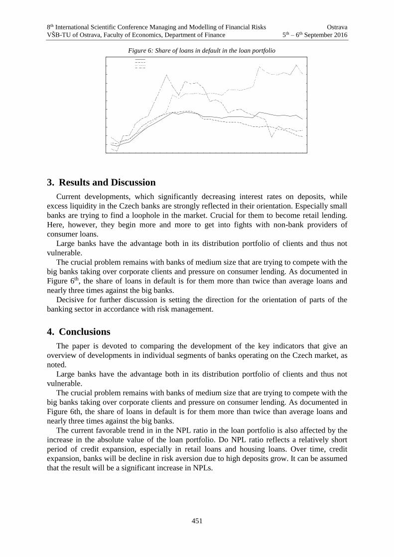
8th International Scientific Conference Managing and Modelling of Financial Risks Ostrava
VŠB-TU of Ostrava, Faculty of Economics, Department of Finance 5th – 6th September 2016
451
Figure 6: Share of loans in default in the loan portfolio
3. Results and Discussion
Current developments, which significantly decreasing interest rates on deposits, while
excess liquidity in the Czech banks are strongly reflected in their orientation. Especially small
banks are trying to find a loophole in the market. Crucial for them to become retail lending.
Here, however, they begin more and more to get into fights with non-bank providers of
consumer loans.
Large banks have the advantage both in its distribution portfolio of clients and thus not
vulnerable.
The crucial problem remains with banks of medium size that are trying to compete with the
big banks taking over corporate clients and pressure on consumer lending. As documented in
Figure 6th, the share of loans in default is for them more than twice than average loans and
nearly three times against the big banks.
Decisive for further discussion is setting the direction for the orientation of parts of the
banking sector in accordance with risk management.
4. Conclusions
The paper is devoted to comparing the development of the key indicators that give an
overview of developments in individual segments of banks operating on the Czech market, as
noted.
Large banks have the advantage both in its distribution portfolio of clients and thus not
vulnerable.
The crucial problem remains with banks of medium size that are trying to compete with the
big banks taking over corporate clients and pressure on consumer lending. As documented in
Figure 6th, the share of loans in default is for them more than twice than average loans and
nearly three times against the big banks.
The current favorable trend in in the NPL ratio in the loan portfolio is also affected by the
increase in the absolute value of the loan portfolio. Do NPL ratio reflects a relatively short
period of credit expansion, especially in retail loans and housing loans. Over time, credit
expansion, banks will be decline in risk aversion due to high deposits grow. It can be assumed
that the result will be a significant increase in NPLs.

8th International Scientific Conference Managing and Modelling of Financial Risks Ostrava
VŠB-TU of Ostrava, Faculty of Economics, Department of Finance 5th – 6th September 2016
452
References
[1] Heffernan, S. (2005), Modern banking. 1.rst. ed. Chichester: John Wiley & Sons.
[2] Krajicek, J. (2016). Economics and Management of Banks. 3rd upgraded and revised
edition. Brno.. Masaryk University. Faculty of Science.. Department of Finance - Study
texts.
[3] Slovik, P., Cournede, B. (2011) Macroeconomic Impact of Basel III, OECD Economics
Department Working Papers, vol. 844
[4] CNB (2016). The time series Database. Retrieved from:
http://www.cnb.cz/cnb/STAT.ARADY_PKG.STROM_DRILL?p_strid=0&p_lang=CS

8th International Scientific Conference Managing and Modelling of Financial Risks Ostrava
VŠB-TU of Ostrava, Faculty of Economics, Department of Finance 5th – 6th September 2016
453
Impact of „Covered Call“ Hedging Strategy on Financial Statements
Miloš Kráľ 1,Malgorzata Rówińska 2, Jiří Strouhal 3
Abstract
The paper deals with the hedging strategies used in risk management of open exchange
positions, carried out by corporations to eliminate their exchange rate risks. The analysis was
concerned with one of the strategies that might be used in that respect i.e. “covered call”. For
the better transparency there was opted for the analysis of Polish market. For the case studies
were taken market data from December 2014 with the aim to find out the possible link between
the applied accounting treatment and its contribution to effective exchange risk management of
corporations applying “covered call” hedging strategy. Finally, paper indicates whether the
accounting approach reflects the factual financial results generated by companies out of their
hedging strategies.
Key words
currency hedging, accounting rules, IFRS, Polish market, covered call position
JEL Classification: G30, M41
1. Introduction
Since the collapse of the Bretton Woods system the global financial markets have
demonstrated a high volatility of exchange rates, as well as relations between specific foreign
exchange pairs. This was also the case in 2014, when the Japanese yen lost over 40% of its
value against the US dollar, due to an economic policy advocated by Japanese prime minister
S. Abe, which he himself referred to as ‘abenomics’. Enormous exchange losses were also
reported by oil currencies, such as the Russian ruble (which lost over 60% against the US
dollar and is still continuing its downward trend), the Brazilian real, the Norwegian kronor
and many others. From this perspective the effective exchange risk management is an
important component of corporate strategy.
Banks have prepared a wide range of financial products which may help corporations to
partially eliminate the exchange risk exposure. The most popular banking products are
forward contracts and futures options.
For the presented research we applied case study approach when testing a single banking
product designed for the elimination of exchange rate risks – we will test “covered call”
option strategy.
The covered call strategy is used by the corporations which anticipate some considerable
fluctuations of the currency, i.e. ranging from 1% to 3% of the exchange rate, compared to the
exchange rate effective on conclusion of the prime contract – a business agreement. The
1 Doc. Ing. Miloš Kráľ, Ph.D., University of Economics in Katowice, e-mail:
[email protected]. 2 Assoc. Prof. dr. Malgorzata Rówińska, University of Economics in Katowice, e-mail:
[email protected]. 3 Prof. Ing. Jiří Strouhal, Ph.D., Škoda Auto University Mladá Boleslav, e-mail: [email protected].

8th International Scientific Conference Managing and Modelling of Financial Risks Ostrava
VŠB-TU of Ostrava, Faculty of Economics, Department of Finance 5th – 6th September 2016
454
contractual currency is the currency in which the long position is denominated, i.e. it is
different from the domestic currency (in this case PLN).
The covered call strategy involves taking a short position in a call option, where the
contractual price equals to the price stated in the underlying instrument. Therefore, the
covered call strategy means taking a long position on the underlying instrument (in this case it
would be the trade receivable of EUR 100,000) and a short position on the derivative, i.e. the
short-call option. Both positions are of the same value and the same maturity. These
dependencies provide the basis for the covered call product.
There shall be mentioned that the covered call strategy does not entirely eliminate the
exchange rate risk resulting from the open position. The export company researched by the
authors used this position because they had not anticipated any significant fluctuations in the
PLN exchange rates in the short run. Consequently, the selected strategy seemed a more
favorable solution for the company, when compared to a futures product. Moreover, in some
cases the covered call provides an export company with an opportunity to generate an extra
profit (see the case studies).
Should the PLN exchange rates change adversely (cases 1 and 2) in an open long position,
a loss generated on the underlying instrument would be adjusted by the profit gained from the
call option. This is due to the fact that the company receives a benefit of a non-refundable
cash premium. This is a specific amount (in PLN, in our case), and its size is determined by (i)
the strike price, and (ii) the volatility of exchange rate.
If the exchange rate on the contract performance date exceeds the strike price, the exporter
is obliged to exercise the option contract and sell the amount of EUR to the other party at the
strike price. Consequently, the company will also close its long position. As a result, the
company will report a loss, to be partially compensated by a profit gained on received
premium. If the exchange rate falls below the strike price, however, the option won’t be
exercised. Then the exporter’s profit on the option will equal to the premium.
The reminder of this paper is as follows: firstly, we will focus on a brief literature review
on approached area of research, and analyse the topic from financial and accounting
perspective. Major part of the paper is discussing the results of the adoption of covered call
option strategy.
2. Literature Review and Accounting Insight
In order to acknowledge the critical changes underlying the present state of the financial
sector, one must go back in time, half a century. Those minutes that were necessary for the use
of the telegraph are now reduced to microseconds, due to technological developments, which
give us free access to information, fast data transfers and rapid ways to communicate and
transport. All of these have contributed to the present sophistication of the financial field,
sustained especially through the boom of derivatives (Strouhal et al., 2008).
The main concern regarding derivatives is linked to their capacity to transfer risks through
contracts, thus being placed in wrong places and not being recognized correctly (Strouhal et
al., 2008). Such an unwanted situation is generated when risks are transferred from persons
who comprehend them to others who don’t, the informational advantage being in the favor of
the first category, thus creating the premise that the first category (the ones who understand
the risks of derivatives) can exploit the second category (the ones who are less informed), with
dangerous consequences for the whole financial system. Analyzing this situation from an
accounting perspective, we must not forget about the possibility of the transfer of these risks
from entities that evaluate them using market to market information to entities that do not
have this obligation, thus having the opportunity to round their own revenues and profits

8th International Scientific Conference Managing and Modelling of Financial Risks Ostrava
VŠB-TU of Ostrava, Faculty of Economics, Department of Finance 5th – 6th September 2016
455
(Strouhal et al., 2008). Evidently, for the parties involved in such an operation - the two
parties involved in the contract and the third parties from the markets in which the first two
protagonists act - a classic case of information asymmetry appears. A well known aspect of
any market is that when the competitive conditions are affected, new opportunities appear,
market niches become more obvious and companies become more agile in reorienting their
plans so as to benefit as much as they can by the emerging innovations. As a consequence,
derivatives can become the best friend or the worst enemy for any company, depending on the
way in which they are conceived, evaluated, used, and on the control of the risk exposure
(Chorafas, 2008).
It is necessary to accentuate the fact that the current problems linked to the use of fair value
accounting for financial instruments - especially in the case of instruments such as derivatives
- are closely tied to the type of capital that these imply, i.e. the fictitious capital which has a
fundamentally different motion than the real one. In other words, the nature of the fictitious
capital resides in its’ evaluation through capitalization, being completely different in
comparison to the goods movement (Ishikawa, 2005). Fictitious capital has a dynamic of its
own, due to the fact that the capital itself is converted into goods, which is different to the
motion of the real capital - a metamorphose of goods (Ishikawa, 2005).
Hilferding (1981) describes the specific manner of the fictitious capital’s motion as it can
be seen from the following figure. Therefore, when shares are issued (S), these are sold for
money (M), part of this money (m1) representing the circulation of the promoter in this cycle.
The other part (M1) is transformed in productive capital, becoming part of the cycle of
industrial capital, which is better known comparative to the fictitious one. Considering that
these shares were sold, in order for theme to circulate again, a new sum of money will be
necessary (M2) - this sum being a mean for this movement - this process (S-M2-S) taking
place on the stock market. Once a share has been issued, it has nothing to do with the
industrial capital which it represents. Furthermore, none of the events (positive or negative)
that take place after it was transacted on the market will have an effect on the cycle of the
productive capital (Hilferding, 1981). Also, accounting aspects regarding the promoters’
capital have already been debated within trade literature since the 50’s, taking the form of the
so-called equity premium controversy, thus becoming an early preoccupation of the debate
that fictitious capital generates an accounting problem. The defining trait of the current
accounting problems regarding fictitious capital is its’ reinstatement as an important aspect of
financial asset counting and not of capital within the balance sheet (Ishikawa, 2005).
Whether fair values really provide more relevant information than other measurement
attributes as claimed by the IASB is highly disputed in contributions to accounting theory and
has not yet been unambiguously proved; in fact, the results achieved in empirical
investigations are quite heterogeneous (Choy, 2006; Chen et al., 2006). Especially in the
absence of market prices the relevance of fair values as well as the cross-firm comparability of
the amount recognized in the accounts is questionable. When market prices for liabilities are
not available – which is almost regularly so in the case of non-financial liabilities –,
management needs to estimate fair value by means of various valuation techniques, in which
different possible cash flow scenarios are weighted by their related probabilities. Barth (2006,
p. 3) claims that “the fair value of any particular asset or liability is the same for every entity”.
In accounting theory the quest for consistency as regards the application of accounting
principles is reasoned with the requirement for comparability of financial statements
(Schipper, 2003, p. 62). Some believe that there is another reason, which is of equal
importance: Apart from providing decision-useful information, accounting is also frequently
used in contracts, e.g. in employment contracts and debt covenants, in order to calculate
annual bonuses or to limit future debt levels (Watts and Zimmermann, 1986). Many

8th International Scientific Conference Managing and Modelling of Financial Risks Ostrava
VŠB-TU of Ostrava, Faculty of Economics, Department of Finance 5th – 6th September 2016
456
researches (e.g. Smith and Warner, 1979) have provided sound empirical evidence that
managers make use of this flexibility in order to avoid costly violations of the contract (Beatty
and Weber, 2003; El-Gazzar et al., 1989; Sweeney, 1994).
According to IFRS rules (IASB, 2016) based on IFRS 9 Financial Instruments and IFRS 7
Financial Instruments – Disclosures, all hedging transactions shall be reflected within
financial statements obviously at fair value. Every entity (i.e. exporter or importer) shall
present: (i) a prime trade contract confirming the sale/purchase of a specific amount of goods,
and (ii) a hedging financial contract used by the corporation to protect themselves against the
exchange rate risk it might be exposed to under the prime contract.
The contract itself is obviously measured at nominal value (or amortised costs) and shall be
translated onto functional currency using the spot rate of local central bank. Problematic might
be the case of year-end where all contracts denominated in foreign currencies shall be
translated onto local currency using the spot rate of local central bank at year-end.
Derivative contracts are measured at fair value. Questionable might be the impact of
revaluation in case that the corporation is applying hedge accounting. In such case varies the
implementation of fair value hedge (revaluation is applied through profit or loss) and cash
flow hedge (revaluation is applied through other comprehensive income). In case corporation
is dealing with complex financial instruments, for accounting purposes shall be separated long
and short positions (for the analytical purposes also call and put options) and their results shall
be presented on financial statements separately.
Despite the case study is primarily focused on Polish exporter delivering goods to Slovakia,
it shall be pointed out that accounting treatments is similar when using local accounting rules
(Polish, Slovak), but also applying IFRS approach. Same impact would have also the
application of Czech accounting rules.
3. Methodology
Within this paper there are applied following research methods: a comparative analysis,
distribution and synthesis and an analysis of historical and logical data through case study
approach.
The case studies will show how the covered call financial product behaves, looking at all
the basic alternatives which may occur on its maturity day. Using the trade data about the
PLN/EUR exchange rates on the covered call maturity dates, the impact on the financial
results has been analysed.
The case study approach allows us to provide a thorough explanation of the covered call
strategy and identify the financial effects generated out of this strategy, as well as looking at
how its effects are presented in the corporate financial statements. The results are important
from the point of view of the corporations as well as financial authorities.
4. Case Study
4.1 Assumptions
A Polish exporter manages its exchange risk, resulting from an open currency position, in a
relatively conservative way. The company intends to close a long position from the prime
export contract, using the covered call strategy, for the entire amount of EUR 100,000, at the
strike price of PLN/EUR 4.20. This method means that the company is going to hedge against
a rise in the PLN/EUR exchange rate of 0.178% (based on the PLN 730 / PLN 416,200
relation) or more. Should the Polish currency drop, the company will achieve a gain of over

8th International Scientific Conference Managing and Modelling of Financial Risks Ostrava
VŠB-TU of Ostrava, Faculty of Economics, Department of Finance 5th – 6th September 2016
457
1% ((the difference between the exchange rate of 4.2073 and the exchange rate on the contract
conclusion date, i.e. PLN/EUR 4.162). The exchange rate of 4.2073 is the marginal rate,
determined on the basis of the strike price and the premium.
Based on the presented cases and their effects, the following assumptions are made for
the needs of the analysis of the financial consequences resulting from the covered call
strategy, to be reflected in the company’s accounting records (for the PLN/EUR pair):
the actual exchange rate on the sale of goods (10 Dec.,2014), worth EUR 100,000, by
the Polish company to a Slovak contracting party (e.g. a Polish exporter of cheese to
LIDL - a German chain of retail outlets located in Slovakia): PLN/EUR 4.162,
the date of the option contract conclusion: 10 December 2014,
the strike price: PLN/EUR 4.20,
the maturity day: 23 December 2014,
the premium: 0.73%,
The Polish company is going to receive the due amount on its bank account on 23
December 2014 (both the Polish company and the LIDL importer hold their bank
accounts with the same bank, therefore the transfer of the funds from the LIDL
importer’s account into the Polish company’s account will be carried out on the same
day).
From the theoretical as well as practical point of view, 6 basic situations may be applicable
on the financial markets on the maturity day. These are the following cases:
Case 1 – PLN has risen; the PLN/EUR exchange rate is below the rate specified on the
contract conclusion date (PLN/EUR 4.162) and equals PLN/EUR 4.1401.
Case 2 – PLN has risen, but not as much as above and the PLN/EUR exchange rate is
PLN/EUR 4.1600.
Case 3 – PLN has dropped slightly – to reach PLN/EUR 4.1823.
Case 4 – PLN has dropped and equals the strike price, i.e. PLN/EUR 4.2000.
Case 5 – PLN has dropped and the exchange rate is slightly higher than the strike price,
i.e. PLN/EUR 4.2043.
Case 6 – PLN has fallen considerably, the PLN/EUR exchange rate is well over the
strike price and it equals PLN/EUR 4.2745 (almost the same exchange rate was
announced on 23 December 2014 – PLN/EUR 4.2747).
4.2 Results
In case 1 (4.1401 PLN/EUR) the exporter shall report:
loss from the negative difference on the paid receivable – PLN 2,190
gain from the received option premium – PLN 730
The total loss on the covered call strategy would be PLN 1,460.
In case 2 (4.1600 PLN/EUR) the exporter shall report:
loss from the negative difference on the paid receivable – PLN 200
gain from the received option premium – PLN 730
The total profit on the covered call strategy would be PLN 530.
In case 3 (4.1823 PLN/EUR) the exporter shall report:
gain from the positive difference on the paid receivable – PLN 2,030
gain from the received option premium – PLN 730
The total profit on the covered call strategy would be PLN 2,760.
In case 4 (4.2000 PLN/EUR) the exporter shall report:
gain from the positive difference on the paid receivable – PLN 3,800
gain from the received option premium – PLN 730

8th International Scientific Conference Managing and Modelling of Financial Risks Ostrava
VŠB-TU of Ostrava, Faculty of Economics, Department of Finance 5th – 6th September 2016
458
The total profit on the covered call strategy would be PLN 4,530.
In case 5 (4.2043 PLN/EUR) the exporter shall report:
gain from the positive difference on the paid receivable – PLN 4,230
gain from the received option premium – PLN 300
The total profit on the covered call strategy would be PLN 4,530.
In case 6 (4.2745 PLN/EUR) the option premium is not sufficient to cover the loss made on
the short call. As a result, the exporter will lose on the option contract, while gaining on the
long position.
The exporter shall report:
gain from the open long position – PLN 11,250
loss due to the negative exchange rate difference on the option – PLN 6,720
The total profit on the covered call strategy would be PLN 4,530.
5. Conclusions
The cases examined above present a situation in which the hedging strategy is used and
accounted for within the same period. Then, as indicated above, the financial effects on the
covered call positions, which are disclosed in the accounting system, present the actual results
generated by the company. Consequently, the economic and book results are identical. In case
that transaction is exercised within next period it shall be noted that the corporation shall
report the fair value of the opened positions at the year-end as well as to revaluate the account
receivable based on actual exchange rate.
Based on performed analysis, the financial effects of the covered call strategy shall be
presented separately for every single position according to the accounting rules. The profit
recognised in the long position results from the difference between the exchange rate on the
date of sale and the exchange rate on the due date for the receivables.
The following conclusions may be drawn:
[1] in a situation when the exchange rate on the maturity date is equal to or higher than the
strike price, the company will inevitably achieve a similar financial result,
[2] the actual financial result generated by the company was higher than the one estimated
on the contract conclusion date,
[3] the covered call strategy has led to a higher financial result for the company than it
would have been the case if the company had not used that hedging strategy (except for
case 6), which means a higher tax on the transaction,
[4] in case 6, the result made on the strategy does not reflect the optimal tax situation from
the financial authorities’ point of view.
As a major limitation of the presented research might be mentioned two facts: (i) case
studies do not reflect the tax implications lowering the net income of the corporation, and (ii)
this studies are exercised within the single accounting period. In case that the real business
transaction is realised within two or more periods, there shall be taken in account the
revaluation of derivatives at fair value and revaluation of accounts receivable using the spot
rate upon year-end.
References
[1] Barth, M. (2006). Including Estimates of the Future in Today’s Financial Statements. BIS
Working Papers, No. 208.

8th International Scientific Conference Managing and Modelling of Financial Risks Ostrava
VŠB-TU of Ostrava, Faculty of Economics, Department of Finance 5th – 6th September 2016
459
[2] Beatty, A., and Weber, J. (2003). The Effects of Debt Contracting on Voluntary
Accounting Method Changes. The Accounting Review, 78(1), pp. 119-142.
[3] Chen, K., Sommers, G. A., and Taylor, G. K. (2006). Fair Value’s Affect on Accounting’s
Ability to Predict Future Cash Flows: A Glance Back and a Look at the Potential Impact
of Reaching the Goal. Available at:
http://papers.ssrn.com/sol3/papers.cfm?abstract_id=930702.
[4] Chorafas, D. N. (2008). Introduction to derivative financial instruments. New York:
McGraw-Hill Finance and Investing, 2008.
[5] Choy, A. K. (2006). Fair Value as a Relevant Metric: A Theoretical Investigation.
Available at: http://ssrn.com/abstract=613421.
[6] El-Gazzar, S., Lilien, S., and Pastena, V. (1989). The Use of Off-Balance Sheet Financing
to Circumvent Financial Covenant Restrictions. Journal of Accounting, Auditing and
Finance, 4(2), pp. 233-235.
[7] Hilferding, R. (1981). Finance capital: a study of the latest phase of capitalist
development. London: Routledge.
[8] IASB (2016). International Financial Reporting Standards 2016. London: IASB.
[9] Ishikawa, J. (2005). A social science of contemporary value-based accounting: economic
foundations of accounting for financial instruments. Critical Perspectives on Accounting,
16, pp. 115–136.
[10] Schipper, K. (2003). Principles-Based Accounting Standards. Accounting Horizons,
17(1), pp. 61-72.
[11] Smith, C., and Warner, J. (1979). On Financial Contracting: An Analysis of Bond
Covenants. Journal of Financial Economics, 7, pp. 117-161.
[12] Strouhal, J., Bonaci, C. G., and Matis, E. A. (2008). Trading and Reporting for
Derivatives. The Czech and Romanian Experience. 3rd Audit and Accounting
Convergence 2008 Annual Conference, Babes-Bolyai University, Cluj Napoca.
[13] Sweeney, A. P. (1994). Debt-Covenant Violations and Managers’ Accounting Responses.
Journal of Accounting and Economics, 17(3), pp. 281-308.
[14] Watts, R., and Zimmermann, J. (1986). Positive Accounting Theory. London: Prentice
Hall.

8th International Scientific Conference Managing and Modelling of Financial Risks Ostrava
VŠB-TU of Ostrava, Faculty of Economics, Department of Finance 5th – 6th September 2016
460
Management of audit risk and its impact on the audit of financial statements
Petra Krišková, Ján Užík 1
Abstract
The paper deals with the consideration and quantification of audit risk and its consequences in
the implementation of various audit procedures during the audit of the financial statements.
Audit risk is the risk that the auditor expresses a disproportionate opinion on the financial
statements, which influence the economic decisions of users of financial statements
information. Audit risk includes partial risk, while some of these auditor can´t influence, but
their possible existence must be quantified to the planned audit procedures.
Key words
Audit, audit risk, financial statements
JEL Classification: M42
1. Vymedzenie audítorského rizika a jeho vplyvu na názor audítora na
účtovnú závierku
Audit účtovnej závierky predstavuje vyjadrenie názoru audítora na to, či je účtovná
závierka vo všetkých významných súvislostiach v súlade so zákonnými požiadavkami. Ako už
z uvedeného vyplýva, audítor pri overovaní účtovnej závierky vyjadruje názor na súlad
účtovnej závierky a zákonných požiadaviek vo významných (teda abstrahuje od
nevýznamných) súvislostiach. Z hľadiska nákladovosti a efektívnosti audítor nenadobúda
absolútnu (100 %-tnú) istotu, ale zameriava sa na odhalenie významných súvislostí.
V audítorskej terminológii to znamená, že vykonáva také postupy, aby získal primerané
uistenie2 pre svoje stanoviská a závery. Z dôvodu, že audítor získava primerané a nie
absolútne uistenie, do auditu účtovnej závierky vchádza faktor rizika. V tejto súvislosti možno
definovať audítorské riziko ako riziko, že audítor vyjadrí neprimeraný názor na účtovnú
závierku. V praxi je audítorské riziko nevyhnutné a nie je možné ho eliminovať na nulovú
hodnotu. Audítorské riziko sa zvyčajne stanovuje na úrovni 5 % pre audity, ktoré poskytujú
primeranú istotu. V tejto súvislosti je možné stanoviť stupeň istoty auditu nasledovne:
DA = 100 – AR = 100 – 5 = 95 %, kde: DA – degree of assurance (stupeň istoty)
AR – audit risk (audítorské riziko)
udítorské riziko (súhrnne) tvoria tri zložky, a to: prirodzené (inherentné) riziko, kontrolné
riziko a detekčné riziko. Zjednodušene možno definovať jednotlivé zložky nasledovne:
prirodzené riziko súvisí s povahou účtovnej jednotky a predstavuje náchylnosť jednotlivých
zostatkov a ostatných informácií na nesprávnosti; kontrolné riziko súvisí s kontrolami
1 Petra Krišková Ing., PhD.; University of Economics in Bratislava; [email protected]
Ján Užík, Ing., PhD., University of Economics in Bratislava; [email protected] 2 Primerané uistenie znamená vysokú mieru uistenia, nie však absolútnu.

8th International Scientific Conference Managing and Modelling of Financial Risks Ostrava
VŠB-TU of Ostrava, Faculty of Economics, Department of Finance 5th – 6th September 2016
461
účtovnej jednotky a predstavuje neschopnosť vnútorného kontrolného systému predchádzať
a odhaľovať nesprávnosti a detekčné riziko je riziko, že audítor vplyvom zvolených
audítorských postupov neodhalí nesprávnosti v účtovnej závierke. Model audítorského riziko
možno vyjadriť nasledovne:
Audítorské riziko (AR) = prirodzené riziko (IR) x kontrolné riziko (CR) x detekčné riziko (DR)
V praxi nie je možné jednoznačne kvantifikovať každú zložku audítorského rizika. Audítor
úroveň pridelenú každej zložke skôr odhaduje na základe svojho odborného úsudku3. Rovnica
audítorského rizika je vždy vyrovnaná. Čím vyššie audítor hodnotí úroveň inherentného rizika
a/alebo kontrolného rizika, tým nižšie bude detekčné riziko4. Uvedené platí aj naopak, čím
nižšie audítor hodnotí riziká účtovnej jednotky (inherentné a kontrolné riziko), tým vyššie
bude detekčné riziko, pri zachovaní prijateľnej úrovni celkového rizika. V praxi sa používajú
rôzne modely určenia a hodnotenia rizika auditu. Cieľom týchto postupov je kvantitatívne
hodnotiť celkové riziko a jeho komponenty so zámerom určovať rozsah audítorského
testovania.
V rozdelení rizika auditu možno postupovať detailnejšie. Inherentné a kontrolné riziko
sa týkajú účtovnej jednotky a jej fungovania, súhrnne ich možno označiť ako riziko výskytu
chýb. Na druhej strane detekčné riziko sa dotýka samotného audítora a ide o riziko, že chyby
nebudú (audítorom) odhalené. Riziko, že chyby nebudú odhalené, je ovplyvnené dvoma
kategóriami neistoty, a to výberovým rizikom a nevýberovým rizikom. Výberové riziko
vyplýva zo skutočnosti, že určitá auditovaná vzorka nemusí byť typickým zástupcom
testovanej populácie. To znamená, že vzorka môže obsahovať neprimerane viac, príp. menej
odchýlok alebo finančných rozdielov, než existuje v celku5. Naopak, nevýberové riziko
obsahuje všetky ostatné faktory, ktoré nesúvisia s výberom. Výberové riziko obsahuje
následne ďalšie dva aspekty. Riziko nesprávneho odmietnutia predstavuje riziko, že
výsledok vzorky indikuje skutočnosť skreslenia celku, z ktorého sa vzorka vyberala, pritom
celok skreslený nie je a audítor ho nesprávne odmietne. Protikladným prípadom je riziko
nesprávneho prijatia, keď výsledok vzorky indikuje skutočnosť, že celok nie je významne
skreslený, pričom v skutočnosti skreslený je (audítor ho nesprávne prijal). Vzťahy medzi
jednotlivými zložkami rizika auditu zobrazuje nasledovná schéma:
3 Odborný úsudok definujú Medzinárodné audítorské štandardy ako uplatnenie zodpovedajúcich
školení, poznatkov a skúseností v súvislostiach daných audítorskými, účtovnými a etickými
štandardmi pri prijímaní informovaných rozhodnutí o opatreniach, ktoré sú vhodné za okolností
zákazky na audit 4 Príručka na vykonanie finančného auditu a auditu zhody, Európsky dvor audítorov, 2012 5 Kareš, L.; 2014. Audítorské postupy. Bratislava: Wolters Kluwer.

8th International Scientific Conference Managing and Modelling of Financial Risks Ostrava
VŠB-TU of Ostrava, Faculty of Economics, Department of Finance 5th – 6th September 2016
462
Figure 1: Riziko auditu pri vykonávaní audítorských testov6
2. Kvantifikácia audítorského rizika
Audítorské riziko je potrebné brať do úvahy v každej fáze auditu, od plánovania auditu cez
vykonávanie audítorských postupov až po hodnotenie výsledkov vykonaných audítorských
testov. Úroveň audítorského rizika má vplyv najmä na určenie hladiny významnosti, rozsahu
vykonaných audítorských testov a v neposlednom rade aj na veľkosť vzorky, na ktorej bude
audítor uplatňovať testovanie s cieľom prijatia záveru na celú množinu. Ako už bolo uvedené
vyššie, audítor úroveň jednotlivých zložiek rizika nevie presne kvantifikovať, ale odhaduje ich
približnú úroveň. Z tohto dôvodu sa úroveň inherentného, kontrolného a detekčného rizika
vyjadruje obvykle najmä slovne v závislosti od jej veľkosti ako nízka / stredná / vysoká
úroveň. Možno konštatovať, že stanovenie úrovne rizika má mimoriadny význam najmä pri
rozhodovaní o rozsahu substantívnych testov a v tejto súvislosti najmä pri určovaní veľkosti
zvolenej vzorky, na ktorej sa budú testy aplikovať.
Výber vzorky v audite znamená aplikovanie audítorských postupov na menej ako 100 %
položiek v rámci populácie relevantnej z hľadiska auditu tak, aby všetky jednotky zahrnuté do
výberu vzorky mali šancu byť vybrané s cieľom poskytnúť audítorovi primeraný základ pre
vytvorenie záverov týkajúcich sa celej populácie7. V tomto význame hovoríme o populácii,
ktorá predstavuje celý súbor dát, z ktorého sa vzorka vyberá. Vhodné je uplatňovať tzv.
stratifikáciu, čo znamená rozdeliť populáciu na subpopulácie, z ktorých každá predstavuje
skupinu položiek vzorky a tie majú podobnú charakteristiku (napr. peňažnú hodnotu).
Stratifikácia podľa peňažnej hodnoty umožňuje, aby sa pozornosť audítora nasmerovala na
položky s vyššími hodnotami, ktoré môžu obsahovať najväčšiu časť potenciálnych
nesprávností. V súvislosti s výberom vzorky je nutné brať do úvahy, t. j. kvantifikovať
výberové riziko. Ako sme uvádzali vyššie, výberové riziko obsahuje dve zložky, riziko
nesprávneho prijatia (označované aj ako riziko beta) a riziko nesprávneho odmietnutia
(označované ako riziko alfa). Pre audítora je dôležitejšie sledovanie najmä rizika nesprávneho
6 RICCHIUTE, D. N. 1994 Audit. [prekl.] M., Třaskalík, L., Janečková. 1. vyd. Praha: Victoria Publishing 7 ISA 530 – Výber vzorky v audite
Riziko výskytu chýb Riziko, že chyby nebudú
odhalené
Výberové riziko Nevýberové riziko
Riziko nesprávneho odmietnutia Riziko nesprávneho prijatia
Riziko auditu
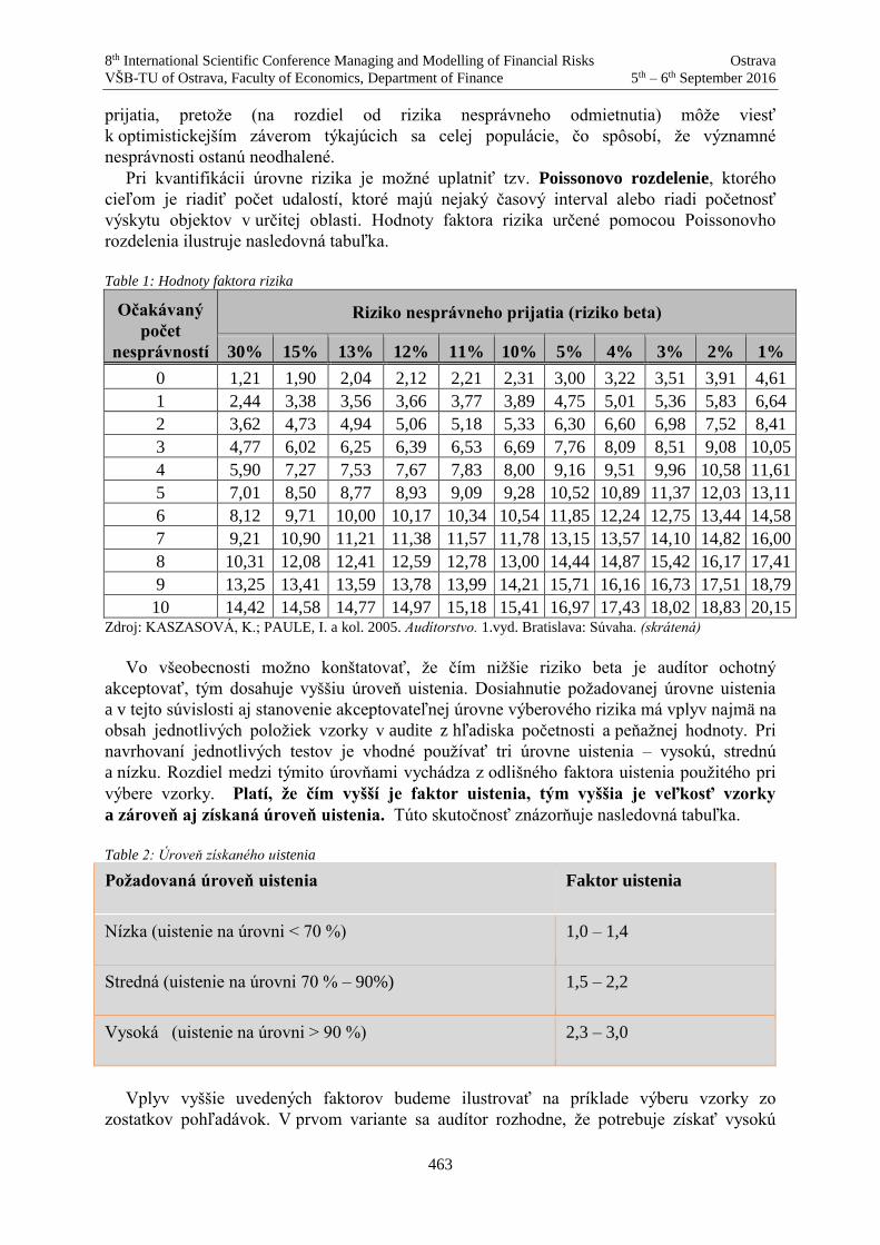
8th International Scientific Conference Managing and Modelling of Financial Risks Ostrava
VŠB-TU of Ostrava, Faculty of Economics, Department of Finance 5th – 6th September 2016
463
prijatia, pretože (na rozdiel od rizika nesprávneho odmietnutia) môže viesť
k optimistickejším záverom týkajúcich sa celej populácie, čo spôsobí, že významné
nesprávnosti ostanú neodhalené.
Pri kvantifikácii úrovne rizika je možné uplatniť tzv. Poissonovo rozdelenie, ktorého
cieľom je riadiť počet udalostí, ktoré majú nejaký časový interval alebo riadi početnosť
výskytu objektov v určitej oblasti. Hodnoty faktora rizika určené pomocou Poissonovho
rozdelenia ilustruje nasledovná tabuľka.
Table 1: Hodnoty faktora rizika
Očakávaný
počet
nesprávností
Riziko nesprávneho prijatia (riziko beta)
30% 15% 13% 12% 11% 10% 5% 4% 3% 2% 1%
0 1,21 1,90 2,04 2,12 2,21 2,31 3,00 3,22 3,51 3,91 4,61
1 2,44 3,38 3,56 3,66 3,77 3,89 4,75 5,01 5,36 5,83 6,64
2 3,62 4,73 4,94 5,06 5,18 5,33 6,30 6,60 6,98 7,52 8,41
3 4,77 6,02 6,25 6,39 6,53 6,69 7,76 8,09 8,51 9,08 10,05
4 5,90 7,27 7,53 7,67 7,83 8,00 9,16 9,51 9,96 10,58 11,61
5 7,01 8,50 8,77 8,93 9,09 9,28 10,52 10,89 11,37 12,03 13,11
6 8,12 9,71 10,00 10,17 10,34 10,54 11,85 12,24 12,75 13,44 14,58
7 9,21 10,90 11,21 11,38 11,57 11,78 13,15 13,57 14,10 14,82 16,00
8 10,31 12,08 12,41 12,59 12,78 13,00 14,44 14,87 15,42 16,17 17,41
9 13,25 13,41 13,59 13,78 13,99 14,21 15,71 16,16 16,73 17,51 18,79
10 14,42 14,58 14,77 14,97 15,18 15,41 16,97 17,43 18,02 18,83 20,15 Zdroj: KASZASOVÁ, K.; PAULE, I. a kol. 2005. Audítorstvo. 1.vyd. Bratislava: Súvaha. (skrátená)
Vo všeobecnosti možno konštatovať, že čím nižšie riziko beta je audítor ochotný
akceptovať, tým dosahuje vyššiu úroveň uistenia. Dosiahnutie požadovanej úrovne uistenia
a v tejto súvislosti aj stanovenie akceptovateľnej úrovne výberového rizika má vplyv najmä na
obsah jednotlivých položiek vzorky v audite z hľadiska početnosti a peňažnej hodnoty. Pri
navrhovaní jednotlivých testov je vhodné používať tri úrovne uistenia – vysokú, strednú
a nízku. Rozdiel medzi týmito úrovňami vychádza z odlišného faktora uistenia použitého pri
výbere vzorky. Platí, že čím vyšší je faktor uistenia, tým vyššia je veľkosť vzorky
a zároveň aj získaná úroveň uistenia. Túto skutočnosť znázorňuje nasledovná tabuľka.
Table 2: Úroveň získaného uistenia
Požadovaná úroveň uistenia Faktor uistenia
Nízka (uistenie na úrovni < 70 %) 1,0 – 1,4
Stredná (uistenie na úrovni 70 % – 90%) 1,5 – 2,2
Vysoká (uistenie na úrovni > 90 %) 2,3 – 3,0
Vplyv vyššie uvedených faktorov budeme ilustrovať na príklade výberu vzorky zo
zostatkov pohľadávok. V prvom variante sa audítor rozhodne, že potrebuje získať vysokú

8th International Scientific Conference Managing and Modelling of Financial Risks Ostrava
VŠB-TU of Ostrava, Faculty of Economics, Department of Finance 5th – 6th September 2016
464
úroveň uistenia, až 95 %-tnú, v druhom variante audítor zvolí požadovanú úroveň uistenia na
strednej úrovni, 70 % (z dôvodu, že získal uistenie aj z iných zdrojov).
Variant č. 1
Základné údaje:
Účel testu Potvrdenie existencie pohľadávok
Riziko významnej nesprávnosti Existencia – vysoké riziko
Testovaný súbor Zostatky pohľadávok na konci obdobia
Peňažná hodnota súboru 268 240 eur
Špecifické položky, ktoré sa testujú osobitne
(nespadajú do výberu vzorky)
58 350 eur
Uistenie z testov kontrol Žiadne
Použitý faktor uistenia (znížený o uistenie z
iných zdrojov)
Žiadne ďalšie zdroje uistenia, použije sa 95 %
(faktor 3,0)8
Významnosť9 15 000 eur
Očakávané miery odchýlky vo vzorke žiadne
Výpočet veľkosti vzorky a intervalu vzorkovania:
1. Výpočet intervalu vzorky
Interval vzorky = významnosť / faktor uistenia
Interval vzorky = 15 000/3,0 = 5 000 eur
2. Výpočet veľkosti vzorky
Veľkosť vzorky = súbor na testovanie / interval vzorky
Veľkosť vzorky = (268 240 – 58 350)/5000 = 41,978, zaokrúhlene 42 položiek
V tomto prípade interval vzorkovania je 5 000 eur. Ak by teda prvá položka bola vybraná
náhodne na hodnote 879 eur, tak nasledujúca položka by bola vybraná v bode, kde sa
dosiahne kumulatívne hodnota 5 879 eur. Tretia položka by sa vyberala v kumulatívnej
hodnote 10 879 eur a takto ďalej, až kým by bolo vybraných 42 položiek do vzorky.
Variant č. 2
Vychádzajúc z tých istých základných údajov ako vo variante č. 1, avšak použitý zdroj
uistenia by sa zmenil na úroveň 70 % (faktor 1,2110)
Výpočet veľkosti vzorky a intervalu vzorkovania:
8 Viď table 1: Hodnoty faktora rizika, kde riziko nesprávneho prijatia je na úrovni 5 % a očakávaný
počet nesprávností = 0 9 Významnosť vyjadruje hranicu medzi tým, čo je pravdepodobne nevýznamné a tým, čo je naopak
pravdepodobne významné. Stanovenie úrovne významnosti je vecou odborného úsudku audítora. 10 Viď table 1: Hodnoty faktora rizika, kde riziko nesprávneho prijatia je na úrovni 30 % a očakávaný
počet nesprávností = 0

8th International Scientific Conference Managing and Modelling of Financial Risks Ostrava
VŠB-TU of Ostrava, Faculty of Economics, Department of Finance 5th – 6th September 2016
465
1. Výpočet intervalu vzorky
Interval vzorky = významnosť / faktor uistenia
Interval vzorky = 15 000/1,21 = 12 396,69 eur, zaokrúhlene 12 397 eur
2. Výpočet veľkosti vzorky
Veľkosť vzorky = súbor na testovanie / interval vzorky
Veľkosť vzorky = (268 240 – 58 350)/12 397 = 16,93, zaokrúhlene 17 položiek
V prípade zvolenia strednej úrovne uistenia, t. j. vyššieho rizika, interval vzorkovania je
12 397 eur. Ak by teda prvá položka bola vybraná náhodne na hodnote 879 eur, tak
nasledujúca položka by bola vybraná v bode, kde sa dosiahne kumulatívne hodnota 13 276
eur. Tretia položka by sa vyberala v kumulatívnej hodnote 25 673 eur a takto ďalej, až kým by
bolo vybraných 17 položiek do vzorky.
Z ilustračného príkladu vidieť, že vplyv akceptovateľnej úrovne rizika má významný dopad
na veľkosť vzorky auditu, na základe ktorej by audítor prijímal celkové závery pre populáciu
s finálnym dôsledkom na názor audítora na celú účtovnú závierku. V prípade, ak je audítor
schopný získať aj inú podpornú dokumentáciu k overovanej populácii, môže zvýšiť
akceptovateľnú úroveň rizika. V tomto príklade mohol audítor získať uistenie z iných zdrojov,
či na základe interných konfirmácií zostatkov pohľadávok, ktoré účtovná jednotka získala
sama, alebo vnútroskupinových konfirmácií, právnej analýzy pohľadávok a pod.
3. Záver
Riziko vo všeobecnosti existuje a pôsobí pri každej ekonomickej činnosti. Mnohokrát nie
je priamo merateľné, ale jeho výskyt a vplyv je nutné neignorovať. V rámci audítorskej
činnosti, ktorej závery majú vplyv na ekonomické rozhodnutia bežných užívateľov, ale aj
finančných trhov je riziko významným faktorom. Jeho vplyv nie je možné znížiť na nulovú
úroveň, ale skôr eliminovať na čo možno najnižšiu úroveň, ktorú je audítor ochotný
akceptovať. Zhodnotenie rizika auditu sa nekončí určitým okamihom, ale v priebehu auditu sa
môžu vyskytnúť ďalšie informácie a vykonanie audítorských postupov môže identifikovať
dodatočné riziká. Z tohto vyplýva, že riziko je sprievodným javom celého auditu. Posúdenie
jeho tolerovanej úrovne má priamy vplyv najmä na výber vzorky v audite. Keďže väčšina
audítorských postupov sa vykonáva výberovým spôsobom (t. j. výberom vzorky
a aplikovaním výsledkov zo vzorky na celú množinu), možno konštatovať, že vplyv rizika
a jeho kvantifikácia je významným aspektom audítorskej práce. Dôsledné zváženie vplyvu
audítorského rizika je povinnosťou audítora, pretože profesia audítora je profesia vykonávaná
vo verejnom záujme, a opomenutie rizikového faktora má vplyv na celkovú efektívnosť
a výsledky auditu.
References
[1] KAREŠ, L.; 2014. Audítorské postupy. Bratislava: Wolters Kluwer
[2] KASZASOVÁ, K.; PAULE, I. a kol.; 2005. Audítorstvo. 1.vyd. Bratislava: Súvaha.
[3] KUBAŠČÍKOVÁ, Z.; PAKŠIOVA, R.; 2014. Risk in finance from the perspective of an
accounting theory. 16th International Scientific Conference on Finance and Risk 2014
Location: Univ Econ Bratislava, Dept Finance, Bratislava, NOV 24-25, 2014.
PROCEEDINGS OF THE 16TH INTERNATIONAL SCIENTIFIC CONFERENCE
FINANCE AND RISK 2014, VOL 1 Pages: 125-128.

8th International Scientific Conference Managing and Modelling of Financial Risks Ostrava
VŠB-TU of Ostrava, Faculty of Economics, Department of Finance 5th – 6th September 2016
466
[4] RICCHIUTE, D. N. 1994. Audit. [prekl.] M., Třaskalík, L., Janečková. 1. vyd. Praha:
Victoria Publishing
[5] TUMPACH, M.; JUHASZOVÁ, Z.; MELUCHOVA, J.; 2013. Is there any relevance of
business-related financial reporting in Slovakia. 9th International Scientific Conference
on Financial Management of Firms and Financial Institutions Location: VSB TU
Ostrava, Fac Econ, Finance Dept, Ostrava, SEP 09-10, 2013. 9TH INTERNATIONAL
SCIENTIFIC CONFERENCE PROCEEDINGS, PTS I-III Book Series: Financial
Management of Firms and Financial Institutions-Ostrava. Pages: 987-994.
[6] Príručka na vykonanie finančného auditu a auditu zhody, Európsky dvor audítorov,
2012
[7] Príručka medzinárodných usmernení na kontrolu kvality, audit, preverenie, iné
uisťovacie a súvisiace služby; zväzok 1, vydanie 2014

8th International Scientific Conference Managing and Modelling of Financial Risks Ostrava
VŠB-TU of Ostrava, Faculty of Economics, Department of Finance 5th – 6th September 2016
467
Forecasting electricity prices using nonlinear method
Radko Kříž1, Kateřina Seinerová2
Abstract
The goal of this paper is to analyze the electricity prices using chaos theory and to predict using
nonlinear method. At first we estimated the time delay and the embedding dimension, which is
needed for the Lyapunov exponent estimation and for the phase space reconstruction.
Subsequently, we computed the largest Lyapunov exponent, which is one of the important
indicators of chaos. The results indicated that chaotic behaviors obviously exist in electricity
price series. If the system behaves chaotically, we are forced to accept limited predictions.
Finally we computed predictions using a radial basis function to fit global nonlinear functions
to the data. In this paper we analyze electricity price series of the biggest European
energy markets EEX (Central European Energy Exchange).
Key words
Forecasting, Electricity prices, Chaos theory, Time series analysis, Phase space reconstruction,
Gaussian radial basis function
JEL Classification: C53
1. Introduction
Electricity is one of those commodities with which price is highly volatile and with
considerable number of jumps. That is especially caused by the fact that the electricity is not
possible to store. Thus the prediction of electricity price is a really complicated problem.
Forecasting electricity energy prices began in the 1990’s, at the beginning of the liberalization
process (Kříž et Kratochvíl, 2014). It is very important for electricity traders to forecast
electricity prices with the highest possible precision as the precision of the forecast is
connected to the trading strategy and thus with profit or lost. An electricity price depends on
the demand and supply and on the costs of transportation in the grid. The first two features are
strongly dependent on the weather, economic situation, government interventions etc. These
dependencies result in a very complex fluctuation of electricity prices, which may seem to be
slightly chaotic. Electricity is a flow commodity with unique characteristics that influence the
way it is traded and thus the behavior of spot and futures prices in the market. The price is set
by an interaction between supply and demand and in set in auction at a single time for the
whole 24 hours of the following day. Demand for electricity is highly inelastic. In short run, it
is absolutely inelastic so that the price is determined by the supply curve completely. The
curve resembles upward sloping stairway, each step approximately represents a different type
of a power plant and thus a different level of marginal costs. The price on the market rises
until it reaches the marginal costs for a MWh of the power plant of the next level, after that
1 University of Pardubice/Institute of Administrative and Social Sciences, Studentská 95, 532 10
Pardubice, Czech Republic, e-mail: [email protected]. 2 University of Pardubice/ Institute of Mathematics and Quantitative Methods, Studentská 95, 532 10
Pardubice, Czech Republic, e-mail: [email protected].

8th International Scientific Conference Managing and Modelling of Financial Risks Ostrava
VŠB-TU of Ostrava, Faculty of Economics, Department of Finance 5th – 6th September 2016
468
the supply rises (Kristoufek et Lunackova, 2013). The electricity spot prices can also be split
up into deterministic and stochastic parts. The deterministic part describes the seasonality and
all the periodic patterns (intra-day, intra-weak, peak, weekend patterns). This part is easily
observable and we can describe it simply. The stochastic part (also called volatility), on the
contrary, is unobservable and seems chaotic (Kříž et Kratochvíl, 2014). Real processes in
nature, according to the expectation of Mandelbrot (1983), lie somewhere between pure
deterministic process and white noise. This is why we can describe reality either by a
stochastic or deterministic model. Long memory in time series are characteristic with values
in past in past influencing the present and future values. Few works is focused to analyze a
long memory in electricity price time series e.g. Kříž et Lešáková (2016b), Kristoufek et
Lunackova (2013), Weron et Przybyłowicz (2002). According Weron et Przybyłowicz (2002)
the whole complex process of electricity price formation results in behavior not observed in
the financial or even other commodity markets. Forecasting of any commodity or derivative
price is a common problem discussed in a lot of articles. Prediction on electricity prices have
been discussed in several recent papers e.g. Kratochvíl et Starý (2013). Numerous new
methods of electricity prices time series analysis have been developed for dealing with
nonlinear data e.g. Conejo et al. (2005), Misiorek et al. (2006), Pao (2007).
To be able to use these methods and models we will have to prove first that electricity spot
prices behave chaotically and that it is adequate to use a chaotic description. The basic
question is therefore the existence of chaotic behavior. If the system behaves chaotically, we
are forced to accept only limited predictions. Nevertheless chaotic behavior is much better
than random processes (Kříž et Kratochvíl, 2014).
2. Methodology
2.1 Chaos theory
Chaos theory allows for the reconstruction of phase space from time series, which can be
used for specifying the system states (Abardanel et al., 1973). This analysis is based on
Takens (1980) embedding theorems. Takens’ theorem transforms the prediction problem from
time extrapolation to phase space interpolation (Kříž, 2013). For more information see Kříž et
Lešáková (2016b).
Let there be given a time series x1, x2, … , xN which is embedded into the m-dimensional
phase space by the time delay vectors. A point in the phase space is given as:
)1(,...,2,1 ,...,, )1( mNnxxxY mnnnn , (1)
where is the time delay and m is the embedding dimension. Different choices of and m
yield different reconstructed trajectories. Kodba et al. (2005) discuss how we can determine
optimal and m. We use method developed by Fraser et Swinney (1986), which is based on
the mutual information between xn and xn+ as a suitable quantity for determining . The
mutual information between xn and xn+ quantifies the amount of information we have about
the state xn+ presuming we know the state xn. The mutual information function is:
j
h
j
k kh
kh
khPP
PPI
1 1
,
,
)(ln)()(
, (2)
where Ph and Pk denote the probabilities that the variable assumes a value inside the hth and
kth bins, respectively, and Ph,k() is the joint probability that xn is in bin h and xn+ is in bin k.
The first minimum of I() then marks the optimal choice for the time delay.
The embedding dimension m can be chosen using the “false nearest neighbors’” method.
This method measures the percentage of close neighboring points in a given dimension that

8th International Scientific Conference Managing and Modelling of Financial Risks Ostrava
VŠB-TU of Ostrava, Faculty of Economics, Department of Finance 5th – 6th September 2016
469
remain so in the next highest dimension. The minimum embedding dimension capable of
containing the reconstructed attractor is that for which the percentage of false nearest
neighbors drops to zero for a given tolerance level μ.
In order to calculate the fraction of false nearest neighbors the following algorithm is used
according to Kennel et al. (1982). Given a point p(i) in the m-dimensional embedding space,
one first has to find a neighbor p(j), so that
)()( jpip . (3)
We then calculate the normalized distance Ri between the (m + 1)th embedding coordinate
of points p(i) and p(j) according to the equation:
)()( jpip
xxR
mjmi
i
. (4)
If Ri is larger than a given threshold Rtr , then p(i) is marked as having a false nearest
neighbor. Equation (4) has to be applied for the whole time series and for various m = 1, 2, …
until the fraction of points for which Ri > Rtr is negligible Kodba et al. (2005).
Lyapunov exponent λ of a dynamical system is a quantity that characterizes the rate of
separation of infinitesimally close trajectories. The largest Lyapunov exponent can be defined
as follows:
00
)(ln
1lim
0 Z
tZ
ttZ
. (5)
A positive largest Lyapunov exponent is usually taken as an indication that the system is
chaotic. We have used the Rosenstein (1983) algorithm, which counts the largest Lyapunov
exponent as follows:
iM
jj
j
d
id
iMtii
11)0(
)(ln
)(
1.
1)( , (6)
where dj(i) is distance from the j point to its nearest neighbor after i time steps and M is the
number of reconstructed points.
2.2 Nonlinear prediction
Predictability is one way how correlations between data express themselves (Hegger et al.,
1999). Most properties of chaotic systems are much more easily determined from the
governing equations than from a time series. Unfortunately, the governing equations are
usually not known, except for well controlled laboratory experiments. Analyzing an empirical
model, and maybe synthetic time series data generated from it, can provide a valuable
consistency test for the results of time series analysis. Chaotic dynamical systems generically
show the phenomenon of structural instability (Kantz et Schreiber, 1997).
According Kantz et Schreiber (1997), using the reconstructed phase space for m and τ, a
functional relationship f between the current state X(t) and future state X(t + T) can be given as
))(()( tXfTtX , (7)
where T represents the number of time steps ahead that one wishes to perform the
prediction. Function f represents the approximation to unknown dynamical system. It is shown
that for sufficiently large values of the embedding dimension and if some additional
conditions are satisfied, the reconstructed trajectory has the same topological and geometrical
properties as the system’s phase space trajectory (Takens, 1981). The predictive mapping can
be expressed as
))(()( tXfTtX p . (8)

8th International Scientific Conference Managing and Modelling of Financial Risks Ostrava
VŠB-TU of Ostrava, Faculty of Economics, Department of Finance 5th – 6th September 2016
470
The aim is to find the predictor fp, so that x(t + T) can be predicted based on the
reconstructed time series. If the time series is chaotic, then fp is necessarily nonlinear. Several
local and global approaches are available in the literature to find the function fp (Farmer et
Sidorowich, 1987).
The idea of locally linear predictions is following. If there is a good reason to assume that the
relation
)(1 nn sfs (9)
is fulfilled by the experimental data in good approximation (say, within 5%) for some
unknown f and that f is smooth, predictions can be improved by fitting local linear models.
They can be considered as the local Taylor expansion of the unknown f, and are easily
determined by minimizing
nj Us
njnn bsas 21
2 )( , (10)
with respect to an and bn, where Un is the ε-neighborhood of sn, excluding sn, as before.
Then, the prediction is
nnnn bsas 1ˆ (11)
The minimization problem can be solved through a set of coupled linear equations, a
standard linear algebra problem (Hegger et al., 1999).
The local linear fits are very flexible, but can go wrong on parts of the phase space where
the points do not span the available space dimensions and where the inverse of the matrix
involved in the solution of the minimization does not exist. Moreover, very often a large set of
different linear maps is unsatisfying. Therefore many authors suggested fitting global
nonlinear functions to the data, i.e. to solve
n
npn sfs 21
2 ))(( , (12)
where fp is now a nonlinear function in closed form with parameters p, with respect to
which the minimization is done. The results depend on how far the chosen ansatz fp is suited
to model the unknown nonlinear function, and on how well the data are deterministic at all
(Hegger et al., 1999). A radial basis function (RBF) is a real-valued function whose value
depends only on the distance from the origin, or alternatively on the distance from some other
point xi, called a center, or alternatively on the distance from some other point c, called a
center, so that
)(),( cxcx (13)
Gaussian kernel is used in this analysis. 22
)( xcex (14)
Hence the prediction made is:
i
n
i
ip xxaaf 1
0 (15)
respectively
2)(
1
01ixxc
n
i
it eaax
(16)
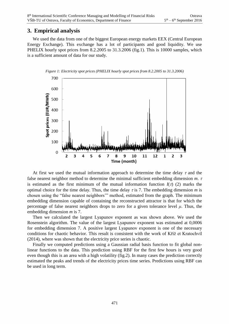
8th International Scientific Conference Managing and Modelling of Financial Risks Ostrava
VŠB-TU of Ostrava, Faculty of Economics, Department of Finance 5th – 6th September 2016
471
3. Empirical analysis
We used the data from one of the biggest European energy markets EEX (Central European
Energy Exchange). This exchange has a lot of participants and good liquidity. We use
PHELIX hourly spot prices from 8.2.2005 to 31.3.2006 (fig.1). This is 10000 samples, which
is a sufficient amount of data for our study.
Figure 1: Electricity spot prices (PHELIX hourly spot prices from 8.2.2005 to 31.3.2006)
At first we used the mutual information approach to determine the time delay and the
false nearest neighbor method to determine the minimal sufficient embedding dimension m.
is estimated as the first minimum of the mutual information function I() (2) marks the
optimal choice for the time delay. Thus, the time delay is 7. The embedding dimension m is
chosen using the “false nearest neighbors’” method, estimated from the graph. The minimum
embedding dimension capable of containing the reconstructed attractor is that for which the
percentage of false nearest neighbors drops to zero for a given tolerance level μ. Thus, the
embedding dimension m is 7.
Then we calculated the largest Lyapunov exponent as was shown above. We used the
Rosenstein algorithm. The value of the largest Lyapunov exponent was estimated at 0,0006
for embedding dimension 7. A positive largest Lyapunov exponent is one of the necessary
conditions for chaotic behavior. This result is consistent with the work of Kříž et Kratochvíl
(2014), where was shown that the electricity price series is chaotic.
Finally we computed predictions using a Gaussian radial basis function to fit global non-
linear functions to the data. This prediction using RBF for the first few hours is very good
even though this is an area with a high volatility (fig.2). In many cases the prediction correctly
estimated the peaks and trends of the electricity prices time series. Predictions using RBF can
be used in long term.

8th International Scientific Conference Managing and Modelling of Financial Risks Ostrava
VŠB-TU of Ostrava, Faculty of Economics, Department of Finance 5th – 6th September 2016
472
Figure 2: Electricity spot prices and its prediction (last 200 values)
4. Conclusion
Chaos theory has changed the thinking of scientists and the methodology of science.
Making a theoretical prediction and then matching it to the experiment is not possible in
chaotic processes. Long term forecasts are, in principle, also impossible according to chaos
theory. Now it is known that real processes are nonlinear and a linear view can be wrong. The
basic question is therefore - the existence of chaotic behavior. If the system behaves
chaotically, we are forced to accept only limited predictions. But it is much better than random
processes.
We shown in this paper that the NOx concentration time series is chaotic. First, we
computed the values of the time delay = 7 and the embedding dimension m = 7. The
estimated largest Lyapunov exponent is 0,0006. If the correlation dimension is low, the largest
Lyapunov exponent is positive and the Kolmogorov entropy has a finite positive value, chaos
is probably present. From these estimations it can be concluded that electricity prices time
series is chaotic. Finally we computed predictions using a Gaussian RBF to fit global
nonlinear functions to the data. Considering all these findings, we recommend the Gaussian
RBF to fit global non-linear functions as one of the methods used for prediction. As it may not
be reliable under certain circumstances, it should be used in combination with other prediction
methods.
References
[1] Abarbanel, H. D., Brown, R., Sidorowich, J. J. and Tsimring, L., S. (1993). The analysis
of observed chaotic data in physical systems. Reviews of modern physics. 65(4), p. 1331.
[2] Conejo, A. J., Contreras, J., Espinola, R., and Plazas, M. A. (2005). Forecasting
electricity prices for a day-ahead pool-based electric energy market. International Journal
of Forecasting, 21(3), pp. 435-462.

8th International Scientific Conference Managing and Modelling of Financial Risks Ostrava
VŠB-TU of Ostrava, Faculty of Economics, Department of Finance 5th – 6th September 2016
473
[3] Farmer, D., J. and Sidorowich, J., J. (1987). Predicting chaotic time series, Phys. Rev.
Lett. 59, pp. 85–848.
[4] Fraser, A. M. and Swinney, H. L. (1986). Independent coordinates for strange attractors
from mutual information. Physical review A. 33(2), p.1134.
[5] Hegger, R., Kantz, H., Schreiber, T. (1999). Practical implementation of nonlinear time
series methods: The TISEAN package Chaos, 9(2), pp. 413-435.
[6] Kantz, H. and Schreiber, T. (1997). Nonlinear time series analysis. Cambridge University
Press, Cambridge.
[7] Kennel, M., B., Brown, R. and Abarbanel, H., D. (1992). Determining embedding
dimension for phase-space reconstruction using a geometrical construction. Physical
review A, 45(6), p. 3403.
[8] Kodba, S., Perc, M., Marhl, M. (2005). Detecting chaos from a time series. European
journal of physics. 26(1), p. 205.
[9] Kratochvíl, Š. and Starý, O. (2013). Predicting the Prices of Electricity Derivatives on the
Energy Exchange." Acta Oeconomica Pragensia 2013(6). pp. 65-81.
[10] Kristoufek, L. and Lunackova, P., (2013). Long-term Memory in Electricity Prices:
Czech Market Evidence. Czech Journal of Economics and Finance. 63(5), pp 407-424.
[11] Kříž, R. and Kratochvíl, Š. (2014). Analyses of the chaotic behavior of the electricity
price series. In ISCS 2013: Interdisciplinary Symposium on Complex Systems. Springer
Berlin Heidelberg, Germany, pp. 215-226.
[12] Kříž, R. (2013). Chaotic Analysis of the GDP Time Series. In: Nostradamus 2013:
Prediction, Modeling and Analysis of Complex Systems. Springer. pp. 353-362.
[13] Kříž, R., & Lešáková, P. (2016a). Prediction of NOX Concentration Time Series Using
the Chaos Theory. In Proceedings of the Second International Afro-European
Conference for Industrial Advancement AECIA 2015 (pp. 465-475). Springer
International Publishing.
[14] Kříž, R. and Lešáková, P. (2016b). Long memory in electricity price time series. In
SGEM2016 Conference Proceedings.
[15] Mandelbrot, B. B. (1983). The Fractal Geometry of Nature. W.H. Freeman and Co., New
York, USA.
[16] Misiorek, A., Trueck, S., and Weron, R. (2006). Point and interval forecasting of spot
electricity prices: Linear vs. non-linear time series models. Studies in Nonlinear
Dynamics & Econometrics, 10(3).
[17] Pao, H. T. (2007). Forecasting electricity market pricing using artificial neural networks.
Energy Conversion and Management, 48(3), pp. 907-912.
[18] Rosenstein, M., T., Collins, J., J. and De Luca, C., J. (1993). A practical method for
calculating largest Lyapunov exponents from small data sets. Physica D: Nonlinear Phe-
nomena, 65(1), pp. 117-134.
[19] Takens, F. (1981). Detecting strange attractors in turbulence. In Dynamical systems and
turbulence, Warwick 1980 (pp. 366-381). Springer Berlin Heidelberg.
[20] Weron, R. and Przybyłowicz, B. (2000). Hurst analysis of electricity price dynamics.
Physica A: Statistical Mechanics and its Applications, 283(3), pp. 462-468.

8th International Scientific Conference Managing and Modelling of Financial Risks Ostrava
VŠB-TU of Ostrava, Faculty of Economics, Department of Finance 5th – 6th September 2016
474
The Application of Benford's Law in Accounting
Zuzana Kubaščíková1, Renáta Pakšiová 2
Abstract
Application of Benford’s law is possible in the case of detecting accounting errors and
manipulation of accounting data. Benford's law is generally promoted as a simple and effective
tool for detecting fraud. Benford's Law is a mathematical law that says that in most natural data
files (but not all) numbers much more likely to begin with the digit 1 than other numbers. In
general, it is expected that most of the data from the accounting division is subject to Benford´s
law. But the application of Benford's law is not sufficient to detect errors and fraud. The aim of
this paper is to apply existing Benford’s law theory in forensic accounting and complete this
theory by other models concerning the analysis of accounting data especially when processing
big data. The aim of the paper is to choose specific mathematic model and then test it to see
whether it can complement Benford's law model.
Key words
Her Benford’s law, Bayes´ rule, forensic accounting, fraud.
JEL Classification: M41
1. Introduction
Fraud or misrepresentation often creates clear patterns of error within complex financial
data. There are developed sophisticated tools and techniques for uncovering these patterns and
demonstrating that they are the result of deliberate malfeasance. Numerical data exploration
technique that is used for fraud detection is known as Bedford’s law (Baesens, Vlasselaer,
Verbeke, 2015).
Benford´s law describes the frequency distribution of the first digit in many real-life data
sets. When comparing the expected distribution following Bedford’s law with the observed
distribution in a data set, strong deviations from the expected frequencies may indicate the
data to be suspicious and possible manipulated. Manipulated or made-up numbers will not
comply with the expected observed frequency of the first or second digit as expressed by
Bedford’s law (Tumpach, 2009).
Benford’s Law was published for the first time in 1881 by American astronomer Simon
Newcomb, but it was rediscovered only in 1938 by physicist Frank Benford. Benford's Law
refers to the probability of occurrence of numbers d (d = 1, 2, 3, 4, 5, 6, 7, 8, 9) on the first
quantifiable features in any sufficiently large set of data.
Benford's Law can be used for the detection of possible frauds in the lists of socio -
economic data submitted in support of public planning decisions (Hal Varian, 1972). Carslaw
applied Benford's Law to accounting data in the late 80s of the 20th century and his findings
revealed also the importance of the 2nd digit position. He analysed financial statements of
1 Ing. Zuzana Kubaščíková, PhD., Faculty of Economics Informatics, University of Economics in
Bratislava, [email protected]. 2 doc. Ing. Mgr. Renáta Pakšiová, PhD., Faculty of Economics Informatics, University of Economics
in Bratislava, [email protected].

8th International Scientific Conference Managing and Modelling of Financial Risks Ostrava
VŠB-TU of Ostrava, Faculty of Economics, Department of Finance 5th – 6th September 2016
475
companies in New Zealand (Carslaw, 1988). Similar study was conducted by Thomas who
analysed financial statements of American companies (Thomas, 1989). Thomas Hill presented
that Benford's distribution is a "second generation" distribution, or combination of other
distributions (Hill, 1995). Mark J. Nigrini showed that Benford's Law could be used in
forensic accounting and auditing serving as an indicator of fraud (Nigrini, 1996).
A digit analysis using Benford's Law was also used as evidence of voter fraud in the 2009
Iranian election. In fact, Benford's Law is legally admissible as evidence in the USA in
criminal cases at the federal, state and local levels. This fact alone substantiates the potential
usefulness of using Benford's Law (Parajka, 2015).
Bedford’s law applies to a data set, meaning that a sufficient amount of numbers related to
an individual case need to be gathered in order for Bedford’s law to be meaningful, which is
typically the case when dealing with financial statements. But Bedford’s law is not satisfied,
there is probable that the involved data were manipulated and further investigation or testing
is required (Juhászová, Užík, 2015).
Bayes´ Rule, formulated in the mid-eighteenth century, reverses probabilistic reasoning
form determining probabilities of hat effects would be caused to that of assessing that caused
those effects. The difference is not just semantics, in the former the cause is known of certain,
whereas in the latter the effect has been observed with certainty. In a forensic accounting
context the latter is more relevant. In these settings, the accountant observes the evidence and
assesses the possibility that a particular action (such as fraud or financial impropriety) was the
underlying cause.
Robins showed that the Bayes estimator can minimize the squared error loss (Robins,
1956). This method was widely uses also in several early traffic safety studies (Hauer,
Persaud,1987), (Carlin, Louis, 2000).
Later Bayes rule began to be mentioned in publications in connection with the accounting,
forensic accounting and fraud (Duta, 2013).
2. Methodology and data
Previous research demonstrates that Benford’s Law is effective in detecting data bias in
the journal entries of companies. The purpose of this paper is to determine which tool can be
used in case that manipulation was detected by using Benford´s law and we need to find
specific error in between the journal entries of selected companies. For these purposes we
have chosen Bayes´ Rule.
Bayes's rule relates the odds of event A1 to the odds of event A2, before and after
conditioning on another event B. When arbitrarily many events A are of interest, not just two,
the rule can be rephrased as posterior is proportional to prior times likelihood, P (A│B) = P
(A) P (B│A) / P (B) where the proportionality symbol means that the left hand side is
proportional to (i.e., equals a constant times) the right hand side as A varies, for fixed or given
B (Duta, 2013).
Bayes' rule may be preferred to the usual statement of Bayes' theorem for a number of
reasons. One is that it is intuitively simpler to understand. Another reason is that normalizing
probabilities is sometimes unnecessary: one sometimes only needs to know ratios of
probabilities. Finally, doing the normalization is often easier to do after simplifying the
product of prior and likelihood by deleting any factors which do not depend on A, so we do
not need to actually compute the denominator P(B) in the usual statement of Bayes' theorem
P (A│B) = P (A) P (B│A) / P (B).
Bayes´ Rule is applicable in accounting as following: A company has three big groups of
accounting entries - liabilities, receivables, other accounting transactions. The error rates for

8th International Scientific Conference Managing and Modelling of Financial Risks Ostrava
VŠB-TU of Ostrava, Faculty of Economics, Department of Finance 5th – 6th September 2016
476
these vary, it is calculated according occurrence of error in previous years. While liabilities’
error rate is 0,015, receivables´ error rate is 0,025 and other accounting transactions´ error rate
is 0,068. Liabilities are 40% of the accounting data, while receivables are 30% of accounting
data and other accounting transactions are remaining 30% of data.
Table 1: Probability of error
Error rate Percentage of transactions
Liabilities transactions 0,015 48%
Receivables transactions 0,025 37%
Other accounting transactions 0,068 15%
Source: Own processing.
If we want to determine the order in which the three groups of accounting entries should
be verified, the problem can be solved using conditional probabilities and the Bayes´ rule.
3. Results and discussion
Although we do not know any of probabilities directly, we know the following:
P (randomly selected liabilities transactions) = 0,48
P (error / processed transactions) = 0,015
P (randomly selected receivables transaction) = 0,37
P (error / processed transactions) = 0,025
P (randomly selected other accounting transactions) = 0,15
P (error / processed transactions) = 0,068
The only information that we need to be able to compute these conditionals is the
denominator, or P (error) because using the six probabilities here, we can derive the numerator
of the three equations as
P (processed liability transactions and error occurs) = P (processed a random liability
transactions) x P (error / processed liability transactions) = 0,48 * 0,015 = 0,0072
P (processed receivables transactions and error occurs) = P (processed a random
receivables transaction) x P (error / processed receivables transactions) = 0,37 * 0,025 =
0,0093
P (processed other accounting transactions and error occurs) = P (processed a random other
accounting transactions) x P (error / processed other accounting transactions) = 0,15 * 0,068 =
0,0102
This is a-priori probability of error = P (processed liability transactions and error occurs) +
P (processed receivables transactions and error occurs) + P (processed other accounting
transactions and error occurs) = 0,0072 + 0,0093 + 0,0102 = 0,0267
Now when is known that the probability of error = 0,0267, we can substitute this as the
denominator in the given equations and solve for the posterior probabilities as follows:
P (processed liability transactions and error occurs) = 0,0072 / 0,0267 = 0,27
P (processed receivables transactions and error occurs) = 0,0093 / 0,0267 = 0,35
P (processed other accounting transactions and error occurs) = 0,0102 / 0,0267 = 0,38
However there is the highest number of liabilities transactions, it is more likely that there is
error in receivables transactions. In fact, it is least likely that processed liabilities transactions
in error because liabilities transactions has an error rate so much less than the other two
groups of transactions. However there are more liabilities transactions, it is unlikely that there
is an error.

8th International Scientific Conference Managing and Modelling of Financial Risks Ostrava
VŠB-TU of Ostrava, Faculty of Economics, Department of Finance 5th – 6th September 2016
477
What is important in the above results is not the precise algebraic calculations that are
essential to any scientific investigation of accounting issues, but the qualitative insights that
are obtained from them. As long as not every accounting entry can be investigated by
regulatory body (internal or external), it would clearly be helpful to quickly target the highest
imprecision in accounting data that can be investigated later with more sophisticated tools and
techniques.
4. Conclusion
Benford's law is effective in detecting data bias in journal entries but ineffective in
detecting the specific error or fraud. The probability that Benford's law will detect error or
fraud is highly likely and the auditor should apply further techniques to evaluate all
possibilities before launching a full-fledged re-examination of the data and its sources. One
tool that can be used and be very effective is called Bayes´ Rule.
Bayes´ Rule is applied in situations where new information changes the probability of
events of interest. These changes in probability are called belief revisions. Belief revisions
could be applicate widely in forensic accounting as new items of evidence collected
sequentially prompts auditors to reassess their beliefs on the assertions.
In forensic accounting and auditing, the use of conditional probabilities is extremely
pertinent, as the forensic accountant attempts to assess the occurrence of fraud and other
financial irregularities based on observation of financial data. However, in many practical
situations while the occurrence of the event, or evidence, is known with certainty, the chances
of the event occurring before the fact are difficult to assess directly. For these types of
problems, an extension of conditional probabilities through Bayes´ Rule (also known as
Bayes´ theorem) has to be applied. However Benford´s law is necessary part of many an
auditing and a forensic accounting software, the application of Bayes´ rule is absent however
it can effectively complete any auditing or forensic accounting software.
Acknowledgments
This article is an output of the project of the Scientific Grant Agency of the Ministry of
Culture of the Slovak Republic and Slovak Academy of Sciences (VEGA) no. 1/0512/16
(2016-2018) “Retention and Development of Business Property of Company as a Relevant
Tool for Sustainable Development.”
References
[1] Baesens, B., Vlasselaer, V., Verbeke, W. (2015). Fraud Analytics Using Descriptive,
Predictive, and Social Network Techniques. New Yersey: Wiley.
[2] Carlin, B., Louis, T. (2000) Bayesian Methods for Data Analysis. Third Edition,
Chapman and Hall/CRC.
[3] Carslaw, C. (1988). Anomalies in Income Numbers: Evidence of Goal Oriented
Behavior. In: The Accounting Review, LXIII (2), pp. 321-327.
[4] Dutta, K. S. (2013). Forensic Accounting. New Yersey: FT Press.
[5] Hal R. Varian (1972). Banford´s Law. In: An American Statistician, 26 (3), pp. 65-66.

8th International Scientific Conference Managing and Modelling of Financial Risks Ostrava
VŠB-TU of Ostrava, Faculty of Economics, Department of Finance 5th – 6th September 2016
478
[6] Hauer, E., Persaud, B.N. (1987). How to estimate the safety of rail-highway grade
crossing and the effects of warning devices. Transportation Research Record 1114, pp.
131-140.
[7] Hill, T.P. (1995). A Statistical Deviation of the Significant Digit Law. In: Statistical
Scientist. 10(4), pp. 354-363.
[8] Juhászová, Z. - Užík, J. (2015) Účtovníctvo ako súčasť ekonomických vied. In:
Ekonomické rozhľady: vedecký časopis Ekonomickej univerzity v Bratislave. -
Bratislava: Ekonomická univerzita v Bratislave, pp. 382-387.
[9] Nigrini, M. J. (1996). A Taxpayer Compliance Application of Benford's Law. In: The
Journal of the American Taxation Association, 18, 72-91.
[10] Parajka, B. (2015) Are information needs of financial entities served by financial
statements in the Slovak Republic. In Financial management of firms and financial
institutions. International scientific conference., Ostrava: VŠB - Technical university of
Ostrava, pp. 950-957
[11] Robbins, H. (1956) An Empirical Bayes Approach to Statistics. Proceedings of the Third
Berkeley Symposium on Mathematical Statistics and Probability, Volume 1:
Contributions to the Theory of Statistics, pp. 157-163, University of California Press,
Berkeley.
[12] Shin, K. (2008) Empirical Bayes Method in the Study of Traffic Safety Accounting for
Spatial and Temporal Heterogeneity. Arizona State University: ProQuest, pp. 189.
[13] Thomas, J. (1989). Unusual Patterns in Reported Earnings. In The Accounting Review,
LXIV (4), pp. 773-787.
[14] Tumpach, M. (2009) Benfordov zákon rozdelenia číslic a jeho využitie vo forenznom
účtovníctve. In Teória a prax v účtovníctve a v audítorstve po vstupe Slovenskej
republiky do eurozóny: zborník príspevkov z piateho vedeckého seminára k výsledkom
vedeckovýskumnej činnosti Katedry účtovníctva a audítorstva. Bratislava: Ekonóm, pp.
86-87.

8th International Scientific Conference Managing and Modelling of Financial Risks Ostrava
VŠB-TU of Ostrava, Faculty of Economics, Department of Finance 5th – 6th September 2016
479
Elimination of Tax Avoidance in EU by Introducing of Interest Limitation Rules
Milada Kucekova1
Abstract
In July 2016 the Economic and Financial Affairs Council formally adopted the directive
addressing tax avoidance practices commonly used by large companies. The scope of directive
covers all taxpayers that are subject to corporate tax in one or more member state, including
subsidiaries of companies based in third countries. Content of the article is an analysis of the
provisions regarding the limitations of the deductibility of interest that aim to discourage
companies from creating artificial debt arrangements designed to minimise taxes.
Key words
Tax avoidance, interest limitation rules, thin capitalisation
JEL Classification: M40, H26
1. Úvod
Prvotným cieľom EÚ v oblasti zdaňovania bola celková harmonizácia základu dane
aj daňových sadzieb u priamych aj nepriamych daní. Vzhľadom k tomu, že prijatie opatrení
na priblíženie daňových systémov a nakoniec aj samotná harmonizácia daní v EÚ si vyžaduje
jednotný súhlas všetkých členských štátov, EÚ upustila od pôvodných zámerov úplnej
harmonizácie a jej inštitúcie sa zamerali na odstránenie prekážok fungovania jednotného trhu
a vytváranie podmienok spravodlivej hospodárskej súťaže. Kým v oblasti nepriamych daní
sa EÚ podarilo nastaviť vo viacerých aspektoch spoločné podmienky zdanenia nevyhnutné
pre fungovanie jednotného trhu, pri priamych daniach sa doteraz presadili len minimálne
štandardy zdaňovania vybraných druhov pasívnych príjmov, a to dividend, úrokov a licenčných
poplatkov. V záujme boja proti vyhýbaniu sa daňovým povinnostiam však EÚ v roku 2015
zverejnila akčný plán pre spravodlivý a efektívny systém dane z príjmov právnických osôb, kde
zámerom deklarovaných cieľov je v krátkodobom horizonte rozhodnúť o spôsobe
implementácie výsledkov medzinárodného projektu OECD zameranom na eróziu základu dane
a presun ziskov nadnárodných spoločností (Base erosion and profit shifting - BEPS) v EÚ
a v strednodobom a dlhodobom horizonte zverejniť revidovaný návrh týkajúci sa spoločného
konsolidovaného základu dane z príjmov právnických osôb (Common Consolidated Corporate
Tax Base - CCCTB) [5]. Dôkazom dôsledného plnenia cieľov EÚ je aktuálne prijatie Smernice
proti vyhýbaniu sa daňovým povinnostiam, ktoré majú priamy vplyv na fungovanie vnútorného
trhu (Anti Tax Avoidance Directive - ATAD) [1]. Obsahom ustanovení tejto smernice je aj
obmedzenie daňovej uznateľnosti úrokov z úverov a pôžičiek.
1 Ing. Milada Kuceková, Katedra účtovníctva a audítorstva, FHI, EU v Bratislave,
[email protected]. Príspevok bol spracovaný ako jeden z výstupov riešenia projektu grantovej
agentúry Vedecká grantová agentúra MŠ SR a Slovenskej akadémie vied (VEGA) č. 1/0512/16 (2016-
2018) „Zachovanie a rast majetkovej podstaty ako relevantný nástroj trvalo udržateľného rozvoja
podniku.“

8th International Scientific Conference Managing and Modelling of Financial Risks Ostrava
VŠB-TU of Ostrava, Faculty of Economics, Department of Finance 5th – 6th September 2016
480
2. Súčasný stav zdaňovania úrokov z úverov a pôžičiek v EÚ
Zdaňovanie úrokov v EÚ aktuálne upravuje Smernica Rady 2003/49/ES2, ktorá eliminuje
zrážkovú daň z úrokov a licenčných poplatkov medzi združenými spoločnosťami z rôznych
členských štátov, kde spoločnosti sa na účely tejto smernice považujú za združené, ak jedna
zo spoločností má bezprostredný minimálny podiel 25 % na kapitále druhej spoločnosti alebo
tretia spoločnosť má bezprostredný minimálny podiel 25 % na kapitále prvej spoločnosti, ako
aj druhej spoločnosti.3
Okrem toho viaceré členské štáty v súvislosti s úrokovými platbami využívajú v rámci
národných pravidiel ustanovenia, ktoré majú priamy vplyv na výpočet základu dane z príjmov.
Cieľom týchto ustanovení je zabrániť daňovníkom, najmä nadnárodným spoločnostiam,
využívať rozdiely v národnej úprave zdaňovania štátov za účelom vyhýbania sa daňovej
povinnosti.
Vo všeobecnosti sú úroky finančnou kompenzáciou veriteľa, ktorý na určitý čas poskytuje
peňažné prostriedky dlžníkovi. Z hľadiska vplyvu úrokových platieb na základ dane z príjmov
je potrebné sledovať dva aspekty. U veriteľa sú úroky zdaniteľným príjmom, ktorý zvyšuje
základ dane a naopak u dlžníka zdaniteľným výdavkom, ktorý znižuje základ dane.
Spoločnosti, ktoré patria do jednej skupiny a majú sídlo v rôznych daňových jurisdikciách,
môžu za účelom vyhýbania sa daňovej povinnosti využívať úrokové platby na zníženie základu
dane u dlžníka v jurisdikcii s vyšším daňovým zaťažením a naopak u veriteľa v jurisdikcii
s nižším daňovým zaťažením dochádza k zvýšeniu základu dane. Výsledkom tohto konania je
nižšia daňová povinnosť nadnárodnej skupiny.
Niektoré členské štáty za účelom eliminácie tohto konania využívajú národné pravidlá na
obmedzenie výšky daňovo uznaných úrokov v príslušnom zdaňovacom období. Tieto pravidlá
sa väčšinou aplikujú na úroky z úverov a pôžičiek od závislých osôb, ale v niektorých
prípadoch pokrývajú aj úroky z úverov a pôžičiek voči nezávislým osobám (tretím osobám).
Rozdiely sú badateľné aj v spôsobe výpočtu daňovo uznateľných úrokov. Pravidlá limitácie
úrokov vo všeobecnosti stanovujú sumu úrokových nákladov (výdavkov), ktorú si daňovník
môže odpočítať na daňové účely. Tieto pravidlá zahŕňajú pravidlá nízkej kapitalizácie založené
na určitom fixnom pomere, napríklad pomere dlhu k výške vlastného imania daňovníka (Česká
republika) alebo pravidlá založené na ukazovateli EBITDA4, t. j. výške zisku pred úrokmi,
zdanením, odpismi a amortizáciou (Nemecko, Slovenská republika).
2.1 Slovenská republika
Pravidlo limitácie úrokov sa v Slovenskej republike aplikuje na úroky z úverov a pôžičiek,
ako aj súvisiace výdavky (náklady) na prijaté úvery a pôžičky (napr. znalecké posudky,
poplatky za záruky, sprostredkovateľské provízie), ak veriteľ je závislou osobou vo vzťahu
k dlžníkovi. Daňovými výdavkami daňovníka v takomto prípade nie sú úroky presahujúce
25 % hodnoty ukazovateľa EBITDA, vypočítaného ako súčet výsledku hospodárenia pred
zdanením (vykázaného v účtovnej závierke), nákladových úrokov a odpisov.
Závislou osobou v súlade so zákonom o dani z príjmov je blízka osoba definovaná podľa
Občianskeho zákonníka (napr. príbuzný v priamom rade, súrodenci, manželia) alebo
ekonomicky, personálne alebo inak prepojená osoba.
Ekonomickým alebo personálnym prepojením je účasť osoby na majetku, kontrole alebo
vedení inej osoby alebo vzájomný vzťah medzi osobami, ktoré sú pod kontrolou alebo vedením
2 Smernica Rady 2003/49/ES o spoločnom systéme zdaňovania uplatňovanom na výplaty úrokov a
licenčných poplatkov medzi združenými spoločnosťami rôznych členských štátov. 3 Členské štáty majú možnosť nahradiť uvedené kritérium minimálnym podielom na hlasovacích
právach. 4 Earnings before interest, tax, depreciation and amortisation (EBITDA).

8th International Scientific Conference Managing and Modelling of Financial Risks Ostrava
VŠB-TU of Ostrava, Faculty of Economics, Department of Finance 5th – 6th September 2016
481
tej istej osoby alebo v ktorých má táto osoba priamy alebo nepriamy majetkový podiel, pričom
účasťou na:
1. majetku alebo kontrole sa rozumie viac ako 25 % priamy alebo nepriamy podiel alebo
nepriamy odvodený podiel na základnom imaní alebo na hlasovacích právach,
2. vedení sa rozumie vzťah členov štatutárnych orgánov alebo členov dozorných orgánov
obchodnej spoločnosti alebo družstva k tejto obchodnej spoločnosti alebo družstvu.
Iným prepojením je obchodný vzťah vytvorený predovšetkým na účel zníženia základu dane
alebo zvýšenia daňovej straty.
Okrem toho, ak veriteľ poskytuje úver alebo pôžičku dlžníkovi, ktorý je na základe vyššie
uvedených pravidiel nezávislou osobou k veriteľovi, ale veriteľ súčasne sám príjme priamo
súvisiaci úver od osoby závislej vo vzťahu k dlžníkovi, veriteľ a dlžník sa na účely vyššie
uvedených pravidiel považujú za závislé osoby.
Obmedzenie daňovej uznateľnosti úrokov sa v Slovenskej republike nevzťahuje na dlžníka,
ktorý je bankou, poisťovňou alebo zaisťovňou, osobou podľa osobitného predpisu
(t. j. vymedzeným finančným sprostredkovateľom a poradcom, subjektom kolektívneho
investovania, správcovskou spoločnosťou, realitnou spoločnosťou) alebo lízingovou
spoločnosťou [6].
2.2 Spolková republika Nemecko
Nákladové úroky daňovníka sú v Nemecku odpočítateľné do výšky úrokových výnosov.
Podľa základného pravidla nákladové úroky, ktoré nie sú kryté úrokovými výnosmi, je možné
odpočítať od základu dane len do výšky 30 % ukazovateľa EBITDA, t. j. zisku pred zdanením,
úrokmi a odpismi.
Ak suma vypočítaného pomeru ukazovateľa EBITDA je vyššia ako suma úrokových
nákladov, legislatíva v Nemecku umožňuje daňovníkovi prenos nevyčerpanej EBITDA
do piatich nasledujúcich hospodárskych rokov. Podobne ak nastane opačná situácia, t. j.
úrokové náklady nie sú plne odpočítateľné ani po zohľadnení úrokových výnosov, stanoveného
pomeru ukazovateľa EBITDA z aktuálneho zdaňovacieho obdobia, resp. prenesených súm
nevyčerpanej EBITDA z minulých rokov, daňovník si môže tieto nevyčerpané úroky preniesť
neobmedzene do ďalších období.
Vyššie uvedené pravidlá sa však neaplikujú v prípade, že výška nákladových úrokov
po odpočítaní úrokových výnosov nepresiahne fixný prah 3 mil. EUR. V tomto prípade sú
úroky odpočítateľné v plnej výške.
Pravidlá pre obmedzenie výšky úrokov sa v Nemecku vzťahujú na daňovníkov tvoriacich
skupinu podnikov.5 Oslobodenie od uplatnenia pravidla sa týka daňovníka, ktorý je členom
skupiny podnikov, ak pomer vlastného imania daňovníka k jeho majetku je vyšší alebo rovný
ako pomer vlastného imania celej skupiny k majetku tejto skupiny, pričom odchýlka nižšia ako
dva percentuálne body je akceptovateľná. V takomto prípade má daňovník nárok na odpočet
úrokov v plnej výške.
Vyššie uvedená výnimka sa neaplikuje v prípade škodlivého dlhového financovania
spoločníkmi. Toto škodlivé financovanie nastáva ak viac ako 10 % úrokových nákladov súvisí
s pôžičkami od spoločníkov s viac ako 25 %-tným priamym alebo nepriamym podielom
v spoločnosti [2] [3].
5 V súlade s nemeckým zákonom o dani z príjmov sa pre skupinu podnikov, na účely limitácie výšky úrokov,
používa pojem koncern, ktorý vo všeobecnosti tvorí podnik s jedným alebo viacerými podnikmi, ktoré sú alebo
by mohli byť konsolidované v súlade s IFRS alebo inými účtovnými štandardmi. Príslušnosť ku koncernu vzniká
aj v prípade, že finančná a obchodná politika podnikov môže byť pre tieto podniky stanovovaná jednotne.

8th International Scientific Conference Managing and Modelling of Financial Risks Ostrava
VŠB-TU of Ostrava, Faculty of Economics, Department of Finance 5th – 6th September 2016
482
2.3 Česká republika
Daňovník v Českej republike si nemôže znížiť základ dane o finančné výdavky (náklady),6
ak veriteľ je závislou osobou vo vzťahu k dlžníkovi, a to vo výške finančných výdavkov
(nákladov) zo sumy, o ktorú úhrn úverových finančných nástrojov od závislých osôb v priebehu
zdaňovacieho obdobia alebo obdobia, za ktoré sa podáva daňové priznanie, presahuje:
- šesťnásobok výšky vlastného imania, ak príjemcom úverového finančného nástroja
je banka alebo poisťovňa, alebo
- štvornásobok výšky vlastného imania u ostatných príjemcov úverových finančných
nástrojov.
V súlade so zákonom o dani z príjmov sú závislými osobami kapitálovo alebo inak
prepojené osoby.
Osoby sa v Českej republike považujú za kapitálovo prepojené, ak jedna osoba má priamy
alebo nepriamy aspoň 25 % podiel na základnom imaní alebo hlasovacích právach druhej
osoby, alebo jedna osoba má priamy alebo nepriamy aspoň 25 % na základnom imaní alebo
hlasovacích právach viac osôb.
Iné prepojenie nastáva, ak jedna osoba sa podieľa na vedení alebo kontrole inej osoby.
Závislými osobami sú aj osoby, na ktorých vedení alebo kontrole sa podieľajú rovnaké osoby
alebo osoby blízke, ďalej osoby, ktoré ovládajú alebo sú ovládané, tiež osoby kontrolované
rovnakou ovládajúcou osobou. Závislými osobami sú aj blízke osoby a osoby, ktoré vytvorili
právny vzťah prevažne za účelom zníženia základu dane alebo zvýšenia daňovej straty.
V prípade, že podmienkou pre poskytnutie úverového finančného nástroja dlžníkovi
veriteľom je poskytnutie priamo súvisiaceho úveru, pôžičky alebo vkladu tomuto veriteľovi
závislou osobou vo vzťahu k dlžníkovi, považuje sa na účely tohto ustanovenia a vzhľadom
k tomuto úverovému finančnému nástroju veriteľ za závislú osobu vo vzťahu k dlžníkovi [7].
3. Opatrenia EÚ proti vyhýbaniu sa daňovým povinnostiam
V júli 2016 bolo v EÚ oficiálne prijaté znenie smernice, ktorou sa zavádzajú pravidlá proti
praktikám vyhýbania sa daňovým povinnostiach v piatich7 konkrétnych oblastiach:
limitácia (odpočítateľnosť) úrokov (Akcia 4 projektu BEPS),
zdaňovanie pri odchode (prepojenosť na CCCTB),
všeobecné pravidlo proti zneužívaniu (prepojenosť na CCCTB),
pravidlá pre kontrolované zahraničné spoločnosti (Akcia 3 projektu BEPS),
hybridné nesúlady (Akcia 2 projektu BEPS).
Cieľom smernice je zabezpečenie koherentnej a koordinovanej implementácie troch
akčných plánov projektu BEPS, ako aj dvoch ďalších pravidiel nad rámec projektu BEPS, ktoré
sa zaoberajú aspektmi BEPS súvisiacimi s návrhom CCCTB.
Rozsah smernice pokrýva daňovníkov, ktorí podliehajú dani z príjmov právnických osôb
v jednom alebo viacerých členských štátoch, vrátane stálych prevádzkarní subjektov, ktorí
sú daňovými rezidentmi v tretej krajine.
Členské štáty budú povinné implementovať ustanovenia smernice (s výnimkou zdaňovania
pri odchode8) do národných zákonov a predpisov do 31. decembra 2018. Na žiadosť členských
štátov však bola do smernice doplnená výnimka týkajúca sa pravidla limitácie úrokov.
Vzhľadom na to, že práca v OECD na Akcii 4, z ktorej toto ustanovenie vychádza nebola
6 Finančnými výdavkami (nákladmi) sú úroky z úverových finančných nástrojov a súvisiace výdavky (náklady),
vrátane výdavkov (nákladov) na obstaranie, spracovanie úverov, poplatkov za záruky. 7 Obsahom pôvodného návrhu smernice bolo aj ustanovenie o zmene metódy vyňatia príjmu na metódu
zápočtu dane (Switch-over clause). Z dôvodu, že viaceré ČŠ nesúhlasili s týmto pravidlom, príslušné
ustanovenie upravujúce túto oblasť bolo zo smernice odstránené. 8 Povinná implementácia do 31. decembra 2019.

8th International Scientific Conference Managing and Modelling of Financial Risks Ostrava
VŠB-TU of Ostrava, Faculty of Economics, Department of Finance 5th – 6th September 2016
483
v niektorých aspektoch ešte dokončená, členské štáty, ktoré v národnej legislatíve upravujú
rovnako účinné pravidlá ako pravidlo limitácie úrokov, môžu tieto pravidlá uplatňovať
do konca nasledujúceho roku od dátumu dosiahnutia dohody medzi členmi OECD, najneskôr
však do 1. januára 2024.
3.1 Pravidlo limitácie úrokov
Podkladom pre spracovanie tohto pravidla v smernici ATAD bola Akcia 4 projektu BEPS.
Dôležitým aspektom tohto pravidla je to, že sa vzťahuje na úroky z úverov a pôžičiek
od závislých aj nezávislých osôb.
Pravidlom sa zavádzajú obmedzenia pre odpočítateľnosť čistých úrokových
nákladov, t. j. úrokových nákladov znížených o úrokové výnosy. Príslušný článok v smernici
ATAD je tvorený ustanoveniami, ktoré členské štáty musia povinne implementovať v národnej
legislatíve. Obsahom niektorých ustanovení sú však aj výnimky a oslobodenia, ktoré budú
členské štáty zavádzať na báze dobrovoľnosti.
Na základe pravidla limitácie úrokov, čisté úrokové náklady sú odpočítateľné v zdaňovacom
období, v ktorom vznikli len do sumy, ktorá zodpovedá 30 % zdaniteľného zisku pred úrokmi,
zdanením, odpismi a amortizáciou (EBITDA).9 Keďže smernicou sa zavádzajú minimálne
štandardy, členské štáty môžu za účelom vyššej ochrany stanoviť nižší percentuálny pomer
alebo pri výpočte príslušného pomeru vychádzať aj zo zdaniteľného zisku pred úrokmi a
zdanením (EBIT).
Mimo tohto základného pravidla smernica zavádza možnosť využitia výnimiek
a oslobodení, ktorých implementácia v členskom štáte bude dobrovoľná. Patrí sem:
využitie bezpečného prístavu, t. j. bez ohľadu na výšku pomeru EBITDA umožniť
daňovníkom odpočet úrokov do výšky 3 mil. EUR;
plný odpočet úrokov v prípade samostatného podniku, t. j. daňovníka, ktorý nie je
súčasťou skupiny, za ktorú sa zostavuje konsolidovaná účtovná závierka, nemá
závislý podnik10 alebo stálu prevádzkareň;
možnosť vylúčiť z rozsahu pôsobnosti ustanovenia úroky z pôžičiek, ktoré boli
uzavreté pred 17. júnom 2016 a úroky z pôžičiek použitých na financovanie
dlhodobých verejných infraštruktúrnych projektov.
Ďalšie osobité výnimky pre limitáciu úrokov sa môžu uplatniť v prípade daňovníka, ktorý je
členom skupiny zostavujúcej konsolidovanú účtovnú závierku. Členský štát môže tomuto
daňovníkovi umožniť:
1. plné odpočítanie čistých úrokov, ak daňovník môže preukázať, že pomer jeho vlastného
imania k celkovému majetku je rovný alebo vyšší ako ekvivalentný pomer skupiny a zároveň
sú splnené dve podmienky:
a) pomer vlastného imania daňovníka k jeho celkovému majetku sa považuje za rovný
k ekvivalentnému pomeru skupiny aj v prípade odchýlky nižšej o dva percentuálne
body,
b) majetok a záväzky sú ocenené rovnakými metódami ako v konsolidovanej účtovnej
závierke.
9 EBITDA sa vypočíta tak, že k príjmu, ktorý podlieha dani z príjmov právnických osôb v členskom
štáte daňovníka sa pripočítajú daňovo upravené sumy čistých úrokových nákladov, ako aj daňovo
upravené sumy odpisov a amortizácie. Príjem oslobodený od dane sa z EBITDA daňovníka vylúči. 10 V smernici ATAD sa miesto pojmu závislá osoba (related party) používa pojem prepojený podnik
(associated enterprise), kde prepojeným podnikom je subjekt, v ktorom má daňovník priamu alebo
nepriamu účasť z hľadiska hlasovacích práv alebo vlastníctva kapitálu vo výške 25 % alebo viac alebo
má nárok na 25 % alebo viac zisku tohto subjektu. Prepojeným podnikom je aj fyzická osoba alebo
subjekt, ktorý má priamu alebo nepriamu účasť na daňovníkovi z hľadiska hlasovacích práv alebo
vlastníctva kapitálu vo výške 25 % alebo viac alebo má nárok na 25 % alebo viac zisku tohto daňovníka.

8th International Scientific Conference Managing and Modelling of Financial Risks Ostrava
VŠB-TU of Ostrava, Faculty of Economics, Department of Finance 5th – 6th September 2016
484
2. odpočítanie čistých úrokov v sume vyššej ako 30 % EBITDA na základe výpočtu
pozostávajúceho z dvoch krokov:
a) v prvom kroku sa vypočíta skupinový koeficient ako podiel čistých úrokových nákladov
celej skupiny voči tretím osobám a ukazovateľa EBITDA za celú skupinu,
b) v druhom kroku sa EBITDA daňovníka vynásobí skupinovým koeficientom
vypočítaným v prvom kroku.
Členský štát môže tiež zaviesť pravidlá pre prenos nevyčerpaných úrokov a úrokovej
kapacity, t. j. členský štát môže daňovníkom umožniť:
prenos nevyčerpaných úrokov do budúcich období bez časového obmedzenia alebo
prenos nevyčerpaných úrokov do budúcich období bez časového obmedzenia
a uplatnenie nevyčerpaných úrokov v predchádzajúcich obdobiach po dobu maximálne
3 rokov alebo
prenos nevyčerpaných úrokov do budúcich období bez časového obmedzenia
a nevyužitej úrokovej kapacity po dobu maximálne 5 rokov.
Hoci sa vo všeobecnosti pripúšťa, že obmedzenia pre odpočet úrokov by sa mali týkať
aj finančných spoločnosti (napr. poisťovne), diskusia k tejto téme nie je v EÚ ani
v medzinárodnom kontexte ešte uzavretá. Z tohto dôvodu smernica umožňuje vylúčiť z rozsahu
uplatňovania pravidla limitácie úrokov finančné spoločnosti.
3.2 Dôsledky pravidla limitácie úrokov na financovanie podnikov
Pravidlo má za cieľ zabrániť skupinám podnikov presúvať zisky z jurisdikcií s vysokým
zdanením do krajín s režimami s nižším zdanením prostredníctvom platieb úrokov z úverov
a pôžičiek. Zámerom navrhovaného pravidla je zamedziť tomuto postupu tak, že sa obmedzí
výška úrokov, na odpočet ktorej má daňovník nárok v zdaňovacom období bez ohľadu na to, či
poskytovateľom pôžičky je závislá alebo nezávislá, t. j. tretia osoba. To môže mať negatívny
dopad na podnikateľské subjekty, ktoré získajú legitímny úver od banky na rozvoj
podnikateľských aktivít. Hoci podkladom pre znenie tohto ustanovenia bola Akcia 4
projektu BEPS, v samotnom texte tejto akcie sa uvádza, že k erózii základu dane a presunu
ziskov dochádza v dôsledku štruktúrovaných transakcií s tretími stranami; príkladom takejto
transakcie je platba úrokov v situácii, keď veriteľ poskytne pôžičku tretej osobe (t. j. veriteľ
a dlžník sú nezávislé osoby), pričom finančné prostriedky na túto pôžičku získal veriteľ od
závislej osoby k dlžníkovi, ktorej následne vypláca úrokové platby inkasované od dlžníka [3].
Tieto umelé situácie v národnej legislatíve zohľadňujú napr. Slovenská aj Česká republika.
Za určitú kompenzáciu proti týmto negatívnym dopadom je možné považovať zavedenie
ustanovení, ktorých obsahom sú výnimky, respektíve aj oslobodenia z rozsahu uplatňovania
pravidla. Na druhej strane všetky tieto formy zmierňujúcich opatrení sú založené na báze
dobrovoľnej implementácie v národnej legislatíve členských štátov, čo môže výrazne ovplyvniť
výpočet základu dane daňovníkov v jednotlivých štátoch.
Nasledujúca analýza poukazuje na možné dopady využitia týchto výnimiek na výpočet
odpočtu úrokov daňovníka v zdaňovacom období.
Aplikácia pravidiel pre limitáciu úrokov
Daňovník B je súčasťou nadnárodnej skupiny, ktorá zostavuje konsolidovanú účtovnú
závierku, kde vstupné údaje nevyhnutné pre výpočet výšky daňovo uznateľných úrokov
v zdaňovacom období prezentuje tabuľka č. 1.

8th International Scientific Conference Managing and Modelling of Financial Risks Ostrava
VŠB-TU of Ostrava, Faculty of Economics, Department of Finance 5th – 6th September 2016
485
Tabuľka 1: Údaje o nadnárodnej skupine v mil. EUR
Spoločnosť Vlastné
imanie
Majetok Pôžičky
od tretích
osôb
Čisté úroky EBITDA
Materská spoločnosť 200 200 0 0 20
Spoločnosť A 200 200 0 0 20
Spoločnosť B 200 400 200 19 20
Konsolidované údaje 600 800 200 19 60
Členské štáty po implementácii pravidla budú povinné obmedziť odpočítateľnosť úrokov
daňovníka B do výšky 30 % ukazovateľa EBITDA. Toto obmedzenie sa bude týkať úrokov
z úverov a pôžičiek od závislých, ako aj nezávislých osôb voči daňovníkovi.
Na možnosť vzniku diferencií vo výpočte daňovo uznateľných úrokov využijeme tri
simulácie, kde:
1. spoločnosť B je rezidentom štátu, ktorý uplatňuje len základné pravidlo, t. j. úroky sú
odpočítateľné do výšky 30 % EBITDA;
2. spoločnosť B je rezidentom štátu, ktorý okrem základného pravidla uplatňuje pri
úrokoch bezpečný prístav, t. j. fixnú sumu 3 mil. EUR;
3. spoločnosť B je rezidentom štátu, ktorý okrem základného pravidla a bezpečného
prístavu aplikuje výnimky pre konsolidovanú skupinu.
Spôsob výpočtu odpočítateľnej výšky úrokov za zdaňovacie obdobie prezentuje nasledujúca
tabuľka.
Tabuľka 2: Aplikácia pravidiel pre limitáciu úrokov v spoločnosti B
Limitácia úrokov v spoločnosti B
Základné
pravidlo
30 % EBITDA
Výnimka
(bezpečný
prístav)
Výnimky pre účtovnú konsolidovanú skupinu (KS)
6 mil. EUR
3 mil. EUR
1. Odpočet čistých
úrokov v plnej sume, ak
VIB/MB VIKS/MKS
2. Odpočet úrokov v sume
prevyšujúcej 30% EBITDA
0,50 0,75
a) K = ČÚ tretie strany/EBITDAKS
K = 19/60 = 0,32
b) EBITDAB x K
20 x 0,32 = 6,4 mil. EUR Zoznam použitých skratiek: VI - vlastné imanie, M - majetok, K - skupinový koeficient, ČÚ - čisté úroky.
V prvom prípade, ak daňovník B je rezidentom členského štátu, ktorý neuplatňuje aplikáciu
žiadnych výnimiek mimo základného pravidla, daňovník si zníži základ dane o 6 mil. EUR.
V druhom prípade je daňovníkovi umožnené zohľadniť navyše bezpečný prístav 3 mil. EUR,
ale vzhľadom na to, že základné pravidlo mu umožňuje odpočet vyššej sumy, daňovník si zníži
základ dane o 6 mil. EUR.
V treťom prípade, aplikujúc výnimky pre konsolidovanú skupinu, daňovníkovi by síce
nevznikol nárok na plný odpočet úrokov, pretože podľa prvého kritéria pomer vlastného imania
daňovníka k jeho majetku nie je vyšší alebo rovný ako ekvivalentný pomer konsolidovanej
skupiny, no vďaka druhému kritériu by sa odpočet úrokov daňovníka zvýšil o 400 tis. EUR,
t. j. na sumu 6,4 mil. EUR.
Dôležité v tomto prípade je poznamenať, že možné navýšenie odpočtu v prípade
konsolidovanej skupiny je možné, len ak niektorý člen zo skupiny eviduje úver alebo pôžičku
8th International Scientific Conference Managing and Modelling of Financial Risks Ostrava
VŠB-TU of Ostrava, Faculty of Economics, Department of Finance 5th – 6th September 2016
486
voči nezávislej (tretej) osobe. To znamená, že ak by daňovník B evidoval pôžičku od nezávislej
osoby, nemohol by aplikovať výnimku pre konsolidovanú skupinu.
Ďalšou eventuálnou výnimkou v jednotlivých prípadoch by navyše mohlo byť povolenie
prenosu nevyčerpaných (daňovo neuznaných) úrokov do nasledujúcich alebo predchádzajúcich
období.
4. Záver
Na žiadosť členských štátov bola do smernice ATAD doplnená výnimka týkajúca sa pravidla
limitácie úrokov. Vzhľadom na to, že práca v OECD na Akcii 4, z ktorej toto ustanovenie
vychádza nebola v niektorých aspektoch ešte dokončená, členské štáty, ktoré uplatňujú
v národnej legislatíve k 8. augustu 2016 pravidlá rovnako účinné ako pravidlo limitácie úrokov,
môžu tieto pravidlá používať do konca nasledujúceho roku od dátumu dosiahnutia dohody
medzi členmi OECD, najneskôr však do 1. januára 2024.
Z analyzovaných štátov sa k pravidlu limitácie úrokov najviac približuje Nemecko,
čo vychádza z faktu, že nemecké pravidlá boli zohľadňované pri tvorbe návrhu
smernice ATAD. V prípade Slovenskej republiky je možné identifikovať niekoľko rozdielov.
Prvým je rozsah uplatnenia, ktorý sa na rozdiel od smernice ATAD vzťahuje len na závislé
osoby, t. j. úprava sa netýka úrokov od nezávislých (tretích) osôb. Pri posudzovaní výšky
daňovo uznateľných úrokov sa vychádza len zo sumy úrokových nákladov, pričom v súlade so
znením smernice ATAD sa ich suma znižuje o úrokové výnosy. Diferencia je aj v samotnom
výpočte ukazovateľa EBITDA. Kým v Slovenskej republike sú podkladom pre výpočet tohto
ukazovateľa údaje z účtovníctva, smernica ATAD sa priamo odvoláva na príjem, ktorý
podlieha dani z príjmov právnických osôb. Pomer pre určenie daňových výdavkov je
v Slovenskej republike síce stanovený na nižšej úrovni 25 %, smernica však stanovuje len
minimálne štandardy a uplatňovanie prísnejších pravidiel je povolené. Podobne aj v Českej
republike sa príslušné pravidlá vzťahujú len na závislé osoby. Podstatným rozdielom je však
skutočnosť, že tieto pravidlá vychádzajú z pravidiel nízkej kapitalizácie založenej na pomere
dlhu k vlastnému imaniu daňovníka (tento princíp bol v minulosti využívaný v Nemecku aj
v Slovenskej republike).
To, či sú vnútroštátne pravidlá členského štátu, zamerané na predchádzanie BEPS rizík
v súvislosti s úrokovými platbami, rovnako účinné ako pravidlá limitácie úrokov
v smernici ATAD zhodnotí Európska komisia.
Napriek tomu, že členské štáty dosiahli konsenzus k zneniu smernice ATAD, naďalej
ostávajú otvorené body na dopracovanie, a to nielen v prípade pravidla limitácie úrokov.
Aktuálnou úlohou Európskej komisie je predložiť do októbra 2016 nový návrh úpravy
hybridných nesúladov, ktorý na rozdiel od aktuálnej úpravy zohľadní riziko vzniku hybridných
nesúladov v súvislosti so zapojením tretích krajín do týchto umelých štruktúr. Prijatie nového
znenia sa očakáva do konca roka 2016, čiže ešte počas predsedníctva Slovenskej
republiky Rade EÚ.
References
[1] Council Directive (EU) 2016/1164 of 12 July 2016 laying down rules against tax avoidance
practices that directly affect the functioning of the internal market. <http://eur-
lex.europa.eu/legal-content/EN/TXT/PDF/?uri=CELEX:32016L1164&from=SK>
[2] Einkommensteuergesetz (EStG) § 4h Betriebsausgabenabzug für Zinsaufwendungen
(Zinsschranke). Available at: <https://www.gesetze-im-internet.de/estg/__4h.html>

8th International Scientific Conference Managing and Modelling of Financial Risks Ostrava
VŠB-TU of Ostrava, Faculty of Economics, Department of Finance 5th – 6th September 2016
487
[3] Körperschaftsteuergesetz (KStG) § 8a Betriebsausgabenabzug für Zinsaufwendungen bei
Körperschaften (Zinsschranke). <http://www.gesetze-im-
internet.de/kstg_1977/__8a.html>
[4] OECD (2015), Limiting Base Erosion Involving Interest Deductions and Other Financial
Payments, Action 4 - 2015 Final Report, OECD/G20 Base Erosion and Profit Shifting
Project, OECD Publishing, Paris. <http://dx.doi.org/10.1787/9789264241176-en>
[5] Spravodlivý a efektívny systém dane z príjmu právnických osôb v Európskej únii: Päť
kľúčových oblastí, v ktorých treba konať.
<https://ec.europa.eu/transparency/regdoc/rep/1/2015/SK/1-2015-302-SK-F1-1.PDF>
[6] Zákon č. 595/2003 Z. z. o dani z príjmov v znení neskorších predpisov.
[7] Zákon č. 586/1992 Sb., o daních z příjmů.

8th International Scientific Conference Managing and Modelling of Financial Risks Ostrava
VŠB-TU of Ostrava, Faculty of Economics, Department of Finance 5th – 6th September 2016
488
Stock market volatility in the euro area countries with highest government debt1
Lumír Kulhánek2
Abstract
The main objective of this paper is to investigate and evaluate development of stock market
volatility in the euro area countries with highest public debt. Seven countries with the highest
public debt to gross domestic product ratio in 2014 are analysed: Greece, Italy, Portugal,
Cyprus, Ireland, Belgium, and Spain. First, we will take notice of the development of the
selected stock markets both before and during the debt crisis. Subsequently, a comparison of
returns and volatility will be made. Both returns and risks of stock market indexes will be
analysed, as well as trends of volatility development among particular countries. The
comparison of stock market volatility in examined period from 2003:12 to 2016:09 has
confirmed divergence in volatility development trends in analysed euro area countries with
highest public debt after end of the year 2009.
Key words
stock market returns, risk, euro area, public debt
JEL Classification: G11, G15
1. Úvod
Dluhová krize v eurozóně podstatně zvýšila zájem teoretiků a tvůrců hospodářské politiky
o problematiku dlouhodobých úrokových sazeb a vývoje trhu dluhopisů. Poněkud stranou
přitom zůstaly otázky vzájemných vazeb mezi vývojem trhů dluhopisových a akciových,
velikostí veřejného zadlužení, změnami dlouhodobých úrokových sazeb a možných dopadů na
výnosy a riziko na akciových trzích. Proto je cílem tohoto příspěvku zjistit, zda vývoj
akciových trhů v sedmi zemích eurozóny s nejvyšším veřejným zadlužením v poměru k
hrubému domácímu produktu vykazuje odlišné charakteristiky vývoje, projevující se ve
výnosech a volatilitě akciových indexů. Analýza je provedena pro 7 zemí eurozóny (Řecko,
Itálie, Portugalsko, Kypr, Irsko, Belgie a Španělsko), které vykazovaly v roce 2014 nejvyšší
míru zadlužení.
Vývoj volatility bude posouzen jednak v průběhu času, jednak ve vztahu k změnám výnosů
na akciových trzích. V první části příspěvku bude podána stručná charakteristika
analyzovaných ekonomik a bude provedena komparace jejich veřejného zadlužení. V druhé
části bude představen vývoj akciových indexů v období před a po vzniku dluhové krize
eurozóny a budou vzájemně porovnány základní kvantitativní charakteristiky akciových trhů
sledovaných zemí. V třetí části budou analyzovány měsíční výnosy a riziko spjaté s výnosy s
využitím národních indexů akciových trhů příslušných zemí a jejich změny. V závěrečné části
bude posouzen vývoj volatility výnosů a porovnány trendy vývoje volatility akciových trhů po
1 This paper was supported within SGS Project VSB – TU Ostrava 2016/54 Modelling of Behavioural
Factors in Financial Markets. 2 Prof. Ing. Lumír Kulhánek, CSc., VŠB-Technická univerzita Ostrava, Ekonomická fakulta, katedra
financí. Sokolská třída 33, 702 00 Ostrava 1. E-mail: [email protected].

8th International Scientific Conference Managing and Modelling of Financial Risks Ostrava
VŠB-TU of Ostrava, Faculty of Economics, Department of Finance 5th – 6th September 2016
489
vzniku dluhové krize eurozóny. Srovnání akciových trhů je provedeno pro roky 2007 a 2015,
výnosy a volatilita jsou analyzovány za období 2003:12-2016:09. Pro postižení vlivu dluhové
krize je toto období rovněž rozčleněno na dvě dílčí období: 2003:12-2010:04 a 2010:05-
2016:09. Přestože první dílčí období zahrnuje jednotlivé fáze globální finanční krize 2007-
2009 a počátky3 dluhové krize eurozóny na konci roku 2009, zvláštní pozornost je věnována
vývoji akciových trhů v období 2010:05-2016:09.
2. Vybrané charakteristiky analyzovaných ekonomik
Velikost analyzovaných sedmi ekonomik eurozóny s nejvyšším veřejným zadlužením je
značně rozdílná. Zatímco Itálie a Španělsko jsou z hlediska počtu obyvatel řazeny v eurozóně
do skupiny velkých zemí, Portugalsko, Řecko a Belgie náleží mezi ekonomiky střední. Irsko
řadí Baldwin a Wyplosz (2015) mezi "malé státy" a Kypr pak mezi "úplně nejmenší státy".
Rovněž hospodářská síla sledovaných ekonomik posuzovaná podle velikosti hrubého
domácího produktu je značně rozdílná. Itálie a Španělsko jsou podle velikosti tohoto
ukazatele klasifikovány jako ekonomiky velké. Portugalsko, Řecko, Belgie i Irsko náleží mezi
ekonomiky malé, jejichž podíl na celkovém HDP eurozóny se pohybuje mezi 1 až 3 %. Kypr
je nutno podle tohoto ukazatele řadit mezi ekonomiky "drobné" či "nepatrné" s podílem na
celkovém produktu méně než 1 %, resp. méně než 0,1 % EU. Podíly jednotlivých zemí s
nejvyšším zadlužením na počtu obyvatel eurozóny a na celkovém HDP eurozóny v tržních
cenách jsou uvedeny v tabulce č. 1, která také postihuje pokles podílů analyzovaných zemí na
HDP eurozóny v roce 2015 oproti roku 2007.
Table 1: Relativní velikost analyzovaných ekonomik (podíl na populaci a na HDP eurozóny)
Podíl na populaci (%) Podíl na HDP (%)
2007 2015 2007 2015
Itálie 18,3 18,0 17,4 15,7
Španělsko 14,1 13,7 11,7 10,3
Belgie 3,3 3,3 3,7 3,9
Irsko 1,4 1,4 2,1 2,4
Portugalsko 3,3 3,1 1,9 1,7
Řecko 3,5 3,2 2,5 1,7
Kypr 0,24 0,25 0,19 0,17 Zdroj: Vlastní výpočet podle http://appsso.eurostat.ec.europa.eu/nui/show.do?dataset=demo_pjan&lang=en,
http://appsso.eurostat.ec.europa.eu/nui/show.do?dataset=nama_10_gdp&lang=en.
Z hlediska ekonomické vyspělosti vykazují dvě z analyzovaných ekonomik (Belgie a Irsko)
hrubý domácí produkt na obyvatele v tržních cenách vyšší než průměr eurozóny (EA=100), a
to jak v jednotkách společné měny (EUR), tak v standardu parity kupní síly (PPS). Toto
konstatování platí jak pro rok 2007, tak pro rok 2015. HDP na obyvatele v paritě kupní síly
Itálie a Španělska je pod průměrem eurozóny, v roce 2015 v porovnání s rokem 2007 poklesl,
pohybuje se však nadále nad úrovní 91 %, resp. 84 % jejího průměru. Jak je zřejmé z tabulky
č. 2, nejnižší HDP na obyvatele vykazují Řecko, Kypr a Portugalsko. Oproti průměru
3 Cílem stati není datování vzniku a etapizace krizí. Proto je aplikován v případě globální finanční krize přístup
Federal Reserve Board of St. Louis (2009) a Bank for International Settlements (2009, s. 16-19). U dluhové krize
eurozóny je využit přístup Evropské centrální banky (ECB, 2010, s. 73), která 10. 5. 2010 oznámila zavedení
Securities Markets Programme. Analogická členění používají také Arghyrou a Kontonikas (2012), Constancio
(2012), Kalbaska a Gatkowski (2012) či Cline (2016).

8th International Scientific Conference Managing and Modelling of Financial Risks Ostrava
VŠB-TU of Ostrava, Faculty of Economics, Department of Finance 5th – 6th September 2016
490
eurozóny jeho úroveň vzrostla v roce 2015 pouze v Portugalsku, v Řecku a Kypru byl oproti
roku 2007 zaznamenán značný pokles.
Veřejné zadlužení v poměru k hrubému domácímu produktu začalo v analyzovaných
zemích dynamicky růst po roce 2007. Jak je zřejmé z grafu č. 1, v období let 2003-2007
dokonce pokleslo s výjimkou Řecka a Portugalska u všech dalších analyzovaných zemí. Od
roku 2007 se však veřejné zadlužení Řecka zvýšilo do roku 2011 o dvě třetiny z103,1 % HDP
na 172,1 % HDP a v roce 2015 dosáhlo 176,9 % HDP. S podobnou dynamikou vzrostlo
portugalské zadlužení z 68,4 % HDP v roce 2007 na 111,4 % HDP v roce 20011, resp. 129,0
% HDP v roce 2015.
Table 2: Vyspělost analyzovaných ekonomik (Hrubý domácí produkt na 1 obyvatele, Eurozóna = 100)
HDP/obyv. (EUR) HDP/obyv. (PPS)
2007 2015 2007 2015
Itálie 94 88 96 91
Španělsko 82 75 93 84
Belgie 112 119 102 110
Irsko 154 179 133 166
Portugalsko 57 56 71 73
Řecko 73 53 82 66
Kypr 79 68 93 77 Zdroj: http://appsso.eurostat.ec.europa.eu/nui/show.do?dataset=nama_10_pc&lang=en.
Figure 1: Vývoj veřejného zadlužení nejvíce zadlužených zemí eurozóny (% HDP)
0
40
80
120
160
200
03 04 05 06 07 08 09 10 11 12 13 14 15 16
BE CY ES GR
IR IT PT EA
Zdroj: AMECO online (http://ec.europa.eu/economy_finance/ameco/user).
Irsko a Španělsko, které před krizí vykazovaly nízké veřejné zadlužení (23,9 % a 35,5 %
HDP v roce 2007), vykázaly do roku 2011 růst zadlužení na 4,5násobek a dvojnásobek hodnot
roku 2007. Do roku 2015 zadlužení Španělska dále vzrostlo na 99,2 % HDP, v Irsku naproti
tomu pokleslo ze 109 % na 93,8 % HDP. V Itálii a Belgii, které již před krizí vykazovaly
relativně vysoké zadlužení ve vztahu k HDP, byla dynamika nižší, přesto se zadlužení do roku
2015 zvýšilo přibližně o třetinu a pětinu úrovně roku 2007. Jak je rovněž zřejmé z grafu č. 1,
zadlužení ve vztahu k HDP je ve všech sledovaných zemích vyšší než činí průměr eurozóny
(92,9 % HDP v roce 2015). Požadovanou maximální úroveň veřejného zadlužení ve výší 60
% HDP však kromě analyzovaných zemí v roce 2015 překračuje také dalších 7 zemí eurozóny
a stanovené kritérium je tak naplňováno pouze v 5 malých ekonomikách (Slovensko, Litva,
Lotyšsko, Lucembursko a Estonsko). Vysoké veřejné zadlužení je jednou z příčin dluhové

8th International Scientific Conference Managing and Modelling of Financial Risks Ostrava
VŠB-TU of Ostrava, Faculty of Economics, Department of Finance 5th – 6th September 2016
491
krize v eurozóně, která se postupně rozvinula od roku 2009. V jejím průběhu se financování
veřejného dluhu na finančním trhu pro některé země stalo příliš drahé nebo dokonce nemožné.
Výše veřejného dluhu přitom hrozila, že se jeho financování vymkne kontrole. V těchto
podmínkách došlo nejen k růstu výnosů státních dluhopisů řady zemí, ale také k růstu
dlouhodobých úrokových sazeb obecně a k změnám ratingu mnoha zemí eurozóny.
Po pádu banky Lehman Brothers v září 2008 a vypuknutí finanční krize, začaly finanční
trhy diferencovat v eurozóně mezi bonitou vládních dluhů různých členských zemí. Jak je
zřejmé z grafu č. 2, tendence k růstu spreadu dlouhodobých úrokových sazeb sledovaných
zemí vůči Německu sice v roce 2009 zeslábla, s plnou silou se však projevila v roce 2010 a
pokračovala v roce 2011. Výnosy desetiletých státních dluhopisů od roku 2009 prudce rostly v
především Řecku, kde se v únoru 2012 přiblížily téměř k 30 %. S mírným časovým
zpožděním a s poněkud nižší dynamikou poté vzrostly výnosy desetiletých státních dluhopisů
na úroveň mezi 10 až 15 % také v Irsku a Portugalsku. Nad úroveň 6 % vzrostly výnosy
státních dluhopisů v roce 2011 a 2012 také v Itálii a Španělsku, kde vyvolaly vážné problémy
s financováním vládních dluhů. Spready italských a španělských dlouhodobých úrokových
sazeb vůči Německu po jejich snížení v roce 2013 dodnes osciluji mezi 1,0 až 1,5 %. V Belgii
naproti tomu spready desetiletých státních dluhopisů nepřekročily úroveň 3 % a dlouhodobé
úrokové sazby od prosince roku 2011 začaly postupně klesat. Od prosince 2012 jsou pak
oproti sazbám německým vyšší jen o 0,5 p.b. až 1 p.b.
Figure 2: Spready dlouhodobých úrokových sazeb vybraných zemí vůči Německu (%)
0
5
10
15
20
25
30
03 04 05 06 07 08 09 10 11 12 13 14 15 16
GR IR
PT CY
0
1
2
3
4
5
6
03 04 05 06 07 08 09 10 11 12 13 14 15 16
BE ES
IT
Zdroj: ECB (http://sdw.ecb.europa.eu).
Vývoj spreadů dlouhodobých úrokových sazeb po roce 2007 naznačuje, že relativní výše
veřejného zadlužení zdaleka není jediným faktorem určujícím vývoj výnosů státních
dluhopisů na finančním trhu. I země s relativně vysokým podílem dluhu na HDP se může při
dobrém ratingovém hodnocení vyhnout neudržitelně vysokým nákladům financování
veřejného dluhu.
3. Akciové trhy analyzovaných ekonomik
Vývoj akciových trhů a riziko byl nejprve analyzován za období od prosince 2003 do září
2016. Východisko pro analýzu a následnou komparaci výnosů a volatility představovaly
národní akciové indexy s měsíční frekvencí dat publikované OECD. Vývoj kyperského trhu je
posuzován na základě Dow Jones Cyprus Total Stock Market Index, vývoj v eurozóně ve
složení 19 zemí (EA_19) je reprezentován široce koncipovaným indexem The Dow Jones

8th International Scientific Conference Managing and Modelling of Financial Risks Ostrava
VŠB-TU of Ostrava, Faculty of Economics, Department of Finance 5th – 6th September 2016
492
EURO STOXX, který zahrnuje více 320 společností ze zemí eurozóny. Časové řady
měsíčních dat jsou kalkulovány jako průměry denních uzavíracích hodnot indexů v
příslušném měsíci, všechny akciové indexy byly přepočteny na shodný základ 2010:04 =100.
Z vývoje akciových indexů za celé období 2003:12-2016:09 znázorněného v grafu č. 3, je
zřejmý relativně velmi dynamický růst sledovaných akciových trhů do roku 2007. Poté
následoval prudký propad akciových trhů trvající do března roku 2009, kdy byly zaznamenány
minimální hodnoty akciových indexů ve všech sledovaných zemích. Následující krátké
oživení akciových trhů bylo ukončeno ještě v druhé polovině roku 2009. Od počátku roku
2010 je vývoj akciových trhů sledovaných zemí podstatně méně synchronní, v průběhu roku
2011 se pak v jejich vývoji začíná projevovat výrazná divergence. V Belgii a Irsku akciové
trhy v druhé polovině roku 2011 opět rostou, dokonce s vyšší dynamikou než index pro
EA_19. Akciové trhy v Itálii, Španělsku a Portugalsku vykazují do poloviny roku 2014
mírnou dynamiku růstu, následující pokles trhů vyústí v roce 2016 ve stagnaci indexů na
hodnotě 80-90 % výchozí úrovně z dubna/května roku 2010. Na řeckém akciovém trhu se
prosadila tendence k poklesu a na konci sledovaného období hodnota indexu je nižší než 30 %
výchozí úrovně. Vývoj kyperského indexu lze označit jako kolaps trhu.
Figure 3: Vývoj indexů akciových trhů v období 2003:12 – 2016:09 (2010:04 = 100)
0
50
100
150
200
250
300
350
400
03 04 05 06 07 08 09 10 11 12 13 14 15 16
BE GR IRIT PT ES
CY EA
Zdroj: OECD (http://stats.oecd.org/index.aspx?queryid=21761#).
Základní kvantitativní charakteristiky akciových trhů jednotlivých zemí vycházejí z
vybraných ukazatelů velikosti trhů a likvidity trhů. Velikost akciových trhů je sledována
prostřednictvím ukazatele tržní kapitalizace v absolutních hodnotách, pro mezinárodní
srovnání a pro posouzení významu akciového trhu v ekonomice je pak tržní kapitalizace
vyjadřována ve vztahu k HDP. Současně je sledována celková hodnota uzavřených obchodů s
akciemi za příslušné období ve vztahu k HDP a likvidita trhu prostřednictvím ukazatele míry
obratu. Míra obratu akciového trhu (turnover ratio) porovnává celkovou hodnotu akcií
zobchodovaných za příslušné období s průměrnou tržní kapitalizací tohoto období (Kulhánek,
Polouček, Stavárek, 2004, s. 3-4). Analyzovaných 7 akciových trhů se na celkové tržní
kapitalizaci akciových trhů eurozóny ve výši 6120,6 mld. USD v roce 2015 podílelo celkem
33 % (Worldbank, 2016, serie CM.MKT.LCAP.CD). Podíly jednotlivých nejvíce zadlužených
zemí eurozóna však byly značně rozdílné. V zásadě však tyto podíly odrážely již výše
uvedenou odlišnou velikost sledovaných ekonomik. Celkově je však nutno konstatovat, že
tržní kapitalizace všech sledovaných akciových trhů nejvíce zadlužených zemí eurozóny je ve
srovnání s trhy největšími malá, resp. velmi malá. Například největší ze sledovaných trhů,

8th International Scientific Conference Managing and Modelling of Financial Risks Ostrava
VŠB-TU of Ostrava, Faculty of Economics, Department of Finance 5th – 6th September 2016
493
akciový trh Španělska s tržní kapitalizací 787,2 mld. USD v roce 2015, nedosahuje ani 40 %
velikosti trhu francouzského. Jak již však bylo uvedeno výše, pro mezinárodní komparace je
nutno použít zejména ukazatel tržní kapitalizace ve vztahu k hrubému domácímu produktu.
Poměr tržní kapitalizace akciových trhů k HDP je v jednotlivých zemích eurozóny značně
odlišný, v roce 2009 se například pohyboval od 5,7 % HDP na Slovensku po 208,5 % HDP v
Lucembursku (Worldbank, 2016, serie CM.MKT.LCAP.GD.ZS). Průměr eurozóny přitom
činil 53,1 % HDP. Tržní kapitalizace ve Francii je proti průměru eurozóny vyšší (72,3 % HDP
v roce 2009), v Německu naopak tradičně nižší (37,8 % v roce 2009). Jak je zřejmé z tabulky
č. 3, v roce 2015 vykazoval mezi analyzovanými zeměmi největší poměr tržní kapitalizace k
HDP belgický akciový trh. S průměrem eurozóny (65,3 %) je srovnatelný španělský trh, který
zaznamenal od roku 2007 výrazný propad tržní kapitalizace. Tržní kapitalizace všech dalších
trhů byla ve sledovaném období nižší než průměr eurozóny, přičemž všechny zaznamenaly
podobně jako Španělsko významné snížení tohoto ukazatele v roce 2015 oproti roku 2007.
Table 3: Tržní kapitalizace, objem obchodů na akciových trzích a turnover ratio
Tržní
kapit.
(% HDP)
Tržní
kapit.
(% HDP)
Hodnota
obchodů
(% HDP)
Hodnota
obchodů
(% HDP)
Turnover
ratio
(%)
Turnover
ratio
(%)
2007 2015 2007 2014 2007 2014
Itálie* 48,7 27,3 100,5 95,6 206,4 350,0
Španělsko 121,7 65,7 154,0 71,8 126,6 99,9
Belgie 81,7 91,1 49,1 20,2 60,1 28,3
Irsko 53,3 45,1 9,1 6,5 17,1 11,6
Portugalsko 55,1 30,1 57,2 20,3 103,9 81,0
Řecko 83,2 21,6 38,2 14,0 45,9 59,9
Kypr 71,6 13,8 18,5 0,2 25,9 1,4 Zdroj: Vlastní výpočet podle World Bank (2016). Pozn.: * Tržní kapitalizace Itálie - rok 2014.
Údaje v tabulce č. 3 rovněž potvrzují velmi podobné tendence ve vývoji objemu obchodů s
akciemi na trzích sledovaných zemí. Celková hodnota uzavřených obchodů s akciemi v
poměru k HDP se podstatně snížila v Řecku, Portugalsku a na Kypru. Pokles objemu obchodů
ve Španělsku a Belgii je svou intenzitou srovnatelný s průměrem eurozóny. Naproti tomu v
Itálii a částečně i v Irsku byl pokles relativně nízký. V Itálii navíc při současném poklesu tržní
kapitalizace došlo k zvýšení likvidity trhu a míra obratu italského trhu dosáhla mezi
sledovanými zeměmi eurozóna extrémně vysoké úrovně 350 %. Míra obratu jednotlivých
akciových trhů není v tomto příspěvku dále podrobněji analyzována, v Itálii je však přibližně
čtyřnásobná oproti eurozóně jako celku. Vyšší míru obratu než je průměr eurozóny vykazuje
také Španělsko. Tyto hodnoty ukazatele názorně ilustrují velmi rozdílnou likviditu akciových
trhů v nejvíce zadlužených zemích eurozóny.
4. Výnosy a riziko akciových trhů nejvíce zadlužených zemí eurozóny
Výnosy akciových trhů jsou sledovány jako měsíční neanualizované výnosy v procentech.
Jsou vypočteny podle standardního vztahu jako rozdíl přirozených logaritmů indexů (x100).
Historická volatilita je určena jako směrodatná odchylka logaritmů historických výnosů. Pro
posouzení dynamiky vývoje výnosů a volatility v čase jsou použity rovněž klouzavé
dvanáctiměsíční průměry příslušných veličin a jejich trendové hodnoty, které byly získány
filtrováním Hodrick-Prescottovým filtrem se standardním vyhlazovacím parametrem pro
měsíční data. Jak je zřejmé z vybraných základních popisných charakteristik měsíčních

8th International Scientific Conference Managing and Modelling of Financial Risks Ostrava
VŠB-TU of Ostrava, Faculty of Economics, Department of Finance 5th – 6th September 2016
494
výnosů za období 2003:12-2016:09 v tabulce č. 4, akciové trhy těchto zemí vykazují některé
rysy vlastní méně vyspělým trhům nebo dokonce emerging4 markets. Výnosy akcií na těchto
trzích jsou v dlouhodobém horizontu vyšší než výnosy na nejvyspělejších trzích (Kulhánek,
Šoltés, 2010, s. 273), vyšší míra výnosů je však pochopitelně dosahována při vyšší míře rizika
spjatého s těmito výnosy. V krátkodobých časových horizontech pak lze na těchto trzích
zaznamenat také mnohem vyšší negativní výnosy, než zpravidla vykazují nejvyspělejší trhy.
Table 4: Vybrané popisné charakteristiky měsíčních výnosů (2003:12 – 2016:09)
Kypr1) Řecko Itálie Špaň. Irsko Portug. Belgie Euroz. Něm.
Průměr -5,04 -0,87 -0,15 0,10 0,17 0,20 0,45 0,21 0,47
Sm. odch. 18,31 8,02 5,22 5,04 5,54 4,75 4,40 4,57 4,80
Max. 31,6 16,7 16,8 13,5 14,5 10,6 9,4 12,5 13,0
Min. -152,8 -30,9 -22,7 -15,6 -31,8 -22,1 -27,2 -22,1 -23,4
Var. rozp. 184,5 47,6 39,5 29,1 46,3 32,7 36,6 34,6 36,4
Šikmost -4,53 -0,45 -0,79 -0,70 -1,66 -1,13 -1,97 -1,28 -1,41
Špičatost 37,73 3,66 5,70 3,82 9,79 5,84 12,35 6,97 7,76
Jarque-B. 6279,4 8,1 62,7 16,9 366,5 84,5 659,8 142,6 197,0 Pozn.: Kypr od 2007:01.
Akciové trhy Kypru, Řecka a Itálie vykazují negativní střední hodnotu měsíčních výnosů za
celé sledované období a současně také (společně s Irskem) nejvyšší riziko, nepodmíněná
variabilita výnosů měřená směrodatnou odchylkou se pohybuje v rozmezí 5,22 až 18,31.
Kladná střední hodnota měsíčních výnosů akciových trhů Portugalska, Španělska a Belgie je
nižší ve srovnání s nejvyspělejšími trhy (Německem, Velkou Británií a USA) a jak je zřejmé z
grafu č. 4, je spjata také s vyšší směrodatnou odchylkou v rozmezí 4,75 až 5,54 oproti
směrodatné odchylce měsíčních výnosů v eurozóně (4,57).
Table 5: Vybrané popisné charakteristiky měsíčních výnosů v období dluhové krize (2010:05 – 2016:09)
Kypr Řecko Itálie Špaň. Irsko Portug. Belgie Euroz. Něm.
Průměr -6,35 -1,60 -0,19 -0,33 0,79 -0,13 0,51 0,20 0,49
Sm. odch. 20,34 8,74 5,13 5,18 3,83 4,38 3,37 4,25 4,61
Max. 27,8 15,4 9,5 9,5 7,5 8,8 8,0 7,7 7,9
Min. -152,8 -21,4 -18,0 -14,6 -14,6 -11,1 -10,6 -17,6 -20,4
Var. rozp. 180,6 36,8 27,5 24,1 22,1 19,8 18,6 25,3 28,3
Šikmost -4,94 -0,04 -0,71 -0,57 -0,96 -0,47 -0,55 -1,20 -1,35
Špičatost 36,26 2,51 3,95 3,32 5,17 3,12 3,72 5,65 6,91
Jarque-B. 3862,3 0,8 9,4 4,5 27,0 2,9 5,6 41,2 72,4
Dopad dluhové krize eurozóny na sledované akciové trhy je zřejmý při porovnání výše
uvedených charakteristik s daty pro období od května 2010, která jsou uvedena v tabulce č. 5.
Pouze dvě země (Belgie a Irsko) v tomto období zaznamenaly kladnou střední hodnotu
výnosů. K zvýšení rizika spjatého s výnosem přitom došlo u tří zemí (Kypr, Řecko,
Španělsko). V důsledku poklesu rizika na irském a belgickém trhu vykázaly tyto trhy nižší
riziko než trh německý a eurozóny. Z popisných charakteristik měsíčních výnosů pro celé
zkoumané období i pro období dluhové krize také plyne, že špičatost empirického rozdělení
4 V této souvislosti stojí za zmínku, že např. Morgan Stanley International Corp. přesunul Řecko z vyspělých trhů
mezi emerging markets.

8th International Scientific Conference Managing and Modelling of Financial Risks Ostrava
VŠB-TU of Ostrava, Faculty of Economics, Department of Finance 5th – 6th September 2016
495
výnosů je ve všech případech kladná a je ve shodě s obecnou tendencí pozorovanou ve
finančních časových řadách, podobně jako negativní šikmost ve všech případech.
Figure 4: Směrodatné odchylky výnosů a výnosy akciových trhů (2003:12 – 2016:09)
Další typickou vlastnost finančních časových řad, shlukování volatility, kterou vykazují
měsíční výnosy všech národních akciových trhů nejvíce zadlužených zemí eurozóny za
sledované období 2003:12-2016:09 zachycuje graf č. 5.
Figure 5: Měsíční výnosy indexů akciových trhů analyzovaných zemí
-60
-40
-20
0
20
40
04 06 08 10 12 14 16
CY
-20
-10
0
10
04 06 08 10 12 14 16
GR
-20
-10
0
10
04 06 08 10 12 14 16
IR
-20
-10
0
10
04 06 08 10 12 14 16
IT
-20
-10
0
10
04 06 08 10 12 14 16
ES
-20
-10
0
10
04 06 08 10 12 14 16
PT
-20
-10
0
10
04 06 08 10 12 14 16
BE
-20
-10
0
10
04 06 08 10 12 14 16
DE
-20
-10
0
10
04 06 08 10 12 14 16
EA
Volatilita výnosů na vyspělých i méně vyspělých akciových trzích má tendenci objevovat
se v některých obdobích ve shlucích nízkých volatilit, v jiných obdobích pak ve shlucích
vysokých volatilit výnosů akciových trhů. Názornou ilustrací této skutečnosti pro období
nízkých volatilit je vývoj měsíčních výnosů indexů sledovaných akciových trhů v letech 2004
až 2006. Při srovnání s výší spreadů desetiletých státních dluhopisů zemí eurozóny (viz dříve
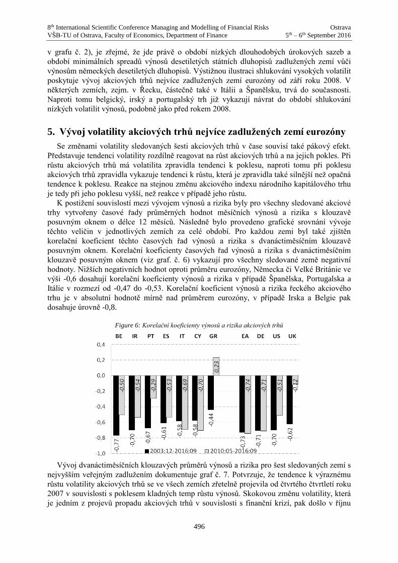
8th International Scientific Conference Managing and Modelling of Financial Risks Ostrava
VŠB-TU of Ostrava, Faculty of Economics, Department of Finance 5th – 6th September 2016
496
v grafu č. 2), je zřejmé, že jde právě o období nízkých dlouhodobých úrokových sazeb a
období minimálních spreadů výnosů desetiletých státních dluhopisů zadlužených zemí vůči
výnosům německých desetiletých dluhopisů. Výstižnou ilustraci shlukování vysokých volatilit
poskytuje vývoj akciových trhů nejvíce zadlužených zemí eurozóny od září roku 2008. V
některých zemích, zejm. v Řecku, částečně také v Itálii a Španělsku, trvá do současnosti.
Naproti tomu belgický, irský a portugalský trh již vykazují návrat do období shlukování
nízkých volatilit výnosů, podobně jako před rokem 2008.
5. Vývoj volatility akciových trhů nejvíce zadlužených zemí eurozóny
Se změnami volatility sledovaných šesti akciových trhů v čase souvisí také pákový efekt.
Představuje tendenci volatility rozdílně reagovat na růst akciových trhů a na jejich pokles. Při
růstu akciových trhů má volatilita zpravidla tendenci k poklesu, naproti tomu při poklesu
akciových trhů zpravidla vykazuje tendenci k růstu, která je zpravidla také silnější než opačná
tendence k poklesu. Reakce na stejnou změnu akciového indexu národního kapitálového trhu
je tedy při jeho poklesu vyšší, než reakce v případě jeho růstu.
K postižení souvislostí mezi vývojem výnosů a rizika byly pro všechny sledované akciové
trhy vytvořeny časové řady průměrných hodnot měsíčních výnosů a rizika s klouzavě
posuvným oknem o délce 12 měsíců. Následně bylo provedeno grafické srovnání vývoje
těchto veličin v jednotlivých zemích za celé období. Pro každou zemi byl také zjištěn
korelační koeficient těchto časových řad výnosů a rizika s dvanáctiměsíčním klouzavě
posuvným oknem. Korelační koeficienty časových řad výnosů a rizika s dvanáctiměsíčním
klouzavě posuvným oknem (viz graf. č. 6) vykazují pro všechny sledované země negativní
hodnoty. Nižších negativních hodnot oproti průměru eurozóny, Německa či Velké Británie ve
výši -0,6 dosahují korelační koeficienty výnosů a rizika v případě Španělska, Portugalska a
Itálie v rozmezí od -0,47 do -0,53. Korelační koeficient výnosů a rizika řeckého akciového
trhu je v absolutní hodnotě mírně nad průměrem eurozóny, v případě Irska a Belgie pak
dosahuje úrovně -0,8.
Figure 6: Korelační koeficienty výnosů a rizika akciových trhů
Vývoj dvanáctiměsíčních klouzavých průměrů výnosů a rizika pro šest sledovaných zemí s
nejvyšším veřejným zadlužením dokumentuje graf č. 7. Potvrzuje, že tendence k výraznému
růstu volatility akciových trhů se ve všech zemích zřetelně projevila od čtvrtého čtvrtletí roku
2007 v souvislosti s poklesem kladných temp růstu výnosů. Skokovou změnu volatility, která
je jedním z projevů propadu akciových trhů v souvislosti s finanční krizí, pak došlo v říjnu

8th International Scientific Conference Managing and Modelling of Financial Risks Ostrava
VŠB-TU of Ostrava, Faculty of Economics, Department of Finance 5th – 6th September 2016
497
roku 2008. Podobný růst volatility byl například zaznamenán také ve třetím čtvrtletí roku
2001, kdy vývoj výnosů akciových trhů byl spjat s internetovou bublinou a jejím následným
splasknutím.
Figure 7: Vývoj výnosů a rizika
-12
-8
-4
0
4
8
12
16
04 06 08 10 12 14 16
BE_RET
BE_SD-12
-8
-4
0
4
8
12
16
04 06 08 10 12 14 16
IR_RET
IR_SD-12
-8
-4
0
4
8
12
16
04 06 08 10 12 14 16
PT_RET
PT_SD
-12
-8
-4
0
4
8
12
16
04 06 08 10 12 14 16
ES_RET
ES_SD-12
-8
-4
0
4
8
12
16
04 06 08 10 12 14 16
IT_RET
IT_SD-20
-10
0
10
20
30
40
50
04 06 08 10 12 14 16
CY_RET
CY_SD
-12
-8
-4
0
4
8
12
16
04 06 08 10 12 14 16
GR_RET
GR_SD-12
-8
-4
0
4
8
12
16
04 06 08 10 12 14 16
EA_RET
EA_SD-12
-8
-4
0
4
8
12
16
04 06 08 10 12 14 16
DE_RET
DE_SD
DEEAGR
CYITES
PTIRBE
Změny volatility akciových trhů byly analyzovány také z hlediska trendů jejich vývoje,
přičemž trendové hodnoty byly získány filtrováním časových řad s využitím Hodrick-
Prescottova filtru (výsledky na tomto místě neuvádíme). Následně byla graficky provedena
mezinárodní komparace trendů vývoje volatility akciových trhů. v průběhu sledovaného
období 2003:03 – 2013:02 vykazovala volatilita akciových trhů všech sledovaných vysoce
zadlužených ekonomik, Německa i Velké Británie přibližně do února roku 2009 přes
rozdílnou úroveň volatility v zásadě shodné trendy vývoje. Následující vývoj je však nutno
považovat za divergentní. V Řecku trend rostoucí volatility dále strmě pokračuje, ve
Španělsku a Portugalsku došlo k zvolnění jeho růstu, v případě Itálie se trend rostoucí
volatility v zásadě zastavil. V Irsku a Belgii se naproti tomu začal prosazovat relativně strmý
trend poklesu volatility k úrovni let 2004-2005, podobně jako ve Velké Británii. Trend k
poklesu volatility se začal prosazovat také na německém akciovém trhu, byť jen s velmi
pozvolným průběhem. Trendy vývoje volatility největších akciových trhů, britského a
německého, jsou při vyšší úrovni volatility německého trhu více vzájemně sladěné než trendy
vývoje volatility trhů zemí s nejvyšším veřejným zadlužením. Podobně jsou také více
korelovány výnosy nejvyspělejších akciových trhů.

8th International Scientific Conference Managing and Modelling of Financial Risks Ostrava
VŠB-TU of Ostrava, Faculty of Economics, Department of Finance 5th – 6th September 2016
498
6. Shrnutí
Akciové trhy zemí eurozóny jsou vyspělými akciovými trhy. Jejich velikost v absolutním i
relativním vyjádření, objemy obchodů a likvidita vykazují četné odlišnosti. Výnosy akciových
trhů šesti zemí eurozóny s největším veřejným zadlužením vykazují obecně vyšší variabilitu a
jsou spjaty s vyšším rizikem. V případě významných změn na finančních trzích nebo v době
finančních krizí se tyto rozdíly dále zvyšují.
Od vzniku eurozóny vykazovaly akciové trhy analyzovaných zemí eurozóny s nejvyšším
veřejným zadlužením přibližně do března roku 2009 v zásadě shodné trendy ve vývoji výnosů
a volatility. Finanční krize a vznik dluhové krize se však v těchto zemích kromě jiného
projevily podstatně více v poklesu výnosů akciových trhů a růstu jejich volatility. Trend
poklesu volatility výnosů akciových indexů a současného růstu výnosů se dosud projevil
pouze v Belgii a v Irsku. K mírnému snížení volatility, avšak při negativní střední hodnotě
výnosů došlo v Itálii a Portugalsku. V dalších třech zemích dále vzrostla volatilita při
přetrvávající negativní střední hodnotě měsíčních výnosů. Růst indexů národních akciových
trhů v Řecku a na Kypru se neobnovil a akciové indexy Portugalska, Španělska a Itálie jsou
hluboko pod úrovní roku 2007 či 2010.
References
[1] Arghyrou, M.G. and Kontonikas, A. (2012). The EMU sovereign-debt crisis:
fundamentals, expectations and contagion. Journal of International Financial Markets,
Institutions and Money, 22, pp. 658–677.
[2] Baldwin, R. and Wyplosz, C. (2015). The Economics of European Integration. 5th. ed.
London: McGraw-Hill Education.
[3] Bank for International Settlements (2009). BIS 79th Annual Report - June 2009. Basel:
Bank for International Settlements.
[4] Cline, W.R. (2016). Managing The Euro Area Debt Crisis. New York: Columbia
University Press.
[5] Constancio, V. (2012). Contagion and the European debt crisis. Financial Stability
Review, 16, pp. 109–121.
[6] ECB (2010). Monthly Bulletin. October 2010.
[7] Federal Reserve Bank of St. Louis (2009). Financial Crisis Timeline. [online]. Dostupný
z WWW: < http://timeline.stlouisfed.org/index.cfm?p=timeline>.
[8] Kalbaska, A. and Gatkowski, M. (2012). Eurozone sovereign contagion: evidence from
the CDS market (2005–2010). Journal of Economic Behavior and Organization, 83, pp.
657–673.
[9] Kulhánek, L., Polouček, S. and Stavárek, D. (2004). The Financial and Banking Sectors
in Transition Countries. In Polouček, S. (ed.) Reforming the Financial Sector in Central
European Countries. Houndmills: Palgrave Macmillan.
[10] Kulhánek, L. and Šoltés, V. (2010). Finančné trhy. In Polouček, S. a kol. Peniaze, banky,
finančné trhy. Bratislava: Iura Edition.
[11] Worldbank (2016): World Development Indicators 2016. Washington: The World Bank.

8th International Scientific Conference Managing and Modelling of Financial Risks Ostrava
VŠB-TU of Ostrava, Faculty of Economics, Department of Finance 5th – 6th September 2016
499
Comparing inequality of distributions on the basis of mixed Lorenz curves
Tommaso Lando1, Lucio Bertoli-Barsotti2
Abstract
The Lorenz dominance (LD) is generally used to rank Lorenz curves (LCs) or, equivalently, the
corresponding distributions, in terms of inequality. When LCs intersect, the LD is not verified,
but we can rely on weaker orders such as the upward or downward second-degree Lorenz
dominance (2-LD), which emphasize the effect of the left or the right tail, respectively. The main
idea of this paper it to propose a dominance relation that lies between the LD and the 2-LD, i.e.
weaker than the former and stronger than the latter. For this purpose, we introduce a mixed Lorenz
curve, that is, a mix of the original LC and a symmetric trasformation of it. By so doing, our
approach is also intended to emphasize both tails of the distribution, rather than one. We provide
an exemplification with regard to distributions of income.
Key words
Lorenz ordering, majorization, inequality, disparity, stochastic dominance
JEL Classification: D31, D63, I32
1. Introduction
The Lorenz curve (LC) is a primary tool for comparison of distributions of non-negative
variables (e.g. random variables or statistical variables) in terms of inequality. Its use in the
field of economics, for the measurement of income inequality is well known. The LC gives rise
to a preorder, that is, the Lorenz dominance (LD), that is generally used to rank distributions
based on their degree of inequality. In particular, according to the LD, the higher of two non-
intersecting Lorenz curves shows less inequality compared to the lower one, therefore we can
establish a preference relation between the two corresponding distributions. In an economic
framework, the LD is coherent with the Pigou-Dalton condition, i.e. the so called “principle of
transfers”. According to this principle, the higher of two non-intersecting Lorenz curves can be
obtained from the lower one by an iteration of income transfers from “richer” to “poorer”
individuals (the so called elementary transfers or T-transforms, Marshall et al., 2009, p. 32, also
called progressive transfers, Shorrocks and Foster, 1987). For this reason, the “coherence” with
the LD represents a fundamental property for all inequality measures.
However, many empirical studies revealed that Lorenz curves often intersect in the practice,
therefore it is not rare to find couples of distributions that cannot be ranked based on the LD.
In such cases, we can compare the intersecting distributions by relying on weaker orders of
inequality, such as the second-degree Lorenz dominance, 2-LD (Aaberge, 2009). The basic idea
of the 2-LD is to move from the (first-degree) LD to a dominance relation of higher degree by
cumulating LCs i) from the bottom or, ii), from the top. In the first case (i), this idea has been
analysed in several works, related to the concept of third-order stochastic dominance (see e.g.
Atkinson, 2008) or third-degree inverse stochastic dominance (Muliere and Scarsini, 1989).
These orderings emphasize the left tail of the distribution. Indeed, many authors (see e.g.
1 Tommaso Lando, University of Bergamo and VŠB-TU Ostrava, [email protected]. 2 Lucio Bertoli-Barsotti, University of Bergamo, [email protected].

8th International Scientific Conference Managing and Modelling of Financial Risks Ostrava
VŠB-TU of Ostrava, Faculty of Economics, Department of Finance 5th – 6th September 2016
500
Shorrocks and Foster, 1987; Dardanoni and Lambert, 1988; Atkinson, 2008) agree that an
elementary transfer should be more equalizing the “lower” it occurs in the distribution, that is,
the principle of aversion to downside inequality (Davies and Hoy, 1995). On the other hand,
the second idea (ii), introduced by Muliere and Scarsini (1989) and more recently developed by
Aaberge (2009), emphasizes the right tail of the distribution. This can be interesting, for
instance, in an economic context, where a lot of attention is recently given to those variations
occurring at the top of the income distribution (Makdissi and Yazbeck, 2014).
The basic idea of this paper is to overcome some possible (related) issues of the 2-LD. First,
the 2-LD may be a too weak dominance relation for comparing distributions. In this regard, we
recall that, distributions with equal values of the Gini index can be easily ranked with the 2-LD,
especially if they are single-crossing (see e.g. Zoli, 1999 or Lando and Bertoli-Barsotti, 2016).
Thus, 2-LD may be too restrictive, because the weight that it attaches to one of the two tails
may be excessive so that it may reverse an extreme situation such as the equality of the Gini.
Moreover, by choosing to emphasize the left (right) tail, the 2-LD logically downsizes the effect
of those variations occurring in the right (left) one. Thus, it might be preferable to combine
those two approaches into a single dominance relation that emphasizes both of the tails at the
same time, as recently proposed by Lando and Bertoli-Barsotti (2016).
2. Preliminaries
In this section we define the LD and analyze its relation with the majorization preorder. We
recall that a preorder is a binary relation ≤ over a set 𝑆 that is reflexive and transitive. In
particular, observe that a preorder ≤ does not generally satisfy the antisymmetry property (that
is, 𝑎 ≤ 𝑏 and 𝑏 ≤ 𝑎 does not necessarily imply 𝑎 = 𝑏) and it is generally not total (that is, each
pair 𝑎, 𝑏 in 𝑆 is not necessarily related by ≤).
Let ℱ be the space of non-negative distributions 𝐹 with finite expectation 𝜇𝐹, ℱ =
{𝐹: 𝐹(𝑧) = 0 ∀ 𝑧 < 0 ∧ ∫ 𝑧𝑑𝐹 = 𝜇𝐹∞
0< ∞}. The (generalized) inverse or quantile
distribution of a distribution function 𝐹 ∈ ℱ is given by
𝐹−1(𝑝) = inf{𝑧: 𝐹(𝑧) ≥ 𝑝}, 𝑝 ∈ (0,1) (1)
If 𝐹 has finite expectation, 𝜇𝐹, then the Lorenz curve 𝐿𝐹: [0,1] → [0,1] is defined as follows
[16]:
𝐿𝐹(𝑝) =1
𝜇𝐹∫ 𝐹−1(𝑡)𝑑𝑡
𝑝
0, 𝑝 ∈ (0,1). (2)
We recall that the Gini index is given by twice the area between the Lorenz curve and the
45° line:
Γ(𝐹) = 1 − 2 ∫ 𝐿𝐹(𝑡)𝑑𝑡1
0. (3)
Let us also define the complementary curve [13], ��𝐹: [0,1] → [0,1], given by
��𝐹(𝑝) =1
𝜇𝐹∫ 𝐹−1(1 − 𝑡)𝑑𝑡
𝑝
0= 1 − 𝐿𝐹(1 − 𝑝), 𝑝 ∈ (0,1) (4)
Actually, for a given percentage 𝑝, 𝐿𝐹(𝑝) represents the percentage of “total” possessed by the
low 100𝑝% part of the distribution, while ��𝐹(𝑝) represents the percentage of “total”
corresponding to the top 100𝑝% part of the distribution. From a geometrical point of view,

8th International Scientific Conference Managing and Modelling of Financial Risks Ostrava
VŠB-TU of Ostrava, Faculty of Economics, Department of Finance 5th – 6th September 2016
501
��𝐹(𝑝), increasing and concave, is the 180° rotation of 𝐿𝐹(𝑝), increasing and convex, with
respect to the point (0.5,0.5).
In the sequel we shall also need the following curve:
��𝐹−1(𝑝) = 1 − 𝐿𝐹
−1(1 − 𝑝), (5)
where ��𝐹−1 and 𝐿𝑋
−1 denote, respectively, the inverse functions of ��𝐹 and 𝐿𝐹 (that are clearly
invertible).
��𝐹−1(𝑝) represents the percentage of population that holds the top 100𝑝% part of the “total”.
We observe that ��𝐹−1 is also a Lorenz curve, in that it is non-decreasing, convex, differentiable
almost everywhere and defined on the set [0,1] (��𝐹−1(0) = 0, ��𝐹
−1(1) = 1), see Sordo et al.
(2014). From a geometrical point of view, the LC ��𝐹−1 is symmetric with respect to the LC 𝐿𝐹,
where the axis of symmetry is the line 𝑡 = 1 − 𝑝.
3. Dominance relations
The Lorenz dominance (or ordering) ≤𝐿 is a pre-order defined over the space ℱ. It can be
defined as follows.
Definition 1. Let 𝐹, 𝐺 ∈ ℱ: we write 𝐹 ≤𝐿 𝐺 if and only if 𝐿𝐹(𝑝) ≥ 𝐿𝐺(𝑝), ∀ 𝑝 ∈ (0,1).
When the LD is not fulfilled, i.e. when LCs intersect, we need to introduce some weaker
criteria in order to obtain unambiguous rankings. Muliere and Scarsini (1989) suggest using the
third-degree inverse stochastic dominance to rank intersecting Lorenz curves. While the LD
compares the percentages of total (wealth) corresponding to the low 100𝑡% parts of the
distributions, by using the 3-ISD an integration is performed. Hence the comparison concerns
the cumulated percentages of total corresponding to the low 100𝑡% parts of the distributions.
In other words, by so doing we emphasize the left tail of the distribution (i.e. lower incomes).
A parallel approach consists in cumulating LCs from the right: that is, attaching more weighting
to top incomes. In this paper we find it more convenient to adopt the normalized (i.e. based on
the LC) version of the 3-ISD: that is, the second-degree Lorenz dominance (Aaberge, 2009),
defined as follows. Note that our definition slightly differs from Aaberge’s definition in that,
coherently with the literature (see e.g. Marshall et al., 2009) and our definition of LD (Def. 1),
we consider “dominant” the distribution that presents greater inequality.
Definition 2. We say that 𝐺 second-degree upward Lorenz dominates 𝐹, and write 𝐹 ≤𝐿2 𝐺 iff:
∫ 𝐿𝐹(𝑝)𝑑𝑝𝑡
0≥ ∫ 𝐿𝐺(𝑝)𝑑𝑝
𝑡
0, ∀𝑡 ∈ [0,1].
We say that 𝐺 second-degree downward Lorenz dominates 𝐹, and write 𝐹 ≤��2 𝐺 iff any of the
following equivalent conditions is true:
i) ∫ ��𝐹(𝑝)𝑑𝑝𝑡
0≤ ∫ ��𝐺(𝑝)𝑑𝑝
𝑡
0, ∀𝑡 ∈ [0,1]
ii) ∫ 1 − 𝐿𝐹(𝑝)𝑑𝑝1
𝑡≤ ∫ 1 − 𝐿𝐺(𝑝)𝑑𝑝
1
𝑡, ∀𝑡 ∈ [0,1]
iii) ∫ ��𝐹−1(𝑝)𝑑𝑝
𝑡
0≥ ∫ ��𝐺
−1(𝑝)𝑑𝑝𝑡
0, ∀𝑡 ∈ [0,1]
Observe that 𝐹 ≤𝐿 𝐺 implies 𝐹 ≤𝐿2 𝐺 and 𝐹 ≤��
2 𝐺, but the converse is not necessarily true,
i.e. 𝐹 ≤𝐿2 𝐺 and 𝐹 ≤��
2 𝐺 do not imply the LD. Moreover, note that 𝐹 ≤𝐿2 𝐺 implies that 𝐿𝐹 starts
above 𝐿𝐺 and presents a larger (underlying) area: that is, a lower (or equal) value of the Gini
8th International Scientific Conference Managing and Modelling of Financial Risks Ostrava
VŠB-TU of Ostrava, Faculty of Economics, Department of Finance 5th – 6th September 2016
502
index. Differently, 𝐹 ≤��2 𝐺 implies that 𝐿𝐹 starts below 𝐿𝐺 but still has a lower (or equal) Gini.
Hence it is apparent that in both cases the condition ∫ 𝐿𝐹(𝑝)𝑑𝑝1
0≥ ∫ 𝐿𝐺(𝑝)𝑑𝑝
1
0 (i.e. Γ(𝐹) ≤
Γ(𝐺)) is necessary to establish a dominance. In particular, Zoli (1999) argues that if Lorenz
curves cross only once, the value of the Gini index is crucial for determining the (upward)
second-degree Lorenz dominance (this result can be trivially extended to the downward 2-LD).
4. A mixed approach
As stated in the introduction, the objective of this paper is to propose a dominance relation
that emphasizes both the tails of the distributions. Moreover, we aim at defining a preorder that
is finer than the LD (i.e. it can rank a major number of couples of distributions, such as those
that intersect) but less restrictive, i.e. stronger, then the 2-LD. In particular, we focus on the
issue of ranking single-crossing LCs. Indeed, it should be stressed that, in an economic context,
single-crossing LCs occur in most practical cases, as highlighted by the empirical analyses of
Atkinson (1970) and Davies and Hoy (1985), whilst multiple-crossing LCs are very rare. The
formal definition of single-crossing LCs is as follows.
Definition 3. 𝐿𝐹 single-crosses 𝐿𝐺 from above if there exist a point 𝑡0 (where 0 < 𝑡0 < 1) such
that 𝐿𝐹(𝑡) ≤ 𝐿𝐺(𝑡) for 0 ≤ 𝑡 < 𝑡0, where the inequality is strict for some for some 0 < 𝑡′ <𝑡0, and 𝐿𝐹(𝑡) ≥ 𝐿𝐺(𝑡) for 𝑡0 ≤ 𝑡 < 1, where the inequality is strict for some 𝑡0 ≤ 𝑡′′ < 1.
Similarly, 𝐿𝐹 single-crosses 𝐿𝐺 from below iff 𝐿𝐺 single-crosses 𝐿𝐹 from above.
Let us introduce a new LC, that is a compound between the LCs 𝐿𝐹 and ��𝐹−1:
𝐿𝐹𝑎 (𝑝) = 𝑎𝐿𝐹(𝑝) + (1 − 𝑎)��𝐹
−1(𝑝), 0 ≤ 𝑎 ≤ 1. (6)
We denote 𝐿𝐹𝑎 as the mixed Lorenz curve (MLC) of order 𝑎. By construction, 𝐿𝐹
𝑎 (𝑝)
represents a weighted average between the percentage of “total” possessed by the low 100𝑝%
part of the distribution and the percentage of population that holds the top 100𝑝% part of the
“total”. Clearly, inequality decreases if both these percentage increase, in that inequality
aversion generally corresponds to the principle that i) the low parts of the population should not
be too “poor”, and, symmetrically, ii) the top parts of the total should not be possessed by a too
small number of “rich” people. Therefore, 𝐿𝐹𝑎 combines two complementary approaches into a
single representation of inequality, where the number 𝑎 may be used as a “mixing” coefficient.
For 𝑎 = 1 we obtain 𝐿𝐹1 = 𝐿𝐹, whilst, for 𝑎 = 0, the right tail is moved to the left and vice-
versa, so that 𝐿𝐹0 = ��𝐹
−1. Hence, generally, 𝑎 represent the proportion that we want to use in
order to mix the left and right parts of the distribution. We also observe the following properties.
1) 𝐿𝐹𝑎 is a Lorenz curve.
2) The LCs 𝐿𝐹 , ��𝐹−1, 𝐿𝐹
𝑎 yield equal values of the Gini coefficient.
3) The LCs 𝐿𝐹 , ��𝐹−1, 𝐿𝐹
𝑎 cross the line 𝑡 = 1 − 𝑝 in the same point.
4) For 𝑎 = 0.5, 𝐿𝐹0.5 is symmetric w.r.t. the line 𝑡 = 1 − 𝑝.
Clearly, if 𝐿𝐹(𝑝) ≥ 𝐿𝐺(𝑝), ∀ 𝑝 ∈ (0,1) then 𝐿𝐹𝑎 (𝑝) ≥ 𝐿𝐹
𝑎 (𝑝), ∀𝑎, 𝑝 ∈ (0,1). But when the
original LCs intersect it may be useful to introduce a dominance relation that is based on the
integral of 𝐿𝐹𝑎 , rather than 𝐿𝐹 or ��𝐹
−1. By cumulating such a “mix”, we emphasize both tails at
the same time (with different weights, according to 𝑎) and obtain a preorder that generalizes

8th International Scientific Conference Managing and Modelling of Financial Risks Ostrava
VŠB-TU of Ostrava, Faculty of Economics, Department of Finance 5th – 6th September 2016
503
the upward and downward 2-LD. We define this preorder as the second-degree mixed Lorenz
dominance of order 𝑎 (2-MLD of order 𝑎).
Definition 4. We say that 𝐺 second-degree Lorenz dominates 𝐹 with mixing order 𝑎 (𝑎 ∈
[0,1]), and write 𝐹 ≤𝐿2,𝑎 𝐺, iff ∫ 𝐿𝐹
𝑎 (𝑝)𝑑𝑝𝑡
0≥ ∫ 𝐿𝐺
𝑎 (𝑝)𝑑𝑝𝑡
0, ∀𝑡 ∈ [0,1]
Because the cumulation of the MLC is performed from the left to the right, we may easily
understand that the coefficient 𝑎 determines the disproportion of weights that we want to attach
to the right tail compared to the left one. Moreover, we observe that the 2-MLD has the
following interesting properties.
1) 𝐹 ≤𝐿2,1 𝐺 is equivalent to 𝐹 ≤𝐿
2 𝐺.
2) 𝐹 ≤𝐿2,0 𝐺 is equivalent to 𝐹 ≤��
2 𝐺.
3) 𝐹 ≤𝐿 𝐺 implies 𝐹 ≤𝐿2,𝑎 𝐺, ∀𝑎 ∈ [0,1].
4) If 𝐿𝐹 , 𝐿𝐺 cross once from above and 𝐹 ≤𝐿2,𝑎0 𝐺, then 𝐹 ≤𝐿
2,𝑎 𝐺 ∀𝑎 ∈ [𝑎0, 1].
5) If 𝐿𝐹 , 𝐿𝐺 cross once from below and 𝐹 ≤𝐿2,𝑎0 𝐺, then 𝐹 ≤𝐿
2,𝑎 𝐺 ∀𝑎 ∈ [0, 𝑎0].
From the properties above we may observe that the 2-MLD is a preorder between the first
and the second-degree LD. Indeed, the 2-MLD is weaker than the LD but, when LCs are single
crossing, from above or from below, it is stronger than the upward 2-LD or the downward LD,
respectively. Moreover, the 2-MLD is progressively stronger if 𝑎 gets closer to 0 (if 𝐹, 𝐺 cross
once from above) or to 1 (if 𝐹, 𝐺 cross once, from below). Clearly, if 𝐹, 𝐺 are single-crossing,
it is not possible to have 𝐹 ≤𝐿2,𝑎 𝐺 ∀𝑎 ∈ [0,1] because this would imply that the LCs do not
intersect. Thus, it would be interesting to find the extreme value of 𝑎 (that is, the minimum if
the LCs cross from above, the maximum if they cross form below) because this number
provides information about the “strenght“ of the dominance. Indeed, 𝐹, 𝐺 cross once from above
1) 𝑎 is close to 1 means that the dominance of the second-degree is very weak because it mainly
depend on the disproportion between the left and right tails, whilst 2) 𝑎 is close to 0 means that
the dominance is stronger and almost independent from such disproportion, as it still holds even
if we almost invert the weights of the tails. The concept is very similar, but inverse, if , 𝐹, 𝐺
cross once from below.
4.1 A practical exemplification
In order to better understand the basic logic of the 2-MLD, in this section we present a case
study. As well known, the LD is commonly used to compare income distributions. We
dowloaded the data from the WIID, that is, the World Income Inequality Database, (UNU-
WIDER, 2015) which collects and stores information on income inequality for developed,
developing, and transition countries. The WIID provides a comprehensive set of income
inequality statistics available and can be downloaded for free. In particular, the WIID provides
the deciles of income distributions, that can be used to determine the LCs, at least approximately
(i.e. consisting of 10 segments). The last version of WIID, that is version 3.3, was released in
2015 and the income distributions correspond to different years and different sources (we refer
to the user guide for further information). The most recent data, for most countries, are generally
referred to years 2009-2010 and, in the whole database, there is no information available after
year 2013. Let us focus on a particular couple of european countries, that is, France and Spain.
The deciles (expressed in percentage) of the income distribution of France, for the year 2011
(source=Eurostat) are
3.5, 5.1, 6.2, 7, 7.9, 8.8, 10, 11.5, 14, 25.9;

8th International Scientific Conference Managing and Modelling of Financial Risks Ostrava
VŠB-TU of Ostrava, Faculty of Economics, Department of Finance 5th – 6th September 2016
504
whilst, for Spain (year=2011, source=Eurostat), we have
1.6, 4.3, 5.7, 6.9, 8.1, 9.5, 11, 13.1, 16, 23.9.
Observe that the LCs can be derived very easily by cumulating the deciles.
Let us denote by 𝐹, 𝐺, respectively, the income distributions of France and Spain. The LCs
of France and Spain, represented in Figure 1, are single-crossing from above, thus the LD is not
verified. In particular, Spain exhibits a greater degree of inequality in the low part of the
distribution, whilst France in exhibits a greater degree of inequality in the high part. The main
questions at this point are: 1) is the right tail of 𝐹 “heavier“, or comparable to the left tail of 𝐺?
2) Are we “close“ to the LD or the difference (in terms of inequality) between the two
distributions is weak?
As the Gini index of France is higher than that of Spain (this is evident from the ares under
the LCs in Fig.1), a result of Zoli (1999) guarantees that France dominates Spain w.r.t. the
upward 2-LD, so the left tail of 𝐺 is “heavier“ than the right tail of 𝐹. Moreover, by using the
MLD, we can analyze and understand the strenght of the 2-LD dominance. After some
iterations, we obtain that 𝐹 ≤𝐿2,𝑎 𝐺, ∀𝑎 ∈ [0.04,1], so the dominance relation is quite strong
because, in order to compensate the disproportion between the inequality in the left tail of 𝐺
and that in the right tail of 𝐹, we need a mixing coefficient that is very close to 0. Put otherwise,
the dominance is strong and quite independent from the tails, because it holds even if we move
the 96% of the left tail to the right and vice-versa.
Figure 1: LCs of France (dashed) and Spain (solid)
5. Conclusion
We proposed a new ordering for comparing distributions in terms of inequality. Our
objective was 1) to obtain an dominance relation that can be placed between the LD and the 2-
LD; 2) to emphasize both tails of the distribution rather than one. Future work will be aimed at
further analysing the mathematical relations beween the 2-MLD and other orders and at
performing larger empirical analysis in order to verify the usefulness of our approach when
dealing with real data.
0.2 0.4 0.6 0.8 1.0
0.2
0.4
0.6
0.8
1.0

8th International Scientific Conference Managing and Modelling of Financial Risks Ostrava
VŠB-TU of Ostrava, Faculty of Economics, Department of Finance 5th – 6th September 2016
505
Acknowledgement
The research was supported through the Czech Science Foundation (GACR) under project
15-23699S and through SP2015/15, an SGS research project of VŠB-TU Ostrava, and
furthermore by the European Social Fund in the framework of CZ.1.07/2.3.00/20.0296.
References
[1] Aaberge, R. (2009). Ranking intersecting Lorenz curves. Soc. Choice Welf. 33, pp. 235-
259.
[2] Atkinson B. (1970). On the measurement of inequality. Journal of economic theory, 2
(3), pp. 244-263.
[3] Atkinson, A.B. (2008). More on the measurement of inequality. J. Econ. Inequal. 6, pp.
277-283.
[4] Dardanoni, V. and Lambert, P.J. (1988). Welfare rankings of income distributions: A role
for the variance and some insights for tax reforms. Soc. Choice Welf. 5, pp. 1-17.
[5] Davies J., Hoy M.: Comparing income distributions under aversion to downside
inequality. London: Department of Economics, University of Western Ontario (1985).
[6] Davies, J.B. and Hoy, M. (1995). Making inequality comparisons when Lorenz curves
intersect. Am. Econ. Rev. 85, pp. 980-986.
[7] Gastwirth, J.L. (1971). A general definition of the Lorenz curve. Econometrica 39: pp.
1037-1039.
[8] Lando, T. and Bertoli-Barsotti, L. (2016). Weak orderings for intersecting Lorenz curves.
Metron 7, DOI 10.1007/s40300-016-0087-6, pp.1-16.
[9] Madkissi, P. and Yakbeck, M. (2015). On the measurement of plutonomy. Soc. Choice
Welf. 44, pp.703-717.
[10] Marshall, A.W., Olkin, I. and Arnold, B.C. (2009). Inequalities: theory of majorization
and its applications. (second edition), Springer.
[11] Muliere P., Scarsini M. (1989). A note on stochastic dominance and inequality measures.
Journal of Economic Theory, 49 (2), pp. 314-323.
[12] Sordo, M. A., Navarro, J., & Sarabia, J. M. (2014). Distorted Lorenz curves: models and
comparisons. Social Choice and Welfare, 42(4), pp. 761-780.
[13] Shorrocks, A.F. and Foster J.E. (1987). Transfer sensitive inequality measures. Rev. Econ.
Stud., 14, pp. 485-497.
[14] UNU-WIDER, World Income Inequality Database (WIID3c), September 2015,
<http://www.wider.unu.edu/research/Database/en_GB/wiid/>
[15] Zoli C. (1999). Intersecting generalized Lorenz curves and the Gini index. i, 16 (2), pp.
183-196.

8th International Scientific Conference Managing and Modelling of Financial Risks Ostrava
VŠB-TU of Ostrava, Faculty of Economics, Department of Finance 5th – 6th September 2016
506
Relationship Between Stock Prices and Microeconomic Variables: Evidence From Prague
Stock Exchange
Marie Ligocká1, Tomáš Pražák 2
Abstract
The influencing variables of stock value can be devided into two basic categories,
macroeconomic and microeconomic factors. This paper is oriented on selected part of
microeconomic factors. The aim of paper is to investigate the existence of relationship between
selected financial ratios and stock prices of companies on the Prague Stock Exchange. The
sector for the analyse is manufacturing for the period from 2005 to 2015. To recognize the
existence of short-time and long-time causality between variables are, used cointegration
methods. It is expected to demonstrate relationship between debt equity ratios and stock prices.
Key words
Financial ratios, cointegration, stock prices, Prague Stock Exchange.
JEL Classification: C32, D24, G32.
1. Introduction
The paper is oriented on factors which have an impact on individual stocks of
manufacturing sector in the Czech Republic. Results can be beneficial for investors who think
about investment to analyzed companies because contemplated variables are factors which
influence firms by business activity. Further attention in the empirical literature is not focused
on the Czech stock market due to small number of publicly traded companies and limited
database. Compared with world exchanges, the market capitalization of the Prague Stock
Exchange is only 952 mld. CZK (39 mld. USD). But despite some limitations time series is
recommended to deal with the Czech stock market of potential causes of the country, because
the Czech Republic was the first post-communist country which has become a wealthy
member of the Group World Bank. Czech crown also well represented a safe haven in the
financial crisis due to the relative stability of the country. At the manufacturing were taken
into account in connection with the position of the national economy both in the Czech
Republic and in the other countries of Central and Eastern Europe.
The aim of the paper is to research existence and strong of relationship between stock
prices of selected Czech manufacturing companies and financial ratios. We examine short –
time links from the microeconomic environment to the Czech stock market. Using data of
stock prices are values of companies listed on Prague Stock Exchange: Čez, Toma, Unipetrol
and Energoaqua. Financial ratios used in study are commonly used ratios of liquidity, activity,
profitability, indebtedness and market value.
1 PhD. Student, Department of Finance and Accounting, [email protected]. 2 PhD. Student, Department of Finance and Accounting, [email protected].

8th International Scientific Conference Managing and Modelling of Financial Risks Ostrava
VŠB-TU of Ostrava, Faculty of Economics, Department of Finance 5th – 6th September 2016
507
Contribution is divided into several sections. Review of Literature is following after
Introduction where can be found some studies dealing with the issue. Information sources of
data and using methodology are contained in the chapter Data and methodology. Achieved
results are included in other part Empirical results containing the outputs used econometric
tests. The important section of the article is also Conclusion.
2. Review of Literature
A lot of studies have been conducted to examine the link between microeconomic variables
and stock prices or stock returns. The classification can be performed by selected financial
ratios, development of the stock market or methodology used. We take account only literature
that is relevant to the topic. We cite priority papers which are oriented on Central and Eastern
European markets even when they are not dealing directly with the issue of financial ratios.
The reason is the lack of papers focus on the topic of financial ratios.
There can be included Dzikevičius and Šaranda (2011) who aimed to determine whether it
is possible to forecast stock prices by estimating the financial ratios of a particular company in
the Lithuanian stock market. They used correlation and covariance as the main analytical
tools. They chose 5 companies and calculated with 20 financial ratios. They found out positive
and negative links between stock returns and financial ratios, but results can be different
depending on the method of calculation ratios.
Bistrova, Lace and Titko (2013) analyzed the relationship between the market and
economic performance of 117 Central and Eastern European companies’. The research
including Czech Republic, Poland, Slovakia and Slovenia were processed by correlation and
quartile analysis. They declared that correlation was insignificant or even negative in the
majority of cases.
Pajuste, Kepitis and Högfeldt (2000) examined a wide set of risk factors that may influence
equity market fluctuations in the Czech Republic, Estonia, Hungary, Poland and Slovenia.
They found out that local risk factors are the most important in explaining fluctuations of
stock returns in these 5 countries. And the most significant factor is the market risk.
Following papers are concentrated on Central and Eastern European market and crisis
period. There we can involve Égert and Kočenda (2006) who researched movements and
interdependence between Western European and Central and Eastern European stock markets.
They did not find robust cointegration relationship for any of the stock index pairs. But it is
possible to say that there exist signs of short-term spillover effects both in terms of stock
returns and stock price volatility.
Syllignakis and Kouretas (2011) investigated time-varying conditional correlations to the
weekly index returns of the Czech Republic, Estonia, Hungary, Poland, Romania, Slovakia
and Slovenia. The main finding of the present analysis is that there is a statistically significant
increase in conditional correlations between the US and the German stock returns and the
CEE stock returns, particularly during the 2007 – 2009 financial crises, implying that these
emerging markets are exposed to external shocks.
Baruník and Vácha (2011) examined comovement and contagion by researching the
interconnections between Czech, Hungarian, Polish and German stock markets during the
recent crisis. The result of analysis is finding that interconnection between all stock market
changes significant in time. And the strongest interdependencies were found among Czech
and Polish stock market.
Filip, Pece and Pochea (2015) researched the herding behavior of investors in 10 stock
markets for size – ranked portfolios and the impact of the recent financial crisis on the cross –
sectional deviation of stock returns during the extreme market movements. They found

8th International Scientific Conference Managing and Modelling of Financial Risks Ostrava
VŠB-TU of Ostrava, Faculty of Economics, Department of Finance 5th – 6th September 2016
508
evidence of herding in Bulgaria, Slovenia, and Latvia for the largest stock portfolio and for
medium-sized portfolios in Estonia.
3. Data and Methodology
First, we used stock prices of four manufacturing companies listed on the Prague stock
exchange. Because of small number of companies working in the same yield we chose
companies of a similar type: Čez, Unipetrol, Toma and Energoaqua. The main subject of
production activity is electricity sales, production, distribution and sale of heat. Unipetrol
processes crude oil and make petrochemical products. Toma operates in the yields of tanning
and chemical production and provides energy services. Energoaqua manufactures and
distributes gas, heat, water, electric energy and cleans waste water. Two companies must be
selected because of short time series. All data on stock prices were retrieved from the Prague
stock exchange. Stock prices are always values to the end of the year. Second, we used
financial ratios which were calculated from financial statements (balance, income statement
and cash flow) of the individual companies. Our dataset covers the period 2005 – 2015 and all
data time series are on annual frequency. All financial ratios were calculated with using
standard methods of financial analysis. We used cash ratio (l1), acid test (l2), current ratio
(l3), return on assets (ROA), return on capital employed (ROCE), return on equity (ROE),
return on sales (ROS), debt ratio (dr), equity ratio (er), turnaround of inventories (to_inv),
turnover of liabilities (to_lia), turnover of receivables (to_rec) and market to book ratio (m_b).
Before the empirical estimation we present overview of stock prices and financial ratios
development along with elementary descriptive statistics. Figure 1 contains development of
stock prices of Čez, Unipetrol, Toma and Energoaqua during 2005 – 2015, all data are in
Czech crowns.
Figure 1: Development of stock prices of selected companies (in CZK)
0
500
1,000
1,500
2,000
2,500
3,000
05 06 07 08 09 10 11 12 13 14 15
Cez Energoaqua
Toma Unipetrol Source: Prague stock exchange, authors´ calculations
We can see that development of stock prices of Unipetrol and Toma is very similar, up to
half of the year 2006 when the price of Unipetrol fell down and price of Toma increased. Such
effect is also visible at these two companies since 2012. Interesting trend is in the case of Čez
when stock price rapidly decreased in 2006 and the price gradually fell down during the
analyzed period. Development of stock prices of Energoaqua because price exhibited an
opposite situation.

8th International Scientific Conference Managing and Modelling of Financial Risks Ostrava
VŠB-TU of Ostrava, Faculty of Economics, Department of Finance 5th – 6th September 2016
509
Table 1 shows descriptive statistics of four selected companies listed on Prague stock
exchange. We declare mean, median, maximum, minimum, standard deviation, skewness and
kurtosis. We can say that stock prices of Čez, Energoaqua and Unipetrol are positively skewed
and stock price of Toma is negatively skewed. The stocks of Energoaqua and Toma indicated
glut of kurtosis and leptokurtic distribution.
Table 1 Descriptive statistics of stock prices
ČEZ ENERGOAQUA TOMA UNIPETROL
Mean 777.2320 1730.000 654.2200 186.2850
Median 783.9000 1502.000 676.0000 169.5000
Maximum 1362.220 2506.000 822.0000 337.6000
Minimum 444.3000 1400.000 400.1000 130.5000
Std. Dev. 259.4893 435.1439 129.9468 60.84930
Skewness 0.972252 1.121799 -0.613021 1.675553
Kurtosis 3.715325 2.604573 2.720118 4.920826 Source: Authors´ calculations
Further we present development of selected financial ratio, the ROA. Figure 2 shows that
ROA had the most stabile development in TOMA, but penetrative fluctuation of this financial
ratio is typical for other companies. The most significant decline of ROA was recorded for
Čez in 2013, for Toma in 2006, for Energoaqua in 2005 and for Unipetrol in 2007.
Figure 2 Development of ROA (in %)
0
2
4
6
8
10
12
14
16
2005 2006 2007 2008 2009 2010 2011 2012 2013 2014
Cez Energoaqua
Toma Unipetrol
Source: Authors´ calculations
In the Table 2, there we can find descriptive statistics of ROA of Čez, Energoaqua, Toma
and Unipetrol. We declare mean, median, maximum, minimum, standard deviation, skewness
and kurtosis again. The ROA of Energoaqua, Toma and Unipetrol are positively skewed and
ROA of Čez is negatively skewed. The ROA of Čez and Energoaqua showed the kurtosis.
Table 2 Descriptive statistics of ROA
ČEZ ENERGOAQUA TOMA UNIPETROL
Mean 9.578000 7.136000 3.682000 5.505000
Median 10.24000 6.135000 3.265000 4.210000
Maximum 14.58000 15.53000 5.450000 13.23000

8th International Scientific Conference Managing and Modelling of Financial Risks Ostrava
VŠB-TU of Ostrava, Faculty of Economics, Department of Finance 5th – 6th September 2016
510
Minimum 1.900000 2.400000 2.410000 0.190000
Std. Dev. 3.783575 4.067175 1.190936 4.359509
Skewness -0.645027 0.863476 0.547366 0.477568
Kurtosis 2.735034 2.737192 1.675061 1.904924
Source: Authors´ calculations
The adequate method to examine the issue of causation is Granger causality test. It
determines whether the selected microeconomic variables can be useful in forecasting the
stock prices short-run fluctuations and whether these microeconomic variables are affected by
the stock prices. The principal mathematic representation of a Granger causality test is
according Granger (1969):
t
q
i
iti
q
i
itit XYY 1
1
2
1
10
(1)
(2)
where Yt and Xt represent stock prices, respectively macroeconomic variables. Coefficient t
denotes the time period, t1 and t2 are uncorrelated stationary random variables. The aim of
test is to reject the H0: q = 0. This hypothesis implies that microeconomic
fundamentals do not Granger cause stock prices. Likewise, failing to reject H0:
r = 0 suggest that stock prices do not Granger cause microeconomic
variables.
4. Empirical Results
Before using Granger cointegration test was chosen optimal lag structure. We were able to
set correct lag to one year.
We tried to identify long – time linkages between stock prices and financial ratios but
because of characteristic of time series it was impossible. We used other possibility; it is to
identify short – time relationship between stock prices and financial ratios. This causality
linkage can be researched by Granger causality test. The results of Granger causality tests of
companies Energoaqua and Toma are contained in Table 3. At the beginning we must say that
it was necessary eliminated time series of financial ratios which were stationary to second
difference.
Table 3 Granger causality tests of Energoaqua and Toma
F-statistic Probablity
Energoaqua
L1 =/=> Energoaqua 0.53649 0.4915
Energoaqua =/=> L1 0.03196 0.8640
L2 =/=> Energoaqua 0.33537 0.5836
Energoaqua =/=> L2 0.00668 0.9375
ROA =/=> Energoaqua 20.2058* 0.0041
Energoaqua =/=> ROA 0.77232 0.4133
ROCE =/=> Energoaqua 21.3526* 0.0036
Energoaqua =/=> ROCE 0.72491 0.4272
ROE =/=> Energoaqua 15.2396* 0.0079
t
r
i
iti
r
i
itit YXX 2
1
2
1
10

8th International Scientific Conference Managing and Modelling of Financial Risks Ostrava
VŠB-TU of Ostrava, Faculty of Economics, Department of Finance 5th – 6th September 2016
511
Energoaqua =/=> ROE 1.67255 0.2435
ROS =/=> Energoaqua 5.63405*** 0.0552
Energoaqua =/=> ROS 1.92219 0.2149
TO_LIA =/=> Energoaqua 0.69299 0.4370
Energoaqua =/=> TO_LIA 0.79784 0.4061
TO_REC =/=> Energoaqua 0.07493 0.7935
Energoaqua =/=> TO_REC 0.11477 0.7463
ER =/=> Energoaqua 1.81451 0.2266
Energoaqua =/=> ER 1.08524 0.3377
MB =/=> Energoaqua - -
Energoaqua =/=> MB - -
Toma
ROA =/=> Toma 0.31366 0.5996
Toma =/=> ROA 0.15829 0.7072
ROE =/=> Toma 0.74338 0.4280
Toma =/=> ROE 0.49287 0.5140
ROCE =/=> Toma 0.43679 0.5379
Toma =/=> ROCE 0.13463 0.7287
TO_INV =/=> Toma 0.09625 0.7689
Toma =/=> TO_INV 0.16949 0.6976
TO_LIA =/=> Toma 1.56592 0.2662
Toma =/=> TO_LIA 0.11544 0.7478
TO_REC =/=> Toma 5.29622*** 0.0697
Toma =/=> TO_REC 2.25013 0.1939
DR =/=> Toma 0.93132 0.3788
Toma =/=> DR 0.46895 0.5239
MB =/=> Toma - -
Toma =/=> MB - - Source: Authors´ calculations, Note: *, ** and *** denote significance at 1, 5 and 10% levels.
The results of F-statistic show that short-time dynamics do not exist between financial
ratios and stock prices of all selected manufacturing companies and then it is not possible to
do comparison of these companies. In Table 3 we can see that statistic significant influence in
the case of Energoaqua have ratios of profitability (Roa, Roce, Roe, Ros) and for Toma it is
only turnover of receivables.
Table 4 Granger causality tests of Čez and Unipetrol
F-statistic Probablity
Čez
L1 =/=> Čez 25.7121* 0.0039
Čez =/=> L1 6.39752*** 0.0526
L2 =/=> Čez 30.8834* 0.0026
Čez =/=> L2 12.3618** 0.0170
ROA =/=> Čez 1.35942 0.2962
Čez =/=> ROA 0.16631 0.7003

8th International Scientific Conference Managing and Modelling of Financial Risks Ostrava
VŠB-TU of Ostrava, Faculty of Economics, Department of Finance 5th – 6th September 2016
512
ROE =/=> Čez 1.88071 0.2286
Čez =/=> ROE 0.01337 0.9125
TO_INV =/=> Čez 0.00047 0.9836
Čez =/=> TO_INV 0.41680 0.5470
DR =/=> Čez 6.99573** 0.0457
Čez =/=> DR 5.05367*** 0.0745
ER =/=> Čez 7.34784** 0.0422
Čez =/=> ER 3.60830 0.1159
MB =/=> Čez - -
Čez =/=> MB - -
Unipetrol
L1 =/=> Unipetrol 1.34668 0.2983
Unipetrol =/=> L1 0.66229 0.4528
L2 =/=> Unipetrol 0.44775 0.5331
Unipetrol =/=> L2 0.26712 0.6273
L3 =/=> Unipetrol 0.11259 0.7508
Unipetrol =/=> L3 0.17409 0.6938
ROS =/=> Unipetrol 0.01252 0.9153
Unipetrol =/=> ROS 0.00696 0.9367
ROE =/=> Unipetrol 0.01154 0.9186
Unipetrol =/=> ROE 0.00463 0.9484
ROCE =/=> Unipetrol 0.14904 0.7153
Unipetrol =/=> ROCE 0.09892 0.7658
TO_INV =/=> Unipetrol 1.55630 0.2675
Unipetrol =/=> TO_INV 2.06797 0.2099
TO_LIA =/=> Unipetrol 0.63541 0.4615
Unipetrol =/=> TO_LIA 1.66387 0.2535
TO_REC =/=> Unipetrol 0.21067 0.6655
Unipetrol =/=> TO_REC 1.81774 0.2354
ER =/=> Unipetrol 0.68233 0.4464
Unipetrol =/=> ER 0.09555 0.7697
MB =/=> Unipetrol 7.14632** 0.0442
Unipetrol =/=> MB 7.35297** 0.0422 Source: Authors´ calculations, Note: *, ** and *** denote significance at 1, 5 and 10% levels.
In the Table 4, there are results of Granger causality tests of companies’ Čez and Unipetrol.
The significant statistic influence is visible for Čez in the situation of ratios liquidity (L1, L2)
and indebtedness (debt ratio, equity ratio). Company Unipetrol has significant coefficient only
in M/B ratio.
Conclusion
The aim of the paper was to research existence and strong of relationship between stock
prices of selected Czech manufacturing companies listed on Prague stock exchange and

8th International Scientific Conference Managing and Modelling of Financial Risks Ostrava
VŠB-TU of Ostrava, Faculty of Economics, Department of Finance 5th – 6th September 2016
513
selected financial ratios of liquidity, activity, profitability, indebtedness and market value.
Particular period was 2005 – 2015 which included global financial crisis.
We chose Granger causality test to analyzing short – time links between stock prices and
financial ratios. We found some examples of microeconomic variables that Granger causes
stock prices. We determined the causality between stock prices of Energoaqua and return on
assets (ROA), return on capital employed (ROCE), return on equity (ROE), and return on
sales (ROS), stock prices of Toma and turnover of receivables (to_rec). Than it was found
between stock prices of Čez and cash ratio (l1), acid test (l2), debt ratio (dr) and equity ratio
(er) and the last was the causality between stock prices of Unipetrol and market to book ratio
(m_b). We also detected the causality in opposite direction going from stock prices to cash
ratio (l1), acid test (l2), debt ratio (dr) for Čez and market to book ratio (m_b) for Unipetrol.
The conclusions of this study show that business activity of companies has influence on
stock prices in various extents. It is reason why studies of this type can be useful for investors.
They can know what the key financial ratios are for companies where they invest and they can
monitor development of these financial ratios.
Acknowledgements
Publication of this paper was supported by the Student Grant System of Silesian
University in Opava within the project “The effect of fundamental factors and corporate
governance on stock prices”. The support is greatly acknowledged.
References
[1] Barundík, J. and Vácha, L. (2013). Contagion among Central and Eastern European stock
markets during the financial crisis. Finance a Úvěr – Czech Journal of Economics and
Finance, 63(5), p. 443 – 453.
[2] Bistrova, J., Lace, N. and Titko, J. (2013). CEE companies: Economic vs. market
performance. 17th World Multi-Conference on Systemics, Cybernetics and Informatics, 2,
p. 1 – 6.
[3] Dzikevičius, A. and Šaranda, S. (2011). Can financial ratios help to forecast stock prices?
Journal of Security and Sustainability Issues, 1(2), p. 147 – 157.
[4] Égert, B. and Kočenda, E. (2006). Interdependence between Eastern and Western
European stock markets: Evidence from intraday data. Economic Systems, 31, p. 184 –
203.
[5] Filip, A. M., Pece, A. M. and Pochea, M. M. (2015). An Empirical Investigation of
Herding Behavior in CEE Stock Markets under the Global Financial Crisis. Procedia
Economics and Finance, 25, p. 354 – 361.
[6] Granger, C. W. J (1969). Investigating Causal Relations by Econometric Models and
Cross-spectral Methods. Econometrica, 37(3), p. 424 – 438.
[7] Pajuste, A., Kepitis, G. and Högfeldt, P. (2000). Risk Factors and Predictability of Stock
Returns in Central and Eastern Europe. Emerging Markets Quarterly, p. 1 – 18.
[8] Syllignakis, M. N. and Kouretas, G. P. (2011). Dynamic correlation analysis of financial
contagion: Evidence from the Central and Eastern European markets. International
Review of Economics and Finance, 20, p. 717 – 732.

8th International Scientific Conference Managing and Modelling of Financial Risks Ostrava
VŠB-TU of Ostrava, Faculty of Economics, Department of Finance 5th – 6th September 2016
514
Urban environmental externalities and location effect – hedonic analysis of residential housing
market in Warsaw (Poland)
Magdalena Ligus, Piotr Peternek 1
Abstract
This study aimed to investigate the home-buyers’ preferences in relation to structural, location
and urban environmental attributes (two types of air pollution and five types of noise) for
Warsaw, Poland. The AMRON database of Polish Banks Association is used with 6318
observations between 2012-2014 years. The GIS technique is applied for implementation to the
database location and environmental attributes. Results of the hedonic regression analysis for
semi-log and model with Box-Cox transformation give good explanatory power (adjusted R
square more than 0,75). Most of structural and location attributes occurred statistically
significant with expected signs of influence on prices, nevertheless most of environmental
attributes occurred to be statistically insignificant. The only significant environmental variables
are rail noise and industrial noise.
Key words
hedonic pricing method, environmental effects
JEL Classification: Q51, R21, C51, C52
1. Introduction
In this study, the Hedonic Pricing Method (HPM) is our core analysis tool. The basic
premise of the method is that the price of marketed goods is related to its constituent
characteristics. Rosen (1974) is the first to present a theory of hedonic pricing (preceded by
Lancaster’s (1966) seminal paper presenting groundbreaking theory of hedonic utility). Rosen
argues that an item can be valued as the sum of its utility generating characteristics; that is, an
item’s total price should be the sum of the individual prices of its characteristics. This implies
that an item’s price can be regressed on the characteristics to determine the way in which each
characteristic uniquely contributes to the price. The method has been commonly applied to
assess variations in housing prices in relation to the value of inherent and external attributes
(Freeman, 2003).
The hedonic pricing method could also effectively value environmental externalities
(Garrod and Willis, 1999; Freeman, 2003). The fundamental assumption is that in purchasing
a house, the homebuyer is paying not only for the dwelling unit but also its surrounding
environmental and neighbourhood qualities (Jim and Chen, 2007). Freeman (1979) listed the
environmental attributes among other variables when conducting a statistical test to measure
people’s willingness to pay for housing with different attributes. There are many aspects that
1 Magdalena Ligus, Ph.D., Department of Corporate Finance and Value Based Management, Faculty
of Management, Computer Science and Finance, Wroclaw University of Economics, Komandorska
118/120, 53-345 Wroclaw, Poland, [email protected] ; Piotr Peternek, Ph.D., Department
of Operation Research, Faculty of Management, Computer Science and Finance, Wroclaw University
of Economics, Komandorska 118/120, 53-345 Wroclaw, Poland, [email protected]

8th International Scientific Conference Managing and Modelling of Financial Risks Ostrava
VŠB-TU of Ostrava, Faculty of Economics, Department of Finance 5th – 6th September 2016
515
contribute to environmental attributes, for instance: noise and air quality (Hui, et al., 2007).
These factors are to be investigated it this paper. The hedonic pricing method has been applied
in Europe and the USA to assess environmental externalities and the marginal value of
associated factors.
As for air quality, its relationship with property price was first investigated by Ridker and
Henning (1967) to estimate the effect of air pollution on property values in St. Louis. They
found negative relationship between property values and sulfate measures. Diamond (1980)
also found a significant negative effect in Chicago by using annual air particulate count.
Repeating the study by Ridker and Henning (1967), Wieand (1973), however, fund no
significant relationship between property value and the level of suspended particulates, SO2
and SO3. A much larger number of cities were examined in further studies in the USA (Chau,
et al., 2011). In Asia a spatial-econometric hedonic housing analysis for Seul metropolitan
area was conducted by (Kim, Phipps and Anselin, 2003) in order to measure the marginal
value of improvements in sulfur dioxide (SO2) and nitrogen oxides (NOx) concentrations.
They found that marginal WTP for a 4% improvement in mean SO2 concentrations is about
2333$ or 1.4% of mean housing price, while NOx pollution levels occurred to be statistically
insignificant.
It is believed that noise level is negatively related to property price. Palmquist (1992),
Tayor, Breston and Hall (1982) studied the externality of traffic noise. They found significant
negative relationship between traffic noise and property prices. There are a lot of studies on
airport noise, confirming negative significant impact of airport noise on property prices i.e.
(Espey and Lopez, 2000; Levesque, 1994).
This paper discusses the results of a study which aimed to (1) investigate home-buyers’
preferences in relation to outdoor environmental attributes, also structural, location and
neighborhood characteristics of a residential property; (2) assess actual marginal monetary
values attributed to separate characteristics by a hedonic pricing analysis, and (3) test the
applicability of the hedonic pricing method in Poland, since the limitation in applicability of
the method is developed private housing market requirement.
This section has provided an introduction. The following will elaborate on the
methodology and data used in this study. Section 3 will report the results. The concluding
remarks are given in Section 4.
2. Methodology and data
2.1 Study area and data collection
Warsaw is the capital and largest city in Poland. It stands on the Vistula River in east-
central Poland. The metropolitan area has 1.740 million inhabitants, 2.666 million inhabitants
if you include the surrounding communities. Warsaw is divided into 18 districts: Mokotow,
Praga Poludnie, Ursynow, Wola, Bielany, Targowek, Srodmiescie, Bemowo, Bialoleka,
Ochota, Wawer, Praga Polnoc, Ursus, Zoliborz, Wlochy, Wilanow, Rembertow, Wesola (see
figure 1).
The city dates back to fourteen century and this long history has made it one leading hubs
of Polish administrative, academic, cultural, touristic and economic life. Therefore housing
prices in Warsaw are the highest in Poland. In 2015 year, according to Home Broker and Open
Finance (2015), median housing prices were as high as 7195 zl/m2 in Warsaw and 6519 zl/m2
in Cracow (the second largest city in Poland), while only 3461 zl/m2 in Lodz - the third largest
city in Poland in terms of population.

8th International Scientific Conference Managing and Modelling of Financial Risks Ostrava
VŠB-TU of Ostrava, Faculty of Economics, Department of Finance 5th – 6th September 2016
516
In this study, 6318 transaction records in Warsaw City between 2012 and 2014 years were
selected from the Polish Banks Association property transaction database, containing data
regarding mainly structural characteristics and transaction prices of properties. The database is
currently considered the best for property information mining and analysis in Poland. Figure 1
presents the location of records together with the division into eighteen city districts.
Figure 1: Districts in Warsaw
Spatial data, as registry of buildings with addresses, were obtained from the Department of
Geodesy, Cartography and Cadastre in Warsaw, the flood area from the Regional Water
Management Office in Warsaw and noise and pollution information from the Marshal Office
of the Mazowieckie Voivodeship in Warsaw. Spatial analysis of attributes were conducted
with using ARC GIS 10.2.2. Distances from buildings to city center were calculated using
distance matrix option with QGIS 2.6.
2.2 Regression model
The precursor of hedonic price theory was Rosen (1974), preceded by Lancaster’s (1966)
seminal paper presenting groundbreaking theory of hedonic utility. Rosen demonstrated that
the valuation of the object can be carried out as the sum of the price characteristics with which
the object is composed. This implies that an item’s price can be regressed on the
characteristics to determine the way in which each characteristic uniquely contributes to the
price. The implicit price of each selected attributes could be evaluated by the marginal value.
Table 1 gives details for the attributes enlisted in the study for Warsaw.
Table 1: Variables and their definitions enlisted in the hedonic pricing study of residential properties in Warsaw
Variable Definition Unit or coding Expected signa
Housing price variable
P Transaction price of the apartment PLN n.a.
Housing structural attributes
s1 Total floor area of the apartment m2 +
s2 Age of the building Year of construction +
Housing location and neighborhood attributes

8th International Scientific Conference Managing and Modelling of Financial Risks Ostrava
VŠB-TU of Ostrava, Faculty of Economics, Department of Finance 5th – 6th September 2016
517
l1 Distance to the city center m -
l2 Flood area 1 if yes, 0 if no -
Environmental attributes
e1 Rail noise dB -
e2 Traffic noise dB -
e3 Industrial noise dB -
e4 Tram noise dB -
e5 Aircraft noise dB -
e6 NO2 (nitrogen dioxide) ug/m3 -
e7 Particulate matter PM10 ug/m3 - a”+” sign denotes augmenting; “-“suppressing effect on apartment price; “?” indicates an inherently indeterminate
effect.
Selection and evaluation of the hedonic price equation f is one of the most important steps
in the analysis. There is not enough guidance from economic theory on the relationship
between the price of the house and its attributes (Cropper, et al., 1988). As a result, many
forms can be used to describe the functional relationship between the home and its properties.
There are considered linear, logarithmic, Box-Cox transformation and square forms in the
literature (Habb and McConnell, 2002). To avoid the problem of spatial autocorrelation more
often autoregressive model (SAR) and spatial error model (SEM) are used (Hui, et al., 2007;
Kim, et al., 2003). However, in practical applications attributes selection is strongly limited by
data availability. In presented analysis three kinds of functional relations were considered,
classical linear model, semi-log model and model with Box-Cox transformation. Logarithmic
model is probably mostly used relationship in hedonic price technique (Bockstael, 1996;
Bolitzer and Netusil, 2000; Geoghegan, 2002; Jim and Chen, 2007). Other models (linear and
model with transformation) were used to confirm and compare the dependence.
Construction of hedonic price model was started by transformation of all necessary
variables. The one-parameter Box-Cox transformation is defined as:
0ln
01
dlay
dlay
y
i
i
i
where the parameter λ is estimated using the maximum likelihood method. In the next step,
analysis of correlation matrix between variables in liner model and between transformed
variables in the other two models were performed. These analysis concerned on two problems:
finding attributes without significant influence on housing prices and finding coolinearity (too
much dependence between variables). After removing non-significant variables, models were
estimated and t-test was performed. Non-significant variables were eliminated from the
models again. The second stage of the analysis concerned on analysis of coolinearity. We used
variance inflation factor to find coolinearity.
Table 2: Correlation matrix for variables without transformation (linear model)
variable P s1 s2 e6 e7 l1 e2 e3 e5 e1 e4 l2
P 1,00 0,70 -0,02 0,05 0,06 -0,06 -0,02 -0,04 -0,03 -0,05 -0,01 -0,01
s1 0,70 1,00 -0,12 -0,10 -0,08 0,11 -0,06 -0,08 -0,05 -0,06 -0,16 -0,02
s2 -0,03 -0,12 1,00 0,14 0,14 -0,16 0,07 0,06 0,05 0,00 0,09 0,00
e6 0,05 -0,10 0,14 1,00 0,92 -0,64 0,05 0,03 0,00 0,01 0,42 0,07
e7 0,06 -0,08 0,14 0,92 1,00 -0,63 0,05 0,03 0,00 0,07 0,33 0,07

8th International Scientific Conference Managing and Modelling of Financial Risks Ostrava
VŠB-TU of Ostrava, Faculty of Economics, Department of Finance 5th – 6th September 2016
518
l1 -0,06 0,11 -0,16 -0,64 -0,63 1,00 -0,04 -0,01 0,01 -0,10 -0,46 -0,05
e2 -0,02 -0,06 0,07 0,05 0,05 -0,04 1,00 0,99 0,99 -0,02 0,02 0,01
e3 -0,04 -0,08 0,06 0,03 0,03 -0,01 0,99 1,00 0,99 -0,04 0,00 0,00
e5 -0,03 -0,05 0,05 0,00 0,00 0,01 0,99 0,99 1,00 -0,04 -0,03 0,00
e1 -0,05 -0,06 0,00 0,01 0,07 -0,10 -0,02 -0,04 -0,04 1,00 0,16 -0,02
e4 -0,03 -0,16 0,09 0,42 0,33 -0,46 0,02 0,00 -0,03 0,16 1,00 0,04
l2 -0,01 -0,02 0,00 0,07 0,07 -0,05 0,01 0,00 0,00 -0,02 0,04 1,00
Our analysis concentrates on environmental attributes but unfortunately the most important
variables (NO2 and PM10) are strongly dependent on each other. In addition there is
correlation between distance to the city center and the tram noise (see. Table 2).
Next step concerned on potential problem with residuals in hedonic price models. Analysis
of a few classical figures of residuals has not revealed any valid problems with residuals.
Figure 2. Distribution of residuals in model with Box-Cox transformation
Distributon of residuals in model with Box-Cox transformation
-0,012-0,011
-0,010-0,009
-0,008-0,007
-0,006-0,005
-0,004-0,003
-0,002-0,001
0,0000,001
0,0020,003
0,0040,005
0,0060,007
0,0080,009
0
500
1000
1500
2000
2500
3000
3500
3. Results
At final we selected three significant models to explore the relationship between housing
price and housing attributes: - Linear with multiple R-squared: 0.515 (Adjusted R-squared: 0.514; F-statistic:
1676,7). Table 3 gives the results of regression analysis for this model.
Table 3: Results for regression analysis for linear model for Warsaw
Variable Coefficients Test-t p-value
constant -65815,1 -5,2882 0,000000
s1(floor_area) 10028,3 81,2345 0,000000
s2 (age) 145,9 5,3964 0,000000
l1 (dist_cent) -15,9 -15,0580 0,000000
e4(no_rail) -248,8 -2,8880 0,003890
- Logarithmic with multiple R-squared 0.759 (Adjusted R-squared: 0.758; - F-statistic: 4960,6). Table 4 gives the results of regression analysis for this model.

8th International Scientific Conference Managing and Modelling of Financial Risks Ostrava
VŠB-TU of Ostrava, Faculty of Economics, Department of Finance 5th – 6th September 2016
519
Table 4: Results for regression analysis for logarithmic model for Warsaw
Variable Coefficients Test-t p-value
constant 9,700519 173,8631 0,000000
lns1(lnfloor_area) 1,031440 138,7177 0,000000
lns2 (lnage) 0,014257 5,8091 0,000000
lnl1 (lndist_cent) -0,119025 -22,7917 0,000000
e4(no_rail) -0,000555 -6,9790 0,000000
- Model with Box-Cox transformation with multiple R-squared 0.751 (Adjusted R-
squared: 0.750;F-statistic: 3792,9). Tables 5 and 6 give the results of regression analysis for this model.
Table 5: Parameters for Box-Cox transformation calculated in STATISTICA
Lambda shift
P -0,441156 0,00000
s1 -0,221771 0,00000
s2 0,927640 0,00000
e6 0,615906 0,00000
e7 0,241566 0,00000
l1 0,599802 0,00000
e2 2,571536 1,00000
e3 2,852775 1,00000
e8 3,035963 1,00000
e1 -0,516914 40,57000
e4 0,054639 58,59000
Table 6: Results for regression analysis for model with Box-Cox transformation for Warsaw
Variable Coefficients Test-t p-value
constant 2,237647 13072,58 0,000000
s1(floor_area) 0,008304 135,44 0,000000
s2 (age) 0,000001 5,74 0,000000
l1 (dist_cent) -0,000002 -20,46 0,000000
e3(no_indus) -0,000000 -3,38 0,000734
e4(no_rail) -0,000108 -8,14 0,000000
Results of the hedonic regression analysis for both, model with Box-Cox transformation
and logarithmic model give good explanatory power, log model being slightly better fitted. In
all estimated models the same four variables (floor area, the year of construction, distance to
the city center and rail noise) appear. Expected signs of dependency were confirmed.
Additional variable occurred only in model with Box-Cox transformation. It was industrial
noise but the value of coefficient for this variable was very low.
The highest value of multiple R-squared was achieved for semi-log model, therefore we
confirmed earlier researches in which the most widely used model was logarithmic one.
Major factor influencing on apartment price is floor area. On average 1,03% growth in the
price would be observed if the apartment floor area would increase by 1%. Sale price would
increase by 0,014% if the house would be younger by one year. Other factors would lower the
sale price: by 0,119% if there is longer distance to the city center by 1%, and 0,006 % drop of
the apartment price, if the rail noise would increase by 1 dB.

8th International Scientific Conference Managing and Modelling of Financial Risks Ostrava
VŠB-TU of Ostrava, Faculty of Economics, Department of Finance 5th – 6th September 2016
520
4. Conclusions
This study focuses on environmental (also structural and location) characteristics of a
residential property on its market value in Warsaw, Poland. Our study uses a GIS technique as
a more advanced computational tool.
Three significant models were selected to explore the relationship between housing price
and housing attributes: linear, logarithmic and model with Box-Cox transformation. Results of
the hedonic regression analysis for the last two models give good explanatory power (log
model being slightly better fitted). Only four from analyzed attributes occurred to be
statistically significant, one of them is rail noise being environmental attribute. What is
interesting, the authors conducted similar analysis for Cracow, Poland and also found rail
noise to be statistically significant as the only environmental variable (Ligus and Peternek, in
press). Unfortunately other environmental variables (four types of noise and two types of air
pollution) are not significant. That might indicate insufficient degree of efficiency of the real
estate market in Poland in order to value the environmental attributes.
Acknowledgements
This paper was prepared as part of the research project “Evaluation of the environmental
effects in a cost-benefit analysis of the investments in low-emission energy sources” [UMO-
2011/01/B/HS4/02322], executed by the Wroclaw University of Economics and financed by
the National Science Centre, Poland.
References
[1] Bockstael, N.E. (1996). Modeling economics and ecology: the importance of a spatial
perspective. American Journal of Agricultural Economics, 78, pp. 1168–1180.
[2] Bolitzer, B. and Netusil, N.R. (2000). The impact of open spaces on property values in
Portland, Oregon. Journal of Environmental Management, 59, pp. 185–193.
[3] Ceny mieszkań w największych miastach Polski. Kwiecień 2016. [online]. Available at:
<http://regiodom.pl/portal/wiadomosci/analizy-raporty/ceny-mieszkan-w-najwiekszych-
miastach-polski-kwiecien-2016> [Accessed 10 June 2016]
[4] Chau, K.W., Wong, S.K., Chan, A.T. and Lam, K. (2011). The value of clean air in high-
density urban areas. In: B. Yuen, A.G.O. Yeh, eds. High-rise living in Asian cities.
Springer Science and Business Media B.V.
[5] Cropper, M.L., Deck, L.B., McConnell, K.E. (1988). On the choice of functional form for
hedonic price functions. Review of Economics and Statistics, 70, pp. 668–675.
[6] Diamond, D.B. (1980). The relationship between amenities and urban land prices. Land
Economics, 56, pp. 21-32.
[7] Espey, M. and Lopez, H. (2000). The impact of airport noise and proximity on residential
property values. Growth and Hange, 31, pp. 408-419.
[8] Freeman, A.M. (1979). Hedonic prices, property values and measuring environmental
benefits: a survey of the issues. Scandinavian Journal of Economics, 81, pp. 154-171.
[9] Freeman, A.M. (2003). The measurement of environmental and resource values: Theory
and methods. 2d Edition, Washington, DC, Resources for the Future.

8th International Scientific Conference Managing and Modelling of Financial Risks Ostrava
VŠB-TU of Ostrava, Faculty of Economics, Department of Finance 5th – 6th September 2016
521
[10] Garrod, G. and Willis, K.G. (1999). Economic valuation of the environment: methods
and case studies. Edward Elgar, Cheltenham, UK.
[11] Geoghegan, J. (2002). The value of open spaces in residential land use. Land Use
Policy, 19, pp. 91–98.
[12] Habb, T.C. and McConnell, K.E. (2002). Valuing Environmental and Natural
Resources: The Econometrics of Non-Market Valuation. Edward Elgar, Cheltenham,
UK.
[13] Hui, E.C.M., Chau, C.K., Pun, L., et al. (2007). Measuring the neighboring and
environmental effects on residential property value: Using spatial weighting matrix.
Building and Environment, 42, pp. 2333-2343.
[14] Jim, C.Y. and Chen, W.Y. (2007). Consumption preferences and environmental
externalities: A hedonic analysis of the housing market in Guangzhou. Geoforum, 38,
pp. 414-431.
[15] Kim, C.W., Phipps, T.T. and Anselin, L. (2003). Measuring the benefits of air quality
improvement: a spatial hedonic approach. Journal of environmental economics and
management, 45(1), pp. 24-39.
[16] Lancaster, K.J. (1966). A new approach to consumer theory. Journal of Political
Economy, 74, pp. 132–157.
[17] Levesque, T.J. (1994). Modelling the effects of airport noise on residential housing
markets: a case study of Winnipeg International Airport. Journal of Transport
Economics and Policy, 28(2), pp. 199-210.
[18] Ligus, M. and Peternek, P., (in press) Measuring the environmental effects on residential
property value: A hedonic analysis of the housing market in Cracow, Poland.
[19] Palmquist, R.B. (1992). Valuing localized externalities. Journal of Urban Economics,
31, pp. 59-68.
[20] Ridker, R.G. and Henning, J.A. (1967). The determinants of residential property values
with special reference to air pollution. The Review of Economics and Statistics, 49, pp.
246-257.
[21] Rosen, S. (1974). Hedonic prices and implicit markets: product differentiation in pure
competition. Journal of Political Economy, 82(1), pp. 34–55.
[22] Tayor, S.M., Breston, B.E. and Hall, F.L. (1982). The effect of road traffic noise on
house prices. Journal of Law and Economics, 18, pp. 523-541.
[23] Wieand, K.F. (1973). Air pollution and property values: a study of the St. Louis area.
Journal of Regional Science, 13(1), pp. 91-95.

8th International Scientific Conference Managing and Modelling of Financial Risks Ostrava
VŠB-TU of Ostrava, Faculty of Economics, Department of Finance 5th – 6th September 2016
522
Effective Tax Rate of the Biggest Czech Companies
Karolina Lisztwanová, Iveta Ratmanová 1
Abstract
Corporate income tax is a kind of a direct tax and is determined to tax created corporate`s
profit. Final impact of this tax on corporate`s decisions is influenced not only with a value of a
statutory tax rate but with a value of taxable profit, profit that plays a significant role in
identification of final tax liability of corporates. Thanks to corrections of tax base and options
to decrease tax base and apply tax reliefs reducing a value of tax payable we tried to
concentrate on following aspects. Whether there is significant difference between a statutory
tax rate and an effective tax rate of the largest Czech companies, whether effective tax rates of
individual periods vary and whether correlation between effective tax rates and selected
explanatory variables can be identified. As variables a number of employees, turnover, total
assets, proportion of fixed assets to total asset, interest coverage ratio, financial leverage and
return on assets were used.
Key words
Tax, corporate income tax, statutory tax rate, effective tax rate
JEL Classification: G30, K34
1. Introduction
Effective tax rate is a rate which can be deferred from the statutory tax rate. Main reasons
which influence these differences can be found on the side of corporate incomes or on the side
of corporate costs and expenses as well. It means that two corporate results can be identified –
accounting profit and profit devoted from tax base. A value of accounting profit is derived
from real turnover, valuation methods used for assets and debts and a value of costs and
expenses as consumed sources with respect of accrual principle. Conversely profit devoted
from tax base (taxable profit) can be different more or less from accounting profit. Main
reason is various assessment of taxable incomes, costs and expenses. Items reducing tax base
and tax allowances are other facts that play significant role in this area.
Relevant summary data describing a value of the effective tax rate of the Czech companies
has not yet been published. Presented information connected with this area is either devoted
from a value of the implied corporate tax rate (Koštuříková, 2011) or has been detected with
usage of selected Czech companies` database (Pelouch, 2016). But the value of the effective
corporate tax rate of the biggest Czech companies has not yet been determined.
Regarding this reality, the aim of our article concentrates on following facts in our selected
sample. Firstly, to verify whether there is significant difference between the statutory tax rate
and the effective tax rate of the largest Czech companies, whether the effective tax rates of
these companies within individual periods vary and whether correlation between the effective
tax rates and the selected explanatory variables can be identified.
1 Karolina Lisztwanová, Ph.D. VSB-TU Ostrava, Faculty of Economics, Department of Finance,
Sokolská třída 33, Ostrava, [email protected]
Iveta Ratmanová, Ph.D. VSB-TU Ostrava, Faculty of Economics, Department of Finance, Sokolská
třída 33, Ostrava, [email protected].

8th International Scientific Conference Managing and Modelling of Financial Risks Ostrava
VŠB-TU of Ostrava, Faculty of Economics, Department of Finance 5th – 6th September 2016
523
2. Empirical Methodology
Identifying a significant level of the effective corporate income tax is influenced with usage
of a different input information that can be used. The main approaches are detailed indicated
in (Lisztwanová, Ratmanová, 2015). The assessment of the effective tax rate of our sample is
derivated from the interrelationship between the value of the total corporate income tax and
untaxed profit. The way of calculation can be described with the following formula:
EBT
CITETR , (2.1)
where EBT is earnings before taxation and CIT is a corporate income tax value. The value of
corporate income tax was stated as a sum of tax payable and deferred tax. Deferred tax is an
accounting instrument how to describe temporary differences between accounting and taxable
profit but does not take into account a permanent character of these differences and an impact
of items reducing tax base and tax reliefs. Hence impact of these facts can be evident in a
calculated value of an effective tax rate that has been determined by this way.
With respect results of previous researches describing differences between a statutory tax
rate and an effective tax rate can be stated that in certain countries there are systematic links
between firm characteristics and effective tax rates and more over presented results had been
dependent on the particular specification of the relationship between these characteristics and
effective tax rates. In previously published study (Buijink, 1999) we can find following facts
which had been tested as characteristics influencing this tax rate: a firm size, a number of
employees, research and development expenses, an investment activity, a kind of industry or a
level of financial leverage.
3. Analysis of Effective Tax Rate of Selected Companies
Thanks to the reality that the Czech tax system of corporate income tax is very
complicated, corporates must spend a lot of time to adjust accounting profit to taxable profit.
Only for comparison total time necessary to state corporate`s tax liability takes about 94 hours
per year, but for instance in Slovak Republic only 42 hours, in Hungary 35, in Poland 62
hours or 26, 37 and 41 hours in France, in the United Kingdom and in Germany
(PricewaterhouseCoopers and WorldBank Group, 2015). Complexity is reproached the Czech
tax system by the European Commission. As in the report of the Supreme Audit Office (2016)
is claimed that the Czech government since 2010 declared the simplification of tax collection,
but advances are minimal. According to a rank describing complexity of the tax systems of
individual countries published by PWC and World Bank (arranged from the simplest tax
system to the most complicated tax system) can be stated that the Czech Republic was put in
the 119th place in the year 2015. It is clear that with raising of the tax system complicacy costs
of tax payers grow up and that they have to take into account a lot of additional facts,
adjustments, allowances which can influence taxable profit and final tax payable.
Regarding many adjustments of tax legislation connected with corporate income tax,
companies placed in the Czech Republic must treat their accounting profit to find out a
relevant value of taxable profit. For instance, we can identify more than fifty accounting profit
adjustments before determining final tax liability. With respect this fact can be supposed that
is not possible to detect a company whose accounting profit is equal to tax base derivated
from taxable profit. Naturally this incompatibility influences a ratio between a final corporate
tax payable value and earnings before tax identified with an accounting principle.

8th International Scientific Conference Managing and Modelling of Financial Risks Ostrava
VŠB-TU of Ostrava, Faculty of Economics, Department of Finance 5th – 6th September 2016
524
3.1 Identification of Selected Variables
With respect above mentioned facts we have tried to verify using real data of the selected
period (2012-2014) that larger and stronger companies are able more efficiently to spend time
necessary to find out their final tax liability. Consequently, it means that effective tax rate of
these enterprises should be lower than the statutory tax rate. We assume that big companies
more invest, use modern technology, their level of price policy is high, their value of sales,
costs are planned and checked, processes are optimized and management is experienced. All
these aspects finally are evident in a value of profit. Moreover, because a value of corporate
income tax is an important part of profit and loss statement, attention is concentrated on
planning, checking and optimizing this item. Low level of income tax means a high value of
earnings after tax and this information can play an important role in a valuation of a company
by investors.
As characteristics that can have impact on the final value of the effective tax rate we
decided to use the total value of the following variables: turnover, assets, fixed assets, equity,
interest-bearing long term capital, return on assets or number of employees. All information
had been determined in balance statements or in profit and loss statements of individual
companies.
A size of a firm can be measured with different variables for example with a sales value, a
value of total assets or with a number of employees. We can claim that a value of sales
revenue is the most commonly used parameter describing companies. Nevertheless, strength
and stability of companies is not observed only in a value of sales revenue but in a total sum
of assets as well. We assume that it does not valid that high level of a sales turnover is
accompanied with high a value of assets. That is why we extended our observation moreover
except turnover level on context between a total sum of assets and an effective tax rate. Last
characteristic of this area a number of employees was used because this variable is not
influenced with a valuation and financial accounting methods comparing it with sales and
assets value.
Depreciation can play an important role in detecting of final corporate tax liability and in
an assessment of a deferred tax as well (Ďurinová, 2015). That is why we tried to express an
impact of this variable through determining a value of fixed assets. The influence of
depreciation is measured with the ratio between fixed assets and the total value of assets. It
can be supposed that higher level of the fixed assets implies higher depreciations and that
impacts the corporate income tax. Moreover, the value of fixed assets can influence the final
tax liability from a different perspective. Variable fixed assets reflect an investment activity as
well. Companies with high level of these items may exploit a reduction their tax payable
throughout an investment incentive.
3.2 Determining of the Effective Tax Rate
We selected one hundred manufacturing and trading Czech companies with the highest
value of the turnover for every year within period 2012-2014. The maximum value of the
turnover was close to CZK 314.9 billion and the minimum value was slightly more than CZK
2.471 billion. As source information we used data presented in financial statements of these
companies. Because our aim was to state the effective tax rate we chose data about earnings
before taxation and total value of corporate tax. It means that the value of corporate income
tax was connected with two kinds of information - the tax payable and the deferred tax.
Collecting data, we found out that companies generating the high value of the turnover must
not create the profit or although the profit had been made, the value of corporate`s tax income
was very low or sometimes was lower than zero. Respecting data of our sample we calculated

8th International Scientific Conference Managing and Modelling of Financial Risks Ostrava
VŠB-TU of Ostrava, Faculty of Economics, Department of Finance 5th – 6th September 2016
525
following level of the effective tax rate. The values that are presented in table 1 correspond
with the mean value of our findings.
Table 1: Comparison statutory and effective corporate income tax rate of selected companies in %
2012 2013 2014
STR 19.0 19.0 19.0
ETR 15.28 15.91 18.44
Source: Act no. 586/1992 Coll., on Income Taxes and authors` calculation according individual data of selected
companies
In order to show variability of the effective tax rate we described in detail our findings
through descriptive statistics like mean, median, maximum, minimum value, sample variance,
standard deviation, skewness, kurtosis and percentiles 25 and 75 as can be seen in table 2.
Moreover, there are stated information respecting outliers and extreme values. The column
signed I contains data including the outliers and the extreme values and the column II contains
data without the outliers and the extreme values.
Table 2: Effective corporate tax rate - corporate database 2012 - 2014
2012 2013 2014
I II I II I II
Mean 0.2030 0.1528 0.2044 0.1591 0.1929 0.1844
Median 0.1807 0.1807 0.1852 0.1845 0.1893 0.1918
Standard deviation 0.4774 0.1010 0.5073 0.0712 0.1646 0.0570
Variance 0.228 0.012 0.257 0.005 0.027 0.003
Skewness 7.869 -0.295 5.057 -0.771 1.961 -0.499
Kurtosis 71.487 0.370 44.588 0.209 6.742 1.146
Maximum 4.5586 0.4130 4.292 0.3217 0.9688 0.3125
Minimum -0.3333 -0.1538 -1.636 0.0000 -0.1494 0.0237
Percentiles 25 0.0618 0.0676 0.1141 0.1215 0.1334 0.1671
Percentiles 75 0.2141 0.2091 0.2056 0.2021 0.2149 0.2098
Source: Authors` calculation according individual data of selected companies
Taking into account the total value of the effective corporate income tax including the
deffered tax we can see the final impact of the permanent differences between accounting and
taxable profit on this tax rate and the influence of the items reducing tax base and the tax
reliefs. After excluding extreme values and outliers median values show that the final impact
of above mentioned facts is not so much significant.
3.3 Non-parametric Tests of Median of Effective Tax Rate
Thanks to the appearance of the outliers and the extreme values we tested normality of our
sample with Shapiro-Wilk test as well. As the null-hypothesis of this test we used the
hypothesis that our sample is normally distributed. As can be seen in figure 1, figure 2 and
figure 3 the original distribution of ETR showed the non-normal distribution.

8th International Scientific Conference Managing and Modelling of Financial Risks Ostrava
VŠB-TU of Ostrava, Faculty of Economics, Department of Finance 5th – 6th September 2016
526
Figure 1: Normal Q-Q plot of ETR 2012 Figure 2: Normal Q-Q plot of ETR 2013
Source: Authors` calculation according individual data of selected
companies
Source: Authors` calculation according individual data of selected
companies
Figure 3: Normal Q-Q plot of ETR 2014
Source: Authors` calculation according individual data of selected companies
The following facts that we tested were statistic significant differences not only between
the statutory tax rate and the effective tax rate but between the determined effective tax rates
for the individual years as well. In order to state it, we applied the non-parametric tests for all
our observations containing the outliers and the extreme values. Firstly, we used Wilcoxon-
signed rank test for significant level 0.05. The null hypothesis was stated as the equality
between the median of the effective corporate tax rate for every period and the statutory
corporate tax. The results of these tests are presented in table 3.
Table 3: Wilcoxon-signed rank test
Null hypothesis Decision
The median of ETR 2014 equals 19 % Retain the null hypothesis
The median of ETR 2013 equals 19 % Retain the null hypothesis
The median of ETR 2012 equals 19 % Reject the null hypothesis Source: Authors` calculation according individual data of selected companies
With respect the results stated in previous table we can claim, that only for the year 2012
the null hypothesis was rejected. It means that can be confirmed statistically significant
difference between effective corporate and statutory tax rate due significance level 0.05 only
for year 2012.
To verify the statistic significant differences among the calculated effective tax rates of the
selected period we used Friedman`s two-way analysis of variance. The null hypothesis was
stated as the assumption that the distributions of the effective corporate tax rate among the
years 2012, 2013 and 2014 are the same. Thanks to this test we cannot confirm respecting

8th International Scientific Conference Managing and Modelling of Financial Risks Ostrava
VŠB-TU of Ostrava, Faculty of Economics, Department of Finance 5th – 6th September 2016
527
significant level 0.05 the statistic significant differences among these periods as it seen in
Figure 4.
Table 4: Friedman`s two-way analysis of variance
Null hypothesis Decision
The distributions of ETR 2014, ETR 2013 and ETR
2012 are the same
Retain the null hypothesis
Source: Authors` calculation according individual data of selected companies
Results of above mentioned test can be explained as reflection of not important changes of
tax legislation connected with corporate income tax in this specific period.
Figure 4: Related-Samples Friedman`s Two-Way Analysis of Variance
Source: Authors` calculation according individual data of selected companies
3.4 Correlation Effective Tax Rate and Selected Variables
The aim of this chapter is to investigate level of the correlation among the company
characteristics and the effective tax rate. Thanks to the non-normal distribution of our sample
only Spearman correlation test has been performed. To understand the results better, we have
used information about the value of the significant level. The significant level is able to
express the chance that the correlation could be observed only randomly. The following table
5 represents the results of these tests within the period 2012-2014. The variables which we
tested had been described in chapter 3.1.
Table 5: Correlation coefficient between ETR and selected variables
2012 2013 2014
Correlation
coefficient
Sig.
(2-tailed)
Correlation
coefficient
Sig.
(2-tailed)
Correlation
coefficient
Sig.
(2-tailed)
Number of
employees
0.244 0.015 0.081 0.423 -0.005 0.965
Turnover
-0.018 0.861 0.053 0.602 0.108 0.285
Total Assets
0.078 0.439 0.038 0.711 0.149 0.139
Fixed assets/Total
assets
-0.012 0.905 -0.151 0.133 -0.036 0.724
Interest payment
burden
0.195 0.052 0.179 0.075 0.144 0.153
Financial
leverage
0.128 0.203 0.137 0.173 0.147 0.144
Return on assets 0.045 0.658 0.090 0.373 -0.212 0.034
Source: Authors` calculation according individual data of selected companies

8th International Scientific Conference Managing and Modelling of Financial Risks Ostrava
VŠB-TU of Ostrava, Faculty of Economics, Department of Finance 5th – 6th September 2016
528
With respect the above mentioned results of our testing we cannot confirm that the all
determined variables affected the level of the effective tax rate of the selected companies. In
the observed period the statistically significant correlations were confirmed only in the
explanatory variables as the number of employees and return on assets. Moreover, in case of
these variables we cannot state the correlations for the all selected period.
4. Conclusions
The aim of our findings was to confirm and statistically verify that there are the differences
between the statutory tax rate and the effective tax rate of the largest Czech companies during
the certain period. In our findings the total value of the corporate income tax was been taken
into account, it means the income tax including the deferred tax. The presented results showed
that the effective tax rates in the all periods differed from the statutory tax rate but statistical
significant difference could be confirmed only for year 2012. Regarding assessment of the
statistically important differences between the effective tax rates of the individual period it
could not be affirmed. This fact reflects the reality that the important changes of the Czech
corporate tax were not accomplished in the selected period. With respect to the correlations
between effective tax rates and used variables statistically significant correlation was not
confirmed of the most indicators. We were able to confirm this only for two variables namely
for number of employees and return on asset in two years 2012 and 2014.
References
[1] Avi-Yonah, R.S. and Y. Lahav. (2011). The effective tax rate of the largest US and EU
multinationals. Online at http://www.lax,umich.edu/.
[2] Blechová, B. (2008). Charakteristika přístupů používaných v EU pro hodnocení
efektivního daňového zatížení příjmů korporací. Theoretical and Practical Aspects of
Public Finance. VŠE Praha.
[3] Buijink, W., Janssen B. and Y. Schols. (1999). Corporate effective tax rates in The
European Union. Maastricht: MARC.
[4] Czech top 100. (2015). 100 nejvýznamnějších firem ČR. Online at: http://
czechtop100.cz/menu/aktualne/100-nejvyznmanejsich-firem-cr.html
[5] Devereux, M.P. and R. Griffith. (2002) The impact of corporate taxation on the location
of capital. Swedish economic policy review. Online at http://eap-
journal.com/download.php?file=466
[6] Ďurinová, I. (2015). The depreciation policy in the context of income tax in terms of
businesses. Financial Management of Firms and Financial Institutions. VŠB – Technical
University of Ostrava.
[7] European Commision (2014). Taxation trends in the European Union — Data for the EU
Member States, Iceland and Norway. Available on
http://ec.europa.eu/taxation_customs/resources/documents/taxation/gen_info/economic_a
nalysis/tax_structures/2014/report.pdf
[8] Financnisprava.cz.
[9] Justice.cz.

8th International Scientific Conference Managing and Modelling of Financial Risks Ostrava
VŠB-TU of Ostrava, Faculty of Economics, Department of Finance 5th – 6th September 2016
529
[10] Koštuříková, I. (2011). Corporate tax burden in the Czech Republic and European Union.
Acta academica karviniensia. Karviná: OPF Slezská univerzita v Opavě.
[11] Kozelský, T. and J. Jedlička. (2013). Korporátní daně v Evropské unii. Praha: EU office
ČS. Online at http://www.businessinfo.cz.
[12] Kubátová, K. (2015). Daňová teorie a politika. Praha: Wolters Kluwer.
[13] Lisztwanová, K. and I. Ratmanová. (2015). The Effective Tax Rate of the Czech
Companies. Financial Management of Firms and Financial Institutions. VŠB –
Technical University of Ostrava.
[14] Ministry of Industry and Trade. Finanční analýza podnikové sféry za rok 2007, 2008,
2009, 2010, 2011, 2012, 2013, 2014. Praha: MPO.
[15] Mintz, J. and D. Chen. (2014). The U.S. corporate Effective tax rate: myth and the fact.
Online at http://taxfoundation. org/.
[16] Nicodeme G. (2007). Computing effective corporate tax rates: comparison and results.
Munich: MPRA Paper Online at http://mpra.ub.uni.muenchen.de/3808/.
[17] Pelouch, J. (2016). Rozdíly mezi nominální a efektivní sazbou daně z příjmů právnických
osob v období 1995-2014. Diplomová práce. Praha: VŠE, Fakulta financí a účetnictví.
[18] PricewaterhouseCoopers (2011). Global effective tax rates. Online at:
http://www.pwc.com.us.nes.
[19] PricewaterhouseCoopers and WorldBank Group. Paying Taxes 2015. Online at:
https://www.pwc.com/gx/en/paying-taxes/pdf/pwc-paying-taxes-2015-low-resolution.
[20] Supreme Audit Office (2016). Stanovisko k návrhu státního závěrečného účtu České
Republiky za rok 2015. Online at: http://www.nku.cz/assets/publikace/stanovisko-k-szu-
2015.
[21] Act no. 586/1992 Coll., on Income Taxes.

8th International Scientific Conference Managing and Modelling of Financial Risks Ostrava
VŠB-TU of Ostrava, Faculty of Economics, Department of Finance 5th – 6th September 2016
530
Risk Management Linked with Investment Life Insurance Products
Anna Majtánová, Mária Bláhová1
Abstract
The necessity of cumulating future finacial supplies makes clients focus on a variety of
investments. The submitted paper´s goal is to evaluate financial investment risks through
investment life insurance products by analyzing investment life insurance as well as by
analyzing present share funds and their efficiency. We briefly outline the price for insurance –
insurance premium – in investment life insurance. Special attention is paid to share funds which
present significant investment tool in investment life insurance. We introduce a model situation
where fund efficiency risks are analyzed within investment life insurance.
Key words
Investment life insurance, share funds, insurance premium
JEL Classification: G22
1 Investment Trends Regarding Investment Life Insurance Products
The need to create future financial supplies has gained ground. There are several reasons
for it – one is the pension reform that requires supplementary income for retirement, the other
one results from reducing consequence impacts caused by people´s income decreases in
different life periods. There is a host of ways how to create financial supplies. Some people
prefer banking products – fixed-term deposits, savings books, savings accounts, others may
favour cumulating cash or enter into more risky but much higher profit-bearing opportunities,
such as bonds, shares or share funds investments or they take advantage of some other tools
provided by financial markets. In case a client decides for share funds investments there are
hosts of mediators offering share funds investments with various investment strategies starting
from banks up to life and universal insurance companies. They all enable investments with
special focus on specific insurance product – investment life insurance. To evaluate whether
investment life insurance is a very risky means or not, it is important to learn the character as
well as goal of that particular product.
These current issues are subject of the submitted paper, the main goal of which is to
evaluate financial investment risks through investment life insurance products from client´s
point of view. The given goal is to be achieved by analyzing investment life insurance as well
as present share funds investments efficiency.
1.1 Share Funds – Investment Tool for Investment Life Insurance
Investment life insurance is to be defined as a type of life insurance where particular
components: investment component, cost component as well as administration and risk
components are clearly identified. Until the 1960s most life insurance products were 1 Anna Majtánová, prof. Ing. PhD. Department of Insurance, Faculty of National Economy,
University of Economics in Bratislava, [email protected]
Mária Bláhová, PhDr., PhD. Department of Intercultural Communication, Faculty of Applied
Languages, University of Economics in Bratislava, [email protected]

8th International Scientific Conference Managing and Modelling of Financial Risks Ostrava
VŠB-TU of Ostrava, Faculty of Economics, Department of Finance 5th – 6th September 2016
531
traditional types of life insurance. Clients were absolutely unaware either of costs within the
total insurance rate or the extent of insurance rate that was allocated to investment component.
The first step meant separating investment component from the other ones – it lasted for a
couple of years – to achieve the present status quo. The 1960s and 1970s faced situations
when both cost and risk components had been separated. It resulted in the following: either
decreasing or removing guarantees in the given components thus letting them face
competition struggle. By separating particular components, transparency of investment life
insurance products has been increased thus enabling clients to get all information regarding
total costs connected with the product as well as present investment component efficiency in
advance (Munich, 2000).
The ratio of risk and supply-cumulating components within insurance premium depends
on a number of parameters, e.g. client risk classification, particular insurance claims
connected with whole life insurance or endowment insurance.
Both Slovak as well as foreign insurance markets follow the trend of offering potential
clients more attractive products that would comply with their ever increasing needs.
Therefore insurance companies enter the market proposing modified investment life insurance
products that differ in a number of aspects. The most common modification probably is
introducing guarantees in supply-cumulating components of investment life insurance
products.
In general, investment guarantees within the framework of investment life insurance
products are defined by the following groups:
a) personal account value increase is guaranteed by at least x % per annum,
b) personal account value will never decrease,
c) personal account value will never fall below the total sum of insurance premium paid,
d) price of a share unit will always be at least x % of the higest negotiated price,
e) personal account value by the end of insurance period shall be at least as high as the
premium paid plus additional yield x % (Munich, 2000).
Insurance premium paid that was involved in supply-cumulating component of investment
life insurance will be invested with the purpose of valorizing the means as well as retaining
certain yield.
Insurance premium regarding investment life insurance products is to be paid either by a
single application or in a regular way. In some cases insurance companies prefer annual
payments. In case of regular insurance premium payment insurance companies gross up
insurance premium paid monthly, quarterly or biannually by extra charge. Model values for
extra charges are reported in Table No. 1, where we considered annual payment of 240 EUR
premium rate and additional 2% charge for every more frequented way of payment, i.e. charge
for biannual payment was 2%, quarterly way of payment 4%, and monthly payment 6%.
Table 1: Model Situation for Extra Charges
Frequency of
insurance premium
payment
Basic
insurance
pemium
Total insurance
premium paid
per annum
Extra charge
Annually 240 EUR 240 EUR 0%
Biannually 122.40 EUR 244.80 EUR 2%
Quarterly 62.40 EUR 249.60 EUR 4%
Monthly 21.20 EUR 254.40 EUR 6%
Source: Authors´ own analysis

8th International Scientific Conference Managing and Modelling of Financial Risks Ostrava
VŠB-TU of Ostrava, Faculty of Economics, Department of Finance 5th – 6th September 2016
532
The principle reason for extra charge is time value of money, i.e. every euro obtained today
is of higher value than the one that will be obtained in the following year, plus increased
cashing and administration costs that follow from frequency of insurance premium payments
(Gladiš, 2005).
Regarding life insurance products and especially investment life insurance ones, insurance
companies usually do not set extra charges and monthly paid insurance premium is the most
favourite way of payment.
It is due to cost average effect or dollar cost averaging, sometimes called investment
strategy of cost averaging. Cost average effect in fact means averaging a share unit price.
According to Chovancová and Žofčák ( 2012, p.93) “the principle of such a strategy lies in
investing fixed sums of money in particular investment product in regular time intervals.”
When a share unit price increases investors who regularly invest equal sums of money
purchase less units for higher prices, however when the share unit price decreases, they
purchase more units for lower prices. The point is to take advantage from swinging basic
assets exchange rates for their own purposes. However, average cost effect may prove as
inefficient in case of permanent continual increase of share units when purchasing more share
units might be more costly for clients. Therefore clients should prefer investing the lump sum
in the beginning when a share unit price was the lowest. The final conclusion of this analysis
is that regular investment in share funds would be more convenient because such a
permanent growth without drops is less probable from long-term point of view. Thus a client
can purchase share units for lower prices in case of short-term drops. For better understanding
of the average cost effect from investor´s point of view, we submit comparison of regular
investment with one-time investment in two specific situations, namely in case of swinging
basic assets price and in case of its increase. The model situation takes no account of other
parameters, such as costs, taxes, etc.
Table 2: Average Cost Effect in Case of Swinging Prices
Month 1. 2. 3. 4. 5. 6. 7. 8. Sum
Invested sum in
EUR 100 100 100 100 100 100 100 100 800
Price per share in
EUR 30 23 18 14 10 14 17 20
Total sum of shares 3.3 4.3 5.6 7.1 10 7.1 5.9 5 48.4 Source: Authors´ own analysis
In case of basic assets price swinging the value of investor´s account by the end of the
eighth month would be 968 EUR (20 EUR * 48.4 shares), i.e. investor might gain profit due to
average cost effect, in spite of the fact that the basic assets price has not reached the basic
level yet. On the contrary, in case of one-time investment when investor would invest the
lump sum in the first month when he would purchase 26.67 shares (800 EUR / 30 EUR), by
the end of the eighth month he would still have loss - his account value of 533.4 EUR (26.67 *
20 EUR).
In case of basic assets price growth, investor should prefer investing the lump sum in the
very beginning - it is more profitable for him – due to this he might purchase 26.67 shares,
compared to regular investment when he would purchase no more than 22 shares. His account
value would be 968 EUR (22 * 44 EUR) by the end of the eighth month. However, in case of
one-time investment, his account value would be higher - 1,173.48 EUR (26.67 * 44 EUR)
(see Table 3).

8th International Scientific Conference Managing and Modelling of Financial Risks Ostrava
VŠB-TU of Ostrava, Faculty of Economics, Department of Finance 5th – 6th September 2016
533
Table 3: Average Cost Effect in Case of Price Growth
Month 1. 2. 3. 4. 5. 6. 7. 8. Sum
Invested sum in
EUR 100 100 100 100 100 100 100 100 800
Price per share in
EUR 30 32 34 36 38 40 42 44
Total sum of shares 3.3 3.1 2.9 2.8 2.6 2.5 2.4 2.3 22
Source: Authors´ own analysis
Considering inflation followed by the decreasing of currency purchasing power, it should
not be omitted that there is a chance for bargaining regarding indexation or dynamisation.
Indexation or dynamisation mean automatic increase of insurance policy value as well as
insurance premium, depending on consumer price index growth – client is able to ensure
constant purchasing power of insurance premium over decades.
Insurance rate installments are deposited in insured party´s personal investment account
and later they will be utilized for purchasing share units. While insurance policy is valid two
types of share units are purchased, namely starting share units and accumulating share units.
During the first two years of insurance policy duration starting share units are purchased for
the total sum of regular insurance premium having been paid by insured party – they are
intended to cover insurance company´s costs and they gain lower yields than accumulating
shares. During the following years the regular insurance premium is used for purchasing
accumulating share units – these are invested to particular funds having been chosen by clients
themselves. Extra insurance premium, as well as one-time insurance premium are fully
determined for purchasing accumulating share units (Investičné životné poistenie - online).
When contracting an investment life insurance, client can choose from particular share
funds through insurance company and it is entirely up to him which of the given funds and
what proportion of insurance premium paid he would invest. Such a division of insurance
premium is called allocation rate. This type of investment is advantageous for more
experienced clients - those who have certain knowledge of financial markets investments.
Less experienced clients are offered to choose from a group of pre-defined investment
strategies or programmes, in which particular rate of assets of money and capital markets are
fixed in advance.
To meet client´s expectations regarding investment life insurance it is necessary to assist
him when choosing appropriate investment strategy, i.e. allocation rate from particular share
funds. This is a task for insurance mediator who should analyze client´s needs and recommend
him the most advantageous choice. And it should be client´s task as well - to evaluate
parameters of the offered product.
However, within the framework of insurance products innovation on insurance market
there are also products with fixed investment strategies – here client has no choice of strategy.
For the most part they are predominantly products with one-time insurance premium for
beforehand fixed period that are invested in particular share indices, bonds or commodities.
Allianz Slovenská poisťovňa, a.s. launched such products on the Slovak market – “Allianz
Index” product line, where the yield for the Allianz Index Max product has been tied to three
share indices ((DJ EUROSTOXX 50SM, S&P 500, NIKKEI 225). American insurance
companies also offer indexed life insurances the yield of which is usually tied to American
shares indices S&P 500® (Standard & Poor`s 500). The American General has an
interesting product in their portfolio - AG Choice Index GULSM Life Insurance – where
client can purchase a certain scheme the yield of which depends upon the two best share
indices out of three (AG Choice Index GULSM Life Insurance - online).

8th International Scientific Conference Managing and Modelling of Financial Risks Ostrava
VŠB-TU of Ostrava, Faculty of Economics, Department of Finance 5th – 6th September 2016
534
The most popular investment tool within investment life insurance are share funds of
various kinds. The Act of the National Assembly of the SR No. 594/2003 Z.z. on joint
investment defines a share fund as “joint property of shareholders cumulated by a provider by
issuing allotment certificates as well as by investing the given property. Shareholders´
property rights are validated by allotment certificates” (Act of the National Assembly of the
SR No. 594/2003 Z.z.).
Share fund is managed by provider that is entitled to provide the activity based on the
licence issued by the supervising body for securities market (in Slovakia it is the National
Bank of Slovakia). Share fund´s property is not involved in provider´s property – it is part of
investors´ property.
Regarding investment tools involved in share funds they are divided in the following way:
share funds, bond funds, the so called fixed-income funds, money market funds, mixed funds,
real estate funds, etc.
If client is not interested in choosing pre-selected investment strategy but he prefers his
own choice – it is good to have enough information on funds that would help him consider
sufficient yield potential of share funds. The so called quantitative and qualitative fund
analyses may help in obtaining appropriate information. Quantitative analysis evaluates fund
efficiency as well as its risk, volatility, etc. Qualitative analysis focuses on share fund size,
provider, etc. According to Chovancová (2006 p. 32 ), basic quantitative indicators are as
follows:
fund efficiency
fund efficiency consistence
benchmark analysis
risk and volatility
correlation analysis
fund costs
In the beginning of the year 2014, there were 17 insurance companies in the Slovak
Republic that had investment life insurance in their portfolio – as stated in Table No. 4.
Evaluation regarding the competition environment within the framework of investment life
insurance market has been provided by means of Herfindahl – Hirschman index that reports
on the market saturation. According to Borovcová (2013 p. 79), insurance market in the Czech
Republic on 2006-2011 years had 22-24 insurance companies with investment life insurance
in their portfolio and value of HHI was 1 380-1 144 (mean concentrated) for life insurance.
Table 4: Insurance Companies on Investment Life Insurance Market
Insurance company Market share
Allianz-Slovenská poisťovňa, a.s. 14.53 %
Generali Poisťovňa, a.s. 11.64 %
AXA životní pojišťovna a.s. 10.26 %
ING Životná poisťovňa, a.s. 9.20 %
MetLife Amslico poisťovňa, a.s. 8.97 %
KOOPERATIVA poisťovňa, a.s. VIG 7.93 %
Poisťovňa Slovenskej Sporiteľne, a.s. VIG 7.42 %
ČSOB Poisťovňa, a.s. 7.37 %
AEGON Životná poisťovňa, a.s. 5.23 %
Wustenrot poisťovňa, a.s. 5.19 %
KOMUNÁLNA poisťovňa, a.s. VIG 4.33 %
ERGO Poisťovňa, a.s.* 3.05 %
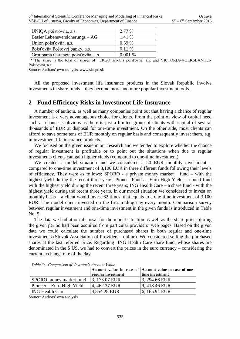
8th International Scientific Conference Managing and Modelling of Financial Risks Ostrava
VŠB-TU of Ostrava, Faculty of Economics, Department of Finance 5th – 6th September 2016
535
UNIQA poisťovňa, a.s. 2.77 %
Basler Lebensversicherungs – AG 1.41 %
Union poisťovňa, a.s. 0.59 %
Poisťovňa Poštovej banky, a.s. 0.11 %
Groupama Garancia poisťovňa a. s. 0.001 % * The share is the total of shares of ERGO životná poisťovňa, a.s. and VICTORIA-VOLKSBANKEN
Poisťovňa, a.s.
Source: Authors´ own analysis, www.slaspo.sk
All the proposed investment life insurance products in the Slovak Republic involve
investments in share funds – they become more and more popular investment tools.
2 Fund Efficiency Risks in Investment Life Insurance
A number of authors, as well as many companies point out that having a chance of regular
investment is a very advantageous choice for clients. From the point of view of capital need
such a chance is obvious as there is just a limited group of clients with capital of several
thousands of EUR at disposal for one-time investment. On the other side, most clients can
afford to save some tens of EUR monthly on regular basis and consequently invest them, e.g.
in investment life insurance products.
We focused on the given issue in our research and we tended to explore whether the chance
of regular investment is profitable or to point out the situations when due to regular
investments clients can gain higher yields (compared to one-time investment).
We created a model situation and we considered a 50 EUR monthly investment –
compared to one-time investment of 3,100 EUR in three different funds following their levels
of efficiency. They were as follows: SPORO - a private money market fund – with the
highest yield during the recent three years; Pioneer Funds – Euro High Yield - a bond fund
with the highest yield during the recent three years; ING Health Care – a share fund - with the
highest yield during the recent three years. In our model situation we considered to invest on
monthly basis – a client would invest 62 times, that equals to a one-time investment of 3,100
EUR. The model client invested on the first trading day every month. Comparison survey
between regular investment and one-time investment in the given funds is introduced in Table
No. 5.
The data we had at our disposal for the model situation as well as the share prices during
the given period had been acquired from particular providers´ web pages. Based on the given
data we could calculate the number of purchased shares in both regular and one-time
investments (Slovak Association of Providers - online). We considered selling the purchased
shares at the last referred price. Regarding ING Health Care share fund, whose shares are
denominated in the $ US, we had to convert the prices in the euro currency – considering the
current exchange rate of the day.
Table 5: Comparison of Investor´s Account Value
Account value in case of
regular investment
Account value in case of one-
time investment
SPORO money market fund 3, 173.07 EUR 3, 294.66 EUR
Pioneer – Euro High Yield 4, 462.37 EUR 9, 418.46 EUR
ING Health Care 4,854.28 EUR 6, 165.94 EUR Source: Authors´ own analysis

8th International Scientific Conference Managing and Modelling of Financial Risks Ostrava
VŠB-TU of Ostrava, Faculty of Economics, Department of Finance 5th – 6th September 2016
536
The Table clearly shows that the highest yield in case of regular investment was gained in
the ING Health Care share fund. The lowest yield was gained in the SPORO money market
fund. The result is quite obvious following the portofolio of each particular fund. However, it
is quite interesting to compare regular investment with one-time investment – from client´s
point of view - the investment does not seem that convenient. Almost all regular investments
gained lower account value compared to one-time investment. The only exception was TAM
NewMarkets fund – it was included in comparison study especially due to its swinging flow
since the very beginning of its existence. The other reason was to determine whether the one-
time investment would prove to be more profitable than it was in previous case. However, this
situation proved that both investments were equal. For better illustration we introduce Table
No. 6 which reveals particular investment efficiency expressed since their very beginning.
Table 6: Comparison of Efficiency
Efficiency in case of
regular investment
Efficiency in case of one-time
investment
SPORO money market fund 2.36 % 6.28 %
Pioneer – Euro High Yield 43.95 % 203.82 %
ING Health Care 56.59 % 98.90 % Source: Authors´ own analysis
Analysis of the Table No. 6 clearly shows the significant difference between the two types
of investments - it points out the disadvantage in case of regular investment. One-time
investment brought investor almost or even more than two times higher profit in case of share
as well as money markets. In case of bond fund - the profit was almost five times higher.
All types of investments, however are significantly influenced by the period clients plan to
invest. If we consider that life insurance is contracted from 25 to 30 years on average - the
long period of investment clearly proves disadvantage for regular investment. The longer the
time horizon, the higher the probability of growing both share and bond markets. Similarly,
our model situation proved that in case of more than four-year time horizon the regular
investment was unable to reach the same outputs as in case of one-time investment.
To sum up, we can conclude that if client enters the financial market through investment
life insurance products – such a decision can be risky, but at the same time it may bring him
certain advantages, too. Model situations outlined that by means of bond and share funds
investment client can gain considerably high yields depending on global financial market
development.
Aknowledgment
The paper is submitted as an output of the VEGA 1/0242/16 research project “Globalized
trends and dynamism of changes on the EU insurance market “ being solved in the
Department of Insurance in the Faculty of National Economy, University of Economics in
Bratislava
References
[1] AG Choice Index GULSM Life Insurance. [online] Available at:
<http://www.americangeneral.com/life/life.nsf/contents/productsindividuals_life_AGCh
oiceIndexGUL>. [Accessed 8 June 2016 ].

8th International Scientific Conference Managing and Modelling of Financial Risks Ostrava
VŠB-TU of Ostrava, Faculty of Economics, Department of Finance 5th – 6th September 2016
537
[2] Borovcová, M. (2013). Insurance Market Assessment in the Czech Republic. In:
Conference Proceedings from 9th International Scientific Conference Financial
Management of Firms and Financial Institutions. Ostrava: VŠB-TU Ostrava.
[3] Gladiš, D. (2005). Naučte se investovat. 2. rozšířené vydání. Praha: Grada Publishing,
a.s.
[4] Chovancová, B. (2006). Finančný trh. Bratislava: IURA Edition.
[5] Chovancová, B., Žofčák, S. (2012). Kolektívne investovanie. Bratislava: IURA Edition.
[6] Investičné životné poistenie. [online] Available at:
<http://www.poistenie.sk/investicne-zivotne-poistenie>. [Accessed 10 June 2016 ].
[7] Munich, R. E. (2000). Unit-linked Insurance. A general report. [online] Available at:
<http://www.isp.pt/winlib/cgi/winlibimg.exe?key=&doc=18678&img=5977> [Accessed
8 June 2016 ].
[8] Slovenská asociácia správcovských spoločností. [online] Available at:
<http://ass.sk/Default.aspx?CatID=53&NewsID=218>. [Accessed 31 May 2016].
[9] Zákon 592/2003 Z.z. o kolektívnom investovaní. [online] Available at:
http://www.nbs.sk/sk/legislativa/uplne-znenia-zakonov-patriacich-do-kompetencie-nbs
[Accessed 6 June 2016 ].

8th International Scientific Conference Managing and Modelling of Financial Risks Ostrava
VŠB-TU of Ostrava, Faculty of Economics, Department of Finance 5th – 6th September 2016
538
Managing Risk With Simulated Copula
Malavasi1 M., Previtali R., Ortobelli2 S., Nardelli1 C.
Abstract
The aim of this study is verify whether the Average Value at Risk (AVaR) can be a good
alternative to Value at Risk (VaR), for estimating great portfolio losses, especially regarding tail
events. To do so we use copula framework to estimate dependence between stock returns of a
portfolio composed by 94 stock of the S&P100 in order to compute AVaR and VaR and compare
the results with respect to a Gaussian Exponentially Weighted Moving Average (EWMA). For
computing simulated returns, we use the algorithm presented in [Biglova et all, 2014] and then
the model is back-tested with Kupiec's and Christoffersen's tests. The results are coherent with
the literature and in particular VaR computed both via copula and EWMA seems to fail to provide
an accurate risk measurement while AVaR under copula and EWMA looks more reliable.
Key words
Value at Risk, Average Value at Risk, Copula, EWMA model.
JEL Classification: G17, C15, G12
1. Introduction
The aim of this study is verify whether the Average Value at Risk (AVaR) can be a good
alternative to Value at Risk (VaR) for estimating great portfolio losses, especially regarding tail
events. To do so we consider the stocks belonging to Standard & Poor’s 100. The interval time
chosen covers the last 10 years recorded with 2591 daily price observations for each stock from
the 1st December 2005 to the 18th March 2016. Since stocks belonging to the index can be
substituted by other stocks along time, the sample used is reduced to those which are present in
all 10-year period considered: Thus the number of remaining stocks is 94 respect to the original
100.
In portfolio risk management, we have to combine some well known stylized facts: typical
features of return series (as asymmetry fat tails and volatility clusters) with asymmetry in
dependence structure (lower tail dependence stronger than upper tail dependence) and high
dimensionality (see [Cont, 2000] [Papp et al., 2005] [Kondor et al., 2007] [Hong et al. 2007]).
According to [Cont and Tankov, 2003] [Schoutens, 2007], we deal excess kurtosis and
skewness using different distributions from the Gaussian law. As for [Cherubini et al., 2003],
we examine asymmetry in dependence structure proposing an appropriate copula. Moreover,
considering that high dimensionality in portfolio problems might affect the unbiasedness of risk
estimators (see [Rachev et al., 2005] [Sun et al., 2008]) and that estimating the impact of tail
event requires a high number of observations (see [Papp et al., 2005] [Kondor et al., 2007]),
then we model risk of portfolios using proper simulated multivariate scenarios. Finally, we
compare the ex post results with those obtained by using the classical RiskMetrics methodology
(EWMA model).
1 University of Bergamo, Italy 2 University of Bergamo, Italy and VSB-TU Ostrava, Czech Republic.

8th International Scientific Conference Managing and Modelling of Financial Risks Ostrava
VŠB-TU of Ostrava, Faculty of Economics, Department of Finance 5th – 6th September 2016
539
2. The framework
Following [Rachev et al.,2007]. [Biglova et al., 2008] and [Biglova et al., 20014] we tackle
all the observed return features by computing VaR and AVaR (often called Conditional Value
at Risk - CVaR) on realistic simulated scenarios. The general idea is to assume that each log-
return 𝑟𝑗,𝑡,follows a ARMA(1,1)-GARC(1,1):
𝒓𝒋,𝒕 = 𝒂𝒋,𝟎 + 𝒂𝒋,𝟏𝒓𝒋,𝒕−𝟏 + 𝒃𝒋,𝟏𝜺𝒋,𝒕−𝟏 + 𝜺𝒋,𝒕
𝜀𝑗,𝑡 = 𝜎𝑗,𝑡𝑢𝑗,𝑡 (1)
𝜎𝑗,𝑡2 = 𝑐𝑗,0 + 𝑐𝑗,1𝜎𝑗,𝑡−1
2 + 𝑓𝑗,1𝜀𝑗,𝑡−12
and a skewed t-copula with 5 degrees of freedom for the dependence structure, defined as:
𝑿 = 𝝁 + 𝜸𝒈(𝑾) + √𝑾𝒁 (2)
with g:[0, ∞)→:[0, ∞),in this work g(W)=W, γ vector of skewness parameters, Z N(0,Σ) with
Σ = [𝜎𝑖𝑗] and W Ig(d/2,d/2). The density function the X vector is
𝑓(𝑥) = 𝑐
𝐾𝑑+𝑛2
(√(𝑑 + (𝑥 − 𝜇)′Σ−1(𝑥 − 𝜇))𝛾′Σ−1𝛾) exp((𝑥 − 𝜇)′Σ−1𝛾)
(√(𝑑 + (𝑥 − 𝜇)′Σ−1(𝑥 − 𝜇))𝛾′Σ−1𝛾)−
𝑑+𝑛2
(1 +(𝑥 − 𝜇)′Σ−1(𝑥 − 𝜇)
𝑑)
𝑑+𝑛𝑛
with the normalizing parameter: 𝑐 =2
2−(𝑑+𝑛)2
Γ(𝑑
2)(𝜋𝑑)
𝑛2|Σ|
12
where Kλ is a Bessel function of the third kind
which is a function that solves the differential equation [Abramowitz and Stegun, 1965]
[Demarta and McNeil, 2004]:
𝑧2𝑑2𝑦
𝑑𝑧2+ 𝑧
𝑑𝑦
𝑑𝑧+ (𝑧2 − 𝑣2)𝑦 = 0.
Then we generates the future scenarios according to the following algorithm (see [Biglova
et al., 2008] [Biglova et al., 2014][Rachev et al.,2007]).
Step 1: Margins of the innovation of each log-return series.
Perform the Maximum likelihood estimation of the model in (1). Then approximate the
standardized innovations ��𝑗,𝑡 =��𝑗,𝑡
𝜎𝑗,𝑡 with a 𝛼𝑗-Stable distribution 𝑆𝛼𝑗
(𝜇𝑗, 𝜎𝑗 , 𝛽𝑗). Then simulate
N scenario from a Stable distribution for each of the future scenario and compute the sample
distribution for each ��𝑗,𝑇+1:
𝐹𝑢𝑗,𝑇+1(𝑥) =
1
𝑁∑ 𝐼
{𝑢𝑗,𝑇+1(𝑖)
≤𝑥}
𝑁
𝑖=1
Step 2: Dependence structure.
Fit the vector of �� = [��1, … , ��94] with the asymmetric t-copula defined in (2) and compute
the maximum likelihood to obtain the parameters (𝑑, ��𝑖, ��𝑖𝑖, ��𝑖) which allows to compute the
estimator for variance covariance matrix of Z:
Σ = (𝑐𝑜𝑣(𝑋) −2𝑑2
(𝑑 − 2)2(𝑑 − 4)𝛾𝛾′)
𝑑 − 2
𝑑.
Now generate N scenarios for the vector �� from (2) and call them: [��1𝑖, … , ��94
𝑖 ] for 𝑖 =1, … , 𝑁 and let 𝐹𝑉𝑗
(𝑥) be the marginal of the estimated asymmetric t-distribution. Now generate
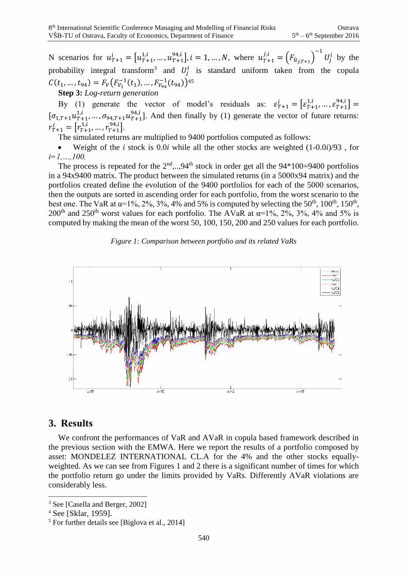
8th International Scientific Conference Managing and Modelling of Financial Risks Ostrava
VŠB-TU of Ostrava, Faculty of Economics, Department of Finance 5th – 6th September 2016
540
N scenarios for 𝑢𝑇+1𝑖 = [𝑢𝑇+1
1,𝑖 , … , 𝑢𝑇+194,𝑖 ], 𝑖 = 1, … , 𝑁, where 𝑢𝑇+1
𝑗,𝑖= (𝐹𝑢𝑗,𝑇+1
)−1
𝑈𝑗𝑖 by the
probability integral transform3 and 𝑈𝑗𝑖 is standard uniform taken from the copula
𝐶(𝑡1, … , 𝑡94) = 𝐹𝑉(𝐹𝑉1
−1(𝑡1), … , 𝐹𝑉94
−1(𝑡94))45
Step 3: Log-return generation
By (1) generate the vector of model’s residuals as: 𝜀𝑇+1𝑖 = [𝜀𝑇+1
1,𝑖 , … , 𝜀𝑇+194,𝑖 ] =
[𝜎1,𝑇+1𝑢𝑇+11,𝑖 , … , 𝜎94,𝑇+1𝑢𝑇+1
94,𝑖 ]. And then finally by (1) generate the vector of future returns:
𝑟𝑇+1𝑖 = [𝑟𝑇+1
1,𝑖 , … , 𝑟𝑇+194,𝑖].
The simulated returns are multiplied to 9400 portfolios computed as follows:
Weight of the i stock is 0.0i while all the other stocks are weighted (1-0.0i)/93 , for
i=1,…,100.
The process is repeated for the 2nd,..,94th stock in order get all the 94*100=9400 portfolios
in a 94x9400 matrix. The product between the simulated returns (in a 5000x94 matrix) and the
portfolios created define the evolution of the 9400 portfolios for each of the 5000 scenarios,
then the outputs are sorted in ascending order for each portfolio, from the worst scenario to the
best one. The VaR at α=1%, 2%, 3%, 4% and 5% is computed by selecting the 50th, 100th, 150th,
200th and 250th worst values for each portfolio. The AVaR at α=1%, 2%, 3%, 4% and 5% is
computed by making the mean of the worst 50, 100, 150, 200 and 250 values for each portfolio.
Figure 1: Comparison between portfolio and its related VaRs
3. Results
We confront the performances of VaR and AVaR in copula based framework described in
the previous section with the EMWA. Here we report the results of a portfolio composed by
asset: MONDELEZ INTERNATIONAL CL.A for the 4% and the other stocks equally-
weighted. As we can see from Figures 1 and 2 there is a significant number of times for which
the portfolio return go under the limits provided by VaRs. Differently AVaR violations are
considerably less.
3 See [Casella and Berger, 2002] 4 See [Sklar, 1959]. 5 For further details see [Biglova et al., 2014]

8th International Scientific Conference Managing and Modelling of Financial Risks Ostrava
VŠB-TU of Ostrava, Faculty of Economics, Department of Finance 5th – 6th September 2016
541
Figure 2: Comparison between portfolio and its related AVaRs
In order to check if VaRs and AVaRs computed with the copula model are accurate we
compute Kupiec’s6 and Christoffersen’s7 test for all the 9400 portfolios. The results are reported
in Table 1.
Table 5.1: Percentages of VaRs and AVaRs accepted by Kupiec’s and Christoffersen’s test
As we can see from this table VaRs most of the times fail to provide an acceptably accurate
measure of risk. The percentage of successfully tested AVaRs at 1% and 2% is greater but only
AVaR at 1% seems to provide an acceptable measure of risk given its 83.89% success from
Kupiec’s test and 92.72% from Christoffersen’s test. For AVaR at 5% both tests are always
rejected.
Similar observations can be taken regarding EMWA VaRs and AVaRs from Figure 3 and 4.
In particular there is a significant number of times for which portfolio a) returns go under the
limits provided by EWMA VaRs. Differently, EWMA AVaR violations are fewer than EWMA
VaR.
The results of Kupiec’s and Christoffersen’s test are reported in Table 2. Even in this case
most of VaRs provided by the model are not acceptably accurate for measuring risk. The
percentage of successfully tested AVaRs at 1% and 2% is considerably greater. In particular,
AVaR at 2% provide an acceptable measure of risk given its 98.83% success from Kupiec’s
test and 99.31% from Christoffersen’s test.
6 See [Kupiec, 1995] 7 See [Christoffersen, 1998].

8th International Scientific Conference Managing and Modelling of Financial Risks Ostrava
VŠB-TU of Ostrava, Faculty of Economics, Department of Finance 5th – 6th September 2016
542
Figure 3: Comparison between portfolio and its related EWMA VaRs
Figure 4: Comparison between portfolio and its related EWMA AVaRs
Table 2: Percentages of EWMA VaRs and AVaRs accepted by Kupiec’s and Christoffersen’s test
Then in order to compare the performance between the copula model and the EMWA model.
we examine the mean VaR and mean AVaR.(Figure 5)

8th International Scientific Conference Managing and Modelling of Financial Risks Ostrava
VŠB-TU of Ostrava, Faculty of Economics, Department of Finance 5th – 6th September 2016
543
Figure 5: mean VaRs and CVaRs for copula and EWMA model
Comparing the mean VaRs and AVaRs for both models, it appears that there is no great
difference between VaRs and EWMA VaRs, except from the first percentile where we can see
that VaR is clearly higher than EWMA VaR, while AVaR are higher than EWMA AVaRs.
Then we perform the Kupiec’s and the Christofferen’s tests. Results are in table 3.
Table 3: comparison of copula and EWMA test results
The copula model VaR at the first percentile provide a better estimation of risk than the
corresponding EWMA one. On the other hand, at greater percentiles the EWMA model
performs considerably better than the copula one. Analogous results can be derived from the
AVaRs comparisons: at the first percentile the copula AVaR is a more accurate risk measure
than EWMA CVaR, but at the second and fifth percentile its accuracy is remarkably lower than
EWMA one. Given the results of the tests, it is possible to derive the following suppositions:
since all the copula AVaRs are greater than EWMA AVaRs and their accuracy is better for the
first percentile but worse for the second percentile, we can presume that EWMA CVaR at α=1%
underestimates risk while CVaR at α=2% and more overestimates risk.

8th International Scientific Conference Managing and Modelling of Financial Risks Ostrava
VŠB-TU of Ostrava, Faculty of Economics, Department of Finance 5th – 6th September 2016
544
4. Conclusions
An accurate measure of risk in portfolio selection should be able to capture extreme values
of risk along the distribution tail belonging to the first percentiles. We focus on market risk
estimation by applying a skewed t-copula model on portfolios composed by 94 stocks of the
S&P100 in order to compute VaR and AVaR and then we compare its results with the outcomes
of a Gaussian EWMA model. For computing returns simulations we have made use of
ARMA(1,1)-GARCH(1,1) algorithm provided by [Biglova et al., 2014]. Comparing the mean
VaRs and AVaRs for both models, it appears that there is no great difference between VaRs
and EWMA VaRs, except from the first percentile where we can see that copula VaR is clearly
higher than EWMA VaR, while copula AVaRs are higher than EWMA AVaRs. By computing
Kupiec’s and Christoffersen’s tests we discover that, for both copula and EWMA models, the
VaRs provided are not acceptably accurate for measuring risk while copula AVaR at α=1 and
EWMA AVaR at α=2% are acceptable measure of risk. Moreover, it is possible to presume that
EWMA AVaR at α=1% underestimates risk while copula AVaR at α=2% and more
overestimates risk. The results of this study should enlighten that VaR is not a good risk
measure as believed before the financial crisis, while CVaR is a better estimate of risk,
especially for the first two percentiles.
Acknowledgements
This work was supported by the Italian funds ex MURST 60% 2016. The research was also
supported through the Czech Science Foundation (GACR) under project 15-23699S and
through SP2016/11, an SGS research project of VSB-TU Ostrava, and furthermore by the
European Social Fund in the framework of CZ.1.07/2.3.00/20.0296.
References
[1] Abramowitz, M., & Stegun, I. A. (1965). Chapter 9. Handbook of Mathematical
Functions with Formulas, Graphs, and Mathematical Tables, Dover Publications, Inc.,
New York.
[2] Biglova, A., Ortobelli, S., Rachev, S., & Fabozzi, F. (2009). Modeling, estimation, and
optimization of equity portfolios with heavy-tailed distributions.Optimizing optimization:
The next generation of optimization applications and theory, 117-141..
[3] Biglova, A., Ortobelli, S., & Fabozzi, F. J. (2014). Portfolio selection in the presence of
systemic risk. Journal of Asset Management, 15(5), 285-299.
[4] Casella, G., & Berger, R. L. (2002). Statistical inference (Vol. 2). Pacific Grove, CA:
Duxbury.
[5] Cherubini, U., Luciano, E., & Vecchiato, W. (2004). Copula methods in finance. John
Wiley & Sons.
[6] Christoffersen, P. F. (1998). Evaluating interval forecasts. International economic
review, 841-862.
[7] Cont, R. (2001). Empirical properties of asset returns: stylized facts and statistical issues.
[8] Cont R.,Tankov, P. (2003). Financial modelling with jump processes (Vol. 2). CRC press.
[9] Demarta, Stefano, and Alexander J. McNeil. "The t copula and related
copulas."International Statistical Review/Revue Internationale de Statistique (2005):
111-129.

8th International Scientific Conference Managing and Modelling of Financial Risks Ostrava
VŠB-TU of Ostrava, Faculty of Economics, Department of Finance 5th – 6th September 2016
545
[10] Hong, Y., Tu, J., & Zhou, G. (2007). Asymmetries in stock returns: statistical tests and
economic evaluation.Review of Financial Studies, 20(5), 1547-1581.
[11] Kondor, I., Pafka, S., & Nagy, G. (2007). Noise sensitivity of portfolio selection under
various risk measures.Journal of Banking & Finance, 31(5), 1545-1573.
[12] Kupiec, P. H. (1995). Techniques for verifying the accuracy of risk measurement
models.The J. of Derivatives, 3(2).
[13] Rachev, S. T., Menn, C., & Fabozzi, F. J. (2005).Fat-tailed and skewed asset return
distributions: implications for risk management, portfolio selection, and option pricing
(Vol. 139). John Wiley & Sons
[14] Rachev, S.T.,Mittnik, S., Fabozzi, F.J., Focardi, S.M., Jasic, T.: Financial econometrics:
from basics to advanced modeling techniques, vol. 150. John Wiley & Sons (2007)
[15] Schoutens, W. (2003). Lévy process in finance.Pricing financial derivatives, John Wiley
& Sons Ltd.
[16] Sklar, M. (1959).Fonctions de répartition à n dimensions et leurs marges. Publications
del'Institut de Statistique de L'Université de Paris,8,229-231.
[17] Sun, W., Rachev, S., Stoyanov, S. V., & Fabozzi, F. J. (2008). Multivariate skewed
Student's t copula in the analysis of nonlinear and asymmetric dependence in the German
equity market.Studies in Nonlinear Dynamics & Econometrics,12(2).
[18] Papp, G., Pafka, S., Nowak, M. A., & Kondor, I. (2005). Random matrix filtering in
portfolio optimization.arXiv preprint physics/0509235.

8th International Scientific Conference Managing and Modelling of Financial Risks Ostrava
VŠB-TU of Ostrava, Faculty of Economics, Department of Finance 5th – 6th September 2016
546
Bonds Return Modeling Using High Frequency Data
Jiří Málek1, Bohumil Stádník2, Tran van Quang3
Abstract
The work will examine the probability distributions of returns of certain bonds in the US market.
This returns are taken from the minute, half-hourly and hourly and data. The first four moments
(mean, variance, skewness, kurtosis) and Sharpe ratio are computed, explained and compared.
Tails thickness alpha of bond returns probabilistic distribution is calculated using 𝛼-stable
distribution as an aproximation the emphirical ones
Key words
High fequency data, skewness, kurtosis, Sharpe ratio, 𝛼-stable distribution
JEL Classification: G10, G120
1. Introduction
It is known that most investors prefer higher expected rate of return and less risk. If we
measure the risk by standard deviation this measure of risk may be misleading in certain
circumstances. Standard deviation is a good measure of risk for the normal distribution, but if
the distribution has a nonzero skewness and high kurtosis, it should taken into account higher
moments when making investment decisions
In the following article, we focus on investments in US government bonds with different
maturities (2y, 10y, 30y). There are used high-frequency data of varying frequencies (3min,
10min, 30min, 1h) which are calculated the first four moments (mean, variance, skewness,
kurtosis) for. All data show high kurtosis and nonzero skewness.
The paper is organized as follows. The first part defines the skewness and kurtosis, their
interpretation and implications for investment decisions are discussed. The next section
describes the data used. In the practical part of the paper are calculated first four moments of
individual bonds at different frequencies, then there are further developed portfolio of 2y and
30y bonds at various ratios. Finally using stable distribution approximation "fatness" ends of
probability distributions of some data are calculated.
2. Skewness and kurtosis
Skewnes is defined as folows:
𝛾 =𝐸(𝑋 − 𝐸𝑋)3
(𝐸(𝑋 − 𝐸𝑋)2)3 2⁄ .
Skewness is a measure of the asymmetry of the probability distribution of a random
variable about its mean. For a unimodal distribution, negative skew indicates that the tail on the
left side of the probability density function is longer or fatter than the right side and
contrary positive skew indicates that the tail on the right side is longer or fatter than the left
1 Department of Banking and Insurance, University of Economics Prague, [email protected]. 2 Department of Banking and Insurance, University of Economics Prague, bohumil.stadnik@ vse.cz. 3 Department of Statistics and Probability, University of Economics Prague, [email protected].

8th International Scientific Conference Managing and Modelling of Financial Risks Ostrava
VŠB-TU of Ostrava, Faculty of Economics, Department of Finance 5th – 6th September 2016
547
side. When we say “long tail” this is named by comparison to the normal distribution which is
symmetric and has a skewness of zero. More precisely, skew measures the relative length of
the tails; it tells us that one is longer than the other. but this is really just a generally true rule of
thumb rather than an always true statement In many textbook we may read followinng
relationships:
If random variable posses positive skewnes, then mean>median> modus and for negative
skewness modus>median>mean.
This is really just a generally true rule of thumb rather than an always true statement, it can
fail in multimodal distributions, or in distributions where one tail is long but the other is heavy
Skewness risk can arise in any quantitative model that assumes a symmetric distribution (such
as the normal distribution) but is applied to skewed data. Positive skewness is preferred, but
uncommon. A positively skewed return distribution shows small frequency of very big profits,
while a negatively skewed trading strategy will lead to a lot of small gains and a few large
losses.
Looking across various asset classes and time periods, one notices the prevalence of negative
numbers. Knowing how markets behave, this makes sense. When markets melt down, they tend
to melt down in a dramatic fashion. Think of the Credit Crisis, the Dot-Com Bust, the Asian
Contagion, or the Long Term Capital Management crisis. On the upside, gains tend to be less
dramatic. While the overall, long-term returns of the markets are positive, those gains come in
slower, steadier gains than big bursts. The worst of the worst months tend to be more extreme
than the best of the best months. This is what is meant by negative skewness.
𝜅 =𝐸(𝑋 − 𝐸𝑋)4
(𝐸(𝑋 − 𝐸𝑋)2)2
Kurtosis measures the fat-tail degree of a distribution. High risk-averse investors prefer a
distribution with low kurtosis (i.e. returns not far away from the mean). A distribution with
kurtosis grater then 3 exhibits a peak in the middle and fat tails versus a normal distribution. A
distribution to be normal should have an kurtosis equal to 3. In case of a positive skewness, it
is possible to have a high excess kurtosis and to have no future extreme negative returns. The
extreme returns will only be positive. This is only possible when the skewness is positive. As
soon as the skewness is negative, the impact of a high kurtosis affects the extreme negative
returns. The most interesting thing is when the return distribution has a skewness lower than -
1 and an kurtosis higher than 4. In this case, the probability to have sudden high negative returns
increases.
3. Data
US Treasury government bonds with maturities 30, 10 and 2 years were used for the
empirical part of the research. Particularly: UST 2.5 15/5/2046; UST 1.625 25/15/2026 and
UST 2.375 30/6/20184. We have used the time series of yields to maturity (YTM) for each of
these bonds on frequencies 3, 10, 30 minutes, 1 hour and 1 day. The series was transferred then
to the series of YTM differences (∆YTM series) according to the formula ∆YTMt=YTMt -
YTMt+1. According to this formula the changes of price and also ∆YTMt has the same sign,
means the risk for a bond holder resulting from a yield shift in ∆YTM series is in the left side
of respective histogram. This series was used for the calculation of the moments.
4 Complete time series are available at www.pozemstan.cz/data_bondy.xls.

8th International Scientific Conference Managing and Modelling of Financial Risks Ostrava
VŠB-TU of Ostrava, Faculty of Economics, Department of Finance 5th – 6th September 2016
548
4. Results
The folowing table shows the first four moments, followed histograms for all bonds and
trading frequencies
Table 1: Bonds moments
Bond Frequency Mean Variance Skewness Kurtosis Sharpe
index
30Y 3 min 0.0000020 0.0000015 -1.3759849 70.2306210 0.00163
10 min 0.0000155 0.0000104 -0.4593729 16.0484220 0.00481
30 min 0.0000422 0.0000310 -0.1012959 11.1241500 0.00758
1 hour 0.0000833 0.0000574 0.0285210 8.0560119 0.01100
1 day 0.0004429 0.0013180 -0.5573887 3.5005891 0.01221
10Y 3 min -0.0000002 0.0000030 -0.0455176 61.6943630 -0.00012
10 min -0.0000017 0.0000116 0.3996222 31.3845550 -0.00050
30 min -0.0000033 0.0000332 0.9327564 26.4722020 -0.00061
1 hour -0.0000064 0.0000644 0.5079486 20.0116710 -0.00080
1 day 0.0010793 0.0018047 -0.4147576 4.7366690 0.02541
2Y 3 min 0.0000204 0.0000139 0.5066228 22.6215150 0.00547
10 min 0.0000409 0.0000239 1.7515355 46.7824700 0.00837
30 min 0.0000338 0.0000502 1.8874916 42.3962630 0.00477
1 hour 0.0000588 0.0000834 1.3355274 26.9074650 0.00644
1 day 0.0016315 0.0019453 0.1200944 5.3067758 0.03699
¨
Fig. 1: 2y, 3 min Fig 1b 10y, 3 min
Figure 1c: 30y, 3 min Figure 2a: 2y, 10 mi

8th International Scientific Conference Managing and Modelling of Financial Risks Ostrava
VŠB-TU of Ostrava, Faculty of Economics, Department of Finance 5th – 6th September 2016
549
Figure 2b: 10y, 10min Figure 2c: 30y, 10 min
Figure 4a: 2y, 30mim Figure 4b: 10y, 30 min
Figure 4c: 30y, 30min
The following table shows alpha as the power of fat tails using 𝛼-stable distribution as an
aproximation of the emphirical ones for 3min data. The 𝛼 parameter has been estimated
using MLE method (e.g. Weron 1995)
Tab. 2: Parameters of alpha distribution, 3 min data
Type of Bond alpha
30Y 1.7430
10Y 1.9575
2Y 1.9335

8th International Scientific Conference Managing and Modelling of Financial Risks Ostrava
VŠB-TU of Ostrava, Faculty of Economics, Department of Finance 5th – 6th September 2016
550
The following graphs show the first four moments for portfolios of 2y and 30y bonds , trading
frequency 3min. (On the horizontal axis is the relative size 30y bonds in the portfolio)
Figure 5a : Mean Figure 5b: Variance
Figure 5c: Skewnes Figure 5d: Kurtosis
Figure 6: Sharpe index for the portfolio for 2y and 30y bonds

8th International Scientific Conference Managing and Modelling of Financial Risks Ostrava
VŠB-TU of Ostrava, Faculty of Economics, Department of Finance 5th – 6th September 2016
551
One day moments
Figure 7 : Number of entries Figure 8 : 2y bonds
Figure 9 :10y bonds Figure 10 :30y bonds
5. Interpretation of Results and Conclusions
High-frequency data are compared to only a given frequency (3min, 10min, 30min, 1h). 2y
bonds show the highest average return on the frequency 3min and 10min while 30y bonds show
the best average return on the frequency of 30 minutes and 1 hour. Regarding the variance
(risk), then 30y bonds have the lowest risk at all frequencies 3min, 10min and 30min and 1h.
All these data show a high kurtosis but mild skewness. Highest kurtosis in all three bonds is,
as expected, with 3min of data, but it decreases rapidly with increasing length of the time
trading interval.
Sharpe index index allows us to compare performance (at least for the first two moments)
over different time frequencies. It confirms the most risky it is trading at the shortest frequency
(3min). Sharpe index is the smallest data for 3min for all three bonds, then it gradually grows
and becomes maximum at daily data. The highest index of the three bonds is for 2y bond.
One possible explanation of the most significant negative skewness we have measured (30Y,
3 min, the value = -1.376) is the existence of a “dramatic” crashes of price in comparison to
relatively slow upward movements. The idea is supporting by the way of example in the figures
11a,b.

8th International Scientific Conference Managing and Modelling of Financial Risks Ostrava
VŠB-TU of Ostrava, Faculty of Economics, Department of Finance 5th – 6th September 2016
552
Figure 11a: 30y returns with “crashes” Figure11b:30y returns without “crashes
n the figure 11a there is ∆YTM development we have measured with the value of skewness=
-1.376. If we remove the crash (highlighted by the circle in the figure) we obtain the
development according to the figure11b) with the value of skewness = 0.223. This simple
demonstration support the interpretation above and also points to the sensitivity of skewness
value.
In high frequency area the financial interpretation could result from behavioral finance:
“black swans” and “long shots” (Tversky, Kahneman 1974, 1992; Teleb 2007; Snowberg,
Wolfers 2010; Vaughan, Paton 1997, Woodland, Woodland 1994). They argue that
“impossible” events, “black swans”, are neglected whereas “possible” but low probability
events, “longshots”, are overweighed. As expressed by Tversky and Kahneman: “A change
from impossibility to possibility or from possibility to certainty has a bigger impact than a
comparable change in the middle of the scale.” Applying to financial market: the crash as the
“black swan” is overweighed when it is suddenly deemed possible.
Acknowledgments
Jiří Málek has been supported by the Czech Science Foundation Grant 15-00036S ''Credit Risk
Modeling for Financial and Commodity Assets Portfolios" and by the VŠE institutional grant
IP100040. Bohumil Stádník has been supported by Czech Science Foundation Grant GA 16-
21506S and by the VŠE institutional grant IP100040. Tran van Quang has been supported by
the VŠE institutional grant IP100040.
References
[1] Fama, E.,and Roll R.(1971). Parameter Estimates for Symmetric Stable Distributions. J. Amer. Statist. Assoc. 66 (1971), 331–338.
[2] Fujiwara, I. and Körber, L.M. and Nagakura, D. (2011): How much Asymmetry is there in Bond Returns and Exchange Rates? Bank of Japan Working Paper Series
[3] Fujiwara, I. and Mareen Korber, L. and Nagakura D. (2013): Assymmetry in government bond returns. AJRC Working Paper No. 1, March 2013. Australia-Japan Research Centre, Crawford School of Public Policy, The Australian National University.
I-Hsuan Ethan Chiang (2016). Skewness and Co-Skewness in Bond Returns. Journal of Financial Research, vol. 39, No. 2.
[4] Madan,D. B. and McPhail, G. S and Smith, R. H. (2000). Investing in Skews. The Journal of Risk Finance, vol. 2 Iss: 1, pp.10 – 18.

8th International Scientific Conference Managing and Modelling of Financial Risks Ostrava
VŠB-TU of Ostrava, Faculty of Economics, Department of Finance 5th – 6th September 2016
553
[5] McCulloch, J. H. (1986). Simple Consistent Estimators of Stable Distribution Parameters. Commun. Statist.–Simula. 15 (4) (1986), 1109–1136.
[6] McCulloch, J. H.(1997). Measuring Tail Thickness to Estimate the Stable Index α: A Critique. Journal of Business and Economic Statistics 15, No 1.
[7] Ruge-Murcia, F. (2012). Skewness Risk and Bond Prices. Working paper The Center for Interuniversity Research in Quantitative Economics (CIREQ).
[8] Snowberg, E.; Wolfers, J. (2010). “Explaining the Favourite-Long Shot Bias: Is it Risk-Love or Misperceptions?” Journal of Political Economy 118(4): 723-746.
[9] Taleb, N, N. (2007). The Black Swan: The Impact of the Highly Improbable. Random House.
[10] Tversky, A.; Kahneman, D. (1974). “Judgment under Uncertainty: Heuristicsand Biases.” Science 185(4157): 1124-31.
[11] Tversky, A.; Kahneman, D. (1992). “Advances in Prospect Theory: Cumulative Representation of Uncertainty.” Journal of Risk and Uncertainty 5(4): 297-323.
[12] Vaughan, L.; D. Paton, (1997). Why is There a Favourite-Longshot Bias in British Racetrack Betting Markets? The Economic Journal, vol. 107, No. 440 (Jan., 1997), pp. 150-158.
[13] Weron, R. (1995): Performance of the Estimators of Stable Law Parameters, Wroclav University of Technology, Research Report HSC/95/1.
[14] Woodland, L., M.; Woodland B.M., (1994). Market Efficiency and the Favourite-Longshot Bias: The Baseball Betting Market. Journal of Finance, vol. 49, No. 1 (Mar., 1994), pp. 269-279

8th International Scientific Conference Managing and Modelling of Financial Risks Ostrava
VŠB-TU of Ostrava, Faculty of Economics, Department of Finance 5th – 6th September 2016
554
Advanced Artificial Neural Networks as the Support in Risk Eliminating Process in Finance
Dusan Marček1, Lukáš Falát2, Tomáš Barcůch3
Abstract
This paper deals with models of artificial neural networks applied in financial management.
Artificial neural networks as a machine learning technique are a modern part of quantitative
prediction models which are one of the most used approaches in finance for making right
decisions. There is a hypothesis that advanced neural networks which are able to learn and then
predict the future state can also be helpful for managers in decision making process. Therefore,
authors create apply these models in financial risk management to test this hypothesis. Study
shows that neural networks combined with genetic algorithm provide more accurate prediction
than standard network and therefore can be helpful in management by eliminating the risk of
making the bad decision in decision-making process performed regularly in every company.
Key words
Artificial neural network, risk elimination, quantitative models, decision-making, soft
computing, finance, genetic algorithm.
JEL Classification: C13, G32.
1. Introduction
One of the main tasks of every economic subject is to maximize profits. There are various
approaches how to achieve this goal. One of them is by eliminating the risk. It is obvious that
maximizing profit as well as minimizing risk can be realized by making accurate prediction
about various variables in the company (i.e. future demand, future prices, future
unemployment, future inflation, etc.).
One of the most important factors is that the managers would make right decision.
However, this is not always as easy as it looks. Lots of different factors come into account in
managerial decision-making process; in addition to that, they have to decide fast. Managers
usually make their decision regarding various factors, including financial aspects, workers’
conditions, actual cash flow and economic (micro as well as macro) situation. Moreover, the
losses have to be as minimal as possible, i.e. risk has to be eliminated or minimized. Those
who can do this are the most successful ones.
In order to achieve this goal more conditions need to be fulfilled. Probably one of the most
important factors for being successful is to have good managers. These managers by adaption
of new information technologies have to make correct, fast and reliable decisions as it is them
who control the company (Hanclova et al. 2015). They usually make their decision regarding
1 prof. Ing. Dušan Marček, CSc., Department of Applied Informatics, Faculty of Economics, VŠB-
Technical University of Ostrava, Sokolská 33, 701 21 Ostrava, Czech Republic,
[email protected]. 2 Ing. Lukáš Falát, PhD., Department of Macro and Microeconomics, Faculty of Management Science
and Informatics, Univerzitná 8215/1, 010 01 Žilina, Slovakia, [email protected]. 3 Ing. Tomáš Barcůch, Department of Applied Informatics, Faculty of Economics, VŠB- Technical
University of Ostrava, Sokolská 33, 701 21 Ostrava, Czech Republic, [email protected].

8th International Scientific Conference Managing and Modelling of Financial Risks Ostrava
VŠB-TU of Ostrava, Faculty of Economics, Department of Finance 5th – 6th September 2016
555
various factors, including financial aspect, workers’ conditions, actual cash flow and
economic (micro as well as macro) situation. Managers who can do this are the most
successful ones. It is therefore no surprise that predictions play very important role in today’s
world and are need in almost every are of our lives. Usually there are two types of approaches
managers can apply in their work. They can use either qualitative approach (they decide on
base of the current market situation or economic situation, they rely on feelings and tendencies
of their current customers) or quantitative approach. Qualitative approach is based on
mathematics or statistics and is based on historical data. This set of equation then tries to
interpret the system and to predict its future state. Nowadays, more and more managers focus
on this kind of decision making, therefore, making precise quantitative predictions is a must.
In the past quantitative approach was represented by statistical models which started to be
applied in 1960s (techniques of exponential smoothing). Nevertheless, the breakthrough came
with publishing a study by (Box and Jenkins, 1976) where authors integrated all the
knowledge about autoregressive and moving average models. From that time ARIMA models
have been very popular in time series modelling for long time as (Bollershev, 1986) showed
that these models provided better results than other models used in that time. However, in
1982 Engle (Engle, 1982) showed that using ARIMA models in financial modelling is not
correct as these series usually have conditional variance instead of constant. Therefore, he
suggested ARCH (autoregressive conditional variance) models for financial modelling.
However, later it was found out that statistical models were not always so good as they
should be, they were not so accurate and sufficient. So, with the massive expansion of
information technology, models based on machine learning started to be created. New models
were created also due to the fact that Bollershev (1986) proved the existence of nonlinearity in
the financial data.
One of the main representative of regression prediction models of machine learning are
artificial neural networks. Artificial neural networks which is the mathematical model inspired
by biological neural system is a universal approximator of functional type and is able to
perform tasks like pattern recognition, classification or predictions Anderson and Rosenfeld
1988; Hecht-Nielsen 1990; Hertz et al. 1991; Hiemstra and Jones 1994). According to some
publications such as (Gooijer & Hyndman 2006), ANNs are the prediction models which have
the biggest potential in predicting time series which are applied very often in financial and risk
management. The big potential in applying ANN in finance is also confirmed in (Hill et al.,
1994), where authors showed that ANNs works best in connection with high-frequency
financial data. The most used model of regression neural network is called the RBF neural
network (Orr, 1996; Marček, 2004).
2. Artificial Neural Network
Neural networks can be understood as a system which produces output based on inputs the
user has defined. It is important to say that user has no knowledge about internal working of
the system of ANN. Figure 1: Black Box Principle of ANNs

8th International Scientific Conference Managing and Modelling of Financial Risks Ostrava
VŠB-TU of Ostrava, Faculty of Economics, Department of Finance 5th – 6th September 2016
556
Examples are brought forward the network and then the network tries to get as close as
possible to the given output by adapting its parameters (weights). Neural network model has a
large number of internal variables which are supposed to set up well in order to optimize the
outputs. This approach is based almost exclusively on finding non-linear function defined as
s
j
k
i
itijjjtt xwvvxFy1 1
00 ))((),( (1)
where j ,0 are known non-linear functions, are weights or parameters of the network
usually marked as v0, vj a wij. Estimation of these weights is usually realized by least squares
method. The function with its known parameters is used as a model function for making
neural network predictions of specified process.
2.1 Mathematical model of neural network
Mathematical models of the neuron were constructed on the base of functional neuron as a
central element of human nervous system whose task is to transform information from one
neuron to the others.
The goal of mathematical neuron is the process identification. In other words, we try to
find an input-output function so that the output would have desired parameters and the
predicted error would be minimal.
Let F: 1RyRx t
k
t is a projection assigning k-dimensional vector of inputs
),.....,,( 21 kttt
T
t xxxx one dimensional output yt in specific time t.
Let G: 1:),( traint
k
trainttt RyRxwxG is a restriction of F. The task is then to find the
values of wt so that functional values of G would be so close to known sample as it is possible.
Let E(w) is function defined as
ktraintt Ryx
tttt ywxGwE,
)),(()( 2 (2)
This function represents squares of deviations of function G from expecting values of
function F. If a minimum is found, G is adapted for approximation of F. Training or adaption
is performed on training set. Validation set is used for validation of training network.
The most common used neural networks for prediction processes are feed-forward neural
networks where is signal is forwarding through the network to output and the network is then
adapting its weights according to error by using back-propagation algorithm [2] The most
known representatives of feed-forward networks are perceptron and its upgraded version
called RBF network [9].
2.2 Radial Basis Neural Network
Because of not perfect classification ability as well as other cons of perceptron, RBF
networks were developed (Orr, 1996). RBF which stands for radial basis function is, just like
the perceptron, a feed-forward neural network. The architecture illustrated in figure 2 is quite
similar to perceptron network, however there are some differences which include calculation
of potentials of hidden neurons, different activation function of processing (hidden) neurons
and different activation function of output neuron.

8th International Scientific Conference Managing and Modelling of Financial Risks Ostrava
VŠB-TU of Ostrava, Faculty of Economics, Department of Finance 5th – 6th September 2016
557
Figure 2: Architecture of RBF with 2 outputs
Potentials of hidden perceptron (the first neural network of feedforward type) neurons are a
simple linear operation of scalar product of vectors W and X. In RBF, the potential of the
inner neuron is counted as follows: RBF defines potential of jth hidden neuron as a difference
of Euclidean distance given by vectors
2|||| jj wxu , for j = 1,2,....s (3)
RBF also uses different types of activation functions known as Gaussian or radial basis
function. Activation function for jth hidden neuron is defined as
2
2
2 2
||||
2
2 )( j
j
j
j wxu
j eeu
, for j = 1,2,....s (4)
where 2
j is a variance of jth neuron. If the components of input vector are not orthogonal then
the activation function looks like this
2
)()(
2
1
)(
jTj wxwx
j eu
(5)
Activation function of output neuron is also different; output neuron is always activated by
a linear function y = x.
3. Genetic Algorithm in Artificial Neural Network
Genetic algorithms are computing algorithms for optimization. They are stochastic search
techniques that guide a population of solutions towards an optimum using the principles of
evolution and natural genetics. (Dharmistha, 2012). They are characterized by their
representation and operators. Basic genetic operators include reproduction, crossover and
mutation (Dharmistha, 2012).
This group of algorithms is inspired by the evolution of populations and therefore, it is no
surprise that they are based loosely on several features of biological evolution (Montana,
1989). In genetic algorithm individuals which better fit the environment will be able to
survive and hand down their chromosomes to their descendants, while less fit individuals will
become extinct. The aim of genetic algorithms is to use simple representations to encode
complex structures and simple operations to improve these structures.
In order to start working, certain criteria must be met (Davis, 1987). At first, a way of
encoding solutions to the problem on chromosomes must be created. In the original
implementation of genetic algorithm an individual chromosome is represented by a binary
string. The bits of each string are then called genes and their varying values are called alleles.
A group of individual chromosomes is called a population. Second, an evaluation function

8th International Scientific Conference Managing and Modelling of Financial Risks Ostrava
VŠB-TU of Ostrava, Faculty of Economics, Department of Finance 5th – 6th September 2016
558
which returns a rating for each chromosome given to it, has to be defined as well as a way of
initializing the population of chromosomes. To correct working of GA, operators of the
algorithm have to be defined too. Standard operators are mutation and crossover and are
applied to parents when they reproduce to alter their genetic composition. Finally, for good
outputs of GA, parameters of this GA algorithm must be set correctly and appropriately.
The operation of the GA is executed according to two steps:
1) Initialization of the population using the initialization procedure, evaluation of each
member of the initial population.
2) Reproduction process until a stop criterion is met.
In reproduction process one or more are chosen for reproduction. The selection is
stochastic, but the individuals with the highest evaluations are usually favored in the selection.
Afterwards the genetic operator (crossover, mutation) is applied to parents. Finally, children
are created, evaluated and accumulated into a new generation. After accumulating enough
individuals, they are inserted into the population, the worst current members of the population
are replaced. When components of the GA are chosen appropriately, the reproduction process
will generate better children from parents, converging finally on results close to a global
optimum.
3.1 Genetic Algorithm Implementation in ANN
Genetic algorithms have become a popular optimization tool. This technique is
incorporated into the neural network in various ways. For example, Rivas et al. (2004) use
genetic algorithms for creating „Evolving“ RBF – i.e. to automatically find the ideal number
of hidden neurons.
In our model we use genetic algorithm in the process of neural network learning. We
substitute the standard learning algorithm for neural network by genetic algorithm. It is due to
the fact that back-propagation itself is considered to be a big weakness of the artificial neural
network. The convergence is really slow and it generally converges to any local minimum on
the error surface, since stochastic gradient descent exists on a surface which is not flat. So the
gradient method does not guarantee to find optimal values of parameters and imprisonment in
local minimum is quite possible. Another drawback to backpropagation is the "scaling
problem". Backpropagation works well on simple training problems. However, as the problem
complexity increases (due to increased dimensionality and/or greater complexity of the data),
the performance of back-propagation falls off rapidly.
For weights adaptation (learning) we use our own implementation of the genetic algorithm.
We set the chromosome length set according to the formula:
CL = D * s + s, (6)
where s is the number of hidden neurons and D is the dimension of the input vector. A
specific gene of a chromosome was a float value and represented a specific weight in the
ANN. The whole chromosome represented weights of the whole network. The fitting function
for evaluating the chromosomes was the mean square error function. The chromosome with
the best MSE was automatically transferred into the next generation. The other individuals of
the next generation were chosen as follows: by tournament selection (size of the tournament
equalled to 100) 100 individuals were randomly chosen from the population. The fittest of
them was then chosen as a parent. The second parent was chosen in the same way. New
individual was then created by the crossover operation. If the generated value from <0,1) was
lower than 0.5, the weight of the first parent at the specific position was assigned to the new
individual. Otherwise, the new individual received the weight of the second parent.
The mutation rate was set to 0.01. If performed, the specific gene of a chromosome was
changed to a random value. The size of the population and the number of generations was set

8th International Scientific Conference Managing and Modelling of Financial Risks Ostrava
VŠB-TU of Ostrava, Faculty of Economics, Department of Finance 5th – 6th September 2016
559
accordingly to the settings of BP. In BP, there were 5000 cycles of the forward signal
propagation plus 5000 cycles of backward error propagation. In GA we used the size of the
population equalled to 1000 and 10 as the number of generations.
4. Experiment and Settings
To test whether neural network with implemented GA is able to produce more accurate
outputs and hence to lower the risk in finance in better way than standard statistical models or
standard neural network models we use high-frequency time series data - daily close prices of
the USD/CAD currency pair. It is due to the fact that this data is very dynamic, volatile,
extremely difficult to predict and there is an assumption that if the advanced neural network is
able to predict this type of data, the network will be able to predict correctly other types of
time series in finance. We use post-crisis period in order to imply dynamics and volatility into
our model. We divided the data into two parts. The first part included 912 observations
and was used for training of the model. The second part of data (5/1/2012 to 10/31/2012)
counting 132 observations, was used for model validation by making static one-day-ahead ex-
post forecast. This was done in order to find out the prediction power of model as there is an
assumption that if the model can handle to predict ex-post data, it will also be able to perform
real predictions.
We use own application of the feedforward neural network of RBF type with one hidden
layer. For the standard neural network as well as for the GA neural network we tested three to
ten hidden neurons to achieve best results of network. For every model, only the result with
the best configuration is stated. We used the identity function as an activation function for the
output layer too. The weights of network were initiated randomly – generated from the
uniform distribution <0,1). The learning rate of back-propagation was set to 0.001 to avoid the
easy imprisonment in local minimum. The final results were taken from the best of 5000
epochs and not from the last epoch in order to avoid overfitting of the neural network.
5. Results
Experiment for every model configuration was performed 12 times; the best and worst
results were eliminated and from the rest the mean and standard deviation were counted. We
used MSE (Mean Squared Error) numerical characteristic for assessing models.
N
t
N
t
ttt eN
yyN
MSE1 1
22 1)(
1 (7)
We also performed Box-Jenkins analysis (Box-Jenkins, 1976) to make a comparison
between standard statistical models and our neural network models. For statistical modelling
Eviews software was used. We used Berndt-Hall-Hall-Hausman optimization for finding the
optimal values of GARCH parameters; Finally, AR(0) + EGARCH(1,1,1) with Gaussian error
distribution was chosen as the model with best evaluation characteristics (MSE).
ttt hey (8)
)log(992135,0||
037398.0||
117148,0172109,0)log( 111
t
t
t
t
tt h
hhh
(9)

8th International Scientific Conference Managing and Modelling of Financial Risks Ostrava
VŠB-TU of Ostrava, Faculty of Economics, Department of Finance 5th – 6th September 2016
560
As for the results (see Table 1) the advanced artificial neural network performed better than
the standard one. The standard deviation of genetic algorithm compared to the standard ANN
was lowered by 85.23 per cent. Another advantage of the GA implementation into ANN is the
convergence of the network. Backpropagation seemed to reach its global minimum as even
with the higher number of epochs (we tested 10000) the results were almost the same. In GA
upgrade the convergence was considerably faster than at BP. In most cases the genetic
algorithm converged in 5 generations what is 50 per cent faster than the standard back-
propagation.
Also, there are other advantages of using GA in the process of neural network learning.
Genetic algorithm does not have the same problem with scaling as BP as it generally improves
the current best candidate monotonically. It does this by keeping the current best individual as
part of their population while they search for better candidates. Moreover, supervised learning
algorithms suffer from the possibility of getting trapped on suboptimal solutions. Genetic
algorithms are generally not bothered by local minima. The mutation and crossover operators
can step from a valley across a hill to an even lower valley with no more difficulty than
descending directly into a valley.
If we compare the neural network models with standard statistical Box-Jenkins models, the
quantified statistical model provided better results than the standard as well as advanced
neural network. However, parameters of the genetic algorithm in the neural network were set
to the comparable scale with back-propagation and therefore, the results of GA are not the
optimal values as statistical models. There is a reasonable assumption that if we used more
replication in the optimization process of the neural network models (f. ex. more than ten
generations in the process of forming weights of ANN via GA), predictions would be more
accurate. However, in that case the comparable part between genetic algorithm and back-
propagation would be lost.
Table 1: Qualities of predictions – out-of-sample predictions measured by MSE
Model mean MSE standard deviation
Artificial Neural Network 1,83763.10-5 2,8765.10-6
Artificial Neural Network with genetic algorithm 1,76860.10-5 6,219.10-7
AR(0)+EGARCH(1,1,1) 1,70651.10-5 -
6. Summary
Risk elimination is one way how to maximize profits of the company. In order to do this,
managers use various approaches. One of them is based on historical data and is called
quantitative approach. In the past quantitative approach was represented by statistical models;
ARIMA and (G)ARCH models have been popular and preferable models in this area.
However, with the massive expansion of IT, models based on machine learning started to be
implemented also in financial area. One of the main representative of regression prediction
models of machine learning are artificial neural networks. Artificial neural networks which is
the mathematical model inspired by biological neural system is a universal approximator of
functional type and is able to perform tasks like pattern recognition, classification or
predictions.
In this paper we suggested an artificial neural network with alternative technique for
optimizing parameters of the network due to the fact that standard learning technique is
considered a weakness of the RBF neural network. We tested the hypothesis that this type of
neural network was supposed to provide more accurate forecasts than the standard one and
8th International Scientific Conference Managing and Modelling of Financial Risks Ostrava
VŠB-TU of Ostrava, Faculty of Economics, Department of Finance 5th – 6th September 2016
561
hence, this network should be more efficient in eliminating risk in finance. The genetic
algorithm was incorporated into the neural network. This was due to the fact that genetic
algorithms are especially capable of handling problems in which the objective function is
discontinuous or non-differentiable, nonconvex, multimodal or noisy. Our hypothesis was
confirmed and the neural network with genetic algorithm provided forecasts with higher
accuracy. The final comparison of the implemented suggestion for weight adaptation with
standard network was performed and the upgrade showed to be helpful in the process of
creating better forecasts using neural networks.
Finally, on base of our experiments we can say that the artificial neural network combined
with genetic algorithm has a big potential to perform even better forecasts (as there are more
parameters had to optimized) and therefore, can be helpful in financial risk management by
providing more accurate predictions.
Acknowledgement
This work was supported within Operational Programme Education for Competitiveness –
Project No. CZ.1.07./2.3.00./20.0296 and partially by VEGA grant project 1/0942/14:
Dynamic modelling and soft techniques in prediction of economic variables.
References
[1] Anderson, J. A., Rosenfeld, E. (1998). A collection of articles summarizing the state-of-
the-art as of 1988. Neurocomputing: Foundations of Research, MIT Press.
[2] Bollershev, T. (1986). Generalized Autoregressive Conditional Heteroskedasticity.
Journal of Econometrics, Vol. 31, p. 307-327.
[3] Box, G. E. P., Jenkins, G. M. (1976). Time series analysis: forecasting and control. San
Fransisco, CA: Holden-Day (1976).
[4] Davis, L. (1987). Genetic Algorithms and Simulated Annealing. Pitman, London.
[5] Dharmistha D.Vishwakarma Genetic Algorithm based Weights Optimization of
Artificial Neural Network International Journal of Advanced Research in Electrical,
Electronics and Instrumentation Engineering Vol. 1, Issue 3, August 2012
[6] Engle, R. F. (1982). Autoregressive Conditional Heteroskedasticity with Estimates of
the Variance of United Kingdom Inflation. Econometrica, 50, p. 987-1008.
[7] Gooijer, J. G., Hyndman, R. J. (2006). 25 years of time series forecasting. International
Journal of Forecasting, 22, p. 443-473.
[8] Hanclova, J., Rozehnal, P., Ministr, J., Tvrdikova, M. (2015). The Determinants of IT
Adoption in SMEs in the Czech-Polish Border Areas. Information Technology for
Development, Vol. 21, Issue 3, p. 426-444, ISSN: 02681102.
[9] Hecht-Nielsen, R. (1990) Neurocomputing, Reading, MA: Addison-Wesley.
[10] Hertz, H., Krogh, A., Palmer, R. G. (1991). Introduction to the Theory of Neural
Computation. Westview Press.
[11] Hiemstra, C. Jones, J. D. (1994). Testing for linear and nonlinear Granger causality in
the stock price-volume relation, Journal of Finance, 49, 1639-1665.

8th International Scientific Conference Managing and Modelling of Financial Risks Ostrava
VŠB-TU of Ostrava, Faculty of Economics, Department of Finance 5th – 6th September 2016
562
[12] Hill, T. L., Marquez, M., O’Connor, Remus, W. (1994). Neural networks models for
forecasting and decision making. International Journal of Forecasting, 10.
[13] Marček, D. (2004). Some Intelligent Approaches to Stock Price Modelling and
Forecasting. Journal of Information, Control and Management Systems, 2.
[14] Montana, D. J., Davis, L. (1989). Training Feedforward Neural Networks Using
Genetic Algorithms.
[15] Orr, M. J. L. (1986). Introduction to Radial Basis Function Networks.
[16] Rivas, V. M., Merelo, J. J., Castillo, P. A., Arenas, M. G., Castellano, J. G. (2004).
Evolving RBF neural networks for time-series forecasting with EvRBF. Information
Sciences, 165, p. 207-220.

8th International Scientific Conference Managing and Modelling of Financial Risks Ostrava
VŠB-TU of Ostrava, Faculty of Economics, Department of Finance 5th – 6th September 2016
563
Risk analysis of foreign currency bank loans offered on the Polish Capital Market
Adrianna Mastalerz-Kodzis 1
Abstract
The article discusses the risk of foreign currency bank loans offered by financial institutions on
the Polish Capital Market. Commitments undertaken in currencies other than the currency of a
given country are charged with a double risk: the alteration in the interest rate and the alteration
in the rate of currency exchange. With the use of selected methods of analysis of non-stationary
time series we analysed the variability of chosen currency exchange rates (USD, EUR and
CHF) in relation to PLN. Currency exchange rates alter dynamically in time, their value is
dependent not only on the situation on the capital market but also on political decisions,
decisions of central banks, as well as on the policy of commercial banks directly granting the
loans. The financial and social situation of many currency debtors in Poland is currently very
difficult, what is more, market trends and banks’ policy do not forecast any improvement of this
situation in the near future.
Key words
Risk analysis, time series modelling, credits in foreign currency
JEL Classification: C21, C58, D14, E44
1. Introduction
In the end of 20th and in the beginning of 21st century taking out long-term credits in
foreign currency was very popular amongst businessmen as well as amongst households in
Poland. Many Polish citizens, wanting to pay lower values of credit instalments, decided to
take out foreign currency bank loans instead of credits in domestic currency (PLN). Loans
taken out in foreign currency are, however, subject to considerable risk, on the one hand, it is
the risk connected with changes in the interest rate and on the other hand with the changes in
values of foreign currency exchange rates. Currency exchange rates alter dynamically in time,
their value is dependent not only on the situation on the capital market but also on a great
scale on political decisions, decisions of the central banks of given countries, as well as on the
policy of commercial banks directly granting the loans. Facing the dynamically changing
economic conditions, the economic, financial, and foremost, social results of currency
exchange rates fluctuations are, at present time, a very big challenge for the debtors, banks and
for the Polish government.
From a mathematical point of view, changes of the currency exchange rates constitute the
implementation of random value in time. Many factors influencing the currency rate can be
explained with the use of mathematical rules. However, there is always a group of factors not
subject to econometric modelling left, which is included in the random factor. Modelling of
currency rates’ alterations is possible with the use of econometric methods, however, the
1 Adrianna Mastalerz-Kodzis, PhD., University of Economics in Katowice, Faculty of Mathematics,
address: 40-287 Katowice, 1-Maja street, [email protected]

8th International Scientific Conference Managing and Modelling of Financial Risks Ostrava
VŠB-TU of Ostrava, Faculty of Economics, Department of Finance 5th – 6th September 2016
564
forecasting of future currency rates is always subject to an error. Therefore, investing on the
capital market, as well as taking out bank loans, is always encumbered by risk.
The article concerns a very current nowadays problem in Poland connected with bank loans
taken out in foreign currencies. The problem with liabilities in the form of foreign currency
loans is not only the problem of debtors alone but also a social problem. The aim of the article
is the modelling of currency rates (USD, EUR and CHF) in relation to PLN and analysis of the
alteration of these rates with the use of non-stationary stochastic processes. The article
consists of the following parts: introduction, discussing the problem of currency risk,
description of the method of study, empirical analysis and conclusion.
2. The risk of foreign currency bank loans
Both investing, as well as taking out long-term financial liabilities is risky. Before making
a decision about taking out a credit, we have to define risk factors, which can be connected
with a given liability [Jajuga, K. and Jajuga, T. (2015)].
Literature names various types of risk factors, these are, among others: the risk of interest
rate, risk of currency exchange rate (concerns a transaction conducted in a foreign currency or
based on the change in currency rate), risk of liquidity, credit risk (concerns a situation where
one of the parties in an agreement does not pay liabilities on behalf of the other party),
political risk (concerns a situation where the passing of a law can negatively influence the
economic situation in a country and, in the same way, influence interest rates).
Currency risk is strictly connected with liability in foreign currency. The increase in
currency rate can lead to a situation, in which, after a couple of years of liability repayment,
the debtor owes a higher amount of money to the bank than at the beginning of the credit
period.
There are two types of credits in foreign currency:
- Indexed currency bank loan is granted and paid off in foreign currency. The loan is
concluded for a certain amount of money in PLN but, at the moment of signing the agreement
its value is converted into foreign currency according to the current rate of exchange. The
amount of the following instalments is given in foreign currency but the repayment is
conducted in domestic currency, which is converted at the exchange rate on the day of the
repayment. The repayment can be conducted on the base of fixing (average exchange rate) or
with the consideration of the exchange rate spread. Indexed currency credit is a bank loan in
which the amount of money to be paid in PLN is known. If the bank possesses such a type of
currency loan on offer, then in the agreement the amount of credit will be expressed in PLN.
This means that, only at the time when the credit is paid, the amount will be converted at the
current exchange rate into a given currency of the loan. If then, the debtor applies for a credit
in the amount of 200, 000 PLN, such an amount once or in tranches, regardless of the current
rate of exchange, shall be paid into the account of the applicant or the account of e.g. a person
selling a real estate.
-Denominated currency bank loan is granted in foreign currency, related to as a reference
point. The bank states the credit amount (both in the decision concerning the loan and in the
credit agreement) in the given credit currency (e.g. in USD, CHF or in EUR). The bank
converts the applied for amount into PLN at the exchange rate from the day of the credit
decision. In the credit agreement the bank states the amount of credit e.g. 50, 000 EUR. In the
course of the payment of the credit this amount is converted into PLN at the current exchange
rate on the day of payment (of the whole amount of credit or its tranche). In this case the
debtor does not know in the long run what amount of credit calculated into PLN will be paid –
if the exchange rate from the day of credit payment is lower than at the time of granting the
8th International Scientific Conference Managing and Modelling of Financial Risks Ostrava
VŠB-TU of Ostrava, Faculty of Economics, Department of Finance 5th – 6th September 2016
565
credit decision then the final amount of credit may not be enough to cover e.g. the costs of the
real estate purchased!
Bank loans in foreign currency possess both advantages and disadvantages. Amongst the
advantages of currency bank loans we can enumerate inter alia: lower interest by a couple of
interest points in relation to bank loans in PLN as well as the possibility of gaining through
conversion conducted at the right time after analysing its profitability (conversion into PLN is
financially profitable in rare situations, e.g. in the case of a fall in the value of foreign
currency and simultaneous forecasts of its long-term appreciation). Amongst the most
significant disadvantages of foreign currency bank loans we can firstly enumerate the
dependence of the amount of credit instalment (converted into PLN) on the currency exchange
rate and its fluctuations and secondly - spread – the hidden cost of currency loan, that is the
difference between the price of purchase and sale.
Spread is an additional cost of a credit in foreign currency which is not stated in the
agreement. Within a period of a few decades we can pay several thousand zlotys for the
exchange of the currency. Commercial banks treat foreign currency turnover as a source of
income. Currency credit is paid by the bank at its own, higher exchange rate (that is at the
price at which the bank buys the currency from the customer), but it is repaid by the debtor at
lower exchange rate – also determined internally by the bank (that is at the price at which the
currency is purchased from the bank).
In Poland, the financial and social hardships growing amongst the foreign currency debtors
are remedied by law changes. From July 2009, people who have taken out loans in foreign
currency can alter the way of repaying the instalments and make the payment directly in the
foreign currency (the debtor becomes independent of spread). In 2014 a further restriction in
foreign currency crediting was made – foreign currency credits, indexed or denominated, can
only be offered to customers who receive permanent income in the currency of the credit.
3. Methodology of study – modelling of variability in time-series with
the use of non-stationary stochastic processes.
In the modelling of economic phenomena and processes, including the ones of financial
nature, we deal with random variables dependent on parameter. Most frequently this
parameter is time t. Currency exchange rates can, inter alia, be modelled with the use of
stochastic processes [Sobczyk, K. (1998)].
During capital market analyses two hypotheses are considered: of an effective market and
of a market which keeps memory (short-term and long-term). An effective market is a one in
which the price discounts all the information, all important events which can influence the
price are already included in it. However, in many scientific research papers, as well as works
of empirical nature, the effectiveness of capital market is undermined. It is believed that long
and short memory (included in the structure of values) exists [Mastalerz-Kodzis, A. (2003);
Mastalerz-Kodzis, A. (2013)]. The hereby article supports the second trend – the existence of
memory in time-series of the changes in currency exchange rates.
In order to describe the changes in currency exchange rates we can use the generalized
process of Brown’s motion [Daoudi, K. (1998); Peltier, R.F. (1995); Mastalerz-Kodzis, A.
(2013)]. It is a stochastic process, dynamically changing in time, taking into consideration the
random factor. Hölder’s function, which characterizes the variability of the process depends
on time. The values of Hölder’s function are located in the range (0,1). Interpretation of H(t)
value for time-series is as follows: with probability H(t) after increase (of the price of stock
exchange value) another increase of the price will take place, with probability 1-H(t) there will
be a fall. Therefore, H(t) value is the probability of maintaining the direction of changes.

8th International Scientific Conference Managing and Modelling of Financial Risks Ostrava
VŠB-TU of Ostrava, Faculty of Economics, Department of Finance 5th – 6th September 2016
566
Let there be a function RDf : RD and parameter 1,0 .
Function f is at point 0x the function of Hölder’s class
0xC
0xCf , if constants
0, c exist, such, that for each 00 ,xxx the following inequality is fulfilled
00 xxcxfxf (1)
Hölder’s point exponent of function f at point 0x is number 0xf defined by the
formula:
0
:sup0 xf Cfx (2)
Hölder’s function assigns for each Dx the number xf .
Let 1,0,0: tH be the Hölder’s function with exponent 0 . Generalized multi-
fractional process of Brown’s motion with functional parameter tH i - a real number, is
the process RtH tB
, such, that for each Rt
dBe
tBn D
tH
it
H
n
n
05,0,
1 (3)
where 1:0 D , for all 1n , nn
nD 1: .
Estimation of function tHt has been described in the works [Peltier, R.F. (1995);
Mastalerz-Kodzis, A. (2003)]. The estimator of any element on the time axis is the value
defined by the formula:
1nlog
iS2/logH�
n,k1n/i
(4)
for
2/ki
2/kijn,jn,1jn,k BB
1n
miS and ni0,BB
ni
Hn,i - of Brown’s motion
process with exponent H; then .HHlim nn
Hölder’s function values – Hölder’s point exponents – inform about the variability of the
elements of series within the surrounding of a point on time axis. However, this information is
more precise than e.g. standard deviation, for it takes into consideration both the value of the
variations as well as their direction. Stochastic analysis additionally includes information
about the memory in time-series. The more the observations of the series deviated from the
present ones, the weaker the memory. Additionally, the empirical analysis has also been
enriched with selected elements of technical analysis methodology, among others, the analysis
of trend and turning points [Kaufman, P. (2005)].
4. Empirical analysis – modelling of the changes in exchange rates
The article analysed selected currency exchange rates: USD, EUR and CHF in the period
from January 2000 to July 2016 (4191 recordings). The diagrams illustrating the purchase of
the foreign currencies are shown in figure 1.
On the base of the data included in figure 1 we can state the following:
1. The stationarity of the three analysed series was studied using the Statistica programme and
it proved that the time-series of the currency purchase exchange rates are not stationary
series.

8th International Scientific Conference Managing and Modelling of Financial Risks Ostrava
VŠB-TU of Ostrava, Faculty of Economics, Department of Finance 5th – 6th September 2016
567
2. Within the analysed period the exchange rates altered significantly in time. Average
exchange rate in the studied period, standard deviation and classic coefficient of variation
are shown in table 1
Table 1. Selected characteristics of data analysis (01.200-07-20016)
USD EUR CHF
mean 3,3786 4,0439 2,9230
standard deviation 0,5545 0,2955 0,5168
coefficient of variation (%) 16,414 7,307 17,681
Figure 1: Selected currency exchange rates: USD, EUR and CHF in the period from January 2000 to July 2016.
1,5
2,0
2,5
3,0
3,5
4,0
4,5
5,0
2000-0
1-0
3
2001-0
1-0
3
2002-0
1-0
3
2003-0
1-0
3
2004-0
1-0
3
2005-0
1-0
3
2006-0
1-0
3
2007-0
1-0
3
2008-0
1-0
3
2009-0
1-0
3
2010-0
1-0
3
2011-0
1-0
3
2012-0
1-0
3
2013-0
1-0
3
2014-0
1-0
3
2015-0
1-0
3
2016-0
1-0
3
PLN
USD EUR CHF
3. Moreover, within the studied period of time clear upward and downward trends emerged,
namely:
- starting with year 2001, the exchange rate of USD decreased systematically by the middle
of 2008 – a very clear, long-term downward trend was recorded; from the middle of 2008
the rate of exchange lingers in a long-term upward trend with significant fluctuations (we
can also enumerate three short-term downward trends in this sub-period).
- the exchange rate of EUR in the years 2001-2003 revealed an upward tendency, from 2004
to the middle of 2008 – a downward tendency, after a sharp growth in the end of 2008 it
lingers in a horizontal trend:
- the largest upward tendency among the above mentioned currencies belongs to CHF, from
2000 to the middle of 2008 the graph lingers in a horizontal trend ( we can enumerate two
periods: a weak growth 2000-2003 and a weak fall 2004 - mid 2008). From the increase in
2008 on, the exchange rate of CHF lingers in a strong upward trend:
- the largest growth of exchange rates was recorded for all the three currencies in the period
from 09.2008 to 02.2009;
- there exists a moderate positive correlation between the exchange rate of CHF and EUR
(Pearson’s correlation factor equal to 0,638), there also exists a low positive
interdependence between the exchange rates of USD and EUR (Pearson 0,333); moreover,
the analysis does not prove the existence of linear correlation between USD and CHF
(Pearson 0,18).
Analyzing the graphs of the above mentioned currencies, taking interest in foreign currency
bank loans in the years 2000 – 2008 seems justified. With decreasing currency exchange rate,
loans, both indexed and denominated, additionally with low interest, were very profitable for
the debtors. However, the capital market changes dynamically and stochastically. In view of
law changes, world financial crisis and in the result of banks’ policy the trends of exchange
rates in the second half of 2008 altered. Exchange rates of CHF and USD, which remained in
a downward trend changed in 2008 to an upward trend and they still remain in it. This is a
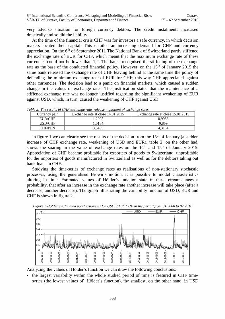
8th International Scientific Conference Managing and Modelling of Financial Risks Ostrava
VŠB-TU of Ostrava, Faculty of Economics, Department of Finance 5th – 6th September 2016
568
very adverse situation for foreign currency debtors. The credit instalments increased
drastically and so did the liability.
At the time of the financial crisis CHF was for investors a safe currency, in which decision
makers located their capital. This entailed an increasing demand for CHF and currency
appreciation. On the 6th of September 2011 The National Bank of Switzerland partly stiffened
the exchange rate of EUR for CHF, which meant that the maximum exchange rate of these
currencies could not be lower than 1,2. The bank recognised the stiffening of the exchange
rate as the base of the conducted financial policy. However, on the 15th of January 2015 the
same bank released the exchange rate of CHF leaving behind at the same time the policy of
defending the minimum exchange rate of EUR for CHF; this way CHF appreciated against
other currencies. The decision lead to a panic on financial markets, which caused a sudden
change in the values of exchange rates. The justification stated that the maintenance of a
stiffened exchange rate was no longer justified regarding the significant weakening of EUR
against USD, which, in turn, caused the weakening of CHF against USD.
Table 2: The results of CHF exchange rate release – quotient of exchange rates.
Currency pair Exchange rate at close 14.01.2015 Exchange rate at close 15.01.2015
EUR/CHF 1,2005 0,9986
USD/CHF 1,0184 0,859
CHF/PLN 3,5455 4,3164
In figure 1 we can clearly see the results of the decision from the 15th of January (a sudden
increase of CHF exchange rate, weakening of USD and EUR), table 2, on the other had,
shows the soaring in the value of exchange rates on the 14th and 15th of January 2015.
Appreciation of CHF became profitable for exporters of goods to Switzerland, unprofitable
for the importers of goods manufactured in Switzerland as well as for the debtors taking out
bank loans in CHF.
Studying the time-series of exchange rates as realisations of non-stationary stochastic
processes, using the generalised Brown’s motion, it is possible to model characteristics
altering in time. Estimated values of Hölder’s function state in these circumstances a
probability, that after an increase in the exchange rate another increase will take place (after a
decrease, another decrease). The graph illustrating the variability function of USD, EUR and
CHF is shown in figure 2.
Figure 2 Hölder’s estimated point exponents for USD, EUR, CHF in the period from 01.2000 to 07.2016
0
0,1
0,2
0,3
0,4
0,5
0,6
0,7
2000
-01-
03
2001
-01-
03
2002
-01-
03
2003
-01-
03
2004
-01-
03
2005
-01-
03
2006
-01-
03
2007
-01-
03
2008
-01-
03
2009
-01-
03
2010
-01-
03
2011
-01-
03
2012
-01-
03
2013
-01-
03
2014
-01-
03
2015
-01-
03
2016
-01-
03
H(t) USD EUR CHF
Analyzing the values of Hölder’s function we can draw the following conclusions:
- the largest variability within the whole studied period of time is featured in CHF time-
series (the lowest values of Hölder’s function), the smallest, on the other hand, in USD

8th International Scientific Conference Managing and Modelling of Financial Risks Ostrava
VŠB-TU of Ostrava, Faculty of Economics, Department of Finance 5th – 6th September 2016
569
(the higher the value of Hölder’s point exponent, the lower the local variability of the
series);
- a low variability for all the three series can be seen in the period from 08.2008 to 06.2009
and in the period from 02.2010 to 04.2012; this means that in this period there was a strong
increase or decrease of exchange rates (unidirectional changes, not oscillating around the
average);
- we can clearly notice that for the CHF series the value of Hölder’s function soared to
approx. 0,68 in 01.20015 (the black Thursday 15.01.2015); this was caused by the decision
of the National Bank of Switzerland and by the lasting for a few days, constant increase of
CHF exchange rate; according to the interpretation of Hölder’s function, after an increase
in the price there was another increase with probability of around 0,7, and a decrease with
probability of around 0,3 (this can be observed in diagram 1)
- the second half of 2008 features higher values of the function and unidirectional changes –
increase of exchange rates of all the three currencies,
- the values of Hölder’s point exponents are however in the time range 01.2000 - 07.2016
substantially lower than 0,5, so, according to the interpretation, the series feature a very
large variability, increases and decreases of exchange rates occur one after another
(currently in an upward trend for CHF and USD and horizontal trend for EUR);
- the best moment to convert the taken out liabilities was the rating from before the upward
trend in 2008 .
Calculating the spread for the considered series, that is the difference between the exchange
rate of purchase and of sale, for the analysed currencies, according to the National Bank of
Poland exchange rate, it amounts to approximately 8-9 gr. per one currency, which constitutes
around 2-2,5% of the price. This is a considerable, additional expense for the debtor!
Moreover, commercial banks as well as other financial institutions directly granting credits set
the value of spread according to their own, internal exchange rates of purchase and sale, which
very often differ significantly from the exchange rates of the NBP. Therefore, a considerable
number of debtors become independent of spread in the repayment of a credit in foreign
currency, buying foreign currencies at the lowest available exchange rate in a period of time.
Let us consider an example: a bank granted credit in CHF in the middle of 2008. The CHF
exchange rate amounted to approx. 2 PLN at that time, lasting fifteen-years credit in the
amount of 350, 000 PLN was equalized to approx. 175, 000 CHF. In the period of seven years
of timely repayment of the liability, the value of liability in CHF decreased, the debtor repaid
approx. 82, 000 CHF, so the value of his liability decreased to approx. 93,000 CHF. However,
from the time of taking out of the credit the exchange rate of the currency changed and rose to
about 4 zlotys. In these circumstances, the debtor was left with a liability of approx. 4 zlotys x
93,000 CHF = 372,000 PLN. The increase in the exchange rate lead to a situation in which the
debtor, after seven years of repayment of the credit, is liable to the bank in conversion to PLN
more than on the day of taking out of the credit. The example takes into consideration only the
increase in the exchange rate, it does not consider the costs of the credit, including interest rate
and spread, which additionally increases the liability!
The increase in the exchange rate of the currency entails an increase of the liability
converted into zlotys and influences the value of the foreign currency credit instalment. If, for
example, the credit instalment amounted to 1000 CHF, then, converted into PLN, in 2008 it
was around 2000 zlotys, in 2013 it increased to around 3400 zlotys, and in the middle of
January 2015 it increased over twice – it amounted to 4300 zlotys! What is more, the amount
of credit very often exceeds e.g. the value of a real estate, which constitutes its security. The
increase in the exchange rate of foreign currencies also leads to a situation, where the sale of
the property, which constitutes credit security, and the repayment of the liability is

8th International Scientific Conference Managing and Modelling of Financial Risks Ostrava
VŠB-TU of Ostrava, Faculty of Economics, Department of Finance 5th – 6th September 2016
570
unprofitable because, in such a situation, the funds obtained from the sale of the property are
not large enough to cover the repayment of the credit capital left. Considering the above, the
debtor is left with no other choice, but to repay the large instalments of the credit and hope for
a decrease in the exchange rate.
5. Conclusion
The difficult situation of foreign currency debtors in Poland requires the conduct of social,
financial, and economic analyses in order to find a solution to the problem which would
satisfy both debtors and banks or other institutions granting credits in foreign currency.
Nowadays in Poland there is a significant number of debtors who have financial problems
connected with the repayment of liabilities taken out in a foreign currency. Most often, the
currency of the credit was CHF.
Modelling of exchange rates in connection to risk analysis of foreign currency credits is
justified on the base of many economic, micro- and macroeconomic, as well as social reasons.
Indexed and denominated foreign currency credits were in the years 2000 – 2008 most popular
among people seeking ready capital. However, after a few years time, it turned out that these
people fell into a currency trap. In view of the increase of exchange rates, there followed a
drastic increase in the value of credit instalments, the value of liability rose significantly, and
in view of a fall in the prices of properties, very often the value of investment for which the
loan was taken out, does not cover the value of the liability. The difficult situation of the
debtors has recently become a concern of the government, however, without any positive
result up to the present moment.
Investing on the capital market, as well as taking out long-term financial liabilities, we
have to consider the dynamics of changes and the stochastic nature of capital market. The risk
should, as precisely as possible, be defined and, if possible, measured. Only after the
consideration of all possible variants of the investment or liability, should the optimum variant
be chosen. Mathematical and econometric methods allow us to model financial time-series
(including the ones of exchange rates) and to study their variability, however, some political
decisions, the scales of crises on financial markets and their economic as well as social
consequences can not be forseen.
References
[1] Daoudi, K., Lévy Véhel, J. and Meyer, Y. (1998). Construction of continuous functions
with prescribed local regularity, Journal of Constructive Approximations, 014(03), 349-
385.
[2] Jajuga, K. and Jajuga, T. (2015). Inwestycje. Instrumenty finansowe, aktywa
niefinansowe, ryzyko finansowe, inżynieria finansowa. Wydawnictwo PWN, Warszawa.
[3] Kaufman, P. (2005). New Trading Systems And Methods, John Wiley & Sons, New York.
[4] Mastalerz-Kodzis, A. (2003). Modelowanie procesów na rynku kapitałowym za pomocą
multifraktali. Prace Naukowe, Akademia Ekonomiczna im. Karola Adamieckiego
w Katowicach, Katowice.
[5] Mastalerz-Kodzis, A. (2013). Zastosowanie funkcji Höldera w modelu FRAMA. Studia
Ekonomiczne, Uniwersytet Ekonomiczny w Katowicach, Nr 159 - Zastosowanie metod
matematycznych w ekonomii i zarządzaniu, p. 73-81.

8th International Scientific Conference Managing and Modelling of Financial Risks Ostrava
VŠB-TU of Ostrava, Faculty of Economics, Department of Finance 5th – 6th September 2016
571
[6] Peltier, R. F. and Lévy Véhel, J. (1995). Multifractional Brownian Motion: Definition
and Preliminary Results, INRIA Recquencourt, Rapport de recherché, No. 2645.
[7] Sobczyk, K. (1996). Stochastyczne równania różniczkowe, Wydawnictwa Naukowo-
Techniczne, Warszawa.
[8] www.nbp.pl, table C, (01.08.2016).

8th International Scientific Conference Managing and Modelling of Financial Risks Ostrava
VŠB-TU of Ostrava, Faculty of Economics, Department of Finance 5th – 6th September 2016
572
Economic Value Added as a Measurement Tool of Capital Structure Effectiveness at the Power-
Producing Enterprises
Dmytro Mastiuk, Petr Valouch, Petro Krush1
Abstract
This paper contributes to the investigation of Economic Value Added (EVA) measurement process
and approaches of its calculation as an assessing tool of Capital Structure effectiveness. The main
objects included into author’s investigation are power-producing enterprises of Ukraine and Czech
Republic listed on a stock exchange market. The main aim of the research is to demonstrate the
modified author’s approach to Economic Value Added calculation, which gives an opportunity to
adjust interpretation of results depending on used types of capital and desired units of measure. Thus,
provided approach directed on improving capital structure effectiveness at the power-producing
enterprises as a part of a capital-intensive branch. Introduced approach derives from standard method
or evaluation and split capital into its two constituent parts that give the advantage to measure the
effectiveness of Debt and Equity separately. Moreover, author’s approach reduce the complexity of
investigation due to modification of standard decomposed formula of Economic Value Added.
Therefore, enterprises can easily calculate the effectiveness of committed capital and its structure
using EVA measurement tool in their activities.
Key words
Economic value added, capital structure, effectiveness, power-producing enterprise.
JEL Classification: D24, G32
1. Introduction
The power-producing industry is one of the biggest, powerful and capital-intensive
branches (Hanks, 2013), which is highly necessary for the overall economic growth of any
country. Nevertheless, this industry faces numerous problems that, sometimes, have to be
urgently overcome by enterprise’s management decisions. One of these relevant problems is
capital structure and its effectiveness. As it was mentioned before, the power-producing
industry is capital-intensive. Thus, we can state that enterprises at this industry borrow a
significantly high amount of capital from different sources, which has to be allocated and
controlled in a proper way and effectiveness of which has to be estimated. Such assessment of
capital structure effectiveness is important part of financial and entrepreneurial activity, which
helps to find answers to questions as:
Does enterprise have needs in the capital?
Which type of capital is the most effective and efficient for the enterprise?
1 Dmytro Mastiuk, 1MSc, Ph.D. student, National Technical University of Ukraine “Kiev Polytechnic
Institute”,Faculty of Management and Marketing, Department of Economic and
Entrepreneurship,Peremohy ave. 37a, 03056 Kiev, Ukraine,E-mail: [email protected]
Petr Valouch, Ing., Ph.D.,Masaryk University,Faculty of Economics and Administration, Department
of Public Economics,Lipová 41a, 60200 Brno, Czech Republic,E-mail: [email protected]
Petro Krush, Prof., CSc., National Technical University of Ukraine, “Kiev Polytechnic
Institute”Faculty of Management and Marketing, Department of Economic and
Entrepreneurship,Peremohy ave. 37a, 03056 Kiev, Ukraine,E-mail: [email protected]

8th International Scientific Conference Managing and Modelling of Financial Risks Ostrava
VŠB-TU of Ostrava, Faculty of Economics, Department of Finance 5th – 6th September 2016
573
What exact amount of money company needs?
How to distribute capital among assets?
What price for borrowed capital should be to achieve higher effectiveness?
Various scientific sources represent various alternative estimators that assess and show,
directly and indirectly, how enterprise’s capital works and how effective it is. Among these
estimators could be defined the most shared and significant such as Earnings per Share (EPS),
Return on Equity (ROE), Return on Assets (ROA), Return on Invested Capital (ROIC),
Weighted Average Cost of Capital (WACC) (Madhavi E., Prasad M.S.V., 2015), Financial
Leverage Multiplier (FLM) or, in other words, Equity Multiplier (EM) (Gitman, Lawrence J.,
2010). Moreover, we can consider Economic Value Added (EVA) as one of the measurement
tool of capital structure performance and its effectiveness. In this paper, we will stop
particularly on Economic Value Added as a measurement instrument of capital structure
performance at the power-producing enterprises.
Following G. Bennett Stewart (2013), EVA is not just a performance measure; it is a tool
and fundament for gauging investments, valuing and making decisions, perfecting the process
of planning and shaping strategies. Joel M. Stern, John S. Shiely and Irwin Ross (2001)
provide such definition of Economic Value Added as the profit that remains after deducting
the cost of capital invested to generate profit. Besides, EVA is considered as a value created
more than the required returns of the investors (Roca F., 2011). Madhavi E. and Prasad
M.S.V. (2015) define EVA as a corporate financial index, which gives true profitability of the
firm, being used to assess the financial performance of companies. Financial education
source, Investopedia LLC (2014) provides such explanation of EVA as a measure of a
company's financial performance based on the residual wealth calculated by deducting
the cost of capital from its operating profit.
The aim of this paper is to create clear understanding about EVA as a measurement tool of
capital structure effectiveness for energy sector enterprises. Moreover, to show classic and
alternative conceptions of EVA evaluation and introduce the authors’ approach to its
calculation from the capital structure point of view, which is possible to implement for chosen
enterprises, to evaluate the difference between methods and factors affecting the level of EVA
as the index of capital structure performance at the enterprises of represented sector.
2. Methodology and Data
For the research stated in this paper, the variety of sources were used. The list of producing
companies of electro energy in the Czech Republic and Ukraine was taken based on annual
information provided by National Energy and Utilities Regulatory Commission in Ukraine
(2015) and Reegle agency (2013), which states in REEEP Public-Private partnership. The list
of the power-producing companies includes PJSC CentrEnergo (CEEN), PJSC KievEnergo
(KIEN), PJSC ZahidEnergo (ZAEN), PJSC DonbasEnergo (DOEN), PJSC DniproEnergo
(DNEN), ČEZ a.s. (CEZ) and E.ON PJSC (EAON). For the purpose of EVA evaluation and
analysis of chosen companies in order to determine capital structure effectiveness we used in
the paper a compiled dataset for the time span from 2010 to 2015, which was taken from
Bloomberg and official annual reports of companies.
It is important to define and clarify approaches to measurement of some valuable financial
indexes such as Net Operating Profit after Taxes (NOPAT), Invested Capital (IC), Weighted
Average Cost of Capital (WACC), Cost of Debt and Cost of Equity, which is applied in this
paper. First, we pay attention on NOPAT calculation as a crucial element of EVA
measurement. The first approach to computing this indicator was taken from the Bloomberg
Database and widely spread among scholars (Blocher, 2010; Investopedia, 2014).
(1)

8th International Scientific Conference Managing and Modelling of Financial Risks Ostrava
VŠB-TU of Ostrava, Faculty of Economics, Department of Finance 5th – 6th September 2016
574
The stated formula has several advantages than the simplified methods as it uses wider
inputs to evaluate NOPAT. Hence, it increases the level of credibility of results and makes
stakeholders involved in company’s activity feel more confident. The usage of wider and
specific inputs generate negative side effect. Many of elements included in formula might be
concealed from the broad public what disrupts calculation. In addition to possible lack of
information, the complexity of calculation makes sense.
For the purpose of the research paper, another approach was used (Gitman, 2010; Madhavi,
2015). In this case, NOPAT regarded as a dependence from Earnings before Interest and
Taxes reduced by amount of taxes payable:
(2)
From our point of view, this formula gives and advantage of faster and simplified
evaluation of NOPAT, avoiding the usage of specific elements. Therefore, this approach is
applied to this paper. Invested Capital is considered to be a part of EVA calculation and under
the Bloomberg’s approach consist of Debt, Equity and some additional non-interest parts.
Stewart (2013), Blocher (2010) and Roca (2011) applied the same method:
(3)
Where:
– a total sum of Debt including Short-Term Borrowings, Notes Payable and Long-Term
Debt;
– the total Equity.
Allowance for Doubtful Accounts, Deferred Tax Liabilities and Accrued Income Tax, are
the elements that exist in company’s financial statements. In our opinion, these items do not
have any interest to be paid and do not generate any additional value and, consequently, can
be excluded from the evaluation process. The contributions of these elements to Invested
Capital and, eventually, to EVA are sometimes insignificant. Besides, for us, it is much
important to see EVA that comprises the difference of real generated profit and expenses,
which influence and reduces this profit.
Classical Approach to Weighted Average Cost of Capital is included into calculation
process of EVA and comprises from Debt, Equity and costs of these two types of capital
(Gitman, 2010; Stewart, 2013):
(4)
Where:
– Cost of Debt after Taxation and Debt Adjustment factor influence;
– Cost of Equity based on CAPM methodology.
For further calculations, additional relevant ratios, which provides a thorough basis, are
required. As the measurement of Economic Value Added depends not only on absolute data
but includes relative ratios, the calculation uses such indexes as Cost of Equity, Cost of Debt,
and Weighted Average Cost of Capital (WACC).
Table 1: Cost of Capital and Return ratios for EVA calculations at Power-Producing companies

8th International Scientific Conference Managing and Modelling of Financial Risks Ostrava
VŠB-TU of Ostrava, Faculty of Economics, Department of Finance 5th – 6th September 2016
575
Ticker 2010 2011 2012 2013 2014 2015
Co
st o
f E
qu
ity
CEEN 13,54% 12,27% 10,59% 10,28% 6,89% 5,81%
KIEN 1,44% 10,69% 10,51% 9,77% 9,24% 9,36%
ZAEN 11,25% 5,85% 3,43% 7,80% 3,10% 5,24%
DOEN 4,70% 6,73% 0,00% 11,61% 13,09% 16,56%
DNEN 11,86% 7,88% 4,35% 5,96% -5,06% -2,65%
CEZ 7,70% 7,30% 11,56% 7,91% 8,22% 7,37%
EAON 14,15% 12,59% 12,97% 10,22% 9,08% 8,52%
Co
st o
f D
ebt
CEEN 2,80% 4,83% 7,38% 8,12% 5,49% 8,05%
KIEN 3,29% 2,59% 11,36% 0,00% 42,62% 31,71%
ZAEN 7,48% 4,52% 4,55% 0,00% 42,62% 31,71%
DOEN 3,22% 16,91% 7,52% 4,17% 5,63% 7,41%
DNEN 4,43% 5,56% 3,96% 3,55% 0,00% 0,00%
CEZ 3,83% 3,50% 1,80% 2,27% 0,69% 0,48%
EAON 2,93% 3,46% 1,65% 1,76% 0,59% 1,35%
WA
CC
CEEN 10,14% 10,77% 9,92% 9,75% 6,77% 6,12%
KIEN 2,05% 9,79% 10,51% 9,77% 13,25% 9,36%
ZAEN 9,50% 5,08% 3,98% 7,80% 14,06% 10,21%
DOEN 4,15% 9,98% 3,32% 8,25% 11,00% 14,93%
DNEN 9,87% 7,43% 4,30% 5,89% -5,06% -2,55%
CEZ 6,08% 5,59% 7,35% 5,48% 5,14% 4,05%
EAON 9,48% 9,14% 8,44% 6,98% 5,48% 5,69%
Source: own proceedings based on Bloomberg raw data and annual reports of companies
On the basis of given data we can gauge Economic Value Added for chosen companies in
energy sector and compare classic and modified authors’ approaches.
3. Results and Discussion
In different scientific sources, such formula of Economic Value Added that considered as a
standard is given (5). It is widely used by scholars, financial managers and agencies for
calculation due to its simplicity, viability and feasibility of results:
(5)
Where:
NOPAT – Net Operating Profit after Taxes;
WACC – Weighted Average Cost of Capital;
IC – Invested Capital.
Next step, which appeared during the research, was what exact amount of EVA produce
each type of capital? To find that amount of Economic Value Added generated by types of
capital, the formula (5) was decomposed on two constituents. The result of the measurement
does not change, but in this case, we can see which part of the economic value added belongs
to which type of capital (Debt or Equity). The decomposition of EVA formula is useful for
such evaluations when the company and its management want to evaluate the effectiveness of
their types of capital and to know how to improve its efficiency.

8th International Scientific Conference Managing and Modelling of Financial Risks Ostrava
VŠB-TU of Ostrava, Faculty of Economics, Department of Finance 5th – 6th September 2016
576
(6)
Where:
EBIT – Earnings before Interest and Taxes;
– Cost of Equity;
E – Amount of Equity;
– Cost of Debt;
D – Debt capital.
The splitting of formula (6) into two components gives such result. Formula (6.1) shows
economic value added generated by Equity.
(6.1)
Formula (6.2) shows economic value added generated by Debt.
(6.2)
Nevertheless, the only disadvantages of these formulas are the number of calculations and
if the company does not provide clear data, some of the components can be lost, which makes
the result equal to “0”.
To step aside from absolute values in EVA measurement and find how much return each
part of capital produces following EVA formulas were introduced. These formulas make the
basis of author’s approach to EVA assessment. Here we can see the difference between the
return and cost of each type of capital.
(7)
Where:
ROEa – Return on Equity adjusted;
RODa – Return on Debt adjusted.
To calculate two mentioned ratios we split Net Operating Profit after Taxes into two
different parts and defined sums of NOPAT generated by each type of capital.
(7.1.1)
(7.1.2)
Formula (7) provides EVA measurement from the capital structure point of view. In this
case, Return on Equity (ROE) is taken as a performance indicator of shareholders capital.
Return on Debt (ROD) is not a standard indicator of Debt performance. Nevertheless, it is
used to understand the profitability of Debt capital incurred and allocated by a company.
Substituting ROE and ROD with formulas (7.1.1) and (7.1.2) the EVA calculation gets such
form:
(7.2),
or, consequently

8th International Scientific Conference Managing and Modelling of Financial Risks Ostrava
VŠB-TU of Ostrava, Faculty of Economics, Department of Finance 5th – 6th September 2016
577
(8)
The formula (8) provides information about EVA using the alternative approach. As it can
be seen, calculation of EVA is based on two constituents and includes Equity, Debt, Costs of
Equity and Debt, the sum of Invested Capital and NOPAT. Thus, we can evaluate what exact
percentage of EVA (premium or loss) generated by each type of capital and find its absolute
result. Equation (9.1) introduce Economic Value Added of Equity using such indicators as 1)
profitability of Invested Capital and 2) value spread as a difference between
profitability and Cost of Equity :
(8.1)
Neumaier, I. and Neumaierová, I. (March 2014) in their research introduced similar
formula to EVA calculation that uses ROE as a performance indicator of capital, Cost of
Equity deducted from ROE and multiplied by Equity amount. In this paper, EVA of Debt
Capital is considered which makes all financial sources to be included. The following formula
(8.2) uses same indicators as in previous equation, but Cost of Debt is used instead of
Cost of Equity and Equity is substituted by Debt:
(8.2)
The results interpretation of equations 8.1 and 8.2 can be next:
if EVA of Debt or/and Equity takes the negative result, it means that either company
generates losses, or it overpays for Debt or/and Equity and allocates these resources
ineffectively;
if EVA of Debt or/and Equity takes the positive result, it means that company
generates enough earnings and uses its resources effectively.
Talking about advantages of author’s approach it can be mentioned that equation of EVA
proposed in this paper (8) is much easier to understand comparing to decomposed formula (6),
nonetheless, it provides the same results as a standard approach. The second advantage of
author’s approach is that formulas can be used for calculation of EVA as a performance
measurement tool for all stated types of capital separately. It means that if the company does
not provide full information about Debt or Equity, analytics can use an alternative approach.
Such situation is common in Ukraine where enterprises that obliged to submit comprehensive
information exclude some important indexes.
Furthermore, formulas (8), (8.1) and (8.2) exclude mean ratios such as WACC and use a
direct difference between the percentage of earnings and cost of each type of capital.
Moreover, using author’s approach it is possible to pick out Value Spread of each type of
capital and calculate EVA in relative meanings, which gives the chance to apply this method
to enterprises of different size, with different earnings and even from different countries.
Along with this, such approach gives an opportunity to calculate the influence of components
and define the percentage of EVA (E) and EVA (D) in total EVA of the enterprise. Results of
calculation are provided below in Table 2.

8th International Scientific Conference Managing and Modelling of Financial Risks Ostrava
VŠB-TU of Ostrava, Faculty of Economics, Department of Finance 5th – 6th September 2016
578
Table 2: Results of different approaches of EVA calculation
Ticker 2010 2011 2012 2013 2014 2015
EV
A
CEEN -171573 -4229 159152 318745 -12995 -417446
KIEN 95871 -1880584 2349810 812439 -272509 -747268
ZAEN -213180 -64958 -35708 631449 51202 -1800159
DOEN -170794 -35913 137850 591838 890211 -130575
DNEN 140414 276155 795752 1206172 1005659 -1380311
CEZ 40995548 37970029 22477292 21004901 12016012 6241525
EAON 158736 -5158825 -1744030 137654 -3001543 -10302354
EV
A (
E)
CEEN -215787 -178685 -133131 -98656 -153410 -161324
KIEN 24671 -657902 -417072 -435490 -366570 -372430
ZAEN -114240 0 -15198 -132645 69887 -432812
DOEN -78882 -25520 78230 208356 137979 -196262
DNEN -140505 -170929 -115577 -340867 381491 128061
CEZ 9721846 10723938 -5514106 -827446 -7477839 -6555494
EAON -3303799 -4736928 -3545149 -2105238 -2620252 -5389867
EV
A (
D)
CEEN 44214 174455 292282 417401 140414 -256122
KIEN 71200 -1222683 2766882 1247929 94061 -374838
ZAEN -98940 0 -20510 764094 -18686 -1367346
DOEN -91912 -10394 59620 383482 752232 65687
DNEN 280919 447084 911329 1547039 624168 -1508372
CEZ 31273702 27246090 27991398 21832347 19493852 12797020
EAON 3462535 -421898 1801119 2242892 -381291 -4912487 Source: authors’ proceedings based on selected data
Analysing calculation, we can admit that results of EVA assessment at the power-
producing enterprises using standard EVA approach and modified author’s EVA approach are
the same, even though author’s approach includes a different way of calculation; in most of
the cases, power-producing enterprises non-effectively use their Equity that generates a loss in
Economic Value-Added. The reason is that rate of return is lower than Cost of Equity. EVA
of Debt is positive almost at each power-producing enterprise, but it does not help to exceed
the generated loss by Equity. Therefore, the main recommendations are to find external
reliable and safe sources of capital, which can supply with enough amount debt capital and
ensure owners in the necessity of capital structure optimisation to reach higher wealth value
and pursue growth speed. Besides, to implement quarterly and annually monitoring and
controlling activity based on EVA measurement approach to increase effectiveness of capital
at the power-producing enterprises.
4. Conclusion
The Economic Value Added is considered as universal and comprehensive measurement
tool of capital performance. Different scientists and companies all over the world approved
the significance of this financial instrument. Talking about capital-intensive power-producing
enterprisesб it is important to admit that necessity of EVA measurement rapidly increases
with the importance of monitoring and controlling their financial resources. The more precise,
easier and clear is the assessing process of capital and its structure effectiveness, the more
effective and efficient financial decisions and the more value capital produces. Provided
approach gives an opportunity to investigate Economic Value Added, generated by each type
8th International Scientific Conference Managing and Modelling of Financial Risks Ostrava
VŠB-TU of Ostrava, Faculty of Economics, Department of Finance 5th – 6th September 2016
579
of owed financial resource either in absolute or relative measurement units. Furthermore, such
EVA formula can be expanded for distinct financial sources included to Debts or Equity that
gives the further understanding of financial sources performance. Comparing to standard
decomposed approach, it can be seen that authors’ submitted method of EVA evaluation is
much easier to apply and understand. Thus, it makes advantages for this approach to be
implemented at power-producing enterprises as a capital structure performance indicator.
Further development of measurement tools of capital structure will enhance its investigation
and give a chance to involve and allocate extra recourses in a way that is more effective.
Acknowledgments
This research was supported by Finance Department, Faculty of Economics and
Administration, Masaryk University within Erasmus Mundus exchange programme, project
HUMERIA. We thank Petr Valouch, Head of the Department for assistance with
methodology calculation techniques, for comments, provided insight and expertise that
greatly improved the research paper.
References
[1] Hanks S. (2013) The most Capital Intensive Industries, Available at:https://www.quora.
com/What-are-the-most-capital-intensive-industries (Accessed: 5th March 2016).
[2] Madhavi E., Prasad M.S.V. (2015) 'An Empirical Study on Economic Value-Added and
Market Value-Added of Selected Indian FMCG Companies', The IUP Journal of
Accounting Research & Audit Practices, Vol. XIV(3), pp. 45-65.
[3] Gitman, Lawrence J. (2010) Principles of managerial finance, 13th ed., Boston:
Prentice Hall.
[4] Investopedia LLC. (2014) Equity Multiplier, Available at:http://www.investopedia.com/
terms/e/equitymultiplier.asp?layout=infini&v=4B&adtest=4B (Accessed: 5th March
2016).
[5] Stewart G.B., III (2013) Best-Practice EVA, Hoboken, New Jersey: John Wiley & Sons,
Inc.
[6] Joel M. Stern, John S. Shiely, Irwin Ross (2001) The EVA Challenge: Implementing
Value-Added Change in an Organization, USA: John Wiley & Sons.
[7] Roca F. (2011) Economic Value Added (EVA), interview with Joel M. Stern, Available
at: http://newmedia.ufm.edu/gsm/index.php?title=Sternevainterview (Accessed: 6
March 2016).
[8] Madhavi E., Prasad M.S.V. (2015) 'Assessing Corporate Performance with Measures of
Value Added as Key Drivers of Shareholder Wealth: An Empirical Study', The IUP
Journal of Business Strategy, Vol. XII(4), pp. 19-34.
[9] Neumaier, I., Neumaierová, I. (March 2014) 'INFA Performance Indicator Diagnostic
System', Central European Business Review, 3(1), pp. 35-41.
[10] Investopedia LLC. (2014) Economic Value Added - EVA, Available
at:http://www.investopedia.com/terms/e/eva.asp?layout=infini&v=4B&adtest=4B(Acce
ssed: 5 March 2016).

8th International Scientific Conference Managing and Modelling of Financial Risks Ostrava
VŠB-TU of Ostrava, Faculty of Economics, Department of Finance 5th – 6th September 2016
580
[11] Reegle agency (2013) Policy and Regulatory Overview in Czech Republic, Available
at: http://www.reegle.info/policy-and-regulatory-overviews/CZ (Accessed: 7 March
2016).
[12] NERC, Ukraine (2015) Annual Report on the Results of NERC, Available at:
http://www.nerc.gov.ua/?id=11895 (Accessed: 7 March 2016).
[13] Edward Blocher (2010) Cost management: a strategic emphasis, Boston: McGraw-
Hill/Irwin.

8th International Scientific Conference Managing and Modelling of Financial Risks Ostrava
VŠB-TU of Ostrava, Faculty of Economics, Department of Finance 5th – 6th September 2016
581
Risk impact on the quality of accounting information provided in the current conditions of globalization
Martina Mateášová 1
Abstract
Current developments and globalization trends in the economy and finance have the
effect of increasing the level of risk that affect the internal and external environment of
the enterprise. In order to keep the company competitive must learn to identify and
manage the risks that affect the prosperity and effectiveness of all of its activities.
Instrument to counter this trend, the introduction of effective risk management, internal
control system, internal audit to achieve integrated management of business risks. In
order for this strategy to be successful you need to have built quality information system
company, established control mechanisms using modern IT technology. All events
company ultimately translate into financial transactions and will be shown in the
accounts of an enterprise which the enterprise presents the external environment (ie.
user). It is therefore essential that the information is useful, objective, reliable and
present a true and fair view of the assets, liabilities and financial situation.
Key words
Globalization, shared services centers, Service Level Agreement, business risks, accounting
JEL Classification: M48, G15, G17
1. Vplyv globalizácie na centrá zdieľaných služieb
Globalizácia, proces v ktorom či už človek, obchod, investície, informácie, trh
alebo demokracia stále častejšie prekračujú štátne hranice, nám odstraňuje postupne
obmedzenia. Moderným trendom v súvislosti s globalizáciou sú aj zmeny vo vlastníckych
transakciách. Ich neustály rast a potreba sú nevyhnutné pre zachovanie konkurencieschopnosti
(Ondrušová, Parajka, 2014). Globalizácia nám neprináša iba rast obchodu s tovarom,
výrobkami a presúvanie priemyselnej výroby do lacnejších krajín, ale prináša aj dynamický
rozvoj sektora obchodovateľných služieb.
V druhej polovici osemdesiatych rokov minulého storočia začali nadnárodné korporácie
zakladať aj v Európe prvé centrá zdieľaných služieb. Shared service center (angl.) je centrum
zdieľaných služieb, ktoré realizuje špecifické interné procesy s cieľom znižovania nákladov
(napríklad finančné služby a účtovníctvo, IT podporu, služby v oblasti ľudských zdrojov), čím
podporuje kľúčové činnosti materskej a dcérskych spoločností ale aj materskej a sesterských
spoločností. Centrá zdieľaných služieb prešli svojim prirodzeným vývojom. Vo svojich
začiatkoch sa venovali predovšetkým financiám a účtovníctvu. Vykonávali sa v nich iba
1 Martina Mateášová, Ing., PhD., EU v Bratislave, FHI, KÚA, Dolnozemská cesta 1/b, Bratislava, SR,
e-mail: [email protected].
Príspevok je výstupom z výskumného projektu VEGA MŠVVaŠ SR a SAV č. V-14-035-00 (2014 –
2016) Význam oceňovania transakcií medzi závislými osobami a ich vplyv na výsledok hospodárenia
účtovnej jednotky

8th International Scientific Conference Managing and Modelling of Financial Risks Ostrava
VŠB-TU of Ostrava, Faculty of Economics, Department of Finance 5th – 6th September 2016
582
jednoduché transakčné, operatívne aktivity bez veľkej pridanej hodnoty. Postupne sa ale
prepracovali k intelektuálne náročnejším funkciám s vyššími nárokmi na odborné zručnosti
a prax, centralizovali sa v nich ucelené aktivity a procesy, a v neposlednom rade aj tzv.
vlastníctvo štandardizovaných procesov.
Podľa metodiky vypracovanej spoločnosťou PricewaterhouseCoopers prechádzajú centrá
zdieľaných služieb vo svojom vývoji štyrmi vývojovými štádiami (fázami)2:
prvá fáza – „start-up“ – do centra zdieľaných služieb sa presúvajú jednoduché a hlavne
manuálne náročné procesy s nízkou úrovňou štandardizácie – využívajú to najmä
spoločnosti s jednoduchou organizačnou štruktúrou,
druhá fáza –„rast“ – centrum zdieľaných služieb má zavedené štandardizované
procesy, postupne sa začínajú implementovať kontrolné mechanizmy procesov
a nástroje na podporu zákazníckeho servisu,
tretia fáza – „expanzia“ – centrum zdieľaných služieb má okrem interných aj externých
klientov, má zautomatizované biznis procesy, zavedený systém kontrolných procesov,
tréningov a priebežného vzdelávania zamestnancov, má implementované štandardné
podnikové IT systémy a funkčný risk management riešiaci efektívnosť nastavených
procesov,
štvrtá fáza (druhá generácia) – „centrum excelentnosti“ – centrum zdieľaných služieb
už vystupuje ako suverénna organizácia, ktorá generuje zisk, poskytuje vysoko
profesionálne, odborné a strategické služby interným aj externým zákazníkom.
V súčasnosti sa cez centrách zdieľaných služieb realizuje už aj nákup vstupov, podpora
zákazníkov tzv. call centrá, veda a výskum, či IT služby. Stávajú sa tak z nich centrá druhej
generácie na úrovní biznis partnerstva s materskou spoločnosťou.
Obchodné spoločnosti po celom svete investovali a naďalej investujú mnoho úsilia do
zvýšenia efektivity hlavne svojich finančných oddelení (napríklad účtovníctva, oddelenia
treasury). Presun procesov mimo domovských krajín pomáha nadnárodným korporáciám
zvyšovať ich konkurencieschopnosť najmä v úspore nákladov a zefektívnení činností. Medzi
atraktívne „off-shore“ lokality patria India, Filipíny, Čína, Kostarika, Brazília, Mexiko a iné.
V Európe medzi najatraktívnejšie krajiny patria Írsko, Poľsko, Česká republika ale aj
Slovensko. Na druhej strane začínajú vlády príslušných krajín vyvíjať legislatívny tlak na
nadnárodné korporácie a začína sa čoraz častejšie spomínať i otázka „návratu domov“ (tzv.
onshoring). Dôvodom je, že globalizačné tendencie týchto spoločností presahujúce rámec
jednej krajiny, sa vymykajú dôslednej regulácii a kontrole. Onshoring začínajú aktívne
podporovať aj krajiny ako sú Spojené štáty americké a Kanada prostredníctvom daňových
a dotačných stimulov, pretože v mnohých prípadoch offshoring a outsourcing nenaplnili
očakávania samostatných nadnárodných korporácií, alebo ich význam z hľadiska
poskytovaných výhod a efektivity práce sa za posledných desať rokov zmenil.
Centrá zdieľaných služieb na Slovensku
Prvé centrá zdieľaných služieb renomovaných nadnárodných korporácií začali vznikať aj
na Slovensku približne pred 15 rokmi, kedy tieto nadnárodné korporácie začali presúvať svoje
„back-office“ aktivity zo svojich západoeurópskych centrál do východnej Európy. Sú to
hlavne dcérske spoločnosti nadnárodných korporácií, ktorých tlak na ziskovosť a nutnosť
zvyšovať efektívnosť procesov viedli k centralizácii ich aktivít do lokalít mimo ich centrál
a výrobných základní. Investori si vyberajú Slovensko hlavne pre nízke mzdové náklady,
vzdelanú, flexibilnú a jazykovo vybavenú pracovnú silu s dobrými pracovnými návykmi, pre
polohu a stupeň rozvoja infraštruktúry a v neposlednom rade aj pre stabilné politické
2 Dostupné na internete: http://www.etrend.sk/trend-archiv/rok-2016/cislo-16/slovenske-servisne-
centra-su-na-ceste-do-prvej-ligy.html
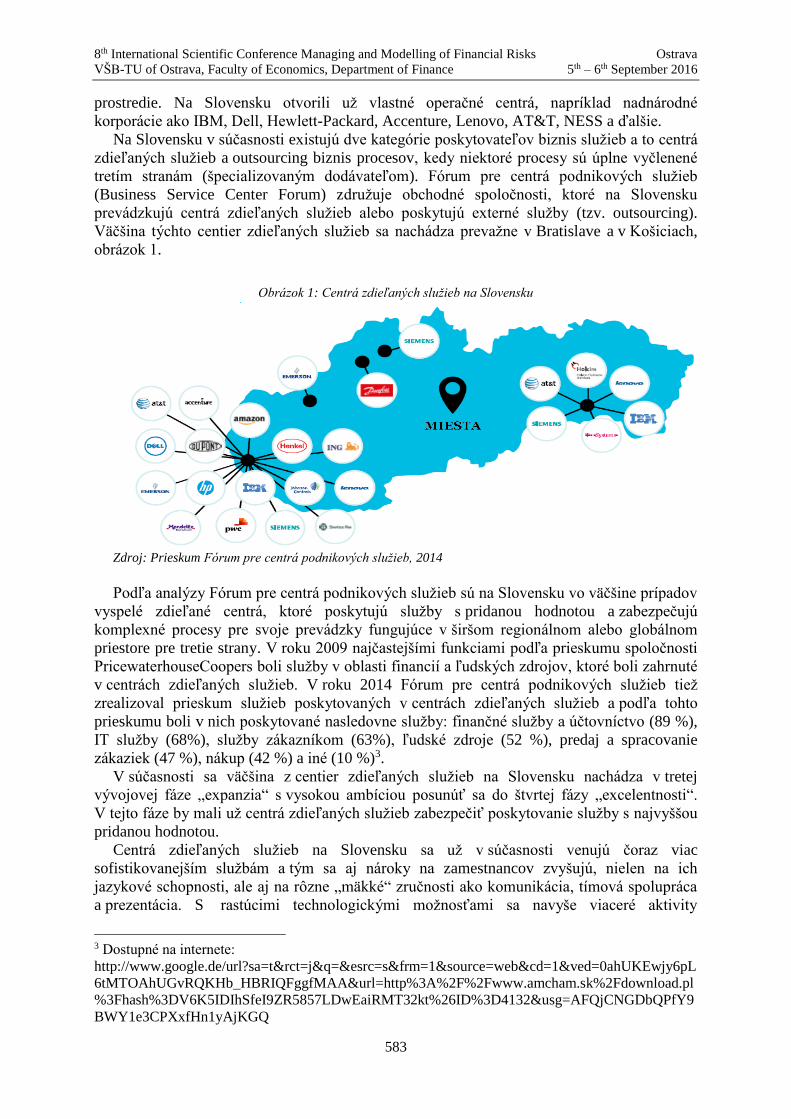
8th International Scientific Conference Managing and Modelling of Financial Risks Ostrava
VŠB-TU of Ostrava, Faculty of Economics, Department of Finance 5th – 6th September 2016
583
prostredie. Na Slovensku otvorili už vlastné operačné centrá, napríklad nadnárodné
korporácie ako IBM, Dell, Hewlett-Packard, Accenture, Lenovo, AT&T, NESS a ďalšie.
Na Slovensku v súčasnosti existujú dve kategórie poskytovateľov biznis služieb a to centrá
zdieľaných služieb a outsourcing biznis procesov, kedy niektoré procesy sú úplne vyčlenené
tretím stranám (špecializovaným dodávateľom). Fórum pre centrá podnikových služieb
(Business Service Center Forum) združuje obchodné spoločnosti, ktoré na Slovensku
prevádzkujú centrá zdieľaných služieb alebo poskytujú externé služby (tzv. outsourcing).
Väčšina týchto centier zdieľaných služieb sa nachádza prevažne v Bratislave a v Košiciach,
obrázok 1.
Obrázok 1: Centrá zdieľaných služieb na Slovensku
Zdroj: Prieskum Fórum pre centrá podnikových služieb, 2014
Podľa analýzy Fórum pre centrá podnikových služieb sú na Slovensku vo väčšine prípadov
vyspelé zdieľané centrá, ktoré poskytujú služby s pridanou hodnotou a zabezpečujú
komplexné procesy pre svoje prevádzky fungujúce v širšom regionálnom alebo globálnom
priestore pre tretie strany. V roku 2009 najčastejšími funkciami podľa prieskumu spoločnosti
PricewaterhouseCoopers boli služby v oblasti financií a ľudských zdrojov, ktoré boli zahrnuté
v centrách zdieľaných služieb. V roku 2014 Fórum pre centrá podnikových služieb tiež
zrealizoval prieskum služieb poskytovaných v centrách zdieľaných služieb a podľa tohto
prieskumu boli v nich poskytované nasledovne služby: finančné služby a účtovníctvo (89 %),
IT služby (68%), služby zákazníkom (63%), ľudské zdroje (52 %), predaj a spracovanie
zákaziek (47 %), nákup (42 %) a iné (10 %)3.
V súčasnosti sa väčšina z centier zdieľaných služieb na Slovensku nachádza v tretej
vývojovej fáze „expanzia“ s vysokou ambíciou posunúť sa do štvrtej fázy „excelentnosti“.
V tejto fáze by mali už centrá zdieľaných služieb zabezpečiť poskytovanie služby s najvyššou
pridanou hodnotou.
Centrá zdieľaných služieb na Slovensku sa už v súčasnosti venujú čoraz viac
sofistikovanejším službám a tým sa aj nároky na zamestnancov zvyšujú, nielen na ich
jazykové schopnosti, ale aj na rôzne „mäkké“ zručnosti ako komunikácia, tímová spolupráca
a prezentácia. S rastúcimi technologickými možnosťami sa navyše viaceré aktivity
3 Dostupné na internete:
http://www.google.de/url?sa=t&rct=j&q=&esrc=s&frm=1&source=web&cd=1&ved=0ahUKEwjy6pL
6tMTOAhUGvRQKHb_HBRIQFggfMAA&url=http%3A%2F%2Fwww.amcham.sk%2Fdownload.pl
%3Fhash%3DV6K5IDIhSfeI9ZR5857LDwEaiRMT32kt%26ID%3D4132&usg=AFQjCNGDbQPfY9
BWY1e3CPXxfHn1yAjKGQ

8th International Scientific Conference Managing and Modelling of Financial Risks Ostrava
VŠB-TU of Ostrava, Faculty of Economics, Department of Finance 5th – 6th September 2016
584
automatizujú a klesá podiel manuálnej práce aj v aktivitách vykonávaných v centre
zdieľaných služieb. Mnohé činnosti sú vykonávané pravidelne a rutinne, a preto sú súčasťou
tzv. automatizácie účtovníctva. Všetko dianie v obchodnej spoločnosti sa v konečnom
dôsledku premietne do účtovných operácií a transakcií. Skutočnosti zachytené v účtovných
prípadoch sú následne vykázané v účtovnej závierke, ktorou sa obchodná spoločnosť
prezentuje predovšetkým externému prostrediu (tzv. používateľom). Je preto nevyhnutné, aby
informácie boli užitočné, objektívne, spoľahlivé a podávali verný a pravdivý obraz o majetku,
záväzkoch a finančnej situácii obchodnej spoločnosti (Tumpach, Manová, Meluchová, 2014).
2. Účtovníctvo ako zdroj informácií
V dnešnom globalizovanom svete zohrávajú kvalitné informácie poskytnuté včas
najdôležitejší zdroj pre správne rozhodovanie a cieľavedomé riadenie obchodnej spoločnosti.
Kvalitné informácie sú v súčasnosti najväčším zdrojom bohatstva. Často môžeme počuť vetu:
„Informácie majú cenu zlata“. Účtovníctvo ako úplný a komplexný informačný systém je
jedným z aktívnych nástrojov finančného riadenia obchodnej spoločnosti. Účtovníctvo je
dôležitou súčasťou informačného systému spoločnosti a jeho primárnou úlohou je poskytovať
informácie pre plánovanie, rozhodovanie a kontrolu (Soukupová, 1994). Úlohou účtovníctva
v súčasnosti už nie je len poskytovať informácie o tom, že sa uskutočnila určitá transakcia,
prípadne aký bol jej dopad na finančnú situáciu a ekonomické výsledky obchodnej
spoločnosti ale aj pripraviť informácie, ktoré umožňujú vedeniu spoločnosti prijímať
rozhodnutia do budúcnosti a zároveň spätne posudzovať efektivitu, s akou sa tieto
rozhodnutia realizovali. Aby účtovníctvo mohlo spĺňať všetky požiadavky, ktoré sú na neho
kladené, je potrebné účtovný informačný systém správne nastaviť, „odladiť“ a prispôsobiť
potrebám konkrétnej spoločnosti tak, aby tieto údaje spĺňali potrebné kvalitatívne
charakteristiky (boli zrozumiteľné, relevantné, spoľahlivé, porovnateľné a boli poskytnuté
včas). Účtovníctvo tak poskytuje rôzne druhy výstupov vo forme číselných zostáv, analýz a
výkazov pre interné ako i externé potreby, ktoré sú určené širokému okruhu používateľov a
slúžia na rôzne účely. Pravdivosť informácií tvorí základ finančného účtovníctva (Meluchová,
Mateášová, 2015).
Pôsobením globalizácie dochádza k prehlbovaniu medzinárodných ekonomických vzťahov
a narastá význam ekonomických informácií. Súbežne s týmto vývojom rastie potreba
porovnateľnosti ekonomických informácií v podobe účtovných závierok. Účtovná závierka
ako najdôležitejší kvantifikovateľný výstup z účtovníctva predstavuje dôležitý účtovný
záznam, ktorý obsahuje cieľavedome usporiadaný súbor informácií o spoločnosti (účtovnej
jednotke) za účtovné obdobie, je zdrojom informácií na zistenie jej ekonomickej situácie a
finančného zdravia, v snahe zabezpečiť budúci rast. Účtovná závierka je aj základom pre
finančnú analýzu, ktorej cieľom je poskytnúť manažmentu podklady pre strategické
plánovanie a finančné riadenie. V definovaní cieľa účtovnej závierky sa spájajú funkcie dvoch
základných subjektov, ktoré sú na účtovnej závierke bezprostredne zainteresované a to
majiteľov (investorov) a manažmentu (výkonného a riadiaceho orgánu). Požiadavky
investorov sa sústreďujú na riziká spojené s ich súčasnou alebo budúcou investíciou do
obchodnej spoločnosti a na návratnosť vložených investícií. Investori od účtovnej závierky
očakávajú, že spĺňa kvalitatívne charakteristiky, tzn. obsahuje významné, spoľahlivé a úplné
informácie, ktoré sú pre ich rozhodovanie užitočné a tým poskytuje verný a pravdivý obraz
o danej spoločnosti. Povinnosťou manažmentu je zabezpečiť hlavný cieľ účtovnej závierky -
splnením základných predpokladov platných v účtovníctve a dodržaním všeobecne
uznávaných účtovných zásad. (Tumpach, Juhászová, Meluchová, 2013).
Na kvalitu informácií a v neposlednom rade aj na informácie prezentované v účtovnej
závierke majú, podľa nášho názoru, veľký vplyv tri základné elementy a to ľudia, nástroje

8th International Scientific Conference Managing and Modelling of Financial Risks Ostrava
VŠB-TU of Ostrava, Faculty of Economics, Department of Finance 5th – 6th September 2016
585
(ktoré zahŕňajú automatizáciu a softvér podniku) a procesy (tzn. zmeny, ktoré by mali
zredukovať variabilitu, zautomatizovať a zmodernizovať každú transakciu).
Zautomatizovaním procesov, rutinných úkonov vykonávaných v rámci účtovných operácií
dochádza k tomu, že sa jednotlivé úkony naprogramujú a tak sa vykonávajú s minimálnym
zásahom človeka (napríklad účtovníka). Mnohé spoločnosti prostredníctvom centier
zdieľaných služieb zoštandardizovali finančné procesy, zaviedli jednotnú definíciu
ukazovateľov, dát, reportov pre jednoznačnú interpretáciu výsledkov, jednotnú účtovú
osnovu, jednotný set systémov pre účtovníctvo, aby mohli spracovať obrovské množstvo
údajov a poskytovať kvalitné informácie a následne ich aj prezentovať v účtovnej závierke.
3. Prínosy a riziká oucourcingu finančných služieb
Centrá zdieľaných služieb poskytujú svoje činnosti najčastejšie zakladajúcej obchodnej
spoločnosti, ako aj ostatným entitám v rámci organizačnej štruktúry nadnárodnej korporácie.
Tieto služby sa zvyčajne poskytujú naprieč regiónmi ako Európa, Blízky východ a Afrika,
región Ázie a Pacifiku, Severná a Južná Amerika. Samotná štruktúra a organizácia
vykonávaných služieb a procesov závisí od potrieb materskej spoločnosti a požiadaviek trhu
v príslušnej krajine.
Ako to ale funguje v praxi? Pre príklad uveďme medzinárodnú obchodnú spoločnosť,
ktorá pôsobí v 10 štátoch sveta. V každom má svoju pobočku, kde okrem iného zamestnáva aj
ľudí zodpovedných za účtovníctvo. Niektoré pobočky sú také malé, že zamestnávajú
účtovníka len na polovičný úväzok, čo obchodnej spoločnosti môže spôsobovať nemalé
problémy so zastupiteľnosťou zamestnanca. Aj napriek tomu, že sa materská spoločnosť
snažila vytvoriť jednotné pravidlá vedenia účtovníctva pre všetky pobočky, každá pobočka si
ich mala prispôsobiť vzhľadom na lokálnu legislatívu. Takže sú pobočky, kde sa pravidlá
dodržiavajú. Ďalej sú pobočky, kde sa pravidla dodržiavajú len z časti, a naopak pobočky,
ktoré si zaviedli ešte prísnejšie opatrenia ako od nich žiadala materská spoločnosť. Čím
vzniká rôzne spektrum rizík z titulu dodržiavania globálnych verzus lokálnych pravidiel.
Ak sa obchodná spoločnosť rozhodne vytvoriť centrum zdieľaných služieb a teda zdieľať
účtovníctvo ako jeden z hlavných procesov, bude to znamenať, že sa vedenie účtovníctva pre
všetky pobočky centralizuje na jedno miesto do vybranej krajiny. Tento krok môže priniesť
obchodnej spoločnosti množstvo výhod ale aj množstvo nevýhod a to vo väzbe na
poskytovanie kvalitných informácií, ich včasnosť, dostupnosť, zrozumiteľnosť a úplnosť.
Centrá zdieľaných služieb garantujú, na základe tzv. SLA (Service Level Agreement),
poskytovanie služieb v požadovanej kvalite, rozsahu, ktoré vychádzajú z konkrétnych potrieb
a požiadaviek danej obchodnej spoločnosti. Na druhej strane sa obchodná spoločnosť môže
stretnúť aj s radom problémov a to hlavne v prípade, že SLA nie je v praxi implementované
dostatočne. Hlavnými dôvodmi je nedostatočné nastavenie kľúčových hodnôt (napr.
vytvorenie objednávky ku každej faktúre alebo včasné uhrádzanie faktúr), nedostatočné
definovanie procesov (napr. pravidelné čistenie salda zálohových platieb) a nedostatočné
zainteresovanie ľudských zdrojov (napr. nekvalifikovaná pracovná sila na určitej pracovnej
pozícii). Týmto sa zvyšuje niektoré z významných druhov podnikateľských rizík a to:
strategické riziko (napríklad neschopnosť flexibilne reagovať na požiadavky trhu,
vysoká konkurencia v danej oblasti podnikania, fúzie, akvizície),
operačné alebo prevádzkové riziko (napríklad kvalita služieb, informačné technológie,
zmena legislatívy, prírodné udalosti),
finančné riziko (napríklad likvidita, výnosnosť, úver, náklady) a
riziko nesúladu (napríklad rozdielna fiškálna politika, účtovná legislatíva). Výsledkom
rizika nesúladu môže byť finančná transakcia (vykonaná v akejkoľvek krajine, podľa

8th International Scientific Conference Managing and Modelling of Financial Risks Ostrava
VŠB-TU of Ostrava, Faculty of Economics, Department of Finance 5th – 6th September 2016
586
rovnakých pravidiel a rovnakým spôsobom), avšak nezohľadňujúca lokálne
legislatívne požiadavky, keďže sa spracováva štandardizovane.
Tieto riziká majú vplyv na kvalitu a porovnateľnosť prezentovaných informácií v účtovnej
závierke. Eliminovať a riadiť tieto riziká je zložitý proces, ktorý si vyžaduje kvalitné a včasné
informácie, prepracované metódy a techniky, pretože jednotlivé riziká spolu navzájom často
súvisia (Mokošová, Bednárová, Tkáčová, 2013).
Výhodu centier zdieľaných služieb je predovšetkým úspora personálnych nákladov
vrátane nákladov na pracovné miesto a nevyhnutných režijných nákladov. Znižovanie
nákladov sa považuje za najsignifikantnejšiu výhodu. Ďalšou výhodou je, že v centre
zdieľaných služieb sa jednoduchšie rieši problém zastupovania či tréningov zamestnancov.
Produktivita práce a špecializácia činností je v centre zdieľaných služieb vysoká, rovnako
flexibilnosť systému a automatický reporting je bežným štandardom. Nespornou výhodou je
aj jednotná celopodniková systémová platforma – rovnaký ERP systém a optimalizácia
procesov, ktoré sa dajú zabezpečiť s nižším počtom zamestnancov vo vopred zadefinovanej
štandardnej kvalite. Rozdelením procesu na menšie celky sa dá dosiahnuť vyššia
automatizácia, včasné spracovanie a eliminácia chýb ľudského faktora. Keďže je proces
centralizovaný, centrum zdieľaných služieb poskytuje rovnakú kvalitu dodávanej služby pre
všetky pobočky bez obmedzenia miesta výskytu. Ďalšou z výhod je aj jednoduchšia kontrola
a nastavenie samotného procesu. Vzhľadom na absenciu širšej zodpovednosti za celý proces
je možné v niektorých prípadoch zamestnávať aj menej kvalifikovanú pracovnú silu, ktorá je
stále schopná naučiť sa a obslúžiť svoj úzko definovaný rozsah práce (rutinná práca)
vzhľadom na štandardizované postupy a výstupy.
Na druhej strane, ako nedostatky využitia centra zdieľaných služieb, je možné
identifikovať znížené kvalifikačné požiadavky na pracovníkov nakoľko nie je potrebné, aby
pri spracovávaní účtovníctva ovládali účtovnú a daňovú problematiku, pretože iba rutinne
vyberajú položky z vopred nastaveného systému a databáz za použitia manuálu činností. Tým
sa zvyšuje predovšetkým riziko nesprávneho posúdenia daňových a nedaňových výdavkov čo
môže mať vplyv na zníženie kvality informácií prezentovaných v účtovnej závierke a v
daňovom priznaní. Znížené kvalifikačné požiadavky na zamestnanca - účtovníka sa môžu
negatívne prejaviť v neschopnosti flexibilne a kompetentne identifikovať a následne riešiť
neštandardné situácie, ktoré sa v každej obchodnej spoločnosti vyskytnú. Toto riziko môže
znamenať nemalé finančné straty, ak daný zamestnanec nevie situáciu správne vyhodnotiť a
riešiť vo všetkých vzájomných súvislostiach. Ďalšou nevýhodou je, že štandardizované
procesy boli citlivo definované so zreteľom na potreby globálnej korporácie. Štandardizácia
sama o sebe znamená zúženie priestoru pre flexibilitu a ad hoc požiadavky. Absencia
komplexných znalostí a zručností, ktorá je dôsledkom úzkej špecializácie, si žiada
kompenzáciu existenciou tzv. koordinátorov, ktorí majú širšie „end to end“ znalosti a dokážu
úspešne zodpovedať za kvalitu výstupu a spokojnosť širšej obchodnej spoločnosti. (Bódi,
2014). Od jednotlivých článkov pobočky aj mimo nej sa vyžaduje zvýšená disciplína
a presnosť pri dodávaní vstupov, nakoľko nepresnosti, či nekompletné vstupy, nemusia byť
správne rozpoznané a spracované a tým budú skreslené informácie prezentované účtovnej
závierke. V neposlednom rade viaceré procesy centralizované v centre zdieľaných služieb
majú interakciu s externým svetom, a preto je nevyhnutná aj komunikácia v inom ako
lokálnom jazyku, čím sa môže zvýšiť niektoré z uvedených podnikateľských rizík.
Záver
Súčasný vývoj a globalizačné tendencie v ekonomike a financiách majú za následok, že stúpa
miera rizík, ktoré ovplyvňujú vnútorné aj vonkajšie prostredie obchodnej spoločnosti. Určitá
miera rizík vzniká aj v centrách zdieľaných služieb, ktoré si zriaďujú najmä nadnárodné
8th International Scientific Conference Managing and Modelling of Financial Risks Ostrava
VŠB-TU of Ostrava, Faculty of Economics, Department of Finance 5th – 6th September 2016
587
korporácie. Ak sa nadnárodná korporácia rozhodne vytvoriť centrum zdieľaných služieb
a teda zdieľať účtovníctvo ako jeden z hlavných procesov, musí si uvedomiť, že tento krok
môže jej a jej pobočkám priniesť množstvo výhod ale aj množstvo nevýhod a to aj vo väzbe
na poskytovanie kvalitných informácií, ich včasnosť, dostupnosť, zrozumiteľnosť a úplnosť.
Národná korporácia a jej pobočky sa preto musí naučiť identifikovať a riadiť riziká, ktoré
majú vplyv na prosperitu a efektívnosť všetkých jeho činností. Nástrojom ako čeliť týmto
tendenciám je zavedenie účinného risk manažmentu, systému vnútornej kontroly, interného
auditu aby sa dosiahlo integrovaného riadenia podnikových rizík. Na to, aby táto stratégia
bola úspešná je potrebné mať vybudovaný kvalitný informačný systém entity, zavedené
kontrolné mechanizmy s využitím modernej IT technológie.
References
[1] Bódi Marián. (2014): Prínosy a úskalia centralizácie podporných činností vo firmách. In.
Finančný manažér. Ročník XIV. č.3. Periodikum Slovenskej asociácie podnikových
finančníkov. s. 10-14. ISSN 1335-5813.
[2] Meluchová, J., Mateášová, M. (2015): Účtovníctvo a účtovnícka profesia v 21. storočí.
In. AIESA – budovanie spoločnosti založenej na vedomostiach: zborník: 16.
medzinárodná vedecká konferencia: Bratislava, 5.-6. November, 2015, s. 285-291. ISBN
978-80-225-4151-0.
[3] Mokošová, D., Bednárová, B. Tkáčová, L. (2013). Impact of fair value adoption in
national and international frameworks for the business accounting and reporting. In
Financial management of firms and financial institutions: proceedings: 9th international
scientific conference. VŠB. Ostrava. PTS I-III Book Series: Pages: 589-596.
[4] Ondrušová, L., Parajka, B. (2014). The revaluation of assets and liabilities at fair value in
merger. 7th International Scientific Conference on Managing and Modelling of Financial
Risks Location: VŠB. Ostrava. SEP 08-09, 2014. PTS I-III Pages Series: 577-581.
[5] SOUKUPOVÁ, B. (1994). Účtovníctvo. Bratislava: SOFA. 156 s. ISBN 80-85752-14-X.
[6] Tumpach, M., Manová, E., Meluchová, J. (2014). Relevance of System of National
Financial Reporting from the Point of View of Creditors as Non-privileged
Users. EKONOMICKÝ ČASOPIS, Volume: 62. Issue: 5. Page: 495-507.
[7] Tumpach, M., Juhászová, Z., Meluchová, J. (2013). Is there any relevance of business-
related financial reporting in Slovakia. 9th International Scientific Conference on
Financial Management of Firms and Financial Institutions Location: VSB TU Ostrava,
FacEcon, Finance Dept, Ostrava, SEP 09-10, 2013. PTS I-III Book Series. Page: 987-
994.
[8] PwC: http://www.etrend.sk/trend-archiv/rok-2016/cislo-16/slovenske-servisne-centra-su-
na-ceste-do-prvej-ligy.html
[9] Fórum pre centrá podnikových služieb:
http://www.google.de/url?sa=t&rct=j&q=&esrc=s&frm=1&source=web&cd=1&ved=0a
hUKEwjy6pL6tMTOAhUGvRQKHb_HBRIQFggfMAA&url=http%3A%2F%2Fwww.a
mcham.sk%2Fdownload.pl%3Fhash%3DV6K5IDIhSfeI9ZR5857LDwEaiRMT32kt%26
ID%3D4132&usg=AFQjCNGDbQPfY9BWY1e3CPXxfHn1yAjKGQ

8th International Scientific Conference Managing and Modelling of Financial Risks Ostrava
VŠB-TU of Ostrava, Faculty of Economics, Department of Finance 5th – 6th September 2016
588
Intergeneration Comparison of the Perception of Communication Media in the Context of the Nature
of their Ownership
Lucja Matusiková 1
Abstract
Media are an integral part of the life of every society. The nature of their ownership, i.e. their
public or private character, may be an important factor when perceiving individual media. The
author’s objective is to ascertain the respondents’ general opinion of the media, above all, in
the area of their credibility. Subsequently, these research activities were focused on the fact
whether the mentioned character of the medium ownership in respondents has the impact on its
perceiving, whether this perception is also influenced by the age or the gender division. The
research was primarily focused on the so-called Generation Y and Generation Z. The Chi-
square test of independence served to confirm or reject the established hypotheses. Social
media were not included in the currently conducted research, so that we could compare the
research projects carried out with the benefit of hindsight.)
Key words
Mass Media, Public, Private, Gender, Generation Y, Generation Z
JEL Classification: D70, J16, M30
1. Definition of Basic Terms
Marketing communication is carried out via a lot of channels. Media are one of the
possibilities how to address potential customers. The effect of advertising impulses of
broadcast media, i.e. communication media, depends on a lot of factors. They include for
example their credibility. And right the media credibility in the context of their ownership
character became the essential research artefact. With respect to the fact that a clear
specification of private and public media may be implemented only in the case of television
and radio media, the results of the research activities will be intended right and only for them.
For the purposes of a correct interpretation of achieved results, we need to approach at least
in basic dimensions the main notions that we will subsequently work with. Only the facts that
are essential and more closely specifying or explaining individual concepts will be included.
1.1 Media
The Dictionary of Foreign Words (Collective of Authors, 1996, p. 214) defines the notion
Medium as “a mediation agent, environment, also as person arranging spiritistic information
and, last but not least, as mass (collective) media printed (newspapers, magazines) as well as
electronic (radio, television), mass medium”.
The word medium is similarly characterised also by other authors (Jirák, Köpplová, 2003,
p. 16), who state that “it is of the Latin origin and means a mediator, intermediating agent, that 1 Lucja Matusiková, Ing., Ph.D., VŠB – TU Ostrava, Faculty of Economics, Department of
Management, [email protected].
This paper was supported within Operational Programme Education for Competitiveness – Project
No. CZ.1.07/2.3.00/20.0296.
8th International Scientific Conference Managing and Modelling of Financial Risks Ostrava
VŠB-TU of Ostrava, Faculty of Economics, Department of Finance 5th – 6th September 2016
589
is anything that mediates, arranges something”. Subsequently, the authors develop this idea
with the fact that “the branches that deal with different manifestations of interpersonal, social
communication mark the notion medium/media as something that mediates some information
for somebody that is the communication medium”.
An analogical characteristic may be also found with other authors (Reifová, 2004, p. 139)
with that in this version the medium “does not have exactly and generally accepted borders”.
The medium is presented here as a direct individual means of communication as well as as
labelling a technical means of communication. On the one hand, we encounter such
characteristics as facial expressions, gestures or speech and, on the other hand, the computer
network, cable television, etc. (Urban, Dubský, Murdza, 2011).
The notion mass media, whose content is more specific, forms a separate chapter. “Mass
media mean means of communication and institutions that are able to produce in the large
scale public notification and distribute it towards the scattered, varied and individually
unidentified public.” (Urban, Dubský, Murdza, 2011, p. 48)
Communication media, in our case the mass media, may be divided according to a number
of viewpoints. Cold and hot, or classical, printed which is used in the Anglo-Saxon literature,
and electronic ones are the most frequent type of classification. The ownership viewpoint that
is the classification as public media and private media is another viewpoint. And right the
nature of the ownership or its impact on perceiving credibility of the respective medium by the
addressed group of respondents will be our focus.
1.2 Public and Private Media
In the Czech Republic, following the European model, at the beginning of the 1990s, the
so-called dual system of television and radio broadcasting was elected, that is the co-existence
of the public and private sectors. Concurrently, the rights and obligations of the radio and
television broadcasting operators, licence procedures and registration of the operators of the
taken-over broadcasting were determined. This state is regulated by Act No. 231/2001 Coll.,
on Operating Radio and Television Broadcasting, as amended.
Yet, talking about public broadcasting, we mean the Czech Television Company and the
Czech Radio Company. These institutions operate on the media market on the basis of
separate laws. It is Act No. 483/1991 Coll., on the Czech Television Company and Act No.
484/1991 Coll., on the Czech Radio Company, always as amended. The public character of
financing these institutions is implemented by Act No. 348/2005 Coll., on Radio and
Television Charges, as amended
“The Czech Television Company and the Czech Radio Company are broadcasting
operators by law with specific tasks of the public service. Both the operators are independent
of the state, they do not receive any state subsidies and their activity is financed by the income
from radio and television charges and the income from their own business activity (above all,
it is the sales of advertising time as well as the revenues from copyrights, leases of equipment,
etc.)” (The Ministry of Culture, 2012, [online]). The Czech Television Company and the
Czech Radio Company fulfil their service for the public via own production and co-
production and also by television and radio broadcasting and other services. Regarding the
question of funding the Czech Television Company and the Czech Radio Company, the idea
of financial security via the state budget was originally discussed. Yet, this idea was
abandoned in connection with a threat of weakening the independence of the relevant medium
of the state (Jirák, Köpplová, 2003).
Private broadcasting is ensured by a number of entities, which were established on the
basis of the commercial law as joint-stock companies, limited liabilities companies, etc. In
their case it is a classical form of a business activity operated to achieve a profit. Under the

8th International Scientific Conference Managing and Modelling of Financial Risks Ostrava
VŠB-TU of Ostrava, Faculty of Economics, Department of Finance 5th – 6th September 2016
590
obtained licences or registrations, they operate nationally or only regionally. The records of
these operators are kept by the Council for Radio and Television Broadcasting, which issues
licences and registration certificates.
1.3 Generation
According to the Dictionary of Foreign Words, the notion “generation” (Collective of
Authors, 1996, p. 117) has a number of meanings. The generation is characterised first, that is
a set of people born and living approximately at the same time. A generation sometimes
means descendants of one pair of parents. The third semantic unit makes it possible to identify
a generation as a specific set of concurrently living individuals of the same kind. A generation
also means a membership of the type of technical equipment of a certain development stage.
From the viewpoint of perceiving communication media, we undoubtedly need to identify
basic grounds that have had the impact on this age group of inhabitants, above all, from the
sociological viewpoint. According to the Australian study of the labour market from 2007
(Bohutinská, 2008, [online]), currently, we may specify the following generationally
differentiated groups of population:
Born before 1946 = Pre Boomers
Born from 1947 to1960 = Baby Boomers
Born from 1961 to1975 = Generation X
Born between 1976 and 1990 = Generation Y
Born between 1995 and 2020 = Generation Z
For the purposes of presenting the results of the present research, only two generation
cohorts are specified in detail that is Generation Y and Generation Z.
The Australian study mentioned above (Bohutinská, 2008, [online]) states for the
Generation Y a decisive range of birth is between 1976-1990. According to the study of
Deloittte ČR (Portal „www.kariera.ihned.cz“, 2007, [online]), these include individuals born
between 1982-1993. And other specialists in other sectors are not of the same opinion as
regards the determination of the exact range, because overlapping of generation layers is very
intensive in this group and it depends on a number of aspects, chiefly on the specific
characteristics of individuals.
As far as information technologies are concerned, they are light years ahead of their senior
fellow workers. They are not afraid to study multiple universities at the same time; in
particular, if they are not sure what they would like to do in their life. They are not particularly
against formalised methods of education; they simply need to combine them with gaining
experience and verification of theoretical findings in practice. For them, a change is a life
credo, not an obstacle, because in their life they do not need security. Work with one company
for the entire life like their parents is a nonsensical idea. In their decisions, they are practically
or even pragmatically concentrated. They focus on the price by which they trade off the
quality. They do not tend to forsake the family nest, since they enjoy their parents’ service.
Those born between 1991-2005 are marked as Generation Z. As the Grail Research study
states (Grail Research, [online]), the GZ representatives include young people whose date of
birth is usually determined by the middle 1990s and year 2010, whereas it should be noted that
different studies e.g. Howe, Strauss (1991) freely work with this time factor, when they
include the GZ into the period from 2000 to the present time.
With respect to the method of communication (they are constantly on-line via their mobile
phones, they share a lot of information via You Tube etc.) and the ability of both the intensive
and extensive use of the state-of-the-art technologies, they are also called the so-called
“Digital Natives”. Their relation to technologies may be even characterised as a certain form

8th International Scientific Conference Managing and Modelling of Financial Risks Ostrava
VŠB-TU of Ostrava, Faculty of Economics, Department of Finance 5th – 6th September 2016
591
of addiction. They seek more and more sophisticated devices and appreciate particularly their
simple and interactive design. In spite of their currently low age in most cases, they appear to
be socially more responsible than their predecessors. Owing to the sufficient amount of
available information, far more intensively they are aware of the current problems, such as
terrorism or climate changes.
If we summarise all the mentioned above, we may observe that the GZ is constantly on-line
via a number of social networks and their decision-making processes are in many areas
influenced by the ability to obtain information across the countries, cultures as well as
religions.
2. Concept of the Research, Determination of Objectives and
Hypotheses
At the Economic Faculty of VŠB – Technical University of Ostrava, a number of research
activities are being continuously conducted within a wide spectrum of majors and also across
these majors. The research activities are part of the centrally organised research projects of the
universities and individual faculties as well as the lecturers’ individual activities. One of them
is the research which results are presented here.
The research set not only one but several objectives. They particularly concerned the efforts
to:
• ascertain how often the respondents follow the surrounding events in media;
• determine whether the respondents prefer a certain type of media and which type;
• determine whether the nature of the ownership is a factor that has impact on media
credibility.
For the purposes of the research to preserve unambiguousness of terms, two types of media
were used, namely radio and television. There we could compare the impact of the ownership
on the medium perception. Therefore, ČT1, ČT2 and ČT24 television stations represent public
media. Concerning radio stations, they are Radiožurnál, Praha and Vltava. All remaining
television and radio stations are private. In their responses, the respondents were also offered a
possibility to supplement additional radio and television stations that they follow. Such media
as the internet, social networks and others were disregarded.
In this connection the following hypotheses were determined:
H0 In general, there is not dependence between the generation structure of the respondents and
their responses.
H1 The respondents’ generation structure has impact on their responses.
From the methodological viewpoint, it was preceded from theory to practice, from general
to specific. Retrospectively, the knowledge obtained in the primary and secondary research is
applied in the theoretical grounds. During the research and evaluation activities, the methods
of analysis, synthesis, induction, deduction and comparison were also used. The Chi-square
test of independence in the contingency table will be used to confirm or reject the established
hypotheses. The test was carried out in MS Excel via the statistical function CHITEST.
Yet, the original intention to carry out the project via the method of random sampling (the
quota selection for the purposes of ensuring objectiveness) could not be implemented. Since
the pilot project of the research showed that as far as media are concerned, the potential
respondents are either too open and they are not willing to answer questions but on the
contrary they raise questions themselves on the assumption that they will receive a satisfactory
answer to them, or they will only wave it off with resignation and reject to continue in
cooperation. In such a case, we needed to be satisfied with a much smaller sample and also
with a sample of respondents that really wanted to answer the questions. Eventually, we

8th International Scientific Conference Managing and Modelling of Financial Risks Ostrava
VŠB-TU of Ostrava, Faculty of Economics, Department of Finance 5th – 6th September 2016
592
conducted the research by a questionnaire enquiry. This way, we managed to receive 120
questionnaires. After checking their completeness, we used 107 for further processing. The
research was carried out in the streets of the city of Ostrava during February and March 2016.
We utilised the results of the research activities from 2013 Matusiková (2014) to compare
them with the GY representatives as a whole.
3. Perception of the Communication Medium in the Context of the
Nature of its Ownership in Practice
The questionnaires were completed by the respondents via standardised anonymous face-
to-face dialogues with the respondents in public. After the experience from the pilot part of
the project, the enquirers were instructed to address the individuals, when the willingness to
answer and the year of birth (1995 and more) were the decisive criteria for addressing
respondents. The completed questionnaires were subjected to the optic inspection;
subsequently they were rewritten into the data matrices in MS Excel and processed with the
use of MS Excel.
3.1 Target Group Identification
A total of 107 completed questionnaires from amongst the GZ representatives were
received. The numerical representation of the enquired within genders in the form of the
absolute value (hereinafter only A) and the percentage value (hereinafter only %) is shown in
Table No. 1.
Table 1: Division of Respondents according to Gender (Source: Author)
In spite of the fact that due to a low number in individual categories the educational factor
was not taken into account as an identification element, Table No. 2 shows the structure of the
respondents’ education. The structure of the respondents is undoubtedly affected by the time
when the project was implemented. In the morning, more university students may be seen in
the city centre when compared to secondary school students or apprentices or primary school
pupils.
Table 2: Respondents Distribution by Education (Source: Author)
Education Male Female Total
A %
Basic 2 2 4 4
Secondary vocational without school-leaving exam 3 3 3
Complete secondary with school-leaving exam 46 54 100 93
The residence or the region in which the respondents live became the third identification
factor. Also several respondents from Slovakia were included into this category. The results
are shown in Table No. 3.
Age Male Female
15-20 (GZ) 48 59
Total A 107
% 45 55

8th International Scientific Conference Managing and Modelling of Financial Risks Ostrava
VŠB-TU of Ostrava, Faculty of Economics, Department of Finance 5th – 6th September 2016
593
Table 3: Respondents Distribution by Education (Source: Author)
Residence – Region Male Female Total
A %
Ostrava 35 35 70 65
Olomouc 3 6 9 8
Brno 1 2 3 3
Pardubice 2 2 2
Hradec Králové 1 2 3 3
Zlín 1 8 9 8
Slovakia 7 4 11 10
Also the respondents’ structure from the viewpoint of their residence reflects to a large
extent the structure of the inhabitants or visitors of the city of Ostrava. We compared the
results of the current GZ sample with the GY sample, which was researched and analysed in
2013.
3.2 esults of GZ Questionnaire Enquiry by Age Structure of GZ and GY Samples
To the questionnaire enquiry included two age categories. The age groups marked as the
GY (year of birth 1976–1990) and the GZ (year of birth 1995–2015). In both analysed
generations, the women prevailed among the enquired, which might influence the evaluation
of the individual sets of respondents to a certain extent.
When analysing the intensity of following surrounding events in media, we could observe
that while in the GY with a decrease of the intensity of ratings also the numbers of the
respondents dramatically decreased, in the GZ, it was not definitely that way. As mentioned
above, in the GZ, the respondents occurred that do not follow surrounding events at all. The
conducted CHITEST with the P-value of 7.7 % did not prove, although only by 2.7%,
dependence of respondents’ replies on their age. Other results are shown in Table No. 4.
Table 4: Intensity of following media (Source: Author)
Intensity of following media GY GZ
A % A %
Daily 39 58 46 43
Several times a week 21 31 29 27
From time to time 7 11 26 24
I do not follow -
6 6
P-value 0.0774 7.7
If we analyse media confidence of the enquired sample, we may notice that whereas in the
GY confidence prevails, although only minimally, in the GZ, no-confidence has the value of
almost 60% and it prevails over confidence by the full 30%. Simultaneously, we have
identified a relatively high percentage of those enquired that are not able to decide. The results
in absolute terms as well as in percentage are shown in Table No. 5. Regarding the statistical
verification, we may observe that the responses of the enquired were at the level that shows
independence of the analysed variables, which was again proved by the CHITEST, whose
value was 8.5%.

8th International Scientific Conference Managing and Modelling of Financial Risks Ostrava
VŠB-TU of Ostrava, Faculty of Economics, Department of Finance 5th – 6th September 2016
594
Table 5: Confidence in New (Source: Author)
Confidence in New GY GZ
A % A %
Yes 29 43.3 28 26
No 27 40.3 60 56
I do not know 11 16.4 19 18
P-value 0.08509 8.5
In the question focused on following individual television stations, there was a special
agreement, namely in the first and last place. The private NOVA television station was the
first for both the cohorts, while the private station BARRANDOV was similarly for both the
cohorts last. The stations that were mentioned as “Different” by the GY included
predominantly sports channels and the stations focused on cooking, the GZ stated
predominantly music, film and adventurous stations (HBO, MTV, Očko, Discovery etc.).
Regional broadcasting and Slovak stations were also commonplace not only in the Slovak
respondents. The CHITEST with the P-value at the level of 99.6% did not confirm estimated
dependence of the stated responses on respondents’ age.
In the case of the order of the television station during following news, an exceptional
agreement occurred right in the first four places. NOVA won, followed by ČT1. The place of
the purely news public-law station, ČT24, is interesting, which overtook the private station
Prima usually stated in this place. Neither in this case, was the estimated dependence of
responses on respondents’ age confirmed, the statistical test had the value of 98%.
Like as in the case of the general ratings of TV stations, radio broadcasting showed the
agreement if it concerns the most and the least followed stations. Evropa 2 became the
number one among radios, stations Praha or Vltava finished up at the end of the listening
field, which was assumable owing to the composition and programme structure. The
agreement occurred also in the 6th and 7th place, which were taken by Čas and Radiožurnál
stations. Other orders were homogeneously jumbled. The CHITEST did not prove the
estimated dependence of replies on respondents’ age.
When analysing the ratings of the news on radios, we could notice even larger
fragmentation, when, apart from the unequivocally last place of the Vltava station in both the
cohorts, we could not find any agreement. Here we may say that in spite of the respondents’
small age difference in many cases, their spectrum of opinions is relatively different. Also in
this case the conducted test of independence did not prove dependence of age on the
respondents’ replies. The specific order and the CITEST results are shown in Table No. 6.
Table : Ratings of News on Radio Stations (Source: Author)
Ratings of News on Radio Stations
Ra
dio
žurn
ál
Pra
ha
Vlt
av
a
Fre
kv
ence
1
Imp
uls
Ev
rop
a 2
Ča
s
Ori
on
Kis
s
Hel
ax
Do
es n
ot
foll
ow
!
GY 5 8 9 1 2 3 6 2 7 4 4
GZ 8 9 9 5 3 1 7 4 2 6
P-value 0.8974 89.7%
8th International Scientific Conference Managing and Modelling of Financial Risks Ostrava
VŠB-TU of Ostrava, Faculty of Economics, Department of Finance 5th – 6th September 2016
595
The following results concern confidence in followed news and the impact of the nature of
a presented medium ownership on credibility. The data is interesting, above all, in the context
of the representation of the individual types of ownerships (public-law versus private stations)
among the offered variants.
More than 60% enquired of the GY, but only 36% GZ have confidence in news in general.
The case of the GY, this value also corresponds with another value, namely that the nature of
the medium ownership does not have impact of such credibility. In the case of the GZ, the
value of the mentioned parameter reached the value of almost 50%. It is obvious that the
nature of the medium ownership in the GZ is not considered only by those who have
confidence in it, but also by those who lack such confidence. Like in the the case of
confidence, also in the case of the impact by the medium ownership structure, there is
considerable manoeuvring space for those who did not decide, when the dispersion of both
confidence and ownership ranges from 9 to 28%.
There may be a lot of reasons for no confidence in media irrespective of their ownership
structure. Firstly, dissatisfaction or no confidence in some individual persons (editors,
journalists, etc.), overload, tiredness with the excess, in many cases, unmeaning information.
In the case of the GZ, certainly it is also the availability of opponent opinions via social
networks across the international structure.
The conducted test of independence via the CHITEST function did not prove dependence
of the respondents’ replies on their age.
4. Conclusion
In order to ensure a suitable way of communication with the client, by all means we need to
utilise the most reliable communication medium. The ability of the medium to obtain
credibility and maintain it may be characterised as a significant competitive factor.
If we compare the total results of the GZ and GY, then we receive the ratings ratio of both
the cohorts 70:89. A more distinct difference may be seen in the case of less frequent
following the surrounding events in media. The ratio is 30:11. In none of the cases the
hypothesis of dependence of respondents’ replies on respondents’ age was confirmed.
Generally comparing both the generations, we may say that whereas the GY is balanced in
its responses regarding media credibility, the GZ clearly speaks against the mentioned
confidence in the ratio 26:56.
When analysing the ratings of individual TV stations and related news at these stations we
may observe that both the GZ and GY will agree on the first and the last place of the ratings.
An exceptional agreement occurred in the order of the ratings of news at these stations, which
was in fact identical for both the generations. The agreement across the generations was also
at the general ratings of radio stations in the form of the first place. Yet, there was no
agreement in following the news.
The major areas of the research included news credibility in the followed medium and the
impact of its ownership structure (private versus public) on such credibility.
We may ascertain that the GZ, in general, has far less confidence in the analysed news, it is
only 36% of respondents, whereas the same percentage denies credibility. The GY is here
much more unequivocal, as more than 60% respondents consider the followed news as
credible. In the intergeneration comparison, this question did not confirm dependence on age
only by 2%
So what is the impact of the media ownership structure on their credibility? Between the
generations, the effect of the owner was more distinct in the GZ when compared to the GY,
8th International Scientific Conference Managing and Modelling of Financial Risks Ostrava
VŠB-TU of Ostrava, Faculty of Economics, Department of Finance 5th – 6th September 2016
596
providing that in the GY even more than 60% of the respondents declined such effect
completely.
Of course, the conducted research has its limitations. It would be ideal to have a chance to
collect the sample according to the quota selection, but, as mentioned earlier, respondents’
willingness to cooperate decreases from year to year. In addition, there is a problem with a
regional focus. Yet, for comparison it is positive that all the author’s research activities have a
regional focus and, therefore, the data may be compared even if there is a certain time between
the research projects. If we wanted to compare the research results with the similar results, we
would get into a difficult situation. For comparison, the categories that may be compared need
to be determined and it is also purposeful. And at this point we could identify a principal
problem. The present research focused on two specific generations, namely the GY and the
GZ. Above all, the GY was recently subjected to a number of research projects in the area of
perception of communication media and social networks. To name some of the recent
projects, there was research focused on the impact of Facebook advertising on GY
representatives’ purchasing behaviour in South Africa (Duffet, 2015) or on GY purchasing
behaviour in the area of luxury fashion, awareness of their brands and buying motivations
(Giovannini, Xu, Thomas, 2015), earlier for example the research focused on GY opinions in
the area of enterprise social applications (Boughzala, 2014) and many others. Social networks,
their impact on decision-making in the area of education, purchasing behaviour and
employment became the alpha and omega of these research projects. None of them deals with
traditional information channels (TV and radio).
Above all, marketing companies (Grail Research a Division of Integreon, 2011) show an
eminent interest in the GZ. For the time being, the Generation Z is at the very beginning of
consumer-study-professional activities. If we take into account that today the oldest one is 20
years old and the youngest one, according to the statistics (Czech Statistical Institute, 2015), is
being born, then we have something to do with more than a two-million consumer potential in
the Czech Republic. The scale of this cohort is unpredictable now and the information about it
should be collected continuously and, above all, across the whole spectrum. In the future, we
may be surprised not only by the scope, but particularly by the depth of enquired services
ordered without the need of personal contact. Finally, it may have a principal effect on the
employment and performance of economies.
The foregoing indicates that the traditional forms of communication transmission that is
radio and television have got to the side-lines of research activities. However, their influence
does not fall, despite the presence of Facebook, Instagram and any other less or more
specialized servers of the social networks do not fall; even though the communication via
social media is by its nature a complex concept (Ungerman, Myslivcová, 2014).
Continuously, their activities get connected and their results may be observed day in day
out. Owing to social networks, the overview of the medium ownership structure is vanishing,
it is very difficult to identify the real sources of information and attribute them someone’s
authorship. In the end, quite often we cannot say whether it is expert and relevant information
of the public medium or an advertising message of private investors.
The last events both in Europe and the world show that media are a very significant, strong
and never-ending source for investigating their impact on the society. They are also a
noticeable way of addressing not only potential clients via marketing communication in the
form of advertising spots but, presently, this is mainly the information of a safety character, on
which basis a significant part of our life decision-making processes are made in the area of
employment, portfolio of purchases, travelling, etc. It remains on us, our society, to whom and
how large credibility we will attach to them, which is the substance of the present media
events. “Like the society – like the media!”

8th International Scientific Conference Managing and Modelling of Financial Risks Ostrava
VŠB-TU of Ostrava, Faculty of Economics, Department of Finance 5th – 6th September 2016
597
References
[1] BOHUTÍNSKÁ, J. Generace Y – nový pojem také u podnikatelů. [online], 2008, [cit.
2009-08-20]. Dostupné z.: <http://www.podnikatel.cz/clanky/generace-y-novy-pojem-
take-u-podnikatelu/>.
[2] BOUGHZALA, I. You: What Generation Y thinks about Corporate Social Networking
Applications? Proceedings of the Annual Hawaii International Conference on System
Sciences. New York: IEEE, 2014, p. 688 – 696. ISBN 978-1-4799-2504-9.
[3] BURTON, G.; JIRÁK, J. Úvod do studia médií. Brno: Barrister & Principal, 2001, 392
s. ISBN 80-85947-67-6.
[4] DUFFET, R. G. The influence of Facebook advertising on cognitive attitudes amid
Generation Y. Elecronic Commerce Research. Volume:15. Issue: 2, p. 243-267.
Dordrecht: Springer, 2015. ISSN 1389-5753.
[5] Generace Y mění tvář výrobní sféry. [online], 2007, [cit.2009-08-20]. Dostupné z:
<http://kariera.ihned.cz/c4-10115350-22067010-q06000_d-generace-y-meni-tvar-
vyrobni-sfery.
[6] GIOVANNINI, S.; XU, Y.J.; THOMAS, J. Luxury fashion consumption and
Generation Y consumers Self, brand consciousness, and consumption motivations.
Journal of Fashion Marketing and Management. Volume: 19. Issue: 1, p. 22 – 40.
Yorkshire: EMERALD GROUP PUBLISHING LIMITED, 2015. ISSN 1361-2026.
[7] Grail Research a Division of Integreon. Consumers of Tomorrouw. Insights and
Observations About Generation Z. [online], November, 2011, [vid. 20.5.2015].
Dostupné z: http://www.slideshare.net/baurzhan/consumers-of-tomorrow-insights-and-
observations-about-generation-z-15753651.
[8] JIRÁK, J; KÖPPLOVÁ, B. Média a společnost. Praha: Portál, 2003, 208 s. ISBN 80-
7178-697-7.
[9] KOLEKTIV AUTORŮ A KONZULTANTŮ. Slovník cizích slov: Praha:
Encyklopedický dům, spol. s r. o., 1998, 117s. ISBN 80-90-1647-8-1.
[10] MIKUŠOVÁ, M., HORVÁTHOVÁ, P. The Research Approaches On Crisis And Its
Management. Proceedings of World Academy of Science, Engineering and Technology.
Volume 73, January 2011, p. 610-618. ISSN: 2010376X
[11] PLAŠKOVÁ, A.; NEJEDLO, T.; HYKŠ, O.; RYŠÁNEK, P. Společenská odpovědnost
firem (CSR). Aplikace a hodnocení. Podnikatelský sektor. Praha: NISPK, 2009, s. 116.
ISBN 978-80-02-02205-3.
[12] PLAŠKOVÁ, A.; NEJEDLO, T.; HYKŠ, O.; RYŠÁNEK, P. Společenská odpovědnost
firem (CSR). Aplikace a hodnocení. Veřejný sektor. Praha: NISPK, 2009, s. 119. ISBN
978-80-02-02206-0.
[13] REIFOVÁ, I. Slovník mediální komunikace. Praha: Portál, 2004, 328 s. ISBN 80-7178-
926-7.
[14] URBAN, l.; DUBSKÝ, J.; MURDZA, K. Masová komunikace a veřejné mínění. Praha:
Grada Pubishing, 2011, 240 s. ISBN 978-80-247-3563-4.
[15] UNGERMAN, O.; MYSLIVCOVÁ, S. Model of communication usable for small and
medium-sized companies for the consumer communication in social media. E+M, rok
2014, ročník 17, str 167 – 184 dx.doi.org/10.15240/tul/001/2014-1-013
[16] TURČÍNKOVÁ, Z. Méně než polovina žen pracujících ve vedoucích pozicích se cítí
být připravena uspět v globálním podnikatelském prostředí. [online], 2008, [cit. 2009-
08-15]. Dostupné z:
<http://www.accenture.com/Countries/Czech_Republic/About_Accenture/MeneProstre
di.htm>

8th International Scientific Conference Managing and Modelling of Financial Risks Ostrava
VŠB-TU of Ostrava, Faculty of Economics, Department of Finance 5th – 6th September 2016
598
[17] Veřejnoprávní vysílání [online]. Praha: Ministerstvo kultury, 2012, [cit. 2012-01-15].
Dostupné z: <http://www.mkcr.cz/cz/media-a-audiovize/rozhlasove-a-televizni-
vysilani/verejnopravni-vysilani-81273/>
[18] Zákon č. 231 /2001 Sb., o provozování rozhlasového a televizního vysílání, ve znění
pozdějších předpisů.
[19] Zákon č. 483/1991 Sb., o České televizi, ve znění pozdějších předpisů.
[20] Zákon č. 484/1991 Sb., o Českém rozhlase, ve znění pozdějších předpisů.
[21] Zákon č. 348/2005 Sb., o rozhlasových a televizních poplatcích, ve znění pozdějších
předpisů.

8th International Scientific Conference Managing and Modelling of Financial Risks Ostrava
VŠB-TU of Ostrava, Faculty of Economics, Department of Finance 5th – 6th September 2016
599
Elimination of the risk and its impact on the reliability of the information presented in financial
reporting
Jitka Meluchová 1
Abstract
The globalization brings positives and negatives. Positives need to be used effectively and
efficiently eliminate the negatives. The process of globalization can't be stopped. Current
developments and globalization trends in the economy and finance have the effect of increasing
the level of risk that affect the internal and external environment of each entity. That's especially
true for the financial market and the insurance market. In order to be competitive insurance
company must establish an effective risk management system to ensure its financial stability
and capital adequacy in line with European rules. The instrument to eliminate the risks arising
from its activities is the creation implementation of effective risk management, internal control
system and internal audit. For this strategy to be successful it is necessary to have quality the
data base and have in place effective controls using IT technologies. The aim of this paper is to
examine the process with a focus on the reliability of the information presented on the risks
within the external reporting.
Key words
Globalization, risk management, insurance company, internal control system, internal audit
JEL Classification: M48, G15, G17
Risk manažment v poisťovni
Poisťovne pri posudzovaní rizík, ktoré preberajú od klientov využívajú najnovšie poznatky
z teórie manažmentu rizík a majú vypracované vlastné systémy, stratégie a modely na
riadenie rizík. Cieľom je vytvoriť rovnováhu medzi rizikami, návratnosťou z investícií
a vlastným imaním poisťovne. Poisťovňa by musela použiť vlastné zdroje v prípade, ak by
nemala vytvorené dostatočné cudzie zdroje (technické rezervy) na výplatu záväzkov z
poistenia. To je dôvod prečo sú na poisťovne kladené požiadavky, aby podrobne informovali
o riadení poistného a finančného rizika tak, aby používatelia týchto informácií pochopili
dopady týchto rizík na hodnotu aktív (investícií), záväzkov a vlastného imania. Cieľom risk
manažmentu je ochrániť finančnú silu poisťovne pre potreby zabezpečenia budúcich úhrad,
ktoré jej vzniknú z uzatvorených zmlúv a podporovať aj zachovanie progresie. Poisťovňa
pravidelne vykonáva analýzu rizík vyplývajúcich z aktív a záväzkov podľa princípov
Asset/Liability Management (ďalej aj ALM). Hlavným cieľom ALM je zabezpečiť primeranú
návratnosť investovaných aktív na ich budúce použitie, t. j. na úhradu záväzkov z poistných
a investičných zmlúv. Koncepcia ALM priraďuje každej skupine finančných záväzkov
samostatné portfólio finančného majetku, so zreteľom na druh plnenia a predpokladanú
1Jitka Meluchová, doc. Ing., PhD., EU v Bratislave, FHI, KÚA, Dolnozemská cesta 1/b, Bratislava,
SR, e-mail: [email protected].
Príspevok je výstupom z výskumného projektu: KEGA č. 026EU-4/2016, Potreba skvalitnenia
účtovných informácií s využitím nadnárodných úprav, osobitne IFRS, v legislatívnych podmienkach
Slovenskej republiky.

8th International Scientific Conference Managing and Modelling of Financial Risks Ostrava
VŠB-TU of Ostrava, Faculty of Economics, Department of Finance 5th – 6th September 2016
600
splatnosť záväzku. Tieto aktíva sú oceňované na rovnakom základe ako záväzky (technické
rezervy) tvorené k týmto zmluvám. Primárnym cieľom investovaného kapitálu je zabezpečiť,
aby dané aktívum bolo schopné generovať dostatočné peňažné toky v požadovanom objeme a
čase na pokrytie očakávaných záväzkov a dosiahnuť tak dlhodobú návratnosť z investícií,
ktoré by prevyšovali zmluvné záväzky poisťovne (Hornická, 2016). Aby mohlo dôjsť
k naplneniu týchto cieľov, poisťovňa musí analyzovať a primerane riadiť riziká vyplývajúce
z investovania prostriedkov technických rezerv. Najdôležitejším výstupom ALM analýzy je
porovnanie účtovnej hodnoty aktív a záväzkov s ich reálnou hodnotou. Aktíva a záväzky sú
diskontované rovnakou metódou, aby ich hodnota bola porovnateľná. To umožňuje sledovať
a porovnávať vývoj a pohyby v štruktúre finančných aktív a záväzkov podľa splatnosti,
dosahovaných, garantovaných úrokových sadzieb a menovej štruktúry. Výsledky tejto
analýzy sú podkladom pre ďalšie rozhodovanie o investičnej stratégii v oblasti finančných
nástrojov, ktorými budú kryté záväzky z uzavretých zmlúv. Táto činnosť je (v závislosti od
organizačnej štruktúry) realizovaná útvarom pre riadenie rizík v spolupráci s investičným
útvarom, útvarom interného auditu a s využitím externej spolupráce medzinárodných
organizácií zaoberajúcich sa riadením poistných a finančných rizík (Mateášová, 2007).
Schéma 1: Manažment rizík v poisťovni
Koncepciu riadenia aktív a záväzkov upravuje smernica (Solvency II, článok 44). Podľa
nej poisťovne majú, v rámci riadenia rizík, vyhodnocovať najmä tieto informácie:
opis postupu identifikácie a posúdenia rôznych dôvodov vzniku nesúladu medzi
aktívami a záväzkami, minimálne týkajúce sa podmienok a druhu meny,
opis techník používaných na zmierňovanie rizika a očakávaného účinku príslušných
techník zmierňovania rizika na riadenie aktív a záväzkov,
opis povoleného zámerného nesúladu aktív a záväzkov,
opis podkladovej metodiky a frekvencie záťažových testov a stresových scenárov,
ktoré sa majú vykonať.
Nadväzne na to nový zákon (Zákon o poisťovníctve, 2015), podľa koncepcie Solvency II,
vymedzil činnosti, ktorých sa systém riadenia rizík týka. Ide najmä o oblasť upisovania rizík a
tvorbu technických rezerv, oblasť riadenia aktív a pasív (ALM), oblasť investičnej stratégie
(najmä pri derivátoch a podobných finančných nástrojoch), oblasť riadenia likvidity a
koncentrácie rizík, operačného rizika ako aj diverzifikácie rizík zaistením či inými technikami
na zmierňovanie rizika. Informácie o riadení rizík poisťovňa predkladá národnému orgánu

8th International Scientific Conference Managing and Modelling of Financial Risks Ostrava
VŠB-TU of Ostrava, Faculty of Economics, Department of Finance 5th – 6th September 2016
601
dohľadu (NBS), kde sumarizuje výsledky posúdenia uvedených rizík a ich vplyv na
kapitálovú požiadavky plnenia solventnosti.
1.1 Identifikácia a posúdenie rizík
Poisťovňa je pri vykonávaní svojej činnosti vystavená existencii a dopadu mnohých rizík.
Táto skutočnosť spôsobuje, že medzi hlavnú náplň činnosti poisťovne patrí komplexný,
efektívny a profesionálny manažment rizík, ktorý zahŕňa činnosti zamerané na predchádzanie
možným stratám včasnou a primeranou identifikáciou rizík, meraním veľkosti rizík a ich
zmierňovaním. Aby poisťovňa mohla účinne riadiť svoje riziká musí vykonávať vlastné
posúdenia rizík a solventnosti a to na základe stanovenia vlastného rizikového profilu a
limitov tolerancie rizika. Neoddeliteľnou súčasťou obchodnej stratégie každej poisťovne by
mal byť štandardný postup hodnotenia celkových potrieb solventnosti vzhľadom na jej
špecifický rizikový profil. Uvedené hodnotenie nevyžaduje vývoj vnútorného modelu, ani
neslúži na výpočet kapitálovej požiadavky odlišnej od kapitálovej požiadavky na solventnosť
alebo od minimálnej kapitálovej požiadavky. Hodnotenie sa má vykonávať v pravidelných
intervaloch, avšak minimálne raz ročne, ako aj po každej významnej zmene rizikového
profilu. Na účely dohľadu sa budú výsledky každého hodnotenia poskytovať NBS, vrátane
metód použitých na uvedené posúdenie. Zákon o poisťovníctve stanovuje poisťovniam
povinnosť zaviesť a uplatňovať účinný systém riadenia rizík zahrnujúci stratégie, procesy a
postupy oznamovania potrebné na účely priebežného zisťovania, merania, monitorovania,
riadenia a oznamovania rizík vrátane ich vzájomnej závislosti, ktorým sú vystavené a ktorým
by mohli byť vystavené. Poisťovňa je zo zákona povinná zabezpečiť, aby systém riadenia rizík
bol účinný a vhodne začlenený do organizačnej štruktúry a rozhodovacích procesov vo väzbe
na kľúčové funkcie a zodpovednosť osôb riadiacich poisťovňu. Cieľom je nastavenie tzv.
fit & proper čo predstavuje skĺbenie odborných vedomostí, skúseností, kvalifikácie osôb
zodpovedných za riadenie a iné kľúčové funkcie, s cieľom zabezpečiť dôveryhodnosť a
finančné zdravie poisťovne.
Aby mohla poisťovňa riadiť riziká, ktoré ohrozujú jej činnosť, musí ich poznať resp.
identifikovať. Jednotlivé poisťovne majú vypracované vlastné systémy identifikácie,
ohodnocovania, riadenia a eliminácie rizík. Ide o riziká, ktoré môžu spôsobiť budúcu
neschopnosť plnenia záväzkov z uzavretých zmlúv, ale aj riziká druhotne vyvolané následnou
činnosťou poisťovne. Medzi hlavné skupiny rizík vyhodnocovaných poisťovňou patria:
poistné riziká (vyplývajú z poisťovacej činnosti),
finančné riziká (súvisia s investovaním do finančných nástrojov),
externé riziká (vyplývajú z externého prostredia, v ktorom poisťovňa pôsobí, nie sú
ovplyvniteľné ani kontrolovateľné poisťovňou),
interné riziká (vyplývajú zo samotného chodu a riadenia poisťovne).
Poistné riziko predstavuje pre poisťovňu kombináciu náhodnosti a nepredvídateľnosti
výskytu nežiaducej udalosti s neurčitým rozsahom, ktorú vzniknutá udalosť spôsobila.
Pravdepodobnosť výskytu poistnej udalosti a neistá suma poistného nároku predstavuje
riziko, ktoré je obsiahnuté v každej poistnej zmluve, ktorá spĺňa definíciu podľa
medzinárodného štandardu IFRS 4 Poistné zmluvy2. Pri portfóliu poistných zmlúv, kde sa
teória pravdepodobnosti používa na kalkuláciu predpisu poistného a výšky tvorených
technických rezerv, je najvýznamnejším rizikom (ktorému je poisťovňa vystavená) realita, že
skutočne vzniknuté poistné plnenia budú vyššie, ako je účtovná hodnota kalkulovaných
technických rezerv určených na ich úhradu. Poisťovňa vykonáva odhady počtu poistných
2 IFRS 4: Poistná zmluva je zmluva v rámci ktorej jedna strana (poisťovateľ) akceptuje významné
poistné riziko od druhej strany (poistenca) tak, že poskytne poistné plnenie poistencovi, v prípade
vzniku budúcej špecifikovanej neistej udalosti (poistná udalosť), ktorá negatívne ovplyvní poistenca.

8th International Scientific Conference Managing and Modelling of Financial Risks Ostrava
VŠB-TU of Ostrava, Faculty of Economics, Department of Finance 5th – 6th September 2016
602
udalostí a rozsahu plnení pomocou štatistických a poistno-matematických metód. Poistnému
riziku čelí, ak frekvencia alebo závažnosť poistných udalostí a výška plnení prekročí
uskutočnené odhady. V rámci nadnárodnej úpravy je poistné riziko vymedzené štandardom
IFRS 4 Poistné zmluvy ako riziko, ktoré je iné ako finančné riziko, prevedené z držiteľa
zmluvy na emitenta. Zmierňovanie poistného rizika je vykonávané napríklad homogenizáciou
poistného kmeňa, diverzifikáciou rizík z hľadiska druhu a výšky rizika, geografickej lokality
a kategórie odvetvia, vypracovaním stratégie upisovania poistného (akceptácia rizík, výber
a schválenie rizík, použitie rizikových limitov...), vypracovaním interných modelov riadenia
a monitorovania rizík (analýza senzitivity na rizika, sledovanie vývoja škodovosti, skúmanie
primeranosti predpisu poistného, dostatočnosť technických rezerv...), postúpením rizika do
zaistenia (diverzifikácia rizík).
Definícia poistného rizika sa vzťahuje na riziko, ktoré poisťovateľ preberá od poistenca,
tzn. ide o už existujúce riziko postúpené na poisťovňu. Nové riziko vytvorené zmluvou už nie
je poistným rizikom (napr. riziko stornovanosti zmlúv). Poistná zmluva kryje významné
poistné riziko, ktoré poisťovňa preberá od poistenca a tým sa zaväzuje, že ak v budúcnosti
nastane zmluvou špecifikovaná neistá udalosť, ktorá má na poistenca negatívny dopad,
vyplatí mu finančnú kompenzáciu formou poistného plnenia. Poistné riziko je významné
vtedy, ak by v dôsledku poistnej udalosti musela poisťovňa vyplatiť významnú sumu
dodatočných plnení. Podstatou poistnej zmluvy je teda definovanie neistoty plynúcej
z prenosu rizika. Neistá budúca udalosť je podľa IFRS 4 udalosť, pri ktorej existuje neistota či
poistná udalosť vôbec nastane, kedy nastane a koľko bude musieť poisťovateľ zaplatiť, ak
nastane.
Poisťovateľ preberie riziko na základe analýzy a miery akceptácie rizika pre dané odvetvie
poistenia. Poisťovňa má k dispozícii množstvo nástrojov na identifikáciu, posúdenie
a riadenie rizika (napr. štatistické údaje o škodovosti pre dané odvetvie poistenia, spôsoby
a metódy určenia prognózy škodovosti, spôsob tvorby technických rezerv, stratégia zaistenia a
spolupoistenia, využitie spoluúčasti poisteného atď.). Po celkovom posúdení rizika je
rozhodujúcim predpokladom stanoviť cenu poistenia. Poisťovňa je povinná stanoviť výšku
predpisu poistného (t.j. ocenenie poistnej služby) na základe poistno-matematických metód
tak, aby suma zaplateného poistného zabezpečovala trvalú splniteľnosť všetkých jej
záväzkov, vrátane tvorby dostatočných technických rezerv. Dôvodom je dodržanie
efektívnosti pri určení výšky predpísaného poistného najmä z dôvodu, aby tlak
konkurenčného prostredia nespôsobil podhodnotenie ceny poistenia a tým ohrozenie
splniteľnosti budúcich plnení. Poisťovňa v účtovnej závierke v poznámkach povinne
zverejňuje informácie o významných rizikách. V súvislosti s akceptáciou rizika od poistenca
identifikuje najmä poistno-technické riziko, ktoré predstavuje neistotu spojenú s frekvenciou,
veľkosťou alebo okamihom výplaty budúcich poistných plnení vyplývajúcich z prevzatých
rizík. Najvýznamnejšou súčasťou poistno-technického rizika je riziko plynúce z kalkulácie
výšky poistného (napr. riziko plynúce zo zmien vývoja úmrtnosti, úrazovosti a výskytu
chorôb, početnosti a výšky poistných plnení), riziko dostatočnosti technických rezerv a riziko
kapitálovej vybavenosti poisťovne. Testovanie dostatočnosti očakávaných záväzkov sa
sleduje v súčinnosti s príslušnými aktívami (investíciami) a zmenami úrokových sadzieb,
menových kurzov atď. tak, aby aktíva a záväzky boli oceňované sumou, za ktorú by ich mohli
vymieňať v nezávislej transakcii medzi informovanými dobrovoľne súhlasiacimi
zúčastnenými stranami, ako stanoví § 36 (Zákon o poisťovníctve, 2015).
Ďalšie významné riziko, ktoré poisťovňa kvantifikuje v poznámkach je riziko nárastu
administratívnych nákladov resp. cenovej inflácie spojené zo správou poistenia. Ide
o skutočnosť, že reálne náklady kalkulované na správu zmlúv budú vyššie ako tie, ktoré sa
použili pri ocenení poistných produktov a stanovení poistného. Významným rizikom je aj
stornovateľnosť zmlúv. Vyjadruje pravdepodobnosť, že poistenec predčasne zruší zmluvu

8th International Scientific Conference Managing and Modelling of Financial Risks Ostrava
VŠB-TU of Ostrava, Faculty of Economics, Department of Finance 5th – 6th September 2016
603
alebo prestane platiť predpísané poistné skôr, ako sa predpokladalo pri oceňovaní zmluvy.
Poisťovňa je tak vystavená riziku straty, ktoré plynie z menej priaznivého vývoja ako
predpokladala pri oceňovaní produktu, čím dochádza k zmene štruktúry peňažných tokov a k
zmene schopnosti generovania očakávaných príjmov. Najväčšia citlivosť na zrušenie zmlúv je
do troch rokov od uzatvorenia zmluvy.
Dôležitým rizikom, ktoré poisťovňa hodnotí v poznámkach je riziko koncentrácie. Určuje
rozsah, v akom môže určitá poistná udalosť ovplyvniť výšku záväzkov poisťovne. Riziko
koncentrácie môže vzniknúť z jednej zmluvy alebo malého počtu súvisiacich zmlúv a viaže sa
k okolnostiam, ktoré by boli dôvodom plnenia významných poistných súm, napriek tomu, že
tieto zmluvy netvoria podstatnú časť z celkového portfólia zmlúv. Riziko územnej
koncentrácie vyjadruje prieskum skupín poistených z pohľadu sociálnych, profesijných,
vekových, zdravotných a iných kritérií. Poisťovňa analyzuje aj riziko terorizmu, riziko
z katastrofických udalostí, riziko zo súdnych sporov a riziko plynúce z povinného zmluvného
poistenia zodpovednosti.
Druhú skupinu rizík predstavujú finančné riziká. Podľa štandardu IFRS 4 Poistné zmluvy
je finančné riziko definované ako riziko možnej budúcej zmeny jednej alebo viacerých
špecifikovaných úrokových sadzieb, ceny finančného nástroja, ceny komodity, výmenného
kurzu, indexu cien alebo sadzieb, úverového ohodnotenia (ratingu), úverového indexu alebo
inej premenlivej veličiny, ktorá je nezávislá od zmluvných strán. Poistné zmluvy môžu
obsahovať aj finančné riziko. Zmluvy, v ktorých prevod poistného rizika od poistenca na
poisťovňu nie je významný, ale prenášajú významné finančné riziko, sú klasifikované ako
investičné zmluvy. Finančné riziko vyjadruje možnosť, že investície do aktív neprinesú
dostatočné zhodnotenie potrebné na krytie budúcich finančných záväzkov. Úlohou investičnej
stratégie poisťovne je identifikovať možné finančné riziká, tieto analyzovať, vyhodnotiť
a následne vykonať účinné opatrenia na zabezpečenie ich eliminácie. Stratégia riadenia rizík
sa zameriava na nepredvídateľnosť situácií na finančných trhoch, na minimalizáciu možných
negatívnych dopadov, ktoré by mohli ovplyvniť výsledok hospodárenia a finančné toky
poisťovne. Poisťovňa čelí celej škále rizík spojených s investovaním do finančných aktív.
Schéma 2 Druhy rizík podľa IFRS 7
Najvýznamnejšou súčasťou finančného rizika je riziko likvidity, ktoré ohrozuje schopnosť
poisťovne hradiť svoje zmluvné záväzky v požadovanom objeme a čase. Smernica
Solvency II ho identifikuje ako riziko, neschopnosti poisťovne a zaisťovne využiť svoje
investície a ďalšie aktíva za účelom vyrovnania svojich finančných záväzkov v okamihu, kedy
sa stávajú splatnými.
Úverové riziko vyjadruje možnosť, že zmluvná strana nebude schopná splatiť sumy v plnej
výške alebo v dohodnutej dobe splatnosti. V účtovníctve poisťovne predstavujú najmä
možnosť nesplatenia pohľadávok z poistenia, pohľadávok zo zaistenia, pohľadávok voči
obchodným partnerom a pod. Úverové riziko je aj riziko vznikajúce v súvislosti s investičnou
Úverové riziko
Riziko likvidity
Trhové riziká
Druhy rizík Úrokové riziko
Menové riziko
Iné cenové riziko
Komoditné riziko
Akciové riziko
Riziko predčasného
splatenia
Iné riziko

8th International Scientific Conference Managing and Modelling of Financial Risks Ostrava
VŠB-TU of Ostrava, Faculty of Economics, Department of Finance 5th – 6th September 2016
604
stratégiou napr. v prípade, ak je poisťovňa veriteľom emitenta, ktorý nebude schopný uhradiť
svoje záväzky vyplývajúce z emisných podmienok tzn. predstavuje riziko investície
vyjadrujúce konkrétnu hodnotu možnej straty v dôsledku nesplnenia záväzku. Smernica
Solvency II ho identifikuje ako riziko straty, alebo nepriaznivej zmeny vo finančnej situácií
vyplývajúcej z kolísania kreditného ratingu emitentov cenných papierov, protistrán a
akýchkoľvek dlžníkov, ktorému sú poisťovne a zaisťovne vystavené, v podobe zlyhania
protistrany alebo rizika kreditného rozpätia alebo koncentrácie tržných rizík.
Trhové riziko predstavuje vplyv volatility na budúcu hodnotu investícií na finančných
trhoch, prejaví sa ako riziko straty zo zníženia reálnej hodnoty, úrokových sadzieb,
výmenných kurzov, cien cenných papierov a pod. Poisťovňa v súvislosti s trhovým rizikom
analyzuje menové riziko, úrokové riziko, cenové riziko. Ďalším rizikom, ktoré poisťovňa
skúma je riziko insolventnosti vyjadrujúce dočasnú alebo trvalú neschopnosť plniť dlhodobo
svoje záväzky. Ide o riziko vyplývajúce z nevhodnej štruktúry aktív vzhľadom na potreby
finančného krytia poistných plnení (záväzkov).
1.2 Riadenie rizík a vykazovanie informácií o rizikách
Aby mohla poisťovňa zaviesť efektívny systém správy a riadenia svojich rizík musí mať
nastavené aj účinné nástroje na elimináciu následkov nesprávneho posúdenia rizika. Medzi
tieto možnosti zmiernenia negatívnych dopadov rizík na ekonomiku poistenia patrí najmä:
stanovenie maximálnych limitov náhrad škôd (ohraničenie rizika),
kvalifikované oceňovanie rizík a následne stanovenie ceny poistenia,
vysoko odborný systém manažmentu rizík, ktorý dokáže pracovať s rizikami na
základe najnovších poznatkov, techník a technológií, používa účinné nástroje
a metódy pri riadení súčasných rizík a skúma vývoj a možnosti budúcich rizík,
optimálna štruktúra produktového portfólia – homogenizácia poistného kmeňa (riziká,
s ktorými poisťovňa nemá skúsenosti alebo na ne nie je primárne zameraná riešiť
diverzifikáciou rizika formou zaistenia alebo spolupoistenia),
kvalitná databáza informácií a štatistická analýza údajov o situácii na poistnom trhu, o
vývoji škodovosti, štruktúre poistného kmeňa, o analýze zaistenia, spolupoistenia,
spoluúčasti klienta,
účinná prevencia a zábranné opatrenia v rámci zmluvných podmienok a dojednaní, za
akých bude poistné plnenie vyplatené, nastavenie motivačného systému bonusov a
malusov atď.
Dôvodom je, že ani ten najlepší systém riadenia rizík nie je schopný dokonale predvídať
všetky možne riziká a ich dopady. Na overenie použitých odhadov a predpokladov, pri
analýze rizík, poisťovňa využíva rôzne nástroje a techniky napr. stresového testovania
(vytvorenie stresových scenárov, pomocou ktorých sa doplnia informácie o citlivosti na
jednotlivé druhy rizík pre potreby kvantifikovania dopadu zmien rôznych veličín na portfólio
rizík poisťovne, s cieľom zistiť najlepší odhad a odhaliť slabiny), analýza citlivosti (poskytuje
prehľad o tom, do akej miery je výsledok odhadu citlivý na zmenu parametrov a
predpokladov modelu, je významným nástrojom stanovovania dôležitosti rizikových činiteľov
a celkového určenia rizika). Poisťovňa v rámci systému riadenia rizík skúma riziko v jeho
podstate, rieši možnosti jeho ovplyvňovania alebo úplnej eliminácie. Každé riziko je
ohodnotené na základe kvalifikovaného odhadu, stanovením maximálnej výšky poistného
plnenia a pravdepodobnosti vzniku poistnej udalosti počas nasledujúceho obdobia. Súčin
týchto hodnôt stanoví rizikový profil. Pri hodnotení rizika vychádzajú poisťovne z najhoršej
možnej varianty rizikového potenciálu, na základe ktorého je možné riziká porovnávať.
Medzi spôsoby riadenia rizík, za účelom zníženia možných strát z poistenia, patrí rôzne
techniky na zmierňovanie rizika (Solvency II, článok 44).

8th International Scientific Conference Managing and Modelling of Financial Risks Ostrava
VŠB-TU of Ostrava, Faculty of Economics, Department of Finance 5th – 6th September 2016
605
Pri informovaní o rizikách v účtovnej závierke musí poisťovňa rešpektovať nadnárodnú a
národnú legislatívu. Podľa požiadaviek IFRS 4 Poistné zmluvy uvedie najmä povahu a rozsah
rizík vyplývajúcich z poistných zmlúv (aby mohli používatelia zhodnotiť riziká plynúce
z poistných zmlúv), k naplneniu týchto požiadaviek musí poisťovňa zverejniť najmä:
svoje ciele, postupy a metódy uplatňované pri riadení rizík vyplývajúcich z poistných
zmlúv a investičných zmlúv,
informácie o poistnom riziku (pred aj po zmiernení rizika pomocou zaistenia, vrátane
informácií o koncentrácii poistného rizika a skutočnej výške poistných udalostí,
v porovnaní s odhadovaným vývojom poistných udalostí),
informácie o investičnom riziku z investícií, ktoré sú finančným umiestnením
prostriedkov technických rezerv,
informácie o úverovom riziku, riziku likvidity a trhovom riziku,
informácie o riziku vyplývajúcom z vložených derivátov (opcií a garancií)
obsiahnutých v poistnej zmluve,
informácie o analýze citlivosti voči poistnému riziku, najmä ich vplyv výsledok
hospodárenia (zisk alebo stratu) a vlastné imanie,
opis situácií ktoré viedli k inému vývoju rizikovosti, vrátane kvantifikácie dopadov.
Podľa požiadaviek IFRS 7 Finančné nástroje: Zverejnenie uvedie poisťovňa
v poznámkach údaje, ktoré používateľov informujú o rizikovej angažovanosti poisťovne
a spôsobe, akým riadi svoje riziká, aby získali kvalifikovaný úsudok o podstupovaných
rizikách a výnosoch, ako aj o miere istoty budúcich peňažných tokov (Juhászová, Z.,
Domaracká, D., 2015). K naplneniu týchto požiadaviek poisťovňa zverejní najmä:
význam finančných nástrojov pre finančnú pozíciu a výkonnosť poisťovne,
profil a mieru rizík plynúcich z finančných nástrojov,
koncentráciu jednotlivých rizík,
kvalitatívne a hodnotové informácie o rizikách vyplývajúcich z finančných nástrojov,
ktorým je poisťovňa vystavená v priebehu vykazovaného obdobia, vrátane
zverejnenia úverového rizika, rizika likvidity, trhového rizika a ďalších rizík,
Riadenie rizík je zložitý proces, ktorý si vyžaduje kvalitné a včasné informácie,
prepracované nástroje, metódy a techniky, pretože jednotlivé riziká spolu navzájom často
súvisia (Mokošová, Bednárová, Tkáčová, 2013). Tieto požiadavky vyplývajú aj z iniciatív ako
je Sarbanes-Oxley, Basel II, Solvency II a snahy minimalizovať náklady, čo vytvára tlak na
poisťovne, aby chápali akceptáciu a riadenie rizík, ako hlavnú súčasť obchodnej a investičnej
stratégie a skvalitňovali svoje postupy, odhady a predpoklady budúceho vývoja. Všetky tieto
dôležité informácie musí poisťovňa transformovať aj do prezentácie údajov uvádzaných vo
svojej účtovnej závierke. Riadenie rizík sa v poisťovni zabezpečuje kontrolnými procesmi,
ktoré predstavujú vypracované postupy a činnosti, ktoré majú zaistiť, že riziká poisťovne sú
identifikované a miera rizík (stanovená procesom riadenia rizík) nie je prekročená. Jedine tak
budú poisťovne aj v budúcnosti schopné riziká predvídať, eliminovať a tak predchádzať
výkyvom v ekonomických výsledkoch spôsobených napríklad finančnou krízou,
hospodárskou recesiou a ďalšími udalosťami v európskom a svetovom hospodárstve. Pri
prezentácii informácií v rámci finančného výkazníctva musí poisťovňa rešpektovať nielen
požiadavky stanovené Európskym systémom finančného dohľadu (ESFS) vo forme smerníc a
nariadení ale aj pravidlá stanovené medzinárodnými štandardmi pre finančné vykazovanie
(IFRS). Spoločným cieľom obidvoch je dosiahnuť porovnateľné, spoľahlivé, objektívne a
relevantné informácie, ktoré budú verne a pravdivo informovať o ekonomickej situácii,
riadení rizík a finančnej sile poisťovne.

8th International Scientific Conference Managing and Modelling of Financial Risks Ostrava
VŠB-TU of Ostrava, Faculty of Economics, Department of Finance 5th – 6th September 2016
606
Záver
Príspevok sa zaoberá analyzovaním jednotlivých rizík, ktorým je poisťovňa vystavená a
skúma ich v kontexte s novým režimom solventnosti platným od 1. januára 2016. Hlavným
prínosom Solvency II by malo byť zavedenie prístupu citlivého na riziko, ktorý poskytuje
poisťovniam stimuly na správne meranie a riadenie ich rizík. To prispeje k lepšej ochrane
všetkých zúčastnených strán a prinesie finančnú stabilitu a prosperitu na poistnom trhu EÚ.
Zosúladenie by sa malo zvýšiť aj stanovením pravidiel reálneho oceňovania aktív a záväzkov
vrátane technických rezerv. Predpokladom úspešnosti projektu je nastavenie trhovej
disciplíny a dôveryhodnosti vykazovaných údajov, ktorými sa budú poisťovne prezentovať
navonok tzn. orgánu dohľadu, akcionárom, poistencom a ostatným stakeholders. Informácie
musia spĺňať kvalitatívne charakteristiky, medzi ktoré patrí najmä spoľahlivosť údajov,
pretože na základe nich budú zúčastnené strany realizovať svoje rozhodnutia. Informácie sú
spoľahlivé, ak nie sú zaujaté a neobsahujú významné chyby, aby sa na ne mohli používatelia
spoľahnúť. Primárnou podmienkou spoľahlivosti je pravdivá prezentácia informácií,
dodržiavanie prednosti podstaty pred formou, neutralita, opatrnosť a úplnosť údajov
prezentovaných vo finančných výkazoch.
Jedným z prejavov globalizácie je finančné prepojenie kapitálu jednotlivých poisťovní,
vzájomná spolupráca medzi poisťovňami napr. pri vytváraní poisťovacieho poolu, ako aj
spolupráca s ostatnými finančnými subjektmi, napr. bankami pri vytváraní bankovo-
poisťovacích služieb. Ekonomické a majetkové prepojenie vedie k vytváraniu finančných
konglomerátov (zmiešaných finančných holdingov) pôsobiacich ako nadnárodné spoločnosti
v rámci celého sveta. Globalizácia poistného trhu so sebou prináša aj negatíva v podobe
vysokej citlivosti na rôzne situácie, ktoré môžu v rámci celosvetovej ekonomiky nastať.
Poisťovne, rovnako ako aj ostatné subjekty, ohrozuje celá škála rizík, ktoré predstavujú
možnú negatívnu odchýlku od očakávaného priebehu a finálneho výsledku. Poisťovne pri
posudzovaní rizík, ktoré preberajú od klientov využívajú najnovšie poznatky z teórie
manažmentu rizík a majú vypracované vlastné systémy, stratégie a modely na riadenie rizík.
Cieľom je vytvoriť rovnováhu medzi rizikami, návratnosťou z investícií a vlastným imaním
poisťovne. Cieľom európskej legislatívy je nastaviť taký model regulácie, ktorý zabezpečí
kontrolu kvantitatívnych i kvalitatívnych požiadaviek kladených na poisťovne, nastaví
funkčný systém správy a riadenia ako aj dodržiavania solventnosti a plnenia kapitálových
požiadaviek, aby tak poisťovne v budúcnosti ustáli ekonomické zmeny či nepriaznivé výkyvy
na finančných trhoch. Pre dosiahnutie tohto cieľa je nevyhnutná trhová disciplína,
dôveryhodné a transparentné zverejňovanie ekonomických výsledkov v súlade s
požiadavkami IFRS, ktoré zabezpečí lepšiu informovanosť orgánov dohľadu, investorov,
poistencov a ostatných používateľov.
Referencie
[1] Hornická, R. (2016). Possible accounting approaches related to goodwill after initial
recognition and its impact on financial position of the accounting entity. In The creation
of an entity's financial position through accounting policy instruments: proceedings of
international scientific conference. Bratislava: EKONÓM. s. 19-26.
[2] Juhászová, Z., Domaracká, D. (2015). Premiums earned in the financial statements. In
Financial management of firms and financial institutions: proceedings: 10th
international scientific conference. VŠB. Ostrava. CD-ROM. s. 479-483.
[3] Mateášová, M. (2007). Oceňovanie menových forwardov. In Teória, prax a vzdelávanie
v účtovníctve a audítorstve vo svetle medzinárodných noriem: zborník z medzinárodnej
vedeckej konferencie. Bratislava: EKONÓM. s. 124-126.

8th International Scientific Conference Managing and Modelling of Financial Risks Ostrava
VŠB-TU of Ostrava, Faculty of Economics, Department of Finance 5th – 6th September 2016
607
[4] Mokošová, D., Bednárová, B., Tkáčová, L. (2013). Impact of fair value adoption in
national and international frameworks for the business accounting and reporting. In
Financial management of firms and financial institutions: proceedings: 9th international
scientific conference. VŠB. Ostrava. PTS I-III Book Series: s. 589-596.
[5] IFRS 4 Insurance Contracts (2009). [online]. Dostupné na:
<http://ec.europa.eu/internal_market/accounting/docs/consolidated/ifrs4_en.pdf>.
[6] Rada ES. (2009). Smernica 2009/138/ES o začatí a vykonávaní poistenia a zaistenia
(Solvency II – prepracované znenie). [online]. Úradný vestník EÚ. L 335/1, 2009,
Dostupné na: <http://eur-lex.europa.eu/LexUriServ/LexUriServ.do?uri=OJ:L:2009:335:
0001:0155:SK:PDF>.
[7] Zákon č. 39/2015 Z. z. o poisťovníctve a o zmene a doplnení niektorých zákonov v znení
neskorších predpisov. [online]. Dostupné na: <http://www.nbs.sk/_img/Documents/_Legislativa/_UplneZneniaZakonov/Z0392015.pdf >.

8th International Scientific Conference Managing and Modelling of Financial Risks Ostrava
VŠB-TU of Ostrava, Faculty of Economics, Department of Finance 5th – 6th September 2016
608
The optimal capital structure and the credit risk effect
Lucia Michalkova 1, Katarina Frajtova Michalikova2
Abstract
Nowadays, company market value maximization is the primary goal of nearly every company.
Hence companies face many challenges to achieve this goal. One of them is to optimize the
capital structure. Selection of the appropriate capital structure (i.e. selection between financing
by equity, debt or combination of them) is one of the most difficult managerial decisions and it
should take into account two aspects of debt financing: tax benefits (tax shield) and the
existence of financial distress or bankruptcy. These aspects are linked by the trade-off theory of
capital structure. This contribution is dedicated to the credit risk models dealing with this issue
and also to the analysis of their advantages and disadvantages.
Key words
Capital structure, Credit risk, Optimal leverage.
JEL Classification: G30, G32, G33
1. Úvod
Významným faktorom hodnoty podniku je rozhodnutie o zdrojoch financovania
podnikových aktivít. Problematika finančnej resp. kapitálovej štruktúry je súčasťou teórie
podnikových financií už viac ako päťdesiat rokov. Priekopníkmi optimalizácie kapitálovej
štruktúry boli Modigliani a Miller (1958) s prácou pod názvom „The Cost of Capital,
Corporate Finance and the Theory of Investment“. Trhová hodnota podniku je tvorená súčtom
trhových hodnôt vlastného imania a cudzích zdrojov, táto je hodnota závislá len od výnosnosti
celkového kapitálu a naopak nezávislá od kapitálovej štruktúry zdrojov daného podniku.
(Bartosova, Majercak and Hraskova, 2015)
Koncepcia bola v roku 1963 ( Modigliani and Miller, 1963) upravená o hodnotu úrokového
daňového štítu, čo vytvorilo preferenciu cudzích zdrojov oproti vlastným zdrojom podniku.
Model je napriek rozšíreniu oproti predchádzajúcemu kritizovaný za odporúčanie
maximalizácie zadlženia, čo nerešpektuje rast rizika spojeného s možnosťou bankrotu.
Zreálnenie stanovenia optimálnej kapitálovej štruktúry priniesol model kompromisnej teórie,
ktorá zahŕňa do hodnoty podniku aj riziko finančnej tiesne resp. bankrotu.
Výber medzi cudzími a vlastnými zdrojmi krytia majetku je teda spojený s rizikom, pričom
najdôležitejším typom je kreditné riziko. Je definované ako riziko straty spôsobenej situáciou,
že protistrana nebude schopná splniť svoje záväzky, ako aj riziko zmeny hodnoty spôsobenej
zmenami úverového hodnotenia. (Gazdikova and Sustekova, 2009) Z hľadiska vývoja
1 Ing. Lucia Michalkova, University of Zilina, Faculty of Operation and Economics of Transport and
Communications, Department of Economics, Univerzitna 1, 010 26 Zilina, Slovak Republic,
[email protected] 2 Ing. Katarina Frajtova Michalikova, PhD., University of Zilina, Faculty of Operation and Economics
of Transport and Communications, Department of Economics, Univerzitna 1, 010 26 Zilina, Slovak
Republic, [email protected]

8th International Scientific Conference Managing and Modelling of Financial Risks Ostrava
VŠB-TU of Ostrava, Faculty of Economics, Department of Finance 5th – 6th September 2016
609
modelov kreditného rizika existujú dve základné kategórie: štrukturálne a redukované modely.
Štrukturálny prístup je založený na predpoklade, že hodnota podnikových pasív v určitom
čase je závislá na hodnote podnikových aktív v danom čase a na očakávanej hodnote týchto
aktív. (Cisko and Kliestik, 2013)
Priekopníkom štrukturálnych modelov je Merton (1974). Modely vychádzajú
z predpokladov kapitálovej štruktúry podľa Modiglianiho a Millera (1958) t.j dokonalých
kapitálových trhov. Vzhľadom k tomu, že táto koncepcia má mnoho nedostatkov ( napr.
konštantnú bezrizikovú úrokovú mieru, cudzie zdroje tvorené len dlhopisom s nulovým
kupónom), bol model niekoľkokrát upravovaný.
Geske (1977) rozšíril Mertonov model z hľadiska typov cudzích zdrojov a default môže
nastať aj pred splatnosťou cudzích zdrojov. Black and Cox (1976) predpokladajú, že default
môže nastať pred splatnosťou cudzích zdrojov v prípade, že hodnota podniku je nižšia ako
defaultná bariéra. Na základe tejto práce Leland (1994) zahrnul do modelu kreditného rizika
existenciu daní a bankrotných nákladov. Oproti predchádzajúcim modelom je tento špecifický
tým, že po prvýkrát charakterizoval optimálnu kapitálovú štruktúru v spojitosti s kreditným
rizikom. Na Slovensku sa problematikou kreditného rizika zaoberá napr. Kliestik, Misankova
and Adamko (2014), Valaskova and Zvarikova (2014) alebo Kollar and Kliestik (2014).
Tento príspevok je rozdelený na štyri kapitoly. V kapitole dva charakterizujeme
kompromisnú teóriu kapitálovej štruktúry. Kapitola tri sa zaoberá Lelandovým modelom
kreditného rizika vychádzajúcimi z tejto teórie rizikovým faktorom ovplyvňujúcim trhovú
hodnotu. V poslednej kapitole sumarizujeme niektoré výhody a nevýhody tohto modelu a jeho
ďalšie smery výskume kreditného rizika.
2. Kompromisná teória kapitálovej štruktúry
Teoretický model Modiglianiho and Millera (1963) rozšíril problematiku kapitálovej
štruktúry o existenciu daní, pretože úroky sú daňovo odpočítateľnou položkou a úrokový
daňový štít zvyšuje hodnotu podniku. Na druhej strane vysoká miera zadlženia zvyšuje riziko
finančných ťažkostí (finančnej tiesne), ktoré je nevýhodou dlhového financovania. Tieto
faktory sú zahrnuté v modeli kompromisnej teórie kapitálovej štruktúry.
Stav finančnej tiesne (finančných ťažkostí) môže nastať v prípade, že podnik nie je
schopný plniť si svoje záväzky, prípadne ich plní len s ťažkosťami. Náklady finančnej tiesne
sa delia na priame a nepriame. Medzi priame náklady patria právne ako aj administratívne
náklady; nepriame náklady zahŕňajú morálny hazard, náklady na monitorovanie záväzkov.
(Myers, 1984) Obrázok 1 Vplyv daňového štítu a nákladov finančnej ťažkostí na hodnotu podniku

8th International Scientific Conference Managing and Modelling of Financial Risks Ostrava
VŠB-TU of Ostrava, Faculty of Economics, Department of Finance 5th – 6th September 2016
610
Zdroj: Ross, S.A., Westerfield R.W. and Jaffe J.: Corporate finance, 9th ed. pp.530.
Rovná línia na Obrázku 1 zobrazuje hodnotu podniku, ak nie sú zohľadnené náklady
finančej tiesne (CFD); krivka naopak hodnotu pri ich existencií. S rastom zadlženia sa zvyšuje
CFD, až do okamihu, keď marginálna súčasná hodnota CFD sa rovná marginálnej súčasnej
hodnote TS. V tomto bode podnik dosahuje maximálnu hodnotu pri hodnote zadlženia D*.
Od tohto bodu CFD rastú rýchlejšie ako hodnota TS a hodnota podniku s rastom zadlženia
naopak klesá. (Ross, Westerfield and Jaffe, 2010)
Náklady finančnej tiesne znižujú hodnotu podniku, a preto je hodnota zadlženého podniku
vyjadrená ako:
kde je hodnota zadlženého podniku; hodnota nezadlženého podniku;
predstavuje súčasnú hodnotu daňového štítu a je súčasná hodnota budúcich
nákladov finančnej tiesne. (Lehutova, Krizanova and Kliestik, 2013)
Súčasná hodnota budúcich nákladov finančnej tiesne je závislá od pravdepodobnosti
vzniku finančnej tiesne a súčasnej hodnoty týchto nákladov. Pravdepodobnosť vzniku
finančnej tiesne ovplyvňuje niekoľko faktorov:
výška úrokov platených podnikom,
výška očakávaného prevádzkového zisku a prevádzkového rizika podniku,
schopnosť podniku prekonať začínajúci stav finančnej tiesne,
veľkosť podniku atď. (Vochodzka, 2010)
Táto veličina môže byť kvantifikovaná na základe pravdepodobnosti defaultu pre rôzne
hodnoty ratingového hodnotenia alebo pomocou štatistických metód (napr. probit) na základe
niektorých podnikových charakteristík pre každú úroveň zadlženia. (Damodaran, 2002)
Priame náklady finančnej tiesne sú podľa Warnera (1977) relatívne malé (cca 5% hodnoty
podniku), a preto je možné ich s určitou presnosťou odhadnúť. Kvantifikácia nepriamych
nákladov je náročná, ich výšku môžeme odhadovať len na základe empirických skúseností.
Oproti priamym nákladom sú významnejšou zložkou CFD. Shapiro and Titman (1985)
uvádzajú, že nepriame náklady sa pohybujú v rozmedzí 25-30% hodnoty podniku.
Štúdia Andradeho and Kaplana (1998) zdôrazňuje, že očakávané CFD sú oveľa nižšie
oproti daňovým štítom. Z tohto dôvodu by mali podniky daňový štít využívať omnoho viac.
Napriek tomu vzniká paradox, najziskovejšie podniky sú najmenej zadlžené a využívajú vo
väčšej miere vlastný kapitál. Veľké podniky využívajú vo väčšej miere akciový kapitál oproti
cudziemu kapitálu v dôsledku možnosti vstupu na kapitálové trhy a ich nedokonalosti. Pre
podniky je výhodnejšie zvýšiť základné imanie, čo znižuje zadlženosť podniku. Menšie
podniky nemajú zvyčajne možnosť obchodovania na kapitálových trhoch a atraktivita ich
akcií je nižšia a využívajú predovšetkým cudzie zdroje financovania.
3. First passage modely a Lelandov model
Mertonov model (1974) vychádza z predpokladu, že default môže nastať len v čase
splatnosti dlhopisu. V praxi je to nereálne, pretože podnik môže zbankrotovať aj pred
splatnosťou dlhopisu. Takéto modely sa nazývajú first passage modely a priekopníkom boli
Black and Cox (1976). Okrem možnosti defaultu pred dobou splatnosti sú tieto modely
charakteristické aj existenciou tzv. defaultnej bariéry. Tá stanovuje minimálnu hodnotu, pod
ktorú nesmie klesnúť hodnota podnikových aktív, inak nastane default.

8th International Scientific Conference Managing and Modelling of Financial Risks Ostrava
VŠB-TU of Ostrava, Faculty of Economics, Department of Finance 5th – 6th September 2016
611
Prvým z modelov, ktoré dávajú do súvislosti optimálnu kapitálovú štruktúru a kreditné
riziko je Lelandov model (1994). Kapitálová štruktúra podniku je tvorená vlastným imaním
a cudzími zdrojmi reprezentovanými dlhopisom s nekonečnou dobou splatnosti (konzolou).
Konzola umožňuje odhadnúť hodnotu rizikového dlhopisu nezávisle od času. Hodnota
podniku vychádza z kompromisnej teórie kapitálovej štruktúry; je tvorená hodnotou aktív
podniku, hodnoty daňového štítu a hodnoty nákladov finančnej tiesne (v tomto prípade
nákladov bankrotu). (Gavlakova and Kliestik , 2014)
Model sa riadi geometrickým Brownovým pohybom. Medzi predpoklady modelu patrí
nezávislosť investičných aktivít od finančnej štruktúry, kapitálová štruktúra sa nemení
a kupónové platby musia byť financované len emisiou nových akcií.
Ďalej podobne ako v Mertonovom modeli sa predpokladá existencia bezrizikovej úrokovej
sadzby rf, konzoly s konštantnou hodnotou kupónu C vyplácanom kým podnik nezbankrotuje.
Hodnota cudzích zdrojov (dlhu) je označovaná ako D(V) a hodnota aktív vyplatených
v prípade bankrotu označíme VB. Ak nastane bankrot (V=VB), potom časť hodnoty je
pohltená nákladmi bankrotu, veritelia dostanú a akcionári nedostanú nič. V prípade,
že hodnota aktív rastie (V→ ∞) hodnota dlhu sa blíži k hodnote kapitalizovaného kupónu
(D(V)→C/R). Potom dlh bude mať hodnotu:
kde je súčasnou hodnotou jednej jednotky záväzku v prípade bankrotu a .
Zmena výšky dlhu ovplyvňuje hodnotu podniku dvojako: bankrotné náklady znižujú
hodnotu podniky a daňový štít naopak zvyšuje hodnotu v dôsledku úrokov ako daňovo
odpočítateľnosti. Oba efekty sú ohodnocované podobne ako dlh. Bankrotné náklady (BC(V))
reprezentujú trhovú hodnotu záväzku αVB zaplatenú v prípade bankrotu. Okrajové podmienky
pre hodnotu BC(V) sú
Potom súčasná hodnota nákladov bankrotu je rovná
Hodnota daňového štítu závisí od hodnoty kupónu a daňovej sadzby T. Daňové
zvýhodnenie dosahuje podnik, ktorý je solventný, v prípade, že nastane bankrot, potom
podnik stráca hodnotu daňového štítu. Okrajové podmienky pre hodnotu daňového štítu TB(V)
sú
Daňový štít bude mať hodnotu
Hodnota podniku je súčtom troch zložiek: hodnoty aktív podniku, hodnoty nákladov
bankrotu a hodnoty daňových štítov:
Hodnota v(V) je hodnotou zadlženého podniku a môže byť vyjadrená aj ako súčet vlastného
imania a dlhu. Hodnota vlastného imania je rozdielom hodnoty podniku a dlhu:

8th International Scientific Conference Managing and Modelling of Financial Risks Ostrava
VŠB-TU of Ostrava, Faculty of Economics, Department of Finance 5th – 6th September 2016
612
Hodnota podniku je závislá od ukazovateľa VB, ktorý stanovuje defaultnú hranicu.
Defaultná hranica je v Lelandovom modeli určená endogénne, pretože optimálna hodnota je
na takej úrovni, ktorá maximalizuje hodnotu podniku.
Zo predchádzajúceho vzťahu vyplýva, že hodnota defaultnej hranice je ovplyvnená
niekoľkými faktormi:
klesá pri raste daňovej sadzby T,
rastie s rastom C,
je nepriamo úmerne ovplyvnená bezrizikovou úrokovou sadzbou rf,
klesá pri raste rizika podniku σ,
je nezávislá od hodnoty bankrotných nákladov a hodnoty aktív podniku.
Z predchádzajúceho vyplýva, že na stanovenie defaultnej hranice nie je potrebné poznať
hodnotu aktív.
3.1 Vplyv rizikových faktorov na hodnotu podniku
Na základe vzťahu pre kvantifikáciu hodnoty zadlženého podniku môžeme určiť ako
jednotlivé premenné ovplyvňujú hodnotu podniku. Tieto faktory určujeme z rovnice pre
výpočet hodnoty cudzích zdrojov D(V). Medzi najvýznamnejšie patrí napríklad nepriama
úmera medzi bankrotnými nákladmi a hodnotou dlhopisu, rast hodnoty cudzích zdrojov pri
raste daňových sadzieb alebo rast hodnoty nezadlženého podniku pri raste hodnoty dlhu.
Hodnota nezadlženého podniku má relevantný význam pre ďalšie hodnotenie vplyvu
hodnotenie rizikových faktorov. Môžu nastať dva okrajové stavy:
ak sa hodnota V blíži k hodnote defaultnej hranice VB, potom
o rast kupónu môže znížiť hodnotu dlhu,
o rast volatility vyvoláva rast hodnoty dlhu,
o bezriziková úroková sadzba priamoúmerne vplýva na hodnotu cudzích
zdrojov,
ak je hodnota nezadlženého podniku veľmi vysoká a konverguje k nekonečnu, potom
o rast kupónu naopak zvyšuje hodnotu dlhu,
o rast volatility má za následok pokles hodnoty cudzích zdrojov,
o rast rf znižuje hodnotu dlhu.
Rozdielne správanie sa rizikových faktorov je spôsobený rozdielnymi podmienkami, zatiaľ
čo v prvom prípade sú cudzie zdroje tvorené tzv. prašivými dlhopismi (junk bonds), druhý je
typický pre dlhopisy s vyšším ratingovým hodnotením (investičným stupňom). Oba prípady
nastanú len v prípade, že daňová sadzba ako aj bankrotné náklady sú nezáporné.
Na objasnenie správania sa hodnoty zadlženého podniku, vlastného imania a cudzích
zdrojov uvádzame modelový príklad hypotetického podniku, pričom premenné modelu sú
uvedené v Tabuľke 1.

8th International Scientific Conference Managing and Modelling of Financial Risks Ostrava
VŠB-TU of Ostrava, Faculty of Economics, Department of Finance 5th – 6th September 2016
613
Tabuľka 1Vstupné údaje pre modelový výpočet Lelandovho modelu
Vstupná
premenná Hodnota
VU 100€
σ 25%
C 6 €
rf 5%
α 40%
T 35%
Na Obrázku 2 je zobrazená závislosť hodnoty VL, D(V) a E(V) na zmene kupónu. Funkcie
celkovej hodnoty podniku a cudzích zdrojov sú konkávne, naopak funkcia vlastného imania
má konvexný tvar.
Potom je možné určiť aká je ideálna kapitálová štruktúra, ktorá maximalizuje hodnotu
zadlženého podniku s prihliadnutím na existenciu kreditného rizika. Na určenie maximálnej
hodnoty podniku je potrebné kvantifikovať ideálnu hodnotu kupónu:
Kde
V modelovom príklade je maximálna hodnota podniku rovná 125,73€, pri hodnote kupónu
4,96€. Cudzie zdroje majú hodnotu 78,63€ a vlastné imanie je rozdielom hodnoty podniku
a dlhu (47,10€). Pre podnik je optimálne mať leverage v hodnote 0,6253 t.j. byť zadlžený na
62,53%.
Obrázok 2 Závislosť hodnoty zadlženého podniku, cudzieho kapitálu a vlastného imania pri
zmene kupónu

8th International Scientific Conference Managing and Modelling of Financial Risks Ostrava
VŠB-TU of Ostrava, Faculty of Economics, Department of Finance 5th – 6th September 2016
614
Z hľadiska analýzy závislosti hodnoty podniku od zadlženia (leverage) Leland navrhuje, že
optimálna hodnota zadlženia by mala byť nižšia ako 100% aj v prípade nulových bankrotných
nákladov. Vysoká miera zadlženia zvyšuje riziko bankrotu a pri výskyte bankrotu je daňový
štít nulový.
Optimálne zadlženie pre podniky s nízkou volatilitou aktív a nízkymi bankrotnými
nákladmi by malo byť na úrovni 75 až 95%. Podniky vyšším rizikom ako aj vyššími
bankrotnými nákladmi by mali byť zadlžené na 50 až 60 percent, ak je daňová sadzba na
úrovni 35%. V prípade daňovej sadzby 15% je najvýhodnejšie zadlženie nižšie o 5 až 25%
oproti vyššej daňovej sadzbe.(Leland, 1994)
4. Záver
Najväčšou výhodou Lelandovho modelu je prepojenie hodnoty podniku, daňových
benefitov a finačných ťažkostí a možnosť stanovenia optimálnej kapitálovej štruktúry pri
zohľadnení kreditného rizika. Na druhej strane predpokladá, že dlhové financovanie je vo
forme konsoly alebo konštatnú bezrizikovú úrokovú mieru, čo je v praxi málo reálne. Určité
zlepšenie priniesol Leland and Toft (1996), ktorí rozšírili o pôvodný model o časové hľadisko;
teda podnik sa pri rozhodovaní o kapitálovej štruktúre opiera aj o splatnosť úveru. Preto je
zásadným rozhodovacím problémom okrem objemu cudzích zdrojov aj ich splatnosť. Iné
prístupy nahrádzajú konštantnú úrokovú mieru stochastickou, čo je bližšie ekonomickej
realite. Medzi takéto prístupy patrí napr. Kim, Ramaswamy, and Sundaresan (1993), Longstaff
and Schwartz (1995). Iným nedostatkom modelu je statická kapitálová štruktúra, ktorú
zakomponovali do svojho modelu Fischer, Heinkel, and Zechner (1989). Kľúčovým
výsledkom ich práce je fakt, že typický podnik nemá stanovenú kapitálovú štruktúru pevne,
ale stanoví interval hodnôt zadlženia, ktoré sú pre podnik optimálne pri meniacich sa
podmienkach.
Acknowledgement
The contribution is an output of the science project VEGA 1/0656/14- Research of
Possibilities of Credit Default Models Application in Conditions of the SR as a Tool for
Objective Quantification of Businesses Credit Risks.
References
[1] Andrade, G. and Kaplan, S.N. 1998. How costly is financial (not economic) distress?
Evidence from highly leveraged transactions that became distressed. Journal of Finance.
No. 53. pp. 1443-1493.
[2] Bartosova, V., Majercak, P. and Hraskova, D., 2015. Taking Risk into Account in the
Evaluation of Economic Efficiency of Investment Projects. Traditional Methods,
Procedia Economics and finance. Vol. 24. pp. 68–75.
[3] Cisko, S and Kliestik, T., 2013. Financny manazment podniku II . Zilina: EDIS
Publishing, University of Zilina.
[4] Damodaran, A., 2002. Investment Valuation: Tools and Technique for Determining the
Value of Any Asset. 2nd ed. New York: John Wiley & Sons.
[5] Fischer, E.O., Heinkel, R. and J. Zechner., 1989. Dynamic Capital Structure Choice:
Theory and Tests. Journal of Finance. 44(1). pp. 19-41.
8th International Scientific Conference Managing and Modelling of Financial Risks Ostrava
VŠB-TU of Ostrava, Faculty of Economics, Department of Finance 5th – 6th September 2016
615
[6] Gavlakova, P. and Kliestik, T., 2014. Credit Risk Models and Valuation, In: 4th
International Conference on Applied Social Science (ICASS 2014). Advances in
Education Research. Vol.51. pp. 139-143. Singapore, 2014.
[7] Gazdikova, J., Sustekova, D., 2009. Selected statistical tools for financial analysis.
Ekonomicko-manazerske spectrum. 3(2). pp. 8-11.
[8] Geske, R., 1977. The Valuation of Corporate Liabilities as Compound Options. Journal
of Financial and Quantitative Analysis. 12(4). pp. 541-552.
[9] Kim, I. J., Ramaswamy, K. and Sundaresan, S. M.,1993. Valuation of Corporate Fixed-
Income Securities. Financial Management. pp.117-131.
[10] Kliestik, T. Misankova, M. and Adamko, P., 2014. Sensitivity Analysis of Credit Risk
Models Based on Greeks. In: 2nd International Conference on Management Innovation
and Business Innovation (ICMIBI 2014), Lecture Notes in Management Science. Vol. 44,
pp. 99 – 104. Bangkok. Thailand, 2014.
[11] Kollar, B. and Kliestik, T., 2014. Simulation Approach in Credit Risk Models, In: 4th
International Conference on Applied Social Science (ICASS). Advances in Education
Research. Vol. 51. pp. 150-155. Singapore. 2014.
[12] Lehutova, K., Krizanova, A. and Kliestik, T., 2013. Quantification of Equity and Debt
Capital Costs in the Specific Conditions of Transport Enterprises. In: 17th International
Conference on Transport Means. Transport Means - Proceedings of the International
Conference. pp. 258-261, Kaunas: Kaunas Univ Technol.
[13] Leland, H. E. and Toft, K.B., 1996. Optimal Capital Structure, Endogenous Bankruptcy
and the Term Structure of Credit Spreads. Journal of Finance. 51(3). pp. 987-1019.
[14] Leland, H., 1994. Corporate debt value, bond covenants, and optimal capital structure.
Journal of Finance, Vol. 49, pp. 1213–1252.
[15] Longstaff, F. A. and Schwartz, E. S., 1995. A Simple Approach to Valuing Risky Fixed
and Floating Rate Debt. Journal of Finance. 50(3). pp. 789-819.
[16] Merton, R.C., 1974. On the pricing of corporate debt: the risk structure of interest rates.
Journal of Finance. Vol.29. pp. 449–470.
[17] Modigliani F. and Miller K.H., 1958. The Cost of Capital, Corporation Finance and the
Theory of Investment. American Economic Review. No. 58. pp.261-297.
[18] Modigliani, F. and Miller, M.H., 1963. Corporate Income Taxes and the Cost of Capital.
A Correction. American Economic Review. Vol. 53, pp.433-443.
[19] Myers, S. C. 1984. The capital structure puzzle. Journal of Finance.No.39. pp. 575-592.
[20] Ross, S.A., Westerfield R.W., Jaffe J., 2010. Corporate finance. 9th ed. New York:
McGraw-Hill/Irwin.
[21] Shapiro, A. C. and Titman, S. 1985. An integrated approach to corporate risk
management. Midland Corporate Finance Journal. No. 3. pp. 41-56.
[22] Valaskova, K. and Zvarikova, K., 2014. Prediction of Credit Risk by Selected Theoretical
Rating Models, In: 2nd International Conference on Social Sciences Research (SSR
2014). Advances in Social and Behavioral Sciences. Vol. 5. pp. 160 – 166. HongKong,
Singapore Management and Sports Science Institute.

8th International Scientific Conference Managing and Modelling of Financial Risks Ostrava
VŠB-TU of Ostrava, Faculty of Economics, Department of Finance 5th – 6th September 2016
616
[23] Vochozka, M., 2010. Development of methods for comprehensive evaluation of business
performance. Politická Ekonomie. 58(5), pp. 675-688
[24] Warner, J.B.,1997. Bankrupcy, absolute priority, and the pricing of risky debt claims.
Journal of Financial Economics. No. 4. pp. 239-276.

8th International Scientific Conference Managing and Modelling of Financial Risks Ostrava
VŠB-TU of Ostrava, Faculty of Economics, Department of Finance 5th – 6th September 2016
617
The Influence of Motivation on the Investment Behavior of Uninformed Investor
Ondřej Mikulec1
Abstract
Conventional financial theory anticipates that people are rational, wealth maximizing beings.
However, this premise is not always fulfilled and emotions or other psychological aspects
influence our decisions. This article tests whether the motivation influences the investment
behavior of uninformed investor. Test group comprised of uninformed investors was examined
on which factors motivated them to achieve the highest balance. First part of the article is
focused on determination and comparison of each of motivational factors and defines whether
motivational factors are perceived and evaluated differently according to the profit/loss-making
ability, gender or obligatorily/voluntarily assigned participants. Second part propose logistic
regression models testing which set of motivational factors can be specific for a certain feature
of the investor (such as profit/loss-makers, female/male or obligatorily/voluntarily assigned.
Key words
Investment behavior; motivational factors; parametric tests; logistic regression model
JEL Classification: C12, C13. G02
1 Introduction
Behavioral economy studies impact of social, cognitive and emotional factors on economic
decision processing of individuals. It researches and examines these factors, heuristics and
systematic biases of decision processing and their influence on markets. Application of
statistical methodology and introduction to the topic is well given in Diamond, Vartiainen
(2007) and Shleifer (2000) while focus on the individual investor in form of overconfidence is
described in Grégoire (2016) and trading behavior and reactions to asymmetry in the market
in Stöckla, Kirchler (2014). This article is focused on analysis of the influence of motivational
factors on the investment behavior of uninformed investor through detailed analysis of
motivational factors and examination whether there are any dependencies. Uninformed
investor is described as non-professional trader.
Secondary it is tested whether being well motivated makes you successful trader and vice
versa through logistic regression models examining which factors are influential and which
not. The use of logistic regression models is described in Allison (2014), Hilbe (2009), Stukel
(1988) and Tjur (2009).
Research data were gathered from sixty-seven university students during summer semester
2015/2016 who performed trading on foreign exchange market in real time with “trade
money” for fixed period of three months as an assignment given to selected study groups.
Five motivational factors are determined and after the assignment was finalized, the students
were questioned to evaluate on a 1 to 5 scale from which factor they consider highly
motivational (1) to which had no effect on their motivation (5) while investing in the foreign
exchange market for the assignment. Motivational factors are stated as described in following
1 Ing. Ondřej Mikulec; Department of Finance, Faculty of Economics, VŠB – Technical University of
Ostrava; This article was created with the financial support of Student Grant Competition Faculty of
Economics, Technical University of Ostrava in the project SP2016/54 "Modelling of behavioral
factors on the financial markets."; email:[email protected]

8th International Scientific Conference Managing and Modelling of Financial Risks Ostrava
VŠB-TU of Ostrava, Faculty of Economics, Department of Finance 5th – 6th September 2016
618
text and furtherly they can be referred to as their related Nr. Motivational factor nr. 1 – “Prize
money reward for winner“ as it was promised that the student with the highest final balance
receives a cash reward. Motivational factor nr. 2 – “Obligatory requirement of the course“ as
the project and thus investing in the foreign exchange market was obligatory assignment and
part of the course. Part of the involved students had a choice between regular assignment in
given course or joining the project, later these are referred to as voluntary. Motivational factor
nr. 3 – “Extra points” as one student with highest final balance in each group received extra
ten percent points to his/her final grade. Motivational factor nr. 4 – “Expanded knowledge” to
assess how students perceive added value of the project to their knowledge. Motivational
factor nr. 5 – “Entertainment” to assess how is it perceived.
This article is divided into three main parts. In the first part is described the methodology
which is applied on observed data in the following chapters. Applied methodology includes
statistical tools such as parametric tests, namely t-test and F-test, and Pearson’s correlation
coefficients analysis. Furtherly estimation of logistic regression model and its application is
described. Second part of the article is devoted to the analysis and examination of
motivational factors with the detail on the differences between obligatorily and voluntarily
assigned groups. Third part is testing proposed logistic regression models calculated using
Stata11 software and examining whether high motivation makes you successful trader and
vice versa are and which other factors are significant or influential.
2 Statistical tools and logistic regression model
Proper statistical tests are important to accept appropriate economic decisions or tested
hypotheses. For the purpose of this article will be used elementary statistical tests such as F-
test, t-test and correlation analysis. It is assumed that the data are normally distributed and so
parametric tests are furtherly described. Also mean, standard deviation and variance are used
as described in Witte (2009) to assess each motivational factor.
2.1 Parametric tests
F-test examines the hypothesis that the means of a given set of normally distributed
populations are all having the same variance. It is also important to compare the accuracy of
two methods of measurement. We are testing a null hypothesis 𝐻0: 𝜎12 = 𝜎2
2. F-test criterion
can be described as following
𝐹 =��1
2
��22
=𝑛1(𝑛2 − 1) ∙ 𝑠𝑥1
2
𝑛2(𝑛1 − 1) ∙ 𝑠𝑥22
, (1)
where 𝑠𝑖2 is a variance and 𝑛𝑖 range belonging to the normal distribution 𝑁(𝜇𝑖; 𝜎𝑖
2).
Critical value is then expressed as.
𝐹1−𝑝(𝑛1 − 1; 𝑛2 − 1) =1
𝐹𝑝(𝑛1 − 1; 𝑛2 − 1). (2)
Student's t-test is testing whether two normal distributions are independent with
significant difference in their means. There are different test criteria according to the
assumption of equality of variance of populations. T-test is optimally applied after F-test
confirms equality and normality of distribution. By t-test we are examining a null hypothesis
𝐻0: 𝜇1 − 𝜇2 = 𝑑0 (for 𝑑0 = 0 we get the hypothesis 𝐻0: 𝜇1 = 𝜇2). For 𝜎12 = 𝜎2
2 as used for
this article the test criterion is defined as following
𝑇 =(��1 − ��2) − 𝑑0
√𝑛1𝑠𝑥12 + 𝑛2𝑠𝑥2
2
∙ √𝑛1 ∙ 𝑛2 ∙ (𝑛1 + 𝑛2 − 2)
𝑛1 + 𝑛2. (3)

8th International Scientific Conference Managing and Modelling of Financial Risks Ostrava
VŠB-TU of Ostrava, Faculty of Economics, Department of Finance 5th – 6th September 2016
619
Correlation represents relationship between two processes or variables. It quantify
dependency of one variable on the other one and also the direction of this dependency.
Pearson’s correlation coefficients can be applied because of assumption of normal
distribution. Pearson's correlation coefficient is defined when the second moments of the
random variables 𝑥1 and 𝑥2 are final. It is based on the idea that the covariance is converted
into a dimensionless number by dividing it with the standard deviations of both variables.
𝜌𝑥1,𝑥2=
𝑐𝑜𝑣(𝑥1, 𝑥2)
𝜎𝑥1𝜎𝑥2
=𝐸((𝑥1 − 𝜇𝑥1
)(𝑥2 − 𝜇𝑥2)
√𝐸(𝑥12) − 𝐸2(𝑥1) ∙ √𝐸(𝑥2
2) − 𝐸2(𝑥2) (4)
Correlation coefficient takes values from the interval <-1; 1>. Coefficient equals to zero when
the variables are unrelated. Correlation coefficient equal to zero doesn’t necessarily mean that
a pair of variables is independent, for example assume 𝑥1 and 𝑥2 = 𝑥12 than 𝜌𝑥1,𝑥2=0.
2.2 Logistic regression model estimation
Logistic regression is a special form of regression analysis which is closely related to
discriminant function analysis. The regression can have binary, ordinal or categorial outcome.
Primary goal of logistic regression model is to estimate independent variables contributing to
explanation of dependent variable.
Dependent variable in binary or categorial expression may acquire a limited amount of
values. If the feature which is followed occurs than the expected value comes with probability
π. The opposite value equals to 1 – π. The value of chance can be expressed as 𝜋
1−𝜋, where 𝜋
represents the probability that given event or feature occurs. Logarithm of previous equation
is equal to the value from interval (-∞; +∞). Logistic model can be expressed as in Hilbe
(2009)
𝜋(𝑥) =𝑒𝛽0+𝛽1∙𝑥
1 + 𝑒𝛽0+𝛽1∙𝑥. (5)
where 𝛽𝑖 is a parameter of each independent variable. 𝜋(𝑥) can be transformed by logit
transformation with the domain (-∞; +∞) as following
𝑔(𝑥) = ln [𝜋(𝑥)
1 − 𝜋(𝑥)] = 𝛽0 + 𝛽1 ∙ 𝑥 (6)
So called “logit” is created by this transformation as a result of weighted sum of
independent variables which can have value from interval (-∞; +∞).
Hosmer, Lemeshow and Sturdivant (2000) and (2013) propose optimal maximum
likelihood function which can be under assumption of independent observations in case of
binomial distribution assuming independent observations can be described as following
𝑙(𝛽) = ∏ 𝜋(𝑥𝑖)𝑦𝑖[1 − 𝜋(𝑥𝑖)]1−𝑦𝑖
𝑛
𝑖=1 (7)
The objective of maximum likelihood method while estimating each parameter is to
maximize the likelihood function. This function express a probability of obtaining a specific
random selection. Logarithm of previous function can be expressed as following
𝐿(𝛽) = ln[𝑙(𝛽)] = ∑{𝑦𝑖 ln[𝜋(𝑥𝑖)] + (1 − 𝑦𝑖) ∙ ln[1 − 𝜋(𝑥𝑖)]}.
𝑛
𝑖=1
(8)
To find a value β maximizing 𝑙(𝛽), we have to differ between 𝛽0 and 𝛽1 and equal the
equations to zero. These equations known also as likelihood equations can be expressed as
∑[𝑦𝑖 − 𝜋(𝑥𝑖)] = 0 ∑ 𝑥𝑖 ∙ [𝑦𝑖 − 𝜋(𝑥𝑖)] = 0 (9)

8th International Scientific Conference Managing and Modelling of Financial Risks Ostrava
VŠB-TU of Ostrava, Faculty of Economics, Department of Finance 5th – 6th September 2016
620
Β value is given by solving equations (8) and (9). It is called maximum likelihood
estimation and final logistic model is defined as following
ln (𝐿(1)
𝐿(0)) = 𝑏0 + 𝑏1 ∙ 𝑥1 + 𝑏2 ∙ 𝑥2 + ⋯ + 𝑏𝑝 ∙ 𝑥𝑝 (10)
Where ln (𝐿(1)
𝐿(0)) represents the logarithm likelihood ratio (logit) and 𝑏𝑖 are individual
regression coefficients.
Logistic model is verified using Likelihood ratio test. The test is in the form of ratio of two
likelihood functions in which simpler model has fewer parameters than the general model.
Stata11 calculates the significance probability of the verified model automatically.
3 Analysis of motivational factors
Firstly the analysis whether each motivational factor can be considered from the same
population by F-test statistics according to (1) and (2) is performed. We can see the results in
Table 1 expressed as the probability of confirmation of null hypothesis. Probability p > 0.05
confirms the validity of null hypothesis about compliance of variances of motivational factors.
Secondly, based on the F-test results we can perform Student’s t-test about the equality of
means according to (3). Probability p > 0,05 expresses the indifference between means and
confirmation of null hypothesis. In Table 1 we can see that statistically significant similarity
in means was confirmed for motivational factors 2-4; 2-5 and 3-5 concluding similar rating
for these pairs of motivational factors. For all other pairs the null hypothesis cannot be
confirmed assuming different means and thus rating evaluation.
Correlation analysis based on (4) shows that motivational are mostly mutually uncorrelated
with little significance for pairs of motivational factors 1-4; 2-3; 3-4 and 3-5 and only one
moderately correlated pair 4-5. Table 1: Motivational factors – parametric tests
Statistics 1 2 3 4 5
Mean 3.254 2.045 2.657 2.015 2.358
SD 1.274 1.177 1.241 1.029 1.116
Variance 1.622 1.386 1.539 1.059 1.245
F-test (prob) 1 2 3 4 5
1 1
2 0.525 1
3 0.831 0.672 1
4 0.086 0.278 0.132 1
5 0.285 0.664 0.391 0.514 1
T-test (prob) 1 2 3 4 5
1 1
2 0.000 1
3 0.004 0.001 1
4 0.000 0.871 0.000 1
5 0.000 0.142 0.091 0.009 1
Correlation 1 2 3 4 5
1 1
2 -0.037 1
3 0.168 0.338 1
4 -0.231 0.098 0.308 1
5 0.041 -0.114 0.283 0.541 1
Table 2 shows the redistribution of motivational factors evaluation which we can connect
with the mean calculated for each motivational factor in Table 1 and make conclusions about
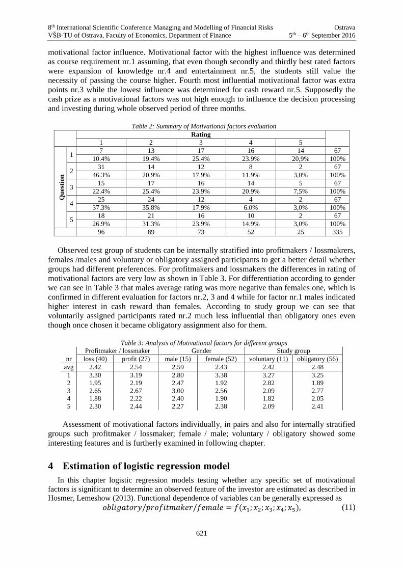
8th International Scientific Conference Managing and Modelling of Financial Risks Ostrava
VŠB-TU of Ostrava, Faculty of Economics, Department of Finance 5th – 6th September 2016
621
motivational factor influence. Motivational factor with the highest influence was determined
as course requirement nr.1 assuming, that even though secondly and thirdly best rated factors
were expansion of knowledge nr.4 and entertainment nr.5, the students still value the
necessity of passing the course higher. Fourth most influential motivational factor was extra
points nr.3 while the lowest influence was determined for cash reward nr.5. Supposedly the
cash prize as a motivational factors was not high enough to influence the decision processing
and investing during whole observed period of three months.
Table 2: Summary of Motivational factors evaluation
Rating
1 2 3 4 5
Qu
esti
on
1 7 13 17 16 14 67
10.4% 19.4% 25.4% 23.9% 20,9% 100%
2 31 14 12 8 2 67
46.3% 20.9% 17.9% 11.9% 3,0% 100%
3 15 17 16 14 5 67
22.4% 25.4% 23.9% 20.9% 7,5% 100%
4 25 24 12 4 2 67
37.3% 35.8% 17.9% 6.0% 3,0% 100%
5 18 21 16 10 2 67
26.9% 31.3% 23.9% 14.9% 3,0% 100%
96 89 73 52 25 335
Observed test group of students can be internally stratified into profitmakers / lossmakrers,
females /males and voluntary or obligatory assigned participants to get a better detail whether
groups had different preferences. For profitmakers and lossmakers the differences in rating of
motivational factors are very low as shown in Table 3. For differentiation according to gender
we can see in Table 3 that males average rating was more negative than females one, which is
confirmed in different evaluation for factors nr.2, 3 and 4 while for factor nr.1 males indicated
higher interest in cash reward than females. According to study group we can see that
voluntarily assigned participants rated nr.2 much less influential than obligatory ones even
though once chosen it became obligatory assignment also for them.
Table 3: Analysis of Motivational factors for different groups
Profitmaker / lossmaker Gender Study group
nr loss (40) profit (27) male (15) female (52) voluntary (11) obligatory (56)
avg 2.42 2.54 2.59 2.43 2.42 2.48
1 3.30 3.19 2.80 3.38 3.27 3.25
2 1.95 2.19 2.47 1.92 2.82 1.89
3 2.65 2.67 3.00 2.56 2.09 2.77
4 1.88 2.22 2.40 1.90 1.82 2.05
5 2.30 2.44 2.27 2.38 2.09 2.41
Assessment of motivational factors individually, in pairs and also for internally stratified
groups such profitmaker / lossmaker; female / male; voluntary / obligatory showed some
interesting features and is furtherly examined in following chapter.
4 Estimation of logistic regression model
In this chapter logistic regression models testing whether any specific set of motivational
factors is significant to determine an observed feature of the investor are estimated as described in
Hosmer, Lemeshow (2013). Functional dependence of variables can be generally expressed as
𝑜𝑏𝑙𝑖𝑔𝑎𝑡𝑜𝑟𝑦/𝑝𝑟𝑜𝑓𝑖𝑡𝑚𝑎𝑘𝑒𝑟/𝑓𝑒𝑚𝑎𝑙𝑒 = 𝑓(𝑥1; 𝑥2; 𝑥3; 𝑥4; 𝑥5), (11)

8th International Scientific Conference Managing and Modelling of Financial Risks Ostrava
VŠB-TU of Ostrava, Faculty of Economics, Department of Finance 5th – 6th September 2016
622
where 𝑥𝑖 represents a certain motivational factor scores.
It is necessary to insert calculated coefficients beta into formula (5), if we want to
determine the probability with which the investor is from the group of obligatory assigned
participants or profitmaker or female.
𝑃(𝑜𝑏𝑙𝑖𝑔𝑎𝑡𝑜𝑟𝑦/𝑝𝑟𝑜𝑓𝑖𝑡𝑚𝑎𝑘𝑒𝑟/𝑓𝑒𝑚𝑎𝑙𝑒) =1
1 + 𝑒−𝛽0−𝛽1∙𝑥1−𝛽2∙𝑥2−𝛽3∙𝑥3−𝛽4∙𝑥4−𝛽5∙𝑥5 (12)
To determine the chance in a form of probability that observed event is detected, it is
necessary to logarithm and equalize as coefficients of Euler’s value. This chance does not
have any maximum value, but minimum value is converging to zero. By logarithm of the
function we receive logit which is natural logarithm of a chance which values can be <-∞;
+∞>. As expressed in (10), we can express this function as following
𝑙𝑛(
𝑃(𝑜𝑏𝑙𝑖𝑔𝑎𝑡𝑜𝑟𝑦)
𝑃(𝑣𝑜𝑙𝑢𝑛𝑡𝑎𝑟𝑦)/
𝑃(𝑝𝑟𝑜𝑓𝑖𝑡𝑚𝑎𝑘𝑒𝑟)
𝑃(𝑙𝑜𝑠𝑠𝑚𝑎𝑘𝑒𝑟)/
𝑃(𝑓𝑒𝑚𝑎𝑙𝑒)
𝑃(𝑚𝑎𝑙𝑒))
= 𝛽0 + 𝛽1 ∙ 𝑥1 + 𝛽2 ∙ 𝑥2 + 𝛽3 ∙ 𝑥3 + 𝛽4 ∙ 𝑥4 + 𝛽5 ∙ 𝑥5
(13)
This deterministic model describe functional relationship of given dependent variable,
depending on the values of explanatory independent variables, ratings of each motivational
factor. This model does not include random variable.
4.1 Logistic regression with motivational factors
In this subchapter logistic regression models based on motivational factors to assess the
influence of motivational factors as predictors and explanatory variables are estimated. The
procedure is described in previous chapter using formulas (11) as basic model function and
continue with (12) and (13) to estimate a model for each internally stratified group. We can
see the results in Table 4.
Table 4: Estimated logistic regression models
Logistic regression Profitmakers / lossmakers Gender Study group
Number of obs = 67 67 67
Log likelihood = -43.813 -31.657 -21.930
LR chi2(5) = 2.720 7.940 15.980
Prob>chi2 = 0.744 0.159 0.007
Pseudo R2 = 0.030 0.112 0.267
Coef. P>|z| Coef. P>|z| Coef. P>|z|
1 cashreward 0.031 0.886 0.306 0.239 -0.181 0.599
2 requirement 0.195 0.409 -0.235 0.385 -1.423 0.005
3 extrapoints -0.157 0.520 -0.241 0.418 1.401 0.012
4 knowledge 0.376 0.245 -0.522 0.206 0.230 0.695
5 entertainment 0.000 0.999 0.463 0.245 -0.304 0.566
0 +_cons -1.247 0.251 1.507 0.236 2.443 0.161
I conclude that motivational factors are significant as explanatory variable only for the
Study group differentiation, where the set of motivational factor nr2 and nr.3 significantly
influence the probability of inclusion into voluntary or obligatory. For the group of
profitmakers / lossmakers and gender none of the motivational factors was significant to
explain the feature of given group. Motivational factors are not recommended as explanatory
variables while defining profitmaker or gender.
5 Conclusion
To summarize the analysis of motivational factors it can be concluded that motivational
factors are differently evaluated on a statistically significant level with low correlation among

8th International Scientific Conference Managing and Modelling of Financial Risks Ostrava
VŠB-TU of Ostrava, Faculty of Economics, Department of Finance 5th – 6th September 2016
623
each of motivational factors pairs. Interesting results were achieved in the analysis of different
evaluation of motivational factors by different internally stratified groups such as profitmaker
/ lossmaker; female / male; voluntary / obligatory. Overall influence of motivation on the
freqency or success in investing was not proved even though preferences of motivational
factors for different internally stratified groups (profitmakers / lossmakers; females / males;
obligatory / voluntary) are significantly different
Possibility to use motivational factors as predictors and explanatory variables in logistic
regression model proved to be inefficient even though individually motivational factors are
evaluated significantly different. Logistic regression model including motivational factors
(requirement, extra points) as independent explanatory variables is suitable only for
explaining obligatory / voluntary group.
References
[1] Allison, P.D. (2014). Measures of Fit for Logistic Regression. Paper 1485-2014
presented at the SAS Global Forum, Washington, DC.
[2] Diamond, P., Vartiainen, H., (2007). Behavioral Economics and Its Applications. New
Jersey: Princeton University Press.
[3] Grégoire, P. (2016). Unskilled traders, overconfidence and information acquisition.
Journal of Behavioral and Experimental Finance Vol. 9, p. 1-5.
[4] Hilbe, J. (2009). Logistic Regression Models. Chapman & Hall/CRC Press.
[5] Hilton, D. J. (2001). The Psychology of Financial Decision-Making: Applications to
Trading, Dealing, and Investment Analysis. The Journal of Psychology and Financial
Markets Vol. 2, p. 37-53.
[6] Hosmer, D. W., Lemeshov, S. (2000). Applied logistic regression. 2nd ed. New York:
Wiley-Interscience Publication.
[7] Hosmer, D. W., Lemeshov S. and Sturdivant R. X. (2013) Applied Logistic Regression.
3rd ed. New Jersey: John Wiley & Sons,
[8] Shleifer, A. (2000). Inefficient Markets: An Introduction to Behavioral Finance. Oxford:
Oxford University Press.
[9] Stöckla, T., Kirchler, M. (2014). Trading behavior and profits in experimental asset
markets with asymmetric information. Journal of Behavioral and Experimental Finance
Vol. 2, p. 18-30.
[10] Stukel, T.A. (1988). Generalized logistic models. Journal of the American Statistical
Association Vol. 83, p. 426-431.
[11] Tjur, T. (2009). Coefficients of determination in logistic regression models – A New
Proposal: The Coefficient of Discrimination. American Statistician Vol. 63, p. 366-372.
[12] Witte R. S., Witte J. S. (2009). Statistics. 9 ed. Wiley

8th International Scientific Conference Managing and Modelling of Financial Risks Ostrava
VŠB-TU of Ostrava, Faculty of Economics, Department of Finance 5th – 6th September 2016
624
Critical assessment of the applicability of selected bankruptcy prediction models in specific conditions
of the Slovak Republic
Maria Misankova1, Jana Majerova2
Abstract
The issue of bankruptcy prediction is a subject of interest of researchers since the beginning of
19th century. Through many years of researches there have been constructed various types of
bankruptcy prediction models in different countries. So there arises a question if the model
developed in one country can be successfully applied for the bankruptcy prediction in other
country. Based on the mentioned can be clarified the main goal of presented study, to provide a
critical assessment of the applicability of selected bankruptcy prediction models constructed
worldwide on the set of Slovak companies, which consists of bankrupt and non-bankrupt
companies. Results of this assessment will serve as a basis for the determination, if there is a
need to construct a unique model, which reflects specific conditions of the Slovak Republic or
other country, or on the other hand can be these models successfully applied without any
modifications.
Key words
Here write the key words (in English)
JEL Classification: Here write the JEL classification code(s)
1. Introduction
The issue of predicting a crisis and bankruptcy holds a special place among theoretical and
practical problems of business management for many years. Slovakia is a country with
developing economy which leads to the instability of many processes and factors forming the
external environment. Thus as a result, it is not only necessary to carry out financial analysis
of a company to determine its state as a given stage of its development, but also to make an
early diagnosis of its possible bankruptcy in the future. Therefore forecasting a financial
health of a company and the identification of its adverse development trends, potential crisis
and bankruptcy possibility is crucial. (Gavlakova, Kliestik, 2014; Kollar, Bartosova, 2014)
In the economic science, as well as in the practice of real world, a huge variety of models
are used for estimating bankruptcy probability of companies and organizations, based on
different principles, techniques and methodologies.
Despite the plenty of researches and publications dedicated to this issue, there are not many
Slovak models that forecast the probability of bankruptcy with high accuracy. In addition, the
predictive ability of a model may vary over time: efficient methods can only be applied to
companies of the same group in the same economic situation in the period for which the
models were originally designed. Foreign models may not take into account the peculiarities
1 Ing. Maria Misankova, PhD., University of Zilina, Faculty of Operation and Economics of Transport
and Communications, Department of Economics, [email protected]. 2 JUDr. Ing. Jana Majerova, PhD., University of Zilina, Faculty of Operation and Economics of
Transport and Communications, Department of Economics, [email protected].

8th International Scientific Conference Managing and Modelling of Financial Risks Ostrava
VŠB-TU of Ostrava, Faculty of Economics, Department of Finance 5th – 6th September 2016
625
of Slovak economy and have less accurate predictions. The applicability of a model can also
vary, depending on the industry and other factors. (Kral, Kliestik, 2015; Bartosova, et. al.,
2014)
Therefore based on the above-mentioned is defined the main goal of presented study to
provide a critical assessment of the applicability of selected bankruptcy prediction models
constructed worldwide on the set of Slovak companies, which consists of bankrupt and non-
bankrupt companies.
2. Literature review
First researches dedicated to the issue of bankruptcy and corporate´s failures had arisen in
30´s of the 20th century. These were oriented mainly on the comparison of financial ratios
between bankrupt and non-bankrupt companies. Fitzpatrick (1932) published his work
oriented on the major differences between successful and unsuccessful businesses. This work
had become the inspiration for many of applied studies that began to emerge in the middle of
60´s of the 20th century. (Valaskova, Zvarikova, 2014; Vochozka, 2010)
However as the turning point is considered the breakthrough work of Beaver (1966) who
applied univariate discriminant analysis which is based on various financial ratios connected
into one final predictor serving as a classification criterion. Despite a lot of limitations and
reservations of this method it was an inspiration for a large amount of studies devoted to the
issue of bankruptcy prediction and corporate´s failure. (Zmijewski, 1984)
One of the most famous researcher dealing with bankruptcy prediction is Altman (1968)
who firstly applied multivariate discriminant analysis for the construction of bankruptcy
prediction models. His work is considered as a symbol of prediction of financial health of
companies. Consecutively he has developed dozens of models for various types of companies
respecting specific conditions and circumstances. (Siekelova, et. al., 2015)
Nowadays there are several hundreds of prediction models that have been developed at a
particular time and in terms of specific national economies. So there exists a great variety in
bankruptcy prediction models from how many and which factors are considered to what
methods are employed to develop the model. The primary methods that have been used for the
development of models are univariate discriminant analysis (UDA), linear discriminant
analysis (LDA), multivariate discriminant analysis (MDA), quadratic discriminant analysis
(QDA), principal component analysis (PCA), logistic regression (LOGIT), probit regression
(PROBIT), neural network (NN), rough sets (RS), linear programming (LP), data
envelopment analysis (DEA), survival analysis (SA), fuzzy techniques (FA), decision trees
(DT), genetic algorithm (GA) and others. (Kliestik, et. al., 2015; Spuchlakova, et. al., 2014)
The most famous authors dealing with the issue of bankruptcy are Deakin (1972), Edmister
(1972), Tamari (1976), Taffler (1976), Springate (1978), Dambolena and Khoury (1980),
Ohlson (1980), Beerman (1982), Fulmer (1984), Zmijewski (1984), Zavgren (1985), Kralicek
(1990), Laitinen (1991), Horrigan (1996), Shirata (2002), Neumaierova and Neumaier (1995,
1999, 2001, 2005), Jakubik and Teply (2008) and others. (Dimitras, et. al., 1996)
3. Data and Methodology
3.1 Data
To accomplish specified goal of this study we applied selected bankruptcy prediction
models constructed worldwide on the set of Slovak companies to provide critical assessment
of their applicability in specific conditions of the Slovak Republic. The set of companies

8th International Scientific Conference Managing and Modelling of Financial Risks Ostrava
VŠB-TU of Ostrava, Faculty of Economics, Department of Finance 5th – 6th September 2016
626
contains 20 companies from which 10 are non-bankrupt and 10 are companies which bankrupt
in 2016. The basis for provided calculations consists of financial statements of chosen set of
companies from years 2013-2015.
3.2 Methodology
Nowadays there are several hundreds of bankruptcy prediction models so after deep
literature review of these models we have selected the most famous models constructed
worldwide with the highest prediction power and complement them with models constructed
in similar conditions to the conditions in the Slovak Republic mainly models constructed in
the Czech Republic.
3.2.1 Altman model (Z´score)
Altman (1968) firstly applied multiple discriminant analysis for the construction of
prediction model and his work relates to the most famous as widely known Z-score model
designated originally for US public firms. Later he has developed also Z-score estimated for
US private firms and Z-score estimated for US non-manufacturers and emerging markets.
(Bellovary, et. al., 2007) These are all well-known and for our needs we apply the second one
Z-score estimated for private firms which formula is as follows:
1 2 3 4 50,717 0,847 3,107 0,420 0,998Z X X X X X (1)
Where: X1 = Current Assets – Current Liabilities / Total Assets
X2 = Retained Earnings / Total Assets
X3 = Earnings Before Interest and Taxes / Total Assets
X4 = Book Value of Equity / Book Value of Total Liabilities
X5 = Sales / Total Assets
Z´ = Overall index
Zones of Discrimination:
Z > 2,99 “Safe“ Zone
1,81 < Z < 2,99 “Grey” Zone
Z < 1,81 “Distress” Zone
3.2.2 Neumaierova and Neumaier model (Index IN)
Neumaierova and Neumaier have constructed the most famous bankruptcy prediction
models in Czech Republic respecting specific conditions of this country. They constructed
also various models for different type of beneficiaries such us IN 95 – creditor´s model, IN 99
– owner´s model, IN 01 – combined creditor-owner´s model, which was modified later as
IN05. (Dengov, Gregova, 2010; Cisko, Kliestik, 2013)
For this study are the most appropriate and relevant the last one IN 05 with formula:
1 2 3 4 505 0,13 0,04 3,97 0,21 0,09IN X X X X X (2)
Where: X1 = Total Assets / Total Liabilities
X2 = Earnings Before Interest and Taxes / Costs of Interest
X3 = Earnings Before Interest and Taxes / Total Assets
X4 = Total Revenues / Total Assets
X5 = Current Assets / Short Term Liabilities
IN05 = Overall index

8th International Scientific Conference Managing and Modelling of Financial Risks Ostrava
VŠB-TU of Ostrava, Faculty of Economics, Department of Finance 5th – 6th September 2016
627
Zones of Discrimination:
IN05 > 1,60 Company creates value
0,90 < IN05 < 1,60 Grey Zone of unallocated results – company doesn´t create
value but also doesn´t bankrupt
IN05 < 0,90 Company is going to bankruptcy
3.2.3 Jakubik and Teply model (JT)
Authors applied logistic regression for the construction of prediction model in condition of
the Czech Republic and this model is also often used by banks and other financial institutions.
(Cisko, Kliestik, 2013) This model has following formula:
1 2 3 4
5 6 7
2,4192 2,5779 1,7863 3,4902 2,4172
1,7679 3,3062 2,2491
JT X X X X
X X X
(3)
Where: X1 = Total Debt / Equity
X2 = Long Term Debt + Long Term Bonds / Equity
X3 = Earnings Before Interest and Taxes / Costs of Interest
X4 = Earnings Before Interest and Taxes / Sales
X5 = Inventory / (Sales / 365)
X6 = Working Capital / Total Assets
X7 = Net Profit / Equity
JT = Overall index
The probability of the bankruptcy is then given by the score:
1
1 JTscore
e
(4)
3.2.4 Springate model (SM)
Springate model was constructed in the highly developed economy of Canada. (Siekelova,
Moravcikova, 2015) We decided its application to compare if the model used in countries
with stable and good economy can be successfully applied in condition of the Slovak
Republic. This model has following discriminant formula:
1 2 3 41,03 3,07 0,66 0,4SM X X X X (4)
Where: X1 = Net Working Capital / Total Assets
X2 = Earnings Before Interest and Taxes / Total Assets
X3 = Earnings Before Taxes / Short Term Liabilities
X4 = Sales / Total Assets
SM = Overall index
Zones of Discrimination:
0,862 < S Good financial health of the company
S < 0,862 Possible financial problems of the company

8th International Scientific Conference Managing and Modelling of Financial Risks Ostrava
VŠB-TU of Ostrava, Faculty of Economics, Department of Finance 5th – 6th September 2016
628
3.2.5 Taffler model (TM)
This model was developed in UK so its similarly to Springate model appropriate for our
study. It is based on following formula including 4 indicators (Cisko, Kliestik, 2013):
1 2 3 40,53 0,13 0,18 0,16TM X X X X (4)
Where: X1 = Earnings Before Taxes / Short Term Liabilities
X2 = Current Assets / Total Liabilities
X3 = Short Term Liabilities / Total Assets
X4 = Sales / Total Assets
TM = Overall index
Zones of Discrimination:
TM > 0,3 Enterprise creates value
0,2 ≤ TM ≤ 0,3 Grey zone
TM < 0,2 Enterprise is going to bankruptcy
4. Results and Discussion
Based on the provided literature review and theoretical backround of selected bankruptcy
prediction models we applied these models on the set of Slovak companies to make
appropriate calculations. We have chosen five various prediction models developed
worldwide and in the Czech Republic.
Results of this assessment will serve as a basis for the determination, if there is a need to
construct a unique model, which reflects specific conditions of the Slovak Republic or on the
other hand can be these models successfully applied without any modifications. Based on the
provided calculations can be also summarized the ability of these models to predict financial
health and potential bankrupt of companies in specific conditions of the Slovak Republic.
All provided calculations are shown in following tables while first two tables show results
for companies which bankrupted in 2016.
Table 1: Companies bankrupted in 2016 – Altman model, Model IN05, Jakubik and Teply model
Company /
Year
Altman model IN05 JT model
2015 2014 2013 2015 2014 2013 2015 2014 2013
B1 1,074 1,094 1,565 -0,175 -2,817 1,703 1,000 1,000 0,001
B2 4,204 1,963 3,003 1,187 0,739 0,974 1,000 1,000 1,000
B3 1,993 0,893 2,628 0,664 -1,071 0,701 1,000 1,000 1,000
B4 2,021 2,321 2,666 -1,369 1,367 0,695 1,000 0,000 1,000
B5 2,123 1,664 1,742 1,266 0,230 0,474 1,000 1,000 1,000
B6 1,845 1,934 2,321 1,871 1,754 1,523 1,000 0,994 1,000
B7 4,441 4,221 4,295 1,631 1,552 1,475 1,000 1,000 1,000
B8 -0,031 -2,196 -1,466 -6,429 -9,367 -8,812 1,000 1,000 1,000
B9 2,842 2,415 2,326 1,469 1,423 1,307 1,000 1,000 1,000
B10 5,671 2,154 9,540 3,603 1,488 8,019 0,000 0,000 0,927
Table specification:
use of italic numbers means that based on the provided calculations the model
shows good health of the company,

8th International Scientific Conference Managing and Modelling of Financial Risks Ostrava
VŠB-TU of Ostrava, Faculty of Economics, Department of Finance 5th – 6th September 2016
629
two different grey colours are used for:
o “grey” zone, which represents potential financial problems of the company
o dark-grey, which means that company is going to bankruptcy.
Table 2: Companies bankrupted in 2016 – Springate model, Taffler model
Company /
Year
SM TM
2013 2014 2015 2013 2014 2015
B1 -0,028 0,072 1,298 0,159 0,200 0,477
B2 1,233 0,675 1,390 0,811 0,468 0,524
B3 -0,019 -0,386 -0,170 0,038 -0,015 -0,099
B4 0,258 0,715 1,121 0,231 0,409 0,495
B5 0,929 0,373 0,906 0,474 0,277 0,313
B6 1,581 2,088 1,848 0,657 0,945 0,791
B7 2,669 2,553 2,811 0,943 0,914 0,893
B8 -1,313 -4,849 -1,212 0,617 1,096 1,067
B9 1,379 1,510 1,516 0,714 0,706 0,630
B10 3,432 1,426 0,049 1,365 0,588 5,278
Selected five bankruptcy prediction models have been applied also on the set of non-
bankrupt companies so we can compare obtained results, which are shown in tables 3 and 4.
Interpretation of gained calculations is same as was used in tables 1 and 2 so same
characteristics are used so we can clearly identify whether the model used can provide
appropriate classification of the company and can predict financial situation of it accurately.
Table 3: Non-bankrupt companies – Altman model, Model IN05, Jakubik and Teply model
Company
/ Year
Altman model IN05 JT model
2013 2014 2015 2013 2014 2015 2013 2014 2015
NB1 2,322 2,036 1,576 1,228 1,051 0,775 0,000 0,001 0,983
NB2 2,728 2,360 2,317 3,169 1,783 1,662 1,000 1,000 1,000
NB3 2,568 3,062 2,687 1,478 1,596 1,313 1,000 1,000 1,000
NB4 3,939 3,624 3,551 3,698 3,076 2,451 0,000 0,975 1,000
NB5 5,471 5,069 4,995 -1,894 1,119 2,052 1,000 1,000 0,001
NB6 4,650 3,954 3,277 9,682 5,736 1,157 0,000 0,000 0,004
NB7 5,743 4,205 3,121 8,940 8,936 4,086 0,000 0,000 0,000
NB8 4,341 3,916 4,031 1,540 1,386 1,610 1,000 1,000 1,000
NB9 4,661 4,643 4,082 1,679 3,246 3,642 0,000 0,000 0,000
NB10 2,045 2,699 3,836 2,303 2,387 3,001 0,000 0,000 0,000
Table 4: Non-bankrupt companies – Springate model, Taffler model
Company
/ Year
SM TM
2013 2014 2015 2013 2014 2015
NB1 1,101 0,964 0,970 0,499 0,442 0,333
NB2 1,255 1,018 1,062 0,687 0,500 0,488
NB3 1,567 1,749 1,683 0,607 0,713 0,583
NB4 2,317 2,331 2,514 0,916 0,882 0,845
NB5 0,028 0,381 0,978 0,312 0,495 0,738
NB6 3,561 2,521 1,837 1,365 1,057 0,685
NB7 2,185 1,866 1,476 1,681 1,067 0,653

8th International Scientific Conference Managing and Modelling of Financial Risks Ostrava
VŠB-TU of Ostrava, Faculty of Economics, Department of Finance 5th – 6th September 2016
630
NB8 1,113 1,158 1,788 0,766 0,660 0,897
NB9 1,905 2,105 2,601 0,819 0,892 0,855
NB10 1,266 2,424 2,240 0,634 1,287 0,978
From realised calculations of five bankruptcy prediction models applied on the set of
Slovak companies can be summarized:
model IN05 and Jakubik and Teply model gained the most relevant results in the set
of bankrupt companies,
Springate model and Taffler model are not suitable for the use in the condition of
the Slovak Republic, while these models can´t show significant differences between
two groups of tested companies,
Springate and Tafler model were constructed in developed economies so based on
the gained results is clear that their use is not suitable for Slovak companies,
Altman model can be used in Slovak conditions but we consider to use it only as a
supplementary model to other more appropriate models, because it can predict
financial situation quite enough but as is clear from tables there are some
shortcomings and mistakes in evaluation,
Jakubik and Teply model doesn´t show proper results in the set of non-bankrupt
companies, while almost half companies are going to bankruptcy based on this
model
overall the most suitable models from our point of view are model IN05, Altman
model and Jakubik and Teply model, but companies should also consider possible
use of other models which were presented in the literature review of this study.
5. Conclusion
The presented study is dedicated to the issue of bankruptcy prediction and the main goal
was to provide a critical assessment of the applicability of selected bankruptcy prediction
models constructed worldwide on the set of Slovak companies, which consists of bankrupt
and non-bankrupt companies. So based on the provided calculations we can summarise that
model IN05, Jakubik and Teply model and Altman model can be apply for the prediction of
bankruptcy in condition of the Slovak Republic but the use of these models is not enough and
calculations provided by them can lead to some mistakes and misunderstandings. We consider
as more appropriate and relevant to construct a unique model for bankruptcy prediction, which
will reflect specific conditions of economy of the Slovak Republic. Unique model would
better predict possible financial problems of the company with higher accuracy.
These facts make it necessary to develop effective forecasting methods of bankruptcy for
Slovak companies and results of this study will serve as a basis for the following researches.
Acknowledgement
This research was financially supported by the Slovak Research and Development Agency
– Grant NO. APVV-14-0841: Comprehensive Prediction Model of the Financial Health of
Slovak Companies.
References
[1] Altman, E. I. (1968). Financial ratios, discriminant analysis and prediction of corporate
bankruptcy. Journal of Finance, 23(4), pp. 589-609.

8th International Scientific Conference Managing and Modelling of Financial Risks Ostrava
VŠB-TU of Ostrava, Faculty of Economics, Department of Finance 5th – 6th September 2016
631
[2] Bartosova, V., Hraskova, D. and Paliderova, M. (2014). Basic Rules and Methodological
Framework of the Financial Analysis of the Group of Companies in the Slovak Republic.
2nd International Conference on Economics and Social Science (ICESS), Shenzhen,
China, Advances in Education Research, Vol. 61, pp. 86-91.
[3] Bellovary, J., Giacomino, D. and Akers, M. (2007). A Review of Bankruptcy Prediction
Studies: 1930 to Present. Journal of Financial Education, 33, pp. 1-43.
[4] Cisko, S. and Kliestik, T. (2013). Financny manazment podniku II. EDIS Publishing,
University of Zilina.
[5] Dengov, V.V. and Gregova, E. (2010). Economic decision-making under uncertainty and
risk. Methodology and criteria for decision-making. Ekonomicko-manazerske spektrum,
4(2), 28-45.
[6] Dimitras, A. I., Zanakis S. H. and Zopounidis, C. (1996). A survey of business failure
with an emphasis on prediction method and industrial applications. European Journal of
Operational Research, 90, pp. 487–513.
[7] Gavlakova, P. and Kliestik, T. (2014). Credit Risk Models and Valuation. 4th
International Conference on Applied Social Science (ICASS), Singapore, Advances in
Education Research, Vol.51, pp. 139-143.
[8] Kliestik, T., Musa, H. and Frajtova-Michalíkova, K. (2015). Parametric methods for
estimating the level of risk in finance. Procedia Economics and finance, 24, pp. 322-330.
[9] Kollar, B. and Bartosova, V. (2014). Comparison of Credit Risk Measures as an
Alternative to VaR. 2nd International Conference on Social Sciences Research (SSR
2014), Hong Kong, Advances in Social and Behavioral Sciences, Vol. 5, pp. 167-171.
[10] Kral P. and Kliestik, T. (2015). Estimation of the level of risk based on the selected
theoretical probability distributions. 10th International Scientific Conference Financial
management of Firms and Financial Institutions, Ostrava, Czech Republic, pp. 603-610.
[11] Siekelova, A. and Moravcikova, K. (2015). Financial health analysis of the selected
company focusing on liquidity. 10th International Scientific Conference Financial
management of Firms and Financial Institutions, Ostrava, Czech Republic, pp. 1121-
1128.
[12] Siekelova, A., Weissova, I. and Kollar, B. (2015). Default Prediction of Chosen Car
Manufacturing Company. 19th International Conference on Transport Means, Transport
Means - Proceedings of the International Conference, Kaunas, Lithuania, pp. 509-512.
[13] Spuchlakova, E., Frajtova-Michalikova, K. and Birtus, M. (2014). Credit Risk
Measurement, 2nd International Conference on Economics and Social Science (ICESS),
Shenzhen, China, Advances in Education Research, Vol. 61, pp. 75-79.
[14] Valaskova, K. and Zvarikova, K. (2014). Prediction of Credit Risk by Selected
Theoretical Rating Models. 2nd International Conference on Social Sciences Research
(SSR 2014), Hong Kong, Advances in Social and Behavioral Sciences, Vol. 5, pp. 160-
166.
[15] Vochozka, M. (2010). Development of methods for comprehensive evaluation of
business performance. Politická Ekonomie, 58(5), pp. 675-688.
[16] Zmijewski, M. (1984). Methodological issues related to the estimation of financial
distress prediction models. Journal of Accounting Research, 22, pp. 59-82.
8th International Scientific Conference Managing and Modelling of Financial Risks Ostrava
VŠB-TU of Ostrava, Faculty of Economics, Department of Finance 5th – 6th September 2016
632
Risks arising from a violation of the obligations stipulated by the legislative accounting regulation to
entities
Daša Mokošová 1
Abstract
Changes in the accounting legislation that contains also regulated rules for the preparation of
financial statements are common in any state. Since the regulation of accounting rules can be
subsequently linked to the issue of the income tax or other taxes payed by entities, or to the
verification of financial statements, so the changes in accounting legislation could impact also
the legislation regulating these areas. If an entity for any reason, new laws and regulations or
changes to existing laws and regulations does not apply, it runs the risk of future adverse
effect on its business. This risk might occur in the future fines or other impacts in relation to
non-compliance with the legislative accounting regulation.
Key words
Accounting regulation, IFRS, fine, OECD, EU, SR
JEL Classification: M 40, M41, K29
1. Úvod
V teórii je riziko súvisiace so zmenou legislatívy resp. so zmenou v zákonodarstve
označované ako systematické riziko, pretože sa dotýka všetkých podnikateľských subjektov
(Sivák et al., 2011). Zároveň patrí aj do skupiny vonkajších rizík, kde je zahrnuté spolu
s rizikom vlády a medzinárodným politickým rizikom. Podľa Holuba (2009, s.573-574) je
možné legislatívne riziko vnímať aj ako daňové riziko, v podrobnejšom členení na všeobecné
a špecifické. Legislatívne riziko resp. daňové riziko všeobecné podľa Holuba (2009, s.573)
„vyplýva zo všeobecnej zmeny práva, alebo všeobecnej zmeny daňovej legislatívy, alebo zo
zavedenia nových noriem, ktoré ovplyvnia celý súkromný alebo verejný sektor“. V prípade
legislatívneho rizika alebo daňového rizika špecifického, podľa Holuba (2009, s.574) ide o
riziko, ktoré môže vzniknúť pri špecifickej zmene práva, alebo pri špecifickej zmene daňovej
legislatívy, ktorá ovplyvní len niektoré podnikateľské subjekty. Avšak, ak účtovná jednotka
alebo podnikateľský subjekt nezaregistruje zmenu v legislatíve alebo z iného dôvodu ju
nezohľadní, potom podstupuje nesystematické riziko, pretože účtovná jednotka má možnosť
ovplyvňovať túto situáciu a zabrániť vzniku takéhoto rizika resp. aspoň zmierniť negatívne
následky na základe prijatia ďalších rozhodnutí.
Mnohé riziká, ktoré môžu vzniknúť podnikateľom, sa dajú poistiť a tým sa zmierni ich
efekt alebo sa prenesie negatívny dôsledok na poisťovňu. Komerčné poistenie podnikateľov
však zmenu v legislatíve nedefinuje ako poistnú udalosť.
1 Ing. Daša Mokošová, PhD., Ekonomciká univerzita v Bratislave, Fakulta hospodárskej informatiky,
Katedra účtovníctva a audítorstva, Dolnozemská cesta 1/b, 852 35 Bratislava,

8th International Scientific Conference Managing and Modelling of Financial Risks Ostrava
VŠB-TU of Ostrava, Faculty of Economics, Department of Finance 5th – 6th September 2016
633
2. Vysporiadanie sa s legislatívnymi rizikami podľa národnej a
medzinárodnej úpravy účtovníctva
Vo finančnom účtovníctve je možné na niektoré udalosti, ktoré súvisia s podnikateľskou
činnosťou a predstavujú pre účtovnú jednotku riziko prípadne stratu, tvoriť rezervy. Tvorba
rezerv môže byť založená na použití poistno-matematických metód, pričom ich hodnota sa
upravuje na súčasnú hodnotu účtovania a vykazovania. Podľa Opatrenia Ministerstva financií
SR č. 23054/2002-92, ktorým sa ustanovujú podrobnosti o postupoch účtovania a rámcovej
účtovej osnove pre podnikateľov účtujúcich v sústave podvojného účtovníctva v znení
neskorších predpisov (ďalej len „opatrenie MF SR pre podnikateľov účtujúcich v sústave
podvojného účtovníctva“) sa tvorba a rozpúšťanie rezerv vzťahuje k povinnostiam
vyplývajúcim zo všeobecne záväzných právnych predpisov, z uzavretých zmlúv,
z dobrovoľného rozhodnutia účtovnej jednotky splniť si povinnosť voči tretím stranám. V §
19 ods. 7 opatrenia MF SR pre podnikateľov účtujúcich v sústave podvojného účtovníctva je
menovite vymedzených 24 rizík, na ktoré sa tvoria rezervy. Medzi týmito rizikami, na ktoré je
možné tvoriť rezervu, sú uvedené aj pokuty a penále a iné riziká a straty súvisiace s činnosťou
účtovnej jednotky. Presne však nie je definované, aké položky sa môžu v týchto kategóriách
nachádzať. Je to však jedna z možností, ako zmierniť dopad rizika v účtovných jednotkách
z pohľadu vykazovania nákladov, aj keď účtovná jednotka negatívne dopady plne znáša, nie
ako v prípade poistenia sa.
Zákon č. 431/2002 Z.z. o účtovníctve v znení neskorších predpisov (ďalej len „zákon
o účtovníctve“), však vymedzuje účtovné jednotky, ktoré postupujú pri vedení účtovníctva
a zostavovaní účtovnej závierky podľa medzinárodných účtovných predpisov vydávaných
Radou pre medzinárodné účtovné štandardy, ktorými sú Medzinárodné štandardy pre finančné
vykazovanie (ďalej len „IFRS“). Aj IFRS upravujú problematiku rizík, poistenia a rezerv.
Existencia rizík, ich definícia, ocenenie a vykazovanie je obsahom rovno niekoľkých
štandardov. Riziká sú najpodrobnejšie vyšpecifikované vo väzbe na finančné nástroje vrátane
zabezpečovacích nástrojov, kde môžu vznikať úverové, likviditné a trhové riziká. Trhovými
rizikami môžu byť finančné riziká. Uvedené riziká sú predmetom pravidiel v IAS 32 Finančné
nástroje: prezentácia, IAS 39 Finančné nástroje: vykazovanie a oceňovanie, IFRS 7 Finančné
nástroje: zverejňovanie, IFRS 9 Finančné nástroje, IFRS 10 Konsolidovaná účtovná závierka,
IFRS 12 Zverejňovanie podielov v iných účtovných jednotkách. Riziko je však uvádzané
napr. aj v IFRS 13 Oceňovanie reálnou hodnotou, v IFRS 15 Výnosy zo zmlúv so zákazníkmi
alebo v IAS 12 Dane z príjmov a IAS 19 Zamestnanecké požitky. Poistenie a v rámci neho
poistné riziko je náplňou IFRS 4 Poistné zmluvy. Kombinácia rizika a rezervy je
obsahom IAS 37 Rezervy, podmienené záväzky a podmienené aktíva. Ak by sme uskutočnili
porovnanie pravidiel uvedených v IAS 37 a opatrením MF SR pre podnikateľov účtujúcich
v sústave podvojného účtovníctva, tak IAS 37 podrobne nešpecifikuje oblasti, na ktoré
účtovná jednotka má tvoriť rezervu, tak ako je tomu v opatrení. Podľa IAS 37 nie je možné
vytvárať rezervy na všeobecné obchodné riziká, alebo na budúce náklady, ktorým sa môže
účtovná jednotka vyhnúť. Jedným z príkladov, ktoré sa nachádzajú v Prílohe C, je
zohľadnenie zákonných požiadaviek účtovnou jednotkou. Čiže, ak dôjde k zmene zákonných
požiadaviek, ktoré účtovná jednotka nezohľadní, tak rezerva sa netvorí na zmenu pravidiel
súvisiacu so zákonnými požiadavkami, ale na pravdepodobnú pokutu alebo penále, pretože
účtovná jednotka nevykonáva svoju činnosť v súlade so zákonom. Pravdepodobnosť, či bude
musieť účtovná jednotka pokutu zaplatiť, závisí od pravdepodobnosti na základe minulých
skúseností s kontrolnými alebo sankčnými orgánmi. Účtovná jednotka sa môže spoliehať, že
kontrolný alebo sankčný orgán nemusí odhaliť jej nesúlad so zákonom. V takomto prípade sa

8th International Scientific Conference Managing and Modelling of Financial Risks Ostrava
VŠB-TU of Ostrava, Faculty of Economics, Department of Finance 5th – 6th September 2016
634
rezerva vykáže ako najlepší odhad pokuty alebo penále, ktorých uloženie je viac
pravdepodobné ako nepravdepodobné (IASB, 2014).
3. Sankcie za porušenie účtovných právnych predpisov v SR
Slovenská republika podlieha aj medzinárodnému právu, keďže je členským štátom
niekoľkých medzinárodných organizácií a zoskupení resp. má uzatvorené medzinárodné
zmluvy, ktoré ju zaväzujú k dodržiavaniu medzinárodných dohovorov.
V oblasti účtovníctva napr. musí dodržiavať smernice a nariadenia, ktoré jej vyplývajú
z členstva v Európskej únii. V súčasnosti je v platnosti len jedna smernica pre účtovníctvo a to
smernica Európskeho parlamentu a Rady 2013/34/EÚ z 26. júna 2013 o ročných účtovných
závierkach, konsolidovaných účtovných závierkach a súvisiacich správach určitých druhov
podnikov v znení neskorších predpisov. Dodržiavanie smernice sa zabezpečí jej transpozíciou
do legislatívnych opatrení členského štátu, čo sa v SR prejavilo v novele zákona o účtovníctve
s účinnosťou od 1. januára 2015. Nedodržanie tejto smernice Európska únia netrestá priamo,
ale udelenie pokút za nedodržanie prenáša na členské štáty a to v čl. 51. Na základe tohto
článku členské štáty majú stanoviť sankcie za porušenie vnútroštátnych ustanovení prijatých v
súlade so smernicou Európskeho parlamentu a Rady 2013/34/EÚ a prijať všetky potrebné
opatrenia na zabezpečenie presadzovania nimi určených sankcií. Požiadavka sa pritom kladie
na skutočnosť, že stanovené sankcie musia byť účinné, primerané a odradzujúce.
Výška sankcií vo forme pokút za nedodržiavanie legislatívnej regulácie účtovníctva bola
predmetom diskusie zo strany OECD. Slovenská republika ešte v roku 1997 pristúpila
k Dohovoru OECD o boji s podplácaním zahraničných verejných činiteľov v medzinárodných
obchodných transakciách (ďalej len „Dohovor OECD“) s účinnosťou od roku 1999. Článok 8
tohto dohovoru je prepojený s účtovníctvom v nasledujúcom znení:
„1. Na účinný boj s podplácaním zahraničných verejných činiteľov urobí každá strana také
opatrenia v rámci svojich zákonov a predpisov o vedení účtovných kníh a výkazov,
zverejňovaní finančných správ a účtovných a audítorských noriem, ktoré zakazujú zakladanie
účtov mimo účtovných kníh, vedenie operácií mimo účtovných kníh alebo neprimerane
identifikovaných transakcií, vykazovanie nejestvujúcich výdavkov, zapisovanie záväzkov s
nesprávnou identifikáciou ich predmetu, ako aj používanie falošných dokumentov
spoločnosťami, ktoré podliehajú týmto zákonom a predpisom, s cieľom podplatiť
zahraničného verejného činiteľa alebo zatajiť takéto úplatkárstvo.
2. Každá strana zabezpečí účinné, úmerné a odradzujúce občianskoprávne, správne alebo
trestnoprávne postihy za takéto opomenutie alebo falšovanie v súvislosti s knihami, výkazmi,
účtami a finančnými správami takých spoločností.“
Podľa tohto dohovoru Pracovná skupina OECD pre úplatkárstvo v medzinárodných
obchodných transakciách (WGB) uskutočňuje monitorovanie a určuje následný mechanizmus
pre jeho úplnú implementáciu v každej krajine, ktorá tento dohovor podpísala a pristúpila k
nemu. Stav v Slovenskej republike bol predmetom už tretej fázy hodnotení, ktorá bola
zrealizovaná v období od septembra 2011 do júna 2012. Následne bola vypracovaná
hodnotiaca správa, ktorá bola prijatá plénom WGB/OECD 15. júna 2012. Zistenia a ich
náprava v rámci tejto tretej fázy boli realizované neskôr. Jedno zo zistení bolo pri sankciách
stanovených zákonom o účtovníctve a Slovenská republika bola vyzvaná prijať opatrenia na
zabezpečenie efektívneho ukladania sankcií za účtovné porušenia súvisiace s korupciou
zahraničných verejných činiteľov. V hodnotiacej správe OECD bolo skonštatované, že od
ostatnej druhej fázy hodnotenia boli pokuty uložené na základe ustanovení zákona
o účtovníctve relatívne nízke. Na hodnotenie boli použité údaje poskytnuté za sledované
obdobie Daňovým riaditeľstvom Slovenskej republiky, tabuľka 1.

8th International Scientific Conference Managing and Modelling of Financial Risks Ostrava
VŠB-TU of Ostrava, Faculty of Economics, Department of Finance 5th – 6th September 2016
635
Tabuľka 1 Prehľad pokút uložených na základe zákona o účtovníctve od fázy 2 OECD hodnotenia
Rok Počet uložených pokút Celková suma pokút
(€)
Priemerná pokuta
(€/ porušenie)
2010 655 1 200 000 1832
2009 1026 1 400 000 1365
2008 760 932 979 1228
2007 613 459324 749
Zdroj: vlastné spracovanie podľa OECD (2012)
Za úmyselné falšovanie účtovníctva, čo už predstavovalo trestný čin a bolo riešené v súlade
so zákonom č. 300/2005 Z. z. Trestný zákon v znení neskorších predpisov podľa § 259 a §
260, boli uložené sankcie šesťdesiatjedenkrát za sledované obdobie od 2006 do 2011.
Aktívnejší prístup k postihovaniu podplácania zahraničného verejného činiteľa a súčasne
eliminácia dlhodobej absencie efektívnej zodpovednosti právnických osôb v právnom
poriadku SR sa prejavil aj úpravami sankcií stanovených v zákone o účtovníctve.
Vláda Slovenskej republiky stanovila termín prehodnotenia efektívneho ukladania sankcií
za účtovné porušenia súvisiace s korupciou zahraničných verejných činiteľov do 31. mája
2014. V rámci hodnotenia stavu plnenia tejto úlohy bolo skonštatované, že Ministerstvo
financií SR zákonom č. 352/2013 Z. z. novelizovalo zákon č. 431/2002 Z. z. o účtovníctve v
časti správnych deliktov a zároveň bolo doplnené, že počas poskytovania školení pre
finančnú správu organizovaných Daňovou školou sa Ministerstvo financií SR venovalo aj
téme efektívneho ukladania pokút za porušenie zákona o účtovníctve.
Zákonom č. 352/2013 Z. z. bol síce novelizovaný § 38 záverečných ustanovení zákona
o účtovníctve, no tieto zmeny boli len veľmi mierne, týkali sa len spresnenia správneho
deliktu v časti neuložených dokumentov a upravenia oznamovacej povinnosti vo vzťahu
k miestne príslušnému daňovému úradu, na daňový úrad bez bližšieho určenia miestnej
príslušnosti s účinnosťou od 1. januára 2014.
V roku 2014 výrazné zmeny pre správne delikty a sankcie za nedodržiavanie zákona
o účtovníctve neboli Ministerstvom financií SR stanovené. Bol síce prijatý zákon č. 333/2014
Z. z., ale ten len opätovne novelizoval časť správnych deliktov pre oblasť neuložených
dokumentov.
OECD v novembri 2014 vydala správu o kontrole stavu v nadväznosti na zistenia v tretej
fáze a ďalších odporúčaniach. Pracovná skupina OECD pre úplatkárstvo v medzinárodných
obchodných transakciách zhodnotila, že SR len čiastočne odstránila nedostatok súvisiaci
s efektívnym ukladaním sankcií, tak aby boli účinné, primerané a odradzujúce od vedenia
chybného účtovníctva a dokonca bolo podotknuté, že sankcie sa od začatia tretej fázy znížili.
Parlament SR následne schválil zákon č. 130/2015 Z. z. zo 6. mája 2015, pričom novela
zákona o účtovníctve v jeho znení pre oblasť pokút nadobudla účinnosť od 1. júla 2015
a neskôr v priebehu roku 2015 bol prijatý zákon č. 423/2015 o štatutárnom audite, ktorým sa
novelizoval zákon o účtovníctve s účinnosťou od 1. januára 2016, ale pre novelizované znenie
v časti, ktorá je venovaná pokutám, bola odložená účinnosť až od 17. júna 2016.
Aj napriek tomu, že zákon č. 130/2015 Z. z. zo 6. mája 2015 bol primárne prijatý pre
splnenie si povinnosti Slovenskej republiky vo vzťahu k Európskej únii pri implementovaní
smernice Európskeho parlamentu a Rady 2013/34/EÚ z 26. júna 2013 o ročných účtovných
závierkach, konsolidovaných účtovných závierkach a súvisiacich správach určitých druhov
podnikov v znení neskorších predpisov, niektoré z jeho ustanovení boli reakciou na zistenia a
odporúčania OECD v rámci tretej fázy hodnotenia. Ako prvé sa doplnilo znenie účtovného
zápisu v § 11 (3), čím sa lepšie implementoval článok 8 Dohovoru OECD, tabuľka 2.

8th International Scientific Conference Managing and Modelling of Financial Risks Ostrava
VŠB-TU of Ostrava, Faculty of Economics, Department of Finance 5th – 6th September 2016
636
Tabuľka 2 Porovnanie zákazu pre účtovný zápis z pohľadu legislatívnej úpravy účtovníctva SR a
Dohovoru OECD o boji s podplácaním zahraničných verejných činiteľov v medzinárodných
obchodných transakciách
Právny predpis/Dohovor Zákaz pre účtovný zápis
Zákon o účtovníctve pred
účinnosťou zákona č.
130/2015 Z. z.
§ 11 (3): Účtovný zápis nemôžu účtovné jednotky vykonať mimo
účtovných kníh.
Zákon o účtovníctve po
účinnosti zákona č.
130/2015 Z. z.
§ 11 (3): Účtovná jednotka nemôže vykonávať účtovné zápisy mimo
účtovných kníh, vykonávať účtovný zápis o účtovnom prípade, ktorý jej
nevznikol, zatajovať a nezaúčtovať skutočnosť, ktorá je predmetom
účtovníctva.
Dohovor OECD o boji s
podplácaním zahraničných
verejných činiteľov v
medzinárodných
obchodných transakciách
Článok 8 (1): Na účinný boj s podplácaním zahraničných verejných
činiteľov urobí každá strana také opatrenia v rámci svojich zákonov a
predpisov o vedení účtovných kníh a výkazov, zverejňovaní finančných
správ a účtovných a audítorských noriem, ktoré zakazujú zakladanie účtov
mimo účtovných kníh, vedenie operácií mimo účtovných kníh alebo
neprimerane identifikovaných transakcií, vykazovanie nejestvujúcich
výdavkov, zapisovanie záväzkov s nesprávnou identifikáciou ich
predmetu, ako aj používanie falošných dokumentov spoločnosťami, ktoré
podliehajú týmto zákonom a predpisom, s cieľom podplatiť zahraničného
verejného činiteľa alebo zatajiť takéto úplatkárstvo.
Zdroj: vlastné spracovanie podľa Zákona č. 431/2002 Z. z. a Učená právnická spoločnosť (2010)
Nadväzne na správu OECD o kontrole stavu vo väzbe na zistenia v tretej fáze a ďalších
odporúčaniach sa rozšírilo vymedzenie správneho deliktu o nevedenie účtovníctva, resp.
neschopnosť účtovnej jednotky preukázať vedenie účtovníctva a o zákaz pre účtovný zápis
podľa § 11 (3), na ktoré sa udeľuje najvyššia forma peňažnej pokuty. V tabuľke 3 sú uvedené
pokuty spolu s vymedzením správnych deliktov v roku 2016.
Tabuľka 3Výška pokút za dopustenie sa správneho deliktu v roku 2016
Výška pokuty za dopustenie sa správneho deliktu:
do 3 000 000 €: do 2 % z celkovej sumy
majetku zistenej:
do 2 % z celkovej sumy
majetku zistenej:
do 2 % z celkovej sumy
majetku zistenej:
za nevedenie
účtovníctva
a nezostavenie
účtovnej
závierky, a
za porušenie ust.
§ 11 zákona
o účtovníctve
o účtovnom
zápise ods. 3.
zo súvahy za
kontrolované obdobie
v časti netto / z výkazu
o majetku a záväzkoch za
kontrolované obdobie
zo súvahy za
kontrolované obdobie
v časti netto / z výkazu
o majetku a záväzkoch za
kontrolované obdobie
zo súvahy za kontrolované
obdobie v časti netto /
z výkazu o majetku
a záväzkoch za
kontrolované obdobie
najviac však 1 000 000 €: najviac však 100 000 €: najviac však 1 000 €:
neotvorenie /
neuzatvorenie účtovných
kníh,
neuloženie /
nezverejnenie
dokumentov, alebo
nevyhovenie výzve,
neoverenie účtovnej
závierky alebo jej súladu
s výročnou správou
audítorom,
neschválenie /
neodvolanie audítora,
porušenie ust. § 9, ktoré
sa týka účtovných sústav,
porušenie ust. § 17, ktoré
sa týka zostavenia
účtovnej závierky,
nedodržanie oceňovania,
porušenie ust. § 31
o účtovnom zázname,
porušenie ust. § 34
o oprave účtovného
záznamu,
nevedenie účtovníctva
správne, úplne,
preukázateľne,
zrozumiteľne a spôsobom
zaručujúcim trvalosť
účtovných záznamov, čo
nemalo vplyv na
vykázanie skutočností
v účtovnej závierke.

8th International Scientific Conference Managing and Modelling of Financial Risks Ostrava
VŠB-TU of Ostrava, Faculty of Economics, Department of Finance 5th – 6th September 2016
637
nevedenie účtovníctva
správne, úplne,
preukázateľne,
zrozumiteľne a spôsobom
zaručujúcim trvalosť
účtovných záznamov, čo
spôsobilo nesprávne
vykázanie skutočností
v účtovnej závierke.
porušenie ust. § 35
o uchovávaní a ochrane
účtovnej dokumentácie.
Zdroj: Spracované podľa Molín, J., Mokošová, D. (2016)
V porovnaní s predchádzajúcimi rokmi, zo správnych deliktov podľa zákona o účtovníctve
bolo vyňaté nezriadenie výboru pre audit. Tento správny delikt sa presunul pod úpravu zákona
č. 423/2015 Z. z. o štatutárnom audite, v ktorom je stanovená výška pokuty do 30 000 €.
Pri porovnaní sankcií, ktoré mohli byť uložené za správne delikty, za jednotlivé roky od
roku 2009, maximálna výška pokuty ako aj percentuálne vymedzenie kolísalo (tabuľka 4).
Tabuľka 4 Prehľad výšky pokút od roku 2009 - 2016
Rok Maximálna výška pokuty Pokuta za nižšie priestupky
2009
2010
2011
do 3 319 391,88 €
(suma prepočítaná z hodnoty
maximálnej výšky pokuty
100 000 000 Sk k 31.12.2008)
• do 1% z celkovej sumy majetku vykázaného v súvahe netto,
alebo vo výkaze o majetku a záväzkoch, alebo
• do 3% z celkovej sumy majetku vykázaného v súvahe netto,
alebo vo výkaze o majetku a záväzkoch, alebo
konsolidovanej súvahe netto
2012
2013
2014
2015
do 1 000 000 €
• do 2% z celkovej sumy majetku vykázaného v súvahe netto,
alebo vo výkaze o majetku a záväzkoch ≤ 1 000 000 € /
100 000 € / 1 000 €
2016
do 3 000 000 €
• do 2% z celkovej sumy majetku vykázaného v súvahe netto,
alebo vo výkaze o majetku a záväzkoch ≤ 1 000 000 € /
100 000 € / 1 000 €
Zdroj: vlastné spracovanie podľa Zákona č. 431/2002 Z. z.
V roku 2012 sa maximálna suma možnej udelenej pokuty naozaj znížila z 3 319 391,88 €
na 1 000 000 € a v súčasnosti platná maximálna výška pokuty, ešte stále nedosahuje hodnotu
z roku 2011, aj keď sa v porovnaní s obdobím od 2012 do 2015 zvýšila trojnásobne.
Poukázanie na tento nedostatok zo strany OECD bolo oprávnené. Otázkou však je aká
maximálna výška pokuty zabráni vzniku správnych deliktov zo strany účtovných jednotiek.
Pokutu za dopustenie sa správneho deliktu účtovnou jednotkou, po tom, ako je odhalený
a účtovnej jednotke dokázaný, ukladá daňový úrad. Daňový úrad najprv vykoná kontrolu
dodržiavania ustanovení zákona o účtovníctve a v prípade zistenia dopustenia sa správneho
deliktu účtovnou jednotkou postupuje podľa zákona č. 563/2009 Z. z. o správe daní (daňový
poriadok) a o zmene a doplnení niektorých zákonov v znení neskorších predpisov. Daňový
poriadok použije daňový úrad primerane nielen na samotné vykonanie kontroly, ale aj na
konanie o uložení pokuty, vrátane jej vymáhania a na opravné prostriedky proti rozhodnutiu
o uložení pokuty.
4. Záver
V roku 2015 OECD začala štvrtú fázu hodnotenia stavu a súladu s Dohovorom OECD,
ktorá ešte nie je ukončená. Výsledkom tretej fázy hodnotenia SR WGB/OECD bolo doplnenie
zákona o účtovníctve v časti správnych deliktov a zvýšenie maximálnej výšky uloženej pokuty

8th International Scientific Conference Managing and Modelling of Financial Risks Ostrava
VŠB-TU of Ostrava, Faculty of Economics, Department of Finance 5th – 6th September 2016
638
z 1 000 000 € na 3 000 000 €. V zákone o účtovníctve sa dovtedy neuvádzalo nevedenie
účtovníctva alebo vykonávanie účtovného zápisu o účtovnom prípade, ktorý jej nevznikol,
zatajovanie a nezaúčtovanie skutočnosti, ktorá je predmetom účtovníctva ako správny delikt.
Zvýšenie maximálnej pokuty a doplnenie správnych deliktov o uvedené závažné skutkové
stavy, má odradiť účtovné jednotky od ich páchania. V prípade, že účtovné jednotky, či už
úmyselne alebo neúmyselne, porušia ustanovenia zákona o účtovníctve, sa samé vystavujú
riziku, že budú musieť platiť pokutu, ktorej výšku ukladá daňový úrad. Aj keď sa môžu
spoliehať na možnosť, že ich protizákonné konanie nebude odhalené, daňový úrad môže
vykonať kontrolu a uložiť pokutu do jedného roka odo dňa, keď sa o správnom delikte
dozvedel, najneskôr však do piatich rokov od skončenia účtovného obdobia, v ktorom
k správnemu deliktu došlo. Čiže plynie päťročné obdobie, počas ktorého je možné správny
delikt odhaliť. Ak sa počas kontroly zistí, že išlo o úmyselné alebo nedbalé konanie proti
právnemu poriadku platnému v SR, potom tieto skutky sú klasifikované ako trestné činy proti
hospodárskej disciplíne v súlade s trestným zákonom. Osobe, ktorá uvedie nepravdivé alebo
hrubo skresľujúce údaje alebo zatají povinné údaje o závažných skutočnostiach vo výkaze, v
hlásení, vo vstupných údajoch vkladaných do počítača alebo v iných podkladoch slúžiacich na
kontrolu účtovníctva, bude odňatá sloboda na šesť mesiacov až tri roky. Odňatie slobody
môže byť aj od troch do ôsmych rokov napr. za konanie z nedbanlivosti, alebo od piatich do
dvanástich rokov. V takomto prípade ide o trestný čin, ktorým je spôsobená škoda veľkého
rozsahu alebo spôsobí obzvlášť závažnú poruchu v chode hospodárstva SR alebo iný obzvlášť
závažný následok. Je na uvážení každej účtovnej jednotky, či bude postupovať v súlade
s účtovnou legislatívou, alebo sa bude vystavovať riziku spáchania správneho deliktu
a následkov spojených s jeho odhalením orgánmi na to určenými.
Príslušnosť ku grantu
Tento príspevok bol spracovaný ako jeden z výstupov projektu KEGA 026EU-4/2016
„Potreba skvalitnenia účtovných informácií s využitím nadnárodných úprav, osobitne IFRS, v
legislatívnych podmienkach Slovenskej republiky“.
References
[1] European Parliament and the Council (2013). Directive 2013/34/EU of the European
Parliament and of the Council of 26 June 2013 on the annual financial statements,
consolidated financial statements and related reports of certain types of undertakings.
[pdf] Available at: http://eur-lex.europa.eu/legal-
content/EN/TXT/?uri=CELEX%3A32013L0034 [Accessed 22 July 2016]
[2] Holub, D., (2009). Projekty verejno-súkromného partnerství – riziká a možnosti.
Ekonomické rozhľady, ročník 38/2009, pp.565-579.
[3] Hornická, R., (2014). Impact of Ethics on the Quality of Information Regarding
Business Combinations in Financial Statements of Acquirer per IFRSs. In Ethics as an
essential condition for sustainable economic development. Bratislava: Vydavateľstvo
EKONÓM, pp.15-22.
[4] IASB (2014). A Guide through IFRS. Part A. London: CPI Group (UK) Ltd.

8th International Scientific Conference Managing and Modelling of Financial Risks Ostrava
VŠB-TU of Ostrava, Faculty of Economics, Department of Finance 5th – 6th September 2016
639
[5] Juhászová, Z., Domaracká, D. (2015). Premiums earned in the financial statements. In
Financial management of firms and financial institutions. International scientific
conference. 10th international scientific conference : 7th - 8th september 2015, Ostrava,
Czech Republic. Ostrava : VŠB - Technical university of Ostrava, 2015. pp.479-483.
[6] Meluchová, J., Mateášová, M. (2015). The Ethical aspect of the business in insurance in
the conditions of a globalized financial market. In Financial management of firms and
financial institutions. 10th international scientific conference : 7th - 8th september 2015,
Ostrava, Czech Republic. Ostrava : VŠB - Technical university of Ostrava, 2015.
pp.783-790.
[7] Molín, J., Mokošová, D. (2016). Právna úprava sankcií za porušenie účtovných
predpisov v Slovenskej republike a Českej republike. In Dane a účtovníctvo v praxi :
mesačník plný informácií z oblasti daní, práva a účtovníctva. - Bratislava : Wolters
Kluwer, 2016. Roč. 21, č. 5, pp. 38-45.
[8] OECD (2014). OECD Economic Surveys SLOVAK REPUBLIC. [pdf] Available at:
http://www.oecd.org/eco/surveys/economic-survey-slovak-republic.htm [Accessed 28
July 2016]
[9] OECD (2014). SLOVAK REPUBLIC: FOLLOW-UP TO THE PHASE 3 REPORT &
RECOMMENDATIONS. [pdf] Available at: http://www.oecd.org/daf/anti-
bribery/Slovak-Republic-Phase-3-Written-Follow-up-Report-EN.pdf [Accessed 25 July
2016]
[10] OECD (2012). PHASE 3 REPORT ON IMPLEMENTING THE OECD ANTI-
BRIBERY CONVENTION IN THE SLOVAK REPUBLIC. [pdf] Available at:
http://www.oecd.org/daf/anti-bribery/SlovakRepublicphase3reportEN.pdf [Accessed 25
July 2016]
[11] Opatrenie Ministerstva financií SR č. 23054/2002-92, ktorým sa ustanovujú podrobnosti
o postupoch účtovania a rámcovej účtovej osnove pre podnikateľov účtujúcich v sústave
podvojného účtovníctva v znení neskorších predpisov
[12] Sivák, R. at al (2011). Slovník znalostnej ekonomiky. Bratislava: Sprint dva.
[13] Učená právnická spoločnosť (2010). Dohovor OECD o boji s podplácaním
zahraničných verejných činiteľov v medzinárodných obchodných transakciách (Paríž,
17.12.1997). [online] Available at:
http://www.ucps.sk/Dohovor_OECD_o_boji_s_podplacanim_zahranicnych_verejnych_
cinitelov_v_medzinarodnych_obchodnych_transakciach [Accessed 25 July 2016]
[14] Úrad vlády SR (2013). Správa o plnení opatrení na zabezpečenie odporúčaní prijatých
Pracovnou skupinou OECD pre úplatkárstvo v medzinárodných obchodných
transakciách pre Slovenskú republiku v rámci Fázy 3 hodnotení. [online] Available at:
http://www.rokovania.sk/File.aspx/ViewDocumentHtml/Mater-Dokum-
166555?prefixFile=m_ [Accessed 25 July 2016]
[15] Zákon č. 423/2015 Z. z. o štatutárnom audite a o zmene a doplnení zákona č. 431/2002
Z. z. o účtovníctve v znení neskorších predpisov
[16] Zákon č. 431/2002 Z. z. o účtovníctve v znení neskorších predpisov
[17] Zákon č. 300/2005 Z. z. Trestný zákon v znení neskorších predpisov

8th International Scientific Conference Managing and Modelling of Financial Risks Ostrava
VŠB-TU of Ostrava, Faculty of Economics, Department of Finance 5th – 6th September 2016
640
The characteristics of the investment through discount certificates
Peter Mokrička 1
Abstract
The aim of this paper is to examine the change in the investment characteristics, especially a
change in the expected return and the risk of investment, provided that the investor will use the
discount certificate instead of a direct investment in the underlying asset. First will be selected
an underlying asset. Then it will be modeled the development of the value of this asset and
development of the value of alternative investments through a discount certificate. The
certificate will be divided into components from which it is comprised, and these will be priced.
Then it will be statistically evaluated and assessed the change in investment characteristics
compared with investment characteristics of direct investment in the underlying asset. Finally,
discussions will be carried out and formulated recommendations for the retail investor.
Key words
Risk, return, discount certificate, investment
JEL Classification: G11, G12, G17
1. Úvod a metodologie
Moderní strukturované produkty, mezi které řadíme také discount certifikáty, umožňují
optimalizovat investici retailového investora podle jeho výnosově-rizikového profilu. Pokud
je investor schopen definovat svůj investiční horizont, sklon k riziku a očekávání ohledně
vývoje hodnoty podkladového aktiva, potom může mezi strukturovanými produkty najít právě
takový, který vyhovuje takto definovanému investičnímu profilu. Optimalizaci investice je
tedy možné dosáhnout díky struktuře těchto produktů, které obsahují derivátové komponenty,
nejčastěji opce.
Dvěma velkými skupinami strukturovaných produktů podle kritéria finanční páky jsou
pákové a investiční produkty (Svoboda, 2005). Tento příspěvek se zaměřuje na investiční
produkty, a sice takové, které nabízí částečnou garanci investovaného kapitálu. Jejich
typickým reprezentantem je také discount certifikát, který bude podroben zkoumání v rámci
této práce.
Cílem tohoto příspěvku je prozkoumat a vyhodnotit změnu základních investičních
charakteristik, jako jsou riziko a výnos investice, pokud se investor rozhodne pro realizaci
investice prostřednictvím discount certifikátu místo přímé investice do podkladového aktiva.
Tento příspěvek volně navazuje na studii profesorů Ulricha Hommela a Dirka Schierecka z
European Business School (Hommel, Schiereck, 2004). Cílem této studie bylo prozkoumat
výhody derivátových finančních nástrojů ve srovnání s klasickými investicemi, jako jsou akcie
nebo dluhopisy.
Discount certifikát je produkt, který obvykle sestává ze dvou komponentů, kterými jsou
přímá investice do podkladového aktiva a prodaná call opce, jejíž realizační cena ohraničuje
maximální výnosový potenciál investice. Z prodeje call opce je inkasována opční prémie,
1 Ing. Peter Mokrička, Ph.D., katedra financí ESF MU, [email protected]

8th International Scientific Conference Managing and Modelling of Financial Risks Ostrava
VŠB-TU of Ostrava, Faculty of Economics, Department of Finance 5th – 6th September 2016
641
kterou emitent certifikátu přenáší na investora v podobě slevy nebo tzv. discountu, odtud tedy
název discount certifikát. Investor může participovat na vývoji podkladového aktiva, které
v podstatě nakoupil se slevou. Tento discount potom vytváří pro investora rizikovou ochranu
a teoreticky je tedy možné dosáhnout s discount certifikátem kladného výnosu i při mírném
poklesu hodnoty podkladového aktiva. Tato částečná garance investovaného kapitálu je však
vykoupena zmíněným ohraničením výnosového potenciálu investice. Podle toho jestli je
prodaná call opce v penězích, na penězích nebo mimo peníze potom mluvíme o
konzervativní, neutrální či agresivní investiční strategii.
Všechny tři případy budou předmětem zkoumání tohoto příspěvku, ve kterém budou
nejdříve vytvořeny tři discount certifikáty, které by za daných tržních podmínek mohly být
hypoteticky emitovány ke dni 12. 8. 2016.
Bude vybráno podkladové aktivum a na základě historického vývoje hodnoty
podkladového aktiva za posledních 5 let (zavírací kurzy za jednotlivé obchodní dny budou
získány z terminálu Bloomberg) budou spočítány potřebné charakteristiky přímé investice do
podkladového aktiva (jako například průměrný historický roční výnos, volatilita, atd.).
Poté bude metodou Monte Carlo simulován vývoj hodnoty podkladového aktiva v
následujícím roce. Tato doba totiž spadá do typické doby trvání reálně emitovaných discount
certifikátů, která činí cca 6-18 měsíců (ZertifikateBörse Frankfurt, 2016). Podle tohoto
simulovaného vývoje hodnoty podkladového aktiva bude odvozen také vývoj hodnoty
zkoumaných discount certifikátů, a to pomocí jejich rozložení na jednotlivé komponenty a
jejich ocenění.
Při Monte Carlo simulaci budou změny hodnoty podkladového aktiva vypočteny podle
následujícího vzorce:
dz dt µ/ PdP (1)
kde:
– změna hodnoty (ceny) aktiva
– hodnota (cena) aktiva
- průměrný roční výnos za sledované období (5,60 %)
– nejkratší časový úsek, pro který je změna počítána (1/252)
– roční volatilita aktiva v sledovaném období (22,14 %)
– náhodný prvek (
Opční součásti discount certifikátů budou oceněny podle základního Black Scholesova
vzorce, který používá také Hull (Hull, 2009). Při tvorbě a oceňování discount certifikátů
budou zanedbány případné dividendové výnosy. Na základě výsledků simulace budou
stanoveny také investiční charakteristiky investic prostřednictvím zkoumaných discount
certifikátů, tyto budou vzájemně porovnány a vyhodnoceny a nakonec budou formulovány
závěry či investiční doporučení pro retailové investory.
2. Výsledky
Jako podkladové aktivum byl vybrán standardní evropský index EURO STOXX 50 (price
index), na který je emitováno množství strukturovaných produktů (a také discount certifikátů)
na největší certifikátové burze v Evropě ZertifikateBörse Frankfurt. Podle teoretické struktury
discount certifikátu uvedené v kapitole 1 byly vytvořeny tři hypotetické discount certifikáty,
které mají reprezentovat konzervativní, neutrální a agresivní variantu investice (investiční
strategii). Hodnota podkladového aktiva, indexu EURO STOXX 50, činila ke dni emise (12.

8th International Scientific Conference Managing and Modelling of Financial Risks Ostrava
VŠB-TU of Ostrava, Faculty of Economics, Department of Finance 5th – 6th September 2016
642
8. 2016) 3044,94 bodu. Parametry tří možných emitovaných discount certifikátů jsou shrnuty
v tabulce níže. Při ocenění opčních komponentů byla uvažována úroková míra 0,01.
Tabulka 1: Parametry zkoumaných discount certifikátů při emisi
Charakteristika Discount certifikát 1 Discount certifikát 2 Discount certifikát 3
Podkladové aktivum
(PA)
EURO STOXX 50
(price)
EURO STOXX 50
(price)
EURO STOXX 50
(price)
Datum emise 12. 8. 2016 12. 8. 2016 12. 8. 2016
Datum splatnosti 11. 8. 2017 11. 8. 2017 11. 8. 2017
PA ke dni emise 3044,94 bodů 3044,94 bodů 3044,94 bodů
Strike (cap) 2845 EUR 3045 EUR 3245 EUR
Poměr odběru (ratio) 1:100 1:100 1:100
Emisní cena 26,57 EUR 27,62 EUR 28,45 EUR
Max. možný výnos 7,09 % 10,23 % 14,06 %
Na základě pětileté historie vývoje hodnoty podkladového aktiva a vzorce uvedeného
v kapitole 1 bylo simulováno 5 tisíc možných variant vývoje hodnoty indexu EURO STOXX
50 v následujícím roce (252 obchodních dnů). Na základě těchto simulací byl poté ke
každému ze tří zkoumaných discount certifikátů spočítán výnos za sledované období a
vyhodnocena četnost dosažených výnosů spadajících do intervalů po 10 %. Výsledky četností
výnosů jak podkladového aktiva, tak zkoumaných certifikátů jsou zobrazeny v následujících
grafech.
Graf 1: Histogram četností výnosů přímé investice do podkladového aktiva a discount certifikátu 1
Graf č. 1 uvádí četnosti výnosů indexu EURO STOXX 50 a zkoumaného discount
certifikátu č. 1 reprezentujícího konzervativní investiční strategii (parametr cap leží pod
spotovou cenou podkladového aktiva v den emise certifikátu). Zatímco u indexu je možné
pozorovat přibližně normální rozdělení, není tomu tak u discount certifikátu 1. Certifikát má
omezený výnosový potenciál (díky parametru cap) a tudíž ani v jednom případě nemohlo být
dosaženo výnosu vyššího než 7,09 %.
Naproti tomu certifikát mohl dosáhnout kladného výnosu i při poklesu hodnoty
podkladového aktiva až na úroveň 2656,68 bodu. Výnosu v intervalu 0 – 10 % bylo s tímto
discount certifikátem dosaženo až v 4041 případech z 5000 zkoumaných. Je možné také

8th International Scientific Conference Managing and Modelling of Financial Risks Ostrava
VŠB-TU of Ostrava, Faculty of Economics, Department of Finance 5th – 6th September 2016
643
konstatovat, že ve zbylých případech discount certifikát 1 dosáhl ztráty, avšak tato byla vždy
nižší než ztráta přímé investice do podkladového aktiva. Ztráty hodnoty vyšší než 40 % dosáhl
index EUROSTOXX 50 ve 27 případech, zatímco discount certifikát pouze ve 2 případech
z 5000 zkoumaných.
Discount certifikát 2 reprezentuje neutrální (vyváženou) investiční strategii. Umožňuje
dosáhnout vyššího maximálního výnosu než discount certifikát 1, ale nabízí také nižší
rizikovou ochranu investice. Tyto skutečnosti se projevují také na rozložení četností výnosů
discount certifikátu 2.
Graf 2: Histogram četností výnosů přímé investice do podkladového aktiva a discount certifikátu 2
Oproti discount certifikátu 1 bylo možno dosáhnout maximálního výnosu až 10,23 % a je
možné pozorovat, že výnosu v intervalu 10,01 až 20,00 % bylo u discount certifikátu 2
dosaženo v 3019 případech z 5000 zkoumaných.
Kladného výnosu certifikát potom dosáhl ještě v 775 dalších případech, čili celkem ve
3794 případech oproti 4041 případech u discount certifikátu 1. Že discount certifikát 2
disponuje nižší rizikovou ochranou, je možné dokumentovat také tím, že ztráty vyšší než 40
% bylo dosaženo už ve 4 případech.
Discount certifikát 3 reprezentuje potom agresivní investiční strategii (parametr cap leží
nad hodnotou podkladového aktiva při emisi). Je s ním možné dosáhnou maximálního výnosu
až 14,06 % p. a., nabízí však také ještě nižší rizikovou ochranu než discount certifikát 2.
Rozložení výnosů za sledované období u tohoto certifikátu znázorňuje graf č. 3 níže.
Výnosu v intervalu 10,01 až 20 % bylo u discount certifikátu 3 dosaženo v 2749 případech,
což je méně než u discount certifikátu 2. Kladného výnosu bylo dosaženo celkem v 3584
případech, což je nejméně ze všech sledovaných discount certifikátů.
O agresivnějším pojetí investice svědčí také to, že ztráty vyšší než 40 % bylo dosaženo již
ve 12 případech (oproti 2 případům u discount certifikátu 1 a 4 případům u discount
certifikátu 2), avšak pořád je to méně případů než u přímé investice do podkladového aktiva
(27 případů).

8th International Scientific Conference Managing and Modelling of Financial Risks Ostrava
VŠB-TU of Ostrava, Faculty of Economics, Department of Finance 5th – 6th September 2016
644
Graf 3: Histogram četností výnosů přímé investice do podkladového aktiva a discount certifikátu 3
Na základě výsledků simulace byly spočítány také další statistické charakteristiky všech
zkoumaných investic a zachycuje je tabulka č. 2 níže.
Tabulka 2: Statistické charakteristiky zkoumaných investic
Charakteristika Discount
certifikát 1
Discount
certifikát 2
Discount
certifikát 3
EURO
STOXX 50
volatilita 7,92% 10,16 % 12,39% 24,25 %
průměrný výnos 3,342 % 4,174 % 4,962 % 8,350 %
medián 7,09 % 10,23 % 13,12 % 5,69 %
šikmost -2,43293 -1,79124 -1,31557 0,74782
špičatost 5,757037 2,57726 0,87566 1,00838
3. Závěry
Derivát (prodaná call opce) obsažená ve struktuře discount certifikátů mění distribuční
rozložení výnosů těchto produktů oproti přímé investici do podkladového aktiva.
Z histogramů četnosti výnosů zkoumaných discount certifikátů je zřejmé, že nevykazují znaky
normálního rozdělení.
Další statistické nástroje jako šikmost a špičatost by tedy mohly pomoci lépe zhodnotit
odhad očekávaného výnosu produktu. Špičatost udává koncentraci hodnot blízko střední
hodnoty. Pozitivní špičatost značí, že většina hodnot se blíží střední hodnotě, kdežto záporná
špičatost naznačuje, že křivka rozložení výnosů je plošší. Šikmost indikuje směr
asymetrického rozložení. Pozitivní šikmost (pravostranná) naznačuje vyšší pravděpodobnost,
že aktivum bude generovat výnos pod průměrem, naopak negativní šikmost (levostranná)
indikuje vyšší pravděpodobnost, že aktivum bude generovat výnos nad průměrem.
U discount certifikátu 1 můžeme pozorovat nejvyšší špičatost a významnou levostrannou
šikmost, což indikuje, že očekávaný výnos bude pravděpodobně ležet nad průměrným
výnosem 3,342 % a bude se přibližovat spíše maximálnímu možnému výnosu certifikátu,
kterému odpovídá také medián výnosů na úrovni 7,09 %. Zároveň můžeme pozorovat
mnohem nižší rizikovost discount certifikátu 1 oproti indexu EURO STOXX 50. U indexu
navíc můžeme pozorovat pozitivní šikmost, která indikuje, že výnos se pravděpodobně bude
nacházet pod průměrným výnosem 8,35 %.

8th International Scientific Conference Managing and Modelling of Financial Risks Ostrava
VŠB-TU of Ostrava, Faculty of Economics, Department of Finance 5th – 6th September 2016
645
Discount certifikát 2 by bylo možné vyhodnotit obdobně s tím, že je tento certifikát
rizikovější (volatilita 10,16 %), ale je také možné očekávat vyšší výnos (pořád záporná
šikmost a medián na úrovni 10,23 %). U discount certifikátu 3 potom již medián (13,12 %)
neodpovídá jeho maximálnímu možnému výnosu (14,06 %), přesto pořád vykazuje
levostrannou šikmost.
Na základě nižší rizikovosti investice prostřednictvím zkoumaných discount certifikátů a
díky negativní šikmosti, která indikuje vyšší pravděpodobnost dosažení výnosu nad prostým
průměrem, je možné tvrdit, že discount certifikáty nabízí pro investory zajímavý prostor pro
optimalizaci jejich investice. Za předpokladu stejného investičního horizontu si investor může
mezi discount certifikáty navíc vybrat produkt s takovými parametry, který se co nejvíce
přibližuje jeho představám o vývoji hodnoty podkladového aktiva a který respektuje jeho
sklon či averzi k riziku.
References
[1] Börse Frankfurt (2016). ZertifikateBörse. Retrieved from: http://www.zertifikate.boerse-
frankfurt.de
[2] Hommel, U., Schiereck, D. (2004). Der Nutzen derivativer Finanzprodukte für
Privatanleger. 1st ed. Oestrich-Winkel: European Business School.
[3] Hull, J. (2009). Optionen, Futures und andere Derivate. 6th ed. München: Pearson
Studium.
[4] Svoboda, M. (2005). Jak ovládnout finanční trhy, 1st ed. Brno: CP Books.
[5] Terminal Bloomberg (2016).

8th International Scientific Conference Managing and Modelling of Financial Risks Ostrava
VŠB-TU of Ostrava, Faculty of Economics, Department of Finance 5th – 6th September 2016
646
The bootstrap method for estimating CVaR using VBA and R
Vladimír Mucha1
Abstract
A traditional computing task in mathematical statistics is detection of point estimate parameters
of the basic set by sample and determination of confidence intervals. For this purpose we use
modern computer technology – bootstrap method. This is known as the so-called resampling,
computer -intensive method. Its main advantages include freedom from assumptions probability
distribution of input data, the possibility to work efficiently and with fewer data and in access
to empirical probability distribution of the estimated parameter. The aim of this paper is
implementing of this method with using MS Excel/VBA and R language.
Key words
bootstrap, resampling, confidence intervals, BCa method, percentil method, conditional value
at risk, package boot, Visual Basic for Applications, open source system R
JEL Classification: C15, C88, G22
1. Úvod
Medzi klasické výpočtové úlohy v matematickej štatistike patrí zisťovanie bodového
odhadu parametra základného súboru prostredníctvom štatistiky výberového súboru
a určovanie jeho konfidenčných intervalov. Za týmto účelom sa hľadané rozdelenie odhadu
parametra za určitých predpokladov aproximuje normálnym rozdelením. Uplatnením
moderných výpočtových techník budeme realizovať spomínaný odhad pomocou metódy
bootstrap. Cieľom príspevku je poukázať na možnosť jej realizácie pomocou jazyka VISUAL
BASIC for Applications (VBA) v prostredí Microsoft Excel a jazyka R v rámci určovania
podmienenej miery v riziku.
Vo všeobecnosti sa pojmom „bootstrap“, alebo „bootstrapping“ označuje spustenie
samostatného procesu, ktorý dokáže pokračovať bez ďalších externých vstupov. V preklade
„bootstrap“ znamená šnúrku na topánkach. Je to referencia na anglickú frázu „pulling oneself
up by one’s boostrap“, čo sa dá preložiť ako „vytiahnuť sa za vlastné šnúrky od topánok (z
niečoho, niekam)“ Tento výraz pochádza z príbehu o barónovi Munchausenovi od nemeckého
autora Rudolpha Ericha Raspeho. Barón sa raz topil v bahne a zachránil sa tak, že sa vytiahol
za šnúrky svojich topánok. Takýto spôsob záchrany neznie príliš uveriteľne a preto sa môže aj
metóda bootstrap zdať na prvý pohľad nedôveryhodná. Prvý dojem býva ale väčšinou mylný.
Metóda bootstrap je vo svojej podstate jednou zo širokej rodiny neparametrických metód,
ktoré sa v angličtine označujú ako „resampling methods“, doslovne preložené ako
„znovuvýberové“, resp. „prevzorkovacie“ metódy, kedy sa v princípe pracuje s náhodnými
výbermi z výberového súboru a na základe výsledkov z týchto výberov sa realizujú ďalšie
kalkulácie. Odhad metódou bootstrap sa vyznačuje rýchlejšou konvergenciou ku skutočnému
rozdeleniu ako v prípade platnosti centrálnej limitnej vety a je vhodný aj pre menšie výbery.
1 doc. Mgr. Vladimír Mucha, PhD. , Ekonomická univerzita v Bratislave, Fakulta hospodárskej
informatiky, Dolnozemská cesta 1, 852 35 Bratislava, Slovensko, e-mail: [email protected]

8th International Scientific Conference Managing and Modelling of Financial Risks Ostrava
VŠB-TU of Ostrava, Faculty of Economics, Department of Finance 5th – 6th September 2016
647
Medzi hlavné prednosti tejto metódy patrí oslobodenie sa od predpokladov
pravdepodobnostného rozdelenia vstupných dát, možnosť efektívne pracovať aj so
spomínaným menším počtom údajov a najmä prístup k empirickému rozdeleniu
pravdepodobnosti odhadovaného parametra, ktoré otvára ďalšie možnosti analýzy dát.
S rozvojom výpočtovej techniky sa jej využitie stáva čoraz jednoduchšie a tým sa zvyšuje aj
jej používanie v praxi, metóda bootstrap je označovaná za počítačovo intenzívnu. Pozornosť treba venovať aj faktu, že samotná metóda bootstrap je priamo obmedzená kvalitou
vstupných dát, na ktoré sa ďalej aplikuje. Niekedy môže poskytnúť klamlivý obraz
skutočnosti u dát s odľahlými pozorovaniami. Na tento účel sa používa metóda jacknife, ktorá
vypočíta niekoľko krát bootstrapový odhad charakteristiky pre každý súbor, ktorý vznikne
z pôvodného vynechaním jedného pozorovania. Ak sa po vynechaní nejakého pozorovania
bootstrapový odhad výrazne odlišuje od ostatných, klasifikuje sa ako odľahlé.
Uvedené výhody metódy bootsrap je možné využiť pri určovaní podmienenej miery
v riziku CVaR (Conditional Value-at-Risk). V príspevku zadefinujeme hodnotu CVaR pre
model portfólia poistných zmlúv neživotného poistenia. Náhodná premenná, ktorá popisuje
rozdelenie celkovej škody S v tomto portfóliu sa riadi zloženým rozdelením, kde N je počet
škôd a X je individuálna výšky škody t. j.
; .N XS Co p n F x
Hodnotu CVaR potom definujeme ako očakávanú celkovú škodu za predpokladu , že
prekročila hodnotu kvantilu px rozdelenia celkovej škody S a budeme ju označovať
( )pCVaR S [4]
( ) ( / )p pCVaR S E S S x , (1)
kde pre px S náhodnej premennej S platí
1 inf : , 0 1p Sx S F p x R F x p p (2)
Mieru rizika ( )pCVaR S prezentujeme aj ako podmienenú strednú hodnotu chvosta
rozdelenia celkovej škody (expected tail loss). V súvislosti s projektom SOLVENTNOSŤ II a
interným modelom poisťovne má ( )pCVaR S dôležitú úlohu pre určenie kapitálu potrebného
na plnenie jej záväzkov. V rámci využitia simulačných techník pre určenie ( )pCVaR S , resp.
pri spracovaní empirických údajov sa stretávame so situáciou malého výberového súboru
údajov,
1/ ,..., p nS S x x x ,
ktoré sú k dispozícii na štatistické spracovanie pre odhad strednej hodnoty ( / ) pE S S x .
Aj náročnosť určenia pravdepodobnostného rozdelenia podmieneného chvosta celkovej
škody / pS S x je jedným z dôvodov pre využitie metódy neparametrického bootstrapu v tejto
problematike.
2. Neparametrický bootstrap a bodový odhad parametra
V tejto časti príspevku sa budeme zaoberať bodovým odhadom parametra základného
súboru pomocou štatistiky výberového súboru metódou bootstrap. Ak nepoznáme rozdelenie
pravdepodobnosti pozorovanej náhodnej premennej / pS S x , tak nahradíme súbor
pozorovaných hodnôt 1,..., nx x náhodného výberu novým súborom získaným z pôvodného, a

8th International Scientific Conference Managing and Modelling of Financial Risks Ostrava
VŠB-TU of Ostrava, Faculty of Economics, Department of Finance 5th – 6th September 2016
648
to náhodným výberom s opakovaním. Takto získaný výber nazývame bootstrapovým výberom
a uvedenú metódu označujeme ako neparametrický bootstrap.
Metóda bootstrap simuluje, čo by sa stalo, ak by sme pozorovali vzorky zo základného
súboru formou opakujúcich sa náhodných výberov z dostupných dát. Empirický výskum
ukázal, že najlepšie výsledky dosahujeme vtedy, ak náhodné výbery budú realizované s
rovnakou veľkosťou ako dostupné dáta. Ak vykonáme veľké množstvo výberov s
opakovaním nn B n a v každom vykonáme odhad hľadaného parametra, dostaneme
histogram hodnôt jeho odhadov. Získame tak prístup aj k jeho pravdepodobnostnému
rozdeleniu v podobe histogramu. Tento proces nazývame Monte Carlo aproximácia pre
metódu bootstrap. Bootstrapový odhad parametra sa dá vypočítať spriemerovaním všetkých
možných odhadov parametra získaných pomocou výberovej štatistiky v rámci jednotlivých
bootstrapových výberov uskutočnených z pôvodného výberového súboru, obrázok 1.
Obrázok 1: Grafické znázornenie metódy bootstrap.
2.1 Presnosť bootstrapového odhadu
Je nutné poznamenať, že metódu bootstrap možno aplikovať len na štatistiky, o ktorých
vieme, že bootstrapová aproximácia spĺňa určité teoretické vlastnosti, a to konzistenciu
a asymptotickú presnosť (tieto požiadavky spĺňa väčšina bežných štatistík).
Pri odhade strednej kvadratickej chyby a vychýlenia odhadu od parametra rozdelenia
náhodnej premennej / pS S x použitím metódy bootstrap postupujeme následovne:
1. Z pozorovaných hodnôt 1,..., nx x náhodného výberu 1,..., nX X vypočítame odhad
parametra .
2. Realizujeme B náhodných bootstrapových výberov (s opakovaním) o rozsahu n
z pozorovaných hodnôt 1,..., nx x náhodného výberu 1,..., nX X . Zvyčajne volíme 1000B .
3. Pre každý bootstrapový výber vypočítame pomocou bootstrapovej štatistiky odhad
parametra , ktorý označíme ,ˆ ,b i kde 1,..., .i B
4. Bootstrapový odhad parametra určíme ako aritmetický priemer vypočítaných
bootstrapových odhadov ,b i podľa vzťahu
,
1
1ˆ ˆ
B
b b i
iB (3)
5. Bootstrapový odhad strednej kvadratickej chyby MSE odhadu určíme podľa vzťahu
2
,
1
1 ˆ ˆ
B
b b i
i
MSEB
(4)
6. Bootstrapový odhad vychýlenia Bias odhadu určíme podľa vzťahu [2]

8th International Scientific Conference Managing and Modelling of Financial Risks Ostrava
VŠB-TU of Ostrava, Faculty of Economics, Department of Finance 5th – 6th September 2016
649
ˆ ˆ ˆˆ bb
B (5)
2.2 Bootstrapový odhad v prostredí jazyka R
Na odhad parametra základného súboru, t. j. strednej hodnoty pomocou štatistiky
výberového súboru, t. j. výberového aritmetického priemeru metódou bootstrap využijeme
prostredie jazyka R a v ňom dostupné balíčky (packages). Ak chceme vyhľadať všetky
dostupné balíky, ktoré sa vzťahujú na metódu bootstrap, zadáme v prostredí okna R Console
príkaz ??bootstrap a dostaneme zoznam balíčkov a ich funkcií zaoberajúcich sa
problematikou bootstrapov, obrázok 2.
Obrázok 2: Ukážka dostupných balíkov zaoberajúcich sa metódou bootstrap
Pre realizáciu metódy bootstrap sme si vybrali balíček boot, ktorý je potrebné
nainštalovať. Ďalej je nutné zabezpečiť import údajov z prostredia Microsoft Excel
do prostredia jazyka R. Využijeme následovnú syntax príkazov, aby sme dané údaje uložené
v excelovskom súbore vo formáte csv s názvom súbor uložili do položky data vo formáte
matice [6].
Potom vytvoríme funkciu
fboot<- function(a,i) mean(a[i]),
ktorá pracuje so vstupom vo formáte poľa a pre každú i-tu položku poľa vypočíta priemer.
Využijeme funkciu boot [1]
bootdata<-boot(pôvodný výberový súbor, charakteristika, počet)
z uvedeného balíka, kde ako parametre zadávame:
pôvodný výberový súbor, z ktorého sa bude bootstrap realizovať,
charakteristiku, ktorú vypočítame cez vytvorenú funkciu
počet bootstrapových výberov, ktoré chceme realizovať
Pre overenie výsledkov metódy bootstrap v rámci ktorej dochádza ku generovaniu
náhodných výberov odoporúčame použiť funkciu set.seed(poradové číslo). Tá pri
opakovanom používaní zabezpečí identický výsledok. Výstup výsledku neparametrického
bootstrapu získame pomocou funkcie print, pričom sa zobrazí odhad parametra ,
bootstrapový odhad vychýlenia Bias a stredná kvadratická chyba bMSE , obrázok 3.
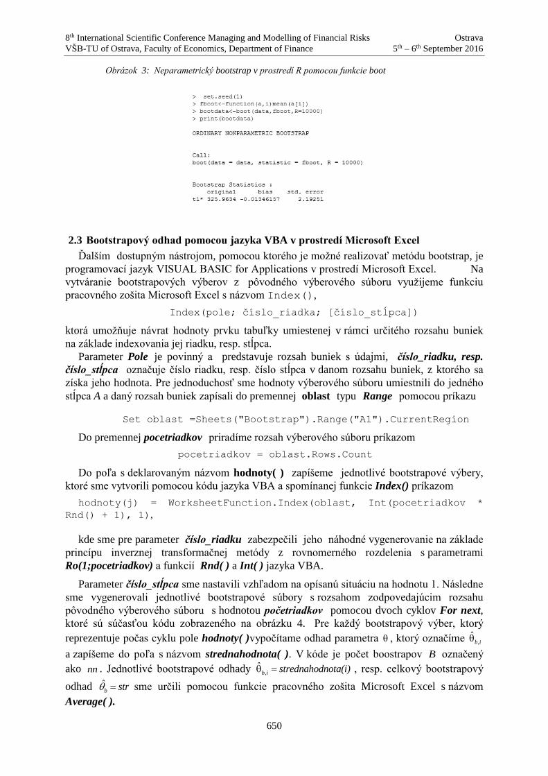
8th International Scientific Conference Managing and Modelling of Financial Risks Ostrava
VŠB-TU of Ostrava, Faculty of Economics, Department of Finance 5th – 6th September 2016
650
Obrázok 3: Neparametrický bootstrap v prostredí R pomocou funkcie boot
2.3 Bootstrapový odhad pomocou jazyka VBA v prostredí Microsoft Excel
Ďalším dostupným nástrojom, pomocou ktorého je možné realizovať metódu bootstrap, je
programovací jazyk VISUAL BASIC for Applications v prostredí Microsoft Excel. Na
vytváranie bootstrapových výberov z pôvodného výberového súboru využijeme funkciu
pracovného zošita Microsoft Excel s názvom Index(),
Index(pole; číslo_riadka; [číslo_stĺpca])
ktorá umožňuje návrat hodnoty prvku tabuľky umiestenej v rámci určitého rozsahu buniek
na základe indexovania jej riadku, resp. stĺpca.
Parameter Pole je povinný a predstavuje rozsah buniek s údajmi, číslo_riadku, resp.
číslo_stĺpca označuje číslo riadku, resp. číslo stĺpca v danom rozsahu buniek, z ktorého sa
získa jeho hodnota. Pre jednoduchosť sme hodnoty výberového súboru umiestnili do jedného
stĺpca A a daný rozsah buniek zapísali do premennej oblast typu Range pomocou príkazu
Set oblast =Sheets("Bootstrap").Range("A1").CurrentRegion
Do premennej pocetriadkov priradíme rozsah výberového súboru príkazom
pocetriadkov = oblast.Rows.Count
Do poľa s deklarovaným názvom hodnoty( ) zapíšeme jednotlivé bootstrapové výbery,
ktoré sme vytvorili pomocou kódu jazyka VBA a spomínanej funkcie Index() príkazom
hodnoty(j) = WorksheetFunction.Index(oblast, Int(pocetriadkov *
Rnd() + 1), 1),
kde sme pre parameter číslo_riadku zabezpečili jeho náhodné vygenerovanie na základe
princípu inverznej transformačnej metódy z rovnomerného rozdelenia s parametrami
Ro(1;pocetriadkov) a funkcií Rnd( ) a Int( ) jazyka VBA.
Parameter číslo_stĺpca sme nastavili vzhľadom na opísanú situáciu na hodnotu 1. Následne
sme vygenerovali jednotlivé bootstrapové súbory s rozsahom zodpovedajúcim rozsahu
pôvodného výberového súboru s hodnotou početriadkov pomocou dvoch cyklov For next,
ktoré sú súčasťou kódu zobrazeného na obrázku 4. Pre každý bootstrapový výber, ktorý
reprezentuje počas cyklu pole hodnoty( )vypočítame odhad parametra , ktorý označíme ,b i
a zapíšeme do poľa s názvom strednahodnota( ). V kóde je počet boostrapov B označený
ako nn . Jednotlivé bootstrapové odhady , b i strednahodnota(i) , resp. celkový bootstrapový
odhad ˆ b str sme určili pomocou funkcie pracovného zošita Microsoft Excel s názvom
Average( ).

8th International Scientific Conference Managing and Modelling of Financial Risks Ostrava
VŠB-TU of Ostrava, Faculty of Economics, Department of Finance 5th – 6th September 2016
651
strednahodnota(i) = WorksheetFunction.Average(hodnoty)
str = WorksheetFunction.Average(strednahodnota)
Obrázok 4: Ukážka kódu pre neparametrický bootstrap v prostredí jazyka VBA.
Hodnoty poľa strednahodnota( ) sú hodnotami odhadu strednej hodnoty základného
súboru určených na základe bootstrapovej štatistiky, t. j. aritmetického priemeru jednotlivých
bootstrapových výberov. V praktickej časti vytvoríme z týchto hodnôt histogram a získame
tak predstavu o pravdepodobnostnom rozdelení odhadu tohto parametra, t. j. strednej hodnoty
základného súboru.
3. Neparametrický bootstrap a odhad intervalov spoľahlivosti
V praktických aplikáciach sa častejšie využíva intervalový odhad, t. j. odhad príslušného
parametra základného súboru pomocou intervalu. Tento odhad je reprezentovaný intervalom
, d h , ktorý s danou pravdepodobnosťou bude obsahovať skutočnú hodnotu odhadovaného
parametra základného súboru. Táto pravdepodobnosť je spoľahlivosťou odhadu a označuje sa
c . Interval , d h sa nazýva 100 %c intervalom spoľahlivosti, resp. konfidenčný interval
pre parameter a platí
d hP c . (6)
Metód na určenie konfidenčného intervalu je niekoľko, napríklad klasické metódy
(opierajúce sa o kvantily normovaného normálneho rozdelenia, resp. Studentovho rozdelenia),
bootstrapové metódy (opierajúce sa empirické kvantily, t-bootstrap, BCA metóda a podobne).
Ich výsledky môžu byť v závislosti od hodnôt vo výberovom súbore kvalitou vypočítaného
intervalu rozdielne. V príspevku na odhad konfidenčných intervalov pre strednú hodnotu
( / )pE S S x použijeme dve metódy, ktoré využívajú princíp metódy bootstrap, a to
percentilovú bootstrap metódu (perc) a BCa metódu (BCa).
Klasický prístup sa opiera o predpoklad, že jej odhad x , t. j. výberový aritmetický
priemer sa riadi približne normálnym rozdelením. Z centrálnej limitnej vety Lindeberg-
Lévyho vyplýva, že pre dostatočne veľký rozsah hodnôt výberového súboru má výberový
aritmetický priemer X asymtoticky normálne rozdelenie t. j. 2
;
X Nn
, resp. náhodná

8th International Scientific Conference Managing and Modelling of Financial Risks Ostrava
VŠB-TU of Ostrava, Faculty of Economics, Department of Finance 5th – 6th September 2016
652
premenná
Xn má približne normované normálne rozdelenie [5]. Práve tento predpoklad
nemusí byť v prípade „malého” rozsahu výberového súboru splnený. Percentilová bootstrap
metóda sa na základe práce s empirickými kvantilmi javí v porovnaní s klasickým prístupom
ako vhodnejší prístup určenia konfidenčných intervalov. Jej výhoda spočíva určite v jej
jednoduchosti, ale na druhej strane nepracuje so samotným odhadom a jeho smerodajnou
odchýlkou, čo sa môže odzrkadliť na skreslení výsledkov. Pre kvalitnejší odhad
konfidenčných intervalov je potrebné zabezpečiť dostatočný počet bootstrapových odhadov
,b i . Metóda BCa predstavuje vylepšenie pre konštrukciu konfidenčných intervalov, pretože
poskytuje korekciu vychýlenia a zohľadňuje aj zošikmenosť, resp. špicatosť rozdelenia hodnôt
výberového súboru. BCa je považadovaná za metódu, ktorá poskytuje v porovnaní
s klasickými metódami, t-bootstrapom a podobne kvalitnejšie výsledky.
3.1 Percentilová bootstrap metóda pre konfidenčné intervaly
V tejto časti si uvedieme postup pre vytvorenie konfidenčného intervalu použitím tejto
metódy [1]:
1.Realizujeme B náhodných bootstrapových výberov (s opakovaním) o rozsahu n
z pozorovaných hodnôt 1,..., nx x náhodného výberu 1,..., nX X . Zvyčajne volíme 1000B .
2. Pre každý bootstrapový výber vypočítame odhad ,b i parametra .
3. - kvantil a 1 kvantil pravdepodobnostného rozdelenia bootstrapovej štatistiky b
odhadneme hodnotami ,ˆb a ,1
ˆb , ktoré spĺňajú čo najpresnejšie podmienky
; ; ;ˆ ˆ ˆ; /b i b i b B ; ; ;1
ˆ ˆ ˆ; / 1 b i b i b B ,
kde ... označuje veľkosť množiny, t. j. v tomto prípade počet jej prvkov.
4. Konfidenčným intervalom so spoľahlivosťou 1 2 c pre parameter platí
, ,1ˆ ˆ;b b (7)
Výhodou tejto metódy spočíva v jej jednoduchosti, pričom konfidenčné intervaly určené
touto metódou môžu vykazovať určitú mieru skreslenia hlavne v prípade viac zošikmených
rozdelení.
3.2 Metóda BCa pre konfidenčné intervaly
Môže sa stať, že konfidenčné intervaly sú vychýlené alebo sú príliš široké oproti hodnotám
pozorovaným v praxi. K odstráneniu týchto nedostatkov preto konštruujeme konfidenčné
intervaly metódou BCa (z anglického bias corrected and accelerated), ktorá je vylepšením
presnosti percentilových intervalov spoľahlivosti. Zlepšenie spočíva v tom, že výber kvantilu
závisí na dvoch parametroch a a 0z nazývaných akcelerácia a korekcia vychýlenia. Veličina
0z zjednodušene meria a odstraňuje vychýlenie mediánu odhadu daného parametra a jeho
bootstrapového odhadu a veličina a meria rýchlosť zmeny smerodajnej odchýlky
bootstrapového odhadu parametra.
Nech ˆ ˆ bG h P h predstavuje bootstrapový odhad distribučnej funkcie parametra .
Potom pre konfidenčný interval určený metódou BCa platí [2]
1 1ˆ ˆ, 1G z G z , (8)

8th International Scientific Conference Managing and Modelling of Financial Risks Ostrava
VŠB-TU of Ostrava, Faculty of Economics, Department of Finance 5th – 6th September 2016
653
kde
0
0
01
z zz z
a z z
a 1 z
Pre určenie konfidenčného intervalu musíme odhadnúť dva parametre 0,a z na základe
bootsrapového prístupu, tak že opäť realizujeme B náhodných bootstrapových výberov
(s opakovaním) o rozsahu n z pozorovaných hodnôt 1,..., nx x náhodného výberu. Zvyčajne
volíme 1000B . Potom z pozorovaných hodnôt 1,..., nx x vypočítame odhad parametra a
pre každý bootstrapový výber vypočítame odhad ,b i parametra . Korekciu 0z určíme zo
vzťahu
; ;
1
0
ˆ ˆ ˆ;
1
b i b i
zB
, (9)
kde je distribučná funkcia normovaného normálneho rozdelenia a ... označuje veľkosť
množiny t. j. v tomto prípade počet jej prvkov. Označme ˆ i odhad parametra vypočítaný
vynechanímiX z náhodného výberu 1,..., nX X , t. j. z náhodného výberu
1 1 1,..., , ,..., i i nX X X X . Ďalej označme
1
1ˆ ˆ
n
i
in
Potom akceleraciu a vypočítame v súvislosti s koeficientom zošikmenia (existuje
alternatíva pre špicatosť) podľa vzťahu [2]
3
1
3
22
1
ˆ ˆ
ˆ ˆ6
n
i
i
n
i
i
a . (10)
Potrebné kvantily 1ˆ G z a 1ˆ 1 G z odhadneme hodnotami b , ktoré
spĺňajú čo najpresnejšie podmienky
; ; ;ˆ ˆ ˆ; /b i b i b B ; ; ;1
ˆ ˆ ˆ; / 1 b i b i b B ,
kde ... označuje veľkosť množiny, t. j. v tomto prípade počet jej prvkov. Konfidenčným
intervalom BCa so spoľahlivosťou 1 2 c pre parameter platí
, ,1ˆ ˆ;b b (11)
3.3 Určenie konfidenčných intervalov v prostredí jazyka R
Pre určenie intervalov spoľahlivosti použijeme funkciu boot.ci balíka boot s následovnou
syntaxou [1]
> boot.ci(data,conf,type)
data – je označenie pre výstup funkcie boot,
conf – je spoľahlivosť intervalu,
type – je typ použitej metódy.

8th International Scientific Conference Managing and Modelling of Financial Risks Ostrava
VŠB-TU of Ostrava, Faculty of Economics, Department of Finance 5th – 6th September 2016
654
Funkcia má k dispozícií nasledovné možnosti voľby pre typ metódy: norm - klasické
aproximatívne vyjadrenie konfidenčného intervalu cez kvantily normovaného normálneho
rozdelenia, basic - jednoduchá bootstrap metóda, perc - percentilová metóda, bca - „bias
corrected and accelerated“ metóda
Obrázok 4: Určenie konfidenčného intervalu metódou BCA v prostredí R pomocou balíčka boot
Na určenie konfidenčných intervalov percentilovou metódou sme využili aj prostredie
jazyka VBA v Microsoft Excel. Na určenie kvantilov pravdepodobnostného rozdelenia
bootstrapovej štatistiky b sme využili funkciu pracovného zošita Microsoft Excel s názvom
Percentile ( ).
kvantil2 = Application.WorksheetFunction.Percentil(strednahodnota,
0.975)
4. Praktická realizácia
Na praktickú ukážku odhadu ( )pCVaR S sme si vybrali oblasť neživotného poistenia
s interným modelom portfólia poistných zmlúv a náhodnou premennou S , ktorá označuje
celkovú škodu. V prípade dostupnosti empirických údajov o celkovej škode získame výberový
súbor 1,..., nx x tak, že akceptujeme iba hodnoty, ktoré splnili podmienku ps x . Táto situácia
sa v praxi nevyskytuje tak často. Na získanie hodnôt celkovej škody S po štatistickom
spracovaní empirických údajov o počte škôd N a individuálnej výške škody X je možné
využiť simulačnú metódu Monte Carlo. Našou úlohou je z výberového súboru
1,..., nx x odhadnúť strednú hodnotu základného súboru / pS S x , ktorú reprezentuje
( )pCVaR S . Pomocou tejto miery rizika sa dá určiť kapitál potrebný pre zabezpečenie
záväzkov poisťovne. Z tohto dôvodu v súvislosti s vytvorením kvalitnej predikcie sústredíme
svoju pozornosť na odhad jej konfidenčných intervalov. Na realizáciu bootstrapových
odhadov použijeme výberový súbor s rozsahom 20n , ktorého hodnoty sú zobrazené na
obrázku. 5.

8th International Scientific Conference Managing and Modelling of Financial Risks Ostrava
VŠB-TU of Ostrava, Faculty of Economics, Department of Finance 5th – 6th September 2016
655
318,3582415 320,5670067 316,6812912 354,8636186 318,9747626 330,5288404
318,1735319 318,3918485 333,5226104 340,9731441 334,6853423 324,4523571
324,9209112 318,7544872 325,4525535 322,9517174 320,236376 330,0151613
317,0804136 324,553904
x<-c(100,500,1000,1500,3000,5000,10000)
y1<-c(-0.09632617,0.09533146,0.001123351,-0.01291797,0.01558909,
- 0.002600598,-0.01346157)
y2<-c(0.05714864,0.0425767,-0.02539113,0.01352994,-0.02095074,-
0.0258149,
-0.01523087)
y3<-c(-0.05543,-0.0175,-0.0166,0.0195,-0.0031,0.0018,-0.00272)
plot(x,y1,type="o",col=1,main="závislosť vychýlenia bias od počtu
realizácii metódy bootstrap ",xlab="B",ylim=c(-0.2,0.2),
ylab="bias",
pch=22,bg=3,cex=2)
lines(x,y2 , type="o", col=1,pch=24,bg=4,cex=2)
lines(x,y3, type="o", col=1,pch=23,bg=5,cex=2)
Obrázok 5: Hodnoty výberového súboru 1 20,...,x x náhodnej premennej / pS S x
Bootstrapový odhad sme zrealizovali v prostredí jazyka R pomocou balíčka boot
prostredníctvom príkazov, ktoré sme opísali v druhej kapitole príspevku, obrázok 6.
Obrázok 6: Bootstrapový odhad vychýlenia ˆBias v prostredí R pomocou funkcie boot
Z výstupu v prostredí R sme pre bootsrapový odhad ( )pCVaR S na základe vzťahu (5)
určili jeho hodnotu
( ) 325,7118037pCVaR S .
V nasledujúcej časti príspevku si graficky ukážeme ako závisí vychýlenie bootstrapového
odhadu ( ˆb od odhadu ) strednej hodnoty náhodnej premennej / pS S x od počtu
bootstrapových realizácií pre tri porovnateľné výberové súbory, obrázok 7. Graf sme zobrazili
v rámci grafického rozhrania (R Graphics) pomocou príkazu Plot, ktorý zadáme v okne R
Console s následovnou syntaxou [6].

8th International Scientific Conference Managing and Modelling of Financial Risks Ostrava
VŠB-TU of Ostrava, Faculty of Economics, Department of Finance 5th – 6th September 2016
656
Obrázok 7: Grafická prezentácia bootstrapového odhadu vychýlenia bias pre počet bootstrapových opakovaní
100;500;1000;1500;3000;5000;10000B v troch prípadoch výberového súboru náhodnej premennej
/ pS S x
Z obrázku 7 je zrejmé, že pre naše údaje je (aj vzhľadom na zobrazený rozsah
vychýlenia) dostačujúci počet bootstrapových realizácií na úrovni 1000B a so zväčšujúcim
sa počtom opakovaní (napríklad 10000B ) sa bootstrapový odhad ˆb ešte presnejšie
približuje ku odhadu vo všetkých troch prípadoch. Porovnateľnú hodnotu pre počet
bootstrapových opakovaní 100000B sme získali aj pomocou jazyka VBA. Rovnaký balíček
sme použili aj na odhad konfidenčných intervalov percentilovou metódou a metódou BCa,
ktoré sme opísali v tretej kapitole príspevku, obrázok 8.
Obrázok 8: Určenie konfidenčného intervalu metódou BCa a percentilovou metódou v prostredí R pomocou
balíčka boot
Pre odhadnuté konfidenčné intervaly metódou BCa a perc sme so spoľahlivosťou 0,95 teda
dostali výsledky:
( ) 322,5;331,2BCa pCVaR S ( ) 322;330,2perc pCVaR S
Obe metódy je možné uskutočniť aj v jazyku VBA na základe algoritmov opísaných
v tretej kapitole. Konfidenčné intervaly sme určili percentilovou metódou pomocou oboch
jazykov VBA, resp. R a dosiahli sme porovnateľné výsledky, ktoré sme v prostredí R graficky
znázornili v závislosti od počtu bootstrapových opakovaní, obrázok 9.

8th International Scientific Conference Managing and Modelling of Financial Risks Ostrava
VŠB-TU of Ostrava, Faculty of Economics, Department of Finance 5th – 6th September 2016
657
set.seed(1)
u0<-mean(data)
bstat<- NULL
for(i in 1:10000){vyber<-sample(data,20,replace=TRUE)
u<-mean(vyber)
bstat[i]<-u}
hist(bstat,breaks=30,xlim= c(315,340))
Obrázok 9: Grafická prezentácia odhadu konfidenčného intervalu percentilovou metódou pre počet
bootstrapových opakovaní 50;100;500;1000;5000B
Z grafu na obrázku 9 je zrejmé, že pre „malý” počet opakovaní sa „šírka“ konfidenčného
intervalu mení a „ustálenú“ hodnotu nadobúda pri počte bootstrapových realizácií 1000B .
Súvisí to s určovaním empirických kvantilov bootstrapovej štatistiky, ktoré si pre získanie
kvalitnejšieho výsledku vyžadujú „väčší“ počet spracovaných údajov. Podobný efekt sa
vyskytuje aj v prípade metódy BCa, ktorá v konečnom dôsledku tiež využíva empirické
kvantily. V prípade nedostatočného počtu realizácií nás výstup v prostredí R upozorní na
možnú „nestabilitu“ dosiahnutých výsledkov.
Na záver sa budeme venovať získaniu informácií o pravdepodobnostnom rozdelení
bootstrapovej štatistiky, v tomto prípade výberového aritmetického priemeru jednotlivých
bootstrapových výberov ,b i , na základe ktorého odhadujeme strednú hodnotu náhodnej
premennej / pS S x .
Túto úlohu sme realizovali aj pomocou jazyka VBA postupom popísaným v druhej
kapitole a z hodnôt poľa strednahodnota vytvorili histogram. V tejto časti príspevku
uvedieme aj spôsob pre získanie hodnôt ,b i v jazyku R a to pomocou nasledujúcich príkazov,
resp. funkcie sample [3].
Na základe vizuálneho posúdenia zostrojeného histogramu môžeme konštatovať, že
pravdepodobnostné rozdelenie bootstrapovej štatistiky, ktorá reprezentuje v zmysle odhadu
strednú hodnotu náhodnej premennej / pS S x nie je symetrické, je pravostranne zošikmené,
obrázok 10. Potvrdzuje to aj hodnota koeficientu zošikmenia odhadnutá pomocou funkcie
skewness balíčka moments.

8th International Scientific Conference Managing and Modelling of Financial Risks Ostrava
VŠB-TU of Ostrava, Faculty of Economics, Department of Finance 5th – 6th September 2016
658
Obrázok 10: Histogram zostrojený z hodnôt bootstrapovej štatistiky v prostredí R pre 10000B
bootstrapových opakovaní
Na základe tejto informácie je zrejmé, že nie je splnený predpoklad o normálnom
rozdelení výberového priemeru a odhad konfidenčných intervalov prostredníctvom klasickej
metódy norm, by sme nemohli považovať za „dosť“ kvalitný. Pre porovnanie výsledkov
odhadu konfidenčných intervalov s metódami perc a BCa uvedieme aj odhad konfidenčného
intervalu určeného metódou norm v prostredí jazyka R, obrázok 11.
Obrázok 11: Určenie konfidenčného intervalu metódou norm v prostredí R pomocou balíčka boot
Pre odhadnutý konfidenčný interval metódou norm sme so spoľahlivosťou 0,95 dostali
výsledok:
( ) 321,6;329,8norm pCVaR S
Naše úvahy o tom, že bootstrapová štatistika sa neriadi normálnym rozdelením, môžu
potvrdiť aj údaje poskytnuté funkciou summary v prostredí jazyka R, resp. Andersonov –
Darlingov test normality, ktorý je súčasťou balíka nortest.
5. Záver
Na základe poznatkov uvedených v príspevku považujeme za „najkvalitnejší” výsledok
odhad konfidenčného intervalu metódou BCa, t. j. ( ) 322,5;331,2pCVaR S . Presvedčili sme
sa, že v prípade „nenáročnej” štatistiky, akou je výberový aritmetický priemer, je v prípade
metódy bootstrap postačujúci počet opakovaní na úrovni 1000B . Realizácia percentilovej
metódy je jednoduchá, využíva prácu s empirickými kvantilmi, ale v porovnaní s metódou
BCa môžu jej výsledky vykazovať prvky nepresnosti. Metóda bootstrap (napríklad
t-bootstrap, basic bootstrap, BCa, ABC) je v súvislosti s využitím klasického prístupu viac
preferovaná. Odhad konfidenčných intervalov môže v prípade „malých” výberových súborov
8th International Scientific Conference Managing and Modelling of Financial Risks Ostrava
VŠB-TU of Ostrava, Faculty of Economics, Department of Finance 5th – 6th September 2016
659
poskytovať pri klasickom prístupe skreslené výsledky. Dôležitou úlohou zo strany aktuára je
v rámci vytvoreného interného modelu zabezpečiť plnenie záväzkov poisťovne, vytvorením
potrebného kapitálu. A keďže sa jeho hodnota určuje pomocou ( )pCVaR S , je potrebné
aj v jeho prípade určiť intervalový odhad založený na konfidenčnom intervale pre ( )pCVaR S .
Príspevok poukazuje na možnosť realizácie algoritmov vybraných bootstrapových metód
prostredníctvom procedúr vytvorených v prostredí jazyka VBA, resp. jazyka R, ktorý už nimi
disponuje v rámci jednotlivých balíčkov. Aktuár by tak mal v rámci realizácie odhadov
klasickými prístupmi venovať pozornosť aj bootstrapovým prístupom s cieľom dosiahnúť
presnejšie výsledky.
References
[1] Davison, A. C. and Hinkley, D. V. (1997). Bootstrap Methods and Their Applications.
Cambridge: Cambridge University Press.
[2] Chernick, R. M. and LaBudde A. R. (2011). Bootstrap Methods with Applications to R.
Hoboken, New Jersey: John Wiley & Sons., Inc.
[3] Páleš M. (2014). Generating a Pseudo-Random Automobile Insurance Portfolio in R.
Managing and Modelling of Financial Risks. Ostrava: VŠB - Technical University,
p. 621-626
[4] Horáková, G., Páleš, M., Slaninka, F. (2015). Teória rizika v poistení. Bratislava: Wolters
Kluwer
[5] Hindls R., Hronová S., Seger J., Fischer J. (2006). Statistika pro ekonomy. 7th ed. Praha:
Professional Publishing.
[6] W. N. Venables, D. M. Smith, and the R Development Core Team (1990-2013). An
Introduction to R, [online] Available at: < https://cran.r-project.org/manuals.html>
[Accessed 20 June 2016].
Príspevok vznikol za podpory výskumneho projektu VEGA Kalkulácia SCR na krytie
rizík neživotného poistenia v súlade s potrebami praxe číslo 1/ 1/0806/14.

8th International Scientific Conference Managing and Modelling of Financial Risks Ostrava
VŠB-TU of Ostrava, Faculty of Economics, Department of Finance 5th – 6th September 2016
660
Quantification of credit risk models
Hussam Musa1, Peter Krištofík2, Peter Sliacky3
Abstract
Credit risk is an unseparated part of financial risk. The credit risk of the company is often
discussed also as the risk of the company default, which is usually associated with the
bankruptcy of the company. Credit risk or default risk involves inability or unwillingness of a
customer or counterparty to meet commitments in relation to any financial transactions. The
Credit Risk is generally made up of transaction risk or default risk and portfolio risk.
Difficulties in credit risk modelling arise due to the fact that the company default occurs mainly
unexpectedly. However, if the default occurs, it often causes the creditors major losses which
size cannot be quantified in advance. The issue of modelling and quantification of credit risk is
the subject of present contribution. The aim of contribution is to analyse and to compare the
basic approaches of credit risk quantification. We have chosen two specific models:
CreditRisk+ and CreditMetrics. The CreditRisk+ model analytically determines the portfolio
credit losses distribution that is caused by defaults of counterparties. In the CreditMetrics
model, the credit migration risk is additionally considered and the future portfolio value
distribution is calculated using the Monte Carlo simulation.
Key words
Company default, CreditRisk+, CreditMetrics, Credit risk modelling
JEL Classification: G32, G34
1. Úvod
Podstupovanie rizika je neoddeliteľnou súčasťou každej podnikateľskej, či investičnej
činnosti. Pre úspech v týchto činnostiach je dôležité riziku venovať veľkú pozornosť, naučiť
sa merať riziko a prispôsobiť svoje kroky a rozhodnutia možným následkom, ktoré riziko
prináša. Rozhodnutiu, či podstúpime riziko, ktoré sme identifikovali a kvantifikovali sa
hovorí manažment alebo riadenie rizika.
Pojem riziko je známy od 17. storočia, kedy boli prvé termínové obchody s tulipánmi
v Holandsku, alebo s ryžou v Japonsku. Následne sa začal vyvíjať obchod s dlhopismi
a cennými papiermi. Riadeniu rizík sa začali venovať bankové a finančné inštitúcie kvôli
poskytovaniu úverov a riadeniu likvidity. Najväčší vývoj v riadení rizík nastal po páde
Bretton-Woodskeho menového systému v 70. rokoch 19. storočia. Následne v 90. rokoch
s rozmachom obchodovania s finančnými derivátmi sa začali riadeniu rizík venovať aj bežné
podniky (Smejkal, Rais, 2006).
Riziká sa vo všeobecnosti klasifikujú podľa zdroja, odkiaľ pochádza neistota. Smejkal
a Rais (2006) delia riziká na finančné a nefinančné. Predkladaný článok sa venuje kreditnému
riziku, ktoré patrí medzi finančné riziká a ide o riziko straty zapríčinené zmenou schopnosti
dlžníka splácať svoje záväzky. Autori ďalej medzi finančné riziká radia trhové riziko (neistota
1 doc. Ing. Hussam Musa, PhD., Faculty of Economics, Matej Bel University in Banská Bystrica,
Tajovského 10, Banská Bystrica 975 90, Slovakia, [email protected] 2 doc. Ing. Peter Krištofík, PhD. Faculty of Economics, Matej Bel University in Banská Bystrica,
Tajovského 10, Banská Bystrica 975 90, Slovakia, [email protected] 3 Ing. Peter Sliacky, Faculty of Economics, Matej Bel University in Banská Bystrica, Tajovského 10,
Banská Bystrica 975 90, Slovakia, [email protected]

8th International Scientific Conference Managing and Modelling of Financial Risks Ostrava
VŠB-TU of Ostrava, Faculty of Economics, Department of Finance 5th – 6th September 2016
661
plynúca zo zmien trhových cien a ich dopadu na zisk), riziko likvidity (riziko, že podnik
nebude mať v istom okamihu dostatok finančných prostriedkov) a operačné riziko (riziko
ľudskej chyby, respektíve zlyhania systému).
2. Kreditné riziko
Kreditné riziko na rozdiel od ostatných finančných rizík vyplýva priamo z vnútornej
povahy danej investície. Je rizikom straty vyplývajúcej z možnosti zlyhania subjektu
(dlžníka), resp. protistrany tým, že nesplní svoje záväzky podľa podmienok kontraktu. Podľa
Gronchyovej (2008) existujú dve príčiny vzniku rizika straty kapitálu:
Insolventnosť subjektu alebo protistrany – priame úverové riziko a riziko vysporiadania
Zmeny kvality ratingu subjektu – zmeny kreditnej prémie
Kľúčovým aspektom kreditného rizika je posúdenie schopnosti zmluvného partnera
splácať svoje záväzky. Subjekty môžu posudzovať túto schopnosť svojim vlastným interným
hodnotiacim systémom, avšak častokrát prenechajú túto úlohu špecializovanej ratingovej
agentúre, ako napríklad Moody´s. Podstatnou rolou pri posudzovaní je nájsť všetky
smerodajné rizikové faktory a priradiť im váhy podľa miery dôležitosti a vplyvu jednotlivých
faktorov (Crosbie and Bohn, 2003).
Analyticky je možné kreditné riziko rozložiť na niekoľko základných zložiek. Cisko
a Klieštik (2013) prezentujú toto rozloženie na základnom dvoj-parametrickom modeli, ktorý
je založený na riziku protistrany a riziku produktu. Na základe tohto modelu je možné
celkovú očakávanú stratu vyjadriť nasledovne:
E(L) = E(A) . P(d) . L(d)
E(A) – očakávaná riziková angažovanosť v okamihu neplnenia záväzkov protistranou
P(d) – pravdepodobnosť neplnenia protistrany
L(d) – očakávaná výška straty v prípade neplnenia
Pri riadení a odhadovaní rizika sa využívajú tiež jedno-parametrické a troj-parametrické
modely. Využitie jedno-parametrických modelov je v praxi veľmi malé, pretože nezohľadňujú
dostatočné parametre pre zložitejšie portfóliá. Používajú sa hlavne pri portfóliách s veľmi
štandardizovanými produktmi alebo pri veľmi bonitných inštrumentoch. Troj-parametrické
modely navyše zohľadňujú oproti základnému modelu vývoj výšky rizikovej angažovanosti
v čase. Tretím parametrom je teda angažovanosť pri neplnení záväzkov, ktorou je očakávaná
hodnota pohľadávky v okamihu, kedy nie je plnenie záväzku (Vlachý, 2006, s.149).
Podľa Mernu (2007 s. 47) sa pre odlíšenie rizík s vysokým dopadom od rizík s nízkym
dopadom využíva nasledovný maticový diagram (Schéma 1). Diagram rozdeľuje
pravdepodobnosť a dopad rizika do štyroch kategórií.

8th International Scientific Conference Managing and Modelling of Financial Risks Ostrava
VŠB-TU of Ostrava, Faculty of Economics, Department of Finance 5th – 6th September 2016
662
Schéma 1: Maticový diagram dopadu rizika
Zdroj: vlastné spracovanie podľa Merna (2007, s. 47)
Merna (2007, s. 47) klasifikuje jednotlivé kategórie nasledovne: šteňatá – projekty
s vysokou pravdepodobnosťou neočakávaných udalostí, ale nízkym dopadom. To znamená,
že je vysoká pravdepodobnosť insolventnosti, ale len krátkodobo, respektíve správnym
manažmentom sa to dá rýchlo napraviť. Tigre – projekty s vysokou pravdepodobnosťou
a dopadom neočakávaných udalostí, čo ich robí nebezpečnými a je potrebné ich rýchlo
neutralizovať. Mačatá – projekty s nízkou pravdepodobnosťou a dopadom neočakávaných
udalostí, čo je ideálny stav pre realizáciu. Aligátory – projekty s nízkou pravdepodobnosťou
neočakávaných udalostí, ale s vysokým dopadom. To znamená, že je nebezpečné takýto
projekt realizovať, ale dá sa nebezpečenstvu vyhnúť.
3. Vybrané modely kvantifikácie kreditného rizika
Posudzovanie bonity klientov, resp. rizikovosti portfólia v minulosti prebiehalo hlavne
prostredníctvom individuálnej analýzy. Dnes sa na toto posudzovanie prevažne využívajú
takzvané scoringové modely, ktoré zohľadňujú pri kvantifikácii rizika viacero parametrov
(Mišánková, Kočišová & Adamko, 2014).
Cisko a Klieštik (2013) rozdeľujú modely na základe definície rizík na dve základné
kategórie. Prvou je skupina modelov „Default-mode“, ktoré sa zameriavajú na predikciu strát
spôsobených defaultom, pričom berú do úvahy len dve možnosti, zlyhanie a nezlyhanie.
Druhou skupinou sú modely „Mark-to-market“, ktoré sa zameriavajú na zmeny trhovej
hodnoty úveru a pomocou ratingových systémov determinujú zmeny kvality úverového
dlžníka. V článku sa ďalej venujeme definícii a porovnávaniu modelov CreditMetrics
a CreditRisk+ z ktorých každý je zástupcom jednej z uvedených skupín modelov.
3.1 Credit Metrics
Tento model patrí do skupiny modelov „Mark-to-market“, pretože odhaduje zlyhania
emitenta na základe zmeny ratingu. Podľa Adamka, Klieštika a Birtusa (2014) analýza celého
portfólia vychádza z posúdenia kreditného rizika jednotlivých inštrumentov. Model bol
vytvorený v roku 1997 bankou J.P. Morgan a od roku 1999 sa stal súčasťou manažmentu
kreditného rizika v skoro všetkých popredných bankách. Podľa Jaroša a kol. (2014) je vývoj
modelov v turbulentnej dobe veľmi dôležitý, čo vidieť aj na modeli CreditMetrics, ktorý sa
konštantne vyvíjal a stal sa dostatočne flexibilný, aby dokázal reagovať na vývoj trhu
a regulačné opatrenia.
Šteňatá Tigre
Mačatá Aligátory
vysoký dopad nízky dopad
vysoká pravdepodobnosť
nízka

8th International Scientific Conference Managing and Modelling of Financial Risks Ostrava
VŠB-TU of Ostrava, Faculty of Economics, Department of Finance 5th – 6th September 2016
663
CreditMetrics je model merania kreditného rizika portfólia, ktorý premieta zmeny
v kredibilite dlžníka do zmien vo výške možných strát. Meria neistotu budúcej hodnoty
portfólia, zapríčinenú možnou migráciou v kreditnej kvalite emitenta, pričom berie do úvahy
okrem defaultu aj zmeny v ratingu dlžníka a ich vplyv na hodnotu portfólia (Kollar, Weissova
& Siekelova, 2015). Ohodnocuje teda nie len riziko defaultu ale aj riziko kreditného spreadu.
Schéma 2: Schéma modelu CreditMetrics
Zdroj: vlastné spracovanie podľa J. P. Morgan (1997)
Podľa dokumentu banky J. P. Morgan (1997) model CreditMetrics pozostáva zo štyroch
základných častí (Schéma 2). Prvou je kreditná hodnota v riziku (VaR – Value at Risk), ktorá
je základnou časťou tohto modelu spoločne s kreditnou portfóliovou hodnotou v riziku.
Treťou časťou je korelácia a poslednou je expozícia. Spoločne tieto časti reflektujú riziko
celého portfólia. Ako vidieť na Schéme 2, prvá časť z troch krokov zobrazuje riziko pre jeden
inštrument pomocou smerodajnej odchýlky a percentilu. Druhá, tretia a štvrtá časť potom
identifikujú kreditné riziko celého portfólia.
3.2 Credit Risk+
Credit Risk+ je metóda výpočtu rozdelenia možných kreditných strát portfólia, ktorú
vyvinula banka Credit Suisse v roku 1997. Používa sa pre stanovenie rizika pre pôžičky,
deriváty a tiež obchodovateľné dlhopisy, ako v maloobchode, tak v korporátnom odvetví.
Metóda je založená na portfóliovom prístupe k modelovaniu rizika defaultu, pričom berie do
úvahy informácie týkajúce sa veľkosti a splatnosti inštrumentov, kreditnej kvality
a systematického rizika dlžníka (Credit Suisse, 1997).
Model CreditRisk+ patrí do skupiny „Default-mode“ modelov kvantifikácie kreditného
rizika. Je to statický model kvantifikácie kreditného rizika, resp. určovania defaultu, ktorý
nevytvára predpoklady o príčinách defaultu, ale predpokladá, že defaulty sa vyskytujú v slede
udalostí tak, že nie je možné predpovedať presný čas ich výskytu ani ich počet (Klieštik &
Cúg, 2015). Model si vyžaduje len niekoľko vstupov, a to: expozíciu, defaultné miery pre
každý inštrument, volatilitu jednotlivých defaultných mier a mieru návratnosti pri defaulte.
Portfólio Ratingová história,
akciová história
Kreditný
spread
Charakteristika
inštrumentu Kreditný rating
Expozícia Kreditný VaR Korelácia
Trhová
volatilita
Pravdepodobnosť
migrácie medzi
ratingmi
Náhrada pri
zlyhaní
Súčasná
hodnota
inštrumentu
Modely
(napr.
korelačné)
Rozloženie
expozície Smerodajná odchýlka hodnoty daná zmenou kvality
ratingu pre jeden inštrument
Združená zmena
kreditného
ratingu
Kreditné portfólio VaR

8th International Scientific Conference Managing and Modelling of Financial Risks Ostrava
VŠB-TU of Ostrava, Faculty of Economics, Department of Finance 5th – 6th September 2016
664
Jednotlivé komponenty metódy, ale aj modelu CreditRisk+ zobrazuje Schéma 3 podľa Credit
Suisse Firs Boston International (1997).
Schéma 3: Komponenty metódy CreditRisk+
Zdroj: vlastné spracovanie podľa Credit Suisse First Boston International (1997)
Podľa Klieštika a Cúga (2015) kvantifikáciu kreditného rizika modelom CreditRisk+
ovplyvňujú vo výraznej miere aj vonkajšie faktory, ako je napríklad stav ekonomiky, pretože
môžu zapríčiniť koreláciu medzi jednotlivými defaultmi. Deje sa tak aj napriek tomu, že
normálne medzi nimi nie je žiadny vzťah. Efekty týchto faktorov sú zapracované do modelu
CreditRisk+ pomocou volatilít defaultných mier a analýzy sektorov namiesto použitia
korelácií defaultov ako priameho vstupu do modelu.
4. Záver
Modely kvantifikácie kreditného rizika je možné porovnávať na základe kľúčových
veličín, ako sú definovanie rizika, zdroje rizika, požadované údaje, charakteristika a volatilita
kreditnej udalosti, výnosové percento, číselné vyjadrenie modelu a klasifikácia nebezpečnosti
(Saunders & Allen, 2002). Modely CreditMetrics a CreditRisk+ sa líšia v mnohých
aspektoch, požadujú rôzne vstupné dáta, majú iné predpoklady, využívajú rôzne prístupy
a líšia sa výstupmi. Tieto základné rozdiely porovnáva Tabuľka 1.
Tabuľka 1: Porovnanie modelov CreditMetrics a CreditRisk+
CreditMetrics CreditRisk+
Autor J.P. Morgan Credit Suisse
Typ modelu Mark-tomarket Default-mode
Definícia rizika riziko kreditného spreadu a defaultu riziko defaultu
Zdroj rizika pravedpodobnosť defaultu
Požadované dáta
historická matica migrácie, kreditné
spready, výnosová krivka, miery
návratnosti, korelácia, výška
expozícií
defaultné miery a ich volatilita,
informácie o vonkajších
faktoroch, miery návratnosti,
výška expozícií
Charakteristika
kreditnej udalosti kreditná migrácia
náhodná pravdepodobnosť
defaultu
Volatilita kreditnej
udalosti konštantná alebo náhodná náhodná
Miera návratnosti náhodná (Beta rozdelenie) konštantná v rámci skupiny
Numerický prístup simulačný aj analytický analytický
Klasifikácia rizika ratingy expozícia skupín
Hlavný výstup rozdelenie hodnôt portfólia rozdelenie strát portfólia
Zdroj: vlastné spracovanie podľa Saunders & Allen (2002)
CreditRisk+
Meranie kreditného rizika Ekonomický kapitál Aplikácia metodiky
CreditRisk+ model
- Expozície
- Defaultné miery
- Volatilita defaultných mier
- Miera návratnosti pri
defaulte
Rozdelenie strát
kreditného defaultu
Analýza scenárov
Provízie
Limity
Manažment portfólia

8th International Scientific Conference Managing and Modelling of Financial Risks Ostrava
VŠB-TU of Ostrava, Faculty of Economics, Department of Finance 5th – 6th September 2016
665
Porovnávané modely sa líšia tiež v rýchlosti ich výpočtu. Výpočet modelu CreditRisk+,
ktorý je počítaný analytickou metódou je oveľa rýchlejší, ako výpočet metódy CreditMetrics,
ktorá využíva simulačné modely. Ďalším rozdielom je prístup týchto modelov k miere
defaultu. Model CreditMetrics považuje mieru defaultu za diskrétnu, pričom model
CreditRisk+ za spojitú veličinu. Tieto prístupy predstavujú rôzne chovanie miery zlyhania.
References
[1] Adamko, P., Klieštik, T., & Birtus, M. (2014). History of Credit Risk Models. Advances
in Education Research, 61(2014), 148-153.
[2] Cisko, Š., Klieštik T. 2013. Finančný manažment podniku. Žilina: EDIS Publishers,
University of Žilina
[3] Credit Suisse First Boston International, 1997. CreditRisk+ [pdf], Available at:
http://www.csfb.com/institutional/research/assets/creditrisk.pdf [Accessed 15. August
2016]
[4] Crosbie, P., Bohn, J. 2003. Modeling Default Risk. [pdf]. Available at:
<http://www.macs.hw.ac.uk/~mcneil/F79CR/Crosbie_Bohn.pdf> [Accessed 14. August
2016]
[5] Gronychová, M. 2008. Měření kreditního rizika model CreditMetrics [pdf], Available
at: <http://www.actuaria.cz/upload/Kreditni riziko.pdf> [Accessed 13.August 2016]
[6] Jaros, J., Melichar, V., Svadlenka, L. 2014. Impact of the Financial Crisis on Capital
Markets and Global Economic Performance. 18th International Conference on
Transport Means, Kaunas Lithuania pp. 431-434
[7] J. P. Morgan 1997. CreditMetricsTM - Technical Document [pdf], Available at:
<http://www.defaultrisk.com/ pdf6j4/creditmetrics techdoc.pdf> [Accessed 16. August
2016]
[8] Klieštik, T., Cúg, J. 2015. Comparison of Selected Models of Credit Risk. Procedia
Economics and Finance 23(2015), pp. 356-361
[9] Kollar, B., Weissova, I., Siekelova, A. 2015. Quantification of credit risk with the use of
CreditMetrics. Procedia Economics and Finance 26(2015) pp. 311-316
[10] Merna, T. 2007. Risk management: řízení rizika ve firmě. Brno: Computer Press.
[11] Mišanková, M., Kočišová, K., & Adamko, P. 2014. CreditMetrics and its use for the
Calculation of Credit Risk. Advances in Education Research, 61(2014), 124-129
[12] Saunders, A., Allen, L. 2002. Credit Risk Measurement: New Approaches to Value at
Risk and Other Paradigms. Wiley, New York
[13] Smejkal, V., Rais, K. 2006. Řízení rizik ve firmách a jiných organizacích. Praha: Grada
Publishing,
[14] Vlachý, J. 2006. Řízení finančních rizik. Praha: Vysoká škola finanční a správní.

8th International Scientific Conference Managing and Modelling of Financial Risks Ostrava
VŠB-TU of Ostrava, Faculty of Economics, Department of Finance 5th – 6th September 2016
666
Financing of small and medium sized enterprises in selected EU countries
Hussam Musa, Zdenka Musová, Zuzana Stroková 1
Abstract
In Europe, small and medium sized enterprises (SMEs) are the source of economic growth and
new jobs. These enterprises, however, often face problems finding money to finance their
research, develop new products or access new markets. Access to finance represents one of the
most significant challenges for SMEs. To ensure SMEs creation, existence and growth it is
vitally important to understand the financing needs of SMEs, the main barriers to finance
availability and accessibility. The aim of this paper is to briefly present the results of surveys
about financing SMEs in selected EU countries. The study highlight the differences and
obstacles in SMEs financing in selected EU countries. The paper focuses on the results of the
own empirical survey about financing SMEs in Slovak Republic.
Key words
Financing, bank loan, bank overdraft, small and medium sized enterprises
JEL Classification: G23, G24, G28
1. Úvod
Malé a stredné podniky sú považované za hybnú silu vyspelých trhových ekonomík.
Význam tohto segmentu spočíva nielen vo funkciách, ale aj v postavení, ktoré zastáva
v národnom hospodárstve (Malá, Sedliačiková and Kaščáková, 2015). Veľkou prekážkou
v rozvoji malých a stredných podnikov bola v posledných rokoch globálna finančná
a hospodárska kríza a jej následky, ktoré zanechali výrazné stopy nielen vo finančnom, ale aj
nefinančnom sektore. Kríza znamenala závažný externý šok aj pre malé a stredné podniky na
Slovensku (ďalej len “MSP”), ktoré pocítili jej dopady najmä v poklese príjmov, úbytku
objednávok, zhoršení platobnej disciplíny (prvotná a druhotná platobná neschopnosť) či v
sprísnení podmienok poskytovania bankových úverov.
Podľa prieskumu Európskej komisie (2015a) sa podnikateľská populácia skladá takmer
výlučne z MSP vo všetkých členských štátoch. Podiel MSP na celkovej podnikovej populácii
sa pohybuje v intervale od 99,5 % (Luxembursko, Nemecko) po viac ako 99,9 %
(Portugalsko, Taliansko a Grécko). Kým MSP tvoria prakticky rovnaký podiel na celkovom
počte podnikov pôsobiacich v členských štátoch, ich ekonomický prínos sa výrazne odlišuje
(napr. v roku 2014 sa počet MSP na milióne eur pridanej hodnoty v nefinančnom sektore
1 doc. Ing. Hussam Musa, PhD., Univerzita Mateja Bela v Banskej Bystrici, Ekonomická fakulta,
Katedra financií a účtovníctva, Tajovského 10, 975 90 Banská Bystrica, Slovenská republika, e-mail:
doc. Ing. Zdenka Musová, PhD., Univerzita Mateja Bela v Banskej Bystrici, Ekonomická fakulta,
Katedra ekonomiky a manažmentu podniku, Tajovského 10, 975 90 Banská Bystrica, Slovenská
republika, e-mail: [email protected]
Ing. Zuzana Stroková, PhD., Univerzita Mateja Bela v Banskej Bystrici, Katedra financií a
účtovníctva, Tajovského 10, 975 90 Banská Bystrica, Slovenská republika, e-mail:

8th International Scientific Conference Managing and Modelling of Financial Risks Ostrava
VŠB-TU of Ostrava, Faculty of Economics, Department of Finance 5th – 6th September 2016
667
pohyboval v rozpätí od 2 v Luxembursku po 27 v Bulharsku). Celkovo možno povedať, že
väčšina stredoeurópskych krajín je charakteristická vysokým počtom MSP na milióne eur
vytvorenej pridanej hodnoty v porovnaní so západoeurópskymi krajinami. Význam MSP je
daný nielen ich podielom na najdôležitejších ukazovateľoch národného hospodárstva, ale
môžeme pozorovať aj ich ďalšie ekonomické a spoločenské prínosy.
Medzi spoločenské prínosy MSP môžeme zaradiť zabezpečenie garancie slobody
a stabilizácie spoločnosti a reprezentáciu miestneho kapitálu. Podľa Vebera, Srpovej a kol.
(2012) sú MSP garanciou zabezpečenia tých najbežnejších slobôd. Dávajú šancu
k slobodnému uplatneniu občanov – podnikateľov, dávajú šancu k realizácii ľudí
v produktívnom procese. MSP nemôžu dosiahnuť monopolné postavenie, sú vlastne
protipólom ekonomickej a politickej moci. Existencia MSP stabilizuje spoločnosť, pretože
akákoľvek výrazná politická neistota a radikálne prúdy sú pre ne zdrojom rizík. Keďže sú
MSP zväčša vlastnené domácimi subjektmi (vlastníctvo zahraničným subjektom je skôr
výnimočné), môžeme povedať, že segment MSP reprezentuje miestne vlastnícke pomery.
Ekonomické oživenie regiónu vedie väčšinou prostredníctvom podpory MSP v danom
regióne, pretože efekty z podnikania týchto podnikov ostávajú v danej oblasti.
Ekonomické prínosy MSP môžeme rozdeliť do troch oblastí, a to: MSP sú protipólom
monopolov, sú flexibilné a sú neoddeliteľnou súčasťou ekonomiky. Veber, Srpová a kol.
(2012) uvádzajú, že MSP tvoria dynamický moment v štruktúre podnikateľských subjektov
a v období nástupu multinacionálnych a transnacionálnych korporácií sú práve MSP tými
podnikmi, ktoré bránia v posilňovaní monopolných tendencií veľkých spoločností. Na jednej
strane je snahou veľkých podnikov vytláčať MSP z trhu a získať ich trhový podiel, ale na
druhej strane MSP stále objavujú nové výklenky, v ktorých sa rozvíjajú. Ďalším
ekonomickým prínosom MSP je ich flexibilita, ktorá spočíva v rýchlom prispôsobovaní sa
meniacim podmienkam na trhu. Nesmieme zabudnúť ani na ekonomické prínosy vyplývajúce
z postavenia MSP ako neoddeliteľnej súčasti ekonomiky, čo dokazuje podiel MSP na
celkovom počte podnikov, podiel na zamestnanosti, na tvorbe pridanej hodnoty, zisku a pod.
MSP majú napriek svojim nesporným prínosom a výhodám aj nevýhody vyplývajúce
z podstaty MSP a zo špecifických podmienok na podnikanie na Slovensku (Fetisovová,
Vlachynský and Sirotka, 2004). Podľa Sobekovej Majkovej (2011) k prvej skupine nevýhod
patrí najmä obmedzený prístup k finančným, resp. úverovým zdrojom, zapríčinený najmä
vysokou rizikovosťou MSP. K rovnakému názoru sa prikláňajú aj Fetisovová, Hucová, Nagy
and Vlachynský (2012) v tom, že obmedzený prístup k úverovým zdrojom považujú
za štandardný problém MSP.
Belanová (2015) dodáva, že situácia, keď významný podiel MSP nemôže naplniť svoje
finančné potreby – nemôže získať finančné zdroje prostredníctvom bankového sektora,
kapitálových trhov, resp. ostatných dodávateľov finančných zdrojov, sa označuje ako finančná
medzera MSP (SME Financing Gap).
1.1 Financovanie MSP cudzími finančnými zdrojmi v členských krajinách EÚ
Bankové úvery umožňujú, napríklad v porovnaní s kapitálovým financovaním, zachovať
vlastníctvo podniku, vytvoriť osobnejší a dlhodobejší vzťah medzi bankou a klientom a
prinášajú nižšie náklady na jeho získanie. Nevýhodou je, že banka poskytuje úvery
podnikateľským subjektom s nižšou mierou rizika a zvyčajne nie je ochotná požičať zdroje na
dlhodobé projekty.
Povolené prečerpanie alebo kontokorentný úver je najrozšírenejším krátkodobým
bankovým úverom. Jeho základom je kontokorentný účet vedený v banke, ktorý je
kombináciou bežného a úverového účtu. Na tento účet prichádzajú príjmy podniku a pomocou
tohto účtu sa vykonávajú aj platby podniku. Na jednej strane je jeho výhodou okamžitá

8th International Scientific Conference Managing and Modelling of Financial Risks Ostrava
VŠB-TU of Ostrava, Faculty of Economics, Department of Finance 5th – 6th September 2016
668
dostupnosť krátkodobých peňažných prostriedkov bez osobitnej žiadosti, na druhej strane je
jedným z najdrahších krátkodobých bankových úverov (Cisko, Štofková et al., 2013; Cisko
and Klieštik, 2009).
Nasledujúci obrázok 1 prezentuje výsledky prieskumu Európskej komisie (2015b) v oblasti
využívania / nevyužívania úverovej linky, kontokorentného úveru alebo kreditného
prečerpania MSP v členských krajinách EÚ v priebehu posledných šiestich mesiacov, t.j.
od Apríla do Septembra 2015. Z obrázka vyplývajú podstatné rozdiely vo využívaní
uvedených foriem financovania medzi členskými krajinami. Približne polovica všetkých MSP
na Malte, v Írsku, Fínsku a Taliansku využila úverovú linku alebo prečerpanie, kým v Grécku
a Estónsku len 15 % MSP využilo tento typ financovania v priebehu posledných šiestich
mesiacov. Slovenské a poľské MSP sa vo využívaní úverovej linky alebo prečerpania
pohybovali na úrovni priemeru EÚ-28 (37 %).
Obrázok 1: Prehľad využívania úverovej linky, kontokorentného úveru alebo kreditného prečerpania MSP
v EÚ28 v posledných 6 mesiacoch (od apríla do septembra 2015)
Nasledujúci obrázok 2 prezentuje výsledky v oblasti využívania bankových úverov MSP v
členských krajinách EÚ v priebehu posledných šiestich mesiacov. Z obrázka vyplýva, že MSP
v Belgicku, Francúzsku a Taliansku využívali bankové úvery najčastejšie. V Estónsku a
Maďarsku menej ako jeden z desiatich MSP využil tento typ financovania. Slovenské MSP sa
vo využívaní bankových úverov nachádzali mierne pod priemerom EÚ-28 (19 %).

8th International Scientific Conference Managing and Modelling of Financial Risks Ostrava
VŠB-TU of Ostrava, Faculty of Economics, Department of Finance 5th – 6th September 2016
669
Obrázok 2: Prehľad využívania bankových úverov MSP v EÚ28 v posledných 6 mesiacoch (od apríla do
septembra 2015)
Výsledky prieskumu vo využívaní povoleného prečerpania a bankových úverov MSP v
členských krajinách poukázali na výraznejšie rozdiely vo využívaní úvedených foriem
financovania MSP medzi členskými krajinami EÚ. Slovensko je jednou z členských krajín, v
ktorej prevláda bankové financovanie a bude aj naďalej dominantným zdrojom financovania
podnikov na Slovensku. V nasledujúcej časti prezentujeme výsledky vlastného prieskumu v
oblasti využívania cudzích finančných zdrojov MSP na Slovensku, ktoré podporujú naše
tvrdenie.
1.2 Výsledky prieskumu zameraného na financovanie MSP na Slovensku
Výskum zameraný na financovanie MSP sme realizovali od 26. októbra 2015 do 27.
novembra 2015. V priebehu mesiaca sme rozposlali 5 000 dotazníkov MSP, pričom sa nám
podarilo získať 214 vyplnených dotazníkov (návratnosť 4,28 %). Cieľom dotazníkového
prieskumu bolo zhodnotiť financovanie MSP na Slovensku v krízovom a pokrízovom období.
Dotazník bol prioritne zameraný na financovanie MSP cudzími finančnými zdrojmi.
Najviac dotazníkov sa nám podarilo získať z Bratislavského (26,17 %), Trnavského
(13,55%), Banskobystrického (12,15 %) a Žilinského kraja (11,21 %). Z ostatných krajov sa
nám podarilo získať relatívne rovnomerný počet dotazníkov, t.j. z Nitrianskeho (9,81 %),
Košického (9,35 %), Prešovského (8,88 %) a Trenčianskeho kraja (8,88 %).
Z hľadiska veľkostného kritéria sa nám podarilo získať najviac dotazníkov z kategórie
malých podnikov (43,93 %) a mikro podnikov (38,32 %). Najmenej dotazníkov sme získali
z kategórie stredných podnikov (17,76 %).
Z hľadiska odvetvovej štruktúry tvorili najpočetnejšiu skupinu priemyselné a stavebné
podniky, ktoré boli v súbore zastúpené rovnakým podielom 25,70 %. Druhú najpočetnejšiu
skupinu tvorili podniky v oblasti veľkoobchodu, maloobchodu, opráv motorových vozidiel

8th International Scientific Conference Managing and Modelling of Financial Risks Ostrava
VŠB-TU of Ostrava, Faculty of Economics, Department of Finance 5th – 6th September 2016
670
a motocyklov (17,29 %). Treťou skupinou s najväčším zastúpením v súbore boli podniky
v oblasti poľnohospodárstva, lesníctva a rybolovu (12,62 %).
Z výsledkov prieskumu vyplynulo, že viac ako polovica (57,0 %) MSP využívala okrem
vlastných finančných zdrojov aj cudzie finančné zdroje (bankový úver, lízing, atď.)
v krízovom a pokrízovom období. Ak sa osobitne pozrieme na mikro podniky a osobitne na
malé a stredné podniky, zistíme, že 63,71 % mikro podnikov zapojených do prieskumu
využívalo cudzie zdroje financovania, pokým v kategórii podnikov s počtom zamestnancov od
10 – 249 využívalo cudzie zdroje financovania 73,45 % podnikov.
V tabuľke 1 uvádzame prehľad intenzity využívania cudzích finančných zdrojov MSP
v krízovom a pokrízovom období. Tabuľka bola spracovaná na základe vyhodnotenia
dotazníkovej otázky, ktorá mala charakter škálovej otázky. Jednotliví respondenti mali
pomocou 5-stupňovej hodnotiacej škály určiť intenzitu využívania jednotlivých finančných
zdrojov, pričom sme jednotlivým stupňom priradili nasledujúce váhy: 1 = žiadna intenzita, 2
= slabá intenzita, 3 = stredne silná intenzita, 4 = vysoká intenzita, 5 = veľmi vysoká intenzita.
Tabuľka 1: Intenzita využívania cudzích finančných zdrojov MSP v krízovom a pokrízovom období
Z tabuľky 1 a z poradia vážených priemerov pri jednotlivých finančných zdrojoch vyplýva,
že MSP v krízovom a pokrízovom období najintenzívnejšie využívali bankový úver, povolené
prečerpanie bankového účtu a lízing.
Z hľadiska veľkostnej kategórie mali najpočetnejšie zastúpenie vo využívaní bankových
úverov malé podniky (50). Druhou najpočetnejšou skupinou vo využívaní bankových úverov
boli mikro podniky (27) a najmenšie zastúpenie mali stredné podniky (18).
Najvyužívanejším druhom bankového úveru medzi MSP v krízovom a pokrízovom období
(50,64 %) bol kontokorentný úver. Táto skutočnosť nie je prekvapujúcim zistením, pretože
tento druh krátkodobého úveru poskytujú banky formou povoleného debetu k bankovému
účtu a podnik ho môže použiť okamžite na financovanie svojich prevádzkových potrieb. Na
poskytnutie kontokorentného úveru banky do určitej výšky úverového limitu nekladú prísne
požiadavky, nepožadujú zabezpečenie, či preukazovanie účelu použitia úveru. Rozvojový
úver bol druhým najvyužívanejším úverom medzi MSP (23,08 %). Tretím najvyužívanejším
úverom boli krátkodobé účelové úvery (13,46 %). Iné úverové formy (devízové úvery, úvery
na otvorenie akreditívu, na krátkodobé preklenutie nedostatku vlastných zdrojov...) využilo
6,41 % MSP. Hypotekárny úver využilo 6 podnikov a 3 podniky využili iné druhy bankových
úverov, t.j. prevádzkový, stavebný a revolvingový úver. Jeden podnik využil eskontný úver a
2 Pri výpočte váženého aritmetického priemeru sme použili váhy a hodnoty sme následne vynásobili
percentuálnym podielom odpovedí pri konkrétnom finančnom zdroji pri konkrétnej hladine
významnosti.
Finančný zdroj / Hodnotiaca škála 1 2 3 4 5 Vážený2 priemer
Povolené prečerpanie bankového účtu 43,69% 15,53% 18,45% 12,62% 9,71% 2,21
Bankový úver 25,00% 17,31% 36,54% 9,62% 11,54% 2,65
Ostatné pôžičky (od rodiny, známych) 63,37% 15,84% 10,89% 8,91% 0,99% 1,68
Lízing 36,89% 21,36% 31,07% 5,83% 4,85% 2,20
Faktoring 91,92% 4,04% 3,03% 1,01% 0,00% 1,13
Forfaiting 98,00% 2,00% 0,00% 0,00% 0,00% 1,02
Dodávateľský úver 75,76% 5,05% 13,13% 2,02% 4,04% 1,54
Obchodný úver 89,00% 3,00% 3,00% 4,00% 1,00% 1,25
Zmenka 95,00% 2,00% 2,00% 1,00% 0,00% 1,09
Preddavky od odberateľov 71,00% 18,00% 10,00% 1,00% 0,00% 1,41
Iné 98,00% 0,00% 2,00% 0,00% 0,00% 1,04

8th International Scientific Conference Managing and Modelling of Financial Risks Ostrava
VŠB-TU of Ostrava, Faculty of Economics, Department of Finance 5th – 6th September 2016
671
lombardný úver nevyužil ani jeden z MSP. Prehľad využívania jednotlivých druhov
bankových úverov prezentuje obrázok 3.
Obrázok 3: Prehľad využívania jednotlivých druhov bankových úverov
V nadväznosti na využívanie cudzích finančných zdrojov MSP v krízovom a pokrízovom
období sme sa v dotazníkovom prieskume zamerali aj na faktory, ktoré MSP ovplyvňujú pri
výbere cudzích finančných zdrojov. V tabuľke 2 uvádzame prehľad faktorov ovplyvňujúcich
MSP pri výbere cudzích finančných zdrojov. Tabuľka bola spracovaná na rovnakom princípe
ako tabuľka 1, pričom respondenti mali možnosť určiť na 5-stupňovej hodnotiacej stupnici
dôležitosť (1 = žiadna dôležitosť, 2 = slabá dôležitosť, 3 = stredná dôležitosť, 4 = vysoká
dôležitosť, 5 = veľmi vysoká dôležitosť) jednotlivých faktorov ovplyvňujúcich výber cudzích
finančných zdrojov.

8th International Scientific Conference Managing and Modelling of Financial Risks Ostrava
VŠB-TU of Ostrava, Faculty of Economics, Department of Finance 5th – 6th September 2016
672
Tabuľka 2: Dôležitosť faktorov ovplyvňujúcich MSP pri výbere cudzích finančných zdrojov
Z tabuľky a z poradia vážených priemerov pri jednotlivých faktoroch vyplýva, že MSP pri
výbere cudzích finančných zdrojov najviac ovplyvňujú náklady na získanie vlastných
a cudzích finančných zdrojov. Ďalším významným faktorom je pre MSP úroveň a stabilita
cash flow a finančná flexibilnosť.
1.3 Vnímanie financovania ako bariéry v rozvoji podnikania MSP
MSP sa pri svojom podnikaní stretávajú okrem štandardných problémov
aj s neštandardnými, špecifickými problémami, ktoré sme spomenuli v úvode príspevku.
Z prieskumu Očakávania podnikateľskej sféry4 (2016), ktorý Slovenská obchodná
a priemyselná komora realizuje každý rok, vyplýva, že podniky na Slovensku považujú
dlhodobo za najvýznamnejšie prekážky, resp. riziká pri podnikaní:
- vysoké daňové a odvodové zaťaženie,
- nízku vymožiteľnosť práva,
- klientelizmus a korupciu pri verejnom obstarávaní.
Podnikateľská sféra dlhodobo nepociťuje zlepšenie v uvedených oblastiach, o čom svedčí
aj poradie významnosti týchto prekážok, ktoré sa nezmenilo od roku 2007.
V súvislosti s odstránením najvýznamnejších bariér v podnikaní na Slovensku Aliancia
podnikateľov Slovenska (2016) zverejnila desatoro požiadaviek podnikateľov, ktorými môže
vláda SR zlepšiť podmienky v ekonomike od roku 2016. Podnikatelia apelujú na vládu SR,
aby došlo k zníženiu daní a odvodov. Medzi ďalšími požiadavkami podnikateľov sa vyskytlo
odstránenie byrokracie v podnikaní, podpora hospodárskej súťaže, zlepšenie vzdelávania,
zvýšenie transparentnosti a očistenie verejného života.
Podľa prieskumu SME´s Access to Finance survey (2015b) MSP v Európskej únii v
súčasnosti považujú za najvýznamnejší problém v podnikaní nedostatok zákazníkov (25 %
MSP). Ďašími bariérami v podnikaní sú dostupnosť kvalifikovanej pracovnej sily
a manažmentu (18 % MSP), konkurencia (14 % MSP), výrobné náklady a náklady na
3 Pri výpočte váženého aritmetického priemeru sme použili váhy a hodnoty sme následne vynásobili
percentuálnym podielom odpovedí pri konkrétnom faktore pri konkrétnej hladine významnosti. 4Do prieskumu Očakávania podnikateľskej sféry sa v roku 2015 zapojilo 203 respondentov, pričom
boli zastúpené všetky veľkostné kategórie podnikov (okrem mikro podnikov).
Faktor / Hodnotiaca škála 1 2 3 4 5 Vážený3 priemer
Majetková štruktúra 33,73% 15,66% 20,48% 18,07% 12,05% 2,59
Náklady na získanie vlastného a
cudzieho kapitálu 15,29% 9,41% 28,24% 27,06% 20,00% 3,27
Náklady finančných ťažkostí 30,95% 20,24% 26,19% 10,71% 11,90% 2,52
Výška a volatilita podnikového zisku 34,52% 13,10% 42,86% 5,95% 3,57% 2,31
Úroveň a stabilita cash flow 28,57% 7,14% 29,76% 23,81% 10,71% 2,81
Spôsob a intenzita zdaňovania 35,71% 9,52% 30,95% 16,67% 7,14% 2,50
Finančná flexibilnost 29,76% 7,14% 30,95% 23,81% 8,33% 2,74
Dividendová politika 67,86% 20,24% 10,71% 1,19% 0,00% 1,45
Snaha o udržanie vlastníckej kontroly
nad podnikom 42,17% 6,02% 21,69% 18,07% 12,05% 2,52
Situácia na finančnom trhu 40,48% 11,90% 25,00% 15,48% 7,14% 2,37
Potenciálne investičné zámery 41,67% 10,71% 26,19% 14,29% 7,14% 2,35
Čas 27,06% 17,65% 29,41% 16,47% 9,41% 2,64
Príslušnosť podniku k odvetviu 53,01% 13,25% 18,07% 9,64% 6,02% 2,02
Fáza životného cyklu podniku 46,43% 15,48% 27,38% 8,33% 2,38% 2,05
Makroekonomické podmienky 40,48% 14,29% 34,52% 9,52% 1,19% 2,17
Iné 89,29% 2,38% 8,33% 0,00% 0,00% 1,19

8th International Scientific Conference Managing and Modelling of Financial Risks Ostrava
VŠB-TU of Ostrava, Faculty of Economics, Department of Finance 5th – 6th September 2016
673
pracovanú silu (13 % MSP) a regulácia (13 % MSP). Prístup k finančným zdrojom je
prekážkou len pre 10 % európskych MSP.
Aj výsledky prieskumu Survey on the Access to Finance of Enterprises (ECB, 2015)
dokazujú, že MSP v eurozóne boli najmenej znepokojené prístupom k finančným zdrojom
ako prekážkou podnikania v porovnaní s inými faktormi súvisiacimi s ich podnikateľskou
činnosťou. Prístup k finančným zdrojom je najmenej dôležitou prekážkou v podnikaní pre
MSP v eurozóne (11 %), kým hľadanie zákazníkov zostáva dominantnou prekážkou
podnikania (25 %). Medzi ďalšími významnými prekážkami sa vyskytli nedostatok
kvalifikovanej pracovnej sily, rastúce výrobné náklady a náklady na pracovnú silu,
konkurenčný tlak a regulácia.
Aj výsledky nášho prieskumu preukázali, že MSP na Slovensku nevnímajú prístup
k finančným zdrojom ako najvýznamejšiu bariéru v rozvoji svojho podnikania. Prehľad
najvýznamnejších bariér v rozvoji podnikania MSP na Slovensku prezentuje obrázok 4.
Obrázok 4: Prehľad najvýznamnejších bariér v rozvoji podnikania MSP
MSP zapojené do prieskumu považovali za najvýznamnejšiu bariéru v rozvoji svojho
podnikania vysoké daňové a odvodové zaťaženie (71,96 %) a dostupnosť kvalifikovanej
pracovnej sily (40,19 %). Približne rovnaké percento respondentov považovalo za rovnako
významnú prekážku v podnikaní administratívnu záťaž (33,18 %) a nepriaznivé trhové
podmienky (32,71 %). Významnou bariérou podnikania boli aj vysoké výrobné náklady
a náklady na pracovnú silu (29,44 %), silné konkurenčné prostredie (20,09 %).
2. Záver
Financovanie podnikov je jednou z najdôležitejších funkcií finančného riadenia podnikov,
ale aj nevyhnutnou podmienkou pre ich prežitie a rast. Malé a stredné podniky najmä
vo svojich začiatkoch bojujú s nedostatkom kapitálu potrebným na rozbehnutie ich
podnikania. Nedostatok finančných zdrojov a obmezený prístup k cudzím finančným zdrojom

8th International Scientific Conference Managing and Modelling of Financial Risks Ostrava
VŠB-TU of Ostrava, Faculty of Economics, Department of Finance 5th – 6th September 2016
674
(najmä bankovým úverom) sú považované za najvýznamnejšie prekážky v rozvoji podnikania
MSP. Vypuknutie globálnej finančnej a hospodárskej krízy spôsobilo ešte väčšie prehĺbenie
týchto problémov, čo sa prejavilo napríklad v sprísnení úverových podmienok zo strany bánk.
V súčasnosti MSP v EÚ-28 nevnímajú prístup k finančným zdrojom ako najvýznamnejšiu
prekážku v rozvoji svojho podnikania. V centre pozornosti sú prekážky ako vysoké daňové
a odvodové zaťaženie, nedostatek zákazníkov, dostupnosť kvalifikovanej pracovnej sily
alebo administratívna záťaž.
References
[1] ALIANCIA PODNIKATEĽOV SLOVENSKA. (2016). Podnikatelia zverejnili svojich
Desatoro požiadaviek pre politikov. [online] 2016. http://alianciapas.sk/podnikatelia-
zverejnili-desatoro-poziadaviek-pre-politikov/.
[2] Belanová, K. (2015). Dostupnosť finančných zdrojov pre malé a stredné podniky v SR.
Finančné trhy, 12(2), s. 1-12.
[3] Cisko, Š., Klieštik, T. (2009). Finančný manažment podniku I. Žilina: Žilinská
univerzita.
[4] Cisko, Š., Štofková, K. et al. (2013). Ekonomika podniku. Žilina : EDIS - vydavateľstvo
Žilinskej univerzity.
[5] EUROPEAN CENTRAL BANK. (2015). Survey on the Access to Finance of
Enterprises in the euro area. [online] 2015.
https://www.ecb.europa.eu/pub/pdf/other/accesstofinancesmallmediumsizedenterprises2
01512.en.pdf?2c146594df6fe424c7adb001e1306c73.
[6] EUROPEAN COMMISSION. (2015a). Annual report on European SMEs 2014/2015 -
SME performance review. [online] 2015. http://ec.europa.eu/growth/smes/business-
friendly-environment/performance-review/index_en.htm.
[7] EUROPEAN COMMISSION. (2015b). Survey on the access to finance of enterprises
(SAFE). [online] 2015. http://ec.europa.eu/growth/access-to-finance/data-
surveys/index_en.htm.
[8] Fetisovová, E., Vlachynský, K. and Sirotka, V. (2004). Financie malých a stredných
podnikov. Bratislava: Iura Edition, spol. s r. o.
[9] Fetisovová, E., Hucová, E., Nagy L. and Vlachynský, K. (2012). Aktuálne problémy
financií malých a stredných podnikov. Bratislava: EKONÓM.
[10] Malá, D., Sedliačiková, M. and Kaščáková, A. (2015). Profound knowledge in small
and medium enterprises in Slovakia. In Globalization and its socio-economic
consequences, Pts I. and II. Pp. 400 – 407. Žilina : University in Žilina.
[11] Sobeková Majková, M. (2011). Ako financovať malé a stredné podniky. Bratislava: Iura
Edition, spol. s r. o.
[12] SLOVENSKÁ OBCHODNÁ A PRIEMYSELNÁ KOMORA. (2015). Očakávania
podnikateľskej sféry. [online] 2015. http://web.sopk.sk/download.php?sekcia=480.
[13] Veber, J., Srpová, J. et al. (2012). Podnikání malé a střední firmy. 3. vydanie. Praha:
Grada Publishing, a.s.

8th International Scientific Conference Managing and Modelling of Financial Risks Ostrava
VŠB-TU of Ostrava, Faculty of Economics, Department of Finance 5th – 6th September 2016
675
Investment Crime Risk
Petr Musílek1
Abstract
The investment markets are mainly based on trust. This confidence is generated not only by
fundamental conditions, but also by adequate protection of market participants. Decline or even
collapse of the public confidence in fair trading and assets management usually causes an
adverse impact on allocational, operational and informational efficiency of the investment
markets. The aim of this paper is to analyze not only the basic sources of the investment crime,
but also to define the non-diversifiable risk of the investment crime. In the conclusion, attention
is paid to the occurrence of the investment crime in various stages of the investment cycle.
Key words
Investment market; Innvestment Crime Risk; White Collar Crime; Illegal Trading; Ponzi Fraud
Schemes.
JEL Classification: G18
1. Regulace investiční trhů a tradiční zdroje rizik
Alokačně, operačně a informačně efektivní fungování investičních trhů předpokládá
participaci dokonale informovaných racionálně uvažujících tržních účastníků. Hlavní směr
teorie investiční regulace (např. Dewatripont a Tirole /1994/ nebo Revenda /2011/)
doporučuje, aby regulace omezila zejména výskyt informační asymetrie prostřednictvím
implementace účinné obezřetností regulace (angl. micro-prudential regulation). Regulace
investičního trhu by měla současně zabránit šíření i záporných externalit. Hlavní směr
regulace investičních trhů je toho názoru, že regulace by také měla zabezpečit přiměřenou
finanční stabilitu. Rovněž nedokonalá konkurence na investičních trzích nejen negativně
ovlivňuje alokační, ale i operační a informační efektivnost finančního systému. Adekvátní
tržní konkurence je pak elementárním předpokladem efektivního fungování investičních trhů.
Cílem regulace je napravení tohoto typu tržního selhání a uchování přiměřeného
konkurenčního prostředí. Z předchozí stručné exkurze do teorie investiční regulace je zřejmé,
že hlavní směr investiční ekonomie spatřuje hlavní příčiny regulace investičního trhu v oblasti
různých zdrojů tržního selhání a nevěnuje prakticky žádnou pozornost riziku výskytu
investiční kriminality.
Riziko investování představuje nebezpečí, že investor nedosáhne očekávané výnosové
míry z držby určitého investičního instrumentu nebo investičního portfolia. Riziko
investičních instrumentů je funkcí více faktorů, přičemž za základní jsou obvykle považovány
tržní, úrokové, inflační, podnikatelské nebo finanční riziko. Tržní riziko ovlivňuje kolísání
výnosových měr v důsledku fluktuace celkového trhu. Tržní riziko zahrnuje širokou paletu
exogenních faktorů (např. zpomalení ekonomického růstu, strukturální změny, změny
spotřebitelských preferencí nebo ekonomické šoky včetně propuknutí finanční krize).
Úrokové riziko ovlivňuje kolísání výnosové míry investičních instrumentů tím, že se mění
1 Prof. Ing. Petr Musílek, Ph.D., prorektor pro vědu a výzkum Vysoké školy ekonomické v Praze,
nám. W. Churchilla 4, 130-67, Praha 3, [email protected]. Příspěvek je zpracován jako jeden z výstupů
výzkumného projektu Fakulty financí a účetnictví VŠE v Praze, který je realizován v rámci
institucionální podpory IP100040.

8th International Scientific Conference Managing and Modelling of Financial Risks Ostrava
VŠB-TU of Ostrava, Faculty of Economics, Department of Finance 5th – 6th September 2016
676
hladina úrokových sazeb. Tyto změny ovlivňují ceny standardních investičních instrumentů
inverzním způsobem. Inflační riziko ovlivňuje reálnou výnosovou míru investičních
instrumentů, poněvadž vysoká míra inflace obvykle způsobí, že investor dosáhne
z investovaných prostředků záporných reálných výnosových měr. Podnikatelská rizika
představují specifické problémy jednotlivých odvětví nebo firem. Finanční riziko je spojeno s
využitím cizího kapitálu při financování soukromého emitenta. Čím větší část aktiv
společnosti je financována cizím kapitálem, tím větší je pak finanční riziko. Zahraničními
investiční instrumenty jsou navíc spojeny s měnovým rizikem, rizikem země, daňovým
rizikem nebo rizikem nízké likvidity. Riziko značně roste v období finanční nejistoty a
extrémních hodnot dosahuje krátce po vypuknutí finanční či investiční krize. Naopak
v období konjunktury a investičního optimismu riziko obvykle výrazně klesá. Výnosová míra
investičních instrumentů je v zásadě ovlivňována dvěma typy rizik, a to jedinečnými
(diverzifikovatelnými) a systematickými (nediverzifikovatelnými) riziky.
V posledních letech se postupně začíná v oblasti managementu rizik věnovat pozornost i
operačním rizikům (zejména riziku selhání informačních systémů), avšak stále se výrazně
podceňuje riziko vlivu investiční kriminality nejen na efektivnost identifikace, ale i na
užitečnost metod řízení tradičních zdrojů investičních rizik prostřednictvím tzv. moderního
risk managementu. Tomuto zdroji investičních rizik se bude věnovat následující část
příspěvku.
2. Zanedbávané investiční riziko: investiční kriminalita
Důvodem regulace investičního trhu by měla být také snaha minimalizovat výskyt
investiční kriminality, mající charakter buď správních přestupků, nebo často i kriminálních
činů. V tomto příspěvku vycházíme z širokého pojetí investiční kriminality, která je součástí
finanční kriminality (např. firemní podvody, podvody s finančními instrumenty, daňové
podvody, podvody v oblasti zdravotnictví, pojišťovací podvody, podvody v oblasti
marketingu nebo praní špinavých peněz). V odborné literatuře existují různé definice
vymezení finanční kriminality, přičemž v následujícím textu prezentujeme několik příkladů.
Např. Ryder (2014, s. 35) uvádí, že ve Velké Británii se za finanční kriminalitu považuje
jakýkoliv trestný čin zahrnující podvod nebo nečestnost, pochybení při jednání či zneužití
informací, týkajících se finančního trhu, nebo při manipulaci s výnosy, které pocházejí z
trestné činnosti. Velmi obecné vymezení finanční kriminality používá Friedrichs (2013). Za
finanční kriminalitu považuje rozsáhlé nezákonnosti, ke kterým dochází ve světě financí a
finančních institucí. Finanční kriminalita je obvykle považována za součást kriminality bílých
límečků (angl. white collar crime). Např. Sutherland (1949, s. 9) vymezuje kriminalitu bílých
límečků jako trestný čin spáchaný slušnou osobou s vysokým společenským postavením v
rámci svého povolání. Bohužel v odborné literatuře jsme nenašli žádné detailní vymezení
investiční kriminality. V tomto příspěvku investiční kriminalitou rozumíme správní
přestupky nebo trestné činy na investičních trzích, které jsou páchány úmyslně s cílem
přisvojení si nebo umožnění získání neoprávněného užitku nejen při vydávání,
obchodování a správě investičních instrumentů, ale také při zajišťování a provozování
investiční infrastruktury a regulatorně-dohledového systému.
Odhalování, omezování či potlačování investiční kriminality by mělo především vycházet
z regulace tržního jednání (angl. market conduct regulation), a to na základě pravidel pro
šíření investičních informací a zpráv emitenty a investičními prostředníky, pravidel nakládání
s důvěrnými informacemi, pravidel jednání poskytovatelů investičních služeb ve vztahu
k zákazníkům a pravidel odborné péče portfolio manažerů. Přirozeně integrální součástí
regulace tržního jednání je i důsledné a účinné vynucování stanovených pravidel.

8th International Scientific Conference Managing and Modelling of Financial Risks Ostrava
VŠB-TU of Ostrava, Faculty of Economics, Department of Finance 5th – 6th September 2016
677
Vstup investičních prostředníků a emitentů investičních instrumentů na investiční trhy
podléhá povolovacímu řízení a následnému dodržování stanovených regulatorních pravidel,
což však přirozeně zvyšuje regulatorní náklady. Někteří účastníci investičních trhů se proto
snaží provozovat licencované činnosti bez povolení příslušného regulatorně-dohledového
orgánu popř. za jiných než licenčních nebo všeobecně platných pravidel. Tržní účastníci tak
vědomě obcházejí regulatorně-dohledový systém (např. záměrné zkreslování informačních
povinností, neúplná či zkreslená hlášení nebo uvedení nepravdivých informací při veřejných
nabídkách) nebo se pokoušejí prostřednictvím finančního inženýrství realizovat nepoctivé
regulatorní arbitráže. Motivy obcházení regulatorního systému jsou tím vyšší, čím vyšší jsou
náklady na splnění regulatorních pravidel. Post-lehmanovská regulace výrazně zpřísňuje
regulaci investičních trhů, a proto se lze domnívat, že již v současné době tržní účastníci
usilují o obcházení nově koncipovaných a nákladných pravidel.
Nerovný a nespravedlivý přístup regulátorů a kontrolorů při koncipování, kontrole a
vynucování regulatorních pravidel, přičemž v některých případech se může jednat až o
kriminální činy. Výskyt nerovného a nespravedlivého regulatorně-dohledového mechanismu
závisí nejen na stupni personální, operační a finanční nezávislosti dohledové autority, ale
zejména na etickém chování regulatorních a dohledových pracovníků. Pokud se rozvinou
„kamarádské“ vztahy mezi zaměstnanci regulatorně-dohledových autorit a některými tržními
účastníky investičních trhů, pak přestávají fungovat standardní pravidla a vzniká specifické
investiční prostředí, které Dooley (1997) označil za „kamarádský“ kapitalismus. Tato zvláštní
varianta tržní ekonomiky generuje pak nejen nevýkonnou správu podniků, ale zejména
alokační neefektivnost.
Jedním z nejvíce rozšířených způsobů nepoctivého obchodování na investičních trzích je
zneužívání neveřejných informací. Za neveřejnou informaci je považována veřejnosti
neznámá kurzotvorná skutečnost týkající se jednoho nebo více investičních instrumentů.
Zneužívání neveřejných informací primární osobou (získává informace ze svého vlastnického,
zaměstnaneckého nebo manažerského postavení) nebo sekundární osobou (získává informace
od primární osoby) jsou standardně považovány za trestný čin. Obchody založené na
neveřejných informacích se „nevyplácejí“ stejně u všech emisí. Především nejsou až tak
atraktivní u velkých akciových společností, které mají své aktivity dostatečně
diverzifikovány. Nové informace pak nevyvolávají až tak výrazné kolísání tržní hodnoty
společnosti. Pozornost je tedy spíše věnována menším akciovým společnostem, jejichž
hodnota značně kolísá. K velkému kolísání hodnoty obchodovaných společností dochází
především při akvizicích a fúzích. Právě tyto informace jsou častým cílem nelegálních
obchodů na akciových trzích. Hlavní směr investiční ekonomie jednoznačně považuje
obchody založené na neveřejných informacích za negativní jev, při kterých dochází k
podlomení důvěry investorů. Na druhé straně však existuje zcela menšinový proud odborníků
(jako např. Manne /1966/), kteří zneužívání neveřejných informací pokládají za prospěšnou
činnost. Uveďme si jejich hlavní argumenty: a) obchody na základě neveřejných informací
zvyšují aktivitu podnikatelů, kteří jsou více zainteresováni na zisku; b) obchody na základě
neveřejných informací umožňují suplovat neschopnost investičního publika ocenit hodnotu
určité kurzotvorné informace; c) obchody na základě neveřejných informací jsou prospěšné v
situaci, kdy některé nové informace týkající se obchodní strategie akciové společnosti nelze
zveřejnit, poněvadž by došlo k ohrožení konkurenčních výhod společnosti. Obchody založené
na základě neveřejných informací pak umožňují reálnější oceňování skutečné hodnoty akcií.
Následující tabulka uvádí počet vyšetřovaných případů s podezřením na zneužití neveřejné
informace v USA v letech 2008-2015.

8th International Scientific Conference Managing and Modelling of Financial Risks Ostrava
VŠB-TU of Ostrava, Faculty of Economics, Department of Finance 5th – 6th September 2016
678
Tab. č.1: Počet vyšetřovaných případů zneužívání neveřejných informací (USA, 2008-2015)
Rok 2008 2009 2010 2011 2012 2013 2014 2015
Počet
případů
61 37 53 57 58 44 87 39
Zdroj: Enforcement Action Summary Chart. SEC, 2016. https://www.sec.gov/reportspubs/select-sec-
and-market-data/secstats2015.pdf
Zkoumání výskytu zneužívání neveřejných informací se tradičně používá při testování
silné formy efektivnosti akciových trhů. Tyto testy jsou založeny na analýze, zda osoby s
nadstandardním přístupem k informacím (burzovní zprostředkovatelé, analytici a manažeři)
dosahují nadprůměrné investiční výsledky. Zejména burzovní zprostředkovatelé jsou schopni
dosáhnout vysoce nadprůměrných výsledků, poněvadž získávají cenné informace tím, že mají
prioritní přístup k aktuálnímu stavu a struktuře objednávek. Naopak se zdá, že analytici nejsou
schopni v dlouhém období vytvářet takové analýzy, na základě jichž by se dalo dosahovat
nadprůměrných investičních výsledků. Manažeři podniků jsou insideři, kteří mají k dispozici
rozsáhlé soubory neveřejných podnikových informací. Testy potvrdily (např. Jaffe /1974/
nebo Lakonishok a Lee /2001/), že tyto osoby obvykle dosahují v dlouhém období
nadprůměrných investičních výsledků.
Podvody emitentů investičních instrumentů jsou tradičně spojeny se skutečností, že
management se snaží používat účetnictví k umělému (někdy i podvodnému) zlepšování
hospodářských výsledků. Management vyvíjí často tlak na účetní, aby byly používány takové
metody, které umožní sledovat určité cíle manažerů (např. maximalizace zisků, optimalizace
daňové pozice nebo vyhlazování zisků). V posledních dvou dekádách jsme na investičních
trzích byli svědky významnějšího rozvinutí vnějšího modelu správy podniků nejen
v anglosaských zemích, ale i v kontinentální Evropě. Manažeři začali stále častěji využívat
investiční trhy pro financování spravovaných podniků včetně jejich uvádění na veřejné trhy.
Jsme toho názoru, že i evropské a další světové manažery - po vzoru anglosaských manažerů -
začala stála častěji lákat finanční odměna ve formě zisků z motivačních programů (obvykle
v podobě kupních opcí na akcie spravovaného podniku). Manažeři veřejně obchodovaných
společností začali být stále více zainteresováni na krátkodobých (zpravidla čtvrtletních,
pololetních nebo ročních) zveřejněných ziscích. Cílem manažerů veřejně obchodovaných
společností je pak v rozhodný den „překvapit“ trhy lepšími než očekávanými zisky. Zejména
po vypuknutí vlny účetních skandálů v USA na počátku nového tisíciletí (např. Enron,
Computer Associates nebo Worldcom)2 byly výrazně zpřísněny pravidla zveřejňování
finančních výsledků. V roce 2002 byl v USA schválen Sarbanes-Oxley Act of 2002 (SOX),
který zavedl privátní dohled účetních aktivit, zpřísnil odpovědnost manažerů za správnost
zveřejněných finančních výkazů, zavedl velmi přísné tresty za nepoctivé účetní praktiky a
oddělil poradenství a auditing. SOX na jedné straně zvýšil ochranu investorů na americkém
trhu, na druhé straně pravděpodobně vedl ke zvýšení emisních nákladů. I když konkurenční
trhy (zejména evropské) zavedly obdobné principy, obsažené v SOX, praktická implementace
však byla značně rozdílná, a tím se začala měnit konkurenční schopnost jednotlivých
emisních trhů a instrumentů. Tradičně velmi slabá regulace byla a stále je v oblasti
podnikových dluhopisů a strukturovaných cenných papírů. Globální finanční krize otevřela
diskusi ohledně adekvátnosti motivačních programů manažerů obchodovaných společností,
které mohly v před-lehmanovském období podněcovat manažery k nadměrně agresivní a
2 Manažeři těchto podniků byli odsouzeni k velmi vysokým trestům, což demonstruje následující
krátký výčet potrestaných manažerů: J. A. Fastow (Enron) – 6 let, S. Kumar (Computer Associates) –
12 let, J. Skilling (Enron) – 24 let a B. Ebbers (Worldcom) - 25 let.

8th International Scientific Conference Managing and Modelling of Financial Risks Ostrava
VŠB-TU of Ostrava, Faculty of Economics, Department of Finance 5th – 6th September 2016
679
rizikové obchodní politice. Nejen doporučení skupiny zemí G-20, ale i různé návrhy
pracovních skupin v rámci EU směřují k tomu, aby manažeři veřejně obchodovaných
společností byli v budoucnu více zainteresováni na dlouhodobějších výsledcích spravované
společnosti.
Neodborná péče je velmi častým příkladem nepoctivých praktik na investičních trzích.
Obvykle se vyskytuje ve formě skrývání některých rizik, nezveřejňování významných
kurzotvorných informací, zneužívání svěřeného majetku nebo ve formě konfliktu zájmů mezi
vlastními a cizími obchody. Zneužívání svěřeného majetku spočívá v postupném
odčerpávání peněžních prostředků z klientských portfolií záměrně nevýhodnými obchodními
transakcemi ve prospěch investičních prostředníků (angl. assets stripping). Zneužívání
svěřeného majetku bývá často doplňováno „čeřením“ (angl. churnings) klientského portfolia.
Obvykle se používá agresivní telemarketing nebo investiční prostředník doporučuje klientům
používat neužitečnou technickou analýzu, která však obvykle přispívá k růstu obrátkovosti
klientských portfolií. V některých případech bývá „čeření“ doplňováno i „predátorskými“
zápůjčkami (angl. predator lending) za účelem povzbudit obchodování na úvěr. Nedostatečné
oddělení aktivit investičních prostředníků způsobuje konflikt zájmů mezi vlastními a cizími
obchody. Potenciálnímu konfliktu zájmů by mělo být předcházeno vybudováními přísné
„čínské zdi“, oddělující obchody na vlastní a cizí účet. Doslova odstrašujícím příkladem
porušení obezřetnostního přístupu při správě aktiv klientů je případ B. L. Madoffa, který se v
prosinci 2008 přiznal, že dlouhodobě, systematicky a účelově poškozoval své klienty a
zpronevěřil jim investiční majetek v hodnotě 65 mld. USD3 (cca 1,6 bil. Kč). Madoff byl již
v červnu 2009 odsouzen na 150 let vězení a náhradu škody ve výši 170 mld. USD.
Investiční důvěra širokého okruhu investorů může být podlomena záměrnou manipulací
tržních cen nebo referenčních indikátorů (např. sazby LIBOR) ze strany úzkého okruhu
účastníků finančních trhů. Mezi nejobvyklejší způsoby manipulace tržních cen nebo
referenčních indikátorů patří „prací prodeje“, vytváření nelegálních obchodních skupin,
pyramidování dluhu nebo skupování trhu. Cílem realizace „pracího prodeje“ (angl. wash
sale) je vyvolat zdání poklesu tržní ceny a změny objemu obchodů. Podvodný obchodník,
který se snaží nakoupit určitý investiční instrument za nižší než tržní cenu, zařídí nejprve
pomocí různých účastníků prodeje tohoto investičního instrumentu, což vytvoří iluzi, že
poklesla jeho tržní cena. Po dosažení „umělého“ snížení tržní ceny začne podvodný
obchodník nakupovat investiční instrument od jeho původního vlastníka, který však netuší, že
jeho nízká cena byla dosažena na základě „pracích prodejů“. Nelegální obchodní skupina
obsahuje dvě nebo více osob, jejichž cílem je manipulovat s tržními cenami investičních
instrumentů. V nelegální obchodní skupině jsou sdruženi nejen ti, kteří poskytují potřebný
kapitál, ale i ti, kteří dodávají potřebné, často neveřejné informace či zajišťují průběh operace
nelegální skupiny. Podstata této operace spočívá v tajném a tichém skupování investičních
instrumentů až do doby než skupina vlastní požadovaný počet konkrétních investičních
instrumentů. Pak pomocí najatých profesionálních osob, novinářů nebo investičních poradců
doporučují koupi daných investičních instrumentů. Když cena dosáhne požadované úrovně,
začne nelegální obchodní skupina investiční instrumenty pomalu a diskrétně rozprodávat.
Pyramidování dluhu (angl. pyramiding of debt) je založeno na nákupu investičních
instrumentů z vypůjčených peněžních prostředků v rozporu s výpůjčními podmínkami.
Skupování trhu (angl. cornering the market) vychází z monopolního určitého tržního
účastníka, který skoupí výraznou část investičních instrumentů dané emise, což mu usnadní
realizovat následné cenové manipulace. Výše zmíněné podvodné obchody uměle ovlivňují
tržní ceny investičních instrumentů, které však nejsou podpořeny fundamentálními
kurzotvornými faktory.
3 Tato částka obsahuje i fiktivní výnosy; čistá škoda se pohybuje mezi 15 – 20 mld. USD.

8th International Scientific Conference Managing and Modelling of Financial Risks Ostrava
VŠB-TU of Ostrava, Faculty of Economics, Department of Finance 5th – 6th September 2016
680
V investiční komunitě byla participace ratingových agentur na dluhových trzích
považována za efektivní způsob, jak za poměrně nízkých nákladů snižovat informační
asymetrii nelikvidních dluhových emisí. Proto výrazným zdrojem nejistoty po pádu Lehman
Brothers byl neočekávaný a výrazný pokles důvěryhodnosti ratingových agentur. Tyto
agentury neselhaly pouze při hodnocení bonity strukturovaných produktů, ale mnohem
závažnější bylo jejich selhání v oblasti dodržování etických a poctivých obchodních praktik.
Zdá se, že v globálních ratingových agenturách zejména neexistovaly pevné a nepropustné
„čínské zdi“ mezi poradenskou a ratingovou činností. Navíc management, analytici a
zaměstnanci ratingových agentur byli téměř výlučně zainteresováni na co největším počtu
vydaných ratingů, které však byly placeny emitenty. Existuje mnoho indicií, že mohlo
existovat i úzké a netransparentní propojení ratingových agentur s některými lukrativními
emitenty, investory či tvůrci sekuritizovaných struktur.
Následující tabulka uvádí přehled nejdůležitějších nepoctivých praktik na americkém
investičním trhu v letech 2014-2015.
Tab. č.2: Donucovací opatření (2014, 2015, USA)
Nepoctivá praktika 2014 2015 Podíl (2015, %)
Neodborná péče investičního prostředníka
(broker nebo dealer)
172 124 15,4
Chybné hlášení 455 132 16,4
Porušení zákona o korupčních praktikách 15 13 1,6
Zneužívání neveřejných informací 87 39 4,8
Neodborná péče v oblasti poradenství a
kolektivního investování
231 126 15,6
Neúplná informační povinnost 213 135 16,7
Manipulace trhu 159 43 5,3
Neodborná péče v oblasti drahých kovů 11 11 1,4
Neodborná péče v oblasti municipálních a
veřejných penzijních instrumentů
82 80 9,9
Neodborná péče ratingových agentur 4 4 0,5
Nepoctivá nabídka cenných papírů 397 98 12,1
Nepoctivé praktiky burz 2 1 0,1
Nepoctivé praktiky depozitářů 2 1 0,1
Celkem 1830 807 100
Zdroj: Enforcement Action Summary Chart. SEC, 2016.
https://www.sec.gov/reportspubs/select-sec-and-market-data/secstats2015.pdf
3. Náklady a diverzifikovatelnost investiční kriminality
Pokud na investičních trzích existuje podezření o výskytu investiční kriminality, pak se
také podstatně zvyšuje riziková averznost investičního publika. Racionálně uvažující investoři
požadují za zvýšené investiční riziko kompenzaci ve formě dodatečné odměny (tzn. rizikové
prémie za výskyt investiční kriminality), kterou v konečném důsledku nesou emitenti
investičních instrumentů tím, že finanční zdroje na investičních trzích získávají za vyšších
kapitálových nákladů. Druhým důsledkem podezření o výskytu investiční kriminality je to, že

8th International Scientific Conference Managing and Modelling of Financial Risks Ostrava
VŠB-TU of Ostrava, Faculty of Economics, Department of Finance 5th – 6th September 2016
681
rizikově averzní investoři začnou omezovat investování do rizikovějších investičních
instrumentů. Na rizikovějších investičních trzích poklesnou objemy obchodů, likvidita a
přirozeně vzrostou transakční náklady, což opět způsobí vzestup ceny kapitálu. Investiční
kriminalita také způsobuje, že nedostatečně informovaní investoři se nechovají zcela
racionálním způsobem a dopouštějí se systematických investičních chyb, které se zpravidla
řetězí a vedou jak ke krátkodobým, tak i dlouhodobým iracionálním spekulativním vlnám. Po
splasknutí cenových bublin často propuká finanční krize, která je spojena s celou řadou
ekonomických a neekonomických nákladů. Musílek (2008) uvádí, že i investiční kriminalita
pravděpodobně výrazně přispěla nejen k rozsahu, ale i k vysokým nákladům jak nedávno
proběhlé globální finanční krize, tak i např. ke krachu amerických akciových trhů v roce
1929. Po 11. září 2011 byly v USA regulatorní zdroje alokovány zejména do sféry boje proti
terorismu při současném omezení alokace zdrojů do oblasti boje s finanční kriminalitou. A
právě značný rozmach finanční kriminality v oblasti hypotečního bankovnictví na počátku
nového tisíciletí pravděpodobně přispěl nejdříve ke vzniku americké hypoteční krize, později
dokonce ke globální finanční krizi.
Riziko investiční kriminality lze dekomponovat na specifické riziko a systematické riziko.
Specifické riziko je spojeno s jednorázovým a ojedinělým výskytem nepoctivých praktik u
konkrétního investičního instrumentu nebo tržního účastníka. Toto riziko je možné při vhodné
alokaci aktiv výrazně eliminovat. Proto ho lze také považovat za diverzifikovatelné riziko.
Naopak systematické riziko je spojeno s rozsáhlým výskytem investiční kriminality na celém
investičním trhu nebo jeho významném segmentu po delší dobu, a to obvykle v období
investičního boomu. Toto riziko je při národním (někdy i mezinárodním) investování obvykle
nediverzifikovatelné. Tato hypotéza by pak měla mimo jiné i ovlivnit i vztah mezi užitky a
náklady investování. Domníváme se, že lze modifikovat klasickou přímku trhu cenných
papírů (angl. security market line) o prémii za nediverzifikovatelnou investiční kriminalitu,
což matematicky lze vyjádřit následujícím způsobem:
E(ri) = rf + i[E(rm) - rf] + pcr , kde (1)
E(ri) je očekávaná výnosová míra aktiva i,
rf je bezriziková výnosová míra ze státních pokladničních poukázek,
E(rm) je očekávaná výnosová míra z tržního portfolia,
i beta faktor, který vyjadřuje citlivost i-té investice na změnu výnosové míry z tržního
portfolia,
pcr je prémie za nediverzifikovatelnou investiční kriminalitu.
Jak lze identifikovat situaci, že se na trhu vyskytuje nediverzifikovatelná investiční
kriminalita? Jednou z možností je zjištění systémově nedostatečné ochrany vnějších investorů,
což se projevuje ve vysoké úrovni koncentrace vlastnictví, investičních pozic nebo objemu
obchodů. Na investičních trzích s nediverzifikovatelnou investiční kriminalitou jsou vnější
investoři vystaveni enormnímu riziku vyvlastnění ze strany vnitřních osob (např. majoritních
akcionářů nebo manažerů). Jestliže vnější investoři zaujmou určité investiční pozice, pak se
vystavují značnému nebezpečí, že jejich výnos nebude nikdy efektivně realizován, poněvadž
vnitřní osoby si jej nepoctivě přivlastní. Pokud práva vnější investorů jsou nedostatečně
chráněna a vnitřní osoby jim mohou vyvlastňovat výnosy a aktiva, pak získání kontroly nad
spravovanou společností nebo určitým tržním segmentem má obrovskou hodnotu.
Nedostatečná ochrana vnějších investorů generuje vysoce koncentrovanou vlastnickou nebo
investiční strukturu, což potvrzují četné ekonomické studie (např. Edwards a Fischer /1994/
nebo Gorton a Schmid /1999/). Pokud vnější investoři jsou dostatečně chráněni před
vyvlastňováním výnosů a aktiv, jsou pak ochotni zaplatit i vyšší tržní cenu za emitované
investiční instrumenty, což podněcuje soukromé subjekty získávat touto cestou ve větším
rozsahu finanční zdroje. Některé empirické studie (např. Claessens, Djankov, Fan a Lang

8th International Scientific Conference Managing and Modelling of Financial Risks Ostrava
VŠB-TU of Ostrava, Faculty of Economics, Department of Finance 5th – 6th September 2016
682
/1999/) potvrzují pozitivní vliv účinné ochrany investorů na tržní cenu akcií. Dokonce
Johnson (1999) prokázal souvislost mezi ochranou investorů a výskytem finančních krizí.
Nedostatečná ochrana investorů a nepříznivá kurzotvorná očekávání generují masivní
výprodej investičních instrumentů vnějšími investory, což vede ke zhroucení jejich tržních
cen. Účinná ochrana vnějších investorů má také pozitivní vliv na reálnou ekonomiku
prostřednictvím urychlování akumulace kapitálu a efektivnější alokaci úspor. Riziko výskytu
nediverzifikovatelné investiční kriminality je zpravidla definiční charakteristikou
nerozvinutých investičních trhů, kde jsou také často rozšířeny i nepoctivé obchodní praktiky
(např. systematické obchodování na základě neveřejných informací nebo cenová manipulace).
Konkurenční výhody na těchto trzích mají zpravidla domácí investoři nebo vnitřní osoby,
protože velmi často disponují lepšími soubory informací nebo lépe rozumí určitým
zvláštnostem či specifikám netransparentního, nespravedlivého nebo nově vzniklého
investičního prostředí. V investiční komunitě se v současné době za příklad takového trhu
považuje např. čínský akciový trh.
4. Investiční cyklus a investiční kriminalita
Jsme toho názoru, že investiční kriminalita má zpravidla potenciál významně se rozvíjet již
v období investičního boomu, a to zejména v situaci, kdy nákup spekulativních investičních
instrumentů je financován z vypůjčených prostředků. Např. Minsky (1995) rozlišuje tři
skupiny deficitních jednotek: a) opatrné finanční jednotky (angl. hedge financing units)
predikují, že očekávané důchodové peněžní toky budou převyšovat budoucí splatné závazky
(úroky a jistiny). Vyšší podíl vlastních zdrojů signalizuje opatrné financování; b) spekulativní
finanční jednotky (angl. speculative financing units) predikují, že očekávané důchodové
peněžní toky a kapitálové zisky budou postačovat pouze pro splacení úrokových závazků,
přičemž předpokládají opakované refinancování svých závazků (např. obnovení úvěrů nebo
získání nových výpůjček). Spekulativní finanční jednotky se dostávají do problémů po
vypuknutí finanční krize; c) Ponziho4 finanční jednotky (angl. Ponzi financing units)
negenerují dostatečné důchodové peněžní toky a kapitálové zisky pro splacení úrokových
závazků, přičemž extrémně spekulují na enormní vzestup cen spekulativních aktiv a prudký
pokles úrokových sazeb resp. zakládají své „podnikání“ na podvodných schématech typu
pyramidových her. Zranitelnost finančního systému je tím větší, čím je v ekonomice větší
podíl spekulativních finančních jednotek a finančních jednotek Ponziho typu. Prvotní zárodky
budoucí finanční krize a rozmachu investiční kriminality lze obvykle spatřovat v exogenním
šoku, který vytváří nové investiční příležitosti, financované především bankovními úvěry
v neadekvátně regulovaném prostředí. Na investičním trhu začne převládat spekulace a
investiční kriminalita nad podnikáním, spojená s prudkým nárůstem cen aktiv. Prioritně
informované osoby si včas uvědomí, že euforie není dále udržitelná a začnou prodávat vysoce
nadhodnocené investiční instrumenty, jejichž cena se zhroutí, což negativně ovlivní peněžní
toky finančních jednotek, které si pokles předpokládaných peněžních toků kompenzují
výprodejem jiných investičních instrumentů. Spekulativní a Ponziho finanční jednotky se
dostávají do insolventní situace, což vede k poklesu hodnoty bankovních aktiv. Finanční krize
a investiční kriminalita se rozšiřuje do zahraničí, pokud tržní účastníci mají mezinárodně
diverzifikované investiční portfolio. Odkrytí přeshraniční investiční kriminality během
finanční krize zesiluje tlak na vytváření nadnárodní regulatorně-dohledové architektury.
Nicméně, nadnárodní uspořádání ještě automaticky nezaručuje efektivní potírání přeshraničně
realizovaných nepoctivých investičních praktik. Nadnárodně integrovaná struktura
institucionálního uspořádání regulace a dohledu může být přínosná, avšak efektivnější boj
4 Ch. Ponzi je považován za zakladatele pyramidových investičních schémat

8th International Scientific Conference Managing and Modelling of Financial Risks Ostrava
VŠB-TU of Ostrava, Faculty of Economics, Department of Finance 5th – 6th September 2016
683
proti investiční kriminalitě předpokládá nezávislé a transparentní regulatorně-dohledové
instituce, vybavené především kvalitními zaměstnanci s dostatečnými vynucovacími
pravomocemi. Pro-aktivní potírání investiční kriminality nesmí být zanedbáno zejména
v období investičního boomu, kdy obvykle nastává rozmach nepoctivých praktik jako
integrální součást investičního šílenství. Nepoctivé praktiky jsou zpravidla odhaleny a některé
i potrestány až v období investiční krize nebo dokonce až v post-krizovém období.
Literatura
[1] Claessens, S., Djankov, S. and Lang. I. (1999). Expropriation of Minority Shareholders in
East Asia. Working paper, č. 2088, World Bank, Washington.
[2] Dewatripont, M. and Tirole, J. (1993). The Regulation of Banks. MIT Press, Cambridge.
[3] Dooley, M. P. (1997). A Model of Crises in Emerging Markets. NBER Working Paper, č.
6300.
[4] Edwards, J. and Fischer, K. (1994). Banks, Finance and Investment in West Germany
since 1970. Cambridge University Press.
[5] Friedrichs, D. (2013). Wall Street: Crime Never Sleeps. In.: Handelman, S. and
Brotherton, S. (2013). How they got away with it – white collar criminals and the
financial meltdown. Columbia University Press, New York.
[6] Gorton, G. and Schmid, E. (1999). Universal Banking and the Performance of German
Firms. University of Pennsylvania.
[7] Jaffe, J. (1974). Special Information and Insider Trading. Journal of Business, č. 3.
[8] Johnson, S. (1999). Does Investor Protection Matter? Evidence from Germany´s Neuer
Markt. MIT Press, Cambridge.
[9] Lakonishok, J. and Lee, L. (2001). Are insiders trade informative. Review of Financial
Studies, č. 14.
[10] Manee, H. G. (1996). Insider Trading and the Stock Market. The Free Press, New York.
[11] Minsky, H. P. (1995). Financial Factors in the Economics of Capitalism. Journal of
Financial Services Research, č. 9.
[12] Musílek, P. (2008). Příčiny globální finanční krize a selhání regulace. Český finanční a
účetní časopis, roč. 3, č. 4, s. 6 – 20.
[13] Revenda, Z. (2011). Centrální bankovnictví. Management Press, Praha.
[14] Ryder, N. (2014). The Financial Crises and White Collar Crime. The Perfect Storm?
Edward Elgar, Cheltenham.
[15] SEC (2016). Enforcement Action Summary
Chart:https://www.sec.gov/reportspubs/select-sec-and-market-data/secstats2015.pdf
[16] Sutherland, E. (1949). The White Collar Crime. Dryden, New York.

8th International Scientific Conference Managing and Modelling of Financial Risks Ostrava
VŠB-TU of Ostrava, Faculty of Economics, Department of Finance 5th – 6th September 2016
684
Modelling of Firm Survival in the Czech Transport Sector
Martina Novotná1
Abstract
The aim of this paper is to estimate survival time of companies from the Czech transport sector.
In this article, the duration time to corporate bankruptcy is based on modelling the time interval
between foundation of a company and its bankruptcy using selected semi-parametric and
parametric methods of survival analysis. For the reason that only a proportion of companies
bankrupted during the observed time, censoring of observations is an important part of the
analysis. In this study, Cox semiparametric model and parametric model assuming Weibull
probability distribution are used. The results show that both approches lead to similar models
which indentify significant financial variables with the impact on duration time.
Key words
Bankruptcy, Cox Model, duration, hazard function, survival analysis, Weibull distribution
JEL Classification: G30, G32, G33
1. Podstata a základní přístupy analýzy přežití
U každého podniku může nastat situace, kdy nebude schopen plnit své závazky, což může
vyústit v bankrot neboli úpadek společnosti. Obecně lze úpadek firmy charakterizovat jako
ohrožení dalšího působení podniku kvůli nepříznivým jevům uvnitř podniku. U společnosti
může nastat bankrot, pokud má dluhy, které není schopen splácet a hodnota těchto dluhů je
vyšší než hodnota majetku daného podniku. Zhodnocení finanční situace podniku je důležité
pro mnoho různých subjektů, jednak pro obchodní partnery dané společnosti, tak pro
bankovní instituce, které rozhodují o poskytnutí půjčky, nebo také pro podnik samotný.
Z tohoto důvodu existuje velké množství metod, pomocí nichž je možné zhodnotit finanční
situaci společnosti a neustále dochází k vyvíjení nových přístupů ve snaze o přesnější
zachycení situace uvnitř podniku. Jedním z takových přístupů je analýza přežití, což je soubor
statistických metod, který byl vyvinut zejména pro potřeby v medicíně, ale v současnosti je
používán také v ekonomii a financích. Tento přístup představuje určitou alternativu ke
scóringovým modelům, které se využívají k hodnocení bonity klienta nebo k predikci úpadku
firem, např. (Novotný, 2014), (Novotný, 2015). Analýza přežití je vhodná jak k analýze
bankrotu podniků (Kelly et al, 2015), tak modelování času prodlení úvěrového portfolia
(Lonzada et al., 2014). Podstatou analýzy přežití je určit dobu přežití daného subjektu,
zároveň je možné zahrnout i vliv nezávislých proměnných.
Analýza přežití patří mezi statistické metody, které se snaží určitým způsobem zachytit
dobu mezi dvěma událostmi. Vstupními údaji nutnými pro analýzu přežití jsou počáteční a
koncová událost a vysvětlující proměnné, které mají vliv na to, zda a kdy koncová událost
nastane. Příspěvek je zaměřen na využití tohoto přístupu ve financích, a to zkoumáním doby
1 Ing. Martina Novotná, Ph.D., Technical University of Ostrava, Faculty of Economics,
[email protected]. This paper was supported by the Operational Programme for
Competitiveness under Project CZ.1.07/2.3.00/20.0296 and SGS Project VŠB – TU Ostrava 2016/54.

8th International Scientific Conference Managing and Modelling of Financial Risks Ostrava
VŠB-TU of Ostrava, Faculty of Economics, Department of Finance 5th – 6th September 2016
685
od založení do bankrotu daného subjektu. Výhodou analýzy přežití na rozdíl od běžných
statistických nástrojů je schopnost pracovat s neúplnými daty, tzv. cenzorování (Hosmer,
2008), Cleves (2010), Collett (2003), Gill (1980), Royston (2011). Obvykle totiž není z
různých důvodů možné sledovat všechny subjekty ve studii až do koncové události. Cílem
příspěvku je odhad Coxova semiparametrického modelu a parametrického modelu za
předpokladu, že doba přežití odpovídá Weibullovu rozdělení pravděpodobnosti. Odhad
modelů je proveden na základě údajů o vybraných českých společnostech ze sektoru doprava.
Záměrem této studie je dále identifikovat takové finanční ukazatele, které ovlivňují dobu do
bankrotu podniku a také vyčíslit vliv těchto ukazatelů.
1.1 Funkce přežití a hazardní funkce
Základními funkcemi, které v analýze přežití umožňují prvotní náhled na získaná data, je
funkce přežití a hazardní funkce. Funkce přežití je inverzní funkcí k distribuční funkci a udává
pravděpodobnost, že subjekt přežije alespoň do času t, přičemž ji je možné definovat podle
Cleves (2010) jako
)Pr()(1)( tTtFtS , (1)
kde S(t) je funkce přežití, F(t) je distribuční funkce, přičemž hodnota funkce v čase t
vyjadřuje pravděpodobnost, že doba přežití nebude větší než čas t a T představuje čas do
výskytu koncové události.
Druhou základní funkci je hazardní funkce, kterou je možné definovat podle Hosmer
(2008) jako pravděpodobnost, že dojde ke koncové události krátce po čase t za předpokladu,
že subjekt dožil do tohoto časového okamžiku. Vztah pro výpočet této funkce je možné zapsat
následujícím způsobem,
t
tTtTttth
t
)Pr(lim)(
0, (2)
kde h(t) udává hazardní funkci.
Dále je možné dokázat vztah mezi hazardní funkcí, funkcí přežití a distribuční funkcí,
který lze zapsat jako
)(
)()(
tS
tFth . (3)
Z hazardní funkce lze rovněž odvodit kumulativní hazardní funkci, která vyjadřuje
pravděpodobnost výskytu události od počátku sledování do času t a je tak možné ji definovat
pomocí hazardní funkce jako
t
duuhtH0
)()( , (4)
přičemž H(t) značí kumulativní hazardní funkci, která kromě pravděpodobnosti výskytu
koncové události od počátku do času t udává také počet výskytů koncových události za daný
časový interval. Tuto funkci je možné odvodit také z funkce přežití, kterou lze s využitím
kumulativní hazardní funkce zapsat jako
.0)),(exp()( ttHtS (5)
Pomocí těchto vztahů je možné odvodit funkci přežití, hazardní funkci a distribuční funkci,
pokud je známa alespoň jedna z těchto funkcí. Pro tyto účely je nutné znát rozdělení
pravděpodobnosti náhodné veličiny, což je v tomto případě čas T. Podle toho, jaké
předpoklady o rozdělení pravděpodobnosti je nutné určit, jsou v analýze přežití rozlišovány tři
základní skupiny metod, neparametrické metody, u kterých není nutné určit žádný předpoklad
rozdělení pravděpodobnost doby přežití a nelze zkoumat vliv vysvětlujících proměnných,
semiparametrické metody, u kterých také není nutné definovat předpoklad o rozdělení
pravděpodobnosti, ale je možné zahrnout vysvětlující proměnné, jejichž odhady mají

8th International Scientific Conference Managing and Modelling of Financial Risks Ostrava
VŠB-TU of Ostrava, Faculty of Economics, Department of Finance 5th – 6th September 2016
686
parametrickou strukturu a parametrické metody, pro jejichž aplikaci je potřebné určit
rozdělení pravděpodobnosti doby přežití, přičemž mezi využívané rozdělení pravděpodobnosti
patří exponenciální, Weibullovo, log-normální nebo zobecněné gamma rozdělení. V další
části bude vzhledem k cíli příspěvku pozornost věnována popisu vybraných
semiparametrických a parametrických přístupů.
1.2 Semiparametrické a parametrické modely
Semiparametrické modely, z nichž nejvyužívanější je Coxův model, jsou charakteristické
zahrnutím nezávislých proměnných, přičemž není potřeba určit předpoklad o rozdělení
pravděpodobnosti doby přežití. Výhodou tohoto zjednodušení je poměrně rychlé zjištění vlivu
jednotlivých faktorů na funkci přežití a hazardní funkci a také určení hazardního poměru.
Regresní model, který navrhl Cox (1972) je ve tvaru
)exp()(),,( 0 xxthxth , (6)
kde h(t,x,β) je hazardní funkce, která je dána jakou součin h0(t), což je základní hazardní
funkce, která je závislá pouze na čase, a exp(xβx), kde βx jsou odhadované koeficienty a x je
vysvětlující faktor. Tato část funkce není závislá na čase, ale udává, jak ovlivňují nezávislé
proměnné hazardní funkci.
Pro lepší interpretaci výsledků je místo koeficientů využíván hazardní poměr (HR), který
Cleves (2010) popisuje jako změnu rizika, že nastane koncová událost při změně dané
proměnné o jednotku a je definován jako
)exp(HR . (7)
Běžně používanou metodou pro odhad parametrů modelu je metoda maximální
věrohodnosti. Nutnou podmínkou pro aplikaci této metody je schopnost určit rozdělení
pravděpodobnosti náhodné veličiny, což u Coxova hazardního modelu není splněno. Z tohoto
důvodu byla navrhnuta metoda parciální maximální věrohodnosti (Cox, 1975), přičemž
věrohodnostní funkce je závislá jen na hledaných parametrech a není závislá na základní
hazardní funkci, tedy náhodné veličině. Předpokladem je, že odhadnuté parametry z této
funkce mají stejné rozdělení pravděpodobnosti jako odhady z plně maximalizované
věrohodnostní funkce.
Další skupinou metod využívanou v analýze přežití jsou parametrické modely. Jejich
výhodou je přesnější odhad parametrů a umožnění predikce času přežití jednotlivých subjektů,
pokud lze odhadnout správně tvar základní hazardní funkce. S tím souvisí odhad parametrů,
který je prováděn využitím metody plné maximální věrohodnosti, namísto metody parciální
maximální věrohodnosti, která je používána při odhadu v Coxově modelu. Nejčastějšími
rozděleními, kterými se řídí doba přežití, jsou exponenciální, Weibullovo, log-logistické nebo
zobecněné Gamma rozdělení. Dále je u parametrických modelů rozlišováno mezi
proporciálním hazardním (PH) modelem, což znamená, že hazardní poměr je konstantní
v čase a je závislý pouze na hodnotě vysvětlujících proměnných a modelem zrychleného času
(AFT), kde jsou vysvětlující proměné vztaženy k rizikové funkci náhodné veličiny. V této
práci je dále pracováno s PH modelem, z důvodu porovnání se semiparametrickým modelem,
kde hazardní poměr také není závislý na čase. Parametrický PH model je možné sestavit
pouze pro určitá rozdělení pravděpodobnosti, jedním z často používaných je rozdělení
Weibullovo, které je použito také v tomto případě.
Pokud se základní hazardní funkce řídí Weibullovým rozdělením, pak je definována podle
Cleves (2010) jako 1
0
ptph , (8)
kde λ, p > 0, přičemž λ je parametr měřítka a p je parametr tvaru. Dále platí, že pokud je
p < 1, pak je hazardní funkce klesající, pokud je p > 1, pak je tato funkce rostoucí a při p = 1
je model možné zredukovat na exponenciální a hazardní funkce je konstantní.

8th International Scientific Conference Managing and Modelling of Financial Risks Ostrava
VŠB-TU of Ostrava, Faculty of Economics, Department of Finance 5th – 6th September 2016
687
Vztah pro pro hazardní funkci za předpokladu Weibullova rozdělení lze popsat následovně,
)exp()exp(),,,,( 0
11
x
p
x
p xtpxtppxth . (9)
Z této hazardní funkce je zřejmé, že parametr tvaru p je pro všechny subjekty stejný a tedy i
hazardní funkce je stejná. Oproti tomu parametr měřítka λ je ovlivněn jednotlivými faktory,
které jsou rozdílné pro dané subjekty, a tak i hazardní funkce je rozdílná pro různé subjekty.
2. Odhad modelů analýzy přežití
Odhad modelů je proveden na základě údajů českých společností ze sektoru doprava.
V analýze jsou uvažovány firmy, které vznikly mezi roky 1990 až 2005, za předpokladu, že
byly v roce 2005 stále fungující a byly u nich zveřejněny výsledky hospodaření za tento rok.
Analýza je zaměřena jak na podniky, u kterých bankrot nenastal, tak firmy, u kterých došlo k
úpadku, přičemž k němu muselo dojít mezi roky 2005 až 2015. Zdrojem informací je databáze
magnusweb, justice.cz a výroční zprávy jednotlivých podniků.
2.1 Coxův proporciální hazardní model
Základní soubor dat o jednotlivých podnicích obsahuje 24 finančních ukazatelů, které
mohou ovlivňovat pravděpodobnost bankrotu společnosti. Užší výběr proměnných
vstupujících do analýzy byl proveden na základě výsledků Coxova semiparametrického
modelu s každým ukazatelem jednotlivě, proměnné byly statisticky testovány Waldovou
statistikou a pokud byla daná proměnná statisticky významná alespoň na 20% hladině
významnosti, pak byla zařazena dále do modelu. Na základě tohoto postupu bylo stanoveno
deset ukazatelů, které byly použity k sestavování modelu. Jedná se o přirozený logaritmus
celkových aktiv, podíl vlastního kapitálu na aktivech, celkovou zadluženost, stupeň krytí
stálých aktiv, dobu obratu aktiv, pohledávek a závazků, dále podíl zásob na oběžných
aktivech, rentabilitu nákladů a okamžitou likviditu. Výsledný model zahrnuje šest
vysvětlujících proměnných, které jsou uvedeny v tabulce (Tab. 1).
Tabulka 1: Coxův model
Proměnná Koeficient Směrodatná
chyba
zvyp p-
hodnota
95% interval
spolehlivosti
ln Celkových aktiv -0,28742 0,08362 -3,44 0,001 -0,45132 -0,12353
Podíl VK na aktivech 0,08663 0,04785 1,81 0,070 -0,00716 0,18042
Celková zadluženost 0,09296 0,04794 1,94 0,052 -0,00100 0,18692
Stupeň krytí stálých aktiv -0,01312 0,00343 -3,83 0,000 -0,01984 -0,00641
DO závazků 2,52E-06 4,05E-07 6,22 0,000 1,72E-06 3,31E-06
ROC 0,00007 0,00002 2,80 0,005 0,00002 0,00012
Hodnota log-parciální věrohodnostní
funkce
-201,246
Pro interpretaci výsledného modelu a jednotlivých ukazatelů je namísto odhadnutých
koeficientů využíván hazardní poměr, který je získán exponenciální úpravou koeficientů.
Pokud je koeficient záporný, tak hazardní poměr je menší než 1 a pokud je kladný, tak je
hazardní poměr vyšší než 1. Výsledné hodnoty odhadnutých koeficientů a hazardních poměrů
jsou uvedeny v tabulce (Tab. 2).

8th International Scientific Conference Managing and Modelling of Financial Risks Ostrava
VŠB-TU of Ostrava, Faculty of Economics, Department of Finance 5th – 6th September 2016
688
Tabulka 2: Odhadnuté koeficienty a hazardní poměry v semiparametrickém modelu
Proměnná ln Celkových
aktiv
Podíl VK
na aktivech
Celková
zadluženost
Stupeň krytí
stálých aktiv
DO
závazků
ROC
Koeficient -0,28742 0,08663 0,09296 -0,01312 2,52E-06 0,00007
Hazardní poměr 0,75019 1,09050 1,09742 0,98696 1,000003 1,00007
Pokud je hazardní poměr menší než 1, pak nárůst hodnoty proměnné vede ke snížení rizika
bankrotu. Tento případ nastal u přirozeného logaritmu celkových aktiv a stupně krytí stálých
aktiv. Hazardní poměr pro logaritmus aktiv je 0,75, což znamená, že při nárůstu přirozeného
logaritmu aktiv o jednotku klesne pravděpodobnost bankrotu na 75 %. Dojde tedy ke snížení
rizika o 25 %. To je z ekonomického hlediska pochopitelné, neboť čím větší firma, tím by
měla být stabilnější a méně náchylná ke krachu. Stejně tak u ukazatele stupeň krytí stálých
aktiv je žádoucí vyšší hodnota, protože hazardní poměr je ve výši 0,987 a tak nárůst ukazatele
o jednotku vede ke snížení rizika bankrotu o 1,3 %. Tento ukazatel vyjadřuje podíl
dlouhodobého kapitálu ke stálým aktivům, tudíž vyšší hodnota přispívá k vyšší stabilitě
společnosti. Hazardní poměr pro ostatní čtyři proměnné je vyšší než 1, nárůst hodnoty
proměnné pak vede ke zvýšení pravděpodobnosti bankrotu. Ukazatel podílu vlastního kapitálu
na aktivech nabývá hodnoty 1,0905, pokud tak dojde ke zvýšení tohoto ukazatele o jednotku,
vzroste riziko bankrotu o 9,05 %. Tento výsledek je poměrně překvapující, vzhledem k tomu,
že ukazatel vyjadřuje poměr vlastního kapitálu k celkovým aktivům a kvůli finanční stabilitě
firmy bývá doporučována co nejvyšší hodnota tohoto ukazatele. Vysvětlení je možné nalézt
v nákladech kapitálu, neboť náklady na vlastní kapitál jsou kvůli neomezené splatnosti a
vyššímu riziku větší, než náklady na cizí kapitál. Pokud tedy podnik má vysokou hodnotu
podílu vlastního kapitálu na aktivech, znamená to, že majetek firmy financují především
vlastníci firmy a firma má vysoké náklady na kapitál, což může vést k finančním problémům
ve společnosti. Podnik může přestat být schopen splácet své závazky a dostat se do platební
neschopnosti. Malý podíl cizích zdrojů v podniku může být způsoben také neochotou věřitelů
zapůjčovat peněžní prostředky danému podniku kvůli nedostatku důvěryhodnosti.
Odpovídající je hodnota hazardního poměru pro celkovou zadluženost, která je 1,0974, a
zvýšení hodnoty o jednotku vede ke zvýšení rizika o 9,74 %. To odpovídá předpokladům,
protože zvyšování zadluženosti firmy může vést k neschopnosti splácet své závazky a může
vyústit v bankrot společnosti. Ukazatele doby obratu závazků a rentability nákladů jsou sice
také vyšší než jedna, ovšem zvýšení těchto ukazatelů o jednotku má jen nepatrný vliv na
zvýšení rizika selhání firmy, konkrétně o 0,0003 % a pro dobu obratu závazků a o 0,007 %
pro rentabilitu nákladů.
Výsledný Coxův model je možné zapsat ve tvaru
.00007,0000003,0
01312,009296,0
0866,0ln2874,0exp()(),,( 0
ROCzávazkůDO
aktivstálýchkrytíStupeňtzadluženosCelková
aktivechnaVKPodílaktivaCelkováthxth
(10)
Coxův model neumožňuje určit přesně základní hazardní funkci, je však možné tuto
funkci, stejně jako základní funkci přežití odhadnout. Odhadnuté funkce jsou zobrazeny
v obrázku (Obr. 1), v levé části je základní kumulativní hazardní funkce a v pravé části je
základní funkce přežití. Tyto křivky jsou pro všechny subjekty shodné, neboť nezahrnují vliv
jednotlivých proměnných, ale doba přežití je závislá pouze na čase.

8th International Scientific Conference Managing and Modelling of Financial Risks Ostrava
VŠB-TU of Ostrava, Faculty of Economics, Department of Finance 5th – 6th September 2016
689
Obrázek 1: Odhad základní kumulativní hazardní funkce a základní funkce přežití
2.2 Parametrický model
Nutnou podmínkou pro sestavení parametrického modelu je určení, kterému rozdělení
pravděpodobnosti odpovídá náhodná složka, tedy doba přežití. Běžně používaným rozdělením
pravděpodobnosti je Weibullovo rozdělení, se kterým je pracováno i v tomto příspěvku.
Výběr významných proměnných, které ovlivňují dobu přežití, je stejný jako u Coxova modelu
(Tab. 3). Rozdíl je pouze v testování pomocí log-věrohodnostní funkce, protože u Coxova
modelu se jednalo o parciální věrohodnostní funkci, zatímco u parametrického modelu se
jedná již o plnohodnotnou věrohodnostní funkci.
Tabulka 3: Parametrický model
Proměnná Koeficient Směrodatná
chyba
zvyp p-hodnota 95% interval
spolehlivosti
ln Celkových aktiv -0,30663 0,08705 -3,52 0,000 -0,47724 -0,13601
Podíl VK na aktivech 0,10602 0,03767 2,81 0,005 0,03219 0,17986
Celková zadluženost 0,11237 0,03764 2,99 0,003 0,03860 0,18613
Stupeň krytí stálých aktiv -0,01148 0,00325 -3,53 0,000 -0,01786 -0,00511
DO závazků 2,60E-06 3,94E-07 6,60 0,000 1,83E-06 3,37E-06
ROC 0,00007 0,00002 2,71 0,007 0,00002 0,00011
Konstanta -23,17407 3,28153 -7,06 0,000 -29,60575 -16,74239
Parametr p 2,593068 0,368967 1,961989 3,427135
Hodnota log-věrohodnostní funkce -129,42
Interpretace zjištěných koeficientů pro jednotlivé proměnné je podobná jako u Coxova
modelu, opět je využíván hazardní poměr. V tabulce (Tab. 4) jsou zobrazeny hodnoty
odhadnutých koeficientů a hazardní poměry pro jednotlivé ukazatele.
Tabulka 4: Odhadnuté koeficienty a hazardní poměry v parametrickém modelu
Proměnná ln Celkových
aktiv
Podíl VK na
aktivech
Celková
zadluženost
Stupeň krytí
stálých aktiv
DO
závazků
ROC
Koeficient -0,30663 0,10602 0,11237 -0,01148 2,60E-06 0,00007
Hazardní poměr 0,73592 1,11185 1,11892 0,98858 1,000003 1,00007
Součástí výsledného modelu jsou odhadnuté hodnoty pro konstantu, parametr měřítka
lambda a parametr p. Výsledné hodnoty pro tyto veličiny jsou v tabulce (Tab. 5). Parametr p je
pro všechny subjekty stejný a určuje tvar hazardní funkce. V tomto modelu je jeho hodnota

8th International Scientific Conference Managing and Modelling of Financial Risks Ostrava
VŠB-TU of Ostrava, Faculty of Economics, Department of Finance 5th – 6th September 2016
690
2,593, což je vyšší než jedna a tak je možné potvrdit, že hazardní funkce je rostoucí, a to je
v souladu s očekáváním, neboť pravděpodobnost bankrotu subjektu by měla v čase růst.
Tabulka 5: Hodnoty parametrů
Parametr Konstanta lambda p
Hodnota -23,174 8,62E-11 2,593
Z odhadnutých hodnot parametrů p a parametru lambda lze získat základní hazardní funkci,
která je pro všechny subjekty stejná a je ve tvaru
1 1,593 1,593
0( ) 8,62 11 2,593 1,998 10 .ph t p t E t E t
(11)
Tato funkce je pro všechny subjekty totožná a dosazením časového údaje ve dnech namísto
t lze zjistit pravděpodobnost úpadku k danému okamžiku, a to bez vlivu vysvětlujících
proměnných. Výsledný model se základní hazardní funkcí a vysvětlujícími veličinami má
následující tvar,
).00007,0000003,00115,0
1124,0106,0
ln3066,0exp(10998,1),,,,( 593,1
ROCzávazkůDOaktivstálýchkrytíStupeň
tzadluženosCelkováaktivechnaVKPodíl
aktivaCelkovátEpxth
(12)
3. Závěr
Cílem příspěvku bylo posouzení doby přežití českých společností od jejich vzniku do jejich
bankrotu. Praktická aplikace byla zaměřena na vybrané podniky ze sektoru doprava. Bylo
analyzováno 1229 českých společností z tohoto sektoru, z nichž u 232 došlo k bankrotu mezi
roky 2005 až 2015. K dispozici bylo celkem 24 finančních ukazatelů pro každou společnost a
tyto informace sloužily jako vstupní údaje pro sestavení Coxova modelu a parametrického
modelu za předpokladu, že doba přežití odpovídá Weibullovu rozdělení pravděpodobnosti.
Oba výsledné modely obsahují šest proměnných s významným vlivem na dobu přežití, jedná
se o přirozený logaritmus aktiv, stupeň krytí stálých aktiv, celkovou zadluženost, podíl
vlastního kapitálu na aktivech, dobu obratu závazků a rentabilitu nákladů.
U přirozeného logaritmu aktiv a stupně krytí stálých aktiv byl odhadnutý koeficient
záporný, to znamená, že rostoucí hodnota tohoto ukazatele vede ke snížení pravděpodobnosti
bankrotu. Koeficient pro celkovou zadluženost a podíl vlastního kapitálu na aktivech vyšel
kladný. Vyšší hodnota těchto proměnných tak vede ke zvýšení rizika úpadku firmy, což je
v souladu s očekáváním. Koeficienty pro dobu obratu závazků a rentabilitu nákladů jsou
téměř nulové a nemají tak prakticky žádný vliv na dobu přežití jednotlivých společností.
Součástí parametrického modelu je také odhadnutí parametrů měřítka a tvaru, díky čemuž
mohla být odhadnuta základní hazardní funkce, která odpovídá Weibullovu rozdělení
pravděpodobnosti. Hodnota parametru tvaru p je větší než jedna, základní hazardní funkce,
která je pro všechny firmy stejná, je tak rostoucí, riziko bankrotu v čase roste.
Výsledky Coxova a parametrického modelu se příliš neliší. U obou modelů byly do
konečného modelu vybrány stejné proměnné, hodnoty koeficientů se sice mírně odlišují, ale
znaménko u jednotlivých koeficientů je vždy stejné. Obecně by parametrický model měl být
přesnější, avšak je výpočetně náročnější a vzhledem k tomu, že výsledky se v tomto případě
liší jen minimálně, tak z hlediska praktického využití je dostačující použití Coxova
semiparametrického modelu.
8th International Scientific Conference Managing and Modelling of Financial Risks Ostrava
VŠB-TU of Ostrava, Faculty of Economics, Department of Finance 5th – 6th September 2016
691
Literatura
[1] CLEVES, Mario Alberto. An introduction to survival analysis using Stata. 3rd ed.
College Station, Tex.: Stata Press, 2010, xxviii, ISBN 978-1-59718-074-0.
[2] COLLETT, D. Modelling survival data in medical research. 2nd ed. Boca Raton:
Chapman & Hall/CRC, c2003. Text in statistical science. ISBN 1-58488-325-1.
[3] COX, D. R. Partial likelihood. Biometrika 1975, vol. 62
[4] COX, D. R. Regression Models and Life-Tables (with discussion). Journal of the Royal
[5] Statistical Society 1972, Series B, vol. 34
[6] GILL, R. Censoring and stochastic integrals. Amsterdam: Mathematisch Centrum,
1980. ISBN 9061961971.
[7] HOSMER, D., W. S. LEMESHOW and S. MAY. Applied survival analysis: regression
modeling of time-to-event data. 2nd ed. Hoboken: Wiley-Interscience, c2008. xiii, ISBN
978-0-471-75499-2.
[8] KELLY, R., BRIEN, E. O., STUART, R. (2015). A long-run survival analysis of
corporate liquidations in Ireland. Small Business Econ, vol. 44, pp. 671–683.
[9] LOUZADA, F., CANCHO, V. D., OLIVEIRA, M. R., BAO, Y. (2014). Modeling Time
to Default on a Personal Loan Portfolio in Presence of Disproportionate Hazard Rates.
Journal of Statistics Applications & Probability, vol. 3, no. 3, pp. 1–11.
[10] NOVOTNÝ, Josef. Determination of Probability of Default of Small and Medium
Companies in the Czech Republic by Scoring Model. In: Financial Managment of
Firms and Financial Institution – Proceedings of the 10th International Scientific
Conference. Ostrava, 2015, p. 882 -881. ISBN 978-80-248-3865-6.
[11] NOVOTNÝ, Josef. Determination of Probability of Default Firms in the Czech
Republic by Scoring Model. In: Managing and Modelling of Financial Risks –
Proceedings of the 7th International Scientific Conference. Ostrava, 2014, p. 554 - 568.
ISBN 978-80-248-3631-7.
[12] ROYSTON, Patrick and Paul C LAMBERT. Flexible parametric survival analysis
using stata: beyond the Cox model. College Station, TX: Stata Press, 2011. ISBN 978-1-
59718-079-5.

8th International Scientific Conference Managing and Modelling of Financial Risks Ostrava
VŠB-TU of Ostrava, Faculty of Economics, Department of Finance 5th – 6th September 2016
692
Determination of Probability of Default of Retail Clients Using Scoring Model
Josef Novotný 1
Abstract
The topic of the paper is focused on the determination of the probability of clients’ default
using scoring model. The objective of the paper is to create scoring model to determine the
probability of clients’ default using the binary logistic regression followed by verification of the
model. The predictive scoring model is constructed based on a real dataset of retail loans.
Key words
regression analysis, credit scoring; probability of default, logistic regression, retail
clients, predictive model
JEL Classification: G21, G24, G28.
1. Úvod
Poznatky metody logistické regrese byly uveřejněny v 60. letech, jako alternativní postup
k metodě nejmenších čtverců. Podstatou logistické regrese je modelování vztahu mezi
vysvětlovanou (závislou) proměnnou a vysvětlujícími (nezávislými) proměnnými. Základní
princip této statické metody vychází z regresní analýzy, avšak na rozdíl od lineární regrese
dokáže predikovat pravděpodobnost určitého jevu, který nastal či nikoliv. Alternativními
přístupy k logistické regresi mohou být modely založeny na analýze přežití např. (Novotná,
2015), nebo různé modifikace jako vícerozměrná logistická regresní analýza např. (Novotná,
2013).
Cílem tohoto příspěvku je vytvoření scóringového modelu pro stanovení pravděpodobnosti
default domácností pomocí pomocí metody binární logistické regrese a jeho následné ověření.
2. Metodika logistické regrese
Vysvětlovaná (závisle) proměnná je tedy binární veličinou, což znamená, že může nabývat
pouze hodnot 0 a 1. Logistická regrese vychází ze zobecněného lineárního modelu,
v němž je pomocí tzv. logitové transformace vystižen tokový logit, a tedy vztah mezi závisle
proměnnou y a vektorem nezávisle proměnných x. Předpokladem klasického lineárního
modelu je, že vysvětlovaná proměnná y je kvantitativní spojitá, kdežto v případě logistické
regrese se pracuje s kategorickou vysvětlovanou proměnnou.
Metoda logistické regrese vychází z přirozeného logaritmu šance či naděje. Vysvětlovaná
proměnná y představuje pravděpodobnost π, s jakou nabude hodnoty 1 (výskyt sledovaného
jevu), což je možné vyjádřit vztahem .)1( YP Pravděpodobnost, že vysvětlovaná
proměnná y nabude hodnoty 0 (nevýskyt sledovaného jevu), je možné označit jako .1
Šance (odds) je pak formulována jako poměr těchto získaných pravděpodobností. Logaritmus
1 Ing. Josef Novotný, Ph.D., VŠB – TU Ostrava, Ekonomická fakulta, Katedra financí, Sokolská 33,
721 01 Ostrava, e-mail: [email protected].

8th International Scientific Conference Managing and Modelling of Financial Risks Ostrava
VŠB-TU of Ostrava, Faculty of Economics, Department of Finance 5th – 6th September 2016
693
šance pro binární proměnnou je označen pojmem logit. Pravděpodobností funkce
alternativního rozdělení má tvar:
,1
lnexp)1()1/()1()1()( 1
yyP
yyy
(1)
přičemž platí, že ),1,0( podíl
1 může nabýt libovolných nezáporných hodnot
z intervalu ;0 a logit
1ln může být jakékoliv reálné číslo z intervalu .;
V případě použití logitové transformace π v zobecněném lineárním modelu dochází ke
vzniku regresního modelu (s k vysvětlujícími proměnnými), který má následující tvar:
,
1ln)( ´
xg
(2)
pro ,...,,,,1 21
´
kxxxx ,...,,1,0
´
k kde k ...,,, 10 jsou parametry modelu a π
je podmíněná střední hodnota vysvětlované proměnné. (Hebák, 2007)
V rámci logistických regresí je možné rozlišovat tzv. binární logistickou regresi, ordinální
a nominální logistickou regresi. Základem binární logistické regrese je předpoklad, že
vysvětlovaná (závislá) proměnná je binární, což znamená, že může nabývat pouze hodnot 0 a
1 (např. muž a žena). Vektor vysvětlujících proměnných se může skládat z jedné či více
proměnných, a to spojitých (prediktory) či kategorických (faktory).
Pokud bereme v úvahu binární vysvětlovanou proměnnou Y a jednu či několik
vysvětlujících (nezávisle) proměnných, pak platí, že binární proměnná nabývá hodnoty 1
s pravděpodobností π a hodnoty 0 s pravděpodobností .1 Charakter pravděpodobnosti π
vysvětlované a vysvětlující proměnné je omezen intervalem hodnot .1;0
Vysvětlovaná veličina Y má alternativní rozdělení s parametrem πi v případě, že vektor
,...,, 21
´
ikiii xxxx pro ni ...,,2,1 představuje i-tou kombinaci hodnot k nenáhodných
vysvětlujících proměnných ....,,, 21 kXXX Pravděpodobnostní funkci alternativního
rozdělení je tedy možno zapsat již zmíněným vztahem (1). V případě, že je pro různé vektory
xi podmíněné rozdělení pravděpodobnosti veličiny Y stejné, pak je vysvětlovaná veličina Y na
těchto proměnných nezávislá. Pokud však je pravděpodobnostní rozdělení veličiny Y různé,
pak lze hovořit o nějakém typu závislosti, jenž je možné znázornit pomocí regresního modelu.
Jak již bylo zmíněno dříve, s použitím logitové transformace v regresní funkci dochází
ke vzniku logistické regresní funkce, viz (2). Ze vztahu (2) dále vyplývá, že:
,
1
´
xe
(3)
pak je možné vyjádřit logistický model, který má následující tvar:
.1
1
1´
´
´
x
x
x
ee
e
(4)
Je zřejmé, že pravděpodobnost π je vyjádřena jako nelineární funkce K vysvětlujících
proměnných.
Pokud platí, že ,1K pak grafem nelineární funkce je symetrická s-křivka, která je rovněž
grafem distribuční funkce normálního a logistického rozdělení. Asymptoty křivky jsou
rovnoběžné s vodorovnou osou a protínají svislou osu v bodech 0 a 1. Distribuční funkce
logistického rozdělení má následující tvar:
,,
1)(
/)(
/)(
xe
exF
bax
bax
(5)

8th International Scientific Conference Managing and Modelling of Financial Risks Ostrava
VŠB-TU of Ostrava, Faculty of Economics, Department of Finance 5th – 6th September 2016
694
kde π je Ludolfovo číslo a parametr a je střední hodnota tohoto rozdělení. Budeme-li
považovat, že b
11 a ,0
b
a pak lze distribuční funkci zapsat ve tvaru:
,
1)(
10
10
x
x
e
exF
(6)
kde hodnota veličiny X10 (a tedy logit) je 100π-procentním kvantilem normovaného
logistického rozdělení. V případě, že β1 > 0, grafem distribuční funkce je symetrická rostoucí
s-křivka. Jak je možné na základě (5) vidět, distribuční funkce je definována v oboru reálných
čísel a pravděpodobnost π může nabývat hodnot v omezeném intervalu .1;0 Pokud naopak
platí, že β1 < 0, pak se jedná o symetrickou klesající s-křivku, která už však není grafem
distribuční funkce.
V případě normovaného normální rozdělení lze taktéž distribuční funkci znázornit pomocí
symetrické s-křivky, kdy 100π-procentní kvantil tohoto rozdělení (nazýván jako probit) je
lineární funkcí vysvětlující proměnné. Tato s-křivka má stejný inflexní bod jako s-křivka
grafu distribuční funkce normovaného logistického rozdělení, avšak její tvar je strmější. Lze
tedy zmínit, že normovaná normální a normovaná logistická rozdělení jsou symetrická
s nulovou střední hodnotou, ale odlišnou variabilitou a koncentrací. (Hebák, 2007) Byť
odhady pravděpodobnosti dle logitových či probitových modelů jsou velmi podobné, ve
statistické literatuře jsou spíše preferovány logitové modely, a to vzhledem k jednodušší
interpretaci a značné blízkosti k loglineárním modelům. (Pecáková, 2007)
Vysvětlující (nezávisle) proměnné
V logistickém regresním modelu, podobně jako u lineárního modelu, je v rámci výpočtu
možné využít i kvantitativní či kategoriální nezávisle proměnné, přičemž základem je
nemožnost opakování jednotlivých kombinací hodnot vysvětlujících proměnných. Povaha
vstupních hodnot je jednak důležitá pro sestavení modelu, ale také pro odhad parametrů,
hodnocení kvality či využití modelu. V případě, že se kombinace hodnot kategoriální
vysvětlující proměnné vyskytují opakovaně, pak jsou získané údaje zaznamenány do tzv.
vícerozměrné kontingenční tabulky. Jsou-li jednotkami pro analýzu pole v tabulce obsahující
počty případů, kdy pro určité kombinace hodnot vysvětlujících proměnných veličina Y nabývá
hodnoty 1, potom platí, že četnosti výskytu kombinací mají binomické rozdělení
s pravděpodobnostní funkcí:
,)1(),( yny
y
nnyP
(7)
kde y představuje počet případů a n označuje celkový počet případů pro konkrétní kombinaci
hodnot vysvětlujících proměnných ).1( Y Vysvětlovanou veličinou je pak relativní četnost
n
yp s podmíněnou střední hodnotou π. (Hebák, 2007)
V případě většího počtu kategorií je možné provést redukci počtu kategorií způsobem, kdy
dojde ke snížení počtu dummy proměnných, ale zároveň bude zachována informační hodnota
těchto proměnných. K tomuto účelu lze využít kritérium WoE (Weight of evidence), které lze
pro kategorii c zjistit dle následujícího vztahu (Witzany, 2012):
),1/Pr(ln)0/Pr(ln)( YcYccWoE
(8)
Zároveň bude v této souvislosti definována proměnná IV (Information value) dle (8):

8th International Scientific Conference Managing and Modelling of Financial Risks Ostrava
VŠB-TU of Ostrava, Faculty of Economics, Department of Finance 5th – 6th September 2016
695
),1/Pr()0/(Pr)(
1
YcYccWoEIVc
c (9)
kde Pr vyjadřuje pravděpodobnost a c počet kategorií dané kategoriální proměnné. Snížení
počtu kategorií je možné provést tak, že budou sloučeny kategorie s podobnou hodnotou WoE
tak, aby zároveň nedošlo k výraznému poklesu IV pro danou proměnnou.
Odhad regresních koeficientů
Pro účely odhadnutí parametrů logistického regresního modelu se v případě, že je alespoň
jedna vysvětlující proměnná kvantitativní spojitá, vychází z netříděné datové matice nebo jsou
použity relativní četnosti vzniku sledovaného jevu pro určitou kombinaci hodnot nezávisle
proměnných získaných po rozčlenění údajů do kontingenční tabulky. (Hebák, 2007)
Vzhledem k tomu, že se v rámci logistické regrese pracuje s dichotomickou vysvětlovanou
proměnnou, není tedy možné k odhadu parametrů použít metodu nejmenších čtverců, jako u
klasické regresní funkce, ale je nutné využít metodu maximální věrohodnosti. V případě
binomického rozdělení vysvětlované (závisle) proměnné je možné vyjádřit věrohodnostní
funkci v následujícím tvaru:
.)(1)()(
1
1
iiy
i
n
i
y
i xxL
(10)
Principem metody maximální věrohodnosti je maximalizace věrohodnostní funkce, nicméně
z matematického hlediska je jednodušší pracovat s logaritmem rovnice (3). Tento výraz je pak
definován vztahem:
.)(1ln)1()(ln)(ln
1
n
i
iiii xyxyl
(11)
Výsledná podoba logistického modelu je formulována následující rovnicí:
,...ln 22110
)0(
)1(
pp xbxbxbbL
L
(12)
kde
)0(
)1(ln
L
L vyjadřuje logaritmus pravděpodobnostního poměru (nazýván jako „poměr
vyhlídek, šancí“) a bi představují jednotlivé regresní koeficienty. (Meloun, 2007) Ke zjištění
hodnoty parametru β, pro něhož je věrohodnostní funkce maximalizována, je nutné provést
první derivaci dle jednotlivých koeficientů β0, β1. Soustava věrohodnostních rovnic je pak
formulována následujícími vztahy:
,0)( ii xy
(13)
.0)( iii xyx
(14)
Vzhledem k tomu, že jsou výrazy ve výše uvedených rovnicích (13) a (14) v parametrech
nelineární, je z tohoto důvodu nutné využít speciálních metod k jejich řešení. (Hosmer a
Lemeshow, 2000) V rámci metody maximální věrohodnosti je využit tzv. iterativní způsob
k nalezení nejpravděpodobnějšího odhadu koeficientů, jehož podstata spočívá v postupném
vylepšování počátečních odhadů. Namísto minimalizace čtverců odchylek (metoda
nejmenších čtverců), je logistickou regresí maximalizována pravděpodobnost, že určitá
událost nastane. Metoda maximální věrohodnosti se zejména používá k výpočtu míry celkové
vhodnosti modelu. Použití této alternativní techniky odhadu rovněž ale vyžaduje posouzení
vhodnosti modelu i dalšími způsoby. (Hair, 2014)
8th International Scientific Conference Managing and Modelling of Financial Risks Ostrava
VŠB-TU of Ostrava, Faculty of Economics, Department of Finance 5th – 6th September 2016
696
Interpretace regresních koeficientů
Aby bylo možné interpretovat odhady jednotlivých parametrů, je důležité objasnit jejich
postavení a úlohu v logistické regresi. Parametrem βj je vyjádřena velikost logitu pro nulové
hodnoty všech vysvětlujících proměnných. Pokud je tedy ,0j pak šance, že 1Y je
.5,0 Kladné hodnoty parametru βj znamenají šanci větší než 1 (π > 1) a naopak záporné
hodnoty znamenají, že šance nastoupení sledovaného jevu je menší než 1 (π < 1). Jinak
řečeno kladné znaménko parametru vyjadřuje pozitivní závislost vysvětlující veličiny
a závisle proměnné a naopak záporná hodnota koeficientu udává negativní vztah mezi
vysvětlující a závislou proměnnou.
Vzhledem k závislosti na jedné či více vysvětlujících proměnných, však může docházet ke
změně logitu, přičemž míra změny je vyjádřena dle exponovaných parametrů βj, kde
,...,,2,1 kj které nemohou nabývat záporných hodnot. V případě hodnoty koeficientu vyšší
než 1 vysvětlující proměnná pozitivně působí ve vztahu k závisle proměnné a hodnoty nižší
než 1 vyjadřují negativní závislost mezi vysvětlující proměnnou a vysvětlovanou veličinou.
V případě, že se nezávisle proměnná změní o jednu jednotku, je šance nastoupení jevu eβj–
krát větší (menší), a to za předpokladu nezměněných hodnot ostatních vysvětlujících
proměnných. (Pecáková, 2007)
Testování významnosti koeficientů
Po provedení odhadu jednotlivých koeficientů regresního logistického modelu, je nutné
ověřit jejich významnost. Podobně jako u lineární regrese je možné ke zjištění statistické
významnosti jednotlivých koeficientů využít tzv. Studentův t-test, avšak pokud je do modelu
zařazeno více nezávisle proměnných, k těmto účelům se využívá tzv. Waldova statistika.
(Meloun, 2011) Při platnosti hypotézy o nulové hodnotě jednoho parametru βj kde
)...,,1,0( kj má Waldova statistika asymptoticky normované normální rozdělení. Waldovo
testovací kritérium je vyjádřeno následujícím vztahem:
,
)ˆ(ˆ
ˆ
jESW
(15)
kde j značí odhad parametru a )ˆ(ˆ jES představuje směrodatnou odchylku odhadnutého
parametru. Waldova statistika W má χ2-rozdělení s jedním stupněm volnosti. Použití Waldovy
statistiky je však spojeno se značnou nevýhodou, jejíž podstata spočívá v nižší spolehlivosti a
tudíž i omezeném využití v případě vysokých absolutních hodnot regresních koeficientů.
Výsledná hodnota Waldovy statistiky je tak nízká, což vede k nezamítnutí nulové hypotézy.
V takovýchto situacích je proto vhodnější využít jiné modely k testování významnosti
regresních koeficientů. (Pecáková, 2007) Pro účely výběru nezávisle proměnných lze využít
tzv. Stepwise regression metodu, kterou je možné aplikovat na dvojím přístupu. První přístup
(označován jako Forward) je založen na postupném zařazování veličin do modelu dle
určitých kritérií, kdežto v rámci druhého přístupu (označován jako Backward) dochází
k opačnému procesu, tedy k postupnému vyřazování proměnných z modelu. Tato metoda je
zejména využívána v lineární regresi a je vhodné ji použít v případech, jejichž cílem je
maximalizovat predikci s nejmenším počtem relevantních proměnných.
Ověření správnosti modelu
K posouzení úspěšnosti a správnosti modelu je možné dle Meloun (2006) použít míru
těsnosti proložení dat logistickým regresním modelem, jež je možné definovat dle
následujícího vzorce:
,ln2 )1(LD
(16)

8th International Scientific Conference Managing and Modelling of Financial Risks Ostrava
VŠB-TU of Ostrava, Faculty of Economics, Department of Finance 5th – 6th September 2016
697
někdy též označována jako .2LLD Hodnota L(1) vyjadřuje pravděpodobnost, že se daná
událost uskuteční. Vysoké těsnosti proložení je dosaženo, pokud výše tohoto ukazatele, tzv.
odchylky se co nejvíce blíží nulové hodnotě. Tento ukazatel má taktéž své opodstatnění i
v případě hodnocení statistické významnosti koeficientů u dvou regresních modelů, což je
možné formulovat tímto vztahem:
),()( proměnnoumodelproměnnémodel sDbezDG
(17)
neboli
,ln2
proměnnoumodelubnostpravděpodo
proměnnémodelubnostpravděpodo
s
bezG
(18)
kde veličina G odpovídá věrohodnostnímu poměru. K ověření správnosti modelu dle
Řeháková (2000) je možné použít i koeficienty determinace R2, využívané zejména v lineární
regresi. Jako příklad uvádí koeficient determinace R2 Coxové a Snella či R2 Nagelkerka, jako
určitou modifikaci R2 Coxové a Snella, neboť tento koeficient nemohl dosáhnout maximální
hodnoty 1. Podobně jako u lineární regrese obecně platí, že čím více je hodnota koeficientu
determinace bližší číslu 1, tím lze hovořit o vyšší kvalitě příslušného modelu. Řezanková
(2011) pro účely posouzení vhodnosti modelu rovněž uvádí i další statistiky, mezi které patří
např. Chí-kvadrát test dobré shody či Hosmerova-Lemeshowova statistika, kdy základem
výpočtu jsou predikce pravděpodobnosti, že závisle proměnná nabude hodnoty 1 vypočítané
pro známé hodnoty nezávislých veličin. Získané empirické hodnoty jsou vzestupně
uspořádány a rozděleny pomocí kvantilů nebo předem stanovených intervalů s definičním
oborem 1;0 do tří či více skupin podobné velikosti. V každé vytvořené skupině je
k výpočtu očekávaných četností použita průměrná odhadnutá pravděpodobnost π.
Hodnocení klasifikační schopnosti modelu
Snahou každého analytika či statistika je sestavit správně fungující model, který by
zajišťoval použitelnost dosažených výsledků. Jinak tomu není ani v případě logistického
regresního modelu, jenž by měl co možná nejlépe vyhovovat nejen vybranému datovému
vzorku, ale také příslušné populaci, z níž byl vzorek vybrán. Hodnocení regresního modelu lze
provést podle toho, na kolik je model schopen na základě hodnot nezávislých veličin
rozlišovat jednotky dle hodnoty závisle proměnné, a jednak dle toho, nakolik jsou shodné
zjištěné a empirické četnosti vzniku sledovaného jevu pro určité kombinace hodnot nezávisle
proměnných. (Pecáková, 2007) Podobně jako v případě diskriminační analýzy se pro účely
posouzení klasifikační schopnosti modelu využívají různé druhy analytických nástrojů, mezi
které lze zmínit např. čtyřpolní klasifikační tabulku či ROC křivku.
3. Sestavení a aplikace scóringového predikčního modelu
Pro účely výstavby scóringového modelu byla použita data společnosti Lending club
o retailových klientech, kterým byla poskytnuta půjčka. Lending club představuje americkou
společnost, která poskytuje půjčky prostřednictvím tzv. peer to peer platformy, kdy dochází
k online propojení mezi investory a žadateli o půjčku.
Pro potřeby této práce byla zvolena data, která obsahují informace o poskytnutých půjčkách
výše zmíněné společnosti za období let 2012 - 2015. Z celkového souboru dat byly vyloučeny
aktuální půjčky, jejichž splácení ještě nebylo ukončeno, a půjčky, u nichž chyběly potřebné
údaje. Do užšího výběru byly dále vybrány půjčky, u nichž byl ověřen příjem žadatele
z důvodu zachování vypovídací hodnoty u veličiny roční příjem žadatele. Takto upravený
soubor obsahoval celkem 89 996 půjček. Dalším krokem bylo definování defaultu a rozdělení
vybraných půjček na dvě skupiny podle toho, zda u nich nastal default, nebo zda byly bez

8th International Scientific Conference Managing and Modelling of Financial Risks Ostrava
VŠB-TU of Ostrava, Faculty of Economics, Department of Finance 5th – 6th September 2016
698
problémů splaceny. Do první skupiny označené default byly zařazeny půjčky zdefaultované
nebo plně odepsané v celkovém počtu 17 8452. Druhá skupina zahrnovala půjčky plně
splacené, kterých bylo celkem 72 151. Míra defaultu vybraných poskytnutých půjček je v této
situaci na úrovni 19,8 %. Pokud by byl model vytvořen na základě takto zvolených dat,
výsledkem by byla predikce, že většina klientů se nedostane do potíží se splácením včetně
těch, kteří ve skutečnosti zdefaultovali. Takový model by byl v praxi nepoužitelný, neboť
správné rozpoznání klientů, kteří půjčku nesplatí, je hlavním smyslem celého modelu.
Z tohoto důvodu byla data upravena tak, aby míra defaultu dosahovala 50 %. Počet
zdefaltovaných půjček byl zanechán a k tomu byl náhodně přiřazen stejný počet půjček, které
byly úspěšně splaceny. Celkový soubor 35 690 půjček byl dále rozdělen v poměru 65:35 na
tzv. analyzovaný a klasifikovaný soubor. Analyzovaný soubor obsahuje 23 198 půjček, které
budou použity k sestavení predikčního modelu, a klasifikovaný soubor je tvořen zbylými 12
492 půjčkami, na základě nichž bude model úpadku verifikován.
Pro jednotlivé půjčky bylo ve všech letech k dispozici 57 proměnných, které byly následně
zredukovány pouze na 12 proměnných, které byly relevantní pro rozhodnutí o úvěrové
schopnosti klienta. Seznam vybraných proměných je zachycen v následující Tab. 1.
Tab. 1: Seznam vybraných proměnných
Název Popis Typ Počet kategorií3
loan_status stav půjčky kategoriální 2
loan_amnt výše půjčky numerická
term doba splatnosti půjčky v měsících kategoriální 2
emp_length délka zaměstnání v letech kategoriální 11
home_ownership typ bydlení žadatele o půjčku kategoriální 3
annual_inc roční příjem žadatele o půjčku numerická
purpose účel půjčky kategoriální 13
addr_state stát žadatele o půjčku kategoriální 46
dti (debt-to-
income ratio)
poměr výše měsíčních splátek dluhů žadatele k
jeho příjmu numerická
delinq_2yrs počet událostí, kdy byl klient v prodlení se
splácením více než 30 dní v posledních 2 letech kategoriální 14
pub_rec počet veřejných kreditních záznamů kategoriální 8
revol_bal aktuální výše dluhu na revolvingových účtech
žadatele o půjčku numerická
revol_util míra využití revolvingového účtu vzhledem k
dostupnému úvěrovému limitu numerická
total_acc celkový počet úvěrových účtů žadatele o půjčku numerická
Vzhledem k velkému množství kategorií u některých nezávysle proměných, bylo nutné
počet kategoií zredukovat, k tomuto účelu bylo využito Weight of evidence a Information
value. Výsledný počet kategoriálně proměných zachyzuje následující Tab. 2.
2 Plně odepsat lze dle amerického práva půjčky, které jsou v prodlení více než 120 dní po splatnosti 3 Počet kategorií je stanoven pouze u kategoriálních proměnných.

8th International Scientific Conference Managing and Modelling of Financial Risks Ostrava
VŠB-TU of Ostrava, Faculty of Economics, Department of Finance 5th – 6th September 2016
699
Tab. 2:Výsledný počet kategorií u kategoriálních proměnných
Proměnná Počet kategorií Kategorie
term 2 36 months, 60 months
emp_length 5 < 1 year, 1-3 years, 4-6 years, 7-9 years, 10+ years
home_ownership 3 own, mortgage, rent
purpose 3 purpA, purp B, purpC
addr_state 5 addrA, addrB, addrC, addrD, addrE
delinq_2yrs 4 0, 1-3, 4-6, 7+
pub_rec 4 0, 1-2, 3-4, 5+
3.1 Logistická regrese
Po očištění, úpravě a výběru vstupních dat je možné přistoupit k samotnému sestavení
modelu s využitím metody logistické regrese. K tomuto účelu je využita metoda binární
logistické regrese, která je nejvíce využívaná k modelování pravděpodobnosti, že nastane
určitá událost. Vysvětlovaná proměnná může nabývat pouze dvou hodnot. V této práci závisle
proměnná vyjadřuje default dlužníka, kdy hodnota 0 znamená, že půjčka byla splacena bez
problémů a hodnota 1 představuje situaci, kdy u dlužníka nastal default.
3.2 Odhad logistického modelu
Po posouzení statistické významnosti vlivu jednotlivých nezávisle proměnných ve vztahu
k závisle proměnné pomocí jednofaktorové analýzy a po odstranění multikolinearity mezi
vysvětlujícícmi proměnými je vytvořen model logistické regrese.
Pro vytvoření modelu logistické regrese je aplikována tzv. binární logistická regrese
s využitím krokové metody (Stepwise regression) založené na přístupu Forward, jehož
podstata spočívá v postupném zařazování veličin do modelu dle určitých kritérií.
Na základě metody Stepwise je pravděpodobnost defaultu klientů predikována pomocí 21
ukazatelů (nezávisle proměnných). Na základě Waldovy statistiky, která slouží k testování
statistické významnosti koeficientů v případě většího počtu nezávisle proměnných v modelu,
byly všechny vysvětlující proměnné zařazeny do predikčních modelů.
Na základě provedeného analyzování a po provedení logitové transformace π, je možné
logistický model (logit) zapsat pomocí následujícího tvaru:
._000,0
)4(_139,0)3(_111,0)2(_093,0)1(_221,0
_011,0_008,0)3(2_197,1)2(2_727,0
)1(2_233,0_000,0)4(_468,0)3(_729,0
)2(_335,0)1(_177,0_000,0)2(669,0)1(170,0
)2(_hom100,0)1(_hom225,0)1(773,0032,0901,0)(
balrevol
lengthemplengthemplengthemplengthemp
acctotalutilrevolyrsdelinqyrsdelinq
yrsdelinqamntloanstateaddrstateaddr
stateaddrstateaddrincannualpurposepurpose
ownershipeownershipetermdtig
Na základě výše uvedené rovnice je možné zaznamenat, že koeficienty beta u jednotlivých
vysvětlujících proměnných mohou nabývat kladných či záporných hodnot. Kladné hodnoty
parametru znamenají šanci větší než 1, což znamená, že daný poměrový ukazatel pozitivně
přispívá k hodnotě závisle proměnné neboli bankrotu klienta. Na druhé straně záporná
hodnota parametru udává negativní závislost, což znamená, že šance nastoupení sledovaného
jevu čili selhání klienta je nižší než 1.

8th International Scientific Conference Managing and Modelling of Financial Risks Ostrava
VŠB-TU of Ostrava, Faculty of Economics, Department of Finance 5th – 6th September 2016
700
3.3 Ověření správnosti modelu
Pro účely posouzení úspěšnosti a správnosti modelu je možné použít míru těsnosti
proložení dat logistickým regresním modelem (-2LL), dále determinační koeficienty R2, jako
například koeficient determinace R2 Coxové a Snella či jeho modifikaci v podobě R2
Nagelkerka. Výsledné hodnoty těchto zmíněných charakteristik jsou v jednotlivých krocích
zachyceny v následující Tab. 3.
Tab. 3: Vývoj charakteristik míry těsnosti (-2LL) a koeficientů determinace R2 pro klienty
Step -2 Log likelihood Cox & Snell R Square Nagelkerke R Square
1 31 312,085a 0,036 0,048
2 30 848,292a 0,055 0,073
3 30 583,433a 0,066 0,088
4 30 424,534a 0,072 0,096
5 30 305,021a 0,077 0,102
6 30 200,595b 0,081 0,108
7 30 095,225b 0,085 0,114
8 30 016,111b 0,088 0,118
9 29 951,048b 0,091 0,121
10 29 873,415b 0,094 0,125
11 29 840,667b 0,095 0,127
12 29 817,020b 0,096 0,128
a. Estimation terminated at iteration number 3 because parameter estimates changed by less than ,001.
b. Estimation terminated at iteration number 4 because parameter estimates changed by less than ,001.
Z výše uvedené Tab. 3 lze vysledovat, že hodnota míry těsnosti proložení dat logistickým
modelem (-2LL) se v jednotlivých krocích postupně snižuje. Původní hodnota této
charakteristiky v nultém kroku dosahovala úrovně 32 159,257 a po postupném zařazování
dalších vysvětlujících proměnných do modelu a jejich následném přehodnocení se snížila na
hodnotu 29 817, 020. Tento trend lze hodnotit za pozitivní, neboť pokles hodnoty -2LL
znamená, že se zlepšila vypovídací schopnost modelu.
V Tab. 3 jsou dále uvedeny hodnoty koeficientů determinace 2R , které také slouží
k posouzení adekvátnosti modelu. U těchto statistik je naopak preferovaná, co nejvyšší
hodnota. Jak lze vidět v Tab. 3 i u těchto parametrů došlo při postupném přidávání nezávisle
proměnných ke zlepšení modelu. Velikost koeficientu determinace 2R Coxové a Snella se
zvýšila z 0,036 na hodnotu 0,096 a determinační koeficient 2R Nagelkerka vzrostl z hodnoty
0,048 na úroveň 0,128. Cílem obou těchto parametrů je určit, jaká část odchylky u závisle
proměnné je vysvětlena pomocí nezávisle proměnných. Problémem u koeficientu determinace 2R Coxové a Snella je však skutečnost, že nemůže dosáhnout maximální hodnoty 1. Proto je
vhodnější použít hodnotu koeficientu 2R Nagelkerka, dle níž lze konstatovat, že odchylka
závisle proměnné je z 12,8 % vysvětlena pomocí zvolených nezávisle proměnných. Tato
charakteristika vypovídá o velmi nízké vypovídací schopnosti modelu, nicméně obecně je
známo, že tyto souhrnné statistiky u logistické regrese dosahují mnohem nižších hodnot než u
lineární regrese (Norušis, 2009).
K posouzení vhodnosti modelu lze taktéž využít i další statistiky, mezi které například
patří Chí-kvadrát test dobré shody. V následující Tab. 4 jsou zachyceny dosažené hodnoty v
prvním a dvanáctém kroku. Řádek s názvem Step vyjadřuje změnu statistiky míry těsnosti (-

8th International Scientific Conference Managing and Modelling of Financial Risks Ostrava
VŠB-TU of Ostrava, Faculty of Economics, Department of Finance 5th – 6th September 2016
701
2LL) po přidání další vysvětlující proměnné v porovnání s modelem předchozím. Zbylé dva
řádky Block a Model definují taktéž změnu míry těsnosti (-2LL) po zařazení nezávisle
proměnných, avšak v porovnání s výchozím modelem, tedy bez zahrnutí vysvětlujících
veličin. Testování modelu je rovněž prováděno na příslušné hranici statistické významnosti
0,05. Tab. 4: Chi-kvadrát test dobré shody pro klienty
Chi-square df Sig.
Step 1
Step 847,172 1 0,000
Block 847,172 1 0,000
Model 847,172 1 0,000
……
……
……
……
Step 12
Step 23,647 4 0,000
Block 2342,237 22 0,000
Model 2342,237 22 0,000
Z posledního kroku lze vyčíst, že celkově došlo ke snížení statistiky -2LL o 2 342,237 při
porovnání finálního modelu s počátečním modelem obsahujícím pouze konstantu. Z Tab. 4.15
lze dále pozorovat, že hranice statistické významnosti nebyla překročena v žádném z kroků,
takže nulovou hypotézu, že koeficienty nabývají hodnoty 0, lze zamítnout..
3.4 Hodnocení klasifikační schopnosti modelů
Aby byla zajištěna použitelnost dosažených výsledků, je z tohoto důvodu nutné posoudit,
zda je daný model správně sestaven. Pro účely zhodnocení klasifikační schopnosti modelu je
možné využít různých druhů analytických nástrojů. Jako první lze uvést tzv. klasifikační
tabulku, jejíž podstata spočívá v názorném zobrazení správně zařazených pozorování do
příslušné skupiny. Ověření klasifikační schopnosti modelu je prováděno v rámci jednotlivých
kroků, a tedy po zařazení nových vysvětlujících proměnných. Klasifikační schopnost
analyzovaných vzorků dat v posledním kroku dokládá následující Tab. 5.
Tab. 5: Klasifikační tabulka analyzovaného vzorku pro malé firmy v posledním kroku
Observed
Predicted
Percentage Correct Loan status
Paid Default
Loan status Paid 7 355 4 244 63,4
Default 4 320 7 279 62,8
Overall Percentage 63,1
Z dosažených výsledků je zřejmé, že model byl schopen správně vyhodnotit 14 634
případů z celkového počtu 23 197, predikční model tak disponuje diskriminační silou na
úrovni 63,1 %, což vypovídá o nižší vypovídací schopnosti modelu. Důvodem této skutečnosti
mohou být konkrétní data, na základě kterých byl model sestaven. Hlavní příčinu nízké
klasifikační schopnosti modelu lze spatřovat v tom, že do modelu byly zahrnutí pouze
žadatelé, kterým byla půjčka poskytnuta, a u nichž je známo, jestli půjčku splatili či nikoli.
Klasifikační schopnost modelu lze názorně vyobrazit i pomocí grafického vyjádření,
neboli tzv. ROC křivky, viz Graf 1, která zachycuje vztah mezi specificitou a senzitivitou,
neboli počtem správně a nesprávně zařazených klientů do příslušné bankrotní skupiny.

8th International Scientific Conference Managing and Modelling of Financial Risks Ostrava
VŠB-TU of Ostrava, Faculty of Economics, Department of Finance 5th – 6th September 2016
702
Graf 1: ROC křivka analyzovaného vzorku
Z Grafu 1 je evidentní, že se ROC křivka modelu je poměrně vzdálená od levého hornímu
rohu, což vypovídá o nižší diskriminační schopnosti sestaveného logistického modelu.
Následně bylo provedeno ověření modelu na klasifikovaném vzorku, který zahrnoval
celkem 12 492 klientů (půjček). Dosažené výsledky předikčního modelu na klasifikovaném
vzorku jsou zachyceny v následující Tab. 6.
Tab. 6: Klasifikační tabulka klasifikovaného vzorku pro klienty
Observed
Predicted
Percentage correct Loan status
Paid Default
Loan status Paid 3 982 2 264 63,8
Default 2 312 3 934 63,0
Overall percentage 63,4
Dle Tab. 6 je patrné, že sestavený predikční model správně zařadil 7 916 klientů (půjček)
z celkového počtu 12 492, což odpovídá diskriminační síle ve výši 63,4 %, jedná se teda o
přibližně stejnou diskriminační sílu jako v případě anylizovaného soboru
4. Závěr
V příspěvku bylo provedeno sestavení scóringového modelu predikce selhání pomocí
metody logistické regrese. K tomuto účelu byly využity informace o retailových klientech
největší americké peer-to-peer společnosti Lending club za období 2012 – 2015. Celkem bylo
do modelu zahrnuto 23 198 půjček, kdy poměr mezi splacenými a nesplacenými půjčkami
odpovídal 50 %. Dalších 12 492 půjček bylo následně použito k verifikaci modelu. Na
základě metody krokového výběru bylo do modelu postupně zařazeno 12 statisticky
významných proměnných, k nimž patří ukazatel poměru dluhu k příjmu, doba splatnosti, typ
vlastnictví domu/bytu, celkový počet úvěrových účtů klienta, míra využití revolvingového
účtu, účel půjčky, bydliště klienta, výše dluhu na revolvingových účtech, počet událostí, kdy
byl klient v prodlení se splácením, výše půjčky, roční příjem a délka zaměstnání. Naopak
vyloučena byla proměnná vypovídající o počtu veřejných kreditních záznamů žadatele. Ke
zjištění diskriminační síly modelu byla využita klasifikační tabulka, dle které byla
vyhodnocena klasifikační schopnost modelu odpovídající 63,1 %. Stejný výsledek byl
potvrzen na základě sestrojené ROC křivky. Nižší klasifikační schopnost modelu lze vysvětlit
tím, že v modelu byli uvažováni klienti, kteří již prošli určitým výběrovým procesem, na jehož
základě jim byla půjčka poskytnuta.

8th International Scientific Conference Managing and Modelling of Financial Risks Ostrava
VŠB-TU of Ostrava, Faculty of Economics, Department of Finance 5th – 6th September 2016
703
References
[1] ANDERSON, Raymond. The Credit Scoring Toolkit: Theory and Practice for Retail Credit
Risk Management and Decision Automation. Oxford University Press Inc., New York, 2007.
s. 731. ISBN 978–0–19–922640–5.
[2] BLAHA, Z.S. (2004) Řízení rizika a finanční inženýrství. Risk Management and
Financial Engineering. Praha: Management Press.
[3] COLQUITT, JoEtta. Credit risk management: how to avoid lending disasters and maximize
earnings. 3rd ed. New York: McGraw-Hill, 2007. 373 s. ISBN 978-007-1446-600.
[4] HAIR, Joseph F. Multivariate data analysis. 7th ed. Harlow: Pearson, 2014. Pearson new
international edition. ISBN 978-1-292-02190-4.
[5] HANČLOVÁ, J. (2012) Ekonometrické modelování: klasické přístupy s aplikacemi.
Praha: Professional Publishing.
[6] HAIR, J. F., et al. (2013) Multivariate Data Analysis. 7th ed. Upper Saddle River:
Prentice Hall.
[7] HEBÁK, P. a kol. (2007) Vícerozměrné statistické metody (3). 2nd edition Praha:
Informatorium.
[8] HOSMER, W. D. and LEMESHOW, S. (2000) Applied Logistic Regression. 2nd ed.
New York: John Wiley & Sons, Inc.
[9] HUŠEK, Roman. Aplikovaná ekonometrie: teorie a praxe. 1. vyd. Praha: OECONOMICA,
2009. 346 s. ISBN 978-80-245-1623-3.
[10] HUŠEK, Roman. Ekonometrická analýza. 1. vyd. Praha: OECONOMICA, 2007. 368 s.
ISBN 978-80-245-1300-3.
[11] KLEINBAUM, David G. a Mitchel KLEIN. Logistic regression: a self-learning text. 2nd ed.
New York: Springer, 2002. Statistics for biology and health. ISBN 03-879-5397-3.
[12] KUBÁNOVÁ, J. (2003) Statistické metody pro ekonomickou a technickou praxi. 1. vyd.
Bratislava: Statis.
[13] LENDING CLUB. Lending club statistics [online]. [cit. 2016-02-02]. Dostupné z:
https://www.lendingclub.com/info/download-data.action
[14] MELOUN, M. a MILITKÝ, J. (2004) Statistická analýza experimentálních dat. 2. upr.
a rozš. vyd. Praha: Academia.
[15] MENARD, Scott W. Applied logistic regression analysis. 2nd ed. Thousand Oaks, Calif.:
SAGE Publications, 2002. Sage university papers series, No. 106. ISBN 978-0-7619-2208-7.
[16] NORUŠIS, Maria. PASW statistics 18: statistical procedures companion. Upper Saddle
River: Prentice Hall, 2009. ISBN 978-0-321-67336-7.
[17] NOVOTNÁ, Martina. A multivariate analysis of financial and market-based variables for bond
rating prediction. Journal of Economic Computation and Economic Cybernetics Studies and
Research, 2013. Vol. 47, No. 2, pp. 67 – 83. ISSN 0424-267X.
[18] NOVOTNÁ, Martina. Estimation of Company Survivor Using the Kaplan-Meier Analysis. In:
Financial Management of Firms and Financial Institutions: 10th International Scientific
Conference. Ostrava: VŠB – Technická univerzita Ostrava, 2015, s. 875–880. ISBN 978-80-
248-3865-6.

8th International Scientific Conference Managing and Modelling of Financial Risks Ostrava
VŠB-TU of Ostrava, Faculty of Economics, Department of Finance 5th – 6th September 2016
704
[19] PECÁKOVÁ, Iva. Logistická regrese s vícekategoriální vysvětlovanou proměnnou. In: Acta
Oeconomica Pragensia: Vědecký sborník Vysoké školy ekonomické v Praze. Praha: VŠE,
2007. roč. 15, č. 1, s. 86-96. ISSN 0572-3043.
[20] VINŠ, P. a LIŠKA V. (2005) Rating. Praha: C. H. Beck.
[21] YE, Nong. The handbook of data mining. Mahwah, N.J.: Lawrence Erlbaum Associates,
Publishers, 2003. ISBN 08-058-4081-8.
[22] WITZANY, Jiří. Credit Risk Management and Modeling. In: Financial engineering [online].
VŠE [cit. 2016- 02- 05]. Dostupné z: http://kbp.vse.cz/wp-
content/uploads/2012/12/Witzany_CreditRiskMan_FG.pdf

8th International Scientific Conference Managing and Modelling of Financial Risks Ostrava
VŠB-TU of Ostrava, Faculty of Economics, Department of Finance 5th – 6th September 2016
705
Determination of Credit Risk for Debt Assets Portfolio
Josef Novotný1, Yuan Tian 2
Abstract
The topic of the conference paper is determination of credit risk for debt assets portfolio. The
main objective of the conference paper is to estimate a benchmark for a well-known credit risk
management, namely the CreditMetrics model, and then determine the value of economic
capital of a portfolio including ten selected debt assets by using the CreditMetrics model.
Key words
credit risk, VaR, asset value model, Monte Carlo simulation, economic capital, CreditMetrics
JEL Classification: G21, G24, G28.
1. Introduction
Credit risk is the potential loss for a bank when a bank borrower will fail to meet its
obligations, such as paying interest on the loan and repaying the amount borrowed, in
accordance with agreed terms. It is the largest and oldest risk that most banks are faced with.
The CreditMetrics is based on the risk measurement methodology originally developed by
the U.S. bank J.P. Morgan in 1997 in order to measure, manage, and control credit risk more
effectively.
The purpose of the conference paper is to calculate the value of economic capital of a
portfolio that consists of ten selected debt assets by applying the CreditMetrics model.
2. Description of the CreditMetrics methodology
The CreditMetrics model is a tool for estimating the distribution of changes in the market
value of a portfolio of credit exposures based on the data for migration rates, default rates, and
spreads of borrowers. We will describe the CreditMetrics model at length in subsequent
pages.
Roughly speaking, there are three main parts in the description of the CreditMetrics
model, including risk management framework, credit quality correlation, and interpretation
and application of results. Before we start, it is essential to know what is the VaR and the
economic capital.
Value at risk (VaR) represents the maximum potential losses at a given confidence level,
usually 99% but more frequently 99.5% or even 99.9%, over a specific time interval. Figure 1
as below presents the return distribution for a portfolio as an example. It can be interpreted in
two ways:
1 Ing. Josef Novotný, Ph.D., VŠB -Technical University of Ostrava, Faculty of Economics,
Department of Finance, Sokolská třída 33, 702 00 Ostrava, e-mail: [email protected]. 2 Ing. Yuan Tian, VŠB -Technical University of Ostrava, Faculty of Economics, Department of
Finance, Sokolská třída 33, 702 00 Ostrava, e-mail: [email protected].

8th International Scientific Conference Managing and Modelling of Financial Risks Ostrava
VŠB-TU of Ostrava, Faculty of Economics, Department of Finance 5th – 6th September 2016
706
a) losses from the portfolio of debt assets set at a significance level of α,
which is greater than the predetermined value losses (VaR), can be expressed as:
Pr VaR ; (1)
b) profit from the portfolio of debt assets set at a significance level of α, set at
a significance level of α, which is less than the predetermined value gains (-VaR),
can be expressed as:
Pr VaR . (2)
Figure 1: Graphical interpretation of value-at-risk
Source: APOSTOLIK, R., CH. DONOHUE and P. WENT. Foundations of Banking Risk: An Overview of
Banking, Banking Risks, and Risk-Based Banking Regulation. Wiley Finance, 2009. 170p.
Economic capital, which is the difference between unexpected losses and expected losses,
represents an estimation of the amount of the required capital to maintain unexpected losses at
a specific significance level. It can be computed when using the probability distribution of
portfolio gains as:
Economic capital VaR E , (3)
where E is the mean value of gains, VaR is determined so that the simulated values
of the portfolio returns are ranked according to the order and the value of VaR at a specific
significance level will be equal to n-th worst. But with the opposite sign, it is possible to use
the following formula mathematically:
n N . (4)
where n is the ordered number of the experiment and N is the number of scenarios.
2.1 Risk management framework
In general, there are four steps to calculate the credit risk for a portfolio by using the
CreditMetrics™ model.
2.1.1 Credit rating migration
The CreditMetrics™ model assumes that each exposure has been assigned a rating either
produced by rating agencies or referred to an internal rating, which is derived from the

8th International Scientific Conference Managing and Modelling of Financial Risks Ostrava
VŠB-TU of Ostrava, Faculty of Economics, Department of Finance 5th – 6th September 2016
707
historical data of the bank itself. Besides, those rating grades are indicative of the default and
migration probabilities for the subsequent year. Then, risk comes. It is important to estimate
both the likelihood of default and the chance of migrating to any possible credit quality state
at the same risk horizon. It is necessary to specify both the default possibility and the
possibilities that companies in one category migrate to other no matter how many rating
categories or how these categories are constructed.
2.1.2 Calculation of the present value of a bond
In this step, values are determined at the risk horizon and there are usually eight
revaluations in simple one-bond case because value should be calculated separately for each
migration state. Moreover, the eight valuations can be divided into two categories – one is in
the event of default, and other is in the event of upgrades or downgrades.
In the first case (in the event of a default), the recovery rate is estimated depended on the
seniority classification of the debt. Table 1 summarizes the RRs in the state of default:
Table 1: Recovery rates by seniority class (% of face value, i.e., “par”)
Seniority Class Mean (%) Standard Deviation (%)
Senior Secured 53.80 26.86
Senior Unsecured 51.13 25.45
Senior Subordinated 38.52 23.81
Subordinated 32.74 20.18
Junior Subordinated 17.09 10.90 Source: Carty & Lieberman [96a] – Moody’s Investors Services
In the second case (in the event of upgrades or downgrades), the change in credit spread is
estimated based on a straightforward present value bond revaluation. The present value (PV)
of a bond can be calculated as:
2 n
C C C MPV
1 i 1 i 1 i
, (5)
where C is coupon payment, n is number of payments, i is interest rate or required yield, M is
value at maturity or par value, and C+M is nominal value.
2.1.3 Calculation of the discount rate
The discount rate accounts for the time value of money and is derived from the forward
zero curve for each specific rating category to discount the cash flows. The calculation of the
rate is based on the risk-free rate and the implicit expectations theory:
t
t
t t 1
t 1
1 rf 1
1 r
, (6)
where tr is the risk-free rate at which it may be selected, such as PRIBOR, LIBOR,
EURIBOR, or IRS (interest rate swap).
2.1.4 Credit risk estimation
The last step is to estimate the volatility or standard deviation of value due to credit
changes for a single exposure. According to what we have already obtained from previous two
steps, it is able to obtain the likelihoods of all possible outcomes and the distribution of value
with each possible outcome.

8th International Scientific Conference Managing and Modelling of Financial Risks Ostrava
VŠB-TU of Ostrava, Faculty of Economics, Department of Finance 5th – 6th September 2016
708
2.2 Credit quality correlation
Generally, it is too simplistic and unrealistic to assume a zero correlation because there are
several common factors, such as the economic cycle, movements in the interest rates, and
shifts in prices of the commodity, that will contribute rating changes and defaults of
companies. CreditMetrics™ model requires the joint likelihood of credit movements among
obligors, which means estimating the credit quality correlation parameters.
2.2.1 Asset value model
Asset value model is based on the proposal that a company’s asset value drives its credit
rating changes and defaults. Because the value of a company’s asset determines the ability to
meet its obligations, and if the value of the company’s asset is too much low to meet its
obligations, the company will default.
Let us parameterize the asset value process to model the change in company’s asset value
to evaluate its credit rating, namely the percent changes in asset value are normally
distributed, the mean is denoted by , and the standard deviation is denoted by . Besides,
given the fact that the value of will not influence the final result of the exposition, we can
assume 0 to make it easier. Use DefZ , CCCZ , BZ , etc. to satisfy the situations in which if
DefR Z , the company will default; if Def CCCZ R Z , the company will be re-rated to CCC;
if CCC BZ R Z , the company will be re-rated to B; and so forth. Table 2 presents the
transition probabilities of a BB-rated company as an example.
Table 2: Transition probabilities and thresholds for a BB-rated company
Rating Probability from transition matrix (%) Cumulative
Probability (%) Threshold
Default DefZ = 1.06 1.06 -2.30
CCC CCC DefZ Z = 1.00 2.06 -2.04
B B CCCZ Z = 8.84 10.90 -1.23
BB BB BZ Z = 80.53 91.43 1.37
BBB BBB BBZ Z = 7.73 99.16 2.39
A A BBBZ Z = 0.67 99.83 2.93
AA AA AZ Z = 0.14 99.97 3.43
AAA AA1 Z = 0.03 100.00
2.2.2 Monte Carlo simulation
Monte Carlo simulations, developed by Stanislaw Ulam and John Von Neumann, are
designed to estimate the parameters of a particular probability distribution from the historical
data and then the extraction of N simulated values for the risk factors.
The Cholesky decomposition, also named Cholesky factorization, is commonly used in the
Monte Carlo simulations. In the case of two variables only, A and B, the covariance matrix
can be decomposed as:

8th International Scientific Conference Managing and Modelling of Financial Risks Ostrava
VŠB-TU of Ostrava, Faculty of Economics, Department of Finance 5th – 6th September 2016
709
2
A,B
A A2 2
A2A A,B 2 2
22 2 2A,B A,B 2B B B 2 A,B
A A B
A
0
AA'
0
. (7)
Similarly, the correlation matrix can be decomposed as:
1 2 1 22 2
1 0 11
1 1 0 1
. (8)
The following equations are often used to calculate individual elements of the Cholesky
decomposition matrix:
1i 1 2
2
ii ii ki
k 1
p p , for i 1,2, ,N
, (9)
i 1
1
ij ij ki kj ii
k 1
p p p p , for i 1,2, ,N
, (10)
ijp 0, for i j;i, j 1,2, ,N , (11)
where iip and ijp are individual elements of the Cholesky decomposition matrix.
2.3 Interpretation and application of results
The best way to present the results is using the statistical tools, such as standard deviations
and percentiles. Besides, the results can be presented in a graphical way, more specifically,
histogram, which is able to estimate the probability distribution of a large volumes of random
scenarios in the portfolio by simply connecting the tops of the columns. Another possible
graphically way is to conduct a figure, where the x-axis is plotted the credit exposure and the
y-axis is the marginal standard deviation expressed as a percentage. The product of these two
quantities is the marginal value of the absolute risk. It is also appropriate to insert the curve
showing the same level of risk, named ISO – risk line, to identify the bonds that contribute
most to the overall risk of the portfolio because these bonds are usually above the line.
2.3.1 Credit risk limits
There are three possible risk limits, including:
Based on the percentage risk (the horizontal line in Figure 2). This limit can set a
restriction to the exposures that are more correlated to the portfolio.
Based on the exposure size (the vertical line in Figure 2). This limit can set a
restriction to the portfolio to have no exposures above a given size regardless of the
quality of credit.
Based on the absolute risk (the curve in Figure 2). This limit can cap the total risk
of the portfolio at a given amount above the current risk.
Each portfolio manager is not able to determine the credit limits alone, and these credit
limits are not exceeded the acceptance of the bond in every situation. Therefore, it is necessary
to distinguish:
soft limits – especially informative and may require more detailed exploration or
security;
hard limits – able to prevent the entry of a particular borrower, industry, region, or
financial instrument in the portfolio.

8th International Scientific Conference Managing and Modelling of Financial Risks Ostrava
VŠB-TU of Ostrava, Faculty of Economics, Department of Finance 5th – 6th September 2016
710
Figure 2: Possible risk limits for an example portfolio
Source: CUPTON, G. M., C. C., FINGER, and M., BHATIA. CreditMetrics Technical Document. New York:
J. P. Morgan, 1997. 135p.
2.3.2 Prioritizing risk reduction actions
Given the fact that there exist many actions that may be taken towards addressing risk,
these actions need prioritizing, especially in a certain portfolio with a large number of
exposures. Originally, there are two features of risk that are worth reducing, namely absolute
exposure size and statistical risk level.
Figure 3: Risk versus size of exposure within a typical credit portfolio
Source: CUPTON, G. M., C. C., FINGER, and M., BHATIA. CreditMetrics Technical Document. New York: J.
P. Morgan, 1997. 134p.
Three essential measures include:
Obligors with the largest absolute exposure sizes (the lower right corner in Figure
3) would have the greater impact on the portfolio compared with other obligors.
Obligors with the highest marginal standard deviations (the upper left corner in
Figure 3) would have higher probability to contribute to portfolio losses.
Obligors with the large absolute exposure sizes and high marginal standard
deviations (points towards the upper right corner in Figure 3) would be the largest
contributors to portfolio risk.

8th International Scientific Conference Managing and Modelling of Financial Risks Ostrava
VŠB-TU of Ostrava, Faculty of Economics, Department of Finance 5th – 6th September 2016
711
3. Determination of credit risk by the CreditMetrics model
To this point, we have briefly described the credit risk and the CreditMetrics™ model. In
this chapter, we will calculate the value of economic capital by the CreditMetrics™ model in
a step-by-step way.
Firstly, the input data and the portfolio will be described. Ten different companies are
selected. Then, the calculations of economic capital according to the CreditMetrics™ model
will be presented. Finally, the results will be summarized. Time horizon is one year and starts
at the beginning of January 1st, 2016.
3.1 Input data
The comparison of methods for calculating the capital requirements is performed in a
portfolio that consists of ten different debt assets traded on the Frankfurt Stock Exchange
(FSE) with a total nominal value of 10 million euro. Each bond, therefore, is represented
equally in a nominal value of 1 million euro in order to avoid bias caused by high nominal
values of some bonds. All basic information about the issued bonds can be accessed on the
official website of the Frankfurt Stock Exchange.
The important information mainly includes the nominal value, the size of the coupon, the
maturity date, the market price, ratings, and seniority. All bonds have a seniority Senior
Unsecured, because they are bonds of renowned companies, which are not required to cover
mortgage bonds. The basic information about these bonds are presented in Table 3 below.
Table 3: Basic information about individual bonds
Name Rating Coupon Nominal
value Maturity
Market
price pcs.
Deutsche Post A- 2.75% 1,000 € 10/2023 113.67% 1,000
E.ON A- 5.80% 1,000 € 4/2018 106.69% 1,000
Metro BBB- 1.50% 1,000 € 3/2025 100.01% 1,000
Volkswagen A+ 2.37% 100,000 € 9/2022 105.80% 10
NIKE AA- 2.25% 2,000 € 5/2023 99.98% 500
Commerzbank BBB+ 0.08% 1,000 € 6/2023 97.34% 1,000
Bayer A- 1.87% 1,000 € 1/2021 107.25% 1,000
Nestle Holdings AA 4.25% 2,000 € 3/2020 104.26% 500
Danone BBB+ 3.00% 200,000 € 6/2022 101.54% 5
Oracle A+ 2.80% 2,000 € 7/2021 102.81% 500 Source: Frankfurt Stock Exchange (FSE).
As shown in Table 3, all bonds are denominated in euros (€) and the nominal values are
between 1,000 € and 200,000 €. The ratings are provided by the rating agency Standard &
Poor’s (S & P). Issuers of these bonds are all large companies with high credit ratings. The
highest rating among them is AA, while the lowest rating is BBB-.
It is necessary to know the probability of default of individual bonds with different credit
ratings when determining the capital requirements. These probabilities are obtained on the
basis of the transition matrix for European companies issued by Standard & Poor’s as
presented in Table 4.

8th International Scientific Conference Managing and Modelling of Financial Risks Ostrava
VŠB-TU of Ostrava, Faculty of Economics, Department of Finance 5th – 6th September 2016
712
Table 4: The probability of default for different ratings
Rating PD Rating PD
AAA 0.0007% BBB- 0.2747%
AA+ 0.0022% BB+ 0.7117%
AA 0.0024% BB 1.2581%
AA- 0.0044% BB- 4.1917%
A+ 0.0142% B+ 8.8480%
A 0.1075% B 24.4180%
A- 0.2020% B- 48.6187%
BBB+ 0.2045% CCC
BBB 0.2730% Source: Standard & Poor’s.
The values of the risk-free rate from 2016 to 2025 are derived from the interest rate swaps
(IRS), which can be found on the official website of the Deutsche Bundesbank. According to
the equation (6), it is able to calculate the forward rates as shown in Table 5.
Table 5: Spot rates (IRS) and forward rates(F
nf ) from 2016 to 2025 (%)
Year 2016 2017 2018 2019 2020 2021 2022 2023 2024 2025
1 2 3 4 5 6 7 8 9 10
IRS -0.16 -0.18 -0.12 -0.03 0.08 0.20 0.32 0.45 0.56 0.68 F
nf -0.16 -0.19 -0.01 0.23 0.51 0.82 1.02 1.38 1.49 1.69
Source: Deutsche Bundesbank.
3.2 Calculation of the values of bonds
Then the present values of bonds can be determined according to individual rating
categories by applying the equation (5). These values are summarized in Table 6 below.
Table 6: Present values of bonds according to the rating categories
Bond DP E.ON Metro VW NIKE Comm. Bayer Nestle Danone Oracle
AAA 1,109 1,175 988 109,410 2,140 902 1,063 2,372 227,388 2,236
AA+ 1,109 1,175 987 109,386 2,140 902 1,063 2,372 227,341 2,236
AA 1,109 1,175 987 109,385 2,140 902 1,063 2,372 227,338 2,236
AA- 1,108 1,175 987 109,359 2,139 901 1,063 2,371 227,285 2,236
A+ 1,108 1,174 986 109,304 2,138 901 1,063 2,371 227,172 2,235
A 1,105 1,173 983 109,069 2,133 899 1,060 2,366 226,689 2,230
A- 1,105 1,173 983 109,090 2,133 899 1,061 2,367 226,735 2,231
BBB+ 1,102 1,172 980 108,798 2,127 896 1,058 2,363 226,136 2,226
BBB 1,099 1,171 977 108,546 2,121 893 1,056 2,359 225,620 2,221
BBB- 1,093 1,166 971 107,972 2,109 888 1,051 2,348 224,438 2,210
BB+ 1,093 1,169 970 107,992 2,109 888 1,051 2,350 224,488 2,211
BB 1,081 1,159 959 106,817 2,085 877 1,040 2,328 222,066 2,189
BB- 1,049 1,141 927 103,788 2,023 850 1,013 2,274 215,840 2,132
B+ 1,028 1,124 909 101,733 1,983 832 993 2,232 211,601 2,090
B 983 1,080 870 97,241 1,896 795 949 2,136 202,297 1,998

8th International Scientific Conference Managing and Modelling of Financial Risks Ostrava
VŠB-TU of Ostrava, Faculty of Economics, Department of Finance 5th – 6th September 2016
713
B- 842 948 743 83,256 1,622 677 813 1,841 173,350 1,714
CCC 679 746 602 67,099 1,309 549 654 1,472 139,619 1,377
D 511 511 511 51,130 1,023 511 511 1,023 102,260 1,023
The cells in boldface denote the default values if bonds with the assigned credit ratings.
The values of bonds in the case of default can be determined by multiplying the recovery rate
and the size of the exposure. Moreover, Table 6 also indicates that the present value of a
certain bond is lower with a lower credit rating.
3.3 Calculation of the value of economic capital
Within the Monte Carlo simulation, it is necessary to generate a series of random yields.
This can be realized by using the function of MS Excel – Data/Data Analysis/Random
Number Generator. The standard normal distribution N (0, 1) is applied to generate these
25,000 random yields for each bond.
Table 7 below illustrates the value of each bond at their initial ratings and their expected
values. The last column, their expected losses, is the difference between the previous two
columns.
Table 7: Results of the portfolio value (€)
Value at initial
rating Expected value Expected loss
Deutsche Post 1,105,132 1,101,332 3,799
E.ON 1,173,249 1,172,971 278
Metro 970,857 970,448 409
Volkswagen 1,093,040 1,092,838 202
NIKE 1,069,454 1,069,278 177
Commerzbank 895,744 895,799 -56
Bayer 1,060,761 1,060,684 77
Nestle Holdings 1,185,854 1,185,815 39
Danone 1,130,682 1,130,785 -103
Oracle 1,117,341 1,117,108 233
Portfolio 10,802,113 10,797,057 5,056
It is clear that the expected loss of the overall portfolio is 5,056 €, which represents only
0.05% of the total portfolio value. This is mainly because of the high quality of the bonds in
the portfolio. Deutsche Post is associated with the highest expected loss, which is 3,799 € and
accounts for 75.15% of the total expected loss, because it is highly correlated with other
companies in the portfolio, which means its stock prices are more fluctuated. Besides,
expected losses of Commerzbank’s bond and Danone’s bond are negative, which means these
two bonds are associated with expected gains.
The parameter of risk is usually expressed in the term of standard deviation, which
represent the scatter of values around the mean value. However, given the fact that credit risk
has a normal distribution, it is preferable to consider the marginal standard deviation as well.
The marginal standard deviation does help to evaluate which assets should be included in the
portfolio and which assets should not be. It makes it possible to analyze the effect of each
bond on the size of the overall risk. The values of two risk indicators are presented in Table 8.
The total portfolio risk is relatively low because the standard deviation of the portfolio is
only approximately 0.34%. The riskiest bond is issued by Metro with a standard deviation of
2.81% mainly because of the lowest initial rating. Besides, the value of the marginal standard

8th International Scientific Conference Managing and Modelling of Financial Risks Ostrava
VŠB-TU of Ostrava, Faculty of Economics, Department of Finance 5th – 6th September 2016
714
deviation of Metro’s bond is highest, too. The fact that marginal standard deviations are lower
than standard deviations proves that the diversification has a good effect. The lowest absolute
level of risk is associated with the bond issued by Nestle, whose marginal standard deviation
is only 0.0003%, because it has the highest initial rating.
Table 8: Parameters of risk
Standard deviation Marginal standard deviation
% € % €
Deutsche Post 1.2188% 13,423 0.0648% 6,735
E.ON 0.1525% 1,789 0.0046% 479
Metro 2.8056% 27,227 0.1865% 19,382
Volkswagen 0.0778% 850 0.0011% 115
NIKE 0.0772% 826 0.0009% 89
Commerzbank 0.4727% 4,234 0.0047% 484
Bayer 0.0535% 567 0.0011% 112
Nestle 0.0201% 238 0.0003% 36
Danone 0.0986% 1,115 0.0014% 141
Oracle 0.0797% 890 0.0003% 26
Portfolio 0.3375% 35,081
In order to better understand the marginal risk, Figure 4 below concludes marginal risks of
all bonds and the ISO-risk line, which consists of points with the same level of the absolute
marginal risk. The absolute marginal risk is the product of the market exposure and the
marginal standard deviation. The size of this risk corresponds to the median absolute marginal
risk of individual bonds, which is equal to 14 € approximately. Bonds located below ISO-risk
line are considered less risky than bonds located above it.
Figure 4: Marginal risks
It is clear that bonds issued by Deutsche Post and Metro are above the ISO-risk line, while
other bonds are below it. The results of analysis of marginal risks can be used to determine the
credit limits in Figure 5. Two horizontal lines in Figure 5 are credit risk limits: the orange
line represents the soft limit, which is set at 0.04%, and the red line represents the hard limit,

8th International Scientific Conference Managing and Modelling of Financial Risks Ostrava
VŠB-TU of Ostrava, Faculty of Economics, Department of Finance 5th – 6th September 2016
715
which is set at 0.16%. The bonds issued by Deutsche Post and Metro are above the soft limit,
while only the bond issued by Metro is above the hard limit. Although there exists another
type of limits based on the exposure size, there is no need to consider this type of limits
because the exposures to individual issuers are at a very similar level.
Figure 5: Credit risk limits
The last important parameters are the percentiles, which can determine the economic
capitals. These percentiles, namely significance levels, are usually fixed at 0.1%, 0.5%, or 1%.
The portfolio value, the unexpected loss (VaR), the expected loss, and the value of economic
capital at different selected percentiles are summarized in Table 9 below.
Table 9: Percentiles and corresponding values of the portfolio, losses, and economic capital
alpha Portfolio value (€) VaR (€) Expected loss (€) Economic capital
(€)
0.1% 10,283,741 -518,372
5,056
513,316
0.5% 10,559,473 -242,640 237,602
1% 10,708,479 -93,634 88,578
The value of economic capital is 513,316 € at a significance level of 0.01%, while that is
237,602 € at a significance level of 0.05%. Moreover, the values of economic capitals change
sharply even when the significance levels change slightly because of the effect of heavy ends
typical for credit risk.
4. Conclusion
Credit risk is the potential loss for financial institutions when a borrower will fail to meet
its obligations, such as paying interest on the loan and repaying the amount borrowed, in
accordance with agreed terms. Therefore, it is important to measure and manage credit risk
effectively. The aim of the conference paper was to determine the value of economic capital of
a portfolio consisting of ten pre-selected debt assets using the CreditMetrics™ model.
Naturally, a lower significance level seems to be more conservative. It is believed that the
bank using the 0.01% significance level is concerned with riskier outcomes and is therefore
performing better. The values of economic capital are 513,316 € and 237,602 € at the

8th International Scientific Conference Managing and Modelling of Financial Risks Ostrava
VŠB-TU of Ostrava, Faculty of Economics, Department of Finance 5th – 6th September 2016
716
significance levels of 0.01% and 0.05% respectively. The process of credit risk management is
constantly improved because of the changing world and the customers’ expectations on
financial institutions are rising in line with the changing and advanced technology. Given the
fact that the highly complicated financial instruments ultimately depend on the responsibility
of each individual investor, it is significant to establish the sufficiently diversified portfolios.
References
[1] ANDREA, S. and ANDREA, R. Risk Management and Shareholders’ Value in Banking:
From Risk Measurement Models to Capital Allocation Policies. Wiley Finance, 2007. ISBN
978-0-0470-02978-7.
[2] APOSTOLIK, R., CH. DONOHUE, and P. WENT. Foundations of Banking Risk: An
Overview of Banking, Banking Risks, and Risk-Based Banking Regulation. Wiley Finance,
2009. ISBN 978-0-470-44219-7.
[3] AZIZ, J. and CHARUPAT, N.: Calculating Credit Exposure and Credit Loss: A Case Study
[online]. Algo Research Quarterly [27. 02. 2016]. Available on:
https://www.bis.org/bcbs/ca/alrequse98.pdf.
[4] BAYKAL, Elif Onmus. A Literature Review of Credit Risk Modeling [online]. Georgetown
University [20. 01. 2016]. Available on:
http://www12.georgetown.edu/students/eo57/A%20literature%20Review%20of%20Cre
dit%20Risk%20Models_July.pdf.
[5] CASU, B., GIRARDONE, C., and MOLYNEUX, P. Introduction to Banking. Pearson
Education Limited, 2006. ISBN 978-0-273-69302-4.
[6] CHOUDHRY, M. The Principles of Banking. Wiley Finance, 2012. ISBN 978-0-470-82521-
1.
[7] CUPTON, G. M., C. C., FINGER, and M., BHATIA. CreditMetrics Technical Document.
New York: J. P. Morgan, 1997.
[8] FELSENHEIMER, Jochen, Philip GISDAKIS, and Michael ZAISER. Active Credit
Portfolio Management: A Practical Guide to Credit Risk Management Strategies. Wiley
Finance, 2006. ISBN 3-527-50198-3.
[9] RAGHAVAN, R. S.: Risk Management in Banks [online]. Chartered Accountant [26. 02.
2016]. Available on: http://resource.cdn.icai.org/11490p841-851.pdf.
[10] ROSE, P. and S. HUDGINS. Bank Management and Financial Services. 9th ed. McGraw-
Hill/Irwin, 2012. ISBN 978-0078034671.
[11] STANDARD & POOR’S RATINGA SERVICES. Default, Transition, and Recovery: 2014
Annual Global Corporate Default Study and Rating Transitions [online]. Standard & Poor’s
[29. 12. 2015]. Available on:
https://www.nact.org/resources/2014_SP_Global_Corporate_Default_Study.pdf.

8th International Scientific Conference Managing and Modelling of Financial Risks Ostrava
VŠB-TU of Ostrava, Faculty of Economics, Department of Finance 5th – 6th September 2016
717
Determinants of the Insurance Consumption: Theoretical Approach
Tomáš Ondruška, Erika Pastoráková, Zuzana Brokešová1
Abstract
Paper examines the way how various personal, demographic and economic factors determine
the consumption of the insurance policy. Insurance is complex and abstract service that has
become an increasingly important part of the future planning and protection of individuals by
providing a wide range of policies for consumers. The predominance of the supply-side in the
insurance market points out on the necessity of the knowledge of the factors affecting the
insurance consumption. What are the key determinants associated with the life and non-life
insurance consumption? Paper summarizes most robust predictors of the life and non-life
insurance consumption that could be used in predictions of consumer’s demand. These results
can help insurers to better understand their potential consumers and to improve their acquisition
and segmentation techniques. In addition, as insurance is an important tool in individuals and
household’s future security schemes and risk management. The understanding of consumers
who buy and do not buy private insurance is crucial also for policymakers that could easier
target state programs and other forms of social security schemes.
Key words
consumer, life insurance, non-life insurance, insurance demand
JEL Classification: D 12, G 22
1. Introduction
Insurance is complex and abstract service that has become an increasingly important part of
the future planning and protection of individuals by providing a wide range of policies for
consumers. The predominance of the supply-side in the insurance market points out on the
necessity of the knowledge of the potential consumers of insurance services and their needs.
Previous research has examined insurance demand empirically for over 50 years
(Liebenberg et al., 2012). Based on earlier findings, Hau (2000) notes conflicting evidence for
various determinants of insurance demand (e.g. age, marital status, number of dependents,
education, and income). Similarly, Zietz (2003) brings overview of previously published
researches that show conflicting results for certain variables that are expected to be
determinants of the demand for the life insurance (e.g., education, saving motive, head of
household). On the other hand, there is just a few researches that examined demand for non-
life insurance. The reason may lie in the obligation to purchase this insurance, but also in the
character of demand, which may by represented by natural and legal persons. The aim of the
1 doc. Ing. Erika Pastoráková, PhD., University of Economics in Bratislava, Faculty of National
Economy, Department of Insurance, [email protected],
Ing. Tomáš Ondruška, PhD., University of Economics in Bratislava, Faculty of National Economy,
Department of Insurance, [email protected],
Ing. Zuzana Brokešová, PhD., University of Economics in Bratislava, Faculty of National Economy,
Department of Insurance, [email protected].

8th International Scientific Conference Managing and Modelling of Financial Risks Ostrava
VŠB-TU of Ostrava, Faculty of Economics, Department of Finance 5th – 6th September 2016
718
paper is to examine the way that various personal, demographic and economic factors
determine the consumption of the life or non-life insurance policies.
The paper is organized as follows. Section 2 presents the literature review of the previous
papers about life and non-life insurance demand and key findings of the insurance demand.
The results of the research and discussion are given in the section 3. The paper finishes with
some concluding remarks and suggestions for the future research that are outlined in section 4.
2. Literature review
Theoretical models of the demand for life insurance have been derived by many authors,
including Yaari (1965), Fischer (1973), Pissarides (1980), Campbell (1980), Karni and Zilcha
(1986), and Bernheim (1991). The models view life insurance as the means by which
uncertainty in the household's income flow related to the possible premature death of a head
of household is reduced. Lewis's (1989) treatment of the demand for life insurance differs
from prior studies by setting the goal of the household as maximization of the beneficiaries'
expected lifetime utility. The demand for life insurance is attributed to a person's desire to
bequeath funds to dependents and also provide income for retirement. The consumer
maximizes lifetime utility subject to a vector of interest rates and a vector of prices including
insurance premium rates (Beck and Webb, 2003).
Determinants that influence insurance purchases have been the focus of insurance research
for many years. Studies define numerous variables that might be significant in explaining the
demand for insurance (Zietz, 2003). Most of the researches analyze solely life insurance
products because of the specific character of the non-life insurance products (some policies
are mandatory in many countries, e.g. MTPL). Many studies find results conflicting with
previous research, and some of the contradictions are shown to be attributed to economic
conditions of the country, demographics, or geographic factors. Forty-four published,
academic empirical studies examine specific factors that influence a consumer’s demand for
life insurance and these studies are listed chronologically by date of its publication in Table 1.
Table 1: Empirical Studies of life Insurance Demand Determinants
Year Author(s) Journal Original Title
1967 Hammond, Houston,
Melander
JRI Determinants of Household Life Insurance Premium and
Expenditures: An Empirical Investigation
1968 Mantis & Farmer JRI Demand for Life Insurance
1969 Neumann JRI Inflation and Saving through Life Insurance
1969 Duker JRI Expenditures for Life Insurance Among Working-Wife
Families
1971 Lee & Whitaker MVJ Competition Among Life Insurance Products Lines:
Determinants of Demand
1972 Berekson JRI Birth Order, Anxiety, Affiliation and the Purchase of
Life
Insurance
1972 Fortune JRI Inflation and Saving Through Life Insurance: Comment
1973 Fortune JF A Theory of Optimal Life Insurance: Development and
Test
1974 Headen & Lee JRI Life Insurance Demand and Household Portfolio
Behavior
1975 Anderson & Nevin JRI Determinants of Young Marrieds’ Life Insurance
Purchasing Behavior: An Empirical Investigation
1980 Ferber & Lee JRI Acquisition and Accumulation of Life Insurance in Early
Married Life
1980 Diacon GPRIIP The Demand for U.K. Ordinary Life Insurance: 1946-68

8th International Scientific Conference Managing and Modelling of Financial Risks Ostrava
VŠB-TU of Ostrava, Faculty of Economics, Department of Finance 5th – 6th September 2016
719
Year Author(s) Journal Original Title
1981 Babbel JRI Inflation, Indexation, and Life Insurance Sales in Brazil
1984 Burnett & Palmer JRI Examining Life Insurance Ownership Through
Demographic and Psychographic Characteristics
1985 Babbel JF The Price Elasticity of Demand for Whole Life
Insurance
1985 Miller MLR Age-Related Reductions in Worker’s Life Insurance
1986 Williams JRI Higher Interest Rates, Longer Lifetimes, and the
Demand for Life Annuities
1987 Fitzgerald JRI The Effects of Social Security on Life Insurance
Demand by Married Couples
1989 Lewis AER Dependents and the Demand for Life Insurance
1989 Auerbach & Kotlikoff JRI The Demand for Life Insurance in Mexico and the
United States: A Comparative Study
1990 Truett & Truett NBER How Rational Is the Purchase of Life Insurance?
1991 Bernheim JPE How Strong Are Bequest Motives? Evidence Based on
Estimates of the Demand for Life Insurance and
Annuities
1993 Browne & Kim JRI An International Analysis of Life Insurance Demand
1994 Showers & Shotick JRI The Effects of Household Characteristics on Demand for
Insurance: A Tobit Analysis
1996 Gandolfi & Miners JRI Gender-Based Differences in Life Insurance Ownership
2000 Hau JRI Liquidity, Estate Liquidation, Charitable Motives, and
Life Insurance Demand by Retired Singles
2001 Chen,Wong, Lee JRI Age, Period, and Cohort Effects on Life Insurance
Purchases in the U.S.
2002 Ward & Zurbruegg GPRIIP Law, Politics and Life Insurance Consumption in Asia
2003 Beck & Webb WBER Economic, Demographic, and Institutional Determinants
of Life Insurance Consumption across Countries
2003 Hwang & Gao JMF The Determinants of the Demand for Life Insurance in
an Emerging Economy—The Case of China
2004 Somerville AER Insurance Consumption and Saving: A Dynamic
Analysis in Continuous Time
2005 Hussels, Ward, Zurbruegg RMIR Stimulating the Demand for Insurance
2005 Baek & DeVaney JPF Human Capital, Bequest Motives, Risk, And The
Purchase of Life Insurance
2007 Lin & Grace JRI Household Life Cycle Protection: Life Insurance
Holdings, Financial Vulnerability, and Portfolio
Implication
2007 Li, Moshirian, Nguyen,
Wee
JRI The Demand for Life Insurance in OECD Countries
2008 Gutter & Hatcher JRI Racial Differences in the Demand for Life Insurance
2008 Chui & Kwok JIBS National Culture and Life Insurance Consumption
2008 Sen WP An Analysis of Life Insurance Demand Determinants for
Selected Asian Economies and India
2010 Kakar & Shukla JAER The Determinants of Demand for Life Insurance in an
Emerging Economy-India
2012 Kjosevski IJEF The Determinants of Life Insurance Demand in Central
and Southeastern Europe
2012 Liebenberg, Carson, Dumm JRI A Dynamic Analysis of the Demand for Life Insurance
2013 Mahdzan & Victorian ASS The Determinants of Life Insurance Demand: A Focus
on Saving Motives and Financial Literacy
2013 Ćurak, Džaja, Pepur IJBSS The Effect of Social and Demographic Factors on Life
Insurance Demand in Croatia
2013 Sliwinski, Michalski,
Roszkiewicz
GPRIIP Demand for Life Insurance - An Empirical Analysis in
the Case of Poland
Source: authors based on (revised): Zietz, 2003. (Journal abbreviations: JRI - The Journal of Risk and Insurance;
RMIR - Risk Management and Insurance Review; JGS - Journal of Geographical Systems; MVJ - Mississippi

8th International Scientific Conference Managing and Modelling of Financial Risks Ostrava
VŠB-TU of Ostrava, Faculty of Economics, Department of Finance 5th – 6th September 2016
720
Valley Journal; JF - Journal of Finance; MLR - Monthly Labor Review; AER - American Economic Review;
NBER - National Bureau of Economic Research; JPE - Journal of Political Economy; GPRIT - The Geneva
Papers on Risk and Insurance Theory; GPRIIP - The Geneva Papers on Risk and Insurance-Issues and Practice;
WP – working paper; JMF - Journal of Managerial Finance; JIBS - Journal of International Business Studies;
JAER - The Journal of Applied Economics Research; ASS - Asian Social Science; IJEF - International Journal of
Economics and Finance; IJBSS - International Journal of Business and Social Science; JPF – Journal of Personal
Finance; WBER - World Bank Economic Review)
As can be seen in Table 1 the list of researches examining life insurance demand is wide
and consists of more than forty published papers. The Table 2 below illustrates the empirical
studies of non-life insurance demand determinants.
Table 2: Empirical Studies of life Insurance Demand Determinants
Year Author(s) Journal Original Title
1985 Szipiro JRI Optimal Insurance Coverage
1988 Beenstock, Dickinson &
Khajuria
JRI The Relationship between Property-Liability Insurance
Premiums and Income: An International Analysis
1990 Outreville JRI The Economic Significance of Insurance Markets in
Developing Countries
2000 Browne, Chung & Frees JRI International Property-Liability Insurance Consumption
2004 Esho, Kirievsky, Ward &
Zurbruegg
JRI Law and the Determinants of Property-Casualty
Insurance
2005 Hussels, Ward &
Zurbruegg
RMIR Stimulating the Demand for Insurance
2011 Millo & Carmeci JGS Non-Life Insurance Consumption in Italy: A Sub-
Regional Panel Data Analysis
Source: authors. (Journal abbreviations: JRI - The Journal of Risk and Insurance; RMIR - Risk Management and
Insurance Review; JGS - Journal of Geographical Systems)
The Table 2 illustrates the significant disproportion of previous studies focused on the non-
life insurance demand compared with life insurance. As already mentioned the reason may be
the non-life insurance character and the frequent presence of the requirement to have a certain
type of life insurance in many countries.
3. Results and discussion
On the basis of the existing theoretical and empirical literature, we identify most examined
demographic and economic characteristics that could affect the demand for life or non-life
insurance. These factors are: age, gender, education, dependents, employment (social) status,
marital status, income, savings and religion.
An empirical study by Hammond et al. (1967) and theoretical paper by Campbell (1980)
both found that one of the main purposes of life insurance is to protect dependents against
financial hardship in the case of the wage earner's premature death. Campbell (1980) and
Burnett and Palmer (1984) argue that the protection of dependents against financial hardships
is the major force driving life insurance consumption. Chui and Kwok (2008) find that with
the increasing number of dependents of a person, this person needs to buy more life insurance.
Most of the previous studies have provided empirical evidence that the consumption of life
insurance and the number of dependents in a country are positively related (e.g. Hammond et
al, 1967; Ducker, 1969, Berekson, 1972; Burnett and Palmer, 1984; Beenstock et al, 1989;
Truett and Truett, 1990).
Education lengthens the dependency period. Therefore, in groups where individuals are
educated over a longer period of time there should be a greater demand for life insurance
Outreville (1996). Moreover, a higher level of education may lead to a greater degree of risk

8th International Scientific Conference Managing and Modelling of Financial Risks Ostrava
VŠB-TU of Ostrava, Faculty of Economics, Department of Finance 5th – 6th September 2016
721
aversion and more awareness of the necessity of insurance in general (Browne and Kim, 1993)
because the level of an individual's education may determine his/her ability to understand the
benefits of risk management and savings (Beck and Webb, 2003). Education is hypothesized
to be positively related to life insurance consumption (Li et al., 2007; Beck and Webb, 2003;
Truett and Truett, 1990). Education is one of the few demographic determinants examined in
studies of demand for non-life insurance. Outreville and Esho et al. confirmed its positive
impact on demand in the non-life insurance. Education is related to greater awareness of the
different types of risks and mitigation of their impact through insurance.
Age is found to be positively significant in studies: Berekson (1972), Showers and Shotick
(1994), Truett and Truett (1990) and negatively significant in studies: Ferber and Lee (1980),
Auerbach and Kotlikoff (1989), Bernheim (1991), Chen et al. (2001). Another studies
examine this variable age and find that it is not a significant determinant of life insurance
consumption (Hammond et al. (1967); Duker (1969); Anderson and Nevin (1975); Burnett
and Palmer (1984); Fitzgerald (1987); Gandolfi and Miners (1996). There were also some
specifications regarding the determinant age. Hammond et al. (1967) found age to be a
significant factor affecting premium expenditures for life insurance for the low income and
middle income groups. Showers and Shotick (1994) used the age of the respondent as a proxy
for the general "stage" of the family unit.
There are limited papers considering the gender as the determinant of the life and non-life
insurance demand. Gandolfi and Miners (1996) focus on the gender-based differences in life
insurance ownership. Their results indicate that there are meaningful differences between
husbands and wives in their demand for life insurance functions. Many studies confirm that
women are more risk averse than men (Halek and Eisenhauer, 2001). Another recent study by
Luciano et al. (2015) finds that women are less likely to be insured than men.
Browne and Kim (1993) suggest that religious people tend to purchase less life insurance,
because they perceive that buying life insurance shows a distrust of God's protection. In
addition, Zelizer (1979) notes that religion has historically provided a strong source of cultural
opposition to life insurance. Browne and Kim (1993) and Beck and Webb (2003) find that life
and non-life insurance consumption is significantly lower in Islamic countries than in other
countries, whereas Outreville (1996) finds that this relationship is weak. Feyen et al. (2011)
proved that the presence of Islamic individuals in the population has the negative impact also
on the development of non-life insurance market.
Employment status is expected to be positively related to life and non-life insurance
demand as a Miller (1985) reports that retirees have less life insurance than active workers of
the same age, which may be attributed to not having an employer to share in the cost or the
lack of mandated retiree coverage. Positive effect of the employment on the life insurance
consumption supported another papers (Hammond et al., 1967; Mantis and Farmer, 1968;
Duker, 1969; Ferber and Lee, 1980; Auerbach and Kotlikoff, 1989). Life insurance is often
used as a form of protection for surviving spouse to retain their income in shortfall of
partner’s earnings (Mahdzan and Victorian, 2013). Marital status influences the interest in life
insurance positively (Eisenhauer and Halek, 1999; Baek and DeVaney, 2005). Although there
is not any paper directly focused on the determinant head of household, we included it in our
analysis. Several studies (e.g. Hammond et al., 1967; Campbell, 1980) suggest that the head of
household has its unique place, which makes it suitable to an increased interest in insurance.
Key determinant of the life or non-life insurance demand in majority of studies is income
(Browne et al., 2000; Beenstock et al. 1989; Babbel, 1985; Outveville, 1996; Browne and
Kim, 1993). Higher income increases not only the standard of living but also wealth of
individuals. As income increases, insurance becomes more affordable. In addition, the need
for life insurance increases with income as it protects dependents against the loss of expected

8th International Scientific Conference Managing and Modelling of Financial Risks Ostrava
VŠB-TU of Ostrava, Faculty of Economics, Department of Finance 5th – 6th September 2016
722
future income due to premature death of the wage earner. Same as in life insurance industry,
mostly examined determinant of demand for non-life insurance can be considered income. Its
positive impact has shown majority of the studies that include Beenstock et al. (1988),
Outreville (1990), Browne et al. (2000), Esho et al. (2004). The growth of individuals’ income
is followed by the growth of their assets, which are the subject of non-life insurance.
Ultimately, growth in assets is moving to the need for the additional coverage through
insurance, thereby increasing the demand for non-life insurance.
Savings of the individuals are undoubtedly connected with the income. But the impact of
savings as a variable of the life insurance and non-life insurance demand is ambiguous in
previous studies. While Rose and Mehr (1980) argue that the savings have a negative effect on
the consumption of life insurance, Headen and Lee (1974) find the opposite. These attitudes
come from the perception of savings as a compensation of insurance or as an additional source
of funding.
We mentioned only the most important determinants of the demand for insurance from
previous papers. However, we can identify other determinants of the individuals’ demand for
life and non-life insurance as bequest motive, race, ownership of credit cards, house
ownership, occupation and others.
4. Conclusion
Research has examined insurance demand empirically for many years in various countries
or group of countries according their common territorial or economic scope. We identified key
factors affecting the consumption of the insurance services according to previous studies.
These factors are: age, gender, education, dependents, employment status, marital status,
income, savings and religion. We also discussed the effect of these factors on the life and non-
life insurance demand. Most of the researches analyze solely demand for life insurance
products because of the specific character of the non-life insurance products (some policies
are mandatory in many countries, e.g. Motor Third Party Liability).
The knowledge of the key determinants of the life and non-life insurance demand can help
insurers to better understand their potential consumers and to improve their acquisition and
segmentation techniques. In addition, as insurance is an important tool in individuals and
households’ future security schemes and risk management.
The understanding of consumers who buy and do not buy private insurance is crucial also
for policymakers that could easier target state programs and other forms of social security
schemes. A suggestion for future research may be detailed examination of different types of
life insurance coverage.
This research could be performed due to research grants VEGA entitled ‘Insurance
Relationship as a Key Element of the Insurance Sector Operation in the Context of Socio-
economic Changes’ No. 1/0431/14 and VEGA ‘Economic and Social Aspects of the
Information Asymmetry in the Insurance Market’ No. 1/0849/15 provided by the Ministry of
Education, Science, Research and Sport of the Slovak Republic.
References
[1] Anderson, D.R. and Nevin, J.R. (1975) Determinants Of Young Marrieds' Life Insurance
Purchasing Behavior: An Empirical Investigation. The Journal Of Risk And Insurance,
42(3), pp. 375 - 387.

8th International Scientific Conference Managing and Modelling of Financial Risks Ostrava
VŠB-TU of Ostrava, Faculty of Economics, Department of Finance 5th – 6th September 2016
723
[2] Auerbach, A.J. and Kotlikoff, L.J. (1989). How Rational Is The Purchase Of Life
Insurance? National Bureau Of Economic Research Working Paper. NBER, no. W3063,
47 pp.
[3] Babbel, D.F. (1981) Inflation, Indexation, And Life Insurance Sales In Brazil. The
Journal Of Risk And Insurance, 48(1), pp. 111-135.
[4] Babbel, D.F. (1985) The Price Elasticity Of Demand For Whole Life Insurance. The
Journal Of Finance. 40(1), pp. 225-239.
[5] Baek, E. and Devaney, S.A. (2005) Human Capital, Bequest Motives, Risk, And The
Purchase Of Life Insurance. Journal Of Personal Finance. 4(2).
[6] Beck, T. and Webb, I. (2003) Economic, Demographic, And Institutional Determinants
Of Life Insurance Consumption Across Countries. World Bank Economic Review, 17(1),
pp. 51-88.
[7] Beenstock, M., Dickinson, G. and Khajuria, S. (1988) The Relationship between
Property-Liability Insurance Premiums and Income: An International Analysis. The
Journal of Risk and Insurance, 55(2), pp. 259 - 272.
[8] Beenstock, M., Dickinson, G. and Khajuria, S. (1989) The Determination Of Life
Premiums: An International Cross-Section Analysis 1970 - 1981. Insurance:
Mathematics And Economics, 5(4), pp. 261–270.
[9] Berekson, L.L. (1972) Birth Order, Anxiety, Affiliation And The Purchase Of Life
Insurance. The Journal Of Risk And Insurance, 39(1), pp. 93-108.
[10] Bernheim, B.D. (1991) How Strong Are Bequest Motives? Evidence Based On Estimates
Of The Demand For Life Insurance And Annuities. Journal Of Political Economy, 99(5),
pp. 899-927.
[11] Browne, M. J. and Kim, K. (1993) An International Analysis Of Life Insurance Demand.
The Journal Of Risk And Insurance, 60(4), pp. 616-634.
[12] Browne, M. J., Chung, J. and Frees, E. W. (2000) International Property-Liability
Insurance Consumption. The Journal of Risk and Insurance, 67(1), pp. 73 - 90.
[13] Burnett, J.J. and Palmer, B.A. (1984) Examining Life Insurance Ownership Through
Demographic And Psychographic Characteristics. The Journal Of Risk And Insurance. 51
(3), pp. 453-467.
[14] Campbell, R.A. (1980). The Demand For Life Insurance: An Application Of The
Economics Of Uncertainty, The Journal Of Finance, 35(5), pp. 1155–1172.
[15] Chen, R., Wong, K.A. and Lee, H.C. (2001) Age, Period, And Cohort Effects On Life
Insurance Purchases In The U.S. The Journal Of Risk And Insurance, 68(2), pp. 303 -
327.
[16] Chui, A.C.W. and Kwok, C.C.Y. (2008) National Culture And Life Insurance
Consumption. Journal Of International Business Studies, 39(1), pp. 88-101.
[17] Ćurak, M., Džaja, I. and Pepur, S. (2013) The Effect Of Social and Demographic Factors
on Life Insurance Demand in Croatia. International Journal of Business and Social
Science, 4(9), pp. 65-72.
[18] Diacon, S.R. (1980) The Demand For UK Ordinary Life Insurance: 1946-1968. The
Geneva Papers On Risk And Insurance. 5(17), pp. 3 - 22.

8th International Scientific Conference Managing and Modelling of Financial Risks Ostrava
VŠB-TU of Ostrava, Faculty of Economics, Department of Finance 5th – 6th September 2016
724
[19] Duker, J.M. (1969) Expenditures For Life Insurance Among Working-Wife Families. The
Journal Of Risk And Insurance. 36(5), pp. 525-533.
[20] Eisenhauer, J. and Halek, M. (1999) Prudence, Risk Aversion, And The Demand For Life
Insurance. Applied Economics Letters. 6(4), pp. 239–242.
[21] Esho, N., Kirievsky, A., Ward, D. and Zurbruegg, R. (2004) Law and the Determinants of
Property-Casualty Insurance. The Journal of Risk and Insurance, 71(2), pp. 265 -283.
[22] Ferber, R. and Lee, L. C. (1980) Acquisition And Accumulation Of Life Insurance In
Early Married Life. The Journal Of Risk And Insurance, 47(4), pp. 132-152.
[23] Feyen, E. Lester, R and Rocha, R. (2011) What Drives the Development of the Insurance
Sector? An Empirical Analysis Based on a Panel of Developed and Developing
Countries. Policy Research Working Paper Series No. 5572, The World Bank, 2013. 45
pp.
[24] Fischer, S. (1973) A Life Cycle Model Of Life Insurance Purchases. International
Economic Review. 14(1), pp. 132-152.
[25] Fitzgerald, J. (1987) The Effects Of Social Security On Life Insurance Demand By
Married Couples. The Journal Of Risk And Insurance, 54(1), pp. 86-99.
[26] Fortune, P. (1972) Inflation And Saving Through Life Insurance: Comment. The Journal
Of Risk And Insurance, 39(2), pp. 317-326.
[27] Fortune, P. (1973) A Theory Of Optimal Life Insurance: Development And Test. The
Journal Of Finance, 28(3), pp. 587-600.
[28] Gandolfi, A.S. and Miners, L. (1996) Gender-Based Differences In Life Insurance
Ownership. The Journal Of Risk And Insurance. 63(4), pp. 683–693.
[29] Gutter, M.S. and Hatcher, C.B. (2008) Racial Difference In The Demand For Life
Insurance. The Journal Of Risk And Insurance. 75(3), pp. 677-689.
[30] Halek, M. and Eisenhauer, J.G. (2001) Demography Of Risk Aversion. The Journal Of
Risk And Insurance. 68(1), pp. 1–24.
[31] Hammond, J.D., Houston, D.B., Melander, E. R. (1967) Determinants Of Household Life
Insurance Premium Expenditures: An Empirical Investigation. The Journal Of Risk And
Insurance. 34(3), pp. 397-408.
[32] Hau, A. (2000) Liquidity, Estate Liquidation, Charitable Motives, And Life Insurance
Demand By Retired Singles. The Journal Of Risk And Insurance, 67(1), pp. 123-141.
[33] Headen, R.S., Lee, J.F. (1974) Life Insurance Demand And Household Portfolio
Behavior. The Journal Of Risk And Insurance, 41(4), pp. 685- 698.
[34] Hussels, S., Ward, D., Zurbruegg, R. (2005) Stimulating The Demand For Insurance.
Risk Management And Insurance Review, 8(2), pp. 257 - 278.
[35] Hwang, T.T., Gao, S. (2003) The Determinants Of The Demand For Life Insurance In An
Emerging Economy - The Case Of China. Managerial Finance, 29(5/6), pp. 82-96.
[36] Kakar, P., Shukla, R. (2010) The Determinants Of Demand For Life Insurance In An
Emerging Economy – India. The Journal Of Applied Economic Research, 4(1), pp. 49–
77.

8th International Scientific Conference Managing and Modelling of Financial Risks Ostrava
VŠB-TU of Ostrava, Faculty of Economics, Department of Finance 5th – 6th September 2016
725
[37] Karni, E., Zilcha, I. (1986) Risk Aversion In The Theory Of Life Insurance: The
Fisherian Model. The Journal Of Risk And Insurance., 53(4), pp. 606-620.
[38] Kjosevski, J. (2012) The Determinants Of Life Insurance Demand In Central And
Southeastern Europe. International Journal Of Economics And Finance, 4(3), pp. 237–
247.
[39] Lee, J.F., Whitaker, W. (1971) Competition Among Life Insurance Product Lines:
Determinants Of Demand. Mississippi Valley Journal Of Business And Economics, 7, pp.
23 - 34.
[40] Lewis, F.D. (1989) Dependents And The Demand For Life Insurance. The American
Economic Review, 79(3), pp. 452-467.
[41] Li, D., Moshirian, F., Nguyen, P., Wee, T. (2007) The Demand For Life Insurance In
OECD Countries. The Journal Of Risk And Insurance, 74(3), pp. 637-652.
[42] Liebenberg, A.P., Carson, J.M., Dumm, R.E. (2012) A Dynamic Analysis Of The
Demand For Life Insurance. The Journal Of Risk And Insurance, 79(3), pp. 619-644.
[43] Lin, Y., Grace, M.F. (2007) Household Life Cycle Protection: Life Insurance Holdings,
Financial Vulnerability, And Portfolio Implications. The Journal Of Risk And Insurance,
74(1), pp. 141-173.
[44] Luciano, E., Outreville, F., Rossi, M. (2015) Life Insurance Demand Evidence From
Italian Households: A Microeconomic View And Gender Issues. Netspar 2015.
[45] Mahdzan, N.S., Victorian, S.M.P. (2013) The Determinants Of Life Insurance Demand:
A Focus On Saving Motives And Financial Literacy. Asian Social Science, 9(5), pp. 274–
284.
[46] Mantis, G., Farmer, R.N. (1968) Demand For Life Insurance. The Journal Of Risk And
Insurance, 35(2), pp. 247-256.
[47] Miller, M.A. (1985) Age-Related Reductions In Workers’s Life Insurance. Monthly
Labor Review, pp. 29-34.
[48] Millo, G., Carmeci, G. (2011) Non-Life Insurance Consumption in Italy: A Sub-Regional
Panel Data Analysis. Journal of Geographical Systems, 13(3), pp. 273 - 298.
[49] Neumann, S. (1969) Inflation And Saving Through Life Insurance. The Journal Of Risk
And Insurance, 36(5), pp. 567-582.
[50] Outreville, J.F. (1990) The Economic Significance of Insurance Markets in Developing
Countries. The Journal of Risk and Insurance, 57(3), pp. 487 - 498.
[51] Outreville, J.F. (1996) Life Insurance Markets In Developing Countries. The Journal Of
Risk And Insurance, 63(2), pp. 263-278.
[52] Pissarides, C.A. (1980) The Wealth-Age Relation With Life Insurance. Economica,
47(188), pp. 451-457.
[53] Rose, T., Mehr, R.I. (1980) Flexible Income Programming. The Journal Of Risk And
Insurance, 47(1), pp. 44-60.
[54] Sen, S. (2008) An Analysis Of Life Insurance Demand Determinants For Selected Asian
Economies And India. Working Paper 36/2008, 26 pp.

8th International Scientific Conference Managing and Modelling of Financial Risks Ostrava
VŠB-TU of Ostrava, Faculty of Economics, Department of Finance 5th – 6th September 2016
726
[55] Showers, V.E., Shotick, J.A. (1994) The Effects Of Household Characteristics On
Demand For Insurance: A Tobit Analysis. The Journal Of Risk And Insurance, 61(3), pp.
492–502.
[56] Sliwinski, A., Michalski, T., Roszkiewicz, M. (2013) Demand For Life Insurance - An
Empirical Analysis In The Case Of Poland. The Geneva Papers On Risk And Insurance,
38(1), pp. 62 - 87.
[57] Somerville, R.A. (2004) Insurance, Consumption, And Saving: A Dynamic Analysis In
Continuous Time. The American Economic Review, 94(4), pp. 1130-1140.
[58] Szipiro, G.G. (1985) Optimal Insurance Coverage. The Journal of Risk and Insurance,
52(4), pp. 704 - 710.
[59] Truett, D.B., Truett, L. J. (1990) The Demand For Life Insurance In Mexico And The
United States: A Comparative Study. The Journal Of Risk And Insurance, 57(2), pp. 321-
328.
[60] Ward, D., Zurbruegg, R. (2002) Law, Politics And Life Insurance Consumption In Asia.
The Geneva Papers On Risk And Insurance: Issues And Practice, 27(3), pp. 395-412.
[61] Williams, A. (1986) Higher Interest Rates, Longer Lifetimes, And The Demand For Life
Annuities. The Journal Of Risk And Insurance, 53(1), pp. 164-171.
[62] Yaari, M.E. (1965) Uncertain Lifetime, Life Insurance, And The Theory Of The
Consumer. Review Of Economic Studies, 32(2), pp. 137-150.
[63] Zelizer, V.A.R. (1983) Morals And Markets: The Development Of Life Insurance In The
United States. New York: Columbia University Press, 1983. 210 pp.
[64] Zietz, E.N. (2003). An Examination Of The Demand For Life Insurance. Risk
Management And Insurance Review, 6(2), pp. 159-191.

8th International Scientific Conference Managing and Modelling of Financial Risks Ostrava
VŠB-TU of Ostrava, Faculty of Economics, Department of Finance 5th – 6th September 2016
727
The revaluation of assets and liabilities at the fair value in amalgamation into a separate accounting
entity
Lucia Ondrušová, Katarína Máziková1
Abstract
Amalgamation into a separate accounting entity is one of the ownership transactions where two or
more companies are cancellation without liquidation and its capitals are transferred to the newly
constituted entity that becomes a successor entity. In this ownership transaction is necessary to
revaluating the assets and liabilities at the fair value in companies whose are cancellating withou
liquidation. Revaluation of assets and liabilities at the fair value resulting from the recognition of the
true value of assets and liabilities within the company and in view of the fact that the Slovak Republic
is the preferred method of reporting of assets and liabilities at historical cost. The contribution will be
focused on the revaluation of assets and liabilities at fair value i amalgamation into a separate
accounting entity.
Key words
fair value, amalgamation into a separate accounting entity, financial statement, cancellation of
company without liquidation
JEL Classification: M40, M41
1. Splynutie spoločností
Uskutočňovaním podnikateľskej činnosti a možnosťou zabezpečiť si dodatočné zdroje
resp. získať konkurenčný podnik, sa mnohé spoločnosti rozhodli riešiť prostredníctvom
vlastníckej transakcie akou je splynutie spoločností. Splynutie spoločností je potrebné
uskutočniť s prihliadnutím na požiadavky podnikateľskej etiky, ktorá posudzuje ekonomické
aktivity podniku na základe morálnych hodnôt, kde primárnym cieľom nie je maximalizácia
zisku, ale zameranie sa na dlhodobý rozvoj a prosperitu (Mateášová and Meluchová, 2015).
Splynutie podľa § 69 ods. 3 zákona č. 513/1991 Zb. Obchodný zákonník v znení
neskorších predpisov (ďalej len Obchodný zákonník) je postup, pri ktorom na základe
zrušenia bez likvidácie dochádza k zániku dvoch alebo viacerých spoločností, pričom imanie
zanikajúcich spoločností prechádza na inú novozaloženú spoločnosť, ktorá sa svojím vznikom
stáva právnym nástupcom zanikajúcich spoločností.
1 Lucia Ondrušová, Katarína Máziková Ing., PhD., Katedra účtovníctva a audítorstva, FHI, EU
v Bratislave, [email protected]
Katarína Máziková, doc., Ing., PhD., Katedra účtovníctva a audítorstva, FHI, EU v Bratislave,

8th International Scientific Conference Managing and Modelling of Financial Risks Ostrava
VŠB-TU of Ostrava, Faculty of Economics, Department of Finance 5th – 6th September 2016
728
Schéma 1: Splynutie spoločnosti
Na uskutočnenie splynutia spoločností sa vyžaduje schválenie zmluvy o splynutí, ktorá
obsahuje všetky potrebné náležitosti týkajúce sa obchodného mena, sídla spoločnosti,
podielov jednotlivých spoločníkov spoločností, určenie dňa, od ktorého sa úkony zanikajúcich
spoločností považujú z hľadiska účtovníctva za úkony vykonané na účet nástupníckej
spoločnosti.
Účinky splynutia spoločností nastávajú zápisom zmeny do obchodného registra. Zápisom
do obchodného registra:
- prechádza imanie zanikajúcich spoločností na nástupnícku spoločnosť,
- spoločníci zanikajúcich spoločností sa stávajú spoločníkmi nástupníckej spoločnosti,
- spoločnosti zanikajúce splynutím zanikajú,
- pri splynutí vzniká nástupnícka spoločnosť.
Výmaz zanikajúcich spoločností a zápis novovzniknutej spoločnosti sa vykoná v
obchodnom registri k tomu istému dňu.
V obchodnom registri je potrebné uviesť výšku základného imania nástupníckej -
novovzniknutej obchodnej spoločnosti. Základné imanie nástupníckej účtovnej jednotky môže
mať rôznu výšku, pri spoločnosti s ručením obmedzeným a akciovej spoločnosti musí mať
minimálnu výšku stanovenú v Obchodnom zákonníku2. Spoločníci sa môžu rozhodnúť, že
výšku základného imania bude tvoriť súčet základných imaní zanikajúcich účtovných
jednotiek, základné imanie môže zostať vo výške základného imania jednej zo zúčastnených
účtovných jednotiek na splynutí, spoločníci sa môžu rozhodnúť, že výšku základného imania
ponechajú len na minimálnej výške základného imania stanovej v Obchodnom zákonníku pre
ten ktorý typ obchodnej spoločnosti.
Okrem základných ustanovení v zmluve o splynutí, ktoré sú ustanovené v Obchodnom
zákonníku je potrebné určiť aj podiely jednotlivých spoločníkov na základnom imaní v
účtovnej jednotke, ktorá je nástupníckou účtovnou jednotkou. Niektorí spoločníci sa môžu
rozhodnúť, že zo spoločnosti odstúpia. V tom prípade, spoločnosť musí vyplatiť
odstupujúcemu spoločníkovi vyrovnací podiel.
2. Účtovné hľadisko splynutia spoločností
Zanikajúce účtovné jednotky pri splynutí obchodných spoločností sú povinné dodržiavať
zákon o č. 431/2002 Z. z. o účtovníctve v znení neskorších predpisov (ďalej len zákon o
účtovníctve) ) a opatrenie MF SR č. 23054/2002-92, ktorým sa ustanovujú podrobnosti
o postupoch účtovania a rámcovej účtovej osnove pre podnikateľov účtujúcich v sústave
podvojného účtovníctva v znení neskorších predpisov (ďalej len postupy účtovania).
Zanikajúce účtovné jednotky sú pri splynutí povinné viesť účtovníctvo odo dňa svojho
vzniku až do dňa, ktorý predchádza rozhodnému dňu. Rozhodným dňom sa rozumie deň,
ktorý si účtovné jednotky určili v zmluve o splynutí a od ktorého sa úkony zanikajúcich
2 Spoločnosť s ručením obmedzeným musí mať minimálne základné imanie vo výške 5 000 eur.
Akciová spoločnosť musí mať základné imanie minimálne vo výške 25 000 eur.
Spoločnosť A Spoločnosť B
Spoločnosť C
(spoločnosť A + spoločnosť B)

8th International Scientific Conference Managing and Modelling of Financial Risks Ostrava
VŠB-TU of Ostrava, Faculty of Economics, Department of Finance 5th – 6th September 2016
729
spoločností považujú z hľadiska účtovníctva za úkony vykonávané na účet nástupníckej
spoločnosti. Tento deň nesmie byť neskorší ako deň nadobudnutia účinkov splynutia
spoločností, čiže deň zápisu zmeny do obchodného registra.
Zanikajúce účtovné jednotky sú zároveň povinné ku dňu predchádzajúcemu rozhodnému
dňu preceniť majetok a záväzky na reálnu hodnotu a k tomuto dňu aj zostaviť mimoriadnu
účtovnú závierku.
2.1 Precenenie majetku a záväzkov na reálnu hodnotu
V Slovenskej republike sa preferuje ocenenie majetku a záväzkov v historických
(obstarávacích) cenách. Pri splynutí spoločností je potrebné preceniť majetok a záväzky na
reálnu hodnotu a to z dôvodu vyjadrenia správnej hodnoty majetku a záväzkov vzhľadom k
meniacim sa trhovým podmienkam. Precenenie majetku a záväzkov na reálnu hodnotu
uskutočňujú zanikajúce účtovné jednotky a to s prihliadnutím na zásadu opatrnosti a vykážu
len predpokladané riziká a straty.
Reálnou hodnotou na účely ocenenia majetku a záväzkov ku dňu, ktorý predchádza
rozhodnému dňu sa podľa zákona o účtovníctve rozumie:
- trhová cena;
- hodnota zistená oceňovacím modelom, ktorý využíva prevažne informácie z operácií
alebo z kotácií na aktívnom trhu, ak nie je trhová cena známa;
- hodnota zistená oceňovacím modelom, ktorý využíva prevažne informácie z operácií
alebo z kotácií na inom ako aktívnom trhu, ak nie sú na aktívnom trhu informácie,
ktoré by bolo možné použiť v predchádzajúcom oceňovacom modeli;
- posudok znalca, ak pre oceňovanú položku nie je možné zistiť reálnu hodnotu podľa
predchádzajúcich spôsobov, alebo pre oceňovanú položku majetku nie je dostupný
oceňovací model odhadujúci s postačujúcou spoľahlivosťou cenu majetku, za ktorú by
sa v danom čase predal, alebo jeho použitie by vyžadovalo od účtovnej jednotky
vynaloženie neprimeraného úsilia alebo nákladov v pomere s prínosom jeho použitia
pre kvalitu zobrazenia finančnej pozície účtovnej jednotky v účtovnej závierke.
Trhovou cenou sa rozumie podľa § 27 ods. 3 zákona o účtovníctve:
- záverečná cena vyhlásená na burze v deň ocenenia, za predpokladu, že trh s
príslušným majetkom, ktorý burza organizuje, je aktívnym trhom3,
- najpočetnejšia cena ponuky, alebo ak táto nie je reprezentatívna, medián cien ponúk na
inom aktívnom trhu v deň ocenenia (ak náklady na dopravu kúpeného majetku z
miesta jeho uloženia na účely obchodovania na aktívnom trhu na miesto jeho použitia
u kupujúceho nie sú zanedbateľné, prirátajú sa k trhovej cene).
Oceňovacie modely využívané pri zistení reálnej hodnoty vychádzajú buď z trhového
prístupu4, výdavkového prístupu5 alebo príjmového prístupu6.
3 Aktívnym trhom sa podľa zákona o účtovníctve, § 27 ods. 5 rozumie trh, na ktorom:
a) sa obchoduje s majetkom podľa druhu majetku s podobnými vlastnosťami za obdobných
podmienok,
b) sú obvykle osoby ochotné kúpiť alebo predať,
c) informácia o cenách na ňom je dostupná verejnosti. 4 Trhový prístup používa informácie vytvárané operáciami na trhu (napr. cena podobného majetku
dosiahnutá na aktívnom trhu, pričom sa táto upraví o vplyv charakteristík majetku, v ktorých a v akom
rozsahu sa líši od charakteristík oceňovaného majetku). 5 Výdavkový prístup vychádza z peňažnej sumy, ktorú by bolo potrebné vynaložiť na obstaranie
majetku, ktorý by mal pre účtovnú jednotku porovnateľný prínos ako oceňovaný majetok (tento
prístup sa používa predovšetkým na ocenenie nefinančného majetku).

8th International Scientific Conference Managing and Modelling of Financial Risks Ostrava
VŠB-TU of Ostrava, Faculty of Economics, Department of Finance 5th – 6th September 2016
730
Posudok znalca je ďalšou možnosťou ako vyčísliť reálnu hodnotu majetku a záväzkov.
Posudok znalca nie je v zákone o účtovníctve presne definovaný, ale predpokladáme, že sa
jedná o posudok súdneho znalca. Súdny znalec postupuje pri vyčíslení hodnoty majetku a
záväzkov podľa Vyhlášky Ministerstva spravodlivosti č. 492/2004 Z. z. o stanovení
všeobecnej hodnoty majetku v znení neskorších predpisov. Všeobecná hodnota majetku je
výsledná objektivizovaná hodnota majetku, ktorá je znaleckým odhadom
najpravdepodobnejšia cena hodnoteného majetku ku dňu ohodnotenia v danom mieste a čase,
ktorú by mal dosiahnuť v podmienkach voľnej súťaže, pri poctivom predaji, keď kupujúci aj
predávajúci budú konať s patričnou informovanosťou a opatrnosťou a s predpokladom, že
cena nie je ovplyvnená neprimeranou pohnútkou. Súdny znalec môže na ocenenie majetku
použiť jednu z nasledovných metód:
- majetková metóda,
- podnikateľská metóda,
- kombinovaná metóda,
- likvidačná metóda,
- porovnávacia metóda.
Pri majetkovej metóde znalec stanoví všeobecnú hodnotu podniku a časti podniku súčtom
všeobecných hodnôt jednotlivých zložiek majetku podniku znížených o všeobecnú hodnotu
cudzích zdrojov ku dňu ohodnotenia.
Pri podnikateľskej metóde stanoví znalec všeobecnú hodnotu podniku alebo časti
podniku kapitalizáciou odčerpateľných zdrojov za hodnotené časové obdobie podnikania.
Pri kombinovanej metóde súdny znalec stanoví všeobecnú hodnotu spoločnosti alebo
časti spoločnosti ako vážený aritmetický priemer hodnôt získaných z majetkovej a
podnikateľskej metódy.
Likvidačnú metódu použije súdny znalec na určenie všeobecnej hodnoty spoločnosti
alebo časti spoločnosti pri zrušení spoločnosti s likvidáciou alebo pri skončení činnosti
spoločnosti konkurzom. Všeobecnou hodnotou sa rozumie pri tejto metóde realizačná cena,
ktorá zostane vlastníkovi po predaji podniku, splatení všetkých záväzkov, po vyplatení
odmeny likvidátorovi a po vyplatení všetkých nákladov spojených s likvidáciou.
Pri porovnávacej metóde určí súdny znalec všeobecnú hodnotu spoločnosti porovnaním
so vzorovými spoločnosťami rovnakého zamerania a odvetvia, porovnaním ich veľkosti a
štruktúry, ktoré boli kúpené alebo predané v nedávnom období.
Po preskúmaní jednotlivých metód, ktoré môžu využívať súdny znalci pri určení hodnoty
majetku, je možné konštatovať, že pri zrušení spoločnosti bez likvidácie - splynutím, môže
súdny znalec použiť iba majetkovú metódu. Pri ostatných metódach sa stanovuje hodnota
spoločnosti ako celku resp. len jej časti a nie jednotlivých druhov majetku.
Podľa zákona o účtovníctve je zanikajúca účtovná jednotka povinná použiť pri precenení
majetku a záväzkov na reálnu hodnotu primárne trhovú cenu, následne oceňovacie modely a
ako poslednú možnosť má využiť posudok znalca. Avšak ďalší právny predpis, ktorým je
zákon č. 595/2003 Z. z. o dani z príjmov v znení neskorších predpisov stanovuje pre účtovné
jednotky, ktoré oceňujú nepeňažný majetok predstavujúci vklad do spoločnosti použiť práve
posudok znalca ako jediný spôsob ocenenia nepeňažného majetku. Vzhľadom k uvedenému je
teda potrebné, aby si účtovné jednotky pri precenení majetku a záväzkov na reálnu hodnotu
samy stanovili, ktorý spôsob vyčíslenia reálnej hodnoty je pre nich najvýhodnejší aj z hľadiska
6 Príjmovým prístupom sa rozumie napr. model súčasnej hodnoty, ktorý je založený na súčasnej
hodnote budúcich peňažných príjmov z majetku a budúcich peňažných výdavkov na majetok, pričom
diskontná sadzba sa určí ako vnútorná miera návratnosti požadovaná investormi pre daný druh
majetku ku dňu jeho ocenenia, ktorý nesie danú mieru rizika.

8th International Scientific Conference Managing and Modelling of Financial Risks Ostrava
VŠB-TU of Ostrava, Faculty of Economics, Department of Finance 5th – 6th September 2016
731
významnosti, úsilia a nákladov potrebných na vynaloženie na získanie reálnej hodnoty
majetku a ten následne použili.
Pri precenení majetku a záväzkov na reálnu hodnotu môžu vzniknúť rozdiely medzi
reálnou hodnotou a účtovnou hodnotou preceňovaného majetku a záväzkoch. Vzniknuté
rozdiely zaúčtuje podľa postupov účtovania zanikajúca účtovná jednotka nasledovne:
- na účet opravných položiek, ak je reálna hodnota majetku nižšia ako účtovná hodnota
tohto majetku,
- na účet rezerv, kde sa ich tvorba a zúčtovanie uskutočňuje na základe postupov
nástupníckej účtovnej jednotky,
- výsledkovo alebo na účet 414 - Oceňovacie rozdiely z precenenia majetku a záväzkov,
ak sa jedná o cenné papiere a podiely, deriváty, pri ktorých sa účtuje zmena reálnej
hodnoty z dôvodu zostavenia účtovnej závierky,
- v iných prípadoch, neuvedených v predchádzajúcich bodoch na účet 416 - Oceňovacie
rozdiely z precenenia pri zlúčení, splynutí a rozdelení.
Účtovnou hodnotou majetku sa podľa postupov účtovania rozumie:
- hodnota majetku po zohľadnení odpisov vytvorených ku dňu, ku ktorému sa zostavuje
účtovná závierka,
- ocenenie metódou vlastného imania pri cenných papieroch a podieloch oceňovaných
metódou vlastného imania ku dňu, ku ktorému sa zostavuje účtovná závierka,
- hodnota majetku po zohľadnení opravných položiek vytvorených ku dňu, ku ktorému
sa zostavuje účtovná závierka za bezprostredne predchádzajúce účtovné obdobie,
- rezervy vytvorené ku dňu, ku ktorému sa zostavuje účtovná závierka za bezprostredne
predchádzajúce účtovné obdobie.
Nástupnícka účtovná jednotka vykazuje v otváracej súvahe okrem majetku a záväzkov aj
zostatok účtu 416 - Oceňovacie rozdiely z precenenia pri zlúčení, splynutí a rozdelení
všetkých zanikajúcich účtovných jednotiek. Účtovná jednotka sa môže rozhodnúť, že tento
vzniknutý rozdiel ponechá na účte 416 - Oceňovacie rozdiely z precenenia pri zlúčení,
splynutí a rozdelení alebo môže zostatok tohto účtu preúčtovať na jednotlivé účty z účtových
skupín 41 - Základné imanie a kapitálové fondy a 42 - Fondy tvorené zo zisku a prevedené
výsledky hospodárenia a to v súlade so zmluvou o splynutí spoločností. Z uvedeného vyplýva,
že účtovná jednotka môže použiť zostatok tohto účtu na základné imanie, ak sa napr. mení
spoločnosť s ručením obmedzeným na akciovú spoločnosť a je potrebné navýšiť výšku
základného imania, vytvoriť fondy - rezervný fond, štatutárny fond, ostatné fondy alebo môže
časť zostatku previesť aj na nerozdelený zisk minulých rokov alebo usporiadať neuhradenú
stratu minulých rokov jednej zo zanikajúcich účtovných jednotiek.
Okrem vysporiadania účtu 416 - Oceňovacie rozdiely z precenenia pri zlúčení, splynutí a
rozdelení, musí nástupnícka účtovná jednotka v otváracej súvahe vysporiadať vzniknuté
rozdiely z titulu vylúčenia vzájomných pohľadávok a záväzkov vrátane rezerv a účtov
časového rozlíšenia medzi účtovnými jednotkami zúčastnenými na splynutí spoločností. Tieto
rozdiely sa vysporiadajú prostredníctvom účtov 428 - Nerozdelený zisk minulých rokov alebo
429 - Neuhradená strata minulých rokov.
Z hľadiska účtovníctva je potrebné zohľadniť aj účtovanie o odloženej dani z príjmov7. V
prípade, že zanikajúce účtovné jednotky nemali povinnosť účtovať o odloženej dani pred
splynutím obchodných spoločností, nemusí o nej účtovať ani nástupnícka účtovná jednotka,
ak nesplnila po splynutí dvoch resp. viacerých spoločností podmienky, za ktorých už bude
7 O odloženej dani z príjmov účtujú účtovné jednotky, ktoré majú povinnosť mať účtovnú závierku
overenú audítorom a to podľa zákona o účtovníctve, § 19.

8th International Scientific Conference Managing and Modelling of Financial Risks Ostrava
VŠB-TU of Ostrava, Faculty of Economics, Department of Finance 5th – 6th September 2016
732
musieť účtovať o odloženej dani z príjmov. Ak čo len jedna zanikajúca účtovná jednotka mala
povinnosť účtovať o odloženej dani, táto povinnosť automaticky prechádza aj na nástupnícku
účtovnú jednotku a teda bude musieť účtovať o odloženej dani z príjmov (Mateášová and
Vašeková, 2015).
V prípade, že nastáva splynutie spoločností, ktoré sú vzájomne prepojené, je potrebné
upraviť majetok a vlastné imanie o tento podiel na základnom imaní. V súvislosti s
uskutočnením takejto transakcie je možnosť vzniku goodwillu alebo záporného goodwillu.
Goodwill vzniká pri splynutí spoločností vtedy, ak účtovná hodnota podielu jednej
zúčastnenej spoločnosti v inej zúčastnenej spoločnosti je vyššia ako reálna hodnota majetku a
záväzkov pripadajúca na tento podiel. Účtovnou hodnotou podielu pri splynutí a rozdelení sa
rozumie hodnota podielu ocenená reálnou hodnotou.
2.2 Zostavenie účtovnej závierky
Účtovná závierka je podľa zákona o účtovníctve štruktúrovaná prezentácia skutočností,
ktoré sú predmetom účtovníctva, poskytovaná osobám, ktoré tieto informácie využívajú -
používatelia. Cieľom účtovnej závierky je poskytovanie informácií o finančnej situácií,
výkonnosti a zmenách vo finančnej situácií účtovnej jednotky (Parajka, 2015). Používateľmi
informácií z účtovnej závierky sú predovšetkým vlastníci, investori - súčasní aj potenciálni,
manažéri, obchodní partneri a pod.
Účtovná jednotka zostavuje účtovnú závierku ako riadnu, mimoriadnu alebo priebežnú.
Mimoriadnu účtovnú závierku okrem iných prípadov zostavuje zanikajúca účtovná jednotka
ku dňu, ktorý predchádza rozhodnému dňu. Tento deň je aj deň, kedy zanikajúca účtovná
jednotka uzavrie účtovné knihy.
Účtovné jednotky sa môžu rozhodnúť, že deň, ku ktorému zostavujú mimoriadnu účtovnú
závierku - deň predchádzajúci rozhodnému dňu, je totožný s dňom, kedy účtovná jednotka má
povinnosť zostaviť aj riadnu účtovnú závierku. V takomto prípade sa mimoriadna účtovná
závierka považuje aj za riadnu účtovnú závierku.
Informácie, ktoré sa uvádzajú v mimoriadnej účtovnej závierke musia byť pre
používateľov užitočné, zrozumiteľné, porovnateľné a spoľahlivé.
V súvislosti so zostavením mimoriadnej účtovnej závierky sú účtovné jednotky povinné
vykonať aj rôzne uzávierkové operácie. Jednou z najvýznamnejších uzávierkových operácií sú
inventarizácia majetku a záväzkov, kontrola a zaúčtovanie všetkých účtovných prípadov,
ktoré súvisia s bežným účtovným obdobím, kontrola účtov, ktoré nesmú mať zostatok ku dňu,
ku ktorému zanikajúca účtovná jednotka zostavuje mimoriadnu účtovnú závierku, zaúčtovanie
položiek časového rozlíšenia, rezerv, opravných položiek, výpočet a zaúčtovanie kurzových
rozdielov, kontrola správnosti účtovných zápisov a pod.
V prípade, že mala zanikajúca účtovná jednotka pred splynutím povinnosť mať účtovnú
závierku overenú audítorom, musí mať overenú aj mimoriadnu účtovnú závierku. Účtovná
jednotka, ktorá túto povinnosť nemala, nie je povinná dať overiť audítorovi ani mimoriadnu
účtovnú závierku. Avšak na základe poznatkov z praxe môžeme konštatovať, že zanikajúce
účtovné jednotky si dávajú mimoriadnu účtovnú závierku overiť audítorom, aj keď túto
povinnosť nemajú, aby si tak zabezpečili správny postup pri zostavovaní mimoriadnej
účtovnej závierky.
3. Záver
Splynutie spoločností predstavuje spôsob, prostredníctvom ktorého si môžu spoločnosti
udržať postavenie na trhu a získať konkurenčnú výhodu oproti ostatným spoločnostiam. Pri

8th International Scientific Conference Managing and Modelling of Financial Risks Ostrava
VŠB-TU of Ostrava, Faculty of Economics, Department of Finance 5th – 6th September 2016
733
splynutí dochádza k zániku dvoch a viac spoločností, ktorých imanie prechádza na právneho
nástupcu, ktorým je novovzniknutá spoločnosť.
Pri splynutí je potrebné, aby zanikajúce účtovné jednotky precenili majetok a záväzky na
reálnu hodnotu. Požiadavka precenenia majetku a záväzkov vyplýva z pravdivého
vykazovania hodnoty majetku a záväzkov v obchodnej spoločnosti. Vzhľadom k tomu, že
v Slovenskej republike je preferovaný spôsob ocenenia majetku v historických (obstarávacích)
cenách, je potrebné pri zmene vo vlastníckych vzťahoch akou je splynutie spoločností
preceniť majetok a záväzky na reálnu hodnotu.
Pri precenení majetku a záväzkov na reálnu hodnotu majú účtovné jednotky použiť podľa
zákona o účtovníctve trhovú cenu, oceňovacie modely alebo posudok znalca. Posudok znalca
má byť použitý ako posledná možnosť, ak nie je známa trhová cena, oceňovacie modely,
alebo ak by na získanie reálnej hodnoty uvedenými spôsobmi bolo potrebné vynaložiť
neprimerané úsilie alebo finančné prostriedky.
Oproti zákonu o účtovníctve, zákon o dani z príjmov stanovuje pre účtovné jednotky, ktoré
oceňujú nepeňažný majetok použiť posudok znalca, na stanovenie jeho hodnoty.
Vzhľadom k tomu, je potrebné, aby každá zanikajúca účtovná jednotka sama zvážila, ktorá
možnosť jej najviac vyhovuje pri vyčíslení reálnej hodnoty majetku a aj to, ktorá z uvedených
možností najvernejšie stanovuje samotnú reálnu hodnotu majetku, aby mimoriadna účtovná
závierka verne a pravdivo prezentovala informácie z účtovníctva, ktoré využívajú pri
rozhodovaní jednotliví používatelia.
Acknowledgments
The contribution is the result of grant project: The importance of valuation of transactions
between related parties and their impact on entity profit, registration number 1/0486/14.
References
[1] Mateášová, M. – Meluchová, J. (2015). The ethical aspect of the business in insurance in
the conditions of a globalized financial market. In Financial management of firms and
financial institutions [elektronický zdroj] : proceedings : 10th international scientific
conference : 7th - 8th september 2015, Ostrava, Czech Republic: VŠB - Technical
university of Ostrava, 2015. pp 783 - 790.
[2] Mateášová, M. - Vašeková, M. (2015). Zákon o dani z príjmov - zmeny od 1. januára
2016. In Účtovníctvo - audítorstvo - daňovníctvo : v teórii a praxi = Accounting - audit -
taxation : in theory and praxis. - Bratislava : Slovenská komora certifikovaných
účtovníkov, 2015. - ISSN 1335-2024. - Roč. 23, č. 11 (2015), s. 5-12.
[3] Parajka, B. (2015). Are Information Needs of Financial Entities served by Financial
Statements in the Slovak Republic. In Financial management of firms and financial
institutions [elektronický zdroj] : proceedings : 10th international scientific conference :
7th - 8th september 2015, Ostrava, Czech Republic: VŠB - Technical university of
Ostrava, 2015. pp 950 - 957.
[4] Zákon č. 513/1991 Zb. Obchodný zákonník v znení neskorších predpisov.
[5] Zákon č. 431/2002 Z. z. o účtovníctve v znení neskorších predpisov.
[6] Zákon č. 595/2003 Z. z. o dani z príjmov v znení neskorších predpisov.

8th International Scientific Conference Managing and Modelling of Financial Risks Ostrava
VŠB-TU of Ostrava, Faculty of Economics, Department of Finance 5th – 6th September 2016
734
[7] Opatrenie MF SR zo 16. decembra 2002, ktorým sa ustanovujú podrobnosti o postupoch
účtovania a rámcovej účtovej osnove pre podnikateľov účtujúcich v sústave podvojného
účtovníctva, v znení neskorších predpisov.
[8] Vyhlášky Ministerstva spravodlivosti č. 492/2004 Z. z. o stanovení všeobecnej hodnoty
majetku v znení neskorších predpisov