The Spite Dilemma Revisited: Comparison between Chinese and Japanese

The Spite Dilemma Revisited:

Comparison between Chinese and Japanese

April 2007

Tatsuyoshi Saijo* Research Institute for Sustainability Science, Osaka University, Japan, and

Institute of Social and Economic Research, Osaka University, Japan

Junyi Shen Osaka School of International Public Policy, Osaka University, Japan, and

Institute of Social and Economic Research, Osaka University, Japan

Xiangdong Qin Antai College of Economics and Management, Shanghai Jiao Tong University, China

Kenju Akai

Graduate School of Economics, Osaka University, Japan

* Corresponding author. Email address: [email protected]

2

The Spite Dilemma Revisited: Comparison between Chinese and Japanese

Abstract

This paper studies Chinese choice behavior in the provision of public goods via the

voluntary contribution mechanism. The laboratory experiment conducted in China adopts

the same design as the one used in Saijo and Nakamura (1995), i.e. either cooperating (full

contribution) or free riding (no contribution) is predicted as the unique Nash equilibrium

with a high (larger than one) or low (smaller than one) marginal return of contribution.

Comparing the results of Chinese subjects with their Japanese counterparts, we find

significant differences between these two countries in terms of their choice behavior,

despite the similarities in their cultures and the proximity in geographical positions.

Japanese subjects are more likely to act spitefully, and, in contrast, Chinese subjects are

more likely to perform cooperatively. In addition, concerning the deviations from the

Nash equilibria with different marginal returns, the statistical results indicate that Chinese

subjects behave more consistent with the theoretical prediction in the high marginal

return case, while Japanese choice behavior seems less different from the theoretical

expectation in the low marginal return case.

Keywords: voluntary contribution mechanism, spite dilemma, Chinese, Japanese

JEL classification: C91,H41,D71

3

1. Introduction

A large part of experimental literature studies the voluntary provision of a public

good through a voluntary contribution mechanism. Public goods experiments usually

study how the randomly recruited subjects make decisions on dividing their initial

endowment between private saving and public investment. Most of the previous studies

in this field have applied a linear n-person design, given the marginal return from public

investment being smaller than that from private saving (Anderson and Putterman, 2006;

Chaudhuri et al., 2006; Cinyabuguma et al., 2005; Cookson, 2000; Fischbacher et al., 2001;

Gächter et al., 2006). Under such situation, especially in the case where subjects participate

repeatedly with the same group of people, the data do not support the theoretical

prediction of no voluntary contributions.

Explanations on this phenomenon include the existence of altruism or a warm glow

from giving in the preferences of at least some subjects or notions of inherent cooperative

values, which lead individuals to make contributions that appear to be inconsistent with

individual rationality, but are consistent with maximizing the payoff of the group

(Brunton et al., 2001; Fischbacher et al., 2001). Alternatively, in another environment

where the marginal return from public investment is larger than that from private saving,

which predicts the full contribution of initial endowments being the dominant strategy,

Saijo and Nakamura (1995) have reported that Japanese subjects were found to deviate

from standard behavior in a surprising manner due to their spiteful motivation. To

examine this issue, Brunton et al. (2001) have applied the same experimental design and

procedure as those of Saijo and Nakamura (1995) in their study, but they did not find the

spiteful behavior in Canadian subjects.

The seeming differences of choice behavior across countries have inspired

experimental economists to study via international comparisons. Cason et al. (2002) apply

a non-linear two-stage1 experiment to compare the choice behavior between American

and Japanese subjects. They document that Japanese subjects are more likely to act

spitefully than their US counterparts. However, in another study on international

1 The two-stage refers to a way where the individual subject has an additional choice on whether or not participating in the next step for choosing public investment amount.

4

comparison by Brandts et al. (2004), the authors report that differences in choice behavior

across four countries (Japan, Netherlands, Spain and USA) are minor.

Most of the microeconomic theories are based on the fundamental assumption that

individual is rational and self-interested.2 However, the above two phenomena (i.e.

altruistic and spiteful behaviors) found in laboratory experiments of public good

provision imply that the rationality and self-interest assumptions seem inconsistent with

the behaviors of a wide range of subjects. The existence of altruistic or spiteful motivation

demonstrates that an economic man cannot be viewed as representing individuals in a

society like ours, and irrational and /or nonself-interested behaviors should be expected

(Frohlich and Oppenheimer, 1984).

In this paper, we investigate Chinese choice behavior in the provision of public

goods and compare that with the Japanese data in Saijo and Nakamura (1995), with an

aim to identify Chinese choice behavior in public goods contribution so to include China

in the international comparison pool. The reasons why we select China as the country to

compare with Japanese data include a number of considerations. First, China and Japan

have similar geographical positions and traditional cultures. This is important since

culture and national character have played a central role in explaining differences in

business management and performance across countries, both in the popular press and in

management research (Cason et al., 2002). Second, to date, there is no published literature

examining Chinese choice behavior in the field of public goods experiment. We believe

that this void in international comparison pool should be filled. The third reason for

studying China is that previous public goods provision experiments are conducted almost

exclusively in developed countries and rarely in developing countries. As the largest

developing country in the world, China could act, to some extents, as a typical country of

less developed countries.

The rest of the paper proceeds as follows. In Section 2, we review the voluntary

contribution mechanism and spite dilemma. In Section 3, we describe the experimental

design and procedures. We report statistical results in Section 4, and summarize our 2 Rationality refers to the individual’s capacity to choose so as to maximize relative to a given set of preferences, and self-interest refers to the conjecture that the welfare of others is not an element in those preferences (Frohlich and Oppenheimer, 1984).

5

findings and provide concluding comments in Section 5.

2. The Voluntary Contribution Mechanism and Spite Dilemma

The voluntary contribution mechanism (VCM) gives individuals the choices of

whether or not to contribute to a public good and, if choose to contribute, how much to

contribute. In a VCM game, there are n subjects, and subject i has iw units of initial

endowment or money. Each subject faces a decision of splitting iw between saving ( )ix

and investment ( )iy . The subject keeps the saving and receives ( )g y from the investment,

where iy y= ∑ and g is the investment function. Indeed, ( )g y is the production

function of the public good, and hence it is the level of public good when the sum of all

participants’ investments is y. In the following, we assume that ( )g y y= α with 0α ≥ .

Here, α is the marginal return from one unit of an investment to the public good. Therefore,

subject i’s payoff function is given as:

( )i i iw y g y x y− + = + α . (1)

Assuming that the utility function of each subject is strictly monotonic in payoff, we can

write subject i’s utility function as:

( , )i iu x y x y= + α (2)

Hence each subject’s decision problem is

max ( , )iu x y subject to i i jj ix y w y≠+ = + ∑ (3)

Consider the case with 1 0> α > , which we call the low marginal return case. It is well

known that no contribution to the investment is the dominant strategy for every subject in

the one-shot game. Although there is no dominant strategy in the repeated game, no

investment in all periods for every subject is a unique sub-game perfect equilibrium.

Consider the case with 1α > , which we call the high marginal return case. Regardless of

the total investments of other subjects, investing all of his or her money is the individual

subject’s dominant strategy. Hence full investment of the initial endowment in all periods

for every subject is the unique dominant strategy equilibrium, which is different from that

in the former case.

However, if the assumption of the utility function of each subject being strictly

6

monotonic in money is broken, i.e. the utility function of at least several subjects is not

monotonic in money but related to their ranking against the opponents, it is necessary to

reconsider the dominant strategy equilibrium in both low and high marginal return cases3.

Saijo and Nakamura (1995) have shown that, in this ranking maximization case4, no

contribution is still the unique dominant strategy equilibrium in the low marginal return

case. However, comparing to full investment in the payoff maximization case, zero

contribution turns out to be the dominant strategy of those subjects whose purposes are to

defeat other subjects in the high marginal case. In other words, to make money, the subject

should invest all of his or her initial endowment; and to maximize ranking, the subject

should invest none. In addition, the degree between full investment and no investment

should depend on the relative strengths of the profit and spite motives. This phenomenon,

which was named as the spite dilemma by Saijo and Nakamura, has been well applied to

explain why some Japanese subjects did not invest their full initial endowments but chose

a spiteful strategy in the high marginal return case in their study and Cason et al. (2002).

The definition of spiteful strategy has been given in Cason et al. (2004): “A subject is

said to choose a spiteful strategy if she selects a strategy reducing both her own payoff and

the other subject’s payoff in comparison to the payoffs when she takes an own

payoff-maximizing strategy, given an expected strategy of the other subject. It is also

useful to distinguish spiteful strategies into two subcategories in our two-stage game. A

spiteful strategy is called ‘punishably spiteful’ if the other subject pre-commits to

contributing nothing, while it is called ‘rivalistically spiteful’ otherwise.” To illustrate this

definition in our case of marginal return being larger than 1, consider the situation with

only two subjects i and j, as shown in Figure 1. The horizontal axis is the investment for

private goods or saving by subject k ( , )k i j= , while the vertical axis stands for the sum of

public goods investment made by subjects i and j. Assume iI and jI are indifferent

curves of subjects i and j respectively when both of them choose to contribute all the

3 In a slightly different context, Ito, Saijo, and Une (1995) identified over exploitation of the commons as ranking maximization behavior. 4 Ranking maximization refers to the situation where individual subject intending to be the winner defeats the other subjects by maximizing his or her ranking in the group.

7

endowments to public goods. Suppose that subject i reduces her contribution from point a

to point b, then the indifferent curve going through b is iI′ . Due to the reduction of

contribution to public goods from subject i, the sum of investment for public goods is

dropped to point c. Therefore, the indifference curve of subject j shifts downwards from

jI to jI′ . Although subject i’ s utility is sacrificed according to her decision of less

investment for public goods, it is obvious that this decision makes subject j’s utility be

reduced more. This phenomenon refers to so-called ‘rivalistically spiteful’ in Cason et al.

(2004).

3. Experimental Design and Procedures

We conducted non-computerized classroom experiments on September 14 and 15

of 2006 by using 56 inexperienced undergraduates at Shanghai Jiao Tong University in

China.5 The format of our experiments is based on Saijo and Nakamura (1995) who

conducted the same experiments at the University of Tsukuba in Japan.6 The instructions

and forms were translated from Japanese to Chinese by a bilingual co-author. Like the

experiments in Japan, communication among the subjects was prohibited, and we

declared that the experiments would be stopped if communication among the subjects

was observed. This never happened in either Chinese experiment or Japanese experiment.

It took approximately 70 minutes to conduct one session. The mean payoff per subject was

$11.13 (89RMB if $1.00=8.00RMB). The maximum payoff among these subjects was $13.88

(111RMB), and the minimum payoff was $7.75 (62 RMB).7

The initial endowment, iw , is 10 for all i, and the number of subjects in a session, n,

is 7. There are two cases in our experiments: (1) the low marginal per-capita return from

the investment ( 0.7α = ) and (2) the high marginal per-capita return from the investment

5 We applied the same experimental design and procedures as those for the experiments conducted during the fall of 1991 at the University of Tsukuba in Japan. By using the same design and procedures, we were able to have direct and meaningful comparison of results in China and Japan. 6 The effect of payoff information (detailed table vs. rough table) on investment has also been examined in Saijo and Nakamura (1995). In the case of experiments in China, however, we just applied the detailed payoff table. 7 For the experiments in Japan, the mean payoff per subject was $10.55 (1371.8 yen if $1.00=130 yen). The maximum payoff was $13.90 (1806 yen), and the minimum payoff was $8.24 (1071 yen).

8

( 1/0.7α = ). Each group in a session faced two experiments according to the value of α

consecutively. Hence there are two types of experiments: (L,H) and (H,L).8 For example,

(L,H) represents a type in which a low marginal return experiment is carried out first and

a high marginal return experiment later. We repeated each type of experiment four times.

The assignments of subjects to various conditions were random.

Let us describe a (L,H) experiment. Seven subjects and two experimenters gathered

in a classroom at Shanghai Jiao Tong University. At the beginning of the experiment,

experimenters distributed an experimental instruction sheet, a record sheet, a dividend

table, 20 investment sheets, and 3 practice investment sheets.9 Each instruction was given

by a tape recorder to minimize the interaction between subjects and experimenters. We

carefully avoided the use of words such as “contribution”, “public”, and “group” so to

eliminate the possibility of such words drastically influencing the amount of investment

because of the connotations of these words. First, each subject read the experimental

instruction sheet while listening to the tape recorder. In the instruction sheet, subjects

were notified that there were two stages of experiments. In each stage, each subject faced

10 investment decisions. For each of these decisions, each subject had 10 units of initial

holding that was nontransferable between periods. In each period, each subject decided

how many units of initial holding he or she should contribute based on the dividend table

distributed. Once a subject had decided the investment from his or her initial holding, the

subject circled the number on an investment sheet and handed it to an experimenter. One

of the experimenters collected all the investment sheets from 7 subjects and wrote the total

sum of investment on the blackboard. Each subject computed the payoff of the period

based on the interaction of the subject’s own investment and the total sum of other

subjects’ investment in the dividend table. This decision was repeated 10 times. Then,

each subject received a new dividend table, and 10 decision makings were completed in a

similar manner. The first 10 decision makings corresponded to a low marginal experiment

and the second 10 to a high marginal return experiment.

8 The conducted (L,H) and (H,L) sessions in China correspond to the (DL,DH) and (DH,DL) sessions in Saijo and Nakamura’s study in Japan. 9 Three practices were conducted to ensure that each subject would understand the procedure of the experiment.

9

The (H,L) experiment was conducted completely as same as the (L,H) procedure, except

for the first 10 decisions corresponded to α = 0.7 and the second 10 decisions

corresponded to α = 1/0.7.

4. Results

4.1 Statistical tests of investments

Hypothesis 1. Investments are the same across two countries.

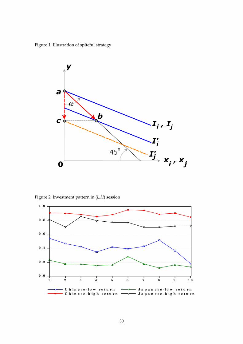
Result 1. The subjects’ mean investments with both low and high marginal returns for

both countries are plotted by periods in Figures 2 and 3. As shown from the figures, in

both (L,H) and (H,L) experiments, Chinese subjects contributed differently from their

Japanese counterparts regardless of low or high marginal return. Actually, the mean

investment lines of Chinese subjects with both high and low marginal returns are always

higher than those of Japanese subjects. To provide statistical supports on this issue, we

apply a number of tests. First, as a preliminary check, we list the descriptive statistics of

subjects’ investment in Table 1a. From the table, it is easy to find that mean of Chinese

investments is higher than that of Japanese subjects. Second, the nonparametric Wilcoxon

rank-sum test (Wilcoxon, 1945), which is also known as Mann-Whitney U test (Mann and

Whitney, 1947), is performed for testing both Chinese and Japanese data from populations

with the same distribution. The results listed in Table 1b indicate that Chinese data have

significantly different distribution from Japanese data with a wide margin, implying that

there is statistical difference in the behavior of public goods contribution between Chinese

and Japanese. Third, the results of t test suggest that the mean investment of Chinese

subjects with either low or high marginal returns in both (L,H) and (H,L) experiments is

significantly larger than that of Japanese subjects (see the final row in Table 1b).10 In

10 The Wilcoxon test and t test have also been applied to examining the similarity of investments across two countries in each period. Based on 5% significance level, both tests significantly reject the hypothesis of equal investment in 8 of 10 periods (periods 1-5 and 7-9) in (L,H) sessions with low marginal return, in 6 of 10 periods (periods 2 and 5-9) in (L,H) sessions with high marginal return, 7 of 10 periods (periods

10

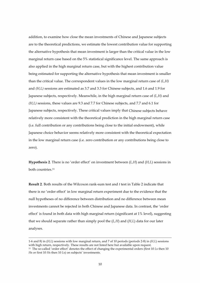
addition, to examine how close the mean investments of Chinese and Japanese subjects

are to the theoretical predictions, we estimate the lowest contribution value for supporting

the alternative hypothesis that mean investment is larger than the critical value in the low

marginal return case based on the 5% statistical significance level. The same approach is

also applied in the high marginal return case, but with the highest contribution value

being estimated for supporting the alternative hypothesis that mean investment is smaller

than the critical value. The correspondent values in the low marginal return case of (L,H)

and (H,L) sessions are estimated as 3.7 and 3.3 for Chinese subjects, and 1.6 and 1.9 for

Japanese subjects, respectively. Meanwhile, in the high marginal return case of (L,H) and

(H,L) sessions, these values are 9.3 and 7.7 for Chinese subjects, and 7.7 and 6.1 for

Japanese subjects, respectively. These critical values imply that Chinese subjects behave

relatively more consistent with the theoretical prediction in the high marginal return case

(i.e. full contribution or any contributions being close to the initial endowment), while

Japanese choice behavior seems relatively more consistent with the theoretical expectation

in the low marginal return case (i.e. zero contribution or any contributions being close to

zero).

Hypothesis 2. There is no ‘order effect’ on investment between (L,H) and (H,L) sessions in

both countries.11

Result 2. Both results of the Wilcoxon rank-sum test and t test in Table 2 indicate that

there is no ‘order effect’ in low marginal return experiment due to the evidence that the

null hypotheses of no difference between distribution and no difference between mean

investments cannot be rejected in both Chinese and Japanese data. In contrast, the ‘order

effect’ is found in both data with high marginal return (significant at 1% level), suggesting

that we should separate rather than simply pool the (L,H) and (H,L) data for our later

analyses.

1-6 and 8) in (H,L) sessions with low marginal return, and 7 of 10 periods (periods 2-8) in (H,L) sessions with high return, respectively. These results are not listed here but available upon request. 11 The so-called ‘order effect’ denotes the effect of changing the experimental orders (first 10 Ls then 10 Hs or first 10 Hs then 10 Ls) on subjects’ investments.

11

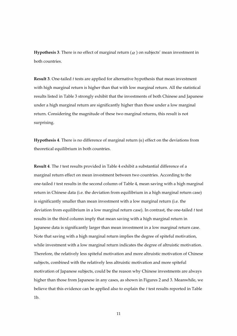
Hypothesis 3. There is no effect of marginal return (α ) on subjects’ mean investment in

both countries.

Result 3. One-tailed t tests are applied for alternative hypothesis that mean investment

with high marginal return is higher than that with low marginal return. All the statistical

results listed in Table 3 strongly exhibit that the investments of both Chinese and Japanese

under a high marginal return are significantly higher than those under a low marginal

return. Considering the magnitude of these two marginal returns, this result is not

surprising.

Hypothesis 4. There is no difference of marginal return (α) effect on the deviations from

theoretical equilibrium in both countries.

Result 4. The t test results provided in Table 4 exhibit a substantial difference of a

marginal return effect on mean investment between two countries. According to the

one-tailed t test results in the second column of Table 4, mean saving with a high marginal

return in Chinese data (i.e. the deviation from equilibrium in a high marginal return case)

is significantly smaller than mean investment with a low marginal return (i.e. the

deviation from equilibrium in a low marginal return case). In contrast, the one-tailed t test

results in the third column imply that mean saving with a high marginal return in

Japanese data is significantly larger than mean investment in a low marginal return case.

Note that saving with a high marginal return implies the degree of spiteful motivation,

while investment with a low marginal return indicates the degree of altruistic motivation.

Therefore, the relatively less spiteful motivation and more altruistic motivation of Chinese

subjects, combined with the relatively less altruistic motivation and more spiteful

motivation of Japanese subjects, could be the reason why Chinese investments are always

higher than those from Japanese in any cases, as shown in Figures 2 and 3. Meanwhile, we

believe that this evidence can be applied also to explain the t test results reported in Table

1b.

12

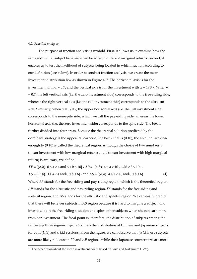
4.2 Fraction analysis

The purpose of fraction analysis is twofold. First, it allows us to examine how the

same individual subject behaves when faced with different marginal returns. Second, it

enables us to test the likelihood of subjects being located in which fraction according to

our definition (see below). In order to conduct fraction analysis, we create the mean

investment distribution box as shown in Figure 4.12 The horizontal axis is for the

investment with α = 0.7, and the vertical axis is for the investment with α = 1/0.7. When α

= 0.7, the left vertical axis (i.e. the zero investment side) corresponds to the free-riding side,

whereas the right vertical axis (i.e. the full investment side) corresponds to the altruism

side. Similarly, when α = 1/0.7, the upper horizontal axis (i.e. the full investment side)

corresponds to the non-spite side, which we call the pay-riding side, whereas the lower

horizontal axis (i.e. the zero investment side) corresponds to the spite side. The box is

further divided into four areas. Because the theoretical solution predicted by the

dominant strategy is the upper-left corner of the box – that is (0,10), the area that are close

enough to (0,10) is called the theoretical region. Although the choice of two numbers a

(mean investment with low marginal return) and b (mean investment with high marginal

return) is arbitrary, we define

{( , )|0 4FP a b a= ≤ < and 6 10}b< ≤ , {( , )|4 10AP a b a= ≤ < and 6 10}b< ≤ ,

{( , )|0 4FS a b a= ≤ < and 0 6}b≤ ≤ , and {( , )|4 10AS a b a= ≤ < and 0 6}b≤ ≤ (4)

Where FP stands for the free-riding and pay-riding region, which is the theoretical region,

AP stands for the altruistic and pay-riding region, FS stands for the free-riding and

spiteful region, and AS stands for the altruistic and spiteful region. We can easily predict

that there will be fewer subjects in AS region because it is hard to imagine a subject who

invests a lot in the free-riding situation and spites other subjects when she can earn more

from her investment. The focal point is, therefore, the distribution of subjects among the

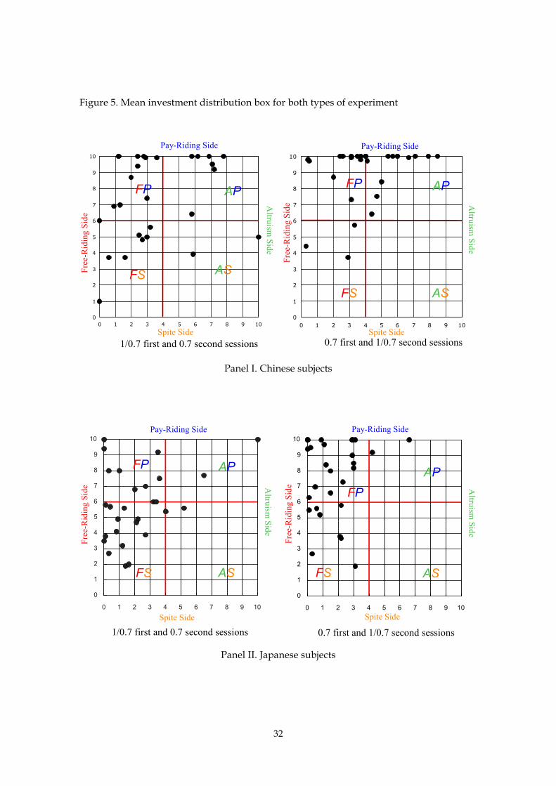
remaining three regions. Figure 5 shows the distribution of Chinese and Japanese subjects

for both (L,H) and (H,L) sessions. From the figure, we can observe that (i) Chinese subjects

are more likely to locate in FP and AP regions, while their Japanese counterparts are more 12 The description about the mean investment box is based on Saijo and Nakamura (1995).

13

likely to locate in FP and FS regions. (ii) More Chinese subjects are at or close to the

pay-riding side, while more Japanese subjects are at or close to free-riding side. This

observation may indicate that Chinese behavior is consistent with theoretical prediction in

a high marginal return case, while Japanese behavior is consistent with theoretical

prediction in a low marginal return case.13

In order to get some statistical supports for the above observations, we apply a

number of proportion tests and present the results in Table 5. Some notations defined as:

PFP,China, PAP,China, PFS,China ,PAS,China and PFP,Japan, PAP,Japan, PFS,Japan, PAS,Japan correspond to the

proportions of Chinese and Japanese subjects in FP, AP, FS and AS regions, respectively.

From the second to fifth rows of Table 5, we may conclude that (i) Chinese subjects are

more likely to locate in region AP and less likely to locate in region FS than their Japanese

counterparts (see results of tests (1) and (2)). (ii) More Chinese subjects locate in region AP

than FS in (L,H) sessions (see result of test (3)), while more Japanese subjects locate in

region FS than AP in both (L,H) and (H,L) sessions (see result of test (4)). In addition,

results of tests (5) – (8) suggest that whether (L,H) sessions or (H,L) sessions, Chinese

subjects are likely to locate in regions FS and AP, while Japanese subjects are likely to

locate in regions FP and FS. Therefore, the observations from Figure 5 are well supported

by these tests.

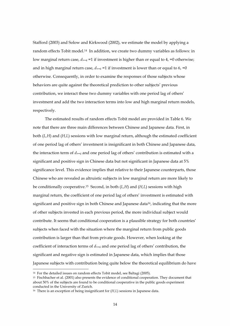
4.3 A random effects Tobit model of investments

We consider a model with a linear time trend and one period lag of other subjects’

investment to examine their effects on the individual subject’s own contribution. The

effect of lag of others’ investment on the individual subject’s own contribution has been

examined and found to exist in several previous studies (Chaudhuri et al., 2006;

Fischbacher et al., 2001). Because the possible investment levels are bounded by 0 and 10,

the dependent variable (i.e. investment) is censored and ordinary least squares will

therefore yield biased estimates. Hence, following the methodology of Anderson and

13 This observation is quite consistent with the evidence from critical value estimates reported in Result 1.

14

Stafford (2003) and Solow and Kirkwood (2002), we estimate the model by applying a

random effects Tobit model.14 In addition, we create two dummy variables as follows: in

low marginal return case, d>=4 =1 if investment is higher than or equal to 4, =0 otherwise;

and in high marginal return case, d<=6 =1 if investment is lower than or equal to 6, =0

otherwise. Consequently, in order to examine the responses of those subjects whose

behaviors are quite against the theoretical prediction to other subjects’ previous

contribution, we interact these two dummy variables with one period lag of others’

investment and add the two interaction terms into low and high marginal return models,

respectively.

The estimated results of random effects Tobit model are provided in Table 6. We

note that there are three main differences between Chinese and Japanese data. First, in

both (L,H) and (H,L) sessions with low marginal return, although the estimated coefficient

of one period lag of others’ investment is insignificant in both Chinese and Japanese data,

the interaction term of d>=4 and one period lag of others’ contribution is estimated with a

significant and positive sign in Chinese data but not significant in Japanese data at 5%

significance level. This evidence implies that relative to their Japanese counterparts, those

Chinese who are revealed as altruistic subjects in low marginal return are more likely to

be conditionally cooperative.15 Second, in both (L,H) and (H,L) sessions with high

marginal return, the coefficient of one period lag of others’ investment is estimated with

significant and positive sign in both Chinese and Japanese data16, indicating that the more

of other subjects invested in each previous period, the more individual subject would

contribute. It seems that conditional cooperation is a plausible strategy for both countries’

subjects when faced with the situation where the marginal return from public goods

contribution is larger than that from private goods. However, when looking at the

coefficient of interaction terms of d<=6 and one period lag of others’ contribution, the

significant and negative sign is estimated in Japanese data, which implies that those

Japanese subjects with contribution being quite below the theoretical equilibrium do have 14 For the detailed issues on random effects Tobit model, see Baltagi (2005). 15 Fischbacher et al. (2001) also presents the evidence of conditional cooperation. They document that about 50% of the subjects are found to be conditional cooperative in the public goods experiment conducted in the University of Zurich. 16 There is an exception of being insignificant for (H,L) sessions in Japanese data.

15

a tendency to spite others. This evidence supports the findings in Saijo and Nakamura

(1995) and Cason et al. (2002), which document that several Japanese subjects behave

spitefully. In contrast, the spiteful behavior seems unlikely to occur in Chinese subjects

because the coefficient in both sessions is not significant.17 Third, there is no time trend

effect found to influence individual subject’s investment in almost all the cases for both

Chinese and Japanese data, except that in (H,L) sessions under low marginal return, there

is a decreasing effect of time trend on the contribution found in Chinese data.

Finally, as an alternative methodology to confirm the above differences from the

random effects Tobit estimates, we produce the Spearman rank correlation coefficients

(Spearman, 1904; Conover, 1999) of two interaction terms and linear time trend with

subject’s own investment. From the results in Table 7, we find that all of the Spearman

rank correlation coefficients are strongly consistent with the random effects Tobit

estimates, as expected.

5. Summary and Conclusion

Our results can be summarized as follows. The Chinese data are roughly consistent

with the theoretical prediction in the high marginal return case, while the Japanese data

are generally consistent with the theoretical expectation in the low marginal return case.

The choice behavior of Chinese and Japanese subjects under voluntary contribution

mechanism is typically different. Compared with their Chinese counterparts, Japanese

subjects tend to invest less in both marginal return cases. Why does this happen? The

statistical tests, fraction analysis, and random effects Tobit estimation provide a detailed

examination. As discussed in the previous section, the differences between two countries’

subjects in the propensity to act altruistically or spitefully can explain their behavior

difference. Indeed, the implication behind it should correspond to the difference between

monetary maximization and ranking maximization.

The spiteful tendency of Japanese subjects has been reported in several previous

17 There is a consideration that Chinese subjects probably have not realized that reducing their investments can defeat others. However, from the questionnaire we took after the experiments, it is clear that more than half of the subjects realized the spite dilemma but did not behave spitefully since their motivations were to maximize their earnings from the experiments.

16

public goods experiments (e.g. Saijo and Nakamura, 1995; Cason et al., 2002). Although

China and Japan have similar traditional cultures, the recent wave of Western culture’s

influence over Chinese youth since the implementation of Economic Reform and Opening

Policy in 1979 leads to a possible gap in current cultures between China and Japan.

Therefore, from this point of view, it is not surprising that Chinese subjects behave

significantly different from their Japanese counterparts. We plan to let Japanese and

Chinese subjects attend the same sessions under the environments such as this or a

two-stage game. We believe that this will produce more fruitful results for the sake of

comparison across countries.

Acknowledgement

The authors would like to appreciate the Japanese Ministry of the Environment for

their financial support through the project numbered as H-062. We thank Hainan Wang,

Bing Yu, Jun Zhang, and Xiue Li for their help in preparing and conducting the

experiments in Shanghai Jiao Tong University. All the views expressed in this paper and

any errors are the sole responsibility of the authors.

References

Anderson, C. M., and L. Putterman. 2006. Do non-strategic sanctions obey the law of

demand? The demand for punishment in the voluntary contribution mechanism.

Games and Economic Behavior 54: 1-24.

Anderson, L. R., and S. L. Stafford. 2003. Punishment in a regulatory setting: experimental

evidence from the VCM. Journal of Regulatory Economics, 24(1): 91-110.

Baltagi, B. H. 2005. Econometric Analysis of Panel Data. 3rd edition, John Wiley & Sons, New

York.

Brandts, J., T. Saijo, and A. Schram. 2004. How universal is behavior? A four country

comparison of spite and cooperation in voluntary contribution mechanisms. Public

Choice 119: 381-424.

Brunton, D., R. Hasan, and S. Mestelman. 2001. The ‘spite’ dilemma: spite or no spite, is

there a dilemma?. Economics Letters, 71: 405-412.

17

Cason, T. N., T. Saijo, and T. Yamato. 2002. Voluntary participation and spite in public

good provision experiments: an international comparison. Experimental Economics, 5(2):

133-153.

Cason, T. N., T. Saijo, T., Yamato, and K. Yokotani. 2004. Non-excludable public good

experiments. Games and Economic Behavior, 49: 81-102.

Chaudhuri, A., S. Graziano, and P. Maitra. 2006. Social learning and norms in a public

goods experiment with inter-generational advice. Review of Economic Studies, 73(2):

357-380.

Cinyabuguma, M., T. Page, and L. Putterman. 2005. Cooperation under the threat of

expulsion in a public goods experiment. Journal of Public Economics 89: 1421-1435.

Conover, W. J. 1999. Practical Nonparametric Statistics. 3rd edition, New York: Wiley.

Cookson, R. 2000. Framing effects in public goods experiments. Experimental Economics, 3:

55-79.

Fischbacher, U., S. Gachter and E. Fehr. 2001. Are people conditionally cooperative?

Evidence from a public goods experiment. Economic Letters, 71: 397-404.

Frohlich, N., and J. Oppenheimer. 1984. Beyond economic man: Altruism, egalitarianism,

and difference maximizing. Journal of Conflict Resolution, 28: 3-24.

Gächter, S., B. Herrmann, and C. Thöni. 2004. Trust, voluntary cooperation, and

socio-economic background: survey and experimental evidence. Journal of Economic

Behavior & Organization, 55: 505-531.

Ito, M., T. Saijo, and M. Une. 1995. The Tragedy of the Commons Revisited. Journal of

Economic Behavior and Organization, 28: 311-335.

Mann, H. B., and D. R. Whitney. 1947. On a test of whether one of two random variables is

stochastically larger than the other. Annals of Mathematical Statistics, 18: 50-60.

Saijo, T., and H. Nakamura. 1995. The “Spite” Dilemma in Voluntary Contribution

Mechanism Experiments. Journal of Conflict Resolution, 39: 535-560.

Solow, J. H., and N. Kirkwood. 2002. Group identity and gender in public goods

experiments. Journal of Economic Behavior & Organization, 48: 403-412.

Spearman, C. 1904. The proof and measurement of association between two things.

American Journal of Psychology, 15: 72-101.

18

Wilcoxon, F. 1945. Individual comparisons by ranking methods. Biometrics, 1: 80-83.

19

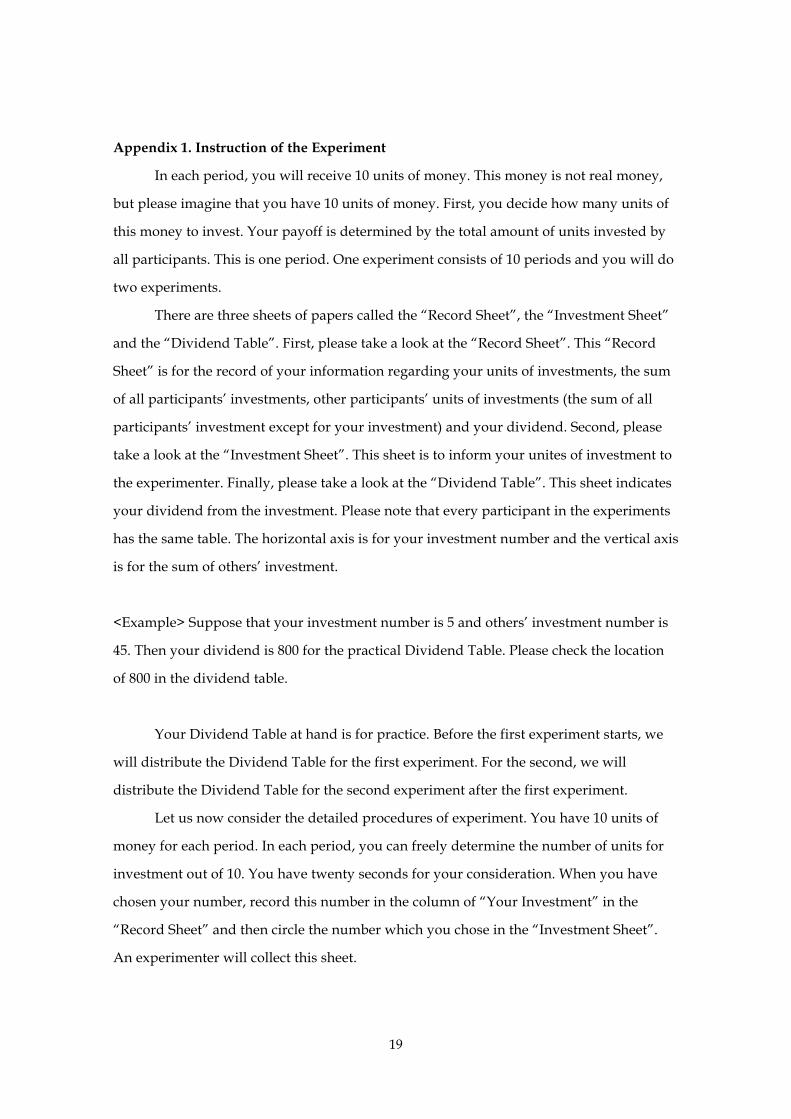
Appendix 1. Instruction of the Experiment

In each period, you will receive 10 units of money. This money is not real money,

but please imagine that you have 10 units of money. First, you decide how many units of

this money to invest. Your payoff is determined by the total amount of units invested by

all participants. This is one period. One experiment consists of 10 periods and you will do

two experiments.

There are three sheets of papers called the “Record Sheet”, the “Investment Sheet”

and the “Dividend Table”. First, please take a look at the “Record Sheet”. This “Record

Sheet” is for the record of your information regarding your units of investments, the sum

of all participants’ investments, other participants’ units of investments (the sum of all

participants’ investment except for your investment) and your dividend. Second, please

take a look at the “Investment Sheet”. This sheet is to inform your unites of investment to

the experimenter. Finally, please take a look at the “Dividend Table”. This sheet indicates

your dividend from the investment. Please note that every participant in the experiments

has the same table. The horizontal axis is for your investment number and the vertical axis

is for the sum of others’ investment.

<Example> Suppose that your investment number is 5 and others’ investment number is

45. Then your dividend is 800 for the practical Dividend Table. Please check the location

of 800 in the dividend table.

Your Dividend Table at hand is for practice. Before the first experiment starts, we

will distribute the Dividend Table for the first experiment. For the second, we will

distribute the Dividend Table for the second experiment after the first experiment.

Let us now consider the detailed procedures of experiment. You have 10 units of

money for each period. In each period, you can freely determine the number of units for

investment out of 10. You have twenty seconds for your consideration. When you have

chosen your number, record this number in the column of “Your Investment” in the

“Record Sheet” and then circle the number which you chose in the “Investment Sheet”.

An experimenter will collect this sheet.

20

The experimenter will announce the total sum of investments. Please record this number

in the column of “Total Sum of Investments”. Then subtract your investment number

from the total sum of investments and record this number in the column of “Others’

investments”. Next, please take a look at the Dividend Table and find your dividend.

Record this number in the column of “Your Dividend”.

Let us do practice following the above example. Please find the example raw in the

“Record Sheet”. Write 5 in the column of “Your Investment”. Suppose that the

experimenter collected the investment sheets and then announced 50 as the total number

of investments. Then you are supposed to record 50 in the column of “Total Sum of

Investments”. Now subtract your investment number 5 from 50 and record this difference,

45, in the column of “Others’ Investment”. Now, take a look at the Dividend Table. Look

at 5 in the horizontal axis and 45 in the vertical axis. Then you will find 800. This 800 is

your dividend and record this number in the column of “Your Dividend”.

This is the end of the first period. The next period will start with your choice of a

number from zero to 10.

100 units of dividend is equivalent to 0.5 RMB. That is, the money you will receive

is 0.5% of your sum of dividend. For example, if you obtain 16231 units of money, then

your dividend is 81 RMB.

Please remember that you cannot talk to other participants during the experiments. If this

happens, the experiment will be stopped at that point.

Before the actual experiments, you will do three period practices. You must

understand the procedure of the experiments thoroughly. If you have any questions,

please raise your hand now.

21

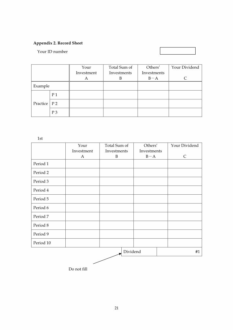
Appendix 2. Record Sheet

Your ID number

Your Investment

A

Total Sum of Investments

B

Others’ Investments

B－A

Your Dividend

C

Example

P 1

P 2 Practice

P 3

1st

Your Investment

A


B


B－A

Your Dividend

C

Period 1

Period 2

Period 3

Period 4

Period 5

Period 6

Period 7

Period 8

Period 9

Period 10

Dividend #1

Do not fill

22

2nd

Your Investment

A


B


B－A

Your Dividend

C

Period 1

Period 2

Period 3

Period 4

Period 5

Period 6

Period 7

Period 8

Period 9

Period 10

Dividend #1

Do not fill

Appendix 3. Investment Sheet

Investment Sheet

Your ID number____________________

Please circle your investment number

0 1 2 3 4 5 6 7 8 9 10

After circling the number, please put this sheet up-side-down on the table.

23

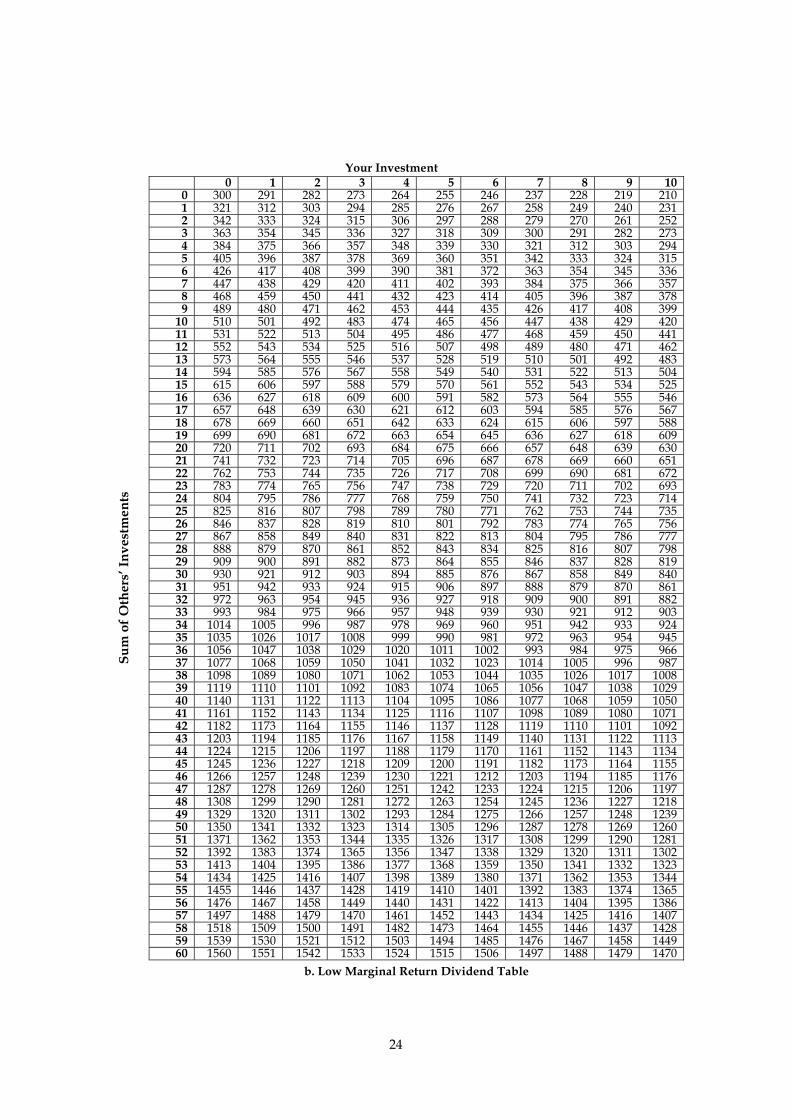
Appendix 4. Dividend Tables

Your Investment 0 1 2 3 4 5 6 7 8 9 10

0 50 77 98 113 122 125 122 113 98 77 50 1 80 104 122 134 140 140 134 122 104 80 50 2 110 131 146 155 158 155 146 131 110 83 50 3 140 158 170 176 176 170 158 140 116 86 50 4 170 185 194 197 194 185 170 149 122 89 50 5 200 212 218 218 212 200 182 158 128 92 50 6 230 239 242 239 230 215 194 167 134 95 50 7 260 266 266 260 248 230 206 176 140 98 50 8 290 293 290 281 266 245 218 185 146 101 50 9 320 320 314 302 284 260 230 194 152 104 50

10 350 347 338 323 302 275 242 203 158 107 50 11 380 374 362 344 320 290 254 212 164 110 50 12 410 401 386 365 338 305 266 221 170 113 50 13 440 428 410 386 356 320 278 230 176 116 50 14 470 455 434 407 374 335 290 239 182 119 50 15 500 482 458 428 392 350 302 248 188 122 50 16 530 509 482 449 410 365 314 257 194 125 50 17 560 536 506 470 428 380 326 266 200 128 50 18 590 563 530 491 446 395 338 275 206 131 50 19 620 590 554 512 464 410 350 284 212 134 50 20 650 617 578 533 482 425 362 293 218 137 50 21 680 644 602 554 500 440 374 302 224 140 50 22 710 671 626 575 518 455 386 311 230 143 50 23 740 698 650 596 536 470 398 320 236 146 50 24 770 725 674 617 554 485 410 329 242 149 50 25 800 752 698 638 572 500 422 338 248 152 50 26 830 779 722 659 590 515 434 347 254 155 50 27 860 806 746 680 608 530 446 356 260 158 50 28 890 833 770 701 626 545 458 365 266 161 50 29 920 860 794 722 644 560 470 374 272 164 50 30 950 887 818 743 662 575 482 383 278 167 50 31 980 914 842 764 680 590 494 392 284 170 50 32 1010 941 866 785 698 605 506 401 290 173 50 33 1040 968 890 806 716 620 518 410 296 176 50 34 1070 995 914 827 734 635 530 419 302 179 50 35 1100 1022 938 848 752 650 542 428 308 182 50 36 1130 1049 962 869 770 665 554 437 314 185 50 37 1160 1076 986 890 788 680 566 446 320 188 50 38 1190 1103 1010 911 806 695 578 455 326 191 50 39 1220 1130 1034 932 824 710 590 464 332 194 50 40 1250 1157 1058 953 842 725 602 473 338 197 50 41 1280 1184 1082 974 860 740 614 482 344 200 50 42 1310 1211 1106 995 878 755 626 491 350 203 50 43 1340 1238 1130 1016 896 770 638 500 356 206 50 44 1370 1265 1154 1037 914 785 650 509 362 209 50 45 1400 1292 1178 1058 932 800 662 518 368 212 50 46 1430 1319 1202 1079 950 815 674 527 374 215 50 47 1460 1346 1226 1100 968 830 686 536 380 218 50 48 1490 1373 1250 1121 986 845 698 545 386 221 50 49 1520 1400 1274 1142 1004 860 710 554 392 224 50 50 1550 1427 1298 1163 1022 875 722 563 398 227 50 51 1580 1454 1322 1184 1040 890 734 572 404 230 50 52 1610 1481 1346 1205 1058 905 746 581 410 233 50 53 1640 1508 1370 1226 1076 920 758 590 416 236 50 54 1670 1535 1394 1247 1094 935 770 599 422 239 50 55 1700 1562 1418 1268 1112 950 782 608 428 242 50 56 1730 1589 1442 1289 1130 965 794 617 434 245 50 57 1760 1616 1466 1310 1148 980 806 626 440 248 50 58 1790 1643 1490 1331 1166 995 818 635 446 251 50 59 1820 1670 1514 1352 1184 1010 830 644 452 254 50 60 1850 1697 1538 1373 1202 1025 842 653 458 257 50

Sum

of O

ther

s’ In

vest

men

ts

a. Practice Dividend Table

24

Your Investment

0 1 2 3 4 5 6 7 8 9 10 0 300 291 282 273 264 255 246 237 228 219 210 1 321 312 303 294 285 276 267 258 249 240 231 2 342 333 324 315 306 297 288 279 270 261 252 3 363 354 345 336 327 318 309 300 291 282 273 4 384 375 366 357 348 339 330 321 312 303 294 5 405 396 387 378 369 360 351 342 333 324 315 6 426 417 408 399 390 381 372 363 354 345 336 7 447 438 429 420 411 402 393 384 375 366 357 8 468 459 450 441 432 423 414 405 396 387 378 9 489 480 471 462 453 444 435 426 417 408 399

10 510 501 492 483 474 465 456 447 438 429 420 11 531 522 513 504 495 486 477 468 459 450 441 12 552 543 534 525 516 507 498 489 480 471 462 13 573 564 555 546 537 528 519 510 501 492 483 14 594 585 576 567 558 549 540 531 522 513 504 15 615 606 597 588 579 570 561 552 543 534 525 16 636 627 618 609 600 591 582 573 564 555 546 17 657 648 639 630 621 612 603 594 585 576 567 18 678 669 660 651 642 633 624 615 606 597 588 19 699 690 681 672 663 654 645 636 627 618 609 20 720 711 702 693 684 675 666 657 648 639 630 21 741 732 723 714 705 696 687 678 669 660 651 22 762 753 744 735 726 717 708 699 690 681 672 23 783 774 765 756 747 738 729 720 711 702 693 24 804 795 786 777 768 759 750 741 732 723 714 25 825 816 807 798 789 780 771 762 753 744 735 26 846 837 828 819 810 801 792 783 774 765 756 27 867 858 849 840 831 822 813 804 795 786 777 28 888 879 870 861 852 843 834 825 816 807 798 29 909 900 891 882 873 864 855 846 837 828 819 30 930 921 912 903 894 885 876 867 858 849 840 31 951 942 933 924 915 906 897 888 879 870 861 32 972 963 954 945 936 927 918 909 900 891 882 33 993 984 975 966 957 948 939 930 921 912 903 34 1014 1005 996 987 978 969 960 951 942 933 924 35 1035 1026 1017 1008 999 990 981 972 963 954 945 36 1056 1047 1038 1029 1020 1011 1002 993 984 975 966 37 1077 1068 1059 1050 1041 1032 1023 1014 1005 996 987 38 1098 1089 1080 1071 1062 1053 1044 1035 1026 1017 1008 39 1119 1110 1101 1092 1083 1074 1065 1056 1047 1038 1029 40 1140 1131 1122 1113 1104 1095 1086 1077 1068 1059 1050 41 1161 1152 1143 1134 1125 1116 1107 1098 1089 1080 1071 42 1182 1173 1164 1155 1146 1137 1128 1119 1110 1101 1092 43 1203 1194 1185 1176 1167 1158 1149 1140 1131 1122 1113 44 1224 1215 1206 1197 1188 1179 1170 1161 1152 1143 1134 45 1245 1236 1227 1218 1209 1200 1191 1182 1173 1164 1155 46 1266 1257 1248 1239 1230 1221 1212 1203 1194 1185 1176 47 1287 1278 1269 1260 1251 1242 1233 1224 1215 1206 1197 48 1308 1299 1290 1281 1272 1263 1254 1245 1236 1227 1218 49 1329 1320 1311 1302 1293 1284 1275 1266 1257 1248 1239 50 1350 1341 1332 1323 1314 1305 1296 1287 1278 1269 1260 51 1371 1362 1353 1344 1335 1326 1317 1308 1299 1290 1281 52 1392 1383 1374 1365 1356 1347 1338 1329 1320 1311 1302 53 1413 1404 1395 1386 1377 1368 1359 1350 1341 1332 1323 54 1434 1425 1416 1407 1398 1389 1380 1371 1362 1353 1344 55 1455 1446 1437 1428 1419 1410 1401 1392 1383 1374 1365 56 1476 1467 1458 1449 1440 1431 1422 1413 1404 1395 1386 57 1497 1488 1479 1470 1461 1452 1443 1434 1425 1416 1407 58 1518 1509 1500 1491 1482 1473 1464 1455 1446 1437 1428 59 1539 1530 1521 1512 1503 1494 1485 1476 1467 1458 1449 60 1560 1551 1542 1533 1524 1515 1506 1497 1488 1479 1470

Sum

of O

ther

s’ In

vest

men

ts

b. Low Marginal Return Dividend Table

25

Your Investment

0 1 2 3 4 5 6 7 8 9 10 0 120 125 130 135 141 146 151 156 161 166 171 1 137 142 147 153 158 163 168 173 178 183 189 2 154 159 165 170 175 180 185 190 195 201 206 3 171 177 182 187 192 197 202 207 213 218 223 4 189 194 199 204 209 214 219 225 230 235 240 5 206 211 216 221 226 231 237 242 247 252 257 6 223 228 233 238 243 249 254 259 264 269 274 7 240 245 250 255 261 266 271 276 281 286 291 8 257 262 267 273 278 283 288 293 298 303 309 9 274 279 285 290 295 300 305 310 315 321 326

10 291 297 302 307 312 317 322 327 333 338 343 11 309 314 319 324 329 334 339 345 350 355 360 12 326 331 336 341 346 351 357 362 367 372 377 13 343 348 353 358 363 369 374 379 384 389 394 14 360 365 370 375 381 386 391 396 401 406 411 15 377 382 387 393 398 403 408 413 418 423 429 16 394 399 405 410 415 420 425 430 435 441 446 17 411 417 422 427 432 437 442 447 453 458 463 18 429 434 439 444 449 454 459 465 470 475 480 19 446 451 456 461 466 471 477 482 487 492 497 20 463 468 473 478 483 489 494 499 504 509 514 21 480 485 490 495 501 506 511 516 521 526 531 22 497 502 507 513 518 523 528 533 538 543 549 23 514 519 525 530 535 540 545 550 555 561 566 24 531 537 542 547 552 557 562 567 573 578 583 25 549 554 559 564 569 574 579 585 590 595 600 26 566 571 576 581 586 591 597 602 607 612 617 27 583 588 593 598 603 609 614 619 624 629 634 28 600 605 610 615 621 626 631 636 641 646 651 29 617 622 627 633 638 643 648 653 658 663 669 30 634 639 645 650 655 660 665 670 675 681 686 31 651 657 662 667 672 677 682 687 693 698 703 32 669 674 679 684 689 694 699 705 710 715 720 33 686 691 696 701 706 711 717 722 727 732 737 34 703 708 713 718 723 729 734 739 744 749 754 35 720 725 730 735 741 746 751 756 761 766 771 36 737 742 747 753 758 763 768 773 778 783 789 37 754 759 765 770 775 780 785 790 795 801 806 38 771 777 782 787 792 797 802 807 813 818 823 39 789 794 799 804 809 814 819 825 830 835 840 40 806 811 816 821 826 831 837 842 847 852 857 41 823 828 833 838 843 849 854 859 864 869 874 42 840 845 850 855 861 866 871 876 881 886 891 43 857 862 867 873 878 883 888 893 898 903 909 44 874 879 885 890 895 900 905 910 915 921 926 45 891 897 902 907 912 917 922 927 933 938 943 46 909 914 919 924 929 934 939 945 950 955 960 47 926 931 936 941 946 951 957 962 967 972 977 48 943 948 953 958 963 969 974 979 984 989 994 49 960 965 970 975 981 986 991 996 1001 1006 1011 50 977 982 987 993 998 1003 1008 1013 1018 1023 1029 51 994 999 1005 1010 1015 1020 1025 1030 1035 1041 1046 52 1011 1017 1022 1027 1032 1037 1042 1047 1053 1058 1063 53 1029 1034 1039 1044 1049 1054 1059 1065 1070 1075 1080 54 1046 1051 1056 1061 1066 1071 1077 1082 1087 1092 1097 55 1063 1068 1073 1078 1083 1089 1094 1099 1104 1109 1114 56 1080 1085 1090 1095 1101 1106 1111 1116 1121 1126 1131 57 1097 1102 1107 1113 1118 1123 1128 1133 1138 1143 1149 58 1114 1119 1125 1130 1135 1140 1145 1150 1155 1161 1166 59 1131 1137 1142 1147 1152 1157 1162 1167 1173 1178 1183 60 1149 1154 1159 1164 1169 1174 1179 1185 1190 1195 1200

Sum

of O

ther

s’ In

vest

men

ts

c. High Marginal Return Dividend Table

26

Appendix 5. Data of Chinese subjects

(L, H) experiment S1 L1 L2 L3 L4 L5 L6 L7 L8 L9 L10 H1 H2 H3 H4 H5 H6 H7 H8 H9 H10

Sub.1 10 0 0 0 2 0 9 8 6 2 10 10 10 10 8 10 10 10 10 10

Sub.2 10 10 10 7 8 4 4 6 8 0 10 10 10 9 10 10 10 10 10 10

Sub.3 9 9 7 7 7 5 10 8 8 9 10 10 10 10 10 10 10 10 10 10

Sub.4 9 0 4 0 2 2 0 7 0 0 10 10 10 10 10 10 10 10 10 10

Sub.5 1 10 10 10 10 0 0 10 10 10 10 10 10 10 10 10 10 10 10 10

Sub.6 10 1 4 3 2 2 3 1 6 1 10 0 2 2 1 10 10 10 2 10

Sub.7 1 10 10 0 0 6 0 10 10 10 10 10 10 10 10 10 10 10 10 10

S2 L1 L2 L3 L4 L5 L6 L7 L8 L9 L10 H1 H2 H3 H4 H5 H6 H7 H8 H9 H10

Sub.1 10 8 9 3 10 9 8 3 0 0 10 10 10 10 10 10 10 10 10 10

Sub.2 10 10 10 0 0 10 10 10 0 0 10 10 10 10 10 10 10 10 10 10

Sub.3 5 6 6 8 10 10 10 10 10 10 10 10 10 10 10 10 10 10 10 10

Sub.4 5 6 0 5 10 8 7 4 8 1 10 10 10 10 10 10 10 10 10 10

Sub.5 0 0 0 2 1 0 0 2 0 0 10 10 9 9 10 10 10 10 9 10

Sub.6 4 5 5 4 4 4 5 5 4 0 10 10 10 10 10 10 10 10 10 10

Sub.7 10 5 5 5 2 2 3 3 1 10 10 10 10 10 10 10 10 10 10 10


Sub.1 0 10 4 2 5 5 7 7 0 0 10 10 10 10 10 10 10 10 10 10

Sub.2 0 0 0 3 0 0 0 0 0 0 0 10 5 0 0 3 7 1 8 10

Sub.3 0 2 1 1 10 0 3 9 5 0 10 10 10 9 10 9 0 1 10 4

Sub.4 7 5 5 2 3 6 6 2 4 1 10 10 10 10 9 9 10 9 10 10

Sub.5 5 5 0 5 10 10 0 0 0 0 10 10 10 10 10 10 10 10 10 10

Sub.6 5 5 4 5 7 4 8 2 2 2 8 2 3 2 8 8 8 10 10 5

Sub.7 0 0 5 6 1 4 3 10 0 0 0 3 2 0 4 8 10 0 0 10


Sub.1 3 1 5 4 0 1 3 4 5 0 10 10 10 10 10 10 10 10 10 10

Sub.2 10 10 0 0 0 0 0 0 0 0 10 10 10 10 8 10 10 9 10 0

Sub.3 5 5 6 1 2 1 3 4 4 0 10 10 10 10 10 10 10 10 10 10

Sub.4 7 7 6 7 7 6 7 0 0 0 6 7 8 8 9 9 9 10 9 0

Sub.5 0 1 0 0 0 1 1 0 0 1 10 10 10 10 10 10 10 10 10 8

Sub.6 10 0 0 0 0 10 10 10 10 0 10 10 10 10 10 10 10 9 5 0

Sub.7 5 0 3 7 4 0 0 9 1 2 10 10 9 10 10 10 10 10 10 10

(to be continued)

27

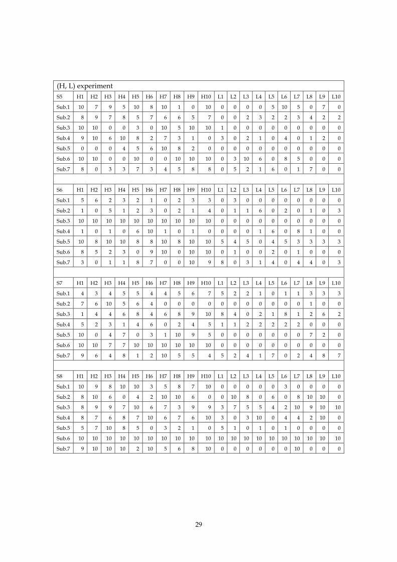
(H, L) experiment S5 H1 H2 H3 H4 H5 H6 H7 H8 H9 H10 L1 L2 L3 L4 L5 L6 L7 L8 L9 L10

Sub.1 10 10 10 10 10 10 10 10 10 10 0 7 10 5 5 10 8 8 5 0

Sub.2 6 5 6 7 7 6 7 6 8 6 6 5 6 6 8 7 8 10 2 0

Sub.3 10 9 10 10 10 10 10 10 10 10 9 7 6 6 0 1 1 2 4 0

Sub.4 10 10 10 10 10 10 10 10 10 10 1 2 0 0 5 1 2 0 1 0

Sub.5 10 10 10 10 10 10 10 10 10 10 10 6 7 0 5 7 7 7 5 8

Sub.6 10 10 10 10 10 10 10 10 10 10 10 10 10 8 10 10 10 10 0 0

Sub.7 10 10 10 10 7 10 10 10 9 9 8 6 8 9 5 7 10 3 5 10

S6 H1 H2 H3 H4 H5 H6 H7 H8 H9 H10 L1 L2 L3 L4 L5 L6 L7 L8 L9 L10

Sub.1 10 10 10 10 10 10 10 10 10 10 4 4 6 8 8 9 7 7 6 10

Sub.2 8 9 2 2 3 10 0 0 3 0 4 0 3 4 4 0 0 1 0 0

Sub.3 10 10 10 10 10 10 10 10 10 10 0 0 3 2 2 0 5 0 0 0

Sub.4 7 3 3 1 4 5 8 2 1 3 0 1 0 1 1 2 0 0 1 0

Sub.5 6 10 4 10 10 10 10 10 7 10 0 0 10 0 0 10 0 0 0 0

Sub.6 10 10 8 8 9 5 4 5 7 3 0 0 3 3 2 0 0 1 0 0

Sub.7 10 10 10 10 8 9 10 9 6 10 9 6 8 9 7 9 5 10 5 4


Sub.1 0 2 6 10 0 2 9 1 0 9 8 9 6 7 2 3 9 9 6 0

Sub.2 10 10 10 10 10 10 10 10 10 10 0 5 8 0 5 5 0 0 0 5

Sub.3 9 10 0 7 9 7 10 3 10 9 4 3 4 3 6 1 3 2 4 0

Sub.4 10 1 5 10 10 0 10 10 0 0 8 10 0 0 0 0 10 0 4 0

Sub.5 9 10 10 8 9 10 10 9 9 10 1 2 0 3 0 0 8 0 0 10

Sub.6 10 9 0 5 6 5 0 4 5 7 0 3 10 0 0 3 4 5 0 0

Sub.7 3 3 3 10 8 4 4 4 8 3 3 8 4 3 10 0 0 0 1 1


Sub.1 1 1 1 1 1 1 1 1 1 1 0 0 0 0 0 0 0 0 0 0

Sub.2 10 9 6 8 3 6 9 6 3 10 2 0 0 1 1 3 1 2 1 2

Sub.3 10 10 10 10 10 10 0 0 0 0 0 0 0 0 0 0 0 0 0 0

Sub.4 0 0 0 0 0 10 10 10 10 10 10 10 10 10 10 10 10 10 10 10

Sub.5 9 8 6 6 5 2 3 4 2 3 2 1 3 2 4 0 1 7 5 2

Sub.6 10 10 9 10 10 10 10 10 10 10 5 8 3 0 4 2 0 7 0 0

Sub.7 10 10 10 10 10 10 10 10 10 10 5 3 2 7 0 1 3 1 2 0

28

Appendix 6. Data of Japanese subjects

(L, H) experiment S1 L1 L2 L3 L4 L5 L6 L7 L8 L9 L10 H1 H2 H3 H4 H5 H6 H7 H8 H9 H10

Sub.1 5 4 3 0 0 4 1 0 2 3 4 3 3 1 6 5 2 6 3 4

Sub.2 0 0 0 0 0 0 0 0 2 1 10 0 5 8 1 0 0 3 0 0

Sub.3 8 5 3 3 1 2 3 2 2 2 0 1 2 2 1 4 1 1 5 2

Sub.4 3 1 3 3 2 3 4 5 5 1 10 10 10 10 10 5 10 5 5 7

Sub.5 0 0 0 0 1 1 2 1 1 2 10 7 7 5 6 2 4 0 3 8

Sub.6 0 2 0 1 5 3 0 2 7 1 3 0 5 2 7 3 2 1 10 5

Sub.7 0 0 0 0 0 0 0 0 0 0 10 10 9 5 10 10 10 10 10 10


Sub.1 0 0 0 0 1 0 0 0 0 0 10 5 10 10 5 8 5 5 5 0

Sub.2 0 0 2 0 10 9 1 0 0 0 10 10 9 0 1 5 0 10 3 10

Sub.3 5 5 3 0 2 3 4 0 0 1 8 8 7 7 6 8 7 7 7 8

Sub.4 1 1 0 1 0 1 1 0 1 0 7 8 6 5 6 6 4 5 3 6

Sub.5 1 0 0 0 0 0 0 0 0 0 10 0 10 10 0 0 5 0 10 10

Sub.6 0 1 0 5 2 4 0 1 0 2 10 9 10 10 8 10 9 0 0 0

Sub.7 1 1 0 0 0 0 0 0 0 0 5 10 10 10 10 10 10 10 10 10


Sub.1 1 1 1 2 1 0 1 2 1 1 10 10 10 10 10 10 10 10 8 9

Sub.2 3 2 2 5 0 10 8 0 1 0 10 10 10 10 10 10 10 10 10 10

Sub.3 0 0 0 0 0 0 0 0 0 0 10 10 10 10 10 10 10 10 10 10

Sub.4 3 4 5 4 5 10 7 8 10 10 10 10 10 10 10 10 10 10 10 10

Sub.5 5 10 2 1 0 2 5 2 0 2 10 10 10 10 10 10 10 5 10 5

Sub.6 0 0 0 0 0 5 0 0 0 0 10 10 10 10 10 10 0 10 0 0

Sub.7 2 0 5 2 1 9 0 3 7 0 10 10 10 10 10 10 10 10 10 10


Sub.1 0 1 10 0 0 4 5 0 0 10 6 0 10 10 10 10 9 10 10 10

Sub.2 5 5 6 6 5 7 0 3 5 0 8 8 8 10 10 10 9 9 10 10

Sub.3 3 3 1 0 2 0 0 3 0 0 6 8 8 8 9 9 9 9 9 9

Sub.4 10 0 0 0 5 0 0 0 0 0 0 0 10 10 10 10 10 10 10 10

Sub.5 1 0 0 5 0 0 3 0 0 0 10 10 10 10 10 10 10 10 10 10

Sub.6 0 0 0 0 0 0 0 0 0 0 10 10 10 10 10 10 10 10 10 10

Sub.7 7 3 2 5 2 2 4 1 1 2 10 10 10 10 10 10 10 10 10 10

(to be continued)

29

(H, L) experiment S5 H1 H2 H3 H4 H5 H6 H7 H8 H9 H10 L1 L2 L3 L4 L5 L6 L7 L8 L9 L10

Sub.1 10 7 9 5 10 8 10 1 0 10 0 0 0 0 5 10 5 0 7 0

Sub.2 8 9 7 8 5 7 6 6 5 7 0 0 2 3 2 2 3 4 2 2

Sub.3 10 10 0 0 3 0 10 5 10 10 1 0 0 0 0 0 0 0 0 0

Sub.4 9 10 6 10 8 2 7 3 1 0 3 0 2 1 0 4 0 1 2 0

Sub.5 0 0 0 4 5 6 10 8 2 0 0 0 0 0 0 0 0 0 0 0

Sub.6 10 10 0 0 10 0 0 10 10 10 0 3 10 6 0 8 5 0 0 0

Sub.7 8 0 3 3 7 3 4 5 8 8 0 5 2 1 6 0 1 7 0 0


Sub.1 5 6 2 3 2 1 0 2 3 3 0 3 0 0 0 0 0 0 0 0

Sub.2 1 0 5 1 2 3 0 2 1 4 0 1 1 6 0 2 0 1 0 3

Sub.3 10 10 10 10 10 10 10 10 10 10 0 0 0 0 0 0 0 0 0 0

Sub.4 1 0 1 0 6 10 1 0 1 0 0 0 0 1 6 0 8 1 0 0

Sub.5 10 8 10 10 8 8 10 8 10 10 5 4 5 0 4 5 3 3 3 3

Sub.6 8 5 2 3 0 9 10 0 10 10 0 1 0 0 2 0 1 0 0 0

Sub.7 3 0 1 1 8 7 0 0 10 9 8 0 3 1 4 0 4 4 0 3


Sub.1 4 3 4 5 5 4 4 5 6 7 5 2 2 1 0 1 1 3 3 3

Sub.2 7 6 10 5 6 4 0 0 0 0 0 0 0 0 0 0 0 1 0 0

Sub.3 1 4 4 6 8 4 6 8 9 10 8 4 0 2 1 8 1 2 6 2

Sub.4 5 2 3 1 4 6 0 2 4 5 1 1 2 2 2 2 2 0 0 0

Sub.5 10 0 4 7 0 3 1 10 9 5 0 0 0 0 0 0 0 7 2 0

Sub.6 10 10 7 7 10 10 10 10 10 10 0 0 0 0 0 0 0 0 0 0

Sub.7 9 6 4 8 1 2 10 5 5 4 5 2 4 1 7 0 2 4 8 7


Sub.1 10 9 8 10 10 3 5 8 7 10 0 0 0 0 0 3 0 0 0 0

Sub.2 8 10 6 0 4 2 10 10 6 0 0 10 8 0 6 0 8 10 10 0

Sub.3 8 9 9 7 10 6 7 3 9 9 3 7 5 5 4 2 10 9 10 10

Sub.4 8 7 6 8 7 10 6 7 6 10 3 0 3 10 0 4 4 2 10 0

Sub.5 5 7 10 8 5 0 3 2 1 0 5 1 0 1 0 1 0 0 0 0

Sub.6 10 10 10 10 10 10 10 10 10 10 10 10 10 10 10 10 10 10 10 10

Sub.7 9 10 10 10 2 10 5 6 8 10 0 0 0 0 0 0 10 0 0 0

30

Figure 1. Illustration of spiteful strategy

α

45o

x , x

y

i

a

c b

0

I'

I'i

jj

I , Ii j

Figure 2. Investment pattern in (L,H) session

0 . 0

0 . 2

0 . 4

0 . 6

0 . 8

1 . 0

1 2 3 4 5 6 7 8 9 1 0

C h i n e s e - l o w r e t u r nC h i n e s e - h i g h r e t u r n

J a p a n e s e - l o w r e t u r nJ a p a n e s e - h i g h r e t u r n

31

Figure 3. Investment pattern in (H,L) session

0 . 0

0 . 2

0 . 4

0 . 6

0 . 8

1 . 0

1 2 3 4 5 6 7 8 9 1 0

C h i n e s e - l o w r e t u r nC h i n e s e - h i g h r e t u r n

J a p a n e s e - l o w r e t u r nJ a p a n e s e - h i g h r e t u r n

Figure 4. Mean investment distribution box

FP AP

FS AS

Pay-Riding Side

AltruismSide

104Spite Side

Free-RidingSide

10

0

TheoreticalPrediction

6

32

Figure 5. Mean investment distribution box for both types of experiment

0

1

2

3

4

5

6

7

8

9

10

0 1 2 3 4 5 6 7 8 9 100

1

2

3

4

5

6

7

8

9

10

0 1 2 3 4 5 6 7 8 9 10

1/0.7 first and 0.7 second sessions 0.7 first and 1/0.7 second sessions

FP AP

FS AS

Spite Side

FP AP

FS AS

Spite Side

Pay-Riding Side Pay-Riding Side

Free

-Rid

ing

Side

Free

-Rid

ing

SideA

ltruism Side

Altruism

Side

Panel I. Chinese subjects

0

1

2

3

4

5

6

7

8

9

10

0 1 2 3 4 5 6 7 8 9 10

0

1

2

3

4

5

6

7

8

9

10

0 1 2 3 4 5 6 7 8 9 10

1/0.7 first and 0.7 second sessions 0.7 first and 1/0.7 second sessions

FP AP

FS AS

Spite Side Spite Side

Pay-Riding Side Pay-Riding Side

Free

-Rid

ing

Side

Free

-Rid

ing

SideA

ltruism Side

Altruism

Side

FPAP

FS AS

Panel II. Japanese subjects

33

Table 1a. Descriptive statistics of investment in Chinese and Japanese data

Mean Std. Dev. Minimum Maximum Observations (L,H) sessions

Chinese Low return 4.075 3.7289 0 10 280 High return 8.961 2.6182 0 10 280

Japanese Low return 1.761 2.5194 0 10 280 High return 7.546 3.4441 0 10 280

(H,L) sessions Chinese Low return 3.571 3.6232 0 10 280

High return 7.432 3.5229 0 10 280 Japanese Low return 2.161 3.1107 0 10 280

High return 5.832 3.6461 0 10 280

Table 1b. Tests for differences in investment between Chinese and Japanese data

(L,H) sessions (H,L) sessions Low return High return Low return High return Wilcoxon rank-sum test for same distribution

7.377** 6.069** 4.864** 5.824**

t test for equality of meana 8.484** 5.152** 5.026** 5.427**

**Significant at 1% level, *Significant at 5% level. a One-tailed t test for alternative hypothesis that mean investment in Chinese data is larger than that in Japanese data.

Table 2. Tests for differences in investment between (L,H) and (H,L) sessions

Chinese Japanese Low return High return Low return High return Wilcoxon rank-sum test for same distribution

1.723 6.228** 1.054 5.792**

t test for equality of meana 1.684 5.776** 1.576 5.717**

**Significant at 1% level, *Significant at 5% level. a Two-tailed t test for alternative hypothesis that mean investment in (L,H) sessions is not same as that in (H,L) sessions.

Table 3. Tests for marginal return to mean investment

Chinese Japanese (L,H) sessionsa 19.129** 23.156**

(H,L) sessionsa 13.683** 13.566**

**Significant at 1% level, *Significant at 5% level. a One-tailed t test for alternative hypothesis that mean investment in a high marginal return case is higher than that in a low marginal return case.

34

Table 4. Tests for marginal return effect on the difference from equilibrium

Chinesea Japaneseb

(L,H) sessions -10.534** 2.664**

(H,L) sessions -3.130** 6.660**

**Significant at 1% level, *Significant at 5% level. a One-tailed t test for alternative hypothesis that saving with high marginal return is smaller than investment with low marginal return in Chinese data. b One-tailed t test for alternative hypothesis that saving with high marginal return is larger than investment with low marginal return in Japanese data.

Table 5. Tests for the fraction of subjects

(L,H) sessions (H,L) sessions

(1) PAP,China= PAP,Japan vs. PAP,China> PAP,Japan 3.550** 1.819*

(2) PFS,China= PFS,Japan vs. PFS,China< PFS,Japan -1.682* -2.445**

(3) PAP,China= PFS,China vs. PAP,China> PFS,China 3.197** 0.000

(4) PAP,Japan= PFS,Japan vs. PAP,Japan< PFS,Japan -2.094* -4.006**

(5) PAP,China+ PFP,China=0.6 vs. PAP,China+ PFP,China>0.6 a 3.163** 1.849*

(6) PFS,Japan+ PFP,Japan=0.6vs. PFS,Japan+ PFP,Japan>0.6 b 3.549** 3.163**

(7)PAP,China+ PFP,China= PAP,Japan+ PFP,Japan

vs. PAP,China+ PFP,China> PAP,Japan+ PFP,Japan 1.682* 2.144*

(8) PFS,China+ PFP,China= PFS,Japan+ PFP,Japan

vs. PFS,China+ PFP,China< PFS,Japan+ PFP,Japan -3.550** -1.954*

**Significant at 1% level, *Significant at 5% level. aBased on 5% significance level, the maximum of PAP,China+PFP,China is 0.76 in (L,H) session and 0.60 in (H,L) session, respectively. bBased on 5% significance level, the maximum of PFS,Japan+PFP,Japan is 0.8 in (L,H) session and 0.76 in (H,L) session, respectively.

35

Table 6. Random effects Tobit model estimates (L,H) sessions (H,L) sessions Chinese Japanese Chinese Japanese Low marginal return

constant 3.308* 0.9943 5.2648** 1.1044

lag of others’ investment -0.0346 -0.0076 -0.0628 -0.0650 d>=4 x lag of others’ invest. 0.1871** 0.2170 0.1886** 0.3836 linear time trend -0.2531 -0.0686 -0.3728** -0.0193 log likelihood -529.1688 -415.4203 -495.3258 -402.0922 High marginal return

constant 6.6567 7.6687* 7.5911** 6.6744**

lag of others’ investment 0.2345** 0.1532** 0.1201** 0.0393 d<=6 x lag of others’ invest. -0.2263 -0.1701** -0.1867 -0.1579*** linear time trend -0.1036 -0.2073 -0.2202 0.0986

log likelihood -230.3804 -378.6994 -388.3304 -537.9391 **Significant at 1% level, *Significant at 5% level.

Table 7. Spearman rank correlation coefficients Variable correlated with own investment (L,H) sessions (H,L) sessions Chinese Japanese Chinese Japanese d>=4 x lag of others’ invest. 0.4736** 0.0499 0.5962** 0.0728 d<=6 x lag of others’ invest. -0.0470 -0.6050** -0.0647 -0.4787**

linear time trend in low marginal return -0.0645 -0.0940 -0.1637** -0.0051 linear time trend in high marginal return -0.0183 -0.0858 -0.0656 -0.0152

**Significant at 1% level, *Significant at 5% level.

The Spite Dilemma Revisited: Comparison between Chinese and Japanese

Documents

Transcript of The Spite Dilemma Revisited: Comparison between Chinese and Japanese