THE SPATIAL STRUCTURES OF EUROPE PROSTORSKE STRUKTURE V EVROPI

Acta geographica Slovenica, 53-1, 2013, 43–70

THE SPATIAL STRUCTURES OF EUROPEPROSTORSKE STRUKTURE V EVROPI

Áron Kincses, Zoltán Nagy, Géza Tóth

Europe is characterized by high regional variety.Evropo zaznamuje pestrost regij.

© U

NE

AR

THE

D O

UTD

OO

RS

201

3

Áron Kincses, Zoltán Nagy, Géza Tóth, The spatial structures of Europe

The spatial structures of Europe

DOI: 10.3986/AGS53103UDC: 711(4)COBISS: 1.01

ABSTRACT: Our study aims at describing the spatial structure of Europe with spatial moving average,potential model and the bidimensional regression analysis based on gravity model. Many theoretical andpractical works aim at describing the spatial structure of Europe. Partly zones, axes and formations, part-ly polycentric models appear in the literature. We illustrate their variegation by listing, without any claimto completeness (since that could be the subject of another study), a part of them. Based on our exami-nations, the engraving of the structures that we described can be seen. The position of the core area ofEU countries clearly justifies the banana shape and in relation to it, the catching up regions take shapein several areas.

KEY WORDS: geography, spatial models, moving average, potential model, gravity model, bidimensionalregression, GDP, Europe

The article was submitted for publication on July 9, 2012.

ADDRESSES:Áron Kincses, Ph. D.Hungarian Central Statistical Office5-7. Keleti K. str., Budapest, HungaryE-mail: aron.kincses�ksh.hu

Zoltán Nagy, Ph. D.University of MiskolcMiskolc-Egyetemváros, HungaryE-mail: regnzozo�uni-miskolc.hu

Géza Tóth, Ph. D.Hungarian Central Statistical Office5-7. Keleti K. str., Budapest, HungaryE-mail: geza.toth�ksh.hu

Contents

1 Introduction 452 Spatial moving average 473 About gravity and potential models 493.1 Relationship between space and weight,

separating potential 493.2 Results of potential analysis 513.3 Gravity models and examination

of the spatial structure 544 Comparison of the applied methods 595 Acknowledgement 606 Refe ren ces 60

44

Acta geographica Slovenica, 53-1, 2013

45

1 IntroductionThere have been many attempts to reveal and visualise the varied economic and social structural imageof Europe in the last decades. These models attempt to demonstrate the determinant elements of the geo-graphic space, the complex systems among them and the characteristics of this space structure. Spatialstructural visualizations are differentiated along two approaches: one including zones, axes and forma-tions and the other one including polycentric models.

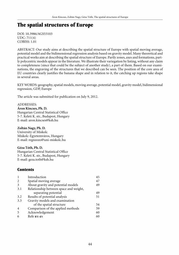
The first provocative form was published in the study of Brunet (1989) as the »European Backbone«.Later it was called by its popular name »Blue Banana«. The authors drew a banana-shaped form to visu-alise the economic core area approximately from Liverpool to Nice or from London to Milan (Figure 1).Our figures present – without any claim to completeness – the approaches that we consider to be the mostimportant ones.

A form similar to the banana can also be found in East-Central Europe called the »Central EuropeanBoomerang« (see Figure 1). According to Gorzelak (1996), the determinant areas of this form – stretch-ing from Gdansk to Budapest and including Poznan, Wroclaw, Prague and the triangle of Vienna-Bratislava-Budapest – are the capitals, the real places of development.

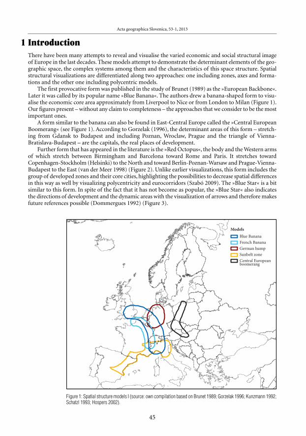
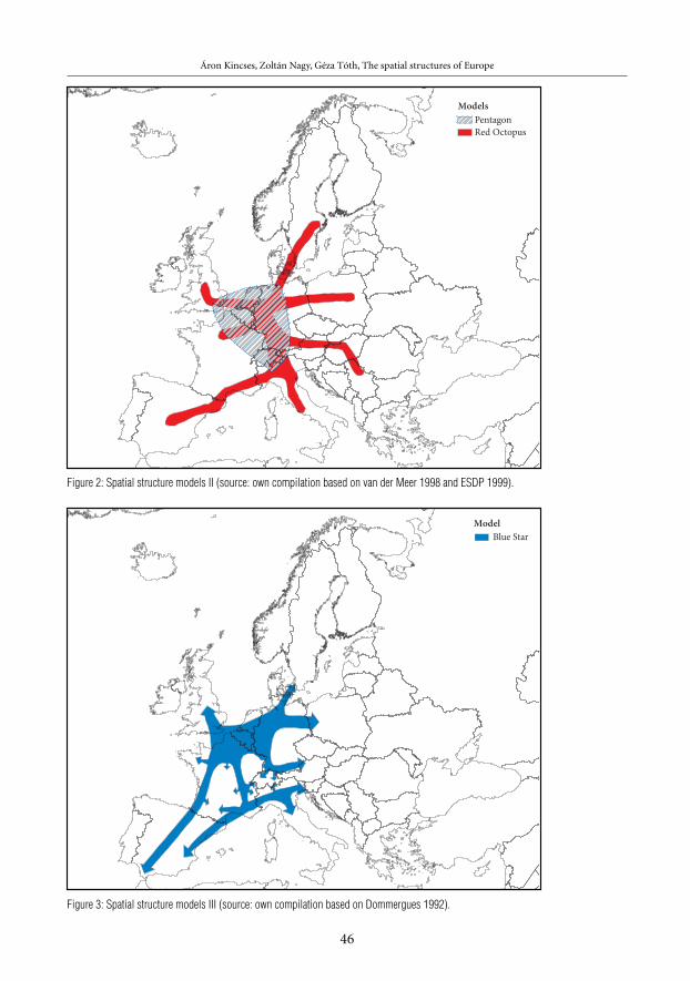
Further form that has appeared in the literature is the »Red Octopus«, the body and the Western armsof which stretch between Birmingham and Barcelona toward Rome and Paris. It stretches towardCopenhagen-Stockholm (Helsinki) to the North and toward Berlin-Poznan-Warsaw and Prague-Vienna-Budapest to the East (van der Meer 1998) (Figure 2). Unlike earlier visualizations, this form includes thegroup of developed zones and their core cities, highlighting the possibilities to decrease spatial differencesin this way as well by visualizing polycentricity and eurocorridors (Szabó 2009). The »Blue Star« is a bitsimilar to this form. In spite of the fact that it has not become as popular, the »Blue Star« also indicatesthe directions of development and the dynamic areas with the visualization of arrows and therefore makesfuture references possible (Dommergues 1992) (Figure 3).

Figure 1: Spatial structure models I (source: own compilation based on Brunet 1989; Gorzelak 1996; Kunzmann 1992;Schatzl 1993; Hospers 2002).

ModelsBlue BananaFrench BananaGerman humpSunbelt zoneCentral Europeanboomerang


46

ModelsPentagonRed Octopus

ModelBlue Star

Figure 2: Spatial structure models II (source: own compilation based on van der Meer 1998 and ESDP 1999).

Figure 3: Spatial structure models III (source: own compilation based on Dommergues 1992).

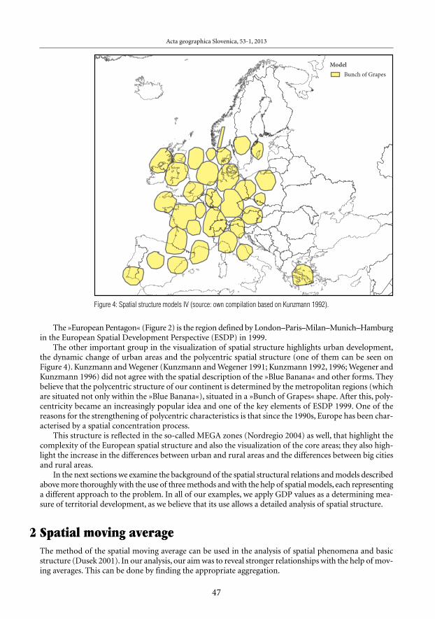
The »European Pentagon« (Figure 2) is the region defined by London–Paris–Milan–Munich–Hamburgin the European Spatial Development Perspective (ESDP) in 1999.

The other important group in the visualization of spatial structure highlights urban development,the dynamic change of urban areas and the polycentric spatial structure (one of them can be seen onFigure 4). Kunzmann and Wegener (Kunzmann and Wegener 1991; Kunzmann 1992, 1996; Wegener andKunzmann 1996) did not agree with the spatial description of the »Blue Banana« and other forms. Theybelieve that the polycentric structure of our continent is determined by the metropolitan regions (whichare situated not only within the »Blue Banana«), situated in a »Bunch of Grapes« shape. After this, poly-centricity became an increasingly popular idea and one of the key elements of ESDP 1999. One of thereasons for the strengthening of polycentric characteristics is that since the 1990s, Europe has been char-acterised by a spatial concentration process.

This structure is reflected in the so-called MEGA zones (Nordregio 2004) as well, that highlight thecomplexity of the European spatial structure and also the visualization of the core areas; they also high-light the increase in the differences between urban and rural areas and the differences between big citiesand rural areas.

In the next sections we examine the background of the spatial structural relations and models describedabove more thoroughly with the use of three methods and with the help of spatial models, each representinga different approach to the problem. In all of our examples, we apply GDP values as a determining mea-sure of territorial development, as we believe that its use allows a detailed analysis of spatial structure.

2 Spatial moving averageThe method of the spatial moving average can be used in the analysis of spatial phenomena and basicstructure (Dusek 2001). In our analysis, our aim was to reveal stronger relationships with the help of mov-ing averages. This can be done by finding the appropriate aggregation.


47

Figure 4: Spatial structure models IV (source: own compilation based on Kunzmann 1992).

ModelBunch of Grapes


48

In the case of a given elemental unit, the spatial moving average of the examined characteristic canbe found by calculating the average of the values for the surrounding areas, defined based on the giventopological characteristics in Equation (1) (Haining 1978):

(1)

for elements where d(xi; xj)≤ m where M(xi) is the moving average of point i, d(xi, xj) is the distance betweenthe centres of i and j regions and m is the extension of the moving average (radius). xj refers to the valueto be averaged belonging to the jth observation, i.e., per capita GDP, and fj is the frequency or weight belong-ing to the jth observation. In this case, if the moving average of per capita GDP is calculated, it is thepopulation.

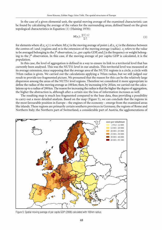
In this case, the level of aggregation is defined in a way to ensure its link to a territorial level that hascurrently been analysed. This was the NUTS1 level in our analysis. This territorial level was measured atits average extension, since supposing that the average area of the NUTS1 regions is a circle, a circle with70 km radius is given. We carried out the calculations applying a 70 km radius, but we still judged ourresult to provide too fragmented picture. We presumed that the reason for this can be the relatively largedispersion among the areas of the NUTS1 level regions. Therefore we considered it more appropriate todefine the radius of the moving average as 100km; then, by increasing it by 20km, we carried out the calcu-lations up to a radius of 200km. The reason for increasing the radius is that the higher the degree of aggregation,the higher the abstraction is, although after a certain size the loss of information increases as well.

The resulting map is much less fragmented compared to the base data, thus providing a possibilityto carry out a more detailed analysis. Based on the map (Figure 5), we can conclude that the regions inthe most favourable position in Europe – the engines of the economy – emerge from the examined areaslike islands. These regions are primarily certain southern provinces in Germany, the regions of Rome andNorthern Italy; the Northern part of Switzerland, a considerable part of Austria, the agglomerations of

M xi

f xfj j

j( )

( )=

⋅∑∑

euro per inhabitant 2 912–12 00012 001–20 00020 001–25 00025 001–30 00030 001–40 00040 001–93 580

Figure 5: Spatial moving average of per capita GDP (2008) calculated with 100 km radius.

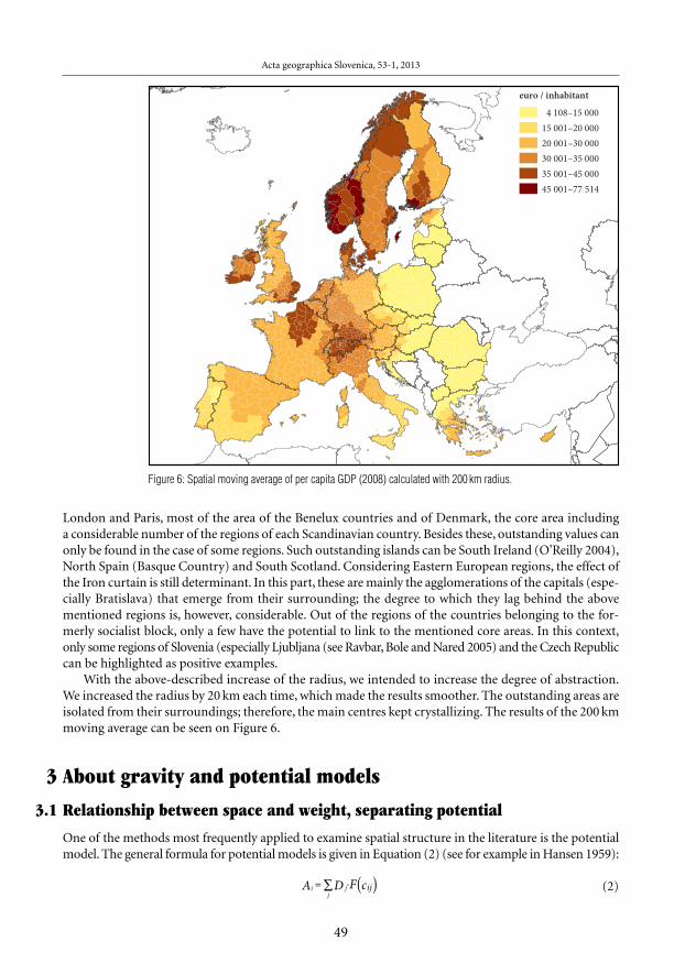
London and Paris, most of the area of the Benelux countries and of Denmark, the core area includinga considerable number of the regions of each Scandinavian country. Besides these, outstanding values canonly be found in the case of some regions. Such outstanding islands can be South Ireland (O'Reilly 2004),North Spain (Basque Country) and South Scotland. Considering Eastern European regions, the effect ofthe Iron curtain is still determinant. In this part, these are mainly the agglomerations of the capitals (espe-cially Bratislava) that emerge from their surrounding; the degree to which they lag behind the abovementioned regions is, however, considerable. Out of the regions of the countries belonging to the for-merly socialist block, only a few have the potential to link to the mentioned core areas. In this context,only some regions of Slovenia (especially Ljubljana (see Ravbar, Bole and Nared 2005) and the Czech Republiccan be highlighted as positive examples.

With the above-described increase of the radius, we intended to increase the degree of abstraction.We increased the radius by 20 km each time, which made the results smoother. The outstanding areas areisolated from their surroundings; therefore, the main centres kept crystallizing. The results of the 200 kmmoving average can be seen on Figure 6.

3 About gravity and potential models

3.1 Relationship between space and weight, separating potential

One of the methods most frequently applied to examine spatial structure in the literature is the potentialmodel. The general formula for potential models is given in Equation (2) (see for example in Hansen 1959):

(2)


49

i jj

A D F cij= ∑ ⋅ ( )

Figure 6: Spatial moving average of per capita GDP (2008) calculated with 200 km radius.

euro / inhabitant

4 108–15 00015 001–20 00020 001–30 00030 001–35 00035 001–45 00045 001–77 514


where Ai is the potential of a region i (NUTS3 regions), Dj is the mass of the region j, cij is the distancebetween the centre of i and j regions (straight line distances) and F(cij) is the resistance factor.

The potential therefore is calculated from the sum of its own and internal potentials (Pooler 1987)using Equation (3):

(3)

where ΣAi is the overall potential of the area i, SAi is its own and BAi is the internal potential. The poten-tial value in a given point is therefore determined by the internal and own potential (the sum of its ownmass and the effect of its own area size). The own potential refer to the effect of the region i on its ownpotential, while internal potential shows the impact of all other regions on the potential of region i.

Based on the topology of the geometry of potential models, one can conclude that whichever modelis used, a common point is that they measure the effects of the position of a space range and the size dis-tribution of the masses as described in Equation (4). The position of the space range is basically definedby the geographical position. This means that for a given potential value, it is not possible to decide whetherit is a consequence of the position of the favourable/unfavourable (settlement, regional) structure, posi-tion or masses, of the area size or of the effect of its own mass. Therefore, we aim at separating these effects,describing the share of the parts in the overall potential values and introducing territorial differences.

(4)

In an arbitrary point of the space, the effect of the potential derived from the spatial location refersto the value that could have been provided that the masses are the same in each of the specified territo-rial units, as in Equation (5):

(5)

where i, j, k are territorial area or units, mk is »mass« in the kth territorial unit, which in this case is theGDP; n is the number of territorial units included in the analysis and f(dij) is the resistance factor, func-tion.

The effect of mass distribution in an arbitrary point of the space is the value-difference between theinternal potential and the location potential at the given point:

(6)

The effects of area size (Equation (7)) and own mass (Equation (8)) can be interpreted accordinglyin the case of their own potentials (the signs are the same as above):

(7)

(8)

where mi is »mass« in the ith territorial unit, which in this case is the GDP; n is the number of territorialunits includd in the analysis, dii is the distance within the region, which is calculated in a way that the areaof a region is considered to be circle. The radius of this circle is equal to the own distance. f(dii) is the resis-tance factor or function.

50

i i iA SA BA∑ = +

A BA SAi i i imassdistribution

ilocation

imassweight

iarU U U∑ = + = + + + eea sizeU

U Uimassdistribution

i ilocationBA= −

U Uiownmass

i iareasizeSA= −

Uilocation

kk

n

ijj

m

n

f d=

∑

∑

=

1

( )

Uiareasize

mii

n

ii

n

f d=

∑=

1

( )

3.2 Results of potential analysis

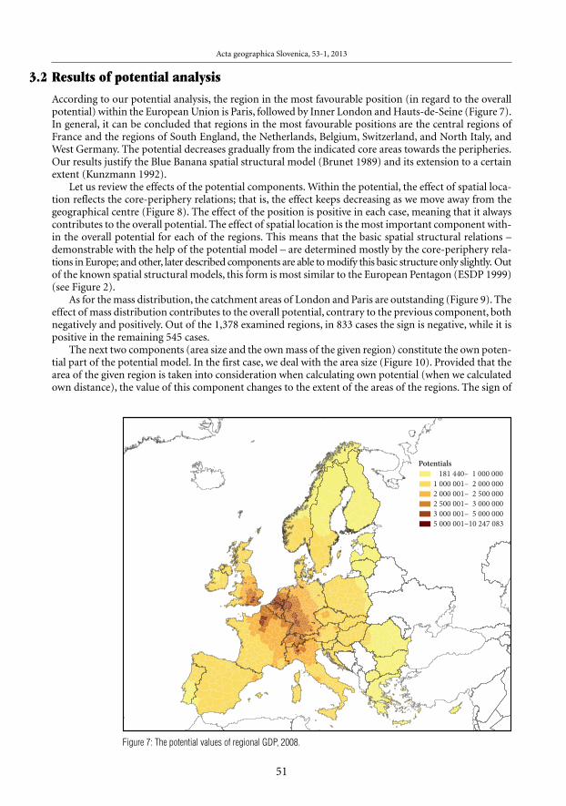
According to our potential analysis, the region in the most favourable position (in regard to the overallpotential) within the European Union is Paris, followed by Inner London and Hauts-de-Seine (Figure 7).In general, it can be concluded that regions in the most favourable positions are the central regions ofFrance and the regions of South England, the Netherlands, Belgium, Switzerland, and North Italy, andWest Germany. The potential decreases gradually from the indicated core areas towards the peripheries.Our results justify the Blue Banana spatial structural model (Brunet 1989) and its extension to a certainextent (Kunzmann 1992).

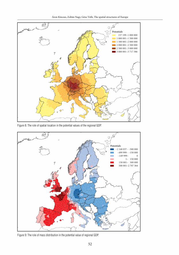
Let us review the effects of the potential components. Within the potential, the effect of spatial loca-tion reflects the core-periphery relations; that is, the effect keeps decreasing as we move away from thegeographical centre (Figure 8). The effect of the position is positive in each case, meaning that it alwayscontributes to the overall potential. The effect of spatial location is the most important component with-in the overall potential for each of the regions. This means that the basic spatial structural relations –demonstrable with the help of the potential model – are determined mostly by the core-periphery rela-tions in Europe; and other, later described components are able to modify this basic structure only slightly. Outof the known spatial structural models, this form is most similar to the European Pentagon (ESDP 1999)(see Figure 2).

As for the mass distribution, the catchment areas of London and Paris are outstanding (Figure 9). Theeffect of mass distribution contributes to the overall potential, contrary to the previous component, bothnegatively and positively. Out of the 1,378 examined regions, in 833 cases the sign is negative, while it ispositive in the remaining 545 cases.

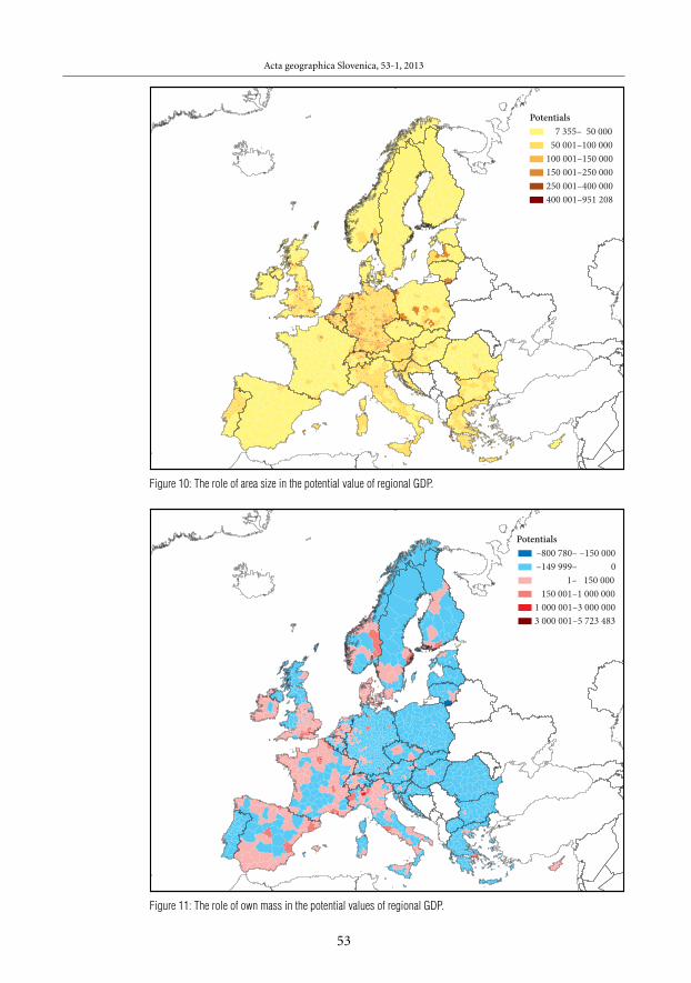
The next two components (area size and the own mass of the given region) constitute the own poten-tial part of the potential model. In the first case, we deal with the area size (Figure 10). Provided that thearea of the given region is taken into consideration when calculating own potential (when we calculatedown distance), the value of this component changes to the extent of the areas of the regions. The sign of


51

Figure 7: The potential values of regional GDP, 2008.

Potentials 181 440– 1 000 0001 000 001– 2 000 0002 000 001– 2 500 0002 500 001– 3 000 0003 000 001– 5 000 0005 000 001–10 247 083


52

Potentials 157 199–1 000 0001 000 001–1 500 0001 500 001–2 000 0002 000 001–2 500 0002 500 001–3 000 0003 000 001–3 717 386

Potentials–1 148 037– –500 000 –499 999– –150 000 –149 999– 0 1– 150 000 150 001– 500 000 500 001–2 707 364

Figure 8: The role of spatial location in the potential values of the regional GDP.

Figure 9: The role of mass distribution in the potential value of regional GDP.


53

Figure 10: The role of area size in the potential value of regional GDP.

Potentials 7 355– 50 000 50 001–100 000100 001–150 000150 001–250 000250 001–400 000400 001–951 208

Figure 11: The role of own mass in the potential values of regional GDP.

Potentials –800 780– –150 000 –149 999– 0 1– 150 000 150 001–1 000 0001 000 001–3 000 0003 000 001–5 723 483


the area size is always positive and its extent is inversely related to the area of the region. Thought we didnot use population data, we can conclude that the value of this component refers primarily to urbanisa-tion, since the regions with smaller area are big cities in most of the cases.

Finally, the last component is the own mass of the given region (Figure 11). Its sign can also be eithernegative or positive.

In total, we can conclude that the different spatial structural models available in the literature can besynthetised by dividing the potential models into parts. The division into axes and zones can be shownin the analyses of spatial position and mass distribution, while the polycentric view can be linked to areasize and to own mass. They visualise the real space structure side by side, complementing each other. Bydividing the potential models into parts, the above described spatial structural ideas that are present inthe space at the same time can be standardised.

3.3 Gravity models and examination of the spatial structure

After separating the potential models as described above, the other approach to examine spatial struc-ture is about gravity models that are based on the application of forces. With the approach that we presenthere, one can assign attraction directions to the given territorial unit. This method complements and spec-ifies the view of spatial structure described by the potential models.

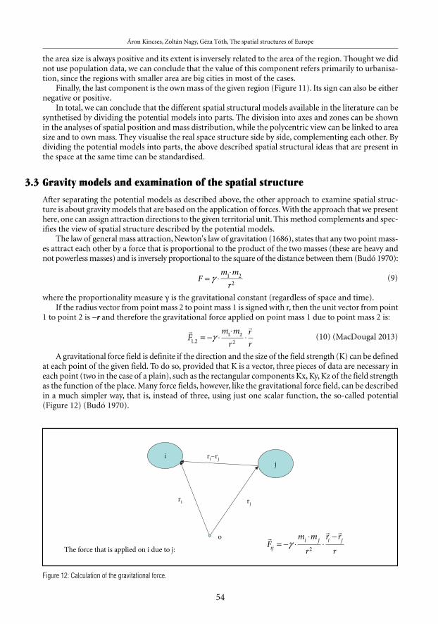
The law of general mass attraction, Newton's law of gravitation (1686), states that any two point mass-es attract each other by a force that is proportional to the product of the two masses (these are heavy andnot powerless masses) and is inversely proportional to the square of the distance between them (Budó 1970):

(9)

where the proportionality measure γ is the gravitational constant (regardless of space and time).If the radius vector from point mass 2 to point mass 1 is signed with r, then the unit vector from point

1 to point 2 is –r and therefore the gravitational force applied on point mass 1 due to point mass 2 is:

(10) (MacDougal 2013)

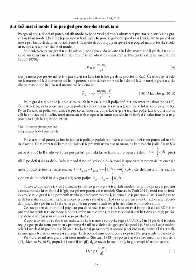
A gravitational force field is definite if the direction and the size of the field strength (K) can be definedat each point of the given field. To do so, provided that K is a vector, three pieces of data are necessary ineach point (two in the case of a plain), such as the rectangular components Kx, Ky, Kz of the field strengthas the function of the place. Many force fields, however, like the gravitational force field, can be describedin a much simpler way, that is, instead of three, using just one scalar function, the so-called potential(Figure 12) (Budó 1970).

54

Figure 12: Calculation of the gravitational force.

ij

o

ri rj

ri–rj

r

r r

Fm m

r

r r

riji j i j= − ⋅⋅

⋅−

γ2The force that is applied on i due to j:

Fm mr

= ⋅⋅

γ 1 22

r

r

Fm mr

rr1 2

1 22, = − ⋅

⋅⋅γ

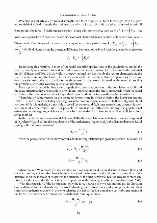
Potential is similarly related to field strength than force or potential force to strength. If in the grav-itation field of K field strength, the trial mass, on which a force of F = mK is applied, is moved to point B

from point A by force –F (without acceleration) along with some curve, then work of has

to be done against force F based on the definition of work. This work is independent of the curve from A to B.

Therefore it is the change of the potential energy of an arbitrary trial mass:

. By dividing by m, the potential difference between points B and A in the gravitational space is:

By utilizing this relation, in most of the social scientific applications of the gravitational model thespace primarily was intended to be described by only one scalar function (see for example the potentialmodel) (Kincses and Tóth 2011), while in the gravitational law, it is mainly the vectors characterizing thespace that have an important role. The main reason for this is that the arithmetic operations with num-bers are easier to handle than calculations with vectors. In other words, for work with potentials, solvingthe problem also means avoiding calculation problems.

Even if potential models often show properly the concentration focus of the population or GDP andthe space structure, they are not able to provide any information on the direction towards which the socialattribute of the other regions attract a specified region and on the force with which they attract it.

Therefore, by using vectors we are trying to demonstrate in which direction the European regions(NUTS1, 2, and 3) are attracted by other regions in the economic space compared to their real geographicalposition. With this analysis, it is possible to reveal the centres and fault lines representing the most impor-tant areas of attractiveness and it is possible to visualise the differences among the gravitationalorientation of the regions, which we will describe in more detail in a later section. First of all, let us lookat the method.

In the traditional gravitational model (Stewart 1948) the »population force« between i and j are expressedin Dij, where Wi and Wj are the populations of the settlements (regions), dij is the distance between i, andj and g is the empirical constant:

(11)

With the generalisation of the above formula, the following relationship is given in Equation (12) and (13):

(12)

(13)

where Wi and Wj indicate the masses taken into consideration, dij is the distance between them andc is the constant, which is the change in the intensity of the inter-territorial relations as a function of thedistance. With the increase of the power, the intensity of the inter-territorial relations becomes more sen-sitive to the distance and at the same time, the importance of the masses gradually decreases (see Dusek 2003).

With this extension of the formula, not only the force between the two regions but also its directioncan be defined. In the calculations, it is worth dividing the vectors into x and y components, and thensummarising them separately. In order to calculate this effect (the horizontal and vertical components ofthe forces), the necessary formulas can be deducted from Equation 14:

(14)


55

U U K dsB A sA

B

− = −∫

iji j

ijD d

gW W

= ⋅⋅

( )2

D DijW Wdiji j

ijc

= =⋅v

v v

DW Wd diji j

ijc ij= −⋅

⋅+1

DW W

dx xjij

X i j

ijc i=⋅

⋅ −+1

( )

L FdssA

B

= −∫

L E E F ds m K dspotB potA sA

B

= − = − = −∫m K dsp s

A

B

− ∫

.


(15)

where xi, xj, yi, yj are the centroids of regions i and j.If, however, the calculation is carried out for each region included in the analysis, the direction and

the force of the effect on the given territorial unit can be defined using Equation (16) and (17):

(16)

(17)

With these equations, in each territorial unit, the magnitude and the direction of the force due to theother regions can be defined. The direction of the vector assigned to the regions determines the attrac-tion direction of the other regions, while the magnitude of the vector is related to the magnitude of theforce. In order to make visualisation possible, the forces are transformed to proportionate movements inEquation (18) and (19):

(18)

(19)

where Xi mod and Yi mod are the coordinates of the new points modified by gravitational force, x and yare the coordinates of the original point set, their extreme values are xmax, ymax, a xmin, ymin, Dij are the forcesalong the axes and k is constant, in this case its value is 0.5. We got this value as a result of an iterationprocedure.

Then it is worth comparing the new point set with the original one. This can naturally be done withvisualisation, but in the case of such a large number of points, this alone probably does not provide a real-ly promising result. Much more favourable results can be obtained by applying bidimensional regressionanalysis (see the equations related to the Euclidean version in Table 1).

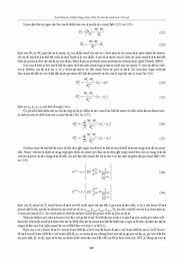
Where x and y refers to the coordinates of the independent form, a and b sign the coordinates of thedependent form, a' and b' are the coordinates of the independent form in the dependent form. α1 refersto the extent of the horizontal shift, while α2 defines the extent of the vertical shift. β1 and β2 are used todetermine the scale difference (Φ) and Θ is the rotation angle. SST is total sum of squares, SSR is sum ofsquares due to regression, SSE is explained sum of squares of errors/residuals that is not explained by theregression).

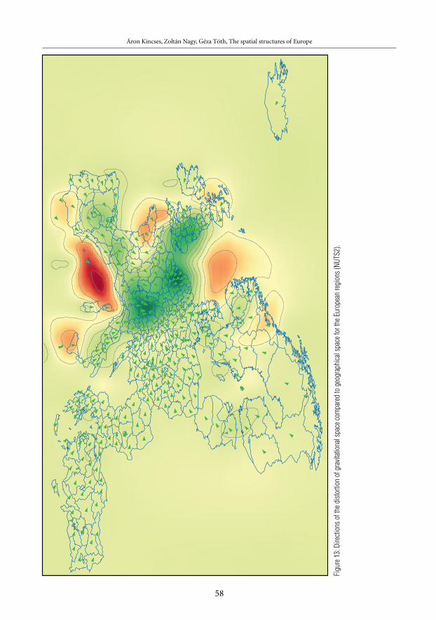
To visualise the bidimensional regression, the Darcy program can be useful (D'arcy 1917). The gridfitted to the coordinate system of the dependent form and its interpolated modified position make it pos-sible to further generalise the information about the points of the regression.

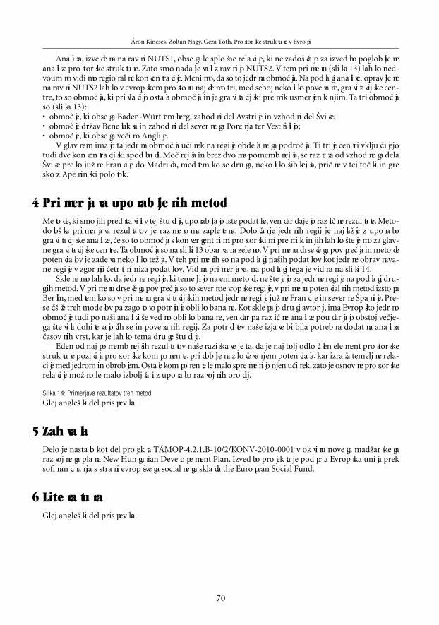
The arrows in Figure 13 show the direction of movement and the grid colour refers to the nature ofthe distortion. Warm colours indicate divergence; that is, the movements in the opposite direction, whichcan be considered to indicate the most important gravitational fault lines. Areas indicated with green andits shades refer to the opposite, namely to the concentration, to the movements in the same directions(convergence), which can be considered to be the most important gravitational centres.

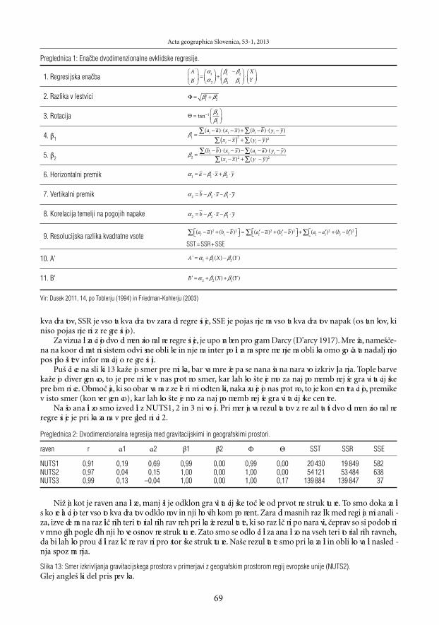
Our analysis can be carried out at the NUTS1, 2, and 3 levels. The comparison of the results with thoseof bidimensional regression can be found in Table 2.

56

DW W

dy yij

Y i j

ijc i j=⋅

⋅ −+1

( )

DW W

dx xij

X i j

ijc i j

j

n= −

⋅⋅ −

+=∑ 1

1( )

DW W

dy yij

Y i j

ijc i j

j

n= −

⋅⋅ −

+=∑ 11

( )

i i ijX

ijX

ijX

x x D xx

kDD

modmax

min max

min

= + ⋅ ⋅

1

i i ijY

ijY

ijY

y y Dyy

kDD

modmax

min max

min

= + ⋅ ⋅

1

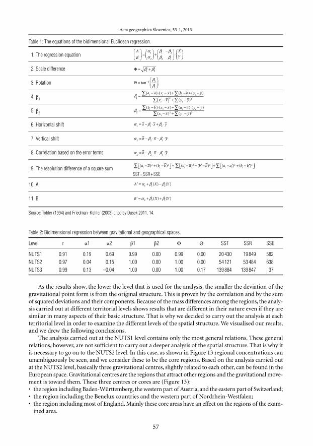
Table 2: Bidimensional regression between gravitational and geographical spaces.

Level r α1 α2 β1 β2 Φ Θ SST SSR SSE

NUTS1 0.91 0.19 0.69 0.99 0.00 0.99 0.00 20 430 19849 582

NUTS2 0.97 0.04 0.15 1.00 0.00 1.00 0.00 54 121 53484 638

NUTS3 0.99 0.13 –0.04 1.00 0.00 1.00 0.17 139 884 139847 37

As the results show, the lower the level that is used for the analysis, the smaller the deviation of thegravitational point form is from the original structure. This is proven by the correlation and by the sumof squared deviations and their components. Because of the mass differences among the regions, the analy-sis carried out at different territorial levels shows results that are different in their nature even if they aresimilar in many aspects of their basic structure. That is why we decided to carry out the analysis at eachterritorial level in order to examine the different levels of the spatial structure. We visualised our results,and we drew the following conclusions.

The analysis carried out at the NUTS1 level contains only the most general relations. These generalrelations, however, are not sufficient to carry out a deeper analysis of the spatial structure. That is why itis necessary to go on to the NUTS2 level. In this case, as shown in Figure 13 regional concentrations canunambiguously be seen, and we consider these to be the core regions. Based on the analysis carried outat the NUTS2 level, basically three gravitational centres, slightly related to each other, can be found in theEuropean space. Gravitational centres are the regions that attract other regions and the gravitational move-ment is toward them. These three centres or cores are (Figure 13):• the region including Baden-Württemberg, the western part of Austria, and the eastern part of Switzerland;• the region including the Benelux countries and the western part of Nordrhein-Westfalen;• the region including most of England. Mainly these core areas have an effect on the regions of the exam-ined area.


57

Table 1: The equations of the bidimensional Euclidean regression.

1. The regression equation

2. Scale difference

3. Rotation

4. β1

5. β2

6. Horizontal shift

7. Vertical shift

8. Correlation based on the error terms

9. The resolution difference of a square sumSST=SSR+SSE

10. A'

11. B'

Source: Tobler (1994) and Friedman–Kohler (2003) cited by Dusek 2011, 14.

A

B

XY

’

’

=

+−

⋅

αα

β ββ β

1

2

1 2

2 1

Φ = +β β12

22

Θ =

−tan 1 2

1

ββ

β1 2 2=

− ⋅ − + − ⋅ −

−( ) + −∑∑∑∑

( ) ( ) ( ) ( )

( )

a a x x b b y y

x x y yi i i i

i i

β2 2 2=− ⋅ − − − ⋅ −

− + −∑∑∑∑

( ) ( ) ( ) ( )( ) ( )

b b x x a a y yx x y y

i i i i

i

α β β1 1 2= − ⋅ + ⋅a x y

α β β2 2 1= − ⋅ − ⋅b x y

α β β2 2 1= − ⋅ − ⋅b x y

A X Y’ ( ) ( )= + −α β β1 1 2

B X Y’ ( ) ( )= + +α β β2 2 1

( ) ( ) ( ) ( ) ( ) (a a b b a a b b a a bi i i i i i i− + − = ′ − + ′ − + − ′ + −∑ ∑2 2 2 2 2 ′′ ∑ bi )2


58

Figure 13: Dire

ctions of the distortion of gravitational space com

pared to geographical space for the European regions (NUT

S2).

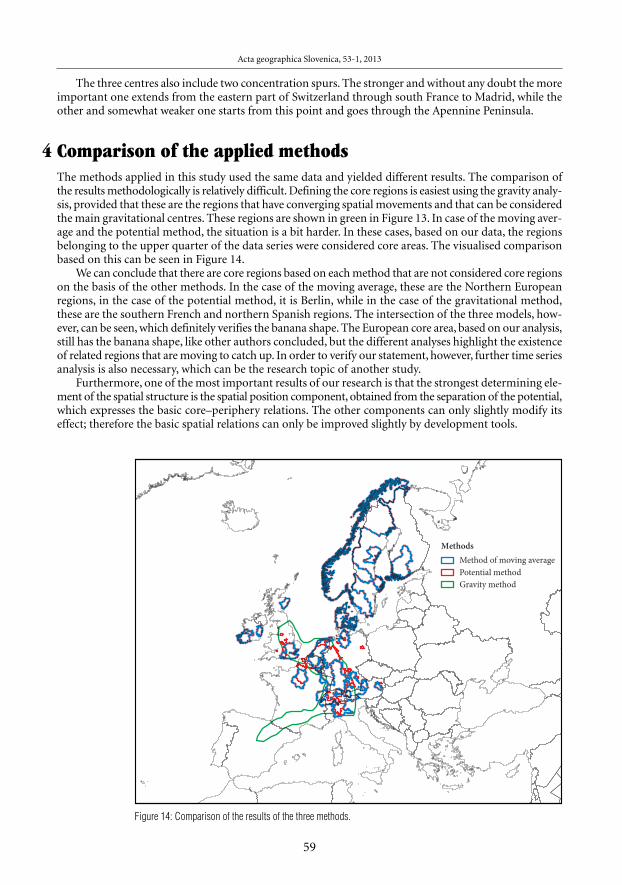
The three centres also include two concentration spurs. The stronger and without any doubt the moreimportant one extends from the eastern part of Switzerland through south France to Madrid, while theother and somewhat weaker one starts from this point and goes through the Apennine Peninsula.

4 Comparison of the applied methodsThe methods applied in this study used the same data and yielded different results. The comparison ofthe results methodologically is relatively difficult. Defining the core regions is easiest using the gravity analy-sis, provided that these are the regions that have converging spatial movements and that can be consideredthe main gravitational centres. These regions are shown in green in Figure 13. In case of the moving aver-age and the potential method, the situation is a bit harder. In these cases, based on our data, the regionsbelonging to the upper quarter of the data series were considered core areas. The visualised comparisonbased on this can be seen in Figure 14.

We can conclude that there are core regions based on each method that are not considered core regionson the basis of the other methods. In the case of the moving average, these are the Northern Europeanregions, in the case of the potential method, it is Berlin, while in the case of the gravitational method,these are the southern French and northern Spanish regions. The intersection of the three models, how-ever, can be seen, which definitely verifies the banana shape. The European core area, based on our analysis,still has the banana shape, like other authors concluded, but the different analyses highlight the existenceof related regions that are moving to catch up. In order to verify our statement, however, further time seriesanalysis is also necessary, which can be the research topic of another study.

Furthermore, one of the most important results of our research is that the strongest determining ele-ment of the spatial structure is the spatial position component, obtained from the separation of the potential,which expresses the basic core–periphery relations. The other components can only slightly modify itseffect; therefore the basic spatial relations can only be improved slightly by development tools.


59

Figure 14: Comparison of the results of the three methods.

MethodsMethod of moving averagePotential methodGravity method


5 AcknowledgementThe described work was carried out as part of the TÁMOP-4.2.1.B-10/2/KONV-2010-0001 project in theframework of the New Hungarian Development Plan. The realization of this project is supported by theEuropean Union, co-financed by the European Social Fund.

6 Refe ren cesBru net, R. 1989: Les vil les euro peénnes. Rap port pour la DATAR. Mont pel lier.Budó, Á. 1970: Kísérle ti Fizi ka I. Buda pest.D'arcy, T. 1917: On growth and form. New York. Inter net: http://spa tial-mo del ling.info/Darcy-2-mo du -

le-de-com pa rai sonDom mer gues, P. 1992: The Stra te gies for Inter na tio nal and Inter re gio nal Coo pe ra tion. Eki stics 59. Athens.Du sek, T. 2001: A területi mozgóátlag. Területi Sta tisz ti ka 41-3. Buda pest.Du sek, T. 2003: A gra vitációs modell és a gra vitációs törvény össze ha sonlítása. Tér és Társa da lom 17-1.

Buda pest.Du sek, T. 2011: Kétdi men ziós regress zió a területi kutatások ban. Területi Sta tisz ti ka 51-1. Buda pest.ESDP 1999: Euro pean Spa tial Deve lop ment Pers pec ti ve. Euro pean Comis sion. Brus sels.Fried man, A., Koh ler, B. 2003: Bidi men sio nal Regres sion: Asses sing the Con fi gu ral Simi la rity and Accu racy

of Cog ni ti ve Maps and Other Two-Di men sio nal Data Sets. Psycho lo gi cal Met hods 8-4. Was hing ton.DOI: 10.1037/1082-989X.8.4.468

Gor ze lak, G. 1996: The Regio nal Dimen sion of Trans for ma tion in Cen tral-Eu ro pe. Lon don.Hai ning, R. P. 1978: The Moving Ave ra ge Model for Spa tial Inte rac tion. Tran sac tions of the Insti tu te of

Bri tish Geo grap hers 3-2. Oxford.Han sen, W.G. 1959: How acces si bi lity sha pes land use – Jour nal of the Ame ri can Plan ning Asso cia tion

25-2. Washington. DOI: 10.1080/01944365908978307Hos pers, G. J. 2002: Beyond the Blue Bana na? Struc tu ral Chan ge in Euro pe's Geo-Eco nomy. 42nd Euro pean

Con gress of the Regio nal Scien ce Asso cia tion. Dort mund. Inter net: http://www-sre.wu-wien.ac.at/ersa/er -sa confs/ersa02/cd-rom/pa pers/210.pdf (1. 9. 2012).

Kinc ses, Á., Tóth, G. 2011: Poten ciálmo del lek geo me triája. Területi Sta tisz ti ka 51-1. Buda pest.Kunz mann, K.R. 1992: Zur Ent wic klung der Stadtsy ste me in Euro pa. Mit tei lun gen der Öster reic hisc hen

Geo grap hisc hen Gesellsc haft 134. Wien.Kunz mann, K.R. 1996: Euro-me ga lo po lis or The me park Euro pe? Sce na rios for Euro pean spa tial deve lop -

ment. Inter na tio nal Plan ning Stu dies 1-2. DOI: 10.1080/13563479608721649Kunz mann, K.R., Wege ner, M. 1991: The pat tern of urba ni za tion in Euro pe. Eki stics 58. Athens.Mac Dou gal, D.W. 2013: New ton's Gra vity. Athens.Meer van der, L. 1998: Red octo pus. A new pers pec ti ve for Euro pean spa tial deve lop ment poli cies. Brook -

field.Nor dre gio 2004: ESPON 1.1.1 Poten tials for poly cen tric deve lop ment in Euro pe, Stock holm/ Luxem bourg:

Nor dre gio/ESPON Moni to ring Com mit tee. Inter net: http://www.es pon.eu. (1. 9. 2012).O'Reilly, G. 2004: Eco no mic Glo ba li sa tions: Ire land in the EU: 1973–2003. Acta geo grap hi ca Slo ve ni ca 44-1.

Ljub lja na. DOI: 10.3986/AGS44103Poo ler, J. 1987: Mea su ring geo grap hi cal acces si bi lity: a re view of cur rent approac hes and prob lems in the

use of popu la tion poten tials – Geo fo rum. 18/3. Oxford. DOI: 10.1016/0016-7185(87)90012-1Rav bar, M., Bole, D., Nared, J. 2005: A crea ti ve mili eu and the role of geo graphy in stud ying the com pe ti ti -

ve ness of cities: the case of Ljub lja na. Acta geo grap hi ca Slo ve ni ca 45-2. Ljub lja na. DOI: 10.3986/AGS45201Schätzl L. 1993: Wirtsc hafts geo grap hie der Europäisc hen Gemeinsc haft. Stutt gart.Ste wart, J.Q. 1948: Demo grap hic Gra vi ta tion: Evi den ce and Appli ca tion Socio me try 11 (1–2).Szabó, P. 2009: Európa térs zer ke ze te különböző szemléle tek tükrében. Földraj zi Közlemények 133-2. Buda pest.Tob ler, W. 1994: Bidi men sio nal Regres sion. Geo grap hi cal Analy sis 26-3. Colum bus. DOI: 10.1111/

j.1538-4632.1994.tb00320.xWe ge ner M. Kunz mann, K.R. 1996: New Spa tial Pat terns of Euro pean Urba ni sa tion. Urban Net works in

Euro pe. Paris.

60

Áron Kincses, Zoltán Nagy, Géza Tóth, Pro stor ske struk tu re v Evro pi

Pro stor ske struk tu re v Evro pi

DOI: 103986/AGS53103UDK: 711(4)COBISS: 1.01

IZVLE^EK: Cilj {tu di je je opis pro stor ske struk tu re Evro pe s kra jev no drse ~im pov pre~ jem, mode lom mo` -no sti in dvo di men zio nal ne regre sij ske ana li ze, teme lje ~e na te` nost nem mode lu. Pro stor sko struk tu ro Evro peopi su je veli ko teo re ti~ nih in prak ti~ nih del. V li te ra tu ri se pojav lja jo del no obmo~ ja, osi in for ma ci je, del -no pa poli cen tri~ ni mode li. Neka te re od teh nava ja mo, brez trdi tev o po pol no sti (kar bi lah ko bila temadru ge {tu di je). Tudi po na{ih opa ̀ a njih so vid ni obri si struk tur, ki jih v ~lan ku opi su je mo. Ume sti tev jedradr`av Evrop ske uni je jasno opra vi ~u je obli ko bana ne in na njo se na ve~ obmo~ jih nave zu je jo osta le, dohi -te va jo ~e jo regi je.

KLJU^NE BESEDE: geo gra fi ja, pro stor ske struk tu re, drse ~e pov pre~ je, poten cial ni model, te` nost ni model,dvo di men zio nal na regre si ja, BDP, Evro pa

Ured ni{ tvo je pris pe vek pre je lo 9. ju li ja 2012.

NASLOVI AVTORJEV:dr. Áron Kinc sesHun ga rian Cen tral Sta ti sti cal Offi ce5–7. Kele ti K. str., Buda pest, Hun garyE-mail: aron.kinc ses�ksh.hu

dr. Zoltán NagyUni ver sity of MiskolcMi skolc-Eg ye temváros, Hun garyE-mail: regn zo zo�uni-mi skolc.hu

dr. Géza TóthHun ga rian Cen tral Sta ti sti cal Offi ce5–7. Kele ti K. str., Buda pest, Hun garyE-mail: geza.toth�ksh.hu

Vse bi na

1 Uvod 632 Kra jev no drse ~e pov pre~ je 643 O te` nost nih in poten cial nih mode lih 643.1 Pove za va med pro sto rom in ute` jo,

ki lo~u je poten cial 643.2 Rezul tati ana li ze poten cia lov 663.3 Te` nost ni mode li in pre gled pro stor ske

struk tu re 674 Pri mer ja va upo rab lje nih metod 705 Zah va la 706 Lite ra tu ra 70

62

1 UvodV zad njih deset let jih je bilo pre cej posku sov odkri va nja in vizua li za ci je raz no li ke gos po dar ske in social -ne podo be Evro pe. Ti mode li sku {a jo pri ka za ti odlo ~il ne ele men te geo graf ske ga pro sto ra, kom plek snihsiste mov in zna ~il no sti struk tur teh pro sto rov. Pro stor ske struk tur ne vizua li za ci je teme lji jo na dveh pri -sto pih: prva vklju ~u je obmo~ ja, osi in for ma ci je, dru ga pa poli cen tri~ ne mode le.

Prva pro vo ka tiv na obli ka je bila objav lje na v Bru ne to vi {tu di ji (1989) kot »evrop ska hrb te ni ca«. Kasne -je se je je pri je lo ime »mo dra bana na« (ang. Blue bana na). Za pred sta vi tev jedra gos po dar ske ga obmo~ jaso avtor ji obkro ̀ i li obmo~ je v ob li ki bana ne, ki sega prib li` no od Liver poo la do Nice ali od Lon do na doMila na (sli ka 1). Na{e sli ke pred stav lja jo – brez kakr {nih koli trdi tev o po pol no sti – pri sto pe, za kate remeni mo, da so naj po memb nej {i.

Sli ka 1: Mode li I kra jev ne struk tu re (vir: last na izde la va po Bru net 1989, Ger ze lak 1996, Kunz mann 1992, Schatzl 1993, Hos pers 2002).Glej angle{ ki del pris pev ka.

Ba na ni podob no obli ko lah ko naj de mo tudi na vzhod u sred nje Evro pe. Pra vi mo ji sred njee vrop skibume rang (ang. Cen tral Euro pean boo me rang; glej sli ko 1). Po Gor ze la ku (1996) so za to obmo~ je, ki seraz te za od Gdan ska do Budim pe {te in vklju ~u je Poz nan, Wroc law, Para go in tri kot nik Dunaj–Bra ti sla -va–Bu dim pe {ta, odlo ~il ne ga pome na glav na mesta, resni~ ni kra ji raz vo ja.

Sli ka 2: Mode li II kra je ve ne struk tu re (vir: last na izde la va po van der Mee ru 1998 in ESDP 1999).Glej angle{ ki del pris pev ka.

Na dalj njaob li ka, ki se pojav lja v li te ra tu ri, je »rde ~a hobot ni ca« (ang. Red octo pus), kate re telo in zahod -ne lov ke se raz te za jo med Bir ming ha mom in Bar ce lo no, ter pro ti Rimu in Pari zu. Na seve ru se raz te za jov sme ri Copen ha gen–Stock holm (Hel sin ki), na vzhod u pa v sme ri Ber lin–Poz nan–Var {a va ter Pra ga–Du -naj–Bu dim pe {ta (van der Meer 1998; sli ka 2). Za raz li ko od zgod nej {ih vizua li za cij ta obli ka vklju ~u je sku pi noraz vi tih obmo~ ji in nji ho va jedr na mesta s pou dar kom na mo` no stih zmanj {a nja pro stor skih raz lik, kottudi z vi zua li za ci jo poli cen tri~ no sti in evro ko ri dor jev (Szabó 2009). »Mo dra zvez da« (ang. Blue star) jetemu neko li ko podob na. êprav ni posta la tako pri ljub lje na, »mo dra zvez da« prav tako naka zu je sme riraz vo ja in dina mi ko obmo ~ij s pu{ ~i ca mi in je zato pri mer na za nadalj nje ana li ze. (Dom mer gues 1992;sli ka 3).

Sli ka 3: Model III kra jev ne struk tu re (vir: last na izde la va po Dom mer gues 1992). Leta 1999 je v Evrop ski pro stor ski raz voj ni pers pek ti vi(Eu ro pean spa tial deve lop ment pers pec ti ve – ESDP) obmo~ je med Lon do nom, Pari zom, Mila nom, Münchnom in Ham bur gom, opre de ljenokot »evrop ski pen ta gon«.Glej angle{ ki del pris pev ka.

Sli ka 4: Model IV kra jev ne struk tu re (vir: last na izde la va po Kunz mann 1992).Glej angle{ ki del pris pev ka.

Dru ga pomemb na sku pi na za vizua li za ci jo pro stor ske struk tu re pou dar ja urba ni raz voj, dina mi~ nespre mem be urba nih obmo ~ij in poli cen tri~ no pro stor sko struk tu ro (eno od teh lah ko vidi mo na sli ki 4).Kunz mann in Wege ner (Kunz mann in Wege ner 1991; Kunz mann 1992; 1996; Wege ner in Kunz -mann 1996) se nista stri nja la s pro stor skim opi som »mo dre bana ne« in dru gi mi obli ka mi. Pre pri ~a na stabila, da mest na obmo~ ja ne leì jo samo zno traj modre bana ne, tem ve~ v groz dih (ang. Bunch of gra pes)in tako dolo ~a jo poli cen tri~ no struk tu ro Evro pe. Poli cen tri~ nost je posta la ena bolj pri ljub lje nih tem ineden od klju~ nih ele men tov Evrop ske pro stor ske raz voj ne pers pek ti ve iz leta 1999. Eden od raz lo gov zakre pi tev poli cen tri~ nih zna ~il no sti je ta, da je bil za 90-a leta 20. sto let ja za Evro po zna ~i len pro ces pro -stor ske kon cen tra ci je.

Ta struk tu ra se kaè tudi v tako ime no va nih MEGA obmo~ jih (Nor dre gio 2004), ki prav tako pou -dar ja jo kom plek snost Evrop ske pro stor ske struk tu re kot tudi vizua li za ci jo jedr nih obmo ~ij; prav tako papou dar ja jo nara{ ~a jo ~o raz li ko med mesti in pode ̀ e ljem.

Z upo ra bo treh metod in s po mo~ jo pro stor skih mode lov, ki vsak zase pred stav lja dru ga ~en pri stopk prob le mu, bomo v na sled njih poglav jih podrob ne je preu ~i li ozad je rela cij pro stor skih struk tur in zgo -


63


raj opi sa nih mode lov. V vseh pri me rih kot odlo ~il no mero za pro stor ski raz voj upo rab lja mo vred no stiBDP-ja, saj meni mo, da nje go va upo ra ba omo go ~a podrob no ana li zo kra jev ne struk tu re.

2 Kra jev no drse ~e pov pre~ jeMe to do kra jev ne ga drse ~e ga pov pre~ ja je mogo ~e upo ra bi ti za ana li zo kra jev nih poja vov in osnov ne struk -tu re (Du sek 2001). Cilj na{e ana li ze je bilo raz krit je mo~ nej {ih rela cij s po mo~ jo kra jev ne ga drse ~e gapov pre~ ja. To je mogo ~e sto ri ti z is ka njem ustrez ne agre ga ci je. Z dano osnov no eno to lah ko izra ~u na mokra jev no drse ~e pov pre~ je opa zo va nih zna ~il no sti s pov pre~ ji oko li{ kih obmo ~ij, na pod la gi danih topo -lo{ kih zna ~il no sti po ena~ bi 1 (Hai ning 1978):

(1)

za ele men te, kjer d(xi;xj)≤m in kjer je M(xi) drse ~e pov pre~ je to~ ke i, d(xi, xj) je raz da lja med sre di{ ~e maobmo ~ij i in j in m radij drse ~e ga pov pre~ ja. xj se nana {a na vred nost, ki se pov pre ~i in pri pa da j-temuopa zo va nju, to je BDP na pre bi val ca in fj je frek ven ca ozi ro ma teà, ki pri pa da j-temu opa zo va nju. ê sera~u na drse ~e pov pre~ je BDP na pre bi val ca, je to {te vi lo pre bi vals tva.

V tem pri me ru je raven agre ga ci je opre de lje na tako, da zago tav lja nje no pove za nost z obrav na va noteri to rial no rav njo. V na {i ana li zi je to raven NUTS1. Ta teri to rial na raven je izmer je na pri pov pre~ nemradi ju ob pred po stav ki, da ima pov pre~ no obmo~ je NUTS1 regij obli ko kro ga s pol me rom 70 km. Na{eizra ~u ne smo spr va izved li na pol me ru 70km, ven dar smo oce ni li, da rezul ta ti daje jo {e ved no pre ve~ raz -drob lje no podo bo. Dom ne va mo, da je raz log za to rela tiv no veli ka raz pr {e nost med obmo~ ji NUTS1 rav ni,zato se nam je zde lo pri mer ne je pove ~a ti radij drse ~e ga pov pre~ ja 100 km. Izra ~un smo nazad nje izved liza vsa kih 20 km za radi je med 100 in 200 km. Raz log za pove ~e va nje radi ja je, da se z vi {a njem stop njeagre ga ci je zvi {u je tudi abstrak ci ja, ~eprav se po dolo ~e ni veli ko sti pove ~u je tudi izgu ba infor ma cij.

Tako dob ljen zem lje vid (sli ka 5) je v pri mer ja vi z os nov ni mi podat ki veli ko manj raz drob ljen, kar zago -tav lja izved bo podrob nej {e ana li ze. Na pod la gi zem lje vi da lah ko ugo to vi mo, da se na obrav na va nem obmo~ ju,obmo~ ja z na ju god nej {i pozi ci jo v Evro pi, pojav lja jo kot oto ki – motor ji eko no mi je. To so pred vsem neka -te ra obmo~ ja ju` ne pro vin ce Nem ~i je, regi je Rima in sever ne Ita li je, sever ni del [vi ce, velik del Avstri je,aglo me ra ci je Lon do na in Pari za, ve~ ji del dràv Bene luk sa in Dan ske, in jedro obmo~ ja, ki vklju ~u je velikdel Skan di nav skih dràv. Poleg teh lah ko izsto pa jo ~e vred no sti naj de mo samo {e na neka te rih obmo~ jihkot so: ju` na Irska (O'Reilly 2004), sever na [pa ni ja (Ba ski ja) in ju` na [kot ska. V pri me ru vzhod noe vrop -skih obmo ~ij je odlo ~u jo~ u~i nek èlez ne zave se. V teh kra jih izsto pa jo iz oko li ce pred vsem aglo me ra ci jeglav nih mest (pred vsem Bra ti sla va), ~eprav je zao sta nek za zgo raj ome nje ni mi obmo~ ji pre cej {en. Meddrà va mi nek da nje ga socia li sti~ ne ga blo ka jih ima le nekaj mo` nost, da se pove ̀ e z ome nje nim osred nji -mi obmo~ ji. V tem kon tek stu lah ko kot pozi tiv ne pri me re izpo sta vi mo le neka te re regi je v Slo ve ni ji (pred vsemLjub lja na; glej Rav bar, Bole in Nared 2005) in na ê{ kem.

Z zgo raj opi sa nim pove ~e va njem radi ja smo pove ~a li stop njo abstrak ci je. Z vsa kim pove ~a njem radi -ja za 20 km so rezul ta ti posta ja li bolj o~it ni. Izsto pa jo ~a obmo~ ja so izo li ra na od svo je oko li ce, zato so seglav ni cen tri kri sta li zi ra li. Rezul ta ti 200-ki lo me tr ske ga radi ja so pri ka za ni na sli ki 6.

Sli ka 5: Kra jev no drse ~e pov pre~ je BDP-ja na pre bi val ca (2008) izra ~u na no na 100 km radi ju.Glej angle{ ki del pris pev ka.

Sli ka 6: Kra jev no drse ~e pov pre~ je BDP-ja na pre bi val ca (2008) izra ~u na no na 200 km radi ju.Glej angle{ ki del pris pev ka.

3 O te` nost nih in poten cial nih mode lih

3.1 Pove za va med pro sto rom in ute` jo, ki lo~u je poten cial

Ena od naj bolj pogo sto upo rab lje nih metod za preu ~e va nje pro stor ske struk tu re v li te ra tu ri je poten cial -ni model. Splo {na for mu la za poten cial ne mode le je poda na v ena~ bi (2) (glej npr. Han sen 1959):

64

M xi

f xfj j

j( )

( )=

⋅∑∑

(2)

kjer je Ai poten cial obmo~ ja i (ob mo~ ja NUTS3), Djmasa obmo~ ja, j, cij raz da lja med sre di{ ~e ma obmo -~ij i in j (pre mo ~rt na raz da lja) in F(cij) fak tor upo ra. Poten cial je vso ta last ne ga poten cia la in notra njihpoten cia lov (Poo ler 1987) po ena~ bi (3):

(3)

kjer je ΣAi skup ni poten cial obmo~ ja i, SAi last ni poten cial in BAi notra nji poten cial. Vred nost poten cia -la v dani to~ ki je torej vso ta notra nje ga in last ne ga poten cia la ozi ro ma vso ta last ne mase in vpli va last neveli ko sti obmo~ ja. Last ni poten cial se nana {a na vpliv obmo~ ja in na last ni poten cial, med tem ko notra -nji poten cial ka`e vpliv vseh osta lih obmo ~ij na poten cial obmo~ ja i.

Gle de na topo lo gi jo geo me tri je poten cial nih mode lov lah ko – ne gle de na to kate ri model upo ra bimo –skle ne mo, da je skup na to~ ka vseh, da meri jo u~i nek pozi ci je raz po na pro sto ra in veli ko sti poraz de li tvemas, kot je opi sa no v ena~ bi (4). Polo ̀ aj raz po na pro sto ra je v bis tvu opre de ljen z geo graf sko pozi ci jo.To pome ni, da je za dano vred nost poten cia la nemo go ~e vede ti ali je posle di ca ugod ne ozi ro ma neu god -ne (na sel bin ske, obmo~ ne) struk tu re, polo ̀ a ja ali mas, veli ko sti obmo~ ja ali u~in ka last ne mase. Zato smou~in ke lo~i li in opi sa li dele ̀ e celot nih poten cial nih vred no stih, ter uved lii teri to rial ne raz li ke:

(4)

V po ljub ni to~ ki v pro sto ru se u~i nek poten cia la, izpe ljan iz pro stor ske loka ci je, nana {a na vred nostpod pogo jem, da so mase vseh nave de nih teri to rial nih enot ena ke, kot v ena~ bi 5:

(5)

kjer so i, j in k te ri to rial na obmo~ ja ali eno te, mk je masa k-te teri to rial ne eno te, ki je v na {em pri me rupome ni BDP; n je {te vi lo teri to rial nih enot vklju ~e nih v ana li zo, f(dij) pa je fak tor upo ra.

U~i nek poraz de li tve mas v po ljub ni to~ ki pro sto ra je raz li ka vred no sti med notra njim poten cia lomin pro stor skim poten cia lom v dani to~ ki:

(6)

U~in ke veli ko sti obmo ~ij (ena~ ba 7) in last ne mase (ena~ ba 8) lah ko ustrez no raz lo ̀ i mo na pri me runji ho vih last nih poten cia lov (oz na ke so ena ke kot zgo raj):

(7)

(8)

kjer je mimasa v i-ti teri to rial ni eno ti, v tem pri me ru BDP; n je {te vi lo teri to rial nih enot zaje tih v ana lizi,dij je raz da lja zno traj kro` ne ga obmo~ ja, kate re ga radij je enak last ni raz da lji, f(dij) pa je fak tor ali funk -ci ja upo ra.


65

i jj

A D F cij= ∑ ⋅ ( )

i i iA SA BA∑ = +

A BA SAi i i imassdistribution

ilocation

imassweight

iarU U U∑ = + = + + + eea sizeU

U Uimassdistribution

i ilocationBA= −

U Uiownmass

i iareasizeSA= −

Uilocation

kk

n

ijj

m

n

f d=

∑

∑

=

1

( )

Uiareasize

mii

n

ii

n

f d=

∑=

1

( )


3.2 Rezul tati ana li ze poten cia lov

Gle de na na{o ana li zo poten cia lov je v naj bolj ugod nem polo ̀ a ju gle de na celo ten poten cial v Evrop -ski uni ji obmo~ je Pari za, sle di jo mu notra nji Lon don in Hauts-de-Sei ne (sli ka 7). Skle ne mo lah ko, daso v naj bolj ugod nem polo ̀ a ju osred nja Fran ci je in ju` na Angli ja, Nizo zem ska, Bel gi ja, [vi ca in sever -na Ita li ja ter zahod na Nem ~i ja. Poten cial upa da od nave de nih obmo~ ji pro ti obrob jem. Na{i rezul ta tipotr ju je jo pro stor sko struk tu ro modre bana ne (Bru net 1989) in do neke mere tudi njen podalj {ek (Kunz -mann 1992).

Sli ka 7: Poten cial ne vred no sti regij ske ga BDP, 2008.Glej angle{ ki del pris pev ka.

Po glej mo {e u~i nek poten cial nih kom po nent. Zno traj poten cia la odra ̀ a u~i nek pro stor ske loka ci jeraz mer je med jedrom in obrob jem; torej se u~i nek zmanj {u je z od da lje va njem od geo graf ske ga cen tra (sli -ka 8). U~i nek lege je v vsa kem pri me ru pozi ti ven, kar pome ni, da ved no pris pe va k ce lot ne mu poten cia lu.Za vsa obmo~ ja je u~i nek pro stor ske loka ci je torej naj po memb nej {a kom po nen ta zno traj celot ne ga poten -cia la. To pome ni, da so temelj ne pro stor ske struk tur ne rela ci je v Evro pi – dokaz lji ve s po ten cial nimmode lom – dolo ~e ne pred vsem z raz mer jem med jedrom in obrob jem. Osta le, poz ne je opi sa ne struk tu -re, lah ko osnov no stuk tu ro le neko li ko spre me ni jo. Od zna nih pro stor skih mode lov je ta obli ka naj boljpodob na evrop ske mu pen ta go nu (ESDP 1999) (glej sli ko 2).

Sli ka 8: Vlo ga pro stor ske loka ci je v po ten cial nih vred no stih regij ske ga BDP.Glej angle{ ki del pris pev ka.

Kar zade va poraz de li tve mase sta izje mi obmo~ ji Lon do na in Pari za (sli ka 9). U~i nek poraz de li tve masepris pe va k ce lot ne mu poten cia lu, v nas prot ju s prej{ njo kom po nen to, tako pozi tiv no kot nega tiv no. Od 1,378pre gle da nih obmo ~ij, je v 833-ih pri me rih predz nak nega ti ven in pozi ti ven v preo sta lih 545 pri me rih.

Sli ka 9: Vlo ga poraz de li tve mase v po ten cial nih vred no stih regij ske ga BDP.Glej angle{ ki del pris pev ka.

Na sled nji dve kom po nen ti (ve li kost obmo~ ja in last na masa dane regi je) pred stav lja ta last ni poten -cial poten cial ne ga mode la. V pr vem pri me ru ima mo oprav ka s po vr {i no obmo~ ja (sli ka 10). ̂ e upo {te va mo,da je pri izra ~u nu last ne ga poten cia la upo {te va na povr {i na dane regi je (ko smo izra ~u na li last no raz da -ljo), se vred nost te kom po nen te spre mi nja v ob se gu povr {in regij. Predz nak veli ko sti obmo~ ja je ved nopozi ti ven in njen obseg je v obrat nem soraz mer ju s po vr {i no obmo~ ja. ^eprav nismo upo ra bi li podat -kov o pre bi vals tvu, lah ko skle ne mo, da se vred nost te kom po nen te nana {a pred vsem na urba ni za ci jo, sajso obmo~ ja z manj {o povr {i no pove ~i ni veli ka mesta.

Sli ka 10: Vlo ga veli ko sti regi je v po ten cial nih vred no stih regij ske ga BDP.Glej angle{ ki del pris pev ka.

Sli ka 11: Vlo ga last ne mase v po ten cial nih vred no stih regij ske ga BDP.Glej angle{ ki del pris pev ka.

Zad nja kom po nen ta je last na masa dane regi je (sli ka 11). Njen predz nak je lah ko ali pozi ti ven alinegativen. Skle ne mo lah ko, da raz li~ ne kra jev ne struk tur ne mode le, ki jih naj de mo v li te ra tu ri, lah ko sin -te ti zi ra mo z raz de li tvi jo poten cial nih mode lov. Deli tev na osi in obmo~ ja lah ko pri ka ̀ e mo z ana li zopro stor ske pozi ci je in raz po re di tve mase, med tem ko poli cen tri ~en pogled lah ko pove ̀ e mo z ve li kost joregi je in last no maso. Dru ga ob dru gi pona zar ja ta resni~ no pro stor sko struk tu ro in se dopol nju je ta. Z de -li tvi jo poten cial nih mode lov lah ko stan dar di zi ra mo zgo raj opi sa ne ide je o pro stor skih struk tu rah, ki soisto ~a sno pri sot ne v pro sto ru.

66

3.3 Te` nost ni mode li in pre gled pro stor ske struk tu re

Po zgo raj opi sa ni lo~i tvi poten cial nih mode lov je na vrsti pri stop k obrav na vi pro stor skih struk tur z gra -vi ta cij ski mi mode li, ki teme lji jo na upo ra bi sil. S pri sto pom, ki ga bomo pred sta vi li tukaj, lah ko pri re di mosme ri pri vla~ no sti dani teri to rial ni eno ti. Ta meto da dopol nju je in spe ci fi ci ra pogled na pro stor ske struk -tu re, opi sa ne s po ten cial ni mi mode li.

Splo {ni, New to nov gra vi ta cij ski zakon (1686) pra vi, da se kate ri ko li dve masni to~ ki pri vla ~i ta s silo,ki je soraz mer na s pro duk tom nju nih mas in obrat no soraz mer na kva dra tu raz da lje med nji ma(Budó 1970):

(9)

kjer je mera pro por cio nal no sti γ gra vi ta cij ska kon stan ta (ne gle de na pro stor in ~as). ê je kra jev ni vek -tor iz masne to~ ke 2 do masne to~ ke 1 r, potem je enot ski vek tor iz to~ ke 1 do to~ ke 2 –r, torej je gra vi ta cij skasila na masno to~ ko 1 za ra di masne to~ ke 2 ena ka:

(10) (Mac Dou gal 2013)

Po lje gra vi ta cij ske sile je dolo ~e no, ~e lah ko v vsa ki to~ ki polja defi ni ra mo smer in jakost polja (K).ê je K vek tor, za to potre bu je mo tri podat ke (dva v pri me ru rav ni ne), kot pra vo kot ne kom po nen te Kx,Ky in Kz jako sti polja kot funk ci je pro sto ra. Jakost na polja, kot je gra vi ta cij sko polje, lah ko opi {e mo naveli ko eno stav nej {i na~in, torej name sto treh z upo ra bo samo ene ska lar ne funk ci je, tako ime no va ne gapoten cia la (sli ka 12; Budó 1970).

Sli ka 12: Izra ~un gra vi ta cij ske sile.Glej angle{ ki del pris pev ka.

Po ve za va med poten cia lom in jakost jo polja je podob na pove za vi med silo ozi ro ma poten cial no siloin jakost jo. ê v gra vi ta cij skem polju jako sti K pre mak ne mo test no maso, na kate ro delu je sila F=m K, iz

to~ ke A v to~ ko B s silo –F (brez pos pe{ ka), po neki kri vu lji mora mo opra vi ti delo pro ti

sili F po defi ni ci ji za delo. Delo je neod vi sno od kri vu lje A–B, torej je spre mem ba poten cial ne ener gi je

neke poljub ne test ne mase ena ka: . ê deli mo z m, je raz li ka

v po ten cia lih to~k B in A v gra vi ta cij skem polju: .

To zve zo upo rab lja jo v ve ~i ni znans tve nih raz prav o gra vi ta cij skih mode lih in z njo opi su je jo pro storz eno samo ska lar no funk ci jo (glej na pri mer poten cial ni model; Kinc ses in Tóth 2011), med tem ko ima -jo v za ko nu o gra vi ta ci ji pomemb no vlo go pred vsem vek tor ji, ki ozna ~u je jo pro stor. Glav ni raz log za toje, da la` je sha ja mo z arit me ti~ ni mi ope ra ci ja mi s {te vil ka mi, kot z ra ~u na njem z vek tor ji. Z dru gi mi bese -da mi, za delo s po ten cia li re{e va nje prob le ma pome ni tudi izo gi ba nje ra~un skim prob le mom.

ê prav poten cial ni mode li pogo sto pra vil no kaè jo usme ri tev kon cen tra ci je popu la ci je ali BDP-ja inpro stor sko struk tu ro, ne more jo poda ti infor ma cij o sme ri, v ka te ro social ni atri bu ti dru gih regij pri vla -~i jo dolo ~e no regi jo in sili s ka te ro jo pri vla ~i jo.

Z upo ra bo vek tor jev sku {a mo naka za ti v ka te re sme ri evrop ske regi je (NUTS1, 2 in 3) pri vla ~i jo ostaleregi je v gos po dar skem pro sto ru v pri mer ja vi z nji ho vo dejan sko geo graf sko pozi ci jo. S to ana li zo je mo`noodkri ti sre di{ ~a in pre lom ni ce, ki pred stav lja jo naj po memb nej {a obmo~ ja pri vla~ no sti, in vizua li zi ra ti razli -ke med gra vi ta cij ski mi orien ta ci ja mi regij, ki jih bomo kasne je podrob ne je opi sa li. Naj prej si oglej mo meto do.

Pri tra di cio nal nem gra vi ta cij skem mode lu (Ste wart 1948) je »po pu la cij ska sila« med i in j izra ̀ e naz Dij, kjer sta Wi in Wj popu la ci ji nase lij (re gij), dij je raz da lja med i in j, in g je empi ri~ na kon stan ta:

(11)


67

Fm mr

= ⋅⋅

γ 1 22

r

r

Fm mr

rr1 2

1 22, = − ⋅

⋅⋅γ

U U K dsB A sA

B

− = −∫

L F dssA

B= −∫

L E E F ds m K dspotB potA sA

B

sA

B

= − = − = −∫ ∫

iji j

ijD d

gW W

= ⋅⋅

( )2


S pos plo {i tvi jo zgor nje for mu le dobi mo zve zi poda ni v ena~ bah (12) in (13):

(12)

(13)

kjer sta Wi in Wj upo {te va ni masi, dij raz da lja med nji ma in c kon stan ta, ki ozna ~u je spre mem bo inten -ziv no sti med te ri to rial nih rela cij kot funk ci jo raz da lje. S po ve ~a njem mo~i inte ziv nost med te ri to rial nihrela cij posta ja dov zet nej {a za raz da ljo, hkra ti pa se pomen mas postop no zmanj {u je (glej Dusek 2003).

S to raz {i ri tvi jo for mu le lah ko opre de li mo silo med regi ja ma in tudi nje no smer. V izra ~u nih je vek -tor je dobro raz ~le ni ti na x in y kom po nen te in jih nato lo~e no pov ze ma ti. Za izra ~un tega u~in ka(ho ri zon tal nih in ver ti kal nih kom po nent sil) lah ko potreb ne for mu le izpe lje mo iz ena~ be (14):

(14)

(15)

kjer so xi, xj, yi, yj cen troi di regij i in j.^e pa izra ~un dela mo za vsa ko regi jo, ki je vklju ~e na v ana li zo, lah ko smer in silo u~in ka na dano teri -

to rial no eno to defi ni ra mo z ena~ ba mi (16) in (17):

(16)

(17)

S tema ena~ ba ma lah ko zara di sile dru gih regij vsa ki teri to rial ni eno ti defi ni ra mo mag ni tu do in smersile. Smer vek tor ja dolo ~e ne ga regi jam dolo ~a smer pri vla~ no sti dru gih regij med tem, ko je mag ni tu davek tor ja pove za na z mag ni tu de sile. Za pri kaz sile trans for mi ra mo v so raz mer na giba nja po ena~ bah (18)in (19):

(18)

(19)

kjer sta Xi mod in Yi mod koor di na ti novih to~k spre me nje nih z gra vi ta cij sko silo, x in y sta koor di na tiprvot nih to~k, nji ho ve ekstrem ne vred no sti so xmax, ymax, xmin, ymin, Dij so sile vzdol` osi in k je kon stan ta,v tem pri me ru 0.5. Ta vred nost je dob lje na kot rezul tat pono vi tve ne pro ce du re.

Nato je dobro pri mer ja ti nove to~ ke z ori gi nal ni mi. To lah ko sto ri mo z vi zua li za ci jo, toda pri tako veli -kem {te vi lu to~k rezul ta ti niso obe tav ni. Bolj obe tav ne rezul ta te lah ko dobi mo z upo ra bo dvo di men zio nal neregre sij ske ana li ze (glej ena~ bo za evklid sko ver zi jo v ta be li 1).

Kjer sta x in y koor di na ti v neod vi sni obli ki, a in b zna ka koor di nat v od vi sni obli ki, sta a' in b' koor -di na ti neod vi sne obli ke v od vi sni obli ki. α1 se nana {a na obseg hori zon tal ne ga pre mi ka, α2 pa ver ti ka lenna pre mik. β1 in β2 upo ra bi mo za dolo ~i tev mer ske raz li ke (Φ) in Θ je kot rota ci je. SST je skup na vso ta

68

D DijW Wdiji j

ijc

= =⋅v

v v

DW Wd diji j

ijc ij= −⋅

⋅+1

DW W

dx xjij

X i j

ijc i=⋅

⋅ −+1

( )

DW W

dy yij

Y i j

ijc i j=⋅

⋅ −+1

( )

DW W

dx xij

X i j

ijc i j

j

n= −

⋅⋅ −

+=∑ 1

1( )

DW W

dy yij

Y i j

ijc i j

j

n= −

⋅⋅ −

+=∑ 11

( )

i i ijX

ijX

ijX

x x D xx

kDD

modmax

min max

min

= + ⋅ ⋅

1

i i ijY

ijY

ijY

y y Dyy

kDD

modmax

min max

min

= + ⋅ ⋅

1

kva dra tov, SSR je vso ta kva dra tov zara di regre si je, SSE je pojas nje na vso ta kva dra tov napak (os tan kov, kiniso pojas nje ni z re gre si jo).

Za vizua li za ci jo dvo di men zio nal ne regre si je, je upo ra ben pro gram Darcy (D'arcy 1917). Mre ̀ a, name{~e -na na koor di nat ni sistem odvi sne obli ke in nje na inter po li ra na spre me nje na obli ka omo go ~a ta nadalj njopos plo {i tev infor ma cij o re gre si ji.

Pu{ ~i ce na sli ki 13 ka`e jo smer pre mi ka, bar va mre ̀ e pa se nana {a na nara vo izkriv lja nja. Tople barveka`e jo diver gen co, to je pre mi ke v nas prot no smer, kar lah ko {te je mo za naj po memb nej {e gra vi ta cij skepre lom ni ce. Obmo~ ja, ki so obar va na z ze le ni mi odten ki, naka zu je jo nas prot no, to je kon cen tra ci jo, premikev isto smer (kon ver gen co), kar lah ko {te je mo za naj po memb nej {e gra vi ta cij ske cen tre.

Na {o ana li zo smo izved li z NUTS1, 2 in 3 ni vo ji. Pri mer ja va rezul ta tov z re zul ta ti dvo di men zio nal neregre si je je pri ka za na v pre gled ni ci 2.

Pre gled ni ca 2: Dvo di men zio nal na regre si ja med gra vi ta cij ski mi in geo graf ski mi pro sto ri.

ra ven r α1 α2 β1 β2 Φ Θ SST SSR SSE

NUTS1 0,91 0,19 0,69 0,99 0,00 0,99 0,00 20 430 19 849 582NUTS2 0,97 0,04 0,15 1,00 0,00 1,00 0,00 54 121 53 484 638NUTS3 0,99 0,13 –0,04 1,00 0,00 1,00 0,17 139 884 139 847 37

Ni` ja kot je raven ana li ze, manj {i je odklon gra vi ta cij ske to~ ke od prvot ne struk tu re. To smo doka za lis ko re la ci jo ter vso to kva dra tov odklo nov in nji ho vih kom po nent. Zara di masnih raz lik med regi ja mi anali -za, izve de na na raz li~ nih teri to rial nih rav neh pri ka ̀ e rezul ta te, ki so raz li~ ni po nara vi, ~eprav so si podob niv mno gih pogle dih nji ho ve osnov ne struk tu re. Zato smo se odlo ~i li za ana li zo na vseh teri to rial nih ravneh,da bi lah ko prou ~i li raz li~ ne rav ni pro stor ske struk tu re. Na{e rezul ta te smo pri ka za li in obli ko va li nasled -nja spoz na nja.

Sli ka 13: Smer izkriv lja nja gra vi ta cij ske ga pro sto ra v pri mer ja vi z geo graf skim pro sto rom regij evrop ske uni je (NUTS2).Glej angle{ ki del pris pev ka.


69

Pre gled ni ca 1: Ena~ be dvo di men zio nal ne evklid ske regre si je.

1. Regre sij ska ena~ ba

2. Raz li ka v les tvi ci

3. Rota ci ja

4. β1

5. β2

6. Hori zon tal ni pre mik

7. Ver ti kal ni pre mik

8. Kore la ci ja teme lji na pogo jih napa ke

9. Reso lu cij ska raz li ka kva drat ne vso te SST = SSR + SSE

10. A'

11. B'

Vir: Dusek 2011, 14, po Tob ler ju (1994) in Fried man-Koh ler ju (2003)

A

B

XY

’

’

=

+−

⋅

αα

β ββ β

1

2

1 2

2 1

Φ = +β β12

22

Θ =

−tan 1 2

1

ββ

β1 2 2=

− ⋅ − + − ⋅ −

−( ) + −∑∑∑∑

( ) ( ) ( ) ( )

( )

a a x x b b y y

x x y yi i i i

i i

β2 2 2=− ⋅ − − − ⋅ −

− + −∑∑∑∑

( ) ( ) ( ) ( )( ) ( )

b b x x a a y yx x y y

i i i i

i

α β β1 1 2= − ⋅ + ⋅a x y

α β β2 2 1= − ⋅ − ⋅b x y

α β β2 2 1= − ⋅ − ⋅b x y

A X Y’ ( ) ( )= + −α β β1 1 2

B X Y’ ( ) ( )= + +α β β2 2 1

( ) ( ) ( ) ( ) ( ) (a a b b a a b b a a bi i i i i i i− + − = ′ − + ′ − + − ′ + −∑ ∑2 2 2 2 2 ′′ ∑ bi )2


Ana li za, izve de na na rav ni NUTS1, obse ga le splo {ne rela ci je, ki ne zado{ ~a jo za izved bo poglob lje neana li ze pro stor ske struk tu re. Zato smo nada lje va li z rav ni jo NUTS2. V tem pri me ru (sli ka 13) lah ko ned -voum no vidi mo regio nal ne kon cen tra ci je. Meni mo, da so to jedr na obmo~ ja. Na pod la gi ana li ze, oprav lje nena rav ni NUTS2 lah ko v evrop skem pro sto ru naj de mo tri, med seboj neko li ko pove za ne, gra vi ta cij ske cen -tre, to so obmo~ ja, ki pri vla ~i jo osta la obmo~ ja in je gra vi ta cij ski pre mik usmer jen k njim. Ta tri obmo~ jaso (sli ka 13):• obmo~ je, ki obse ga Baden-Würt tem berg, zahod ni del Avstri je in vzhod ni del [vi ce;• obmo~ je dr`av Bene luk sa in zahod ni del sever ne ga Pore nja ter Vest fa li jo;• obmo~ je, ki obse ga ve~i no Angli je.

V glav nem ima jo ta jedr na obmo~ ja u~i nek na regi je obde la ne ga podro~ ja. Ti tri je cen tri vklju ~u jejotudi dve kon cen tra cij ski spod bu di. Mo~ nej {a in brez dvo ma pomemb nej {a, se raz te za od vzhod ne ga dela[vi ce pre ko ju` ne Fran ci je do Madri da, med tem ko se dru ga, neko li ko {ib kej {a, pri~ ne v tej to~ ki in gresko zi Ape nin ski polo tok.

4 Pri mer ja va upo rab lje nih metodMe to de, ki smo jih pred sta vi li v tej {tu di ji, upo rab lja jo iste podat ke, ven dar daje jo raz li~ ne rezul ta te. Meto -do lo{ ka pri mer ja va rezul ta tov je raz me ro ma zaple te na. Dolo ~a nje jedr nih regij je naj la` je z upo ra bogra vi ta cij ske ana li ze, ~e so to obmo~ ja s kon ver gent ni mi pro stor ski mi pre mi ki in jih lah ko {te je mo za glav -ne gra vi ta cij ske cen tre. Ta obmo~ ja so na sli ki 13 obar va na zele no. V pri me ru drse ~e ga pov pre~ ja in meto depoten cia lov je zade va neko li ko te` ja. V teh pri me rih so na pod la gi na{ih podat kov kot jedr ne obrav nava -ne regi je v zgor nji ~etr ti ni niza podat kov. Vid na pri mer ja va, na pod la gi tega je vid na na sli ki 14.

Skle ne mo lah ko, da jedr ne regi je, ki teme lji jo na eni meto di, ne {te je jo za jedr ne regi je na pod la gi dru -gih metod. V pri me ru drse ~e ga pov pre~ ja so to sever noe vrop ske regi je, v pri me ru poten cial nih metod izsto paBer lin, med tem ko so v pri me ru gra vi ta cij skih metod jedr ne regi je ju` ne Fran ci je in sever ne [pa ni je. Pre -se ~i{ ~e treh mode lov pa zago to vo potr ju je obli ko bana ne. Kot skle pa jo dru gi avtor ji, ima Evrop sko jedr noobmo~ je tudi po na{i ana li zi {e ved no obli ko bana ne, ven dar pa raz li~ ne ana li ze pou dar ja jo obstoj ve~je -ga {te vi la dohi te va jo ~ih se in pove za nih regij. Za potr di tev na{e izja ve bi bila potreb na dodat na ana li za~asov nih vrst, kar je lah ko tema dru ge {tu di je.

Eden od naj po memb nej {ih rezul ta tov na{e razi ska ve je ta, da je naj bolj odlo ~i len ele ment pro stor skestruk tu re pozi ci ja pro stor ske kom po nen te, pri dob lje na z lo ~e va njem poten cia la, kar izra ̀ a temelj ne rela -ci je med jedrom in obrob jem. Osta le kom po nen te le malo spre me ni jo njen u~i nek, zato je osnov ne pro stor skerela ci je mo` no le malo izbolj {a ti z upo ra bo raz voj nih oro dij.

Sli ka 14: Pri mer ja va rezul ta tov treh metod.Glej angle{ ki del pris pev ka.

5 Zah va laDelo je nasta lo kot del pro jek ta TÁMOP-4.2.1.B-10/2/KONV-2010-0001 v ok vi ru nove ga mad`ar ske garaz voj ne ga pla na New Hun ga rian Deve lo pe ment Plan. Izved bo pro jek ta je pod pr la Evrop ska uni ja preksofi nan ci ra nja s stra ni evrop ske ga social ne ga skla da the Euro pean Social Fund.

6 Lite ra tu raGlej angle{ ki del pris pev ka.

70

THE SPATIAL STRUCTURES OF EUROPE PROSTORSKE STRUKTURE V EVROPI

Documents

Transcript of THE SPATIAL STRUCTURES OF EUROPE PROSTORSKE STRUKTURE V EVROPI