Gene H. Barbee

March, 2014

The Source of the Gravitational Constant at the

Low Energy Scale

Abstract

In general relativity, gravity is attributed to the geometry of space-time. Literature states that the

gravitational constant (G) originates at the Planck scale. The Compton wavelength (Planck

length) L=(\h*G/C^3)^.5 is 1.61e-35 meters and this is associated with the Planck energy 1.2e22

MeV. This energy is far greater than the energy of a proton and the space surrounding each

proton is far greater than the Compton wavelength. It is generally accepted that the Compton

wavelength is nature’s response to geometry and mass at the quantum scale. In this paper, the

author discusses the hierarchy of interactions with a focus on gravity, propose a low energy scale

source of the gravitational constant, and identify a more fundamental coupling constant with the

value 1/exp(90). A unique cellular approach is used to model expansion. A cell is the space

associated with a proton mass and has cosmological properties that allow it to represent the

universe geometrically. Each cell has an initial radius of 7.22e-14 meters and, if it expands

according to the concordance model with WMAP parameters, its current value is 0.54 meters.

WMAP data allows one to estimate the numbers of protons in the universe. By using this

approach, it is possible to compare the kinetic energy that expands cells with potential energy.

Implications for the fraction of dark energy, baryons and cold dark matter are discussed. Several

examples involving the use of the value 1/exp(90) are presented that demonstrate how cellular

values predict large scale observations.

Key Words: gravitational constant, cellular approach, cosmology, WMAP.

Hierarchy of Interactions

Calculation of gravitational force with accepted coupling constant

The gravitational coupling constant αG is the coupling constant characterizing the gravitational

attraction between two elementary particles having nonzero mass. αG is a fundamental physical

constant and a dimensionless quantity, so that its numerical value does not vary with the choice

of units of measurement:

αG =Gme^2/(hC)=(me^2/mp^2)=1.752e-45

where G is the Newtonian constant of gravitation; me is the mass of the electron; C is the speed

of light in a vacuum; ħ is the reduced Planck constant; mp is the Planck mass.

This coupling constant can be understood as follows:

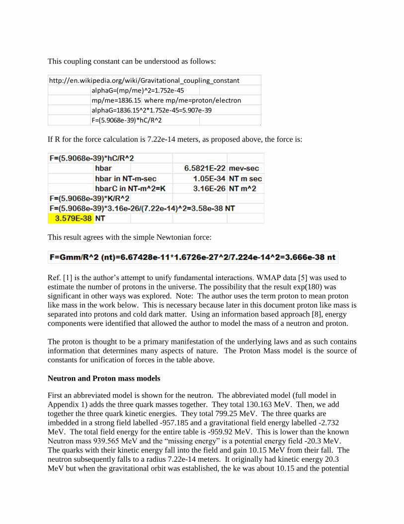
If R for the force calculation is 7.22e-14 meters, as proposed above, the force is:

This result agrees with the simple Newtonian force:

Ref. [1] is the author’s attempt to unify fundamental interactions. WMAP data [5] was used to

estimate the number of protons in the universe. The possibility that the result exp(180) was

significant in other ways was explored. Note: The author uses the term proton to mean proton

like mass in the work below. This is necessary because later in this document proton like mass is

separated into protons and cold dark matter. Using an information based approach [8], energy

components were identified that allowed the author to model the mass of a neutron and proton.

The proton is thought to be a primary manifestation of the underlying laws and as such contains

information that determines many aspects of nature. The Proton Mass model is the source of

constants for unification of forces in the table above.

Neutron and Proton mass models

First an abbreviated model is shown for the neutron. The abbreviated model (full model in

Appendix 1) adds the three quark masses together. They total 130.163 MeV. Then, we add

together the three quark kinetic energies. They total 799.25 MeV. The three quarks are

imbedded in a strong field labelled -957.185 and a gravitational field energy labelled -2.732

MeV. The total field energy for the entire table is -959.92 MeV. This is lower than the known

Neutron mass 939.565 MeV and the “missing energy” is a potential energy field -20.3 MeV.

The quarks with their kinetic energy fall into the field and gain 10.15 MeV from their fall. The

neutron subsequently falls to a radius 7.22e-14 meters. It originally had kinetic energy 20.3

MeV but when the gravitational orbit was established, the ke was about 10.15 and the potential

http://en.wikipedia.org/wiki/Gravitational_coupling_constant

alphaG=(mp/me)^2=1.752e-45

mp/me=1836.15 where mp/me=proton/electron

alphaG=1836.15^2*1.752e-45=5.907e-39

F=(5.9068e-39)*hC/R^2

energy was about 10.15. The neutron plus its associated gravitational energy balances the total

table energy 959.92 MeV.

The proton model is reviewed in Appendix 1.

The table gives the field energy 2.732 MeV as the basis for gravitation. The proposal below

indicates that this field energy is associated with a radius of 7.22e-14 meters. The test for

quantum level is action. Action is 1.0 when momentum*radius/h=pR/h=1. The proposal meets

the test by definition. One question this paper addresses is: Can we substitute this low energy

scale for the Planck scale energy?

Gravity is attributed to the geometry of space-time in general relativity. If a proton with

potential energy falls into the above field and follows the radius 7.22e-14 meters we would

expect an orbit to be established.

These forces are in agreement with the published coupling constant derived force and the

Newtonian force 3.4527e-38 NT. Inertial force mV^2/R*1/exp(90) equals field force

E/R*1/exp(90). The match (highlighted in yellow) is for the quantum scale and the value

1/exp(90) is explained below under the heading “Scaling Cellular Gravitational Values to Large

Scale Gravitation”. Several implications are explored in this paper. Firstly, space at the

quantum level is defined by 7.22e-14 meters. Secondly, a balanced force orbit defines a

geodesic in which the gravitational constant is defined by the inertial force. Thirdly, the

gravitational coupling constant is replaced by the value 1/exp(90) and fourthly, gravitation is

associated with exp(180) proton like masses.

Before considering gravitation more thoroughly, it is instructive to review other interactions

supported by information extracted from the proton mass model. An updated table from [1] is

reproduced below:

The conventional physics and comparison data is shown below.

The field energies for three strong (color) interactions and their associated particles are from the

proton mass table. They are referenced to the Higgs energy since it is considered by many to be

the source of field energies and particle masses. A force coupling constant is calculated to be

1.00 and derived c^2 (E*R) values are presented in MeV-m and joule-m. The author did not find

published values for comparison (quarks are not independently observable). The lower hierarchy

electromagnetic coupling constant is well known and the author’s calculations substantially

agree.

The traditional relationship F=hC/R^2 is too simple to characterize gravity since gravity involves

defining a radius and a proton with potential energy falling to that radius. Justification for

replacing the coupling constant with the value 1/exp(90) is presented below.

Force Table Strong Strong Gravity Electro-

MeV Residual proton Magnetic

Inertial F=M/g*V*2/R nt 7.1E+05 2262.9 3.656E-38 8.24E-08

1/exp(90)

Force=3.16e-26/Range^2 (nt) 7.2E+05 15459.4 ** 1.1E-05

Derived coupling constant 1.0157 0.1472 136.959

Published coupling constant (PDG) 137.036

Derived c^2 (E*R) mev m 2.00E-13 2.90E-14 1.44E-15

Derived c^2 joule m 3.21E-26 4.65E-27 2.31E-28

Derived exchange boson (mev) 942.881 138.019 0.004

*Published c^2 (E*R) mev m 1.5604E-14 1.17E-51 1.442E-15

*Published c^2 joule m 2.5E-27 1.87E-64 2.31E-28

*Published Range (m) 8.98E+25 5.291E-11

*http://www.lbl.gov/abc/wallchart/chapters/04/1.html

** See text

The atomic binding energy curve is considered to be a result of the strong residual interaction.

Again, the proton mass model provides information. The key value is the kinetic energy 10.151

MeV associated with the proton. The strong residual force F=hC/R^2= 15467 NT requires the

coupling constant 0.147 and the derived c^2= 2.9e-14 MeV m is similar to the published value

1.56e-14 MeV m. Also the radius of the proton appears to be credible. Reference 9 describes a

simple model using the value 10.15 MeV as the basis for binding energy. In this model 10.15

MeV is the kinetic energy that changes as atoms fuse. (928.121 MeV+10.151 MeV =938.272

MeV).

A possible candidate for gravitational energy scale

Nomenclature and review

Constants

\h 6.5821E-22 MeV-sec reduced Heisenberg

E 1.2200E+22 MeV Planck energy E

M 2.18E-08 kg Compton mass

G 6.670E-11 nt m^2/kg^2 gravitational constant

C 3.00E+08 m/sec

Relationships

Compton wavelength=GM/C^2

GM/C^2 6.67e-11*2.18e-8/3e8^2

L=GM/C^2 1.62E-35 meters

L=Ch/E=h/MC 1.62E-35 meters

L=h/MC=GM/c^2 1.61E-35 meters

G=hC/M^2

First compare the quantum mechanical action at two levels, the Planck scale and the much lower

level (2.732 MeV) proposed above. Either level could be a candidate for defining quantum

gravity since the action is 1 in both cases.

Planck energy E (MeV) 1.2200E+22

L=Planck length (meters) 1.62E-35

Planck momentum p=E/C 4.07E+13

p*L 6.58E-22

qm action= p*L/\h 1.00E+00

The proton mass (1.67e-27 kg) is analogous to the Compton mass, i.e. proposed mass is 938.27

MeV, not 1.22e22 MeV (1.67e-27 kg, not 2.17e-8 kg). Compare the calculation for gravitational

constant for the Planck scale and the proposed mass level and note that they differ by the large

factor.

Compton mass 2.18e-8 kg

G=hC/M^2

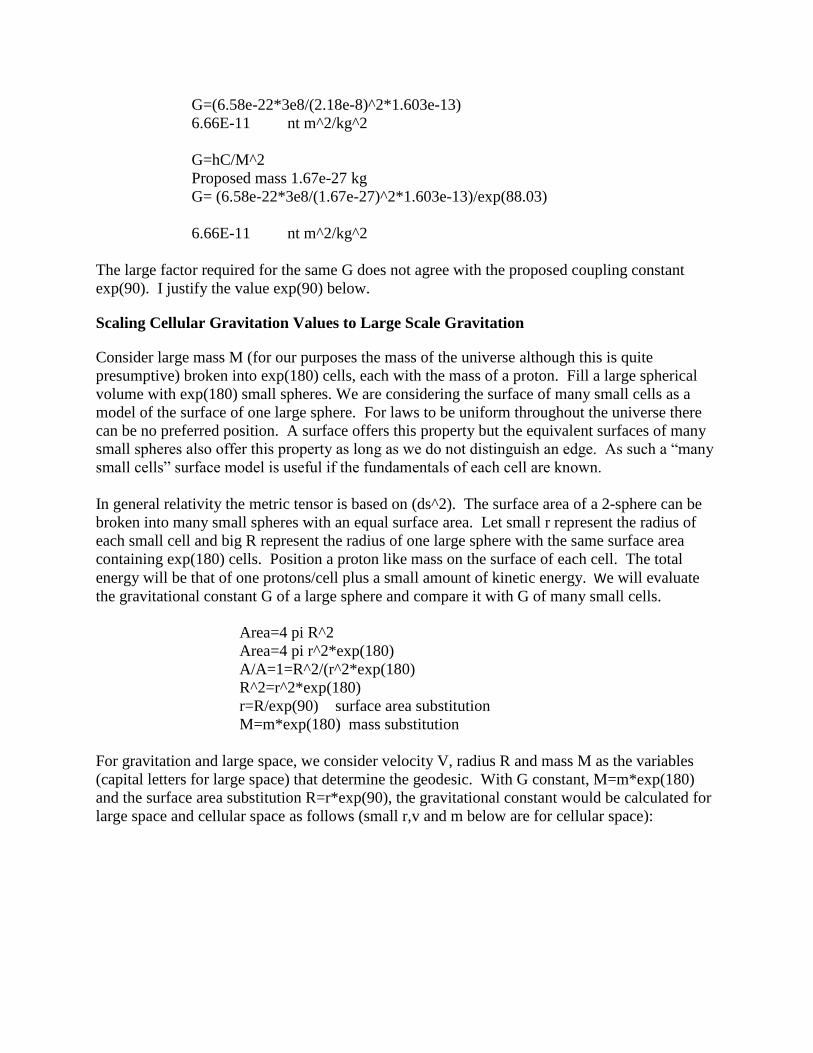
G=(6.58e-22*3e8/(2.18e-8)^2*1.603e-13)

6.66E-11 nt m^2/kg^2

G=hC/M^2

Proposed mass 1.67e-27 kg

G= (6.58e-22*3e8/(1.67e-27)^2*1.603e-13)/exp(88.03)

6.66E-11 nt m^2/kg^2

The large factor required for the same G does not agree with the proposed coupling constant

exp(90). I justify the value exp(90) below.

Scaling Cellular Gravitation Values to Large Scale Gravitation

Consider large mass M (for our purposes the mass of the universe although this is quite

presumptive) broken into exp(180) cells, each with the mass of a proton. Fill a large spherical

volume with exp(180) small spheres. We are considering the surface of many small cells as a

model of the surface of one large sphere. For laws to be uniform throughout the universe there

can be no preferred position. A surface offers this property but the equivalent surfaces of many

small spheres also offer this property as long as we do not distinguish an edge. As such a “many

small cells” surface model is useful if the fundamentals of each cell are known.

In general relativity the metric tensor is based on (ds^2). The surface area of a 2-sphere can be

broken into many small spheres with an equal surface area. Let small r represent the radius of

each small cell and big R represent the radius of one large sphere with the same surface area

containing exp(180) cells. Position a proton like mass on the surface of each cell. The total

energy will be that of one protons/cell plus a small amount of kinetic energy. We will evaluate

the gravitational constant G of a large sphere and compare it with G of many small cells.

Area=4 pi R^2

Area=4 pi r^2*exp(180)

A/A=1=R^2/(r^2*exp(180)

R^2=r^2*exp(180)

r=R/exp(90) surface area substitution

M=m*exp(180) mass substitution

For gravitation and large space, we consider velocity V, radius R and mass M as the variables

(capital letters for large space) that determine the geodesic. With G constant, M=m*exp(180)

and the surface area substitution R=r*exp(90), the gravitational constant would be calculated for

large space and cellular space as follows (small r,v and m below are for cellular space):

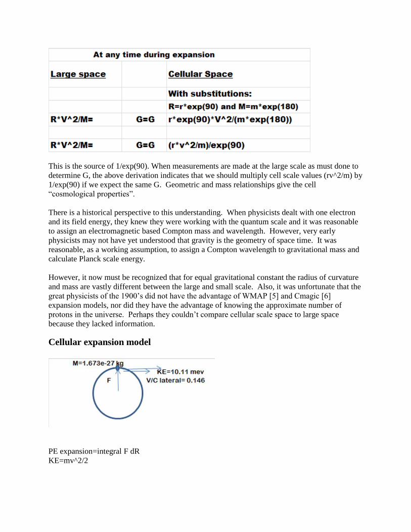
This is the source of 1/exp(90). When measurements are made at the large scale as must done to

determine G, the above derivation indicates that we should multiply cell scale values (rv^2/m) by

1/exp(90) if we expect the same G. Geometric and mass relationships give the cell

“cosmological properties”.

There is a historical perspective to this understanding. When physicists dealt with one electron

and its field energy, they knew they were working with the quantum scale and it was reasonable

to assign an electromagnetic based Compton mass and wavelength. However, very early

physicists may not have yet understood that gravity is the geometry of space time. It was

reasonable, as a working assumption, to assign a Compton wavelength to gravitational mass and

calculate Planck scale energy.

However, it now must be recognized that for equal gravitational constant the radius of curvature

and mass are vastly different between the large and small scale. Also, it was unfortunate that the

great physicists of the 1900’s did not have the advantage of WMAP [5] and Cmagic [6]

expansion models, nor did they have the advantage of knowing the approximate number of

protons in the universe. Perhaps they couldn’t compare cellular scale space to large space

because they lacked information.

Cellular expansion model

PE expansion=integral F dR

KE=mv^2/2

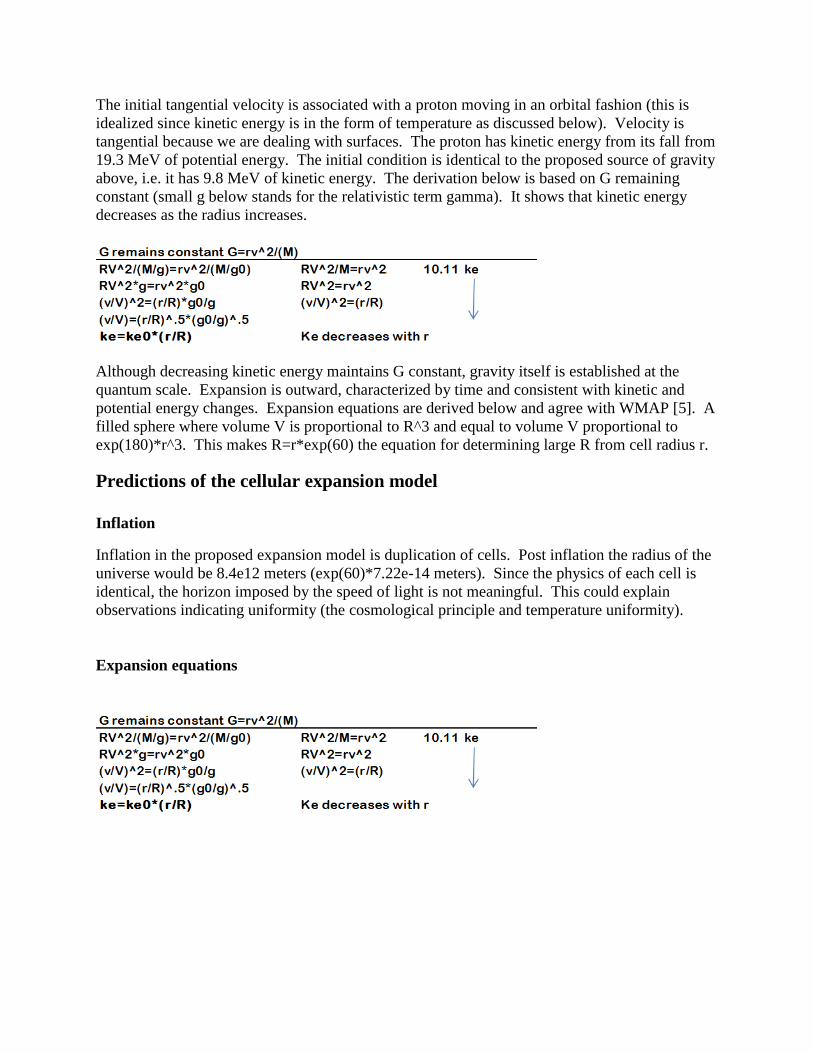
The initial tangential velocity is associated with a proton moving in an orbital fashion (this is

idealized since kinetic energy is in the form of temperature as discussed below). Velocity is

tangential because we are dealing with surfaces. The proton has kinetic energy from its fall from

19.3 MeV of potential energy. The initial condition is identical to the proposed source of gravity

above, i.e. it has 9.8 MeV of kinetic energy. The derivation below is based on G remaining

constant (small g below stands for the relativistic term gamma). It shows that kinetic energy

decreases as the radius increases.

Although decreasing kinetic energy maintains G constant, gravity itself is established at the

quantum scale. Expansion is outward, characterized by time and consistent with kinetic and

potential energy changes. Expansion equations are derived below and agree with WMAP [5]. A

filled sphere where volume V is proportional to R^3 and equal to volume V proportional to

exp(180)*r^3. This makes R=r*exp(60) the equation for determining large R from cell radius r.

Predictions of the cellular expansion model

Inflation

Inflation in the proposed expansion model is duplication of cells. Post inflation the radius of the

universe would be 8.4e12 meters (exp(60)*7.22e-14 meters). Since the physics of each cell is

identical, the horizon imposed by the speed of light is not meaningful. This could explain

observations indicating uniformity (the cosmological principle and temperature uniformity).

Expansion equations

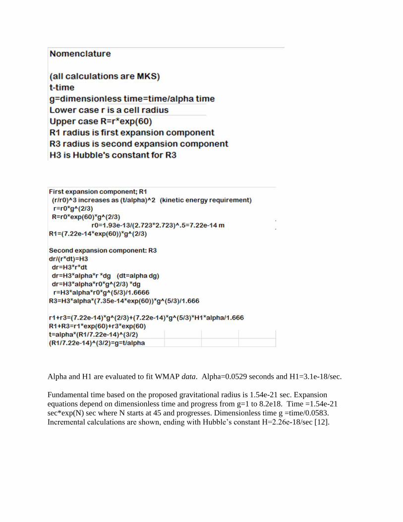
Alpha and H1 are evaluated to fit WMAP data. Alpha=0.0529 seconds and H1=3.1e-18/sec.

Fundamental time based on the proposed gravitational radius is 1.54e-21 sec. Expansion

equations depend on dimensionless time and progress from g=1 to 8.2e18. Time =1.54e-21

sec*exp(N) sec where N starts at 45 and progresses. Dimensionless time g =time/0.0583.

Incremental calculations are shown, ending with Hubble’s constant H=2.26e-18/sec [12].

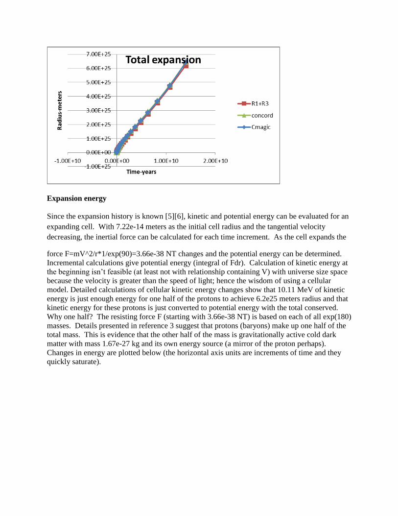
Expansion energy

Since the expansion history is known [5][6], kinetic and potential energy can be evaluated for an

expanding cell. With 7.22e-14 meters as the initial cell radius and the tangential velocity

decreasing, the inertial force can be calculated for each time increment. As the cell expands the

force F=mV^2/r*1/exp(90)=3.66e-38 NT changes and the potential energy can be determined.

Incremental calculations give potential energy (integral of Fdr). Calculation of kinetic energy at

the beginning isn’t feasible (at least not with relationship containing V) with universe size space

because the velocity is greater than the speed of light; hence the wisdom of using a cellular

model. Detailed calculations of cellular kinetic energy changes show that 10.11 MeV of kinetic

energy is just enough energy for one half of the protons to achieve 6.2e25 meters radius and that

kinetic energy for these protons is just converted to potential energy with the total conserved.

Why one half? The resisting force F (starting with 3.66e-38 NT) is based on each of all exp(180)

masses. Details presented in reference 3 suggest that protons (baryons) make up one half of the

total mass. This is evidence that the other half of the mass is gravitationally active cold dark

matter with mass 1.67e-27 kg and its own energy source (a mirror of the proton perhaps).

Changes in energy are plotted below (the horizontal axis units are increments of time and they

quickly saturate).

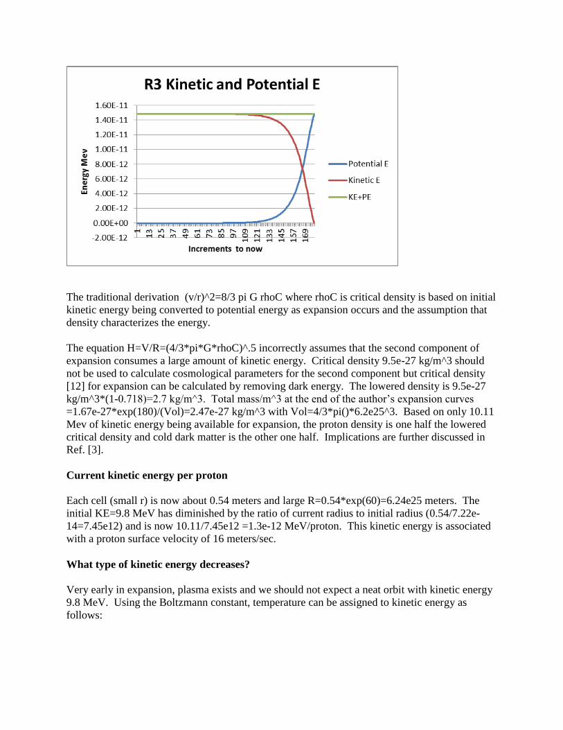
Dark energy

The second component (R3 in this proposal) is late stage expansion and causes the apparent

acceleration observed [6]. Calculations for potential energy required by second expansion

component yields the value 1.5e-11 MeV because late stage expansion is resisted by small

forces. (Stated the other way, when the radius is low forces are high but delta radius is low).

The value 1.5e-11 MeV is a small portion of 10.11 MeV and is negligible. One can make a

strong case against dark energy based on these results.

The traditional derivation (v/r)^2=8/3 pi G rhoC where rhoC is critical density is based on initial

kinetic energy being converted to potential energy as expansion occurs and the assumption that

density characterizes the energy.

The equation H=V/R=(4/3*pi*G*rhoC)^.5 incorrectly assumes that the second component of

expansion consumes a large amount of kinetic energy. Critical density 9.5e-27 kg/m^3 should

not be used to calculate cosmological parameters for the second component but critical density

[12] for expansion can be calculated by removing dark energy. The lowered density is 9.5e-27

kg/m^3*(1-0.718)=2.7 kg/m^3. Total mass/m^3 at the end of the author’s expansion curves

=1.67e-27*exp(180)/(Vol)=2.47e-27 kg/m^3 with Vol=4/3*pi()*6.2e25^3. Based on only 10.11

Mev of kinetic energy being available for expansion, the proton density is one half the lowered

critical density and cold dark matter is the other one half. Implications are further discussed in

Ref. [3].

Current kinetic energy per proton

Each cell (small r) is now about 0.54 meters and large R=0.54*exp(60)=6.24e25 meters. The

initial KE=9.8 MeV has diminished by the ratio of current radius to initial radius (0.54/7.22e-

14=7.45e12) and is now 10.11/7.45e12 =1.3e-12 MeV/proton. This kinetic energy is associated

with a proton surface velocity of 16 meters/sec.

What type of kinetic energy decreases?

Very early in expansion, plasma exists and we should not expect a neat orbit with kinetic energy

9.8 MeV. Using the Boltzmann constant, temperature can be assigned to kinetic energy as

follows:

The temperature 7.6e10 K is reasonable although this model starts with a higher density than

other expansion models. Cosmologists use the expansion ratio z to scale temperatures, i.e.

T(K)=2.725*z. However, starting with 7.6e10 K and scaling downward gives the surprising

present temperature 0.012 K. Isn’t the present temperature 2.725 K? Recall that about 23% of

all He4 is produced in the first few minutes. This releases 7.07*0.23=1.63 MeV. When this

energy is added to the photon related energy, the temperature curve jogs upward to the accepted

2.725*z curve. This is important because temperature affects the radius at equality and de-

coupling but these occur well after the curves are identical.

Gravitational range

Since the four interactions have similar form, each with a radius based on the proton mass model,

we would expect all four interactions to be short range. Gravity is known to be not only weak

but very long range.

One way to evaluate this might be the Heisenberg uncertainty principle (dh proportional to

dx*dp, where dx is the distance scale and dp is the momentum scale or de is the energy scale and

dt is the time scale). If the value 1/exp(90) is applied to the momentum scale, dx would be

multiplied by exp(90) and gravity would be long range. The author tried to determine which of

the variables dx, dp, de or dt should be changed by exp(90). Dividing dx makes the most sense

and this is based on the surface replacement small r=large R/exp(90) described in the heading

“Scaling Cellular Gravitation Values to Large Scale Gravitation”. Choices give interesting

results, i.e. 7.22e-14*exp(90)=7.98e25 meters and 1.5e-21 sec*exp(90) is about 60 billion years.

What about G=(\h C/m^2)?

Should the foundational relationship G=(\h C/m^2) be preserved? In the author’s opinion it

would require the correction G=(\h C*exp(90)/m^2). G would be associated with a mass close to

the proton (350 MeV) but this difference from the proton (938.27 MeV) makes one suspicious of

the relationship altogether.

Examples using the value 1/exp(90) to scale cell values to large size observations

Example 1: The earth’s gravitation

The table above indicates that the surface of the earth must be moving at 7898 m/sec to be on the

geodesic; however rotation only gives the surface 464 m/sec. Since the velocity is low we

experience acceleration of 9.8 m/sec^2.

Of course, to reach a force balance one would increase velocity to the geodesic value.

The table above indicates that the surface of the earth must be moving at 7898 m/sec to be on the

geodesic; however rotation only gives the surface 464 m/sec. Since the velocity is low we

experience acceleration of 9.8 m/sec^2.

Of course, to reach a force balance one would increase velocity to the geodesic value.

Example 2: The geodesic is universe size when expanded proton positions regain kinetic

energy by falling into deep orbits.

First review how orbits are formed. The diagram below shows that there was about 20 MeV of

potential energy (Appendix 1 and reference 1) available (a) and the proposed model for

expansion is based on an orbiting proton with approximately 10 MeV of kinetic energy (b).

Since the proton is attracted to and separated from the center of the field, there was also 10 MeV

of potential energy when the orbit is established. As expansion occurred (process (b)(c)

below), 10 MeV of kinetic energy was converted to 10 additional MeV of potential energy. At a

much later point in expansion (c), although there is motion (temperature) of the proton on the

surface of the expanding cell, there is no motion between cells (protons) except for expansion.

With the proton velocity nil between cells geodesics will be extremely flat (on the order of

5e38m) compared to 6.24e25m. This causes acceleration of particles toward one another

(process 2 below) and external kinetic energy (between protons) increases as protons fall back

toward the geodesic (d)(c). On average the expanded cells do not change their radius.

Theoretically, 10 MeV of external potential energy could be reconverted to10 MeV of kinetic

energy as particles fall toward one another. Overall, process (b)(c)(d)(e) converts

cellular surface kinetic energy to external potential energy between cells.

large space cell size at current expansion

R is the earth size geodesic RV 2̂/M G=G rv̂ 2/m r is the cell radius

R' is the universe size geodesic R'V 2̂/M G=G r'v̂ 2/m r' is the cell size geodesic

R'=r*('v/V) 2̂*(M/m)*1/exp(90)

R' geodesic (meters) 6.40E+06 0.547 r' is the cell size geodesic (m)

Velocity of orbit (m/sec) 7897.71 15.78 meters/sec

Earth mass kg 5.98E+24 1.67E-27 kg

nt m 2̂/kg 2̂ 6.67E-11 G=G 6.67E-11

Mass kg (earth) 5.98E+24

earth R (m) 6378100

a=gm/r 2̂ m/sec 2̂ 9.80

Mass kg (earth) 5.98E+24

earth R (m) 6378100

a=gm/r 2̂ m/sec 2̂ 9.80

What actually happened during expansion was a transition occurred and acoustic waves broke

the total mass into about 27000 clusters. After equality of photon density and mass density,

process (d)(e) occurred, protons accumulated and eventually fell into orbits that we observe as

clusters of galaxies, galaxies, etc.

During expansion, the kinetic energy of the proton on the cell surface decreased by KE/ke =9.8/

7.4e12=1.3e-12 Mev and the current velocity on the surface of each cell fell to15.8 m/sec.

The protons could theoretically regain 4.3e7 m/sec by falling but particles usually fall less than

this where orbits are established. The scaling procedure using 1/exp(90) yields R=9e25 meter.

The original energy/particle is conserved and agrees substantially with Kauffmann (Appendix 2)

[3].

As an engineer one cannot help but be impressed with the approximate energy conservation of

combined processes 1 and 2. These processes represent the largest construction project in nature

and almost no energy is consumed. The “neat trick” seems to be cells that expand, on average

don’t re-contract and are able to move and fall relative to each other after they are far apart.

The radius 9e25 meters is larger than R1+R3=6.24e25 meters. The equations for expansion

cause this difference. Although gravitation is based on the mass of exp(180) protons, this may

be a combination of protons and cold dark matter.

Time dilation

An expanded cell with a surface velocity of 15.8 m/sec gives a special relativistic time shift of

1.33e-15 seconds (calculated from velocity, KE=1.3e-12 MeV, gamma=(938/(938+KE), time

Scaling a cell to universe sized space at KE=9.8 MEV (V=4.3e7 m/sec)

R' is the universe size geodesic R'V 2̂/M G=G r'v̂ 2/m r' is the cell size geodesic

m=1.67e-27 kg

M=m*exp(180) 2.49E+51 1.67E-27 kg

R'=r*('v/V) 2̂*(M/m)*1/exp(90) R 8.998E+25 0.547 r' 6.25E+25 meters

V (meters/sec) 4.30E+07 15.78 v (meters/sec)

G 6.67E-11 6.67E-11 nt m 2̂/kg 2̂

shift =1-gamma, but since KE is low the time shift is approximately KE/(2*938)=1.33e-15

seconds.

The Schwarzschild time shift is a key general relativity prediction. The time shift calculated

below is for one cell undergoing expansion at a radius of 0.54 meters. Agreement (the factor of

2 is Schwarzschild 2 in 2GM/(C^2*R)) indicates that special relativity and general relativity

make the same prediction when the large factor exp(90) is included.

Calculations show that time dilation dt for GR and SR are equal throughout expansion. Dt for a

cell starts at 0.01 sec and decreases to the present value of 1.33e-15 seconds.

Example 3: Agreement with the Schwarzschild radius.

It is demonstrated below that scaling with 1/exp(90) exactly matches the Schwarzschild radius

(S) calculation. Proton mass rather than Compton mass in used in the S equation below. The

equation for S is:

1=1/(2*(Metric)-r) term in solution

2*(Metric)-r=1

r=2*(Metric)

Metric=G M/C^2 M is mass

dt=1/(1-2GM/(C 2̂*R) .̂5

dt=1/((1-EXP(90)*2*6.67e-11*1.67e-27/(3e8 2̂*0.55))) 0̂.5

dt=(expression above-1)/2

1.00000000000000133 1.332E-15 sec

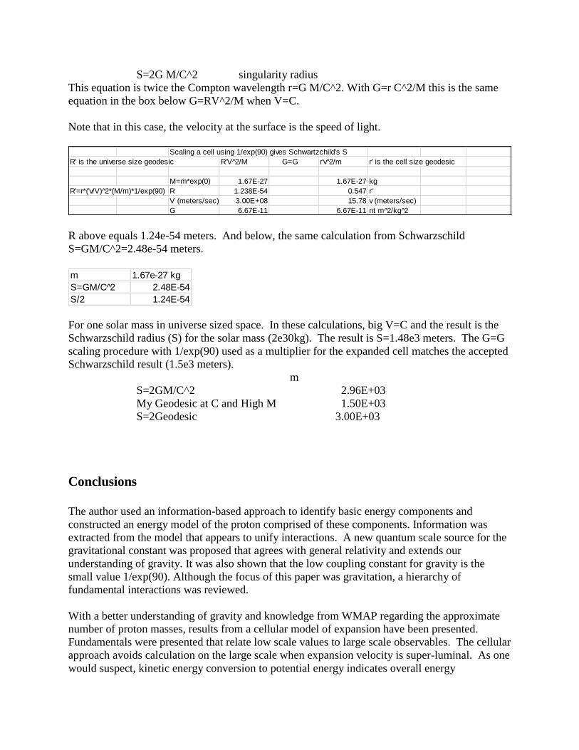
S=2G M/C^2 singularity radius

This equation is twice the Compton wavelength r=G M/C^2. With G=r C^2/M this is the same

equation in the box below G=RV^2/M when V=C.

Note that in this case, the velocity at the surface is the speed of light.

R above equals 1.24e-54 meters. And below, the same calculation from Schwarzschild

S=GM/C^2=2.48e-54 meters.

For one solar mass in universe sized space. In these calculations, big V=C and the result is the

Schwarzschild radius (S) for the solar mass (2e30kg). The result is S=1.48e3 meters. The G=G

scaling procedure with 1/exp(90) used as a multiplier for the expanded cell matches the accepted

Schwarzschild result (1.5e3 meters).

m

S=2GM/C^2 2.96E+03

My Geodesic at C and High M 1.50E+03

S=2Geodesic 3.00E+03

Conclusions

The author used an information-based approach to identify basic energy components and

constructed an energy model of the proton comprised of these components. Information was

extracted from the model that appears to unify interactions. A new quantum scale source for the

gravitational constant was proposed that agrees with general relativity and extends our

understanding of gravity. It was also shown that the low coupling constant for gravity is the

small value 1/exp(90). Although the focus of this paper was gravitation, a hierarchy of

fundamental interactions was reviewed.

With a better understanding of gravity and knowledge from WMAP regarding the approximate

number of proton masses, results from a cellular model of expansion have been presented.

Fundamentals were presented that relate low scale values to large scale observables. The cellular

approach avoids calculation on the large scale when expansion velocity is super-luminal. As one

would suspect, kinetic energy conversion to potential energy indicates overall energy

Scaling a cell using 1/exp(90) gives Schwartzchild's S

R' is the universe size geodesic R'V 2̂/M G=G r'v̂ 2/m r' is the cell size geodesic

M=m*exp(0) 1.67E-27 1.67E-27 kg

R'=r*('v/V) 2̂*(M/m)*1/exp(90) R 1.238E-54 0.547 r'

V (meters/sec) 3.00E+08 15.78 v (meters/sec)

G 6.67E-11 6.67E-11 nt m 2̂/kg 2̂

m 1.67e-27 kg

S=GM/C 2̂ 2.48E-54

S/2 1.24E-54

conservation. The initial kinetic energy 9.8 MeV/proton is enough energy to expand each proton

to 6.24e25 meters but if all exp(180) particles were protons, it would be only one half the

required energy. The basis of this conclusion is that all exp(180) proton like masses contribute

to the resisting gravitational force. This suggests that the other half may be gravitationally active

cold dark mass. Kinetic and potential energy calculations have implications for the ongoing dark

energy search. It appears that the second (accelerating) component of expansion requires

minimal energy. The implied cosmological fractions are omega dark=0, omega baryon=0.5 and

omega cold dark matter=0.5.

Examples were presented utilizing the small factor 1/exp(90) at the cellular scale. Calculations

show that special relativity time dilation is equal to Schwarzschild general relativity time dilation

throughout expansion when the factor 1/exp(90) is used. The purpose of this was to show that a

low energy scale gravitational scale works and perhaps replaces current fundamentals.

It is the author’s view that the radius and time associated with field energy 2.732 MeV and the

associated expansion curves define space and time.

Appendix 1

Neutron and Proton mass models

The proton is thought to be a primary manifestation of the underlying laws and as such contains

information that determines many aspects of nature. The Proton Mass model is the source of

constants for unification of forces in the table above. The full model is shown below. It is based

on interaction explained in Reference 13.

The proton mass is easier to understand if we add the quark masses together and the quark

kinetic energies together as shown below:

The exact proton mass results after a neutrino of 0.671 MeV is ejected and the Strong Residual

kinetic energy 10.15 MeV is added as shown below:

The full proton model is shown above followed by consolidations required to create a simpler

model. They total 129.541 MeV. The three quarks are imbedded in a strong field labelled -

957.185 and a gravitational field energy labelled -2.732 MeV. The total field energy for the

entire table is -959.92 MeV. This is lower than the known Neutron mass 939.565 MeV and the

“missing energy” is a potential energy field -20.3 MeV. The quarks with their kinetic energy fall

into the field and gain 10.15 MeV from their fall. The neutron subsequently falls to a radius

7.22e-14 meters. It originally had kinetic energy 20.3 MeV but when the gravitational orbit was

established, the ke was about 10 and the potential energy was about 10. The neutron plus its

associated gravitational energy balances the total table energy 959.92 MeV.

The neutron decays into a proton, an electron and a neutrino. This gives the measured proton

mass 938.27 MeV below. As the proton and electron split they develop opposite fields of 27.2e-

6 Mev. When the electron falls into the proton field it develops 13.6e-6 Mev.

Information from the proton mass model is used to understand fundamental interactions. Some

may notice that the quark masses are higher than the accepted values associated with down and

up quarks. The author believes based on reference 10 that quarks can transition to lower energy,

converting some of their mass to kinetic energy but conserving mass plus kinetic energy. This

process is observed in mesons and baryons as they decay.

Values extracted from the model are important for fundamental interactions.

Coupling constants quoted in the literature are for protons and this allowed direct comparison.

Appendix 2

S.K. Kauffmann [3] gives the following value for energy.

Radius 1.21E+26

2(c^4/g)r

2.93E+70

m^4/sec^4(kg^2/(nt m^2))*m

m^4/sec^4kg^2/(nt m*m)*m

4.69E+57

m^4/sec^4kg^2 m/(MeV*m)

1.48E+117

m^4/sec^4 MeV^2 m/(MeV*m)

m^4/sec^4 MeV

Energy 1.82E+83 MeV

Volume7.35E+78 m^3

2.48E+04 MeV/m^3

number protons 1.49E+78

4.93E+00 MeV/proton

If the above energy value is divided by exp(180) protons, the result is about 5 MeV/proton. The

value 9.9 MeV/proton [1][2] and the value above compare favorably.

References

1. Barbee, Gene. H., A Top-down Approach to Fundamental Interactions, FQXi essay, June 2012.

viXra:1307.082 revised Feb 2014.

2. Barbee, Gene H., Application of Proton Model to Cosmology, viXra:1307.0090, revised March 2014. Accompanying Microsoft ® spreadsheet unifying concepts.xls

3. Barbee, Gene H., On Expansion Energy, Dark Energy and Missing Mass, Prespacetime Journal Vol. 5 No. 5, May 2014. Previously vixra:1307.0089, revised June 2014.

4. Kauffmann, S.K., A Self-Gravitational Upper Bound on Localized Energy, Including the Virtual Particles and Quantum Fields, which Yields a Passable “Dark Energy” Estimate, arXiv: 1212.046v4, 24 Mar 2013.

5. Bennett, C.L. et al. First Year Wilkinson Microwave Anisotropy Probe (WMAP) Observations: Preliminary Maps and Basic Results, Astrophysical Journal, 2001

6. A Conley, et al., Measurement of Omega from a blind analysis of Type IA supernovae: Using color information to verify the acceleration of the universe, the Supernova Cosmology Project.

7. Private communication with S Kauffmann. 8. Claude Shannon, A mathematical Theory of Communication, 1948. 9. Barbee, Gene H., A Simple Model of Binding Energy, viXra: 1307.0102, revised March 2014. 10. Barbee, Gene H., Baryon and Meson Masses Based on Natural Frequency Components,

viXra:1307.0133. 11. http://www.lbl.gov/abc/wallchart/chapters/04/1.html 12. http://arxiv.org/pdf/1212.5226v3.pdf Table 2.

13. Barbee, Gene H., Unification, vixra:1410.0028.