The simulation of a non-linear unstable system of motion ...

The simulation of a non-linear unstable system of motion, utilising the Solid-Works and Matlab/Simulink extended libraries/toolboxes

Jirí Zátopek1,a

1Tomas Bata University in Zlín, Faculty of Applied Informatics, Nad Stránemi 4511, 760 05 Zlín, Czech Republic

Abstract. This text discusses the use and integration of various support software tools for the purpose of design-ing the motion control law governing mechanical structures with strongly non-linear behaviour. The detailed

mathematical model is derived using Lagrange Equations of the Second Type. The physical model was designed

by using SolidWorks 3D CAD software and a SimMechanics library. It extends Simulink with modelling tools

for the simulation of mechanical “multi-domain” physical systems. The visualization of Simulink outputs is

performed using the 3D Animation toolbox. Control law - designed on the basis of the mathematical model, is

tested for both models (i.e. mathematical and physical) and the regulatory processes’ results are compared.

1 Introduction

Nowadays, a large amount of support software tools is

available. These tools facilitate our work in analysing,

modelling, simulating and designing a control law for

complex mechanical structures. By connecting these re-

sources a considerable simplification of the synthesis can

be achieved as well as clarity by using visualisation in

3D space directly in the regulation process, or creating a

physical model in Simulink directly from CAD software

(SolidWorks), without the need to derive the equations of

motion.

The system which is the object of our interest is called

"Ball and beam", and the description of the dynamic be-

haviour is derived in the most general way as possible for

use in the control of a real model. The ball and beam are

mass objects and are thus situated in the 3D space - only

the movement is limited to planar. The system is located in

the Earth’s gravitational field and has two degrees of free-

dom. The mass of the ball is chosen to have a significant

impact on the movement changes of the beam; the beam

may be unbalanced. The ball position is measured from

the axis of rotation of the beam (i.e. the axis of the shaft

of the driving motor). The Denavit-Hartenberg (DH) no-

tation/method of placement for coordinate systems is used

to determine the ball’s position in a selected global coor-

dinate system.

First, the whole system is sketched-out for the purpose

of compiling a transformation matrix to determine the po-

sition of the ball in the global coordinate system. Using

this transformation, the equations of motion of the system

are derived - which include the moments of inertia, and

the centrifugal/centripetal and Coriolis generalized forces

or linear friction. Than, a 3D model was constructed in the

ae-mail: [email protected]

CAD design software SolidWorks suite, including all kine-

matic constraints and the mass distribution of the whole as-

sembly. This model is also useful for detecting the masses

or matrices/moments of inertia of complex objects, which

cannot be determined analytically. The subsequent CAD

model is then export into the SimMechanics format in

Matlab/Simulink, which leads to a physical model - in-

cluding its kinematic link and the distribution of the mass

of the whole assembly. This model subsequently tests the

proposed control algorithm and compares the outputs with

a mathematical model.

2 “Ball and beam” – the mathematicaldescription

2.1 Transformation of coordinate systems

Figure 1. Model with the selected coordinate system placement

Figure 1 shows the system drawn for the purpose of

determining the transformation matrix from the local coor-

DOI: 10.1051/02016 (2016) matecconf/2016MATEC Web of Conferences 76020167

2016

,6

CSCC

© The Authors, published by EDP Sciences. This is an open access article distributed under the terms of the Creative Commons Attribution License 4.0 (http://creativecommons.org/licenses/by/4.0/).

dinate system (x2, y2, z2) to the global system (X0,Y0,Z0).Rotation of the beam is only possible around the global

axis Z0; rolling the ball only in direction of local axis z1is ideal. The connection of the beam with the frame in

the place where the torque actions provide controlled tilt-

ing of the beam (i.e. the first degree of freedom) is shown

schematically. The second degree of freedom is the move-

ment of the ball on the beam.

The resulting homogeneous transformation matrix be-

tween the coordinate systems is:

0T2 =

⎡⎢⎢⎢⎢⎢⎢⎢⎢⎢⎢⎢⎢⎣− sinϕ(t) 0 cosϕ(t) −h sinϕ(t) + r(t) cosϕ(t)cosϕ(t) 0 sinϕ(t) h cosϕ(t) + r(t) sinϕ(t)0 1 0 0

0 0 0 1

⎤⎥⎥⎥⎥⎥⎥⎥⎥⎥⎥⎥⎥⎦ (1)

For determining the homogeneous coordinates of the

ball position relative to the origin of the global coordinate

system, the equation is:

0r = 0T2 · 2r ⇒

⎡⎢⎢⎢⎢⎢⎢⎢⎢⎢⎢⎢⎢⎣XYZ1

⎤⎥⎥⎥⎥⎥⎥⎥⎥⎥⎥⎥⎥⎦ =

⎡⎢⎢⎢⎢⎢⎢⎢⎢⎢⎢⎢⎢⎢⎢⎢⎢⎢⎢⎢⎢⎢⎢⎢⎣

−(R +

b2

)sinϕ(t) + r(t) cosϕ(t)(

R +b2

)cosϕ(t) + r(t) sinϕ(t)

0

1

⎤⎥⎥⎥⎥⎥⎥⎥⎥⎥⎥⎥⎥⎥⎥⎥⎥⎥⎥⎥⎥⎥⎥⎥⎦(2)

In order to determine the square-size of the absolute

speed vector (in the global coordinate system), it is:

|v|2 =(x2 + y2

)=

(2R + b2

)2ϕ2 + r2ϕ2 + r2 − (2R + b)rϕ (3)

Note, the Ball and beam is only planar in this model

(processes take place in 2D).

2.2 Motion equations

To be able to use Lagrange equations of the second kind, it

is therefore necessary to determine the kinetic and poten-

tial energy of the whole system.

The kinetic energy of the balls is comprised of its

translational and rotational motion:

Ekball =1

2Mv2 +

1

2

2

5MR2︷︸︸︷Jkul

r2

R2︷︸︸︷ω2kul︸��︷︷��︸

1

5Mr2

=

=1

2M

⎡⎢⎢⎢⎢⎢⎣(2R + b2

)2ϕ2 + r2ϕ2 +

7

5r2 − (2R + b)rϕ

⎤⎥⎥⎥⎥⎥⎦

(4)

The potential energy of the ball is:

Epball = Mgy = Mg[(2R + b2

)cosϕ + r sinϕ

](5)

The Beam is cuboid in shape, with an optionally-stored

rotation axis as shown in Figure 1. Its inertia matrix has

3x3 moments of inertia, and is defined as:

J =

⎡⎢⎢⎢⎢⎢⎢⎢⎢⎣Jxx Jxy JxzJyx Jyy JyzJzx Jzy Jzz

⎤⎥⎥⎥⎥⎥⎥⎥⎥⎦ =�

Bρ(x, y, z)

⎡⎢⎢⎢⎢⎢⎢⎢⎢⎣Jxx Jxy JxzJyx Jyy JyzJzx Jzy Jzz

⎤⎥⎥⎥⎥⎥⎥⎥⎥⎦ (6)

in which ρ(x, y, z) is the density of the material body. Ifa new coordinate system is selected such that all the de-

viance moments will be zero; the torques to the individual

axes of the system will be equal to the polar moments of

the inertia matrix with respect to these axes. A well es-

tablished system already meets this assumption, it is not

necessary to introduce a new coordinate system and the

moment of inertia relative to the axis of rotation (axis Z0)will be equal to the polar moment Jzz.

Jbeam = Jzz =1

12m

[b2 + 4

(i2 − i j + j2

)](7)

The kinetic energy of the beam is:

Ekbeam =1

2ϕ2Jbeam =

1

24mϕ2

[b2 + 4

(i2 − i j + j2

)](8)

The relationship between the mass element and the length

element can be expressed as:

dm = ρ a b dr =m

ab la b dr =

mldr (9)

The potential energy of the beam element is:

dEpbeam = dm g sinϕ r =m g sinϕ

i + jr dr (10)

The potential energy of the whole beam is:

Epbeam =∫ j−idEpbeam =

1

2m g sinϕ( j − i) (11)

The total kinetic and potential energy of the system is the

sum of their partial energies:

Ek =1

24mϕ2

[b2 + 4

(i2 − i j + j2

)]+

+1

2M

⎡⎢⎢⎢⎢⎢⎣(2R + b2

)2ϕ2 + r2ϕ2 +

7

5r2 − (2R + b)rϕ

⎤⎥⎥⎥⎥⎥⎦(12)

Ep = Mg[(2R + b2

)cosϕ + r sinϕ

]+1

2mg sinϕ( j − i) (13)

The Lagrangian calculation is:

L =Ek − Ep =1

24mϕ2

[b2 + 4

(i2 − i j + j2

)]+

+1

2M

⎡⎢⎢⎢⎢⎢⎣(2R + b2

)2ϕ2 + r2ϕ2 +

7

5r2 − (2R + b)rϕ

⎤⎥⎥⎥⎥⎥⎦−− Mg

[(2R + b2

)cosϕ + r sinϕ

]− 12mg sinϕ( j − i)

(14)

The linear friction - dependent upon the generalised

speed (i.e. sliding friction with a friction factor k1 androlling resistance with a friction factor k2) will be added tothe system. The equations of motion are therefore:

ddt

(∂Lqi

)− ∂L

qi= Qi ⇒ d

dt

(∂Lr

)− ∂L

r= 0

ddt

{1

2M

[14

5r − (2R + b) ϕ

]}− Mrϕ2 + Mg sinϕ = 0

(15)

75

Mr − 2R + b2

Mϕ − Mrϕ2 + k1r +Mg sinϕ = 0 (16)


2016

,6

CSCC

2

ddt

(∂Lqi

)− ∂L

qi= Qi ⇒ d

dt

(∂Lϕ

)− ∂Lϕ= 0

ddt

{1

2M

[(2R + b)2

2

ϕ + 2r2ϕ − (2R + b) r]+1

12mϕ

[b2+

+ 4(i2 − i j + j2

)]}+ Mg

[r cosϕ −

(2R + b2

)sinϕ

]+

+1

2mg cosϕ ( j − i) = Q

(17)

M(

2R + b2

)2

ϕ +Mr2ϕ +112

m[b2 + 4

(i2 − ij + j2

)]ϕ−

−M2R + b

2r + 2Mrrϕ + k2ϕ +Mgr cosϕ−

−Mg(

2R + b2

)sinϕ +

12

mg(j − i) cosϕ + 2Mrrϕ = Q

(18)

After modification, we can write:

r =

60A

⎡⎢⎢⎢⎢⎢⎢⎣Q − k2ϕ + AMg sinϕ − Mgr cosϕ+

+1

2mg(i − j) cosϕ − 2Mrrϕ

⎤⎥⎥⎥⎥⎥⎥⎦24MA2 + 84Mr2 + 7Bm

−

−5

⎡⎢⎢⎢⎢⎢⎣(12MA2 + 12Mr2 + Bm

)·

·(k1r − Mrϕ2 + Mg sinϕ

)⎤⎥⎥⎥⎥⎥⎦

24M2A2 + 84M2r2 + 7BMm

ϕ =

6

⎡⎢⎢⎢⎢⎢⎢⎢⎢⎣14Q − 14k2ϕ − 10Ak1r + 10AMrϕ2++4AMg sinϕ − 14Mgr cosϕ++7mg(i − j) cosϕ − 28Mrrϕ

⎤⎥⎥⎥⎥⎥⎥⎥⎥⎦24MA2 + 84Mr2 + 7Bm

(19)

in which:

A =(2R + b2

)B =

[b2 + 4

(i2 − i j + j2

)](20)

The block diagram in Simulink that corresponds to the

derived non-linear mathematical model was created from

the Equation (19). The modified equations of motion are

part of the r" and fi" functional blocks, and it is also possi-ble to choose non-zero initial conditions of the mathemat-

ical model.

Figure 2. The non-linear mathematical model in Simulink

For the state vector: [r v ϕ ω]T = [x1 x2 x3 x4]T

and input signal: Q = u the state-space representation willcorrespond to the shape of:

⎡⎢⎢⎢⎢⎢⎢⎢⎢⎢⎢⎢⎢⎣x1x2x3x4

⎤⎥⎥⎥⎥⎥⎥⎥⎥⎥⎥⎥⎥⎦ =

⎡⎢⎢⎢⎢⎢⎢⎢⎢⎢⎢⎢⎢⎢⎢⎢⎢⎢⎢⎢⎢⎢⎢⎢⎢⎢⎢⎢⎢⎢⎢⎢⎢⎢⎢⎢⎢⎢⎢⎢⎢⎢⎢⎢⎢⎢⎢⎢⎢⎢⎢⎢⎢⎢⎢⎢⎢⎢⎢⎢⎢⎢⎢⎢⎢⎢⎢⎢⎢⎢⎢⎢⎢⎢⎢⎢⎢⎢⎢⎣

x2

60A

⎡⎢⎢⎢⎢⎢⎢⎢⎢⎢⎢⎢⎣Q − k2x4 + AMg sin x3−

−Mgx1 cos x3 + 12mg(i − j) cos x3−

−2Mx1x2x4

⎤⎥⎥⎥⎥⎥⎥⎥⎥⎥⎥⎥⎦24MA2 + 84Mx2

1+ 7Bm

−

−5

⎡⎢⎢⎢⎢⎢⎣(12MA2 + 12Mx21 + Bm

)·

·(k1x2 − Mx1x24 + Mg sin x3

)⎤⎥⎥⎥⎥⎥⎦

24M2A2 + 84M2x21+ 7BMm

x4

6

⎡⎢⎢⎢⎢⎢⎢⎢⎢⎣14Q − 14k2x4 − 10Ak1x2 + 10AMx1x24++4AMg sin x3 − 14Mgx1 cos x3++7mg(i − j) cos x3 − 28Mx1x2x4

⎤⎥⎥⎥⎥⎥⎥⎥⎥⎦24MA2 + 84Mx2

1+ 7Bm

⎤⎥⎥⎥⎥⎥⎥⎥⎥⎥⎥⎥⎥⎥⎥⎥⎥⎥⎥⎥⎥⎥⎥⎥⎥⎥⎥⎥⎥⎥⎥⎥⎥⎥⎥⎥⎥⎥⎥⎥⎥⎥⎥⎥⎥⎥⎥⎥⎥⎥⎥⎥⎥⎥⎥⎥⎥⎥⎥⎥⎥⎥⎥⎥⎥⎥⎥⎥⎥⎥⎥⎥⎥⎥⎥⎥⎥⎥⎥⎦

(21)

From these equations, it can be determined that the

system has only one unstable singular point and its steady-

state is only given by the ball position on the lever/beam

x1.All remaining state variables are zero in singular point.

The singular (stationary) point is:

[x01

x02

x03

x04

]T=

[m(i − j)2M

0 0 0

]T(22)

The Steady state is:

xs1 =

us

Mg+

m(i − j)2M

us = Mgxs1 −1

2mg(i − j)

(23)

Linearisation in the working point xs1(i.e. steady state)

can be obtained from the transmission of the linear model:

G(s) =X1(s)U(s)

=b2s2 + b0

s4 + a3s3 + a2s2 + a1s + a0(24)

in which:

b2 =60A

24MA2 + 336Mxs12 + 7Bm

b0 =−60g

24MA2 + 336Mxs12 + 7Bm

a3 =60MA2k1 + 240Mk1xs1

2 + 84Mk2 + 5Bk1m

M(24MA2 + 336Mxs

12 + 7Bm

)2

a2 =

(12096AgM3 + 20160Mk1k2

)xs12−

−10080AgmM2(i − j)xs1+ 864A3M3g+

+1440A2Mk1k2 + 420Bk1k2m + 252ABgmM2

M(24MA2 + 336Mxs

12 + 7Bm

)2

a1 =−60Agk1

24MA2 + 336Mxs12 + 7Bm

a0 =

−60Mg2[24MA2 + 336Mxs

12+

+7Bm − 168m(i − j)xs1

](24MA2 + 336Mxs

12 + 7Bm

)2

(25)


2016

,6

CSCC

3

Linearization is derived in the general position of the

working point, so it is possible to continuously recalculate

it.

3 “Ball and beam” – support softwaretools

3.1 SolidWorks

Figure 3. The complete assembly in SolidWorks

The considered system consists of three basic parts:

the base, the beam and the ball. All of these parts are ma-

terial. Ideally, a rigid base is connected to the frame so

its physical properties are not relevant to the dynamic be-

haviour of the system.

3.2 The SimMechanics – physical model

Figure 4. A Real-time visualisation using the SimMechanics

Second Generation suite

Figure 5. A separate model in the SimMechanics environment

The SolidWorks 3D CAD model (Figure 3) was ex-

ported in SimMechanics second generation xml format andthen imported into theMATLAB/Simulink environment as

a Simulink scheme (Figure 5). The link were revised be-

cause - between SolidWorks and SimMechanics; some are

unknown or illicit.

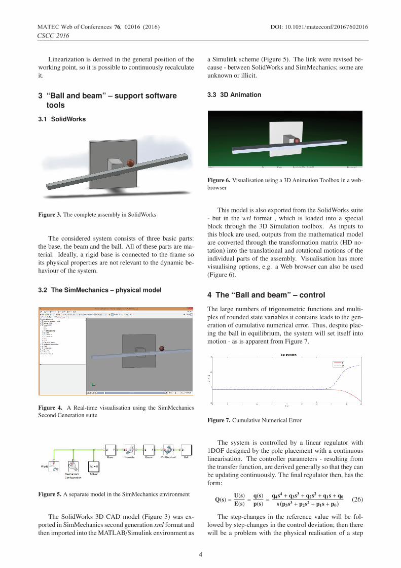
3.3 3D Animation

Figure 6. Visualisation using a 3D Animation Toolbox in a web-browser

This model is also exported from the SolidWorks suite

- but in the wrl format , which is loaded into a specialblock through the 3D Simulation toolbox. As inputs to

this block are used, outputs from the mathematical model

are converted through the transformation matrix (HD no-

tation) into the translational and rotational motions of the

individual parts of the assembly. Visualisation has more

visualising options, e.g. a Web browser can also be used

(Figure 6).

4 The “Ball and beam” – control

The large numbers of trigonometric functions and multi-

ples of rounded state variables it contains leads to the gen-

eration of cumulative numerical error. Thus, despite plac-

ing the ball in equilibrium, the system will set itself into

motion - as is apparent from Figure 7.

Figure 7. Cumulative Numerical Error

The system is controlled by a linear regulator with

1DOF designed by the pole placement with a continuous

linearisation. The controller parameters - resulting from

the transfer function, are derived generally so that they can

be updating continuously. The final regulator then, has the

form:

Q(s) =U(s)E(s)

=q(s)p(s)

=q4s4 + q3s3 + q2s2 + q1s + q0

s(p3s3 + p2s2 + p1s + p0

) (26)

The step-changes in the reference value will be fol-

lowed by step-changes in the control deviation; then there

will be a problem with the physical realisation of a step


2016

,6

CSCC

4

Figure 8. Complete Simulink scheme with SimMechanics and 3D Animation

Figure 9. Control process for the mathematical and physical models

changes in the torque - and thus to the rapidly-changing

tilt of the beam. In combination with the centrifugal forces

and inertia of the system, the process will oscillate; and of-

ten will be an unmanageable state. Therefore, a filter that

prevents such step-changes was introduced into the sys-

tem.

As shown in Figure 9, the control processes (i.e math-

ematical and physical) of both models are nearly identical.

The controller is designed to compensate for disturbance

and the reference value is in the shape of a step-change,

so a lag fault will appear in the transition part of the pro-

cess at the ramp-shaped reference value. The trend of the

reference value however, replicates very well.

5 Conclusion

This article contains a complete control design solution of

a system known as a “Ball and beam” system, substantial

part of the article relate to the derivation of systems mo-

tion equations from their energy balance. The model was

- through to the definition of transmission, derived in a

quite general manner and corresponds to motion equations

linearised at the operating point. Therefore, it is possi-


2016

,6

CSCC

5

ble to carry out a continuous linearisation efficiently - and

with low computational effort. This description however,

applies only in the area surrounding the working point.

When this point changes, linearisation is needed again.

Linking with 3D CAD software and Matlab/Simulink,

while using toolboxes for physical modelling (SimMe-

chanics) and 3D visualisation outputs (3D Animation) is

a very visual and effective control tool for the presentation

of the results. In real time, it is possible to observe dy-

namic processes occurring in the system and for instance -

for to slow then down or to pause them for the purpose of

detailed motion analysis or the exploration of the energy

interactions between system components.

The control methods designed a described herein are

tested on a unbalanced system with variable reference

course and disorders. To achieve the desired quality of

regulation, it is necessary to eliminate a step-change in the

control deviation and to stabilize the course of the regula-

tory process.

References

[1] S. Crandall, D. C, .Karnopp, E.F. Kurz, Dynamics ofmechanical and electromechanical systems (McGraw-Hill, NewYork, 1968) 466

[2] H. K. Khali, Nonlinear Systems (Upper Saddle River,N.J: Pearson, 2001) 750

[3] Y. Shaoqiang, L. Zhong, L. Xingshan, Chinese Con-

trol Conference 27, 161–165 (2008)[4] Z. Úrednícek, Robotika (Zlín, T. Bata university inZlin, 2012) 284

[5] Z. Úrednícek, Elektromechanické akcní cleny (Zlín, T.Bata university in Zlin, 2009) 127

[6] R. C. ROSENBERG, Journal of Dynamic Systems,

Measurement, and Control 94, 6 (1972)[7] D. C. Karnopp, R. C. Rosenberg, System dynamics (AUnifies Approach. Wiley & Sons, New York, 1975) 372

[8] M. H. Loi Tran, International Mechanical Engineering

Congress & Exposition 7, 10 (2011)


2016

,6

CSCC

6

The simulation of a non-linear unstable system of motion ...

Documents

Transcript of The simulation of a non-linear unstable system of motion ...