The Short-Term Inflation-Hedging Characteristics of U.K. Real Estate

Journal of Real Estate Finance and Economics, 15:1, 27±57 (1997)

# 1997 Kluwer Academic Publishers

The Short-Term In¯ation-Hedging Characteristics ofU.K. Real Estate

MARTIN HOESLI

Management Studies, University of Geneva, Switzerland andDepartment of Accountancy, University of Aberdeen, Scotland

BRYAN D. MACGREGOR

Centre for Property Research, Department of Land Economy, University of Aberdeen, Scotland

GEORGE MATYSIAK

Department of Property Valuation and Management, City University Business School, City University, London

NANDA NANTHAKUMARAN

Centre for Property Research, Department of Land Economy, University of Aberdeen, Scotland

Abstract

This study investigates the short-term in¯ation-hedging characteristics of U.K. real estate compared to other U.K.

investments. It considers not only total returns but also changes in income and changes in capital values. The

analyses are undertaken using annual and quarterly data. Stocks, bonds, appraisal-based real estate (including the

three property types, separately), and real estate stocks are considered. Real estate series, constructed from the

original appraisal series to take account of autocorrelation, also are used. The methodology is based on that

devised by Fama and Schwert (1977) and tests are undertaken for stationarity and structural breaks. Hypotheses

are established about the coef®cients on expected and unexpected in¯ation in the model, and these are tested. It is

concluded that real estate has poorer short-term hedging characteristics for total return, change in capital value,

and change in income than stocks but better characteristics than bonds. However, there is evidence to suggest that

the relationships change under different economic environments.

Key Words: in¯ation-hedging, expected in¯ation, unexpected in¯ation, United Kingdom

1. Introduction

One of the main reasons for real estate being regarded as an attractive investment vehicle

is that, as a real asset, it is believed to provide an effective hedge against in¯ation. Indeed,

it has been suggested that real estate provides better protection against in¯ation than

stocks. This characteristic is of particular interest to pension funds, which have to pay to

their members bene®ts linked to earnings that generally rise with in¯ation. Therefore,

these investors would prefer to select investments that provide a complete hedge against

in¯ation.

Only limited evidence supports the proposition that real estate provides a positive hedge

against in¯ation or that it is a more effective hedge against in¯ation than common stocks.

When appraisal-based return series are used for real estate, the general conclusion is that

real estate provides a positive hedge against in¯ation (see Hartzell, Hekman, and Miles,

1987, for the United States; and Limmack and Ward, 1988, for the United Kingdom).

However, when security-based data is used for real estate, the opposite conclusion is

reached; that is, real estate appears to be insigni®cantly or negatively correlated with

in¯ation (see Park, Mullineaux, and Chew, 1990, for the United States; and Liu, Hartzell,

and Hoesli, 1997, for a study encompassing Australia, France, Japan, South Africa,

Switzerland, the United Kingdom, and the United States).

No clear conclusion on the in¯ation-hedging capability of real estate can be reached

from these studies. On the one hand, studies that have relied on appraisal-based return

series may be problematic, as appraisers often adjust the value estimate by an in¯ation

factor. If this is the case, it is not surprising that positive coef®cients are found when such

returns are regressed on in¯ation. On the other hand, as many real estate securities behave

like stocks, which have been found in many countries to be perverse hedges against

in¯ation (GuÈltekin, 1983), a negative relationship is found.

This study investigates the short-term in¯ation-hedging characteristics of U.K. real

estate compared to other U.K. investments. In particular, the study considers whether real

estate provides a better hedge against in¯ation than stocks or government issue bonds.

Both annual and quarterly data are used.

The conventional Fama and Schwert (1977) approach is adopted but the study extends

the scope of the analysis in a number of ways. First, it considers a conceptual framework

for in¯ation hedging. Second, a variety of estimators of expected in¯ation are tested.

Third, it considers not only total returns but also changes in income and changes in capital

values. Stocks, bonds, appraisal-based real estate (including the three property types,

separately), and real estate stocks are considered. Fourth, transformed real estate series,

constructed from the original appraisal series to take account of autocorrelation, also are

used. Finally, tests are undertaken on the stationarity of the series and for structural breaks

in the estimated relationships.

The paper is structured as follows. Section 2 reviews the literature on in¯ation hedging.

Section 3 sets out a conceptual framework for in¯ation hedging. The methodology and

data are considered in section 4. In section 5, the results are discussed, and conclusions are

drawn in section 6.

2. Literature Review

The general conclusion on the in¯ation-hedging ability of real estate differs dramatically

according to the type of return series used. When appraisal-based return series are used,

that is, series that proxy the change in real estate prices by the change in the estimates of

prices of these properties by appraisers, real estate has been found to act as a positive

hedge against in¯ation.

For the United States, Brueggeman, Chen, and Thibodeau (1984), using appraisal-based

unit price data on two commingled real estate funds (CREFs) for 1972Q1 to 1983Q4, and

the lagged three-month T-bill to estimate expected in¯ation, found that real estate returns

are signi®cantly, positively correlated with total in¯ation and expected in¯ation and

28 HOESLI, MACGREGOR, MATYSIAK, AND NANTHAKUMARAN

positively (but not signi®cantly) correlated with unexpected in¯ation. Hartzell, Hekman,

and Miles (1987), using monthly unit trust appraisal-based data from 1973Q4 to 1983Q3,

and both T-bills and an autoregressive integrated moving average (ARIMA) model

procedure to estimate expected in¯ation, found that real estate provides a positive hedge

against both the expected and unexpected components of in¯ation.

For the United Kingdom, Limmack and Ward (1988) used quarterly real estate returns

achieved on institutional investment portfolios managed by Jones Lang Wootton for the

period from 1976Q1 to 1986Q1 to test whether real estate offers a hedge against in¯ation.

They used both constant real interest rates and an ARIMA model procedure to estimate

expected in¯ation. Their results provide tentative support for the hypothesis that real estate

in general is a hedge against in¯ation, particularly against expected in¯ation. The results

also suggest that industrial real estate has provided a better hedge against in¯ation than

of®ces and shops over the period examined. Brown (1991), using monthly data from

January 1979 to December 1982, found that the coef®cient on expected in¯ation was not

signi®cantly different from zero or unity and the coef®cient on unexpected in¯ation was

not different from unity but was different from zero. For Australia, Newell (1995) suggests

strong evidence of in¯ation hedging for of®ce and retail real estate.

These results, however, should be treated with caution because of the way appraisers

may reach an estimate of value. If the value estimate made in tÿ 1 is adjusted by an

in¯ation factor to reach an estimate in t, then a positive correlation between real estate

returns computed on that basis and in¯ation would be expected.

In contrast to the results using appraisal-based data, when security-based data is used as

a proxy, real estate usually appears to act as a perverse hedge against in¯ation. Park,

Mullineaux, and Chew (1990), for example, using T-bills and the ``Livingstone Survey''

of in¯ation expectations, found U.S. real estate investment trust (REIT) returns to be

signi®cantly, negatively related to both expected and unexpected in¯ation. Several

authors, however, have shown that REITs do not constitute a good proxy for the

underlying real estate market. Mengden and Hartzell (1986) showed that the capital

appreciation component of REITs was highly correlated to that of stocks but income was

not. Further, Scott (1990) showed that prices of REIT stocks deviate from market

fundamentals and do not serve as reliable indicators of fundamental value.

These explanations alone, however, are not suf®cient to explain the negative

relationship between real estate returns and in¯ation when security-based data are used.

Liu, Hartzell, and Hoesli (1997) used data for Australia, France, Japan, South Africa,

Switzerland, the United Kingdom, and the United States for the period from March 1980 to

March 1991. They showed that a negative or insigni®cant relationship can be observed

even in countries such as Switzerland, where the design of the real estate security is such

that these stocks should constitute a far better proxy for the underlying real estate than in

most other countries. Therefore, the design of real estate securities alone does not

necessarily explain the negative relationship observed in the United States between REIT

returns and in¯ation.

The general conclusion for stocks is that they do not provide good protection against

in¯ation: Bodie (1976), for example, has shown that U.S. stocks act as a perverse hedge

against in¯ation. To analyze whether the conclusions based on U.S. data are valid for other

THE SHORT-TERM INFLATION-HEDGING CHARACTERISTICS OF U.K. REAL ESTATE 29

countries, GuÈltekin (1983) investigated the relation between stock returns and in¯ation in

25 countries. When the stock returns were regressed on in¯ation rates for the period from

January 1947 to December 1979, 18 of the beta coef®cient estimates were negative. Of the

18, however, only 4 were statistically signi®cant. For Israel and the United Kingdom, the

estimates are positive and statistically signi®cant. The positive coef®cient estimate for the

United Kingdom is consistent with that reported by Firth (1979).

GuÈltekin also examined the relationship between stock returns and expected and

unexpected in¯ation for 14 countries. Two different procedures were used to proxy for

expected in¯ation: ARIMA models and short-term risk-free interest rates. Most

coef®cients were signi®cantly negative and the only signi®cantly positive coef®cient

was for unexpected in¯ation in the United Kingdom.

Solnik (1983) found U.K. stocks to be negatively related to changes in in¯ationary

expectations but no signi®cant relationship was found with expected in¯ation. Boudoukh

and Richardson (1993) found that U.K. stocks were positively and signi®cantly related to

ex post in¯ation with both one and ®ve year increments. The coef®cients were

signi®cantly different from unity. Liu, Hartzell, and Hoesli (1997) found the coef®cients

on expected and unexpected in¯ation not to be signi®cantly different from zero.

One explanation for the negative relationship between U.S. stock returns and in¯ation is

provided by Geske and Roll (1983). They argue that stock returns are the catalyst to

changes in ®scal and monetary policy, which cause an opposite change in the rate of

in¯ation. Consequently, ¯uctuations in asset returns act as the stimulus that alters in¯ation

expectations in contrast to the model of Fama and Schwert (1977), which assumes that the

asset returns merely react to expected and unexpected in¯ation.

Another explanation comes from Fama (1981, p. 545), who argues that: ``the negative

relations between stock returns and in¯ation are proxying for positive relations between

stock returns and real variables which are more fundamental determinants of equity

values. The negative stock return-in¯ation relations are induced by negative relations

between in¯ation and real activity.'' Further, he shows that ``in multiple regressions of

stock returns on real variables and in¯ation measures, the most anomalous of the stock

relations, that between the ex post stock return and ex ante expected in¯ation rate, always

disappears'' (1981, pp. 545±546).

Despite the estimated positive relationship between in¯ation and stock returns for the

United Kingdom, both these explanations may be of value in understanding the

relationships between macro-economic variables and asset returns in that country.

To some extent, the issue of real variables has been addressed in the real estate

literature. Coleman, Hudson-Wilson, and Webb (1994) suggest that real estate's ability to

hedge in¯ation, in part, is a function of the condition of the real estate market. They

computed the elasticity of returns on U.S. of®ce buildings with respect to in¯ation and

compared these ®gures to of®ce vacancy rates. They report that ``when markets are in

equilibrium the elasticity is close to 1.0, indicating a very strong correspondence between

changes in in¯ation and changes in return. When markets are not in equilibrium, the power

of the hedge falls to 50% or less of its prior strength.''

Newell (1995) included vacancy rates in the regressions of of®ce returns on in¯ation

and found these to be signi®cant. A more thorough analysis of the impact of vacancy rates


on the in¯ation-hedging ability of real estate was conducted by Wurtzebach, Mueller, and

Machi (1991). They report that the nominal returns on well-leased of®ces rose during

periods of high in¯ation, because owners could pass on increased costs (either by expense

pass-throughs or high rents). However, when the market balance was affected by

overbuilding, vacancy rates increased, causing returns to decline, thus reducing the

in¯ation-hedging effectiveness of the investment. In the case of industrial properties,

where vacancy rates were lower and more stable, total returns hedged in¯ation during both

high and low periods.

Even though the incorporation of real variables and vacancy rates into the analysis of

the in¯ation-hedging characteristics of real estate merits further work, it is not within the

scope of this paper. The focus here is on developing a simple conceptual framework for

in¯ation hedging; constructing a robust estimator of expected in¯ation; comparing U.K.

real estate with other U.K. assets in terms of their in¯ation-hedging characteristics for

change in income, change in capital value, and total return; and testing for stationarity and

structural breaks in the series.

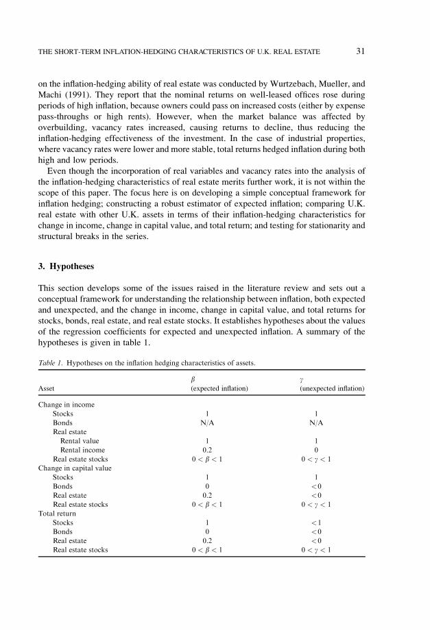
3. Hypotheses

This section develops some of the issues raised in the literature review and sets out a

conceptual framework for understanding the relationship between in¯ation, both expected

and unexpected, and the change in income, change in capital value, and total returns for

stocks, bonds, real estate, and real estate stocks. It establishes hypotheses about the values

of the regression coef®cients for expected and unexpected in¯ation. A summary of the

hypotheses is given in table 1.

Table 1. Hypotheses on the in¯ation hedging characteristics of assets.

b gAsset (expected in¯ation) (unexpected in¯ation)

Change in income

Stocks 1 1

Bonds N/A N/A

Real estate

Rental value 1 1

Rental income 0.2 0

Real estate stocks 0 < b < 1 0 < g < 1

Change in capital value

Stocks 1 1

Bonds 0 <0

Real estate 0.2 <0


Total return

Stocks 1 <1

Bonds 0 <0

Real estate 0.2 <0



3.1. Change in Income and In¯ation

The scope for adjustments to nominal income to accommodate expected and unexpected

in¯ation varies from asset class to asset class. Bond income is ®xed in nominal terms and

so cannot adjust to protect real income from either expected or unexpected in¯ation. In the

United Kingdom, interim stock dividends are paid after six months and ®nal dividends at

the end of the year. In theory, therefore, dividends could be a perfect hedge against both

expected and unexpected in¯ation.

However, Estep and Hanson (1989) argue that the in¯ation compensation for stocks in

the United States is less than perfect and typically is nearer to a half than one. Diermeier

(1990) cites the lag between in¯ation and labor costs and employee bene®ts as possible

explanations. Another explanation for the less than perfect compensation for in¯ation is

provided by Feldstein (1980), who argues that, as taxable pro®ts are calculated by

subtracting a value for depreciation from other net operating income and as this value is

based on historical cost rather than on replacement cost, the real value of depreciation falls

and real taxable pro®ts increase when prices rise. As a result, real pro®ts, net of the

corporate income tax, vary inversely with in¯ation.

Modigliani and Cohn (1979), however, argue that, as in¯ation rises, stockholders will

gain from depreciation in the real value of nominal corporate liabilities. The portion of the

corporation's interest bill that compensates creditors for the reduction in the real value of

their claims represents repayment of capital, rather than an expense to the corporation. As

corporations are not taxed on that part of their return, the stock of pretax operating income

paid in taxes declines as the rate of in¯ation rises. Modigliani and Cohn (1979, p. 24) even

add that ``for the corporate sector as a whole, this effect tends to offset any distortions

resulting from basing taxable income on historic cost.''

The rental value of real estate is determined in the market and might be able to

compensate for both expected and unexpected in¯ation. However, a portfolio of U.K. realestate has more complicated cash ¯ows. For any property, rental income is reviewed every

®ve years so that, on average, 20% of a portfolio is reviewed each year. The rents are set in

advance so that, even for the 20% of the portfolio reviewed in any year, protection should

be provided against expected but not unexpected in¯ation. Therefore, U.K. real estate

income should be a partial hedge against expected in¯ation but no hedge against

unexpected in¯ation.

For real estate stocks, the income is derived in part1 from rental income. Therefore, the

relationship between income and in¯ation, both expected and unexpected, is unlikely to be

as exact as for other stocks. This hypothesis is supported by Mengden and Hartzell (1986),

who showed that the capital appreciation component of REITs is highly correlated to that

of stocks but income was not. The same is true for the data sets used in this study. Although

the capital appreciation of real estate stocks is highly correlated with that of stocks (0.74,

for annual data; 0.77, for quarterly data), income change for real estate stocks is less

correlated to that for stocks (0.38, annual; 0.33, quarterly). For correlations with real

estate, the ®gures are: capital appreciation (0.14, annual; ÿ0.04, quarterly) and income

change (0.41, annual rental value; 0.42, quarterly rental value; 0.13, quarterly rental

income).


3.2. Change in Capital Value and In¯ation

The adjustments to capital value in response to in¯ation are more complex than for

income. The capital value at the start of any period t is the income expected in that period

(Dt) divided by the capitalization rate (Kt). The capital value at the end of period t is the

same as the capital value at the start of period t� 1 and so is Dt�1=Kt�1. Therefore, to

understand the in¯ation hedging characteristics of capital value, it is necessary to consider

the links between expected and unexpected in¯ation during period t and changes to income

and the capitalization rate during period t. Income has been considered already; the

capitalization rate is now considered.

The capitalization rate comprises a number of components and can be approximated

(Baum and MacGregor, 1992) as

K � RF� RPÿ �g� i� � d �1�

where

K is the capitalization rate

RF is the nominal risk free rate (the gross redemption yield on U.K. government

nominal bonds)

RP is the risk premium

g is the expected constant real income growth in perpetuity

i is the expected constant inflation in perpetuity

(g� i) is the expected constant nominal income growth in perpetuity

d is the expected constant depreciation in perpetuity

Estep and Hanson (1989, p. 152) propose a similar model that, using the preceding

terminology and assuming d � 0, can be approximated as

K � RF� RPÿ �g� fi� �2�

where f is the fraction of in¯ation that ¯ows through to nominal pro®t and nominal

dividend growth.

A change in the capitalization rate is the result of a change in any of its component parts.

It should adjust to take account of changing expectations to ensure that the asset is

correctly priced to deliver the required return in the future.

The nominal risk-free rate (the bond capitalization rate) should adjust to changing

expectations of in¯ation. Therefore, for bonds, an increase in in¯ation expectations will

mean a higher capitalization rate for the ®xed income and so a fall in capital value.

Therefore, the relationships between expected and unexpected in¯ation and the change in

capital value, during period t, will depend on the relationship between the level of

expected and unexpected in¯ation and the changes to in¯ation expectations beyond period

t. If the level of expected and unexpected in¯ation in period t is positively related to

changes in expectations beyond period t, then expected or unexpected in¯ation should be

negatively related to changes in capital value during period t.


It may be that the level of unexpected in¯ation is positively related to the change to

expectations and so negatively related to changes in the capital value of bonds. However, it

is dif®cult to see why there should be any link between the level of expected in¯ation in

period t and the change in in¯ation expectations beyond period t. Therefore, for changes in

bond capital values, it seems reasonable to expect no relationship with expected in¯ation

and a negative relationship with unexpected in¯ation.

For stocks, other things being equal, real income expectations will be unchanged and

there should be an adjustment to nominal income equal to the change in the nominal risk-

free rate. Therefore, there should be no effect on the capitalization rate. However,

Diermeier (1990) suggests that the assumption that a change in the discount rate (which

contains the nominal risk-free rate) is equaled by a change in nominal growth (long term)

is ¯awed as labor costs and employee bene®ts lag behind in¯ation. He suggests that the

link between stock value and in¯ation varies in periods of high and low in¯ation: When

in¯ation is high, it may not be compensated; when it is low, there may be

overcompensation. However, as suggested previously, this may be the result of a link

between unexpected in¯ation in a period and changes to expectations beyond that period.

If stock income could adjust perfectly to changes in expected or unexpected in¯ation

and the capitalization rate is unaffected by changing expectations, the change in capital

value should be perfectly related with both expected and unexpected in¯ation. As

suggested already, income may undercompensate and capital value may over- or

undercompensate depending on the level of in¯ation.

However, the ``other things being equal'' quali®cation is unlikely to hold. For the

United States, where negative relationships are found between stocks prices and expected

and unexpected in¯ation, Fama (1981) argues for a negative relationship between in¯ation

and real variables. In contrast, in the United Kingdom, a positive in¯ation/stock returns

relationship is observed. In the United Kingdom, it is at least possible that an increase in

in¯ation expectations could be linked to an increase in growth expectations. If the

in¯ation/real variable relationship were positive, it would mean a decrease in the

capitalization rate and, therefore, a positive relationship between unexpected in¯ation

(linked to increases in in¯ation and growth expectations) and change in capital value

during period t. Under such circumstances, as stock income may protect against

unexpected in¯ation, the capital value change could even be greater than the level of

unexpected in¯ation.

For real estate, there is the complication of income from individual properties being

®xed for ®ve years between rent reviews. Therefore, when in¯ation expectations rise, the

expected real value of future income falls and so the capitalization rate value should rise. If

the level of unexpected in¯ation is positively related to the change in expectations, and as

rental income is unrelated to unexpected in¯ation, real estate capital value should be

negatively related with unexpected in¯ation. As real estate income provides partial

protection against expected in¯ation and as the level of expected in¯ation should be

unrelated to changes in in¯ation expectations, the change in capital value should be

similarly protected.

For real estate stocks, it is probable that the capitalization rate will move in line with the

general stock capitalization rate (see earlier), although the capitalized income will provide


only partial protection against expected and unexpected in¯ation. Therefore, changes in

the capital value of real estate stocks will be less strongly related to in¯ation than stocks

generally.

One further complication is that high levels of unexpected in¯ation also might be linked

to an increase in the risk premium (RP) and so to a decrease in capital values. This would

have the effect of reducing the strength of positive relationships and increasing the

strength of negative relationships.

3.3. Total Return and In¯ation

The total delivered return (DR) comprises two parts, the income return (IR) and the capital

return (CR):

DR � IR� CR �3�

This can be expressed as

DR � �Dt=CVt� � ��CVt�1 ÿ CVt�=CVt� �4�

or

DR � Kt � �CVt�1 ÿ CVt�=CVt �5�

where

Kt is the capitalization rate at the start of period tDt is the income received during period tCVt is the capital value at the start of period tCVt�1 is the capital value at the start of period t� 1Dt=CVt is the income return for period t�CVt�1 ÿ CVt�=CVt is the capital return for period t

The total delivered return therefore is the capitalization rate plus the change in capital

value divided by a constant. The capitalization rate at the start of the period contains

expectations about in¯ation and the ¯ow-through rate for both the period under

consideration and subsequent periods but, as it is ®xed, cannot respond to unexpected

in¯ation. The in¯ation-hedging characteristics of total return follow from this and the

previous discussion on changes in capital value.

With the exception of stocks, the hypotheses are the same as for capital value: for bonds,

no relationship for expected in¯ation and a negative relationship for unexpected in¯ation;

for stocks, perfect hedging for expected in¯ation and partial for unexpected; for realestate, positive hedging for expected but negative for unexpected; and for real estatestocks, positive for both. Although the ranges for the hypotheses are the same, there is no

reason to assume that the actual coef®cient values will be identical. For example, the

change in capital value for real estate stocks is hypothesized to offer a partial positive


hedge for unexpected in¯ation and the initial yield will provide no protection. Therefore,

from equation (5), total return should offer partial but lower hedging than change in capital

value.

4. Methodology and Data

4.1. Methodology

The analysis uses the methodology developed by Fama and Schwert (1977) to test the

relationship between in¯ation, both expected and unexpected, and changes in nominal

income, changes in nominal capital value, and nominal returns. This procedure has been

widely used for returns in previous studies of in¯ation hedging.

The Fama and Schwert (1977) model, developed for returns, is as follows:

Rt � a� bE�Dt� � g�Dt ÿ E�Dt�� et �6�

where

Rt is the asset return in period tE�Dt� is expected inflation for period tDt is actual inflation for period t�Dt ÿ E�Dt�� is unexpected inflation for period ta, b, and g are constants

et is the error term for period t

The regression analysis to estimate a, b, and g requires consideration of the order of

integration of each of the variables in the equation. Previous studies investigating the

in¯ation-hedging characteristics of different assets make the implicit assumption that the

variables are all of the same order of integratedness. The variables used in the regression

were tested for their order of integration using the augmented Dickey-Fuller (ADF)

approach for testing for the presence of unit roots. The results are reported in section 5.

Fama and Schwert (1977) argue that, from ®nancial theory, both b and g should be

positive. An asset is said to be a perfect hedge against expected in¯ation when b � 1 and

to be a perfect hedge against unexpected in¯ation when g � 1. When b � g � 1, the asset

is said to provide a complete hedge against in¯ation. So, in their model, for an asset to be a

partial hedge against in¯ation, the relationship between asset returns and in¯ation should

be positive.

Several different procedures are used in this study to proxy for expected in¯ation. First,

and following GuÈltekin (1983), contemporaneous in¯ation rates are used as proxies for

expected in¯ation rates. Using these in¯ation values means that expectations are perfect;

thus, when in¯ation rates are used as proxies for expected in¯ation, there is no unexpected

in¯ation and the model is simply

Rt � a� bDt � et �7�


Other procedures are used to estimate expected in¯ation:

1. Treasury bills are used as a proxy for expected in¯ation. The ex ante return at the

beginning of each period is a proxy for expected in¯ation in the period. However, T-

bill rates can be used only if real interest rates are assumed to be constant. If this is

the case, nominal rates move on a one-to-one basis with in¯ationary expectations. If

real interest rates are not constant (as suggested for the United States by Fama and

Gibbons, 1982), then a model for the behavior of these rates has to be selected.

2. Following Fama and Gibbons (1984), real interest rates can be forecasted by a

moving average of past real interest rates. This study uses 1-year, 5-year, and 10-

year windows for annual rates, and 1-quarter, 4-quarter, and 12-quarter windows for

quarterly rates. Once expected real interest rates have been forecast, expected

in¯ation rates are computed as the difference between the T-bill rates and real

interest rates.

3. An autoregressive integrated moving average model is used to estimate real interest

rates. Following GuÈltekin (1983), an ARIMA (0; 1; 1) model was chosen. To

construct the expectations for real interest rates, a 40-quarter moving window is

used for the quarterly data and a 40-year moving window for annual data.

In¯ationary expectations then are obtained by subtracting the real interest rate

forecasts from the T-bill rates.

4. A structural time-series approach (Harvey, 1989) is used to determine the

unobserved components of in¯ation. The unobserved component was modeled as

a random walk plus noise. This re¯ects a changing in¯ation level plus a random

disturbance term; that is, the in¯ation rate, Dt, evolves according to the following

process:

Dt � mt � et �8�

where

mt � mtÿ1 � Zt �9�

Zt is a white-noise term driving the level mt; mt captures the underlying level of the

in¯ation rate; et is NID(0; s2e); Zt is NID(0; s2

Z). This speci®cation ®tted the quarterly

data but, for the annual data, the model reduced to a random walk:

Dt � Dtÿ1 � Zt �10�

The preferred estimator of expected in¯ation is obtained by correlating and regressing

ex post values of in¯ation on the ex ante estimator values. The chosen estimator then is

used in the Fama and Schwert procedure (see equation (6)). This procedure is

acknowledged to help choose the best estimator of total in¯ation and not of expected

in¯ation, unless expected in¯ation is regarded as an unbiased estimator of total in¯ation.

This assumption does not seem unreasonable, but no proof is offered.


In all cases, unexpected in¯ation is computed as the difference between actual (ex post)

in¯ation and expected (ex ante) in¯ation.

The analyses using the Fama and Schwert procedure are undertaken for real estate,

stocks, bonds, and real estate company stocks. In each case, the analysis is undertaken for

change in nominal income, change in nominal capital value, and total nominal return.

The analyses are undertaken using annual and quarterly data. In addition to the

aggregate real estate data, where possible, the analyses were carried out on the three main

property types: of®ces, shops, and industrials.

Finally, as all appraisal-based real estate series (but none of the other series) exhibited

serial correlation,2 transformed real estate series were estimated to remove the smoothing

(see Appendix 1 for details). The in¯ation hedging characteristics of these transformed

series were then estimated.

4.2. Data

De®nitions The capital-value data for stocks, bonds, and real estate stocks are from

market price indices. Real estate capital-value data are from appraisal series. The income

data for stocks and real estate stocks are from dividend indices. Real estate rental value is

available for both annual and quarterly data from appraisal series, which comprise

appraisers' estimates of open market rental value. For the quarterly real estate data, a series

of actual rental income also is available. For any individual property this typically is ®xed

for ®ve years (see section 3).

Total return series for all assets also are available from the same sources as the capital

value and income series. The sole exception is the ®rst few years of the real estate stocks

series, which have to be calculated from the dividend and capital value data. However, it is

not possible to construct the real estate return series from the capital-value and rental-

value (as opposed to rental income) series.

Sources of Annual Data The annual data cover the period 1963 to 1993. Data for stocks

and bonds for the annual analyses come from the Barclays de Zoete Wedd (BZW) (1994)

study. The stock data come from the BZW Equity Index, which, from 1918 to 1956, is

similar to the Financial Times (FT) Index and, from 1956 to the present, is similar to the FT

Actuaries All-Share Index. The bond data are from the BZW Gilt Index, which is a

weighted combination of four long-dated U.K. government bonds with an average life of

15 years. The Retail Price Index is used for in¯ation.

The real estate data are from appraisal series for investment portfolios. Investment

Property Databank (IPD) data are used from 1971 to 1993; and, for 1963 to 1970, data

constructed by IPD from MGL/CIG data to ensure consistency with the later IPD data are

used (see Key et al., 1994). This is the longest annual series available. The IPD is by far the

most widely used and widely respected source of appraisal data on U.K. real estate. It also

is the dominant provider of real estate portfolio performance measurement analysis. The

real estate company stock data are from the Financial Times Actuaries Property Index,3

which is available only since 1964.


Sources of Quarterly Data The quarterly data cover the period 1977Q3 to 1993Q4. The

stocks data are from the FT Actuaries All-Share Index and the bonds data are from the FT

Actuaries Over 15 Year U.K. Government Stock Index. The real estate data are from Jones

Lang Wootton (JLW) (1984±1994). JLW, one of the largest U.K.-based ®rms of property

investment advisers, has a substantial international presence. Like the IPD data, the JLW

real estate data is appraisal based but is for a much smaller sample (£446 million in June

1994 compared with £40 billion for the IPD). The quarterly real estate stock data, like the

annual data, are from the FT Actuaries Property Index. The Retail Price Index is used for

in¯ation.

It was necessary to use two different sources for the real estate data because the

quarterly series extends back only to 1977, which is too short for annual analyses. The IPD

annual series was regressed on an annual version of the JLW quarterly series for the period

1978 to 1993. The regression results showed the constant not to be signi®cantly different

from zero and the coef®cient not to be signi®cantly different from unity.

All of the data sets, both annual and quarterly, are publicly available. Summary statistics

are provided in table 2.

Risk-free Rates The nominal risk-free rate is taken to be the quarterly Treasury bill rates

and comes from HMSO (1994). These are prospective rates for 90-day government-issue

Table 2. Summary statistics of the asset data series.

Annuala Quarterlyb

Return Capital value Income Return Capital value Income

Stocks 19.12c 13.57 9.10 5.03 3.75 2.61

(32.79) (31.44) (7.80) (8.93) (8.87) (2.47)

Bonds 10.75 0.39 N/A 3.74 1.01 N/A

(15.04) (13.54) (6.64) (6.63)

Real 14.87 8.81 7.94 2.99 1.43 1.42

estated (10.84) (10.86) (7.65) (2.86) (3.00) (2.59)

RE stocks 20.55 16.04 9.78 4.50 3.55 3.04

(35.37) (35.49) (11.87) (12.33) 12.43 (4.20)

Rate Rate

T-bills 9.65 2.75

(3.38) (0.73)

In¯ation 8.01 1.71

(5.52) (1.34)

Notes:a Annual 1963 to 1993, except real estate stocks, 1966 to 1993.b Quarterly 1977Q3 to 1993Q4.c Figures are means with standard deviations in parentheses.d Real estate rental value is appraisers' estimates of market value rather than income received.


bills. Problems arise for an annual risk-free rate: No data were available for government

issues and data for the best available proxy, local government negotiable bonds, were

available only since 1965. To overcome this problem, BZW (1994) uses four quarterly

rates combined. Strictly, this is not an annual nominal risk-free rate, as it combines

quarterly revised in¯ation expectations. The local authority rate was regressed on the

annualized T-bill rate. The results showed the constant to be signi®cantly greater than zero

at 5% and the coef®cient to be signi®cantly less than unity at 5%. These results are

consistent with a hypothesis that the local government rate is not risk free and,

accordingly, the annualized T-bill rate is used.

5. Results

5.1. Choosing Estimators of In¯ation

The procedures for estimating expected in¯ation are set out in the methodology section.

These include the T-bill rate less a constant real risk free rate (RFR), the T-bill rate less an

ARIMA model estimate of the real risk free rate, the T-bill rate less various moving

averages of past real risk free rates, and a structural time series approach. The ex ante

estimates were compared by regressing each on ex post in¯ation. The results are shown in

tables 3 and 4.

For the annual data, all ®ve estimators have coef®cients signi®cantly different from 0 at

1%, and only the T-bill with a constant real risk-free rate has a coef®cient not signi®cantly

different from 1 at 5% signi®cance. With the exception of the regression on the T-bill with

the ARIMA model, none of the constants in the regressions is signi®cantly different from 0

at 5%.

Overall, when considering the regression results, the T-bill rate less the lagged real risk-

free rate is taken as the best ex ante estimator for the annual data. It has the highest R2, a

coef®cient value close to 1 that is signi®cantly different from 0 and a constant that is not

signi®cantly different from 0 at 5%. The others are rejected because of low R2 values,

inappropriate constant values, or less plausible behavioral links to the formation of

in¯ation expectations.

For the quarterly data, the R2 values generally are lower than for the annual regressions.

With the exception of the structural time-series estimator, the regression coef®cients all

are signi®cantly different from 0 and from 1 at 1%. Three of the constants in the

regressions are signi®cantly different from 0 at 5% and one at 10%.

Overall, the T-bill less a four-quarter moving average risk-free rate is taken as the best

ex ante estimator for the quarterly data. It has the highest R2, the second highest coef®cient

value, and a low value for the constant. As with the annual data, the others are rejected

because of low R2 values, inappropriate constant values, or less plausible behavioral links

to the formation of in¯ation expectations.


5.2. Tests of Nonstationarity

Full details of the results of this analysis can be found in Appendix 2. For the annual data,

apart from in income indices for stocks and real estate stocks, the indices for total return,

capital value, and income appear to be integrated of order 1; that is, I�1�. The other two

series are either I�1� or I�2�. Inspection of the correlograms suggests that all levels indices

are ®rst-difference stationary; that is I�1�. The expected and unexpected in¯ation levels

series are I�1�. Accordingly, in the regression analysis that follows, all the series are

assumed to be conformable and I�1�.For the quarterly data, the results indicate that the orders of integratedness for many of

the series differed from their annual counterparts. For example, all the quarterly real estate

capital series were I�2� compared to I�1� for the annual series. This may be accounted for

by a change in the trend patterns in the longer (annual) series, for example, thereby biasing

the ADF statistics. These underlying differences are not explored in this paper but are left

for further work.4

ADF tests for the quarterly in¯ation series show that expected in¯ation is I�2� and

unexpected in¯ation is I�1�. Given these different orders of integratedness, it may be

Table 3. Regressions between ex post in¯ation and ex ante estimators of in¯ation (annual).

Independent variable Coef®cient (b) Constant (a)

T-bill less constant RFR 0.81 (3.09)*** 0.17 (0.06)

SE � 0:26 SE � 2:68

R2 � 0:25

T-bill less ARIMA for RFR 0.63 (4.58)*** 3.22 (2.49)**

SE � 0:14 SE � 1:30R2 � 0:42

T-bill less 1-year RFR 0.77 (8.00)*** 1.76 (1.83)*

SE � 0:10 SE � 0:96R2 � 0:69

T-bill less 5-year average RFR 0.77 (6.48)*** 1.56 (1.32)

SE � 0:12 SE � 1:19

R2 � 0:59T-bill less 10-year average RFR 0.68 (4.12)*** 2.08 (1.26)

SE � 0:16 SE � 1:65

R2 � 0:37

Structural time series 0.84 (6.15)*** 1.61 (1.30)

SE � 0:14 SE � 1:23

R2 � 0:57

Notes:The t values for H0: a � 0, b � 0 in parentheses.

The signi®cance levels are 1% (2.75), 5% (2.05), 10% (1.70).

*Signi®cant at 10%.

**Signi®cant at 5%.

***Signi®cant at 1%.


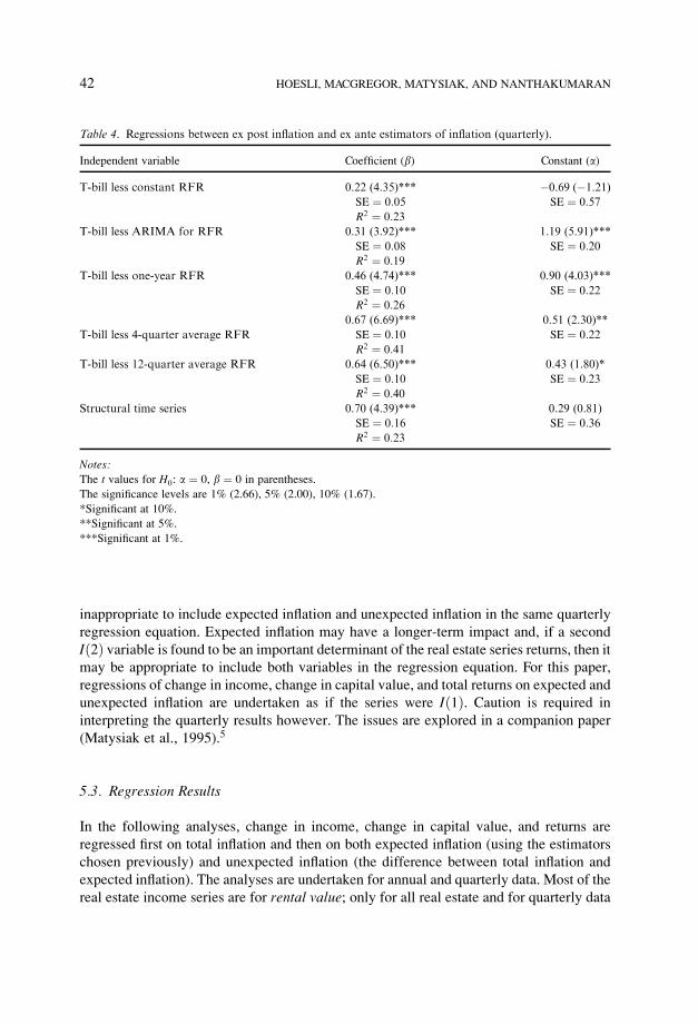
inappropriate to include expected in¯ation and unexpected in¯ation in the same quarterly

regression equation. Expected in¯ation may have a longer-term impact and, if a second

I�2� variable is found to be an important determinant of the real estate series returns, then it

may be appropriate to include both variables in the regression equation. For this paper,

regressions of change in income, change in capital value, and total returns on expected and

unexpected in¯ation are undertaken as if the series were I�1�. Caution is required in

interpreting the quarterly results however. The issues are explored in a companion paper

(Matysiak et al., 1995).5

5.3. Regression Results

In the following analyses, change in income, change in capital value, and returns are

regressed ®rst on total in¯ation and then on both expected in¯ation (using the estimators

chosen previously) and unexpected in¯ation (the difference between total in¯ation and

expected in¯ation). The analyses are undertaken for annual and quarterly data. Most of the

real estate income series are for rental value; only for all real estate and for quarterly data

Table 4. Regressions between ex post in¯ation and ex ante estimators of in¯ation (quarterly).

Independent variable Coef®cient (b) Constant (a)

T-bill less constant RFR 0.22 (4.35)*** ÿ0.69 (ÿ1.21)SE � 0:05 SE � 0:57

R2 � 0:23

T-bill less ARIMA for RFR 0.31 (3.92)*** 1.19 (5.91)***

SE � 0:08 SE � 0:20R2 � 0:19

T-bill less one-year RFR 0.46 (4.74)*** 0.90 (4.03)***

SE � 0:10 SE � 0:22R2 � 0:26

0.67 (6.69)*** 0.51 (2.30)**

T-bill less 4-quarter average RFR SE � 0:10 SE � 0:22

R2 � 0:41T-bill less 12-quarter average RFR 0.64 (6.50)*** 0.43 (1.80)*

SE � 0:10 SE � 0:23

R2 � 0:40

Structural time series 0.70 (4.39)*** 0.29 (0.81)

SE � 0:16 SE � 0:36

R2 � 0:23

Notes:The t values for H0: a � 0, b � 0 in parentheses.

The signi®cance levels are 1% (2.66), 5% (2.00), 10% (1.67).



***Signi®cant at 1%.


is there a rental income series. The results shown give the point estimates of the

coef®cients, their standard errors,6 95 and 99% con®dence interval for the estimates and

the R2 values for the regressions. The results will be summarized in table 9 and compared

with the hypotheses.

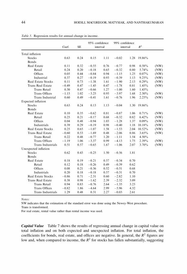
Income Table 5 shows the results of the regressions of the annual change in income on

total in¯ation and on both expected and unexpected in¯ation. For total in¯ation, all

coef®cients are positive. Only for stocks is R2 greater than 10%. For stocks, �1 is in the

con®dence interval but, at 95%, neither 0 or ÿ1 is, suggesting a perfect or partial hedge.

For real estate rental value, 0 is in the con®dence interval, and�1 is in only for of®ces and

industrials at 99%. For real estate stocks, ÿ1, 0, and �1 all are in the con®dence interval.

For the regressions on expected and unexpected in¯ation, all the coef®cients on

expected in¯ation and all on unexpected in¯ation, except that for real estate stocks, are

positive. The R2 ®gures are similar for the regressions on total in¯ation except that the real

estate stocks ®gure, at 11%, now is much higher. Most of the results are consistent with the

hypotheses: The exception is that real estate rental value appears, at best, to be only a

partial hedge against unexpected in¯ation; and, even at 99%, retail real estate, at best, is,

only a partial hedge against expected in¯ation. The transformed series show negative point

estimates for all real estate and for of®ces for expected in¯ation and negative for of®ces

for unexpected in¯ation. In general, the estimates with the transformed series show higher

standard errors and in some cases allow the possibility of perverse hedges.

The quarterly results generally are consistent with the annual results and with the

hypotheses.7 Taken together, the annual and quarterly analyses suggest that stocks could

offer a perfect hedge against expected and unexpected in¯ation, real estate income may

offer some protection against expected in¯ation but not against unexpected in¯ation, and

there is some evidence that real estate rental value may be a perfect hedge against expected

in¯ation but no hedge or a partial hedge against unexpected in¯ation. The one major

difference is real estate stocks, which, from the annual data, appear to offer no protection

against unexpected in¯ation but, from the quarterly data, appear to be a perfect hedge

against both expected and unexpected in¯ation. However, when con®dence intervals are

considered, the results are consistent. The difference suggests a possible structural break in

the estimated relationships.

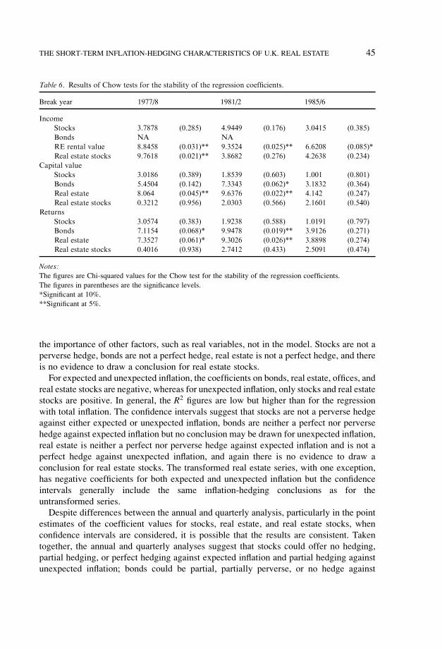
Table 6 shows the results of Chow tests for the structural breaks in the estimated

equations using the annual data. Three breakpoints were tested for all equations: 1977/8;

1981/2; and 1985/6. The ®rst was chosen because the quarterly series starts in mid-1977.

The other years were chosen after estimating 12-year rolling regressions and examining

the graphical results for possible breaks. These were identi®ed in 1981/2 for real estate and

in 1985/6 for stocks and bonds. The real estate results show structural breaks at 1977/8,

1981/2, and 1985/6, suggesting that the relationship between income and in¯ation has

changed throughout the 1980s. Real estate stocks show a break at 1977/8 but not at the

later two years. It is probable that the two results are linked, as real estate companies

depend, at least in part, on real estate for their income. Explanatory variables excluded

from the model, such as economic growth and vacancy rates, may offer some explanation

for the changes in the estimated relationships between income and in¯ation.


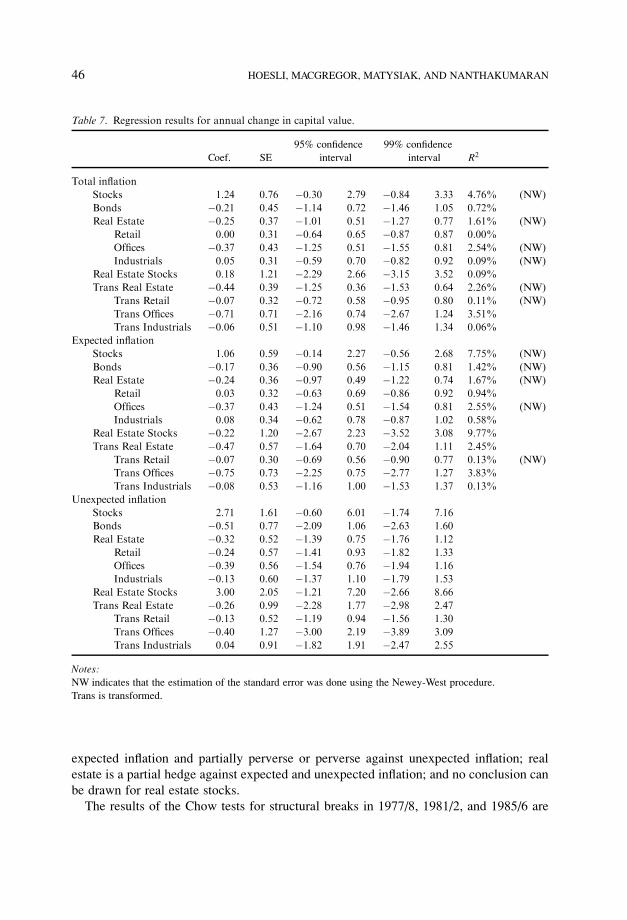
Capital Value Table 7 shows the results of regressing annual change in capital value on

total in¯ation and on both expected and unexpected in¯ation. For total in¯ation, the

coef®cients for bonds, real estate, and of®ces are negative. In general, the R2 ®gures are

low and, when compared to income, the R2 for stocks has fallen substantially, suggesting

Table 5. Regression results for annual change in income.

95% con®dence 99% con®dence

Coef. SE interval interval R2

Total in¯ation

Stocks 0.63 0.24 0.15 1.11 ÿ0.02 1.28 19.86%

Bonds

Real Estate 0.11 0.32 ÿ0.55 0.76 ÿ0.77 0.98 0.58% (NW)

Retail 0.24 0.20 ÿ0.18 0.65 ÿ0.32 0.80 5.74% (NW)

Of®ces 0.05 0.44 ÿ0.84 0.94 ÿ1.15 1.25 0.07% (NW)

Industrial 0.37 0.27 ÿ0.19 0.93 ÿ0.39 1.13 9.25% (NW)

Real Estate Stocks 0.11 0.73 ÿ1.38 1.61 ÿ1.90 2.13 0.29% (NW)

Trans Real Estate ÿ0.49 0.47 ÿ1.45 0.47 ÿ1.78 0.81 1.45% (NW)

Trans Retail 0.30 0.47 ÿ0.66 1.27 ÿ1.00 1.60 1.43%

Trans Of®ces ÿ1.15 1.02 ÿ3.25 0.95 ÿ3.97 1.68 2.30% (NW)

Trans Industrial 0.60 0.49 ÿ0.41 1.61 ÿ0.76 1.96 2.25% (NW)

Expected in¯ation

Stocks 0.63 0.24 0.13 1.13 ÿ0.04 1.30 19.86%

Bonds

Real Estate 0.10 0.35 ÿ0.62 0.81 ÿ0.87 1.06 0.71% (NW)

Retail 0.25 0.21 ÿ0.17 0.68 ÿ0.32 0.82 6.42% (NW)

Of®ces 0.04 0.48 ÿ0.94 1.03 ÿ1.28 1.37 0.09% (NW)

Industrials 0.39 0.29 ÿ0.19 0.98 ÿ0.40 1.18 10.18% (NW)

Real Estate Stocks 0.25 0.65 ÿ1.07 1.58 ÿ1.53 2.04 10.52% (NW)


Trans Retail 0.22 0.48 ÿ0.77 1.20 ÿ1.11 1.54 4.50%

Trans Of®ces ÿ1.19 1.06 ÿ3.37 0.99 ÿ4.13 1.75 2.39% (NW)

Trans Industrials 0.51 0.57 ÿ0.65 1.67 ÿ1.06 2.07 3.70% (NW)

Unexpected in¯ation

Stocks 0.62 0.43 ÿ0.25 1.50 ÿ0.56 1.81

Bonds

Real Estate 0.18 0.19 ÿ0.21 0.57 ÿ0.34 0.70

Retail 0.12 0.18 ÿ0.26 0.49 ÿ0.39 0.62

Of®ces 0.08 0.21 ÿ0.36 0.52 ÿ0.51 0.68

Industrials 0.20 0.18 ÿ0.18 0.57 ÿ0.31 0.70

Real Estate Stocks ÿ0.86 0.71 ÿ2.31 0.60 ÿ2.82 1.10

Trans Real Estate 0.38 0.98 ÿ1.62 2.39 ÿ2.32 3.09

Trans Retail 0.94 0.83 ÿ0.76 2.64 ÿ1.35 3.23

Trans Of®ces ÿ0.82 1.86 ÿ4.64 2.99 ÿ5.96 4.32

Trans Industrials 1.29 0.48 0.31 2.27 ÿ0.03 2.61

Notes:NW indicates that the estimation of the standard error was done using the Newey-West procedure.

Trans is transformed.

For real estate, rental value rather than rental income was used.


the importance of other factors, such as real variables, not in the model. Stocks are not a

perverse hedge, bonds are not a perfect hedge, real estate is not a perfect hedge, and there

is no evidence to draw a conclusion for real estate stocks.

For expected and unexpected in¯ation, the coef®cients on bonds, real estate, of®ces, and

real estate stocks are negative, whereas for unexpected in¯ation, only stocks and real estate

stocks are positive. In general, the R2 ®gures are low but higher than for the regression

with total in¯ation. The con®dence intervals suggest that stocks are not a perverse hedge

against either expected or unexpected in¯ation, bonds are neither a perfect nor perverse

hedge against expected in¯ation but no conclusion may be drawn for unexpected in¯ation,

real estate is neither a perfect nor perverse hedge against expected in¯ation and is not a

perfect hedge against unexpected in¯ation, and again there is no evidence to draw a

conclusion for real estate stocks. The transformed real estate series, with one exception,

has negative coef®cients for both expected and unexpected in¯ation but the con®dence

intervals generally include the same in¯ation-hedging conclusions as for the

untransformed series.

Despite differences between the annual and quarterly analysis, particularly in the point

estimates of the coef®cient values for stocks, real estate, and real estate stocks, when

con®dence intervals are considered, it is possible that the results are consistent. Taken

together, the annual and quarterly analyses suggest that stocks could offer no hedging,

partial hedging, or perfect hedging against expected in¯ation and partial hedging against

unexpected in¯ation; bonds could be partial, partially perverse, or no hedge against

Table 6. Results of Chow tests for the stability of the regression coef®cients.

Break year 1977/8 1981/2 1985/6

Income

Stocks 3.7878 (0.285) 4.9449 (0.176) 3.0415 (0.385)

Bonds NA NA

RE rental value 8.8458 (0.031)** 9.3524 (0.025)** 6.6208 (0.085)*

Real estate stocks 9.7618 (0.021)** 3.8682 (0.276) 4.2638 (0.234)

Capital value

Stocks 3.0186 (0.389) 1.8539 (0.603) 1.001 (0.801)

Bonds 5.4504 (0.142) 7.3343 (0.062)* 3.1832 (0.364)

Real estate 8.064 (0.045)** 9.6376 (0.022)** 4.142 (0.247)

Real estate stocks 0.3212 (0.956) 2.0303 (0.566) 2.1601 (0.540)

Returns

Stocks 3.0574 (0.383) 1.9238 (0.588) 1.0191 (0.797)

Bonds 7.1154 (0.068)* 9.9478 (0.019)** 3.9126 (0.271)

Real estate 7.3527 (0.061)* 9.3026 (0.026)** 3.8898 (0.274)

Real estate stocks 0.4016 (0.938) 2.7412 (0.433) 2.5091 (0.474)

Notes:The ®gures are Chi-squared values for the Chow test for the stability of the regression coef®cients.

The ®gures in parentheses are the signi®cance levels.




expected in¯ation and partially perverse or perverse against unexpected in¯ation; real

estate is a partial hedge against expected and unexpected in¯ation; and no conclusion can

be drawn for real estate stocks.

The results of the Chow tests for structural breaks in 1977/8, 1981/2, and 1985/6 are

Table 7. Regression results for annual change in capital value.



Total in¯ation

Stocks 1.24 0.76 ÿ0.30 2.79 ÿ0.84 3.33 4.76% (NW)

Bonds ÿ0.21 0.45 ÿ1.14 0.72 ÿ1.46 1.05 0.72%

Real Estate ÿ0.25 0.37 ÿ1.01 0.51 ÿ1.27 0.77 1.61% (NW)

Retail 0.00 0.31 ÿ0.64 0.65 ÿ0.87 0.87 0.00%

Of®ces ÿ0.37 0.43 ÿ1.25 0.51 ÿ1.55 0.81 2.54% (NW)

Industrials 0.05 0.31 ÿ0.59 0.70 ÿ0.82 0.92 0.09% (NW)

Real Estate Stocks 0.18 1.21 ÿ2.29 2.66 ÿ3.15 3.52 0.09%


Trans Retail ÿ0.07 0.32 ÿ0.72 0.58 ÿ0.95 0.80 0.11% (NW)

Trans Of®ces ÿ0.71 0.71 ÿ2.16 0.74 ÿ2.67 1.24 3.51%

Trans Industrials ÿ0.06 0.51 ÿ1.10 0.98 ÿ1.46 1.34 0.06%

Expected in¯ation

Stocks 1.06 0.59 ÿ0.14 2.27 ÿ0.56 2.68 7.75% (NW)

Bonds ÿ0.17 0.36 ÿ0.90 0.56 ÿ1.15 0.81 1.42% (NW)

Real Estate ÿ0.24 0.36 ÿ0.97 0.49 ÿ1.22 0.74 1.67% (NW)

Retail 0.03 0.32 ÿ0.63 0.69 ÿ0.86 0.92 0.94%

Of®ces ÿ0.37 0.43 ÿ1.24 0.51 ÿ1.54 0.81 2.55% (NW)

Industrials 0.08 0.34 ÿ0.62 0.78 ÿ0.87 1.02 0.58%

Real Estate Stocks ÿ0.22 1.20 ÿ2.67 2.23 ÿ3.52 3.08 9.77%

Trans Real Estate ÿ0.47 0.57 ÿ1.64 0.70 ÿ2.04 1.11 2.45%


Trans Of®ces ÿ0.75 0.73 ÿ2.25 0.75 ÿ2.77 1.27 3.83%



Stocks 2.71 1.61 ÿ0.60 6.01 ÿ1.74 7.16

Bonds ÿ0.51 0.77 ÿ2.09 1.06 ÿ2.63 1.60

Real Estate ÿ0.32 0.52 ÿ1.39 0.75 ÿ1.76 1.12

Retail ÿ0.24 0.57 ÿ1.41 0.93 ÿ1.82 1.33

Of®ces ÿ0.39 0.56 ÿ1.54 0.76 ÿ1.94 1.16

Industrials ÿ0.13 0.60 ÿ1.37 1.10 ÿ1.79 1.53

Real Estate Stocks 3.00 2.05 ÿ1.21 7.20 ÿ2.66 8.66

Trans Real Estate ÿ0.26 0.99 ÿ2.28 1.77 ÿ2.98 2.47

Trans Retail ÿ0.13 0.52 ÿ1.19 0.94 ÿ1.56 1.30

Trans Of®ces ÿ0.40 1.27 ÿ3.00 2.19 ÿ3.89 3.09

Trans Industrials 0.04 0.91 ÿ1.82 1.91 ÿ2.47 2.55




shown in table 6. These show breaks in 1977/8 and 1981/2 for real estate capital value but

not for real estate stocks. This contrasts with the income results and suggests that, although

real estate stock income is related to real estate income, capital values move in line with

the stock market. The real estate result may again suggest the importance of variables not

in the analysis. Bonds also show a structural break in 1981/2, and the coef®cients become

more negative. This may be linked to changing in¯ation expectations that, in the latter

period, were more weakly related to in¯ation shocks in each year (see section 3).

Only two of the regression results are inconsistent with the hypotheses: Stocks offer

perfect hedging against unexpected in¯ation within the 99% con®dence interval only for

the quarterly data; and real estate offers partial hedging against unexpected in¯ation for

the quarterly data. The latter result is likely to be a consequence of the structural break.

Less likely, it also may be explained by appraisers adjusting capital values in line with ex

post in¯ation, at least for the quarterly appraisal series.

Total Return Table 8 shows the results of regressing annual and quarterly returns on total

in¯ation and on both expected and unexpected in¯ation. For total in¯ation, the coef®cients

for all property types and for real estate stocks are negative. In general, the R2 ®gures are

lower than for capital value. The results suggest stocks and bonds are not perverse hedges,

real estate is not a perfect hedge, no conclusion can be drawn for real estate stocks, and

transformed real estate is not a perfect hedge.

For the regressions on both expected and unexpected in¯ation, the coef®cients on

expected in¯ation are similar to those on total in¯ation. For unexpected in¯ation, the

values become positive for real estate stocks and negative for bonds. In general, the R2

®gures are low but higher than for total in¯ation. The results suggest that, for expected

in¯ation, stocks are neither a perverse or no hedge, bonds are not a perverse hedge, real

estate and transformed real estate are not perfect hedges, and no conclusion can be drawn

for real estate stocks. For unexpected in¯ation, stocks are not a perverse hedge, real estate

is not a perfect hedge, and no conclusion can be drawn for other assets including

transformed real estate.

As with the capital-value estimations, despite differences in the coef®cient values, when

the con®dence intervals of the regression coef®cients are considered, the annual and

quarterly results generally are consistent. Taken together, the annual and quarterly

analyses suggest that stocks could be a partial or perfect hedge against expected in¯ation

and neither a perfect hedge nor a perverse hedge against unexpected in¯ation. Bonds are

neither a perfect hedge nor a perverse hedge against expected in¯ation and a partially

perverse or perfectly perverse hedge against unexpected in¯ation. Real estate is a partial

hedge against both expected and unexpected in¯ation, while transformed real estate is not

a perfect hedge against expected in¯ation and no conclusion can be drawn for unexpected

in¯ation. No conclusion can be drawn for real estate stocks

The results of the Chow tests for structural stability are shown in table 6. These show

structural breaks for both bonds and real estate returns in 1977/8 and 1981/2. In the former

case, the regression coef®cients either switch from positive to negative or become more

negative; in the latter, they switch from negative to positive. The bond results may be

explained by the structural breaks in the capital value regressions discussed previously.


The real estate results are driven by breaks in both income and capital value and suggest

the importance of variables, such as economic growth and vacancy rates, not in the

regression.

Only two results are inconsistent with the hypotheses: Stocks do not have a coef®cient

Table 8. Regression results for annual total return.



Total in¯ation

Stocks 1.47 0.80 ÿ0.17 3.10 ÿ0.74 3.67 6.10% (NW)

Bonds 0.21 0.50 ÿ0.83 1.24 ÿ1.19 1.60 0.58%

Real Estate ÿ0.32 0.36 ÿ1.06 0.41 ÿ1.32 0.67 2.72%

Retail ÿ0.45 0.33 ÿ1.13 0.23 ÿ1.36 0.46 6.02%

Of®ces ÿ0.00 0.37 ÿ0.75 0.75 ÿ1.01 1.01 0.00% (NW)

Industrials ÿ0.06 0.35 ÿ0.77 0.66 ÿ1.02 0.91 0.09%




Trans Of®ces ÿ0.29 0.71 ÿ1.74 1.17 ÿ2.25 1.68 0.58%


Expected in¯ation

Stocks 1.29 0.62 0.01 2.57 ÿ0.44 3.01 8.86% (NW)

Bonds 0.27 0.52 ÿ0.79 1.33 ÿ1.16 1.70 2.10%

Real Estate ÿ0.32 0.37 ÿ1.08 0.45 ÿ1.35 0.71 2.76%

Retail ÿ0.44 0.31 ÿ1.08 0.20 ÿ1.31 0.43 6.12% (NW)

Of®ces ÿ0.01 0.37 ÿ0.76 0.75 ÿ1.02 1.01 0.01% (NW)

Industrials ÿ0.06 0.36 ÿ0.79 0.68 ÿ1.05 0.94 0.09%


Trans Real Estate ÿ0.52 0.55 ÿ1.64 0.61 ÿ2.03 1.00 3.20%


Trans Of®ces ÿ0.39 0.73 ÿ1.89 1.10 ÿ2.40 1.61 2.89%



Stocks 2.94 1.70 ÿ0.54 6.42 ÿ1.75 7.62

Bonds ÿ0.29 0.91 ÿ2.16 1.58 ÿ2.81 2.23

Real Estate ÿ0.38 0.66 ÿ1.72 0.97 ÿ2.19 1.43

Retail ÿ0.54 0.50 ÿ1.57 0.50 ÿ1.93 0.85

Of®ces 0.03 0.53 ÿ1.05 1.11 ÿ1.43 1.49

Industrials ÿ0.05 0.63 ÿ1.36 1.25 ÿ1.81 1.70

Real Estate Stocks 1.92 2.16 ÿ2.51 6.35 ÿ4.04 7.89

Trans Real Estate ÿ0.32 0.95 ÿ2.26 1.63 ÿ2.93 2.30

Trans Retail ÿ0.57 0.62 ÿ1.85 0.70 ÿ2.29 1.15

Trans Of®ces 0.54 1.26 ÿ2.04 3.12 ÿ2.93 4.02

Trans Industrials 0.14 0.90 ÿ1.72 1.99 ÿ2.36 2.63




of unity on unexpected in¯ation; and real estate may be a partial hedge against unexpected

in¯ation. In the former case, the original hypothesis is rejected at 95% but accepted at 99%

con®dence. In the latter case, the problem may be due to the appraisal data as the

transformed series suggests a perverse hedge.

6. Conclusion and Discussion

The original hypotheses and the results of the analysis are set out in table 9. In many cases

the con®dence intervals are large and the results are inconclusive. Taken as a whole, the

results are consistent with the view that stocks have better in¯ation-hedging characteristics

than real estate, which in turn is better than bonds. However, the transformed real estate

series sometimes are worse hedges than bonds.

Only three of the results of this analysis provide evidence to reject the original detailed

hypotheses: The quarterly, but not the annual, real estate returns offer partial hedging

against unexpected in¯ation; real estate rental value appears not to be a perfect hedge

against unexpected in¯ation; the quarterly, but not the annual, analysis suggests that real

estate capital value offers partial protection against unexpected in¯ation.

The quarterly real estate return results can be considered consistent with those of

Limmack and Ward (1988) and Brown (1991), who used, respectively, quarterly and

monthly data. However, when the con®dence intervals are considered, the results of this

study reject the Limmack and Ward possibility that real estate may offer full protection

against unexpected in¯ation and Brown's possibility that real estate may not offer any

hedging against expected in¯ation.

The results for stocks are consistent with those of Firth (1979), and GuÈltekin (1983).

They suggest the possibility, rejected by Boudoukh and Richardson (1993), that stocks are

a perfect hedge. However, they disagree with the results of Solnik (1983), who found

stocks to be a perverse hedge. The inconclusive results for real estate stocks are similar to

those of Liu, Hartzell, and Hoesli (1997).

The three results that are inconsistent with the original hypotheses are now considered:

1. The quarterly result that real estate returns offer partial hedging against unexpected

in¯ation is similar to that of Limmack and Ward (1988) and Brown (1991), who also

allow the possibility that real estate offers full hedging. The annual results of this

study and the transformed quarterly series both suggest a wider range of

possibilities, including a perverse hedge. There are three possible explanations of

the results: general problems with the quarterly data, problems with the capital

component of the data, or differences in the time periods of the analyses. To try to

overcome the ®rst of these, a transformed real estate series was constructed and its

in¯ation hedging estimated. The results, which suggest the possibility of a perverse

hedge, may invalidate the original ®nding. The problem with capital values is

discussed next and this, too, may invalidate the result. The results of the Chow tests

show a structural break in the estimated equation in 1977/8 or 1981/2, which is

suf®cient to explain the differences between the annual and the quarterly results.


Table 9. Comparison of hypotheses and results.

Asset

b (expected

in¯ation)

Result (annual,

quarterly)

g (unexpected

in¯ation)

Result (annual,

quarterly)

Change in income

Stocks 1 A�> 0; 1� 1 A�> ÿ1; 1�Q�> 0; 1� Q�> 0; 1�

Bonds N/A N/A

Real estate

Rental value 1 A�> ÿ1; <1�(*) 1 A�> ÿ1; <1�except O: Q�> ÿ1; <1��> ÿ1; 1� except R:

Q�> ÿ1; 1� �> 0; <1�except R/I:

�> 0; 1�Rental income 0.2 Q�0; <1� 0 Q�> ÿ1; <1�

Transformed RE (rental value) 1 A�ÿ1; <1� 1 A�ÿ1; 1�Q�> ÿ1; 1� Q�ÿ1; <0�

Real estate stocks 0 < b <1 A�ÿ1; 1� 0 < g <1 A�ÿ1; <1�Q�> 0; 1� Q�> 0; 1�

Change in capital value

Stocks 1 A�> ÿ1; 1� 1 A�ÿ1; 1�Q�ÿ1; 1� Q�ÿ1; <1�(*)

Bonds 0 A�> ÿ1; <1� <0 A�ÿ1; 1�Q�ÿ1; <1� Q�ÿ1; <0�

Real estate 0.2 A�> ÿ1; <1� <0 A�ÿ1; <1�except O: except I:

�ÿ1; <1� �ÿ1; 1�Q�ÿ0:2; 1� Q�> 0; <1�except R/I: except I:

�> 0:2; 1��*� �> ÿ1; <1�Transformed RE 0.2 A�ÿ1; <1� <0 A�ÿ1; 1�

Q�ÿ1; <1� Q�ÿ1; 1�Real estate stocks 0 < b <1 A�ÿ1; 1� 0 < g <1 A�ÿ1; 1�

Q�ÿ1; 1� Q�ÿ1; 1�Total return

Stocks 1 A�> 0; 1� <1 A�> ÿ1; 1�Q�ÿ1; 1� Q�ÿ1; <1�

Bonds 0 A�> ÿ1; 1� <0 A�ÿ1; 1�Q�ÿ1; <1� Q�ÿ1; <0�

Real estate 0.2 A�ÿ1; <1� <0 A�ÿ1; <1�except O/I: except O/I:

�> ÿ1; <1� �ÿ1; 1�Q�> 0; 1� Q�> 0; <1�

Transformed RE A�ÿ1; <1� A�ÿ1; 1�Q�ÿ1; <0� A�ÿ1; 1�

Real estate stocks 0 < b <1 A�ÿ1; 1� 0 < g <1 A�ÿ1; 1�Q�ÿ1; 1� Q�ÿ1; 1�

Notes:The brackets indicate whether ÿ1, 0, 1 is in the 95% con®dence intervals.

An asterisk (*) indicates hypothesis value within 99% con®dence interval.

R � retail. O � offices. I � industries.


2. The quarterly, but not the annual, analysis suggests that real estate capital value

offers partial protection against unexpected in¯ation. One possibility is that, at least

for the quarterly appraisal series, appraisers adjust capital values in line with ex post

in¯ation. Another is that, as real estate has traditionally been regarded as an

in¯ation hedge, in times of high in¯ation it becomes a preferred asset and so the

capitalization rate falls and capital value rises. Key et al. (1994) produce evidence to

suggest a negative relationship between capitalization rates and in¯ation, and

Hendershott (1980) and Rosen and Rosen (1980) show that, as in¯ationary

expectations rise, demand for real estate assets increases. The Chow tests show a

structural break in 1977/8 or 1981/2 and the coef®cient moves from negative to

positive. The period before the break was one of relatively high in¯ation, whereas

the period after was one of relatively low in¯ation. Also, variables not in the model,

such as economic growth and vacancy rates, may have been important.

3. Real estate rental value appears not to be a perfect hedge against unexpected

in¯ation: This is the conclusion from both the annual and the quarterly analyses,

suggesting that the original hypothesis was incorrect. Perhaps rental value does not

adjust, ex post, to unexpected in¯ation as values are set on the basis of current and

expected economic circumstances.

To provide comparative results, the approach taken in this study has been similar to that

employed in other studies investigating the translation of expected and unexpected

in¯ation into returns. In addition, it also has examined change in capital value and change

in income and has considered a transformed real estate series. However, as suggested in

previous sections, two main quali®cations limit the conclusions that may be drawn.

The ®rst quali®cation concerns the misspeci®cation of the model as a result of

employing a static regression analysis. The implied assumption is of a linear relationship

between contemporaneous returns and expected and unexpected in¯ation; but as suggested

in section 3, the reality is more complex. By construction, the translation of in¯ation is

assumed instantaneous, without considering the possibility of dynamics within the

estimated relationship; in¯ation, in fact, may lead or lag behind the changes in income and

capital value and the returns. Furthermore, the nature of the dynamics may be different for

the rental and capital components. In essence, the static contemporaneous relationships

that have been estimated may represent only the long-term impact of the in¯ation

components. Accordingly, consideration needs to be given to accounting jointly for any

short-term dynamic impacts and possible long-term impacts. The exclusion of either of

these potentially signi®cant components from the relationship implies a potentially

misspeci®ed equation with biased parameter estimates.

The second quali®cation is that other variables may not have been included within the

equation speci®cation, particularly in the total returns and capital growth speci®cations.

Asset prices are determined within a multivariate framework and, consequently, a joint

estimation procedure that includes all possible asset classes together with any driver

variables is an alternative approach. Indeed, the low levels reported for R2 testify that the

two in¯ation variables account for a small proportion of the variability in changes in

income and capital value and in returns. An omission of relevant variables in each of the


equations again may lead to misspeci®cation. A companion paper (Matysiak et al., 1995)

addresses these issues explicitly, employing multivariate cointegration techniques.

Acknowledgments

The authors thank the following people and organizations for help in assembling the data

sets: John Atkins of UBS Ltd, Tony Key of the Investment Property Databank (IPD),

Barclay de Zoete Wedd (BZW), Jones Lang Wootton (JLW), The Treasury, and The Bank

of England.

Financial support from the British/Swiss Joint Research Programme for Martin Hoesli

and Bryan MacGregor also is gratefully acknowledged.

Helpful comments on earlier drafts were received from an anonymous referee and from

the participants at the Paci®c Asia Property Research Conference (Singapore, 1995), the

International Real Estate Society Conference (Stockholm, 1995) �and the Royal Institution

of Chartered Surveyors Annual Cutting Edge Conference (Aberdeen, 1995).

Appendix 1: The Transformation of the Real Estate Series

Blundell and Ward (1987) and Ross and Zisler (1987) suggest methods for correcting for

smoothing. The methods produce market price proxies by transforming real estate returns

derived from valuations. The methods are similar and the method of Blundell and Ward is

used in this study. In essence, the raw returns data series is analyzed and a time-series

model estimated using the Box-Jenkins technique.

As suggested by Blundell and Ward, the JLW quarterly series exhibits the characteristics

of a ®rst-order autoregressive process (AR1). Theoretically, the autocorrelations of the

returns series should decline geometrically from the ®rst-order value and the partial

autocorrelations should be 0 after the ®rst order. The values of the autocorrelations suggest

that the returns do follow an AR1 process.

The estimated model is given by the following equation:

Rt � 0:82Rtÿ1 � 0:63

�1:89� �9:68��R2 � 0:60

The transformation model is given by

RMt � �1=�1ÿ A��Rt ÿ �A=�1ÿ A��Rtÿ1;

where A � 0:82, or

RMt � 5:61Rt ÿ 4:61Rtÿ1


where RMt is the transformed return series, (see Brown, 1991, pp. 228±230 for further

details).

All series were tested for serial correlation. All the real estate series exhibited ®rst-order

serial correlation and appeared to follow AR1 processes; none of the other series did. The

preceding procedure was applied to all the real estate series, both annual and quarterly. The

values of A in the transformations are given in table 10.

We acknowledge that this procedure assumes an unvarying transformation parameter A.

For a discussion of the implications of this, see Matysiak and Brown (1995).

Barkham and Geltner (1995) use an identical procedure on the annual capital returns

series for a shorter period and estimate a value for A of 0.375, which compares with the

value in table 10 of 0.367.

Appendix 2: Tests for Nonstationarity

The results of the unit root tests reported in table 11 are based on the ADF equation:

Dyt � b0 � b1t� �aÿ 1�ytÿ1 �Xpÿ1

i�1

ciDytÿi � et

where yt is the time series under investigation, t is a time trend, and et is a white-noise

term.

The maximum value of the number of large lags considered, pÿ 1 was determined on

the basis of the ADF regression equation producing a white-noise residual series. The

requirement for the absence of serial correlation in the residuals means that there was no

necessity to employ nonparametric tests, such as the Phillips and Perron (1988) procedure.

Table 10. Values of the transformation parameter A.

Annual Quarterly

Returns

All property 0.34 0.82

Retail 0.26 N/A

Of®ce 0.52 N/A

Industrial 0.33 N/A

Capital value change


Retail 0.25 0.62

Of®ce 0.45 0.78

Industrial 0.37 0.76

Income change


Retail 0.70 0.47

Of®ce 0.85 0.77

Industrial 0.78 0.66


The results of the unit root tests for change in income, change in capital value and

returns for the annual series are shown in table 11. Apart from the income levels for stocks

and real estate stocks, the indices for total return, capital value, and income appear to be

integrated of order 1; that is, I�1�. The other two series are either I�1� or I�2�. Inspection of

the correlograms suggests that all series are ®rst difference stationary; that is, I�1�. The

expected and unexpected in¯ation levels indices are I�1�.These results are indicative of the time series characteristics of the variables under

investigation. It is recognized that the ADF tests for stationarity lack power and that

further analysis of the properties of the variables is required.

The results of the quarterly tests are not presented but are available from the authors.

For fuller details of how to conduct unit root tests and their limitations, see, for example,

Hamilton (1994) or Davidson and MacKinnon (1993).

Notes

1. As the real estate companies in the index combine investment companies, development companies, and

trading companies and as many are highly geared, their income is based only in part on rental income.

2, For discussions of smoothing in real estate series, see, for example, Barkham and Geltner (1994); Geltner

(1989); Geltner (1993); Geltner, Graff, and Young (1994); MacGregor and Nanthakumaran (1992).

3, The real estate companies in the index hold predominantly U.K. assets. There are investment companies,

development companies, and trading companies.

4. It is reported elsewhere in the paper that Chow tests indicate possible structural breaks in some of the estimated

regressions. Perron (1989) suggests that a structural break in a series may bias the ADF test toward

nonrejection of the unit root hypothesis. Consideration of the low power of the ADF test under such

circumstances is beyond the scope of this paper and left for further work.

5. This paper provides preliminary results of some of the analysis and was presented at The Cutting Edge, 1995,

in Aberdeen, Scotland. Copies are available from the authors.

6. In cases where the regression diagnostics indicated problems (at 5%) of heteroscedasticity or autocorrelation,

the Newey-West procedure, adjusted with Parzen weights and using a window of one-third of the available

Table 11. Results of the unit root tests.

Series Total return index Capital value index Income index

Stocks ÿ5.25 (1) ÿ5.41 (1) ÿ1.94 (1)**Bonds ÿ3.67 (1) ÿ5.04 (3) N/A

RE ÿ3.89 (1) ÿ4.67 (3) ÿ7.41 (1)Retail ÿ4.01 (1) ÿ3.02 (1)* ÿ3.06 (1)*Of®ces ÿ5.17 (2) ÿ4.72 (3) ÿ3.89 (1)Industrials ÿ4.00 (2) ÿ4.22 (2) ÿ4.04 (1)RE stocks ÿ3.64 (1) ÿ4.58 (1) ÿ2.70 (1)**

Notes:Figures in parentheses show the number of lags necessary for a white-noise error process in the ADF regression

equation.

*Estimated without a trend term, as this was insigni®cant.

**Not signi®cantly different from zero at 5%; index series either I�1� or I�2�.


observations, was used to estimate an alternative variance-covariance matrix for use in the standard error

calculation.

7. The full quarterly results are available from the authors on request.

References

Barclays de Zoete Wedd (BZW). (1994). ``The BZW Equity-Gilt Study: Investment in the London Stock Market

since 1918.'' London: Barclays de Zoete Wedd.

Barkham, R., and G. Geltner. (1994). `Ùnsmoothing British Valuation-Based Returns Without Assuming an

Ef®cient Market,'' Journal of Property Research 11(2), 81±95.

Barkham, R., and D. Geltner. (1995). `Òwner-Occupied Houses versus Commercial Property in the U.K.: A

Suggestion for Promoting Home Affordability and Investment Opportunities,'' presented at The Cutting Edge,

1995, Aberdeen, Scotland.

Barro, R. J. (1990). ``The Stock Market and Investment,'' Review of Financial Studies 3(1).

Baum, A. E., and B. D. MacGregor. (1992). ``The Initial Yield Revealed: Explicit Valuations and the Future of

Property Investment,'' Journal of Property Valuation and Investment 10(4), 709±726.

Blundell, G. F., and C. W. R. Ward. (1987). ``Property Portfolio Allocation: A Multi-Factor Model,'' LandDevelopment Studies 4(2), 145±156.

Bodie, Z. (1976). ``Common Shares as a Hedge Against In¯ation,'' Journal of Finance 31(2), 447±458.

Boudoukh, J., and M. Richardson. (1993). ``Stock Returns and In¯ation,'' American Economic Review 83(5),

1346±1355.

Brown, G. R. (1991). Property Investment and the Capital Markets. London: E. & F. N. Spon.

Brueggeman, W. B., A. H. Chen, and T. G. Thibodeau. (1984). ``Real Estate Investment Funds: Performance and

Portfolio Considerations,'' AREUEA Journal 12(3), 333±354.

Coleman, M., S. Hudson-Wilson, and J. R. Webb. (1994). ``Real Estate in the Multi-Asset Portfolio,'' vol. 3, pp.

98±123, in S. Hudson-Wilson and C. H. Wurtzebach (eds.), Managing Real Estate Portfolios. Burr Ridge, IL,

and New York: Richard D. Irwin.

Davidson, R., and J. G. MacKinnon. (1993). Estimation and Inference in Econometrics. New York: Oxford

University Press.

Diermeier, J. J. (1990). ``Capital Market Expectations: The Macro Factors,'' vol. 5, pp. 1±77, in J. L. Maginn and

D. L. Tuttle. (eds.), Managing Investment Portfolios: A Dynamic Process. Boston: Warren, Gorham and

Lamont.

Estep, T., and N. Hanson. (1989). ``The Valuation of Financial Assets in In¯ation,'' pp. 149±159, in F. J. Fabozzi

(ed.), Investment Management. Cambridge, MA: Balinger Publishing Company.

Fama, E. F. (1981). ``Stock Returns, Real Activity, In¯ation and Money,'' American Economic Review(September), 545±565.

Fama, E. F. (1990). ``Stock Returns, Expected Returns and Real Activity,'' Journal of Finance 45(4), 1089±1108.

Fama, E. F., and M. R. Gibbons. (1982). `Ìn¯ation, Real Returns and Capital Investment,'' Journal of MonetaryEconomics 9, 297±323.

Fama, E. F., and M. R. Gibbons. (1984). `ÀComparison of In¯ation Forecasts,'' Journal of Monetary Economics13, 327±348.

Fama, E. F., and G. W. Schwert. (1977). `Àsset Returns and In¯ation,'' Journal of Financial Economics 5(2),

115±146.

Feldstein, M. C. (1980). `Ìn¯ation and the Stock Market,'' American Economic Review 70(5), 839±847.

Firstenberg, P. M., S. A. Ross, and R. C. Zisler. (1988). ``Real Estate: The Whole Story,'' Journal of PortfolioManagement 14(3), 22±34.

Firth, M. (1979). ``The Relationship Between Stock Market Returns and Rates of In¯ation,'' Journal of Finance34(3), 743±749.

Geltner, D. (1989). `Èstimating Real Estate's Systematic Risk from Aggregate Level Appraisal-Based Returns,''

Journal of the American Real Estate and Urban Economics Association 17(4), 463±481.


Geltner, D. (1993). `Èstimating Market Values from Appraised Values Without Assuming an Ef®cient Market,''

Journal of Real Estate Research 8(3), 325±345.

Geltner, D., R. A. Graff, and M. S. Young. (1994). ``Random Disaggregate Appraisal Error in Commercial

Property: Evidence from the Russell-NCREIF Database,'' Journal of Real Estate Research 9(4), 403±419.

Geske, R., and R. Roll. (1983). ``The Fiscal and Monetary Linkage Between Stock Returns and In¯ation,''

Journal of Finance 38(1), 1±33.

GuÈltekin, N. B. (1983). ``Stock Market Returns and In¯ation: Evidence from Other Countries,'' Journal ofFinance 38(1), 49±65.

Hamilton, J. D. (1994). Time Series Analysis. Princeton, NJ: Princeton University Press.

Hartzell, D., J. Hekman, and M. Miles. (1987). ``Real Estate Returns and In¯ation,'' Journal of the American RealEstate and Urban Economics Association 15(1), 617±637.

Harvey, A. C. (1989). Forecasting, Structural Time Series Models and the Kalman Filter. Cambridge: Cambridge

University Press.

Hendershott, P. H. (1980). ``Real User Costs and the Demand for Single Family Housing,'' Brookings Papers andEconomic Activity 2, 401±452.

HMSO. (1994). Financial Statistics. London: HMSO.

Hoesli, M. (1993). Investissement immobilier et diversi®cation de portefeuille. Paris: Economica.

Hoesli, M. (1994). ``Real Estate as Hedge Against In¯ation: Learning from the Swiss Case,'' Journal of PropertyValuation and Investment 12(3), 51±59.

Hoesli, M., and M. S. Anderson. (1991). ``Swiss Real Estate: Return, Risk, and Diversi®cation Opportunities,''

Journal of Property Research 8(2), 133±145.

Jones Lang Wootton. (1984). Property Index. London: JLW.

Jones Lang Wootton. (1994). Property Index. London: JLW.

Key, T., B. D. MacGregor, N. Nanthakumaran, and F. Zarkesh. (1994). Understanding the Property Cycle (MainReport: Economic Cycles and Property Cycles). London: RICS.

Limmack, R. J., and C. W. R. Ward. (1988). ``Property Returns and In¯ation,'' Land Development Studies 5(3),

47±55.

Liu, C. H., D. J. Hartzell, and M. E. Hoesli. (1997). `Ìnternational Evidence on Real Estate Securities as an

In¯ation Hedge,'' Real Estate Economics. 25(2), 193±221.

MacGregor, B. D., and N. Nanthakumaran. (1992). ``The Allocation to Property in the Multi-Asset Portfolio: The

Evidence and Theory Reconsidered,'' Journal of Property Research 9(1), 5±32.

Markowitz, H. (1952). ``Portfolio Selection,'' Journal of Finance 7, 77±91.

Markowitz, H. (1959). Portfolio Selection: Ef®cient Diversi®cation of Investments. New York: John Wiley.

Matysiak, G. A., and G. R. Brown. (1995). `Àppraisal Based Returns: Adapting to Parameter Instability,''

Property Research Discussion Paper No. 9. London: City University Business School.

Matysiak, G. A., M. Hoesli, B. D. MacGregor, and N. Nanthakumaran. (1995). ``The Longer Term In¯ation

Hedging Attributes of Asset Classes: Commercial Property and Property Shares,'' paper presented at The

Cutting Edge, 1995, Aberdeen, Scotland.

Mengden, A., and D. J. Hartzell. (1986). ``Real Estate Investment Trusts: Are They Shares or Real Estate?'' in

Stock Research: Real Estate. New York: Salomon Brothers.

Modigliani, F., and R. A. Cohn. (1979). `Ìn¯ation, Rational Valuation and the Market,'' Financial AnalystsJournal (March±April), 24±44.

Newell, G. (1995). In¯ation-Hedging Attributes of Australian Commercial Property. Hawkesbury, Australia:

School of Land Economy, University of Western Australia.

Park, J., D. J. Mullineaux, and I. K. Chew. (1990). `Àre REITs In¯ation Hedges?'' Journal of Real EstateFinance and Economics 3(1), 91±103.

Perron, P. (1989). ``The Great Crash, the Oil Price Shock and the Unit Root Hypothesis,'' Econometrica 57,

1361±1401.

Phillips, P. C. B., and P. Perron. (1988). ``Testing for a Unit Root in Time Series Regression,'' Biometrika 75, 335±

346.

Rosen, H., and K. Rosen. (1980). ``Federal Taxes and Homeownership: Evidence from Time Series,'' Journal ofPolitical Economy 88(1), 59±75.


Ross, S. A., and R. C. Zisler. (1987). ``AClose Look at Equity Real Estate Risk,'' research paper. Goldman Sachs.

Scott, L. O. (1990). ``Do Prices Re¯ect Market Fundamentals in Real Estate Markets?'' Journal of Real EstateFinance and Economics 3(1), 5±23.

Solnik, B. (1983). ``The Relation Between Stock Prices and In¯ationary Expectations: The International

Evidence,'' Journal of Finance 38(1), 35±48.

Wurtzebach, C. H., G. R. Mueller, and D. Machi. (1991). ``The Impact of In¯ation and Vacancy on Real Estate

Returns,'' Journal of Real Estate Research 6(2), 153±168.


The Short-Term Inflation-Hedging Characteristics of U.K. Real Estate

Documents

Transcript of The Short-Term Inflation-Hedging Characteristics of U.K. Real Estate