The Short-Term Economic Impact of Levying E-Tolls on Industries

THE SHORT-TERM ECONOMIC IMPACT OF LEVYING

E-TOLLS ON INDUSTRIES

FRANCOIS JACOBUS STOFBERG* AND JAN VAN HEERDEN†

AbstractTERM is used to analyse the short-term regional economic impact of an increase in industries’transport costs when paying E-Tolls. Market-clearing and accounting equations allow regionaleconomies to be represented as an integrated framework, labour adjusts to accommodateincreasing transportation costs, and investments change to accommodate capital that is fixed.1 Weconcluded that costs from levying E-Tolls on industries are small in comparison to total transportcosts, and the impact on economic aggregates and most industries are marginal: investments(−0.404%), gross domestic product (GDP) (−0.01) and consumer price inflation (−0.10%). Thisis true even when considering costs and benefits on industries as well as consumers. Industries thatexperienced the greatest decline in output were transport, construction and gold. Provinces that arecloser to Gauteng and have a greater share of severely impacted industries experienced larger GDPand real income reductions. Mpumalanga’s decrease in GDP was 17% greater than Gauteng’s.JEL Classification: C68, L91, R10, R48Keywords: Computable general equilibrium models, regional economics, policy modelling, transport cost

1. INTRODUCTION

The Gauteng Provincial Government (Department of Transport, 2011) and Pienaar(2011) state that an inadequate transport network in Gauteng is one of the keyconstraints to economic growth. The Gauteng Freeway Improvement Plan (GFIP) wasintroduced as a solution to the inadequate network. Phase 1 involved a R19.5 billionupgrading of 185 km of freeway in Gauteng (Department of Transport, 2011), as well asthe introduction of E-Tolling; additional upgrades and further phasing projects are set outin the Socio-economic Impact of the Gauteng Freeway Improvement Project and E-tollsReport (2014). The tolling system had to be equitable, affordable, traffic-attracting andefficient, and as a result directional E-Tolls were introduced (Department of Transport,2011). These tolls operate as an Open Road Tolling system to limit the impact on roadtraffic; the system collects tolls 10 km apart and does not require vehicles to slow down

* Corresponding author: Economist, Efficient Group, 81 Dely Road, Hazelwood, Pretoria,Gauteng, 0081, South Africa. E-mail: [email protected]† Department of Economics, University of Pretoria, South Africa.The authors would like to thank and acknowledge Economic Research Southern Africa (ERSA) fortheir financial support. We would also like to thank Makoma Mabitsela, Antony Boting andWerner Zwart for all their help. We are also specifically thankful to the reviewers for their insightfulcomments; any further mistakes or shortcomings lie with the authors.1 TERM is a bottom-up CGE model designed for highly disaggregated regional data. TheEnormous Regional Model’s originate from Horridge et al. (2005) and are better explained inHorridge (2011).

bs_bs_banner South African Journal of Economics

South African Journal of Economics Vol. ••:•• •• 2015

© 2015 Economic Society of South Africa. doi: 10.1111/saje.121061

mailto:[email protected]

or stop. These E-Tolls are only levied in Gauteng, but we show in this paper that theintroduction of E-Tolls influenced the entire economy: directly through other provinces’use of the GFIP and indirectly through Gauteng’s share of total economic activity. Forthis reason, a multiregional model of the country is utilised to measure cross-regionaleconomic effects.2

Most research on the effect of tolling on the economy tends to show partialequilibrium effects and is narrowly focused with weak assumptions. Most models alsoassume that tastes and technology are uniform or are represented by only a few individualsor firms.

An assessment of the likely impact of the GFIP on the regional as well as nationaleconomy was conducted by Economists.co.za (2011). The nature of their analysis isanalytical and limited in the observed variables chosen. In their research, they estimatedthat the toll incidence on the commercial road freight industry could amount to anequivalent 30% company tax increase. We, however, found that, except for the goldindustry, transport cost increases on industries are small in comparison to total transportcosts. Economists.co.za (2011) estimated that consumer price inflation (CPI) wouldincrease by approximately 0.4%, and Standish et al. (2010) concluded that consumerprices would increase between 0.28% and 0.31%, depending on Living Standards Measure(LSM) group. We found that even when considering costs and benefits to both consumersand industries, CPI would only increase by 0.12% in the short term. As suggested inEconomists.co.za (2011), Standish et al. (2010) did a cost–benefit analysis of the GFIPover a 20-year period. Their results showed that at an aggregate level, benefits to road usersare greater when driving on upgraded roads and paying E-Tolls, than not upgrading, butsimply maintaining the road network. The aim of this study was to determine theshort-term economic effects of the direct increase in transport costs on industries, as a resultof levying E-Tolls. However, we briefly consider the short-term case of direct and indirectcosts and benefits on industries as well as consumers, as originally outlined in Standish et al.(2010).

Using a general equilibrium model to forecast an increase in transport cost, thefollowing particular advantages arise: the model captures not only the direct impact of thechange, but also a full system wide pattern of indirect effects (Horridge, 1999), andthe so-called multiplier effects between all regions and commodities of the model. Thisintroduces a more accurate measurement of the macroeconomic implication of levyingE-Tolls on industries. Other dimensions can also be explored with a general equilibriummodel; the effect on unemployment, income distribution and social equity, changes inconsumption, investment patterns, and so on.

As suggested by Haddad and Hewings (2004), we introduced a more comprehensiveapproach to measuring the impact of changes in transport costs by linking regionaleconomic modelling with those of transport models, a need emphasised by De Jong et al.(2004). Haddad and Hewings (2004) evaluated the structural impact of Brazilian policydevelopments that caused a reduction in transport costs, which reduced the gross

2 Some multiregional models that have been developed include Bröcker and Carsten (2010), Daset al. (2005), Horridge and Wittwer (2008), Ishiguro and Inamura (2005), Latorre et al. (2009),Li et al. (2009), and Ueda et al. (2005). Donaghy (2009) is carrying out a survey of literature thatfollows this direction. This type of multiregional models deal with cross-country analysis, thosethat focus on disaggregating one country into separate economies follow later.


© 2015 Economic Society of South Africa.

domestic product (GDP) in those regions. Haddad and Hewings (2004) analysedparameter sensitivity based on Domingues et al. (2003), and found that both short- andlong-run simulated parameters were robust. Steininger et al. (2006) found that levyingtransportation costs had a greater negative effect on wealthier households and those userswho make the most frequent use of the roads. Their results showed that if toll revenuesare used to lower labour taxes, the negative effect on GDP and employment can benegated.

In this paper, we linked a regional economic model, TERM, with models of thetransportation shippers’ market, the national freight flow model (NFFM) andcommodity flow model (CFM) of Havenga and Pienaar (2012) and Havenga (2013),respectively. Initially we simulated the data obtained from the NFFM and CFM modelsin conjunction with the Road Freight Association’s (RFA) vehicle cost structures onGoogle Maps, in order to calculate the costs incurred for each industry in each region asthey make use of the GFIP and hence have to pay E-Tolls. Afterwards the transport costincreases each industry incurs with the introduction of E-Tolls were simulated in TERMto estimate the regional economic impact of levying E-Tolls.

The remainder of this paper is organised as follows. Section 2 considers themethodology of the TERM and transport models. Section 3 explains TERM’s databaseand the process of simulating a transport cost increase; Section 3 also contains our results.Finally, we conclude our findings in Section 4.

2. METHODOLOGY

Most of the research results presented in this paper have been obtained using the TERMCGE model, which is discussed below. We also integrate a partial transport model intothe CGE model, and also discuss how it works. Finally we show how the two modelsinteract to find the simulation results that we present later.

2.1 The TERM CGE ModelDixon et al. (1982) initially introduced the large-scale CGE model, named ORANI.Models of this nature are either based on social accounting matrices (SAMs) orinput–output tables, but all of them assume that the whole economy that they representis balanced in value. CGE models combine the efficiency of linearised algebra ofJohansen-type models with the accuracy of multistep solutions. Through the simplisticnature of CGE modelling, it allows for the development of more disaggregated, elaborateand dynamic models. A typical result from CGE models estimate percentage changes ofendogenous variables after a policy has been implemented. The bottom-up approach inTERM allows simulations with region-specific price effects, and the modelling ofimperfect factor mobility between regions and sectors (Horridge, 2011).

This study builds on work originally done by Horridge (2003) and later in Horridge(2011), as simulations are run using the bottom-up TERM model which allows us toanalyse policy effects on 10 regions, 27 sectors and 27 corresponding commodities inSouth Africa.3 To achieve this purpose, several assumptions were made. First, 10 regions,representing the nine provinces of South Africa as well as a region representing the rest of

3 Other TERM publications include both papers by Glyn and Horridge (2007), Horridge et al.(2005), Haddad and Hewings (2004), and Wittwer (2003).

3South African Journal of Economics Vol. ••:•• •• 2015


the world, are analysed.4 Second, individuals are modelled as utility maximisers who facea discrete number of choices. Through the cost of travel and regional layouts, the patternof labour and industrial activity is influenced. Third, national input–output data for 2005and regional data are combined to aggregate the South African economy into separateregions, commodities and industries.

(i) TERM’s System of Equations TERM shares similar equations with other CGE models,where producers choose to minimise costs according to the constant elasticity ofsubstitution (CES)-type production functions. Producers apply production functions todetermine the correct combination of intermediate commodities and primary factorinputs. TERM assumes that demand for primary factors and intermediate inputs followa Leontief-type nesting structure in proportion to the industries’ output (Horridge,2011). Each of these high-level aggregate decisions is made through a CES-typespecification. Primary factor aggregates follow a CES composite of land, capital andlabour. Within each of these primary factor CES specifications, labour follows a CESspecification between the various skill (occupancy) groups. Commodities follow a CEScomposite between the two sources: domestic or imported. Finally, a constant elasticity oftransformation mechanism is used to transform outputs from intermediate goods andprimary factors into final goods. Wittwer (2003) and Horridge (2011) distinguishregional behavioural equations used in TERM – these are additional to the standardequations of CGE modelling in the ORANI-school (Dixon et al., 1982).5 Regionalequations include regional demand, supply, sourcing and revenue equations, amongothers.

(ii) TERM’s Sourcing Mechanisms Horridge et al. (2005) and Horridge (2011) illustratethe various substitution possibilities of the model (also referred to as “nests”) and showsthe TERM model’s data sourcing ability. To illustrate we use a simple example of a singlecommodity (meat), in a single region (Eastern Cape), used by a single pre-defined user(households).

Households choose through a CES type specification to source a particular commodity(meat), domestically or from abroad. Demand for commodities is guided by purchasers’prices that are user-specific. Demand in each region is summed over all users to obtainaggregate regional demand. The value of regional demand includes trade and transportcosts (basic + margin costs), also referred to as the delivered value.

A CES specification is used to allocate domestically demanded meat from the variousregions. Decisions at this level are accepted for all users as if wholesalers and not finaldemanders decide where meat would be sourced from. This level is therefore without theuser subscript u, implying that in Gauteng the proportion of meat that comes fromLimpopo is the same for households, intermediate users as well as other final demanders.The application of a CES specification allows regions with lower production costs toincrease production relatively more than other regions, in an attempt to increase their

4 These provinces include the Eastern Cape, Free State, Gauteng, Kwazulu-Natal, Limpopo,Mpumalanga, Northern Cape, North West and the Western Cape.5 Core model equations are best represented in standard equations in Steininger et al. (2006), anda full explanation of equations used in CGE modelling is given in Lofgren et al. (2002). TERMmodel equations are best illustrated as standard equations in Wittwer and Horridge (2010).



market share. It is important to remember that sourcing decisions are made on the basisof delivered prices; even if farmers keep prices fixed, a change in transport costs (or othermargin costs) will affect regional market shares.

Delivered meat from Limpopo follows a Leontief composite of basic, margin and tradecosts. Margin costs are derived from a combination of factors sourced from the level bywhich data are disaggregated, and include origin, destination, commodity and source,which influence its share of the commodity’s delivered value. Commodity regional pairsthat are far apart, heavy or bulky, will have a transport cost with a higher share of deliveredvalue than those region pairs that are not (Horridge, 2011).

At an aggregate level, the elasticity of substitution for road margins levied on meat,passing from Gauteng to the Eastern Cape, lies between 0.5 and 0.1, as suggested byHorridge (2011). Horridge (2011) explains that these are common CES amounts usedfor road margins and assume that a region applies the same CES to all commoditiestransported, applying equally to the origin, destination and transit regions. An elasticityof substitution of 0.5 would be a good fit for transport industries, such as truckingservices, which can relocate depots to cheaper regions. Other industries, particularly thosein retail, would see a more fitting CES of 0.1; substitution is less, due to larger sourcingfrom the destination region itself. Sourcing commodities from the same region as itsdestination reduces total transport costs (Horridge, 2011). TERM modelling also allowsfor the ability to involve price competitiveness of freight services among regions.

2.2 The Transport ModelWe estimate the increase in industries’ transportation cost as well as the percentageincrease on total transportation cost for commodities from each province with theintroduction of E-Tolls. To do this we use commodity flow data of Gauteng as providedby the NFFM and the CFM, outlined in Havenga and Pienaar (2012) and Havenga(2013), respectively. The commodity flow data consist of 3.4 million routes, eachconsisting of commodities transported, origin, entry and exit points into Gauteng, enddestination, base tonnage, and route distance, among others. These routes representannual commodity flows from all provinces in South Africa, as well as neighbouringcountries to, through and from Gauteng. The NFFM utilises the South African NationalRoad Agency’s (SANRAL) Traffic Count Yearbooks compiled by Mikros TrafficMonitoring, as well as actual freight flow data obtained from Spoornet. Havenga (2007)explains how, by utilising these sources, the NFFM produces the most complete surfacefreight data in South Africa that includes modal market share, flow data, and roadtonnage for a list of corridors, metropolitan and rural areas.

The CFM was developed to fill the gaps of the NFFM, disaggregating total freighttransported into commodity flows for 73 commodities over different typologies (354magisterial district levels) in South Africa. The CFM was later adapted to include gravitymodelling, which is most commonly used in international freight flow models, based onthe premise that demand and supply drive the flow of commodities between origin anddestination (Havenga, 2013). In addition to the CFM, a freight demand model (FDM)allocates different vehicle types to each commodity for various origin-to-destinationroutes or corridors; this allowed us the possibility to determine the vehicle class, which isrequired to estimate the cost at each gantry. Furthermore, Transnet’s transportationmodel adapted the CFM and disaggregated the magisterial district levels into 977 uniquestations: origin, destination and entry/exit points into Gauteng. By simulating these



commodity flows on Google Maps, we were able to calculate the additional cost fromlevying E-Tolls for each commodity from each province transported to, through or fromGauteng.

From the station assumptions, we obtained coordinates for each station to simulatecommodity flows on Google Maps, utilising each route’s entry and exit point intoGauteng. Google Maps automatically assumes the shortest kilometre route, taking intoaccount time travelled. E-Toll gantries were overlaid on the simulations in order toestimate the additional cost incurred for each commodity flow. For our purposes, weassumed that all users are registered E-Toll users as this will most accurately represents thedirect cost of levying E-Tolls.

Utilising the vehicle types that apply to different routes or corridors and commoditiesin the FDM, a more accurate cost could be estimated as gantry costs differ according tovehicle class. We also employed the RFA’s vehicle cost schedule (2013) in conjunctionwith the FDM to differentiate the payload and load factor for each vehicle type of eachcommodity from a given province. In total there were approximately 780,000 uniqueroutes to, through and from Gauteng that represent 73 commodities and 977 uniquestations. Combining the payload and load factor data with the CFM’s total tonnes of eachcommodity transported per route, the number of times each commodity per province istransported on a certain route or corridor is estimated by applying:

Routes Travelled Base Tonnage Payload Load Factor= ( ) × ( )1 (1)

Important for our analysis is the percentage increase in total transport costs in which casetotal transport cost per commodity from each province to, through and from Gauteng hadto be estimated. By combining the RFM with the RFA’s (2013) VCS, a cost per tonne/kmwas obtained specific to the vehicle used, commodity transported and province of origin.The cost per tonne/km is then multiplied by the distance of each commodity flow(obtained from the NFFM and CFM), the amount of tonnes transported, and adjusted bythe load factor (to take into account return costs), to obtain total cost (TC):

TC Cost per Ton Km Distance Tonnes Load Factor= ( ) × × × ( )1 (2)

By aggregating the 73 commodities into the 27 commodities of the TERM model, wewere able to estimate the total transportation cost (TC), total gantry cost (TGC) andpercentage increase in transport costs for each commodity after the introduction of theE-Tolls.6 The percentage increases were then simulated as transport cost increases of thecorresponding industries in TERM. Among those commodities, gold (8.75%), electricalequipment (5.25%), clothing, textiles and footwear (4.56%), radio and TV (3.81%), andmetal and machinery (1.82%) experienced the largest transport cost increases. Weconcluded from our findings that the increase in transport costs that industriesexperienced after the introduction of E-Tolls was relatively small in comparison to totaltransport costs. This is illustrated in Table 1, which shows the relative increase in

6 Province and commodity specific increases have also been estimated and are available uponrequest.



transport costs, for each industry, in each province, as a result of using the tolled roads andpaying E-Tolls.

As an example we consider the transport costs increases in the gold and metal andmachinery industries; the reason for choosing these two industries will become apparentin the results section of this paper. From the transport data, we observed that the averagecost of transporting a tonne of gold 1 km is R1.35, compared with that of metal andmachinery commodities, which is only R0.51. What the data also showed is that theaverage load factor multiplier is 1.3 in the case of gold and 1.28 in the case of metal andmachinery commodities; the average tonnes of gold transported are only 1.51, comparedwith 19.6 tonnes of metal and machinery commodities. The average distance metal andmachinery is transported is 1,328 km, compared with that of gold, which is 1547 km.Using these variables and applying them to equation (2), we found that the average costper route (from origin to destination) can be calculated: metal and machinery averagedR7544 and gold only R1195. When we then consider the average TGC per route, putdifferently the cost of levying E-Tolls on each industry, metal and machinery averagedR76 and gold R97 per route. Expressing these E-Tolls costs as a percentage of the totalcost of transporting each commodity, we estimate an average increase of 1.01% in metaland machinery industry, and 8.12% for the gold industry. These results differ a bit fromthe tabled results as they contain routes with null values for TGCs, which decrease theaverage value and therefore the percentage value. TGCs with a null value indicate routesthat use Gauteng’s roads, but not the tolled roads.

It is important to note, however, that in this article we focus on a single transportshock, the direct cost of E-Tolls, but that transport is in fact a system, within a largerlogistics system that can be costed on a macroeconomic level, as explained in Havenga(2010). In his research, Havenga (2010) elaborates on other road transport costs thatshould be considered; some of which, including the cost of capital and maintenance, willdecrease with the introduction of new roads in Gauteng.

At the next systematic level, which should also be considered when measuring theeffect of changes in transport costs, is the relationship between transport and logisticscosts, as expressed in Havenga and Simpson (2014). The authors indicate the relationshipbetween logistics costs and inventory at a macro level, and explain how better roads leadto more predictable deliveries that decrease safety and cycle stock levels. The impact ofthis relationship would be of particular interest as the road network was in fact upgradedduring the GFIP, but fall outside of the scope of this paper.

Finally, according to Havenga (2015), if externalities in the group of systematiclogistical costs are taken into account, transport costs might be even higher than our

Table 1. Transport cost Increases – levying E-Tolls on industries

% Increase Gold (%) Electrical (%) Metalmach (%) Glassnonmet (%) Construction (%)

EC 0.00 1.61 2.49 1.39 0.43FS 6.75 10.06 2.46 2.32 0.80GP 10.14 0.68 1.23 1.15 2.70KZ 9.37 1.21 1.01 0.59 0.51MP 0.00 10.71 3.13 1.39 0.73NC 0.00 10.03 0.91 1.13 0.63NW 0.00 5.09 2.22 1.04 0.82WC 0.00 4.47 1.76 0.99 0.28LP 0.00 3.41 1.15 1.21 0.56Average (%) 8.75 5.25 1.82 1.25 0.83



initial estimates. Also, the author implies that although lower congestion, which occursafter phasing in the GFIP, might not reduce direct commodity prices in the short run, itmight do so in the medium to long term. Although these topics do not form part of theoriginal scope of this paper, we do allude to some of the additional costs in the conclusion,the rest can be considered for future research.

Attempting to link transport and economic models is particularly overlooked at aregional level (De Jong et al., 2004). Although our approach does not combine theefficiency of both models as De Jong et al. (2004) suggest, it does create a one directionalpolicy analysis tool sufficient for our analysis.

2.3 Integrating the Transport Model into the TERM CGE ModelBy adjusting an exogenous transportation cost parameter (tpc) in a similar manner asSakamoto (2012), an increase in transportation cost is introduced into the TERMmodel.7 The purchasing price industries pay (PPI) for example is estimated bymultiplying the price final users pay (PD) with the transportation cost (tpc). Here, tpc isan exogenous transportation cost parameter that decides the rate of the transportationcost, and is calculated from the SAM database, as follows:8

tpcPD PC

PD PCr s

r trans r s trans

r ii r s iiii

,, , ,

, , ,

=∑

(3)

Parameters vary by region and industry, and through the summation of alltransportation costs the demand for transportation can be derived. Equations used tospecify the prices that users pay, also referred to as purchaser’s prices, impose zero pureprofits in the distribution of commodities to various users (Haddad and Hewings, 2004).The purchaser’s price paid for commodity i, that was transported from a certain regionto its final user, equate to the sum of its basic value and the costs of the relevant taxes andmargin commodities (Haddad and Hewings, 2004). Margin commodities consist of tradeand transport commodities that are used to facilitate trade between users (also transfercosts) and commodity movements between users and regions, from points of productionor entry to either domestic users or ports of export (Haddad and Hewings, 2004). Thesemargins are produced at the point of consumption, whereas margins on exports areproduced at the point of production. Haddad and Hewings (2004) explain that thedemand for margins, both trade and transport margins, is proportional to the commoditymovements with which the margins are associated and some technical change.

2.4 A Back of the Envelope (BOTE) Exposition of Expected Simulation Outcomes of theTERM and Transport ModelsAs explained in Section 2.2, data from the NFFM (Havenga and Pienaar, 2012) andCFM (Havenga, 2013) models indicate the proportions in which all commodities aretransported from, to, through and in Gauteng. Each of the routes that commodities are

7 The database includes aggregated input–output data as well as regional transactions. This allowsfor calibrating of the transportation cost parameter of which the transportation sector includes allmodes of transportation, and by increasing transportation costs trading costs increases.8 Raw data of the transportation sector are used in the SAM database. The suffix “ii” is indicativeof the sector. A further explanation on production: “i1” indicates the sector that has a constantreturn in production, “i2”a sector with an increasing return in production.



transported on was simulated in Google Maps to observe all the E-Toll gantries thatwould be passed. This enabled us to estimate the direct transport cost increase as a resultof levying E-Tolls, for each commodity from each province, as they make use ofGauteng’s tolled roads, indicated in Table 1.

The short-run causal relationship that follows when transport costs increase areillustrated in Fig. 1, from Haddad and Hewings (2004). This figure helps to illustratehow a change in transport costs affects various regional economic aggregates, as well asother important economic indicators. Fig. 1 is aided by a BOTE representation ofTERM, our CGE model. The adopted BOTE equations from Giesecke and Madden(2011) represent the regional macroeconomy as modelled in TERM.9 Although the

9 The full BOTE model is presented in the Appendix in the back of the paper. For a thoroughdiscussion and interpretation of the BOTE equations, please refer to Giesecke and Madden(2011).

Figure 1. The causal relationship of transport cost increases



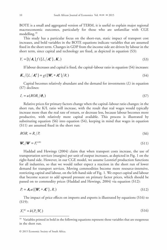
BOTE is a small and aggregated version of TERM, it is useful to explain major regionalmacroeconomic outcomes, particularly for those who are unfamiliar with CGEmodelling.10

This study has a particular focus on the short-run, static impact of transport costincreases, and bold variables in the BOTE equations indicate variables that are assumedfixed in the short term. Changes in GDP from the income side are driven by labour in theshort term, since capital and technology are fixed, as depicted in equation (S3):

Y f Lr r= [ ] { }( )1 A A Kr rL

r, (S3)

If labour decreases and capital is fixed, the capital–labour ratio in equation (S4) increases:

K A W Ar rL

r rLL g Rr r{ } = { }( )∗ (S4)

Capital becomes relatively abundant and the demand for investments (Ir) in equation(S7) declines:

I u RORr r= ( )Jr (S7)

Relative prices for primary factors change when the capital–labour ratio changes: in theshort run, the K/L ratio will increase, with the result that real wages would typicallyincrease more than the real rate of return, or decrease less, because labour becomes moreproductive, with relatively more capital available. This process is illustrated bysubstituting equation (S6) into equation (S4), keeping in mind that wages in equation(S11) are assumed fixed in the short run:

ROR R Pr r r= (S6)

W Wr = ( )FrLR (S11)

Haddad and Hewings (2004) claim that when transport costs increase, the use oftransportation services (margins) per unit of output increases, as depicted in Fig. 1 on theright-hand side. However, in our CGE model, we assume Leontief production functionsfor all industries, so that we would rather expect a reaction in the short run of lowerdemand for transport services. Moving commodities become more resource-intensive,restricting capital and labour, on the left-hand side of Fig. 1. We expect capital and labourthat become scarcer to add upward pressure on primary factor prices, which should bepassed on to commodity prices (Haddad and Hewings, 2004) via equation (S12):

P u Rr r= { }( )∗A W Ar r rL , (S12)

The impact of price effects on imports and exports is illustrated by equations (S16) to(S19):

X b Pr r( )* = ( )Vr (S16)

10 Variables printed in bold in the following equations represent those variables that are exogenousin the short run.



M h P Yr r r( )* ,= ( )P (S17)

M d P Yr r r= ( )P r, ,� (S18)

X s Pr r= ( )P r,� (S19)

We expect that if regional prices increase, the demand for regional tradablecommodities will also increase. Further, we expect regional import volumes for local( Mr

R( )) and foreign ( Mr( )* ) commodities decrease, while their export counterparts

( X rR( )and X r

( )* ) increase (Giesecke and Madden, 2011). Changes in regional import andexport volumes increase regional activity (Yr) through equation (S2).

Price effects of higher composite commodity prices fall on producers, investors as wellas households. Producers experience increased production costs, which in turn reducestheir competitiveness. Investors anticipate lower returns as the cost of producing capitalincreases, and households experience relatively lower real incomes and fewer consumptionpossibilities follow. We expect the lower real incomes to reduce domestic demand and areduction in firm competitiveness to reduce the external demand, which should reduceoverall output in the economy in equation (S2):

Y GRE X M X Mr r r r rR

r= + − + −( )( * * ) ( * )( ) ( ) ( ) (S2)

where GREr is expressed via equation (S1), assuming government expenditure is fixed inthe short run:

GRE C Ir r r= + + +( ) ( )G GrP

rN (S1)

We expect that the reduced output would lower the demand for primary factors insecond and third round price effects that should cause prices of those factors to decline viaequation (S6). In turn, lower primary factor prices should create an accompanyingexpectation that the prices of domestic commodities would also decrease (Haddad andHewings, 2004), via equation (S12). Haddad and Hewings (2004) explain how the effectof second round price changes go in both directions – decreases and increases, wherethe net effect is determined by the relative strength of three major countervailing forces.These countervailing forces include two substitution effects (direct and indirect) andone income effect. The net change in prices will depend on the magnitude of thesecountervailing forces.

3. MODEL SIMULATIONS AND RESULTS

3.1 CGE Database and CalibrationBefore using TERM to model an increase in transport cost, a base or initial solution of themodel is constructed; this process is referred to as calibration. Calibration infers unknownor unobservable parameters and variables from those that are known. A standard modelsolution was implemented in this study: exogenous variables being observable (tastes andtechnological shift variables), and endogenous variables referring to unobservable or



behavioural parameters (genuine data and judgemental priors). Sakamoto (2012) andHorridge (1999) give a list of typical exogenous and endogenous variables that are usedin CGE as well as TERM modelling.

TERM is calibrated using the database, and except for elasticities which are selectedbased on literature, all parameters and exogenous variables are estimated by the databaseand the model’s maximisation conditions. The TERM database starts with the SouthAfrican Reserve Bank’s input–output (IO) tables of 2005. Creating a suitable dataset forTERM’s regional modelling, region and user-defined share estimates were estimated.Region and user-defined share estimates, which indicate each region’s share of nationalactivity for a given user and industry, were required in order to develop a fullinput–output table for each region. These shares include industry shares, industryinvestment shares, household expenditure shares, international export and imports share,and government’s share of consumption. Further, to model the effect of a transport costincrease on industries that use the GFIP and pay E-Tolls, a region and user-defined shareestimate of the cost levied was estimated. A thorough description of the methods used toestimate this share cost is given in Section 2.2.

The main data sources that were used to split industries according to their shareinclude the following: (i) household income and expenditure survey 2005 (STATSSA),(ii) employment data of the Quarterly Employment Statistics (QES) and QuarterlyLabour Force Survey (QLFS) of STATSSA, (iii) Census 2001 data from STATSSA, (iv)regional manufacturing, mining, retail and wholesale production and sales, as well aselectricity data, supplied in various publications of STATSSA, (v) regional demand andsupply totals from the Development Bank, and (vi) import and export demand fromSouth Africa’s Department of Trade and Industry.

Industry technologies do not vary by region when applying regional output shares tothe national dataset. Although the South African TERM model is only applied to 10regions as opposed to the 52 regional TERM model of Australia in Horridge (2011),assuming equal industry technology over regions would therefore not be as crude.

Very little inter-regional trade data are available for South Africa, a problem expressedin McDonald and Punt (2005), similar to the problem in Australia in Horridge (2011).For this reason the same gravity formula was applied to construct trade matrices, similarto Horridge (2011). The gravity formula assumes that trade volumes follow an inversepower distance, which allows constructed trade matrices to align with pre-determinedrow and column totals.11

3.2 Model ResultsAs an initial step in Section 2.2 of this paper, we simulated the size of transport costincreases after the introduction of E-Tolls on all commodities produced and consumed inSouth Africa, by applying the NFFM and CFM data to Google Maps. We then introducethe transport cost increases, which are shown in Table 1, as a series of shocks to TERM;this is done by treating transport cost increases like new transport taxes that were leviedby government. Using TERM in this manner, we are able measure the changes in allprices and quantities of commodities and factors of production. From these results, wewere able to distinguish what the effects were on all provinces, industries and consumergroups.

11 Horridge (2011) raises three points in defence of this assumption to validate its credibility.



Since the Gauteng E-Toll cost forms a very small part of total industry costs in SouthAfrica, the effects of the tolls are almost negligible on macroeconomic variables, such ashousehold consumption (−0.0085%), investment (−0.0404%), exports (0.0009%) andGDP (−0.0102%). However, the signs are significant and insightful. As we expected,regional prices of transported goods increased after transport costs increased as a result oflevying E-Tolls on various industries. This in turn decreased the demand for regionaltradable commodities, as anticipated, leading to a reduction in output caused by thereduction in firm competitiveness.

It is also clear that the drop in total investment is four times as large as the drop inhousehold consumption, and we would like to explain why. As stated above, this study isonly concerned with the short run where changes in GDP from the income side can onlybe driven by labour. If labour decreases and capital is fixed, the capital–labour ratioincreases. Capital becomes relatively abundant and the need for investment declines.Differently put, prices for primary factors change when the capital–labour ratio changes:real wages would typically increase more than the real rate of return (or decrease less)when the ratio increases, because labour becomes more productive, while the price ofcapital would decrease. In the longer term, the capital–labour ratio would then return tosome equilibrium value. The reduction in household and investment demand would alsodecrease imports.

From the initial shock which increased the cost of transportation for industries in eachprovince, the following sectors experienced the largest relative transport cost increases:gold, electrical machinery and apparatus, textiles, clothing and footwear, and radio andTV products. The average transport cost increase for these sectors were 8.75%, 5.25%,4.56% and 3.81%, respectively. Considering each province’s increase in the weightedtotal transportation cost, Limpopo, North-Wes, Gauteng and Mpumalanga had thelargest increases, namely 0.60%, 0.59%, 0.55% and 0.51%, respectively.

Increasing transport costs would put upward pressure on the prices of compositecommodities, especially because there are no substitutes for transport services. Throughsecond and third round price effects, the reduced output would lower the demand forprimary factors, after which their prices would also decline. In turn, this would putdownward pressure on the prices of domestic commodities. The two forces of increasingcosts on the supply side and decreasing demand have different net effects on differentmarkets. Our results show that most commodities experienced price increases, whileprices of some commodities decrease. Those sectors that saw the greatest increase in theirprices are glass and non-metals, metal and machinery, agriculture, and gold. The weightedaverage price increase in each province for each of these sectors was 0.0245%, 0.0149%,0.0092% and 0.0059%, respectively. Industries that experience the greatest declinein output were transport services (−0.051%), metal and machinery (−0.036%), glassand non-metals (−0.027%), construction (−0.026%), and the gold sector (−0.023%),illustrated in Fig. 2.

As an initial step to evaluate the effects of increasing transport costs on industries invarious provinces, we compared the transport cost shock that each province experiencedwith the loss of GDP in that province. After the comparison we weighed the severelyimpacted sectors in each province against their relative share of total output in theprovince, to obtain each severely impacted sector’s contribution towards the loss in GDP.Three provinces stand out from the rest: Mpumalanga, Limpopo and Gauteng, illustratedin Fig. 3. Mpumalanga experienced the largest reduction in GDP (−0.0136%), even



though their total weighted transport cost only increased by 0.51%, the fourth largestamong provinces. The main reasons for Mpumalanga’s relatively large reduction in GDPis that the industries that were most severely hit by transport cost increases represent23.5% of provincial output – the second largest among the provinces. Moreover, thedecline in GDP from these sectors contributed 99% of the loss in Mpumalanga’s GDP(the largest contribution among provinces). Similarly, Gauteng experienced the thirdlargest total weighted increase in transport cost (0.55%), but the second largest decline inGDP (−0.0117%). Limpopo’s decline in GDP was only the fourth largest (−0.0101%),although the weighted increase in transport cost was the largest (0.60%). Severely hitsectors contribute a large share of total output in Limpopo, namely 96%.

(i) The Point of Impact of the Shock: Transport Services Our shock was directly applied totransport services, increasing the cost of these services across all regions. An increase in therelative price of transport services reduced the demand for these services, which finallylead to a consistent reduction in output of transport services.

Except for the direct application of the shock, second round price effects furtherreduced the demand for transport services. This is caused by an increase in the cost foreach unit of production, which reduces real income. Households that use the largest shareof transport services (21.16%) experienced a reduction in real income (income effect),

0.06%

0.05%

0.04%

0.03%

0.02%

–

–

–

–

–

–

0.01%

0.00%

Figure 2. Short-term change in industry output

–

–

–

–

–

–

–0.014%

0.013%

0.012%

0.011%

0.010%

0.009%

0.008%NC NW LP FS GP MP

Figure 3. Short-term change in provincial GDP



which in turn reduced their demand for transport services (substitution effect). Overall,firms that are less competitive after a transport cost increase produce less, which furtherreduces the demand for transport services that facilitate the flow of commodities.

The greatest share of transport services is sourced from the region they are producedin; on average each province consumes 80.6% of transport services that are produced inthe originating province. From the direct cost increase and the nature of consumingtransport services in the originating province, all provinces saw a consistent decrease indemand for transport services. Those provinces with a smaller decrease of transportservices were aided by relatively smaller price increases (or large price decreases) oftransport services; these provinces in turn saw an increase in the export of transportservices to those provinces with higher price increases (or small price decreases).

Mpumalanga saw the largest decrease in prices of transport services (−0.0288%) andhence the greatest export of these services to other provinces like the Free State andLimpopo. However, exporting transport services is limited due to the nature of theseservices; to a certain extent the cost of transport services increase as the distance increases.As an example, given that the cost of transporting precious metals in Limpopo increasedsubstantially, a company in Limpopo considers importing transport services fromMpumalanga. However, the company in Limpopo would have to pay the Mpumalanga-based company the costs of moving transport services (trucks) from Mpumalanga toLimpopo, even before the actual service has been delivered, a very costly exercise. For thisreason exports of transport services in Mpumalanga only increased by 0.0922% and wereonly 7.58% higher than the second largest exporter, namely North-West.

(ii) More Industry Results

(a) Metals and machinery (metalmach)If one looks at the five industries that were affected the most in each of the nine provinces,you will find that metalmach is listed as one of the five in seven of the provinces. It is theindustry affected the most after the transport services industry, where we applied theshock.

There are a few reasons why this industry is hit so hard. The direct impact of the shockis one important reason: of the 27 industries in our CGE model, it is the seventh largestuser of transport services in South Africa: it makes up 6.4% of the industry’s intermediateinputs. The secondary reasons are twofold, and the first is directly related to the impactof the shock. According to our modelling results, almost half (49.2%) of the decrease inmetalmach output is due to a decrease in its exports. Metalmach is an importantexporting industry in South Africa, producing no less than 15.9% of our total exports.This is our second largest exporter after the other mining industry, which exports 16.8%of the total. The increased transportation costs make our industries less competitive in theworld market, and they lose some of their market share. Another 11.3% of the drop inmetalmach output comes from reverse import substitution: what used to be demanded bylocal consumers of metalmach is now replaced by cheaper imports. This means that60.5% of the decrease in this industry’s production is because of a drop in theircompetitiveness in the world market.

The remaining 39.5% of the decrease in metalmach output comes from direct decreasein local demand. The dominating force here is the decrease in total national investmentin the short run. Metalmach is an important input into all investment demand: it makes



up 28.3% of total national investment demand, and with investment demand decreasingseverely, as explained below, the effect on metalmach is as severe.

(b) ConstructionThe fourth largest hit industry as a result of the transportation shock is construction.(Glassnonmet is the third largest but we discuss that in the next section, for reasons thatwill become clear soon.) A decline in the production of construction goods can best beexplained by the relatively large decline in investment demand, discussed above.Construction goods make up 51.4% of total investors demand, used as inputs in theproduction of investment goods. It follows that a substantial decrease in investmentwould decrease the demand for and output of construction goods. The decline in theconstruction sector is further explained by the inputs that are used in production of thoseconstruction goods and services: construction (30%), glass and non-metals (15%), metalsand machinery (12%), and electrical machinery and apparatus (9%). The glass andnon-metals, metal and machinery, as well as the electrical machinery and apparatussectors, experienced the greatest increase in prices. Higher prices in these sectors weigheddown on the production capabilities of the construction sector (increasing the cost ofproducing each unit), which in turn reduced their demand for those commodities.

(c) Glass and non-metals (glassnonmet)The third hardest hit industry was glassnonmet, in terms of output decreases. It is a bitharder to explain than metalmach, because it is neither an important input into theproduction of investment goods, nor an important export commodity. However, onethird of its decline could be explained by the industry becoming less competitive in theworld markets. Although it is a small exporter in comparison to other industries – it onlyexports 0.55% of the total – the drop in exports of glassnonmet causes 24.2% of its totaldecrease in production. A further 8.2% is caused by reverse import replacement, bringingthe total to 32.4% caused by lower international competitiveness. The remaining 67.6%of the decrease came as a result of direct decreases in local demand for the product. Whoare these buyers of glassnonmet that decreased their demand for it? The answer is thatthere is only one large buyer of glassnonmet, and that is the construction industry, whichbuys 45.4% of its total output. We saw above that the construction industry was itselfseverely hit by the transport cost shock so that when its output decreased, it would alsohave a domino effect on all its suppliers, of which glassnonmet is the most prominent one.

(d) GoldTransport costs in the gold industry increased significantly as a result of the E-Toll levies.Overall, these transport cost increases were relatively large compared with othercommodities, which, as we have discerned from our data, stems from the nature oftransporting precious metals. Precious metals are very rarely transported in tonnes likeother commodities; this increased the number of travelled routes required to facilitate thetrade of precious metals. More routes in turn increased the usage of the GFIP whereE-Tolls were levied. Also, transporting commodities in such small amounts decreased thetotal cost of transporting gold, relative to other industries, which in turn increased therelative size of the shock (refer to Section 2.2).

The output decrease in the gold industry was therefore the fifth largest reduction of allindustries nationwide. Relatively large increases in transport costs increased the cost of



producing gold and therefore reduced output in the provinces that are gold producers. Inour application of TERM, we have assumed that all unrefined gold is exported, and it isexactly the decrease in gold exports that caused the drop in production. Our model (anddatabase) shows that 100% of the decrease in gold production was caused by the decreasein gold exports. The transport cost increases made our gold industry less competitive inthe world market and caused a decrease in world demand for our gold. Unlike the otherindustries discussed above, the gold industry is very labour-intensive, and with labourbeing the only variable factor in the short run the industry responds heavily by sheddinglabour and producing less.

(iii) Macroeconomic Results One usually discusses the macroeconomic results of a CGEsimulation exercise before the industry results, but since the shock applied to the modelin this case was an increase in the transportation costs of all industries, we treated theindustry results first. In this case the five industries’ decreased production is driving themacroeconomic results to a large extent. The only exception is construction, which fallsas a direct result of the short-run closure that we adopt.

At the macroeconomic level, total investment decreases significantly as a result of ourassumption that capital is fixed in the short run, while only labour can change. Thedecrease in demand for South African goods that are now more costly to produce causesa decrease in the demand for labour, while capital stays constant. Capital becomesrelatively more abundant than labour, and the real rate of capital therefore decreases,which causes a decrease in investment demand. In brief, capital is abundant so we do notneed more investment.

The only significant other macroeconomic variable is exports, and we have shown thatour most important export commodities are all affected severely negative with the increasein transport costs. Depending on the assumption made about the increases in transportcosts on exported goods, the effect on exports could be a bit smaller or larger, but overallwe can conclude that the increases in transport costs would be detrimental to SouthAfrican exports.

None of the affected goods are consumed by households so we see a very tiny decreasein household total demand. In the initial simulation, we did not let households pay theE-Tolls, but they were only indirectly affected through higher purchasers’ prices ofcommodities. We assumed that the government would keep its spending constant in realterms.

4. CONCLUSION AND FURTHER RESEARCH

This study evaluated the short-term economic impact of a direct transport cost increaseon industries after the introduction of E-Tolls; however, when externalities in the groupof systematic logistical costs are taken into account, transport costs might be even higherthan our initial estimates (Havenga, 2015). Future research can include the relationshipbetween transport and logistics costs expressed in Havenga and Simpson (2014), keepingin mind that transport is a system within a larger logistics system that can be costed at themacroeconomic level (Havenga, 2010).

Through the causal relationship explained via a BOTE representation of the economyin Section 2.4, higher transport costs increased commodity prices and finally decreasedoutput in the economy. Commodity prices increased as a result of first round price effects.



The net effect of second and third round price effects was determined by the substitutionand income effects. Households experience a reduction in real incomes, and fewerconsumption possibilities follow (Haddad and Hewings, 2004). Producers experienced anincrease in their production costs when the cost of transporting commodities increased perunit of output, and a reduction in their competitiveness followed. We continued to explainthat a reduction in competitiveness and higher prices causes a reverse import substitution:what used to be demanded by local consumers is now replaced by cheaper imports. Thisreduction in competitiveness and the negative impact of reverse import substitution wasevident in all the severely impacted industries: transport services, metal and machinery,glass and non-metals, construction, and the gold sector. The total decline in these sectorswere −0.051%, −0.036%, −0.027%, −0.026% and −0.023%, respectively.

GDP decreased by the greatest amount in Mpumalanga (−0.014%), Gauteng(−0.012%), Free State and Limpopo (−0.010%). What is interesting is thatMpumalanga’s reduction in GDP is 17% greater than that of Gauteng, and 31% greaterthan Limpopo and the Free State. We found that provinces that are closer to Gautengmake more frequent use of the GFIP than other provinces; these provinces experiencerelatively larger transport cost increases and hence larger GDP reductions. Apart fromeach province’s use of the GFIP, another major reason for the relative size in regionalGDP reductions originates from the share of severely hit industries in each province.

We conclude that the overall economic impact on household consumption, exports,imports and GDP is relatively small. Aggregate prices declined by 0.1%, which is quitesmall when considering how broad the increase in prices were; we found that mostindustries in each province experienced transport cost increases. Further, aggregateemployment decreased with 0.2%, which is relatively small when considering broad costincreases and the current high unemployment level of 25.4% in South Africa (StatisticsSouth Africa, 2014). From our research, we conclude that the increase in transport costsas a result of levying E-Tolls is relatively small in comparison to the total transport costof physically moving commodities; this is the largest contributing factor to marginalchanges in main macro variables. Compared with changes in other main macro variables,investments decreased by a relatively large amount namely −0.04%, but even here twoimportant factors have to be taken into consideration. First, in our short-term focus, weassumed that transport cost increases are driven through labour adjustments and capitalwas assumed fixed. Later research can evaluate the longer term and even dynamic impactof increasing industries’ transport costs. Second, this study did not take into account theinitial investment of the GFIP, R19.5 billion, as our focus was rather on measuring theshort-term impact of increasing industries’ transport costs.

Although it was not part of our initial research, we have also estimated the changes inindirect costs or benefits on industries and consumers.12 Simulating our initial direct costson industries with the technological advancement brought on by the GFIP, and includingthe direct and indirect costs and benefits to the consumer, a more complete impact on theeconomy can be evaluated. However, there are two major shortcomings that can beovercome in further research. First, we are only evaluating the short-term impact wheretechnology is assumed fixed; a better approach would be to simulate these shocks in thelong term. Second, the current TERM model is static and does not allow shocks to impactone another in a dynamic manner as time progresses. These shortcomings can partially be

12 These findings are available upon request from the author.



overcome by running two separate simulations: a short-term simulation for changes incosts and a longer term simulation for changes in technology that incorporates short-termchanges. However, the lack of dynamics would still not be bridged. Once again our focusis rather on evaluating the short-term impact of transport cost changes. Taking this intoconsideration, the short-term impact of direct and indirect costs and benefits to industriesas well as consumers, after the GFIP was introduced and E-Tolls were levied, wassimulated. The following changes in main macro variables occurred: CPI decreased with0.12% and aggregate employment increased with 0.5%. Other macro variables includehousehold consumption (0.0505%), investments (0.0158%), exports (−0.0174%),imports (0.0215%) and GDP (0.0228%).

Finally, we can conclude that the short-term impact of increasing industries’ transportcosts, as a result of levying E-Tolls, has a marginally negative impact on economicaggregates. However, when considering a more complete set of direct as well as indirectcosts and benefits, the economic impact in the short term is positive, but still rather muted.

REFERENCES

BRÖCKER, J. A. K. and CARSTEN, S. (2010). Assessing spatial equity and efficiency impacts of transport infrastructureprojects. Transportation Research Part B: Methodological, 44(7): 795-811.DAS, G. G., ALAVALAPATI, J. R. R., CARTER, D. and TSIGAS, M. E. (2005). Regional impacts of environmentalregulations and technical change in the US forestry sector: A multiregional CGE analysis. Forrest Policy and Economics, 7(1):25-38.DE JONG, G., GUNN, H. and WALKER, W. (2004). National and international freight transport models: An overviewand ideas for future development. Transport Reviews, 24(1): 103-124.DEPARTMENT OF TRANSPORT. (2011). Gauteng Freeway Improvement Project Steering Committee Report.DIXON, P., PARMENTER, B., SUTTON, J. and VINCENT, D. (1982). ORANI: A Multisectoral Model of the AustralianEconomy. North-Holland, Amsterdam.DOMINGUES, E. P., HADDAD, E. A. and HEWINGS, G. J. D. (2003). Sensitivity Analysis in Applied GeneralEquilibrium Models: An Empirical Assessment for MERCOSUR Free Trade Areas Agreements. University of Illinois (Urbana).DONAGHY, K. P. (2009). CGE modeling in space: A survey. In Capello R. and Nijkamp P. (eds), Handbook of RegionalGrowth and Development Theories. Cheltenham: Edward Elgar, 389-422.ECONOMISTS.CO.ZA. (2011). Consumer impact of the Gauteng Freeway Improvement Program.GAUTENG PROVINCIAL GOVERNMENT. (2014). Socio-economic Impact Gauteng Freeway Improvement Projectand E-tolls. Available at: http://www.gautengonline.gov.za/Campaign%20Documents/E-%20Toll%20Report.pdf[Accessed: 20 April 2015].GIESECKE, J. A. and MADDEN, J. R. (2011). Interregional Dispersion of Impacts from Regional Economic Shocks: A CGEExplanation. Paper presented to the 19th Annual Ingernational Input-Output Conference, Alexandria VA, Centre of PolicyStudies, Monash University.GLYN, W. and HORRIDGE, M. (2007). CGE Modelling of the Resources Boom in Indonesia and Australia Using TERM.Quenstown, New Zealand.HADDAD, E. A. and HEWINGS, G. J. D. (2004). Transportation Costs, Increasing Returns and Regional Growth: AnInterregional CGE Analysis, Department of Economics, University of Brasilia, Working Paper 315.HAVENGA, J. (2007). The Development and Application of a Freight Transport Flow Model for South Africa. PhDDissertation, p. 255, Stellenbosch University.——— (2010). Logistics costs in South Africa – The case for macroeconomic measurement. South African Journal ofEconomics, 78(4): 460-478.——— (2013). The importance of dissaggregated freight flow forecasts to inform transport infrastructure investments.Journal of Transport and Supply Chain Management, 7(1): 1-7.——— (2015). Macro-logistics and externality cost trends in South Africa – Underscoring the sustainability imperative.International Journal of Logistics Research and Applications: A Leading Journal of Supply Chain Management, 18(2): 118-139.——— and PIENAAR, W. J. (2012). The creation and application of a national freight flow model for South Africa.Journal of the South African Institution of Civil Engineering, 54(1): 2-13.——— and SIMPSON, Z. (2014). Reducing national freight logistics costs risk in a high-oil-price evironment: A SouthAfrican case study. The International Journal of Logistics Management, 25(1): 35-53.HORRIDGE, M. J. (1999). A General Equilibrium Model of Australia’s Premier City. Centre of Policy Studies, PreliminaryWorking Paper, Volume 74, pp. 1-19.HORRIDGE, M. (2003). ORANI-G: A generic Single-Country Computable General Equilibrium Model. Centre of PolicyStudies and Impact Project, Monash University, Australia, pp. 1-83.



http://www.gautengonline.gov.za/Campaign%20Documents/E-%20Toll%20Report.pdf

——— (2011). The TERM model and its data base. Centre of Policy Studies and the Impact Project General Paper, G-219:1-21.———, MADDEN, J. and WITTWER, G. (2005). The impact of the 2002-2003 drought on Australia. Journal of PolicyModelling, 27(3): 285-308.——— and WITTWER, G. (2008). SinoTERM, a multi-regional CGE model of China. China Economic Review, 19(4):628-634.ISHIGURO, K. and INAMURA, H. (2005). Identification and elimination of barriers in the operations and managementof maritime transportation. Research in Transportation Economics, 13: 337-368.LATORRE, M. C., OSCAR, B.-R. and ANTONIO, G. G.-P. (2009). The effects of multinationals on host economics:A CGE approach. Economic Modelling, 26(5): 851-864.LI, N., SHI, M. and WANG, F. (2009). Roles of regional differences and linkages on Chinese regional policy effect in CGEanalysis. Systems Engineering – Theory & Practice, 29(10): 35-44.LOFGREN, H., REBECCA, L. H. and SHERMAN, R. (2002). A Standard Computable General Equilibrium (CGE)Model in GAMS. International Food Policy Research Institute: 2033 K Street, N.W., Washington, D.C., 20006-1002,U.S.A.MCDONALD, S. and PUNT, C. (2005). General equilibrium modelling in South Africa: What the future holds. Agrekon,44(1): 60-98.PIENAAR, P. A. (2011). Gauteng Toll Roads: An Overview of Issues and Perspectives. Pretoria, South Africa, s.n., pp.697-710.ROAD FREIGHT ASSOCIATION. (2013). Vehicle cost schedule, A Road Freight Association Publication, Edition 48,October. Available at: http://www.rfa.co.za/rfa/index.php?option=com_content&view=article&id=7&Itemid=101.SAKAMOTO, H. (2012). CGE analysis of transportation cost and regional economy: East Asia and Northern Kyushu.Regional Science Inquiry Journal, IV(1): 121-140.STANDISH, B., BOTING, A. and MARSAY, A. (2010). An Economic Analysis of the Gauteng Freeway ImprovementScheme, Graduate School of Business, University of Cape Town, Strategic Economic Solutions, and Arup Consulting.Prepared for Provincial Government of Gauteng & SANRAL: Cape Town, South Africa.STATISTICS SOUTH AFRICA. (2014). Quarterly Labour Force Survey. Quarter 3. Available at: http://www.statssa.gov.za/?page_id=1854&PPN=P0211&SCH=5935STEININGER, K. W., FRIEDL, B. and GEBETSROITHER, B. (2006). Sustainability impacts of car road pricing: Acomputable general equilibrium analysis for Austria. Ecological Economics, 63(1): 59-69.UEDA, T., KOIKE, A., YAMAGUCHI, K. and TSUCHIYA, K. (2005). Spatial benefit incidence analysis of airportcapacity expansions: Application of SCGE model to the Haneda Project. Research in Transportation Economics, 13:165-196.WITTWER, G. (2003). An outline of TERM and Modifications to Include Water Usage in the Murray-Darling Basin.Victoria: Centre of Policy Studies.——— and HORRIDGE, M. (2010). Bringing regional detail to a CGE model using census data. Spatial EconomicAnalysis, 5(2): 229-255.

APPENDIX

An Adoption of Stylised BOTE (Giesecke and Madden, 2011)

Short-run closure Equation

GRE C I G Gr r r rP

rN= + + +( ) ( ) (S1)

Y GRE X M X Mr r r r rR

r= + − + −( )( * * ) ( * )( ) ( ) ( ) (S2)Y f Lr r= [ ] { }( )1 A A Kr r

Lr, (S3)

K W Ar r rLL A g Rr r

Lr{ } = ∗{ }( ) (S4)

Lr = Qr * PRr * ERr (S5)ROR R Pr r r= (S6)I u RORr r= ( )Jr (S7)Ir rK r = Ψ (S8)W Wr = ( )Fr

LR (S9)P A u Rr r r= ∗{ }( )W Ar r

L , (S10)Cr = APCr * [Yr −NFLr * R] (S11)G Cr

Pr

( ) ( )= wrP (S12)

GrN( ) ( )=Qr r

Nw (S13)X b Pr r

( )* = ( )Vr (S14)M h P Yr r r

( )* ,= ( )P (S15)M d P Yr r r r= ( )P , ,� (S16)X s Pr r r= ( )P ,� (S17)

W t E tp p( )

( )−{ } =

−( )

−( )−{ } +

( )

( )−{ }W t

W tW t E tf

p

f f1 1 1

1

1α (S18)



http://www.rfa.co.za/rfa/index.php?option=com_content&view=article&id=7&Itemid=101

http://www.statssa.gov.za/?page_id=1854&PPN=P0211&SCH=5935

http://www.statssa.gov.za/?page_id=1854&PPN=P0211&SCH=5935

The Short-Term Economic Impact of Levying E-Tolls on Industries

Documents

Transcript of The Short-Term Economic Impact of Levying E-Tolls on Industries