MPRAMunich Personal RePEc Archive

The regional economic structure of Brazilin 1959: an overview based on aninter-State input-output system

Gustavo Barros and Joaquim Jose Martins Guilhoto

University of Sao Paulo

2011

Online at http://mpra.ub.uni-muenchen.de/37698/MPRA Paper No. 37698, posted 27. March 2012 23:30 UTC

1

The Regional Economic Structure of Brazil in 1959: an Overview

Based on an Interstate Input-Output Matrix

Gustavo Barros PhD in Economics, FEA-USP

CNPq Scholar

Department of Economics, School of Economics, Business and Accounting (FEA-USP),

University of São Paulo

E-mail: gb@usp.br

Joaquim José Martins Guilhoto Professor of the Department of Economics, FEA - USP

Researcher of REAL, University of Illinois

CNPq Scholar

(corresponding author)

Department of Economics, School of Economics, Business and Accounting (FEA-USP), University of São

Paulo, Av. Prof. Luciano Gualberto, 908, FEA II, 2nd

floor, 05508-900, Cidade Universitária, São Paulo - SP,

Brazil

E-mail: guilhoto@usp.br

Tel: +55 (11) 3091-5870

Fax: +55 (11) 3813-4743

2

The Regional Economic Structure of Brazil in 1959: an Overview

Based on an Interstate Input-Output Matrix

Abstract

This paper aims to describe the regional configuration of Brazil’s productive

structure in 1959, a crucial moment in the Brazilian industrialization process,

through the estimation of an interstate input-output matrix. The estimated matrix

is the oldest of its kind for Brazil and is made available to other researchers.

Hence, it can be an important tool for the study of the regional productive

structure at a historical moment in which the regional question appeared as a

central national issue. In this paper we describe estimation procedures and data

sources, and present some general characterization of the regional structure of the

economy in 1959 through selected structural indicators.

Key words: regional productive structure, Brazil, input-output analysis, import

substitution industrialization, economic development

JEL Classification: N66, N76, O18, O54, D57

Highlights:

A new perspective on Brazil’s regional economic structure at a key historical

juncture

An estimation of the oldest interstate input-output matrix for Brazil

The estimated matrix made available to other researchers through this paper

3

1. Introduction

During the worldwide economic crisis in the 1930s, Brazil, whose coffee exports made

up the dynamic sector of its economy, also faced harsh difficulties. The crisis in Brazil was

not severer due to a series of political and economic measures taken by the government,

which resulted in the stabilization of the level of aggregate demand and in increased

regulation of the foreign sector. In a certain sense, one can say that the Brazilian government

was Keynesian before there was a Keynesian theory. Given the dimension and duration of the

crisis, alongside these government stabilization policies, the Brazilian economy effected a

displacement of its dynamic center toward its internal market.1 The main expression of this

displacement was a process of industrialization, which led the industrial sector to grow at

annual real rates of above 10% in the period 1933-39 [2].

In the 1940s the intervention of the state in the economy was relatively more intense

during the war period but thereafter decreased until the beginning of the 1950s. During the

Second World War, the Brazilian government engaged in the building of the necessary

infrastructure for the development of the industrial sector. The creation of the Companhia

Siderúrgica Nacional (National Steel Company) in 1941, controlled and managed by the

federal government, and the construction of the Volta Redonda steel mill are the most

eloquent examples of this development. Nevertheless, between 1942 and 1943, an American

Mission – the Cooke Mission – visited Brazil with the aim of evaluating the possibilities of

the Brazilian economy to participate in the war effort. Regarding state intervention in the

economy, the Mission’s recommendations were that “[t]he task of industrialization [...]

should be left to the private sector, while the government should concentrate on general

1 For a good presentation of the intervention of the Brazilian government in the economy in the 1930's and its

effects see [1].

4

industrial planning, developing industrial credit facilities, and providing technical education”

[3: 42].

Accordingly, the decrease in the role of the state in the economy during the second half

of the 1940s was linked to the fall of the Vargas dictatorship in 1945, with the corresponding

regime change into a democratic political system, which was then associated with the idea of

less intervention of the government in the economy. Despite this, the state presented a five-

year expenditure program, the SALTE plan, which was directed to the areas of health, food,

transport, and energy. Still, this plan remained in effect only during one year due to its

overoptimistic estimation about the possibilities of revenues to allow its execution.

In the 1950s the participation of the state in the economy regained impetus, first with

the second Vargas government (1951-54) and then with the Kubitschek government (1956-

60). Despite the fact that both governments participated strongly in the economy, the focus of

their respective programs were different. The Vargas’ policies were directed toward the

creation of a national capitalist system, while Kubitschek’s policies were directed toward the

integration of the Brazilian economy into the international economy.

From 1951 to 1953, the Joint Brazil-United States Economic Commission was formed.

One of its main contributions to the Brazilian economy was the creation of the BNDE

(National Bank for Economic Development), an institution aimed at financing long-term

economic projects. This institution was to be of crucial importance in the development of the

industrial sector in Brazil. At the same time, it contributed to the increasing participation of

the state in the economy. As some of the loans granted by the BNDE were not paid, the Bank

eventually took over the debtor enterprises, thus making the government, indirectly, the

owner of those enterprises. The BNDE was also a central institution in the implementation of

the economic plans that followed its creation.

5

Besides the BNDE, a series of other state enterprises was created during the second

Vargas government, such as the PETROBRAS (the state company linked with oil production,

refinery, distribution, etc.), the Banco do Nordeste do Brasil (Northeast Bank of Brazil), etc.

The first economy-wide large-scale economic plan that reached execution in Brazil was

the Programa de Metas (Target Plan), prepared and executed during the Kubitschek

government between 1956 and 1960. The basic idea of the plan was the development of an

industrial complex through the implementation of an Import Substitution Industrialization

(lSI) policy, with the automotive industry as the leading sector. Besides the industrialization

aspect, the plan also had as an objective the construction of a new capital city (Brasília),

which in turn had, among other goals, the objective of promoting national integration.

The above-mentioned government policies did settle the ground for the Brazilian

economy’s regional productive structure in 1959. With this in sight, this paper aims to

describe the regional configuration of the 1959 Brazilian productive structure through the

estimation of an interstate input-output matrix for that base year at the level of 25 states and

33 sectors. Our estimation was based on the national matrix for 1959 prepared by van

Rijckeghem [4] and was supplemented with data obtained from several sources, including the

economic census of 1960. We employed various estimation techniques, such as simple and

inter-industry locational quotients.

Rijckeghem’s matrix for 1959 is the oldest input-output matrix available for Brazil, and

our estimation is thus the oldest interstate matrix for the country. Hence, it can be an

important tool for the study of the regional productive structure at a historical moment in

6

which the regional question appeared as a central national issue.2 The estimated matrix is

available on request to the authors.

In the next section we describe the estimation procedure and data sources used in this

study. In the third section we present an overview of the productive structure of the Brazilian

economy at the state level in 1959. In the last section, some final comments are made.

2. Data Sources and Estimation Procedures

Considering that a relevant objective of this paper is to make public and available the

estimated interstate input-output matrix for Brazil, it is important to describe the estimation

procedures and data sources in some detail so that other researchers using this database for

their own analyses will be able to assess by themselves its limitations and possibilities.

Our starting point has been Rijckeghem’s national input-output table for 1959 [4, 7].3

Rijckeghem considered the estimation of the national matrix he published in 1967 as

“preliminary” due to the absence of part of the results of the 1960 censuses (base year 1959)

which at that time were yet to be published. He had access to the results of the Industry,

Commerce and Service Censuses, but the Agricultural and Demographic Censuses were still

unpublished when he prepared his estimates. Besides, none of the censuses included

“transportation and communication, construction, electric energy, water and sanitary services,

financial services, medical services, domestic services, and education”. To supply for this

lack of direct information, affecting mainly the nonindustrial sectors, Rijckeghem made use

2 For an example of the use of input-output analyses to historical problems with a regional perspective, see [5].

However, the estimated Input-Output table could subsidize not only other input-output analyses. It is also a

fundamental database for approaches relying on computable general equilibrium models, such as the ones

advocated by [6] to be employed in Economic History. 3 For a contemporary comment on the Rijckeghem’s input-output table see [8].

7

of secondary statistical data. We are, however, unaware of any later revision of this

“preliminary” estimate. Additionally, Rijckeghem resorted to three “fictitious” sectors –

namely, Wastes, Fuels, and Packaging – in order to “profit from the way the cost structure of

industrial enterprises were presented”, making the matrix sectoral structure less than typical.4

These shortcomings of Rijckeghem’s 1967 estimate, many of which he himself

recognized, are inevitably carried over to our own estimate of the interstate matrix, once it is

based on his national matrix. Still, the best information that he had available, and also the

best information that we were able to collect for our regional disaggregation, was that

pertaining to the industrial sectors and their interrelations which constitute the main focus of

many input-output analyses. Moreover, of the 32 sectors of his input-output table, 22 were

covered by the Industrial Census, thus providing a reasonably sound basis for a set of

analyses of some relevant historical questions traditionally addressed regarding this period.

Starting from Rijckeghem’s table and then adding new information and some

hypotheses, we performed two disaggregating steps: a) the original metallurgical sector was

divided into two subsectors in the national matrix, the first covering iron and steel metallurgy

and the second all other metallurgical production, in order to obtain more detail about this

specific sector, thus resulting in a 33-sector national matrix; b) this 33-sector national matrix

was then disaggregated into an Inter-State matrix with 25 states.

In order to disaggregate the metallurgical sector in Rijckeghem’s original matrix into

the “Metallurgical (iron and steel)” and “Metallurgical (other)” sectors, we used the

coefficients for these sectors from a 1970 national input-output matrix for Brazil. The precise

hypotheses involved can be stated as: a) the proportion of internal production, destined for

4 A reasonably detailed account of the procedures he adopted can be found in [4], from where this paragraph’s

quotes were taken (pp. 1-4). The table, but not the description of procedures, was published in [7].

8

each of the other sectors and for final demand, of the “metallurgical (iron and steel)” sector

relative to the “metallurgical (other)” sector within the total metallurgical sector is the same

in 1959 as in 1970; b) the proportion of input consumption, provided by each of the other

sectors and by value added entries, of the “metallurgical (iron and steel)” sector relative to the

“metallurgical (other)” sector within the total metallurgical sector is the same in 1959 as in

1970. We could thus ensure that the 33-sector matrix can be reaggregated back exactly into

the original 32-sector matrix.

The 1970 matrix’s coefficients were the best information available for the purpose at

hand. The censuses of 1960 as they were published do not allow one to recover the necessary

information given that the metallurgical sector was reported aggregated in the Industrial

Census. Moreover, we judged the information of the 1970 matrix to be of better quality, not

only in but also in level of detail, relative to the other pertinent secondary sources for 1959

that we were able to find. It is true that both the iron and steel sector and the other

metallurgical sector changed significantly from 1959 to 1970. However, the soundness of our

hypothesis does not rely on their immutability but on a certain degree of similarity in the

development of each subsector of the metallurgical total, which is much more tenable. We

can thus expect our hypothesis to produce a reasonable approximation – in any case, as good

as we were able to achieve – of the desired ideal of direct information.

The estimation of the interstate matrix, based on the national matrix we just described,

required much additional data, which were found and provided in various degrees of quality.

The following sources were used, in this order of priority: 1st) the censuses of 1960,

especially the Industrial and the Commerce and Services Censuses [9, 10, 11, 12, 13]; 2nd

) the

national accounts [14] or the Statistical Year-Book of 1961 [15]; and 3rd

) estimates based on

proxies from the censuses, the Statistical Year-Book or the national accounts.

9

Basically, what was needed for the estimation was information on: a) the distribution

by state of the (origin of) production for each sector (1); b) the distribution by state of the

(origin of) value added, including gross returns to capital (2), and wages, salaries, and social

security (3); and c) the distribution by state of the (destination of) final demand, including

households’ consumption (4), government consumption (5), investment (6), exports (7), and

imports (8). This information was compiled from the above-mentioned sources and organized

in a set of eight matrices in the form Sector by State. A minute description of the data sources

and hypotheses for the necessary estimates is provided in the Appendix. Still, some general

comments about it are due here. It is important to note that the regional information on the 23

industrial sectors is judged to be of very good quality. It was almost entirely taken from the

Industrial Census – the distribution of production by state was entirely so, value added was

mostly so, final demand was not. This is not only the same source as that of Rijckeghem’s

national matrix but also the best information source we could desire. The source used for the

primary sectors (1 and 2) was the same one Rijckeghem used, the national accounts; hence a

good degree of consistency with the national matrix was assured. The distribution of

production by state of the remaining sectors relied, partly or totally, on estimates. In several

of them – electric energy, services, residuals, fuels, packaging, and transportation – a specific

kind of hypothesis was necessary, which deserves mention. The estimates of origin of

production by state of each of these sectors were made based on information on expenditures

by state in these sectors. Formally, this is an accounting mistake. Here it can be thought of as

implying an implicit hypothesis, namely, we are supposing these sectors to exhibit a high

degree of non-tradability between states. In other words, the less tradable these sectors are,

the better our estimates will be. This hypothesis is reasonably good for most of the concerned

sectors and not that good for some of them – fuels and electric energy being the worst cases,

10

we believe. Hence, due care should be taken in analyses of regional emphasis for these

sectors based on our estimates. The procedures adopted imply an underestimation of the

regional interaction for these sectors. Origin of value added and destination of final demand

by state were also estimated. The estimates of value added for the industrial sectors were

based on consistent primary data from the Industrial Census. The value added for the

remaining sectors and the final demand by state were estimated based on secondary data. The

quality of the results along the estimated interstate matrix should vary according to these

different types of information sources that we used.

With this set of eight matrices in the form 33 sectors by 25 states and the national

matrix with 33 sectors in hand, we then proceeded with the estimation of the inter-state

matrix. Regional coefficients ( RR

ija ) were estimated as proportions of the correspondent

national technical coefficients calculated from the national matrix: N

j

N

ij

N

ij Xza , were N

ijz is

the (national) flow of input from sector i used by sector j to produce its total (national) output

N

jX . For this purpose we used cross-industry location quotients for the intermediary

consumption part of the matrix and simple location quotients for most of the final demand

part of the matrix.5

We have adopted cross-industry location quotients to estimate the intermediary

consumption part of the matrix because this affords greater flexibility by allowing us to

calculate a different coefficient for each cell of the regional matrix. Cross-industry quotients

were thus defined:

N

j

R

j

N

i

R

iR

ijXX

XXCIQ ,

5 For definitions and a discussion on different alternatives for regionalizing coefficients see [16: 349-59].

11

where R

iX and R

jX are the output of sectors i and j, respectively, in region R (states),

and N

iX and N

jX are the outputs of the same sectors at the national level. The (intra)regional

coefficients were then estimated according to the cross-industry quotients:

1 if

1 if )(R

ij

N

ij

R

ij

R

ij

N

ijRR

ijCIQa

CIQCIQaa

The cross-industry quotient measures the region’s share in the national production of

the input sector (i) relative to the region’s share in the national production of the output sector

(j). The idea behind this procedure is that if the region’s share in the input sector is larger

than the region’s share in the output sector, that is, if 1R

ijCIQ , then all the needs of input i

for the production of output j in region R can be supplied from within the region. Conversely,

if 1R

ijCIQ , a part of the input i for the production of output j in region R will have to be

“imported” from other regions. The interregional coefficients were then estimated on the

basis of the market shares of the remaining regions in the input sector:

R

i

N

i

L

iRR

ij

N

ij

LR

ijXX

Xaaa

. ,

where L

iX is the output of sector i in region L, and the remaining variables are defined

as above. An intermediate consumption matrix in the form Sector by State was calculated

from the basic set of Sector-by-State matrices (intermediate consumption = output – gross

returns to capital – salaries, wages, and social security). This matrix was then used to

calculate an interstate intermediate consumption flow matrix, distributing each of the Sector-

by-State matrix’s cells proportionately to the corresponding column of regional coefficients.

The estimation of the regional distribution of household consumption, government

consumption, and investment in the final demand part of the matrix was made using simple

12

location quotients, defined as:

NN

i

RR

iR

iXX

XXLQ ,

where RX is the total production of region R, NX is the total national production, and

the remaining variables are defined as above. The estimation of intra- and interregional

coefficients was then made for these final demand items with these simple location quotients

exactly as it was done for the intermediary consumption with the cross-industry quotients,

and described above.

Regarding imports and exports, we assumed that they were made by each state only

directly with foreign countries. However, this assumption, as well as the use of data on

imports and exports from ports and airports to distribute imports and exports, respectively,

among the states (see Appendix), imply an underestimation of the international trade of the

Brazilian mediterranean states.

For the value added part of the matrix, we assumed that value added items could only

be supplied locally. These assumptions, in turn, implied that the regional distribution of

imports, exports, and value added items could be determined directly from the corresponding

Sector-by-State matrices described above.

At this point, we have our first complete estimate of the inter-state input-output table,

but one that is not yet fully consistent.6 Consistency adjustments were then made, in

handicraft fashion, bearing two general criteria in mind: a) attempt to preserve the estimated

technological relations; and b) attempt to deviate as little as possible from the original

national matrix when reaggregating back the interstate estimated matrix. According to these

6 In the sense that the sums over the columns of the matrix are not equal to the sums over the corresponding

lines of the matrix. Given the procedures employed to obtain this estimate, there was no reason to expect

accounting consistency at this point.

13

criteria, we imposed the consistency adjustments on the final demand items, allowing for

only moderate deviations relative to the original national matrix when reaggregated, and were

able to obtain what we judged to be a reasonable result without further intervention. We were

thus able to assure that there is no distortion of the inter-sector technical relations estimated

from the original sources of data and that the estimated inter-state matrix aggregates back

exactly into the national matrix throughout the intermediate consumption and value added

parts of the matrix. However, this was done at the cost of a poorer estimation of final demand

items. It is important to mention, however, that these adjustments are, although flimsy, not

quite arbitrary, as the consistency of the matrix does carry information regarding its internal

structure. The estimated interstate input-output matrix is thus consistent and can be used for

the study of the regional and productive economic structures of Brazil in 1959.

3. Regional Economic Structure of Brazil in 1959

Having described the data, procedures, and hypotheses used to estimate the interstate

matrix for Brazil in 1959, we now provide a general characterization of the Brazilian

economic structure as depicted in the estimated matrix through selected indicators. The

intention is to supply an overview of the regional economic structure of Brazil at that time by

means of the identification of key sectors and regions. For this purpose, we chose forward

and backward cumulative linkages (Rasmussen-Hirschman type), output multipliers, and

forward, backward, and total pure linkages as indicators.7 In general, the chosen indicators

were calculated and ranked for each sector within each state relative to the national economy.

Rasmussen-Hirschman linkages and output multipliers were also calculated for whole regions

7 For definitions and a discussion on the subject, on which we relied upon, see [17, 18, 19, 16].

14

and whole sectors relative to the national economy.8

To set the notation and terminology, we initially provide some definitions. Given a

general set of monetary terms input-output relations:

Z Y X

W’ – W’.e

X’ e’.Y

where: a) Z is a (N.R x N.R) matrix of intermediate flows; b) Y is a (N.R x 1) vector of

final demand comprising (aggregating), in our case, household consumption, government

consumption, investment, exports and imports; c) X is a (N.R x 1) vector of total output; d) W

is a (N.R x 1) vector of value added comprising (aggregating), in our case, gross returns to

capital, wages, salaries and social security; e) e is a summation vector, a (N.R x 1) vector of

ones, that is, (1, 1, …, 1)’; f) N is the number of sectors; and g) R is the number of states.

Given this set of input-output relations, we can define both a demand-driven (Leontief)

model and a supply-driven (Ghosh) model. The former can be stated as:

XYAX or YAIX1

where 1)ˆ( XZA , A being the matrix of technical input coefficients, and 1 AI is

the Leontief inverse.

Similarly, the supply-driven model can be stated as:

''' XWBX or 1''

BIWX

8 The results and a discussion of these indicators for the Brazilian economy for the period 1959 to 1980 can be

found in [20, 21, 22].

15

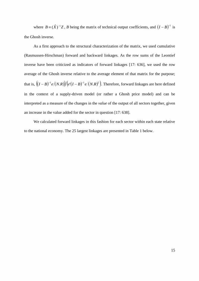
where ZXB 1)ˆ( , B being the matrix of technical output coefficients, and 1 BI is

the Ghosh inverse.

As a first approach to the structural characterization of the matrix, we used cumulative

(Rasmussen-Hirschman) forward and backward linkages. As the row sums of the Leontief

inverse have been criticized as indicators of forward linkages [17: 636], we used the row

average of the Ghosh inverse relative to the average element of that matrix for the purpose;

that is, 211.'. RNeBIeRNeBI

. Therefore, forward linkages are here defined

in the context of a supply-driven model (or rather a Ghosh price model) and can be

interpreted as a measure of the changes in the value of the output of all sectors together, given

an increase in the value added for the sector in question [17: 638].

We calculated forward linkages in this fashion for each sector within each state relative

to the national economy. The 25 largest linkages are presented in Table 1 below.

16

Table 1

Largest Forward Linkages

Rank Sector State FL

1 Chemical industry SP 15.90

2 Transportation goods SP 11.44

3 Food SP 7.37

4 Electrical goods SP 7.28

5 Metallurgy (iron and steel) RJ 6.28

6 Textiles SP 5.95

7 Construction GB 5.81

8 Construction SP 5.57

9 Metallurgy (other) SP 5.10

10 Fuels SP 5.07

11 Machine tools SP 4.70

12 Construction MG 4.32

13 Construction GO 4.23

14 Rubber SP 4.18

15 Food PR 4.05

16 Clothing SP 4.00

17 Chemical industry GB 3.77

18 Food RS 3.76

19 Services RO 3.48

20 Transportation MG 3.40

21 Metallurgy (iron and steel) MG 3.30

22 Nonmetallic minerals SP 3.20

23 Packaging SP 3.17

24 Fuels MG 3.07

25 Transportation SP 3.04

Source: elaborated by the authors.

The results obtained point at the importance of the state of São Paulo (SP) and of basic

industries sectors, such as chemical industry, transportation goods, electrical goods, and

metallurgy. However, some traditional industries, such as food or textiles (in SP), also appear

as important sectors, having highly ranked forward linkages. Also, the construction sectors of

four states (Guanabara - GB, São Paulo - SP, Minas Gerais - MG, Goiás - GO) appear among

the largest linkages. SP counted 14 of its 33 sectors within the first 25 largest forward

linkages, 18 among the first 50, and 20 among the first 100. The corresponding figures are,

respectively: 1, 3, and 4 for Rio de Janeiro (RJ); 2, 5, and 11 for Guanabara (GB); 4, 6, and 6

for Minas Gerais (MG); 1, 3, and 6 for Rio Grande do Sul (RS); and 1, 4, and 6 for Paraná

17

(PR). It is interesting to note that the metallurgical (iron and steel) sector figures twice among

the largest 25, in the states of RJ and MG, but not in the state of SP (which ranks 27th

).

Furthermore, that the forward linkages presented a much-skewed distribution deserves

mention; that is, a few sectors clearly stand out relative to all others. This can already be

perceived in Table 1, if we remember that the average of the linkages obtained is 1 (by

definition) and that the full list comprises a total of 825 sectors.

Cumulative backward Rasmussen-Hirschman linkages were also calculated for each

sector within each state relative to the national economy in traditional fashion, as the column

average of the Leontief inverse relative to the average element of that matrix, that is, as

211.'.' RNeAIeRNAIe

. Some aspects of these results draw the attention.

First, regardless of the state, there is a clear prevalence of the sectors of wastes, fuels, and

packaging among the largest backward linkages. These sectors account for 24 of the 25

largest backward linkages, and 49 of the largest 50. These three sectors come from the

original national matrix estimated by Rijckeghem [4], who called these sectors “fictitious,” as

previously mentioned, because they have no value added assigned for them. The relatively

very high backward linkages obtained for these sectors doubtless stem from this

characteristic. This is, therefore, a caveat carried over from the original national matrix.

The second important aspect to be noted in the results of the backward linkages is that,

disregarding the fictitious sectors, it is the small states of the economy, rather than the large

ones, that exhibit the largest linkages – in several cases, in sectors that are usually

characteristic of the large states; for example, paper in Mato Grosso (1st), Sergipe (4

th),

Espírito Santo (5th

), Paraíba (5th

), and Ceará (9th

); transportation goods in Ceará (10th

), Piauí

(11th

), and Paraíba (13th

); electrical goods in Goiás (7th

) and Espírito Santo (21st); or the

chemical industry in Piauí (8th

).

18

A third relevant aspect is that some sectors display low variability in the backward

linkage along the states, particularly the nonindustrial ones. Indeed, their distribution is, in

general, much more homogeneous than that of the forward linkages. All backward linkages

are within the range of 0.52 to 1.73, without the presence of clear outliers.

These last two aspects of the results obtained for the backward linkages can, as a matter

of fact, be largely imputed to the procedures used to estimate the inter-state input-output

matrix, which has been described above. The low variability in the linkages for each sector

along the states, where this is the case, much likely stems from our initial hypothesis of

estimating the states’ technical coefficients as proportions of the respective national ones. We

can think of this as a sector-specific limitation of the sources of data used in the estimation

procedures. The prominence of small states – disregarding the fictitious sectors – can also be

explained by this same estimation step but in a different sense. The cross-industry quotients

used to estimate the states’ technical coefficients from the national ones were calculated from

market shares. This is an approximation that is more likely to fail the more diverse the

technologies aggregated within each sector are. Larger technological diversity within a sector

is found in higher technology sectors, such as the ones mentioned above. Therefore, an

overestimation of the structural role of this kind of sector in small states results from an

underestimation of the technological diversity within these sectors along the different states.

The fact that the forward linkages are much more skewed than the backward linkages,

however, was already present in the original national matrix.

Although we can understand the results obtained, they are certainly to be considered an

important caveat of the estimation procedures adopted. For this reason, in the case of

backward linkages, we recommend the use of pure backward linkages, as presented below,

which take into consideration the economic size of the respective sector in evaluating its

19

relevance, thus reducing the problems discussed here.

Indeed, it is relevant to mention that not even the forward linkages presented above are

detached from this issue, as shown by the fact that the sector of services in Rondônia (RO)

has the 19th

highest forward linkage in the economy. But they seem to have been less

affected.

Another perspective of the matrix’s structure can be seized from less disaggregated

backward and forward linkages for whole states and whole sectors. We calculated these

linkages by means of definitions analogous to the ones stated above. We present plots of

backward vs. forward linkages in each case in order to grasp the relevance of each state or

sector through the consideration of both indicators simultaneously.

-

0,50

1,00

1,50

2,00

2,50

3,00

3,50

4,00

4,50

0,70 0,80 0,90 1,00 1,10 1,20

backward linkages

forw

ard

lin

ka

ge

s

RR

RO

AC

APAM AL

PA

GO

M

BA

M

MT RN SE

MAPI

RNES

PR

RN

MG

GB

SC

CE

PE

PB

SP

RJ

RNRS

Fig. 1. Backward vs. Forward Linkages of States

Note: The size of the bubbles represents the states’ GDP. Source: elaborated by the authors.

20

Figure 1 presents an interesting picture of the regional economic structure of Brazil in

1959. The first noteworthy feature of these results is that the few (seven) states that exhibit

above-average forward linkages also display above-average backward linkages. Moreover,

almost all of these states are geographically concentrated in the Southeast and South regions

(in the current regional grouping, which is different from the one prevailing at that time). The

case of SP is particularly impressive. Of course, the enormous share of these states in the

national economy is well known. However, this is indeed a remarkable feature, especially

when we recall that Rasmussen-Hirschman linkages have been criticized for not taking into

account the respective level of output. These results thus suggest a self-reinforcing character

of the regional concentration of the economic structure of the country, as well as a large

degree of intra-regional, and even intrastate, endogeneity of intermediate consumption.

It is interesting to remember that 1959 was precisely the year that the Superintendência

do Desenvolvimento do Nordeste (Superintendence for the Development of the Northeast,

SUDENE) was created by the Brazilian government in order to promote the north-eastern

region’s development, directing resources to that region. The results here obtained point to a

short- term trade-off between efforts toward regional economic homogenization and national

output growth.

Still another perspective to this issue can be reached by looking at the following table,

where we present (type I) output multipliers for each state, splitting the effects that take place

inside the state from the ones that take place outside it. Total output multiplier was defined as

the average of the column sums for every sector within each state, that is, as

NeAIe R

1'

, where Re is a (N.R x 1) state-specific summation vector with ones in the

lines corresponding to state R and zeros in the remaining lines:

)'0,,0,0,1,,1,1,0,,0,0(

Rregion

. The inside output multiplier was

21

correspondingly defined as NeAIe RR

1'

, and the outside output multiplier as the

difference between both.

Table 2

Total, Inside, and Outside Output Multipliers for States

Region State Output Multipliers

Total Inside Outside

North

RO 1.47 1.15 (78%) 0.32 (22%)

AC 1.61 1.22 (76%) 0.39 (24%)

AM 1.75 1.46 (84%) 0.29 (16%)

RR 1.38 1.13 (82%) 0.25 (18%)

PA 1.86 1.40 (75%) 0.46 (25%)

AP 1.64 1.23 (75%) 0.41 (25%)

Northeast

MA 1.96 1.54 (79%) 0.42 (21%)

PI 2.03 1.63 (80%) 0.40 (20%)

CE 2.13 1.75 (82%) 0.38 (18%)

RN 1.94 1.57 (81%) 0.37 (19%)

PB 2.15 1.67 (78%) 0.48 (22%)

PE 2.13 1.80 (85%) 0.33 (15%)

AL 1.83 1.42 (78%) 0.41 (22%)

East

SE 1.96 1.52 (77%) 0.44 (23%)

BA 1.89 1.61 (85%) 0.29 (15%)

MG 2.02 1.75 (87%) 0.27 (13%)

ES 2.04 1.60 (79%) 0.43 (21%)

RJ 2.02 1.79 (89%) 0.22 (11%)

GB 2.05 1.62 (79%) 0.44 (21%)

South

SP 2.07 1.83 (89%) 0.23 (11%)

PR 2.02 1.71 (85%) 0.31 (15%)

SC 2.08 1.73 (83%) 0.35 (17%)

RS 2.02 1.76 (87%) 0.26 (13%)

Center-

west

MT 1.93 1.56 (81%) 0.37 (19%)

GO 1.87 1.43 (76%) 0.44 (24%)

Notes: The regional grouping follows the 1959 census. The percentages indicated are the shares of the

total output multiplier for each state. Source: elaborated by the authors.

Once again, we wish to call attention to the larger states. As a rule, these states present

an above-average total output multiplier – as expected, because the total output multiplier is

related to the backward linkage, presented above. But, more interestingly, the seven states

exhibiting a larger proportion of inside output multiplier relative to the total output multiplier

22

(RJ, SP, RS, MG, BA, PE, and PR) belong to the eight economically larger states in the

country, in which at least 84.5% of the output multiplying effects take place within the state

itself. An exception, in this case, is the Federal District (GB), the 16th

on the list, with inside

output multiplier of 78.7%. Note that these results depict that the relevant economic division

is not so much the one between small and large states but rather the one between each of the

large states. This is because the large states present larger inside output multipliers; that is,

the effects of a variation in demand in any of these states unfold more within each one of

them, than is the case for the smaller states. Of course, this reasoning is only relative. In order

to decide whether, for example, an inside output multiplier larger than 88% (as in the case of

SP and RJ) is “high” in a more absolute sense, we would have to provide for relevant points

of comparison, which we are unable to supply within our current framework.

While the focus of this paper is the regional dimension of the Brazilian economic

structure, this being the new characteristic of the matrix we are using for our analysis, before

we move on to pure linkages, we briefly present Rasmussen-Hirschman backward and

forward linkages for whole sectors because, although the original national matrix can produce

a similar set of results, the linkages obtained for whole states from the interstate matrix are

expectedly different.

23

-

0,50

1,00

1,50

2,00

2,50

3,00

- 0,20 0,40 0,60 0,80 1,00 1,20 1,40 1,60 1,80 2,00

backward linkages

forw

ard

lin

ka

ge

s

Vegetable product

Commerce

Animal product

Services Fuels

Packaging

Wastes

Plastics

Extractive industry

Electrical goods

Rubber

Wood

Miscellaneous

Pharmaceuticals

Publishing

Beverages

Paper

Clothing

Perfumery

Transportation

Construction

Chemical industry

Textiles

Transportation goods

Metallurgy (iron and steel)

Nonmetallic minerals

Metallurgy (other)

Food

Fig. 2. Backward vs. Forward Linkages of Sectors

Note: The size of the bubbles represents the sectors’ total output. Source: elaborated by the authors.

Denominating key sectors as the ones that have both above-average backward and

forward linkages, we find in this group the sectors of fuels, packaging, construction, food,

transportation, chemical industry, metallurgy of iron and steel, and transportation goods.

Once again, we find the fictitious sectors to have very high backward linkages, for the same

reasons discussed above.

Pure linkages can provide still another perspective to the structure of the estimated

interstate input-output matrix by emphasizing the value of output in identifying key sectors

and regions, complementing the outlook rendered by the cumulative Rasmussen-Hirschman

linkages presented and discussed above.

The computation of pure linkages9 is based on a partition of the matrix of technical

input coefficients, A:

9 For definitions in the context of and a wider discussion on the subject, see [18].

24

rrrj

jrjj

AA

AAA

where j denotes a sector, or a group of sectors, of interest – in our case, a sector within

a state – and r the remaining sectors of the matrix. Pure backward linkages (PBL) and pure

forward linkages (PFL) were calculated as:

rrjrj

jjrjr

YAPFL

YAePBL

where a) 1)( rrr AI , b) 1)( jjj AI , c) jY is the total output of sector j; and d)

rY is a ((N.R – 1) x 1) vector with the respective total outputs of the remaining sectors. Pure

total linkages (PTL) were defined as the sum of PBL and PFL.

Table 3 presents the ranking of the 25 largest linkages for each of the three indicators.

25

Table 3

Largest Backward, Forward, and Total Pure Linkages

Rank PBL PFL PTL

1 Food (SP) Chemical industry (SP) Food (SP)

2 Construction (SP) Services (SP) Services (SP)

3 Transportation goods (SP) Vegetable products (SP) Construction (SP)

4 Textiles (SP) Metallurgy (other) (SP) Chemical industry (SP)

5 Electrical goods (SP) Metal. (iron and steel) (SP) Commerce (SP)

6 Commerce (SP) Commerce (SP) Transportation goods (SP)

7 Food (RS) Paper (SP) Textiles (SP)

8 Construction (GB) Metal. (iron and steel) (RJ) Vegetable products (SP)

9 Machine tools (SP) Vegetable products (PR) Electrical goods (SP)

10 Food (PR) Vegetable products (RS) Metallurgy (other) (SP)

11 Clothing (SP) Vegetable products (MG) Transportation (SP)

12 Construction (MG) Textiles (SP) Construction (GB)

13 Food (MG) Non-metallic minerals (SP) Food (RS)

14 Transportation (SP) Fuels (SP) Machine tools (SP)

15 Services (SP) Packaging (SP) Construction (MG)

16 Food (GB) Animal products (SP) Vegetable products (PR)

17 Food (RJ) Services (GB) Food (PR)

18 Transportation (MG) Metal. (iron and steel) (MG) Clothing (SP)

19 Construction (RJ) Transportation (SP) Fuels (SP)

20 Food (PE) Chemical industry (GB) Metal. (iron and steel) (SP)

21 Furniture (SP) Rubber (SP) Vegetable products (MG)

22 Construction (GO) Transportation goods (SP) Services (GB)

23 Beverages (SP) Services (RS) Vegetable products (RS)

24 Perfumery (SP) Services (MG) Non-metallic minerals (SP)

25 Pharmaceuticals (SP) Animal products (RS) Food (MG)

Source: elaborated by the authors.

As expected, given the characteristic of pure linkages and the results presented above,

the economically larger states appear in prominence. Moreover, São Paulo clearly stands out

even among the large states. It has 14 of the 25 largest PBL, 15 of the 25 largest PFL, and 16

of the 25 largest PTL.

It is also interesting to note that the profile of the sectors with the largest linkages is

different between SP and the remaining states figuring on the list in Table 3. For example, for

PBL, while SP appears with such sectors as transportation goods, textiles, electrical goods,

and machine tools, among others, the remaining states are only listed on the sectors of food

(RS, PR, MG, GB, RJ, and PE), construction (GB, MG, RJ, and GO), and transportation

26

(MG). Similarly, while SP has within the largest PTL such sectors as chemical industry,

transportation goods, electrical goods, metallurgy (iron and steel) and metallurgy (other),

among others, the remaining states figure only on construction (GB and MG), food (RS, PR,

and MG), vegetable products (PR, MG, and RS), and services (GB). Within the PFL, states

other than SP appear in a somewhat more diversified fashion, with such sectors as metallurgy

of iron and steel (RJ and MG), services (GB, RS, and MG), and chemical industry (GB). This

is per se not a statement about the diversification of each of these states’ economy.

Nevertheless, given that these linkages were calculated and ranked according to the

respective sectors’ importance relative to the national economy, these results give an

interesting assessment not only of the size of the economy of the state of SP within the

Brazilian economy, which is a well-known fact, but also of the state’s structural importance.

4. Final Comments

This paper has presented an overview of the regional economic structure of Brazil in

1959 through the estimation an interstate input-output matrix. One of the main contributions

of this paper is the estimated matrix, which thus becomes available to other researchers on

request to the authors. The matrix here presented is the oldest interstate matrix for Brazil.

Hence, it can be an important tool for the study of the regional productive structure at an

historical moment in which the regional question appeared as a central national issue. The

limitations and caveats of the matrix – stemming from the original national matrix, from

limited sources of data, and from the estimation procedures adopted – were pointed out and

discussed in the paper and should be kept in mind, though.

We have characterized the matrix from two different perspectives. First, from a

27

methodological point of view, we provided a detailed description of the data sources,

estimation procedures, and hypotheses used. The estimation was made based on

Rijckeghem’s (1967) national matrix for 1959 and on additional data obtained from several

sources, using cross-industry and location quotients.

Second, we also provided a panoramic structural portrait of the estimated matrix,

through the use of selected indicators. The distinguished features of the results included the

assessment of the structural importance, besides their economic size, of the larger states,

particularly of São Paulo, as well as some evidence of economic introversion of each of these

large states, when compared to the smaller ones.

Appendix

This appendix describes in some detail the sources of data and the hypotheses assumed

for the compilation of the eight matrices, in the form Sector by State, of additional (regional)

information used to estimate the interstate input-output table from Rijckeghem’s national

table. The eight matrices comprise information on: a) the distribution by state of the (origin

of) production of each sector (1); b) the distribution by state of the (origin of) value added,

including gross returns to capital (2) and wages, salaries, and social security (3); and c) the

distribution by state of the (destination of) final demand, including household consumption

(4), government consumption (5), investment (6), exports (7), and imports (8).

Origin of production by state: Information on the 33 productive sectors came

respectively from:

o Sectors 1 and 2, agricultural sectors: The data source used was the national

accounts [14: 92-5], which was the same source Rijckeghem used in his estimates.

28

It was necessary to estimate production for the states of RO, AC, RR, and AP, as

this information was not reported in the national accounts. The estimation was

done proportionately to the agricultural workforce in 1959 (pessoal ocupado na

agricultura) relative to that in the other states of the northern region, as obtained

from the Agricultural Census [10: 26].

o Sector 3, electric energy: The production of electric energy by state was estimated

from the data on electric energy consumption that we found; hence, there is an

implicit hypothesis here regarding the non-tradability of this product between

states. Data on industrial consumption of electric energy (39% of total electric

energy production) by state were found in the Industrial Census [11: 119]. The

remainder of the value in the national table was then distributed proportionately to

the consumption of electric energy in the municipalities of the states’ capitals in

1959 [15: 276].

o Sectors 4 and 5, commerce and services: Commerce by state was estimated

proportionally to the commercial flux (giro comercial) in 1959; data found in the

Statistical Yearbook [15: 263], which was in turn calculated from data on sales

tax’s (imposto sobre vendas e consignações) collection. Services by state were also

supposed to be non-tradable and were estimated from primary data or estimates of

expenditures on services by state of each sector. Data on industrial expenditure on

services (17% of total service) were obtained from the Industrial Census [11: 119-

20], while data on commercial expenditure on services (13%) were obtained from

the Commerce and Service Census [12: 67]. The expenditures on commerce of the

primary, electric energy, transportation, and construction sectors (adding up to 6%)

were estimated proportionately to their respective production by state. Household

29

expenditure on commerce (60%) was estimated proportionately to each state’s

internal income in 1959 [15: 269]. Finally, the service sector self-consumption

(4%) was estimated proportionately to the service expenditure by state of the

remaining sectors.

o Sectors 6 to 8, fictitious sectors: The residuals for each industrial sector were

distributed by state proportionately to the respective sector total production. Data

on fuel and packaging production were also supplied indirectly by the data and

estimates on expenditures. This implies that here we are making the same

hypothesis on non-tradability, which is especially cumbersome in the case of these

sectors. But we couldn’t avoid it; this is a consequence of Rijckeghem’s decision to

work with these sectors. The only reasonable sources of information to be found on

them were the censuses, and, there, fuel and packaging were accounted for within

the cost structure. Therefore, care is to be taken in making any conclusion of

regional character regarding these sectors. Industrial expenditure on fuels (28% of

total fuel production) by state was obtained from the Industrial Census [11: 119].

The expenditure on fuels of the primary, electric energy, commerce, services,

transportation, and construction sectors (adding up to 56%) was estimated

proportionately to their respective production by state. Government fuel

consumption (4%) was estimated proportionately to public employees by state [9:

101]. Household fuel consumption (11%) was estimated proportionately to each

state’s internal income in 1959 [15: 269]. Export fuel consumption (0.1%) was

assumed to be proportional to the exported tonnage in 1959 [15: 220]. Data on the

industrial expenditure on packaging (92% of total packaging production) were

obtained from the Industrial Census [11: 119]. The packaging expenditure of the

30

vegetable products sector (8%) was estimated proportionally to its production by

state.

o Sectors 9 to 31, industrial sectors: The data on the production by state of the

industrial sectors were the best we were able to obtain, and this is crucial given the

importance of these sectors for several purposes in input-output analyses. Indeed,

the information is not only fully compatible with the one used by Rijckeghem for

the national matrix but also his and ours best-quality data. These were found in the

Industrial Census [11: 92-114].

Sectors 11 and 12, metallurgical sectors: Data on the disaggregated

metallurgical sectors by state were not readily available from the National

Series of the Industrial Census. In order to reconstruct them, we used two

special publications of the Industrial Census. A detailed classification of

industries, which served as the norm for the tabular presentation of the results of

the Industrial Census of 1960 [23], allowed us to produce a list of products for

the “metallurgical (iron and steel)” sector that was consistent with the original

aggregated data, which included “Steel products – iron and steel”, “Steel

products – alloys”, and part of “Various metallurgical products”. The production

by state of each product on this list was then found in the Special Series of the

Industrial Census [13]. The “metallurgical (other)” sector was then calculated as

the residual from the aggregated metallurgical sector [11: 95].

o Sectors 32 and 33, construction and transportation: The construction sector

production by state was estimated as proportional to the consumption of cement in

1959 [15: 277-78]. The transportation sector production was estimated from

information or estimates on transportation expenditure by state for several sectors.

31

The expenditures on transportation of the industrial and commercial sectors

(adding up to 17% of total transportation) were found in their respective censuses

[11: 120][12: 67]. Household expenditure on transportation (54%) by state was

assumed to be proportional to the total population of each state [9: 80]. The

expenditures on transportation of the Construction and Services sectors (adding up

to 3%) were assumed to be proportional to their respective production. The export

sector expenditure on transportation (8%) was assumed to be proportional to the

exported tonnage in 1959 [15: 220]. Government expenditure on transportation

(16%) was assumed to consist of subsidies and hence was distributed by state

proportionately to the sum of the above-mentioned transport expenditures.

Transportation self-consumption (2%) was assumed to be proportional to the

remaining sectors’ expenditures on transportation.

Origin of value added by state: Data on wages and salaries for the industrial sectors

were obtained from the Industrial Census [11: 92-114]. The expenses on Social

security (plus indemnification) by state for all the industrial sectors (aggregated) are

informed in the Industrial Census [11: 120]; the distribution of the total by state

between sectors was done proportionately to the wages and salaries paid by each

sector in the state. The wages, salaries, and social security in the industrial sectors add

up to 25% of the total WSSS. Data on the wages, salaries, and social security paid by

the commercial sector (8%) was obtained from the Commerce Census [12: 64, 67].

The wages, salaries, and social security paid by the government (16%) were assumed

to be proportional to the number of public employees by state [9: 101], and those paid

by households (7%) were assumed to be proportional to the internal income by state

[15: 269]. The wages, salaries, and social security from the remaining sectors (adding

32

up to 44%) were assumed to be proportional to their respective production by state.

To estimate the gross returns to capital of the industrial sectors (adding up to 30% of

the total GRC), we initially estimated the value added by state (but aggregated for

sectors) from data obtained from the Industrial Census [11: 119-20]. This was then

distributed among sectors within each state proportionately to the value of industrial

transformation found in the Industrial Census [11: 92-114]. This resulted in an

estimate for the value added by sector and by state. The gross returns to capital of the

industrial sectors were finally obtained by subtracting from the value added the

respective wages, salaries, and social security that we had already estimated. The

gross returns to capital of the remaining sectors (70%) were assumed to be

proportional to their respective production by state.

Destination of final demand by state: The household consumption of each sector’s

production was distributed proportionally to the internal income by state. Government

consumption was distributed proportionally to the number of public employees by

state. The investment expenses for each sector were estimated proportionally to the

gross returns to capital by state for the respective sector. Total exports by state were

assumed to be equal to the exports through ports and airports, data on which were

found in the Statistical Yearbook [15: 220]. The exports for each sector within each

state were distributed proportionately to the respective state’s production by sector.

Total exports by sector were then distributed among the states proportionately to the

quantities thus obtained. An identical procedure was followed for imports, but based

on the data on imports through ports and airports found in the Statistical Yearbook

[15: 220].

33

Acknowledgments

The authors would like to thank the Biblioteca da Unidade de São Paulo do Instituto

Brasileiro de Geografia e Estatística and its solicitous librarians for providing essential

material for this research. We also thank André Luís Squarize Chagas and Esther Dweck for

valuable comments and bibliographical references. During the preparation of the manuscript,

both authors were scholarship holders of the CNPq – Brazil.

References

[1] Celso Furtado, Formação Econômica do Brasil, São Paulo, Companhia Editora

Nacional, 11th

ed., 1972.

[2] Anibal V. Villela, Resenha Bibliografica: Estado e Planejamento Economico no Brasil,

Pesguisa e Planejamento Economico, 2:1 June (1972) 171-78.

[3] Werner Baer, The Brazilian Economy: Growth and Development, New York, Praeger,

5th

ed., 2001.

[4] Willy van Rijckeghem, with the collaboration of Sérgio Alípio de Oliveira Camargo,

Tabela de Insumo-Produto, Brasil - 1959, Texto para discussão do IPEA, setembro 1967.

[5] M. E. F. Jones, Regional Employment Multipliers, Regional Policy, and Structural

Change in Interwar Britain, Explorations in Economic History 22 (1985) 417-439.

[6] John A. James, The Use of General Equilibrium Analysis in Economic History,

Explorations in Economic History 21 (1984) 231-253.

[7] Willy van Rijckeghem, An intersectoral consistency model for economic planning in

Brazil, in: Howard S. Ellis (Ed.), The economy of Brazil, Berkeley and Los Angeles,

University of California Press, 1969, pp. 376-401.

[8] J. T. Winpenny, Industrialization in Brazil, Journal of Latin American Studies, Vol. 2,

No. 2 (Nov., 1970) 199-208.

34

[9] Brasil, VII Recenseamento Geral do Brasil, Censo Demográfico de 1960, Série

Nacional, Volume I, Fundação Instituto Brasileiro de Geografia e Estatística, Departamento

de Estatísticas da População, [Rio de Janeiro], n.d.

[10] Brasil, VII Recenseamento Geral do Brasil, Censo Agrícola de 1960, Série Nacional,

Volume II – 1ª Parte, IBGE – Serviço Nacional de Recenseamento, Rio de Janeiro, setembro

de 1967.

[11] Brasil, VII Recenseamento Geral do Brasil, Censo Industrial de 1960, Série Nacional,

Volume III, IBGE – Serviço Nacional de Recenseamento, Rio de Janeiro, março de 1967.

[12] Brasil, VII Recenseamento Geral do Brasil, Censos Comercial e dos Serviços de 1960,

Série Nacional, Volume IV, IBGE – Serviço Nacional de Recenseamento, Rio de Janeiro,

junho de 1967.

[13] [Brasil], VII Recenseamento Geral do Brasil, Censo Industrial de 1960: Matérias-primas

e produtos, Série Especial, Volume V, Fundação IBGE – Instituto Brasileiro de Estatística,

Serviço Nacional de Recenseamento, Rio de Janeiro, setembro de 1968.

[14] FGV – Fundação Getúlio Vargas, Contas Nacionais, Revista Brasileira de Economia,

Rio de Janeiro: FGV, Ano 15, No. 1, março de 1961.

[15] IBGE – Conselho Nacional de Estatística, Anuário Estatístico do Brasil – 1961, Ano

XXII, Rio de Janeiro: IBGE, dezembro de 1961.

[16] Ronald E. Miller, Peter D. Blair, Input-Output analysis: Foundations and extensions,

New Jersey, Prentice-Hall, 1985.

[17] Erik Dietzenbacher, In vindication of the Ghosh model: A reinterpretation as a price

model, Journal of Regional Science, Vol. 37, No. 4 (1997) 629-651.

[18] Joaquim J. M. Guilhoto, Michael Sonis, Geoffrey J. D. Hewings, Linkages and

multipliers in a multiregional framework: Integration of alternative approaches, Australasian

Journal of Regional Studies, Vol. 11, No. 1 (2005) 75-89.

[19] Jan Oosterhaven, Gerard J. Eding, Dirk Stelder, Clusters, forward and backward

linkages, and bi-regional spillovers: Policy Implications for the two Dutch mainport regions

and the rural north, Paper presented at the 39th

European Congress of the Regional Science

Association International, August 23-27, 1999, University College Dublin.

[20] Werner Baer, Manuel A. R. da Fonseca, Joaquim J.M. Guilhoto, Structural changes in

Brazil's industrial economy, 1960-80, World Development, 14 (1987) 275-286.

[21] Joaquim J. M. Guilhoto, Michael Sonis, Geoffrey J. D. Hewings, Eduardo B. Martins,

35

Índices de Ligações e Setores Chave na Economia Brasileira: 1959-1980, Pesquisa e

Planejamento Econômico, 24:2 (1994) 287-314.

[22] Michael Sonis, Joaquim J. M. Guilhoto, Geoffrey J. D. Hewings, Eduardo B. Martins,

Linkages, Key Sectors and Structural Change: Some New Perspectives, The Developing

Economies, XXXII:3 (1995) 233-270.

[23] IBGE – Instituto Brasileiro de Geografia e Estatística, Serviço Nacional de

Recenseamento, Classificação de indústrias: Produtos – Matérias-primas, Rio de Janeiro:

IBGE, 1963.

Disclosure Statement

During the preparation of the manuscript both authors were scholarship holders of the

Conselho Nacional de Desenvolvimento Científico e Tecnológico (National Council for

Scientific and Technological Development), CNPq – Brazil. The CNPq had no role in the

study design; in the collection, analysis, and interpretation of data; in the writing of the

report; or in the decision to submit the article for publication. The CNPq only requires that

the funding be explicitly acknowledged in any publications resulting from the funded

research.