THE QUALITY OF FISCAL ADJUSTMENT AND THE LONG-RUNGROWTH IMPACT OF FISCAL POLICY IN BRAZIL1

Fernando BlancoSantiago Herrera

Abstract

This paper describes the main trends of Brazil’s fiscal policy during the last decade, andanalyzes empirically three key aspects: 1) the ability to raise the primary surplus in response toexternal shocks: 2) the procyclical nature of fiscal policy; and 3) the long run impact ofgovernment expenditure composition and taxation. The use of the primary balance as a policytool is analyzed within the Drudi-Prati (2001) model, according to which, the government usesthe primary balance as a signaling tool to reveal its commitment to serve its debt. As the debtincreases, the dependable government will use more actively its primary balance. We verify thatboth the debt ratio and the primary balance are determinants of spreads (ratings) in Brazil.However, the relationship is non-linear, as the impact of the primary balance on spreads isamplified as the debt ratio increases.

The relationship between the primary balance and economic activity is analyzed bymeans of the Autoregressive Distributed Lag (ARDL) approach (Pesaran and Shin, 1999).Results indicate a positive correlation of the primary balance and output in the long run, butnegative in the short run. Fiscal expansions are associated with primary balance reduction andvice-versa during output contractions, verifying the pro-cyclical nature of fiscal balances.

The impact of public expenditure composition and taxation on growth is analyzed in amodified production function framework, in which private and public capital are inputs, jointlywith different types of public expenditure. The tax level is included to incorporate thegovernment’s budget constraint and to capture its potential negative effect on output. The paperuses two complementary approaches: a single equation method (the ARDL) and a multipleequation method (the cointegratng VAR) useful to analyze the interaction between the variables.Similar results are obtained: large elasticities of output with respect to capital stocks, asignificant negative impact of taxation on long-run GDP, and a negative impact on GDP ofincreasing government consumption and transfer payments. These results shed light on the roleof fiscal policy contribution to a disappointing growth performance in Brazil during the pastdecade.

1 The authors wish to thank Gaobo Pang for helpful research assistance and Ethan Weisman for his usefulcomments and suggestions. This paper is a rejoinder of several technical background papers by the authorsfor the Brazil Country Economic Memorandum (Report 25278-BR). A version of this paper was presentedat the EcoMod Policy Modeling Conference in Paris, June 2004. This paper carries the name of the authorsand should be cited accordingly. The findings, interpretations and conclusions are the author’sresponsibility and do not necessarily represent the view of the World Bank or its Executive Directors.Corresponding author: sherrera@worldbank.org

1

I. Introduction

Throughout the 1990s, Brazil started a process of economic reform includingliberalizing trade, relaxing price controls, and privatizing public enterprises. Althoughsome problems remained at first, such as higher public sector deficits and limitedexchange rate flexibility, the country corrected most of these and steered a course towardstability by the end of the millennium. In fact, since 1999, Brazil has made substantialefforts to adjust its fiscal accounts. The country has moved in the direction of crediblerules that govern the outcome of the budget process and procedures that contribute toproviding incentives and constraints to promote fiscal discipline and increasetransparency. The hallmarks of these measures include the Fiscal Responsibility Law andthe impressive primary surplus targets achieved between 1999 and 2005.

Despite the impressive results some vulnerabilities still remains. In particular, thequality of the fiscal adjustment brings doubts about growth prospects and the owncontinuity of the hard fiscal stance. The fiscal adjustment has been accomplished throughstrong revenue increases (the tax burden has grown from 29 percent of GDP in 1998 to35 percent in 2004) and by curtailing public investment (investments by federalgovernment fell from 1.1 percent of GDP in 1998 to 0.5 percent in 2005). The increaseof the tax burden and the compression of public investment are harming growth prospectswhich can make more difficult debt dynamics in the future On the other hand, thepermanent increase of current expenditures and the impossibility to maintain the taxburden growth are negatively affecting the sustainability of the current fiscal adjustmenteffort. To sustain growth while re-orienting public finance towards investment thereforerepresents the next chapter of Brazil’s national economic reforms.

The paper is organized in four sections following this introduction. The firstdescribes the main fiscal trends since the nineties, focusing mostly on the period 1999-2005. The second section focuses on a mechanism that would allow fiscal policy to bemore responsive to shocks, by permitting automatic stabilizers to operate throughout thebusiness cycle to mitigate the pro-cyclicality of Brazilian fiscal accounts. This sectioncomputes the long run effects of different variables on the primary balance and estimatesthe cyclical component of the primary surplus. The third section examines the long-termimpact of public finance on growth, using a modified production function approach, inwhich private and public capital are considered inputs, jointly with different types ofpublic expenditure. Results indicate large elasticities of output with respect to capitalstocks, negative impact of public consumption and transfers in the long run, and asignificant negative impact of taxation on long-run GDP. The fourth section summarizesthe results and concludes.

I. Background: Brazilian Fiscal Policy during 1990-2005

This section is divided into four parts. The first one describes fiscal outcomesduring the last fifteen years, focusing on the fiscal adjustment of 1999-2005. The secondsection highlights the flexibility of fiscal policy during this volatile period, and examinesthe role of the primary surplus as a signaling device in a world of imperfect information.The third section assesses the quality of the fiscal adjustment identifying the type ofadjustment carried out-revenue increasing or expenditure cutting. The fourth sectionattributes the type of fiscal adjustment to the high budget rigidity.

2

A. Fiscal Policy Trends in Brazil

During the last years of the military regime, the Brazilian public sector showedsigns of financial fragility. Slower growth combined with the external shocks, led to afall in public sector savings. The re-democratization process deepened the fiscaldisequilibria, because the new democratic government set out to satisfy repressed socialdemands for redistribution. The 1988 Constitution expanded the social responsibilities ofthe state, guaranteed free access to social services, established higher social securitybenefits, and defined a generous regime for public sector employees (Bevilaqua andWerneck, 1998). The new Constitution also modified the federal fiscal system, creatingan imbalance between resources and responsibilities among levels of government.Finally, the 1988 Constitution increased the rigidity of public spending through theearmarking of an important part of fiscal revenues.

These measures had a very perverse effect on public finances, but inflationpostponed the collapse of the fiscal regime. During this high-inflation period, theasymmetric indexation to inflation of revenues and expenditures, higher for revenues thanfor expenditures, produced artificially positive balances (Cardoso, 1998). Additionally,the negative real interest rates and the inflation tax generated soft budget constraints andpositive fiscal outcomes.

The evolution of fiscal accounts during 1990-2005 can be divided into three sub-periods, as shown in Figure 1. The first one, 1990-1994, registers positive primaryoutcomes and operational equilibriums. In the second one, from 1995 to 1998, theprimary surplus vanishes, while the last sub-period, 1999-2003, corresponds to the fiscaladjustment years and shows a permanent improvement of the primary surplus from –0.2% of GDP in 1998, to 4.7% in 2005.

Figure 1 Brazil: Fiscal Results and Inflation 1990-2005

-10.0

-8.0

-6.0

-4.0

-2.0

0.0

2.0

4.0

6.0

1990 1991 1992 1993 1994 1995 1996 1997 1998 1999 2000 2001 2002 2003 2004 2005

Fisc

al B

alan

ces

(% o

f GDP)

0

500

1000

1500

2000

2500

3000

Infla

tion

(% p

.a)

Primary Balance Total Balance Annual Inflation

Collor Plan(March, 1990)

Real Plan - Cardoso I(July, 1994)

Inflation Targeting Regime - Cardoso II (May, 1999)

President Lula Administration.

The end of the inflationary process in the mid nineties coincided withdeteriorating fiscal outcomes in 1995-98. Inflation was not only a revenue source, butwas also a useful mechanism to control government spending in real terms during thehigh inflation era (Cardoso, 1998). This loss of flexibility, combined with a lack ofdecisive fiscal reform, produced rising public sector deficits. The excess spendingrelative to national income was financed in liquid international capital markets, withpublic debt rising from 29% of GDP in 1994 to almost 42% in 1998.

3

The central bank sterilized these capital inflows through open market operationsto avoid monetary expansion and maintain a pegged exchange rate. This responsecomplicated the situation even more because it entailed rising central bank (domestic)debt and climbing interest rates that raised the cost of servicing public debt. High interestrates combined with the pegged exchange rate attracted even more capital, worsening thestate of affairs. The higher debt and the rigid fiscal, monetary, and exchange ratepolicies, left the economy vulnerable and with no capacity to absorb shocks. When theAsian and Russian financial crises occurred in 1997-1998, Brazil was severely affecteddue to its sizeable external financing requirements. In January 1999, the central bankabandoned its crawling peg exchange rate regime in favor of a flexible rate and adoptedan inflation-targeting framework for managing monetary policy.

In 1999, the country tackled its fiscal imbalance by launching the Fiscal StabilityProgram, which consisted not only in raising taxes, but also in designing a legalframework for fiscal policy management. The government set and met stringent targetsfor the primary fiscal surplus; the public sector primary surplus increased permanentlyfrom 3.3 percent of GDP in 1999 to 4.7 percent of GDP in 2005.

However, the high interest rates and the exchange rate devaluations of 1999, 2001and 2002 prevented a more accentuated reduction of operational deficits. Consequently,the primary surpluses were not sufficient to truncate the rising path of public debt. Table1 compares the three periods. During 1995-98, the operational balance deteriorated byalmost 5% of GDP in comparison with the period 1990-94. This was a result of a rise of1.5% of GDP in interest payments and a fall of the primary surplus of 3.5% of GDP. TheFederal government was responsible for 60% of fall in the operational balance, and formore than 40% in the decrease of the primary surplus. States and local governments andpublic enterprises were responsible for 30% each for the worsening of the results.

Table 1: Fiscal Balances*, 1990-2005

Annual Averages (% of GDP)

1990-1994 1995-1998 1999-2002 2003-2005 (A) (B) (C) (D)

I Operational Balance (III - II) -0.05 -5.01 -1.52 -1.40 Federal Government 0.52 -2.48 -1.55 -1.93 States and Municipalities -0.25 -1.98 -0.37 -0.22 Public Enterprises -0.31 -0.55 0.41 0.70

II Real Interest Payments 3.33 4.84 5.09 5.96 Federal Government 1.26 2.78 3.67 4.71 States and Municipalities 0.86 1.64 0.98 1.21 Public Enterprises 1.20 0.42 0.07 0.08

III Primary Balance 3.27 -0.17 3.58 4.56 Federal Government 1.78 0.30 2.11 2.78 States and Municipalities 0.61 -0.34 0.61 0.99 Public Enterprises 0.89 -0.13 0.85 0.79 * ( + ) Surplus ( - ) Deficit

4

B. The Flexible Primary Surplus as a Device to Signal Fiscal Sustainability

How do governments that are not fully credible signal regime sustainability?Based on the Drudi-Prati (2000)2 model that rationalizes debt accumulation and delayedstabilization, we analyze the Brazilian case. The main testable implication of the Drudi-Prati (DP) model is the existence of a positive relationship between the spreads and thedebt level and a negative association between spreads and primary balances. Thisrelationship is conditioned on the debt level: Given uncertainty about the likelihood ofdefault, the government will use the primary balance as a signaling tool to reveal toinvestors its true type. As the debt level rises, the dependable government (though notfully credible) will use more actively its primary balance as a signaling tool.

Spreads on sovereign debt are crucial determinants of the nominal exchange ratein Brazil and on domestic interest rates. What is the relation between these rates and thefiscal variables? For Brazil, primary balances and spreads show a non-stable association(Figure 2). From 1994 to 1998, when fiscal balances deteriorated, spreads declined.After 1999, when fiscal balances improved, spreads declined further. Drudi and Prativerified this non-monotonic relationship in their study of several European countries. Therelationship between public debt and spreads is also non-monotonic. From 1994 –1997,when the debt ratio was low and slightly rising, spreads fell. Since 1999, however,Brazilian spreads and debt ratios appear to have settled at a higher level (Figure 3).Drudi and Prati (DP) described a similar phenomenon for the European countries.

The DP model predicts that the primary fiscal balances and public debt ratiosenter the rating (spreads) function, and that the primary balance has a more influentialrole when debt ratios are high. This section verifies econometrically the following threetestable implications of the DP model: 1) Debt ratios and primary balances arecomplementary in the spreads function; 2) The signaling role of the primary balance

2 Drudi, F. and A. Prati (2000), “Signaling fiscal regime sustainability,” European Economic Review, Vol.44 pp. 1897-1930.

Figure 2Primary Fiscal Balances and Sovereign Spreads in Brazil

1994-2003

Figure 3Public Debt Ratio and Sovereign Spreads in Brazil

1994 - 2003

-2

-1

0

1

2

3

4

5

0

400

800

1200

1600

2000

2400

2800

94 95 96 97 98 99 00 01 02 03

Primary balance(left scale)

Spreads

bps% of GDP

28

32

36

40

44

48

52

56

60

64

0

400

800

1200

1600

2000

2400

2800

3200

3600

94 95 96 97 98 99 00 01 02 03

Public debt(left axis)

Spreads

bps% of GDP

5

increases with the debt ratio; and, 3) If the government is dependable, then the primarybalance will rise when the debt ratio increases.

To verify the complementary role of fiscal balances and debt ratios in the spreadsfunction, we regressed the sovereign spreads on the first two variables (lagged). Table 3shows that both variables enter significantly in the spreads function with the expectedsigns.

Table 3Complementary Roles of Debt Ratios and Primary Balances as Spreads' Determinants

Dependent Variable: EMBORLATMethod: Least Squares

Variable Coefficient Std. Error t-Statistic Prob.C -0.26 0.06 -4.45 0.00

DEBTY(-1) 0.01 0.00 4.48 0.00PRIMBAL(-1) -0.02 0.01 -2.40 0.02

R-squared 0.454 Mean dependent var -0.011Adjusted R-squared 0.441 S.D. dependent var 0.083S.E. of regression 0.062 Akaike info criterion -2.698Sum squared resid 0.309 Schwarz criterion -2.611Log likelihood 116.295 F-statistic 33.723Durbin-Watson stat 0.362 Prob(F-statistic) 0.000

EMBORLAT= Brazil EMBI spreads orthogonalized from Latin EMBI averageDEBTY= Debt to GDP ratioPRIMBAL= Primary fiscal balance

The second implication of the DP model, namely the changing nature of thesignaling role of primary balances, is captured by the inclusion of an auxiliary whichreflects the interaction of the primary balances with the debt ratio. If this variable issignificant, then the hypothesis of the difference in the signaling role cannot be rejected.Results in table 4 shows that the primary balance coefficient rose with the debt ratio,implying that signaling takes time and is not a once-and-for-all event.

Table 4The changing role of primary balances- Test 2

Dependent Variable: EMBORLATMethod: Least Squares

Variable Coefficient Std. Error t-Statistic Prob.C -0.530713 0.071481 -7.424499 0.0000

DEBTY(-1) 0.014446 0.001826 7.912960 0.0000PRIMBAL(-1) -0.024688 0.003926 -6.288602 0.0000

PRIMBAL(-1)*(DEBTDEV) -0.002630 0.000572 -4.593340 0.0000R-squared 0.632718 Mean dependent var -0.011316Adjusted R-squared 0.618945 S.D. dependent var 0.082535S.E. of regression 0.050949 Akaike info criterion -3.069552Sum squared resid 0.207661 Schwarz criterion -2.953799Log likelihood 132.9212 F-statistic 45.93872Durbin-Watson stat 0.632039 Prob(F-statistic) 0.000000

DEBTDEV=Deviation of the debt ratio from the sample mean

The third and final implication of the DP model, the positive association betweenthe primary balance and the debt ratio if the government is dependable is reflected inTable 5.

6

Table 5Primary Balances and Debt Ratios

Dependent Variable: PRIMBALMethod: Least SquaresWhite Heteroskedasticity-Consistent Standard Errors & Covariance

Variable Coefficient Std. Error t-Statistic Prob.C -2.921112 1.048574 -2.785795 0.0066

DEBTY(-1) 0.112549 0.022527 4.996247 0.0000

R-squared 0.247189 Mean dependent var 1.631294Adjusted R-squared 0.238119 S.D. dependent var 2.060787S.E. of regression 1.798774 Akaike info criterion 4.035336Sum squared resid 268.5538 Schwarz criterion 4.092810Log likelihood -169.5018 F-statistic 27.25346Durbin-Watson stat 0.049271 Prob(F-statistic) 0.000001

C. The Type of Brazilian Fiscal Adjustment, 1999-2005

During the first four years of the Real Plan (1995-98), fiscal accounts wereimbalanced due mostly to the loss of inflation as an adjustment mechanism and to thelack of decisive fiscal reform. As Table 6 shows, the weaker fiscal stance of the 1995-98is explained by rising expenditure, which grew by 16%, with personnel and socialsecurity benefits expanding the most. Revenue rose just 8% or 1.4% of GDP, withgrowth concentrated on taxes, while the revenues of the Social Security System remainedstable. In sum, the fiscal expansion of 1995-98 was caused by rising expenditure and notto revenue reduction.

The adjustment of the federal fiscal accounts in the last six years has been basedon revenue increases and investment cuts. During 1999-2005, tax revenue rose by 4.6 %of GDP. Spending also grew, but at a slower rate: it rose by 2.5 percentage points of GDPduring 1999-2005 As in the 1995-98, current expenditure accounted for the bulk of therise, while capital spending were reduced. In this case, personnel expenditures remainedstable while social security benefits and intergovernmental transfers experienced moredramatic increases.

The revenue-increasing nature of the 1999-2003 fiscal adjustment raises concernsabout its sustainability. International experience shows that revenue-based adjustmentstend to be short-lived (Alesina and Peroti, 1996). As spending follows the rising revenue,the adjustment effort is weakened and the lasting effect is a larger government.

7

D. The rigidity of expenditures as the main explanation of the type of adjustment

Fiscal adjustment was revenue-based because of the rigidity of public spending.At the federal level, this rigidity is caused by three factors: i) the rise of social securityand social assistance benefits; ii) the job tenure stability rules for public servants madeimpossible reducing the public sector payroll; and, iii) the constitutional earmarking ofan important part of federal tax revenues.

The 1988 Constitution reinforced the three factors of expenditure rigidity throughthe concession of higher social security benefits and softening the eligibility criteria,defining a generous regime for official public employees which included job tenure andhigher compensations and pension benefits equal to 100% of exit salaries, extendingthese benefits to all public sector employees and strengthening the intergovernmentaltransfers system. The 1988 Constitution favored the expansion of social responsibilitiesof the state, guaranteeing free access to social services, particularly health services,creating the unemployment insurance, establishing minimum social security benefits (1minimum wage), and universalizing it by extending coverage to rural workers. Figure 4shows the rising share of mandatory spending between 1986 and 2003. The increasingrigidity is due to the rise of personnel, social security and assistance transfers, and theintergovernmental transfers to states and municipalities that increased from 55% of non-financial expenditure in 1986 to almost 80% in 2001.

Categories1990-1994 1995-1998 1999-2005 (B) - (A) Decomp I Decomp II (C) - (B) Decomp I Decomp II(A) (B) (C)

I Total Revenue 17.3 18.6 23.2 1.3 7.7 102 100 4.6 24.6 222 100

Treasury Revenue 11.9 13.6 18.0 1.7 14.6 132 130 4.3 31.8 210 95 Tax Revenue 11.0 12.0 16.6 1.1 9.9 83 81 4.5 37.6 219 99 Other Treasury Revenues 1.2 1.6 1.4 0.4 32.1 29 29 -0.2 -12.0 -9 -4 Social Security Revenue 5.0 5.1 5.3 0.1 2.7 10 10 0.2 3.3 8 4

II Total Expenditure 15.8 18.4 20.8 2.6 16.4 -198 100 2.5 13.5 -120 100

Personnel and Social Contributions 4.4 5.2 5.1 0.7 17.0 -57 29 -0.1 -1.3 3 -3 Social Security Benefits 4.2 5.4 6.7 1.2 30.0 -95 48 1.3 23.4 -61 51 Other Current and Capital Expenditures 4.3 4.8 5.2 0.5 11.1 -36 18 0.4 8.3 -19 16 Subsidies 0.1 0.2 0.3 0.1 98.2 -8 4 0.1 51.3 -5 4 FAT 0.2 0.6 0.6 0.3 138.7 -25 12 0.0 2.4 -1 1 Other- Goods and Services and Investment4.0 4.0 4.3 0.0 1.1 -3 2 0.3 6.8 -13 11 Intergovernmental Transfers 2.9 3.0 3.9 0.1 3.9 -9 4 0.9 29.4 -43 36

Primary Balance (I - II) 1.6 0.3 2.4 -1.3 -81.7 100 2.1 708.1 100

PercentualVariation

PercentualVariation

Table 6: Federal Government Primary Surplus Changes, 1990 - 2005

Annual Averages (% of GDP) Variation 91/94 - 95/98 Variation 95/98 - 99/05

8

As a result of the growing share of mandatory spending, investment and othercurrent expenditures decreased their share from around 51% of non-financialexpenditures to less than 20% in 2001. Clearly, social security transfers are the fastest-increasing type of expenditure, generating a huge deficit that has to be covered by theTreasury. Figure 5 shows the evolution of the social security system imbalances duringthe period 1990-2005. While in 1990 the deficit was 1.4% of GDP, in 2005 it reached5.7%.

Figure 5: Social Security Imbalances, 1990-05

1.4% 1.5%1.0%

2.4%

3.3%3.7% 3.7% 3.8%

4.5%4.9% 5.0% 5.2%

5.5% 5.8% 5.7% 5.7%

0%

1%

2%

3%

4%

5%

6%

7%

1990 1991 1992 1993 1994 1995 1996 1997 1998 1999 2000 2001 2002 2003 2004 2005

Total PAYG Deficits RGPS RPPS FederalRPPS States RPPS Municip.

III. Procyclical Fiscal Policy in Brazil

Figure 4

Brazil: Federal Non Financial Expenditure Composition

0% 10% 20% 30% 40% 50% 60% 70% 80% 90%

100%

1986 1987 1988 1989 1990 1991 1992 1993 1994 1995 1996 1997 1998 1999 2000 2001 2002 2003

(% of Total non Financial Expenditure)

Intergovernmental Transfers Personnel Social Security Transfers Investment and Good and Services

RIGID

EXPEN DITURES

Source: STN

9

The vicious circle of procyclical fiscal policy, volatility and limitedcreditworthiness has been amply documented for Latin America (Gavin, Hausmann,Perotti and Talvi, 1996). Pro-cyclical fiscal policy is explained by the following factors:a) limited access to international credit markets during a shock implies that countries areunable to follow a tax-smoothing approach and have to tighten fiscal policy; b) taxstructures that are heavily dependant on cyclical-sensitive income, such as indirect taxes(Gavin and Perotti, 1997); and c) weak institutional structures that do not allowgeneration of large enough primary surpluses in good times and lead to increasedspending during expansionary phases (Talvi and Vegh, 2000). Several authors haveattempted to documented the procyclical nature of Brazil’s fiscal policy ( IMF, WEO,2002) but results are not very robust.

To examine the relationship between the primary balance and economic activityin the short and in the long run, we adopted the Autoregressive Distributed Lag (ARDL)approach (Pesaran and Shin, 1999, and Pesaran, Shin and Smith, 1999) because it isrobust to the order of integration and cointegration of the regressors, hence the pre-testingprocedures may be avoided. This approach also has the advantage that the lags in each ofthe regressors are allowed to be different, and the endogeneity problem can be eliminatedby appropriate selection of the lag length (Pesaran and Shin, 1999).

This section follows closely Pesaran & Pesaran (1997) and Pesaran and Shin(1999), summarizing briefly the main points, and referring the interested reader to theoriginal sources.

Consider the simplest autoregressive distributed lag ARDL (p, q1, q2,,...,qk)model,

titiik

it uxqLypL +∑=

=),(),(

1βφ (1)

where

pp LLLpL φφφφ −−−= ...1),( 2

21

iqiqiiii LLqL ββββ +++= ...),( 10 , i = 1,2,...,k,

L = lag operator such that Lyt = yt-1A vector of deterministic variables (i.e. intercept term, seasonal dummies or time trend )can be included without problem.

The long run coefficients are calculated for the xit3 :

p

qiiiiii

i

pq

ˆ21

ˆ10

ˆ...ˆˆ1

ˆ...ˆˆ

)ˆ,1(ˆ)ˆ,1(ˆ

ˆφφφ

βββ

φβ

θ−−−−

+++== , i=1,2,...,k

where p̂ and iq̂ , i=1,2,...,k are the selected values of p and q

3 The model is first estimated by OLS method for all possible values of p=0,1,2,...,m, qi=0,,1,2,...,m,i=1,2,...,k. A total of (m+1)k+1. .models are estimated. The maximum lag length might be chosen usingalternative criteria: The R2 criterion, the Akaike information criterion, Schwarz criterion, or Hannan-Quinn.

10

Rewriting equation 1 in terms of lagged values and the first differences of yt andxit derives the error correction model of the estimated ARDL.

∑ +∆∑ ∑−∆∑ −∆+−=∆−

=−

−

= =−

=−

1ˆ

1,

*1ˆ

1 1

*

101)ˆ,1(

iq

jtjtiij

p

j

k

ijtj

k

itititt xyxECpy µβφβφ

where t

k

iititt wxyEC 'ˆˆ

1ψθ∑

=

−−=

The asymptotic variance of the long-run estimators obtained by OLS estimationof (1) can be computed by means of the delta-method, which involves complicatedcomputational procedures (Pesaran & Pesaran, 1997). Fortunately, a statistical package(Microfit) provides this option for single equation estimation. Alternatively, a variant ofthe error-correction form can be estimated by instrumental variables.

Given this number of variables (6), and that the maximum lag was chosen to be 3,a total of (3+1)6+1= 16,384 ARDL regressions were run. Hence we ran the primarybalance as the dependent variable with the following regressors: public debt, spreads,output, real exchange rate, and real interest rates. The model selection process was basedon four different criteria: Akaike Information Criterion (AIC), the R-Bar Squared(RBSC), Schwarz Bayesian (SBC) criterion, and Hannan-Quinn(HQ). Tables 7 and 8summarize both the long-run coefficients and the short-run dynamics of the primarybalance.

Table 7Estimated Long-Run Coefficients for the Primary Balance

1991:01 – 2002:01AIC RBSC SBC HQC

Debt to GDP ratio .14*(.05)

.15*(.05)

.14**(.07)

.12***(.07)

Output (in logs) 18.3*(5.6)

20.8*(5.6)

21.2*(6.9)

18.0*(6.5)

REER (in logs) -7.6*(1.9)

-7.6*(1.8)

-8.96*(2.71)

-9.8***(2.57)

Real interest rate -.01***(.004)

-.01**(.003)

-.01**(.008)

-.01*(.004)

Sovereign spreads (in logs) .30(.65)

.44(.65)

.37(.89)

.01(.84)

Standard error in (). *Significant at the .01 level; ** Significant at the .05 level; *** Significant at the .10level

Table 7 shows that, in the long run, output is positively correlated with theprimary balance. However, Table 8 shows that, in the short run, the correlation isnegative, implying that fiscal expansions are associated with primary balance reductions,and the primary balance increases during output contractions, verifying the pro-cyclicalnature of fiscal balances. Another interesting result depicted in Table 7 is the positive andsignificant relationship between the primary balance and the public debt ratio. This factmay be interpreted as the result of a fiscally responsible sovereign that adjusts its primaryto compensate changes in the debt ratio.

Finally, in this section we estimate the cyclical component of the primary balanceby regressing this variable on the long-run components of each of the explanatoryvariables used in the previous exercise. The residual of such regression is the part of the

11

primary balance explained by the transitory or cyclical components of each of theexplanatory variables. Hence, we interpret this residual as the cyclical component of theprimary balance (Figure 6). In general, we observe that this component fluctuatesbetween plus or minus 1 percent of GDP, with the most recent levels close to lowerbound. That is, at the end of 2003, the economic slowdown and other transitoryfluctuations of variables affecting the primary balance had a negative impact of close toone percent of GDP, compared to the positive impact of more than one percent of GDP inearly 2000. Given that the observed primary balance improved by .5 percent of GDPduring the period, the structural balance improved by close to 1.5 percent of GDP.

Table 8Error-correction Representation for the Selected ARDL models 1991-2002

Dependent variable: d Primary BalanceAIC RBSC SBC HQC

Error-correction term(-1) -.20* -.21* -.13* -.14*

dPrimary(-1) .04 .02dPrimary(-2) .17** .16**dPrimary(-3)Ddebty -.014 .007 .018** .017***Ddebty(-1) -.038 -.013Ddebty(-2) -.027 -.018Ddebty(-3) -.081*** -.085*DOutput -1.87 -1.7 -1.27 -1.5dOutput(-1) -2.36*** -3.1**dOutput(-2) -3.18** -3.6*dOutput(-3) -1.98*** -2.27**Dreer -1.49* -.39 -1.2* -1.4*DREER(-1)DREER(-2)DREER(-3)Dselicr -.0004 -.004 -.001** .006dSelicr(-1) -.001 -.009dSelicr(-2) .001dSelicr(-3)Dembi .44** .45** 0.4** .43**dEmbi(-1) -.66* -.60* -.67** -.63*dEmbi(-2) -.30dEmbi(-3) R-Bar2 .30 .30 .21 .23D.W. 2.15 2.06 2.09 2.05* Significant at the .01 level** Significant at the .05 level*** Significant at the .10 level

Figure 6: Cyclical Component of the Primary Balance(in percent of GDP)

12

-2

-1

0

1

2

3

1 9 9 2 1 9 9 4 1 9 9 6 1 9 9 8 2 0 0 0 2 0 0 2

IV. Public Expenditure Composition and Growth

In this section we estimate the long run and short run impact of governmentexpenditure on Brazilian growth using two related methods. First, we use the single-equation ARDL methodology described in the previous section, and then we use amultiple-equation co-integrating VAR approach to examine the relationship among theseveral variables.

Using data for 1950-2000, the Autoregressive Distributed Lag (ARDL) estimates along run relationship and an error correction representation between income per capita,private and public capital stocks per capita and three components of government currentexpenditure (subsidies, social security and assistance transfers and consumption)4. Theestimation also included tax revenues and public debt as a share of GDP to control for thegovernment’s budget identity and the potential negative effects of the governmentfinancing on economic activity. The data for the stocks of private and public capital wasobtained from Reis et al (2002) and the flow data, that is income per capita andgovernment current expenditures come from the National Accounts System - IBGE.

Tables 9 and 10 report the long-run coefficients and short-run dynamics estimatedwith this method.5 Table 12 shows that, in the long run the elasticity of output withrespect to the public capital stock is larger than in that of the private sector. Theestimated elasticity seems high when it is compared with estimated values for the US orOECD economies (Sturn and de Haan, 1995; Hurlin, 2001), but similar to existingBrazilian estimates for infrastructure (Cavalcanti, 2004) However, the negative impact ofthe tax ratio is surprisingly large: an increase of 1 percentage point in the tax ratio lowersGDP per capita by 1 percent.

4 It also has the advantage that the lags in each of the regressors are allowed to be different, and theendogeneity problem can be eliminated by appropriate selection of the lag length (Pesaran and Shin, 1999)5 The tables report results for the different models: Akaika (AIC), Schwarz (SBC), R-Bar Squared (RBSQ)and Hanaan-Quinn (HQ). The production function was estimated in per capita terms, dividing all thearguments by the economically active population. There are 8 variables: GDP per capita, private capitalstock per capita, public capital stock per capita, government subsidies, government consumption,government social security transfers, tax revenue ratio to GDP, and the public debt ratio to GDP. Themaximum lag was 3. this produced a total of 262,144 possible combinations. THE AIC, SBC and HQCselected an ARDL (1,2,0,1,0,0,0,3) while the RBSC selected a (1,2,1,1,0,1,0,3)model.

13

Table 9Estimated Long-Run Coefficients for the GDP per capita

1950 – 2002AIC RBSC SBC HQC

Private Capital Stock per capita (in logs) 0.30*(0.10)

0.29*(0.10 )

0.30*(0.10)

0.30*(0.10)

Public Capital Stock per capita (in logs) 0.71*(0.11)

0.72*(0.12)

0.71*(0.11)

0.71*(0.11)

Gov. Expenditures: subsidies per capita (inlogs)

-0.04**(0.02)

-0.03***(0.02)

-0.04**(0.02)

-0.04**(0.02)

Gov. Expenditures: consumption per capita (inlogs)

0.11(0.06)

0.10(0.06)

0.11(0.06)

0.11(0.06)

Gov. Expenditures: social security andassistance transfers (in logs)

0.004(0.061)

-0.04(0.07)

0.004(0.061)

0.004(0.061)

Tax Revenue to GDP Ratio -1.01**(0.37)

-0.82**(0.35)

-1.01**(0.37)

-1.01**(0.37)

Total Debt to GDP Ratio 0.30*(0.09)

0.32*(0.08)

0.30*(0.09)

0.30*(0.09)

Constant -0.29(1.00)

0.03(1.12)

-0.29(1.00)

-0.29(1.00)

Trend -0.002(0.003)

-0.001(0.003)

-0.002(0.003)

-0.002(0.003)

Standard errors in (). *Significant at the .01 level.** Significant at the .05 level. *** Significant at the .10level

Government expenditures in consumption or social security have no effect on per-capita GDP, while subsidies have a negative impact. The positive effect of public debtratio is somewhat puzzling and could be reflecting an endogeneity problem i.e. that asGDP per capita increases there is a larger demand for financial assets and public bonds isone of those assets that domestic agents demand. To examine this hypothesis, we usedGranger causality tests and the Wu-Hausman exogeneity test and both lead to the non-rejection of the exogenous public debt hypothesis.

In the short run ( Table 5 ) private capital has a greater impact on GDP per capitathan the public capital. Government expenditures have no effect on GDP, and tax rateshave a negative impact on GDP. Public debt has also negative impact on GDP per capitain the short-run.

The long run results are puzzling for two reasons. First, because the high publiccapital elasticity and, second, because the fact that the public sector elasticity is higherthan the private one. This fact is also present in several of the classic studies for the USand OECD economies, such as Aschauer(1989), Ram and Ramsey (1989), Eisner (1994),Sturn and de Haan (1995), Balmaseda (1997) and Viverberg (1997). Hurlin (2001a,2001b) shows that, in general, papers based on time series analysis of variables in levels,like the present one, tend to find large output elasticities of public capital. Hurlin showsthat there are two potential sources of bias for this finding: one the endogeneity of thefactors of production, i.e. the fact that the productivity of private capital may depend onthe level of public capital; and b) the fact that in most of those studies the output and theinputs are not cointegrated and the variables are non-stationary leading to the spuriousregression problem.

The first source of bias may not be a serious problem in this specific case, given theARDL methodology produces consistent estimates of the long run coefficients (Pesaranan Shin, 1997). We tested for the correlation between both private and public capital andthe residual of the regression, and were unable to reject the exogeneity of these variables.

14

The second source of potential bias may be a problem, because based on the ARDLapproach and the proposed method to test for long run relationships (Pesaran, Shin andSmith, 1999) the computed F-statistic between the upper and lower bounds that do notallow firm rejection or non-rejection of the null hypothesis of no long run relationship.

Table 10Error-correction Representation for the Selected ARDL models 1952-2002

Dependent variable: d GDP per capitaAIC RBSC SBC HQC

Error-correction term (-1) -0.52*(0.08)

-0.57*(0.09)

-0.52*(0.08)

-0.52*(0.08)

d(Private Capital Stock per capita) 1.66*(0.23)

1.87*(0.27)

1.66*(0.23)

1.66*(0.23)

d(Private Capital Stock per capita)-1 0.55***(0.28)

0.63**(0.31)

0.55***(0.28)

0.55***(0.28)

d(Public Capital Stock per capita) 0.37*(0.05)

0.15(0.23)

0.37*(0.05)

0.37*(0.05)

d(Gov. Expenditures: subsidies per capita) 0.004(0.008)

0.004(0.008)

0.004(0.008)

0.004(0.008)

d(Gov. Expenditures: consumption percapita)

0.06(0.04)

0.06(0.04)

0.06(0.04)

0.06(0.04)

d(Gov. Expenditures: social security andassistance transfers)

0.002(0.032)

0.02(0.03)

0.002(0.032)

0.002(0.032)

d(Tax Revenue to GDP Ratio) -0.53*(0.17)

-0.46**(0.18)

-0.53*(0.17)

-0.53*(0.17)

d(Total Debt to GDP Ratio) -0.17**(0.06)

-0.16**(0.06)

-0.17**(0.06)

-0.17**(0.06)

d(Total Debt to GDP Ratio)-1 0.06(0.07)

0.04(0.09)

0.06(0.07)

0.06(0.07)

d(Total Debt to GDP Ratio)-2 0.24*(0.06)

0.26*(0.06)

0.24*(0.06)

0.24*(0.06)

d(Constant) -0.15(0.52)

0.01(0.64)

-0.15(0.52)

-0.15(0.52)

d(Trend ) -0.001(0.002)

-0.001(0.002)

-0.001(0.002)

-0.001(0.002)

R2 0.88 0.89 0.88 0.88D.W. 1.99 1.92 1.99 1.99* Significant at the .01 level. ** Significant at the .05 level. *** Significant at the .10 level

To examine further this potential problem, we adopted a multiple equationcointegrating VAR approach. This approach will also allow examination of relationshipsbetween variables that the single-equation ARDL approach did not allow. With the sameset of variables, we were unable to reject the hypothesis of up to four cointegratingvectors. To reduce the dimensionality of the problem (and based on the variancedecomposition) we excluded the debt variable and were able to reduce the number ofcointegrating vectors to two.6

With the specified system of six variables we examined the response of per capitaGDP to multiple shocks with the Generalized Impulse Response Function. A onestandard deviation shock to public capital (1.7 percent of GDP) that at the end of the

6 See Appendix for the cointegration tests. One of the vectors, however, showed no persistence in thedeviations from the equilibrium relationship to system-wide shocks. The other vector, on the opposite,showed temporary deviations from the equilibrium relationship returning after a few years. We arbitrarilyeliminated the first one and remained with a single cointegrating vector.

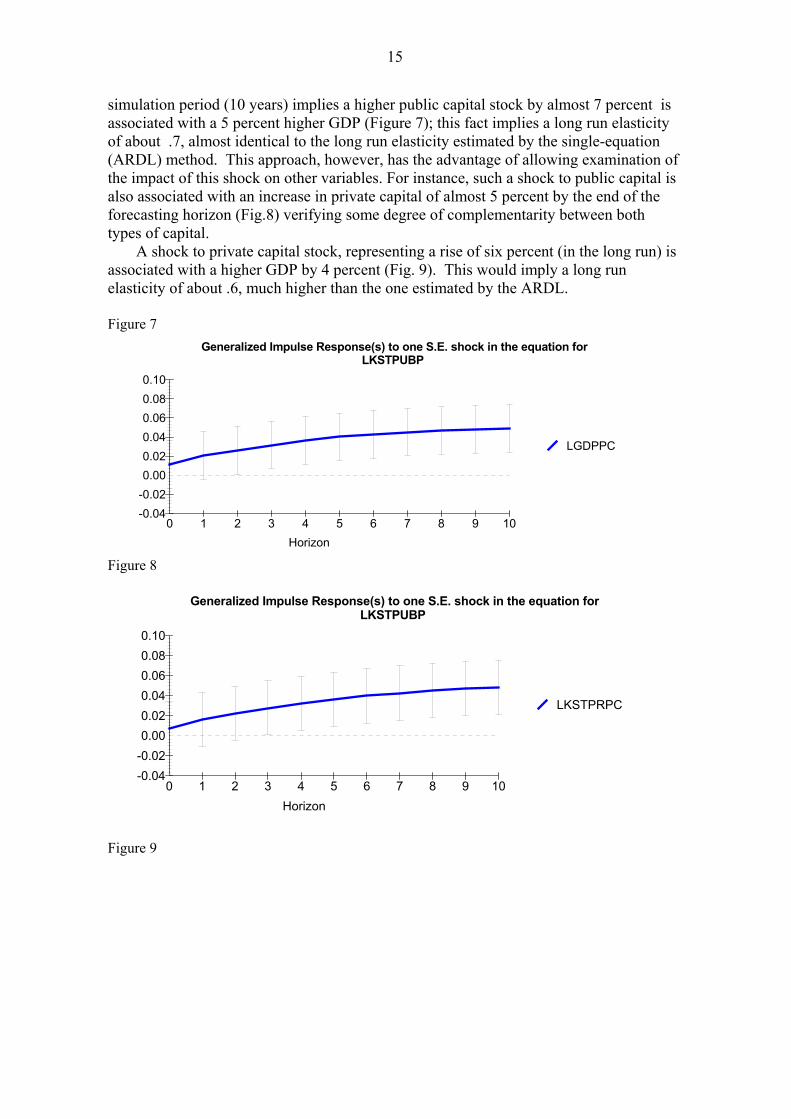
15

simulation period (10 years) implies a higher public capital stock by almost 7 percent isassociated with a 5 percent higher GDP (Figure 7); this fact implies a long run elasticityof about .7, almost identical to the long run elasticity estimated by the single-equation(ARDL) method. This approach, however, has the advantage of allowing examination ofthe impact of this shock on other variables. For instance, such a shock to public capital isalso associated with an increase in private capital of almost 5 percent by the end of theforecasting horizon (Fig.8) verifying some degree of complementarity between bothtypes of capital.

A shock to private capital stock, representing a rise of six percent (in the long run) isassociated with a higher GDP by 4 percent (Fig. 9). This would imply a long runelasticity of about .6, much higher than the one estimated by the ARDL.

Figure 7 Generalized Impulse Response(s) to one S.E. shock in the equation for

LKSTPUBP

LGDPPC

Horizon

-0.02-0.04

0.000.020.040.060.080.10

0 1 2 3 4 5 6 7 8 9 10

Figure 8

Generalized Impulse Response(s) to one S.E. shock in the equation forLKSTPUBP

LKSTPRPC

Horizon

-0.02-0.04

0.000.020.040.060.080.10

0 1 2 3 4 5 6 7 8 9 10

Figure 9

16

Generalized Impulse Response(s) to one S.E. shock in the equation forLKSTPRPC

LGDPPC

Horizon

-0.02

0.00

0.02

0.04

0.06

0.08

0 1 2 3 4 5 6 7 8 9 10

Another interesting result refers to the impact of a tax shock. A permanentincrease of the tax ratio (of 1.5 percent of GDP) is associated with a lower GDP percapita of close to 1 percent (Figure 10), similar to the ARDL result. The same shock isassociated with a lower private capital stock (Figure 11)Figure 10

Generalized Impulse Response(s) to one S.E. shock in the equation forTOTTAXGD

LGDPPC

Horizon

-0.008

-0.010

-0.012

-0.014

-0.006

0 1 2 3 4 5 6 7 8 9 10

Figure 11 Generalized Impulse Response(s) to one S.E. shock in the equation for

TOTTAXGD

LKSTPRPC

Horizon

-0.001-0.002-0.003-0.004-0.005

0.0000.0010.002

0 1 2 3 4 5 6 7 8 9 10

A shock that leads to a permanent rise of government consumption expenditure(of 7 percent in real terms) is associated with a fall in per capita GDP (Figure 12). Thisshock is associated with a higher tax ratio (Figure 13), lower private capital stock (Fig14) and lower public capital stock as well (Figure 15).Figure 12

17

Generalized Impulse Response(s) to one S.E. shock in the equation forLGOVCONP

LGDPPC

Horizon

-0.01

-0.02

-0.03

-0.04

0.00

0.01

0.02

0 1 2 3 4 5 6 7 8 9 10

Figure 13 Generalized Impulse Response(s) to one S.E. shock in the equation for

LGOVCONP

TOTTAXGDP

Horizon

-0.002

0.000

0.002

0.004

0.006

0.008

0 1 2 3 4 5 6 7 8 9 10

Figure 14 Generalized Impulse Response(s) to one S.E. shock in the equation for

LGOVCONP

LKSTPRPC

Horizon

-0.01-0.02-0.03-0.04-0.05

0.000.010.02

0 1 2 3 4 5 6 7 8 9 10

18

Figure 15 Generalized Impulse Response(s) to one S.E. shock in the equation for

LGOVCONP

LKSTPUBPC

Horizon

-0.01-0.02-0.03-0.04-0.05

0.000.010.02

0 1 2 3 4 5 6 7 8 9 10

The other two types of government expenditures, namely the subsidies and socialsecurity transfers have negligible effects on GDP in the medium term and opposingeffects in the long run. Given the small size of this type of expenditure, we will focushere on the effect of social security transfers. Social security transfers have a negativegrowth effect (Figure 16), primarily because of the associated reduction in the publicsector capital (Figure 17). A 5 percent increase in the social security payments isassociated with a fall of 3 percent in the public capital stock.

Figure 16 Generalized Impulse Response(s) to one S.E. shock in the equation for

LGOVSSTP

LGDPPC

Horizon

-0.01-0.02-0.03-0.04

0.000.010.020.03

0 1 2 3 4 5 6 7 8 9 10

Figure 17 Generalized Impulse Response(s) to one S.E. shock in the equation for

LGOVSSTP

LKSTPUBPC

Horizon

-0.02

-0.04

-0.06

-0.08

0.00

0.02

0.04

0 1 2 3 4 5 6 7 8 9 10

19

V. Conclusions and Policy Implications

During the past decade, the successful episodes of Brazilian stabilization coincidewith those when fiscal policy was flexible to change the primary surpluses, while crisesemerge when there is little flexibility to adjust to external shocks. For instance, the 1998-1999 episodes show the importance of the primary balance as a signaling tool in a worldof imperfect information. In contrast to the 1998-1999 stabilization, fiscal policy wasunresponsive to shocks in 2002, causing concerns of fiscal policy sustainability.Compounded by electoral uncertainty, the situation ended in the 2002 debt crisis

Brazilian fiscal adjustment has been of mixed quality. On one hand, most of theadjustment has been revenue-based and cutting capital expenditures. In the early nineties,the tax burden was 25% of GDP while in 2005 it reached 37%. In addition to the highlevel of taxation, the increasing share of indirect cumulative taxes and the over-taxationof a reduced tax base, generated distortions in economic decisions. On the other hand, theexpenditure composition shows the rising trend in pension payments and the inequalitythat the pension regime originated in favor of the public servants.

Our findings show that Brazilian fiscal policy is procyclical in the short run:output expansions are associated with smaller primary balances, while outputcontractions with higher ones. In the long run, however, the evidence shows that fiscalpolicy is countercyclical, that is a 1% increase in output is associated with a higherprimary balance of 0.2% of GDP.

The analyses presented in this chapter support the contention that Brazil maybenefit from increased public spending in the area of economic infrastructure. Theeconometric analysis using historical data from Brazil indicate positive and strong growtheffects of public physical capital stock and public investments. The analysis points outclearly the negative effects of increasing taxation on economic growth. Thus, it is notadvisable for Brazil to pursue its need for increasing public investments via expansionaryfiscal policy that results in a higher tax burden than the current level. Instead, a long-runsolution to recovering an adequate level of public investments must be sought inreallocation of public spending within the fixed overall fiscal envelope. This means theneed to re-examine the composition of the current expenditures, including those allocatedto the social sectors that today consume a lion’s share of Brazil’s public expenditures.

ReferencesAlesina, A and R. Perotti. (1995). “Fiscal Expansions and Adjustment in OECDCountries,” Economic Policy 21: 207-245.Aschauer, D. (1989) “Is public expenditure productive?” Journal of Monetary Economics23:177-200.Barro, R. (1990) “Government spending in a simple model of endogenous growth,”Journal of Political Economy 98(5): 103-125.Bevilaqua, A e R.L.F Werneck (1998) “Delaying Public-sector reforms: Post stabilizationFiscal Strains in Brazil,” Working Paper Series No 364, Office of the Chief Economist,Inter-American Development Bank.Candido, José Oswaldo (2001) “A produtividade dos gastos públicos no Brasil,” Texto deDiscussão No 781, Ipea, Brasilia, Brazil.Cardoso, E. (1998) “Virtual deficits and the Patinkin effect”, IMF Staff Papers, Vol. 45,No.3. DecemberCashin, P. (1995) “Government spending, taxes and economic growth,” IMF StaffPapers, 42 (2): 237-69.

20

Cavalcanti Ferreira, P. And T. Malliagros (2003) Impactos Productivos da Infra-estruturanoBrasil: 1950-1995.Drudi, F. and A. Prati (2000), “Signaling fiscal regime sustainability,” EuropeanEconomic Review, Vol. 44 pp. 1897-1930.Eisner,R.(1994) “Real government spending and the future”, Journal of EconomicBehavior and Organization, 23, pp 111-126Gavin, Hausmann, Perotti and Talvi (1996) “Managing fiscal policy in Latin Americaand the Caribbean: Volatility, Procyclicality and Limited Creditworthiness,” IADB.Mimeo, March.Hurlin, C (2001a) “Estimating the contribution of public capital with time seriesproduction functions: a case of unreliable inference”, Applied Economics Letters 8, pp99-103Hurlin, C. (2001b) How to estimate the productivity of public capital ?. Mimeo.IMF (2002). Debt Crises. What’s different about Latin America? In World EconomicOutlook 2001: Chapter 2: 61-74.Ministerio de Planejamiento (2003) “Vinculacoes das receitas dos orcamentos fiscal e daseguridad social e o poder discricionario de alocacao dos recursos do gobernó federal”.Secretaria de Orcamento Federal. Fevereiro.Muriel, Beatriz, (1999) “Gasto Público e Crescimento Econômico”, MA Dissertation,Economic Department at PUC-RJ, Brazil.Pesaran, H. and Y. Shin (1997) “An Autoregressive Distributed Lag Modeling Approachto Cointegration Analysis,” Econometrics and Economic Theory in the 20th Century: TheRanger First Centennial Symposium, Eds. S. Strom and P. Diamond, CambridgeUniversity Press.Pesaran, H., Y. Shin and R. Smith (1999) Bounds testing approaches to the analysis oflong-run relationships. MimeoReis, E, Blanco, F, Morandi, L, Mérida, M e Marcelo de Paiva Abreu. 2002. O séculoXX nas Contas Nacionais. IBGE (forthcoming)Sturm, J.E. and J. de Haan (1995)“Is public expenditure really productive?” EconomicModeling, 12, 1 pp 60-72Talvi, E and C. Vegh. (2000) Como armar el rompecabezas fiscal?: Nuevos Indicadoresde Sostenibilidad. IADB.