AIP/123-QED

The pulsed to tonal strength parameter and its importance in characterizing

and classifying Beluga whale sounds

Ramon Miralles,a) Guillermo Lara, Jose Antonio Esteban,b) and Alberto Rodriguezc)

Instituto de Telecomunicacion y Aplicaciones Multimedia (iTEAM),

Universitat Politecnica de Valencia,

Spain.

(Dated: January 11, 2012)

The pulsed to tonal strength parameter 1

Abstract

A large number of the vocalization studies in mammals are based on

time-frequency analysis of the produced sounds. The patterns, which

are extracted from the time-frequency representations, determine the

classification in the different sound categories. However, there are sit-

uations where this pattern related recognition does not allow a precise

characterization of the vocalization to be obtained. In these situations,

a feasible alternative, which can help by giving the dominant compo-

nent of the sound, is to measure the strength of the tonal and pulsed

constituent units. In this work, the use of a ratio of pulsed to tonal

strength is proposed to objectively measure the distribution of energy

between these two components. This pulsed to tonal ratio (PTR) can

be computed with the aid of the discrete cosine transform. It is demon-

strated that the PTR can be obtained with a relatively simple expres-

sion without having to go through the time-frequency representation

(TFR). This work presents examples that show how the PTR can be

used to distinguish between two very similar Beluga whale sounds and

how to dynamically track the power distribution between the pulsed

and tonal components in non-stationary signals.

PACS numbers: 4360Hj, 4380Ka, 4330Sf

2

I. MOTIVATION

The time-frequency analysis of the underwater sounds of the Beluga whale is a valuable

research technique for marine biologists. The way the energy is distributed in time and

frequency is used to classify the different sounds that are emitted by the animals. Typical

cetacean sound classifications include pulsed and tonal sounds as well as a large variety

of combinations and alterations of these two main categories. The process of categorizing

whale songs in discrete sets is complex and typically emphasizes the distinctive properties

of proto-typical units that are heard from a distance1.

The classification process, as with many other maritime mammals, involves recognizing

the patterns that the sounds produce in the time-frequency representations (TFR)2,3 and

how the energy is distributed in the different parts of the whale song. The process, which

is normally done with the aid of software tools, is frequently supervised by a trained re-

searcher after listening and analyzing the TFR of a whale sound. However, there are some

situations where the software algorithms based on geometric parameter extraction from the

TFR patterns do not guarantee a correct recognition of the vocalization category. In these

situations, even having an expert carefully listen to the vocalizations does not ensure a pre-

cise and objective classification of the sound. An example of this is what happens when

trying to classify Beluga whale sounds that mix several elements (whistles, regular clicks,

and rapid-click buzzes (creaks)) in the same vocalization. The examination of the TFR of

these sounds using false color images does not allow the researchers to precisely determine

if the sound has a dominant pulsed or tonal component. Figure 1 illustrates this problem.

Establishing a threshold to classify sound units as pulsed or tonal just by listening to it

is also rather arbitrary and subjective. It would be more interesting if we could extract

a)Electronic address: rmiralle@dcom.upv.esb)Parques Reunidos Valencia S. A. L’Oceanografic, Ciudad de las Artes y las Ciencias,

Valencia, Spain.c)Departamento de Ingenierıa de Comunicaciones, Universidad Miguel Hernandez, Spain.

3

Time (seconds)

Fre

quen

cy (

Hz)

Tonal

com

ponen

ts

0 0.1 0.2 0.3 0.4 0.5 0.60

0.5

1

1.5

2

2.5

3

3.5

4

4.5

x 104

Pulsed components

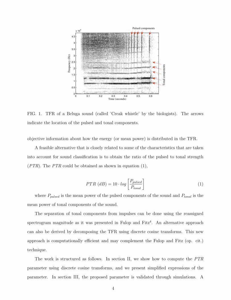
FIG. 1. TFR of a Beluga sound (called ’Creak whistle’ by the biologists). The arrows

indicate the location of the pulsed and tonal components.

objective information about how the energy (or mean power) is distributed in the TFR.

A feasible alternative that is closely related to some of the characteristics that are taken

into account for sound classification is to obtain the ratio of the pulsed to tonal strength

(PTR). The PTR could be obtained as shown in equation (1),

PTR (dB) = 10 · log[Ppulsed

Ptonal

](1)

where Ppulsed is the mean power of the pulsed components of the sound and Ptonal is the

mean power of tonal components of the sound.

The separation of tonal components from impulses can be done using the reassigned

spectrogram magnitude as it was presented in Fulop and Fitz4. An alternative approach

can also be derived by decomposing the TFR using discrete cosine transforms. This new

approach is computationally efficient and may complement the Fulop and Fitz (op. cit.)

technique.

The work is structured as follows. In section II, we show how to compute the PTR

parameter using discrete cosine transforms, and we present simplified expressions of the

parameter. In section III, the proposed parameter is validated through simulations. A

4

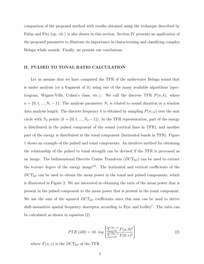
comparison of the proposed method with results obtained using the technique described by

Fulop and Fitz (op. cit.) is also shown in this section. Section IV presents an application of

the proposed parameter to illustrate its importance in characterizing and classifying complex

Beluga whale sounds. Finally, we present our conclusions.

II. PULSED TO TONAL RATIO CALCULATION

Let us assume that we have computed the TFR of the underwater Beluga sound that

is under analysis (or a fragment of it) using one of the many available algorithms (spec-

trogram, Wigner-Ville, Cohen’s class, etc.). We call the discrete TFR P (n, k), where

n = {0, 1, ..., N1 − 1}. The analysis parameter N1 is related to sound duration or a window

data analysis length. The discrete frequency k is obtained by sampling P (n, ω) over the unit

circle with N2 points (k = {0, 1, ..., N2− 1}). In the TFR representation, part of the energy

is distributed in the pulsed component of the sound (vertical lines in TFR), and another

part of the energy is distributed in the tonal component (horizontal bands in TFR). Figure

1 shows an example of the pulsed and tonal components. An intuitive method for obtaining

the relationship of the pulsed to tonal strength can be devised if the TFR is processed as

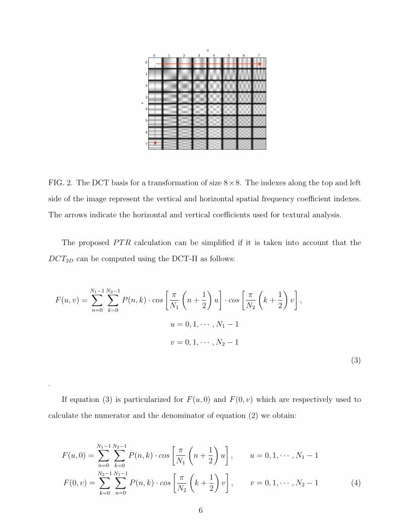
an image. The bidimensional Discrete Cosine Transform (DCT2D) can be used to extract

the texture degree of the energy image5,6. The horizontal and vertical coefficients of the

DCT2D can be used to obtain the mean power in the tonal and pulsed components, which

is illustrated in Figure 2. We are interested in obtaining the ratio of the mean power that is

present in the pulsed component to the mean power that is present in the tonal component.

We use the sum of the squared DCT2D coefficients since this sum can be used to derive

shift-insensitive spatial frequency descriptor according to Frye and Ledley7. The ratio can

be calculated as shown in equation (2)

PTR (dB) = 10 · log

[∑N1−1u=0 F (u, 0)2∑N2−1v=0 F (0, v)2

](2)

where F (u, v) is the DCT2D of the TFR .

5

u

v

0 1 2 3 4 5 6 7

0

1

2

3

4

5

6

7

FIG. 2. The DCT basis for a transformation of size 8×8. The indexes along the top and left

side of the image represent the vertical and horizontal spatial frequency coefficient indexes.

The arrows indicate the horizontal and vertical coefficients used for textural analysis.

The proposed PTR calculation can be simplified if it is taken into account that the

DCT2D can be computed using the DCT-II as follows:

F (u, v) =

N1−1∑n=0

N2−1∑k=0

P (n, k) · cos[π

N1

(n+

1

2

)u

]· cos

[π

N2

(k +

1

2

)v

],

u = 0, 1, · · · , N1 − 1

v = 0, 1, · · · , N2 − 1

(3)

.

If equation (3) is particularized for F (u, 0) and F (0, v) which are respectively used to

calculate the numerator and the denominator of equation (2) we obtain:

F (u, 0) =

N1−1∑n=0

N2−1∑k=0

P (n, k) · cos[π

N1

(n+

1

2

)u

], u = 0, 1, · · · , N1 − 1

F (0, v) =

N2−1∑k=0

N1−1∑n=0

P (n, k) · cos[π

N2

(k +

1

2

)v

], v = 0, 1, · · · , N2 − 1 (4)

6

.

It can be observed from equation (4) that only TFR marginals need to be calculated.

The discrete time and frequency marginals are given by equations (5) and (6), respectively.

P (n) =

N2−1∑k=0

P (n, k) (5)

P (k) =

N1−1∑n=0

P (n, k) (6)

Note that now, in the computation of equation (4), only one-dimensional DCTs are

needed. Depending on the TFR associated to the computed marginals, equations (5) and

(6) can be simplified even more, and optimum and fast algorithms can be devised to calculate

the PTR.

A. Computation of the PTR with marginals of the Spectrogram

As a first example, we can obtain the marginals assuming that P (n, k) is the Spectrogram

computed using the short-time Fourier Transform. We define DFTN2 [.] as an operator to

compute the discrete-time, discrete-frequency Fourier Transform with N2 being the number

of equally spaced samples from ω = 0 to 2π. We use x(n) to design the sound fragment of

interest where we want to compute the PTR. We also call the N2 analysis window w(n),

which is assumed to be non-zero only in the interval n = [0, 1, ..., N2 − 1]. The marginals

(5) and (6) can then be written as equations (7) and (8), respectively:

P (n) =

N2−1∑k=0

| DFTN2 [w(m) · x(n−m)] |2

= N2

N2−1∑m=0

| w(m) · x(n−m) |2= N2 · x(n) (7)

P (k) =

N1−1∑n=0

| DFTN2 [w(m) · x(n−m)] |2= X(k) (8)

7

Equation (7) has been simplified using Parseval’s theorem, and it shows that the time

marginal is proportional to the smoothed energy calculation of the sound fragment using

the sliding window w(n). We use x(n) to refer to this smoothed energy estimation. Equa-

tion (8) shows that the frequency marginal is equivalent (with a scale factor) to smoothed

spectra estimation using Bartlett’s method8. We use X(k) to refer to the smoothed spectra

estimation. Taking all this into account, equation (2) can be computed using the results of

equation (9) and (10).

F (u, 0) = DCT1D[N2 · x(n)] (9)

F (0, v) = DCT1D[X(k)] (10)

with x(n) and X(k) previously defined. In this case, only one-dimensional discrete cosine

transforms are required (DCT1D[.]). This greatly simplifies the computation.

B. Computation of the PTR with distributions that satisfy marginal properties

The computation of the PTR can be simplified even more if the associated discrete

TFR satisfies marginal properties such as discrete Wigner Ville Distribution9,10 or discrete

positive distributions (Coehn’s class type II11, etc.). For these distributions, equations (5)

and (6) result in:

P (n) = K1· | x(n) |2 (11)

P (k) = K2· | X(k) |2 (12)

,

where X(k) = DFTN2 [x(n)]. The constants K1 and K2 depend on how the particular

positive distribution is extended to discrete-time signals. Table I illustrates the possible

values for K1 and K2, which are extracted from some of the alternatives for computing the

discrete-time, discrete-frequency TFRs9,10,12.

8

Thus equation (2) can also be computed using equations (13) and (14).

F (u, 0) = DCT1D[K1 · |x(n)|2] (13)

F (0, v) = DCT1D[K2 · |X(k)|2] (14)

with K1 and K2, which have already been given in Table I.

The proposed computation of the PTR presented in subsections II.A and II.B, which

only involves marginals, is not affected by inherent problems of the TFR computation such

as cross-terms. Additionally, resolution and parameter setup becomes an easy task, and as

a result classical spectral density estimation concepts can be used8.

C. Application to non stationary audio signals with slow variation of the PTR

In the analysis of bioacustic signals, it is quite frequent to find slow variations of the

tonal or pulsed components. The simplifications proposed above allow the PTR parameter

to be easily computed and used to dynamically track the pulsed to tonal strength ratio.

To do so, we refer as r(n) the audio signal where we want to compute the evolution of

the PTR. We also use a temporal rectangular window v(n) of length N = N1 + N2. With

the algorithm described in subsection II.B we can compute the evolution of the PTR as the

moving window v(n) slides over the audio signal r(n). The evolution of the PTR in a given

sound can be a valuable tool for examining and comparing sounds. It can be also used to

establish thresholds to determine if the cetacean vocalization is more pulsed than tonal or

vice versa.

III. SIMULATION

We have used MATLAB to create synthetic sounds with controlled pulsed and tonal

mean power. Equation (15) models how the synthetic sounds were obtained.

9

xi(t) = w(t) +∑m

Π

(t−m · ρ−1

pulsed

Tpulsed

)· m(t) +

Nh∑m=1

A · sin (2πf0 ·m · t) (15)

In equation (15), {w(t)} and {m(t)} are zero mean Gaussian stochastic processes that

respectively model the observation noise (mean power σ2w) and the pulsed bursts (mean power

σ2m). The function Π(t/T ) is the rectangular function of duration T . Some other variables

appear in the model in equation (15): the pulsed burst length (Tpulsed), the density of pulses

per second (ρpulsed), the amplitude of the tonal component (A), the central frequency of

the tonal component (f0) and the number of harmonics (Nh). Parameters in equation (15)

ensure that ρ−1pulsed > Tpulsed to avoid overlapping of pulsed components. In all the simulations

presented in this section, the signals have been sampled at fs = 96 kHz.

Theoretical PTR was computed as stated in equation (16).

PTRtheo (dB) = 10 · log[ρpulsed · Tpulsed · σ2

m

Nh · A2/2

](16)

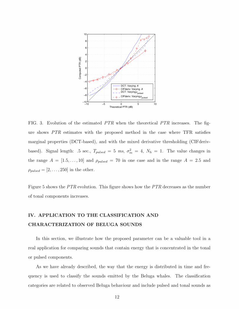
Figure 3 shows simulations of the above equations for the proposed DCT-based esti-

mator in two cases: when the amplitude of the tonal component (A) increases and the

rest of the variables remain fixed; and when ρpulsed increases and the rest of the variables

remain fixed. The figure also shows a comparison of the PTR when the tonal and pulsed

components are separated using the reassigned spectrogram through the Channelized Instan-

taneous Frequency with mixed partial Derivative (CIFderiv) thresholding4. The thresholds

were selected based on the recommendations by Fulop and Fitz (op. cit.). A threshold

value of 0.01 was used for isolating tonal components, whereas threshold values of between

0.75 and 1.25 were used for isolating pulsed components. The reassigned spectrogram was

computed using frames of 256 points and a frame advance of 20 points. A Hanning window

was employed in the spectrogram computation.

The comparison in Figure 3 shows that both techniques give quite an accurate estimation

of the real PTR. However, the proposed DCT-based estimation gives a higher sensitivity to

small changes in low PTR signals. The figure also shows that, even though the proposed

10

estimators of the PTR have some bias and are not linear, they are monotonically increasing

in the simulation range. The maximum bias observed in the [-10,10] dB range is obtained

at the ends of the curve, when the sound is mainly tonal or pulsed. In these situations,

the measured error is approximately 4 dB for the DCT-based estimator and 6 dB for the

CIFderiv-based estimator. Despite the observed bias, the proposed estimator can be a

valuable technique to measure slight variations in the way power changes between the tonal

or pulsed components as we discussed in section IV.

It is interesting to observe that, even though the Fulop and Fitz method allows high

quality TFR to be obtained, it has a high computational cost. Thus, in situations where we

are only interested in obtaining an estimation of the amount of power distributed between

the pulsed and tonal components, the proposed DCT-based computation of the PTR is a

better alternative. Also, the low computational cost allows this technique to be used to

track the PTR in non-stationary signals.

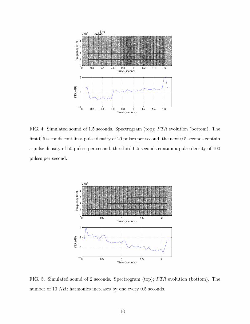
Let us now observe the behaviour when there are non-stationary audio signals with slow

variation of the PTR. Observation noise has been modelled as described above. The pulsed

bursts have been simulated with zero mean Gaussian noise Tpulsed = 5 ms and σ2m = 4. The

number of harmonics has been set to Nh = 3. The signal has been obtained by joining

three fragments of 0.5 seconds. The first 0.5 seconds contain a pulse density of 20 bursts

per second, the second 0.5 seconds contains a pulse density of 50 bursts per second, and,

finally, the third 0.5 seconds contains a pulse density of 100 bursts per second. Figure 4

illustrates the spectrogram (top) of one of these synthetic sounds. Figure 4 (bottom) shows

the estimated PTR evolution. The window length used to obtain the PTR evolution was

N = 5000 samples (≈ 52 ms at fs = 96 kHz). This graph shows that as the density of bursts

increases, the PTR reflects this behaviour.

Similarly, we have created a synthetic sound to illustrate the behaviour when the number

of tonal components increases. We have used a pulse density of 70 bursts per second in the

whole audio register, and we have increased the number of 10 KHz harmonics by one every

0.5 seconds. The top graph of Figure 5 shows the spectrogram and the bottom graph of

11

−10 −5 0 5 10−10

−8

−6

−4

−2

0

2

4

6

8

10

Theoretical PTR (dB)

Co

mp

ute

d P

TR

(d

B)

DCT: Varying A

CIFderiv: Varying ADCT: Varying ρ

pulsed

CIFderiv: Varying ρpulsed

FIG. 3. Evolution of the estimated PTR when the theoretical PTR increases. The fig-

ure shows PTR estimates with the proposed method in the case where TFR satisfies

marginal properties (DCT-based), and with the mixed derivative thresholding (CIFderiv-

based). Signal length: .5 sec., Tpulsed = 5 ms, σ2m = 4, Nh = 1. The value changes in

the range A = [1.5, . . . , 10] and ρpulsed = 70 in one case and in the range A = 2.5 and

ρpulsed = [2, . . . , 250] in the other.

Figure 5 shows the PTR evolution. This figure shows how the PTR decreases as the number

of tonal components increases.

IV. APPLICATION TO THE CLASSIFICATION AND

CHARACTERIZATION OF BELUGA SOUNDS

In this section, we illustrate how the proposed parameter can be a valuable tool in a

real application for comparing sounds that contain energy that is concentrated in the tonal

or pulsed components.

As we have already described, the way that the energy is distributed in time and fre-

quency is used to classify the sounds emitted by the Beluga whales. The classification

categories are related to observed Beluga behaviour and include pulsed and tonal sounds as

12

Time (seconds)

Fre

quen

cy (

Hz)

0 0.2 0.4 0.6 0.8 1 1.2 1.4 1.60

1

2

3

4

x 104

0 0.2 0.4 0.6 0.8 1 1.2 1.4 1.6−5

0

5P

TR

(dB

)

Time (seconds)

5 ms

FIG. 4. Simulated sound of 1.5 seconds. Spectrogram (top); PTR evolution (bottom). The

first 0.5 seconds contain a pulse density of 20 pulses per second, the next 0.5 seconds contain

a pulse density of 50 pulses per second, the third 0.5 seconds contain a pulse density of 100

pulses per second.

Time (seconds)

Fre

quen

cy (

Hz)

0 0.5 1 1.5 20

1

2

3

4

x 104

0 0.5 1 1.5 2−2

0

2

4

PT

R (

dB

)

Time (seconds)

FIG. 5. Simulated sound of 2 seconds. Spectrogram (top); PTR evolution (bottom). The

number of 10 KHz harmonics increases by one every 0.5 seconds.

13

well as a combination of these two main categories. In some situations, simple observation

of the TFR or listening to the sounds is not enough to determine if a given Beluga vocaliza-

tion has a predominant “pulsed” component or a predominant “tonal” component. In these

situations, the calculation of the proposed PTR can help to decide.

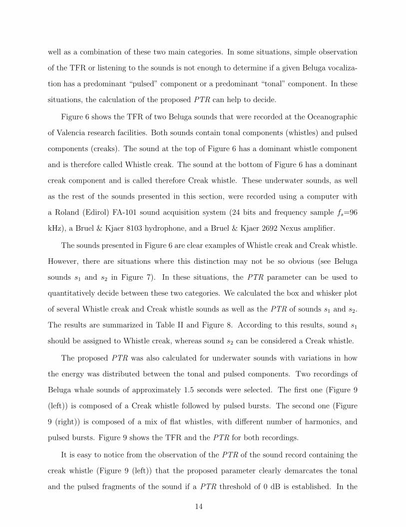
Figure 6 shows the TFR of two Beluga sounds that were recorded at the Oceanographic

of Valencia research facilities. Both sounds contain tonal components (whistles) and pulsed

components (creaks). The sound at the top of Figure 6 has a dominant whistle component

and is therefore called Whistle creak. The sound at the bottom of Figure 6 has a dominant

creak component and is called therefore Creak whistle. These underwater sounds, as well

as the rest of the sounds presented in this section, were recorded using a computer with

a Roland (Edirol) FA-101 sound acquisition system (24 bits and frequency sample fs=96

kHz), a Bruel & Kjaer 8103 hydrophone, and a Bruel & Kjaer 2692 Nexus amplifier.

The sounds presented in Figure 6 are clear examples of Whistle creak and Creak whistle.

However, there are situations where this distinction may not be so obvious (see Beluga

sounds s1 and s2 in Figure 7). In these situations, the PTR parameter can be used to

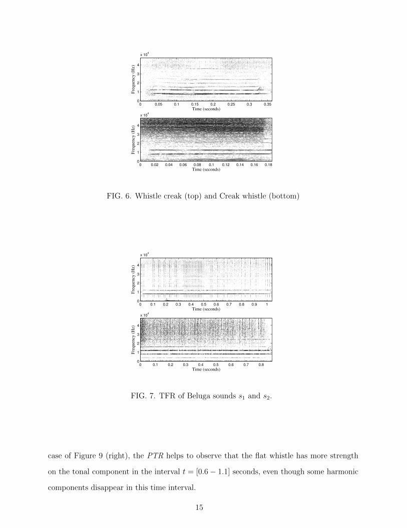
quantitatively decide between these two categories. We calculated the box and whisker plot

of several Whistle creak and Creak whistle sounds as well as the PTR of sounds s1 and s2.

The results are summarized in Table II and Figure 8. According to this results, sound s1

should be assigned to Whistle creak, whereas sound s2 can be considered a Creak whistle.

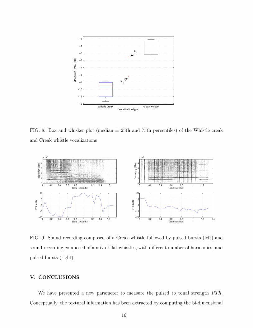
The proposed PTR was also calculated for underwater sounds with variations in how

the energy was distributed between the tonal and pulsed components. Two recordings of

Beluga whale sounds of approximately 1.5 seconds were selected. The first one (Figure 9

(left)) is composed of a Creak whistle followed by pulsed bursts. The second one (Figure

9 (right)) is composed of a mix of flat whistles, with different number of harmonics, and

pulsed bursts. Figure 9 shows the TFR and the PTR for both recordings.

It is easy to notice from the observation of the PTR of the sound record containing the

creak whistle (Figure 9 (left)) that the proposed parameter clearly demarcates the tonal

and the pulsed fragments of the sound if a PTR threshold of 0 dB is established. In the

14

Time (seconds)

Fre

quen

cy (

Hz)

0 0.05 0.1 0.15 0.2 0.25 0.3 0.350

1

2

3

4

x 104

Time (seconds)

Fre

quen

cy (

Hz)

0 0.02 0.04 0.06 0.08 0.1 0.12 0.14 0.16 0.180

1

2

3

4

x 104

FIG. 6. Whistle creak (top) and Creak whistle (bottom)

Time (seconds)

Fre

quen

cy (

Hz)

0 0.1 0.2 0.3 0.4 0.5 0.6 0.7 0.8 0.9 10

1

2

3

4

x 104

Time (seconds)

Fre

quen

cy (

Hz)

0 0.1 0.2 0.3 0.4 0.5 0.6 0.7 0.80

1

2

3

4

x 104

FIG. 7. TFR of Beluga sounds s1 and s2.

case of Figure 9 (right), the PTR helps to observe that the flat whistle has more strength

on the tonal component in the interval t = [0.6− 1.1] seconds, even though some harmonic

components disappear in this time interval.

15

−12

−11

−10

−9

−8

−7

−6

−5

−4

−3

whistle creak creak whistleVocalization type

Me

asu

red

P

TR

(d

B)

*

*

s1

s2

FIG. 8. Box and whisker plot (median ± 25th and 75th percentiles) of the Whistle creak

and Creak whistle vocalizations

Time (seconds)

Fre

qu

ency

(H

z)

0 0.2 0.4 0.6 0.8 1 1.2 1.4 1.60

1

2

3

4

x 104

0 0.2 0.4 0.6 0.8 1 1.2 1.4 1.6−10

−5

0

5

10

PT

R (

dB

)

Time (seconds)

Time (seconds)

Fre

qu

ency

(H

z)

0 0.2 0.4 0.6 0.8 1 1.20

1

2

3

4

x 104

0 0.2 0.4 0.6 0.8 1 1.2 1.4−20

−10

0

10

20

PT

R (

dB

)

Time (seconds)

FIG. 9. Sound recording composed of a Creak whistle followed by pulsed bursts (left) and

sound recording composed of a mix of flat whistles, with different number of harmonics, and

pulsed bursts (right)

V. CONCLUSIONS

We have presented a new parameter to measure the pulsed to tonal strength PTR.

Conceptually, the textural information has been extracted by computing the bi-dimensional

16

cosine transform of the TFR. A mathematical demonstration shows that the proposed pa-

rameter can be easily obtained without computing the TFR and using only one-dimensional

discrete cosine transforms.

Simulations have demonstrated that the proposed PTR gives information about the

mean power in the pulsed component in relation to the mean power in the tonal component

of a given signal. A comparison with previously published techniques, such us the reas-

signed spectrogram, have shown that the proposed method gives similar results with less

computational complexity. A real example has shown the utility of the parameter in helping

to classify Beluga sounds with mixed pulsed and tonal elements in the same vocalization,

using objective criteria. The PTR parameter can also be used in other bioacoustic sounds

or in other completely different areas such us the monitoring of cracks in engines or turbines

using the nondestructive testing technique of acoustic emission.

Acknowledgments

This work was supported by the national R + D program under Grant TEC2011-23403

(Spain), the Generalitat Valenciana PROMETEO 2010/040, and the Catedra Telefonica in

the Universitat Politecnica de Valencia.

References

1 E. Mercado, J. Schneider, A. Pack, and L. Herman, “Sound production by singing hump-

back whales”, J. Acoustic. Soc. Am. 127, 2678–2691 (2010).

2 J. N. Oswald, S. Rankin, J. Barlow, and M. Lammers, “A tool for real-time acoustic

species identification of delphinid whistles”, J. Acoust. Soc. Am. 122, 587–595 (2007).

3 C. Ioana, C. Gervaise, Y. Stephan, and J. I. Mars, “Analysis of underwater mammal

vocalisations using time-frequency-phase tracker”, Applied Acoustics 71, 1070 – 1080

(2010).

17

4 S. Fulop and K. Fitz, “Separation of components from impulses in reassigned spectro-

grams”, J. Acoust. Soc. Am. 121, 1510–1518 (2007).

5 Y. Huang and R. Chang, “Texture features for DCT-coded image retrieval and classifica-

tion”, in Acoustics, Speech, and Signal Processing, 1999. ICASSP ’99. Proceedings., on

1999 IEEE International Conference, volume 6, 3013–3016 vol.6 (1999).

6 D. Sim, H. Kim, and R. Park, “Fast texture description and retrieval of DCT-based

compressed images”, Electronics Letters 37, 18–19 (2001).

7 R. E. Frye and R. S. Ledley, “Texture discrimination using discrete cosine transformation

shift-insensitive (DCTSIS) descriptors”, Pattern Recognition 33, 1585–1598 (2000).

8 J. G. Proakis and D. K. Manolakis, Digital Signal Processing, pp. 910-911, 4 edition

(Prentice Hall, Upper Saddle River, New Jersey) (2006).

9 E. Chassande-Mottin and A. Pai, “Discrete time and frequency Wigner-Ville distribution:

Moyal’s formula and aliasing”, Signal Processing Letters, IEEE 12, 508 – 511 (2005).

10 M. Richman, T. Parks, and R. Shenoy, “Discrete-time, discrete-frequency time-frequency

representations”, in Acoustics, Speech, and Signal Processing, 1995. ICASSP-95, vol-

ume 2, 1029 – 1032 vol.2 (1995).

11 A. Papandreou-Suppappola, Applications in Time-Frequency Signal Processing, pp. 273-

306, 1 edition (CRC Press, Boca Raton, London, New York, Washington, D.C.) (2002).

12 F. Hlawatsch and T. Twaroch, “Extending the characteristic function method for joint a-b

and time-frequency analysis”, in Acoustics, Speech, and Signal Processing, 1997. ICASSP-

97., 1997 IEEE International Conference on, volume 3, 2049 – 2052 vol.3 (1997).

18

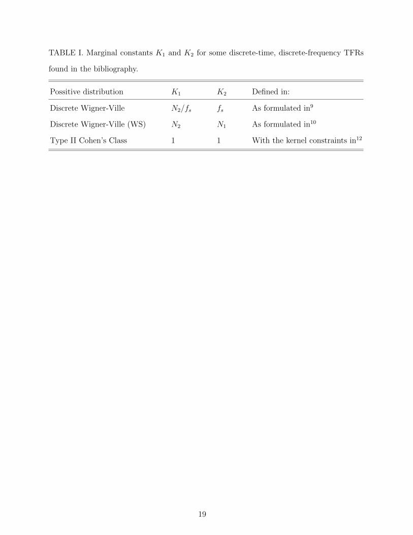
TABLE I. Marginal constants K1 and K2 for some discrete-time, discrete-frequency TFRs

found in the bibliography.

Possitive distribution K1 K2 Defined in:

Discrete Wigner-Ville N2/fs fs As formulated in9

Discrete Wigner-Ville (WS) N2 N1 As formulated in10

Type II Cohen’s Class 1 1 With the kernel constraints in12

19

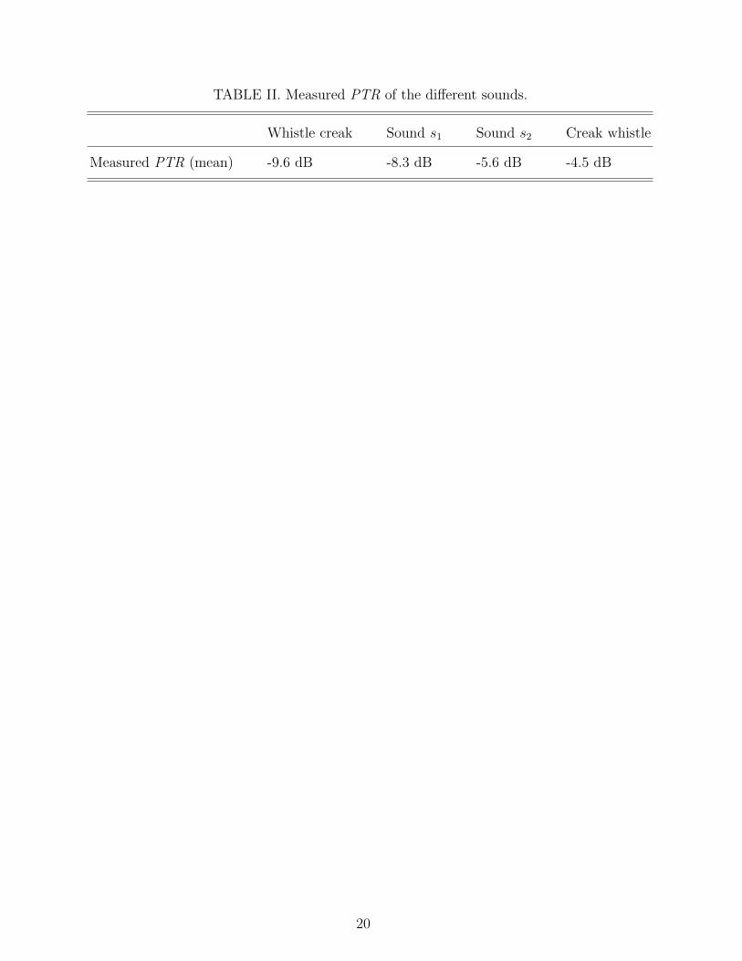
TABLE II. Measured PTR of the different sounds.

Whistle creak Sound s1 Sound s2 Creak whistle

Measured PTR (mean) -9.6 dB -8.3 dB -5.6 dB -4.5 dB

20

List of Figures

FIG. 1 TFR of a Beluga sound (called ’Creak whistle’ by the biologists). The arrows

indicate the location of the pulsed and tonal components. . . . . . . . . . . 4

FIG. 2 The DCT basis for a transformation of size 8 × 8. The indexes along the

top and left side of the image represent the vertical and horizontal spatial

frequency coefficient indexes. The arrows indicate the horizontal and vertical

coefficients used for textural analysis. . . . . . . . . . . . . . . . . . . . . . . 6

FIG. 3 Evolution of the estimated PTR when the theoretical PTR increases. The

figure shows PTR estimates with the proposed method in the case where TFR

satisfies marginal properties (DCT-based), and with the mixed derivative

thresholding (CIFderiv-based). Signal length: .5 sec., Tpulsed = 5 ms, σ2m = 4,

Nh = 1. The value changes in the range A = [1.5, . . . , 10] and ρpulsed = 70 in

one case and in the range A = 2.5 and ρpulsed = [2, . . . , 250] in the other. . . 12

FIG. 4 Simulated sound of 1.5 seconds. Spectrogram (top); PTR evolution (bottom).

The first 0.5 seconds contain a pulse density of 20 pulses per second, the next

0.5 seconds contain a pulse density of 50 pulses per second, the third 0.5

seconds contain a pulse density of 100 pulses per second. . . . . . . . . . . . 13

FIG. 5 Simulated sound of 2 seconds. Spectrogram (top); PTR evolution (bottom).

The number of 10 KHz harmonics increases by one every 0.5 seconds. . . . . 13

FIG. 6 Whistle creak (top) and Creak whistle (bottom) . . . . . . . . . . . . . . . . 15

FIG. 7 TFR of Beluga sounds s1 and s2. . . . . . . . . . . . . . . . . . . . . . . . 15

FIG. 8 Box and whisker plot (median ± 25th and 75th percentiles) of the Whistle

creak and Creak whistle vocalizations . . . . . . . . . . . . . . . . . . . . . . 16

FIG. 9 Sound recording composed of a Creak whistle followed by pulsed bursts (top)

and sound recording composed of a mix of flat whistles, with different number

of harmonics, and pulsed bursts (bottom) . . . . . . . . . . . . . . . . . . . 17

21