The power of backtracking and the confinement of length

THE POWER OF BACKTRACKING AND THE CONFINEMENT

OF LENGTH

TIMOTHY H. MCNICHOLL

Abstract. We show that there is a point on a computable arc that does not

belong to any computable rectifiable curve. We also show that there is a pointon a computable rectifiable curve with computable length that does not belong

to any computable arc.

1. Introduction

The famous traveling salesman problem is, given a finite list of cities and thedistances between them, to determine if there is a route that visits each city exactlyonce and whose total distance is below some given bound. A related problem is theHamiltonian circuit problem: given a finite graph, determine if it has a Hamiltoniancircuit. Both problems iare NP-complete [8].

In 1990, P. Jones proposed and solved the analyst’s traveling salesman problem[12]. Namely, which subsets of the plane are contained in a rectifiable curve? In1992, K. Okikiolu solved the n-dimensional version of this problem [18]. Such curveshave finite length, but may backtrack.

Recently, X. Gu, J. Lutz, and E. Mayordomo considered and solved a computableversion of this problem [9]. Namely, which points in n-dimensional Euclidean spacebelong to computable rectifiable curves? The results uncovered deep connectionswith topics in algorithmic randomness and effective Hausdorff dimension [6], [15].

Here, we consider yet another effective version of the analyst’s traveling sales-man problem: which points belong to computable arcs. By an arc, we mean ahomeomorphic image of [0, 1]. By a computable arc we mean one for which thereis a computable homeomorphism. Thus, an arc can not backtrack, but may haveinfinite length. This problem is thus a computable and continuous variation on theHamiltonian circuit problem. It is well-known that there are computable arcs withinfinite length. In fact, many fractal curves have this property [7].

Interestingly, the continuous version of the Hamiltonian circuit problem wassolved in 1917 by R.L. Moore and J.R. Kline [17]. Whereas the work of Jones andOkikiolu seems to translate more or less directly into the framework of computabil-ity, the methods of Kline and Moore so not appear to do so.

As suggested in [9], these results can be interpreted in terms of the possible planarmotion of a nanobot. The effective version of the traveling salesman problem askswhich points could be reached if the nanobot is allowed to backtrack but must followa path of finite length. In this case, since backtracking is allowed, the finite lengthrequirement seems to be a reasonable way of excluding space-filling curves [11].

2000 Mathematics Subject Classification. Primary 03F60, 03D32, 54D05 .

1

arX

iv:1

106.

3310

v1 [

mat

h.L

O]

16

Jun

2011

2 TIMOTHY H. MCNICHOLL

The effective version of the Hamiltonian circuit problem asks which points couldbe reached if backtracking is prohibited but paths of infinite length are allowed.

Here, we compare these two classes of points. Our conclusion is that neither iscontained in the other. Accordingly, our first main result is that there is a pointon a computable arc that does not belong to any computable rectifiable curve.Thus, if backtracking is prohibited but the traverse of an infinite length is allowed,there are points which could be reached by the nanobot that it could not reacheven with backtracking once its path is required to have finite length. We give twoproofs which reveal connections with algorithmic randomness as well as effectiveHausdorff dimension.

Our second main result is that there is a ∆02 point that belongs to a computable

rectifiable curve with computable length but that does not belong to any computablearc. That is, if backtracking is allowed, then there are points that can be reachedby a nanobot that could not be reached when backtracking is prohibited even if itmust traverse a path whose length is a computable real. The proof is a finite-injurypriority argument [20] which also uses recent results on effective local connectivityand the computation of space-filling curves [5], [4]. We note that Ko has shownthere is a computable rectifiable curve whose length is not computable [13]. Thus,the point we construct here belongs to a smaller class than that considered by Lutzet. al..

2. Background and preliminaries from computability and computableanalysis

Our approach to computable analysis is more or less that which appears in [21].We assume familiarity with the fundamental concepts of computability [1], [3].

A rational interval is an open interval whose endpoints are rational. A rationalrectangle is a Cartesian product of two rational intervals.

A name of a real number x is a list of all rational intervals to which x belongs.A real is computable if it has a computable name.

A name of a point p ∈ R2 is a list of all rational rectangles to which x belongs.A name of an open set U ⊆ R2 is a list of all rational rectangles R such that

R ⊆ U .A set X ⊆ R2 is computably compact if it is possible to uniformly compute from

a number k ∈ N a finite covering of X by rational rectangles each of which containsa point of X and has diameter less than 2−k.

A function f :⊆ R → R2 is computable if there is a Turing machine with aone-way output tape and with the property that whenever a name of an x ∈ R iswritten on its input tape and the machine is allowed to run indefinitely, a name off(x) is written on the output tape. Equivalently, there is an e-reduction ([3]) thatmaps each name of any x ∈ dom(f) to a name of f(x).

A subset of the plane is a curve if it is the range of a continuous function whosedomain is [0, 1]. If at least one such function is computable, then the curve is alsosaid to be computable. A subset of the plane is an arc if it is a homeomorphic imageof [0, 1]. An arc is computable if at least one such homeomorphism is computable.

Every arc is a curve. Thus, there is a clash of terminology here since thereare arcs which are computable as curves but for which there is no computablehomeomorphism with [0, 1] [10]. However, context will always make clear whichsense of ‘computable’ is intended. That is, whenever we are considering a curve, if

THE POWER OF BACKTRACKING AND THE CONFINEMENT OF LENGTH 3

the curve is also an arc, it will be called computable just in case it is the image of[0, 1] under a computable homeomorphism. Otherwise, it will be called computablejust in case it is the image of [0, 1] under a computable map.

A curve is computably rectifiable if it has finite length and its length is a com-putable real.

Since [0, 1] is compact, a function f : [0, 1] → R2 is a homeomorphism if andonly if it is continuous and injective. See, e.g. Theorem 2-103 of [11].

A set X ⊆ R2 is effectively locally connected if there is a Turing machine witha one-way output tape and two input tapes and with the property that whenevera name of a point p ∈ X is written on the first input tape and a name of an openset U ⊆ R2 that contains p is written on the second input tape and the machineis allowed to run indefinitely, a name of an open set V ⊆ R2 for which p ∈ Vand V ∩ X is connected is written on the output tape. See [16], [2], [5], [4]. Thefollowing is a consequence of the main theorem of [4] and is an effective version ofthe Hahn-Mazurkiewicz Theorem [11].

Theorem 2.1. If X ⊆ R2 is computably compact and effectively locally connected,then there is a computable surjection of [0, 1] onto X.

We will use a number of concepts from [5]. However, as we will only work in R2,we specialize their definitions as follows. To begin, a sequence of sets (U1, . . . , Un)is a chain if Ui ∩Ui+1 6= ∅ whenever 1 ≤ i < n and is a simple chain if Ui ∩Uj 6= ∅precisely when |i− j| = 1.

A simple chain (V1, . . . , Vl) in a topological space refines a simple chain (U1, . . . , Uk)if there are numbers s1, . . . , sk such that

∑sj = l, sj ≥ 2,

V1, . . . , Vs1 ⊆ U1, and

Vs1+...+si−1+1, . . . , Vs1+...+si ⊆ Ui whenever 1 < i ≤ k.

We say that this refinement has type (s1, . . . , sk).A witnessing chain is a chain of rational rectangles. We denote witnessing chains

by ω and its accented and subscripted variants. If ω = (R1, . . . , Rk) is a witnessingchain, then we let:

kω = k

Rω,i = Ri

Vω =⋃i

Ri

An arc chain is a sequence of witnessing chains (ω1, . . . , ωl) such that (Vω1, . . . , Vωl

)is a simple chain. We denote arc chains by p and its accented and subscripted vari-ants. If p = (ω1, . . . , ωl) is an arc chain, then we let:

lp = l

ωp,i = ωi

Vp,i = Vωi

Vp =⋃i

Vωi


We also define the diameter of p to be

maxj

diam(Vωj ).

We denote this quantity by diam(p).We say that an arc chain p0 refines an arc chain p1 if (Vp0,1, . . . , Vp0,lp0

) refines

(Vp1,1, . . . , Vp1,lp1). We say this refinement has type (s1, . . . , slp1

) if the refinement

of (Vp1,1, . . . , Vp1,lp1) by (Vp0,1, . . . , Vp0,lp0

) has this type.

A sequence of arc chains (possibly finite) p0, p1, . . . is descending if pi+1 refinespi.

We will need the following.

Theorem 2.2. If an arc A ⊆ R2 is computable, then there is an infinite, com-putable, and descending sequence of arc chains p0, p1, . . . such that A =

⋂i Vpi

anddiam(pi) < 2−i. Furthermore, if p0, p1, . . . is such a sequence of arc chains, then⋂i Vpi

is a computable arc.

Theorem 2.2 is an immediate consequence of the results in [5]. As these resultshave not yet appeared in print, we include a proof here for which we will need someadditional notions.

Definition 2.3. A labelled arc chain consists of a finite sequence of pairs((ω1, I1), . . . , (ωl, Il)) such that (ω1, . . . , ωl) is an arc chain, (I1, . . . , Il) is a simplechain of closed subintervals of [0, 1] whose endpoints are rational, and [0, 1] =

⋃j Ij .

If Λ = ((ω1, I1), . . . , (ωl, Il)) is a labelled arc chain, we let:

pΛ = (ω1, . . . , ωl)

IΛ,j = Ij

ωΛ,j = ωj

lΛ = l

Definition 2.4. Let Λ0, Λ1 be labelled arc chains. We say that Λ0 refines Λ1

if there are numbers s1, . . . , slΛ1such that pΛ0 is a refinement of pΛ1 of type

(s1, . . . , slΛ1) and (IΛ0,1, . . . , IΛ0,lΛ0

) is a refinement of (IΛ1,1, . . . , IΛ1,lΛ1) of the

same type. Again, we refer to (s1, . . . , slΛ1) as the type of this refinement.

Definition 2.5. If Λ is a labelled arc chain, then the diameter of Λ is

max{diam(pΛ),diam(IΛ,1), . . . ,diam(IΛ,lΛ)}.We denote this by diam(Λ).

We say that a sequence of labelled arc chains Λ0,Λ1, . . . (finite or infinite) isdescending if Λi+1 refines Λi.

The proof of Theorem 2.2 now turns on the following three lemmas.

Lemma 2.6. Suppose {Λj}j∈N is an infinite descending sequence of labelled arcchains such that limj→∞ diam(Λj) = 0.

(1) For each x ∈ [0, 1], the set

Nx =df

∞⋂j=0

⋃{VωΛj ,i

: x ∈ IΛj,i}

contains exactly one point.


(2) If {Λj}j∈N is computable, and if for each x ∈ [0, 1] we define f(x) to be theunique point of Nx, then f is a computable injective map.

Proof. For each j, there are at most two values of i for which x ∈ IΛj ,i. Furthermore,if there are two such values of i, then they differ by 1. Abbreviate VωΛj ,i

by Vj,i,

IΛj ,i by Ij,i, and lΛj by lj .Let j0 < j1. We show that⋃

{Vj1,i : x ∈ Ij1,i} ⊆⋃{Vj0,i : x ∈ Ij0,i}.

Let ik be the smallest number such that x ∈ Ijk,ik . Λj1 refines Λj0 ; let (s1, . . . , slj0 )

be the type of this refinement. Let S0 = {1, . . . , s1}, and let Si = {s1 + . . . si−1 +1, . . . , s1 + . . . si} whenever 1 < i ≤ lj0 . There is a unique u such that i1 ∈ Su.

Hence, Ij1,i1 ⊆ Ij0,u and Vj1,i1 ⊆ Vj0,u. Furthermore, x ∈ Ij0,u ∩ Ij0,i0 . Ifx 6∈ Vj1,i1+1, then we are done. Suppose x ∈ Vj1,i1+1. If i1 + 1 ∈ Su, then weare done. Otherwise, it must be that i1 + 1 ∈ Su+1 and we are done.

It now follows that Nx is non-empty. Since limj→∞ diam(pΛj ) = 0, it followsthat Nx contains exactly one point.

Now, suppose {Λj}j is computable. Given a name of an x ∈ [0, 1], we list arational rectangle R if and only if there exist I, j, i such that x ∈ I and

R ⊇⋃{Vj,i : I ∩ Ij,i 6= ∅}.

It follows that all and only those rational rectangles containing f(x) are listed.Hence, f is computable.

Suppose 0 ≤ x1 < x2 ≤ 1. Thus, there is a j0 such that |i1 − i2| ≥ 2 wheneverj ≥ j0, x1 ∈ Ij,i1 , and x2 ∈ Ij,i2 . Let

Sx,j =⋃{Vj,i : x ∈ Ij,i}.

By definition, f(x) ∈ Sx,j . However, whenever j ≥ j0, Sx1,j ∩ Sx2,j = ∅. So,f(x1) 6= f(x2). �

Lemma 2.7. If {pj}j∈N is a computable and descending sequence of arc chains forwhich limj→∞ diam(pj) = 0, then there is a computable and descending sequence ofarc chains {Λj}j∈N for which pΛj = pj and such that limj→∞ diam(Λj) = 0.

Proof. Let IΛ0,1, . . . , IΛ0,lΛ0be the uniform partition of [0, 1] into lΛ0 subintervals.

Suppose IΛj ,1, . . . , IΛj ,lΛjhave been defined. Suppose pj+1 is a refinement of

pj of type (s1, . . . , sk). Let IΛj+1,1, . . . , IΛj+1,s1 be the uniform partition of IΛj ,1

into s1 subintervals. Let IΛj+1,(s1+...+si−1+1), . . . , IΛj+1,(s1+...+si) be the uniformpartition of IΛj ,i into si subintervals when 1 < i ≤ k. Since each si is at least 2,the conclusion follows. �

Lemma 2.8. Suppose A is an arc and ε > 0. Then, there is a witnessing chainω = (R1, . . . , Rk) such that A ⊆ Vω, Rj ∩A 6= ∅, and diam(Rj) < ε.

Proof. Since A is compact, there are rational rectangles S1, . . . , Sl that cover A,whose diameters are smaller than ε, and each of which contains a point of A.By Theorem 3-4 of [11], there exist R1, . . . , Rk ∈ {S1, . . . , Sl} such that (R1 ∩A, . . . , Rk ∩A) is a simple chain that covers A. Hence, (R1, . . . , Rk) is a chain thatcovers A. �


Proof of Theorem 2.2: Suppose A ⊆ R2 is a computable arc. Let f be a computableinjective map of [0, 1] onto A.

For each j ∈ N, let Ij,1, . . . , Ij,2j be the uniform partition of [0, 1] into subintervals

of length 2−j . Since f is injective, f [Ij,i1 ] ∩ f [Ij,i2 ] = ∅ whenever i1 − i2| ≥ 2. Itfollows from Lemma 2.8 that for each j, i we can choose a witnessing chain ωj,isuch that f [Ij,i] is contained in Vωj,i

and Vωj,i1∩ Vωj,i2

= ∅ whenever |i1 − i2| ≥ 2.

Furthermore, we can choose each ωj,i so that diam(ωj,i) < 2−j . Furthermore, wecan ensure that

Ij+1,i1 ⊆ Ij,i2 ⇒ Vωj+1,i1⊆ Vωj,i2

.

We can then set

pj = (ωj,1, . . . , ωj,2j ).

The other direction follows from Lemmas 2.6 and 2.7.

3. The confinement of length

In this section, we give two proofs of the following.

Theorem 3.1. There is a point on a computable arc that does not belong to anycomputable rectifiable curve.

For the first proof, we employ some concepts from algorithmic randomness. Callan open set U ⊆ R2 computably enumerable (c.e.) if there is a computable sequenceof rational rectangles {Rn}n∈N such that U =

⋃nRn. An infinite sequence {Un}n∈N

of open sets is uniformly c.e. if there is a computable double sequence of rationalrectangles {Rn,k}n,k∈N such that Un =

⋃k Rn,k for each n. A set X ⊆ R2 is said to

have effective measure zero if there is a descending uniformly c.e. sequence of opensets {Un}n∈N such that the Lebesgue measure of each Un is at most 2−n. Such asequence of open sets is said to be a Martin-Lof test. A point p ∈ R2 is Martin-Lofrandom if {p} does not have effective measure zero.

It follows from the constructions of Osgood (see [19]) that for each k ≥ 1, thereis a computable arc A ⊆ [0, 1] × [0, 1] with measure 1 − 2−k. The complements ofthese arcs then yield a Martin-Lof test (after taking intersections with (0, 1)×(0, 1)).Thus, every Martin-Lof random point in (0, 1) × (0, 1) lies on a computable arc.However, by the results in [9], no Martin-Lof random point lies on a computablerectifiable curve.

A pleasant side-effect of this proof is that every Martin-Lof random point lies ona computable arc.

For our second proof of Theorem 3.1, we use effective Hausdorff dimension. LetA denote the quadratic von Koch curve of type 2 (see, e.g., [7]). Then, A is acomputable arc. At the same time, the Hausdorff dimension of A is 3/2. Hence,there is a point on A whose effective Hausdorff dimension is larger than 1 (see [14]).However, as is pointed out in [9], a point on a computable rectifiable curve haseffective Hausdorff dimension at most 1. 1

An interesting consequence of this proof is that even very natural fractal curveswhich are easy to visualize contain points which do not lie on any computablerectifiable curve.

1I am very grateful to Jack Lutz for showing me this line of argument.


4. The power of backtracking

Let {pei}e∈N,i≤ke be an effective enumeration of all computable descending se-quences of arc chains. That is:

• i, e 7→ pei is a computable partial function.• ke ≤ ℵ0.• pei is defined if and only if i < ke.• pei+1 refines pei if i+ 1 < ke.

• diam(pei ) < 2−i if i < ke.

LetAe =

⋂i<ke

Vpei.

By Theorem 2.2, an arc A ⊆ R2 is computable if and only if there is an e ∈ Nsuch that ke = ℵ0 and A = Ae.

Although the proof of the following is a simple exercise, it will be useful enoughin the proof of Theorem 4.2 to state it as a proposition.

Proposition 4.1. If S is a connected subset of a topological space, and if X ⊆ S−S,then S ∪X is connected.

Theorem 4.2. There is a computably rectifiable and computable curve C that con-tains a point p which does not belong to any computable arc.

Proof. We construct C and p by stages. Let X[t] denote the value of X at stage t.For each e ∈ N, let Re be the requirement

ke = ℵ0 ⇒ p 6∈ Ae.Stage 0: Let C0 and S0,e be as in Figure 1. More formally, let:

S0,e = [(−2−e,−2−(e+1)) ∪ (2−(e+1), 2−e)]× (2−e, 2−(e−1)).

C0 = ({0} × [0,3

2]) ∪

∞⋃j=1

([−2−j , 2−j ]× { 3

2j)

p0 = (0, 0)

Let he,0, he,1, . . . denote in order of decreasing length the horizontal line segmentsin Figure 1 that lie above the x-axis. Let qe,0 denote the midpoint of he,0. Let v0

denote the line segment from p0 to q0,0.

Stage t+ 1: If there do not exist e, i and a rational rectangle R such that

• there is no j such that pej [t] ↓ and St,e+1 ∩ Vpej

= ∅,• pei [t] ↓,• R ⊆ St,e,• R ∩ Ct is a line segment,• R ∩ Vpe

i= ∅, and

• diam(R) < 2−t,

then let St+1,e = St,e, pt+1 = pt, and Ct+1 = Ct. Otherwise, choose the least suche, i, R. Let lt = R ∩ Ct. For e′ ≤ e, let St+1,e′ = St,e′ . Assume without loss ofgenerality that lt is horizontal. Define Dt+1 and St+1,e′ for e′ > e as in Figure 2.


-1 1-1/2 1/2-1/4 1/4

S0,0

S0,1

S0,2

Figure 1.

St+1,e+1

St+1,e+2

St+1,e+3

lt

Dt+1

Figure 2.


!

!!

!

!

!

!

Figure 3.

St+1,e+1 is chosen so that its closure is contained in R. Let he+1,t+1, he+2,t1 , . . .denote in order of decreasing length the line horizontal line segments in Figure 2that lie above lt. Dt+1 is constructed so that the length of he′,t+1 is smaller than

2−t2−(e′−e)−1 whenever e′ > e. Let vt+1 denote the vertical line segment in Figure2, and let pt+1 denote the point it has in common with lt. We let Ct+1 = Ct∪Dt+1.We say that Re acts at stage t+ 1.

This completes the description of the construction. We divide its verificationinto a sequence of lemmas. For all e, let Se =df limt→∞ St,e.

Lemma 4.3. Let e ∈ N. Then:

(1) Re acts at most finitely often.(2) Se exists.(3) If ke = ℵ0, then Se+1 exists and contains no point of Ae.

Proof. By way of induction, suppose each R′e with e′ < e acts at most finitely often.Let s0 be the least stage such that no Re′ with e′ < e acts at any stage s ≥ s0.

Let us say that Se′ has settled at stage t if St,e′ = St′,e′ for all t′ ≥ t. It followsthat s0 is the least stage at which Se has settled. If s0 ≥ 1, then some Re′ withe′ < e acts at s0− 1. It then follows from the construction that Se ∩Cs0 is either across or a ‘T’ as in Figure 3. We now show that there is at most one stage t+1 ≥ s0

at which Re acts. For, suppose t+1 is the least number such that t+1 ≥ s0 and Reacts at t+ 1. By construction, in particular by the action performed at t+ 1, thereis a number i such that pei [t] ↓ and St+1,e+1 ∩ Vpe

i= ∅. It now follows by induction

and the conditions which must be met in order for Re to act that St′,e+1 = St+1,e+1


for all t′ ≥ t+ 1 and that Re does not act at any t′ ≥ t+ 1. It now also follows thatSe+1 exists.

Suppose ke = ℵ0. We show that Se+1∩Ae = ∅. We first consider the case wherethere exists t+1 ≥ s0 such that St,e+1∩Vpe

j= ∅ for some j such that pej [t] ↓. Hence,

Re does not act at t+ 1. It then follows by induction that Re does not act at anyt′ ≥ t+ 1. Hence, Se+1 = St+1,e+1. Thus, Se+1 ∩Ae = ∅.

So, suppose that for every t + 1 ≥ s0, St,e+1 ∩ Vpej6= ∅ for every j such that

pej [t] ↓. As noted, Cs0 is either a cross or a ‘T’. In either case, Cs0 contains a uniquepoint q with the property that Cs0 −{q} has at least three connected components.No connected subset of an arc can have this property. Hence, Cs0 6⊆ Ae. Since,R2 −Ae is open, there is a point q1 ∈ Cs0 − {q} that does not belong to Ae. Sinceq1 ∈ Se which is open, it follows that Re acts at some t + 1 ≥ s0. It then followsby what has just been shown that Se+1 settles at t + 1 and contains no point ofAe. �

Let

C =⋃s

Cs.

Let d denote the Euclidean metric on R2. Let Dr(q) denote the open disk ofradius r and center q. When X,Y ⊆ R2, let d(X,Y ) = infq1∈X,q2∈Y d(q1, q2). Whenq ∈ R2 and X ⊆ R2, let d(q,X) = d({q}, X).

Lemma 4.4. p =df limt→∞ pt exists, is ∆02, and does not belong to any computable

arc though it does belong to C.

Proof. Suppose Re0 acts at t0 + 1 and also that no Re′ with e′ ≤ e0 acts at anyt+1 with t > t0. It follows from the construction that d(pt+1, pt0+1) < 2−t0 . Thereare infinitely many such t0. Hence, {pt}t is a Cauchy sequence. It also follows fromthe Limit Lemma that p is ∆0

2. Since pt ∈ Ct for all t, it follows that p ∈ C.It also follows that Se0+1 settles at t0 + 1. It then follows from Lemma 4.3 that

p does not belong to any computable arc. �

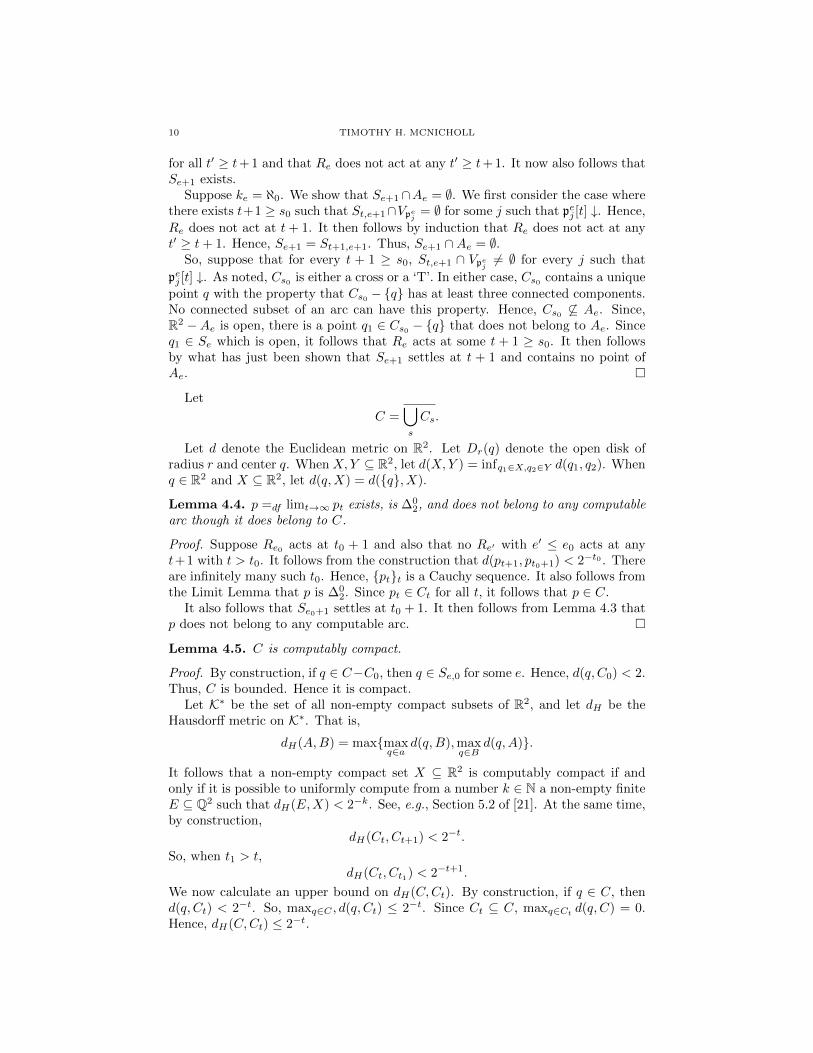
Lemma 4.5. C is computably compact.

Proof. By construction, if q ∈ C−C0, then q ∈ Se,0 for some e. Hence, d(q, C0) < 2.Thus, C is bounded. Hence it is compact.

Let K∗ be the set of all non-empty compact subsets of R2, and let dH be theHausdorff metric on K∗. That is,

dH(A,B) = max{maxq∈a

d(q,B),maxq∈B

d(q, A)}.

It follows that a non-empty compact set X ⊆ R2 is computably compact if andonly if it is possible to uniformly compute from a number k ∈ N a non-empty finiteE ⊆ Q2 such that dH(E,X) < 2−k. See, e.g., Section 5.2 of [21]. At the same time,by construction,

dH(Ct, Ct+1) < 2−t.

So, when t1 > t,dH(Ct, Ct1) < 2−t+1.

We now calculate an upper bound on dH(C,Ct). By construction, if q ∈ C, thend(q, Ct) < 2−t. So, maxq∈C , d(q, Ct) ≤ 2−t. Since Ct ⊆ C, maxq∈Ct

d(q, C) = 0.Hence, dH(C,Ct) ≤ 2−t.


Each Ct is computably compact uniformly in t. That is, from t, k ∈ N it ispossible to uniformly compute a finite Et,k ⊆ Q2 such that dH(Et,k, Ct) < 2−k. So,

dH(Et+1,t+1, C) ≤ dH(Et+1,t+1, Ct+1) + dH(Ct+1, C)

< 2−(t+1) + 2−(t+1) = 2−t

So, C is computably compact. �

Lemma 4.6. C is effectively locally connected.

Proof. Suppose we are given as input a name of an open U ⊆ R2 and a name of apoint q ∈ U ∩C. We show that from these data it is possible to uniformly computea name of an open set V ⊆ U such that q ∈ V and V ∩ C is connected.

We first introduce some notation. Namely, if Re acts at stage t+ 1, then let

Be,t+1 =⋃e′>e

Se′,t+1.

If Re does not act at t+1, then let Be,t+1 = ∅. Also, let Be,0 = ∅. By construction,Be,t+1 ∩ C is connected.

From the given data, it is possible to compute a positive rational number ε suchthat Dε(q) ⊆ U .

We now read the name of q and cycle through all natural numbers until we finde, t0 ∈ N and a rational rectangle F0 such that q ∈ F0, 2−t0+1 + diam(F0) < ε, andone of the following holds.

(1) F0 ∩ Ct0 ⊆ he,t0 − vt0 , F0 ⊆ St0,e, and d(F0, vt0) > 2−t0 .

(2) F0 ∩ Ct0 ⊆ vt0 − he,t0 , F0 ⊆ St0,e, and d(F0, he,t0) > 2−t0 .

(3) qe,t0 ∈ F0 and F0 ⊆ St0,e.(4) F0 ∩ St0,e ∩ St0,e+1 ∩ Ct0 6= ∅, F0 ∩ Ct0 ⊆ vt0 , F0 ⊆ St0,e ∪ St0,e+1, and

d(F0, he,t0), d(F0, he+1,t0) > 2−t0 .

(5) F0 ⊆ Se,t0 and pt1+1 ∈ F0 for some t1 ≤ t0.

Since q ∈ C, this process must terminate.If one of (1) - (4) holds, let

V =⋃{Be1,t1+1 : e1 ∈ N ∧ t1 ≥ t0 ∧ Be1,t1+1 ∩ F0 6= ∅} ∪ F0.

If (5), then let

V =⋃{St0,e′ : e′ > e ∧ diam(St0,e′) < 2−t0} ∪ F0.

Suppose one of (1) - (4) holds. Then, V is open and a name of V can be uniformlycomputed from the given data. It also follows that

V ∩(⋃s

Cs) =⋃{Be1,t1+1∩Ct1+1 : e1 ∈ N ∧ t1 ≥ t0 ∧Be1,t1+1∩F0 6= ∅} ∪ (F0∩Ct0).

In each case, F0∩Ct0 is connected. Suppose e1 ∈ N, t1 ≥ t0, and Be1,t1+1∩F0 6= ∅.By inspection of cases, Be1,t1+1 ∩ Ct0 6= ∅. By Theorem 1-14 of [11], V ∩

⋃s Cs is

connected. It then follows from Proposition 4.1 that V ∩ C is connected.Finally, it follows that the diameter of V is at most 2−t0+1 + diam(F0). Hence,

since q ∈ V , V ⊆ U .Suppose (5). Again, V is open and it is possible to uniformly compute a name

of V from the given data. Also, q ∈ V . The diameter of V is at most 2−t0 . Hence,


V ⊆ U . By construction,

C ∩⋃{St0,e′ : e′ > e ∧ diam(St0,e′) < 2−t0}

is connected. Since (5), Re acts at t1 + 1. Hence, F0 ∩ Ct1 is connected. ByProposition 4.1,

{pt1+1} ∪ C ∩⋃{St0,e′ : e′ > e ∧ diam(St0,e′) < 2−t0}

is connected. But, pt1+1 ∈ R0 ∩ Ct1 . Hence, V ∩ C is connected. �

Thus, by Theorem 2.1, C is a computable curve. However, Lemma 4.6 is notmerely a roundabout way of reaching this conclusion, but is in fact a strongerconclusion. See [4].

Lemma 4.7. C is rectifiable and its length is computable.

Proof. By construction, for each t for which Ct+1 − Ct 6= ∅, Ct+1 − Ct is a curve.Suppose Re acts at t + 1. It follows that the length of he′,t+1 is smaller than

2−t2−(e′−e)−1 whenever e′ > e and that the length of Ct+1 − Ct is at most 2−t+2.It follows that the length of C is finite and that for each t, the length of C differsfrom the length of Ct by at most 2−t+3. Thus, the length of C is computable. �

The proof is complete. �

Acknowledgement

I thank Jack Lutz and the Computer Science Department of Iowa State Univer-sity for their hospitality. I also thank Lamar University for generously supportingmy visit to Iowa State University during the Fall of 2010. I also thank Jack forstimulating conversation and for one of the proofs of Theorem 3.1. Finally, I thankmy wife Susan for support.

References

1. George S. Boolos, John P. Burgess, and Richard C. Jeffrey, Computability and logic, fourth

ed., Cambridge University Press, Cambridge, 2002.2. Vasco Brattka, Plottable real number functions and the computable graph theorem, SIAM J.

Comput. 38 (2008), no. 1, 303–328.

3. S. Barry Cooper, Computability theory, Chapman & Hall/CRC, Boca Raton, FL, 2004.4. P.J. Couch, B.D. Daniel, and T.H. McNicholl, Computing space-filling curves, To appear in

Theory of Computing Systems.5. D. Daniel and T.H. McNicholl, Effective local connectivity properties, Submitted.

6. Rodney G. Downey and Denis R. Hirschfeldt, Algorithmic randomness and complexity, Theory

and Applications of Computability, Springer, New York, 2010.7. Kenneth Falconer, Fractal geometry, second ed., John Wiley & Sons Inc., Hoboken, NJ, 2003,

Mathematical foundations and applications.

8. Michael R. Garey and David S. Johnson, Computers and intractability, W. H. Freeman andCo., San Francisco, Calif., 1979, A guide to the theory of NP-completeness, A Series of Books

in the Mathematical Sciences.

9. X. Gu, J. Lutz, and E. Mayordomo, Points on computable curves, Proceedings of the Forty-Seventh Annual IEEE Symposium on Foundations of Computer Science (Berkeley, CA), IEEE

Computer Society Press, October 2006, pp. 469–474.

10. X. Gu, J.H. Lutz, and E. Mayordomo, Curves that must be retraced, To appear.11. John G. Hocking and Gail S. Young, Topology, second ed., Dover Publications Inc., New York,

1988.12. Peter W. Jones, Rectifiable sets and the traveling salesman problem, Invent. Math. 102 (1990),

no. 1, 1–15.


13. Ker-I Ko, A polynomial-time computable curve whose interior has a nonrecursive measure,

Theoret. Comput. Sci. 145 (1995), no. 1-2, 241–270.

14. Jack H. Lutz, The dimensions of individual strings and sequences, Inform. and Comput. 187(2003), no. 1, 49–79.

15. , Effective fractal dimensions, MLQ Math. Log. Q. 51 (2005), no. 1, 62–72.

16. J. Miller, Degrees of unsolvability of continuous functions, The Journal of Symbolic Logic 69(2004), 555–584.

17. R.L. Moore and J.R. Kline, On the most general plane closed point-set through which it is

possible to pass a simple continuous arc, Ann. of Math. 20 (1919), no. 3, 218–223.18. Kate Okikiolu, Characterization of subsets of rectifiable curves in Rn, J. London Math. Soc.

(2) 46 (1992), no. 2, 336–348.

19. Hans Sagan, Space-filling curves, Universitext, Springer-Verlag, New York, 1994.20. R.I. Soare, Recursively enumerable sets and degrees, Springer-Verlag, Berling, Heidelberg,

1987.21. Klaus Weihrauch, Computable analysis, Texts in Theoretical Computer Science. An EATCS

Series, Springer-Verlag, Berlin, 2000.

Department of Mathematics, Lamar University, Beaumont, Texas 77710

E-mail address: [email protected]

The power of backtracking and the confinement of length

Documents

Transcript of The power of backtracking and the confinement of length