The Possible and the Actual inPhyllotaxis: Bridging the Gap

between Empirical Observations andIterative Models

Scott Hotton,1,3 Valerie Johnson,2 Jessica Wilbarger,2 Kajetan Zwieniecki,3

Pau Atela,2 Christophe Gole,2 and Jacques Dumais3*

1UC Merced Center for Computational Biology, University of California, Merced, California 95344, USA; 2Department of Mathematics,Smith College, Northampton, Massachusetts 01063, USA; 3Department of Organismic and Evolutionary Biology, Harvard University,

Cambridge, Massachusetts 02138, USA

ABSTRACT

This article presents new methods for the geomet-

rical analysis of phyllotactic patterns and their

comparison with patterns produced by simple, dis-

crete dynamical systems. We introduce the concept

of ontogenetic graph as a parsimonious and mech-

anistically relevant representation of a pattern. The

ontogenetic graph is extracted from the local

geometry of the pattern and does not impose large-

scale regularity on it as for the divergence angle and

other classical descriptors. We exemplify our

approach by analyzing the phyllotaxis of two as-

teraceae inflorescences in the light of a hard disk

model. The simulated patterns offer a very good

match to the observed patterns for over 150 itera-

tions of the model.

Key words: Artichoke; Delaunay triangulation;

Dynamical system; Shoot apical meristem;

Phyllotaxis; Sunflower; Voronoi tessellation

INTRODUCTION

Numerous patterns in nature are made of identical

units repeated regularly in space. Microtubules and

viral capsids provide examples at the molecular le-

vel (Erickson 1973). Given that proteins and other

macromolecules assemble over length scales that

are only slightly larger than those of inorganic

crystals, it is not overly surprising that they offer

patterns of similar regularity. However, when crys-

tal-like regularity is found at the level of an entire

living organism, one may justly be astonished. Yet,

this is a common occurrence in plants where the

arrangement of leaves and flowers around the stem,

known as phyllotaxis, yields striking patterns

(Figure 1).

The symmetries found in crystals, biopolymers,

and plants reflect two simple geometrical rules: (1)

equivalent or nearly equivalent units are added in

succession and (2) the position of new units is

determined by interactions with the units already in

Received: 26 June 2006; accepted: 29 June 2006; Online publication: 30

November 2006

*Corresponding author; e-mail: jdumais@oeb.harvard.edu

J Plant Growth Regul (2006) 25:313–323DOI: 10.1007/s00344-006-0067-9

313

place. To visualize these rules in plants, one must

focus on the shoot apical meristem where leaf and

flower primordia are initiated in a stereotypical

manner. Experimental evidence suggests that

primordium initiation is possible only in the

peripheral region of the meristem (Reinhardt and

others 2000, 2003b). Moreover, within that region,

older primordia are thought to exert an inhibitory

effect on primordium initiation (Snow and Snow

1932; Reinhardt and others 2003a). A new pri-

mordium thus forms in the largest gap available

within the peripheral region. Repetition of this

process leads, at the global scale, to the emergence

of two families of spirals called parastichies (these

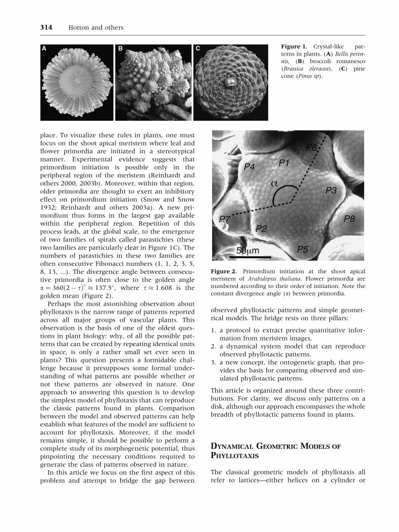
two families are particularly clear in Figure 1C). The

numbers of parastichies in these two families are

often consecutive Fibonacci numbers (1, 1, 2, 3, 5,

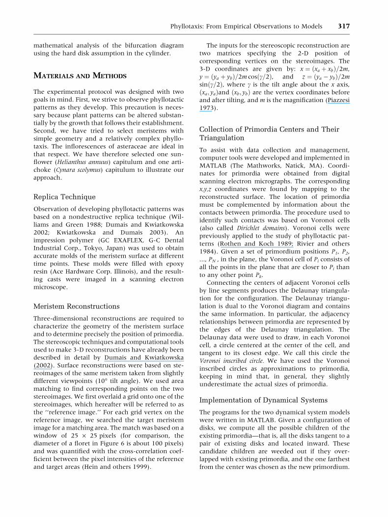
8, 13, ...). The divergence angle between consecu-

tive primordia is often close to the golden angle

a ¼ 360ð2� sÞ� � 137:5�, where s � 1:608 is the

golden mean (Figure 2).

Perhaps the most astonishing observation about

phyllotaxis is the narrow range of patterns reported

across all major groups of vascular plants. This

observation is the basis of one of the oldest ques-

tions in plant biology: why, of all the possible pat-

terns that can be created by repeating identical units

in space, is only a rather small set ever seen in

plants? This question presents a formidable chal-

lenge because it presupposes some formal under-

standing of what patterns are possible whether or

not these patterns are observed in nature. One

approach to answering this question is to develop

the simplest model of phyllotaxis that can reproduce

the classic patterns found in plants. Comparison

between the model and observed patterns can help

establish what features of the model are sufficient to

account for phyllotaxis. Moreover, if the model

remains simple, it should be possible to perform a

complete study of its morphogenetic potential, thus

pinpointing the necessary conditions required to

generate the class of patterns observed in nature.

In this article we focus on the first aspect of this

problem and attempt to bridge the gap between

observed phyllotactic patterns and simple geomet-

rical models. The bridge rests on three pillars:

1. a protocol to extract precise quantitative infor-

mation from meristem images.

2. a dynamical system model that can reproduce

observed phyllotactic patterns.

3. a new concept, the ontogenetic graph, that pro-

vides the basis for comparing observed and sim-

ulated phyllotactic patterns.

This article is organized around these three contri-

butions. For clarity, we discuss only patterns on a

disk, although our approach encompasses the whole

breadth of phyllotactic patterns found in plants.

DYNAMICAL GEOMETRIC MODELS OF

PHYLLOTAXIS

The classical geometric models of phyllotaxis all

refer to lattices—either helices on a cylinder or

Figure 1. Crystal-like pat-

terns in plants. (A) Bellis peren-

nis, (B) broccoli romanesco

(Brassica oleracea), (C) pine

cone (Pinus sp).

Figure 2. Primordium initiation at the shoot apical

meristem of Arabidopsis thaliana. Flower primordia are

numbered according to their order of initiation. Note the

constant divergence angle (a) between primordia.

314 Hotton and others

spirals on a disk. A spiral lattice is a set of points Pk =

(qk, ka), where a is the divergence angle, q is the

plastochrone ratio (that is, the ratio of the radial

distances for two successive primordia), and k is any

integer between zero and infinity. The curve that

joins the lattice points ordered by k is called the

ontogenetic spiral. The visible spirals in these patterns,

joining each point to its nearest neighbors, are

called parastichies (Figure 3). Not all lattices are

similar to the patterns exhibited by plants. The so-

called phyllotactic lattices are represented by a col-

lection of disks centered at the lattice points such

that they are tangent along two families of parasti-

chies winding in opposite directions from each other

(compare Figure 3A and 3B). The set of parameters

(q, a) yielding phyllotactic lattices was studied by

van Iterson (1907) (Figure 3C) and forms a tree

structure within the much larger space of all lattices.

van Iterson�s work represents the first attempt to

interprete phyllotactic patterns in the context of a

wider space of patterns (here lattices).

Dynamical Models of Phyllotaxis

Although much has been learned from the study

of lattices (Bravais and Bravais 1837; van Iterson

1907; Levitov 1991; Adler 1998), they are lacking

in one important aspect: in lattices, the location

of primordia is preset, and therefore they fail to

account for the second developmental rule,

which stipulates that primordium position is

determined by interactions with primordia al-

ready in place. The preset position is at variance

with experimental observations that patterns

build on previous patterns. In this article, we use

a geometric dynamical systems approach that

builds on a previous model by Atela and others

(2002). We were inspired by the iterative models

of Douady and Couder (1996) (see also the re-

lated systems proposed by Williams and Brittain

1984; Schwabe and Clewer 1984; Kunz 1997;

Koch and others 1998; d�Ovidio and Mosekilde

2000).

These dynamical system models are implemen-

tations of the two rules stated in the introduction, as

applied to phyllotaxis. More specifically:

1. Primordia are formed in succession, one or more

at a time.

2. Primordia are positioned in the ‘‘least crowded

spot’’ at the edge of the meristem.

If one assumes that primordia form with fixed per-

iod, one obtains what Douady and Couder called

the Hofmeister hypothesis. If one assumes that new

primordia form when and where there is enough

space, one obtains the so-called Snow hypothesis. The

Snow hypothesis has the advantage of allow-

ing simultaneous formation of several primordia

(sometimes yielding multijugate configurations).

Several reports have established that these dynam-

ical systems can reproduce many features of the van

Iterson diagram (Douady and Couder 1996; Kunz

1997; Koch and others 1998; d�Ovidio and

Mosekilde 2000; Atela and others 2002).

Mathematically, these models can be seen as

discrete dynamical systems acting on points

ðR0; h0Þ; � � � ; ðRN ; hNÞ of the disk (each point

representing the center of a primordium in polar

coordinates) with a transformation from one con-

figuration to the next of the form:

ðR0; h0; . . . ;RN ; hNÞ ! ðf ðR0; h0; . . . ;RN ; hNÞ;R0; h0; . . . ;RN�1; hN�1Þ;

where the function f determines the location of

the new primordium that minimizes its interaction

with the existing ones. In other words, f expresses

the location and time at which the interaction W

falls below a certain threshold. Most authors con-

sider an interaction of the form

Figure 3. (A) A spiral lattice with parastichy numbers

11, 20. This pattern is not a phyllotactic lattice as only one

parastichy family can be formed with tangent disks. (B) A

phyllotactic lattice, with parastichy numbers 13, 21. (C)

The space of all spiral lattice as drawn by van Iterson in

1907. The tree structure is the subset of lattices corre-

sponding to the type of phyllotactic patterns observed in

nature.

Phyllotaxis: From Empirical Observations to Models 315

W ðR; h;R0; h0; . . . ;RN ; hNÞ ¼Xk

uðR; h;Rk; hkÞ;

where (R,h) is the test location of the new pri-

mordium and u is a more or less explicit function of

the distance between (Rk,hk) and (R,h). Douady and

Couder used, among others, u ¼ c=dista, where a

and c are constants and dist is the distance between

(Rk,hk) and (R,h).

The Hard Disk Limit

An important aspect of the dynamical systems is the

nature of the interaction W and, in particular, the

set of primordia directly involved in determining

the location of new primordia. Some of us have

proposed (Atela and others 2002; Atela and Gole

2006) a radical simplification of the interaction as

W �ðR; h;R0; h0; . . . ;RN;hNÞ ¼ maxk

uðR; h;Rk; hkÞ:

In other words, we neglect all but the largest

interaction; equivalently, we assume that a new pri-

mordium only feels its closest neighbor. This limit is

sometimes called the ‘‘hard disk limit.’’

The hard disk limit is in fact inspired from

experimental observations. Ablation experiments

have shown that only the set of most recently

formed primordia around the circumference of the

meristem plays a role in determining the position of

the next primodium (Snow and Snow 1932;

Reinhardt and others 2003a). Moreover, the two

primordia directly contacting a newly formed pri-

mordium help determine its size (Reinhardt and

others 2003a).

In this article we use the hard disk Snow model.

Our goal in defining dynamical models of primordia

formation is to reproduce phyllotactic patterns with

the simplest model possible. We assume that pri-

mordia are small disks placed around a larger disk

that simulates the meristem. Given a configuration

of primordia, a new primordium appears in the

place that is farthest away from the center of the

meristem. This condition is equivalent to minimiz-

ing a potential where only the contribution of the

closest primordium is felt (that is, fast decay of the

potential). The process is then iterated again and

again (Figure 4).

Experimental observations support two qualita-

tively different classes of models (Figure 5):

The constant ratio model assumes that the ratio G of

the new primordium radius over the meristem ra-

dius remains constant. After each iteration, the

configuration of existing primordia (along with

their radii) expands uniformly away from the center

until there is enough room on the edge of the

meristem for a new primordium. This mode of

growth can be sustained indefinitely: primordia

never fill the meristem. It is observed in most

indeterminate meristems and also at intermediate

stages of capitulum development in sunflowers

when the growth of the meristem is balanced by the

progression of the morphogenetic front of primordia

(Palmer and Steer 1985). Only this mode can gen-

erate spiral lattices, which appear as steady states for

this model (for example, the [13, 21] lattice in

Figure 3B is such a steady state).

The constant radius model assumes that new pri-

mordia are formed with constant radius and that the

meristem does not grow at all. As a consequence,

the primordia fill up the center of the meristem.

This has been observed to be approximately the case

in the very latest stage of capitulum development in

sunflowers (Palmer and Steer 1985).

These models are just two notable elements in a

continuum of models in which the ratio parameter

varies with the distance to the center at various

rates. This is not the place to provide a complete

analysis of these models. See Atela and others (2002)

and Douady (1998) for a complete and rigorous

Figure 4. Three iterates of the Snow transformation.

Figure 5. Two modes of growth with the same initial

condition (in dark gray) derived from a micrograph of

Picea abies. (A) The constant ratio model (G = 0.176 on a

unit radius meristem) yields a pattern which, although

not a lattice, does exhibit families of spirals that are par-

astichy like, with parastichy numbers 8, 13 – which are

indeed the parastichy numbers of the original pattern. (B)

The same initial condition yields a very different pattern

with the constant radius model (r = 0.176).

316 Hotton and others

mathematical analysis of the bifurcation diagram

using the hard disk assumption in the cylinder.

MATERIALS AND METHODS

The experimental protocol was designed with two

goals in mind. First, we strive to observe phyllotactic

patterns as they develop. This precaution is neces-

sary because plant patterns can be altered substan-

tially by the growth that follows their establishment.

Second, we have tried to select meristems with

simple geometry and a relatively complex phyllo-

taxis. The inflorescences of asteraceae are ideal in

that respect. We have therefore selected one sun-

flower (Helianthus annuus) capitulum and one arti-

choke (Cynara scolymus) capitulum to illustrate our

approach.

Replica Technique

Observation of developing phyllotactic patterns was

based on a nondestructive replica technique (Wil-

liams and Green 1988; Dumais and Kwiatkowska

2002; Kwiatkowska and Dumais 2003). An

impression polymer (GC EXAFLEX, G-C Dental

Industrial Corp., Tokyo, Japan) was used to obtain

accurate molds of the meristem surface at different

time points. These molds were filled with epoxy

resin (Ace Hardware Corp. Illinois), and the result-

ing casts were imaged in a scanning electron

microscope.

Meristem Reconstructions

Three-dimensional reconstructions are required to

characterize the geometry of the meristem surface

and to determine precisely the position of primordia.

The stereoscopic techniques and computational tools

used to make 3-D reconstructions have already been

described in detail by Dumais and Kwiatkowska

(2002). Surface reconstructions were based on ste-

reoimages of the same meristem taken from slightly

different viewpoints (10� tilt angle). We used area

matching to find corresponding points on the two

stereoimages. We first overlaid a grid onto one of the

stereoimages, which hereafter will be referred to as

the ‘‘reference image.’’ For each grid vertex on the

reference image, we searched the target meristem

image for amatching area. Thematch was based on a

window of 25 · 25 pixels (for comparison, the

diameter of a floret in Figure 6 is about 100 pixels)

and was quantified with the cross-correlation coef-

ficient between the pixel intensities of the reference

and target areas (Hein and others 1999).

The inputs for the stereoscopic reconstruction are

two matrices specifying the 2-D position of

corresponding vertices on the stereoimages. The

3-D coordinates are given by: x ¼ ðxa þ xbÞ=2m,

y ¼ ðya þ ybÞ=2m cosðc=2Þ, and z ¼ ðya � ybÞ=2msinðc=2Þ, where c is the tilt angle about the x axis,

ðxa; yaÞand ðxb; ybÞ are the vertex coordinates before

and after tilting, and m is the magnification (Piazzesi

1973).

Collection of Primordia Centers and TheirTriangulation

To assist with data collection and management,

computer tools were developed and implemented in

MATLAB (The Mathworks, Natick, MA). Coordi-

nates for primordia were obtained from digital

scanning electron micrographs. The corresponding

x,y,z coordinates were found by mapping to the

reconstructed surface. The location of primordia

must be complemented by information about the

contacts between primordia. The procedure used to

identify such contacts was based on Voronoi cells

(also called Dirichlet domains). Voronoi cells were

previously applied to the study of phyllotactic pat-

terns (Rothen and Koch 1989; Rivier and others

1984). Given a set of primordium positions P1, P2,

..., PN , in the plane, the Voronoi cell of Pi consists of

all the points in the plane that are closer to Pi than

to any other point Pk.

Connecting the centers of adjacent Voronoi cells

by line segments produces the Delaunay triangula-

tion for the configuration. The Delaunay triangu-

lation is dual to the Voronoi diagram and contains

the same information. In particular, the adjacency

relationships between primordia are represented by

the edges of the Delaunay triangulation. The

Delaunay data were used to draw, in each Voronoi

cell, a circle centered at the center of the cell, and

tangent to its closest edge. We call this circle the

Voronoi inscribed circle. We have used the Voronoi

inscribed circles as approximations to primordia,

keeping in mind that, in general, they slightly

underestimate the actual sizes of primordia.

Implementation of Dynamical Systems

The programs for the two dynamical system models

were written in MATLAB. Given a configuration of

disks, we compute all the possible children of the

existing primordia—that is, all the disks tangent to a

pair of existing disks and located inward. These

candidate children are weeded out if they over-

lapped with existing primordia, and the one farthest

from the center was chosen as the new primordium.

Phyllotaxis: From Empirical Observations to Models 317

The constant ratio model has the added complica-

tion that the correct ratio must be chosen. To do so,

the program first chooses a candidate of reasonable

radius (for example, the radius of the last primor-

dium); it then solves an equation of degree four to

find the center of the primordium tangent to the

same parents, but with the radius r that yields the

correct ratio G. A new search of candidates is per-

formed with disks of radius r to check whether the

change of radius might have yielded another pos-

sible location farther away from the center. Resizing

is performed once again. We have never observed a

case where this bootstrap process needed more than

two rounds of candidate search.

As Figure 5 shows, only one layer of primordia is

enough to determine the development of the pat-

tern. Therefore, to simulate observed patterns, we

first selected as initial conditions a ring of primordia

given by the plant data at hand. We call this ring of

primordia a primordia front. To find fronts, we wrote

a MATLAB program allowing the user to interac-

tively pick a primordium P0 on a micrograph. The

program then finds the closest data point (recorded

as center of the primordium) and computes its dis-

tance to the meristem center. Each successive point

of the front is then chosen as child or parent of the

previous one, in such a way that its distance to the

center is as small as possible without being closer to

the center than P0. The process stops when a pri-

mordium adjacent to P0 is reached, thus closing the

loop.

RESULTS

Time Sequences and StereoscopicReconstructions

Several experimental approaches have been devel-

oped to observe meristem growth and primordium

initiation over time (Dumais and Kwiatkowska

2002; Grandjean and others 2004; Reddy and others

2004). Here we adopt a replica technique because of

its flexibility and ease of use. Figure 6 shows two

replicas of a sunflower capitulum taken at a 2-day

interval. During this interval, approximately two

new primordia were generated along the steep

parastichies (squares in Figure 6C and 6D) and

three along the shallow parastichies (triangles in

Figure 6C and 6D). Inspection of Figure 6A and 6B

reveals that the development of the pattern has

been accommodated in part by an outward dis-

placement of older flowers and by a short advance

of the pattern into the central unpatterned region.

Because the central region has been reduced

slightly, we can conclude that the development

departs from the constant ratio model described

above. However, given the large size of the mor-

phogenetic region compared to the size of the newly

formed primordia, the deviation is likely to be

negligible.

Figure 7 shows a reconstructed sunflower

capitulum. The level of contrast in the unpatterned

central region was too low to allow reliable

Figure 6. Sequential replicas

of the sunflower capitulum.

(A) and (B) Epoxy casts of the

same capitulum collected two

days apart. (C) and (D) Close-

ups showing the development

of the parastichies on the capit-

ulum. Note that some of the

flower primordia are replaced

by voids corresponding to air

bubbles trapped in the epoxy

cast. (E) Typical primordium

development. The flower bract

(upper right structure in each

panel) appears first and is fol-

lowed by the development of

the disk floret.

318 Hotton and others

reconstruction; it was therefore excluded. From the

reconstruction, it is possible to find a projection of

the meristem surface that minimizes the distortion

of the distances between primordia. The local dis-

tortion of distances is equal to 1-cos h where h is

the angle between the local normal to the surface

and the normal of the plane onto which the sur-

face is projected. It is possible to minimize the

overall distortion by selecting a projection plane

that coincides with the mean normal of the sur-

face. We found that the projection error is

everywhere less than 8% (Figure 7C). These

observations support the modeling of the meristem

as a flat disk. Ultimately, the reconstructed surface

could be used in the simulations, but we do not

pursue this direction here to keep the model as

simple as possible.

The Ontogenetic Graph of a Pattern

The locations of the primordia centers (Figures 7

and 8) were collected using a computer-assisted

user interface. The representation of the pattern in

terms of the Voronoi tessellation and the Delaunay

triangulation (Figure 8C) offers a possible basis for

comparing observed and simulated patterns. More-

over, the inclusion of one additional piece of

information can help account for the developmental

history or ontogenesis of the pattern. Given an

iterative process in which primordia are initiated

centripetally around the meristem, we call the par-

ents of a primordium its two closest older neigh-

boring primordia, that is, the two closest primordia

located radially away from a given primordium

(Figure 8B). The directed graph formed by joining

each primordium to its parents is the ontogenetic

graph of the pattern (Figure 8B). It records both the

topology and the ontogenesis of the pattern. The

ontogenetic graph is a subgraph of the Delaunay

triangulation (compare Figure 8B and 8C). Typi-

cally, it corresponds to the parastichies of the pat-

tern, but, although it can be hard to define

parastichies in non-lattice patterns, it is always

possible to define their ontogenetic graph. There-

fore, the ontogenetic graph is a robust and succinct

way of describing a phyllotactic pattern.

Comparison of Observed and SimulatedPatterns

We now consider two ways to compare a pattern

extracted from a meristem micrograph (pattern A)

and a simulated pattern (pattern B) whose outer

boundary is a primordia front F of pattern A. The

first approach presupposes that the Voronoi

inscribed circles of B overlap those of A in a one-to-

one fashion in some region of A. Given this one-to-

one correspondence, we can quantify the degree of

Figure 7. Reconstruction of the sunflower capitulum.

(A) Two concentric circles indicate the region of the

capitulum that was reconstructed. Polygons represent the

Voronoi cell of the primordia. The second stereoimage of

the meristem is not shown. (B) Side-view of the recon-

structed surface. (C) Top-view of the capitulum. The

Voronoi cells computed from the floret positions are

drawn in black. The color map shows the error associated

with the projection of a 3-D surface onto a plane. The

same (parastichy has been highlighted in all three panels.

Phyllotaxis: From Empirical Observations to Models 319

overlap using the following dimensionless measure

of fit. If PA is a target primordium overlapped by PBwith respective radii RA and RB, we define the

percent relative fit (PRF) as:

PRF ¼ 1� distðPA; PBÞRA þ RB

� �100%

Note that PRF = 100% when the centers coincide

and PRF = 0% when the circles representing the

primordia are tangent. Finally, PRF is negative

when the primordia are disjoint. The second

approach is to compare the topologies of the onto-

genetic graphs of B and A. The distance between

these graphs can be measured by computing the

minimal number of edge substitutions that trans-

forms one graph into the other.

We analyzed the geometry of the capitula of one

artichoke and one sunflower using the methods

described above. Both have parastichy numbers 34,

55 (with dislocations in the center for the arti-

choke). Approximating the primordia by the

Voronoi inscribed circles, it is possible to plot the

primordium radii as a function of the distance to

the meristem center (centroid of the data) (Fig-

ures 9D and 10D). One observes a marked differ-

ence in the slopes of the linear fits: the slope in the

sunflower data is three times higher than that for

the artichoke. The small variation in primordium

size in the artichoke indicates that it is close to a

constant radius mode. The ontogenetic graph of

the sunflower near the meristem is topologically

equivalent to that of a spiral lattice; that is, all

interspaces are rhombic (Figure 10C). Because

lattice patterns are possible only within the con-

stant ratio mode, we have used this model to

simulate the sunflower.

We ran 200 iterates with initial conditions given

by the fronts seen in Figures 9 and 10. Parameters

were (roughly) optimized so as to give the best fit in

both cases. It was possible to achieve a better fit for

the artichoke case than for the sunflower case.

There was a one-to-one overlap for all 200 iterates

for the artichoke. For the sunflower, the one-to-one

criterion was satisfied until iterate 195, where the

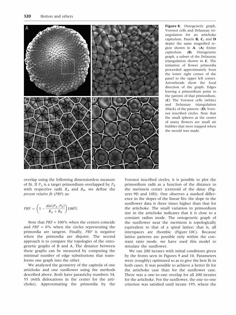
Figure 8. Ontogenetic graph,

Voronoi cells and Delaunay tri-

angulation for an artichoke

capitulum. Panels B, C, and D

depict the same magnified re-

gion shown in A. (A) Entire

capitulum. (B) Ontogenetic

graph, a subset of the Delaunay

triangulation shown in C. The

initiation of flower primordia

proceeded approximately from

the lower right corner of the

panel to the upper left corner.

Arrowheads show the local

direction of the graph. Edges

leaving a primordium point to

the parents of that primordium.

(C) The Voronoi cells (white)

and Delaunay triangulation

(black) of the pattern. (D) Voro-

noi inscribed circles. Note that

the small spheres at the center

of many flowers are small air

bubbles that were trapped when

the mould was made.

320 Hotton and others

simulated primordium landed on a site already

overlapped. We found a mean PRF of 85.3% for the

artichoke and of 78.5% for the sunflower. However,

restricted to the last 100 iterates, the mean PRF was

81.3% for the artichoke, but only 68.2% for the

sunflower.

As expected, the Voronoi circles seem to

underestimate the primordia size, as indicated by

the optimal radius for the dynamics. This discrep-

ancy is much more significant in the sunflower

than in the artichoke. Indeed, the Voronoi radius

is 93% of the optimal radius in the artichoke. In

the sunflower this percentage is 63%. We suspect

that the discrepancy in the sunflower is amplified

by the marked elliptical shape of the young

primordia.

DISCUSSION

The phyllotactic patterns observed in plants are

based on a few standard types, with the Fibonacci

type patterns being predominant. Curiously, the

commonly observed plant patterns are but a small

fraction of a much larger universe of patterns (Fig-

ure 3) (van Iterson 1907). (For an interactive

exploration of the universe of spiral lattices, see

www.math.smith.edu/phyllo/Applets.) Why, then,

have plants adopted some specific patterns? This

central question served as the motivation for our

work. This article offers a framework and numerical

methods to compare the patterns observed in Nat-

ure with those generated by simple dynamical sys-

tems. At the center of the comparison is the concept

of ‘‘ontogenetic graph’’ which records the devel-

opmental history of a pattern. The comparison is

supported by a set of tools and ancillary concepts

both at the experimental level and the theoretical

level.

We have shown that two geometrical dynamical

systems based on the hard disk assumption can ac-

count for the patterns observed in the inflorescence

of asteraceae. For this work, we deliberately selected

meristems with nearly flat geometries so that sim-

pler dynamical systems could be used. The sim-

plicity of the models is a great advantage because

the dynamical systems can be studied in detail to

probe the universe of all phyllotactic patterns. We

performed such an analysis previously in the

cylindrical geometry (Atela and others 2002).

Figure 9. Dynamical simula-

tion on an artichoke capitu-

lum using constant radius

r = 0.095 mm, 150 iterates are

shown. (A) SEM of the capitu-

lum with simulated primordia

superimposed in black. The ini-

tial front is represented by a

black zigzagging loop. (B) Same

information as in A with the

primordia of the artichoke rep-

resented by the Voronoi in-

scribed circles (in gray). (C)

The ontogenetic graph of the

simulation (black) superim-

posed to that of the data (gray).

(D) Graph of primordium ra-

dius vs. distance to the center,

shown in same scale ratio as

Figure 10D. The slope of the

linear fit is 0.0075. (E) Graph of

the Percent Relative Fit of the

nth primordium and the simu-

lated primordium that overlaps

it. Primordia were ordered

according to decreasing dis-

tance from center. The radius

r was chosen to maximize the

PRF.

Phyllotaxis: From Empirical Observations to Models 321

Although many articles have emphasized the

similarity between observed and simulated patterns,

there are relatively few instances where an explicit

one-to-one comparison was performed. Couder

(1998) directly compared the location of leaves

along sunflower stems with simulations obtained

from the computer model he helped develop

(Douady and Couder 1996). Good agreement was

achieved between the data from many specimens

and the computer simulations. Another comparison

of a dynamical model to a phyllotactic pattern was

performed by Battjes and Prunsikiewicz (1998). The

floret patterns in Microseris pigmaea inflorescences

were simulated by a collision disk model. This

model places congruent disks with a divergence

angle equal to the golden angle and readjusts their

positions to find the closest tangent fit to the older

ones. As mentioned by the authors, the initial

angular bias reduces the generality of the approach,

but otherwise the model bears many similarities to

our constant radius model.

From Hard Disks to Squishy Biology

It may seem paradoxical at a time when great strides

are being made in our understanding of the

molecular and cellular basis of phyllotaxis that

geometrical models of this process are used instead

of mechanistic ones. The developmental rules

implemented in the geometrical model are taken to

be ‘‘downstream’’ consequences of the molecular

and cellular controls of primordium initiation. The

advantages of operating at a slightly more abstract

level are many. First, although detailed mechanistic

models can reproduce some phyllotactic patterns,

their complexity is such that the analysis of their

morphogenetic potential must be performed

numerically. To understand fully how the posi-

tioning of new primordia creates the classic plant

patterns, models of greater simplicity are required

because they allow a detailed analysis of the uni-

verse of patterns accessible to them. Second, several

distinct mechanistic models have been shown to

reproduce plant-like patterns. Therefore, there is

not a unique mechanistic model to study. Many

experiments are required before the validity of the

current mechanistic models can be ascertained.

The type of interactions implemented in our

models (that is, the hard disk assumption) may

seem a priori quite remote from the type of inter-

actions likely to be at work in the meristem. We

believe, however, that simple developmental rules

may emerge from the common molecular and cel-

lular controls invoked for phyllotaxis. In particular,

Figure 10. Simulation study

on a sunflower capitulum with

constant ratio G = 0.0444 and

200 iterates. (A) SEM of the

capitulum with simulated pri-

mordia superimposed in black.

The initial front is represented

by a black zigzagging loop. (B)

Same information, with the pri-

mordia of the sunflower repre-

sented by the Voronoi inscribed

circles (in gray). (C) Ontoge-

netic graphs of the simulation

(black) and data (gray) super-

posed. (D) Graph of primor-

dium radius vs. distance to

center, shown in same scale

ratio as Figure 9D. The slope of

the linear fit is 0.028. (E) Graph

of the Percent Relative Fit of the

nth primordium and the simu-

lated primordium that overlaps

it.

322 Hotton and others

the diffusion and transport of auxin from cell to cell

may very well be compatible, at a larger scale, with

the simple spacing rule embodied in the hard disk

assumption. Perhaps the most important contribu-

tion of geometrical models is to reduce complex

phyllotactic patterns to a set of local rules that are

repeated recursively. These local rules, rather than

the overall patterns, are ultimately what needs to be

explained at the mechanistic level.

ACKNOWLEDGMENTS

This work was supported in part by National Science

Foundation (NSF) collaborative grant 0540740 to

P.A. and C.G., and collaborative grant 0540662 to

J.D. We acknowledge Smith College for additional

funds to support V.J. and J.W., and the Mellon

Foundation for supporting exchange travels of the

senior authors. Finally, we thank the Center for

Nanoscale Systems (Harvard) for use of their imag-

ing facilities.

REFERENCES

Adler I. 1998. Generating phyllotaxis patterns on a cylindrical

point lattice In: Jean RV, Barabe D editors. Symmetry in Plants

Singapore: World Scientific. pp. 249–279.

Atela P, Gole C, Hotton S. 2002. A dynamical system for plant

pattern formation: a rigorous analysis. J Nonlinear Sci 12:641––

676.

Atela P, Gole C. 2006. New concepts in phyllotaxis: multilattices

and primordia fronts, in preparation.

Battjes J, Prusinkiewicz P. 1998. Modeling meristic characters in

asteracean flowerheads In: Jean RV, Barabe D. editors. Sym-

metry in Plants Singapore: World Scientific. pp. 281–312.

Bravais L, Bravais A. 1837. Essai sur la dispositions des feu-

illes curviseriees. Ann Sci Nat Bot 7, deuxieme serie: 42–

110.

Couder Y. 1998. Initial transitions, order and disorder in phyl-

lotactic patterns: the ontogeny of Helianthus annuus, a case

study. Acta Soc Bot Pol 67:129–150.

Douady S. 1998. The selection of phyllotactic patterns In: Jean

RV, Barabe D. editors. Symmetry in Plants Singapore: World

Scientific. pp. 335–358.

Douady S, Couder Y. 1996. Phyllotaxis as a dynamical self

organizing process (Part I, II, III). J Theor Biol 139:178–312.

Dumais J, Kwiatkowska D. 2002. Analysis of surface growth in

shoot apices. Plant J 31:229–241.

Erickson RO. 1973. Tubular packing of spheres in biological fine

structure. Science 181:705–716.

Grandjean O, Vernoux T, Laufs P, Belcram K, Mizukami Y, and

others. 2004. In vivo analysis of cell division, cell growth, and

differentiation at the shoot apical meristem in Arabidopsis. Plant

Cell 16:74–87.

Hein LRO, Silva FA, Nazar AMM, Ammann JJ. 1999. Three-

dimensional reconstruction of fracture surfaces: area matching

algorithms for automatic parallax measurements. Scanning

21:253–263.

van Iterson G. 1907. Mathematische und Mikroskopisch-Ana-

tomische Studien uber Blattstellungen nebst Betraschtungen

uber den Schalenbau der Miliolinen. Gustav Fischer, Jena,

Germany.

Koch AJ, Bernasconi G, Rothen F. 1998. Phyllotaxis as a

geometrical and dynamical system In: Jean RV, Barabe D.

editors. Symmetry in Plants Singapore: World Scientific.

pp. 459–486.

Kunz M. 1997. Ph.D. Phyllotaxie, billards polygonaux et theorie

des nombres (Thesis). Universite de Lausanne, Switzerland.

Kwiatkowska D, Dumais J. 2003. Growth and morphogenesis at

the vegetative shoot apex of Anagallis arvensis L. J Exp Bot

54:1585–1595.

Levitov LS. 1991. Energetic approach to phyllotaxis. Europhys

Lett 14:533–539.

d�Ovidio F, Mosekilde E. 2000. Dynamical system approach to

phyllotaxis. Phys Rev E 61:354–365.

Palmer JH, Steer BT. 1985. The generative area as the site of floret

initiation in the sunflower capitulum and its integration to

predict floret number. Field Crops Res 11:1–12.

Piazzesi G. 1973. Photogrammetry with the scanning electron

microscope. J Phys E: Sci Instr 6:392–396.

Reddy GV, Heisler MG, Ehrhardt DW, Meyerowitz EM. 2004.

Real-time lineage analysis reveals oriented cell divisions asso-

ciated with morphogenesis at the shoot apex of Arabidopsis

thaliana. Development 131:4225–4237.

Reinhardt D, Mandel T, Kuhlemeier C. 2000. Auxin regulates the

initiation and radial position of plant lateral organs. Plant Cell

12:507–518.

Reinhardt D, Frenz M, Mandel T, Kuhlemeier C. 2003a. Micro-

surgical and laser ablation analysis of interactions between the

zones and layers of the tomato shoot apical meristem. Devel-

opment 130:4073–4083.

Reinhardt D, Pesce ER, Stieger P, Mandel T, Baltensperger K, and

others. 2003b. Regulation of phyllotaxis by polar auxin trans-

port. Nature 426:255–260.

Rivier N, Occelli R, Pantaloni J, Lissowski A. 1984. Structure of

Benard convection cells, phyllotaxis and crystallography in

cylindrical symmetry. J Physique 45:49–63.

Rothen F, Koch AJ. 1989. Phyllotaxis, or the properties of spiral

lattices. I. Shape invariance under compression. J Physique

50:633–657.

Schwabe WW, Clewer AG. 1984. Phyllotaxis—a simple computer

model based on the theory of a polarly-translocated inhibitor.

J Theor Biol 109:595–619.

SnowM, SnowR. 1932. Experiments on phyllotaxis. II—the effect

of displacing a primordium. Phil Trans R Soc Lond 222:353–400.

Williams MH, Green PB. 1988. Sequential scanning electron

microscopy of a growing plant meristem. Protoplasma 147:77–

79.

Williams RF, Brittain EG. 1984. A geometrical model of phyllo-

taxis. Aust J Bot 32:43–72.

Phyllotaxis: From Empirical Observations to Models 323