The physical and geochemical controls on heavy ... - CORE
285
The Physical and Geochemical Controls on Heavy Metal Cycling in Mangal Sediments, Wynnum, Brisbane. by Malcolm Clark -;? September 1992 A Thesis Presented as Partial Fulfilment for the Degree of Masters of Science at the University of Canterbury.
-
Upload
khangminh22 -
Category
Documents
-
view
3 -
download
0
Transcript of The physical and geochemical controls on heavy ... - CORE
The Physical and Geochemical
Controls on Heavy Metal Cycling in Mangal Sediments, Wynnum,
Brisbane.
by
Malcolm Clark -;?
September 1992
A Thesis
Presented as Partial Fulfilment for the Degree of Masters of Science at
the University of Canterbury.

2
TABLE OF CONTENTS
TABLE OF CONTENTS
LIST OF FIGURES
LIST OF PLATES
LIST OF TABLES
ABSTRACT
INTRODUCTION Project Background Aims and Objectives
SETTING Geographic Setting Historical Setting Climatic Setting
Temperature Rainfall
Hydrological Setting Geological Setting Geomorphic Setting
Sedimentation over the last 6000 years Recent changes in drainage
METHODOLOGY Sediment Sampling
Core samples Surface grab samples
Surface Water Sampling Ground Water Sampling Surveying the Field Area
Height survey Eh survey pH survey Salinity
Ground water salinity 24 Hour Variations Eh/pH
Method Eh/pH Transitions
Methods Core Sub-sampling Grab Sample Sub-sampling Sample Preparation
page
2
5
8
9
10
12 13 14
17 20 22 23 24 24 25 27 30 32 35
40 40 40 42 43 43 43 44 44 45 45 46 47 48 48 50 50 50 50
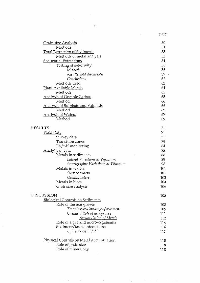
Grain size Analysis Methods
3
Total Extraction of Sediments Methods of metal analysis
Sequential Extractions Testing of selectivity
Methods Results and discussion Conclusions
Methods used Plant Available Metals
Methods Analysis of Organic Carbon
Method Analysis of Sulphate and Sulphide
Method Analysis of Waters
Method
Field Data Survey data Transition zones Eh/ pH monitoring
Analytical Data Metals in sediments
Lateral Variations at Wynnum Stratigraphic Variations at Wynnum
Metals in waters Surface waters Groundwaters
Metals in biota . Grainsize analysis
DISCUSSION Biological Controls on Sediments
Role of the mangroves Trapping and binding of sediment Chemical Role of mangroves
Accumulation of Metals Role of algae and micro-organisms Sediment/ fauna interactions
Influence on Eh/pH
Physical Controls on Metal Accumula tion Role of grain size Role of mineralogy
page
50 51 53 53 54 56 56 57 62 63 64 65 65 66 66 67 67 69
71 71 71 79 84 88 88 89 96 101 101 102 104 106
108
108 109 111 112 114 116 117
118 118 118
4
page
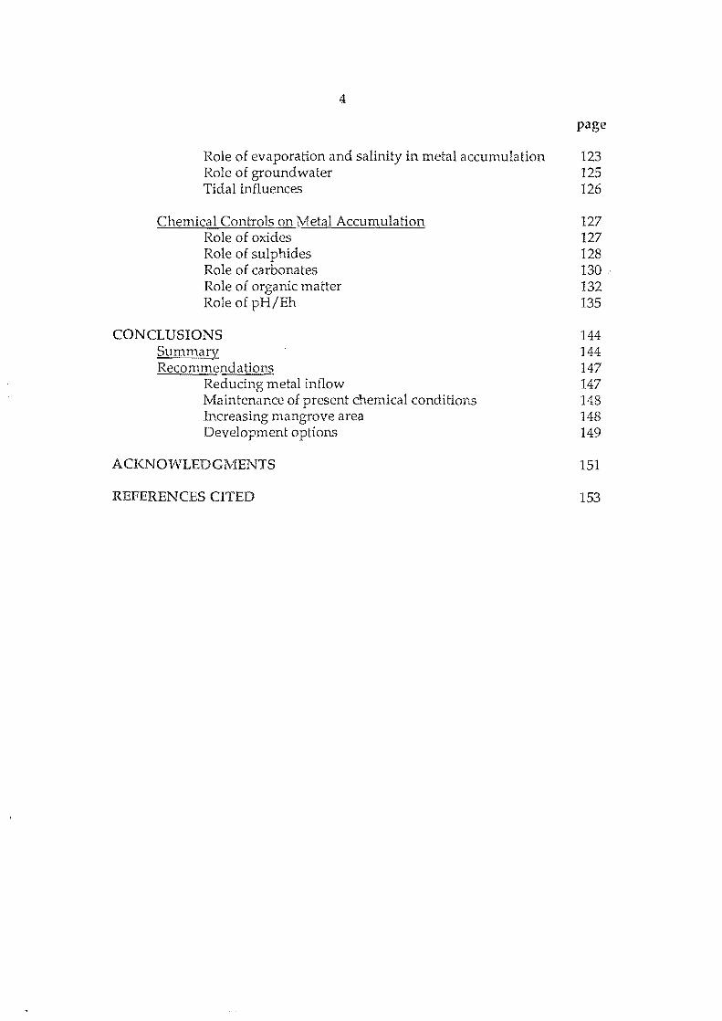
Role of evaporation and salinity in metal accumulation 123 Role of groundwater 125 Tidal influences 126
Chemical Controls on Metal Accumulation 127 Role of oxides 127 Role of sulphides 128 Role of carbonates 130 Role of organic matter 132 Role of pH/Eh 135
CONCLUSIONS 144 Summary 144 Recommendations 147
Reducing metal inflow 147 Maintenance of present chemical conditions 148 Increasing mangrove area 148 Development options 149
ACKNOWLEDGMENTS 151
REFERENCES CITED 153
5
LIST OF FIGURES
page
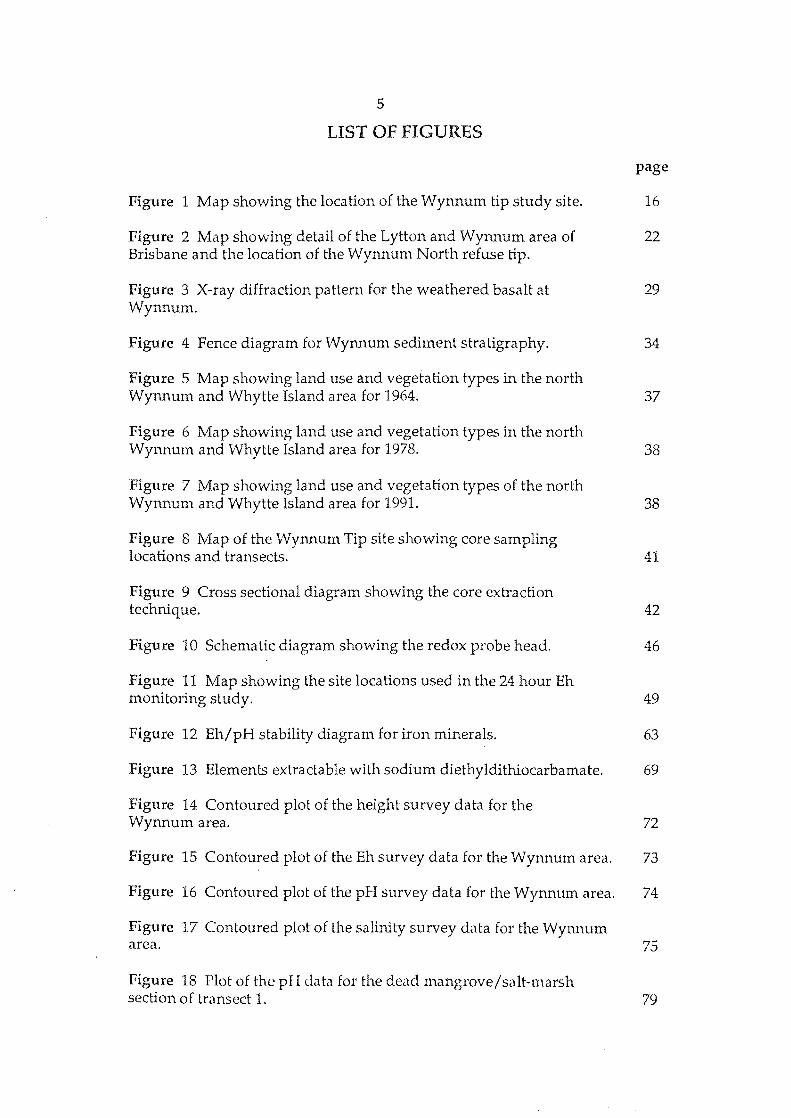
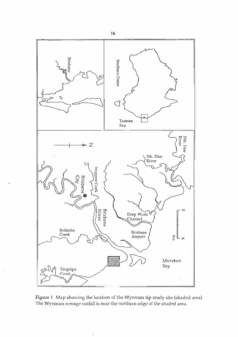
Figure 1 Map showing the location of the Wynnum tip study site. 16
Figure 2 Map showing detail of the Lytton and Wynnum area of 22 Brisbane and the location of the Wynnum North refuse tip.
Figure 3 X-ray diffraction pattern for the weathered basalt at 29 Wynnum.
Figure 4 Fence diagram for Wynnum sediment stratigraphy. 34
Figure 5 Map showing land use and vegetation types in the north Wynnum and Whytte Island area for 1964. 37
Figure 6 Map showing land use and vegetation types in the north Wynnum and Whytte Island area for 1978. 38
Figure 7 Map showing land use and vegetation types of the north Wynnum and Whytte Island area for 1991. 38
Figure 8 Map of the Wynnum Tip site showing core sampling locations and transects. 41
Figure 9 Cross sectional diagram showing the core extraction technique. 42
Figure 10 Schematic diagram showing the redox probe head. 46
Figure 11 Map showing the site locations used in the 24 hour Eh monitoring study. 49
Figure 12 Eh/pH stability diagram for iron minerals. 63
Figure 13 Elements extractable with sodium diethyldithiocarbamate. 69
Figure 14 Contoured plot of the height survey data for the Wynnum area. 72
Figure 15 Contoured plot of the Eh survey data for the Wynnum area. 73
Figure 16 Contoured plot of the pH survey data for the Wynnum area. 74
Figure 17 Contoured plot of the salinity survey data for the Wynnum area. 75
Figure 18 Plot of the pH data for the dead mangrove/salt-marsh section of transect 1. 79
6
page
Figure 19 Plot of the Eh data for the dead mangrove/ salt-marsh section of transect 1. 80
Figure 20 Plot of the pH data for the dead mangrove/salt-marsh section of transect 3. 80
Figure 21 Plot of the Eh data for the dead mangrove/salt-marsh section of transect 3. 81
Figure 22 Plot of the pH data for the mud-flat section of transect 1. 81
Figure 23 Plot of the Eh data for the mud-flat section of transect 1. 82
Figure 24 Plot of the pH data for the mud-flat section of transect 3. 82
Figure 25 Plot of the Eh data for the mud-flat section of transect 3. 83
Figure 26 Plot of the Eh pH conditions for the surface, 2 cm, 4 cm and 10 cm depths in core 1. 86
Figure 27 Plot of the Eh pH conditions for the surface, 2 cm, 4 cm and 10 cm depths in core 2. 86
Figure 28 Plot of the Eh pH conditions for the surface, 2 cm, 4 cm and 10 cm depths in core 3. 87
Figure 29 Plot of the Eh pH conditions for the surface, 2 cm, 4 cm and 10 cm depths in core 4. 87
Figure 30 Plot of the total analysis data for transect 1. 90
Figure 31 Plot of the total analysis data for transect 2. 91
Figure 32 Plot of the total analysis data for transect 3. 92
Figure 33 Plot of the total analysis data for transect 4. 93
Figure 34 Plot of the total analysis data for transect 5. 94
Figure 35 Plot of the total analysis data from core MCC 012. 97
Figure 36 Plot of the total analysis data from core MCC 010. 98
Figure 37 Plot of the total analysis data from core MCC 011. 99
Figure 38. Graph of the long term chemical data from piesometer 1. 104
7
page
Figure 39 Plot of the variation in groundwater salinity for the 105 Wynnum study site over a tidal cycle.
Figure 40 Plot of plant available metal and the total metal in the 106 sediment at the Wynnum site.
Figure 41 Ternary plot of the grain size data for the Wynnum area. 107
Figure 42 Major morphological root types found in mangroves. 110
Figure 43 Schematic representation of the plant, soil metal relationships. 114
Figure 44 Schematic representation of the important trace-element sinks on the surface of an idealised kaolinite crystal. 120
Figure 45 Schematic diagram of the flow paths of leachate, surface water and ground water from the Wynnum Tip. 126
Figure 46 Variation in the solubility of some common oxides as a function of pH. 140
Figure 47 The process of pyrite formation in mangrove soils. 141
Figure 48 Schematic diagram of the chemical fluxes to, from and within the sediments at Wynnum. 143
8
LIST OF PLATES page
Plate 1 Photograph looking seaward from the tip. 17
Plate 2 Photograph showing the algae covered black sulphidic muds that occupy the area of dead mangrove. 18
Plate 3 Photograph showing some of the metallic refuse within the mangrove forest. 18
Plate 4 Photograph showing some of the metallic refuse within the mangrove forest. 19
Plate 5 Photograph showing some of the metallic refuse within the mangrove forest. 19
Plate 6 Photograph showing some of the metallic refuse within the mangrove forest. 20
9
LIST OF TABLES
Table 1. Summary of maximum and minimum daily temperatures recorded at the Brisbane Airport for 1991.
Table 2. Summary of rainfall and sunshine hours recorded at the Brisbane Airport for 1991.
Table 3 Summary of the high tide maximum heights for 1991 measured at the Brisbane Bar.
Table 4. Compaction factors for sample core.
Table 5 Methods for the extraction of metals from major chemical phases in sediments.
Table 6. Selectivity data for metal extraction procedures.
Table 7 Selectivity data for metal extraction procedures for 1:1:1:1:1 mixture of zinc, caldum, copper, and lead carbonates and iron monosulphide.
Table 8 The selectivity of soil constituent for divalent metal ions.
Table 9 Summary of the positive and negative effects of anoxic sulphidic conditions in sludges.
Table 10 Isoelectric points for common colloidal materials.
Table 11 Dissociation constants for hydrated metals.
page
24
25
27
42
55
58 &59
59
122
130
137
137
10
ABSTRACT
Mangroves in Australia are recognised as having considerable
environmental and economic value and as such are accorded legislative
protection by state governments. However, despite this recognition and
protection, mangrove forests and adjacent areas are still being used as dumping
sites for sewage effluent and solid refuse. This study investigates a site at
Wynnum, Brisbane, where mangroves provide a barrier between a source of
metallic pollutants and the sea; abundant solid metallic refuse is also scattered
through the mangrove forest.
Chemical analyses (for Cu, Cd, Pb, 2n, Hg, Cr, Ni, Sn and Fe) of
sediments and waters within the mangrove forest and from adjacent salt marsh
reveal elevated metal loads and suggest that metals are entering the mangrove
ecosystem from the tip by surface runoff and via groundwater. The mangroves
form an effective baffle to tidal current and wave action that promotes the
accumulation of fine grained organic matter-rich sediment, within and
shoreward of the mangrove forest; this sediment in turn provides provides a
suitable habitat for large populations of sulphate reducing bacteria. Direct metal
adsorption onto the fine sediment, complexing with organic matter in the
sediment, and the formation of insoluble sulphides by reaction with bacterially
generated sulphide, all contribute to the trapping of metals in and near the
mangrove forest. The fine sulphidic mangal sediments make the major
contribution to the biogeochemical metal trap but metal uptake by the mangrove
plants is also important.
Sediment grainsize is an important control on the vertical distribution of
metals in the study area, but the vertical distribution of metals of the sediment
column also reflects the position of geochemically distinct horizons which favour
either metal trapping (fine grained, neutral to high pH, low Eh horizons) or
metal mobilisation (coarse grained, low pH, high Eh horizons). Consequently,
the distribution of metals in the sediment column is not fixed because the
position of the geochemical horizons can change seasonally in response to
changes in rainfall induced ground water influx and depression of the water
table during prolonged dry periods. The lateral distribution of 11letals over the
surface of the study area is largely controlled by subtle changes in Eh and pH
conditions caused by a combination of biological (e.g., the presence or absence of
11
an algal cover) and physical factors (e.g., the presence or absence of surface
depressions, the frequency of tidal inundation and the extent of seasonal
desiccation). The lateral distribution of metals in sediment beneath the surface is
largely controlled by proximity to the tip face and lateral variations in sediment
grainsize and in the hydrological conditions that influence the position of
geochemically distinct horizons.
The findings of this study show that for environments such as the
mangrove community at the Wynnum Tip site, it is important to understand the
geochemical conditions in the environment before developing management
strategies. Because the reduced sulphidic sediment makes such an important
contribution to the metal trapping in the mangrove forest, future land
management planning for the area will need to ensure that these sediments are
not drained and allowed to oxidise. Oxidation, which would be a likely result of
draining the sediment, would not only release many of the presently trapped
metals but would probably also create the type of problems typically associated
with acid sulphate soil formation.

12
INTRODUCTION
Mangrove ecosystems can be found in all but the most southerly estuaries
and harbours of Australia where they provide nursery or breeding grounds for
several commercially important species of marine fauna (e.g., Saenger et aI.,
1977; Hutchings & Saenger, 1987); many mariculture operations are also
undertaken in or near mangrove forests. In Australia, recognition of the
primary environmental and economic importance of mangrove ecosystems is
reflected in the legislative protection accorded to them by state governments
but despite this protection many Australian mangrove forests are polluted by
metallic and non-metallic anthropogenic wastes. At some sites effluent is
discharged directly into the mangroves, at others various solid wastes are
dumped among the mangroves and at others a belt of mangroves separates a
source of potential pollutants (such as a refuse tip) from adjacent marine or
estuarine environments. Observations in urban mangrove forests in eastern
Australia show clearly that although scientific awareness of the importance of
these forests as a natural resource has increased, the mangroves are still being
used extensively as convenient sites for dumping domestic garbage and
installing industrial and local government effluent outfalls (e.g., the sewage
outfall ca. 1 km north of the tip site, Fig. 1).
The case for the protection of mangrove ecosystems as a buffer between
sources of metallic pollutants and nearby aquatic ecosystems has been made
previously (Harbison, 1981), but there are surprisingly few papers in the
scientific literature on the response of mangrove ecosystems to heavy metals.
Although some work on the reaction of mature mangrove plants (Montgomery
& Price, 1979; Peterson et al., 1979) and seedlings (Walsh et al., 1979; Thomas &
Eong, 1984) to elevated heavy metal loads has been published, most of the work
has been carried out overseas and little is known about how Australian

13
mangrove communities respond to metallic pollutants.
Project Background
The metal load in mangroves at Wynnum, Brisbane, (Fig. 1) was first
examined by P. Saenger and D. McConchie in early 1989 as part of a project to
compare two potentially polluted mangrove sites and two unpolluted sites; this
project had the following aims:
a) to compare heavy metal concentrations in mangroves growing in areas with
low metal loads with concentrations in mangroves from areas where high
metal loads are likely,
b) to determine whether common species of mangroves show any tendency
toward selective metal accumulation in, or exclusion from, particular parts
of the plant,
c) to investigate pathways for metal transfer between mangroves and
associated sediment, water, and detritivores, and
d) to assess the value of mangrove forests a buffer between marine
environments and sources of metallic pollutants.
The Brisbane River was selected by Saenger and McConchie as one of the
potentially polluted sites and the Wynnum mangroves were sampled because
they are adjacent to a large refuse tip near the Brisbane River and are readily
accessible. The Wynnum mangroves were found to contain the second highest
metal loads of all sites sampled.
The findings of Saenger and McConchie were subsequently used by the
Deputy Leader of the Opposition (now Deputy Premier, T. Burns) as the basis
for a series of questions to the Queensland State Parliament seeking to find out
how these mangroves were being polluted, who was responsible for the
pollution, and why was the government allowing continued pollution of these
protected mangroves? As a result of these questions, and the publicity they
generated, the Minister of the Environment and Heritage commissioned his
14
department to investigate the site. The brief Environment and Heritage study
reported lower metal concentrations than those found by McConchie and
Saenger (D. Neale, Department of Environment and Heritage, Queensland,
pers. comm.) largely because sample site selection did not allow for the
influence of environmental biogeochemical factors on metal distribution.
The parliamentary questions also resulted in further protection for the
mangroves with the early closure of the tip in August 1991 and the declaration
of the mangroves as part of the Moreton Bay National Park. In September of
1991, to allay environmental concerns the Brisbane City Council installed a
leachate drain to trap tip leachate for disposal as a toxic waste or treatment. No
data on the effectiveness of this drain have so far been presented by the council.
Aims and Objectives
This study was designed to obtain a more detailed understanding of
chemical processes controlling the accumulation and distribution of heavy
metals in the Wynnum mangroves and associated sediments. Processes
requiring investigation included the modes of transport of metals from the tip
into the mangroves, metal transport mechanisms within the mangal sediments,
processes involved in immobilisation and mobilisation of metals in the
sediments, and the role of biota in these processes.
This study also was designed to extend the range of metals examined by
McConchie and Saenger to include Hg, Cr, Ni, Sn, and Fe with the Cu, Cd, Zn,
and Pb previously studied. These metals were chosen after a brief survey of
refuse at the tip revealed high volumes of chromium/nickel plated metals tin
cans, batteries, paint cans and assorted electrical and electronic components.
Iron was included because iron oxyhydroxides are a major sink for many
pollutants and also provide a major transport medium (Salomons & Forstner,
1984; Forstner & Wittman, 1981; Forstner, 1989; McConchie & Lawrance, 1991).
Specific aims of this study are to investigate:

15
1. the mechanisms of metal immobilisation and/or mobilisation within
sediments at the Wynnum site;
2. the roles of biota in the accumulation and/ or mobilisation of metals at the
Wynnum site;
3. the concentrations of metals entering the mangroves from the tip;
4. the directions of metal movement into and through the mangrove forest;
5. the influence of sediment composition and texture and of local geological
factors on metal movement;
6. and the formulation of management strategies for possible remediation of
the site.
16
---+----l..., .. Z
Tasman Sea
Moreton Bay
Figure 1 Map showing the location of the Wynnum tip study site (shaded area). The Wynnum sewage outfall is near the northern edge of the shaded area.
17
SETTING
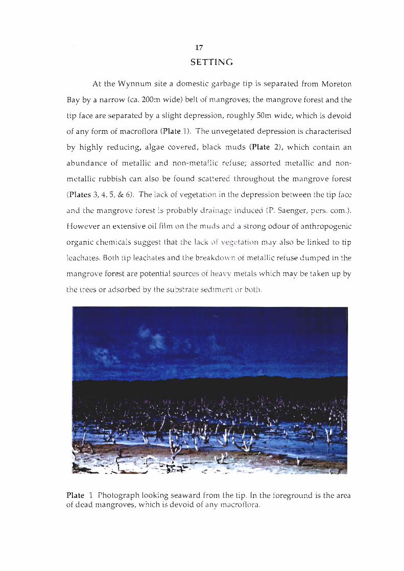
At the Wynnum site a domestic garbage tip is separated from Moreton
Bay by a narrow (ca. 200m wide) belt of mangroves; the mangrove forest and the
tip face are separated by a slight depression, roughly SOm wide, which is devoid
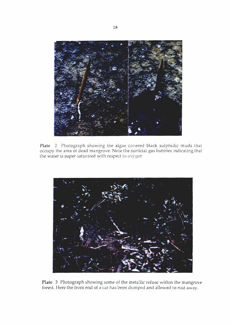
of any form of macroflora (Plate 1). The unvegetated depression is characterised
by highly red ucing, algae covered, black muds (Plate 2), which contain an
abundance of metallic and non-metallic refuse; assorted metallic and non-
metallic rubbish can also be found scattered throughout the mangrove forest
(Plates 3, 4,5, & 6). The lack of vegetation in the depression between the tip face
dnd the mangrove forest is probably dra inage indu ced (P. Saenger, p ers . com.).
How ever an extensive oil film on the mud s .lll.d a strong odour of anthropogenic
organic chemicals suggest that the lack l )f vege tat i )n may also be linked to tip
leachates. Both tip leachates and the breakdown of metallic refuse Jumped in the
mangrove forest are potentia l sources of heavy metals which may be taken up by
the trees or c1dsorbed by the substrate seLiim l:: nt ur buth.
Plate 1 Photograph looking seaward from the tip . In the foreground is the area of dead mangroves, which is devoid of any mJcroflora.
18
Plate 2 Photograph showing the algae co vered black sulphidic muds that occupy the area of dead mangrove. Note the surficial gas bubbles indicating that the water is super saturated with respect to oxygen
Plate 3 Photograph showing some of the metallic refuse within the mangrove forest. Here the front end of a car has been dumped and allowed to rust away.
19
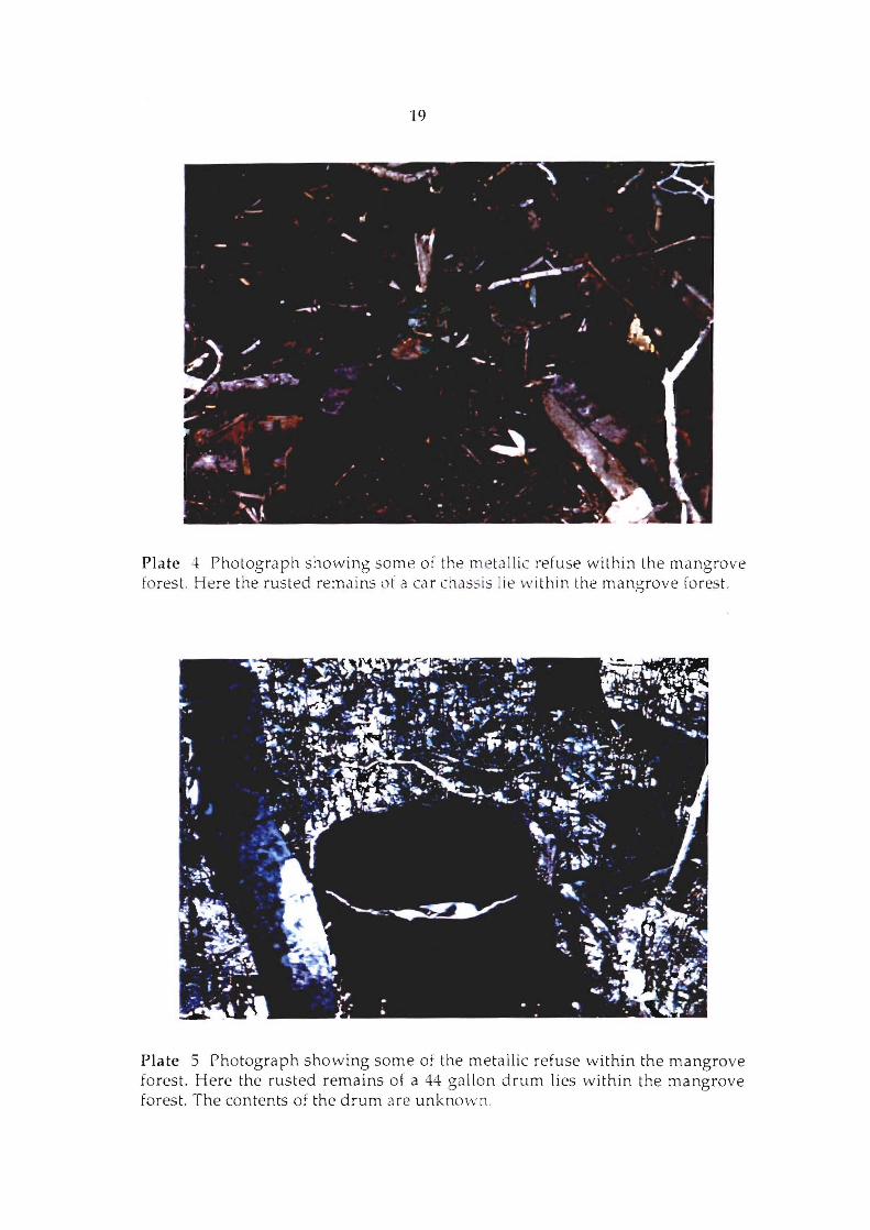
Plate 4 Photograph showing some of the me tallic refuse within the mangrove fo rest. Here the rusted remains of a car chass is lie wi thin the mangrove fore -L
Plate 5 Photograph showing some of the metallic refuse within the mangrove forest. Here the rusted remains of a 44 gallon drum lies within the mangrove forest. The contents of the drum are unknmvn.
20
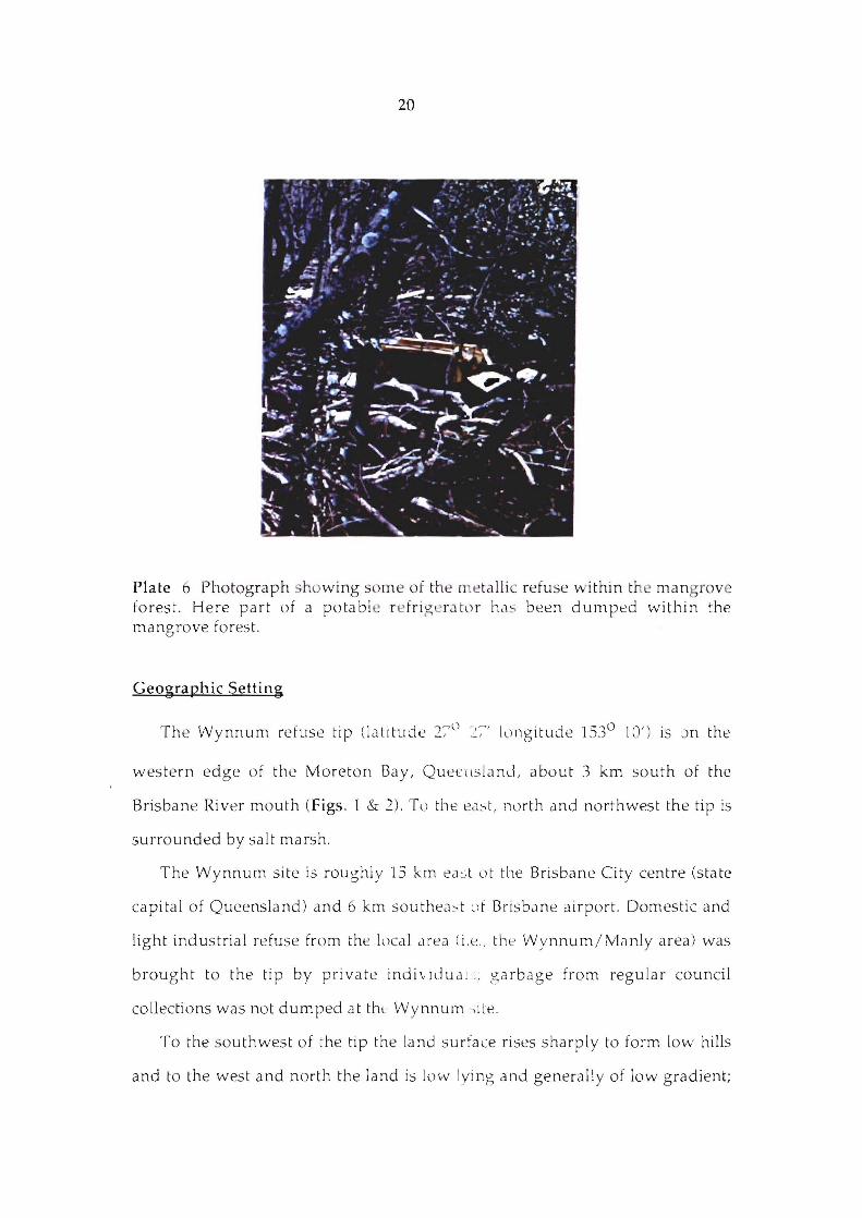
Plate 6 Photograph sho wing some of the m etalli c refuse within the mang rove forest. Here part of a potabl e r efrig l! r.)tor h.) s been dumped within the mangrove forest.
Geographic Setting
The Wynnum refuse tip (latitude 270 =:~" longitude 1530 10') is on the
western edge of the Moreton Bay, Queensland, about 3 km south of the
Brisbane River mouth (Figs. 1 & 2). Tu the ea:--t, nurth and northwest the tip is
surrounded by salt marsh.
The Wynnum site is roughly 15 km ea ~;t ot the Brisbane City centre (state
capital of Queensland) and 6 km sou thea~t uf Brisbane airport. Domestic and
light industrial refuse from the local Mea (i.e. , the Wynnum/Manly area) was
brought to the tip by private indi\Iduc11 ,; garbage from regular council
collections was not dumped at the Wynnum,iLe
To the southwest of the tip the land surface rises sharply to form low hills
and to the west and north the land is low lying and generally of low gradient;
21
the flat land including the tip, is part of the progradational deltaic surface of the
Brisbane River.
About 1.S km north of the Wynnum site is a major distributary channel of
the Brisbane River (the Boat Passage) that separates Fisherman's Island from
the mainland (Fig 2). The Port of Brisbane is on the western edge of Fishermans
Island just south of the Brisbane Bar (the site for tidal readings),
At the Wynnum site numerous small tidal channels enter the mangroves
particularly in the area south of the fisherman's access road (Fig. 2). Tidal
channels extend up to about 30 m into the forest and are characterised by a
lack of mangrove pneumatophores, an increase in algae cover, and a tendency
for channel sediment to be less consolidated than adjacent channel margin
deposits. Measurements during this study indicate that channel sediments are
more anoxic and have a higher pH than other parts of the mangrove forest.
Filling of the Wynnum tip has lead to some drainage changes and caused
most surface waters to drain northward into the salt marsh before moving to
the east and into the area of dead mangroves. Despite the blocking of the major
southeasterly drainage line by the fisherman's access road, surface waters still
migrate in that direction from the salt marsh. Other surface waters from the tip
drain to the south and onto the fisherman's access between the two tip cells.
km
AMPOL OIL REFINERY
SEWAGE TREATME1~-ffl~~~~~ PLANT.
MORETON BAY.
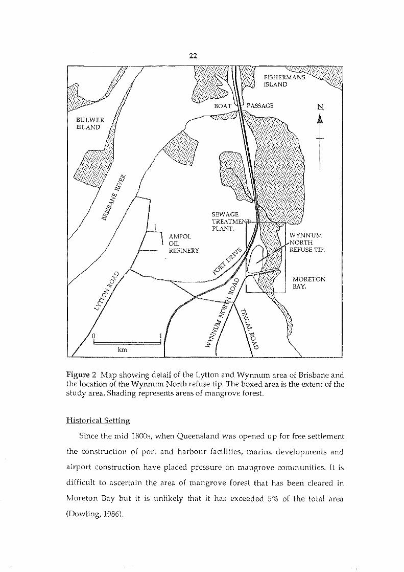
Figure 2 Map showing detail of the Lytton and Wynnum area of Brisbane and the location of the Wynnum North refuse tip. The boxed area is the extent of the study area. Shading represents areas of mangrove forest.
Historical Setting
Since the mid 1800s, when Queensland was opened up for free settlement
the construction of port and harbour facilities, marina developments and
airport construction have placed pressure on mangrove communities. It is
difficult to ascertain the area of mangrove forest that has been cleared in
Moreton Bay but it is unlikely that it has exceeded 5% of the total area
(Dowling, 1986).
23
Domestic and minor industrial refuse has been dumped at the Wynnum site
since 1925. The first cell, the southern "Old Tip" was open until March 1984 (1.
Woods, Manager, Department of Works, Brisbane City Council, pers. comm.)
The Northern Tip is separated into two triangular sections by the
fisherman's access road. An agreement with the land holders to the west of the
tip site allowed the council to merge the tip with their properties. The merging
of the tip and the free hold properties above the original high water mark is
said to have eliminated a drainage and mosquito breeding problem (I. Woods,
pers. comm.).
The Northern Tip cell had an expected life of eleven years but was closed by
the council in June 1991 as a result of both economic and environmental
concerns. At the time of closure the council applied 600 mm of cover over the
garbage in an attempt to control infiltration of rain water and leachate
formation. In September of 1991 the council also laid a leachate drain along the
seaward margin of the tip to collect leachate for recirculating or treatment (1.
Woods, pers. comm.).
Climatic Setting
The climate of the area is controlled by the seasonal oscillation of the high
pressure anticyclone belt in the southern hemisphere. This oscillation results in
the southeast of Queensland experiencing two major weather patterns. The
first, is controlled by the movement of air from the southwest over the
continent during the winter months when the anticyclone belt is at its most
northerly position. The second, is controlled by onshore easterly winds in
summer when the anticyclone belt is in its most southerly position (Lindacre &
Hobbs, 1977; Coordinator General's Department, Queensland, 1974).
The climate of Moreton Bay is classified as Cfa on the Koppen-Geiger
system (Koeppe & Long, 1958; Lindacre & Hobbs, 1977; Saenger et al., 1977) or a
humid subtropical climatic region (Gentilli, 1972; Koeppe & Long, 1958). This
24
climate is characterised by high rainfall and humidity during the warmer
summer months and drier conditions, with a wide temperature range the
winter months.
Temperature
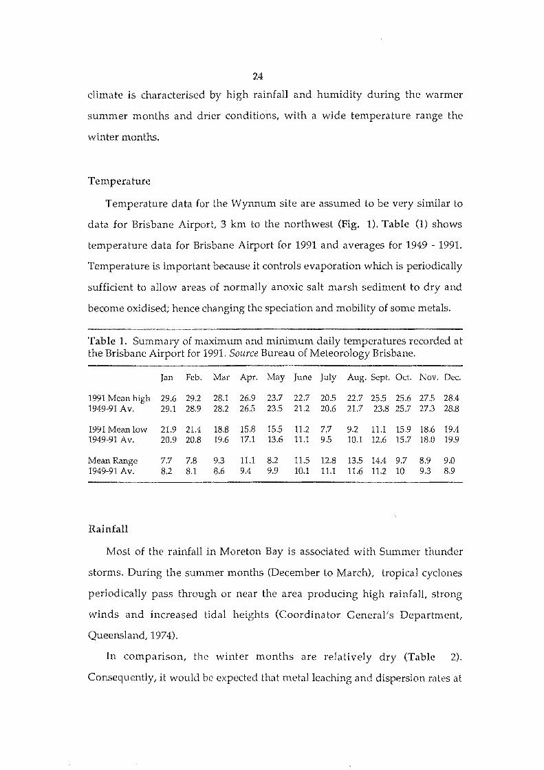
Temperature data for the Wynnum site are assumed to be very similar to
data for Brisbane Airport, 3 km to the northwest (Fig. 1). Table (1) shows
temperature data for Brisbane Airport for 1991 and averages for 1949 1991.
Temperature is important because it controls evaporation which is periodically
sufficient to allow areas of normally anoxic salt marsh sediment to dry and
become oxidised; hence changing the speciation and mobility of some metals.
Table 1. Summary of maximum and minimum daily temperatures recorded at the Brisbane Airport for 1991. Source Bureau of Meteorology Brisbane.
Jan Feb. Mar Apr. May June July Aug. Sept. Oct. Nov. Dec.
1991 Mean high 29.6 29.2 28.1 26.9 23.7 22.7 20.5 22.7 25.5 25.6 275 28.4 1949-91 Av. 29.1 28.9 28.2 26.5 23.5 21.2 20.6 21.7 23.8 25.7 27.3 28.8
1991 Mean low 21.9 21.4 18.8 15.8 15.5 11.2 7.7 9.2 11.1 15.9 18.6 19.4 1949-91 Av. 20.9 20.8 19.6 17.1 13.6 11.1 9.5 10.1 12.6 15.7 18.0 19.9
Mean Range 7.7 7.8 9.3 11.1 8.2 11.5 12.8 13.5 14.4 9.7 8.9 9.0 1949-91 Av. 8.2 8.1 8.6 9.4 9.9 10.1 11.1 11.6 11.2 10 9.3 8.9
Rainfall
Most of the rainfall in Moreton Bay is associated with Summer thunder
storms. During the summer months (December to March), tropical cyclones
periodically pass through or near the area producing high rainfall, strong
winds and increased tidal heights (Coordinator General's Department,
Queensland,1974).
In comparison, the winter months are relatively dry (Table 2).
Consequently, it would be expected that metal leaching and dispersion rates at
25
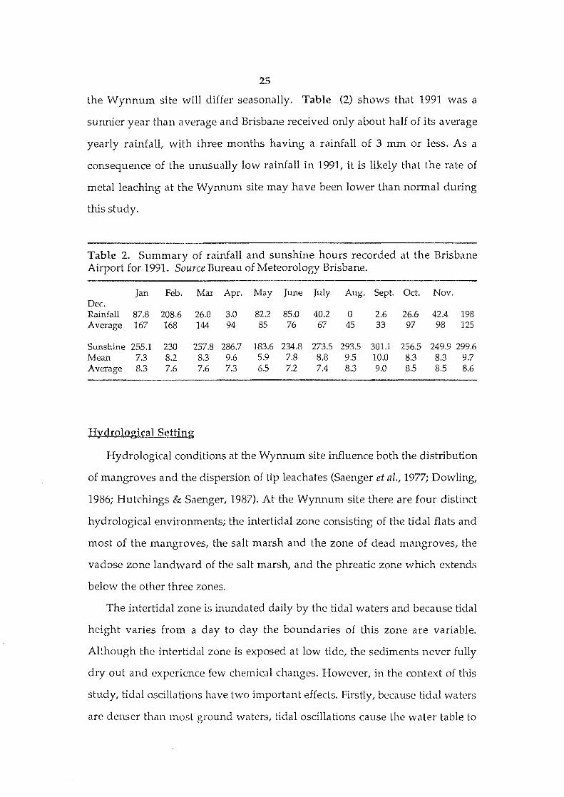
the Wynnum site will differ seasonally. Table (2) shows that 1991 was a
sunnier year than average and Brisbane received only about half of its average
yearly rainfall, with three months having a rainfall of 3 mm or less. As a
consequence of the unusually low rainfall in 1991, it is likely that the rate of
metal leaching at the Wynnum site may ha ve been lower than normal during
this study.
Table Summary of rainfall and sunshine hours recorded at the Brisbane Airport for 1991. Source Bureau of Meteorology Brisbane.
Jan Feb. Mar Apr. May June July Aug. Sept. Oct. Nov. Dec. Rainfall 87.8 208.6 26.0 3.0 82.2 85.0 40.2 0 2.6 26.6 42.4 198 Average 167 168 144 94 85 76 67 45 33 97 98 125
Sunshine 255.1 230 257.8 286.7 183.6 234.8 273.5 293.5 301.1 256.5 249.9 299.6 Mean 7.3 8.2 8.3 9.6 5.9 7.8 8.8 9.5 10.0 8.3 8.3 9.7 Average 8.3 7.6 7.6 7.3 6.5 7.2 7.4 8.3 9.0 8.5 8.5 8.6
Hydrological Setting
Hydrological conditions at the Wynnum site influence both the distribution
of mangroves and the dispersion of tip leachates (Saenger et al., 1977; Dowling,
1986; Hutchings & Saenger, 1987). At the Wynnum site there are four distinct
hydrological environments; the intertidal zone consisting of the tidal flats and
most of the mangroves, the salt marsh and the zone of dead mangroves, the
vadose zone landward of the salt marsh, and the phreatic zone which extends
below the other three zones.
The intertidal zone is inundated daily by the tidal waters and because tidal
height varies from a day to day the boundaries of this zone are variable.
Although the intertidal zone is exposed at low tide, the sediments never fully
dry out and experience few chemical changes. However, in the context of this
study, tidal oscillations have two important effects. Firstly, because tidal waters
are denser than most ground waters, tidal oscillations cause the water table to

26
rise and fall through chemically different zones in the sediment profile.
Secondly, tidal water is chemically distinct from the ground water and the
mixing of the two water types can lead to chemical reactions which do not
occur in either original water type.
Tides in Moreton Bay are generally larger and fractionally delayed relative
to the oceanic tides (Dowling, 1986). The Brisbane Bar is used as a reference
point for tides in Moreton Bay, although there is evidence that some of the
islands in the bay experience slightly larger tides than the bar (Coordinator
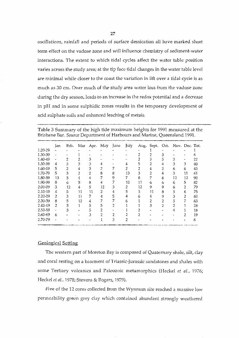
General's Department, Queensland, 1974). Table (3) summarises the tidal data
for the Brisbane Bar in 1991. Because the highest spring tides (Table 3) occur
only a few times a year; the salt marsh surrounding the tip is seldom totally
inundated by tidal waters.
Maximum water depths in the marsh zone varies from a few centimetres in
the eastern portion to about 0.5 m just north of the tip (Fig. 2); during the dry
season a large proportion of the salt marsh has no surface water. As a result of
the shallowness of the marsh, seasonal variations in water level are marked and
during the dry season, salinity increases substantially due to evaporation;
during the rainy season the salinity of the water in the salt marsh drops as fresh
water influx becomes dominant.
Water in the phreatic zone responds to tidal pressures daily as saltwater
wedging forces the ground water to on the incoming tide. The saltwater
wedge exposes the deeper sediments and the weathered basalt to cyclically
varying chemical conditions and may influence metal dispersion and
speciation. The extent of the tidally driven movement of the boundary between
phreatic zone groundwaters and tidal waters will also vary seasonally in
response to variations in the hydrostatic pressure of the groundwaters,
groundwater flow volumes, and capillary suction through the vadose zone.
Water levels and water chemistry in the vadose zone (above the water
table) are more variable than they are in the other three zones. Tidal
27
oscillations, rainfall and periods of surface dessication all have marked short
term effect on the vadose zone and will influence chemistry of sediment-water
interactions. The extent to which tidal cycles affect the water table position
varies across the study area; at the tip face tidal changes in the water table level
are minimal while closer to the coast the variation in lift over a tidal cycle is as
much as 30 cm. Over much of the study area water loss from the vadose zone
during the dry season, leads to an increase in the redox potential and a decrease
in pH and in some su1phidic zones results in the temporary development of
acid sulphate soils and enhanced leaching of metals.
Table 3 Summary of the high tide maximum heights for 1991 measured at the Brisbane Bar. Source Department of Harbours and Marine, Queensland 1991.
Jan Feb. Mar Apr. May June July Aug. Sept. Oct. Nov. Dec. Tot. 1.20-29 1 1 1.30-39 1 2 2 3 6 1.40-49 2 2 3 2 5 5 3 22 1.50-59 4 5 3 3 4 4 5 2 4 3 3 40 1.60-69 5 2 4 3 2 7 2 2 4 2 6 6 45 1.70-79 5 3 2 2 8 8 13 3 2 4 3 11 61 1.80-89 13 5 4 4 7 9 7 8 7 6 12 12 90 1.90-99 8 6 5 8 4 7 10 11 6 6 6 5 82 2.00-09 3 12 4 5 12 3 2 12 9 9 6 2 79 2.10-19 4 5 11 11 2 4 5 3 11 8 5 6 75 2.20-29 2 3 11 7 4 5 4 6 4 9 3 2 60 2.30-39 8 5 12 4 7 7 6 1 2 2 5 7 63 2.40-49 2 3 1 5 5 2 1 1 3 2 2 1 28 2.50-59 3 5 2 1 2 4 1 18 2.60-69 6 3 2 2 2 2 2 19 2.70-79 1 3 2 6
Geological Setting
The western part of Moreton Bay is composed of Quaternary shale, silt, clay
and coral resting on a basement of Triassic-Jurassic sandstones and shales with
some Tertiary volcanics and Paleozoic metamorphics (Heckel et al., 1976;
Heckel et aI., 1978; Stevens & Rogers, 1979).
Five of the 12 cores collected from the Wynnum site reached a massive low
perm.eability green grey clay which contained abundant strongly weathered
28
basalt clasts; these clasts suggests that the underlying basement at the
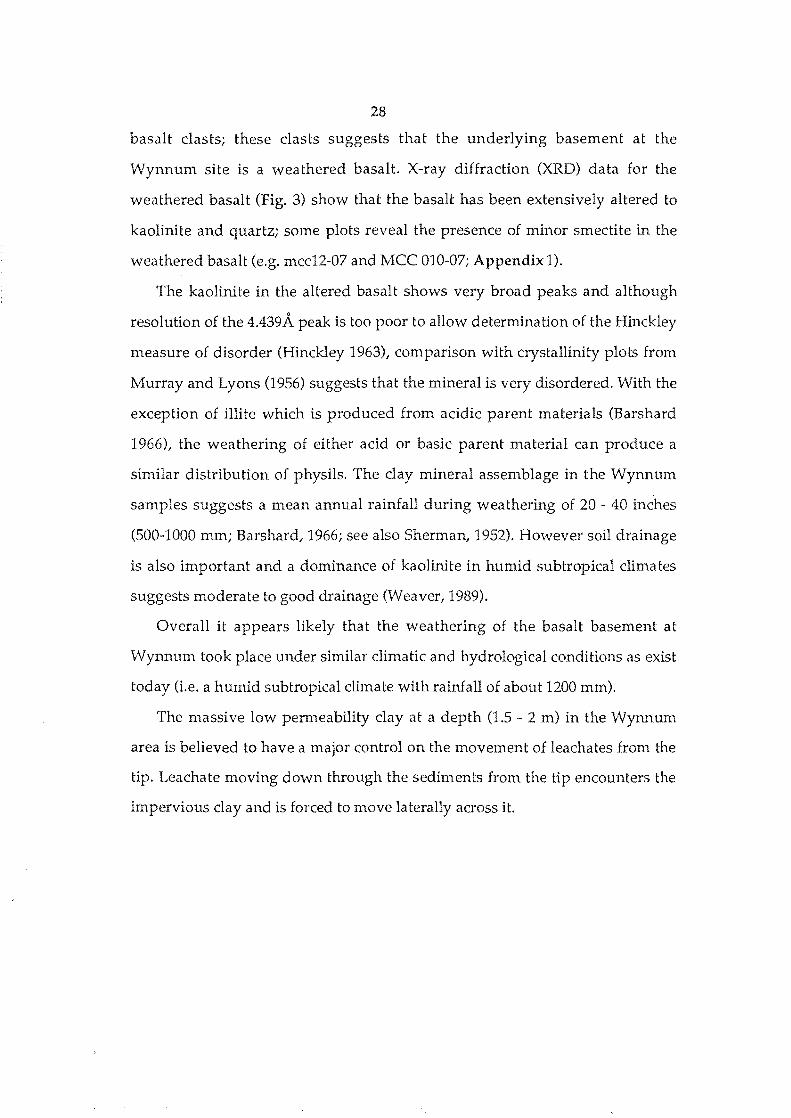
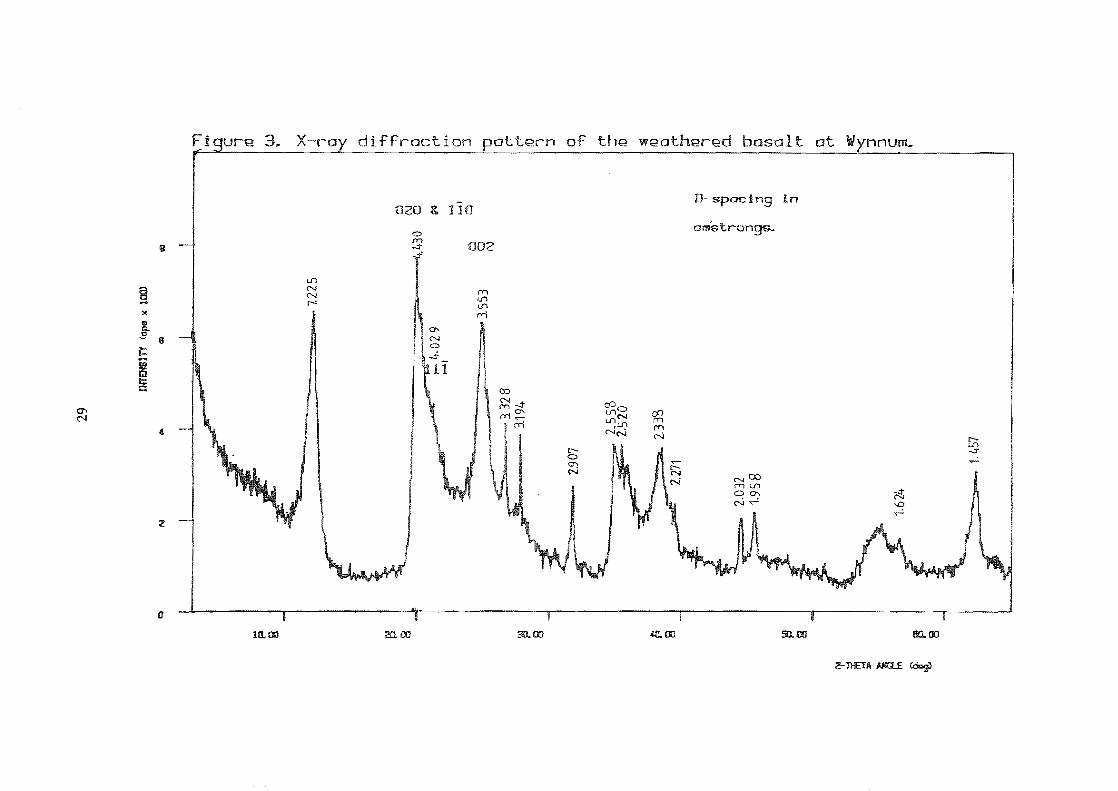
Wynnum site is a weathered basalt. X-ray diffraction (XRD) data for the
weathered basalt (Fig. 3) show that the basalt has been extensively altered to
kaolinite and quartz; some plots reveal the presence of minor smectite in the
weathered basalt (e.g. mcc12-07 and MCC 010-07; Appendix 1).
The kaolinite in the altered basalt shows very broad peaks and although
resolution of the 4,439A peak is too poor to allow determination of the Hinckley
measure of disorder (Hinckley 1963), comparison with crystallinity plots from
Murray and Lyons (1956) suggests that the mineral is very disordered. With the
exception of illite which is produced from acidic parent materials (Barshard
1966), the weathering of either acid or basic parent material can produce a
similar distribution of physils. The clay mineral assemblage in the Wynnum
samples suggests a mean annual rainfall during weathering of 20 40 inches
(500-1000 mm; Barshard, 1966; see also Sherman, 1952). However soil drainage
is also important and a dominance of kaolinite in humid subtropical climates
suggests moderate to good drainage (Weaver, 1989).
Overall it appears likely that the weathering of the basalt basement at
Wynnum took place under similar climatic and hydrological conditions as exist
today (Le. a humid subtropical climate with rainfall of about 1200 mm).
The massive low permeability clay at a depth (1.5 - 2 m) in the Wynnum
area is believed to have a major control on the movement of leachates from the
tip. Leachate moving down through the sediments from the tip encounters the
impervious clay and is forced to move laterally across it.
29
I Iff
ENS m
(op
e l>I
10
0)
N
'" ."
"". C
., ....
10
p W
8
1 X
7.22
5 I ., a a..
,..- -t
, ~
0 '""
t)
8 N
.,
.430
C
l 0 il
>-
4.02
9
!I'Q
(1'
.....
t ,...-
.... 0
.....
1
0 0
:J
1553
a N
a
13
28
~
l!J 3.
194
r- IO
8 ., :J
a .,., (1'
2.55
'0
......
--'
2.52
0 to :IIi
P
2.33
B
f1) a
8 (T
::r'
Q
" f1
)
~,
I .,
til ro
.-r
-0
Cl.
1 ~
2.03
2 0
IT
:J
.... 1.
958
~ ::J
n lQ
IJ
) a 19
.... I-
"
::J ('
I"
B
a (T
~ ~
IE:
".
::l
a ::J
c: 1.
624
3. ,
~ ~ 8
1.45
7
30
Geomorphic Setting
At the Wynnum site there are five major geomorphic features; these are the
intertidal mudflats, the mangrove belt, the salt marsh, the tip, and the
fisherman's access road. The intertidal mudflats are extensive to the east of the
mangrove fringe and extend up to 1 km from the seaward edge of the trees. The
mudflats have a low gradient and are cut by a series of anastomosing tidal
channels draining the surface in a southeasterly direction. The wide mudflats
provide a protective barrier for the mangroves because the shallow water
reduces wave action, which might otherwise undermine the mangrove root
system (Dowling, 1986).
Mangroves at Wynnum form a narrow fringe parallel to the coast and
because of their ability of to trap and accrete sediment there is a sharp drop of
about 30 cm from the forest margin onto seaward mudflats. The gradient on the
mangal sediment surface is shallow and rises gently to the west. As a result of
the rise in elevation to the west there is a zonation in tree species and tree
morphology. The zonation is a response to tidal inundation and results in
sequential changes in dominant tree species and a progressive reduction in tree
height for Avicennia from tall trees at the coast to a low shrub inland (Saenger
et al., 1977, Dowling, 1986; Hutchings & Saenger, 1987).
The low gradient and low relief within the mangrove forest results in local
pooling of water, especially to the south of the fisherman's access. Drainage
from within the forest in an easterly direction is via a number of short (c.a. 30
m) tidal channels, though some also drain in a more southerly direction. As
with the small pools most of these channels are concentrated south of the access
way. Tidal channels contain an abundance of unconsolidated fine sediment and
at low tide often contain pools of surface water. As a result of the combination
of low relief and the large nUlll.ber of drainage lines with pooled water, the
forest south of the fisherman's access way is more waterlogged and
consequently the sediment is more anoxic than the forest north of the access.
31
The fisherman's access way cuts the field area into two unequal portions
and, compared to the mangrove forest floor, has a significant relief. The road
surface consists of compacted, mostly schistose, rubble and the road while
sloping gently to the east, also slopes from its northern edge to the south; the
southern margin of the road merges smoothly with the southern mangrove
forest floor. Whereas the northern edge of the road is raised (c.a. 15 cm) above
the mangal sediments. The raised northern edge of the road acts as a dam and
causes pooling of the surface water except where small drainage lines cut across
the road. The road also acts as a conduit for runoff from the tip; run off tends to
accumulate in the depression between the two tip cells before draining to the
south into the mangroves.
The saltmarsh occupies the zone between the mangroves and the more
elevated mainland. The marsh is nearly flat and has a low gradient that gently
rises to the west. The eastern portion of the marsh is normally inundated, with
the water occupying a shallow depression landward of the mangrove forest.
This shallow depression allows the accumulation of about 40 cm of water that
extends into the area of dead mangroves on the seaward side of the tip. Both
the salt marsh and the area of dead mangroves are subject to intense
evaporation and salinities twice that of seawater are common during the dry
season.
The tip has an elevation of about 6m above that of the mean high water
level (1. Woods, pers. comm.). The, nearly level, upper surface of the tip cell
falls sharply to the saltmarsh to the northwest, the dead mangroves to the east
and the fisherman's access way to the south. These steep slopes at the edge of
the tip are heavily rilled by surface runoff and sediment transported down the
rills extends several metres into the saltmarsh and dead mangroves to provide a
thin veneer of oxidised sediment.
32
Sedimentation over the last 6000 yrs
The marginal marine sediments at Wynnum rest unconformably on a
weathered basalt. The sediment cover is about 1.5 m thick in the southern part
of the site, and thickens northward as a result of the gradual northerly dip on
the unconformity.
Overlying the basalt is a shelly deposit with many shells embedded in the
top of the weathered basalt. Carbon dated (by Beta Analytical, Florida) shell
material from MCC 003 returned an age of 2660± 70 yrs.B.P .. This date gives a
minimum age for the erosional surface on the weathered basalt. Another
sample from 690 mm down core MCC 003 returned an age of 1440±70 yrs.B.P ..
These two dates indicate average sedimentation rates for the area of 0.33
mm/yr. for the lower portion of the core and a rate of 0.48 mm/yr. for the
upper part of the core. The greater sedimentation rate for the upper portion of
the core reflects accelerated accretion following colonisation of the sediments by
mangroves which trap and bind fine grained sediments. The dated shell species
were either Anadara trapezia (Sydney Cockle) or Batilleria australis (mudwelk);
both of these molluscs are found in estuarine environments; with sandy to
muddy sediments (Shepard & Thomas, 1989).
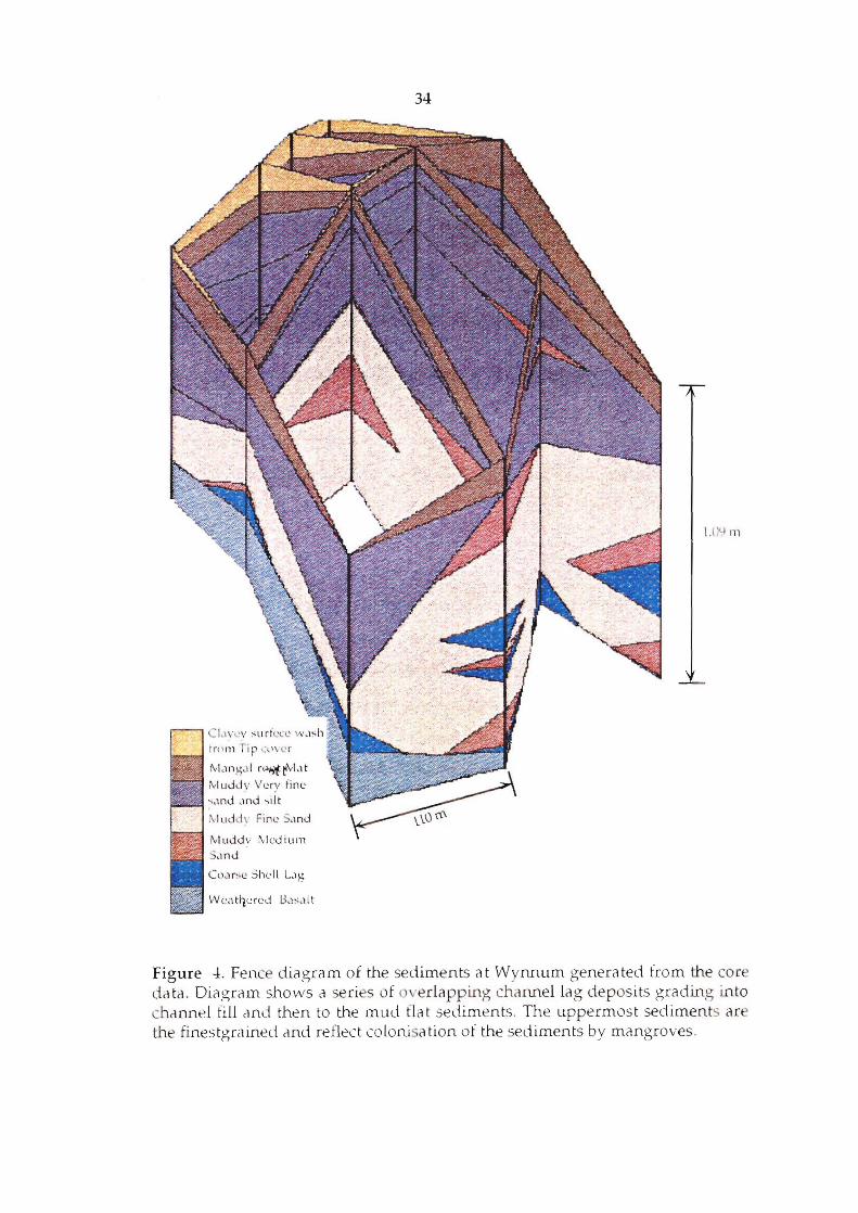
Stratigraphic data from the 12 cores taken from the site are presented in a
fence diagram (Figure 4) which shows the spatial distribution of sediments. The
logged cores showed no primary sedimentary structures other than a few sharp
contacts which probably correspond to erosional surfaces and/or periods of
non-deposition; however subtle structures may be revealed by techniques such
as x-ray radiography (e.g. Hamblin, 1962). All cores show a fining upwards
trend in mean grainsize with a typical sequence grading upward from a coarse
shelly lag deposit through a muddy medium to medium fine sand then a
muddy fine sand and finally a silty or clayey mud.
Higher velocity tidaL flows in channels have locally winnowed fine
sediments to leave a coarse lag deposit; shells are abundant in these channel
33
deposits. Lateral migration of modern tidal channels has produced
discontinuous units characterised by longitudinal crossbedding (e.g. see
Reineck & Singh, 1975), but none of these units were intersected in the test
cores.
Heckle et al. (1978) interpret the area as tidal flats associated with the
development of the Brisbane River bird foot delta and Figure (4) shows a series
of overlapping shelly deposits that are interpreted as lag deposits of
distributary tidal channels; the fining upward sequence reflects infilling
followed by tidal flat development and finally by muddy deposits associated
with mangrove colonisation of the intertidal zone. Tidal flats (e.g. Jade Bay,
Germany) show a similar tendency for muds occupy the zone closest to the
shore while sand becomes progressively coarser off shore (Gadow, 1970 in
Reineck & Singh, 1975).
The tidal mud flat and mangal forest sediments are heavily bioturbated by
polychaetes, amphiopods, crustaceans, and gastropods (Frey et aI., 1989).
Infauna population densities of up to 20,000 individuals per m 2 have been
recorded for similar sites (Gerdes et al., 1985) and it is likely that any primary
sedimentary structures which may have been present were rapidly destroyed
during bioturbation. All available evidence suggests that it is unlikely the
environment for sediment accumulation at the Wynnum site has changed
radically over the last 3,000 years.
t r<l 1l1 Ti P ( , ' \. ' r
1\ ,1.1[1 :.;,\1 n'~ ~\I ,\ t
;'vluJdv Verv fine ~.md .mJ -, ilt
.\1 L1dd v Fi ne S.md
j'vlLlJdv :\·lediuln S.md
Ct' ,1r~ e She ll L'\f;
34
LIN m
Figure -:1:. Fenc diagram of the sediments at Wynnum generated from the core data, Diagram shows a seri s of 0 'eriapp ing channel lag deposits grading into -hannel fill c1nd then to the mud flat sediments. The uppermost sediments ar the finestgrained and reflect coiorusa tion of the sediments by mangroves.
35
Recent changes in drainage
Analysis of aerial photos 6f the Wynnum area since 1964 reveals several
changes in drainage patterns and the effect of these changes on vegetation
cover. Some of the drainage and vegetation changes are associated with
construction work that has been undertaken in the area since 1964. For example
the blocking of drainage lines during construction works caused mangroves to
die off in several areas when they were cut off from tidal influences. Although
mangroves need not be directly inundated by the tide, most species do need to
feel tidal action through their root systems (Hutchings & Saenger; 1987).
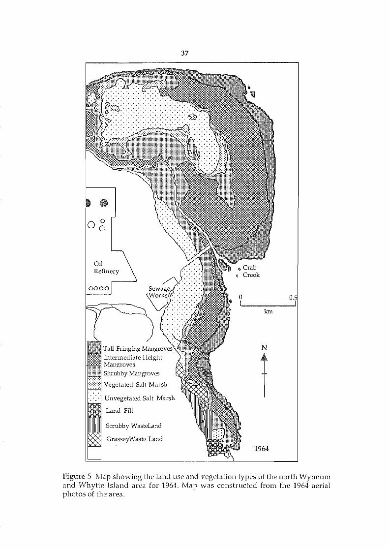
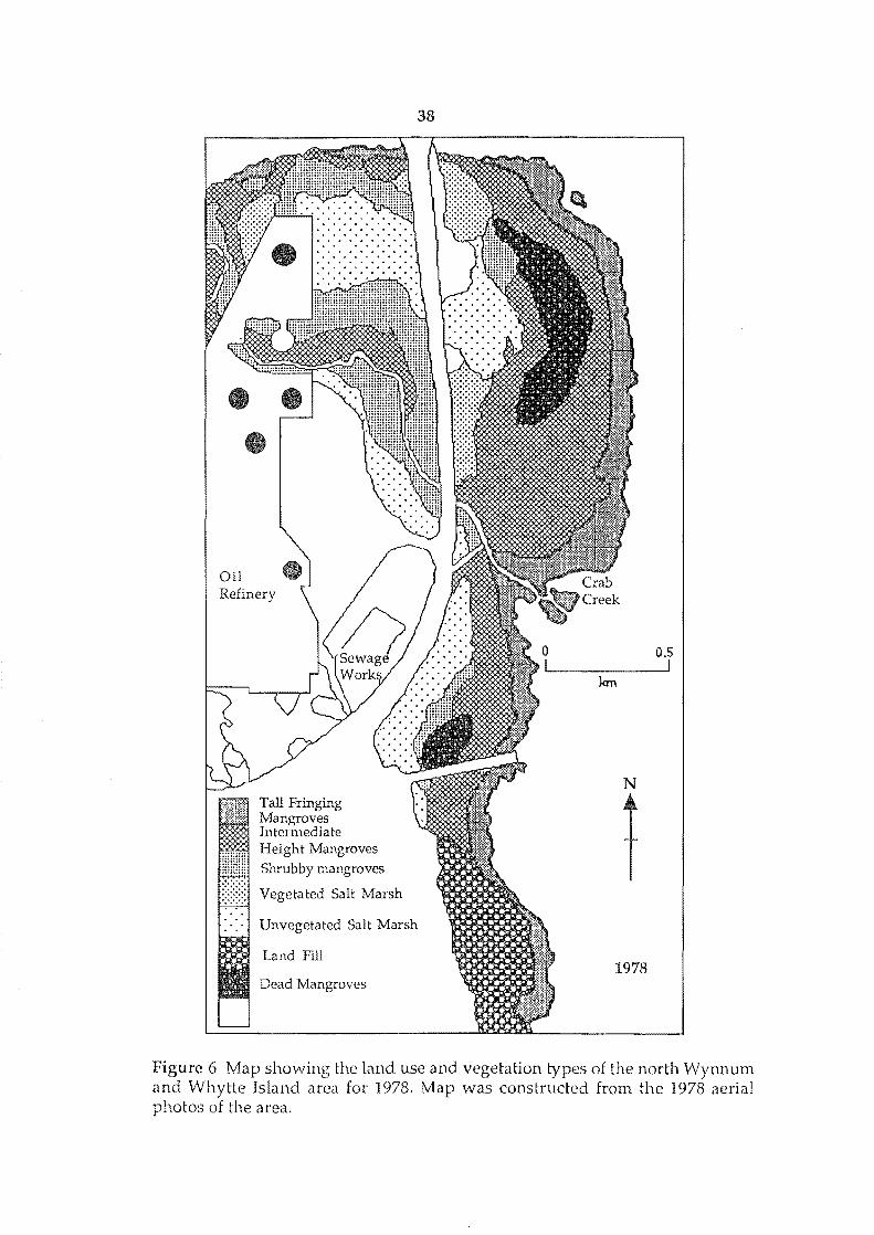
Figures 5, 6 and, 7 show the changes in drainage and vegetation patterns in
the North Wynnum area recorded by 1964, 1978, and 1991 aerial photographs.
A comparison between the 1964 and 1978 photos (Figs 5 & 6) shows that
construction of Port Drive and the railway to Fisherman's Island through the
middle of the salt marsh has disrupted a westerly directed drainage resulting in
the dying off of an area of mangroves to the east of the road (Figure 6). The
northward extension of the refinery appears to have stressed the mangroves
between Port Drive and the refinery but these trees are not yet dead. In contrast
the tall trees on the seaward fringe of Whytte Island appear unaffected by
construction work, and growth of the trees at the mouth of Crab Creek has been
enhanced by nutrient supply from the sewage out fall in the creek.
The extension of Wynnum North Road to the coast, as a fisherman's access,
has crossed a drainage line between the salt marsh and the coast and caused the
drowning of a patch of mangroves north of the road. The actual date for the
construction of the access way is unclear, but it is believed to have been around
1969 (N. Gibson, Roads and Works Department, Brisbane City Council, pers.
comm.), and by 1978 the original drainage line has become indistinct.
By 1978 the southern cell of the tip complex was well developed and
extended over an area of scrub land and scrubby mangroves so that only the
tallest fringing trees remained (Figs 5 & 6).

36
A comparison of the 1978 and 1991 aerial photographs reveals further
changes in the area. The construction of the marina and port facilities to the
west of Port Drive led to the death of mangroves between Port Drive and the oil
refinery (Figs 6 & 7). The marina facilities and the roadway servicing them,
have probably isolated the mangroves from tidal movement. Parts of the
southern end of the mangrove forest in this section have been infilled as part of
an extension of the refinery.
Between 1978 and 1991 the large area of dead mangroves north of the
fisherman's access way increased in size and the northern cell of the Wynnum
tip was built over the western edge of the mangrove forest. It is unclear
whether establishment of the tip helped increase the area of dead mangroves or
if this was a natural continuation of the die off initiated by construction of the
access way.
Since 1978 the mangrove island at the mouth of Crab Creek has increased in
area so that is now joined to the mainland to create a sheltered embayment
(Figure 6 & 7). The embayment is now being colonised by many mangrove
seedlings which will presumably increase sediment accretion and push the
coastline seaward in future.
0° o
:: Tall Fringing Mangroves Intermediate Height Mangroves Shrubby Mangroves
Vegetated Salt Marsh
Unvegetated Salt Marsh
Land Fill
Scrubby WasteLand
GrasseyWaste Land
37
o O. I
km
N
1964
Figure 5 Map showing the land use and vegetation types of the north Wynnum and Whytte Island area for 1964. Map was constructed from the 1964 aerial photos of the area.
Oil Refinery
Height Mangroves Shrubby mangroves
38
Vegetated Salt Marsh
Unvegetated Salt Marsh
Dead Mangroves
km
N
t 1978
Figure 6 Map showing the land use and vegetation types of the north Wynnum and Whytte Island area for 1978. Map was constructed from the 1978 aerial photos of the area.
Oil Refinery
Tall Fringing Mangroves Intennediate Height Mangroves Shrubby mangroves
Vegetated Salt Marsh
Dead Mangroves
39
Unvegetated Salt Marsh
Land Fill
Unvegetated Areas, Eg Roads and Residential
km
N
t 1991
0.5 . I
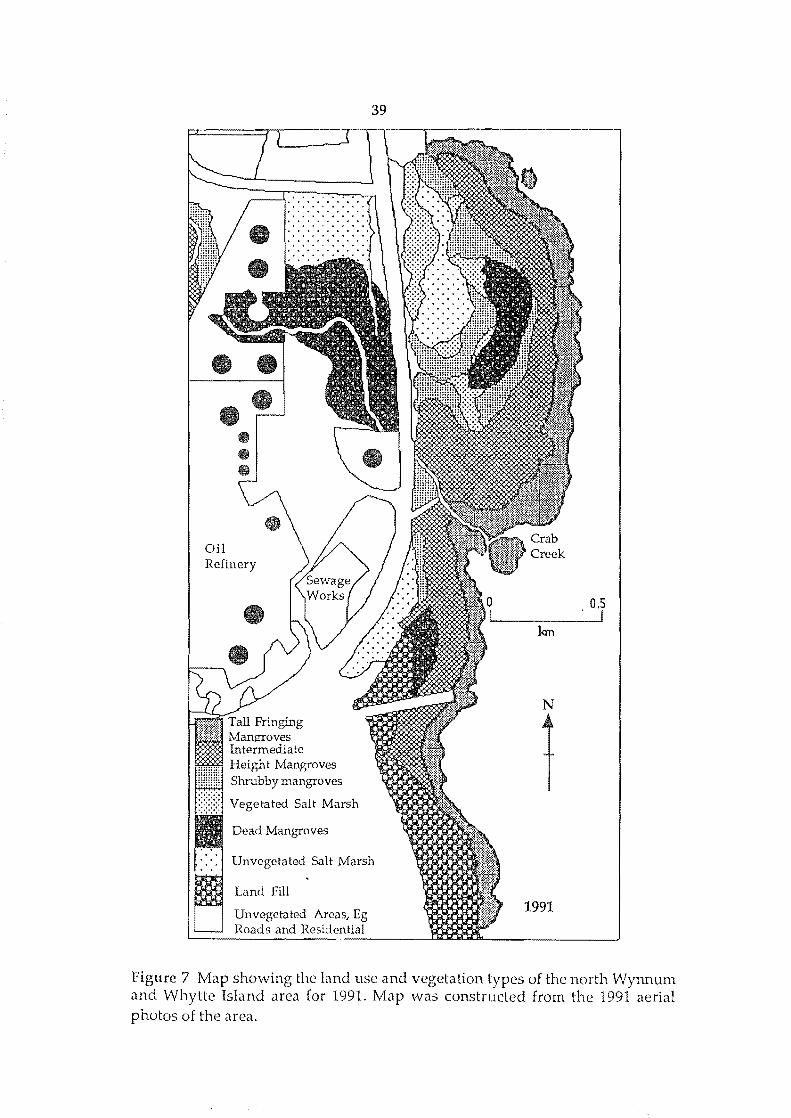
Figure 7 Map showing the land use and vegetation types of the north Wynnum and Whytte Island area for 1991. Map was constructed from the 1991 aerial photos of the area.
Sediment Sampling
40
METHODOLOGY
Core and grab samples were collected across the site from a parallel line
sampling grid (Forstner, 1989; Fig. ,8). An unequal sample spacing for core
samples is employed because Saenger, McConchie and Clark (1991), show that
contamination decreases away from the tip; hence sampling frequency is
highest in the area of most rapid change in metal concentrations near the tip.
The same parallel line grid with an equal spacing was used for surface grab
samples.
Core samples.
Cores were extracted by driving a 3 m length of 50 mm P.V.c. into the
sediment until about 500 mm of pipe remained above ground. Compaction
fadors are determined, by measuring the internal depth to the sediment (Di),
the external depth to the sediment (De), and the total length of the pipe (L); and
using of the given equation:
(Di- De) Compadion factor (%) (100 * -----1
(L - De)
compaction factors are summarises in Table (4).
Filling the above-ground pipe with seawater and sealing the end with a
water filled plumbers dummy allows the core to be extracted with two
opposing lifting handles (Fig. 9). The excess pipe is then cut off and the ends
sealed with plastic bags.
41
MORI:TON BAY
WRECK
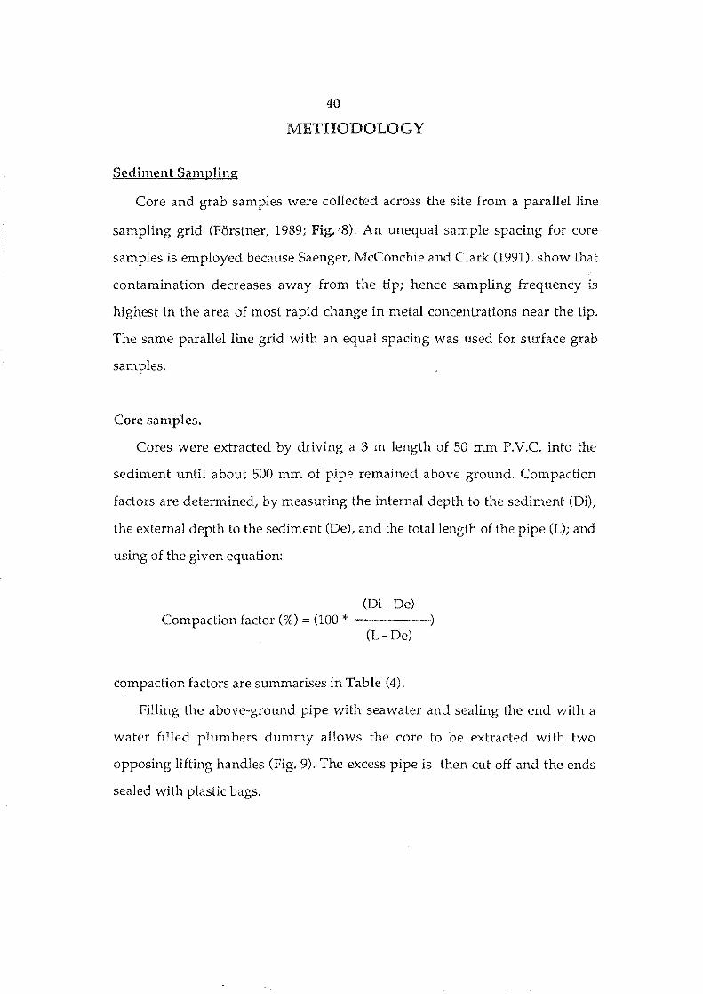
Figure 8 Map of the Wynnum Tip site showing the locations of cores and transects: T1 (transect 1), T2 (transect 2), T3 (transect 3), T4 (transect 4), and TS (transect 5; transect 5 continues to the coast off the northern edge of map). Filled circles denote core holes and Xs indicate where water or sediment samples were taken.
42
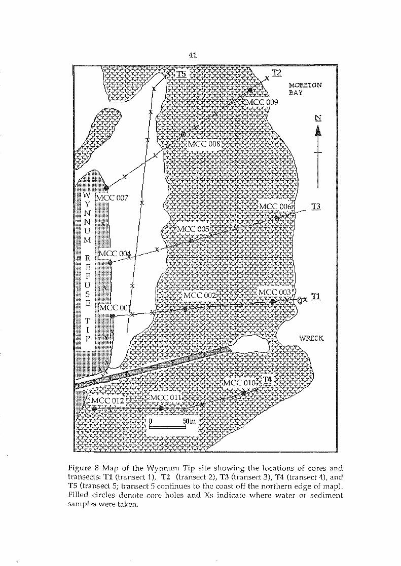
Table 4. Compaction factors for sample cores see figure 8 for location.
Core MCC 001 MCC 002 MCC 003 MCC 004 MCC 005 MCC 006 MCC 007 MCC 008 MCC 009 MCC 010 MCC 011 MCC 012
% 39.0 56.5 51.9 53.6 54.6 49.6 59.1 47.4 54.6 48.0 47.3 25.5
Direction of lift
Water filled pipe
Direction of lift
Figure 9 Cross sectional diagram of the core extraction technique using a plumber's dummy and a water filled PVC pipe; suction caused by the water extracts the sediment with the pipe during lifting.
Surface grab samples
A spade was used to take grab samples by shaving off a 5 10 cm slab
from the side of holes dug into the sediment. Samples were collected from 2
depths at each sampling site: a surface sample spanning the depth from 0-5 cm
and a sample spanning the range from 30-35 cm. As much air as possible was
excluded from sample bags before sealing and labelling; air exclusion is
necessary to avoid, or at least minimise oxidation of sulphidic material by
43
atmospheric oxygen.
Surface Water Samples
Water samples from natural pools of water on the sediment surface, or
waters in the holes from which grab samples were taken, make up the bulk of
surface waters collected from the Wynnum site. Other samples of storm water
runoff from the tip and samples from the leachate drain are also included as
surface water samples. Water collection was in 1 litre plastic bottles, which
were washed in 1 M. nitric acid and rinsed three times with the water to be
sampled. Air was excluded from the bottle before sealing and labelling the
sample; air exclusion, to minimise oxidation reactions by atmospheric oxygen,
required either complete filling of the bottles, or squeezing the bottle to reduce
available air space to zero.
Groundwater Samples
Groundwater samples were taken from 6 piesometers set up in the core
holes of transect 2 and 4 (Fig. 8). Piesometers constructed for this purpose
consist of a 2 m length of 50 mm PVC pipe with numerous holes drilled the
lower 1.5 m to allow groundwater inflow. The collection of groundwater
followed the same procedure as for surface waters, but required sample
extraction from the piesometer using a small hand pump.
Piesometers were monitored and sampled about every fortnight to detect
changes in metal concentrations that might relate to events such as heavy
rainfall or drought periods.
Surveying of the Field Area
Because pollutant movement in a setting such as the Wynnum site may be
linked to leaching processes, both within the tip and within the mangal
sediments, tidal flushing, and drainage patterns a detailed site relief survey is
44
likely to be particularly informative. In the salt marsh where there are areas of
ponded water and areas which are relatively dry; there can be little doubt that
chemical conditions in these subzones will differ. Similarly parts of the
mangrove forest experience differing levels of tidal inundation: those closest to
the coast experience diurnal variations whereas those parts nearest the marsh
may only e'fperience tidal inundation once a month. Hence Eh, pH and salinity
conditions, which will influence metal distribution, are likely to vary as a
function of small changes in site morphology and position.
Height survey
The height survey (levelling) of the Wynnum site was conducted using the
reduced level method and a D.CL. Tw-20A theodolite. This method uses the
principle of height relationships and not the absolute height above sealevel. For
the information that the survey was designed to provide (Le., where are the
high and the low spots in the field area, and in what direction might the metals
move in response to relief gradients) this method is quite acceptable. As a
starting point forthe survey peg 1 was driven in about midway along the
eastern edge of the northern tip cell and was assigned a height of zero metres.
All other points in the survey are relative to peg 1 and consequently have no
relationship to an absolute elevation.
Eh survey
The Eh survey was carried out simultaneously with the height survey. Eh
readings were recorded at all possible height stationsi Eh could not be
measured along the fisherman's access way or on the tip cell itself.
Eh was measured in the area of dead mangroves with a Chemtronics RSP
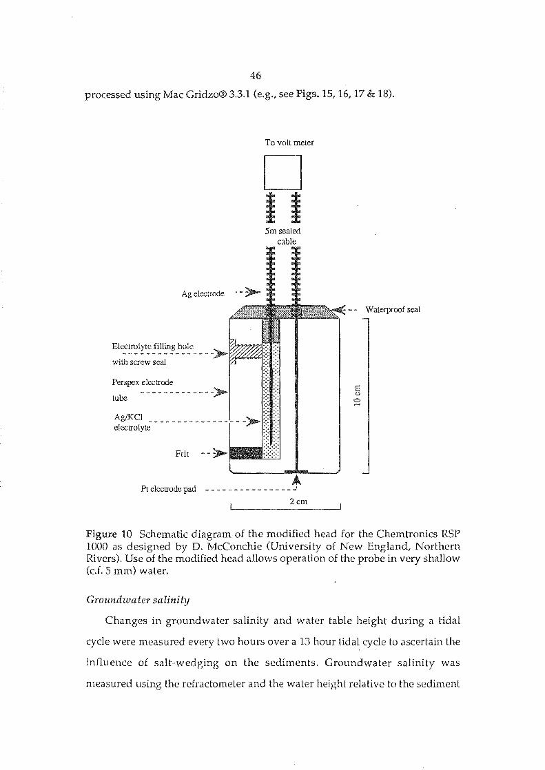
1000 Eh probe, with modified head (Fig. 10); an Activon BJ513 combination
Eh/pH probe connected to an Activon 205D combination digital pH/mY meter
was used within the trees and on the mudflats. Two types of probe were used
45
because the RSP 1000 requires several mm of water to allow closure of the
electrical circuit. At the time of surveying insufficient water among the trees
prevented use of the probe there. Similarly the Activon probe can not be used
in areas such as the dead mangrove area where water depth is over a few
centimetres because the probe cannot be submerged. The Activon probe, thus
could not be used in the area of dead mangroves. The advantage of the Activon
system, for the work in the trees, is that only one instrument need be carried.
Probes were standardised against Zobells solution (1:1 mixture of 1/300 M
potassium ferro- and ferri- cyanides), which has a standard potential of + 244
m V. The probes were inserted into the soft sediment and allowed to equilibrate
for about one minute before taking the reading.
pH survey
The pH survey in the dead mangroves used an leI 200 microcomputer pH
meter and probe. An Activon BJ513 combination Eh/pH probe and Activon
205D combination digital pH/m V meter was used within the trees and on 'the .
mudflats. Two probes were again used because of the problems outlined for Eh
data collection. Probe calibration was achieved by immersion in commercially
available pH 4.0 and pH 7.0 buffers. Readings were taken after the probe had
equilibrated with the sediment for about one minute.
Salinity survey
The salinity of the surface waters was measured using a Reichert-Jung
10419 temperature-compensating refractometer. A sample of water was
collected with an eye-dropper and placed on the refractometer for
measurement. This method of measuring salinity is likely to be more accurate
than methods involving the conversion of conductivity to salinity because
major-ion ratios may not be sufficiently constant to permit calibration using a
single conductivity-salinity plot. Data collected from each survey was
46
processed using Mac Gridzo® 3.3.1 (e.g., see Figs. IS, 16, 17 & 18).
To volt meter
D I i 5m sealed
cable
Ag electrode . -
Electrolyte filling hole
with screw seal
Perspex electrode
tube
Ag/KCl _ electrolyte
Frit
Pt electrode pad - - , --_ ... _---_ .... _--
- - Waterproof seal
Figure 10 Schematic diagram of the modified head for the Chemtronics RSP 1000 as designed by D. McConchie (University of New England, Northern Rivers). Use of the modified head allows operation of the probe in very shallow (c,f. 5 mm) water.
Groundwater Salil1inj
Changes in groundwater salinity and water table height during a tidal
cycle were measured every two hours over a 13 hour tidal cycle to ascertain the
influence of salt-wedging on the sediments. Groundwater salinity was
measured using the refractometer and the water height relative to the sediment

47
surface was determined as:
Height = Di - De
where Di is the height of piesometer collar (top of the pipe above ground) to
the water surface and De is the height of the collar to the sediment surface.
24 Hour Variation ofEh
Hansen et al. (1978) show that H 2S release from shallow lagoonal sediments
is a diurnal event. Indeed the smell of H 2S in the field area was more noticeable
in the early morning than later in the day. This diurnal event is regulated by
the photosynthetic production of oxygen by algal mats during the day and
subsequent .oxygen depletion by respiration at night. The result of this
alternation is that surface sediments are subjected to both oxic and anoxic
conditions on a daily cycle.
The diurnal redox cycle has implications for the mobility and accumulation
of metals in this type of environment. Metals entering the surface waters in the
salt marsh during the day, when waters are well oxygenated and oxidising,
may remain mobile for several hours, and may pass entirely through the zone.
Metals entering the dead mangroves at night would be exposed to oxygen
depleted sulphidic waters and consequently become immobilised as insoluble
sulphides.
Because the influence of cyclic oxidation and reduction events on metal
dispersion in contaminated sediments has not been documented in the
literature, the sediments at Wynnum were monitored over a twenty-four hour
period to observe the diurnal changes in the pH and Eh, and to determine the
depth to which changes influence.
48
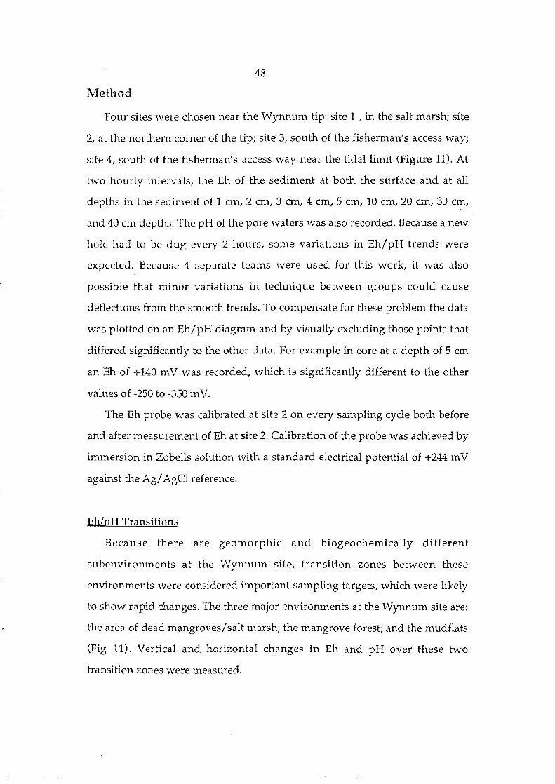
Method
Four sites were chosen near the Wynnum tip: site 1 , in the salt marsh; site
2, at the northern corner of the tip; site 3, south of the fisherman's access way;
site 4, south of the fisherman's access way near the tidal limit (Figure 11). At
two hourly intervals, the Eh of the sediment at both the surface and at all
depths in the sediment of 1 cm, 2 cm, 3 cm, 4 cm, 5 cm, 10 cm, 20 cm, 30 cm,
and 40 cm depths. The pH of the pore waters was also recorded. Because a new
hole had to be dug every 2 hours, some variations in Eh/pH trends were
expected. Because 4 separate teams were used for this work, it was also
possible that minor variations in technique between groups could cause
deflections from the smooth trends. To compensate for these problem the data
was plotted on an Eh/pH diagram and by visually excluding those points that
differed significantly to the other data. For example in core at a depth of 5 cm
an Eh of +140 mV was recorded, which is significantly different to the other
values of -250 to -350 m V.
The Eh probe was calibrated at site 2 on every sampling cycle both before
and after measurement of Eh at site 2. Calibration of the probe was achieved by
immersion in Zobells solution with a standard electrical potential of +244 m V
against the Ag/ AgCI reference.
Eh/pH Transitions
Because there are geomorphiC and biogeochemically different
subenvironments at the Wynnum site, transition zones between these
environments were considered important sampling targets, which were likely
to show rapid changes. The three major environments at the Wynnum site are:
the area of dead mangroves/salt marsh; the mangrove forest; and the mudflats
(Fig 11). Vertical and horizontal changes in Eh and pH over these two
transition zones were measured.
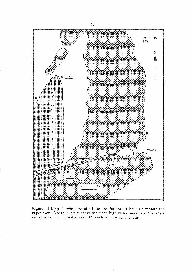
49
MORETON BAY
WRECK
Figure 11 Map showing the site locations for the 24 hour Eh monitoring experiment. Site four is just above the mean high water mark. Site 2 is where redox probe was calibrated against Zobells solution for each run.

50
Method
Sediment Eh and pH at depths of 0, 5, 10, 20 and 30 cm were measured in
series of holes dug across the transition zones. Eh was measured with the
Chemtronics RSP 1000 with modified head (Figure 10) and pH measured with
an ICI 200 microcomputer pH meter and probe.
Core Subsampling
Cores were first split by routing opposing sides of the PVC pipe to leave
about 0.5 mm of tube wall. The 0.5 mm plastic wall remaining was cut with a
sharp scalpel and a thin nylon cord was dragged along the core's length to split
the sediment.
Subsamples were taken along the length of the core, with a closer sampling
density in the upper part of the core. A 5 cm long sub-sample was taken at
depths of 0, 10,20,30,40,50,75, 100 cm, and if the core was long enough, at 125
cm. The samples were taken to leave a c. 5 mm zone of sediment next to the
PVC to eliminate possible metal contamination come from the PVc. During
sub-sampling, cores were logged for reconstruction of sedimentary
environments (Fig. 4).
Grab Sample Subsampling
Grab samples were treated in similar way to core samples, in that sediment
in contact with the plastic was not taken as part of the subsample. The
sediment was split in two and the central portion of each half taken.
Approximately a quarter of the total sample was taken as a subsample.
Sample Preparation
In dealing with sulphidic sediments, some specialised techniques are
recommended to prevent sulphide oxidation by atmospheric oxygen. These
include anaerobic glove-boxes, where the atmosphere has been replaced

51
(normally with nitrogen or argon) and sample manipulation is via a pair of air-
tight rubber gloves in one wall (Rapin et al., 1986). Other authors argue that
delays between the time of sampling and extraction and the method and time
of sam pIe storage are important factors in preserving the chemical
characteristics of the sediment, with sulphidic sediments being at one extreme
(Thomson et al., 1980). Thomson et ai. (1980) and Rapin et al. (1986) go on to
conclude that no storage or preparation procedure can preserve the initial
characteristics of the sediment and that samples should be analysed as soon as
possible after sam pIing.
Another technique involves the analysis of wet samples to avoid conversion
of sulphidic material during drying in an oxygenated atmosphere. This
technique requires a sample of known wet weight to be dried and a conversion
factor used to transfer data from wet to dry weight values. However, because
some of the reactions involving sulphide transformation result in mass
changes, the calculated dry weight is not the true dry weight of the sample
analysed.
Whether or not specialised techniques are employed, the most important
consideration in comparative studies is to ensure that all samples are treated in
exactly the same way. In this study samples from the Wynnum site were oven-
dried at 65°C for 3 days and then ground in a Labtechnics Pulveriser Mill
(Model LM I/P) for 2 minutes. The crushed sediments were then sealed in air
tight containers for latter analysis. This procedure has the advantage of
allowing the exact duplication of sample preparation conditions for a large
number of samples
Grainsize Analysis
A number of authors (e.g., Tessier et al. I 1982; Forstner & Wittman, 1981;
Luoma, 1990) have shown that the finer fractions of the sediment consistently
have higher concentrations of trace metals than do the coarser (sand and
52
gravel) fractions. Clays playa dual role in metal accumulation, by exchanging
metal cations (e.g., Cal Mg, Na and K) from interlayer positions for contaminant
metals, and by acting as a mechanical substrate onto which metals bound into
organics and/or hydrous iron oxides can precipitate (Carrot 1959; Grim, 1968;
Teissier et al., 1979; Jenne, 1977). Harbison (1986) noted that mangal sediments
form an effective sink for heavy metals because of the abundance of fine
grained sediment, which provides a large surface area for metal adsorption.
Many studies (e.g., Bouyocos, 1932; Olmstead, 1931; and Nelsen, 1983) have
shown that the grainsize distribution not only depends on the duration of
sample treatment, but also on the method employed; hence sample suites need
to be treated in a consistent way.
Method
Dried and weighed sediment samples were soaked in 100 ml of 50 voL
hydrogen peroxide to destroy organic matter and to aid in the dispersion of
clays. Because of the high salt content of many samples, each sample was
washed with distilled water several times until the conductivity of the water
was < 0.5 !lSI or until deflocculation had occurred. Fifty ml of 0.6 gl-l calgon
solution (Lewis, 1984) was added to each sample and stubborn, samples were
treated with an additional 2 ml of 40 % NaOH. Samples were then washed with
deionised water and mechanically stirred with a hand-held homogeniser (food
mixer type) for 5 minutes.
Samples were wet sieved at -2, 0, 2, & 40 on a Retsch shaker for 10 minutes
at 70 % power. The sand fractions were then placed in pre-weighed plastic
punnets and dried at 65°C for 24 hours before weighing. The silt and clay
fractions (4, 6, 8, & 100 ) were analysed by standard pipette analysis (Lewis,
1984).
53
Total Extractions
Chemical extraction techniques used in this project provide data on the
total metal concentration of a sediment excluding metals bound into silicate
lattices. While "total extractions" may give a clear indication of whether metal
concentrations are elevated, they do not assessment of interactions within the
sediment or biological impacts (Thomson et al. 1980). "Total extractions" use
concentrated mineral acid either singly (e.g., nitric acid) or combinations of
these acids (e.g., H2S04/HN03/HCL04/HCI mixture, Forstner, 1989).
Because the organic content of the sediments is high, a nitric acid digest
with an added oxidising agent such as hydrogen peroxide was considered to be
most appropriate. About 1 g of sediment was transferred to a 100 ml beaker
and allowed to react for a period of 15 minutes with 10 ml of 70% nitric.
Samples were then heated and at 50°C the first of three 3 ml additions of 100
vol. hydrogen peroxide was made. After each addition of hydrogen peroxide
the mixture was allowed to react completely before the addition of the next 3
ml. Once all the hydrogen peroxide was added samples were cooled, filtered
through a 0.45 j.lm membrane filter and the filtrate was boiled down to < 10 ml
and made up to 10 ml with deionised water.
Methods of metal analysis
A plethora of analytical techniques exist for the analysis of metal species.
Samples from the Wynnum site were analysed by one of two methods: anodic
stripping voltammetry (ASV), or atomic adsorption spectroscopy (AAS).
Anodic stripping voltammetry was used to determine (Cu, Cd, Pb and Hg)
because it is capable of simultaneous analysis of several metal species and
because it provides better detection limits for many metals than does flame
AAS (Potts, 1987; Chemtronics, 1986). Copper, cadmium and lead were
analysed on the PDV 2000 using the standard technique outlined in the
instruction manual (Chemtronics, 1986), while mercury was analysed using the
54
Chlor-Acetate buffer system (Jaya et al. 1985). Atomic adsorption was used for
(Ni, Cr, Zn, Fe, & Sn) which do not require low detection limits because it is
quick and accurate. The lower limit of detection depends on the method used
(e.g., the detection limit for Cu by AAS is 25 Jlg/ g, but by ASV it is 0.2 Jlg/ g).
Sequential Extractions
Many researchers use sequential extractions (differential analysis) to
distinguish trace metals in the various sedimentary sinks. As a result, many
sequential extraction procedures have been proposed over the years (e.g.,
Tessier et al., 1979; Rapin & Forstner, 1983; Engler et al., 1977; Chao &
Theobald, 1976; and Kersten & Forstner, 1986) (Table 5). Sequential analysis
allows a clearer definition of the geochemical processes controlling metal
concentrations and can provide predictive data on potential biological impacts
of elevated metal concentrations (Thomsonet al., 1980).
While there are clear advantages in differential analysis over total analysis;
stepwise chemical extractions have many problems (Kersten & Forstner, 1986;
Rapin et aL, 1986; Campbell & Tessier, 1987; Forstner, 1989). The most
significant of these problems are:
1) reactions are not selective and are not only influenced by the
duration of the experiment but also by the solid-matter to extractant
volume ratio (Campbell & Tessier, 1987, and Forstner, 1989). If the
ratio of solid matter to extractant volume is too high, and there is an
increase in buffering capacity, and the system will become overloaded.
These effects may be reflected in changes in pH over time (Forstner,
1989).
2) Labile phases may be transformed during sample preparation. For
example oxidation of phases may occur, especially in the case of
samples from anoxic settings, or metals may be redistributed during
extraction (Ajayi & Valoon, 1989). Campbell and Tessier (1987) argue
55
that over the 10 years prior to their paper, most environmental
samples had been "mistreated" and that the geochemical and
environmental relevance of the data from those samples was highly
suspect.
In their study of extraction selectivity, Rapin and Forstner (1983) subjected
pure carbonates (Cd, Ca, Mn, and Pb), amorphous iron/manganese oxides
from deep sea nodules, two crystalline iron oxides (goethite and haematite), an
amorphous iron sulphide and a crystalline lead sulphide (galena) to a number
of extractants. Selectivity of their extraction methods was successful for
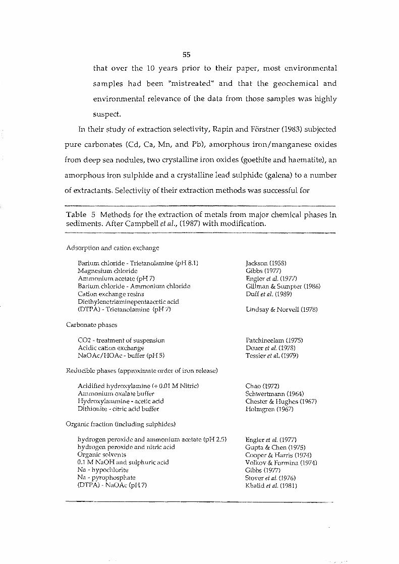
Table 5 Methods for the extraction of metals from major chemical phases in sediments. After Campbell et al., (1987) with modification.
Adsorption and cation exchange
Barium chloride - Trietanolamine (pH 8.1) Magnesium chloride Ammonium acetate (pH 7) Barium chloride - Ammonium chloride Cation exchange resins Diethylenetriaminepentaacetic acid (DTPA) - Trietanolamine (pH 7)
Carbonate phases
C02 - treatment of suspension Acidic cation exchange NaOAc/HOAc - buffer (pH 5)
Reducible phases (approximate order of iron release)
Acidified hydroxylamine (+ om M Nitric) Ammonium oxalate buffer Hydroxylammine - acetic acid Dithionite - citric acid buffer
Organic fraction (including sulphides)
hydrogen peroxide and ammonium acetate (pH 2.5) hydrogen peroxide and nitric acid Organic solvents 0.1 M NaOHand sulphuric add Na - hypochlorite Na - pyrophosphate (DTPA) - NaOAc (pH 7)
Jackson (1958) Gibbs (1977) Engler et aT. (1977) Gillman & Sumpter (1986) Duff et al. (1989)
Lindsay & Norvell (1978)
Patchineelam (1975) Deuer et al. (1978) Tessier et at (1979)
Chao (1972) Schwertmann (1964) Chester & Hughes (1967) Holmgren (1967)
Engler et al. (1977) Gupta & Chen (1975) Cooper & Harris (1974) Volkov & Formina (1974) Gibbs (1977) Stover et al. (1976) Khalid et at. (1981)
56
carbonates (>85% extraction) and was acceptable for metals associated with the
iron or manganese oxides, but the method was not selective for sulphides; the
iron sulphide showed considerable progressive mobilisation in the early stages
of the extraction sequence.
Testing selectivity
A similar experiment to that conducted by Rapin and Forstner (1983) was
made to ascertain the selectivity of some chemical extractants. Ten naturally
occurring and 5 synthetic sedimentary phases were treated with 15 (later
extended to 16) extracting phases. Natural phases were pyrite, haematite,
goethite, magnetite, siderite, chalcopyrite, galena, gypsum, marble, and a black
calcite; the laboratory reagents consisted of red (mostly haematite) and brown
(mostly goethite) iron oxides, lead carbonate, calcium carbonate and an iron
monosulphide (troilite).
Method
Use of extracting phases was kept as simple as possible for ease of
reproducibility and speed of analysis; complex extraction procedures which
required multiple additions and rinsings of the samples were avoided.
Procedures requiring heating were boiled for a quarter of an hour to avoid
evaporation because extractant volumes were small. Cold extracts were shaken
for 1 hour on a variable-speed rotary shaker, except for the dithionite
extraction which was shaken for 12 hours as recommended by Holmgren
(1967).
Five ml of the extractant was added 0.5000 0.0005 g of solid phase in a 50
ml conical flask. After the reaction time the filtered samples were made up to
25 ml in a volumetric flask with deionised water. To avoid precipitation of
insoluble iron oxides samples containing large quantities iron have to be
acidified with nitric acid and evaporated before being made up to 25 ml with
57
deionised water.
Several methods were then tested on 1:1:1:1:1 mixtures of copper, lead,
zinc, calcium carbonates, and iron sulphide. Because an extractant may
mobilise an isolated phase, the behaviour of the extractant may be different for
samples containing mixed mineralogy. The same ratio of solid-phase to
extractant that was used for the single extractions was therefore used in this
procedure.
Water was used as a baseline control for the extractions, and the
concentrations the other extractants followed the procedures as outlined in the
source reference (Table 5), except for the dithionite and the ascorbic acid/Hel
extracts. The dithionite extractant was 90 gl-l Citrate and -30 gl-l dithionite,
while the ascorbic acid/HCl extractant was 90 gl-l ascorbic acid in 6% HC!.
Results and discussion
Results of the sequential extraction experiments are presented in Table (6)
and results for the extractions for the 1:1:1:1:1 mixtures of metal carbonates
and iron sulphide are presented in Table (7).
Water showed the lowest mobilisation of test minerals which was to be
expected because solubility products for the various solid phases are low.
Gillman Sumpter (Table 6) was the next poorest extractant, mobilising less than
1 % of most solid phases, except the calcium carbonate and the marble. This
extractant is commonly used to mobilise metals in the interlattice layers of clay
minerals and metals loosely associated with organic matter (Le., to measure the
cation exchange capacity of the soil; Gillman & Sumpter, 1986). DTPA/TEA
which is a stronger extractant than Gillman Sumpter showed moderate attack
on the FeS and siderite phases. DTP A/TEA extractions are commonly used as
an indicator of metals available to plants in soils (Lindsay & Norvell, 1978)
because plants are able to extract metals from soils by the exudation of organic
chelating agents and hydronium ions (Alloway, 1990). These chelating agents
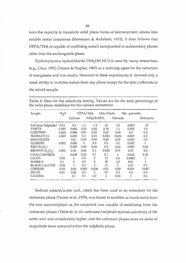
58
have the capacity to transform solid phase forms of micronutrient cations into
soluble metal complexes (Stevenson & Ardakani, 1972), it then follows that
DTP A/TEA is capable of mobilising metals incorporated in sedimentary phases
other than the exchangeable phase.
Hydroxylamine hydrochloride (NH20H.HCl) is used by many researchers
(e.g., Chao, 1972; Chester & Hughes, 1967) as a reducing agent for the reduction
of manganese and iron oxides. However in these experiments it showed only a
weak ability to mobilise metals from any phase except for the zinc carbonate in
the mixed sam pIe.
Table 6. Data for the selectivity testing. Values are for the total percentage of the solid phase mobilised for the various extractants.
Sample H 2O DTPA/TEA HAc/NaAc Alk. peroxide
Gillman NH20HHCL Peroxide Dithionite
FeS (Iron Sulphide) 0.03 0.2 1.4 1.4 16 25 0.003 19 PYRITE 0.005 0.008 0.22 0.04 0.19 1.1 0.003 1.3 GOETHITE 0.003 0.006 0.05 0.Q2 0.03 0.04 0.4 0.3 HAEMATITE 0.003 0.005 0.1 0.Q1 0.003 0.004 0.003 0.2 MAGNETITE 0.Q1 0.09 0.08 0.09 0.02 0.004 0.3 SIDERITE 0.002 0.004 5 0.3 0.5 0.2 0.007 2 RED (Fepx) 0.005 0.09 0.04 0.2 0.04 0.002 0.04 BROWN (FeyO,,) 0.002 0.06 0.04 0.1 0.003 0.Q1 0.02 0.3
CHALCOPYRITE 0.008 0.02 0.1 0.1 4 0.002 0.35 CaC03 0.03 2 0.6 2 13 0.6 0.0005 1 MARBLE 0.1 2 0.7 3 18 0.5 0.01 1 BLACK CALCITE 0.04 1 0.5 3 15 2 0.01 0.5 GYPSUM 0.03 0.03 0.005 0.008 0.01 0.09 0.001 0.007 PbC03 0.Q1 0.05 0.2 2 57 0.5 0.6 0.3 GALENA 0.1 0.1 0.3 2 0.05 3 0.9
Sodium acetate/ acetic acid, which has been used as an extractant for the
carbonate phase (Tessier et al., 1979), was found to mobilise as much metal from
the iron monosulphide as the extractant was capable of mobilising from the
carbonate phases (Table 6). In the carbonate/sulphide mixture selectivity of the
acetic acid was considerably higher, and the carbonate phases were an order of
magnitude more extractable than the sulphidic phase.
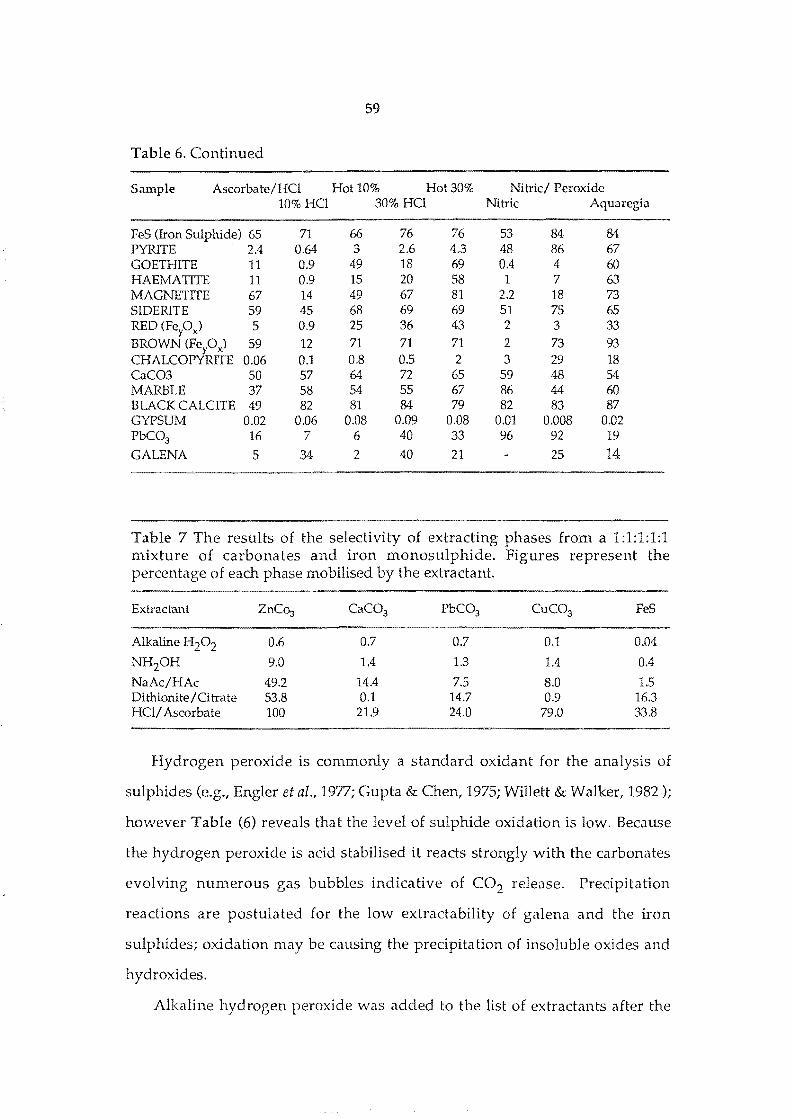
59
Table 6. Continued
Sample Ascorbate/HCl Hot 10% Hot 30% Nitric/ Peroxide 10% HCl 30%HO Nitric Aquaregia
FeS (Iron Sulphide) 65 71 66 76 76 53 84 84 PYRITE 2.4 0.64 3 2.6 4.3 48 86 67 GOETHITE 11 0.9 49 18 69 0.4 4 60 HAEMATITE 11 0.9 15 20 58 1 7 63 MAGNETITE 67 14 49 67 81 2.2 18 73 SIDERITE 59 45 68 69 69 51 75 65 RED (Fepx) 5 0.9 25 36 43 2 3 33
BROWN (Fepx) 59 12 71 71 71 2 73 93 CHALCOPYRITE 0.06 OJ 0.8 0.5 2 3 29 18 CaC03 50 57 64 72 65 59 48 54 MARBLE 37 58 54 55 67 86 44 60 BLACK CALCITE 49 82 81 84 79 82 83 87 GYPSUM 0.02 0.06 0.08 0.09 0.08 0.01 0.008 0.02 PbC03 16 7 6 40 33 96 92 19
GALENA 5 34 2 40 21 25 14
Table 7 The results of the selectivity of extracting phases from a 1:1:1:1:1 mixture of carbonates and iron monosulphide. Figures represent the percentage of each phase mobilised by the extractant.
Extractant ZnCo3 CaC03 PbC03 CuC03 FeS
Alkaline H 20 2 0.6 0.7 0.7 0.1 0.04
NH20H 9.0 1.4 1.3 1.4 0.4
NaAc/HAc 49.2 14.4 7.5 8.0 1.5 Dithionite/Citrate 53.8 0.1 14.7 0.9 16.3 HO/ Ascorbate 100 21.9 24.0 79.0 33.8
Hydrogen peroxide is commonly a standard oxidant for the analysis of
sulphides (e.g., Engler et al., 1977; Gupta & Chen, 1975; Willett & Walker, 1982);
however Table (6) reveals that the level of sulphide oxidation is low. Because
the hydrogen peroxide is acid stabilised it reacts strongly with the carbonates
evolving numerous gas bubbles indicative of CO2 release. Precipitation
reactions are postulated for the low extractability of galena and the iron
sulphides; oxidation may be causing the precipitation of insoluble oxides and
hydroxides.
Alkaline hydrogen peroxide was added to the list of extractants after the
60
carbonates were seen to suffer attack by standard hydrogen peroxide. By
addition of sodium hydroxide to the hydrogen peroxide to a pH of 8.5
(carbonate/bicarbonate buffer limit), the attack on the carbonates by free H+ is
removed. Alkaline hydrogen peroxide acted solely as an oxidising agent, as
shown upon addition to PbC03 and siderite. Lead carbonate reacted violently
with alkaline hydrogen peroxide resulting in the transformation of the initially
white solid to a dark brown solid. During this reaction, a large amount of heat
and effervescent gas evolved. Because of the heat evolved in the reaction some
of this effervescent gas is 02 through the thermal decomposition of H20 2,
where:
The other component of the evolved gas is CO2, which would be given off in a
2-electron oxidation reaction where:
The presence of Pb02 was confirmed by treating a large sample with the
hydrogen peroxide, then analysing the product by x-ray diffraction; the
resulting pattern showed Pb02 peaks.
Siderite and the sulphidic substrates also produced vigorous reactions, with
the originally pale siderite blackening. A 2 electron oxidation for the siderite is
also proposed where:
2FeC03 + H20 2 ---~> Fe203 + 2C02 + H20
or 3FeC03 + H20 2 » Fe304 + 3C02 + H20
The rapid rate of reaction of the alkaline hydrogen peroxide with the
sulphidic and oxidisable carbonate substrates indicates that:
(1) the acid stabilisation of hydrogen peroxide causes a reduction in the rate
of reaction probably due to the creation of H30 2 + or similar species.
(2) acid stabilisation allows the undesirable dissolution of carbonates.
Alkaline-destabilised hydrogen peroxide, however, shows a marked decrease in
61
ability to extract sulphidic material (Table 6 & 7) due to uncontrollable reaction
rates, which lead to thermal decomposition of the hydrogen peroxide.
Sodium dithionite/ citric acid has been shown to mobilise iron oxides
effectively (e.g., Holmgren, 1967; Forstner, 1989), but the data from Table (6)
reveal that iron sulphide was attacked strongly by the dithionite and that iron
oxides were relatively unaffected by it. The carbonate/sulphide mixture
showed a moderate selectivity for· the iron sulphide; zinc carbonate was
strongly mobilised and the lead carbonate which was mobilised at a similar
level to the sulphide. These findings are not consistent with the widespread use
of dithionite as a reducing agent for ferric oxides and hydroxides possibly
because the substrates used for this experiment were too crystalline for the
extractant to mobilise effectively. The dithionite method may be best suited to
removing amorphous iron oxides and hydroxides (e.g., Follett, 1965; Holmgren,
1967); which have a large surface area and weak interlattice bonds which are
easily broken. In this study the apparent mobilisation of the sulphidic material
may have been related to pre-oxidation of the sulphide by atmospheric oxygen
prior to extraction. A X-ray powder-diffraction pattern of the sulphide shows
that the mineral is not mono-mineralic and that magnetite, greigite and jarosite
were present; it is possible that these other components provided the Fe
extracted by the dithionite.
The stronger acids (e.g., Hel, HN03) showed little or no selectivity for any
of the substrates present. While the Hell Ascorbate and the other Hel
treatments showed a selectivity for the more crystalline iron sulphides (pyrite
and chalcopyrite), these extractants strongly mobilised either the FeS or the PbS
phases. With the more oxidising extractants (e.g., nitric, nitric and hydrogen
peroxide and aquaregia), a11 phases were mobilised without selectivity.
As showed that, Whereas it is easy to construct sequential extraction
procedures for an oxic sediment, when sulphidic material is present, extraction
methods currently used are not adequate (Rapin & Forstner~ 1983). Even though
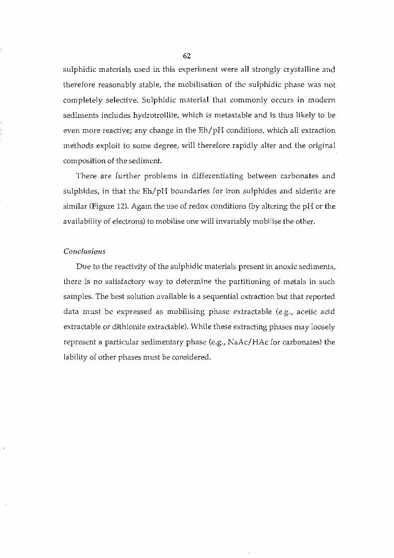
62
sulphidic materials used in this experiment were all strongly crystalline and
therefore reasonably stable, the mobilisation of the sulphidic phase was not
completely selective. Sulphidic material that commonly occurs in modern
sediments includes hydrotroilite, which is metastable and is thus likely to be
even more reactive; any change in the Eh/pH conditions, which all extraction
methods exploit to some degree, will therefore rapidly alter and the original
composition of the sediment.
There are further problems in differentiating between carbonates and
sulphides, in that the Eh/pH boundaries for iron sulphides and siderite are
similar (Figure 12). Again the use of redox conditions (by altering the pH or the
availability of electrons) to mobilise one will invariably mobilise the other.
Conclusions
Due to the reactivity of the sulphidic materials present in anoxic sediments,
there is no satisfactory way to determine the partitioning of metals in such
samples. The best solution available is a sequential extraction but that reported
data must be expressed as mobilising phase extractable (e.g" acetic acid
extractable or dithionite extractable). While these extracting phases may loosely
represent a particular sedimentary phase (e.g., NaAc/HAc for carbonates) the
lability of other phases must be considered.
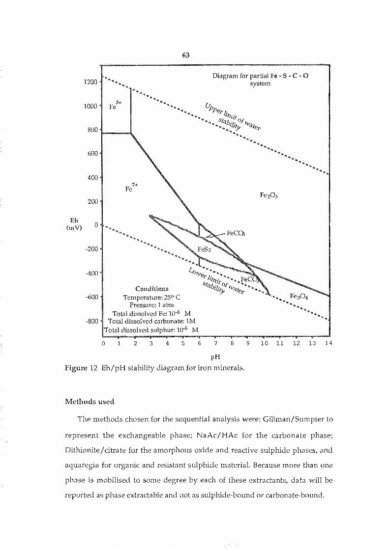
Eh (mV)
1200
1000
.... .... ......
3+ Fe
800 1----'"
600
400 2+
Fe
200
0 .,
" .. .... -200
63
Diagram for partial Fe S· C q 0 system
.... .... .... .... ....
-400 l.or.. .. • vel' 1: " ....
Sf. l.t:Qif 0'" ...... fe ilb,"· < Ii;: .... Conditions '1-1.1ty ilfer ........
-600 Temperature: 25° C Pressure: 1 a tm
... .... .... ....
.... ......
Total dissolved Fe: 10-6 M -800 Total dissolved carbonate: 1M
Total dissolved sulphur: 10-6 M
.... .... .... ......
o 1 2 3 4 5 6 7 8
pH
Figure 12 Eh/pH stability diagram for iron minerals.
Methods used
9 10 11 12 13 14
The methods chosen for the sequential analysis were: Gillman/Sumpter to
represent the exchangeable phase; NaAc/HAc for the carbonate phase;
Dithionite/citrate for the amorphous oxide and reactive sulphide phases, and
aquaregia for organic and resistant sulphide materiaL Because more than one
phase is mobilised to some degree by each of these extractants, data will be
reported as phase extractable and not as sulphide-bound or carbonate-bound.
64
Approximately 2 g of crushed sample were placed in 100 ml beakers with 10
ml of 0.1 M BaC12/NH 4Cl and shaken for 1 Hr. on a variable speed rotary
shaker (Gillman & Sumpter, 1986). The sample was then filtered to 0.45 Ilm, the
solid phase and filter returned to the beaker and the filtrates evaporated to near
dryness and made up to 10 ml with ultrapure water.
The filter and sediment were then treated with 10 ml of 1 M NaAc/HAc
(Tessier et al., 1979), shaken on the rotary shaker for 1 hour, and filtered using
the rinsed filter. Five ml of nitric acid was added to the filtrate before samples
were boiled to near dryness and made up to 10 ml with ultrapure water.
The remaining sediment was then shaken for 12 hrs with 10 ml of 30 gt1
sodium dithionite and 90 gl-l citric acid. The sample was filtered and the filter
removed and washed. 5 ml of 100 vol. hydrogen peroxide and 5 ml of nitric
acid were added to the filtrate, boiled to near dryness and made up to 10 ml
with ultrapure water. Removal of the cellulose acetate filter from the sediment
at this point is to avoid filter destruction during aquaregia treatment.
Ten ml of aquaregia was added to the sediment and allowed to stand for 1
Hr. before being boiled for 15 minutes. Cooled solutions were filtered and the
filtrate boiled to near dryness then made up to 10 ml with ultra pure water.
Plant Available Metals
One of the most widely-explored phases in soil-science studies is the
adsorbed or exchangeable phase (Thomas, 1982; Lindsay & Norvell, 1978).
These readily exchangeable metals are thought to represent metal that is
weakly adsorbed on organics or occupying the interlattice positions of clay
minerals (Grim, 1968; Jenne, 1977; Waller & Pickering, 1990). These metals are
considered to be readily available for plant uptake (Brown, 1955). As a
consequence of the nutrient-supply role that the exchangeable phase plays a
number of extraction techniques for its investigation have developed (Table 5).
It has been shown (Stevenson & Ardakani, 1972; Krom & Sholkovitz, 1975Ythat
65
the cation exchange capacity (CEC) of the soil/sediment (a measure of
exchangeable metal) not only depend on mineralogy, but also on the organic
matter type, and content.
Such non selectivity is consistent with the data from the sequential
extraction data (Table 6 & 7), which indicates that the now commonly-accepted
DTP A/TEA extraction mobilise portions of all physiochemical sedimentary
phases, as required if the extractant is to reflect the plant available metal
content of soils (Lindsay & Norvell, 1978).
Method
One g of crushed sediment was weighed into a 100 ml conical flask and
shaken with 10 ml of 0.005 M DTPA, 0.01 M CaCl2, and 0.1 M TEA (adjusted to
a pH of 7.3) for 2 hours (Lindsay & Norvell, 1978). Samples were then filtered,
boiled to near dryness, and 5 ml of concentrated nitric acid was added to
destroy organics molecules that may complex with the metals and thus
interfere with analysis by anodic stripping voltammetry. Samples were made
up to 10 ml with ultra pure water.
Analysis of Organic Carbon
Organic matter contributes to the binding of metals in soil or sediment by
both adsorption and chelation processes; Nye (1990) found that for Rhizophora
mangal, the organic matter content of the sediment was the prime control on the
metal load in the plant.
Organic matter undergoes several phases of oxidation, which may affect
metal levels. The first is an initial loss of metals from decaying matter followed
by a second phase of metal concentration as humification continues (Rice &
Windom, 1982). Because many other authors also show that organic matter
plays a major role in the mediation of heavy metals (Sohn & Rajski, 1990;
Ephriam, et ai. 1989b; Yeoman, et ai. 1989; and Lion et al. 1982) it is likely that
66
this phase may play an important direct or indirect role in the mediation of
heavy metals at the Wynnum site.
Method
In this study organic carbon is determined by the Walkley-Black method
(Walkley & Black, 1934), which uses potassium dichromate and sulphuric add
as an oxidant and then back titrates the unused oxidant against ferrous
sulphate to determine the concentration of organic carbon. For sulphidic
sediments this method may give an overestimation of the organic content due
to the oxidation of sulphide by the dichromate (Willett & Beech, 1987) but these
errors are expected to be much less than natural sample variation over small
distances at each site. Possible subsampling errors may also be significant
because only about 0.06 g of sample is used in each analysis, but the speed of
analysis is sufficiently high that multiple analyses of each sample can be
conducted and averaged.
Analysis of Sulphate and Sulphide.
Sulphides in soils and sediments are likely to be an important sink for
metals in mangrove sediments, which normally support a large population of
sulphate reducing bacteria in a reducing organic-rich substrate (Wada &
Seisuwan, 1986; Hutchings & Saenger, 1987; Forstner, 1989). The analysis of
soil sulphate and sulphide is also important because these parameters define
the acid-sulphate potential of the soil. Where a soil contains greater than 0.3%
sulphur as sulphide, the soil is considered to be potentially acid-sulphate.
Potentially acid-sulphate soils do not become acid-sulphate until the sulphidic
material is oxidised as a result of a fall in the water table and soil drying.
Sulphide oxidation and the associated production of sulphuric acid have
significant affects on metal mobility in the soils (Willett & Walker, 1982; Dent,
1986; Olson, 1986; Wada & Seisuwan, 1986).

67
Method
Analysis of sulphate and sulphide involved the separate determination of
water soluble sulphur (in the form of sulphate) and hydrogen peroxide
oxidisable sulphur. The difference between these represents Sulphur present as
sulphide.
For hydrogen peroxide-oxidisable sulphur, about 0.5 g of sediment is
allowed to react for 48 hours with 10 ml of 50 voL hydrogen peroxide. Samples
are then filtered at 0.2 11m and diluted by 50:1 for HPLC (high pressured liquid
chromatography) determination of sulphate. To determine water soluble
sulphate about 0.5 g of sediment was shaken with 10 ml of ultrapure water,
filtered to 0.2 ~m and diluted by 5:1 for the HPLC determination of sulphate.
Samples were analysed by anion chromatography on a Dionex® AS4A
column with Dionex® AG4A guard column and a post column Dionex® AMMS
II counter current anion suppressor (to reduce background). A 1.8 mM/1.7 mM
Na2C03/NaHC03 buffer solution pumped by a Kortec K350 pump at 2.0
ml/min was used as an eluent; suppression was achieved by 50 mM sulphuric
acid delivered via a Dionex®pressure bottle, at 4 ml/min. Anionic species were
detected by a Kortec® conductivity detector.
The above conditions gave a retention time of 6.7 minutes for the sulphate
peak, with concentrations calculated by Nelson® peak-integration software
using a calibration curve of 6 standard solutions.
Analysis of Waters
Direct analysis of water can be difficult because natural waters often contain
very low levels of trace metals and for many elements a preconcentration step
is necessary before analysis.
Preconcentration steps may be simple such as concentration by evaporation,
68
or more complex such as through the use of complexing agents and their
extraction into organic solvents by a liquid-liquid extraction. For the analysis of
trace metals by atomic adsorption, Clesceri et al. (1989) recommended the use of
ammonium pyrolidine dithiocarbamate (APDC) as a complexing agent and
methyl isobutyl ketone (MIBK) as the extracting solvent. There are many other
complexing agents such as oxine, sodium diethyl dithiocarbamate (DETC),
silver diethyl dithiocarbamate (SDDC), and dithiozone, which complex many
metals, but each of these agents is specific only for a limited number of metals,
(e.g. oxine does not extract Zn, Cd, Cr, or Hg whereas DETC does; Frieser &
Morrison, 1959).
Although it is recommended that the Standard Methods (e.g., Clesceri et
aI., 1989) be followed while conducting environmental chemical analyses, the
APDC/MIBK extraction system is not, according to the authors, capable of
extracting Hg. The inability to extract Hg is a problem because Hg is of
environmental significance (Senaraten & Dissanayake, 1989) and it is a known
contaminant from tip leachate (Garland & Mosher, 1975).
DETC has a similar structure to APDC, and also has the capability of
complexing with all the metals to be analysed in this study (Frieser & Morrison,
1959) and was thus chosen as a replacement ligand for APDC. One advantage
of the dithiocarbamate family is that they are able to complex metals that
readily form insoluble sulphides in weakly-acidic conditions (Fritz & Schenk,
1979). DETC is also an extremely sensitive ligand for copper, with a very large
(12 000) molar absorbtivity (BDH Chemicals, 1991).
Bauer et al. (1978) give an extraction method using DETC at a pH of 4.5 5.0
to extract copper into n-Butylacetate with EDT A (Ethylendiaminetetraacetic
acid) as a masking agent to increase copper selectivity. By buffering the
extraction system to a pH of 7.0, using a pthalate/hydroxide solution, and
removing the masking agent, all metals requiring analysis in this study are
completely extractable (Figure 13; Frieser & Morrison, 1959).
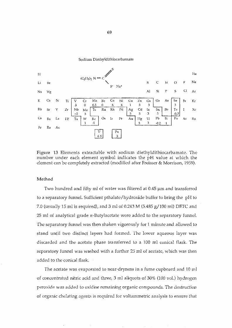
69
Sodium Diethyldithiocarbamate
H /S He (C2HSh N - C
Li Be , B C N 0 F Ne S- Na+
Na Mg Al Si P S CI Ar
K Ca Sc Ii V Fe Co Ni Zn Ga As Se Br Kr 0 6 6 3 3 3
Rb Sr Y Zr Ru Rh Pd Cd In Sb Te Xe 3 3 -0.7
Cs Ba La Hf Os Ir Pt Hg Tl Bi Po At Rn 3 3 -0.2 1
Fr Ra Ac
I ~51 I P; I
Figure 13 Elements extractable with sodium diethyldithiocarbamate. The number under each element symbol indicates the pH value at which the element can be completely extracted (modified after Freisser & Morrison, 1959).
Method
Two hundred and fifty ml of water was filtered at 0.45 11m and transferred
to a separatory funnel. Suf£icient pthalate/hydroxide buffer to bring the pH to
7.0 (usually 15 ml is required), and 3 ml of 0.243 M (5.485 g/100 m!) DETC and
25 ml of analytical grade n-Butylacetate were added to the separatory funnel.
The separatory funnel was then shaken vigorously for 1 minute and allowed to
stand until two distinct layers had formed. The lower aqueous layer was
discarded and the acetate phase transferred to a 100 ml conical flask. The
separatory funnel was washed with a further 25 ml of acetate, which was then
added to the conical flask.
The acetate was evaporated to near-dryness in a fume cupboard and 10 111.1
of concentrated nitric acid and three, 3 ml aliquots of 30% (100 vol.) hydrogen
peroxide was added to oxidise remaining organic compounds. The destruction
of organic chelating agents is required for voltammetric analysis to ensure that
70
metals are electrochemically free and not locked up as stable chelates. Samples
were then boiled to near dryness and made up to 10 ml with ultrapure water.
This method gave a 25 fold increase in metal concentration for the PDV and a 5
fold increase in metal concentration for analysis by atomic adsorption.
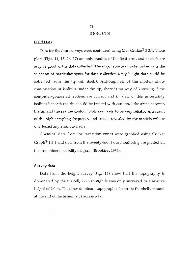
Field Data
71
RESULTS
Data for the four surveys were contoured using Mac Gridzo® 3.3.1. These
plots (Figs. 14, 15, 16, 17) are only models of the field area, and as such are
only as good as the data collected. The major source of potential error is the
selection of particular spots for data collection (only height data could be
collected from the tip cell itself). Although all of the models show
continuation of isolines under the tip, there is no way of knowing if the
computer-generated isolines are correct and in view of this uncertainty
isolines beneath the tip should be treated with caution. I the areas between
the tip and the sea the contour plots are likely to be very reliable as a result
of the high sampling frequency and trends revealed by the models will be
unaffected any absolute errors.
Chemical data from the transition zones were graphed using Cricket
Graph® 1.3.1 and data from the twenty-four hour monitoring are plotted on
the iron mineral-stability diagram (Brookins, 1986).
Survey data
Data from the height survey (fig. 14) show that the topography is
dominated by the tip cell, even though it was only surveyed to a relative
height of 2.0 m. The other dominant topographic feature is the shelly mound
at the end of the fisherman's access way.
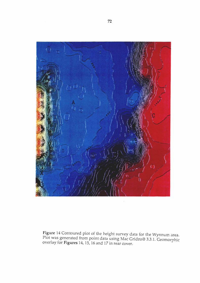
72
Figure 14 Contoured plot of the height survey data for the Wynnum area. Plot was generated from point data using Mac Gridzo® 3.3.1. Geomorphic overlay for Figures 14, 15, 16 and 17 in rear cover.
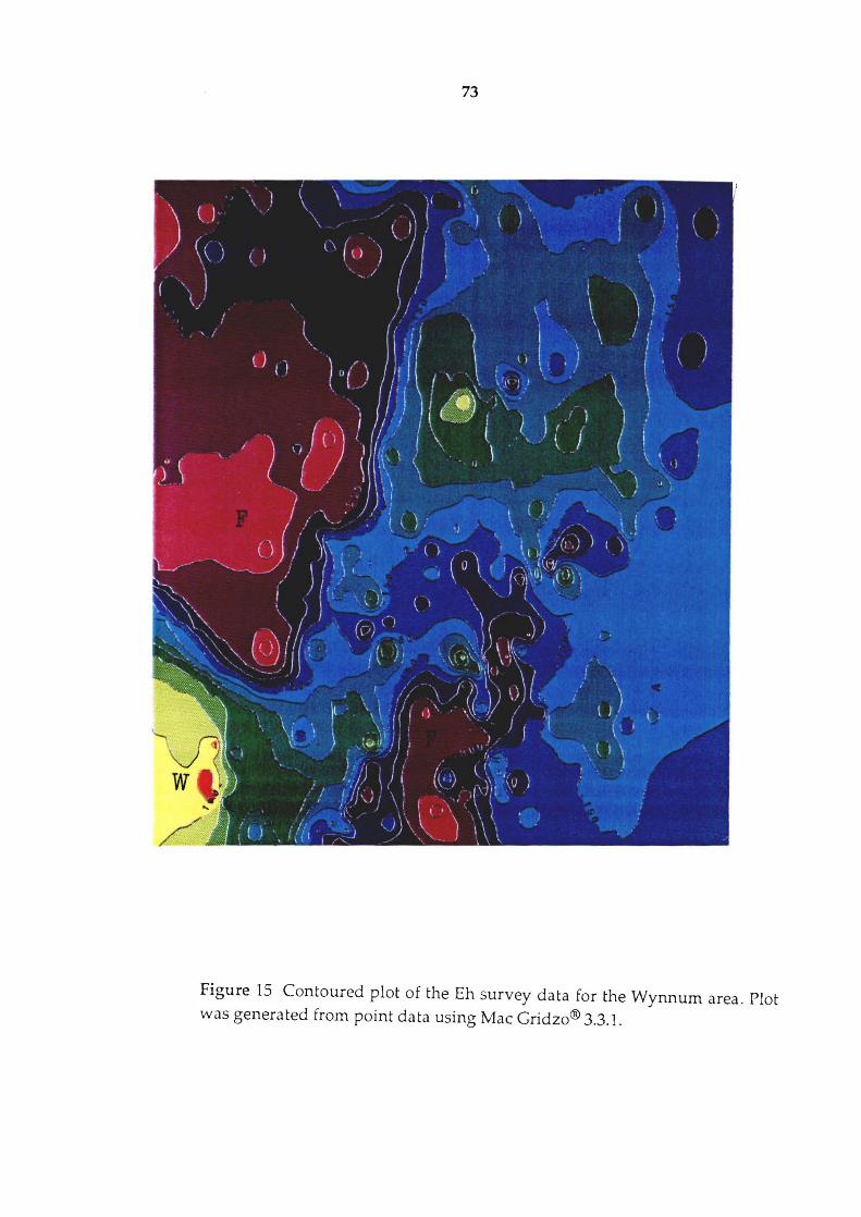
73
Figure 15 Contoured plot of the Eh survey data for the Wynn urn area. Plot was generated from point data using Mac Cridzo® 3.3.1.
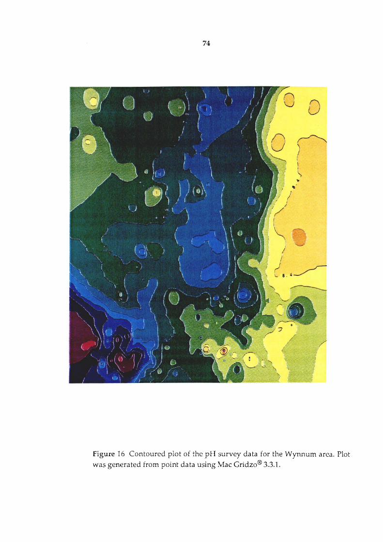
74
o ~ ) .. l , I
Figure 16 Contoured plot of the pH survey data for the Wynnum area. Plot was generated from point data using Mac Gridzo® 3.3.1.
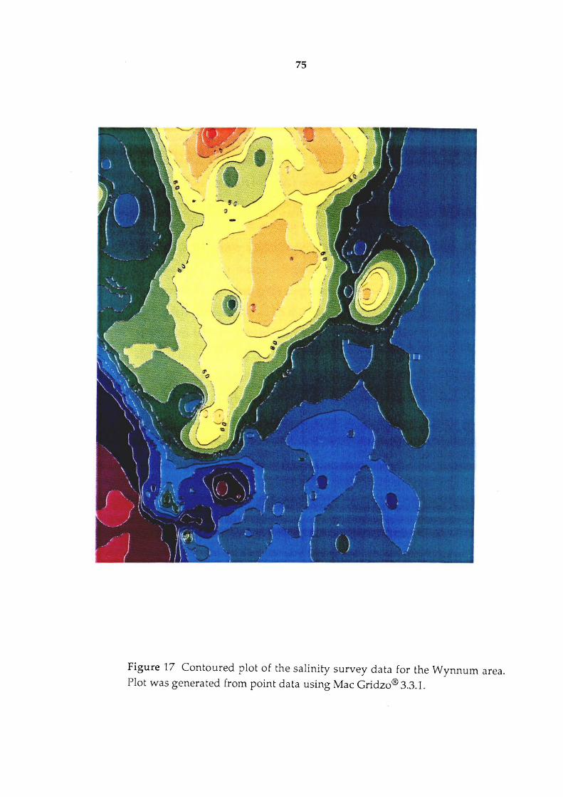
75
Figure 17 Contoured plot of the salinity survey data for the Wynnum area. Plot was generated from point data using Mac Gridzo® 3.3.1.
76
Two important topographic features are shown by the map (i.e. fig 14): 1)
the water-filled depression that contains the dead mangroves (A), this rather
patchy depression has an ill-defined seaward margin and; 2) The mangrove
covered area, which slopes gently towards the coast, then steepens through
the transition zone (B) from the mangroves to the mud-flats (C). (Note: the
contour intervals of 50 mm, reveals changes in slope are not always obvious
in the field). The 50 mm contour interval also makes the transition zone (B),
which falls 1.5 m over a 50 m horizontal distance, appears cliff-like.
There are two main deficiencies in the computer contours of the
topographic map. Firstly, the depression landward of the shelly mound at
the coast is not fully closed on the map, whereas in the field it is water-filled
and drains through a very narrow exit to the southeast. Secondly the area
south of the access way (D) is depicted as a steady slope from the road to the
coast whereas it actually contains large numbers of shallow depressions and
tidal channels, in which tidal waters remain at low tide. The symbol (X) in
figure (14) marks the position of a leachate seep (see Metals in waters
Surface waters page 101).
The Eh data, contoured in figure (15), reveals several distinct zones in the
area. Areas of standing water (F) are sharply contrasted with those areas that
are well drained, because where water is allowed to stagnate, the Eh falls
sharply. These two stagnant-water areas, connected by a thin ribbon of low
and discontinuous Eh values, are interpreted to be a drainage line for the
dead mangroves which the height survey was not able to detect. This zone of
lowered Bh runs parallel to the fisherman's access way, then merges with the
pooled water at its eastern end. This zone is the most likely position for the
drainage channel for the dead mangroves because the original drainage ran
in a southerly direction before the construction of the road.
In well drained areas (W), such as the mangrove flats to the south of the
road and just east of the southern tip cell, the Eh rises to + 250 m V and the
77
sediment is well oxidised. The only other major zone that has a positive Eh
are the mangrove flats east (F) of the dead mangroves; the higher Eh in these
areas is probably related to a low frequency of tidal flooding.
The Eh map (Fig. 15) defines the shallow depression that contains the
dead mangroves better than the height survey because the Eh is a direct
reflection of soil anerobis hence the water-logging of the sediment.
The pH contour map (Fig. 16) shows reverse patterns to those of Eh (Le.,
where Eh is high the pH is low). The lowest pH (c. 4.5) corresponds to the
highest Eh (+ 250 mV) and occurs south of the fisherman's access way and
east of the southern tip cell. The pH of water in the area of dead mangroves
ranges between 7.2 to 8.1, depending slightly on the position of the reading,
most of these readings were taken in early morning, which may account for
differences between the survey readings and other pH readings taken from
this area in the afternoon (c.f. the plot of 24 Hr. Eh/pH variation in figure
for this site).
Sediment pH falls in the mangrove forest as Eh rises, but rises again as
the influence of tidal water increases toward the coast. The fall in pH within
the trees probably linked to the rise in Eh, which reflects some surficial
oxidation of sulphides and resulting production of minor quantities of
sulphuric acid. Another possible explanation for the fall in pH may be the
absence of the carbonate/bicarbonate buffer (pH 8.2) that is present in
seawater; without the carbonate buffer, soil falls back to near or slightly
below neutral value.
To the south of the fisherman's access, where there is an abundance of
tidal channels and pooled water, the pH of the sediment is high; a pH of 9.5
was recorded in one pool of water; the pH of the pooled water is more
commonly near that of seawater, at about pH 8.2. The elevated pH in some
pools is thought to reflect local bacterial ammonia production. The high pH
anomalies are superimposed on the regional trend for sediment that is in
78
regular contact with seawater expected to have a pH close to that of the sea
water, while areas not in contact with seawater are expected to show a fall in
soil pH to near or slightly below neutral.
The salinity map (Fig. 17) depicts areas that are influenced by fresh water
run-off, by regular tidal inundation, and by tidal inundation followed by
evaporation. Sediments regularly inundated by tidal waters have a soil
salinity close to that of the tidal water, whereas evaporation produces local
areas with higher salinities and freshwater runoff leads to areas with a
reduced salinity.
The area of mangroves affected by sulphide oxidation (high Eh, low pH)
is also affected by freshwater runoff, with salinity for the area falling to < 15
ppk (parts per thousand). The salinity together with the data for Eh and pH,
indicates that this site is well drained and experiences little or no tidal
inundation. In contrast, the area of dead mangroves shows an increased
salinity, commonly 1.5 times that of seawater, indicating infrequent tidal
inundation and substantial evaporation. Because there was significant
rainfall several days prior to collection of the survey data, it is likely that
salinities in the area of dead mangroves are normally higher than the values
recorded here .. The highest salinities recorded in the area (90 ppk) are in the
northern part of the dead mangroves where the last surface water remains
after prolonged evaporation. Another area of elevated salinity (twice that of
seawater) occurs mid-way up the seaward edge of the mangroves between
the end of the road and the northern extent of the map where a topographic
high (Fig. 14) prevents regular tidal flushing.
To the south of the road, soil salinity shows that the area is subjected to
regular tidal flushing and that there is little or no evaporation of pooled
water. This interpretation is consistent with the other survey data for this
area, which indicate that the area is water-logged and anoxic, with a pH
similar to that of seawater.
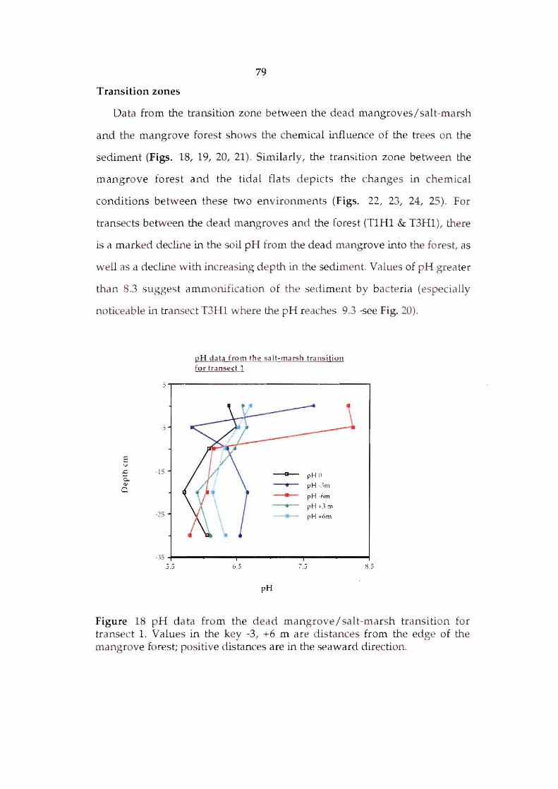
79
Transition zones
Data from the transition zone between the dead mangroves/salt-marsh
and the mangrove fores t shows the chemical influence of the trees on the
sediment (Figs. 18, 19, 20, 21). Similarly , the transition zone be tween the
mangrove forest and the tidal Ha ts depicts the cha nges in chemical
conditions between these two environments (Figs. 22, 23, 24, 25) . For
transects be tween the dead mangroves and the forest (T1H1 & T3Hl), there
is a marked decline in the soil pH from the dead mangrove into the forest, as
well as a decline with mer asing depth in the sedi ment. Values of pH greater
than 8.3 suggest ammonification of the sediment by bacte ria (especially
no ticeable in transec t T3Hl where the pH reaches 9.3 -see Fig. 20) .
E v .c ~ <lJ
a
p H dat a fro m the s alt -mars h transi tion for tra nsect 1
5 ~------------------------------~
-~
I J ---G---o pH () - pH ·Jm -- pH -Am -.-- pH +.1 m
-25 '- pH +6m
-.15 -I-----.....,-----...,..--------l ~ .~ 6.5
pH
., -, .:> ,~ .5
Figure 18 pH da ta fro m the dead mangrove / salt-marsh transition for transect 1. Values in the key -3, +6 ma re di tances from the edge of the mangrove forest; positive distances are in the seaward direction.
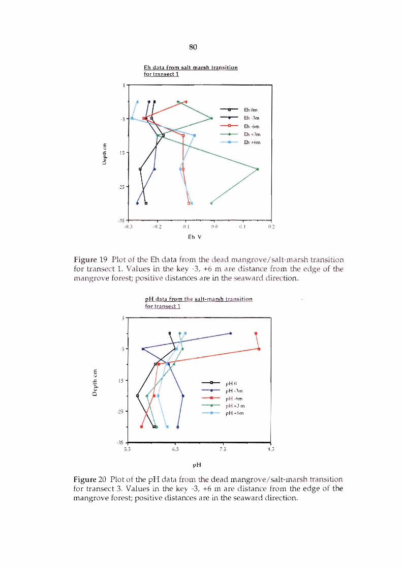
e ... .s: ·15 15.. Qj
~
25
80
Eh data from salt marsh transi tion for transect 1
-- Eh Om
----- Eh -Jm --0-- Eh-6m
-- Eh +Jm
- Eh +6m
-.• 5 +-- - - .------,-----r--....--.------1 -IU -0.2 -n . l 110 il. 1 il .2
Eh V
Figu re 19 Plot of the Eh da ta fro m the dead mangro ve/salt-marsh trcmsition for transect 1. Values Ln the key -3, +6 m are dis tance from the edge of th mangrove fo rest; positive distances are in the sea ward direction.
1: v
-= ~ OJ
a
-J
15
25
pH dat a from the salt- ma rsh transi t ion fo r t r;'lnsect 1
--a-- pH () -- p H -.lm
----- pH -om ---.-- pH +J m -- pH -+- Am
·35 +------"T""-----"'T"'-----...., 5.5 6.5 7.5
pH
Figure 20 Plot of the pH data from the dead mangrove/salt-marsh transition for transect 3. Values in the key -3, +6 m are distance from the edge of the mangrove forest; positive distances are in the seaward direction.
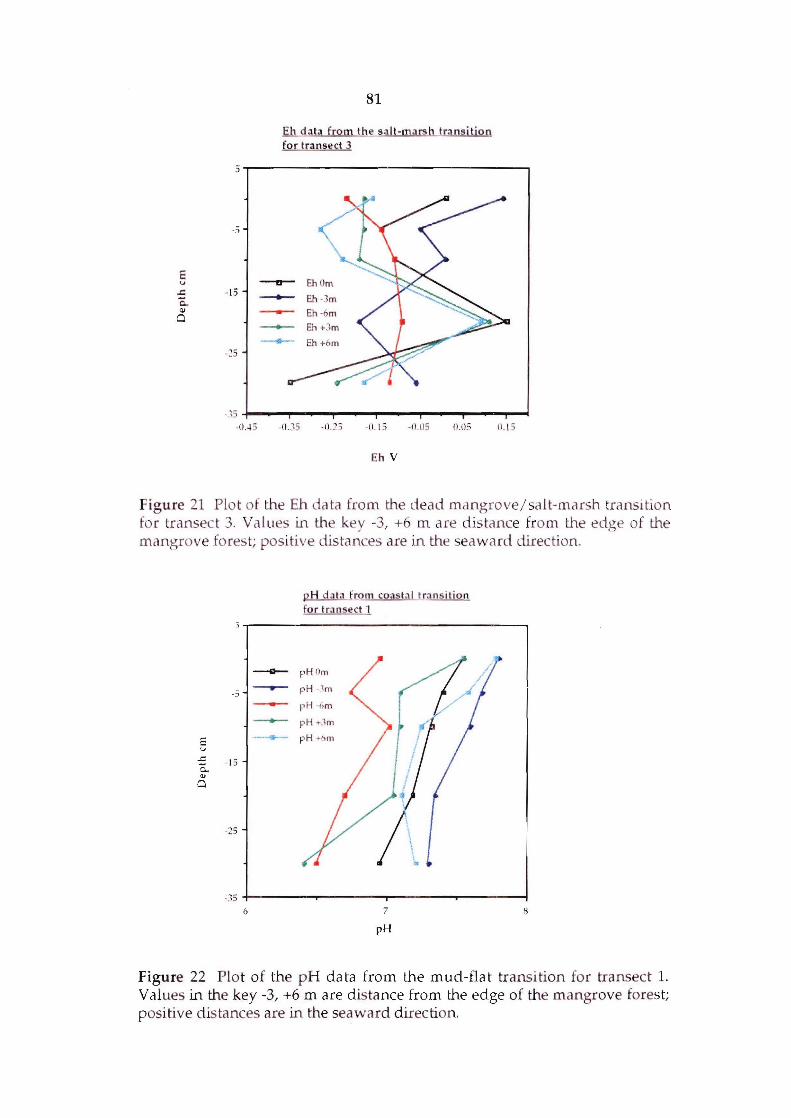
E v
..c 0.. <II Q
81
Eh d ata fro m the s a lt -mars h transition fo r transect 3
5 ~----------------------------------~
-~
-- Eh Om -15 - Eh -1m --- Eh -6m - Eh +Jm ---Eh +6m , -. _J
-~5 -!--.....,.---r---...--...,.--.,....-.....,. .... -il .-I 5 iU 5 -1 l. 25 -1l . I S -il .OS (l.OS tl. 15
Eh V
Figure 21 Plot of the Eh data from the dead mangrove/salt-mdch tr(,lnsi tion fo r transect 3. Values in th key -3, +6 m Me distance from the edge of the mangrove fore t; positive distance dre in the seaward direction.
E v
..c Q.. <II
Q
----.....-- ;) --.- ...-.
15
-2'3
p H data fro m coas tal trans itio n for t ra nsect 1
pH 11m
pH ·Jm
pH ·;;m
pH+.1m
pH +bm
-.15 +--------.--------"T""-------.----- ----1 6 7
pH
Figure 22 Plo t of the pH data from the mud-flat transi tion for transect l. Values in the key -3, +6 m are distance from the edge of the mangrove forest; positive d istances are in the seaward d irec tion.
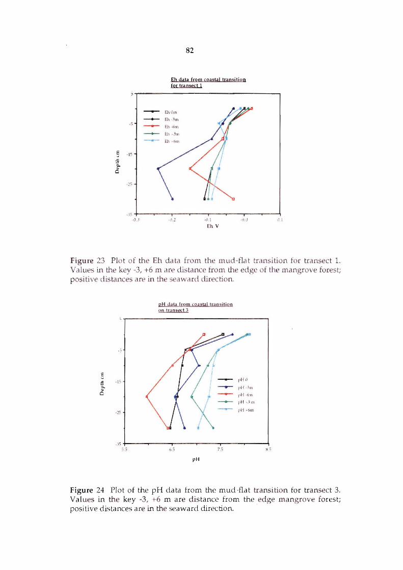
E v
-<: 0..
'" 0
-15
-:!5
82
Eb data fro m cOilstal transi tion for transec t 1
. ':' +--""'T"----r--..--""T'"-~--.__-.....--___\ ~ll . ! ~ I 1
Eb V
Figure 23 Plot of the Eh d Clta from the mud-flat trCln sition for transect 1-Values in the key -3, +6 m are d istance from the edge of the mangrove forest; positive distance are in the eaward direc tion.
E v
.J::
0.. '" 0
- I~
.:!5
p H <lag from wasta ! tran s ition on tr.Jnse.;t 3
-------1,1-1 d
pi { • 'Ill pH -~; 111
pH ... ~ III
I' I r 61l\
· 5 +-----~---~----~---,_----""T'"----~ 3.5 6 S 7.r-.,
pH
Figure 24 Plot of the pH data from the mud-flat transition for transect 3. Values in the key -3, +6 m are d is tance from the edge mangrove forest; positive distances are in the seaward direction.
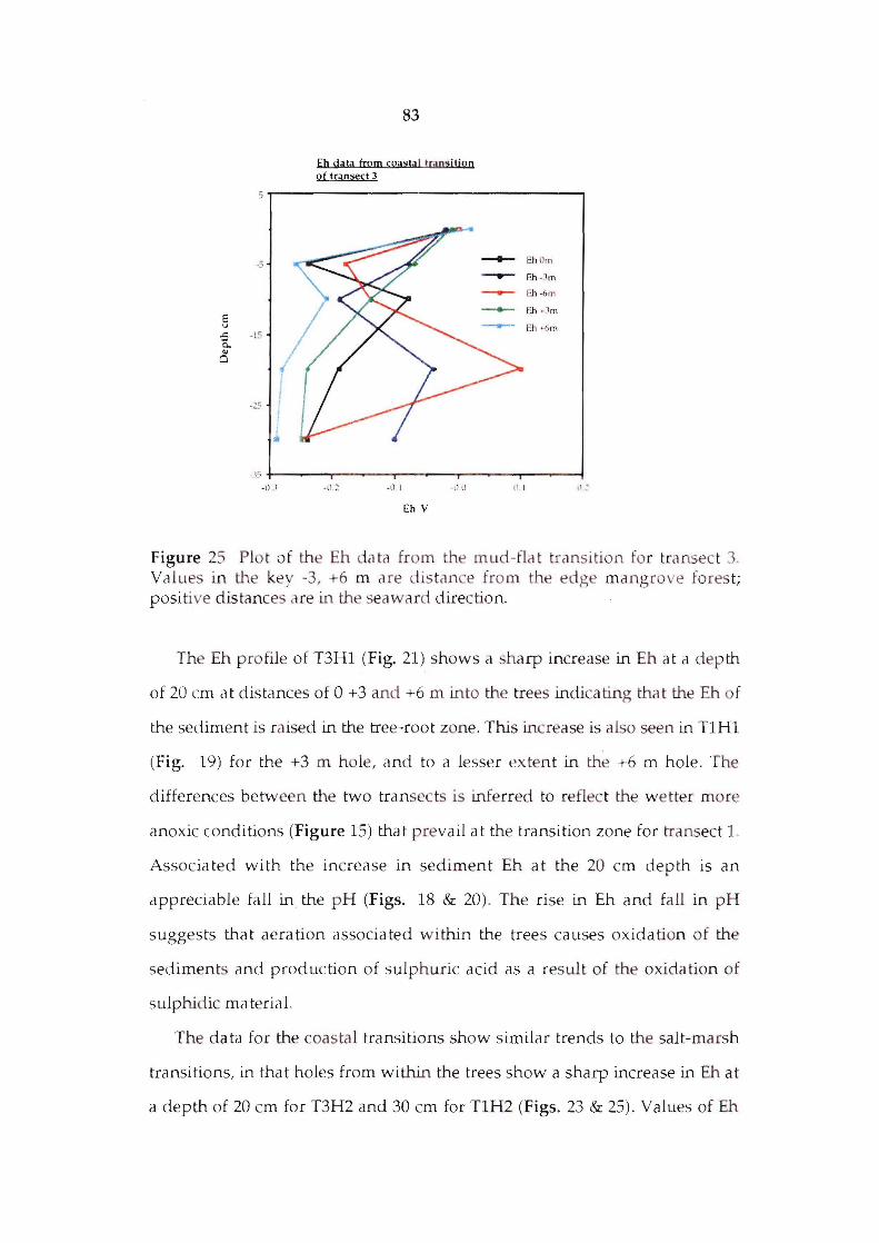
E u
.c: a.. ., a
83
Eh dati! from coasta l tran:zjtjon of transect 3
5 ~------------------------------~
·5
·l ~
-Z5
Eh Om
Eh ·310
I'll ·6m
. 'Co +---...,..-----r-----.,~---...._-----_I -,1..' - ll l d () , I
Eh V
Figure 25 Plo t of the Eh data from the mud-fla t transition for transec t 3. Val ues in the key -3, +6 m Me dis tance from the edge mang rove fores t; positive distances are in th seawMd direction.
The Eh profile of T3H1 (Fig. 21) shows a harp increase in Eh at a dep th
of 20 ern at distances of 0 +3 and +6 m into the trees indicating that the Eh of
the sediment is raised in the tree-root zone. This increase is also seen in T1Hl
(Fig. 19) for the +3 m hole, and to a lesser extent in the +6 m hole. The
differences between the two transec ts is infe rred to reflec t the we tter more
anoxic conditions (Figure 15) that prevail a t the transition zone for transect 1-
Associa ted with the increa se in sedimen t Eh a t the 20 cm depth is an
appreciable fall in the p H (Figs. 18 & 20) . The rise in Eh and fall in pH
suggests that aeration associated within the trees causes oxidation of the
sediments and production of sulph uric acid as a result of the oxida tion of
sulphidic rna teriaL
The data for the coastal transitions show similar trends to the salt-marsh
transitions, in that holes from within the trees show a sharp increase in Eh at
a depth of 20 ern for T3H2 and 30 ern for TIH2 (Figs. 23 & 25) . Values of Eh
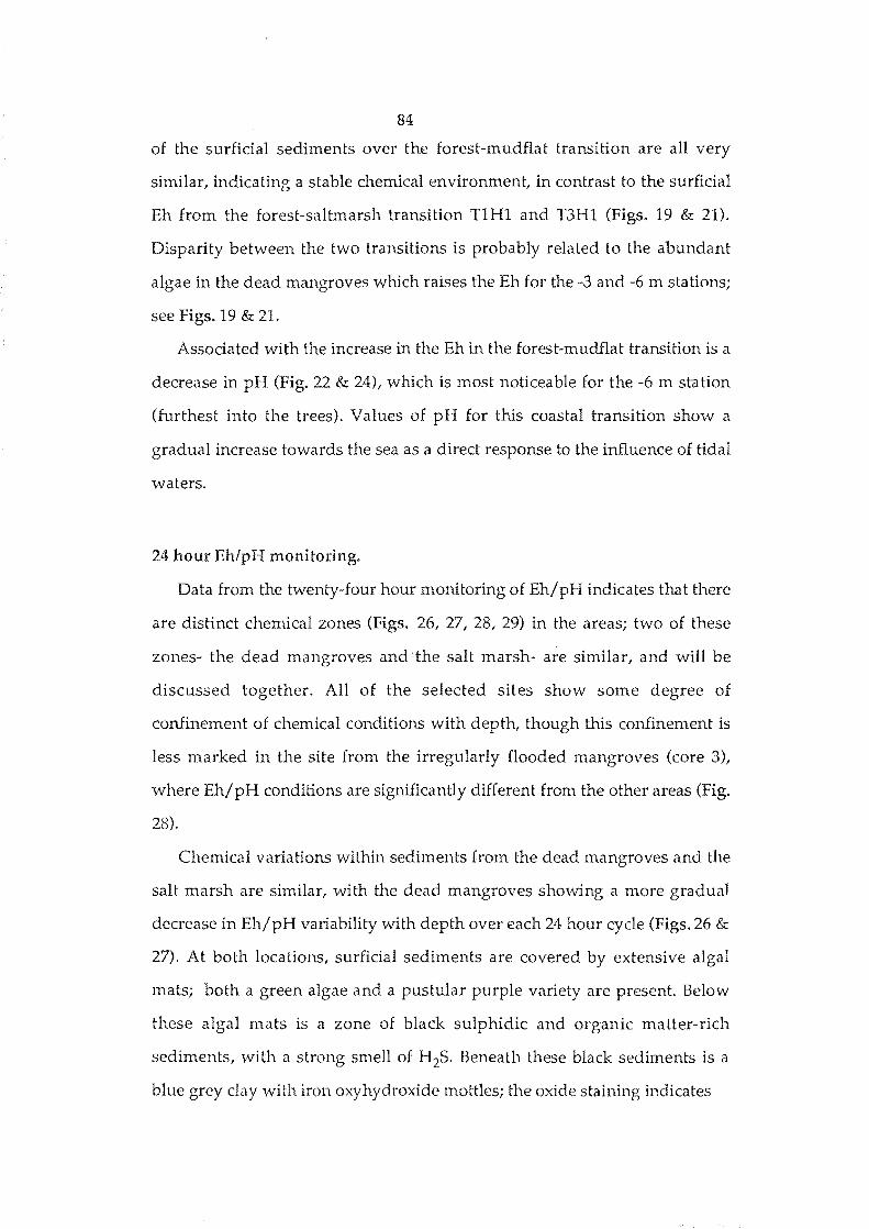
84
of the surficial sediments over the forest-mudflat transition are all very
similar, indicating a stable chemical environment, in contrast to the surficial
Eh from the forest-saltmarsh transition T1H1 and T3H1 (Figs. 19 & 21).
Disparity between the two transitions is probably related to the abundant
algae in the dead mangroves which raises the Eh for the -3 and -6 m stations;
see Figs. 19 & 21.
Associated with the increase in the Eh in the forest-mudflat transition is a
decrease in pH (Fig. 22 & 24), which is most noticeable for the -6 m station
(furthest into the trees). Values of pH for this coastal transition show a
gradual increase towards the sea as a direct response to the influence of tidal
waters.
24 hour Eh/pH monitoring.
Data from the twenty-four hour monitoring of Eh/pH indicates that there
are distinct chemical zones (Figs. 26, 27, 28, 29) in the areas; two of these
zones- the dead mangroves and the salt marsh- are similar, and will be
discussed together. All of the selected sites show some degree of
coniinement of chemical conditions with depth, though this coniinement is
less marked in the site from the irregularly flooded mangroves (core 3),
where Eh/ pH conditions are significantly different from the other areas (Fig.
28).
Chemical variations within sediments from the dead mangroves and the
salt marsh are similar, with the dead mangroves showing a more gradual
decrease in Eh/ pH variability with depth over each 24 hour cycle (Figs. 26 &
27), At both locations, surficial sediments are covered by extensive algal
mats; both a green algae and a pustular purple variety are present. Below
these algal mats is a zone of black sulphidic and organic matter-rich
sediments, with a strong smell of H2S. Beneath these black sediments is a
blue grey clay with iron oxyhydroxide mottles; the oxide staining indicates
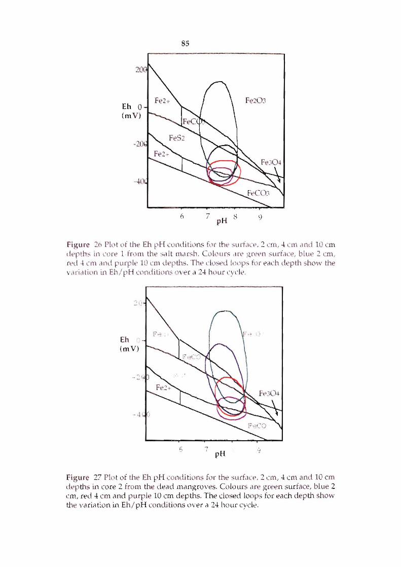
20
Eh 0 (m V )
-20
85
6
Fe20J
7 pH ~ 9
Figure 2A Plllt of the Eh p H --:nnditiuns f~H' tht> s llr f~1(p , 2 e111 .. -! em dnd 10 em d t'~)l h ~ in (~) rt> 1 fr'.> 11l the s(l it I11llfs h . C olo Llt"s Me:' grt't>n surfdee, blue 2 em , rf:-'d -! em M Id ~) u rp lt' 10 'm dep ths . Tlw d osed l up ~)s for t",l 'h dept'h sho w the v M id l illn in Eh/pH cond ition ... ..; over <l 2-1: hnur l."), c1 t'.
Eh Ii
(mV)
6 ..., ,
pH
Fig u re 27 Plo t of the Eh pH condi ti ns fV I" the s lIff,K f', 2 I~ m: 4 (111 and 10 em dt'~) ths in core 2 from the dead mangroves. Colours Me green surface, blue 2 eln, red -I: em (Inti purple 10 em deptlls. The dosed loops for each depth show th!:>. vClfi.-Hion in Eh/ pH condi tions over () 24 hOllr cyde.
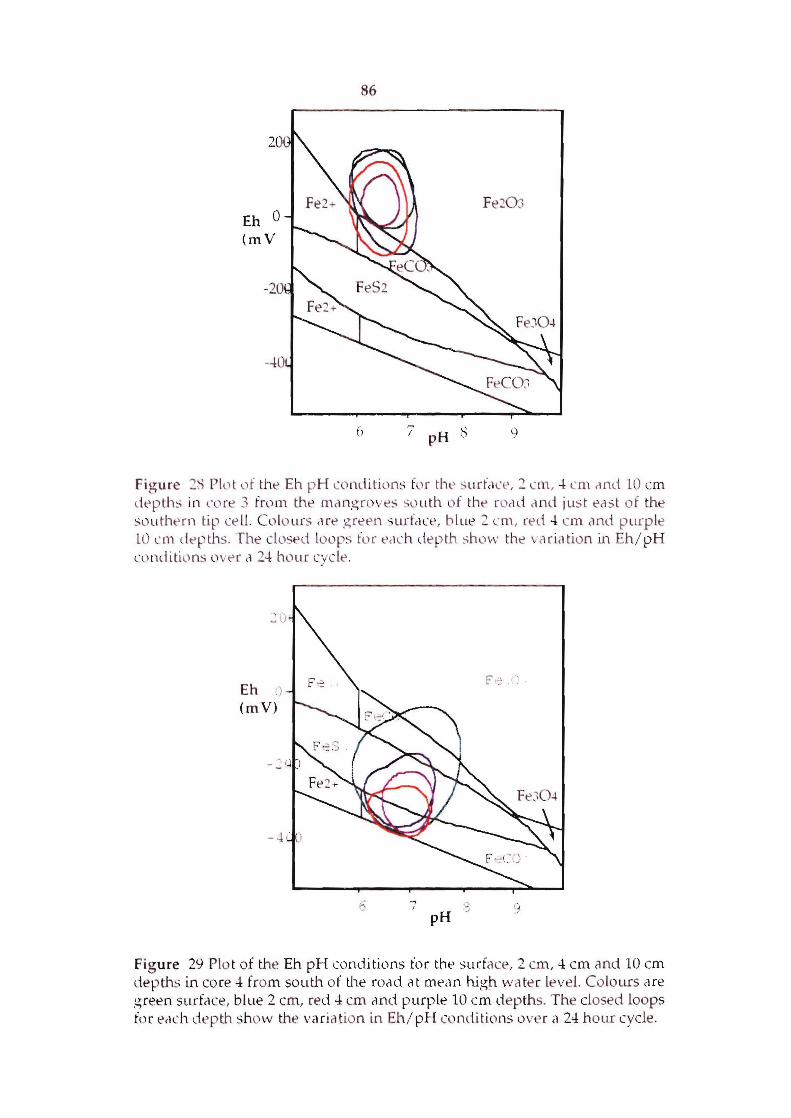
20
Eh 0 (mV
86
6
F~20J
7 p H b 9
Figu re 211 Pint L)f tlw Eh p H conditions for the s ll rLKt' , 2 el11 , -I: em clnd 10 em dt:>ptlb in co r 3 from the mclngroves SLHlth of the w,ld ond just east of the sO ll ti'wrn tip ce lL Colo urs are green s llrtc1c t', bl ue 2 em, red -I: em clnd purple ll) l 'Ll1 depths. The dosed loops fl)r 1:',1\:11. depth sho\-" the vcHiation in Eh/ p H
L' ontiitil) nS oVt'[ cI 2-l ho ur cycle.
Eh '.1 (mV)
i ;~ pH
Figure 21:1 Plo t of the Eh pH conditions for tht' surt,lCt', 2 em, 4: em and 10 em depths in core 4 fro m south o f the w ,Hi at rnt'Cln high \Vcl te r leve l. Colo urs are green surfcl ce, blue 2 em, red 4 em ,md purple 10 em d ep th s. The closed loop s for t' ,l(h dep th show the vClfiil tion in Eh/ pH cl)ndi tions o ver ,1 24 h our cycle.
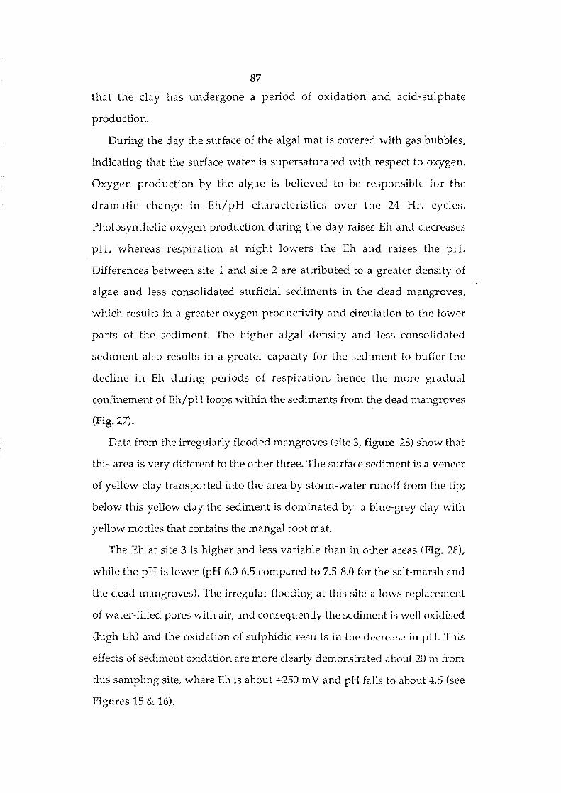
87
that the clay has undergone a period of oxidation and acid-sulphate
production.
During the day the surface of the algal mat is covered with gas bubbles,
indicating that the surface water is supersaturated with respect to oxygen.
Oxygen production by the algae is believed to be responsible for the
dramatic change in Eh/pH characteristics over the 24 Hr. cycles.
Photosynthetic oxygen production during the day raises Eh and decreases
pH, whereas respiration at night lowers the Eh and raises the pH.
Differences between site 1 and site 2 are attributed to a greater density of
algae and less consolidated surficial sediments in the dead mangroves,
which results in a greater oxygen productivity and circulation to the lower
parts of the sediment. The higher algal density and less consolidated
sediment also results in a greater capacity for the sediment to buffer the
decline in Eh during periods of respiration, hence the more gradual
confinement of Eh/pH loops within the sediments from the dead mangroves
(Fig. 27).
Data from the irregularly flooded mangroves (site 3, figure 28) show that
this area is very different to the other three. The surface sediment is a veneer
of yellow clay transported into the area by storm-water runoff from the tip;
below this yellow clay the sediment is dominated by a blue-grey clay with
yellow mottles that contains the mangal root mat.
The Eh at site 3 is higher and less variable than in other areas (Fig. 28),
while the pH is lower (pH 6.0-6.5 compared to 7.5-8.0 for the salt-marsh and
the dead mangroves). The irregular flooding at this site allows replacement
of water-filled pores with air, and consequently the sediment is well oxidised
(high Eh) and the oxidation of sulphidic results in the decrease in pH. This
effects of sediment oxidation are more clearly demonstrated about 20 m from
this sampling site, where Eh is about +250 m V and pH falls to about 4.5 (see
Figures 15 & 16).
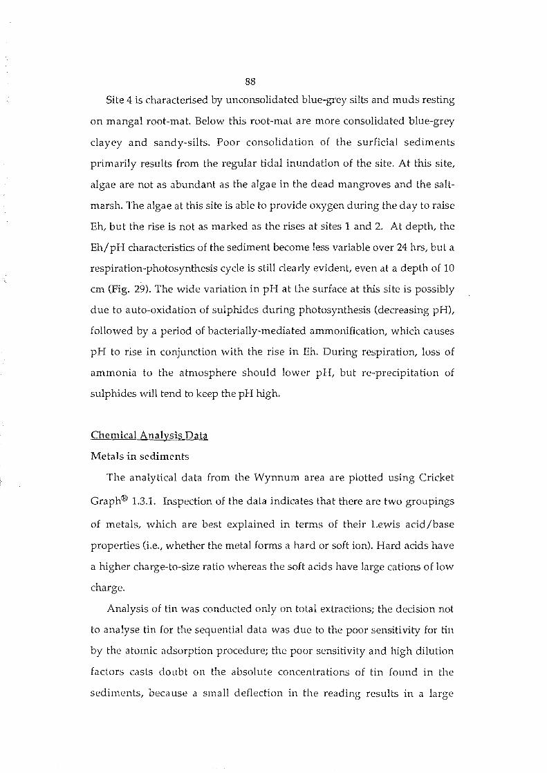
88
Site 4 is characterised by unconsolidated blue-grey silts and muds resting
on mangal root-mat. Below this root-mat are more consolidated blue-grey
clayey and sandy-silts. Poor consolidation of the surficial sediments
primarily results from the regular tidal inundation of the site. At this site,
algae are not as abundant as the algae in the dead mangroves and the salt
marsh. The algae at this site is able to provide oxygen during the day to raise
Eh, but the rise is not as marked as the rises at sites 1 and 2. At depth, the
Eh/pH characteristics of the sediment become less variable over 24 hrs, but a
respiration-photosynthesis cycle is still clearly evident, even at a depth of 10
cm (Fig. 29). The wide variation in pH at the surface at this site is possibly
due to auto-oxidation of sulphides during photosynthesis (decreasing pH),
followed by a period of bacterially-mediated ammonification, which causes
pH to rise in conjunction with the rise in Eh. During respiration, loss of
ammonia to the atmosphere should lower pH, but re-precipitation of
sulphides will tend to keep the pH high.
Chemical Analysis Data
Metals in sediments
The analytical data from the Wynnum area are plotted using Cricket
Graph® 1.3.1. Inspection of the data indicates that there are two groupings
of metals, which are best explained in terms of their Lewis acid/base
properties (Le., whether the metal forms a hard or soft ion). Hard acids have
a higher charge-to-size ratio whereas the soft acids have large cations of low
charge.
Analysis of tin was conducted only on total extractions; the decision not
to analyse tin for the sequential data was due to the poor sensitivity for tin
by the atomic adsorption procedure; the poor sensitivity and high dilution
factors casts doubt on the absolute concentrations of tin found in the
sediments, because a small deflection in the reading results in a large
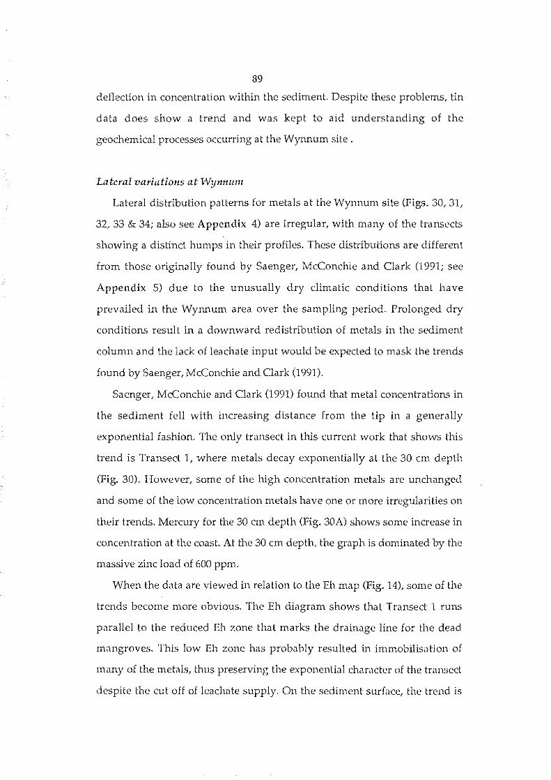
89
deflection in concentration within the sediment. Despite these problems, tin
data does show a trend and was kept to aid understanding of the
geochemical processes occurring at the Wynnum site.
Lateral variations at Wynnu111
Lateral distribution patterns for metals at the Wynnum site (Figs. 30,31,
32,33 & 34; also see Appendix 4) are irregular, with many of the transects
showing a distinct humps in their profiles. These distributions are different
from those originally found by Saenger, McConchie and Clark (1991; see
Appendix 5) due to the unusually dry climatic conditions that have
prevailed in the Wynnum area over the sampling period. Prolonged dry
conditions result in a downward redistribution of metals in the sediment
column and the lack of leachate input would be expected to mask the trends
found by Saenger, McConchie and Clark (1991).
Saenger, McConchie and Clark (1991) found that metal concentrations in
the sediment fell with increasing distance from the tip in a generally
exponential fashion. The only transect in this current work that shows this
trend is Transect I, where metals decay exponentially at the 30 cm depth
(Fig. 30). However, some of the high concentration metals are unchanged
and some of the low concentration metals have one or more irregularities on
their trends. Mercury for the 30 cm depth (Fig. 30A) shows some increase in
concentration at the coast. At the 30 cm depth, the graph is dominated by the
massive zinc load of 600 ppm.
When the data are viewed in relation to the Eh map (Fig. 14), some of the
trends become more obvious. The Eh diagram shows that Transect 1 runs
parallel to the reduced Eh zone that marks the drainage line for the dead
mangroves. This low Eh zone has probably resulted in immobilisation of
many of the metals, thus preserving the exponential character of the transect
despite the cut off of leachate supply. On the sediment surface, the trend is
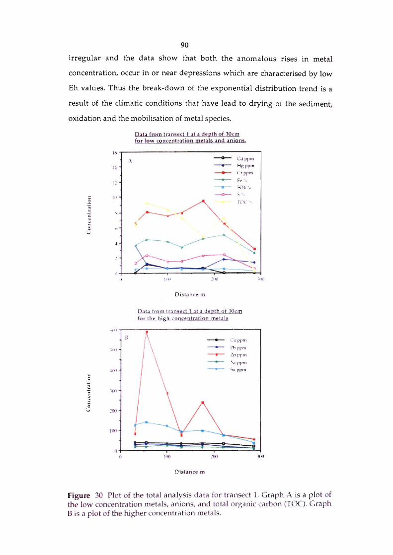
90
irregular and the data show that both the anomalous rises in metal
concentration, occur in or near depressions which are characterised by low
Eh values. Thus the break-down of the exponential distribution trend is a
result of the climatic conditions that have lead to drying of the sediment,
oxidation and the mobilisation of metal species.
-;::
" 'J
.-;:: -" 'J
::: ~
Data frum tra nsect J at J depth of 30cm for low concentration metals .1Od anio ns .
l b ~----------------------------------, ,-\
--0-- Cd ppm
I~ -.- H); ppm - er ppm
12 --- Fe " -:... .. '"
1,1 --0- S "
~ rL'L .,
" t ,
..
, , )
,I j' ''. ~I ~ \ ;'kl
Di st.ln ct' m
th o f 30cm
"'~)
13 - L Uf."'pm
\ - It- ppm ~ .. ) • -y-- in rpm
,-, ppm
.. , ~ \ .;", ppm
~ N1
~lO
I(M)
,)
II I!~I _(M) .'iW)
Distance m
Figure 30 Plot of the total ana lysis data fo r transect 1. Gra ph A is a plot of the low concentration metals, anions, and total o rganic carbon (TOC). Graph B is a plot of the higher concentration metals.
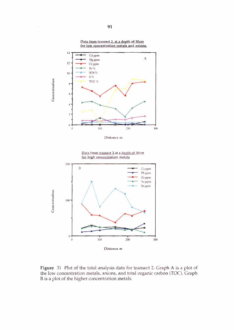
c: .~
t'! C OJ v c: 0 U
0
-;; ... C OJ v c: 0
U
14
12
10
8
6
.t
2
0 ()
91
Data fro m transect 2 at a depth of 30cm for low concentration metals an d anions .
-- Cd ppm -- Hg ppm A -- C rppm - Fe% -- S04 !~~ - 5 I~I, )
~v ~
..... ..... - -- ---..... -"'"
I(X) XI()
Distance m
Data from transect 2 at.1 depth of 30cm for hiSh concentra tion metals
100
200 "T"'""- - ----- -------------, 13 - CLl ppm
~ l'bppm -- lnppm --,-- I ppm
----- 5n ppm
lUO
I) -+------...,-------,..-------1 o 100 200 300
Distance m
Figure 31 Plot of the total analysis data for transect 2. Graph A is a p lot of the low concentra tion metals, anions, and total organic carbon (TOC) . Graph B is a plo t of the higher concentra tion meta ls.

c .~ ... ... c "" v
0
-;;; ...
"" u
0 U
14
12
10
R
6
o
ibO
I ·ll)
120
100
HO
b (J
-10
20
()
0
92
Data fro m transect 3 at a depth of 30cm for lo w conce ntra tion meta ls and an io ns
-- Cd ppm
-....-- Hg ppm --- Crppm -- Fe %
--.r-- 504 %
~ s'r.
~~
100 2lX) 100
Distance m
Dat.l from tr:lnsect 3.:1t .1 depth of 30cm for high concentra tion metals
- Cu ppm
-- ['!:> ppm
- Znppm
--- \iippm
-- Sn ppm
/?-----/ ,I' .-
/,.AI ".. ..... -
100 200
Distan ce m
300
A
-100
13
.I(x)
Figure 32 Plot of the total ana lysis data for transect 3. Graph A is a plot of the low concentration metais, amons, and total organic carbon (TOC). Graph B is a plo t of the higher concentration metals.
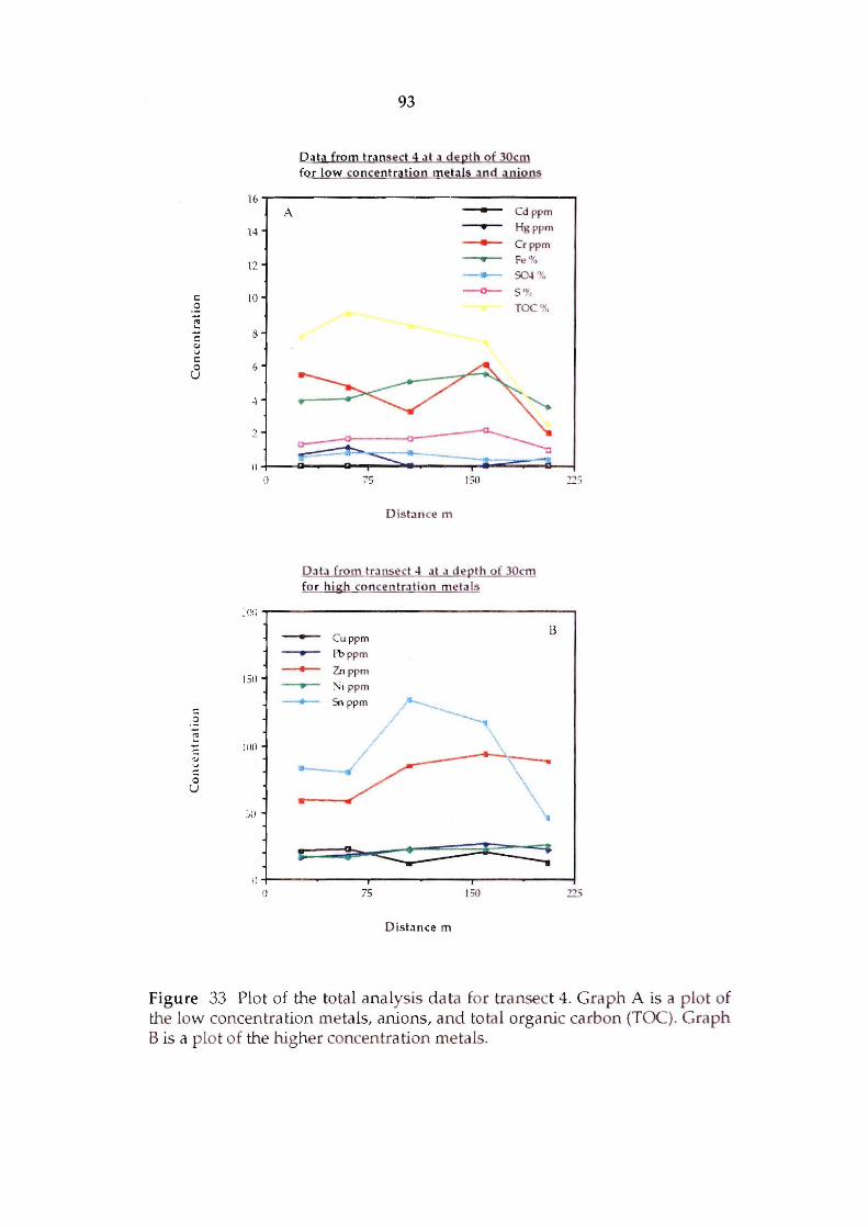
c: .~ -;; ... c '" v c: 0 U
0
~ ~
OJ v
0 U
16
14
12
10
8
6
-I
:>.
0 ()
~(lil
ISO
100
:,D
93
Data from transect 4 at a de pth o f 30cm for low concentration metals an d a n io ns
A -- Cd ppm -- Hgppm -- Crppm -- Fe 0 -- 504 'Yo --.0-- S %
TOC %
75 150
D is ta nce m
D:l ta from transect 4 :I t J depth o f 30cm fo r high co nce nt r:l tio n meta ls
------.--------Cuppm
Pb pp m
Zn ppm
'\J I ppm
_ Sn ppm / 4_
I ---./'
/ /
- ----., \
\
\
O+------------r----------~r_--------~ u 75 130 225
Distance m
Figure 33 Plot of the tota l analysis data for transect 4. Graph A is a p lot of the low concen tra tion metals, anions, and total organic carbon (TOC). Graph B is a p lot of the higher concentration metals.
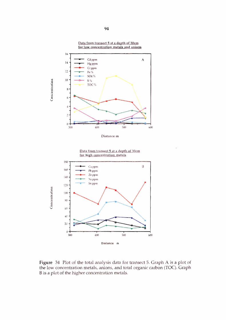
c .S!
~ .. v c: o U
c: a
c: .. v c: o U
16
14
12
10
8
6
94
Da ta from t ransect 5 at a de pth o f 30cm for low concentratio n metals and a nions
-- Cd ppm ---- Hgppm - Crppm -- Fe% -- 504 % --0- 5 %
TOC %
A
I ~~~~~a§-~~~~·~· o ~ .-•. ~ ,100
ISO
160
l.tO
I ~O
l ilO
~O
6()
-\0
20
.too 500 bOO
Distance m
Da ta from transect 5 J t J dep th of 30cm for high concen tra ti on metals
-- Cu ppm ---- f'b ppm - Zn ppm - :\, ppm -,-- Sn ppm
{) +------------r------------.---------~ 100 600
Dist an ce m
Figure 34 Plot of the total ana lysis data fo r transect 5. Gra ph A is a plot of the low concentration metals, anions, and total organic carbon (TOe). Graph B is a plot of the higher concen tration metal.
95
Trends for the second transect confirm the importance of low Eh holes
depressions retaining otherwise mobile metals. However these depressions,
while capturing some metals, are not totally effective for all (e.g. zinc in the
surficial sediment of transect 2; Fig. 31). Zn shows a curiously large increase
in concentration in the last sampling site (about 30m from the edge of the
trees), indicating that some of these mobilised metals are reaching the coast.
Transect 3 (Fig. 32) also indicates theremobilisation of metals (especially
Zn), and a major spike in zinc concentration is evident in the forest zone.
This spike has advanced further from the tip in the deeper sediments than in
the upper sediments due to the more persist water saturation.
Transect 4 (Fig. 33) shows that in the area of high Eh and low pH, metals
have been have mobilised under oxidising conditions and have been
stripped from the area. The movement of the mobilised metals down the
hydraulic gradient has produced rise in metal concentration at about 150 m
from the site for the surficial sediments and a bout 100 m for the sediments at
depth; iron and sulphur show a substantial increase in concentration at the
distances. The arresting of metal migration from zone of acid sulphate soil
formation is primarily due to the Eh gradient; as the Eh decreases towards
the coast there is a corresponding rise in metal accumulation.
Transect 5 (Fig. 34) shows that metal concentrations in the surficial
sediments in the dead mangroves increase toward the south suggesting that
there is a general southerly hydraulic gradient. When the transects change
bearing towards the coast, metal concentrations in the sediment decreases
toward the coast. As with the other transects, metal concentrations along
transect 5 show a few concentration peaks that are again related to the
migration of the metals and accumulation in areas of low Eh. At a depth of
30 cm , Zn, Hg and S show a sharp rise in concentration at the coast, which
may be due to the proximity of the sewage outfall to this sampling site.
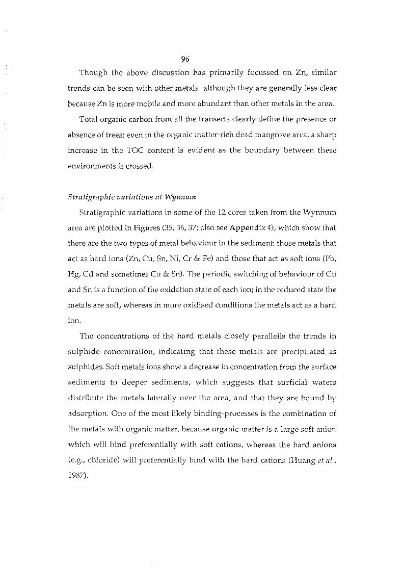
96
Though the above discussion has primarily focussed on Zn, similar
trends can be seen with other metals although they are generally less clear
because Zn is more mobile and more abundant than other metals in the area.
Total organic carbon from all the transects clearly define the presence or
absence of trees; even in the organic matter-rich dead mangrove areal a sharp
increase in the TOC content is evident as the boundary between these
environments is crossed.
Stratigraphic variations at Wymwm
Stratigraphic variations in some of the 12 cores taken from the Wynnum
area are plotted in Figures (351 361 37; also see Appendix 4)1 which show that
there are the two types of metal behaviour in the sediment: those metals that
act as hard ions (Zn, CUI Sn, Nil Cr & Fe) and those that act as soft ions (Pb,
Hg, Cd and sometimes Cu & Sn). The periodic switching of behaviour of Cu
and Sn is a function of the oxidation state of each ion; in the reduced state the
metals are soft whereas in more oxidised conditions the metals act as a hard
ion.
The concentrations of the hard metals closely parallells the trends in
sulphide concentration, indicating that these metals are precipitated as
sulphides. Soft metals ions show a decrease in concentration from the surface
sediments to deeper sediments, which suggests that surficial waters
distribute the metals laterally over the areal and that they are bound by
adsorption. One of the most likely binding-processes is the combination of
the metals with organic matter, because organic matter is a large soft anion
which will bind preferentially with soft cations, whereas the hard anions
(e.g. I chloride) will preferentially bind with the hard cations (Huang et ai"
1987).
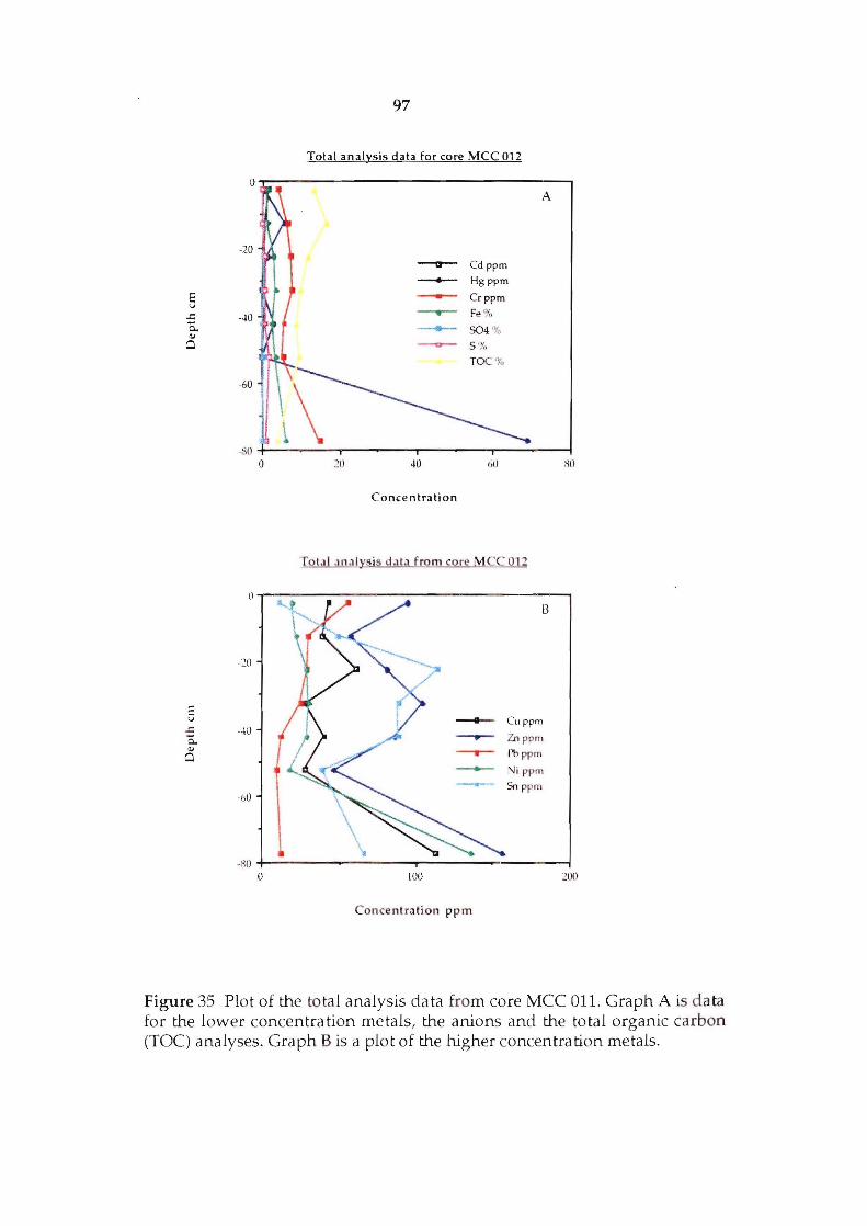
97
Total analysis data for core MCC 012
u~----------------------------------~ A
-20 -- Cd ppm ---- Hgppm
E ---v Crppm
~ -40 --.-- Fe ~{) 0.. --.-- 504 % OJ
a ----- 5 '1.,
TOC %
.~ O +---- --.......,r------'"T""----.......,r-------i (] 20 40 so
Concentration
Total .lnalys is data from core MCC 012
0....-------------------------- ------, B
-20
~ ~
v Cuppm ~ --10 :l. Zn ppm
'" [,bppm a 'I i ppm
So ppm -60
-so -r--------------.,....-------- ---- ---i o lOO 200
Concen trat ion pp m
Figure 35 Plot of the total analysis data fro m core MCC all. Graph A is data for the lower concentra tion metals, the anions and the total organic carbon (TOC) analyses. Graph B is a plot of the higher concentration metals.
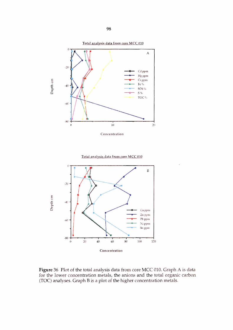
E v ~
c::.. QI
0
E v ~
c;..
'" D
98
Total ana lysis data from core MCC 0]0
o ~----------------------------------~ A
-20 -- Cd ppm -- Hgppm - Crppm
-40 --- Fe <}Il
-..,.,........ 504 ,},. --0-- S (~11
TOC')"
-60
-Hil +------.--------------------1 II 10 20
Concen tra tion
Tota l an alysis data from core MCC 010
II "T'""--------------------------------.....
-211
-4 11
-6(\ -
13
C"ppm
Zn ppm
1'1:> ppm
~) ppm
So ppm
-80 +----.....----.....----.-- --.-----.------1 (I 20 40 60 80 HlO 120
Con cent ratio n
Figure 36 Plot of the total analysis data from core MCC 010. Graph A is data for the lower concentration meta ls, the anions and the total organic carbon (TOC) analyses. Graph B is a plot of the higher concentration metals.
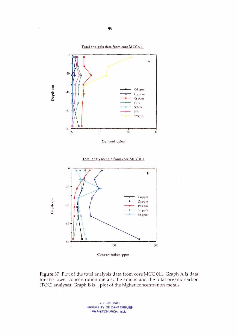
99
Total analysis data from core M CC 011
o~----------------------------------~
A
-20
E u - Cd ppm
..c: -oW 0.. - Hg ppm QJ --- Cr ppm 0 --- Fe ( ~~ - 504%
-6() -0-- 5 'YP
TOe'o",
-1'\0 +---------r------ --....,...-------I o 10 2U
Co ncentration
Tot.ll analys is data from core MCC 011
1),----------------------------,
-20
-- Cu ppm 1= ;:; -- Zn ppm
-= --III ---- l'b ppm 0..
'., ppm <lI --0 ---- 50 ppm
-bl)
-KO +-------- --------....,...--------------1 I) tOO 200
Concentration ppm
Figure 37 Plot of the total analysi da ta from core MCC 011 . Graph A is data fo r the lower concentra tion meta ls, the anions and the to tal orga nic carbon (TOe) ana lyses. Graph 8 is a plot of the higher concentration metals.
, '"11: LltlHAHl
VEHSITY OF CANTEABUIiIl eIllAI.TCHlIRCH. .. ....
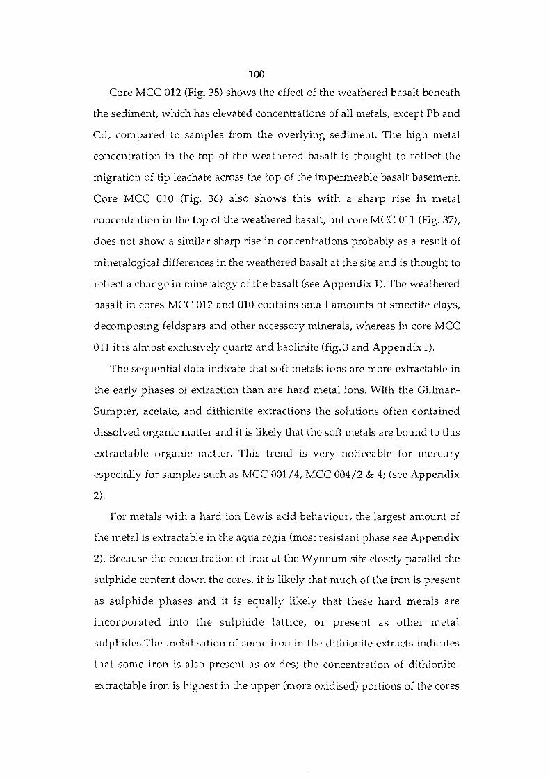
100
Core MCC 012 (Fig. 35) shows the effect of the weathered basalt beneath
the sediment, which has elevated concentrations of all metals, except Pb and
Cd, compared to samples from the overlying sediment. The high metal
concentration in the top of the weathered basalt is thought to reflect the
migration of tip leachate across the top of the impermeable basalt basement.
Core MCC 010 (Fig. 36) also shows this with a sharp rise in metal
concentration in the top of the weathered basalt, but core MCC all (Fig. 37),
does not show a similar sharp rise in concentrations probably as a result of
mineralogical differences in the weathered basalt at the site and is thought to
reflect a change in mineralogy of the basalt (see Appendix 1). The weathered
basalt in cores MCC 012 and 010 contains small amounts of smectite clays,
decomposing feldspars and other accessory minerals, whereas in core MCC
all it is almost exclusively quartz and kaolinite (fig. 3 and Appendix 1).
The sequential data indicate that soft metals ions are more extractable in
the early phases of extraction than are hard metal ions. With the Gillman
Sumpter, acetate, and dithionite extractions the solutions often contained
dissolved organic matter and it is likely that the soft metals are bound to this
extractable organic matter. This trend is very noticeable for mercury
especially for samples such as MCC 001/4, MCC 004/2 & 4; (see Appendix
2).
For metals with a hard ion Lewis add behaviour, the largest amount of
the metal is extractable in the aqua regia (most resistant phase see Appendix
2). Because the concentration of iron at the Wynnum site closely parallel the
sulphide content down the cores, it is likely that much of the iron is present
as sulphide phases and it is equally likely that these hard metals are
incorporated into the sulphide lattice, or present as other metal
sulphides.The mobilisation of some iron in the dithionite extracts indicates
that some iron is also present as oxides; the concentration of dithionite
extractable iron is highest in the upper (more oxidised) portions of the cores
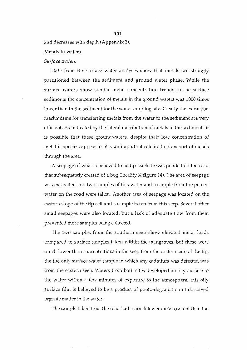
101
and decreases with depth (Appendix 2),
Metals in waters
Surface waters
Data from the surface water analyses show that metals are strongly
partitioned between the sediment and ground water phase. While the
surface waters show similar metal concentration trends to the surface
sediments the concentration of metals in the ground waters was 1000 times
lower than in the sediment for the same sampling site. Clearly the extraction
mechanisms for transferring metals from the water to the sediment are very
efficient. As indicated by the lateral distribution of metals in the sediments it
is possible that these groundwaters, despite their low concentration of
metallic species, appear to play an important role in the transport of metals
through the area.
seepage of what is believed to be tip leachate was ponded on the road
that subsequently created of a bog (locality X figure 14). The area of seepage
was excavated and two samples of this water and a sample from the pooled
water on the road were taken. Another area of seepage was located on the
eastern slope of the tip cell and a sample taken from this seep. Several other
small seepages were also located, but a lack of adequate flow from them
prevented more samples being collected.
The two samples from the southern seep show elevated metal loads
compared to surface samples taken within the mangroves, but these were
much lower than concentrations in the seep from the eastern side of the tip;
the the only surface water sample in which any cadmium was detected was
from the eastern seep. Waters from both sites developed an oily surface to
the water within a few minutes of exposure to the atmosphere; this oily
surface film is believed to be a product of photo-degradation of dissol ved
organic matter in the water.
The sample taken from the road had a much lower metal content than the
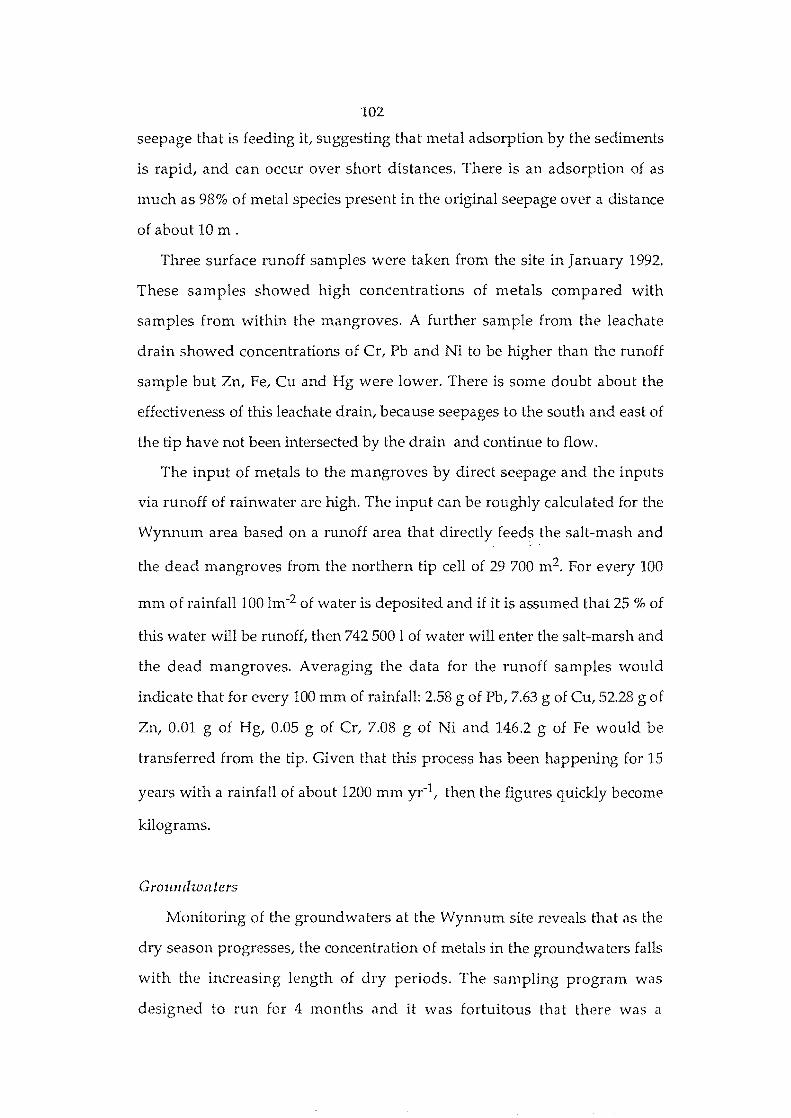
102
seepage that is feeding it, suggesting that metal adsorption by the sediments
is rapid, and can occur over short distances. There is an adsorption of as
much as 98% of metal species present in the original seepage over a distance
of about 10 m .
Three surface runoff samples were taken from the site in January 1992.
These samples showed high concentrations of metals compared with
samples from within the mangroves. A further sample from the leachate
drain showed concentrations of Cr, Pb and Ni to be higher than the runoff
sample but Zn, Fe, Cu and Hg were lower. There is some doubt about the
effectiveness of this leachate drain, because seepages to the south and east of
the tip have not been intersected by the drain and continue to flow.
The input of metals to the mangroves by direct seepage and the inputs
via runoff of rainwater are high. The input can be roughly calculated for the
Wynnum area based on a runoff area that directly feeds the salt-mash and
the dead mangroves from the northern tip cell of 29 700 m2. For every 100
mm of rainfall 100 Im-2 of water is deposited and if it is assumed that 25 % of
this water will be runoff, then 742 5001 of water will enter the salt-marsh and
the dead mangroves. Averaging the data for the runoff samples would
indicate that for every 100 mm of rainfall: 2.58 g of Pb, 7.63 g of Cu, 52.28 g of
Zn, 0.01 g of Hg, 0.05 g of Cr, 7.08 g of Ni and 146.2 g of Fe would be
transferred from the tip. Given that this process has been happening for 15
years with a rainfall of about 1200 mm yr-1, then the figures quickly become
kilograms.
Gr01t1ldwaters
Monitoring of the groundwaters at the Wynnum site reveals that as the
dry season progresses, the concentration of metals in the ground waters falls
with the increasing length of dry periods. The sampling program was
designed to run for 4 months and it was fortuitous that there was a
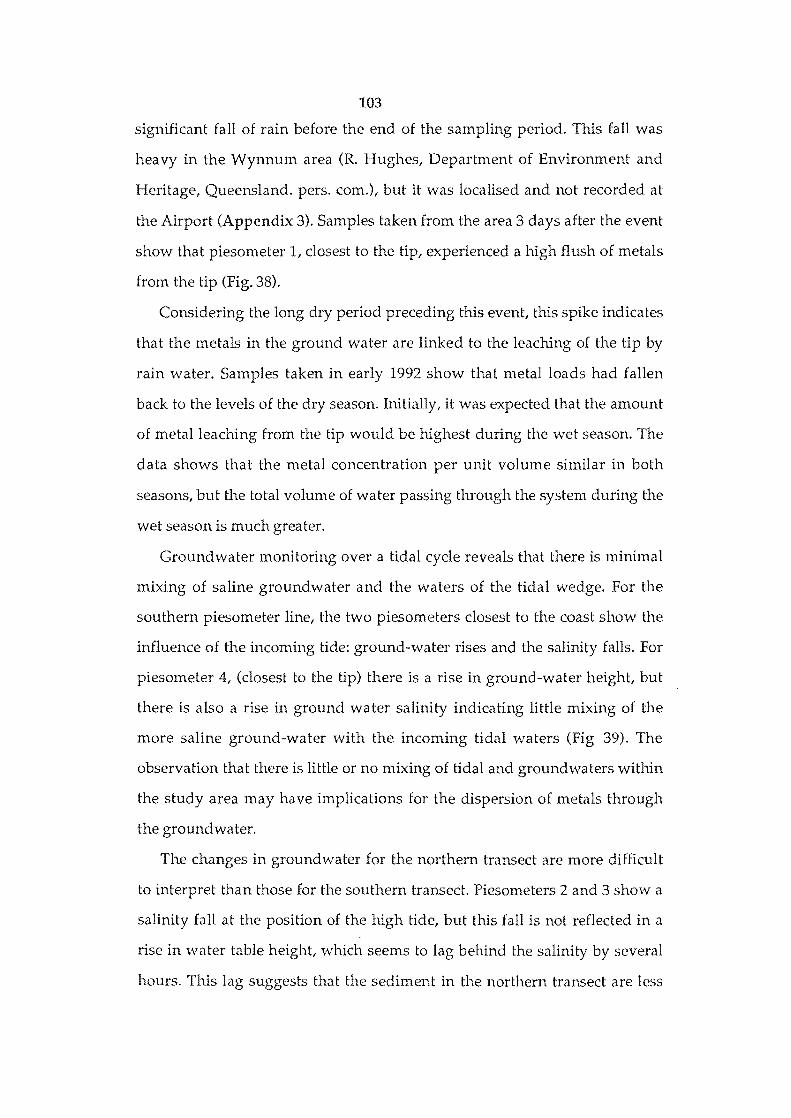
103
significant fall of rain before the end of the sampling period. This fall was
heavy in the Wynnum area (R. Hughes, Department of Environment and
Heritage, Queensland. pers. com.), but it was localised and not recorded at
the Airport (Appendix 3). Samples taken from the area 3 days after the event
show that piesometer 1, closest to the tip, experienced a high flush of metals
from the tip (Fig. 38).
Considering the long dry period preceding this event, this spike indicates
that the metals in the ground water are linked to the leaching of the tip by
rain water. Samples taken in early 1992 show that metal loads had fallen
back to the levels of the dry season. Initially, it was expected that the amount
of metal leaching from the tip would be highest during the wet season. The
data shows that the metal concentration per unit volume similar in both
seasons, but the total volume of water passing through the system during the
wet season is much greater.
Groundwater monitoring over a tidal cycle reveals that there is minimal
mixing of saline groundwater and the waters of the tidal wedge. For the
southern piesometer line, the two piesometers closest to the coast show the
influence of the incoming tide: ground-water rises and the salinity falls. For
piesometer 4, (closest to the tip) there is a rise in ground-water height, but
there is also a rise in ground water salinity indicating little mixing of the
more saline ground-water with the incoming tidal waters (Fig 39). The
observation that there is little or no mixing of tidal and ground waters within
the study area may have implications for the dispersion of metals through
the groundwater.
The changes in groundwater for the northern transect are more difficult
to interpret than those for the southern transect. Piesometers 2 and 3 show a
salinity fall at the position of the high tide, but this fall not reflected in a
rise in water table height, which seems to lag behind the salinity by several
hours. This lag suggests that the sediment in the northern transect are less
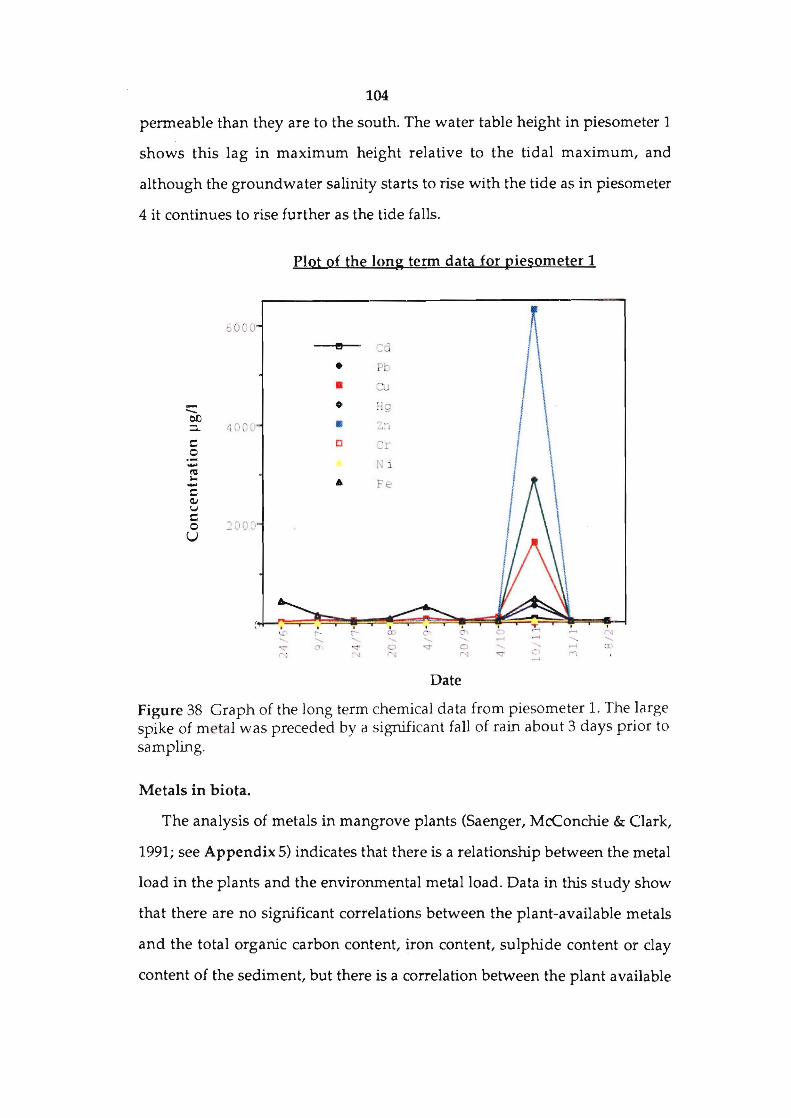
104
permeable than they are to the south. The water table height in piesometer 1
shows this lag in maximum height relative to the tidal maximum, and
although the groundwater salinity starts to rise with the tide as in piesometer
4 it continues to rise further as the tide falls.
bO OD
-"'"'-00 :::1. 4 0 ~ (1
s:: 0 .--' ~ .. -' s:: Q.I v s:: 0 ~OO(1
U
Plot of the long term data for piesometer 1
!! Cd
I • p
• :.J
0 Hg
\ • :n 1
c :::1 J\ i
6 FE:-
Date
, M -.... cr·
Figure 38 Graph of the long term chemical data from piesometer 1. The large spike of metal was preceded by a significant fall of rain about 3 days prior to sampling.
Metals in biota.
The analysis of metals in mangrove plants (Saenger, McConchie & Clark,
1991; see Appendix 5) indicates that there is a relationship between the metal
load in the plants and the environmental metal load. Data in this study show
that there are no significant correlations between the plant-available metals
and the total organic carbon content, iron content, sulphide content or clay
content of the sediment, but there is a correlation between the plant available
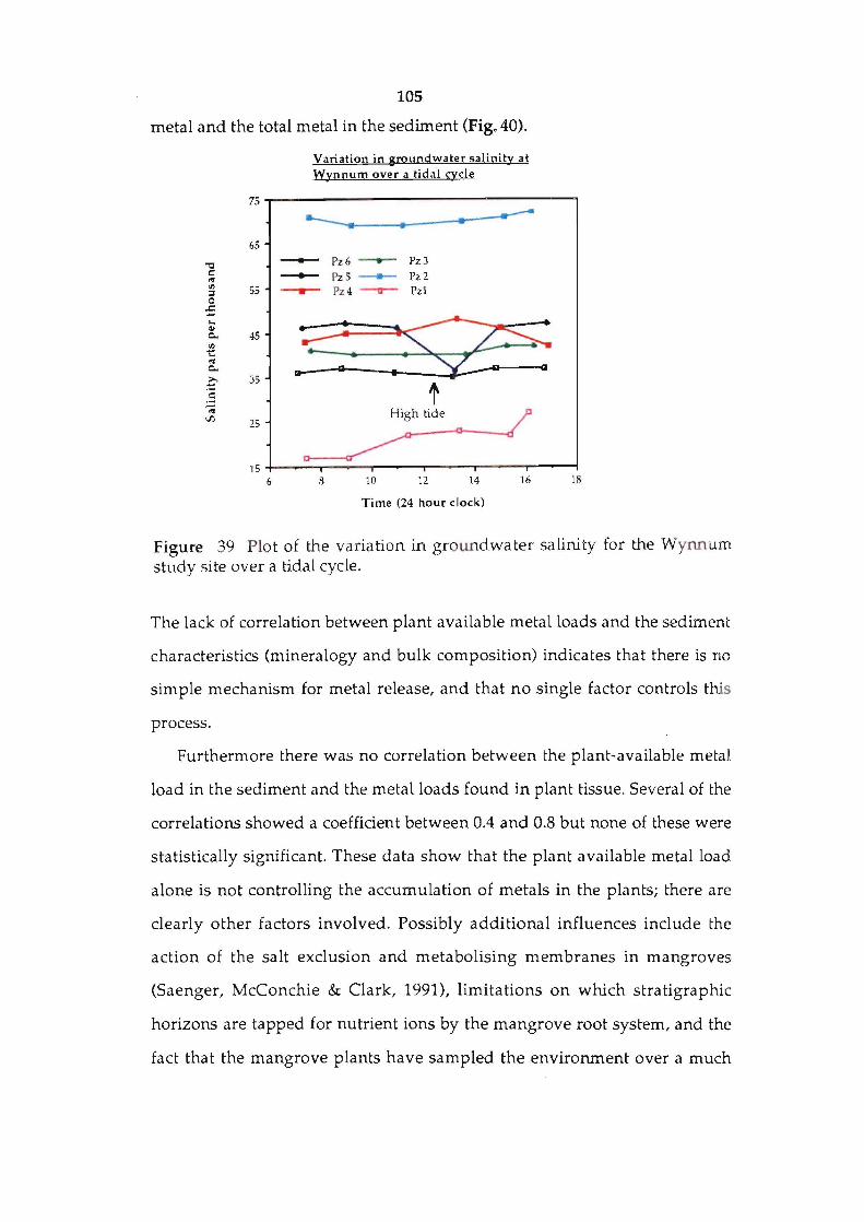
105
metal and the total metal in the sediment (Fig. 40).
"0 c: '" <I> :::I 0
-= .. OJ Q.
<I> t::
'" Q.
.Co c: ;; <JJ
Variation in groundwater salinity at Wynnum over a tidal cycle
75~--------------------------------'
~~.~--~.----~.~--------65 -- Pz6 -...- pzJ -- pz5 - Pz2 55 -- Pz 4 --v- Pzl
~ s 45
35
f 25
High tide
15 6 8 10 12 14 16 18
Time (24 hour clock)
Figure 39 Plot of the variation in groundwater salinity for the Wynnum study site over a tidal cycle.
The lack of correlation between plant available metal loads and the sediment
characteristics (mineralogy and bulk composition) indicates that there is no
sim pIe mechanism for metal release, and that no single factor controls this
process.
Furthermore there was no correlation between the plant-available metal
load in the sediment and the metal loads found in plant tissue. Several of the
correlations showed a coefficient between 0.4 and 0.8 but none of these were
statistically significant. These data show that the plant available metal load
alone is not controlling the accumulation of metals in the plants; there are
clearly other factors involved. Possibly additional influences include the
action of the salt exclusion and metabolising membranes in mangroves
(Saenger, McConchie & Clark, 1991), limitations on which stratigraphic
horizons are tapped for nutrient ions by the mangrove root system, and the
fact that the mangrove plants have sampled the environment over a much
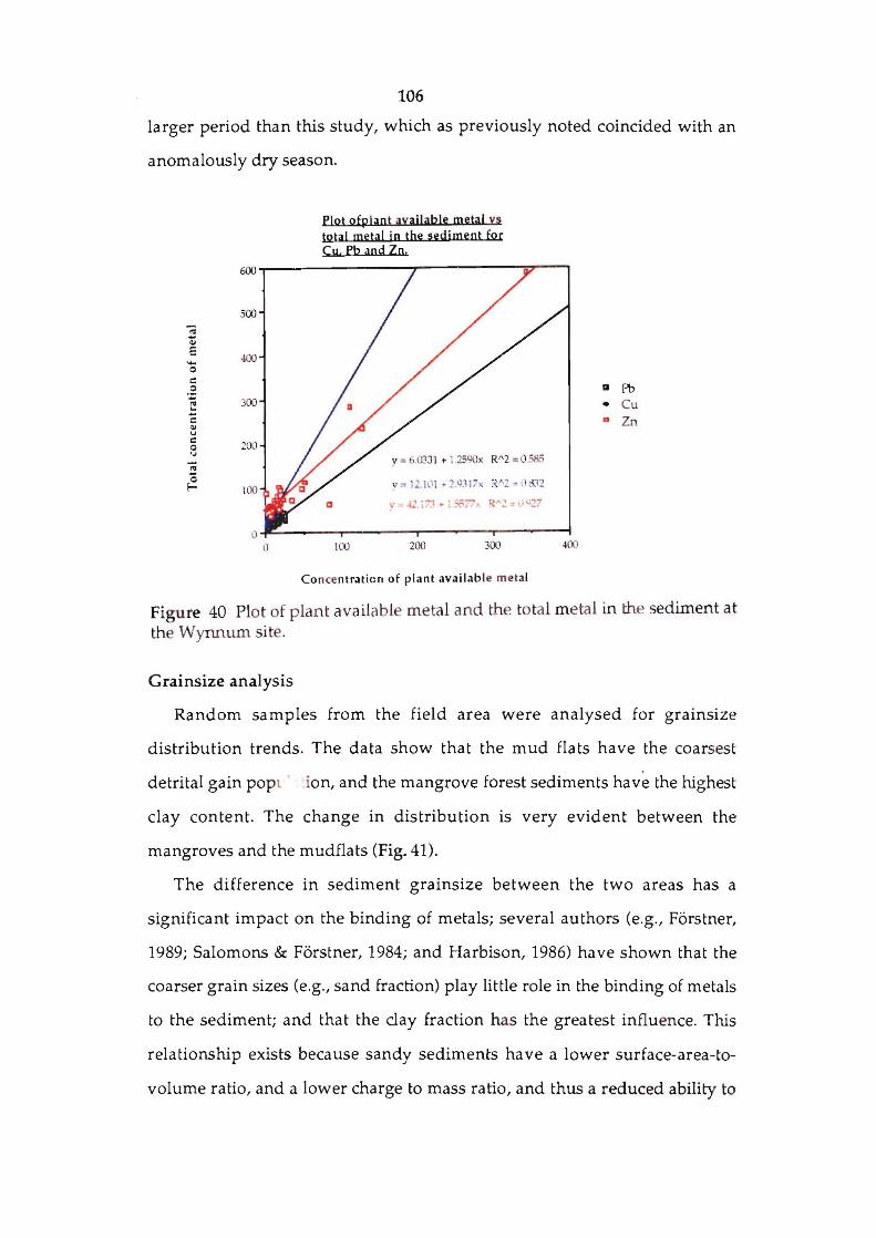
106
larger period than this study, which as previously noted coincided with an
anomalously dry season.
600
500 ;;; 0; E
400 ..... 0 c 0
".; 300 ... -c ... u c 200 0 u
'" "0 f- 100
0 n
Plot ofplant ayaiIable metal ys total metal in the sediment for Cu. Pb and Zn.
100 200 300
Co ncentration of plant availab le metal
4lXl
II Pb
• Cu a Zn
Figure 40 Plot of plant available metal and the total metal in the sediment at the Wynnum site.
Grainsize analysis
Random samples from the field area were analysed for grainsize
distribution trends. The data show that the mud flats have the coarsest
detrital gain pOpt ' ion, and the mangrove forest sediments have the highest
clay content. The change in distribution is very evident between the
mangroves and the mudflats (Fig. 41).
The difference in sediment grainsize between the two areas has a
significant impact on the binding of metals; several authors (e.g., Forstner,
1989; Salomons & Forstner, 1984; and Harbison, 1986) have shown that the
coarser grain sizes (e.g., sand fraction) play little role in the binding of metals
to the sediment; and that the clay fraction has the greatest influence. This
relationship exists because sandy sediments have a lower surface-area-to
volume ratio, and a lower charge to mass ratio, and thus a reduced ability to
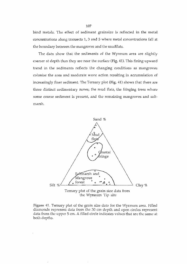
107
bind metals. The effect of sediment grainsize is reflected in the metal
concentrations along transects I, 3 and 5 where metal concentrations fall at
the boundary between the mangroves and the mudflats.
The data show that the sediments of the Wynnum area are slightly
coarser at depth than they are near the surface (Fig. 41). This fining-upward
trend in the sediments reflects the changing conditions as mangroves
colonise the area and moderate wave action resulting in accumulation of
increasingly finer sediment. The Ternary plot (Fig. 41) shows that there are
three distinct sedimentary zones; the mud flats, the fringing trees where
some coarse sediment is present, and the remaining mangroves and salt
marsh.
Sand %
angrove .. .. forest .. 0 0+ ~ 0
Silt % ~~,-----------",--.,,---~----->
Ternary plot of the grain size data from the Wynnum Tip site
Clay %
Figure 41. Ternary plot of the grain size data for the Wynnum area. Filled diamonds represent data from the 30 cm depth and open circles represent data from the upper 5 cm. A filled circle indicates values that are the same at both depths.
108
DISCUSSION
Biological Controls on Sediments
Biological controls on sediments at the Wynnum site include
accumulation and stabilisation of sediments by the mangroves, establishment of
micro-habitats for growth of algae and bacteria, and the affects of burrowing
organisms on the sediments. Although there may be some direct metal uptake
by biota, most of 'the biological controls influence metal behaviour indirectly by
changing the geochemical conditions in the environment (e.g., Eh), by producing
metal binding substances (e.g., decomposition products with a chelating
capacity), by aerating the sediments by burrowing or root penetration, or by
creating new subenvironments (e.g., by influencing drainage). For example,
bacteria involved in the decomposition of organic matter do not effect the
speciation of Cd directly, but some decomposition products readily complex Cd
and the decomposition reactions commonly alter both pH and Eh.
Role of the mangroves
The distribution of mangrove species at the site is influences by tides
(Stevens & Rogers, 1979; Dowling, 1986; and Hutchings & Saenger, 1987).
Dowling (1986), and consequently there is a distinct zoning of mangrove species
parallel to the coastline (Stevens & Rogers, 1979; and Dowling, 1986). Avicennia
marina (Grey Mangrove) is predominant as a pioneer species which becomes
established when enough siltation has occurred to enable growth of
seedlings.Rhizophora stylosa (Spotted or Red Mangrove) can also act as a pioneer
species, but around the Moreton Bay area it normally occurs behind the
Avicennia fringe (Stevens & Rogers, 1979). Other species such as Ceriops tagal are
common in the moderately wet parts of the forest and Aegiceres corniculatum (the
river mangrove) and Excocaria agallocha (the milky mangrove) are abundant in
drier parts of the forest.
109
Trapping and bittding of sediment
The presence of mangroves results in increased sedimentation because
the pneumatophores trap floating debris and act as a baffle to slow down water
currents. Mangrove roots have adapted to the three major growth problems
associated with coastal sediments: saltwater, anoxia, and the weakness of an
unconsolidated substrate; different species have developed differing root
adaptions to cope with these problems. Most mangroves posses a laterally
spreading root cable system with smaller vertically descending anchor roots
which carry fine nutritive roots. Though the root system is shallow « 2 m.),
there is a high-below ground to above-ground biomass ratio exists (Hutchings &
Saenger, 1987).
Different species of mangrove also posses different above ground root
systems all of which can influence sediment trapping and binding (Fig 42). These
include: (1) pneumatophores, which rise from the cable roots as small conical
projection; (2) knee roots, which are modified cable roots which bend up out of
the sediment and then dip back again; (3) stilt roots, which grow out and down
from the trunk into the substrate; (4) buttress roots, which are similar to stilt
roots but flatten into blade-like structures; (5) aerial roots, which are similar to
stilt roots but are generally unbranched and not usually in contact with the
sediment (Hutchings & Saenger, 1987). All of these above-ground roots that
provide aeration for the subsurface roots which anchor the plant (Hook &
Scholtens, 1978) and will tend to raise the Eh of adjacent sediment. Extensive
development of above-ground roots significantly to reduces water movement
around the plant and enhance sediment deposition ( Saenger & Siddiqi, in press;
Bird, 1971; & Stephens, 1962); for example, tidal currents entering a Rhizophora-
dominated forest can be reduced from 40 cm sec-1 to zero within 1m of entering
the root network (Scoffin, 1970). Even a sparse vegetation cover can cause a
substantial reduction in current velocity, and thus a reduction in the competence
of the current to transport sediment (Fonseca, 1989).
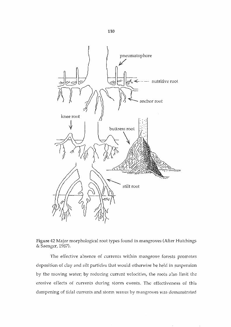
110
pneumatophore
j/
nutritive root
anchor root
knee root ...
stilt root
Figure 42 Major morphological root types found in mangroves (After Hutchings & Saenger, 1987).
The effective absence of currents within mangrove forests promotes
deposition of clay and silt particles that would otherwise be held in suspension
by the moving water; by reducing current velocities, the roots also limit the
erosive effects of currents during storm events. The effectiveness of this
dampening of tidal currents and storm waves by mangroves was demonstrated
111
in Bangladesh in 1990 when a storm moved 2 ton steel-reinforced blocks of a sea
wall up to 100 m inland, while the mangrove forest about 0.5 km away suffered
less than 1 % damage (McConchie & Saenger, 1991).
Chemical role of mal1groves
The mangrove environment is characterised by the presence of high
salinity water, and mangroves have developed a number of mechanisms by
which to survive in a high salt environment. Jennings (1968) reviews these
mechanisms, which are: 1) uptake of saline water and; secretion of the salt;
uptake of water while excluding the entry of the salt; development of a tolerance
to the high salt levels and accumulation of the salt in tissues. Some species of
mangrove emphasise one mechanism, others another (Hutchings & Saenger,
1987).
Pyrite is thought to form in mangrove soils within the boundary zone
between the upper more oxidised sediments and the lower more strongly
reduced horizons. In this zone, H2S formed below will react with ferric
compounds deposited above (Wada & Seisuwan, 1986). Transport of the metals
to the upper, oxidised region will be primarily by bisulphide complexes (Lu &
Chen, 1977; Salomons, 1985; and Salomons et al., 1987). Pyrite in this
environment forms microcrystalline spherical or framboidal clusters. and
although some may be contained in organic debris, the majority is free of the
organic matter (Rickard, 1973; van Darn & Pons, 1973).
Upper horizons of mangrove soils have highly variable redox
characteristics, which result in a mottled appearance and rapid changes in Eh
over short distances. Tunnels of burrowing animals and young active roots of
the trees supply oxygen to the upper horizons and oxidise their surroundings
whereas organic debris, especially debris from fine roots, causes localised highly
reduced zones (Wada & Seisuwan, 1986).
112
Soil aeration is directly related to soil drainage and is therefore highly
variable in mangrove forests; it depends on elevation, relief, and the physical
characteristics of the substrate, particularly texture, but because mangroves
promote the accumulation of clays, drainage in mangrove forests is usually poor
and aeration is localised around roots and burrows. Low rates of infiltration can
compound already adverse soil conditions, as shown by Clarke and Hannon
(1967) for salt marsh soils in Sydney. In addition, because many mangrove soils
are nearly saturated most of the time, spaces in the soil are water-filled and
penetration of oxygen, an essential requirement for active root development, is
reduced (Hutchings & Saenger, 1987).
Aerial roots of Rhizophora undergo several changes as they penetrate the
sediment surface including an increase in gas spaces (acrenchyma) from 5 to
50%; these gas spaces may serve as an oxygen reservoir or as a system that
allows a maximum root surface area per quantity of living tissue. These gas
filled roots leak oxygen into the surrounding sediment causing localised
increases in Eh. Radial oxygen loss, enzymatic oxidation within and at the root
surface, and microorganism-dependent oxidations near plant roots in
waterlogged soils all help exclude soil-borne metals and other toxins
(Armstrong, 1978; Armstrong; 1982; and Gleason & Zieman 1981). Radial oxygen
loss from the roots results in the formation of an oxygenated zone in 1-2 mm
wide zone between the root and the surrounding soil (rhizosphere), which then
forms a buffer between the cells of the root and the hostile soil environment; iron
oxyhydroxides (e.g., goethite or lepidocrocite; Armstrong, 1982) are commonly
deposited in this oxygenated buffer zone.
Accumulation of metals ,
Factors affecting metal absorption by plants are those controlling 4 steps:
(1) concentration and speciation of the metal in the surrounding soil; (2)
movement of the metal from the soil to the root surface; (3) transport of the metal
113
from the root surface into the root; and (4) translocation of the metal through the
plant (Fig. 43; Alloway, 1990). In mangroves, the same adaptations that act to
exclude salt will act to exclude metal at steps 2 and 3 depending on the species.
Metals will also be lost at step 4 by species (e.g., Avicennia marina) that actively
excrete salt from their leaves (metals are carried out as chloride complexes).
Uptake of mobile metals by plants largely depends on the total quantity of metal
available, whereas in the case of strongly adsorbed metals, adsorption is more
dependent on the amount of root produced. Roots possess a high cation
exchange capacity (CEC), due largely to the presence of carboxyl groups, and
each exchange assists movement of ions through the outer part of the root to the
plasmalemma where active absorption occurs. Adsorption mechanisms vary for
different metals, but ions which are adsorbed by the same mechanism will
compete with each other (e.g., Zn absorption is inhibited by Cu and H+, but not
by Mn or Fe; Cu is inhibited by Zn, NH4 +, Ca and K; Alloway, 1990).
The rhizosphere receives appreciable amounts of organic material from
the roots, including exudates, mucilage, sloughed-off cells and their lysates.
These organic com pounds give rise to intense microbiological and biochemical
activity, which enables plants to mobilise metals which are strongly adsorbed in
the soil (Alloway, 1990).
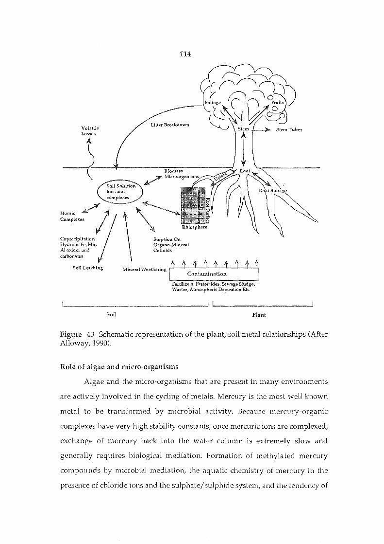
Volatile
Humic Complexes
Copredpitatlon Hydrous Fe, Mn, AI oxides and carbonates
Soil Leaching
Soil
114
Litter Breakdown
Sorption On Organo-Mineral Colloids
, ,111111111 MIneral Weathenng I . . J
Contanunation
Fertilizers, Pestercides, Sewage Sludge, Wastes, Atmospheric Deposition Etc,
Plant
Stem Tuber
Figure 43 Schematic representation of the plant, soil metal relationships (After Alloway, 1990).
Role of algae and micro-organisms
Algae and the micro-organisms that are present in many environments
are actively involved in the cycling of metals. Mercury is the most well known
metal to be transformed by microbial activity. Because mercury-organic
complexes have very high stability constants, once mercuric ions are complexed,
exchange of mercury back into the water column is extremely slow and
generally requires biological mediation. Formation of methylated mercury
compounds by microbial mediation, the aquatic chemistry of mercury in the
presence of chloride ions and the sulphate/sulphide system, and the tendency of
115
mercury to be adsorbed on suspended solids are reviewed by Gavis and
Furguson (1972) and Summers and Silver (1978). Cadmium, lead and tin also
form volatile methyl complexes similar to those of mercury and are produced by
the same variety of bacteria (Pseudomonas) that is responsible for the methylation
of mercury. Methylation subsequently raises the toxicity of all metals several
fold (Summers & Silver, 1978).
Bacteria have also been shown to be involved in the cycling of nickel
(Wood, 1987). In sediments, nickel forms stable and insoluble complexes with
sulphide and thiolates to give nickel sulphides, as well as stable complexes with
organic compounds which contain thiol groups. However, at the sediment water
interface nickel forms weaker coordination complexes with oxygen donors such
as carboxylate, hydroxyl, and other oxy-ligands (e.g., humic and fulvic acids,
clays, metal oxides, etc.). Nickel does form stronger bonds with the oxygen
donors associated with the cell surfaces of bacteria and algae, but these
complexes are sufficiently unstable that nickel can exchange rapidly with Ca2+
or Mg2+ in the water. Several other metals that experience this type of exchange
SUlphate-reducing bacteria such as Desulphiovibrio desulphuricans utilise
simple organic molecules and the products of organic oxidation as an energy
source (J0rgensen, 1982) and produce an abundance of potentially metal binding
sulphide as a by product of their metabolic activity. The high sulphide ion
activity associated with sulphate reducing bacteria also depresses the Eh in their
environment and can thus have a major affect on metal mobility. The overall
process of sulphate reduction is represented by the simple reaction:
2CH O+SO 2-2 4
where sedimentary organic matter is represented by the idealised formulae
Zueberer and Silver (1978), found that most nitrogen fixation in mangal
116
sediments was carried out by photosynthetic bacteria followed by the cyano-
bacteria (blue green algae). Establishment of nitrogen-fixing bacteria around
roots may be a critical factor in mangrove establishment, because during the
early stages of development trapped, detritus is minimal and the sediment is
nitrogen deficient. Ammonification, where organic nitrogen is converted by
proteolytic bacteria and fungi to ammonia, may also occur in mangal sediments.
The production of ammonia (NH3) raises pH by its interaction with water to
form ammonium (NH4 +), which may then act as an energy source for nitrifying
bacteria (Hutchings & Saenger, 1987).
Algae not only indirectly influence the dissolved metal concentration by
raising pH and precipitating insoluble hydroxides, but also by direct uptake of
metals from the solution. This accumulation may either be passive (adsorption
on the outside of the cell) or active (incorporation in the cell tissue). Algae are
responsible for about 4-14 % of metal removal (especially eu) from the
sediments of Ijsselmeer, Netherlands (Salomons & Mook, 1980).
Algae may also playa role in the binding and trapping of sediments.
Sediment adheres to the sticky algal filaments even under quite strong currents.
Where algae form mats, a smooth continuous surface is often produced; these
mats protect the sediment surface from erosion and may withstand current
velocities up to 100 cm sec-I. However, where an edge of the mat is exposed the
mat will quickly break-up under high current flow as the current undermines
this edge (Scoffin, 1970).
Sediment/Fauna Interactions
Sediments are often considered as the ultimate sink for contaminants, be
they chlorinated hydrocarbons, metals, radionuclides or nutrients. They are
deposited in sediments and may persist long after the original sources of
contamination are eliminated. A number of biologically-mediated processes
could affect the cycling of these contaminants through the benthic ecosystem
117
including bioaccumulation, trophic transfer, migration, biodegradation,
biodeposition, and bioturbation (Reynoldson, 1987).
A major process in mangrove forests involves sediment turnover by
burrowing fauna. One of the best examples of bioturbation is reworking of
mangal sediments by mud lobsters (Thalasia anomala), which produce mounds of
excavated sediment up to 75 cm high above U shaped tubes that can extend up
to 1.5 m below surface (Macnae, 1966; and Bennett, 1968). Large amounts of
sediment rich in organic and sulphidic material are brought to the surface by
such activity (Andriesse et al., 1973). This sulphidic material then oxidises with
the subsequent production of sulphuric acid (H2S04) and may cause localised
acid leaching of the sediment. Numerous burrowers at the Wynnum site also
must be responsible for a significant turnover of sediment. The burrows also
allow aeration of the sediment and subsurface waters, enhancing mangrove
growth, increasing infiltration of surface waters, facilitating subsurface flow of
water and causing some subsurface sulphide oxidation(Hutchings & Saenger,
1987).
Influence on Eh/pH conditions
Increased Cd, Cu and Ni concentrations in the oxidised sediments
overlying reduced H2S -bearing sediments has been attributed to removal of
sulphide from the pore water as a result of biologically-mediated ventilation of
the upper sediment. Such biological activity significantly enhances metal fluxes
to waters (Emerson et al., 1984) and tidal flats may act as significant sources for
heavy metals (Morris et al., 1982). Aller (1978) noted that the construction and
irrigation of permanent tube-dwellings by sedentary infauna results in complex
patterns of chemical reactions and diffusion gradients in sedimentary deposits.
These complex patterns are reflected in the three-dimensional distribution of
pore water constituents, diagenetically-mobile solid phases, biogeochemically
important microorganisms, and meiobenthos (Aller, 1978).
118
In addition to the above effects, bioturbation of the sediment tends to
keep the system open with respect to sulphate, i.e. fresh sulphates can infiltrate
the sediment and are then available for bacterial reduction. Whether the system
was closed or open for the accumulation of sulphides can be shown by the
measurement of stable sulphur isotopes in the resulting pyrites (Bloch & Krouse,
1992).
Physical Controls on Metal Accumulation
Physical controls an the accumulation of metallic ions in sediments
involve the affects and interaction of grain size, mineralogy, evaporation,
groundwater and tidal inundation.
Role of grainsize
Jenne (1977), in his review of clays as a mechanical substrate for the
accumulation of trace metals, considered that precipitation of other geochemical
metal sinks are important in the accumulation of metallic species. These sinks
include the carbonates, phosphates, and both oxides and sulphides of iron and
manganese. Forstner and Salomons (1980) recommended that the < 63 flm
sediment fraction be analysed because this is where most metals occur because
the finest grainsize fractions have high charge to mass ratios and high surface
area to volume ratios and therefore have a large capacity to bind metals than do
the coarse sedimentary fraction. At the Wynnum site the < 63 llm fraction
commonly accounts for 80% of the total sediment (Fig. 41).
Role of mineralogy
Mineralogy of the sediment has an important control on the adsorption
of metallic ions. Sandy soils with a high concentration of quartz and feldspars
have a low capacity to accumulate metals (Forstner & Wittman, 1981; Salomons
& Forstner, 1984; and Forstner, 1989), whereas clay minerals have a high to

119
accumulate metals by adsorption into interlayer sites as a result of ion exchange
Minerals such as the aluminium and iron oxyhydroxides also have a high
ca pacity to adsorb metal ions and will be discussed in the chemical controls
section.
The net negative charge on clays arises from the isomorphic substitution
of trivalent cations for silicon in the tetrahedral silicon layer (mostly trivalent
aluminium, Follett, 1965; and Grim, 1968). Sometimes such substitutions are
balanced by other lattice changes, for example, OH for 0, or by filling more than
two-thirds of the possible octahedral positions.
Clays may act in the mediation of metals in two distinct ways. They may
either act directly to bind metals through their cation exchange capacity (CEC),
or as a mechanical substrate onto which other sedimentary metal sinks may
precipitate. (Fig. 44, Jenne, 1977). Processes of metal adsorption onto clays are
similar to those onto iron or aluminium oxide surface coatings. In addition to
the cation exchange sites, many metals may establish covalent bonds to
functional groups on grain surfaces (Ellis & Knezek, 1972).
Eecause of the electrostatic attraction of metals to clay.minerals, anion
behaviour of the clay can be described in terms of Lewis acid-base properties.
The degree of "softness" or "hardness" (degree of surface charge to unit area) of
the clay depends on the degree of isomorphic substitution that has occurred
within the lattice (Puis & Eohn, 1988).
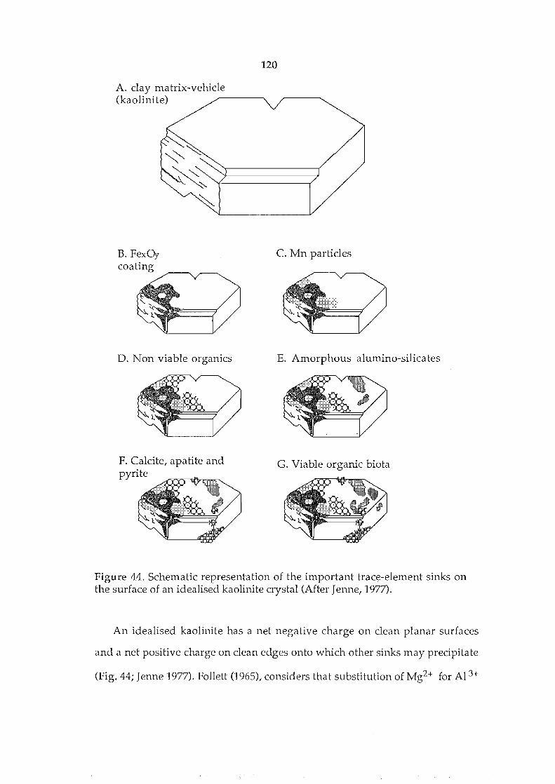
120
A. clay matrix-vehicle (kaolinite) ~-----".
B. FexOy coating
D. Non viable organics
F. Calcite, apatite and pyrite
C. Mn particles
E. Amorphous alumino-silicates
G. Viable organic biota
Figure 44. Schematic representation of the important trac~-element sinks on the surface of an idealised kaolinite crystal (After Jenne, 1977).
An idealised kaolinite has a net negative charge on clean planar surfaces
and a net positive charge on clean edges onto which other sinks may precipitate
(Fig. 44; Jenne 1977). Follett (1965), considers that substitution of Mg2+ for A13+
121
into the octahedral aluminium layer is less likely in kaolinite, but such
substitution is a major source of charge in montmorillonite, (McBride,et ai.
1975). To obtain a cation exchange capacity of 2 meq/100g for kaolinite only
about 1 in every 400 silicons need be replaced by aluminium (Schofield &
Samson, 1953).
Anionic exchange sites may develop on the clay edges where due to
structural discontinuities edges are incomplete and thus expose multivalent
structural cations (Si4+ and AI3+). Exposed cations are then partially or
wholly screened by hydroxyl and/ or other anions, which may in turn be
susceptible to exchange by other anionic solutes e.g. organic material (Follett,
1965; Grim, 1968).
The structural source of the charge deficiency in montmorillonite (i.e., the
octahedral or the surficial tetrahedral layer) may also affect the chemical
properties surface. The number of cationic or anionic exchange sites on the
clay also depends on the pH of the system: as pH rises, the number of
cationic exchange sites increases and the number of anionic exchange sites
decreases. There is also an apparent increase in the CEC, depending on the
amount of hydrolysis of the exchanging ion. The hydroxyl complexes (e.g.,
CuOH+, FeOH2+, HgOH+) tend to be softer than the uncomplexed cation i.e.,
Cu2+, Fe3+, or Hg2+ and will bind more readily with soft clay anions (Jenne,
1977; PuIs & Bohn, 1988). Similarly, adsorption of cations will depend on the
degree of softness and hardness of the anionic clay. The binding preference of
various clay minerals is shown in Table (8). PuIs & Bohn (1988) showed that
cadmium is preferentially bound relative to zinc on kaolinite (Table 8), but
for montmorillonite both metals bind equally. The greater degree of
isomorphic substitution in montmorillonite, gives it a higher cation exchange
capacity (CEC), but makes it a harder Lewis base than kaolinite and hence its
ability to bind cadmium, a soft Lewis acid, is reduced.

122
Table 8 The selectivity of soil constituent for divalent metal ions (modified after 1990).
Adsorbent
Montmorillonite (Na)
Illite (Na)
Kaolinite (Na)
Selectivity
Ca > Pb > Cu > Mg > Cd > Zn
Cd = Zn > Ni
Pb > Cu > Zn > Ca > Cd > Mg
Pb > Ca > Cu > Mg > Zn > Cd
Cd> Zn> Ni
Zn > Mn > Cd > Hg
Reference
Bittel & Miller, 1974
Puts & Bohn, 1988
Bittel & Miller, 1974
Bittel & Miller, 1974
Puts & Bohn, 1988
Stuanes, 1976 Smectite, Vermiculite &
Kaolinite Zn > Cd > Mn > Hg Stuanes, 1976
Albite, Labradorite Pb > Cu > Zn > Ni> Cd > Co > Sr > Mg Kinniburgh et al., 1976
ferrihydrite Pb > Cu > Zn > Co > Ni
Fe hydrous oxides hematite Cu > Pb > Zn > Co > Cd
goethite Pb > Cu > Zn > Cd > Ca
Mineral soil on marine clay Pb > Cu > Cd = Zn > Ca
Mackenzie, 1980
Forbes et al.,1976
Harmsen, 1977
Bunzel et al., 1976
Electrostatically-adsorbed divalent and trivalent cations also hold clay
particles together by acting as bridging ion (Piccolo Mbagwu, 1989). These
binding ions effectively flocculate the clay and increase the grain size
distribution. Flocculated clay are more resistant to transport and at the
interface of nonmarine and marine waters, where monovalent ions are
replace primarily by divalent calcium and magnesium, flocculation is a major
cause of clay sedimentation (Grim, 1968; and Weaver, 1989).
The vertical distribution of metals at the Wynnum site appears to be
strongly influenced by the distribution of clay minerals. The lower portion of
each core comprises fine to very fine sand with a much lower metal
concentration than in the overlying kaolinite clay-rich sediment. Cores MCC
012 and MCC 010 show that metal concentration increases where clays are
present. The top of the weathered basalt is mostly kaolinite clay, with some
smectite and other accessory minerals. These clays strongly adsorb metals
that migrate across them in the groundwater.
Core MCC 011 does not show this increase in metals at the top of the
basalt. There are two possible reasons for this: firstly, the mineralogy in this core
is mostly quartz and kaolinite, with minor accessory minerals, whereas the other
123
two cores contain some smectite clay and secondly, the groundwater leachate
flow around this area due to a local structural high. The sequential data for the
cores show that about 10 % of the available Pb2+ is bound to the exchangeable
phase. For some samples this rises to 20 - 25 % (e.g., MCC 003/2) but this is
uncommon. Pb2+ and the other soft Lewis cations show decay curves down
through the cores, indicating that the surface increase in clay content absorbs
Pb2+ in preference to other metals (Alloway, 1990). Because kaolinite is a softer
Lewis base, the adsorption of Pb2+ onto this sediment is expected (Brown, 1955;
and PuIs & Bohn, 1988).
For the lower sections of cores MCC 012 and 010, the exchangeable metal
value is about 25 % of the total metal present. Throughout the sequential
extraction procedure, organic matter was extracted progressively and hence
organic matter bound metals cannot be accessed separately. Progressive
extraction of organic matter has a significant affect on the concentration of
metals in the other phases because it provides a major sinks for metallic species
(Jenne, 1977; Inoue et al., 1990; and Raspor, 1989). Because organic matter is
strongly attracted to differentially-charged particles, clays not directly acting as
the site for metal adsorption nevertheless probably playa major role by acting as
a site for the adsorption of organic matter and iron oxides.
Figure (41) shows that clay and silt fractions dominate within the trees
and the salt marsh. These data also show that at the coast there is a sharp
increase in the proportion of the sand fraction. Once the transect passes out of
the mangal area onto the mud flats, there is a fall in the concentration of metals,
which is inferred to be a direct result of the decrease in metal-binding clays.
Role of evaporation and salinity in metal accumulation
Evaporation of tidal waters initially leads to an increase in the ionic
strength of the soil pore waters and ultimately may result in the deposition of
new sedimentary minerals (e.g., gypsum and halite). Evaporation will also dry
124
the sediment causing changes in the redox condition, and thus the speciation of
metals present.
For the sediments taken from the Wynnum site, very little gypsum or
other sulphate-containing minerals were found, but in all samples large amounts
of halite were present. The precipitation of gypsum precedes the precipitation of
halite from sea water and it is likely that the absence of gypsum from the
sediment is due to the continual removal of sulphate as sulphide by sulphate
reducing bacteria. Continual removal and replenishment of sulphate in the
Wynnum sediments would strongly indicate that the system is open (Bloch &
Krouse, 1992).
The role of salinity in heavy metal cycling is ignored by some authors, but
increases in salinity have been shown to mobilise cadmium from estuarine
sediments (Salomons & Forstner 1984). Metals released from anoxic sediments
by oxidation are also mobilised through complexing with chloride ions or
ligands released from decomposing organic matter (Salomons & Mook, 1980).
When the ionic strength of the pore water rises, the large quantities of
chloride and sulphate present have a major affects on the adsorption of metallic
species by clays and organic matter. Increased chloride concentration due to
evaporation sets up competitive complexing reactions for metallic ions, and
many metallic species form soluble complexes with chloride e.g., Cu, Ag, Hg, Fe,
Pb, Co and Cd (Fritz & Schenk, 1979; and Aylward & Findlay, 1989). For
cadmium, which forms soluble chloride complexes, exposure to 1000 ppm CI
reduces cadmium adsorption by as much as 20 % (Salomons & Mook, 1982; and
Forstner, 1989). Conversely, Zn adsorption shows the reverse trend to that of
cadmium and as chloride concentration increases the adsorption of Zn by
kaolinite and montmorillonite increases beca use few Zn-Cl complexes form in
solution (Stanley & Byrne, 1990). Increases in sulphate concentration reduces Ni
adsorption because sulphate competes with the clay surface to form [NiS04]O
(PuIs & Bohn, 1988).
125
Role of groundwater
Transport of metals and organic leachates via groundwater depends on
the hydraulic factors governing water movement and on chemical interactions
between the sediment and water. Contaminated ground water tends to flow as a
relatively undiluted plug or plume along with the ground water in the aquifer
(Manahan, 1990).
The degree of attenuation of the contaminant depends on the
characteristics of the substrate through which fluid is passing and on the
chemical conditions within that substrate. The presence of colloidal material in
the groundwater will significantly enhance contaminant transport; when colloids
are stable (i.e., do not aggregate easily or adhere to surfaces), they may be
expected to travel long distances. When they are unstable (Le., when they
aggregate rapidly or attach), they can be expected to deposit in porous media
and to reduce aquifer permeability. Where humic and other organic
macromolecules are present, it is expected that ground-water transport will be
enhanced because of the natural surfactant nature of these molecules (O/Melia,
1989). Unfortunately, the determination of colloids in groundwater is next to
impossible because the digging of a hole to obtain a sample will change the
chemical characteristics of the ground water and alter the character of the colloids
present (McCarthy & Zachera, 1989).
At Wynnum, groundwater plays a major role in the distribution of
metallic species (Fig. 45). The presence of elevated metal concentrations in the
lower portions of cores shows that there is a subsurface flow of metallic ions.
The analysis of the groundwaters and samples from the leachate drain reveals
low dissolved metal loads (in the lO's of ppb), but even a low concentration can
result in a large total if these ions are deposited over a long period of time.
The piesometric head across the field area is from the tip to the coast. This
piesometric head is less during the high tide period than during the low tide
period, but the flow of groundwater is always from the tip toward the coast; the
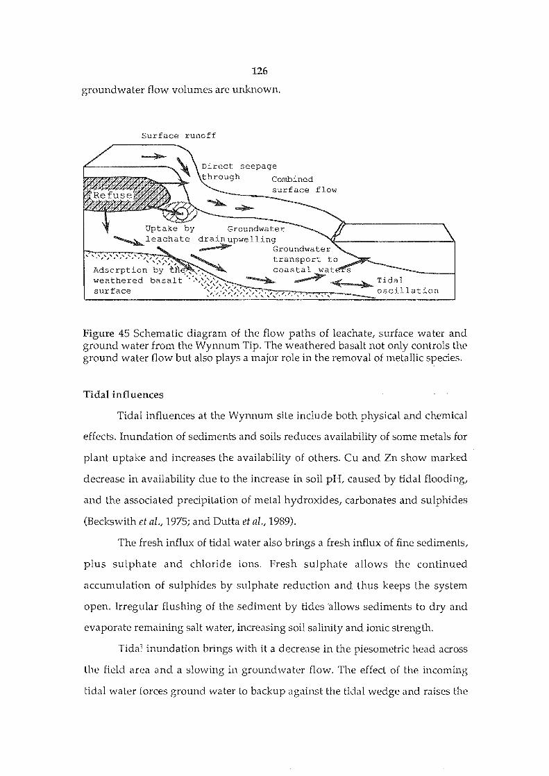
126
groundwater flow volumes are unknown.
Surface runoff
Adsorption by weathered basalt surface
Direct seepage hrough Combined
oscillation
Figure 45 Schematic diagram of the flow paths of leachate, surface water and ground water from the Wynnum Tip. The weathered basalt not only controls the ground water flow but also plays a major role in the removal of metallic species.
Tidal influences
Tidal influences at the Wynnum site include both physical and chemical
effects. Inundation of sediments and soils reduces availability of some metals for
plant uptake and increases the availability of others. eu and Zn show marked
decrease in availability due to the increase in soil pHI caused by tidal flooding,
and the associated precipitation of metal hydroxidesI carbonates and sulphides
(Beckswith et al., 1975; and Dutta et al., 1989).
The fresh influx of tidal water also brings a fresh influx of fine sediments,
plus sulphate and chloride ions. Fresh sulphate allows the continued
accumulation of sulphides by sulphate reduction and thus keeps the system
open. Irregular flushing of the sediment by tides 'allows sediments to dry and
evaporate remaining salt water, increasing soil salinity and ionic strength.
Tidal inundation brings with it a decrease in the piesometric head across
the field area and a slowing in groundwater flow. The effect of the incoming
tidal water forces ground water to backup against the tidal wedge and raises the
127
groundwater levels. Raising the groundwater may cause an increase in mixing of
tip leachate, thereby diluting the leachate. In contrast the falling tide is drawing
out the more saline leachate waters from the tip, as reflected in the salinity
profile for piesometer 1. Piesometer 1 shows a continual increase in salinity
throughout the tidal cycle an initial increase in salinity due to the influx and
mixing of coastal waters and a second increase in salinity is due to the drawing
out of the saline tip leachate (see Fig. 39).
Chemical Controls on Metal Accumulation
Chemical processes operating in sediments are probably the most
important controls on accumulation and mobilisation of metals but many
physical factors such as bioturbation exert major influences on the chemical
conditions.
Role of oxides
Metal oxides in the aqueous environment are generally covered with
hydroxyl groups, making them capable of cation exchange; several authors have
calculated the adsorption potentials for both aluminium and iron oxides (e.g.,
Quirk & Posner, 1975; Kinninburgh et aI., 1976; and Schindler, 1985).
Kinniburgh et al. (1976), reported that the adsorption of heavy metals
onto iron oxides depended strongly on pH, and found the following
relationships: Pb (3.1) > Cu (4.4) > 2n (5.4) >Ni (5.6) > Cd (5.8) > Co (6.0) > Sr
(7.4) > Mg (7.8) (numbers inside the brackets are the pHs at which half the
possible sites for the oxide gel are filled by the metal). For the aluminium oxides,
the order was Cu (4.8) > Pb(5.2) > 2n (5.6) > Ni (6.3) > Co (6.5) > Cd (6.5) > Mg
(8.1) > Sr (9.2). The high ability of iron oxide to adsorb the large Pb cation is
thought to be due to the relative openness of the iron oxide structure compared
to that of aluminium oxide (Kinniburgh et al.I 1976).
Because there is oxygen loss from the mangrove roots under anaerobic
128
conditions and the formation of oxyhydroxide material around leaking roots
(Armstrong, 1978; Armstrong; 1982; Gleason & Zieman 1981; and Wada &
Seisuwan, 1986), oxides probably play an important role in the cycling of heavy
metals at the Wynnum site. The sequential analysis data indicate that the
surficial sediments do contain appreciable quantities of oxide-bound metal
(Appendix 2), although the extraction of organic matter with the dithionite
shows that some of the contribution to the oxide phase is due to organic matter.
The extraction of lead from the section of Transect 4 (closest to the tip, Fig. 33)
by dithionite is in keeping with the literature that suggests Pb is adsorbed by
iron oxides even at low pH and is not readily desorbed (Kinniburgh et al., 1976).
The sequential data from elsewhere in the Wynnum area show that
oxides account for about 20 % (and in some samples 80%) of the available metal.
Samples with a high percentage of oxide-bound metals are always from the
lower redoxcline, where the excretion of oxygen by mangroves raises Eh, or at
the very surface of the sedimentary pile (see later Fig. 49).
Role of sulphides.
Metal sulphides playa major role in the immobilisation of metals in the
environment as a result of the low solubility of metal sulphides compared with
their respective oxide, carbonate and phosphate compounds. I
Iron sulphides have also been shown to accumulate non-ferrous metals in
polluted sediments (e.g., Luther, 1980; Forstner & Wittman, 1981; and Forstner,
1989) may incorporate significant quantities of metals such as Mn, even though
the other metals are capable of forming their own sulphides. However, some
metals such as Cd and Hg tend not to be incorporated in iron sulphides. In some
studies it has been found that when Zn concentrations exceed 1000 ppm, a
discrete ZnS is formed, which may contain trace amounts of Ni and up to 25 %
iron (Luther et ai., 1980); lead should also have formed a free sulphide, but it was
129
not observed, probably because of lead absorption by clay minerals. Clearly, the
copredpitation of metals with the more abundant iron sulphides provides the
dominant, metal sulphide precipitation mechanism and it is only when
concentrations of contaminant metals cross a threshold level that precipitation of
discrete metal sulphides occurs (e.g., Zn concentrations of about 1000 ppm are
required for the precipitation of ZnS).
At Wynnum sulphides playa major role in the immobilisation of metallic
species. From the sequential data (Appendix 2), about a third of the total metal
was extractable by the aquaregia, though this value often fell to below a quarter
for samples from the redoxclines (about 30 cm depth and at the surface). There
are also several sites in the area where re-accumulation of the metals is occurring
(e.g., the more seaward parts of Transect I, 2 and 4) due to an increase in
sulphide concentration, increase in pH, and decrease in Eh.
Sulphide ions compete with dissolved organic matter (DaM) in the
sequestering of Cu, Zn, & Cd from the environment often to the extent that DaM
does not complex with the metals (Pauli, 1975; and Salomons et al., 1987). The
affinity of sulphide anions for metals is so great that Kester et al. (1983)
recommended that where contaminated sediments cannot be successfully
removed, a constant anoxic environment be maintained for the retention and
control of pollutants. A summary of the positive and negative effects of anoxic
conditions on the mobility of heavy metals, methyl mercury and organochlorine
compounds is given in Table (9). Lu and Chen (1977) find that the migration of
metals from the sediment to overlying waters under anaerobic conditions is
largely controlled by sulphide complexes of Cd, Hg, & Pb.
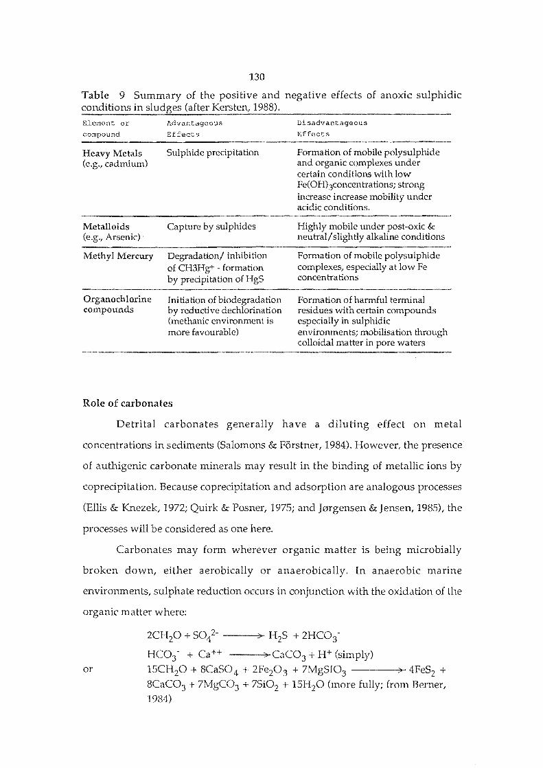
130
Table 9 Summary of the positive and negative effects of anoxic sulphidic conditions in Kersten, 1988). Element or
compound
Heavy Metals (e.g., cadmium)
Metalloids (e.g., Arsenic)
Methyl Mercury
Organochlorine compounds
Advantageous
Effects
Sulphide precipitation
Capture by sulphides
Degradation/ inhibition of CH3Hg+ formation by precipitation of HgS
Initiation of biodegradation by reductive dechlorination (methanic environment is more favourable)
Role of carbonates
Disadvantageous
Effects
Formation of mobile polysulphide and organic complexes under certain conditions with low Fe(OH)3concentrations; strong increase increase mobility under acidic conditions.
Highly mobile under post-oxic & neutral/slightly alkaline conditions
Formation of mobile polysulphide complexes, especially at low Fe concentrations
Formation of harmful terminal residues with certain compounds especially in sulphidic environments; mobilisation through colloidal matter in pore waters
Detrital carbonates generally have a diluting effect on metal
concentrations in sediments (Salomons & Forstner, 1984). However, the presence
of authigenic carbonate minerals may result in the binding of metallic ions by
coprecipitation. Because coprecipitation and adsorption are analogous processes
(Ellis & Knezek, 1972; Quirk & Posner, 1975; and Jengensen & Jensen, 1985), the
processes will be considered as one here.
Carbonates may form wherever organic matter is being microbially
broken down, either aerobically or anaerobically. In anaerobic marine
environments, sulphate reduction occurs in conjunction with the oxidation of the
organic matter where:
or HC03 - + CaH :> CaC03 + H+ (simply)
15CH20 + 8CaS04 + 2Fe203 + 7Mg5I03 :> 4FeS2 + 8CaC03 + 7MgC03 + 75i02 + 15H20 (more fully; from Berner, 1984)
131
It can be seen from the above equations that the simultaneous production of
sulphides and carbonates can occur in anaerobic environments, but the
production of free sulphide precludes the precipitation of siderite (FeC03)
because Fe preferentially combines with S-2; this preference for sulphide can be
seen in the sequential analysis data (Appendix 2) where very little iron is
released by the BaCl2 and acetate phases (Berner, 1984; and Dutta et al., 1989).
Lead can be strongly affected by coprecipitation with carbonate minerals
to give cerrusite (PbC03) and it is common in high Mg calcites. In
coprecipitation with calcite, the activity of Pb is reduced more than if a discrete
cerrusite phase precipitated; in a coprecipitate with CaC03, the activity of
PbC03 will be less than 1 and should decrease roughly in proportion to its mole
fraction in the mixture. The reduction in activity implies a parallel reduction in
lead solubility, mobility, and bioavailability (Sposito & Page, 1985). Within the
sediments at Wynnum the carbonate phase accounts for between 10 and 20 % of
available lead. The higher values are from the surficial sediments where more
carbonate is produced (Appendix 2, see later Fig. 49). Overall it would seem that
lead in the Wynnum sediments is preferentially adsorbed by clays and the
production of cerrusite is minor.
Cadmium is also affected by the presence of carbonate minerals. Ionic
cadmium replacement of calcium can take place on the surface layer of carbonate
minerals when through a solid solution process and only when all of the calcite
surface has reacted will free CdC03 precipitate (Papadopoulos & Rowell, 1988;
and Alloway, 1990).
The acetate-extractable carbonate phase in the Wynnum area is
insignificant in the mobilisation of iron « 100 ppm or 0.01 % iron was mobilised);
indicating that sulphide preferentially sequesters iron. Data for the carbonate
phase will be affected by the Significant amounts of organic matter extracted by
the acetate. However, the acetate-extractable (carbonate) phase is important in
132
the accumulation of other metals at Wynnum, especially in the surficial
sediments. Acetate-extractable metal is at a maximum in the 10 to 15 cm depths
in the cores and from the grab samples taken at the surface. This depth in the
cores corresponds with the zone of maximum competitiveness for metals where
carbonates, organics, oxides, sulphides and clays all have metal binding
potential (see later Fig. 49). The acetate-extractable phase accounts for 10 -20 % of
the bound metals at Wynnum, though this value depends on the metal involved
(e.g., the mechanism is more important for Pb and Zn) and the sample's
stratigraphic position (Appendix 2).
Role of organic matter
The ability of soil and sedimentary organic matter to form stable
combinations with metal ions is well established. with a variety of compounds
being involved, particularly humic and fulvic acids (Stevenson & Ardakani,
1972).
Humic and fulvic acids are the stable end products of microbial
breakdown of organic particulate matter. Fulvic acids are the lower weight
«10,000 Daltons) acid-soluble fraction, whereas humic acids are the high weight
(>10,000 Daltons) acid-insoluble but fraction. The structures of these compounds
is not known, but they contain phenolic, amine, aliphatic and carboxylic groups
that have a metal binding capacity (Raspor, 1989); the range of compound
present depends on the environment of formation and on the type of parent
material (Anderson et aL, 1990; and Malcolm, 1990). Present with the humic and
fulvic acids are tannic acids, which have the capacity chelate metal ions (Branca
etal., 1990).
A number of authors (e.g., Cooper & Harris, 1974; Nissenbaum & Swaine,
1976; and Mackey & O'Sullivan, 1990), found that the most Cu, Mo and Zn were
bound in humic substances. The organic fraction becomes less important for Ni,
Co and Pb, and is insignificant for Mn, V, and Fe. For a salt marsh, 95 % of
133
metals in the sediments were associated with inorganic matter. The exception to
this was Cd, where 12% of the total cadmium was extractable with the organic
phases (Pellenbarg, 1981).
Humic and fulvic acids can bind metal ions through both electrostatic
forces (attraction of a positively charged metal ion to an ionised COOH group)
and by electron-pair sharing (formation of a covalent linkage). Many kinds of
complexes are possible, and no single stability or formation constant can be used
to describe the strength with which metals bind to humic substances (Stevenson
& Ardakani, 1972). Jonasson (1977) established a probable order of the binding
strength of metals onto fulvic acids of Hg > Cu > Pb> Zn > Ni > Co. However,
the binding capacity for a metal varies with the pH of the soil solution; for
example at pH 6 the binding order of humic material is Cd > Zn > Ni > Mn > Cu
> Pb > Hg (Brummer, 1986), whereas at pH 5.0 the binding order is Cu > Pb> Fe
> Ni > Mn "" Co > Ca > Zn > Mg; at pH 3.5 the order is Cu > Fe> Ni > Pb > Co>
Ca > Zn > Mn > Mg (Ellis & Knezek, 1972).
Pauli (1975) showed that where metal humates are in contact with
hydrogen sulphide, the precipitation of the metal sulphide is likely to take place
in preference to organic chelation. Under certain physiochemical conditions,
elements like Cu, Zn, Cr and Cd can simultaneously form metal sulphides and
metal-organic complexes; but this is not common (Hirner et al., 1990).
Humic-like substances in anaerobic seeps from landfill site are similar to
organic substances found in soils, though these compounds have lower
molecular weight, hence a higher mobility and it is believed that these organics
represent an early stage in the development of humic acids (Weis et al., 1989).
The decay of organic matter follows the process of initial loss of metals
associated with protein and carbohydrate loss, which has been linked to the
process of humic precipitation via a "Millard Reaction" (Yamamoto &
Ishiwatari, 1989) followed later by an increase in metal uptake as molecular size
grows (Rice & Windom, 1982). The production of organic chelates within the tip
134
probably provides major transport mechanism for moving metals from the tip to
the surrounding sediment. Although a high proportion of metals may be leached
from the tip as chelates, conversion to sulphides and other chemical forms in the
upper portions of the sediments within the mangrove forest and adjacent
environments rapidly reduces the proportion of metals bound to organic
compounds. However the stability of these organic chelates in groundwaters is
unknown and their low weight and high mobility indicate that they may be
important in the subsurface transport of metals.
Humic molecules are adsorbed on the surface of some clay minerals
through polyvalent cation bridging, to form humus-clay complexes (Piccolo &
Mbagwu, 1989) This adsorption not only binds the clay, but should also orient
the hydrophobic components of humic molecules toward the outside of the clay
aggregate, thereby preventing water infiltration. By this mechanism organic
matter can effectively increase the binding capacity of clays. However, Piccolo
and Mbagwu (1989) show that if humic matter reaches a threshold concentration
then the flocculated clays will disperse, infill pore spaces, decrease infiltration
and consequently raise Eh.
Data from Saenger, McConchie and Clark (1991; Appendix 5), shows that
while levels of Cu and 2n are quite high in the organic litter Pb levels are low
and tends to show that Cu and 2n have a preference for organic matter over
lead. The export of organic matter-bound metals from Wynnum by the
mechanism postulated by Boto and Bunt (1981) is likely to be insignificant
because of the small tidal range, lack of deep tidal channels for out-flowing
water to concentrate in and entrain large amounts of fine grained organiC matter,
and because there is an apparent migration of metals from the sewage outfall
into the coastal strip of trees.
At the coast Transect 5 there i£ an increase in the mercury and zinc
concentrations at a depth of 30 cm, which is also associated with an increase in
sulphide. These metals are likely to be derived from the sewage outfall about 200
135
m north of the sample site and are most likely to have been transport with the
incoming tide from the outfall as suspended organic matter (2.5 - 53 Ilm;
Petronio et ai., 1989; and Yeoman et al., 1989)., which has then settled to infiltrate
the sandy sediments (Molenar, 1986).
Organic matter at the Wynnum site may playa minor role in the
immobilisation of metals, because the high-weight organics compounds are
generally immobile in the sedimentary environment (Himer et al., 1990). The
higher weight organic molecules would not be mobilised, during sequential
analysis until the aquaregia extraction, and as such are more likely to represent
the organic sedimentary sink than are the more mobile lower-weight, fractions.
Although, there is some correlation between the total organic carbon and the
accumulation of metals at Wynnum, this accumulation is often accompanied by
an increase in the sulphide content.
Because much of the lower weight organics were progressively extracted
during sequential analysis it is therefore likely that low weight organic
molecules playa role in metal mobilisation within the Wynnum sediments. For
example for core MCC 002/03, nearly half of the total zinc is readily extractable
and it likely that a large proportion of this zinc is bound to the readily-soluble,
lower-weight organics as zinc has a preference for these types of organic
molecules (Cooper & Harris, 1974); the slightly less soluble, and higher-weight
organic fractions extracted by the acetate may also account for significant levels
of zinc (Mirave & Odoli, 1989). However, although organic chelates are probably
responsible for much of the metal transport within the Wynnum area they are
unlikely to be responsible for long term immobilisation
Role of pHlEh
The pH strongly affects the binding of metallic species onto organic
matter because below a pH of 4.3, COO- (carboxylate) groups become
protonated leading not only to a size reduction in the humic molecule (John ct
136
ai., 1988; and Vasconcelos et al., 1989), but also to the loss of metallic ions, which
are then free for animal and plant uptake (Gjessing et ai., 1989).
The pH of sediment/water system plays an important role in the
adsorption of metal ions because pH determines the isoelectric point of the
absorbing solid. The isoelectric point is where the surface charge of colloidal
material is 0; it marks the change in charge from negative to positive (Yariv &
Cross, 1979). In seawater and associated sediments, where pH is near neutral to
slightly alkaline, most colloidal material is negatively charged, but as the pH
falls the isoelectric point is approached and may be passed (Table 10). Once the
isoelectric point of the colloid is passed, metals associated with the colloid will
be desorbed. This ability of colloidal material to change electrical charge and
desorb metals has been shown to be significant in the contamination of oysters
by cadmium (McConchie, 1987; McConchie & Lawrence, 1991).
Free hydronium ion plays only a minor role in the charge neutralisation
of clay minerals in water; it is the other ions in solution such as K, Na, Mg and
Ca that are primarily involved in this process. However, the extent of metal ion
adsorption is greatly affected by pH because both the surface acidity and the
hydrolysis of the metal ion increase abruptly at a specific pH value and then
remain constant over a wide pH range. The pH value at which adsorption
density increases is referred to as the pH of adsorption edge. This pH value has
been correlated to the first hydrolysis constant (Table 11; Huang et ai., 1987) of
the metal ion, and these pH values imply that MOH+ species playa major role in
metal-ion adsorption (Brummer, 1986; and Huang et al., 1987). In close
agreement to the order of metal ion hydrolysis pH's is the order of relative
mobility of the metal ions. In acidic soils the mobility of metals decreases in the
order Cd> Zn> Ni> Mn> Cu> Pb> Hg (Brummer, 1986).
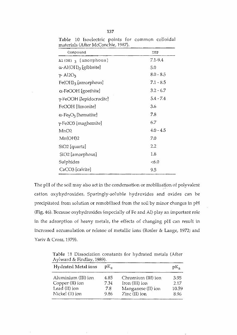
137
Table 10 Isoelectric points for common colloidal materials (After McConchie/ 1987).
Compound
Al (OH) 3 [amorphous]
a-AI(OH)3 [gibbsite]
y- A1203
Fe(OH)3 [amorphous]
a-FeOOH [goethite]
y-FeOOH [lepidocrocite]
FeOOH [limonite]
a-F~03 [hematite]
y-Fe203 [maghemite]
Mn02
Mn(OH)2
Si02 [quartz]
Si02 [amorphous]
Sulphides
CaC03 [calcite]
IEP
7.1-9.4
5.0
8.0 - 8.5
7.1 - 8.5
3.2 6.7
5.4 - 7.4
3.6
7.8
6.7
4.0 - 4.5
7.0
2.2
1.8
<6.0
9.5
The pH of the soil may also act in the condensation or mobi1is~~on of polyvalent
cation oxyhydroxides. Sparingly-soluble hydroxides and oxides can be
precipitated from solution or remobilised from the soil by minor changes in pH
(Fig. 46). Because oxyhydroxides (especially of Fe and Al)'Play an important role
in the adsorption of heavy metals/ the effects of changing pH can result in
increased accumulation or release of metallic ions (RosIer & Lange/ 1972; and
Yariv & Cross/ 1979).
Table 11 Dissociation constants for hydrated metals (After & 1989).
Hydrated Metal ions pKa pKa
Aluminium (III) ion 4.85 Chromium (III) ion 3.95 Copper (II) ion 7.34 Iron (I II) ion 2.17 Lead (II) ion 7.8 Manganese (II) ion 10.59 Nickel (II) ion 9.86 Zinc (II) ion 8.96
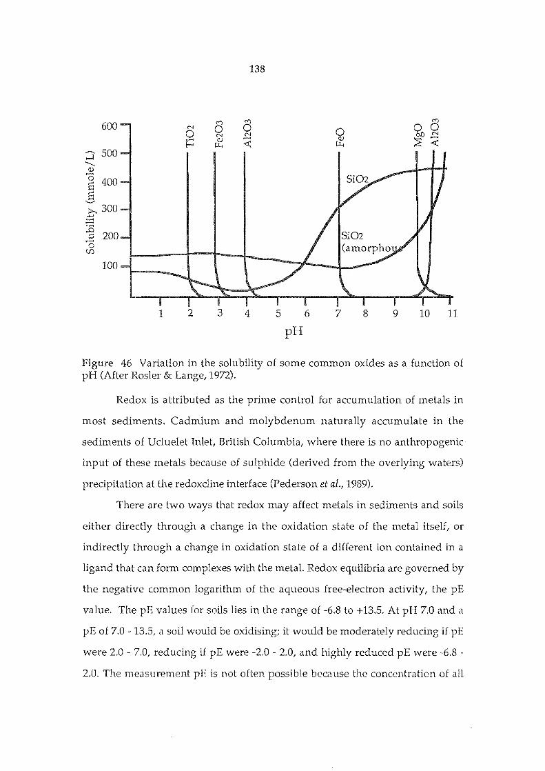
600
:3 500 .........
<lJ
'0 400 S S
"-"
>... 300 4J ......... :E ;::i 200 '0 CJ)
100
1 2
138
3 4 5 6 7 8 9 10 11
pH
Figure 46 Variation in the solubility of some common oxides as a function of pH (After RosIer Lange, 1972).
Redox is attributed as the prime control for accumulation of metals in
most sediments. Cadmium and molybdenum naturally accumulate in the
sediments of Uc1uelet Inlet, British Columbia, where there is no anthropogenic
input of these metals because of sulphide (derived from the overlying waters)
precipitation at the redoxcline interface (Pederson et ai., 1989).
There are two ways that redox may affect metals in sediments and soils
either directly through a change in the oxidation state of the metal itselt or
indirectly through a change in oxidation state of a different ion contained in a
ligand that can form complexes with the metal. Redox equilibria are governed by
the negative common logarithm of the aqueous free-electron activity, the pE
value. The pE values for soils lies in the range of -6.8 to +13.5. At pH 7.0 and a
pE of 7.0 - 13.5, a soil would be oxidising; it would be moderately reducing if pE
were 2.0 - 7.0, reducing if pE were -2.0 - 2.0, and highly reduced pE were -6.8 -
2.0. The measurement pE is not often possible because the concentration of all
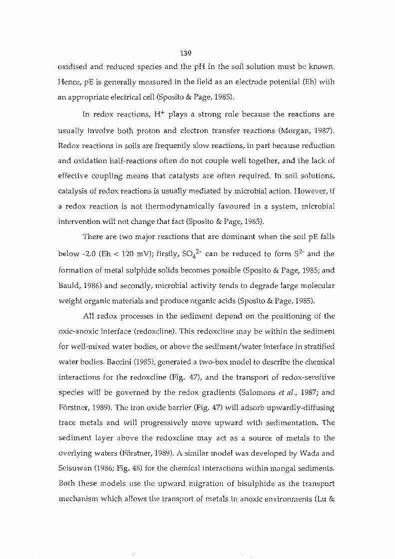
139
oxidised and reduced species and the pH in the soil solution must be known.
Hence, pE is generally measured in the field as an electrode potential (Eh) with
an appropriate electrical cell (Sposito & Page, 1985).
In redox reactions, H+ plays a strong role because the reactions are
usually involve both proton and electron transfer reactions (Morgan, 1987).
Redox reactions in soils are frequently slow reactions, in part because reduction
and oxidation half-reactions often do not couple well together, and the lack of
effective coupling means that catalysts are often required. In soil solutions,
catalysis of redox reactions is usually mediated by microbial action. However, if
a redox reaction is not thermodynamically favoured in a system, microbial
intervention will not change that fact (Sposito & Page, 1985).
There are two major reactions that are dominant when the soil pE falls
below -2.0 (Eh < 120 mY); firstly, sol- can be reduced to form S2- and the
formation of metal sulphide solids becomes possible (Sposito & Page, 1985; and
Bauld, 1986) and secondly, microbial activity tends to degrade large molecular
weight organic materials and produce organic acids (Sposito & Page, 1985).
All redox processes in the sediment depend on the positioning of the
oxic-anoxic interface (redoxcline). This redoxcline may be within the sediment
for well-mixed water bodies, or above the sediment/water interface in stratified
water bodies. Baccini (1985), generated a two-box model to describe the chemical
interactions for the redoxcline (Fig. 47L and the transport of redox-sensitive
species will be governed by the redox gradients (Salomons et al.I 1987; and
Forstner, 1989). The iron oxide barrier (Fig. 47) will adsorb upwardly-diffusing
trace metals and will progressively move upward with sedimentation. The
sediment layer above the redoxcline may act as a source of metals to the
overlying waters (Forstner, 1989). A similar model was developed by Wada and
Seisuwan (1986; Fig. 48) for the chemical interactions within mangal sediments.
Both these models use the upward migration of bisulphide as the transport
mechanism which allows the transport of metals in anoxic environments (Lu &
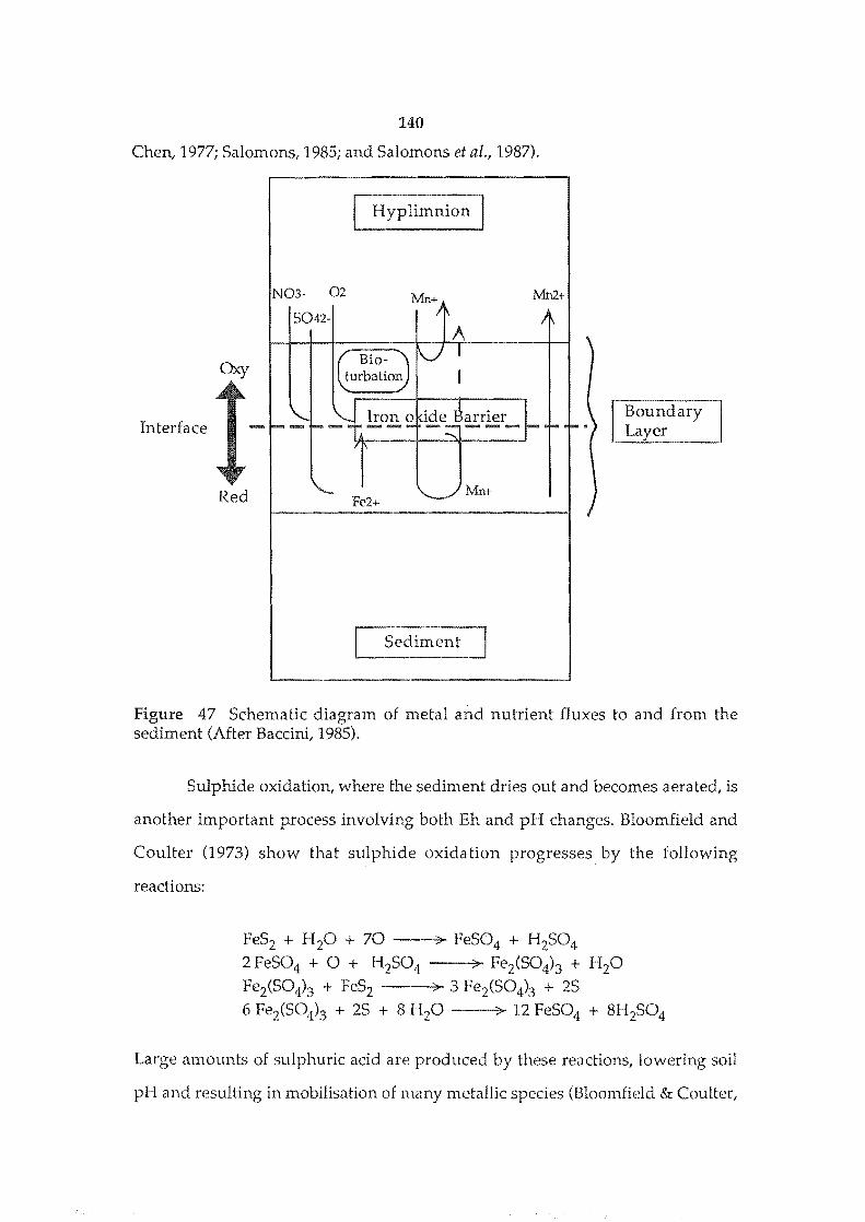
140
Chen, 1977; Salomons, 1985; and Salomons et aC 1987).
Hyplimnion
N03- 02 Mn+ Mn2+
Oxy
Interface
Red
Boundary Layer
Figure 47 Schematic diagram of metal and nutrient fluxes to and from the sediment (After BaccinC 1985).
Sulphide oxidation, where the sediment dries out and becomes aerated, is
another important process involving both Eh and pH changes. Bloomfield and
Coulter (1973) show that sulphide oxidation progresses by the following
reactions:
FeS2 + H 20 + 70 ). FeS04 + H2S04 2 FeS04 + ° + H2S04 ). Fe2(S04)3 + H20 Fe2(S04)3 + FeS2 '> 3 Fe2(S04)3 + 2S 6 Fe2(S04)3 + 2S + 8 tI20 '> 12 FeS04 + 8H2S04
Large amounts of sulphuric acid are produced by these reactions, lowering soil
pH and resulting in mobilisation of ll).any metallic species (Bloomfield & Coulter,
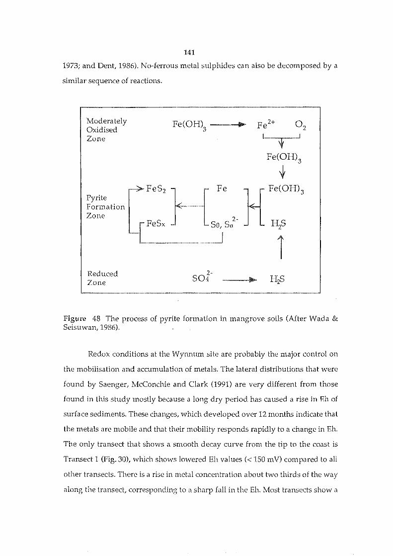
141
1973; and Dent, 1986). No-ferrous metal sulphides can also be decomposed by a
similar sequence of reactions.
Moderately Oxidised Zone
Pyrite Formation Zone
Reduced Zone
-
Fe(OH)3 ---II~po.
,.. Fe5x -
,... Fe
2-504
Figure 48 The process of pyrite formation in mangrove soils (After Wada & Seisuwan, 1986).
Redox conditions at the Wynnum site are probably the major control on
the mobilisation and accumulation of metals. The lateral distributions that were
found by Saenger, McConchie and Clark (1991) are very different from those
found in this study mostly because a long dry period has caused a rise in Eh of
surface sediments. These changes, which developed over 12 months indicate that
the metals are mobile and that their mobility responds rapidly to a change in Eh.
The only transect that shows a smooth decay curve from the tip to the coast is
Transect 1 (Fig. 30), which shows lowered Eh values « 150 mV) compared to all
other transects. There is a rise in metal concentration about two thirds of the way
along the transect, corresponding to a sharp fall in the Eh. Most transects show a
142
similar relationship between rises in metal concentration and sharp falls in Eh.
To the south of the fisherman's access way (Figs. 15 & 16), the sediment is
well oxygenated and the pH depressed compared to the northern section. The
low pH has caused a number of metals to desorb from clay minerals and the
oxidation of sulphidic material is evident (free S2- is reduced see Appendix 2).
The pH has not been lowered enough to cause desorption of Pb (Kinniburgh et
al., 1976), and the profile for this element is relatively unchanged from that
reported in Saenger, McConchie and Clark (1991).
Transition zones between the dead mangroves and the living mangroves
and between the mangrove forest and the mud flats show that there is a sharp
increase in Eh and a decrease in pH at depths of about 25 cm. It is likely that this
is the depth at which the maximum oxygen loss from mangrove roots is taking
place (Armstrong, 1978). The 25 cm depth also corresponds to the depth of
maximum deposition of sulphide and oxide material as proposed by Wada and
Seisuwan (1986; Fig. 48), and would represent the lower redoxcline. A maximum
concentration of metals is also evident in the cores at the depth of 20- 30 cm (see,
Appendix 2), corresponding to this lower redoxcline. At Wynnum, there is good
evidence that two redoxclines are present, at the surface and at 25 cm and allows
the construction of (Fig. 49). Partitioning of metals at the redoxclines shows the
influence of upwardly-moving hydrogen sulphide and bisulphide complexes.
Figure 49 Schematic diagram of the chemical fluxes to, from and within the sediments at Wynnum. The depth of the upper and lower redoxclines is dependent n the position within the forest. On the mudflats and within the area of dead mangroves only the upper redoxcline is applicable as the lower redoxcline is absent because the influence of the trees is lost. Sulphate is able to migrate to the levels of the sediment by infiltrating burrows in the upper bioturbated zone. In the upper reduced zone other metals (M) may substitute for iron in the sulphide lattice, or form their own free sulphides.
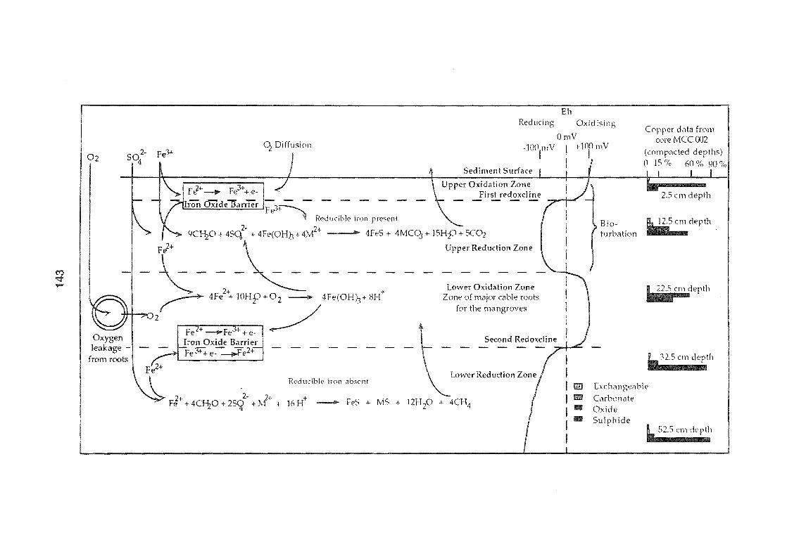
M ~ ~
Diffusion
02 502- Fe3+ 4
Oxygen leakage -
from roots
Sediment Surface
F J+ --II>- Fe3+ + e-Upper Oxidation Zone
First redoxdine
Iron OXide'"]'arrTe'r 'Fe-*---"" ~ Reducible iron present
9CHzO + 4SC{ + 4Fe(OHb +4}.i+ .. 4FeS + 4MCC3 + 15Hp + SCO,z
Fi+ \ Upper Reduction Zone
~ - 2 - ~ - - - - - - - Low"O,;d.t;onZon,
2
~ 4Fe \ 10H9 + 02 ----+- + Zone of major cable roots
( ~ for the mangroves
--i"" Fe'o , + e· Iron Oxide Barrier
e~e2+
2· + 4CHzO + 25Q +
Lower Reduction Zone Reducible· iron .,bsC'nt
+ 16 - FeS + MS + 12Hp + 4CH4
Ell Oxid
OmY
E
144
CONCLUSIONS
Summary
The distribution of metals at the Wynnum site is complex and there has
been a significant breakdown of the simple decay curves for metals that were
reported in Saenger, McConchie and Clark (1991). The breakdown, which
appears to be the result of a long dry period, indicates that metals have been
remobilised and redistributed in the sediment and may have leached into
Moreton Bay.
Lateral distribution of metals at the Wynnum site appear to be primarily
controlled by Eh, whereas the vertical distribution is primarily controlled by the
abundance of fine sediment, especially the clay fraction. Sharp increases in metal
concentration correspond to decrease in sediment Eh. Because metal distribution
is so greatly affected by Eh, the very low rainfall conditions in 1991, which have
caused sediments to dry and the Eh to rise (drying also increases salinity where
tidal inundation is irregular) have caused metals to be redistributed as chloride
complexes. Metal mobilisation as a consequence of drying is also aided by
sulphuric acid produced as a result of sulphide oxidation when the water table
falls; the low pH conditions facilitate desorption of metals from clays, iron
oxides, organic matter and sulphides.
Metal transport within the mangroves is by the lower weight organic
fractions, which remain mobile under acidic conditions, and as dissolved
species, probably primary chloride complexes. Immobilisation of metals in the
mangrove forest is primarily by the formation of sulphides produced by
bacterial sulphate reduction in areas with low Eh. Sequential cycles of
mobilisation and immobilisation result in a progressive seaward movement of
metals down the hydraulic gradient. Metal transport through the sediment by
groundwater is also very important, especially for the movement of leachate
from the tip, but the quantities being transported by this means are unknown.
145
The rate and direction of leachate movement in the lower sediments is controlled
by the underlying weathered basalt, the permeability of the sediment, the
positioning of the tidal plane, and the location of small basement highs.
Groundwater data show a rapid rise in highly concentrated leachate
entering the deeper sediments about three days after rainfall that is preceded by
a long period of dry weather (Fig. 38) confirming the major role played by
ground water in leachate dispersion. To reduce environmental concerns about
the tip the Brisbane City Council built a leachate interception drain to collect
easterly directed leachate. The drain is at depth of about 2.0 m below the
manhole cover or about 30 em below the level of the sediment in the dead
mangroves (E.A., Callipolitis, Brisbane City Council, pers com.). This drain,
while a positive move by the council, probably falls short of expectations for the
removal of the threat from leachate movement for two reasons: firstly the drain
appears unable to cope with direct seepage from the sides of the tip cell and
secondly, it is unable to interrupt the deeper flow of leachate in ground water
(Fig. 45).
Although groundwater appears to be the major mechanism for metals
entering sediments near the Wynnum Tips the input via surface runoff is also
significant. Surface runoff data collected during this study were collected after
the tip was closed and it is likely that metal concentrations are lower than they
would have been if samples had been collected while the tip was open.
However, the data collected for this work suggest that even after tip closure for
every 100 mm of rainfall about: 2.58 g of Pb, 7.63 g of Cu, 52.28 g of Zn, 0.01 g of
Hg, 0.05 g of Cr, 7.08 g of Ni and 146.2 g of Fe enter the dead mangroves and the
salt marsh.
A high proportion of the metal that enter the dead mangroves is able to
pass through this zone because the algae, keep the surficial sediments well
oxygenated during the day preventing the metals being immobilised as
sulphides. Metals present in the dead mangroves at night, when the area
146
becomes oxygen deficient, are precipitated as sulphides, but most of the
precipitated metals are remobilised on re-oxygenation of the overlying water
and continue to migrate toward the trees. The metals also migrate southward
along the weakly functioning drainage line that has been blocked by the building
of the fisherman's access way. The Eh map (Fig. 15) defines where the drainage
line has been redirected in an easterly direction and it is at the head of this
easterly directed drainage that the highest concentration of metals is found.
Another high in metal concentration occurs at the head of a second small
drainage line to the north east (Fig. 15).
The relationship between the concentration of metals available to plants,
sediment characteristics and the metal distribution in the sediment have shown
that no single characteristic of the sediment (e.g., TOC, sulphide content, clay
content, etc. controls the availability of metal to plants). The only significant
correlations were between the total metal content for a sample site and the plant
available metals, with Pb R2 = 0.585, Cu R2 = 0.832 and == 0.927. These
correlations indicate that the plant available metal is independent of the
sediment chemical conditions and that total metal concentrations are the limiting
factor. Similarly there was no significant correlation between the concentration
of plant available metals in the sediment and the metal concentrations in plants.
The lack of relationship between plant available metal concentrations and the
metal load in the plants is probably related to the specialised salt management
strategies that have evolved in mangroves to enable them to survive exposure to
highly saline water.
Data presented here show that the tip is the major source of metals that
are now present in the sediments at Wynnum. Data from samples such as core
MCC 012 (Fig. 35) leave little doubt that other possible sources such as the oil
refinery, have a negligible impact on metal levels at Wynnum. However, there is
evidence that the discharge of sewage into Crab Creek is responsible for some of
the mercury and zinc found in the coastal sediments.
147
Samples collected during the dry season for this work, confirm the
hypothesis of Saenger, McConchie and Clark (1991), that metal trapping in the
Wynnum sediments can be reversed, with samples obtained near the sediment
surface having much lower metal loads than they do during the wet season.
During the dry season, the metal concentrations in sediment 25-50 cm below the
surface are higher than they are during the wet season. These seasonal changes
in metal distribution show that some of the metal load is redistributed as the
water table rises and falls and hence, that the metal concentration in a sediment
sample will depend to some extent on the position of the water table relative to
the sampling depth. It is also evident that although the mangroves are the
primary cause for metal accumulation; the trees are a major factor in the
remobilisation of the metals as oxygen leakage from the root system raises Eh
and desta bilises metal sulphides the previously bound metals.
Recommendations
Reducing metal inflow
There are two ways in which metals may enter the sediments at
Wynnum; firstly by surface runoff of rain waters and secondly, by infiltration of
groundwater to produce metal bearing leachates. The control of runoff can be
readily achieved, but the control of leachate is far more difficult. Furthermore
there is a problem in that reducing runoff must increase infiltration and hence
metal leaching into the groundwater; consequently, controlling one source of
metals may well enhance the effectiveness of the other.
To reduce the metal load in runoff water it is necessary to increase runoff
rates to reduce the time that water has to strip metals from the sediments. This
course of action will also reduce infiltration and hence leaching, but it will
accelerate surface runoff.
Leachate can be intercepted by drains and removed but as shown by this
study such drains are not completely effective. The only way to control both
148
runoff and leachate completely is to seal the site and surround the tip site with
leachate interception drains, but these strategies are incompatible with the
present environmental setting at Wynnum. Consequently, control of runoff and
leachate is not the best option for managing metals at the Wynnum site and
protecting the waters of Moreton Bay.
Maintenance of present chemical conditions
The most important environmental protection strategy for the site is to
maintain the present chemical conditions in the area to keep the metals bound to
the sediments.
The metal trapping mechanisms at Wynnum depends on the presence of
fine grained reducing sulphidic sediment and the trapping can be easily
reversed (releasing bound metal) if the mangroves are destroyed or the sediment
is drained and allowed to oxidise. From an environmental management view
point, these observations make a strong case for ensuring that the mangrove belt
is preserved in its present form and that neither the mangrove belt nor the
unvegetated zone are drained.
The unvegetated zone could in the future be covered with top soil as part
of any land development work, but any lowering of the water table must be
avoided because the resulting oxidisation of the muds would not only encourage
the release of the presently bound metals but would also trigger the formation of
acid sulphate soils which would constitute an additional environmental hazard.
Increasing mangrove area
The extension of the area of mangroves is an option that has merit in this
area. At present there is a natural extension in the northern section where the
trees at the mouth of crab creek are providing a sheltered embayment for the
development of seedlings. It is possible to accelerate this natural progression of
the shoreline to provide an extension of the chemical conditions and produce a

149
wider buffer zone between the tip and Moreton Bay. In Bangladesh the planting
of mangrove species is well established as a technique to stabilise and accelerate
accretion of sediments to provide new agricultural lands (Saenger & Siddiqi, in
press, see the references there in). This extension should also include the area of
dead mangroves because this would trap metals before they reach the existing
mangrove forest; as a result of exposure to cyclic wetting and drying and the
presence of an algal cover metals can still move through the area of dead
mangroves.
Development options
The presently proposed development options for the Wynnum site are
the most commonly employed for old tip sites, which is the creation of sports
fields (I. Woods pers. com.). This is an acceptable plan for the Wynnum site
because the rate of surface runoff from a grassed area will not be significantly
less than for the bare tip and will keep runoff high, while providing some soil
stability. It must be stressed that by decreasing runoff there will be an increase in
infiltration and thus leachate production. Hence the maintenance of a high
runoff status from the tip is strongly advised.
Development options for the remaining salt marsh and the dead
mangroves are limited as well. While the area may be infilled any lowering of
the water table will have detrimental effects on the bound metals in these areas
and within the mangrove forest. Draining will allow the production of add
sulphate soil conditions and metal will be mobilised from the sediments. Even
though the add sulphate soil development may be confined to the area of salt
marsh, the sulphuric add that is produced as a by product of sulphide oxidation,
will move down the hydraulic gradient and mobilise metals from sediments that
it passes through. Metals mobilised by such an event, which if they reach the
coast will be as a concentrated slug, which will have serious environmental
consequences for the biota of Moreton Bay.

150
Any development option that is undertaken for the Wynnum site must
consider what effects there will be on the water table. If development will in any
way lower the groundwater table, then the development must not be allowed to
proceed.

151
ACKNOWLEDGEMENTS
I would like to most sincerely thank my supervisors Dr.s D McConchie
and D. Lewis for their support during this project, for their supply of
information and the critical reviews of early drafts of this manuscript. Many
thanks are also extended to Professor P. Saenger for his comments on chapters
and diagrams and his supply of information, especially in regard to the biology
of mangroves.
I would like to thank the Australian Research Council (ARC) for the
funding provided to Dr. D. McConchie and Prof. P. Saenger for their study of
metals in mangroves; further thanks are extended to Dr. McConchie and As.
Prof. Saenger for inviting me to work on this project. My appreciation and
thanks are extended to Earthwatch (Australia) and Dr. T Loader for the
switching of Earthwatch volunteers onto aspects of this project when another
project was incapable of being run. Many thanks also to the volunteers who
tolerated the at times, unpleasant conditions and were still willing to do it all
again the next day. You were a great bunch of people and thoroughly deserve all
the praise I can give you.
I would also like to thank M. Pillsworth and the Brisbane Port Authority
for access to the site and for tidal data used in this thesis; the Meteorological
Bureau for the meteorological data; C. PaiUies for accommodation during field
excursions; E.A. Callipolitis and I. Woods from the Brisbane City Council for
information regarding the history of the tip and its construction and; R. Hughes
District Ranger, Moreton Bay for the routine collection of groundwater from
piesometers.
Many thanks are extended to the staff and students of the University of
New England (Northern Rivers) who have made me more than welcome at the
institution. To Graham and J 0 Lancaster go my best wishes for the support that
they have given me. Graham thank you for the help that you have given me in

152
the laboratory and in retyping parts of reviewed chapters, which has freed me to
do other things. J 0 thank you for the invitations to stay for relaxing weekends
when common sense demanded periods of rest.
Finally I would like to thank my parents Peter and Verna Clark for the
support that they have given me throughout my life; this thesis is much a
testament to the hard work that they have put into me over the years as to the
work that I have put in in the last 16 months. To my fiancee Pratin I thank you
for the support and understanding that you have given me, thank you also for
the tolerance that you have shown when aspects of this work left little time for
your own needs.
153
REFERENCES CITED,
Ajayi, S.O. and Vanloon, G.W. (1989): Studies on redistribution during the analytical fractionation of metals in sediments. Sci. Tot. Environ., 87/88, 171-187.
Aller, R.c. (1978): The effects of animal-sediment interactions on geochemical processes near the sediment-water interface. In Estuarine Interactions", 1st. edn. (Ed:) Academic Press, Inc., , 157-173.
Alloway, B.J. (1990): Soil processes and the behaviour of metals. In: Heam) Metals in Soils., 1st. edn. (Ed: Alloway, RJ.) Blackie and Son Ltd., Glasgow, 7-28.
Anderson, H.A., Hepburn, A., Miller, J.D., Stuart, M., Ferrier, R.C. and Walker, T.A.B. (1990): Humic substance throughflow relationships in two forested ecosystems. Anal. Chimica Acta, 232, 3-10.
Andriesse, J.P., Breeman, N. van and Blokhuis, W.A. (1973): The influence of mudlobsters (Thalassia anomal) on the development of acid sulphate soils in mangrove swamps in Sarawak (East Malaysia). In: Acid Sulphate Soils. (Ed. H. Dorst) VoL 2. Intern. Inst. Land Reclamation and Improvement, Wageningen, Holland, 11-32.
Armstrong, W. (1978): Root aeration in the wetland condition. In: Plant Life in Anaerobic environments. (Eds. D.O. Hook and R.M.M. Crawford), Ann Arbor Science Publishers Inc., Ann Arbor, 269-297.
Armstrong, W. (1982): Chapter 10. Waterlogged soils. In: Environment and Plant Ecology. Etherington, J.R., John Wiley & Sons, Chichester. 290-372.
Aylward, G.H. and Findlay, T.J.V. (1989):SI Chemical Data. John Wiley & Sons, Hong Kong.136 pp.
Baccini, P. (1985): Phosphate interactions at the sediment water interface. In: Chemical Processes in Lakes. (Ed. W. Stumm) John Wiley & Sons, New York,
Barshard,1. (1966): The effect of a variation in precipitation on the nature of clay mineral formation in soils from acidic and basic igneous rocks. proc. Int. Clay Conf.,J erusalem,l,167-173.
Bar-Tal, A., Bar-Yousef, B. and Chen, Y. (1988): Effects of fulvic acid and pH on zinc sorption on montmorillonite. Soil Sci., 146, 367-373.
Bauer, H.H., Christian, G.D. and O'Reilly, J.E. (1978): Instrumental Analysis. , Allyn and Bacon, Inc., Boston, 832 pp.
Bauld, J. (1986): Transformations of sulphur species by phototrophic and
154
chemotrophic microbes. In: The Importance of Chemical "Speciation" in Environmental Processes., (Eds. Bernhard, M., Brinkman, F.E., and Sadler, P.J.), Springer-Verlag, Berlin, 255-273.
Bennett, L (1968): The mudlobster. Aust. Nat. Hist., 16, 22-25.
Berner, RA. (1984): Sedimentary pyrite formation: an update. Geochim. Cosmochim. Acta, 48, 605-615.
BDH Chemicals (1991): Chemicals 1991-92 .. BDH Chemicals, Poole, 448 pp.
Bird, E.CF. (1971): Mangroves as land builders. Vic. Nat., 88, 189-197.
Bloch, J. and Krouse, RH. (1992): Sulphide diagenesis and sedimentation in the Albian Harmon Member, Western Canada. J. Sed. Petrol., 62, 235-249.
Bloomfield, C and Coulter, J.K (1973): Genesis and management of acid sulphate soils. Adv. Agron., 25, 265-326.
Boto, KG. and Bunt, J.s. (1981): Tidal export of particulate organic matter from a northern Australian mangrove system. Est. Coast. Shelf. Sci., 13, 247-255.
Bouyocos, G.J. (1932): Studies on the dispersion procedure used in the hydrometer method for making mechanical analysis of soils. Soil Sci., 33, 21-26
Branca, M., Micera, G., Dessi, A. and Sanna, D. (1990): Complexation of oxovanadium (IV) by humic and tannic acids. J. Inorg. Biochem., 39, 109-115.
Brookins, D. G. (1986): Eh - pH diagrams for geochemistry. Springer-Verlag, New York. 176pp.
Brown, D.A. (1955): Ion exchange in soil plant environments, II, The effects of type of clay mineral upon nutrient uptake by plants. Soil Sci. Soc. Am. Proc., 19,296-300.
Briimmer, G.W. (1986): Heavy metal species, mobility and availability in soils. In: The Importance of Chemical It Speciation It in Environmental Processes. (Eds. M. Bernard, F.E. Brinckman and P.J. Sadler) Springer-Verlag, Berlin, 169-192.
Campbell, P.G.C and Tessier, A. (1987): Current status of metal metal speciation studies. In:Metals Speciation, Separation and Recovery. 1st edn. (Eds: Patterson J.W. and Pussino R) Lewis Publishers Inc., Chelsea (Michigan), 201-224.
Carrolt D. (1959): Ion exchange in clays and other minerals. Geol. Soc. Am. Bull., 70,749-780.
Chao, LL (1972): Selective dissolution of manganese oxides from soils and sediments with acidified hydroxlamine hydrochloride. Soil Sci. Soc. Am. Froc., 36, 764-768.
155
Chao, T.T. and Theobald, P.K. Jr. (1976): The significance of secondary iron and manganese oxides in geochemical exploration. Econ. Ceol., 71, 1560-1569.
Chemtronics, (1986): The Portable Digital Voltammeter PDV 2000 Instruction Manual. Park Printing Co., Perth, 86 pp.
Chester, R and Hughes, M.J. (1967): A chemical technique for the separation of ferro-manganese minerals, carbonate minerals, and adsorbed trace elements from pelagic sediments. Chem. Ceol., 2, 233-248.
Cl~1rke, L.D. and Hannon, N.J. (1967): The mangrove swamp and the salt marsh communities of the Sydney district. I. Vegetation, soils and climate. J. Ecol., 55, 753-771.
Clesceri, L.S., Greeberg, A.B. and Tressell, RR (Eds.) (1989): Standard Methods for the Examination of Water and Wastewater. , 17 th edn., American Public Health Association., Washington D.C., 1466 pp.
Cooper, B.S. and Harris, RC. (1974): Heavy metals in organic phases of river and estuarine sediments. Mar. Poll. Bull., 5, 24-26.
Coordinator General's Department, Queensland (1974): Coastal Management Investigation. Queensland New South Wales Border to Northern Boundary of Noosa Shire. Meteorology and Oceanography.
Dent, D. (1986): Acid sulphate soils: a baseline for research and development. Internal. Inst. for Land Reclamation and Improvement, Wageningen, Netherlands,
Deurer, R, Forstner, U. and Schmoll, G. (1978): Selective chemical extraction of carbonate - associated metals from recent lacustrine sediments. Geochim. Cosmochim. Acta, 42, 425-427.
Dowling, RM. (1986): The Mangrove Vegetation of Moreton Bay. Queensland Botany Bulletin, No 6. Queensland Department of Primary Industries, Brisbane. 45 pp.
Duff, S.J., Hay, G.W., Micklethwaite, R.K. and Vanloon, GW. (1989): Distribution and classification of metal species in soil leachates. Sci. Tot. Environ., 87/88, 189-197.
Dutta, D., MandaI, B. and MandaI, L.N. (1989): Decrease in the availability of zinc and copper in acidic to near neutral soils on submergence. Soil Sci., 147, 187-195.
Ellis, B.G and Knezek, BD. (1972): Adsorption reactions of micronutrients in soils. In: Micronutrients in Agriculture. (Eds. J.J. Mortvedt, P.M. Giordano and W.L. Lindsay). Soil Science Society of America, Inc., Madison, 59-78.
Emerson, S., Jahnke, R and Heggie, D. (1984): Sediment-water exchange in shallow water estuarine sediments. J. Mar. Res., 42, 709-730.
Engler, R.M., Brannon, J.M., Rose J. and Bigham, G (1977): A practical selective
156
extraction procedure for sediment characterisation. In: Chemistry of Marine Sediments. (Ed. Yen T.F.), Ann. Arbor. Sci. PubL,Ann. Arbor., 163-180.
Ephriam, J.B., Marinsky, J.A. and Cramer, S.J. (1989): Complex-forming properties of natural organic acids. Fulvic acid complexes with Cobolt, Zinc and Europium. Talanta, 36, 437-443.
Follett, E.A.C. (1965): The retention of amorphous, colloidal 'ferric hydroxide' by kaolinites. J. Soil. Sci., 16, 334-341.
Fonseca, M.s. (1989): Sediment stabilisation by Halophila decipiens in comparison to other seagrasses. Est. Coast. Shelf. Sci., 29, 501-507.
Forstner, U. (1989): Contaminated Sediments. Lecture Notes in Earth Science, #21. 1st edn. Springer-Verlag, Amsterdam. 157 pp.
Forstner, U. and Salomons, W. (1980): Trace metal analysis on polluted sediments. Assessment of sources and intensities. Environ. Technol. Lett., t 494-505.
Forstner, U. and Wittmann, G.T.W. (1981): Metal pollution in the aquatic environment. Springer - Verlag, Berlin, pp.
Freisser, B. and Morrison, G.H. (1959): Solvent extraction in radiochemical separations.Ann. Rev. Nucl. Sci., 9, 221-244.
Frey, RW., Boward, J.D., Han, S.J. and Park, B.K. (1989): Sediments and sedimentary sequences on a modern macrotidal flat, Inchon, Korea.J. Sed. Petrol. 59 28-440.
Fritz, J.S. and Schenk/ G.H. (1979): Quantitative Analytical Chemistry. 4 th edn., Allyn and Bacon, Inc., Boston, 661 pp.
Gadow, S. (1970): 1. Sedimente und chemismas. In: Das Watt, Ablgerungs - und Lebensraum. Reineck, H.E. Ed., W. Kramer, Frankfurt,33-35.
Garland, G.A., and Mosher, D.C. (1975): Leachate effects of improper land disposal. Waste Age., March, 42-48.
Gavis, J., and Ferguson, J.F. (1972): The cycling of mercury through the environment. Water Res., 6,989-1008.
Gentilli, J. (1972): Australian Climatic Patterns. Thomas Nelson (Australia) Ltd., Melbourne. 285 pp.
Gerdes, G., Krumbein, W.E. and Reineck, H.E. (1985): The depositional record of sandy, versicolored tidal flats (Mellum Island, Southern North Sea). J. Sed. Petrol. 55 265-278.
Gibbs, R.J. (1977): Transport phases of transition metals in the Amazon and Yukon Rivers. Ceol. Soc. Am. Bull.. 88, 829-843.
157
Gillman, G.P. and Sumpter, E.A. (1986): Modification to the compulsive exchange method for measuring exchange characteristics of soils. Aust. J. Soil Res., 24,61-66.
Gjessing, E.T., RUse, G., Petersen, Re. and Andruchow, E. (1989): Bioavailability of aluminium in the presence of humic substances at low and moderate pH. Sci. Tot. Environ., 81/82, 683-690.
Gleason, M.L. and Zieman, J.e. (1981): Influence of tidal inundation on internal oxygen supply of Spartina alterniflora and Spartina patens. Est. Coast. Shelf. Sci., 13, 47-57.
Grim, RE. (1968): Clay Mineralogy. McGraw-Hill Book Company, New York. 596 pp.
Gupta, S.K. and Chen, K.Y. (1975): Partitioning of trace metals in selective chemical fractions of near-shore sediments. Environ. Lett., 10, 129-158.
Hamblin, W.E. (1962): X-ray radiography in the study of structures in homogeneous sediments. J. Sed. Petrol. 32,201-210.
Hansen, M.H., Ingvorsen, K. and J0rgensen, RB. (1978): Mechanisms of hydrogen sulphide release from coastal marine sediments to the atmosphere. Limnol. Oceanogr. 23,68-76.
Harbison, P. (1986): Mangrove mud: A sink and source for trace metals. Mar. Poll. Bull., 17,246-250.
Heckel, H., Jones, M. and Searle, D.E. (1976): Relict sediments in Moreton Bay. Queensland Government Mining Journal, 77, 36-45.
Heckel, H., Ward, W.T., Jones, M. and Searle, D.E. (1978): Geological development of Northern Moreton Bay. In: Northern Moreton Bay Symposium. 1st. edn., (eds. Bailey, A. and Stevens, N.C.), Royal Society of Queensland, Brisbane, 7-18.
Hinckley, D.N. (1963): Variability in "crystallinity" values among kaolin deposits of the coastal plain of Georgia and South Carolina. Clays. Clay Min., 13,229-235.
Hirner, A.V., Kritsotakis, K. and Tobschall, H.J. (1990): Metal-organic associations in sediments-I. Comparison of unpolluted recent and ancient sediments and sediments affected by anthropogenic pollution. Appl. Geochem., 5, 491-505.
Holmgren, G.G.s. (1967): A rapid citrate-dithionite extractable iron procedure. Soil Sci. Soc. Am. Proc., 31, 210-211.
Hook, D.O. and Scholtens, l.R (1978): Adaptations and flood tolerance of tree species. In: Plant Life in Anaerobic environments. (Eds. D.O. Hook and R.M.M. Crawford) Ann Arbor Science Publishers Inc., Ann Arbor, 299-331.
158
Huang, CP., Hsieh, Y.S., Park, S.W., Corapcioglu, M.O., Bowers, A.R and Elliott, H.A. (1987): Chemical interactions between heavy metal ions and hydrous solids. In: Metals Speciation, Separation, and Recovery. (Eds. J.W. Patterson & R Passino) Lewis Publishers, Inc., Chelsea, 439-465.
Hutchings, P. and Saenger, P. (1987): Ecology of mangroves. University of Queensland Press, Brisbane, 388pp.
Inoue, K., Zhao, L.P. and Huang, P.M. (1990): Adsorption of humic substances by hydroxy aluminium- and hydroxyaluminosilicate- montmorillonite complexes. Soil Sci. Soc. Am.]., 54, 1166-1172.
Jackson, M.L. (1958): Soil Chemical Analysis., Prentice Hall, Englewood Cliffs, N.J., 498 pp.
Jaya, S., Rao, T.P. and Rao, G.P. (1985): Simplified anodic-stripping voltammetric determination of mercury in sea water using a glassy carbon electrode and an acetate-chloride buffer. Analyst, 110, 1361-'-1364.
Jenne, E.A. (1977): Trace element sorption: sediments and soils. In: Molybdenum in the Environment. Vol. 2. (Eds. Chapple, Wand Peterson, K.G.) Marcel Dekker Inc.,
Jennings, D.H. (1968): Halophytes, succeedance and sodium - a unified theory. New Phyt., 67, 899-911.
John, J., Salbu, B., Gjessing, and Bj0rnstad, H. (1988): Effect of pH, humus concentration and molecular weight on conditional stability constants of cadmium. Water Res., 1381-1388.
Jonasson, LR. (1977): Geochemistry of sediment/water interactions of metals, including observations on availability. In: The Fluvial Transport of SedimentAssociated Nutrients and Contaminants. (Eds. H. Shear and A.E.P. Watson) IJC/PLURARG, Windsor, 255-271.
J0rgensen, B.B. (1982): Ecology of the bacteria of the sulphur cycle with special reference to anoxic-oxic interface environments. Phil. Trans. Roy. Soc. London, B298,543-561.
J0rgensen, S.E. and Jensen, A. (1985): Processes of metal ions in the environment. In: Metals Ions in Biological Systems. (Ed. H. Sigel) Circulation of Metals in the Environment-Vol. 18. Marcel Dekker, Inc., New York, 61-103.
Kersten, M. and Forstner, U. (1986): Chemical fractionation of heavy metals in anoxic estuarine and coastal sediments. Water Sci. Technol., 18, 121-130.
Kester, D.R. et al. (Eds.) (1983): Wastes in the Ocean, Vol. 2: Dredged Material Disposal in the Ocean., Wiley, New York, 299 pp.
Khalid, RA., Crambrell, R.P. and Patrick, W.H. Jr. (1981): Chemical availability of
159
cadmium in Mississippi River sediment. J. Environ. Qual., 10,523-528.
Kinniburgh, D.C., Jackson, M.L. and Syers, J.K. (1976): Adsorption of alkaline earth and heavy metal cations by hydrous oxide gels of iron and aluminium. Soil Sci. Soc. Am. J., 40, 796-799.
Koeppe, e.E. and Long, C.e. (1958): Weather and Climate. Krieger, Melbourne. 341 pp.
Krom, M.D. and Sholkovitz, E.R (1978): On the association of iron and manganese with organic matter in anoxic marine pore waters. Geochim. Cosmochim. Acta, 42,607-611.
Lewis, D.W. (1984): Practical Sedimentology. Hutchinson Ross Publishing Company, Stroudsburg, 229 pp.
Lindacre, E. and Hobbs,]. (1977): The Australian Climatic Environment. Wiley Press, Brisbane. 354 pp.
Lindsay, W.L. and Norvell, W.A. (1978): Development of a DTPA soil test for zinc, iron, manganese, and copper. Soil Sci. Soc. Am. J., 42, 421-428.
Lion, L.W., Altman, RS. and Lecie, J.O. (1982): Trace-metal adsorption characteristics of estuarine particulate matter: evaluation of contributions of Fe/Mn oxide and organic surface coatings. Environ. Sci. Tech., 16,660-666.
Louma, S.N. (1990): Processes affecting metal concentrations in estuarine and coastal marine sediments. In: Heavy metals in the marine environment. (Eds: Furness RW.; Rainbow p.s.) e.Re. Press Inc., Boca Raton, 51-65.
Lu, e.S.]. and Chen, KY. (1977): Migration of trace metals in interfaces of seawater and polluted surficial sediments. Environ. Sci. Techno!., 11, 174-182.
Luther, C.W.(IIl), Meyerson, A.L., Krajewski, J.J. and Hires, R (1980): Metal sulphides in estuarine sediments. J. Sed. Petrol., 50,117-1120.
Mackey, D.J. and O'Sullivan, J.E. (1990): Metal-organic interactions in sea water: an ecosystem experiment. Anal. Chimica Acta, 232, 161-170.
Macnae, W. (1966): Mangroves in eastern and southern Australia. Aust. J. Bot., 14, 67-104.
Malcolm, R.L. (1990): The uniqueness of humic substances in each soil, stream and marine environments. Anal. Chimica Acta, 232, 19-30.
Manahan, S.E. (1990): Environmental Geochemistry. 4th edn. Lewis Publishers Inc., Chelsea (Michigan). 612 pp.
McBride, M.B., Mortland, M.M. and Pinnavaia, T.J. (1975): Exchange ion positions in smectite: effects on electron spin resonance of structural iron. Clays and Clay
160
Minerals, 23, 162-164.
McCarthy, J.F. and Zachara, J.M. (1989): Subsurface transport of contaminants. Mobile colloids in the subsurface environment may alter the transport of contaminants. Environ. Sci. Techno!., 25, 496-502.
McConchie, D.M. (1987): Nutrient transport by inorganic colloids. Workshop on Nutrients in the Great Barrier Reef. Townsville. 161-171.
McConchie, D.M. and Lawrance, L.M. (1991): The origin of high cadmium loads in some bivalve molluscs from Shark Bay, Western Australia: A new mechanism for cadmium uptake by filter feeding organisms. Archives of Environ. Contam. & Toxicol. 21,303-310.
McConchie, D. and Saenger, P. (1991): Mangrove forests as an alternative to civil engineering works in coastal environments of Bangladesh: lessons for Australia. Proceedings of 1990 Workshop on Coastal Zone Management. Yepoon, Queensland. 220-233.
Mirave, J.P. and Orioli, G.A. (1989): Zinc adsorption and transport from complete humate and medium molecular weight fractions. Sci. Tot. Environ., 81/82, 679-682.
Molenar, N. (1986): The interrelation between clay infiltration, quartz cementation, and compaction in lower Givetian terrestrial sandstones, northern Ardennes, Belgium. J. Sed. Petrol., 56, 359-369.
Montgomery, J.R and Price, M.T. (1979): Release of trace metals by sewage sludge and the subsequent uptake by members of a turtle grass mangrove ecosystem. Environ. Sci. & Technol., 13, 546-549.
Morgan, J.J. (1987): General affinity concepts, equilibria and kinetics in aqueous metal chemistry. In : Metals Speciation, Separation and Recovery. (Ed. J.W. Patterson & R Pussino) Lewis Publishers Inc., Chelsea (Michigan), 27-63.
Morris, A.W., Bale, A.J. and Howland, RM.J. (1982): The dynamics of estuarine manganese cycling. Estuar. Coastal Shelf Sci., 13, 175-192.
Murray, H.H. and Lyons, S.c. (1956): Degree of crystal perfection of kaolinite. Clays Clay Minerals Proc. Fourth Conj. Natl. acado Sci. Pub!. 456, 455-464.
Nelson, T.A. (1983): Time and method dependent size distributions of fine-grained sediments. Sed., 30, 249-259.
Nissenbaum, A. and Swaine, D.J. (1976): Organic matter-metal interactions in recent sediments: the role of humic substances. Geochim. Cosmochim. Acta, 40, 809-816.
Nye, L.B. (1990): Trace Metal Accumulation Under Differing Sediment Conditions in the Mangrove, Rhizophora mangal L., in Key Largo, Florida. M.S., Marine
161
Biology and Fisheries, University of Miami. 50 pp.
Olmstead, L.B. (1931): Dispersion of soils by a supersonic method. J. Agric. Res., 42, 841-852.
Olson, G.J. (1986): Microbial intervention in trace metal-containing process streams and waste products. In: The Importance of Chemical "Speciation It in Environmental Processes. (Ed. M. Bernard, F.E. Brinkman & P.J. Sadler) Springer-Verlag, Berlin, 493-513.
O'Melia, C.R (1989): Particle-particle interactions in aquatic systems. Colloids and Surfaces, 39, 255-271.
Papadopoulos, P. and Rowell, D.L. (1988): The reactions of cadmium with calcium carbonate surfaces. J. Soil Sci., 39, 23-36.
Patchineelan, S.R (1975): Untersuchunger ilber die Hauptbindungsarten und die moiIiserbarkeit Von Schwertmetallen in fluviatilen sedimenton. Thesis, University of Heidelberg: FRG.
Pauli, F.W. (1975): Heavy metal humates and their behaviour against hydrogen sulphide. Soil Sci., 119, 98-105.
Pellenbarg, R (1981): Trace metal partitioning in the aqueous surface micro layer of a salt marsh. 13, 113-117.
Pederson, T.F., Waters, RD. and MacDonald, RW. (1989): On the natural enrichment of cadmium and molybdenum in the sediments of Ucluelet Inlet, British Columbia. Sci. Tot. Environ., 79, 125 - 139.
Peterson, P.J., Burton, M.A., Gregson, M., Nye, S.M. and Porter, E.K. (1979): Accumulation of tin by mangrove species in West Malaysia. Science of the Total Environment, 11, 213-221.
Petronio, B.M., Campanella, L., Ferri, T. and Pupella, A. (1989): Composition of organic matter in an urban sludge and metal transport. Part II: treatment with S02.H20 solutions. Annali di Chimica, 79, 15-25.
Piccolo, A. and Mbagwu, J.S.c. (1989): Effects of humic substances and surfactants on the stability of soil aggregates. Soil Sci., 147, 47-54.
Potts, P.J. (1987): A handbook of silicate rock analysis. Blackie & Son Ltd., Glasgow, 622pp.
PuIs, RW. and Bohn, H.L. (1988): Sorption of cadmium, nickel and zinc by kaolinite and montmorillonite suspensions. Soil Sci. Soc. Am. J., 52, 1289-1292.
Quirk, J.P. and Posner, A.M. (1975): Trace element adsorption by soil minerals. In: Trace Elements in Soil-Plant-Animal Systems. (Ed. D.J.D. Nicholas and A.R Egan) Academic Press, Inc., New York,
162
Rapin, R and Forstner, U. (1983): Sequential Leaching techniques for particulate metal speciation: the selectivity of various extractants. In: Proceedings 4th Int. Conf. on Heavy Metals in the Environment., Heidelberg (Edinbrough, U.K.: CEP Consultants.), 1074-1077.
Rapin, F., Tessier, A., Campbell, P.G.c. and Carigan, R (1986): Potential artifacts in the determination of metal partitioning in sediments by a sequential extraction procedure. Environ. Sci. Tech., 20, 826-840.
Raspor, B. (1989): Adsorption of humic substances at differentially charged surfaces. Sci. Tot. Environ., 81/82, 213-223.
Reynoldson, T.B. (1987): Interactions between sediment contaminants and benthic organisms. Hydrobiologia,149, 53-66.
Rice, D.L. and Windom, H.L. (1982): Trace metal transfer associated with the decomposition of detritus from estuarine macrophytes. Bot. Mar., 15, 213-223.
Rickard, D.T. (1973): Sedimentary iron sulphide formation. In: Acid Sulphate Soils., (Ed. Dorst, H.), ILRI, Wageningen, Netherlands, PubL 18, VoL 1: 28-65.
Rieneck, H.E. and Singh, LB. (1975): Depositional Sedimentary Environments. Springer-Verlag, Berlin. 439 pp.
RosIer, H.J. and Lange, H. (1972): Geochemical Tables. Elsevier, Amsterdam.
Saenger, P. and Siddiqi, N.A. (in press): Land from the sea: the mangrove afforestation program of Bangladesh. J. Ocean and Shoreline Management.
Saenger, P., McConchie, D. and Clark, M. (1991): Mangrove forests as a buffer between anthropogenically polluted areas and the sea. 1990 Workshop on Coastal Zone Management. Yeppoon, Queensland. 1. 280-300.
Saenger, P., Specht, M., Specht, RL. and Chapman, V.J. (1977): Mangal and coastal salt-marsh communities in Australasia. In: Ecosystems of the world. Volume I. Wet Coastal Ecosystems. (Ed. Chapman V.J.), Elsevier, Amsterdam. 293-345.
Salomons, W. (1985): Sediments and water quality. Environ. Tech. Lett., 6, 315-368.
Salomons, W. and Forstner, U. (1984): Metals in the Hydrocycle. SpringerVerlag,Berlin. 349 pp.
Salomons, W. and Mook, W.G. (1980): Biogeochemical processes affecting metal concentrations in lake sediments (IJsselmeer, The Netherlands), Sci. Total Environ., 16, 217-229.
Salomons, W., deRooji, N.M., Kerdiijk, H. and Bril, J. (1987): Sediments as a source for contaminants? Hydrobiol., 149, 13-30.
163
Schindler, P.W. (1985): Surface complexation. In: Metals Ions in Biological Systems. (Ed. H. Sigel) Circulation of Metals in the Environment.Vol. 18. Marcel Dekker, Inc., New York, 105-135.
Schofield, R.K. and Samson, H.R. (1953): The deflocculation of kaolinite suspensions and the accompanying changes from positive to negative chloride adsorption. Clay Mins. Bull., 2, 45-51.
Schwertmannn, U (1964): Differenzierung der eisenoxide des bodens durch photochemische extraktion mit sauerer ammonimoxalat-Losung. Z. Pflanzenernahr. Dung. Bodenkde, lOS, 194-202.
Scoffin, T.P. (1970): The trapping and binding of subtidal, carbonate sediments by marine vegetation in Bimi Lagoon, Bahamas. J. Sed. Petrol., 40, 249-273.
Seki, H., Suzuki, A and Kashiki, I. (1990): Adsorption of lead ions on immobilised humic acid. J. Colloi and Interface Sci., 134, 59-65.
Senaraten, A. and Dissanayake, CB. (1989): The geochemistry of mercury in some coastal sediments fro Sri Lanka. Chern. Geol., 75, 183-190.
Shanmukhappa, H. and Neelakantan, K. (1990): Influence of humic acid on the toxicity of copper, cadmium and lead to the unicellular algae, Synechosystis Aquatilis. Bull. Environ. Contam. Toxicol., 44, 840-843.
Shepard, S.A. and Thomas, LM. (1989): Marine Invertabrates of South Australia. Part II. South Australian Government Printing Division, Adelaide. 900 pp.
Sherman, D.G. (1952): The genesis and morphology of the aluminia-rich laterite clays. In: Problems of Clay and Latterite Genesis. Amer. Inst. Min. Mettall. Engr., New York, 154-161.
Sohn, M. and Rajski, S. (1990): The adsorption of Cd(II) from seawater by humic acids of various sources and origin. Organic Geochem. 15,439-447.
Sposito, G. and Page, At. (1985): Cycling of metal ions in the soil environment. In: Metal Ions in Biological Systems. (Ed. A Sigel) Marcel Dekker, Inc., New York, 287-332.
Stackhouse, RA and Benson, W.H. (1989): The effect of humic acid on the toxicity and bioavailability of trivalent chromium. Ecotox. Environ. Safety, 17, 105-111.
Stanley, J.K. and Byrne, RH. (1990): Inorganic complexation of Zn(II) in seawater. Geochim. Cosmochim. Acta, 54, 753-760.
Stephens, W.M. (1962): Tree that makes land. Sea FronL, 8, 219-230.
Stevens, G.N. and Rogers, RW. (1979): The macrolichen flora from the mangroves of Moreton Bay. Proc. Royal Soc. Queensland. 90,109-120.
164
Stevenson, F.J. and Ardakani, M.S. (1972): Organic matter reactions involving micronutrients in soils. In: Micronutrients in Agriculture. (Eds. Mortvedt, J. J., Giordano, P.M., and Lindsay, W.L.), Soil Science Society of America, Inc., Madison, 79-114.
Stover, RC, Sommers, L.B. and Silviera, D.J. (1976): Evaluation of metals in waste water sludge. J. Water Pollut. Cont. Fed., 48, 2165-2175.
Summers, A.a. and Silver, S. (1978): Microbial transformations of metals. Ann. Rev. Microbiol., 32,637-672.
Tessier, A., Campbell, P.G.C and Bisson, M. (1979): Sequential extraction procedure for the speciation of particulate trace metals. Anal. Chern., 51, 844-850.
Tessier, A., Campbell, P.G.C and Bisson, M. (1982) Particulate trace metal speciation in stream sediments and relationships with grain size: Implications for geochemical exploration. J. Geochem. Explor., 16 77-104.
Thomas, G.W. (1982): Exchangeable cations. In: Methods of Soil Analysis, Part 2. Chemical and Microbiological Properties., 2nd. Edn., ASA-SSSA, Madison., Agronomy Monograph no. 9.159-165.
Thomas, C and Eong, O. }. (1984): Effect of heavy metals zinc and lead on Rhizophora mucronata Lam. and Avicennia alba Bl. seedlings. Proc. As. Symp. Mangr. Env. Res. Manag., 568-574.
Thomson, E.A., Luoma, S.N., Cain, D.}. and Johansson, C (1980): The effect of sample storage on the extraction of Cu, Zn, Fe, Mn and organic material from oxidised estuarine sediments. Water, Air, Soil Poll., 14,215-233.
van Dam, D. and Pons, L.J. (1973): Some micromorphological observations on pyrite reaction products related to its oxidation. In: Acid Sulphate Soils., (Ed. Dorst, H.), ILRI, Wageningen, Netherlands, PubL 18, Vol. 2: 169-196.
Vasconcelos, M.T.S.D., Santos, A.P.L.M.G. and Machado, A.A.S.C (1989): Evidence of conformational changes in fulvic acids from dialysis. Sci. Tot. Environ., 81/82, 489-499.
Volkov, 1.1. and Formina, L.S. (1974): Influence of organic material and processes of sulphide formation on distribution of some trace elements in deep-water sediments of Black Sea. Am. Ass. Pet. Geol. Mem., 20,456-476.
Wada, H. and Seisuwan, B. (1986): The process of pyrite formation in mangrove soils. In: Selected Papers of the Dakar Symposium on Acid Sulphate Soils., (Ed. Dorst, H.), ILRI, Wageningen, Netherlands. 24-37.
Walkley, A. and Black, LA. (1934): An examination of the Degtjareff method for determining soil organic matter and a proposed modification of the chromic acid titration method. Soil Sci., 37, 29-38.
165
Waller, P.A. and Pickering, W.F. (1990): Evaluation of "labile" metal in sediments by anodic stripping voltammetry. Talanta, 37, 981-993.
Walsh, G.E.R, Ainsworth, KA. and Rigby, R. (1979): Resistance of red mangrove (Rhizophora mangle L.) seedlings to lead, cadmium, and mercury. Biotropica, 11,22-27.
Weaver, C.E. (1989): Clays, Muds, and Shales. Elsevier, Amsterdam. 819 pp.
Weis, M., Abbt-Braun, G. and Frimmel, F.H. (1989): Humic-like substances from landfillieachates - characterisation and comparison with terrestrial and aquatic humic substances. Sci..Tot. Environ .. , 81/82, 343-352.
Willett, LR and Beech, T.A. (1987): Determination of organic carbon in pyritic and acid sulphate soils. Commun. Soil Sci. Plant Anal., 18,715-724.
Willett, LR and Walker, P.H. (1982): Soil morphology and distribution of iron and sulphur fractions in a coastal flood plain toposequence. Aust. J. Soil Res., 21, 283-294.
Wood, J.M. (1987): Biological process involved in the cycling of elements between soil or sediments and the aqueous environment. Hydrobiologia, 149, 31-42.
Yamamoto, S. and Ishiwatari, R. (1989): A study of the formation mechanism of sedimentary humic substances - II. Protein-based melanoidin modeL Org. Geochem., 14, 479-489.
Yariv, S. and Cross, H. (1979): Geochemistry of Colloid Systems. For Earth Scientists. Springer-Verlag, Berlin. 450 pp.
Yoeman, S., Sterrit, RM., Rudd, T. and Lester, J.N. (1989): Particle size fractionation and metal distribution in sewage sludges. Water, Air, Soil, Poll., 45,27-42.
Zuberer, D.A. and Silver, W.s. (1978): Biological dinitrogen fixation (acetylene reduction) associated with Florida mangroves. Appl. Environ. Microbiol., 35, 567-575.
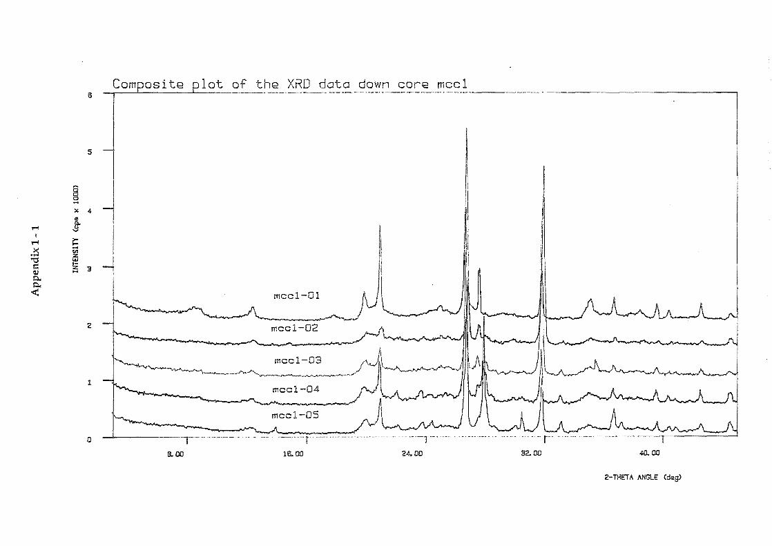
Comoosite of the XRD data down core mccl B --.---'--------''--------------- ----------.----------.----------,
5
§ -x " \II Q..
!""4 ~ I
!""4 j::
. ~ .... In
"0 in I:; ~ 3 (I) .... Q.. Q..
.;:( meel 1
2 meel-02
meel ~_/"v.-".I' ~
1 meel-04
meel-OS
(.) - -- ,~--.- .- .-,~--.--~ --
6.00 16. 00 24.00 32.00 4D.00
2-THETA ANGlE (dQg)
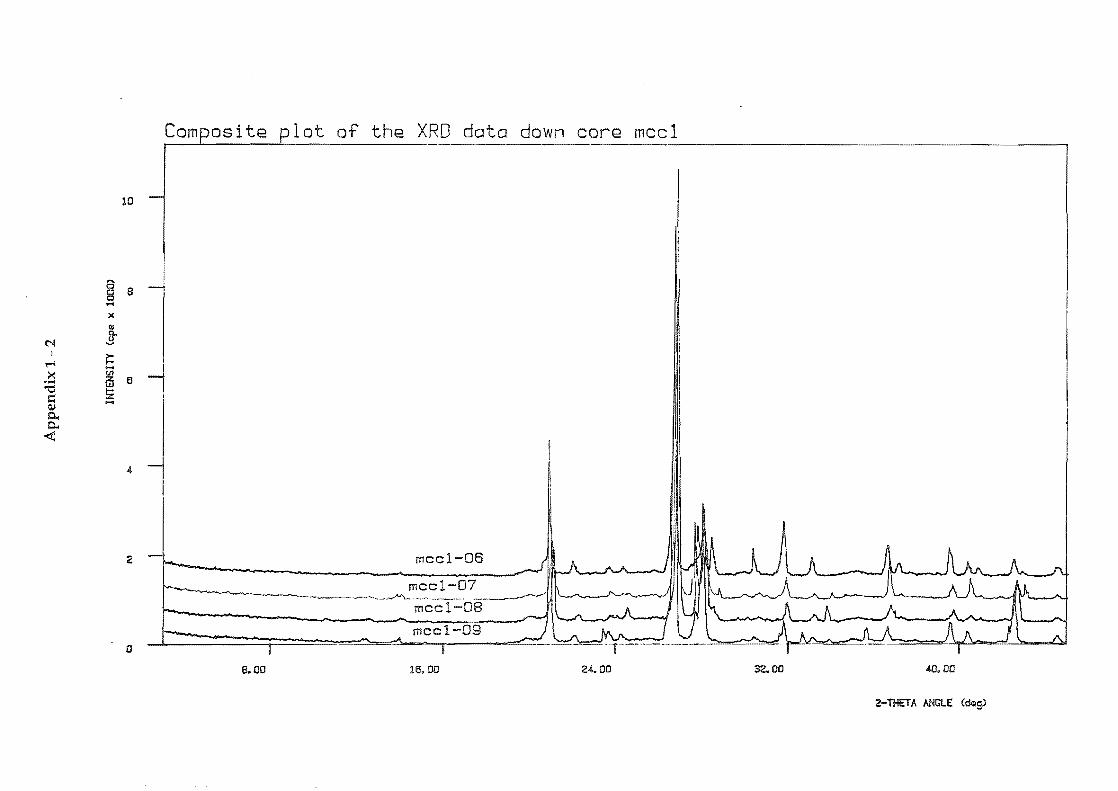
lot of the X data down core mccl
10
.... § 6 ... )(
III
€:"I B-.....
'r"'I r= ><
.....
-1 til .,.., Gi "1:1 6
= s: (lJ
.... j
c.. c.. <
" l 2 mccl-06
.~ mccl-07 -----.~--.--~ ~-.. ---- ._---.,.-
mcc
mccl-09 o
8.00 HI. 00 24.00 32. 00 40.00
2-THETA ANGlE (tKlg)
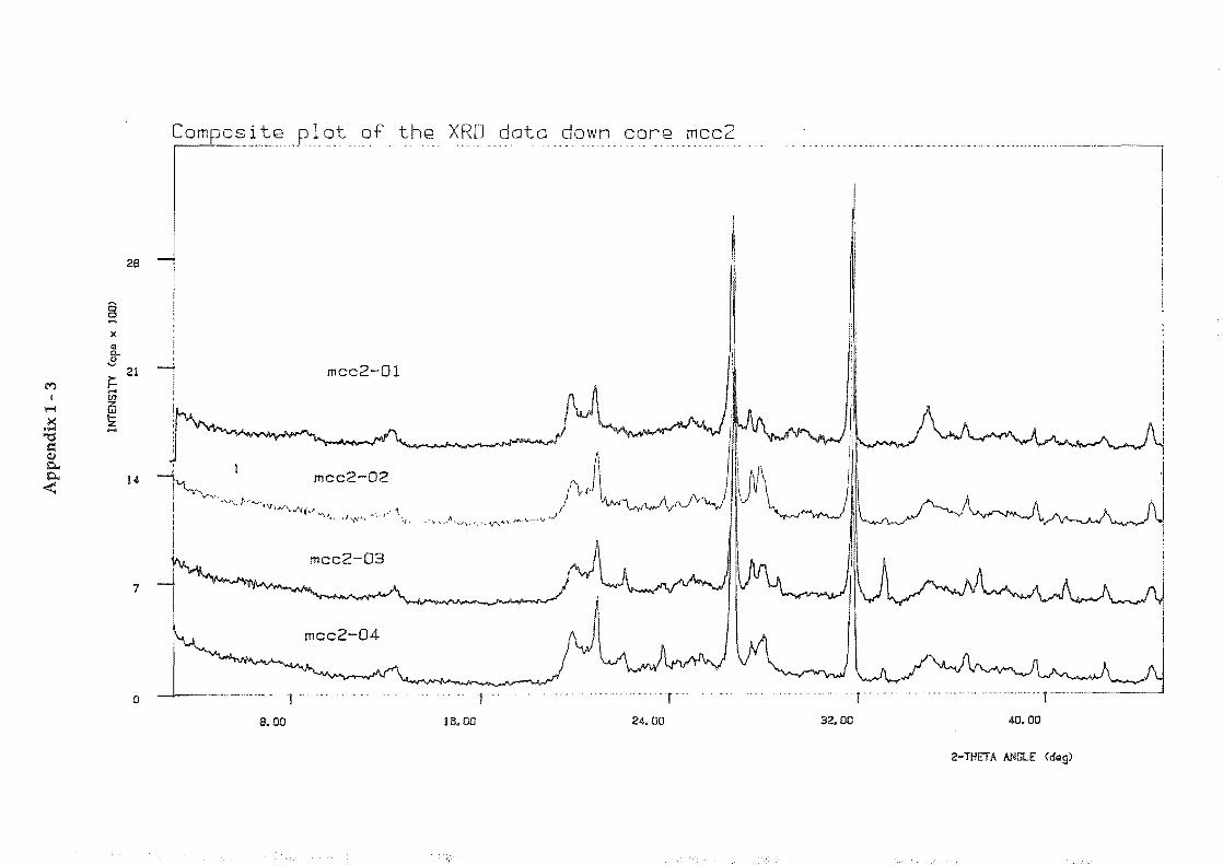
N I -I
-:r: ::j
> s: Fl IT! '"
Cl. III
<e,
!D
0 0 .- ?'
0 0 t: o o P 0 0
0 '"
h i I ! .... 3
3 ()
()
()
N
()
I I\
l 0
! .j:>
.. 0 W
....
--,. (' " t f j ., or " '. --
" .c
;'
c '>
Z :
Ap
pen
dix
1-
3
INTE
NSI
TY
(cp
s x
10m
-N
N
"" ...
til
------
_____ .
1
3 ()
3 n
n f\
) ()
I
I\l
0 I
f\)
0 I-'
I~ ,] ,(J)
I
1-'_
ic+
lID
:-u
; I-
--'
,0
c+
:0
--t-;
.c+
'-
:y
:ID
.X
::::D
:0
: D
...
,0
:D...
.0
:::
;: ::
J
:0
:0
'J
'ID
:3
:0
'0
.N

Ap
pen
dix
1 -
4
INTE
NSIT
Y (c
pa
x
1000
) ...
o N
0
n a '3
I
a (j) .......
et- ID
( l [ .....
.... i ,
a et-t
a -!-)
" ( et- =r- ID
x :::0
0
3'
'3
'3
()
,()'
()
.... ()/
()
()
?I
f\):
f\
) f\
) 0
II
I I
0 0
, 0
0 '-
lj en
U
l
Q.
a (i'
a Q.
0 ~
, , \ \ :J
N
0 t-
0 ')
I'D
g
'3
0 0 N
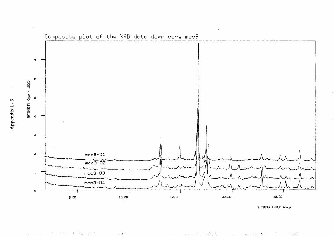
Composite plot of the XRD data down core mcc3 i ------~-------- ~ ... ___ ~~._.u~, ----~,.~-.--
7
6
§ ... )(
§.. 5 It') ......
i I r: i ~
~ 4 J .~ "'d =
- . ~ OJ t:I. t:I. «
I :2
1
mcc3-04
o . -- ...... r' -. 8.00 16.00 24.00 32.00 40.00
2-THETA ANGlE (dgg.)
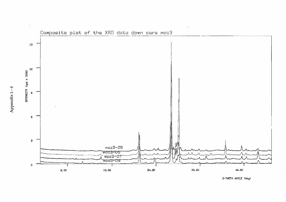
Ap
pen
dix
1-
6
INTE
NSI
TY
(cp
s )
( 10
00)
0 ...
.-C
l)
!D
N
IJl
n 0 3
I 0 (f
) 1-
"
Pl
J ei
' c
m
0
1 , .....
... 0 lei'
10
I-t;
le
i'
I:;
1m
.-Ix
PI
0
::::0
0 0 0.
. Q
ei
' Q
10
..
I~ N
0
t-o
8 J
1m
, 1
3
10
1
0
w
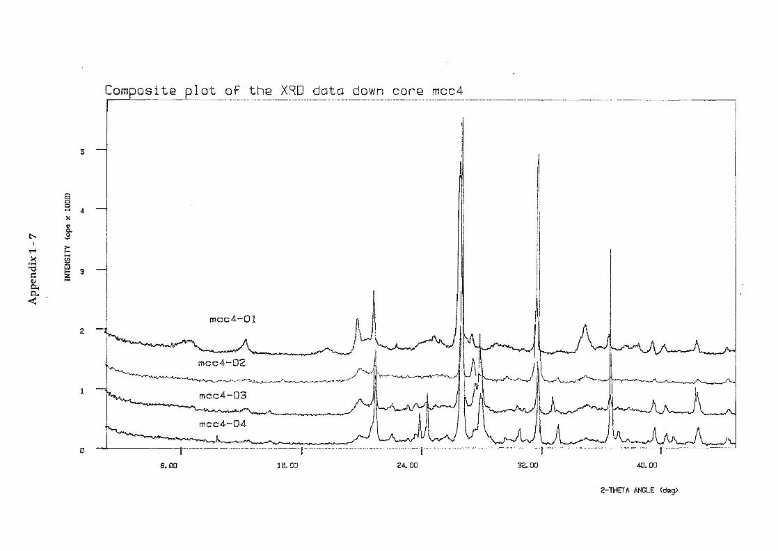
Composite ~ot of the XRD data down core mcc4 i --~---.-.-- --.---~--~ ~---- .. ---. ~---------.---"-----.-.---" '" ...... -.--~
5
§ .... 4. )(
III
t-.. a-'"
~ ~ ><
.... .....
~ "t:I c: 3 CIi ... C. C. <
mcc4-01 2
mcc4-02
~_r--'-'~
1 mcc4-03
mcc4-04
o 8.00 16. DO 24.00 32.00 40.00
2-THETA ANGLE Cd;g)
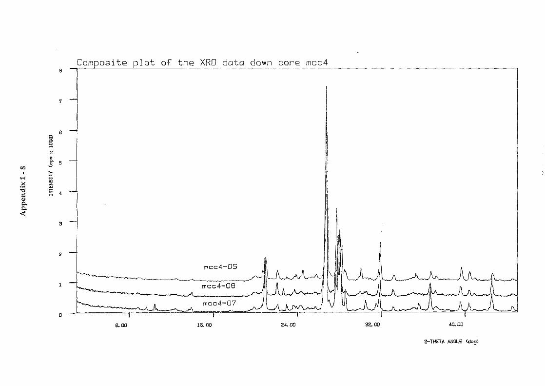
Ap
pen
dix
1 -
8
INTE
NS
ITY
(c
ps x
100
0)
o ...
N
U1
0 (f)
1-'
-
ID
ct"
8 ID
I I-
-'
0 ct"
I 0 -t
)
ct" :r- ID
.....
f1l
'3
::I
'3
X
8 0
0 0
:::0
0 0
0 0
I .r:..
~
.r:..
I I
I 0.
. a
a 0
0 -..
.] Q
) tJ
I ct
" 0 0.
. 0 ;€
:J
N
0 f"-
a 9
) (D
3 0 0 +>-
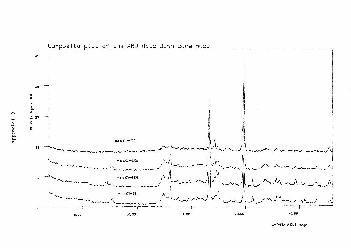
Composite plot of the XRD data down core mcc5 i ,---,
45
36
.... § x
0'1 ]-
'1-1 ~ 27 ....
.~ UI
"tI ffi
= !i: QJ
.... ~ ~
< I
'I
mcc5-01 18
mcc5-02
~,.,...,....." __ J-"'~~~
9 mcc5-03
mcc5-04
o --~----~~-----
aoo 16.00 24.00 32.00 MJ.OO
2-THETA ANGLE (deS>

lD
o o
o N
Ap
pen
dix
1
10
INTE
NSIT
Y (c
ps
x lO
On>
m
... o .... N
n 0 3 0 (J) ......
c+
to
1;--
.c+
10
I: I~
X
:;::0
0 0.
. 0 c+
0 0.
. 0 ~
:J
0 0 ) to
3 0 0 U1
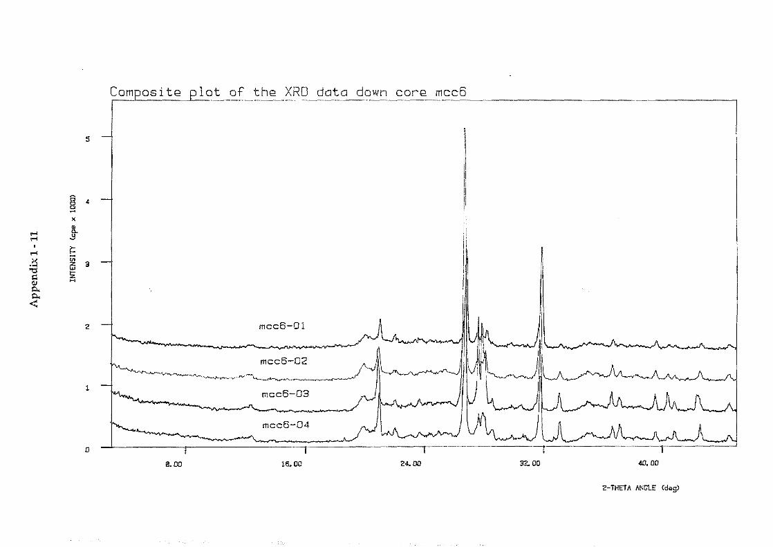
N I ~ >
>
Z ~
IT!
g
Ap
pen
dix
1-1
1
INTE
NSI
TY
(cps
)(
lOoo
)
1:1
Ul
~--+----7~--~--~~--.--------~--------~---------J----~(J
3 o o Ol I o ~
3 3
o 0
o 0
Ol
Ol
I I
o 0
W
I\l
3 o o (J) I o .....
o 3 o (f) ......
('1-
ID
I---
'
.0
!('1
- ,0 : -!
-)
I 1('1
- I~
, 'X
j::u o Q.
o ('1- o Q.
;0
::E
:J o o "l I: o o OJ
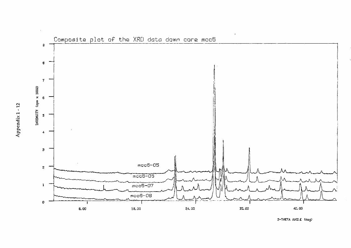
ED
a a ~
~
a 0 1\1 ,.. g £tl a o p g
0
3 0 0 OJ , 0 00
.... 3 3
0 0
0 0
OJ J
OJ J
0 0
-..,J
OJ
App
endi
x 1
-12
1 NTE
NS 1
TV
(cpa
x 1
000)
1\1
• ti
l 0
) -..
l 1.
0
_-1
n 0 3 0 (J)
1-'
-
c+
ro I--'
0 I: I: :T
ro X
3 :;.
:0
0 0
0 m
0..
r 0
0 c+
U
l 0 0.
. 0 ~
::J
0 0 I to
3
~.~--","",---~-
I~ .""
""'. ~.-~~-----~
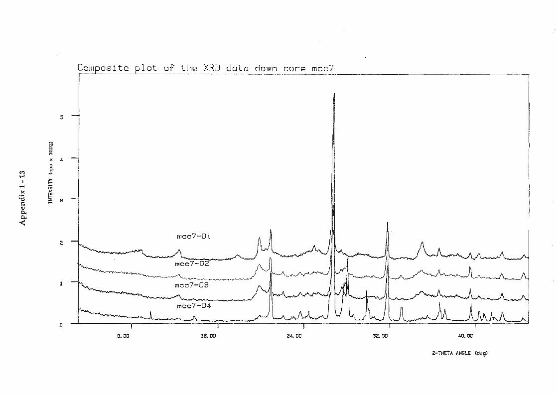
p>
0 0 ... P 0 0 N I- 0 0 p o o
0
3 [)
[)
-....] I 0 .p,.
... N
3 3
[)
[)
[)
[)
-....]
-....]
I
I 0
0 W
I-'
Ap
pen
dix
1 -
13
INTE
NS
ITY
(c
pa x
10
00)
U!
.$b
UI
n 0 3 0 ({)
\-'.
("1- CD
I--'
0 ("1- 0 -t)
("1- :T
CD
X
:;0
0 Q
..
0 ("1- 0 Q..
0 :::!
; :J
0 0 ) CD
3 0 0 -....J
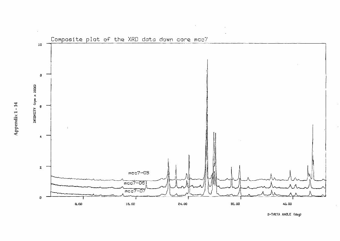
App
endi
x 1
-14
INTE
NSI
TY
(cpa
X
1000
> ...
0 N
01
CD
0
n a 3 a (f) ......
50
cT
9 ro I-
-'
a cT
a -t")
cT
:r
ID
... 3
3 50
(1
(1
3
X
8 (1
(1
(1
:::
0 ....:
J ....:
J (1
0
I I
....:J
D
D
I ....:
J (J
) D
0.
. U
i 0 cT
0 .0..
10
I~ I~
N F-
iO
0
I~
0
:3
0 0 .. ~
--------.
--.....J
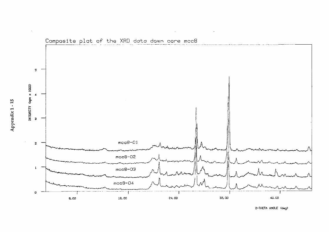
Composite-plot of i --.~ ~-.-.~.- _.-.---> ~.u -.- •• ~ ~~
data core mcc8
5
§ ... )( 4 II'!
It) ~ !
I
~ ~ ... .~ ~ "0 I:: 3 aJ -p., p., <:
2 mcc8-01
mcc8-02
mcc8-03
mcc8-04
o _ ... -. _ .. _- ... -.- -r .. --_. '- p, - - ,
e. 00 16.00 24.00 32. 00 40.00
2-THET /I ANGLE <dag>
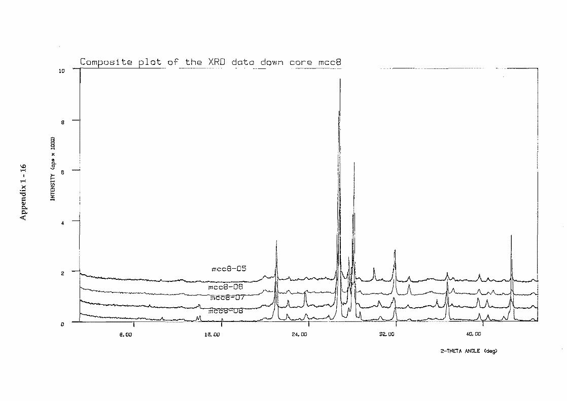
- fll o o
o N
3 ()
()
CD I a U
1
Ap
pen
dix
1 -
16
INTE
NSI
TY
(cp
e x
UlOI
D
-o n o 3 o (J) .......
cT
fD o o "'1 ro 3 o o OJ
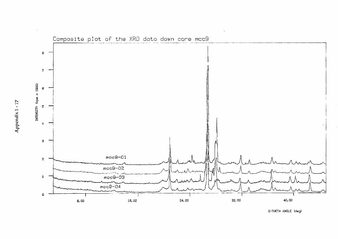
... PI
0 0 w
!'l
o o
I , I J !
3 0 3
0 0
(0
0 I
(0
0 I
.j:>.
0 w
Ap
pen
dix
1 -
17
INTE
NSI
TY
(cps
x 1
(00)
U1
CD
n 0 3 -0
0 (J)
1-'
-
(T
ID
'LJ Ir--
0 (T
3 0 3
0 0
0 ""i')
(0
0
I (0
0 I
N
0 .....
(T
"I
ID
X
:::0
0 0..
0 (T
0 0..
0 ~
:J
0 0 "1
ID
3 0 0 to
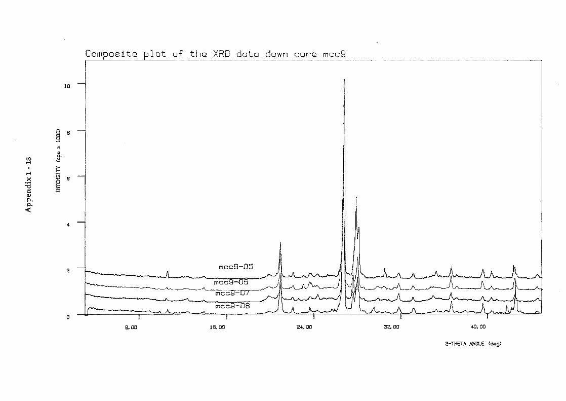
o N
... jll
3 g
(')
3 (')
(')
(Q
(')
I to
0
I m
0 U
1
~ 0 0
Ap
pen
dix
1 -
18
INTE
NSI
TY
(cp
s x
1000
) ... o
n o 3 o (J)
1-"
(1'
I1J
(1' :r- ID
X
:;::lJ
0 0.
. 0 (1
' 0 0.
. 0 :E
:J
0 0 ) ID
3 0 0 (.D
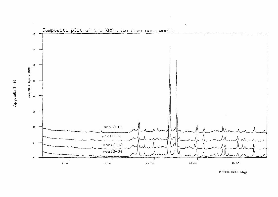
Ap
pen
dix
1 -
19
INTE
NSIT
Y (c
pa
)( 10
(0)
I:)
N
a en ....,-
~
ct
I:)
ro I:
)
t---
'
a ct a
I j"+
> i
'ct
I iT
I
!ro
... ,
3 3
Ix
PI
I 0
()
10
()
()
::
0 I:
) .....
l a
......
0 I
0 0
I ,
N
0 I
......
I I I I I I N
I
0 f"
~ a
0 .,
0 ro
I I 3 0 0 I-"
0

sn 8 - PI 0 0 N t- IS CAl
I"
o CJ p CJ o
0
I 0 '-l
... '3
0 '3
0
0 ~
0 D
.....
I
0 D
I
0)
0 Ul
Ap
pen
dix
1 -
20
INTE
NS
ITY
(c
ps
)(
1000
)
N
CAl
,. lI
\ 0
)
"-I
W
CD
--1-
__
n 0 3 0 (f
) 1
-'.
c+
([)
I--'
0 c+
0 -t)
c+
=r- ([) X
:::0
0 (l
I~
0 (l
0 ::E
:J
()
o ")
([) 3 0 ()
I ...
......
..
:0

of the XRO data core mccll 8
7
§ 6
-x
~ ]- 5 I
11
N ~
I ~ ....
l! In x ~
II
..... "'d
l = ~ '" (IJ Q.., Q..,
< 3
2 mccll-01
1
mccll
D
8.00 16.00 24.00 32.00 40.00
2-TH£T A ANGLE (dgg.>
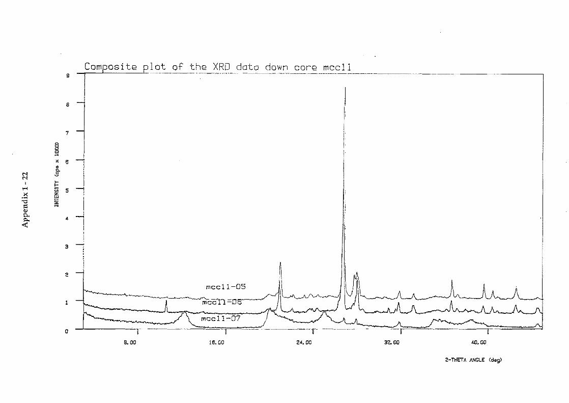
9
8
7
§ ..... x 6 £II
N N
]->-I-
\'""I
>< .... !II 5
..... ~ "'0 CO .... (!,.I
0.. ~ 4
-<:
3
2
1
I)
lot of
I
J . I
J I I
I . ---l
I I
13.00
Q XRD data down corQ mccll
mee11
meell-07
16.00 24.00
I I: I I
I, j, i,
32.00 40.00
2-THETA ANGlE (c:k!g>
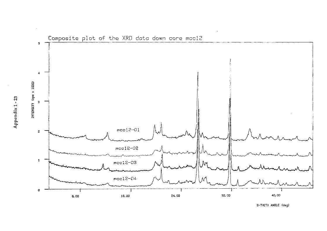
Com lot of th8 XRD data down cor8 mcc12 5
<I-
§ -)(
~ §. ......
~ ~ 3 .... . ~ II)
ffi '"0 ~ ::::
(1J -0.. 0.. < -I mcc12-01 2
1 mcc12-03
mcc12-04
o 8. 00 lB. 00 24. 00 32. 00 40.00
2-Tl-lETA ANGlE (deS>
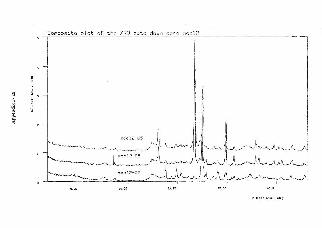
Ap
pen
dix
1-
24
INTE
NSIT
Y (c
pa X
1OQ
[U
0 N
CA
l ~
CJ\
n 0 '3
0 (f)
1-'
-
PI
rt"
IS ID
I--'
0 rt"
0 -I-)
rt" :r- ID
... 3
3 f»
0
0 3
X
IS 0
0 0
::u
I-'
I-'
0 D
N
N
I-'
I I
N
n.
0 a
! "'-
l Q
) a
0 U
1 rt
" 0 n.
0 ~
::J
N
I 0
t-o
0 "l
0
l ID
:3
0
I 0 I-
-"
I f\
)
I -
~----
.:::-:-:--=::~---:::;::::::::"-==--
I I CA
l I
j\I
I 0 0
l I I I I I ~
I
~ I
> ~
p ~
0 m
0
.... g- te,
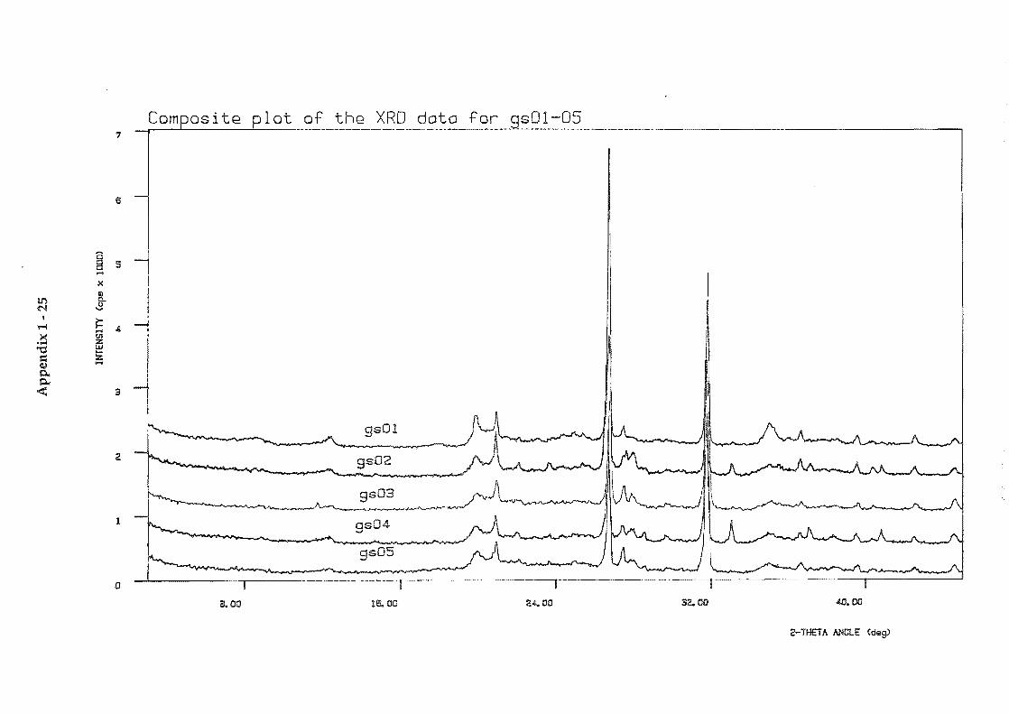
so 0 0 ... PI 8 N I- 0 0 w
1"
o o
0
, I I I I i , I , [ , I , - I ! I I I I I I I I I J , , I
....
1O
1O
to
({)
({)
({)
a 0
0 .f>
. U1
W
App
endi
x 1
-25
INTE
NS
ITY
(c
ps
)(
100m
N
(jJ
~
til
" ---
-L--_
_ l _
____
_ -L
.... n 0 '3
0 (f) .-..
rl"
(0
u r~ , :0
!-t;
I Irl"
1'"
"J"
lQ
1(0
({)
lQ
I
a ((
) Ix
N
0 l::
u I-'
10
I IQ
1
0
!rl"
1
0
I-t;
10
l"
l , k.o
iC
/) iO
!~
, I
, :0
!Ul
I I .--.---~--
... ~ ...
I I 1
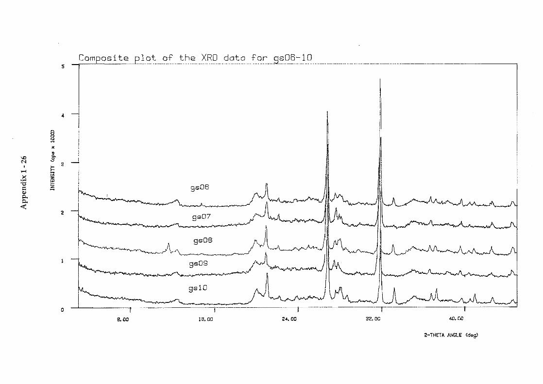
fD
0 0 .... Pl is N
1"
0 0 {6 o o
0
ill (J)
I-"
0
... 1\
1
ill
ill
(J)
ill
fI)
0 (J)
(D
0
0 ro
'-J
App
endi
x 1
-26
INTE
NSI
TY
(cps
)(
1000
)
Ul
.... U
I
n 0 '3
0 (J) ......
(1" ~ if-'
io
rt"
0 -t-)
!rt"
:"'
J""
ill
lID
(J)
i 0
:X
OJ
';::
0
0 Q. a rt
" a :-
1-)
:0
i'l
, I k.D
!(J)
'0
1m
:
I !J
-I<
'0
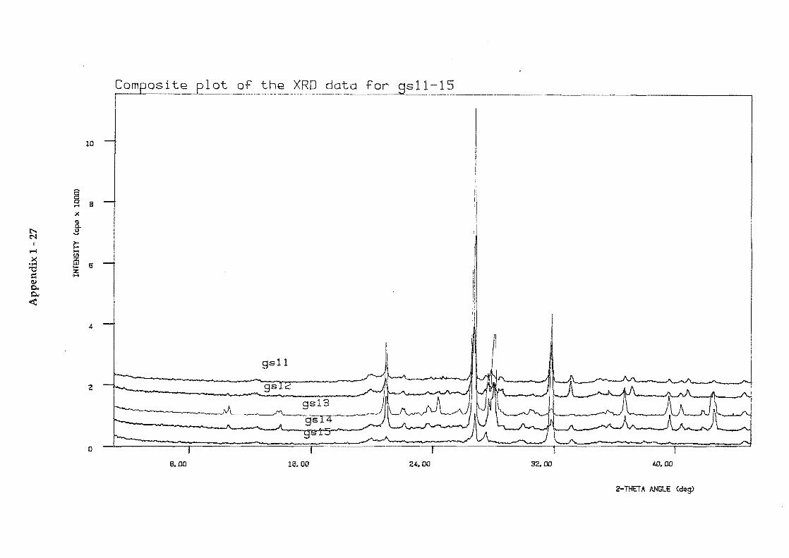
... p:!
o o
o N
to
(f) .....
. .....
.
App
endi
x 1
-27
INTE
NS
ITY
(c
pa x
10
00)
.... m
o
n o 3 o (j)
1-'
-
('1"
1
m
ro
I~
1(1-
10
:-t'
) i :(
'1"
::::
J 1m
i :x
1
;0
o 0.. o
1('1
"
iO
I-t'
)
10 l: I(
j)
I:=:
I ,
I I-
-"
iU1
I I I
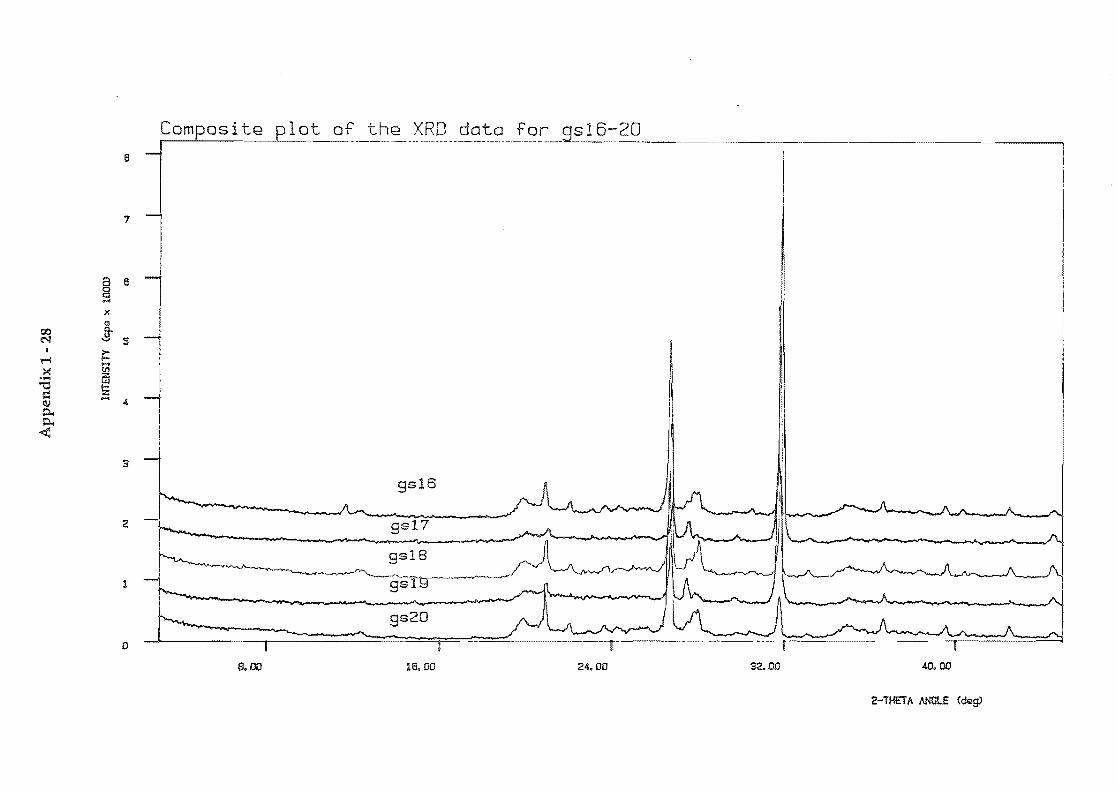
Ap
pen
dix
1-
28
INTE
NSI
TY
(cp
a x
1000
)
o ...
N
til
0 Ul
....,-
!II
~ 8
I: :-t)
1
(1"
I::;
(.Q
lQ
>
lQ
lQ
!([)
I[)
I[) I
I[)
I[)
(.Q
-N
1 .....
I[)
ix
£»
.....
0 ro
'-.
J I-
"
1:;0
0
C1l
0
iO
\
, 10
...
in
'(1
"
!n
1
I !-
t) 1
0
I !'
J I
I !
~
N
I I~
f"
I
8 I
I(J)
-i !
1
I IN
,0
I I
i I
,
I 1 I I
t6 I , I
8 I -1
.----~---
.. -~
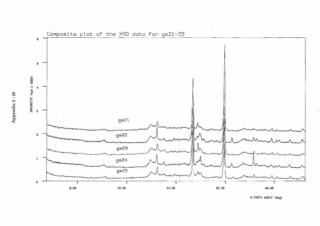
t of the XRD data for 21-25 6
5
§ Q -X 4-
0"1 j-N
I
1""'i i': I .... I
~ .... CIl
"1j 2:
~ IJ.I
t:: s: ... 3 (IJ
0.
~ 1
2 gs22
gs23
1 gs24
gs25
o -----... , ,------ r----8.00 16.00 2.£..00 32. 00 ..w.oo
2-THETA /INGLE (dQg.)
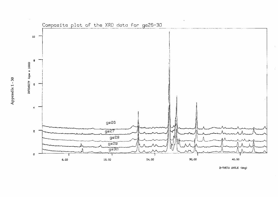
o N
to
fI)
N
Ol
Ap
pen
dix
1 -
30
INTE
NSIT
Y C
epe
x 10
0m O
J ... o
n o 3 o (f) ...... -
c-t
ID
0..
:0
;c
-t
:0
i-1J
;0
I')
I rg iN
10)
, I
lw 1° ! i ! I I I
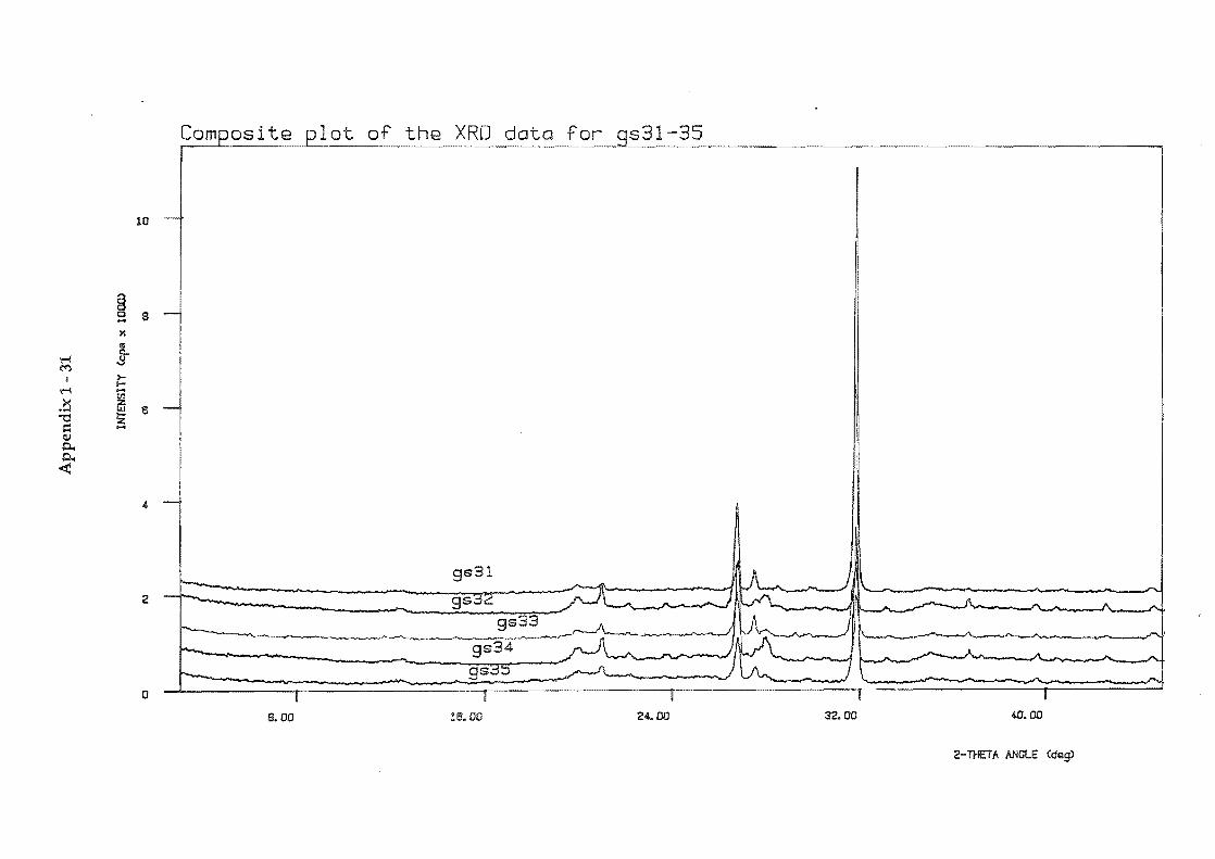
Ap
pen
dix
1-
31
INTE
NSI
TY
(cp
a l
( 10
(0)
.... 0
N
a:I
(I)
0
n 0 3 0 (J)
1-"
!D
(i'
0
ID 0
I--'
0 (i'
0 )
-T)
} , 1<
+ I
l:r
... to
lID
fll
'x
0
(j)
1::::
0 0
10
ID- 10 ,<+
10
I-T) I~ to
N
(f)
!-W
0
.......
0
1t1
IUl
, I , 1 ,
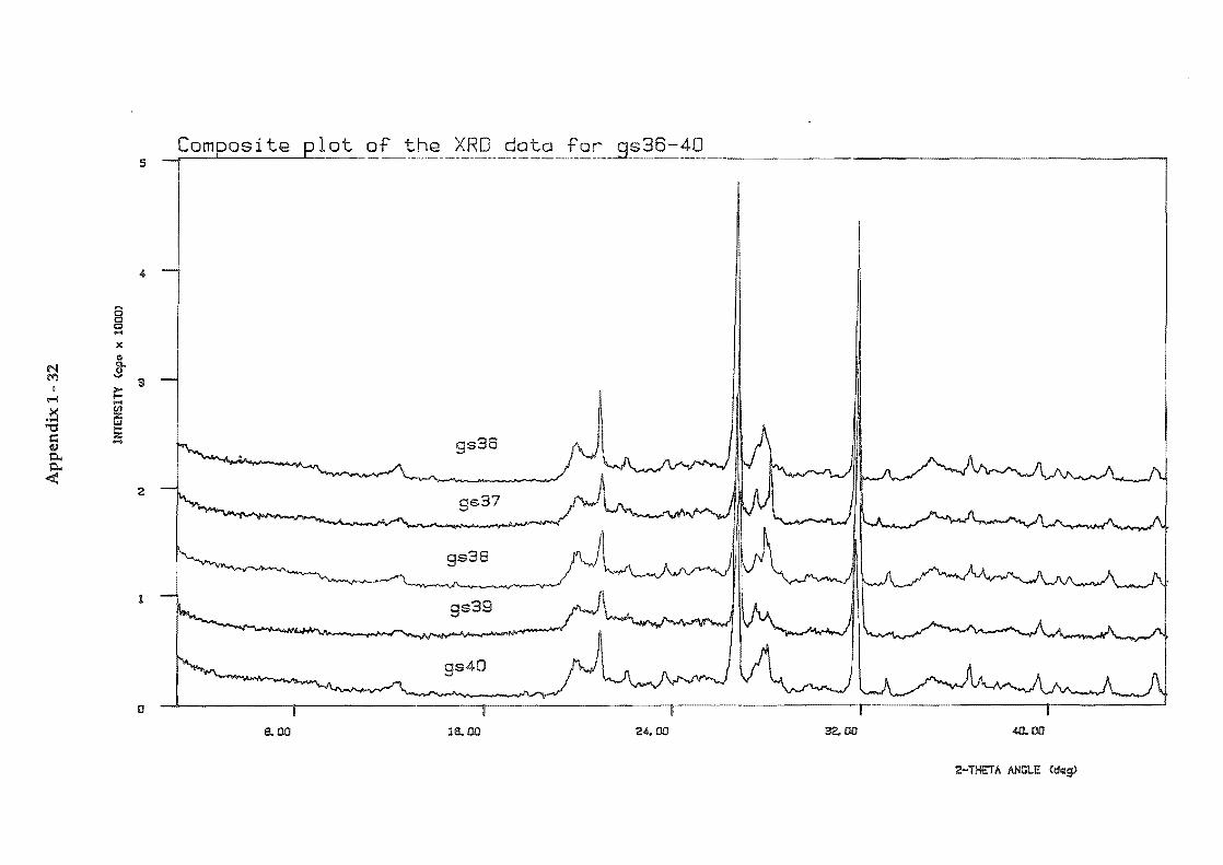
ot of the XRD data for 36-40 5
4
'" 8 0 .... )II;
II)
N .9 ~ ~ 3 I
\""l .... X III ..... ffi ~ !Z c k- 9s36 (I)
.... p" p"
« 2
9s37 .........
9s38
I .• V-Y~~~
1 I 9s39
~
9s4O
IJ
aoo 16..00 24.00 32.00 40. 00
2-TtiETA JINGLE (dt;lg)
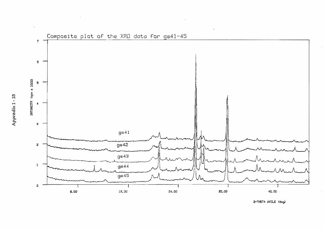
so 8 - PI c c I\l !'" El l8 c c
c I ill (JJ 1 +:-.
Ul
N
ill
ill
ill
(JJ
(JJ
(JJ
+:-.
~
+:-.
.".
W
N
Ap
pen
dix
1 -
33
INTE
NSI
TY
(cp
s x
1000
)
U)
~
UI
'-l
n 0 3 0 C/) ......
(1"
(D
........
. 0 (1
"
0 -tj
ill (J) +:-.
I-'
Q
0 <+
0 -tj
0 ., C/) .t:>-
I-"
I .t:>-
Ul
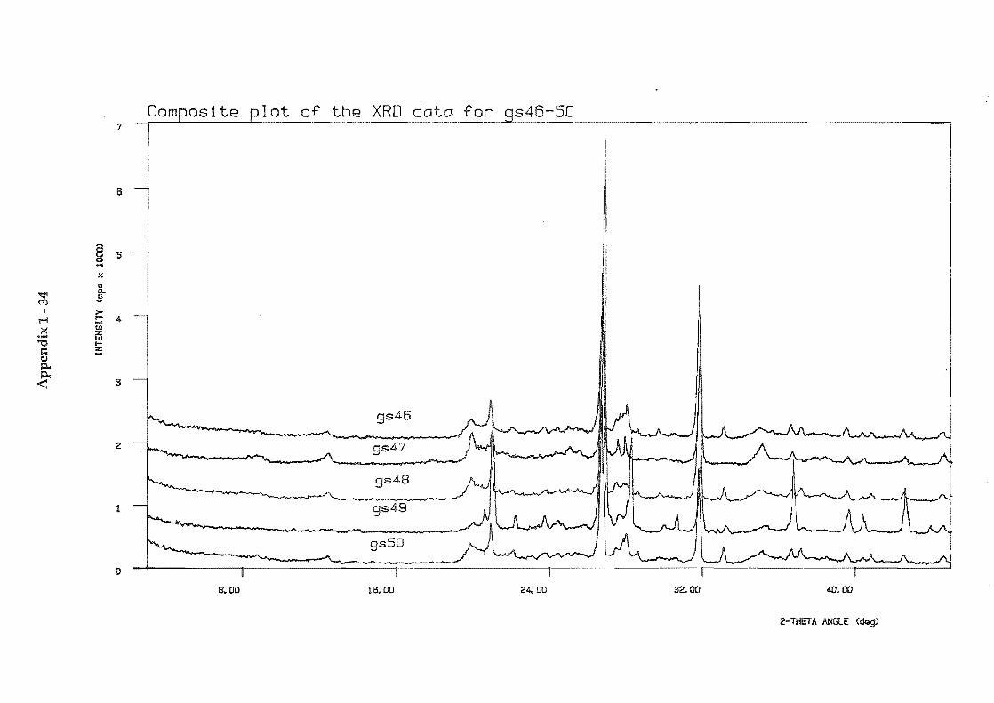
lot of XRD data for 50 1 --~--~----~-----
6
a g 5 .... X III
~ ~
M ,s I
~ \""'I ... " .~
II)
ffi "'0 .... I:: :z; .... (lJ p., p..
< 3
-.........-.-2 9s47
-9s48
1
9s5O ,-, '.."...,,~
o 6000 16.00 24. 00 32.00 40.00
2-THET A ANGlE <OilS>
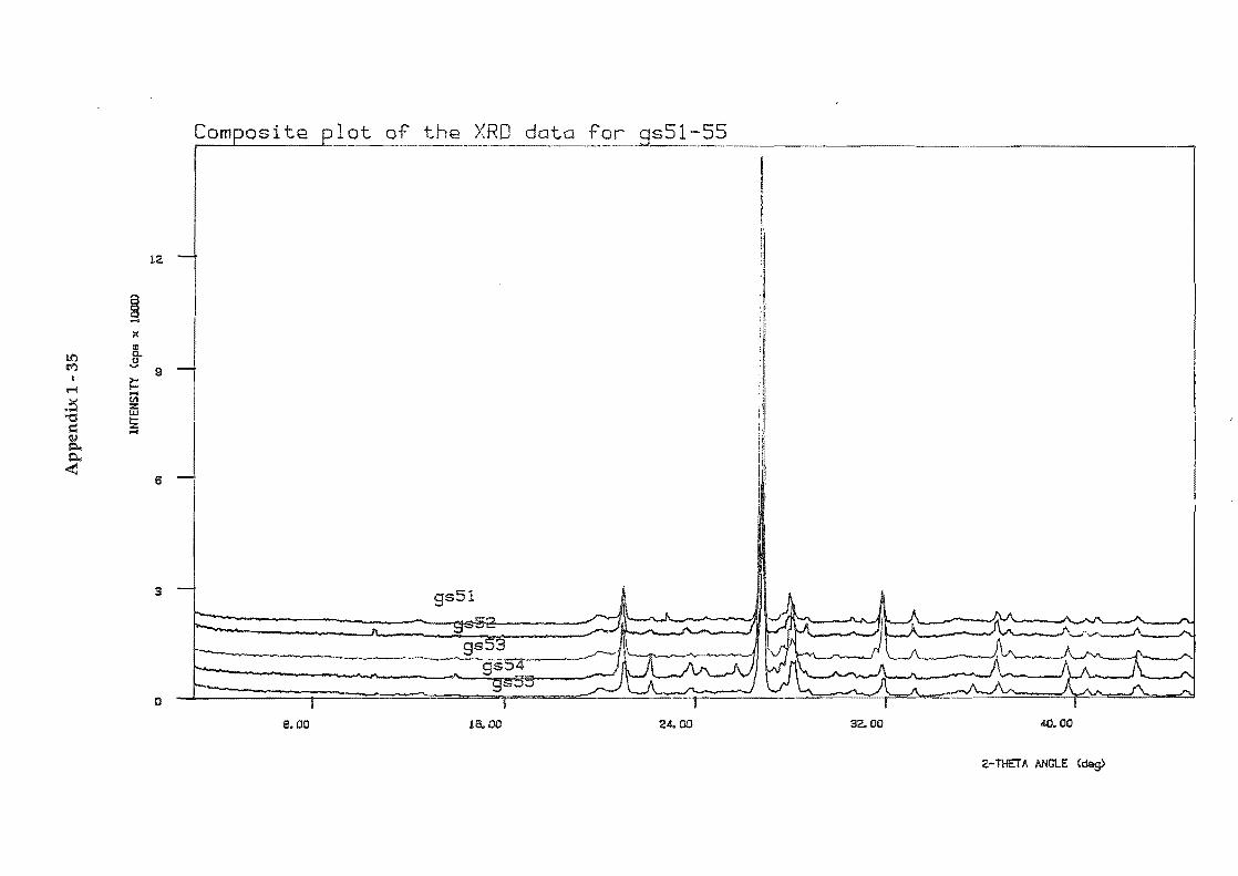
!»
a a - fll a a N I'- 8 p a a
to
(J)
U1
.....
Ap
pen
dix
1 -
35
INl E
NS lT
Y
(cpa
x
1000
)
(0
-.----.--.~--.-.-
. __ .. -
--.-.--~ -.
-."
' _.
,--,
--~-
-~-.~
-~
_.
... N
n 0 3 0 (f)
1-'
-
("I-
(0
.-.
0 ("I-
0 -t)
(0
X
:::0
0 Q. 1° 1("1- 1° .-t)
10
I)
La
I~
! I
lUI
lUI
I ·---:-::--::~C":-""="_-="'_=
__
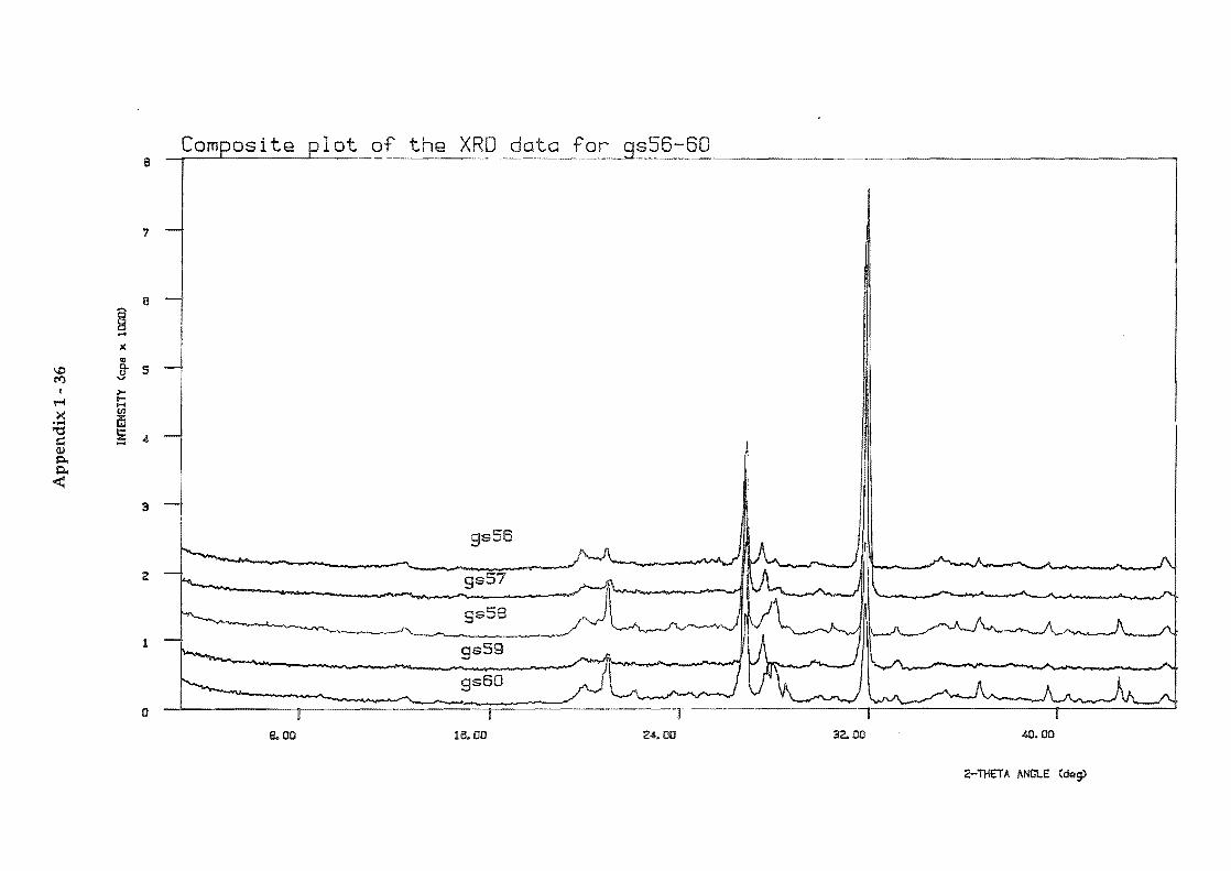
sn 8 - ?l 0 0 N f"
0 0 16 o o P 8
0
lQ
i ({J
C1
l a
... N
J~ (0
(J
) ({J
(J
) U1
U1
U1
CD
ro
'-..
J
Ap
pen
dix
1 -
36
INTE
l/SIT
'( (c
pa )
( 10
00)
W
.. U
l a
I !J
)
_-1-
L-
n 0 3 0 (f) .....
c+
rn t-
-'
0 c+
I 10
i-t
) I c+
:T
rn X
lQ
;:
::0
({J
:0
U1
C1
l 10
.. 1
0
'c+
10
!-t
) 1
0
!'"1 lo jm
1U1 Icr
len 10
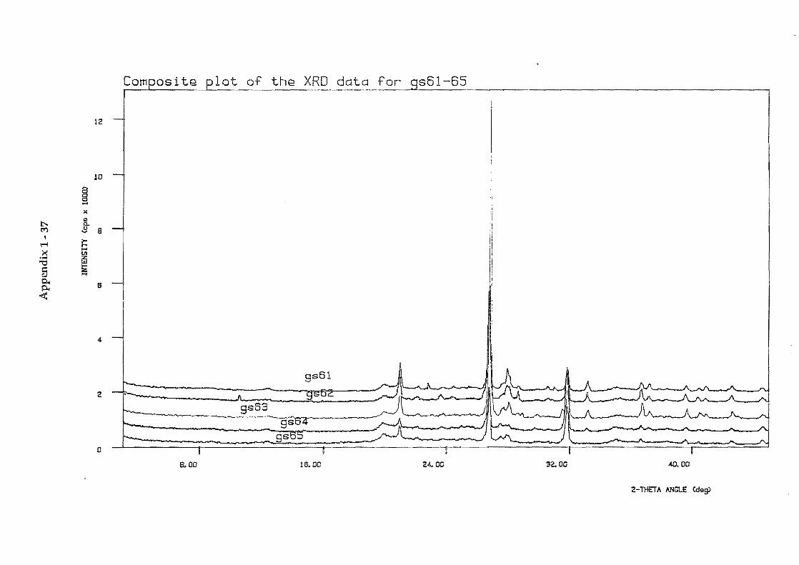
... p:1
o o N f- a 16 o o p o o
o N
App
endi
x 1
-37
INTE
NSI
TY
(cpa
X
1000
) ... o
.... N
--J--------~------~--------~--~n
a 3 a ({) ......
c+
(0
I--'
a I: -t)
c+
:T
(0
X
;:::0
10 10..
10
Ic+
,0
! I~ ({) OJ
I---
" ! OJ
U1
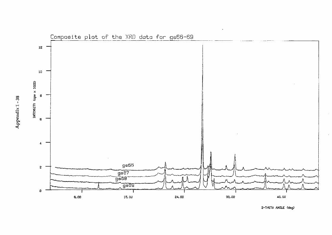
Ap
pen
dix
1 -
38
INTE
NSI
TY
(cp
e x
10
00)
... -
I:)
1\1
ill
m
0 N
_J._
n 0 3 0 Cf
) 1-
'-p>
(i
" 0
ID
0
I-'
0 (i"
0 -1")
(i" ::r
ID
.... (Q
p
Ci)
X
0 Q
) ::D
c
O"l
0 0..
0 (i
" 0 -1
")
10
I)
1\
1 ~
~
10
} c
iO}
0 I
0}
(.Q
.. _-:::---;;-~_FtI'I
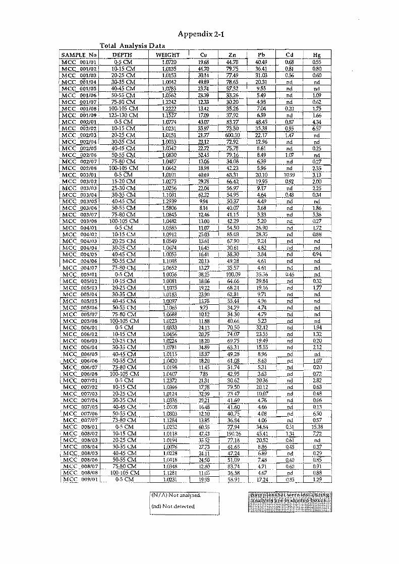
Appendix 2-1
ota nalYS1S T lA l"D ata • SAMPLE No DEPTH MCC 001/01 0-5CM MCC 001/02 10-15 CM MCC 001/03 20-25 CM MCC 001104 30-35 CM MCC 001105 40-45CM
IMCC 001/06 ! 50-55 CM MCC 001/07 75-80 CM MCC 001108 100-105CM MCC 001/09 125-130 CM MCC 002101 0-5CM MCC 002/02 10-15 CM MCC 002/03 20-25 CM MCC 002/04 30-35 CM MCC 002105 40-45 CM MCC 002/06 I SO-55 CM
'MCC 002/07 75-80 CM MCC 002/08 100-105CM MCC 003/01 0-5 MCC 003/02 15-20 CM MCC 003/03 25-30CM MCC 003/04 30-35 CM
,MCC 003/05 40-45 CM MCC 003/06 50-55 CM MCC 003/07 75-80CM
:MCC 003/08 • 100-105CM MCC 004/01 0-5CM
IMCC 004/02 10-15 CM
~(2 004/03 20-25 CM MCC 004/04 30-35 CM MCC 004/05 40-45 CM MCC 004/06 50-55 CM MCC 004/07 75-80 CM
, MCC 005/01 0-5 CM MCC 005/02 10-15 CM MCC 005/03 20-25 CM
'MCC 005/04 I 30-35 CM MCC 005/05 4O-45CM
iMCC OS 50-55 CM MCC 00 75-80 CM MCC 005/08 100-105 CM
~r 0-5CM
C 006/02' 10-15 CM 6/03 20-25 CM
MCC 006/04, 30-35 CM MCC 006/05 40-45 CM MCC 006/06 50-55 CM
.MCC 006/07 75-80 CM
. MCC 006/08 100-105 CM MCC 007/01 0-5 CM
i MCC 007/02 ' 10-15 CM MCC 007/03 20-25 CM MCC 007/04 30-35 eM MCC 007/05 40-45 CM
,MS:C 007/06. 50-55 CM MCC 007/07 75-80 CM MCC 008/01 0-5CM MCC 008/02 10-15 CM MCC 008/03 20-25 CM MCC 008/04 30-35 CM MCC 008/05 4O-45CM MCC 008/06 50-55 CM MCC 008/07 75-80 CM MCC 008/08 i 100-105 CM
LMCC 009/0! I ()'5CM
I
!
I
!
i
I
WEIGHT Cu umo 19.68 1.0135 44.70 1.0153 30.14 UJ042 49.89 1.0783 23.74 1.0562 2339 1.2242 1233 1.2222 13.42 1.1527 17.09 1.0774 43.07 1.0231 35.97 1.0151 21.77 1.0033 23.12 1.0342 'l2.72 1.0830 52.45 1.0487 13.06 1.0642 18.98 1.0101 40.69 1.0275 29.78 1.0256 'l2.04 1.1081 62.32 1.2939 9.94 1.5806 8.14 1.0845 12.46 1.0482 13.00 1.0585 11.07 1.0912 25.03 1.0549 15.61 1.0674 16.45 1.0053 .41 1.1048 20.13 1.0652 1327 1.0036 3825 1.0081 18.06 UCB5 19.22 1.0183 23.90 1.0097 15.78 1.1065 I 9.73 1.0688 I 10.12 1.0223 11.88 1.0333 24.13 1.0456 20,75 1,0224 18,20
1~1=$1 1.0115 18.87 1.0420 1820 1.0198 1.0407 7.85 1.2372 2131 l.CB96 17,78 1.0124 32.99 1.CB38 2921 1.0508 16.48 1.08CB 12.10 1.1284 13.85
1.0252=i 60.55
1.0118 47.43 1.0194 35.52 1.0076 Tl.73 1.0228 24.11 1.0418 24,50 1.0348 12.80 1.1281 11.05 1,0231 19,93
(N/ A) Not analysed.
(nd) Not detected
I
I
I
I
i I I I ,
I I I
I
I
I
I
Zn Pb Cd Hg 44.78 40.49 0.68 0.55 79.75 36.41 0.81 0.80 77.49 31.03 0.56 0.60 78.65 20.31 nd nd 57.32 9.55 nd nd 33.26 5.49 nd 1.09 30.20 4.98 nd 0.62 35.26 7.04 0.20 1.75 37.92 6.59 nd 1.66
MM~·45 0.87 4.34 73. 35.38 0.95 6.57 600. 22.17 1.47 nd 72.92 12.96 nd nd 75.78 8.61 nd 0.25 79.16 8.49 W7 nd 34.08 6.39 nd 0.27 42.23 5.96 nd I 2.35 63.31 20.10 10.99 3.13 66.42 19.95 0.92 I 2.00 56.97 9.17 nd I 2.25 54.95 4.64 0.48 I 0.34 50.37 4.49 nd ! nd I 40.07 3.68 nd 1.86 41.15 3.33 nd 538 42.29 520 nd 0.27 54.50 26.90 nd 1.72 85.CB 28.35 nd
~ 67.90 924 nd 30.61 4.82 nd nd 38.30 3.84 nd I 0.94 49.28 ! 4.61 nd nd 35.57 4.61 nd nd 100.09 35.56 0.46 ! nd 64.66 39.84 nd v.;;)L
68.24 19.16 nd 1.77 i 62.81 9.71 nd ! nd 55.44 4.96 nd nd 34.79 4.74 nd nd I 34.30 4.79 nd nd 40,66 523 nd nd 70.50 32.12 nd 1.94 74,07 23.55 nd 132 69,75 19,49 nd 0.20 63.31 15.55 nd 2.12 49,28 8.96 nd nd '" (10 8,63 nd 1.07 I 31.74 531 I nd 0.20 42,95 3.63 nd I 0.72 30,62 20.36 nd I 282 !
79.50 20.12 nd 0,63 73,47 I 10,07 nd 0.48 41.69 i 4.76 nd 0,66 41.60 4.66 nd 0.13 40.75 4.08 ~6.50 36,84 4.06 nd 0.57 77,94 34,84 0.51 15,38 190.26 45.41 1.:» 7.72 77.18 20.52 0.61 od 61.65 8.86 O.4S 0,37 47,24 6.89 nd 0,29 51.09 7,48 0.40 0.85 83,74 4.71 0.60 ! 0,91 I 36.58 4.67 nd 0.88 58.91 17.24 0,85 1.29
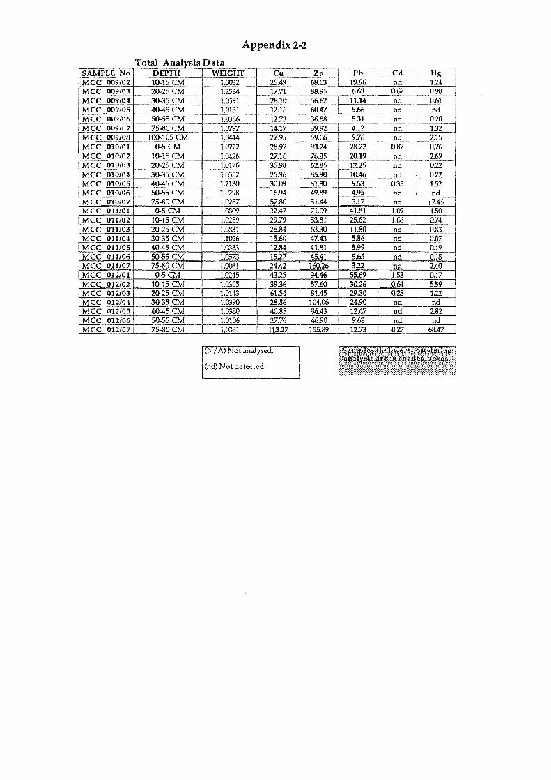
SAMPLE No MCC 009/02 MCC 009/03 MCC 009/04 MCC 009/05 MCC 009/06 MCC 009/07 MCC 009/08 MCC 010/01 MCC 010/02 MCC 010/03
'MCC 010/04 MCC 010/05 MCC 010/06 MCC 010/07 MCC 011/01 MCC 011/02 MCC 011/03 MCC 011/04 MCC 011/05 MCC 011/06 MCC 011/07 MCC 012101 MCC 012/02 MCC 012103
i MCC 012104 ~ 012/05 ~. 012106 MCC 012/07
Appendix 2-2
ola nalysls T lA I'D ala DEPTH 10-15 CM 20-25 CM 30-35 CM 4O-45CM 50-55 CM 75-80CM
100-105 CM 0-5CM
10-15 CM 20-25 CM 30-35 CM 4O-45CM 50-55 CM 75-80 CM 0-5CM
10-15 CM 20-25 CM 30-35 CM 40-45 CM 50-55 CM 75-80 CM 0-5CM
10-15 CM 20-25 CM 30-35 CM 40-45 CM 50-55 CM 75-80 CM
WEIGHT Cu 1.0032 25.49 1.2534 17.71 1.0591 28.10 1.0131 12.16 1.1)356 12.73 1.0797 14.17 1.0414 27.95 1.0222 28.97 1.006 27.16 1.0176 35.98 1.0552 25.96 1.2130 30.09 1.0298 16.94 1.0287 57.80 1.0009 32.47 1.0289 29.79 UID! 25.84 1.1026 15.60 t,()383 12.84 1.0573 15.27 1.0081 24.42 1.0245 43.25 1.0305 39.36 1.0143 61.54 U)390 28.86 1.Q380 40.85 1.0106 27.76 1.Cl381 113.27
(N/ A) Not analysed.
(nd) Not detected
I
I
I
Zn Pb Cd Hg 68.03 19.% nd 1.24 88.95 6.63 0.67 0.90 56.62 I 11.14 nd 0.61 60.47 5.66 nd nd 36.88 I 531 nd 0.20 39.92 4.12 nd 132 59.06 9.76 nd 215 93.24 28.22 0.87 0.76 76.35 20.19 nd 269 6285 12.25 nd 0.22 85.90 10.46 nd 0.22 8130 9.53 0.35 1.52 49.89 4.95 nd nd 51.44 3.17 nd 17.45 71.09 41.81 1.00 1.50 53.81 25.82 1.66 0.74 63.30 11.80 nd 0.83 47.43 5.86 nd 0.07 41.81 5.99 nd 0.19 45.41 5.65 nd 0.18 160.26 3.22 nd 240 94.46 55.69 1.53 0.17 57.60 30.26 0.64 5.59 81.45 29.30 0.28 1.22 I
104.06 24.90 nd nd 86.43 12.47 nd 282 46.90 9.63 nd nd 155.89 12.73 0.27 68.47
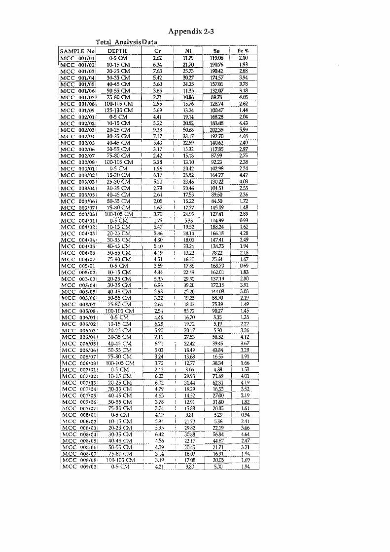
Appendix 2-3 ota nalYSlS T lA 1 "0 ata
SAMPLE Nol DEPTH Cr •
Ni Sn Fe %
MCC 001/011 0-5CM
~ 119.06 210
MCC 001/02i 10-15 CM 21.70 190.76 1.93 MCC 001/031 20-25 CM 190.42 288 MCC 001/041 30-35 CM 17457 3.94 MCC 001/05 I 4(}..45 CM 157.01 3.78 MCC 001/061 50-55CM 3.65 • 1135 13207 3.18 MCC 001/071 75-80 CM 2.71 10.86 89.78 4.05 MCC 001/081 100-105CM 128.74 262 MCC 001/09. 125-130 CM 100.47 1.44 MCC 002/011 0-5CM 4.41 19.14 16828 204 MCC 002/021 10-15 CM 5.22 20.82 183.08 4.43
.MCC 002/031 20-25 CM 938 SO.68 202.35 5.99 MCC 002/041 30-35 CM 7.17 I 33.17 19270 4.48 MCC 002/051 40-45 CM 5.43 1 2259 140.62 240 MCC 002/061 50-55 CM 3.17 i 1532 117.85 297 MCC 002/07! 75-80 CM 2.42 I 15.18 87.99 275 MCC 002/081 tOO-105 CM 328 I 13.10 92.23 238
.MCC 003/01: 0-5CM 1.96 I 20.42 102.98 224 MCC 003/021 15-20 CM 6.17 I 26.82 164.77 4.47 MCC 003/031 25-30 CM 510 i 23.46 130.22 4.m
,MCC 003/041 30-35 CM 2.73 1 20.46 10451 255 .MCC 003/05 i 40-45 CM 2.64 17.53 89.SO 236 MCC 003/061 50-55 CM 2.05 ! 15.22 8450 I 1.72 MCC 0031 • ... 77 145.09 1.48 MCC 003/081 100-105 CM 3.70 i 24.95 127.41 289 MCC 004/011 0-5CM 1.75 i 5.33 114.99 0.93 MCC 004/02 ! IO-IS CM 5.47 I 19.52 18824 1.62 MCC 004/031 20-25 Ov1 5.86 28.14 166.18 4.28
.MCC 004/04 : 30-35 CM 4.80 I 147.41 I 249 I MCC 004/05 i 40-45 CM 5.40 I 2314
~ MCC 004/06 i 50-55 CM 4.19 1 1312 MCC 004/071 75-80 CM 451 I 1620 MCC 005/01 ! 0-5CM 3.69 17.86 168.70 i • 0.69 MCC 005/021 10-15 CM 434 I 22.49 16201 1.83
.MCC 005/031 20-25 CM 535 I 29.SO 137.19 I 2.80 MCC 005/041 30-35 CM 6.96 ! 3920 17215 3.92 MCC 005/05 I 4(}..45 CM 3.98 i 2520 144.m I 3.03 MCC 005/06 i 50-55 CM 332 I 19.25 88.70 219 MCC 005/07, 75-80 CM 2.64 ! 18.03 7539 1.49 MCC 005/0S1 100-105 CM 2.54 I 85.72 9027 1.45 MCC 006/011 0-5CM 4.46 I 16.70 5.25 1.35
iMCC 006/021 10-15 CM 6.28 19.72 5.19 I 2!ii MCC 006/03 : 20-25 CM 5.90 i 20.17 530 3.26 MCC 006/041 30-35 CM 7.11 2753 5852 4.12
IMCC 006/05 i 40-45 CM 6.71 ; 22.42 39.45 3.67 IMCC 006/061 50-55 CM s.m
;
18.49 43.84 3.29 .MCC 006/071 75-80 CM 324
, 1655 1.91 i
MCC 006/081 100-105 CM 3.75 1 12.77 3834 1.66 MCC 007/011 0-5CM 2.42 j 3.06 438 1.53 MCC 007/021 10-15 CM 6.m I 29.93 71.89 4.01 MCC 007/03 i 20-25 CM 6.02 ! 31.44 6231 1 4.19
• MCC 007/041 30-35 CM 4.79 i 1919 16.33 I 3.52 • MCC 007/051 40-45 CM 4.63 I 1452 27.00
~ MCC 007/061 50-55 CM 3.78 I 12.91 MCC 007/071 75-80 CM 3.74 : 15.88 20.05 MCC 008/01 i 0-5 Ov1 4.19 I 9.81 519
• MCC 008/021 10-15 CM 534 .. _ ..
i 21.73 5.36 2.41 .MCC 008/031 20-25 CM 5.93 • 29.82 2219 3.66 MCC 00S/041 30-35 CM 6.42 30.88 56.84 4.64 MCC 008/051 40-45 CM 4.56 I 22.17 44.67 247 MCC 008/061 50-55 CM 439 1 20.45 21.71 3.21 MCC 008/07: 75-80 CM 3.14 16.03 1631 1.94 MCC 008/08 i 100-105 CM 3.19 I 17.08 20.05 1.69
.M<.::C 009/01 0-5 eM 4.21 9.83 530 1.94
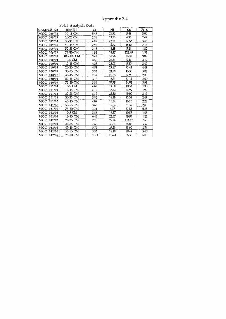
Appendix 2-4 ob natYSIS T 1 A I . 0 ata
!SAMPLE No DEPTH Cx
~ Sn Fe %
• MCC 009/02' 10-15 0v1 5.43 3.;6
5.41 3.00 MCC 009/03 20-25 0v1 258 4.33 242 MCC 009/04 30-35 0v1 4.87 22.71 37.68 3.43 MCC 009/05 40-45 0v1 293 15.72 16.66 218 MCC 009/06 50-550v1 tl 15.38 5.24 1.80 MCC 009/07 75-80 0v1 18.47 123.69 1.56 MCC 009/08 100-105 0v1 3.42 31.96 3832 3.09 MCC 010/01 0-5 0v1 4.56 21.51 5.31 3.19 MCC 010/02 10-15 0v1 4.38 25.08
~ 3'1H MCC 010/03 20-25 0v1 4.93 29.87 4.43 MCC 010/04 30-35 0v1 3.3-t 24.78 3.02
~ 40-45 0v1 2.52 25.65 32.90 283
MCC 50-55 0v1 3.17 18.71 33.15 200 MCC 010/07 75-80 0v1 3.84 57.78 84.01 3.99
,MCC 011/01 0-5 0v1 4.08 19.08 1031 1.90 MCC 011/02 10-15 0v1 4.17 18.73 21.99 ! 1.99
.MCC 011/03 20-25 CM 6.73 ,
23.50 69.00 3.13 . iMCC 011/041 30-35 CM 3.91 16.25 t=; I 243 ,MCC 011/05 40-45 CM 4.09 1534 223 MCC 011/06 ' 50-55 0v1 3.63 ! 15Jl6 208 MCC 011/071 75-80 0v1 331 ! 4.37 33.86 0.25 MCC 012/01' 0-50v1 3.88 ; 19.47 10.88 1.08 I
MCC 012/02i 10-15 0v1 6.46 1 22.67 49.95 1259 MCC 0121031 20-25 CM 735 I 29.26 114.17 i 2.68 MCC 012/041 30-35 CM 7.66 30.64 88.82 : 3.32 MCC 012/051 40-45 CM -'7)
J.I~ ; 29.28 88.90 : 254 MCC 012/061 50-55 CM 533 ! 18.40 39.49 3.40 MCC 012/071 7S-80CM I 14.83 I 135.61 6638 ; 6.03
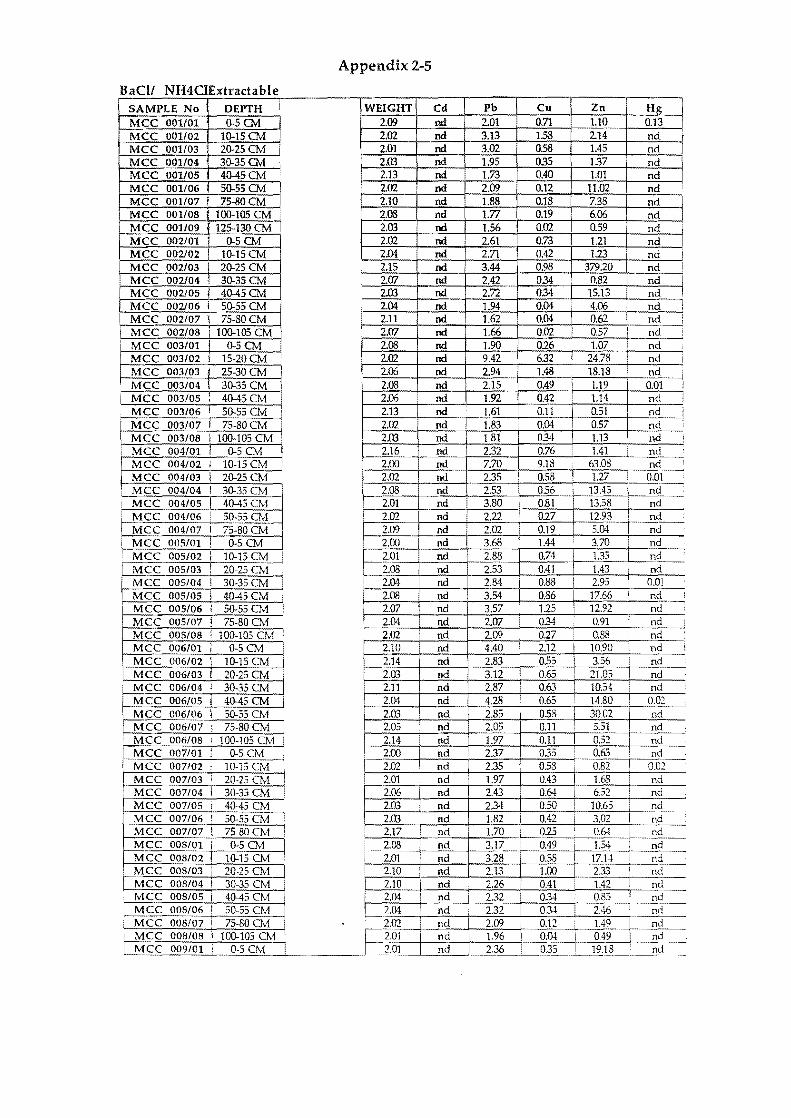
Appendix 2-5
BaClI NH4CIExtractabie SAMPLE No DEPTH WEIGHT Cd Pb Cu Zn Hg
~CC 001101 0-5CM 2.09 nd 2.01 0.71 1.10 0.13 MCC 001/02 10-15 CM 2.02 nd 3.13 1.58 2.14 od MCC 001/03 20-25CM 2.01 nd 3.02 058 1.45 od MCC 001/04 30-35CM 2.03 nd 1.95 035 1.37 od MCC 001/05 40-45CM 2.13 nd 1.73 0.40 1.01 od MCC 001/06 50-55CM 2.02 nd 2.09 0.12 11.02 nd MCC 001107 ! 75-80CM 2.10 nd 1.88 0.18 7.38 nd MCC 001108 100-105 CM 2.08 nd 1.77 0.19 6Jl6 nd MCC 001/09 125-130CM 2.03 nd 1.56 0.02 0.59 od MCC 002/01 0-5CM 2.02 nd 2.61 0.73 1.21 od MCC 002/02 10-15 CM 2.04 nd 2.71 0.42 1.23 nd I MCC 002/03 20-25 CM 2.15 nd 3.44 0.98 379.20 od I
MCC 002/04 30-35CM 2.W nd 2.42 034 0.82 nd I MCC 002/05 40-45 CM 2.03 nd 2.72 034 15.13 od MCC 002/06 i 50-55CM 2.04 nd 1.94 0.04 4.06 od : MCC 002/07 I 75-80CM 2.11 nd 1,62 0.04 i 0.62 od I
MCC 002108 . 100-105 CM 2.W nd 1.66 0.02 0.57 od ! MCC 003/01 0-5CM 2.08 nd 1.90 026 i 1.07 od i
MCC 003/02 i 15·20 CM 2.02 nd 9.42 632 24.78 od i MCC 003/03 25-30CM 2.06 nd 2.94 1.48 I 18.18 nd I MCC 003/04 30-35 CM 2.08 nd 2.15 0.49 I 1.19 0.01 I
I MCC 003/05 ,
40-45CM !
2.06 nd 1.92 0.42 1.14 nd I , MCC 003/06 I 30-53 CM 2.13 nd 1.61 0.11 0.51 od i I MCC 003/07 I 75-80CM i 2.02 nd 1.83 0.04 0.57 od : MCC 003/08 I 100-105 CM 2.03 nd 1.81 034 1.13 nd !
i MCC 004/01 I 0-5CM , 2.16 nd 2.32 0.76 1.41 nd MCC 004/02 I 10-15 CM 2.00 nd 7.70 9.18 63.08 od MCC 004/03 I 20-25 CM 2.02 nd 2.35 0.58 1.27 0.01 MCC 004/04 I 30-35 CM 2.08 nd 2.53 0.56 13.45 nd I
MCC 004/05 40-45 a1 2.01 nd 3.80 0.81 13.58 I od MCC 004/06 S0-3SCM 2.02 nd 2.22 027 12.93 ! nd MCC 004107 ! 7S-80CM 2.09 nd 2.02 0.19 S.W nd
! MCC 005/01 I 0-5CM 2.00 od 3.68 1.44 3.70 nd MCC 005/02 I 10-15 CM 2.01 nd 2.88 0.74 1.35 nd ,
r-M-CC 005/03 20-25 CM 2.08 nd 2.53 0.41 1.43 nd MCC 005/04 I 30-35 C"M ! ! 2.04 nd 2.84 0.88 I 2.95 0.01 MCC 005/05 , 4O-45CM 2.08 nd 3.54 0.86 17.66 nd I
MCC 005/06 i 50-55 CM 2.W od 3.57 125 12.92 I nd MCC 005/07 i 75-80CM 2.04 od 2.W 0.34 0.91 l nd !
MCC 005/08 ; 100-105 CM 2.02 od 2.09 027 0.88 nd MCC 006/01
, O-SCM 2.10 od 4.40 2.12 I 10.90 i nd I ,
MCC 006/02 1 10-15 CM 2.14 nd 2.83 0.55 3.56 i nd MCC 006/03 ! 20-25 CM 2.03 nd 3.12 0.65 21.05 nd ~CC 006/04 i 30-35 CM 2.11 nd 2.87 0.63 10.54 nd I
MCC 006/05 I 40-45 CM 2.04 nd 4.28 0.65 14.80 0.02 MCC 006/06 I 50-55 CM 2.03 nd 2.85 0.58 30.02 od MCC 006/07 i 75-80 a1 2.05 nd 2.05 0.11 5.51 nd
I MCC 006/08 : 100-105 CM I 2.14 od 1.97 0.11 0.52 nd MCC 007/01
, 0-5CM I 2.00 od 2.37 035 0.63 od
MCC 007/02 i 10-15 CM 2.02 l nd I 2.35 0.58 0.82 0.02 MCC 007/03 i 20-25 CM 2.01 od 1.97 0.43 I 1.68 nd
! MCC 007104 l 30-35 CM 2.06 nd 2.43 : 0.64 ! 6.51 od MCC 007/05 i 40-45 eM 2.03 od 2.34 0.50 10.63 nd MCC 007/06 ! 50-55 CM 2.03 I nd 1.82 I 0.42 3.02 od MCC 007/07 \ 75-80CM 2.17 nd 1.70 023 0.64 od MCC 008/01 i O-SCM L~08 od 3.17 I 0.49 1.54 nd MCC 008/02 I 10-15 CM ! I 2.01 nd 3.28 0.58 17.14 I od
. MCC 008/03 20-25 CM I 2.10 nd 2.13 1.00 2.33 I nd rMCC 008/04 ! 30-35 CM 2.10 nd 2.26 0.41 1.42 nd
MCC 008/05 I 40-45 CM 2.04 nd 2.32 0.34 0·85 I od I MCC 008/06 I 50-55 CM 2.04 nd i 2.32 034 2.46 I od
MCC 008/07 75-80 CM 2.02 nd 2.09 I 0.12 1.49 nd ! MCC 008/08 \ 100-10S CM 2.01 nd 1.96 O.W 0.49 nd I MCC 009/01 0-5 CM ·2.01 nd 2.36 oj:; 19.18 nd
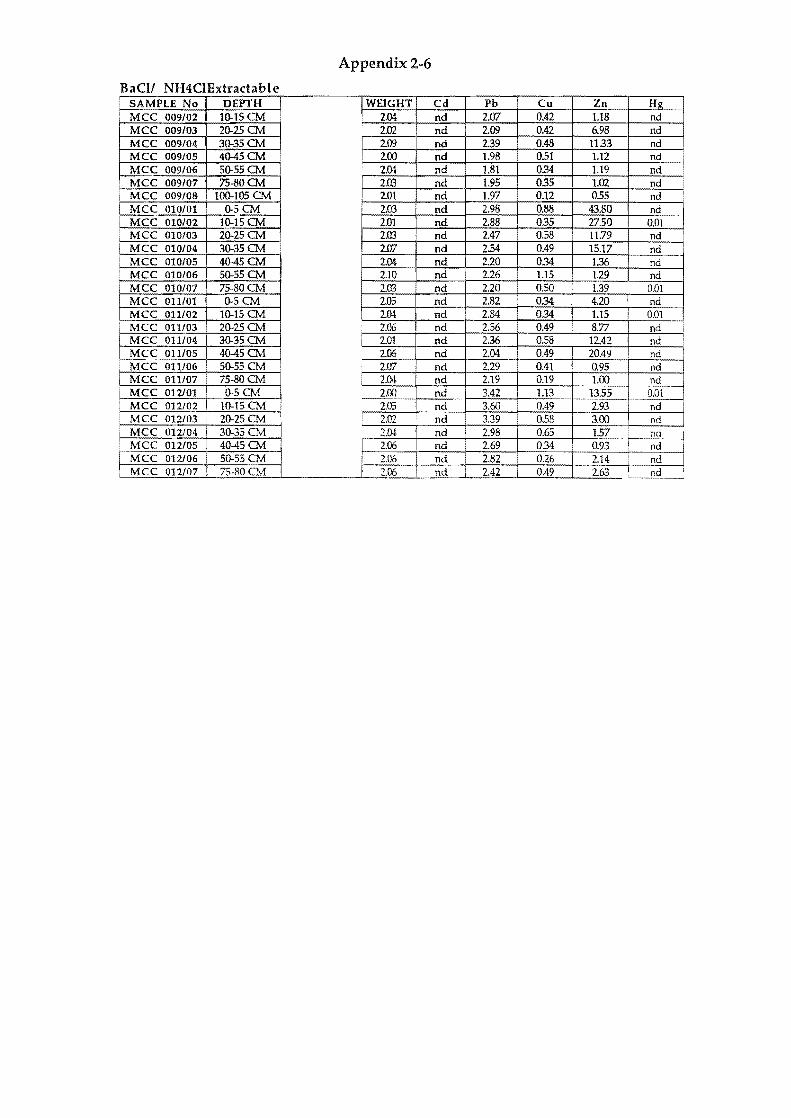
Appendix 2-6
BaCII NH4CIExtractabie SAMPLE No DEPTH WEIGHT Cd Ph Cu Zn Hg MCC 009/02 10-15CM 2JJ4 nd UJ7 0,42 1.18 nd MCC 009/03 20-25CM 2m nd 2.09 0.42 6.98 nd MCC 009/04 30-35CM 209 nd 2.39 0.48 1133 nd MCC 009/05 4O-45CM 200 nd 1.98 051 1.12 nd MCC 009/06 50-S5CM i 2.04 nd 1.81 0.34 1.19 nd MCC 009/01 75-80CM 2.03 nd 1.95 035 1.02 nd I MCC 009/08 100-105 CM 2.01 nd 1.97 0.12 0.55 nd
,
MCC 010/01 O-SCM 203 nd 2.98 0.88 43.80 nd I MCC 010/02 10-15CM 2.01 nd 2.88 035 2750 0,01
MCC 010/03 20-25 CM 2.03 nd 2.47 058 11.79 nd MCC 010/04 30-35CM W nd 254 0.49 15.17 nd MCC 010/05 40-45 CM 204 nd 220 0.34 136 nd MCC 010/06 SO-55 CM 2.10 nd 2·W 1.15 1.29 nd
I MCC 010/07 75-80CM 203 nd 2.20 0.50 1.39 0,01 MCC 011/01 0-5CM 2.05 nd 2.82 0.34 4.20 nd MCC 011/02 10-15 CM 2.M nd 2.84 0.34 1.15 0,01 MCC 011/03 I 20-25 CM 2.06 nd 256 0.49 8.77 nd MCC 011104 30-35 CM 2.01 nd 2.36 0.58 12.42 nd MCC 011/05 4O-45CM 206 nd 2.04 0.49 20.49 nd MCC 011/06 SO-55 CM 2J.17 nd 2.29 0.41 I 0.95 nd MCC 011/07 75-80CM 2M nd 2.19 0.19 1.00 nd
i MCC 012101 0-5CM 2.00 nd 3.42 1.13 13.55 0,01 MCC 012/02 10-15CM 2.05 nd 3.60 0.49 2.93 nd
! MCC 012/03 20-25 CM ! 2.02 nd 3.39 0.58 3.00 nd MCC 012104 30-35 CM 2.1J.l, nd 2.98 0.65 1.57 no I MCC 012/05 40-45 CM 2.06 nd 2.69 034 0.93 I nd I MCC 012106 50-55 CM 2.06 nd 2.82 026 2.14 , nd I MCC 012/07 75-80CM 2.06 nd 2.42 0.49 263 nd I
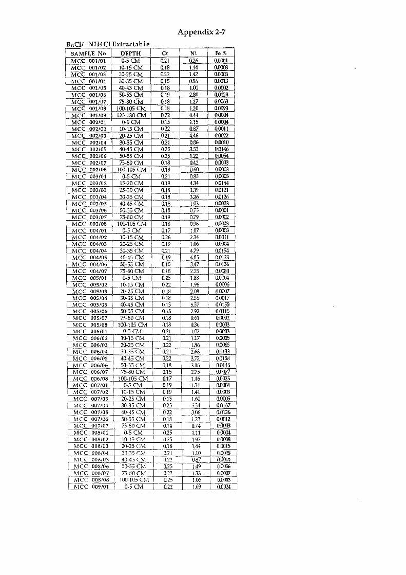
Appendix 2-7
BaClI NH4Cl Extractable I SAMPLE No DEPTH Cr Ni Fe % i MCC 001/01 0-5CM 0.21 026 0.0001
MCC 001102 10-15 CM 0.18 1.14 O.llOO3 MCC 001103 20-25 CM 0.22 1.42 0.0003 MCC 001/04 30-35 CM 0.15 0.96 0.0013 MCC 001/05 40-45 CM 0.18 1.00 0.0Q02
MCC 001/06 50-55 CM I 0.19 2.80 0.0128 MCC 001/07 75-80CM I 0.18 =F 127 0.0063 MCC 001/08 100-105CM 0.18 120 0.D093 MCC 001/09 125-130CM 0.22 0.44 0.0004 MCC 002/01 0-5CM 0.15 1.15 0.D004 MCC 002/02 10-15 CM 0.22 0.87 0.0011 MCC 002/03 20-25 CM 0.21 4.46 0.D022 MCC 002/04 30-35 CM 0.21 0.86 0.0010 MCC 002/05 40-45 CM 0.25 3.53 0.0146
~C 002/06 50-55 CM 0.25 1= 122 0.0054
MCC 002/07 75-80 CM 0.18 0.42 0.0003 MCC 002/08 100-105 CM 0.18 0.60 0.0003 MCC 003/01 0-5CM 0.21 0.85 0.0005 MCC 003/02 15-20 CM 0.19 434 0.0144
r-MCC 003/03 25-30 CM 0.18 339 0.0121 I MCC 003/04 30-35 CM 0.18 336 0.0126
MCC 003/05 40-45 CM 0.18 1.03 O.llOO3 MCC 003/06 50-55 CM I 0.18 I 0.75 I 0.0001
i MCC 003/07 75-80CM I 0.19 I 0.79 0.0002
I MCC 003/08 100-105 CM 0.18 0.96 0.0003 MCC 004/01 0-5 CM 0.17 1.07 0.D003 MCC 004/02 10-15 CM 0.26 234 0.0011 MCC 004/03 20-25 CM 0.19 U)6 0.0004 MCC 004/04 I 30-35 CM 0.21 4.79 0.0154
! MCC 004/05 40-45 CM 0.19 4.85 0.0123 MCC 004/06 50-55 CM 0.15 3.47 0.D136 MCC 004/07 75-80CM 0.18 225 I 0.0080 MCC 005/01 i 0-5CM 0.25 1.88 0.0004
~CC 005/02 ... 10-15 CM 0.22 1.96 0.0006 MCC 005/03 20-25 CM 0.18 2.08 0.0007 MCC 005/04 30-35 CM 0.18 2.86 i 0.0017 MCC 005/05 40-45 CM 0.15 5.57 0.Q150 MCC 005/06 I 50-55 CM 0.18 2.92 0.0115 MCC 005/07 ! 75-80 CM 0.18 0.61 i 0.0002 MCC 005/08 100-105 CM 0.18 036 0.0003 MCC 006/01 0-5CM 0.21 1.02 0.0003 MCC 006/02 10-15 CM 0.21 i 1.17 0.0005 MCC 006/03 20-25 CM 0.22 1.86 0.0065 MCC 006/04 30-35 CM 0.21 2.68 0.0133 MCC 006/05 40-45 CM 0.22 I 3.72 0.0158
I MCC 006106 50-55 CM 0.18 3.16 0.0146 MCC 006107 75-80 CM 0.15 2.75 0.0077 MCC 006/08 100-105 CM , 0.17 I 1.16 0.0025 MCC 007101 0-5 CM 0.19 134 I 0.0004 MCC 007/02 10-15 CM 0.19 1.41 0.0003 MCC 007103 20-25 Ov1 0.15 1.60 0.0005
I MCC 007/04 I 30-35 CM 0.25 5.54 0.0167
i MCC 007/05 40-45 CM 0.22 3.06 0.0136 MCC 007/06 SO-55 Ov1 0.18 123 0.0012 MCC 007107 I 75-80 CM 0.14 0.74 0.0003 MCC 008/01 0-5CM 0.25 1.11 0.0004 MCC 008/02 10-15CM 0.25 1.97 0.0003 MCC 008103 20-25 CM 0.18 i 1.44 0.0015 MCC 008/04 30-35 CM 0.21 1.10 O.OlX5 l\iCC 008105 40·45 CM 0.22 0.87 0.000t MCC 008/06 50-55 CM 0.25 1.49 O.D<XXi I'viCC 008/07 75-80 CM 0.22 133 0.0007
L MCC 008/08 100-105 CM 0.25 1.06 O.O<XB i\lCC 009/01~_~5G'1~ ... 0.22 1.69 0.0024
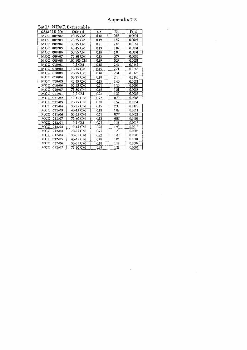
Appendix 2-8
BaClI NH4Cl Extractable SAMPLE No DEPTH Cr Nt Fe % MCC 009/02 1()..15 CM 0.18 0.87 0.0004 MCC 009/03 2()"25CM Q.19 159 0.0019 MCC 009/04 3Q..35 CM 021 2.88 0.0161 MCC 009/05 40-45 CM 0.19 1.07 0.0004 MCC 009/06 5()..55 CM 0.18 1.05 0.0004 MCC 009/07 75·80 CM 0.15 0.79 0.0005 MCC 009/08 100-105 CM 0.19 017 0.0003 MCC 010/01 ()"5CM 0.18 2.49 0.0145 MCC 010/02 1()..15 CM 0.15 2.71 0.0143 MCC 010/03 2()"25CM 0.18 231 0.0176 MCC 010/04 3()"35CM 0.18 2.18 0.0140 MCC 010/05 40-45 CM 0.15 1.40 0.0004 MCC 010/06 5()..55 CM 0.21 1.10 0.0005 MCC 010/07 75-80 CM 0.18 131 0.0008 MCC 011101 ()"5CM 0.22 139 0.0005 MCC 011/02 1()..15 CM 0.22 0.70 0.0008 MCC 011/03 2()"25 CM 0.18 I 157 0.0054 MCC 011/04 3()"35CM 0.15 I 2.33 0.0178 MCC 011/05 40-45 CM 0.18 1.03 0.0011
I MCC 011106 5()..55 CM 0.21 0.71 0.0022 i MCC 011/07 75-80CM 0.18 0.87 0.0005
MCC 012/01 ()"5CM 0.22 1.16 0.0018 MCC 012/02 10-15 CM 0.28 1.93 0.0013
I MCC 012/03 2()"25CM 0.25 123 0.0006 MCC 012/04 3()"35 CM 0.22 1.40 0.0005 MCC 012/05 40-45 CM 0.18 1.04 0.0004 I MCC 012/06 I 5()"55CM 0.18 1.12 0.0007 MCC 012/07 75-80 CM 0.18 121 0.0004
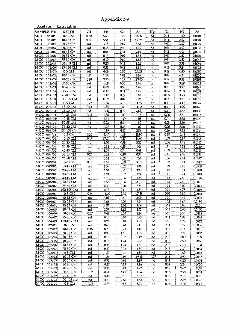
Appendix 2-9
Acetate Extrctable SAMPLE No DEPTH Cd Pb Cr Ni Fe MCC 001101 0-5CM 010 5.43 0.11 1.40 O.OH)9
001/02 10-15 CM 0.24 551 0.11 2.62 0.0004 001103 20-25 CM nd 3.15 0.07 3.47 0.0029 001104 30-35 CM nd 0.58 0.06 3.93 0.0037
40-45 CM 0.54 nd 0.11 4.06 50-55 CM 0.13 nd 0.06 2.62 75-80CM 0.10 0.04 2.52
1 020 0.<» 335 0.31 0.11 524 4.06 0.09 4.95 1.53 0.09 424 3.95 0.17 839
MCC nd 1.09 0.09 3.69 MCC nd 0.80 0.09 3.92 MCC nd 0.17 0.04 3.59 !MCC nd 0.1 0.06 3.93 MCC 0.09 0.04 3 MCC 5.86 nd 0.11 4.47
nd 0.11 4.95 nd 0.11 3.87 nd 0.06 3.51
nd nd 0.04 338 OJXl23 nd nd 0.08 3.59 0.0013 nd nd 0.06 3.46 0.0052 nd nd 0.16 0.0044
MCC 0.20 nd 0.10 MCC 0.17 nd 0.09 MCC nd 0.06 MCC 004/04 nd 0.11 MCC 004/05 nd 0.09 MCC 004/06 nd 0.11 MCC 004/07 nd rid 0.06 MCC 005/01: 0-5CM 0.13 nd 0.07 MCC 005/02 10-15 eM nd 1.86 nd 0.09 MCC 20-25 CM nd 323 rid 0.13 MCC 30-35 CM nd 1.74 nd 0.11 MCC 40-45 CM nd 135 nd 0.13 MCC 50-55 eM nd 3.13 nd 0.13 MCC 75-80 CM nd 214 nd 0.11 !M 100-10:) eM nd 154 nd 010
0.34 17.58 nd 0.06 nd 1 3.09 nd 0.10 nd 3.61 0.90 2.94 nd 0.13 0.0150 nd 1.57 2.90 3.06 nd 0.11 0.0241
40-45 CM nd 237 1.12 232 nd 0.13 0.0170 006/06 50-55 eM 0.07 0.42 0.50 134 nd 0.0024 006/07 75-80 CM nd 0.10 020 093 nd 0.0044 006108 100-105 0,1 nd 0.23 0.28 1.63 nd 0.0012 007/01! 0-5 eM nd 0.65 0.70 5.11 nd 0.0096 007/02 10-15 eM 0.46 015 023 1.42 nd 0.0021 007/03 20-25 CM nd 039 1.61 135 nd 0.0062 007/04 30-35 CM nd 0.16 0.92 0.49 nd 0.0109
40-45 CM 0.18 114 652 nd 0.0016 114 O.Q1o.l 0.93 0.15 0.0054 011 0.13 0.0013 0.19 0.11 0.0042 0.80 0.13 O.02o.l 055 033 0.0030 0.43 0.13 0.G108 1.49 .16 2.58 0.0054
008/07 0.86 .16 2.14 0.0070 008/08 100-105 eM 0.63 2.89 0.00-lS 009/01 0-5 CM 0.88 2.05 OJXJ67
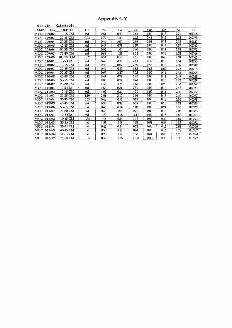
Appendix 2~10
Acetate Extrctable SAMP~ DEPTH Hrd Ph Cu Zn Hg Cr Ni Fe MCC 10-15 CM d 0.61 033
=t=~ 0.00 0.13 i 211 0.0018
MCC 009/03 20-25 CM 0.02 0.74 1.43 0.48 0.13 2.13 0.0075 MCC 009/04 30-35 CM nd 0.44 2.00 2.06 om 0.13 2.15 0.0133 MCC 009/05 40-45 CM I nd 0.47 0.78 1.07 0.00 0.16 1.97 0.0042 MCC 009/06 50-55 _M I nd 0.92 1.00 1.40 0.00 0.13 2.58 0.0072 I MCC 009/07 75-80 CM nd 0.96 116 1.14 0.00 0.16 3.53 0.0046 MCC 009/08 100-105 CM 0.02 0.53 0.58 2.55 0.00 0,45 I 3.09 0.0042 ! MCC 010101 0-5CM nd 0.40 035 2.89 039 . 0.18 I 1.84 0.0155 ! MCC 010/02 10-15 CM nd 036 0.07 I 2.10 0.55 0.16 2.05 0.0087 !
MCC 010/03 20-25 CM nd 0.44 0.89 I 1.58 0.68 0.Q9 212 0.0215 !
MCC 010/04 30-35 CM nd 0.69 217 318 0.00 0.13 235 0.0205 ! MCC 010/05 40-45 CM 0.12 0.44 0.79 1.40 0.00 0.16 2.49 0.0025 MCC 010/06 50-55 CM nd 0.05 0.94 0.48 0.00 0.15 2.42 0.0029 i MCC 010/07 75-80 CM nd 0.52 316 0.68 0.00 010 258 0.0051 ;
MCC 011/01 0-5 CM nd 1.62 0.51 7.91 0.00 0.13 2.47 0.0023 MCC 011/02 10-15 CM nd LOS 014 +4.71 0.00 0.11 230 0.0062 MCC 011/03 20-25 CM 1.19 2.01 2.12 2.01 0.00 0.13 2.10 0.0097 MCC 011/04 30-35 CM 0.03 0.48 0.81 0.91 0.00 0.18 1.86 0.0098
cMCC 011/05 40-45 CM nd 033 039 039 0.00 0.15 L 1.82 0.0033 IMCC 011/06 50-55 CM nd 0.45 0.54 1.02 0.00 014 I 216 0.0029 MCC 011/071 75-80 CM nd 0.48 1.05 0.76 0.00 0.18 2.02 0.0035 IMCC 012/01 0-5 CM nd 1.73 0.16 14.11 0.00 0.18 1.87 0.0021 MCC 012/02. 10-15 CM 0.38 1.41 034 3.15 0.00 0.20 1.65 OJXl13 MCC 012/03 20-25 CM nd 1.55 0.93 1.83 om 013 1.85 0.0032 MCC 012/04 30-35 CM nd 0.48 0.54 0.72 0.00 0.18 2.03 0.0060 MCC 012/05 40-45 CM nd 0.50 0.82 0.64 0.00 0.11 1.73 0.0067 MCC 012/06 50-55 CM nd i 018 1.32 1.56 om 0.09 1.28 I 0.0070 MCC 012/07 75-80 CM 0.35 0.51 5.38 10.39 0.00 0.15 1.36 0.0079
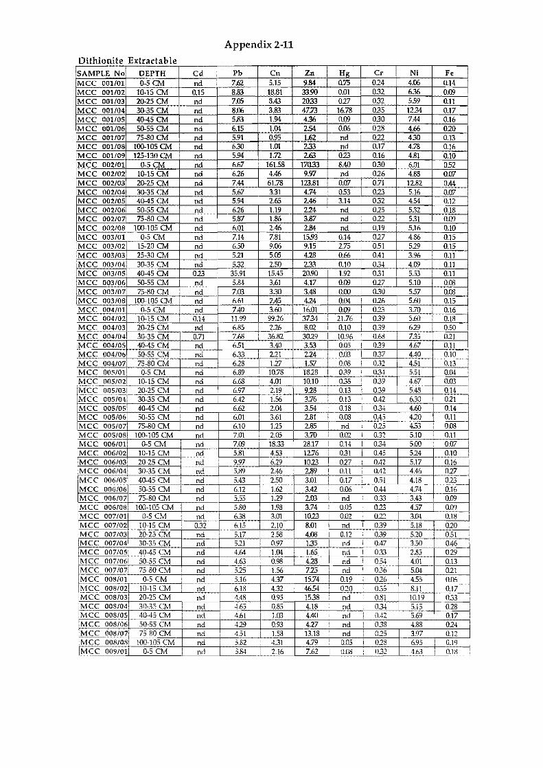
Appendix 2-11
Oithionite Extractable ISAMPLE No DEPTH Cd Pb Cu Zn Hg Cr Ni Fe MCC 001/01 0-5 CM nd 7.62 5.15 9.84 0.75 024 4.06 0.14
1001102 10-15 CM 0.15 8.83 18.81 33.90 0.Q1 032 6.36 0.09 001/03 20-25 CM 7.05 8.43 20.33 027 032 559 0.11 001/04 30-35 ( 8.06 3.83 47.73 16.78 035 1234 0.17 001105 40-45 5.83 4.36 0.09 030 7.44 0.16
MCC 001/06 50-55 6.15 2.54 0.06 028 4.66 020 IMCC 001107 75-80 5.91 0.95 1.62 nd 0.22 430 0.13 MCC 001/08 100-105 CM nd 630 1.01 2.33 nd 0.17 4.78 0.16 MCC 001109 125-130 CM nd 5.94 1.72 2.63 023 0.16 4.81 0.10 .MCC 002/01 0-5CM nd 6.67 161.58
iii 6.01 052
MCC 002/02 10-15 CM nd 626 4.46 26 I 4.88 0.07 MCC 002/03 20-25 CM nd 7.44 61.78 1 71 12.82 0.44 MCC 002/04 30-35 CM nd 5.67 3.31 5.16 0.07 MCC 002/05 40-45 CM nd 5.94 2.65 2.46 3.14 032 4.54 0.12 MCC 002/06 50-55 CM nd 626 1.19 224 nd 025 532 0.18 MCC 002/07 75-80 CM nd 5.87 1.86 3.87 nd 0.22 5.31 0.09 MCC 002/08 100-105 CM nd 6.01 2.46 2.84 nd 1 0.19 5.16 0.10 MCC 003/01 0-5CM nd 7.14 7.81 15.93 0.14 027 4.86 0.15 MCC 003/02 15-20 CM nd 6.50 9.06 9.15 2.75 0.51 529 0.15 MCC 003/03 25-30 CM nd 521 5.05 428 I 0.66 0.41 3.96 0.11
'MCC 003104130-35 CM nd 532 2.50 2.33 0.10 034 4.09 0.11 MC 40-45 CM 023 35.91 15.45 20.90 1.92 I 0.31 5.53 0.11 MC 50-55 CM nd 5.84 3.61 4.17 0.09 027 5.10 0.08 MC 75-80 CM nd 7.03 330 3.48 0.00 0.30 5.57 0.08 MCC 100-105 CM nd 6.61 2.45 424 0.04 ! 026 5.60 0.15 MCC 004/01 0-5CM nd 7.40 3.60 16.Q1 0.09 I 023 3.70 0.16 MCC 004/02 10-15 CM 0.14 11.99 99.26 3734 21.76 ~ 039 5.60 0.18 .MCC 004103 20-25 CM nd 6.85
~~o 039 629 0.50
MCC 004/04 30-35 CM 0.71 7.68 36.82 .96 0.68 7.35 021 'MCC 004/05 40-45 CM nd 651 3.40 .05 I 039 4.67 0.11 MCC 004/06 50-55 CM nd 633 2.21 .03 1 0.37 4.40 0.10 MCC 004/071 75-80 CM nd 6.28 1. .08 ! 032 451 0.13 MCC 005101, 0-5 CM nd 6.89 10.78 1828 I 039 I 034 5.51
~ MCC 005/02 10-15 CM nd 6.68 4.01 10.10 038 I 039 4.67 MCC 005/03 20-25 CM nd 6.97 2.19 928 0.13 i 0.39 5.48 MCC 005/04 30-35 CM nd 6.42 1.56 3.76 I 0.13 I 0.42 6.30 I
MCC 005/05 40-45 CM nd 6.62 2.04 3.54 0.18 I 034 4.60 0.14 MCC 005106 50-55 CM nd 6.01 3.61 2.81 ! 0.08 i 0.45 420 0.11 MCC 0051071 75-80 CM nd 6.10 1.25 2.85 nd , 025 453 0.08
~ nd 7.01 2.05 3.70 I 0.02 I 0.32 5.10 0.11
MCC nd 7JE 18.33 28.17 0.14 I 034 5.00 0.07 MCC nd 5.81 4.53 12.76 031 i 0.45 524 ... QJL MCC nd 9.97 6.29 1023 027 I 0.42 5.17 0.16 MCC 006/04 30-35 CM nd 5.89 2.46 2.89 I 0.11 0.42 4.46 027 MCC 006/051 40-45 CM nd
II 2.50 3.01 0.17 I 0.51 4.18 &~~ MCC 006/06 50-55 CM nd 1.62 3.42 0.06
, OM 4.74 MCC 006/07 75-80 CM nd 1.29 2.03 I nd I 033
~ Ij MCC 006/08 100-105 CM nd 1.98 3.74 I 0.05 023 IMCC 007/01 0-5 CM nd I 1023 ! 0.02 . 0")'1
MCC 007/02 10-15 CM 0.32 6.15 2.10 8.01 nd ! 039 5.18 020 • MCC 007/03 20-25 CM nd 5.17 2.58 4.08 I 0.12 ; 039
m iMCC 007/04 30-35 CM nd 521 0.97 1.35 I nd i 0.47 0.46 MCC 007/05 40-45 CM nd 4.64 1.04 1.65 I nd I 033 019 MCC 007/06 50-55 CM nd 4.63 0.98 4.28 I nd ,
0.54- 0.13 MCC 007107 75-80 CM nd 525 1.56 725 nd I 021 MCC 008/01 0-5CM nd 5.16 4.37 15.74 : 0.19 I 026 455 0.06 MCC 008/02 10-15 CM nd 6.18 4.32 46.54 ! 010 I 0.35 8.11 0.17 IMCC 008/03 20-25 CM nd 4.48 0.95 1538 ; nd I 0.81 10.19 0.33 IMCC 008/04 30-35 CM nd 4.65 0.85 4.18 I nd 1 0.34 5.15 018 MCC 008/05 40-45 CM nd a±m I nd I 0.42 5.69 0.171 MCC 008106 50-55 CM nd 27 I nd i 038 4.88 024 MCC 008/07 75-/10 CM nd ; nd 0'- 3.97 0.12 ~:J
MCC 008/08 100-105 CM nd 5.82 • 4.31 4.79 , 0.05 I 018 6.95 0.19 1~1CC 009/01 O-SCM nd 5.84 1 2.16 7.62 O.OS : O~')
.:;>" 4.63 0.18

Appendix 2-12
Dithionite Extractable SAMPLE No DEPTH Cd Pb Cu Zn Hg Cr Ni Fe !MCC 009/02 1()"15 CM nd 5.43 1.56 11.25 I nd 033 5.62 0.11 MCC 009/03 2()..25 CM nd 4.66 1.26 1121 I nd 0.42 4.71 0.18 MCC 009/04 30-35 CM nd 4.18 0.80 1.91 I nd 039 351 032 D404Sa. nd 4.86 0.89 758 ! nd 030 4.81 0.17 MC 5()..55 CM nd 5.1~--t--h00 4.95 i nd 026 521 0.19 ,MC 75-80CM nd 5.46 1.15 338 0.10 026 451 0.16 MCC 009/08 100..105 CM nd 6.00 4.27 20.97 0.06 025 7.14 0.19 MCC 010/01 ()"5CM nd 627 2.70 4.12 0.10 052 4.81 025 MCC 010/02 1()"15 CM nd i 5.66 1.42 2.74 0.13 0.42 5.03 023 MCC 010/03 2()"25 CM nd i 5.12 0.88 2.63 0.04 0.49 4.66 035 MCC 010/04
1
3()"35 CM nd 4.86 2.20 16.53 nd 0.63 7.44 025 MCC o 40-45 CM nd 526 0.72 9.06 0.10 0.44 5.62 021 MCC 01 55 CM nd 5.60 0.90 7.92 0.03 0.41 5.71 021 MCC 010/07 75-80 CM nd 4.79 6.90 1.89 i 0.08 026 457 MCC 011/011 ()"SCM nd 6.04 3.68 18.99 I 032 036 5.49 0.12 MCC 011/02 1()..15 CM 5.73 2.80 10.18 I 0.03 028 520 0.14 MCC 011/03 20-25 CM S38 0.92 4.12 I 0,06 0.50 5.41 024 MCC 011/04 30-35 CM nd 5.17 1.21 3.65 I nd 0.41 438 035 MCC 011/05, 40-45 CM nd 520 0.71 4.69 i nd 038 4,03 0.17 MCC 011/06 50..55 CM nd 4.69 1.02 4.49 I 0.14 038 3.55 0.13 MCC 011/07 75-80 eM nd 429 5.00 2.31 i 0,03 026 2.14 om MCC 012/01 ()"5CM nd 6.90 6.97 25.73 0,06 0.36 2.11 0.15 MCC 012/02 1()..15 CM nd 523 4.93 8.94 I 0.14 035 526 0,08 MCC 012/03 20-25 CM nd 4.82 1.04 15.69 0.05 0.54 7.45 0.12 MCC 012/04 30-35 CM nd 4.46 1.00 14.42 0.03 I 0.40 4.73 0.11 MCC 012/05 40-45 CM nd 3.94 1.49 8.13 i 0.06 i 0.41 6.89 0.15 MCC 012/06 50-55 CM nd 4.42 0.50 7.59 nd 0.55 5.98 039 I MCC 012/07, 75-80 CM nd 4.40 3.81 36.55 0.10 0.43 2.87 I 011
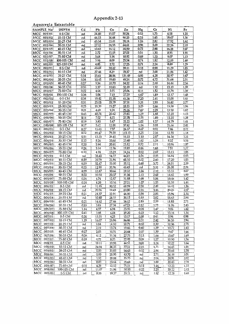
Appendix 2-13 A .quaregxa Est t bi rae a e SAMPLE No. DEPTH Cd Pb Cu Zn Hg Cr Ni Fe MCC 001/01 0-5CM nd 26.40 13.00' 3024 053 1.75 6.58 120 MCC 001102 10-15 CM nd 44.53 34.44 9813 0.55 1.65 19.67 136 MCC 001/03 20-25 CM nd 1 45.54 23.41 7824 126 2.82 17.52 1.62 MCC 001/04 3O-35CM nd 27.12 24.55 64.61 0.98 3.69 22.36 253 MCC 001/05 40-45 CM nd 10.63 16.12 35.90 0.73 2.88 16.28 2.00' MCC 001106 50-55 CM nd I 2.72 15.05 Tl.02 0.51 1.30 8.95 1.91
·MCC 0011071 75-80CM nd 3.64 5.14 18.92 0.69 1.53 9,(17 1.13 MCC 001/0s1 100-105 CM nd 5.96 8.09 25.54 0.74 1.82 12.09 1.40 MCC 001/09 125-130 CM nd 4.85 2.72 17.25 0.71 2.34 8.89 1.29 MCC 002/01 0-5CM nd 43.69 30.22 39.11 0.18 0.98 11.29 1.03 MCC 002/02 10-15 CM nd 27.46 829 78.37 nd 3.00 21.86 1.42
IMCC 002/031 20-25 CM 054 23.61 38.84 131.49 0.95 428 30.97 3.47 MCC 002/041 30-35 CM 0.34 10.45 19.60 4924 0.72 4.72 31.68 2.31 MCC 0021051 40-45 CM 027 9.34 20.70 34.32 0.14 2.68 I 14.44 2.56 MCC 002/061 50-55 CM 0.35 I 337
w.I nd 1.92 I 13.19 159
MCC 002/071 75-80 CM 022 4.04 0.11 1.52 11.79 139 !
.MCC 0021081 100-10SCM 036 5.06 4.67 1.89 12.17 1.48 MCC 003/011 0-5CM 0.34 I 19.42 15.58 4126 720 2.41 ISH 1.,41 MCC 003/021 15-20CM 031 I 25.03 33.79 I 37.51 331 2.93 16. 2.77
IMCC 003~ 025 i 11.39 15.27 33.55 3.25 2.66 15.58 1.96 MCC 0031 021 i 4.69 9.74 2526 7.67 229 1 13.58 1.82 MCC 0031051 40-45 CM 0.45 40.74 20.62 29.65 129 1.68 1 12.20 1.13 MCC 003/061 50-55 CM 0.11 7,(12 8.72 25.78 2.55 1.80 15.20 138 MCC 0031071 75-80CM 0.19 I 3.83 5.47 2522 1.02 137 I 14.79 1.41 1 MCC 00310S i 100-105 CM 0.17 I 5.62 1 12.01 37.42 1.14 3.18 i 21.66 2.42
IMCC 004/011 0-5CM 0.27 15.63 1 737 2637 4.67 I 0.92 I 7.46 0.72 IMCC 004/021 10-15 CM 0.72 I 89.47 I 79.59 113.15 225 I 2.16 I 12.55 1.18 MCC 004/031 20-25 CM 0.51 I 13.53 I 26.45 5413 1.10 I 2.87 ,
14.56 314 I I
'MCC 004/041 30-35 CM 033 I 826 20.68 I 23.40 1.62 1.58 i 832 1.86~ I
MCC 004/051 40-45 CM 030 5.94 20.61 I 23.12 0.92 I 2.11 ! 10.96 1.87 ~ ... 004/061 50-55 CM 024 1 3.54 12.96 19.89 0.86 i 1.63 7.51 1.77 MCC 004/071 75-80 CM 0.18 4.55 13.29 24.14 0.82 ! 2.69 • 13.13 1.88 i
i MCC 005/011 0-5CM nd ! 38.43 54.77 44.93 0.56 1 0.95 I 16.84 I 0.93 1
IMCC 005/021 10-15 CM 039 20.79 21.96 1 65.10 032 2.60 I 17.20 UE I
MCC 005/031 20-25 CM 029 I 32.47 35.00 55.12 • 0.40 3.72 i 24.81 259 MCC 005/041 30-35 CM 0.23 I 12.90 I 35.96
M~ 3.32 i 26.38 2.84-
IMCC 005/051 40-45 CM 029 12.87 1 30.66 2932 1 2.10 I 15.55 3.07 i IMCC 005/061 50-55 CM 0.23 I 10.50 20.37 3136 I 2.63 i 14.65 1.99 MCC 005/071 75-80CM 026 ! 4.74 I 12.87 31.88 1.09 1.84 I 10.48 1.42 MCC 005/081 100-105 CM 024 I 4.20 I 10.16 2721 1.00' 1 1.55 ! 11.59 1,44
IMCC 006/011 0-5CM nd 51.85 80.52 68.99 0.58 I 2.49 16.42 136 'MCC 006/021 10-15 CM nd ! 20.56 I 19.43 : 60.00 0.16 1 3.46 i 20.25 2.ffl
MCC 006/031 20-25 CM 0.21 I 24.37 1 22.91 44.80 038 2.85 ! 15.94 2.34 I MCC 006/041 30-35 CM ! nd i 10.40 24.55 i 38.15 0.19 ! 2.82 18.63 2.84 MCC 006/051 40-45 CM 0.21 1 14.62 27.46 36.12 0.19 i 2.59 i 11.83 2.71 MCC 006/061 50-55 CM 033 3.89 27.34 67.23 0.12 i 1.73 ! 11.96 2.43
IMCC 006/071 75-80CM 1.14 I 4.97 ! 6.94 23.93 028 I 1.47 I 9.06 I 1.62 IMCc 006/osl 100-105 CM 0.41 I 5.98 i 6.04 2920 013 i 1.12 13.16 1.34 MCC 0071011 0-5CM 026 : 13.51 I 425 13.17 0.58 l 0.41 0.94 0.98 MCC 007/021 10-15 CM 129 i 16.00' i 23.96 i 86.06 031 2.42 36.35 2.94 MCC 007/03 20-25 CM i nd I 9.84 ! 14.10 53.71 0.10 I 2.30 32.36
, 2.78
MCC 007/041 30-35 CM nd I 2.19 13.74 19.46 0.40 I 139 I 10.72 2.43 MCC 007/051 40-45 CM 0.27 2.05 , 10.31 24.44 0.00' 1.39 9.67 1.66 MCC 007/061 50-55 Ovf 026 I 4.12 I 11.34 27.75 0.13 1.66 13.67 "~I
IMCC 007/07 75-80 CM 028 4.72 I 815 22.99 0.09 I 127 ! 10.50 136 MCC 008/011 0-5CM nd 1 19.11 I 19.98 44.51 0.02 I 124 ! 12.22 1.04 1 MCC 008/02! 10-15 CM nd I 24.04 34.35 77.51 0.15 1.71 • 14.45 1.81 MCC 008/031 20-25 CM nd I 0.00 i 35.85 54.63 0.52 I 2.84
, 30.68 2.70 I I
MCC 008/041 30-35 CM nd 0.00 28.95 43.70 nd 2.71 ,
36.58 3.01 i I
.MCC 008/051 4O-45CM nd I 1.92 i 28.88 35.75 nd 2.06 : 20.91 2.02 MCC 008/061 50-55 CM nd I 0.00 I 23.64 I 35.63 nd 1.88 1 20.45 :!"S
:MCC 008/071 75-80CM 0.51 ! 419 12.52 71.11 0.13 1.46 i 12.23 1.53 MCC 008/081 100-105 CM i nd 11.07 21.96 50.50 0.22 1 228 · 33.22 2.43 -I ~009/011 0-5 CM nd i 8.58 19.37 35.11 nd I 1.62 12.26 \.68
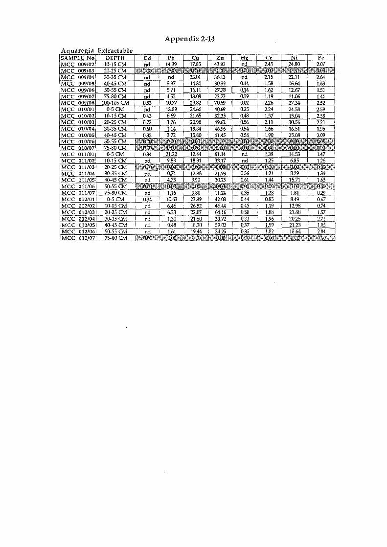
Appendix 2-14

Appendix 2-15 Total Extractable
SAMPLE No DEPTH Cd Pb Cu Zn Hg Cr Ni Fe I MCC 001101 0-5CM 020 41.46 22.68 55.05 1.41 2.31 12.30 1.35 I MCC 001/02 10-15 CM 0.39 62.00 56.94 149.86 0.56 226 29.80 1.45 .j
·MCC 001/03 20-25 CM nd 58.77 3332 108.65 153 3.42 28.00 1.73 1 MCC 001/041 30-35 CM nd 37.71 29.09 115.67 17.76 I 425 39.61 2.70 I MCC 001/05 40-45 CM nd 18.74 18.81 43.40 0.81 3.46 28.79 223 1 MCC 001106 50-55 CM nd 11.10 1631 41.94 0.56 1.84 19.03 2.14 i MCC 001/07 75-80 CM nd 11.53 6.37 29.04 I 0.69 1.96
• MCC 001108· 100-105 CM nd 14.23 9.42 35.16 0.74 211 1.58 I
MCC 001/09 125-130 CM nd 12.67 4.87 23.57 I 0.94 2.83 1.40 i MCC 002/01 ! 0-5CM nd 57.02 19535 23159 857 I 152 23.39 1.56· MCC 002/02 i 10-15 CM 021 37.96 14.22 93.22 nd 3.57 ,31.85 1.50 I
,MCC 002/03 20-25 CM 0.74 38.44 103.79 76754 1.02 537 . 56.63 3.93 i MCC 002/04 30-35 CM 034 19.62 23.79 56.27 115 514 41.38 2.38 1 MCC 002/051 40-45 CM 017 18.80 24.08 53.66 318 3.33 26.43 2.70 MCC 002/06 ' 50-55 CM 0.35 11.74 12.17 40.55 nd 2.46 23.33 1.78 MCC 002/071 75-80 CM 012 11.71 6.07 31.23 0.11 It: m'~
i MCC 002/081 100-105 CM 0.36 12.82 9.74 31.77 4.67 231 21.14 1.58 ;
MCC 003/01 1 0-5CM 055 3431 26.81 69.81 734 3.00 25.26 1.57 I
MCC 003/021 15-20 CM 0.44 47.49 51.01 82.77 6.06 3.74 31.21 2.95 MCC 003/03 1 25-30 CM 025 2222 22.59 58.66 3.91 336 26.80 2.00
, , MCC 003/041 30-35 CM 0.36 1275 13.75 I 29.96 7.78 2.87 24.54 1.% MCC 003/051 40-45 CM 0.67 83.18 37.88 52.77 321 221 22.15 1.23 MCC 003/06 50-55 CM 0.11 14.69 12.87 31.% 2.65 2.33 24.65 1.46 1
MCC 003/071 75-80 CM 0.19 12.78 9.13 30.88 1.02 1.92 24.62 1.50 MCC 003/081 100-105 CM 0.17 j 14.44 15.22 45.67 1.19 3.79 34.78 2.57 MCC 004/011 0-5CM 0.47 28.82 12.87 63.69 4.76 1.43 16.70 0.91 MCC 004/021 10-15 CM 1.02 i 126.17 195.91 23822 24.01 2.90 ! 24.65 136 MCC 004/03 i 20-25 CM 051 23.73 30.24 66.78 121 3.51 25.37 3.76
IMCC 004/041 30-35 CM 1.04 19.44 58.41 68.62 12.59 2.58 23.00 2.11 MCC 004/051 40-45 CM 0.30 17.35 25.56 40.83 0.97 2.77 22.95 2.00
IMCC 004/061 50-55 CM 0.48 12.33 15.74 36.00 0.89 227 17.84 }.89 MCC 004/071 75-80 CM 0.18 13.09 14.82 32.30 0.90 325 23.23 2.02
IMCC 005/011 0-5 CM 0.13 53.37 68.09 76.01 0.95 1 27.54 0.97 ·MCC 005/021 10-15 CM 0.39 31.72 26.73 78.40 0.69 26.64 1.00 MCC 005/03 20-25 CM 029 43.51 38.42 69.06 053 4.42 35.87 2.73 MCC 005/041 30-35 CM 023 24.10 39.22 51.88 0.14 4.rn 39.29 3.06 MCC 005/051 40-45 CM 029 24.14 33.92 51.87 2.54 2.72 28.58 i 3.24-
IMCC 005/061 50-55 CM 023 21.60 25.59 50.22 222 339 24.17 2.12 iMCC 005/071 75-80 CM 016 13.20 14.46 37.78 1.09 2.38 18.71 I 1.51
•
'MCC 005/081 100-105 CM 014 13.72 12.S9 33.34 1.10 225 21.82 155 iMCC 006/01 0-5CM 034 77.41 104..33 125.65 0.72 3.10 1 26.25 I 1.43 MCC 006/021 10-15 CM nd 32.28 25.12 79.40 0.47 4.22 30.08 2.17
,MCC 006/031 20-25 CM 021 41.06 30.76 79.02 0.66 3.62 26.57 2.53 MCC 006/041 30-35 CM nd 20.74 30.54 54.64 019 i 3.56 28.76 3.14 MCC 006/051 40-45 CM 021 26.70 31.73 56.25 0.38 3.44 22.33 2.97 .. -.~-
MCC 006/061 50-55 CM 0.40 13.28 30.03 102.00 0.18 2.60 23.19 2.61 'MCC 006/07! 75-80 CM 1.14 12.68 8.54 32.39 028 2.05 17.15 1.72 IMCC 006/081 100-105 CM 0.41 13.98 8.41 35.09 I 017 1.70 21.62 }.43 ·MCC 007/011 O-SCM 026 22.91 8.31 29.15 1 0.59 0.92 i 8.04 I 1.17 IMCC 007/021 10-15 CM 2.07 24.82 26.87 96.30 033 3.13 45.08 3.14 MCC 007/031 20-25 CM nd 17.37 18.71 60.81 022 2.97 41.87 , 3.30 MCC 007{041 30-35 CM nd 9.99 16.27 27.82 0.40 21-1 21.85 2.92
I,MCC 007/051 40-45 CM Q27 9.21 13.09 "
43.26 0.07 2.00 18.07 1.97 MCC 007/061 50-55 CM 0.26 10.91 13.98 36.86 ~2~ 21.31 1.83 MCC 007/071 75-80 CM 028 1220 lUX! 32.72 1.92 18.61 1.57
.MCC 008/01 i 0-5CM nd 29.32 25.05 66.64 o 1.87 19.77 1.10 rMCC 008/021 10-15 CM nd 35.09 39.45 160.34 0.35 2.43 27.52 1.98 'MCC 008/03 ! 20-25 CM nd 7.36 i 38.60 80.43 052
, 3.96 47.12 3.05 ·MCC 008/041 30-35 CM nd 7.18 30.76 50.66 nd 3.59 45.07 3.29 IMCC 008/051 4O-45CM nd 9.22 30.69 42.77 nd 2.83 1 30.14 I 2.19 MCC 008/061 50-55 CM 0.02 7.'23 26.40 44.20 nd 2.67 29.39 i 2.53
IMCC 008/07 : 75-RO CM 0.51 11.37 15.08 89.00 0.13 2.00 19.66 1.66 IMCC 008/081 100-105 CM nd 19.09 26.94 57.61 I 017 2.95 44.12 2.62 IMCC 009/011 0-5 CM 0.02 17.57 22.76 65.62 0.08 2.32 20.6.3 1.87
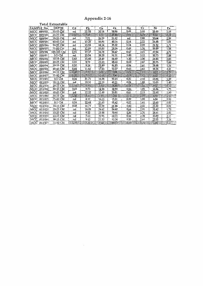
Appendix 2-16
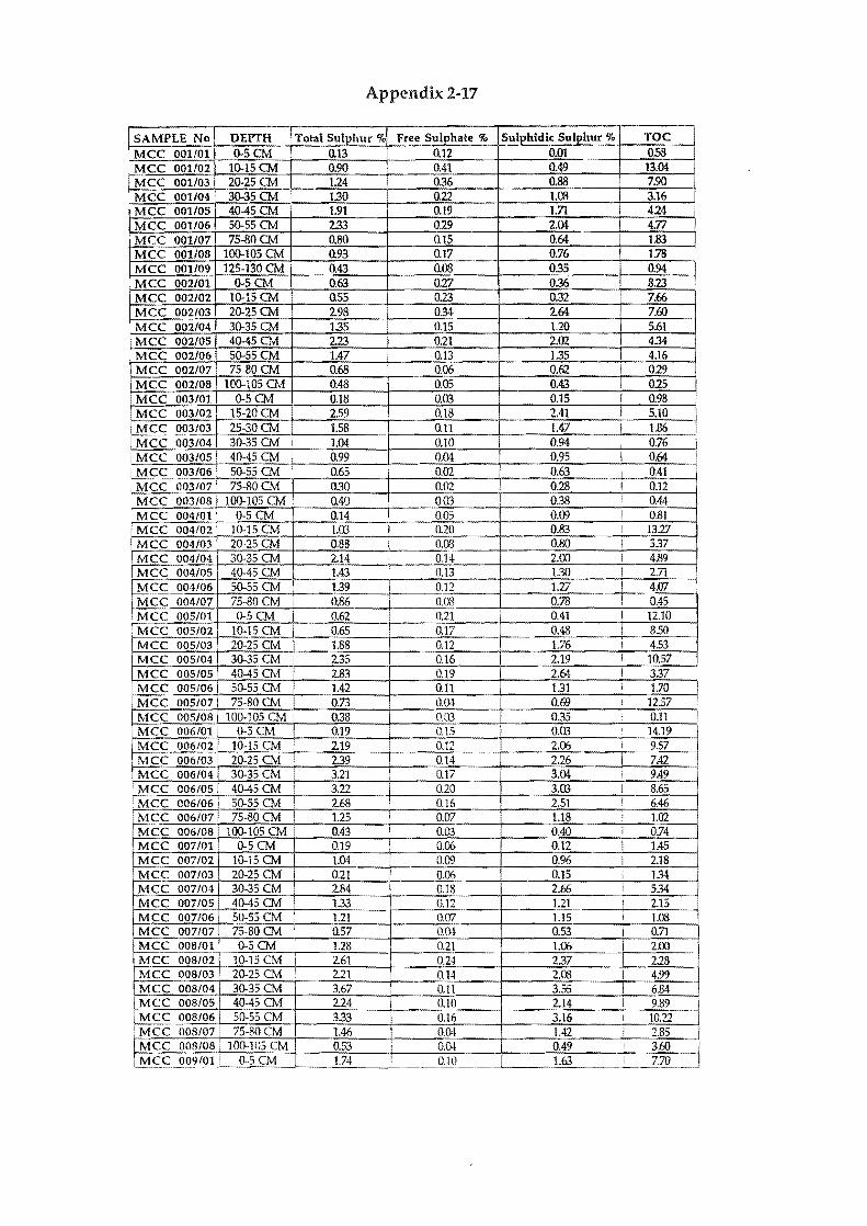
Appendix 2-17
SAMPLE No DEPTH Total Sulphur % Free Sulphate % Sulphidic Sulphur % TOC
MCC 001101 0-5CM 0.13 0.12 0.01 0.58 MCC 001/02 10-15 CM 0.90 0.41 0.49 13.04 MCC 001/03 20-25CM 1.24 036 0.88 7.90 MCC 001/04 30-35CM , 1.30 0.22 1.00 3.16 MCC 001/05 4O-45CM 1.91 0.19 1.71 424 MCC 001106 50-55 CM 2.33 0.29 2.04 471 MCC 001/01 75-80CM 0.80 0.15 0.64 1.83 MCC 001/08 lQ()..105 CM 0.93 0.17 0.76 1.78 I
MCC 001109 125-130 CM 0.43 0.08 0.35 0.94 I IMCC 002/01 0-5CM 0.63 0.27 036 8.23 I MCC 002/02 IO-l5 CM 0.55 0.23 0.32 7.66
~f 002103 20-25CM 2.98 0.34 2.64 7.60 .MCC 002/04 30-35CM 1.35 0.15 1.20 5.61 MCC 00210S 40-45 CM 2.23 0.21 2.02 4.34 MCC 002/06 50-55CM 1.47 0.13 1.35 4.16 MCC 002/01 75-BOCM 0.68 0.06 0.62 I 0.29 MCC 002108 lQ()..105 CM 0.48 0.05 0.43 I 0.25 MCC 003/01 0-5CM 0.18 0.03 0.15 I 0.98
'MCC 003/02 15-20CM 2.59 0.18 2.41 5.10 MCC 003/03 25-30CM 1.58 0.11 1.47 I 1.86 I ~ .•.. ~.-MCC 003/04 30-35 CM 1.04 0.10 0.94 0.76 i MCC 003/05 40-45 CM 0.99 0.04 0.95 ! 0.64
! MCc:....00~06 50-55 CM , 0.65 I 0.02 0.63 I 0.41 • MCC 003/07 75-BOCM Q.30 0.02 0.28 I 0.12 'MCC 003/08 lQ()..105 CM 0.40 0.03 0.38 I 0.44 'MCC 004/01 0-5CM 0.14 0.05 0.00 I 0.81 MCC 004/02 i 10-15 CM 1.03 0.20 0.83 I 13.27 MCC 004103 i 20-25CM 0.88 0.08 0.80 I 537 MCC 004/04 30-35CM 2.14 I 0.14 2.00 I 4.89 MCC 004/05 40-45 CM 1.43 0.13 1.30 I 2.71
'"Met 004/06 50-55 CM 1.39 0.12 1.27 4.07 MCC 004/07 75-80 CM 0.86 0.03 0.78 0.45 MCC 005/01 0-5CM 0.62 0.21 0.41 I 12.10
f"Mcc 005/02 10-15 CM 0.65 0.17 0.48 I 8.50 IMCC 005/03· 20-25CM 1.88 0.12 1.76 I 453
~ 005/04 30-35 CM 2.35 0.16 2.19 I 10.57 MCC 005/05, 40-45 CM 2.83 0.19 2.64 I 337 ,
IMCC 005/06 50-55 CM 1.42 0.11 1.31 : 1.70 IMCC 005/07 75·80CM 0.73 0.04 0.69 ! 12.:1I MCC 005/08 100-105 CM 0.38 0.03 0.35 0.11
.MCC 006/01 0-5CM 0.19 0.15 0.03 , 14.19 MCC 006/02 10·15 CM 2.19 0.12 2.C6 I 9.57 MCC 006/03 20-25 CM 2.39 0.14 2.26
, 7.42
MCC 006/04 30-35 CM 3.21 0.17 3.04 I 9.49 MCC 006/05 40-45 CM I 3.22 0.20 3.m I 8.65 ~CC 006/06 50-55 CM I 2.68 0.16 2.51 i 6.46 'MCC 006/07 75-80CM ! 1.25 0.07 1.18 i 1.02 MCC 006/08 100-105 CM . 0.43 0.03 0.40 i 0.74 MCC 007/01 0-5CM 0.19 0.C6 0.12 I 1.45 MCC 007/02 10-15 CM 1.04 0.00 0.96 I 2.18
~c 007/03 20-25 CM 0.21 0.06 0.15 I 1.34 MCC 007/04 30-35 CM 2.84 0.18 2.66 I 5.34
r¥-CC 007/05 40-45 CM 1.33 0.12 1.21 ---t 2.15 MCC 007/06 50-55 CM 1.21 0.07 1.15 : 1.08 MCC 007/07 75-80 CM U57 0.04 0.53 I 0.71
~c 008/01 i 0-5CM 1.28 0.21 1.C6 j 2.00 MCC 008/02 10-15 CM 2.61 0.24 2.37 I 2.28
'M'cc 008/03. 20-25 CM 2.21 0.14 2.08 I 4.99 MCC 008/04 30-35CM 3.67 0.11 3.55 6.84
j MCC 008/05 40-45 CM 2.24 0.10 2.14 I 9.89 I MCC 008/06 50-55 CM 3.33 0.16 3.16 I 10.21 'MCC 008/07! 75-80CM 1.46 0.04 1.42 ! 2.85 I MCC 008/08' 100-105 CM 0.53 0.04 0.49 I 3.60 LM<:;,<:;,Jl.Q'i/0 l' 0·5 CM 1.74 0.10 1.63 7.70
.-.~--
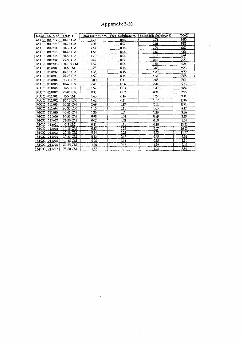
SAMPLE No DEPTH Total Sulphur 0/, Free Sulphate % Sulphidic Sulphur % TOC MCC 009/02 10-15 CM 2.78 0.06 2.71 9.50
·MCC 009/03 20-25 CM 2,(17 0.07 2.01 5.82 MCC 009/04 30-35CM 187 0.14 2.74 6.82 MCC 009/05 4O-45CM 1.65 0.04 loW 4.06 MCC 009/06 50-55 CM 1.20 0,04 1.16 3.98 MCC 009/01· 75-80CM 0,49 0,02 0.47 2:J9 MCC 009/08 100-105 CM 1.59 0.04 1.55 414 MCC 010/01 0-5CM 3.78 0.14 3.63 9.23 MCC 010/02 10-15 CM 4.35 0.15 4,20 9.79 MCC 010/03 20-25 CM 4.59 0.14 4.44 7.68 MCC 010/04 30-35 CM 3.00 0.11 2.88 7.01 i
iMCC 010/05 40-45CM 2.48 0.06 2.41 553 :MCC 010/06 50-55 CM 1.52 0.03 1.49 3.84 MCC 010/~ 75-80 CM 0.33 0.02 0.31 2:JS MCC 011/0 0-5CM 1.43 0.16 1.27 21.03 MCC 011/0 10-15 CM 1.68 0.11 1.57 13.02 MCC 011/03 20-25 CM 2.69 0.17 2.52 12.C)8 MCC 011/04 30-35 CM 1.15 0.11 1.05 4.47 MCC 011/05 ! 40-45 CM I 1.36 0.07 1.29 i 336 MCC 011/06 50-55 CM 0.93 0.04 0.89 319 MCC 011/07 75-80CM 0.02 0.03 0,00 1.54
r¥-CC 012/01 O-SCM 0.21 0.11 0.10 13.22 MCC 012102 10-15 CM 033 0.26 0,07 16.48 MCC 012103 20-25 CM 0.64 0,22 0,43 11.77 MCC 012/04· 30-33 CM 0.83 0.17 0.63 9.90 !
MCC 012/05 1 40-43 CM 0.66 0.11 0.55 8.81 .MCC 012/06 50-55 CM 1.76 0.17 1.59 I 9.45 MCC 012/07 75-80 CM 1.37 0.12 1,25 3.80 I
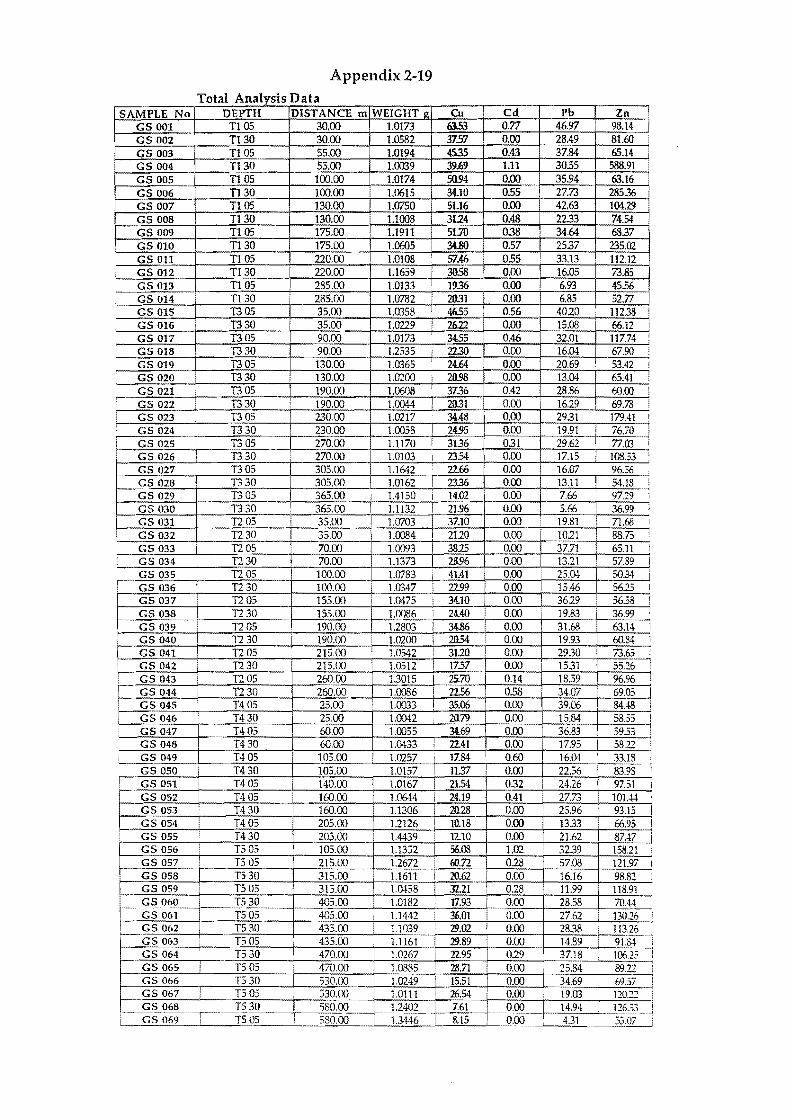
Appendix 2-19
ota nalYSIS a a T lAl'Dt SAMPLE No DEPTH DISTANCE m WEIGHT e: en Cd Pb Zn
GS 001 T1 05 30.00 1.0173 63.53 0.77 46.97 98.14-GS 002 T130 30.00 1.0582 '957 0.00 28.49 81.60 GS 003 TIOS 55.00 1.0194 45.35 0.43 37.84 65.14 GS 004 T130 53.00 1.0039 39.69 1.11 3055 588.91 GS 005 T1 05 100.00 1.0174 5094 0.00 35.94 63.16 GS 006 T130 100.00 UJ615 34..10 055 27.73 285.36 GS 007 T1 05 130.00 1.0750 5Ll6 0.00 42.63 10419 GS 008 T130 130.00 1.1008 3124 0.48 22.33 74.54 GS 009 T1 05 175.00 1.1911 51.70 0.38 34.64 68.37 GS 010 T130 175.00 1.0605 3l.IlO 0.57 2537 235.02 Gson T1 05 220.00 1.0108 57.46 0.55 33.13 112.12 GS 012 T130 220.00 1.1659 I 30.58 0.00 16.0S 73.85 GS 013 T1 OS 285.00 1.0133 ! 1936 0.00 6.93 45.56 GS 014 T130 28S.OO 1.0782 2031 0.00 6.85 52.77 GS 015 DOS 35.00 1.0358 I 4655 0.56 4020 11238 ! GS 016 D30 35.00 1.0229 I 26.21 0.00 15.08 66.12 ! GS 017 DOS 90.00 1.0173 I 3455 0.46 32.01 117.74-GS 018 D30 90.00 1.2535 2230 0.00 16.04 67.90 !
! GS 019 DOS 130.00 1.0365 i 24.64 0.00 20.69 53.42 I GS 020 D30 130.00 1.0200 I 2D.98 0.00 13.04 65.41 GS 021 DOS 190.00 1.0608 3136 0.42 28.86 60.00 I GS 022 T330 190.00 1.0044 2031 0.00 1629 69.78 I
i GS 023 D05 230.00 1.0217 34..4-8 0.00 2931 ! 179.41 ! GS 024 I D30 230.00 1.0058 24.95 0.00 19.91 76.70 GS 025 DOS I 270.00 1.1170 I 3136 031 29.62 77.03 I GS 026 D30 270.00 1.0103 I 23.54- 0.00 17.1S 108.53 I
GS 027 T305 30S.oo 1.1642 22.66 0.00 16.07 96.56 I ~~S028 D30 305.00 1.0162 23.36 0.00 13.11 54.18
, I
GS 029 DOS 365.00 1.4150 14.02 0.00 7.66 97.29 i
GS 030 D30 365,00 1.1132 21.96 0.00 5.66 36.99 , GS 031 T205 35.00 1.0703 37.10 0.00 19.81 71.68 I
GS 032 T230 35.00 1.0084 2120 0.00 1021 88.75 , ! GS 033 T20S 70.00 1.0093 38.25 0.00 37.71 65.11 I I GS 034 ! T230 70.00 1.1373 2&96 0.00 1321 57.89 i GS 035 T205 100.00 1.0783 L 41.41 0.00 i 25.m 5O,3.l
GS 036 T230 100.00 i 1.0347 j 22..99 0.00 I 15.46 56 ~-.LJ I
GS 037 T205 155.00 i 1.0475 34..10 0.00 I 3619 ! 56.58 ! GS 038 T230 155.00 1.0086 24.40 0.00 19.83 36.99 GS 039 T205 190.00 1.2803 3U6 0.00 31.68 63.14 ! GS 040 T2 30 190.00 1.0200 I 2!l54 0.00 19.93 60.84 I
GS 041 T20S 215.00 1.0542 ! 3120 0.00 29.30 73.65 GS 042 T230 21S.OO 1.0512 I 17.57 0.00 15.31 55.26 i
'r--' GS 043 T20S 260,00 1.3015 25.70 0.14 18.59 %.96 I GS 044 T230 260.00 1.0086 I 22.56 0.58 34.07 69,05 I
GS 045 T40S 25.00 1.0033 35.06 0.00 39.06 84.4-8 j GS 046 T430 25.00 1.0042 20.79 0.00 15.84 58.53 ! GS 047 T405 60.00 1.0055 34...69 0.00 36.83 ! 59.53 GS 048 T430 60.00 1.0433 22.41 0.00 i 17.95 58." I
~049 T405 105.00 1.0257 i 17.84- 0.60 16.m 33.lS I
GS 050 i T430 105.00 i 1.0157 1137 0.00 22.56 I 83.93 ! GS 051 T40S 140.00 I 1.0167 21.54 032 i 24.26 97.51 I GS 052 nos 160.00 1.0644 I 24.19 0.41 27.73 101.44 ,
GS 053 T430 160.00 1.1306 20.28 0.00 25.96 93.15 I GS 054 T405 205.00 1.2126 I 10.18 0.00 13.33 66.95 ! GS 055 T430 205.00 1.4439 12.10 0.00 21.62 87,47 GS 056 T505 105.00 1.1352 56.08 1.02 32.39 158.21 i
GS 057 TS05 215.00 1.2672 W.72 0.28 57.08 121.97 I GS 058 T530 315.00 1.1611 20.62 0.00 16.16 98.82 GS 059 T50S I 315.00 l.otS8 32.21 028 11.99 118.91
~S060 T530 405.00 1.0182 17.93 0.00 28.58 70.44 GS 061 T505 405.00 1.1442 36.01 0.00 27.62 130.16 r GS 062 T530 435.00 1.1039 29.02 0.00 28.38 113.26 GS 063 T505 435.00 1.1161 29.89 0.00 14.89 9U\4 GS064 T530 470.00 i 1.0267 22.95 029 37.18 106.25 I GS 065 T505 470.00 1.0885 28.71 0.00 I 25.84- 89,;'1 1 GS 066 T530 530.00 1.0249 15.51 0.00 34.69 69.57 GS 067 T505 530.00 1.0111 26.54 0.00 19.03 I 120.'" i
~}6~: --t---fs~~ 580.00 1,2402 7.61 0.00 14.94 I 126.33 580.00 1.3446 IU5 0.00 I 4.31 i 55.07
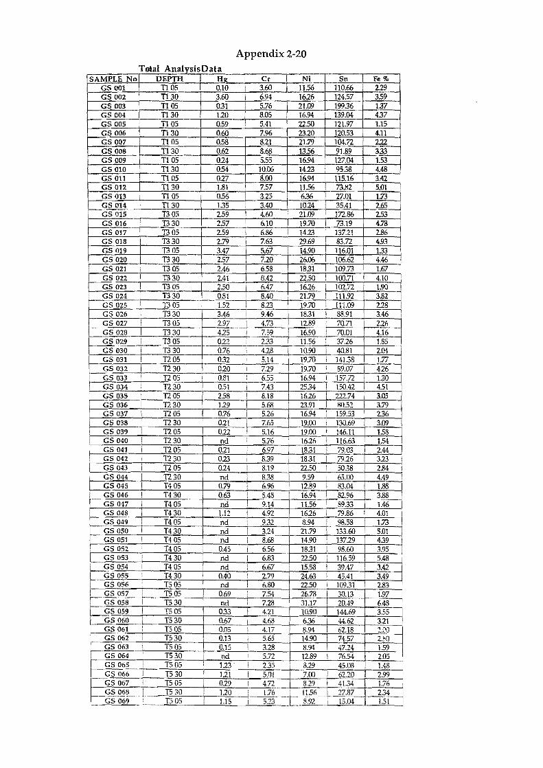
Appendix 2-20 eta nalYSlS T I A I . D ata
SAMPLE No DEPTH Hit Cr Ni Sn Fe % GS 001 nos 0.10 3.60 11.56 110.66 229 GS 002 n30 3.60 6.94 1626 124.57 3.59 GS 003 nos 031 5.76 2Ul9 19936 137 GS 004 n30 120 8.05 16.94 139.04 437 GS 005 nos 0.59 5.41 22.50 121.97 1.15 GS 006 n30 0.60 I 7.96 2320 120.53 4.11 GS 001 nos 058 8.21 21.79 104.72 222 GS 008 n30 0.62 8.68 13.56 91.89 333 GS 009 I nos 024 5.55 16.94 127.04 1.53 GS 010 n30 0.54 10.06 1423 9538 4.48 GSOll I nos 027 8.00 16.94 115.16 3.42 !
GS 012 n30 1.81 7.57 11.56 73.82 5.01 I GS 013 nos 0.56 3.25 636 27.01 1.73 I GS 014 n30 135 3.40 1024 35.41 2.65 J GS 015 T305 259 4.60 2Ul9 172.86 2.53 i
GS 016 T330 257 6.10 19.70 73.19 4.78 I
GS 017 T305 259 6.86 1423 137.21 2.86 GS 018 T330 2.79 7.63 29.69 83.72 4.93 GS 019 T305 3.47 5.67 14.90 116.01 133 GS020 T330 257 7.20 26.06 106.62 4.46 GS 021 I T305 2.46 I 6.58 1831 109.73 1.67 i
~.022 I T330 2.41 8.42 22.50 I 100.71 4.10 GS 023 T305 250 6.47 1626 102.72 1.90 GS 024 T3 30 0.81 i 8.40 21.79 I 111.92 3.82 GS 025 T305 1.52 I 8.23 19.70 I 111.09 228 GS 026 I T330 3.46 9.46 18.31 I 88.91 3.46 GS 027 I T305 2.97
I 4.73 12.89 i 70.71 i 2.26
GS 028 I 1330 425 7.59 16.90 I 70.01 4.16 GS 029 I T305 022 ! 233 11.56 i 37.26 1.85 GS 030 ! 1330 0.76 I 4.28 10.90 i 40.81 2.04 I !
GS 031 I 1205 0.32 i 5.14 19.70 ,
141.38 1.77 I I
GSon I 1230 020 I 7.29 19.70 i 89.07 426 I i GS 033 I 1205 0.81 I 6.55 16.94 , 157.72 i 1.30 I
GS 034 1230 0.51 I 7.43 25.34 1 150.42 4.51 GS 035 ! 1205 2.58 ! 8.18 16.26 222.74 3.05
I GS 036 i 1230 129 5.68 23.91 80.52 3.79 GS 031 1205 0.76 i 5.26 16.94 i 159.53 2.36
L GS 038 1230 021 I 7.65 19.00 i 130.69 3.09 ! GS 039 1205 022 5.16 19.00 I 146.11 158
GS 040 I 1230 nd I 5.76 1626 I 116.63 1.54 GS 041 i 1205 021 I 6.97 1831 I 79.03 2.44 GS 042 I 1230 023 I 8.39 1831 I 79.26 323 , GS 043 i 1205 0.24 , 8.19 22.50 I 50.38 2.84 I
I
GS 044 1230 nd ! 8.38 9.59 65.00 4.49 ! GS 045 I T405 0.79 i 6.96 12.89 83.04 1.88 GS 046 ! T430 0.63 ! 5.48 16.94 82.96 3.88 GS 047 i T405 nd I 9.14 11.56 89.33 1.46 GS 048 j T430 1.12 ! 4.92 1626 I 79.86 4.01 GS 049 T405 nd I 9.32 8.94 I 98.58 1.73
i GS 050 I T430 nd I 3.24 21.79 133.60 5.01 GS 051 I T405 nd I 8.68 14.90 137.29 439 GS 052 I T405 0.45 I 6.56 18.31 ! 98.60 3.95 GS 053 I T430 nd I 6.83 22.50 I 116.59 5.48 I
L GS 054 i T405 nd I 6.67 15.58 I 39.47 3.42 , i GS 055 I T430 I 0.40 I 2.79 24.63 i 45.41 3.49 i GS 056 i T505 ! nd i 6.80 22.50 i 109.31 2.83
GS 057 I T505 0.69 i 7.54 26.78 30.13 1.97 !
GS 058 I T530 nd , 7.28 31.17 20.49 6.48 GS 059 I T505 033 ! 4.21 10.90 I 144,69 3.55 GS 060 i T530 0.67 I 4.68 636 44.62 321 I
GS 061 ,
T505 0.05 I 4.17 8.94 I 62.18 :!.~) I
GS 062 i T530 0,}3 I 5,63 14.90 74.57 2.bO GS 063 i T505 0.15 I 3,28 8.94 47.24 1.59 I
GS 064 I T530 nd I 5.72 12.89 I 76.54 2.05 I
GS 065 I T505 123 2.35 8,29 45.08 1.48 I
GS 066 j T530 121 5.01 7.00 62,20 2.99 I
GS 067 i T505 0.29 4,72 8.29 I 41.34 1.76 _9S068 I T530 120 1.76 rlr 27.87 2.34 j _ GS 069 : T505 1.15 5.23 8.92 I 15.04 1.51
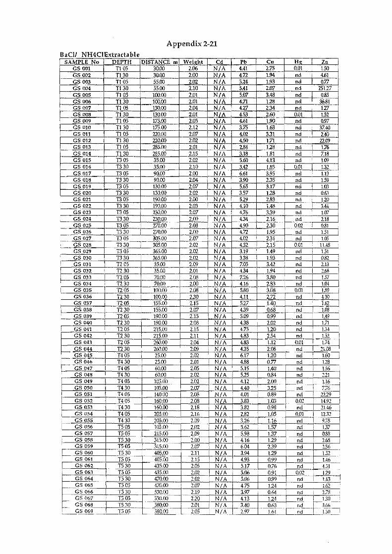
Appendix 2-21 BaCl/ NH4CIExtractable
SAMPLE No DEPTH DISTANCE m Weij];ht Cd Pb eu Hg Zn GS 001 T1 05 30.00 2.06 N/A 4.41 2.75 0.01 ! 1.50 GS 002 T130 30.00 2.00 N/A 4.72 1.94 nd 4.61 GS 003 T1 05 55.00 2.02 N/A 5.24 1.93 nd o:T/ GS 004 T130 55.00 2.10 N/A 5.41 2.W nd 25117 GS 005 T1 05 100.00 2.01 N/A 5.W 3.48 nd 0.85 GS 006 T130 100.00 2.01 N/A 4.71 1.28 nd 36.81 GS 007 T1 05 130.00 2.04 N/A 4.27 2.34 nd 1.27 GS 008 T130 130.00 2.01 N/A 4.53 2.60 0.01 152 GS 009 T1 05 175.00 2.05 N/A 4.61 1.90 nd 097 GS 010 T130 175.00 2.12 N/A 3.75 1.63 nd 37 . .w GS 011 T1 05 220.00 2.W N/A 4.02 331 nd 2.40 GS 012 T130 220.00 2.02 N/A 4.50 1.71 nd 22.09 GS 013 T1 05 285.00 2.01 N/A 2.84 1.28 nd 1.76 GS 014 T130 285.00 2.1S N/A 3.18 1.81 nd 7.18 GS 015 TI05 35.00 2.02 N/A 5.60 4.13 nd 1.09 GS 016 TI30 35.00 2.10 N/A 3.42 1.85 I 0.01 132 GS 017 TI05 90.00 2.00 N/A 6.61 3.95 nd 1.13 GS 018 TI30 90.00 2.04 N/A 3.90 235 nd 159 GS 019 TI05 130.00 2.W N/A 5.65 3.17 nd Lffi GS 020 TI30 130.00 2.02 N/A 3.57 1.28 nd 0.63 GS 021 TI05 190.00 2.00 N/A 5.29 2.83 nd 110
I GS 022 TI30 190.00 2.03 N/A 4.10 1.48 nd 3.44 I GS 023 TIOS 230.00 2.W i N/A 4.76 339 nd 1.07
GS 024 TI30 230.00 2.00 N/A 4.34 2.16 nd 2.18 GS 025 TIOS 270.00 2.08 N/A 4.90 230 0.02 0..81
i GS 026 TI30 270.00 2.00 N/A 4.72 i 1.95 nd 151 GS 027 TIOS 305.00 2.W N/A 4.02 231 nd HE !
GS 028 TI30 305.00 2.02 N/A 432 2.15 0.01 11 AS GS 029 TI05 365.00 2.02 N/A 3.19 1.49 nd 1.51 GS 030 TI30 365.00 2.02 N/A 3.38 1.93 nd 0.82 GS 031 TZ 05 35.00 2.09 N/A 7.05 3.42 nd 2.13 GS 032 TZ30 35.00 2.01 N/A 4.34 1.94 nd 2.68 GS 033 TZ05 70.00 2.08 N/A 7.26 3.80 nd 1.:>, GS 034 TZ30 70.00 2.00 N/A 4.16 2.83 nd l.W GS 035 TZ05 100.00 2.08 N/A 5.80 3.08 om 1.39 I GS 036 TZ30 100.00 230 N/A 4.11 2.72 nd I 430 GS 037 TZ05 155.00 2.15 N/A I 5.27 1.40 I nd I 1.62 GS 038 TZ30 155.00 2.07 N/A 439 0.68 nd 1.03 GS 039 TZ05 190.00 2.15 N/A 5.09 0.99 nd 1.49
i GS 040 T230 190.00 2.08 N/A 438 2.02 nd 1.71 GS 041 T205 215.00 2.15 N/A 4.75 1.20 nd 1.34 !
GS 042 TZ30 215.00 2.11 N/A 4.83 2.54 nd I 1 "' -:l. I GS 043 T205 260.00 2.04 N/A 4.83 1.12 om IJ4 GS 044 TZ30 260.00 I 2.09 N/A 4.35 2.08 nd , 21.03 GS 045 T405 25.00 2.02 N/A 6.17 1.20 nd I 1.60 GS 046 T430 25.00 2.01 N/A 4.88 0.77 nd 118 GS 047 T405 60.00 2.05 N/A 5.15 1.40 nd 1.56 GS 048 T430 60.00 2.02 N/A 5.25 0.84 nd 211 GS 049 H05 103.00 2.02 N/A 4.12 2.00 nd 1.16 GS 050 T430 105.00 2.W N/A 4.40 3.25 nd 776 GS 051 I 1405 140.00 2.08 N/A 4.01 0.89 nd "'9 GS 052 i T405 160.00 2.08 N/A 3.83 1.03 i 0.02 14.92 GS 053 T430 160.00 2.18 N/A 3.82 0.98 nd 21A6 GS 054 T405 205.00 2.16 N/A 2.82 I 1.05 om 1232
i GS 055 T430 205.00 2.09 N/A 3.26 1.16 nd I 9.78 GS 056 T505 105.00 2.02 N/A 5.62 1.57 nd i 137 GS 057 T505 215.00 2.09 N/A 5.98 137 nd 0.88
~ GS 058 T530 315.00 2.00 N/A 4.16 1.29 nd 2.68 I GS 059 T505 315.00 2.07 N/A 6.04 239 nd 2.56 GS 060 T530 405.00 2.11 I N/A 3.94 1.29 nd 1.52 GS 061 T505 405.00 2.15 IN/A 4.93 0.99 nd 1.46
L GS 062 T530 435.00 2.05 N/A 5.17 0.76 nd 4.51 GS 063 T505 435.00 2.02 N/A 5.06 0.91 0.02 i 119 i
GS 064 T530 470.00 2.02 N/A 5.06 0.99 nd 1.43 ! GS 065 T505 470.00 2.07 N/A 4.75 1.24 nd 1.62 I GS 066 T530 530.00 2.19 N/A 3.97 0.64 nd 2.78 ! GS 067 T505 530.00 220 N/A 4.13 1.24 nd 130 GS 068 T530 580.00 2.01 N/A 3.40 0.63 nd 3.66 GS069 T505 580.00 2.05 N/A 2.97 1.61 11e1. 1.50
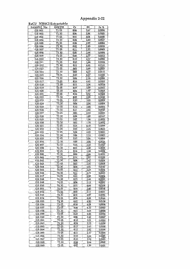
Appendix 2-22 BaCl/ NH4Cl Extractable
SAMPLE No DEPTH Cr Ni Fe '10 GS 001 TIOS 0.06 2.67 0.0004 GS002 TI 30 0.06 2.84 0.0005 GS 003 TI 05 0.15 3.01 0.0008 GS 004 TI 30 0.06 4.60 0.0027 GS 005 TIOS 0.06 2.92 0.0004 GS006 TI30 (1(}2 2.83 0.0019 GS007 TIOS 0.11 232 0.0005 GS 008 TI30 0.06 2.64 0.0004 GS 009 TIOS 0.06 277 0.0013 GS 010 TI 30 0.10 277 0.0004 GS 011 TIOS 0.10 1.64 0.0006 GS 012 TI30 0.11 6.41 0.0161 GS 013 TIOS 0.02 1.69 0.0005 GS 014 TI 30 0.02 4.77 0.0115 GS 015 1305 0.20 i 427 0.0005 GS 016 1330 0.06 i 2.16 0.0004 GS 017 1305 0.16 4.41 0.0005 GS 018 1330 0.11 2.04 0.0010 GS 019 13 05 0.19 I 359 0.0005 GS 020 1330 0.06 1.97 0.0003
i GS 021 13 OS 0.16 3.52 0.0008 I GS 022 1330 0.02 2.99 0.0008
GS 023 13 05 0.20 3.03 0.0009 GS 024 1330 0.06 2.84 0.0004 GS 025 , 13 05 0.10 I 2.64 0.0005 GS 026 1330 0.11 i 2.65 0.0048 GS 027 13 OS 0.06 2.10 0.0003 GS 028 1330 0.06 5.69 0.0167 GS 029 1'305 0.02 , 1.% 0.0003 GS 030 1330 0.02 I 1.78 0.0002 GS 031 12 05 0.24 6.18 0.0098 GS 032 1230 0.15 ! 226 0.0003 GS 033 12 05 0.24 4.43 0.0005 GS 034 1230 0.06 2.55 0.0005
_GS035 12 OS 0.15 3.86 0.0006 GS 036 1230 0.09 3.06 0.0024 GS 037 1205 (114 3.18 0.0007 GS 038 1230 0.11 2.38 0.0003 GS 039 12 05 0.14 1.58 GS 040 12 30 0.06 2.46 I 0.0003 GS 041 12 OS 0.14 2.92 0.0003 GS 042 1230 0.06 2.42 0.0004 GS 043 1205 0.02 I 232 0.0008 GS 044 12 30 0.06 5.01 0.0142 GS 045 T405 0.15 329 0.0004 GS 046 T430 0.11 2.?3 0.0003 GS 047 T405 un 2.58 0.0004 GS 048 T430 0.15 2.44 0.0002 GS 049 T405 0.06 2.15 0.0002 GS 050 TOO 0.11 4.66 0.0104
l GS 051 nos 0.06 3.40 0.0018 GS 052 T405 0.02 3.11 0.0031
I GS 053 TOO 0.01 4.97 i 0.0092 GS 054 T40S 0.06 4Jl8 0.0066 GS 055 TOO 0.02 4.80 I 0.0104 GS 056 T505 0.20 4.08 I 0.0004 GS 057 T505 0.24 433 0.0003 GS 058 T530 0.11 3.03 0.0004 GS 059 T505 0.20 I 4.66 0.0004 GS 060 T530 0.06 2.42 0.0007 GS 061 TSOS 0.10 3.01 OJJOOt GS 062 I TS30 0.24 325 0.0004 GS 063 I T505 0.15 2.63 0.0004
I GS 064 T530 0.15 2.92 0.0004 GS 065 I T50S 0.11 2.47 0.0003 GS 066 I T530 0.10 224 O.OOOS GS 067 T505 0.10 224 0.0005 GS 068 T530 0.06 2.64 0.0008 GS 069 T5 OS 0.02 139 I 0.0001
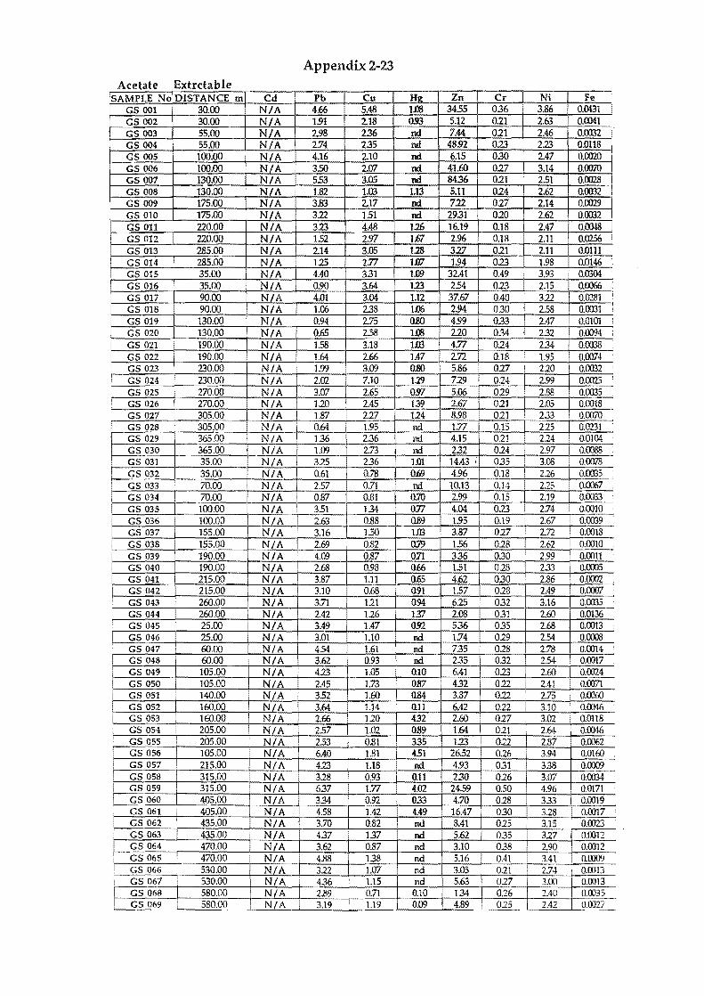
Appendix 2-23 Acetate Extrctable
'SAMPLE NOIDISTANCE m Cd Pb Cu Hit Zn Cr Ni Fe GS 001 30.00 N/A 4.66 5.48 1..1l! 3455 036 3.86 o.om GS 002 30.00 N/A 1.91 2.18 0.93 5.12 021 2.63 0.0041 GS 003 55.00 N/A 2.98 2.36 nd 7.44 021 2.46 0.0032 GS 004 55.00 N/A 2.74 235 nd 48.92 023 223 0.0118 GS 005 100.00 N/A 4.16 2.10 nd 6.15 030 2.47 0.0020 GS 006 100.00 N/A 3.50 2.07 nd 41.60 027 3.14 OJX>70 GS 007 130.00 N/A 553 3.05 nd 8436 021 251 0.0028 GS 008 130.00 N/A 1.82 1.03 1.13 5.n 024 2.62 0.0032 I
GS 009 175.00 N/A 3.83 2.17 nd 722 027 2.14 0.0029 I GS 010 175.00 N/A 322 151 nd 29.31 020 2.62 0.0032 i
i GSOll 220.00 N/A 323 4.48 1.26 16.19 0.18 I 2.47 0.0048 GS 012 220.00 N/A 152 2.97 IS 2.% 0.18 2.11 0.02.56 i
I GS 013 I 285.00 N/A 2.14 3.05 128 327 021 2.11 0.0111 I GS014 285.00 N/A 125 2.77 1.(17 1.94 023 1.98 0.0146
,
GS 015 i 35.00 N/A 4.40 331 1.09 32.41 0.49 3.93 0.0304 \
GS 016 35.00 N/A I 0.90 3.64 1.23 254 023 2.15 0.0066 ,
GS 017 90.00 N/A 4.01 3.04 1.12 37.67 0.40 322 0.1P-B1 I
GS 018 90.00 N/A 1.06 238 1~ 2.94 030 2.58 0.0031 ,
GS 019 130.00 N/A I 0.94 2.75 0.80 4.99 033 2.47 0.0101 , GS 020 130.00 N/A 0.65 258 1.00 220 0.34 232 0.0094 , GS 021 190.00 N/A 158 3.18 1113 4.77 024 234 0.0038 GS 022 190.00 N/A 1.64 2.66 1.47 2:71. 0.18 1.95 0.0074
I GS023 230.00 N/A 1.99 3.09 0.80 5.86 027 210 0.0032 GS 024 230.00 N/A 2.02 7.10
i:f;~ 024 2.99 0.0025
, i GS 025 270.00 N/A 3.07 2.65 029 2.88 0.0035
GS 026 270.00 N/A 120 2.45 2.67 021 2.05 0.0018 ! GS 027 305.00 N/A 1.87 227 114 8.98 021 2..13 0.0070
GS 028 I 305.00 N/A 0.64 1.95 nd 1.77 0.15 215 0.0231 GS 029 365.00 N/A 1.36 236 nd 4.15 021 214 0.0104 GS 030 365.00 N/A 1.09 2.73 nd 232 024 2.97 0.0088 GS 031 35.00 N/A 325 2.36 1m 14.43 ; 0.35 3.08 0.0078
I GS 032 35.00 N/A 0.61 0.78 Q.69 4.96 0.18 216 0.0035 GS 033 70.00 N/A 257 0.71 00 10.13 0.14 225 0.0067 GS 034 70.00 N/A I 0.87 0.81 010 2.99 0.15 2.19 0.0033 GS 035 100.00 N/A 351 134 o:J7 4.04 023 2.74 0.0010
I GS 036 100.00 NlA I 2.63 0.88 Q.89 1.95 0.19 2.67 0.0039 GS 037 155.00 N/A 3.16 1.50 UB 3.87 027 2.72 0.0018
I GS 038 155.00 N/A 2.69 0.82 0J9 156 028 2.62 0.0010 GS 039 190.00 N/A 4.09 0.87 0.71 3.36 030 2.99 0.0011
i GS 040 190.00 N/A 2.68 0.98 U66 1.51 018 2..13 0.0005 i GS 041 215.00 N/A 3.87 1.11 0.65 4.62 0.30 2.86 0.0002
GS 042 215.00 N/A 3.10 0.68 <l91 157 028 2.49 0.0007 I GS 043 260.00 N/A 3.71 111 <l94 625 032 3.16 0.0033 I GS 044 260.00 N/A 2.42 116 137 2.08 0.31 2.60 0.0136 I GS 045 25.00 N/A 3.49 1.47 <l92 536 035 2.68 0.0013
GS 046 25.00 N/A 3.01 1.10 00 1.74 029 2.54 0.00l8 GS 047 60.00 N/A 4.54 1.61 nd 735 028 2.78 0.0014 . GS 048 60.00 N/A 3.62 0.93 nd 235 0.32 2.54 0.0017 GS 049 105.00 N/A 423 1.05 0,10 6.41 0.23 2.60 0.0024 GS 050 105.00 N/A 2.45 1.73 0.87 432 022 2.41 0.0071 GS 051 140.00 N/A 352 1.60 !l84 3.87 022 2.75 0.0060 GS 052 160.00 N/A 3.64 1.14 0.11 6.42 I 022 3.10 0.0046 GS 053 160.00 N/A 2.66 120 432 2.60 017 3.02 0.On8 GS 054 205.00 N/A 257 1.02 0.89 1.64 011 2.64 0.0046
I GS 055 205.00 N/A 253 0.81 335 1.23 022 I 2.87 0.0062 GS 056 105.00 I N/A 6.40 1.81 451 26.52 026 3.94 0.0160 GS 057 215.00 N/A 423 1.18 nd 4.93 0.31 3.38 0.0009 GS 058 315.00 N/A 328 0.93 0.11 230 016 3.07 0.0034 GS 059 315.00 N/A 637 1.77 4.02 24.59 050 4.96 0.0171 GS 060 405.00 N/A 334 0.92 033 4.70 018 3..13 0.0019 GS 061 I 405.00 N/A 4.58 1.42 4.49 16.47 I 030 328 0.0017 GS 062 435.00 N/A 3.70 0.82 nd 8.41 015 3.15 0.0023 GS 063 I 435.00 N/A 4.37 137 nd 5.62 035 317 0.0012 GS064 470.00 N/A 3.62 0.87 nd 3.10 i 038 2.90 0.0012 GS 065 ! 470.00 N/A l 4.88 138 nd 5.16 0.41 3.41 0.0009 GS 066 I 530.00 N/A 322 1.07 nd 3.05 ! 0.21 I 2.74 O.m13 GS 067 530.00 N/A I 436 1.15 nd 5.63 ! 017 3.00 O.m13 GS 068 580.00 N/A 2.89 I 0.71 0.10 1.34 0.26 2.40 0.0035 GS 069 580.00 N/A I 3.19 1.19 0.09 4.89 015 2.42 0.0027
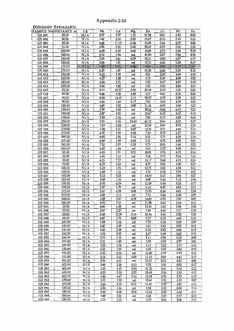
Appendix 2-24 Dithionite Extractable SAMPLE No DISTANCE m Cd Pb Cu Hg Zn Cr Ni Fe
GS 001 30.00 N / A 957 7.Ul 112 21.98 0.81 5.10 058 GS 002 30.00 N / A 7 Gl 2.50 0.33 14.67 0.76 5.1 0 0.33 GS 003 55.00 N / A 6.68 11.13 0.56 15.00 0.63 4.78 0.08 GS 004 55.00 N / A 6.95 3.22 0.66 50.23 0.79 4.94 0.28 GS 005 100.00 N / A 630 6.59 0.46 18.88 0.73 5.28 0.10 GS 006 100.00 N/A 672 1.94 nd 40.80 0.67 7.84 024 GS 001 130.00 N / A 6.35 5.61 0.29_+-1:::;8.;:;:.2::-1 -+-;;0.;:;:.60;;--!-_4;;=:.8;:::7_+-70.:,::19:;----1
~~ ::: ~~:~ N / A I 6.06 1.81 313
9'.3815
I 0° .. 64
66
~ 1-....;~::-;;:~:-~==i:.;:.~-t---;;~=:o:=-::~~-t--7:~~ 1/~~'---!r-"";;~;;::~-=-2-+--=~:.:-::::-+-_n~n~7--+--=47'.4':::1;"'-+--::'0.657.:-~-4.44 0.40
GS 011 220.00 N I A 6.29 1.38 nd 3.72 0.67 4.08 032 GS 013 285.00 N / A 6.84 ~ nd 555 0.67 437 0.15 GS 014 285.00 N / A 5.66 nd 1.92 0.54 5.84 0.11
t--~G~S~0~1~5~t---=3~5.=00=--t--N~/~A~--~8~.13~- ~~~036~-+-2~4~.44~~~0=.~~4-~~OO~-+~0~~~
GS 016 35.00 N I A 6.66 3.38 0.18 4.57 0.61 4.78 0.44 GS 011 90.00 N I A 834 16.95 2.15 90.25 O.~ 539 052 GS 018 90.00 N / A I 6.62 1.82 0.17 7.65 0.63 4.59 0.25 GS 019 130.00 N I A 6.89 7.58 0.09 I 11.14 0.59 4.86 0.13 GS 020 130.00 N I A I 7.49 3.66 nd 1 28.64 0.64 6.15 023 GS 021 190.00 N I A 6.87 4.53 nd 10.67 I 0.58 4.32 0.14 GS 022 190.00 N / A 7.43 2.C» nd, 7.01 0.75 4.88 0.24 GS 023 230.00 N I A : 7.05 6.56 13.65 I 67.13 ',0.65 453 0.15
--.9S 024 230.00 N / A 753 2.20 nd I 12.56 I 0.67 8.16 0.14 GS 025 270.00 N / A 7.38 4.31 O.W 12.76 0.71 4.43 0.13 GS 026 270.00 N / A 6.Ul 1.98 0.00 1 7.20 O.~ 5.17 0.13 GS 021 300.00 N / A 6.90 2.84 0.16 9.31 0.71 4.38 0.14 GS 028 305.00 N I A 6.(1} 1.80 0.46 2.21 0.70 3.88 0.23 GS 029 365.00 N / A I 7.33 2.82 0.28 9.75 I 0.85 5.46 023 GS 030 365.00 N / A 6.02 1.92! nd 394 0.57 4.40 0.14 GS 031 35.00 N / A I 6.45 5.51 031 18.01 0.76 425 036 GS 032 35.00 N I A 6.45 1.55 nd 5.C» 0.73 5.14 033
i GS 033 ~.OO N / A 6.35 7:0 nd 16.17 I 0.68 4.75 0.24 GS 034 ~.OO N I A 620 233 nd 4.72 i 0.86 5.80 0.27
I GS 035 100.00 N / A 5.29 5.74! nd 12.75 I 0.62 4.54 0.12 I GS 036 100.00 N I A 4.68 1.21 nd I 3.76 I 0.58 3.74 0.21 I GS 031 155.00 N I A 5.23 5.25 I nd I 10.00 037 3.93 027
GS 038 155.00 N I A 5.68 1.94 nd 6.09 036 5.13 0.16 GS 039 190.00 N I A 5.00 4.59 nd 12.09 I 0.40 420 0.17 GS 040 190.00 N I A 5.Ul 2.78 nd i 6.15 I 0.42 4.84 0.12 GS 041 215.00 N / A I 5.47 4.78 0.06 13.53 034 4.41 014 GS 042 215.00 N I A 5.09 2.11 nd 7.13 I, 0.44 4.48 0.09 GS 043 260.00 N / A 5.89 2.<]7 0.99 I 14.69 i 0.39 5.W 0.09 GS 044 260.00 I N I A 6.95 7.21 nd 21.08 0.42 5.16 0.13 GS 045 25.00 N I A 6.06 6.38 nd 23.34 0.40 5.04 0.10 GS 046 25.00 N I A 5.47 2:0 nd 7.49 0.40 527 0.10 GS 047 60,00 N / A 8.40 12.99 0.10 24.54 I 0.46 5.Q3 0.38 GS 048 60.00 N I A 6Ill 2.73 0.00 957 0.50 4.69 0.19
I--:G:--:S:-0=4":-9_t----:-107:5:=-:.00:::-_t--::--:N~/.!.!.A'____1-_::5:=;.68::_-- 2.44 nd 7.~ 036 3.69 O.Ul GS 050 105,00 N I A 5.45 2.98 nd 1 5.61 0.42 3.82 0.18 GS 051 140.00 N / A 6.26 2.38 nd 8.16 0.42 4.64 i 0.19 GS 052 160.00 N / A 5.78 3.95 nd I 8.47 0.48 4.63 0.10
i GS 053 160.00 N / A 5.73 1.53 nd I 4.11 0.56 420 0.28 GS 054 205.00 N / A 521 1.89 nd I 3.~ i 018 2.97 0.06
1 GS 055 205.00 N I A 550 1.51 nd I 4.13 I 0.32 357 0.14 I GS 056 105.00 N / A 6.32 1.99 nd I 4.45 I 053 3.86 0.19
GS 057 215.00 N I A 635 6.14 nd I 10.90 '039 4.10 0.12 GS 058 315.00 N I A 614 3.12 0.09 11.10 0.47 4.42 0.17 GS 059 315.00 N I A 934 6.51 nd 23.57 I 0.52 4.81 0.45 GS 060 405.00 N I A 1 5.68 238 0.13 9.78 0.41 4.85 0.17 GS 061 405.00 N I A 5.35 4,13 0.10 31.50 0.41 3.83 0.22 GS 062 435.00 N I A i 635 333 0.25 18.69 0.56 524 0.13 GS 063 435.00 N fA I 5.46 4.67 0.14 13.34 033 3.70 0.19 GS 064 470.00 N / A 5.71 1.99 nd 13.61 033 431 0.07 GS 065 470.00 N I A 5.44 4.29 031 13.87 0.39 3.91 0.15 GS 066 530.00 N I A '536 1.66 nd 8.04 i 0.43 4.04 0.14 GS 067, 530.00 N / A 6.03 4.00 0.14 12.42 I 0.49 3.68 0.17 GS 068 580.00 N I A! 5.48 3.01 nd i 4.63 0.40 3.57 0.12 GS 069 580.00 J N I A 5.25 2.2Z nd I 6.70 ! 0.36 3.06 0.12
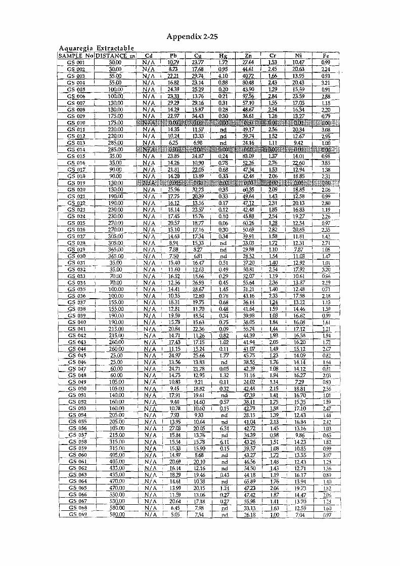
Appendix 2-25
A .quarel?;ta E t t bl x rae a e SAMPLE NoiDlSTANCE m Cd Pb Cu HfI: Zn Cr Ni Fe
GS 001 30.00 N/A 10.79 23.77 1.72 27.64 153 10.47 0.99 r----2S 002 30.00 I N/A 8.73 17.68 0.95 44.61 2.45 20.63 U4
GS 003 55.00 NIA 22.21 29.74 4.10 40.72 1.66 13.95 0.93 GS 004 55.00 N/A I 16.82 23.14 0.88 BO.48 2.43 20.43 311 GS 005 I 100.00 N/A I 24.39 25.29 0.20 43.90 1.29 15.59 0.91
I--GS 006 100.00 N{A I 23.33 13.76 0.21 97.56 2.84 23.59 2.88 GS 007 130.00 N/A I 29.29 29.16 0.31 57.10 155 17.05 1.18 I
GS 008 130.00 N/A 14.29 15.87 0.28 48.67 254 I 16.34 UO GS 009 175.00
N/A ir~ 0.30
~ 1.26 I O~ GS 010 175.00 :§.~Nl~l£:f:~::: ~1%~*: .:;'
GSOll 220.00 NI A 1 11.57 I nd 2.56 3.08 GS 012 220.00 N/ A 1 13.33 nd ~~ 152 2.95 GS 013 285.00 N/A I 6.98 I nd 24 1.11 1.00 GS 014 285.00 i~\\!~1:'~~~!!!~!Ui ~! :~~~::::.(lntt···· GS 015 35.00 N / A I 23.85 24.87 0.24 83.09 1.37 I 14.01 098 GS 016 35.00 N/A i 14.26 10.90 0.78 52.26 2.76 22.60 3.85 GS 017 90.00 N/A : 21.81 22.05 I 0.68 47.34 153 12.94 1.38 GS 018 90.00 N/A I 14.20 13.89 I 0.33 42.48 I 2.06 18.85 231 GS 019 130.00 ~j:jj~:~: ~4'.?, \OO:~t *,!:!:!Q.nr~:tm:m};OO:N:! ;~1wnro!1;~~~:m-::::n$.i:tm::!:~:r :\:p,a:;.::,,::;:: il:rg!QW:!}:: GS 020 130.00 N/A I 25.96 32.73 I 0.35 60.35 I 2.09 I 18.85 2.06 GS 021 190.00 N/A I 17.75 20.39 0.33 49.64 I 1.43 I 12.58 0.99 GS 022 190.00 N/A ! 16.12 13.56 0.17 47.12 I 2.31 I 20.13 2.80 GS023 230.00 N/A ! 18.14 23.57 : 0.12 42.48 I 1.85 i 16.83 1.19 GS 024 230.00 N/A 17.45 15.76 I 0.10 45.88 I 2.54 I 19.27 U6 GS 025 270.00 N/A 20.57 18.77 0.06 60.26 1.28 12.54 0.97 GS 026 270.00 N/A
, 13.10 17.16 I 0.30 50.69 j 2.82 I 20.85 235
, , GS 027 305.00 N/A 14.63 17.34 0.34 39.91 158 I 11.81 1.42 GS 028 i 305.00 N/A I 8.94 15.33 nd 33.03 : 1.72 12.31 2.701 GS 029 365.00 N/A 7.88 817 nd 29.88 i 1.10 7.87 l.OS ! GS 030 I 365.00 N/A I 750 6.81 nd 28.52 I 154 , 11.03 1.47 , GS 031 35.00 N/A 15.40 16.47 0.51 37.20 ! 1.40 : 12.92 1.01 GS 032 i 35.00 N/A , 11.60 12.63 0.49 50.81 I 2.54 i 17.92 320 GS 033 i 70.00 N/A 16.52 18.66 0.29 32.07 I 1.19
, 10.61 I 0.96 I
GS 034 \ 70.00 N/A 12.56 26.93 0.45 55.64 I 2.36 I 13.87 2.59 GS 035 100.00 N/A 14.41 28.67 1.45 31.21 1.40 I 12.48 0.71 I
GS 036 100.00 N/A 10.35 12.80 0.78 43.16 2.33 I 17.98 I 2.18 GS 037 \ 155.00 N/A 18.31 19.75 0.68 36.14 I 124 ! 13.22 1.13 GS 038 I 155.00 N/A
, 12.81 11.70 0.48 41.64 i 159 I 14.46 139 GS 039 190.00 I N/A I 19.59 18.54 L 0.34 39.98 1.03 I 16.62 0.99 GS 040 I 190.00 I N/A : 15.78 15.63 0.75 38.05 I 1.84 ; 16.08 1.61 I
GS 041 215.00 NLA I 20.84 22.36 0.09 55.74 I 1,44 : 17.12 111 GS 042 215.00 I N/A 14.71 11.26 0.82 44.39 i 1.93 I 16.58 1.94-GS 043 i 260.00 N/A 17.43 17.15 1.02 41.94 2.05 I 16.20 1.72 GS 044 260.00 N/A I 11.15 I 15.24 0.11 41.07 1.49 15.12 2.07 GS 045 25.00 N/A I 24.97 I 25.66 1.77 45.75 : 123 : 14.09 0.82 GS 046 25.00 N/A 13.56 13.83 nd 38.55 i 1.76 , 14.14 1.64 GS 047 60.00 N/A 24.71 : 21.78 0.05 42.39 I 1.08 I 14.12 0.81 ,
i GS 048 60.00 N/A 14.75 I 12.95 1.32 51.16 ! 1.94 I 16.27 2.(13 GS 049 105.00 N/A I 1M3 911 L 0.11 24.02 1.14 719 q:~ GS 050 105.00 NLA , 9.45 18.82 0.32 42.48 I 2.15 I 18.81 2.56 .
I GS 051 140.00 N/A 17.91 19.61 nd 47.39 I 1.41 i 16.70 1.01 GS 052 160.00 N/A i 9.40 14.60 0.57 38.11 1.75 I 15.35 1.89 !
GS 053 I 160.00 N/A 10.78 10.60 I 0.15 42.79 158 i 17.10 2.47 GS 054 205.00 N/A I 7.93 i 933 nd 28.15 I 139 I 12.43 1.48 GS 055 205.00 N/A I 13.95 10.64 nd 41.04 I 2.13 i 16.84 2.42 GS 056 105.00 N/A ! 27.00 ! 20.05 6.31 42.72 I 1.45 ! 13.16 1.03
I GS 057 I 215.00 N/A , 15.84 13.76 nd 34.39 \ 0.98 I 9.86 0.65 ,
GS 058 315.00 I N/A I 15.54 15.78 6.11 43.26 151 ! 14.23 1.82 GS 059 315.00 N/A I 1533 I 15.90 0.15 39.57 I 1.08 I 10.85 0.99 GS 060 405.00 I N/A : 14.97 8.68 nd 43.27 I 1.72 I 13.55 3.97 GS 061 ! 405.00 N/A I 20.69 i 20.10 nd 46.56 1 1.48 : 12.43 123 GS 062 i 435.00 I N/A 16.14 12.16 nd 54.50 I 1.43 ! 12.71 136 GS 063 I 435.00 N/A I 18.29 ! 19.46 0.43 44.18 I 1.19 I 16.17 0.89 GS 064 470.00 N/A I 14.61 I 1038 nd 65.89 I 1.76 13.94 1.40 GS 065 470.00 N/A ! 13.99 20.15 1.24 4723 2.06 19.73 1.82 I GS 066 530.00 N/A 11.59 13.06 0.27 47.42 1.87 I 14.47 2.06
r--GS 067 530.00 I N/A I 20.64 I 17.18 i 0.27 I 55.98 1.41 I 13.70 11:l GS 068 580.00 I N/A I 6.45 I 7,!lLt- nd 33.13 1.63 i 12.59 l.@ .-. I 5.05-r-7.54 nd
.~
GS 069 580.00 N/A I 26.18 1.00 ! 7.O-t I 097
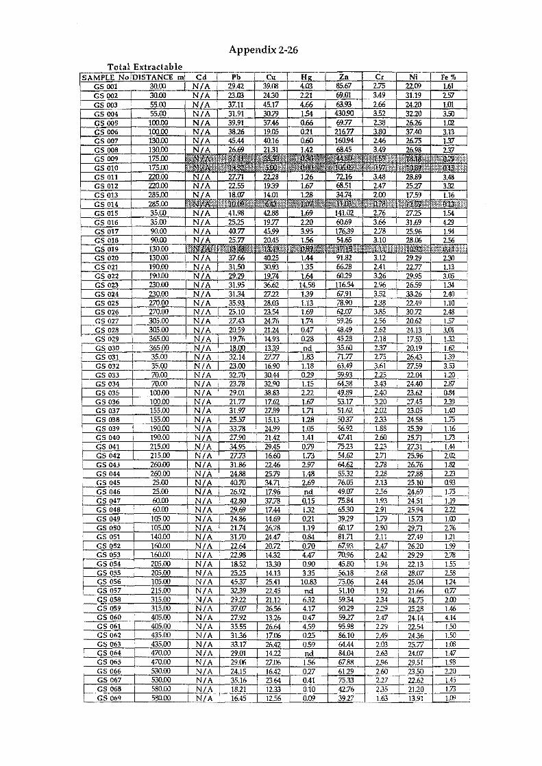
Appendix 2-26
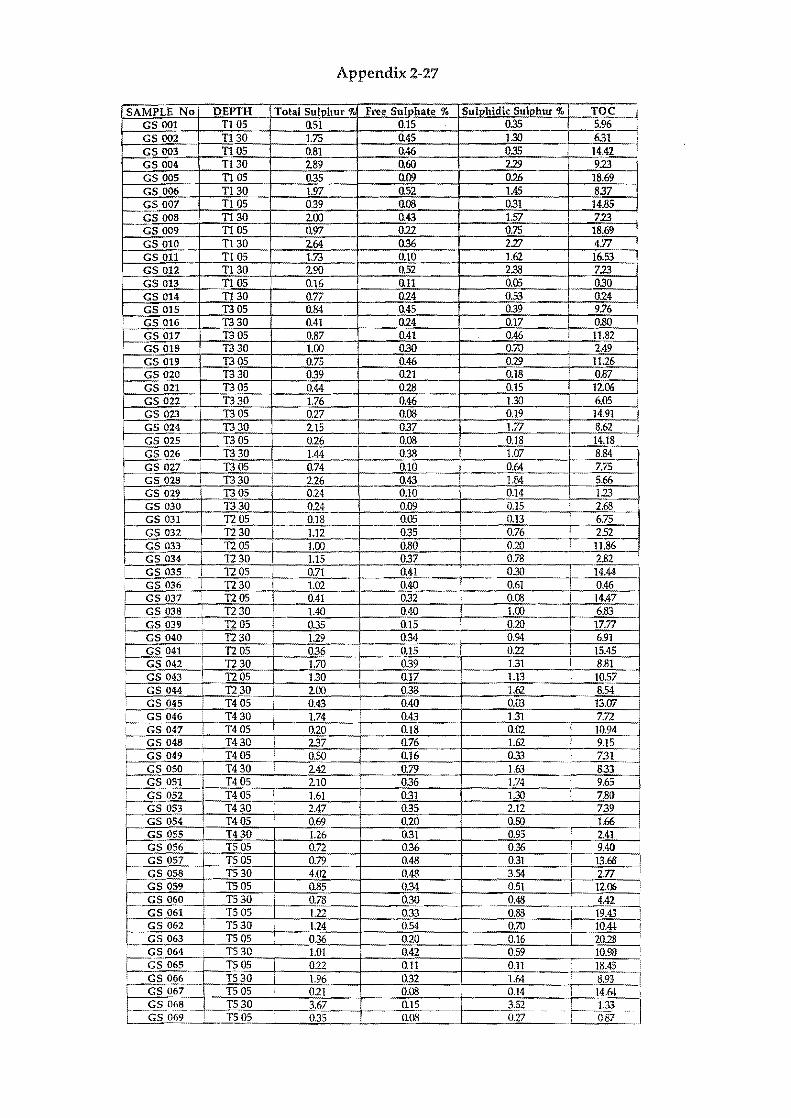
Appendix 2-27
SAMPLE No DEPTH Total Sulphur '" Free Sulphate 'Yo Sulphidk Sulphur 'Yo Toe GS 001 T1 05 0.51 0.15 0.35 5.96 GS 002 T130 1.75 0.45 1.30 631 GS 003 T1 05 0.81 0.46 0.35 14.42 GS 004 T130 2.89 0.60 U9 9.23 GS 005 T1 05 0.35 0.09 0.26 18.69 GS 006 T130 1.97 0.52 1.45 837 GS 007 T1 05 039 0.08 0.31 14.85 GS 008 T130 2.00 0.43 1.57 7.23 GS 009 T1 05 0.97 0.22 0.75 18.69 GS 010 T130 2.64 Q.36 2::0 4.77 GSOll TI05 1.73 0.10 1.62 16.53 GS 012 T130 2.90 0.52 2.38 713 GS 013 T1 05 0.16 0.11 0.05 030 Gson T130 0.77 0.24 0.53 024 GS 015 1'305 0.84 0.45 039 i 9.76 GS 016 1'330 0.41 0.24 0.17 ! 0.80 GS 017 1'305 0.87 0.41 0.46 11.82 GS 018 1'330 1.00 0.30 0.70 I 2.49 GS 019 1'305 0.75 0.46 0.29 11.26 GS 020 1'330 0.39 0.21 0.18 0.87 GS 021 1'305 0.44 0.28 0.15 12.06 GS 022 1'330 1.76 0.46 1.30 6.05 GS023 1'305 0.27 0.08 0.19 14.91 GS 024 1'330 2.15 037 1.77 8.62 GS 025 1'305 0.26 0.08 0.18 14.18 GS 026 1'330 1.44 0.38 1.(]7 I 8.84 GS 027 1'305 0.74 0.10 0.64 I 7.75
I------C I 1'330 2.26 0.43 1.84 I 5.66 GS028
GS 029 1'305 0.24 0.10 0.14 123 GS 030 1'330 024 0.09 0.15 2.68 GS 031 TI 05 0.18 0.05 0.13 6.75 GS 032 TI30 1.12 0.35 0.76 252 GS 033 TIOS 100 0.80 0.20 11.86 GS 034 TI30 1.15 0.37 0.78 2.82 GS 035 TIOS 0.71 Q.41 0.30 14.44 GS 036 TI30 1.02 0.40 0.61 0.46 GS 037 TI05 0.41 0.32 0.08 14.47 GS 038 TI30 1.40 0.40 1.00 6.83
r- GS 039 TI05 0.35 0.15 I 0.20 I 17.77 GS 040 TI30 1.29 0.34 0.94 I 6.91
I GS 041 TIOS 0.36 0.15 0.22 I 15.45 GS 042 TI30 1.70 0.39 1.31 I 8.81
I GS 043 TIOS 130 0.17 1.13 10.57 GS 044 i TI30 2.00 0.38 1.62 8.54
~045 T40S 0.43 0.40 o.m 13.07 GS 046 T430 1.74 0.43 131 7.72
IGS047 T40S 0.20 0.18 0.02 10.94 GS 048 T430 2.37 0.76 1.62 9.15
, GS 049 T405 0.50 0.16 0.33 7.31 r----cs 050 T430 2.42 0.79 1.63 8.33 GS 051 T405 2.10 0.36 1.74 9.65 GS 052 T405 1.61 0.31 1.30 7.80
I GS 053 T430 2.47 035 2.12 739 GS 054 T405 0.69 0.20 0.50 1.66 GS 055 T430 1.26 0.31 0.95 2.41
! GS 056 T505 0.72 0.36 036 9.43 I GS 057 T505 0.79 0.48 031 13.68 GS 058 T530 4.02 0.48 3.54 2.77
-CS 059 T505 0.85 0.34 0.51 12.06 GS 060 T530 0.78 0.30 0.48 4.42 GS 061 T505 1.22 0.33 0.88 19.43 GS 062 T530 I 1.24 0.54 0.70 10.4l GS 063 T505 036 0.20 0.16 i 20.28 I GS 064 T530 101 0.42 0.59 10.9il
j GS 065 T505 0.22 0.11 0.11 , 18.45 GS 066 T530 1.96 0.32 1.64 I 8.93 GS 067 T505 021 0.08 0.14 14.&1 J
_<:;~.068 T530 i 3.67 0.15 3.52 , 1.33 ~ .~.
GS 069 T505 035 0.08 0.27 0.87
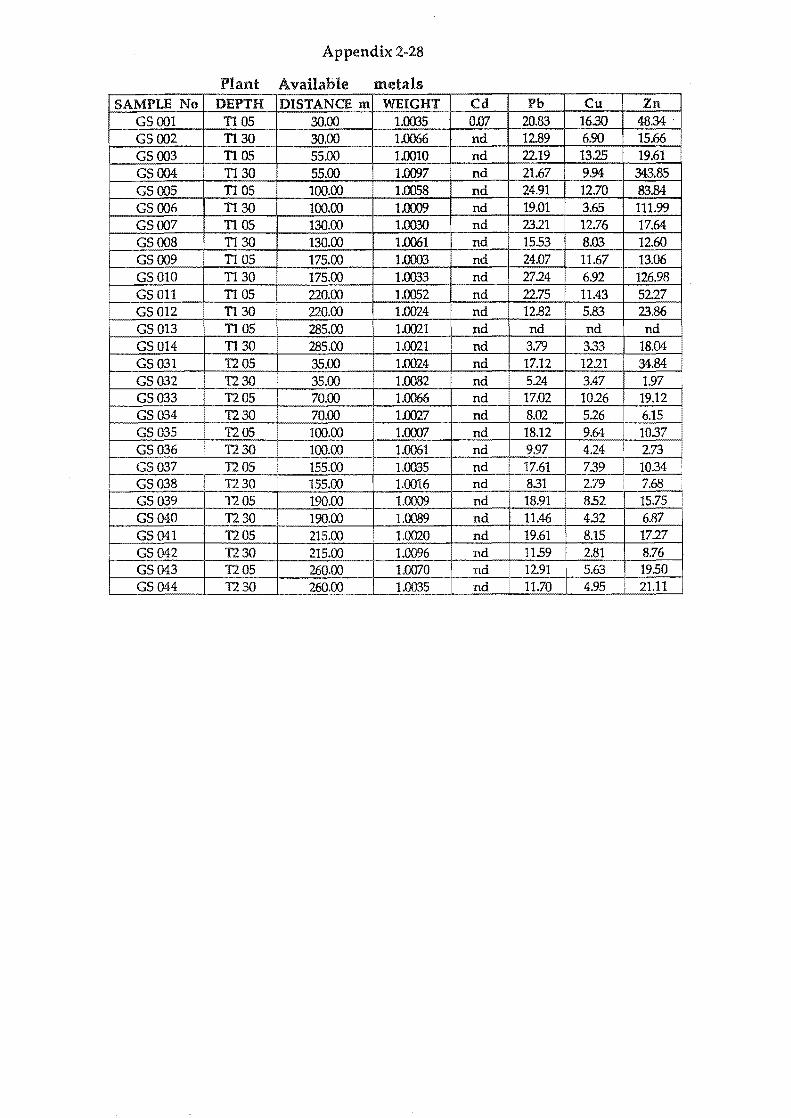
SAMPLE No GSOOI GS002 GS003 GSOO4 GS005
RtOO6 007
GS008 GS009 GSOlO GS 011 GS012 GS013 GS0l4 GS031 GS032 GS033 GS034 GS035 GS036 GS037 GS038 GS039 GS040 GS041 GS042 GS043 GS044
Appendix 2-28
Plant Available metals DEPTH DISTANCE m WEIGHT
Tl 05 30.00 1.Q035 Tl30 30.00 1.0066 TlOS 55.00 1.0010 Tl30 55.00 1.0097 Tl 05 100.00 I l.oos8 Tl30 100.00 1.0009 TlOS 130.00 1.Q030
Tl30 130.00 U)061 Tl OS 175.00 1.0003 Tl30 175.00 1.0033 Tl 05 220.00 l.oos2 Tl30 220.00 1.Q024
Tl OS 285.00 1.Q021 Tl30 285.00 1.0021 T205 35.00 1.0024 T230 35.00 1.0082 T205 70.00 1.0066 T230 70.00 1.Q027 T20S 100.00 1.0007 T230 100.00 1.0061 T20s 155.00 1.0035 T230 155.00 1.0016 T205 190.00 1.0009
30 190.00 1.0089 T20s 215.00 1.0020 T230 215.00 1.0096 T205 260.00 1.0070 T230 260.00 1.0035
Cd Pb Cu Zn
O.07~ 16.30 48.34' nd 690 15.66 nd 2219 13.25 19.61 nd 21.67 9.94 343.85 nd 24.91 12.70 83.84 nd 19.01 3.65 nd 2321 12.76 I 17.64 nd 1553 8.03 12.60 nd
24,07 I 11.67 13.06 nd 6.92 126.98 nd 11.43 52.27 nd 12.82 5.83 23.86 nd nd nd n nd 3.79 3.33 18.04 nd 17.12 1221 34.84 nd 524 3.47 1.97 nd ! 17.02 1026 19.12 nd 8.02 526 6.15 nd 18.12 9.64 10.37 nd 9.97 4.24 273 nd 17.61 7.39 10.34 nd 8.31 2.79 7.68 nd
l~m 15.75
nd 11 2 6.87
fnd 19.61 8.15 1727 nd 1159 2.81 8.76 nd 1291 i 5.63 1950 nd 11.70 4.95 21.11
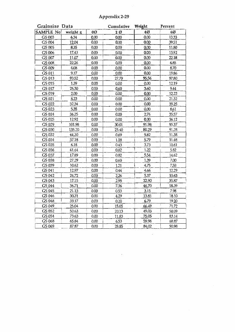
Appendix 2-29
G . ralnS12:e D t a a C l' umu atlve W' h elgl t P ercent
SAMPLE No weight g 00 ! 20 40 60 GS003 6.34 0.00 I 0.00 0.00 1333 GSOO4 12.04 0.00 0.00 0.00 39.51 GS005 835 0.00 0.00 0.00 11.80 GS006 17.43 0.00 0.00 0.00 13.92 GS007 11.07 0.00 0.00 0.00 22.18 GS008 2226 0.00 0.00 0.00 6.85 GS009 4.08 0.00 0.00 0.00 8.70 GS011 9.17 0.00 0.00 0.00 19.86 GS013 93.52 0.00 27.79 95.56 97.80 GS015 139 0.00 0.00 0.00 12.19 GS017 26.30 0.00 ! 0.60 3.60 9.44 GS019 2.00 0.00 0.00 0.00 12.22 GS021 8.23 0.00 I 0.00 0.00 21.32 GS022 32.34 0.00 ! 0.00 0.00 39.25 GS023 535 0.00 0.00 0.00 8.61 GS024 36.25 0.00 0.00 2.76 35.57 GS025 12.92 0.00 0.00 0.00 36.12 GS029 101.98 0.00 I 30.01 91.98 9537 GS030 135.20 0.00 I 23.40 80.29 9128 GS032 44.30 0.00 0.69 9.82 11.38 GS034 37.18 0.00 1.18 5.79 11.48 GS035 6.18 0.00 0.43 3.73 10.61 GS036 41.64 0.00 0.82 1.22 5.82 GS037 17.89 0.00 0.82 554 14.62
I GS038 2729 0.00 0.60 1.39 7.00 GS039 10.62 0.00 1.21 4.75 7.58 GS041 I 12.97 0.00 0.44 4.66 1229 GS042 24.72 0.00 I 2.26 537 10.63 GS043 i 17.15 0.00 2.95 22.90 35.87 GS044 36.71 0.00 I 7.36 46.70 58.39 GS045 21.13 0.00 0.53 3.15 i 7.98 GS046 30.31 0.00 I 4.29 13.85 18.10 GS048 33.17 0.00 020 6.79 ! 19.20 GS049 25.04 0.00 I 15.05 66.49 71.72 GS052 50.63 0.00 i 20.13 49.03 58.09 GS054 73.63 I 0.00 11.83 75.05 83.14 GS068 65.84 0.00 6.53 59.98 68.87 GS069 87.87 0.00 28.85 84.02 90.98
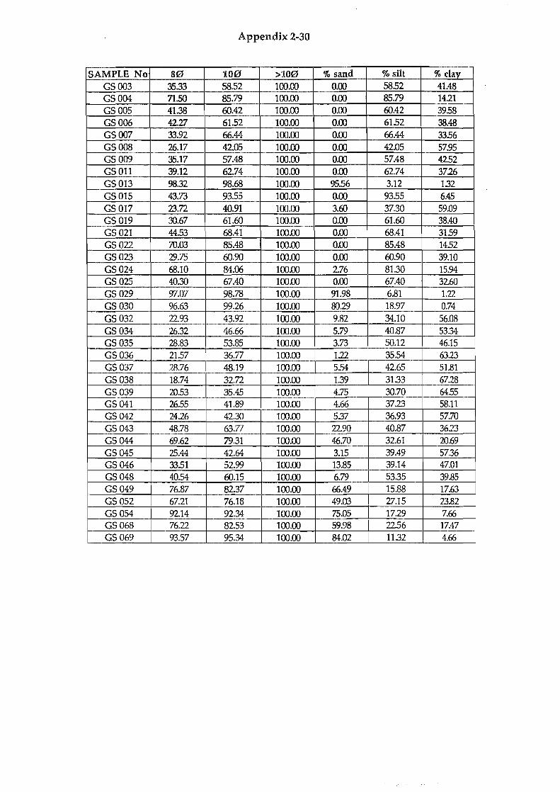
Appendix 2-30
SAMPLE No 80 100 >100 % sand % silt %clav GS003 35.33 58.52 100.00 0.00 5852 41.48 GS004 71.50 85.79 100.00 0.00 85.79 14.21 GS005 41.38 60.42 100.00 0.00 60.42 39.58 GS006 42.27 61.52 100.00 0.00 6152 38.48 GS007 33.92 66.44 100.00 0.00 66.44 33.56 GS008 26.17 42.05 100.00 0.00 42.05 5795 GS009 35.17 57.48 100.00 0.00 57.48 42.52 GS011 39.12 62.74 100.00 0.00 62.74 37.26 GS013 98.32 98.68 100.00 95.56 3.12 1.32 GS015 43.73 93.55 100.00 0.00 9355 6.45 GS 017 23.72 40.91 100.00 3.60 37.30 59.09 GS019 30.67 61.60 100.00 0.00 61.60 38.40 GS 021 44.53 68.41 100.00 0.00 68.41 31.59 GS022 70.03 85.48 100.00 0.00 85.48 14.52 GS023 29.75 60.90 100.00 0.00 60.90 39.10 GS024 68.10 84.06 100.00 2.76 81.30 15.94 GS025 40.30 67.40 100.00 0.00 67.40 3260 GS029 97.W 98.78 100.00 91.98 6.81 1.22 GS030 %.63 99.26 100.00 80.29 18.97 0.74 GS032 22.93 43.92 100.00 9.82 34.10 56.08 GS034 26.32 46.66 100.00 5.79 40.87 5334 GS035 28.83 53.85 100.00 3.73 50.12 46.15 GS036 2157 36.71 100.00 1.22 35.54 63.23 GS037 28.76 48.19 100.00 554 42.65 51.81 GS038 18.74 32.72 100.00 1.39 31.33 67.28 GS039 20.53 35.45 100.00 4.75 30.70 64.55 GS041 2655 41.89 100.00 4.66 37.23 58.11 GS042 24.26 42.30 100.00 5.37 36.93 57.70 GS043 48.78 63.71 100.00 22.90 40.87 36.23 GS044 69.62 79.31 100.00 46.70 32.61 20.69 GS045 25.44 42.64 100.00 3.15 39.49 5736 GS046 3351 52.99 100.00 13.85 39.14 47.01 GS048 40.54 60.15 100.00 6.79 53.35 39.85 GS049 76.87 82.37 100.00 66.49 15.88 17.63 GS052 67.21 76.18 100.00 49.03 27.15 23.82 GS054 92.14 92.34 100.00 75.05 17.29 7.66 GS068 76.22 82.53 100.00 59.98 2256 17.47 GS069 93.57 95.34 100.00 84.02 11.32 4.66
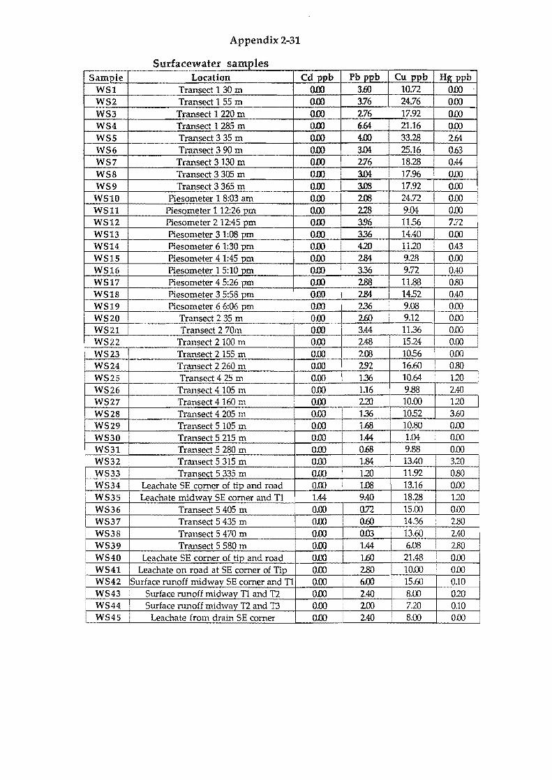
Appendix 2-31
Surfacewater samples Sample Location Cd ppb Pb ppb Cu ppb H~ ppb
WSI Transect 130m 0.00 3.60 10.72 0.00 WS2 Transect 1 55 m 0.00 3.76 24.76 0.00 WS3 Transect 1 220 m 0.00 276 17.92 0.00 WS4 Transect 1 285 m 0.00 6.64 21.16 0.00 WS5 Transect 3 35 m 0.00 4.00 33.28 2.64 WS6 Transect 390m 0.00 3.Q4 25.16 H*--WS7 Transect 3 130 m 0.00 276 18.28
WS8 Transect 3 305 m 0.00 3.Q4 17.96 0.00 WS9 Transect 3 365 m 0.00 3.08 17.92 am
WSIO Piesometer 1 8:03 am
Ei 2.08 24.72 am
WSll Piesometer 112:26 pm 228 9.04 0.00 WS12 Piesometer 2 12:45 pm 3.% 11.56 7.72 WS13 Piesometer 3 1:08 pm 3.36 14.40 am WS14 Piesometer 6 1:30 pm 0.00 4.20 11.20 0.43 WS15 Piesometer 4 1:45 pm 0.00 2.84 9.28 am WS16 Piesometer 1 5:10 pm 0.00 3.36 9.72 0.40 -
! WS17 Piesometer 4 5:26 pm 0.00 288 11.88 aBO ! WS18 Piesometer 3 5:58 pm 0.00 2.84 14.52 0.40
WS19 Piesometer 6 6:06 pm oro I 236 9.08 am WS20 Transect 2 35 m 0.00 260 9.12 am WS21 Transect 2 70m 0.00 ml1~ 0.00 WS22 Transect 2 100 m oro 15.24 0.00 WS23 Transect 2155 m 0.00 2.08 10.56 am I WS24 Transect 2 260 m 0.00 292 16.60 OBO I WS25 Transect 4 25 m 0.00 1.36 10.64 120 WS26 Transect 4 105 m 0.00 1.16 I 9.88 2.40 WS27 Transect 4 160 m 0.00 220 10.00 120 WS28 Transect 4 205 m 0.00 1.36 10.52 3.60 WS29 Transect 5 105 m 0.00 1.68 10.80 0.00 WS30 Transect 5 215 m 0.00
~ am
WS31 Transect 5 280 m oro 0.00 WS32 Transect 5 315 m 0.00 1.84 13.40 320 WS33 Transect 5 335 m oro 1.20 11.92 aBO WS34 Leachate SE comer of tip and road 0.00 1.08 13.16 0.00 WS35 Leachate midway SE comer and T1 1,44 9.40 18.28 120 WS36 Transect 5 405 m 0.00 0.72 15.00 am WS37 Transect 5 435 m 0.00 0.60 l!$f •
WS38 Transect 5 470 m 0.00 0.03 13. 2.40 WS39 Transect 5 580 m 0.00 1.44 6. 2.80 WS40 Leachate SE comer of tip and road 0.00 1.60 21 am WS41 Leachate on road at SE comer of Tip 0.00 2.80 10.00 0.00 WS42 Surface runoff midway SE comer and T1 0.00 6.00 15.60 0.10 WS43 Surface runoff midway T1 and T2 0.00 2.40 8.00 020 WS44 Surface runoff midway T2 and T3 0.00 200 7.20 0.10 WS45 Leachate from drain SE comer 0.00 2.40 8.00 am
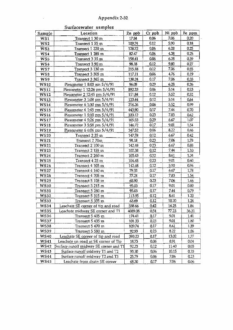
Appendix 2-32
Surfacewaler samples Sample Location Zn oob Cr ppb Ni ppb Fe ppm
WSl Transect 1 30 m 17.84 0.06 7.06 0.20 WS2 Transect 1 55 m 109.74 0.12 5.90 0.18
WS3 Transect 1 220 m 128.72 0.06 6.28 0.25 WS4 Transect 1 285 m 82.47 0.06 4.38 0.25 WS5 Transect 3 35 m 158.41 0.06 6.28 0.39 WS6 Transect 3 90 m 98.18 0.12 9.80 027 WS7 Transect 3 130 m 215.18 0.12 7.06 055 WS8 Transect 3 305 m 117.11 0.06 4.76 0.19 WS9 Transect 3 365 m 13824 0.17 7.06 0.33 WSI0 Piesometer 1 8:03 am 5/4/91 %.08 029 6.28 026 WSll Piesometer 1 12:26 pm 5/4/91 89233 0.06 5.14 0.53 WS12 Piesometer 2 12:45 pm 5/4/91 111.84 0.12 5.52 0.52 WS13 Piesometer 31:08 pm 5/4/91 123.44 0.12 t 5
.14 0.64 WS14 Piesometer 6 1:30 pm 5/4/91 21626 0.06 5.52 0.99 WS15 Piesometer 41:45 pm 5/4/91 443.90 0.17 7.44 0.70 WS16 Piesometer 15:10 pm 5/4/91 333.12 023 7.83 0.62 WS11 Piesometer 45:26 pm 5/4/91 105.53 029 6.67 1.07 WS18 Piesometer 3 5:58 pm 5/4/91 146.72 0.17 9.01 1.54 WS19 Piesometer 6 6:06 pm 5/4/91 34752 0.06 8.22 0.46 WS20 Transect 2 35 m 147.78 0.12 6.67 0.42 WS21 Transect 2 70m 98.18 023 7.06 1.78 WS22 Transect 2100 m 142.48 023 6.67 0.88 WS23 Transect 2 155 m 102.38 0.12 7.44 1.10 WS24 Transect 2 260 m 103.43 0.12 8.61 1.34 WS25 Transect 4 25 m 104.48 0.23 9.01 0.60 WS26 Transect 4 105 m 142.48 0.12 5.90 0.% WS27 Transect 4 160 m I 79.33 0.17 6.67 1.78 WS28 Transect 4 205 m I 7724 0.17 7.83 1.54 WS29 I Transect 5 105 m 68.90 023 7.06 1.66 WS30 Transect 5 215 m 95.03 0.17 9.01 0.80 I WS31 Transect 5 280 m 95.03 0.17 7.44 0.79 WS32 Transect 5 315 m 113.95 0.12 8.61 1.20 ! WS33 Transect 5 335 m 63.69 0.12 10.20 124 WS34 Leachate SE comer of tiP and road 338.66 0.42 14.25 1.84 WS35 Leacha te mid way SE comer and T1 4089.38 0.54 77.23 36.31 WS36 Transect 5 405 m 174.41 0.17 9.01 1.41 WS37 Transect 5 435 m 101.33 0.23 9.01 1.80 WS38 Transect 5 470 m 109.74 0.17 8.61 1.39 WS39 Transect 5 580 m 9293 023 8.22 1.86 WS40 Leachate SE comer of tiP and road 39323 0.17 13.02 1.77 WS41 Leachate on road at SE comer of Tip 18.73 0.06 8.91 0.04 WS42 Surface runoff midway SE comer and T 92.23 0.12 11.40 0.03 WS43 Surface runoff midway T1 and 12 93.30 0.06 10.15 033 WS44 Surface runoff midway T2 and T3 25.79 0.06 7.06 0.23 WS45 Leachate from drain SE corner 68.30 0.17 7.06 OJJ6
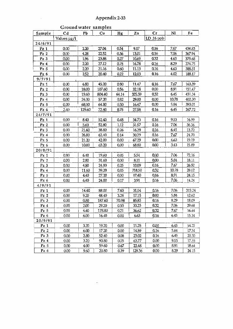
Appendix 2-33
G roun d I water sampl es Sample Cd Ph Cu H9; Zn Cr Ni Fe
Values 1.112:/1 LD .16ppb 24/6/91
pz 1 0.00 220 27.04 0.54 9.17 0.16 7.67 434.83
F*! 0.00 4.28 2252 0.36 13.01 0.16 7.Q6 367.94 0.00 1.96 23.88 0.27 10.69 0.32 4.63 379.68
o~ 0.75 16.78 0.16 8.29 274.75
I pz 5 o 21.16 0.60 11.13 0.16 4.63 38851 pz 6 O. 0.22 12.03 0.16 4.02 188.17
9/7/91 pz 1 0.00 45.20 0.80 11.47tl=j 7.67 16339 pz 2 0.00 107.60 056 32.18 8.91 151.47 pz 3 0.00 19.60 804.40 64.14 32559
~ pz 4 0.00 24.00 57.20 0.82 29.00 0.00 10.78 pz 5 0.00 68.00 64.80 050 16.47 0.00 5.84 ! 393.01 pz 6 2.40 129.60 72.40 0.75 2758 0.16 6.45 267.72
24/7/91 pz 1 0.00 I 8.40 52.40 0.48 34.73 0.16 9.53 16.99 pz 2 0.00 5.60 I 52.80 1.12 3157 0.16 7.06 36.36
I~ 0.00 21.60 38.80 026 1629 0.16 6.45 13.70 0.00 26.80 62.40 0.14 3029 0.16 7.67 24.70
pz 5 0.00 I 2~42.00 0.00 6729 0.00 4.63 19.19 pz 6 0.00 10 63.20 0.00 3.43 15.89
20/8/91 pz 1 0.80 I 6.40 19 0.00 7.06 72.16 pz 2 0.00 2.80 31.60 0 8.11 0.00 5.84 18.11 pz 3 0.00 I 4.80 24.80 0 10.09 0.16 7.67 26.92 pz 4 0.00 11.60 39.20 0.05 718.50 0.32 10.78 28.02 pz 5 0.00 4.40 27.20 0.00 17.40 0.16 8.91 24.15 pz 6 0.00 6.40 24.00 0.17 391 0.16 7.06 14.24 I
4/9/91 pz 1 0.00 14.40 88.00 7.60 31.04 0.16 7.06 315.24 pz 2 0.00 9.20 48.40 3.28 17.15 0.00 5.84 12.62 pz 3 0.00 0.80 187.60 70.98 85.85 0.16 8.29 18.09 pz 4 0.00 2.00 29.20 050 3325 0.32 7.06 29.68
~o.oo 4.40 178.80 0.21 36.62 0.32 7.67 16.44 pz 6 0.00 6.00 I 16.40 0.00 6.63 0.16 6.45 15.34
20/9/91 pz 1 0.00 i 3.20 19.20 0.00 1125 0.00 6.45 14.25 pz 2 0.00 6.00 17.20 0.00 1459 0.16 5.84 1754 pz 3 0.00 2.80 52.40 0.08 23.02 0.16 6.45 2030 pz 4 0.00
•
3.20 90.80 0.55 63.77 0.00 9.53 1755 pz 5 0.00 4.00 59.60 0.67 22.48 0.00 8.91 18.64 pz 6 0.00 9.60 20.80 0.39 128.36 0.00 8.29 24.15

Appendix 2-34
Ground water samples SamEle Cd Pb Cu Hg Zn Cr Ni Fe
Values flg/l LD .16ppb 4/10/91
pz 1 0.00 7.20 112.40 0.10 35.75 0.16 7.67 18.78 pz 2 0.00 5.20 84.40 0.00 1192 0.32 7.06 26.91 pz 3 0.00 3.60 20.80 0.00 8.17 0.16 6.45 73.32 pz 4 0.00 - - - - - - -pz 5 0.00 6.00 75.60 0.00 119.21 0.32 8.91 21.94 pz 6 0.00 4.40 38.80 0.90 8.17 0.32 7.67 24.15
10/11/91 pz 1 80.00 340.00 1625.60 2866.11 632729 1.61 13.30 46353 pz 2 0.00 28.00 29.20 0.00 12.15 0.32 6.45 24.70 pz 3 0.00 I 40.00 28.00 0.07 8.22 0.16 6.45 i 19.19 pz 4 0.00 - - - - - I -pz 5 0.00 - - - - - -pz 6 0.00 5.20 155.20 0.60 60.29 0.00 5.23 25.25
3111/92 pz 1 0.00 24.80 16.00 0.00 20.15 0.00 8.29 25.81 pz 2 0.00 2.80 ffi 0.00 12.03 0.00 7.06 28.02 pz 3 0.00 1.20 0.07 7.75 0.00 5.84 21.41 pz 4 0.00 I 4.40 2240 0.00 153 0.16 7.06 20.30 I pz 5 0.00 ! 4.40 19.60 0.00 7.29 0.16 5.84 26.91 I pz 6 0.00 2.40 9.20 0.00 0.80 0.00 5.23 23.M
8/2/92 pz 1 0.00 I 6.40 18.80 0.00 19.12 0.00 7.52 24.74 i
pz 2 0.00 i 8.80 12.80 0.00 6.93 0.00 4.07 26.39 I pz 3 0.00 I 2.00 10.80 0.00 14.00 0.00 5.44 40.26 i
i pz 4 0.00 2.40 8.40 0.00 2.95 0.16 4.75 35.80
L pz 5 4.40 i 7.20 12.40 0.11 2.95 0.00 4.75 24.15 pz 6 0.00 I 2.00 10.40 ! 0.08 2.49 0.00 5.44 25.80
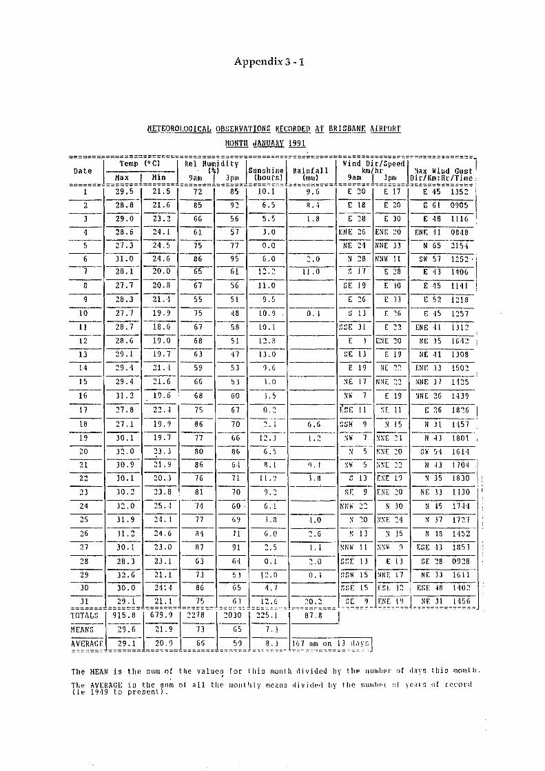
Appendix 3-1
METEOROLOGICAL OOI:ERVIlTIONS ~[CORDEl!. ,\T BRISBANE: AfRf'OIlT
MONTH JANUARY 1991
'::::<'I<'=T;~~=(:CI=«I<R;1<H1~rdltY=I:::::;::1";:;:;:;;'J<'i;d:~1~1s;;;dj";::<:;::<:::;i =======_==~~~=J==~!~==_==~:~=J==!~~=_=!~~~;;~_===!~~~===_==;:~==t=!~~==_~!~~~~;~;!;!~~:
1 29.5 21. 5 72 85 10.1 9.6 E ::lO E 17 E 45 1352 I --- I 2 28.8 21. 6 85 92 6.5 I!. ·1 E 18 E ~O E 61 0905 --- 5.5 1.8 111G 1 3 29.0 23.2 66 56 E 28 E 30 E 48
---<I 28.6 24.1 61 57 3.0 ENE 2G ENt: 20 ENE 41 08<18
---5 27.3 24.5 75 77 0.0 NE 21 NNE 3l N 65 2154
---6 H.O 24.6 86 95 6.0 ::'.0 N 28 NNW 11 SW 57 1252 .
7 28.1 20.0 65 61 12.2 11.0 ::: 1'1 E ~8 E'l) HOG ---
S 27.7 20.8 67 56 11.0 ~E 19 E 10 £15 llH ---
9 28.3 21. ·1 55 51 9.5 E 26 E )) E 52 1218 --
10 27.7 19.9 75 <18 LO.9 0.\ S 13 E :(. E ,15 1257 --- ---
11 28.7 18.6 67 58 LO.l SEE 31 E ~2 ENE H 1312 I ---12 28.6 19.0 68 51 12.R E ) ENE ~O NE )5 11;·12 I
13 29.1 19.7 63 ,n 13.0 SE 13 E 19 NE 41 1)08 ---
14 29.1 21.1 59 53 'J.G E 19 NE ...... ENE 33 1502 I-;J !
15 29.4 21. 6 6G 1.0 NE 11 NNE ~'l NNE J7 1425 -~
--16 )1. 2 19.6 68 60 1.5 ~" 1 E 19 ~NE 26 14]9
-- i 17 27.8 22.4 75 61 0.2 ESE 11 \~ t: II E 26 182G I .ii ..
--18 27.1 19.9 86 10 2. \ G.6 ssw 9 :l 15 NJl 1451
---19 )0.1 19.7 17 6G 12.3 1.2 Nli 7 ~NE ~ I N 4) 180t I
---20 32.0 3).J 80 8G 6.5 :-I 5 ~~lE ~O ::;W 54 IG 1-1
21 )0.9 :!1. 9 86 1--:-:-
!L 1 fl. I 'iii 5 NNE ~'l N 43 1104 --2:: 30.1 20 . .) 76 71 11. 'J 3.8 S 13 f.H 1') N 35 18)0
-- -33 )O.:! 3J.8 81 70 9.2 SE 9 ENE ~O NE )) ll]O ---
24 32.0 ~5 .\ 14 GO . 6.1 NNIi 'l'l N ]0 N 45 17H ---
25 31.9 ::!4. 1 11 69 3.8 1.0 :-l ~O NXE ~4 ~ 31 11 2'1 --
26 31.2 24.6 81 11 G.O ~.6 N 1] N )5 N 18 1452 ---
27 ]0.1 2].0 81 91 2.5 1.1 NNII' 11 ~JN\I' <) ESE U 185J ---
28 28.] 23.1 6] 6~ 0.1 2.0 s~r 1J E 1 ) SE ~8 0928 ---
29 32.6 21.1 13 53 . ~:!. 0 O. I ~:sw 15 NNE 17 HE )) 1(; 11
30 30.0 21 ~.\ 86 65 jil.l Sf:E 1!1 f.~E 32 Ef,E ~II 1·102
Jl 29.1 21.1 75 6J 12.6 20.2 SE 9 ENE 19 NE 31 1456 =======_=======_=======_=======_==~~==_=====7-~~~~~=~~~=~=. -:"'"".,.,.. ~-= =
81.8
161 mm on 13 d~YGJ _~=-=:~=-=====~===c
The MEAN is the sum of the value~ [or thig monlh <lidded by the 1I11l1li>e[' ot days this monlh,
The AVERAGE is the sum of all the mOlllllty means divide!! by the Ilumhpl' o[ reinG of record (ie 191\9 to present).
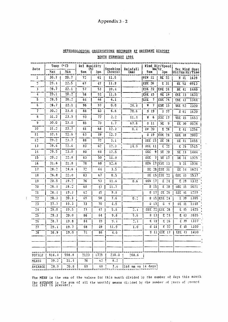
Appendix 3 - 2
METEOROLOGICAL OBSERVATIONS RECORDED AT BRISBANE AIRPORT
MO~TH FEBRUARY 1991
-----------------------------------------------------------------------------------------Date (%1 Sunshine Rainfall km/hr ~ax Wind GUSt
1 Temp (OCl 1 ReI Humidity 1 1 1 Wind Dirlspeedl
=======_==~~;==l==~!~==_==~~~==l==~~~=_=!~~~~~!_===!~~!===_==~!~==l==~~~==_~~~!~~~~~!~~; 1 ]0.7 20.7 72 61 11.5 WSW 11 NE 22 ~ n 1639
2 29. t 22.5 67 47 11.9 ESE 26 E J1 SE 52 0913 --] 28.7 22.1 57 53 10.4 ESE 22 ENE 24 :iE H 1440 4 29.1 20.2 58 52 U.S E.lfE 15 ~E 19 E.'>E J] 1632 --5 28.5 20.2 66 66 6.1 ESE 1 ENE 24 ~E 13 1344 --6 26.7 22.1 96 93 0.0 24.1 II' 7 ENE 15 ~'NE 52 2]20 7 30.2 23.0 88 8] 6.6 78.6 N 19 X 37 ~ 61 1620 --8 ]1.2 23.9 9] 77 " " 11.1 Ii 6 NNE 17 ~~E ~5 165] ....... --9 30.0 23.0 85 73 1.7 67.6 S 11 ~E 9 SE ]0 0028 --10 ]1. 2 23.7 31 68 12.3 0.1 SI! 20 E 28 E U 1256
11 ]2.4 22.6 63 19 12.7 S 19 ESE ~4 ESE 18 200] 12 29.2 23.7 88 72 3.1 SSE 15 SE 23 SE H 1455 13 29.6 "".6 83 62 1:'.3 14.0 SSE 11 E "12 E 35 1515
29.5 -- . 14 23.0 80 64 12.5 SSE 9 ~E ~O XE 33 1444 --15 29.:" "1"1.8 83 50 11. 9 SSE 7 ~E 17 NE 31 1325 --16 31. 6 21.3 18 60 12.6 SSW 17 !~XE LJ N 31 1936
11 28.2 21.6 12 64 ].5 SE ~8 ESE Jl SE 54 1621
18 ~6.8 ~2.0 83 61 0.5 SE 15 ESE ::!:! ESE -13 1531
19 28.5 19 . .:! 16 53 11. 6 0.6 SSli 11 E ~:l E 39 133:!
20 28.4 18.~ 68 ~3 11. 7 S 15 E 20 nSE 15 1021
21 ~8.4 19.3 6::: 45 9.:.1 S 11 :';E ~5 ESE n 1~19
::!:! :28.3 20.3 69 58 1.6 o ., S 15 EXE ~4 E 39 1305
~3 ~7.J 19.3 13 10 4.5 :> 13 S 9 SE n IHE
I I I
I ; I , I I I i I
I ,
. I
I
I , , , , ;
i I
i 21 ~9.0 19.5 13 41 5.8 2.1 SSE 22 ESE ~8 E -IS 1425 ;
25 29.3 20.0 86 64 9.8 5.6 S 13 Ii: 21 E 43 1035 i
--:!6 28.1 19.8 84 i9 9. 1 ~. 1 E 11 E 26 £ J9 l337 : --':.7 29. I 19.1 68 -l9 11.9 1.0 11 11 E 2~ E l5 1329
~6 26.9 19.0 1! 66 4.6 11 11 ,ESE 11 ESE -l3 1430
rom, 816.1 1 598 .81 om 1 m5 "0.0 '08.6 :1EAXS 29.2 21.·1 76 62 8.2
~VERAGE __ :~:~_l __ :~:~ ____ ~~ _____ ~~_j ___ ~:~ ___ ~~~_~~_~~_~~_~~~~ 0"0""==1_______________________________________________________ J
The MEAN is the sum ot the values tor this month divided by the number ot days this month rbe AVERAGE is the .um of all the monthly means dilided by [he number ~t ~edr~ of :ecord (Ie 1949 to present) .
I
;
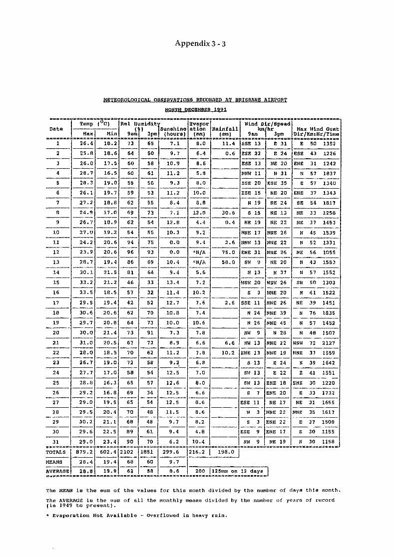
Appendix 3 - 3
METEQRQLOGICAL OBSERvaTIONS RECORDED AT BRISBANE AIRPORT
MONTH DECIMBIS 1991
.--m-··I·-;;;~·(O~;···I;:i· Data
Maxi Hin 9a ••••••• = •• _= __ s •••• au ••• a.
1 26.4 ---2 25.8
---3 26.0
---4 2S.7 ---5 2S.3
---6 26.1
7 27.2 ---
8 24.9 ---9 26.7
---10 27.0
---11 24.2 ---12 23.9 ---13 28.7
---- ---14 30.1
---IS 33.2 ---16 33.5
---17 29.5 ---is 30.6
---19 29.7
---20 30.0
---21 31.0 ---22 28.0
---23 26.7 ---24 27.7
---25 28.8
---26 29.2 ---27 29.0 ---28 29.5
---29 30.2
30 29.6
31 29.0 , .. "' ........ ,
TOTALS 879.2 ---
MEANS 28.4 ---AVll!RAQI 28.1'1
18.2
18.6 ---
17.5
16.5
19.0
19.7
IB.8 ---
17.0 ---IB.9
---19.2 ---20.6 ---20.6
---19.4
---21.5
---21.2
---18.5
19.4 ---
20.6 ---
20.8 ---21.4
---20.5 ---18.5 ---19.0 ---17.0 ---16.3
---" 16.8 ---19.5 ---20.4
---21.1 ---22.5
---23.4
F ........ "' .. , 602.4 ---
19.4 ---19.9
f .... 21
73
64
60
60
55
59
62
69
62
54
94
96
86
81
46
57
42
62
64
73
67
70
72
58
65
69
65
70
68
89
90
02
68
•••••••••••••••••••••••• a ••••••••••••••••••••••••••••• • ____ ••• ~
Humiditl /Bveporl I Wind Dirlspsadl (i' Sunshine ation Rainfall kmfhr MaK Wind Qust m 3pm (hours, (rom, (rom, 9am 3pm Oir/KmfHr/Tlme .......... _._a_ ... _ .. s ....... __ ........ __ .. __ ~_ ... _ ............
65 7.1 8.0 11.4 SSE 13 E 31 E 50 1352 ---50 9.7 6.4 0.6 ESE 22 E 24 ESE 43 1226 -- ---58 10.9 8.6 ESE 13 NE 20 ENE 31 1242 -- ---61 11.2 5.8 NNW 11 N 31 N 57 1837 -- ---56 9.3 8.0 SSE 20 ESE 35 E 57 1340 -- ---53 11.2 10.0 ESE 15 NE 20 ENE 37 1343
-- ---55 8.4 8.8 N 19 NE 24 SE 54 1817 -- ---73 7.1 12.8 30.6 S Hi NE 13 NI!! 33 1258
-- ---54 12.8 4.4 0.4 NE 19 NE 22 NE 37 1453
-- -55 10.3 9.2 NNE 17 NNE 26 N 45 1539 -- ---75 0.0 9.4 2.6 NNW 13 NNI!! 22 N 52 1331 -- ---93 0.0 "N/A 75.0 ENE 31 NNE 26 NE 56 1055
-- ---69 10.4 "N/A 58.0 SY! 9 NE 20 N 43 1553 -- ----64 9.4 5.6 N 13 N 37 N 57 1552
-- ---33 13.4 7.2 WSW 20 WSW 26 SW 50 1303
-- ---32 11.4 10.2 S 3 NNE 20 N 41 1522
-- ---52 12.7 7.6 2.6 SSE 11 NNE 26 NE 39 1451
-- ---70 10.8 7.4 N 24 NNE 39 N 76 1835 -- ---73 10.0 10.6 N 26 NNE 45 N 57 1452
-- ---91 7.3 7.8 NY! 9 N 28 N 48 1507
-- ---73 8.9 6.6 6.6 NW 13 NNE 22 WSW 72 2127
--62 11.2 7.8 10.2 ENE 13 NNE 19 NNE 37 1559 -- ---58 9.2 6.8 II 13 E 24 E 39 1642 -- ---54 12.5 7.0 sw 13 E 22 E 41 1551
-- ---57 12.6 8.0 SW 13 ENE 18 ENE 30 1220 -- ---34 12.5 6.6 S 7 ENE 20 E 33 1732
-- ---54 12.5 8.6 ESE 11 NE 17 NE 31 1655 -- ---48 11.5 8.6 Ii 3 NNE 22 NNE 35 1617 -- ---48 9.7 8.2 S 3 ENE 22 E 37 1508 -- --- ---~
61 9.4 4.8 ESE 9 ENE 17 E 30 1155 -- --- ---70 6.2 10.4 NW 9 NE 19 N 30 1158
"" "''''==, ....... , ... ,," u,,'===, 1851 299.6 2: --
60 9.7 --!l8 8.6 200 I 125rom on 12 daya
The MEAN is the sum of the values for this month divided by the number of days this month.
The AVERAGE is the sum of all the monthly means divided by the number of years of record (ie 1949 to present) •
• Evaporation Not Available - Overflowed in heavy rain.
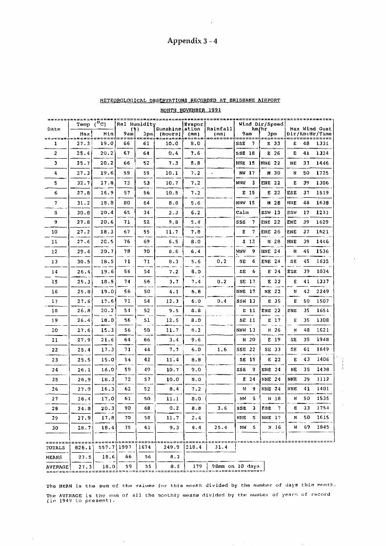
Appendix 3 - 4
METEOROLOGICAL OBSERVATIONS RECORDED AT BRISBANE aIRPORT
MONTH NOVEMBER 1991
a====mz._==c===c~u._========~ft==.=========_=c======ac=._._.====_==_3.a========e====_==cc
I
Temp (oC) IRel Humiditl IEvaporl I WInd DIr,speedl Date . I i I Sunshine ation Rainfall km hr Max Wind Gust
Maxi Ml.n 9am 3pm (hours) (rom) (rom) 9am f 3pm. Dlr/Km:Hr/Tlme =========================================================================================
1 27.3 19.0 66 61 10.0 8.0 SSE 7 E 33 E 48 1331 --- -- -- ---
2 25.4 20.2 67 64 0.4 7.6 SSE 18 E 26 E 41 1324 --- -- -- ---
3 25.7 20.2 66 52 7.3 5.8 NNE 15 NNE 22 NE 33 1446 --- --- -- ---
4 27.3 19.6 59 59 10.1 7.2 NW 17 N 30 N 50 1725 --- --- -- ---
5 32.7 17.8 73 53 10.7 7.2 WNW 3 ENE 22 E 39 1306 --- --- -- ---
6 27.8 16.9 57 56 10.5 7.2 E 15 E 22 ESE 37 1519 --- -- -- ---
7 31. 2 18.8 80 64 8.8 5.6 NNW 15 N 28 NNE 48 1638 --- --- -- ---
B 30.8 20.4 65 34 2.3 6.2 Calm SSW 13 SSW 17 1233 --- --- -- ---
9 27.8 20.6 71 52 9.8 5.4" SSE 7 ENE 22 ENE 39 1629 --- --- --
10 27.2 18.3 67 55 11. 7 7.8 E 7 ENE 26 ENE 37 1621 --- --- -- ---
11 27.6 20.5 76 69 6.5 8.0 S 13 N 28 NNE 39 1446 --- --- -- -- --- ----
12 29.4 20.7 78 70 B.6 6.4 WNW 9 NNE 24 N 45 1536 --- I-~- -- ---
13 30.5 1B.5 71 71 S.3 5.6 0.2 SE 6 ENE 24 SE 45 1635 --- --- -- -- ---
14 26.4 19.6 56 54 7.2 8.0 SE 6 E 24 ESE 39 1034 _._._- --- --- -- -- ---IS 25.3 18.5 74 56 3.7 7.4 0.2 SE 17 E 22 E 41 1337
--- --- --- -- ---16 25.8 19.0 56 50 4.1 6.8 NNE 17 NE 22 N 43 2249
- --- --- --- -- ---17 27.6 17.6 71 54 12.3 6.0 1 0.4 SSW 13 E 35 E 50 1507
--- --- -- -- ---, 18 26.8 20.2 54 52 9.5 8.8 E 11 ENE 22 ENE 35 1654
--- --- -- -- --- --~.-~
19 26.4 IB.O! 56 51 12.5 8.0 SE 11 E 17 E 35 1308 --- --- --- --- -- --_.-
20 27.6 15.3 56 50 11.7 B.2 NNW 13 N 26 N 48 1621 --- --- --- -- --- ---
21 27.9 21.6 64 66 3.4 9.6 N 20 E 19 SE 39 1948 --- --- --- -- ---
22 25.4 17.3 71 44 7.7 6.0 1.6 SSE 22 SE 33 SE 61 1649 --- --- --- -- ---
23 25.5 15.0 S4 42 If. 4 8.B SE 15 E 22 E 43 1406 --- -- -- --~ -
24 26.1 16.0 59 49 10.7 9.0 SSE 9 ENE 24 NE 35 143B --- --- --- -- --- -
25 26.9 IB.3 72 57 10.0 8.0 E 24 NNE 24 NNE 39 1112 --- --- -- -- ---
26 27.9 16.3 62 52 8.4 7.2 W 9 NNE 24 NNE 41 1401 ._-- --- --I- ---27 2B.4 17.0 61 50 11. 1 B.O NW 5 N 18 N 50 1535
--- --- --- -- --~
28 24.8 20.3 90 68 0.2 8.8 3.6 SSE 3 ESE 7 I!l 33 1754 --- --- --- -- --- ---- ----
29 27.9 17.8 70 58 11. 7 2.4 NNE 5 NNE 17 N 50 1615 --- --- --- -- --- ---- ----
3D 28.7 18.4 75 61 9.3 9.4 25.4 NW 5 N 16 W 69 1845 --- --- -- -- ---~ ----
,=== .===== ,= '===, 11, ~==I .-~-
TOTALS 826.1 557.7 1997 1674 249.9 2 ---.~~ 1--- --
MEANS 27.5 18.6 66 56 8.3 --- --~- --- -- J AVERAGE 27.3 18.0 59 55 8.5 179 98rom on 10
,===== ,==,::
The MEAN is the sum of the values for this month divided by the number of daye this month.
The AVERAGE is the sum of all the monthly means divided by the number of years of record (ie 1949 to present).

1 25.2 ---
:2 25.6 ---
3 25.4 ---
4 25.4 ---5 24.9
---6 24.9
---7 25.9
---8 28.2
---9 27.3 ---
10 23.2 ---
11 25.9 ---
12 24.8 ---
13 27.7 ---
14 25.7 ---
IS 25.6 ---
16 27.9 ---
17 25.3 ---
18 22.2
19 24.9 ---20 24.4
---21 25.3
---22 29.1 ---23 23.4 ---24 23.1
---25 26.6
---26 32.S!
---27 26.1
---28 23.8
---29 23.5
---30 24.0
---31 25.6
Appendix 3 - 5
METEOROLOGICAL OBSERVATIONS RECORDEP AT BRISBANE AIRPORT
MONTH OCTOBER 1991
en ••••••••••••••••••••••••••••••••••• • •••••••••• ___ •• •~. 1 IEvaporl I Wlnd Dlr/speedl Sunshlne atlon Rainfall kmfhr Max Wind Gust (hours) (mm) (rom) 9am 3pm Dlr/Km:Hr/Time
:_ac:_====_===CB:aRcuu •• ==._===_.= •• cc==a=::=D==C:=C===a 14.9 55 32 11.2 8.2 E 13 N 20 ENE 31 1050 --- ----12.9 64 57 11.0 7.8 NW 9 HNE 22 N 33 1643 ---14.2 74 54 11.0 4.8 ENE 13 NNE l7 ENE 28 0848 --- ---16.2 54 62 8.4 5.8 I!! 15 I!: 22 ENE 39 1136 --- ----17.4 49 50 10.9 5.8 E 18 NE 20 NE 35 1138
---14.3 55 47 11.2 7.2 SW 11 ENE 22 ENE 33 1440 --- ---12.2 53 60 10.7 7.2 N 20 N 31 N 45 1606
--- ----18.0 53 84 9.0 6.6 0.4 SW 5 N 24 N SO 1347
--- ----17.7 61 51 10.4 4.8 2.8 E 13 BE 31 ESE 54 1557 ---16.9 68 68 2.4 7.B 0.2 SSE 19 I!: 15 SE 37 0807 --- ---15.5 59 59 9.4 3.0 SE 9 ESE 31 ESE 50 1555 --- ---17.8 56 54 6.4 6.6 ESE 13 NE 20 NE 33 1309 --- ---13.6 56 51 10.9 6.0 NW 9 HNE 24 N 37 1604 --- ---18.6 49 56 10.2 7.4 ESE 19 HE 26 E 39 0936
--- ---18.0 60 57 7.5 7.6 N 15 NNE 22 NNE 41 1538
--- ---16.8 64 65 10.8 7.2 N 20 N 43 N 59 1431
--- ----19.4 55 58 1.1 8.0 ESE 26 SE 31 ESE 61 1646
---15.2! 82 64 0.3 7.6 6.6 sl1 ESE 22 ESE 48 1358
---13.8 62 59 9.2 3.6 5 19 E 30 E 41 1337
---15.2 61 62 6.2 7.2 SSE 11 ENE 26 ESE 39 1021
--- ---17.7 53 47 11.8 6.8 NE 17 N 25 N 37 1355
--- ---14.7 57 39 9.5 6.4 WNW 5 NNE 28 NNE 41 1534
----20.5 65 65 0.0 6.0 0.6 SE 20 ESE 22 E 45 1024
----16.9 67 73 0.0. 5.0 4.6 E 13 ENE 9 5E 35 0104
---16.9 75 61 6.9 2.4 9.8 N 17 NNE 26 N 41 1534
--- -- ----15.0 70 15 12.1 4.8 1.6 SE 3 WSW 37 W 63 1518
--- -- ---14.4 66 54 11.6 10.0 SSW 7 ENE 24 SE 45 2029
-- -- ---13.9 43 46 II. 3 7.2 S 19 ENE 24 E 41 1314
--- -- -- ---14.4 58 60 8.7 8.6 SE 17 E 20 ENE 35 1132
--- ---14.7 71 55 3.4 5.4 SE 7 NE 20 NNE 31 1349
--- ---13.7 61 61 11.0 !I.O NW 13 NNE 33 N 48 1506
m __ .au_a==~_Dma_~m ••• u ___ m_.m ___ .~=am.caA~xa==a.Kg __ ._mm
TOTALS 793.4 491.4 1878 1726 256.5 197.8 I ------ ----- ----- ---- ----1------- 26.6 I MEANS 25.6 15.9 61 56 8.3
The MEAN 1s the Bum of the values for this month divided by the number of days this month.
The AVERAGE is the sum of all the monthly means divided by the number of years of record (ie 1949 to present).
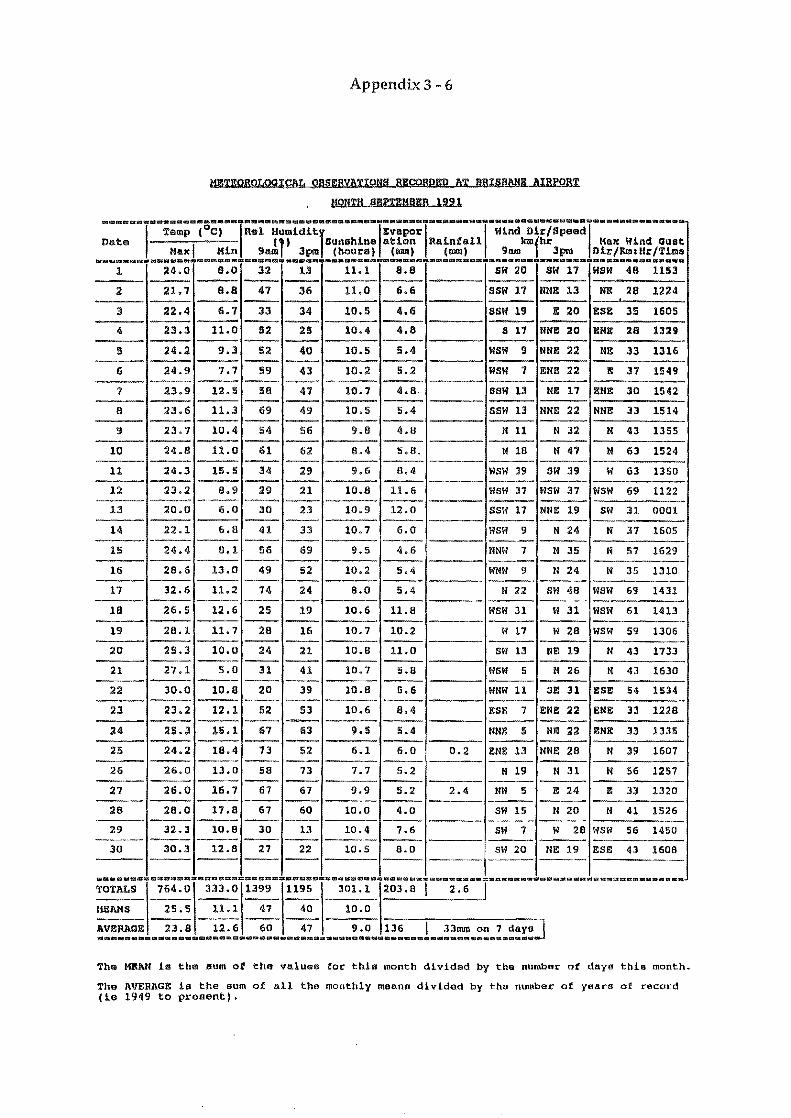
1
2
;]
" 5
6
1
8
9
10
11
12
13
14
15
16
17
18
19
20
21
22
23
24
25
26
27
26
29
.30
MEANS
24.0
21.7
22.4
23.3
24.2
24.9
23.9
2.3.6
23.7
24.S
24.3
23.2
20.0
22.1
24.4
28.6
32.6
26.5
28.1
25.3
27.1
30.0
23.2
25.3
24.2
26.0
26.0
28.0
32.3
30.3
25.5
Appendix 3 - 6
METEOROLOGICAL OBSERVATIONS RECORDED AT BRISBANE AIRPORt
HOHTH SBrrEHBBR 1991
8.0 ----8.8 ---1i.7 - 11.0
---9.3 ---7.7 ---
12.5 ----l1.l ---10.4 ---11.0
15.5
8.9 ---6.0 ---6.8
---B.l
---13.0
11.2
12.6 ---
11. 7 ----
10.0 ---
5.0 ---
10.S ---12.1
---llLl
18.4 ---
13.0 ---
16.7 ---17.B ---10.8
---12.8
---
11.1
32
47
33
112
S2
S9
SB
69
S4
61
34
29
lO
41
56
49
74
25
28
24
31
20
52
67
73
58
67
67
30
27
47
13 ---36 ---34 ---25 ---40 ---43 ----47 --49 ---56 ---62 --29
I-n ---23
--33
--69
---52
---24 ---19
---16
--21 ---41
---39 ---53 ---63 --52
--73 --67 --60
--13 --22 --
40
11.1
11.0
10.5
10.4
10.5
10.2
10.7
10.5
9.B
B.4
9.6
10.8
10.9
10.7
9.5
10.2
B.O
10.6
10.7
10.B
10.7
10.B
10.6
9.S
6.1
7.7
9.9 ----
10.0 ----
10.4
10.5 -----
10.0
8.8
6.6
4.6
4.8
5.4
5.2
4.8
5.4
4.8
5.13.
8.4
11.6
12.0
6.0
4.6
5.4
5.4
11.8
10.2
11.0
S.B
5.6
8.4
S.4
6.0
5.2
5.2
4.0
7.6
8.0
. __ ._._n. ___ ..•............ ___ .• _. ___ .. ~ I I Wind Dir/speedj Rainfall kmfbr Max Wind Quat (mm, 9 11m 3pm Dir/bIUr/Time ........ -_ ..................•.•.......•.
SW 20 SH 17 Haw 4B 1153
SSW 17 NNE 13 Nt!: 28 1224 !
SSW 19 II: 20 ESE 3S 1605
S 11 NNE 20 ENI: 28 1329
WSW 9 NNE 22 NE 33 1316
WSW 7 ENE 22 I!: 37 1549
ssw 13 NE 17 ENE 30 1542
SSW 13 NNE 22 NNE 33 1514
If 11 N 32 N 43 1355
If 18 N 47 If 63 1524
wsw 39 Sif 39 W 63 1350
WSW 37 WSW 37 wsw 69 1122
ssw 17 NNE 19 sw 31 0001
WSW 9 If 24 N 37 1605
NNW 7 N 35 N 57 1629
WNW 9 N 24 If 35 1310
H 22 Sill 48 WSw 69 1431
WSW 31 W 31 WSW 61 1413
w 17 III 28 WSW 59 1306
SN 13 NE 19 N 43 1733
WSW 5 If 26 H 43 1630
WNW 11 BE 31 ESE 54 1534
ESE 7 ENE 22 ENE 33 122B
NNE 5 NIll 22 ENE 33 1335
0.2 ENE 13 NNE 28 N 39 1607
If 19 If 31 If 56 1257
2.4 NW 5 E 24 Ii!: 33 1320
SW 15 If 20 If 41 1526
SW 7 III 28 WSW 56 1450
SW 20 NE 19 ESE 43 1608
_. ____ . __ =.u __ .. _c .. _._.=._._m=._._. ___ ~
The MEAN i8 the Bum of the values tor this month divided by the number of daya this month.
The AVERAGE is the sum of all the monthly means divided by the number of yeara of record (ie 1949 to present).

Appendix 3 -7
METEOROLOGICAL OBSERVATIONS RECORDED AT BRISBANE AIRPORT
MoNTH AUGYST 1991
m···· __ I_·;::~_(~~a.~-.=cd .. 2 •• _G •• =.a._._=.m.=.-m __ am ______ ax
Date MaxI
.... .. _ _;:.'I _ aa.a:;: .= _
) IRel Humiditj I EvaporI / Wind Dir,speedl I) Sunshine at ion Rainfall km hr Max Wind Gust
Min 9aml 3pm (hours) (mm) (mm) 9am f 3pm Dir/Km:Hr/Time _=_== __ m=~sm_ .. _m .. __ .=.c=._.m ...... a. ___ a .... _ .. ___ . ____ ======5=_==:=== .. _._=-_ .... _-=.-1 24.7 6.5 54 21 10.2 3.4 SSE 3 W 37 WSW 57 1438
--- -- -- ---2 22.0 6.7 52 34 10.2 5.4 SW 18 ENE 11 SW 33 0922
--- -- -- ---3 21.5 7.3 61 45 10.4 4.2 SSW 15 tiE 18 NNE 28 1221
--- -- -- ---4 22.3 7.2 74 51 9.9 3.4 SSW 9 tiE 17 N 31 2232
--- -- -- ---5 22.8 9.4 78 69 9.1 2.8 WNW 4 N 39 N 54 1549
--- -- --6 27.9 12.7 75 32 8.2 4.0 N 20 WSW 22 W 48 1124
--- -- -- --- ----7 23.2 II. 6 38 31 7.8 8.0 SSW 20 N 19 WSW 28 0159
--- -- -- ---B 22.9 8.5 27 16 10.4 4.0 WSW 24 W 35 WSW 56 1502
--- -- -- ---9 21.0 10.1 33 13 10.6 9.6 WSW 24 SW 22 aw 45 1053
--- -- -- ---10 19.7 8.7 36 35 10.4 6.8 ssW 22 Ii: 22 Ii: 39 1523
-- -- ---11 21.2 10.6 53 47 9.0 5.4 SSW 17 E 24 BE 35 1106 --- --- -- -- ---12 21.6 11.2 61 41 10.5 3.8 SSW 19 NE 15 SSW 26 0747
--- --- -- ---13 21.5 9.1 72 52 10.3 3.4 SSW 11 N 28 N 35 1502
--- -- -- ---14 25.6 6.B 69 17 10.0 4.0 WSW 5 W 17 W 41 1408
--- -- -- ---IS 24.3 7.3 43 22 10.7 4.8 SW 15 W 19 WSW 35 1505 --- -- -- ---16 23.2 9.7 33 21 10.8 7.2 sw 19 WSW 22 SW 48 1019
--- -- -- ---17 20.4 12.0 52 46 5.4 5.2 SSE 17 ESE 24 SE 37 1026
--- -- -- ---18 20.5 11.5 58 51 7.0 5.6 SSE 15 E 20 SE 37 1001
--- -- -- ---19 21.3 10.1 70 53 9.6 3.0 SSW 15 ENE 9 ENE 30 1405
--- -- -- --- ----20 23.0 7.3 72 57 10.6 3.0 W 5 N 33 N 48 1451
--- -- -- ---21 26.2 14.5 36 15 10.7 5.0 NW 19 WSW 30 WSW 56 1059 --- -- -- ---22 23.0 6.2 35 24 10.9 9.0 SW 9 NE 15 HE 30 1320
--- -- -- ---23 22.8 5.2 45 54 10.5 5.0 WSW 11 N 24 N 41 1542 --- --- -- ---
24 23.4 11.3 31 22 10.9 4.0 W 30 WSW 52 WSW 81 1340 --- -- ---
25 113.5 7.7 31 26 10.9 11.2 SSW 20 ENE 18 SW 35 0356 --- -- -- ---
26 20.2 6.8 49 48 5.4 4.8 SW 19 ENE 13 SSW 28 0818 --- -- -- ---27 21.3 8.3 62 48 10.6 3.2 SSW 13 NNE 20 NE 30 1412
--- -- -- ---28 24.3 "1.2 65 64 10.3 3.4 N 13 N 39 N 56 1408 --- -- -- ---29 26.4 13.0 67 61 9.1 4.8 NW 15 N 22 N 31 1110
--- -- -- ---30 22.3 13.1 72 31 2.1 4.0 WSW 5 W 20 WSW 31 1429 -- -- ---31 23.7 6.7 24 13 11.0 4.0 SW 19 W 20 W 39 1442
~"'==="'=' TOTALS 702.7 2 84.3 1628 1160 293.5 155.4 Ii
--- -- --MEANS 22.7 9.2 53 37 9.5
--- -- --AVERAGE 21.7 10.1 63 44 8.3 103 I 45 mm on 7 days
The MEAN is the Bum of the values for this month divided by the number of days this month.
The AVERAGE is the sum of all the monthly maana divided by the number of years of record (ie 1949 to present).
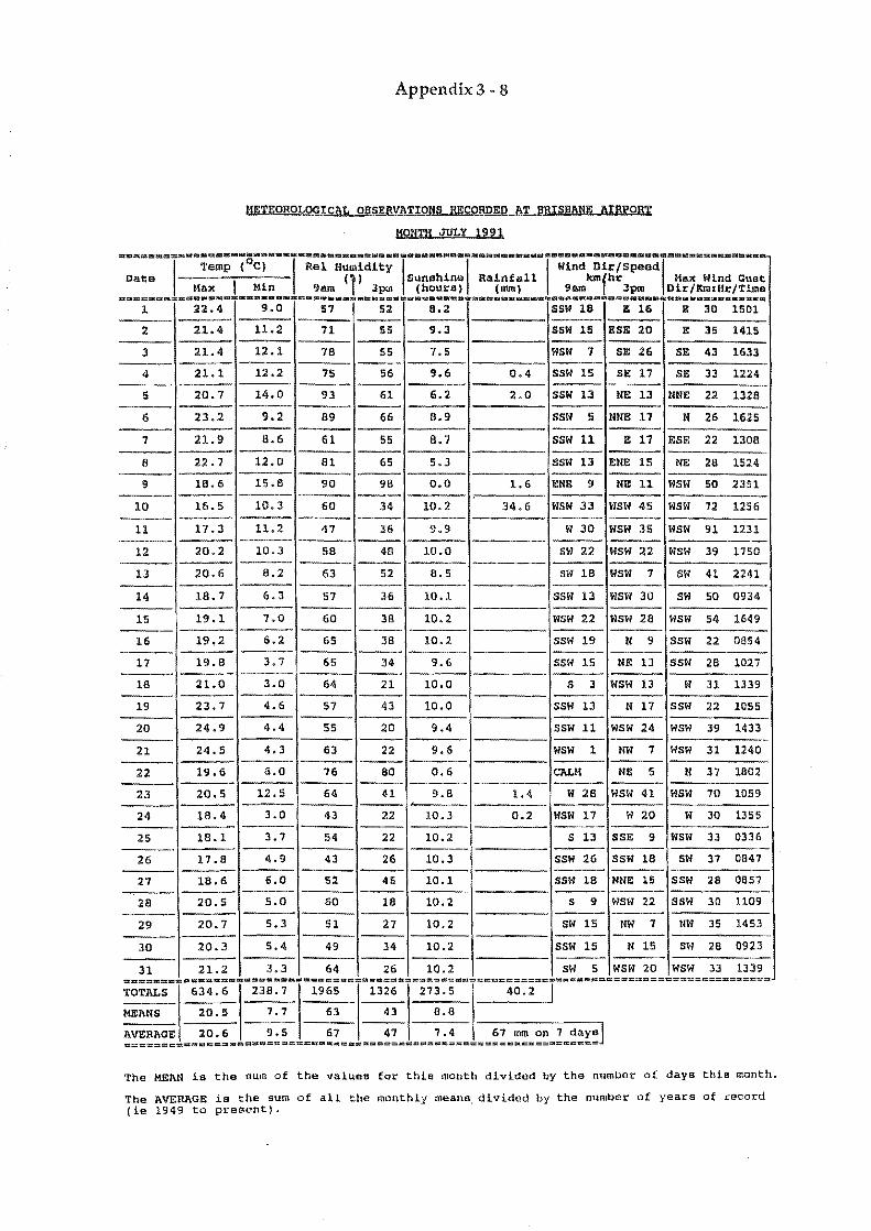
Appendix 3 - 8
HETEOROLOGICaL OBSERVATIONS RECORDEP AT BRISBANE AIRPORT
MONTH JULY 1991
·-=···-=\-··;:;~-7S~j-···\-;:i·~~;idi~ Date (l' Max I Min gam Jpm
._ .•. _______ =m_.a. __ ._ .... ___ .=._=_.m •••.• ___ ._ .. _._~ y I I \ Wind DirlSpeed\ Sunshine Rainfall kmfhr Max Wind Gust
(hours) (mm) gam 3pm Dir/KlIlIHr/Time aa.~.g_~. ____ •••• __ ·· ____ • •• ___ • __ .m •• _ •• __ •••• ___ •• _________ •• ___ • ______ • ____ • __ 2 ___ ••••
1 22.4
2 21.4
3 21.4
4 21.1
5 20.7
6 23.2
7 21.9
a 22.7
'3 18.6
10 16.5
11 17.3
12 20.2
13 20.6
14 IB.7
15 19.1
16 19.2
17 19.8
18 21.0
19 23.7
20 24.9
21 24.5
22 19.6
23 20.5
24 18.4
25 IB.l
26 17.8
27 18.6
28 20.5
29 20.7
30 20.3
31 2L2 ..... >F ..
TOTALS 634.6
MEANS 20.5
AVERAGE 20.6
9.0 57
11.2 71
12.1 78
12 .2 75
14.0 93
9.2 89
8.6 61
12.0 81
15.8 90
10.3 60
11.2 47
10.3 58
8.2 63
6.3 57
7.0 60
6.2 65
3.7 65
J.O 64
4.6 57
4.4 55
4.3 63
6.0 76
12.5 64
3.0 43
3.7 54
4.9 43
6.0 52
5.0 60
5.3 51
5.4 49
3.3 64
-
5
S
S
S
6
6
5
6
9
2
.3
:3
4
5
3
3
3
.3
2
4
2
5
5
6
1
6
5
5
8
4
6
B
2
6
B
8
'" 1
.3
a 22
80
41
22
22
26
45
IS
27
34
26 , ...... , ' .. m"'="' .... ' ~ .. "' ..
238.7 1965 13 26
7.7 63 43
9.5 67 47 - --
8.2
9.3
7.5
9.6
6.2
8.9
8.7
5.3
0.0
10.2
9.9
10.0
8.5
10.1
10.2
10.2
9.6
10.0
10.0
9.4
9.6
0.6
9.8 ,
10.3
10.2
10.3
10.1
10.2
10.2
10.2
10.2
273.5
8.8
7.4
SSW 18 E 16 E 30 1501
SSW Hi ESE 20 I!! 35 1415
WSW 7 SE 26 SE 43 1633
0.4 SSW 15 SE 17 SE 33 1224
2.0 SSW 13 NE 13 NNE 22 1328
SSW 5 NNE 17 N 26 1625
SSW 11 E 17 ESE 22 1308 --- ----SSW 13 ENE 15 NE 28 1524
1.6 ENE 9 NE 11 WSW 50 2351
34.6 WSW 33 WSW 45 WSW 72 1256
W 30 WSW 35 WSW 91 1231
SW 22 WSW 22 WSW 39 1750
SW 18 WSW 7 SW 41 2241
ssw 13 WSW 30 SW 50 0934
WSW 22 WSW 28 WSW 54 1649
SSw 19 N 9 SSW 22 OB54
SSW 15 NE 13 SSW 28 1027
S 3 WSW 13 W 31 1339
SSw 13 N 17 ssw 22 1055
SSW 11 WSW 24 WSw 39 1433
WSW 1 NW 7 WSW 31 1240
CALM NE 5 N 37 1802
1.4 W 28 WSW 41 WSW 70 1059
0.2 wsw 17 W 20 W 30 1355
S 13 SSE 9 WSW 33 0336
SSW 26 SSW 18 SW 37 OB47
SSW 18 NNE 15 SSW 28 OB57
S 9 WSW 22 SSW 30 1109
sw 15 NW 7 NW 35 1453
SSW 15 N 15 SW 28 0923
SW 5 WSW 20 WSW 33 1339
67 mm on 7 days
The MEAN is the sum of the values for this month divided by the number of days this month.
The AVERAGE is the sum of all the monthly means, divided by the number of years of record (ie 1949 to present).
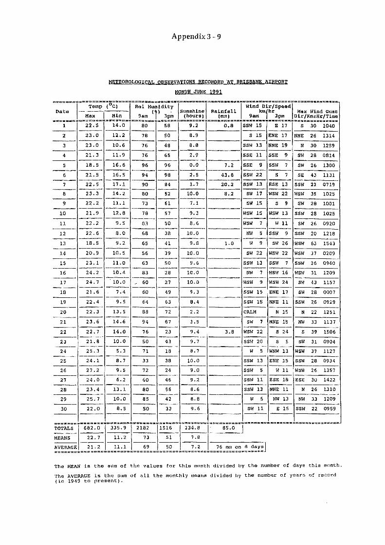
Appendix 3 - 9
METEOROLOGICAL OBSERVATIONS RECORDED 'AT BRISBANE AIRPORT
MONTH JUNE 1991
m===a.==ld_.;::~-70~;=-==I=;:iU~::idi==.G_-.. =.nmc=.~ __ ..... =._=. __ .~~=-=--=-D=====_.==_==~ Date (i)
Max I Min 9am 3 t~ I sunshine I Rainfall
I Wind Dir/SP;;dl -krn hr Max Wind Gust
pm (hours) (mrnl 9am f 3pm Dir/KrnIHr/TLme ==n=.ca-D_-u~m.=_B==_m_m=m=c= __ c_.c - - ==m=d_a===a===_E.==R_.mE._ ••• _____ .~c_~=_.ca_Da_Q •••• _
1 22.S 14.0 80
2 23.0 12.2 78
3 23.0 10.6 76
4 21. 3 11.9 76
5 18.5 16.6 96
6 21.S 16.5 94
7 22.5 17.1 90
a 23.3 14.2 80
9 22.2 11.1 73
10 21.9 12.8 78
11 22.2 9.S 83
12 22.6 8.0 68
13 18.S 9.2 65
14 20.9 10.S 56
15 23.1 11.0 63
16 24.2 10.4 83
17 24.7 10.0 ~ 60
18 21.6 7.4 60
19 22.4 9.S 64
20 22.3 13.5 88
21 23.6 14.6 94
22 22.7 14.0 76
23 21. 8 10.0 50
24 25.3 5.3 71
25 24.1 8.7 33
26 27.2 9.5 72
27 :24. a 6.2 60 ---28 23.4 13.1 80
29 25.7 10.0 85
30 22.0 8.5 50
.. "'"..... . .. -........ -....... ~ .... , .......... , TOTALS 682.0 335.9 2182
MEMS 22.7 11.2 73
AVERAGE 21.2 11.1 69
5
5
4
6
9
9
a 5
6
8
0
8
5
6
8
4
2
1
57
50
3
4
3
5
8
1
9
0
28
27
49
63
72
67
23
43
18
38
24
46
56
42
33
15 16
51
50
9.2
B.9
B.B
2.9
0.0
2.5
1.7
10.0
7.1
9.3
8.6
10.0
9.8
10.0
9.6
10.0
10.0
9.3
B.4
2.2
3.5
9.4
9.7
B.7
10.0
9.0
9.2
8.6
8.8
9.6
... " .. ' 234.B
7.8
7.2
0.8 SSW 15 E 17 S 30 1040
S 15 ENE 17 NNE 26 1314
SSW 13 NNE 19 N 30 1259
SSE 11 SSE '3 SW 2B 0814
7.2 SSE '3 SSW 7 SW 26 1300
43.6 SSW 22 S 7 SE 43 1131
20.2 SSW 13 ESE 13 SSW 22 0719
8.2 SW 17 WSW 22 WSW 35 1025
SW 15 S 9 SW 26 1001
WSW IS WSW 13 SSW 28 1025
WSW 7 W 11 SW 26 0920
NW 5 SSW 9 SSW 20 121B
1.0 W 9 SW 26 WSW 63 1543
SW 22 WSW 22 WSW 37 0209
SSW 13 SSW 7 SSW 26 0940
NW 7 WSW 16 WSW 31 1209
WSW 9 WSW 24 SW 43 1157
SSW 15 'ENE 17 SW 28 0007
SSW 15 NNE 11 SSW 26 0929
CALM N 15 N 22 1251
SW 7 NNE 15 NW 33 1137
3.B WSW 22 S 24 S 39 1506
SSW 20 S 5 sw 31 0904
W 5 WNW 13 WSW 37 1127
SSW 13 ENE 15 SSW 28 0934
SSW 5 W 11 WSW 26 1357
SSW 11 ESE 18 ESE 30 1422
SSW 13 NNE 11 N 26 1310
W 5 NW 13 NW 33 1209
SW 11 E 15 SSW 22 0959
... '
76 mm on B days
The MEAN is the sum of the values for this month divided by the number of days this month.
The AVERAGE is the sum of all the monthly means divided by the number of years of record (ie 1949 to present).
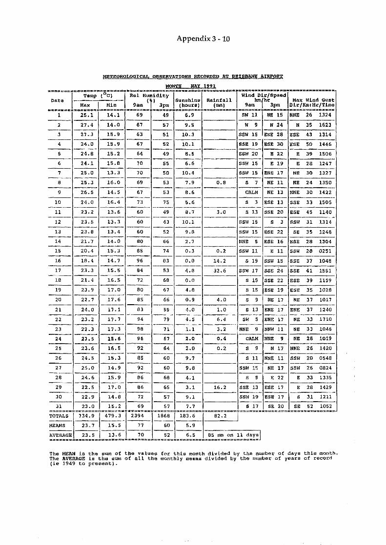
Appendix 3 - 10
HETEOROLOGICAL OBSERVATIONS BZCORDEp AT BRISBANE AIRPORT
MONTH flAX 1991 •• mam_= ••••• aDd. __ •••••••••••• a •••• =.ma ••••••••••• u •••• _ ••• _ ••• a __ ._ •••• _=~ •• _. __ ._ ••• _.~ I Temp (oC) I ael Humidity I I I Wind Dir/SP8edl Date ( ) Sunshine Rainfall km hr Max Wind Gust
Max I Min gam 1 3pm (hours) (mm) 9am f 3pm Dir/Km:Hr/Time .c.===az=.====.~ •• ====_=._.==._=_.===.=ft=====.&=.a= ••• = ••• =_==== •• = •••••••••• ====:_== ••••
1 25.1 14.1 69 49 6.9 SW 11 NE 15 NNE 26 1324 ---:2 27.4 14.0 67 57 9.S VI 9 N 24 N 35 1623 ---3 27.3 l!i. 9 63 51 10.3 SSW 1S ESE 28 ESE 43 1314 ---4 24.0 15.9 67 52 10.1 SSE 19 BSE 30 ESE SO 1446 ---5 24.8 15.2 64 49 8.5 SSW 20 E 22 II: 39 1506
6 24.1 15.8 70 55 6.6 SSW 15 E 19 E 28 1247 ---7 25.0 13.3 70 50 10.4 SSW 15 ENE 17 NE 30 1327 ---8 25.3 16.0 69 53 7.9 0.8 S 7 NE 11 NE 24 1350
---9 26.5 14.5 67 53 8.6 CALM NE 13 NNE 30 1422
---10 24.0 16.4 73 75 5.6 S 3 ESE 13 SSE 33 1505
---11 23.2 13.6 60 49 8.7 3.0 S 13 SSE 20 ESE 45 1140
---12 23.5 13.3 60 43 10.1 SSW 15 S 3 SSW 31 1314 ---13 23.8 13.4 60 52 9.8 SSW 15 ESE 22 SE 35 1248 ---14 21.7 14.0 80 66 2.7 NNE S ESE 16 ESE 28 1304 ---IS 20.4 15.3 85 74 0.3 0.2 SSW 11 E 11 SSW 28 0251
---16 18.4 14.7 96 83 0.0 14.2 S 19 SSW 15 SSE 37 1048 ---17 23.3 15.5 84 53 4.8 32.6 SSW 17 SSE SSE 41 1551 ---- ---18 21.4 16.5 72 68 0.0 S 15 SSE 22 ESE 39 1159
---19 23.9 17.0 80 67 4.8 S 15 ESE 19 ESE 35 1028
---20 22.7 17.6 85 66 0.9 4.0 S 9 NE 17 NE 37 1017
---21 24.0 17.1 83 55 4.0 1.0 S 13 ENE 17 ENE 37 1240
---22 23.2 17.7 94 79 4.5 6.4 SW 5 ENE 17 NE 33 1710
---23 22.3 17.3 98 71 1.1 3.2 NNE 9 NNW 11 NE 33 1046 ---:ii4 :iil.S 113.6 9!i iS7 2.0 0.4 CALM NNIll , NE 28 1019 ---25 23.6 16.5 92 64 2.0 0.2 S 9 N 17 NNE 26 1420
---26 24.5 15.3 85 60 9.7 S 11 NNE 11 SSW 20 0548
---27 25.0 14.9 92 60 9.8 SSW IS NE 17 SSW 26 0824
28 24.6 15.9 86 68 4.1 5 5 E 22 E 33 1335 ---
29 22.5 17.0 86 65 3.1 16.2 SSE 13 ESE 17 E 28 1429 ---
30 22.9 14.8 72 57 9.1 SSW 19 ESE 17 S 31 1211 ---31 23.0 15.2 69 57 7.7 5 17 SE 20 5E 52 1052
,==-=., TOTALS 734.9 479.3 2394 1868 183.6
---MEANS 23.7 15.5 77 60 5.9 ---AVERAGE 23.5 13.6 70 52 6.5 85 rom on 11 days
The MEAN ia the sum of the values for this month divided by the number of days this month. The AVERAGE is the sum of all the monthly means divided by the number of years of record (ie 1949 to present).
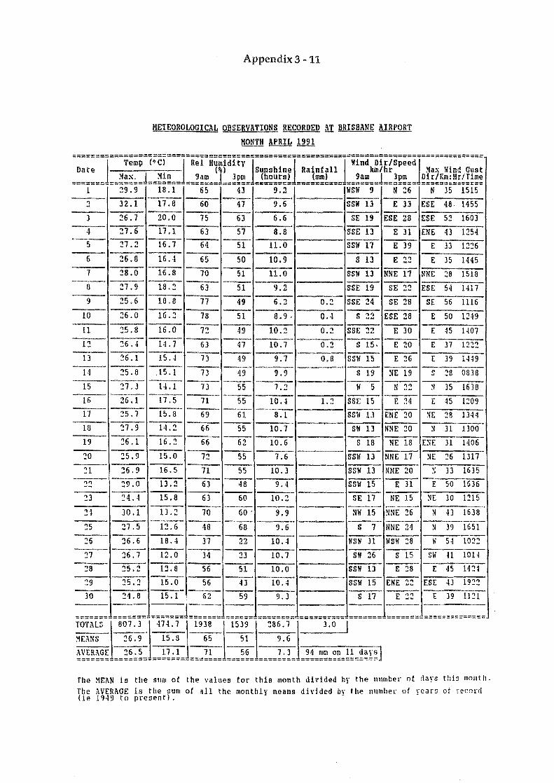
Appendix 3 - 11
METEOROLOGICAL OBSERVATIONS RECORDED AT BRISBANE AIRPORT KONTH APRIL 1991
-------l---T;~P-(;C)---l-R;l-Hu;idlty-]--------]----------]-wi~d-Dir7speedJ--------------Date (!\ol Sunshine Rainfall km/hr :-la,' wind Gust
=======_==~~~;=j==~~~==-==~:~==l==;~~=_=!~~~;~~_===!~~~===_==!:~==l==~~~==_~!;!~~;~;L!~~; 1 29.9 18.1 65 43 9.:! WSW 9 N 36 N 35 1515
~ 32.1 17 .8 60 47 9.6 SSW 13 E 33 ESE 48. 1455
3 26.7 20.0 75 63 6.6 SE 19 ESE 28 ESE 52 160]
4 :'7.6 17 .1 63 51 0.8 SSE 13 E 31 DIE 43 1254 --5 27. 3 16.1 64 51 11.0 SSW 17 E 39 E 33 13~6 --6 26.8 16.4 65 50 10.9 S 13 E '1'1 uu E 35 1445 1 :>8.0 16.8 70 51 11.0 SSW 13 NNE 11 NNE 28 1518 --8 :n .9 18.2 63 51 9.2 SSE 19 SE 22 ESE 54 1411 --9 25.6 18.8 71 49 6.::! O.::! SSE 24 SE 28 SE 56 1116 --10 26.0 16.2 18 51 8.9 ' 0.4 S 22 ESE 28 E 50 1249
11 25.8 16.0 1':'. 49 10 :> O.::! SSE 22 E 30 E 45 1401 1'1 ,!6.~ 14.1 63 41 10.7 0.2 S 15, E 20 E 31 122::' 1] 26.1 15.-1 13 49 9.7 0.8 SSW 15 E ~6 E 39 1449 --.15.1 13 9.9 ~E 19 ~8 0838 14 25.8 49 S 19 <'
" 15 '!7.J 14.1 13 55 1.2 If 5 N ::!2 ~ ]5 16]8
--16 26.1 11.5 11 55 10.4 1.2 SSE 15 E 24 E 45 1'!09
17 '!5.1 15.8 69 61 8.1 SSW 1] ENE 20 ~E 28 1344
18 27.9 14 . .::! 66 55 10.7 SW 13 NNE 20 ~ 31 1300 --19 26.1 16.::1 66 62 10.6 S 18 NE 18 [~E 31 1406 --
~O 25.9 15.0 7:! 55 1.6 SSW 13 NNE 11 !-IE :!6 lJ17 --~1 ::l6.9 16.5 71 55 10. J SSW 13 NNE 20 X ]] 1635 '1'1 :!9.0 13.2 63 4S 9.4 SSW 15 E 31 E 50 1636 --23 '14.4 15.8 63 60 10.::1 SE 11 NE 15 ~E 30 1215
--2 ,} )0.1 13. :! 10 60 . 9.9 NW 15 ~NE 26 ~ ~J 16]8
::l5 21.5 12.6 48 68 9.6 S 7 NNE 24 N 39 1651 ---26 :J6.6 18.4 J1 22 10.4 WSli Jl WSW :lS II' 54 1022 --:!7 ::16.1 12.0 J4 23 10.7 Sit ::16 S 15 SW H IOU
28 25.2 1:!.8 56 51 10.0 SSW 13 E 28 E 45 1421
29 25.2 15.0 56 n 10. -I SSIt 15 ENE 22 ESE 43 19':'.2
30 ::14.8 15.1 62 59 9.] S 11 E 'I'! E 39 1121 --
:======-=======-=====::-======:-======-========-==========-=======-=======-====~=========
The MEAN is the slim ot the values tor this month divided Ill' the Ilumber of clays this month. The AVERAGE is the sum ot all the monthly means divided by the number of rears at record (ie 19H to present).
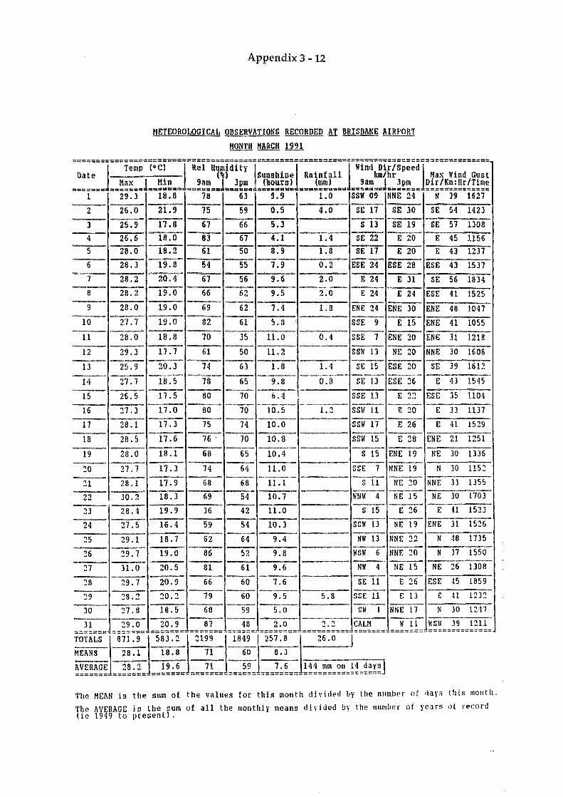
Appendix 3 ~ 12
METEOROLOGICAL OBSERVATIONS RECORDED ,AT BRIS8A~E AIRPORT
MONTH HARCH 1991
-------------------========---------------------------------------------------------------------]---., •• -(.01 j Rei-H.mldltY-I--------I----------I-vlndlilris"edI--------------Date ()Sunshine Rainfall kIII/hr Max Wind Gust
Ba==3 •• • m~~;B.l .• ~~~.9 .=~:: .. l~.;~~a'=£~~~~:! .=.!~! ••••• ~!:3.J •• ~2~== ~!~!~~~;!!!~; 1 29.3 18.8 78 63 9.9 1.0 SSW 09 NNE 24 N 39 1627
2 26.0 21.9 75 59 0.5 4.0 SE 17 SE ]0 SE 54 1423 -J 25.9 17.8 67 66 5.3 S 13 SE 19 SE 57 1308
4 26.6 18.0 83 67 4.1 1.4 SE 22 E 20 E 45 1156 5 28.0 18.2 61 50 8.9 1.8 BE 17 E 20 E 43 1237
6 28.3 19.8 54 55 7.9 0.2 ESE 24 ESE 28 ESE 43 1531
1 28.2 20.4 67 56 9.6 2.0 E 24 E 31 SE 56 1834
8 28.2 19.0 66 62 9.5 2.0 E 24 E 24 ESE 41 1525
9 28.0 19.0 69 62 7.4 1.8 ENE 24 ENE 30 ENE 48 1041 --10 21.1 19.0 82 61 5.8 SSE 9 Eis ENE 41 1055
11 28.0 18.11 70 35 11.0 0.4 SSE l' ENE 20 ENE 31 1218 --12 29.3 11.7 61 50 11. 2 SSW 13 NE 20 NNE )0 1608
13 25.9 20.3 74 Ii) 1.8 1.4 SE IS ESE 20 SE 39 1612
14 21.1 18.5 78 65 9.8 6.B SE 13 ESE 36 E 43 lS'lf 15 26.5 11.5 -- b.4 SSE 13 80 10 E 2::! ESE 35 1104
--16 :n.3 17.0 80 70 10.5 1.3 SSW 11 E 20 E J3 1131
11 28.1 17. J 15 14 10.0 SSW 17 E -26 E 41 15 18 28.5 17 .6 76 ' 70 10.8 SSW 15 E 28 ENE 21 1251
19 2B.O 18.1 68 65 10.4 S 15 ENE 19 NE 30 1336 ---
30 21.7 17.3 14 64 11.0 SSE 1 NNE 19 N )0 115~ - 11.1 S -Ii J1 28.1 17.9 68 68 NE JO NNE )) 1355 -22 JO.2 18.3 69 54 10.1 liN II 4 NE 15 NE )0 1703
23 28.4 19.9 36 42 11.0 S -15 E~6 E H 152) - ----
24 31.S 16.4 59 54 10.3 SSW 13 NE 19 ENE 31 1536 --
~5 29.1 18.7 62 64 9.4 Nil IJ NNE 32 N 48 1135
26 39.1 19.0 86 52 9.8 118116 NNEW N J7 1550
31 81 -- 9.6 Ntt 4 NE 15 31.0 20.5 61 NE ~6 D08 -38 29.1 20.9 66 60 7.6 SE 11 E 36 ESE i5 1859
';9 28.::! 30.::! 79 60 9.5 5.8 SHI! E 13 E H 12)2
)0 27.8 18.5 68 59 5.0 8W -1 NNE T7 N )0 13·1/
Jl 29.0 20.9 81 48 2.0 2.:! CALM If 11 w~m 39 1211 ======~-=======-=====~=-=======-======-========-=====~====-~======-=======-===========~==
The MEAN is the sum ot the values tor this month dividE'li by the number at dar s this mOlltl!.
The AVERAGE is the sum ot all the monthly means divided Ili' the number of years ot record tie 1949 to presentl.
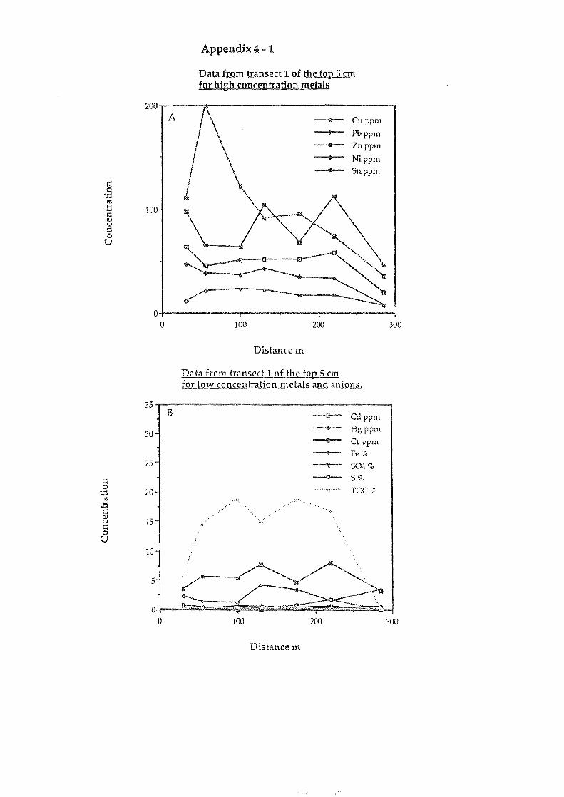
t:: o .... ..... ro
Appendix 4 - 1
Data from transect 1 of the top 5 cm for high concentration metals
200~----~----------------------------~ A --0- Cuppm
t Pbppm
------ Znppm
-+-- Nippm --- Snppm
J:l 100 t:: QJ (j
t:: o
U
o 100 200
Distance m
Data from transect 1 of the top 5 cm for low concentration metals and anions.
B ---a-- Cd ppm
30 -- Hgppm --iI- Crppm -- Fe %
25 ~ SO-I '7a ---n- S%
20 TOC%
15
10
.3
O~--J~~, .. ~h~';;~'~"~~'~~·~""~-'Oz~~,~£i~'i~:~~;';:~~~'~',,~y~ o 100 200
Distance m
300
300
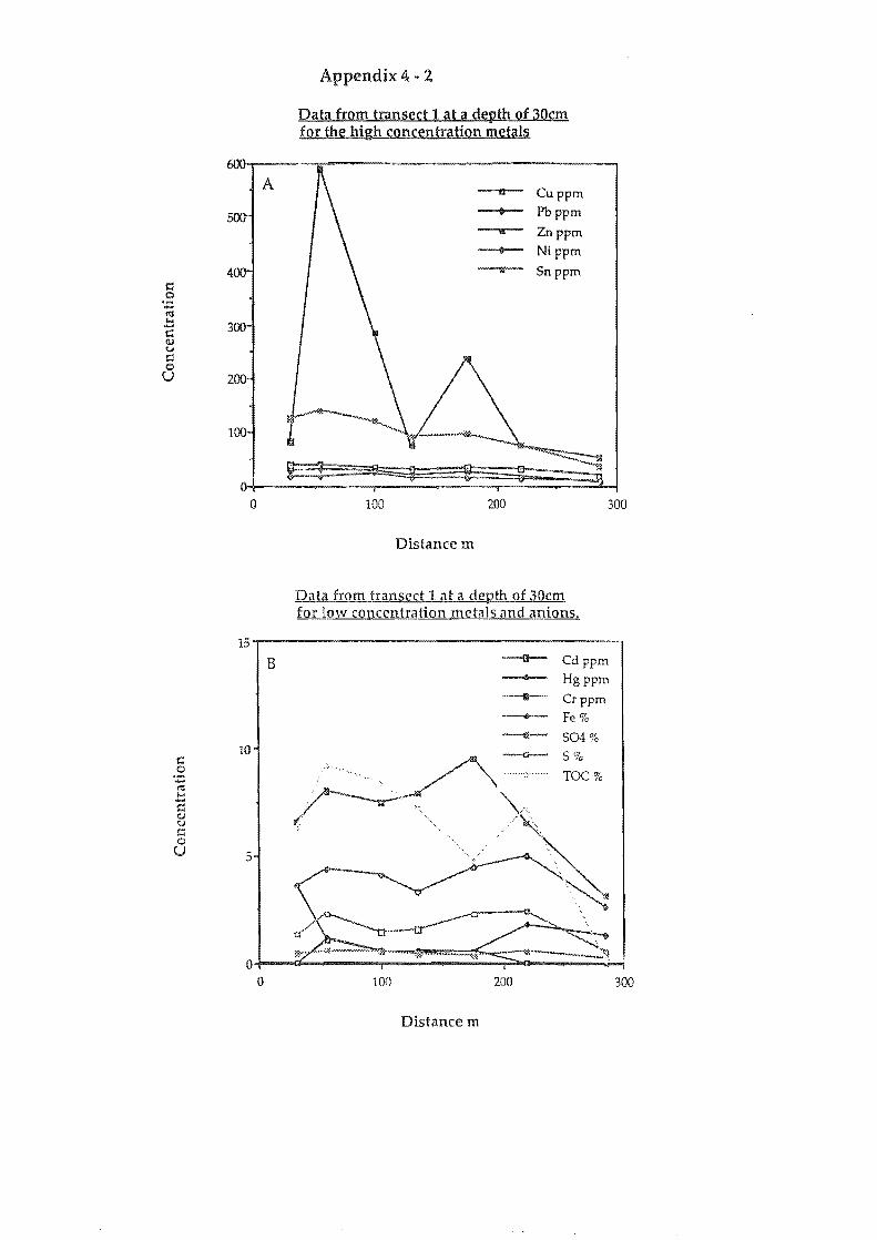
600
A
400 t.1 0 ..... ..... !U Jj 300 t.1 (jJ <..I t.1 0 U 200
100
0 0
15
B
10 t:: 0 .-..... <':I .... ..... t:: CJ u ::.: 0 U .5
o
Appendix 4 - 2
Data from transect 1 at a depth of 3Qcm for the high concentration metals
Cuppm Pbppm
Znppm Nippm
Snppm
--~
100 200 300
Distance m
Data from transect 1 at a depth of 30cm for low cQncentration metals and anions.
----a- Cd ppm Hgppm
-II-- Crppm --+-- Fe % ~ 504%
5%
TOC%
100 200 300
Distance m
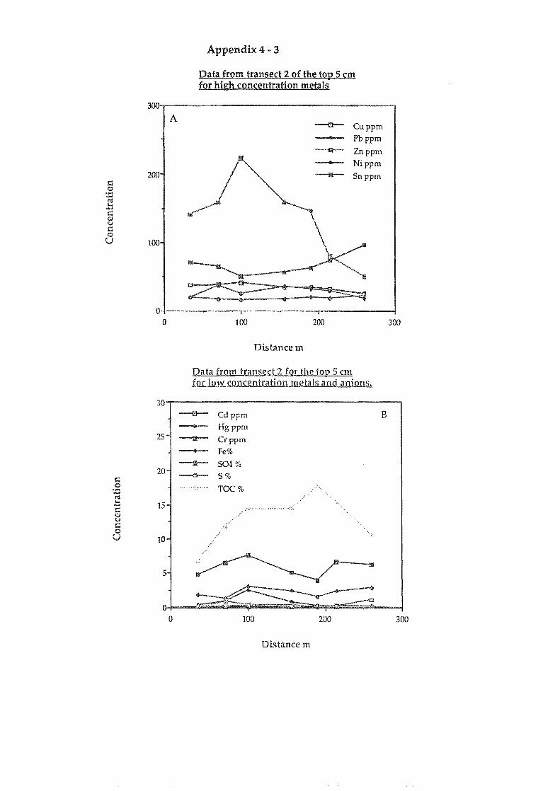
t:l <:;) ..... ...... fU
.!::I t:l <l.I <.J t:l <:;)
U
Appendix 4 - 3
Data from transect 2 of the top 5 cm for high concentration metals
300,-------------------------------------~
A -a-- Cuppm Pbppm ---- Znppm --- Nippm
200 ~ Snppm
100
o 100 200 300
Distance m
Data from transect 2 for the top 5 cm for low concentration metals and anions.
30 ~ Cdppm B
0- Hgppm 25
i !.1 Crppm .. Fe%
~ S04% 20 ---0-- S%
...... :::.,.,.,., TOC%
15 ,,., .... ;:;: . .. -,.
10
o 100 200 300
Distance m
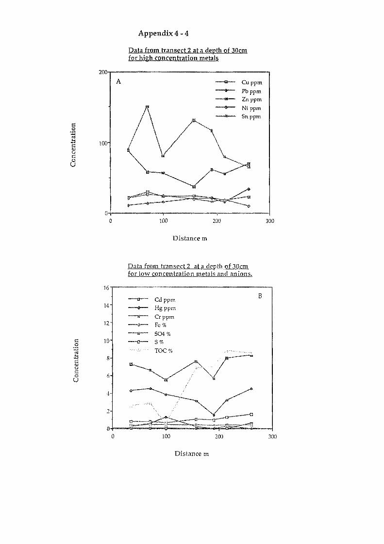
Appendix 4 - 4
Data from transect 2 at a depth of 30cm for high concentration metals
20~------------------------------------~ A
100
o
14
12
10
8
6
o
100
Distance m
---Q- Cuppm
---.-- Pb ppm
--- Znppm
200
Nippm Snppm
~~,
Data from transect 2 at a depth of 30cm for low concentration metals and anions.
a Cd ppm
• Hgppm --w- Crppm --0-- Fe 0/0
;:;: S04% ---0-- S%
"';;0" TOC%
~··;:;;""V·"·' ",
... ...
100 200
Distance m
B
300
300
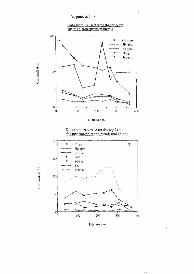
Appendix 4 - 5
Data from transect 3 for the top 5 em for high concentration metals
200~------------------------------------~
c o .... ..... t1:I
.l::: 100 C \lJ u C o
U
o
24
18
12
A
o
-a-- Cuppm .. Pbppm !!II Znppm .. Nippm ~ Snppm
100 200 300 400
Distance m
Data from transect 3 for the top 5 em for low concentration metals and anions
---('J-- Cd ppm B .. Hgppm iit Crppm ~ Fe%
Iii 504% --t:I- S%
'::;,'''''' TOC%
-,<:"
100 200 300 400
Distance m
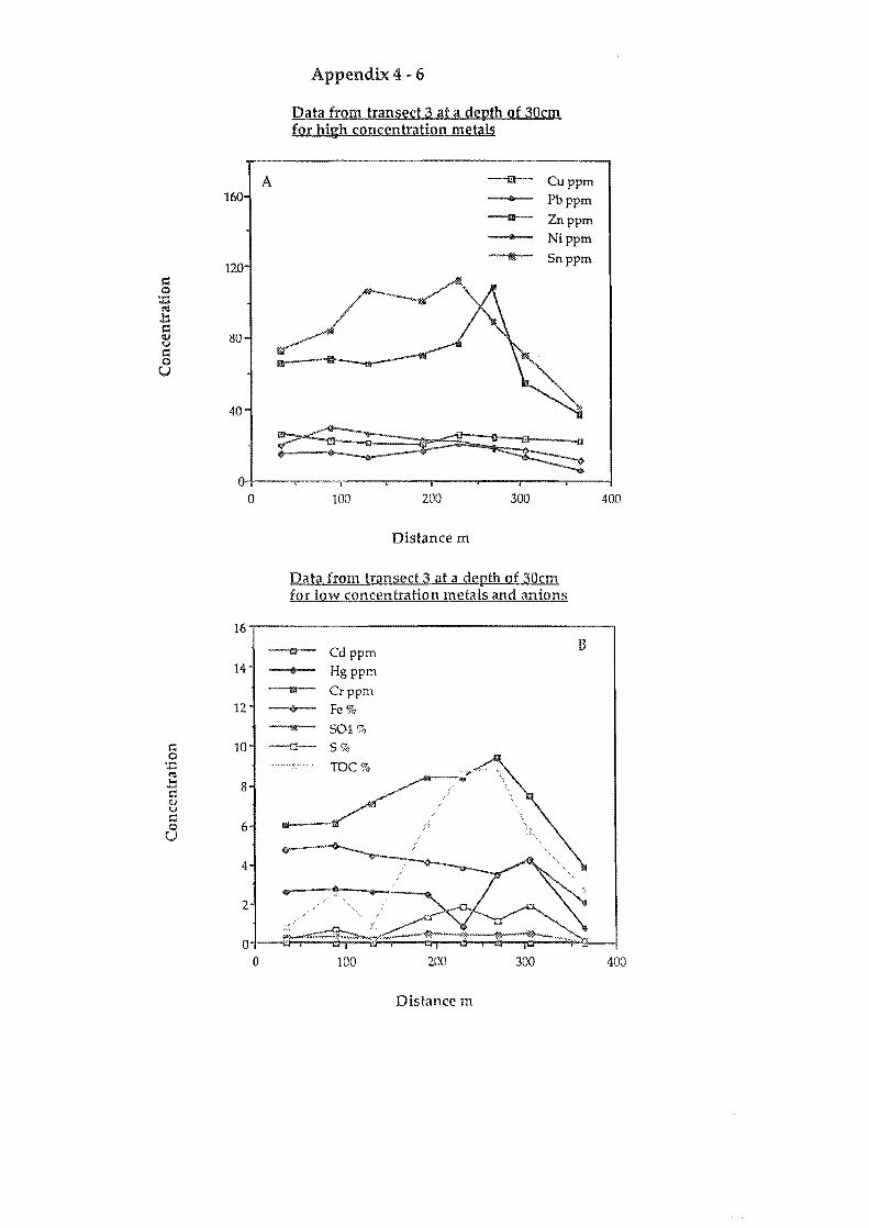
160
120
80
40
0 0
16
14
12
r:::; 10 0 ..... ..... f<l .l:::l 8 r:::; OJ U r:::;
6 0 U
4
2
0 0
A
Appendix 4 ~ 6
Data from transect 3 at a depth of 3Qcm for high concentration metals
-a-- eu ppm
• Pbppm --a- Zn ppm --- Nippm ~ Sn ppm
100 200 300
Distance ill
Data from transect 3 at a deJ;!th of 30cm for low concentration metals and anions
c:! Cd ppm B
• Hgppm 1:11 Crppm c. Fe%
~ 504% ---0-- S% ,. ...... <:: •• TOC%
100 200 300
Distance m
400
400
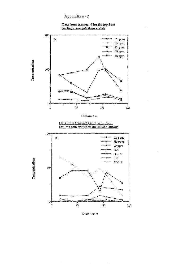
= o ..... .... <'CI
Appendix 4 - 7
Data from transect 4 for the to" 5 em for high concentration metals
200~--------------------------------------~ A -ill-=- Cuppm -- Pbppm
a Znppm -- Nippm
Snppm
l:! 100 = (IJ u = o
U
o 75 ISO 225
Distance m
Data from transect 4 for the top 5 cm for low concentration metals and anions
B --1:1'--- Cd ppm -- Hgppm ---«-- Crppm --- Fe% ~ 501% ---0- 5%
TOC%
o+-~,,>·~~~~~~~~==~~~ o 75 150 225
Distance m
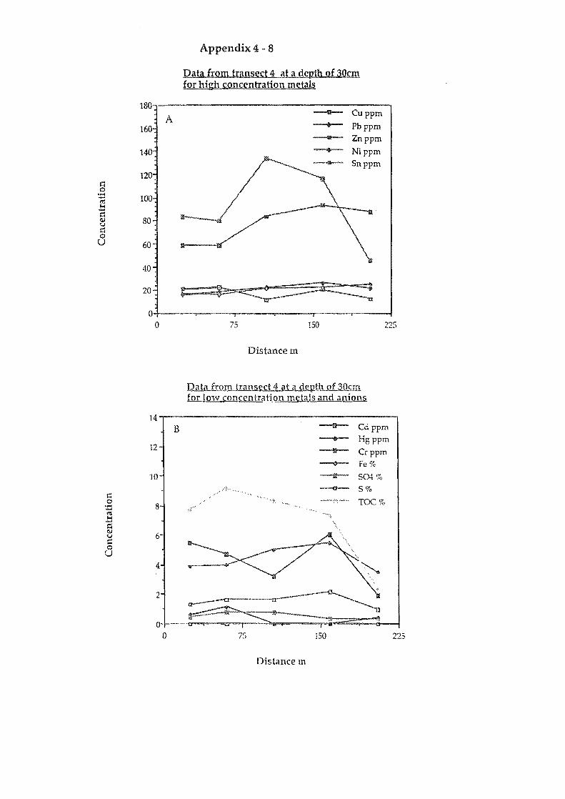
180
A 160
140
120 ~ 0 ....
100 ..... fI:!
"'" .... ~ <l) 80 (.J
~ 0
U 60
40
20
0 0
14 B
12
10
~ 0
8 ..... .... fI:!
"'" .... ~ <l)
6 <..I ~ 0
U 4
2
0 0
Appendix 4 - 8
Data from transect 4 at a depth of 30cm for high concentration metals
iii Cuppm
• Pbppm III Znppm
• Nippm It Snppm
75 150 225
Distance m
Data from transect 4 at a depth of 30cm for low concentration metals and anions
-il'-- Cd ppm -.- Hgppm
!II Crppm 0< Fe%
~ 50! % <.;.;" --<:!- 5%
::;.+-•••• TOC% .",.
""':-,
75 150
Distance m
225
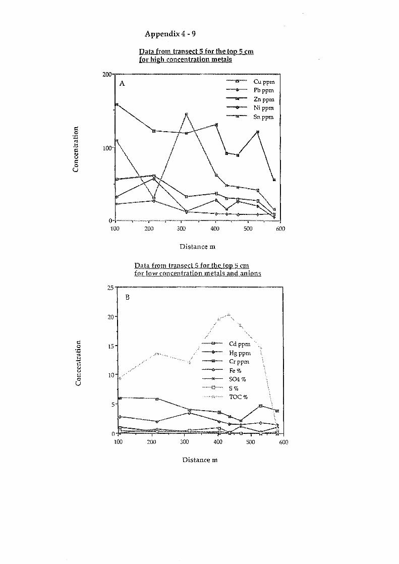
c: 0 ..... .... ~
l::I c: OJ u c: 0 U
Appendix 4 - 9
Data from transect 5 for the top 5 em for high concentration metals
2oo,-----------------------------------~ A Il:I Cu ppm
• Pbppm ... Zn ppm r Ni ppm I!t Sn ppm
100
O·;---~--~--_r--_r--_T--~--~--~--~--~
100 200 300 400 500 600
Distance m
Data from transect 5 for the top 5 em for low concentration metals and anions
B
20
15 ---m-- Cd ppm , -+-- Hgppm ....
Crppm ---r Fe% 10
504% ~
~ S% .~,~ ...• , , ::::~-, .-" ... TOC%
5
O~~~~~~~~~~~~~~~ 100 200 300 400 500 600
Distance m
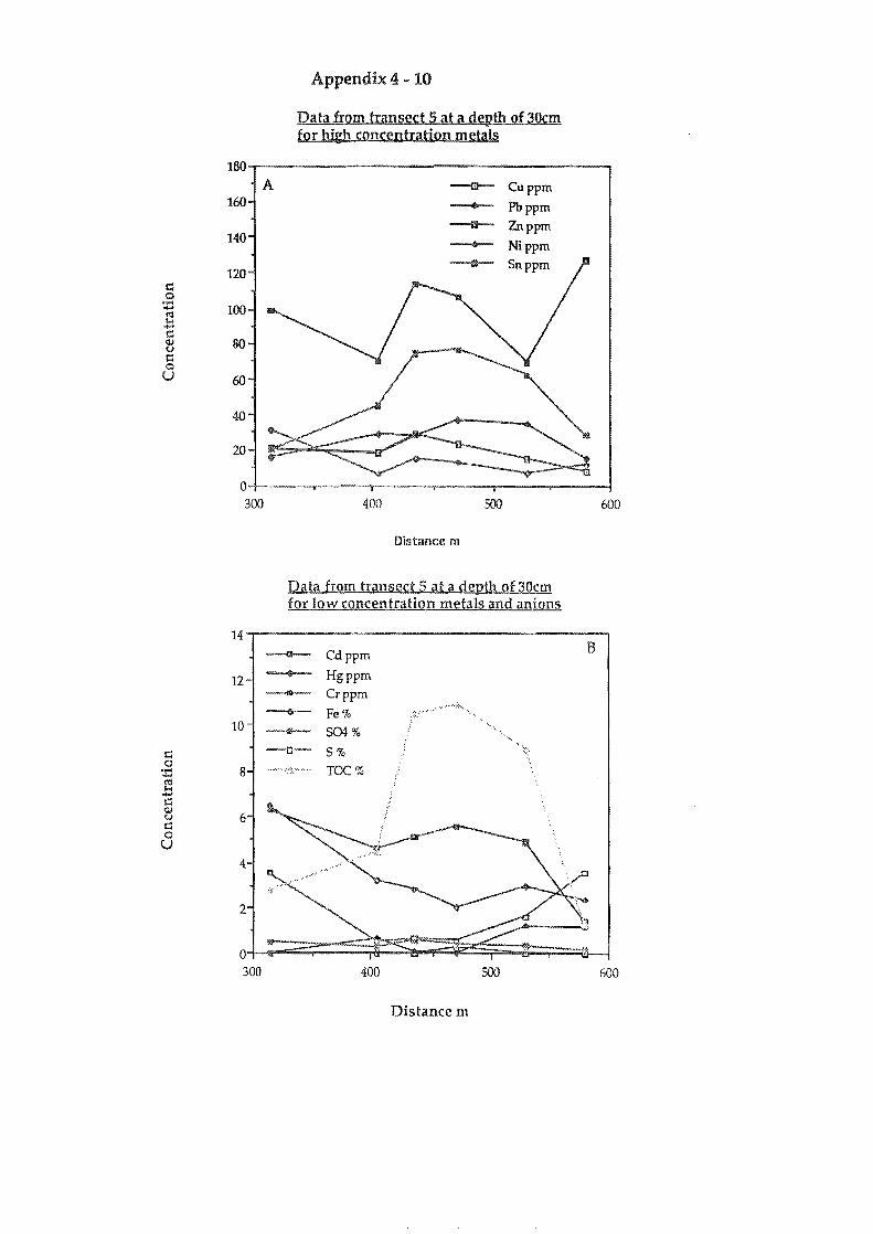
= 0 ..... .... rn 1-1 .... = (lJ v
= 0 U
180
Appendix 4 - 10
Data from transect 5 at a depth of 30cm for high concentration metals
A -m-- Cuppm 160
140
120
100
80
60
40
20
0 300
14
12
10
8
4.
2
- Pbppm -tI-- Znppm - Nippm --@-- Snppm
400 500
Distance m
Data from transect 5 at a depth of 3Qcm for low cone en tration metals and anions
- Cd ppm
• Hgppm -- Crppm ~ Fe% -- SOi% -0-- S% •••.•. ".,'c.;:: •.•.•..... TOC% :
600
B
o.l;~~~es~~~~~~·~~~ 300 400 500 600
Distance m
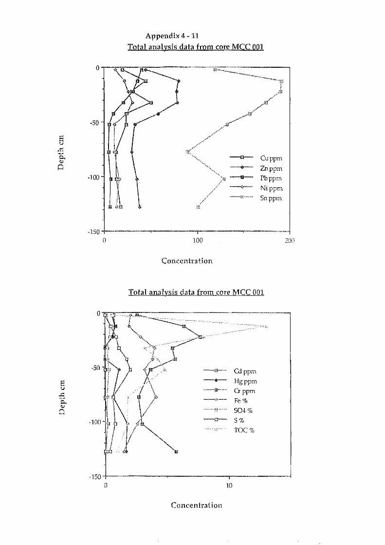
e u ~ ..... 0... QJ
0
E u
-so
-100
Appendix 4-11
Total analysis data from core MCC 001
Cuppm
Znppm
Pbppm
Nippm
Snppm
-1504-----------~---------r--------------~------------~
o
-so .
100
Concentra tion
Total analysis data from core MCC 001
.......... ::;::; .......
Cd ppm
Hgppm
Crppm Fe%
504%
S%
TOC%
200
-150~------------~------------~------------~
o 10
Concentration
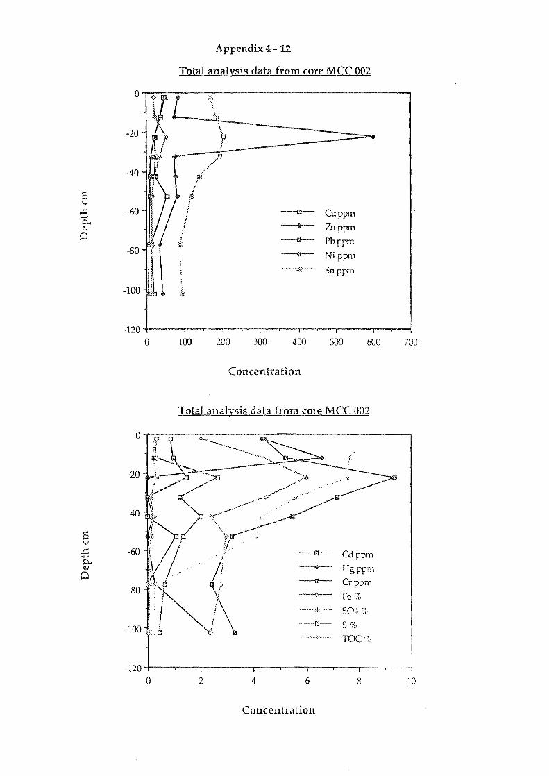
S u
,.c ...... p.. (lJ
0
S u
..r::: ..... 0.. (lJ
0
Appendix 4 - 12
Total analysis data from core MCC 002
o~----------------------------------------~ ~~l
-20
-40
-60
-80
-100
, ';
b '. , ~b , !
Cuppm
Znppm
Pbppm
Nippm
-1204-~--~~--~~--~~--~~--~~~~-,--~
o 100 200 300 400 500 600 700
Concentration
Total analysis data from core MCC 002
-40
-60 -I!I-- Cd ppm
• Hgppm --Q-- Crppm ~...- Fe% -~::::::.,,~ 504 ':'c ~- 5%
Toe '1:
-120 0 2 4 6 8 10
Concentration
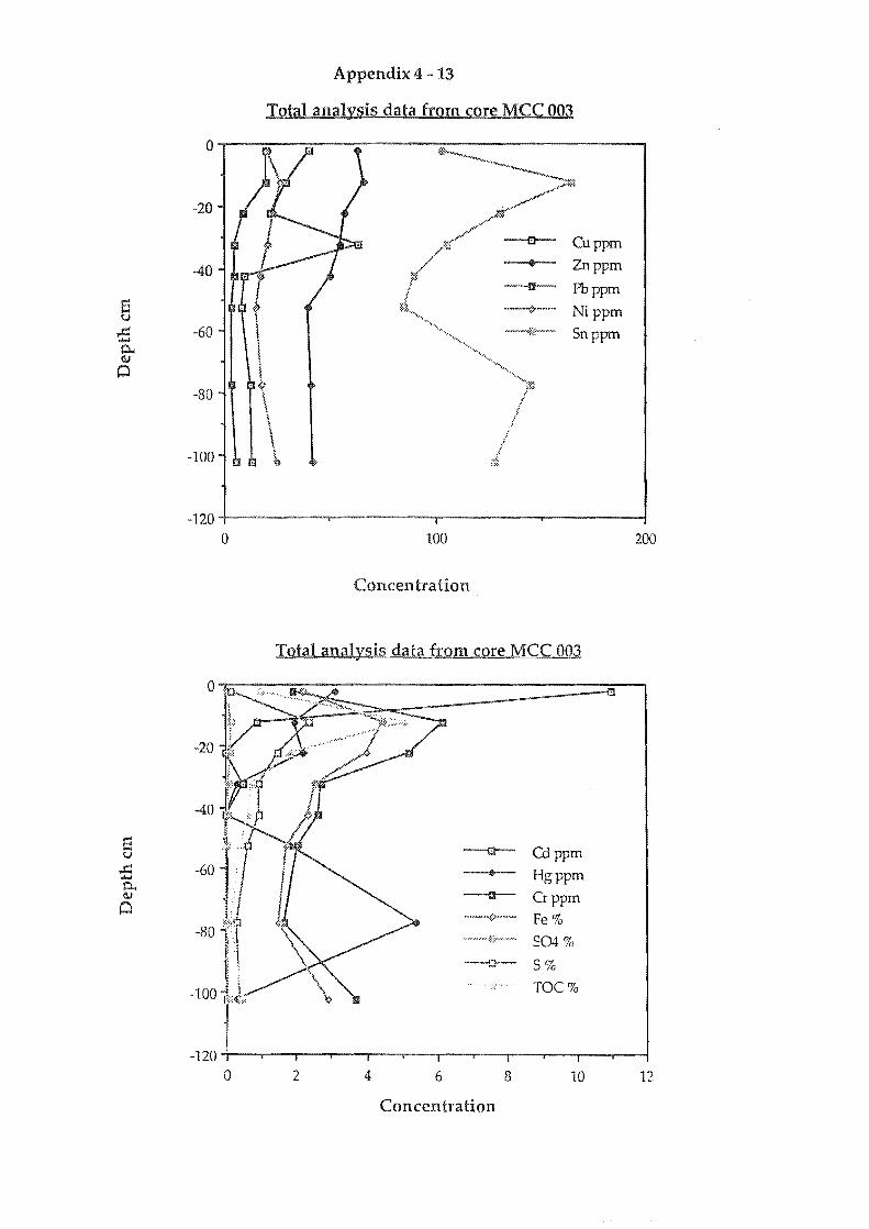
Appendix 4 - 13
Total analysis data from core MCC 003
-120~--------~---------r--------~--------~
o 100 200
Concentration
Total analysis data from core MCC 003
IS -e--- Cd ppm (,j
,.c: • Hgppm ...... 0.. <!J -1:t-- Crppm 0
"-'''{;r'''- Fe% .~""""""~~'::;;~:"-'-""''''' 504%
---0-- 5%
TOC%
-120~--r--r--~--.-~---.--,---~~---.--~~
o 2 4 6 8 10 12
Concentration
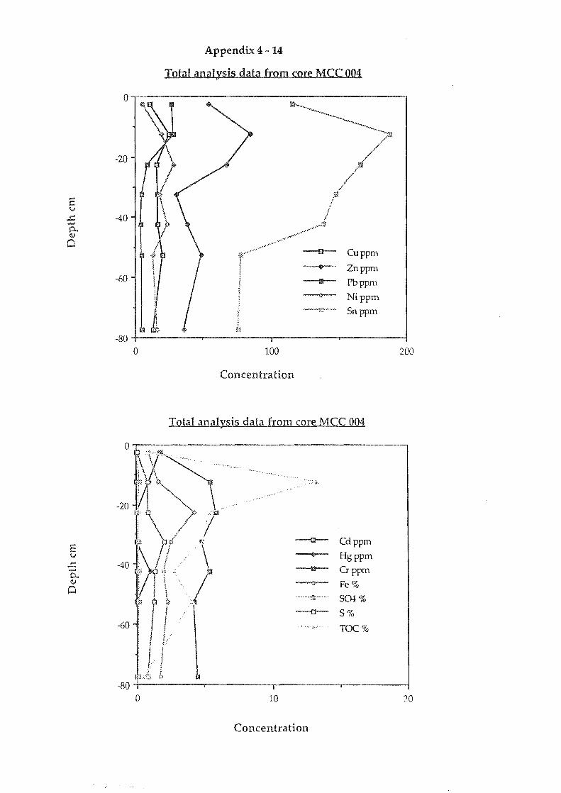
Appendix 4 - 14
Total analysis data from core MCC 004
o~------------------------------------------~
-20
E u
-40
----l1I-- Cuppm .. Znppm
-60 III Pbppm ~ Nippm -::;:; ... - Snppm
o 100 200
Concentration
Total analysis data from core MCC 004
-{ll--- Cd ppm E u • Hgppm
..= -40 ~ Crppm ...... c.. <lJ ~ Fc% Q , ..... ··~~;:;i ....... S04%
~ S%
TOC%
Concentration
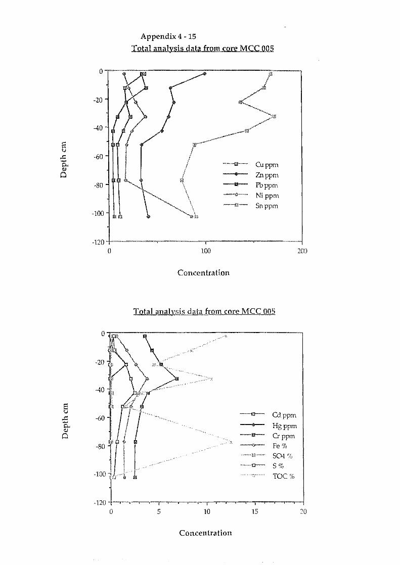
Appendix 4 -15
Total analysis data from core MCC 005
o 100 200
Concentration
Total analysis data from core MCC 005
s y
--0-- Cd ppm
'" Hgppm u Crppm ~ Fe% .. .-.-.... ~:::;'.~ ... ~' 504% ~- 5%
TOC%
-1204-~~~-r~~~~~~~~r-r-~~~~~~~
o 5 10 15 20
Concentration
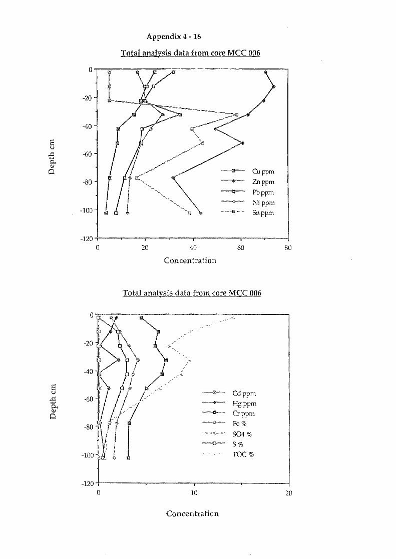
S !;J
...t:: ...... p,.. Q)
0
S !;J
...t:: ....... p,.. Q)
0
Appendix 4 - 16
Total analysis data from core MCC 006
-40
-60
-m-- Cuppm
-80 .. Znppm ~ Pbppm
", ~ Nippm '"
""""""'li;~ u.u.~ ....... Snppm
-120+---~------~----~---r----~----~----~--~
o
-40
-60
20 40
Concentration
60
Total analysis data from core MCC 006
~ Cd ppm
• Hgppm III Crppm
..• -~ Fe% .... H ... :::~, ••••• ~ 504% ---0- 5%
TOC%
80
-120 +------.------.-----...-----~
o 10 20
Concentration
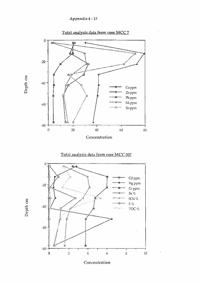
o
E !;.J
o
0
d' 4 17 Appen IX -
fr m core MCC 7 Total analysis data 0
~---~ /"
....-~
~ . .,..;".".. .....
~.,...,.-,...,~~
-a--.. 1m
~
' ......... ' ........ ~!~ .... 'H
t " n Concentra 10
Cuppm
Znppm
Pbppm
Nippm
Snppm
m core MCC 007 Total analysis dallcta!UJfr;}lo!.!!..!....=_
-a-- Cd ppm
• Hgppm a Crppm ~ Fe% u ..... u •••. :::;: ........ 50-l % ~---- 5'70 .' ....... :.:: TOC%
Concentration
10
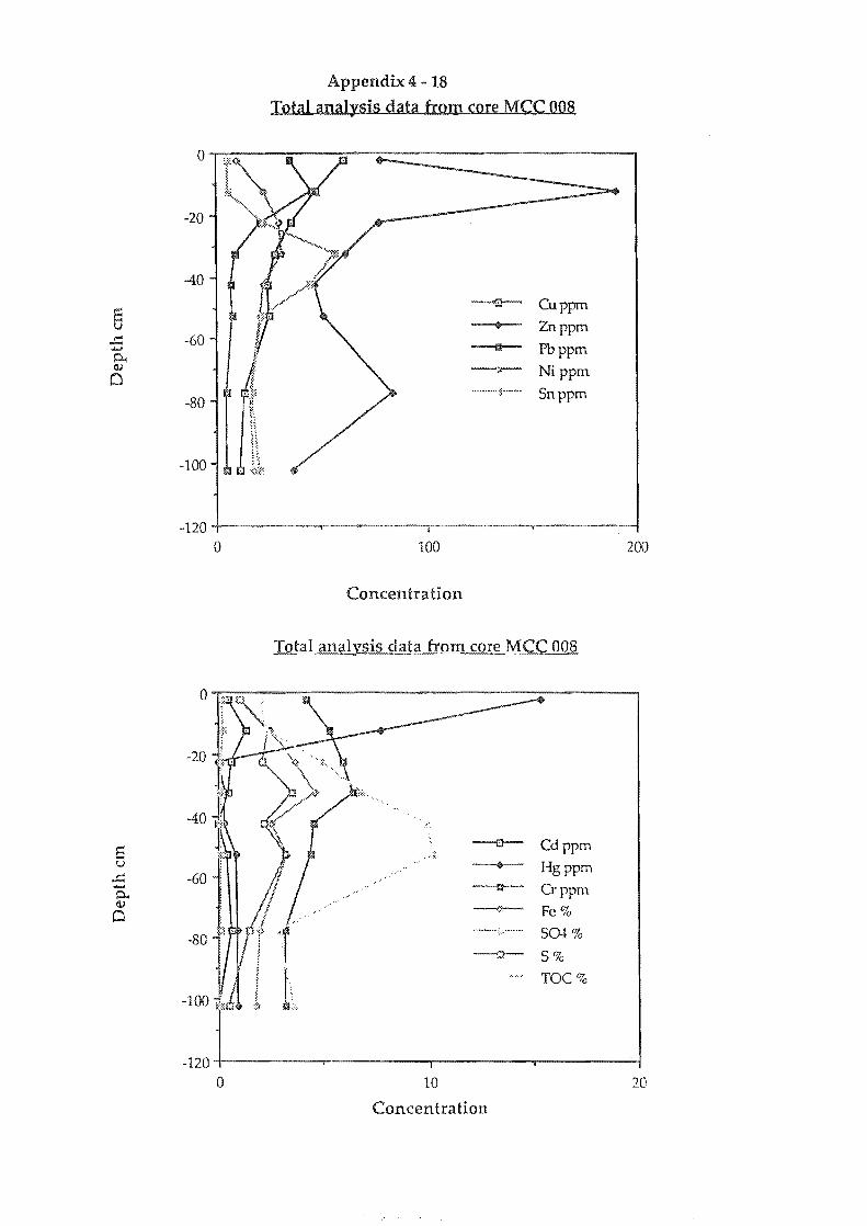
e v ...c:: ..... p,.. (l)
0
e u
Appendix 4 - 18
Total analysis data from core MCC 008
-40 ~ Cuppm
$ Znppm -60
~ Pbppm -';J-- Nippm .~ .... """"'-",,~ •• u ....... Snppm
-80
-120+----------r----------r---------~--------~
o
-80
100
Concentration
Total analysis data from core MCC 008
... ~.~ ... :::: ..... ....
Cd ppm
Hgppm Crppm Fe%
50-1 %
5% TOC%
200
-120+----------r---------=r---------~--------~
o 10
Concentration
20
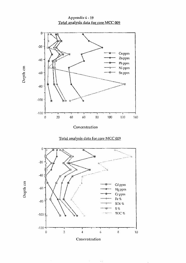
Appendix 4 19 Total analysis data for core MCC 009
o~~-=~--------~--------------------~
-20
III Cuppm
• Znppm -40 III Pbppm
e ~- Nippm u ,,£: -60 ~ Snppm ..... j':I.. Il.I
Cd -80
-100
-120 -I----..-.....-......--..--.......... ---,--.----r-..-.....,----..-...,-----.-----1
o 20 40 60 80 100 120 140
Concentration
Total analysis data for core MCC 009
e --a-- Cd ppm u .c .. Hgppm .....
j':I.. Il.I --a--- Crppm
Cd ~ Fe% ,-:~~~.- S04% --u-- S%
."' .. ;:; ....... " TOC%
-120 -t--...,..---,---...,..---,---...,,----r---.---...,...---.-------1
o 2 4 6 8 10
Concentra tion
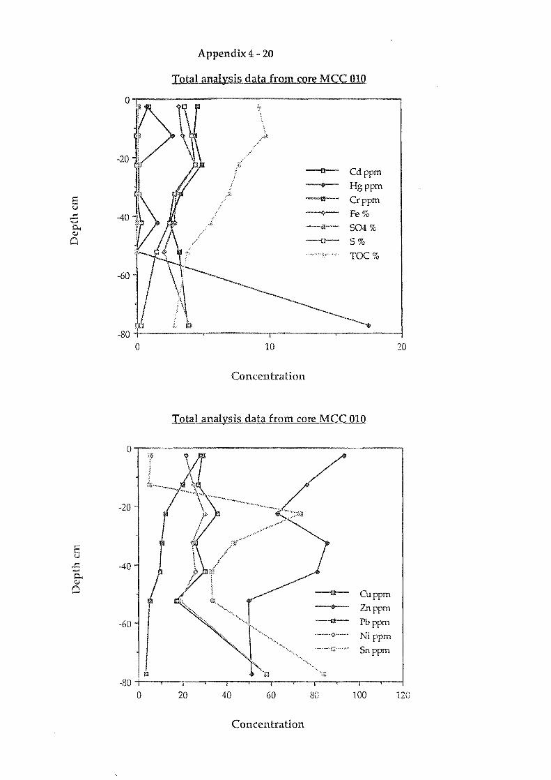
e y
0.. OJ
0
Appendix 4 - 20
Total analysis data from core MCC 010
o~------------------------------------------~
-20
--40
-60 -
o
-20
-40
-60
o
-a--- Cd ppm
• Hgppm tI Crppm ~ Fe% '-"~"'''''''''''''' 504% -n-- 5% ...... ~" ';:,:' ....... ,. TOC%
10
Concentration
Total analysis data from core MCC 010
20 40 60
Concentration
Cuppm
Zn ppm
Pbppm .. -..... ,"~.-. Ni ppm
.~.-.,:,:.-- .. ~ 5n ppm
80 100
20
120
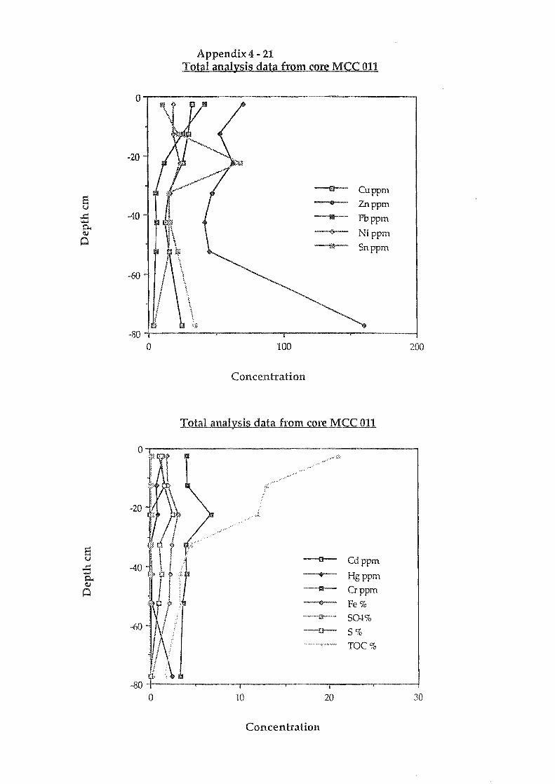
Appendix 4 - 21 Total analysis data from core MCC 011
o~------------------------------------------------~
-20
~ Cuppm e • Znppm ("J
,.d -40 III Pbppm .... 0..
~ Nippm (lJ
0 ~ Snppm
-60
-80 -+-------,------,------.------1 o 100 200
Concentration
Total analysis data from core MCC 011
s ("J -a-- Cd ppm ,.c: ...... • Hgppm 0.. (lJ a Crppm 0
~ Fe% .--.~ ... - SO!%
-60 ---!::l-- 5% .. ~::; TOC%
-80~----~-----~----~------r-----~----~
o 10 20 30
Concentration
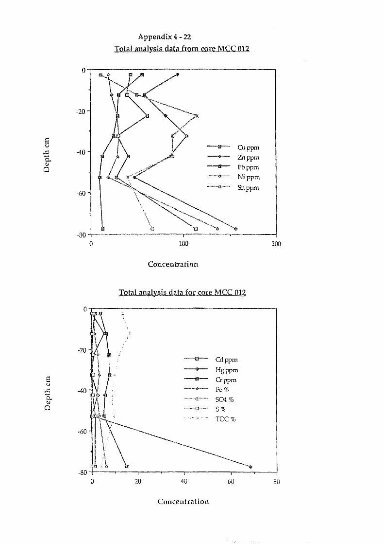
Appendix 4 - 22
Total analysis data from core MCC 012
o~------------------------------------~
-20
IS u = -40 0..
-e-- Cuppm
• Znppm (iJ
o III Pbppm ~ Nippm
-60 :;s Snppm
-80+---------~--------~--------~------~ o 100 200
Concentration
Total analysis data for core MCC 012
o~------------------------------------~
-20 --a-- Cd ppm
• Hgppm III Crppm ~ Fe% .......... ~~?;::' ~"'''~ .. S04% -n-- S%
::.; ..... ,. TOC %
-80+---~----~--~----r---~----r---~--~
o 20 40 60 80
Con centra Hon
MANGROVE FORESTS AS A BUFFER ZONE BETWEEN ANTHROPOGENTCALLY POLLUTED AREAS AND THE SEA
P. Saenger, D. McConchie & M. Clark
Centre for Coastal Management P.O. Box 125 East Lismore, 2480, N.S.W.
ABSTRACT
In Australia, recognition of the environmental and economic importance of mangrove ecosystems is reflected in the legislative protection accorded to them by state governments but despite this protection there are many sites where effluent is discharged directly into the mangroves, others where solid wastes are dumped among the mangroves and many where a mangrove forest separates a source of potential pollutants from adjacent marine or estuarine environments. This study of a site near Wynnum tip, Brisbane, is an example of a setting where a mangrove forest separates a source of metallic pollutants from the sea.
Chemical analyses of sediments and mangrove plant tissues show that the mangrove forest and an unvegetated salt flat between the tip face and the forest form an effective barrier against the movement of any metallic tip leachates to Moreton Bay. The mangroves form a baffle which reduces the flow velocity of tidal currents and allows fine grained sediment to accumulate both within and shoreward of the mangrove forest and this in turn provides a suitable habitat for large populations of sulphate reducing bacteria. Direct metal adsorption onto the fine sediment, complexing with organic matter in the sediment and the formation of insoluble metal sulphides, by reaction with bacterially generated sulphide, all contribute to the trapping of metals carried in tip leachates. The fine sulphidic mangrove sediments probably make the major contribution to the biogeochemical trap but direct metal uptake by the manI:,Tfove plants also traps substantial quantities of copper, zinc and lead. The extent of metal export from the forest is unclear at this stage but it appears to be quantitatively minor.
Because the reduced sulphidic sediments make such an important contribution to the metal trapping efficiency of the mangrove forest, future land management planning for the area will need to ensure that these sediments are not drained and allowed to oxidise. Oxidisation, which would be a likely result of any draining of the sediment, would not only release many of the presently trapped metals but would probably also create the type of environmental problems typically associated with acid sulphate soil formation.

Appendix 5 - 2
INTRODUCTION
Mangrove ecosystems can be found in all but the most southerly estuaries and harbours of Australia where they provide nursery or breeding grounds for several commercially important species of marine fauna (e.g., Saenger et al., 1977; Hutchings & Saenger, 1987); many mariculture operations are also undertaken in or near mangrove forests. In Australia, recognition of the primary environmental and economic importance of mangrove ecosystems is reflected in the legislative protection accorded to them by state governments but despite this protection many Australian mangrove forests are polluted by metallic and non-metallic anthropogenic wastes. At some sites effluent is discharged directly into the mangroves, at others a variety of solid wastes are dumped among the mangroves and at others a belt of mangroves separates a source of potential pollutants (such as a refuse tip) from adjacent marine or estuarine environments. Observations in urban mangrove forests in eastern Australia show clearly that although scientific awareness of the importance of these forests as a natural resource has increased, the mangroves are still being used extensively as convenient sites for dumping domestic garbage and siting industrial and local government effluent outfalIs (e.g., the sewage outfall ca. Hem north of the tip site, Fig. 1).
The case for the protection of mangrove ecosystems as a buffer between sources of metallic pollutants and nearby aquatic ecosystems has been made previously (Harbison, 1981), but there are surprisingly few papers in the scientific literature on the response of mangrove ecosystems to heavy metals. Although some work on the reaction of mature mangrove plants (Montgomery & Price, 1979; Peterson et ai., 1979) and seedlings (Walsh et al., 1979; Thomas & Eong, 1984) to elevated heavy metal loads has been published, most of the work has been carried out overseas and little is known about how Australian mangroves respond to metallic pollutants. To investigate how Australian mangrove ecosystems respond to heavy metals a study was initiated in 1989 by Saenger and McConchie with the following aims:
a) to compare heavy metal concentrations in mangroves growing in areas with low metal loads with those in mangroves from areas where high metal loads are likely,
b) to determine whether common species of mangroves show any tendency toward selective metal accumulation in, or exclusion from, particular parts of the plant,
c) to investigate pathways for metal transfer between mangroves and associated sediment, water, and detritivores, and
d) to assess the value of mangrove forests a buffer between marine environments and sources of metallic pollutants.
In this paper we report on the part of this larger study involving metal distribution in mangrove trees and their substrate sediments at a site near the Wynnum tip-face (Brisbane; Fig. 1). At this site a domestic garbage tip is separated from Moreton Bay by a narrow (ca. 200m wide) belt of mangroves; the mangrove forest and the tip face are separated by a slight depression, roughly SOm wide, which is devoid of any form of macroflora. The unvegetated depression is characterised by highly reducing muds (Fig. 2) which contain an abundance of metallic and non-metallic refuse; assorted metallic and non-metallic rubbish can also be found scattered throughout the mangrove forest. The lack of vegetation in the depression between the tip face and the mangrove forest is probably largely salinity induced and may be compounded by anthropogenic effects. An extensive oil film on the muds and a strong odour of anthropogenic organic chemicals suggest that the lack of vegetation may also be linked to the leachates from the tip. Both tip leachates and the breakdown of metallic refuse dumped in the mangrove forest are potential sources of heavy metals which may be
taken up by the trees or adsorbed by the substrate sediment or both.
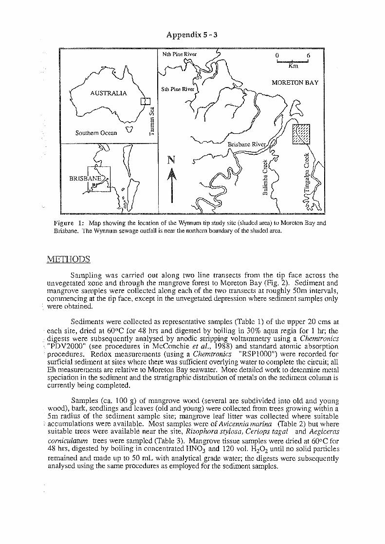
Appendix 5· 3
o 6
MORETON BAY
Southern Ocean
Figure 1: Map showing the location of the Wynn urn tip study site (shaded area) to Moreton Bay and Brisbane. The Wynnurn sewage outfall is near the northern boundary of the shaded area.
METHODS
Sampling was carried out along two line transects from the tip face across the unvegetated zone and through the mangrove forest to Moreton Bay (Fig. 2). Sediment and mangrove samples were collected along each of the two transects at roughly SOm intervals, commencing at the tip face, except in the unvegetated depression where sediment samples only were obtained.
Sediments were collected as representative samples (Table 1) of the upper 20 ems at each site, dried at 60°C for 48 hrs and digested by boiling in 30% aqua regia for 1 hr; the digests were subsequently analysed by anodic stripping voltammetry using a Chemtronics
- "PDV2000" (see procedures in McConchie et al., 1988) and standard atomic absorption procedures. Redox measurements (using a Chemtronics "RSPlOOO") were recorded for surficial sediment at sites where there was sufficient overlying water to complete the circuit; all Eh measurements are relative to Moreton Bay seawater. More detailed work to determine metal speciation in the sediment and the stratigraphic distribution of metals on the sediment column is currently being completed.
Samples (ca. 100 g) of mangrove wood (several are subdivided into old and young wood), bark, seedlings and leaves (old and young) were collected from trees growing within a Sm radius of the sediment sample site; mangrove leaf litter was collected where suitable
. accumulations were available. Most samples were of Avicennia marina (fable 2) but where suitable trees were availabl~ near the site, Rizophora sty[osa, Ceriops tagal and Aegiceras corniculatwn trees were sampled (Table 3). Mangrove tissue samples were dried at 600 C for 48 hrs, digested by boiling in concentrated HN03 and 120 vol. H20 2 until no solid particles remained and made up to 50 mL with analytical grade water; the digests were subsequently analysed using the same procedures as employed for the sediment samples.
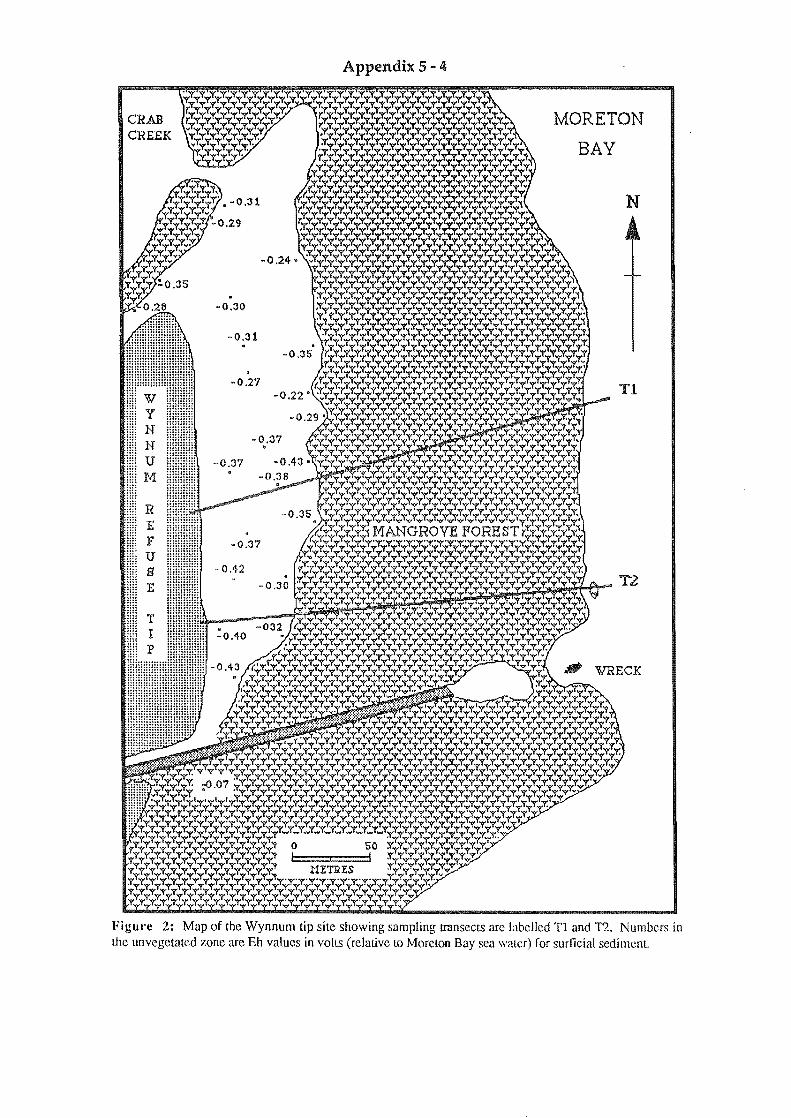
CRAB CREEK
-0.30
-0.31
-0.27
-0.37 .
-0.37
-0.42
Appendix 5 - 4.
MORETON
BAY
N
Figure 2: Map of the Wynnum tip site showing sampling transects are labelled Tl and 1'2. Numbers in the un vegetated zone are Eh values in volLS (relative LO Moreton Bay sea waLer) for surficial sediment.
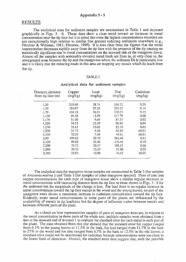
Appendix 5 - 5
RESULTS
The analytical data for sediment samples are summarised in Table 1 and depicted graphically in Figs. 3 - 6. These data show a clear trend toward an increase in metal concentration near the tip face but it is noted that even the highest concentrations recorded are not exceptionally high relative to similar fine grained reducing sediments elsewhere (e.g., Forstner & Wittman, 1981; Forstner, 1989). It is also clear from the figures that the metal concentration decreases rapidly away from the tip face with the presence of the tip causing no statistically significant rise in metal concentrations on the seaward side of the mangrove forest. Almost all the samples with noticeably elevated metal loads are from in, or very close to, the
. unvegetated zone between the tip and the mangroves where the sediment Eh is particularly low and it is likely that the reducing muds in this area are trapping any metals which do leach from the tip.
TABLE 1
Analytical data for sediment samples
Transect, distance Copper Lead Zinc Cadmium from tip face (m) (mg/kg) (mg/kg) (mglkg) (mg/kg)
1,20 210.69 38.74 339.22 0.29 1,50 184.07 29.29 293.25 0.14 1,70 134.18 26.91 210.55 0.15 1,120 69.58 13.98 117.79 0.08 1,170 31.00 9.69 87.37 0.02 1,220 34.22 12.19 96.86 0.04 1,270 35.63 13.02 85.18 0.03 1,320 31.73 8.43 62.63 5;0.01 1,360 32.25 7.98 48.81 5;0.01 2,80 199.82 28.75 283.40 0.51 2,120 99.88 21.40 176.56 0.19 2,200 79.72 20.17 108.53 0.06 2,280 39.33 15.83 53.00 0.03 2,360 25.03 10.06 46.42 5;0.01
The analytical data for mangrove tissue samples are summarised in Table 2 (for samples of Avicennia marina) and Table 3 (for samples of other mangrove species). Plots of zinc and copper concentrations for each type of mangrove tissue show a similar regular decrease in metal concentration with increasing distance from the tip face to those shown in Figs. 3 6 for the sediment but the magnitude of the change is less. For lead there is no regular increase in metal concentration toward the tip face except in the wood and the young leaves; no part of the mangrove trees shows a consistent increase in cadmium concentration toward the tip face. Evidently, some metal concentrations in some parts of the plants are influenced by the availability of metals in tip leachates but the degree of influence varies between metals and between different parts of the plant.
As a check on how representative samples of parts of mangrove trees are, in relation to the metal concentration in those parts of the whole tree, multiple samples were obtained from a tree at the seaward end of transect 1 to evaluate the standard error for each metal in each part of the plant. The data obtained from this tree showed that the standard error for copper ranged from 6.1 % in the young leaves to 11.5% in the bark, for lead ranged from 11.7% in the bark to 27% in the wood and for zinc ranged from 6.7% in the bark to 12.5% in the old leaves; a standard error could not be determined for cadmium because concentrations were too close to the lower limit of detection. Overall, the standard error data suggest that, with the possible

Appendix 5 - 6
exception of lead, the metal concentrations in single samples (roughly 100 g) of each tissue type obtained from part of a mangrove tree are representative of the metal concentrations in that tissue type for the whole tree to within less than ± 15%.
300~------------------------------~
c: 200 o ..... g c: <l,) u s::: 8 I-< <l,) 0.. 0.. o
U
100
o
It TRANSECT 1
IIiI TRANSECT 2
100 200 300 Distance from tip face (m)
400
Figure 3: Plot showing the variation in copper concentration in sediment samples as a function of distance from the tip face.
---.. b1)
t E 30
'--'
o
It TRANSECT 1
III TRANSECT 2
100 200 300 Distance from tip face (m)
400
Figure 4: Plot showing the variation in lead concentration in sediment samples as a function of distance [rom the tip face.
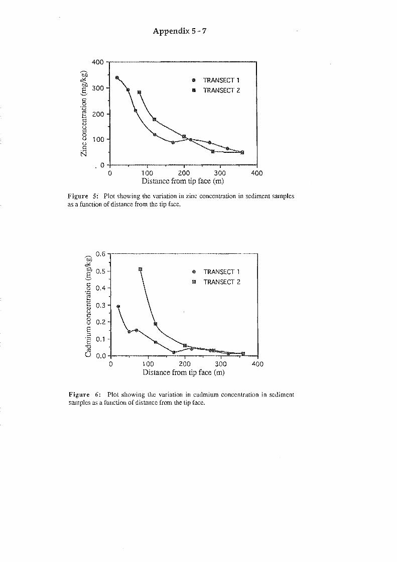
Appendix 5 - 7
400~------------------~--------~
c o ...... ~ 200 5 <..) c 8 <..) c N
100
o
• TRANSECT 1
II TRANSECT 2
100 200 300 Distance from tip face (m)
400
Figure 5: Plot showing the variation in zinc concentration in sediment samples as a function of distance from the tip face.
/""', 0.6 OJ:)
~ 0.5 E '--' c
0.4 0 '0
C':i b c 0.3 0 () c 0 0.2 ()
E ::l
'8 0.1 '"'0
C':i U 0.0
a
TRANSECT 1
!!It TRANSECT 2
100 200 300 400 Distance from tip face (m)
Figure 6: Plot showing the variation in cadmium concentration in sediment samples as a function of distance from the lip face.
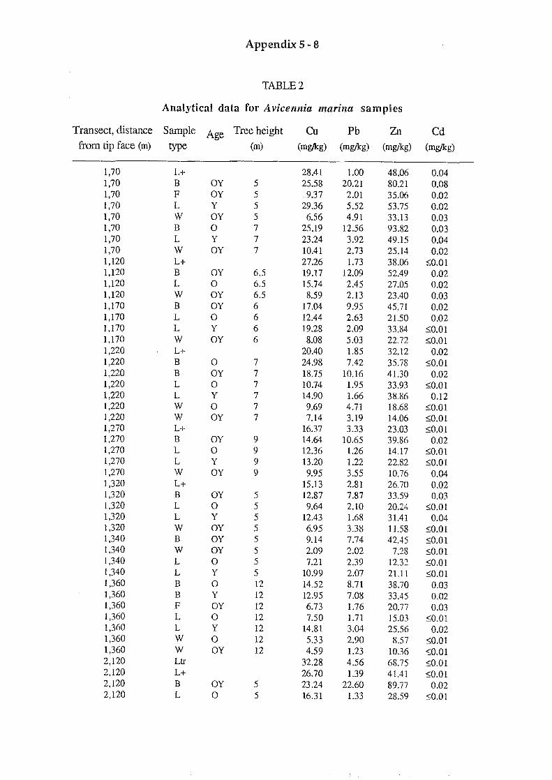
Appendix 5 - 8
TABLE 2
Analytical data for A vicennia marina samples
Transect, distance Sample Age Tree height Cu Pb Zn Cd from tip face (m) type (m) (mglkg) (mg/kg) (mg/kg) (mg/kg)
1,70 L+ 28.41 1.00 48.06 0.04 1,70 B Oy 5 25.58 20.21 80.21 0.08 1,70 F Oy 5 9.37 2.01 35.06 0.02 1,70 L Y 5 29.36 5.52 53.75 0.02 1,70 W Oy 5 6.56 4.91 33.13 0.03 1,70 B 0 7 25.19 12.56 93.82 0.03 1,70 L Y 7 23.24 3.92 49.15 0.04 1,70 W Oy 7 10.41 2.73 25.14 0.02 1,120 L+ 27.26 1.73 38.06 ::;0.01 1,120 B OY 6.5 19.17 12.09 52.49 0.02 1,120 L 0 6.5 15.74 2.45 27.05 0.02 1,120 W Oy 6.5 8.59 2.13 23.40 0.03 1,170 B OY 6 17.04 9.95 45.71 0.02 1,170 L 0 6 12.44 2.63 21.50 0.02 1,170 L Y 6 19.28 2.09 33.84 ::;0.01 1,170 W OY 6 8.08 5.03 22.72 ::;0.01 1,220 L+ 20.40 1.85 32.12 0.02 1,220 B 0 7 24.98 7.42 35.78 ::;0.01 1,220 B Oy 7 18.75 10.16 41.30 0.02 1,220 L 0 7 10.74 1.95 33.93 ::;0.01 1,220 L Y 7 14.90 1.66 38.86 0.12 1,220 W 0 7 9.69 4.71 18.68 ::;0.01 1,220 W Oy 7 7.14 3.19 14.06 ::;0.01 1,270 L+ 16.37 3.33 23.03 ::;0.01 1,270 B OY 9 14.64 10.65 39.86 0.02 1,270 L 0 9 12.36 1.26 14.17 ::;0.01 1,270 L Y 9 13.20 1.22 22.82 ::;0.01 1,270 W OY 9 9.95 3.55 10.76 0.04 1,320 L+ 15.13 2.81 26.70 0.02 1,320 B Oy 5 12.87 7.87 33.59 0.03 1,320 L 0 5 9.64 2.10 20.24 ::;0.01 1,320 L Y 5 12.43 1.68 31.41 0.04 1,320 W Oy 5 6.95 3.38 11.58 ::;0.01 1,340 B OY 5 9.14 7.74 42.45 ::;0.01 1,340 W Oy 5 2.09 2.02 7.28 ::;0.01 1,340 L 0 5 7.21 2.39 12.32 ::;0.01 1,340 L Y 5 10.99 2.07 21.11 ::;0.01 1,360 B 0 12 14.52 8.71 38.70 0.03 1,360 B Y 12 12.95 7.08 33.45 0.02 1,360 F OY 12 6.73 1.76 20.77 0.03 1,360 L 0 12 7.50 1.71 15.03 ::;0.01 1,360 L Y 12 14.81 3.04 25.56 0.02 1,360 W 0 12 5.33 2.90 8.57 ::;0.01 1,360 W OY 12 4.59 1.23 10.36 ::;0.01 2,120 Ltr 32.28 4.56 68.75 ::;0.01 2,120 L+ 26.70 1.39 41,41 ::;0.01 2,120 B Oy 5 23.24 22.60 89.77 0.02 2,120 L 0 5 16.31 1.33 28.59 ::;0.01
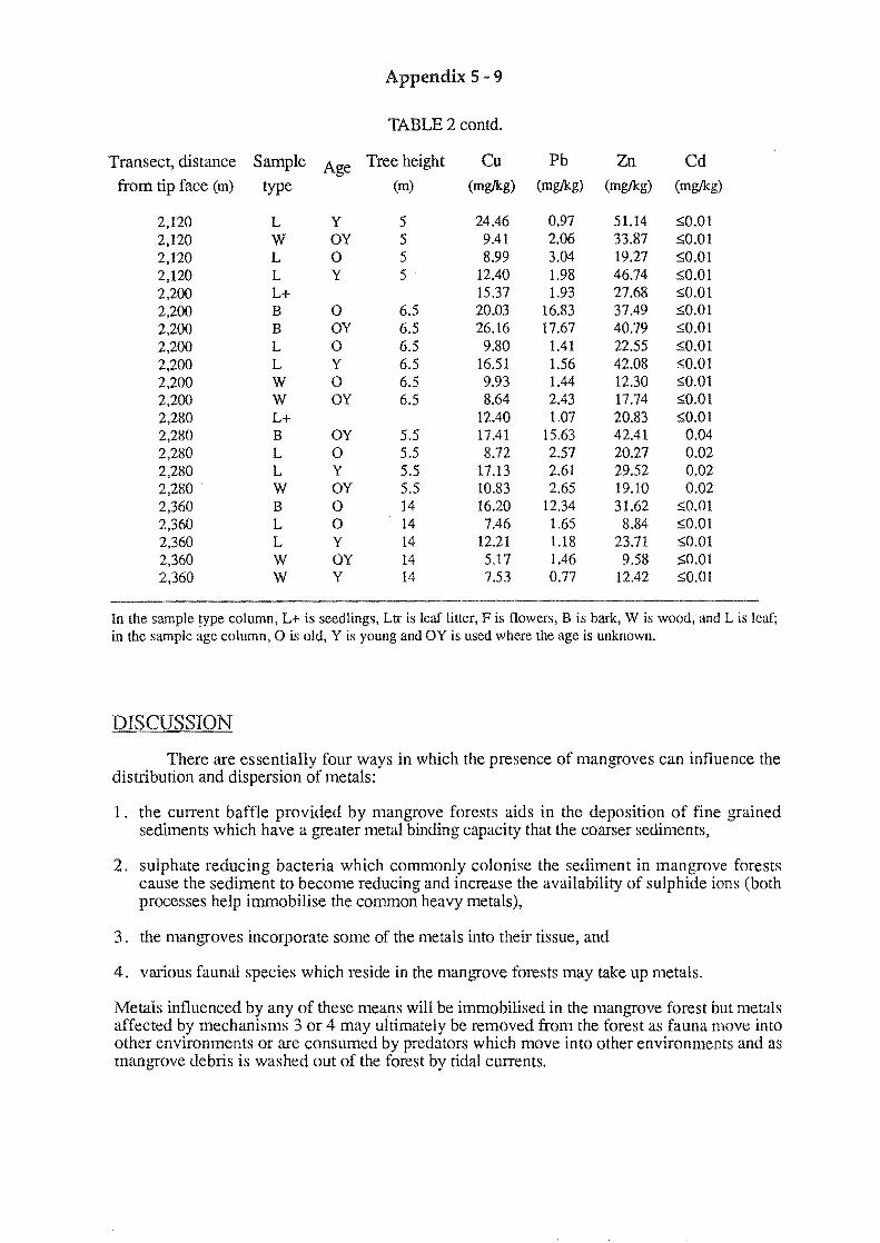
Appendix 5 ~ 9
TABLE 2 contd.
Transect, distance Sample Age Tree height Cu Pb Zn Cd
from tip face (m) type (m) (mglkg) (mglkg) (mg/kg) (mg/kg)
2,120 L Y 5 24.46 0.97 51.14 ::;0.01 2,120 W Oy 5 9.41 2.06 33.87 ::;0.01 2,120 L 0 5 8.99 3.04 19.27 ::;0.01 2,120 L Y 5 12.40 1.98 46.74 ::;0.01 2,200 L+ 15.37 1.93 27.68 ::;0.01 2,200 B 0 6.5 20.03 16.83 37.49 ::;0.01 2,200 B Oy 6.5 26.16 17.67 40.79 ::;0.01 2,200 L 0 6.5 9.80 1.41 22.55 ::;0.01 2,200 L Y 6.5 16.51 1.56 42.08 ::;0.01 2,200 W 0 6.5 9.93 1.44 12.30 ::;0.01 2,200 W Oy 6.5 8.64 2.43 17.74 ::;0.01 2,280 L+ 12.40 1.07 20.83 ::;0.01 2,280 B Oy 5.5 17.41 15.63 42.41 0.04 2,280 L 0 5.5 8.72 2.57 20.27 0.02 2,280 L Y 5.5 17.13 2.61 29.52 0.02 2,280 . W Oy 5.5 10.83 2.65 19.10 0.02 2,360 B 0 14 16.20 12.34 31.62 ::;0.01 2,360 L 0 14 7.46 l.65 8.84 ::;0.01 2,360 L Y 14 12.21 1.18 23.71 ::;0.01 2,360 W Oy 14 5.17 1.46 9.58 ::;0.01 2,360 W Y 14 7.53 0.77 12.42 ::;0.01
In the sample type column, L+ is seedlings, Ltr is leaf litter, F is flowers, B is bark, W is wood, and L is leaf; in the sample age column, 0 is old, Y is young and OY is used where the age is unknown.
DISCUSSION
There are essentially four ways in which the presence of mangroves can influence the distribution and dispersion of metals:
1. the current baffle provided by mangrove forests aids in the deposition of fine grained sediments which have a greater metal binding capacity that the coarser sediments,
2. sulphate reducing bacteria which commonly colonise the sediment in mangrove forests cause the sediment to become reducing and increase the availability of sulphide ions (both processes help immobilise the common heavy metals),
3. the mangroves incorporate some of the metals into their tissue, and
4. various faunal species which reside in the mangrove forests may take up metals.
Metals influenced by any of these means will be immobilised in the mangrove forest but metals affected by mechanisms 3 or 4 may ultimately be removed from the forest as fauna move into other environments or are consumed by predators which move into other environments and as mangrove debris is washed out of the forest by tidal currents.
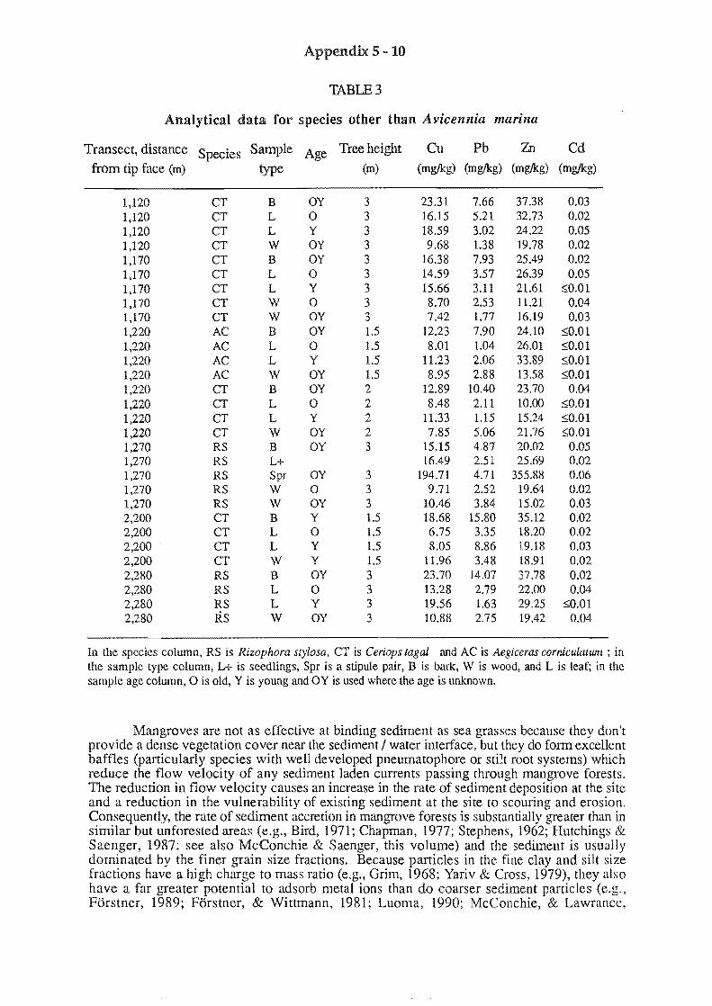
Appendix 5 ~ 10
TABLE 3
Analytical data for species other than Avicennia marina
Transect, distance Species Sample Age Tree height Cu Pb Zn Cd
from tip face (m) type (m) (mg/kg) (mg/kg) (mg/kg) (mg/kg)
1,120 CT B OY 3 23.31 7.66 37.38 0.03 1,120 CT L 0 3 16.15 5.21 32.73 0.02 1,120 CT L Y 3 18.59 3.02 24.22 0.05 1,120 CT W OY 3 9.68 1.38 19.78 0.02 1,170 CT B OY 3 16.38 7.93 25.49 0.02 1,170 CT L 0 3 14.59 3.57 26.39 0.05 1,170 CT L Y 3 IS.66 3.11 21.61 :<;;0.01 1,170 CT W 0 3 8.70 2.53 11.21 0.04 1,170 CT W Oy 3 7.42 1.77 16.19 0.03 1,220 AC B OY 1.5 12.23 7.90 24.10 :<;;0.01 1,220 AC L 0 l.S 8.01 1.04 26.01 :<;;0.01 1,220 AC L Y l.S 11.23 2.06 33.89 :<;;0.01 1,220 AC W Oy 1.5 8.95 2.88 1358 :<;;0.01 1,220 CT B Oy 2 12.89 10.40 23.70 0.04 1,220 CT L 0 2 8.48 2.11 10.00 :<;;0.01 1,220 CT L Y 2 11.33 1.15 15.24 :<;;0.01 1,220 CT W OY 2 7.85 5.06 21.76 :<;;0.01 1,270 RS B OY 3 IS.15 4.87 20.02 O.OS 1,270 RS L+ 16.49 2.51 25.69 0.02 1,270 RS Spr Oy 3 194.71 4.71 355.88 0.06 1,270 RS W 0 3 9.71 2.52 19.64 0.02 1,270 RS W OY 3 10.46 3.84 15.02 0.03 2,200 CT B Y 1.5 18.68 15.80 35.12 0.02 2,200 CT L 0 l.S 6.75 3.35 18.20 0.02 2,200 CT L Y 1.5 8.05 8.86 19.18 0.03 2,200 CT W Y 1.5 11.96 3.48 18.91 0.02 2,280 RS B OY 3 23.70 14.07 37.78 0.02 2,280 RS L 0 3 13.28 2.79 22.00 0.04 2,280 RS L Y 3 19.56 1.63 29.25 :<;;0.01 2,280 RS W OY 3 10.88 2.75 19.42 0.04
In the species column, RS is Rizophora stylosa. CT is Ceriops lagal and AC is Aegiceras corniculatwn ; in the sample type column, L+ is seedlings, Spr is a stipule pair, B is bark, W is wood, and L is leaf; in the sample age column. 0 is old, Y is young and OY is used where the age is unknown.
Mangroves are not as effective at binding sediment as sea grasses because they don't provide a dense vegetation cover near the sediment I water interface, but they do form excellent baffles (particularly species with well developed pneumatophore or stilt root systems) which reduce the flow velocity of any sediment laden currents passing through mangrove forests. The reduction in flow velocity causes an increase in the rate of sediment deposition at the site and a reduction in the vulnerability of existing sediment at the site to scouring and erosion. Consequently, the rate of sediment accretion in mangrove forests is substantially greater than in similar but unforested areas (e.g., Bird, 1971; Chapman, 1977; Stephens, 1962; Hutchings & Saenger, 1987; see also McConchie & Saenger, this volume) and the sediment is usually dominated by the finer grain size fractions. Because particles in the fine clay and silt size fractions have a high charge to mass ratio (e.g., Grim, 1968; Yariv & Cross, 1979), they also have a far greater potential to adsorb metal ions than do coarser sediment particles (e.g., Forstner, 1989; Forstner, & Wittmann, 1981; Luoma, 1990; McConchie, & Lawrance,
Appendix 5 - 11
1991). Hence, if metal ions are present in surface or groundwaters entering a mangrove forest, the physical properties of the sediment deposited within the forest confer on that sediment a greater capacity to extract metals from solution than exists in coarser sediments, outside the forest.
Although sediment particle size alone would make mangrove sediments an effective sink for metals (Harbison, 1986), biogeochemical processes associated with the sediment further enhance its metal storage capacity. In mangrove forests, low energy conditions, muddy organic matter-rich sediments, and a regular supply of sulphate ions, make an ideal environment for sulphate reducing bacteria (e.g., Desulphiovibrio desulphuricans). The existence of colonies of sulphate reducing bacteria in mangrove forest sediments is commonly indicated by the presence of highly reducing black sulphidic muds at or just below the sediment surface; similar sediment is also common in marsh land shoreward of the mangrove forest (e.g., the unvegetated zone in Fig. 2). Because many metals, including those examined in this study, are less mobile under reducing conditions and form sulphides with very low solubilities (e.g., Brookins, 1988; Hoffman, 1986), both the sulphide production and the low Eh conditions resulting from the presence of sulphate reducing microbes contribute to the trapping of any metal ions which come in contact with the sediment (Harbison, 1986).
At the Wynnum tip site both the abundance of fine sediments in the mangrove forest and unvegetated zone and the chemical impact of the microbial communities in these muds, contribute to the trapping of any metals which are leached from metallic wastes in the tip. The metal concentration trends in Figs. 3 - 6 are entirely consistent with the trapping of metals from tip leachates by these mechanisms and they also suggest that, with the possible exception of muds adjacent to the tip face, the sediment has the capacity to trap much higher metal loads than have yet been immobilised. Hence, it is evident that these mangrove muds form a very effective trap for any metals which do leach from the tip and thus afford the waters of Moreton Bay some protection from any metals in the tip leachates. However, because the trapping mechanisms depend on the presence of fine grained reducing sulphidic sediment, the trapping effect could easily be reversed (and the metals released) if the mangroves are destroyed or the sediment is drained and allowed to oxidise. Recent data from samples collected during the dry season confirm that the metal trapping can easily be reversed with samples obtained near the sediment surface having lower metal loads than they do during the wet season; during the dry season, the metal concentrations in sediment 50-100 cms below the surface are higher than they are during the wet season. These seasonal changes in metal distribution suggest that some of the metal load is redistributed as the water table rises and falls and hence, that the metal concentration in a sediment sample will depend to some extent on the position of the water table relative to the sampling depth. From an environmental management view point, these observations make a strong case for ensuring that the mangrove belt (Fig. 2) is preserved in its present form and that neither the mangrove belt nor the unvegetated zone are drained. The unvegetated zone could in the future be covered with top soil as part of any land development work, but any lowering of the water table would need to be avoided because the resulting oxidisation of the muds would not only encourage the release of the presently bound metals but would also trigger the formation of acid sulphate soils which would constitute an additional environmental hazard
The mangrove trees in the belt between the unvegetated zone and the sea show a rise in the concentration of some metals in some plant tissues toward the tip face indicating that the trees themselves contribute to forming the buffer between the tip and the sea. However, the change in metal concentration, in each tissue type, across the forest is less than that evident in the sediments implying that the metal trapping efficiency of the plants is less than that of the sediments they are growing on. Furthermore, because the magnitude of the change in concentration across the mangrove forest differs for each metal, it would appear that the metal concentration in each plant tissue type is not just a function of the metal availability to the plant.
We are not able to form any conclusions about the distribution of cadmium because cadmium concentrations in most types of tissue in most plants were at or near the lower limit of detection for the procedures used; all cadmium concentrations appear to be remarkably low. Lead shows a marked tendency to concentrate in the bark of all the mangrove species
Appendix 5 - 12
examined, and to a lesser extent in the wood (Tables 2, 3), but only in the bark does the lead concentration increase systematically toward the tip face; the lead content of the wood and leaves changes toward the tip face by less than one standard deviation and the lead content of the seedlings actually shows a small decrease toward the tip.
The concentrations of zinc and copper in all tissue types in the mangroves examined show a small rise (by a factor of about 2 - 3 times) toward the tip except for copper in the wood samples which shows no consistent trend. Both zinc and copper show a tendency to concentrate in the bark, seedlings and young leaves of the mangroves with much lower concentrations being evident in the wood and old leaves. The tendency for seedlings and young leaves to have higher copper and zinc concentrations than old leaves (Tables 2, 3) is unusual because in most organisms the metal load tends to increase with increasing organism age. The data obtained during this study imply that older mangrove leaves are able to reduce their metal load probably as an indirect consequence of the operation of their salt excretion mechanisms. Although we are still investigating this phenomenon, preliminary evidence suggests that because both copper and zinc form highly soluble chloride complexes, some metal is lost as chloride complexes when the mangrove leaves excrete salt; because the salt pumps in young leaves and seedlings are inefficient relative to older leaves, the rate of metal excretion is far greater in older leaves and hence they have lower metal loads. The apparent ability of mature mangrove leaves to excrete some of their metal load means that such plants may be able to tolerate exposure to abnormally high concentrations of metals such as copper and zinc but the same tolerance would not be expected for juvenile plants or young leaves which do not have the same metal excretion capacity.
The mangrove leaf litter (Table 2) analysed from this site, and other litter samples examined during this study, show that on average the mangrove leaf litter contains higher concentrations of most metals than any other part of the plant with the exception of lead in the bark; similar concentration of metals in mangrove leaf detritus has also been found in other studies (e.g., Rice & Windom, 1982). The reason for the high metal concentrations in the litter is unclear but it is clear that if the export of mangrove detritus from the forests by tidal flushing is as high as suggested by BOlO & Bunt (1981) then significant amounts of metal may be exported from the mangrove forest in this manner. Some further loss of metals from the mangrove forest may be associated with fauna which take up metals while in the forest and then move into other environments or are consumed by predators which move into other environments. However, for this site, the gradient in metal concentrations in both the sediment and the mangrove plants suggests that net metal uptake within the forest is significantly greater than any metal loss to the sea by biological processes or by any seaward reworking of sediment.
CONCLUSIONS AND IMPLICATIONS
The data obtained in this study indicate that the mangrove forest and the unvegetated zone between the tip face and the forest are forming an effective barrier against the movement of any metallic tip leachates to the waters of Moreton Bay. Metal trapping by the fine grained reducing sulphidic sediments within and shoreward of the mangrove forest probably makes the major contribution to the biogeochemical barrier. However, direct metal uptake by the mangrove plants also traps substantial quantities of copper, zinc and lead. The extent of metal export from the forest is unclear at this stage but it appears to be quantitatively minor.
Recognition of the buffering effect described above and the means by which it operates is significant both scientifically and in terms of its importance to land use planners and environmental managers. In particular, recognition of the major metal trapping capacity of the reducing sulphidic sediments indicates that future land management planning for the area will need to ensure that these sediments are not drained and allowed to oxidise. Oxidisation of the sediments, which would be a likely consequence of any draining of the sediment, would not only release many of the presently trapped metals but would probably also result in the creation of the type of environmental problems typically associated with acid sulphate soil formation.
Appendix 5 - 13
REFERENCES
Bird, E. C. E, 1971. Mangroves as land builders. VictoriaNatur., 88, 189-197. Boto, K. G., and Bunt, J. S., 1981. Tidal export of particulate organic matter from a northern Australian
mangrove system. Estuar. Coast. Shelf Sci., 13, 247-255. Brookins, D. G., 1988. Eh - pH diagramsfor geochemistry. Springer-Verlag, N. Y., 176pp. Chapman, V. J., (Ed.), 1977. Ecosystems of the World 1: Wet Coastal Ecosystems. Elsevier, Amsterdam. F5rstner, U., 1989. Contaminated sediments. Springer - Verlag, N.Y. Forstner, U., and Wittmann, G.T.W., 1981. Metal pollution in the aquatic environment. Springer - Verlag. Grim, R. E., 1968. Clay mineralogy. McGraw Hill, N.Y., 596pp. Harbison, P., 1981. The case for the protection of mangrove swamps: Geochemical considerations. Search,
12(8), 273-276. Harbison, P., 1986. Mangrove muds - a sink or source for trace metals. Mar. Poll. Bull., 17(6),246-250. Hoffman, S. J., 1986. Soil sampling. In J. M. Robertson (ed.) Exploration geochemistry: design and
interpretation of soil surveys. Reviews in economic geology, v3, 39-77. Hutchings, P., and Saenger, P., 1987. Ecology of mangroves. University of Queensland Press, 388pp. Luoma, S. N., 1990. Processes affecting metals concentrations in estuarine and coastal marine sediments. In R.
W. Furness and P. S. Rainbow (eds.) Heavy metals in the marine environment, CRC Press, 51-66. McConchie, D. M., Mann, A. W., Lintem, M. J., Longman, D., Talbot, V., Gabelish, A. 1., and Gabelish, M.
J., 1988. Heavy metals in marine biota, sediments, and waters from the Shark Bay area, Western Australia. J. Coastal Res., 4(1),51-72.
McConchie, D. M., and Lawrance, L.M., 1991. The origin of high cadmium loads in some bivalve molluscs from Shark Bay, Western Australia: A new mechanism for cadmium uptake by filter feeding organisms. Archives of Environ. Contam. & Toxicol. 21,303-310.
Montgomery, J.R., and Price, M.T., 1979. Release of trace metals by sewage sludge and the subsequent uptake by members of a turtle grass mangrove ecosystem. Environ: Sci. & Technol., 13,546-549.
Peterson, P. J., Burton, M. A., Gregson, M., Nye, S. M., and Porter, E. K., 1979. Accumulation of tin by mangrove species in West Malaysia. Science of the Total Environment, 11,213-221.
Rice, D. L., and Windom, H. L., 1982. Trace metal transfer associated with the decomposition of detritus derived from estuarine macrophytes. Bot. Mar., 25, 213-223.
Saenger, P., Specht, M.M., Specht, R.L., and Chapman, V.I., 1977. Mangal and coastal saltmarsh communities in Australasia. In: Chapman, V. J. (Ed.), Ecosystems of the World. I. Wet Coastal Ecosystems. Elsevier, Amsterdam, pp. 293-345.
Stephens, W. M., 1962. Trees that make land. Sea frontiers, 8,219-230. Thomas, C., and Eong, O. J .• 1984. Effeet of heavy metals zinc and lead on Rhizophora mucronata Lam. and
Avicennia alba BI. seedlings. Proc. As. Symp. Mangr. Env. Res. Manag., 568-574. Walsh, G. E. R., Ainsworth, K. A., and Rigby, R., 1979. Resistance of red mangrove (Rhizophora mangle L.)
seedlings to lead, cadmium, and mercury. Biotropica, 11(1),22-27. Yariv, S., and Cross, H., 1979: Geochemistry of colloid systems for earth scientists. Springer-Verlag, N.Y.

Appendix 5 -14
To Whom it may concern,
Malcolm Clark has contributed to the production of this paper by
supplying all of the figures used and all of the data used to construct figure 2; data collected for
figure 2 represents part of the data collected for the construction of the contour maps used in
his thesis. Malcolm also made a significant contribution to the interpretation of the data and
development of the scientific ideas on which the paper is based.