2012 Auction Catalog - University of Pennsylvania Law School
Upload
khangminh22Category
view
0download
0
The Pennsylvania State UniversityThe Graduate SchoolCollege of Engineering
MODEL-BASED RECEDING HORIZON CONTROL AND
ESTIMATION FOR NONLINEAR SYSTEMS VIA CARLEMAN
APPROXIMATION
A Dissertation inChemical Engineering
byYizhou Fang
© 2018 Yizhou Fang
Submitted in Partial Fulfillmentof the Requirementsfor the Degree of
Doctor of Philosophy
December 2018

The dissertation of Yizhou Fang was reviewed and approved∗ by the following:
Antonios ArmaouAssociate Professor of Chemical EngineeringDissertation Advisor, Chair of Committee
Robert M. RiouxFriedrich G. Helfferich Professor of Chemical Engineering
Xueyi ZhangAssistant Professor of Chemical Engineering
Hosam K. FathyBryant Early Career Professor of Mechanical Engineering
Phillip SavageProfessor of Chemical EngineeringDepartment Head of Chemical Engineering
∗Signatures are on file in the Graduate School.
ii

AbstractThis dissertation aims at developing model-based control and estimation algo-rithms via Carleman approximation to improve the performance of nonlinear modelpredictive controller (NMPC) and nonlinear moving horizon estimation (NMHE).
Despite the many advantages of model predictive control (MPC) and movinghorizon estimation (MHE) as advanced control and estimation technologies, compu-tational delay is one of the most significant problems holding back their industrialapplications. This dissertation addresses this problem by developing NMPC andNMHE algorithms based on Carleman approximation to improve their computa-tional efficiency. We also integrate other mathematics and optimization tools inour algorithms, including control vector parameterization (CVP) and nonlinearprogramming (NLP) sensitivity analysis, to further improve their performances.
We model the original nonlinear system with a Two-Tier approximation. First,we approximate the system through a Taylor expansion and arrive at a polynomialformulation. Second, we extend the state variables to higher orders following theKronecker product rule. After that, we approximate the system for a second timethrough Carleman approximation (also known as Carleman linearization). After thisTwo-Tier approximation, we draw an extended bilinear expression to represent thenonlinear dynamics. With little loss of nonlinear information, it enables analyticalprediction of future system evolution. Assuming piecewise constant control signals,the manipulated inputs are entering the cost function as parameters. ThroughCarleman approximation, the dynamic models are directly incorporated into thecost function, releasing the optimization from these equality constraints. This alsoallows the computer to analytically calculate the sensitivity of the cost function tothe manipulated inputs. The analytical sensitivity facilitates the solver by servingas the search gradient, and also allows us to develop sensitivity-updating algorithms.All of these together contributes to significantly increased computational efficiency.
We present an analysis of error accumulation caused by Carleman approximationand then improve the accuracy of this approach by resetting extended statesperiodically. The idea of efficient temporal discretization in CVP is embedded in theCarleman model predictive control (CMPC) formulation to improve the controllerperformance. The advantages are illustrated with two application examples where
iii
we solve a tracking problem and a regulation problem.A computationally efficient approach of economic-oriented model predictive
control (EMPC) is developed, Carleman EMPC. Carleman approximation workswell with set-point free economic cost function. In this way, we predict the futureeconomic performance analytically and provide the sensitivity of the economicperformance to the manipulated inputs as the search gradient. Hence, despite theeconomic stage costs are mostly non-tracking and non-quadratic, we achieve signifi-cant acceleration in the computation of EMPC. An oxidation of ethylene exampleis demonstrated as a case study example. We optimize multiple manipulated inputsand achieve optimal control by establishing a non-tracking cyclic operation.
In this dissertation, we also develop an algorithm that fuses Carleman movinghorizon estimation (CMHE) and CMPC together, to design an output feedbackreceding horizon controller. CMHE identifies the system states as the initial condi-tion for CMPC to make optimal control decisions. The control decisions made byCMPC update the dynamic models used in CMHE to make more precise estimations.Modeling the nonlinear system with Carleman approximation, we estimate thesystem evolution for both CMHE and CMPC analytically. The Gradient vectorsand Hessian matrices are then provided to facilitate the optimizations. To furtherreduce real-time computation, we adapt the advanced-step NMHE and advanced-step NMPC concepts to our CMHE/CMPC pair to develop an asCMHE/asCMPCpair. It pre-estimates the states and pre-designs the manipulated input sequenceone step in advance with analytical models, and then it updates the estimation andcontrol decisions almost in the real-time with pre-calculated analytical sensitivities.A nonlinear CSTR is studied as the illustration example. With CMHE/CMPC pair,the computational time is decreased to one order of magnitude less than standardNMHE/NMPC. With asCMHE/asCMPC pair, the real-time estimation and controldecisions takes a negligible amount of wall-clock time.
iv

Table of Contents
List of Figures viii
List of Tables xii
Acknowledgments xiii
Chapter 1Introduction 11.1 Research Background . . . . . . . . . . . . . . . . . . . . . . . . . . 11.2 Literature Review . . . . . . . . . . . . . . . . . . . . . . . . . . . . 11.3 Motivations . . . . . . . . . . . . . . . . . . . . . . . . . . . . . . . 41.4 Dissertation Overview and Outline . . . . . . . . . . . . . . . . . . 6
Chapter 2Carleman Approximation-based Model Predictive Control 92.1 Introduction . . . . . . . . . . . . . . . . . . . . . . . . . . . . . . . 92.2 Preliminaries and Basic Formulation . . . . . . . . . . . . . . . . . 11
2.2.1 Preliminaries . . . . . . . . . . . . . . . . . . . . . . . . . . 112.2.2 Basic MPC Controller Design . . . . . . . . . . . . . . . . . 122.2.3 Carleman Approximation and Sensitivity-based Optimization 13
2.3 Resetting the Extended States . . . . . . . . . . . . . . . . . . . . . 162.4 Proposed Formulation . . . . . . . . . . . . . . . . . . . . . . . . . 18
2.4.1 Nonlinear Dynamic Constraints and Bilinear Representation 182.4.2 Resetting Extended States in Sensitivity Calculation . . . . 222.4.3 The Proposed MPC Formulation: Carleman Approximation-
based MPC (CMPC) . . . . . . . . . . . . . . . . . . . . . . 232.5 Application . . . . . . . . . . . . . . . . . . . . . . . . . . . . . . . 24
2.5.1 Example Application of Resetting Extended States . . . . . 242.5.2 Example Application: Stable CSTR . . . . . . . . . . . . . . 272.5.3 Example Application: Unstable CSTR . . . . . . . . . . . . 29
v

2.6 Conclusion . . . . . . . . . . . . . . . . . . . . . . . . . . . . . . . . 39
Chapter 3Control Vector Parameterization 463.1 Introduction . . . . . . . . . . . . . . . . . . . . . . . . . . . . . . . 463.2 Formulation: Embedding Control Vector Parameterization . . . . . 483.3 Simulations . . . . . . . . . . . . . . . . . . . . . . . . . . . . . . . 523.4 Conclusions . . . . . . . . . . . . . . . . . . . . . . . . . . . . . . . 54
Chapter 4Economic-oriented Carleman Model Predictive Control 594.1 Introduction . . . . . . . . . . . . . . . . . . . . . . . . . . . . . . . 594.2 Definition and Formulation . . . . . . . . . . . . . . . . . . . . . . . 60
4.2.1 EMPC Formulation . . . . . . . . . . . . . . . . . . . . . . . 604.2.2 Two-Tier Approximation . . . . . . . . . . . . . . . . . . . . 624.2.3 Gradient-based Optimization . . . . . . . . . . . . . . . . . 65
4.3 Simulations . . . . . . . . . . . . . . . . . . . . . . . . . . . . . . . 684.4 Conclusions . . . . . . . . . . . . . . . . . . . . . . . . . . . . . . . 72
Chapter 5Combination of Moving Horizon Estimation and Model Predic-
tive Control 755.1 Introduction . . . . . . . . . . . . . . . . . . . . . . . . . . . . . . . 755.2 Preliminary Information . . . . . . . . . . . . . . . . . . . . . . . . 78
5.2.1 Nonlinear System Under Investigation . . . . . . . . . . . . 785.2.2 Mathematics Background: Carleman Approximation . . . . 78
5.3 Fusing CMHE and CMPC . . . . . . . . . . . . . . . . . . . . . . . 805.3.1 CMHE Design . . . . . . . . . . . . . . . . . . . . . . . . . . 805.3.2 CMPC Design . . . . . . . . . . . . . . . . . . . . . . . . . . 825.3.3 Analytical Prediction of System Evolution . . . . . . . . . . 835.3.4 Gradient Vector and Hessian Matrix to Facilitate Optimization 84
5.3.4.1 CMHE Part . . . . . . . . . . . . . . . . . . . . . . 845.3.4.2 CMPC Part . . . . . . . . . . . . . . . . . . . . . . 86
5.4 Simulation . . . . . . . . . . . . . . . . . . . . . . . . . . . . . . . . 875.4.1 Example Description . . . . . . . . . . . . . . . . . . . . . . 875.4.2 CMHE/CMPC Pair . . . . . . . . . . . . . . . . . . . . . . . 88
5.5 Conclusion . . . . . . . . . . . . . . . . . . . . . . . . . . . . . . . . 91
vi

Chapter 6Advanced-step CarlemanMoving Horizon Estimation andModel
Predictive Control 986.1 Introduction . . . . . . . . . . . . . . . . . . . . . . . . . . . . . . . 986.2 Strategy of Adapting Advanced-step Algorithm to CMHE/CMPC
Pair . . . . . . . . . . . . . . . . . . . . . . . . . . . . . . . . . . . 996.3 Algorithm Specifics . . . . . . . . . . . . . . . . . . . . . . . . . . . 101
6.3.1 asCMHE Algorithm . . . . . . . . . . . . . . . . . . . . . . . 1016.3.2 asCMPC Algorithm . . . . . . . . . . . . . . . . . . . . . . . 102
6.4 Simulation . . . . . . . . . . . . . . . . . . . . . . . . . . . . . . . . 1036.4.1 Example Description . . . . . . . . . . . . . . . . . . . . . . 1036.4.2 asCMHE . . . . . . . . . . . . . . . . . . . . . . . . . . . . . 1046.4.3 asCMPC . . . . . . . . . . . . . . . . . . . . . . . . . . . . . 1046.4.4 asCMHE/asCMPC Pair . . . . . . . . . . . . . . . . . . . . 104
6.5 Conclusion . . . . . . . . . . . . . . . . . . . . . . . . . . . . . . . . 105
Chapter 7Conclusion 1107.1 Dissertation Summary . . . . . . . . . . . . . . . . . . . . . . . . . 1107.2 Contributions . . . . . . . . . . . . . . . . . . . . . . . . . . . . . . 1127.3 Recommendations for Future Work . . . . . . . . . . . . . . . . . . 113
Appendix AKronecker Product & Extended System Matrices 114A.1 Kronecker Product . . . . . . . . . . . . . . . . . . . . . . . . . . . 114A.2 Extended System Matrices . . . . . . . . . . . . . . . . . . . . . . . 115
Appendix BSensitivity Derivation Specifics 116B.1 Components of CMHE Sensitivity . . . . . . . . . . . . . . . . . . . 116B.2 Components of CMPC Sensitivity . . . . . . . . . . . . . . . . . . . 118B.3 Components of Exponential Term Derivatives . . . . . . . . . . . . 119
Appendix CSimulation Example Parameters 122C.1 Open-loop Stable Isothermal CSTR . . . . . . . . . . . . . . . . . . 122C.2 Open-loop Unstable Exothermic CSTR . . . . . . . . . . . . . . . . 123C.3 Catalytic Ethylene Oxidation CSTR . . . . . . . . . . . . . . . . . 123
Bibliography 127
vii

List of Figures
1.1 Hierarchy of modern process system engineering . . . . . . . . . . . 2
2.1 Diagram of resetting extended states . . . . . . . . . . . . . . . . . 18
2.2 Schematic diagram of isothermal CSTR with three parallel reactions 26
2.3 Effect of reseting extended states in analytical simulation via Carle-man approximation . . . . . . . . . . . . . . . . . . . . . . . . . . . 28
2.4 Open-loop stable CSTR controlled under CMPC . . . . . . . . . . . 30
2.5 Open-loop stable CSTR controlled under standard NMPC . . . . . 30
2.6 Schematic diagram of open-loop unstable CSTR . . . . . . . . . . . 31
2.7 Change of operating condition in the unstable CSTR . . . . . . . . 33
2.8 Open-loop response of unstable CSTR under a −10% step changein the feeder concentration CAf . . . . . . . . . . . . . . . . . . . . 34
2.9 Open-loop unstable CSTR regulated under operation condition change 35
2.10 Comparison of the effect of resetting extended states at differentfrequencies under operating condition change . . . . . . . . . . . . . 37
2.11 Comparison of values of the cost function . . . . . . . . . . . . . . . 38
2.12 Unstable open-loop behavior under negative unknown disturbance . 39
viii

2.13 Open-loop unstable CSTR regulated under unknown negative dis-turbance . . . . . . . . . . . . . . . . . . . . . . . . . . . . . . . . . 40
2.14 Comparison of the effect of resetting extended states at differentfrequencies under unknown negative disturbance . . . . . . . . . . . 41
2.15 Open-loop response of the CSTR under positive disturbance . . . . 42
2.16 Open-loop unstable CSTR regulated under unknown negative dis-turbance . . . . . . . . . . . . . . . . . . . . . . . . . . . . . . . . . 43
2.17 Comparison of the effect of resetting extended states at differentfrequencies under unknown positive disturbance . . . . . . . . . . . 44
3.1 Diagram: sampling time as design variable . . . . . . . . . . . . . . 48
3.2 Formulation I of CVP embedded CMPC . . . . . . . . . . . . . . . 51
3.3 Formulation II of CVP embedded CMPC . . . . . . . . . . . . . . . 51
3.4 Open-loop response of unstable CSTR under negative disturbance . 52
3.5 Comparison of Formulation I with standard CMPC under change ofoperating condition . . . . . . . . . . . . . . . . . . . . . . . . . . . 53
3.6 Comparison of Formulation II with standard CMPC under changeof operating condition . . . . . . . . . . . . . . . . . . . . . . . . . 54
3.7 Comparison of Formulation I with standard CMPC under negativedisturbance . . . . . . . . . . . . . . . . . . . . . . . . . . . . . . . 55
3.8 Comparison of Formulation II with standard CMPC under negativedisturbance . . . . . . . . . . . . . . . . . . . . . . . . . . . . . . . 56
3.9 Open-loop response of unstable CSTR under positive disturbance . 56
3.10 Comparison of Formulation I with standard CMPC under positivedisturbance . . . . . . . . . . . . . . . . . . . . . . . . . . . . . . . 57
ix

3.11 Comparison of Formulation II with standard CMPC under positivedisturbance . . . . . . . . . . . . . . . . . . . . . . . . . . . . . . . 58
4.1 Schematic diagram of the catalytic ethylene oxidation CSTR . . . . 68
4.2 Standard EMPC under system noise . . . . . . . . . . . . . . . . . 72
4.3 Carleman EMPC under system noise . . . . . . . . . . . . . . . . . 73
4.4 Standard EMPC under model mismatch . . . . . . . . . . . . . . . 73
4.5 Carleman EMPC under model mismatch . . . . . . . . . . . . . . . 74
5.1 A schematic diagram of CMHE/CMPC pair . . . . . . . . . . . . . 77
5.2 Open-loop system under noise: real states compared with estimatedstates under 2nd order CMHE and standard NMHE . . . . . . . . . 93
5.3 Closed-loop system under noise: real states compared with estimatedstates under 2nd order CMHE . . . . . . . . . . . . . . . . . . . . . 94
5.4 Closed-loop system under noise: real states compared with standardNMHE . . . . . . . . . . . . . . . . . . . . . . . . . . . . . . . . . . 95
5.5 Comparison of open-loop response and closed-loop response under2nd order CMHE/CMPC . . . . . . . . . . . . . . . . . . . . . . . . 96
5.6 Comparison of open-loop response and closed-loop response underNMHE/NMPC . . . . . . . . . . . . . . . . . . . . . . . . . . . . . 97
6.1 A schematic diagram of advanced-step NMPC algorithm . . . . . . 99
6.2 A schematic diagram of asCMHE/asCMPC algorithm . . . . . . . . 100
6.3 Comparison of real open-loop system and estimated system under2nd order CMHE/asCMHE . . . . . . . . . . . . . . . . . . . . . . 106
x

6.4 Comparison of 2nd order CMPC and asCMPC under process noise 107
6.5 Comparison of 2nd order CMPC and asCMPC under model mismatch 108
6.6 Comparison of CMHE/CMPC and asCMHE/asCMPC . . . . . . . 109
xi

List of Tables
2.1 Parameters of Open-loop Stable CSTR . . . . . . . . . . . . . . . . 25
2.2 Deviation between solutions from Carleman approximation andnumerical integration . . . . . . . . . . . . . . . . . . . . . . . . . . 27
2.3 Parameters of Open-loop Unstable CSTR . . . . . . . . . . . . . . . 32
2.4 Comparison of Computational Time . . . . . . . . . . . . . . . . . . 38
4.1 Dimensionless Parameters of the Ethylene Oxidation CSTR . . . . 72
4.2 Comparison of Computational Time: Standard EMPC vs CarlemanEMPC . . . . . . . . . . . . . . . . . . . . . . . . . . . . . . . . . . 74
5.1 Parameters Used in the CMHE/CMPC Design for the Simulation . 89
5.2 Comparison of Computational Time . . . . . . . . . . . . . . . . . . 91
C.1 Parameters of Open-loop Stable CSTR . . . . . . . . . . . . . . . . 123
C.2 Unstable CSTR Parameters and Nominal Steady State . . . . . . . 124
C.3 Dimensionless Parameters of the Ethylene Oxidation CSTR . . . . 126
xii

Acknowledgments
I would like to thank my advisor Dr. Antonios Armaou for serving as the chairof my committee. Thank you for leading me into the door to advanced processcontrol, for the knowledge and guidance that direct me throughout my graduatestudy. This dissertation would not have been accomplished without you.
Many thanks to my committee members Dr. Robert Rioux, Dr. Xueyi Zhangand Dr. Hosam Fathy. Thank you for your time and insights that are all veryvaluable to my work. I also thank Dr. Ashok Belegundu, Dr. Hosam Fathy andDr. Constanino Lagoa for offering these wonderful courses that help me acquireknowledges on control and optimization.
I would love to extend my deep appreciation to colleagues at Shell GlobalSolutions for offering me this valuable opportunity to work on industrial R&D ofMPC. I owe a sincere gratitude to my supervisor Dr. Rishi Amrit, my mentorDr. Jie Yu, my buddy Dr. Xue Yang, and all the colleagues from the ProcessAutomation, Control and Optimization (PACO) department. Thank you for thiswonderful experience that helped me gain the passion on process control and findout what I’ve been learning can make real values to the world. That summer wasnot only enjoyable but also helped me generating new ideas in research during mylast year of Ph.D. study.
I must give special honors to my family for your unconditional, unceasing love,understanding, support and encouragement. I would not be who I am today withoutyou. I would award the highest honor that I can give to my parents Ping Fang andWen Zhang. Thank you dad, for guarding and enlightening me on every step of mylife, for “pushing” me to join the 2+2 program that changed the entire track of mylife. You really are a genius! Thank you mom, for always been loving, warm andsupportive, for caring for every aspect of my life, and for raising me with endlesslove. I feel so blessed to have such a great mom! I would love to give specialacknowledgment to my grandmother, Yueying Xiang. You are my role model ofbeing a strong and self-motivated woman no matter how hard the situation canbe. I feel so proud when people say I resemble you. I am also highly thankful to
xiii

my cousins Kan Fang and Lina Yuan. Thank you for coming all the way to StateCollege to give your blessings at my wedding. I would also love to acknowledgemy little nephew and niece, Yuhao Fang and Yufei Chen. Your cute little facesbrighten up my days whenever I feel tired. Last and the most importantly, mysincere thanks go to my husband Renxuan Xie. You are the most amazing humanbeing on the planet! Thank you for making me smile whenever I feel upset, foralways believing in me no matter what happens, for standing by me during thedifficult times, and for always being so trustworthy, encouraging and supportive.Because of you, even tough days are joyful and sweet.
My sincerely thanks go to my lab mates, Dr. Negar Hashemian and Dr. JiLiu, for the discussions, help and encouragements that supported me during myPh.D research and career development. I’m also thankful to my buddies back fromFudan University, the “Five Armbands Gang”, for their long-lasting support andfriendship. I feel so blessed to have so many brothers and sisters from State CollegeChinese Alliance Church, Penn State International Christian Fellowship, and KatyChristian Community Church. Your prayers, care, and encouragements have andwill keep supporting and blessing me.
Most importantly, I would love to give all the glory to the Lord, for leading meto Penn State, for guarding me on every high and low of my life, and for grantingme the strength to continue striving to today. I am so grateful for the joy of lifethat comes through the salvation in Christ Jesus. YOU, are ultimately controllingand optimizing my life.
This research is supported by the National Science Foundation, Grant CBETAward No. 12-64902. We gratefully acknowledge the financial support. The findingsand conclusions in this dissertation do not necessarily reflect the view of the fundingagency.
xiv

To Mommy, Daddy, and the love of my life Xiao Xuanxuan

Chapter 1 |Introduction
1.1 Research BackgroundFigure 1.1 presents a typical hierarchy of modern process system engineering. Itis composed of several layers. The time scales of decision making grow larger asmoving from the bottom layer to the top layer. The Measurements/Instruments ofUnits layer represents all the hardwares, such as valves, pumps, heaters, meters, etc.The Automation layer automatically controls all the measurements and instrumentsof each operation unit. On top of it is the Process Control layer, which is thebasic regulatory control layer, has a time scale of seconds; Proportional-Integral-Differential (PID) controllers are the most commonly seen in this layer. TheAdvanced Process Control (APC) layer acts as a superior substitution for theProcess Control layer. The Real-Time Optimization (RTO) layer generates set-points for the APC layer to pursue in order to achieve the optimized economicperformance in the presence of changes and disturbances. The APC layer and theRTO layer both deal with disturbances, but the APC layer, whose time scale is ofminutes, handles short-term disturbances, while the RTO layer, with a time scaleof hours, takes care of long-term disturbances.
1.2 Literature ReviewThe past four decades witnessed the widespread applications of model predictivecontrol (MPC) in chemical, pharmaceutical, petroleum, and many other industries.The basic idea of MPC is to use models to predict future states of a dynamic system
1

Figure 1.1: The hierarchy of modern process system engineering
and then manipulate control signals to force the outputs of the system to track thedesired trajectory [1]. The basic control architecture of MPC is to determine thecurrent control action by solving an optimal control problem (OCP) within a finitehorizon at each sampling time and implementing only the first control action in thesequence [2]. This architecture enables MPC to cope with constraints, includingstate, input, output and process constraints, which is highly applicable in realindustrial processes [3]. With the strategy of converting a control problem to anoptimization problem, MPC is a powerful tool in handling multiple-input-multiple-output (MIMO) systems. Since control actions are computed by repeatedly solvingreceding-horizon optimization problems, they adjust themselves as the dynamicprocess evolves, which enables MPC to reject external disturbances and to toleratemodel mismatches [1] [4]. Reviews on MPC formulations, stability analysis andperformance can be found in [5] [6].
Linear MPC (LMPC) is a relatively mature technology that is well handled by
2

linear, quadratic and Gaussian control theories [2]. Linear control theories basedon transfer function models and state-space models construct a solid foundationfor LMPC [7].
Nonlinear MPC (NMPC) applies to nonlinear reactors and plants that vary overlarge regions of state space, for example, changeovers in continuous processes andtracking problems in startup or batch processes [2]. The development of large scalenonlinear programming (NLP) algorithms and dynamic optimization (DO) strategiesintroduced great opportunities to NMPC in industry [8]. An important openproblem of NMPC is the stability of closed-loop process operation. NLP propertiesof NMPC are investigated to achieve stable and robust NMPC [9]. Research hasalso been focused on Lyapunov-based formulations, which address stability issues,and the effect of initial condition on the feasibility of optimization [10–14]. Anothersignificant challenge to NMPC is its complexity in computation compared withclassical controllers. Complex chemical processes with large number of states orhigh nonlinearity require even more significant amount of computational work.The resulting feedback delays, consequent loss of performance and stability issuesbecome significant barriers to the industrial applications of NMPC. Researchershave developed many approaches to achieve computational acceleration. Theadvanced-step NMPC (asNMPC) algorithm, published by Biegler and coworkersin [15–18], has focused on solving complex optimization problems off-line thenperforming an update with linear approximation of nonlinear sensitivity. Multi-parametric MPC developed by Pistikopoulos and coworkers in [19,20] acceleratescomputation via querying response hypersurfaces. Researchers have also reportednice work on the application aspect of NMPC. Fathy and coworkers investigatedMPC applications on lithium-ion batteries [21]. They use extended differentialflatness as a fast approach in both control [22–25] and estimation [26]. As tolarge scale distributed parameter systems, such as solid sorbent-based CO2 capturesystems, dynamic reduced order models are proposed to facilitate NMPC to workmore computationally efficient [27–29]. More review papers on NMPC can be foundin [30].
More recently, research interests are starting to arise in economic-oriented MPC(EMPC). EMPC is formulated using an economic objective function to minimizethe future cost; it emphasizes more on the process path since it directly optimizesthe economic performance [31–33]. The formulations of economic cost functions
3

are generally not in quadratic forms as those of conventional MPC, but there areformulations to guarantee stability and to improve numerical performances [34].Typical examples include adding quadratic regularization terms in the economiccost function and reformulations using Lyapunov functions [31–33]. Christofidesand co-workers have published nice work on several EMPC topics [35], includinghandling preventive actuator maintenance and economics [36], applications ofEMPC on transport-reaction processes [37, 38], applications of EMPC on parabolicpartial differential equation systems [39], and using EMPC together with robustmoving horizon estimation [40].
With the development of data science, first principle modeling is no longer theonly source of process models. Data-driven models are starting to gain attentionsin model-based control and estimation [41–44].
1.3 MotivationsModel predictive control, as the most commonly used technology of advancedprocess control, is an optimization-based strategy in control engineering. It hasbeen attracting attention for its readiness in dealing with multi-input-multi-outputsystems, in handling various bounds, in rejecting disturbances and in toleratingmodel-mismatches. Despite the many advantages it has, the application in indus-trial environment has been limited. Originally Linear MPC is utilized the most inindustry. It uses linear dynamic models for slightly nonlinear systems, such as refin-ery and petrochemical plants. However, as science and technology keep developing,many systems in the manufacturing industry today have high nonlinearity, such asthe manufacturing of advanced electronic materials [45,46]. Nonlinear MPC is usedto better model the dynamics with high nonlinearity, including pharmaceutical,polymer, gas, pulp and paper plants [47]. As stated in the previous section, oneof the major barriers holding back the wide application of NMPC, is the heavycomputational burden in solving the associated dynamic optimization problem inthe real-time. This is the most significant motivation of this dissertation.
There have been several issues reported with the two-layer RTO-APC structure[47]. First, with no knowledge of real-time disturbances affecting the plant, theRTO layer may not generate the economically optimal set-point in the presence ofreal-time disturbances. Second, there may exist inconsistency between the models
4

used by the RTO layer and the APC layer. Consequently, the set-points generatedby RTO may be infeasible for APC. Third, the RTO layer may have time delaysbecause of its larger time scale. These issues give rise to the development ofEconomic-oriented MPC, or Economic MPC. EMPC, as a combination of these twolayers, directly optimizes the economic performance of the plant, while rejectingreal-time disturbances. As a result, the cost functions of EMPC are usually morecomplex than traditional MPC, which can be non-quadratic, or even non-convex,leading to more burden on computational efforts in the real-time. This motivatedour investigation of EMPC, which will be presented in Chapter 4.
Most MPC designs assume that all system states are measurable and immediatelyavailable at the beginning of each sampling time. This assumption is rarely true inindustrial practice. Estimators are required to obtain the information of the systemstate. In addition, estimators help reducing the effect of model mismatches andunknown disturbances [47]. It is reasonable to integrate the design of controller withan estimator to account for the lack of state information. Huang et al. presentedan Extended Kalman Filter (EKF) and NMPC scheme in [48,49]. Haseltine et al.reported a critical evaluation of EKF vs moving horizon estimation (MHE) in [50].MHE, as the counterpart to MPC, is an optimization-based estimation method. Ituses limited information regarding the input, output and plant model to discoversystem states. The basic design of MHE is similar to that of MPC. It also handlesconstraints and bounds in a straightforward manner, but instead of predictinginto the future, MHE uses a sliding window of outputs into the past. Despite theongoing debate between EKF and MHE [51], for the purpose of developing anestimation and control pair, we pick MHE as the ideal technology to combine withMPC, since they share the same state-space model.
A basic MHE and MPC pair has the following interconnection. The stateestimation identified by MHE serves as the initial condition of each receding timewindow for MPC to make optimal control decisions. As the process recedes, thesecontrol decisions are continuously updated in the process model used by MHE tomake MHE work more precisely. In this way, the interconnection between MHE andMPC is completed. The designs of MHE and MPC are done separately, aligningwith the Separation Principle, but they collaborate closely with each other to forma fused MHE/MPC pair. Expectedly, MHE has computational delay issues forthe same reasons as MPC. That is a significant obstacle for the application of the
5

MHE/MPC pair. Motivated by the above issue, we investigate new schemes of theMHE/MPC pair, which will be discussed in Chapter 5 and 6.
1.4 Dissertation Overview and OutlineThe objective of this project is to accelerate MPC and MHE calculations fornonlinear systems. Standard search algorithms are employed for the optimizationcomputations. The developed method significantly improves computation time andconvergence speed. This project started with two routes: Carleman MPC (CMPC)and Carleman MHE (CMHE), and eventually merges the two routes together,leading to numerous publications [52–60].
The CMPC route includes the design, sensitivity analysis, and extension toeconomic-oriented MPC [52,53,55]. We approximate the nonlinear dynamic systemwith a Two-tier Carleman Approximation and draw an extended bilinear formula-tion. With little loss of nonlinear information, the formulation enables analyticalprediction of future states. It also analytically calculates the sensitivity of the costfunction to the manipulated inputs to facilitate the search algorithm by serving asthe gradient. We present a brief analysis of error accumulation caused by Carlemanapproximation and then improve the accuracy of the approach by resetting ex-tended states periodically. The idea of efficient temporal discretization is embeddedin control vector parameterization to improve the controller performance [53,55].Additionally, we apply our CMPC algorithm to economic-oriented MPC context.Despite the economic stage costs are non-tracking and non-quadratic, we achievesignificant acceleration in the computation [60].
The CMHE route includes the design, stability analysis and its application totwo-component coagulation process. This route has been reported in the Ph.D.Dissertation of Negar Hashemian [61].
Accumulating the two routes together, we develop an algorithm that combinesCMHE and CMPC to design an output feedback receding horizon controller [59].CMHE identifies the system state and noise terms from noisy measurements.The identified process state is then provided as the initial condition to CMPC,which then makes optimal control decisions based on predications made via theprocess model. The first decision is then enacted on the process and the optimalcontrol decisions made by the CMPC update the dynamic model used in the
6

CMHE to increase the precision of the estimations. The Gradient vectors andHessian matrices are then provided to facilitate the optimizations by these observercontroller designs. To further reduce real-time computation, we adapt the advanced-step NMHE and advanced-step NMPC concepts to our CMHE/CMPC pair todevelop an asCMHE/asCMPC pair [57, 59]. The new design pre-estimates thestates and pre-designs the manipulated input sequence one step in advance ofreal-time using the analytical solutions to the process model, and then it updatesthe estimation and control decisions almost in the real-time using pre-calculatedanalytical sensitivities of the estimation and control solutions to the system state.Using standard nonlinear MHE/nonlinear MPC, the controller takes more thanone sampling time to make a decision, which is infeasible in practice. With theCMHE/CMPC pair, computational time is decreased by at least one order ofmagnitude. With asCMHE/asCMPC pair, the computational time of estimationand control is further reduced to a negligible amount in terms of on-line calculation.
This dissertation is organized as the following chapters:Chapter 2 introduces the preliminary information of our proposed algorithms,
including the fundamental mathematics behind Carleman approximation, the basicMPC design and the basic formulation of sensitivity-based optimization. It presentsreformulation of the Bilinear Carlema linearization-based MPC in [52] by involvingresetting of extended states in both the CMPC formulation and sensitivity analysis.It also discusses the reason and effects of resetting extended states. Two applicationexamples are presented as case studies to demonstrate the performance of CMPC.
Chapter 3 introduces the theory of Control Vector Parameterization (CVP). Itthen discusses the embedding of CVP in CMPC, and presents two new formula-tions of CVP embedded CMPC. Simulation examples are presented to show theperformance of these two formulations. The work of Chapter 2-3 are also reportedin [62].
Chapter 4 investigates Carleman EMPC. It presents the formulation of non-tracking economic stage costs based on Carleman approximation. An EthyleneOxidation CSTR system is presented as the application example to demonstratethe non-tracking periodic optimal control operation achieved by Carleman EMPC.
Chapter 5 presents the formulation of output feedback control of CMHE/CMPCpair. It investigates the design of CMHE/CMPC pair and the Gradient and Hessianmatrices. A case study example on an exothermic CSTR is presented to showcase
7

the improvement in computational efficiency.Chapter 6 presents the strategy and algorithm of advanced-step CMHE/CMPC
(asCMHE/asCMPC) pair. It first introduces the idea of advanced-step NMHE/N-MPC, and then presents the adaption of this idea with CMHE/CMPC to form theasCMHE/asCMPC pair. Simulation examples are presented to demonstrate theperformance of the asCMHE/asCMPC pair.
Chapter 7 concludes this dissertation by stating the contribution of this workand provide directions for future research.
8

Chapter 2 |Carleman Approximation-basedModel Predictive Control
2.1 IntroductionModel predictive control (MPC) has attracted increasingly wide attention in chem-ical, pharmaceutical and petroleum refinery industries. The basic strategy of MPCis to use dynamic models to predict future behavior of a system and design inputsto manipulate the system into tracking reference trajectories [63]. The fundamen-tal architecture of MPC is to determine the current control action by solving anopen-loop optimal control problem (OCP) within a finite horizon at each samplingtime and implementing only the first control action in the sequence [2, 63]. Thisarchitecture equips MPC with advantages over other control strategies such ascoping with constraints, including state, input, output and process constraints,which is highly applicable in real industrial processes [3]. MPC is practical formultiple-input-multiple-output systems based on its definition of converting theoptimal control problem to an optimization one. The control policies adapt asthe dynamic processes evolve since control actions are computed by repeatedlysolving receding-horizon optimization problems. This property enables MPC toreject external disturbances and tolerate model mismatch [2, 63]. Reviews on MPCformulations, stability analysis and a variety of MPC applications can be foundin [5,6, 64–67]. Since MPC focuses on optimality rather than stability by nature,the stability of closed-loop process operation is an important open problem of MPC.To address the issue of stability, a large amount of research has been focused on
9

Lyapunov-based formulations, which address stability issues, and the effect of initialcondition on the feasibility in optimization [10–14].
More recently, economic-oriented MPC (EMPC) has started to gain popularity.The primary difference of EMPC from traditional MPC is its formulation orienta-tion towards minimizing economic costs, which naturally put more emphasis onthe process paths through directly effecting economic performance [31–33]. Theformulations of economic cost functions are generally non-quadratic contrary totraditional MPC, but there are formulations to guarantee stability and to improvenumerical performance, including adding quadratic regularization terms in theeconomic cost function and using Lyapunov functions [68,69].
Linear MPC (LMPC) is a relatively mature technology based on a solid founda-tion of linear control theory and quadratic programming technology [7,70]. Overtwo thousand applications of LMPC were reported by the end of last century [2].More challenges and opportunities lie in Nonlinear MPC (NMPC). NMPC ap-plies to nonlinear reactors and plants that vary over large regions of state space,including changeovers in continuous processes, tracking problems in startup andbatch processes [2]. The development of large scale nonlinear programming (NLP)algorithms and dynamic optimization strategies further assure a promising futureof NMPC in industrial application [8,71,72]. One of the most significant challengesfaced with NMPC is the issue of computational time for the optimal control policyexceeding the sampling time. MPC controllers require more computational effortthan classical controllers. Due to the nonlinearity, optimization is non-convex formost of the cases, which leads to even greater increase in computational effort.The resulting feedback delays, consequent loss of performance and stability issuesbecome significant barriers to the industrial implementation of NMPC [16]. Adetailed collection of reviews on NMPC can be found in [30].
The primary focus of this chapter is to develop an advanced NMPC formu-lation that reduces the amount of computational effort in order to circumventfeedback delay, improve controller performance and maintain stability of the system.Mathematical concepts, such as the Kronecker product and convolution integral,are combined with optimization methods, such as control vector parameterization(CVP) and gradient-based search algorithms for the purpose of accelerating thesearch. The optimal control problems are formulated as receding horizon ones, soan optimization problem is solved at each time the finite horizon moves on. Based
10

on Carleman approximation, also known as Carleman linearization [73, 74], wefirst approximate the dynamic constraints with a finite polynomial form and thenextend the state variables to higher orders following the Kronecker product rule.The nonlinear dynamic process can thus be modeled with an extended bilinearrepresentation while keeping most of the nonlinear dynamic information, which en-ables analytical solutions and speeds up computation. This algorithm also providesanalytically computed sensitivities of cost functions to control signals to the searchalgorithm [52,54,56,62].
The proposed algorithm resembles both collocation and shooting methods forthe following reasons. First, the states of the system are discretized explicitly intime while the sensitivity of the control signals are computed analytically [75].Second, the states are nonlinear functions of the control signals, releasing theoptimization problem from equality constraints and reducing the number of designvariables. We embed the idea of efficient temporal discretization in control vectorparameterization in the formulation to improve the controller performance evenmore. Compared with other existing NMPC approaches, the proposed method hasthe following advantages: (i) It analytically predicts future behavior of nonlinearsystems and hence reduces computational efforts. (ii) It analytically calculatessensitivity as the gradient to facilitate the search algorithm.
2.2 Preliminaries and Basic Formulation
2.2.1 Preliminaries
In this chapter, we focus on input-affine nonlinear dynamic systems of the followingform:
x = f(x) +m∑j=1
gj(x)uj (2.1)
x(t0) = x0 (2.2)
where the inputs enter the system linearly. x ∈ Rn is the state vector, and u ∈ Rm isthe vector of manipulated variables. f(x) and gj(x) are nonlinear vector functions.
To facilitate the introduction, we now present the Kronecker product rule, whichCarleman approximation is based on. The Kronecker product of matrix X ∈ CN×M
11

and matrix Y ∈ CL×K is defined as matrix Z ∈ C(NL)×(MK) [76].
X =
∣∣∣∣∣∣∣∣∣∣x1,1 x1,2 · · · x1,M
x2,1 x2,2 · · · x2,M
· · · · · · · · · · · ·xN,1 xN,2 · · · xN,M
∣∣∣∣∣∣∣∣∣∣Y =
∣∣∣∣∣∣∣∣∣∣y1,1 y1,2 · · · y1,K
y2,1 y2,2 · · · y2,K
· · · · · · · · · · · ·yL,1 yL,2 · · · yL,K
∣∣∣∣∣∣∣∣∣∣
Z = X ⊗ Y ≡
∣∣∣∣∣∣∣∣∣∣x1,1Y x1,2Y · · · x1,MY
x2,1Y x2,2Y · · · x2,MY
· · · · · · · · · · · ·xN,1Y xN,2Y · · · xN,MY
∣∣∣∣∣∣∣∣∣∣2.2.2 Basic MPC Controller Design
The optimal control problem is recast as a recursion of receding finite-horizondynamic optimization problems at every time point t0, which have a general form:
U∗ = argminU
∫ tf
t0
J(x, U)dt (2.3)
s.t.
uj(t) =N∑i=1
Uj,iB(t;Ti−1;Ti),∀j = 1, · · · ,m (2.4)
T0 = t0, TN ≤ tf (2.5)
x− f(x)−m∑j=1
gj(x)uj(t) = 0 (2.6)
x(t0) = x0 (2.7)
f c(x, U) ≤ 0 (2.8)
J is the cost function and x is the vector of state variables. U denotes the matrix ofdecision variables. Uj,i is the i-th decision for the j-th manipulated variable, whichmeans it is the control signal of the j-th manipulated variable in its correspondingsampling time (Ti−1, Ti]. The sampling time (Ti−1, Ti] is also defined as the i-thsampling time, which has a length of ∆Ti. f(x) and gj(x) are nonlinear vectorfunctions, accounting for the impacts of the states and the j-th manipulated variablerespectively. x0 is the initial condition of system states. f c denotes a vector function
12

of equality and inequality constraints.The summation of the sampling times is the control horizon. N is the number
of sampling times. T0 is the beginning of control horizon and TN is the end ofcontrol horizon. t0, same as T0 is the beginning of prediction horizon and tf is theend of prediction horizon. The length of prediction horizon can be equal to, orgreater than the control horizon, depending on the requirement of robustness ofcontrollers.
We define B(t;Ti−1;Ti) = H(t−Ti−1)−H(t−Ti) as a rectangular pulse function,where H is the standard Heaviside function. Ti−1 and Ti denote the initiation timeand the termination time respectively.
Remark 1. When considering systems that aren’t input affine, the modification tothe formulation depends heavily on the type of nonlinearity. If the input nonlinearityis in the form of g(x)h(u) it can be easily accounted for via the introduction of anew input variable to recast the dynamics of the system of (2.6) as an input affinedifferential-algebraic equation form instead of an ODE one. The case when theinput and state variables can’t be separated is more challenging and requires anelaborate exposition that is beyond the scope of the current dissertation.
2.2.3 Carleman Approximation and Sensitivity-based Optimiza-tion
Carleman approximation is implemented to approximate the nonlinear dynamicprocess model with a polynomial representation to derive analytical solutions andsensitivities in order to accelerate computation efforts. Exponential terms can beapproximated by the definition of matrix exponential:
exp(A) =∞∑l=0
1l!A
l (2.9)
For simplicity of presentation and without loss of generality, we assume thenominal operating point of the system is at the origin x = 0. This can be easilyaccounted for by expressing the variables in deviation form from any desired nominalpoint x0 and u0. Please see Remark 2 for more details.
Nonlinear vector functions f(x) and gj(x) are expanded by Maclaurin series in
13

the following form:
f(x) = f(0) +∞∑k=1
1k!∂f[k]
∣∣∣∣x=0
x[k] (2.10)
gj(x) = gj(0) +∞∑k=1
1k!∂gj[k]
∣∣∣∣x=0
x[k] (2.11)
We assume f(x) and gj(x) are analytic functions (i.e., Taylor expansion is locallyconvergent). ∂f[k] and ∂gj[k] are the k-th order derivative of f(x) and gj(x) over thek-th order Kronecker product of x, x[k]. So the original nonlinear dynamic systemcan be approximated by a polynomial form:
x ∼=p∑
k=0
Akx[k] +
m∑j=1
p∑k=0
Bjkx[k]uj (2.12)
where Ak denotes 1k!∂f[k]|x=0 and Bjk denotes 1
k!∂gj[k]|x=0, ∀k. A0 denotes f(0) andBj0 denotes gj(0). The polynomial order p is assumed to be high enough to reducetruncation errors [76].
To implement Carleman approximation, the states of the system x are extendedto x⊗ = [xTx[2]T · · ·x[p]T ]T , where x[p] denotes the p-th order Kronecker productof x. The bilinear formulation x⊗ = Ax⊗ +
m∑j=1
(Bjx⊗ + Bj0)uj + C carries the
information of nonlinear dynamic constraints. A, Bj, Bj0, and C are matrices ofthe following form
A =
∣∣∣∣∣∣∣∣∣∣∣∣
A1,1 A1,2 · · · A1,p
A2,0 A2,1 · · · A2,p−1
0 A3,0 · · · A3,p−2
· · · · · · · · · · · ·0 0 · · · Ap,1
∣∣∣∣∣∣∣∣∣∣∣∣, C =
∣∣∣∣∣∣∣∣∣∣∣∣
A1,0
00· · ·0
∣∣∣∣∣∣∣∣∣∣∣∣,
Bj =
∣∣∣∣∣∣∣∣∣∣∣∣
Bj1,1 Bj1,2 · · · Bj1,p
Bj2,0 Bj2,1 · · · Bj2,p−1
0 Bj3,0 · · · Bj3,p−2
· · · · · · · · · · · ·0 0 · · · Bjp,1
∣∣∣∣∣∣∣∣∣∣∣∣, Bj0 =
∣∣∣∣∣∣∣∣∣∣∣∣
Bj1,0
00· · ·0
∣∣∣∣∣∣∣∣∣∣∣∣,
14

where Ak,i =k−1∑l=0
I[l]n ⊗ Ai ⊗ I [k−1−l]
n and Bjk,i =k−1∑l=0
I[l]n ⊗Bji ⊗ I [k−1−l]
n [73] [74].
One important assumption for the analysis in the following sections is that thecontrol signals are all piecewise constant, which is generally the case in industrialprocess MPC. Thus, the formulation x⊗ = Ax⊗ +
m∑j=1
(Bjx⊗ + Bj0)uj + C allows
for analytical integration of nonlinear models. Providing the sensitivity of the
cost function:tf∫t0
J(x, U)dt to uk,K (the K-th control action in the sequence of
the k-th design variable) also accelerates the computation of the optimal controlpolicy [52,54,56,62]. More reviews on bilinear control systems and their optimizationare reported in [77–79].
Remark 2. The accuracy of Carleman approximation is affected by the choice ofthe nominal point. (Every state variable and input of this system is in the formof deviation from a nominal point.) Since in our formulation the optimizationinvolves algebra of large matrices, we need to choose the nominal point that reducesnumerical errors induced by matrices with large condition numbers. Later in thischapter we will discuss the simulation errors caused by Carleman approximationand the algorithms to minimize those errors by resetting extended states.
Remark 3. As the order of Carleman approximation increases, the dimension ofx⊗, A, Bj, Bj0, and C grows geometrically. For example, a system with n-stateswhich is approached with a p-th order Carleman approximation, the dimensionof extended state vector x⊗ = [xTx[2]T · · · x[p]T ]T is d =
p∑i=1
ni. The dimensions of
A, Bj are both (p∑i=1
ni) × (p∑i=1
ni). After extending the state variables, the terms
that are not unique in the extended state vector may lead to potential rank issuesand thus cause controllability or observability problems. The large expansion indimensionality also increases computational requirements.
One possible solution is to merge identical terms in the state vector x⊗ to yieldx⊗,reduced. For example, to approximate a 2-state nonlinear system with 3rd orderCarleman approximation, the original state x = [x1, x2]T with a dimension of 2 isextended to x⊗ = [x1, x2, x
21, x1x2, x2x1, x
22, x
31, x
21x2, x1x2x1,
x1x22, x2x
21, x2x1x2, x
22x1, x
32]T with a dimension of 14. This extended state x⊗ can
be reduced to x⊗,reduced = [x1, x2, x21, x1x2, x
22, x
31, x
21x2, x1x
22, x
32]T with a dimension
15

of 9. The dimensions of constant matrices A, Bj, Bj0, and C can also be reducedsimilarly.
Remark 4. The approaches of stabilizing systems controlled by MPC feedbacklaws can be divided into three major categories, (i) penalty on the deviation ofterminal state from the set-point, (ii) applying local control Lyapunov functions inthe terminal cost, and (iii) using a long enough optimization horizon.
A main assumption for the (iii) approach is that for an optimization horizonlength N , the value of cost function is bounded by a linear function s 7→ LNs
(LN ≥ 1) and the sequence Li is bounded by some positive real number L from theabove. An optimization horizon of N ≥ [1 + L ln(γ(L − 1))] ensures closed-loopstability, where γ is a real number that can be chosen as L− 1 in the worst case.Detailed proof of the (iii) approach can be found in [80–83] .
In our proposed formulation of bilinear Carleman approximation-based MPC,we follow the (iii) approach and choose a prediction horizon longer than the controlhorizon. It is ensured that the prediction horizon is long enough to stabilize open-loopunstable systems.
2.3 Resetting the Extended StatesIn addition to the truncation errors caused by the polynomial approximation to theoriginal nonlinear system, Carleman approximation introduces simulation errorsbecause of the inconsistency within the original states and extended states. Thisdirectly leads to integration errors when the extended bilinear representation isintegrated to predict future states.
For simplicity in presentation, we use a nonlinear unforced system as an example:x = f(x). Through Taylor expansion, the nonlinear system is approximated with apolynomial form:
x ∼= A0 + A1x+ A2x2 + · · ·+ Apx
p (2.13)
After extending the original states x to extended states x⊗, the next approxi-mation is taken when the dynamics of the system are represented with an extendedlinear system: x⊗ = Ax⊗
x⊗ = [xT x[2]T · · · x[p]T ]T (2.14)
16

The dynamics of the k-th order extended states, x[k], ∀ 1 ≤ k ≤ p has theexpression:
x[k] = x[k−1]k−1∑l=0
I [l]n ⊗ x⊗ I [k−1−l]
n
∼= x[k−1]k−1∑l=0
I [l]n ⊗ (
p∑n=0
Anx[n])⊗ I [k−1−l]
n (2.15)
which is expressed with orders of x[k−1], x[k], · · · , x[p+k−1]. But in x⊗ = Ax⊗, thehighest order is x[p]. So the expression of x[k] is truncated to:
x[k] ∼= x[k−1]k−1∑l=0
I [l]n ⊗ (
p−k+1∑n=0
Anx[n])⊗ I [k−1−l]
n (2.16)
The dynamic information recorded by x[p+1], · · · , x[p+k−1] is all lost in thisexpression. With a higher order k, more terms in the expression of x[k] are truncatedand thus there is a faster accumulation of integration error. Since the terms oforder x[k], k > 1 in the extended states x⊗ retain less nonlinear information ask increases, it results to them being inconsistent with the original states x. Theoriginal states x are relatively the most accurate within the extended states x⊗.
Figure 2.1 is a diagram of resetting extended states, showing the way to reducethe integration error. We periodically discard the higher order terms in x⊗ and usethe first order states x to re-calculate them to obtain a new x⊗ denoted as x⊗(reset).This process is repeated frequently during simulation, and is defined as “resettingthe extended states”. This process is similar to the integration step of the Eulerintegration method of dynamic systems.
In the CMPC formulation, each sampling time is discretized into smaller “reset-ting intervals” in order to reset the extended states at the end of each “resettinginterval” following the Kronecker product rule to minimize integration errors causedby the approximation. We discretize the i-th sampling time ∆Ti into r smaller “re-setting intervals", so [x⊗,i−1, x⊗,i]⇒ [x⊗,i−1, · · · , x⊗,i− 2
r, x⊗,i− 1
r, x⊗,i]. The number
of resetting intervals r is determined based on the nonlinearity of the dynamicsand the deviation from the nominal point. A case study example discussing theimportance and further analysis of resetting extended states will be presented inthe Application section.
17

Figure 2.1: Diagram of resetting extended states: keep the first order states x,discard the higher order states in x⊗; re-expand the higher order states using x toobtain x⊗(reset).
2.4 Proposed Formulation
2.4.1 Nonlinear Dynamic Constraints and Bilinear Representa-tion
We represent the dynamic constraints in a bilinear expression after Carlemanapproximation.
x⊗ = Ax⊗ +m∑j=1
(Bjx⊗ + Bj0)Uj,i + C, t ∈ (Ti−1, Ti] (2.17)
During each sampling time t ∈ (Ti−1, Ti], each Uj,i is a piece-wise constantcontrol action. The future state is predicted with the analytical solution of theequation above:
x(t)⊗ = exp[(A+
m∑j=1
Bjx⊗Uj,i)(t− Ti−1
)]x(Ti−1
)⊗
+t∫
Ti−1
exp[(A+
m∑j=1
Bjx⊗Uj,i)(t− τ
)]dτ ·
( m∑j=1
Bj0Uj,i + C)
(2.18)
18

Define the following notations for the purpose of simplicity in derivations:
Ai = A+m∑j=1
BjUj,i, (2.19)
Gx(Ui) = exp(Ai∆Ti), (2.20)
Gu(Ui) = Ai−1[Gx(Ui)− I], (2.21)
DGx(Ui) = exp(Ai∆Tir
), (2.22)
DGu(Ui) = Ai−1[DGx(Ui)− I], (2.23)
Fi =m∑j=1
Bj0Uj,i + C. (2.24)
Then we integrate the states during the i-th sampling time ∆Ti to obtain analyt-ical prediction and reset extended states of x⊗,i−1+ 1
r, · · · , x⊗,i− 1
r, x⊗,i respectively
using their original states xi−1+ 1r, · · · , xi− 1
r, xi :
x⊗,i−1+ 1r
= DGx(Ui)x⊗,i−1 +DGu(Ui)Fi (2.25)
· · · · · ·
x⊗,i− 1r
= DGx(Ui)x⊗,i− 2r
+DGu(Ui)Fi (2.26)
x⊗,i = DGx(Ui)x⊗,i− 1r
+DGu(Ui)Fi (2.27)
After resetting x⊗,i−1+ 1r, · · · , x⊗,i− 1
r, x⊗,i following the Kronecker product rule, the
integral of states over ∆Ti becomes:∫ Ti
Ti−1
x⊗ dt = DGu(Ui)[x⊗,i−1(reset) + x⊗,i−1+ 1r
(reset) + · · ·+ x⊗,i− 1r
(reset)]
+ Ai−1[r · DGu(Ui)−∆Ti · I]Fi (2.28)
which is used to construct the cost function.The cost function J(x, U) and equality/inequality constraints can both be
approximated through differentiation:
J(x, U) =∞∑k=0
∞∑l=0
1(k + l)!
∂[k+l]J
∂xk∂U l
∣∣∣∣0xkU l
19

∼= J0 + JAx⊗ +m∑j=1
JBjU⊗,j +m∑j=1
JNjU⊗,j ⊗ x⊗ (2.29)
J0, JA, JBj and JNj are Jacobian matrices. The last termm∑j=1
JNjU⊗,j,i⊗x⊗ is not
necessary for a quadratic cost function J = (x−xs)TQ(x−xs)+(u−us)TR(u−us).
f c(x, U) = f c(0, 0) +∞∑k=1
∞∑l=1
1(k + l)!
∂[k+l]f c
∂xk∂U l
∣∣∣∣0xkU ll
∼= f c0 + F cAx⊗ +
m∑j=1
F cNjU⊗,j ⊗ x⊗ +
m∑j=1
F cBjU⊗,j (2.30)
∫ TN
T0
J dt ∼= J0(TN − T0) +N∑i=1
(JA +m∑j=1
JNjU⊗,j,i⊗)∫ Ti
Ti−1
x⊗dtl
+N∑i=1
m∑j=1
JBjU⊗,j,i∆Ti (2.31)
The sensitivity of the cost function to Uk,K is:
∂
∂Uk,K
∫ TN
T0
J dt = (JA +m∑j=1
JNjU⊗,j,i⊗)N∑i=K
∫ Ti
Ti−1
∂x⊗∂Uk,K
dt (2.32)
+ JNk(∂U⊗,k,K)⊗∫ TK
TK−1
x⊗dt+ JBk(∂U⊗,k,K)∆TK
Define
N∑i=K
∫ Ti
Ti−1
∂x⊗∂Uk,K
dt = Gk(i,K) (2.33)
20

Gk(i,K) =
∫ TK
TK−1
∂x⊗∂Uk,K
dt, i = K
∫ TK+1
TK
∂x⊗∂x⊗,K
dt∂x⊗,K∂Uk,K
, i = K + 1
N∑i=K+2
∫ Ti
Ti−1
∂x⊗∂x⊗,i−1
dt(i−1∏
l=K+1
∂x⊗,l∂x⊗,l−1
)∂x⊗,K∂Uk,K
, i > K + 1
(2.34)
where
∂ U⊗,k,K = [1 2 Uk,K · · · p Up−1k,K ] (2.35)
∂x⊗,i∂x⊗,i−1
= Gx(Ui) (2.36)
∫ Ti
Ti−1
∂x⊗∂x⊗,i−1
dt = Gu(Ui) (2.37)
Define EK(t) = exp[AK(t− TK−1)].
∂x⊗,K∂Uk,K
= ∂EK(TK)∂Uk,K
x⊗K−1 + AK−1∂EK(TK)
∂Uk,KFK + Gu(UK)Bk0 − AK
−1BkGu(UK)FK
(2.38)
The sensitivity of the time integral of extended states x⊗ is the following.∫ TK
TK−1
∂x⊗∂Uk,K
dt =∫ TK
TK−1
∂EK∂Uk,K
dt · x⊗,K−1
+ AK−1∫ TK
TK−1
∂EK∂Uk,K
dt · FK + AK−1[Gu(UK)−∆TK · I]Bk0 (2.39)
− AK−1BkAK
−1[Gu(UK)−∆TK · I]FK
21

∂EK∂Uk,K
and∫ TK
TK−1
∂EK∂Uk,K
dt can both be computed analytically:
∂EK∂Uk,K
=∞∑l=1
(∆TK)ll!
l∑λ=1
Aλ−1K BkA
l−λK (2.40)
∫ TK
TK−1
∂EK∂Uk,K
dt =∞∑l=1
(∆TK)l+1
(l + 1)!
l∑λ=1
Aλ−1K BkA
l−λK (2.41)
2.4.2 Resetting Extended States in Sensitivity Calculation
It is required to consider the effect of resetting extended states to calculate thesensitivity accurately. Equation (2.36) indicates the sensitivity of extended statesat the next sampling time to the accurate extended states at the current samplingtime. That means ∂x⊗,l
∂x⊗,l−1(reset)= Gx(Ul).
Chain rule is applied in order to achieve a more accurate sensitivity.
∂x⊗,l(reset)∂x⊗,l−1(reset)
=∂x⊗,l(reset)
∂xl· ∂xl∂x⊗,l
· ∂x⊗,l∂x⊗,l−1(reset)
(2.42)
∂x⊗,l(reset)∂xl
and ∂xl∂x⊗,l
can be readily calculated based on the number of statevariables n and the dimension of extended states x⊗, p.
∂x⊗,l(reset)∂xl
= [∂xl(reset)∂xl
T
,∂x
[2]l(reset)
∂xl
T
, · · · ,∂x
[p]l(reset)
∂xl
T
]T (2.43)
For example, in a system of n = 2 state variables with reduced 3rd-orderCarleman approximation, the dimension p of extended states x⊗ is 14.
∂xl(reset)∂xl
=[
1 00 1
]T(2.44)
∂x[2]l(reset)
∂xl=[
2x1 x2 x2 00 x1 x1 2x2
]T(2.45)
22

∂x[3]l(reset)
∂xl=[
3x21 2x1x2 2x1x2 x2
2 2x1x2 x22 x2
2 00 x2
1 x21 2x1x2 x2
1 2x1x2 2x1x2 3x22
]T(2.46)
∂xl∂x⊗,l
has a dimension of n× p. It consists of an identity matrix of a dimensionn× n and the rest of the elements being zeros.
∂xl∂x⊗,l
=
1 0 0 . . . 0 0 . . . 00 1 0 . . . 0 0 . . . 00 0 1 . . . 0 0 . . . 0... ... ... . . . ... ... . . . ...0 0 0 . . . 1 0 . . . 0
(2.47)
Similarly, Chain rule is applied in the calculation of ∂x⊗,K∂∆Uk,K
and ∂x⊗,K∂∆TK
in Chapter2 to reset extended states.
2.4.3 The Proposed MPC Formulation: Carleman Approximation-based MPC (CMPC)
In summary, Carleman approximation-based MPC has a general formulation:
U∗ = argminUJ (2.48)
= J0(TN − T0) +m∑j=1
JBjU⊗,j,i(TN − T0) +N∑i=1
(JA +m∑j=1
JNjU⊗,j,i⊗)∫ Ti
Ti−1
x⊗dt
s.t.
U⊗,j,i = [Uj,i U2j,i · · ·U
pj,i]T , (2.49)
∀j = 1, . . . ,m, ∀i = 1, . . . , N
x⊗,0 = [x(t0)T x(t0)[2]T · · ·x(t0)[p]T ]T , (2.50)
x(t)⊗ = exp[Ai(t− Ti−1
)]x(Ti−1)⊗ +
t∫Ti−1
exp[Ai(t− τ
)]dτ · Fi, (2.51)
t ∈ (Ti−1, Ti]
f c0 + F cAx⊗ +
m∑j=1
F cNjU⊗,j ⊗ x⊗ +
m∑j=1
F cBjU⊗,j ≤ 0 (2.52)
23

The design variables of the controller are the piece-wise constant control actionsequence U . The choice of a larger prediction horizon N helps guarantee the systemstability at the cost of extra computation. We predict future behavior of the systemanalytically with an extended bilinear expressing approximating the nonlineardynamic process. Thus, the dynamics constraints are readily incorporated into thecost function.
We reset extended states in the calculation of both the cost function and thesensitivity to minimize the accumulation of integration errors caused by Carlemanapproximation, as presented in the following equations:∫ Ti
Ti−1
x⊗(reset) dt = DGu(Ui)[x⊗,i−1(reset) + x⊗,i−1+ 1r
(reset) + · · ·+ x⊗,i− 1r
(reset)]
+ Ai−1[r · DGu(Ui)−∆Ti · I]Fi (2.53)
∂
∂Uk,K
∫ TN
T0
J dt = (JA +m∑j=1
JNjU⊗,j,i⊗)N∑i=K
∫ Ti
Ti−1
∂x⊗(reset)
∂Uk,Kdt
+JNk(∂U⊗,k,K)⊗∫ TK
TK−1
x⊗(reset)dt+ JBk(∂U⊗,k,K)∆TK (2.54)
Each sampling time (Ti−1, Ti] is discretized evenly into a number of r smaller“resetting intervals”. The extended states are reset at the end of each “resettinginterval”. The choice of a larger r leads to more accurate results at the cost of morecomplex calculation.
2.5 Application
2.5.1 Example Application of Resetting Extended States
In this section, we will initially present the effect of resetting extended states.We will then compare the cases where we reset the extended states at differentfrequencies with the case where we do not reset.
We use a classic open-loop stable example, the Van de Vusse Reactor, todiscuss the effect of resetting extended states. In the worst-case scenario, thenominal operating condition is unknown, so we perform Carleman approximation
24

Parameter Description Valuek1 Reaction Rate Constant 5
6 min−1
k2 Reaction Rate Constant 53 min−1
k3 Reaction Rate Constant 16 gmol/L·min
CAf Feed Concentration of A 10 gmol/LCA0 Initial Concentration of A 3 gmol/LCB0 Initial Concentration of B 1.117 gmol/L
Table 2.1: Parameters of Open-loop Stable CSTR
around the trivial steady-state, which is the wash-out condition of the reactor(The concentrations and feeding flow all equal to zero). In this isothermal CSTR,controlling the feed flow rate is an approach to control the product concentrationsince it changes the residence time in a constant volume reactor. The parallelreactions are:
Ak1−−−→ B
k2−−−→ C
2Ak3−−−→D
Cyclopentadiene, denoted by A, is the reactant. Cyclopentenol, denoted by B,is the intermediate component and the desired product. Cyclopentanediol andDicyclopentadiene, denoted by C and D respectively, are side products. Derivedfrom conservation equations, the dynamic constraints are expressed by the followingtwo ODEs:
CA = F
V(CAf − CA)− k1CA − k3C
2A (2.55)
CB = −FVCB + k1CA − k2CB (2.56)
where FV, the inverse of residence time, directly controls the reaction conversion;
this is the manipulated input. CAf is the concentration of the feeding reactant A, asa fixed parameter. The other parameters of the system are listed in Table 2.1 [70].The CSTR system initiates at a steady-state of CA0 = 3 gmol/L, CB0 = 1.117gmol/L. The input F
Vchanges as a step function, starting at 0.5714 min−1, and
25

Figure 2.2: Isothermal CSTR with three parallel reactions: FV
is the control input.CAf is a fixed parameter. CA and CB are the outputs.
decreasing by 0.025 min−1 at t=2 min, followed by another 0.025 min−1 at t=4 min.In Figure 2.3, the solid black lines denote the numerical prediction simulated withMATLAB ode45. They are the profiles that Carleman approximation-based model issupposed to analytically predict. The dashed lines present the analytical predictionusing Carleman approximation under different resetting intervals. The deviationsbetween Carleman approximation and numerical integration are quantified in Table2.2, which is a summary presenting values of the time integral of the norm deviations∫ 6
0|x1 − x1s|dt and
∫ 6
0|x2 − x2s|dt, under different resetting intervals.
As is shown in Figure 2.3, the dashed red lines are the analytical prediction byCarleman approximation without resetting extended states. The integration errorsaccumulate as time proceeds. Resetting the extended states every 2 min yieldsthe dashed magenta lines that are tracking the numerical prediction better thanthe dashed red lines, but the offsets are still large. The dashed dark blue lines arethe analytical prediction by Carleman approximation-based model with a resetting
26

Line Color Resetting Interval∫ 6
0|x1 − x1s|dt
∫ 6
0|x2 − x2s|dt
Red — 0.3455 0.1192Magenta 2 min 0.2835 0.0969Blue 0.2 min 0.0242 0.0084Green 0.1 min 0.0070 0.0024
Table 2.2: Deviation between solutions from Carleman approximation and numericalintegration
interval of 0.2 min. That means that during the process evolution, the extendedstates are reset 10 times evenly within each control interval of 2 min. The profilesof CA and CB are tracking the numerical simulation results expressed with thesolid black lines with minor differences. When we reset the extended states morefrequently, resetting interval at 0.1 min, the extended states are reset 20 times evenlyper control interval. The green lines express the analytical prediction by Carlemanapproximation. The deviation is reduced to an order of 10−3 as reported in Table2.2. This example indicates the worst case scenario that the nominal operatingcondition is unknown and large integration errors accumulate as we predict futurestates. In terms of the design of MPC controllers, simulation errors will lead tounavoidable influence on optimization and degrade the controller performance.Resetting extended states compensates for this loss. Interested readers may referto [76,84] for more discussion.
2.5.2 Example Application: Stable CSTR
To illustrate the performance of this algorithm, a controller is designed to transfer theCSTR system from an initial steady-state of CA = 3gmol/L, CB = 1.117gmol/L toa new steady-state of CA = 2.5gmol/L, CB = 1gmol/L. The original cost functionwe try to minimize is in the following quadratic form
N∑i=1
∫ Ti
Ti−1
(xTwAx+ uTwBu)dt
27

(a) Concentration of A
(b) Concentration of B
Figure 2.3: Effect of reseting extended states in analytical simulation via Carlemanapproximation: the analytical simulation via Carleman approximation is supposedto track the numerical simulation (black lines). There are significant deviationsfrom the numerical simulation (black lines) when there is no resetting of extendedstates (dashed red lines) or every 2 min(dashed magenta lines). The deviationsbecome small at a resetting interval of 0.2 min (dashed blue lines) and smallerwhen resetting every 0.1 min (dashed green lines).
28

where wA and wB are weighting matrices. wA = wTA > 0 and wB = wTB ≥ 0. Thenwe reformulate the cost function with extended states x⊗ and extended controlsignals u⊗ based on the original cost function, and decide J0, JA, JB, consideringthe dimension of extended states.
Since the system has 2nd-order dynamic constraints, 2nd-order Carleman ap-proximation is sufficient in this case. The control horizon and the prediction horizonboth have a length of 0.8 min. The action horizons are of the same length at 0.2min. Each action horizon is discretized into 20 smaller resetting intervals to resetextended states. The system is simulated for a 5-min presenting horizon. Figure2.4 briefly shows the simulation results.
The lower bound for ∆Ui is set at −0.1714min−1. Since the system is transitingto a steady-state of lower concentration. The lower bound for ∆Ui is a dominantfactor affecting how fast the system reaches the new steady-state.
In this case, the system is open-loop stable, so stability is not an issue here.Keeping other conditions identical, using the same Matlab searching function(fmincon) and the same searching algorithm (interior-point algorithm), the proposedmethod takes 5.723 s CPU time in total to calculate the optimal control policywith Intel Core i7-3770 CPU at 3.40GHz, which is 38% faster than of 9.288 s thatNMPC takes. The difference between the final steady-state control actions are lessthan 1%. Figure 2.4 and Figure 2.5 demonstrate the proposed CMPC and NMPCboth achieve the same control goals.
The case study example is a second order system with two state variables. Whenthe proposed formulation is applied to systems with higher nonlinearity and largerstate-space, the advantage of it is predicted to be more obvious, especially forsystems that include exponential terms in their dynamic constraints.
2.5.3 Example Application: Unstable CSTR
To illustrate the applicability and computational efficiency of the proposed CMPCformulation, a nonlinear jacketed CSTR is used as a case study example [85]. Inthe CSTR jacketed by the coolant, there is an exothermic first-order reaction. Thedynamic process can be described with two ODEs:
CA = q
V(CAf − CA)− k0 exp(− E
R TR) CA (2.57)
29

Figure 2.4: The red lines show the concentration profiles CA, CB and the optimizedinput, the dilution rate F
V, calculated with the proposed CMPC. Both CA and CB
are regulated to the set-point.
Figure 2.5: The blue lines show the concentration profiles CA, CB and the optimizedinput, the dilution rate F
V, calculated with standard NMPC. The simulation results
are similar to CMPC.
30

Figure 2.6: Schematic diagram of the unstable CSTR: open-loop unstable systemwith first order exothermic reaction
TR = q
V(Tf − TR)− ∆H
ρ Cpk0 exp(− E
R TR) CA + UA
V ρ Cp(Tc − TR) (2.58)
The two state variables are the concentration of reactor contents, CA, and thereactor temperature, TR. The manipulated input is the coolant temperature Tcin the jacket. Table 2.3 is a list of the nominal operating conditions. The abovesystem is nonlinear around the nominal operating condition. Any perturbationin the parameters may cause large and potentially unstable oscillations. Undera step change of −10% in the feeder concentration CAf at t=0.3 min shown byFigure 2.7, Figure 2.8 presents the open-loop response of the system to a −10%perturbation in the feeder concentration CAf . The unstable oscillations grow largeras the operating process proceeds.
31

Parameter Description Value
q Feed Flow Rate 100 L/minCAf Feeder Concentration 1 gmol/LTf Feed Temperature 350 KV Reactor Volume 100 LUA Heat Transfer Coefficient 5× 10⁴ J/(min· K)k0 Exponential Factor 7.2×10¹⁰ min−1
E/R Reduced Activation Energy 8750 K∆H Heat of Reaction -5× 10⁴ J/molρ Density of Reactor Contents 1000 g/LCp Heat Capacity of Reactor Contents 0.239 J/(g· K)Tc Coolant Temperature 311.1 KCA Nominal Concentration of Reactor Con-
tents9.3413×10−2
gmol/LTR Reactor Temperature 385 K
Table 2.3: Parameters of open-loop unstable CSTR
Formulation and Tuning Parameters
The proposed CMPC formulates the optimal control problem as the one directlyoptimizing piece-wise constant control actions over a finite prediction horizon. Thesensitivities of the cost function to the control actions are provided to facilitateoptimization. We also include the work of resetting extended states for the purposeof more accurate simulation.
A controller is designed to regulate the system at the reactor temperature ofTR = 385 K when the operating condition goes through a step-change of −10%in the feeder concentration CAf at t=0.3 min as is presented in Figure 2.8. Weperform 4th order Carleman approximation to represent the nonlinear system witha bilinear expression. The sampling time is set at t=0.03 min. We reset theextended states at the end of each sampling time to ensure accurate simulation.The prediction horizon is chosen at N = 8 and the control horizon at Nc = 4. Inthis way, we assure stability of the system without a constraint on the terminal
32

Figure 2.7: A step change in the operating condition of −10% in the feederconcentration CAf at t=0.3 min.
state.The original cost function we aim to minimize is in the following quadratic
form:N∑i=1
∫ Ti
Ti−1
(xTQx+ uTRu) dt
where Q and R are weighting matrices. Q = QT > 0 and R = RT ≥ 0; x andu are the deviations of the states and the manipulated input from their nominalconditions respectively. Then we re-formulate the cost function with extendedstates x⊗ and extended control signals u⊗ and decide the coefficient vectors J0, JAand JB. The dimensions of these vectors are consistent with the order of extendedstates and extended control signals.
Simulation Results with Changing Operating Condition
Figure 2.9 presents a comparison between the performances of the proposed MPCformulation (dashed red lines) and NMPC (blue lines). They both stabilize theopen-loop unstable system and regulate the reactor temperature at TR = 385 Kwithout offsets. As presented in Figure 2.9, both NMPC and the proposed MPCgenerate the same profiles.
We keep the same MATLAB searching function (fmincon) and the same searchingalgorithm (Interior-point). The proposed MPC takes an average time of 0.302 s
33

(a) Concentration of reactor contents CA
(b) Reactor temperature TR
Figure 2.8: Under a −10% step change in the feeder concentration CAf : (a)concentration of reactor contents CA and (b) reactor temperature TR both gothrough growing oscillations.
to calculate each optimized manipulated input with Intel Core i7-3770 CPU at3.40GHz. It is 41% of the time of 0.730 s that NMPC takes. The simulation resultsin Figure 2.9 along with the computational time demonstrate the proposed CMPCformulation is more computationally efficient than NMPC.
We present another circumstance under which the control actions can not beswitched as frequently as in Figure 2.9. The sampling time for each piece-wise
34

(a) Concentration of reactor contents CA
(b) Reactor temperature TR
(c) Coolant temperature Tc
Figure 2.9: Open-loop unstable CSTR regulated to the desired temperature TR =385 K under a −10% step change in the feeder concentration CAf : 4th orderCMPC, using 0.302 s per calculation of optimal control input (dashed red lines),and standard NMPC (blue lines), using 0.730 s per calculation of optimal controlinput, generate almost identical simulation results.
35

constant control action is t=0.3 min. We compare resetting extended states atthe end of each sampling time (dashed red lines) with resetting 10 times evenlywithin each sampling time (dashed blue lines) in Figure 2.10. The optimal policyresults show resetting within each sampling time improved the capability of theMPC controller to track the desired trajectory accurately. To further quantify theperformance of the MPC controllers, Figure 2.11 presents the comparison betweenthe values of cost functions at each sampling time. The blue bars present smallervalues than the red bars, showing a smaller cost at each sampling time. Since theweight on the control action is negligible compared with the weight on the states, asmall cost can represent a smaller deviation from the reference system trajectory.
Simulation Results with Unknown Disturbance
Figure 2.12 presents the open-loop response of the system under a disturbance of−10% in the feeder concentration CAf . Considering the −10% change in the feederconcentration CAf as unknown parameter uncertainty, the proposed MPC regulatesthe reactor temperature to 384.94 K (−0.06 K offset) as presented in Figure 2.13.The computation of each control action takes 0.216 s on average. Compared with0.736 s that NMPC takes, the proposed CMPC reduces the computational time to29%. Thus, the proposed CMPC is more efficient in terms of computation whenregulating the system under unknown disturbances.
We consider the case corresponding to a sampling time of 0.2 min (12 s). Figure2.14 presents the difference between resetting extended states every 0.2 min andevery 0.02 min (10 times evenly in each sampling time). As Figure 2.14 shows,the controller regulates the system to a stable reactor temperature at 382.47 K(−2.53 K offset) faster if we reset extended states more frequently. It helps thecontroller to stabilize the system faster by resetting extended states to minimizethe accumulated integration errors.
Figure 2.15 presents the open-loop response of the system under a disturbanceof +10% in the feed flow rate q. The system automatically converges to a differentsteady-state at CA = 7.2644× 10⁻² gmol/L and TR = 391 K. The objective is tomaintain the reactor temperature at the original nominal condition TR = 385 K.Both the proposed CMPC formulation and NMPC regulate the reactor temperatureto a steady-state of 384.96 K (−0.04 K offset), using the time of 0.388 s and 0.730s on average to calculate one control action respectively. The results are shown
36

(a) Concentration of reactor contents CA
(b) Reactor temperature TR
(c) Coolant temperature Tc
Figure 2.10: Under a −10% step change in the feeder concentration CAf , with asampling time of 0.3 min, the closed-loop system is regulated closer to the desiredtemperature TR = 385 K every 0.03 min (dashed blue lines) than every 0.3 min(dashed red lines) within 4th order CMPC.
37

Figure 2.11: The value of the cost function at each sampling time when the extendedstates are reset every 0.3 min (red bars) and every 0.03 min (blue bars).
Operating Condition CMPC NMPC
Under a Known Step-change of -10% in CAf 0.302 s 0.730 sUnder an Unknown Disturbance of -10% in CAf 0.216 s 0.736 sUnder an Unknown Disturbance of +10% in q 0.388 s 0.730 s
Table 2.4: Comparison of Computational Time
in Figure 2.16. The proposed formulation is computationally more efficient thanNMPC when achieving the same control purpose. Investigating the case when thecontrol action can be switched every 0.2 min(=12 s), we compare the formulationin which we reset extended states every 0.2 min and every 0.02 min. The resultsin Figure 2.17 show that resetting extended states 10 times per sampling timeimproves the controller performance in stabilizing the system faster to a steady-stateat 386.42 K (+1.42 K offset). It is worthwhile to reset the extended states withineach sampling time to reduce oscillations and to help regulate the system faster.
38

(a) Concentration of reactor contents CA
(b) Reactor temperature TR
Figure 2.12: The unstable open-loop behavior of the CSTR under unknown negativedisturbance of −10% in the feeder concentration CAf
2.6 ConclusionThis chapter proposed a formulation that leads to a computationally efficient NMPCmethod. Similar to traditional NMPC, it converts optimal control problems toreceding horizon control ones with dynamic constraints and performance criteriasatisfied. The nonlinear dynamic constraints are modeled with extended bilinearrepresentations. In this way, it enables analytical prediction of future states that
39

(a) Concentration of reactor contents CA
(b) Reactor temperature TR
(c) Coolant temperature Tc
Figure 2.13: The closed-loop system is regulated to TR = 384.94 K (-0.06 K offset)under an unknown disturbance of −10% in the feeder concentration CAf : 4thorder CMPC, using 0.216 s per calculation of optimal control input (dashed redlines), and standard NMPC, using 0.736 s per calculation of optimal control input,generate similar simulation results.
40

(a) Concentration of reactor contents CA
(b) Reactor temperature TR
(c) Coolant temperature Tc
Figure 2.14: Under an unknown negative disturbance of −10% in the feederconcentration CAf , with a sampling time of 0.2 min, the controller stabilizes thesystem faster by resetting extended states every 0.02 min (dashed blue lines) thanevery 0.2 min (dashed red lines) to minimize the accumulated integration errors.
41

(a) Concentration of reactor contents CA
(b) Reactor temperature TR
Figure 2.15: Open-loop response of the CSTR under a disturbance of +10% in thefeed flow rate q: the system diverges to another steady state.
is computationally efficient. The proposed formulation also provides analyticallycomputed sensitivity of the cost function to the design variables. Thus, thisanalytically computed sensitivity serves as the search gradient to enable standardand gradient-based search algorithms to be used in optimization. The proposedmethod discretizes the states of the system explicitly in time and formulatesthe states as nonlinear functions of the control actions. Thus it reduces thenumber of design variables. Since the nonlinear dynamic constraints can be readily
42

(a) Concentration of reactor contents CA
(b) Reactor temperature TR
(c) Coolant temperature Tc
Figure 2.16: The closed-loop system is regulated to a temperature of TR = 384.96 K(-0.04 K offset) under an unknown disturbance of +10% in the feed flow rate q, 4thorder CMPC, using 0.388 s per calculation of optimal control input (dashed redlines), and standard NMPC, using 0.730 s per calculation of optimal control input,generate almost identical simulation results.
43

(a) Concentration of reactor contents CA
(b) Reactor temperature TR
(c) Coolant temperature Tc
Figure 2.17: Under an unknown disturbance of +10% in the feed flow rate q, with asampling time of 0.2 min, the closed-loop system is regulated faster when resettingextended states every 0.02 min (dashed blue lines) than every 0.2 min (dashed redlines).
44

incorporated into the cost functions, it releases the optimization problem fromequality constraints.
To improve the temporal accuracy of the extended model, we periodically discardthe extended states and re-extend them using only the original state values. This“resetting extended states” process is repeated frequently during both the predictionof future states and the calculation of sensitivity. The purpose is to minimize theaccumulation of integration errors caused by Carleman approximation.
45

Chapter 3 |Control Vector Parameterization
3.1 Introduction[86, 87] presented the control vector parameterization (CVP) approach to solvemulti-stage dynamic optimization problems. The transient of the system is de-scribed by differential algebraic equations (DAEs) or ordinary differential equations(ODEs). These two papers introduced two primarily used approaches to converta dynamic optimization problem to a finite dimensional nonlinear programming(NLP) problem:
1. Complete discretization, is to discretize all variables. It can be done throughmethods including finite difference approximation to system constraints, and or-thogonal collocation. Complete discretization requires large amount of calculation.Usually decomposition is used to perform calculation with reduced space for largescale NLP. 2. CVP, discretize only the control variables u(t). The number ofdiscretization steps does not necessarily have to be constant, or known in advance.
The main difference of these two approaches is the precise method to approximatethe infinite dimensional DAEs by a finite number of constraints. The advantagesof CVP over complete discretization include: (i) small size of optimization, (ii)“feasible path”, since the DAEs/ODEs are satisfied at every optimization step, (iii)efficient control of discretization errors through continuous adjustment of the sizeand order of each integration step.
In these two papers, CVP is defined as replacing control variables u(t) bythe appropriate parametrized polynomials over each stage. For simplicity, u(t) isexpressed in terms of a set of Lagrange polynomials. Over stage k, the j-th control
46

variable is written as
u(k)j (t) =
Mj∑i=1
uijkφ(Mj)i (τ (k)), j = 1, . . . ,m (3.1)
t ∈ [tk−1, tk], k = 1, . . . , N (3.2)
where τ is the normalized time over stage k,
τ (k) = t− tk−1
tk − tk−1, k = 1, . . . , N (3.3)
φ(M)i are the Lagrange polynomials of order M :
φ(M)i (τ) = 1, M = 1 (3.4)
φ(M)i (τ) =
M∏i′=1,i′ 6=i
τ − τi′τi − τi′
, M ≥ 2 (3.5)
There are N stages and m control variables in total. Eq. (3.1) expresses thej-th control variable at the k-th stage in terms of a finite vector of parametersuijk, i = 1, · · · ,Mj. This finite vector is to be determined in the optimization.
[86,87] focused on a multi-stage system, which originates from practical processproblems involving a sequence of distinct operations. The duration and the operatingconditions of each stages are designed to achieve optimal control results. When weapply the CVP approach to our MPC design, one stage of the multi-stage systemcorresponds to a receding window. The duration of each stage is divided into severalcontrol intervals. These control intervals correspond to the sampling times withineach receding window. The length of each sampling time are to be determinedin the optimization as well. As presented in Figure 3.1, unlike traditional MPCthat uses a constant duration of sampling times, the MPC with CVP algorithmformulate the sampling times as design variables in addition to the control inputs.
Bounds are imposed on the sampling times depending on the specific process:
∆Tmin ≤ ∆Ti ≤ ∆Tmax (3.6)
The sampling times are constant when ∆Tmin = ∆Tmax.
47

Figure 3.1: Sampling time as design variable
The control variables u(t) are also subject to bounds, which may vary over theduration of each stage:
umink ≤ u(t) ≤ umaxk , t ∈ [tk−1, tk] (3.7)
3.2 Formulation: Embedding Control Vector Param-eterizationTo increase efficiency, we embed the idea of CVP into our formulation of Carlemanapproximation-based MPC. The control move∆U , which is the change of the controlaction with regard to the previous step and the sampling time ∆Ti can both bedesign variables, which means the Carleman approximation-based MPC algorithm(CMPC) is reformulated as optimizing the control move ∆U and optimizing thesampling time ∆Ti.
Optimizing the control move ∆U is computationally more favorable than opti-mizing U in dynamic optimization problems in the cases that the set-point of controlactions are not known. Unknown set-points of control actions are commonly seenin economic-oriented MPC (EMPC). This is a further complication to identifying anominal expansion point which motivates us to consider resetting extended states.
The sampling time, or the action horizon, is the time period that a piece-wiseconstant control action lasts for. ∆Ti is the corresponding sampling time of thei-th control action Ui. In traditional MPC formulations, the length of the sampling
48

time and the total number of the sampling time throughout the operating processare both predefined. We propose an idea to optimize the length of each samplingtime and expect the following three advantages over traditional MPC: (i) Withflexible sampling times, we may expect a better resolution of the system withinthe same time window. (ii) We may use less design variables to achieve the samecontrol purpose with adaptive sampling times. (iii) It may be easier to maintainsystem stability using a design of a larger prediction horizon, at a reduced costcompared to one with fixed sampling times.
After embedding CVP algorithm, Carleman approximation-based MPC has thefollowing formulation:
u∗j,i,∆Ti∗ = argmin
∫ TN
T0
Jdt (3.8)
= J0
N∑i=1
∆Ti +N∑i=1
m∑j=1
JBju⊗,j,i∆Ti +N∑i=1
(JA +m∑j=1
JNju⊗,j,i⊗)∫ Ti
Ti−1
x⊗dt
s.t.
uj,min ≤ uj,i(t) ≤ uj,max (3.9)
∆Tmin ≤ ∆Ti ≤ ∆Tmax (3.10)N∑i=1
∆Ti = TN − T0 (3.11)
x(t)⊗ = exp[Ai(t− Ti−1
)]x(Ti−1)⊗ +
t∫Ti−1
exp[Ai(t− τ
)]dτ · Fi, (3.12)
t ∈ (Ti−1, Ti]
f c0 + F cAx⊗ +
m∑j=1
F cNju⊗,j ⊗ x⊗ +
m∑j=1
F cBju⊗,j ≤ 0 (3.13)
∀j = 1, . . . ,m, ∀i = 1, . . . , N
The sensitivity of the cost function to the K-th sampling time ∆TK is:
∂
∂∆TK
∫ TN
T0
J dt ∼= J0 +N∑i=K
(JA +m∑j=1
JNjU⊗,j,i⊗)∫ Ti
Ti−1
∂x⊗∂∆TK
dt+m∑j=1
JBjU⊗,j,K
(3.14)
49

Denote the sensitivity of the time integral of extended states as:
N∑i=K
∫ Ti
Ti−1
∂x⊗∂∆TK
dt = H(i,K) (3.15)
H(i,K) =
∫ TK
TK−1
∂x⊗∂∆TK
dt, i = K
∫ TK+1
TK
∂x⊗∂x⊗,K
dt∂x⊗,K∂∆TK
, i = K + 1
N∑i=K+2
∫ Ti
Ti−1
∂x⊗∂x⊗,i−1
dt(i−1∏
l=K+1
∂x⊗,l∂x⊗,l−1
)∂x⊗,K∂∆TK
, i > K + 1
(3.16)
where
∂x⊗,K∂∆TK
= AKGx(UK)x⊗,K−1 + Gx(UK)FK (3.17)
∫ TK
TK−1
∂x⊗∆TK
dt = x⊗,K (3.18)
We propose two formulations that optimize both the control action sequenceand the sampling time sequence:Formulation I: Implement only the first sampling time in the sequence as theoptimal policy results turn out to be. In this way, the sampling time is reduced orincreased to adapt the system behavior. This formulation has limitations since thecomputational time may exceed the sampling time if the sampling time is a smallvalue. Figure 3.2 presents a schematic diagram of Formulation I.Formulation II: Despite the length of each sampling time, implement till it reachesthe sampling time designed for standard CMPC. That means if the first samplingtime is smaller than that designed for standard CMPC, continue to implementthe second the sampling time in the sequence until it reaches the standard CMPCsampling time. If the first sampling time is larger than standard CMPC samplingtime, implement only as the standard CMPC. Figure 3.3 presents a schematicdiagram of Formulation II.
50

Figure 3.2: Formulation I of CVP embedded CMPC
Figure 3.3: Formulation II of CVP embedded CMPC
Formulation I generates a better resolution in system behavior than Formula-tion II since it is relatively more adaptive. Formulation II is less demanding incomputation since the optimization only needs to be performed at the beginning ofeach standard CMPC sampling time. Application examples can be found later inthis chapter to illustrate the comparison between Formulation I and FormulationII.
51

Figure 3.4: Open-loop profiles of (upper) the concentration of reactor contents CAand (lower) the reactor temperature TR under negative disturbance, -10% in thefeeder concentration CAf . Both states go through growing oscillations.
3.3 SimulationsWe use the same open-loop unstable coolant jacketed CSTR as in Section 2.5.3as the example system for simulations. Keeping both the control horizon and theprediction horizon constant, we formulate each sampling time as design variablesin addition to the control actions.
Under -10% step-change in the feeder concentration CAf , standard CMPC,which optimizes only the control actions, minimizes the total value of cost functionover the operating process to 0.2475, while Nonlinear MPC yields a total valueof 0.4647. As presented in Figure 3.5 and 3.6, Formulation I and II reduce thetotal value of cost function to 0.1581 and 0.2203 respectively. This quantitativelyproves that Formulation I and II regulate the system to the desired steady-statemore accurately than standard CMPC and standard Nonlinear MPC. Both of theseformulations optimize U and ∆T . They improve the controller performance bymaking the optimal control policy less restricted by the length of sampling time.Hence, they increase the flexibility of controllers designed by standard CMPC. Thedecrease in the total value of cost function shows the system has better resolutionwithin the same time window.
52

Figure 3.5: Closed-loop temporal profiles of (upper) the concentration of reac-tor contents CA, (middle) the reactor temperature TR, and (lower) the coolanttemperature TC , which is the manipulated input, response to a −10% operatingcondition change in the feeder concentration CAf : The solid green lines show thesystem response under the CMPC Formulation I and the dashed red lines showthe system response under the standard CMPC formulation with constant actiontime-interval (of 0.03 min). CMPC Formulation I design regulates the system closerto the set-point TR = 385 K than the standard CMPC design.
We keep the other conditions and treat the −10% change in the feeder concen-tration CAf as an unknown disturbance. Figure 3.7 and 3.8 show the controllersdesigned with Formulation I and II regulate the system close to the desired reactortemperature, but both with a chattering of around 0.1 K. Formulation II is demon-strated to be more sensitive to the unknown disturbance since it is less adaptiveto model mismatches than Formulation I. One possible solution is to introducean adaptive loop in the formulation to compensate for parameter uncertainty ormodel mismatches. Hence the controller is expected to suppress the chattering inthe optimal control result profiles.
Figure 3.9 presents the open-loop response of the system under an unknowndisturbance of +10% in the feed flow rate q. The open-loop system converges toanother steady-state at CA = 7.2644× 10⁻² gmol/L and TR = 391 K. Our goal is tomaintain TR at the original nominal condition TR = 385 K. Applying FormulationI and Formulation II to optimize both the sampling times and the control actions,
53

Figure 3.6: Closed-loop temporal profiles of (upper) the concentration of reactorcontents CA, (middle) the reactor temperature TR, and (lower) the coolant temper-ature TC (the manipulated input) response to a −10% operating condition changein the feeder concentration CAf at t=0.3 min: The solid blue lines show the systemresponse under the CMPC Formulation II and the dashed red lines show the systemresponse under the standard CMPC formulation with constant action time-interval(of 0.03 min). CMPC Formulation II design regulates the system more efficientlythan the standard CMPC design.
the optimal control results are shown in Figure 3.10 and 3.11. The total valuesof the cost function throughout the full operating process of 1.5 min are 0.5056(Formulation I) and 0.3491 (Formulation II), compared with 0.9470 of CMPC. Thisshows the system is regulated closer to the desired trajectory. The systems underFormulation I and Formulation II are less stable than that under standard CMPC.
3.4 ConclusionsThis chapter introduces the idea of control vector parameterization (CVP) andthen presents the design of embedding CVP into the formulation of CMPC. Weformulate the sampling times as design variables in addition to the control actionsand propose two new formulations, Formulation I and II. In Formulation I, weimplement each sampling time as the optimization result turn out to be. Only
54

Figure 3.7: Closed-loop temporal profiles of (upper) the concentration of reactorcontents CA, (middle) the reactor temperature and (lower) TR, the coolant temper-ature TC (the manipulated input) response to an unknown disturbance of −10% inthe feeder concentration CAf : The solid green lines show the system response underthe CMPC Formulation I and the dashed red lines show the system response underthe standard CMPC formulation with constant action time-interval (of 0.03 min).Compared with the standard CMPC formulation, Formulation I is more sensitiveto model-mismatches.
the first sampling time in the sequence is implemented. In Formulation II, weimplement the sampling times and their corresponding control actions until wereach the original fixed sampling time. These two formulations help improve thesystem resolution within the same time window. Since we may expect less designvariables with adaptive sampling times, these two formulations make it easier tomaintain system stability by designing a larger prediction horizon.
55
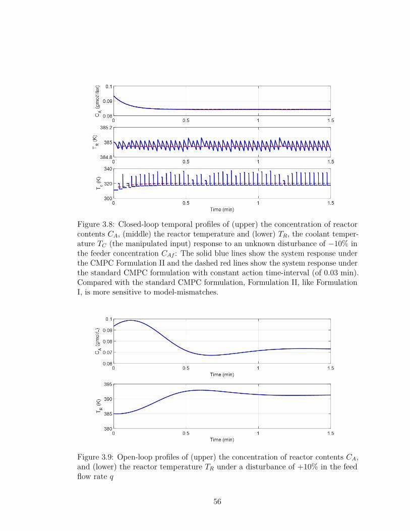
Figure 3.8: Closed-loop temporal profiles of (upper) the concentration of reactorcontents CA, (middle) the reactor temperature and (lower) TR, the coolant temper-ature TC (the manipulated input) response to an unknown disturbance of −10% inthe feeder concentration CAf : The solid blue lines show the system response underthe CMPC Formulation II and the dashed red lines show the system response underthe standard CMPC formulation with constant action time-interval (of 0.03 min).Compared with the standard CMPC formulation, Formulation II, like FormulationI, is more sensitive to model-mismatches.
Figure 3.9: Open-loop profiles of (upper) the concentration of reactor contents CA,and (lower) the reactor temperature TR under a disturbance of +10% in the feedflow rate q
56

Figure 3.10: Closed-loop temporal profiles of (upper) the concentration of reactorcontents CA, (middle) the reactor temperature TR, and (lower) the coolant temper-ature TC (which is the manipulated input) response to an unknown disturbance of+10% in the feed flow rate q. The solid green lines show the system response underthe CMPC Formulation I, and the dashed red lines show the system response underthe standard CMPC formulation with constant action time-interval (of 0.03 min).The total values of the cost function throughout the presented operating processare 0.5056 (Formulation I), compared with 0.9470 of the standard CMPC. Thisshows the system is regulated closer to the desired trajectory but not as stable asthe system under standard CMPC.
57

Figure 3.11: Closed-loop temporal profiles of (upper) the concentration of reactorcontents CA, (middle) the reactor temperature TR, and (lower) the coolant temper-ature TC (which is the manipulated input) response to an unknown disturbance of+10% in the feed flow rate q. The solid blue lines show the system response underthe CMPC Formulation II and the dashed red lines show the system response underthe standard CMPC formulation with constant action time-interval (of 0.03 min).The total values of the cost function throughout the presented operating processare 0.3491 (Formulation II), compared with 0.9470 of the standard CMPC. Thisshows the system is regulated closer to the desired trajectory but not as stable asthe system under standard CMPC.
58

Chapter 4 |Economic-oriented Carleman ModelPredictive Control
4.1 IntroductionIn recent years, economic-oriented model predictive control (EMPC) has gainedpopularity in chemical and petrochemical industries. The primary difference ofEMPC from traditional MPC is that EMPC is directly formulated to maximizethe economic profits. It naturally puts more emphasis on the process path [31] [33].Typically, the economic operation of a process is a two-layer scheme [88]. Theupper layer is the real-time optimization (RTO) layer, which performs economicprocess optimization and determines the optimal operation trajectory. The lowerlayer is the MPC layer. It forces the system to track the optimal process trajectoryobtained from the upper layer and to reject disturbances. However, the RTO resultsmay be inconsistent with the MPC objectives and may lead to infeasibility. Theseissues give rise to the development of EMPC [34,89,90].
An increasing number of results on EMPC studies was recently published; [88]presents a good review. However, one of the remaining major challenges is theheavy burden on computation. Unlike traditional tracking MPC, the economicallyoptimal cost functions representing the economic performances, are usually non-quadratic or even non-convex. They may require significant amount of calculationsand put heavy load of work on the optimizer. If the optimizer fails to convergeto the optimum fast enough, the delay in sending the control signals, or sendingnon-converged control signals may degrade its closed loop performance, or even
59
cause potential stability issues. There are formulations to guarantee the stabilityof systems under EMPC, including adding quadratic regularization terms in theeconomic cost function, applying terminal constraints, and using Lyapunov-basedconstraints [68, 69]. These formulations further exacerbate the computationalburden of EMPC.
To address the computational delay issue of EMPC, we propose an approachbased on Carleman approximation. It builds on our previous work that focusedon efficient reformulations of nonlinear MPC (NMPC) published in [52] [53] [55].In this chapter, we intend to show the readers the features of our approach whenworking with non-tracking economic stage costs and path-emphasized optimization.Our approach significantly reduces computational efforts in EMPC context.
The approach we are proposing is built upon two foundations: the theory ofCarleman approximation and the theory of bilinear control systems. After a Two-Tier approximation, we use high order polynomial states to capture the nonlinearityof the original dynamic process. With an extended bilinear expression and assumingpiecewise constant manipulated inputs, we analytically predict future states andfuture economic performances. We also analytically calculate the sensitivity ofthe economic cost function to the manipulated inputs. The sensitivity servesas the gradient to facilitate the optimizer by reducing the number of iterationstremendously. Hence, the computational effort in solving the EMPC problem issufficiently reduced. This approach circumvents feedback delays in the following twoways: First, the economic performance of the plant becomes a nonlinear function ofthe manipulated inputs, releasing the optimization problem from equality dynamicconstraints. Second, it analytically predicts future economic performance of thesystem and provides the sensitivity as the search gradient to facilitate the optimizer.
4.2 Definition and Formulation
4.2.1 EMPC Formulation
The stage cost, representing the process economics over each sampling time [ti−1, ti],is expressed as:
ti∫ti−1
Le(x(τ), u1(τ), u2(τ), · · · , um(τ))dτ, (4.1)
60

∀i = 1, · · · , N
In this context, the overall economic cost function, which describes the economicperformance of the plant, is maximized over a finite time window, the predictionhorizon [t0, tN ]:
tN∫t0
Je(x(τ), u1(τ), u2(τ), · · · , um(τ))dτ
=N∑i=1
ti∫ti−1
Le(x(τ), u1(τ), u2(τ), · · · , um(τ))dτ (4.2)
x ∈ Rn is the vector of states, and uj, j = 1, · · · ,m are the vectors of themanipulated inputs. t0 and tN denote the starting and ending of the predictionhorizon.
The economically optimal control problems are recast as receding finite horizondynamic optimization ones. We use control vector parameterization (CVP) toreformulate dynamic optimization problems (DOP) as finite dimensional nonlinearprogramming (NLP) ones [91]. The basic principle is to express the manipulatedinputs in a finite vector of design variables as the parameters to be optimized [86] [87].Assuming piecewise constant manipulated inputs during every sampling time, theEMPC problem has a general form:
maxu1,u2,··· ,um
tN∫t0
Je(x, u1(τ), u2(τ), · · · , um(τ))dt
s.t.
uj(t) =N∑i=1
uj,iB(t;Ti−1;Ti),
∀j = 1, · · · ,m (4.3)
x = f(x) +m∑j=1
gj(x)uj(t)
x(t0) = x0
xmin ≤ x(t) ≤ xmax,∀ t ∈ [t0, tN ]
umin ≤ u(t) ≤ umax,∀ t ∈ [t0, tN ]
f c(x, u1, u2, · · · , um) ≤ 0
uj,i denotes the i-th element in the j-th design variable vector. From a view
61

of control, it denotes the i-th piecewise constant signal of the j-th manipulatedinput in its corresponding time period (Ti−1, Ti]. We use u to represent all ofthem in the rest of this chapter. The time period [Ti−1, Ti] is defined as the i-thsampling time and has a length of ∆Ti = Ti − Ti−1. We define a pulse functionwith B(t;Ti−1;Ti) = H(t− Ti−1)−H(t− Ti), where H is the standard Heavisidefunction. N is the total number of the sampling times within each control horizon.In typical MPC designs, the length of the prediction horizon is usually greater thanthe control horizon, depending on the robustness requirement [80,81,83]. In thischapter, we set the prediction horizon equal to the control horizon for the purposeof simplicity. The last three equations in Eq. (4.3) denote the bounds on the states,on the manipulated inputs, and any other equality/inequality constraints on thesystem. These constraints may account for physical limitations, safety concerns,and other requirements on the system performance.
4.2.2 Two-Tier Approximation
The nonlinear system, which is a continuous one, is represented by the followingordinary differential equation (ODE):
x = f(x) +m∑j=1
gj(x)uj(t) (4.4)
x(t0) = x0
f(x) and gj(x), j = 1, · · · ,m are nonlinear vector functions. uj(t) denotes the j-thdesign variable. x0 is the initial condition of the system.
Tier OneFor the simplicity of derivation, we perform Taylor expansion around the origin
x = 0. In NMPC problems, the desired steady states that we are tracking, areoften the ideal points to perform Taylor expansion around. In EMPC problems,unlike traditional MPC, there are usually not any desired steady states to track.In these cases, we pick the steady states within or close enough to the economicallyoptimal set to perform Taylor expansion around.
Nonlinear vector functions f(x) and gj(x) are expanded by Maclaurin series in
62

the following form:
f(x) = f(0) +∞∑k=1
1k!∂f[k]|x=0x
[k] (4.5)
gj(x) = gj(0) +∞∑k=1
1k!∂gj[k]|x=0x
[k] (4.6)
x[k] denotes the k-th order Kronecker product of x. Details of the Kroneckerproduct rule are presented in the next section.
∂f[k]|x=0 ∈ Cn×(nk) and ∂gj[k]|x=0 ∈ Cn×(nk) are the k-th partial derivatives off(x) and gj(x) with respect to x, based on the Kronecker product rule:
∂f[k] = ∂
∂x⊗ ∂f[k−1], ∂gj[k] = ∂
∂x⊗ ∂gj[k−1], (4.7)
For example, if x = [x1 x2], k = 2,
∂f[2] = [∂2f
∂x21
∂2f
∂x1x2
∂2f
∂x1x2
∂2f
∂x22] (4.8)
With the approximations above, the nonlinear dynamic system described byEq. (4.4) can be approximated with the following polynomial form:
x ∼=p∑
k=1Akx[k] + A0 +
m∑j=1
(p∑
k=1Bjkx[k] +Bj0)uj (4.9)
Ak = 1k!∂f[k]|x=0; Bjk = 1
k!∂gj[k]|x=0;
A0 = f(0); Bj0 = gj(0);
Tier TwoWe first extend the states of the system x to x⊗:
x⊗ = [xTx[2]T · · · x[p]T ]T (4.10)
where x[p] denotes the p-th order Kronecker product of x. For the rest of thischapter, a p-th order x⊗ means the term of the highest order in x⊗ is x[p]. So far,there has been no systematic method reported in literature to determine the orderof Carleman approximation. In our proposed method, we simulate the system after
63

performing a Taylor expansion. When selecting the order of Taylor expansion, wemake sure the truncation error caused by the simulator can be compensated laterby the optimizer. We extend Eq. (4.9) to a bilinear form:
x⊗ = Ax⊗ +A0 +m∑j=1
(Bjx⊗ + Bj0)uj, (4.11)
where the nonlinear dynamic information recorded in Tier One approximation iscarried by the extended matrices: A, A0, Bj and Bj0. Details of these extendedmatrices are collected in Appendix A.
Arriving at Eq. (4.11) means we have finished Tier Two approximation. Thisextended bilinear formulation carries nonlinear dynamic information of the originalsystem.
There are two important assumptions in our proposed approach: (i) Themanipulated inputs are all piecewise constant signals within each sampling time.(ii) Each manipulated input enters or can be reformulated to enter the systemlinearly. This means the system is or can be reformulated as input affine withrespect to all manipulated inputs. Fortunately, these two assumptions are commonlysatisfied in practice.
Hence, we are able to perform convolution integral and draw an analyticalsolution to predict system evolution within each sampling time:
x(t)⊗ = exp[(A+
m∑j=1
Bjuj,i)(t− Ti−1
)]x(Ti−1
)⊗
+t∫
Ti−1
exp[(A+
m∑j=1
Bjuj,i)(t− τ
)]dτ ·
(A0 +
m∑j=1
Bj0uj,i)
t ∈ (Ti−1, Ti] (4.12)
x(Ti)⊗ = exp[(A+
m∑j=1
Bjuj,i)∆Ti
]x(Ti−1
)⊗
+(A+
m∑j=1
Bjuj,i)−1[(A+
m∑j=1
Bjuj,i)∆Ti − I
]
64

·(A0 +
m∑j=1
Bj0uj,i)
(4.13)
This also enables us to perform analytical sensitivity calculation to serve as thesearch gradient. Detailed derivations are presented in the next section.
Using analytical solutions to predict future economic performance takes lesscomputational efforts. With the search gradient provided, less iterations are requiredby the optimizer, which further saves computational efforts. This method leads tocomplexity in modeling the dynamic process. However, since the modeling partis performed off-line, it is an acceptable trade-off for saving tremendous on-linecomputational efforts.
4.2.3 Gradient-based Optimization
The economic cost function Je(x, u) or Je(x, uj), j = 1, · · · ,m can be approximatedwith the following form:
Je =∞∑k=0
∞∑l=0
1(k + l)!
∂[k+l]Je∂xk∂U l
|0xkU l (4.14)
∼= Je,0 + Je,Ax⊗ +m∑j=1
Je,Bjuj,⊗ +m∑j=1
Je,Njuj,⊗ ⊗ x⊗
where Je,0 is a scalar; Je,A, Je,Bj and Je,Nj are Jacobian matrices. The last termm∑j=1
Je,Njuj,⊗ ⊗ x⊗ is useful for a non-quadratic economic cost function.
Either the control actions u or the control moves ∆u can be chosen as thedesign variables, depending on the knowledge of the reference trajectories of themanipulated inputs.
We define the following notations to be used later:
AK = A+m∑j=1
Bjuj,K, (4.15)
EK = exp(AK∆TK), (4.16)
GuUK = AK−1(EK − I), (4.17)
FK =m∑j=1
Bj0uj,K +A0. (4.18)
65

where I is the identity matrix with the corresponding dimension.
By constructing the time integral of the economic cost function∫ TN
T0
Jedt, we
aim at maximizing the economic performance over the path in [T0, TN ]:∫ TN
T0
Je dt ∼= Je,0(TN − T0)
+N∑i=1
[Je,A +m∑j=1
Je,Njuj,i⊗⊗]∫ Ti
Ti−1
x⊗dt
+N∑i=1
m∑j=1
Je,Bjuj,i⊗∆Ti (4.19)
We incorporate the integral of the extended states x⊗ over each sampling time:∫ Ti
Ti−1
x⊗ dt = GuUix⊗,i−1 + Ai−1(GuUi −∆Ti · I)Fi (4.20)
Hence, we free the optimization from the equality constraint that represents thesystem dynamics.
uk,K denotes the K-th element in the k-th design variable vector, which is thevalue of the k-th manipulated input during the K-th sampling time. The sensitivityof the economic cost function to uk,K is:
∂
∂uk,K
∫ TN
T0
Je dt =[Je,A +
N∑i=K
m∑j=1
Je,Njuj,i⊗ ⊗]×[ ∫ TK
TK−1
∂x⊗∂uk,K
dt+∫ TK+1
TK
∂x⊗∂x⊗,K
dt∂x⊗,K∂uk,K
(4.21)
+N∑
i=K+2
∫ Ti
Ti−1
∂x⊗∂x⊗,i−1
dt(i−1∏
l=K+1
∂x⊗,l∂x⊗,l−1
)∂x⊗,K∂uk,K
]+ Je,Nk∂(uk,K)⊗ ⊗
∫ TK
TK−1
x⊗dt+ Je,Bk∂(uk,K)⊗∆TK
The following derivations are used to compose Eq. (4.21):
∂(uk,K)⊗ = [1 2uk,K · · · puk,Kp−1] (4.22)
66

∂x⊗,K∂x⊗,K−1
= EK (4.23)
∫ TK
TK−1
∂x⊗∂x⊗,K−1
dt = GuUK (4.24)
∂x⊗,K∂uk,K
= ∂EK∂uk,K
x⊗K−1
+ AK−1 ∂EK∂uk,K
FK + GuUKBk0 (4.25)
− AK−1BkGuUKFK
∫ TK
TK−1
∂x⊗∂uk,K
dt
=∫ TK
TK−1
∂EK∂uk,K
dt · x⊗,K−1
+ AK−1∫ TK
TK−1
∂EK∂uk,K
dtFK (4.26)
+ AK−1[GuUK −∆TK · I]Bk0
− AK−1BkAK
−1[GuUK −∆TK · I]FK
∂EK∂uk,K
andTK∫
TK−1
∂EK∂uk,K
dt can both be computed analytically:
∂EK∂uk,K
=∞∑l=1
(∆TK)ll!
l∑λ=1
Aλ−1K BkA
l−λK (4.27)
TK∫TK−1
∂EK∂uk,K
dt =∞∑l=1
(∆TK)l+1
(l + 1)!
l∑λ=1
Aλ−1K BkA
l−λK (4.28)
During the optimization, we discretize the system in time by performing con-
67

Figure 4.1: Schematic diagram of the catalytic ethylene oxidation CSTR
volution integral within each sampling time. We make sure the system behaviorsatisfies the bounds on the states, the bounds on the manipulated inputs, and theequality/ inequality constraints f c(x, u) ≤ 0 at the end of each sampling time.
4.3 SimulationsIn this section, we demonstrate the proposed Carleman EMPC approach is applica-ble and computationally efficient by comparing it with numerical EMPC approachthat is the standard method.
As a case-study example, we consider a CSTR where ethylene is oxidized by airin a catalytic environment [92]. Figure 4.1 presents a diagram of this reactor. Theproduct is ethylene oxide (C2H4O). This CSTR is non-isothermal, so a coolantjacket is used to remove heat. The chemical reactions are:
68

C2H4 +1
2O2
r1−−−→ C2H4O
C2H4 + 3O2
r2−−−→ 2CO2 + 2H2O
C2H4O+5
2O2
r3−−−→ 2CO2 + 2H2O
where ri, i = 1, 2, 3 are the reaction rates expressed by
r1 = k1 exp(−E1
RT)P
12E (4.29)
r2 = k2 exp(−E2
RT)P
14E (4.30)
r3 = k3 exp(−E3
RT)P
12EO (4.31)
ki and Ei, i = 1, 2, 3 are the reaction rate constant and activation energy, respectively.R is the ideal gas constant. T is the temperature. PE and PEO denote thepartial pressures of ethylene (E) and ethylene-oxide (EO), respectively. Under theassumption of ideal gas, the concentrations of E and EO can be written as:
CE = PERT
, CEO = PEORT
(4.32)
The states and the manipulated inputs of the system are all normalized and becomeunit-less:
x1 = ρ
ρref, x2 = CE
Cref, x3 = CEO
Cref, x4 = T
Tref(4.33)
x1 is the normalized vapor density in the reactor. x2 and x3 are the concentrationsof E and EO in the reactor. x4 is the normalized reactor temperature.
u1 = Qf
Qref, u2 = CE,f
Cref, u3 = Tc
Tref(4.34)
u1 is the normalized feeding flow rate. u2 is the normalized feeding concentrationof ethylene. u3 is the normalized coolant temperature. The dynamic process isdescribed with four ODEs:
69

x1 = u1(1− x1x4)
x2 = u1(u2 − x2x4)−A1 exp(γ1x4
)(x2x4)12 −A2 exp(γ2
x4)(x2x4)
14
x3 = −u1x3x4 +A1 exp(γ1x4
)(x2x4)12 −A3 exp(γ3
x4)(x3x4)
12
x4 = u1x1
(1− x4) + B1x1
exp(γ1x4
)(x2x4)12 + B2
x1exp(γ2
x4)(x2x4)
14
+B3x1
exp(γ3x4
)(x3x4)12 − B4
x1(x4 − u3) (4.35)
The parameters are listed in Table 4.1, referring to [93, 94]. We also refer to [89] todecide our EMPC parameters.
In order to apply the proposed Carleman EMPC method, we define u∗2 = u1u2,which is the normalized amount of E in the reactor feed, and replace u1u2 withit. Hence, all our manipulated inputs uT = [u1, u∗2, u3] are entering the systemlinearly.
The economic performance of the reactor is characterized by the time-averagedyield of EO:
Y (tf ) =∫ tf
0 u1(τ)x3(τ)x4(τ)dτ∫ tf0 u∗2(τ)dτ
(4.36)
which is the amount of EO produced compared with the amount of E fed to thereactor over an operating window tf . The amount of E is uniformly provided overeach operating window. So our EMPC is subject to the following constraint:
1tf
∫ tf
0u∗2(τ)dτ = 0.175 (4.37)
Over each operating window tf = 4.68 min, the prediction horizon Np = 11shrinks at each sampling time, Np,k = Np − k, and is reset to NP when startingthe next operating window. Accumulated constraints are applied to make sure theconstraint 1
tf
∫ tf0 u∗2(τ)dτ = 0.175 is strictly satisfied. The system is simulated for
10 operating windows.Since the system under investigation has nonlinear dynamics, standard EMPC is
calculated numerically. We model the system with numerical simulations (MATLABode45) and construct the cost function numerically. For Carleman EMPC, we choose
70

an asymptotically stable steady-state xTs = [0.9980, 0.4235, 0.0320, 1.0020] andthe corresponding steady-state input uTs = [0.35, 0.175, 1.0] as the nominal pointto perform Carleman approximation. Through trial and error, we find 4th orderCarleman approximation is sufficient for this example. The system is simulated withanalytical solutions. The cost function is calculated analytically with the analyticalsearch gradient supplied. To make a fair comparison, we use interior-point methodas the search algorithm for both standard EMPC and Carleman EMPC with IntelCore i7-3770 CPU at 3.40GHz.
In our simulation, the system is initialized at xT0 = [0.997, 1.264, 0.209, 1.004].We simulate the system under nominal condition. Standard EMPC generates atime-averaged yield of 9.22% and spends 226.701 s in calculating the optimal controlinputs. Carleman EMPC achieves a time-averaged yield of 8.81% and spends 83.375s, which cuts down the computational time by 63.2%.
We also simulate the process under system noise. At each sampling time,bounded Gaussian white noise is added to the system, which has zero mean anda range of δ = ±[0.005, 0.03, 0.01, 0.02]. Figure 4.2 shows the closed loopperformance of the system under standard EMPC. The time-averaged yield is9.19% and takes 225.861 s to calculate the control policy. In comparison, thesimulation under 4th order Carleman EMPC is shown in Figure 4.3. It generatesa time-averaged yield of 8.83% and spends 83.715 s, which saves 62.9% of thecomputational time.
We test a case where there is a model mismatch between the real system and theparameters we use to design the EMPC controller. The parameter γ1 is assumedto be -10% smaller than the given value in the real system. Figure 4.4 shows theperformance of the closed loop system under standard EMPC scheme. Figure 4.5shows the performance under the proposed Carleman EMPC. They are both able totolerate the model mismatch and generate the same time-averaged yield of 17.6%.The proposed Carleman EMPC spends 125.254 s in computation, which is 36.4%faster than standard EMPC spending 197.014 s.
Therefore, the proposed Carleman EMPC method demonstrates significantcomputational efficiency. Table 4.2 presents a summary of different computationaltimes under different conditions. The difference in the yield probably comes fromthe approximation of the process and the effect of random noises. In our futurework, we will address error prediction methods to compensate for the loss in
71

Parameter Value Parameter ValueA1 92.80 B3 2170.57A2 12.66 B4 7.02A3 2412.71 γ1 -8.13B1 7.32 γ2 -7.12B2 10.39 γ3 -11.07
Table 4.1: Dimensionless Parameters of the Ethylene Oxidation CSTR
Figure 4.2: Standard EMPC: the closed loop performance of the system undersystem noise
approximation.
4.4 ConclusionsIn this chapter, we proposed an approach to increase the computational efficiencyof EMPC problems based on Carleman approximation. Our approach worked wellwith non-tracking, non-quadratic stage costs of EMPC emphasizing on the path. Wepredicted future states and economic performances of the system with fast analyticalcalculations. We also supplied the sensitivity of the economic performance to themanipulated inputs as the search gradient to accelerate optimization. A CSTRproducing ethylene-oxide was studied as an application example. We established a
72

Figure 4.3: Carleman EMPC: the closed loop performance of the system undersystem noise
Figure 4.4: Standard EMPC: the closed loop performance of the system undermodel mismatch
non-tracking, cyclic operation. The computational effort was significantly reducedwith the proposed Carleman EMPC method.
73

Figure 4.5: Carleman EMPC: the closed loop performance of the system undermodel mismatch
Condition Standard EMPC Carleman EMPC
Nominal 226.701 s 83.375 sUnder system noise 225.861 s 83.715 sUnder model mismatch 197.014 s 125.254 s
Table 4.2: Comparison of Computational Time: Standard EMPC vs CarlemanEMPC
74

Chapter 5 |Combination of Moving Hori-zon Estimation and Model Pre-dictive Control
5.1 IntroductionModel predictive control (MPC) is fast becoming the yardstick over which controlsystem performance is evaluated. This is due to its optimality, ease of use andimplicit robustness characteristics. An issue that still confounds its use is thatknowledge of the process state is essential in the design of the control signals. Inpractice, some of the state variables (or even the controlled outputs) may not bedirectly measurable, or even not have a physical meaning. Therefore, the needto pair estimation and control is a promising future direction of research in theMPC area of control engineering. [95] and [49] presented work in pairing extendedKalman filter (EKF) and nonlinear model predictive control (NMPC).
Moving horizon estimation (MHE) and model predictive control, as dual prob-lems, have been widely attracting attention for their several advantageous properties,including: 1) they are readily applied to multi-input-multi-output (MIMO) systemsdue to their formulations; 2) they handle constraints and bounds in a straightfor-ward manner due to their optimization-based nature; 3) their self-evolving policiesincrease the ability in dealing with model-mismatches. MHE uses a receding timewindow of outputs into the past. With limited information regarding the dynamicmodel, it estimates the unmeasurable state variables. MPC predicts future evolution
75

of the system and computes the control signals over a receding time window into thefuture. Expectedly, together they form a good candidate for an estimation/controlpair, sharing the state-space model of the process. The state estimation obtainedby MHE serves as the initial condition for the MPC to design optimal controlsignals. These control signals are continuously updated in the dynamic model usedin MHE, completing the interconnection.
Both MHE and MPC involve solving dynamic optimization problems in real-time,which requires a considerable amount of computational effort. With increasinglylarger and more complicated process models, the computations by MHE and MPCbecome even more expensive. If the MHE/MPC pair fails to generate an optimalsolution in time, the consequent feedback delays canl cause unavoidable performanceloss or even stability issues [96]. This is one of the most significant barriers holdingback the application of MHE/MPC pair.
Researchers in control engineering have proposed many approaches to reducecomputational expense for MHE and MPC. The advanced-step NMHE/NMPC(asNMHE/asNMPC) algorithms, published by Biegler and coworkers in [9, 15,16], focuses on solving complex optimization problems off-line then performinga linear approximation in the real-time. Multi-parametric MPC developed byPistikopoulos and coworkers in [19,20] accelerates computation via querying responsehypersurfaces.
Motivated by the computational issue, we propose Carleman approximationto formulate a new scheme of the MHE/MPC pair, CMHE/CMPC. Reviews onbilinear control systems and their optimization are reported in [77–79]. Carlemanapproximation is also known as Carleman linearization [73, 74, 76, 97] since thebasic idea is to express a finite dimensional nonlinear system with an infinitedimensional linear one. First, we choose a desired steady state point to performTaylor expansion to the nonlinear system under investigation. This step naturallytransforms the original state vector to a deviation from the desired steady state.Second, we expand the new states vector and the coefficient matrices based on theKronecker product rule and introduce an augmented state vector containing thehigher order deviation mononomials. This results in a bilinear system that has alarger dimension. It carries the nonlinear dynamic information of the original system,and reduces approximation errors compared with classic linearization methods.Our previous work has reported the structure of CMPC [52], more explorations
76

Figure 5.1: A schematic diagram of the proposed CMHE/CMPC pair: CMHE usesa sliding window (dashed red) to identify the noise and state at Tk−1. The statex⊗,k−1 serves as the initial condition for the CMPC window (dashed blue). CMPCdesigns the optimal input sequence and implements uk to the system. As CMHErecedes to the next sliding window (black), uk is updated in CMHE to increase theprecision of esimation.
in its formulation [55], the structure and stability analysis of CMHE [58]. In thispaper, we improve and expand our previous work by proposing a CMHE/CMPCpair, combining these two algorithms together. CMHE and CMPC share the sameextended bilinear model. With this model, we simulate the system evolution viaanalytical solutions. The cost functions for both CMHE and CMPC are constructedanalytically. Analytical Gradient and Hessian matrices are supplied to facilitatesearching for the optimum. CMHE identifies the initial condition of each recedingtime window for CMPC to make optimal control decisions. These control decisionsare continuously updated in the process model used by CMHE to make it moreprecise. A schematic diagram of CMHE/CMPC pair is presented in Figure 5.1.
77

5.2 Preliminary Information
5.2.1 Nonlinear System Under Investigation
Considering a nonlinear system with noise,
x = f(x) + g(x)u+ γ(x)w (5.1)
y = h(x) + ν (5.2)
x(t0) = x0 (5.3)
where x ∈ Rnx is the state vector. u ∈ Rm is the vector of manipulated variables;u = [u1 u2 · · · um]. w ∈ Rn is the vector of unknown process noises; w =[w1 w2 · · · wn]. y ∈ Rp is the output vector; ν ∈ Rp is the vector of unknownsensor noises. x0 is the initial condition at the beginning time t0. f(x) is a nonlinearvector function. g(x) and γ(x) are nonlinear matrix functions. In this chapter, weassume f(x), g(x), γ(x) and h(x) are known and locally analytic.
For simplicity of the presented formulations later, we expand matrix functionsg(x) and γ(x) as summations of vector functions, gj(x), j = 1, · · · , m and γl(x), l =1, · · · , n. Eq (1) is re-expressed as:
x = f(x) +m∑j=1
gj(x)uj +n∑l=1
γl(x)wl (5.4)
y = h(x) + ν (5.5)
5.2.2 Mathematics Background: Carleman Approximation
Carleman approximation has two tiers: First, we choose a desired steady state pointto perform Taylor expansion to the nonlinear system under investigation. This stepnaturally expresses the original state vector as deviations from the desired steadystate. These deviation terms are in a polynomial form and contain higher orders.Second, we expand both the transfered state vector and the coefficient matricesbased on the Kronecker product rule. This results in a bilinear system that has alarger dimension.
To implement Carleman approximation, the states of the system x are extended
78

tox⊗ = [xTx[2]T · · ·x[p]T ]T , (5.6)
where x[p] = x⊗ x[p−1] denotes the p-th order Kronecker product of x.For simplicity of presentation and without loss of generality, we assume the
nominal operating point is at the origin x = 0. Nonlinear vector functions f(x),gj(x), γl(x) and h(x) are expanded by Maclaurin series in the following form:
f(x) = f(0) +∞∑k=1
1k!∂f[k]
∣∣∣∣x=0
x[k] (5.7)
gj(x) = gj(0) +∞∑k=1
1k!∂gj[k]
∣∣∣∣x=0
x[k] (5.8)
γl(x) = γl(0) +∞∑k=1
1k!∂γl[k]
∣∣∣∣x=0
x[k] (5.9)
h(x) = h(0) +∞∑k=1
1k!∂h[k]
∣∣∣∣x=0
x[k] (5.10)
As mentioned earlier, we assume f(x), gj(x), γl(x) and h(x) are analytic functions(i.e., Taylor expansion is locally convergent), so nonlinear dynamic systems ofEq. (5.4)(5.5) can be approximated by a polynomial form with arbitrarily chosenaccuracy:
x ∼=p∑
k=0
Akx[k] +
m∑j=1
p∑k=0
Bjkx[k]uj +
n∑l=1
p∑k=0
Dlkx[k]wl (5.11)
y ∼=p∑
k=1
Ckx[k] + ν (5.12)
Ak = 1k!∂f[k]|x=0; Bjk = 1
k!∂gj[k]|x=0; Dlk = 1k!∂γl[k]|x=0; Ck = 1
k!∂h[k]|x=0. A0 = f(0);Bj0 = gj(0); Dl0 = γl(0). The polynomial order p is assumed to be high enough toreduce truncation errors to below a chosen threshold [76].
A notable detail: ∂f[k], ∂gj[k], ∂γl[k] and ∂h[k] are derivatives based on theKronecker product rule.
∂f[k] = ∂
∂x⊗ ∂f[k−1], ∂gj[k] = ∂
∂x⊗ ∂gj[k−1], (5.13)
79

∂γl[k] = ∂
∂x⊗ ∂γl[k−1], ∂h[k] = ∂
∂x⊗ ∂h[k−1] (5.14)
For example, if x = [x1 x2], k = 2,
∂f[2] =[∂2f
∂x21
∂2f
∂x1x2
∂2f
∂x1x2
∂2f
∂x22
](5.15)
We also expand the coefficient matrices in Eq. (5.11) to A, A0, Bj , Bj0, Dl, Dl0and C, based on the Kronecker product rule. Details are collected in Appendix A.
The resulting bilinear ODE has an expanded dimension and carries nonlineardynamic information.
x⊗ = Ax⊗ +A0 +m∑j=1
(Bjx⊗ + Bj0)uj +n∑l=1
(Dlx⊗ +Dl0)wl (5.16)
y = Cx⊗ + ν (5.17)
Further details on the expanded dimension can be found in [55].
5.3 Fusing CMHE and CMPC
5.3.1 CMHE Design
MHE uses a sliding time window of past output trajectory to update estimationsin the past, and to obtain the most probable current states. It has the followinggeneral form:
minx0,wi
JE = Λ(x0) +NE∑i=1
Li(wi, νi) (5.18)
i = 1, · · · , NE
s.t.
xi ∈ X , wi ∈ D, νi ∈ V (5.19)
νi = yi − yi (5.20)
Λ(x0) = (x0 − x0)TΠ0(x0 − x0) (5.21)
Li(wi, νi) = νTi QE νi + wTi RE wi (5.22)
80

In this optimization problem, the design variables are x0 and wi, i = 1, · · · , NE.x0 is the state estimate at the beginning of the sliding window. wi is the estimateof wi, the weight averaged noise in the i-th time interval, [Ti−1, Ti).X , D, and V are compact sets. νi is the estimation error. Λ(x0) is the arrival
cost, which summarizes the past data before the sliding time window. In thisdissertation, we pick the estimation of state x0 at the previous sampling time torepresent x0, which is one step before the sliding window. Li, i = 1, · · · , NE denotesthe stage costs. QE and RE are weighting matrices that have symmetric positivedefinite structures.
With control signals u continuously generated by CMPC (details presented inthe next section), the dynamic model of the system is continuously updated tosimulate it more precisely. It has the following form over the i-th sampling time[Ti−1, Ti):
x⊗ = Ax⊗ +A0 +m∑j=1
(Bjx⊗ + Bj0)uj,i +n∑l=1
(Dlx⊗ +Dl0)wl,i (5.23)
yi = Cx⊗,i + νi (5.24)
x⊗,0 = x⊗(t0) (5.25)
Consequently, the following model is used in solving the MHE problem Eq. (5.18)-(5.22)
˙x⊗ = Ax⊗ +A0 +m∑j=1
(Bjx⊗ + Bj0)uj,i +n∑l=1
(Dlx⊗ +Dl0)wl,i (5.26)
yi = Cx⊗,i + νi (5.27)
x⊗,0 = x⊗(t0) (5.28)
Remark 5. Since MHE uses discrete-time models, we discretize the continuousnoise signal w(t) in time and model them as piecewise constant noise signals
affecting the system, wi = 1Ti − Ti−1
∫ Ti
Ti−1
w(t)dt. This is based on the Mean Value
Theorem [98].
81

5.3.2 CMPC Design
To distinguish MHE and MPC, we use subscript E to denote Estimation (MHE)and subscript C to denote Control (MPC).
The optimal control problem is recast as a recursion of receding finite horizonoptimization problems, which has a general form:
minu
∫ tf
t0
JC(x, u, w)dt (5.29)
s.t.
uj(t) =NC∑i=1
uj,iB(t;Ti−1;Ti),∀j = 1, · · · ,m (5.30)
T0 = t0, TNC ≤ tf (5.31)
x− f(x)−m∑j=1
gj(x)uj(t)−n∑l=1
γl(x)wl(t) = 0 (5.32)
x(t0) = x0 (5.33)
f c(x, u) ≤ 0 (5.34)
JC is the cost function of CMPC. Similar as in CMHE, we discretize each manip-ulated input in time: u denotes the matrix of manipulated inputs; uj is the j-thmanipulated input, a vector of uj,i, i = 1, · · · , NC , the i-th piecewise constant valueof uj . It takes place in the i-th time interval (Ti−1, Ti], also defined as the i-th sam-pling time, with a length of ∆Ti. We define B(t;Ti−1;Ti) = H(t−Ti−1)−H(t−Ti)as a rectangular pulse function, where H is the standard Heaviside function. Ti−1
and Ti denote the initiation time and the termination time respectively. T0 is thebeginning of control horizon and TNC is the end of control horizon. t0, same as T0
is the beginning of prediction horizon and tf is the end of prediction horizon. Thelength of prediction horizon can be equal to, or greater than the control horizon,depending on the requirement of controller robustness [83]. f c denotes a vectorfunction of equality and inequality constraints.
When we predict the evolution of future states, the unknown noise in the futureis not yet estimated. So w, i.e. wl, l = 1, · · · , n are assumed to be zero. The costfunction JC(x, u, w) is reduced to JC(x, u). JC(x, u) can be approximated through
82

differentiation:
JC(x, u) =∞∑k=0
∞∑l=0
1(k + l)!
∂[k+l]JC∂xk∂ul
∣∣∣∣0xkul
∼= J0 + JAx⊗ +m∑j=1
JBju⊗,j +m∑j=1
JNju⊗,j ⊗ x⊗ (5.35)
where J0, JA, JBj and JNj are Jacobian matrices. The last termm∑j=1
JNju⊗,j,i ⊗ x⊗
does not appear when we consider a quadratic cost function:
JC = (x− xs)TQC(x− xs) + (u− us)TRC(u− us) (5.36)
For some cases, the time integral∫ TN
T0
JC(x, u)dt is a better choice as the cost
function, especially in regulation or tracking problems.
∫ TN
T0
JC(x, u) dt ∼= J0(TN − T0) +N∑i=1
(JA +m∑j=1
JNju⊗,j,i⊗)∫ Ti
Ti−1
x⊗dt
+N∑i=1
m∑j=1
JBju⊗,j,i∆Ti (5.37)
5.3.3 Analytical Prediction of System Evolution
As presented earlier, the nonlinear system under investigation is re-expressedin an extended bilinear formulation. The system has m manipulated inputs,uj, j = 1, · · · , m and n sources of noise, wl, l = 1, · · · , n.
x⊗ = Ax⊗+A0 +m∑j=1
(Bjx⊗+Bj0)uj,i+n∑l=1
(Dlx⊗+Dl0)wl,i, t ∈ (Ti−1, Ti] (5.38)
We perform convolution integral to obtain an analytical solution to the equationabove:
x(t)⊗ = exp[Ai(t− Ti−1
)]x(Ti−1
)⊗ +
t∫Ti−1
exp[Ai(t− τ
)]dτ · Fi (5.39)
83

Ai = A+m∑j=1
Bjuj,i +n∑l=1
Dlwl,i, (5.40)
Fi = A0 +m∑j=1
Bj0uj,i +n∑l=1
Dl0wl,i (5.41)
This analytical solution is used in the CMHE/CMPC pair. The cost functions
JE and∫ TN
T0
JC(x, u) are both calculated analytically. These analytical calculations
accelerate the optimizations. Furthermore, it enables us to provide analyticalGradient vector and Hessian matrix to facilitate the search process, presented inthe next section.
Remark 6. In the cases where the disturbance information is known,n∑l=1Dlwl and
n∑l=1Dl0wl are provided in the CMPC model. Otherwise, they are eliminated from
the CMPC model, by setting wl = 0.
5.3.4 Gradient Vector and Hessian Matrix to Facilitate Opti-mization
In the section, we present detailed algorithms to calculate the Gradient vector andthe Hessian matrix of the CMHE/CMPC pair.
5.3.4.1 CMHE Part
At the l-th sampling time, the Gradient vector of CMHE, GE,has the followingform:
GE,l =[∂JE∂x0,l
,∂JE∂w1,l
,∂JE∂w2,l
, · · · , ∂JE∂wp,l
]; (5.42)
The elements to compose the Gradient vector are:
∂JEx0,l
= 2(x0 − x0)T Π0 Γl +N∑i=1
2vTi QE( ∂vi∂x0,l
) (5.43)
and∂JE∂wp,l
= 2wTl RE Γl +N∑i=j
2vTi QE( ∂vi∂wp,l
) (5.44)
84

where Γl is a vector with zero elements except the l-th element which has the unityvalue.
By differentiating Eq. (5.42), the Hessian matrixHE has the following symmetricform at the l-th sampling time:
HE,l =
∂2JE∂x0,l∂x0,l
∂2JE∂x0,l∂w1,l
∂2JE∂x0,l∂w2,l
· · · ∂2JE∂x0,l∂wp,l
· · · ∂2JE∂w1,l∂w1,l
∂2JE∂w1,l∂w2,l
· · · ∂2JE∂w1,l∂wp,l
· · · · · · ∂2JE∂w2,l∂w2,l
· · · ∂2JE∂w2,l∂wp,l
· · · · · · · · · · · · · · ·
· · · · · · · · · · · · ∂2JE∂wp,l∂wp,l
(5.45)
By differentiating Eq. (5.43) and (5.44), the Hessian matrix elements are givenby the following equations
∂2JE∂x0,l∂x0,k
= 2ΓTl Π0 Γk + 2N∑i=1
( ∂vi∂x0,k
)TQE( ∂vi∂x0,l
) + 2N∑i=1
vTi QE( ∂2vi∂x0,l∂x0,k
) (5.46)
∂2JE∂x0,l∂wp,k
= 2N∑i=1
( ∂vi∂x0,l
)TQE( ∂vi∂wp,k
)+2N∑i=1
vTi QE( ∂2vi∂x0,l∂wp,k
) (5.47)
and,
∂2JE∂wq,l∂wp,k
= 2ΓTl REΓk+2N∑i=1
( ∂vi∂wq,l
)TQE( ∂vi∂wp,k
)+2N∑i=1
vTi QE( ∂2vi∂wq,l∂wp,k
) (5.48)
Detailed derivations of ∂vi∂x0,l
,∂vi∂wp,l
,∂2vi
∂x0,l∂x0,k,
∂2vi∂x0,l∂wp,k
,∂2vi
∂wp,l∂wp,k,
∂2vi∂wp,l∂wq,k
are presented in Appendix B.1.
85

5.3.4.2 CMPC Part
The Gradient vector of CMPC, GC , which is the sensitivity of∫ TN
T0
JC dt to
each manipulated input vector, for example, the k-th manipulated input vectoruk = [uk,1, uk,2, · · · , uk,p]:
GC,k =[
∂
∂uk,1
∫ TN
T0
JC dt, ∂
∂uk,2
∫ TN
T0
JC dt, · · · , ∂
∂uk,p
∫ TN
T0
JC dt]
(5.49)
The K-th element in the Gradient vector of uk above is:
∂
∂uk,K
∫ TN
T0
JC dt = (JA +m∑j=1
JNju⊗,j,K⊗)N∑i=K
∫ Ti
Ti−1
∂x⊗∂uk,K
dt (5.50)
+ JNk(∂u⊗,k,K)⊗∫ TK
TK−1
x⊗dt+ JBk(∂u⊗,k,K)∆TK
By differentiating the Gradient vector Eq. (5.49), the Hessian matrix HC to thek-th input has the following symmetric form:
HC,k =
∂2
∂2uk,1
∫ TN
T0
JC dt ∂2
∂uk,1∂uk,2
∫ TN
T0
JC dt · · · ∂2
∂uk,1∂uk,p
∫ TN
T0
JC dt
· · · ∂2
∂uk,2∂uk,2
∫ TN
T0
JC dt · · · ∂2
∂uk,2∂uk,p
∫ TN
T0
JC dt
· · · · · · · · · · · ·
· · · · · · · · · ∂2
∂uk,p∂uk,p
∫ TN
T0
JC dt
(5.51)
∂2
∂2uk,K
∫ TN
T0
JC dt =
(JA +m∑j=1
JNju⊗,j,K⊗)N∑i=K
∫ Ti
Ti−1
∂2x⊗
∂2uk,Kdt+ 2JNk∂u⊗,k,K ⊗
N∑i=K
∫ Ti
Ti−1
∂x⊗∂uk,K
dt
+ JNk(∂2u⊗,k,K)⊗∫ TK
TK−1
x⊗dt+ JBk(∂2u⊗,k,K)∆Tk (5.52)
86
For K < q < N
∂2
∂uk,q∂uk,K
∫ TN
T0
JC dt =
(JA +m∑j=1
JNju⊗,j,K⊗)N∑i=K
∫ Ti
Ti−1
∂2x⊗∂uk,q∂uk,K
dt
+ JNk∂u⊗,k,q ⊗N∑i=K
∫ Ti
Ti−1
∂x⊗∂uk,K
dt
(5.53)
Detailed derivations ofN∑i=K
∫ Ti
Ti−1
∂x⊗∂uk,K
dt,N∑i=K
∫ Ti
Ti−1
∂2x⊗
∂2uk,Kdt,
N∑i=K
∫ Ti
Ti−1
∂2x⊗∂uk,q∂uk,K
dt,
∂u⊗,k,K, ∂2u⊗,k,K are presented in Appendix B.2.
Remark 7. The cost functions of CMHE and CMPC are JE and∫ TN
T0
JC dt,
respectively. Since the cost function of CMPC is a time integral of the original costfunction JC , which has a similar form to JE, the calculation of its Gradient vectorand Hessian matrix involves a higher level of complexity than those of CMHE.
Remark 8. The computational acceleration is achieved by the analytical calculationof the dynamic system evolution that is directly inserted in the cost functionaland the respective Gradient vector and Hessian matrix that are provided to thesearch algorithm, thus reducing the number of numerical computations with a givenaccuracy. The formulas thus facilitate the search process in order to accelerateoptimization.
5.4 Simulation
5.4.1 Example Description
We use the same nonlinear jacketed CSTR as in Section 2.5.3 as the simulationexample [85] to demonstrate the proposed algorithms. (All details are collectedin Appendix C.2.) There is an exothermic first-order reaction in the CSTR. Thereactor is jacketed with coolant water. The dynamics of this system are described
87

with the following two ODEs:
CA = q + w
V(CAf − CA)− k0 exp(− E
R TR) CA
TR = q + w
V(Tf − TR)− ∆H
ρ Cpk0 exp(− E
R TR) CA + UA
V ρ Cp(Tc − TR) (5.54)
The manipulated input is the coolant water temperature Tc. The feeding flow rateq is affected by unknown noises w. The state variables are the concentration in thereactor, CA, and the reactor temperature, TR. In this illustration example, TR ismeasurable while CA is not directly available. The proposed CMHE/CMPC pairestimates CA by measuring TR first, and then design the control signals based onthe state estimation to form a closed-loop system.
Table C.2 lists the parameters and the nominal operating condition. The abovesystem is highly nonlinear around the nominal steady state listed in Table C.2.Any small perturbation in the operating condition may cause large oscillations onboth the concentration and the reactor temperature. For example, if we introducea −10% change in the feed concentration CAf as in Figure 2.7, the consequentialbehavior of the system is demonstrated in Figure 2.8. Unstable oscillations occurin both concentration and temperature, growing larger as the process operationproceeds.
We apply 2nd order Carleman approximation to model the system and createthe CMHE/CMPC pair. Carleman matrices are created offline and only once. Theapproximation is performed around the nominal steady state listed in Table C.2.In other words, a change of variables is performed to transfer the current nominalsteady state to the origin.
5.4.2 CMHE/CMPC Pair
In this simulation example, we assume the unmeasured noise w affecting the flowrate q, is a uniformly distributed white noise, which is bounded in [−10, 10]L/min. In addition, there are sensor noises θ affecting the measurement of reactortemperature TR. It also has a uniform distribution and is bounded in [−0.02, 0.02]K. The sampling time for both CMHE and CMPC is 0.05 min. The CMHE design
88

Parameter Description Value
p Order of Carleman Approximation 2∆T Sampling Time 0.05 minw Uniformly Distributed Process Noise [−10, 10] L/minθ Uniformly Distributed Sensor Noise [−0.02, 0.02] KNE CMHE Horizon 3QE CMHE Weighting Parameter 1
RE CMHE Weighting Parameter[10−5 0
0 10−5
]Π0 CMHE Weighting Parameter
[10−6 0
0 10−6
]Np CMPC Prediction Horizon 8Nc CMPC Control Horizon 4QC CMPC Weighting Parameter 1RC CMPC Weighting Parameter 10−5
Table 5.1: Parameters Used in the CMHE/CMPC Design for the Simulation
is:
min JE = (x0 − x0)TΠ0(x0 − x0) +NE∑i=1
(νTi QE νi + wTi RE wi) (5.55)
where x0, wi, i = 1, ..., NE are the design variables, subject to the dynamicsconstraint Eq. (5.54) and the following constraints:
0.08 ≤ CA ≤ 0.11, −10 ≤ wi ≤ 10, −0.02 ≤ νi ≤ 0.02 (5.56)
i = 1, 2, 3
Table 5.1 lists the parameters used in CMHE/CMPC design. Figure 5.2 presentsthe estimation of the open-loop system under 2nd order CMHE (dashed red lines)
89

and standard NMHE (dashed green lines). Compared with the real system (bluelines), both CMHE and NMHE sucessfully estimate the real system, and presentalmost identical estimation.
The goal is to regulate the system at a temperature of TR = 385 K, underprocess noise w affecting q. On one hand, CMHE continuously estimates the initialconditions for CMPC to make control decisions upon them. On the other hand,CMPC continuously updates the dynamic models used by CMHE to make themmore accurate.
The cost function of CMPC is in the following quadratic form:
min
∫ TNp
T0
JC(x, u)dt =Np∑i=1
∫ Ti
Ti−1
(xTQCx+ uTRCu) dt
where u is the design variable, subject to the dynamics constraints Eq. (5.54). Thecost function is reconstructed with extended states x⊗ and extended control signalsu⊗. Correspondingly, the coefficient vectors J0, JA and JB have dimensions thatare consistent with x⊗ and u⊗.
∫ TNp
T0
JC(x, u) dt ∼= J0(TNp − T0) +Np∑i=1
JA
∫ Ti
Ti−1
x⊗dt+Np∑i=1
m∑j=1
JBju⊗,j,i∆Ti
(5.57)
Figure 5.3 and Figure 5.4 present the estimations of the closed-loop systemunder CMHE/CMPC and NMHE/NMPC, respectively, which serve as the initialconditions of each sampling time for CMPC and NMPC to make control decisions.Figure 5.5 presents the closed-loop behavior under 2nd order CMHE/CMPC pair.It is compared with its open-loop response under the same process noise w. Theopen-loop system goes through a periodic orbit under the effect of noise. Theclosed-loop system identifies the noise and the state, regulates the system backto the desired temperature of 385 K, with [−0.36, 0.52] K deviations. Figure5.6 presents the closed-loop behavior under standard NMHE/NMPC, which hasa negligible difference from the 2nd order CMHE/CMPC pair. This shows theCMHE/CMPC pair leads to no loss of controller performance.
To make fair comparisons, all simulations are performed using 3.4 GHz IntelCore i7 processor. We use MATLAB ode45 for all the numerical simulations of
90

GradientMHE
HessianMHE
GradientMPC
HessianMPC
2nd orderCMHE/CMPC
NonlinearMHE/MPC
no no no no 32.438 (s) 170.343 (s)yes no yes no 25.305 (s)yes yes yes no 16.807 (s)yes yes yes yes 11.220 (s)
Table 5.2: Comparison of Computational Time in CPU Seconds: all simulationsare performed with 3.4 GHz Intel Core i7 processor. We use MATLAB ode45for all the numerical simulations of ODEs. We employ the trust-region-reflectivealgorithm when the gradient vector and Hessian matrix are supplied. For the rest,the interior-point algorithm is used.
ODEs. With the Gradient vector and Hessian matrix provided, the computationof CMHE/CMPC pair is accelerated by over 1 order of magnitude. Table 5.2presents a detailed comparison of computation time: CMHE/CMPC pair versusstandard NMHE/NMPC. Their closed-loop performances are almost identical, asexemplified in Figure 5.5 and Figure 5.6. With standard NMHE/NMPC, theaverage computation time is 3.4 s, which exceeds the length of one sampling time0.05 min (=3 s). As mentioned in the introduction, in practice this delay may causesignificant performance degradations and safety issues. With the CMHE/CMPCpair, the analytical solutions reduce the total computation time from 170.343 s (3.4s per sampling time) to 32.438 s (0.64 s per sampling time). With the Gradientvector and the Hessian matrix supplied analytically, the CMHE/CMPC pair furtherreduces computation time to 11.220 s (0.22 s per sampling time).
5.5 ConclusionIn this chapter, we present a design of Carleman approximation-based MHE andMPC pair, CMHE/CMPC. In this structure, CMHE continuously estimates theinitial conditions for CMPC to make control decisions upon them, and CMPCcontinuously updates the dynamic models used by CMHE to increase the precision
91

of estimation. The dynamic system is modeled with an extended bilinear ODE.It allows us to perform analytical prediction of system evolution while carryingnonlinear information. The optimizations of both CMHE and CMPC are releasedof dynamic constraints, since they are directly incorporated in the analytical costfunctions. With this reformulation, we can provide the Gradient vectors and Hessianmatrices to facilitate the optimizations. These efforts reduce the computation timeto less than 10 % of standard NMHE/NMPC.
92

(a) Concentration of reactor contents CA
(b) Reactor temperature TR
Figure 5.2: Open-loop system under noise: real states (blue lines) compared withestimated states under 2nd order CMHE (dashed red lines) and standard NMHE(dashed green lines)
93

(a) Concentration of reactor contents CA
(b) Reactor temperature TR
Figure 5.3: Closed-loop system under noise: real states (blue lines) compared with2nd order CMHE (red dashed lines)
94

(a) Concentration of reactor contents CA
(b) Reactor temperature TR
Figure 5.4: Closed-loop system under noise: real states (blue lines) compared withstandard NMHE (green dashed lines)
95

(a) Concentration of reactor contents CA
(b) Reactor temperature TR
Figure 5.5: Under the same noise signal sequence, the open-loop response (red lines)(a) concentration of reactor contents CA and (b) reactor temperature TR both showperiodic behavior. The closed-loop response under the 2nd order CMHE/CMPC pairis also presented (blue lines). The controller regulates the system to [−0.36, 0.52]Kdeviation from the desired trajectory 385 K.
96

(a) Concentration of reactor contents CA
(b) Reactor temperature TR
Figure 5.6: Under the same noise signal sequence, the closed-loop response understandard NMHE and NMPC is presented (green lines), compared with the open-loop response (red lines). Negligible difference from the closed-loop behavior under2nd order CMHE/CMPC pair (blue lines in Figure 5.5) is observed here.
97

Chapter 6 |Advanced-step Carleman Mov-ing Horizon Estimation and ModelPredictive Control
6.1 IntroductionThe advanced-step NMPC (asNMPC) algorithm, published by Biegler and coworkersin [15–18], has focused on solving complex optimization problems off-line thenperforming an update with linear approximation of nonlinear sensitivity in real-time.Figure 6.1 presents a schematic diagram of the advanced-step NMPC algorithm. Abrief description of the concept is the following.
a) One step ahead of tk+1, during [tk, tk+1), the following calculations areperformed in the background:
1) p0 = z(k + 1) = f(x(k), u(k)), where the nominal solution p0 = z(k + 1) is afunction of the previous state vector x(k) and the previous input vector u(k).
Define the solution vector sT = [λT0 , zT0 , uT0 , λT1 , zT1 , uT1 , · · · , λTN , zTN ]2) Calculate the optimal solution s∗(p0) and the sensitivity ∂s∗
∂pthrough first-
order optimality or Karush-Kuhn-Tucker (KKT) conditions.b) Arriving at tk+1, perform the following instantaneous update on-line:3) Obtain the true state p = x(k + 1) through sensors or observers.4) Perform an update with linear approximation of nonlinear sensitivity :s(p) = s∗(p0) + ∂s∗
∂p(p− p0).
5) Extract the updated input u(k + 1) from s(p) and inject into the system.
98

Figure 6.1: A schematic diagram of advanced-step NMPC algorithm
We extend the fused CMHE/CMPC algorithm with advanced-step NMHE (as-NMHE) [15] and NMPC (asNMPC) [16] concept to develop an asCMHE/asCMPCpair. The developed pair further reduces real-time computational efforts to anegligible amount, with significant impact on its applicability to fast processes. Inthe following sections we describe the strategy and algorithm specifics of adaptingthe advanced step algorithm to our CMHE/CMPC pair.
6.2 Strategy of Adapting Advanced-step Algorithmto CMHE/CMPC PairFigure 6.2 presents a schematic of advanced-step CMHE (asCMHE) and advanced-step CMPC (asCMPC) pair. At time Tk, the asCMHE/asCMPC pair estimatesx∗⊗,k and designs the input u∗k+1 for [Tk, Tk+1) both instantaneously. The sequence ofcalculations for time Tk starts immediately after the input for time Tk−1 is computedand proceeds during the evolution of the system as the following. (Superscript *means the state or input is updated from its pre-calculated value.)
a) One step ahead, calculation during [Tk−1, Tk),1) At Tk−1, the CMHE estimates the value of x∗⊗,k−1|k−1 with a window of
[Tk−1−NE , Tk−1]. Analytical sensitivities to wk−NE , · · · , wk−1, are provided andwill be used again later in step 5).
2) With x∗⊗,k−1|k−1 as the initial condition, asCMPC updates u∗k within negligible
99

Figure 6.2: A schematic diagram of the proposed asCMHE/asCMPC algorithm:the CMHE window (dashed red) identifies x∗k−1|k−1, predicts xk|k−1 and reports theanalytical sensitivity in window [Tk−4, Tk−1]. With asCMPC updates u∗k instanta-neously, one more step of sensitivity is generated for asCMHE in window [Tk−1, Tk](dashed magenta). At Tk, asCMPC uses the analytical sensitivity in window[Tk−4, Tk] (dashed red+dashed magenta) to update x∗k|k from xk|k−1 instantaneously.As soon as x∗k|k is obtained, asCMPC updates u∗k+1 from uk+1 pre-calculated in theCMPC window (dashed blue).
amount of time.3) Pre-estimate the value of x⊗,k|k−1 with u∗k and wk = 0, assuming the next
step is noise-free. Since yk is not available at this time, this pre-estimation step isperformed through the analytical prediction:
x⊗,k|k−1 = exp(Ak∗∆Tk
)x∗⊗,k−1|k−1 + Ak
∗−1[
exp(Ak∗∆Tk
)− I]F∗k (6.1)
Ak∗ = A+ Bu∗k +Dwk, (6.2)
F∗k = A0 + B0u∗k +D0wk (6.3)
4) Pre-design the input sequence uk+1, · · · , uk+NC , for the next CMPC window[Tk, Tk+NC ], using x⊗,k|k−1 as the initial condition. Analytical sensitivities touk+1, · · · , uk+NC are provided to facilitate optimization, and will be used again
100

later in step 6).b) Arriving at Tk,5) Update x∗⊗,k|k with the pre-estimated state x⊗,k|k−1 as soon as the real
measurement y∗k is obtained. In this updating step, we use analytical sensitivitiesto wk−NE , · · · , wk−1 calculated in step 1), together with the analytical sensitivityto wk = 0.
6) Update u∗k+1 with the pre-designed input sequence uk+1, · · · , uk+NC as soonas the updated state x∗⊗,k|k is available. Again, we use the analytical sensitivitiescalculated in step 4).
6.3 Algorithm Specifics
6.3.1 asCMHE Algorithm
In the window of asCMHE, the inputs u∗l , l = −NE − 1, · · · , −1 are calculated byprevious asCMPC, and enter the model as known parameters. We use a simplenotation to present the extended bilinear model Eq. (5.39).
x⊗,l+1 = fl(x⊗,l, u∗l , wl) (6.4)
yl = hl(x⊗,l) (6.5)
l = −NE − 1, · · · , −1 (6.6)
The following notations are used for simplicity of derivations:
ATl = ∂fl∂x⊗,l
, GTl = ∂fl
∂wl, CT
l = ∂hl∂x⊗,l
(6.7)
Pl = ∂2JE∂x⊗,l∂x⊗,l
, Wl = ∂2JE∂wl∂wl
, Fl = ∂2JE∂x⊗,l∂wl
, (6.8)
For asCMHE, we use forward Riccati decompostion to calculate the gain matrixK0. Detailed derivations are reported in [15].
Π−NE−1 = (P−NE−1 − F−NE−1W−1−NE−1F
T−NE−1)−1 (6.9)
Ml+1 = (GlW−1l F T
l − Al)Πl(FlW−1l GT
l − ATl ) +GlW−1l GT
l (6.10)
Πl+1 = (Pl+1 +M−1l+1 − Fl+1W
−1l+1F
Tl+1)−1 (6.11)
101

l = −NE − 1, . . . ,−1
K0 = Π0CT0 QE (6.12)
K0 is the gain matrix to update the extended states x∗⊗,0 from the prediction x⊗,0,as soon as the true measurement y∗0 is obtained.
K0 = ∂x⊗,0∂y0
(6.13)
x∗⊗,0 − x⊗,0 = K0(y∗0 − y0) (6.14)
In the asCMHE presented here, Al, Gl, Cl, Pl, Wl and Fl are all computedanalytically beforehand during optimization, with the extended bilinear model. QE
is the weighting matrix in Eq. (5.22). When we update the current state, all thesesensitivities are ready to use since they have been calculated one step ahead.
6.3.2 asCMPC Algorithm
We use a simple notation to present Eq. (5.39). In the window of asCMPC, thereis no estimation of future noises yet. A noise-free model is used.
x⊗,l+1 = fl(x⊗,l, ul, 0) (6.15)
l = 0, · · · , NC − 1 (6.16)
The following notations are used for simplicity of derivations:
ATl = ∂fl∂x⊗,l
, BTl = ∂fl
∂ul(6.17)
Ql = ∂2JC∂x⊗,l∂x⊗,l
, Wl = ∂2JC∂x⊗,l∂ul
, Rl = ∂2JC∂ul∂ul
, (6.18)
For asCMPC, we apply backward Riccati decomposition to calculate the sensitivitygain matrix K1. Detailed derivations are reported in [16]. The major difference inour formulation is the extended bilinear models that carry nonlinear informationwhile using analytical sensitivities.
ΠNC = QNC (6.19)
Kl = −(Rl +BTl Πl+1Bl)−1(BT
l Πl+1Al +WTl ) (6.20)
102

Πl = Ql + ATl Πl+1Al + (ATl Πl+1Bl +Wl)Kl (6.21)
l = NC − 1, . . . , 1
The sensitivity gain matrix K1 is used to update the manipulated input u∗1 from itspre-determined value u1 one step ahead. The update, which is the only calculationin the real-time, takes negligible amount of time once the updated state x∗⊗,0 isobtained.
K1 = ∂u1
∂x⊗0(6.22)
u∗1 − u1 = K1(x∗⊗,0 − x⊗,0) (6.23)
Remark 9. Inequality constraints are handled within the optimization part of theobserver/controller pair. During the updating procedure, if there are minor pertur-bations to the system the updated state estimation and control decision shouldn’tviolate inequality constraints. If the updates do lead to violation of the constraints,in the current formulation we employ saturation bounds to the control action. Anapproach to account for this eventuality is to reformulate the cost functional ofthe discretized dynamic optimization problem as a Lagrange function, followingan interior point approach similar to [15] [16]. Detailed derivations and proof ofupdating the estimated states and the control decision with nonlinear programmingsensitivity are presented in [15] [16]. It is also possible to extend the sensitivityanalysis to handle inequality constraints explicitly at the expense of more complicatedcost function and derivation of sensitivities.
6.4 Simulation
6.4.1 Example Description
We use the same nonlinear jacketed CSTR as in Chapter 5 as the simulationexample [85] to demonstrate the proposed asCMHE/asCMPC pair. The statevariables are the concentration in the reactor, CA, and the reactor temperature,TR. Again, we assume TR is measurable and CA is not directly available. AssumingTR is measured immediately, the proposed asCMHE/asCMPC pair estimates CAin real-time, and then make the decision of the control signals based on the state
103

estimation, in real-time as well.We apply 2nd order Carleman approximation to model the system and create
the asCMHE/asCMPC pair. Carleman matrices are created offline and only once.The approximation is performed around the nominal steady state listed in TableC.2. In other words, a change of variables is performed to transfer the currentnominal steady state to the origin.
6.4.2 asCMHE
Figure 6.3 presents a comparison of the estimation by CMHE (dashed red lines) andby asCMHE (dashed green lines), both 2nd order, together with the real open-loopsystem behavior (blue lines) under the same process noises described in section5.4. CMHE and asCMHE achieve almost identical estimations. But the real-timecalculation of asCMHE is instantaneous, while CMHE, despite the much fastercalculation than standard NMHE, still takes a portion of the sampling time.
6.4.3 asCMPC
Figure 6.4 presents a comparison of 2nd order CMPC (red lines) and 2nd orderasCMPC (green lines) under the same process noise. They both successfully regulatethe system back to TR = 385 K with [−0.1, 0.1] K deviations. Figure 6.5 presents acomparison of CMPC (red lines) and asCMPC (green lines) under the same modelmismatch. As expected, asCMPC is more sensitive to model mismatches thanCMPC since the sensitivity updating step only has knowledge of the mismatcheddynamic model.
6.4.4 asCMHE/asCMPC Pair
With CMHE/CMPC pair, the computation time is reduced to 11.220 s (0.22s per sampling time), which accounts for 7.48 % of one sampling time. WithasCMHE/asCMPC pair, we further reduce the computation time to a negligi-ble amount. Figure 6.6 shows a comparison of closed-loop performances of theCMHE/CMPC pair (blue lines) versus the asCMHE/asCMPC pair (green lines).Their differences are almost negligible, but with the asCMHE/asCMPC pair, thereal-time computation is practically instantaneous. The sensitivities constructed
104

with extended bilinear models carry most of the nonlinear information while allowinganalytically solutions.
For comparison, we linearize the system and calculate sensitivities with thelinear model. These sensitivities are only used in the updating steps. Figure6.6 presents the difference of their closed-loop performances. The sensitivitiesconstructed with the linear model leads to truncation errors that are degrading theregulation action (orange lines).
6.5 ConclusionOur CMHE/CMPC pair works particularly well with the asNMHE/asNMPCconcepts [15] [16]. Combing them together, we proposed an algorithm of as-CMHE/asCMPC pair, which further reduces the real-time computation to a negligi-ble amount. This chapter first introduces the idea of advanced-step NMHE/NMPC,and then presents the adaption of this idea with CMHE/CMPC to form the as-CMHE/asCMPC pair. It describes the strategy and the detailed algorithms ofasCMHE/asCMPC. Simulation examples of a nonlinear CSTR under process noisesand under model mismatches are presented to demonstrate the performance ofasCMHE, asCMPC, and the asCMHE/asCMPC pair.
105

(a) Concentration of reactor contents CA
(b) Reactor temperature TR
Figure 6.3: The real open-loop system (blue lines) compared with estimated statesunder 2nd order CMHE (dashed red lines)/ 2nd order asCMHE (dashed greenlines): (a) concentration of reactor contents CA; (b) reactor temperature TR.
106

(a) Concentration of reactor contents CA
(b) Reactor temperature TR
Figure 6.4: Under the same process noise, 2nd order CMPC (red lines) comparedwith 2nd order asCMPC (green lines): (a) concentration of reactor contents CA;(b) reactor temperature TR.
107

(a) Concentration of reactor contents CA
(b) Reactor temperature TR
Figure 6.5: Under the same model mismatch, CMPC (red lines) compared withasCMPC (green lines): (a) concentration of reactor contents CA; (b) reactortemperature TR.
108

(a) Concentration of reactor contents CA
(b) Reactor temperature TR
Figure 6.6: The closed-loop system behavior under the asCMHE/asCMPC pair(green lines) has negligible difference from the CMHE/CMPC pair (blue lines).Using the extended bilinear model in the sensitivity calculation (green lines), thesystem is regulated closer to the desired steady state 385 K than using the linearmodel in the sensitivity calculation (orange lines): (a) concentration of reactorcontents CA; (b) reactor temperature TR.
109

Chapter 7 |Conclusion
7.1 Dissertation SummaryThis dissertation proposed a formulation that leads to a computationally efficientNMPC method. Similar to traditional NMPC, it converts optimal control problemsto receding horizon control ones with dynamic constraints and performance criteriasatisfied. The nonlinear dynamic constraints are modeled with extended bilinearrepresentations. In this way, it enables analytical prediction of future states thatis computationally efficient. The proposed formulation also provides analyticallycomputed sensitivity of the cost function to the design variables. Thus, thisanalytically computed sensitivity serves as the search gradient to enable standardand gradient-based search algorithms to be used in optimization. The proposedmethod discretizes the states of the system explicitly in time and formulatesthe states as nonlinear functions of the control actions. Thus it reduces thenumber of design variables. Since the nonlinear dynamic constraints can be readilyincorporated into the cost functions, it releases the optimization problem fromequality constraints.
To improve the temporal accuracy of the extended model, we periodically discardthe extended states and re-extend them using only the original state values. This“resetting extended states” process is repeated frequently during both the predictionof future states and the calculation of sensitivity. The purpose is to minimize theaccumulation of integration errors caused by Carleman approximation. Based onthe idea of control vector parameterization, we formulate the sampling times asdesign variables in addition to the control actions and propose two new formulations.
110

In Formulation I, we implement each sampling time as the optimization resultturn out to be. Only the first sampling time in the sequence is implemented. InFormulation II, we implement the sampling times and their corresponding controlactions until we reach the original fixed sampling time. These two formulationshelp improve the system resolution within the same time window. Since we mayexpect less design variables with adaptive sampling times, these two formulationsmake it easier to maintain system stability by designing a larger prediction horizon.
In this dissertation, we proposed an approach to increase the computationalefficiency of EMPC problems based on Carleman approximation. Our approachworked well with non-tracking, non-quadratic stage costs of EMPC emphasizingon the path. We predicted future states and economic performances of the systemwith fast analytical calculations. We also supplied the sensitivity of the economicperformance to the manipulated inputs as the search gradient to accelerate opti-mization. A CSTR producing ethylene-oxide was studied as an application example.We established a non-tracking, cyclic operation. The computational effort wassignificantly reduced with the proposed Carleman EMPC method.
An algorithm for the design of Carleman approximation-based MHE and MPCpair is presented. In this structure, CMHE continuously estimates the initialconditions for CMPC to make control decisions upon them, and CMPC continuouslyupdates the dynamic models used by CMHE to increase the precision of estimation.The dynamic system is modeled with an extended bilinear ODE. It allows usto perform analytical prediction of system evolution while carrying nonlinearinformation. The optimizations of both CMHE and CMPC are released of dynamicconstraints, since they are directly incorporated in the analytical cost functions.With this reformulation, we can provide the Gradient vectors and Hessian matrices tofacilitate the optimizations. These efforts reduce the computation time to less than10 % of standard nonlinear MHE/MPC. Our CMHE/CMPC pair works particularlywell with the asNMPC/asNMHE concepts [15] [16]. Combing them together, weproposed an algorithm of asCMHE/asCMPC pair, which further reduces the real-time computation to a negligible amount. While standard CMHE/CMPC stilloccupies a portion of the sampling time to compute the control actions beforeinjecting them into the system, the decision under asCMHE/asCMPC is almostinstantaneous.
111

7.2 ContributionsThe major contributions of this dissertation are listed as follows:
In Chapter 2, we reformulate Bilinear Carlema linearization-based MPC in [52]by including resetting of extended states in both the CMPC formulation andsensitivity analysis. We also investigate the reason and effects of resetting extendedstates in Carleman MPC. We demonstrate the performance of the new CMPCformulation with two application examples, an open-loop stable isothermal CSTRand an open-loop unstable exothermic CSTR. The work is published in [53,55].
In Chapter 3, we develop two formulations of embedding control vector parame-terization in CMPC, Formulation I and II. Both formulations treat the samplingtimes as design variables in addition to the manipulated inputs. Formulation I im-plements only the first sampling time sequence with its corresponding manipulatedinput. Formulation II implements the sampling times with their correspondingmanipulated inputs until reaching the original sampling time designed for standardCMPC. By adding the sampling times as design variables, CMPC achieve moreadaptive performance. We demonstrated the improvement in controller performanceby case study examples of regulating unstable CSTR under different disturbances.The work is published in [55].
In Chapter 4, we present a computationally efficient approach to economic-oriented MPC, Carleman EMPC. The reformulation of cost functions based onCarleman approximation works well with the non-tracking/non-quadratic economicstage costs. We demonstrate the improvement in EMPC performance by simulationof a catalytic ethylene oxidation CSTR. Optimal control is achieved by optimizingthe economic performance through establishing a set-point free cyclic operation.The work is published in [60].
In Chapter 5, we develop an output feedback control algorithm by fusingCarleman MHE and Carleman MPC together. CMHE identifies the system statesas the initial condition for CMPC to make optimal control decisions. The controldecisions made by CMPC update the dynamic models used in CMHE to make moreprecise estimations. Modeling the nonlinear system with Carleman approximation,we estimate the system evolution for both CMHE and CMPC analytically. Thedynamic model is incorporated in the cost functions of both CMHE and CMPC,releasing the optimization from dynamic constraints. The Gradient vectors and
112

Hessian matrices are then provided to facilitate the optimizations. We present theimprovement in computational efficiency with no loss of controller performance,compared with standard NMHE/NMPC, by simulations examples of an unstableCSTR under noises. The work is published in [59].
In Chapter 6, we adapt the advanced-step NMHE and advanced-step NMPCconcepts to our CMHE/CMPC to develop an asCMHE/asCMPC pair. It pre-estimates the states and pre-designs the manipulated input sequence one step inadvance with analytical models, and then it updates the estimation and controldecisions almost in the real-time with pre-calculated analytical sensitivities. Anonlinear unstable CSTR is studied as the illustration example to showcase thatwith no loss of performance, the real-time estimation and control decisions takes anegligible amount of computational time. The work is published in [57,59].
7.3 Recommendations for Future WorkTo proceed on beyond this dissertation, we are planning to develop a proof ofstability for both the CMHE/CMPC pair and the asCMHE/asCMPC pair. Tocompensate for the natural focus of MHE/MPC on optimality rather than stability,researchers have developed Lyapunov-based methods to guarantee the stability ofclosed loop operation. [13] [99] [100]. We intend to adapt these methods into ouralgorithms.
We are also interested in applying our algorithms to large scale systems, wherethe large dimensionality might be a challenging problem to address.
Accuracy is another challenging research topic. We intend to investigate accu-racy due to system nonlinearity and errors, including unmeasured disturbances,process/sensor noises, plant-model mismatch and set-point change.
As to the improvement in the core of the Carleman approximation approach, weintend to minimize the loss caused by approximation of the original system. We willalso improve our algorithms so they can be applied to more complex systems wherethe manipulated inputs may not necessarily enter the system in an independentway.
113

Appendix A|Kronecker Product & ExtendedSystem Matrices
A.1 Kronecker Product
The Kronecker product of matrix X ∈ CN×M and matrix Y ∈ CL×K is defined asmatrix Z ∈ C(NL)×(MK) [76].
X =
∣∣∣∣∣∣∣∣∣∣x1,1 x1,2 · · · x1,M
x2,1 x2,2 · · · x2,M
· · · · · · · · · · · ·xN,1 xN,2 · · · xN,M
∣∣∣∣∣∣∣∣∣∣Y =
∣∣∣∣∣∣∣∣∣∣y1,1 y1,2 · · · y1,K
y2,1 y2,2 · · · y2,K
· · · · · · · · · · · ·yL,1 yL,2 · · · yL,K
∣∣∣∣∣∣∣∣∣∣
Z = X ⊗ Y ≡
∣∣∣∣∣∣∣∣∣∣∣∣∣∣∣∣∣∣∣∣∣
x1,1y1,1 · · · x1,1y1,K · · · · · · x1,My1,1 · · · x1,My1,K... . . . ... · · · · · · ... . . . ...
x1,1yL,1 · · · x1,1yL,K · · · · · · x1,MyL,1 · · · x1,MyL,K
· · · · · · · · · · · · · · · · · · · · · · · ·· · · · · · · · · · · · · · · · · · · · · · · ·
xN,1y1,1 · · · xN,1y1,K · · · · · · xN,My1,1 · · · xN,My1,K... . . . ... · · · · · · ... . . . ...
xN,1yL,1 · · · xN,1yL,K · · · · · · xN,MyL,1 · · · xN,MyL,K
∣∣∣∣∣∣∣∣∣∣∣∣∣∣∣∣∣∣∣∣∣
114

A.2 Extended System MatricesWe expand the coefficient matrices in Eq. (5.11) to A, A0, Bj, Bj0, Dl, Dl0 and C,based on the Kronecker product rule. They are composed in the following form:
A =
∣∣∣∣∣∣∣∣∣∣∣∣
A1,1 A1,2 · · · A1,p
A2,0 A2,1 · · · A2,p−1
0 A3,0 · · · A3,p−2
· · · · · · · · · · · ·0 0 · · · Ap,1
∣∣∣∣∣∣∣∣∣∣∣∣, A0 =
∣∣∣∣∣∣∣∣∣∣∣∣
A1,0
00· · ·0
∣∣∣∣∣∣∣∣∣∣∣∣,
Bj =
∣∣∣∣∣∣∣∣∣∣∣∣
Bj1,1 Bj1,2 · · · Bj1,p
Bj2,0 Bj2,1 · · · Bj2,p−1
0 Bj3,0 · · · Bj3,p−2
· · · · · · · · · · · ·0 0 · · · Bjp,1
∣∣∣∣∣∣∣∣∣∣∣∣, Bj0 =
∣∣∣∣∣∣∣∣∣∣∣∣
Bj1,0
00· · ·0
∣∣∣∣∣∣∣∣∣∣∣∣,
Dl =
∣∣∣∣∣∣∣∣∣∣∣∣
Dl1,1 Dl1,2 · · · Dl1,p
Dl2,0 Dl2,1 · · · Dl2,p−1
0 Dl3,0 · · · Dl3,p−2
· · · · · · · · · · · ·0 0 · · · Dlp,1
∣∣∣∣∣∣∣∣∣∣∣∣, Dl0 =
∣∣∣∣∣∣∣∣∣∣∣∣
Dl1,0
00· · ·0
∣∣∣∣∣∣∣∣∣∣∣∣,
C =
∣∣∣∣∣∣∣∣∣∣∣∣
C1,1 C1,2 · · · C1,p
C2,0 C2,1 · · · C2,p−1
0 C3,0 · · · C3,p−2
· · · · · · · · · · · ·0 0 · · · Cp,1
∣∣∣∣∣∣∣∣∣∣∣∣where Ak,i =
k−1∑m=0
I[m]n ⊗ Ai ⊗ I [k−1−m]
n , Bjk,i =k−1∑m=0
I[m]n ⊗ Bji ⊗ I [k−1−m]
n , Dlk,i =k−1∑m=0
I[m]n ⊗Dli ⊗ I [k−1−m]
n , and Ck,i =k−1∑m=0
I[m]n ⊗ Ci ⊗ I [k−1−m]
n .
115

Appendix B|Sensitivity Derivation Specifics
B.1 Components of CMHE SensitivityThe 1st order derivatives of the estimation error, vi, with respect to x0,l and wp,lare given by:
∂vi∂x0,l
= −C ∂x⊗,i∂x⊗,i−1
∂x⊗,i−1
∂x⊗,i−2...∂x⊗,2∂x⊗,1
∂x⊗,1∂x⊗,0,l
= −CEiEi−1...E1∂x⊗,0∂x0,l
(B.1)
and for p ≤ i,
∂vi∂wp,l
= −C ∂x⊗,i∂x⊗,i−1
...∂x⊗,p+1
∂x⊗,p
∂x⊗,p∂wp,l
= −CEiEi−1...Ep+1
{∂Ep∂wp,l
x⊗,p−1
+[A−1p
∂Ep∂wp,l
+∂A−1
p
∂wp,l(Ep − I)
](A0 +
m∑j=1
Bj0up,j +m∑j=1
Dj0wp,j)
+ A−1p (Ep − I)Dl0
}(B.2)
where the following notation is defined to simplify the derivations:
Ei := exp(Ai∆Ti), (B.3)∂x⊗,i∂x⊗,i−1
= Ei (B.4)
116

Note, to derive the Gradient vector and the Hessian matrix, we need to derive thederivatives with respect to the original estimated states x0 (not x⊗,0). Also, it isobvious that for p > i, ∂vi
∂wp,k= 0.
The 2nd order derivatives of vi are also available analytically:
∂2vi∂x0,l∂x0,k
= −CEiEi−1...E1∂2x⊗,0
∂x0,l∂x0,k
(B.5)
∂2vi∂x0,l∂wp,k
= −CEiEi−1...Ep+1∂Ep∂wp,k
Ep−1...E1∂x⊗,0∂x0,l
(B.6)∂2vi
∂wp,l∂wp,k= −CEiEi−1...Ep+1
{∂2Ep
∂wp,l∂wp,kx⊗,p−1 +
[∂A−1p
∂wp,l
∂Ep∂wp,k
+∂A−1
p
∂wp,k
∂Ep∂wp,l
+ A−1p
∂2Ei∂wp,l∂wp,k
+∂2A−1
p
∂wp,l∂wp,k(Ep − 1)
](A0 +
m∑j=1
Bj0up,j +m∑j=1
Dj0wp,j)
+[A−1p
∂Ep∂wp,k
+∂A−1
p
∂wp,k(Ep − I)
]Dk0 +
[A−1p
∂Ep∂wp,l
+∂A−1
p
∂wp,l(Ep − I)
]Dl0},
(B.7)
and
∂2vi∂wp,l∂wq,k
= −CEiEi−1...Ep+1∂Ep∂wp,l
Ep−1...Eq+1
{∂Eq∂wq,k
x⊗,q−1 + A−1p (Eq − I)Bk0
+ [A−1q
∂Eq∂wq,k
+∂A−1
q
∂wq,k(Eq − I)](A0 +
m∑j=1
Bj0uq,j +m∑j=1
Dj0wq,j)}
(B.8)
Both 1st order and 2nd order derivatives of the exponential term Ep are presentedlater in B.3.
117

B.2 Components of CMPC Sensitivity
Detailed derivatives ofN∑i=K
∫ Ti
Ti−1
∂x⊗∂uk,K
dt,N∑i=K
∫ Ti
Ti−1
∂2x⊗
∂2uk,Kdt,
N∑i=K
∫ Ti
Ti−1
∂2x⊗∂uk,q∂uk,K
dt,
∂u⊗,k,K, ∂2u⊗,k,K are presented in this section.
N∑i=K
∫ Ti
Ti−1
∂x⊗∂uk,K
dt = Gk(i,K) (B.9)
Gk(i,K) =
∫ TK
TK−1
∂x⊗∂uk,K
dt, i = K
∫ TK+1
TK
∂x⊗∂x⊗,K
dt∂x⊗,K∂uk,K
, i = K + 1
N∑i=K+2
∫ Ti
Ti−1
∂x⊗∂x⊗,i−1
dti−1∏
l=K+1
El∂x⊗,K∂uk,K
, i > K + 1
(B.10)
We define the following notations for the purpose of simplicity in derivations:
GuUi := Ai−1[Ei − I] (B.11)
∫ Ti
Ti−1
∂x⊗∂x⊗,i−1
dt = GuUi (B.12)
∂x⊗,K∂uk,K
= ∂EK∂uk,K
x⊗K−1 + AK−1 ∂EK∂uk,K
FK + Gu(UK)Bk0 − AK−1BkGu(UK)FK (B.13)
∫ TK
TK−1
∂x⊗∂uk,K
dt =∫ TK
TK−1
∂EK∂uk,K
dt · x⊗,K−1
+ AK−1∫ TK
TK−1
∂EK∂uk,K
dt · FK + AK−1[Gu(UK)−∆TK · I]Bk0
− AK−1BkAK
−1[Gu(UK)−∆TK · I]FK (B.14)
118

N∑i=K
∫ Ti
Ti−1
∂2x⊗
∂2uk,Kdt = ∂Gk(i,K)
∂uk,K(B.15)
∂Gk(i,K)∂uk,K
=
∫ TK
TK−1
∂2x⊗
∂2uk,Kdt, i = K
∫ TK+1
TK
∂x⊗∂x⊗,K
dt∂2x⊗,K
∂2uk,K, i = K + 1
N∑i=K+2
∫ Ti
Ti−1
∂x⊗∂x⊗,i−1
dti−1∏
l=K+1
El∂2x⊗,K
∂2uk,K, i > K + 1
(B.16)
N∑i=K
∫ Ti
Ti−1
∂2x⊗∂uk,q∂uk,K
dt = ∂Gk(i,K)∂uk,q
(B.17)
∂Gk(i,K)∂uk,q
=
0, q < K
∫ TK+1
TK
∂2x⊗∂uk,q∂x⊗,K
dt∂x⊗,K∂uk,K
, q = K + 1
N∑i=K+2
∫ Ti
Ti−1
∂x⊗∂x⊗,i−1
dt Ei−1 · · ·∂Eq∂uk,q
· · · EK+1∂x⊗,K∂uk,K
, q > K + 1
(B.18)
u⊗,k,K = [uk,K, u2k,K, · · · , u
pk,K] (B.19)
∂u⊗,k,K = [1, 2 uk,K, · · · , p up−1k,K ] (B.20)
∂2u⊗,k,K = [0, 2 , · · · , p(p− 1) up−2k,K ] (B.21)
B.3 Components of Exponential Term Derivatives
∂Ei∂wj,i
=∞∑γ=1
∆T γ
γ!
γ∑λ=1
Aλ−1i
∂Ai∂wj,i
Aγ−λi (B.22)
119

∂2Ei∂wq,i∂wj,i
=∞∑γ=2
{∆T γ
γ! ×( γ−1∑κ=1
[ ∂Ai∂wj,i
Aκ−1i
∂Ai∂wq,i
Aλ−κ−1i + Aκ−1
i
∂Ai∂wq,i
Aγ−κ−1i
∂Ai∂wj,i
]
+γ−1∑λ=2
λ−1∑κ=1
Aκ−1i
∂Ai∂wq,i
Aλ−κ−1i
∂Ai∂wj,i
Aγ−λi
+γ−1∑λ=2
γ−λ∑κ=1
Aλ−1i
∂Ai∂wj,i
Aκ−1i
∂Ai∂wq,i
Aγ−λ−κi
)}(B.23)
∂Ai∂wq,i
= Dq,∂Ai∂wj,i
= Dj (B.24)
∂Ei∂uk,i
=∞∑γ=1
(∆T )γγ!
γ∑λ=1
Aλ−1i
∂Ai∂uk,i
Aγ−λi (B.25)
∫ Ti
Ti−1
∂Ei∂uk,i
dt =∞∑γ=1
(∆T )γ+1
(γ + 1)!
γ∑λ=1
Aλ−1i
∂Ai∂uk,i
Aγ−λi (B.26)
∂2Ei∂up,i∂uk,i
=∞∑γ=2
{(∆T )γγ! ×
( γ−1∑κ=1
[ ∂Ai∂uk,i
Aκ−1i
∂Ai∂up,i
Aλ−κ−1i + Aκ−1
i
∂Ai∂up,i
Aγ−κ−1i
∂Ai∂uk,i
]
+γ−1∑λ=2
λ−1∑κ=1
Aκ−1i
∂Ai∂up,i
Aλ−κ−1i
∂Ai∂uk,i
Aγ−λi
+γ−1∑λ=2
γ−λ∑κ=1
Aλ−1i
∂Ai∂uk,i
Aκ−1i
∂Ai∂up,i
Aγ−λ−κi
)}(B.27)
120

∫ Ti
Ti−1
∂2Ei∂up,i∂uk,i
dt =∞∑γ=2
{(∆T )γ+1
(γ + 1)! ×( γ−1∑κ=1
[ ∂Ai∂uk,i
Aκ−1i
∂Ai∂up,i
Aλ−κ−1i + Aκ−1
i
∂Ai∂up,i
Aγ−κ−1i
∂Ai∂uk,i
]
+γ−1∑λ=2
λ−1∑κ=1
Aκ−1i
∂Ai∂up,i
Aλ−κ−1i
∂Ai∂uk,i
Aγ−λi
+γ−1∑λ=2
γ−λ∑κ=1
Aλ−1i
∂Ai∂uk,i
Aκ−1i
∂Ai∂up,i
Aγ−λ−κi
)}(B.28)
∂Ai∂up,i
= Bp,∂Ai∂uk,i
= Bk (B.29)
Remark 10. Theoretically, the order of γ is up to ∞, but we use a finite order 3for all the Exponential term derivatives related to CMHE and a finite order 4 forall the Exponential term derivatives related to CMPC, depending on the requirementof approximation errors.
121

Appendix C|Simulation Example Parameters
C.1 Open-loop Stable Isothermal CSTRIn this isothermal CSTR, controlling the feed flow rate is an approach to controlthe product concentration since it changes the residence time in a constant volumereactor. The parallel reactions are:
Ak1−−−→ B
k2−−−→ C
2Ak3−−−→D
Cyclopentadiene, denoted by A, is the reactant. Cyclopentenol, denoted by B,is the intermediate component and the desired product. Cyclopentanediol andDicyclopentadiene, denoted by C and D respectively, are side products. Derivedfrom conservation equations, the dynamic constraints are expressed by the followingtwo ODEs:
CA = F
V(CAf − CA)− k1CA − k3C
2A (C.1)
CB = −FVCB + k1CA − k2CB (C.2)
where FV, the inverse of residence time, directly controls the reaction conversion;
this is the manipulated input. CAf is the concentration of the feeding reactantA, as a fixed parameter. The other parameters of the system are listed in Table
122

Parameter Description Valuek1 Reaction Rate Constant 5
6 min−1
k2 Reaction Rate Constant 53 min−1
k3 Reaction Rate Constant 16 gmol/L·min
CAf Feed Concentration of A 10 gmol/LCA0 Initial Concentration of A 3 gmol/LCB0 Initial Concentration of B 1.117 gmol/L
Table C.1: Parameters of Open-loop Stable CSTR
C.1 [70].
C.2 Open-loop Unstable Exothermic CSTRThere is an exothermic first-order reaction in this CSTR. The reactor is jacketedwith coolant water. The dynamics of this system are described with the followingtwo ODEs:
CA = q
V(CAf − CA)− k0 exp(− E
R TR) CA
TR = q
V(Tf − TR)− ∆H
ρ Cpk0 exp(− E
R TR) CA + UA
V ρ Cp(Tc − TR) (C.3)
The manipulated input is the coolant water temperature Tc. The feeding flow rateis q. The state variables are the concentration in the reactor, CA, and the reactortemperature, TR. Table C.2 presents detailed description of the parameters of thisCSTR and the nominal steady state.
C.3 Catalytic Ethylene Oxidation CSTREthylene is oxidized by air in a catalytic environment in a CSTR [92]. The productis ethylene oxide (C2H4O). This CSTR is non-isothermal, so a coolant jacket isused to remove heat. The chemical reactions are:
C2H4 +1
2O2
r1−−−→ C2H4O
123
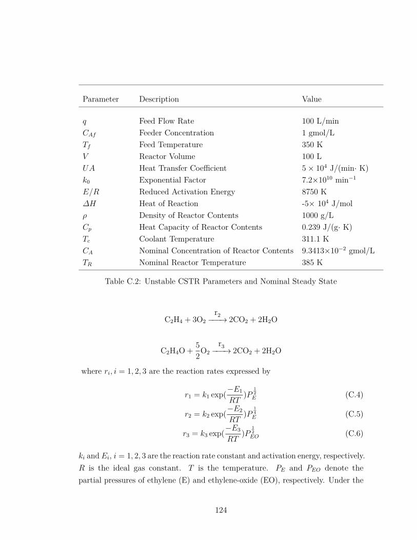
Parameter Description Value
q Feed Flow Rate 100 L/minCAf Feeder Concentration 1 gmol/LTf Feed Temperature 350 KV Reactor Volume 100 LUA Heat Transfer Coefficient 5× 10⁴ J/(min· K)k0 Exponential Factor 7.2×10¹⁰ min−1
E/R Reduced Activation Energy 8750 K∆H Heat of Reaction -5× 10⁴ J/molρ Density of Reactor Contents 1000 g/LCp Heat Capacity of Reactor Contents 0.239 J/(g· K)Tc Coolant Temperature 311.1 KCA Nominal Concentration of Reactor Contents 9.3413×10⁻² gmol/LTR Nominal Reactor Temperature 385 K
Table C.2: Unstable CSTR Parameters and Nominal Steady State
C2H4 + 3O2
r2−−−→ 2CO2 + 2H2O
C2H4O+5
2O2
r3−−−→ 2CO2 + 2H2O
where ri, i = 1, 2, 3 are the reaction rates expressed by
r1 = k1 exp(−E1
RT)P
12E (C.4)
r2 = k2 exp(−E2
RT)P
14E (C.5)
r3 = k3 exp(−E3
RT)P
12EO (C.6)
ki and Ei, i = 1, 2, 3 are the reaction rate constant and activation energy, respectively.R is the ideal gas constant. T is the temperature. PE and PEO denote thepartial pressures of ethylene (E) and ethylene-oxide (EO), respectively. Under the
124
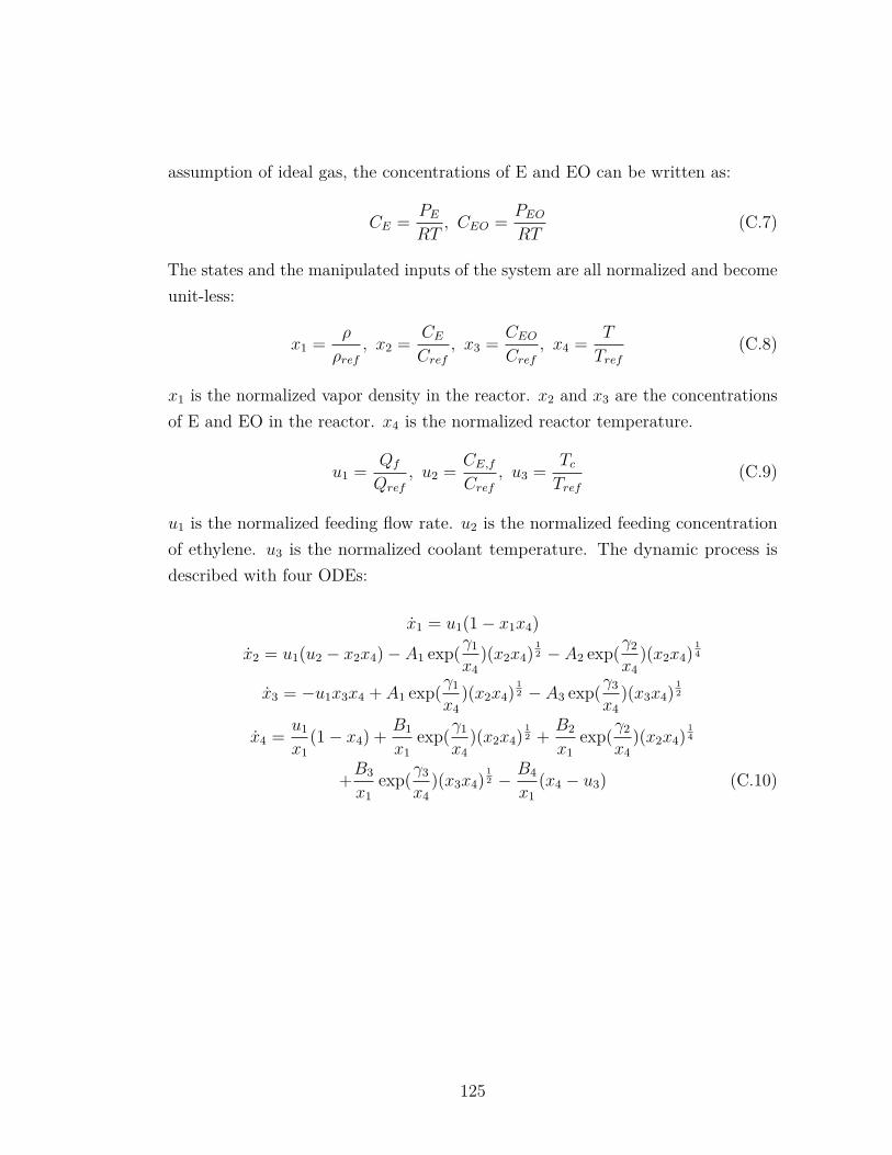
assumption of ideal gas, the concentrations of E and EO can be written as:
CE = PERT
, CEO = PEORT
(C.7)
The states and the manipulated inputs of the system are all normalized and becomeunit-less:
x1 = ρ
ρref, x2 = CE
Cref, x3 = CEO
Cref, x4 = T
Tref(C.8)
x1 is the normalized vapor density in the reactor. x2 and x3 are the concentrationsof E and EO in the reactor. x4 is the normalized reactor temperature.
u1 = Qf
Qref, u2 = CE,f
Cref, u3 = Tc
Tref(C.9)
u1 is the normalized feeding flow rate. u2 is the normalized feeding concentrationof ethylene. u3 is the normalized coolant temperature. The dynamic process isdescribed with four ODEs:
x1 = u1(1− x1x4)
x2 = u1(u2 − x2x4)− A1 exp(γ1
x4)(x2x4) 1
2 − A2 exp(γ2
x4)(x2x4) 1
4
x3 = −u1x3x4 + A1 exp(γ1
x4)(x2x4) 1
2 − A3 exp(γ3
x4)(x3x4) 1
2
x4 = u1
x1(1− x4) + B1
x1exp(γ1
x4)(x2x4) 1
2 + B2
x1exp(γ2
x4)(x2x4) 1
4
+B3
x1exp(γ3
x4)(x3x4) 1
2 − B4
x1(x4 − u3) (C.10)
125

Parameter Value Parameter ValueA1 92.80 B3 2170.57A2 12.66 B4 7.02A3 2412.71 γ1 -8.13B1 7.32 γ2 -7.12B2 10.39 γ3 -11.07
Table C.3: Dimensionless Parameters of the Ethylene Oxidation CSTR
126

Bibliography
[1] Morari, M. and J. H. Lee (1999) “Model predictive control: past, presentand future,” Computers & Chemical Engineering, 23(4-5), pp. 667–682.URL http://linkinghub.elsevier.com/retrieve/pii/S0098135498003019
[2] Mayne, D. Q., J. B. Rawlings, C. V. Rao, P. O. M. Scokaert,C. National, and F. Telecom (2000) “Constrained model predictivecontrol : Stability and optimality,” Automatica, 36, pp. 789–814.
[3] Qin, S. J. and T. A. Badgwell (2003) “A survey of industrial modelpredictive control technology,” Control Engineering Practice, 11(7), pp. 733–764, arXiv:1402.6991v1.
[4] Huang, R., L. T. Biegler, and S. C. Patwardhan (2010) “Fast Offset-Free Nonlinear Model Predictive Control Based on Moving Horizon Estima-tion,” Industrial & Engineering Chemistry Research, 49(17), pp. 7882–7890.URL http://pubs.acs.org/doi/abs/10.1021/ie901945y
[5] García, C. E., D. M. Prett, and M. Morari (1989) “Model predictivecontrol: Theory and practice-A survey,” Automatica, 25(3), pp. 335–348.
[6] Rawlings, J. B. (2000) “Tutorial overview of model predictive control,”IEEE Control Systems Magazine, 20(3), pp. 38–52.
[7] Friedland, B. (1986) Control System Design: An Introduction to State-Space Methods., NewYork: McGraw-Hill.
[8] Lopez-Negrete, R., F. J. D’Amato, L. T. Biegler, and A. Kumar(2013) “Fast nonlinear model predictive control: Formulation and indus-trial process applications,” Computers & Chemical Engineering, 51, pp. 55–64.URL http://linkinghub.elsevier.com/retrieve/pii/S0098135412001871
[9] Yang, X., D. W. Griffith, and L. T. Biegler (2015) “Nonlinear Pro-gramming Properties for Stable and Robust NMPC,” in IFAC-PapersOnLine,vol. 48, Elsevier B.V., pp. 388–397.URL http://dx.doi.org/10.1016/j.ifacol.2015.11.310
127

[10] Kokotović, P. and M. Arcak (2001) “Constructive nonlinear control: ahistorical perspective,” Automatica, 37(5), pp. 637–662.URL http://www.sciencedirect.com/science/article/pii/S0005109801000024
[11] Christofides, P. D. and N. H. El-farra (2005) Control of Nonlinearand Hybrid Process Systems: Designs for Uncertainty, Constraints and TimeDelays, Springer, Netherlands.URL http://pdclab.seas.ucla.edu/Publications/Book/PDChristofides_NHEl-Farra_Springer_2005_book.pdf
[12] Mhaskar, P., N. H. El-Farra, and P. D. Christofides (2005) “Pre-dictive Control of Switched Nonlinear Systems With Scheduled Mode Transi-tions,” IEEE Transactions on Automatic Control, 50(11), pp. 1670–1679.
[13] ——— (2006) “Stabilization of nonlinear systems with state and controlconstraints using Lyapunov-based predictive control,” Systems & ControlLetters, 55(8), pp. 650–659.URL http://linkinghub.elsevier.com/retrieve/pii/S0167691106000405
[14] Mahmood, M. and P. Mhaskar (2010) “On constructing constrainedcontrol Lyapunov functions for linear systems,” Proceedings of the 2010American Control Conference, (1), pp. 5191–5196.
[15] Zavala, V., C. Laird, and L. Biegler (2008) “A fast moving horizonestimation algorithm based on nonlinear programming sensitivity,” Journalof Process Control, 18(412), pp. 876–884.URL http://linkinghub.elsevier.com/retrieve/pii/S0959152408001091
[16] Zavala, V. M. and L. T. Biegler (2009) “The advanced-step NMPCcontroller: Optimality, stability and robustness,” Automatica, 45(1), pp.86–93.URL http://linkinghub.elsevier.com/retrieve/pii/S0005109808004196
[17] Yang, X. and L. T. Biegler (2013) “Advanced-multi-step nonlinear modelpredictive control,” Journal of Process Control, 23(8), pp. 1116–1128.URL http://dx.doi.org/10.1016/j.jprocont.2013.06.011
[18] Biegler, L. T., X. Yang, and G. A. Fischer (2015) “Advances insensitivity-based nonlinear model predictive control and dynamic real-timeoptimization,” Journal of Process Control, 30, pp. 104–116.URL http://dx.doi.org/10.1016/j.jprocont.2015.02.001
[19] Dua, V. and E. Pistikopoulos (1999) “Algorithms for the solution ofmultiparametric mixed-integer nonlinear optimization problems,” Ind. Eng.Chem. Res, 38, pp. 3976–3987.URL http://discovery.ucl.ac.uk/86105/
128

[20] Dua, V., N. A. Bozinis, and E. N. Pistikopoulos (2002) “A multi-parametric programming approach for mixed-integer quadratic engineeringproblems,” Computers and Chemical Engineering, 26(4-5), pp. 715–733.
[21] Liu, J., Y. Chen, and H. K. Fathy (2017) “Nonlinear Model-PredictiveOptimal Control of an Active Cell-to-Cell Lithium- Ion Battery Pack Balanc-ing Circuit,” in IFAC-PapersOnLine, vol. 50, Elsevier B.V., pp. 15048–15053.URL https://doi.org/10.1016/j.ifacol.2017.08.2297
[22] Liu, J., G. Li, and H. K. Fathy (2015) “A Computationally EfficientApproach for Optimizing Lithium-Ion Battery Charging,” Journal of DynamicSystems, Measurement, and Control, 138(2), pp. 021009–1–021009–8.URL http://dx.doi.org/10.1115/1.4032066
[23] ——— (2015) “Efficient Lithium-Ion Battery Model Predictive ControlUsing Differential Flatness-Based Pseudospectral Methods,” in Proceedingsof the ASME 2015 Dynamic Systems and Control Conference, ASME, p.V001T13A005.URL http://proceedings.asmedigitalcollection.asme.org/proceeding.aspx?doi=10.1115/DSCC2015-9765
[24] ——— (2016) “An Extended Differential Flatness Approach for the Health-Conscious Nonlinear Model Predictive Control of Lithium-Ion Batteries,”IEEE Transactions on Control Systems Technology, pp. 1–8.URL http://ieeexplore.ieee.org/document/7763805/
[25] Liu, J. (2017) Computationally Efficient Online Model-Based Control andEstimation for Lithium-ion Batteries, Ph.D. thesis.
[26] Liu, J., S. Mendoza, and K. Fathy (2017) “Total Least Squares State ofCharge Estimation for Lithium-Ion Batteries: An Efficient Moving HorizonEstimation Approach,” in IFAC-PapersOnLine, vol. 50, Elsevier B.V., pp.14489–14494.URL https://doi.org/10.1016/j.ifacol.2017.08.2298
[27] Yu, M., D. C. Miller, and L. T. Biegler (2015) “Dynamic ReducedOrder Models for Simulating Bubbling Fluidized Bed Adsorbers,” Industrial& Engineering Chemistry Research, 54(27), pp. 6959–6974.URL http://pubs.acs.org/doi/abs/10.1021/acs.iecr.5b01270
[28] Yu, M. and L. T. Biegler (2016) “A Stable and Robust NMPC Strategywith Reduced Models and Nonuniform Grids,” in IFAC-PapersOnLine, vol. 49,Elsevier B.V., pp. 31–36.URL http://dx.doi.org/10.1016/j.ifacol.2016.07.212
129

[29] Yu, M. (2017) Model Reduction and Nonlinear Model Predictive Controlof Large-Scale Distributed Parameter Systems with Applications in SolidSorbent-Based CO2 Capture, Ph.D. thesis.
[30] Allgöwer, F. and A. Zheng (2000) Nonlinear Model Predictive Control,vol. 26, Birkhäuser.
[31] Ferramosca, A., J. B. Rawlings, D. Limon, and E. F. Camacho(2010) “Economic MPC for a changing economic criterion,” Proceedings ofthe IEEE Conference on Decision and Control, pp. 6131–6136.
[32] Huang, R. and L. T. Biegler (2012) “Economic NMPC for energy intensiveapplications with electricity price prediction,” Computer Aided ChemicalEngineering, 31(July), pp. 1612–1616.URL http://dx.doi.org/10.1016/B978-0-444-59506-5.50153-X
[33] Amrit, R., J. B. Rawlings, and L. T. Biegler (2013) “Optimizingprocess economics online using model predictive control,” Computers &Chemical Engineering, 58, pp. 334–343.URL http://linkinghub.elsevier.com/retrieve/pii/S0098135413002354
[34] Ellis, M. and P. D. Christofides (2014) “Integrating dynamic economicoptimization and model predictive control for optimal operation of nonlinearprocess systems,” Control Engineering Practice, 22, pp. 242–251.URL http://linkinghub.elsevier.com/retrieve/pii/S0967066113000348
[35] Lao, L. (2015) Economic Model Predictive Control: Handling PreventiveActuator and Sensor Maintenance and Application to Transport-ReactionProcesses A, Ph.D. thesis.
[36] Lao, L., M. Ellis, and P. D. Christofides (2014) “Smart manufactur-ing: Handling preventive actuator maintenance and economics using modelpredictive control,” AIChE Journal, 60, pp. 2179–2196.
[37] ——— (2014) “Economic Model Predictive Control of Transport-ReactionProcesses,” Industrial & Engineering Chemistry Research, 53, pp. 7382–7396.
[38] ——— (2015) “Handling State Constraints and Economics in FeedbackControl of Transport-Reaction Processes,” Journal of Process Control, 32,pp. 98–108.
[39] ——— (2014) “Economic model predictive control of parabolic PDE systems:Addressing state estimation and computational efficiency,” Journal of ProcessControl, 24, pp. 448–462.
130

[40] ——— (2015) “Real-Time Preventive Sensor Maintenance Using RobustMoving Horizon Estimation and Economic Model Predictive Control,” AIChEJournal, 61, pp. 3374–3389.
[41] Kumar, A., M. Baldea, T. F. Edgar, and O. A. Ezekoye (2015)“Smart manufacturing approach for efficient operation of industrial steam-methane reformers,” Industrial & Engineering Chemistry Research, 54(16),pp. 4360–4370.
[42] Kumar, A., M. Baldea, and T. F. Edgar (2016) “Real-time optimizationof an industrial steam-methane reformer under distributed sensing,” ControlEngineering Practice, 54, pp. 140–153.
[43] Kumar, A., T. F. Edgar, and M. Baldea (2017) “Multi-resolutionmodel of an industrial hydrogen plant for plantwide operational optimizationwith non-uniform steam-methane reformer temperature field,” Computers &Chemical Engineering, 107, pp. 271–283.
[44] Kumar, A. (2016) Model based operation of industrial steam methane re-formers using large scale sensor data, Ph.D. thesis.
[45] Xie, R., Y. Lee, M. P. Aplan, N. J. Caggiano, C. Müller, R. H.Colby, and E. D. Gomez (2017) “Glass Transition Temperature of Conju-gated Polymers by Oscillatory Shear Rheometry,” Macromolecules, 50(13),pp. 5146–5154.
[46] Xie, R., R. H. Colby, and E. D. Gomez (2017) “Connecting the Mechani-cal and Conductive Properties of Conjugated Polymers,” Advanced ElectronicMaterials, 1700356, pp. 1–14.
[47] Yang, X. (2015) Advanced-Multi-Step and Economically Oriented NonlinearModel Predictive Control, Ph.D. thesis.
[48] Huang, R., S. C. Patwardhan, and L. T. Biegler (2009) “Robustextended Kalman filter based nonlinear model predictive control formulation,”Proceedings of the 48h IEEE Conference on Decision and Control (CDC) heldjointly with 2009 28th Chinese Control Conference, pp. 8046–8051.
[49] ——— (2013) “Robust stability of nonlinear model predictive control withextended Kalman filter and target setting,” International Journal of Robustand Nonlinear Control, 23, pp. 1240–1264, 1709.01050.URL http://arxiv.org/abs/1709.01050
[50] Haseltine, E. L. and J. B. Rawlings (2005) “Critical evaluation ofextended Kalman filtering and moving-horizon estimation,” Industrial andEngineering Chemistry Research, 44(8), pp. 2451–2460, arXiv:1011.1669v3.
131

[51] Schneider, R. and C. Georgakis (2013) “How to NOT make the extendedkalman filter fail,” Industrial and Engineering Chemistry Research, 52(9), pp.3354–3362.
[52] Armaou, A. and A. Ataei (2014) “Piece-wise constant predictive feedbackcontrol of nonlinear systems,” Journal of Process Control, 24(4), pp. 326–335.URL http://dx.doi.org/10.1016/j.jprocont.2014.02.002
[53] Fang, Y. and A. Armaou (2015) “Nonlinear Model Predictive Control usinga bilinear Carleman linearization-based formulation for chemical processes,” inProceedings of the 2015 American Control Conference, vol. 1, pp. 5629–5634.
[54] Hashemian, N. and A. Armaou (2015) “Fast Moving Horizon Estimationof Nonlinear Processes via Carleman Linearization,” in Proceedings of the2015 American Control Conference, vol. 1, pp. 3379–3385.
[55] Fang, Y. and A. Armaou (2016) “Carleman approximation based quasi-analytic model predictive control for nonlinear systems,” AIChE Journal,62(11), pp. 3915–3929.URL http://doi.wiley.com/10.1002/aic.15298
[56] Hashemian, N. and A. Armaou (2016) “Simulation, Model-Reduction,and State Estimation of a Two-Component Coagulation Process,” AIChEJournal, 62(5), pp. 1557–1567.
[57] Fang, Y. and A. Armaou (2016) “A Formulation of Advanced-step BilinearCarleman Approximation-based Nonlinear Model Predictive Control,” inProceedings of the 55th IEEE Conference on Decision and Control, pp. 4027–4032.
[58] Hashemian, N. and A. Armaou (2017) “A Moving Horizon EstimationAlgorithm Based on Carleman Approximation: Design and Stability Analysis,”Industrial and Engineering Chemistry Research, 56(36).
[59] Fang, Y. and A. Armaou (2018) “Output Feedback Receding HorizonRegulation via Moving Horizon Estimation and Model Predictive Control,”Journal of Process Control, 69, pp. 114–127.URL https://doi.org/10.1016/j.jprocont.2018.07.003
[60] ——— (2018) “A Mathematics Approach to Improve the ComputationalEfficiency of Economic-oriented Model Predictive Control,” in Proceedings ofthe 23rd International Symposium on Mathematical Theory of Networks andSystems.
[61] Hashemian, N. (2017) Estimation and Control of Two-Component Granu-lation Processes, Ph.D. thesis.
132

[62] Fang, Y. (2015) Carleman Linearization-Based Nonlinear Model PredicitiveControl, Master’s thesis.
[63] Mayne, D. Q. (1995) Optimization in Model Based Control, Copenhagen,Denmark.
[64] Dubljevic, S., P. Mhaskar, N. H. El-Farra, and P. D. Christofides(2005) “Predictive control of transport-reaction processes,” Computers &Chemical Engineering, 29(11-12), pp. 2335–2345.URL http://www.sciencedirect.com/science/article/pii/S0098135405001419
[65] Shi, D., N. H. El-Farra, M. Li, P. Mhaskar, and P. D. Christofides(2006) “Predictive control of particle size distribution in particulate processes,”Chemical Engineering Science, 61(1), pp. 268–281.URL http://www.sciencedirect.com/science/article/pii/S0009250905004598
[66] Cacace, F., V. Cusimano, and A. Germani (2011) “An efficient approachto the design of observers for continuous-time systems with discrete-timemeasurements,” Proceedings of the IEEE Conference on Decision and Control,(July 2015), pp. 7549–7554.
[67] Lou, Y., G. Hu, and P. D. Christofides (2008) “Model Predictive Controlof Nonlinear Stochastic Partial Differential Equations with Application to aSputtering Process,” AIChE Journal, 54, pp. 2065–2081.
[68] Diehl, M., R. Amrit, and J. B. Rawlings (2011) “A Lyapunov functionfor economic optimizing model predictive control,” IEEE Transactions onAutomatic Control, 56(3), pp. 703–707.
[69] Heidarinejad, M., J. Liu, and P. D. Christofides (2013) Economicmodel predictive control of switched nonlinear systems, vol. 62, Elsevier B.V.URL http://linkinghub.elsevier.com/retrieve/pii/S0167691112002137
[70] Bequette, B. (2003) Process Control: Modeling, Design and Simulation,Upper Saddle River, NJ: Prentice Hall PTR.
[71] Biegler, L. (1998) “Advances in nonlinear programming concepts for processcontrol,” Journal of Process Control, 8(5-6), pp. 301–311.
[72] Rodriguez, M. and D. Perez (2005) “First Principles Model Based Con-trol,” European Symposium on Computer Aided Process Engineering, pp.1285–1290.
[73] Steeb, W. H. and F. Wilhelm (1980) “Non-linear autonomous systemsof differential equations and Carleman linearization procedure,” Journal ofMathematical Analysis and Applications, 77(2), pp. 601–611.URL http://www.sciencedirect.com/science/article/pii/0022247X80902504
133
[74] Steeb, W. H. (1989) “A note on Carleman linearization,” Physics LettersA, 140(6), pp. 336–338.
[75] Biegler, L. T. (1984) “Solution of Dynamic Optimization Problems bySuccessive Quadratic Programming and Orthogonal Collocation,” Computers& Chemical Engineering, 8(3), pp. 0–4.
[76] Svoronos, S., D. Papageorgiou, and C. Tsiligiannis (1994) “Discretiza-tion of Nonlinear Control Systems via the Carleman Linearization,” ChemicalEngineering Journal, 49(19), pp. 3263–3267.
[77] Mohler, R. (1973) Bilinear Control Processes: with Applications to Engi-neering, Ecology, and Medicine., New York: Academic Press.
[78] Pardalos, P. and V. Yatsenko (2008) Optimization And Control ofBilinear Systems: Theory, Algorithms, and Applications., New York: Springer.
[79] Elliott, D. (2009) Bilinear Control Systems: Matrices in Action, London:Springer.
[80] Teel, A. R. (2004) “Control : Is the Stability Robust ? Part I : AsymptoticStability Theory,” , pp. 3–27.
[81] ——— (2004) “Discrete Time Receding Horizon Optimal Control: Is theStability Robust?” in Optimal Control, Stabilization and Nonsmooth Analysis,Springer-Verlag, Berlin Heidelberg, pp. 3–27.
[82] Grimm, G., M. Messina, S. Tuna, and A. Teel (2005) “Model predictivecontrol: for want of a local control Lyapunov function, all is not lost,” IEEETrans. on Automatic Control, 50(5), pp. 546–558.
[83] Tuna, S., M. Messina, and A. Teel (2006) “Shorter horizons for modelpredictive control,” in Proceedings of the 2006 American Control Conference,pp. 863–868.
[84] Hatzimanikatis, V., G. Lyberatos, S. Pavlou, and S. Svoronos (1993)“A method for pulsed periodic optimization of chemical reaction systems,”Chemical Engineering Science, 48(4), pp. 789–797.
[85] Henson, M. A. and D. E. Seborg (1993) “Theoretical analysis of un-constrained nonlinear model predictive control,” International Journal ofControl, 58(5), pp. 1053–1080.
[86] Vassiliadis, V., R. Sargent, and C. Pantelides (1994) “Solution of aClass of Multistage Dynamic Optimization Problems. 1. Problems withoutPath Constraints V.” Industrial & Engineering Chemistry Research, 33, pp.2111–2122.
134

[87] ——— (1994) “Solution of a Class of Multistage Dynamic OptimizationProblems. 2. Problems with Path Constraints,” Industrial & EngineeringChemistry Research, 33, pp. 2123–2133.
[88] Ellis, M., H. Durand, and P. D. Christofides (2014) “A tutorial reviewof economic model predictive control methods,” Journal of Process Control,24(8), pp. 1156–1178.URL http://dx.doi.org/10.1016/j.jprocont.2014.03.010
[89] Ellis, M. and P. D. Christofides (2014) “Optimal Time-varying Opera-tion of Nonlinear Process Systems with Economic Model Predictive Control,”Ind. Eng. Chem. Res, 53, pp. 4991–5001.
[90] Durand, H., M. Ellis, and P. D. Christofides (2016) “Economic modelpredictive control designs for input rate-of-change constraint handling andguaranteed economic performance,” Computers and Chemical Engineering,92, pp. 18–36.URL http://dx.doi.org/10.1016/j.compchemeng.2016.04.026
[91] Zavala, V. and L. Biegler (2009) “Nonlinear programming strategies forstate estimation and model predictive control,” in Nonlinear model predictivecontrol, vol. 384 of Lecture Notes in Control and Information Sciences(L. Magni, D. Raimondo, and F. Allgower, eds.), Springer, Berlin Heidelberg,pp. 419–432.URL http://link.springer.com/chapter/10.1007/978-3-642-01094-1_33
[92] Alfani, F. and J. Carberry (1970) “An Exploratory Kinetic Study ofEthylene Oxidation Over an Unmoderated Supported Silver Catalyst,” LaChimica e L’Industria, (52), pp. 1192–1196.
[93] Ozgulsen, F., R. Adomaitis, and A. Cinar (1992) “A Numerical Methodfor Determining Optimal Parameter Values in Forced Periodic Operation,”Chemical Engineering Science, 47(3), pp. 605–613.
[94] Ozgulsen, F., S. J. Kendra, and A. Char (1993) “Nonlinear PredictiveControl of Periodically Forced Chemical Reactors,” AIChE Journal, 39(4),pp. 589–598.
[95] Huang, R., V. M. Zavala, and L. T. Biegler (2009) “Advanced stepnonlinear model predictive control for air separation units,” Journal of ProcessControl, 19(4), pp. 678–685.URL http://dx.doi.org/10.1016/j.jprocont.2008.07.006
[96] Findeisen, R. and F. Allgöwer (2004) “Computational Delay inNonlinear Model Predictive Control,” IFAC Proceedings Volumes, 37(1), pp.
135

427–432.URL http://linkinghub.elsevier.com/retrieve/pii/S1474667017387694
[97] Mare, J. B. and J. A. De Dona (2006) “Moving Horizon Estimation ofConstrained Nonlinear Systems by Carleman Approximations,” Proceedingsof the 45th IEEE Conference on Decision and Control, pp. 2147–2152.URL http://ieeexplore.ieee.org/document/4178063/
[98] Stewart, J. (2016) Calculus, 8 ed., Cengage Learning, Boston, MA, USA.
[99] Homer, T. and P. Mhaskar (2017) “Constrained control Lyapunovfunction-based control of nonlinear systems,” Systems and Control Letters,110, pp. 55–61.URL https://doi.org/10.1016/j.sysconle.2017.10.004
[100] Das, B. and P. Mhaskar (2018) “Adaptive output-feedback Lyapunov-based model predictive control of nonlinear process systems,” InternationalJournal of Robust and Nonlinear Control, 28(5), pp. 1597–1609.URL http://doi.wiley.com/10.1002/rnc.3973
[101] Chen, M.-S. and C.-y. Kao (1997) “Control of linear time-varying systemsusing forward Riccati equation,” Journal of dynamic systems, measurement,and control, 119(3), pp. 536–540.
[102] Angeli, D., R. Amrit, and J. B. Rawlings (2012) “On average perfor-mance and stability of economic model predictive control,” IEEE Transactionson Automatic Control, 57(7), pp. 1615–1626.
136

VitaYizhou Fang
Education:Pennsylvania State University, University Park, PAPh.D. Chemical Engineering 08/2013-08/2018M.S. Chemical Engineering 08/2013-08/2015
University of Arizona, Tucson, AZB.S. Chemical Engineering 08/2010-05/2012
Fudan University, Shanghai, ChinaB.S. Environmental Science 09/2008-07/2010
Experience:Research Assistant, Pennsylvania State University, 01/2014-08/2018Teaching Assistant, Pennsylvania State University, 01/2015-05/2018Advanced Process Control Intern, Shell Global Solutions, 05/2017-08/2017
Website: https://www.linkedin.com/in/yizhoufangpsu/
Publications:
1. Y. Fang and A. Armaou, “Output Feedback Receding Horizon Regulationvia Moving Horizon Estimation and Model Predictive Control”, Journal ofProcess Control 69 (2018) 114-127.
2. Y. Fang and A. Armaou, “A Mathematics Approach to Improve the Com-putational Efficiency of Economic-oriented Model Predictive Control”, in:Proceedings of the 23rd International Symposium on Mathematical Theoryof Networks and Systems.
3. Y. Fang and A. Armaou, “A Formulation of Advanced-step Bilinear CarlemanApproximation-based Nonlinear Model Predictive Control”, in: Proceedings ofthe 55th IEEE Conference on Decision and Control, volume 1, pp. 4027-4032.
4. Y. Fang and A. Armaou, “Carleman Approximation Based Quasi-AnalyticModel Predictive Control for Nonlinear Systems”, AIChE Journal 62 (2016)3915-3929.
5. Y. Fang and A. Armaou, “Nonlinear Model Predictive Control using a bilinearCarleman linearization-based formulation for chemical processes”, in: Pro-ceedings of the 2015 American Control Conference, volume 1, pp. 5629-5634.
Copyright © 2022 FDOKUMEN