PLEASE SCROLL DOWN FOR ARTICLE

This article was downloaded by: [Engwerda, Jacob]On: 28 October 2009Access details: Access Details: [subscription number 916265099]Publisher Taylor & FrancisInforma Ltd Registered in England and Wales Registered Number: 1072954 Registered office: Mortimer House,37-41 Mortimer Street, London W1T 3JH, UK

International Journal of ControlPublication details, including instructions for authors and subscription information:http://www.informaworld.com/smpp/title~content=t713393989

The open-loop discounted linear quadratic differential game for regular higherorder index descriptor systemsJ. C. Engwerda a; Salmah b; I. E. Wijayanti b

a Department of Econometrics and OR, Tilburg University, Tilburg, The Netherlands b Department ofMathematics, Gadjah Mada University, Yogyakarta, Indonesia

First Published:December2009

To cite this Article Engwerda, J. C., Salmah and Wijayanti, I. E.(2009)'The open-loop discounted linear quadratic differential game forregular higher order index descriptor systems',International Journal of Control,82:12,2365 — 2374

To link to this Article: DOI: 10.1080/00207170903079194

URL: http://dx.doi.org/10.1080/00207170903079194

Full terms and conditions of use: http://www.informaworld.com/terms-and-conditions-of-access.pdf

This article may be used for research, teaching and private study purposes. Any substantial orsystematic reproduction, re-distribution, re-selling, loan or sub-licensing, systematic supply ordistribution in any form to anyone is expressly forbidden.

The publisher does not give any warranty express or implied or make any representation that the contentswill be complete or accurate or up to date. The accuracy of any instructions, formulae and drug dosesshould be independently verified with primary sources. The publisher shall not be liable for any loss,actions, claims, proceedings, demand or costs or damages whatsoever or howsoever caused arising directlyor indirectly in connection with or arising out of the use of this material.

International Journal of ControlVol. 82, No. 12, December 2009, 2365–2374

The open-loop discounted linear quadratic differential game for regular

higher order index descriptor systems

J.C. Engwerdaa*, Salmahb and I.E. Wijayantib

aDepartment of Econometrics and OR, Tilburg University, PO Box 90153, Tilburg, The Netherlands;bDepartment of Mathematics, Gadjah Mada University, Yogyakarta, Indonesia

(Received 19 December 2008; final version received 30 May 2009)

In this article we consider the discounted linear quadratic differential game for descriptor systems that havean index larger than one. We derive both necessary and sufficient conditions for existence of an open-loopNash (OLN) equilibrium. In a small macro-economic stabilisation game we illustrate that the correspondingoptimal response is generically cyclic.

Keywords: linear quadratic differential games; open-loop information structure; descriptor systems

1. Introduction

Dynamic game theory brings together three featuresthat are key to many situations in economy, ecologyand elsewhere: optimising behaviour, presence ofmultiple agents and enduring consequences of deci-sions. For that reason this framework is often usedto analyse various policy problems in these areas(see e.g. Dockner, Jørgensen, Long and Sorger 2000;Jørgensen and Zaccour 2003; Plasmans, Engwerda,van Aarle, Di Bartolomeo and Michalak 2006).

In applications one often encounters, however,systems described by a set of ordinary differentialequations subject to some algebraic constraints. Thesesystems are known as descriptor systems.

Differential games for descriptor systems weree.g. already studied by Xu and Mizukami (1993,1994). More recently Engwerda and Salmah (2008)and Engwerda, Salmah and Widjayanti (2008) studiedfor index one systems the linear quadratic differentialgame. In Engwerda and Salmah (2008) the open-loopinformation case is studied, whereas in Engwerda et al.(2008) the case that players use linear state feedbackcontrols is dealt with.

In this article we take a first step to solvedifferential games for descriptor systems which havean index that is higher than one. We consider theproblem of two players who like to optimise theirperformance given by a usual quadratic cost functiondepending both on the state and control variables inwhich both variables are discounted. The underlyingsystem is described by a set of differential and algebraic

equations and we assume that the system is regular,that is, consistent initial states yield a unique statetrajectory. The index of the system is k41. It is wellknown that in that case the state trajectory includes(k� 1)-th order derivatives of the applied input. Forthat reason we consider the (k� 1)-th order derivativeof the applied input as our control instrument.

We assume that the information structure of thegame is of the open-loop type. That is, both playersonly know the initial state and structure of the system,and the set of admissible inputs, U, are functions oftime which are k� 1 times differentiable.

Linear quadratic control problems play an impor-tant role in applications. Particularly in economicsusually the cost of the players is discounted to stressthe short-term cost. Since the derivatives of the inputfunction naturally appear in the state trajectory ofdescriptor systems it seems natural to include theseterms in the cost function of the players too. Thismotivates the problem setting that will be formulatedin the next section in detail. The linear quadraticcontrol problem subject to descriptor systems hasbeen considered in the literature by various authors.The approach taken here, to introduce additionalstates and to consider the (k� 1)-th derivative of theinput function as the control instrument, was consid-ered e.g. in Pandolfi (1981). More references on theregulator problem for descriptor systems can be founde.g. in Mehrmann (1991), Kunkel and Mehrmann(1997), Zhu, Ma and Cheng (2002) and Engwerda et al.(2008). Like many approaches for solving the linear

*Corresponding author. Email: engwerda@uvt.nl

ISSN 0020–7179 print/ISSN 1366–5820 online

� 2009 Taylor & Francis

DOI: 10.1080/00207170903079194

http://www.informaworld.com

Downloaded By: [Engwerda, Jacob] At: 12:39 28 October 2009

quadratic control problem for descriptor systems,in this article we solve the corresponding gameproblem using the Weierstrass canonical form of thepencil �E�A (1). Using the corresponding statetransformation, it is possible to reduce the problemto a reduced order standard game problem. Using thetheory for affine linear quadratic differential gamesas documented in Engwerda (2005, 2008) it is possiblethen to solve the game for both a finite and infiniteplanning horizon.

The outline of this article is as follows. The nextsection formalises the problem statement and sum-marises some basic properties about descriptorsystems. In Section 3 we present the main results forthe finite planning horizon, whereas Section 4 containsthose about the infinite planning horizon. In Section 5we illustrate some of the theory by a simple examplefrom macro-economics. The example demonstratesin particular that cyclic behaviour may arise withinthis framework. Finally Section 6 concludes.

2. Preliminaries

Consider the differential algebraic equation

�E _xðtÞ ¼ �AxðtÞ þ f ðtÞ, xð0Þ ¼ x0, ðDAEÞ

and the associated matrix pencil

� �E� �A: ð1Þ

From e.g. Brenan, Campbell and Petzold (1996) werecall the following results. System (DAE) and (1) aresaid to be regular if the characteristic polynomialdetð� �E� �AÞ is not identically zero. If the pencil (1)is not regular, then the system (DAE) is under-determined in the sense that consistent initial conditionsdo not uniquely determine solutions (Gantmacher1959). If the pencil (1) is regular, then the roots of thecharacteristic polynomial are the finite eigenvalues ofthe pencil. If �E is singular, the pencil is said to haveinfinite eigenvalues which may be identified as thezero eigenvalues of the inverse pencil �E� � �A. FromGantmacher (1959) we recall the so-called Weierstrasscanonical form.

Theorem 2.1: If (1) is regular, then there exist non-singular matrices X and Y such that

YT �EX ¼In 0

0 N

� �and YT �AX ¼

J 0

0 Ir

� �, ð2Þ

where J 2 Rn�n is a matrix in Jordan form whose

elements are the finite eigenvalues, Ir 2 Rr�r is the

identity matrix and N 2 Rr�r is a nilpotent matrix also

in Jordan form. J and N are unique up to permutationof Jordan blocks.

If (1) is regular the solutions of (DAE) take the form

xðtÞ ¼ X1x1ðtÞ þ X2x2ðtÞ, ð3Þ

where with X ¼ ½X1 X2�, Y ¼ ½YT1 YT

2 �, X1, YT1 2

RðnþrÞ�n, X2,Y

T2 2 R

ðnþrÞ�r and

x1ðtÞ ¼ e Jtx1ð0Þ þ

Z t

0

e Jðt�sÞY1 f ðsÞds; ð4Þ

x1ð0Þ ¼ ½In 0�X�1x0

x2ðtÞ ¼ �Xk�1i¼0

NiY2di

dtif ðtÞ, ð5Þ

under the consistency condition that x2(0)¼ 0 (see

e.g. Kalogeropoulos and Arvanitis 1998). Here k is the

degree of nilpotency of N. That is the integer k for

which Nk¼ 0 and Nk�1

6¼ 0. The index of the pencil (1)

and of the descriptor system (DAE) is the degree k of

nilpotency of N. If E is non-singular, we define the

index to be zero.From the above formulae it is obvious that the

solution x(t) will not contain derivatives of the

function f if and only if k� 1. In that case the solution

x(t) is called impulse free. In general, the solution x(t)

involves derivatives of order k� 1 of the forcing

function f if (DAE) has index k. To verify whether

(DAE) has an index of at most one, see e.g. Kautsky,

Nichols and Chu (1989).In this article we assume that the dynamics of the

game is described by

�E _xðtÞ ¼ �AxðtÞ þ �B1u1ðtÞ þ �B2u2ðtÞ, xð0Þ ¼ x0, t4 0;

ð6Þ

where �E, �A 2 RðnþrÞ�ðnþrÞ, rankð �EÞ ¼ n, �Bi 2 R

ðnþrÞ�mi ,

ui 2 Rmi is the input by which player i can manipulate

the system and x0 is assumed to be a consistent initial

state (so x0¼ x(0þ)). That is, x0 is such that the system�E _xðtÞ ¼ �AxðtÞ, xð0Þ ¼ x0, has a unique solution for

t40. Assuming that system (6) has index k41 let

uði Þj :¼

diuj ðtÞ

dti , i ¼ 1, . . . , k� 2, vjðtÞ :¼dðk�1Þuj ðtÞ

dtðk�1Þand

x eT ðtÞ :¼hxTðtÞ uT1 ðtÞ � � � u

ðk�2ÞT

1 uT2 ðtÞ � � � uðk�2ÞT

2 vT1 vT2 �:

ð7Þ

We consider then the next quadratic cost functional

Ji for player i:Z T

0

e��tnxe

T

ðtÞ �MixeðtÞodtþ e��Txe

T

ðT Þ �QiTxeðT Þ: ð8Þ

Here all matrices are constant in time, both �Mi and�QiT are symmetric and �40 is the discount factor.

2366 J.C. Engwerda et al.

Downloaded By: [Engwerda, Jacob] At: 12:39 28 October 2009

The problem addressed in this article is to find the

open-loop Nash (OLN) equilibria for the game (6) and

(8) as defined below.

Definition 2.2: Assume (6) is regular and has index

k41. Let x0 be a consistent initial state and ui(0),

i¼ 1, . . . , k� 2 be given. Furthermore, let U denote the

set of functions which are k� 1 times differentiable

with u(k�1) piecewise continuous. Then ðu�1, u�2Þ 2 U

is an OLN equilibrium if for every ðu1, u�2Þ and

ðu�1, u2Þ 2 U, J1ðu�1, u�2Þ � J1ðu1, u

�2Þ and J2ðu

�1, u�2Þ �

J1ðu�1, u2Þ.With

x1ðtÞ

x2ðtÞ

� �:¼ X�1x, with x1 2 R

n and x2 2 Rrð9Þ

we have from Equations (3)–(5) that for any consistent

initial state the system dynamics (6) can be rewritten as:

_x1ðtÞ ¼ Jx1ðtÞ þ Y1�B1u1ðtÞ þ Y1

�B2u2ðtÞ,

x1ð0Þ ¼ ½I 0�X�1x0 ð10Þ

x2ðtÞ ¼ �Xk�1i¼0

NiY2

��B1uði Þ1 ðtÞ þ

�B2uði Þ2 ðtÞ

�ð11Þ

¼ �Xk�2i¼0

NiY2

��B1uði Þ1 ðtÞ þ

�B2uði Þ2 ðtÞÞ

�Nk�1Y2�B1v1ðtÞ �Nk�1Y2

�B2v2ðtÞ: ð12Þ

Next introduce the discounted state and control

vector

xTz :¼ e�12�thxT1 ðtÞ u

T1 ðtÞ � � � u

ðk�2ÞT

1 ðtÞ uT2 ðtÞ � � � uðk�2ÞT

2 ðtÞi

and wiðtÞ :¼ e�12�tvTi ðtÞ ð13Þ

together with zTðtÞ :¼ xTz ðtÞ wT1 ðtÞ w

T2 ðtÞ

� �: ð14Þ

Then, with m :¼m1þm2,

Pi :¼�Y2

�Bi NY2�Bi � � � N

k�2Y2�Bi�, i¼ 1,2, and ð15Þ

Z1 : ¼ ½In 0n�km�;

Z2 : ¼ �½0r�n P1 P2 Nk�1Y2�B1 Nk�1Y2

�B2�ð16Þ

we have that

e�12�txðtÞ ¼X

e�12�tx1ðtÞ

e�12�tx2ðtÞ

" #¼X

Z1

Z2

� �zðtÞ ¼:L1zðtÞ: ð17Þ

Furthermore, with E2 :¼ ½0km�n Ikm�, we have that

e�12�txeðtÞ ¼

L1

E2

� �zðtÞ ¼:LzðtÞ: ð18Þ

Next, let Ai :¼ ½Y1�Bi 0n�ðk�2Þmi

�, i ¼ 1, 2; and with

I 2 Rmi�mi

Di :¼

�1

2�I I 0 � � � 0

0 ...

..

. . .. . .

.0

I

0 � � � 0 �1

2�I

266666666664

3777777777752R

ðk�1Þmi�ðk�1Þmi

and Bzi :¼

0

..

.

0

I

26666664

377777752Rðk�1Þmi�mi :

Using this, it is obvious then that the game (6) and

(8) has a set of OLN equilibrium actions (u1(�), u2(�)) if

and only if (v1(�), v2(�)) are OLN equilibrium actions for

the game defined by

_xzðtÞ ¼

J�1

2�I A1 A2

0 D1 0

0 0 D2

26643775xzðtÞ

þ

0

Bz1

0

264375w1ðtÞ þ

0

0

Bz2

264375w2ðtÞ

¼: AxzðtÞ þ B1w1ðtÞ þ B2w2ðtÞ, ð19Þ

with xTz ð0Þ :¼ xz0 ¼ ½ð½I 0�X�1x0Þ

T uT1 ð0Þ � � � uðk�2ÞT

1 ð0Þ

uT2 ð0Þ � � � uðk�2ÞT

2 ð0Þ� is such that (10) and (11) holds and

Ji ¼

Z T

0

zTðtÞLT �MiLzðtÞ�

dtþ zTðT ÞLT �QiTLzðT Þ:

ð20Þ

To avoid the inclusion of controls in the scrap

value, we make the standard assumption (see also

Mehrmann (1991)) that

LT �QiTL ¼QiT 0

0 0

� �, i ¼ 1, 2, where

QiT 2 Rnþðk�1Þm�nþðk�1Þm:

Moreover, let

LT �MiL ¼: Mi ¼:

Qi Vi Wi

VTi R1i Ni

WTi NT

i R2i

264375, where

Qi 2 Rnþðk�1Þm�nþðk�1Þm, Rji 2 R

mj�mj :

ð21Þ

Then, (20) can be rewritten as

Ji ¼

Z T

0

zTðtÞMizðtÞ�

dtþ xTz ðT ÞQiTxzðT Þ: ð22Þ

International Journal of Control 2367

Downloaded By: [Engwerda, Jacob] At: 12:39 28 October 2009

3. The finite planning horizon

In this section we consider the game (6) and (8) under

the assumption that T is finite. As shown in the

previous section the OLN equilibria are found by

determining the OLN equilibria of the game defined

by (19) and (22). Assuming that Rii40, i¼ 1, 2 and

matrix G (see the Appendix for the introduced

notation, in particular for matrix ~M (35)) is invertible

the solution for the last-mentioned game is well known.

From e.g. Engwerda (2005) we recall the next result.

Theorem 3.1: Assume that the two Riccati differential

equations

_K1ðtÞ ¼�ATK1ðtÞ�K1ðtÞAþðK1ðtÞB1þV1Þ

�R�111 ðBT1K1ðtÞþVT

1 Þ�Q1, K1ðT Þ¼Q1T, ð23Þ

_K2ðtÞ ¼�ATK2ðtÞ�K2ðtÞAþðK2ðtÞB2þW2Þ

�R�122 ðBT2K2ðtÞþWT

2 Þ�Q2, K2ðT Þ ¼Q2T, ð24Þ

have a symmetric solution Ki(�) on [0,T], i¼ 1, 2.

(1) Then (19) and (22) has an OLN for every initial

state if and only if matrix

~HðT Þ ¼ ½I 0 0�e�~MT

I

Q1T

Q2T

264375

is invertible.(2) Assume that the non-symmetric Riccati differ-

ential equation

_PðtÞ ¼ � ~AT2PðtÞ � PðtÞ ~Aþ PðtÞBG�1 ~BTPðtÞ � ~Q;

PTðT Þ ¼�QT

1T, QT2T

�ð25Þ

has a solution P on [0,T].

Then (19) and (22) has a unique OLN for every initial

state. Moreover, the equilibrium actions are

w�1ðtÞ

w�2ðtÞ

� �¼ �G�1ðHþ ~BTPðtÞÞ ~�ðt, 0Þxz0,

where ~�ðt, 0Þ is the solution of the transition equation

_~�ðt, 0Þ ¼ ðA� BG�1ðHþ ~BTPðtÞÞÞ ~�ðt, 0Þ; ~�ð0, 0Þ ¼ I:

Assumptions (23) and (25) imply that for both

players the optimal control problem that arises if the

action of his opponent is known is solvable. In case

item (1) in the above theorem holds, but item (2) does

not apply, then the corresponding equilibrium actions

can be determined by solving a linear two-point

boundary value problem. The reader should then

proceed similarly as in e.g. Engwerda and Salmah(2008, Theorem 5).

Corollary 3.2: Assume that the two Riccati differen-tial equations (23) have a symmetric solution Ki(t) on[0,T] and the non-symmetric Riccati differential equa-tion (25) has a solution P(t) on [0,T]. Then (6) and (8)has a unique OLN for every initial consistent state x0and u(i)(0), i¼ 1, . . . , k� 2. Moreover, the equilibriumactions are

u�1ðtÞ

u�2ðtÞ

� �¼ e

12�t

0m1�n Im10m1�ðk�2Þmþm2

0m2�nþðk�2Þm1Im2

0m2�ðk�2Þm2

� �xzðtÞ,

where xz(t) solves

_xzðtÞ ¼ ðA� BG�1ðHþ ~BTPðtÞÞxzðtÞ, xzð0Þ ¼ xz0:

Moreover, by (17), the corresponding equilibrium statetrajectory equals

x�ðtÞ ¼ L1

�e12�txTz ðtÞ v

T1 ðtÞ v

T2 ðtÞ

�T:

4. The infinite planning horizon

In this section we assume that the cost functionalplayer i¼ 1, 2, likes to minimise is:

limT!1

Ji�x0, u1ð0Þ, . . . , u

ðk�2Þ1 ð0Þ, u2ð0Þ, . . . , u

ðk�2Þ2 ð0Þ,

u1, u2,T�, ð26Þ

where

Ji�x0, u1ð0Þ, . . . , u

ðk�2Þ1 ð0Þ, u2ð0Þ, . . . , u

ðk�2Þ2 ð0Þ, u1, u2,T

�¼

Z T

0

e��t�xe

T

ðtÞ �MixeðtÞdt

subject to (6).We assume that the matrix pairs ð �E, �A, �BiÞ, i ¼ 1, 2,

are finite dynamics stabilisable. That is1 rankð½� �E� �A, �Bi�Þ ¼ nþ r, 8� 2 C

þ0 .

Following the analysis of Section 2 it can be easilyshown that the game (6) and (26) has an OLN if andonly if the game defined by

limT!1

Z T

0

�zTðtÞMizðtÞ

dt ð27Þ

subject to (19) has an OLN. Furthermore, ð �E, �A, �BiÞ isfinite dynamics stabilisable if and only if (A,Bi) isstabilisable. So under this assumption, in principle,each player is capable to stabilise the system (6) on hisown. This property is a prerequisite to derive the mainresults below.

We assume that the players choose control func-tions belonging to the set of functions of time which

2368 J.C. Engwerda et al.

Downloaded By: [Engwerda, Jacob] At: 12:39 28 October 2009

are k� 1 times differentiable and which are such that

the state of the closed-loop system converges to zero,

Us. Notice that the assumption that the players use

simultaneously stabilising controls implies that stabi-

lisation of the system is a common objective of both

players (see e.g. Engwerda (2005) for a discussion).In the rest of this article the symmetric algebraic

Riccati equations

0¼�ATK1�K1AþðK1B1þV1ÞR�111 ðB

T1K1þVT

1 Þ�Q1,

0¼�ATK2�K2AþðK2B2þW2ÞR�122 ðB

T2K2þWT

2 Þ�Q2

ð28Þ

and the asymmetric algebraic Riccati equation

0 ¼ eAT2Pþ PeA� PBG�1eBTPþ eQ ð29Þ

or, equivalently,

0 ¼ AT2Pþ PJ� PBþ

H1

H2

� � �G�1 eBTPþH

� þQ

play a crucial role. Let �(X) denote the spectrum of a

matrix X.

Definition 4.1: A solution P2R2n�n of the algebraic

Riccati equation (29) is called

(a) stabilising, if �ð ~A� BG�1 ~BTPÞ � C�;

(b) left-right stabilising2 (LRS) if

(i) it is a stabilising solution and(ii) �ð� ~AT

2 þ PBG�1 ~BTÞ � Cþ0 :

The next lemma summarises the relationship between

the LRS solution of (29) and the stable graph subspace

(or disconjugate subspace, see Ionescu, Oara and Weiss

(1997)) of matrix ~M introduced in (35). A proof of it

can be found in Kremer (2002) and Engwerda (2008).

One way to calculate the (left–right) stabilising

solutions of (29) is by determining the invariant

subspaces of matrix M. Details on this issue can be

found e.g. in Engwerda (2005).

Lemma 4.2:

(1) The algebraic Riccati equation (29) has an LRS

solution P if and only if matrix ~M has an

n-dimensional stable graph subspace and ~M has

2n eigenvalues (counting algebraic multiplicities)

in Cþ0 .

(2) If the algebraic Riccati equation (29) has an

LRS solution, then it is unique.

From Engwerda (2008) we recall the following two

main results.

Theorem 4.3: Assume that

(1) the set of coupled algebraic Riccati equation

(29) has a set of stabilising solutions Pi, i¼ 1, 2

and(2) the two algebraic Riccati equations (28) have

a stabilising solution Ki(�), i¼ 1, 2.

Then the linear quadratic differential game (19) and

(27) has an OLN for every initial state.Moreover, with F :¼ �G�1ðHþ ~BTPÞ, one set of

equilibrium actions is given by:

w�1ðtÞ

w�2ðtÞ

� �¼ F ~�ðt, 0Þxzð0Þ, ð30Þ

where ~�ðt, 0Þ is the solution of the transition equation

_~�ðt, 0Þ ¼ ðAþ BFÞ ~�ðt, 0Þ; ~�ð0, 0Þ ¼ I:

The costs by using the actions (30) for the players are

xTz ð0Þ�Cixzð0Þ, i ¼ 1, 2, where, with Acl :¼ Aþ BF, �Ci is

the unique solution of the Lyapunov equation

½I, FT�Mi½I, FT�Tþ AT

cl�Ci þ �CiAcl ¼ 0: ð31Þ

Notice that in case the algebraic Riccati equation

(29) has more than one stabilising solution, there exist

more than one OLN equilibrium. Matrix M has then a

stable subspace of dimension larger than n. In that

case, generically, for every initial state there will exist

an infinite number of OLN equilibria.The next Theorem 4.4 gives conditions under

which there exists a unique OLN. Moreover, it

shows that in case there is a unique equilibrium the

corresponding actions are obtained by those described

in Theorem 4.3.

Theorem 4.4: Consider the differential game (19)

and (27).This game has a unique OLN equilibrium for every

initial state if and only if

(1) the asymmetric algebraic Riccati equation (29)

has an LRS solution and(2) the two algebraic Riccati equations (28) have

a stabilising solution.

Moreover, in case this game has a unique equili-

brium, the unique equilibrium actions are given by (30).

Similarly like we did for the finite-planning horizon

case one can reformulate the above results also in

terms of the original system. Corollary 4.5 below states

such a result if there is a unique equilibrium. In that

case the corresponding equilibrium strategies can also

be synthesised as a feedback strategy.

International Journal of Control 2369

Downloaded By: [Engwerda, Jacob] At: 12:39 28 October 2009

Corollary 4.5: Assume that the two Riccati equations(28) have a symmetric stabilising solution Ki andthe non-symmetric Riccati equation (29) has an LRSsolution P.

Then (6) and (8) has a unique OLN for every initialconsistent state x0 and u

(i)(0), i¼ 1, . . . , k� 2.Moreover,the equilibrium actions are

u�1ðtÞ

u�2ðtÞ

� �¼ e

12�t

0m1�n Im10m1�ðk�2Þmþm2

0m2�nþðk�2Þm1Im2

0m2�ðk�2Þm2

� �xzðtÞ,

where xz(t) solves

_xzðtÞ ¼ ðA� BG�1ðHþ ~BTPÞÞxzðtÞ, xzð0Þ ¼ xz0:

Moreover, by (17), the corresponding equilibriumstate trajectory equals

x�ðtÞ ¼ L1½e12�txTz ðtÞ v

T1 ðtÞ v

T2 ðtÞ�

T:

The corresponding costs are as in Theorem 4.3.

Remark 4.6: Notice that the open-loop strategies areindependent of the cost player that i attaches to theactual control instruments used by player j (i.e. theyare independent of Rij, i 6¼ j. So in this case player i willignore the effects of the (k� 1)-th order derivative ofthe control uj, used by player j.

5. An example

In this section we consider a simple macro-economicstabilisation problem. Assume that a monetary andfiscal authority likes to stabilise some key macro-economic variables, i.e. the real interest rate, r,inflation, _p, and the output gap, y, after a shock hasoccurred. The system is described by the followingequations:

rðtÞ ¼ iðtÞ � _pðtÞ ð32Þ

_yðtÞ ¼ ��ðiðtÞ � _pðtÞÞ þ �f ðtÞ ð33Þ

mðtÞ � pðtÞ ¼ �yðtÞ � �iðtÞ: ð34Þ

Here p(t) is the price level, i(t) denotes the nominalinterest rate, m(t) is the money supply and f(t) the fiscalpolicy. The first two instruments, the nominal interestrate and money supply, are determined by the mon-etary authority of the country, whereas the level of thethird instrument, the fiscal policy, is set by thegovernment. Here, Equation (32) models the realinterest rate, (33) is a simple growth equation of theoutput gap and (34) models asset market equilibrium(see e.g. Neck and Dockner 1995). Assume that aninitial shock in the real interest rate, price level andoutput gap has occurred, all equal to one.

Introducing as the state variable xðtÞ :¼½rðtÞ pðtÞ yðtÞ�T, u1ðtÞ :¼ ½iðtÞ mðtÞ�

T and u2(t):¼ f(t) themodel can be rewritten as (6), where

�E ¼

0 1 0

0 �� 1

0 0 0

2666437775, �A ¼

�1 0 0

0 0 0

0 �1 ��

2666437775,

�B1 ¼

1 0

�� 0

� 1

2666437775, �B2 ¼

0

�

0

2666437775 and xð0Þ ¼

1

1

1

2666437775:

It is easily verified that this system is regular if andonly if :¼ 1þ�� 6¼ 0. With

YT :¼

0 1 0

� �1

0 0 �1

26643775; X :¼

1

0 �1 1

�� 0 1

1 0 �

26643775,

k¼ 2; n¼ 1 and r¼ 2, we have

YT �EX ¼

1 0 0

0 0 1

0 0 0

264375 and YT �AX :¼

0 0 0

0 1 0

0 0 1

264375:

So this model has index two.Elementary calculations show that our model

(32)–(34) can be rewritten into the form (19) with

xzðtÞ :¼ e�12�t½yðtÞ iðtÞmðtÞ f ðtÞ�T; w1ðtÞ :¼ e�

12�t½_iðtÞ _mðtÞ�T;

w2ðtÞ :¼ e�12�t _fðtÞ; J¼ 0; A1¼ ½�� 0�; A2¼�;

D1¼

�1

2� 0

0�1

2�

26643775; D2¼

�1

2�;

Bz1 ¼ I2 and Bz2 ¼ 1:

Assuming that the cost functional matrices are ofthe form �Mi ¼ ½diagðijÞ�, i ¼ 1, 2, where 17, 18 and29 are positive, we get from (21) that with

L ¼L1

E2

" #, where

L1 ¼1

0 1 0 �� �� �1 0

�� � 1 0 0 0 0

1 �� � 0 0 0 0

26643775 and

E2 ¼ ½01�6 I6�,

2370 J.C. Engwerda et al.

Downloaded By: [Engwerda, Jacob] At: 12:39 28 October 2009

Here �i :¼ i2 þ �2i3 and �i :¼ ��i2 þ �i3.

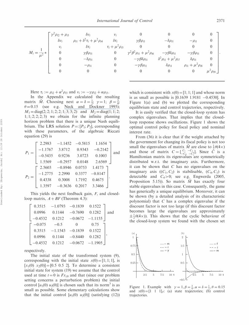
In the Appendix we calculated the resultingmatrix ~M. Choosing next � ¼ � ¼ 1

2; � ¼ 1; � ¼ 34;

�¼ 0.15 (see e.g. Neck and Dockner 1995);M1¼ diag(2; 2; 1; 2; 2; 1; 3; 3; 2) and M2¼diag(1; 1; 2;1; 1; 2; 2; 2; 3) we obtain for the infinite planninghorizon problem that there is a unique Nash equili-brium. The LRS solution P¼: [P1;P2], correspondingwith these parameters, of the algebraic Riccatiequation (29) is

P1 ¼

2:2983 �1:1452 �0:5815 1:1654

�1:1767 3:8712 0:9343 �0:2142

�0:5435 0:9236 3:0723 0:1003

1:5569 �0:2957 0:0148 2:6569

2666437775 and

P2 ¼

2:5603 �0:8946 0:0753 1:4173

�1:2775 2:2990 0:3377 �0:8147

0:4338 0:3008 1:7192 0:4675

1:3597 �0:3636 0:2017 3:3466

2666437775:

This yields the next feedback gain, F, and closed-loop matrix, AþBF (Theorem 4.3):

0:3515 �1:0793 �0:1839 0:1522

0:0996 0:1144 �0:7690 0:1282

�0:4532 0:1212 �0:0672 �1:1155

264375 and

�0:075 �0:5 0 0:75

0:3515 �1:1543 �0:1839 0:1522

0:0996 0:1144 �0:8440 0:1282

�0:4532 0:1212 �0:0672 �1:1905

2666437775,

respectively.The initial state of the transformed system (9),

corresponding with the initial state x(0)¼ [1; 1; 1], is[x1(0) x2(0)]¼ [0.5 0.5 2]. To determine a consistentinitial state for system (19) we assume that the controlused at time t¼ 0 is Fxz0 and that (since our problemsetting concerns a perturbation problem) the initialcontrol [u1(0) u2(0)] is chosen such that its norm3 is assmall as possible. Some elementary calculations showthat the initial control [u1(0) u2(0)] (satisfying (12))

which is consistent with x(0)¼ [1; 1; 1] and whose normis as small as possible is [0.1639 1.9181 �0.4530]. InFigure 1(a) and (b) we plotted the correspondingequilibrium state and control trajectories, respectively.

It is easily verified that the closed-loop system hascomplex eigenvalues. That implies that the closed-loop response shows oscillations. Figure 1 shows theoptimal control policy for fiscal policy and nominalinterest rate.

From (36) it is clear that if the weight attached bythe government for changing its fiscal policy is not toosmall the eigenvalues of matrix ~M are close to 1

2 �ð4�Þand those of matrix C ¼ ½ C1 �C2

�C4 �CT1

�. Since C is aHamiltonian matrix its eigenvalues are symmetricallydistributed w.r.t. the imaginary axis. Furthermore,it can be shown that C has no eigenvalues on theimaginary axis ((C1,C2) is stabilisable, (C4,C1) isdetectable and C440; see e.g. Engwerda (2005,Proposition 5.15)). So matrix ~M has exactly fourstable eigenvalues in this case. Consequently, the gamehas generically a unique equilibrium. Moreover, it canbe shown (by a detailed analysis of its characteristicpolynomial) that C has a complex eigenvalue if thediscount factor is not too large (if this discount factorbecomes large the eigenvalues are approximately 1

2 �ð4�)). This shows that the cyclic behaviour ofthe closed-loop system we found with the chosen set

Mi ¼1

2�

�2i2 þ i3 ��i �i 0 0 0 0

��i i1 þ �2�i þ

2i4 ��i ��i1 ��i1 �i1 0

�i ��i �i þ 2i5 0 0 0 0

0 ��i1 0 �2�2i1 þ 2i6 ����i1 ���i1 0

0 ��i1 0 ����i1 �2i1 þ 2i7 �i1 0

0 �i1 0 ���i1 �i1 i1 þ 2i8 0

0 0 0 0 0 0 2i9

2666666666664

3777777777775:

2:5 5 7:5 10 t

0:25

0:5

0:75

1

= m= r= y

(a)

2:5 5 7:5 10 t

–0:5

0:5

1

1:5

2

= f= i= m

(b)

Figure 1. Example with � ¼ 1,� ¼ 34 ,� ¼ � ¼

12 , � ¼ 0:15

and x(0)¼ [1 1 1]T: (a) state trajectories; (b) controltrajectories.

International Journal of Control 2371

Downloaded By: [Engwerda, Jacob] At: 12:39 28 October 2009

of parameters in this example is not a coincidence,but holds in general (for a reasonable choice ofparameters).

6. Concluding remarks

In this article we considered the linear-quadraticdifferential game for descriptor systems which havean index k, larger than one. Since the state trajectory inthat case is a function of up to the (k� 1)-th orderderivatives of the applied control, we considered herecost functions which take this dependency intoaccount. By actually penalising the (k� 1)-th deriva-tives of the input function, in fact this (k� 1)-th orderderivative can be viewed as the control instrument andone obtains a regular linear-quadratic differentialgame. Using the standard results on the regularlinear-quadratic differential games we derived thenboth necessary and sufficient conditions for OLNequilibria in this game.

We considered both a finite and infinite planninghorizon. For the infinite horizon the standard liter-ature on linear-quadratic differential games requiresthat the system should be stabilisable by all playersindividually. For that reason we considered in thegeneral set-up a cost function where future costs arediscounted. For the finite planning horizon thisassumption can be dropped.

The above results can be generalised straightfor-wardly to the N-player case. Furthermore, since Qi areassumed to be indefinite, the obtained results can bedirectly used to (re)derive properties for the zero-sumgame. Notice, moreover, that if the discount factor � is‘large enough’ the infinite horizon game has genericallya unique OLN equilibrium.

We illustrated the theory by a simple macro-economic stabilisation problem. The example showsthat the optimal response by the players gives rise tooscillatory behaviour of the closed-loop system underfairly generally accepted choices for the set of modelparameters. A phenomenon one often observes ineconomics. This raises the question whether this kindof response is typical for this type of control problems.A more detailed analysis of this phenomenon isplanned for the future.

Obviously there are still many open problems to besolved. In particular, we did not worry about numer-ical aspects. The calculation of the equilibrium actionsusing the approach followed in this article requiresthe computation of the Weierstrass canonical form ofthe regular pencil (2). In applications it is well knownthat for higher order index systems this is a seriousissue. Recently in Zhang (2006) and Kalogeropoulos,Mitrouli, Pantelous and Triantafyllou (2009) some

algorithms are proposed to calculate this Weierstrasscanonical form. Unfortunately, we have no experienceyet how good these numerical techniques perform inthe context of our problem. This remains a topic forfuture research. Another perspective that might beworthwhile to pursue from a numerical point of view isto consider index reduction algorithms that havebeen developed in the literature (see e.g. Mattssonand Soderlind 1993; Kunkel and Mehrmann 2004) toreduce the system to an index one system first and nextuse the results from Engwerda and Salmah (2008) tocalculate the OLN equilibria. Maybe such an approachwould also facilitate to analyse the undiscounted casefor an infinite planning horizon. Furthermore, all ofthese problems can also be analysed under differentinformation structures.

Acknowledgements

The authors would like to thank Hans Schumacher andthe referees for their comments on a previous draft of thisarticle.

Notes

1. C�¼ {� 2 CjRe(�)50}; C

þ0 ¼ f� 2 C j Reð�Þ 0g.

2. In Engwerda (2005) such a solution is called stronglystabilising.

3. For simplicity reasons we choose all weights in the normhere to be the same, an assumption which, of course,can be simply adapted.

References

Brenan, K.E., Campbell, S.L., and Petzold, L.R. (1996),Numerical Solution of Initial-value Problems in Differential-algebraic Equations, Philadelphia: SIAM.

Dockner, E., Jørgensen, S., Long, N. van, and Sorger, G.(2000), Differential Games in Economics and Management

Science, Cambridge: Cambridge University Press.Engwerda, J.C. (2005), Linear Quadratic DynamicOptimization and Differential Game Theory, Chichester:

John Wiley & Sons.Engwerda, J.C. (2008), ‘Uniqueness Conditions for theAffine Open-loop Linear Quadratic Differential Game’,

Automatica, 44, 504–511.Engwerda, J.C., Salmah, (2008). ‘The Open-loop LinearQuadratic Differential Game for Index One Descriptor

Systems’, Proceedings IFAC WC 2008, Seoul, South Korea,July 6–11, pp. 3952–3957; also Automatica, 45, 585–592.

Engwerda, J.C., Salmah, and Wijayanti, I.E., (2008). ‘The

Optimal Linear Quadratic Feedback State RegulatorProblem for Index One Descriptor Systems’. CentER DP2008-90 http://greywww.uvt.nl:2080/greyfiles/center/ctr\_

py\_2007.html. Submitted.Gantmacher, F. (1959), Theory of Matrices, Vol. I,II.New York: Chelsea.

2372 J.C. Engwerda et al.

Downloaded By: [Engwerda, Jacob] At: 12:39 28 October 2009

Ionescu, V., Oara, C., and Weiss, M. (1997), ‘General MatrixPencil Techniques for the Solution of Algebraic Riccati

Equations: A Unified Approach’, IEEE Transactions onAutomatic Control, 42, 1085–1097.

Jørgensen, S., and Zaccour, G. (2003), Differential Games in

Marketing, Deventer: Kluwer.Kalogeropoulos, G., and Arvanitis, K.G. (1998), ‘A Matrix-pencil-Based Interpretation of Inconsistent Initial

Conditions and System Properties of GeneralizedState-space’, IMA Journal of Mathematical Control &Information, 15, 73–91.

Kalogeropoulos, G., Mitrouli, M., Pantelous, A.,Triantafyllou, D. (2009). ‘The Weierstrass CanonicalForm of a Regular Matrix Pencil: Numerical Issues and

Computational Techniques’, in Numerical Analysis and itsApplications: 4th International Conference, NAA 2008Lozenetz, Bulgaria, June 16–20. Revised Selected Papers,

eds. S. Margenov, L.G. Vulkov, and J. Wasniewski,Lecture Notes in Computer Science, Vol. 5434, Springer-Verlag, Berlin, Heidelberg, 322–329.

Kautsky, J., Nichols, N.K., and Chu, E.K.-W (1989),‘Robust Pole Assignment in Singular Control Systems’,Linear Algebra and its Applications, 121, 9–37.

Kunkel, P., and Mehrmann, V. (1997), ‘The LinearQuadratic Control Problem for Linear DescriptorSystems with Variable Coefficients’, Mathematics of

Control, Signals, and Systems, 10, 247–264.Kunkel, P., and Mehrmann, V. (2004), ‘Index Reduction forDifferential-Algebraic Equations by Minimal Extension’,

Zeitschrift fur Angewandte Mathematik and Mechanik, 84,579–597.

Kremer, D. (2002). ‘Non-Symmetric Riccati Theory and

Noncooperative Games’, Ph.D. thesis, RWTH-Aachen,Germany.

Mattsson, S.E., and Soderlind, G. (1993), ‘Index Reduction

in Differential-Algebraic Equations using DummyDerivatives’, SIAM Journal on Scientific Computing, 14,677–692.

Mehrmann, V.L. (1991), ‘The Autonomous Linear QuadraticControl Problem’, in Lecture Notes in Control andInformation Sciences, eds. M. Thoma, & A. Wyner,

Berlin: Springer.Neck, R., and Dockner, E.J. (1995), ‘Commitment andCoordination in a Dynamic Game Model of International

Economic Policy-making’, Open Economies Review, 6,5–28.

Pandolfi, L. (1981), ‘On the Regulator Problem for Linear

Degenerate Control Systems’, Journal of OptimizationTheory and Applications, 33, 241–254.

Plasmans, J., Engwerda, J., van Aarle, B., Di Bartolomeo, B.,and Michalak, T. (2006). Dynamic Modeling and

Econometrics in Economics and Finance, Series: DynamicModeling of Monetary and Fiscal Cooperation Among

Nations (Vol. 8), Berlin: Springer.Xu, H., and Mizukami, K (1993), ‘Two-Person Two-CriteriaDecision Making Problems for Descriptor Sytems’, Journalof Optimization Theory and Applications, 78, 163–173.

Xu, H., and Mizukami, K. (1994), ‘On the Isaacs Equation ofDifferential Games for Descriptor Systems’, Journal ofOptimization Theory and Applications, 83, 405–419.

Zhang, X. (2006), ‘Calculating the Eigenstructure of a

Regular Matrix Pencil-an Approach Based on the

Weierstrass Form’, International Mathematical Forum, 1,

1033–1041.Zhu, J., Ma, S., and Cheng, Z. (2002), ‘Singular LQ Problem

for Nonregular Descriptor Systems’, IEEE Transactions on

Automatic Control, 47, 1128–1133.

Appendix

Notation

The following shorthand notation will be used.

Si :¼ BiR�1ii BT

i ;

G :¼0 I 0½ �M1

0 0 I½ �M2

� � 0 0

I 0

0 I

264375 ¼ R11 N1

NT2 R22

� �

A2 : ¼ diagfA,Ag; B :¼ ½B1, B2�;

~BT : ¼ diagfBT1 ,B

T2 g;

~BT1 :¼

BT1

0

� �;

~BT2 :¼

0

BT2

� �; Hi :¼ ½I 0 0�Mi

0 0

I 0

0 I

264375 ¼ ½Vi, Wi�,

i ¼ 1, 2; H :¼0 I 0½ � M1

0 0 I½ � M2

� � I

0

0

264375 ¼ VT

1

WT2

" #;

~A :¼ A� BG�1H; ~Si :¼ BG�1 ~BTi ; ~Qi :¼ Qi �HiG

�1H;

~AT2 :¼ AT

2 �H1

H2

� �G�1 ~BT and

~M :¼~A � ~S

� ~Q � ~AT2

" #, where ~S :¼ ½ ~S1, ~S2�, ~Q :¼

~Q1

~Q2

" #:

ð35Þ

Matrix ~M for the example

Following the notation of the appendix above one canconstruct matrix ~M for the example. After some lengthyelementary calculations we get that with �1 :¼ 1

2 � anddet :¼ �21118 þ 1117 þ

21718

~M ¼

C1 �C2 �C3

�C4 �CT1 04�4

�C5 �C6 C7

264375, ð36Þ

where

C1 ¼ ��1I4 þ

0 �� 0 �

0 c11 0 ��c11

0 c12 0 ��c12

0 0 0 0

2666437775, with c11 ¼

�1118det

,

International Journal of Control 2373

Downloaded By: [Engwerda, Jacob] At: 12:39 28 October 2009

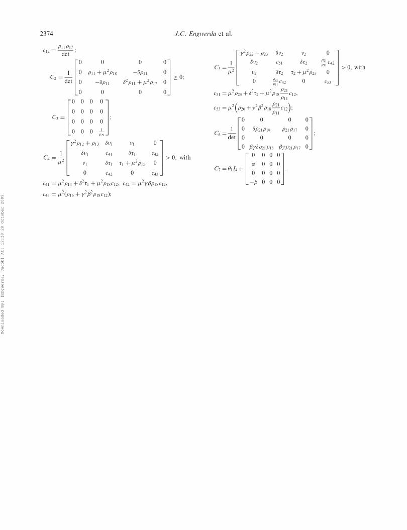
c12 ¼1117det

;

C2 ¼1

det

0 0 0 0

0 11 þ 218 ��11 0

0 ��11 �211 þ 217 0

0 0 0 0

266664377775 0;

C3 ¼

0 0 0 0

0 0 0 0

0 0 0 0

0 0 0 129

266664377775;

C4 ¼1

2

�212 þ 13 ��1 �1 0

��1 c41 ��1 c42

�1 ��1 �1 þ 215 0

0 c42 0 c43

2666643777754 0, with

c41 ¼ 214 þ �

2�1 þ 218c12, c42 ¼

2��18c12,

c43 ¼ 2ð16 þ �

2�218c12Þ;

C5 ¼1

2

�222þ 23 ��2 �2 0

��2 c51 ��22111

c42

�2 ��2 �2þ225 0

0 2111

c42 0 c53

26666437777540, with

c51 ¼ 224þ �

2�2þ218

2111

c12,

c53 ¼ 2�26þ �

2�2182111

c12

;

C6 ¼1

det

0 0 0 0

0 �2118 2117 0

0 0 0 0

0 ���2118 ��2117 0

2666437775;

C7 ¼ �1I4þ

0 0 0 0

� 0 0 0

0 0 0 0

�� 0 0 0

2666437775:

2374 J.C. Engwerda et al.

Downloaded By: [Engwerda, Jacob] At: 12:39 28 October 2009