The numerical inversion of two classes of Kontorovich ... - CORE

ELSEVIER Journal of Computational and Applied Mathematics 61 (1995) 43-72

JOURNAL OF COMPUTATIONAL AND APPUED MATHEMATICS

The numerical inversion of two classes of Kontorovich-Lebedev transform by direct quadrature

Ulf Torsten Ehrenmark Department of CIS, London Guildhall University, 100, Minories, London EC3 N 1JY, United Kingdom

Received 15 September 1993

Abstract

The inversion of the conventional Kontorovich-Lebedev transform with the Macdonald function as kernel and also with a Kelvin function as kernel is considered. Strategies are presented first for computing values of these functions for purely imaginary order (the interior strategy) and these are tested in the subsequent inversion routines (the exterior strategy) which are developed for use where high-speed (mainframe or workstation) computing is available. Both the interior and exterior strategies can exploit the W-transformation and the W-algorithm pioneered by Sidi. It is shown that conventional NAG quadrature software is often incapable of carrying out the inversion without an implementation of this type. Examples considered show that relative error can generally be kept to O(1. D - 8) although for work requiring hundreds of full inversion computations this would have to be relaxed somewhat to obviate the need for overnight computer runs. Application to a divergent inversion integral, summable in the sense of Abel, is made with satisfactory results. A case with weaker summability is also considered with somewhat inferior results.

Keywords: Integral transforms; Helmholtz equation; Macdonald function; Kelvin function; Poincar~ expansion; W- algorithm; NAG routines; Abel summability

1. Introduction

Integral transforms are a common tool for use in constructing solutions of boundary value problems. Over the years numerical methods for evaluating solutions to these problems have slowly evolved from, for example, asymptotic methods such as "steepest descent" [18] to direct quadrature routines only now made possible by the enormous computer power available even to desk-top users. Such routines appear to have become practical around the time when the Fast Fourier Transform was poineered. Even then we have many examples of expansion techniques being given preference to direct methods, e.g., [19] on the numerical inversion of a class of Mellin transforms using Laguerre polynomials or [13] on the inversion of the Laplace transform. Earlier, in 1951, Sneddon pointed out, in the Appendix of [18] that the Filon rule could be used to evaluate some oscillatory-type transform inversions, al though clearly any attempt at a tabulation over a two-dimensional domain was in those days totally impractical.

0377-0427/95/$09.50 © 1995 Elsevier Science B.V. All rights reserved SSDI 0377-0427(94)00052-3

44 U.T. Ehrenmark/Journal of Computational and Applied Mathematics 61 (1995) 43-72

The present author has used direct techniques on the Mellin transform in a number of papers, e.g., [3, 5-1 dealing with water waves in a wedge-shaped domain. The inversion of these transforms, along with say, Fourier and Laplace transforms, can under certain conditions be carried out routinely. That, on the other hand, of, e.g., Mehler-Fock or Kontorovich-Lebedev transforms (KL hereafter) presents a much more substantial problem since the special functions arising in the kernels have to be strategically defined in the routine usually by integral expressions. Moreover these functions often change character on the inversion contour so that different expressions are optimum on different intervals.

In the present work we shall examine the numerical inversion of the KL transform, using direct quadrature techniques. The end result will be a set of routines for tabulating the Macdonald and Kelvin functions [20] together with fully coded routines for carrying out numerically, the inversions of KL transforms using either of these functions as kernel. Readers are welcome to request copies of these routines which are coded in Fortran 77.

Jones [8-1 has pointed out that KL arising from the Helmholtz equation have to be treated differently from those arising essentially in time-dependent problems. Jones wrote

fo f(y)H (y)dy o ( v ) = ) (I.1)

and found that the simple example f = exp( - ay), R(a) > 0 yielded a g for which the associated inversion integral diverged. Meanwhile, Kontorovich and Lebedev [10-1 in one of the earliest papers of a series, had considered solutions to the Helmholtz equation

(V 2 + k2)~k = 0 (1.2)

when the imaginary part of k was negative (the branch of k assumed was in the fourth quadrant). Those authors held a view that physical restrictions would demand that k could not be purely real and the transform was defined by

g ( V ) = e - inv/2 y)H~2)(ky)dy. (1.3)

Indeed, certain contour closure arguments used in that work would be invalid if k was taken purely real. With the function now being even in v it is a straightforward matter to derive the formal KL in the form

f ( y ) = -~ sg(s)sinhrcsKi~(y)ds,

g(z) = r |°°f(x) Ki~(x)dx, (1.4) Jo x

under suitable restrictions. This involves some "rotation" in the u plane. It may be noted that the (intended) failure in Jones' test example is essentially due to the fact that, with k taken as 1, the natural functions occurring are wave-like without dissipation. Thus the example would have worked "better" with R(a) = 0. If the form (1.3) is used, with k purely imaginary, the Helmholtz

U.T. Ehrenmark/Journal of Computational and Applied Mathematics 61 (1995) 43-72 45

equation has a "type change" and the fundamental solutions are exponential. Jones' example, with R(a) > 0 would now produce a convergent inversion integral. Moreover, then, there should be no reason why the strategy proposed by Jones for inverting (1.1) in the difficult cases, could not also be applied to cases of the type (1.3) or (1.4) when the solution demanded is, in the above sense, "out of phase" by ½rt with the natural solution for the equation.

The present author has found [6-1 in considering viscous water waves in a wedge, that the KL type arising falls essentially between the two considered by Jones and Kontorovich and Lebedev (K&L). The diffusive equation of motion gives rise to the field equation

(V 2 - i2)g~ = 0

where ~. is real. This corresponds to the case of zero dielectric constant in the electromagnetic diffraction problem considered by K&L. Because of this, it is Kelvin functions which are the naturally occurring solution in the transform space. A subsequent convergence dilemma in [6] was however resolved by an alternative strategy of subtracting out a number of terms that could be inverted exactly, disregrading the nature of 2 and then establishing independently that these represented valid parts of the required solution.

In pursuing the aims of this paper, we find severe shortcomings in the documentation of computed values of both Macdonald's function Kv(x) and the Kelvin function Kv(xe i~/4) for purely imaginary order. The only tabulations in, for example, Abramowitz and Stegun [1] are of ker and kei, i.e., essentially Kelvin functions of order zero. A major contribution of the present work therefore, is a systematic derivation of a quadrature tool for computing both the said functions with pure imaginary order.

Once sound procedures for computing K~(. ) have been established in Section 2, and these include the derivation of an asymptotic expansion for large v, we develop a routine for inverting the conventional KL transform. This routine, like that for computing K~(. ), relies heavily for speed on the extrapolative theory for oscillatory integrals developed over the last decade or so by Sidi in a series of papers [14-17-1. It is shown that conventional library routines (e.g. NAG library) are not sufficient to deal with the integrals arising in their standard form. Moreover, recent work by K6hler [9-1 on global error improvement by careful choice of free parameters, is shown to have an impact on the computations, particularly for users without access to large numerical libraries. Examples of inversion are examined critically in Section 3 and with double precision work, relative errors are generally kept to the order (1. d - 8).

In Section 4 we deal with the problem of computing Kelvin functions for purely imaginary order. It is found that efficient computation for large s of Kis(. ) for use in the inversion routine, requires the construction of a new integral expression for exp(¼ns). Kis ( • ). This is derived in an appendix and in Section 5 are considered the applications of this integral in a full KL inversion using Kelvin functions. Examples are given for comparison, one of which is a full two-dimensional computation of the solution to a classical problem of periodic thermal diffusion in a wedge-shaped domain and described by Ditkin and Prudnikov [2]. Some insight into the construction of a general "far-field" asymptotic development from the inverse KL is gained from a study of the result of this example.

In Section 6 we discuss briefly the successful application of the inversion tool to a conditionally convergent case and also to a case where the integral diverges but is summable in the sense of Abel. Sidi [14, 16] has shown that extrapolation methods can be used successfully for both of these. Finally, concluding remarks are found in Section 7 where we also consider, speculatively, the

46 U.T. Ehrenmark/Journal of Computational and Applied Mathematics 61 (1995) 43- 72

possibility of using the technique on an inversion which is not summable in the sense of Abel but which is summable in the limiting sense defined by Jones [8] which itself is a generalisation of Abel summability, essentially replacing the Abel convergence factor exp( - et) by exp( - et2).

2. Computation of Macdonald's function for purely imaginary order

Values of K~(x) are given by Watson [20] for a large range of real values of x but only for a very modest range of real values of the order. Values of Kv(x) for purely imaginary v do not appear to be readily available in the literature however and the present objective of numerical KL inversion must be initiated with purposeful strategies for computing values of both Kis(x) and K~s(xx/i ) where (x, s) ~ R 2 . Again, values of ker~(x), [1], are generally only available for purely real v and so these strategies can only be tested for reliable results where v = s = 0, although the ultimate testing is done subsequently when known inverse KL transforms are computed through their use.

In this present section we focus attention on the computation of K~,(x) for real s, x noting that all values on [0, oo [ could be taken by both s and x. The simplest possible useful definition of K~(z) appears to be [11]

K~(z) = foe-~C°Sh'coshvtdt; Re(z) > 0. (2.1)

We have to remind ourselves however, that if z is real,

Ivl/2K~(z)l ,~O{exp(-½rclvl)} as v ~ oo,

when v is purely imaginary [2]. The problem with this is that very often the required KL inversion integral [i~° Kv (z)f(vl)dv converges only conditionally. This implies, of course, that the exponen-

• " / 0 . " . . . . .

tlal decay of K~(z) will be cancelled by exponentially large contributions from f (v I.). This potential source of numerical instability must be avoided, if at all possible, and so we take the alternative definition [11]

Kv( x ) cos(½rcv) = f o cos{x sinh t} cosh vt dt (2.2)

where x > 0, - 1 < Re(v) < 1. This clearly only converges for real x and so cannot be used in computing Kelvin functions.

The transformation

w = sinh t (2.3)

reduces (2.2) to more manageable behaviour particularly for large x;

Kis(x) cosh(½7ts) = f o cos(xw) cos(s sinh- l w) (W 2 "{- 1)- 1/2 dw. (2.4)

U. T. E hr enmar k /Journal of Computational and Applied Mathematics 61 (1995) 43-72 47

Experiments with the QUADPACK routines available on the NAG package indicate problems in computing either of the two forms (2.2) and (2.4) for extreme values of the parameters s and x. Fig. 1 is a scatter diagram representing the extreme values of s, beyond which, for a given value of x, it was impossible to obtain reliable values using the subroutine DOlasf which seemed to be the most appropriate. The points in the diagram show an extraordinary sensitivity to the breakdown value for s (smax) as a function of specified values of x. The EPSABS value (absolute error requested by user) set at 1E - 4 resulted for example in Table 1 (tabulation ofx against s=ax). Safe application can therefore only be made if s < Infx~x sm~(x) where X is the domain of x.

The algebraic decay and the pseudo Fresnel-type behaviour seen in (2.4) however, makes the application of Sidi's extrapolative technique perfectly feasible. In I-15] Sidi extended earlier work to show that with sufficient computing power available, the exact determination of zeros of the oscillatory phases and a precise Poincar6 asymptotic analysis of the non-oscillatory part of the integrand was not necessary. Instead it proved sufficient to "home in asymptotically" on fixed phases of the oscillation and disregard the asymptotic Poincar6 development at the expense of introducing a further few points for the extrapolation procedure. In practice then, we require the asymptotic approximations to a sequence of points of fixed phase of the oscillations, say w~, and we then compute a sequence of finite integrals

~0 ~rt In = ( - )dw. (2.5)

100

80

60

40

20

. . . . . . . . . . . . . . . . . . . i 5 I0 15 20

Fig. 1. Scatter diagram showing the applications relationship between chosen values of x (horizontal axis) and the critical value of s (vertical axis) in the NAG routine DOlas f applied to the integral (2.2).

Table 1

x 6.96 6.99 7.00 7.001 7.1 Sr~a~ 48 81 34 75 81


This so-called "user-friendly transformation" then involves approximating Lim,_. o~ I , by the very elegant W-transformation [14] which is based upon the fact that the sequence ( - )" I, will also have Poincar6 type behaviour w.r.t, the sequence { w, }. The reader is referred to the works [ 14, 15] for a complete description of this now well tested method and the very useful W-algorithm which is exploited comprehensively in the present work.

If Sidi's "user-friendly" approach was taken to its extreme, then since w dominates sinh- 1 w asymptotically as w --. ~ it should be sufficient to compute the w, from x w , = mt (n ~ [~ ). However for small ( x / s ) it may be quite impractical to do this, as the values of w for which the dominance of x w over s sinh - 1 w is established, would be inordinarely large. This could, to some extent, defeat the purpose of the extrapolative exercise which is to reduce significantly the amount of oscillatory integration required. The obvious alternative, which will be used here, is to break (2.4) into two separate integrals with oscillations having phase functions q~+, ~_ where

• + ( x , s ) - x w + s log{w + x/(w 2 + 1)}.

Then (2.4) becomes

2 K i ~ ( x ) c o s h ( ½ ~ s ) = f o (w2 + 1)- 1/2 {COS t~_ Jr COS t~+ } dw = I_ - I+. (2.6)

The treatment by Sidi's transformation of the integral I+ is relatively straightforward but that of I_ is more complicated because of the possible turning point of ~_ at w = w0, where Wo = x / ( s 2 / x 2 - 1). Thus whilst s / x < 1 the behaviour of ~_ is qualitatively similar to that of q~+ and results are comparatively easy to obtain. When s ix > 1 however, this turning point appears and divides the interval [ 0 , ~ [ into two regions: [0,Wo] where the oscillations are mainly controlled by the logarithmic term and [Wo, oo [ where they are controlled by the asymptotically dominant part of ~_ on which the W-transform is to be designed. It is not possible, of course, to commence construction of the Sidi iterates I , until we are beyond this critical value Wo. If s ix >> 1 this can place a considerable burden on the amount of quadrature that has to be done prior to the W-transformation and this quadrature is moreover itself oscillatory. In Fig. 2 are plotted phase functions q~_ for x = 1 and s = 0.1, 1.0, 5, 10, 15 where the features discussed can be easily seen by superposing a set of horizontal lines spaced equally a distance of rt apart, the intercepts of these representing constant points of the various phase functions. Parts of the curves of cos q~_ are also shown for these cases in Figs. 3(a)-(e) and a study of Figs. 3(c)-(e) for example, reveals the two near and far oscillatory zones and a "quieter" intermediate zone of transition which is really a conse- quence of simple interference. Comparison with Fig. 2 confirms that this zone is centred at the turning points of ~_ .

The details of KL inversion computat ions (exterior strategy) are dealt with later in this work, but this being the ultimate objective, it is perhaps prudent to remember at least two important features involved with this computation. The first is that, regardless of the value of x, the KL inversion integral willconverge perhaps only conditionally, so that, for desirable accuracy in the final answer, we are likely to require a very large "truncated" upper limit, with the obvious implication that Ki~(. ) will need to be computable for very large s. This has already been referred to but, secondly, Ki~ is itself oscillatory in the real variable s with a frequency that increases like Ins. The numerical difficulties in the outer (inversion) integral are therefore likely to be equally severe to those

U. T. E hr enmar k /Journal of Computational and Applied Mathematics 61 (1995) 43-72 49

I00

80

(a)

60

40

20

-20

20 4~ ~ 60 / 80

(d)

(e)

. . d ._ 100

W

Fig. 2. Plot of phase functions tk- = w - s l o g { w + x / ( w 2+1)} for (a) s=0.1; (b) s = l ; (c) s=5; (d) s = 10; (e) s = 15.

0 . 5

- 0 . 5

- 1

w

Fig. 3(a). Graph of cos ~_ for s/x = 0.1.

discussed for the inner (present) integral. If the C P U time to compute (2.6) is O ( N ) in double precision we could expect O ( N ~s) for each single precision KL inversion and we could infer O ( N 6) for a two-dimensional tabulation, over a "semi-infinite" rectangular region, of a physical quantity calculated in this way. In practice this would probably be less as the number of "field-points" in

50 U.T. Ehrenmark/Journal of Computational and Applied Mathematics 61 H995) 43-72

0.5 '~ '~

" I r '. i - - W , I/I o

-0 .5 , i q r ~k L 'i

-1 '

Fig. 3(b), (c). Graphs of cos ~_ for (b) s / x = 1 (full) and (c) s / x = 5 (dashed).

°.5I I I I I I I , /

-0.5 /

/t

/ -i

/~ I Ix J t i I

/

'l , 5'0 /

/

/ Fig. 3(d), (e). Graphs of cos4,_ for (d) six = 10 (full) and (e) s/x = 15 (dashed).

any direction should be substantially less than the number of subdivisions required to do the numerical integration. Nevertheless it is quite clear that every opportunity must be taken to minimise the computational effort in the inner integral computing the Macdonald function. The Sidi procedure has already gone a long way in this respect by reducing the amount of oscillatory integration required. With regard to the computat ion of the integrals { I. + 1 - I . } there is another recent advance that can also be put to good use.

In [4] Ehrenmark developed the use of a generalised Simpson rule for numerical quadrature of oscillatory integrals. The rule contained a free parameter, strategic choice of which could optimise the quadrature. In that early work, parameter variation was in some cases chosen so that the trigonometric interpolant would have approximately the local frequency of the function being

U.T. Ehrenmark/Journal of Computational and Applied Mathematics 61 (1995) 43- 72 51

integrated. More recently however, K6hler [91 has shown that a single choice of the parameter can often reduce the global error by O(H 2) where H is the step-length. The present author reported considerable success [6] with an application of K6hler's approach to a problem of the type considered here, relative errors being reduced typically from l d - 3 to l d - 10 by halving step-length while making the K6hler parameter choice. The reader is referred to [6, 9"1 for full details of these procedures. For the present work we state simply that K6hler's routine has been included, wherever practical, in the programs from which the results given here have been computed. In particular, for users without access to NAG or similar routines, the computation of the element integrals (2.6) require the use of K6hler's strategy in order to achieve full KL inversions in a tolerable time.

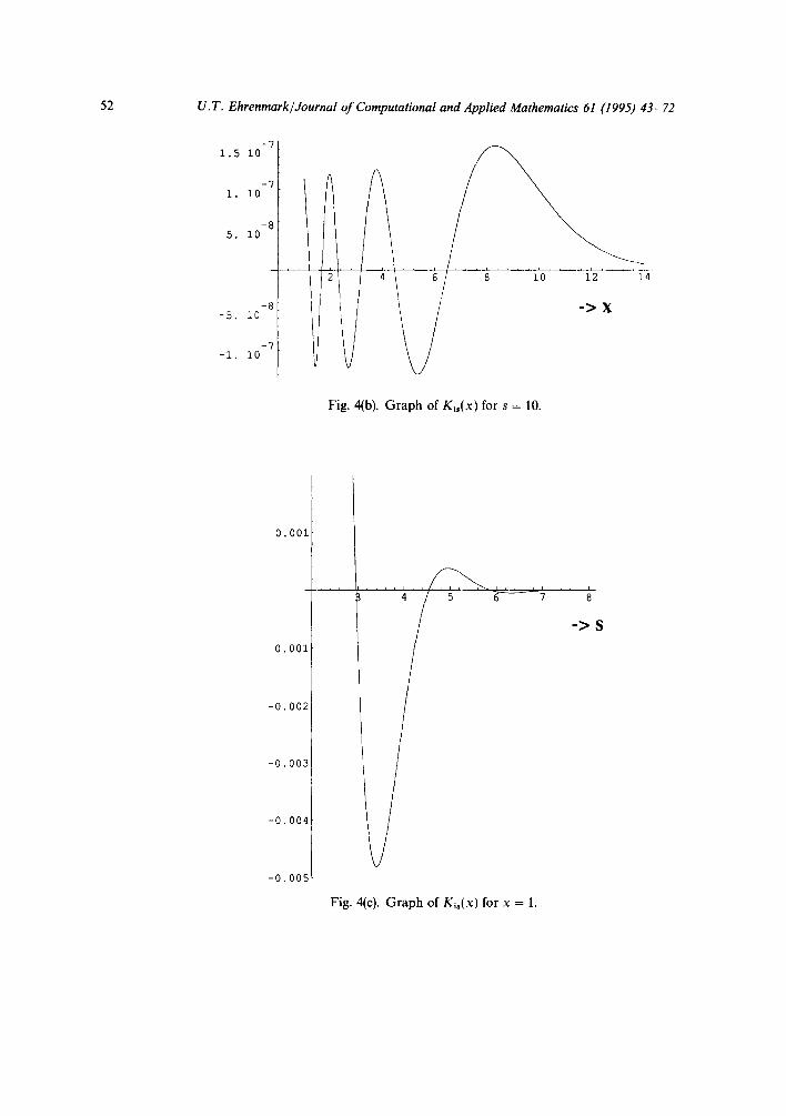
The results of computation of K i(10), K loi(1) and K ~ o i(10) are given in Table 2 and displayed in Fig. 4 are curves of Kis(x). Up to 10 Sidi iterates were used each time, although when s >> x not very many are needed. In Fig. 4(a) s = 1, in Fig. 4(b) s = 10 and in Fig. 4(c) x = 1.

Table 2 Macdonald functions computed by quadrature

Computed Asymptotic value (Eqn. (3.1))

Ki(10) 1 . 6 9 5 0 7 0 D - 5 K10i(1) 1.129456D - 7 1.129476D - 7 Kloi(10 ) 9.824148 D - 8 8.385838D - 8

0.04

0.03

0.02

0.01

2 4 6 8 i0 12 14

- > X

Fig. 4(a). Graph of Kis(x) for s = 1.

52 U. T. Ehrenmark /Journal of Computational and Applied Mathematics 61 (1995) 43-72

-7 1.5 i0

i

-7 i. I0

5. 10 -8

-5. 10 -8 -7

-i. i0

' ~ iq

T -> X

Fig. 4(b). Graph of Ki,(x) for s = 10.

0.001

-0.00

-0. 002

-0.003

-0.004

-0.005

4 / 5 6

Fig. 4(c). Graph of Ki~(x) for x = 1.

7 8

" > S

U. T. Ehrenmark/Journal of Computational and Applied Mathematics 61 (1995) 43- 72 53

Excellent agreement is noted for the middle value where the asymptotic formula is definitely applicable (see Appendix A).

3. Numerical inversion of the conventional Kontorovich-Lebedev transform

Having established a sound procedure for computing values of Kis(x ) where (x,s) ~ R 2 we are now in a position to consider numerical quadrature of the inversion integral (1.1). We shall consider a variety of transforms F(s) which have an exact result available for comparison. If IF(s)l = O{exp[(½rc- 2)s]} as s ~ ~ for some 2 > 0 then (1.1) converges absolutely with exponential decay. Depending on the size of 2, computation could then be relatively straightforward, although Sidi [14] has given examples, which would be of the type where 2 is quite small, where accurate computation requires the use of the W-transform despite the absolute convergence. Moreover, in the examples encountered by the present author in viscous water wave theory I-5] the principal integral for, e.g., wave height on the surface, will often converge only conditionally and the use of the W-transform is essential if a number of these integrals are to be computed in a reasonable time. Also, in these examples, any oscillations in F(s) tend to be slow compared to those in Kis(- ) which accelerate at a rate proportional to In s. Accordingly the W-transformation is nominally based upon fixed phases of Kis rather than F(s). Ki~(. ). This is acceptable on the basis of the "user-friendly" approach presented by Sidi [17] where only the asymptotically dominant part of the phase need be considered. In the exceptional circumstances where F(s) oscillates faster as s ~ ~ (e.g., F(s) ~ cos s 2) it is perfectly straightforward to alter the program coding again with the provison that care is taken to ensure that Wa,W2,... used to compute (2.5) are chosen sufficiently large to reflect this dominance in oscillation.

The numerical work then requires a sequence of points of fixed phase of the oscillation of Kis(x). We would normally assume that x is not inordinately large. If x is very large then the zeros of Kis(X ) a r e approximately x + fltx 1/3 where the fll are zeros ofAi( - 2 1 / 3 f l ) , 1 = 1, 2, ... , see e.g. [11] and Ai is the usual Airy function. Moreover if x is large we would probably wish to use direct asymptotic techniques on (1.1) valid if x>> 1.

In the following therefore, we will use an asymptotic expansion for Ki~(x) valid for x fixed and s >> 1. This expansion appears to be given in the present literature only in very restricted form, the full leading term being given in 1-12] and its modulus in [2]. Watson [19] in the context of discussing Jr(x) for large v and fixed x, remarks that such an expansion is essentially trivial and is therefore not written down. However, as can be seen in Appendix A of the present work, the derivation, albeit trivial, involves a considerable tedium algebraically. We have chosen here to compute terms up to and including O(s-4). The reader is reminded that the restriction on x mentioned above is a purely practical one. In principle x can be as large as we please so long as we then select the w, according to the rule discussed earlier. We find that, with 4~ = x 2,

Kis(x) ,-, x/(2n/s) exp { - (s½~) O1 (s)} cos { Q2 (s)}, (3.1)

where

O, ( s ) = 1 - 2 ~ s - 3 {1 + s -2 (2~ - 1)} (3.2)


and

~r'22(S ) = s log (2s / ex ) -- ¼7[ + s - 1 ( ~ - - ~2) + s - 3 ( - - _.L_360 - - ~ + ½~2)

+ s - 5 ( _ ~ + ~ _ 2 ~ 2 + ½~3). (3.3)

Practically, the w, would have to be selected so that the above form for ~22 dominates its asymptotic error term in s > Wo. A condition which appears to ensure this numerically is Wo >> ~. We shall see below, in examples, that the accuracy of the numerical inversion of (1.1) using the W-transform based on constant values of f22(s) above diminishes with x if we keep either Wo or the number of points N + 1 (Wo, . . . , WN) fixed. Therefore if it becomes impractical, through excessive CPU requirements, to increase either Wo or N when x becomes very large, we must resort to an alternative asymptotic expansion of Debye, Nicholson or Langer type [11] where s and x are considered large together, or use the form x + fltx */a for the asymptotic positions of the zeros of Kis(X) referred to earlier. In the present work we shall generally restrict x to be less than 20 and values of the inversion (1.1) can then be comfortably achieved.

Example 3.1. We first use the strategy described to compute approximations to

fo Kis(x) ds

-9 3. I0

-9 2.5 i0

-9 2. i0

-9 1.5 I0

-9 i. i0

- I ( 5. i0

4 6 8 I0

Fig. 5(a). Graph of absolute error function for the computation in Example 3.1.

-8 3.5 I0

-8 3. i0

-8 2.5 i0

2.10 .8

1.510 .8

-8 I. I0

-9 5. i0 ,,,!

2


, , , J , , , , i . . . .

4 6 8 I0

Fig. 5(b). Graph of relative error function for the computation in Example 3.1 using 15 Sidi iterates at each point of computation.

-7 1. I0

-8 8. i0

6. 10 -8

-8 4. I0

-8 2. i0

f, 1

,/ /

i

2 4 6 8 lO

Fig. 5(c). Computation of relative errors for the computation in Example 3.1 using (i) 15 Sidi iterates (full curve) and (ii) 10 Sidi iterates (dashed curve) at each point of computation.


knowing the exact value of the integral to be ½r~e -x. This example can be done using the NAG routine do l amf for the exterior strategy. We have used respectively, 10 and 15 Sidi iterates for the interior strategy and computations are displayed through Fig. 5. Shown in Fig. 5(a) is the absolute

error computed with 10 Sidi iterates on x [0.5(0.1)10.0]. In Fig. 5(b) is shown the relative error for

Table 3 Sample values of the error f rom the numerical quadra tu re in Example 3.1. N u m b e r of Sidi i terates = 10

x Er ror Cumula t ive funct ion call

0.50 7 . 6 9 6 2 8 9 7 E - 1 0 165 0.60 - 6.1222400E - 09 330 0.70 - 6 . 9 9 7 6 5 4 5 E - 0 9 495 0.80 - 2.5737736E - 09 630

-8 5. i0

-8 2.5 I0

-8 -2.5 i0

-8 -5. i0

-8 -7.5 I0

• ° O 0 0 o • o • O °

e • o O O o O m O o ° • • _ T o O • o O , . . , t - - ' . . . . . . . . ' . . . . t i J ,

4 5 6 • "-7 " •'~ " 9 • o O • •

, ° o

3. i0~9 I . .

2. i0

J '5 ~ '7, ~,,,,,.9 ~o I. I0- , '

-(

io -i.

-2. I0-

, I

lO

0

Fig. 6. Ma in graph: Relative errors for the com pu t a t i on in Example 3.2 using 15 Sidi iterates. Inset g raph shows absolute errors.


the case of 15 iterates and for comparison Fig. 5(c) shows this error for the two cases together. It can be seen from this that some caution should be exercised in specifying the number of Sidi iterates if very large values of s are intended although this choice can easily be automated "on-line" if required. The method clearly works very well overall but it must be remebered that the convergence of the integral is very strong and the actual performance is not easy to assess from this example. Table 3 gives a sample of the data output for the first run and also gives typical number of calls made to the subroutine computing Ki~. The author is unaware of any existing exposure on the present topic, but other authors wishing to consider improved methods, may find this "local function-call" count useful.

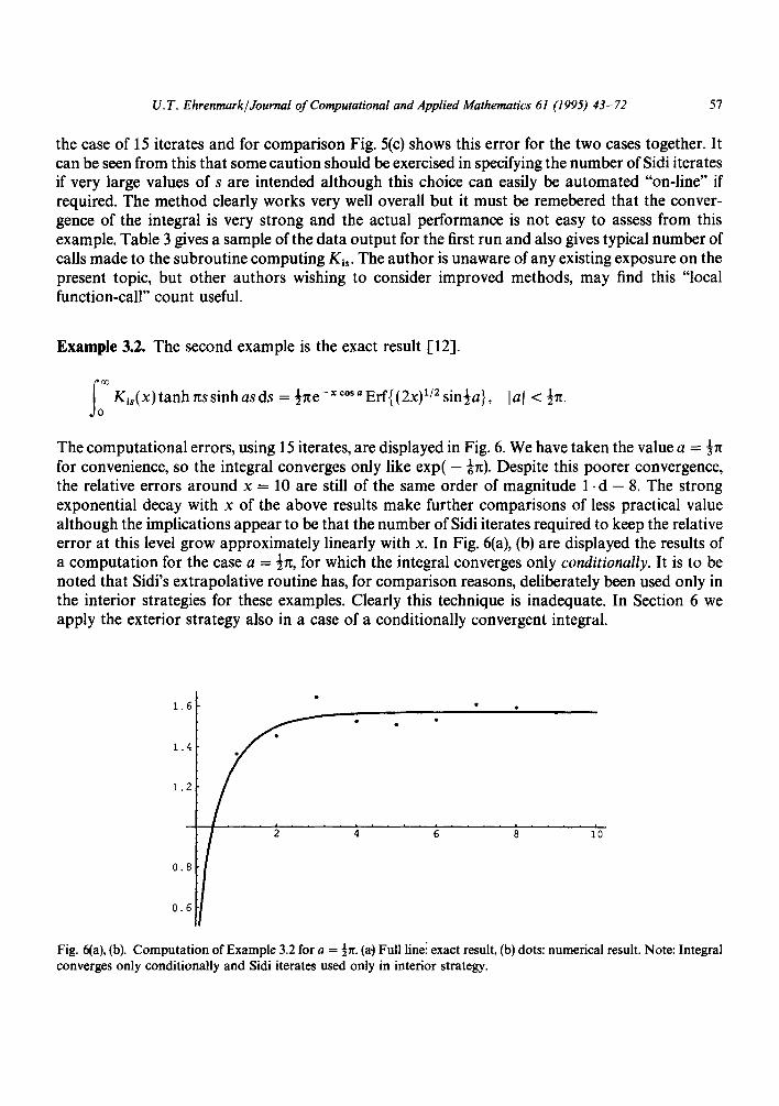
Example 3.2. The second example is the exact result [12].

fo K i , ( x ) t a n h n s s i n h a s d s = ½rce-~°~"Erf{(2x) 1/2 sin½a}, lal < ½n.

The computational errors, using 15 iterates, are displayed in Fig. 6. We have taken the value a -- ½~ for convenience, so the integral converges only like exp( - 16n). Despite this poorer convergence, the relative errors around x = 10 are still of the same order of magnitude 1. d - 8. The strong exponential decay with x of the above results make further comparisons of less practical value although the implications appear to be that the number of Sidi iterates required to keep the relative error at this level grow approximately linearly with x. In Fig. 6(a), (b) are displayed the results of a computation for the case a = ½7t, for which the integral converges only conditionally. It is to be noted that Sidi's extrapolative routine has, for comparison reasons, deliberately been used only in the interior strategies for these examples. Clearly this technique is inadequate. In Section 6 we apply the exterior strategy also in a case of a conditionally convergent integral.

1.6

1.4

1.2

0.8

0.6

S I i ..... I 2 4 6 8

, I

10

Fig. 6(a), (b). Computation of Example 3.2 for a = ½x. (a.) Full linei exact result, (b) dots: numerical result. Note: Integral converges only conditionally and Sidi iterates used only in interior strategy.

5 8 U.T. Ehrenmark/Journal of Computational and Applied Mathematics 61 (1995) 43-72

4. Computation of Kelvin functions for purely imaginary order

As indicated in Section 2, Eq. (2.2) cannot be generalised to compute Kelvin functions which themselves are a generalisation of Macdonald's function with argument ¼re. The formula (2.1) can, on the other hand, be used although we shall see that, in cases where the Kelvin function is to be used as kernel of an inverse Kontorovich-Lebedev transform which converges only conditionally then formulae with properties similar to (2.2) are to be preferred.

Watson [20, p. 182] gives a contour integral expression for Kv(z), namely

2K~(z) = ~cU-V- l exp ( - ½z(u + ! ) }du, (4.1)

where C is a certain contour. Details of C are given in Appendix B where it also shown that the expression can be transformed into the numerically more convenient form

2e ~s/4 Kis(x e i=/4) = f o e-X/2" exp { i(s log u - ½xu)} du u

a result which, in any case, appears to be absent from some of the more usual reference texts, e.g., [1, 19]. The further substitution xu = 2t gives the alternative form

2e~S/4 + is log (x/2) Ki~ ( x e in/4 ) = fO e - x:/4, exp { i( s log u -- u ) } dU,u (4.2)

which is near optimal for the numerical work envisaged. If the domain of s had a positive infimum we could usefully make the further change of variable u = st, however as it is, we are going to require values of the Kelvin function for arbitrarily small s and it would clearly be numerically dangerous to make this general substitution.

It is also noteworthy that, in view of the equality between Kis and K_is we could consider rewriting (4.2) in a form where the phase becomes essentially (s log u + u) and has only one zero for all values of s. This facilitates the numerical quadrature in (4.2). The reader will note however, that such a move would yield an unstable procedure, which respect to a KL inversion where the integrand converges only conditionally. The reasons are similar to those for which (2.2) was preferred to (2.1) in cases where the Macdonald function was used as argument. In its present form (4.2) exploits the exponential decay of Kis without compromising the subsequent inversion. If we make the modification then the revised form of (4.2) will yield results O(e-~s/2) which will then need to be multiplied by large quantities of order O(e ~s/2) when KL is carried out. For this reason we will proceed with (4.2) in its spresent form.

To best exploit the properties of (4.2), let us assume for the moment that s < ¼x 2 and partition the interval of integration into [0, s] w [S, ¼X 2] L.) [¼X 2, ~ [.

The first integral converges exponentially as u ~ 0 and is easily computed by conventional means (e.g., NAG d01amf). This was tested successfully with a relative error (EPSREL) set at 1 .d - 12 for values of x between 0.5 and 20 with s taken as large as 400. Beyond this value for s the value for EPSREL had to be gradually reduced on account of increased rate of oscillation. If s>>(¼x2), however, we would normally use the asymptotic formula,

U. T. Ehrenmark /Journal of Computational and Applied Mathematics 61 (1995) 43-72 59

as d iscussed in Sec t ion 2, a n d it m a y on ly be of a c a d e m i c interes t to no t e tha t exp( - x2/4 u)/u has the requ i red Po i nca r6 series b e h a v i o u r as u --+ 0 to enab le Sidi 's t heo ry to be used for this in tegra l also.

T h e s econd in tegra l is finite a n d osc i l l a tory a n d easi ly c o m p u t e d us ing for e x a m p l e N A G d01akf .

T h e th i rd in tegra l conve rges on ly cond i t i ona l ly a n d m u s t be t r ea ted using e x t r a p o l a t i v e t h e o r y

for r ea sons discussed earlier. T h e r eade r will obse rve tha t the second pa r t i t i on of the a b o v e three was i n t r o d u c e d to ensu re t ha t the osc i l l a to ry a r g u m e n t has no tu rn ing po in t s in the th i rd par t i t ion .

As was seen in Sec t ion 2, the Sidi i tera tes cou ld on ly be c o m p u t e d f r o m a po in t on, where this a r g u m e n t r e m a i n s m o n o t o n i c .

F ina l ly we no t e tha t if s > ¼x 2 we can ins tead use the pa r t i t i on ing

[0,1 2 1 2 4x ] w [ , x , s ] u

Table 4 Sample values of F = Ki~(x(1 + i))

S R e ( F ) Im(F)

x = 0.5(R)00000000000~ 0.2000 0.550342 -0.583877 0.4000 0.541899 -0.538065 0.6000 0.526158 -0.466520 0.8000 0.501175 -0.375928 1.0000 0.465207 -0.274635 1.2000 0.432572 -0.139856 1.4000 0.363089 -0.059874 1.6000 0.291196 0.012997

x = 3.5C00D000000C0000 0.2000 -- 0.012387 0.011151 0.4000 -- 0.012366 0.010965 0.6000 -- 0.012328 0.010658 0.8000 -- 0.012270 0.010236 LO000 - 0.012187 0.009706 1.2000 - 0.012074 0.009079 1.4000 - 0.011925 0.008366 1.6000 - 0.011733 0.007580

x = 10~00000000000000 0.2000 - 0.000009 0.000012 0.4000 - 0.000009 0.000012 0.6000 - 0.000009 0.000012 0.8000 - 0.000009 0.000012 1.0000 - 0.000009 0.000012 1.2000 - 0.000009 0.000012 1.4000 - 0.000009 0.000011 1.6000 - 0.000009 0.000011

-0.02

8

-> $

-0.06

6 8

-0.04

i'0

-0.01

-0.02

-0.03

-0.04

-0.05

-0.06

-0.07

60 U. T. Ehrenmark /Journal of Computational and Applied Mathematics 61 (1995) 43-72

10

- > S

Fig. 7(a). Real (upper) and imaginary (lower) parts of Ki,(x exp(¼in)), x = 2.

not ing only that the case may be s t rengthened for using the extrapolative theory in both the first and third integrals. In the work below we have used it only in the third integral.

Compu ta t ions were under taken to tabulate Kis(xe i~/4) for values 0 ~< s ~< 400 and 0.5 ~< x ~< 20. Only sample ou tpu t is given below in Table 4 but the graphs shown in Figs. 7(a)-(c) for x = 2, 10 and 18 respectively, show the general behaviour of the function and no evidence of the transit ion across domains where the asymptot ic formulae are used instead of the integral computat ions . Here we have selected the asymptot ic formula for large x [20, p. 202] whenever x > 10 and x 2 > 40s, whilst the asymptot ic formula for large s (derived herein) has been applied under the restrictions s > 2 and s > 10x 2. At most 30 terms were taken in the former formula and exactly those terms given were taken in the latter.

-6 -2. 10

. . . . . . . . . 15

-4. 10 -6

-6. 10 -6

-6 -8. I0

U. T. Ehrenmark /Journal of Computational and Applied Mathematics 61 (1995) 43-72 61

-> S

2'0

0.000012

0.00001

8. 10 -6

6. 10 -6

4. 10 -6

2. 10 -6

-6 -2. I0

15

- > S 20

Fig. 7(b). Real (upper) and imaginary (lower) parts of Kis(x exp(¼i•)), x = 10.

A desk-top version of the coding has been written. This implements K6hler's technique and exploits the quadrature formula derived in [4]. Whilst this is adequate for computation of Kis, it will prove to be too slow to use for inversion of the integral transform, especially if a tabulation is required, on all but "Workstation" type machines. The Archimedes 5000 series, for example, would take over a day to achieve 7 significant figure accuracy on a single transform inversion. This aspect is discussed more fully in the next section.

-9 3. i0

-9 2.5 i0

-9 2. i0

-9 1.5 i0

-9 i. i0

-I0 5 . I0

5 ~qo

- > S


20

-9 1.5 i0

-9 I. I0

-I0 5. i0

-> S

Fig. 7(c). Real (upper) and imaginary (lower) parts of Ki,(x exp(¼in)), x = 18.

5. Inversion of the Kontorovich-Lebedev transform with Kelvin function kernel

,We can now use the techniques described earlier to compute full inversions of KL when the kernel is the Kelvin function Kis(xei~/4). In the coding prepared for the two examples considered below we have used the added built-in facility of the asymptotic formula for large x. This helps control the evident growth in the relative error experinced earlier, e.g., in Example 3.2.

A further improvement in the CPU time required has been obtained by starting the Sidi iterates in the outer integral at a lower value of s. The asymptotic formula (A.7) was used to determine the

U. T. E hr enmark /Journal of Computational and Applied Mathematics 61 (1995) 43-72 63

posi t ion of the points of constant phase for Kis but it does not reveal a suitable s-value, from which point on, the behaviour required for the implementa t ion of Sidi's process may safely be used. In Section 3 we took the safe start ing value s = ¼x 2. With the benefit of the hindsight of working with the examples therein and the knowledge that asymptotically, zeros of Kis(x) approach x + f l l x 1/3 as s becomes large, we have experimented here with a starting value of order x. As can be seen below this works perfectly well.

Having set z = xe i~/4 in the formula (A.7) (Appendix A) we obtain the following asymptot ic expansion for large s:

gis(Z) ~-" x/(rc/2s) exp{c lh(s )} exp{i4~2ts)},

where

,1 2r/ ( - l + { t r / 2 ) sTt r / + s 3 s 4 + s s , 45= 4 s

It (X2__~) 1 r/ (T~-6 q- ½r/2) t/ (1--~t6-6 -- l~tr/2) ~2 = ~ + s log -- ~ + ~ s3 s4 s5

and r / = ¼x 2.

Example 5.1. We investigate the error of approximat ion to the exact result,

;o Kis(x e i"/4) ds = ½re exp( - xei"/a).

-8 6. i0

-8 4. i0

-8 2. i0

o • o I I o • . . . . . . . . . . • . . . . . . . . . . . . . . . . Io o eooeoeo • • , . . . . . . . • . . . . . . . . . . . . . . . . . . . . . . . A . . . . . . . . . .m

5 ..... i0 15 2'0

Fig. 8. Relative errors for the computation in Example 5.1 using 10 Sidi iterates.

64 U.T. Ehrenmark/Journal of Computational and Applied Mathematics 61 (1995) 43 - 72

The relative errors in this computat ion are shown in Fig. 8 for the range x [0.5, 20]. The values found are below the ESPREL value set in the coding for the use of the NAG routine D01ajf.

Example 5.2. As a final test of the routines derived, we have taken an example from [2]. The solution to a classical problem of heat conduction in a solid wedge of angle ct is given by the expression for temperature

T = Real { To V exp(kot)},

where t is time, To and co are constants and V is given by

2 [,oo sinh sO V = e z s i n ° + - ~ J0 K i s ( z ) c o s h s ( X 2 r ~ - o O ~ d s , ¼7r<7<a4rc. (5.1)

Here, z = ikr, k 2 = - i~o/a, r and 0 are the usual polar coordinates and T satisfies the equation

a V 2 T = ST~St, (5.2)

together with the boundary conditions, which in terms of V are

V = I o n O = O and V = O o n O = - ~ .

We have achieved a two-dimensional tabulation of the solution (5.1) correct to seven significant digits. It was decided to compute the solution on a mesh in cylindrical polar coordinates for x = 1.5(0.5)20 and 0 = 0 ( - ~ ) - ~. This represents a total of 11 x 38 inversions of the Kon- torovich-Lebedev transform and with the accuracy demand,:~, not surprisingly, took, over a day to

I~ IO,O

I RoOn = 1.0 R I

R•oo•=-.01 ~¢/~(V)=-.001

/

R~oo~=.001 /

Fig. 9(a). Iso-therms for real part of V computed from Eq. (5.1).

U.T. Ehrenmark/Journal of Computational and Applied Mathematics 61 (1995) 43-72

l1.25 Ira(V) = 0 R i10

lm(V) =-.1 im~(~~iV)i.O~/Im(V)l=-,01

Fig. 9(b). Iso-therms for imaginary part of V computed from Eq. (5.1).

65

achieve on the Vax mainframe. Figs. 9(a) and (b) show a graphical construction, from colouring of pixels, of the isotherms at respective times cot = 0 and cot = ½n. Since the variation is harmonic, these two fundamenta l solutions will yield the true solution at any time by addi t ion following mult ipl icat ion with cos cot and sin cot, respectively.

One immediate observat ion from the diagrams is that the solution "in the large" depends on a "vertical" coordinate y = r sin 0. However, near the arm 0 = - c( solutions appear to depend instead on a coordinate perpendicular to that arm, Y = r sin(2c( + 0). This is a very worthwhile observation, for upon not ing the identity

sinh qbscosh (½re - ~0s = sinh 0(scosh(½rc - 2~( + $ ) s - sinh (0( - (k)scosh(½r~ - 20()s (5.3)

we can make a further exact inversion of the K L transform and obtain

2/00 V = e =sin° -- e -zsin(°+2~) + ~ K i s ( Z ) c o s h s ( ½ n - - 2~t) sinh s(Ctsinh s~ + O) ds

in place of (5.1). There are two observations arising. On the one hand we are essentially developing an asymptot ic expansion for large r. On the other hand, the new result is valid in the interval ~in < 0( < ~ , and in part icular therefore we can carry on these arguments and obtain results valid for arbitrarily small ~(. Fo r example, replacing 0( by 20( and 0 by 0( + 0 in (5.3) results in a formula valid in ~ n < o( < ¼n after a further exact KL inversion. The implication in 1-2] that there was a physical l imitat ion on the solution, is thus refuted.


6. Some generalisations

(i) A conditionally convergent inversion integral with Kelvin function kernel. We saw in Example 3.2 that in the case of conditional convergence it was essential to use the W-transformation in the exterior strategy also. This has been done for the example below.

Example 6.1

fo COSh(¼rcr)Ki,(u)dz = ½rce-"/"/5; u = x e i~/4. (6.1)

The absolute error using 6 Sidi iterates in the exterior strategy and 10 in the interior strategy are displayed in Fig. 10(a).

(ii) A divergent inversion inteoral summable in the sense of Abel. In [16] Sidi first established that certain divergent integrals can be computed in the sense of Abel summability. Convincing examples were given also in [17] and in view of the success in the previous example it was decided to examine the application of the technique to an inverse KL which is divergent but Abel summable. The absolute errors in the example below are shown in Fig. 10(b) and illustrate the excellent results that can be obtained with no increase in CPU above that used in Example 6.1.

Example 6.2

foZsinh(¼~xz)Ki,(u) z = 7t 2x/~ue-"/,/~; u = xe ~/4. (6.2)

We are finally led to speculate then, whether even weaker properties can be tolerated with this process. In particular the convergence process defined by Jones 1-8] could be applied, at least

0.00002

0.000015

0.00001

5. i0 -E

• • 0 0 0 . 9 . . . . . . . . . e .

2 4 6 8 I0 12 14

Fig. 10(a). Computation of Example 6.1 showing absolute error. Note: Integral conditionally convergent. Sidi iterates used in exterior and interior strategies.


0.00014

0.00012

0.0001

0.00008

9.00006

0.00004

0.00002

2 4 6 8

8

Fig. 10(b). Computation of Example 6.2 showing absolute error. Note: Integral divergent but Abel summable. Sidi iterates used in exterior and interior strategies.

theoretically, to yield the result

21im e - ~ ' 2 z s i n h ( ½ r c z ) K i , ( u ) d z = u; u = x e i~/4. (6.3) ~--,o Jo

Some remarks relating to results from experiments with this are found in the section below.

7. Concluding remarks

In this work we have highlighted a need for developing a sound numerical strategy to invert two types of KL transforms that frequently arise in physical problems in a wedge-shaped domain. The quest for adequate strategies revealed also that there was a shortage of hard numerical results simply for the evaluation of both the Macdonald function and the Kelvin function of purely imaginary order. Thus routines were devised which could readily compute these for a large range of values of the argument, in particular those ranges for which asymptotic formulae were unreliable or simply not appropriate.

It was also emphasised that integral expressions for Kis(z), to be used in the inversion quadrature, had to be carefully investigated for "stability" in the sense that the exponential decay of Kis(z) as s ~ ~ should not be exploited in cases where the whole of the KL integrand was only of algebraic decay. Here it was shown that for the case where Arg(z) = ¼n (Kelvin function) there was a need for a new integral expression. This was derived and the numerical inversion routine was based upon it. That routine, like the one for the case Arg(z) = 0, was based upon Sidi's extrapolative theory described fully in 1-14, 171.

Various attempts have been made to reduce the time of execution of the numerical inversion. A typical time is about 2 min for one inversion determined correct to six significant digits on the


VAX 6320 although this of course is also governed by the complexity of the rest of the integrand. The figure quoted is an optimum figure based on the inversion in Example 5.2. One difficulty with improving the time is that if EPSREL demands are relaxed in the interior strategy then the adaptive exterior strategy has more difficulty in satisfying its own EPSREL requirements. It is of course the interior strategy that is the most time consuming. The present author has experimented considerably with this trade-off between EPSREL settings in the interior and exterior strategies but has been unable significantly to reduce the essential time taken for a full inversion using the NAG routines described.

It seems that faster implementation will require more sophisticaed treatment. Possibly higher- order generalised Newton-Cotes rules with parameter choice governed by K/Shler's strategy could yield some improvement. Adaptive routines could also be designed more carefully with the specific integrals in mind for the interior strategy. However, for the occasional user, the present package seems to provide a viable option for computing inverses of the Kontorovich-Lebedev transform for both wave and time independent problems whilst at the same time inviting the obvious challenge of deriving faster techniques.

We conclude the main text of this work with some remarks regarding the possible implementation of the W-transformation for an integral summable in the sense of Jones [8] but not in the sense of Abel [17]. Equation (6.3) above is one such example. The experiments performed by the present author indicate that it is possible to achieve the result. In particular for small values of x, results were obtained with a relative error of O(1.E - 2). There were many difficulties however. Some of these may be programming difficulties but most problems seemed to stem from the very large functional and integral evaluation values that arose. Thus, when the formula was tested, e.g., for x = 10 no sensible result was achieved whereas for values of x around 1 it was perfectly possible to get at least a "reasonable approximation" to the result. The reader puzzled by large x having this effect on functional values is reminded that the values of x determine implicitly the starting values of z for which the W-transformation may be implemented.

Sidi has himself implicitly expressed surprise at the range of applicability of the W-transformation. The application has been shown to work for a wide class of functions not covered by the theory and it seems to the present author that just making the simple transformation z 2 = s, the integral in (6.3) is transformed into a type defined by Sidi [17] as being external to the set B. Some of these examples were treated successfully by Sidi and it seems probable that the difficulties with (6.3) experienced herein are more practical than theoretical. Clearly further work and experimenta- tion is required in this area but the range of applications afforded by the W-transformation is clearly quite considerable.

Appendix A

This appendix deals with the calculation of gis(z ) for large values of s2/lzl. As was stated in the text, this is essentially a routine exercise, since the normal series expansion for Iv(z) becomes a Poincar6 expansion for large I uI when z is held fixed. Nevertheless, there does not appear to be any data available in the literature where the coefficients of this expansion are given other than to the leading term. In our work we require this expansion for two reasons. Firstly it is used to compute values of Kis(z) to speed the outer quadrature routine whenever appropriate, but


secondly and more importantly, we use the expression to determine approximately a succession of points on the s-axis giving fixed phases of the oscillations in Kis(z). These are required in the Sidi extrapolations invoked.

We start with the expression [20],

(½z)V 1)fv(z), (A.1) Iv(z) - F(v +

where

(½z)2mr(v + 1) f~(z)= "" m!F(v + m + l) (A.2)

m = O

is a Poincar6 type asymptotic expansion as v --, ~ . Turning f~(z) into an asymptotic power series in v-1 is trivial also. We write ~ = ¼z 2 for convenience and select terms correct to O(v-5). After a further expansion using a Taylor series for Log(1 + z) we get

Now define for convenience,

G(v) = F(v) (½z) -v f_ v (A.4)

so that, in view of the definition of K,(z) by Macdonald [20] we have

2Kv(z) = G(v) + G( - v). (A.5)

Use of Stirling's formula enables us to write

) r - lB2r l°gG(V~V))"(v-½)l°gv- vl°g(½ez) + Z 2r~r 1)v2,_ 1 + l o g f - v (A.6)

x/2~ ,=1 -

where the B2, are Bernoulli numbers. If the last two terms of (6) are expressed as Y,, = 1 ~, v - ' then, in view of (5) we can conveniently write

Kv( z )~ 7 exp - T + Z ~z,v- cos ~ + s + i Z ~,v-" (A.7) r even r odd

although z of course is not necessarily going to remain real. The number of coefficients ~, that are determined is only restricted by the decision to truncate the expansion for Logfv at O(v-5). Comparing coefficients we get

0~5 ~ (1--~60 - - ~ -~- J ~ 2 __ ½ ~ 3 ) ,

having noted the Bernoulli numbers as defined in [7]. From these results we have immediately the results for z real, quoted in this work as Eqs. (3.1)-(3.3).

It is also a straightforward matter to substitute z = x. e ~/4 in the above and obtain similar asymptotic formulae for the Kelvin function. These have been worked out to the above order and are given in Section 5.

70 U.T. Ehrenmark/dournal of Computational and Applied Mathematics 61 H995) 43-72

Appendix B

In this append ix we derive certain express ions for a Kelvin funct ion of purely imaginary order. W e begin with a basic formula given by W a t s o n [20, p. 182-1, namely,

Kv(z)=~ u- exp - ½ z u + du,

where C is a c o n t o u r jo in ing the origin to oo, a sympto t i c to A r g u = fl for small lul and to Arg u = - fl for l ul>> 1. If - n < fl < n we require tha t

- ½ n + fl < Argz <½r~ + ft.

It is p ruden t to examine the convergence. Let us set z = re i°, v = / t + ip. Then if l ul>> 1 the in tegrand is d o m i n a t e d by

l u l - " - x exp { - ½rlul e i~°- a'} d lul.

Thus if 10 - fll = ½r~, we will still have convergence p rov ided # + 1 > 0. O n the o ther hand, if l ul<< 1 the in tegrand is d o m i n a t e d by

' { ----~r e i ~ ° - a ~ d l u l lul-"- exp -- 21ul J

or, if v = 1/lul,

# ' - ' exp { - ½rv~,ii'°-a' } dr.

Thus again, if 10 - fll < -t2n, we have convergence near u = 0 for all v, bu t if 10 - fll = ½n, only if / ~ - 1 < 0 .

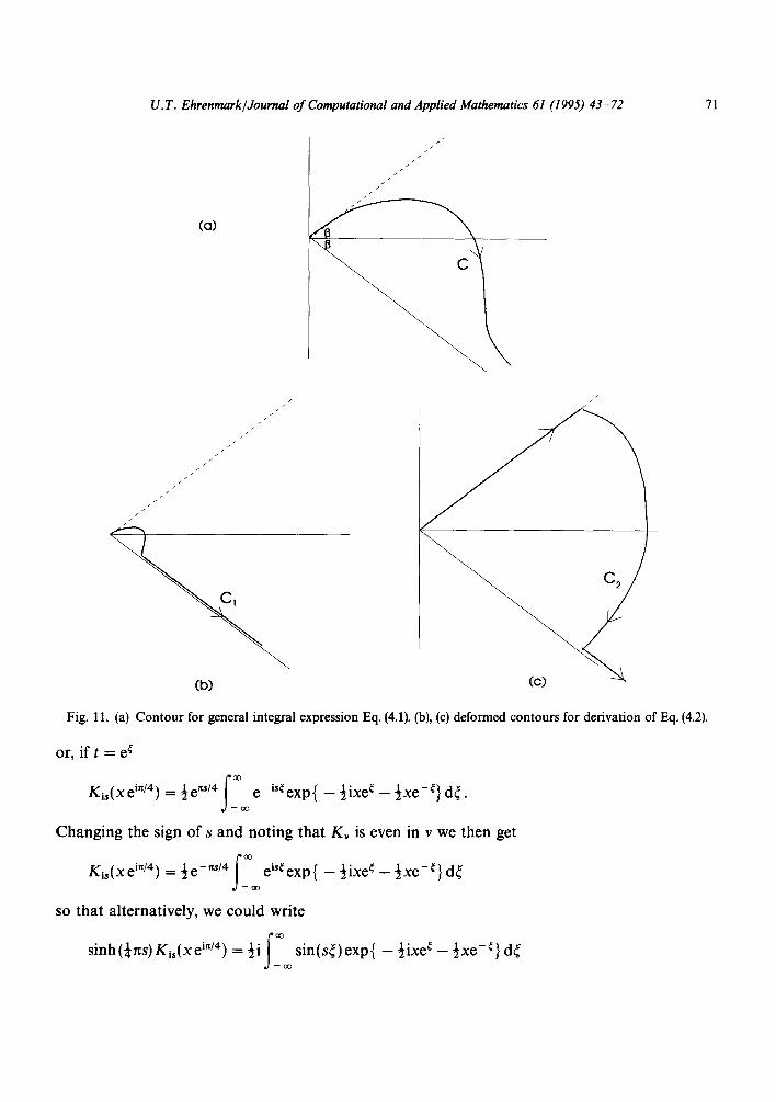
It follows that if [0 - ~bl < ½x for - fl ~< ~b ~< fl then we cou ld dis tor t the c o n t o u r C into either C1 or C2 as s h o w n in the a t t ached d iagram (Fig. 11).

Since the con t r ibu t ions f rom the circular arcs, in bo th cases, can be made as small as we please we can effectively take the integral a long either Arg u = - fl or Arg u = ft. Thus we cou ld do this for unrest r ic ted v if

I/~1 - ½r~ < 0 < ½ ~ - I/~1,

Either sign < can be replaced by ~< p rov ided we restrict # appropr ia te ly . In ou r case s is real, v = is, # = 0 and bo th restr ict ions are au tomat ica l ly satisfied.

Tak ing x > 0, z = xe ~i/4 and choos ing fl = ¼n in the second contour , u = te hi/4 we get

f o ° { ixt X } dt (*) Kis(X e i ' t /4) = ½e ~/4 t- is - 1 exp 2 2t

U.T. Ehrenmark /Journal of Computational and Applied Mathematics 61 (1995) 43-72

i/i// I//~

[o)

(b) (c)

Fig. 11. (a) Contour for general integral expression Eq. (4.1). (b), (c) deformed contours for derivation of Eq. (4.2).

or, if t = e ~

K"(xe'~/4)=½e~s/4f ~- o~ e - i ~ exp{ -- ½ixe~ -- ½xe-¢} d~"

Chang ing the sign of s and no t ing tha t Kv is even in v we then get

Kis(xe i~/4) = ½e -~/4 elS~ exp{ - ½ixe ~ - ½xe -¢ } d~ - - Q O

so tha t a l ternat ively , we cou ld wri te

sinh (~s)K,~(~ e'~") -- ½i ~ sin(s~lexp~ - ½ixe~ - ½xe-~ d~ , / - a o

71


with a similar expression involving cosh, namely

cosh(¼rcs)Kis(xe I~/4) = ½ c o s ( s ~ ) e xp { - ½ixe ~ - ½xe -~} d~. - - 0 0

Of the above, it is Eq. ( • ) which has been used in Section 4, with - s r ep lac ing s.

Re ferences

[ 1] M. Abramowitz and I. Stegun, Handbook of Mathematical Functions (National. Bur. of Standards, Washington DC, 1965).

[2] V.A. Ditkin and A.P. Prudnikov, Integral Transforms and Operational Calculus (Pergamon, Oxford, 1965). [3] U.T. Ehrenmark, Far field asymptotics of the two-dimensional linearised sloping beach problem, SIAM J. Appl.

Math. 47(5) (1987) 965-981. [4] U.T. Ehrenmark, A three-point formula for numerical quadrature of oscillatory integrals with variable frequency,

J. Comput. Appl. Math. 21 (1988) 87-99. [5J U.T. Ehrenmark, A mixed problem for the Biharmonic equation in a wedge with application to dissipating linear

waves on a plane beach, Quart. J. Mech. Appl. Math. 45(3) (1992) 407-433. [6] U.T. Ehrenmark, On computing uniformly valid approximations for viscous waves on a plane beach, J. Comput.

Appl. Math. 50 (1994) 263-281. [7] F.B. Hildebrand, Introduction to Numerical Analysis (McGraw-Hill, New York, 1956). [8] D.S. Jones, The Kontorovich-Lebedev transform, J. Inst. Math. Appl. 26 (1981) 133-141. [9] P. K6hler, On the error of parameter-dependent compound quadrature formulas, J. Comput. Appl. Math. 47(1)

(1993) 47-60. [10] M.J. Kontorovich and N.N. Lebedev, On a method of solutions of some problems of the diffraction theory, J. Phys.

1 (1939) 229-241. [11] W. Magnus, F. Oberhettinger and R.P. Soni, Special Functions of Mathematical Physics (Springer, Berlin, 1966). [12] F. Oberhettinger, Tables of Bessel Transforms (Springer, Berlin, 1972). [ 13] R. Piessens, New quadrature formulas for the numerical inversion of the Laplace transform, BIT 9 (1969) 351-361. [14] A. Sidi• The numerica• eva•uati•n •f very •sci••at•ry in•nite integra•s by extrap••ati•n• Math. C•mp. 3• ( • 58) ( • 982)

517-529. [15] A. Sidi, An algorithm for a special case of a generalization of the Richardson extrapolation process, Numer. Math.

38 (1982) 299-307. [16] A. Sidi, Extrapolation methods for divergent oscillatory integrals that are defined in the sense of summability,

J. Comp. Appl. Math. 17 (1987) 105-114. [17] A. Sidi, A user-friendly extrapolation method for oscillatory infinite integrals, Math. Comp. 51 (1988) 249-266. [18J I.H. Sneddon, The Use of Integral Transforms (McGraw-Hill, New York, 1972). [19] P.S. Theocaris and A.C. Chrysakis, Numerical inversion of the Mellin transform, J. Inst. Math. Appl. 20 (1977)

73-83. [20] G.N. Watson, A Treatise on the Theory of Bessel Functions (Cambridge University Press, Cambridge, 1944).

The numerical inversion of two classes of Kontorovich ... - CORE

Documents

Transcript of The numerical inversion of two classes of Kontorovich ... - CORE