The MultiRISK platform: The technical concept and application of a regional-scale multihazard...
17
The MultiRISK platform: The technical concept and application of a regional-scale multihazard exposure analysis tool M.S. Kappes a, ⁎, K. Gruber a, b , S. Frigerio a, c , R. Bell a , M. Keiler a, d , T. Glade a a University of Vienna, Geomorphic Systems and Risk Research Unit, Universitätsstraße 7, 1010 Vienna, Austria b Johannes Kepler University Linz, Altenberger Straße 69, 4040 Linz, Austria c C.N.R., I.R.P.I., C.so Stati Uniti, 4, 35127 Padova, Italy d University of Bern, Institute of Geography, Hallerstrasse 12, 3012 Berne, Switzerland abstract article info Article history: Received 24 July 2011 Received in revised form 28 January 2012 Accepted 29 January 2012 Available online 3 February 2012 Keywords: Multihazard risk Modeling software Web-mapping Barcelonnette Many regions worldwide are threatened by multiple natural hazards with the potential to cause high dam- ages and losses. However, the modeling of multiple hazards in a joint analysis scheme is still in the early stages of development as a range of serious challenges emerges in the multihazard context such as differing modeling approaches in use for contrasting hazards; the time- and data-demanding conduct of each single preparative, intermediate and analysis step; and the clear visualization of the modeling outcome. Under con- sideration of these difficulties, a regional multihazard exposure analysis concept is developed for five natural hazards: debris flows, rock falls, shallow landslides, avalanches, and river floods, complemented by a visual- ization scheme to present the modeling outcome. An automation of the two schemes resulted in a beta ver- sion of the MultiRISK modeling and the MultiRISK visualization software tool forming together the MultiRISK platform. To test the analysis scheme and the software implementation of MultiRISK a case study is per- formed in the Barcelonnette basin in France with a worst-case parameterization of the models on the basis of extensive literature reviews. Experiences from this case study offered many insights into the multihazard topic and even more questions, e.g. with respect to coherent multihazard model parameterization, validation or the comparability and interpretation of single-hazard modeling results, respectively. Although analysis schemes can be proposed and software tools can be provided to facilitate many steps, a well-conceived and reflective approach to multihazard settings is essential. The worst-case analysis based on literature values apparently leads to an overestimation of the susceptible areas and the number of exposed elements. Nevertheless, depending on the data situation of an area, especially in areas without any information on past events, this approach may offer the determination of general hazard distributions, overlaps, and areas of potential risk without data-demanding calibration. © 2012 Elsevier B.V. All rights reserved. 1. Introduction Many areas of this world – as for example coastal zones, moun- tainous regions, or volcano vicinities – are threatened by multiple natural hazards. However, natural hazards are usually still examined and managed separately. Only in a few studies are multiple threats analyzed jointly and the overall hazard and/or risk are assessed, e.g. by van Westen et al. (2002), Bausch (2003), Bell and Glade (2004), Glade and van Elverfeldt (2005), Reese et al. (2007), Bründl et al. (2009), or Marzocchi et al. (2009). Considering a joint analysis of multiple hazards, numerous challenges and difficulties arise (Kappes et al., in review): (i) hazards are not directly comparable as their characteristics and their describing metrics differ, for instance inundation depth of floods versus impact pressure of rock falls. More- over, various hazard types act at very differing spatial and temporal scales. While rock falls are very local phenomena with an often high frequency of smaller events, earthquakes are regional scale processes with mostly low frequency but high magnitude. Furthermore, (ii) the analysis methods and models used for distinct hazards also diverge widely with respect to inherent assumptions and model principles. These differences complicate the comparability of analysis results (Kappes et al., 2010). Apart from the challenges concerning the com- parability of modeling results, another major issue is (iii) the perfor- mance of such an analysis since knowledge and experience in many different disciplines is required. Moreover, (iv) the data acqui- sition and the preparation as well as the modeling and assessment of hazards, exposure (elements at risk/vulnerability) and risk for single- hazard procedures consist of a large number of different analysis steps that are complicated and thus time-consuming and prone to Geomorphology 151–152 (2012) 139–155 ⁎ Corresponding author at: The World Bank, 1818 H St. NW, Washington, DC 20433, USA. E-mail address: [email protected] (M.S. Kappes). 0169-555X/$ – see front matter © 2012 Elsevier B.V. All rights reserved. doi:10.1016/j.geomorph.2012.01.024 Contents lists available at SciVerse ScienceDirect Geomorphology journal homepage: www.elsevier.com/locate/geomorph
Transcript of The MultiRISK platform: The technical concept and application of a regional-scale multihazard...

Geomorphology 151–152 (2012) 139–155
Contents lists available at SciVerse ScienceDirect
Geomorphology
j ourna l homepage: www.e lsev ie r .com/ locate /geomorph
The MultiRISK platform: The technical concept and application of a regional-scalemultihazard exposure analysis tool
M.S. Kappes a,⁎, K. Gruber a,b, S. Frigerio a,c, R. Bell a, M. Keiler a,d, T. Glade a
a University of Vienna, Geomorphic Systems and Risk Research Unit, Universitätsstraße 7, 1010 Vienna, Austriab Johannes Kepler University Linz, Altenberger Straße 69, 4040 Linz, Austriac C.N.R., I.R.P.I., C.so Stati Uniti, 4, 35127 Padova, Italyd University of Bern, Institute of Geography, Hallerstrasse 12, 3012 Berne, Switzerland
⁎ Corresponding author at: The World Bank, 1818 H SUSA.
E-mail address: [email protected] (M
0169-555X/$ – see front matter © 2012 Elsevier B.V. Aldoi:10.1016/j.geomorph.2012.01.024
a b s t r a c t
a r t i c l e i n f oArticle history:Received 24 July 2011Received in revised form 28 January 2012Accepted 29 January 2012Available online 3 February 2012
Keywords:Multihazard riskModeling softwareWeb-mappingBarcelonnette
Many regions worldwide are threatened by multiple natural hazards with the potential to cause high dam-ages and losses. However, the modeling of multiple hazards in a joint analysis scheme is still in the earlystages of development as a range of serious challenges emerges in the multihazard context such as differingmodeling approaches in use for contrasting hazards; the time- and data-demanding conduct of each singlepreparative, intermediate and analysis step; and the clear visualization of the modeling outcome. Under con-sideration of these difficulties, a regional multihazard exposure analysis concept is developed for five naturalhazards: debris flows, rock falls, shallow landslides, avalanches, and river floods, complemented by a visual-ization scheme to present the modeling outcome. An automation of the two schemes resulted in a beta ver-sion of the MultiRISK modeling and the MultiRISK visualization software tool forming together the MultiRISKplatform. To test the analysis scheme and the software implementation of MultiRISK a case study is per-formed in the Barcelonnette basin in France with a worst-case parameterization of the models on the basisof extensive literature reviews. Experiences from this case study offered many insights into the multihazardtopic and even more questions, e.g. with respect to coherent multihazard model parameterization, validationor the comparability and interpretation of single-hazard modeling results, respectively. Although analysisschemes can be proposed and software tools can be provided to facilitate many steps, a well-conceivedand reflective approach to multihazard settings is essential. The worst-case analysis based on literaturevalues apparently leads to an overestimation of the susceptible areas and the number of exposed elements.Nevertheless, depending on the data situation of an area, especially in areas without any information onpast events, this approach may offer the determination of general hazard distributions, overlaps, and areasof potential risk without data-demanding calibration.
© 2012 Elsevier B.V. All rights reserved.
1. Introduction
Many areas of this world – as for example coastal zones, moun-tainous regions, or volcano vicinities – are threatened by multiplenatural hazards. However, natural hazards are usually still examinedand managed separately. Only in a few studies are multiple threatsanalyzed jointly and the overall hazard and/or risk are assessed, e.g.by van Westen et al. (2002), Bausch (2003), Bell and Glade (2004),Glade and van Elverfeldt (2005), Reese et al. (2007), Bründl et al.(2009), or Marzocchi et al. (2009). Considering a joint analysis ofmultiple hazards, numerous challenges and difficulties arise(Kappes et al., in review): (i) hazards are not directly comparable as
t. NW, Washington, DC 20433,
.S. Kappes).
l rights reserved.
their characteristics and their describing metrics differ, for instanceinundation depth of floods versus impact pressure of rock falls. More-over, various hazard types act at very differing spatial and temporalscales. While rock falls are very local phenomena with an often highfrequency of smaller events, earthquakes are regional scale processeswith mostly low frequency but high magnitude. Furthermore, (ii) theanalysis methods and models used for distinct hazards also divergewidely with respect to inherent assumptions and model principles.These differences complicate the comparability of analysis results(Kappes et al., 2010). Apart from the challenges concerning the com-parability of modeling results, another major issue is (iii) the perfor-mance of such an analysis since knowledge and experience inmany different disciplines is required. Moreover, (iv) the data acqui-sition and the preparation as well as the modeling and assessment ofhazards, exposure (elements at risk/vulnerability) and risk for single-hazard procedures consist of a large number of different analysissteps that are complicated and thus time-consuming and prone to
140 M.S. Kappes et al. / Geomorphology 151–152 (2012) 139–155
mistakes. However, re-running the analysis repeatedly would be de-sirable in order to evaluate, e.g., the effect of management optionsor to consider changes in land use, in the climate, in the general envi-ronmental setting, or in alterations of the elements at risk (Dai et al.,2002; Fuchs and Keiler, 2006; Slaymaker and Embleton-Hamann,2009).
A possible approach considering these challenges is the selectionof methods according to previously defined criteria, and their subse-quent merging in one software tool in which preparative and inter-mediate steps are automated. Such a procedure leads to comparablesingle-hazard results since the single hazards are analyzed accordingto a coherent analysis scheme, and result in a higher time and effortefficiency for the user by automatically performing purely elementarysteps. Although still expert input from different disciplines is neededto calibrate the models, profound knowledge on existing methodsand models for the choice of the approaches is not necessarily re-quired as they are included in the software tool. Current pioneer ap-proaches include HAZUS in the USA (Schneider and Schauer, 2006;FEMA, 2008), that offers hurricane, earthquake and flood hazardand risk modeling. RiskScape in New Zealand (Reese et al., 2007) fa-cilitates currently volcanic ashfalls, floods, tsunamis, landslides,storms, and earthquakes. CAPRA (Central America Probabilistic RiskAssessment) provides the analysis of hurricanes, heavy rainfalls, land-slides, floods, earthquakes, tsunamis, and volcanic hazards(CEPREDENAC et al., 2010). Such tools enable user-friendly andstraightforward performance of multihazard analyses and compara-bility between single hazards, furthermore their widespread and re-peated use also guarantees comparability between results ofanalysis from different municipalities or departments and betweenanalysis results over time.
A final issue in the multihazard context is the huge data require-ment. Extensive and qualitatively high standard inventories of pastevents – including detailed spatiotemporal patterns, particularlywith an equivalent standard for multiple hazards – are rare. In mostregions huge differences in quality and dimension exist between thesingle-hazard inventories — if records of past events are available atall. Furthermore, the more detailed the models, the more detaileddata on topography, geology, soils, land use, precipitation distribu-tion, etc. is required. A possibility to partly overcome these con-straints is a top-down approach. Thereby, a simple and fast analysisapproach at a small scale provides an approximation. In a next step,more detailed and sophisticated (and thus also more data-requiring) methods at a larger scale are applied. By using the small-scale modeling results to define those areas for which detailed studieshave to be carried out, resources can be utilized very efficiently.
Under consideration of the previously mentioned challenges, theMultiRISK platform has been designed. This software is projected tooffer the analysis of multihazard risk according to a top-down ap-proach, in relation with a visualization tool to display the results. Inthe current version of MultiRISK, the GIS-based regional-scale suscep-tibility and exposure analysis (elements at risk) is completed(1:10,000–1:50,000) for the typical mountain hazards avalanches,debris flows, rock falls, shallow landslides, and river floods. In thenext step detailed vulnerability considerations and risk analyses at ascale b1:10,000 will be implemented (cf. Kappes et al., 2011b for afirst attempt regarding vulnerability in the context of multihazardrisk). Therefore, the name MultiRISK platform is chosen althoughuntil now only susceptibility/hazard and exposure analysis can becarried out by applying the current version of the tool while thevulnerability of elements is not taken into consideration so far. Theapplied scale levels correspond to the approaches used in severalalpine countries such as Germany, France and Switzerland withhazard indication maps (Gefahrenhinweiskarten) at the scale1:10,000–1:25,000 and the hazard zone plans b1:10,000 (Stötter etal., 1999). Thereby, the hazard indication maps comprise an overlayof susceptibility maps and elements at risk and provide a first
approximation, while hazard zone plans offer a level of detail thatallows decision making to reduce risks.
In this article, the development of the regional scale analysis ofMultiRISK and the resulting methods and software will be presentedtogether with the performance of a multihazard exposure analysiscase study in the Barcelonnette basin, France. First, the analysisscheme for hazard modeling with well-available data used as input,hazard model validation, and exposure analyses is presented inSection 2. Thereafter, a visualization scheme to display and communi-cate the results in a well-structured way is outlined in Section 2.4.The analysis scheme is automated in a user-friendly software(Section 3.1). The visualization outline is implemented into a visuali-zation tool to present the results automatically in a web browser in-terface (Section 3.2). In order to test the developed MultiRISKmodeling and visualization tools, they are applied in the Barcelonn-ette basin (Section 4). Finally, the challenges and specifics in amultihazard setting are discussed in Section 5 based on the insightswhich emerged during the development and implementation of theanalysis scheme and of the MultiRISK platform.
The definition of key terms differs between scientists as well asbetween disciplines and processes. This has become evident whenworking in the field of multihazards and risks. In this contributionthe definition of hazard (in the general and technical context) and ex-posure are used according to UN-ISDR (2009b), and susceptibilityconsidering Guzzetti et al. (2005, p. 277). The term risk is based onthe definition of WMO (1999, p. 2) and the social dimension of risk(e.g., Wisner et al., 2004) is not addressed in this contribution.
2. Development of a regional-scale analysis and visualizationscheme of multihazard exposure
The multihazard risk analysis scheme proposed in the presentstudy follows a top-down approach in which a regional exposureanalysis provides the identification of hazard distributions, hazardoverlaps, and zones of potential damages and losses. Subsequently,detailed, local hazard and risk analyses on the basis of more sophisti-cated models are to be carried out for the previously defined points.In the present study, however, only the regional-scale exposure anal-ysis scheme is outlined and its implementation into a software tool ispresented, while the local-level analysis will be elaborated in futureworks and only its function is defined here.
The regional exposure analysis is composed of three components:the hazard modeling, the validation of the modeling results, and theexposure analysis. These will be explored in the following sections.
2.1. Hazard modeling
The first step in a multihazard top-down approach offers a region-al approximation by means of fast and simple methods. As explainedbefore, the data need for multihazard analyses is, in general, a limitingfactor. Consequently, the availability of input data is a major criterionfor the model choice and determines significantly the tool's applica-bility. For GIS-based models, input refers to two types of information:(i) areawide information, i.e. information layers (e.g., elevation, landuse or geology) and (ii) information to calibrate or parameterize themodel, e.g. inventory data, soil properties, and precipitation or dis-charge time series.
(i) Topographic characteristics, derived from digital elevationmodels (DEM), are usually the most important spatial inputdata for GIS-based modeling of natural hazards. This in-formation is already available in many regions of the worldor can be produced with acceptable effort from topographicmaps, satellite imagery, and laser scanning. From the DEM, avariety of derivatives such as slope angle, curvature, aspect,or distance to ridge/drainage line can be deduced. Mountain

Fig. 1. Coupled consideration of slope angle and upslope area for debris flow modeling(Horton et al., 2008). Below an upslope area of 2.5 km2, the slope angle to start themovement is rising with decreasing area, while above 2.5 km2 it is assumed to be con-stant at 15°. Reasons for this approach are the difference in water and sedimentavailability.
141M.S. Kappes et al. / Geomorphology 151–152 (2012) 139–155
hazards are particularly coupled with topographic characte-ristics and therefore these data are highly valuable for anymodel. Consequently, the regional analysis is primarilybased on the DEM including its derivatives, and the requiredmodels to be chosen have to be operable with this topographicinput.To optionally extend the topographic information, additionaldata such as land use/cover were implemented. These data arerather easy to create, for example, from remote sensing imagesor, in coarse resolution, as free image sharing from GoogleEarth.Furthermore, lithological information is included into themodel-ing approach as geological maps exist in many countries and re-gions and the lithology and tectonic lineaments influence manynatural hazards significantly.
(ii) The second criterion for the model choice is the straightfor-wardness of the model calibration/parameterization (in thisarticle calibration is understood as the process of adjustmentof a model to measured data, while parameterization refersto expert appraisal or adoption of parameters used in otherstudies). Models with indispensible need of data from field orlaboratory analyses, time series, or extensive inventories donot fit the objective of a simple and fast first approximationof an area. The models have to be straightforward and com-prehensive to enable a flexible calibration on the basis ofdetailed information, if available. For cases of low data avail-ability, the objective is to choose models that allow completionwith expert knowledge or even parameterization exclusivelywith expert experience or studies carried out in comparablesettings.
Furthermore, only models developed for a regional scale(1:10,000–1:50,000) were selected to ensure, as far as possible in amultihazard environment, the comparability of the results. Apartfrom these criteria, the model choice is open and the models selectedhere can be exchanged by other suitable ones (concerning scale, datainput needs etc.). In the current version of MultiRISK, the processes ofsnow avalanches, shallow landslides, debris flows, rock falls, andriver floods are considered. The different selected models and themethodology of their implementation are presented in the followingsections.
2.1.1. Debris flowsThe source identification is carried out with the Flow-R model
(Horton et al., 2008, 2011). This model is based on the three topo-graphic parameters slope angle, upslope area, and planar curva-ture. These parameters represent directly (slope) or indirectly(upslope area and planar curvature) three major factors for debrisflow disposition (Takahashi, 1981; Rickenmann and Zimmermann,1993): slope gradient, sediment availability, and water input.Upslope area and planar curvature serve as indicators for theconvergence of sufficient water and material in gully structures.Upslope area is considered in combination with slope anglebecause in smaller catchments, less material is accumulated andmore water from steeper slopes is needed to enable the debrisflow initiation. In contrast, larger catchments are supposed toaccumulate higher volumes of sediment and water that start movingat lower angles (Fig. 1).
Additionally, certain land use/cover types and lithologicalunits can optionally be excluded. For example, dense forest influ-ences surface runoff and buildup areas or outcropping rocksdetermine material availability. For more details on Flow-R, refer toHorton et al. (2008, 2011), Blahut et al. (2010) and Kappes et al.(2011a).
For the runout modeling, again the methodology proposed inFlow-R has been applied. The spreading of the flow is computedwith the multiple flow direction algorithm according to Holmgren
(1994), an expansion of the basic multiple flow direction algorithmdeveloped by Quinn et al. (1991):
f i ¼tanβið Þx
∑8j¼1 tanβj
� �x for all tanβ > 0 ð1Þ
where i,j=flow direction (1–8), fi=flow proportion (0–1) [%] in di-rection I, tan βi=slope gradient between the central cell and cell indirection I, and x is an exponent introduced by Holmgren (1994).For x=1, the algorithm converts into the basic multiple flow direc-tion after Quinn et al. (1991), and for x→∞, into a single flow. Thespreading is complemented by a persistence function. This functionaccounts for the inertia of the flow by a weighting of the change ofangle from the last flow direction. For 0°, a weight of 1 is assigned,for 45° 0.8, for 90° 0.4, for 135° and for 180° 0. The distance of therunout is computed with a constant friction loss angle, thus not con-sidering the surface roughness. This angle corresponds to the Fahr-böschung of Heim (1932), translated as angle of reach by Corominas(1996), which refers to the angle between a line from the highestpoint of the source area to the maximum runout and the horizontal.In Flow-R the angle is applied as a constant loss variable in an ener-getic computation while the flow propagates from pixel to pixel(Horton et al., 2008):
Eikin ¼ Ei−1kin þ Eipot−Eiloss ð2Þ
with the time step i, the kinetic energy Ekin, the change in potentialenergy ΔEpot, and the constant loss Eloss. The flow stops as soon asthe kinetic energy drops below zero. At the overlap of the flowsfrom different sources, the maximum value of the spatial probabilitythat this pixel might be hit and the maximum kinetic energy of alloverlapping flows are calculated.
Two runout calculation modes are offered: quick and complete. Inthe complete mode, each single source pixel is propagated. In thequick models, first the superior sources are propagated. If lowerones follow the same path with a similar or lower kinetic energy,they are neglected. This reduction of single calculations enables sig-nificant time saving.
2.1.2. Rock fallsA commonly used method for automatic rock fall source identifi-
cation is the classification of the slope gradient map. Hereby, a thresh-old angle is defined above which the area is identified as potentiallyrock fall producing rock face (Ayala-Carcedo et al., 2003; Guzzetti et

142 M.S. Kappes et al. / Geomorphology 151–152 (2012) 139–155
al., 2003; Jaboyedoff and Labiouse, 2003; Wichmann and Becht, 2006;Frattini et al., 2008). As already described for the debris flow sourcemodeling, specific land use/cover and lithological units, e.g., outcrop-ping marls, can also be excluded as potential rock fall source areas. Asfor debris flows, the runout is modeled by means of the Flow-R modelaccording to Horton et al. (2008).
2.1.3. Shallow landslidesIn contrast to the processes treated until now, areas susceptible
to shallow landslides are usually analyzed with statistical and physi-cally based methods rather than with empirical models. However,statistical models are commonly not easy to transfer, and physicallybased models require a high quantity of geotechnical input data andthus are also not suitable for a regional approach. Nevertheless, a va-riety of physical models were adjusted to the input of information de-rived from DEMs. Because topographic characteristics control waterconfluence, downslope forces, etc. this effort proved to be successfulas multiple models indicate, e.g. SLIDISP of Liener and Kienholz(2000), SHALSTAB of Montgomery and Dietrich (1994) and Dietrichand Montgomery (1998), or SMORPH of Shaw and Johnson (1995).Among these methods, SHALSTAB (SHAllow Landsliding STABility;Montgomery and Greenberg, 2009) was selected because it offersthe option to compute a first approximation of an area without theneed of detailed calibration. The slope stability package afterMontgomery and Greenberg (2009), which refers to SHALSTAB, waschosen because it can be directly included as a toolbox in ArcGIS9.x, while the original version of Dietrich and Montgomery (1998)is an ArcView 3.x application. SHALSTAB couples a “hydrologicalmodel to a limit-equilibrium slope stability model to calculate thecritical steady-state rainfall (Qc) necessary to trigger slope instabilityat any point in a landscape” (Montgomery et al., 1998, p. 944). Undernegligence of soil cohesion, the following equation emerges(Montgomery and Dietrich, 1994; Montgomery et al., 1998):
Qc ¼T sinθa=b
ρs
ρw1− tanθ
tanϕ
� �� �ð3Þ
with the soil transmissivity T [m2/d], the hillslope angle θ [°], thedrainage area a [m2], the outflow boundary length b [m], the soilbulk density ρs [kg/m3], the water bulk density ρw [kg/m3], and theangle of internal friction ϕ [°]. By using a “single set of parametervalues” (ρs, ϕ and ρw are constants) plus the areawide DEM deriva-tives (a, b and θ) the “regional influence of topographic controls onshallow landsliding” can be assessed without any specific calibration(Montgomery et al., 1998, p. 943). Dietrich and Montgomery (1998)explained that SHALSTAB was not performing well in areas dominat-ed by rocky outcrops or cliffs. Hence, an option is included to option-ally exclude, e.g., limestone outcrops and other lithological units aspotential sources.
Although much less used, the angle of reach principle can alsobe applied for the runout calculation of shallow landslides (e.g.,Corominas et al., 2003), and thus the Flow-R model was applied inthis case as well.
2.1.4. AvalanchesMaggioni and Gruber (2003) developed a methodology for the de-
termination of potential release areas primarily based on topographicparameters that was simplified by Barbolini et al. (2011). This meth-odology applies the following criteria: For avalanche initiation, acertain minimum slope angle is necessary to enable the movement;however, very steep slopes will not accumulate enough snow foravalanche formation. Thus, avalanches can be expected at slopesbetween a lower and an upper threshold angle. Specific land usetypes, especially dense forest that will stabilize the snow pack in therelease area, can be excluded as potential sources as well as ridgeswhere too little snow accumulation can be assumed.
For the computation of the avalanche runout, apart from the angleα, which corresponds to the angle of reach, further angles are in use:β is the angle of the avalanche track between the source and the pointof the slope with 10° (β point), and δ is the average angle of therunout zone between the β point and the stopping point of the ava-lanche (Bakkehøi et al., 1983; Keylock, 2005). To keep the metho-dology simple, the angle of reach (equivalent to the angle α) waschosen, and runout calculation is performed by means of Flow-R aswell.
2.1.5. FloodsThe simplest method to estimate floodplain inundations is the lin-
ear interpolation of a gauge water level in intersection with a DEM(Apel et al., 2009). Models representing hydrodynamic characteristicssuch as HEC-RAS (US Army Corps of Engineers, 2011), Sobek(Deltares, 2011), and others need more detailed information on chan-nel geometry and roughness, hydrograph information, etc. The ArcGISextension FloodArea of Geomer (2008) offers both methods: model-ing on the basis of a certain inundation depth or by means of a hydro-graph and several more options. In the modeling scheme of theMultiRISK software both options were included to offer a choicedepending on the quantity and type of data available for the modelcalibration/parameterization.
The combination of the previously described single-hazard modelsto one overall analysis scheme is challenging. However, it is evidentthat different natural hazard models require similar data, and thereforethe combination of these models in a multihazard analysis provides amajor advantage in order to gain synergies and consequently time-savings in a joint study. The flow chart of the resulting model setup ispresented in Fig. 2.
2.2. Validation
Because comprehensive event inventories at a comparable qualityand extent for a multitude of hazards are scarce, not only the calibra-tion/parameterization of the models but also the validation has to beflexible concerning the input of information on past events. Becauseof their simplicity, confusion matrices as described by Beguería(2006) and Carranza and Castro (2006) meet exactly this need.They are based on an overlay of the binary (yes/no) layer containingthe modeling result with the layer of the recorded events. The modelsdescribed in the previous section produce directly binary source mapswhile the runout computations yield spatial probability and kineticenergy, respectively, and the flood modeling outputs the inundationdepth. Reclassifying the continuous results, binary maps were pro-duced. Two options of validation of the modeled source and of valida-tion of the complete area as a composite of the modeled sources andrunout are given. Since, especially in the case of shallow landslides, aclear differentiation between source area and runout is often not pos-sible this division in sources and complete area seems to be muchmore practical than to differentiate between sources and runout.Furthermore, river flooding cannot be subdivided into source andrunout zone; however, the area susceptible to floods can be perfectlyassigned to the complete category.
From the overlay of the modeling results and the recordedevents, four classes emerge. In these classes, the totality of pixelsis classified and the numbers are depicted in a confusion matrix(Table 1).
The true positives (TP) refer to the recorded events that were cor-rectly modeled as threatened, while the false negatives (FN) draw at-tention to those zones that were missed by the model. The falsepositives (FP) are de facto not errors but “cases highly propense to de-velop the dangerous characteristic in the future” (Beguería, 2006, p.322). The identification of these areas in which still no events tookplace, but a high potential for future incidences exists, is the objectiveof hazard modeling. However, a too conservative modeling approach

Fig. 2. Flow chart of the analysis scheme for rock fall, shallow landslides, debris flows, avalanches, and floods. On the basis of the DEM and optionally land use and lithology (in darkgray boxes on the left side), a multitude of derivatives (such as slope, planar curvature or flow accumulation; medium gray boxes) are computed. They form the input for the models(light gray boxes with rounded edges) by means of which first the source areas are identified and second the runout is modeled (dashed lines).
143M.S. Kappes et al. / Geomorphology 151–152 (2012) 139–155
could lead to a strong overestimation of the actual threat, thus theproportion of false negatives should be compared to the proportionof true positives to better appraise the quality of the prediction. Thetrue negatives (TN) are even more difficult to evaluate because, ingeneral, inventories indicate only the recorded zones but not unsus-ceptible ones. Thus, the remaining area adjacent to zones of recordedevents is not surely safe but events might simply not have beenrecorded or happened yet. However, this does not indicate a sure ex-clusion of the possibility that it could happen and consequently notrue negatives exist in the strict sense of the term.
On the basis of the four classes of the confusion matrix (Table 1),Beguería (2006) proposes several quality indicators. Two of themwere chosen for the multihazard context:
Sensitivity: TP= TP þ FNð Þ ð4Þ
Positive Prediction Power: TP= TP þ FPð Þ: ð5Þ
While the sensitivity indicates which proportion of the recordedevents has been modeled correctly and which proportion not, thepositive prediction power (PPP) serves as a measure of the effective-ness of the modeling. For instance, a very high sensitivity might sug-gest a very good modeling result; however, a coincident low PPPindicates an overestimation of the threatened area.
Table 1Confusion matrix according to Beguería (2006). Either the area [m2] or the area propor-tion [%] can be depicted in the cells.
Observed
Yes No
Predicted Yes True positive (TP) False positive (FP)No False negative (FN) True negative (TN)
2.3. Exposure analysis
The exposure is analyzed by overlaying the process footprintswith the elements at risk, and endangered elements are marked. Asfor the validation, two options are offered: the area susceptible tosource instabilities and the complete susceptible area. Especiallyfor the comparison with the elements exposed to river flooding,the complete options is very important; however, for shallowlandsliding, a significant difference exists between those houses sit-uated on the slide and those possibly being hit by a slide. By offeringboth options (sources and complete), the specifics of landslides andfloods are accounted for, as well as for the comparability betweenthem.
In accordance to overlay options and the feature classes availablein ArcGIS, three different exposure analyses are possible:
(i) Punctual, lineal, or areal elements (points, lines, or polygons) areuploaded and are treated as entire units: the element is identi-fied as exposed if it intersects at least partly with the susceptiblearea and the number of affected elements is counted. This optionis suitable for elements such as buildings or pylons.
(ii) Linear elements (lines): the length of the line intersecting withthe susceptible area is identified, marked, and measured. Thisoption is offered for the examination of the exposure of linealelements such as roads or water supply lines.
(iii) Areal elements (polygons): the area intersecting with thesusceptible area is identified, marked measured. This optionespecially suits the analysis of built-up areas and land useunits.
2.4. Visualization scheme for the display ofmultihazard risk analysis results
As identified in the review of Kappes et al. (in review), the visual-ization of the multidimensional result of a multihazard risk analysis

144 M.S. Kappes et al. / Geomorphology 151–152 (2012) 139–155
poses a major challenge. Several options to depict the differentfacets of the output have been identified in this contribution (referto Kappes et al., in review, for details):
▪ Visualization of susceptibility, hazard, exposure or risk of each sin-gle hazard type separately and in detail (e.g. Odeh Engineers, Inc.,2001; Bell, 2002; Dilley et al., 2005). This option allows discover-ing and recognizing single-hazard patterns without confusingthe map reader with too much information.
▪ Visualization of the overlay of several hazard types (e.g., Bell,2002; UN-ISDR, 2009a). The number of hazards that can be includ-ed is limited because overloading with too much information maylead to confusion.
▪ Visualization of a joint variable such as the number of overlappinghazards (e.g., Odeh Engineers, Inc., 2001).
The identified options were adopted and used as the core of a vi-sualization scheme that communicates step by step the different as-pects and results of the multihazard exposure analysis. Details aredescribed in chapter 3.2.
3. The MultiRISK platform
3.1. MultiRisk modeling tool
Because of the large number of single steps (Fig. 2) and the time-consuming and error-prone performance of a multihazard analysis,the whole procedure was automated in the software called MultiRISKModeling Tool. MultiRISK is programmed in Python accessing ArcGIS9.x toolboxes and offers a graphical user interface for the straightfor-ward operation. The single models are implemented either by activa-tion of external software (e.g., the Matlab-programmed stand-alonesoftware Flow-R), direct inclusion (e.g., the ArcGIS toolbox Flood-Area) or programming in Python on the basis of ArcGIS tools of theArcToolbox (e.g., the source identification method after Maggioni,2004). The user is guided through the single steps of the three maincomponents of the modeling tool (Fig. 3): the process modeling, theprocess model validation, and the exposure analysis. If for one or sev-eral processes an analysis has already been carried out, the tool offersthe upload of this project and the subsequent performance of any ofthe three further steps (see bended arrows in Fig. 3). After having fin-ished the multihazard exposure analysis, the preparation of the Mul-tiRISK visualization can be directly launched to view the resultsthereafter.
Fig. 3. Flow chart of the Mu
The preparation primarily implies the copying of all result files in apreviously defined project folder from which the visualization toolobtains the information for display. Running all modeling, validationand exposure analysis steps up to 29 result files are produced. Thus,to not burden the user with the naming of the many output files,the names are generated automatically according to a modular termi-nology. Appended to the user-defined project name (max. seven let-ters), extensions referring to the process (_av for avalanches or _rffor rock fall), to the area (_s for sources, _r for runout, and _c for com-plete), and to the analyses carried out (_val for validation) are added.Consequently, the VALidation result of the Complete area susceptibleto AValanches for a project called Barcelo would be named Barce-lo_av_val_c (for more detail refer to Kappes, 2011).
3.2. MultiRISK visualization tool
The visualization has been automated to prevent the user fromhaving to open each of the max. 29 result files in ArcGIS, and definecolors, patterns, and symbols. Additionally, the contemplation of theoutcome in such an application does not require GIS and cartographyexperience and in this way enables the presentation of the results to abroader audience. The visualization tool is designed with the compre-hensive and freeWeb-GIS framework CartoWeb and is embedded in aMapServer engine. The visualization is accessible by the user with astandard internet browser. Currently the visualization tool is appliedin a local host environment but can be modified in the future to bepublished in the internet, potentially also considering different usergroups and respective access to the various data sets. It is structuredin different switches, i.e., interactive maps (Fig. 4):
(i) General settings: display of basic information on the area as theinput data of the hazard models (e.g., slope, curvature, litholo-gy, land use/cover, etc.) and others. The user gets the possibil-ity to become acquainted with the area and its characteristics.All basic information of interest to the users can be included.
(ii) Single hazards: only one hazard type can be visualized at atime, but in detail, i.e., the spatial probability of the runout(e.g. of debris flows) or the inundation depth (floods) is pre-sented. The color scheme for the hazard types is adoptedfrom the Swiss Symbolbaukasten after Kienholz andKrummenacher (1995).
(iii) Overlapping hazards: a maximum of three hazards can beshown simultaneously. The overlapping areas are displayed
ltiRISK modeling tool.

Fig. 4. Screenshot of the visualization tool. The following descriptions refer to the red numbers in the graphic: (1) Layers tree, managed by the user. According to predefined optionslayers can be switched on, off, overlain, etc. (2) Tabs for query, printing, and online guide. (3) Map area and key map visualization. (4) Tools for cartographic interaction as zoom in/out, spatial query, etc. (5) Scale and map size customization. (6) Tabs to access the different interactive maps.
145M.S. Kappes et al. / Geomorphology 151–152 (2012) 139–155
as combinations of the colors and patterns of the respectivehazards. No details are given on the single hazards; only thefootprints are shown to not confuse the map reader.
(iv) Number of hazards: to give the full overlay information but notconfuse the reader, the number of overlapping hazards isshown without depicting the type of hazards summing up tothis number. By means of a spatial query the user obtains theinformation which hazards combine to the respective number.
(v) Past events: the records on past events that were uploaded forthe validation are presented. The user gets the opportunity toobserve the distribution, coverage, and patterns of recordedpast events.
(vi) Validation: visualization of the overlay of records and model-ing result for each single hazard separately showing the truepositives, the false negatives, and the false positive. The distri-bution of true positives and false negatives may indicate situa-tions the model can account for very well and others it cannot.Furthermore, the pattern of those zones that have not been af-fected until now (or at least no events have been recorded) butmight in the future be hit, the false positive manifests. By click-ing on a hyperlink, an additional tab opens showing the confu-sion matrix as a table indicating the areas in each class in [m2].
(vii) Exposure: for one hazard at a time the process areas (eithersource or complete area) are depicted together with thehighlighted exposed elements. By clicking on a hyperlink, anadditional tab opens with, e.g., the number of buildings (entire
elements), length of infrastructure and/or built-up area (pro-portion of polygons) exposed.
Basic information is offered for display in each tab and includesthe hillshaded DEM, buildings, infrastructure, buildup areas, andwater courses.
4. Case study: an exposure analysis in Barcelonnette, France,considering multihazard
A case study is performed to accomplish two objectives: (i) to testthe practicality and user-friendliness of the MultiRISK platform; and(ii) to appraise the ability of the multihazard exposure analysisscheme to account for challenges arising in this context. By contrast,the objective is not to perform scenario analyses based on detailedcalibration offering as reasonable results as possible, since the time-consuming data gathering and model adjustments go beyond thescope and possibilities of this case study.
4.1. The Barcelonnette basin
The Barcelonnette basin is located in the southern French Alps inthe Département Alpes des Haute Provence. It covers the major partof the Community of Communes ‘Vallé de l'Ubaye’, an alliance ofeight communities with a population of ~6500 inhabitants. The valleyvaries between an altitude of 1100 and 3100 m asl and is drained by

146 M.S. Kappes et al. / Geomorphology 151–152 (2012) 139–155
the Ubaye River which consists of a large number of torrents (seeFig. 5). The study area exhibits (i) a mountain climate with pro-nounced interannual rainfall variability (735±400 mm) and 130freezing days per year, (ii) continental influence with large intradaythermal amplitudes (>20°) and multitudinous freeze–thaw cycles,and (iii) Mediterranean influence with summer rainstorms providingoccasionally more than 50 mm/h (Flageollet et al., 1999; Maquaire etal., 2003; Kappes et al., 2011a). Apart from summer rainstorms, heavyprecipitation onto melting snow accumulations in spring result inhigh discharge (Flageollet et al., 1999). Mesoclimatic differencesemerge because of the east–west orientation of the valley, especiallybetween the north- and south-facing slopes. Geologically, the valleypresents a structural window with autochtonous Callovo-Oxfordianblack marls (the ‘Terres Noires’) below allochtonous Autapie and Par-paillon flysch (Évin, 1997; Maquaire et al., 2003).
The geological setting is reflected in the specific morphology. Theupper slopes between 1900 and 3000 m asl are composed by thrustsheets of cataclastic calcareous sandstones and exhibit slope anglessteeper than 45°. These slopes are partly covered by layers of noncon-solidated debris with thickness ranging between 0.5 and 5 m. Thelower slopes from 1100 to 1900 m asl consist of Callovo-Oxfordianblack marls, fragile plates, and flakes in a clayey matrix that aremuch gentler with slope angles between 10 and 30°. These slopesare mostly covered by Quaternary deposits as poorly sorted debrisat taluses, moraine deposits, or landslide material (Kappes et al.,2011a).
The situation and the specific characteristics of the basin give riseto the occurrence of several natural hazards. A large number of riverfloods produced by the Ubaye are recorded with major events in1856 and 1957 (Le Carpentier, 1963; Sivan, 2000). Likewise, the tor-rents are very active, Remaître (2006) collected information from~100 debris flows and 461 flash floods in the period between 1850and 2004. Three large earthflows (Super Sauze, La Vallette, andPoche) pose a threat of possible unexpected mobilization and releaseof debris flows (Malet et al., 2004). In the year 2000, about 250 activerotational and translational landslides were mapped by Thiery et al.(2004). Although rock falls occur predominantly in the higher partsof the valley, several low-lying regions, for example in the municipal-ity of Jausiers, also are threatened (RTM, 2000). The avalanche inven-tories of the ‘Enquête Permanente sur les Avalanches’ (EPA) and ‘LesDonnees de la Carte de Localisation des Phéonoènes d'Avalanche’(CLPA, MEDD, 2009) indicate a rather high avalanche activity. As inthe case of rock falls, however, their concentration is in the upper
Fig. 5. Presentation of the study area indicating the prin
zone of, e.g., the Riou Bourdoux and the Sanières catchment or inuninhabited catchments such as the Abries.
4.2. Input data
A digital elevation model (DEM) with a resolution of 10 m was in-terpolated from the digitized contour lines and breaklines of channelsof the 1:10,000 topographic maps from IGN (Institut GéographiqueNational) by Thiery et al. (2007). Furthermore, a digital surfacemodel (DSM) and a digital terrain model (DTM) with a resolution of5 m are available, derived from airborne interferometric synthetic ap-erture radar (IFSAR). The DEM was used due to the higher quality forthe processes primarily occurring on the slopes (debris flows, rockfalls, shallow landslides, and avalanches); while for the flood model-ing, the DTM was employed because no forest cover interferes withthe radar image and consequently quality-reducing filtering of forestwas not necessary.
On basis of the aerial photographs of the year 2000, land use wasdigitized and classified into 13 classes (e.g., dense coniferous forest,natural grassland, arable land/permanent crops and urban areas) byBordonné (2008). The information on the lithology was digitizedfrom the geological map (1:50,000) constituting 10 classes (e.g.,marls, torrential alluvium, limestone, lacustrine deposits, moraines;Bordonné, 2008).
With respect to elements at risk, databases with the footprints ofall buildings, outline of the settled areas, and infrastructure (roadsand paths) were provided from the LIVE institute (LaboratoireImage, Ville, Environment) of CNRS, University of Strasbourg.
Considering past events the following information was available:
▪ Debris flows: envelopes (polygons) of the deposition of the debrisflow events observed in 1996, 2002, and 2003 based on post-eventfield observations (Remaître, 2006). For the 2003 event in the Fau-con catchment, the full process area is available (source, transport,and deposition).
▪ Shallow landslides: translational (debris) slides were extracted ofthe landslide inventory compiled by Thiery (2007) and Thiery etal. (2007) compiled at a scale of 1:10,000 on the basis of literatureanalysis, aerial photo interpretation and field surveys. A limitationof this inventory is its restriction to the eastern part of the studyarea, from Faucon and Galamonds to the east.
▪ Rock fall: rock fall records were also taken out from the landslideinventory of Thiery (2007). This information was merged with
cipal settlements and catchments (in blue letters).

147M.S. Kappes et al. / Geomorphology 151–152 (2012) 139–155
the rock fall zones indicated by the risk prevention plan of Jausiers(RTM, 2000).
▪ Avalanches: the CLPA inventory (Les Donnees de la Carte de Loca-lisation des Phéonomènes d'Avalanche, MEDD, 2009) provides in-formation on terrain observations and photo interpretation resultsfor the southeastern part of the study area comprising primarilythe north-facing slopes.
▪ Flood: no spatial information on the extent of past events is avail-able. Thus, the flood risk zones indicated in the different risk pre-vention plans (RTM, 2000, 2002, 2008) were collected and usedfor the flood model validation. Based on the hydrological reportsof IDEALP and Hydroetudes (2008, 2010) information about the100-year discharge values was derived for the Ubaye River atfive points between Jausiers and Barcelonnette.
4.3. Hazard modeling — parameter choice
The calibration and/or parameterization of a model is a very diffi-cult task, especially in a multihazard setting. To enable the compari-son of the exposure to single hazards, the reference of the analyseshas to be synchronized primarily. The reference relates to qualitativeor quantitative scenarios as medium-frequency events, events with a100-year return period, high-magnitude events, worst-case, or the like.The selection of parameters or the model calibration for such scenar-ios can either be based on statistical inventory analyses, expertknowledge, or on literature review of comparable studies and transferof the parameter values. A challenge all options share in the multiha-zard environment is the unequal availability of information for thedifferent hazards:
▪ Inventories hold much more information on frequently occurringhazard types having affected settled areas and might completelyunderestimate very rare processes or events outside ofsettlements.
▪ Experts have in very few cases a profound background concerninga wide range of different hazards.
▪ Literature of studies with very similar conditions is not for anyconstellation and for any hazard equally available.
Although the Barcelonnette basin has been investigated for nu-merous years by many scientists, not enough inventory data are avail-able to calibrate all five processes without further detailed literatureexamination, field surveys, and photo interpretation. Thus, in thisstudy, in accordance with the objective to facilitate the computationof a fast and simple approximation without high data requirements,the computation of worst-case scenarios1 has been chosen. Based onthe literature of comparable settings, parameter values are chosenthat are related to the largest recorded events or methodologies se-lected to estimate empirically these parameter values. Consequently,no inventory data are needed for the calibration but can, if available,be used for the validation. Scientific journals and reports weresearched for the necessary input parameters and always the roundedvalue leading to the largest area identified as threatened was chosen.In the following, the examined literature is presented shortly.
4.3.1. Debris flowsSources: for the identification of gullies for debris flow initiation, a
planar curvature of b−2/100 m was adopted as proposed by Hortonet al. (2008). Between rare and extreme fitting, the second one waschosen because, in the case of small upslope areas, the existence ofa source is assumed, though without very steep slope angles. Areasof outcropping limestone can be excluded as potential sources.
Runout: Rickenmann and Zimmermann (1993) mapped about800 debris flow events triggered in the Swiss Alps during intense
1 In this study, worst-case is defined as an event of very high magnitude and ratherlow frequency.
rainstorms in the summer of 1987 and identified a minimum slopeangle of nearly 11°. Bathurst et al. (1997) mentioned an angle ofabout 0.2 (~11°) for Japan according to personal communicationwith Takahashi in 1995. Huggel et al. (2002) established a worst-case angle of reach for debris flows resulting from glacier lake out-bursts. Reviewing a quantity of cases in the Alps and Canada, theyfitted a curve to the angle of reach as a function of the maximum dis-charge and assessed a threshold angle of 11°. Zimmermann et al.(1997) studied a set of debris flows especially in the Swiss Alps andfound a minimum average slope angle of 0.2 (~11°) for coarse andmiddle-granular debris flows and 0.12 (~7°) for fine-grained debrisflows. Prochaska et al. (2008) identified, reviewing a large quantityof investigations, a minimum angle of reach of 6.5°. Consequently,the lowest value detected, 7° rounded, was adopted for the worst-case modeling.
4.3.2. Rock fallsSources: Guzzetti et al. (2003) identified a slope angle threshold of
60° for Cretaceous granitic rocks, including granite, granodiorite, anddiorite for a 10-m DEM resolution. Ayala-Carcedo et al. (2003)worked with 45° in a granitic paleozoic zone for 5-m distance eleva-tion lines; and Jaboyedoff and Labiouse (2003) determined an angleof 40° for local and 45° for regional analyses for a valley in Vaud, Swit-zerland, consisting of carbonates. Wichmann and Becht (2003) usedan angle of 40° for two catchments in the northern Limestone Alps,Germany, with a DEM resolution of 5 m, and Frattini et al. (2008) ap-plied an angle of 37° for an area composed of sandstones and carbon-ate rocks, mixed intermittently with intrusive and effusive rocks anda DEM resolution of 10 m. Because material and DEM resolution fit,the lowest identified angle of 37° was adopted for the rock fall sourcemodeling under exclusion of outcropping black marls and clays.
Runout: Rickli et al. (1994) distinguished the angle of reachaccording to the resistance and the size of the blocks: 33° for smallrocks if the resistance is low and the underground smooth or theblocks are larger, resistance is high and the underground is notsmooth, 35° for middle to small blocks, and 37° for small blockswith high resistance and no smooth underground. For the Solà d'An-dorra la Vella (granodiorite and hornfels), a statistical analysis of a setof past events resulted in the 90, 99, and 99.9 percentiles at 41.3°,39.5°, and 36.9°, respectively (Copons and Vilaplana, 2008; Coponset al., 2009). Jaboyedoff and Labiouse (2003) applied in their studyan angle of reach of 33° (carbonates) and Domaas (1985, cited byToppe, 1987) detected that 95% of the rockfalls stop within an angleof 32°. Onofri and Candian (1979, cited in Jaboyedoff, 2003) assumed100% of rock fall events within the 28.5° runout. The lowest slopeangle was 28.5°, and thus the rounded value of 29° was applied inthis study.
4.3.3. Shallow landslidesSources: concerning the parameterization of SHALSTAB, Real de
Asua et al. (2000) suggested that for comparison purposes standardvalues of 1700 kg/m3 for the bulk density and 45° for the frictionangle. With this high friction angle, Real de Asua et al. (2000)attempted to compensate the negligence of factors as the rootstrength of forest and understory as well as for the elimination of co-hesion (Montgomery and Dietrich, 1994; Dietrich et al., 1998; Real deAsua et al., 2000). However, for a worst-case scenario, the assumptionof areawide stabilization from these effects is not meeting the objec-tive of identifying all susceptible areas. Montgomery et al. (1998) ap-plied a friction angle of 33° while Meisina and Scarabelli (2006) usedan angle of 28°, which was adopted for this study. For the determina-tion of the critical steady-state rainfall, a study on rainfall thresholdsfor shallow landslides and debris flows in the Barcelonnette basin car-ried out by Remaître et al. (2010) has been consulted. Because thelandslide threshold values are much more influenced by antecedentrainfall than the debris flow values, Alexandre Remaître (personal

Table 2Summary of the parameters to be defined in the software for the modeling of the different hazards and the selection made for the case study.
Source Runout
Parameters Values chosen Parameters Values chosen
Debris flow Planar curvature threshold b−2/100 m−1 Holmgren exponent 1Slope angle–upslope area threshold Extreme fittingLand use/cover & lithological units to be excluded Outcropping limestone Angle of reach (= constant friction loss angle) 7°
Rock falls Slope threshold 37° Holmgren exponent 1Land use/cover & lithological units to be excluded Outcropping marls & clays Angle of reach 29°
Shallow landslides Soil bulk density 1700 kgm3 Holmgren exponent 1Slope threshold (friction angle) 28°Critical rainfall threshold 30 mm Angle of reach 20°Lithological units to be excluded Outcropping limestone
Avalanches Slope threshold 30–60° Holmgren exponent 1Land use/cover units to be excluded Dense forest Angle of reach 14°
River flood Hydrograph, 100-year flood x 1.6 48 h duration
148 M.S. Kappes et al. / Geomorphology 151–152 (2012) 139–155
communication, 14th February 2011) recommended to the use of de-bris flow thresholds and advised daily rainfall values of 30–50 mm onthe basis of a database of past records (Remaître et al., 2010). Thelower value of 30 mm per day was adopted for this study. For areaswithout comparable information, theweb page of the ‘Istituto di Ricercaper la Protezione Idrogeologica’ (IRPI, 2011) gives an overview ongeneral rainfall thresholds and can perfectly serve as first orientationin cases for which no statistical analyses have been carried out.
Runout: the angle of reach is rarely used for the shallow landsliderunout computation and only a few studies were found. Corominas(1996) mentioned a tangent of the angle of reach of b0.8 (about39°) for all recorded shallow landslides in his inventory. Corominaset al. (2003) assumed in their study 26° (30°) for small b800 m3,22° (25°) for medium 800–2000 m3 and 20° (23°) for large slides>2000 m3 for unobstructed (obstructed) paths. On the basis of thescarce literature, a constant friction loss angle of 20° was assumed.
4.3.4. AvalanchesSources: in accordance with Maggioni (2004), hillsides with a slope
between 30° and 60° were chosen while densely forested regions wereexcluded. Ridges, identified by a curvature >1/100 m and a change ofaspect >40° (refer to Maggioni, 2004, for further detail), are automati-cally excluded in MultiRISK.
Runout: according toMcClung and Schaerer (1993), the runout angleof avalanches ranges between 15° and 50°, while Liévois (2003)mentioned a range between 55° and 28–30°, in exceptional cases evenas low as 20° for slush flows. Lied and Bakkehøi (1980) investigated423 avalanches and observed values between 18° and 50° with a meanvalue of 33°. Hereby, 95% showed a gradient >23° and about 75%>27°. Mc Clung et al. (1989) investigated four mountain ranges andfound for the set of 100-year avalanches a minimum angle of 14° (theSierra Nevada) and a maximum of 42° (western Norway). Mc Clungand Lied (1987) investigated 212 avalanches and found a range of18–49°with amean of 30.3°. Barbolini et al. (2011) calculated an averageslope angle of 27.3° with a standard deviation of 5.1° for an inventory of2004 extreme avalanches in the Italian mountain range (Alps andApennines). The lowest detected angle of 14°was adopted for this study.
4.3.5. FloodA parameter value choice, as for the previous processes, is not pos-
sible in the case of floods because the maximum possible dischargevalues or inundation depths dependmore strongly on the specific set-ting then in the case of the previous processes. An equivalent of aworst-case run-out is presumably the probable maximum flood(PMF), which is defined by Francés and Botero (2003 p. 223) as the“biggest flood physically possible in a specific catchment”. The PMFcan be computed on the basis of the probable maximum precipitationand a precipitation-runoff model as proposed in Ely and Peters(1984) or alternatively, empirically by means of statistical analyses
of discharge time series (Francés and Botero, 2003). An alternativeconcept to the PMF is the extreme flood, defined by the CEC (2006)and in the Flood Assessment and Management Directive (EP and EC,2007) as an event of low probability and, as the term indicates, ofvery high magnitude. Alternatives to compute extreme floods differwidely but are, in general, more pragmatic and exhibit lower data re-quirements than the methods used for the PMF:
• Assumption of a certain return period of the extreme flood: RuizRodriguez et al. (2001) used the 1250–10,000-year return periodfor the flood modeling of the Rhine delta. Bründl (2008) applied a1000-year event as an extreme flood in a case study of the riverLonza in the communities of Gampel and Steg in the Canton Wallis.
• Increase of a certain flood scenario by a defined inundation depth asextreme value addition (Extremwertzuschlag; UVM, 2005): UVM(2005) proposed the 100-year or 200-year flood+x m: for one par-tition of the Oder, the 200-year flood+1 m is used (OderRegio,2006); and for the extreme flood computation for several parts ofthe Rhine, Ruiz Rodriguez et al. (2001) applied the 200-year flood+0.5 m.
• Multiplication of a certain discharge scenario by a defined factor:the practitioners having participated in the workshop on risk man-agement of alpine torrents and rivers (Klumpp and Hörmann, 2010)defined the threshold for acceptable residual risk, which corre-sponds to the extreme event of the EU flood directive to 100-yearflood×1.6. This method is also frequently used for the designingof spillways as shown in the study of the TUWien (2009) and in riv-ershed analyses (André Assmann, Geomer GmbH, personal commu-nication November 2010). Hydrotec (2009) used the 100-yearflood×1.3 for identification of areas beyond the flood protectiongoal for the Solmsbach.
The methods to assess the PMF are rather sophisticated and data-demanding. For the statistical computation of a very low frequencyscenario as, e.g. a 10,000-year event, an extensive inventory is neces-sary — if such estimations are possible at all, on the basis of rathershort-period inventories. The increase of a certain flood scenario bya defined inundation depth depends strongly on the specific mor-phology and is not really transferable to other regions. Furthermore,this method is also very problematic if channeled and braided riversections alternate, as is the case in the Barcelonnette basin. Therefore,the multiplication of a comparably frequent and thus better assessableevent (100-year event) with a certain factor was chosen to determinethe discharge of the extreme flood, which is assumed to be a suitableequivalent to the worst-case modeling of the other hazards. Themodeling was run for 48 h at the constant discharge of the 100-yearflood×1.6 to achieve a steady-state flooding.
In Table 2, an overview of the parameters to be defined in the Mul-tiRISK modeling tool and the values assumed for the worst-case anal-ysis in the Barcelonnette basin are compiled.

Table 3Overview over the analysis results for the processes debris flows (DF), rock fall (RF),shallow landslides (SL), avalanches (AV) and floods (FL) (TP — true positives, FP —
false negatives, FN — false negatives, and TN — true negatives).
Quick Complete areasusceptible
Validation of thecomplete susc. area
Exposureto sources
Exposurecomplete
(complete) (% of thewhole area)
TP, FP, FN, (TN) No. of buildings [−]Road length [m]Settled area [m2]
[h] [m2] [m2] [%]
DF ~1 (36) 62,995,900 210,936 0.06 1 1143→ runout (17%) 62,784,964 16.90 463 110,911
42,259 0.01 225 1,249,831(308,442,833) 83.03
RF ~4 (11) 86,629,178 555,834 0.15 10 49→ runout (23%) 86,073,344 23.17 6,638 40,081
53,328 0.01 4,389 34,765284,798,486 76.67
SL 10 (~336) 195,782,092 503,463 0.14 297 872→ runout (53%) 195,278,465 52.57 104,327 228,825
40,394 0.01 157,803 651,148(175,658,670) 47.29
AV ~10 (>340) 212,672,507 49,144,230 13.23 36 1633→ runout (57%) 163,528,277 44.02 18,111 254,718
2,377,168 0.64 11,628 1,684,640(156,431,317) 42.11
FL ~24 10,447,502 3,366,192 0.91 1319(3%) 7,081,310 1.91 64,419
296,430 0.08 1,902,747(360,737,060) 97.11
149M.S. Kappes et al. / Geomorphology 151–152 (2012) 139–155
4.4. Validation and exposure analysis
The validation has been carried out for the complete susceptibleareas by means of the inventory information described in the inputdata section. No use has been made of the option to validate thesource susceptibilities separately because respective inventory infor-mation is lacking.
The exposure analysis has been performed for the available build-ing database, while the buildings are treated as entire units. Likewise,the exposure of infrastructure and settled areas was examined; inthese cases the exposed fractions were quantified.
4.5. Results and discussion
The setup of the model took about 5 min including definition ofthe project folder and name, upload of the input files and enteringof the parameters. With the choice of the quick mode for the runoutcalculations, the modeling ran in total about 50 h2 whereof the pro-cesses runout computation took most of the time. Moreover, the du-ration of the computation is dependent on the number of sourcesidentified. The complete modeling takes much longer as the valuesin brackets behind the duration of the quick analysis indicate(Table 3). Thus, with the present computer characteristics, the com-plete approach does not offer fast and therefore flexible modeling;while the quick run serves, as comparisons with the complete methodindicated, very well. Hence, the modeling has been carried out in thequick mode. The data preparation, derivative production, and sourceidentification of all processes lasted for about 20 min in total. The val-idation for all five processes took about 5 min, and the exposure anal-ysis around 5 min. The preparation of the data for the visualizationaccounted for another max. 10 min.
4.5.1. Process analysisThe results indicate the largest susceptible area for snow ava-
lanches with over 200 km2, directly followed by shallow landslideswith almost 200 km2 (Table 3). Rock falls (~87 km2) and debrisflows (~63 km2) affect a much smaller region. River floods exhibitthe smallest susceptibility zone with only about 11 km2, however,affecting the most densely populated region. Apart from the parame-terization, this area distribution is a result of the repartition betweenslopes and floodplains in the study site. Moreover, processes charac-teristics are also of a major relevance, e.g. rock falls or debris flowsare spatially not as extensive as snow avalanches.
In Fig. 6, examples for the presentation of the results of the hazardmodeling step in the MultiRISK visualization tool are given. The pro-duced information is shown in three different shifts: first, the singlehazards are displayed; secondly, the overlay of three hazards; and fi-nally, the number of hazards with the option to spatially query theunderlying processes. The map depicting the number of overlappinghazards (Fig. 6 at the bottom) indicates a high potential of the coinci-dence of two, three, or even four hazards, especially on the slopes.The upper slopes are prone to three or four processes, while the tor-rent channels at lower altitudes mostly unite only two hazards.
4.5.2. Process validationThe sensitivity of all five hazards is rather high with at least 83%
for debris flows and up to 95% for avalanches (Table 4). This meansthat between 83% and 95% of the recorded events are covered bythe corresponding hazard modeling results. However, a very highsensitivity is to be expected in a worst-case analysis that aims at indi-cating all susceptible areas. In return, a rather low positive predictionpower (PPP) can be suspected for worst-case scenarios, and indeedthe good sensitivity results are relativized by PPP values below 1%
2 Computer specifications: Intel® Core(TM)2 CPU 6400 @ 2.13 GHz, 2.13 GHz,3.25 GB RAM, Windows XP.
for debris flows and rock falls followed by shallow landslides withabout 7%. In addition to the very conservative modeling approachthat underlies worst-case studies, the amount of records within theinventories regarding these three processes are particularly smalland consequently result in low proportions of true positives andlow PPP.
The positive prediction power of avalanches (~23%) is exceededonly by the flood result (~32%). The same two processes exhibitalso the highest sensitivity values. However, the validation resultscannot be interpreted without considering the hazard type and itsspecific characteristics (cf. Fig. 7). One example for a necessary carefulinterpretation of the validation results is flooding. The positive pre-diction power is high because river floods take place in the limitedarea of the floodplain which leads to a high potential that the mod-eled areas were already covered by a few records of past events. Bycontrast, the area susceptible to the occurrence of shallow landslidesis much less restricted to a certain region such as a floodplain and, ad-ditionally, landslides will not recur as this is the case for river floods.
Accordingly, the false positive proportion of shallow landslides isprobably always higher than for floods because of the described pro-cess characteristics. Consequently, PPP values achievable for floodmodeling may not be realistic for shallow landslide models. Further-more, floods, avalanches, rock falls and debris flows are (to a greateror lesser extent) recurring events; while shallow landslides may reac-tivate but the characteristics differ from the initial failure. These dif-ferent aspects complicate a clear ranking of the modeling result.
For the present study, a clear quality difference is notable, at leastbetween the avalanche and flood modeling results with comparative-ly high sensitivity and the outcome of the rock falls, debris flows, andshallow landslides computation. A more detailed ranking is difficultand depends on the weighting of sensitivity versus the PPP or theFN versus TP and objective of the analysis procedure. The suscep-tibility of 53% and 57% of the study area to shallow landslides andavalanches may suggest an overestimation of modeling result, yetthe objective was the worst-case scenario. However, the validationbased on mostly rather low number of records within the inventoriesdoes not enable a clear judgment.

Fig. 6. Examples for the presentation of the hazard modeling results in the MultiRISK visualization tool (note: the brown colors in the lower graphic refer to the number of hazardsin each pixel).
150 M.S. Kappes et al. / Geomorphology 151–152 (2012) 139–155
In summary, confusionmatrices provedwell-utilizable in amultiha-zard context. Nevertheless each single validation result has to be inter-preted carefully considering of the process specificities, the inventorysize, etc. The same is true for the comparison between process valida-tions. Nevertheless, these difficulties are rather issues related to themultihazard context than to the choice of the validation method.
4.5.3. ExposureThe lowest exposure results from rock fall with only ~40 km of
roads and paths, 49 buildings, and 34,765 m2 of settled area
(Table 3). In contrast, the highest numbers exhibit debris flows,floods, and avalanches with far more than 1000 buildings exposed.Because of the close vicinity of many cities and villages to theriver course, a very high exposure arises from river flooding,although, only about 3% of the study area are susceptible to thisthreat. On the contrary, shallow landslides cover more than 50% ofthe area, but the exposure concerning buildings and built-up areaamounts to less than half of area of the avalanches. In Fig. 8, anexample for the visualization of the exposures in MultiRISK isprovided.

Table 4Presentation of the proportions of TP, FN, and FP as well as the quality indicators sen-sitivity (SY) and positive prediction power (PPP) of the modeling results.
DF RF SL AV FL
TP 0.06% 0.15% 0.14% 13.23% 0.91%FN 0.01% 0.01% 0.01% 0.64% 0.08%FP 16.90% 23.17% 52.57% 44.02% 1.91%SY 83.31% 91.25% 92.57% 95.39% 91.91%PPP 0.33% 0.64% 7.43% 23.11% 32.22%
151M.S. Kappes et al. / Geomorphology 151–152 (2012) 139–155
Summarizing, the analysis of the Barcelonnette case study usingthe software tool MultiRISK proved much more comfortable, user-friendly, and much less error-prone than the separate modeling ofall single steps; previous attempts to step-by-step perform the analy-sis enabled the authors to come to this conclusion. By means of a lit-erature review complemented by advice from experts and statisticalanalyses, a worst-case parameterization followed by hazard modelvalidation and exposure assessment could be carried out. Thus, itcan be concluded that the MultiRISK tool leads to a higher efficiencyin susceptibility and exposure modeling for multihazards so far. How-ever, due to the partly very low PPP values, which stands for a highoverestimation of the modeling result, the effectiveness in the casestudy shows quite some potential for optimization. Nevertheless, aconsiderable advantage is that long time- and resource-consumingdata acquisition has been avoided. However, the applicability andusefulness of such an approach for a very first approximation of anunknown area has to be examined in future studies together withstakeholders.
Fig. 7. Maps of the v
5. Overall discussion and conclusions
In this study, the development of a modeling and a visualizationscheme was presented, their automation in software tools was out-lined, and a case study was performed. Thereby, many challengesarising in a multihazard context were faced. Although many issuesand difficulties could be coped with, this study raised even morenew perspectives and questions which will be discussed in thefollowing.
(i) The comparability of modeling results is one of the main objec-tives of the analysis scheme proposed here. To achieve thisgoal, similar or at least somehow equivalent models shouldbe selected. However, two major problems emerged: (a) theexistence and detection of similar models and (b) the questionif similar models assure comparability. (a) In the presented setof hazards, difficulties arose with the selection of similarmodels; for instance with respect to methods for source iden-tification: while simple empirical methods are commonly inuse for rock falls, debris flows, and avalanches, slopes suscepti-ble to shallow landsliding are usually analyzed by statisticallyand physically based models. Moreover, while two-step ap-proaches of source identification and runout modeling arecommonly applied for rock falls, debris flows, and avalanches,the analysis of floods follows completely different procedures,assumptions and decisions. Other processes (such as earth-quakes, storms or forest fires) differ even more strongly fromthe processes presented here, not only with respect to the
alidation result.
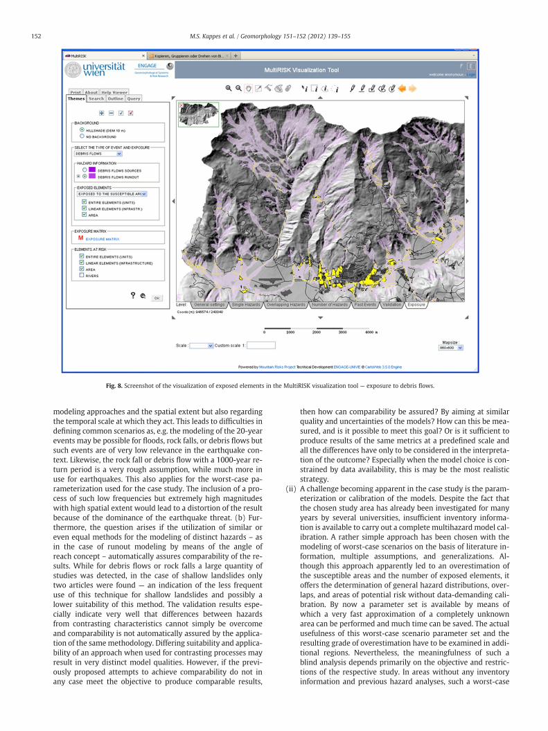
Fig. 8. Screenshot of the visualization of exposed elements in the MultiRISK visualization tool — exposure to debris flows.
152 M.S. Kappes et al. / Geomorphology 151–152 (2012) 139–155
modeling approaches and the spatial extent but also regardingthe temporal scale at which they act. This leads to difficulties indefining common scenarios as, e.g. the modeling of the 20-yearevents may be possible for floods, rock falls, or debris flows butsuch events are of very low relevance in the earthquake con-text. Likewise, the rock fall or debris flow with a 1000-year re-turn period is a very rough assumption, while much more inuse for earthquakes. This also applies for the worst-case pa-rameterization used for the case study. The inclusion of a pro-cess of such low frequencies but extremely high magnitudeswith high spatial extent would lead to a distortion of the resultbecause of the dominance of the earthquake threat. (b) Fur-thermore, the question arises if the utilization of similar oreven equal methods for the modeling of distinct hazards – asin the case of runout modeling by means of the angle ofreach concept – automatically assures comparability of the re-sults. While for debris flows or rock falls a large quantity ofstudies was detected, in the case of shallow landslides onlytwo articles were found — an indication of the less frequentuse of this technique for shallow landslides and possibly alower suitability of this method. The validation results espe-cially indicate very well that differences between hazardsfrom contrasting characteristics cannot simply be overcomeand comparability is not automatically assured by the applica-tion of the samemethodology. Differing suitability and applica-bility of an approach when used for contrasting processes mayresult in very distinct model qualities. However, if the previ-ously proposed attempts to achieve comparability do not inany case meet the objective to produce comparable results,
then how can comparability be assured? By aiming at similarquality and uncertainties of the models? How can this be mea-sured, and is it possible to meet this goal? Or is it sufficient toproduce results of the same metrics at a predefined scale andall the differences have only to be considered in the interpreta-tion of the outcome? Especially when the model choice is con-strained by data availability, this is may be the most realisticstrategy.
(ii) A challenge becoming apparent in the case study is the param-eterization or calibration of the models. Despite the fact thatthe chosen study area has already been investigated for manyyears by several universities, insufficient inventory informa-tion is available to carry out a complete multihazard model cal-ibration. A rather simple approach has been chosen with themodeling of worst-case scenarios on the basis of literature in-formation, multiple assumptions, and generalizations. Al-though this approach apparently led to an overestimation ofthe susceptible areas and the number of exposed elements, itoffers the determination of general hazard distributions, over-laps, and areas of potential risk without data-demanding cali-bration. By now a parameter set is available by means ofwhich a very fast approximation of a completely unknownarea can be performed and much time can be saved. The actualusefulness of this worst-case scenario parameter set and theresulting grade of overestimation have to be examined in addi-tional regions. Nevertheless, the meaningfulness of such ablind analysis depends primarily on the objective and restric-tions of the respective study. In areas without any inventoryinformation and previous hazard analyses, such a worst-case

153M.S. Kappes et al. / Geomorphology 151–152 (2012) 139–155
analysis may offer helpful indications of which areas have to beregarded in more detail.For better adjusted parameterization or calibration of themodels, difficulties have to be solved in each single situationindividually. This means that solutions have to be foundaccording to the available data and the legislative frameworkrequiring the computation of certain scenarios or the like.Thereby, expert appraisal seems to be an indispensible compo-nent in multihazard analyses. Multihazard information, espe-cially regarding inventory data, is probably always fragmentaryand has to be complemented and pieced together. Nevertheless,a problem is that only a few experts have real multihazardexperience.
(iii) Although the presented analysis concept is designed as a top-down approach, in this study only the first step is outlined:the regional exposure analysis scheme. Nevertheless, in theelaboration of a local analysis scheme many additional prob-lems will emerge, such as the development of a vulnerabilityanalysis scheme. Depending on the type of hazard, differentmethods are used such as curves, matrices, or indicator-basedapproaches (Kappes et al., 2011b). For instance, vulnerabilitycurves are frequently applied for flood and earthquake model-ing but are still not available for rock falls. Thus, the question ishow to combine different methods or identify one method(e.g., vulnerability matrices) that can be applied for all process-es. Moreover the vulnerability is altered by simultaneous or se-quential hazard impacts (Kappes et al., 2011b). Furthermore,local multihazard risk analyses require much detailed informa-tion; and although with the regional analysis zones of specialinterest are identified, the acquisition of the necessary infor-mation for these areas is a challenge.An extension of MultiRISK toward hazard and risk modeling ata local scale is planned to facilitate detailed examination ofthose areas determined at a regional scale. Moreover, the in-clusion of further processes as, for instance, earthquakes andflash floods is under consideration.
(iv) Important phenomena arising in a multihazard context are re-lations and interactions between hazards. This issue has notbeen dealt with in this article due to two reasons: first, becausehazard relations are, until now, not automated in the MultiRISKmodeling tool, they were not presented in the present study.Nevertheless, ideas and recommendations for regarding thisissue at a regional scale are already presented in Kappes et al.(2010) and Kappes and Glade (in press). Primarily, the imple-mentation of feedback loops and the identification of areas sus-ceptible to hazard chains with the overlay of modeling resultsare proposed.
(v) Multihazard analyses have to be followed by the interpretationof the results, which especially includes the determination ofacceptable and tolerable levels of risk for certain types of useor the planning of mitigation measures. In Switzerland andFrance, broad guidelines for the performance of multihazardanalyses already exist, directly linked to the implementationof the modeling results into spatial planning. This implies,that any modeling approach has to be adjusted to the legalframework and the requirements of the stakeholders takingdecisions on the basis of this information.
(vi) So far, the MultiRISK Platform has been developed without in-tensive stakeholder interaction. The major reasons were, first,the objective to approach the challenge to develop a multiha-zard analysis scheme and implement it into a software from ascientific point of view, to identify general challenges and tonot only provide practical solutions to one specific problem.Second, to develop a beta version that offers a basis for discus-sions with stakeholders and prevents from abstract design pro-cesses. The experience of the usefulness of a first software
proposal as starting point for a detailed adjustment to userneeds has also been made with RiskScape in New Zealand (Ste-fan Reese, NIWA, personal communication, December 2010).Thereby, adjustment refers to requirements in terms of spatialresolution, quality and level of uncertainty of the results, pro-cesses to be considered, data availability and user-friendlinessof the software but also to the administrative and legal settingof the country and the hazard and risk modeling capacities. Sofar, the performance of hazard and risk analyses is often out-sourced to consultants since technical know how and person-nel situation do not permit the realization within theadministrative units. However, this involves the danger oflow transparency of and little information on the modelingprocedure and does not offer the option to flexibly computescenarios, update the analyses etc. The performance of multi-hazard risk analyses by means of a specific software tool –
which has to be adapted to the specific requirements, legisla-tion, and other user-specific needs –would accelerate and sim-plify the procedure and make the results more transparent.Nevertheless, at least the first parameterization and adaptationto the specific area and user needs will in most cases requireexpert support from outside, the tool itself could stay in thehand of, e.g., the municipalities and offer flexible and fast re-running. How realistic the introduction of such a tool in admin-istrative bodies and institutions is depends on the legislation,the duties of the administrative units, and many more aspects.An interesting example offers HAZUS, elaborated by and freelyavailable from FEMA (U.S. Federal Emergency ManagementAgency). With a variety of videos and manuals as well asHAZUS training courses, FEMA provides support with thetool. Moreover, HAZUS is delivered together with a nationwidedatabase offering sufficient information to carry out a firstoverview analysis of any region in the U.S.Transferring this approach to the Alpine context, a tool adjust-ed to the necessity to first, perform a susceptibility analysis at ascale 1:10,000–1:50,000, and second, to elaborate a hazardzoning map could be adjusted to the local conditions and cali-brated in first place by external (consultants) or national gov-ernmental experts. The model itself, not only the results,remains with the respective administrative units, offering thisway an update by consultants, governmental experts, or,according to the respective experience and expertise, by thetechnicians of this unit. Due to differences in the administra-tive structure and legal framework of each country, the author-ities in charge of arranging/performing these analyses vary. InFrance, the municipality, with the support of the RTM service,has to take care of the elaboration of hazard and risk informa-tion while in Germany governmental agencies as the hydrolog-ical or the geological survey are in charge.
Concluding, multihazard settings pose a wide range of challenges.Although several difficulties can be solved by a coherent analysisscheme and the automation of the analysis procedure, many prob-lems persist and require experience in handling and analyzing of mul-tiple hazards as well as careful interpretation of analysis results.
Acknowledgments
The authors thank the European Commission for funding the pro-ject Mountain Risks (http://mountain-risks.eu; contract numberMCRTN03598) in the framework of which this study has been carriedout. Furthermore, the authors want to express their gratitude to Jean-Philippe Malet and Alexandre Remaître for the provision of informa-tion, support and always very constructive feedbacks. Many thanksalso to Cees van Westen, Stefan Greiving, Stefan Jäger and André Ass-mann for very helpful discussions and valuable advice. Also the whole
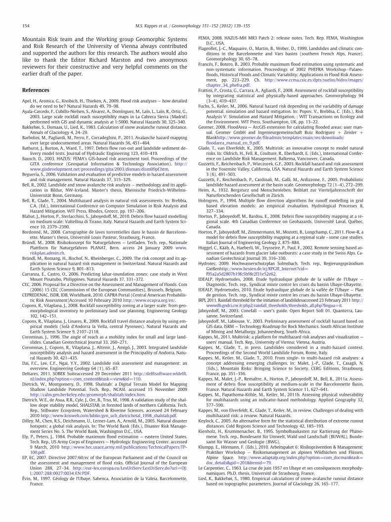
154 M.S. Kappes et al. / Geomorphology 151–152 (2012) 139–155
Mountain Risk team and the Working group Geomorphic Systemsand Risk Research of the University of Vienna always contributedand supported the authors for this research. The authors would alsolike to thank the Editor Richard Marston and two anonymousreviewers for their constructive and very helpful comments on theearlier draft of the paper.
References
Apel, H., Aronica, G., Kreibich, H., Thieken, A., 2009. Flood risk analyses — how detaileddo we need to be? Natural Hazards 49, 79–98.
Ayala-Carcedo, F., Cubillo-Nielsen, S., Alvarez, A., Domínguez, M., Laín, L., Laín, R., Ortiz, G.,2003. Large scale rockfall reach susceptibility maps in La Cabrera Sierra (Madrid)performed with GIS and dynamic analysis at 1:5000. Natural Hazards 30, 325–340.
Bakkehøi, S., Domaas, U., Lied, K., 1983. Calculation of snow avalanche runout distance.Annals of Glaciology 4, 24–29.
Barbolini, M., Pagliardi, M., Ferro, F., Corradeghini, P., 2011. Avalanche hazard mappingover large undocumented areas. Natural Hazards 56, 451–464.
Bathurst, J., Burton, A., Ward, T., 1997. Debris flow run-out and landslide sediment de-livery model tests. Journal of Hydraulic Engineering 123, 410–419.
Bausch, D., 2003. HAZUS: FEMA's GIS-based risk assessment tool. Proceedings of theGITA conference (Geospatial Information & Technology Association). http://www.gisdevelopment.net/proceedings/gita/2003/disman/dism09pf.htm.
Beguería, S., 2006. Validation and evaluation of predictive models in hazard assessmentand risk management. Natural Hazards 37, 315–329.
Bell, R., 2002. Landslide and snow avalanche risk analysis —methodology and its appli-cation in Bíldur, NW-Iceland. Master's thesis, Rheinische Friedrich-Wilhelms-Universität Bonn, Germany.
Bell, R., Glade, T., 2004. Multihazard analysis in natural risk assessments. In: Brebbia,C.A. (Ed.), International Conference on Computer Simulation in Risk Analysis andHazard Mitigation. WIT Press, Rhodes, Greece, pp. 197–206.
Blahut, J., Horton, P., Sterlacchini, S., Jaboyedoff, M., 2010. Debris flow hazard modellingon medium scale: Valtellina di Tirano, Italy. Natural Hazards and Earth System Sci-ence 10, 2379–2390.
Bordonné, M., 2008. Cartographie de laves torrentielles dans le bassin de Barcelonn-ette. Master's thesis, Université Louis Pasteur, Strasbourg, France.
Bründl, M., 2008. Risikokonzept für Naturgefahren — Leitfaden. Tech. rep., NationalePlattform für Naturgefahren PLANAT, Bern. access 24 January 2009 www.riskplan.admin.ch.
Bründl, M., Romang, H., Bischof, N., Rheinberger, C., 2009. The risk concept and its ap-plication in natural hazard risk management in Switzerland. Natural Hazards andEarth System Science 9, 801–813.
Carranza, E., Castro, O., 2006. Predicting lahar-inundation zones: case study in WestMount Pinatubo, Philippines. Natural Hazards 37, 331–372.
CEC, 2006. Proposal for a Directive on the Assessment and Management of Floods. Com(2006) 15 CEC (Commission of the European Communities), Brussels, Belgium.
CEPREDENAC, ISDR, IDB, Worldbank, 2010. CAPRA Portal (Central American Probabilis-tic Risk Assessment)Accessed 10 February 2010 http://www.ecapra.org/en/.
Copons, R., Vilaplana, J., 2008. Rockfall susceptibility zoning at a larger scale: from geo-morphological inventory to preliminary land use planning. Engineering Geology102, 142–151.
Copons, R., Vilaplana, J., Linares, R., 2009. Rockfall travel distance analysis by using em-pirical models (Solà d'Andorra la Vella, central Pyrenees). Natural Hazards andEarth System Science 9, 2107–2118.
Corominas, J., 1996. The angle of reach as a mobility index for small and large land-slides. Canadian Geotechnical Journal 33, 260–271.
Corominas, J., Copons, R., Vilaplana, J., Altimir, J., Amigó, J., 2003. Integrated landslidesusceptibility analysis and hazard assessment in the Principality of Andorra. Natu-ral Hazards 30, 421–435.
Dai, F.C., Lee, C.F., Ngai, Y.Y., 2002. Landslide risk assessment and management: anoverview. Engineering Geology 64 (1), 65–87.
Deltares, 2011. SOBEK Suiteaccessed 29 December 2011 http://delftsoftware.wldelft.nl/index.php?option=com_content&task=view&id=110.
Dietrich, W., Montgomery, D., 1998. Shalstab: a Digital Terrain Model for MappingShallow Landslide Potential. Tech. Rep., NCASI. accessed 15 November 2009http://calm.geo.berkeley.edu/geomorph/shalstab/index.htm.
Dietrich, W.E., de Asua, R.R., Cyle, J., Orr, B., Trso, M., 1998. A validation study of the shal-low slope stability model, SHALSTAB, in forested lands of northern California. Tech.Rep., Stillwater Ecosystem, Watershed & Riverine Sciences. accessed 24 February2010 http://www.krisweb.com/biblio/gen_ucb_dietrichetal_1998_shalstab.pdf.
Dilley, M., Chen, R.S., Deichmann, U., Lerner-Lam, A., Arnold, M., 2005. Natural disasterhotspots: a global risk analysis. In: The World Bank (Eds.), Disaster Risk Manage-ment Series No. 5. The World Bank, Washington D.C., USA.
Ely, P., Peters, J., 1984. Probable maximum flood estimation — eastern United States.Tech. Rep., US Army Corps of Engineers — Hydrologic Engineering Center. accessed9 March, 2010 http://www.hec.usace.army.mil/publications/TechnicalPapers/TP-100.pdf.
EP, EC, 2007. Directive 2007/60/ec of the European Parliament and of the Council onthe assessment and management of flood risks. Official Journal of the EuropeanUnion 288, 27–34. http://eur-lex.europa.eu/LexUriServ/LexUriServ.do?uri=OJ:L:2007:288:0027:0034:EN:PDF.
Évin, M., 1997. Géology de l'Ubaye. Sabenca, Association de la Valeia, Barcelonnette,France.
FEMA, 2008. HAZUS-MH MR3 Patch 2: release notes. Tech. Rep. FEMA, WashingtonD.C., USA.
Flageollet, J.-C., Maquaire, O., Martin, B., Weber, D., 1999. Landslides and climatic con-ditions in the Barcelonnette and Vars basins (southern French Alps, France).Geomorphology 30, 65–78.
Francés, F., Botero, B., 2003. Probable maximum flood estimation using systematic andnon-systematic information. Proceedings of 2002 PHEFRA Workshop—Palaeo-floods, Historical Floods and Climatic Variability: Applications in Flood Risk Assess-ment, pp. 223–229. Ch. http://www.ccma.csic.es/dpts/suelos/hidro/images/chapter_34_phefra.pdf.
Frattini, P., Crosta, G., Carrara, A., Agliardi, F., 2008. Assessment of rockfall susceptibilityby integrating statistical and physically-based approaches. Geomorphology 94(3–4), 419–437.
Fuchs, S., Keiler, M., 2006. Natural hazard risk depending on the variability of damagepotential. simulation and hazard mitigation. In: Popov, V., Brebbia, C. (Eds.), RiskAnalysis V: Simulation and Hazard Mitigation. : WIT Transactions on Ecology andthe Environment. WIT Press, Southampton, UK, pp. 13–22.
Geomer, 2008. FloodArea — ArcGIS extension for calculating flooded areas: user man-ual. Geomer GmbH and Ingenieurgemeinschaft Ruiz Rodriguez + Zeisler +Blankhttp://www.geomer.de/fileadmin/templates/main/res/downloads/floodarea_manual_en_9.pdf.
Glade, T., van Elverfeldt, K., 2005. Multirisk: an innovative concept to model naturalrisks. In: Oldrich, H., Fell, R., Coulture, R., Eberhardt, E. (Eds.), International Confer-ence on Landslide Risk Management. Balkema, Vancouver, Canada.
Guzzetti, F., Reichenbach, P., Wieczorek, G.F., 2003. Rockfall hazard and risk assessmentin the Yosemite Valley, California, USA. Natural Hazards and Earth System Science3 (6), 491–503.
Guzzetti, F., Reichenbach, P., Cardinali, M., Galli, M., Ardizzone, F., 2005. Probabilisticlandslide hazard assessment at the basin scale. Geomorphology 72 (1–4), 272–299.
Heim, A., 1932. Bergsturz und Menschenleben. Beiblatt zur Vierteljahresschrift derNaturforschenden Gesellschaft in Zürich.
Holmgren, P., 1994. Multiple flow direction algorithms for runoff modelling in gridbased elevation models: an empirical evaluation. Hydrological Processes 8,327–334.
Horton, P., Jaboyedoff, M., Bardou, E., 2008. Debris flow susceptibility mapping at a re-gional scale. 4th Canadian Conference on Geohazards, Université Laval, Québec,Canada.
Horton, P., Jaboyedoff, M., Zimmermann, M., Mozotti, B., Longchamp, C., 2011. Flow-R, amodel for debris flow susceptibility mapping at a regional scale - some case studies.Italian Journal of Engineering Geology 2, 875–884.
Huggel, C., Kääb, A., Haeberli, W., Teysseire, P., Paul, F., 2002. Remote sensing based as-sessment of hazards from glacier lake outbursts: a case study in the Swiss Alps. Ca-nadian Geotechnical Journal 39, 316–330.
Hydrotec, 2009. Hochwasserschutzplan Solmsbach. Tech. rep., RegierungspräsidiumGießenhttp://www.hessen.de/irj/RPGIE_Internet?cid=f95a2a5d2807b19fc5b9fe2f31e52e62.
IDEALP, Hydroetudes, 2008. Etude hydraulique globale de la vallée de l'Ubaye —Diagnostic. Tech. rep., Syndicat mixte contre les crues du bassin Ubaye-Ubayette.
IDEALP, Hydroetudes, 2010. Etude hydraulique globale de la vallée de l'Ubaye — Plande gestion. Tech. rep., Syndicat mixte contre les crues du bassin Ubaye-Ubayette.
IRPI, 2011. Rainfall threshold for the initiation of landslidesaccessed 23 February 2011 http://wwwdb.gndci.cnr.it/php2/rainfall_thresholds/thresholds_all.php?lingua=it.
Jaboyedoff, M., 2003. Conefall — user's guide. Open Report Soft 01. Quanterra, Lau-sanne, Switzerland.
Jaboyedoff, M., Labiouse, V., 2003. Preliminary assessment of rockfall hazard based onGIS data. ISRM — Technology Roadmap for Rock Mechanics. South African Instituteof Mining and Metallurgy, Johannesburg, South Africa.
Kappes, M., 2011. Multirisk: a platform for multihazard risk analyses and visualization —
users' manual. Tech. Rep., University of Vienna; Vienna, Austria.Kappes, M., Glade, T., in press. Landslides considered in a multi-hazard context.
Proceedings of the Second World Landslide Forum, Rome, Italy.Kappes, M., Keiler, M., Glade, T., 2010. From single- to multi-hazard risk analyses: a
concept addressing emerging challenges. In: Malet, J.-P., Glade, T., Casagli, N.(Eds.), Mountain Risks: Bringing Science to Society. CERG Editions, Strasbourg,France, pp. 351–356.
Kappes, M., Malet, J.-P., Remaître, A., Horton, P., Jaboyedoff, M., Bell, R., 2011a. Assess-ment of debris flow susceptibility at medium-scale in the Barcelonnette Basin,France. Natural Hazards and Earth System Science 11, 627–641.
Kappes, M., Papathoma-Köhle, M., Keiler, M., 2011b. Assessing physical vulnerabilityfor multihazards using an indicator-based methodology. Applied Geography 32,577–590.
Kappes, M., von Elverfeldt, K., Glade, T., Keiler, M., in review. Challenges of dealing withmultihazard risk: a review. Natural Hazards.
Keylock, C., 2005. An alternative form for the statistical distribution of extreme runoutdistances. Cold Regions Science and Technology 42, 185–193.
Kienholz, H., Krummenacher, B., 1995. Symbolbaukasten zur Kartierung der Phäno-mene. Tech. rep., Bundesamt für Umwelt, Wald und Landschaft (BUWAL), Bunde-samt für Wasser und Geologie (BWG).
Klumpp, E., Hörmann, F. (Eds.), 2010. Arbeitspaket 6: Risikoprävention & Management:Praktiker Workshop — Risikomanagement an alpinen Wildbächen und Flüssen.Alpine Space. http://www.adaptalp.org/index.php?option=com_docman&task=doc_details&gid=201&Itemid=79.
Le Carpentier, C., 1963. La crue de juin 1957 en Ubaye et ses conséquences morphody-namiques. Ph.D. thesis, Université de Strasbourg, France.
Lied, K., Bakkehøi, S., 1980. Empirical calculations of snow-avalanche runout distancebased on topographic parameters. Journal of Glaciology 26, 165–177.

155M.S. Kappes et al. / Geomorphology 151–152 (2012) 139–155
Liener, S., Kienholz, H., 2000. Modellierung von flachgründigen Rutschungen mit demModell SLIDISP. Internationales Symposium — INTERPRAEVENT. InternationaleForschungsgesellschaft INTERPRAEVENT, Villach, Austria, pp. 259–269.
Liévois, J., 2003. Guide méthodologique plans de prévention des risques d'avalanches.Tech. rep., Ministère de l'Écologie et du Développement et de l'Aménagement.
Maggioni, M., 2004. Avalanche release areas and their influence on uncertainty in ava-lanche hazard mapping. Ph.D. thesis, Universität Zürich, Switzerland.
Maggioni, M., Gruber, U., 2003. The influence of topographic parameters on avalancherelease dimension and frequency. Cold Regions Science and Technology 37,407–419.
Malet, J.-P., Maquaire, O., Locat, J., Remaître, A., 2004. Assessing debris flow hazard as-sociated with slowmoving landslides: methodology and numerical analyses. Land-slides 1, 83–90.
Maquaire, O., Malet, J.-P., Ramaître, A., Locat, J., Klotz, S., Guillon, J., 2003. Instabilityconditions of marly hillslopes: towards landsliding or gullying? The case of theBarcelonnette basin, south east France. Engineering Geology 70, 109–130. http://eost.u-strasbg.fr/omiv/Publications/Maquaire_et_al_2003_EG.pdf.
Marzocchi, W., Mastellone, M., Di Ruocco, A., 2009. Principles of Multi-risk Assessment:Interactions Amongst Natural and Man-induced Risks. European Commission.http://www.scribd.com/doc/16902233/Principles-of-MultiRisk-Assessment.
Mc Clung, D., Lied, K., 1987. Statistical and geometrical definition of snow avalancherunout. Cold Regions Science and Technology 13, 107–119.
Mc Clung, D., Schaerer, P., 1993. The Avalanche Handbook. The Mountaineers, Seattle,USA.
Mc Clung, D., Maers, A., Schaerer, P., 1989. Extreme avalanche run-out: data from fourmountain ranges. Annals of Glaciology 13, 180–184. http://www.nrc-cnrc.gc.ca/obj/irc/doc/pubs/nrcc31059/nrcc31059.pdf.
MEDD, 2009. Programmes d'études des avalanchesAccessed 20 October 2009 http://www.avalanches.fr/.
Meisina, C., Scarabelli, S., 2006. A comparative analysis of terrain stability models forpredicting shallow landslides in colluvial soils. Geomorphology 87, 207–223.
Montgomery, D., Dietrich, W., 1994. A physically based model for the topographic con-trol on shallow landsliding. Water Resources Research 30, 1153–1171.
Montgomery, D., Greenberg, H., 2009. Dave and Harvey's Slope Stability PackageAc-cessed 11 November 2010 http://gis.ess.washington.edu/stability/index.html.
Montgomery, D.R., Sullivan, K., Greenberg, H.M., 1998. Regional test of a model forshallow landsliding. Hydrological Processes 12, 943–955.
Odeh Engineers, Inc., 2001. Statewide hazard risk and vulnerability assessment for theState of Rhode Island. Tech. Rep., NOAA Coastal Services Center. http://www.csc.noaa.gov/rihazard/pdfs/rhdisl_hazard_report.pdf.
OderRegio, 2006. Vorsorgender raumordnerischer Hochwasserschutz im Einzugsgebietder Oder — Transnationales Handlungsprogramm. Tech. rep., INTERREG III B-Projekt OderRegio. http://www.oderregio.org/download/OR_HP_DE_Web.pdf.
Prochaska, A., Santi, P., Higgins, J., Cannon, S., 2008. Debris-flow runout predictionsbased on the average channel slope (ACS). Engineering Geology 98, 29–40.
Quinn, P., Beven, K., Chevallier, P., Planchon, O., 1991. The prediction of hillslope flowpaths for distributed hydrological modelling using digital terrain models. Hydro-logical Processes 5, 59–79.
Real de Asua, R., Bellugi, D., Dietrich, E., 2000. Shalstab — Tools Tutorial. BlueG Soft-ware, Stillwater Sciences and the U.C.B. Geomorphology Group, Oakland, USA.
Reese, S., Bell, R., King, A., 2007. RiskScape: a new tool for comparing risk from naturalhazards. Water & Atmosphere 15, 24–25.
Remaître, A., 2006. Morphologie et dynamique des laves torrentielles: applications auxtorrents des Terres Noires du bassin de Barcelonnette (Alpes du Sud). Ph.D. thesis,Université de Caen/Basse-Normandie, France.
Remaître, A., Malet, J.-P., Cepeda, J., 2010. Landslides and debris flows triggered by rain-fall: the Barcelonnette basin case study, south French Alps. In: Malet, J.-P., Glade, T.,Casagli, N. (Eds.), Mountain Risks: Bringing Science to Society. CERG Editions,Strasbourg, France, pp. 141–145.
Rickenmann, D., Zimmermann, M., 1993. The 1987 debris flow in Switzerland: docu-mentation and analysis. Geomorphology 8, 175–189.
Rickli, C., Böll, A., Gerber, W., 1994. Ganzheitliche Gefahrenbeurteilung — Kursunterla-gen. Tech. rep., Eidgenössische Forschungsanstalt für Wald, Schnee und Landschaftand Forstliche Arbeitsgruppe Naturgefahren.
RTM, 2000. Plan de prevention des risques naturals previsibles — Department desAlpes de Haute-Provence, Commune de Jausiers. Tech. rep.
RTM, 2002. Plan de prevention des risques naturels previsibles — Departement desAlpes de Haute-Provence, Commune de Faucon de Barcelonnette. Tech. rep.
RTM, 2008. Commune de barcelonnette: Plan de prevention des risques naturels previ-sibles — reglement. Tech. rep., Restauration des Terrains de Montagne, provisoire.
Ruiz Rodriguez, Zeisler, geomer GmbH, PlanEVAL, HASKONING, 2001. Übersichtskartender Überschwemmungsgefährdung der möglichen Vermögensschäden am Rhein —Abschlussbericht: Vorgehensweise zur Ermittlung der hochwassergefährdeten Flä-chen, Vorgehensweise zur Ermittlung der möglichen Vermögensschäden. Tech. rep.Internationale Kommission zum Schutz des Rheines (IKSR).
Schneider, P., Schauer, B., 2006. HAZUS — its development and its future. Natural Haz-ards Review 7, 40–44.
Shaw, S., Johnson, D., 1995. Slope morphology model derived from digital elevationdata. Proceedings, Northwest Arc/Info Users Conference, p. 12. http://www.krisweb.com/biblio/gen_xxxx_shawetal_1995_slopemorph.pdf.
Sivan, O., 2000. Torrents de l'Ubaye. Sabenca, Association de la Valeia, Barcelonnette,France.
Slaymaker, O., Embleton-Hamann, C., 2009. Mountains. In: Slaymaker, O., Spencer, T.,Embleton-Hamann, C. (Eds.), Geomorphology and Global Environmental Change.Cambridge University Press, Oxford, UK, pp. 37–70.
Stötter, J., Belitz, K., Frisch, U., Geist, T., Maier, M., Maukisch, M., 1999. Konzeptvors-chlag zum Umgang mit Naturgefahren in der Gefahrenzonenplanung — Herausfor-derung an Praxis und Wissenschaft zur interdisziplinären Zusammenarbeit.Innsbrucker Geographische Gesellschaft — Jahresbericht, pp. 30–59.
Takahashi, T., 1981. Estimation of potential debris flows and their hazardous zones;soft countermeasures for a disaster. Journal of Natural Disaster Science 3, 57–89.
Thiery, Y., 2007. Susceptibilité du bassin de Barcelonnette (Alpes du sud, France) aux‘mouvements de versant’: cartographie morphodynamique, analyse spatiale etmodélisation probabiliste. Ph.D. thesis, Université de Caen/Basse-Normandie.
Thiery, Y., Sterlacchini, S., Malet, J.-P., Puissant, A., Remaître, A., Maquaire, O., 2004.Strategy to reduce subjectivity in landslide susceptibility zonation by GIS in com-plex mountainous environments. 7th AGILE Conference on Geographic Informa-tion Science, AGILE, Heraklion, Greece.
Thiery, Y., Malet, J.-P., Sterlacchini, S., Puissant, A., Maquaire, O., 2007. Landslide sus-ceptibility assessment by bivariate methods at large scales: application to a com-plex mountainous environment. Geomorphology 92, 38–59.
Toppe, R., 1987. Terrain models— a tool for natural hazard mapping. Avalanche Forma-tion, Movement and Effects, IAHS publication no. 162, Davos, Switzerland, pp.629–638. http://iahs.info/redbooks/a162/iahs_162_0629.pdf.
TU Wien, 2009. Leitfaden zum Nachweis der Hochwassersicherheit von Talsperren.Tech. rep., Bundesministerium für Land- und Forstwirtschaft.
UN-ISDR, 2009a. Global Assessment Report on Disaster Risk ReductionTech. Rep.http://www.preventionweb.net/english/hyogo/gar/report/index.php?id=9413.
UN-ISDR, 2009b. UNISDR terminology on disaster risk reduction. Tech. Rep., United Na-tions International Strategy of Disaster Reduction. accessed 18 November 2009http://www.undp.org.ge/new/files/24_619_762164_UNISDR-terminology-2009-eng.pdf.
US Army Corps of Engineers, 2011. HEC-RASaccessed 28 December 2011 http://www.hec.usace.army.mil/software/hec-ras/index.html2011.
UVM, 2005. Hochwassergefahrenkarten in Baden-Württemberg. Tech. rep., Ministeriumfür Umwelt, Naturschutz und Verkehr. http://www.uvm.baden-wuerttemberg.de/servlet/is/1253/HWGK_Leitfaden_DEU.pdf.
van Westen, C., Montoya, A., Boerboom, L., Badilla Coto, E., 2002. Multihazard risk as-sessment using GIS in urban areas: a case study for the city of Turrialba, CostaRica. Proceedings of the Regional Workshop on Best Practices in Disaster Mitiga-tion: Lessons Learned from the Asian Urban Disaster Mitigation Program andOther Initiatives, Bali, Indonesia, pp. 120–136.
Wichmann, V., Becht, M., 2003. Modelling of geomorphic processes in an alpine catch-ment. In: Martin, D. (Ed.), 7th International Conference on GeoComputation.University of Southampton, Southampton, UK. http://www.ku-eichstaett.de/Fakultaeten/MGF/Geographie/physisch/Forschung/sedag.en.
Wichmann, V., Becht, M., 2006. Rockfall modelling: methods and model application inan Alpine basin (Reintal, Germany). Göttinger Geographische Abhandlungen 115,105–116.
Wisner, B., Blaikie, P., Cannon, T., Davis, I., 2004. At Risk: Natural Hazards, People's Vul-nerability and Disasters. Routledge, London, UK.
WMO, 1999. Comprehensive risk assessment for natural hazards. Technical Document955, World Meteorological Organisation.
Zimmermann, M., Mani, P., Gamma, P., 1997. Murganggefahr und Klimaänderung— einGIS-basierter Ansatz. vdf Hochschulverlag AG, ETH Zürich, Switzerland.