1

THE MODELING OF SOIL TEMPERATURE WITH DEPTH

B. Poudel*, P.C. Poudel* & S. Gurung*

*Central Department of Physics, Tribhuvan University, Nepal

ABSTRACT: The work comprises a model to determine the temperature of the soil for predefined depths under the

ground surface at any day of the year. The model suggested here is sinusoidal curve of temperature versus day number

of the year. For a given depth, temperature could be determined in any given day of the year. The chi-square test was

done to compare the observed and calculated data, and the result was found to be highly reliable. Transient heat flow

principle was used and certain assumptions were made for example: the heat flow in soil was one-dimensional and

thermal diffusivity was taken as constant. The curve was fitted for the depths 5 cm, 10 cm, 30 cm, and 50 cm. The

average annual absolute difference between observed and estimated values varied from 1.367 to 1.921 for these depths.

This model can be successfully applied to find the temperature of the soil under the ground at any day of the year, given

that thermal diffusivity remains constant and average climatic conditions do not vary drastically throughout the year.

The winter and summer variation of the soil temperature was also studied. It was found that in winter, the soil

temperature increases with depth and in summer, it first decreases up to certain depth and then starts to increase with

depth. This is due to the effects of solar thermal energy and ground thermal energy. In winter, ground thermal energy is

dominant at all depth and in summer, solar thermal energy is dominant up to certain depths and soil temperature varies

accordingly.

Key Words: Soil temperature, transient heat flow, thermal diffusivity

1. Introduction

The loose material that covers the land surfaces of earth

and supports the growth of plants is called soil. Soil is an

unconsolidated, or loose, combination of inorganic and

organic materials. The inorganic components of soil are

principally the products of rocks and minerals. These

minerals have been gradually broken down by weather,

chemical action, and other natural processes. The

organic materials are composed of debris from plants

and from the decomposition of the many tiny life forms

that inhabit the soil. Ramann has defined the soil as ‘the

upper weathering layer of the solid crust’. This definition

is scientific as it does not make any reference to crop

production or to any other use of soil. (Rai, 1995). Joffe,

a representative of the Russian School of Soil Science,

did not agree with Ramann’s definition because it failed

to distinguish between soil and loose rock material. Joffe

defined soil as follows: “Soil is a natural body,

differentiated into horizons of mineral and organic

constituents, usually unconsolidated, of variable depth

which differs from the parent material below in

morphology, physical properties and constitution,

chemical properties and composition and biological

characteristics.” (Rai, 1995).

The soil temperature has its importance in many

agricultural and scientific instances. The temperature at

different depths has great influence on germination of

seeds as well as root growth of the crops and plants. A

model to determine the temperature of soil at various

depths, thus, would be a great help in agricultural and

botanical field. Thus, taking into mind this consideration

we have presented a simple model to determine the

temperature of soil at various depths. The modeling

equation is based on the second degree of thermal

equation and the value of thermal diffusivity was taken

constant throughout the year and other assumption was

made that heat flow is one dimensional.

In addition to the study of soil temperature, comparative

study of summer and winter variation of soil temperature

at different depths was also presented. The soil

temperature does not follow the same pattern in summer

and winter seasons: in winter the temperature of soil

increases with depths whereas in summer the temperate

of soil first decreases up to certain depth then increases

with depths. The raw data for temperature of soil for

different depths was taken from meteorological

department of Institute of Agriculture & Animal Science,

Rampur, Chitwan, Nepal. The estimated temperature of

soil was found form the modelling equation and

compared with the original data. Similarly, the curve for

summer and winter season was plotted using the origianl

data and reason for the shape of the curve was

explained.

2. Sample

The sample data was obtained from meteorological

department of Institute of Agriculture & Animal Science,

2

The modeling of soil temperature with depth: B. Poudel, P.C. Poudel & S. Gurung

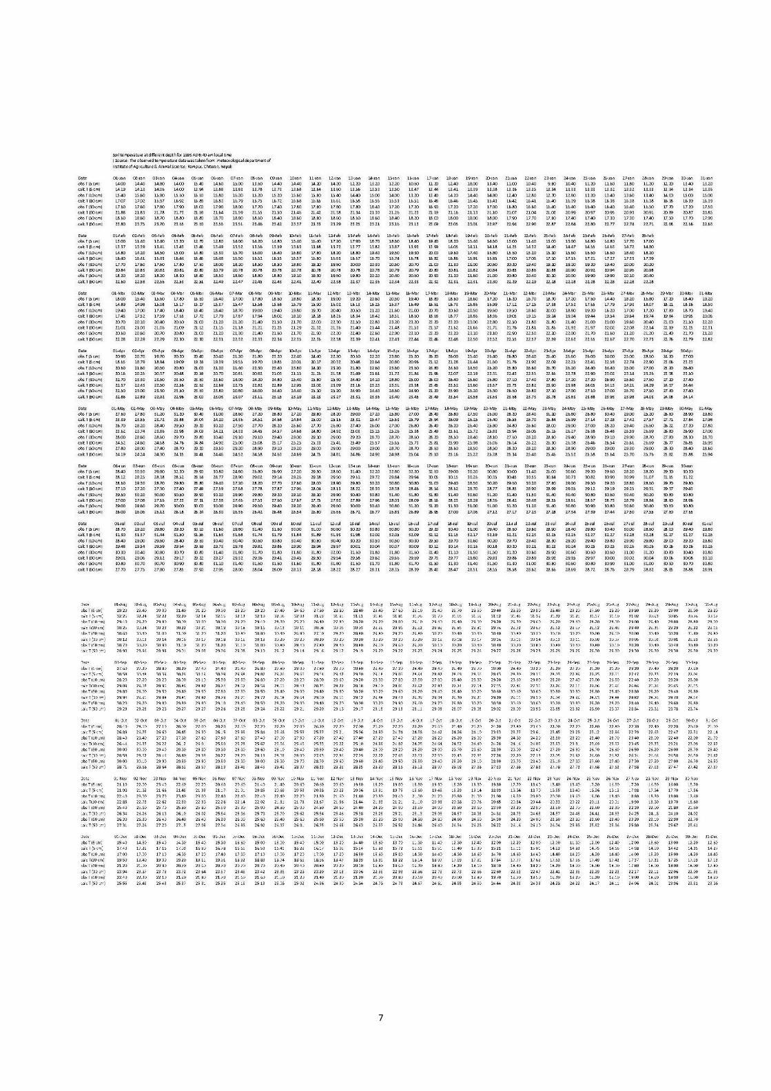
Rampur, Chitwan, Nepal which presents the soil

temperature for 1993 AD at 8:40 am local time. The

detailed sample data along with calculated data is

presented at the end of the paper under “ appendices”

heading.

3. Method of Analysis

Here we used the second degree thermal equation to

derive the relation of temperature of the soil with depth

and time. The proportionality constant was taken as

thermal diffusivity and the heat flow was considered one

dimensional.

The partial second degree equation of heat flow in soil

when we only consider heat flow is due to conduction is

given by, (Hillel,1980).

= Dh ……………1)

Where T is soil temperature, Dh = к/C is the thermal

diffusivity, k is the thermal conductivity and C is the

volumetric heat capacity, t is time, and z is soil depth.

We apply the boundary conditions for z=0 and z→∞ . We

assume that at infinite depth (z→∞) the temperature is

constant and equal to Ta. The temperature at the surface

and infinite depth can be expressed respectively as:

T(0,t) = Ta + A0 sin ωt …………..2)

T(∞,t) = Ta …………..3)

Using these boundary conditions the equation (1) yields:

T(z,t) = Ta + A0 e-z/d sin[(ωt – z/d] …….4)

Where T(z, t) is the soil temperature at time t (day

number of year) and soil depth z (meter), Ta is the

average soil temperature (℃), A0 is the annual amplitude

of the surface soil temperature (℃), d is the damping

depth (meter) of daily fluctuation.

The damping depth is defined as ,

d= (2Dh/ω) ½ ……...…..5)

Where Dh is the thermal diffusivity and ω = 2π/365 day-1

is the radial frequency, in the case of annual variation the

period is 365 days.

From equations (2) and (4) we have seen that the

quantity A0 is a constant regardless of depths.

Here the equation (4) is the solution to the second order

equation (1). The solution is not affected with the addition

of constants. So let us take the equation

T (z, t) = Ta + A0 e-z/d sin [2π (t-t0)/365 – z/d – π/2)] ……6)

This equation satisfies equation (1) so the equation (6) is

also one of the solutions of equation (1).

The empirical values (i.e. to and π/2) used in this

equation are used by Hillel. Choosing suitable value of

thermal diffusivity the equation can be used for any type

of soil and also for snow-capped areas. There are many

models to calculate the soil temperature using different

values of Dh and t0 for various types of the soil. In this

equation (6) the value of t0 is the lowest temperature day

number of the year. For example if the temperature of a

year is minimum at January 23 then t0 =23.

4. Observations and Modeling :

4.1 Plots for soil temperature modeling

The solution of second degree equation can be used as a

model to determine the temperature at given depht at

given time of the year. There may be different methods to

choose the constants Dh and t0 . Here we have chosen

the value of thermal diffusivity (Dh) to be 288 cm2/day and

it is assumed constant throughtout the year . Transient

heat flow principles were used and heat flow was

considered one-dimensional. And the value of empirical

constant t0 is taken as the day number of the year such

that the day has the lowest temperature. The primary

data for soil temperature of year 1993 for various depths

5 cm, 10 cm, 30 cm, and 50 cm at 8:40 am local time

were taken from meteorological department of Institute of

Agriculture & Animal Science, Rampur, Chitwan, Nepal.

The graphs of temperature versus day number of the

year was plotted for different depths for observed and

calculated values.

Here, the one dimensional heat flow equation is :

T (z, t) = Ta + A0 e-z/d sin [2π (t-t0)/365 – z/d – π/2)]

Where,

Ta = Annual average temperature

Ao = Annual amplitude = Tmax – Ta

Tmax = Maximum temperature of the year

to = Day number for minimum temperature day of the

year

Dh = Thermal diffusivity (here taken constant as 288

cm2/day)

ω = Angular frequency= 2π/T

T= time period =365 days

d = Damping depth = (2Dh/ω)1/2

The observed and estimated plots of the temperature

variations are shown below:

3

The modeling of soil temperature with depth: B. Poudel, P.C. Poudel & S. Gurung

4

The modeling of soil temperature with depth: B. Poudel, P.C. Poudel & S. Gurung

4.2 Plot of monthly average

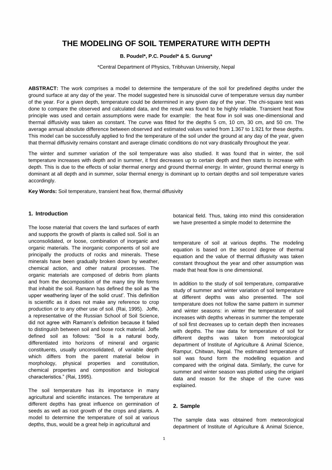
Fig. 9: Monthly average temperature plot of 1993 for soil

at depth 5 cm.

This plot shows that the temperature follows sinusoidal

pattern. The average monthly soil temperature is

minimum at January (12.97 oC) and maximum at July

(29.89 oC).

4.3 Plots for winter and summer variation

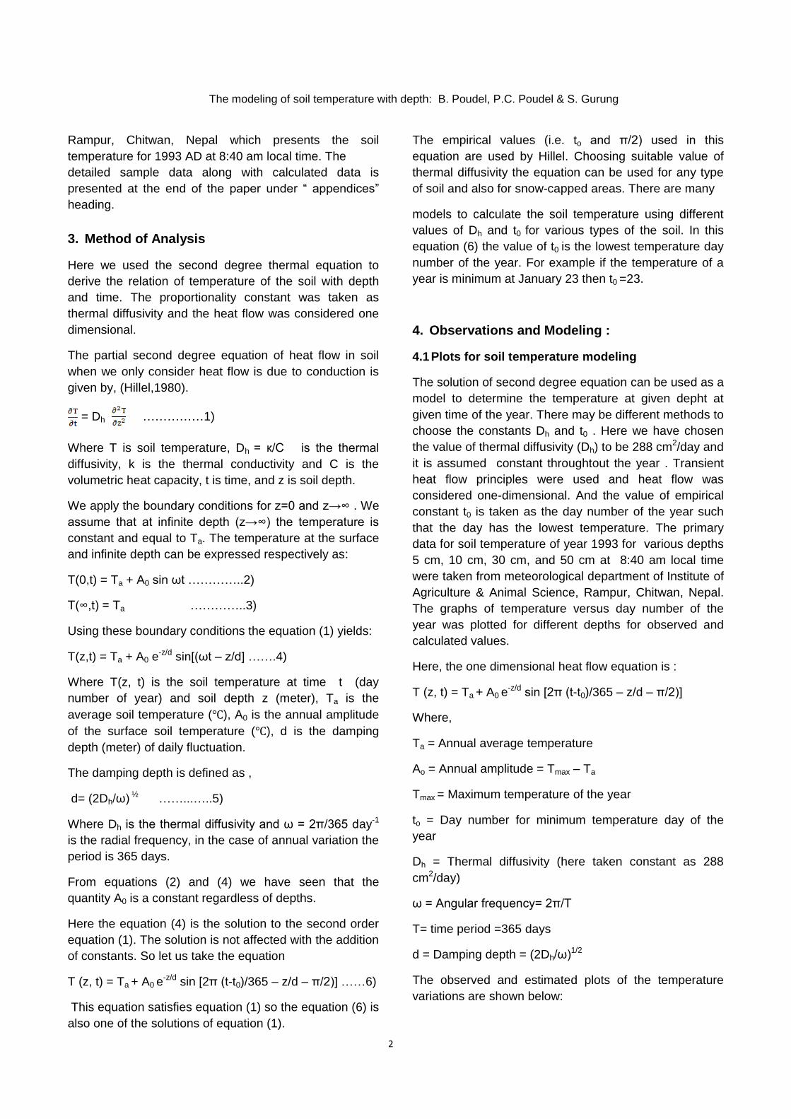
Fig.10 Temperature variation in different depth for 1993

December 1,2,3,4

Fig.11: Temperature variation in different depth for 1993

January 1, 2, 3, 4

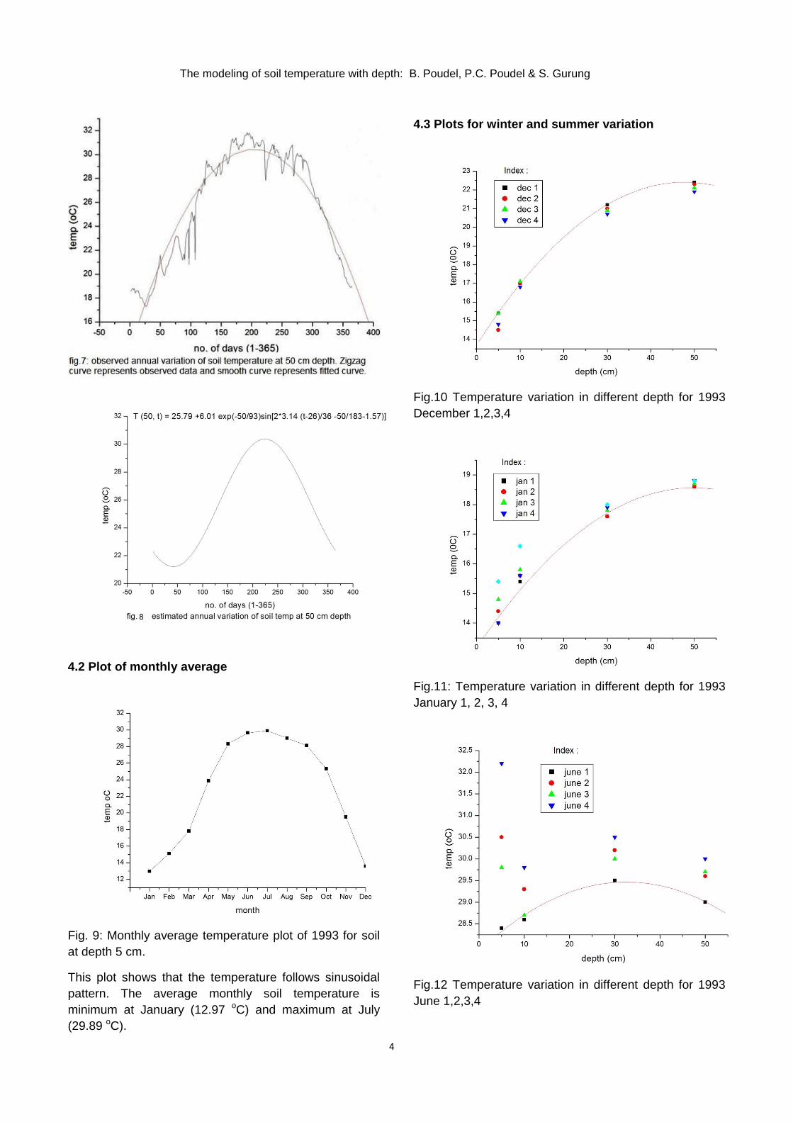
Fig.12 Temperature variation in different depth for 1993

June 1,2,3,4

5

The modeling of soil temperature with depth: B. Poudel, P.C. Poudel & S. Gurung

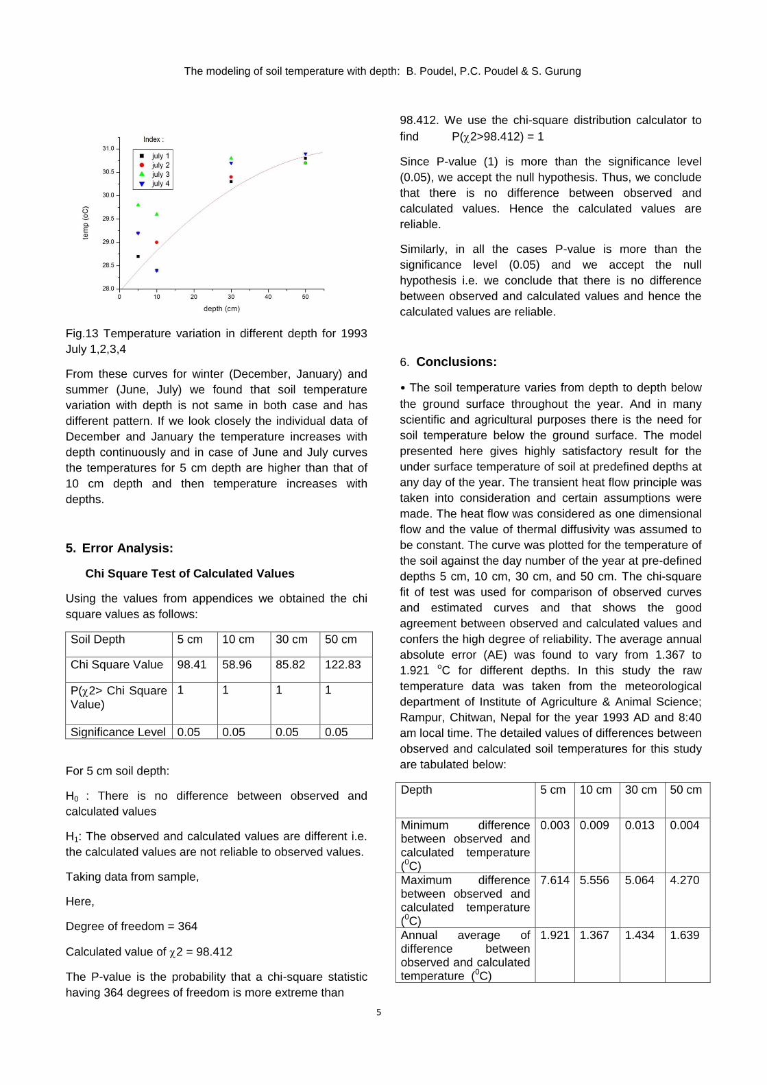
Fig.13 Temperature variation in different depth for 1993

July 1,2,3,4

From these curves for winter (December, January) and

summer (June, July) we found that soil temperature

variation with depth is not same in both case and has

different pattern. If we look closely the individual data of

December and January the temperature increases with

depth continuously and in case of June and July curves

the temperatures for 5 cm depth are higher than that of

10 cm depth and then temperature increases with

depths.

5. Error Analysis:

Chi Square Test of Calculated Values

Using the values from appendices we obtained the chi

square values as follows:

Soil Depth 5 cm 10 cm 30 cm 50 cm

Chi Square Value 98.41 58.96 85.82 122.83

P(2> Chi Square Value)

1 1 1 1

Significance Level 0.05 0.05 0.05 0.05

For 5 cm soil depth:

H0 : There is no difference between observed and

calculated values

H1: The observed and calculated values are different i.e.

the calculated values are not reliable to observed values.

Taking data from sample,

Here,

Degree of freedom = 364

Calculated value of 2 = 98.412

The P-value is the probability that a chi-square statistic

having 364 degrees of freedom is more extreme than

98.412. We use the chi-square distribution calculator to

find P(2>98.412) = 1

Since P-value (1) is more than the significance level

(0.05), we accept the null hypothesis. Thus, we conclude

that there is no difference between observed and

calculated values. Hence the calculated values are

reliable.

Similarly, in all the cases P-value is more than the

significance level (0.05) and we accept the null

hypothesis i.e. we conclude that there is no difference

between observed and calculated values and hence the

calculated values are reliable.

6. Conclusions:

• The soil temperature varies from depth to depth below

the ground surface throughout the year. And in many

scientific and agricultural purposes there is the need for

soil temperature below the ground surface. The model

presented here gives highly satisfactory result for the

under surface temperature of soil at predefined depths at

any day of the year. The transient heat flow principle was

taken into consideration and certain assumptions were

made. The heat flow was considered as one dimensional

flow and the value of thermal diffusivity was assumed to

be constant. The curve was plotted for the temperature of

the soil against the day number of the year at pre-defined

depths 5 cm, 10 cm, 30 cm, and 50 cm. The chi-square

fit of test was used for comparison of observed curves

and estimated curves and that shows the good

agreement between observed and calculated values and

confers the high degree of reliability. The average annual

absolute error (AE) was found to vary from 1.367 to

1.921 oC for different depths. In this study the raw

temperature data was taken from the meteorological

department of Institute of Agriculture & Animal Science;

Rampur, Chitwan, Nepal for the year 1993 AD and 8:40

am local time. The detailed values of differences between

observed and calculated soil temperatures for this study

are tabulated below:

Depth 5 cm 10 cm 30 cm 50 cm

Minimum difference between observed and calculated temperature (0C)

0.003 0.009 0.013 0.004

Maximum difference between observed and calculated temperature (0C)

7.614 5.556 5.064 4.270

Annual average of difference between observed and calculated temperature (0C)

1.921 1.367 1.434 1.639

6

The modeling of soil temperature with depth: B. Poudel, P.C. Poudel & S. Gurung

We also studied the summer and winter variation of soil temperature at different depths : 5 cm, 10 cm, 30 cm, and 50 cm. we found that the temperature increases with depth in winter ( e.g. December, January) and the temperature first decreases up to the depth about 10 cm and then increases with depth in case of summer (e.g. June, July). This can be explained on the basis of two energy sources viz. solar thermal energy and ground thermal energy. In winter ground thermal energy is dominant at all depth and its value increases with depth. But, in summer, there is dominant role of solar thermal energy up to certain depth than ground thermal energy and temperature is higher in upper layer than lower layer up to certain depths and after crossing effective penetration depth of solar energy again temperature increases with depth as given by ground thermal energy.

Acknowledgements:

We would like to express our sincere gratitude to all the

faculty members and students at Central Department of

Physics - Tribhuvan University, Kirtipur, Nepal for their

valuable helps and suggestions. We acknowledge

meteorological department of Institute of Agriculture &

Animal Science; Rampur, Chitwan, Nepal for providing

raw data. And we also extend our thanks for our friends

and other persons who encouraged and supported us in

any kind of ways.

References:

1. Agrawal, R.R., 1967. Soil Fertility in India. Asia

Publishing House.

2. Baver, L.D., et al., 1976. Soil Physics. Wiley

Eastern Limited, First Wiley Eastern Reprint.

3. Cruickshank, J.G., 1972. Soil Geography. David

and Charles Publishers Limited.

4. de Vries, D.A., 1963. Thermal Properties of Soils. In

W.R. van Wijk (ed.) Physics of Plant Environment.

North-Holland Publishing Company, Amsterdam.

5. de Vries, D.A.,1975. Heat Transfer in Soils. In de

Vries, D.A. and Afgan, N.H. Heat and Mass

Transfer in the Biosphere, pp.5-28, Scripta Book

Co., Washington, DC.

6. Foth, H.D. & Turk L.M., 1972. Fundamentals of Soil

Science. Wiley Eastern University Edition, Fifth

Edition.

7. Gruzdyev, G.S.,1983. The Chemical Protection of

Plants. Mir Publishers.

8. Hanks, R.J. & Ashcroft, G.L., 1980. Applied Soil

Physics. Springer-Verlag Publication, Berlin

Heidelberg.

9. Hillel, D., 1980. Fundamentals of Soil Physics.

Academic Press.

10. Hillel, D., 1971. Soil and Water Physical Principles

& Processes. Academic Press.

11. Jenny, H., 1941. Factors of Soil Formation: A

System of Quantitative Pedology. McGraw-Hill

Book Company, Inc.

12. Marshall, T.J., et al., 1996. Soil Physics.

Cambridge University Press.

13. Oswal, M.C. A Textbook of Soil Physics. Vikas

Publishing House Pvt Ltd.

14. Piper, C.S., 1952. Soil and Plant Analysis. Hans

Publishers.

15. Rai, M.M., 1995. Principles of Soil Science.

Macmillan India Limited, Third Edition.

16. Russel, E.J., 1957. The World of the Soil. Collins

Clear-Type Press.

17. Southworth, H., 1972. Farm Mechanization in East

Asia. The Agricultural Development Council, Inc.

18. Tschiersch, J.E., 1978. Appropriate Mechanization

for Small Farmers in Developing Countries. Verlag

bretenbach Saarbrucken.

19. Van Wijk, W. R. and de Vries, D. A., 1963. Periodic

temperature variations in a homogeneous soil. In:

van Wijk, W. R. (Editor) Physics of the plant

environment. North-Holland Publ. Co., Amsterdam,

P. 102-143.

20. Website1: www. Wikipedia.com

21. Website2: www.encartaencyclopaedia.com

22. Website3:www.mesonet.com

Appendix:

7

8