
the-Meter Battery Storage: Advanced Smart Inverter Controls ...
88
Energy Research and Development Division FINAL PROJECT REPORT Photovoltaic and Behind- the-Meter Battery Storage: Advanced Smart Inverter Controls and Field Demonstration California Energy Commission Gavin Newsom, Governor May 2019 | CEC-500-2019-XXX
-
Upload
khangminh22 -
Category
Documents
-
view
4 -
download
0
Transcript of the-Meter Battery Storage: Advanced Smart Inverter Controls ...
Energy Research and Development Division
FINAL PROJECT REPORT
Photovoltaic and Behind-the-Meter Battery Storage: Advanced Smart Inverter Controls and Field Demonstration
California Energy Commission Gavin Newsom, Governor
May 2019 | CEC-500-2019-XXX

PREPARED BY:
Primary Author(s):
Christoph Gehbauer ([email protected])
Joscha Müller
Tucker Swenson
Evangelos Vrettos
Lawrence Berkeley National Laboratory
One Cyclotron Road
Berkeley, CA 94720
Phone: 510-486-4000 | Fax: 510-486-4000
https://www.lbl.gov/
Contract Number: EPC-14-035
PREPARED FOR:
California Energy Commission
Hassan Mohammed
Project Manager
Aleecia Gutierrez
Office Manager
ENERGY GENERATION RESEARCH OFFICE
Laurie ten Hope
Deputy Director
ENERGY RESEARCH AND DEVELOPMENT DIVISION
Drew Bohan
Executive Director
CALIFORNIA ENERGY COMMISSION DISCLAIMER
This report was prepared as the result of work sponsored by the California Energy Commission. It does
not necessarily represent the views of the Energy Commission, its employees or the State of California.
The Energy Commission, the State of California, its employees, contractors and subcontractors make no
warranty, express or implied, and assume no legal liability for the information in this report; nor does any
party represent that the uses of this information will not infringe upon privately owned rights. This report
has not been approved or disapproved by the California Energy Commission nor has the California Energy
Commission passed upon the accuracy or adequacy of the information in this report.

LAWRENCE BERKELEY NATIONAL LABORATORY DISCLAIMER
This document was prepared as an account of work sponsored by the United States Government. While
this document is believed to contain correct information, neither the United States Government nor any
agency thereof, nor The Regents of the University of California, nor any of their employees, makes any
warranty, express or implied, or assumes any legal responsibility for the accuracy, completeness, or
usefulness of any information, apparatus, product, or process disclosed, or represents that its use would
not infringe privately owned rights. Reference herein to any specific commercial product, process, or
service by its trade name, trademark, manufacturer, or otherwise, does not necessarily constitute or imply
its endorsement, recommendation, or favoring by the United States Government or any agency thereof, or
The Regents of the University of California. The views and opinions of authors expressed herein do not
necessarily state or reflect those of the United States Government or any agency thereof of The Regents of
the University of California.

i
ACKNOWLEDGEMENTS
This work was supported by the California Energy Commission through its Electric Program
Investment Charge Program on behalf of the citizens of California and under the United States
Department of Energy, under Contract No. DE-AC02-05CH11231.
The authors would like to thank the following contributors at Lawrence Berkeley National
Laboratory:
Rahul Chopra
Ravi Prasher
Ramesh Ramamoorthy
Cindy Regnier
Alastair Robinson
Alina Sari
Alecia Ward
The authors would also like to thank SolarEdge, and in particular Noah Tuthill, for the support
with setting up the StorEdge inverters and Tesla PowerWall, and providing full control access to
their inverters.
Technical Advisory Committee Members included:
Bill Abolt, AECOM
Richard Bravo, Southern California Edison
Angela Gould, California Energy Commission
Thomas Lee, Strategen
Alexandra Sascha von Meier, University of California Berkeley, California Institute for Energy
and Environment
Sankar Narayan, Microgrid Labs
Harby Sehmar, Pacific Gas and Electric Company
Franz Stadtmueller, Pacific Gas and Electric Company
Kristine Walker, Prospect Silicon Valley

ii
PREFACE
The California Energy Commission’s Energy Research and Development Division supports
energy research and development programs to spur innovation in energy efficiency, renewable
energy and advanced clean generation, energy-related environmental protection, energy
transmission and distribution and transportation.
In 2012, the Electric Program Investment Charge (EPIC) was established by the California Public
Utilities Commission to fund public investments in research to create and advance new energy
solution, foster regional innovation and bring ideas from the lab to the marketplace. The
California Energy Commission and the state’s three largest investor-owned utilities – Pacific Gas
and Electric Company, San Diego Gas & Electric Company and Southern California Edison
Company – were selected to administer the EPIC funds and advance novel technologies, tools,
and strategies that provide benefits to their electric ratepayers.
The Energy Commission is committed to ensuring public participation in its research and
development programs that promote greater reliability, lower costs, and increase safety for the
California electric ratepayer and include:
• Providing societal benefits.
• Reducing greenhouse gas emission in the electricity sector at the lowest possible
cost.
• Supporting California’s loading order to meet energy needs first with energy
efficiency and demand response, next with renewable energy (distributed generation
and utility scale), and finally with clean, conventional electricity supply.
• Supporting low-emission vehicles and transportation.
• Providing economic development.
• Using ratepayer funds efficiently.
Photovoltaic and Behind-the-Meter Battery Storage: Advanced Smart Inverter Controls and Field
Demonstration is the final report for the Demonstration of Integrated Photovoltaic Systems and
Smart Inverter Functionality Utilizing Advanced Distribution Sensors project (Grant Number
EPC-14-035) conducted by Lawrence Berkeley National Laboratory. The information from this
project contributes to the Energy Research and Development Division’s EPIC Program.
For more information about the Energy Research and Development Division, please visit the
Energy Commission’s website at www.energy.ca.gov/research/ or contact the Energy
Commission at 916-327-1551.

iii
ABSTRACT
Electric utilities have little visibility of the electrical distribution system, and consequently,
limited diagnostic capabilities. The distribution grid was designed for a unidirectional power
flow, where energy is supplied by few large centralized power plants; however, this is set to
change to meet California’s aggressive decarbonization goals. The large-scale deployment of
distributed renewable generation, such as photovoltaics (PV), can have many negative effects on
an unprepared grid. As illustrated in the California “duck curve,” PV generation modifies load
profiles during the day, which causes steep ramping in the evening. This effect indicates the
need to revise the electrical grid’s design and operation. This project sought to (a) create a
centralized resource in California to test and validate distribution technology controls with
industry standard PV, storage, and high-fidelity sensors, (b) support strategic and operational
decisions for new grid architectures by providing simulation models, (c) promote new ways to
control clusters of PV smart inverters, in accordance with California Rule 21, and (d) innovate,
develop, and field test a predictive controller to maximize economic profit for the customer
while supporting the grid. The controller was built using the state-of-the-art model predictive
control methodology to optimally control behind-the-meter PV and battery storage. In
consideration of the duck curve, the controller optimally controls the battery dispatch by
charging during excess generation periods and discharging during the critical afternoon
demand hours. The controller was evaluated in annual simulations and revealed the potential
cost-effectiveness of behind-the-meter battery storage. The simulations showed that the annual
electricity bill could be reduced by as much as 35 percent, with a payback period of the
investment in battery storage in about 6 years – significantly shorter than the manufacturer’s
10-year warranty. All developed simulation models, the grid event library, and the MPC
controller are open-source and available online.
Keywords: Smart Inverter, Behind-the-Meter Battery Storage, Advanced Distribution Grid Sensor,
Model Predictive control, Machine Learning
Please use the following citation for this report:
Gehbauer, Christoph, Joscha Müller, Tucker Swenson and Evangelos Vrettos. 2019. Photovoltaic
and Behind-the-Meter Battery Storage: Advanced Smart Inverter Controls and Field
Demonstration. California Energy Commission. Publication Number: CEC-500-2019-XXX.
iv
TABLE OF CONTENTS
Page
ACKNOWLEDGEMENTS ....................................................................................................................... i
PREFACE ................................................................................................................................................... ii
ABSTRACT .............................................................................................................................................. iii
TABLE OF CONTENTS ......................................................................................................................... iv
LIST OF FIGURES .................................................................................................................................. vi
LIST OF TABLES .................................................................................................................................. viii
EXECUTIVE SUMMARY ........................................................................................................................ 1
Introduction................................................................................................................................................ 1
Project Purpose .......................................................................................................................................... 2
Project Process ........................................................................................................................................... 3
Project Results ........................................................................................................................................... 4
Technology/Knowledge Transfer/Market Adoption (Advancing the Research to Market) ....... 6
Benefits to California ................................................................................................................................ 6
CHAPTER 1: Introduction ....................................................................................................................... 7
CHAPTER 2: Experimental Test Facility ............................................................................................ 11
Installation of Photovoltaic and Storage Systems ............................................................................... 11
Installation of Advanced Measurement Devices ................................................................................. 12
CHAPTER 3: Data Collection and Analysis ....................................................................................... 14
High-Fidelity Data Collection ................................................................................................................... 14
Grid Event Definition ................................................................................................................................. 15
Event Detection Algorithm ....................................................................................................................... 15
Analysis ........................................................................................................................................................ 17
Grid Events .............................................................................................................................................. 18
Library of Events .................................................................................................................................... 20
Control Applications ................................................................................................................................. 20
Time-Series Clustering .......................................................................................................................... 20
Parameter Clustering ............................................................................................................................. 21
Timing and Communication Requirements ..................................................................................... 22

v
CHAPTER 4: Modeling and Simulation ............................................................................................. 24
Model Environment .................................................................................................................................... 24
Model Development ................................................................................................................................... 25
Inverter Model ......................................................................................................................................... 27
Battery Model .......................................................................................................................................... 32
Photovoltaic Model ................................................................................................................................. 33
Other Models ........................................................................................................................................... 33
System Validation................................................................................................................................... 34
Model Library .............................................................................................................................................. 36
Dynamic Simulation .................................................................................................................................. 37
Feeder Model ........................................................................................................................................... 38
Dynamic Load Profiles .......................................................................................................................... 39
Random Load Allocation ...................................................................................................................... 40
Photovoltaic Allocation ......................................................................................................................... 43
Results ...................................................................................................................................................... 45
Control Parameter Optimization ............................................................................................................ 47
Experimental Setup ................................................................................................................................ 48
Results ...................................................................................................................................................... 49
Discussion ................................................................................................................................................ 51
CHAPTER 5: Controller Design and Evaluation .............................................................................. 53
Design ........................................................................................................................................................... 53
Framework ............................................................................................................................................... 54
Forecasting............................................................................................................................................... 55
Controller ................................................................................................................................................. 57
Utility Modules ........................................................................................................................................ 60
Simulation Evaluation ............................................................................................................................... 60
Setup ......................................................................................................................................................... 60
Results ...................................................................................................................................................... 62
Pilot Test ...................................................................................................................................................... 63
Results ...................................................................................................................................................... 63
Discussion.................................................................................................................................................... 66
CHAPTER 6: Summary and Benefits Assessment ............................................................................ 68

vi
GLOSSARY .............................................................................................................................................. 70
REFERENCES .......................................................................................................................................... 72
APPENDIX A: Documentation of Flexgrid .......................................................................................... 1
Pictures ............................................................................................................................................................ 1
Overview.......................................................................................................................................................... 2
APPENDIX B: Simulation Settings ....................................................................................................... 1
Simulation Settings ....................................................................................................................................... 1
MPC Settings ............................................................................................................................................... 1
Pacific Gas & Electric E-19 Tariff ............................................................................................................ 1
LIST OF FIGURES
Page
Figure ES-1: California Duck Curve ........................................................................................................ 2
Figure 1: California Duck Curve .............................................................................................................. 8
Figure 2: Overview of Flexgrid Facility ................................................................................................ 11
Figure 3: Overview of Synchrophasor Measurement Unit Sensor Installation............................... 13
Figure 4: Structure of the Berkeley Tree Database .............................................................................. 14
Figure 5: Exponential Event Search Functionality .............................................................................. 16
Figure 6: Visualization of Event Parameterization .............................................................................. 18
Figure 7: Long-Term Current Magnitude Trend at Building 90 ....................................................... 19
Figure 8: Hourly and Weekly Voltage Imbalance at Building 90 ...................................................... 20
Figure 9: Example of Time-Series Event Clustering ............................................................................ 21
Figure 10: Parameter Clustering of Voltage Sags ................................................................................ 22
Figure 11: Simple Capacitor Model in Modelica ................................................................................. 25
Figure 12: Example Modelica Model of Flexgrid ................................................................................ 26
Figure 13: Example of Modelica Parameter Window ......................................................................... 27
Figure 14: Inverter Model in SCooDER Modelica Package ................................................................ 28
Figure 15: Inverter Power Balance Testing ........................................................................................... 30
vii
Figure 16: Validation of Transient Inverter Power Control ............................................................... 31
Figure 17: Battery Energy Balance Testing ........................................................................................... 32
Figure 18: Testing of Volt-Var-Watt Control ........................................................................................ 34
Figure 19: Illustration of Shading of Photovoltaics at Flexgrid ......................................................... 35
Figure 20: Validation of the Flexgrid Model in Modelica .................................................................. 36
Figure 21: Structure of SCooDER Package ........................................................................................... 37
Figure 22: Modeled IEEE 13 Feeder ....................................................................................................... 38
Figure 23: Power Flow at Feeder Head on Peak- and Low-Load Day ............................................. 42
Figure 24: Nodal Power Flow on Peak- and Low-Load Day ............................................................. 42
Figure 25: Nodal Voltages on Peak- and Low-Load Day ................................................................... 43
Figure 26: Power Flow at Feeder Head for the Peak Photovoltaic Generation Day with Different Penetrations .............................................................................................................................................. 45
Figure 27: Nodal Power Flow for Peak Photovoltaic Generation Day with Different Penetrations .................................................................................................................................................................... 46
Figure 28: Nodal Voltages for Peak Photovoltaic Generation Day with Different Penetrations .. 47
Figure 29: Volt-Var Parameter Definition ............................................................................................. 48
Figure 30: Comparison of Volt-Var Hysteresis Settings ..................................................................... 49
Figure 31: Comparison of Volt-Var Threshold Settings ..................................................................... 50
Figure 32: Optimized Settings for Clustered Inverters to Reduce Reactive Imbalance ................. 50
Figure 33: Controller Framework and Communication ..................................................................... 53
Figure 34: Example of Emulated Functional Mockup Unit Wrapper ............................................... 54
Figure 35: Example of Controller Linkage ............................................................................................ 55
Figure 36: Schematic of the Hybrid Photovoltaic Forecasting Algorithm ....................................... 56
Figure 37: Evaluation of Hybrid Photovoltaic Forecasting Algorithm ............................................ 57
Figure 38: Time-Varying Error of Hybrid Photovoltaic Forecasting Algorithm............................. 57
Figure 39: Reevaluation Process of the Model Predictive Control Controller ................................ 58
Figure 40: Example of Model Predictive Control Control During Extreme Grid Event ................ 59
Figure 41: Annual Photovoltaic Generation Profile for Simulation .................................................. 61
Figure 42: Annual Load Profile for Simulation .................................................................................... 61
Figure 43: Field Test Results for Photovoltaic and Load Forecast .................................................... 64

viii
Figure 44: Field Test Results for the Battery Control and Net Load using Model Predictive Control ....................................................................................................................................................... 65
Figure 45: Measured Total Energy Cost at Field Test ......................................................................... 66
LIST OF TABLES
Page
Table 1: Feeder Line Parameters ............................................................................................................ 39
Table 2: Original IEEE13 Load Table ..................................................................................................... 41
Table 3: Nodes Sorted by Electrical Distance ....................................................................................... 43
Table 4: Simulation Results of the Model Predictive Control at Lawrence Berkeley National Laboratory ................................................................................................................................................. 62
Table 5: Simulation Results of Model Predictive Control at Lawrence Berkeley National Laboratory (Scaled by 10) ....................................................................................................................... 63

1
EXECUTIVE SUMMARY
Introduction
Today’s electric distribution system is designed for a limited number of large central power
plants serving mostly residential and commercial buildings and industrial facilities. However,
California’s aggressive goals to reduce the state’s greenhouse gas emissions to 1990 levels by
2020, 40 percent below 1990 levels by 2030, and 80 percent below 1990 levels by 2050 is
leading to increasing amounts of renewable generation in the system, particularly from
photovoltaics (PV) and battery storage. This transition changes the architecture by introducing
many small-sized generation plants which are distributed along the power grid and alter the
power flows from one-way to two-way. In turn, this creates new challenges to the existing
power distribution system and requires more advanced scenario-based planning combined with
real-time data management, new control frameworks, and cyber-risk mitigation, to maintain
safety and reliability.
Voltage variability is one of the system challenges posed by increased levels of distributed
generation. The critical aspect here is the voltage level at the customer, which is defined by
United States standards to be within plus-or-minus 5 percent of 120 volts (114 volts to 126
volts). When voltages are outside this range, motors, electronics, lights, or other equipment
could be permanently damaged and pose a safety risk for the user. With only few large power
plants, up to now the voltage change from the point of supply to the customer has been
relatively straightforward to estimate using the physics of electrical systems and connecting
cables. However, as the grid network changes to include many small-scale distributed
generators, projecting voltage changes becomes more difficult because voltages at different
points along the power grid can rise or fall, depending on whether distributed generation is
present or not. Aggravating the situation, existing power distribution systems have little
visibility (that is, data on the location and size of distributed resources and how they are being
operated on a real-time basis), and consequently have limited diagnostic capabilities. So when
distributed generation causes voltage variability issues, utilities and system operators cannot
anticipate or quantify them.
In addition to voltage variability challenges, distributed generation results in a “masked load”,
where renewable generation offsets the load, resulting in a distorted net load (the difference
between customer load and expected electricity production from variable generation resources).
Modified net load profiles due to the deployment of PV are becoming common within the
California power grid. The California “duck curve,” shown in Figure ES-1, is an early indicator of
the need to revise the way the electrical grid is designed and operated to address short, steep
ramps when the system operator must increase or decrease generation to meet varying
electricity demand, and to deal with the risk of oversupply when more electricity is supplied
than is needed to satisfy real-time demand.
A typical load profile (the use of electricity over time) of the California power grid in 2012 is
shown in gray, with two peaks. In the morning hours, the residential and commercial loads
ramp up, and in the evening hours the commercial loads decrease but are compensated by the
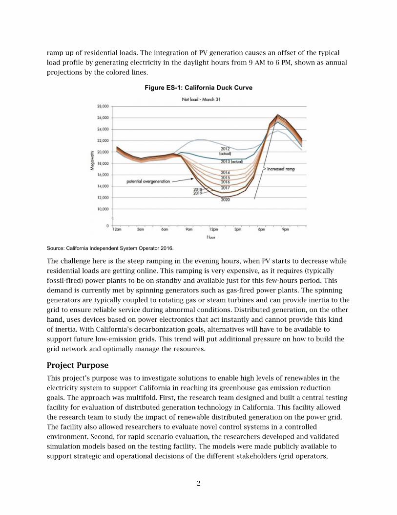
2
ramp up of residential loads. The integration of PV generation causes an offset of the typical
load profile by generating electricity in the daylight hours from 9 AM to 6 PM, shown as annual
projections by the colored lines.
Figure ES-1: California Duck Curve
Source: California Independent System Operator 2016.
The challenge here is the steep ramping in the evening hours, when PV starts to decrease while
residential loads are getting online. This ramping is very expensive, as it requires (typically
fossil-fired) power plants to be on standby and available just for this few-hours period. This
demand is currently met by spinning generators such as gas-fired power plants. The spinning
generators are typically coupled to rotating gas or steam turbines and can provide inertia to the
grid to ensure reliable service during abnormal conditions. Distributed generation, on the other
hand, uses devices based on power electronics that act instantly and cannot provide this kind
of inertia. With California’s decarbonization goals, alternatives will have to be available to
support future low-emission grids. This trend will put additional pressure on how to build the
grid network and optimally manage the resources.
Project Purpose
This project’s purpose was to investigate solutions to enable high levels of renewables in the
electricity system to support California in reaching its greenhouse gas emission reduction
goals. The approach was multifold. First, the research team designed and built a central testing
facility for evaluation of distributed generation technology in California. This facility allowed
the research team to study the impact of renewable distributed generation on the power grid.
The facility also allowed researchers to evaluate novel control systems in a controlled
environment. Second, for rapid scenario evaluation, the researchers developed and validated
simulation models based on the testing facility. The models were made publicly available to
support strategic and operational decisions of the different stakeholders (grid operators,

3
investors, and owners). Third, the team conducted a simulation study on optimally controlled
distributed generation to reduce the overall cost of electricity and maximize usage of
distributed resources. Fourth, researchers developed a controller for combined PV and storage
systems to mitigate the California duck curve, provide benefit to the grid operator, and
maximize revenue for the customer in the current regulatory framework.
Project Process
The project included four consecutive steps that addressed the test facility, simulation models,
optimal control of smart inverter, and optimal control to mitigate the duck curve.
Test Facility (Flexgrid)
The project team designed and built Flexgrid, a full-scale testbed for renewable distributed
generation. The facility includes a 1,000 square foot PV installation, with 15 kilowatts (kW) of
peak power, and three household-scale batteries, totaling 19 kilowatt-hours (kWh) of storage.
The high-fidelity sensing devices installed – micro-synchrophasor measurement units – provide
readings of 120 samples per second to accurately evaluate and analyze the electrical power grid
during critical conditions. The equipment manufacturers include Tesla Energy, SolarEdge, and
Power Standards Lab, all located in California. The first use of the facility was to study the
impact of renewables on the power grid. The sensing equipment was used to record any
variation in supply voltage during periods with and without PV generation. The measured
voltage violations were stored in a digital library of grid events, and used to prototype an
algorithm to predict the severity of these very short-lived (typically in the order of 0.1 second)
events. The library is published online to provide access to academia, researchers, and industry.
Simulation Models
The data recorded at the testing facility was also used to inform the creation and validation of
simulation models. These models include component and system models of PV, batteries,
inverters (electronic devices used to convert direct current to alternating current), and the
power grid. Simulation models are very important for grid planning and controls evaluation.
With a simulation model of the entire grid, researchers can study different levels of PV
deployment and quantify their impact. However, a full grid simulation involves many
components that are typically not designed to be simulated together. One example would be a
power grid simulation, which focuses on the electrical power flow, and a battery storage
simulation, which focuses on the battery chemistry. The simulation models developed in this
project are not domain-specific and allow the simulation of full grids. They are open-source to
allow researchers and stakeholders to make informed decisions.
Optimal Control of Smart Inverters
A smart inverter is the improved version of an inverter that can actively regulate power
generation in accordance with locally observed quantities, which could be voltages. The
functionalities are based on California Rule 21 (a mandate that describes the interconnection
and of generation facilities to be connected to a utility’s distribution system) to allow more
flexibility and adaptability of distributed generation. In an example application of the

4
developed simulation models, the objective was to determine the best control setpoints for
various smart inverters connected within the electrical grid. While these configurable
parameters are currently predetermined by the utility company and are static for all locations,
this project investigated the use of dynamic setpoints that depend on the location and season.
Optimizing these parameters can also lead to reductions in the levelized cost of electricity,
especially for grid networks with high PV penetrations.
Optimal Control to Mitigate Duck Curve
While the optimal control of smart inverters focused on control settings of the inverter, the
team also took a deeper dive into the capabilities of distributed generation. Here, the
combination of distributed PV and battery storage was analyzed and the operation optimized.
The controller was implemented as a model predictive control, where an internal mathematical
model is evaluated and solved to a global optimum at each controller time step. The inputs
were forecasts of weather data, PV generation, and load for the upcoming 24 hours. The
objective was to maximize the revenue for the generating asset owner while providing
additional services to the grid. The grid services explored in this project included time-varying
pricing schemes and the response to critical periods.
From the projections illustrated in the California duck curve, it is anticipated that more and
more ramping in the evening hours will be required. Model predictive controllers can optimally
control the battery by charging it during periods with excess generation and discharging it
during the critical afternoon or evening hours. This active participation in the grid management
will help to maximize the number of renewables that can be connected to the grid. The
controller was evaluated in annual simulations and in a field test conducted at the Flexgrid test
facility.
Project Results
The results of this project are multifold and well-aligned with the overall objective of enabling
large renewable generation on the electrical power grid. The results are ranked by their
immediate benefit to California, if deployed widely:
• During the field test for the model predictive controller for PV and battery storage, the
controller responded to changing environmental conditions and provided near optimal
control of the storage system for a time-varying electricity price. The annual simulation
indicated cost savings of up to 35 percent, with a payback time of about 6 years. This is
significantly shorter than the manufacturer’s warranty of 10 years. The installation of a
battery storage system can financially benefit both residential and commercial
ratepayers, as well as grid operation and reliability overall. Further benefits assessment
could be conducted at the Flexgrid facility, where synthetic grid events or different
customer configurations could be generated and applied to the controller in a full-scale
field test.
• The assignment of variable smart inverter control setpoints revealed the potential to
decrease the capacity of the inverter while providing the same generation output. This
would decrease the levelized cost of electricity (the measure of lifetime costs divided by

5
energy production over the lifetime of the resource) for distributed generation. In
scenarios with high PV penetration, it would be even more advantageous to use variable
control setpoints by preventing the curtailment of PV power generation during peak
hours, a common industrial practice today. Ratepayers would see improved reliability
compared to a case where high PV penetration exists but is not coordinated and
managed as proposed in this project. Further investigations of associated grid
distribution losses and inverter investment costs could be conducted to thoroughly
evaluate the control approach and benefit for different customer types in California.
• The Flexgrid facility, built with funds from this project award, is a central base for
testing new renewable technologies and their integration issues in California. It allows
the evaluation of novel control systems in a controlled, emulated environment and
enables real-time comparisons between end-user demand, renewables, inverters, and
storage. Flexgrid was used throughout this four-year project, serving the data collection,
simulation model development for component and system models related to PV, smart
inverter and battery storage, development of a grid event detection algorithm, and
evaluation of a novel model predictive controller. This state-of-the-art research facility is
available for future research projects in California.
• The measurements from Flexgrid were used to develop and validate a package of
simulation models that include PV, battery, smart inverter, and the power grid
component and system models. While the models were mainly developed for this
project, they are generic and can be combined and parameterized to reflect other
systems. The package is published online and can support stakeholders, regulators and
researchers involved in investment and planning decisions.
• The micro-synchrophasors installed at Flexgrid recorded roughly two years’ worth of
data, with 120 samples per second which totals about 4 terabytes of data. An event
detection algorithm was developed and applied, which resulted in the detection of 27
voltage events over the course of this study. The events were stored in a digital library
and used to perform two methods of short-term forecasting. Both methods revealed
that the initial slope of a voltage event is a good parameter to predict the event’s
severity and duration. This information can be vital for inverter settings, in accordance
with California Rule 21, with the overall objective to improve the reliability of the
electrical grid.
Both control approaches, namely, (1) the controller for PV and battery storage and (2) the
variable smart inverter control setpoints, can increase the allowable amount of PV on the grid
in different ways: (a) offsets retail energy purchases; (b) increases the ability to earn PV-based
revenue due to an increase in the type of energy services PV and battery storage can provide
(that is, grid support or mitigation of the duck curve); and (c) helps California to achieve its
aggressive climate goals to decarbonize the grid.
All simulation models, the grid event library, and the model predictive control framework
developed by this project are open-source and available online.

6
Technology/Knowledge Transfer/Market Adoption (Advancing the Research to Market)
This project was conducted with a variety of industry project partners and advisors. These
included Tesla Energy, SolarEdge, Power Standards Lab, Pacific Gas and Electric, Southern
California Edison, Microgrid Labs, Strategen, Prospect Silicon Valley, as well as the University of
California Berkeley as an academic partner, all located in California. Two technical advisory
committee meetings were held to incorporate insights and feedback from industry, and specify
use cases for the developed tools. Results from this project were presented in two conferences.
The developed tools and models were published on four public repositories on GitHub.
The electricity tariff for commercial customers, with its time-varying energy cost and demand
charge, provides a good opportunity to employ the developed controller, especially if battery
storage is already installed. However, the electricity grid and rate structure are undergoing
incremental restructuring to better represent the actual energy production cost, particularly
with increasing levels of renewable generation. With energy storage as a central resource to
balance this fluctuating generation, the role of residential customers will get more significant.
At this point, the developed controller for battery storage could provide financial benefits to
both commercial and residential customers.
With all developments and findings being publicly available, and the collaboration with industry
leaders, it is up to them to pick up the technology for commercialization. Important to note is
that this project conducted the ground work to investigate different control approaches and
identified a path to a potentially cost-effective operation. While the published controller is one
example of viable technical implementation, companies may adopt the underlying control logic
within their framework, for example, to be implemented inside the inverter of a combined PV
and storage system. That said, the technology is particularly interesting for PV inverter
manufacturers and system integrators of combined PV and battery storage systems.
Benefits to California
The project resulted in a variety of outcomes for California, its residents, investors,
stakeholders, and developers. This includes the design and installation of a central testing
facility for renewable generation to test new developments from industry in a controlled and
safe environment, before the deployment at California ratepayers. All funds to build this facility
and conduct the research were spent in California to promote local businesses. And the goals
and challenges of the California electricity grid were discussed at two conferences and two
technical advisory committee meetings. However, most compelling is the development and field
testing of a model predictive control framework that showed potential cost-effectiveness of
battery storage, by reducing annual electricity bills by up to 35 percent. The payback time is
about 6 years, which is significantly shorter than the manufacturer’s offered warranty of 10
years. When deployed, this technology can increase the allowable amount of renewable
generation on the grid, for example by avoiding the need to upgrade grid infrastructure such as
distribution lines, while providing financial benefits to both residential and commercial
ratepayers realized as lower electricity charges due to responding to dynamic grid tariffs.

7
CHAPTER 1: Introduction
Historically, power distribution systems have not been the focus of research and development
investments and have little visibility and consequently limited diagnostic capabilities.
Distribution systems were designed for a radial and unidirectional power flow, supplied by
centralized power plants. This scenario, however, is set to change. California has aggressive
goals to grow distributed energy resources (DER), in particular solar photovoltaic (PV), to reduce
the state’s greenhouse gas emissions to 1990 levels by 2020, 40 percent below 1990 levels by
2030, and 80 percent below 1990 levels by 2050.1 A future grid with large installations of this
often inertia-less2 distributed generation from PV or batteries will require different, and more
complex, control mechanisms. Coordinated control of utility distribution equipment with DER
will become a necessity. The detrimental impacts of high levels of PV on the current
distribution grid involve: (a) voltage violations and phase imbalances, (b) potential flicker and
other power quality issues, (c) reverse power flow and protection coordination issues,
(d) increased wear and tear on utility equipment, (e) real and reactive power imbalances, and (f)
ramping issues as recently discovered in California’s “duck curve” models. These impacts are
potential barriers to the widespread dissemination of DER; however, advanced sensors and
controls, combined with existing technologies, could mitigate or overcome those barriers. This
project seeks to understand and mitigate these issues depicted in events ranging from sub-
seconds up to minutes or even hours.
Grid events are sudden conditions that occur randomly and without notification. The current
electrical grid architecture, which consists of a relatively small number of large power
generators, makes grid events relatively straightforward to identify, control or isolate. However,
future grids with high levels of DER pose a significant challenge to safe and reliable grid
operation. One example of a grid event is a voltage-sag, where the system voltage momentarily
drops below 90 percent of the nominal voltage value for a short period of time. A single voltage
sag could trip thousands of DER, which in turn would abruptly increase the load on the grid. In
the worst case scenario, this could result in wide-area blackouts. Further aggravating the
situation, voltage sags typically occur on a very fast timescale and only last for fractions of a
second. While current monitoring of distribution grids is mainly focused on the aggregated
feeder head,3 at timescales larger than seconds grid events may occur on nodes remote to the
feeder head and on much faster timescales, which often make them invisible to system
operators. Advanced distribution phase measurement units (PMUs) can provide highly precise
1 Assembly Bill 32, Núñez, Chapter 488, Statues of 2006; Senate Bill 32 (Pavley, Chapter 249, Statutes of 2016); and Governor Edmund G. Brown, Jr. Executive Order B-30-15.
2 Traditional power plants use spinning generators which inherently have inertia that helps reduce frequency fluctuations. On the other hand, inverters, as used for DER, are based on power electronics and cannot provide such a type of inertia.
3 This is the point of interconnection of the distribution feeder with the transmission or sub-transmission grid.
8
measurements on timescales well beyond traditional systems. The microsynchrophasor
measurement unit (µPMU), as an example of distribution PMU, is able to take measurements at a
rate of 30,000 Hertz (Hz), and output the measurements in 120 Hz, or 120 samples per second.
This rate is sufficient to capture most voltage sags.
To capture, characterize, and mitigate grid events, this project was conducted to install a total
of three distribution PMUs at Lawrence Berkeley National Laboratory (LBNL) campus. Further, a
15 kilowatt (kW) PV system from SolarCity/Tesla Energy, three 6.4 kilowatt-hour (kWh) Tesla
PowerWall energy storage systems, and three single-phase 7.6 kilovolt-ampere (kVA) SolarEdge
StorEdge inverters were installed to form a testbed (Flexgrid) and study the impact of DER on
the grid, with a sub-campus of LBNL acting as a fully functioning living lab. This testbed also
allows the study of effects caused by different penetration levels of PV.
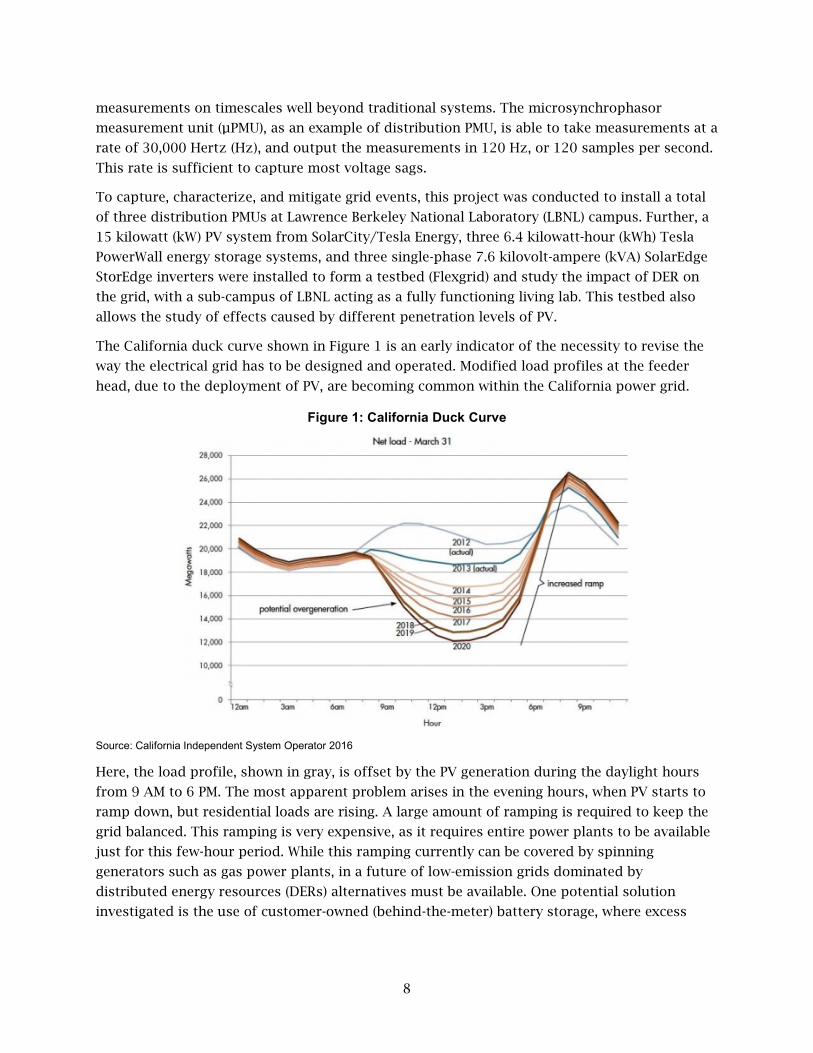
The California duck curve shown in Figure 1 is an early indicator of the necessity to revise the
way the electrical grid has to be designed and operated. Modified load profiles at the feeder
head, due to the deployment of PV, are becoming common within the California power grid.
Figure 1: California Duck Curve
Source: California Independent System Operator 2016
Here, the load profile, shown in gray, is offset by the PV generation during the daylight hours
from 9 AM to 6 PM. The most apparent problem arises in the evening hours, when PV starts to
ramp down, but residential loads are rising. A large amount of ramping is required to keep the
grid balanced. This ramping is very expensive, as it requires entire power plants to be available
just for this few-hour period. While this ramping currently can be covered by spinning
generators such as gas power plants, in a future of low-emission grids dominated by
distributed energy resources (DERs) alternatives must be available. One potential solution
investigated is the use of customer-owned (behind-the-meter) battery storage, where excess

9
energy can be stored during the daytime and used in the evening hours, coinciding with the
ramp up demands shown in the California duck curve.
This project’s broad goals were to:
• Develop a centralized testbed in California for advancing the understanding of DER
technologies.
• Accelerate distributed PV deployment by using new sensor technology and simulation
tools to prototype novel control systems.
• Identify functional requirements and control algorithms for existing and future grid
integration issues of controllable PV and/or behind-the-meter battery storage.
• Develop a controller for optimal control of behind-the-meter energy resources.
• Conduct simulations to represent high PV penetrations on the distribution grid and
assess potential benefits for advanced controls in California.
This project’s specific objectives were to:
• Work with Solar City, Tesla Energy, and SolarEdge to develop and demonstrate control
of an advanced PV inverter storage system and load using data collected from Power
Standard Lab’s µPMUs installed on the LBNL distribution grid and PV/storage system.
• Conduct applied research using the integrated PV system with relevant conditions or
anomalies on LBNL distribution feeders that require a mitigation strategy, including
voltage sags/swells and reverse power flow.
• Simulate the installation to scale, using state-of-the-art cosimulation tools, and validate
the models with the distribution PMU data.
• Use this testbed to design and enable predictive multi-objective control functionality for
both mitigation and control of voltage and power variability issues in high-penetration
scenarios, while optimizing customer’s local economic objectives.
• Quantify the benefit of advanced sensor networks and multi-objective control strategy
for both PV inverters and storage, to both California and the local commercial system.
The project advanced scientific and technical knowledge and innovation in this area and
California by:
• Having a central testbed in California to study effects of DER integration.
• Validating grid performance, including steady-state and time-series voltage profile
before and after installation of a distributed PV system, as well as with and without
advanced control objectives.
• Developing a functional control strategy for advanced PV inverters, in conjunction with
behind-the-meter battery storage, which can be replicated at the high penetration feeder
level.
• Using high-fidelity sensor data for visualization, event identification, and control
objectives.

10
This report covers the full spectrum, from data collection to controller development and
testing, to improve DER utilization, in particular smart PV inverters, in accordance with the
latest California Rule 21 interconnection standard (CEC 2014), and the optimal control of
behind-the-meter battery storage. It begins by describing Flexgrid (the test facility) and outlines
the data collection and grid event analysis. It then illustrates the development of the required
simulation models and design of a controller to maximize economic and grid supportive
operation, and evaluates the controller in simulation and real-world situations. It concludes
with a summary of benefits for California.
11
CHAPTER 2: Experimental Test Facility
The LBNL campus is a widespread research community, located in Berkeley, California. It
consists of more than 100 office buildings and experimental research facilities. Examples are
the Advanced Light Source,4 which is a synchrotron facility that provides users access to high-
energy beams for scientific research and technology development in a wide range of disciplines,
and the Facility for Low Energy Experiments for Buildings5 (Flexlab), which enables users to
develop and test energy-efficient building systems individually or as integrated system, under
real-world conditions. The Flexlab facility is also part of the campus that hosts the power grid-
related research at LBNL.
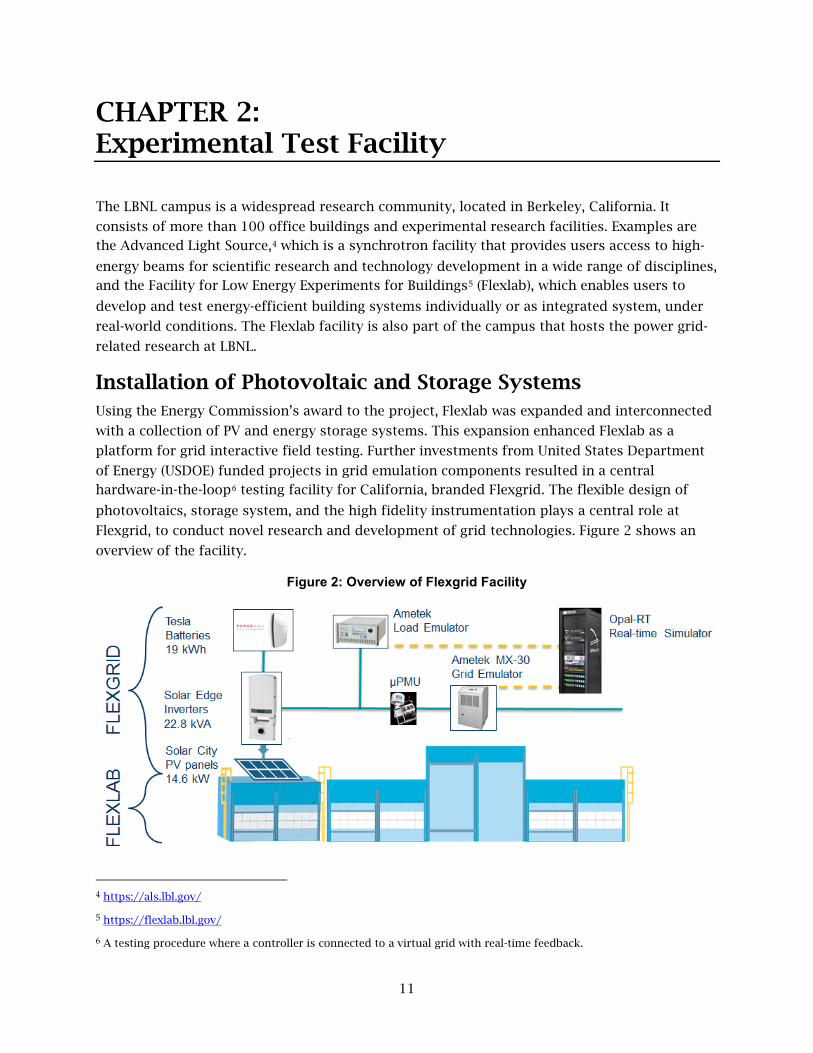
Installation of Photovoltaic and Storage Systems Using the Energy Commission’s award to the project, Flexlab was expanded and interconnected
with a collection of PV and energy storage systems. This expansion enhanced Flexlab as a
platform for grid interactive field testing. Further investments from United States Department
of Energy (USDOE) funded projects in grid emulation components resulted in a central
hardware-in-the-loop6 testing facility for California, branded Flexgrid. The flexible design of
photovoltaics, storage system, and the high fidelity instrumentation plays a central role at
Flexgrid, to conduct novel research and development of grid technologies. Figure 2 shows an
overview of the facility.
Figure 2: Overview of Flexgrid Facility
4 https://als.lbl.gov/
5 https://flexlab.lbl.gov/
6 A testing procedure where a controller is connected to a virtual grid with real-time feedback.

12
Source: Lawrence Berkeley National Laboratory
Flexgrid allows for a systematic evaluation of a broad range of scenarios to be tested under
emulated or real-world conditions. The Flexgrid setup includes an Opal-RT real-time simulator7
as the center of operation, with an Ametek 30 kVA variable voltage source8 as a grid emulator,
and one Ametek 3 kVA load emulator.9 The PV array consists of four strings with a total output
of 14.6 kW, which feeds a three delta-connected and single-phase SolarEdge StorEdge10 inverter,
with a maximum output of 7.6 kVA each. Three 6.4 kWh Tesla PowerWall11 batteries are
connected to the inputs of each inverter. The power flow is measured by high-fidelity
distribution phasor measurement units (PMUs).
Installation of Advanced Measurement Devices The microsynchrophasor measurement unit12 (µPMU) is a low-cost distribution PMU developed
by Power Standards Lab in partnership with LBNL and the University of California, Berkeley,
with support of an Advanced Research Projects Agency-Energy (ARPA-E) grant in 2014. The
accurate measurement of phase angles and magnitudes was for a long time a privilege of the
transmission grid only. The compact µPMU makes available this unique capability to the
distribution grid, at a significantly reduced cost (von Meier et al. 2017). It reports data at a 120
Hz acquisition rate, which is twice per cycle or 120 samples per second, as a phasor
representation13 of voltage and current for each phase. The measurements are based on the
fundamental grid frequency of 60 Hz in the United States. For synchronicity, µPMUs are
connected to a global positioning system receiver to synchronize the timestamp for the phase
angles accurately, to an order of 50 nanoseconds. The data is available as a continuous live
stream, in accordance with the Institute of Electrical and Electronics Engineers (IEEE) C37.118
communication protocol for PMUs, or periodically sent as a comma-separated values file to a
central server. To enable research on power quality issues associated with DER, an array of
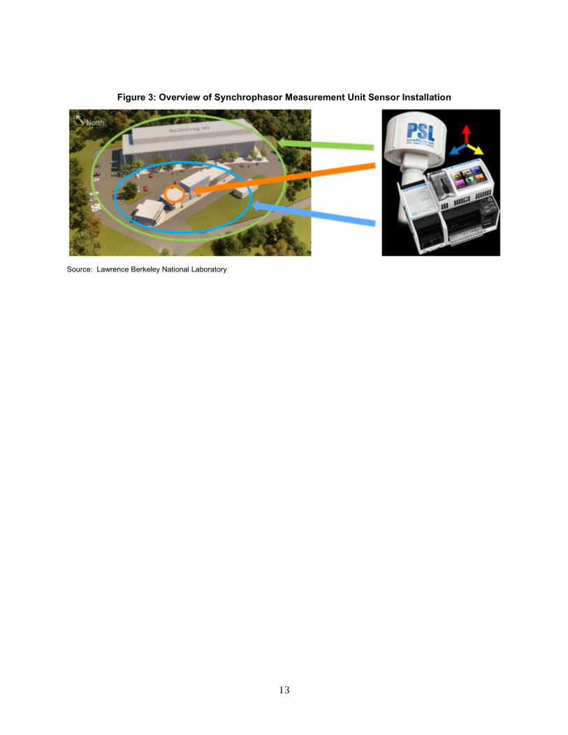
µPMUs was deployed at Flexgrid to study impacts of PV, battery storage, and transactive
buildings on the power grid. Figure 3 shows an overview of the installation and system
boundaries.
The three PMUs are arranged in a layered setup, stretching over different system boundaries of
Flexgrid only (orange), Flexgrid and Flexlab (blue), and the addition of a medium-sized office
building (green).
7 Opal-RT Technologies. https://www.opal-rt.com/
8 AMETEK. California Instruments MX Series. https://www.powerandtest.com/power/ac-power-sources/mx-series
9 AMETEK. California Instruments 3091LD Series. https://www.powerandtest.com/power/electronic-loads/ac-electronic-load-3091ld
10 SolarEdge. StorEdge™ Products for On-grid Applications & Backup Power. https://www.solaredge.com/us/products/storedge
11 Tesla. Powerwall. https://www.tesla.com/powerwall
12 PSL. microPMU. https://www.powerstandards.com/product/micropmu/highlights/
13 Magnitude and phase angle.
13
Figure 3: Overview of Synchrophasor Measurement Unit Sensor Installation
Source: Lawrence Berkeley National Laboratory
14
CHAPTER 3: Data Collection and Analysis
This chapter describes the data collection architecture and framework from the distribution
PMUs installed at LBNL, the grid event detection and analysis using a custom algorithm
developed at LBNL, and results from Flexgrid. The whole chapter is based on a conference
paper accepted to the IEEE Power & Energy Society General Meeting in 2019 (Swenson et al.
2019).
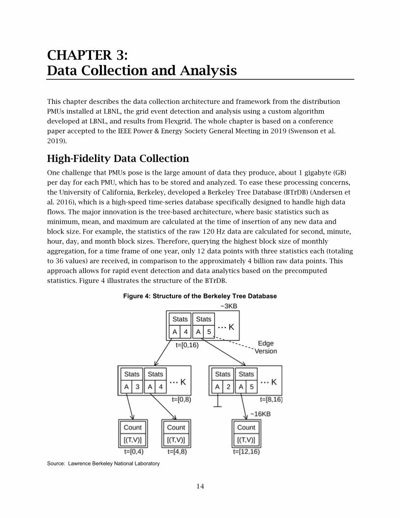
High-Fidelity Data Collection One challenge that PMUs pose is the large amount of data they produce, about 1 gigabyte (GB)
per day for each PMU, which has to be stored and analyzed. To ease these processing concerns,
the University of California, Berkeley, developed a Berkeley Tree Database (BTrDB) (Andersen et
al. 2016), which is a high-speed time-series database specifically designed to handle high data
flows. The major innovation is the tree-based architecture, where basic statistics such as
minimum, mean, and maximum are calculated at the time of insertion of any new data and
block size. For example, the statistics of the raw 120 Hz data are calculated for second, minute,
hour, day, and month block sizes. Therefore, querying the highest block size of monthly
aggregation, for a time frame of one year, only 12 data points with three statistics each (totaling
to 36 values) are received, in comparison to the approximately 4 billion raw data points. This
approach allows for rapid event detection and data analytics based on the precomputed
statistics. Figure 4 illustrates the structure of the BTrDB.
Figure 4: Structure of the Berkeley Tree Database
Source: Lawrence Berkeley National Laboratory
15
The lowest level in the BTrDB, shown at the bottom of Figure 4, is the raw data stored as pairs
of time, T, and value, V. Note that time can be accurately stored in a nanosecond timescale.
BTrDB then calculates basic statistics, for the higher level block sizes. This structure accelerates
the search for grid events by an order of magnitude in comparison to other real-time databases,
by allowing search algorithms to zoom into the data starting from the highest block size,
ultimately down to the raw data of the grid event in question. The aggregations can be seen by
the time indices. The middle layer in this example aggregates eight time steps, from 0 to 7 and
8 to 16. The highest aggregation aggregates the two middle layers, which results in an
aggregation of the full 16 time steps.
Grid Event Definition To detect and categorize grid events, the numeric thresholds that characterize them must first
be identified. To detect voltage sags and swells, where the voltage momentarily falls or rises,
this analysis refers to the voltage ranges and durations put forth by IEEE, which stringently
defines voltage swells and sags as a ±10 percent deviation from nominal site voltage, for
durations from 0.5 cycles, which are about 8 milliseconds (ms), up to one minute (Alves and
Ribiero 1999). Furthermore, as this analysis is concerned with distribution feeders, it is also
relevant to refer to the American National Standards Institute’s (ANSI) tolerable end-use voltage
range, which prohibits deviations more than ±5 percent of the nominal service voltage for
periods of time longer than momentary excursions (ANSI 2016; PG&E 1999). Extended voltage
deviations outside of these bounds will then constitute an over- or under-voltage event.
To detect significant frequency events, the threshold the frequency bound that will prompt
inverters to trip and become inactive. This defines the upper bound of acceptable frequencies
as 60.5 Hz, while the lower bound is defined as 59.3 Hz (CEC 2014). However, these thresholds
constitute extreme and uncommon frequency deviations in the bulk power system (Dargatz
2010). Thresholds for grid events of abnormal current and power flow, phase angle imbalances,
grid impedance, power factor, and rates of change of voltage and current magnitudes are not
easily objectively defined, so these grid events were omitted in this analysis. Instead, this study
focused primarily on detection and characterization of voltage sags and swells that are well
defined and occur relatively frequently. However, it is plausible to detect events by metrics
other than voltage, should one have a quantifiable threshold with which to define the
occurrence of an event as measured by that quantity.
Event Detection Algorithm This project used the programming language Python14 to interface with BTrDB and the recorded
PMU data. An event search algorithm was developed to detect events and return the
corresponding data. The inputs to the program module are the universal unique identifiers of
the PMU data channels and the search window start and end times. The program separately
14 Python 3.7.2 documentation. https://docs.python.org/.
16
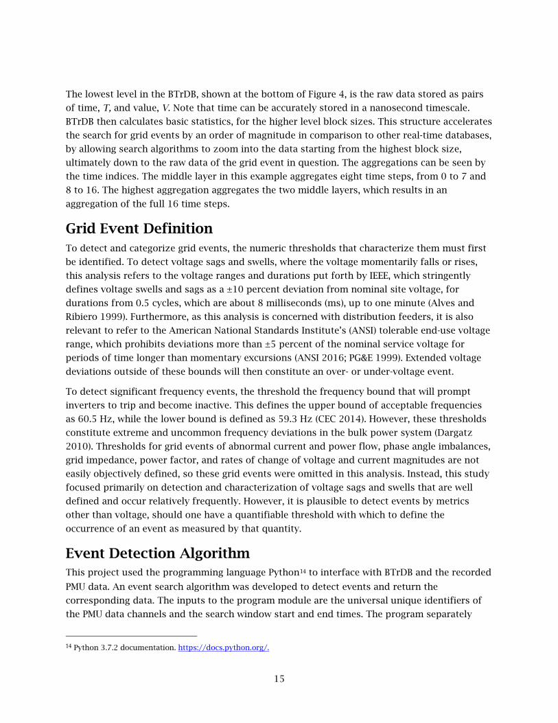
looked at each channel within each location, splitting the data from its start time to its end time
into a user-defined number of subsections, and it leveraged the BTrDB’s functionality to look
only at the extreme values of each section. The timestamp corresponding to any window in
which an extreme value crossing the event threshold was logged for further processing. After
all subsection time windows were investigated at this coarse level, the program discarded all
windows in which the extreme values did not show an event occurring. Then, windows that
contained extreme values were themselves successively cut with a user-defined number of
points of division. This created further subregions whose extreme values were retrieved from
the BTrDB to further narrow the time interval over which the event transpired; this also served
the purpose of detecting whether or not multiple events occurred within one larger time
interval. This exponential process of window refinement occurred until the time window was
narrowed to approximately one second, or until the BTrDB’s mean value for that time window
exceeded the threshold that defined the event. In this way, the program did not “over-zoom”
into longer, more sustained sags or swells exceeding one second in duration. Figure 5 shows the
refinement process that the exponential search function undergoes when presented with the
entire dataset.
Figure 5: Exponential Event Search Functionality
Source: Swenson et al. 2019

17
The program initially split the roughly two years of data into six-day-long subsections, and then
represented each window with its minimum value obtained from the BTrDB. The script then
noted that, for example, a data window in January contains a minimum value below the defined
voltage sag threshold, here indicated by the red dotted line at 0.9 per unit. It refined this
window by progressively splitting it until the script ultimately determined that an event
occurred somewhere within the time window of 23:29:17 (hh:mm:ss) to 23:29:19. Once the time
window was narrowed to this scale, the raw data of the event could be quickly queried, as
illustrated on the last plot in Figure 5.
There are notable trade-offs that one must consider while determining how many points of
division should be drawn by the exponential search function at each step. With a high number
of points of division, it is possible to adequately zoom into an event with fewer calls to the
BTrDB’s database, and thus experience less overhead in communication time. However, this
approach runs the risk of heavy-handedly zooming in too far and accidentally capturing only
portions of events. Furthermore, if a large number of events exist in the time window that is
presented to the script, computation time is wasted, as the program processes the values of the
many time windows that do not contain events. Meanwhile, if a small number of points of
division are drawn at each step, that is, splitting the windows in half each time, very little
computation is wasted in dealing with time windows whose extreme values do not indicate an
event. However, the extreme coarseness of this approach causes some events to be missed
entirely, and means that the BTrDB might need to be called upwards of 20 to 30 times per PMU
to isolate events at the level of one second, increasing communication overhead. For these
reasons, an optimal section size of 2^11 (2048) for the first call to the BTrDB was determined
on the data available to this project. This was followed by subsequent splits into 32 subsections
as events were refined. The initial, fine-granularity split allows for events to immediately be
identified to a narrow time window, with only one call to the BTrDB.
Analysis Once each detected event was trimmed in time to only the relevant abnormal data, the raw
120 Hz data of current and voltage magnitudes and phase angles, across all three phases, was
stored. The subsequent sets of distilled PMU measurements were used to calculate and store
data of active, reactive, and apparent power, as well as frequency and power factor. Detected
events also were parameterized to enable further analysis and categorization. The
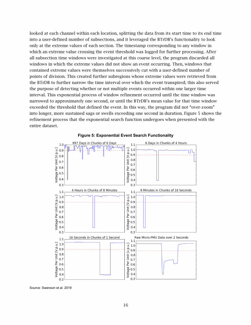
parameterization function began by splitting the raw event data into five sections, as illustrated
with a sample voltage sag in Figure 6.
The first section captures the half-second, front-padded data that preceded the voltage event.
The second section encapsulates data from the point of the event start, that is, the point at
which grid conditions began to deviate from normal operating conditions, to the point at which
the threshold constituting a voltage, frequency, or current sag/swell was crossed. To take
voltage sags as an example, the second section would capture data from the event start, to the
data point at which voltage magnitude drops below 90 percent. The third section captures all
data points for which the threshold was actively exceeded. Following the previous voltage sag
example, this would correspond to all data points below the 90 percent threshold.
18
Figure 6: Visualization of Event Parameterization
Source: Swenson et al. 2019
The fourth section of data corresponds to all data points over which the event threshold was no
longer exceeded and in which the data points were returning to normal operating conditions.
The fifth and final section contains the half-second of padded data immediately following the
voltage event. With these separations in place, the parameterization function combed through
the data points within each section separately and determined the following parameters:
• Flags to indicate the type of event, for example, voltage sag or swell, and whether PV
generation was present.
• The start time and duration of the section.
• The maximum, minimum, and mean slopes achieved for voltages and currents.
• The maximum, minimum, and mean voltage and current magnitude values.
If, however, the parameterization function cannot identify any data points which drop below
the event threshold, it instead defaults to placing all abnormal data (that is, the raw data that is
bound by the slopes which constitute an event start and end) into one all-encompassing region
whose parameters are measured. In this case, the first and last regions that covered nominal
operations immediately preceding and following the event were still parameterized separately.
This created three regions of parameters instead of the typical five for a full event.
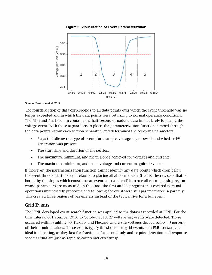
Grid Events
The LBNL developed event search function was applied to the dataset recorded at LBNL. For the
time interval of December 2016 to October 2018, 27 voltage sag events were detected. These
occurred within Building 90, Flexlab, and Flexgrid where site voltages dipped below 90 percent
of their nominal values. These events typify the short-term grid events that PMU sensors are
ideal in detecting, as they last for fractions of a second only and require detection and response
schemes that are just as rapid to counteract effectively.
19
Because the threshold for grid events is user-defined and the program collects duration as an
event parameter of interest, events may be filtered based upon their duration. Using this
method, a search for prolonged under-voltage events, exceeding one second in duration, was
conducted. While no extended voltage sags meeting IEEE’s criteria occurred, three such
extended under-voltage events were detected using ANSI’s definition of acceptable distribution
voltages. All three events in question occurred on October 24, 2017, during a week in which the
building loads in Building 90 and Flexlab were twice that of their typical daytime loads. A likely
explanation for these conditions is an unusually heavy air conditioning load during a
particularly hot week, as evidenced by historical weather data. This created an environment on
the distribution grid in which the most minor voltage dips were liable to pull operating voltages
below ANSI tolerable limits for a prolonged period of time while voltage recovered. This
provides insight into the types of ambient grid conditions that create an environment in which
prolonged voltage deviations are most prone to occur, and future grid simulations will seek to
determine whether or not proactive action on the part of smart inverters, once these risky
ambient grid conditions are detected, might prevent the occurrence of such prolonged
voltage deviations.
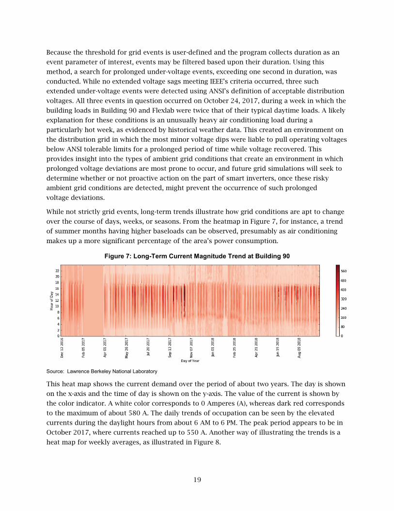
While not strictly grid events, long-term trends illustrate how grid conditions are apt to change
over the course of days, weeks, or seasons. From the heatmap in Figure 7, for instance, a trend
of summer months having higher baseloads can be observed, presumably as air conditioning
makes up a more significant percentage of the area’s power consumption.
Figure 7: Long-Term Current Magnitude Trend at Building 90
Source: Lawrence Berkeley National Laboratory
This heat map shows the current demand over the period of about two years. The day is shown
on the x-axis and the time of day is shown on the y-axis. The value of the current is shown by
the color indicator. A white color corresponds to 0 Amperes (A), whereas dark red corresponds
to the maximum of about 580 A. The daily trends of occupation can be seen by the elevated
currents during the daylight hours from about 6 AM to 6 PM. The peak period appears to be in
October 2017, where currents reached up to 550 A. Another way of illustrating the trends is a
heat map for weekly averages, as illustrated in Figure 8.

20
Figure 8: Hourly and Weekly Voltage Imbalance at Building 90
Source: Lawrence Berkeley National Laboratory
The site voltage at Building 90 is drawn down during the working hours of weekdays while the
building is at full load, and is relatively high when loads are low on weekends, in the early
morning, and during nighttime hours. Foreknowledge of this trend is important, as presented in
the case of the extended under-voltage events on October 24, 2017 in the previous section.
Library of Events
The whole dataset of extracted grid events was appended into a library of events for which each
individual event received its own folder denoted by the time stamp. The library is open source
to the research community and can be found in Swenson et al. (2019). It currently contains the
27 voltage sag events that occurred at LBNL, but will be continuously updated as new voltage
events occur.
Control Applications An important aspect of the conducted analysis is the transfer of observations to a control
system for mitigation. For this purpose, two clustering methods of clustering were applied:
time-series clustering and parameter clustering.
Time-Series Clustering
Events can be clustered based on the auto-correlated time-series data to identify typical event
shapes and parameters. The time-series clustering presented in this report used the Ward
method (Ward 1963). Figure 9 displays the clusters produced by feeding all recorded voltage
sags for one PMU location into the clustering algorithm, with the stipulation that three clusters
should be created. This number was determined as the knee region in the trade-off between
number of clusters and loss function, defined as squared distance to the centroids.

21
Figure 9: Example of Time-Series Event Clustering
Source: Swenson et al. 2019
The algorithm returned three bold-colored average voltage sags that represent sags that fall
into that particular cluster. The individual sags are plotted in a lighter color, in accordance to
their cluster. This clustering portrays three archetypal events, where the red cluster
corresponds to the most common voltage sag event at LBNL, the green cluster corresponds to
voltage sags that occur asymmetrically where this phase is not directly affected, and the blue
cluster corresponds to prolonged voltage sags that occur rarely but are distinct in their
behavior. The most common event types, represented by the red and green clusters, display
similarity in their evolution with time and differ greatly only in sag magnitude. Sags in both
clusters take approximately 60 ms to reach their most severe point, and persist for 60 ms past
the minimum voltage, making the most typical voltage sags at LBNL about 120 ms in duration,
regardless of how deep the sag is. The red cluster was typified by a minimum voltage slope of
around -6.67 to -11.67 percent per cycle and tended to sink to about 85 to 90 percent of the
nominal value. Meanwhile, for the green cluster, the minimum voltage slope achieved was
typically in the range of -1.67 to -3.33 percent per cycle and tended to sink no lower than
95 percent of nominal. The remaining cluster was an abnormally long one, indicated by the blue
curve. This cluster sunk lower than the other two clusters, to about 80 to 85 percent, and
achieved a more extreme voltage minimum slope of -11.67 percent per cycle on phase one. On
phases two and three, the minimum voltage slope achieved for the long cluster was -55 percent
per cycle and -21.67 percent per cycle, respectively. Correlations between the various
parameters of each cluster can facilitate models which might seek to predict voltage sag
severity or duration based upon minimum voltage slope.
Parameter Clustering
Events may also be clustered based upon their parameters, such as magnitudes, slopes, or
durations, calculated by the event parameterization script. The selection of parameter to be
clustered is a complex problem of dimension reduction where the many parameters available
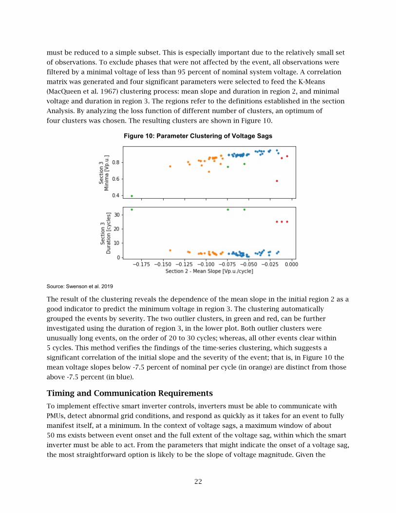
22
must be reduced to a simple subset. This is especially important due to the relatively small set
of observations. To exclude phases that were not affected by the event, all observations were
filtered by a minimal voltage of less than 95 percent of nominal system voltage. A correlation
matrix was generated and four significant parameters were selected to feed the K-Means
(MacQueen et al. 1967) clustering process: mean slope and duration in region 2, and minimal
voltage and duration in region 3. The regions refer to the definitions established in the section
Analysis. By analyzing the loss function of different number of clusters, an optimum of
four clusters was chosen. The resulting clusters are shown in Figure 10.
Figure 10: Parameter Clustering of Voltage Sags
Source: Swenson et al. 2019
The result of the clustering reveals the dependence of the mean slope in the initial region 2 as a
good indicator to predict the minimum voltage in region 3. The clustering automatically
grouped the events by severity. The two outlier clusters, in green and red, can be further
investigated using the duration of region 3, in the lower plot. Both outlier clusters were
unusually long events, on the order of 20 to 30 cycles; whereas, all other events clear within
5 cycles. This method verifies the findings of the time-series clustering, which suggests a
significant correlation of the initial slope and the severity of the event; that is, in Figure 10 the
mean voltage slopes below -7.5 percent of nominal per cycle (in orange) are distinct from those
above -7.5 percent (in blue).
Timing and Communication Requirements
To implement effective smart inverter controls, inverters must be able to communicate with
PMUs, detect abnormal grid conditions, and respond as quickly as it takes for an event to fully
manifest itself, at a minimum. In the context of voltage sags, a maximum window of about
50 ms exists between event onset and the full extent of the voltage sag, within which the smart
inverter must be able to act. From the parameters that might indicate the onset of a voltage sag,
the most straightforward option is likely to be the slope of voltage magnitude. Given the

23
analysis of voltage sag clusters at LBNL, the emergence of voltage slopes around -2.5 to -
7.5 percent per cycle seems likely to result in a minor voltage dip, while slopes lower than -
7.5 percent per cycle are likely to result in more extreme voltage sags. These slopes present
themselves early on in the sag, and so with rapid enough communication times, the smart
inverter should be capable of acting to mitigate these events. Early tests using an embedded
controller to ping LBNL’s PMUs revealed average communication times, through non-
deterministic Ethernet, of approximately 20 ms. This is just slightly under half of the time that
a typical voltage sag takes to achieve its minimum value. In addition, the measured time
constant of an external control setpoint change for the smart inverters at LBNL was about
33 ms. With this knowledge, the value of streaming the live 120 Hz data of potentially
thousands of PMUs must be questioned. An alternative solution may be to process PMU data on
the device, and communicate based on interrupts, in case of an event.

24
CHAPTER 4: Modeling and Simulation
This chapter introduces an open-source package of simulation models in the context of smart
inverter, battery storage, and distribution grids, and the simulation of variable voltage control
setpoints for smart inverters. The Flexgrid facility is used for model development and
validation.
Model Environment The simulation of distribution grids involves a variety of components, such as smart inverter,
PV, battery storage, and distribution feeder models. In addition, control models representing
the smart inverter capabilities of Volt-Var and Volt-Watt controls, where the reactive and active
power output is regulated in accordance to locally observed voltages, are required. This mode
of control is also described in California Rule 21 (CEC 2014). Modelica (Fritzson and Bunus
2002) is an open source modeling language allowing multi-domain simulations, and it is well
suited to formulate models of the various components. It allows straightforward decoupling of
model and solver due to the equation based formulation. Several tools are available to improve
the usability with a graphical user interface and built-in debugger. Examples are the open-
source tool OpenModelica15 and the proprietary Dymola.16 Other toolchains such as JModelica17
allow the direct translation of simulation models into optimization problems, that is, to find
the optimal size of PV installation, or to minimize the voltage impact of DER. All of the listed
tools also support the compilation and export of models in compliance with the functional
mockup interface (FMI) co-simulation standard18 (Modelisar 2014), to use them for third-party
applications. Modelica is also backed up by a large community that already developed a variety
of model libraries relevant to power systems (Brkic et al. 2018; Einhorn et al. 2011; Vanfretti et
al. 2016). This group also includes the Modelica Buildings library (MBL) (Wetter et al. 2014),
which is a large ensemble of detailed building models as well as electrical power system
models. One example of a simple capacitor model in Modelica is given in Figure 11.
The declaration of a model in Modelica starts with a model statement, followed by the model
name. Variables are declared by their type, that is, Real, followed by the name. The declaration
also allows some optional arguments such as unit, start value, or lower and upper bounds.
Specifying units is a good practice to avoid the connection of incompatible components. In
addition to the declaration itself, Modelica provides three basic types – parameter, input, and
output – to externally interface with the model. Within the Modelica modeling area, models are
represented as blocks with input and output connectors. In the example in Figure 11, the model 15 OpenModelica. https://openmodelica.org/
16 Dassault Systemes. DYMOLA Systems Engineering. https://www.3ds.com/products-services/catia/products/dymola/
17 JModelica.org. https://jmodelica.org/
18 Functional Mock-up Interface (FMI). https://fmi-standard.org/

25
would have voltage, V, as input connector; current, I, as output connector; and the capacity, C,
as parameter. The model section is followed by the equation section and is completed with an
end statement. Equations can be any mathematical formulation, including algebraic operations
and derivatives.
Figure 11: Simple Capacitor Model in Modelica
Source: Lawrence Berkeley National Laboratory
Model Development The Flexgrid facility involves many basic components of power systems, as well as control
loops and grid interaction through PMU sensors. While separate libraries exist (such as detailed
battery or PV library), Flexgrid requires the combination of the many models. In addition,
simulations should be conducted over longer time frames such as hours, days, or years to
thoroughly assess the impact of PV and storage with seasonal effects. To fulfill these
requirements, a model package – Smart Control of Distributed Energy Resources (SCooDER) –
was developed in the Modelica framework. It relies on other libraries and introduces custom
additions to better represent the Flexgrid installation. To illustrate the user interaction in
Modelica, the full Flexgrid model is shown in Figure 12.
In Modelica, all models are delivered as blocks with inputs, outputs, and parameters. The blocks
can be connected to form larger systems by the input and output connectors. The Flexgrid
model is based on the physical infrastructure and components of Flexgrid. Here, a PV system
(for example, pv1) and a battery (for example, battery1) are connected to a single-phase inverter
(for example, inverter1). The pv system is fed by a weather input (weaBus) and a shading input
(for example, shade1) to simulate shading of the PV string. The inverter provides an inverter
control bus (for example, invCtrlBus1) which allows to control battery charging and discharging
power, PV curtailment, and reactive power, and to read power flow, such as voltage and power
data. This setup is duplicated two more times, and then connected to three single-phase
transformers which are in turn connected in delta at the grid interconnection, within mpz_dist.
A meter, sens_FLEXGRID, is added before the line of the Flexlab feed, FL_feed. Each model
allows the setting of a number of parameters, which are described in detail in the following
sections. The parameters are preset to reflect the Flexgrid setup, but can be simply overwritten
by the user. An example parameter setup of inverter1 is shown in Figure 13. The dialog can be
opened with a double-click on the model.
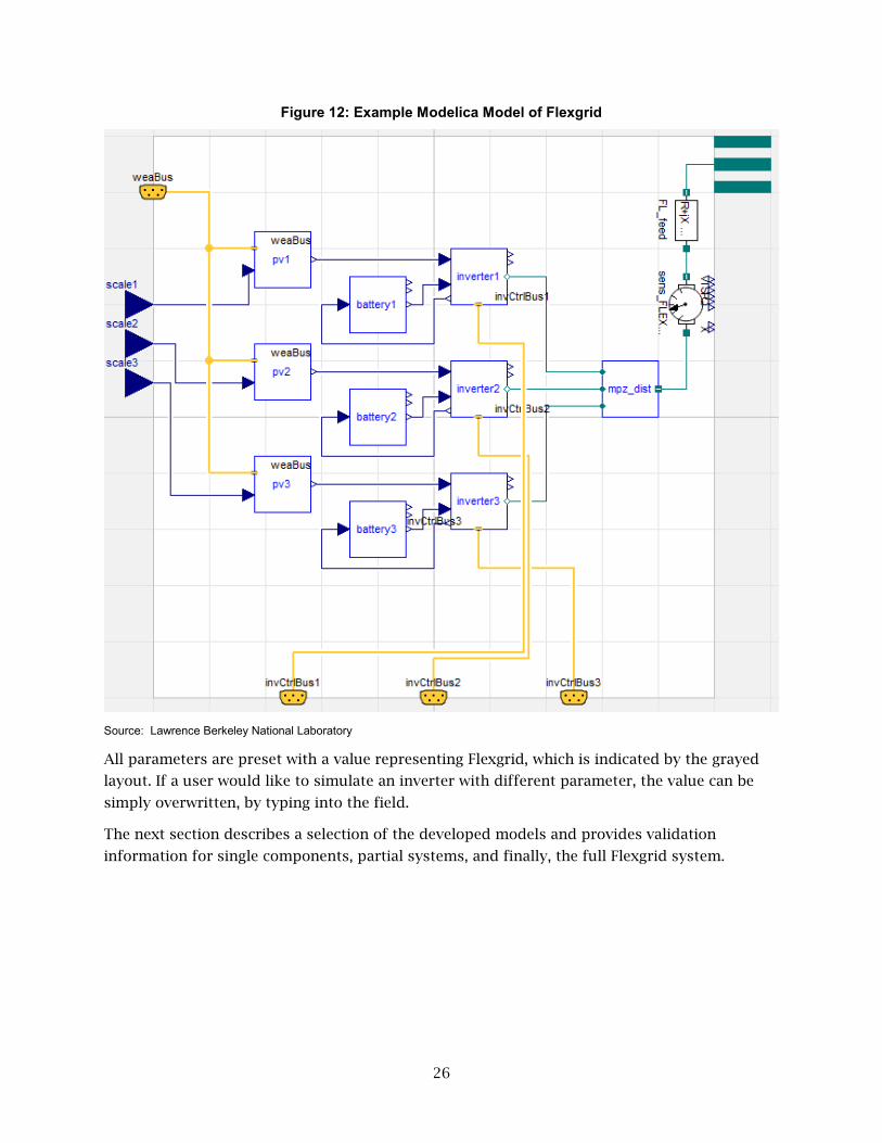
26
Figure 12: Example Modelica Model of Flexgrid
Source: Lawrence Berkeley National Laboratory
All parameters are preset with a value representing Flexgrid, which is indicated by the grayed
layout. If a user would like to simulate an inverter with different parameter, the value can be
simply overwritten, by typing into the field.
The next section describes a selection of the developed models and provides validation
information for single components, partial systems, and finally, the full Flexgrid system.

27
Figure 13: Example of Modelica Parameter Window
Source: Lawrence Berkeley National Laboratory
Inverter Model
The inverter is the most detailed model within the SCooDER package, as this is the central point
of research in the project. It is therefore required to accurately represent the behavior of
SolarEdge’s StorEdge19 inverter installed at Flexgrid. Figure 14 shows the components and
layout of the inverter model.
19 SolarEdge. StorEdge. https://www.solaredge.com/products/storedge#/.
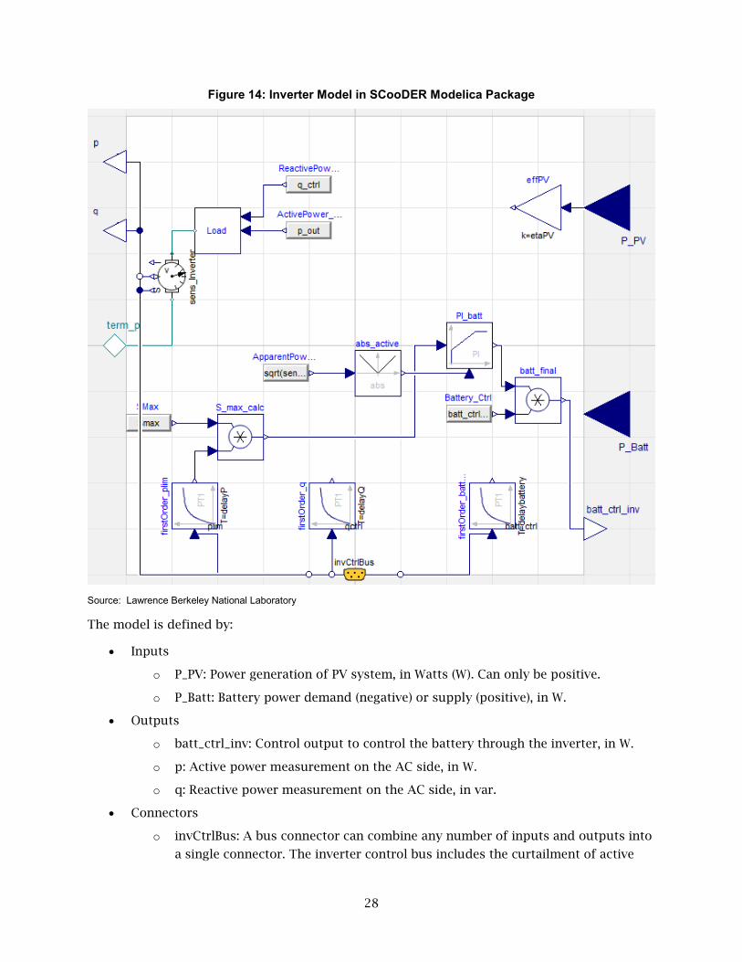
28
Figure 14: Inverter Model in SCooDER Modelica Package
Source: Lawrence Berkeley National Laboratory
The model is defined by:
• Inputs
o P_PV: Power generation of PV system, in Watts (W). Can only be positive.
o P_Batt: Battery power demand (negative) or supply (positive), in W.
• Outputs
o batt_ctrl_inv: Control output to control the battery through the inverter, in W.
o p: Active power measurement on the AC side, in W.
o q: Reactive power measurement on the AC side, in var.
• Connectors
o invCtrlBus: A bus connector can combine any number of inputs and outputs into
a single connector. The inverter control bus includes the curtailment of active

29
power, plim in %, regulate reactive power, qctrl in %, the battery control signal,
batt_ctrl in W, and measurements of active power, p in W, reactive power, q in
var, and voltage in V.
o term_p: Connection point to the electrical grid which is defined by the Modelica
Buildings library. It includes the voltage, v, and current, i, in complex form, and
the reference phase angle, theta.
• Parameters: All parameters are pre-defined to the configuration of Flexgrid, but can be
configured for any other inverter type.
o V_nominal: The nominal system voltage, in V. Default is 240 V.
o etaPV: Conversion efficiency of PV generation and DC/AC conversion. Default is
0.962.
o etaBatt: Conversion efficiency of AC/DC or DC/AC battery conversion. Default is
0.974.
o delayP: Time constant for active power control, in s. Default is 0.03 s.
o delayQ: Time constant for reactive power control, in s. Default is 0.03 s.
o delaybattery: Time constant for battery control, in s. Default is 0.03 s.
o Smax: Total power limit of the inverter, in VA. Default is 7600 VA.
o QIndmax: Inductive reactive power limit, in var. Default is 2500 var.
o QCapmax: Capacitive reactive power limit, in var. Default is 2500 var.
The inverter was built to seamlessly connect to any grid model within the framework of the
Modelica Buildings library, through the term_p connector. To model the StorEdge inverters that
are installed at Flexgrid, the model can be simply dragged and dropped into the simulation
setup within Modelica. If desired, an external PV generation can be connected to P_PV and an
external battery can be connected to P_Batt. If no external model is connected, the inputs will
default to 0 W to keep the structural integrity of the inverter model. If external control is
enabled, that is, by a voltage-dependent control loop, then the invCtrlBus can be used. The
SCooDER package includes a Volt-Var and Volt-Watt control, using the invCtrlBus. All inputs
communicated to the inverter via the invCtrlBus are filtered by a first-order function to
simulate the behavior of control execution time. Another input is plim, which is used to reduce
the power limit in case of PV curtailment. In such case, the Smax parameter is linearly scaled
down by the S_max_calc multiplication, on the lower left in Figure 14. The power limit is then
passed along to the battery control Proportional Integral limiting controller, PI_batt, which
scales the battery control signal, batt_ctrl_filtered. The control variable of PI_batt is the
apparent power output measured at the AC interconnection at sens_inverter. The curtailment of
PV generation is implemented as a secondary control action, once all battery power is curtailed
to 0. This prioritizes the generation of PV over the discharge of battery power.
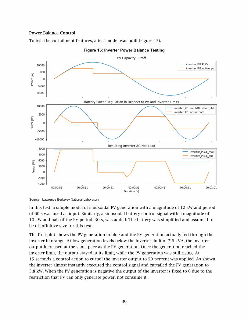
30
Power Balance Control
To test the curtailment features, a test model was built (Figure 15).
Figure 15: Inverter Power Balance Testing
Source: Lawrence Berkeley National Laboratory
In this test, a simple model of sinusoidal PV generation with a magnitude of 12 kW and period
of 60 s was used as input. Similarly, a sinusoidal battery control signal with a magnitude of
10 kW and half of the PV period, 30 s, was added. The battery was simplified and assumed to
be of infinitive size for this test.
The first plot shows the PV generation in blue and the PV generation actually fed through the
inverter in orange. At low generation levels below the inverter limit of 7.6 kVA, the inverter
output increased at the same pace as the PV generation. Once the generation reached the
inverter limit, the output stayed at its limit, while the PV generation was still rising. At
15 seconds a control action to curtail the inverter output to 50 percent was applied. As shown,
the inverter almost instantly executed the control signal and curtailed the PV generation to
3.8 kW. When the PV generation is negative the output of the inverter is fixed to 0 due to the
restriction that PV can only generate power, not consume it.
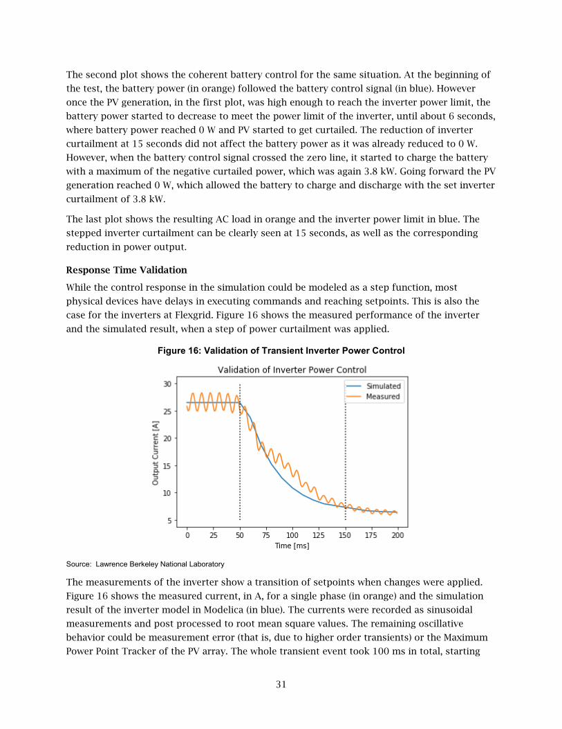
31
The second plot shows the coherent battery control for the same situation. At the beginning of
the test, the battery power (in orange) followed the battery control signal (in blue). However
once the PV generation, in the first plot, was high enough to reach the inverter power limit, the
battery power started to decrease to meet the power limit of the inverter, until about 6 seconds,
where battery power reached 0 W and PV started to get curtailed. The reduction of inverter
curtailment at 15 seconds did not affect the battery power as it was already reduced to 0 W.
However, when the battery control signal crossed the zero line, it started to charge the battery
with a maximum of the negative curtailed power, which was again 3.8 kW. Going forward the PV
generation reached 0 W, which allowed the battery to charge and discharge with the set inverter
curtailment of 3.8 kW.
The last plot shows the resulting AC load in orange and the inverter power limit in blue. The
stepped inverter curtailment can be clearly seen at 15 seconds, as well as the corresponding
reduction in power output.
Response Time Validation
While the control response in the simulation could be modeled as a step function, most
physical devices have delays in executing commands and reaching setpoints. This is also the
case for the inverters at Flexgrid. Figure 16 shows the measured performance of the inverter
and the simulated result, when a step of power curtailment was applied.
Figure 16: Validation of Transient Inverter Power Control
Source: Lawrence Berkeley National Laboratory
The measurements of the inverter show a transition of setpoints when changes were applied.
Figure 16 shows the measured current, in A, for a single phase (in orange) and the simulation
result of the inverter model in Modelica (in blue). The currents were recorded as sinusoidal
measurements and post processed to root mean square values. The remaining oscillative
behavior could be measurement error (that is, due to higher order transients) or the Maximum
Power Point Tracker of the PV array. The whole transient event took 100 ms in total, starting
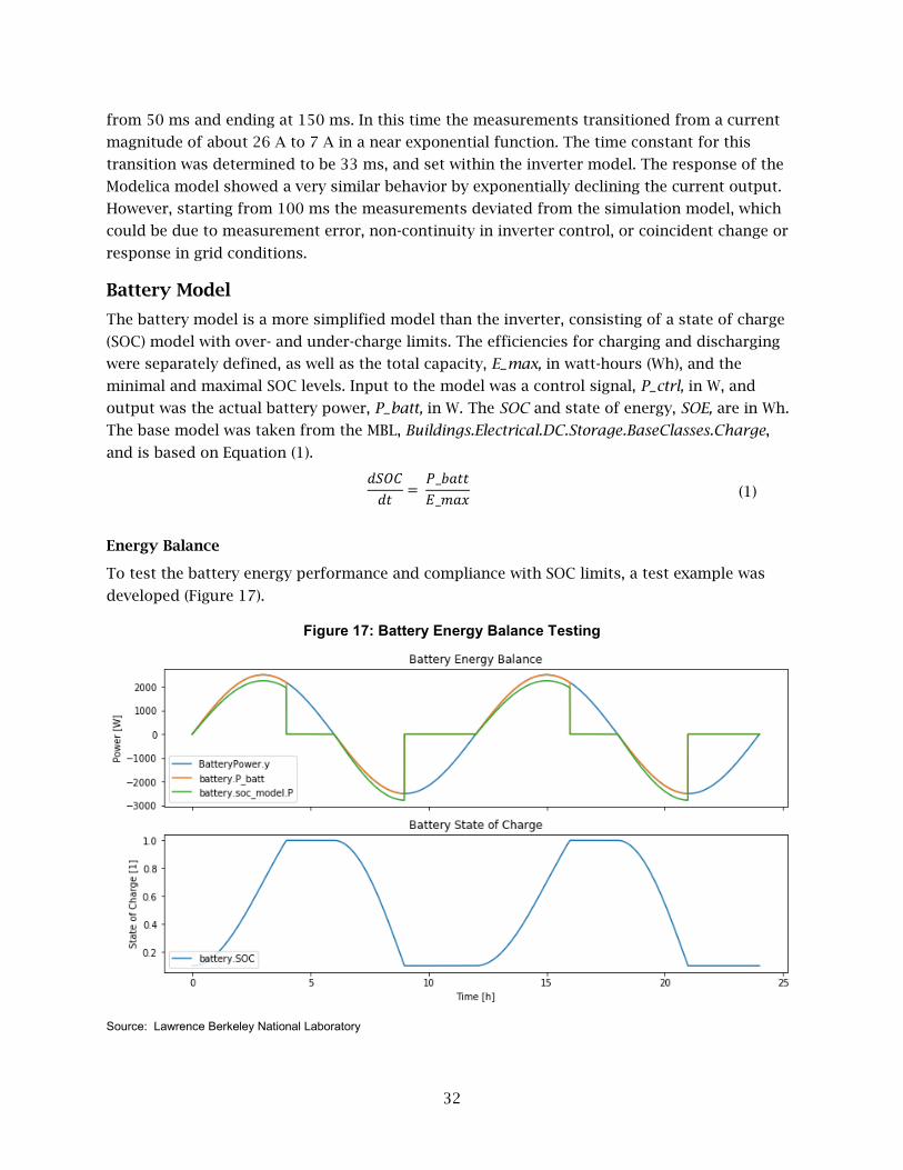
32
from 50 ms and ending at 150 ms. In this time the measurements transitioned from a current
magnitude of about 26 A to 7 A in a near exponential function. The time constant for this
transition was determined to be 33 ms, and set within the inverter model. The response of the
Modelica model showed a very similar behavior by exponentially declining the current output.
However, starting from 100 ms the measurements deviated from the simulation model, which
could be due to measurement error, non-continuity in inverter control, or coincident change or
response in grid conditions.
Battery Model
The battery model is a more simplified model than the inverter, consisting of a state of charge
(SOC) model with over- and under-charge limits. The efficiencies for charging and discharging
were separately defined, as well as the total capacity, E_max, in watt-hours (Wh), and the
minimal and maximal SOC levels. Input to the model was a control signal, P_ctrl, in W, and
output was the actual battery power, P_batt, in W. The SOC and state of energy, SOE, are in Wh.
The base model was taken from the MBL, Buildings.Electrical.DC.Storage.BaseClasses.Charge,
and is based on Equation (1).
𝑑𝑑𝑑𝑑𝑑𝑑𝑑𝑑𝑑𝑑𝑑𝑑
= 𝑃𝑃_𝑏𝑏𝑏𝑏𝑑𝑑𝑑𝑑𝐸𝐸_𝑚𝑚𝑏𝑏𝑚𝑚
(1)
Energy Balance
To test the battery energy performance and compliance with SOC limits, a test example was
developed (Figure 17).
Figure 17: Battery Energy Balance Testing
Source: Lawrence Berkeley National Laboratory

33
Here, a battery control signal, in blue, was modeled as a sinusoidal signal with a magnitude of
2.5 kW and a period of 12 hours. The battery power absorbed from the external sources, that is,
the inverter, is shown in orange, and the battery power actually feeding into the SOC model in
green. The difference between the absorbed power and the power in the SOC model is the
efficiency of the battery, which was set to 0.96 for charging and 0.96 for discharging. The
efficiency can be seen in the first plot, where the absorbed power followed the control signal
while the SOC power was either below the absorbed power, when charged, or above it, when
discharged. After about four hours the battery was fully charged, which caused the battery
power to drop to 0 W. The cause can be seen in the lower plot showing the SOC in blue. The
battery started with a SOC of 0.1 and SOC limits between 0.1 to 1. Once the battery reached a
full state, here 1, the charging power stopped immediately. On the other hand, once the battery
control requested to discharge, the battery started to discharge until the lower bound of SOC
0.1 was reached.
Model Validation
While the model proved to work on simulated data, a second validation was performed where
the model input was defined by measured inputs during a test at Flexgrid, and model outputs
were compared to measurements from Flexgrid. The battery was charged with a nearly constant
power of 1.12 kW (C-rate of 0.175), with a short reduction in charging power for about
5 minutes. At the end of the charging period the measured SOC was 0.995, and the modeled
SOC was 0.999. The marginal difference of 0.5 percent SOC is well below a threshold relevant
for this project and also well below the estimated error of SOC measurements, which are on the
order of ±2.5 percent.
Photovoltaic Model
The PV model is a simplified efficiency model where the total solar irradiation is calculated for
the tilted and rotated surface, and then multiplied with a static efficiency. The model was based
on the MBL, Buildings.Electrical.AC.OnePhase.Sources.PVSimple, in conjunction with an
anisotropic sky model (Perez et al. 1990).
Other Models
A variety of supportive and utility models were also added to the library to facilitate usage.
Examples are models to incorporate measurement data from PMU sensors, as voltage source
within the simulation, and a variety of controls. The most relevant control for this project is a
combined Volt-Var-Watt control where the reactive power and active power are regulated in
respect to locally observed grid voltages. At its base, this control model consists of two models,
one parameterized as Volt-Var and the other as Volt-Watt. It also introduces a higher level of
detail, where the inverter output is limited by its apparent power limit and where active power
is curtailed in favor of reactive power when reaching the limit. Figure 18 shows an example of
its operation.

34
Figure 18: Testing of Volt-Var-Watt Control
Source: Lawrence Berkeley National Laboratory
The figure shows the active power profile in the upper plot, reactive power in the middle plot,
and the resulting local voltage in the lower plot. The response of a base case without control is
shown in red, and the case with the Volt-Var-Watt control in blue. The controller provides
reactive power support as voltage increases. Once the inverter reactive power limit was reached,
the inverter started to curtail the active power in accordance to the voltage. The result was a
peak nodal voltage of about 104 percent; whereas, the base case without control resulted in
voltages above 106 percent of nominal.
System Validation
This section describes two steps taken to validate the full Flexgrid model, consisting of a set of
three inverters, batteries, PV arrays, and transformers, all parameterized to match Flexgrid.
The first step was the validation of PV generation profiles based on recorded historical weather
at LBNL. A toolchain was developed in Python to automatically read the EnergyPlus Weather file
(.epw), which is part of the input to Modelica, and to replace the typical meteorological year
data with measurements from LBNL. The generated .epw file was then converted to an .mos
Modelica readable file. This was done using the existing tool ConvertWeatherData.jar, which is
part of the MBL. The next step was to determine shading levels from obstructions, which are
not included in the model. Figure 19 shows an example screenshot from Google Maps. Note that
this image does not show the PV installation, which is located on top of the two lower-bay
testbeds on the left and right, marked in red.
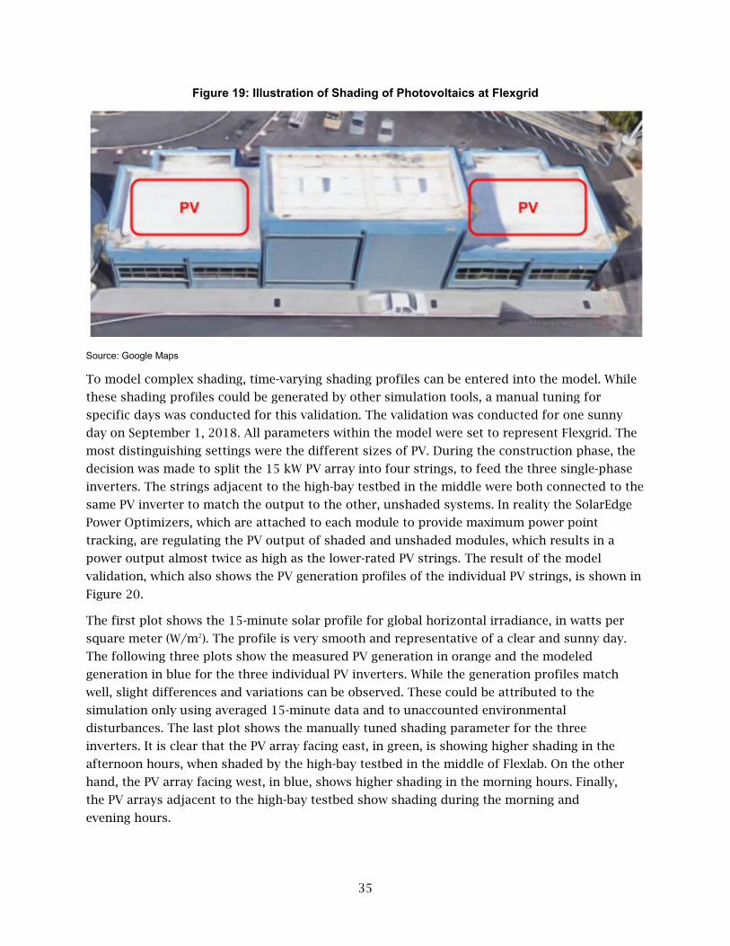
35
Figure 19: Illustration of Shading of Photovoltaics at Flexgrid
Source: Google Maps
To model complex shading, time-varying shading profiles can be entered into the model. While
these shading profiles could be generated by other simulation tools, a manual tuning for
specific days was conducted for this validation. The validation was conducted for one sunny
day on September 1, 2018. All parameters within the model were set to represent Flexgrid. The
most distinguishing settings were the different sizes of PV. During the construction phase, the
decision was made to split the 15 kW PV array into four strings, to feed the three single-phase
inverters. The strings adjacent to the high-bay testbed in the middle were both connected to the
same PV inverter to match the output to the other, unshaded systems. In reality the SolarEdge
Power Optimizers, which are attached to each module to provide maximum power point
tracking, are regulating the PV output of shaded and unshaded modules, which results in a
power output almost twice as high as the lower-rated PV strings. The result of the model
validation, which also shows the PV generation profiles of the individual PV strings, is shown in
Figure 20.
The first plot shows the 15-minute solar profile for global horizontal irradiance, in watts per
square meter (W/m2). The profile is very smooth and representative of a clear and sunny day.
The following three plots show the measured PV generation in orange and the modeled
generation in blue for the three individual PV inverters. While the generation profiles match
well, slight differences and variations can be observed. These could be attributed to the
simulation only using averaged 15-minute data and to unaccounted environmental
disturbances. The last plot shows the manually tuned shading parameter for the three
inverters. It is clear that the PV array facing east, in green, is showing higher shading in the
afternoon hours, when shaded by the high-bay testbed in the middle of Flexlab. On the other
hand, the PV array facing west, in blue, shows higher shading in the morning hours. Finally,
the PV arrays adjacent to the high-bay testbed show shading during the morning and
evening hours.
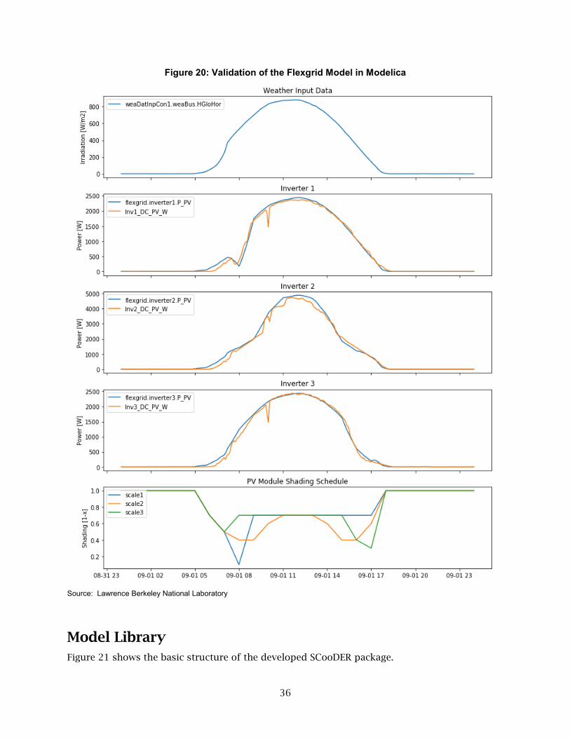
36
Figure 20: Validation of the Flexgrid Model in Modelica
Source: Lawrence Berkeley National Laboratory
Model Library Figure 21 shows the basic structure of the developed SCooDER package.
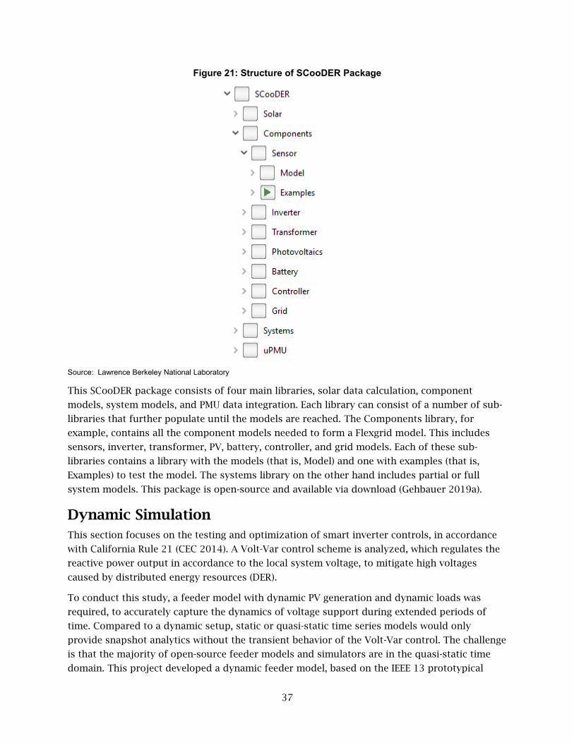
37
Figure 21: Structure of SCooDER Package
Source: Lawrence Berkeley National Laboratory
This SCooDER package consists of four main libraries, solar data calculation, component
models, system models, and PMU data integration. Each library can consist of a number of sub-
libraries that further populate until the models are reached. The Components library, for
example, contains all the component models needed to form a Flexgrid model. This includes
sensors, inverter, transformer, PV, battery, controller, and grid models. Each of these sub-
libraries contains a library with the models (that is, Model) and one with examples (that is,
Examples) to test the model. The systems library on the other hand includes partial or full
system models. This package is open-source and available via download (Gehbauer 2019a).
Dynamic Simulation This section focuses on the testing and optimization of smart inverter controls, in accordance
with California Rule 21 (CEC 2014). A Volt-Var control scheme is analyzed, which regulates the
reactive power output in accordance to the local system voltage, to mitigate high voltages
caused by distributed energy resources (DER).
To conduct this study, a feeder model with dynamic PV generation and dynamic loads was
required, to accurately capture the dynamics of voltage support during extended periods of
time. Compared to a dynamic setup, static or quasi-static time series models would only
provide snapshot analytics without the transient behavior of the Volt-Var control. The challenge
is that the majority of open-source feeder models and simulators are in the quasi-static time
domain. This project developed a dynamic feeder model, based on the IEEE 13 prototypical

38
feeder model (IEEE 2000), within the framework of Modelica. The IEEE 13 model has a
standardized base, is easy to replicate and is widely known in the research community.
Load profiles were gathered from the USDOE prototypical buildings’ simulations (Deru et al.
2011) and were assigned to nodes along the feeder using a developed dynamic load generator.
PV was evenly distributed along the feeder, and simulated in scenarios of 0, 25, 50, 75, and
100 percent of PV penetration. Initial simulations were conducted for a full year to identify the
peak day of the year for each PV penetration scenario. In a second step, the simulations were
limited to only this day, and a framework was developed to allow a parameter sweep through
Volt-Var configuration. The parameter sweep was conducted using a grid-search methodology,
where an evenly sized grid of Volt-Var parameters was tested. Finally, the parameter
optimization was conducted in two setups: one where all inverters along the grid used the same
setpoints, which is the typical configuration of utilities, and one where inverters were grouped
into clusters and individual parameters were assigned.
Feeder Model
The feeder was modeled in the Modelica environment as a variant of the IEEE 13 prototypical
feeder model. The Modelica Buildings library provides a convenient template to rapidly design
new feeder models based on existing or new types of lines. A simple connection list was written
in Modelica describing the line segments between nodes by their length, type, and nodal
connection. Figure 22 shows the developed feeder as a variant of the IEEE 13 prototypical
feeder model.
Figure 22: Modeled IEEE 13 Feeder
Source: Lawrence Berkeley National Laboratory
The numbering of nodes and lines was replaced by a continuous count from 1 to 13 for nodes
and 1 to 12 for lines. The black numbers indicate nodes and the red numbers lines. The
transformer between nodes 5 and 6 and the switch between nodes 7 and 10 were replaced by
line segments. These modifications were made to simplify the model, because neither a
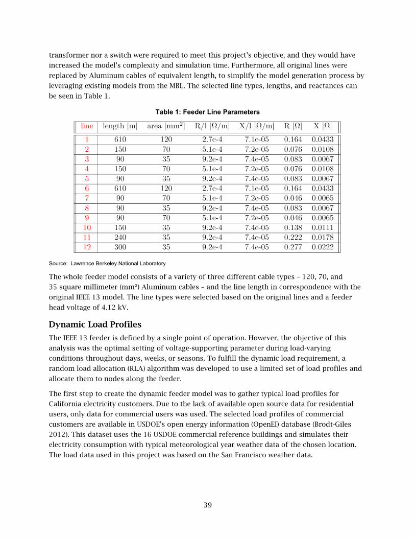
39
transformer nor a switch were required to meet this project’s objective, and they would have
increased the model’s complexity and simulation time. Furthermore, all original lines were
replaced by Aluminum cables of equivalent length, to simplify the model generation process by
leveraging existing models from the MBL. The selected line types, lengths, and reactances can
be seen in Table 1.
Table 1: Feeder Line Parameters
Source: Lawrence Berkeley National Laboratory
The whole feeder model consists of a variety of three different cable types – 120, 70, and
35 square millimeter (mm²) Aluminum cables – and the line length in correspondence with the
original IEEE 13 model. The line types were selected based on the original lines and a feeder
head voltage of 4.12 kV.
Dynamic Load Profiles
The IEEE 13 feeder is defined by a single point of operation. However, the objective of this
analysis was the optimal setting of voltage-supporting parameter during load-varying
conditions throughout days, weeks, or seasons. To fulfill the dynamic load requirement, a
random load allocation (RLA) algorithm was developed to use a limited set of load profiles and
allocate them to nodes along the feeder.
The first step to create the dynamic feeder model was to gather typical load profiles for
California electricity customers. Due to the lack of available open source data for residential
users, only data for commercial users was used. The selected load profiles of commercial
customers are available in USDOE’s open energy information (OpenEI) database (Brodt-Giles
2012). This dataset uses the 16 USDOE commercial reference buildings and simulates their
electricity consumption with typical meteorological year weather data of the chosen location.
The load data used in this project was based on the San Francisco weather data.

40
Random Load Allocation
While the three biggest OpenEI loads – hospital, large office building, and secondary school –
are an order of magnitude larger than the IEEE 13 model loads, most other loads are
significantly smaller. Thus, it is not possible to directly assign the OpenEI loads to nodes with
the original IEEE 13 loads. An approach was developed to allow some loads to be manually
assigned to nodes, and scaled down to the peak value, in accordance with IEEE 13, while the
remainder of the nodes used randomly assigned load profiles with a peak-power equivalent to
the original IEEE 13 loads. The hospital was manually assigned to one of the most stable
electrically nodes, node 7, as a balanced three-phase load. Similarly, the secondary school was
assigned to another centered node, node 2, as a balanced three-phase load. The large office was
not further used in this allocation process due to its similarity with smaller-scale medium and
small office buildings, which are more flexible to assign. The remaining 13 loads were assigned
using the random load allocation (RLA) algorithm developed for this project. This algorithm
adds random loads from the OpenEI loads to each phase at each node, until the annual peak
load at this phase and node exceeds the assigned power in the IEEE 13 model, denoted in Table
2. This function is called for every phase at every node until all the nodes have random loads
assigned. To make the random results replicable, seeds, which are fixed start points for random
load generators, were used for the random generator. With a specific seed, the random function
always produces the same random output.
The algorithm is initialized with an assignment of the random seed, which can be any real
number, and the peak load to be reached. The RLA then selects a random initial load from the
available OpenEI loads and starts the allocation process. An initial step checks if the current
peak load is lower than the target peak. If it is below the limit, then another random load is
added to the current load profile. To select this new random load, the seed is increased by 1 at
each step. This load addition is repeated, until the peak load is higher than the targeted peak.
To avoid overlapping seeds during this allocation process, the numbers of node and phase were
combined and multiplied by a factor of 1000. For example, the seed for node 12 and phase 2
would be 122000, for node 6 and phase 1 it would be 61000, and for node 6 and phase 2 it
would be 62000. During the allocation process this number is increased by one, so assuming it
takes three iterations to build up the load profile, the seeds would be 62000, 62001, and 62002
for node 6, phase 2. In case of a balanced three-phase load, the same initial seed can be
supplied for all three phases, which would result in the RLA selecting the same loads for each
phase. The resulting load profiles were exactly the same, representing a balanced three-phase
system. However, the only balanced node in the system was node 7, where the hospital was
manually assigned.
While the RLA was assigning active power loads to the nodes, another process was applied to
assign reactive power to the nodes. Here the active power profiles generated by the RLA were
multiplied with the reactive power peak load, Q, and divided by the active power peak load, P.
In other words, the profiles for Q were assigned proportional to P, with a different multiplier
for every node, depending on the specified values for maximum active and reactive power.

41
When applying the RLA algorithm to the feeder model, the resulting loads were to some extent
higher than specified within the IEEE13 model. This results in voltage dropps below 95 percent
of the nominal voltage for several nodes, for the most critical day of the year. According to the
American National Standards Institute, voltages below 95 percent of nominal for an extended
period of time are seen as voltage violations (ANSI 2016). To prevent those voltage violations,
the original IEEE 13 loads were scaled down until no more voltage violations occurred. The final
load table, which was used for the RLA algorithm, can be seen in Table 2.
Table 2: Original IEEE13 Load Table
Source: Lawrence Berkeley National Laboratory
The loads were significantly decreased, up to 40 percent, to keep voltages above the 95 percent
threshold. The reason for this high scaling factor was a compounded error of different feeder
topology, line types, connections, and overshooting of the RLA, in comparison to the original
IEEE 13 model. However, the feeder model was still representative of a real system with a
diversity of load profiles along the different nodes.
In Figure 23, the resulting power and voltage profiles for the generated feeder model are
illustrated for two example days. The days represent the peak day of the year, with the lowest
measured voltages, and a low-load Sunday in January.
The blue line in Figure 23 shows the active power, and the green line the reactive power, of
Phase 3 at the feeder head. Phase 3 was chosen because it has the highest and therefore most
critical load. The peak load was approximately 2.5 megawatts (MW) and 1.4 mega volt amps
reactive (Mvar). At the low-load Sunday, the peak load was only 1.1 MW and 0.7 Mvar. The shape
of active and reactive loads is similar due to the fixed relationship of active and reactive power,
by the power factor. To further analyze the load distribution, Figure 24 shows the loads at each
node along the grid.
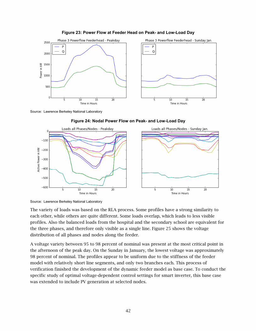
42
Figure 23: Power Flow at Feeder Head on Peak- and Low-Load Day
Source: Lawrence Berkeley National Laboratory
Figure 24: Nodal Power Flow on Peak- and Low-Load Day
Source: Lawrence Berkeley National Laboratory
The variety of loads was based on the RLA process. Some profiles have a strong similarity to
each other, while others are quite different. Some loads overlap, which leads to less visible
profiles. Also the balanced loads from the hospital and the secondary school are equivalent for
the three phases, and therefore only visible as a single line. Figure 25 shows the voltage
distribution of all phases and nodes along the feeder.
A voltage variety between 95 to 98 percent of nominal was present at the most critical point in
the afternoon of the peak day. On the Sunday in January, the lowest voltage was approximately
98 percent of nominal. The profiles appear to be uniform due to the stiffness of the feeder
model with relatively short line segments, and only two branches each. This process of
verification finished the development of the dynamic feeder model as base case. To conduct the
specific study of optimal voltage-dependent control settings for smart inverter, this base case
was extended to include PV generation at selected nodes.
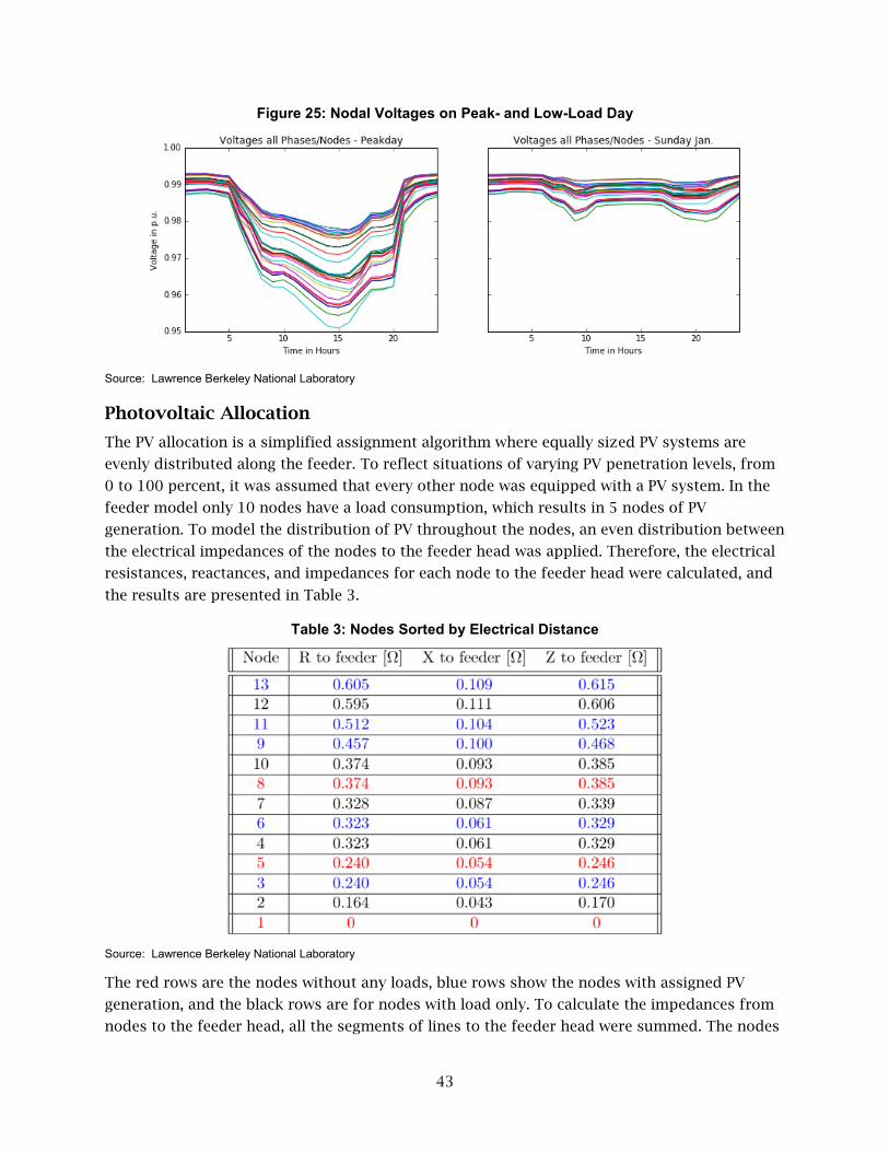
43
Figure 25: Nodal Voltages on Peak- and Low-Load Day
Source: Lawrence Berkeley National Laboratory
Photovoltaic Allocation
The PV allocation is a simplified assignment algorithm where equally sized PV systems are
evenly distributed along the feeder. To reflect situations of varying PV penetration levels, from
0 to 100 percent, it was assumed that every other node was equipped with a PV system. In the
feeder model only 10 nodes have a load consumption, which results in 5 nodes of PV
generation. To model the distribution of PV throughout the nodes, an even distribution between
the electrical impedances of the nodes to the feeder head was applied. Therefore, the electrical
resistances, reactances, and impedances for each node to the feeder head were calculated, and
the results are presented in Table 3.
Table 3: Nodes Sorted by Electrical Distance
Source: Lawrence Berkeley National Laboratory
The red rows are the nodes without any loads, blue rows show the nodes with assigned PV
generation, and the black rows are for nodes with load only. To calculate the impedances from
nodes to the feeder head, all the segments of lines to the feeder head were summed. The nodes

44
were sorted by their impedances to the feeder head and a PV system was assigned to the node
with the highest impedances. Moving toward lower impedances, PV was assigned to every
second node with load consumption. Note that due to initial problems with the model, the PV
system at node 10 was moved to node 9.
The PV generation was split into five scenarios, where the PV penetration was set to 0, 25, 50,
75, and 100 percent of the annual energy demand. A basic PV system was created and scaled up
to fit those demands. Each PV panel of the basic PV system has a size of 1.65 m² and an
efficiency of 0.158, which results in a power output of 260.7 W per module at standard test
conditions (STC). This model was designed using operational data from the Flexgrid facility.
Each PV system has an inverter with a maximum apparent power of 7,600 VA and a maximal
power factor of 0.9 at peak power. The inverter can accommodate up to 30 PV modules, but
only 26 panels were assigned per inverter, to allow a certain capacity range for reactive power
control without curtailing the active power generation. This number of panels was determined
by a calculation of the maximum apparent power of the inverter multiplied with the power
factor and divided by the rated power, shown in Equations (2) and (3).
𝑃𝑃 = 𝑑𝑑 ⋅ 𝑝𝑝𝑝𝑝 = 7600 𝑉𝑉𝑉𝑉 ⋅ 0.9 = 6840 𝑊𝑊 (2)
6840 𝑊𝑊260.7 𝑊𝑊/𝑝𝑝𝑏𝑏𝑝𝑝𝑝𝑝𝑝𝑝
= 26.24 𝑝𝑝𝑏𝑏𝑝𝑝𝑝𝑝𝑝𝑝𝑝𝑝 (3)
The applied power factor allows the inverter to still provide or absorb reactive power of up to
3313 var, which results from the following Equation (4):
𝑄𝑄 = �𝑑𝑑2 − 𝑃𝑃2 = �76002𝑉𝑉𝑉𝑉2 − 68402𝑊𝑊2 = 3313 𝑣𝑣𝑏𝑏𝑣𝑣 (4)
The annual PV generation of the feeder for one PV system for each phase at each of the five
chosen nodes, here called E_PV, is 206.3 megawatt-hours per year (MWh/a). The energy
consumption E_load without PV generation is 27,788.2 MWh/a. Therefore, the amount of PV
systems needed to generate 100 percent of the annual electricity consumption can be
calculated by dividing the annual consumed energy with the annual generated energy per PV
system. This calculation is shown in Equation (5).
𝐸𝐸𝑙𝑙𝑙𝑙𝑙𝑙𝑙𝑙𝐸𝐸𝑃𝑃𝑃𝑃
=27,788.2 𝑀𝑀𝑊𝑊ℎ
206.3 𝑀𝑀𝑊𝑊ℎ= 134.7 (5)
The PV generation for the 100 percent scenario was multiplied by 0, 0.25, 0.5, 0.75, and 1,
depending on the penetration scenario. This resulted in 0, 34, 67, 101, and 135 PV systems at
each of the three phases and each of the five chosen PV nodes. These are 0, 102, 201, 303, and
405 PV systems at each of the nodes or 0, 510, 1005, 1515, and 2025 individual PV systems in
the whole feeder.
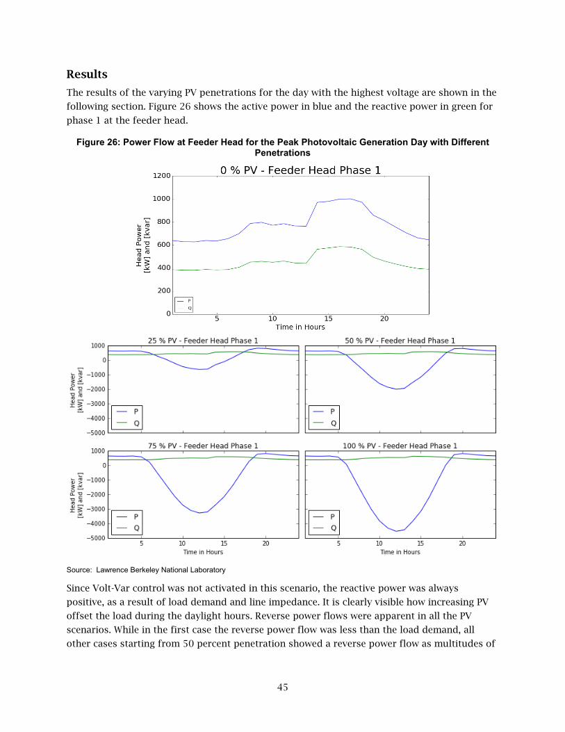
45
Results
The results of the varying PV penetrations for the day with the highest voltage are shown in the
following section. Figure 26 shows the active power in blue and the reactive power in green for
phase 1 at the feeder head.
Figure 26: Power Flow at Feeder Head for the Peak Photovoltaic Generation Day with Different Penetrations
Source: Lawrence Berkeley National Laboratory
Since Volt-Var control was not activated in this scenario, the reactive power was always
positive, as a result of load demand and line impedance. It is clearly visible how increasing PV
offset the load during the daylight hours. Reverse power flows were apparent in all the PV
scenarios. While in the first case the reverse power flow was less than the load demand, all
other cases starting from 50 percent penetration showed a reverse power flow as multitudes of
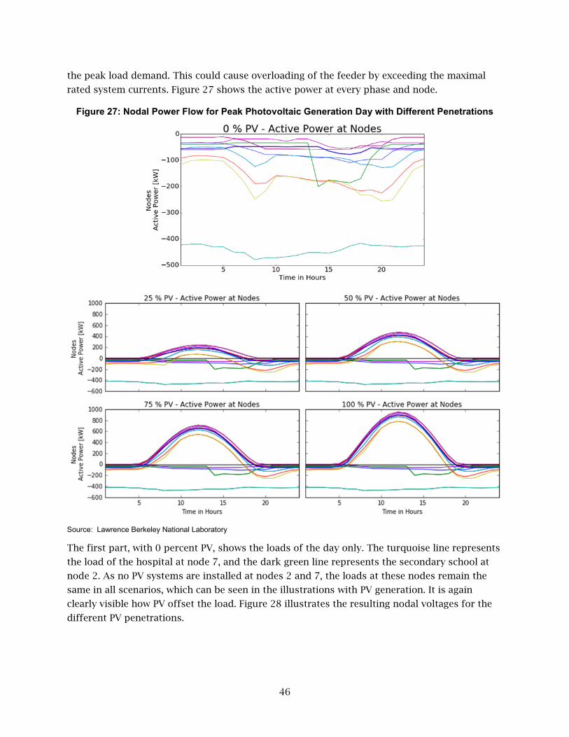
46
the peak load demand. This could cause overloading of the feeder by exceeding the maximal
rated system currents. Figure 27 shows the active power at every phase and node.
Figure 27: Nodal Power Flow for Peak Photovoltaic Generation Day with Different Penetrations
Source: Lawrence Berkeley National Laboratory
The first part, with 0 percent PV, shows the loads of the day only. The turquoise line represents
the load of the hospital at node 7, and the dark green line represents the secondary school at
node 2. As no PV systems are installed at nodes 2 and 7, the loads at these nodes remain the
same in all scenarios, which can be seen in the illustrations with PV generation. It is again
clearly visible how PV offset the load. Figure 28 illustrates the resulting nodal voltages for the
different PV penetrations.
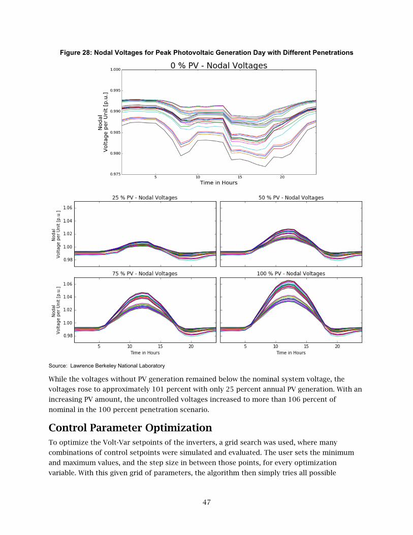
47
Figure 28: Nodal Voltages for Peak Photovoltaic Generation Day with Different Penetrations
Source: Lawrence Berkeley National Laboratory
While the voltages without PV generation remained below the nominal system voltage, the
voltages rose to approximately 101 percent with only 25 percent annual PV generation. With an
increasing PV amount, the uncontrolled voltages increased to more than 106 percent of
nominal in the 100 percent penetration scenario.
Control Parameter Optimization To optimize the Volt-Var setpoints of the inverters, a grid search was used, where many
combinations of control setpoints were simulated and evaluated. The user sets the minimum
and maximum values, and the step size in between those points, for every optimization
variable. With this given grid of parameters, the algorithm then simply tries all possible
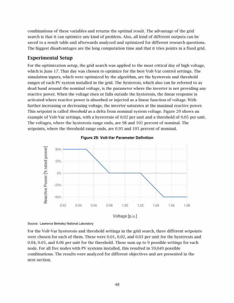
48
combinations of these variables and returns the optimal result. The advantage of the grid
search is that it can optimize any kind of problem. Also, all kind of different outputs can be
saved to a result table and afterwards analyzed and optimized for different research questions.
The biggest disadvantages are the long computation time and that it tries points in a fixed grid.
Experimental Setup
For the optimization setup, the grid search was applied to the most critical day of high voltage,
which is June 17. That day was chosen to optimize for the best Volt-Var control settings. The
simulation inputs, which were optimized by the algorithm, are the hysteresis and threshold
ranges of each PV system installed in the grid. The hysteresis, which also can be referred to as
dead band around the nominal voltage, is the parameter where the inverter is not providing any
reactive power. When the voltage rises or falls outside the hysteresis, the linear response is
activated where reactive power is absorbed or injected as a linear function of voltage. With
further increasing or decreasing voltage, the inverter saturates at the maximal reactive power.
This setpoint is called threshold as a delta from nominal system voltage. Figure 29 shows an
example of Volt-Var settings, with a hysteresis of 0.02 per unit and a threshold of 0.05 per unit.
The voltages, where the hysteresis range ends, are 98 and 102 percent of nominal. The
setpoints, where the threshold range ends, are 0.95 and 105 percent of nominal.
Figure 29: Volt-Var Parameter Definition
Source: Lawrence Berkeley National Laboratory
For the Volt-Var hysteresis and threshold settings in the grid search, three different setpoints
were chosen for each of them. These were 0.01, 0.02, and 0.03 per unit for the hysteresis and
0.04, 0.05, and 0.06 per unit for the threshold. These sum up to 9 possible settings for each
node. For all five nodes with PV systems installed, this resulted in 59,049 possible
combinations. The results were analyzed for different objectives and are presented in the
next section.
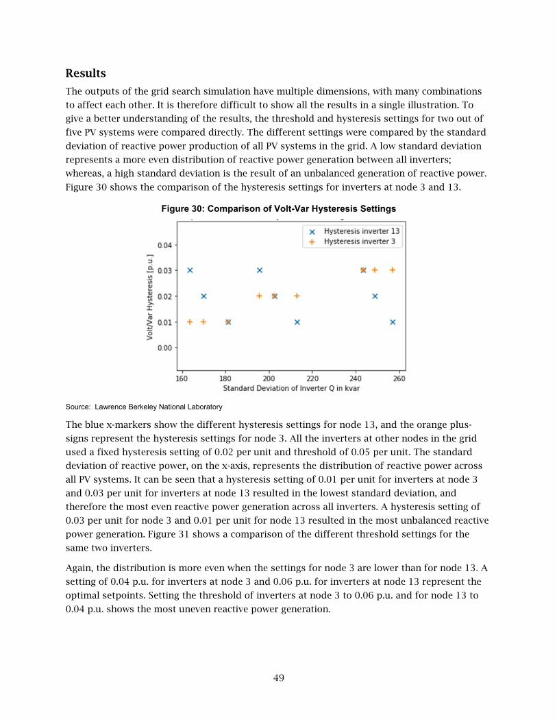
49
Results
The outputs of the grid search simulation have multiple dimensions, with many combinations
to affect each other. It is therefore difficult to show all the results in a single illustration. To
give a better understanding of the results, the threshold and hysteresis settings for two out of
five PV systems were compared directly. The different settings were compared by the standard
deviation of reactive power production of all PV systems in the grid. A low standard deviation
represents a more even distribution of reactive power generation between all inverters;
whereas, a high standard deviation is the result of an unbalanced generation of reactive power.
Figure 30 shows the comparison of the hysteresis settings for inverters at node 3 and 13.
Figure 30: Comparison of Volt-Var Hysteresis Settings
Source: Lawrence Berkeley National Laboratory
The blue x-markers show the different hysteresis settings for node 13, and the orange plus-
signs represent the hysteresis settings for node 3. All the inverters at other nodes in the grid
used a fixed hysteresis setting of 0.02 per unit and threshold of 0.05 per unit. The standard
deviation of reactive power, on the x-axis, represents the distribution of reactive power across
all PV systems. It can be seen that a hysteresis setting of 0.01 per unit for inverters at node 3
and 0.03 per unit for inverters at node 13 resulted in the lowest standard deviation, and
therefore the most even reactive power generation across all inverters. A hysteresis setting of
0.03 per unit for node 3 and 0.01 per unit for node 13 resulted in the most unbalanced reactive
power generation. Figure 31 shows a comparison of the different threshold settings for the
same two inverters.
Again, the distribution is more even when the settings for node 3 are lower than for node 13. A
setting of 0.04 p.u. for inverters at node 3 and 0.06 p.u. for inverters at node 13 represent the
optimal setpoints. Setting the threshold of inverters at node 3 to 0.06 p.u. and for node 13 to
0.04 p.u. shows the most uneven reactive power generation.
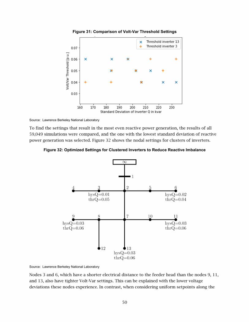
50
Figure 31: Comparison of Volt-Var Threshold Settings
Source: Lawrence Berkeley National Laboratory
To find the settings that result in the most even reactive power generation, the results of all
59,049 simulations were compared, and the one with the lowest standard deviation of reactive
power generation was selected. Figure 32 shows the nodal settings for clusters of inverters.
Figure 32: Optimized Settings for Clustered Inverters to Reduce Reactive Imbalance
Source: Lawrence Berkeley National Laboratory
Nodes 3 and 6, which have a shorter electrical distance to the feeder head than the nodes 9, 11,
and 13, also have tighter Volt-Var settings. This can be explained with the lower voltage
deviations these nodes experience. In contrast, when considering uniform setpoints along the

51
grid, which is the standard for most utilities, the inverters at node 3 and 6 would start to
generate reactive power only with a much higher PV penetration than the inverters at nodes 9,
11, and 13. It is therefore necessary to compensate for this effect by having inverters at node 3
and 6 generate reactive power already at lower voltage levels. With these settings applied, the
standard deviation between the reactive power generation of all nodes in the grid is
51,350 kVar. The best possible standard deviation, with uniform setpoints, is 142,500 kVar,
with a hysteresis setting of 0.01 per unit and a threshold setting of 0.06 per unit.
Discussion
The created model shows a significant variety of loading and voltages over an entire year.
Hence, it can be used to conduct annual simulations to test different control algorithms, but is
also applicable for single-day simulations. Due to the distribution of the inverters at several
locations along the grid, the impact of individual inverter control settings for different
locations can be easily investigated. The models developed in Modelica allow the physics of an
electric power grid to be represented realistically and dynamically. The usage of different load
profiles, based on local weather conditions, create a realistic variety of customers on the grid.
Another strong advantage of this model and approach is the straightforward implementation of
different locations within California and the United States. The load profiles are available for all
locations with historical weather data, which is also input to simulate the PV generation.
However, one limitation of the current setup is the usage of commercial load data only. This
limitation is due to the lack of accessible load data for residential or industrial customers.
Another limitation is that the load data are simulated in hourly timesteps, based on the typical
meteorological year weather data, which is only partially representative of real loads with more
dynamics and noise. Another point of discussion is the computation time of dynamic models
compared to static or quasi static time series simulations, and therefore the increased
complexity when optimizing them, where each simulation takes longer than a comparable static
model would take. Since parameter studies of control setpoints are based on simulations, the
computation time of large grid searches can easily become infeasible. One possible workaround
to significantly reduce the computation time needed to find the optimal solution is to employ
optimization solvers, which use gradients or other heuristics to quickly converge. Future work
may focus on such methods to make large, region scale simulations possible.
The results show that different control settings for different clusters of inverters can
accomplish a more even reactive power generation across locations. With such optimal settings,
inverters at critical nodes, with higher voltages, have to produce less reactive power than they
would with non-optimized settings. Conversely, inverters at nodes with lower voltages have to
generate more reactive power than they would with uniform settings. With the assumption that
inverters typically have similar technical specifications to provide reactive power, inverters
would need to be less oversized, or more PV modules could be connected to the same inverter.
This can decrease the capital cost when voltage-dependent controls are applied, as is the case
with California Rule 21 (CEC 2014). The increased reactive power generation would also result
in lower voltages throughout all nodes on the distribution feeder and could therefore decrease
possible Volt-Watt curtailments at critical nodes. Such a situation would result in a higher

52
generation of active power at the nodes, increasing the power output of PV systems. However, a
potential downside of this approach is the overall increased reactive power in the system,
which can lead to higher distribution losses along the feeder. Future work might focus on the
combination of Volt-Var-Watt controls and the economic trade-off when deployed at scale.
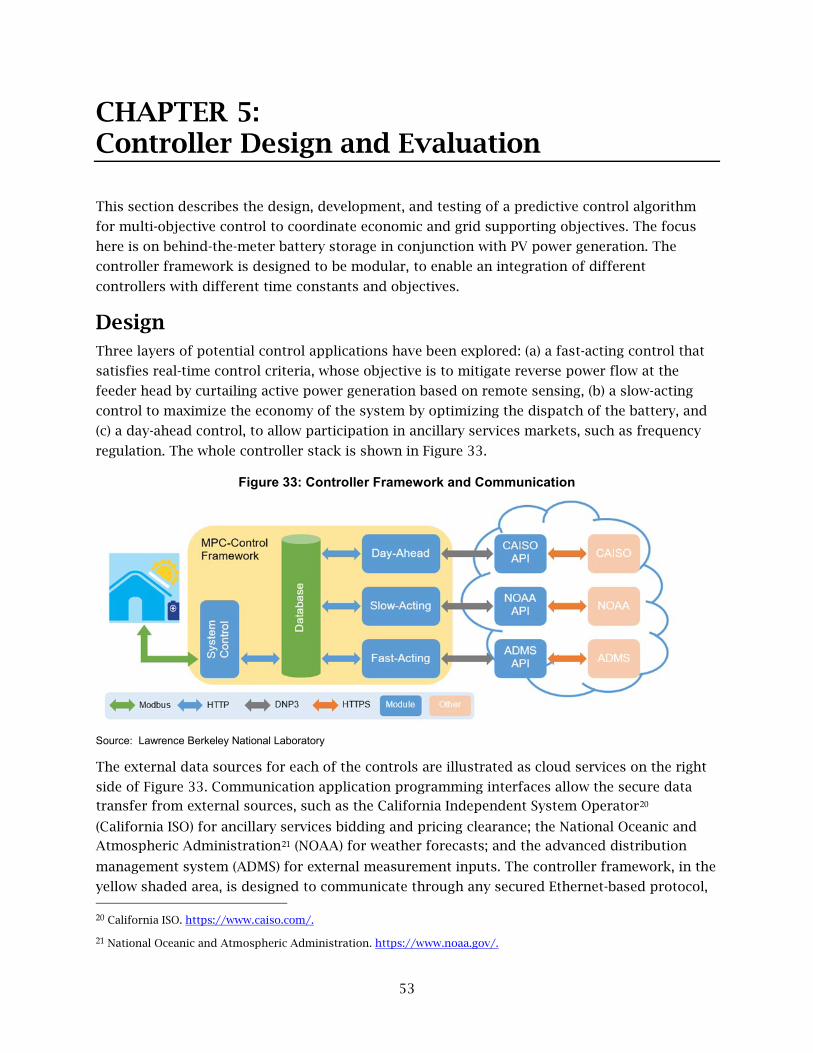
53
CHAPTER 5: Controller Design and Evaluation
This section describes the design, development, and testing of a predictive control algorithm
for multi-objective control to coordinate economic and grid supporting objectives. The focus
here is on behind-the-meter battery storage in conjunction with PV power generation. The
controller framework is designed to be modular, to enable an integration of different
controllers with different time constants and objectives.
Design Three layers of potential control applications have been explored: (a) a fast-acting control that
satisfies real-time control criteria, whose objective is to mitigate reverse power flow at the
feeder head by curtailing active power generation based on remote sensing, (b) a slow-acting
control to maximize the economy of the system by optimizing the dispatch of the battery, and
(c) a day-ahead control, to allow participation in ancillary services markets, such as frequency
regulation. The whole controller stack is shown in Figure 33.
Figure 33: Controller Framework and Communication
Source: Lawrence Berkeley National Laboratory
The external data sources for each of the controls are illustrated as cloud services on the right
side of Figure 33. Communication application programming interfaces allow the secure data
transfer from external sources, such as the California Independent System Operator20
(California ISO) for ancillary services bidding and pricing clearance; the National Oceanic and
Atmospheric Administration21 (NOAA) for weather forecasts; and the advanced distribution
management system (ADMS) for external measurement inputs. The controller framework, in the
yellow shaded area, is designed to communicate through any secured Ethernet-based protocol, 20 California ISO. https://www.caiso.com/.
21 National Oceanic and Atmospheric Administration. https://www.noaa.gov/.

54
which could be the distributed network protocol or hypertext transfer protocol secure. All
control modules, in blue, within the controller stack communicate through a socket
communication which allows wide flexibility in integration, such as parallel, asynchronous
control. The central resource here is a Python-based database, in green, to store all inputs and
outputs of the control modules. The System Control module is then responsible to
communicate with the physical devices located on site. The installed inverters at LBNL use
Modbus; however, any other protocol could be implemented through Python.
Framework
One major focus in the development of the controller framework is its modularity, and its
ability to host multiple modules with different timesteps, potentially ranging from sub-seconds
up to hours to compute a single control action. To satisfy the modularity, the whole framework
is built based on Python base classes inspired by the Functional Mockup Interface (FMI)
(Modelisar 2014). A functional mockup unit (FMU) is a simulation or control model exported in
accordance with the FMI standard. While the framework does not directly support FMUs in its
current state, it is built in a similar fashion and relies largely on standard functions found in
FMI. To register controller instances in the framework, an emulated FMU, eFMU, wrapper class
is available to host the control algorithm. Figure 34 shows a simple example of an algorithm
wrapped in the eFMU class to be plugged into the controller.
Figure 34: Example of Emulated Functional Mockup Unit Wrapper
Source: Lawrence Berkeley National Laboratory
In this example the testcontroller1 class is registered as an expansion of the Python base class
eFMU. Only two functions have to be added to complete the development. First, the __init__
function must include definitions for inputs (self.input) and outputs (self.output). Second, the
compute function, which includes the algorithm to compute the output of the control, must be
defined. With these few lines of code a fully functional module is completed and ready to be
plugged into the controller framework. For more complex modules, the user can add any
number of class functions and local variables. The latest version of the framework includes the
ability to store variables and executed classes, which avoids the need to re-instantiate them at
each controller evaluation. This feature was implemented with the switch to a parallel
architecture using the multiprocessing package in Python to spawn the controller modules as
sub-processes.
The second part of the framework is the controller stack handler, which links controller
modules together and handles the flow control. Controller modules are defined in a Python
dictionary containing the controller class, that is, testcontroller1 in the example above, and the
sample time in seconds. Note that the sample time can be in sub-seconds and is only limited by

55
computational resources. Similarly, the linking relies also on a Python dictionary with the
controller name as key and dependent controller as value. A simple example is given in Figure
35.
Figure 35: Example of Controller Linkage
Source: Lawrence Berkeley National Laboratory
Here the controller modules – forecast1, mpc1, and control1 – are linked. In the first line the
input variable a of mpc1 is assigned a fixed value of 10. In the next line the output variable a of
forecast1 is linked to the input b of mpc1. Similarly, the outputs a and c of mpc1 are linked to
inputs a and b of control1, accordingly.
While for typical applications controllers are stacked, the framework also allows the definition
of constants by replacing the dependent controller name with any real number. This is
particularly useful to set parameters of the controller such as time zone or external
data addresses.
The third and last part of the framework is a triggering class that allows the flow control of the
control modules. Here, timesteps for the main loop (typically 100 ms), data logging (typically
5 minutes), and printing (typically 5 minutes) are defined.
The controller stack is initiated by passing the three described inputs. During operation each
control module is monitored using Python-implemented failsafe functions, such as try and
except, to improve the resilience and reliability of the control. At each control evaluation of the
main loop (typically 100 ms), all controller modules are queried to check if they are due to
trigger. If triggered, the inputs to the control module are written to the central database, and
the controller module function is evaluated in a parallel thread.
Forecasting
Predictive controllers require a forecast of PV generation and load demand. Therefore, a
forecast module was developed in Python. This novel hybrid power forecasting method with
parallel architecture combines a seasonal auto-regressive integrated moving average (SARIMA)
model with an artificial neural network (ANN) model using weighting factors. These factors are
computed periodically using a least-squares custom optimization method. Optionally,
persistence or a regression model can be used within a post-processing unit to improve very
short-term predictions, a few time steps ahead. The overall structure of the hybrid forecasting
model is shown in Figure 36. This whole section is based on a conference paper submitted to
the Power Tech conference, in 2019 (Vrettos and Gehbauer 2019).
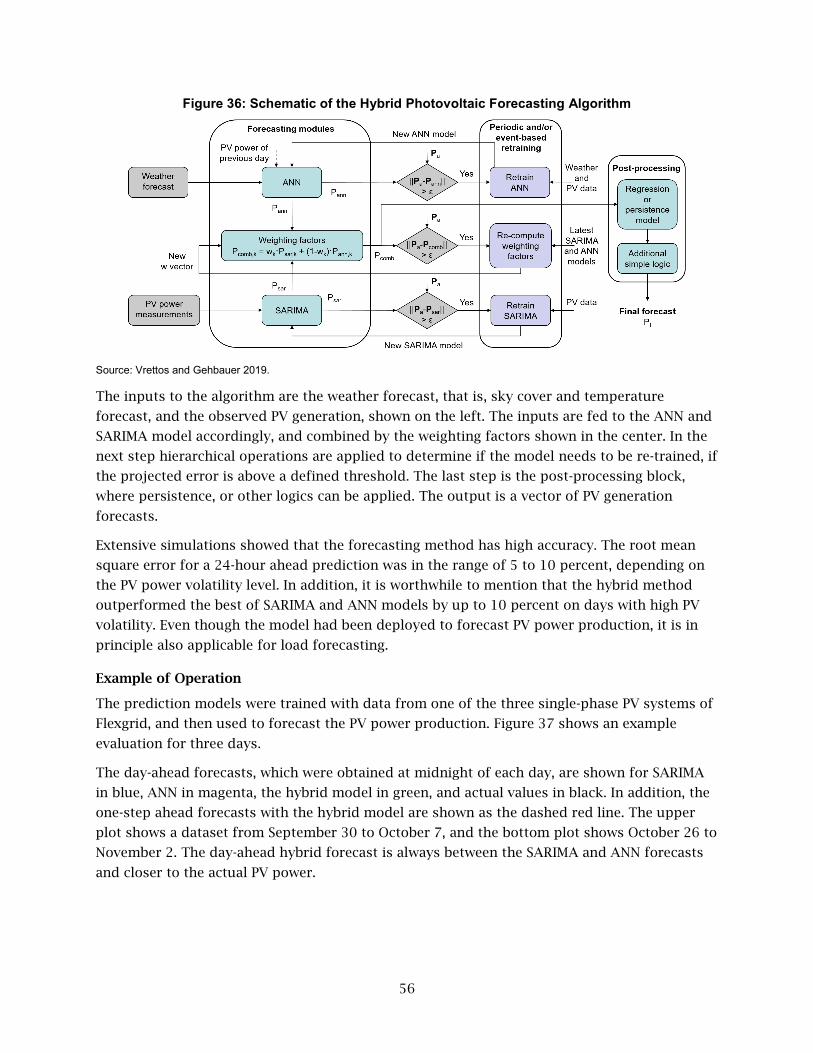
56
Figure 36: Schematic of the Hybrid Photovoltaic Forecasting Algorithm
Source: Vrettos and Gehbauer 2019.
The inputs to the algorithm are the weather forecast, that is, sky cover and temperature
forecast, and the observed PV generation, shown on the left. The inputs are fed to the ANN and
SARIMA model accordingly, and combined by the weighting factors shown in the center. In the
next step hierarchical operations are applied to determine if the model needs to be re-trained, if
the projected error is above a defined threshold. The last step is the post-processing block,
where persistence, or other logics can be applied. The output is a vector of PV generation
forecasts.
Extensive simulations showed that the forecasting method has high accuracy. The root mean
square error for a 24-hour ahead prediction was in the range of 5 to 10 percent, depending on
the PV power volatility level. In addition, it is worthwhile to mention that the hybrid method
outperformed the best of SARIMA and ANN models by up to 10 percent on days with high PV
volatility. Even though the model had been deployed to forecast PV power production, it is in
principle also applicable for load forecasting.
Example of Operation
The prediction models were trained with data from one of the three single-phase PV systems of
Flexgrid, and then used to forecast the PV power production. Figure 37 shows an example
evaluation for three days.
The day-ahead forecasts, which were obtained at midnight of each day, are shown for SARIMA
in blue, ANN in magenta, the hybrid model in green, and actual values in black. In addition, the
one-step ahead forecasts with the hybrid model are shown as the dashed red line. The upper
plot shows a dataset from September 30 to October 7, and the bottom plot shows October 26 to
November 2. The day-ahead hybrid forecast is always between the SARIMA and ANN forecasts
and closer to the actual PV power.
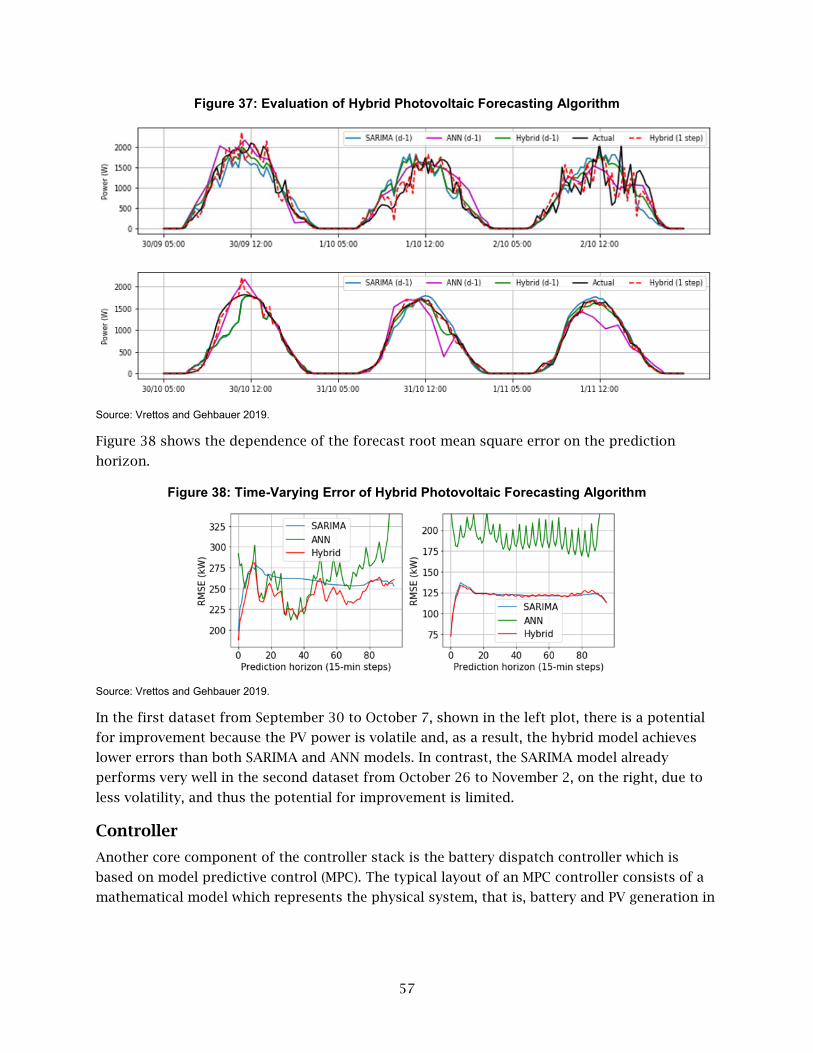
57
Figure 37: Evaluation of Hybrid Photovoltaic Forecasting Algorithm
Source: Vrettos and Gehbauer 2019.
Figure 38 shows the dependence of the forecast root mean square error on the prediction
horizon.
Figure 38: Time-Varying Error of Hybrid Photovoltaic Forecasting Algorithm
Source: Vrettos and Gehbauer 2019.
In the first dataset from September 30 to October 7, shown in the left plot, there is a potential
for improvement because the PV power is volatile and, as a result, the hybrid model achieves
lower errors than both SARIMA and ANN models. In contrast, the SARIMA model already
performs very well in the second dataset from October 26 to November 2, on the right, due to
less volatility, and thus the potential for improvement is limited.
Controller
Another core component of the controller stack is the battery dispatch controller which is
based on model predictive control (MPC). The typical layout of an MPC controller consists of a
mathematical model which represents the physical system, that is, battery and PV generation in
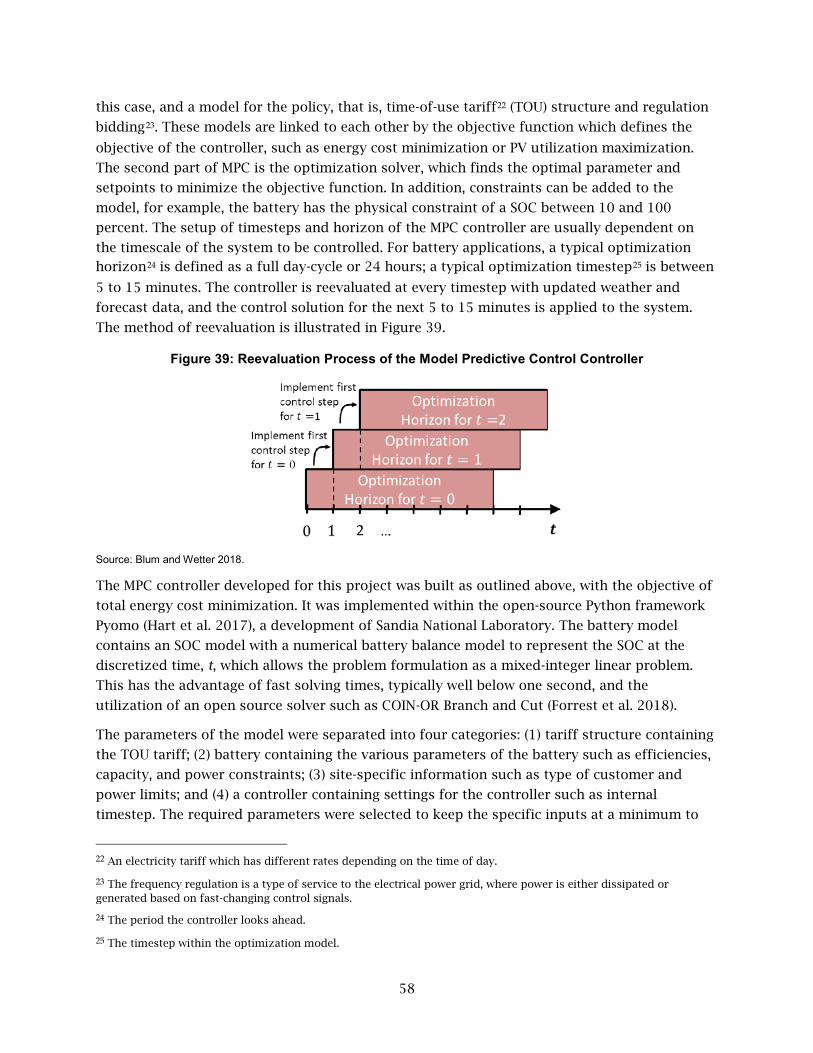
58
this case, and a model for the policy, that is, time-of-use tariff22 (TOU) structure and regulation
bidding23. These models are linked to each other by the objective function which defines the
objective of the controller, such as energy cost minimization or PV utilization maximization.
The second part of MPC is the optimization solver, which finds the optimal parameter and
setpoints to minimize the objective function. In addition, constraints can be added to the
model, for example, the battery has the physical constraint of a SOC between 10 and 100
percent. The setup of timesteps and horizon of the MPC controller are usually dependent on
the timescale of the system to be controlled. For battery applications, a typical optimization
horizon24 is defined as a full day-cycle or 24 hours; a typical optimization timestep25 is between
5 to 15 minutes. The controller is reevaluated at every timestep with updated weather and
forecast data, and the control solution for the next 5 to 15 minutes is applied to the system.
The method of reevaluation is illustrated in Figure 39.
Figure 39: Reevaluation Process of the Model Predictive Control Controller
Source: Blum and Wetter 2018.
The MPC controller developed for this project was built as outlined above, with the objective of
total energy cost minimization. It was implemented within the open-source Python framework
Pyomo (Hart et al. 2017), a development of Sandia National Laboratory. The battery model
contains an SOC model with a numerical battery balance model to represent the SOC at the
discretized time, t, which allows the problem formulation as a mixed-integer linear problem.
This has the advantage of fast solving times, typically well below one second, and the
utilization of an open source solver such as COIN-OR Branch and Cut (Forrest et al. 2018).
The parameters of the model were separated into four categories: (1) tariff structure containing
the TOU tariff; (2) battery containing the various parameters of the battery such as efficiencies,
capacity, and power constraints; (3) site-specific information such as type of customer and
power limits; and (4) a controller containing settings for the controller such as internal
timestep. The required parameters were selected to keep the specific inputs at a minimum to
22 An electricity tariff which has different rates depending on the time of day.
23 The frequency regulation is a type of service to the electrical power grid, where power is either dissipated or generated based on fast-changing control signals.
24 The period the controller looks ahead.
25 The timestep within the optimization model.
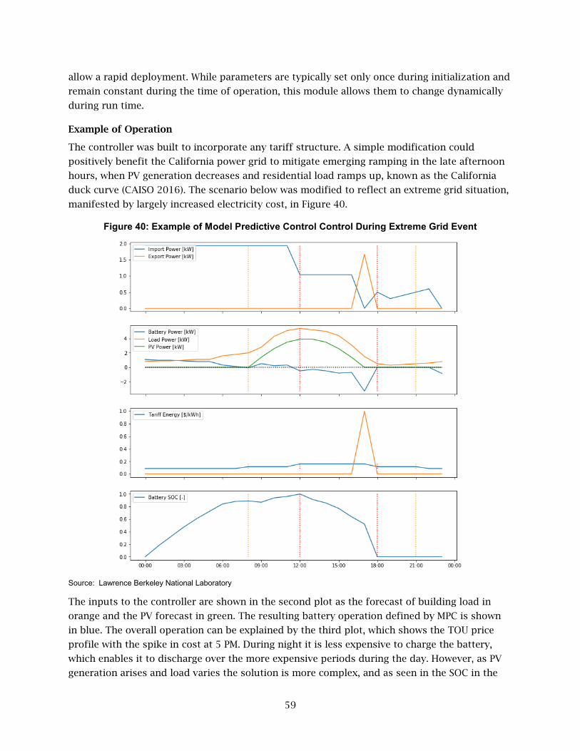
59
allow a rapid deployment. While parameters are typically set only once during initialization and
remain constant during the time of operation, this module allows them to change dynamically
during run time.
Example of Operation
The controller was built to incorporate any tariff structure. A simple modification could
positively benefit the California power grid to mitigate emerging ramping in the late afternoon
hours, when PV generation decreases and residential load ramps up, known as the California
duck curve (CAISO 2016). The scenario below was modified to reflect an extreme grid situation,
manifested by largely increased electricity cost, in Figure 40.
Figure 40: Example of Model Predictive Control Control During Extreme Grid Event
Source: Lawrence Berkeley National Laboratory
The inputs to the controller are shown in the second plot as the forecast of building load in
orange and the PV forecast in green. The resulting battery operation defined by MPC is shown
in blue. The overall operation can be explained by the third plot, which shows the TOU price
profile with the spike in cost at 5 PM. During night it is less expensive to charge the battery,
which enables it to discharge over the more expensive periods during the day. However, as PV
generation arises and load varies the solution is more complex, and as seen in the SOC in the

60
fourth plot, charging also takes place during the mid-peak period starting from 8 AM to 12 PM.
In addition, the battery is discharged in a non-continuous pattern, shown in blue in the second
plot. The result of this control action can be seen in the first plot where the net load at the
utility meter is shown in blue. The optimization seeks to generate a flat load profile, which is
the most economic strategy for the TOU tariff structure. However, during the price spike, the
electricity demand is largely reduced, which practically mitigates the duck curve. Further, a
price for energy export is defined within the controller to feed in power to the grid and actively
mitigate any grid event. This capability of providing energy to the electrical grid is especially
interesting when largely deployed. While this example is simplistic, the controller is capable of
reacting to real-time pricing signals, as well as a price event trigger. All of the functionality is
built into the controller and tested in simulation mode. One possible extension would be to
further develop and field test the controller.
Utility Modules
The MPC controller and PV forecast are the main modules of the controller stack, but a number
of utility modules are required to enable the interface with real equipment. Among others, the
controller stack at LBNL uses a time synchronization module to get accurate time
measurements, a module to read the inverter telemetry, and a module to control the inverter.
While other modules are generic to fit different applications, the inverter telemetry and inverter
control module are somewhat specific to the inverters installed at LBNL. They use a hypertext
transfer protocol wrapper for Modbus to communicate with the actual inverter at Flexgrid. For
different types of inverters, these modules would have to be adopted to fit the specific
communication protocol.
Simulation Evaluation This section highlights the findings of the MPC controller for behind-the-meter battery storage
in conjunction with PV, in an annual simulation study, which represent the technical potential
of the developed MPC algorithm.
Setup
The MPC controller requires a variety of inputs, such as weather and load forecasts, and real-
time measurements, such as PV generation and battery SOC. To conduct annual simulations of
the MPC controller, all external links to data must be emulated. For this study the PV generation
was emulated using the PV model introduced in the Model Development section in Chapter 4,
and parameterized to represent Flexgrid in a simplified way. Here, all three PV systems are
oriented toward the south, with a 10-degree tilt and no module shading. The PV generation
profile was then simulated with historical weather data from San Francisco. Figure 41 shows the
annual PV profile.
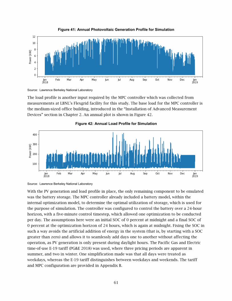
61
Figure 41: Annual Photovoltaic Generation Profile for Simulation
Source: Lawrence Berkeley National Laboratory
The load profile is another input required by the MPC controller which was collected from
measurements at LBNL’s Flexgrid facility for this study. The base load for the MPC controller is
the medium-sized office building, introduced in the “Installation of Advanced Measurement
Devices” section in Chapter 2. An annual plot is shown in Figure 42.
Figure 42: Annual Load Profile for Simulation
Source: Lawrence Berkeley National Laboratory
With the PV generation and load profile in place, the only remaining component to be emulated
was the battery storage. The MPC controller already included a battery model, within the
internal optimization model, to determine the optimal utilization of storage, which is used for
the purpose of simulation. The controller was configured to control the battery over a 24-hour
horizon, with a five-minute control timestep, which allowed one optimization to be conducted
per day. The assumptions here were an initial SOC of 0 percent at midnight and a final SOC of
0 percent at the optimization horizon of 24 hours, which is again at midnight. Fixing the SOC in
such a way avoids the artificial addition of energy in the system (that is, by starting with a SOC
greater than zero) and allows it to seamlessly add days one to another without affecting the
operation, as PV generation is only present during daylight hours. The Pacific Gas and Electric
time-of-use E-19 tariff (PG&E 2018) was used, where three pricing periods are apparent in
summer, and two in winter. One simplification made was that all days were treated as
weekdays, whereas the E-19 tariff distinguishes between weekdays and weekends. The tariff
and MPC configuration are provided in Appendix B.

62
The simulation was conducted with three different cases and two scenarios:
• Building load only without PV and battery, as base case
• Building load and PV, but without battery, to quantify the benefit of PV only
• Building load, PV, and battery, controlled by the MPC controller
The first scenario used the 15 kW PV array installation at Flexgrid, and three of the most recent
Tesla PowerWall 2 units with a total of 40.5 kWh storage. In the second scenario, the
installation was scaled by a factor of 10, due to its relatively small size in comparison to the
approximately 400 kW peak building load. The resulting system was 150 kW of PV with
405 kWh of battery storage.
Results
The simulation was conducted for one full year to capture the full seasonal effects of PV and
loads. The results were aggregated for the summer and winter seasons, which are May to
October and November to April, respectively.
The first study conducted was the Flexgrid installation and medium-office building load, shown
in Table 4.
Table 4: Simulation Results of the Model Predictive Control at Lawrence Berkeley National Laboratory
Load only Load + PV Load + PV + Battery
Summer Total cost [$] 150,210.00 146,449.80 143,775.60
Savings [$] 3,760.20 6,434.40
Winter Total cost [$] 77,746.80 76,373.50 75,149.10
Savings [$] 1,373.30 2,597.70
Source: Lawrence Berkeley National Laboratory
Both cases, Load+PV and Load+PV+Battery resulted in savings in both the summer and winter
seasons. The total annual savings were $5,133.50 (2.3 percent) and $9,032.10 (4.0 percent) for
the two cases. The total incremental savings of battery utilization was $3,898.60 (1.7 percent).
The savings in winter were significantly lower, which can be attributed to the decreased solar
generation and lower electricity demand cost. The overall battery utilization, defined as the
time when battery is either charged or discharged divided by the 8,760 hours of a full year,
came to 37.8 percent. As described in the previous section, the savings are overall very small in
comparison to the load of the office building. A second simulation was conducted where the
installation was scaled by a factor of 10. Results are presented in Table 5.

63
Table 5: Simulation Results of Model Predictive Control at Lawrence Berkeley National Laboratory (Scaled by 10)
Load only Load + PV Load + PV + Battery
Summer Total cost [$] 150,210.0 115,092.20 86,457.90
Savings [$] 35,117.80 63,752.1
Winter Total cost [$] 77,746.80 66,586.70 59,949.70
Savings [$] 11,160.10 17,797.1
Source: Lawrence Berkeley National Laboratory
The total annual savings were $46,277.90 (20.3 percent) for Load+PV and $81,549.20
(35.8 percent) for Load+PV+Battery, which is a significant increase from the previous scenario
but less than the scaling factor of 10. The reason could be the nature of the demand cost, which
is based on the single peak demand of each month. The higher the peak reduction, the more
energy is necessary, resulting in less-effective cost reduction. The battery utilization increased
to 75.3 percent. The incremental annual savings, this includes the summer and winter season,
of battery utilization were $35,271.30 (19.4 percent).
Pilot Test To confirm the results from the simulation study, the MPC controller was integrated and tested
at the Flexgrid facility. The setup included the control of one inverter at Flexgrid with a system
size of 3.75 kW of PV and 6.4 kWh of battery storage. The MPC controller was configured to a
control timestep of five minutes, and an optimization horizon of 22 hours. A significant
amount of the field testing time was used to establish and test communication, validate
models, test continuous operation over multiple days, and further advance the controller based
on the tests conducted. The results presented in this section are the most representative for the
controller to (a) demonstrate the functionality of the controller and (b) confirm the results from
the simulation study. The field tests are typically conducted in five-day periods, where the first
day can be seen as a warmup period and should not be considered in the analysis.
Results
The Figure 43 shows the forecast results for PV and load, which are conducted by the internal
control modules and then fed to the MPC controller.
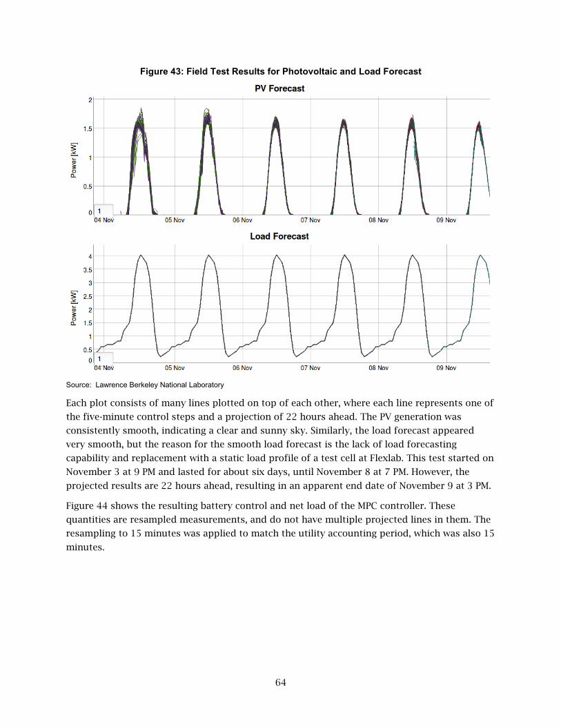
64
Figure 43: Field Test Results for Photovoltaic and Load Forecast
Source: Lawrence Berkeley National Laboratory
Each plot consists of many lines plotted on top of each other, where each line represents one of
the five-minute control steps and a projection of 22 hours ahead. The PV generation was
consistently smooth, indicating a clear and sunny sky. Similarly, the load forecast appeared
very smooth, but the reason for the smooth load forecast is the lack of load forecasting
capability and replacement with a static load profile of a test cell at Flexlab. This test started on
November 3 at 9 PM and lasted for about six days, until November 8 at 7 PM. However, the
projected results are 22 hours ahead, resulting in an apparent end date of November 9 at 3 PM.
Figure 44 shows the resulting battery control and net load of the MPC controller. These
quantities are resampled measurements, and do not have multiple projected lines in them. The
resampling to 15 minutes was applied to match the utility accounting period, which was also 15
minutes.

65
Figure 44: Field Test Results for the Battery Control and Net Load using Model Predictive Control
Source: Lawrence Berkeley National Laboratory
The resulting battery control is shown in the upper plot. This is the control actually applied to
the battery. During the field test multiple iterations were necessary to closely match the control
signal from the MPC controller to the control signal actually sent to the battery. As all
communication is handled by the inverter, setpoints are not directly passed to the battery,
which results in small but constant offsets in power, and occasional signal timeouts. One
example for a timeout can be seen on November 5 at about 3 AM, as the negative drop in
battery power from about 0.85 kW down to 0.3 kW and then back up to 0.85 kW. Zooming into
the five-minute data, a drop to 0 kW was found, caused by an inverter timeout. However, it
appears that the timeout problems only happen during the night, and therefore have little
effect on the MPC controller performance. The lower plot shows the resulting net-load profile
where the base case of Load+PV is shown in turquoise, the MPC projected result for the five-
minute ahead is in purple, and the measured MPC performance is in yellow. The difference
between the MPC projected and measured performance is the compounded error of forecast
error, control error, and MPC model error. The effect of this compounded error on the energy
cost can be seen in Figure 45.
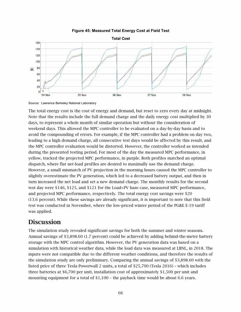
66
Figure 45: Measured Total Energy Cost at Field Test
Source: Lawrence Berkeley National Laboratory
The total energy cost is the cost of energy and demand, but reset to zero every day at midnight.
Note that the results include the full demand charge and the daily energy cost multiplied by 30
days, to represent a whole month of similar operation but without the consideration of
weekend days. This allowed the MPC controller to be evaluated on a day-by-day basis and to
avoid the compounding of errors. For example, if the MPC controller had a problem on day two,
leading to a high demand charge, all consecutive test days would be affected by this result, and
the MPC controller evaluation would be distorted. However, the controller worked as intended
during the presented testing period. For most of the day the measured MPC performance, in
yellow, tracked the projected MPC performance, in purple. Both profiles matched an optimal
dispatch, where flat net-load profiles are desired to maximally use the demand charge.
However, a small mismatch of PV projection in the morning hours caused the MPC controller to
slightly overestimate the PV generation, which led to a decreased battery output, and then in
turn increased the net load and set a new demand charge. The monthly results for the second
test day were $146, $125, and $121 for the Load+PV base case, measured MPC performance,
and projected MPC performance, respectively. The total energy cost savings were $20
(13.6 percent). While these savings are already significant, it is important to note that this field
test was conducted in November, where the low-priced winter period of the PG&E E-19 tariff
was applied.
Discussion The simulation study revealed significant savings for both the summer and winter seasons.
Annual savings of $3,898.60 (1.7 percent) could be achieved by adding behind-the-meter battery
storage with the MPC control algorithm. However, the PV generation data was based on a
simulation with historical weather data, while the load data was measured at LBNL, in 2018. The
inputs were not compatible due to the different weather conditions, and therefore the results of
the simulation study are only preliminary. Comparing the annual savings of $3,898.60 with the
listed price of three Tesla Powerwall 2 units, a total of $25,700 (Tesla 2016) – which includes
three batteries at $6,700 per unit, installation cost of approximately $1,500 per unit and
mounting equipment for a total of $1,100 – the payback time would be about 6.6 years.

67
Considering that Tesla offers a warranty of 10 years, the 6.6 years of payback would be very
cost effective. However, it is important to note that the savings are subject to a perfect
knowledge of forecasted PV and load, which is not practical and one of the challenges with
MPC.
Another consideration is the size of the PV and battery system. While the first scenario of the
simulation study included the Flexgrid system as built as a pilot facility for research
applications, a second scenario scaled both the PV and battery to more closely match the load.
This increased the savings, but at a lower rate than the scale of the system. An important
decision for a customer would be to size the system right to gain maximum revenue. Sizing
tools such as the Distributed Energy Resources Customer Adoption Model (Stadler et al. 2014)
from Berkeley Lab are available as a public resource to assist with DER investment decisions.
The MPC controller requires a load forecast for the next 24 hours ahead at each control
timestep of five minutes. However, the load profile of the field test was fixed to a single profile
for a sunny day of a test cell at Flexlab. The reason behind this modification was the lack of
simplified load forecasts that can be implemented on an embedded controller. The developed
PV forecasting module could, in principle, provide load forecasts to feed the MPC controller.
However, at the time of the field test the forecasting module was not validated, and would
likely have led to bad control. The conducted field test is relevant because PV generation was
fully forecasted, and the loop between measurements and actuation was closed through the
MPC controller. The basic application of MPC was demonstrated in this field test, and potential
energy cost savings and benefits for the power grid were outlined. MPC can significantly
facilitate large PV penetrations while cost-effectively relieving the accompanying contingency
on the power grid. In particular, the colocation of battery storage can be beneficial for both
customers and grid operation.
The measured savings of the field test, which were 13.6 percent, are significantly higher than
those from the simulation study, which were about 1.5 percent for the winter period. In
addition, the simulation study showed that the savings for the winter period were lower than
those achieved in the summer, so higher savings from the field test could be expected when the
test is conducted in summer. While the savings are significant, the results were distorted by the
fact that the test setup was different. The simulation study used the full Flexgrid system in
conjunction with the medium-sized office building load, with a peak load of about 400 kW, but
the field test only used one of the PV and battery systems in conjunction with an emulated load
of a single test cell at Flexlab, with a peak load of approximately 4 kW. So, while the PV and
battery system was reduced by a factor of 3, the load was reduced by a factor of 100. The tests
were set up this way because of Flexgrid's physical size and the option to use the remaining
inverters to conduct other tests of the controller, and to continue on data collection.

68
CHAPTER 6: Summary and Benefits Assessment
This project designed and built the Flexgrid facility with its PV, storage, and distribution PMU
installation; developed and validated a broad range of simulation models to conduct annual
simulations of DER; used these models to determine optimal setpoints for a smart inverter, in
accordance with California Rule 21; and developed and field tested an MPC controller to
maximize battery use for the customer, while supporting the power grid during critical periods.
The Flexgrid facility serves as a central testbed and utility for hardware-in-the-loop and DER
technology integration testing in California. It allows the evaluation of novel control systems in
a controlled, emulated environment and enables real-time comparisons between demand,
renewables, inverters, and storage. Flexgrid was used throughout this four-year project,
supporting data collection; simulation model development of PV, smart inverter, and battery
storage; development of a grid event detection algorithm; and evaluation of a novel MPC
controller and the associated forecasting methods. Investments from other USDOE-funded
projects further expanded the capabilities by adding power systems testing hardware.
Throughout this project, high-fidelity grid measurements in a 120 Hz rate (120 samples per
second) were recorded at three strategic positions within the LBNL distribution grid. An event
detection algorithm was developed and applied, which resulted in the detection of 27 voltage-
sag events in the last two years of the project. The events were stored in a digital library of grid
events and two methods to perform short-term forecasting of grid event parameters were
applied. Both methods revealed the initial slope of a voltage-sag as a good parameter to predict
its severity and duration. This information can be important for determining inverter ride-
through settings, in accordance with California Rule 21, with the overall objective of improving
electrical grid reliability.
To further explore the potential of smart inverters, a framework to optimally select Volt-Var
control setpoints for different nodes along the feeder was developed. The result of this
algorithm showed that it could be advantageous to distribute the burden of reactive power
generation, by having variable Volt-Var setpoints for clusters of inverters. Variable Volt-Var
settings could decrease the curtailment of active power generation in the feeder when less
critical nodes provide reactive power at lower voltages than critical ones. This results in a
reduced oversizing of inverters and decreased curtailment of active power generation, which
both can reduce the levelized cost of electricity for distributed PV applications. However, one
downside of this approach is the increased distribution loss due to higher reactive currents. A
further investigation of the associated grid distribution losses and inverter investment cost is
needed to thoroughly evaluate the control approach for different types of customers in
California. Ratepayers would see improved reliability compared to a case where high PV
penetration exists but is not coordinated and managed as proposed in this project.

69
The data collected at Flexgrid was also used to develop an advanced control system for PV and
battery storage, using the state-of-the-art MPC technology. In this process, a new hybrid
forecasting method was developed for short-term PV power forecasting, which was shown to
outperform existing common approaches. Through coordinated control using this predictive
algorithm, high penetrations of renewable resources at the feeder scale can be achieved. One
key attribute here is the capability to shape the load using battery storage. In the case of the
California duck curve, the MPC controller optimally controls the battery dispatch by charging
the battery during periods with excess PV generation and discharging it during the critical
afternoon hours. This active participation in grid management helps to maximize the
deployment of distributed generation overall.
The controller was evaluated in annual simulations and revealed the potential cost-
effectiveness of behind-the-meter battery storage. In the simulation conducted, 35 percent of
the annual electricity bill could be saved, with a payback time of the investment in the battery
storage of about 6 years. This duration is significantly shorter than the manufacturer’s
warranty of 10 years. Therefore, the installation of a behind-the-meter battery storage system
can financially benefit both residential and commercial ratepayers, as well as the grid operation
and reliability overall. The controller was also tested in a field test at Flexgrid, where it showed
significant savings, but with different sizes of PV, storage, and load.
Both control approaches, the variable Volt-Var settings and the MPC control, can increase the
allowable PV penetration, which (a) offsets retail energy purchases, (b) increases the ability to
earn PV-based revenue due to an increase in the type of energy services PV and battery storage
can provide, such as reactive power support or mitigation of the duck curve, and (c) supports
California with its aggressive climate goals to decarbonize the grid.
All developed simulation models, the grid event library, and the MPC controller are open-source
and available in Gehbauer (2019a), Gehbauer (2018), and Gehbauer (2019b), accordingly.

70
GLOSSARY
Term Definition
ANN Artificial neural network; A machine-learning model based on neural
connections in multiple dimensions.
ANSI American National Standards Institute
ARPA-E Advanced Research Projects Agency for Energy
BTrDB Berkeley Tree Database; A time-series database designed to handle large
amounts of data.
California ISO California Independent System Operator; the electrical power grid
operator for California
DER Distributed energy resources; examples are photovoltaics, electric
vehicles, batteries, or buildings equipped with remote controllable loads.
EPIC Electric Program Investment Charge
Flexgrid Facility for power systems testing located at Lawrence Berkeley National
Laboratory
Flexlab Facility for Low Energy Experiments for Buildings; A testing facility at
Lawrence Berkeley National Laboratory.
FMI Functional mockup interface; A variant of application programming
interface relevant for simulation applications.
FMU Functional mockup unit; A simulation model exported in accordance to
FMI.
IEEE Institute of Electrical and Electronics Engineers
LBNL Lawrence Berkeley National Laboratory
MBL Modelica Buildings Library; A Modelica library for buildings simulation.
MPC
Model predictive control; A type of controller which is based on a model
of the system to be controlled, and an optimization engine to determine
optimal operation to minimize or maximize an objective function.
NOAA National Oceanic and Atmospheric Administration; the United States
weather service.
OpenEI Open Energy Information; A database with simulation results from
USDOE reference buildings using typical meteorological weather data.
71
Term Definition
PMU Phasor measurement unit; A precise measurement device to monitor the
electric power grid.
PV Photovoltaics; A technology which converts solar irradiation to electrical
energy.
RLA Random load allocation; An algorithm to generate dynamic load profiles
in power systems simulation.
SARIMA Seasonal Auto-Regressive Integrated Moving Average; A machine-learning
model based on the correlation of data-points in time.
SCooDER Smart Control of Distributed Energy Resources; A Modelica library for
power systems simulation.
SOC State of charge; The energy level currently available in a storage device.
Must be grater or equal than zero, and smaller or equal then the capacity.
STC
Standard test conditions; An industry-wide standard to evaluate the
performance of PV modules. It specifies a cell temperature of 25 degree
Celsius (°C) and an irradiance of 1,000 watt per square-meter (W/m2) with
an air mass of 1.5.
TMY Typical meteorological year; A detailed weather file of historic and
representative weather.
TOU Time-of-use; This represents a type of electricity rate which varies based
on time of the day and day of the year.
µPMU Microsynchrophasor measurement unit; a low-cost PMU specifically
designed for the electrical distribution grid
USDOE United States Department of Energy
72
REFERENCES
Alves, M. F. & Ribiero T. N. 1999. Voltage Sag: An Overview of IEC and IEEE Standards and Application Criteria. IEEE Transmission and Distribution Conference.
Andersen, M. P. & Culler, D. E. 2016. BTrDB: Optimizing Storage System Design for Timeseries Processing. 14th USENIX Conference on File and Storage Technologies.
ANSI - American National Standard for Electric Power Systems and Equipment. 2016. Voltage Ratings (60 Hertz).
Blum, D. and M. Wetter. 2018. Next-Generation Building Control with Model Predictive Control.
Brkic, J., Ceran, M., Elmoghazy, M., Kavlak, R. & Kral, C. 2018. PhotoVoltaics Modelica library. Github.
Brodt-Giles, D. 2012. Wref 2012: OpenEI – An Open Energy Data and Information Exchange for International Audiences. National Renewable Energy Laboratory (NREL).
California Energy Commission (CEC). 2014. Rule 21. Smart Inverter Working Group Technical Reference Materials.
California Independent System Operator. 2016. What the duck curve tells us about managing a green grid.
Dargatz, M. 2010. Utility Interactive: What it Means, What Protection it Ensures. Enphase Energy.
Deru, M., Field, K., Studer, D., Benne, K., Griffith, B., Torcellini, P., Liu, B., Halverson, M., Rosenberg, D. & Yazdanian, M. 2011. Commercial Reference Building Models of the National Building Stock. United States Department of Energy.
Einhorn, M. Conte, F. V., Kral, C., Niklas, C., Popp, H. & Fleig, J. 2011. A Modelica Library for Simulation of Electric Energy Storages.
Forrest, J., Ralphs T., Vigerske, S., Hafer, L., Kristjansson, B., Straver, E., Lubin, M., Santos, H. G. & Saltzman, M. 2018. COIN-OR Branch and Cut.
Fritzson, P. & Bunus P. 2002. Modelica – A General Object-Oriented Language for Continuous and Discrete-Event System Modeling. IEEE Proceedings 35th Annual Simulation Symposium.
Gehbauer, C. 2018. PMU Event Library. https://github.com/LBNL-ETA/pmu_event_library.git.
Gehbauer, C. 2019a. Smart Inverter Modelica Library. https://github.com/LBNL-ETA/SCooDER.git.
Gehbauer, C. 2019b. An Optimal Control for Behind-the-Meter Storage. https://github.com/LBNL-ETA/DOPER.git.
Hart, W. E., Laird, C. D., Watson, J. P., Woodruff, D. L., Hackebeil, G. A., Nicholson, B. L. & Siirola, j. D. 2017. Pyomo – Optimization Modeling in Python. Springer Vol. 67.
Institute of Electrical and Electronics Engineers (IEEE). 2000. Radial Distribution Test Feeders. IEEE Distribution Planning Working Group Report. http://sites.ieee.org/pes-testfeeders/files/2017/08/testfeeders.pdf.

73
MacQueen, J. 1967. Some Methods for Classification and Analysis of Multivariate Observations. Proceedings of the Fifth Berkeley Symposium on Mathematical Statistics and Probability, Vol. 1, No. 14, 281–297.
Modelisar 2014. Functional Mock-up Interface 2.0.
Pacific Gas and Electric (PG&E). 1999. Voltage tolerance boundary.
Pacific Gas and Electric (PG&E). 2018. Electric Schedule E-19.
Perez, R., Ineichen, P., Seals, R., Michalsky, J. & Stewart, R. 1990. “Modeling Daylight Availability and Irradiance Components from Direct and Global Irradiance.” Solar Energy 44(5): 271–289.
Stadler, M., Groissböck, M., Cardoso, G. & Marnay, C. 2014. “Optimizing Distributed Energy Resources and Building Retrofits with the Strategic DER- CAModel.” Applied Energy 132, 0306–2619.
Swenson, T. J., Vrettos, E., Muller, J. & Gehbauer, C. 2019. Open PMU Event Dataset: Detection and Characterization at LBNL Campus. IEEE PES General Meeting.
Tesla. 2016. PowerWall 2, https://www.tesla.com/powerwall.
Vanfretti, L., Rabuzin, T., Baudette M. & Murad, M. 2016. iTesla Power Systems Library (iPSL): A Modelica library for phasor time-domain simulations. SoftwareX, ISSN 2352-7110, DOI: 10.1016/j.softx.2016.05.001.
Vrettos, E. & Gehbauer, C. 2019. A Hybrid Approach for Short-Term PV Power Forecasting in Predictive Control Applications. Power Tech conference in Milano.
von Meier, A., Stewart, E., McEachern, A., Andersen, A., & Mehrmanesh, L. 2017. “Precision Micro-Synchrophasors for Distribution Systems: A Summary of Applications.” IEEE Transactions on Smart Grid Vol. 8, No. 6.
Ward, J. H. Jr. 1963. “Hierarchical grouping to optimize an objective function.” Journal of the American statistical Association 58 (301): 236–244.
Wetter, M., Zuo, W., Nouidui, T.S. & Pang, X. 2014. “Modelica Buildings Library.” Journal of Building Performance Simulation 7 (4): 253–270.

A-1
APPENDIX A: Documentation of Flexgrid
A brief documentation of Flexgrid.
Pictures
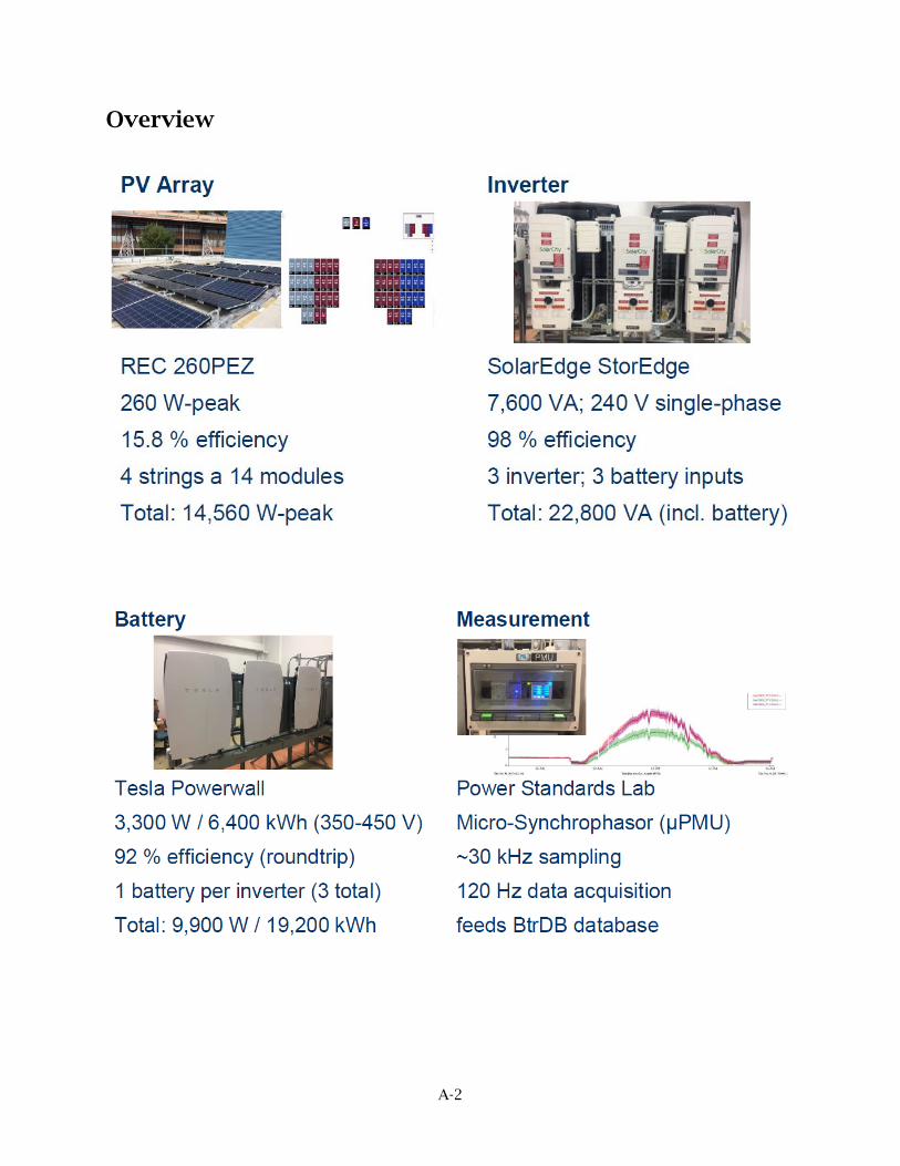
A-2
Overview
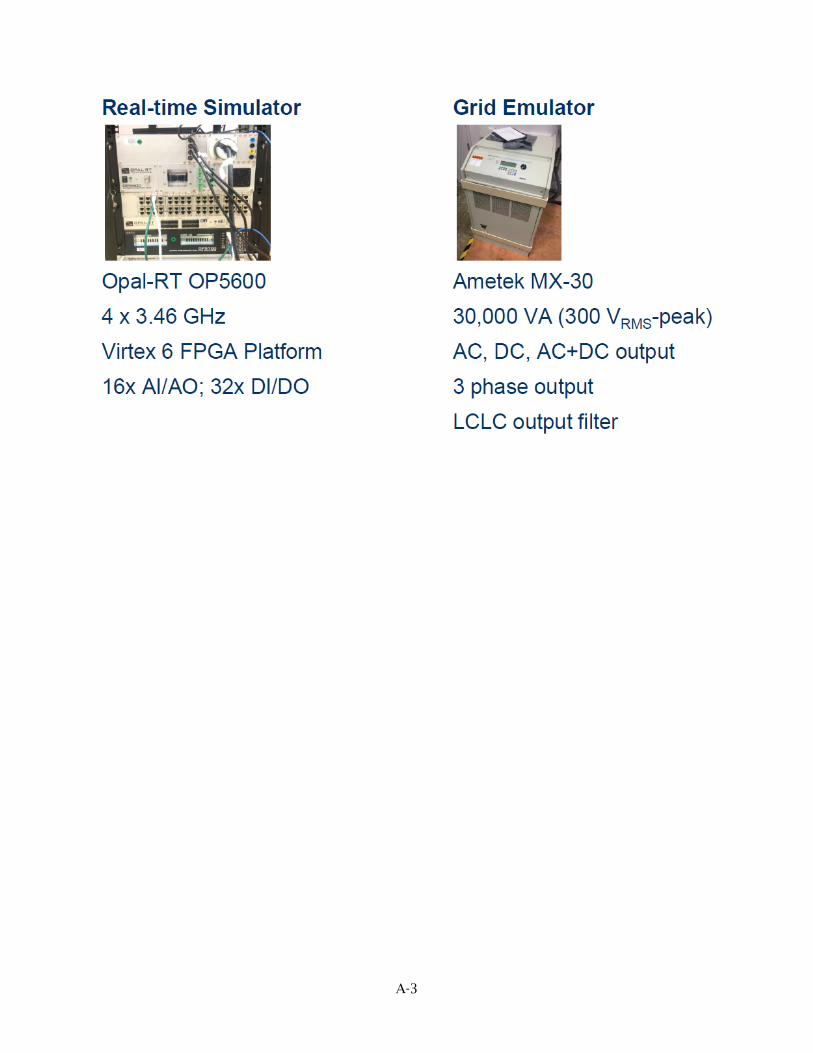
A-3
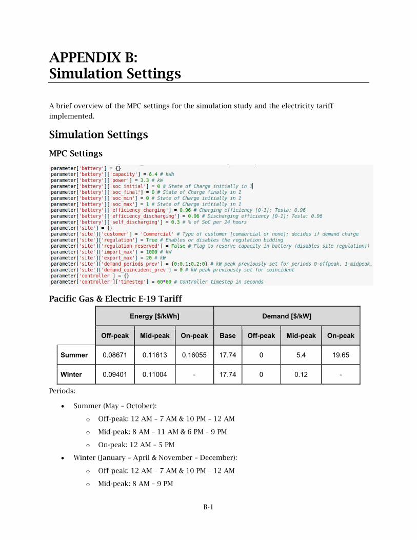
B-1
APPENDIX B: Simulation Settings
A brief overview of the MPC settings for the simulation study and the electricity tariff
implemented.
Simulation Settings
MPC Settings
Pacific Gas & Electric E-19 Tariff
Energy [$/kWh] Demand [$/kW]
Off-peak Mid-peak On-peak Base Off-peak Mid-peak On-peak
Summer 0.08671 0.11613 0.16055 17.74 0 5.4 19.65
Winter 0.09401 0.11004 - 17.74 0 0.12 -
Periods:
• Summer (May – October):
o Off-peak: 12 AM – 7 AM & 10 PM – 12 AM
o Mid-peak: 8 AM – 11 AM & 6 PM – 9 PM
o On-peak: 12 AM – 5 PM
• Winter (January – April & November – December):
o Off-peak: 12 AM – 7 AM & 10 PM – 12 AM
o Mid-peak: 8 AM – 9 PM