The Impact of Training Policies in Latin America and the Caribbean: The Case of Programa Joven

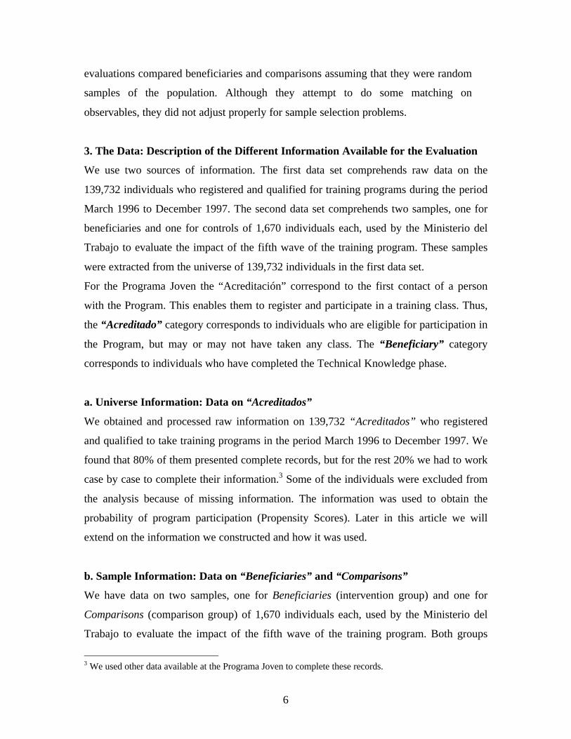
The Impact of Training Policies in Latin America and

the Caribbean: The Case of “Programa Joven” *

Cristián Aedo and Sergio Nuñez**

Graduate Program in EconomicsILADES/Georgetown University

May 2001

* Financial support from the Interamerican Development Bank is gratefully acknowledged. This paper hasbeen presented at the IADB research network seminars in Washington D.C. and Rio de Janeiro. I thankparticipants for helpful comments. I am particularly grateful to Jeffrey Smith, Petra Todd, JamesHeckman, and Gustavo Marquez for many helpful comments and suggestions. All remaining errors andomissions are my own. We acknowledged the cooperation of the Unidad de Estadísticas y Evaluación deImpacto, in providing the information used in this research. In particular, we are grateful to MónicaMuscolino, consultant of the Unidad de Estadística, and Sergio Diba, Coordinator of the Programa Joven.

** Correspondence to Cristian Aedo, Professor of Economics, Graduate Program in EconomicsILADES/Georgetown University, Universidad Alberto Hurtado. Email: [email protected].

1

Abstract

This research evaluates the “Programa Joven”, a training program conducted by the

Ministerio del Trabajo of Argentina. We adapt and apply a non-experimental evaluation

methodology to answer the following questions: Does “Programa Joven” increase the

labor income of the trainees? Does “Programa Joven” increase the probability of being

employed? And (3) what is the rate of return to dollars spent on the “Programa Joven”?

We used Propensity Scores Matching Estimators as our basic methodology to obtain a

measure of the impact of the training program. Our choice of this methodological

approach was based upon both the theoretical developments in the area of Program

Evaluation and the availability of relevant information. We used three different set of

data to estimate the Propensity Scores which allowed us to analyze the question on how

sensitive Program impact estimates are to different propensity score specifications? This

question has not been addressed by the previous literature.

Our results indicate first, that Program impact on earnings were statistically significant

for young males and adult females. This result was not sensitive to the number of nearest

neighbors. Second, the estimated Program impact on employment was statistically

significant for adult females only. Again the result was not sensitive to the number of

nearest neighbors. Third, impact estimates on earnings and employment for the groups

with statistically significant results were not sensitive to the different sources of

information used to estimate the propensity scores. This was a surprising result as we

expected to observe greater variability in the impact results across different propensity

score specifications. Fourth, the cost-benefit exercise conducted suggest that we required

at least 9 years of duration of the earnings impact for the Program to have a positive net

present value for the groups with statistically significant results.

2

Index

1. Introduction

2. Description of “Programa Joven”

3. The Data: Description of the Different Information Available for the Evaluation

4. Program Participation:

4.1 Determinants

4.2 Strategic Behavior

5. Estimation of Program Participation (Propensity Scores):

5.1 Universe (PSTOT)

5.2 Universe and Sample (PSUN)

5.3 Sample (PSMU)

5.4 A comparison of the propensity score estimates

5.5 Common Support

6. Impact Estimates: labor earnings and employment

6.1 Labor Earnings

6.2 Employment

7. Cost-benefit analysis:

7.1 Cost Data Description

7.2 Simulations

7.3 Results

8. Conclusions

Appendix

A1. Variables Description

A2. Common Support

A6. MATLAB Codes.

a. Average Nearest Neighbor Estimators.

b. Bootstrapping

3

1. Introduction

Latin-American countries invest a significant amount of resources in training programs.

An evaluation of these experiences is needed in order to learn from them and to design

more effective programs. However, Program evaluation faces many difficulties

(Heckman, LaLonde and Smith, 1999): first, due to the heterogeneity of impacts that

Programs produce there are many parameters of interest in their evaluation. Second, there

is no unique way of conducting Program evaluations. The choice of an appropriate

Program impact estimate depends upon the question to be answered and data availability.

Third, to produce “good” evaluations it is needed to have “good data”. Usually

econometric methods need to be used to correct for data problems. Fourth, to obtain

Program impact estimates it is necessary to compare comparable individuals, which

increases the complexities of Program evaluation. Thus, it is necessary to reduce the

biases by comparing comparable individuals, by administering similar questionnaires to

participant and non-participants, by using similar time frameworks, and by drawing the

samples of participants and non-participants from similar labor markets. Fifth, non-

experimental Program impact estimates solve the selection problem under different

assumptions, which generates variability in their results. An experimental evaluation

provides an important reference framework to analyze the performance of alternative

non-experimental evaluation methodologies. Sixth, social Programs at the national or

regional levels have an impact on both participants and non-participants. The usual

approach to deal with this Program “contamination” is to assume that the impact on non-

participants is not significant.

This research evaluates the “Programa Joven”, a training program conducted by the

Ministerio del Trabajo of Argentina. We adapt and apply a non-experimental evaluation

methodology to answer the following questions: (1) Does “Programa Joven” increase the

labor income of the trainees? (2) Does “Programa Joven” increase the probability of

being employed? And (3) what is the rate of return to dollars spent on the “Programa

Joven”?

To answer these questions we used the Matching Estimators approach as our basic

methodology. This choice was based upon both the theoretical developments in the area

of Program Evaluation (Heckman et al., 1995, 1997, 1998 & 1998) and the availability

4

and quality of relevant information. As described in Tood (1999) the application of this

methodology requires two steps: first, the estimation of a model of program participation

(Propensity Scores) and second, and conditional on the estimated propensity scores, the

usage of matching estimators to obtain the impact of the Program.

To estimate the propensity scores we used three sources of information: first, the data for

all the individuals who registered and qualified to take training programs in the period

March 1996 to December 1997 (approximately 140,000 individuals). Second, the

information contained in a sample of beneficiaries and controls used by the Ministerio del

Trabajo of Argentina to evaluate the Program (3,340 individuals in total).1 And third, the

information contained in the first database but restricted to the 3,340 individuals

contained in the second database. The access to these different sources of information

allowed us to analyze the additional question on how sensitive Program impact estimates

are to different propensity score specifications? This question has not been addressed by

the previous literature and we face it here. Our hypothesis is that impact estimates are

sensitive to different propensity score specifications.

We report and compare the Propensity Scores estimated from each one of these data

sources and we estimate the program impact on earnings and employment based upon

these propensity scores.

Finally, based upon cost information and the program impact estimates (benefits), we

applied a cost benefit analysis of the Programa Joven. This analysis was conducted under

different scenarios with regard to benefit duration, discount rate and the ratio of indirect

to direct cost.

2. Description of “Programa Joven”

The “Programa Joven” offers training to facilitate the labor force participation of the

beneficiaries in the formal labor market. To this purpose, the program provides

intensive training for positions in the productive sector of the economy and training

internships in firms.

The target population of the Program is young persons, males and females, coming

from poor households, with a low educational level, without working experience, and

1 These individuals were extracted from the universe of potential trainees (first data source).

5

who are unemployed, underemployed or inactive. The selection criteria for the

program are: minimum 16 years of age; education level no greater than secondary

education; to belong to a household considered poor and not to participate in the labor

market.

The program comprehend the following benefits: an average of 200 hours of training,

transportation expenses, a subsidy for females with young children, medical

checkups, books, material and working clothing.

The duration of the training program varies from 14 to 20 weeks. The training is

intensive and can be divided into two main activities:

a. Technical Knowledge phase: the beneficiaries receive knowledge and technical

skills to undertake an occupation in classrooms. The duration of this activity varies

from 6 to 12 weeks.

b. Internships phase: the beneficiaries complement their technical knowledge with an

applied work in firms in the occupations they have been trained. The duration of this

activity is of 8 weeks.

The criteria for selecting firms for internships are: general characteristics of the firm,

tasks to be done by the trainees, personal involved in similar positions in the firm,

equipment, supplies and infrastructure of the firm.

To carry out the training the Ministerio del Trabajo hires Instituciones de

Capacitación (ICAP) using an international bidding process. The distribution of the

training activities at the national level is determined in accordance to the quantity of

inhabitants in the regions. The program executor is the Ministerio del Trabajo y

Seguridad Social through the Secretaría de Empleo and Capacitación Laboral. The

program will continue its operation until the year 2,000, being jointly funded by the

Inter American Development Bank (IDB) and governmental funds.

The Programa Joven has been evaluated in terms of the impacts of the Program. The

Unidad de Estadísticas y Evaluación de Impacto of the Programa Joven conducted

studies for a sample of courses executed in 1993, for courses contained in the second

and third bidding process (study conducted in 1996) and for courses from the fifth

bidding process (study conducted in 1998 with a sample of 3,340 individuals). 2 These

2 In Section 3, we describe this sample with more detail.

6

evaluations compared beneficiaries and comparisons assuming that they were random

samples of the population. Although they attempt to do some matching on

observables, they did not adjust properly for sample selection problems.

3. The Data: Description of the Different Information Available for the Evaluation

We use two sources of information. The first data set comprehends raw data on the

139,732 individuals who registered and qualified for training programs during the period

March 1996 to December 1997. The second data set comprehends two samples, one for

beneficiaries and one for controls of 1,670 individuals each, used by the Ministerio del

Trabajo to evaluate the impact of the fifth wave of the training program. These samples

were extracted from the universe of 139,732 individuals in the first data set.

For the Programa Joven the “Acreditación” correspond to the first contact of a person

with the Program. This enables them to register and participate in a training class. Thus,

the “Acreditado” category corresponds to individuals who are eligible for participation in

the Program, but may or may not have taken any class. The “Beneficiary” category

corresponds to individuals who have completed the Technical Knowledge phase.

a. Universe Information: Data on “Acreditados”

We obtained and processed raw information on 139,732 “Acreditados” who registered

and qualified to take training programs in the period March 1996 to December 1997. We

found that 80% of them presented complete records, but for the rest 20% we had to work

case by case to complete their information.3 Some of the individuals were excluded from

the analysis because of missing information. The information was used to obtain the

probability of program participation (Propensity Scores). Later in this article we will

extend on the information we constructed and how it was used.

b. Sample Information: Data on “Beneficiaries” and “Comparisons”

We have data on two samples, one for Beneficiaries (intervention group) and one for

Comparisons (comparison group) of 1,670 individuals each, used by the Ministerio del

Trabajo to evaluate the impact of the fifth wave of the training program. Both groups

3 We used other data available at the Programa Joven to complete these records.

7

come from individuals who meet the selection criteria to be considered as a potential

participant of the program (“Acreditados”). In addition, the Beneficiaries are the ones

who actually completed the Technical knowledge phase.

Both samples comprehend 1,670 cases (3,340 cases in total). To make both samples

comparable the sample design used by the Ministerio del Trabajo controlled for the

following variables: age, sex, level of education, labor force participation, socioeconomic

level, and to have a children with 5 years of age or less. Therefore, the comparison group

is not selected at random. For both samples, there is information for the period covered

by the first contact with the program to 12 months after the Beneficiaries finished the

training (the follow-up information for the comparisons was obtained at the same time as

the information for the beneficiaries). This information allows us to construct the

individual labor history for both samples.

Beneficiaries Sample

The sample was designed by the Ministerio del Trabajo to have statistical representation

by gender and region of residence. The first variable was introduced to study the program

impact by gender, given the different labor market conditions for males and females. The

regional variable was introduced to study the differential impact of socioeconomic

characteristics and regional labor markets on program outcomes. In total, they considered

11 geographic units denominated “regions”.

To define the sample size it was considered the observed variation in the values for

variables such as proportion of employed/unemployed workers and average income

received by employed workers. These variables present the greatest variation among the

outcomes variables. It was considered a percentage of non-response of 5%. The

determination of the sample sizes was estimated under the hypothesis that a proportion of

P=0.35 of unemployed wants to be estimated with a precision of 10%, with a risk level of

1%. In other words, the interval (P-0.1, P+0.1) contains the estimated “p”, of the

population proportion P, with probability 0.95.

8

Comparison Sample

Once the Beneficiaries sample was obtained, a comparison sample was constructed. For

each beneficiary a “twin” was selected among the people who have approached the

Program, satisfied the selection criteria but did not take the training program (“certified”

individuals). The “twin” was obtained at random from the universe of “certified”

individuals, which presented similar socioeconomic characteristic as the person included

in the Beneficiaries sample.

The Ministerio del Trabajo used the following variables to match the individuals: first,

region, sex and age, and second, educational level, and presence of children. In the cases

in which it was not possible to find an “identical” individual, a replacement was found to

match as close as possible the socioeconomic and geographic characteristics. This

procedure generated a sample, which is identical in terms of region and sex, presenting

some differences in terms of level of education.

4. Program Participation

4.1 Determinants

The estimation of the probability of program participation is one of the main elements

needed to apply a cross-sectional propensity score Matching Estimator methodology. We

estimated three models of program participation: the first one, using the universe of

“Acreditados” (139,732 individuals), that is, we estimated the conditional probability of

program participation conditioning on eligibility. These estimated propensity scores are

denoted by PSTOT. The second one, restricted to the sample of 3,340 individuals but

using the information available at the “Acreditación”. These are denoted as PSUN.

Finally, a third one, using the sample of 3,340 individuals and using the information

available at the sample. These are denoted as PSMU.

It is important to recall the requisites for eligibility. An individual is eligible if:

• Housing: they don’t live in a house or if the house they live in does not have a

bathroom or if the house they live in is “crowded” (more than 3 person per room).

• Income: Per capita household income below US$ 120 per month.

9

• Labor Status: The individual is searching for a job or she/he works for a wage

under US$200 a month or she/he is head of the household and her/his labor

income is below US$400 a month and she/he is looking for a new job or she/he

neither is working or searching for a job but she/he wishes to work.

• Capability of Living: Ratio head of the household to number of dependent smaller

than 0.25 and head of the household did not complete primary education.

We tried to obtain information related to the “pre-acreditación” labor history of program

participants; unfortunately this information was not available in the data sets. According

to the authorities in charge of the Program they did not include these types of questions

because individuals did not have incentives (in fact, in some cases they have

disincentives) to reveal the truth and there was no readily available mechanism to check

this information. For this reason, the information gathered at first contact

(“Acreditación”) did not contained information on labor history.

The information on the universe of “acreditados” was useful because it allowed us to

construct the “Program History” of any individual who has been “Acreditado”. As

mentioned before, the Programa Joven is composed of a Technical Knowledge phase and

an Internships phase. Therefore an “Acreditado” may be in different states: she/he may

or may not have started a training program; she/he may have started the Technical

Knowledge phase but she/he may or may not have finished it and she/he may have started

the Internships phase but she/he may or may not have finished. In fact we have

information to classify the universe of “Acreditados” in the following mutually exclusive

categories:

• “Acreditado” only: Individuals who are eligible for training programs but have

not started the Technical Knowledge phase.

• Incomplete Technical Knowledge phase: Individuals who did not finish the

Technical Knowledge phase because of a justified reason (family problems,

pregnancy, obtained a job, etc.).

• Deserter of Technical Knowledge phase: Individuals who did not finish the

Technical Knowledge phase and did not have a justified reason.

10

• Did not approve the Technical Knowledge phase: Individuals who did not reach

the minimum standards required for approval.

• Incomplete Internships phase: Individuals who did not finish the Internships

phase because of a justified reason (family problems, pregnancy, obtained a job,

etc.).

• Deserter of Internships phase: Individuals who did not finish the Internships

phase and did not have a justified reason.

• Did not approve the Internship phase: Individuals who did not reach the

minimum standards required for approval.

• Completes: Individuals who have successfully completed both phases

Empirically, around a 52% of the “Acreditados” are in the “Acreditado” only category,

and 37% of the “Acreditados” are in the category Completes. Another useful piece of

information obtained is the type of training program undertaken by the Beneficiaries.4

This information will be used in future research to address the issues of multi-treatment

and trainees’ progression in the program.

Given that individuals can be in different program “states” an important question for the

propensity score model is how to define when an individual has taken the program (value

1) and when the individual has not taken the program (value 0). The option we took was

to consider an individual as a Beneficiary if she/he has successfully completed the

Technical Knowledge phase and 0 otherwise. This choice allowed us to use most of the

“Acreditado” (around a 89% of them) and it is consistent with the way in which the

Ministerio del Trabajo obtained its samples of Beneficiaries and Controls.

The following individual dimensions, which are measured at the time of accreditation,

were used in the model of program participation:

4 Tertiary Sector (educative services, administration and accounting), assistant of firms and services, dentalassistant, old men services, computation, gastronomy, hotel and tourism, janitor and maintenance, mediaand publicity, photography, hairdressing, sales, telephony, surveillance); industrial sector (construction,quality control, electronics, textiles, chemical laboratories, auto mechanic, industrial painting, plastic,refrigeration, graphic industry); agricultural, forest and mining (gardening, cultivation, watering, miningexploitation, cattle production).

11

• Labor Status Dimension: This variable reflects the labor status of the individual

(employed, unemployed with and without labor experience, and inactive).

• Poverty Dimension: We use an index of unmet basic needs (NBI). This index

consider an individual as poor if the person lives in an special home (minors, or

unmarried mothers) or if the house they live in does not have a bathroom or if the

house they live in is “crowded” (more than 3 person per room) or if the ratio head

of the household to number of dependent smaller than 0.25 and the level of

education of head of the household at most incomplete primary.

We considered also the Poverty Line criteria, using as reference the income level

of the individuals at the moment of “Acreditación” and as poverty line $120 per

month.

• Sociodemographic Dimension: We use gender and age.

• Education and Marital Status Dimension: We use several indicators of years of

education completed, as well as school attendance at the moment of

“Acreditación”. The Marital dimension was considered by measuring whether the

individual was married or single, whether he/she had children (specially young

children) and whether the individual was or not the head of the household.

• Geographical Dimension: We worked with the same 11 regions, which were used

by the evaluation samples considered by the Ministerio del Trabajo.

Table 4.1

Regions Participation (%) GBA Sur Nea Centro Litoral Cuyo Noa Córdoba Mendoza Sta.Fe Tucumán

36.2 6.0 1.4 8.7 5.4 4.1 7.1 9.3 9.9 8.0 3.9

Total 100

12

Finally, we considered four groups in our estimations based upon gender and age. The

groups were:

1. Adult Males – ages 21 to 35.5

2. Young Males – ages less than 21.

3. Adult Females – ages 21 to 35.

4. Young Females – ages less than 21.

4.2 Strategic Behavior

According to the authorities in charge of the Program they suspected that individuals

followed strategic behavior in order to became eligible for the Program. However, the

authorities did not have a readily available mechanism to check the information provided

by the individuals at the “acreditación”. To address this issue we compared information

available at the “acreditación” with some information revealed at the survey by the 3,340

individuals in the beneficiaries and comparisons groups twelve months after the Program.

The questions refer to their labor status at the “acreditación”.6

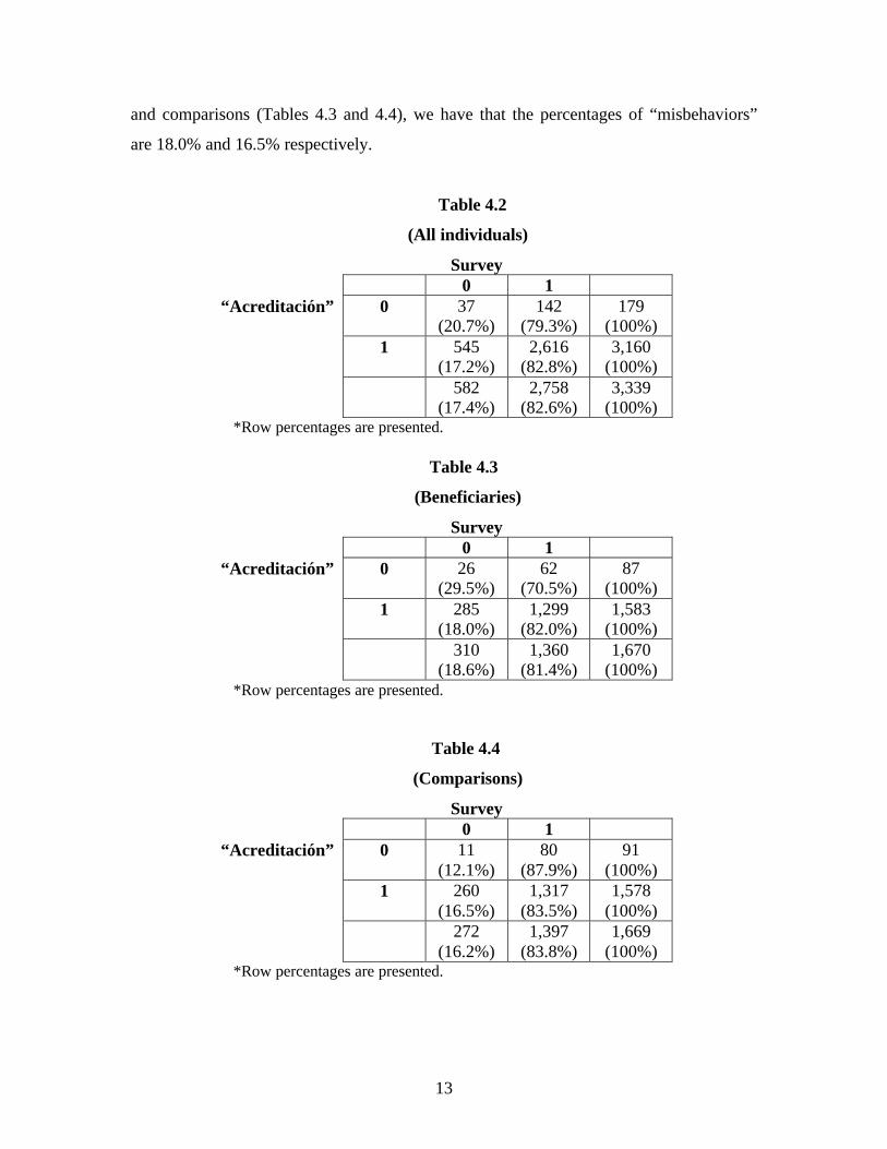
The Tables 4.2 to 4.4 present cross-information about unemployment status (1

unemployed and 0 otherwise) at both “acreditación” and survey, for all the individuals,

for beneficiaries only and for comparisons only. The information related to

“acreditación” is presented in the rows while the information related to the survey is

presented in the columns.

We could consider that the individuals who declare to be unemployed at the

“acreditación” but revealed not to be unemployed at the survey were the ones who

behaved strategically at the “acreditación”. Using this as an indicator we have in Table

4.2 that 542 individuals out of 3,160 (17.2% of this individuals) who declared to be

unemployed at the “acreditación” were “misbehaving”. Separating between beneficiaries

5 We had some cases of beneficiaries older than 35 years of age. They were included with the adult malesand females.6 The “acreditación” information that was asked was rather limited and refers mainly to their labor statusprevious to the Program.

13

and comparisons (Tables 4.3 and 4.4), we have that the percentages of “misbehaviors”

are 18.0% and 16.5% respectively.

Table 4.2

(All individuals)

Survey0 1

“Acreditación” 0 37(20.7%)

142(79.3%)

179(100%)

1 545(17.2%)

2,616(82.8%)

3,160(100%)

582(17.4%)

2,758(82.6%)

3,339(100%)

*Row percentages are presented.

Table 4.3

(Beneficiaries)

Survey0 1


62(70.5%)

87(100%)

1 285(18.0%)

1,299(82.0%)

1,583(100%)

310(18.6%)

1,360(81.4%)

1,670(100%)


Table 4.4

(Comparisons)

Survey0 1


80(87.9%)

91(100%)

1 260(16.5%)

1,317(83.5%)

1,578(100%)

272(16.2%)

1,397(83.8%)

1,669(100%)


14

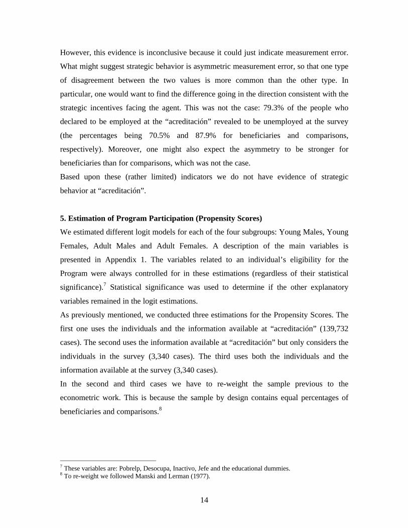
However, this evidence is inconclusive because it could just indicate measurement error.

What might suggest strategic behavior is asymmetric measurement error, so that one type

of disagreement between the two values is more common than the other type. In

particular, one would want to find the difference going in the direction consistent with the

strategic incentives facing the agent. This was not the case: 79.3% of the people who

declared to be employed at the “acreditación” revealed to be unemployed at the survey

(the percentages being 70.5% and 87.9% for beneficiaries and comparisons,

respectively). Moreover, one might also expect the asymmetry to be stronger for

beneficiaries than for comparisons, which was not the case.

Based upon these (rather limited) indicators we do not have evidence of strategic

behavior at “acreditación”.

5. Estimation of Program Participation (Propensity Scores)

We estimated different logit models for each of the four subgroups: Young Males, Young

Females, Adult Males and Adult Females. A description of the main variables is

presented in Appendix 1. The variables related to an individual’s eligibility for the

Program were always controlled for in these estimations (regardless of their statistical

significance).7 Statistical significance was used to determine if the other explanatory

variables remained in the logit estimations.

As previously mentioned, we conducted three estimations for the Propensity Scores. The

first one uses the individuals and the information available at “acreditación” (139,732

cases). The second uses the information available at “acreditación” but only considers the

individuals in the survey (3,340 cases). The third uses both the individuals and the

information available at the survey (3,340 cases).

In the second and third cases we have to re-weight the sample previous to the

econometric work. This is because the sample by design contains equal percentages of

beneficiaries and comparisons.8

7 These variables are: Pobrelp, Desocupa, Inactivo, Jefe and the educational dummies.8 To re-weight we followed Manski and Lerman (1977).

15

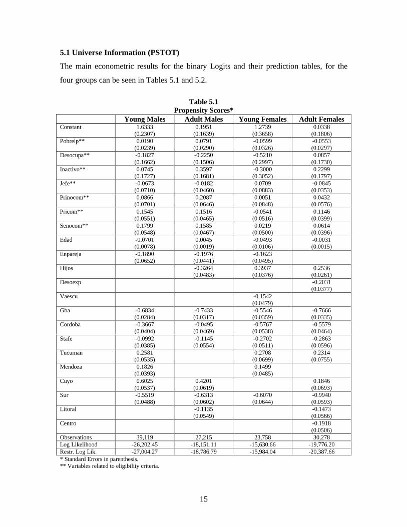
5.1 Universe Information (PSTOT)

The main econometric results for the binary Logits and their prediction tables, for the

four groups can be seen in Tables 5.1 and 5.2.

Table 5.1Propensity Scores*

Young Males Adult Males Young Females Adult FemalesConstant 1.6333

(0.2307)0.1951

(0.1639)1.2739

(0.3658)0.0338

(0.1806)Pobrelp** 0.0190

(0.0239)0.0791

(0.0290)-0.0599(0.0326)

-0.0553(0.0297)

Desocupa** -0.1827(0.1662)

-0.2250(0.1506)

-0.5210(0.2997)

0.0857(0.1730)

Inactivo** 0.0745(0.1727)

0.3597(0.1681)

-0.3000(0.3052)

0.2299(0.1797)

Jefe** -0.0673(0.0710)

-0.0182(0.0460)

0.0709(0.0883)

-0.0845(0.0353)

Prinocom** 0.0866(0.0701)

0.2087(0.0646)

0.0051(0.0848)

0.0432(0.0576)

Pricom** 0.1545(0.0551)

0.1516(0.0465)

-0.0541(0.0516)

0.1146(0.0399)

Senocom** 0.1799(0.0548)

0.1585(0.0467)

0.0219(0.0500)

0.0614(0.0396)

Edad -0.0701(0.0078)

0.0045(0.0019)

-0.0493(0.0106)

-0.0031(0.0015)

Enpareja -0.1890(0.0652)

-0.1976(0.0441)

-0.1623(0.0495)

Hijos -0.3264(0.0483)

0.3937(0.0376)

0.2536(0.0261)

Desoexp -0.2031(0.0377)

Vaescu -0.1542(0.0479)

Gba -0.6834(0.0284)

-0.7433(0.0317)

-0.5546(0.0359)

-0.7666(0.0335)

Cordoba -0.3667(0.0404)

-0.0495(0.0469)

-0.5767(0.0538)

-0.5579(0.0464)

Stafe -0.0992(0.0385)

-0.1145(0.0554)

-0.2702(0.0511)

-0.2863(0.0596)

Tucuman 0.2581(0.0535)

0.2708(0.0699)

0.2314(0.0755)

Mendoza 0.1826(0.0393)

0.1499(0.0485)

Cuyo 0.6025(0.0537)

0.4201(0.0619)

0.1846(0.0693)

Sur -0.5519(0.0488)

-0.6313(0.0602)

-0.6070(0.0644)

-0.9940(0.0593)

Litoral -0.1135(0.0549)

-0.1473(0.0566)

Centro -0.1918(0.0506)

Observations 39,119 27,215 23,758 30,278Log Likelihood -26,202.45 -18,151.11 -15,630.66 -19,776.20Restr. Log Lik. -27,004.27 -18.786.79 -15,984.04 -20,387.66* Standard Errors in parenthesis.** Variables related to eligibility criteria.

16

We will not discuss the estimated coefficients of the variables included in the regressions

because of eligibility considerations. With regard to the others, it seems that age and the

presence of a spouse or companion are, in general, related to a lower likelihood of

Program participation. The presence of children was positively related to Program

participation for females. However, for males this variable was not significant (young

males) or it was positively related to Program participation (adult males). The variables

related to unemployed with working experience and school attendance were significant

and negatively related to Program participation only in the cases of young females and

adult females respectively. The regional dummies for Gba, Cordoba, Santa Fe, Sur,

Litoral (significant only in the cases of adult males and females) and Centro (significant

only for adult females) were negatively related to propensity scores. Tucuman, Mendoza

and Cuyo dummies were positively related to propensity scores (although they were not

significant in all the sub samples).

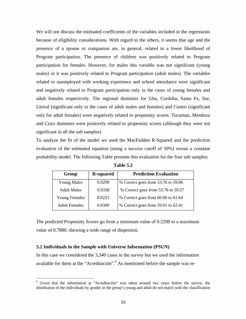
To analyze the fit of the model we used the MacFadden R-Squared and the prediction

evaluation of the estimated equation (using a success cutoff of 50%) versus a constant

probability model. The following Table presents this evaluation for the four sub samples:

Table 5.2

Group R-squared Prediction Evaluation

Young Males

Adult Males

Young Females

Adult Females

0.0299

0.0338

0.0221

0.0300

% Correct goes from 53.76 to 59.06




The predicted Propensity Scores go from a minimum value of 0.2298 to a maximum

value of 0.7880, showing a wide range of dispersion.

5.2 Individuals in the Sample with Universe Information (PSUN)

In this case we considered the 3,340 cases in the survey but we used the information

available for them at the “Acreditación”.9 As mentioned before the sample was re-

9 Given that the information at “Acreditación” was taken around two years before the survey, thedistribution of the individuals by gender in the group’s young and adult do not match with the classification

17

weighted prior to estimation to correct for Choice-Based Sampling. Following Manski

and Lerman (1977) we reweighed each observation by the ratio of the proportion of

beneficiaries in a random population divided by the proportion of beneficiaries in our

sample. The sample proportion of beneficiaries was used to estimate the latter, while for

the former we used the universe information to estimate the proportion of beneficiaries in

the universe.

The main econometric results for the binary Logits and their prediction tables, for the

four groups can be seen in Tables 5.3 and 5.4.



(1.2763)0.4506

(0.2403)6.4998

(1.4969)0.0578

(0.2292)Pobrelp** -0.0126

(0.1427)-0.0991(0.1484)

0.0866(0.1781)

-0.0176(0.1374)

Desocupa** -0.1654(0.2098)

-0.3939(0.1848)

-0.5446(0.3622)

0.0199(0.1977)

Inactivo** -0.2352(0.3388)

-0.6296(0.5545)

0.0173(0.4385)

0.1221(0.3060)

Jefe** -0.0908(0.1976)

0.1310(0.1484)

0.5552(0.2986)

0.1086(0.1597)

Prinocom** -0.4856(0.4064)

-0.6572(0.3447)

-0.5280(0.5318)

0.0738(0.2696)

Pricom** -0.3008(0.2668)

-0.1827(0.2086)

-0.2845(0.2987)

0.0700(0.1779)

Senocom** -0.1063(0.2268)

-0.0769(0.1890)

-0.0161(0.1765)

-0.0113(0.1571)

Edad -0.5771(0.0634)

-0.3138(0.0768)

Enpareja 0.7099(0.3126)

Hijos -0.6201(0.3455)

Vaescu -0.3995(0.1679)

-0.3498(0.2021)

Nea 0.6099(0.3010)

0.6320(0.4096)

0.7889(0.3082)

Gba -0.5082(0.2809)

-0.2215(0.1908)

Observations 914 807 587 1031Log Likelihood -579.327 -550.585 -385.333 -707.496Restr. Log Lik. -630.744 -557.8036 -405.589 -712.633* Standard Errors in parenthesis. ** Variables related to eligibility criteria.

in the sample. This explains the different sizes of the groups when we use this information and the surveyinformation.

18

As before, we will not discuss the estimated coefficients of the variables included in the

regressions because of eligibility considerations. With regard to the others, it seems that

age, the presence of children and school attendances are, in general, related to a lower

likelihood of Program participation (although these effects are not significant for all the

subgroups). The presence of a spouse or companion was positively related to Program

participation only for young males. The regional dummy for Nea and Gba were positively

related and negatively related to Propensity Scores, respectively.

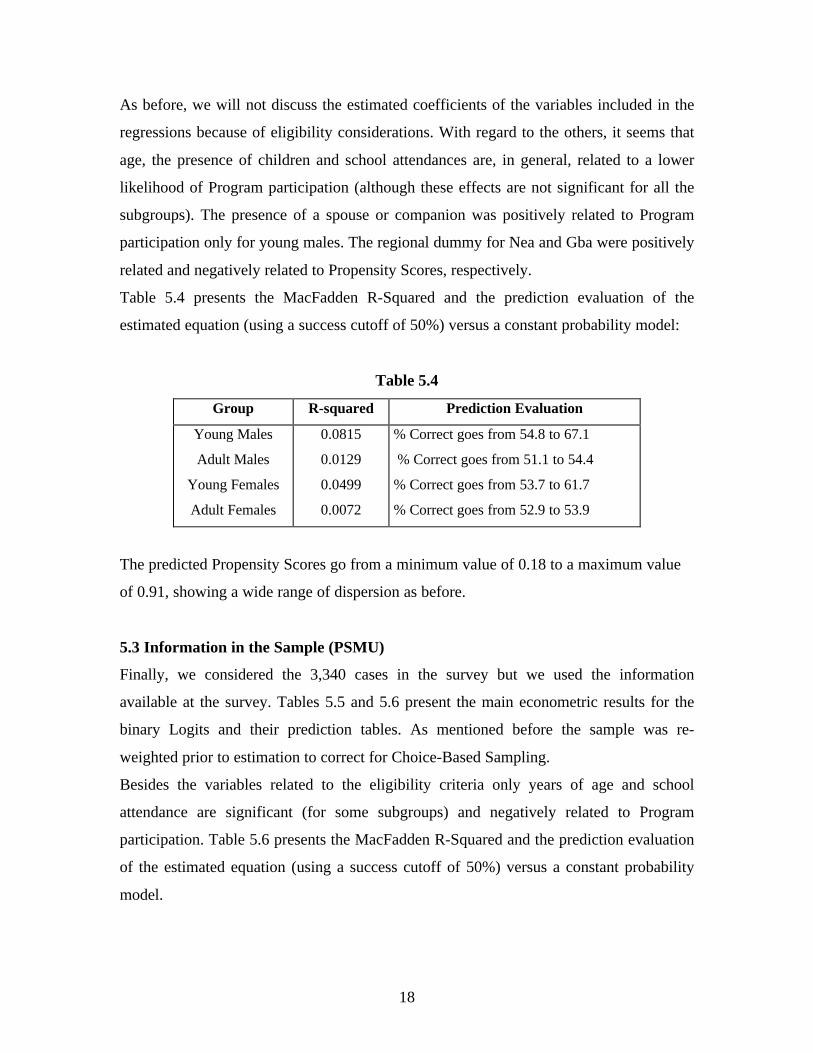
Table 5.4 presents the MacFadden R-Squared and the prediction evaluation of the

estimated equation (using a success cutoff of 50%) versus a constant probability model:

Table 5.4


Young Males

Adult Males

Young Females

Adult Females

0.0815

0.0129

0.0499

0.0072





The predicted Propensity Scores go from a minimum value of 0.18 to a maximum value

of 0.91, showing a wide range of dispersion as before.

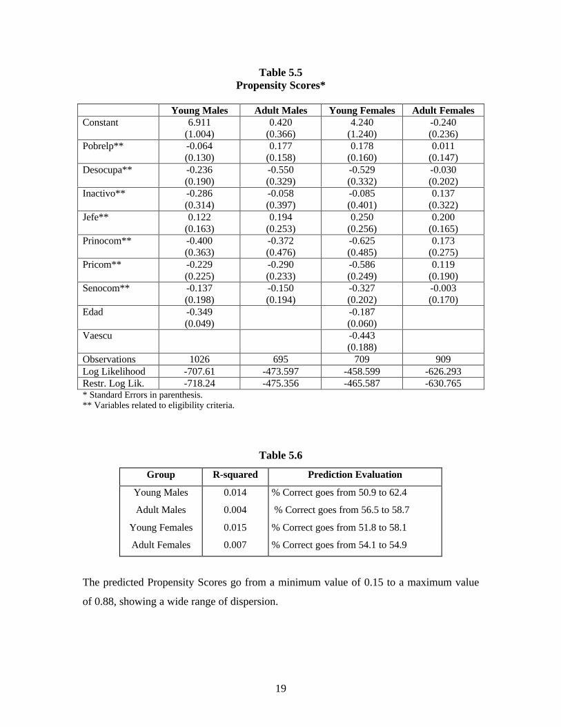
5.3 Information in the Sample (PSMU)

Finally, we considered the 3,340 cases in the survey but we used the information

available at the survey. Tables 5.5 and 5.6 present the main econometric results for the

binary Logits and their prediction tables. As mentioned before the sample was re-

weighted prior to estimation to correct for Choice-Based Sampling.

Besides the variables related to the eligibility criteria only years of age and school

attendance are significant (for some subgroups) and negatively related to Program

participation. Table 5.6 presents the MacFadden R-Squared and the prediction evaluation

of the estimated equation (using a success cutoff of 50%) versus a constant probability

model.

19



(1.004)0.420

(0.366)4.240

(1.240)-0.240(0.236)

Pobrelp** -0.064(0.130)

0.177(0.158)

0.178(0.160)

0.011(0.147)

Desocupa** -0.236(0.190)

-0.550(0.329)

-0.529(0.332)

-0.030(0.202)

Inactivo** -0.286(0.314)

-0.058(0.397)

-0.085(0.401)

0.137(0.322)

Jefe** 0.122(0.163)

0.194(0.253)

0.250(0.256)

0.200(0.165)

Prinocom** -0.400(0.363)

-0.372(0.476)

-0.625(0.485)

0.173(0.275)

Pricom** -0.229(0.225)

-0.290(0.233)

-0.586(0.249)

0.119(0.190)

Senocom** -0.137(0.198)

-0.150(0.194)

-0.327(0.202)

-0.003(0.170)

Edad -0.349(0.049)

-0.187(0.060)

Vaescu -0.443(0.188)

Observations 1026 695 709 909Log Likelihood -707.61 -473.597 -458.599 -626.293Restr. Log Lik. -718.24 -475.356 -465.587 -630.765* Standard Errors in parenthesis.** Variables related to eligibility criteria.

Table 5.6


Young Males

Adult Males

Young Females

Adult Females

0.014

0.004

0.015

0.007





The predicted Propensity Scores go from a minimum value of 0.15 to a maximum value

of 0.88, showing a wide range of dispersion.

20

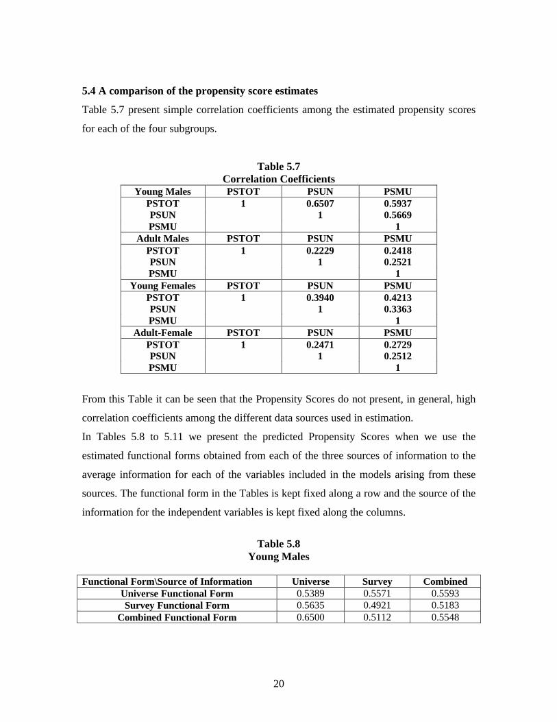
5.4 A comparison of the propensity score estimates

Table 5.7 present simple correlation coefficients among the estimated propensity scores

for each of the four subgroups.

Table 5.7Correlation Coefficients

Young Males PSTOT PSUN PSMU PSTOT 1 0.6507 0.5937 PSUN 1 0.5669 PSMU 1

Adult Males PSTOT PSUN PSMU PSTOT 1 0.2229 0.2418 PSUN 1 0.2521 PSMU 1

Young Females PSTOT PSUN PSMU PSTOT 1 0.3940 0.4213 PSUN 1 0.3363 PSMU 1

Adult-Female PSTOT PSUN PSMU PSTOT 1 0.2471 0.2729 PSUN 1 0.2512 PSMU 1

From this Table it can be seen that the Propensity Scores do not present, in general, high

correlation coefficients among the different data sources used in estimation.

In Tables 5.8 to 5.11 we present the predicted Propensity Scores when we use the

estimated functional forms obtained from each of the three sources of information to the

average information for each of the variables included in the models arising from these

sources. The functional form in the Tables is kept fixed along a row and the source of the

information for the independent variables is kept fixed along the columns.

Table 5.8Young Males

Functional Form\Source of Information Universe Survey CombinedUniverse Functional Form 0.5389 0.5571 0.5593Survey Functional Form 0.5635 0.4921 0.5183

Combined Functional Form 0.6500 0.5112 0.5548

21

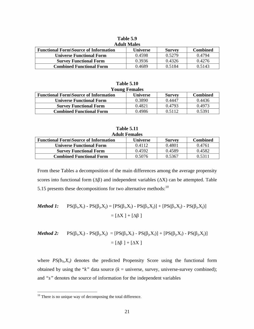
Table 5.9Adult Males



Table 5.10Young Females



Table 5.11Adult Females



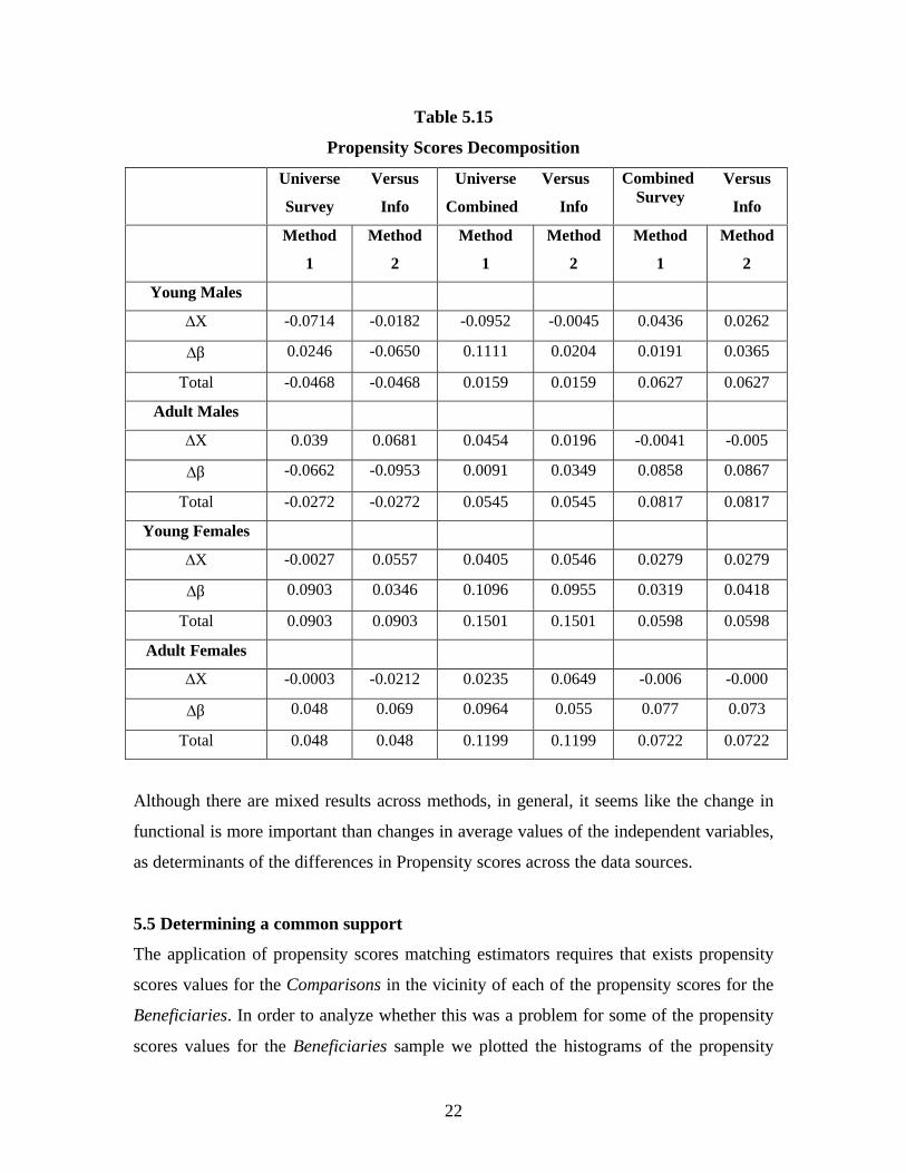
From these Tables a decomposition of the main differences among the average propensity

scores into functional form (Δβ) and independent variables (ΔX) can be attempted. Table

5.15 presents these decompositions for two alternative methods:10

Method 1: PS(βi,Xi) - PS(βj,Xj) = [PS(βi,Xi) - PS(βi,Xj)] + [PS(βi,Xj) - PS(βj,Xj)]

= [ΔX ] + [Δβ ]

Method 2: PS(βi,Xi) - PS(βj,Xj) = [PS(βi,Xi) - PS(βj,Xi)] + [PS(βj,Xi) - PS(βj,Xj)]

= [Δβ ] + [ΔX ]

where PS(βk,Xs) denotes the predicted Propensity Score using the functional form

obtained by using the “k” data source (k = universe, survey, universe-survey combined);

and “s” denotes the source of information for the independent variables

10 There is no unique way of decomposing the total difference.

22

Table 5.15

Propensity Scores Decomposition

Universe

Survey

Versus

Info

Universe

Combined

Versus

Info

CombinedSurvey

Versus

Info

Method

1

Method

2

Method

1

Method

2

Method

1

Method

2

Young Males

ΔX -0.0714 -0.0182 -0.0952 -0.0045 0.0436 0.0262

Δβ 0.0246 -0.0650 0.1111 0.0204 0.0191 0.0365

Total -0.0468 -0.0468 0.0159 0.0159 0.0627 0.0627

Adult Males

ΔX 0.039 0.0681 0.0454 0.0196 -0.0041 -0.005

Δβ -0.0662 -0.0953 0.0091 0.0349 0.0858 0.0867

Total -0.0272 -0.0272 0.0545 0.0545 0.0817 0.0817

Young Females

ΔX -0.0027 0.0557 0.0405 0.0546 0.0279 0.0279

Δβ 0.0903 0.0346 0.1096 0.0955 0.0319 0.0418

Total 0.0903 0.0903 0.1501 0.1501 0.0598 0.0598

Adult Females

ΔX -0.0003 -0.0212 0.0235 0.0649 -0.006 -0.000

Δβ 0.048 0.069 0.0964 0.055 0.077 0.073

Total 0.048 0.048 0.1199 0.1199 0.0722 0.0722

Although there are mixed results across methods, in general, it seems like the change in

functional is more important than changes in average values of the independent variables,

as determinants of the differences in Propensity scores across the data sources.

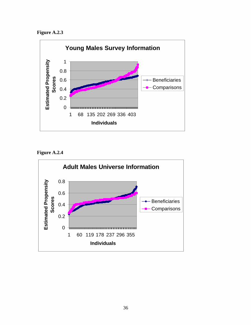
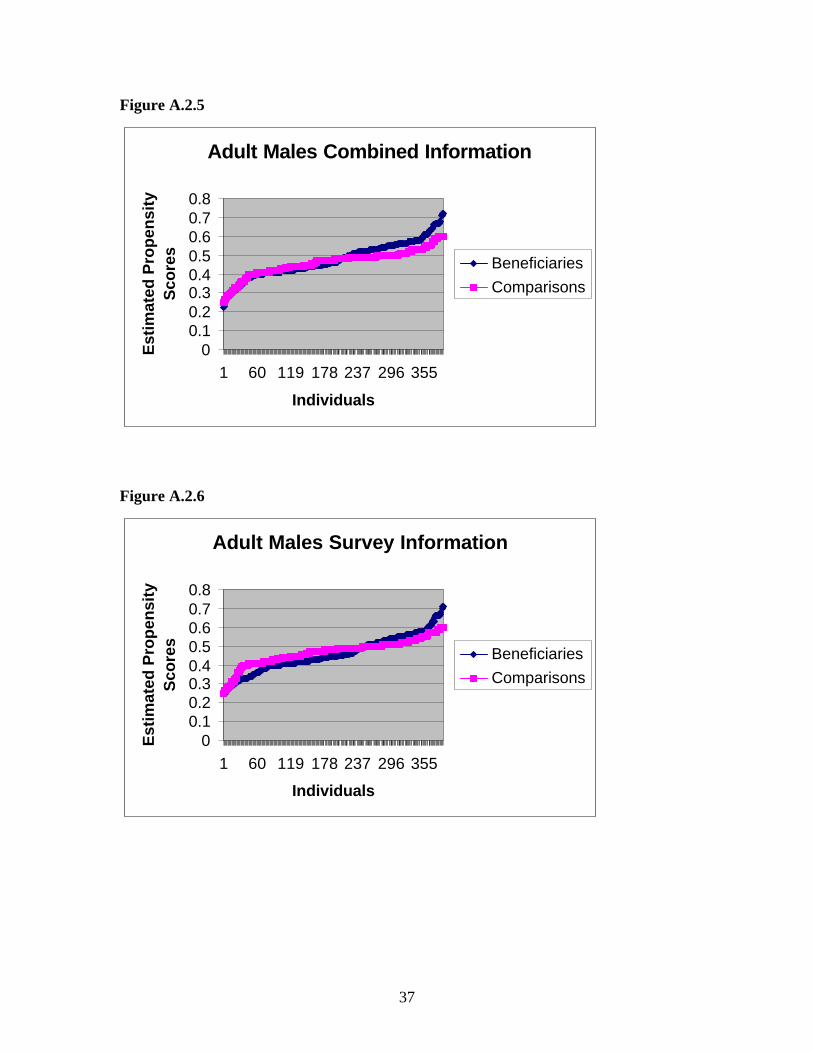
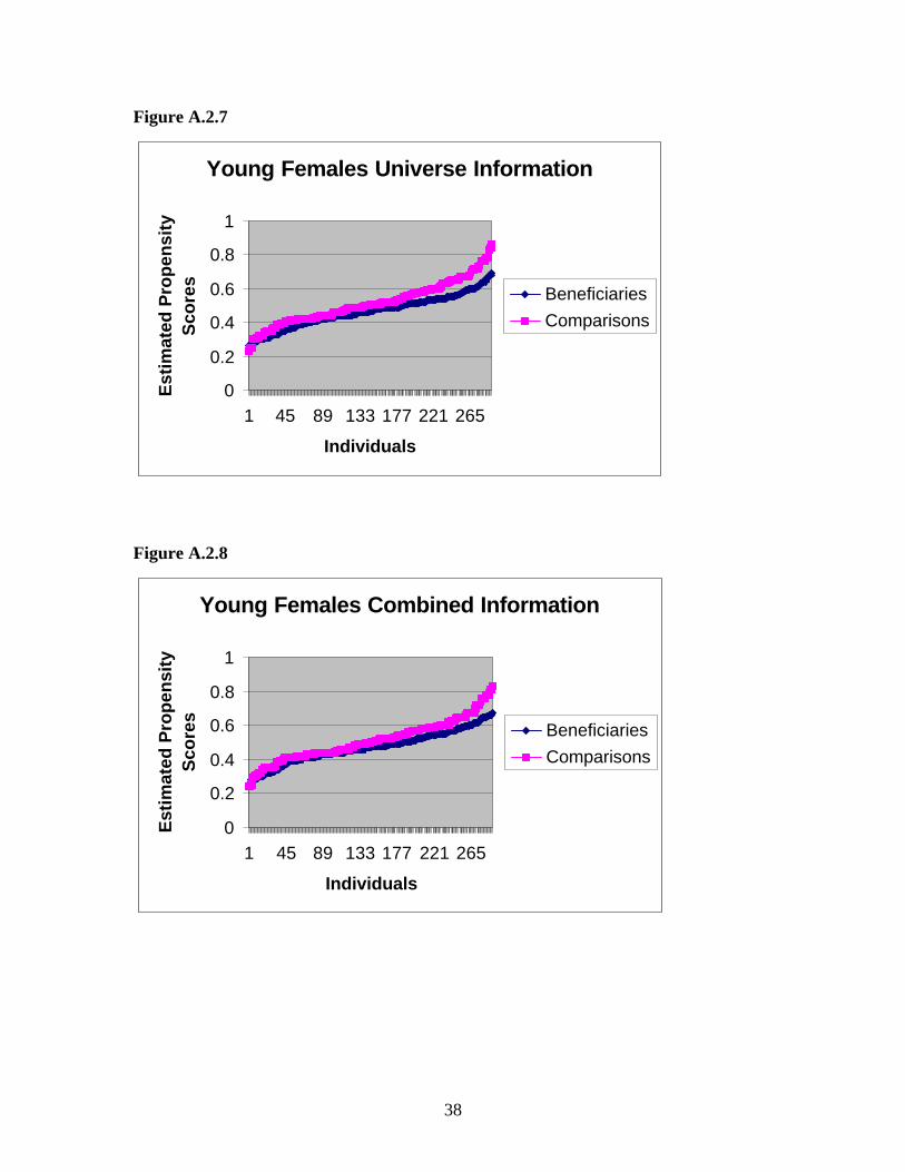
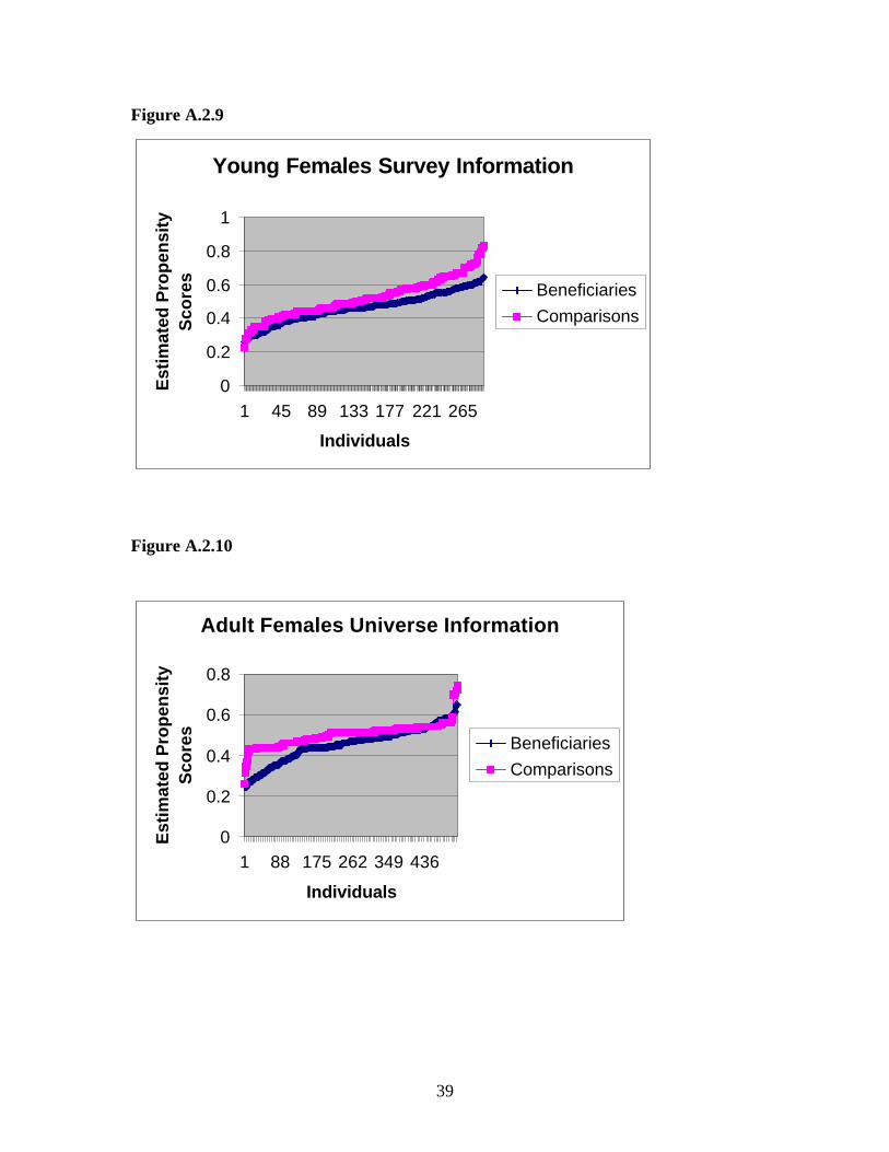
5.5 Determining a common support

The application of propensity scores matching estimators requires that exists propensity

scores values for the Comparisons in the vicinity of each of the propensity scores for the

Beneficiaries. In order to analyze whether this was a problem for some of the propensity

scores values for the Beneficiaries sample we plotted the histograms of the propensity

23

scores for both groups for each of the three estimated propensity scores. The Appendix 2

presents these figures for each of the four subgroups.

Visually we do not observe values of propensity scores for Beneficiaries for which we

cannot find in its vicinity propensity scores in the sample of Comparisons in the cases of

young males, adult males and young females. In the case of adult females we found 20

beneficiaries adult females in the combined universe-survey data for which there were no

close matches in the comparison sample. Appendix 2 presents histograms for the three

sets of estimated scores showing their distribution for the Beneficiaries and Comparisons

groups.

The results we report in the next section assume a common support. It is important to

mention that in the Programa Joven they considered several criteria to select the

Comparisons, controlling by some variables such that age, gender, labor status, marital

status and existence of Children and controlling also by their distribution. This makes

more likely that the two populations present similar propensity scores.

6. Impact estimates: labor earnings and employment

The parameter being estimated is the impact of treatment on the treated. The outcome

variables considered were: earnings and probability of employment in the 12th month

after the Program.

We worked with a cross-sectional (CS) matching estimator, given that this methodology

compares the results for the Beneficiaries and Comparisons at the same period after the

program. The information available allows us to apply this methodology.

The specific cross-sectional matching estimator was the Nearest Neighbor Matching

Estimator:11 This is the simplest method to implement and its specific formulas can be

seen in Todd (1999). The number of neighbors to include from the Comparisons sample

for each Beneficiary is taken as given. For each Beneficiary we included only income

information of the specified number of Comparisons with the lowest Euclidean distance

to the ith Beneficiary propensity scores.

11 As in the case of any propensity score matching estimators, it is necessary to assume that E[Y0 P(X),D=1]=E[Y0 P(X), D =0] and 0 < Pr(D=1 X) <1.

24

The technique of bootstrapping was used to obtain the sample variance of the impact

estimates. The Appendix 3 presents the Matlab (version 5.3.1) codes, which were used in

estimation.

Table 6.1 presents some descriptive statistics for the four subgroups, for beneficiaries and

comparisons, on labor earnings and employment in the 12th month after the Program.

Table 6.1Descriptive Statistics

Young-Males Mean Std. Dev. Beneficiaries Income at 12 months $138.38 $163.28

Beneficiaries Employment at 12 months 0.677 0.4681 Comparisons Income at 12 months $127.51 $152.63

Comparisons Employment at 12 months 0.6499 0.4775

Adult-Males Mean Std. Dev Beneficiaries Income at 12 months $180.61 $192.07



Young-Females Mean Std. Dev. Beneficiaries Income at 12 months $86.24 $141.41


Comparisons Employment at 12 months 0.4333 0.49.60

Adult-Females Mean Std. Dev. Beneficiaries Income at 12 months $111.82 $115.46



6.1 Labor Earnings Results

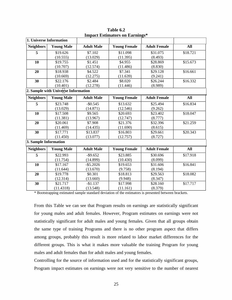
The main results for the program impact estimates on earnings are presented in Table 6.2.

We present impact estimates for 5, 10, 20 and 30 neighbors, for the four sub-groups and

for the whole sample.12 We report program impact estimates using the three estimated

Propensity Scores: 1) using the universe individuals and information; 2) using the

universe information but the individuals in the survey; and 3) using the individuals and

the information from the survey.

12 The estimate for the whole sample is constructed by weighting the individual results by sampleproportions in the beneficiary sample of 1,670 individuals.

25

Table 6.2 Impact Estimators on Earnings*

1. Universe Information

Neighbors Young Male Adult Male Young Female Adult Female All

5 $19.626(10.555)

$7.102(13.029)

$11.098(11.395)

$31.075(8.493)

$18.721

10 $19.755(10.707)

$1.451(12.574)

$4.955(11.486)

$28.869(8.830)

$15.673

20 $18.938(10.669)

$4.522(12.275)

$7.341(11.639)

$29.128(9.241)

$16.661

30 $22.176(10.401)

$2.484(12.278)

$8.020(11.446)

$26.244(8.989)

$16.332

2. Sample with Universe Information


5 $23.748(13.029)

-$0.545(14.871)

$13.632(12.546)

$25.494(9.262)

$16.834

10 $17.508(11.381)

$9.565(13.967)

$20.693(12.747)

$23.402(8.777)

$18.047

20 $20.061(11.469)

$7.908(14.435)

$21.376(11.690)

$32.396(8.615)

$21.259

30 $17.771(11.450)

$13.837(13.077)

$16.803(12.757)

$29.661(8.727)

$20.343

3. Sample Information


5 $22.993(11.754)

-$9.652(14.899)

$23.885(10.430)

$30.696(8.099)

$17.918

10 $17.167(11.644)

-$5.2026(13.670)

$19.653(9.758)

$31.606(8.194)

$16.841

20 $19.778(12.314)

$0.301(13.660)

$18.813(9.948)

$29.563(8.347)

$18.082

30 $21.717(11.4318)

-$1.137(13.548)

$17.998(11.161)

$28.160(8.379)

$17.717

* Bootstrapping estimated sample standard deviation of the estimators is presented between brackets.

From this Table we can see that Program results on earnings are statistically significant

for young males and adult females. However, Program estimates on earnings were not

statistically significant for adult males and young females. Given that all groups obtain

the same type of training Programs and there is no other program aspect that differs

among groups, probably this result is more related to labor market differences for the

different groups. This is what it makes more valuable the training Program for young

males and adult females than for adult males and young females.

Controlling for the source of information used and for the statistically significant groups,

Program impact estimates on earnings were not very sensitive to the number of nearest

26

neighbors.13 Also impact estimates for the different propensity score specifications were

very similar, even though the low correlations among the different scores reported earlier.

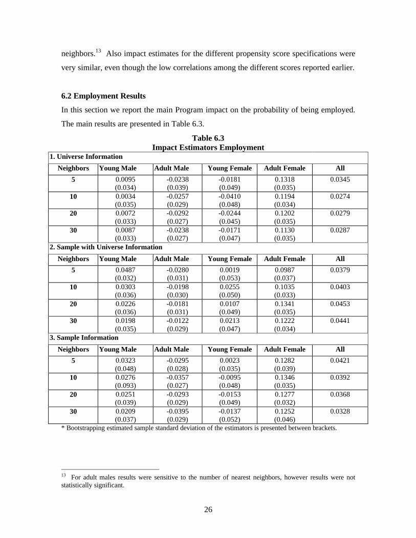
6.2 Employment Results

In this section we report the main Program impact on the probability of being employed.

The main results are presented in Table 6.3.

Table 6.3 Impact Estimators Employment

1. Universe Information


5 0.0095(0.034)

-0.0238(0.039)

-0.0181(0.049)

0.1318(0.035)

0.0345

10 0.0034(0.035)

-0.0257(0.029)

-0.0410(0.048)

0.1194(0.034)

0.0274

20 0.0072(0.033)

-0.0292(0.027)

-0.0244(0.045)

0.1202(0.035)

0.0279

30 0.0087(0.033)

-0.0238(0.027)

-0.0171(0.047)

0.1130(0.035)

0.0287

2. Sample with Universe Information


5 0.0487(0.032)

-0.0280(0.031)

0.0019(0.053)

0.0987(0.037)

0.0379

10 0.0303(0.036)

-0.0198(0.030)

0.0255(0.050)

0.1035(0.033)

0.0403

20 0.0226(0.036)

-0.0181(0.031)

0.0107(0.049)

0.1341(0.035)

0.0453

30 0.0198(0.035)

-0.0122(0.029)

0.0213(0.047)

0.1222(0.034)

0.0441

3. Sample Information


5 0.0323(0.048)

-0.0295(0.028)

0.0023(0.035)

0.1282(0.039)

0.0421

10 0.0276(0.093)

-0.0357(0.027)

-0.0095(0.048)

0.1346(0.035)

0.0392

20 0.0251(0.039)

-0.0293(0.029)

-0.0153(0.049)

0.1277(0.032)

0.0368

30 0.0209(0.037)

-0.0395(0.029)

-0.0137(0.052)

0.1252(0.046)

0.0328

* Bootstrapping estimated sample standard deviation of the estimators is presented between brackets.

13 For adult males results were sensitive to the number of nearest neighbors, however results were notstatistically significant.

27

From this Table it can be observed that the estimated Program impact on employment

was statistically significant for adult females only. For this group the estimated impact

was not sensitive to the number of nearest neighbors. Also, the impact estimates for the

different propensity score specifications were very similar. For the non-statistically

significant groups we observed a greater sensitivity of the estimates to the number of

nearest neighbors and to the different sources of information used to estimate the

propensity scores.

7. Cost Benefit Analysis

Based on the identification and quantification of the outcome measures, it is possible to

estimate the benefits of Programa Joven, for the time period considered. This information

is used in this section, together with information on costs of the program, to conduct a

cost-benefit analysis and to calculate a rate of return to dollars spent on the Program.

We have information on:14

• Direct Cost of Training: This includes the cost of the training services rendered by

the ICAP, the insurance for short-term stays in firms, and the fellowships and

subsidies to the program beneficiaries for children.

• Indirect Costs: This includes the costs of personal, infrastructure, inputs and

operational expenses of the unit that carries out the Program. It also includes, among

others, information on bidding costs, promotion, computer services and supervision.

The problem with the information is that the unit that carries out the Program has also

other projects, however the Programa Joven is the most important in terms of

expenditure.15 This means that we will have to distribute these costs among the

different projects (components) to have a reliable estimate of administrative costs of

the Programa Joven.

The accumulated total cost within the period second semester 1993 to December 1998

has the following composition:

14 The Programa Joven provided this information.15 Other components include Proyecto Microempresas, Proyecto Imagen y Fortalecimiento Institucional.

28

Table 7.1

Cumulative Budget Execution at 12/31/1998

Category Cumulative %

Direct Costs $152,504,951.33 75.34%

Administration $31,407,058.68 15.52%

Concurrent Costs $5,417,166.29 2.68%

Financial Costs $13,083,500.00 6.46%

Total $202,412,676.30 100%

We did not have access to the detailed costs information needed to separate and allocate

the Administrative costs among its several components (Programa Joven, Proyecto

Microempresas, Proyecto Imagen and Fortalecimiento Institucional). As a compromise

we assumed that the administrative, concurrent and financial costs maintain a constant

proportionality with the direct costs. Thus, we assume that the direct costs represent

3.055 times the indirect costs (3.055=Direct Costs/administration+concurrent+financial).

The Programa Joven has estimated the Direct Cost of the courses in the fifth bidding

wave of the training program. They estimated in US$ 1,342 the direct cost per student

graduated at least from the technical knowledge phase. Given the assumption of a

constant proportionality between indirect to direct cost, this means that we have an

indirect cost of US$ 483.83 per student graduated from at least the technical knowledge

phase, which gives a total cost of US$ 1,780.83 per student.

In addition, we assumed that there is a zero opportunity cost while the trainee is being

treated and that there is a constant impact of the treatment on labor income. We

conducted the cost benefit analysis under different scenarios for the duration of benefits,

discount rate and ratio direct to indirect costs.

The specific formula used to obtain the net present value (NPV) is as follows:

∑=

+−

=T

tttt

r

CENPV

0 )1(

29

where Et denotes the mean earnings effect on the treated,16 Ct denotes the costs of

Programa Joven (we assume that they take place at time zero), T denotes the duration of

benefits and r denotes the opportunity cost of capital.

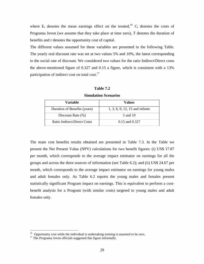
The different values assumed for these variables are presented in the following Table.

The yearly real discount rate was set at two values 5% and 10%, the latest corresponding

to the social rate of discount. We considered two values for the ratio Indirect/Direct costs

the above-mentioned figure of 0.327 and 0.15 a figure, which is consistent with a 13%

participation of indirect cost on total cost.17

Table 7.2

Simulation Scenarios

Variable Values

Duration of Benefits (years) 1, 3, 6, 9, 12, 15 and infinite

Discount Rate (%) 5 and 10

Ratio Indirect/Direct Costs 0.15 and 0.327

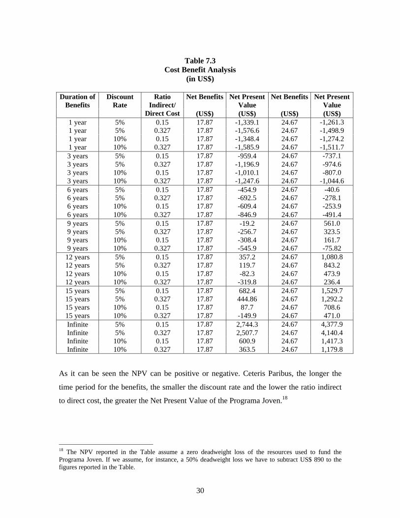
The main cost benefits results obtained are presented in Table 7.3. In the Table we

present the Net Present Value (NPV) calculations for two benefit figures: (i) US$ 17.87

per month, which corresponds to the average impact estimator on earnings for all the

groups and across the three sources of information (see Table 6.2); and (ii) US$ 24.67 per

month, which corresponds to the average impact estimator on earnings for young males

and adult females only. As Table 6.2 reports the young males and females present

statistically significant Program impact on earnings. This is equivalent to perform a cost-

benefit analysis for a Program (with similar costs) targeted to young males and adult

females only.

16 Opportunity cost while the individual is undertaking training is assumed to be zero.17 The Programa Joven officials suggested this figure informally.

30

Table 7.3Cost Benefit Analysis

(in US$)

Net Benefits Net PresentValue

Net Benefits Net PresentValue

Duration ofBenefits

DiscountRate

RatioIndirect/

Direct Cost (US$) (US$) (US$) (US$)1 year 5% 0.15 17.87 -1,339.1 24.67 -1,261.31 year 5% 0.327 17.87 -1,576.6 24.67 -1,498.91 year 10% 0.15 17.87 -1,348.4 24.67 -1,274.21 year 10% 0.327 17.87 -1,585.9 24.67 -1,511.73 years 5% 0.15 17.87 -959.4 24.67 -737.13 years 5% 0.327 17.87 -1,196.9 24.67 -974.63 years 10% 0.15 17.87 -1,010.1 24.67 -807.03 years 10% 0.327 17.87 -1,247.6 24.67 -1,044.66 years 5% 0.15 17.87 -454.9 24.67 -40.66 years 5% 0.327 17.87 -692.5 24.67 -278.16 years 10% 0.15 17.87 -609.4 24.67 -253.96 years 10% 0.327 17.87 -846.9 24.67 -491.49 years 5% 0.15 17.87 -19.2 24.67 561.09 years 5% 0.327 17.87 -256.7 24.67 323.59 years 10% 0.15 17.87 -308.4 24.67 161.79 years 10% 0.327 17.87 -545.9 24.67 -75.82

12 years 5% 0.15 17.87 357.2 24.67 1,080.812 years 5% 0.327 17.87 119.7 24.67 843.212 years 10% 0.15 17.87 -82.3 24.67 473.912 years 10% 0.327 17.87 -319.8 24.67 236.415 years 5% 0.15 17.87 682.4 24.67 1,529.715 years 5% 0.327 17.87 444.86 24.67 1,292.215 years 10% 0.15 17.87 87.7 24.67 708.615 years 10% 0.327 17.87 -149.9 24.67 471.0Infinite 5% 0.15 17.87 2,744.3 24.67 4,377.9Infinite 5% 0.327 17.87 2,507.7 24.67 4,140.4Infinite 10% 0.15 17.87 600.9 24.67 1,417.3Infinite 10% 0.327 17.87 363.5 24.67 1,179.8

As it can be seen the NPV can be positive or negative. Ceteris Paribus, the longer the

time period for the benefits, the smaller the discount rate and the lower the ratio indirect

to direct cost, the greater the Net Present Value of the Programa Joven.18

18 The NPV reported in the Table assume a zero deadweight loss of the resources used to fund thePrograma Joven. If we assume, for instance, a 50% deadweight loss we have to subtract US$ 890 to thefigures reported in the Table.

31

8. Conclusions

This article was aimed at answering the following questions: (1) Does “Programa Joven”

increase the labor income of the trainees? (2) Does “Programa Joven” increase the

probability of being employed? (3) How sensitive Program impact estimates are to

different propensity score specifications? And (4) what is the rate of return to dollars

spent on the “Programa Joven”?

Our results indicate first, that Program impact on earnings were statistically significant

for young males and adult females only. In our opinion this result, which makes more

valuable the training Program for these specific groups, is more related to the different

labor market conditions that they face than to Program specific components (all groups

obtain the same type of programs and there is no other program aspect that differs among

groups). Program impact estimates on earnings were not sensitive to the number of

nearest neighbors.

Second, estimated Program impact on employment was statistically significant for adult

females only. For this group the estimated impact was not sensitive to the number of

nearest neighbors. A greater sensitivity of the estimates to the number of nearest

neighbors was observed for the other groups.

Third, impact estimates on earnings and employment for the different propensity score

specifications and for the statistically significant groups were very similar, even though

the low correlations among the different scores reported in the article. For the non-

statistically significant groups we observed a greater sensitivity of the estimates to the

different sources of information used to estimate the propensity scores. This was a

surprising result as we expected to observe greater variability in the impact results across

different propensity score specifications.

Finally, the cost-benefit exercise conducted suggest that, Ceteris Paribus, the longer the

time period for the benefits, the smaller the discount rate and the lower the ratio indirect

to direct cost, the greater the Net Present Value of the Programa Joven. For the all the

beneficiaries we required 12 years of duration of benefits for the Program to have a

positive NPV. For young males and adult females, which present higher and statistically

significant earning impacts, we required a duration of benefits around 9 years for the

Program to have a positive NPV.

32

References

Hardle, W. 1992. “Applied Nonparametric Regression”.

Heckman, J., Ichimura, H., Smith, J., and Todd, P. 1998. “Characterizing Selection Bias

Using Experimental Data”. Econometrica. 66 (5).

Heckman, J., Ichimura, H., and Todd, P. 1997. “Matching As an Econometric Evaluation

Estimator: Evidence from Evaluating a Job Training Programme”. Review of Economic

Studies. 64 (4).

Heckman, J., Ichimura, and Todd, P. 1998. “Matching As an Econometric Evaluation

Estimator”. Review of Economic Studies. 65 (2): 605-654.

Heckman, J., LaLonde, R., and Smith, J. 1999. “The Economics and Econometrics of

Active Labor Market Programs”. In: O. Ashenfelter and D. Card, editors. Handbook of

Labor Economics, Volume IIIA: 1865-2097. Amsterdam: North-Holland.

Heckman, J. and Smith, J. 1998. “Evaluating the Welfare State”. In: Steiner Strom,

editor. Econometrics and Economic Theory in the 20 th Century: The Ragnar Frisch

Centennial. Cambridge, United Kingdom: Cambridge University Press for Econometric

Society.

Heckman, J. and Smith, J. 1999. “The Pre-Program Dip and the Determinants of

Participation in a Social Program: Implications for Simple Program Evaluation

Strategies”. Economic Journal. 109 (143): 1-37.

Heckman, J., Smith, J., and Clements, N. 1997. “Making the Most Out of Programme

Evaluations and Social Experiments: Accounting for Heterogeneity in Program Impacts”.

Review of Economic Studies. 64 (4): 487-536.

Jones, Marron & Sheather. 1996. “A Brief Survey of Bandwidth Selection for Density

Estimation”, JASA.

LaLonde, Robert. 1986. “Evaluating the Econometric Evaluations of Training Programs

with Experimental Data”. American Economic Review. 76 (4): 604-620.

Manski Charles F. 1995. “Learning about Social Programs from Experiments with

Random Assignment of Treatments”. Journal of Human Resources. 31(4): 707-733.

Manski, C. F. and S.R. Lerman, 1977. “The Estimation of the Choice Probabilities from

Choice-Based Samples”. Econometrica 45: 1977-1988.

33

Todd, P. 1999. “A Practical Guide to Implementing Matching Estimators”, mimeo

presented at the IADB meeting in Santiago Chile, October.

Silverman, B.W. 1986. “Density Estimation for Statistics and Data Analysis”. (London:

Chapman and Hall).

Ministerio de Trabajo y Seguridad Social de la República Argentina. “Base de datos e

información del Programa Joven”. Secretaría de Empleo y formación Profesional.

Gerencia de Evaluación de Impacto y Estudios Especiales.

34

Appendix 1: Variable Description

Variable DescriptionEDAD AgeESTADO 1=Beneficiary, 0=ComparisonSEXO 1=Male, 0=FemaleEDAD35 Dummy Age between 16 and 35 years of ageHIJOS Children, 1=Yes, 0=NoHMENOR Children younger than 5 years of age, 1=Yes, 0=NoVAESCU School Attendance, 1=Yes, 0=NoJEFE Head of the Household, 1=Yes, 0=NoENPAREJA Married, 1=Yes, 0=NoPRINOCOM Primary Education Incomplete, 1=Yes, 0=NoPRICOM Primary Education Completed, 1=Yes, 0=NoSENOCOM Secondary Education Incomplete, 1=Yes, 0=NoSECOM Secondary Education Completed, 1=Yes, 0=NoDESOCUPA Unemployed, 1=Yes, 0=NoOCUPADO Employed, 1=Yes, 0=NoDESOEXP Unemployed with labor experience, 1=Yes, 0=NoDESONEXP Unemployed without labor experience, 1=Yes, 0=NoINACTIVO Out of the Labor Force, 1=Yes, 0=NoPOBRELP Poor by Income line, 1=Yes, 0=NoGBA Reside in GBA, 1=Yes, 0=NoSUR Reside in the South, 1=Yes, 0=NoNEA Reside in the North East (NEA), 1=Yes, 0=NoCENTRO Reside in the Center, 1=Yes, 0=NoLITORAL Reside in the Coast, 1=Yes, 0=NoCUYO Reside in Cuyo, 1=Yes, 0=NoNOA Reside in the North West (NOA), 1=Yes, 0=NoCORDOBA Reside in Córdoba, 1=Yes, 0=NoMENDOZA Reside in Mendoza, 1=Yes, 0=NoSTAFE Reside in Santa Fe, 1=Yes, 0=NoTUCUMAN Reside in Tucumán, 1=Yes, 0=NoMUESTRA Internal Control VariableGRUPO Internal Control Variable

35

Appendix 2: Common Support

Figure A.2.1

Figure A.2.2

Young Males Universe Information

0

0.2

0.4

0.6

0.8

1

1 69 137 205 273 341 409

Individuals

Est

imat

ed P

rop

ensi

ty

Sco

res

Beneficiaries

Comparisons

Young Males Combined Information

0

0.2

0.4

0.6

0.8

1

1 68 135 202 269 336 403

Individuals

Est

imat

ed P

rop

ensi

ty

Sco

res

Beneficiaries

Comparisons

36

Figure A.2.3

Figure A.2.4

Young Males Survey Information

0

0.2

0.4

0.6

0.8

1

1 68 135 202 269 336 403

Individuals

Est

imat

ed P

rop

ensi

ty

Sco

res Beneficiaries

Comparisons

Adult Males Universe Information

0

0.2

0.4

0.6

0.8

1 60 119 178 237 296 355

Individuals

Est

imat

ed P

rop

ensi

ty

Sco

res

Beneficiaries

Comparisons

37

Figure A.2.5

Figure A.2.6

Adult Males Combined Information

00.10.20.30.40.50.60.70.8

1 60 119 178 237 296 355

Individuals

Est

imat

ed P

rop

ensi

ty

Sco

res

Beneficiaries

Comparisons

Adult Males Survey Information

00.10.20.30.40.50.60.70.8

1 60 119 178 237 296 355

Individuals

Est

imat

ed P

rop

ensi

ty

Sco

res

Beneficiaries

Comparisons

38

Figure A.2.7

Figure A.2.8

Young Females Universe Information

0

0.2

0.4

0.6

0.8

1

1 45 89 133 177 221 265

Individuals

Est

imat

ed P

rop

ensi

ty

Sco

res

Beneficiaries

Comparisons

Young Females Combined Information

0

0.2

0.4

0.6

0.8

1

1 45 89 133 177 221 265

Individuals

Est

imat

ed P

rop

ensi

ty

Sco

res

Beneficiaries

Comparisons

39

Figure A.2.9

Figure A.2.10

Young Females Survey Information

0

0.2

0.4

0.6

0.8

1

1 45 89 133 177 221 265

Individuals

Est

imat

ed P

rop

ensi

ty

Sco

res

Beneficiaries

Comparisons

Adult Females Universe Information

0

0.2

0.4

0.6

0.8

1 88 175 262 349 436

Individuals

Est

imat

ed P

rop

ensi

ty

Sco

res

Beneficiaries

Comparisons

40

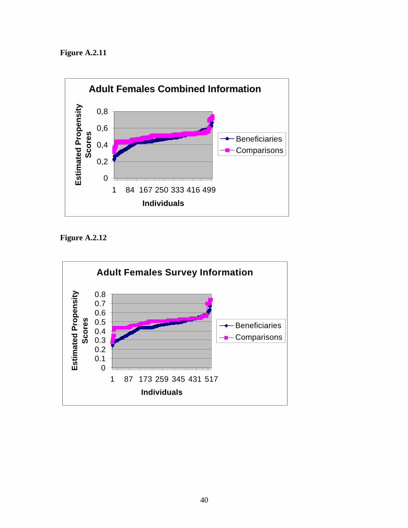
Figure A.2.11

Figure A.2.12

Adult Females Combined Information

0

0,2

0,4

0,6

0,8

1 84 167 250 333 416 499

Individuals

Est

imat

ed P

rop

ensi

ty

Sco

res

BeneficiariesComparisons

Adult Females Survey Information

00.10.20.30.40.50.60.70.8

1 87 173 259 345 431 517

Individuals

Est

imat

ed P

rop

ensi

ty

Sco

res

Beneficiaries

Comparisons

41

Appendix 3: MATLAB Codes

a) Nearest Matching Estimators

%PROGRAM NEAREST MATCHING%%Developed by: Cristian Aedo ([email protected])%%Date: August 1, 2000%Last Update: August 10, 2000%%Purpose: To estimate program impact using the Nearest%Matching Estimator Approach.%Subjects: Whole sample%

%%Loading and defining information matrix%

clear;load tresps2.dat;m=tresps2;

%%Defining Number of observations and location of%beneficiaries and comparisons in the%sample. Data set is ordered: first the beneficiaries and%then the comparisons%

n=3339;n1=1670;n2=1671;

%%Transferring information matrix data into column vectors%

dniclave=m(1:n,1);grupos=m(1:n,2);sexo=m(1:n,3);subgrupo=m(1:n,4);ing0=m(1:n,5);ing1=m(1:n,6);

42

ing2=m(1:n,7);ing3=m(1:n,8);ing4=m(1:n,9);ing5=m(1:n,10);ing6=m(1:n,11);ing7=m(1:n,12);ing8=m(1:n,13);ing9=m(1:n,14);ocupa5=m(1:n,15);desocu5=m(1:n,16);inact5=m(1:n,17);ocupa9=m(1:n,18);desocu9=m(1:n,19);inact9=m(1:n,20);ocupa0=m(1:n,21);desocu0=m(1:n,22);inact0=m(1:n,23);joven=m(1:n,24);pstot=m(1:n,25);psun=m(1:n,26);psmu=m(1:n,27);

%%Defining income data and propensity scores%

yb=m(1:n1,5);yc=m(n2:n,5);pstotb=m(1:n1,25)/10000;pstotc=m(n2:n,25)/10000;psunb=m(1:n1,26)/10000;psunc=m(n2:n,26)/10000;psmub=m(1:n1,27)/10000;psmuc=m(n2:n,27)/10000;

%%Defining number of neighbors%

neighbor=50;

%%The following loop defines the comparisons which are%going to be used for each beneficiaries. Then it%calculates the average earnings for the number of%neighbors considered.%

43

for i=1:length(yb);

difp=abs(pstotb(i)-pstotc); sortdifp=sort(difp); dist=sortdifp(neighbor);

r=0; ycc=0;

for j=1:length(yc);

if difp(j) <= dist;

r=r+1; ycc=ycc+yc(j);

end;

end;

ycp(i)=ycc/r; ybb(i)=yb(i);

end;

%%Finally, we calculate the mean Program impact%

imp=mean(ybb-ycp);imp

b) Nearest Matching Estimator: Bootstrapping

%%PROGRAM BOOTSTRAPPING FOR THE NEAREST MATCHING ESTIMATOR%%Developed by: Cristian Aedo ([email protected])%%Date: August 10, 2000%Last Update: August 18, 2000%%Purpose: The Program will generate 100-paired samples ofbeneficiaries and of comparisons (each of the samples will%be of equal size as the original samples). For each of%these 100 paired samples a Program Impact estimate will be

44

%obtained. The variance of the Mean Impact estimates will%be computed as the sample analog using as a mean the%original estimate of the Program Impact.%%Subjects: Whole sample%

%%Loading and defining information matrix%

load madulta.dat;m=madulta;

%%Defining Number of observations and location ofbeneficiaries and comparisons in the sample. Data set%is ordered: first the beneficiaries and then the%comparisons%

n=3339;n1=1670;n2=1671;nn1=1670;nn2=1669;

%%Transferring information matrix data into column vectors%

dniclave=m(1:n,1);grupos=m(1:n,2);sexo=m(1:n,3);subgrupo=m(1:n,4);ing0=m(1:n,5);ing1=m(1:n,6);ing2=m(1:n,7);ing3=m(1:n,8);ing4=m(1:n,9);ing5=m(1:n,10);ing6=m(1:n,11);ing7=m(1:n,12);ing8=m(1:n,13);ing9=m(1:n,14);ocupa5=m(1:n,15);desocu5=m(1:n,16);

45

inact5=m(1:n,17);ocupa9=m(1:n,18);desocu9=m(1:n,19);inact9=m(1:n,20);ocupa0=m(1:n,21);desocu0=m(1:n,22);inact0=m(1:n,23);joven=m(1:n,24);pstot=m(1:n,25);psun=m(1:n,26);psmu=m(1:n,27);

%%Define some constant terms for the Random Number Generator%

p=2147483647.0;q=2147483655.0;r=16807.0;

%%Obtain 200 seeds to initialize each random sample%

nseeds = 200;seed=20;

for i=1:nseeds;

seed=MOD(r*seed,p); x(i,1)=seed/q;

end;

%%Now iterate over each of these paired samples to obtainthe Program Estimate for each%

for i=1:100;

seed1=x(i,1); seed2=x(100+i,1);

for j=1:nn1;

seed1=MOD(r*seed1,p);

46

x1=seed1/q; rut=round(x1*nn1+0.5); yb(j)=m(rut,21); pstotb(j)=m(rut,25)/10000; psunb(j)=m(rut,26)/10000; psmub(j)=m(rut,27)/10000;

end;

for j=1:nn2;

seed2=MOD(r*seed2,p); x2=seed2/q; rut=n1+round(x2*nn2+0.5); yc(j)=m(rut,21); pstotc(j)=m(rut,25)/10000; psunc(j)=m(rut,26)/10000; psmuc(j)=m(rut,27)/10000;

end;

%%Define the number of neighbors%

neighbor=30;

%%The following loop defines the comparisons that are%going to be used for each beneficiaries. Then it%calculates the average earnings for the%neighbors considered.%

for k=1:length(yb);

difp=abs(psmub(k)-psmuc); sortdifp=sort(difp); dist=sortdifp(neighbor);

s=0; ycc=0;

for j=1:length(yc);

if difp(j) <= dist;

47

s=s+1; ycc=ycc+yc(j);

end;

end;

ycp(k)=ycc/s; ybb(k)=yb(k);

end;

% %Calculate the mean Program impact %

imp(i)=mean(ybb-ycp);

end;

%%Now we calculate the variance and the standard deviation%of the mean Program Impact%

meaneffe=mean(imp); boot=sqrt(var(imp)); meaneffe, boot

The Impact of Training Policies in Latin America and the Caribbean: The Case of Programa Joven

Documents

Transcript of The Impact of Training Policies in Latin America and the Caribbean: The Case of Programa Joven