-1-

The Impact of the WWI Agricultural Boom and Bust on Female Opportunity Cost and

Fertility

by Carl T. Kitchens1 and Luke P. Rodgers2,3

Abstract:

Using variation in crop prices induced by large swings in demand surrounding World

War I, we examine the fertility response to increases in crop revenues during the period

1910-1930. Our estimates from samples utilizing both complete count decennial census

microdata and newly collected county-level data from state health reports indicate that a

doubling of the agricultural price index reduced fertility by around 10-13 percent

throughout the period. This effect persists years after the collapse of the war boom. We

further show that fertility declines along both the extensive and intensive margins,

which is consistent with predictions from models of rising opportunity costs. Our

findings are robust to many potential confounds.

1 Carl T. Kitchens, Associate Professor of Economics, Florida State University and NBER, ckitchens@fsu.edu 2 Luke P. Rodgers, Assistant Professor of Economics, Florida State University, lprodgers@fsu.edu 3 Acknowledgements: We would like to thank Rachel Johnson, Ian Linares, Melissa Pregason, Marco Taylhardat, Justin Bailey, and Anthony Manucci for data entry assistance. We would also like to thank Martin Fiszbein, James Feigenbaum, Carolyn Moehling, Melissa Thomasson, and Lauren Hoehn Velasco for making data available. We thank E. Jason Baron, Brian Beach, Briggs Depew, Ezra Goldstein, Alex Hollingsworth, Matt Jaremski, Taylor Jaworski, Shawn Kantor, Paul Rhode, Nicolas Ziebarth and seminar participants at 2019 WATE, 2020 EHA Meetings, 2020 SEA meetings, 2021 AEA Meetings, 2021 NBER DAE Spring Meeting, Florida State University, and Vanderbilt for helpful feedback. Finally, any errors contained within are our own.

-2-

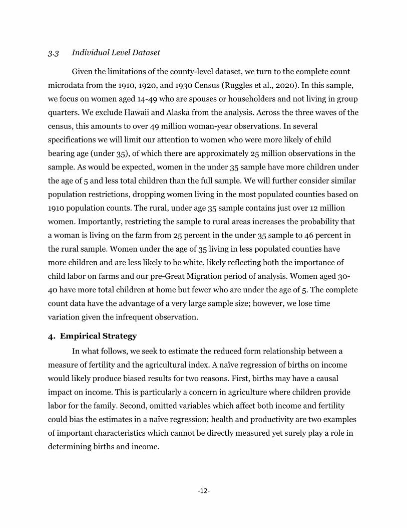
1. Introduction

A recurring theme in economics and demography is that as economies develop, a

demographic transition will occur, whereby declining fertility rates accompany rising

incomes (Galor, 2005; Jones and Tertilt 2009; Galor and Weil, 2000, Brueckner and

Schwandt, 2015). Theory makes sharp predictions regarding the relationship between

fertility, income shocks, and changes in the opportunity cost of time (Becker, 1960;

Becker and Lewis; 1973; Becker and Tomes, 1976; Rosenzweig, 1977), however,

empirical evidence is needed to understand whether pure income shocks or changes in

the opportunity costs of time dominate in specific contexts. A recent literature has

developed that takes advantage of exogenous variation in income, employment, or

wealth to identify their impact on fertility.4 The recent literature has broadly shown that

increases in the male wage or income leads to increases in fertility, while increasing

female wages result in reductions in fertility. Most of this evidence comes from the

period including or following the Baby Boom. Scholars know relatively less about the

causal factors contributing to the decline from the late 19th Century through about 1930.

In this paper, we draw on rich, historical data from the United States to understand

how fertility responds to aggregate shocks that change both incomes and the relative

opportunity costs of women. Specifically, we take advantage of a period of significant

agricultural price variation, the agricultural commodity boom and bust in the United

States surrounding World War I (WWI). During the period we study, 1910-1930, both

the General Fertility Rate and Crude Birth rate fell by approximately 29 percent, which

is as large a decline as the Baby Boom was a boom. The agricultural price variation

induced by international events combined with large changes in fertility make it an ideal

setting to explore the link between income shocks and fertility. The agricultural

commodity boom in WWI was entirely unexpected as fields in Europe were destroyed.

Additionally, the magnitude of the shock was massive. U.S. agricultural exports doubled

in the second half of the 1910s, in some cases prices more than doubled, and agricultural

receipts increased by 70 percent (Henderson, Gloy, and Boehlje, 2011). Farmers

4 See for example Lindo, 2010; Ananat, Gassman-Pines, and Gibson-Davis, 2013; Huttunen and Kellokumpu, 2017; Black et al., 2013; Yonzan, Timilsina, and Kelly, 2020; Fishback, Haines, and Kantor, 2007; Lovenheim and Mumford, 2013; Dettling and Kearney, 2014; Bailey and Collins, 2011; Lewis, 2018; Fujii and Shonchoy, 2020; Wanamaker, 2012; Schaller, 2016.

-3-

expected the boom to persist, as documented by rising land prices.5 The subsequent

bust following the Treaty of Versailles also came as a surprise as Europe rapidly

recovered post war.6 We document a close link between female agricultural wages and

the crop price variation, which we argue makes changes in female opportunity costs the

driving mechanism for the fertility response.

The first few decades of the 20th Century United States are understudied due to

limited data availability. The federal government did not begin recording births until

1915 with the creation of the Birth Registration Area (BRA), which was not complete

until Texas joined in 1933. To gain insight in the pre-war period, we digitize annual

county-level birth tabulations from available state health reports prior to a state’s entry

into the BRA to push back the series to 1910 for thirty-two states. The longer panel

enables us to capture any variation in pre-trends that might confound our estimate.

Additionally, we turn to the complete count Population Census for the years 1910, 1920,

and 1930 to compare birth outcomes for women differentially exposed to the

agricultural boom and bust, netting out common locational and cohort effects.

To identify the empirical relationship between changes in fertility and changes in

agricultural income, we complement our birth data with a measure of annual county-

level agricultural crop revenue. Specifically, we augment the approach of Rajan and

Ramcharan (2015) and Jaremski and Wheelock (forthcoming) to construct a county-

level agricultural price index. The index combines pre-war crop production bundles at

the county-level with aggregate crop specific price shocks to generate our key source of

spatial-temporal variation. We use the index as our measure of agricultural income

because annual county-level crop receipts and gender specific wages are otherwise

unavailable consistently at a disaggregated level. We then estimate the relationship

between the agricultural price index and fertility, controlling for a rich set of covariates,

location specific fixed effects, and time fixed effects. Under the assumption that that the

5 Agricultural land prices increased an average of 170 percent nationally by 1920 relative to prewar prices (Table 540, USDA Yearbook of Agriculture, 1931). In places such as Arkanasas, Georgia, Mississippi, North Carolina, and South Carolina, average land prices increased between 217-230 percent per acre relative to their prewar levels. 6 In the years following WWI, significant price volatility remained, at least in part as a result of increased international competition and new domestic policy (i.e., Capper-Volstead Act, 1922, Fordney-McCumber Tariff, 1922).

-4-

initial crop specialization patterns are driven by agro-climatic variables and that

national crop specific prices are driven by international events and climate shocks,

variation in the agricultural price index is exogenous to the measures of birth and

fertility, thus permitting a causal interpretation for our estimates. We also implement an

instrumental variables strategy exploiting crop suitability measures to generate

predicted crop shares and find a similar pattern of results.

Our estimates consistently show that the agricultural boom reduced fertility in

the short-run, measured by annual county-level births, as well as in the medium and

long-run, measured by counts of children from the population census. In the short-run,

we estimate that annual county-level births fell by 13-16 percent when crop prices

doubled. Evaluated at the average value of the agricultural index, agricultural crop

variation led to a 3.7 percent decline in births which explains about 12.75 percent of the

overall decline in fertility between 1910 and 1930. This estimate is robust to a variety of

potential confounds, including county-level WWI induction rates, exposure to the

Spanish Influenza Pandemic, and Prohibition controls. Turning to the complete count

census samples, we estimate that the number of children under the age of 5 for women

in prime child bearing years fell 9 percent evaluated at the mean. Using a proxy for long-

run fertility, we estimate a 3.7-4.8 percent relative decline in the total number of

children in the home, indicating that fertility was not merely delayed or retimed. We

then test for changes in both the extensive and intensive margins of fertility. Here we

estimate that changes at the extensive margin explain one-third of the net decline while

changes at the intensive margin explain two-thirds. These findings are consistent with

theoretic predictions found in Galor (2012) and Aaronson, Lange, and Mazumder

(2014), who highlight the effects of increasing the price of child quantity on fertility.

In the full draft, we consider several mechanisms including delayed marriage, the

differential effects by ownership, capital adoption, the labor intensity of agriculture, and

implement an instrumental variables strategy based on agricultural suitability.

Our paper contributes to multiple strands of literature. First, our paper

complements the body of work that seeks to understand the causal relationship between

economic shocks and fertility. Our paper fills a gap in the literature regarding

-5-

demographic changes within the United States prior to the Baby Boom. Relative to

recent work by Ager, Herz, and Brueckner (forthcoming), who examine the impact of

the Boll Weevil on structural transformation and fertility in the American South, our

paper examines the broader impacts of agricultural price volatility on family structure

and brings several new data sources to light. Second, we view our work as contributing

to the broader modern development economics literature that relates agricultural and

natural resource shocks on families and family structure (Beegle, Dehejia, and Gatti,

2006; Kruger, 2007; Akresh, 2009; Cogneau and Jedwab, 2012). Our estimates show

that agricultural commodity price shocks can also affect the size of the family, which

closely relates to Schultz (1985) and Corno, Hildebrandt, and Voena (forthcoming).

Finally, our work contributes to a recent historical literature that seeks to understand

the economic impacts of WWI, joining a growing body of work that explores family

formation in Europe (Abramitzky, Delavande, and Vasconcelos, 2011; Vandenbrouke,

2014; Gay, 2019; and Boehnke and Gay, 2020).

2. World War I Agricultural Boom and Bust

The 1910s and 1920s were a period of significant volatility within American

agriculture. WWI created an unprecedented demand shock for American agricultural

products. As war raged in Europe, wheat production fell by over 50 percent in both

France and Italy, oat production dropped 59 percent in Germany, and livestock

plummeted to a quarter of their prewar levels in Denmark (Nourse, 1924). Distress in

ocean shipping further increased demands for US products that were less exposed on

ocean shipping lanes than goods originating from more distant sources, such as

Argentina and Australia. In response, prices for American goods rose sharply, with

significant crop specific variation.

Because of the rapid increase in agricultural prices, production on the home front

ramped up. Between 1914 and 1919, 30 million new acres of land were brought into

production, representing a 9 percent relative increase (Olmstead and Rhode,

2006).Given the sharp increase in prices and the increased production, the aggregate

value of crops harvested in the United States more than doubled over the same time

horizon (Acquaye, Alston, and Pardey, 2006). The rapid increase in production strained

-6-

input markets. Labor was particularly scarce in rural areas as people flocked to cities to

take advantage of the wartime manufacturing boom. While America’s war effort was

modest in WWI relative to World War II in terms of manpower, over 4 million young

men were drafted to become doughboys, further tightening the labor market.

Ultimately, these factors led to higher wages in agriculture.

How would higher agricultural wages affect fertility? Following models presented

in Galor (2012) and Aaronson, Mazumder, and Lange (2014), individuals that maximize

utility over consumption and children while investing in child quality will adjust their

optimal fertility if either the fixed cost of child rearing changes or if the cost of child

quality changes. Factors that affect the fixed cost of raising children independent of

quality investments unambiguously lead to declines in fertility along both the extensive

and intensive margins. In our context, increasing labor tightness that leads to higher

market wages would increase the fixed cost of raising children and should result in

declines in fertility along both margins of adjustment.

Ideally, we would observe gender specific county-level wages annually and relate

changes in wages or income to fertility along both the extensive and intensive margins.

However, no data exist with national coverage that enable us to test the direct link

between gender specific wages and changes in fertility. While we do not generally have

disaggregated wage data, we have two key sources that suggest a close link between

wages and agricultural receipts. In Figure 1, Panel A, we report the average annual crop

price index that we construct and describe Section 3. We also plot the national average

farm labor wage index from 1910-1930 (USDA, 1931). The USDA labor index closely

tracks the crop index prior to WWI. In 1919, at the peak of the crop index, the wage

index doubled from its prewar levels, remaining elevated through the price index bust in

1920. Throughout the remainder of the 1920s, agricultural wages remained 50 to 70

percent above their prewar levels.

Our second piece of evidence comes from Pennsylvania. The Pennsylvania

Department of Agriculture reported the weekly wage of women hired as domestic help

on farms with board and the annual wage with board for males at the county-level

between 1908 and 1922. In Figure 1 Panel B, we construct the crop price index for

-7-

Pennsylvania. In Pennsylvania, the crop index reached a peak of 2.3 in 1919, while the

male and female wage indices peak in 1920 and remain elevated through 1922 when the

series ends. Female wages increased by a factor of 2.2, while male wages increased by a

factor of 2.37. As with the national wage data, wages in Pennsylvania remain elevated in

the post war years, 1920-1922. These data highlight a strong link between our measured

crop index and female wages.

Figure 1 - Agricultural Price Index and Wage Index 1910-1930

Panel (A) Panel (B)

Notes: Panel A reports the average national crop index over our analysis timeframe. The index is a function of the county’s baseline crop mix from 1908 – 1914 and national price fluctuations (Carter et al., 2006). The farm wage index is drawn from the USDA Yearbook of Agriculture (1931). In Panel B, we construct the average crop index in Pennsylvania. Additionally, we report indexed values for the weekly wage of women working on farms with board and the male annual wage, as reported by the Pennsylvania Department Agriculture’s Crop and Livestock report 1906-1922.

Outside of Pennsylvania, there is anecdotal evidence of efforts undertaken to

alleviate tight labor markets that also led to wage gains. Here we provide one example,

the Women’s Land Army. At its peak, the Women’s Land Army recruited upwards of

20,000 women from colleges and universities work on farms while living in camps (SSA,

1942). In California, women working under the direction of the Women’s Land Army

earned a minimum wage of $2/day or the market wage, whichever was greater. Based

on reports by the USDA, published in newspapers across the country in 1918, the wage

paid to the Women’s Land Army was equivalent to the male daily wage that included

room and board. To the extent that there were real wage increases for women in

agriculture, this would tend to increase the opportunity cost of child bearing, at least in

the short-run.

-8-

The agricultural boom in the US was short-lived and was followed by an abrupt

and unexpected bust. The fields of Europe recovered quickly following the signing of the

Treaty of Versailles. For example, Buyst and Franaszek (2010) report that crop specific

yields recovered for most of Europe by 1922. Even Russia, in the midst of a civil war,

was able to increase its agricultural output to pre-war levels by the mid-1920s

(Markevich and Harrison, 2011). Following the end of WWI, agricultural commodity

prices and wages remained elevated while the vast expansion in agriculture would be the

source of foreclosures and financial hardship through the 1920s and 1930s (Alston,

1983; Rajan and Ramcharan, 2015).

3. Data

To estimate the relationship between the agricultural price volatility and fertility,

we combine data from the county-level agricultural Census with two different samples

detailing fertility. First, we construct a newly digitized dataset of county-level birth

counts that predate the Federal Birth Registration Area (BRA), sourced from state

health reports between 1910 and 1930 for 32 states. Second, we turn to the complete

count public use data from the US Population Census for the years 1910, 1920, and 1930

(Ruggles et al., 2020).

3.1 Population and Agricultural Data

To create the agricultural price index at the county-level, we augment the index

suggested by Rajan and Ramcharan (2015) and Jaremski and Wheelock (forthcoming).

We begin by collecting county-level output for the 12 crops (corn, wheat, oats, barley,

rye, buckwheat, flaxseed, cotton, tobacco, Irish potatoes, sweet potatoes, and forage

crops) from the 1910 Census of Agriculture (Haines, Fishback, and Rhode, 2018).7 We

then multiply each county’s 1910 crop output 𝑄𝑄𝑖𝑖,𝑐𝑐,1910, by the crop’s annual national

price, 𝑃𝑃𝑖𝑖,𝑡𝑡, drawn from Carter et al. (2006) to compute the annual county-level crop

7 Rajan and Ramcharan (2015) and Jaremski and Wheelock (forthcoming) omit forage crops from their index. We include them here because hay and other field grasses account for over 50 percent of cattle feed inputs and are the largest share of acreage in the arid West (https://www.usdairy.com/news-articles/do-dairy-cows-eat-food-people-could-eat).

-9-

revenue. Finally, we normalize the annual county-level crop revenue by the average

county-level revenue for the period 1908 and 1914, using the average crop price, 𝑃𝑃𝚤𝚤�.

𝐶𝐶𝐶𝐶𝐶𝐶𝐶𝐶𝐼𝐼𝑛𝑛𝑛𝑛𝑛𝑛𝑛𝑛𝑐𝑐,𝑡𝑡 =∑ 𝑄𝑄𝑖𝑖,𝑐𝑐,1910 × 𝑃𝑃𝑖𝑖,𝑡𝑡12𝑖𝑖=1

∑ 𝑄𝑄𝑖𝑖,𝑐𝑐,1910 × 𝑃𝑃𝚤𝚤�12𝑖𝑖=1

By fixing the output at the 1910 value, and using national prices, we ensure that the

variation we exploit is exogenous to the decisions of local farmers. For instance, we do

not have to be concerned with the potential of endogenous crop mixes in response to the

movement in prices.

In Figure 1, we highlighted the time variation in the index. Beginning in 1915, the

time when agriculture began to collapse in Europe, crop prices begin to rise

dramatically, reaching a peak in 1918, with prices increasing by over 250 percent.

Following the signing of the Treaty of Versailles in 1919, agricultural prices fell

dramatically, yet remained above their pre-WWI level. While WWI was a significant

source of crop price variation, there were also meaningful swings in crop prices

throughout the 1920s. Given prewar agricultural production and crop specialization

patterns, there was significant heterogeneity across space in terms of the local intensity

of the agricultural boom. Cotton, Irish Potatoes, Tobacco, and Flaxseed all experienced

price increases exceeding 300%. Thus, areas such as the Southeast, where cotton and

tobacco are grown, experienced relatively larger shocks than the Midwest or West.

Similarly, portions of Minnesota and North Dakota experienced relatively larger price

spikes due to their production of flax. In Figure 2, Panels A-D, we highlight the spatial

temporal variation in the normalized index for the years 1914, 1919, 1924, and 1929.

In addition to the data from the Census of Agriculture, we also merge several

county-level economic and demographic variables from the 1910 population census

(Haines, 2010). The primary variables we use include the population, percent non-

white, percent urban, percent aged 6-14, percent illiterate, and the value of

manufactured goods per capita.

-10-

Figure 2 - Spatial Variation in Agricultural Index

(a) 1914 (b) 1919

(c) 1924 (d) 1929

Notes: Four snapshots of the geographic variation in the crop index over our analysis timeframe. WWI caused demand shocks to be concentrated in different counties based on their preexisting crop composition. Data from the Agricultural Census and Carter et al. (2006).

3.2 Annual County Level Birth Data

Our first measure of fertility is comprised of county-level birth counts

constructed from a combination of Birth Registration Area data and State Board of

Health Reports sources. We begin with county-level birth data reported by the Federal

Birth Registration Area (Eriksson, Niemesh, and Thomasson, 2018). The Federal Birth

Registration Area (BRA) was formed in 1915 and included 10 states at its inception,

primarily in the Northeast and upper Midwest. States joined the BRA following an

application and certification process, whereby the US Census Bureau verified that the

state in question accurately recorded 95 percent of births. The BRA was not complete

until 1933, when Texas joined. To supplement these data, we collected and entered

county-level birth data using a combination of state health department annual reports,

-11-

state vital statistics annual reports, and state board of health monthly and quarterly

bulletins published prior to a state’s entry into the BRA back to 1910.

To appear in the sample, a state must not have missing data for more than 2 years

between 1910 and its entry into the BRA. We are able to construct an annual county-

level birth panel covering 32 states between 1910 and 1930 (see Appendix Figure 3).8 In

Appendix Table 2 we report the year that each state in our sample entered the BRA and

the years for which we collected and coded the state-level reports.

The advantage of the county-level data are that they allow us to test for

instantaneous responses in fertility associated with the crop index variation at high

frequency. However, these data also have limitations. First, the states that appear in our

sample tend to be located in the northeast, upper Midwest, and West. Thus, our county-

level sample does not use the most extreme variation stemming from large swings in

cotton and tobacco prices. Secondly, given the reporting accuracy requirements to enter

the BRA, an obvious concern with the use of pre-BRA data is its reliability (i.e.,

measurement error). Finally, the birth counts do not allow us to examine the whether

the net change in fertility is driven by intensive or extensive margin responses.

While there is a strong correlation between the county-level data and the Census

data, there still may be a lingering concern that the reporting quality is suspect. Our

estimates would be biased if measurement error is systematically correlated with

movements in agricultural commodity prices. To alleviate these types of measurement

concerns, our regressions include a variety of county-level covariates, county fixed

effect, and year fixed effects.

Our county-level dataset consists of 33,374 county-year observations. In several

specifications, we restrict this sample, dropping counties with populations above the

90th percentile of the 1910 population. We do this to ensure that our estimates are

driven by changes in agricultural commodity prices and are not driven by other

economic consequences of WWI such as industrial growth in urban centers.

8 Each state set their own policy in regards to the tracking of vital statistics. In many cases, states did not pass enabling legislation early enough to begin the certification process to enter the Census Birth Registration Area or Death Registration Area during our sample period.

-12-

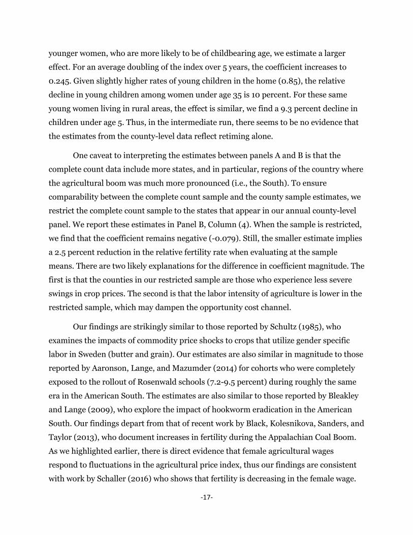
3.3 Individual Level Dataset

Given the limitations of the county-level dataset, we turn to the complete count

microdata from the 1910, 1920, and 1930 Census (Ruggles et al., 2020). In this sample,

we focus on women aged 14-49 who are spouses or householders and not living in group

quarters. We exclude Hawaii and Alaska from the analysis. Across the three waves of the

census, this amounts to over 49 million woman-year observations. In several

specifications we will limit our attention to women who were more likely of child

bearing age (under 35), of which there are approximately 25 million observations in the

sample. As would be expected, women in the under 35 sample have more children under

the age of 5 and less total children than the full sample. We will further consider similar

population restrictions, dropping women living in the most populated counties based on

1910 population counts. The rural, under age 35 sample contains just over 12 million

women. Importantly, restricting the sample to rural areas increases the probability that

a woman is living on the farm from 25 percent in the under 35 sample to 46 percent in

the rural sample. Women under the age of 35 living in less populated counties have

more children and are less likely to be white, likely reflecting both the importance of

child labor on farms and our pre-Great Migration period of analysis. Women aged 30-

40 have more total children at home but fewer who are under the age of 5. The complete

count data have the advantage of a very large sample size; however, we lose time

variation given the infrequent observation.

4. Empirical Strategy

In what follows, we seek to estimate the reduced form relationship between a

measure of fertility and the agricultural index. A naïve regression of births on income

would likely produce biased results for two reasons. First, births may have a causal

impact on income. This is particularly a concern in agriculture where children provide

labor for the family. Second, omitted variables which affect both income and fertility

could bias the estimates in a naïve regression; health and productivity are two examples

of important characteristics which cannot be directly measured yet surely play a role in

determining births and income.

-13-

To address these concerns, we exploit exogenous variation in the prices of different

crops. The primary specification when using the county-level dataset derived from state

health reports is:

𝐿𝐿𝐶𝐶𝐿𝐿𝐿𝐿𝐿𝐿𝐶𝐶𝐿𝐿ℎ𝑠𝑠𝑐𝑐,𝑡𝑡 = 𝛼𝛼 + 𝜙𝜙𝐼𝐼𝑛𝑛𝑛𝑛𝑛𝑛𝑛𝑛𝑐𝑐,𝑡𝑡−1 + 𝑋𝑋𝑐𝑐,𝑡𝑡′ 𝛽𝛽 + 𝜏𝜏𝑡𝑡 + 𝜎𝜎𝑐𝑐 + 𝜖𝜖𝑐𝑐,𝑡𝑡. (1)

The dependent variable is the log number of births in county c and year t. The primary

coefficient of interest is 𝜙𝜙 which should capture the lagged effect of the previous year’s

crop index on county births. We use the lagged value of the index rather than the

contemporaneous value given the nine-month gestation period. Year (𝜏𝜏) and county (𝜎𝜎)

fixed effects account for national differences over time and stationary differences

between counties, respectively. The vector X is comprised of interactions between the

year fixed effects and various baseline county-level characteristics. These controls are

measured in 1910 and include the fraction of the population who is non-white, between

the ages of 6 and 14, illiterate, and living in urban areas with over 2500 residents. We

also interact year fixed effects with county-level manufacturing output per capita in

1910. By interacting these baseline observable characteristics with year fixed effects, this

specification should net out differential trends in these dimensions that may otherwise

be picked up by the lagged crop index.

Estimating the impact of the crop index on births using decennial census data

requires alternative specifications due to the timing of the data collection and variable

availability. Ideally, we would be able to use a measure of completed fertility, however

this variable is not available in either the 1920 or 1930 Census.9 The primary dependent

variables we use from the complete count data are the number of children under age 5,

the total number of children in the household, and an indicator of any children in the

household. Given the available data, our specification compares women of the same age

across Census years, netting out time specific and county specific effects. Because the

available variables represent the cumulative fertility response over multiple years, we

assign each woman a cumulative or average crop index. When investigating the impact

on children under the age of 5, we use the average county index over the last 5 years.

9 We are primarily interested in how agricultural prices affected fertility, making the “children ever born” variable another relevant outcome. Unfortunately, this variable is only available in the 1910 and 1940 censuses.

-14-

When focusing on the total number of children or presence of children we use the

average county index over the previous decade. The general specification when using the

census data is:

𝐾𝐾𝐿𝐿𝑛𝑛𝑠𝑠𝑖𝑖,𝑐𝑐,𝑡𝑡 = 𝛼𝛼 + 𝜙𝜙𝐴𝐴𝐴𝐴𝐿𝐿𝐼𝐼𝑛𝑛𝑛𝑛𝑛𝑛𝑛𝑛𝑖𝑖,𝑐𝑐,𝑡𝑡 + 𝑋𝑋𝑖𝑖,𝑐𝑐,𝑡𝑡′ 𝛽𝛽 + 𝜏𝜏𝑡𝑡 + 𝜎𝜎𝑐𝑐 + 𝜖𝜖𝑖𝑖,𝑐𝑐,𝑡𝑡. (2)

The observations are at the mother (i), county of residence (c), and census year (t) level.

The index variable is one of those described above and is assigned to each mother based

on her age and county of residence. Census year fixed effects (𝜏𝜏) and county fixed effects

(𝜎𝜎) are included, as are fixed effects for age, marital status, race, size of residence

location (based on total population), and whether the mother lives on a farm. The

dependent variable is either the number of children under age 5 at the time of the

census, the woman’s total number of kids at the time of the census, an indicator of any

children in the household, or the number of children in the household conditional on

having at least one child present. The latter two measures allow us to examine fertility

responses along the extensive and intensive margins directly.

Both equation (1) and (2) are intended to address the same underlying question: how

did agricultural commodity price variation affect fertility decisions? A priori, it is

unclear whether the estimates from both specifications should point in the same

direction. For instance, fertility could immediately fall during the wartime boom due to

increased labor scarcity and increased opportunity cost of childbearing. However, at the

war’s conclusion, as labor demand subsides, and the supply constraint is lessoned as

men return from Europe, women may simply retime children, resulting in no net change

in total children in the long-run. Similarly, the sudden wealth shock could lead to an

immediate increase in child bearing, while in the long-run there is no change in the total

number of children born.

An underlying assumption in all of the regression models is that the baseline

county-level crop share weights, 𝑄𝑄𝑖𝑖,𝑐𝑐,1910, used in the construction of the index, are

exogenous. Recently, economists have raised concerns that the weights in shift-share

variables may generate a source of bias (Goldsmith-Pinkham, Sorkin, and Swift, 2020).

In our context, agro-climatic variables such as precipitation, temperature, soil type, and

the biological pest environment likely drive agricultural productivity and crop choice

-15-

decisions. In the full draft we also implement an IV strategy following Fiszbein

(forthcoming).

5. Estimates

Below we present our estimates from several different empirical specifications. We

proceed by discussing our estimates in the short-run by examining the county-year

sample and the complete count sample that focuses on children under 5 in the

household. We then discuss several robustness checks that address many of the

potential confounds. After describing the short-run estimates, we outline our estimates

over a longer time horizon (10 years), where it is possible for families to adjust along

multiple dimensions. After highlighting our main empirical estimates, we explore some

of the underlying mechanisms and heterogeneity along key dimensions.

5.1 Short-Run Fertility Effects of Agricultural Boom

In Table 1, we report our estimates from equation (1) and equation (2). In Panel

A, we report the baseline results using the county-level birth sample. Panel B includes

the estimates using the number of children under age 5 from the complete count data as

the outcome of interest. In each case, we report standard errors in parentheses,

clustered at the state level. Our estimates are robust to several different assumptions

regarding standard errors.10 Using the county-level sample, we find that doubling the

agricultural price index results in a statistically significant 12.8 log point reduction in

births. After dropping urban counties, the estimated decline in births increases to 14.4

log points. When we include our set of county level covariates in Columns 3 and 4, the

magnitude our estimate remains similar, declining by 12.6 – 14.8 log points. Given an

average of 435 births per rural county, our estimates suggest that there were between 55

and 64 fewer births per county-year given a doubling in agricultural prices. Evaluating

at the average agricultural index value throughout the period, our estimates suggest a

3.7 percent reduction in fertility. Given the 29 percentage point decline in aggregate

fertility, 1910-1930, the agricultural price volatility explains about 12.75 percent of the

10 Clustering at the state level generates the most conservative estimates. Clustering at the county level or computing Conley (1999) standard errors for the county sample using a distance cutoff of 100 miles results in smaller standard errors.

-16-

overall decline. In the full draft we add in several different fixed effect combinations and

time trends.

Table 1 - Baseline Estimates, Fertility 1910-1930 (1) (2) (3) (4) Ag. Crop Index -0.128** -0.144** -0.126** -0.148***

(0.055) (0.057) (0.050) (0.052)

Population Restriction Y Y Controls Y Y Observations 33,374 29,960 32,141 28,727 Panel B: Y = #Children Under 5 Average Ag. Crop Index -0.171*** -0.245*** -0.240*** -0.079**

(0.023) (0.037) (0.034) (0.031)

Controls Y Y Y Y Age Restriction Y Y Y Population Restriction Y Y Same States as County Sample Y Observations 49,092,654 25,468,347 12,040,507 5,860,021 Notes: Panel A estimated using the county-level birth records. Panel B uses the complete count for 1910-1930. Every regression includes county and year fixed effects. Panel A controls include separate interactions between year fixed effects and baseline fractions of population who are non-white, between the ages of 6 and 14, and living in an urban area, as well as interactions with a baseline manufacturing output per capita. Panel B controls include dummy variables for age, race, marital status, farm status, and population size of place of residence. The population restriction drops the counties which are in the top 10 percent of population in 1910. The age restriction in Panel B is for women under the age of 35. Standard errors clustered at the state level: *** p < 0.01, ** p < 0.05, * p < 0.1

The instantaneous decline in births could simply reflect retiming due to the war

disruption. Indeed, a model that allows for household savings would predict that the

number of children born should fall in the current period when female wages rise, but

the increase in savings would result in more children in the future. We now turn to the

complete count data samples in Panels B. In Panel B, we report the estimated impact of

the average agricultural price index over the previous 5 years on the number of children

under the age of 5 in the household. We estimate that a doubling of the price index over

a 5-year period results in 0.171 fewer children under the age of five in the home. During

our sample period, the average 5-year price index was 1.35 and the average number of

children under age 5 was 0.61. Thus, on average, we estimate that the agricultural boom

reduced the number of young children by about 9.8 percent relative to the mean. For

-17-

younger women, who are more likely to be of childbearing age, we estimate a larger

effect. For an average doubling of the index over 5 years, the coefficient increases to

0.245. Given slightly higher rates of young children in the home (0.85), the relative

decline in young children among women under age 35 is 10 percent. For these same

young women living in rural areas, the effect is similar, we find a 9.3 percent decline in

children under age 5. Thus, in the intermediate run, there seems to be no evidence that

the estimates from the county-level data reflect retiming alone.

One caveat to interpreting the estimates between panels A and B is that the

complete count data include more states, and in particular, regions of the country where

the agricultural boom was much more pronounced (i.e., the South). To ensure

comparability between the complete count sample and the county sample estimates, we

restrict the complete count sample to the states that appear in our annual county-level

panel. We report these estimates in Panel B, Column (4). When the sample is restricted,

we find that the coefficient remains negative (-0.079). Still, the smaller estimate implies

a 2.5 percent reduction in the relative fertility rate when evaluating at the sample

means. There are two likely explanations for the difference in coefficient magnitude. The

first is that the counties in our restricted sample are those who experience less severe

swings in crop prices. The second is that the labor intensity of agriculture is lower in the

restricted sample, which may dampen the opportunity cost channel.

Our findings are strikingly similar to those reported by Schultz (1985), who

examines the impacts of commodity price shocks to crops that utilize gender specific

labor in Sweden (butter and grain). Our estimates are also similar in magnitude to those

reported by Aaronson, Lange, and Mazumder (2014) for cohorts who were completely

exposed to the rollout of Rosenwald schools (7.2-9.5 percent) during roughly the same

era in the American South. The estimates are also similar to those reported by Bleakley

and Lange (2009), who explore the impact of hookworm eradication in the American

South. Our findings depart from that of recent work by Black, Kolesnikova, Sanders, and

Taylor (2013), who document increases in fertility during the Appalachian Coal Boom.

As we highlighted earlier, there is direct evidence that female agricultural wages

respond to fluctuations in the agricultural price index, thus our findings are consistent

with work by Schaller (2016) who shows that fertility is decreasing in the female wage.

-18-

5.2 Quartile Event Study Results

The annual, county-level birth data make it possible to estimate the fertility

response to crop prices over time. Instead of estimating a single coefficient on the price

index, we modify equation 1 by interacting year fixed effects with separate dummy

variables for the top three quartiles of the average price index at the WWI peak, 1916-

1919:

𝐿𝐿𝐶𝐶𝐿𝐿𝐿𝐿𝐿𝐿𝐶𝐶𝐿𝐿ℎ𝑠𝑠𝑐𝑐,𝑡𝑡 = 𝛼𝛼 + ∑ 𝛿𝛿𝑘𝑘,𝑡𝑡4𝑘𝑘=2 𝜏𝜏𝑡𝑡 × 1(𝐼𝐼𝑛𝑛𝑛𝑛𝑛𝑛𝑛𝑛 𝑄𝑄𝑄𝑄𝑄𝑄𝐶𝐶𝐿𝐿𝐿𝐿𝑄𝑄𝑛𝑛𝑐𝑐 == 𝑘𝑘) + 𝑋𝑋𝑐𝑐,𝑡𝑡

′ 𝛽𝛽 + 𝜏𝜏𝑡𝑡 + 𝜎𝜎𝑐𝑐 + 𝜖𝜖𝑐𝑐,𝑡𝑡. (3)

The 𝛿𝛿𝑘𝑘,𝑡𝑡 coefficients on these interaction terms, which we plot in Figure 6, capture the

deviation in births relative to the counties in the bottom quartile. The first thing to note

is that each quartile had fairly similar birth trends leading up to WWI, providing a check

on the assumption that underlying trends are not driving our main results. Once prices

began to rise in response to WWI-induced demand, the birth patterns of each quartile

diverge according to the intensity of their respective price boom.11 While many of the

95% confidence intervals overlap, the pattern is consistent with both the expected

timing and intensity of this natural experiment.

Figure 31 – Quartile event study results

Notes: Coefficients on the interaction between year fixed effects and dummy variables for the top three price index quartiles. 95% confidence intervals based on county-level clustering shown.

11 The main results are similar when restricting the analysis window to end immediately after the post-WWI bust; the most substantial identifying variation is due WWI-related shocks.

-19-

5.4 Robustness – Other Potential Confounds

Given our sample period, there are several potential confounds that raise

concern. First and foremost, our estimates could be the byproduct of a reduction in the

availability of prime age males as a result of WWI. Furthermore, as men returned from

Europe, America experienced the Spanish Influenza Pandemic (Almond, 2006; Beach,

Ferrie, and Saavedra, 2018) which hit prime age males especially hard, which may have

also affected fertility patterns. Our sample period also contains several secular

movements that likely alter the returns to children, either through changes in the

underlying health risk or through their future labor market returns. For example, the

period we examine is squarely in the middle of the public health and high school

movements. The arrival of boll weevil has also been shown to impact fertility. Finally,

changes in alcohol consumption as a result of prohibition could also affect fertility.

In Figure 4, we present the estimates when controlling for these additional

confounds. The first series, indicated by triangles, shows how these controls affect the

coefficient on the crop index in regressions using the state report data on the annual

number of births at the county-level. The second series, indicated by hollow circles,

shows how the same control variables affect the estimates when using the complete

count sample with the number of children under age 5 as the outcome of interest.

Beginning on the left of Figure 4, we first replicate our preferred baseline estimates from

Table 1. Moving from left to right, we add controls to account for the following potential

confounders: the number of men drafted into WWI, exposure to the Spanish

Influenza,12 the rollout of County Health Organizations (CHO), Rockefeller

Foundation’s Hookworm eradication campaign, exposure to malaria, the presence of a

Rosenwald School, changes in compulsory schooling laws, county-level boll weevil

infestation, and county-level prohibition policies. It is clear from Figure 4 that the

inclusion of these additional controls has little impact on our estimates of how the

12 Note than the complete count sample is much smaller when we control for the impact of the Spanish Flu due to the availability of county-level mortality data.

-20-

agricultural index relates to either outcome of interest.13 In the full version of the paper

we also run several specifications to address concerns regarding migration.

Figure 4 – Robustness checks

Notes: Coefficients on the one year lagged crop index when using the annual county-level births as the outcome variable (state reports) and the 5-year average crop index when using the number of children under age 5 as the outcome variable (complete count) with the inclusion of different control variables. 95% confidence intervals based on state-level clustering show.

5.5 Long-Run Fertility Effects of Agricultural Boom

We now examine how variation in the price index over the prior 10 years affects

the number of children in the household. In a static model, rising opportunity cost

unambiguously decreases fertility along the intensive and extensive margins. In a

dynamic model with additional margins of adjustment, the effects are less clear. Savings

from the boom period may allow families to retime and replace or expand. To the extent

that children are complements (substitutes) to the farm capital, the number of children

may increase (decrease). Likewise, if farms are more profitable, or pay higher wages, it

may influence the decisions of children to stay on the farm longer as they mature, as

highlighted by Rosenzweig (1977). Therefore, a change in the number of children in the

13 We include additional robustness checks in Appendix Table 3 showing that more general concerns about differential trends do not affect our county-level estimates.

-21-

household could reflect changes in when children exit the household rather than

changes in the number of children born.

Measuring the long-run fertility effects with the complete count data

recommends slightly different sample restrictions. We would ideally observe completed

fertility or the total number of children ever born, but the closest variable collected in

each of the Census years from 1910-1930 is the total number of children in the

household at the time of enumeration. Younger women have not yet finished having

children while older women will no longer have all of their children still living at home.

For the long-run fertility regressions, we restrict our analysis to women between the

ages of 30 and 40. We selected this age window because it will better capture the total

fertility of women than the under 35 group. Furthermore, we limit the influence of

endogenous household exit of children on our estimates by excluding women who are

older than 40. The final two columns of Table 2 show that women between the ages of

30-40 have more total kids in the household but fewer children under the age of five

than the under 35 group. They also have more children of any age than the full sample,

reflecting the influence of household exit. While the summary statistics suggest that the

total number of children for women aged 30-40 is the closest measure to completed

fertility reported in the Census, children may have already exited the household at the

time of enumeration and some women in the sample have not completed their fertility.

In Panel A of Table 2, we report estimates of how the average agricultural price

index over the previous 10 years related to the total number of children in the home.

Here we find that for a doubling in prices over a 10-year period, there is a statistically

significant 0.427 reduction in total children relative to a sample mean of 2.19 children.

Given an average 10-year price index of 1.19, this suggest that on average, there was a

3.7 percent reduction in children. Focusing on women who were between the ages of 30-

40, we estimate a statistically significant negative coefficient of 0.654. Evaluated at the

mean number of children and the average price index experienced by women aged 30-

40, this implies a 4.8 percent decline in children. Further restricting to rural areas, we

estimate a negative coefficient of 0.661, which translates to a 4.25 percent decline in

total children. In Column (4), we report the estimate restricting the sample to include

the same states used in the county-level annual birth sample. Here the coefficient

-22-

remains negative but becomes much smaller in magnitude. Later in the paper we

explore sources of heterogeneity, some of which may be related to this result. Finally, in

Columns (5) and (6), we report estimates from samples that restrict to people living in

their state of birth (Column 5), or to mothers born in the United States (Column 6).

These restrictions have little impact on the estimated coefficient, alleviating concerns

that our results reflect selective migration.

How could WWI and elevated agricultural prices lead to a permanent drop in

fertility? As Galor (2012) and Aaronson, Lange, and Mazumdar (2014) note, increasing

the price of child quantity decreases fertility along both the extensive and intensive

margins. Thus, one possibility is that women had fewer children. Another is that more

women remained childless. The next two panels of Table 5 explore the extensive and

intensive margins of fertility. In Panel B of Table 2, we examine changes at the extensive

margin, using an indicator that equals 1 if the woman has any children in the household,

and is zero otherwise. In column 1, we report estimates using the sample of all women.

We estimate a negative 0.069. Evaluated at the mean agricultural price index

throughout the sample (1.19), this implies 1.29 percent decrease in the probability of a

woman having children in the household. Focusing on agricultural households and

women of prime age, the magnitude of the coefficient increases to -0.08. Evaluated at

the index mean, this is a 1.5 percentage point reduction in the probability a woman has

children in the household. The relative magnitude of this effect is quite large. For rural

women aged 30-40, only 14 percent of women had no children in the household. Thus,

elevated agricultural prices increase childlessness by about 10 percent relative to the

mean. Consistent with Aaronson, Lange, and Mazumdar (2014), the fertility response is

also driven by changes along the intensive margin. Using the same set of sample

restrictions, Panel C shows that, conditional on having any children in the home, women

had fewer children because of higher crop prices. To put this in context, the coefficients

in Panel C which range from -0.328 to -0.506 are around two-thirds the size of the

coefficients in Panel A.14 The combined results of Table 2 indicate that both intensive

and extensive margin responses meaningfully contributed to declines in overall fertility.

14 The combined results from Column 4 suggest that the limited variation in crop prices for the state report sample primarily affected fertility through the extensive margin.

-23-

Table 2 - Number of Children in Home

(1) (2) (3) (4) (5) (6) Panel A: Y = # of children in home

Average Ag. Crop Index -0.427*** -0.654*** -0.661** -0.035 -0.684*** -0.698** (0.143) (0.181) (0.220) (0.147) (0.241) (0.219)

Panel B: Y = Any kids

Average Ag. Crop Index -0.069*** -0.078*** -0.080*** -0.043*** -0.078*** -0.086*** (0.014) (0.012) (0.014) (0.013) (0.018) (0.015) Panel C: Y = (# of children in home | any kids > 0)

Average Ag. Crop Index -0.328** -0.506*** -0.408* 0.117 -0.499** -0.491** (0.147) (0.183) (0.203) (0.135) (0.216) (0.202)

Age Restriction Y Y Y Y Y Population Restriction Y Y Y Y Only States in County Sample Y Live in State of Birth Y Not Foreign Born Y Observations (A and B) 49,092,654 18,138,191 7,887,813 4,213,270 5,259,385 7,317,018 Observations (C) 37,846,641 14,835,267 6,768,714 3,607,568 4,544,434 6,265,822 Notes: 1910-1930 complete count census data. Each regression includes county and year fixed effects as well as dummy variables for age, race, marital status, farm status, and population size of place of residence. The population restriction drops the counties which are in the top 10 percent of population in 1910. The age restriction is for women between the ages of 30 and 40. Standard errors clustered at the state level: *** p < 0.01, ** p < 0.05, * p < 0.1

6. Conclusions

Identifying the causal relationship between income and fertility continues to be

an important goal for economists, one with substantial implications for demography

and policy design. In this paper, we presented evidence that income shocks that change

the wages and opportunity costs of women can have significant impacts on fertility

decisions, along both the extensive and intensive margins. The agricultural boom-and-

bust of WWI, which differentially affected the wages and output prices of farms across

the US based on their preexisting composition of crops, provided the necessary

exogenous variation to study how families responded to income shocks. Analysis using

newly-digitized annual birth records revealed that counties with larger price shocks

experienced larger fertility declines in the short-run. This pattern was confirmed using

an alternative measure of short-run fertility (children under the age of 5) in the

complete count Census data. An important follow-on question is whether women simply

-24-

retimed their fertility to take advantage of temporary wage increases. This does not

appear to be the case: results focusing on the total number of children in the household

from the complete count support the conclusion that these price shocks lowered the

long-run fertility of affected women. These effects tended to be permanent, as a larger

share of women never had children. Consistent with the notion that rising female wages

(higher opportunity costs), were the dominant mechanism, we document that women

delayed marriage in response to the elevated agricultural prices. In areas with higher

rates of farm owner operators, the declines were partially offset due to the wealth effects

as land values appreciated. There may have also been a limited role for investment in

farm capital, yet these findings are less conclusive. Although data limitations prevent us

from ruling out the importance of alternative factors, the bulk of the evidence points to

female wages as being a significant contributor to the decline in fertility over this time

period.

Much of the literature on fertility and family size focuses on the theoretical

tradeoff between quality and quantity or how costs, both opportunity and explicit, have

changed over time. Our work compliments this literature and shows that these are the

primary underlying forces at play, even though children may directly affect family

income in a rural setting. This additional dimension is still present in agricultural

societies today even if many other factors (cultural, institutional, etc.) differ from those

in the US in the early 20th century. Although the roles and expectations of children have

changed substantially over the last century, parents still consider economic

opportunities when deciding how many children to have. As policymakers consider

potential responses to the many challenges that declining fertility presents to existing

social programs, the results of this paper serve as a reminder that gender-specific

changes to opportunity costs are central to the discussion. Put another way, there is

more to the relationship between income and fertility than just income effects.

-25-

References

Aaronson, D., & Mazumder, B. (2011). The impact of Rosenwald schools on black achievement. Journal of Political Economy, 119(5), 821-888.

Aaronson, D., Lange, F., & Mazumder, B. (2014). Fertility transitions along the extensive and intensive margins. American Economic Review, 104(11), 3701-24.

Aaronson, D., Mazumder, B., Sanders, S. G., & Taylor, E. (2017). Estimating the effect of school quality on mortality in the presence of migration: Evidence from the Jim Crow south. Available at SSRN 3045447.

Abramitzky, R., Delavande, A., & Vasconcelos, L. (2011). Marrying up: the role of sex ratio in assortative matching. American Economic Journal: Applied Economics, 3(3), 124-57.

Acquaye, Albert K. A., Julian M. Alston and Philip G. Pardey, “Agricultural output – gross and net value, by crop and livestock: 1910–1998.” Table Da1063-1081 in Historical Statistics of the United States, Earliest Times to the Present: Millennial Edition, edited by Susan B. Carter, Scott Sigmund Gartner, Michael R. Haines, Alan L. Olmstead, Richard Sutch, and Gavin Wright. New York: Cambridge University Press, 2006. http://dx.doi.org/10.1017/ISBN-9780511132971.Da1063-1265

Adams County Independent. Forty Tractors to Help Penna. Farmers. April 5, 1918.

Ager, P., Brueckner, M., & Herz, B. (2017). The boll weevil plague and its effect on the southern agricultural sector, 1889–1929. Explorations in Economic History, 65, 94-105.

Ager, P., Herz, B., & Brueckner, M. (forthcoming). Structural change and the fertility transition. Review of Economics and Statistics, 1-45.

Akresh, R. (2009). Flexibility of household structure child fostering decisions in Burkina Faso. Journal of Human Resources, 44(4), 976-997.

Alam, S. A., & Pörtner, C. C. (2018). Income shocks, contraceptive use, and timing of fertility. Journal of Development Economics, 131, 96-103.

Almond, Douglas. "Is the 1918 influenza pandemic over? Long-term effects of in utero influenza exposure in the post-1940 US population." Journal of political Economy 114, no. 4 (2006): 672-712.

Almond, Douglas, and Bhashkar Mazumder. "The 1918 influenza pandemic and subsequent health outcomes: an analysis of SIPP data." American Economic Review 95, no. 2 (2005): 258-262.

Alston, Lee J. "Farm foreclosures in the United States during the interwar period." Journal of Economic History (1983): 885-903

Ananat, E. O., Gassman-Pines, A., & Gibson-Davis, C. (2013). Community-wide job loss and teenage fertility: Evidence from North Carolina. Demography, 50(6), 2151-2171.

Ashraf, N., Field, E. and Lee, J., 2014. Household bargaining and excess fertility: an experimental study in Zambia. American Economic Review, 104(7), pp.2210-37.

Bailey, M. J., & Collins, W. J. (2011). Did improvements in household technology cause the baby boom? Evidence from electrification, appliance diffusion, and the Amish. American Economic Journal: Macroeconomics, 189-217.

Baker, R. B. (2015). From the field to the classroom: the Boll Weevil's impact on education in Rural Georgia. The Journal of Economic History, 75(4), 1128-1160.

Baker, R. B., Blanchette, J., & Eriksson, K. (2020). Long-run impacts of agricultural shocks on educational attainment: Evidence from the boll weevil. The Journal of Economic History, 80(1), 136-174.

-26-

Beach, Brian, Joseph P. Ferrie, and Martin H. Saavedra. Fetal shock or selection? The 1918 influenza pandemic and human capital development. No. w24725. National Bureau of Economic Research, 2018.

Becker, G. S. (1960). An economic analysis of fertility. In Demographic and economic change in developed countries (pp. 209-240). Columbia University Press.

Becker, G. S.. (1981). A Treatise on the Family. Harvard university press.

Becker, G. S., & Lewis, H. G. (1973). On the Interaction between the Quantity and Quality of Children. Journal of political Economy, 81(2, Part 2), S279-S288.

Becker, G. S., & Tomes, N. (1976). Child endowments and the quantity and quality of children. Journal of political Economy, 84(4, Part 2), S143-S162.

Beegle, K., Dehejia, R. H., & Gatti, R. (2006). Child labor and agricultural shocks. Journal of Development economics, 81(1), 80-96.

Bengtsson, T., & Dribe, M. (2006). Deliberate control in a natural fertility population: Southern Sweden, 1766–1864. Demography, 43(4), 727-746.

Ben-Porath, Y. (1973). Economic analysis of fertility in Israel: Point and counterpoint. Journal of Political Economy, 81(2, Part 2), S202-S233.

Bharadwaj, P. (2015). Impact of changes in marriage law implications for fertility and school enrollment. Journal of Human Resources, 50(3), 614-654.

Black, D. A., Kolesnikova, N., Sanders, S. G., & Taylor, L. J. (2013). Are children “normal”? The Review of Economics and Statistics, 95(1), 21-33.

Blau, F. D., Kahn, L. M., & Waldfogel, J. (2000). Understanding young women's marriage decisions: The role of labor and marriage market conditions. ILR Review, 53(4), 624-647.

Bleakley, H. (2007). Disease and development: evidence from hookworm eradication in the American South. The quarterly journal of economics, 122(1), 73-117.

Bleakley, H., & Lange, F. (2009). Chronic disease burden and the interaction of education, fertility, and growth. The review of economics and statistics, 91(1), 52-65.

Bleakley, H. (2010). Malaria eradication in the Americas: A retrospective analysis of childhood exposure. American Economic Journal: Applied Economics, 2(2), 1-45.

Bloome, D., Feigenbaum, J., & Muller, C. (2017). Tenancy, Marriage, and the Boll Weevil Infestation, 1892–1930. Demography, 54(3), 1029-1049.

Boehnke, J., & Gay, V. (2020). The missing men: World War I and female labor force participation. SSRN Working Paper # 2931970.

Brown, Ryan, & Thomas, Duncan. (2018). On the long term effects of the 1918 US influenza pandemic. Unpublished Manuscript

Brueckner, M., & Schwandt, H. (2015). Income and population growth. The Economic Journal, 125(589), 1653-1676.

Buyst, E. & Franaszek, P. (2010). Sectoral developments, 1914-1945. In S. Broadberry & K. O’Rourke (Authors), The Cambridge Economic History of Modern Europe (The Cambridge Economic History of Modern Europe, pp.208-231). Cambridge: Cambridge University Press.

Carter, S. B., Gartner, S. S., Haines, M. R., Olmstead, A. L., Sutch, R., & Wright, G. (2006). Historical statistics of the United States: millennial edition (Vol. 3). Cambridge: Cambridge University Press.

-27-

Centers for Disease Control. Communicable Disease Center Activities 1946-1947. Atlanta, Georgia. 1948.

Chicago Daily Tribune. 4,279 Tractors Now in Use on Farms of Oho. Feb 2, 1919.

Clay, Karen, Joshua Lewis, and Edson Severnini. Pollution, infectious disease, and mortality: evidence from the 1918 Spanish influenza pandemic. The Journal of Economic History 78, no. 4 (2018): 1179-1209.

Cogneau, D., & Jedwab, R. (2012). Commodity price shocks and child outcomes: the 1990 cocoa crisis in Cote d’Ivoire. Economic Development and Cultural Change, 60(3), 507-534.

Committee on School Boys for Farm Service to the Executive Committee, Massachusetts Committee on Public Safety. (1919). Weight and Potter Printing Co. Boston, MA.

Conley, T. G. (1999). GMM estimation with cross sectional dependence. Journal of econometrics, 92(1), 1-45.

Correia, Sergio and Luck, Stephan and Verner, Emil. (2020). Pandemics Depress the Economy, Public Health Interventions Do Not: Evidence from the 1918 Flu. SSRN Working Paper 3561560. http://dx.doi.org/10.2139/ssrn.3561560

Corno, L., Hildebrandt, N., & Voena, A. (forthcoming). Age of marriage, weather shocks, and the direction of marriage payments. Econometrica.

Dettling, L. J., & Kearney, M. S. (2014). House prices and birth rates: The impact of the real estate market on the decision to have a baby. Journal of Public Economics, 110, 82-100.

Eriksson, K., Niemesh, G. T., & Thomasson, M. (2018). Revising infant mortality rates for the early twentieth century United States. Demography, 55(6), 2001-2024.

Feigenbaum, J. J., Mazumder, S., & Smith, C. B. (2020). When Coercive Economies Fail: The Political Economy of the US South After the Boll Weevil (No. w27161).

Final Report of the Provost Marshall General to the Secretary of War. (1920). U.S. Government Printing Office. Washington, D.C.

Fishback, P. V., Haines, M. R., & Kantor, S. (2007). Births, deaths, and New Deal relief during the Great Depression. The Review of Economics and Statistics, 89(1), 1-14.

Fiszbein, M. (forthcoming). Agricultural Diversity, Structural Change, and Long-Run Development: Evidence from the US. American Economic Journal: Macroeconomics.

Fujii, T., & Shonchoy, A. S. (2020). Fertility and rural electrification in Bangladesh. Journal of Development Economics, 143, 102430.

Galor, O. (2005). From stagnation to growth: unified growth theory. Handbook of economic growth, 1, 171-293.

Galor, O. (2012). The demographic transition: causes and consequences. Cliometrica, 6(1), 1-28.

Galor, Oded, and David N. Weil. 2000. "Population, Technology, and Growth: From Malthusian Stagnation to the Demographic Transition and Beyond." American Economic Review, 90 (4): 806-828.

Gay, V. (2019). The legacy of the missing men: The long-run impact of World War I on female labor force participation. SSRN Working Paper #3069582.

Goldin, C., & Katz, L.F. (2002). “The Power of the Pill: Oral Contraceptives and Women’s Career and Marriage Decisions.” Journal of Political Economy, 110(4), 730-770.

-28-

Goldin, C., & Katz, L. F. (2008). Mass secondary schooling and the state: the role of state compulsion in the high school movement. In Understanding long-run economic growth: Geography, institutions, and the knowledge economy (pp. 275-310). University of Chicago Press

Goldsmith-Pinkham, P., Sorkin, I., & Swift, H. (2020). “Bartik instruments: What, when, why, and how.” American Economic Review, 110(8), 2586-2624.

Gross, D. P. (2018). Scale versus scope in the diffusion of new technology: evidence from the farm tractor. The RAND Journal of Economics, 49(2), 427-452.

Hahn, Y., Islam, A., Nuzhat, K., Smyth, R., & Yang, H. S. (2018). Education, marriage, and fertility: Long-term evidence from a female stipend program in Bangladesh. Economic Development and Cultural Change, 66(2), 383-415.

Haines, Michael R., and Inter-university Consortium for Political and Social Research. Historical, Demographic, Economic, and Social Data: The United States, 1790-2002. Inter-university Consortium for Political and Social Research [distributor], 2010-05-21. https://doi.org/10.3886/ICPSR02896.v3

Haines, Michael, Fishback, Price, and Rhode, Paul. United States Agriculture Data, 1840 - 2012. Ann Arbor, MI: Inter-university Consortium for Political and Social Research [distributor], 2018-08-20. https://doi.org/10.3886/ICPSR35206.v4

Hankins, S., & Hoekstra, M. (2011). Lucky in life, unlucky in love? The effect of random income shocks on marriage and divorce. Journal of Human Resources, 46(2), 403-426.

Henderson, J., Gloy, B., and Boehlje, M. (2011). Agriculture’s boom-bust cycles: is this time different? Economic Review, 96(4), 81-103.

Hoehn-Velasco, L. (2018). Explaining declines in US rural mortality, 1910–1933: The role of county health departments. Explorations in Economic History, 70, 42-72.

Hoehn-Velasco, L. (2019). The Long-term Impact of Preventative Public Health Programs. Working paper. http://www.laurenhoehnvelasco.com/research/

Hong, S. C. (2007). The burden of early exposure to malaria in the united states, 1850–1860: Malnutrition and immune disorders. The journal of economic history, 67(4), 1001-1035.

Hong, S. C. (2011). Malaria and economic productivity: a longitudinal analysis of the American case. The Journal of Economic History, 71(3), 654-671.

Hong, S. C. (2013). Malaria: An early indicator of later disease and work level. Journal of health economics, 32(3), 612-632.

Huttunen, K., & Kellokumpu, J. (2016). The effect of job displacement on couples’ fertility decisions. Journal of Labor Economics, 34(2), 403-442.

Jacks, D., Pendakur, K., & Shigeoka, H. (2020). Urban Mortality and the Repeal of Federal Prohibition. NBER Working Paper Series, #28181.

Jaremski, Matthew and Wheelock, David C. (forthcoming). Banking on the Boom, Tripped by the Bust: Banks and the World War I Agricultural Price Shock. Journal of Money, Credit, and Banking.

Jensen, R. (2012). Do labor market opportunities affect young women's work and family decisions? Experimental evidence from India. The Quarterly Journal of Economics, 127(2), 753-792.

Johnson, H. Thomas. "Postwar Optimism and the Rural Financial Crisis of the 1920's." Explorations in Economic History 11, no. 2 (1973): 173.

Jones, L., & Tertilt, M. (2009). An Economic History of Fertility in the U.S.: 1826-1960. In P. Rupert (Ed.), The Handbook of Family Economics

-29-

Kirkpatrick, E., & Tough, E. (1932). Prohibition and Agriculture. The ANNALS of the American Academy of Political and Social Science, 163(1), 113-119.

Kitchens, C. (2013). The effects of the Works Progress Administration's anti-malaria programs in Georgia 1932–1947. Explorations in Economic History, 50(4), 567-581.

Kruger, D. I. (2007). Coffee production effects on child labor and schooling in rural Brazil. Journal of development Economics, 82(2), 448-463.

Lange, F., Olmstead, A. L., & Rhode, P. W. (2009). The impact of the boll weevil, 1892–1932. The Journal of Economic History, 685-718.

Lewis, J. (2018). Infant Health, Women's Fertility, and Rural Electrification in the United States, 1930–1960. The Journal of Economic History, 78(1), 118-154.

Lindo, J. M. (2010). Are children really inferior goods? Evidence from displacement-driven income shocks. Journal of Human Resources, 45(2), 301-327.

Logan, T. D. (2015). A Time (Not) Apart: A Lesson in Economic History from Cotton Picking Books. The Review of Black Political Economy, 42(4), 301-322.

Lovenheim, M. F., & Mumford, K. J. (2013). Do family wealth shocks affect fertility choices? Evidence from the housing market. Review of Economics and Statistics, 95(2), 464-475.

Markevich, A., & Harrison, M. (2011). Great War, Civil War, and recovery: Russia's national income, 1913 to 1928. The Journal of Economic History, 71(3), 672-703.

Moehling, C. M., & Thomasson, M. A. (2012). The political economy of saving mothers and babies: The politics of state participation in the Sheppard-Towner Program. The Journal of Economic History, 72(1), 75-103.

New York Times. Motors on the Farm Replace Hired Labor. Oct. 26, 1919.

Nourse, E. G. (1924). American agriculture and the European market. McGraw-Hill Book Co., New York.

National Center for Health Statistics. (2017). NCHS – Births and General Fertility Rates. National Center for Health Statistics, National Vital Statistics System. Date accessed: 06/01/2020. https://data.cdc.gov/NCHS/NCHS-Births-and-General-Fertility-Rates-United-Sta/e6fc-ccez

Olmstead, A. L., & Rhode, P. W. (2018). Slave Productivity in Cotton Picking. Working Paper

Olmstead, Alan L. and Paul W. Rhode, “Cropland – acreage harvested and indexes of cropland use and production per acre: 1910–1990.” Table Da661-666 in Historical Statistics of the United States, Earliest Times to the Present: Millennial Edition, edited by Susan B. Carter, Scott Sigmund Gartner, Michael R. Haines, Alan L. Olmstead, Richard Sutch, and Gavin Wright. New York: Cambridge University Press, 2006. http://dx.doi.org/10.1017/ISBN-9780511132971.Da661-1062

Rajan, R., & Ramcharan, R. (2015). The anatomy of a credit crisis: The boom and bust in farm land prices in the United States in the 1920s. American Economic Review, 105(4), 1439-77.

Rosenzweig, M. R. (1977). The demand for children in farm households. Journal of Political Economy, 85(1), 123-146.

Ruggles, Steven, Sarah Flood, Ronald Goeken, Josiah Grover, Erin Meyer, Jose Pacas and Matthew Sobek. IPUMS USA: Version 10.0 [dataset]. Minneapolis, MN: IPUMS, 2020. https://doi.org/10.18128/D010.V10.0

Salisbury, L. (2017). Women's income and marriage markets in the United States: Evidence from the Civil War pension. The Journal of Economic History, 77(1), 1-38.

Schaller, Jessamyn. (2016). Booms, Busts, and Fertilty: Testing the Becker Model Using Gender-Specific Labor Demand. Journal of Human Resources, 51(1), 1-29.

-30-

Schultz, T. P. (1985). Changing world prices, women's wages, and the fertility transition: Sweden, 1860-1910. Journal of Political Economy, 93(6), 1126-1154.

Social Security Administration. Bureau of Employment Security (1942). Employment o Women in War Production. U.S. Government Printing Office. Washington, D.C.

United States Department of Agriculture. Office of the Secretary – Circular No. 112. (1918). The Farm Labor Problem: Man-Power Sufficient if Properly Mobilized by Cooperation and Community Action. U.S. Government Printing Office. Washington, D.C.

United Stated Department of Agriculture. (1964). Farm Production Economics Division: Economic Research Service. Labor Used to Produce Field Crops: Estimates by States. Statistical Bulletin No. 346. U.S. Government Printing Office. Washington, D.C.

United States Department of Labor. (1918). Booklet of Information: U.S. Boys’ Working Reserve. U.S. Government Printing Office. Washington, D.C.

United States Department of Labor. (1945). War and Postwar Wages, Prices, and Hours 1914-23 and 1939-44. Bulletin No. 852. U.S. Government Printing Office. Washington, D.C.

Vandenbroucke, Guillaume. (2014). "Fertility and Wars: The Case of World War I in France." American Economic Journal: Macroeconomics, 6 (2): 108-36.

Wanamaker, M. H. (2012). Industrialization and fertility in the nineteenth century: Evidence from South Carolina. The Journal of Economic History, 72(1), 168-196.

Yonzan, N., Timilsina, L., & Kelly, I. R. (2020). Economic Incentives Surrounding Fertility: Evidence from Alaska's Permanent Fund Dividend (No. w26712). National Bureau of Economic Research.