The Impact of Simulated Motion Blur on Breast Cancer ...
286
I The Impact of Simulated Motion Blur on Breast Cancer Detection Performance in Full Field Digital Mammography (FFDM) Ahmed Khalid Abdullah School of Health Sciences, UNIVERSITY OF SALFORD, SALFORD, UK Submitted in Partial Fulfilment of the Requirements of the Degree of Doctor of Philosophy, May 2018 (Medical physics)
-
Upload
khangminh22 -
Category
Documents
-
view
2 -
download
0
Transcript of The Impact of Simulated Motion Blur on Breast Cancer ...

I
The Impact of Simulated Motion Blur on Breast Cancer Detection
Performance in Full Field Digital Mammography (FFDM)
Ahmed Khalid Abdullah
School of Health Sciences,
UNIVERSITY OF SALFORD, SALFORD, UK
Submitted in Partial Fulfilment of the Requirements of the Degree of
Doctor of Philosophy, May 2018
(Medical physics)

I
Contents
Contents .................................................................................................................................... I
List of Tables ...................................................................................................................... VIII
List of Figures ....................................................................................................................... XII
List of Publications ............................................................................................................ XIX
List of Development Skills ................................................................................................. XXI
Training Sessions Attended .............................................................................................. XXII
Acknowledgement ............................................................................................................ XXIV
Dedications......................................................................................................................... XXV
Abbreviations ................................................................................................................... XXVI
Abstract ......................................................................................................................... XXVIII
Chapter One: Introduction and Thesis Outline .................................................................... 1
1.1 Introduction ...................................................................................................................... 1
1.2 Aim ................................................................................................................................... 2
1.3 Objectives ......................................................................................................................... 2
1.4 Research Questions .......................................................................................................... 2
1.5 Rational of the thesis ........................................................................................................ 2
1.6 The Contribution of this Thesis: ....................................................................................... 3
1.7 Thesis Structure ................................................................................................................ 4
Chapter Two: Literature Review ........................................................................................... 7
2.1 Overview of the Chapter .................................................................................................. 7
2.2 Breast Anatomy ................................................................................................................ 7

II
2.3 Breast Cancer ................................................................................................................. 11
2.3.1 Factors Affecting Breast Cancer .............................................................................. 12
2.4 Mammography ............................................................................................................... 13
2.4.1 Characteristics of Malignant Microcalcifications within Mammography Images .. 16
2.4.2 Breast Masses .......................................................................................................... 18
2.5 Factors Affecting Diagnostic Efficiency ........................................................................ 20
2.5.1 Mammographic Breast Density (MBD) Assessment .............................................. 22
2.5.2 Effect of Mammographic Breast Density on Lesion Detection Performance ......... 23
2.5.3 Effect of Image Quality on Lesion Detection Performance .................................... 25
2.5.4 Mammography Image Interpretation ....................................................................... 29
2.6 Full-field Digital Mammography ................................................................................... 30
2.6.1 Components of FFDM Systems .............................................................................. 31
2.6.2 Automatic Exposure Control (AEC) ........................................................................ 33
2.6.3 Paddles ..................................................................................................................... 33
2.7 Motion Blur in Mammography Images .......................................................................... 34
2.7.1 Causes and Effects of Image Blurring ..................................................................... 36
2.7.2 Paddle Movement Effects ........................................................................................ 37
2.7.3 Thixotropic Behavior and Breast Tissue Characteristics ........................................ 39
2.8 Physics of Mammography System ................................................................................. 40
2.8.1 X-ray Spectrum ........................................................................................................ 40
2.8.2 X-rays Incident on the Detector ............................................................................... 44
III
2.8.3 Digitization .............................................................................................................. 44
2.8.4 Pixel Size in Mammography ................................................................................... 45
Chapter Three: Medical Images Assessment Methods ...................................................... 46
3.1 Chapter Overview .......................................................................................................... 46
3.2 The Relationship between Visual Performance and Medical Image Interpretation ....... 47
3.3 Human Visual Function ................................................................................................. 49
3.3.1 Visual Acuity ........................................................................................................... 51
3.3.2 Contrast Sensitivity.................................................................................................. 51
3.3.3 Visual Function Assessment .................................................................................... 52
3.4 Receiver Operating Characteristics (ROC) Methods ..................................................... 53
3.5 Free-Response Receiver Operating Characteristics (FROC) Method ............................ 57
3.5.1 Constructing Curves from FROC Data ................................................................... 58
3.5.2 FROC Data Analysis ............................................................................................... 59
3.5.3 Jackknife Analysis of FROC Data (JAFROC) ........................................................ 60
3.6 Perceptual Measures ....................................................................................................... 61
3.7 The Physical Measures of Mammographic Images ....................................................... 62
3.7.1 Measuring Conspicuity Index .................................................................................. 62
3.7.2 Factors Affecting Conspicuity ................................................................................. 64
Chapter Four: Methodology ................................................................................................. 66
4.1 Chapter Overview .......................................................................................................... 66
4.2 Step 1: Image Selection .................................................................................................. 69
4.3 Step 2: Image Assessment .............................................................................................. 69

IV
4.4 Step 3: Applying & Validating Simulated Motion Blur ................................................ 70
4.4.2 Validation Method for Simulated Motion Blur Software ........................................... 76
4.5 Step 4: Observer Performance Study ............................................................................. 77
4.6 Step 5: Statistical Analysis ............................................................................................. 82
4.6.1 Data Analysis for Single Observer Free-response Method ..................................... 83
4.6.2 Data Analysis for Combined Observer Data Method .............................................. 83
4.7 Step 6: Lesion Conspicuity (Masses) ............................................................................. 85
4.8 Step 7: Dispersion Index ................................................................................................ 88
4.9 Step 8: Missed Lesion Calculation Method ................................................................... 93
4.10 Ethical Issues ................................................................................................................ 94
4.10.1 Ethical Approval in Observers’ Studies ................................................................ 94
4.11 Chapter Summary ......................................................................................................... 96
Chapter Five: Results ............................................................................................................ 97
5.1 Chapter Overview .......................................................................................................... 97
5.2 Section One: Results of the Free-response Study .......................................................... 98
5.2.1 Overview of wJAFROC Analysis ........................................................................... 98
5.2.2 Microcalcifications .................................................................................................. 98
5.2.3 Masses ................................................................................................................... 103
5.3 Section Two: Results of the Combining Two Observers’ Data ................................... 108
5.3.1 The Combining Two Observers’ Data of Microcalcifications .............................. 109
5.3.2 Combining Two Observers’ Data of Masses ........................................................ 111
5.4 Section Three: A Comparison between the Results of Single Observer and the Combining Two Observers’ Data ......................................................................................................... 113

V
5.4.1 Microcalcification .................................................................................................. 113
5.4.2 Masses ................................................................................................................... 115
Chapter Six: Results of Physical Measures ...................................................................... 118
6.1 Chapter Overview ........................................................................................................ 118
6.2 Part I: Physical Measures of Breast Masses ................................................................. 119
6.2.1 Normality Test of Masses Data ............................................................................. 121
6.2.2 Conspicuity Index (χ) ............................................................................................ 122
6.2.3 Edge Angle ............................................................................................................ 124
6.2.4 The Grey Level Change (ΔGL): ............................................................................ 126
6.2.5 Signal to Noise Ratio (SNR): ................................................................................ 128
6.3 Part II: Physical Measures of Microcalcifications ....................................................... 130
6.3.1 Normality Tests of Microcalcifications Data ........................................................ 130
6.3.2 Dispersion Index (DI) of Microcalcifications ....................................................... 131
6.3.3 Contrast of Microcalcifications ............................................................................. 133
6.3.4 Dispersion Index and Contrast of Microcalcifications .......................................... 135
6.3.5 Signal to Noise Ratio (SNR) of Microcalcifications Images: .............................. 136
6.4 The Relationship between Physical Measures and Detectability of Microcalcifications ............................................................................................................................................ 138
6.5 Missed Lesion Analysis ............................................................................................... 146
Chapter Seven: Discussion .................................................................................................. 150
7.1. Overview ..................................................................................................................... 150
7.2 Free-response Performance Study (single observer) .................................................... 150

VI
7.2.1 Microcalcifications ............................................................................................... 153
7.2.2 Masses Cases ......................................................................................................... 155
7.2.3 Reflection – comparison of laboratory and clinical studies .................................. 157
7.3 The Combined two Observers’ Data ............................................................................ 158
7.3.1 Microcalcifications Combined two Observers’ Data ........................................... 159
7.3.2 Masses Combined Two Observers’ Data ............................................................. 160
7.4 Physical Measures: ....................................................................................................... 161
7.4.1 Physical Measures of Microcalcifications ............................................................. 161
7.4.2 Physical Measures of Malignant Masses ............................................................... 163
7.5 The Impact of Motion Blur on Mammographic Features of Microcalcifications ........ 166
7.6 The Impact of Motion Blur on Mammographic Image Features of Breast Masses: .... 175
7.6.1 Examples of Masses Affected by Simulated Motion Blur .................................. 180
7.6.2 Masses Not Affected by Simulated Motion Blur .................................................. 186
7.7 Limitations of this Thesis: ............................................................................................ 189
7.8 Chapter Summary: ........................................................................................................ 191
Chapter 8: Conclusion, Recommendations and Future work ......................................... 192
8.2 Statement of Novelty .................................................................................................... 193
8.7 Recommendations and Future work ............................................................................. 194
Appendices: .......................................................................................................................... 196
Appendix A: Ethics Application HSCR 15-107 ................................................................ 196
Appendix B: Ethics Application HSCR 15-110 ................................................................. 197
Appendix C : Organisation Management Consent/ Agreement Letter .............................. 198

VII
Appendix D: Participant Invitation Letter .......................................................................... 200
Appendix E: Participant Information Sheet ....................................................................... 201
Appendix F: Poster to Invite the Participants ..................................................................... 205
Appendix G: Tables of the Collected Data ........................................................................ 206
Appendix H: ROCView Instructions ................................................................................. 214
Appendix I: ......................................................................................................................... 218
Table (I-1) The results of observation session for one observer represent true positive cases
(images contain malignant masses without image blurring). ......................................... 218
Table (I-2) The results of observation session for one observer represent true positive cases
(images contain malignant masses with image blurring 0.7 mm). ................................. 220
Table (I-3) The results of observation session for one observer represent true positive cases
(images contain malignant masses with image blurring 1.5 mm). ................................. 222
Table (I-4) The results of observation session for one observer represent false positive
cases (images contain malignant masses with image blurring). ..................................... 224
Appendix J: The Results of Combined Two Observers Data ............................................ 226
Appendix K: Conspicuity Index ......................................................................................... 228
Appendix M: Dispersion Index Tables .............................................................................. 231
References ............................................................................................................................. 237

VIII
List of Tables
Chapter Two Table 2.1 Main types of benign and malignant breast lesions ............................................................. 18
Chapter Three
Table 3.1 Summary of development and comparison between ROC methods. ...................... 55
Chapter Four
Table 4.1 Demonstrates the sample size of the images and the number of the observers with the normal distribution of the population of breast density for this study. ................................................. 78
Table 4.2 Shows the single and combined two observers’ data assessments and the rating score for each case ............................................................................................................................................... 84
Table 4.3 Illustrates the physical measures of breast lesion with three levels of simulated motion blur using conspicuity software .................................................................................................................... 88
Table 4.4 Demonstrates the physical measures of breast lesion with three levels of simulated motion blur using ImageJ software ................................................................................................................... 92
Table 4.5 demonstrates the missed lesion calculation method ............................................................. 93
Chapter Five
Table 5.1 Demonstrates a summary of the wJAFROC FOM with confidence interval (95% CI),
sensitivity and specificity analysis for microcalcifications case. .......................................................... 99
Table 5.2 Demonstrates the wJAFROC FOM with confidence interval (95% CI), sensitivity and
specificity analysis for each observer for the image with no motion blur and two levels of simulated
motion blur of microcalcifications. ..................................................................................................... 100
Table 5.3 Shows a comparison of the p-values difference between treatment pairs of average
wJAFROC FOMs (95%) of single observer for microcalcification images. ...................................... 100

IX
Table 5.4 A summary of the wJAFROC analysis for masses. Shows the observer averaged wJAFROC
FOM and 95% confidence intervals (CIs), Sensitivity % (HrSe) and Specificity % (HrSp). ............. 103
Table 5.5 Demonstrates a comparison of the p-value difference between two treatment pairs of
average wJAFROC FOMs (95%) and the p-value difference between two sensitivity and specificity
for single observer of masses cases. .................................................................................................... 104
Table 5.6 The wJAFROC FOM with confidence interval (95% CI), sensitivity and specificity analysis
for each observer at 0 mm, 0.7 mm, and 1.5 mm of simulated motion blur for masses. .................... 106
Table 5.7 A summary of the wJAFROC analysis of microcalcification. Shows the observer averaged
wJAFROC FOM and 95% confidence intervals (CIs), Sensitivity % (HrSe) and Specificity % (HrSp)
of combining two observers’ data. ...................................................................................................... 109
Table 5.8 A summary of the wJAFROC analysis of masses. Shows the observer averaged wJAFROC
FOM and 95% confidence intervals (CIs), Sensitivity % (HrSe) and Specificity % (HrSp) of
combined two observers’ data............................................................................................................. 111
Table 5.9 Demonstrates the comparison between wJAFROC FOMs, sensitivity and specificity of
single and combined two observers’ data with three levels of simulated blur. ................................... 113
Table 5.10 Demonstrates a comparison of the p-value difference between treatment pairs of average
wJAFROC FOMs (95%) and the p-value difference between two sensitivity and specificity for single
observer and combined two observers’ data of microcalcifications. .................................................. 114
Table 5.11 Demonstrates a comparison between wJAFROC FOMs and sensitivity and specificity for
single observer and combined two observers’ data of masse. ............................................................ 115
Table 5.12 Demonstrates a comparison of the p-value difference between two treatment pairs of
average wJAFROC FOMs (95%) of masses. ...................................................................................... 116
Table 5.13 The wJAFROC FOM and 95% confidence intervals (CI) for single and combined
observers for masses and microcalcifications. .................................................................................... 117

X
Chapter Six
Table 6.1 Physical measurements of breast masses within mammographic images using conspicuity
software. ........................................................................................................................... 120
Table 6.2 Values of Kolmogorov-Smirnov test and Shapiro-Wilk normality test for the physical
measures data of breast masses ........................................................................................ 121
Table 6.3 The results of conspicuity index of 23 masses cases for images with no motion blur and two
levels of simulated motion blur. ....................................................................................... 123
Table 6.4 Demonstrates the results of edge angle measures for 23 masses cases of images with no
motion blur and two levels of simulated motion blur. ...................................................... 125
Table 6.5 Demonstrates the grey level measures of 23 masses cases for images with no blur and two
levels of simulated motion blur. ....................................................................................... 127
Table 6.6 Demonstrates SNR measures of 23 masses cases for images with no motion blur and two
levels of simulated motion blur. ....................................................................................... 129
Table 6.7 Values of Kolmogorov-Smirnov test and Shapiro-Wilk normality test for the physical
measures data of breast masses ........................................................................................ 130
Table 6.8 Demonstrates dispersion index of microcalcifications between images without motion blur
(0.0 mm), and images with simulated motion blur (0.7 mm & 1.5 mm). ......................... 132
Table 6.9 Demonstrates the P-values of Wilcoxon Signed Ranks Test of physical measures of
microcalcifications between images with no motion blur (0.0 mm), and images with
simulated motion blur (0.7 mm & 1.5 mm). ..................................................................... 133
Table 6.10 Demonstrates contrast of microcalcifications for images without motion blur (0.0 mm),
and images with simulated motion blur (0.7 & 1.5 mm). ................................................. 134
Table 6.11 Demonstrates measures DI x contrast of microcalcifications for images without motion
blur (0.0 mm), and images with simulated motion blur (0.7 & 1.5 mm). ........................ 135
Table 6.12 demonstrates SNR of microcalcification for images with no blur and two levels of
simulated motion blur. ...................................................................................................... 137

XI
Table 6.13 The physical measures of microcalcifications in image with no simulated motion blur (0.0
mm), and images with simulated motion blur (0.7 & 1.5 mm). ....................................... 138
Table 6.14 The detectability of malignant masses by the observers in images without motion blur (0.0
mm), and images with simulated motion blur (0.7mm & 1.5 mm). ................................. 146
Table 6.15 The detectability of malignant microcalcifications by the observers in images without
motion blur (0.0 mm), and images with simulated motion blur (0.7mm & 1.5 mm). ...... 148
Chapter Seven
Table 7.1 The types of clustered microcalcifications and the impact of motion blur on each type. .. 168
Table 7.2 Summary of the impact of motion blur on detection performance on each type of breast
masses.. ............................................................................................................................. 175

XII
List of Figures
Chapter One
Figure 1.1 A flowchart demonstrating the structure of this PhD thesis ................................................. 6
Chapter Two
Figure 2.1 Structures of the adult woman breast: (A1) schematic breast anatomy and (B1) the
corresponding mammographic features (Hogg et al., 2015). .................................................................. 9
Figure 2.2 Demonstrates a simplified drawing of the structure of a Terminal Ductal Lobular Unit
(TDLU). ................................................................................................................................................ 10
Figure 2.3 Mammographic Projections (Imaginis Corporation, 2014). ............................................... 14
Figure 2.4 Normal mammography- Cranio-Caudal Projection (A&B) and Medio-Lateral Oblique
Projection (C&D). ................................................................................................................................. 15
Figure 2.5 Malignant microcalcifications in different shapes, sizes and distributions pattern. ........... 17
Figure 2.6 shapes and Margins of Breast Lesions (The radiology Assestant, 201 ............................... 19
Figure 2.7 Mammographic images demonstrating benign and malignant masses ............................... 19
Figure 2.8 Malignant microcalcification and mass with different lesion characteristics. .................... 21
Figure 2.9 Variations in breast density according to BI-RADS classification system ......................... 23
Figure 2.10 Demonstrate same breast image with different spatial and contrast resolution. ............... 28
Figure 2.11 Full- field digital mammography equipment (Ossati 2015; Hologic Inc., 2014). ............ 32
Figure 2.12 Molybdenum / Molybdenum spectrum (Sprawls, 1995) .................................................. 41
Figure 2.13 Molybdenum / Rhodium spectrum (Sprawls, 1995). ........................................................ 42
Figure 2.14 The interaction of X-ray through Compton scatter (Haidekker, 2013)............................. 43
Figure 2.15 The pathways of transmitted X-ray A: through normal tissue of breast B: during interest
structure (Yaffe, 2010). ......................................................................................................................... 44
Chapter Three
Figure 3.1 Relationship between visual performance, image interpretation and image quality
assessment methods. ........................................................................................................... 47
Figure 3.2 Three categories of perceptual mistakes in observing mammograms (Zuley, 2010; Ossati,
2015) ..................................................................................................................................................... 49
Figure 3.3 Anatomical structures of the human eye (Van De Graaff, 2001) ....................................... 50

XIII
Figure 3.4 The use of FROC methods to localise breast lesions .......................................................... 59
Chapter Four
Figure 4.1 Key Steps within Study Methodology ................................................................................ 68
Figure 4.2 Example of FFDM images with two levels of simulated blur and without simulated blur 71
Figure 4.3 Digital convolution: the mask is put on the original image, mask components are
multiplied pixel values, and the outcomes added to form an output pixel (Tobergte &
Curtis 2013). ....................................................................................................................... 73
Figure 4.4 (A) Demonstrates wireframe image of two-dimensional Gaussian (Ma et al. 2015). (B)
Demonstrates Gaussian profile (one-dimensional) (Tobergte & Curtis 2013). .................. 75
Figure 4.5 Shows different convolution masks; (i) averaging mask (3x3); (ii) averaging mask (5x5);
(iii) weighted-average mask (3x3) (Tobergte & Curtis 2013). ........................................... 75
Figure 4. 6 Confidence scale variant. ................................................................................................... 81
Figure 4.7 A mammographic image containing malignant clustered microcalcification and the mark
placed in the centre of the clusters using ROCView software. .......................................... 82
Figure 4.8 The conspicuity software demonstrates the measurement of a breast mass.. ..................... 87
Figure 4.9 Line profiles are drawn 180° surrounding the region of interest. ....................................... 87
Figure 4.10 The Imagej software demonstrates the measurement of breast microcalcification. Shows
the first stage for selecting the region of interest ................................................................ 90
Figure 4.11 (A) Demonstrates the step 2 of measurement of breast microcalcification using Imagej
software. (B) demonstrates the regions of interest data sets are stored as TSV files in the
same directory as the analysed images for three levels of simulated motion blur. ............. 91
Figure 4.12 demonstrates the same region of interest for clustered microcalcification for the three
levels of simulated motion blur. ......................................................................................... 92

XIV
Chapter Five
Figure 5.1 Demonstrates the distribution of FOM difference and 95% CIs for all FOM treatment pairs
in the analysis of microcalcifications (this is the same data as indicated in Table 5.3). .. 101
Figure 5.2 Demonstrates the wAFROC curve of microcalcification cases with three levels of motion
blur. The highest performance is represented in level 0.0 mm (blue line) and the
performance decreased with increase motion blur 0.7 mm (red line) .............................. 101
Figure 5.3 demonstrates the highest-rating inferred ROC curve of microcalcification for the image
with no motion blur and two levels of simulated motion blur. ......................................... 102
Figure 5.4 The observers averaged FOM of microcalcifications for the image without motion blur and
two levels of simulated motion blur. ................................................................................ 102
Figure 5.5 Demonstrates the distribution of FOM difference and 95% CIs for all FOM treatment pairs
in the analysis of masses (this is the same data as indicated in Table 5.5). ...................... 104
Figure 5.6 Demonstrates the wAFROC curve of masses in image with no blur (0.0 mm) and two
levels of simulated motion blur (0.7 & 1.5 mm). ............................................................. 105
Figure 5.7 Demonstrates the observers averaged FOM of masses at 0.0 mm, 0.7 mm, and 1.5 mm of
simulated motion blur. ...................................................................................................... 106
Figure 5.8 The wJAFROC FOM and 95% confidence intervals for microcalcifications and masses at
0.0 mm, 0.7 mm, and 1.5 mm of simulated motion blur. ................................................. 107
Figure 5.9 Demonstrates averaged FOM of the combining two observers’ data of microcalcifications
at 0 mm, 0.7 mm, and 1.5 mm of simulated motion blur. ................................................ 110
Figure 5.10 Demonstrates wAFROC curve of combined two observers’ data of microcalcifications
cases at 0.0 mm, 0.7 mm, and 1.5 mm of simulated motion blur. .................................... 110
Figure 5.11 Demonstrates averaged FOM of the combining two observers’ data in images with no
motion blur and two levels of simulated motion blur of masses ...................................... 112
Figure 5.12 Demonstrates wAFROC curve of combined two observers’ data of masses with three
levels 0.0 mm, 0.7 and 1.5 mm. ........................................................................................ 112

XV
Figure 5.13 The comparison between wJAFROC FOMs for single observer and combined two
observers’ data in microcalcification. ............................................................................... 113
Figure 5.14 The difference between the wAFROC curve of single observer and combined two
observers’ data of microcalcifications. ............................................................................. 114
Figure 5.15 The comparison between wJAFROC FOMs for single observer and combined two
observers’ data of masses. ................................................................................................ 115
Figure 5.16 The difference between wAFROC curve of single and combined two observers’ data of
masses. .............................................................................................................................. 116
Chapter Six
Figure 6.1 Demonstrates the relationship between the magnitudes of simulated motion blur and
conspicuity index of breast masses. .................................................................................. 123
Figure 6.2 demonstrates the relationship between the magnitudes of simulated motion blur and edge
angle of masses. ................................................................................................................ 125
Figure 6.3 Relationship between the magnitude of simulated motion blur and the grey level of breast
masses. .............................................................................................................................. 127
Figure 6.4 Relationship between the magnitude of simulated motion blur and the signal to noise ratio
(SNR) of breast masses. ................................................................................................... 129
Figure 6.5 The relationship between the magnitude of simulated motion blur and Dispersion Index.
.......................................................................................................................................... 132
Figure 6.6 The relationship between the magnitude of simulated motion blur and contrast of
malignant microcalcifications. ......................................................................................... 134
Figure 6.7 The relationship between the magnitude of simulated motion blur and DI x contrast of
microcalcifications. .......................................................................................................... 136
Figure 6.8 The relationship between the magnitude of simulated motion blur and SNR of
microcalcifications. .......................................................................................................... 137

XVI
Figure 6.9 Shows the relationship between dispersion index of microcalcifications and their
detectability in images without motion blur. .................................................................... 140
Figure 6.10 Demonstrates the relationship between the contrast of microcalcifications and their
detectability in images without simulated motion blur. ................................................... 140
Figure 6.11 Demonstrates the relationship between the DI x contrast of microcalcifications and their
detectability in images without simulated motion blur. ................................................... 141
Figure 6.12 Demonstrates there is no relationship between dispersion index of microcalcifications
and the detectability of the lesion in images with blurring (0.7mm). ............................... 142
Figure 6.13 Demonstrates there is no relationship between the contrast of microcalcifications and the
detectability of the lesion in images with blurring (0.7mm). ........................................... 142
Figure 6.14 Demonstrates there is no relationship between DI x contrast of microcalcifications and
the detectability of the lesion in images with blurring (0.7mm). ...................................... 143
Figure 6.15 Shows the relationship between dispersion index of microcalcifications and their
detectability in images with (1.5 mm) motion blur. ......................................................... 144
Figure 6.16 Demonstrates that there is no relationship between Dispersion index of
microcalcifications and the detectability of the lesion in images with blurring (1.5 mm).
.......................................................................................................................................... 144
Figure 6.17 Demonstrates there is no relationship between DI x contrast of microcalcifications and
the detectability of the lesion in images in images with blurring (1.5 mm). .................... 145
Chapter Seven
Figure 7.1 Magnified area of right cranio-caudal projection. Demonstrates a cluster of
microcalcifications have irregular shapes. ........................................................................ 154
Figure 7.2 Magnified views of images without simulated motion blur (0.0mm) and blurred
mammography images (0.7mm & 1.5mm). The images illustrate a cluster of malignant
microcalcifications, which were affected by simulated motion blur. ............................... 155

XVII
Figure 7.3 Magnified mammographic images contain clustered microcalcification. The DI in the
image without motion blur (0.0mm) was 0.608 per cm2, while the DI for images with
motion blur (0.7 and 1.5mm) were 0.405 and 0.262 per cm2 respectively. ..................... 162
Figure 7.4 A group of malignant microcalcifications, which were affected by motion blur. ............ 169
Figure 7.5 A group of malignant microcalcifications, which are not affected by motion blur. ......... 169
Figure 7.6 (A) Right CC projection demonstrates (B) Magnified areas of FFDM images at 0 mm, 0.7
mm, and 1.5 mm of simulated motion blur. ..................................................................... 170
Figure 7.7 (A) left CC projection demonstrates (B) Magnified areas of FFDM images at 0 mm, 0.7
mm, and 1.5 mm of simulated motion blur. ..................................................................... 171
Figure 7.8 (A) Screening mammography image of right CC Projection. Magnified areas of a cluster
of microcalcifications. ...................................................................................................... 172
Figure 7.9 Screening mammography image of right cranio-caudal projection. ................................. 173
Figure 7.10 (A) a magnified mediolateral Projection demonstrates a small irregular mass with
pleomorphic clustered microcalcifications. (B) Magnified cranio-caudal Projection
demonstrates a small irregular mass with pleomorphic clustered microcalcifications. .... 174
Figure 7.11 Demonstrates mammography images containing breast masses with different lesion
appearance due to location, size and tissue background. ................................................. 177
Figure 7.12 Demonstrates a group of malignant of breast masses, which are not affected by motion
blur.................................................................................................................................... 178
Figure 7.13 Demonstrates a group of malignant of breast masses, which are not affected by motion
blur.................................................................................................................................... 179
Figure 7.14 (A) mammography images with left MLO Projection, contains different magnitudes of
motion blur (0.7 & 1.5 mm) and image without motion blur (0.0mm). (B) Magnified views
show small malignant mass (signposted by red arrows). ................................................. 180
Figure 7.15 Left CC Projection, this mammography image shows a spiculated mass (arrow) that has
an irregular shape with indefinite edges. .......................................................................... 181

XVIII
Figure 7.16 Left Cranio-Caudal Projection mammography image contains a stellate mass (arrow) that
has an irregular outline (Lesion size 2.2 cm2). ................................................................. 182
Figure 7.17 Mammography image left Medio-lateral oblique Projection shows indistinct breast mass
(arrow) that has an irregular outline. ................................................................................ 183
Figure 7.18 Mammography image with left Cranio-Caudal Projection demonstrates a stellate mass
(arrow) that has an irregular outline. ................................................................................ 184
Figure 7.19 Mammography image with left mediolateral oblique Projection contains breast mass
(arrow) that has an irregular outline (fuzzy edges). .......................................................... 185
Figure 7.20 Mammography images of left CC projection contain focal breast mass (arrow) with the
dense central area. ............................................................................................................ 186
Figure 7. 21 Screening mammography image of right Medio-lateral Oblique projection. ................ 187
Figure 7.22 Screening mammography image of left CC projection. ................................................. 187
Figure 7.23 Left MLO projection, mammography images show malignant breast mass, with an oval
or round shape and definite edges. ................................................................................... 188
XIX
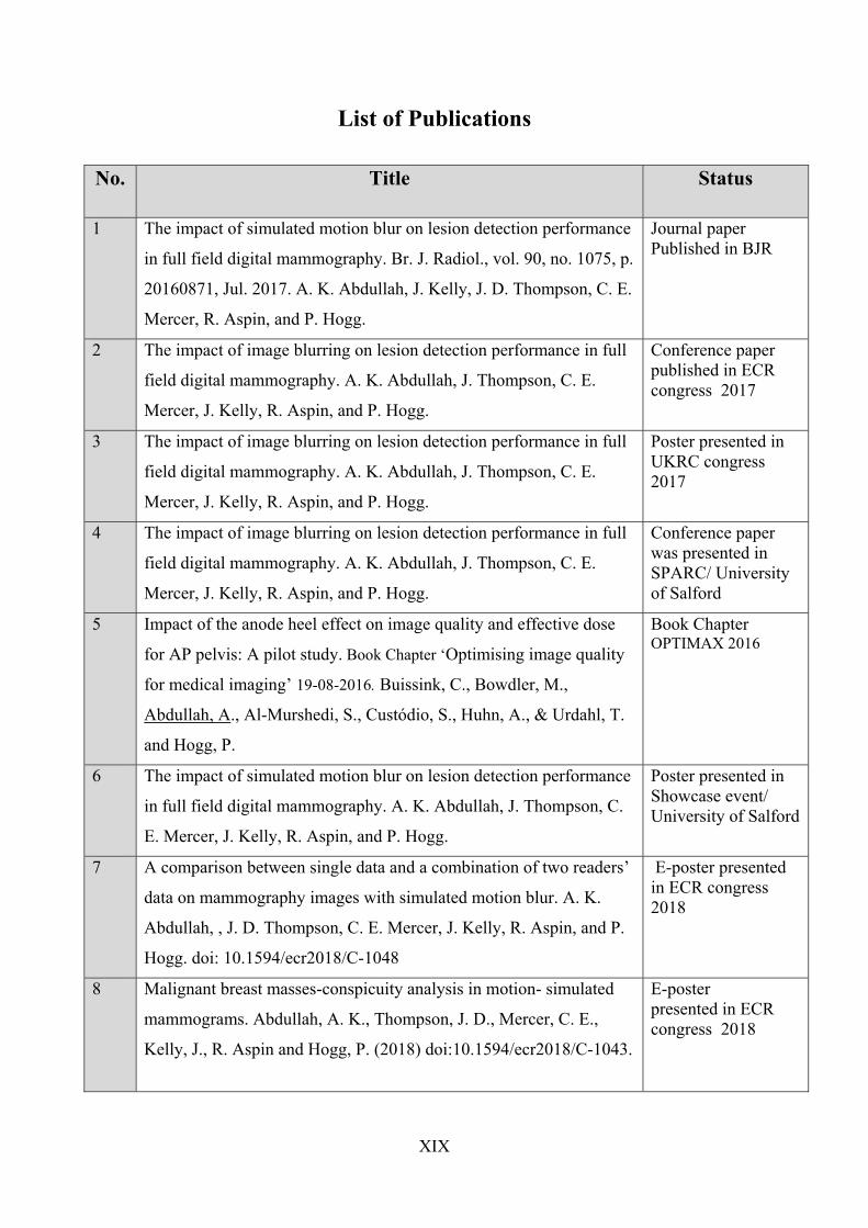
List of Publications
No. Title
Status
1 The impact of simulated motion blur on lesion detection performance
in full field digital mammography. Br. J. Radiol., vol. 90, no. 1075, p.
20160871, Jul. 2017. A. K. Abdullah, J. Kelly, J. D. Thompson, C. E.
Mercer, R. Aspin, and P. Hogg.
Journal paper Published in BJR
2 The impact of image blurring on lesion detection performance in full
field digital mammography. A. K. Abdullah, J. Thompson, C. E.
Mercer, J. Kelly, R. Aspin, and P. Hogg.
Conference paper published in ECR congress 2017
3 The impact of image blurring on lesion detection performance in full
field digital mammography. A. K. Abdullah, J. Thompson, C. E.
Mercer, J. Kelly, R. Aspin, and P. Hogg.
Poster presented in UKRC congress 2017
4 The impact of image blurring on lesion detection performance in full
field digital mammography. A. K. Abdullah, J. Thompson, C. E.
Mercer, J. Kelly, R. Aspin, and P. Hogg.
Conference paper was presented in SPARC/ University of Salford
5 Impact of the anode heel effect on image quality and effective dose
for AP pelvis: A pilot study. Book Chapter ‘Optimising image quality
for medical imaging’ 19-08-2016. Buissink, C., Bowdler, M.,
Abdullah, A., Al-Murshedi, S., Custódio, S., Huhn, A., & Urdahl, T.
and Hogg, P.
Book Chapter OPTIMAX 2016
6 The impact of simulated motion blur on lesion detection performance
in full field digital mammography. A. K. Abdullah, J. Thompson, C.
E. Mercer, J. Kelly, R. Aspin, and P. Hogg.
Poster presented in Showcase event/ University of Salford
7 A comparison between single data and a combination of two readers’
data on mammography images with simulated motion blur. A. K.
Abdullah, , J. D. Thompson, C. E. Mercer, J. Kelly, R. Aspin, and P.
Hogg. doi: 10.1594/ecr2018/C-1048
E-poster presented in ECR congress 2018
8 Malignant breast masses-conspicuity analysis in motion- simulated
mammograms. Abdullah, A. K., Thompson, J. D., Mercer, C. E.,
Kelly, J., R. Aspin and Hogg, P. (2018) doi:10.1594/ecr2018/C-1043.
E-poster presented in ECR congress 2018

XX
9 A comparison of the performance of a 2.4 MP colour monitor and a
5.0 MP monochrome monitor in visualising low contrast detail using
the CDRAD phantom. S. Al-Murshedi, P. Hogg, Abdullah, A. and A.
England (2017)
E-poster Poster presented in ECR congress 2018
10 The impact of simulated motion blur on the physical characteristics
of malignant breast masses in full field digital mammography.
A. K. Abdullah, J. Thompson, C. E. Mercer, J. Kelly, R. Aspin, and
P. Hogg.
Poster accepted in Symposium Mammographican 2018
11 The impact of simulated double reporting on the detection
performance of masses and microcalcifications in FFDM images
containing different magnitudes of image blurring. A. K. Abdullah, J.
Thompson, C. E. Mercer, J. Kelly, R. Aspin, and P. Hogg.
Poster accepted in Symposium Mammographican 2018

XXI
List of Development Skills
No. Type of Skill
1 Applying simulated motion using image blurring software
2 Operation and set-up the ROCView software for ROC assessment
3 Data analysis using JAFROC software
4 How to utilise Conspicuity software for physical measures and data
manipulation.
5 How to utilise ImageJ software for advanced image processing and
manipulation.
6 How to use Endnote software for references coding
7 How to use SPSS software for different and advanced statistics.
8 How to use Excel, Word, PowerPoint and publisher at an advanced
level
9 How to operate and set-up the bespoke software for 2-AFC assessment
10 How to write journal papers (review & empirical), and design poster for
conference presentation
11 How to critically analyse literature
12 How to use TLD system for the direct measurement of dose.
13 How to operate the Unfors dosimeter for dose measurements and QC
protocols

XXII
Training Sessions Attended
Date Title of training course/module/conference
Key learning point
1 02-10-2014 Introduction to the module / Research methods
2 06-10-2014 Electronic Resources
3 09-10-2014 Developing research questions and approaches to research
4 15-10-2014 Time management
5 16-10-2014 Researching for evidence and information
6 23-10-2014 Over view of critiquing research papers
7 28-10-2014 Completing a learning agreement and PhD progression points
8 29-10-2014 Introduction to Nvivo
9 30-10-2010 Quantitative designs
10 06-11-2014 Qualitative designs / Research methods Methods of data collection
11 11-11-2014 The interview: its place in social scientific research strategies
12 12-11-2014 Doing a literature Review
13 12-11-2014 Inspiration: Mind Mapping Software Training
14 13-11-2014 Analysis, presentation, and interpretation of quantitative research
Fundamentals of statistical analysis
15 18-11-2014 Endnote 7
16 20-11-2014 Analysis, presentation, interpretation, and rigour in qualitative research
Fundamentals of thematic and content analytic approaches
17 24-11-2014 Open Access publishing
18 27-11-2014 Advance statistic data analysis
19 04-12-2014 Ethical issues in research
20 05-12-2014 Excel Basic
21 11-12-2014 Excel Charts
22 11-12-2014 Dissemination and publication of research/ Implementation strategies
23 12-12-2014 Excel Formulas Functions

XXIII
24 18-12-2014 Research in the real world
25 02-02-2015 Seminar diagnostic medical image
26 12-02-2015 Working in the UK during and after PhD
27 16-02-2015 Turbo churching your writing
28 17-02-2015 How to publish in IEEE
29 19-02-2015 Word scope workshop for writing
30 02-03-2015 LEAP Higher Language Review Session 1
31 06-03-2015 LEAP Higher Language Review Session 2
32 09-03-2015 LEAP Higher Language Review Session 3
33 17-03-2015 LEAP Higher Language Review Session 6
34 19-11-2015 Word scope workshop for writing
35 24-11-2015 Learning English for Academic Purposes- LEAP Unit 3
Critical writing skills
36 30-11-2015 Learning English for Academic Purposes- LEAP Unit 3
Critical writing skills
37 10-12-2015 Learning English for Academic Purposes- LEAP Unit 3
Critical writing skills
38 13-01-2016 Quantitative research method SPSS
39 14-01-2016 Quantitative research method SPSS
40 15-01-2016 Quantitative research method SPSS
41 10-02-2016 Controversial issues in breast cancer diagnosis using full field digital mammography
Seminar
42 26-02-2016 PhD students session Critical reading and writing
43 1-03-2016 LEAP Higher writing session Critical writing 44 7-03-2016 Theory and content as methodology 45 4-05-2016 LEAP higher session for academic writing Critical writing skills
46 10-05-2016 LEAP higher session for academic writing Critical writing skills
47 17-05-2016 LEAP higher session for academic writing Critical writing skills

XXIV
Acknowledgement
First and foremost, I would like to start with ‘In The Name of Allah Most Gracious Most
Merciful’ I am grateful to God for the good health and wellbeing that were essential to the
completion of this thesis.
I would like to express my deepest appreciation to my supervisors Professor Peter Hogg and
Dr John D. Thompson my Co-supervisors Dr Claire Mercer, Mrs Judith Kelly and Dr Rob
Aspin. Without their guidance and persistent help, this thesis would not exist. In addition, they
imparted a lot of knowledge necessary in becoming a good researcher. Stressing the importance
of always thinking critically and being patient.
I am also grateful to Mrs Katy Szczepura a lecturer in the school of health sciences. I am
extremely thankful and indebted to her for sharing her expertise and sincere, valuable guidance,
which helped me to complete this thesis. I would like to thank Professor David Manning, who
gave valuable suggestions and interesting feedback. I would also like offer a special thank you
to all the practitioners who participated as observer in this study.
I also thank my Father and my Mother for their endless support, encouragement and attention.
I am also grateful to my beloved wife Nabaa Sameer Al-Dulaimi for her support, kindness and
patience as she accompanied me along this journey. I would like to thanks my Aunt Radhiyah
Kamil to here support and encouragement.
I would like to acknowledge The Ministry of Higher Education in Iraq/ Iraqi Cultural Attaché-
London for their financial support in which they have covered the tuition fees and living
expenses that were needed for the completion of this thesis. I also would like to acknowledge
the University of Diyala for their allowing me to take a study leave to do my PhD in the UK.
Finally, I would like to express my upmost gratitude to all who, whether directly or indirectly,
have aided me in this thesis.

XXV
Dedications
I dedicate this thesis to my Father Khalid Abdullah, my Mother Kareema Hamdan and my
wife Nabaa Sameer Al-Dulaimi; I never forget their prayers and their love, which motivate
me forward. Their words and feelings keep me working hard to finish this thesis. I also dedicate
this thesis to my lovely children Hagr, Ans, Abdullah and Humam.

XXVI
Abbreviations
AUC Area under the Curve
AFROC Alternative Free-response Receiver Operating Characteristic
BI-RADS Breast Imaging-Reporting and Data System
CC Cranio-Caudal
CR Computed Radiography
CT Computed Tomography
X Conspicuity Index
DCIS Ductal Carcinoma in Situ
DICOM Digital Imaging and Communications in Medicine
DR Digital Radiography
DI Dispersion Index
FFMM Full Field Digital Mammography
FROC Free-response Receiver Operating Characteristics
FOM Figure of Merit
HVS Human Visual System
IDC Invasive Ductal Carcinoma
IQA Image Quality Assessment
JAFROC Jackknife Free-response Receiver Operating Characteristics
kV kilo-Voltage
LLF Lesion Localisation Fraction
LROC Localisation Receiver Operating Characteristic

XXVII
mA milliampere
MLO Medio-Lateral Oblique
mm millimetre
NLF Non-lesion Localisation Fraction
NHSBSP National Health Services Breast Screening Programme
ROC Receiver Operating Characteristics
UK United Kingdom
wJAFROC weighted Jackknife Alternative Free-response Receiver Operating Characteristic
ΔGL Change in grey level

XXVIII
Abstract
Objective: Full-field Digital Mammography (FFDM) is employed in breast screening for the
early detection of breast cancer. High quality, artefact free, diagnostic images are crucial to the
accuracy of this process. Unwanted motion during the image acquisition phase and subsequent
image blurring is an unfortunate occurrence in some FFDM images. The research detailed in
this thesis seeks to understand the impact of motion blur on cancer detection performance in
FFDM images using novel software to perform simulation of motion, an observer study to
measure the lesion detection performance and physical measures to assess the impact of
simulated motion blur on image characteristics of the lesions.
Method: Seven observers (15±5 years’ reporting experience) evaluated 248 cases (62
containing malignant masses, 62 containing malignant microcalcifications and 124 normal
cases) for three conditions: no motion blur (0.0 mm) and two magnitudes of simulated motion
blur (0.7 mm and 1.5 mm). Abnormal cases were biopsy proven. A free-response observer
study was conducted to compare lesion detection performance for the three conditions. Equally
weighted jackknife alternative free-response receiver operating characteristic (wJAFROC) was
used as the figure of merit. A secondary analysis of data was deemed important to simulate
‘double reporting’. In this secondary analysis, six of the observers are combined with the
seventh observer to evaluate the impact of combined free-response data for lesion detection
and to assess if combined two observers data could reduce the impact of simulated motion blur
on detection performance. To compliment this, the physical characteristics of the lesions were
obtained under the three conditions in order to assess any change in characteristics of the
lesions when blur is present in the image. The impact of simulated motion blur on physical
characteristics of malignant masses was assessed using a conspicuity index; for
microcalcifications, a new novel metric, known as dispersion index, was used.
Results: wJAFROC analysis found a statistically significant difference in lesion detection
performance for both masses (F (2,22) = 6.01, P=0.0084) and microcalcifications (F(2,49) =
23.14, P<0.0001). For both lesion types, the figure of merit reduced as the magnitude of
simulated motion blur increased. Statistical differences were found between some of the pairs
investigated for the detection of masses (0.0mm v 0.7mm, and 0.0mm v 1.5mm) and all pairs
XXIX
for microcalcifications (0.0 mm v 0.7 mm, 0.0 mm v 1.5 mm, and 0.7 mm v 1.5 mm). No
difference was detected between 0.7 mm and 1.5 mm for masses.
For combined two observers’ data of masses, there was no statistically significant difference
between single and combined free-response data for masses (F(1,6) = 4.04, p=0.1001, -0.031
(-0.070, 0.008) [treatment difference (95% CI)]. For combined data of microcalcifications,
there was a statistically significant difference between single and combined free-response data
(F(1,6) = 12.28, p=0.0122, -0.056 (-0.095, -0.017) [treatment difference (95% CI)]. Regarding
the physical measures of masses, conspicuity index increases as the magnitude of simulated
motion blur increases. Statistically significant differences were demonstrated for 0.0–0.7 mm
t(22)=-6.158 (p<0.000); 0.0–1.5 mm t(22)=-6.273 (p<0.000); and 0.7–1.5 mm (t(22)=-6.231
(p<0.000). Lesion edge angle decreases as the magnitude of simulated motion blur increases.
Statistically significant differences were demonstrated for 0.0–0.7 mm t(22)=3.232 (p<0.004);
for 0.0–1.5 mm t(22)=6.592 (p<0.000); and 0.7–1.5mm t(22)=2.234 (p<0.036). For the grey
level change there was no statistically significant difference as simulated motion blur increases
to 0.7 and then to 1.5mm. For image noise there was a statistically significant difference, where
noise reduced as simulated motion blur increased: 0.0–0.7 mm t(22)=22.95 (p<0.000); 0.0–
1.5mm t(22)=24.66 (p<0.000); 0.7–1.5 mm t(22)=18.11 (p<0.000). For microcalcifications,
simulated motion blur had a negative impact on the ‘dispersion index’.
Conclusion: Mathematical simulations of motion blur resulted in a statistically significant
reduction in lesion detection performance. This reduction in performance could have
implications for clinical practice. Simulated motion blur has a negative impact on the edge
angle of breast masses and a negative impact on the image characteristics of
microcalcifications. These changes in the image lesion characteristics appear to have a negative
effect on the visual identification of breast cancer.

1
Chapter One: Introduction and Thesis Outline
1.1 Introduction
Full-field Digital Mammography (FFDM) is the current standard imaging technique for the
early detection of breast cancer. High quality, artefact free, diagnostic images are crucial to the
accuracy of this process. Unwanted motion during the image acquisition phase and subsequent
image blurring are unfortunate consequences in some FFDM images (Rosen, Baker and Soo,
2002). It is thought that this could lead to a reduction in diagnostic performance. The cause of
motion blur can be patient-based (e.g. breast and/or chest wall motion), or technology-based
(e.g. paddle movement) (Geiser et al., 2011). This can lead to distortion of the image in one or
more directions. Chest wall motion could be due to respiration, and by its nature, fairly
predictable, but it is reasonable to hypothesise that breast motion could be more complex, and
could be the outcome of a combination of paddle movement, thixotropic behaviour and blood
being forced away from the breast due to the applied compression force (see section 2.7.3).
Thixotropic behaviour represents a time-dependent reduction of viscosity and modulus induced
by deformation when mechanical loading changes breast volume and results in the motion of
fixed structures (glandular and adipose tissues) (Geerligs, Peter, Ackermans, Oomens and
Baaijens, 2010).
Anecdotal evidence within the National Health Service Breast Screening Programme
(NHSBSP) suggests that image blurring requires images to be repeated, thus increasing patient
radiation dose, anxiety, and service costs. The paucity of literature on this topic suggests that
this technical issue continues to be under-reported. Recent research ( Ma, Aspin, Kelly,
Millington, and Hogg, 2015) suggests that motion blur can be visible to practitioners at sub-
millimetre levels, but presently we do not know the impact of motion blur on breast cancer
detection. At the current level of understanding it can only be assumed that motion blur will
have a negative impact on cancer detection. Consequently, this thesis seeks to understand
whether motion blur does indeed have an impact on cancer detection performance in FFDM.
The methodological approach applied in this work uses novel software to perform a pixel shift
simulation of motion to introduce simulated motion blur to clinical FFDM images. These
images are the foundation of an observer performance assessment to realise the impact of
simulated motion blur on cancer detection.

2
1.2 Aim
The aim of this thesis is to assess the impact of simulated motion blur on lesion detection
performance in FFDM using the free-response receiver operating characteristic (FROC)
method. The research will evaluate the impact on lesion detection performance on two different
magnitudes of simulated motion blur. The selection of two different magnitudes of motion blur
was to determine whether performance would become incrementally worse with greater
magnitudes of motion blur.
1.3 Objectives
1. Characterise non-simulated blurring in FFDM images and determine the magnitude of
computer generated blurring required to simulate this. A validation study of the non-
simulated blur will be conducted to see if experienced FFDM observers could differentiate
between real blur and simulated blur.
2. Determine the impact of simulated motion blur on lesion detection performance.
3. Determine the impact of simulated motion blur on physical characteristics of:
a. malignant masses using Conspicuity Index, and,
b. microcalcifications using a novel metric, described as the ‘dispersion index’.
1.4 Research Questions
What is the impact of different magnitudes of simulated motion blur on:
Lesion detection performance in FFDM images
Physical characteristics of lesion images
1.5 Rational of the thesis
Motion blur in FFDM images has the potential to obscure breast lesions; as a result, clinically
significant abnormalities could go undetected which may have a negative impact on patient
care. Anecdotal evidence suggests that many practitioners in mammography have realised the
potential impact of motion blur in digital mammography but they do not know how much of
an impact this can have on breast cancer diagnosis, or indeed, whether they are even detecting
the smaller magnitudes of motion. If motion blur is detected, this could lead to repeated images
or increased recall rates, both of which will increase radiation dose to the patient. If motion

3
blur is not recognised, this could lead to missed diagnosis, late detection or symptomatic
presentation as an interval cancer. On the other hand, motion blur also has the potential to
increase the number of lesion mimics (false positives), which may lead to unnecessary biopsy,
with the consequence of an unnecessary invasive procedure and increased anxiety for the
patient. Presently, no study exists to determine the impact of simulated motion blur on observer
performance. Therefore, this thesis aims to evaluate the impact of motion blur on breast cancer
detection performance in FFDM using novel image blurring software.
1.6 The Contribution of this Thesis:
This thesis demonstrates for the first time, that motion blur has a negative and statistically
significant impact on the detection performance of malignant masses and microcalcifications
in FFDM images. In view of this, caution should be exercised when making decisions about
the acceptability of images that appear to contain blur as false-negative decisions could be
reached. This thesis recommends further research is required to highlight the impact of this
problem. This thesis also provides a number of recommendations to breast specialist clinicians,
particularly radiographers and radiologists. Firstly, it has recommended that radiographers be
aware about motion blur during quality assessment of images in the mammography imaging
room. Secondly, clinicians during image reading, should be aware of the impact of motion blur
on cancer detection, in relation to the potential for false positives and false negatives.

4
1.7 Thesis Structure
This thesis is composed of eight distinct chapters, summarised in Figure (1.1).
Chapter One– Introduction and Thesis Outline: comprises a brief introduction, aim,
objectives and thesis rational.
Chapter Two– Literature Review: This chapter provides a review of areas of interest that are
of critical relevance to this thesis. In respect of one of the key objectives of this thesis, it is
important that the anatomy of the breast is explored and understood in detail. In addition to this
it was important to develop a working understanding of the presentation of breast cancer and
the characteristics of breast tissue, as displayed in mammographic images. Since it has been
hypothesized that image blurring may originate from the equipment used to generate the
mammographic images it was also valuable to understand the detailed operation and technical
aspects of these systems. This work is heavily influenced by the observers’ ability to detect
cancer in images, so it is vitally important that the factors affecting diagnostic performance in
mammography are understood.
Chapter Three– Medical Image Assessment Methods: The relationship between visual
performance and medical image interpretation is explored here, with a focus on the human
visual system due to the fact that medical image interpretation is based on visual performance
of an observer and visual appearance of the image. Image perception was evaluated to help
understand the challenges presented to clinicians who evaluate FFDM images. The methods to
evaluate observer performance were reviewed in detail and this helped inform the choice of
optimal method to apply for the thesis research question. In addition to the perceptual
evaluation by the observers, it was valuable to understand what is happening to the
characteristics of the breast tissue and lesions, as presented in the images. Understanding how
lesion characteristics change when simulated motion blur is applied and the methods available
for physically evaluating these characteristics was another critical step in the literary analysis,
as this help inform the design of the methods.
Chapter Four– Methodology: In this section the methodological choices are explained and
justified for the following components of the research: (i) the design of the free-response study,
(ii) the method to apply simulated motion blur to the FFDM images, and (iii) the methods used

5
to measure the physical characteristics of the lesions. This section describes eight logical steps
using five different software applications; each having a specific function in the thesis.
Chapter Five– The Results of the Free-response Study: This chapter presents the results of
the observer performance study. The main outcomes focus on the detection of malignant
masses and microcalcifications under three conditions: (i) no motion blur, (ii) 0.7 mm of
simulated motion blur, and (iii) 1.5 mm of simulated motion blur. In addition to this, a decision
was made to investigate the impact of dual reader evaluations on detection performance in the
presence of simulated motion blur. This was done following a method to combine the free-
response data of two observers. The aim was to mimic the double reporting scheme used in
screening mammography.
Chapter Six– The Results of Physical Measures: In this chapter the physical characteristics
of the lesions are described and compared at different magnitudes of simulated motion blur.
Generating this data also enabled an analysis of ‘missed lesions’ to try and establish whether
simulated motion blur had a greater impact, thus causing a greater reduction in detection, on
lesions of different characteristics.
Chapter Seven– Discussion: This chapter evaluates the results of the free-response study and
the physical measures. This chapter is set out in the same manner as the results chapter, where
the data from each section is discussed separately. The impact of motion blur on the detection
performance of breast masses and microcalcifications are discussed. The missed lesion
calculation method and the impact of motion blur on lesion characteristics image are discussed.
Chapter Eight: Conclusion, Recommendations and Future work:
This chapter summarises the results of the thesis in a concise manner. The final conclusions
that were obtained from free-response study, and then an overall conclusion regarding the
impact of motion blur on physical characteristics of malignant masses and microcalcifications
is presented. A statement of novelty and recommendations for future work is presented.

6
Figure 1.1 A flowchart demonstrating the structure of this PhD thesis
Chapter Eight
Conclusion, Recommendations
and Future Work
Chapter One
Introduction and Thesis Outline
Introduction Aim and Objectives Rational of the Study Thesis Structure
Chapter Two
Literature Review
Conclusion Statement of Novelty Recommendations and Future Work
Physical Measures of Breast Masses Physical Measures of Microcalcifications Missed Lesions Calculation Method of Breast Masses Missed Lesions Calculation Method of Microcalcifications
Visual Performance and Image Interpretation Human Visual System (HVS) Receiver Operating Characteristics (ROC) Methods Free-response ROC method Perceptual measures Physical measures
Breast anatomy Breast cancer Mammography Full Field Digital Mammography (FFDM) Motion Blur in Mammography Images Physic of Mammography System
Step 1: Images Selection .Step 5: Statistical Analysis
Step 2: Images Assessments .Step 6: Conspicuity of Masses
Step 3: Simulated Motion blur .Step 7: Dispersion Index
Step 4: Observer Performance Study .Step 8: Missed lesion Analysis
Results of Free-response Study (single observer) Microcalcifications Breast masses Results of Combined two Observers’ Data A Comparison between Single and Combined Data
Chapter Three
Medical Image Assessment
Methods
Chapter Four
Methodology
Chapter Five
Results of Free‐response Study
Chapter Seven
Discussion
Free-response Study (single observer) for Masses and Microcalcifications Combined two observers’ data Physical Measures of Masses and Microcalcifications Missed Lesions Calculation Method for Microcalcifications
Chapter Six
Results of Physical Measures

7
Chapter Two: Literature Review
2.1 Overview of the Chapter
This literature review provides a critical analysis of previous studies, which investigated the
cause and effect of motion blur in FFDM images. A literature search was undertaken, and was
followed by assessment of study elements. This assessment offers justification for the method
described in chapter four, in addition to the rationale for the research study described in chapter
one. The literature search was implemented utilising Medline, Google scholar and Solar
databases at the University of Salford, with different sets of the keywords such as motion blur,
full field digital mammography, lesion detection performance, breast cancer. There were no
limits applied for publishing dates.
This chapter is organized into seven main sections. The first section (2.2) will focus on breast
anatomy. The second section (2.3) will focus on breast cancer and factors effecting the risk of
breast cancer. The third section (2.4) will focus on mammography and the characteristics of
breast tissue in mammography images. The fourth section of this literature review will focus
on the factors affecting diagnostic efficiency of breast cancer detection in mammographic
images such as breast density, image quality and the effect of shape and margin of breast lesion
on detection performance. In the fifth section (2.6), the focus will centre on the components of
FFDM system. The sixth section (2.7) will focus on motion blur in mammography images and
the contributory factors. The reviewed studies in this section were sub-divided for structure.
The first (2.7.1) investigated the causes of motion blur in FFDM images according to extra and
intra patient movement focusing into the causes of motion blur related to both patient and
system parts; paddle movements, inadequate compression and pain related to paddle
compression. The second (2.7.2) reviews the papers that investigated the visual detection of
motion blur on FFDM using different types of monitors. The third (2.7.3) relates to the
thixotropic behaviours of breast tissue. The seventh section focuses on the physics of
mammography systems, X-ray production and X-ray incident on the detectors.
2.2 Breast Anatomy
The breast is tear-shaped and supported by the front of the chest wall. It is located over the
pectoral muscles and attached to the upper border of the chest wall by fibrous ligaments known
as Cooper’s ligaments. The composition of the breast is a mass of soft tissue consisting of fatty,

8
fibrous and glandular tissue (Hogg et al., 2015). The development of the breast begins during
puberty when the female body undergoes changes to prepare for reproduction. Puberty often
starts around the ages of 10 or 11 year when the breast responds to hormonal changes in the
body. The production of two hormones, progesterone and oestrogen, signal the development
of the glandular tissue of breast (Pathmanathan, 2006).
The anatomical structures of the female breast are represented in Figure 2.1. The interior part
of the female breast consists of three major tissue types: glandular or parenchymal tissue, fatty
and fibrous tissue. The glandular tissues are typically divided into 15-20 lobes, wherein the
production of milk occurs. The lobes are divided into smaller sections known as lobules and
separated by fibrous walls (Darlington, 2015). The nipple is connected to the lobules by a
network of small ducts (intralobular ducts). The ducts often start as tiny ductules at the lobules;
after that they combine near the nipple to become larger sized ducts (Van De Graaff, 2001).
The connective or fibrous tissue in the breast contains and supports both the ducts and lobules.
The ducts and lobes (glandular tissue) can be grouped with fibrous tissue, together forming the
fibro-glandular tissue. The fibro-glandular tissue is covered on the outside by a layer of fat or
adipose tissue (Van De Graaff, 2001). The variation between adipose to glandular tissue
proportion is due to age and individual characteristics. However, the features of the female
breast are like a unique map for every individual; the breast structure alters over time according
to age, hormonal changes, and menopausal status (Ossati, 2015). It is because of this that the
interpretation of mammographic images is considered a complex task.
Breast parenchyma comprises of three kinds of tissues–adipose and subcutaneous tissue,
functional glandular tissue, and skin. The macroscopic anatomy of the breast, divides the
component female breast into two main parts. The first part known as glandular component
(milk production) and the second part comprising muscles, fascia (connective tissue) and fat,
which are concerned with support and make up the breast (Darlington, 2015). The variations
in breast structure can be illustrated by differences in breast density on mammography.
Commonly, younger aged females tend to increase dense glandular tissue. Likewise, the breast
density in older age females tend to have less density through the changing of fatty tissue
instead of glandular tissue. Lactation and pregnancy are among some of the compounding
factors that are indicative of being important in raising the density of breast tissue (McDonald,
2015).

9
The microscopic anatomy of the breast was firstly described by Welling in (Wellings et al.,
1975). He identified the terminal ductal lobular units (TDLU) as the functional unit of the
breast, consisting of acini (built up from 10 to 100 sac-like units), an extralobular duct and an
intralobular terminal duct. The TDLU is important physiologically due to its responsibility for
milk production during the period of lactation. Figure 2.2 illustrates a simplified drawing of
the structure of a Terminal Ductal Lobular Unit (TDLU). During pregnancy and lactation,
increases in oestrogen, prolactin and progesterone produce enlargement of the acini, an
evolution in myoepithelial cells and hyperplasia of the lactogenic epithelium to prepare for
milk producing. During lactation, the breast passes through many of changes and deferent
degrees of involution, and its appearance might seem to consist of a smaller amount glandular
tissue than before the pregnancy period. This process continues for about three months before
returning to a new baseline.
Figure 2.1 Structures of the adult woman breast: (A1) schematic breast anatomy and (B1) the
corresponding mammographic features (Hogg et al., 2015).

10
Figure 2.2 Demonstrates a simplified drawing of the structure of a Terminal Ductal Lobular Unit
(TDLU).
Breast size is fundamentally identified via the amount of adipose tissue (fat cells) in the breast.
The adipose tissue reaches from the collarbone to the armpit and to the middle of the ribcage
(Whitman and Haygood, 2012). Commonly, smaller breasts have a smaller amount of adipose
tissue compared to their glandular tissue, while the larger size of breasts have a higher amount
of adipose tissue compared to their glandular tissue (Spear et al., 2004). The shape and size of
the breast varies according to several factors: diet, age, race, the situation menopausal of
women and parity (Williams, 1995). Physical techniques can be used to identify breast volume
or size through either casting the breast in plastic or through immersion of the breast in water
and identifying its volume by calculating the displaced water volume based on Archimedes’
principle. Precise identification of breast volume is not easy though can be achieved using
digital techniques (Veitch, Burford, Dench, Dean, & Griffin, 2012). Alonzo-Proulx et al.,
(2012) utilised digital mammograms to investigate some of the breast features such as the
breast volume for digital mammographic images of 15,351 females. They reported that the
mean breast volume for all examined cases was 687 cm3 with small variances in several age
groups. For instance, it was around 703 cm3 for 50-55 year and 736 cm3 for 55-65 year age
groups. Diffey, (2012) found a highest mean breast volume about 820 cm3. However, Wang et
al., (2013) used ultrasound to calculate breast volume of women and they reported that the
breast volume for about 57% of 306 adult women was 400-800 cm3.

11
2.3 Breast Cancer
Breast cancer is an uncontrolled growth and an abnormal change of breast tissue due to
abnormal cell divisions (proliferation). In a normal condition, two types of genes are
responsible for controlling the division of the cell, named as a tumour suppressor and proto-
oncogenes genes. These genes continuously mutate, this leads to uncontrolled cell division
(Shannon & Chittenden, 2015). This cancer can metastasise or diffuse to other parts through
the lymphatic system or the blood circulation (Shetty, 2015a).
Breast cancer is characterised by malignant tumours that arise from the glandular tissue within
the breast. It is an insidious disease that will affect one in seven women over their lifetime
(Cancer research UK, 2016). There are several types of breast cancer which can be classified
by the physical characteristics of the tumour and location within the breast. One of these types
is known as cancer in situ. This appears as a non-invasive disease in which the cancer cells stay
inside the basement membrane and do not invade the surrounding tissues. Another type of
breast carcinoma is known as an invasive breast carcinoma. This invades surrounding tissue
and has the ability to metastasise, which means that the cancer transfers from one part of the
body to another through the lymph system or the blood stream (Evans et al., 2002). According
to Danziger and Simonsen, (2011), Invasive Ductal Carcinoma (IDC) is an example of an
invasive breast cancer which involves different subtypes (Papillary Carcinoma, Medullary
Carcinoma, and Tubular Carcinoma), while Ductal Carcinoma in Situ (DCIS) is an example of
a non-invasive breast cancer. Other types of breast cancer (American Cancer Society, 2014)
such as carcinoma, sarcoma and adenocarcinoma, originate in various lobes of the breast.
Carcinomas originate in the lining layer of the breast, Sarcomas originate from connective
tissues (fat, blood vessels or muscle), and Adenocarcinomas originate in the glandular tissue
such as the breast lobules.
The American Cancer Society (2014) found that approximately 8 out of 10 invasive breast
cancers could be categorised as IDC. The shape and margins of IDC are most commonly
spiculated firm masses with ill-defined and irregular margins and it is difficult to detect. The
second most common breast cancer, which starts in lobules or in the milk-producing glands, is
Invasive Lobular Carcinoma (ILC). DCIS is the most common type and it originates in the milk
ducts. It is also recognised that there are other types of breast cancer such as Lobular Carcinoma
in Situ (LCIS) (Evans & Blanks, 2002; Winchester &Winchester, 2006).
12
The TDLUs are important units within the breast , as over 90 % of breast cancers originate in
these units (Hogg et al., 2015). The ducts and acini consist of three layers including the
epithelial lining, myoepithelial layer and the basement membrane. The epithelial layer is
normally only one cell thick, but when converted to two or three cells thick it is named a
hyperplasia. More proliferation is classified depending on a number of layer cells that are
existent, and the appearance of the atypical cells; these situations range from atypical ductal
hyperplasia to ductal carcinoma in situ. The function of the basement membrane is responsible
for preventing the spread of cancer. When this membrane is breached, a carcinoma is named
invasive. Male breast cancer is extremely rare compared to breast cancer in women,
representing approximately less than 1% of all breast cancers (Garnett, 2015). In the UK, male
breast cancer is of lower incidence than female breast cancer, with only one new case detected
for every 100,000 males (around 350 to 400 cases per year). The male breast is undeveloped
but is affected by testosterone and oestrogen that influences some of the breast tissue located
beyond the nipple. This undeveloped tissue of breast consists of rarely ductal lobular units and
mainly major sub-areolar ducts (Cancer research UK, 2016).
2.3.1 Factors Affecting Breast Cancer
An individual’s likelihood of contracting breast cancer is their breast cancer risk. Many factors
are responsible for breast cancer risk such as gender, age, family personal history, lifestyle
factors and hormonal therapy. However, it is uncontrolled by large number of factors, and there
is no full explanation about the mechanism of how these factors can stimulate the normal cells
to become cancer cells (Hackney, 2015). The two essential unalterable risk factors are gender
and age. In the context of gender, more than 99% of breast cancer incidences are from women
(Kopans, 2007; Garnett, 2015). In women under 20 years of age, breast cancer cases are quite
rare, and approximately 0.3% of the breast cancer incidences happen in women within the 20–
30 age group (Finkel, 2005). However, approximately (48 %) of the breast cancer incidences
occurs in females within their fifth and sixth decade (50–69 year) (Hackney, 2015). This
contributed to the rationale for supporting the UK NHS breast-screening programme to invite
females within the aged 50–70 year for screening mammography every three years (NHSBSP
Publication No 60, 2005).
Other risk factors comprise family history, breast density and personal history. In relation to
family history nearly 15% of the females with breast cancer have a family history of breast

13
cancer (Hackney, 2015). Breast density is a further risk factor and females that have a higher
density of breast tissue have a higher incidence rate of breast cancer (Shetty, 2015a). In relation
to personal history, females who have previous incidence of breast cancer are more liable to
develop breast cancer by about three to five times than other females (Hackney, 2015).
Additional risk factors are related to lifestyle, and they include diet, physical activity, drinking
alcohol and smoking. Hormonal therapy can also cause an increase in breast cancer cases
(Kopans, 2007; ACS, 2015; Hackney, 2015).
Socio-economic circumstances are also important in incidence rate with recent studies
indicating that approximately 53% of breast cancer cases occur in developed nations
(Hackney, 2015). There are significant differences between regions: it is at least 2-3 times less
common in East Asian countries than in Western Europe and America, where the latter
illustrate lesser proportions than African countries (United Nations Scientific Committee on
the Effects of Atomic Radiation (UNSCEAR, 2008). Between 2002 and 2003, breast cancer
studies demonstrated a significant decline of about (7%) in the United States. This decline
might have come according to a decrease of using menopausal hormone therapy (ACS, 2011b).
In the UK, however, obesity, hormone therapy, use of hormones as a contraceptive, and the
lower proportion of pregnancies have contributed to a growing occurrence of breast cancer
between 1975 and 2003 (Health Protection Agency, 2011). In 2012, a study demonstrated that
the proportion of breast cancer incidences have altered to be 39%, 28%, and 15% in Asia,
Europe, and the United State respectively (ACS, 2015). Breast cancer death rates have
gradually reduced in developed nations. For example, in England, it decreased by 37% between
1971 and 2011 (Office for National Statistics [ONS], 2012). Likewise, a 5.2% per year decline
is noticeable in North America between 1990 and 2011 (ACS, 2011b). This decline in death
rate is related to earlier diagnosis of breast cancer via breast cancer screening programmes,
primary prevention of breast cancer incidence reduction, and the development of better cancer
treatment procedures (ACS, 2011b; Säbel & Aichinger, 1996).
2.4 Mammography
Mammography is a well-established imaging procedure which is utilised as both a screening
and diagnostic mammography tool. In the United Kingdom (UK), females between 50 and 70
years of life are offered mammographic screening examinations through a screening
programme to identify those with breast carcinoma, so as to offer them treatment at the earliest

14
possible stage. At present in the UK a randomised controlled trial is ongoing to screen women
50 years or older once every 3 years (Dewar, 2015).
Digital mammography is considered one of the greatest new technologies in screening
mammography due to its superior contrast performance (Muller, 1999; Rafferty, 2007). Digital
mammography has many advantages which enhance and improve sensitivity and specificity
and can enhance lesion detection performance; it has also been seen to decrease diagnosis
errors (Pisano and Yaffe, 2005). An observer’s ability to detect cancer in its early stages is
dependent on high-quality mammographic images being obtained (Kulama, 2009). Although
there are several imaging modalities used for breast cancer detection, mammography is the
most common, most cost effective and best screening tool for the diagnosis of breast
abnormalities (Muller, 1999; Cole et al., 2003; Rafferty, 2007). There are different projections
that can be taken, the most common being mediolateral oblique (MLO), and craniocaudal (CC)
(Hogg et al., 2015). In screening mammography, these two projections of the breast are
acquired. In situations wherein the breast lesions are not well visualised by the CC and MLO,
additional mammographic projections involving the Medio-lateral (ML) and Latero-medial
(LM) can be used (Lewin, D’Orsi and Hendrick, 2004; Whitman and Haygood, 2012). By
utilising the different mammographic projections, the person reading / interpreting the image
can study the breast anatomy and potential lesions from different perspectives in order to
enhance lesion detection performance (Ortiz-Perez and Watson, 2015). Figure 2.3
demonstrates the four mammographic projections.
Figure 2.3 Mammographic Projections (Imaginis Corporation, 2014).

15
Figure 2.4 represents typical mammographic images; Cranio-Caudal Projection (A&B) and
Medio-Lateral Oblique Projection (C&D) for left and right sides. The fact that there is little
difference in contrast between normal breast tissue and lesions can create difficulties in lesion
perception detail such as; boundaries, edges and shapes (Tabar et al., 2005; Kopans, 2006).
However, other factors such individual differences in the relative proportions of high-low
breast densities are found to affect accuracy in interpretation (Masotti, 2005; Al-osta, 2010).
Furthermore, sub-optimal positioning is a major contributor to accurate visualisation of
abnormalities on FFDM images (Debono, 2012).
Figure 2.4 Normal mammography- Cranio-Caudal Projection (A&B) and Medio-Lateral Oblique
Projection (C&D).
It is recognised that the composition of the breast varies among women and depends on the
proportion of fibrous, glandular and adipose tissue. Breast composition changes with the age
of women such that the quantity of adipose tissue will increase with age. The variations of
breast tissue can be observed by mammography due to the attenuation of the x-ray beam that
passes through different levels of tissue density. The adipose tissue is visualised as dark areas
(radiolucent) in mammography while fibrous and glandular tissue appear less dark
(radiopaque). Therefore, these variations of tissues are apparent in the image due to the
absorption of x-ray by different densities and thicknesses of glandular and adipose tissues
(Uchiyama, Nachiko & Zanchetta, 2012).

16
Breast tissues are highly sensitive to (x-ray) radiation and, as such, special characteristics of x-
ray tube are utilised in mammography. Mammography tube characteristics are designed to
achieve high image quality with low radiation dose (Uchiyama et al., 2012). Low-energy
radiation is accomplished through the combination of filters and different x-ray tube targets.
Mammographic x-ray tubes should have a small focal spot to achieve high resolution and
sharpness (Wilson et al., 2011). The increase of x-ray energy can lead to a decrease in the
contrast between different breast tissues. Therefore, low-energy radiation is used in
mammography because this differentiates breast densities in order to achieve high contrast
(Whitman & Haygood, 2009). It is obvious that a weakness of mammography systems is
ionising radiation. However, the radiation risk regarding using x-ray within mammography is
far below the risk of breast cancer (Yaffe and Mainprize, 2011). Consequently, women should
continue for the procedure of screening mammography (Ali et al., 2015). Research illustrates
that screening mammography reduced the mortality rate from breast cancer by approximately
1,300 per year in the UK due to the early detection of cancer (Cancer Research UK, 2014).
2.4.1 Characteristics of Malignant Microcalcifications within Mammography Images
Malignant microcalcifications have different distribution patterns; they can be clustered,
diffused or punctate. Clustered microcalcifications present with a wide range of sizes compared
to benign whereas malignant microcalcifications display homogeneous appearances and
irregular shapes with a low-density (Kaiser, 2009; Bick, 2010) . In addition, individual
malignant microcalcifications are reportedly varied in terms of their size and shape; some are
linear and branching, others microscopic and fine or stellate-shaped (Schueller et al., 2008).
Figure 2.5 illustrates examples of malignant microcalcifications of several shapes, sizes and
distributions patterns. Malignant microcalcifications vary in number, density, size and shape.
They are often clustered within one lobe at the breast. Malignant microcalcifications are
divided into two types- granular and casting, due to their physical characteristics. The granular
type are very small, often ‘uncountable’, with an extended shape. The casting type contains a
large number of small calcifications with different lengths and irregular contours (Shetty,
2015b). Many studies (Gathani et al., 2005; Hizukuri et al., 2013) have classified clustered
microcalcifications into five different types due to histological origins: non-invasive
carcinomas of the comedo type, non-invasive carcinomas of the non-comedo type, invasive
carcinomas, fibroadenomas, and mastopathy. Benign microcalcifications however, are
characterised by a sharp outline, a homogeneous shape and a radiolucent density (Shetty,
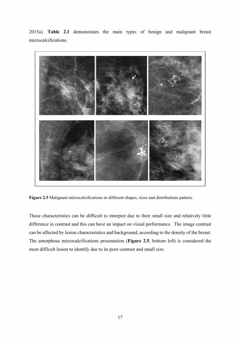
17
2015a). Table 2.1 demonstrates the main types of benign and malignant breast
microcalcifications.
Figure 2.5 Malignant microcalcifications in different shapes, sizes and distributions pattern.
These characteristics can be difficult to interpret due to their small size and relatively little
difference in contrast and this can have an impact on visual performance. The image contrast
can be affected by lesion characteristics and background, according to the density of the breast.
The amorphous microcalcifications presentation (Figure 2.5, bottom left) is considered the
most difficult lesion to identify due to its poor contrast and small size.

18
Lesion type Size Shape Density Appearance Distribution
Pattern
Malignant microcalcification
Variation of sizes
Irregular Low density
Inhomogeneous Clustered innumerable
Benign microcalcification
Uniform in size
Rounder shape, coarse oval
High density
Homogeneous Scattered or diffuse
Malignant masses 3 sizes: Large, medium, small
Circumscribed or spiculate
High density
Stellate spiculated with poorly define margins
Benign masses Rounded Low density
Sharpe define margins
Table 2.1 Main types of benign and malignant breast lesions
Contrast within FFDM images refers to the difference in luminance between a breast lesion
and its background (Apelt et al., 2009). A consequence of low contrast can be that malignant
microcalcifications located within a dense breast are likely to be difficult to visualise as this
represents a high-density lesion within a high-density background (Sabih et al., 2011). This is
also true for malignant masses with poorly defined margins. However, many benign
microcalcifications are often easy to recognise by the human eye due to their high-density and
homogenous appearance, which are often characterised by good contrast with its surroundings.
2.4.2 Breast Masses
The shape and margin of breast masses or lesions can indicate if the lesion is benign or
malignant. The margin can be micro-lobulated, obscured, indistinct, circumscribed, or
spiculated (Shetty, 2015a). The shape can be either lobulated, round, irregular, or oval. Lesions
which have a round or an oval shape and involve a circumscribed margin are commonly benign
while lesions with an irregular shape or lobulated are most likely to be malignant (Shetty,
2015b). Figure (2.6) demonstrates a set of the most common shapes and margins of breast
lesions.

19
Figure 2.6 shapes and Margins of Breast Lesions (The radiology Assestant, 201
Some cases of benign circumscribed masses contain cysts and fibroadenomas. Invasive ductal
carcinoma (IDC) is an example of a cancer with spiculated margins and irregular shapes,
although these can also have well-defined margins (Ossati, 2015). Figure 2.7 illustrates some
malignant and benign breast masses.
Figure 2.7 Mammographic images demonstrating benign and malignant masses
A: Cyst-round circumscribed, B: Fibroadenoma-lobular, low density and circumscribed, and,
C: spiculated margins and irregular shape represents an Invasive ductal carcinoma (IDC)
(Ossati, 2015). Specific lesion characteristics in mammographic images have different degrees
20
of detection difficulty. Some types of breast masses may be difficult to detect as the
surrounding breast tissue obscures the spicules that radiate outwards (Lehman et al., 1999). In
comparison, malignant microcalcifications, which are associated with a high false negative
fraction (FNF), may be misdiagnosed because of the difficulty in identifying the nature of
lesions of suspicious area of the image (Al Mousa et al., 2014). Architectural distortion has a
subtle appearance and may appear similar to normal overlapping breast tissue; this can also
result in missed lesions and lead to false negative presentation (Zwiggelaar, Schumm and
Taylor, 1997).
2.5 Factors Affecting Diagnostic Efficiency
Breast cancer detection, in the early stages, can lead to the creation of more effective treatments
and can result in a decrease in mortality rates. It is therefore a universal health priority when
developing strategies to control breast cancer. Screening mammography represents the most
efficient technique for the early detection of breast cancer; however, the sensitivity of
mammography is in the 68–92% range (Beam et al., 2013). The high occurrence of breast
cancer, aside from the rate of misdiagnosis, highlights the need for a better understanding of
why some breast lesions go undetected.
Many studies suggest that detection performance is related to the observer in terms of
experience, cognitive skills and visual performance (Nodine & Kundel 1987; Chester 1992;
Reed, 2005; Manning et al., 2006; Burgess 2011; Sabih et al., 2011; Lança et al., 2015). Other
studies suggest that lesion characteristics can contribute to challenges in image reading
accuracy. These characteristics include the type, size, contrast, distribution and location of the
lesion within the breast (Figure 2.8). Small lesions with indefinite borders can lead to
perception difficulties (Van Overveld, 1995; Tabar et al., 2005; Kopans, 2006). In the same
context, other studies suggest that factors related to the characteristics of a mammographic
image (image quality, artefacts, spatial resolution, sharpness and contrast resolution) can have
an influence on detection performance.

21
Figure 2.8 Malignant microcalcification and mass with different lesion characteristics.
Perception errors can be considered the main cause of missed cancers in mammography
(Rawashdeh et al., 2014). Misdiagnosed cancers in mammography are commonly located in
the retro-glandular regions (Berlin, 2001a). Whereas, Huynh et al., (1998) highlighted that the
misdiagnosis of cancers were more significant within lower density breasts; they were almost
visible on only one of two projections and were smaller in size. Huynh and colleagues (1998)
also found that masses, rather than calcifications, are more commonly undetected (Huynh,
Jarolimek and Daye, 1998). This is a concern since a large number of lesions are present as
palpable, non-calcified tumours (Yankaskas et al., 2001). However, within these studies it is
noted that limited data exists on the effect of other image and lesion appearances, such as
texture and shape.
When interpreting a mammography image, the image can be divided into several quadrants by
the image reader; this approach is known as the regions of interest (ROI) paradigm. The
selections of ROIs are based on clinical considerations and the quadrants should be equal for
all images. For instance, the mammographic image could be divided into four quadrants
(external upper quadrant, internal upper, external lower and internal lower quadrant). The task
of the observer is to rate each region for the presence of a breast lesion in that ROI (Al-osta,

22
2010). The rating of quadrants per image produces numeric data. It is supposed that the truth
of each ROI is known, whether the lesion exists or absent in ROI and it cannot lesions that
overlap ROIs.
2.5.1 Mammographic Breast Density (MBD) Assessment
There are many methods for measuring breast density. Some are quantitative whilst others are
qualitative (Yaffe, 2008). Qualitative methods involve an observer scoring images using scales;
examples of visual grading scales include Breast Imaging Reporting and Data System. (BI-
RADS), Tabar, visual estimation and Wolfe’s (Wolfe, 1976). According to Gram et al., (1997),
Tabar has categorised breast density into five types:
I: A predominance of fibrous tissue with balanced proportion of all components of
breast tissue (Cooper’s ligaments and scalloped contours)
II: Fatty breast (predominance of fat tissue)
III: Mostly fat tissue with oval-shaped lucent areas
IV: Predominantly nodular and linear densities
V: Extremely dense (mostly fibrous tissue)
However, Wolfe’s (Wolfe, 1976) grading classified breast density into four types:
(i) Fatty breasts (fibro-glandular tissues >25 % and almost all of the tissue appears to
be fat
(ii) Fibro-glandular breasts (Proportion of fibro-glandular tissue 26–50 % of the breast
(iii) Heterogeneously dense breast (heterogeneously compose 51–75 % of tissues)
(iv) Extremely dense (fibrous connective tissue composes more than 75 %)
Breast Imaging Reporting and Data System (BIRADS) (American College of Radiology 2013;
Carl et al., 2013; Geller, et al., 2002) is a qualitative method to assess the density of breasts
which is widely utilised in mammography. Figure 2.9 shows BIRADS for four main density
classifications: (A) fatty breast; (B) fibro-glandular tissue; (C) heterogeneous dense breast; and
(D) for the extremely high-dense breast. The BIRADS system categorises breast density
according to a percent of its compounds, as follows: BIRADS (A) (the breasts are almost
entirely fatty), BIRADS (B) (there are scattered areas of fibro-glandular density), BIRADS (C)
(the breasts are heterogeneously dense, which may obscure small masses), and BIRADS (D)
(the breasts are extremely dense, which lowers the sensitivity of mammography). In spite of

23
the BIRADS method being commonly used worldwide for reporting mammographic breast
densities, the features of the mammographic image are identified subjectively (Taplin et al.,
2002); this method can be susceptible to visual errors and can be influenced by the experience
level of the observer.
Figure 2.9 Variations in breast density according to BI-RADS classification system
2.5.2 Effect of Mammographic Breast Density on Lesion Detection Performance
A number of studies have demonstrated that the sensitivity of mammographic image-observers
to detect breast cancer increases with decreasing breast density (Byng et al., 1994; Lehman et
al., 1999; Kolb et al., 2002; Kriege et al., 2006; Lip et al., 2010; Chiu et al., 2010; Cook et al.,
2010; Al-Mousa et al., 2014). Other studies demonstrated that lesion density contributes to
challenges in screen reading accuracy (American College of Radiology, 2013; The Radiology
24
Assistant, 2013). It can be reasoned that small differences in contrast between lesion density
and density of breast tissue (density of normal and abnormal tissue) could create difficulties in
perception of important lesion details, such as margins or borders. Therefore, it is proposed
that there is an inverse relationship between breast density and lesion detection performance;
an increase in breast density leads to a reduction in detection performance and vice versa.
Many researchers have studied the combined influence of breast density and age on the
sensitivity of mammography and have generally demonstrated lower performance in high-
density mammographic images compared with the low-density breast images in both old and
young age groups. For instance, Rosenberg et al., (1998) demonstrated that the sensitivity in
females aged >50 was 8% higher in fatty breasts than in dense breasts and that for females aged
<50 with fatty breasts, sensitivity was 19% higher than those with dense breasts.
Kerlikowske et al., (1996) demonstrated that the sensitivity in females aged <50 years old was
not significantly higher in low-density breast images (81.1%) compared with high density
breast images (85.4%); nevertheless, the latter outcome may be accounted for by the small
sample size. Just nine cases of breast cancer were included in the study. Kolb et al. (2002)
demonstrated a correlation with a decrease in sensitivity of mammography and age for females
with high mammographic breast density images. They concluded that sensitivity was 50% in
females aged <50 years, compared to the 70.2% in females aged >50 years (p<0.035).
Nevertheless, such age-dependency does not exist for low-dense mammographic images
(Wivell et al., 2003). Chiu et al., (2010) demonstrated that less-dense breasts had a higher
sensitivity than high-dense breasts (82% versus 62.8%) and this higher sensitivity was
significant, regardless of age. In females within the age group >50 years, they found that
sensitivity in higher-dense breasts was 55.3% and increased to 76.8% in lower-dense breasts.
In the same context, a similar increment in females aged >50 years was found, with a sensitivity
of 77.7% in females with dense breasts, which increased to 88.7% in females with fatty breasts
(Chiu et al., 2010).
Specificity is another indicator that is utilised to determine detection performance in
mammography. Studies, such as Lehman et al., 1999 and Carney et al., 2003 suggest that
specificity is reduced within dense breast tissue, with magnitudes shifting from 89.6-89.9% in
females with higher density to 93.5-96.5% in females with almost low-density breasts and this
was the same for both older and younger females (Lehman et al., 1999; Carney et al., 2003).

25
Lehman et al., (1999) also conclude that females with low-density breasts have a lower
probability of resulting in false-positive (FP) mammography (10.4%) than females with fatty
breast tissue (6.5%). Likewise, a study by (Kriege et al., 2006) shows that false-positive (FP)
value decreases from 5.9 in high-dense to 8.3 in the low-dense breast. Cook et al., (2010)
demonstrated that females with highly dense breasts were more likely to be recalled for further
tests. This study also shows that the measurement of the relationship between an exposure, and
a consequence known as the specificity odds ratio, decreased from 0.86 in an extremely dense
breast to 1.85 in almost entirely fatty breast, however, there is no change in the positive
predictive value (PPV) of breast density.
2.5.2.1MammographicImageAssessmentIn the UK, a list of criteria to ensure the quality of an image has is recommended by the National
Health Service Breast Screening Programme (NHSBSP). This should be utilised during the
assessment of mediolateral oblique (MLO) images (NHSBSP Publication No 63, 2006).
• The image should cover the whole breast • Breast Nipple should in profile • Correct annotations • Acceptable radiation dose • Adequate compression force • Absence of movement • Absence of skin folds • Artefacts free • Symmetrical images L (left) MLO versus R (right) MLO
Likewise, the NHSBSP advise the following image quality criteria for craniocaudal (CC)
images (NHSBSP Publication No 63, 2006):
• Medial border should be imaged • Some axillary tail should be present • Pectoral muscle shadow may be shown • Nipple in profile • Correct annotations • Appropriate exposure
2.5.3 Effect of Image Quality on Lesion Detection Performance
The ability of image observers to identify small microcalcifications is dependent upon the
production of high-quality images. Artefacts can reduce image quality in mammography and
can obscure abnormal structures, causing interpretation errors. The identification of artefacts
can improve interpretation and minimise the description of artefacts as breast disease

26
(Schueller et al., 2008). Image blurring, caused by unwanted motion, is a common reason for
a repeat exposure to ionising radiation in mammography. The impact of image blurring is not
currently fully understood within the literature. Artefacts in digital mammography can lead to
a reduction in image quality and may obscure true lesions. In addition, they can create pseudo-
lesions. As such, they represent a serious concern in quality assurance, as some image observers
may be unfamiliar with all possible artefacts; the understanding and knowledge of the types of
artefacts in FFDM and the causes of each type is extremely important for image observers and
radiographers in order to minimise them in the diagnostic process. Overall, familiarity with the
various artefacts encountered can enable the image reader to provide more accurate diagnoses
(Choi et al., 2014).
Chaloeykitti et al., (2006) divided the types of artefacts associated with mammography images
into three causes; patient-related artefacts, software-processing artefacts and hardware-related
artefacts; whilst Ayyala et al., 2008 and Schueller et al., 2008 described them as technical-
related artefacts and patient-related artefacts. Some of these artefacts are similar to the artefacts
in screen-film mammography, however many are unique to digital mammography. The latter
include artefacts due to digital detector deficiencies and software processing errors
(Chaloeykitti et al., 2006). In addition, there are digital mammographic artefacts according to
the detector type (direct or indirect). Therefore, an observer is required to be able to
differentiate artefacts from pathology in order to improve interpretation and prevent the
identification of artefacts as breast disease (Chaloeykitti et al., 2006).
The spatial resolution of FFDM equipment means its ability to identify two neighbouring
structures, or an edge (sharpness), as separate entities. Geometric blurring can cause losses of
spatial resolution. Focal spot size of the x-ray tube, object image distance (OID) and subject
image distance SID impact onto geometric unsharpness. Other factors might also cause loss of
spatial resolution such as a detector element effective aperture and pitch, and relative motion
of the X-ray source, and the breast or the image detector during image acquisition. The impacts
of spatial resolution on clinical image quality can be observed when imaging fine pathological
detail in the breast such as spiculations radiating from a microcalcifications or mass.
Geometric blur can by caused by the shape and design of a mammographic X-ray tube. The
rotating type of the anode with slight anode angulation is used in FFDM equipment to minimise
geometric blur by decreasing the size of the focal spot (Yaffe & Madiment, 2014). In a

27
mammographic X-ray tube, the typical size of the focal spot is 0.1 mm and 0.3 mm for small
and large foci respectively. The small focus is often utilised for magnified views, while the
large focus is used for conventional mammography. The geometric focal spot unsharpness can
be increased due to small focal-object distance is utilised in magnification mammography. To
eliminate geometric blur, the smallest focal spot is employed. However, utilisation of a small
focal spot can increase the thermal load of the X-ray tube which is accounted for by utilising
of the longer time of exposure. This can increase the probability of patient movement blur.
Despite the fact that image processing introduces many advantages to image quality, the user
should also be aware of the potentially harmful consequences of utilising certain image
processing techniques with FFDM. For instance, using some software for processing raw
images or altering the display of the images can improve the sharpness of mass lesion margins;
however it can make indistinct masses appear more circumscribed (Medicine, 2005; Kanal et
al., 2013). Likewise, histogram-based intensity windowing can enhance the conspicuity of
edges but at the cost of losing detail outside of the denser parts of the image. Figure 2.10
demonstrates an example of using different image processing algorithms to process raw data
of same breast image. The spatial resolution of image (a) is less than in image (b) for the same
mammographic image.

28
Figure 2.10 Demonstrate same breast image with different spatial and contrast resolution.
(a) Raw FFDM image reprocessed utilising image processing algorithm
(b) Raw image as in 3.10(a) but reprocessed utilising different algorithm (Zanca et al. 2009).
Contrast resolution of the image (mammographic image contrast) refers to the amount of the
signal difference between the object within the region of interest and its surrounding
background in the displayed image. It is affected by subject contrast and display image contrast
(Woudenberg, Thijssen and Young, 2001; The American College of Radiology, 2014).
Obtaining high mammographic contrast is of particular importance as it enables us to identify
small differences in soft-tissue densities in normal and abnormal structures of the breast, the
concurrent requirement to detect and characterise the structural characteristics of margins of
masses (which is governed more by contrast resolution) and very small microcalcifications
(which is governed more by spatial resolution). However, high-contrast images display two
intensity levels; high and low. Therefore, the ability to identify the difference between the
levels of intensity is necessary because it provides the observer with sufficient information
regarding the region of interest within the mammographic images (The American College of
Radiology, 2014).

29
According to Wilson et al., (2011) there are many specific requirements which should be taken
into account to obtain acceptable mammographic image quality: fibrotic strands and small
microcalcifications should be imaged sharply, with a low level of noise and high contrast
resolution. Although high contrast can be achieved, the mammography image should ensure
the sufficient assessment of regions with large density variations. These can be the tissue
overlying the pectoralis muscle, areas of dense fibrocystic tissue in large breasts or, in small
breasts, fatty areas that might be found behind the nipple or close to the skin.
Since some types of breast cancer can have a similar density to glandular breast tissue, high
image contrast is necessary to distinguish normal areas from suspicious lesion appearance.
There are many factors can influence the contrast between lesions and surrounding areas. These
involve exposure factor optimisation, utilisation of adequate compression force and accurate
breast positioning. Therefore, appropriate techniques are required to ensure sufficient lesion
visibility.
2.5.4 Mammography Image Interpretation
Many studies examined the performance accuracy of radiographers to detect breast cancer and
evidence has been provided which demonstrates that suitably trained and experienced
radiographers have the equivalent accuracy to radiologists (Mucci et al., 1997; Debono, 2012a).
Other studies have provided evidence of the capability of radiographers to participate in
enhancements of the accuracy of the screening programmes. Most importantly are those that
combine radiographer and radiologist in image reading to increase breast cancer detection
efficiency (Wivell et al., 2003; Duijm et al., 2009; Miglioretti et al., 2011; Haneuse et al., 2012).
In the UK, radiographers have been trained to be able to read and interpret the mammographic
image with high accuracy. Consequently, radiographers have been employed within NHSBSP
to read mammograms in the same way as radiologists (Debono, 2012; NHSSCP, 2011). Many
studies have investigated the performance of radiologists and radiographers in the detection of
the breast cancer. Some studies found radiographers have abilities to detect malignant breast
masses in mammography (Duijm et al., 2007; Duijm et al., 2008; Duijm et al., 2009). Wivell
et al., (2003) have found that radiographers are capable of detecting microcalcifications.

30
2.6 Full-field Digital Mammography
The U.S. Food and Drug Administration (FDA) was the first to approve FFDM systems for
clinical utilisation in 2000 (Hendrick, et al., 2010). In 2006, digital radiography systems were
gradually introduced in Canada. Since then, these systems have been utilised extensively in
many countries (Brooks & Morley, 2013).
The principle of full field digital mammography equipment is similar to conventional film-
screen mammography; however, digital detectors have replaced the film-screen system
(Heddson et al., 2007; Data et al., 2009; Hambly et al., 2009; Schulz-Wendtland et al., 2009;
Diekmann et al., 2011; Souza et al., 2013; Knox et al., 2015). Digital detectors were initially
utilised for general radiography and after that were extended into mammography. There are
many potential advantages of digital compared with film-screen mammography. These
include: lower radiation dose, improved contrast resolution and the provision of a wider
dynamic range (Souza et al., 2013). An easier archiving process, soft copy reviewing and
patient data sharing are additional advantages of digital mammography (Taplin et al., 2002;
Samei, 2003). Digital mammography machines can provide two field sizes (24×30 cm and
18×24cm) or a single field size (18×24cm) depending on the manufacturer. Magnification
techniques include the electronic magnification of the image and a physical magnification
platform on the FFDM machine (Whitman & Haygood, 2012).
Digital radiography (DR) systems differ due to the type of detector technology and are
subdivided into indirect and direct digital radiography (Uchiyama et al., 2012). The direct
digital system uses amorphous selenium photo-detectors. The detector in this type of system
has a high intrinsic resolution, high X-ray absorption efficiency and low noise levels. The
indirect digital system utilises Caesium iodide doped with thallium (CsI:Tl) to absorb the X-
rays. These systems produce light scintillation which is detected by an array of photodiodes
(Pisano & Yaffe, 2005). The early digital mammography (DR) devices used indirect
conversion detectors. These detectors utilised charge couple devices (CCD) for image
capturing (Aslund, 2007). The CCD technique utilises phosphor, installed with millions of
optic fibres on coupling plates. The main purpose of the optic fibers is to transfer light from
the phosphor to CCD. In the latter, the light is converted into an electronic signal, this is then
digitised (Muller, 1999; Rafferty, 2007). The early CCD was possible for small field sizes
(5cm×5cm). These detectors coincided with slit collimated X-ray beams to scan the breast in a

31
perpendicular direction to a patient’s body producing a 22x30 cm image. Due to slit collimation
of the X-ray beam, the scatter radiation is minimised, eliminating the need for a grid (Pisano
and Yaffe, 2005).
Computed radiography (CR) is also known as cassette-based technology. The principle of CR
devices depends on photostimulable luminescence. These devices involve photostimulable
phosphor known as storage phosphor screen (SPS) which absorbs the X-ray photons, before a
laser scanning mechanism is used to extract this data. Subsequently, the SPS is scanned with a
red laser light in a separate device, the reader, to convert the latent image to a blue light signal,
proportional to the amount of incident X-ray on the SPS. After that, a photomultiplier in the
reader changes the light signal to an electronic signal which is then digitised (Rafferty, 2007).
To ensure that the SPS is free from any residual charge, it is then scanned with a high-intensity
white light. The main drawback of this sort of digital detector is the lack of spatial resolution
due to light scattering by the detector. It is worth noting, however, that thicker phosphor layer
detectors are more sensitive to radiation however greater light scattering is produced (Pisano
and Yaffe, 2005; Aslund, 2007).
2.6.1 Components of FFDM Systems
The FFDM system consists of many parts; each part with a specific function in the image
production process. These include a collimator, anode / focal spot, field of view, automatic
exposure control (AEC), grid, compression device, collimator, and compression paddles.
Technical review grade computer monitors are also components of such systems. X-ray tubes,
AEC and breast compression functions are utilised to produce optimised mammographic
images. The x-ray tube is an example of an electronic device known as a diode, consisting of
two electrodes the negative part is known as a cathode and the positive part is known as an
anode (Aslund, 2007). In most FFDM systems, the cathode consists of two tungsten-thorium
filaments, one for the large focal spot and a second one for the small focal spot (Muller, 1999).
The electrons that comprise the tube current within the x-ray (milliampere mA) are emitted
thermionically. The current of the x-ray tube is often reduced at high or low kilovolts peak
(kVp) (Pisano and Yaffe, 2005). Figure (2.11) demonstrates the main components of a Full-
felid digital mammography unit.

32
Figure 2.11 Full- field digital mammography equipment (Ossati 2015; Hologic Inc., 2014).
Breast compression is a significant factor in mammographic practice to ensure optimal
diagnostic performance and can be described as the compression of the breast describes that
between the compression paddle and the support table. Compression of the breast is applied to
increase image quality by reducing the amount of scattered radiation, while also reducing the
mean glandular radiation dose. In addition, it spreads apart overlapping tissues, and in this way
can allow for a reduction of false negative and false positive findings (Kallenberg &
Karssemeijer, 2012). Decreased breast thickness can also result in several benefits, such as
shorter exposure time. Compression also aids in immobilisation of the breast, which can reduce
movement unsharpness (blur).
High image quality is required and is essential for the early detection of breast cancer.
However, certain image quality measures are subjective. Image quality can be assessed in terms
of exposure, positioning, the sufficiency of compression force utilisation, noise, sharpness and
contrast (Kallenberg and Karssemeijer, 2012; Murphy et al., 2014). Sharpness is linked with
several factors, including an absence of client/equipment motion, positioning and the
sufficiency of compression force and application exposure. Appropriate exposure is essential
to achieve adequate image contrast, also to produce an appropriately noise-limited image
(Haimo Liu, 2012).
33
2.6.2 Automatic Exposure Control (AEC)
Automatic exposure control (AEC) as a key component in mammography has a vital function
in FFDM. It offers appropriate optimal image exposure despite variances in the skill level of
the radiographers, breast density and breast size (Bick & Diekmann, 2010). It is used to
determine the intensity of the X-ray does not increase up to the limit of the digitizer or detector
(Yaffe, 2010). Though the importance of AEC is essential to determine the exposure level to
the breast and detector, the main function of AEC is to achieve appropriate exposure rather
than identifying the brightness or contrast of the image and to help perform the signal to noise
ratio (SNR) (Yaffe, 2010).
2.6.3 Paddles
The paddle is a plastic ‘plate’ in a mammography system that is used for compressing and
fixing the breast during image acquisition. The compression process is performed between
the support table and the compression paddle. The shape and size are different according to
the purpose of mammography test. Choosing the suitable size of the paddle has an impact on
image quality. Using a large paddle for small breast may prevent access to the breast.
Likewise, the using a small paddle on a large breast might lead to inadequate compression
and can cause inadequate compression of some border areas (Defreitas, Pellegrino, Farbizio,
Janer, & Hitzke, 2008). Several sorts of paddles can be utilised for diagnostic and screening
purposes depending mammography procedure. In spot compression, the concentration of
compression is on a specific region of the breast; consequently, a small paddle is utilised to
acquire the mammographic image. Spot compression can also be utilised to detect
microcalcifications (Canadian Cancer Society, 2014). Biopsy, magnification and male breast
paddles are additional forms of paddles used for different mammographic purposes (AR
Custom Medical Products, 2007). Usually, in breast screening mammography two sizes of the
paddle (24x30 cm and 18x24 cm) are used. These parallel and flat paddles equivalent the
detector size. Flat rigid paddles can be replaced by flexible paddles during the obtaining
mammograms. The tilting mechanism of these spring-loaded paddles gives more uniform
compression from the chest wall to the nipple (Bushberg, Seibert, Leidholdt, & Boone, 2012).
Although manufacturers of mammographic systems have recommendations for using the

34
flexible paddles to minimize discomfort and the pain for females, there is no robust study
regarding the correlation between the pain experience and these two kinds of paddles.
However, the rigid paddle has been recommended for use in CC and MLO Projections
because it promotes better contrast (Broeders et al., 2015). Ma et al., (2016) suggested one
solution to reduce the probability of motion blur is to utilise the fixed paddle with caution, as
their results demonstrate that there is a significant difference in motion for flexible and fixed
paddles. Ma et al., (2014) demonstrated that flexible paddles have approximately less motion
in the compressed state than fixed paddles. Therefore, the radiographer should take extra
caution with fixed paddles when positioning clients.
2.7 Motion Blur in Mammography Images
Motion blur occurs due to the motion of the patient or imaging system, distorting the image in
one or more directions (Cao, Zhao and Ni, 2010). In mammography, motion blur results when
the breast structures or the paddle are relaxing and are moved during time; this motion can
produce blur or motion unsharpness (Massanes and Brankov, 2011; Choi et al., 2014). The
movement of patient or body organs, such as respiratory system and chest wall, is also a source
of motion blur in FFDM images. It appears as un-sharpness in the detail of mammographic
images, especially with low contrast edges of breast tissues. However, this type of artefact can
be reduced by minimising exposure time to reduce the movement of the patient during image
acquisition (Lu et al., 2005).
Image blurring in FFDM images has the potential to obscure breast lesions and lesions which
have low contrast to background ratios; as a result, clinically significant abnormalities could
go undetected which may impact negatively on diagnosis. The source of motion in FFDM can
be related to the patient or equipment (Chaloeykitti, Muttarak and Ng, 2006). The movement
of the patient is one of the problems during the exposure time (Allec et al., 2012). It can be
acknowledged that FFDM images are more vulnerable to image blurring with the increase in
image resolution. Image blurring was no doubt apparent within conventional film
mammography yet probably more difficult to detect due to variation in image resolution (Allec
et al., 2012; Choi et al., 2014; Geiser et al., 2011).

35
Although there are anecdotes within the UK National Health Breast Screening Programme
(NHSBSP) in the UK about image blurring and the requirement to repeat the images because
of blurring, this technical problem continues to be under-reported and there is a scarcity of
literature about it. According to the NHSBSP, (2005) the repeat and technical recall images for
screening have a duty to be under 3% with a target of 2% within the (Public Health England
and NHS Screening Programme, (2017). Some studies (Berry-Smith & Lonsdale, 2000; Wilson
et al., 2011; Bisset, 2014; Rourke et al., 2016) have calculated the repeat and technical recall
with direct reference to image blurring. A study by Rourke et al., (2016) found, within one
screening service, that 86% of females were recalled due to image blurring, forming
approximately one third (29%) of the 3% maximum admissible rate for repeated images
(Rourke et al., 2016). Another study by Seddon et al., (2000) found that more than 90% of their
total technical recalls were due to image blurring. Other studies have shown that image blurring
is one of the highest reasons behind repeat mammographic images (Kelly at al., 2012; Ma et
al., 2014). However, more research studies are required to determine the causes and effects of
this blurring phenomenon in FFDM. The need to repeat mammography images due to blurring
has a direct effect on the female in question; this includes an increase in radiation dose, if a
repeated image is required, coupled with an increase in patient anxiety. Repeated images will
also increase the work load on the mammographic units, which requires effort and is time
consuming.
Ma et al., (2016a) proposed that some of the blurred images can be only detected if they are
displayed on 5MP monitors during reporting of mammograms. In many cases, motion blur
goes undetected during the assessment of images for technical accuracy in mammography
imaging rooms as these use lower grade monitors (less than 5MP). Ma et al., (2017) suggested
that this lack of detection of blurring could be related to the low quality of the non-diagnostic
monitors utilised in clinical rooms coupled with variable and generally brighter ambient
lighting compared to reporting rooms. However, surprisingly, little research has been
conducted into the technical review monitors specifically for the technical review purposes
utilised within imaging rooms (Ma et al., 2017).
In breast cancer screening mammography, the first study by Kinnear and Mercer, (2016) aimed
to compare different types of monitors used in breast screening. They reported the capability
of observers to detect simulated image blur visually in FFDM images on 1MP and 5MP

36
monitors. They found that higher resolution monitors resulted in a higher visual detection rate
for blurred images. Following this Ma et al., (2017) utilised a more robust method to compare
different monitors in the detection of motion blur visually. Compared with Kinnear’s work,
Ma’s was superior in quality, and they increased the number of observers allowing inter-
observer variances to be considered (28 observers evaluated 120 images for motion blur).
Second, simulated motion blur was utilised in Ma’s study in which the magnitude of motion
blur was known exactly, so this allowed for better control of the experimental conditions.
2.7.1 Causes and Effects of Image Blurring
There are several publications that have studied the causes and effects of blurring on image
quality (Van Overveld 1995; Badano, 2003). However, there is no precise description about
the magnitude of image blurring which can influence the appearance of anatomical structures
within the image and how image blurring can affect the visualisation and sharpness of
abnormalities within general radiographic images. To better understand image blurring,
researchers have added simulated blurring to images using algorithms that apply a Gaussian
mask. This was carried out to determine the effect of blurring on edges and to establish how
the impact of image blurring could be minimised using de-blurring (Elder & Zucker, 1998;
Yap et al., 2003; Wee et al., 2007; Wallis & Georgeson, 2009).
Consideration of image blurring has increased in recent times because FFDM images are more
vulnerable to blur with the improvement of contrast resolution. Several studies have
investigated methods to reduce the impact of image blurring with image processing software
(Badano, 2003; Young et al., 2008; Cao et al., 2010). These studies are encouraging, however
there is a noticeable absence of accurate identification of the amount of image blur which can
cause obscured or unperceived breast lesions. Therefore, there is a requirement for an index to
demonstrate how much image blurring can obscure the breast lesion within FFDM images.
Also there is a paucity of information about repeated mammographic images relating to the
amount of motion blur within FFDM images. Saunders et al., (2007) demonstrate that the
existence of blurring and noise within the image can significantly decrease the accuracy of
lesion detection. They examined the influences of various noise levels and resolution on task
performance in digital mammography. The noise influences were most common for the
detection of microcalcifications and the discrimination performance of breast mass. They
reported that the changes of noise from full clinical dose to quarter clinical dose could lead to

37
a decrease in the detection performance of microcalcifications from 89% to 67%. Likewise,
this change can lead to a reduction in the discrimination of breast mass from 93% to 79%,
whereas malignant mass detection performance stayed comparatively constant with values of
88% and 84%, respectively.
2.7.2 Paddle Movement Effects
(Hauge et al., 2011) were the first researchers to report that compression paddles move slightly
after compression force had ceased. Subsequently, research by Kelly et al., (2012)
hypothesised that paddle motion may cause image blur. Ma et al., (2014) assessed ‘Paddle
Motion’ and they utilised a breast phantom to assess six FFDM paddles to determine whether
paddle movement occurred. The breast phantom was mounted in a semi-mobile fashion to a
rigid backboard. Calibrated linear potentiometers were used to document paddle motion at 0.5-
second intervals for 90 seconds. The paddle motion for all acquisition conditions was an
average of 1.8 mm and a range of=0.44–7.46 mm. This research gave the first insight into
paddle movement during exposure times in FFDM. However, the limitation of this study is that
the breast phantom they used cannot completely represent the compression characteristics of
the female breast. The silicone within breast phantom demonstrates a purely elastic
compression characteristic, while the woman’s breast demonstrates a visco-elastic compression
characteristic (Geerligs, Peters, Ackermans & Oomens, 2010).
Another study by Ma et al., (2014a) introduced a new method to assess image blurring, by
considering compression paddle motion in FFDM machines. Image blurring was determined
by measuring the distortion of the ball-bearing diameter using a computer software. It showed
that ball-bearing diameters were increased, indicating the impact of compression paddle motion
on the images. The largest alteration in ball-bearing diameter affected the nipple area. They
concluded that the increase in ball-bearing diameter means that image blurring caused by
paddle movement could be utilised as an indicator of movement severity (Ma et al., 2014a).
The advantages of this study were introduced a novel method to measure paddle movement
leading to important initial results. However, some limitations in this study were related to the
limited number of points in time during which exposures that could be made after compression
force ceased. Previous studies into paddle movement demonstrate that about 60% of motion
happens within the first 20 seconds of paddle compression (Kelly et al., 2012). Whereas, the

38
mammography system used in Ma’s (2014a) study only allowed for repeat imaging after an
average time of 29.5 seconds (Ma et al., 2014). Therefore, many exposures per unit time would
be better, from the point after compression forces ceases to be applied.
A more recent study by Ma et al., (2014b) suggested that patient movement occurring during
the exposure time represents a source of image blurring. In his work two calibrated linear
potentiometers were used to measure the movement at the paddle. A hypothesis was proposed
between the amount of movement and the amount of blurring that could lead to a lesion being
obscured due to movement-related unsharpness in the image. It was suggested that the quantity
of extra patient movement during FFDM imaging could be assessed utilising a linear
relationship between paddle movement and the change in compression force (Ma et al., 2014b).
There are some limitations to this study related to the materials and the method. Firstly, the
FFDM system was only one type; so, the results are likely to be restricted to that system -
Hologic Selenia Dimensions machines. Secondly, only one type of breast phantom was used
to simulate real breasts. Female breasts differ in size, composition and shape, therefore, the
phantom used by Ma et al., (2014b) did not simulate the potential range of women’s breasts.
Recent research by (Ma et al., 2016) identified paddle motion being present in a number FFDM
machines during in the clamping phase, with estimates of motion being as high as 1.7 mm.
Compression paddle motion has been reported to occur during the ‘clamping’ phase and it has
been hypothesised that this may cause image blur (Ma et al., 2016). They utilised a deformable
breast phantom to simulate a woman breast. Vertical motion at the paddle was calculated
utilising two calibrated linear potentiometers. The motion in millimetres was calculated every
0.5s for 40s for each paddle, whereas the compression force of 80N. They concluded that most
motion occurred within the first 10s of clamping, and after 4s, paddle motion will probably be
clinically insignificant. However, the limitation of this work related to the phantom utilised by
Ma et al., (2016) cannot fully represent the compression features of the woman breast.
Other research by Ma et al., (2015) identified the amount of simulated image blurring that can
be detected visually. The findings of this study have determined that the amount of simulated
motion blur for a hard edge software/mathematical simulation mask is 0.8mm and soft edge
software/mathematical simulation mask is 0.7mm, while Gaussian blur software/mathematical
simulation mask is 0.4mm. Whilst the sample size in this study was small (25 cases, 2
observers) and did not provide adequate statistical power, the results are however of interest.
39
Another study by W. K. Ma et al. (2016) assessed the visual detection of motion blur on a
2.3MP monitor and a 5 MP monitor of report grade; also they suggested an observer standard
for the detection blurring visually on a 5 MP monitor. The findings of this study demonstrated
that the technical recall rate for 2.3 MP monitor is 20.3 % while for 5 MP monitors it is 9.1%.
The minimum magnitude of motion blur which can be detected visually is 0.4 mm of motion
blur on 5-MP monitors. For a small amount of motion blur (0.2 mm), the visual detection
difference was not statistically significant between the 5 and 2.3 MP monitors. This study has
some limitations for instance the viewing environment may not fully represent the normal
screening scenario. For instance, practitioners in clinical imaging rooms predominately do not
work in dim light levels consistent with standard conditions of reporting and the volunteers in
Ma’s study possibly had different amounts of time compared to image observers and
practitioners to interrogate the image to determine whether blurring is present.
2.7.3 Thixotropic Behavior and Breast Tissue Characteristics
Thixotropic behaviour, the proportion of adipose tissue within the breast, mechanical properties
of breast tissues, patient movement, paddle movement, and the amount of breast compression
during the mammographic image acquisition are all factors that can cause motion blur in FFDM
images. Geerligs et al., (2010) suggested that thixotropic behaviour of the breast tissue may be
one of the main causes of movement at the paddle. Thixotropic behaviour of the breast tissue
is related to the structural changes in the adipose tissue caused by mechanical loading during
paddle compression. Geerligs et al., (2008) examined the long-term behaviour of adipose tissue
under slight pressure and its response to several large compression magnitudes. The outcomes
demonstrate that the shear modulus increases dramatically when increase loading period, but
returns to its initial value within three hours of recovery from loading. They concluded that
adipose tissue probably behaves as an (anti-) thixotropic material.
Mechanical load transfer from a superficial contact region on skin to deeper tissues has an
impact on various tissue layers. A previous study by Geerligs et al., (2008) on the linear
behaviour of adipose tissue demonstrated that the linear strain is valid only for low strains
(Geerligs et al., 2008). In most fields, however, much higher deformations happen in the
adipose tissue for a longer period of time and with higher pressure. In uniaxial tension
experiments, adipose tissue shows a non-linear stress against strain response; at small strain
levels, the response is linear while at high strain levels, the tissue ‘lock-up’ and the stress level

40
rises promptly. Adipose tissue is capable of changing its microstructure such that at high strains
or long periods of harmonic excitation the material behaviour changes dramatically. This
structural change is reversible after long periods of rest.
A study by (Peters, 2010) reviewed many published studies to provide data on the behaviour
of adipose tissue, most of these are inadequate, and either only concentrate on some sides of
the substance, such as relaxation or creep behaviour (Linder-Ganz et al., 2007) , only compare
the characteristics of tissues (Patel, Smith and Patrick, 2005) or are highly concentrated on one
sort of tissue. However, neither of these studies is comprehensive enough to establish a specific
description about the importance of adipose tissue and breast compression. On the other hand,
some researchers (Samani, Zubovits and Plewes, 2007) used the mechanical properties of
breast tissue to increase the detection performance of breast cancer. Several studies suggested
imaging the stiffness distribution in breast tissue to improve detection of breast lesions
(Wellman et al., 1999). They proposed that cancers are much stiffer than the surrounding tissue.
A study by (Wellman et al., 1999) proposed that there is a relationship between elastic modulus
in compression and histological diagnosis. They also hypothesised that cancer exhibits non-
linearity and its change in modulus with pressure is larger normal breast tissue. The study
results reported that there is a significant difference in the stiffness and the rate of increase in
stiffness with compression between benign and malignant breast tissues.
2.8 Physics of Mammography System
2.8.1 X-ray Spectrum
A mammography system is provided with distinctive anode/filter configurations in order to
work in the suitable range of kilo-voltage (kVp). The typical kVp range differs depending on
several studies. For instance, the International Atomic Energy Agency (IAEA) proposed the
typical range of kilo-voltage as (24-32 kVp), whereas Zhang and Liua, (2012) suggested the
typical range is (18-42 kVp) for conventional mammography (Zhang & Liua, 2012). Likewise,
Ranger et al. (2010) considered the kVp settings ranged between 23–35 kVp (Ranger, & Samei,
2010). These differences in settings of kilo-voltage among several studies may be due to
utilising different models and makes of mammography machines from various manufacturers.
In conventional mammography equipment, the anode/filter combinations are commonly
molybdenum/rhodium (Mo/Rh) or molybdenum/molybdenum (Mo/Mo). Some mammography
systems are provided with a dual-track anode which gives more flexibility to the radiographer
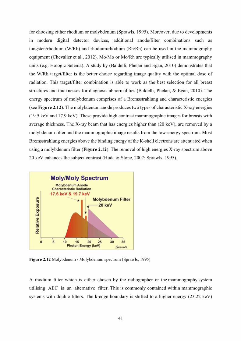
41
for choosing either rhodium or molybdenum (Sprawls, 1995). Moreover, due to developments
in modern digital detector devices, additional anode/filter combinations such as
tungsten/rhodium (W/Rh) and rhodium/rhodium (Rh/Rh) can be used in the mammography
equipment (Chevalier et al., 2012). Mo/Mo or Mo/Rh are typically utilised in mammography
units (e.g. Hologic Selenia). A study by (Baldelli, Phelan and Egan, 2010) demonstrates that
the W/Rh target/filter is the better choice regarding image quality with the optimal dose of
radiation. This target/filter combination is able to work as the best selection for all breast
structures and thicknesses for diagnosis abnormalities (Baldelli, Phelan, & Egan, 2010). The
energy spectrum of molybdenum comprises of a Bremsstrahlung and characteristic energies
(see Figure 2.12). The molybdenum anode produces two types of characteristic X-ray energies
(19.5 keV and 17.9 keV). These provide high contrast mammographic images for breasts with
average thickness. The X-ray beam that has energies higher than (20 keV), are removed by a
molybdenum filter and the mammographic image results from the low-energy spectrum. Most
Bremsstrahlung energies above the binding energy of the K-shell electrons are attenuated when
using a molybdenum filter (Figure 2.12). The removal of high energies X-ray spectrum above
20 keV enhances the subject contrast (Huda & Slone, 2007; Sprawls, 1995).
Figure 2.12 Molybdenum / Molybdenum spectrum (Sprawls, 1995)
A rhodium filter which is either chosen by the radiographer or the mammography system
utilising AEC is an alternative filter. This is commonly contained within mammographic
systems with double filters. The k-edge boundary is shifted to a higher energy (23.22 keV)

42
compared to a molybdenum filter (20 keV) (Figure 2.13). Moving to a higher energy means
that the Bremsstrahlung radiation between (20 and 23.22 keV) is included in the beam of
the X-ray. This extra radiation has a higher penetration and can be utilised for thicker or denser
breasts (Sprawls, 1995). For most clients, the Mo/Mo filter is used. However, for denser/thicker
breasts, a Mo/Rh setting with a higher kVp is automatically designated (Yaffe, 2010).
Figure 2.13 Molybdenum / Rhodium spectrum (Sprawls, 1995).
The interaction of X-ray is often among different types of detectors. Three essential atomic
interaction forms happen between the photons of X-ray and the detectors of mammography
system. These interactions involve the photoelectric effect, Compton (inelastic) scattering, and
elastic scattering (Yaffe, 2010). In elastic scattering, the emitted photon from the matter has
the same energy as the incoming photon. This means the energy of the scattered emitted photon
does not disperse when interacting with the material. In Compton scattering (Figure 2.14),
some of the photon energy is absorbed when the photons liberate a recoil electron which is a
low binding electron. The rest of the energy stays in the scattered photon (Yaffe, 2010).
Consequently, elastic scattering leads to contrast reduction, increased noise and loss of spatial
resolution (Toennies, 2012). The Compton scattering amount increases with the increase of
photon energy. The scattered photon can be dissipated in any orientation and also can be
dangerous for the operator of X-ray system (Zhang, Li and Liu, 2012).

43
Figure 2.14 The interaction of X-ray through Compton scatter (Haidekker, 2013).
The probability of photoelectric absorption per unit mass is related to the following equation.
…………. (2.1)
Where: Z is the atomic number of object and E is the energy of the X-ray (Bushberg, Seibert,
Leidholdt, & Boone, 2012). This equation demonstrates the opposite relationship between the
increment of energy and the photoelectric interaction. At low kVp levels the photoelectric
interaction dominates over Compton scattering, while at high kVp levels, Compton interaction
happens more often. Therefore, since a low energy is required in mammography, the
photoelectric effect represents the essential interaction of X-ray in the detectors (Saha, 2013).
The types of material utilised as detectors have an important impact on the increase of the
photoelectric effect. The high atomic number materials are appropriate materials for making
detectors such as selenium and iodine. At 20 keV, 96% of the interactions of X-ray will occur
via photoelectric interaction for selenium and 94% for iodine (Yaffe, 2010). As photoelectric
absorption needs low photons energies and low photons energies are required in mammography
to obtain images with better visibility, these types of materials are appropriate for
mammography detectors.

44
2.8.2 X-rays Incident on the Detector
As Figure 2.12 and Figure 2.13 illustrate, mammographic machines operate using on low-
energy photons. In order to clarify the cause of utilisation low-energy photons to output
mammographic images, the relationship between the thickness of the region of interest in the
breast, the attenuation coefficient of the breast abnormality and the mammography detector
are discussed. Since the photon of an X-ray transmits through tissues of the breast, different
reactions occur between X-ray and difference densities of the breast tissues (Yaffe, 2010).
Figure 2.15 illustrates two samples of paths that an incident X-ray transfer through the
breast, A and B. In path A, the photon moves through the normal tissue, in path B there is a
breast abnormality with the thickness ‘a’.
Figure 2.15 The pathways of transmitted X-ray A: through normal tissue of breast B: during interest
structure (Yaffe, 2010).
2.8.3 Digitization
In digital mammography, the process of converting the analogue data to a digital signal is
named digitisation. This process includes two stages: sampling and quantization. The analogue
data is produced by a detector initially, and then the detector converts it to digital data using
special electronic circuit named analogue-to-digital convertors (ADCs). The digital signal
transfers to a computer in order to digitize and store it digitally. In digital mammography, the
last step in the process of image formation is the image processing application. Image
processing is utilised to improve the diagnostic information within the image. This can be
achieved by improving the contrast and edge definition or through decreasing image noise

45
(Warren et al., 2014). Every manufacturer utilises their own image processing algorithms, and
the appearances of the image after this processing can vary between manufacturers. Many
studies have investigated the impact of these variations in image appearance (Pisano et al.,
2000; Sivaramakrishna et al., 2000) and objective studies (Chen et al., 2010; Goldstraw et al.,
2010; Kamitani et al., 2010; Warren et al., 2012). Some studies concluded that the difference
between several image-processing algorithms was significant (Goldstraw et al., 2010; Visser
et al., 2012), and others found that the difference was not significant (Kamitani et al., 2010;
Cole et al., 2003; Warren et al., 2014). In digital images many reviewed studies have attempted
to detect and estimate motion blur in digital images. A study by (Ramakrishnan, 2010)
investigated some algorithms which used to detect blurred images. However, no robust
empirical study has been published to detect image blurring in FFDM images mathematically.
Accurate identification of motion blur visually in digital images is not easy and can be carried
out using mathematical methods.
2.8.4 Pixel Size in Mammography
Pixel size and spacing affects the spatial resolution of a digital mammogram. However, more
pixels do not always offer a higher spatial resolution due to the fact that image blurring can
produce scattering of X-ray, scattering of light, and scattering of both in the detector (Chotas,
Dobbins & Ravin, 1999). For instance, the pixel size of direct selenium (about 70 μm) has
higher spatial resolution than a scintillator based system which has larger pixel size of about
(100 μm) per pixel. Commonly, the pixel size on current detectors of mammography systems
is between the range 50 -100 μm per pixel (Freitas, Kemp, Louveira, Fujiwara, & Campos,
2006).

46
Chapter Three: Medical Images Assessment Methods
3.1 Chapter Overview
Image quality assessment (IQA) is increasingly important to medical image enhancement
applications. These applications use several technologies to improve the visual appearance of
the medical images. Conventional IQA indices, such as signal-to-noise ratio (SNR) and mean
squared error (MSE), are used extensively but they do not take into account the human visual
system (HVS) (Krupinski, 2011). Medical images require human interpretation, and despite
software approaches like computer-aided detection, image analysis ultimately requires visual
and cognitive skills. A number of the IQA metrics based on HVS are used to assess perceptual
image quality. The assessment of medical imaging procedures or systems should involve the
observer since the observer’s opinion is considered an integral part of the medical diagnostic
procedure. The measurement of physical parameters is not sufficient to assess the success of
the process. Receiver operating characteristics (ROC) methods are considered a robust
approach involving performance of observer and imaging techniques (Thompson, Manning &
Hogg, 2013). Figure 3.1 demonstrates the relationship between visual performance, image
interpretation and image quality assessment methods.
This chapter is organized into six main themes. The first theme will focus on the relationship
between visual performance and medical image interpretation (section 3.2). The second theme
will focus on the human visual function (section 3.3); the third theme will focus on the receiver
operating characteristics (ROC) methods (section 3.4). The fourth theme will focus on a
location sensitive method of observation study, the free-response receiver operating
characteristics (FROC) method (section 3.5), which will be used for data collection. The fifth
theme will focus on perceptual measures (section 3.6), and finally the sixth theme will focus
on the physical measures of mammographic images and the factors which affect the conspicuity
of the breast lesions (section 3.7).

47
Figure 3.1 Relationship between visual performance, image interpretation and image quality
assessment methods.
3.2 The Relationship between Visual Performance and Medical Image
Interpretation
Visual perception represents the ability to interpret the surrounding environment by processing
information that is contained in visible light. Research in neuroscience, cognitive science and
psychology, collectively referred to as vision science, concerns certain physiological
components which make up the visual system ( Watson & Null, 1997; Manning, 1998).
Medical image interpretation is based on visual performance of an observer and visual
appearance of image. A psychophysical study by Apelt et al., (2009) has illustrated that human
detection performance does not predict pattern recognition performance, which has contributed
to the creation of a visual processing hierarchy. The process evolves as follows: detection→
discrimination→ identification→ recognition. However, it is often impossible to predict the
results at a given hierarchy level based on the results obtained at a different level (Apelt et al.,
2009). Factors affecting error in mammographic image reading are complex and difficult to
isolate. One prospective source of error could be related to reduced visual performance, which

48
in turn decreases an observer’s ability to correctly identify tiny breast lesions (Reed, 2005).
Errors related to visual perception can be classified into two categories: cognitive or visual
errors. Cognitive errors represent approximately 45% of all errors and this concerns the
observer who makes the incorrect decision (Samei & Krupinski, 2010). Visual errors represent
approximately 55% of all errors and relate to an incomplete search of the image. Manning et
al., (2004) concluded that most errors in image perception were failures of decision-making
instead of detection (Manning, Ethell and Donovan, 2004b). Visual errors may occur due to
not seeing the abnormal area or not focusing on lesion location for enough time (Samei, 2003).
Interpretation of mammographic images can be a tedious task, given its repetitive nature of this
task; but the unique nature of each mammogram means there is a unique map for every
individual. Furthermore, the mammogram of a woman changes through time, related to the
age, menopausal status, and hormonal changes (Zuley, 2010). Since breast cancer is a
commonly diagnosed cancer in females, it is important to understand visual perception in
mammography (Zuley, 2010). According to Zuley (2010), the mistakes in perceiving
mammographic images can be categorised into three types: search errors, recognition errors
and decision-making errors. If a lesion is not identified by the observer this is considered a
search error. However, if the lesion ‘catches the observer’s eye’ but is then quickly dismissed
it is considered a recognition error. This will lead to the lesion going unnoticed. Other errors
such as decision-making errors can happen when the lesion is present, however the assessment
of its nature is made incorrectly. This can result in a lesion being falsely identified as
malignancy; a false-positive (FP), or dismissed as benign when it is actually malignant, a false-
negative (FN). Anatomical noise or normal tissue structure in mammography can mask the
abnormal tissue. Decision-making errors can lead to either FP or FN decisions whereas search
and recognition errors can lead to only FN (Zuley, 2010). Figure 3.2 demonstrates the three
categories of perceptual mistakes in observing mammograms. Therefore, there is a well-known
search type called ‘satisfaction of search’ to demonstrate why the lesions stay undetected after
finding the initial lesions (Mello-Thoms, Trieu, & Brennan, 2014). Satisfaction of search can
play an essential role in missing pathologies within an image. In this condition, an expert image
reader may be ignoring other possible lesions after locating the first one.

49
Figure 3.2 Three categories of perceptual mistakes in observing mammograms (Zuley, 2010; Ossati,
2015).
3.3 Human Visual Function
Vision is the eye's ability to detect an electromagnetic spectrum of light; the brain then
interprets this information. The main function of the eye is to convert light into electrical signals
which are then transferred to the brain by the optic nerve (Gao et al., 2010). This process
includes several stages, starting with the light of an object passing through the lens to a reversed
visible image on the retina (Chester, 1992). There are several main concepts related to human
visual function; these can be evaluated with visual tests such as visual acuity, contrast
sensitivity and stereopsis. These visual parameters are recommended to evaluate and decide if
an observer has adequate eye function to participate in medical imaging observer studies
(Lanca et al., 2014). The expression visual acuity is used to designate the capacity of the eye
to resolve the size of an object. Contrast sensitivity makes the discrimination of low and high
contrast frequency information possible. This can be linked to the perception of complex
patterns in FFDM images (Apelt et al., 2009). Stereopsis can describe depth perception of
objects in the central visual area, enhancing vision quality through binocular summation.
Perceived visual errors are computed based on the visual error sensitivities to various factors
of HVS, such as brightness, contrast sensitivity and visual attention (Gao et al., 2010).

50
The main functions of the human eye are to distinguish colours and shapes and to reveal light
in the darkness. This process usually happens when light passes through the lens to a reversed
visible image on the retina (Osberger, 1999; Nadenau et al., 2000). Figure 3.3 illustrates the
anatomical structure of the human eye. The light passes through the cornea and is focused by
the lens to form an image on the retina. The retina is located at the back of the eye. It contains
two types of photoreceptors: the first, known as cones, are responsible for colour and high-
acuity (photopic) vision; the second, known as rods, are responsible for low light level
(scotopic) vision. At light levels between the photopic and scotopic range, i.e., the mesopic
region, both cones and rods provide vision (Gao et al., 2010). Rod cells are extremely sensitive
to small levels of luminance, however, they are capable only of low resolution and are therefore
of little relevance to medical imaging (Kundel, 1995). The pupil works as a diaphragm to
control the amount of light entering the eye. The lens elastically focuses at different distances;
a process referred to as accommodation. The diameter of the eye’s pupil at relaxation is
approximately 1.5 mm (Chester, 1992).
Figure 3.3 Anatomical structures of the human eye (Van De Graaff, 2001)
The construction of an image can be put through many processes at several steps in the visual
pathway from the retina to the cortex area. The retina consists of bipolar and ganglion cells,
which are responsible for transmitting electrical impulses to the brain. Cells such as horizontal
and amacrine work on lateral connections between ganglion and bipolar cells. The transmission
of electrical signals from cones to bipolar cells is responded to with a chain of electrical

51
impulses. The strength of response is coded at all the nervous systems, according to the
frequency of the electrical signal (Osberger, 1999). The visual cortex contains cells which are
responsible for image analysis and is located at the back of the brain. It can be categorised into
simple, complex, hyper-complex and higher-order hypercomplex cells. The primary visual
cortex contains simple cells which have Receptive Fields (RFs) and are characterised by
extremely structured and restricted regions of space. In spite of the fact that a limited quantity
of image processing may occur in the retina and lateral geniculate bodies, the visual cortex is
considered the essential part of image analysis (Chester, 1992).
3.3.1 Visual Acuity
Visual acuity is a measure of the eye's ability to distinguish detail. The ability of the eye to
detect small detail is a significant factor in the diagnosis of medical images. The processing of
visual information by the HVS is connected to the ability of an observer to interpret the medical
image (Safdar et al., 2009). Visual acuity is the most commonly measured aspect of visual
function (Colenbrander, 2001; Kaiser, 2009). This function could determine an observer’s
ability to determine small objects correctly, such as solitary pulmonary nodules (Bass & Chiles,
1990; Thompson et al., 2017). Several factors influence visual acuity, including illumination,
contrast, refractive error and the site of the retina being stimulated (Holladay, 2004). The
impact of the tested object features on visual acuity is related to different factors, such as
contrast of the test object, luminance distribution in the field of view, colour, movement of test
object and criterion for detection of detail (Kaiser, 2009). However, visual acuity is a complex
task. The lowest separation concerns the decision of the site of a visual target, commonly
related to another part of the same target (Holladay, 2004).
3.3.2 Contrast Sensitivity
Two concepts must be considered and differentiated in the discussion of contrast sensitivity
such as objective and subjective contrast. Objective contrast (photometric) concerns the
variation in luminance of objects or adjacent grounds. Subjective contrast (physiologic)
concerns subjective phenomena, such as the modification in the ostensible brightness of objects
of a given luminance, which is related to the luminance of the background. Overall, visual
acuity reduces with a decline in photometric contrast; this becomes clearer with small test
objects (Watson & Null, 1997). The influence of physiologic contrast is important. The
borderline between a dark and luminous surface causes a blurred, unfocused retinal image to

52
be produced by the veiling effect of stray light and the optical aberrations of the eye. These
impacts are off-set by physiologic contrast. The image on a white background appears whiter,
the image on a black background appears darker and the border becomes sharp when the two
edges meet each other (Apelt et al., 2009). With low contrast levels, visual acuity changes
significantly; but at high degrees of contrast, comparatively great variations in objective
contrasts have minimal impact on visual acuity (Jackson, 1996).
3.3.3 Visual Function Assessment
There are different techniques that can be used to measure and specify visual acuity and in its
measurement, it is essential to use eye-validated charts. Typically, these contain capital letters
organised in rows with the largest letters at the upper part of the chart decreasing gradually to
the smaller letters at the bottom of the chart. There are several charts which can be used for
visual acuity measurements, examples include senllen and ETDRS (Kaiser, 2009). The
ETDRS chart is considered to be the gold standard for vision measurement in clinical trials
(Kaiser, 2009). Visual acuity measures are used to describe the capacity of the eye to resolve
the size of an object. It is the sharpness or clearness of vision and this is defined based on the
clarity of focus in the retina of the eye. However, the processing of visual information by the
human visual system describes the ability of the observer to interpret and understand the
(medical) images. The reduced visual acuity might significantly raise the contrast threshold
required to identify high-frequency information. Visual acuity hinges on the site of the retinal
stimulus and reduces sharply with a rise in the distance of the image of an object from the
centre of the fovea. The complex patterns of mammography perception are related to the
contrast sensitivity of the visual system (Apelt et al., 2010). Pattern-detection ability is
provided by eye contrast sensitivity for stimuli of various sizes and if abnormal contrast
sensitivity is present, low-contrast targets are difficult to appreciate and can be missed. The
limitation of visual acuity is caused by aberrations, diffraction and photoreceptor density in the
eye (Holladay, 2004). In comparison, contrast sensitivity measurement is known as the ratio of
the average background intensity to the peak amplitude of the spatial sinusoid at the threshold
that is used as the test stimulus.
There is an additional factor which affects visual performance measurements known as
contrast sensitivity function (CSF). Grading the contrast sensitivity function is a valuable
measure of visual function. It quantifies the capability of an observer to perceive small changes

53
in luminance between areas which are not isolated by definite borders (Arden, 1978; Apelt and
Peitgen, 2008). Higher contrast sensitivity includes the identification of sinusoidal gratings,
which are a model of black parallel bars and parallel light that measure the sensitivity of the
eye through bar widths or a range of spatial frequencies (Drum, Calogero and Rorer, 2007).
Visual Attention is the process of concentration in the sense of excitation, whether this
excitation is sensory or mental. Perceptual quality measures are based on models of human
visual perception. Several perceptual image quality metrics are proposed as alternatives to
objective metrics, such as methods incorporating models of luminance adaptation and Contrast
Sensitivity Function (CSF)(Gao et al., 2010). An early study by Riggs (1965) described the
relationship between luminance intensity and visual acuity; it has been utilised within test
objects within a white background. Riggs (1965) illustrated that visual acuity is low at dark
levels where peripheral rod receptors or parafoveal dominate. As the light intensity level rises,
the cone receptor thresholds increase and acuity rises sharply. As the intensity increases once
more, a level of maximum acuity is reached and this can be maintained across further increases
in intensity. The influence of luminance on visual acuity includes the pupil size. The ideal
visual acuity is related to the pupil size of approximately 2 mm. However, the optimal size
changes with levels of luminance, the size of the test object and other characteristics. A large
pupil means more light will pass through the eye but this can also lead to visual aberrations.
Luminance of the ambient lighting in a radiology reporting room typically should be below 10
lux. These aberrations are reduced with a smaller pupil size, but a very small pupil size can
lead to decreased visual acuity because the impact of light diffraction, through decreasing
retinal luminance, is raised. Luminance of the ambient lighting can significantly affect the
detection of microcalcifications in high density breasts (Thompson et al., 2017).
3.4 Receiver Operating Characteristics (ROC) Methods
The receiver operating characteristic (ROC) method is considered a valuable tool to evaluate
the combined performance of the imaging system and observer in radiology. The historical
background of ROC was established upon the fundamental principles of signal detection theory
(SDT) (Li et al., 2010). This paradigm originated in the 1950s when it was used to establish a
radar’s ability to detect approaching aircrafts. In 1960, a number of studies and books were
published by Dr Lusted that encouraged the utilisation of ROC analysis in diagnostic radiology
(Metz, 2008). However, this recommendation was not implemented until the 1970s, when

54
many laboratory studies were conducted by some researchers at The University of Chicago that
led ultimately to the adoption of ROC analysis in medical imaging, and this lead to the
development of new analytic techniques (Metz, 2008).
There are many applications for ROC methods; they can be utilised in several modalities for
different purposes. The ROC modalities can be used to compare old imaging techniques with
a modern alternative. For instance, the ROC method can be used to make a comparison of the
diagnostic performance between different models and it is a common choice of model (Bator
and Chmielewski, 2008). Also, the ROC method can be used to compare between two new
technologies in mammography such as digital mammography versus digital breast
tomosynthesis (Gennaro et al., 2010). In digital mammographic image screening trials, both
film screening (SF) and full field digital mammography FFDM can be obtained in each patient
and the diagnostic performance of the observers for the two mammograms can be compared.
The ROC paradigm can be generally described as a graphical curve that shows the performance
of a binary classifier process, which consists of the true positive fraction known as sensitivity
(equation 1) plotted against the false positive fraction known as 1-specificity (equation 2)
(Metz, 2008).
………………………. (3.1)
……………………… (3.2)
The performance of any screening programme can be evaluated by three relevant parameters:
sensitivity, specificity and positive predictive value. The expression of sensitivity and
specificity is a measure of the observer performance of a binary decision; yes or no. This is a
limitation in that it is difficult to help the observer estimate the probability of lesions in
individual cases (Akobeng, 2007). A true positive (TP) decision occurs when the disease is
present and identified by the observer while a false negative (FN) decision occurs when the
disease is present and either overlooked or misinterpreted by the observer (Equation 2). The
remaining possibilities are true negative (TN) decisions, wherein the disease is absent and the
observer agrees, and false positive (FP) decisions, wherein the disease is absent and the
observer disagrees (Obuchowski, 2005).

55
Positive predictive value and negative predictive value can be affected by disease prevalence.
Negative predictive value is the probability that the lesion is not present when the result of the
test is negative while positive predictive value means the ratio of the actual number of cancer
cases to the number of abnormal cases detected by the programme (Equation 3). The same test
can produce different results in two populations (Chakraborty, 2011).
………………. (3.3)
The operating characteristics can be expressed in several forms projected by the search method
from which they have been extracted. Table 3.1 outlines concisely several ROC methods.
Table 3.1 Summary of development and comparison between ROC methods.
Full name Abbreviation Description Description of plot
Properties & comparison between each
method
Receiver Operator Characteristic
ROC Differentiates between normal and abnormal images
TPF versus FPF
Does not consider the location of the lesions. Low statistical power
Localisation ROC
LROC Identifies localisation of one abnormality in the images. This can be used as it is still a single rating per case/image
TPF versus FPF
Incorrect location of lesion considered as false positive
Free-response ROC
FROC Identifies and localises several abnormalities within the images Discriminates between malignant and benign
LLF versus NLF
localised several abnormalities Mark-rating according to BI-RADS Confidence level Multi-reader multi-cases
Jackknife alternative FROC Analysis
JAFROC A re-sampling method that does not assume independence of responses within the same study applied to FROC
AFFROC curve is a plot of LLF versus FPF
A high statistical power method required multiple observers and multi-cases
The ROC curve is the graphical scheme of true positive fraction (TPF) versus false positive fraction (FPF)
while the FROC curve is the graphical scheme of lesion localisation fraction (LLF) versus non lesion
localisation fraction (NLF) and the AFROC curve is the scheme of LLF versus FPF
The ROC modalities have several measures which can be used, according to the design or the
purpose of each study. According to Metz (2008), the ROC study can be divided into two types

56
of designs: clinical and laboratory studies. This refers to where the image-reading data is
collected, either in clinical or laboratory based research, and it is important to understand the
pros and cons of each approach. In laboratory studies, data collection can be most closely
controlled so that statistical variation is decreased with increased statistical power, and the
situations that led to the study’s conclusion are better understood (Gur, 2007; Metz, 2008).
However, in the routine clinical practice, the data collection better represents the ‘real world’
with regard to a condition which we would like to draw conclusions about (Metz, 2008).
ROC analysis considers the ability of human observers to distinguish between patients that are
actually negative and positive for disease, which has been previously confirmed by a suitable
arbiter (Metz, 2008). Since the performance in ROC methods depends on the human observer,
there is a reasonable probability that the performance may be affected by the individuality of
the observer; for instance the expertise of the image reader, fatigue, display environment and
other conditions (Chakraborty and Yoon, 2008). Rating scales utilised in ROC analysis allow
an observer to provide a numeric rating to an image, based on the perceived probability that
disease is present (Chakraborty, 2002). This rating is used to assess the disease existence or
absence. The low confidence level means that the observer believes that the image is more
likely to be negative for disease (normal). In contrast, the higher confidence ratings reserved
for cases that the observer believes are positive for disease (abnormal) (Chakraborty, 2011).
The decision threshold is a scalar quantity; not a random variable, used in an observer
performance study. It is different from the confidence level; a random variable.
The capabilities of the classic ROC analysis can be limited in some applications. For instance,
the location of the lesion is ignored and the task of the observer is just to decide if a case is
normal or abnormal (Chakraborty and Yoon, 2008). The true positive (TP) is insufficient if the
lesion location is obscure or incorrectly localised (Chakraborty and Berbaum, 2004). In
addition, the classical method may not take into consideration if there is more than one lesion
present in the same image. This can lead to clinical consequences resulting from missing
lesions and can have an effect on the truth of image quality description (Svahn and Tingberg,
2005). The ROC method is extensively described (Park et al., 2004; Chester, 1992; Metz, 2008)
and has been the method predominantly chosen to assess the detection performance of a single
pathology for many years. However, there are some limitations associated with the classic
method. For example, not all of the information available within an image is taken into account

57
and the system has trouble coping with multiple pathologies. Although ROC methods are
considered the typical process to evaluate performance and ROC is very useful for evaluating
diffuse disease such as chest infection or pneumonia, the limitations discussed above are
considerable and have led to the development of more advanced methods such as FROC and
AFROC.
3.5 Free-Response Receiver Operating Characteristics (FROC) Method
The free-response ROC (FROC) method takes into account the precise location of disease,
where it can accurately measure cancer detection performance in FFDM images (Ruschin,
Timberg and Båth, 2007a). In a FROC study, theoretically unlimited numbers of abnormalities
can be localised in a single image by observers, with each localisation requiring an individual
rating to describe the observer’s certainty that the abnormality (suspected lesion) is malignant.
The FROC method allows observers to localise multiple lesions in each case (Chakraborty and
Berbaum, 2004). The main aspect of the FROC method is the ability to penalise incorrect
localisations and to reward correct localisations, this means making the use of location
information efficient. It should be acknowledged that the FROC method has more clinical
relevance than the ROC for masses and lesions; however, it is a demanding perceptual task for
the observer. In the FROC method, the observer does not know the number of lesions that
might exist in an image. Thereby, the observer’s task is to search the image for disease and
mark all areas which raise suspicion of an abnormality; for each of these marks they must also
provide a rating from a confidence scale; this process is known as creating a series of mark-
rating pairs, which is considered the basic unit of data.
The fundamental variations between ROC and the Free-response ROC methods are in the
figure of merit (FOM) quantifying observer performance and in the data collection step
(Chakraborty and Yoon, 2008). In the ROC paradigm, lesion localisation is not required and a
single rating is collected for each image, while in the free-response ROC paradigm, the data
involves mark-rating pairs. These are classified into lesion-localisation (LL) and non-lesion
localisation (NL) by a proximity criterion (Chakraborty, 2002). Secondly, in a ROC study, the
FOM refers to the areas under the ROC curve. In contrast, computation of the FROC FOM
includes creating two lists: an abnormal-list and a normal list. The abnormal-list is a record of
the ratings for each lesion. The normal list is a record of the higher mark-rating (essentially a
non-lesion) for each normal image (Chakraborty, 2010a). The number of normal images

58
represents the number of entries in the normal list. The total number of lesions is the
corresponding number for the abnormal-list. The calculation of FOM includes making all
probable comparisons between the quantities in the two lists (Chakraborty and Berbaum,
2004). The FOM is considered as the possibility that a lesion rating skips all non-lesion
localisation ratings on normal images (Ruschin, Timberg and Båth, 2007a).
3.5.1 Constructing Curves from FROC Data
In FROC, the observer’s task is to search the image and mark areas, which are expected to have
lesions. The ROC curve can be computed in a similar process to those for the FROC curve.
Nevertheless, they are normalised to a different denominator. The LLF is normalised to the
number of lesions whereas the NLF stays normalised to the number of cases. The significant
variation between accounts of the operating points for the FROC curve is that it covers all of
the ratings that are made for each image within its calculations, whereas the ROC curve only
considers the highest ratings.
The overriding value of observer performance studies is the calculation of a figure of merit
(FOM) to summarise the performance of the imaging system and observer, which rewards
correct decisions and penalises wrong decisions. It provides a single value summarising
performance which can be compared statistically. For instance, to compare two types of
imaging systems, one calculates a FOM for each method and a statistical test is performed to
identify the difference between two FOMs and whether the difference is considered large
enough to be different in consideration of the pre-test value of alpha (Chakraborty, 2011). The
value of probability is quantified by the p-value (Chakraborty, 2011) When the p-value is
smaller than 0.05, one deduces that there is a significant statistical performance variation
between two modalities - a difference greater than would be expected by chance alone. The
calculation of the overall regions of interests (ROIs) produces the nonparametric area under the
curve (AUC) of a receiver operating characteristic curve known as a figure of merit (FOM)
(Chakraborty et al. 2011).
The AFROC curve is represented as the plot of LLF versus FPF. It can be noted that the
difference between the ROC curve and AFROC curve is just in the descriptions of the y-axes,
which means TPF versus LLF. Lesion localisation can be distinguished in good assessments
by using the FOM or the area under the AFROC curve while non-lesion localisations on the
normal image can be penalised to different marks. For instance, an upper rated FP is penalised

59
more than a lesser rated FP. Figure 3.4 demonstrates use of the FROC method to localise breast
lesions. In the FROC method, two different types of the curve can be generated: the FROC
curve and the alternative FROC (AFROC) curve. On the FROC curve the y-axis is normalised
to the number of lesions (LLF) rather than the number of abnormal cases, as in ROC analysis.
Thus, ROC is a case based analysis and the observers make case based decisions, whereas
FROC is lesion based analysis.
3.4(A) 3.4 (B)
Figure 3.4 The use of FROC methods to localise breast lesions
(A) 5 confidence levels and other available functions (Chakraborty, 2002).
(B) ROCView tools utilised within in this study
3.5.2 FROC Data Analysis
An increase in the number of observers that read or assess the same image set, leads to an
increase in the statistical power of the study. This procedure is known as the multi-reader multi
cases (MRMC) method. Furthermore, an increase in the number of cases in the study leads to
an increase in the statistical efficiency. JAFROC analysis successfully overcomes obstacles
such as the limitations in the classical ROC method, through the use of the multi-reader multi
cases method (Federica Zanca et al., 2012). The JAFROC figure of merit refers to the
probability that lesions ratings (LL marks) are rated higher than all noise sites (NL marks) on

60
normal images (Chakraborty & Berbaum, 2004). There are two approaches for MRMC
analysis, (i) the Obuchowski-Rockette (OR) method and (ii) the Dorfman-Berbaum-Metz
(DBM) method. The OR and DBM methods are equivalent and are precisely equal when the
jackknife method is utilised (Hillis, Berbaum, & Metz, 2008). The DBM-MRMC process is a
widely utilised method in ROC analysis, whereas the AUC (Area under the curve) is utilised
as the FOM and data are analysed utilising analysis of variance (ANOVA) (Obuchowski et al.,
2004; Buissink et al., 2014). The DBM method distinguishes between the variables of case
difference and the variance within and among observers to evaluate whether the observed
difference is caused by the observers or by the cases of the study. This is known as the jackknife
method, where pseudovalues are computed by systematically excluding one case at a time and
then searching the variance in accuracy assessments between the evaluation of all data and with
that case excluded (Chakraborty, 2010a).
3.5.3 Jackknife Analysis of FROC Data (JAFROC)
The JAFROC method is the equivalent method for analysing free-response rating data and the
JAFROC figure of merit refers to the probability that lesions ratings (LL marks) are rated
higher than all noise sites (NL marks) on normal images. The JAFROC figure of merit is the
trapezoidal under the AFROC curve, θ. The JAFROC figure of merit can be described by
equation 4:
∑ ∑ , …………….. (3.4)
Where Xi is the maximum noise rating (mark on a normal case) for a case i, Yj is the rating for
the jth lesion, NN is the number of normal cases, and NL is the number of lesions. The psi (ψ)
function is the comparison of the highest rated noise rating and the lesion rating (Chakraborty,
2010c). For the ψ function, if Xi (abnormal) is greater than Yj (normal) then ψ=1; if Xi is less
than Yj, then ψ=0; if they are equal ψ=0.5 (Chakraborty, 2010b).
Chakraborty et al., (2006) illustrated that the statistical power of JAFROC is greater than the
statistical ability of the previous ROC methods (Chakraborty and Berbaum, 2004). JAFROC
was developed as a multi-reader, multi-cases process in order to be able to deal with the
limitations in the classic ROC method. The statistical power of diagnostic performance of
JAFROC analysis is increased according to the sample size, in comparison with ROC.

61
The similarities are recognised by the pseudovalue denotation in JAFROC analysis (Equation
5):
1 …………… (3.5)
Where the pseudovalue for each modality i, observer j and case k is defined by PVijk, NT is the
total number of cases, θij is the figure of merit for modality i and observer j for all data, and
θij(k) is the figure of merit with case k removed – identifying the dependence of each case
(Chakraborty and Berbaum, 2004).
3.6 Perceptual Measures
When comparing methods of image quality assessment, perceptual and physical methods,
perception methods are considered more helpful to determine diagnostic abilities than objective
methods (Goossens et al., 2013). However, some human observer studies, such as two alternate
forced choice (2AFC), may be time consuming, and therefore expensive, so supplementary
objective measures are helpful to support human observer studies (E. Burgess, 1994; Richard
and Siewerdsen, 2008). The 2AFC method can be utilised to compare the subtle variances
between the performances of different imaging modalities (Burgess, 2011). Revesz et al.,
(1974) calculated the conspicuity of lung nodules. Image observers were requested to find the
existence of a lesion and localise it. They concluded that the computed conspicuity correlated
with the possibility to detect an abnormality within a limited range of conspicuity values. Samei
et al., (2003) calculated the contrast-diameter product, according to local anatomical noise, and
concluded a correlation between the ability to detect lesions and this measure. However,
attempting to find a correlation between human observer studies and objective measures has
not proved successful (Samei et al., 2003). Manning et al., (2002) demonstrated a poor
relationship between the measure of conspicuity index and undetected lesions in chest
radiography and pointed out that decision errors were more common detection errors.
However, it must be noted that the study size was small, and only four regions around the lesion
(four profiles) were used which means that the computing of conspicuity had some limitations.
The study also included other categories of observer error as initially mentioned by Kundel et
al., (1974) (Manning and Ethell, 2002). Mello-Thoms et al. (2005) demonstrated, through an
eye tracking study, that undetected lesions predominantly received sufficient visual attention.
Other eye tracking studies such as (Chesters, 1992; Manning, Ethell and Donovan, 2004a;

62
Mello-Thoms, 2006) demonstrated that lesion conspicuity, or the period of time it is viewed,
is not the only reason they go undetected. Mello-Thoms et al., (2005) assessed the effects of
breast masses’ conspicuity on the decision outcome of the observers. They suggested that
breast mass conspicuity has an impact on the visual search in a mammography reading. They
compared the visual search strategy utilised by an expert in mammography and concluded that
most undetected malignant masses did attract a certain amount of visual attention; nevertheless,
it was in the processing of the produced information in the lesion location that most errors
happened. In summary, errors in Radiology are unlimited to observers missing lesions because
they are poorly clarified; it is valuable to inform efforts to enhance the radiological task with
calculated image quality that utilise functional data on visual performance (Mello-Thoms et
al., 2005).
3.7 The Physical Measures of Mammographic Images
The image quality of mammographic images can be assessed in several methods. Medical
imaging devices are quality controlled utilising structured phantoms; measures such as spatial
resolution, in terms of modulation transfer function (MTF), signal to noise ratio (SNR) and
contrast to noise ratio (CNR) are utilised to assess if the equipment is working within
acceptable performance standards (Samei, 2003; NHSBSP Equipment Report, 2007).
However, these physical parameters are not exemplifications of a diagnostic image and their
output measure is not related to any particular radiological task (Samei, 2003). Therefore, there
is a requirement that these measures (SNR and CNR), and other parameters, are utilised to
determine the effect of image quality on detection performance and to provide support
investigations about the influence of physical measures on visual appearance of lesion futures
within the images (Desai, Singh & Valentino, 2010). Other parameters such as the conspicuity
of lesions, the size and contrast of lesions is helpful to characterise lesion features (Manning et
al., 2004a).
3.7.1 Measuring Conspicuity Index
Initially, conspicuity was introduced as a concept to quantify errors made by observers in
radiology. The conspicuity of a lesion represents a ratio between the contrast of a lesion and its
surrounding complexity. A study by Kundel et al., (1976), introduced a new method to describe
and determine the conspicuity of the lesion. They utilised a measurement of lesion conspicuity

63
to describe the probability of detection of a lung nodule in the chest X-ray. The lesion contrast
is represented by the density alteration around the lesion edge, while the surrounding
complexity is the rate of change of the density around the lesion border. This produces a
description of anatomical, or structural, noise which puts into consideration the surrounding
structures and artefacts. However, Szczepura & Manning, (2016) identified that this equation
does not take into account other characteristics that can affect lesion conspicuity such as noise,
contrast and lesion size.
In observer studies, Likert scales are commonly utilised in attempts to measure conspicuity,
whilst drawing comparisons between different acquisition parameters or utilising varying
contrast agents (Van Ravesteijn et al., 2013; Marin et al., 2013). The Likert scales within these
studies were quite different in terms of the number of points included on the scale and terms
set for each point. This means that the scale is entirely task dependant. However, Likert scales
are open to bias as both cognitive and perceptual errors may become involved within the task,
as such the use of Likert scales is not an ideal measure of conspicuity (Weiner, 2010).
Conspicuity can be measured utilising just noticeable difference techniques, such as two 2AFC
methods, which the task of the observer is to select between two images. The first image is
known as a static reference image and the other differs based on the research question being
asked. According to the design technique of the studies, this method is more likely to be un-
bias than Likert scales and has a low variability (Szczepura & Manning, 2016). The 2AFC
method requires a considerable group of images and is time consuming, according to the
number of observers that are required; this leads to raise the cost of the study. Furthermore, the
observer can be asked a number of questions via 2AFC, not only about conspicuity, which can
lead to the obtainment of a more complex depth of data (Burgess, 2011). In 2AFC, the order
of data should be taken into account. This means a creation of ordinal data, where the images
are arranged in order, and the variance between the ranks are presumed to be equal. Thus, the
outcomes are in accordance to the dataset utilised within the study. Brook et al., (2013) and
Chang et al., (2013) utilised region of interest data to evaluate conspicuity with a comparison
made between the lesion and its surrounding background. In spite of being an objective method
to quantify lesion conspicuity, it does consider other factors such as sharpness and lesion size,
which affect the conspicuity of a lesion.

64
3.7.2 Factors Affecting Conspicuity
Szczepura & Manning, (2016) summarised the factors affecting lesion conspicuity; these
factors are the; sharpness of the edges, lesion size, structural noise (within and surrounding a
lesion) and contrast. Following is a review each of these factors individually:
3.7.2.1Sharpness
Sharpness means the capability of the system to demonstrate distinctive anatomical structures
within the object being imaged (Samei, 2003). For example, the sharpness of the edge of a
lesion is important because it affects its visibility. There are mathematical methods to quantify
the sharpness of system. Point and line spread functions and their Fourier transform, the MTF,
all measure the resolving ability (Samei, 2003) or spatial resolution of a system. They take a
number of things into consideration that can lead to blurring of borders, such as: the poly
energetic beam, focal spot size and any magnification. Blurring can also occur because of
movement of the imaging system or patient. Blurring is the reason behind reduction of visibility
of fine details, decreased spatial resolution and minimal sharpness of image.
3.7.2.2LesionSize
The size of a focal lesion is a significant factor used to determine the conspicuity of a lesion. A
study by Plöckinger (2012) demonstrated that small lesions, of less than 1cm, can be undetected
when imaged by 2-dimensional images (Plöckinger, 2012). According to Delrue et al., (2011)
3mm is considered the threshold size limit for perceiving a lesion. If the edges of the tested
object are parallel to the X-ray beam, or when the borders are bevelled (either caused by blur,
or anatomical reasons) then this affects the visible threshold size (Delrue, Gosselin & Ilsen,
2011). Birdwell et al., (2001) demonstrated that in mammography about 81% of undetected
lesions in their study were less than 20mm. In addition, a study by Michealson et al., (2008)
demonstrated that the median size of detected lesions by screening mammography was 7mm,
with 40% of lesions measuring 5mm (Michealson et al., 2008). Anatomical structure
superimposition: during the measurement of contrast to noise ratio or signal to noise, the noise
is commonly calculated from a background that does not involve complex surrounding
structures; thereby these complexities that affect the lesion detection can be unrecognised with
these standard measures (Eckstein and Whiting, 1995).

65
3.7.2.3Noise
Noise refers to undesirable changes within an image that do not exist within the imaged subject.
(Samei, 2003), when considering lesion conspicuity, said there are two types of noise that
should be taken into account, radiographic noise and structural noise. Radiographic noise can
be calculated utilising SNR, and offers information about the capability of the system,
nevertheless it does not give the full information about the noise within a clinical image. It is
stochastic in nature and due to several factors, such as the detector capability and the exposure
factors utilised (Samei, 2003). Radiographic noise, however, is not dependent on the subject
being imaged (Szczepura & Manning, 2016). During the explanation of radiographic noise,
two terms should be clarified: absolute noise and relative noise. The term noise is commonly
utilised to describe both quantities, (relative and absolute). Relative noise represents the
amount of image changes relevant to the signal existing in the image; for instance, it is equal
pixel standard deviation divided by mean signal. Relative noise represents the relevant factor
in the detection of lesions. When unqualified, the term noise is predominantly referring to
relative noise whilst absolute noise is referring to the absolute amount of changes within the
image, which equals pixel standard deviation (Samei, 2003).
3.7.2.4Contrast
Contrast is an important measurement of the diagnostic ability of a device. SNR and CNR are
standard measurements used to characterise this within the clinical evaluation of images and in
quality control. They refer to the variance in signal amplitude between the lesion and the
background (Michaelson et al., 2003). Both SNR and CNR are utilised as an objective measure
of the image quality. Calculations are made based on the signal of the abnormality and the
signal of the surrounding regions; this data is then utilised to measure either the SNR or the
CNR.

66
Chapter Four: Methodology
4.1 Chapter Overview
This chapter gives an overview of methods used in the thesis. The chapter commences by
outlining the design of the free-response study and how simulated motion blur was applied to
the FFDM images. The study comprised of 8 logical steps, using five different software
applications; each having a specific function in the study.
Step 1: Image selection- In the first step it was necessary to identify a selection of suitable
FFDM mammography images with half of them containing disease (malignant mass or
microcalcification) and the remaining half being disease free. The cases were selected via a
retrospective review of 420 cases from a single UK Hospital Trust.
Step 2: Image assessment- The selected images were assessed by an experienced reporting
consultant radiographer with two purposes in mind (i) to ensure that the images were free from
motion blur, and (ii) to confirm the precise anatomical location of all malignant lesions.
Step 3: Applying and validating simulated motion blur- Novel mathematical simulation
software was used to mimic the effect of blurring produced by breast movement during image
acquisition. Different magnitudes of simulated blurring were applied to the images. A face
validity check was performed with 8 mammography practitioners. This was done to establish
whether a difference in appearance could be detected between simulated blur and real blur.
Step 4: Observer performance study- The design of the free-response study gave due
consideration to sample size, in order to produce a statistically powerful outcome. Other aspects
to consider included data collection, monitor specification, ambient lighting, fatigue, case
memory, training, the truth status (location of disease) of the images, and the acceptable level
of error for localisation.
Step 5: Statistical analysis- Data analysis of free-response data was performed using Rjafroc
(Chakraborty and Zhai, 2015); where I also used alternative FOMs to provide values of
sensitivity (FOM = HrSe) and specificity (FOM = HrSp). A method is also described for
combining data to represent the dual reporting that occurs in clinical practice in the UK.
Step 6: Lesion conspicuity (Masses) - Conspicuity software was used examine the physical
parameters of malignant lesions; this included the conspicuity index, edge angle, contrast, and

67
SNR. The objective is to identify a relationship between physical parameters, lesion
detectability, and the impact of different magnitudes of simulated blurring.
Step 7: Dispersion Index (Microcalcifications)- It is not possible to evaluate conspicuity for
very small objects. A Dispersion Index (DI) is proposed to evaluate the detectability of
microcalcifications: this accounts for the spread of microcalcifications (units of distance),
contrast, and SNR.
Step 8: Missed lesion analysis- This was completed in an attempt to establish a reason why
observers failed to detect lesions, and where the changes in detection occurred because of
image blurring. The following question was posed: What affects the ability of the observer to
differentiate/characterise lesions into benign and malignant categories? The method for this
thesis is summarised into the following steps (Figure 4.1).

68
Figure 4.1 Key Steps within thesis methodology
Step 6: Lesion Conspicuity (Masses)
Step 4: Observer Performance Study
Step 5: Statistical Analysis
Step 3: Applying & Validating Simulated Motion Blur
Step 1: Images Selection
Step 2: Images Assessment
Step 8: Missed Lesion
Analysis
Step 7: Dispersion Index
(Microcalcifications)

69
4.2 Step 1: Image Selection
In total, 420 retrospective cases were provided by the Predicting of Cancer at Screening
(PROCAS) data set under the supervision of a Hospital Trust; ethical approval was granted via
organisational management consent (Appendices A, B & C). Each case included four images
(Right and Left CC and MLO), 150 of these cases were classified as normal and 270 cases
were reported as abnormal and contained biopsy proven cancers. The abnormal cases were
further classified into microcalcifications (120 cases) and masses (150 cases). All abnormal
cases were evaluated by a reporting consultant radiographer with 17 years reporting experience
to confirm the presence and precise location and disease and to determine (i) the distribution
of different types of breast cancer (according to shape, size, and distribution) and (ii) breast
density within this sample. The Breast Imaging-Reporting and Data System (BI-RADS) was
used to categorise cancers by shape, distribution, and size of lesion. This reporting consultant
radiographer also assessed the images to ensure that they were free from motion blur. Tables
of the Collected Data (see section 4.12) demonstrate the features mammographic images (view
of image, breast density, and number of lesion per image). The characteristics of malignant
breast masses with different shapes of margins, lesions’ BI-RADS and sizes of lesions are
presented in (Appendix G).
The GE Seno Essential FFDM system was used to acquire images for all the cases in the
PROCAS dataset. This FFDM unit has a 23x19.2 cm2 field of view, alpha-Si flat panel coupled
with a CsI (Tl) scintillator image receptor with 100-micron pixel size and spatial resolution of
7.1 lp/mm; this conforms to the standards of the UK Breast Screening Programme. This system
was operating within the NHSBSP quality assurance guidelines for mammography quality
control in the UK (NHSBSP Publication No 60, 2005; NHSBSP Publication No 63, 2006;
NHSBSP Publication No 59, 2011). The working principle of the FFDM machine has been
discussed in Chapter 2.
4.3 Step 2: Image Assessment
The normal images were previously formally reviewed and identified as normal through the
standard NHS Breast Screening Programme double reading process by two breast imaging
professionals. In addition, two different breast imaging professionals verified the images were
correctly classified as normal. The verification task was conducted with ambient lighting levels
set to less than 10 lux, being similar to hospital reporting rooms.

70
Artefact-free mammographic images were selected from a set of FFDM images. The images
were assessed visually to ensure that all anatomical structures had distinct /sharp edges. Two
clinicians classified the images and then subdivided according to the following criteria:
a) Type of lesion (malignant microcalcification and malignant masses)
b) Lesion localisation (determining the location of the lesion within the breast and marking
the lesion)
c) Denoting whether the image is sharp/unsharp (free of motion blur or not)
d) Identifying lesion size (measurement the size and create the acceptance radius).
e) Determining the lesion BI-RADS according to suspicion suspicious of malignancy of
breast lesion.
f) The breast density: the images were subdivided into four groups according to BI-
RADS.
When denoting whether the image was sharp or unsharp the two clinicians took the following
into consideration (Taplin et al. 2002; European Commission 1996):
a) Visualisation of pectoral muscle margin fibrous strands and all vessels should be sharp
(absence of movement)
b) Visually sharp medial breast tissue and lateral glandular tissue.
c) Visualisation of skin structure along the pectoral muscles should be sharp.
d) Visualisation of the retroglandular fat tissue and skin outline should be sharp.
4.4 Step 3: Applying & Validating Simulated Motion Blur
A mathematical model was used to simulate motion in the FFDM images (Ma et al., 2015).
Simulated motion blur was applied using a convolution mask that provided a 3 standard
deviation (3SD) distribution of blur over the desired blur radius. The 3SD range is consistent
with the application of a Gaussian blur mask, typically used to generate generic blur effects
(equivalent to a semi-transparent film being placed over an image). However, the Gaussian
distribution profile did not match the characteristics of a typical blur effect. To determine an
appropriate blur distribution function a simulation of image pixel motion, under elastic
restitution, was made. This allowed an individual pixel to be displaced by a random vector
(within the range of the blur effect) and the pixel contribution to the overall image sampled by
sub-steps, as the pixel returned to the central position. Sampling of the motion pixel was
enacted as a pixel sized Gaussian distribution within a super-sampled image frame to allow for

71
fractional motion within each sub-step. Repeated iterations of this process enabled a
representative distribution profile to be generated that showed a sharper central peak, more
rapid initial distribution decay, and longer continuation, than with a traditional Gaussian
function. Multiple applications of the simulation were made to define an average distribution
function. To ensure that the intensity window of the pixel values remained the same after
blurring, the pre-blurring minimum and maximum pixel intensities were corrected post-
blurring through intensity scale and shift.
Ma et al. (2014) suggested that paddle motion could be one source of motion blur. They
concluded that the extent of paddle motion, through acquisition of mammographic images,
could be as much as 1.5 mm in the vertical plane. Ma et al. (2015) illustrated that simulated
motion blur at 0.7 mm is the minimum amount of simulated breast movement required for
visual detection of blurring. Therefore, the minimum and maximum visual levels for blurring
were selected as 0.7mm and 1.5mm respectively. Figure 4.2 shows an example of FFDM
images, with and without simulated blur imposed.
Figure 4.2 Example of FFDM images with two levels of simulated blur and without simulated blur

72
4.4.1 The Convolution-based Operations and Blurring masks
The fundamental process in image processing is a digital convolution in the spatial domain and
is utilised to either sharpen or smooth an image. It includes a “shift” and a “sum-of-products”
operation. The main concept is that a kernel or mask, principally a matrix of k × k elements,
is rotated by 180° and animated in a bitmap model across an input image of M×M pixels; k is
normally an odd integer, considerably lesser than the linear size of the image. Every pixel of
the output image is the weighted sum of the input pixels within an area known via the mask,
with the elements of the mask which set the weights (Tobergte & Curtis, 2013).
When the input image is F (of size M×M), and the convolution mask is H (size k × k), the
output image G is given by:
∗ ………… (4.1) The above mathematical process is demonstrated in Figure 4.3. The mask is rotated by 180°
and is placed on top of the input image beginning at the upper left position. The mask
components are doubled by the corresponding pixel value in the image beneath and the outputs
are summed and normalised to create a measured restraint, which is the value of the product
pixel at the placement congruous to the middle of the mask. Nearly all the mask k is selected
to be odd so that the middle of the mask is readily visible. After that, the mask is moved one
place to the right, the total of products re-studied and normalised to show the following pixel
amount in the production image. This operation is reduplicated as the mask is passed towards
the inserted image in a raster scan (Tobergte & Curtis, 2013).
Predominantly, the “sum-of-products” formulation can result in pixel overflow. Normalisation,
by dividing the total of the mask components, produces a weighted response that stays within
the initial range of pixel values in the input image. The product of output image pixels
predominantly have non-integral values. Therefore, working with floating-point numbers is
important to avoid “round-off” errors (Young et al., 2008).

73
Figure 4.3 Digital convolution: the mask is put on the original image, mask components are multiplied
pixel values, and the outcomes added to form an output pixel (Tobergte & Curtis 2013).
The primary rotation of the mask through 180° is not obvious when the mask is circularly
symmetric, as it is for several common masks utilised in sharpening and smoothing. However,
this is not usually the case for the masks utilised in locating vertical and horizontal edges in an
image. This initial rotation is what distinguishes correlation from convolution. The cross-
correlation includes two images that are approximately similar sizes, while the sum of product,
scanning and replacement processes happens without the initial 180° rotation. The outcomes
of the cross-correlation function are utilised predominantly for locating the characteristics of
one image that appears in another and can be utilised for registering or aligning images.
Gedraite & Hadad, (2011) and Fallis, (2013) demonstrated that the pixels surrounding the
boundaries of the input image have deficiency a full series of neighbours. For convolution with
a 3 × 3 mask this includes pixels in a boundary one pixel wide surrounding the input image,
while for convolution with a 5 × 5 mask, the boundaries are two pixels wide, and so on. It is
not an important problem if k is much smaller than M. It can be alleviated through extending
image (A) using different techniques such as repeating its boundary pixels, or stuffing it out
with zeroes or considering that the input image wraps surround the vertical and horizontal
trends (cyclic convolution). The complexity calculation for the convolution of an image of
M×M pixels with a mask of size k × k is the organisation of k 2 per pixel, according to the

74
number of multiply and-adds (MADDs). This can lead to problems for big masks, like this
alternative process to convolution utilising calculations within the spatial frequency field.
Gaussian blurring is commonly utilised in graphics software to change image quality and to
reduce fine detail and image noise. However, the simulated motion blur in this thesis is based
on a real motion of the subject through the capture time of the pixel. Therefore, it is not
appropriate to replicate the features of blur viewed in this type of image (Ma et al., 2015).
Despite the convolution mask utilised in the Gaussian blurring method, the same magnitude of
simulated motion blur is used as with the soft edge method, it is creates a larger distribution of
the pixel intensity through a more gradual spread of the function within the specific motion.
The simulation technique, which has been implemented by replicating the motion of the subject
as a stochastic sampling procedure, illustrates that the profile of distribution within a motion-
based blur is described by a function in which the intensity drop-off is much more rapid (Ma
et al., 2015). This shows that the same level of simulated motion applied by a Gaussian-based
function produces a larger level of visual blur than the estimated mask used in this thesis
proposes. This explains the reason why the human visual system is more sensitive to the
Gaussian blurring method at smaller magnitudes.
The visual impact of the smooth blur of the Gaussian technique is similar to displaying the
image using a translucent screen (Yap et al., 2003). On the other hand, computer vision
algorithms use Gaussian smoothing as a pre-processing stage to enhance image constructs at
different scales (Yap et al., 2003). Applying the Gaussian blur to an image mathematically is
similar to convolving the image with a Gaussian function. Figure 4.4 shows a wireframe image
of two-dimensional Gaussian function (Ma et al., 2015). It has the impact of decreasing the
high-frequency of image structures; therefore, a Gaussian blur acts as a low pass filter (Waltz
& Miller, 1998).

75
A B
Figure 4.4 (A) Demonstrates wireframe image of two-dimensional Gaussian (Ma et al., 2015)
(B) Demonstrates Gaussian profile (one-dimensional) (Tobergte & Curtis, 2013)
A simple example of the smoothing process is that of neighbourhood averaging; this means
that every pixel in the output image is created from the average of the pixel values in a region
around the pixel in the input image at that location. The mask that implements this is a k × k
mask, with all coefficients equal to unity (Figure 4.5 (i) and (ii)) acting as constant pre-
multiplier of 1/k2; it is known as an averaging or box mask. The averaging procedure decreases
the abrupt differences in local pixel values, smoothing the input image by decreasing its noise.
A reduced smoothing effect can be obtained by utilising a weighted-average mask (Figure
4.5(iii)).
Figure 4.5 Shows different convolution masks; (i) averaging mask (3x3); (ii) averaging mask (5x5);
(iii) weighted-average mask (3x3) (Tobergte & Curtis, 2013).
According to Fallis (2013), the fact that the averaging mask blurs the edges in an image is a
significant drawback. However, smoothing an image can minimise the signal-to-noise ratio and
shift the grey-level histogram of the images. Therefore, there are many advantages of this

76
operation. One function of smoothing is to blur out features smaller than the mask. In addition,
smoothing can be helpful as a precursor to segmentation of an image into a region of interest.
Furthermore, it can be utilised as a mask to smooth out the false contours that can happen in
images obtained with an inadequate number of grey levels. In practice, the size of the mask, k,
must be larger than or equal to 2w + 1 when characteristics of diameter (w) are to be blurred
out; k must be lesser or equal to 2w − 1 when characteristics like these are to be retained while
decreasing the overall noise.
The novel motion simulation software used in this thesis can be applied with 15 magnitudes,
from 0.0 to 1.5 mm stepping through 0.1 mm increments. This produces a total of 15 images
with different magnitudes of blur from each original image (no blur). Simulated motion blur
was achieved mathematically via the accumulated pixel points moving randomly. The
simulated motion blur software can add blurring equivalents to the actual motion to the
mammographic images. This blurring has been created using image processing techniques to
produce soft edge mask estimation (Dougherty, 2009).
4.4.2 Validation Method for Simulated Motion Blur Software
Simulated blur has been used as it is extremely difficult to control and/or measure sub-
millimetre movement of the breast during mammography in a physical study. Attempting to
replicate motion in patients at the point of imaging would result in an unwanted and unethical
increase in radiation dose. Since simulation was being performed, it was important to ensure
that simulated motion blur gave the same appearance as real blur. A validation check was
performed with 8 mammography practitioners who had been trained to recognise the
appearance of real blur. The practitioners comprised mammography qualified radiographers,
ranging from basic grade through advanced practitioner to consultant level. A forced choice
study was prepared to evaluate the performance of practitioners in recognising simulated blur,
and thus indicating the overall success of the procedure to simulate motion blur. The
practitioners were informed that all images contained blur; either real or simulated and that
they must decide which was present.
Twenty images containing real blur and 20 images containing simulated blur were shown to
the 8 practitioners in a different randomised order. The twenty images containing real blur had
been selected by an expert in mammography reporting. These images contained a range of
magnitudes of real blur, affecting different image features, including breasts of different shapes

77
and density. The twenty images containing simulated blur had two magnitudes of simulated
blurring (10 at 0.7mm and 10 at 1.5mm). For images containing simulated blurring the average
incorrect rate was 34% (SD=13.8); for real blur, the average incorrect rate was 34% (SD=20).
The incorrect rate refers to the proportion of images incorrectly identified as either real blur or
simulated blur. On this basis, it can be proposed that the visual appearance of simulated blur to
be comparable to that of a real blur.
4.5 Step 4: Observer Performance Study
The free-response receiver operating characteristic (FROC) method has been determined to be
the appropriate method as it accounts for the precise localisation of lesions and can deal with
multiple decisions (localisations) per case. This is an advantage over traditional ROC methods
that only permit a single rating to be applied to each case and do not distinguish between correct
and incorrect identifications of pathology on abnormal cases. Several previous studies have
applied FROC methods in detection studies in mammography (Obuchowski et al., 2000;
Chakraborty & Berbaum, 2004; Bator & Chmielewski, 2008; Chakraborty, 2011; Biltawi, Al-
Najdawi & Tedmori, 2012; Zanca et al., 2012). In an FROC study the observer is instructed to
localise all suspicious areas of the image, as defined by the task. In this thesis the observers are
instructed to localise all lesions (masses or microcalcifications) that they believe may be
malignant. For each localisation, the observers are required to provide a confidence rating. The
higher the level of suspicion of malignancy, the higher the rating. The lower end of the rating
scale can be used for lesions where the observer is unsure if the lesion is benign or malignant.
One of the most important aspects of an observer study is to ensure that there is sufficient
statistical power to ensure that the results of the study are meaningful. This requires a statistical
power calculation based on several different criteria relating to the design of the study.
Fortunately, this process has been made relatively straightforward with sample size estimation
tables provided by Obuchowski (Obuchowski, 2000).The sample size calculation in this thesis
was based on recruiting a minimum of 6 observers. All observers participate in the NHSBSP
approved biannual external audit which evaluates their performance for difficult cases
specifically selected by expert radiologists (Wivell et al., 2003; Van den Biggelaar et al., 2008).
Local Directors of screenings would be notified of any outliers regarding poor performance.
One of the difficulties in an observer study is getting the balance between a sufficient number

78
of abnormal cases to test the intervention proposed (in this case simulated motion blur) against
the prevalence of disease in a clinical situation. It is nearly impossible to accurately represent
the reality of a screening population, where the prevalence of disease is extremely low. The
burden on the group of observers would be too high when trying to get a meaningful evaluation
of detection performance in the presence of simulated blur. The primary outcome of the study
is not to evaluate the performance of individual practitioners, but to test the impact of simulated
blurring. This is a key concept to remember.
It was decided that a 50:50 ratio of normal-to-abnormal images would be selected. This would
ensure adequate variation in the type of lesion and the density of the breast. In total, 124 cases
(62 normal, 62 abnormal) were selected for the evaluation of masses and the same number for
microcalcifications. These would be displayed to each observer in the following three
conditions (i) no simulated blur (0 mm) and two magnitudes of simulated blurring, (ii) 0.7 mm
and, (iii) 1.5 mm. Overall, this would require three image evaluations, assessing 248 images
on each occasion. These were reviewed visually to identify a range of BIRADS density grades
and to ensure that the cases did not contain blurring. Cases were chosen from a bank of 300 to
ensure a representative distribution of breast density (A=10%, B=40%, C=40%, D=10%) while
also excluding cases where the pathology was too obvious to control difficulty and also
excluding cases that contained artefacts other than blurring. Table (4.1) shows the number of
cases used, with the normal distribution of population breast density.
Table 4.1 Demonstrates the sample size of the images and the number of the observers with the normal
distribution of the population of breast density for this study.
Number of
observers
Number of images
NO. OF Images
Total sample size Breast density
7 62 normal 62 breast masses
124 A 12 B 50 C 50 D 12
7 62 normal 62 single calcification
124 A 12 B 50 C 50 D 12

79
It would have been acceptable to have one single set of normal images which could have been
used in both FROC studies. However, a decision was taken to use two separate sets of normal
images. This increased case variation which made for a study which more closely simulated
clinical routine in breast screening. Microcalcifications and masses could have been included
as one large dataset and then that dataset could have been split into two sub-sets for the observer
study. This approach would have achieved the same outcome as the use of one dataset for micro
calcifications and one for masses, however it was hypothesised that simulated image blurring
may have a different impact on micocalcification and masses. Therefore, a decision was taken
to separate the images into masses and microcalficiations dataset. Furthermore, the use of
separate masses and microcalcifications datasets allowed for easier display and analysis.
Importantly, observers were blinded to what the case mix was, in terms of microcalcifications
and masses, and they did not know whether they were looking for microcalcifications or
masses.
The following factors were taken into account during the design of the protocol in order to
reduce error and minimise unwanted variation. To minimise the influence of inter-observer
variation, seven observers (advanced and consultant radiography mammography practitioners)
with approximately similar years of experience (average 10 years’ experience reporting
mammograms) participated in the study. The purpose of performing a multi-reader multi-case
(MRMC) study is to decrease the effect of observer experience and variance in the difficulty
of the interpreted images such that any observed variance between the compared modalities
(magnitudes of simulated blurring) is not masked (Chakraborty, 2011b). The environment
where image viewing occurs makes a contribution to the overall accuracy of the procedure
(Gur et al., 2003). Viewing conditions were therefore carefully controlled, with ambient
lighting set to be lower than 10 lux for all image evaluations. A 5-megapixel grey-scale
reporting grade monitor (2560x2048, 21.3”EIZO RadiForce GS521-CL-LCD, 12-bit) was used
to view the mammographic images for all aspects of the work (case selection, validation of
simulated blurring, observer study). The monitor was calibrated prior to each image evaluation
to the digital imaging and communications in medicine (DICOM) greyscale standard display
function (GSDF) standard (Wilson et al., 2011). The images were presented in a random order
to observers for both microcalcification and masses datasets. Observers were also blinded to
the proportion / number of confirmed cancer cases within each dataset, whether blurring was

80
present or whether they were looking for microcalcifications or masses. ROCView (Thompson
et al., 2012) was used for image display and recording of free-response data.
For the observer study, it is necessary to mark the true location of lesions (masses and
microcalcifications) in each abnormal case. This was done using the data provided by the
experienced image reader, as described in Step 1. This localisation data is saved in a database
in ROCView and all subsequent localisations made by the observers are compared to these
marks. The marks made by the observers are classified as true (lesion localisation, LL) or false
(non-lesion localisation, NL) by a proximity criterion, which in this case is an acceptance
radius. The size of the acceptance radius has been determined by the size of the masses or the
spread of the cluster of microcalcifications. The acceptance radius, was based on the largest
lesion size (Chakraborty, 2011; Haygood et al., 2012) emanate from the centre of the lesion.
The acceptance radius was set at 42 pixels (11 mm) for masses and 50 pixels (13 mm) for
microcalcifications. This was based on measurements made in ImageJ (Schindelin et al., 2012).
If the localisation made by the observer is within the acceptance radius emanating from the
centre of the true lesion, then the localisation will be considered as LL; otherwise it will be
considered NL. All LL marks are stored in a database that indicates the observer number,
modality (magnitude of simulated blurring), case number, lesion number, and the rating
(confidence). All NL marks are stored in a separate database that indicates the observer
number, modality, case number, and rating. Notice that there is no lesion number for the NL
database as these all represent incorrect localisations, where no real lesion is present.
The aims and objectives of the study were explained to all observers (Appendix H); those who
agreed to take part were trained to use the software and how to using the rating scale to assign
a confidence rating to localisation. Prior to their first evaluation, a 5-minute presentation was
given to explain the difference between a mammographic report and the FROC study, and what
was required from the observer. The observers were then able to familiarise themselves with
the software and task with a training dataset of 15 cases, that were not used in the main study.
The cases included different lesion types and different magnitudes of simulated blurring.
Each abnormal image contained 1 or more lesions. The observers were asked to localise any
areas of the image that they thought were suspicious of malignancy and then rate their suspicion
of malignancy using a confidence scale. Figure 4.6 (A&B) demonstrates a mammographic
image containing a malignant mass and demonstrates a scoring with a high level of confidence.
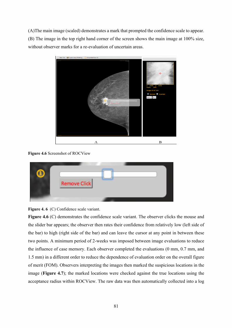
81
(A)The main image (scaled) demonstrates a mark that prompted the confidence scale to appear.
(B) The image in the top right hand corner of the screen shows the main image at 100% size,
without observer marks for a re-evaluation of uncertain areas.
Figure 4.6 Screenshot of ROCView
Figure 4. 6 (C) Confidence scale variant.
Figure 4.6 (C) demonstrates the confidence scale variant. The observer clicks the mouse and
the slider bar appears; the observer then rates their confidence from relatively low (left side of
the bar) to high (right side of the bar) and can leave the cursor at any point in between these
two points. A minimum period of 2-weeks was imposed between image evaluations to reduce
the influence of case memory. Each observer completed the evaluations (0 mm, 0.7 mm, and
1.5 mm) in a different order to reduce the dependence of evaluation order on the overall figure
of merit (FOM). Observers interpreting the images then marked the suspicious locations in the
image (Figure 4.7); the marked locations were checked against the true locations using the
acceptance radius within ROCView. The raw data was then automatically collected into a log
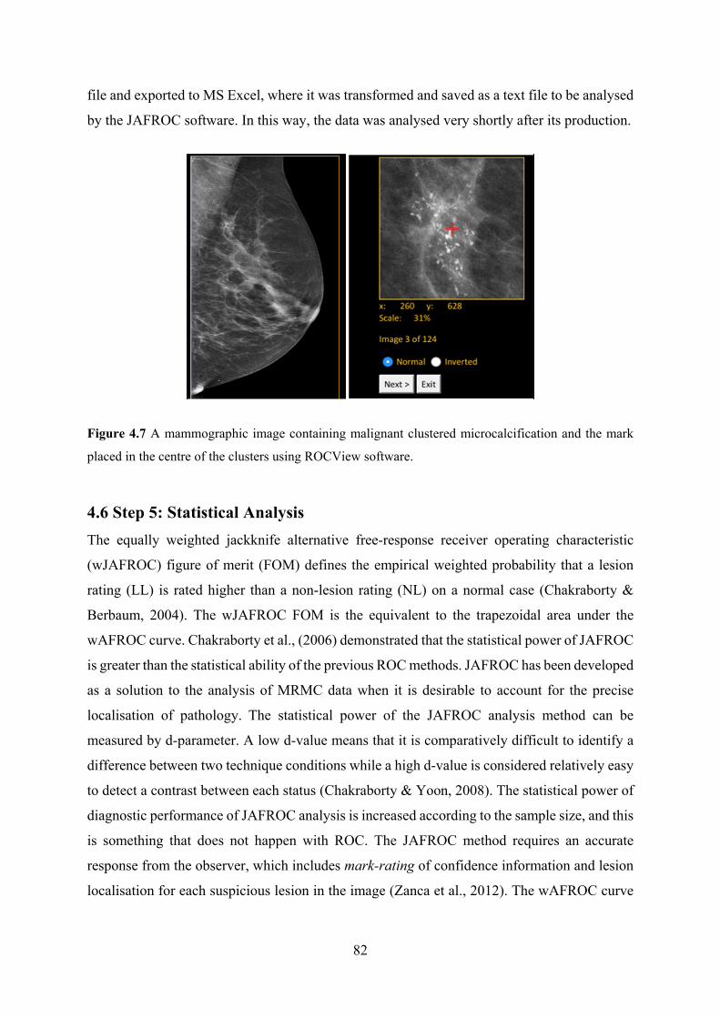
82
file and exported to MS Excel, where it was transformed and saved as a text file to be analysed
by the JAFROC software. In this way, the data was analysed very shortly after its production.
Figure 4.7 A mammographic image containing malignant clustered microcalcification and the mark
placed in the centre of the clusters using ROCView software.
4.6 Step 5: Statistical Analysis
The equally weighted jackknife alternative free-response receiver operating characteristic
(wJAFROC) figure of merit (FOM) defines the empirical weighted probability that a lesion
rating (LL) is rated higher than a non-lesion rating (NL) on a normal case (Chakraborty &
Berbaum, 2004). The wJAFROC FOM is the equivalent to the trapezoidal area under the
wAFROC curve. Chakraborty et al., (2006) demonstrated that the statistical power of JAFROC
is greater than the statistical ability of the previous ROC methods. JAFROC has been developed
as a solution to the analysis of MRMC data when it is desirable to account for the precise
localisation of pathology. The statistical power of the JAFROC analysis method can be
measured by d-parameter. A low d-value means that it is comparatively difficult to identify a
difference between two technique conditions while a high d-value is considered relatively easy
to detect a contrast between each status (Chakraborty & Yoon, 2008). The statistical power of
diagnostic performance of JAFROC analysis is increased according to the sample size, and this
is something that does not happen with ROC. The JAFROC method requires an accurate
response from the observer, which includes mark-rating of confidence information and lesion
localisation for each suspicious lesion in the image (Zanca et al., 2012). The wAFROC curve

83
is determined as the plot of lesion localisation fraction (LLF) vs false positive fraction (FPF)
plus a straight-line segment linking the uppermost operating point to (1, 1).
4.6.1 Data Analysis for Single Observer Free-response Method
Data analysis was performed using Rjafroc (Chakraborty & Zhai, 2015) where alternative
FOMs were used to provide values of sensitivity (FOM = HrSe) and specificity (FOM = HrSp).
Test alpha was set at 0.05 to control the probability of Type I error. The calculation of
wJAFROC FOM is performed to reward true lesion localisations and penalise incorrect lesion
localisations. It provides a single value summarising performance of single observer which can
be compared statistically. For example, comparing two magnitudes of simulated blurring one
calculates a FOM for each method and a statistical test is performed to identify the difference
between the two FOMs. When the difference is large enough to be different in consideration
of the pre-test value of alpha (0.05), then there is a statistical difference, if the result of the
overall F-test is also significant (Chakraborty, 2011). The result of the overall F-test and the
95% confidence interval (CI) of each pair of modalities must not include zero for a difference
in detection performance to be considered significant. The F-statistics, the denominator degree
of freedom (the numerator degree of freedom was always one) and the p-values. The observer
averaged FOM and 95% CI will be reported for all magnitudes of simulated blurring.
4.6.2 Data Analysis for Combined Observer Data Method
The double reporting method in screening mammography involves two observers interpreting
the same case independently (Taplin et al., 2000). The aim of the double method is to analyse
the combined two observers’ reports in the same process in clinical practice (Tanaka et al.,
2015). Consequently, additional analysis method was conducted utilising the same data from
FROC study obtained (248 cases) to determine the benefit of double reporting on lesion
detection performance in sharp and blurred FFDM images. In this analysis method, the
simulated double reporting evaluations were conducted by performing a comparison between
free-response data from one observer, with combined free-response data from two observers.
This is a secondary analysis of data from a first free response study which evaluates the impact
of simulated motion blur on observer performance. The single observer analysis demonstrated
a detrimental effect of simulated motion blur on the detection of masses and microcalcifications
for the sample of seven observers. Secondary analysis of data was deemed important partly
‘mimic’ this combined data result.

84
The observer study was split into two components: the evaluation of (i) microcalcifications and
(ii) masses. Seven observers (15±5 years’ clinical reporting experience in mammography) have
previously evaluated images with no simulated blurring (0 mm), and with 0.7 and 1.5 mm of
simulate blurring. These have acted as the distinct modalities (1st, 2nd, and 3rd) that were
compared statistically. In this secondary analysis of data, these three modalities have been
combined. The 1st modality in the current work comprises of all observer data created for
images of 0.0 mm, 0.7 mm, and 1.5 mm of simulated motion blur for six single observers. The
2nd modality in the current study comprises of the combined observer data for the six single
observers with each combined with an additional (seventh) observer. It has used the following
rules to combine the data from the free-response study. For lesion localisations (LL) the highest
rating for the two observers was adopted, regardless of whether one or both of the observers
had successfully localised the lesion. For non-lesion localisations (NL) all unique data was
maintained. This follows a similar method to the work of (Tanaka et al., 2015). The overall F-
test, p-values for FOM pairs (pairs of motion blur levels), and the observer averaged FOM and
95% confidence interval (CI) of double reporting for each magnitude of simulated motion blur
are reported. The F-statistics, the denominator degree of freedom (the numerator degree of
freedom was always one) and the p-values are also reported. The rating score in combined two
observers’ data congruent cases was automatically assigned the highest rating provided by one
of the two observers see (Table 4.2).
Table 4.2 Shows the single and combined two observers’ data assessments and the rating score for
each case
Single observer 1
Single observer 2
Double observer
Rating score
Situation 1 True True True Higher rating adopted
Situation 2 True False True Rating of true observer
Situation 3 False True True Rating of true observer
Situation 4 False False Rejected Rejected

85
4.7 Step 6: Lesion Conspicuity (Masses)
Measuring the conspicuity of lesions attempts to characterise the visibility of a lesion in terms
of the imaging systems diagnostic capabilities, and the lesion structure within the tissue
surrounding it (Kundel et al., 1976). The purpose of this method is to identify physical
parameters, such as lesion conspicuity, SNR, and lesion edge angle and the relationship they
have with detection in the presence of different magnitudes of simulated motion blur. In
addition, the behaviour of image blurring software has been evaluated. A new conspicuity
software programme and associated Excel spread sheet has been used to perform objective
measures of the expected visual detectability of focal breast lesions (masses) (Szczepura &
Manning 2016). However, the conspicuity index using this software could not be applied to
microcalcifications due to their individual size and their wide distribution pattern.
Manning and Ethell, (2002) initially suggested a procedure to evaluate lesion conspicuity; this
method combines the factors that define conspicuity into a single equation (Manning et al.,
2002). The conspicuity equation, which takes into consideration all factors that influence
conspicuity of a lesion, depends on the appearance of the image characteristic to the visual
system. Line profiles were built around a lesion, covering the immediate surrounding
background and the equation for conspicuity measure was developed, and can be given by:
χ tan 1 ∆
2 2……………… (4.2)
Where:
χ = conspicuity index
d = maximum lesion dimension
θ = is the maximum slope angle to the edge of the lesion profile in degrees
SNRforthenodule ∆ / σs = mean noise within the lesion
σn= mean background noise
A study by Manning et al., (2004) used the physical characteristic measurements of the lesions
to determine the conspicuity (x) of the nodules and to investigate possible causes of false

86
detection. The term conspicuity helped to understand why some lesions are missed by the
observers (Manning, Ethell & Donovan, 2004a).
This part of the thesis is focused on the physical measures of mammographic images. It utilises
a new software implementation by Szczepura and Manning, (2016) for measuring the
conspicuity of lesions and other physical parameters, such as edge angles of lesions, contrast
and SNR. The method is as follows:
1. A JAVA based programme allows the operator to draw a region of interest (ROI)
around a lesion (Figure 4.8)
2. Line profiles are then drawn 180° surrounding the area of interest and are extended by
one lesion dimension outside the drawn lesion (Figure 4.8)
3. A fit is applied for every line profile (Figure 4.8 and Figure 4.9) wherein:
a. The edges of the region of interest drawn by the operator are denoted by green
lines
b. The line profile is denoted by a blue line
c. The plotted fit is denoted by a red line
4. The regions of interest data sets are stored as TSV files in the same directory as the
analysed images
5. The image file name is labelled first, the region of interest second (starting at 0).
6. The data is transferred from the TSV file into the Raw Data worksheet in the Excel
spreadsheet.
7. Conspicuity is automatically calculated in the conspicuity index worksheet (Table 4.3)

87
A B
Figure 4.8 The conspicuity software demonstrates the measurement of a breast mass. (A) Demonstrates
the first stage through selecting the region of interest while (B) shows the second stage, where line
profiles are drawn 180° surrounding the region of interest and are extended one lesion dimension
outside the drawn lesion. Only DICOM images can be utilised with this software.
Figure 4.9 Line profiles are drawn 180° surrounding the region of interest.
The X and Y are co-ordinates of each of the plotted fit edges (X0, Y0; X1, Y1; etc), the standard
deviation of the Y values between X2 & X3 (SDTop) are utilised to represent the lesion noise

88
and the standard deviations of the Y values between X0 & X1 (SD1) and X4 & X5 (SD2) are
utilised to represent the noise of background.
Table 4.3 Illustrates the physical measures of breast lesion with three levels of simulated motion blur
using conspicuity software
Blur Level mm
Conspicuity Index
d (max lesion
diameter)
θ (degrees)
ΔGL σ Lesion
σ Background
μ Lesion
μ Background
Cases 1
0.0 51.631 24.450 63.765 88.903 42.734 69.744 192.939 104.036
0.7 66.389 18.589 61.030 93.344 21.061 40.134 194.894 101.550
1.5 74.993 17.133 59.797 93.600 16.109 31.417 194.417 100.817
Cases 2
0.0 71.577 42.183 69.151 69.483 60.864 82.009 178.011 108.528
0.7 101.672 39.644 67.259 70.189 34.217 51.973 178.272 108.083
1.5 110.622 38.578 66.415 69.886 27.714 45.491 178.044 108.158
4.8 Step 7: Dispersion Index
The second part of the physical measures analysis in this thesis is focused on the physical
features of microcalcifications. ImageJ software was utilised for measuring a new metric,
which has been called the Dispersion Index (D.I). Dispersion index of microcalcifications
repsesents the number of calcifications within a specified area divided by the area (equation
4.2). DI was measured because the conspicuity index could not be applied to
microcalcifications due to their individual size and their wide distribution pattern. This takes
into account the contrast of lesions, SNR and D.I. x contrast. The purpose of this method is to
demonstrate the relationship between dispersion index, contrast, SNR and lesion detection. The
aim was to assess the impact of simulated motion blur on the detection of microcalcifications.
The method is as follows:
1. A JAVA based programme (ImageJ) allows the operator to draw a region of interest (ROI)
around a cluster of microcalcifications for three levels of simulated motion blur (Figure 4.10).
2. The area of a cluster of microcalcifications will be measured using analysis tool manager of imageJ software (Figure 4.11 A).

89
3. The ROI data sets are stored as TSV files in the same directory as the analysed images
(Figure 4.11 B). After that, the data is transferred from the TSV file into the Raw Data
worksheet in the Excel spreadsheet to calculate the dispertion of microcalcifications.
4. The number of microcalcifications per cluster are calculated manually by the operator for
each image of with for three conditions: no motion blur (0 mm) and two magnitudes of
simulated motion blur 0.7 mm and 1.5 mm (Figure 4.12). A quality control test was performed
to minimise error on this, two observers have counted them individually and were blinded to
each other’s answers.
5. Dispersion index, lesion contrast and SNR are automatically calculated in the Excel
worksheet (Table 4.4).
The equation for the dispersion index measure was used and can be given by:
D.I = C/A………… (4.3)
Where:
D.I = Dispersion Index
C = the number of single calcifications per clustered
A = Area of selected region of interest

90
Figure 4.10 The Imagej software demonstrates the measurement of breast microcalcification. Shows
the first stage for selecting the region of interest

91
A
B
Figure 4.11 (A) Demonstrates the step 2 of measurement of breast microcalcification using Imagej
software. (B) demonstrates the regions of interest data sets are stored as TSV files in the same directory
as the analysed images for three levels of simulated motion blur.

92
0.0 mm 0.7mm 1.5mm
Figure 4.12 Demonstrates the same region of interest for clustered microcalcification for the three
levels of simulated motion blur.
Table 4.4 Demonstrates the physical measures of breast lesion with three levels of simulated motion
blur using ImageJ software
Area1 Mean1 StdDev1 Min1 Max1 Calc.
NO.
DI Contrast DI x
Con
SNR Detect
ability
Case 1
0.0 mm 13.731 2609.767 62.231 2457 2933 11 0.801 0.890 0.220 41.937 1.00
0.7 mm 13.731 2607.006 39.558 2544 2774 11 0.801 0.940 0.753 65.903 1.00
1.5 mm 13.731 2604.941 32.185 2555 2718 11 0.801 0.958 0.768 80.936 0.85
Case 2
0.0 mm 23.549 2967.666 89.657 2702 3361 25 1.062 0.883 0.937 33.100 1.00
0.7 mm 23.549 2966.361 73.434 2766 3191 25 1.062 0.930 0.987 40.395 1.00
1.5 mm 23.549 2965.665 69.593 2776 3137 25 1.062 0.945 1.004 42.614 0.85

93
4.9 Step 8: Missed Lesion Calculation Method
The calculation of missed lesions was used to identify the detectability of each lesion by each
observer. A comprehensive table has been created to present a full detailed explanation to the
seven observers on three levels of simulated motion blur. This table shows the sensitivity of
each lesion for all images related to the each level of simulated motion blur (Table 4.11). The
detectability of each lesion represents the number of observers detect the lesion divided on the
total number of observers. For instance, when all the observers detected the lesions (7/7), this
means that the percentage detecting the abnormality is 100% in 0.0 mm of motion blur.
Whereas, if only six observers detected the lesion from seven (6/7) the detectability will be
reduced to 85.8 % for 0.7 mm of simulated motion blur , and to 57.2% (4/7) for 1.5 mm of
simulated motion blur (see case 3 and case 5 Table 4.5).
Table 4.5 demonstrates the missed lesion calculation method Observ
er 1 Observer 2
Observer 4
Observer 5
Observer 6
Observer 7
Observer 9
Detectability of each lesion by the observers
0.0
0.7
1.5
0.0
0.7
1.5
0.0
0.7
1.5
0.0
0.7
1.5
0.0
0.7
1.5
0.0
0.7
1.5
0.0
0.7
1.5
0.0 0.7 1.5
1 ✓ ✓ X ✓ ✓ X ✓ ✓ X ✓ ✓ ✓ ✓ ✓ ✓ ✓ ✓ ✓ ✓ ✓ ✓ 1.00 1.00 0.572
2 ✓ ✓ X ✓ ✓ ✓ ✓ ✓ ✓ ✓ ✓ ✓ ✓ ✓ ✓ ✓ ✓ ✓ ✓ ✓ ✓ 1.00 1.00 0.850
3 ✓ ✓ X ✓ X X ✓ ✓ ✓ ✓ ✓ X ✓ ✓ ✓ ✓ ✓ ✓ ✓ ✓ ✓ 1.00 0.858 0.572
4 X X X ✓ ✓ X ✓ X X ✓ X X X ✓ X ✓ ✓ X X X X 0.572 0.429 0.00
5 ✓ ✓ X ✓ X X ✓ X X ✓ ✓ X ✓ X X X ✓ ✓ ✓ X X 0.858 0.429 0.143
6 ✓ ✓ ✓ ✓ ✓ ✓ ✓ ✓ ✓ ✓ ✓ ✓ ✓ ✓ ✓ ✓ ✓ ✓ ✓ ✓ ✓ 1.00 1.00 1.00
7 ✓ ✓ ✓ ✓ ✓ ✓ ✓ ✓ ✓ ✓ ✓ ✓ ✓ ✓ ✓ ✓ ✓ ✓ ✓ ✓ ✓ 1.00 1.00 1.00
8 ✓ ✓ X ✓ ✓ ✓ ✓ ✓ X ✓ ✓ ✓ X ✓ X ✓ ✓ ✓ ✓ X X 1.00 0.858 0.429
9 ✓ ✓ X ✓ ✓ X ✓ X ✓ ✓ ✓ ✓ ✓ ✓ ✓ ✓ ✓ X ✓ ✓ X 1.00 0.858 0.429
10
✓ ✓ X ✓ X ✓ X ✓ X ✓ ✓ ✓ ✓ ✓ ✓ ✓ ✓ X ✓ X X 1.00 0.715 0.429
The mark (✓) represents the detected lesion while mark (X) represents the missed lesion.

94
4.10 Ethical Issues
As this study involved human participation, special care must be paid to the rights of the
participants (Polit and Beck, 2003). Ethical approval for this study was granted by the
University of Salford (HSCR15-107) (Appendix A and B) and with consent from The
University Hospital of North Manchester, Nightingale Centre (Appendix C). This was a
retrospective study of breast screening images. Ethical approval has been provided by the
University of Salford (UOS). Most of the observation sessions took place at the University of
Salford medical imaging facility; the sessions included the explanation of the study using an
information sheet (Appendix D) and an explanatory PowerPoint presentation (Appendix H).
The observers were invited to participate in the study through several ways, such as Participant
Invitation Letter (Appendix E) and Poster (Appendix F).
All participants in this study signed a consent form before conducting the tasks. Participants
were informed that the results of the study would be included in a research thesis, would be
discussed at research conferences and published in peer-reviewed research journals. Data was
anonymised and stored on a password protected computer. No financial reward or otherwise
was offered. Participants were advised that their involvement may help to improve quality and
raise awareness of the impact of motion blur on cancer detection performance. All the observers
have received feedback on the outcomes of this study. They have received e-mail told them
there was a statistically significant impact of motion blur on the detection performance of
malignant masses and microcalcifications.
The Data Protection Act (DPA) 1998 (Legislation.gov.uk, 1998) can be applied to all observer
studies. Participants should be provided with adequate information about the study to enable
them to make a decision to participate in a study. All participants must inform and know the
target of the data collection, the period of the data can be kept and what will be achieved with
the data when it has been completed.
4.10.1 Ethical Approval in Observers’ Studies
In general, ethical issues aim to ensure the integrity and interests of persons and adherence to
standards. In the observer study implemented for this Ph.D. thesis, it was necessary to conserve
the privacy of all the observers and to make sure that any collected data was not definable to
them. Duquenoy et al., (2008) suggested that the ethical standards for electronic collection data

95
should be established in the code of ethics to ensure security, material quality, integrity,
accessibility, and usability. Therefore, this thesis reviewed by the University of Salford
Research and Ethics Committee, to protect the participants’ safety, rights, wellbeing, and
dignity. This Committee is run by the University of Salford, but its members are not connected
to the research they examine.
The Declaration of Helsinki (World Medical Association, 2013) summed up the role of
individuals participant in medical researches. The integrity and interests of the participants
should be the primary concern through the study, and while this declaration mentions to
participants as patients, the same standards must be utilised to those who participate as
observers. According to (Duquenoy et al., 2008), the medical informatics require that the
regulations in place ought to support the study, prevent the participants from experiencing
danger and keep information confidential. This is applicable to the existing work.

96
4.11 Chapter Summary
In summary, a novel mathematical simulation method has been designed to determine whether
simulated motion blur has an influence on lesion detection performance using observer
performance study. The stages of this observation method can be summarised into several
phases. First, suitable FFDM images were selected. Next, simulated motion was applied
through a novel mathematical technique within computer software. Then, the mammographic
images have been evaluated using an FROC method. Finally, JAFROC was used to analyse the
data for assessing the impact of simulated motion blur on lesion detection performance.
In this thesis, several additional methods have been used to manipulate the data. To start with,
two methods were used to analyse the FROC data combined two observers’ data and single
observer data (see the results chapter 5). After that, two physical methods have been applied to
investigate the impact of simulated motion blur on the physical parameters of the breast masses
using conspicuity software. ImageJ software was used to investigate the impact of motion blur
on microcalcifications. Finally, the missed lesion calculated method has been utilised to
determine the detectability for each lesion by each observer.

97
Chapter Five: Results
5.1 Chapter Overview
This chapter presents the results of the free response study. The presentation of results is
organised into three main sections. The first section shows the results of seven observers (single
reporting) of the free response study to determine the impact of simulated motion blur on the
detection of malignant masses and malignant microcalcifications. The results demonstrate that
there is a statistically significant influence of simulated motion blur on lesion detection
performance between images without motion blur (0.0 mm) and images with two levels of
motion blur (0.7 and 1.5 mm) for masses and microcalcification.
Section two presents the results of second analysis method; this is where two observers’ data
have been combined in an attempt to mimic the double reporting method in screening
mammography. The results of combining two observers’ data demonstrate that there is a
reduction in the impact of motion blur on detection performance compared to single observer.
However, there is still a statistically significant impact of simulated motion blur on lesion
detection performance between three levels of simulated motion blur for masses and
microcalcification.
Section three involves a comparison between the detection performance of single observer and
the detection performance of combining two observers’ data. The result of the third section
demonstrates that there is a significant difference between single and combined two observers
analysis of microcalcification lesions, whereas there no statistically significant difference for
detection performance of masses. This means that the impact of simulated motion blur remains
significant even when double reporting implemented.

98
5.2 Section One: Results of the Free-response Study
5.2.1 Overview of wJAFROC Analysis
An equally weighted jackknife alternative free-response receiver operating characteristic
(wJAFROC) analysis was performed to analyse the detection of: (i) microcalcifications, and
(ii) masses, for three conditions (0.0 mm (no motion blur), 0.7 mm simulated motion blur,
and 1.5 mm simulated motion blur). Random observer random case analysis was reported for
both analyses.
For these analyses the following data has been reported:
F-statistic and p-value
Observer averaged wJAFROC figure-of-merit (FOM) for all conditions and 95%
confidence intervals (CI)
Observer averaged sensitivity and specificity derived from the highest ratings
FOM difference and 95% CI for all treatments pairs of simulated motion blur
wAFROC curves for all magnitudes of simulated motion blur
In this analysis, the free-response data for seven observers is reported. For a difference in
detection performance to be declared statistically significant, the result of the overall F-test
must be significant and the 95% confidence interval of the treatments pair must not include
zero.
5.2.2 Microcalcifications
For microcalcifications, the observer averaged wJAFROC FOM and 95% confidence intervals
(CIs) are displayed in Table (5.1). Differences between FOM treatment pairs are displayed in
Figure 5.1, with the p-values to indicate significance. For a difference in FOMs to be declared
significant, the 95% CI of the FOM treatment pairs must not include zero, in addition to the
result of the overall F-test being significant. The observer averaged wAFROC curves for
microcalcifications are displayed in Figure 5.2.
When sensitivity (HrSe) was used as the FOM, a significant difference was found between all
treatment pairs of magnitudes of simulated motion blur (F(2,18) = 10.48, p=0.0010). This
implies that the false negative rate was increasing significantly as the magnitude of simulated
motion blur was increased. When specificity (HrSp) was used as the FOM, there was no

99
significant difference between magnitudes of simulated motion blur (F(2,13) = 0.21,
p=0.8110). This reveals that the false positive rate did not increase significantly with image
blurring (Table 5.3).
Average number of non-lesion localisation marks per observer on non-diseased cases
0.094
Average number of non-lesion localisation marks per observer on diseased cases
0.393
Average number of lesion localisation marks per observer 0.888
Table 5.1 Demonstrates a summary of the wJAFROC FOM with confidence interval (95% CI),
sensitivity and specificity analysis for microcalcifications case.
Higher sensitivity (HrSe) corresponds to higher negative predictive value and higher specificity
(HrSp) corresponds to higher positive predictive value is the ideal property of a test.
Magnitude of Simulated Motion blur (mm)
wJAFROC FOM (95% CI)
Sensitivity % (HrSe)
Specificity % (HrSp)
0 mm 0.899 (0.859,0.939) 97.9 84.8
0.7 mm 0.813 (0.757,0.870) 86.4 84.3
1.5 mm 0.746 (0.679,0.812) 76.5 86.6

100
Table 5.2 Demonstrates the wJAFROC FOM with confidence interval (95% CI), sensitivity and
specificity analysis for each observer for the image with no motion blur and two levels of simulated
motion blur of microcalcifications.
wJAFROC FOM
Sensitivity %
(HrSe)
Specificity %
(HrSp)
Observer 0mm 0.7mm 1.5mm 0.0mm 0.7mm 1.5mm 0.0mm 0.7mm 1.5mm
1 0.896 0.728 0.690 98.4 72.6 53.2 85.5 90.3 98.4
2 0.937 0.818 0.813 100 96.8 90.3 93.5 83.9 91.9
3 0.902 0.822 0.781 95.2 82.3 74.1 96.8 96.8 98.4
4 0.885 0.799 0.715 100 79.0 59.7 91.3 87.1 87.1
5 0.913 0.859 0.776 96.8 82.3 80.6 98.4 100 88.7
6 0.902 0.874 0.782 95.2 93.5 83.9 96.8 88.6 87.1
7 0.858 0.794 0.662 100 98.4 93.5 30.6 43.5 54.8
Average
0.899 0.813 0.746 97.7 86.4 76.5 84.8 84.3 86.6
Table 5.3 Shows a comparison of the p-values difference between treatment pairs of average
wJAFROC FOMs (95%) of single observer for microcalcification images.
Magnitude of Simulated Motion blur (mm)
The p-value difference between two pairs of average wJAFROC FOM (95% CI)
0.0 – 0.7 mm 0.0016
0.0 – 1.5 mm 0.0000
0.7 - 1.5 mm 0.0043
Overall F-test & average wJAFROC FOM (95% CI)
F (2, 12) = 18.13, p = 0.000)

101
Figure 5.1 Demonstrates the distribution of FOM difference and 95% CIs for all FOM treatment pairs
in the analysis of microcalcifications (this is the same data as indicated in Table 5.3).
This displays the inter-levels differences for the three treatment pairs (0.0 mm v 0.7 mm; 0.0
mm v 1.5 mm; 0.7 mm v 1.5 mm) for the analysis of microcalcifications. For a difference to
be declared statistically significant the 95% confidence interval of the treatment pair must not
include zero and the overall F-test must be significant.
Figure 5.2 Demonstrates the wAFROC curve of microcalcification cases with three levels of motion
blur. The highest performance is represented in level 0.0 mm (blue line) and the performance decreased
with increase motion blur 0.7 mm (red line). The lowest performance is represented in level 1.5 mm of
motion blur (green line).
0.000
0.125
0.250
0‐0.7 mm 0‐1.5 mm 0.7‐1.5 mm
wJAFROC FOM (95% CI)
Simulated motion blur levels
Microcalcifications Treatments Difference
0
0.2
0.4
0.6
0.8
1
0 0.2 0.4 0.6 0.8 1
Les
ion
Loc
alis
atio
n F
ract
ion
False Positive Fraction
wAFROC for Microcalcifications
0.0 mm
0.7 mm
1.5 mm

102
Figure 5.3 demonstrates the highest-rating inferred ROC curve of microcalcification for the image
with no motion blur and two levels of simulated motion blur.
Figure 5.4 The observers averaged FOM of microcalcifications for the image without motion blur and
two levels of simulated motion blur.
0
0.2
0.4
0.6
0.8
1
0 0.2 0.4 0.6 0.8 1
Tru
e po
siti
ve F
ract
ion
False Positive Fraction
ROC for Microcalcifications
0.0 mm
0.7 mm
1.5 mm
0.0
0.2
0.4
0.6
0.8
1.0
0 mm 0.7 mm 1.5 mm
wJA
FR
OC
FO
M (
95%
CI)
Levels of simulated motion blur
Microcalcifications FOM

103
5.2.3 Masses
For masses, the observer averaged wJAFROC FOM and 95% confidence intervals (CIs) are
displayed in Table 5.4. Differences between FOM treatment pairs (magnitudes of simulated
motion blur) are displayed in (Table 5.5) with the p-values to indicate significance. The
observer averaged wAFROC curves for masses are displayed in Figure 5.5.
When sensitivity (HrSe) was used as the FOM, there was no significant difference between
magnitudes of simulated motion blur (F (2, 16) = 0.43, p=0.6575). This implies that the false
negative rate was not changing significantly as a result of simulated motion blur. When
specificity (HrSp) was used as the FOM, again there was no significant difference between
magnitudes of simulated motion blur (F (2, 12) = 1.31, p=0.3043) (see Table 5.5).
Average number of non-lesion localisation marks per observer on non-diseased cases
0.217
Average number of non-lesion localisation marks per observer on diseased cases
0.211
Average number of lesion localisation marks per observer 0.885
Table 5.4 A summary of the wJAFROC analysis for masses. Shows the observer averaged wJAFROC
FOM and 95% confidence intervals (CIs), Sensitivity % (HrSe) and Specificity % (HrSp).
Higher sensitivity (HrSe) corresponds to higher negative predictive value and higher specificity
(HrSp) corresponds to higher positive predictive value is the ideal property of a test.
Magnitude of Simulated Motion
blur (mm)
wJAFROC FOM (95% CI)
Sensitivity % (HrSe)
Specificity % (HrSp)
0 0.905 (0.859,0.952) 92.3 82.7
0.7 0.869 (0.814,0.924) 91.19 73.3
1.5 0.862 (0.810,0.915) 90.5 77.6

104
Table 5.5 Demonstrates a comparison of the p-value difference between two treatment pairs of average
wJAFROC FOMs (95%) and the p-value difference between two sensitivity and specificity for single
observer of masses cases.
Magnitude of Simulated Motion blur (mm)
The p-value difference between two levels of average wJAFROC
0.0 – 0.7 mm 0.0122
0.0 – 1.5mm 0.0041
0.7 - 1.5 mm 0.6408
Overall F-test & average wJAFROC FOM (95% CI)
F(2,21.53) = 6.01, p= 0.0084
Figure 5.5 Demonstrates the distribution of FOM difference and 95% CIs for all FOM treatment pairs
in the analysis of masses (this is the same data as indicated in Table 5.5).
This displays the inter- levels differences for the three level pairs (0.0 mm v 0.7 mm; 0 mm
v 1.5 mm; 0.7 mm v 1.5 mm) for the analysis of masses. For a difference to be declared
statistically significant the 95% confidence interval of the levels pair must not include zero and
the overall F-test must be significant. Therefore, in this case, the level pairs 0.0 mm v 0.7 mm,
and 0.0 mm v 1.5 mm are significantly different, while 0.7 mm v 1.5 mm, which does include
zero is not significantly different despite the overall F-test does reach significant levels. The
treatment differences were all a lot smaller for masses than microcalcifications (see Figure
‐0.125
0.000
0.125
0.250
0‐0.7 mm 0‐1.5 mm 0.7‐1.5 mm
wJA
FR
OC
FO
M (
95%
CI)
Levels of motion blur
Masses levels Difference

105
5.8). This means that the malignant masses is less affected by motion blur than
microcalcifications.
Figure 5.6 Demonstrates the wAFROC curve of masses in image with no blur (0.0 mm) and two levels
of simulated motion blur (0.7 & 1.5 mm).
The highest performance is represented in images with no simulated motion blur 0.0 mm (blue
line) and the performance decreased with increase motion blur 0.7 mm (red line). The lowest
performance is represented in level 1.5 mm of motion blur (green line).
0
0.2
0.4
0.6
0.8
1
0 0.2 0.4 0.6 0.8 1
LLF
False Positive Fraction
wAFROC curve of Masses
0.0mm
0.7mm
1.5mm

106
Figure 5.7 Demonstrates the observers averaged FOM of masses at 0.0 mm, 0.7 mm, and 1.5 mm of
simulated motion blur.
Table 5.6 The wJAFROC FOM with confidence interval (95% CI), sensitivity and specificity analysis
for each observer at 0 mm, 0.7 mm, and 1.5 mm of simulated motion blur for masses.
Masses cases
wJAFROC FOM (95% CI)
Sensitivity %
(HrSe)
Specificity %
(HrSp)
Observer 0.0 mm 0.7 mm 1.5 mm 0.0mm 0.7mm 1.5mm 0.0mm 0.7mm 1.5mm
1 0.898 0.833 0.802 85.5 82.3 79.0 96.8 91.9 85.5
2 0.943 0.879 0.876 96.8 96.8 87.0 85.5 62.9 85.5
3 0.836 0.816 0.843 90.3 87.0 88.7 69.4 80.6 83.9
4 0.936 0.895 0.907 96.8 87.1 92.0 75.8 88.7 87.1
5 0.925 0.922 0.900 93.5 98.4 98.4 88.7 80.6 66.1
6 0.920 0.930 0.894 93.5 98.4 96.8 90.3 72.6 79.0
7 0.879 0.808 0.816 90.3 93.5 91.9 72.6 35.5 56.5
Average 0.905 0.869 0.862 92.3 91.9 90.5 82.7 73.3 77.6
0.0
0.2
0.4
0.6
0.8
1.0
0 mm 0.7 mm 1.5 mm
wJA
FR
OC
FO
M (
95%
CI)
level of Image Blurring
Masses FOM

107
Figure 5.8 The wJAFROC FOM and 95% confidence intervals for microcalcifications and masses at
0.0 mm, 0.7 mm, and 1.5 mm of simulated motion blur.
0
0.2
0.4
0.6
0.8
1
0 mm 0.7 mm 1.5 mm
wJA
FR
OC
FO
M (
95%
CI)
Levels of motion blur
wJAFROC FOMMicrocalcifications and Masses
Microcalcifications Masses

108
5.3 Section Two: Results of the Combining Two Observers’ Data
As it is recognised that double reporting is an essential element of NHSBSP standards,
secondary analysis of the data was deemed essential to partly ‘mimic’ this combined data result.
In this analysis ‘a single result for each observer’ is compared to ‘the combined result of this
observer and a second observer; the latter being referred to as a ‘combined result’. The outcome
of the combined result is classified as follows: a positive outcome is assigned if one of the two
observers suspects a lesion; the negative outcome is assigned if both observers indicate no
lesion present. Seven observers completed the study and their data was analysed collectively
to establish the impact of simulated motion blur on detection of breast lesions. This means that
observer ratings have been combined. For the TP worksheet, the highest rating of the two
observers was adopted as the rating for each lesion. For the FP worksheet, all unique ratings
were kept (see Appendix I and Appendix J).
Since the results of combining two observers’ data process have used the same data of the free-
response study, the data for observers’ pairs from combining two observers’ data is
implemented and the following data analysis will be reported:
F-statistic and p-value
Observer averaged wJAFROC figure-of-merit (FOM) for all conditions and 95%
confidence intervals (CI)
Observer averaged sensitivity derived from the highest ratings
FOM difference and 95% CI for all treatment pairs of simulated motion blur
wAFROC curves for all magnitudes of simulated motion blur
For a difference in detection performance to be declared statistically significant, the result of
the overall F-test must be significant and the 95% confidence interval of the treatment pairs
must not include zero.
Two observers’ data were combined for the detection of malignant microcalcifications and
masses for three conditions; (i) no simulated motion blur (0 mm), and for two magnitudes of
simulated motion blur (ii) 0.7 mm, and (iii) 1.5 mm. A statistically significant difference was
found for the detection of masses (F (2, 48) = 5.64, p< 0.0038) and for the detection of
microcalcifications (F (2, 12) = 18.13, p < 0.0000). For both analyses, a significant difference
was observed between 0.0 mm and 0.7 mm, and between 0.0 mm and 1.5 mm of simulated
motion blur, and also between 0.7 mm and 1.5 mm for microcalcifications. No significant

109
difference was detected between 0.7 mm and 1.5 mm for masses. Rjafroc was also used to
calculate observer averaged sensitivity (FOM = HrSe) and specificity (FOM = HrSp) as the
FOM for all conditions for microcalcifications and masses, (Table 5.7 & Table 5.9).
5.3.1 The Combining Two Observers’ Data of Microcalcifications
A statistically significant difference for the detection performance of microcalcifications was
demonstrated (F (2, 11) = 13.68, p = 0.000) between all three levels pairs 0.0 mm V 0.7 mm
(p < 0.01). All FOM pairs (0 mm V 1.5 mm, and 0.7 mm V 1.5 mm) were significantly
different (Figure 5.11). The observer averaged wJAFROC FOMs and 95% CIs are presented
in (Table 5.7).
Average number of non-lesion localisation marks per observer on non-diseased cases
0.459
Average number of non-lesion localisation marks per observer on diseased cases
0.126
Average number of lesion localisation marks per observer 0.943
Table 5.7 A summary of the wJAFROC analysis of microcalcification. Shows the observer averaged
wJAFROC FOM and 95% confidence intervals (CIs), Sensitivity % (HrSe) and Specificity % (HrSp)
of combining two observers’ data.
These results demonstrate there is a reduction in the impact of motion blur on detection
performance compared to single observer.
Magnitude of Simulated Motion
blur (mm)
wJAFROC FOM (95% CI)
Sensitivity % (HrSe)
Specificity % (HrSe)
0 0. 923 (0.883,0.964) 99.7 72.0
0.7 0.876 (0.831,0.921) 96.0 70.9
1.5 0.826 (0.771,0.880) 89.6 75.3

110
Figure 5.9 Demonstrates averaged FOM of the combining two observers’ data of microcalcifications
at 0 mm, 0.7 mm, and 1.5 mm of simulated motion blur.
Figure 5.10 Demonstrates wAFROC curve of combined two observers’ data of microcalcifications
cases at 0.0 mm, 0.7 mm, and 1.5 mm of simulated motion blur.
The highest performance is represented in level 0.0 mm (blue line) and the performance
decreased with increase motion blur 0.7 mm (red line). The lowest performance is represented
in level 1.5 mm of motion blur (green line).
0.0
0.2
0.4
0.6
0.8
1.0
0 mm 0.7 mm 1.5 mm
wJA
FR
OC
FO
M (
95%
CI)
Levels of Image Blurring
Microcalcifications FOM
0
0.2
0.4
0.6
0.8
1
0 0.2 0.4 0.6 0.8 1
Les
ion
Loc
alis
atio
n F
ract
ion
False positive Fraction
wAFROC curve of combining two observers' of Microcalcifications
0.0 mm
0.7 mm
1.5 mm

111
5.3.2 Combining Two Observers’ Data of Masses
A statistically significant difference for the detection performance of masses was
demonstrated (F (2,484) = 5.64, p = 0.0038). The observer averaged wJAFROC FOMs and
95% CIs are presented in (Table 5.11). A statistically significant difference was detected
between all motion blur levels pairs except between 0.7 and 1.5 mm for masses (Table 5.13)
Average number of non-lesion localisation marks per observer on non-diseased cases
0.369
Average number of non-lesion localisation marks per observer on diseased cases
0.392
Average number of lesion localisation marks per observer 0.873
Table 5.8 A summary of the wJAFROC analysis of masses. Shows the observer averaged wJAFROC
FOM and 95% confidence intervals (CIs), Sensitivity % (HrSe) and Specificity % (HrSp) of
combined two observers’ data.
These results demonstrate that there is a reduction in the impact of motion blur on detection
performance.
Magnitude of Simulated Motion
blur (mm)
wJAFROC FOM (95% CI)
Sensitivity % (HrSe)
Specificity % (HrSe)
0 0. 948 (0.915, 0.982) 98.2
70.5
0.7 0.915 (0.873,0.954) 97.9 55.1
1.5 0.913 (0.874,0.956) 97.5 62.7

112
Figure 5.11 Demonstrates averaged FOM of the combining two observers’ data in images with no
motion blur and two levels of simulated motion blur of masses
Figure 5.12 Demonstrates wAFROC curve of combined two observers’ data of masses with three levels
0.0 mm, 0.7 and 1.5 mm.
The highest performance is represented in level 0.0 mm (blue line) and the performance decreased with increase motion blur 0.7 mm (red line). The lowest performance is represented in level 1.5 mm of motion blur (green line).
0.0
0.2
0.4
0.6
0.8
1.0
0 mm 0.7 mm 1.5 mm
wJA
FR
OC
FO
M (
95%
CI)
Levels of simulated motion blur
Average FOM for Masses cases
0
0.2
0.4
0.6
0.8
1
0 0.2 0.4 0.6 0.8 1
Les
ion
Loc
alis
atio
n F
ract
ion
False Positive Fraction
wAFROC curve of combining two observers' data of Masses
0.0 mm
0.7 mm
1.5 mm

113
5.4 Section Three: A Comparison between the Results of Single Observer
and the Combining Two Observers’ Data
5.4.1 Microcalcification
A statistically significant difference for the detection performance of microcalcifications was
demonstrated (F (2, 11) = 13.68, p = 0.000) between single observer and combined two
observers’ data (see Figure 5.13); Figure 5.13 demonstrates the difference between
wAFROC curve of single observer and combined two observers’ data of microcalcifications
cases.
Table 5.9 Demonstrates the comparison between wJAFROC FOMs, sensitivity and specificity of single
and combined two observers’ data with three levels of simulated blur.
Simulated Motion
blur
wJAFROC FOM (95% CI)
Sensitivity % (HrSe)
Specificity % (HrSe)
Combined two observers’ data
Single Observer Combined two
observers’ data
Single Observer
Combined two
observers’ data
Single Observer
0 mm 0. 923 (0.883,0.964) 0.899 (0.859, 0.939) 99.7 97.9 72.0 84.8
0.7 mm 0.876 (0.831,0.921) 0.813 (0.757,0.870) 96.0 86.4 70.9 84.3
1.5 mm 0.826 (0.771,0.880) 0.746 (0.679,0.812) 89.6 76.5 75.3 86.6
Figure 5.13 The comparison between wJAFROC FOMs for single observer and combined two
observers’ data in microcalcification.
0
0.1
0.2
0.3
0.4
0.5
0.6
0.7
0.8
0.9
1
0 mm 0.7 mm 1.5 mm
wJA
FR
OC
FO
M (
95%
)
levels of simulated motion blur
Single and combining two observers' data FOM of microcalcificationsSingle observerCombining two observers' data

114
Table 5.10 Demonstrates a comparison of the p-value difference between treatment pairs of average
wJAFROC FOMs (95%) and the p-value difference between two sensitivity and specificity for single
observer and combined two observers’ data of microcalcifications.
Magnitude of Simulated Motion blur (mm)
The p-value difference between two pairs of average wJAFROC FOM (95% CI)
Combined two observers’ data
Single Observer
0.0 – 0.7 mm 0.0000 0.0016
0.0 – 1.5 mm 0.0000 0.0000
0.7 - 1.5 mm 0.0000 0.0043
Overall F-test & average wJAFROC FOM (95% CI)
F (2, 12) = 18.13, p = 0.0000. significant
F (2, 12) = 18.13, p = 0.000. significant
Figure 5.14 The difference between the wAFROC curve of single observer and combined two
observers’ data of microcalcifications.
There is a reduction in the impact of motion blur when using the combined two readers’ data
(green line), the results demonstrate there is a statistically significant difference for detection
performance of microcalcification.
0
0.2
0.4
0.6
0.8
1
0 0.2 0.4 0.6 0.8 1
Lesion Localisation Fraction
False Positive Fraction
wAFROC curve of Microcalcifications
Single reporting
Combining tworeaders' data

115
5.4.2 Masses
For masses, no significant difference for the detection performance was demonstrated (F (1,5)
= 4.04, p = 0.1001) between single observer and combined two observers’ data (see Figure
5.16); Figure 5.16 demonstrates the difference between wAFROC curve of single observer
and combined two observers’ data of masses cases.
Table 5.11 Demonstrates a comparison between wJAFROC FOMs and sensitivity and specificity for
single observer and combined two observers’ data of masses.
Magnitude of
Simulated Motion
blur (mm)
wJAFROC FOM (95% CI)
Sensitivity % (HrSe)
Specificity % (HrSe)
Combined two observers’ data
FOMs
Single Observer FOMs
Combined two observers’ data
Single Observer
Combined two
observers’ data
Single Observer
0 0. 948 (0.915,0.982) 0.905 (0.859,0.952) 98.2
92.3 70.5 82.7
0.7 0.913 (0.873,0.954) 0.869 (0.814,0.924) 97.9 91.19 55.1 73.3
1.5 0.915 (0.874,0.956) 0.862 (0.810,0.915) 97.5 90.5 62.7 77.6
Figure 5.15 The comparison between wJAFROC FOMs for single observer and combined two
observers’ data of masses.
0
0.1
0.2
0.3
0.4
0.5
0.6
0.7
0.8
0.9
1
0 mm 0.7 mm 1.5 mm
wJA
FR
OC
FO
M (
95%
)
levels of Simulated motion blur
FOM of Masses for Single and Combined two observers' data Single Observer
Combined two observers' data

116
Table 5.12 Demonstrates a comparison of the p-value difference between two treatment pairs of average
wJAFROC FOMs (95%) of masses.
Magnitude of Simulated Motion blur (mm)
The p-value difference between two levels pairs average wJAFROC
Combined two observers’ data
Single Observer
0.0 – 0.7 mm 0.0031 0.0122
0.0 – 1.5 mm 0.0047 0.0041
0.7 - 1.5 mm 0.8952 0.6408
Overall F-test & average wJAFROC FOM (95% CI)
F(2,484.78) = 5.64, p = 0.0038 significant
F(2,21.53) = 6.01, p= 0.0084. significant
Figure 5.16 The difference between wAFROC curve of single and combined two observers’ data of
masses.
Despite the slight reduction in the impact of motion blur when using combined two observers’
data method and increase the detection performance (green line), the results demonstrate there
no statistically significant difference for detection performance of masses between two
methods. This means that the impact of motion blur remains even when two observers’ data
have been combined.
0
0.2
0.4
0.6
0.8
1
0 0.2 0.4 0.6 0.8 1
Les
ion
loca
lisat
ion
Fra
ctio
n
False Positive Fraction
wAFROC curve of Masses
SingleReporting
Combiningtwo readers'data

117
Table 5.13 The wJAFROC FOM and 95% confidence intervals (CI) for single and combined observers
for masses and microcalcifications.
The inter-modality difference and confidence intervals are also presented for the analysis of
masses and microcalcifications. For a difference to be declared statistically significant, the
result of the overall F-test must be significant and the 95% CI of the modality difference must
not include zero. The sensitivity and specificity were calculated in Rjafroc using the HrSe and
HrSp FOMs.
Analysis Modality wJAFROC FOM
(95% CI)
Difference (95%
CI)
Sensitivity
HrSe (%)
Specificity
HrSp (%)
Masses
1st
(single) 0.885 (0.844,0.927)
-0.03 (-0.07,0.01)
92 82
2nd
(combined) 0.916 (0.885,0.947) 97 63
Micro-
calcifications
1st
(single) 0.820 (0.780,0.860)
-0.06 (-0.10,-0.17)
85 92
2nd
(combined) 0.876 (0.842,0.909) 93 82

118
Chapter Six: Results of Physical Measures
6.1 Chapter Overview
This chapter presents physical measures taken from the cases containing lesions. The results
are organised into three main themes:
The first theme focuses on calculating the impact of motion blur on focal lesions (masses). This
is primarily done using conspicuity index software (Szczepura & Manning, 2016). The
conspicuity of a lesion represents a ratio between the contrast of a lesion and its surrounding
complexity. Conspicuity index help to explain the function of the blurring software (e.g. how
the edge angle degreases with increasing blur simulation) and how it impacts on the visual
characteristics of the masses’ images.
The second theme focuses on the impact of simulated motion blur on microcalcifications.
This includes a novel metric, that has been named the ‘dispersion index’ (DI), lesion contrast,
and dispersion index X contrast (DI x contrast). A relationship between lesion detectability
and these physical measures has been investigated.
The third theme focuses on an analysis of missed lesions. This aspect focusses purely on
detection, ignoring the confidence rating assigned for the free-response study. In this case,
detectability is defined as the number of successful detections (for all observers) over the total
number of opportunities to detect the lesion.

119
6.2 Part I: Physical Measures of Breast Masses
Several parameters, such as conspicuity index (χ), maximum lesion diameter (d), edge angle of
the lesion (θ), mean noise within the lesion (σs), and mean background noise (σn) were recorded
for all breast masses using conspicuity index software. This was not possible for
microcalcifications due to their size and distribution patterns; this represents a limitation of the
conspicuity software. This prompted the development of the Dispersion Index; see section
6.3.1). Overall, simulated motion blur has a significant impact on the edge angle of the lesion.
In addition, these results illustrate the relationship between simulated motion blur and a change
in grey level (ΔGL) of the image. Where ΔGL represents the difference between contrast of
the lesion (μ L) and background (μ b). Table 6.1 displays the results of the conspicuity data of
breast masses with different levels of motion blur. This resulted in the conspicuity index for 23
cases out of 62 cases being measured because of limitations in the conspicuity software. Only
masses which have clear edges can be measured by conspicuity software. The SNR for images
is also presented to illustrate the impact of simulation motion blur on the image noise. When
the magnitude of simulated motion blur increases, there is a reduction in the image noise as
consequence of a smoothing effect incurred by blurring. A full range of physical measures
acquired data for masses for image without simulated motion blur (0.0 mm), and images with
simulated motion blur (0.7 & 1.5 mm) is presented in (Appendix K).

120
Table 6.1 Physical measurements of breast masses within mammographic images using conspicuity
software.
The physical measurements include the conspicuity index (χ), the θ represents the maximum slope
angle to the edge of the lesion profile in degrees, the change of grey level (ΔGL) and SNR.
Magnitude of Simulated Motion Blur (mm)
0.0 0.7 1.5
Case No. χ
Edge angle (θ) ΔGL SNR χ
Edge angle (θ) ΔGL SNR χ
Edge angle (θ) ΔGL SNR
1 51.63 63.77 63.77 2.77 66.39 61.52 93.34 4.86 74.99 59.80 93.60 6.19
2 71.58 69.15 69.48 2.93 101.67 67.26 70.19 5.21 110.62 66.42 69.89 6.42
3 45.00 66.95 76.64 3.60 55.62 72.36 84.80 3.74 58.38 62.93 79.35 12.15
4 108.88 73.24 84.33 2.38 153.36 67.95 67.71 2.49 169.43 71.57 84.60 4.54
5 66.27 70.83 66.46 1.73 78.11 67.95 67.71 2.49 81.13 66.38 68.27 2.87
6 40.11 65.04 59.04 2.15 43.76 58.81 63.08 4.00 47.46 57.77 63.04 4.69
7 170.73 70.65 133.19 2.99 252.59 70.53 133.54 4.12 272.50 70.26 133.61 4.54
8 140.63 72.61 96.36 2.98 222.31 71.96 96.80 5.74 238.35 71.29 96.84 6.83
9 113.44 72.97 99.35 2.96 150.18 71.94 99.56 4.48 162.84 71.20 98.87 5.44
10 124.98 71.21 108.73 2.23 169.81 70.48 109.86 4.38 181.56 70.15 109.91 5.21
11 116.22 73.52 115.36 2.72 155.95 72.93 114.86 4.01 168.74 72.24 114.26 4.83
12 82.89 69.51 107.98 2.71 117.32 68.93 108.10 5.22 127.94 68.53 107.41 6.21
13 123.43 71.09 86.52 2.76 179.01 69.64 87.26 4.52 192.82 68.76 87.49 5.15
14 127.07 69.54 127.66 3.47 166.60 69.14 128.66 5.89 178.28 68.76 128.76 7.39
15 57.37 62.53 60.31 1.92 81.94 58.64 61.53 3.87 85.67 57.08 61.61 4.66
16 79.12 67.11 106.27 3.30 91.03 65.51 107.71 6.28 94.90 64.99 107.72 7.71
17 80.79 71.39 70.40 2.98 111.91 69.11 71.13 5.49 116.82 67.75 71.31 7.19
18 85.85 71.76 106.42 3.66 100.98 70.68 107.37 5.73 102.30 70.07 107.34 6.52
19 53.48 66.07 114.96 2.85 55.35 64.89 115.66 4.62 56.32 64.52 115.58 5.24
20 76.51 72.45 92.41 3.05 92.79 71.38 93.15 4.15 99.26 70.82 92.85 4.60
21 53.21 62.49 101.20 1.58 53.40 60.80 102.91 2.19 51.83 59.82 103.81 2.57
22 56.28 71.26 57.73 3.27 63.86 68.75 58.54 5.37 62.09 67.09 58.04 6.64
23 82.01 64.38 121.77 2.08 111.60 64.82 126.05 2.23 119.60 64.76 127.35 2.43
Max 170.73 73.52 133.19 3.662 252.59 72.929 133.54 6.279 272.5 72.239 133.61 12.148
Min 40.113 62.49 57.73 1.575 43.759 58.64 58.54 2.194 47.462 57.08 58.04 2.429
Ave. 87.282 69.109 92.450 2.741 116.328 67.63 94.326 4.394 124.080 66.649 94.848 5.653

121
6.2.1 Normality Test of Masses Data
Normality test of the data of the physical measures is required to check the suitability of the
overall data for further analysis (Field et al., 2013). For this data, the Kolmogorov-Smirnov
test and Shapiro-Wilk test showed that the physical parameters data such as the conspicuity
index, the change in grey level and SNR were normally distributed with P ≥ 0.05, and the edge
angle data was not normally distributed with P ≤ 0.05 as illustrated in (Table 6.2).
Table 6.2 Values of Kolmogorov-Smirnov test and Shapiro-Wilk normality test for the physical measures
data of breast masses
Kolmogorov-Smirnova Shapiro-Wilk
Statistic df Sig. Statistic df Sig.
Conspicuity Index 0.0 m 0.169 23 0.089 0.934 23 0.133
Edge Angle 0.0 mm 0.190 23 0.031 0.899 23 0.024
GL 0.0 mm 0.131 23 0.200* 0.945 23 0.227
SNR 0.0 mm 0.171 23 0.080 0.955 23 0.376
Conspicuity Index 0.7 mm 0.145 23 0.200* 0.928 23 0.099
Edge Angle 0.7 mm 0.182 23 0.047 0.888 23 0.014
GL 0.7 mm 0.149 23 0.200* 0.946 23 0.245
SNR 0.7mm 0.119 23 0.200* 0.936 23 0.150
Conspicuity Index 1.5 mm 0.138 23 0.200* 0.927 23 0.092
Edge Angle 1.5 mm 0.138 23 0.200* 0.904 23 0.030
GL 1.5 mm 0.114 23 0.200* 0.959 23 0.451
SNR 1.5 mm 0.162 23 0.123 0.892 23 0.180
*. This is a lower bound of the true significance
a. Lilliefors Significance Correction

122
6.2.2 Conspicuity Index (χ)
The conspicuity of a mass represents a ratio between the contrast of a mass and its surrounding
complexity. A paired sample t-test (2-way) was performed to test the hypothesis that the
conspicuity index of masses was equal on images with no motion blur (0.0 mm) (M= 87.282,
SD= 34.715) and images with 0.7 mm motion blur (M= 116.33, SD=56.169), 1.5 mm motion
blur (M= 124.08, SD= 61.566). Prior to conducting the analysis, the assumption of normally
distributed difference scores was examined, and the data was normally distributed see (Table
6.2). The Conspicuity Index difference between the two magnitudes of simulated motion blur
and no motion blur were statistically significant for all comparisons (See Table 6.3). This could
influence on lesion characteristics and the changes in the features of breast masses could have
negatively influence the differential diagnosis between malignant and benign masses. Figure
6.1 graphical represents the means and confidence interval 95% of the two magnitudes of
simulated motion blur and no motion blur. As can be seen, the conspicuity index increases
significantly when simulated motion blur increases from 0mm to 0.7 mm and then to 1.5mm.
The diagram illustrates a variety of different box plot positions and shapes. The box plot of
conspicuity index in images without motion blur (0.0 mm) is comparatively short. This
suggests that the distribution of overall data is convergent. The median is about (80.790,
101.672, and 110.622) for images without blur 0.0mm, images with blur 0.7 mm and 1.5mm
respectively.

123
Table 6.3 The results of conspicuity index of 23 masses cases for images with no motion blur and two
levels of simulated motion blur.
Conspicuity Index of 23 masses 0.0 mm
0.7 mm 1.5 mm
Mean 87.282 116.33 124.08
95% Confidence Interval for
Mean
Lower Bound 72.270 92.038 97.4570
Upper Bound 102.294 140.617 150.703
5% Trimmed Mean 85.449 112.939 120.307
Median 80.790 101.672 110.622
Std. Deviation 34.715 56.169 61.566
Minimum 40.11 43.76 47.46
Maximum 170.73 252.59 272.50
Range 130.62 208.83 225.04
Interquartile Range 59.94 89.56 94.44
T-test Pairs Result of T-test / Difference (95% CI)
0.0 mm – 0.7 mm t(22) = -6.158, p<0.000 / -29.046 (-38.827,-19.264)
0.0 mm – 1.5 mm t(22) = -6.273, p<0.000 / -36.798 (-48.964, -24.633)
0.7 mm – 1.5 mm t(22) = -6.231, p<0.000 / -7.752 (-10.333, -5.172)
Figure 6.1 Demonstrates the relationship between the magnitudes of simulated motion blur and
conspicuity index of breast masses.
As can be seen, the conspicuity index increases significantly when simulated motion blur
increases from 0mm to 0.7mm and then to 1.5mm.

124
6.2.3 Edge Angle
The edge angle of a mass represents the maximum slope angle across the edge of a lesion
profile in degrees. A non-parametric test was performed to test the hypothesis that edge angle
of masses in images with 0.7mm simulated blur (M= 67.63, SD=4.308), 1.5 mm simulated
motion blur (M= 66.650, SD= 4.546) and edge angle of masses in images with no motion blur
(0.0mm) (M= 69.110, SD= 3.556) are equal. Prior to conducting the analysis, the assumption
of normally distributed difference scores was examined and the data was non-normally
distributed (See Table 6.2). The edge angle difference between the two magnitudes of
simulated motion blur and no motion blur were statistically significant for all comparisons (see
Table 6.4). The edge angle decreased along with the increasing level of simulated motion blur.
Simulated motion blur has an impact on the edge angle of breast masses and this could
influence on image of the lesion characteristics. This means that any changes in the image
characteristics of breast masses could negatively affect the identification of malignant masses.
Figure 6.2 demonstrates the mean of both edge angle and confidence interval 95% of the two
magnitudes of simulated motion blur and no motion blur. Each of the box plots in (Figure 6.2)
shows a different skewness pattern. The distribution of the 0.0mm box plots is skewed up whilst
the distribution of box plots 0.7mm and 1.5mm are skewed down. The median was pointed by
the horizontal line that runs up the centre of the boxes. The median was (67.750) for images
with no motion blur and the median for blurred images 0.7mm, 1.5 mm were 68.925, 70.653,
respectively.

125
Table 6.4 Demonstrates the results of edge angle measures for 23 masses cases of images with no
motion blur and two levels of simulated motion blur.
Edge Angle 0.0 mm
0.7 mm 1.5 mm
Mean 69.110 67.63 66.650
95% Confidence Interval
for Mean
Lower Bound 67.571 65.770 64.683
Upper Bound 70.647 69.492 68.615
5% Trimmed Mean 69.233 67.838 66.870
Median 70.653 68.925 67.750
Variance 12.648 18.555 20.667
Std. Deviation 3.556 4.308 4.546
Minimum 62.490 58.64 57.080
Maximum 73.520 72.930 72.240
Range 11.030 14.290 15.160
Interquartile Range 5.690 5.790 5.740
T-test Pairs Result of T-test / Difference (95% CI)
0.0 mm – 0.7 mm t(22) = 3.232, p<0.004/ 1.4794 (0.530, 2.429)
0.0 mm – 1.5 mm t(22) = 6.592, p<0.000 / 1.4794 (1.686, 3.234)
0.7 mm – 1.5 mm t(22) = 2.234, p<0.036/ 0.980 (0.070, 1.891)
Figure 6.2 Demonstrates the relationship between the magnitudes of simulated motion blur and edge
angle of masses.

126
6.2.4 The Grey Level Change (ΔGL):
The grey level change (ΔGL) represents the difference between the contrast of the lesion (μ L)
and the background (μ b). The same analysis process used for conspicuity index has been used
to analyse the grey level change data. A paired sample t-test was performed to test the
hypothesis that the grey level of masses in images with 0.7 mm simulated blur (M= 94.326,
SD=22.864), 1.5 mm level (M= 94.848, SD= 22.444) and the grey level of masses in images
with no motion blur (0.0mm) (M= 92.450, SD= 23.394) are equal. The assumption of normally
distributed difference scores was examined, and the data was normally distributed (see Table
6.2). The grey level difference between the two magnitudes of simulated motion blur and no
motion blur were no statistically significant for all comparisons of motion blur levels (see
Table 6.5). Figure 6.3 shows the means of ΔGL and confidence interval 95% of the two
magnitudes of simulated motion blur and no motion blur. The boxes of the ΔGL in (Figure
6.3) have approximately the same distribution (similar position and shape).
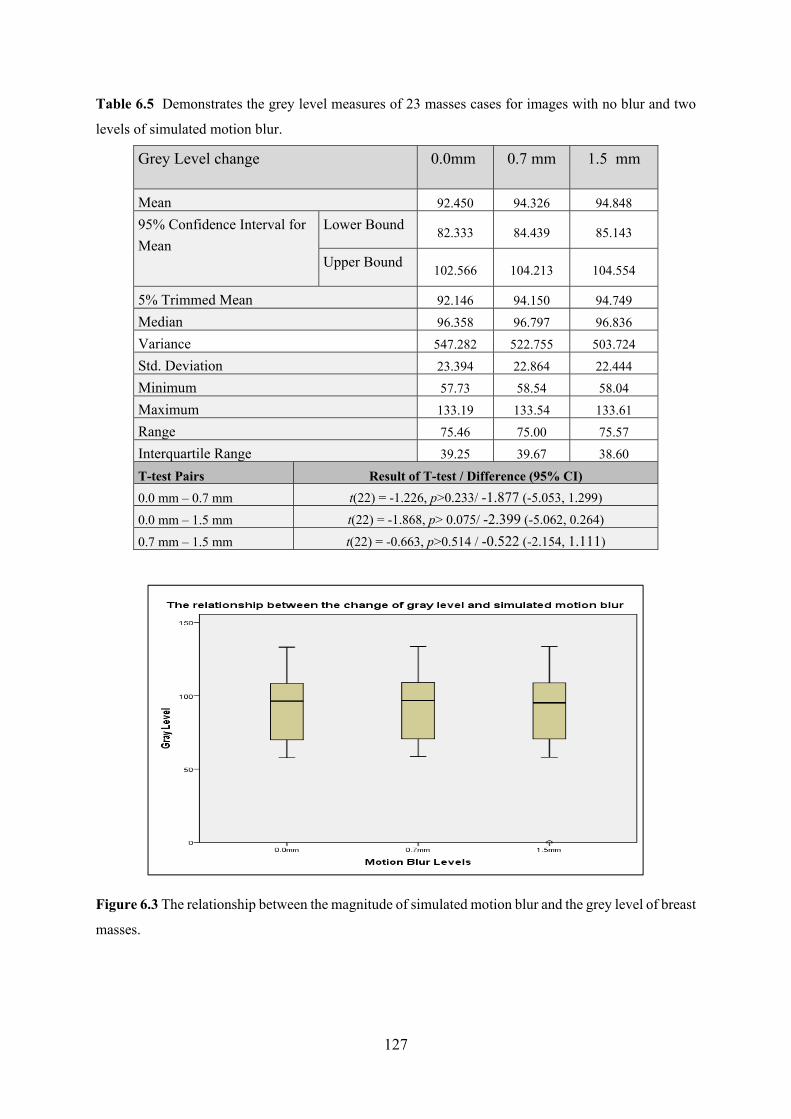
127
Table 6.5 Demonstrates the grey level measures of 23 masses cases for images with no blur and two
levels of simulated motion blur.
Grey Level change 0.0mm
0.7 mm 1.5 mm
Mean 92.450 94.326 94.848
95% Confidence Interval for
Mean
Lower Bound 82.333 84.439 85.143
Upper Bound 102.566 104.213 104.554
5% Trimmed Mean 92.146 94.150 94.749
Median 96.358 96.797 96.836
Variance 547.282 522.755 503.724
Std. Deviation 23.394 22.864 22.444
Minimum 57.73 58.54 58.04
Maximum 133.19 133.54 133.61
Range 75.46 75.00 75.57
Interquartile Range 39.25 39.67 38.60
T-test Pairs Result of T-test / Difference (95% CI)
0.0 mm – 0.7 mm t(22) = -1.226, p>0.233/ -1.877 (-5.053, 1.299)
0.0 mm – 1.5 mm t(22) = -1.868, p> 0.075/ -2.399 (-5.062, 0.264)
0.7 mm – 1.5 mm t(22) = -0.663, p>0.514 / -0.522 (-2.154, 1.111)
Figure 6.3 The relationship between the magnitude of simulated motion blur and the grey level of breast
masses.

128
6.2.5 Signal to Noise Ratio (SNR):
A paired sample t-test was performed to test the hypothesis that SNR in images with simulated
blur (0.7 mm) level (M= 4.394, SD=1.188), 1.5 mm simulated motion blur (M= 5.653, SD=
2.029) and SNR of images without motion blur (0.0mm) (M= 2.741, SD= 0.576) are equal.
The assumption of normally distributed difference scores was examined, and the data was
normally distributed (see Table 6.2). The SNR difference between the two magnitudes of
simulated motion blur and no motion blur were statistically significant for all comparisons (See
Table 6.8). Figure 6.4 illustrates relationship between the magnitude of simulated motion blur
and SNR of breast masses. It can be noted that SNR increases significantly with increase the
level of simulated motion blur as consequence of the smoothing process. Each of the box plots
in (Figure 6.4) is different in size and positions. The distribution of (0.0mm) box plots is lower
than of box plots (0.7 & 1.5 mm). The median of SNR was pointed by the horizontal line, which
runs up the centre of the boxes. The medians of SNR were 2.848 for images without blur
0.0mm, and (4.479, 5.653) for images with simulated motion blur 0.7mm and 1.5 mm
respectively.

129
Table 6.6 Demonstrates SNR measures of 23 masses cases for images with no motion blur and two
levels of simulated motion blur.
SNR 0.0 mm
0.7 mm 1.5 mm
Mean 2.741 4.394 5.653
95% Confidence Interval for Mean
Lower Bound 2.492 3.880 4.776
Upper Bound 2.990 4.908 6.531
5% Trimmed Mean 2.754 4.414 5.503
Median 2.848 4.479 5.238
Variance 0.332 1.413 4.116
Std. Deviation 0.576 1.188 2.029
Minimum 1.581 2.191 2.430
Maximum 3.660 6.280 12.151
Range 2.091 4.090 9.720
Interquartile Range 0.820 1.501 2.040
T-test Pairs Result of T-test / Difference (95% CI)
0.0 mm – 0.7 mm t(22) = -9.307, p<0.000 / -1.653 (-2.021, -1.285)
0.0 mm – 1.5 mm t(22) = -8.608, p<0.000 / -2.913 (-3.614, -2.211)
0.7 mm – 1.5 mm t(22) = -3.714, p<0.01 /-1.260 (-1.963, -0.556)
Figure 6.4 The relationship between the magnitude of simulated motion blur and the signal to noise
ratio (SNR) of breast masses.

130
6.3 Part II: Physical Measures of Microcalcifications
Disperion Index (DI) has been developed for this thesis to test the dispersion index of
microcacifications and also to investigate the relationship between physical measures of
microcalcifications and their detectability. Dispersion index of microcalcifications repsesents
the number of calcifications within a specified area divided by the area. DI was measured
within Imagej software (Schindelin et al., 2012) because the conspicuity index could not be
applied to microcalcifications due to their individual size and their wide distribution pattern.
This represents a limitation of the CI software. No validation has been conducted on DI, but
this could be a focus for post doctoral work. However, during conducting this thesis no
alternative technique existed (aside to DI) to gain a meaningful physical measure in relation to
microcalcifications.
6.3.1 Normality Tests of Microcalcifications Data
For this data, the Kolmogorov-Smirnov test and Shapiro-Wilk test showed that the physical
parameters data such as dispersion index, the contrast and DI x Contrast were not normally
distributed with P ≤ 0.05, and that the SNR data was normally distributed with P ≥ 0.05 as
illustrated in (Table 6.7). A normality test of the data of the physical measures of
microcalcifications is required to check the suitability of the overall data for further analysis
(Field et al., 2013).
Table 6.7 Values of Kolmogorov-Smirnov test and Shapiro-Wilk normality test for the physical
measures data of breast masses
Kolmogorov-Smirnova Shapiro-Wilk
Statistic df Sig. Statistic df Sig.
Dispersion Index 0.0 mm 0.166 62 0.000 0.854 62 0.000
Contrast 0.0 mm 0.148 62 0.002 0.913 62 0.000
DI x Contrast 0.0 mm 0.166 62 0.000 0.849 62 0.000
SNR 0.0 mm 0.076 62 0.200* 0.984 62 0.611
Dispersion Index 0.7 mm 0.168 62 0.000 0.854 62 0.000
Contrast 0.7 mm 0.188 62 0.000 0.867 62 0.000
DI x Contrast 0.7 mm 0.159 62 0.000 0.846 62 0.000
SNR 0.7 mm 0.065 62 0.200* 0.983 62 0.535
Dispersion Index 1.5 mm 0.168 62 0.000 0.854 62 0.000
Contrast 1.5 mm 0.200 62 0.000 0.841 62 0.000
DI x Contrast 1.5 mm 0.163 62 0.000 0.846 62 0.000
SNR 1.5 mm 0.077 62 0.200* 0.976 62 0.257
*. This is a lower bound of the true significance.

131
a. Lilliefors Significance Correction
6.3.2 Dispersion Index (DI) of Microcalcifications
The results demonstrate that the dispersion index of clustered microcalcifications decreases
with an increase in the level of simulated motion blur (Table 6.8). Simulated motion blur has
a statistically significant and negative impact on DI of microcalcifications (Table 6.9). This
means that the changes in the image characteristics of microcalcifications as motion blur
increases from no motion blur could negatively influence the differential features of malignant
microcalcifications. Figure 6.5 graphically illustrates of the mean and confidence interval 95%
of the two magnitudes of simulated motion blur and no motion blur with DI. Each of the box
plots in (Figure 6.5) demonstrates a different skewness pattern. The distribution of (0.0 mm)
box plots is skewed up while the distribution of box plots 0.7 mm and 1.5 mm are skewed
down. The median is (0.687, 0.541 and 0.416) for images without blur 0.0 mm and for images
with simulated motion blur 0.7 mm and 1.5 mm respectively.
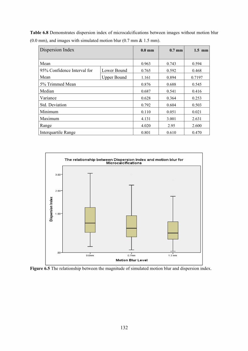
132
Table 6.8 Demonstrates dispersion index of microcalcifications between images without motion blur
(0.0 mm), and images with simulated motion blur (0.7 mm & 1.5 mm).
Dispersion Index 0.0 mm
0.7 mm 1.5 mm
Mean 0.963 0.743 0.594
95% Confidence Interval for
Mean
Lower Bound 0.765 0.592 0.468
Upper Bound 1.161 0.894 0.7197
5% Trimmed Mean 0.876 0.688 0.545
Median 0.687 0.541 0.416
Variance 0.628 0.364 0.253
Std. Deviation 0.792 0.604 0.503
Minimum 0.110 0.051 0.021
Maximum 4.131 3.001 2.631
Range 4.020 2.95 2.600
Interquartile Range 0.801 0.610 0.470
Figure 6.5 The relationship between the magnitude of simulated motion blur and dispersion index.

133
Table 6.9 Demonstrates the P-values of Wilcoxon Signed Ranks Test of physical measures of
microcalcifications between images with no motion blur (0.0 mm), and images with simulated
motion blur (0.7 mm & 1.5 mm).
Simulated motion blur level Dispersion Index Contrast DI x Contrast
0.0 mm - 0.7 mm 0.000 0.000 0.253
0.0 mm- 1.5 mm 0.000 0.000 0.000
0.7 mm- 1.5 mm 0.000 0.000 0.000
6.3.3 Contrast of Microcalcifications
The results demonstrate that the contrast of clustered microcalcifications increases with an
increase in the level of simulated motion blur (Table 6.10). A non-parametric test (Wilcoxon
Signed Ranks Test) was performed to investigate the hypothesis that contrast in images with
simulated blur at 0.7 mm, 1.5 mm and contrast in images with no motion blur (0.0mm) are
equal. Prior to conducting the analysis, the assumption of normally distributed difference
scores was examined and the data was non-normally distributed (Table 6.8). Figure 6.6 shows
the means of contrast and confidence interval 95% of the two magnitudes of simulated motion
blur and no motion blur. The contrast of microcalcifications increases with increase the level
of simulated motion blur. The diagram illustrates a variety of different box plot that positions
and shapes. The distribution of (0.0 mm) box plots is skewed down while the distribution of
box plot (0.7 mm) is skewed up and box plot of 1.5 mm is much higher. The three sections of
the box plot are different in size and position.

134
Table 6.10 Demonstrates contrast of microcalcifications for images without motion blur (0.0 mm), and
images with simulated motion blur (0.7 & 1.5 mm).
Contrast of Microcalcifications 0.0 mm
0.7 mm 1.5 mm
Mean 0.839 0.897 0.916
95% Confidence Interval for
Mean
Lower Bound 0.825 0.884 0.904
Upper Bound 0.852 0.910 0.927
5% Trimmed Mean 0.842 0.901 0.920
Median 0.848 0.910 0.930
Variance 0.003 0.003 0.002
Std. Deviation 0.053 0.051 0.047
Minimum 0.680 0.730 0.750
Maximum 0.930 0.970 0.980
Range 0.260 0.240 0.230
Interquartile Range 0.060 0.050 0.040
Figure 6.6 The relationship between the magnitudes of simulated motion blur and contrast of malignant
microcalcifications.

135
6.3.4 Dispersion Index and Contrast of Microcalcifications
The results demonstrate that DI x contrast of clustered microcalcifications decreases with an
increase in the level of simulated motion blur (Table 6.11). A non-parametric test (Wilcoxon
Signed Ranks Test) was performed to test the hypothesis that DI x contrast in images with
simulated blur 0.7 mm, 1.5 mm and DI x contrast in images without motion blur (0.0mm) are
equal. Prior to conducting the analysis, the assumption of normally distributed difference
scores was examined and the results were non-normally distributed. Simulated motion blur has
a statistically significant negative impact on DI x contrast of microcalcifications (Table 6.8).
A graphical representation of the means and adjusted 95% confidence interval is displayed in
(Figure 6.7).
Table 6.11 Demonstrates measures DI x contrast of microcalcifications for images without motion blur
(0.0 mm), and images with simulated motion blur (0.7 & 1.5 mm).
DI x Contrast of Microcalcifications 0.0 mm
0.7 mm 1.5 mm
Mean 0.824 0.815 0.640
95% Confidence Interval for
Mean
Lower Bound 0.646 0.655 0.508
Upper Bound 1.002 0.975 0.771
5% Trimmed Mean 0.742 0.761 0.592
Median 0.587 0.596 0.466
Variance 0.506 0.410 0.276
Std. Deviation 0.711 0.640 0.525
Minimum 0.080 0.060 0.030
Maximum 3.850 3.100 2.690
Range 3.770 3.040 2.660
Interquartile Range 0.700 0.650 0.520
Skewness 2.007 1.463 1.654
Kurtosis 5.011 1.896 2.942

136
Figure 6.7 The relationship between the magnitude of simulated motion blur and DI x contrast of
microcalcifications.
6.3.5 Signal to Noise Ratio (SNR) of Microcalcifications Images:
A paired sample t-test was performed to test the hypothesis that SNR in images with simulated
blur (0.7 mm) (M= 34.413, SD=13.958), 1.5 mm simulated motion blur (M= 38.035, SD= 17.361)
and SNR in images without motion blur (0.0mm) (M=26.97, SD= 7.859) are equal. Prior to
conducting the analysis, the assumption of normally distributed difference scores was
examined and, the data was normally distributed. The SNR difference between the two
magnitudes of simulated motion blur and no motion blur were statistically significant for all
comparisons (See Table 6.12).
A graphical representation of the means and adjusted 95% confidence interval is displayed in
(Figure 6.8). Each of the box plots in (Figure 6.8) shows a different skewness pattern. The
distribution of (0.0mm) box plots is skewed down while the distribution of box plots (0.7 &
1.5mm) are skewed up. The box plot in 0.0mm is much lower than the box plots in 0.7mm and
1.5mm respectively. The three sections of the box plot are different in size. The box plot in
0.0mm level is comparatively short. The medians of SNR are generally close to the average,
which are approximately (26.725, 33.065, and 37.075) for images without blur 0.0mm and for
images with motion blur 0.7mm and 1.5 mm respectively.

137
Table 6.12 demonstrates SNR of microcalcification for images with no blur and two levels of simulated
motion blur.
SNR of Microcalcifications 0.0 mm
0.7 mm 1.5 mm
Mean 26.97 34.413 38.035
95% Confidence Interval for
Mean
Lower Bound 25.011 30.926 33.702
Upper Bound 28.938 37.899 42.375
5% Trimmed Mean 26.963 34.132 37.427
Median 26.725 33.065 37.075
Variance 61.779 194.849 301.424
Std. Deviation 7.859 13.958 17.361
Minimum 7.740 6.480 3.850
Maximum 43.320 66.740 82.380
Range 35.580 60.260 78.530
Interquartile Range 10.430 20.200 25.250
T-test Pairs Result of T-test / Difference (95% CI)
0.0 mm – 0.7 mm t(61) = -7.598, p<0.000 / -7.438 (-9.394, -5.482 )
0.0 mm – 1.5 mm t(61) = -7.705, p<0.000 / -11.064 (-13.934, -8.195)
0.7 mm – 1.5 mm t(61) = -6.246, p<0.000 / -3.626 (-4.786, -2.466)
Figure 6.8 The relationship between the magnitude of simulated motion blur and SNR of
microcalcifications.

138
6.4 The Relationship between Physical Measures and Detectability of
Microcalcifications
The results of this focuses on the physical parameters of breast microcalcifications such as D.I,
contrast, DI x contrast, signal to noise ratio (SNR) and detectability of lesions with different
levels of motion blur (Table 6.13). A full range of physical measures acquired data for
microcalcifications for image without simulated motion blur (0.0 mm), and images with
simulated motion blur (0.7 & 1.5 mm) is presented in (Appendix M).
Some microcalcifications cases are highly affected by motion blur when the number
calcifications is higher than 10 per cluster; where cluster refers to a collection of
microcalcifications within a specified area. Some studies (Farshid et al., 2011) & Shao et al.
(2011) suggested the probability of malignancy increases with the extent of the lesions on
mammograms. Therefore, a DI metric has been performed to investigate the relationship
between the physical measures of microcalcifications and their detectability with three levels
of motion blur. From Figure 6.9 to Figure 6.17 show there is no relationship between
simulated motion blur and physical measures (D.I, contrast, DI x contrast, and SNR).
Table 6.13 The physical measures of microcalcifications in image with no simulated motion blur (0.0
mm), and images with simulated motion blur (0.7 & 1.5 mm).
Motion blur levels 0.0 mm 0.7 mm 1.5 mm
Lesion No.
DI Cont.
DI x Con
SNR Detect ability
DI Cont. DI x Con
SNR Detect ability
DI Cont. DI x Con
SNR Detect ability
1 1.384 0.890 1.231 41.937 1.00 1.092 1.064 1.162 65.903 1.00 0.801 1.043 0.836 80.936 0.57
2 1.231 0.883 1.087 33.100 1.00 0.934 1.076 1.005 40.395 1.00 1.189 1.058 1.258 42.614 0.85
3 0.918 0.882 0.810 31.978 1.00 0.660 1.077 0.711 38.439 0.86 0.488 1.059 0.516 40.489 0.57
4 0.371 0.850 0.316 25.417 0.57 0.272 1.074 0.292 28.612 0.43 0.198 1.062 0.210 30.236 0.00
5 0.343 0.705 0.242 16.994 1.00 0.225 1.360 0.306 18.511 1.00 0.216 1.296 0.279 19.178 1.00
6 0.426 0.818 0.348 17.616 0.57 0.290 1.154 0.334 18.885 0.43 0.256 1.126 0.288 19.511 0.14
7 0.834 0.820 0.684 26.729 1.00 0.660 1.109 0.732 36.783 1.00 0.487 1.073 0.522 42.352 1.00
8 1.079 0.874 0.943 30.416 1.00 0.863 1.064 0.919 35.927 1.00 0.648 1.050 0.680 37.319 1.00
9 0.292 0.835 0.244 22.641 0.86 0.243 1.146 0.279 24.575 0.57 0.178 1.129 0.202 25.472 0.14
10 0.316 0.829 0.262 24.361 1.00 0.278 1.091 0.303 26.537 0.86 0.215 1.068 0.229 27.239 0.43
11 0.863 0.874 0.754 30.416 1.00 0.648 1.064 0.689 35.927 0.85 0.504 1.050 0.529 37.319 0.43
12 0.524 0.868 0.455 32.058 0.85 0.434 1.089 0.473 38.371 0.72 0.315 1.067 0.336 40.661 0.43
13 1.091 0.861 0.940 25.826 1.00 0.755 1.078 0.814 35.850 0.57 0.587 1.059 0.622 42.052 0.86
14 1.644 0.836 1.375 30.497 1.00 1.644 1.098 1.806 45.660 1.00 1.644 1.070 1.759 52.843 1.00
15 1.039 0.817 0.849 19.745 1.00 0.873 1.142 0.997 26.128 0.57 0.748 1.111 0.831 29.915 0.72
16 3.081 0.902 2.779 36.045 1.00 2.311 1.050 2.427 62.583 0.43 1.797 1.039 1.867 76.603 0.29
17 0.135 0.755 0.102 17.475 0.57 0.072 1.177 0.084 18.153 0.14 0.024 1.151 0.027 18.432 0.29
18 0.138 0.770 0.106 17.204 0.43 0.050 1.236 0.062 17.686 0.29 0.044 1.200 0.053 17.860 0.00
19 0.324 0.814 0.264 19.087 1.00 0.281 1.132 0.318 20.348 0.43 0.195 1.102 0.215 20.891 0.29

139
20 0.519 0.837 0.434 26.142 1.00 0.424 1.106 0.469 29.235 0.43 0.377 1.085 0.409 29.860 0.57
21 1.123 0.847 0.951 26.718 0.72 0.898 1.085 0.974 43.555 0.43 0.786 1.060 0.833 55.100 0.86
22 0.527 0.816 0.430 23.446 1.00 0.461 1.121 0.517 33.045 1.00 0.395 1.089 0.430 40.379 1.00
23 0.610 0.741 0.452 19.164 1.00 0.529 1.217 0.643 21.824 1.00 0.437 1.163 0.508 22.927 1.00
24 0.593 0.816 0.484 23.446 1.00 0.527 1.121 0.591 33.045 0.72 0.461 1.089 0.502 40.379 0.29
25 1.798 0.851 1.529 30.094 1.00 1.498 1.075 1.611 43.183 1.00 1.199 1.053 1.262 51.730 0.72
26 0.400 0.818 0.328 24.267 1.00 0.308 1.120 0.345 27.066 0.14 0.246 1.100 0.271 28.234 0.43
27 0.504 0.873 0.441 29.445 1.00 1.979 1.058 2.094 52.393 1.00 1.715 1.039 1.783 65.020 1.00
28 3.035 0.878 2.666 30.421 1.00 0.395 1.079 0.426 32.785 0.29 0.307 1.068 0.328 34.208 0.00
29 0.355 0.879 0.312 29.415 1.00 0.210 1.084 0.228 33.079 0.86 0.178 1.076 0.191 34.510 0.00
30 1.807 0.813 1.469 22.563 1.00 1.536 1.113 1.709 30.590 1.00 1.084 1.073 1.164 34.509 0.72
31 0.407 0.885 0.360 42.163 1.00 0.356 1.084 0.386 58.661 0.72 0.305 1.063 0.324 68.306 0.72
32 0.344 0.845 0.291 30.250 0.72 0.325 1.054 0.343 50.527 0.43 0.344 1.072 0.369 36.830 0.29
33 1.154 0.857 0.989 23.797 1.00 0.938 1.096 1.027 33.335 1.00 0.649 1.063 0.690 40.408 1.00
34 0.708 0.918 0.650 43.316 1.00 0.472 1.043 0.492 59.089 1.00 0.393 1.035 0.407 62.587 0.72
35 0.797 0.903 0.720 39.172 1.00 0.545 1.058 0.577 50.048 0.43 0.336 1.043 0.350 55.125 0.14
36 1.219 0.896 1.092 37.352 0.72 0.914 1.051 0.961 50.704 0.14 0.711 1.042 0.741 58.915 0.00
37 0.808 0.856 0.692 24.545 0.86 0.539 1.115 0.601 27.471 1.00 0.350 1.098 0.384 28.689 0.72
38 2.195 0.877 1.926 28.573 1.00 1.596 1.072 1.711 41.712 1.00 1.397 1.055 1.474 47.745 1.00
39 0.992 0.875 0.868 33.865 1.00 0.850 1.084 0.922 44.094 1.00 0.709 1.058 0.750 48.152 0.86
40 0.227 0.790 0.179 15.869 0.86 0.212 1.189 0.253 16.741 0.86 0.191 1.169 0.223 17.229 0.72
41 0.949 0.877 0.833 33.421 0.00 0.576 1.086 0.626 45.533 0.00 0.509 1.063 0.541 53.154 0.00
42 0.577 0.778 0.449 21.297 1.00 0.577 1.185 0.684 26.301 1.00 0.577 1.148 0.663 28.756 1.00
43 2.336 0.875 2.044 30.619 1.00 1.934 1.061 2.052 49.347 1.00 1.531 1.042 1.596 58.999 1.00
44 0.800 0.850 0.680 30.134 1.00 0.695 1.106 0.769 40.874 1.00 0.556 1.075 0.598 46.925 0.72
45 0.677 0.863 0.584 28.022 0.86 0.542 1.081 0.586 33.045 0.57 0.316 1.068 0.338 34.799 0.14
46 0.476 0.883 0.421 37.722 0.72 0.278 1.065 0.296 47.684 0.29 0.238 1.046 0.249 51.536 0.00
47 0.521 0.853 0.445 24.452 0.86 0.521 1.118 0.583 27.135 0.72 0.521 1.103 0.575 28.191 0.72
48 0.503 0.820 0.412 21.925 0.72 0.258 1.165 0.300 23.383 0.29 0.225 1.146 0.258 24.122 0.29
49 0.179 0.779 0.139 17.682 0.86 0.124 1.201 0.149 18.750 1.00 0.080 1.168 0.093 19.202 0.86
50 1.605 0.847 1.359 32.138 1.00 0.843 1.088 0.917 40.854 1.00 0.522 1.063 0.554 43.838 0.57
51 2.076 0.845 1.753 30.503 1.00 1.639 1.090 1.787 43.539 0.86 1.202 1.066 1.281 50.335 0.29
52 4.128 0.933 3.852 42.565 1.00 3.002 1.033 3.101 66.743 0.43 2.627 1.023 2.687 82.383 0.29
53 1.304 0.880 1.148 30.465 1.00 1.043 1.082 1.129 36.054 0.86 0.626 1.066 0.667 37.848 0.59
54 2.207 0.812 1.792 18.588 1.00 1.891 1.113 2.106 27.941 0.86 1.366 1.082 1.479 34.383 1.00
55 0.696 0.848 0.590 20.017 0.86 0.544 1.122 0.611 21.552 1.00 0.302 1.108 0.335 21.844 0.57
56 2.064 0.874 1.805 31.030 1.00 1.622 1.103 1.789 6.748 0.86 1.032 1.107 1.142 4.760 0.43
57 0.457 0.848 0.388 38.224 1.00 0.373 1.112 0.414 51.145 1.00 0.288 1.081 0.311 58.309 1.00
58 0.608 0.847 0.515 22.595 1.00 0.405 1.110 0.450 25.336 1.00 0.262 1.097 0.288 26.495 0.86
59 0.399 0.715 0.286 12.505 0.00 0.318 1.288 0.410 13.200 0.00 0.288 1.244 0.359 13.464 0.00
60 0.490 0.802 0.393 19.823 1.00 0.327 1.211 0.396 21.454 1.00 0.272 1.191 0.324 22.394 0.72
61 0.113 0.709 0.080 13.458 0.72 0.083 1.260 0.105 14.581 0.29 0.053 1.192 0.063 14.990 0.29
62 1.266 0.675 0.854 7.745 0.86 1.022 1.363 1.393 6.480 0.72 0.876 1.336 1.171 3.848 0.43
Min. 0.113 0.675 0.080 7.745 0.000 0.050 1.033 0.062 6.480 0.000 0.024 1.023 0.027 3.848 0.000
Max. 4.128 0.933 3.852 43.316 1.000 3.002 1.363 3.101 66.743 1.000 2.627 1.336 2.687 82.383 1.000
Ave. 0.977 0.838 0.837 26.911 0.890 0.754 1.119 0.827 34.438 0.715 0.603 1.096 0.649 38.118 0.556

140
Figure 6.9 Shows the relationship between dispersion index of microcalcifications and their
detectability in images without motion blur. This figure demonstrates there is no relationship (R2=
0.083) between the detectability and dispersion index of microcalcifications.
Figure 6.10 Demonstrates the relationship between the contrast of microcalcifications and their
detectability in images without simulated motion blur. There is no relationship (R2= 0.0737) between
contrast and detectability of microcalcifications.
R² = 0.083
0
0.2
0.4
0.6
0.8
1
0.00 1.00 2.00 3.00 4.00
Detectab
ility
Dispersion Index
Relationship between dispersion index and detectability in (0.0 mm)
R² = 0.0737
0
0.2
0.4
0.6
0.8
1
0.00 0.20 0.40 0.60 0.80 1.00
Detectab
ility
Contrast
Relationship between contrast and detectability in (0.0mm)

141
Figure 6.11 Demonstrates the relationship between the DI x contrast of microcalcifications and their
detectability in images without simulated motion blur. There is no relationship (R2=0.070) between the
DI x contrasts of microcalcification and the detectability of the lesion.
R² = 0.0707
0
0.2
0.4
0.6
0.8
1
0.00 0.50 1.00 1.50 2.00 2.50 3.00
Detectab
ility
DI x Contrast
Relationship between Dispersion Index X contrast and detectability in 0.0mm

142
Figure 6.12 Demonstrates there is no relationship between dispersion index of microcalcifications and
the detectability of the lesion in images with simulated motion blur (0.7mm).
Figure 6.13 Demonstrates there is no relationship between the contrast of microcalcifications and the
detectability of the lesion in images with simulated motion blur (0.7mm).
R² = 0.0592
0
0.2
0.4
0.6
0.8
1
0.00 1.00 2.00 3.00 4.00
Detectability
Desperion Index
Relationship between dispersion index and detectability in 0.7mm
R² = 0.0049
0
0.2
0.4
0.6
0.8
1
0.86 0.88 0.90 0.92 0.94 0.96 0.98
Detectability
Contrast
Relationship between contrast and detectability in 0.7 mm

143
Figure 6.14 Demonstrates there is no relationship between DI x contrast of microcalcifications and the
detectability of the lesion in images with simulated motion blur (0.7mm).
R² = 0.0525
0
0.2
0.4
0.6
0.8
1
0.00 1.00 2.00 3.00 4.00
Detectibility
DI x contrast
Relationship DI x contrast and detectability in 0.7 mm

144
Figure 6.15 Shows the relationship between dispersion index of microcalcifications and their
detectability in images with (1.5 mm) motion blur. This figure demonstrates there is no relationship
(R2 = 0.0027) between the detectability and dispersion index of microcalcifications.
Figure 6.16 Demonstrates that there is no relationship between dispersion index of
microcalcifications and the detectability of the lesion in images with motion blur (1.5 mm).
R² = 0.0027
0
0.2
0.4
0.6
0.8
1
0 20 40 60 80
Detectab
ility
Dispersion Index
Relationship between dispersion index and detectability in 1.5mm
R² = 0.0022
0
0.2
0.4
0.6
0.8
1
0.85 0.90 0.95 1.00
Detectab
ility
Contrast
Relationship contrast and detectability in 1.5 mm

145
Figure 6.17 Demonstrates there is no relationship between DI x contrast of microcalcifications and the
detectability of the lesion in images with simulated motion blur (1.5 mm).
R² = 0.0532
0
0.2
0.4
0.6
0.8
1
0.00 1.00 2.00 3.00 4.00
Detectability
DI x Contrast
Relationship DI x contrast and detectability in 1.5 mm

146
6.5 Missed Lesion Analysis
Missed lesion analysis (i.e. no detection in the free-response study) has been used to evaluate
trends and to identify particular lesion types that have been overlooked frequently. This
analysis has been done for all magnitudes of simulated motion blur such that the impact of
simulated motion blur can be assessed for different lesion types. Comprehensive tables
presented in (Table 6.14 & Table 6.15) to exhibit a list of all lesions missed and detected,
describing detectability as the primary outcome. The detectability for each lesion is represented
by the number of observers who successfully detected the lesion divided by the total number
of opportunities for detection. For instance, when the all observers detected the lesions (7/7),
this means that the detectability is 100%.
Table 6.14 The detectability of malignant masses by the observers in images without motion blur (0.0
mm), and images with simulated motion blur (0.7mm & 1.5 mm).
No. Observer 1
Observer 2
Observer 4
Observer 5
Observer 6
Observer 7
Observer 9
Detectability%
Detectability %
Detectability %
0.0
0.7
1.5
0.0
0.7
1.5
0.0
0.7
1.5
0.0
0.7
1.5
0.0
0.7
1.5
0.0
0.7
1.5
0.0
0.7
1.5
0.0 mm
0.7 mm
1.5 mm
1 ✓ ✓ ✓ ✓ ✓ ✓ ✓ ✓ ✓ ✓ ✓ ✓ ✓ ✓ ✓ ✓ ✓ ✓ ✓ ✓ ✓ 100% 100% 100%
2 ✓ ✓ ✓ ✓ ✓ ✓ ✓ ✓ ✓ ✓ ✓ ✓ ✓ ✓ ✓ ✓ ✓ ✓ ✓ ✓ ✓ 100% 100% 100%
3 X X X x X X X X X X X X X x X X X X X X X 0% 0% 0%
4 ✓ ✓ ✓ ✓ ✓ ✓ ✓ ✓ ✓ ✓ ✓ ✓ ✓ ✓ ✓ ✓ ✓ ✓ ✓ ✓ ✓ 100% 100% 100%
5 ✓ ✓ ✓ ✓ ✓ ✓ ✓ ✓ ✓ ✓ ✓ ✓ ✓ ✓ ✓ ✓ ✓ ✓ ✓ ✓ ✓ 100% 100% 100%
6 ✓ ✓ ✓ ✓ ✓ ✓ ✓ ✓ ✓ ✓ ✓ ✓ ✓ ✓ ✓ ✓ ✓ ✓ ✓ ✓ ✓ 100% 100% 100%
7 ✓ ✓ ✓ ✓ ✓ ✓ ✓ ✓ ✓ ✓ ✓ ✓ ✓ ✓ ✓ ✓ ✓ ✓ ✓ X ✓ 100% 86% 100%
8 ✓ ✓ ✓ ✓ ✓ ✓ ✓ ✓ ✓ ✓ ✓ ✓ ✓ ✓ ✓ ✓ ✓ ✓ ✓ ✓ ✓ 100% 100% 100%
9 X X X ✓ ✓ X ✓ X X ✓ ✓ X ✓ ✓ ✓ X X X ✓ X ✓ 71% 43% 29%
10 ✓ X X ✓ X ✓ ✓ ✓ ✓ ✓ ✓ ✓ ✓ ✓ ✓ ✓ X ✓ X ✓ ✓ 86% 57% 86%
11 X ✓ ✓ ✓ X ✓ ✓ X ✓ ✓ ✓ ✓ ✓ ✓ ✓ ✓ ✓ ✓ X X ✓ 71% 57% 100%
12 ✓ ✓ ✓ ✓ ✓ ✓ ✓ X ✓ ✓ ✓ ✓ ✓ ✓ ✓ ✓ ✓ ✓ ✓ ✓ ✓ 100% 86% 100%
13 X ✓ ✓ ✓ ✓ ✓ ✓ ✓ ✓ ✓ ✓ ✓ ✓ ✓ ✓ ✓ ✓ ✓ ✓ ✓ ✓ 86% 100% 100%
14 ✓ ✓ ✓ ✓ ✓ ✓ ✓ ✓ ✓ ✓ ✓ ✓ ✓ ✓ ✓ ✓ ✓ ✓ X ✓ ✓ 86% 100% 100%
15 ✓ ✓ ✓ ✓ ✓ ✓ ✓ ✓ ✓ ✓ ✓ ✓ ✓ ✓ ✓ ✓ ✓ ✓ ✓ ✓ ✓ 100% 100% 100%
16 ✓ ✓ ✓ ✓ ✓ ✓ ✓ ✓ ✓ ✓ ✓ ✓ ✓ ✓ ✓ ✓ ✓ ✓ ✓ ✓ ✓ 100% 100% 100%
17 ✓ X ✓ ✓ ✓ ✓ ✓ ✓ ✓ ✓ ✓ ✓ ✓ ✓ ✓ ✓ ✓ ✓ ✓ ✓ ✓ 100% 86% 100%
18 ✓ ✓ X ✓ ✓ ✓ ✓ ✓ ✓ ✓ ✓ ✓ ✓ ✓ ✓ ✓ ✓ ✓ ✓ ✓ ✓ 100% 100% 86%
19 ✓ ✓ ✓ ✓ ✓ ✓ ✓ ✓ ✓ ✓ ✓ ✓ ✓ ✓ ✓ ✓ ✓ ✓ ✓ ✓ ✓ 100% 100% 100%
20 ✓ ✓ ✓ ✓ ✓ ✓ ✓ ✓ ✓ ✓ ✓ ✓ ✓ ✓ ✓ ✓ ✓ ✓ ✓ ✓ ✓ 100% 100% 100%
21 ✓ X ✓ ✓ ✓ ✓ ✓ X ✓ ✓ ✓ ✓ ✓ ✓ ✓ ✓ X ✓ ✓ X ✓ 100% 43% 100%
22 ✓ ✓ ✓ ✓ ✓ ✓ ✓ ✓ ✓ ✓ ✓ ✓ ✓ ✓ ✓ ✓ ✓ ✓ ✓ ✓ ✓ 100% 100% 100%
23 ✓ ✓ ✓ ✓ ✓ ✓ ✓ ✓ ✓ ✓ ✓ ✓ ✓ ✓ ✓ ✓ ✓ ✓ ✓ ✓ ✓ 100% 100% 100%
24 ✓ ✓ ✓ ✓ ✓ ✓ ✓ ✓ ✓ ✓ ✓ ✓ ✓ ✓ ✓ ✓ ✓ ✓ ✓ ✓ ✓ 100% 100% 100%
25 ✓ ✓ ✓ ✓ ✓ ✓ ✓ ✓ ✓ ✓ ✓ ✓ ✓ ✓ ✓ ✓ ✓ ✓ ✓ ✓ ✓ 100% 100% 100%
26 ✓ ✓ ✓ ✓ ✓ ✓ ✓ ✓ ✓ ✓ ✓ ✓ ✓ ✓ ✓ ✓ ✓ ✓ ✓ ✓ ✓ 100% 100% 100%
27 X X X ✓ ✓ ✓ ✓ X ✓ ✓ ✓ ✓ ✓ ✓ ✓ ✓ ✓ X X X X 71% 57% 57%
28 ✓ ✓ X ✓ X ✓ ✓ ✓ ✓ ✓ X ✓ ✓ ✓ ✓ ✓ ✓ ✓ X ✓ X 86% 71% 71%
29 X X X X X X X X X ✓ X X X ✓ X X X X X X X 14% 14% 0%
30 ✓ X ✓ ✓ ✓ ✓ ✓ ✓ ✓ ✓ ✓ ✓ ✓ ✓ ✓ ✓ ✓ ✓ ✓ X ✓ 100% 71% 100%

147
31 ✓ ✓ ✓ ✓ ✓ ✓ ✓ ✓ ✓ ✓ ✓ ✓ ✓ ✓ ✓ ✓ ✓ ✓ ✓ ✓ ✓ 100% 100% 100%
32 ✓ ✓ ✓ ✓ ✓ ✓ ✓ ✓ ✓ ✓ ✓ ✓ ✓ ✓ ✓ ✓ ✓ ✓ ✓ ✓ ✓ 100% 100% 100%
33 ✓ ✓ ✓ ✓ ✓ ✓ ✓ ✓ ✓ ✓ ✓ ✓ ✓ ✓ ✓ ✓ ✓ ✓ ✓ ✓ ✓ 100% 100% 100%
34 ✓ X X ✓ X X ✓ ✓ ✓ ✓ ✓ ✓ ✓ ✓ ✓ ✓ ✓ ✓ X ✓ X 86% 71% 57%
35 ✓ ✓ ✓ ✓ ✓ ✓ ✓ ✓ ✓ ✓ ✓ ✓ ✓ ✓ ✓ ✓ ✓ ✓ ✓ ✓ ✓ 100% 100% 100%
36 ✓ ✓ ✓ ✓ ✓ ✓ ✓ X ✓ ✓ ✓ ✓ ✓ ✓ ✓ ✓ ✓ ✓ ✓ ✓ ✓ 100% 86% 100%
37 ✓ ✓ ✓ ✓ ✓ ✓ ✓ ✓ ✓ ✓ ✓ ✓ ✓ ✓ ✓ ✓ ✓ X ✓ ✓ ✓ 100% 100% 86%
38 ✓ ✓ ✓ ✓ ✓ ✓ ✓ ✓ ✓ ✓ ✓ ✓ ✓ ✓ ✓ ✓ ✓ ✓ ✓ ✓ ✓ 100% 100% 100%
39 ✓ ✓ ✓ ✓ ✓ ✓ ✓ ✓ ✓ ✓ ✓ ✓ ✓ ✓ ✓ X ✓ ✓ ✓ ✓ ✓ 86% 100% 100%
40 X X X X X X X X X X X X X X ✓ X X X X X X 0% 0% 14%
41 ✓ X X ✓ ✓ ✓ ✓ ✓ ✓ X ✓ ✓ X ✓ ✓ X ✓ X X ✓ X 43% 86% 57%
42 ✓ ✓ ✓ ✓ ✓ ✓ ✓ ✓ ✓ ✓ ✓ ✓ ✓ ✓ ✓ ✓ ✓ ✓ X ✓ X 86% 100% 86%
43 ✓ ✓ ✓ ✓ ✓ ✓ ✓ ✓ ✓ ✓ ✓ ✓ ✓ ✓ ✓ ✓ ✓ ✓ ✓ ✓ ✓ 86% 100% 100%
44 ✓ X X ✓ X ✓ ✓ X X ✓ ✓ ✓ ✓ ✓ X ✓ ✓ X ✓ ✓ X 100% 57% 29%
45 ✓ ✓ ✓ ✓ ✓ ✓ ✓ ✓ ✓ ✓ ✓ ✓ ✓ ✓ ✓ ✓ ✓ ✓ ✓ X X 100% 86% 86%
46 X ✓ X ✓ ✓ ✓ X X X ✓ ✓ X ✓ ✓ ✓ X X X ✓ X ✓ 71% 57% 43%
47 ✓ ✓ ✓ ✓ ✓ ✓ ✓ ✓ ✓ ✓ ✓ ✓ ✓ ✓ ✓ ✓ ✓ ✓ ✓ ✓ ✓ 100% 100% 100%
48 X X ✓ ✓ ✓ X ✓ ✓ ✓ ✓ X ✓ ✓ X ✓ X X X ✓ ✓ ✓ 71% 43% 71%
49 ✓ ✓ ✓ ✓ ✓ ✓ ✓ ✓ X ✓ ✓ ✓ ✓ ✓ ✓ ✓ ✓ ✓ ✓ ✓ ✓ 100% 100% 86%
50 X ✓ X X ✓ ✓ ✓ X ✓ ✓ ✓ ✓ X ✓ X X ✓ X X ✓ X 29% 86% 43%
51 ✓ X X ✓ ✓ ✓ ✓ ✓ ✓ ✓ X ✓ X ✓ X X X ✓ ✓ X X 71% 43% 57%
52 ✓ ✓ ✓ ✓ ✓ ✓ ✓ ✓ ✓ ✓ ✓ ✓ ✓ ✓ ✓ ✓ ✓ ✓ ✓ ✓ ✓ 100% 100% 100%
53 ✓ ✓ ✓ ✓ ✓ ✓ ✓ ✓ ✓ ✓ ✓ ✓ ✓ ✓ ✓ ✓ ✓ ✓ ✓ ✓ ✓ 100% 100% 100%
54 X X ✓ ✓ ✓ ✓ ✓ ✓ ✓ ✓ ✓ ✓ ✓ ✓ ✓ ✓ ✓ ✓ ✓ ✓ ✓ 86% 86% 100%
55 ✓ X X ✓ ✓ X ✓ ✓ ✓ ✓ ✓ ✓ ✓ ✓ ✓ X ✓ ✓ ✓ ✓ ✓ 86% 86% 71%
56 X X X ✓ ✓ ✓ X ✓ X ✓ ✓ ✓ ✓ ✓ ✓ ✓ ✓ ✓ ✓ X X 57% 71% 57%
57 ✓ ✓ ✓ ✓ ✓ ✓ ✓ ✓ X ✓ ✓ ✓ ✓ ✓ ✓ ✓ ✓ ✓ ✓ X ✓ 100% 86% 86%
58 ✓ ✓ ✓ ✓ ✓ ✓ ✓ ✓ ✓ ✓ ✓ ✓ ✓ ✓ ✓ ✓ ✓ ✓ ✓ ✓ X 100% 100% 86%
59 ✓ ✓ ✓ ✓ ✓ X ✓ ✓ X ✓ ✓ ✓ ✓ ✓ X ✓ ✓ ✓ ✓ ✓ ✓ 100% 100% 57%
60 ✓ ✓ X ✓ ✓ ✓ ✓ ✓ ✓ ✓ ✓ ✓ ✓ ✓ ✓ ✓ ✓ ✓ ✓ X ✓ 100% 86% 86%
61 ✓ ✓ ✓ ✓ ✓ ✓ ✓ ✓ ✓ ✓ ✓ ✓ ✓ ✓ ✓ ✓ ✓ ✓ ✓ ✓ ✓ 100% 100% 100%
62 ✓ X X ✓ ✓ ✓ ✓ ✓ ✓ ✓ ✓ ✓ X ✓ X ✓ ✓ ✓ ✓ X X 86% 71% 57%
The mark (✓) represents the detected lesion while mark (X) represents the missed lesion. The
highlighted results in three columns on the right side represents the average performance of the
observers for lesion which is highly affected by motion blur. The detectability of each lesion
represents the number of observers who detected the lesion divided by the total number of
observers. For instance, when all the observers detected the lesions (7/7), this means that the
percentage detecting the abnormality is 100%. While if only four observers detected the lesion
from seven (4/7) the detectability will be 57.1 %. The highlighted cases represent the affected
cases due to reduce in the detectability of the seven observers as the level of motion blur
increases. The non-highlighted cases represent the non-affected cases due to the detectability
of the observers remaining the same as increase the level of motion blur increases. This means
that some lesion types are not affected by simulated motion blur at all. This table is
complimented by an explanation in the discussion (Chapter Seven) as to why one type is not
affected and why another is affected by simulated motion blur according to lesion features and
breast characteristics.

148
Table 6.15 The detectability of malignant microcalcifications by the observers in images without
motion blur (0.0 mm), and images with simulated motion blur (0.7mm & 1.5 mm).
No. Observer 1
Observer 2
Observer 4
Observer 5
Observer 6
Observer 7
Observer 9
Detectability of each lesion by each observer
0.0
0.7
1.5
0.0
0.7
1.5
0.0
0.7
1.5
0.0
0.7
1.5
0.0
0.7
1.5
0.0
0.7
1.5
0.0
0.7
1.5
0.0 mm 0.7 mm 1.5 mm
1 ✓ ✓ X ✓ ✓ X ✓ ✓ X ✓ ✓ ✓ ✓ ✓ ✓ ✓ ✓ ✓ ✓ ✓ ✓ 1.00 1.00 0.572
2 ✓ ✓ X ✓ ✓ ✓ ✓ ✓ ✓ ✓ ✓ ✓ ✓ ✓ ✓ ✓ ✓ ✓ ✓ ✓ ✓ 1.00 1.00 0.85
3 ✓ ✓ X ✓ X X ✓ ✓ ✓ ✓ ✓ X ✓ ✓ ✓ ✓ ✓ ✓ ✓ ✓ ✓ 1.00 0.858 0.572
4 X X X ✓ ✓ X ✓ X X ✓ X X X ✓ X ✓ ✓ X X X X 0.572 0.429 0.00
5‐1 ✓ ✓ ✓ ✓ ✓ ✓ ✓ ✓ ✓ ✓ ✓ ✓ ✓ ✓ ✓ ✓ ✓ ✓ ✓ ✓ ✓ 1.00 1.00 1.00
5‐2 ✓ ✓ X ✓ X X ✓ X X ✓ ✓ X ✓ X X X ✓ ✓ ✓ X X 0.858 0.429 0.143
6 ✓ ✓ ✓ ✓ ✓ ✓ ✓ ✓ ✓ ✓ ✓ ✓ ✓ ✓ ✓ ✓ ✓ ✓ ✓ ✓ ✓ 1.00 1.00 1.00
7 ✓ ✓ ✓ ✓ ✓ ✓ ✓ ✓ ✓ ✓ ✓ ✓ ✓ ✓ ✓ ✓ ✓ ✓ ✓ ✓ ✓ 1.00 1.00 1.00
8 ✓ X X X X X ✓ ✓ X ✓ ✓ X ✓ ✓ ✓ ✓ ✓ X ✓ X X 0.858 0.572 0.143
8 ✓ ✓ X ✓ ✓ ✓ ✓ ✓ ✓ ✓ ✓ ✓ X ✓ X ✓ ✓ ✓ ✓ X X 1.00 0.858 0.429
9 ✓ ✓ X ✓ ✓ ✓ ✓ X ✓ ✓ ✓ ✓ ✓ ✓ ✓ ✓ ✓ X ✓ ✓ ✓ 1.00 0.858 0.429
10 ✓ ✓ X ✓ X ✓ X ✓ X ✓ ✓ ✓ ✓ ✓ ✓ ✓ ✓ X ✓ X X 1.00 0.715 0.429
11 ✓ ✓ ✓ ✓ ✓ ✓ ✓ X X ✓ X ✓ ✓ ✓ ✓ ✓ ✓ ✓ ✓ X ✓ 1.00 0.572 0.858
12 ✓ ✓ ✓ ✓ ✓ ✓ ✓ ✓ ✓ ✓ ✓ ✓ ✓ ✓ ✓ ✓ ✓ ✓ ✓ ✓ ✓ 1.00 1.00 1.00
13 ✓ X ✓ ✓ ✓ ✓ ✓ X X ✓ ✓ ✓ ✓ X X ✓ ✓ ✓ ✓ ✓ ✓ 1.00 0.572 0.715
14 ✓ X X ✓ X X ✓ ✓ X ✓ X X ✓ ✓ ✓ ✓ ✓ X ✓ X ✓ 1.00 0.429 0.286
15 X X X ✓ X X ✓ X X ✓ X ✓ X ✓ ✓ X X X ✓ X X 0.572 0.143 0.285
15 X X X ✓ X X ✓ X X ✓ X X X X X X X X X ✓ X 0.429 0.285 0.00
16 ✓ X X X X X ✓ X X X X ✓ ✓ ✓ X X X X X X X 0.429 0.143 0.143
16‐2 ✓ X X ✓ ✓ ✓ ✓ ✓ X ✓ X ✓ ✓ ✓ ✓ ✓ ✓ ✓ X ✓ X 0.858 0.715 0.572
17 ✓ ✓ X ✓ ✓ ✓ ✓ X X ✓ X ✓ ✓ X X ✓ ✓ X ✓ X X 1.00 0.428 0.285
18 ✓ X X ✓ ✓ ✓ ✓ X X ✓ ✓ ✓ ✓ X ✓ ✓ ✓ ✓ ✓ X X 1.00 0.428 0.572
19 X ✓ ✓ ✓ X ✓ ✓ X ✓ X X X ✓ X X ✓ ✓ ✓ ✓ ✓ ✓ 0.715 0.428 0.858
20 ✓ ✓ ✓ ✓ ✓ ✓ ✓ ✓ ✓ ✓ ✓ ✓ ✓ ✓ ✓ ✓ ✓ ✓ ✓ ✓ ✓ 1.00 1.00 1.00
21 ✓ ✓ ✓ ✓ ✓ ✓ ✓ ✓ ✓ ✓ ✓ ✓ ✓ ✓ ✓ ✓ ✓ ✓ ✓ ✓ ✓ 1.00 1.00 1.00
22 ✓ X X ✓ ✓ ✓ ✓ ✓ X ✓ X X ✓ ✓ ✓ ✓ ✓ X ✓ ✓ X 1.00 0.715 0.286
23 ✓ ✓ ✓ ✓ ✓ ✓ ✓ ✓ X ✓ ✓ ✓ ✓ ✓ ✓ ✓ ✓ X ✓ ✓ ✓ 1.00 1.00 0.715
24 ✓ ✓ ✓ ✓ ✓ ✓ ✓ ✓ ✓ ✓ ✓ ✓ ✓ ✓ ✓ ✓ ✓ ✓ ✓ ✓ X 1.00 1.00 0.858
25 ✓ X X ✓ X ✓ ✓ X X ✓ X ✓ ✓ X X ✓ ✓ X ✓ X X 1.00 0.143 0.286
26 ✓ ✓ X X ✓ ✓ ✓ ✓ X ✓ ✓ ✓ ✓ ✓ ✓ ✓ ✓ X ✓ ✓ X 1.00 1.00 0.43
27 ✓ ✓ ✓ ✓ ✓ ✓ ✓ ✓ ✓ ✓ ✓ ✓ ✓ ✓ ✓ ✓ ✓ ✓ ✓ ✓ ✓ 1.00 1.00 1.00
28 ✓ X X ✓ X X ✓ ✓ X ✓ X X ✓ ✓ X ✓ X X ✓ X X 1.00 0.286 0.00
29 ✓ X X ✓ ✓ X ✓ ✓ X ✓ ✓ X ✓ ✓ X ✓ ✓ X ✓ ✓ X 1.00 0.858 0.00
30 ✓ ✓ ✓ ✓ ✓ X ✓ ✓ ✓ ✓ ✓ ✓ ✓ ✓ ✓ ✓ ✓ X ✓ ✓ ✓ 1.00 1.00 0.715
31 ✓ X X ✓ ✓ ✓ ✓ X ✓ ✓ ✓ X ✓ ✓ ✓ ✓ ✓ ✓ ✓ ✓ ✓ 1.00 0.858 0.715
32‐1 X ✓ X X ✓ X ✓ X X ✓ X X ✓ ✓ X ✓ X X ✓ X X 0.858 0.429 0.285
32‐2 ✓ ✓ ✓ ✓ ✓ ✓ ✓ ✓ ✓ ✓ X ✓ ✓ ✓ ✓ ✓ ✓ ✓ ✓ ✓ ✓ 1.00 0.858 1.00
33 ✓ ✓ ✓ ✓ ✓ ✓ ✓ ✓ ✓ ✓ ✓ ✓ ✓ ✓ ✓ ✓ ✓ ✓ ✓ ✓ ✓ 1.00 1.00 1.00
34 ✓ ✓ X ✓ ✓ X ✓ ✓ ✓ ✓ ✓ ✓ ✓ ✓ ✓ ✓ ✓ ✓ ✓ ✓ ✓ 1.00 1.00 0.715
35‐1 ✓ X X ✓ X ✓ ✓ ✓ X ✓ X X ✓ X X ✓ ✓ X ✓ X X 1.00 0.429 0.143
35‐2 ✓ X X ✓ X X ✓ X X ✓ X X ✓ ✓ X X X X ✓ X X 0.715 0.143 0.00
36 ✓ ✓ X ✓ ✓ ✓ ✓ ✓ X ✓ ✓ ✓ ✓ ✓ ✓ X ✓ ✓ ✓ ✓ ✓ 0.858 0.858 0.715
37 ✓ ✓ ✓ ✓ ✓ ✓ ✓ ✓ ✓ ✓ ✓ ✓ ✓ ✓ ✓ ✓ ✓ ✓ ✓ ✓ ✓ 1.00 1.00 1.00
38 ✓ ✓ ✓ ✓ ✓ ✓ ✓ X ✓ ✓ ✓ ✓ ✓ ✓ ✓ ✓ ✓ ✓ ✓ ✓ ✓ 1.00 1.00 0.858
39 ✓ X X ✓ ✓ ✓ ✓ ✓ ✓ X ✓ X ✓ ✓ ✓ ✓ ✓ ✓ ✓ ✓ ✓ 0.858 0.858 0.715
40 X X X X X X X X X X X X X X X X ✓ X X X X 0.00 0.00 0.00
41 ✓ ✓ ✓ ✓ ✓ ✓ ✓ ✓ ✓ ✓ ✓ ✓ ✓ ✓ ✓ ✓ ✓ ✓ ✓ ✓ ✓ 1.00 1.00 1.00
42 ✓ ✓ ✓ ✓ ✓ ✓ ✓ ✓ ✓ ✓ ✓ ✓ ✓ ✓ ✓ ✓ ✓ ✓ ✓ ✓ ✓ 1.00 1.00 1.00
43 X ✓ ✓ ✓ ✓ ✓ ✓ ✓ ✓ ✓ ✓ ✓ ✓ ✓ ✓ ✓ ✓ ✓ ✓ ✓ ✓ 0.858 1.00 1.00
44 ✓ ✓ ✓ ✓ ✓ ✓ ✓ ✓ ✓ ✓ ✓ ✓ ✓ ✓ X ✓ ✓ ✓ ✓ ✓ ✓ 1.00 1.00 0.715

149
45‐1 ✓ X X ✓ ✓ X ✓ X X ✓ ✓ X ✓ ✓ ✓ X ✓ X ✓ X X 0.858 0.572 0.143
45‐2 ✓ X X X X X ✓ X X ✓ X X ✓ ✓ X X ✓ X ✓ X X 0.715 0.286 0.00
46‐1 ✓ X X ✓ ✓ ✓ ✓ ✓ ✓ ✓ ✓ X ✓ ✓ ✓ ✓ X ✓ ✓ ✓ ✓ 0.858 0.715 0.715
46‐2 ✓ ✓ ✓ X X X X X X X X X X X X ✓ ✓ ✓ X X X 0.715 0.285 0.285
47 ✓ ✓ ✓ ✓ ✓ ✓ ✓ ✓ ✓ ✓ ✓ ✓ ✓ ✓ ✓ ✓ ✓ ✓ X ✓ X 0.858 1.00 0.858
48‐1 ✓ ✓ X ✓ ✓ X ✓ ✓ ✓ ✓ ✓ ✓ ✓ ✓ ✓ ✓ ✓ X ✓ ✓ ✓ 1.00 1.00 0.572
48‐2 ✓ X X ✓ ✓ X ✓ ✓ ✓ ✓ ✓ ✓ ✓ ✓ X ✓ ✓ X ✓ ✓ ✓ 1.00 0.858 0.286
49 ✓ X X ✓ ✓ ✓ ✓ X ✓ ✓ ✓ X ✓ ✓ X ✓ X X ✓ X X 1.00 0.429 0.286
50 ✓ X X ✓ ✓ ✓ ✓ ✓ ✓ ✓ ✓ X ✓ ✓ X ✓ ✓ ✓ ✓ ✓ ✓ 1.00 0.858 0.585
51 X X X ✓ X ✓ ✓ ✓ X ✓ X ✓ ✓ X ✓ ✓ X X X X X 0.715 0.143 0.572
52 ✓ X ✓ ✓ ✓ ✓ ✓ ✓ ✓ ✓ ✓ ✓ ✓ ✓ ✓ ✓ ✓ ✓ ✓ ✓ ✓ 1.00 0.858 1.00
53 ✓ ✓ X X ✓ ✓ ✓ ✓ ✓ ✓ ✓ ✓ ✓ ✓ X ✓ ✓ X ✓ ✓ ✓ 1.00 1.00 0.572
54 ✓ ✓ ✓ ✓ ✓ ✓ ✓ X X ✓ ✓ ✓ ✓ ✓ X ✓ ✓ X ✓ ✓ X 1.00 0.858 0.429
55 ✓ ✓ ✓ ✓ ✓ ✓ ✓ ✓ ✓ ✓ ✓ ✓ ✓ ✓ ✓ ✓ ✓ ✓ ✓ ✓ ✓ 1.00 1.00 1.00
56 ✓ ✓ ✓ ✓ ✓ ✓ ✓ ✓ ✓ ✓ ✓ ✓ ✓ ✓ ✓ ✓ ✓ ✓ ✓ ✓ ✓ 1.00 1.00 0.858
57 X X X X X X X X X X X X X X X X X X X X X 0.00 0.00 0.00
58 ✓ ✓ X ✓ ✓ ✓ ✓ ✓ X ✓ ✓ ✓ ✓ ✓ ✓ ✓ ✓ ✓ ✓ ✓ X 1.00 1.00 0.715
59 ✓ X X ✓ X X X X X ✓ ✓ ✓ X X X ✓ ✓ X ✓ X X 0.715 0.286 0.286
60 ✓ X X ✓ ✓ ✓ X ✓ X ✓ ✓ ✓ X ✓ ✓ ✓ ✓ ✓ X X X 0.858 0.715 0.429
61 ✓ ✓ ✓ ✓ ✓ ✓ ✓ ✓ ✓ ✓ ✓ ✓ ✓ ✓ ✓ ✓ ✓ ✓ ✓ ✓ ✓ 1.00 1.00 1.00
62 ✓ ✓ X ✓ X ✓ ✓ ✓ X ✓ ✓ ✓ ✓ ✓ ✓ ✓ X X ✓ ✓ X 1.00 0.715 0.429
The mark (✓) represents the detected lesion while mark (X) represents the missed lesion. The
highlighted results in three columns on the right side represents the average performance of the
observers for lesion which is highly affected by motion blur. The highlighted cases were
selected according to the decrease of the detectability when increases simulated motion blur.
The detectability of each lesion represents the number of observers who detected the lesion
divided by the total number of observers. For instance, when all the observers detected the
lesions (7/7), this means that the percentage detecting the abnormality is 100%. While if only
four observers detected the lesion from seven (4/7) the detectability will be 57.1 %. The
highlighted cases represent the affected cases due to reduce in the detectability of the seven
observers as the level of motion blur increases. The non-highlighted cases represent the non-
affected cases due to the detectability of the observers remaining the same as increase the level
of motion blur increases. This means that some lesion types are not affected by simulated
motion blur at all.

150
Chapter Seven: Discussion
7.1. Overview
This chapter evaluates the results of the free-response study and the physical measures
performed on the lesions under different magnitudes of simulated blur. The discussion is
organised into five main themes. The first theme will discuss the impact of motion blur on the
detection performance of breast masses and microcalcifications for single observer data. The
second theme will focus on the result of simulating a dual read versus a single read via the
combination of observer data. The third theme will focus on the impact of simulated motion
blur on the physical characteristics of breast masses and microcalcifications. The fourth theme
will focus on the commonly missed lesions in this study and the impact of motion blur on lesion
characteristics. The physical measures of malignant masses include the conspicuity index, edge
angle, grey level change, image noise and SNR. The physical measures of malignant
microcalcifications include a new novel metric known as the ‘dispersion index’, contrast,
image noise and SNR with the impact of motion blur. The fifth theme will focus on the impact
of motion blur on the image characteristics of malignant masses; discussing the cases where
observer performance was affected by simulated motion blur and those that were not. Finally,
the limitations of the work will be discussed.
7.2 Free-response Performance Study (single observer)
This thesis has investigated the impact of computer simulated motion by means of shifting
accumulated pixel points to blur the resultant image. The results of the single observer free-
response study demonstrate that simulated motion blur had a significant effect on observer
performance, with performance becoming statistically worse for the detection of
microcalcifications as motion blur increased from 0 mm to 0.7 mm, and then on to 1.5 mm. A
similar trend was observed for masses, with the only difference being that there was no
statistically significant difference in lesion detection performance as the magnitude of
simulated motion blur was increased from 0.7 mm to 1.5 mm. For both broad categories of
lesions, it should be noted that motion blur in the magnitude of 0.7 mm and above will have an
adverse impact on lesion detection performance.
Previous work by Ma et al., (2015) suggested that motion blur could be visible at 0.7 mm for
‘soft-edged’ motion blur using software simulation, and the findings of my PhD thesis appear

151
to confirm that a similar effect was observed with a computer simulation motion blur on clinical
mammographic images. This observation may have implications for practice. It suggests that
if motion blur is identified in an image, repeat imaging should be considered as in clinical work
one would simply not know how much motion blur is present or what impact it is having in
terms of masking lesions or potentially changing the appearance of lesions. If image motion
blur has this type of impact it could lead to an incorrect classification of disease status. In order
to explain the significance of motion blur, several scenarios are presented:
Scenario 1– repeated case
Motion blur is detected at the time of image acquisition and a decision is made to repeat the
image while the client is still within the mammography department. The image is repeated
directly after image acquisition and the client is still in the mammography department. This
occurs when the radiographer detects blur during the quality assessment of the image whilst
still in the mammography imaging room. This process will lead to increased cost and radiation
dose, lost time and effort. From the clients perspective, repeating the image at the time of
attendance is better than a recall (i.e. reduced anxiety). However, the image blurring could go
undetected in imaging rooms if low resolution monitors are used (Ma et al., 2016).
Scenario 2– recall case
If motion blur is not identified at the time of acquisition, and is only picked up during the
review of images (on a higher specification of monitor display) then the client may be recalled
for further imaging. This scenario can lead to an increase in client and family anxiety because
they might suspect that an abnormality has been detected. In addition, the decision to recall a
client means a new appointment must be scheduled, which can ultimately lead to delays in the
detection and treatment of breast cancer.
Scenario 3– missed lesion
If motion blur is not detected at any point during the diagnostic decision making stage and a
lesion is ‘missed’, there is a chance that this lesion could later present at follow-up imaging or
as an interval cancer. An interval cancer represents a breast cancer which is detected in the
interval between scheduled screening sessions (Hofvind & de Wolf, 2015).
In the performance study, there were several categories of lesion. First, lesions that are detected
by all observers when motion blur is absent and then missed by the observers in images
containing simulated motion blur (0.7 mm and 1.5 mm), providing a clear indication about the
impact of motion blur on detection performance. Second, some lesions were not affected by

152
the magnitudes of simulated motion blur used in this study. Third, lesions that are either
difficult to detect or decide if they are malignant, when lesions are missed by all observers in
images without blur and in images with motion blur (0.7 mm & 1.5 mm); this means that in
some difficult cases, lesions were missed anyway and blurring had no impact on their detection
performance. In this study, we do not know if it is due to decision or detection error; further
work with eye-tracking may help to answer this.
The impact of motion blur on lesion detection performance could vary with lesion
characteristics. Each lesion within the mammography image has a range of characteristics along
with a range of background features in which the lesion sits. Some of the lesion types, such as
spiculated or indistinct masses, could be affected by motion blur due to the impact of simulated
blur on the edge between the lesion and background tissues; while others, such as well
circumscribed oval or round masses, might be affected or not affected at all. A lesion-by-lesion
analysis of detection performance revealed that larger malignant masses were not affected by
simulated motion blur. In addition, breast masses that have high lesion-to-background contrast
did not demonstrate a detection deficit in the observer study. However, some smaller, low-
contrast breast masses were associated with poorer detection performance. For example, some
small breast masses were detected in images without motion blur by all observers and missed
when simulated motion blur was applied (at 0.7mm and 1.5mm simulated motion blur ) (See
Table 6.15 on page 155).
In the observer study, a high FOM and sensitivity were achieved for images without motion
blur for microcalcifications and masses. For microcalcifications, the observer averaged
wJAFROC FOM was 0.899 (0.757,0.870) in images without motion blur, whereas this
decreased to 0.813 (0.757,0.870) in 0.7mm and 0.746 (0.679,0.812) in 1.5mm levels of
simulated motion blur . For masses, the FOMs in images without motion blur was 0.905
(0.859,0.952) compared with blurred images 0.7mm 0.869 (0.814,0.924) and 0.862
(0.810,0.915) in1.5mm . However, it should be noted that there is no statistically significant
difference between 0.7mm and 1.5mm levels of simulated motion blur for the latter; this gives
an indication that the levels between 0.7 and 1.5 have the same impact on lesion detection
performance.
There are many factors that affect lesion detection performance and these should be taken into
account in both the empirical work presented here and in clinical practice. Many studies suggest
that detection performance is related to the observer in terms of experience, cognitive skills and

153
visual performance (Reed, 2005; Manning et al., 2006; Sabih et al., 2011; Burgess, 2011; Lança
et al., 2015). Other studies suggest that lesion characteristics could contribute to the challenges
of interpreting an image accurately. Lesion characteristics are particularly important in breast
disease. Malignant breast lesions with indefinite edges for normal and pathological tissue can
lead to difficulties in perception (Van Overveld, 1995; Tabar et al., 2005; Kopans, 2006). Other
studies suggest that factors related to the characteristics of mammographic images (e.g. image
quality, artefacts, spatial resolution, sharpness and contrast resolution) can also influence
detection performance (Li et al., 2010; Spuur et al., 2011; Zanca et al., 2012).
7.2.1 Microcalcifications
Free-response data were analysed for the detection of malignant microcalcifications for three
conditions; (i) no simulated motion blur (0.0 mm), and for two magnitudes of simulated motion
blur (0.7 and 1.5 mm). A significant difference was observed between 0 mm and 0.7 mm, and
between 0 mm and 1.5 mm of simulated motion blur, and also between 0.7 mm and 1.5 mm.
This means all levels equal to and above 0.7mm have the potential to obscure lesions or cause
interpretation error. In addition, an even higher significant difference was detected between
(0.0 mm V 1.5 mm, p= 0.004) compared with 0.0mm and 0.7mm (p= 0.0016). This suggests
that the negative impact of simulated motion blur on detection performance increases as the
level of simulated motion blur increases. It should be noted that no study was found in the
literature to compare the results of the impact of motion blur on lesion detection performance
in FFDM, so comparisons to what is already known cannot be done.
Lesions which contain less than 10 calcifications in a cluster and are classified as punctate or
granular types of microcalcifications illustrating irregularity in density, variety, size, or shape
were affected by simulated motion blur and tended to be associated with poorer detection rates.
Figure 7.1 provides an illustration of this, where the calcifications are indicated by red arrows.
The microcalcifications appear as non-focal clusters with irregular outlines. In contrast, the
results demonstrated that the microcalcifications which have definite edges (similar shape,
density and size of individual microcalcifications) with focal clustering were not affected by
motion blur. Overall, detection performance decreased as simulated motion blur increased. In
the case described in Figure 7.1, 100% (7/7) of the observers detected microcalcifications with
no blur (0.0mm), this decreased to 14.3% (1/7) at 0.7mm and 29% (2/7) at 1.5mm of simulated
motion blur.

154
Figure 7.1 Magnified area of right cranio-caudal projection. Demonstrates a cluster of
microcalcifications have irregular shapes.
The cases used in this observer study have been classified into two types according to the
influence of motion blur on detection performance; affected and not affected. The detection
performance of some image characteristics of malignant calcifications are affected by motion
blur more than others. Figure 7.2 describes an example that contains several different shapes
of calcification, such as pleomorphic, diffuse and punctate. These have all been detected by the
observer in images without motion blur (0.0mm). The same microcalcifications have been
missed by the observers when simulated motion blur had been applied in the magnitude of
0.7mm and 1.5mm levels of simulated motion blur. This suggests that motion blur could
obscure certain types of small calcifications. In general, sensitivity represents a measure of
accuracy determined by the true positive rate which is the ability of the observer to accurately
identify cases of disease while specificity represents a measure of the true negative rate or the
ability of the observer to accurately identify cases without lesion. Since the FOM decreased as
simulated motion blur increased, this implies that the false negative rate also increased. This
relationship, between the FOM and motion blur, was significant (F(2,18) = 10.48, p=0.0010).
The results demonstrate that the sensitivity of images without simulated motion blur (0.0mm)
was 97.9, and the sensitivities for blurred images (0.7mm and 1.5mm) were 86.4 and 76.5 %,
respectively. When specificity (HrSp) is used as the FOM, there was no significant difference
between magnitudes of simulated motion blur (F(2,13) = 0.21, p=0.8110). This suggests that
the false positive rate did not increase significantly with increasing motion blur. Although the
false positive (FP) rate at the 1.5mm level was more than 0.0mm level, a low confidence level

155
was provided by the observers (1.5 mm) and the free-response study is designed to not penalise
errors if the observers gives low confidence level.
Figure 7.2 Magnified views of images without simulated motion blur (0.0mm) and blurred
mammography images (0.7mm & 1.5mm). The images illustrate a cluster of malignant
microcalcifications, which were affected by simulated motion blur.
7.2.2 Masses Cases
For masses, a statistically significant difference was detected between two levels (0 mm V 1.5
mm, p=0.0041), this means that detection performance was reduced between images containing
no blur and those containing 1.5mm of simulated motion blur. The result also showed that there

156
was no significant difference between the two magnitudes of simulated motion blur (0.7 mm
and 1.5 mm; p=0.640). This means that all magnitudes of motion blur above 0.7 have a similar
negative impact on mass detection. When sensitivity (HrSe) was used as the FOM, there was
no significant difference between different magnitudes of simulated motion blur (F (2, 16) =
0.43, p=0.6575). This implies that the false negative rate did not change significantly as a result
of simulated motion blur. The sensitivity of images without motion blur (0.0 mm) was 92.3%
and the sensitivity for blurred images were 91.9% and 90.5% for levels 0.7mm and 1.5mm,
respectively. The sensitivity of lesion detection decreases with increasing levels of motion blur,
but not to a significant level. When specificity (HrSp) was used as the FOM, again there was
no significant difference between magnitudes of simulated motion blur (F (2,12) = 1.31,
p=0.3043). Specificity reduces with an increase in the level of simulated motion blur especially
in cases of breast masses, with magnitudes shifting from 82.7% for images without motion blur
(0.0 mm) to 73.3% in blurred images (0.7 mm).
In summary, for both microcalcifications and masses, there was a reduction in sensitivity as
the magnitude of simulated motion blur increased. For masses, this was not statistically
significant and the values in (Table 5.5 on page111) demonstrate that the false negative rate
did not change that much as motion blur increased. For microcalcifications, this was not the
case and there was a statistically significant reduction in sensitivity, (Table 5.3 on page 107)
suggests that an increase in motion blur caused the smaller lesions to become visually
imperceptible. The change in specificity was not significantly different for masses or
microcalcifications.
The literature is relatively sparse on studies that have looked at the impact of motion blur
artefacts, however there are some isolated cases from other image modalities that have assess
the impact of motion blur. Let us now compare the mass results in this thesis with other studies.
Donnelly and Thompson, (2017) assessed the impact of simulating respiratory motion on the
detection of lung nodules in CT. Low-dose images were generated with the intention with the
primary application of CT attenuation correction (CTAC) of nuclear medicine SPECT image
data. They used an anthropomorphic chest phantom and a variety of simulated spherical lung
nodules of different size and density. Physical motion blur was introduced through use of a
mechanical device used to simulate the rate and amplitude of respiratory motion. Five
observers assessed the images with and without simulated motion using a free-response study

157
to determine the detection performance of the nodules. Data were analysed using the
wJAFROC FOM. It was concluded that simulated respiratory motion has a significant negative
impact on nodule detection performance (F(1,4.00) =10.88, p=0.0300).
In comparison to other previous observer studies, the FOM achieved in images containing no
simulated motion blur were associated with generally better performance. This must be
considered in some caution due to differences in study design, purpose of the research, and the
population of client images, and the experience of the observers. For instance, a study by
(Debono, 2012a) evaluated the diagnostic accuracy of reporting radiographers in screening
mammography according to types of breast lesions. Debono used ROC method to assess the
accuracy of 10 radiographers through measuring the area under the curve (AUC). Debono
found that individual sensitivity levels ranged between 76.0% and 92.0%, and individual
specificity levels ranged between 74.8% and 96.2%. Debono (2012a) also summarised
previous studies and found that radiographer sensitivity levels varied between 61.0% and
91.42%, and specificity levels varied between 45.0% and 99.1%. Debono’s study found
radiologist sensitivity levels were between 63.9% and 100%, and specificity levels between
81.0% and 99.2% (Debono, 2012a). In my thesis, the FROC method was used to determine the
detection performance; this is more advanced method than ROC, since ROC ignores location
information. Typically, it is expected that an inflated FOM is generated if location information
is ignored. However, this general level of agreement in performance is encouraging.
7.2.3 Reflection – comparison of laboratory and clinical studies
A laboratory study, as conducted in this thesis, is very different to the clinical reality of
reviewing mammographic images. In a laboratory study there is a heightened expectation of
disease since there is an enriched dataset and the observers know they are probably looking for
a higher proportion of lesions. The consequence of this is that observers are more likely to
indicate the presence of a lesion. This can lead to changed behaviour and in this situation the
likelihood of making more localisation, leading to increased true and false decisions, has little
consequence other than an increase in sensitivity or a reduction in specificity (Table 5.2 on
page 101 and Table 5.6 on page 107). When compared to the clinical scenario, the image
reader also has to consider their recall rate and the risk of over-investigation. It is difficult to
predict how image readers will behave during a laboratory study and consequently this can lead

158
to differences in sensitivity and specificity. This is why laboratory studies are conducted using
multiple readers and cases.
7.3 The Combined two Observers’ Data
Double reading is a routine procedure to interpret mammographic images in breast cancer
screening programmes. In the UK NHSBSP, double reading is ideally conducted blinded for
all cases (Wilson et al., 2011). Discordant cases are arbitrated under locally agreed protocols.
In the case of a suspicious area being noted, a decision is then made to either recall the client
for further assessment or allow them to carry on as normal in routine triennial screening.
Double reading is standard and recommended in many breast screening programmes (e.g.
European and Australia breast cancer screening programmes) due to the advantages of
increased accuracy and sensitivity through decreasing the chance of undetected lesions (Perry
et al., 2008; Debono et al., 2015). With the above in mind, there was an opportunity to combine
the data from individual observers to simulate the outcome of a double reading. The purpose
of combined two observers’ data was to assess the impact of combined observer free-response
data on lesion detection performance in blurred images. Since this was a retrospective analysis
of the data acquired by individual observers, the method to achieve this in my thesis cannot be
generalised to NHSBSP practice as no consensus meeting or arbitration process took place for
discordant cases. However, it is reasonable to assume that the combined read used in this thesis
will give a higher positive outcome rate because in the clinical setting within NHSBSP the
double reading consensus meeting will result in some cases being ‘downgraded’ from positive
to negative.
Different combinations of two observers’ data was likely to enhance the detection performance
of the observers. For random reader random case analysis of breast masses, there was no
statistically significant difference in lesion detection performance between single and
combined free-response data (F(1,6)=4.04, p=0.1001). For the analysis of microcalcifications,
a statistically significant difference in lesion detection performance was demonstrated between
single and combined free-response data (F(1,6)=12.28, p=0.0122). For both masses and
microcalcifications, there was an increase in sensitivity (HrSe) when using two observers in
combination rather than one observer in isolation. This is due to the method used to combine
the data, where the highest rating was taken as the single rating. This means that if one of the

159
two observers correctly localised the lesion it would be classed as true positive. Conversely,
the simulation of a double reading also increased the number of false positive localisations thus
reducing the specificity, as shown by the HrSp FOM (Tables 5.11 on page 122 & Table 5.13
on page 124). These results agree with previous studies (Husien, 1995; Taplin et al., 2000),
where double image reader interpretation resulted in an increase in sensitivity of 10%.
However, there was a decrease in specificity of 1.8%. For my thesis, in the single observer
data, there was a negative significant difference in the impact of motion blur on breast mass
detection performance. A statistical difference in detection performance was found when
motion blur was applied to the images at 0.7 mm for the combined observer data.
Many studies have discussed the advantages and disadvantages of double reporting. Firstly,
double reporting can increase sensitivity through decreasing the chance of undetected lesions
(Blanks et al., 1998; Dinnes et al., 2001; Harvey et al., 2003; Klompenhouwer et al., 2015).
Accordingly, double reporting of mammographic images became normal practice in European
breast screening programmes (Perry et al., 2008). However, there are some disadvantages of
double reporting related to its cost-effectiveness. First, double reporting effectiveness can be
less important when a high level of agreement between image readers is achieved (Taplin et
al., 2000). Second, the benefit of double reporting might be restricted to specific situations
when the detection of cancer is difficult, i.e. mammographic images of females in prevalent
screening (first participation) when previous mammograms do not exist, females with small
lesions that are difficult to detect, or when the image readers are less experienced (Dinnes et
al., 2001; Sickles, 2010). Finally, double reporting increases staff costs and resources utilised
in the interpretation procedure and takes longer time (Posso et al., 2016). However, others
argued that in some contexts more advantages can be achieved from single reporting as it may
decrease costs and FP without significantly decreasing the detection rate of breast cancer
(Varela et al., 2005). Overall, double reporting in clinical practice remains controversial, with
benefits and values being noted in the literature.
7.3.1 Microcalcifications Combined two Observers’ Data
This part of the discussion will focus on the comparison between images which contain two
levels of motion blur (0.7mm & 1.5mm) and images which have no blur (0.0mm). The purpose
of this discussion is to determine whether the combination of two observers’ data reduces the
impact of simulated motion blur in FFDM images in microcalcifications or not. The results of
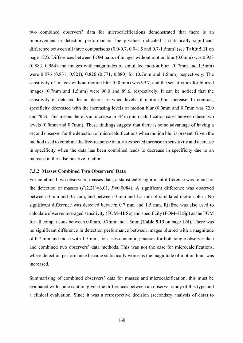
160
two combined observers’ data for microcalcifications demonstrated that there is an
improvement in detection performance. The p-values indicated a statistically significant
difference between all three comparisons (0.0-0.7, 0.0-1.5 and 0.7-1.5mm) (see Table 5.11 on
page 122). Differences between FOM pairs of images without motion blur (0.0mm) was 0.923
(0.883, 0.964) and images with magnitudes of simulated motion blur (0.7mm and 1.5mm)
were 0.876 (0.831, 0.921), 0.826 (0.771, 0.880) for (0.7mm and 1.5mm) respectively. The
sensitivity of images without motion blur (0.0 mm) was 99.7, and the sensitivities for blurred
images (0.7mm and 1.5mm) were 96.0 and 89.6, respectively. It can be noticed that the
sensitivity of detected lesion decreases when levels of motion blur increase. In contrast,
specificity decreased with the increasing levels of motion blur (0.0mm and 0.7mm was 72.0
and 70.9). This means there is an increase in FP in microcalcification cases between these two
levels (0.0mm and 0.7mm). These findings suggest that there is some advantage of having a
second observer for the detection of microcalcifications when motion blur is present. Given the
method used to combine the free-response data, an expected increase in sensitivity and decrease
in specificity when the data has been combined leads to decrease in specificity due to an
increase in the false positive fraction.
7.3.2 Masses Combined Two Observers’ Data
For combined two observers’ masses data, a statistically significant difference was found for
the detection of masses (F(2,21)=6.01, P=0.0084). A significant difference was observed
between 0 mm and 0.7 mm, and between 0 mm and 1.5 mm of simulated motion blur . No
significant difference was detected between 0.7 mm and 1.5 mm. Rjafroc was also used to
calculate observer averaged sensitivity (FOM=HrSe) and specificity (FOM=HrSp) as the FOM
for all comparisons between 0.0mm, 0.7mm and 1.5mm (Table 5.13 on page 124). There was
no significant difference in detection performance between images blurred with a magnitude
of 0.7 mm and those with 1.5 mm, for cases containing masses for both single observer data
and combined two observers’ data methods. This was not the case for microcalcifications,
where detection performance became statistically worse as the magnitude of motion blur was
increased.
Summarising of combined observers’ data for masses and microcalcification, this must be
evaluated with some caution given the differences between an observer study of this type and
a clinical evaluation. Since it was a retrospective decision (secondary analysis of data) to

161
combine the free-response data, there was no opportunity for arbitration to occur in cases in
which they did not agree. Had this occurred, it is possible that the values of specificity could
have been more favourable (i.e. a consensus decision may have reduced the number of non-
lesion localisation marks). However, the converse could be true for sensitivity, where a
consensus decision may result in a true lesion being downgraded. A study by (Tanaka et al.,
2015) investigated the impact of combining data from a free-response study to simulate a dual-
read. They found a general improvement in performance when combining the interpretation of
a radiographer with a radiologist, demonstrated by an inflated FOM, but the overall
significance of combined observations was not stated. The key finding, of Tanaka’s study and
the current thesis, is that a combined read is unlikely to be detrimental to patient outcomes.
7.4 Physical Measures:
7.4.1 Physical Measures of Microcalcifications
This part of the discussion focusses on the impact of motion blur on the physical characteristics
of malignant microcalcifications, including a new experimental metric (dispersion index, DI),
contrast, image noise and SNR. The DI of microcalcifications represents the number of
calcifications within a specified area divided by the area. DI was measured within ImageJ
software because the conspicuity index could not be applied to microcalcifications due to their
small individual size and wide distribution pattern. No validation has been conducted on DI,
but this could be a focus for post-doctoral work. A literature search conducted prior to this
research did not reveal any validated method for achieving a physical measure of
microcalcification clusters; this led to the development of the new DI metric. The result
demonstrates that the DI decreases when the level of simulated motion blur increases (see
Table 6.8 on page 139). Simulated motion blur has a significant negative impact on the
dispersion of calcifications image. Figure (7.3) demonstrates magnified mammographic
images which contain clustered microcalcifications. The DI in the image without motion blur
(0.0mm) was 0.608 per cm2 , while the DI for images with motion blur (0.7 and 1.5mm)
decreased to become 0.405 and 0.262 per cm2, respectively. In general, the lesion background
can have a negative impact on the search pattern. This is referred to as the crowding effect
(Levi 2009). The contrast threshold represents the contrast essential for the visibility of a test
object for a determined task of the image reader, e.g. for detecting an object. A mammographic
image can contain anatomical noise and this can have an impact on the perception of structures
(e.g. lesions). The results of this thesis show that the contrast of clustered microcalcifications

162
increases when in the level of simulated motion blur increases (Table 6.10 page 141). In
addition, the results demonstrate that there is no relationship between (DI. x contrast) and the
detectability of lesions by the observers.
Figure 7.3 Magnified mammographic images contain clustered microcalcification. The DI in the image
without motion blur (0.0mm) was 0.608 per cm2, while the DI for images with motion blur (0.7 and
1.5mm) were 0.405 and 0.262 per cm2 respectively.
Many researchers define a cluster of microcalcifications or suspicious group as at least five
calcifications in a breast volume of 1 cm3 (e.g. Evans et al., 2002; Shetty, 2015). Small subtle
microcalcifications with a size of less than 0.5 mm are a distinctive feature of malignancy,
although this threshold will differ somewhat in the thickness and density of the breast. With
the exception of motion blur, the key determinant for visibility of small calcifications is the
magnitude of image noise relative to the calcification’s signal (Ruschin, Timberg and Båth,
2007b). Since smaller calcifications will provide a signal sometimes as small as a single pixel,
the pixel-to-pixel difference depends on the image noise and it will reduce the visibility of
small calcifications to a much higher extent than the visibility of the mass due to mass being
larger than the size of the individual calcifications. To ensure better visualisation of structures
as small as 0.1 mm in size, the European guidelines for quality assurance in breast cancer
screening determined acceptable threshold levels of contrast for objects ranging from 0.1 to 2.0
mm in size, which should be available in digital mammography at acceptable glandular dose
levels (Perry et al., 2006). For optimal visualisation of microcalcifications at a given glandular
dose, it is typically beneficial to enhance the SNR. The SNR difference between the two

163
magnitudes of simulated motion blur and no motion blur were statistically significant for all
comparisons between 0.0mm, 0.7mm and 1.5mm (Table 6.12 on page 144). A graphical
representation of the means and adjusted 95% confidence intervals are displayed in (Figure
6.8 page 144). The average of SNR was 26.97 for images without simulated motion blur and
the average for blurred images (0.7 mm and 1.5mm motion blur) are 34.413 and 38.035,
respectively. However, there is no relationship between the physical measures and the lesion
detection performance of the observers (lesion detectability).
7.4.2 Physical Measures of Malignant Masses
The physical characteristics of malignant breast masses were determined by physical
parameters including conspicuity index, edge angle, grey level change, and image noise. The
physical measures of malignant masses have been analysed using conspicuity software
(Szczepura and Manning, 2016), partly to demonstrate the behaviour of blurring software and
partly to assess the impact of motion blur on the physical characteristics of breast mass images.
7.4.2.1TheLesionConspicuityandEdgeAngle
The results demonstrated that the conspicuity index increases significantly when simulated
motion blur increased from 0mm to 0.7mm and then to 1.5mm (See Table 6.3 page 130). This
change in the image lesion characteristics and may negatively impact on the differential
diagnosis. It is reasonable to hypothesize that, when the conspicuity of lesions increase this
does not necessarily mean that the detectability of the lesion should also increase. The
observers may see the lesion but it is possible they might not be able to decide if the lesion is
malignant or benign due to the influence of motion blur. It is hypothesised that the motion blur
may cause a decision error rather than a detection error; in the other words, decision-making
errors can happen when the lesion is obvious, but the assessment of its nature is made
incorrectly. It should be noted that further studies are required in future work to evaluate
decision error with eye-tracking. This result in a lesion being falsely dismissed as benign when
it is actually malignant, false-negative (FN). Manning et al., 2004 concluded that most errors
in image perception were failures of decision-making instead of detection errors (Manning,
Ethell and Donovan, 2004b). According to (Zuley, 2010) the mistakes in perceiving
mammographic images can be categorised into three types: search errors, recognition errors
and decision-making errors. If a lesion is not identified by the observer this is considered a

164
search error. However, if the lesion catches the observer’s eye but is then quickly dismissed it
is considered a recognition error. This will lead to the lesion going undiagnosed. Manning et
al., (2002) also demonstrated a poor relationship between conspicuity index and missed lesions
in chest radiography and pointed out the decision errors were mainly related to detection
(Manning and Ethell, 2002).
Perception errors can be considered as the main cause of missed cancers in mammography.
Misdiagnosed breast cancers can be attributed to their subtle characteristics. A suboptimal
technique related to technical factors and/or poor positioning can also lead to reduced lesion
conspicuity leading to poor detection (Goergen et al., 1997). The average of conspicuity index
for malignant masses in this thesis is 87.28 for images without simulated motion blur to 116.33
and 124.08 for images with simulated motion blur (0.7 mm and 1.5mm motion blur), (see
Figure 6.1 on page 130). The size of a focal lesion is a significant factor used to determine the
conspicuity of the lesion. This thesis included a wide range of lesion sizes from approximately
5 mm to 30 mm (see tables of the collected data Appendix G). The cancer lesion sizes were
similar to lesion sizes used in other observer based studies (Michaelson et al., 2003;
Obuchowski et al., 2000). For example, a study by Michaelson et al., (2003) demonstrated that
the size of lesions detected by screening mammography varies between 5 mm and 32 mm
(Michaelson et al., 2003). Some image characteristics of malignant masses can be difficult to
interpret due to their small size due to their relatively low contrast with background tissue; this
can have an impact on visual perception. The difference in edge angle between the two
magnitudes of simulated motion blur and no motion blur were statistically significant for all
comparisons between 0.0mm, 0.7mm and 1.5mm (Table 6.4 on page 132). Edge angle
magnitude decreased as simulated motion blur level increased. The results of edge angle
correlated with the results of the free-response study. The detection performance of breast
masses reduced with a reduction in edge angle, as the magnitude of simulated motion blur was
increased. Simulated motion blur has an impact on edge angle of breast masses and this could
therefore influence the image characteristics of lesions. This suggests that any impact on the
image characteristics of breast masses appearance could negatively affect differentiation
between malignant and benign masses. Figure 6.2 (on page 132) demonstrates the means of
edge angle (confidence interval 95%) of the two magnitudes of simulated motion blur and no
motion blur. The average edge angle is 69.11 for images without simulated motion blur and
165
the range for blurred images (0.7 mm and 1.5mm motion blur) are 67.63 and 66.65, respectively
(Figure 6.2).
7.4.2.2Changeingreylevel(ΔGL)ofmasses
The results demonstrated that there was no difference in the change of grey level when the
level of motion blur increases. The change of the grey level difference between the two
magnitudes of simulated motion blur and no motion blur was not statistically significant for
all comparisons (0.0mm, 0.7mm and 1.5mm) of simulated motion blur. A previous study by
Rawashdeh et al., (2014) measured breast lesion ΔGL for global background regions as the
mean grey level value of lesion minus the mean grey level value of the whole breast without
pectoralis muscle. The aim was to establish the key morphological criteria of the global
background (i.e. the breast that contains the lesion) that impacted on breast cancer detection.
They suggested that there was a relationship between “rating of detectability” and breast
density, lesion size, lesion edge and solidity. Some of these previous results agreed with the
results that have been established in this thesis, however, there is no relationship between
detectability and the change in grey level. This could be related to there being no impact of
motion blur on ΔGL. An early study by (Aldrich & Desai, 1994) used grey level to evaluate
the textual content of digitized mammography images. Statistics calculated from the GL were
utilised to highlight image lesion characteristics. They reported that GL has an apparent
capability to provide discrimination between normal and abnormal areas to enhance breast
cancer diagnosis. A study by (Boher and Collomb-patton, 2012) used temporal measurements
to characterise the motion blur of liquid-crystal display (LCD) displays. This calculation was
conducted automatically for each grey level transition. The contrast sensitivity function of the
human eye was introduced to assess perceived blur edge width and time for each grey level
transition providing a powerful process for a full characterisation of motion blur in such
displays (Boher and Collomb-patton, 2012). The results of my thesis demonstrated that there
was no impact of motion blur on GL and there is no relationship between GL and detection
performance.

166
7.4.2.3ImageNoiseandSignaltoNoiseRatio(SNR)
Both the noise and signal to noise ratio (SNR) of mass images were analysed to investigate the
impact of simulated motion blur on the physical characteristics of the images. The difference
in SNR between the two magnitudes of simulated motion blur and no motion blur were
statistically significant for all comparisons between (0.0-0.7, 0.0-1.5 and 0.7-1.5mm) (Table
6.6 on the page 136). Image noise decreased as the level of simulated motion blur increased;
this is believed to be a consequence of the smoothing process induced by the motion blur
software (Dougherty, 2009). The average of SNR (Figure 6.4 on page 136) is 2.741 for images
without simulated motion blur and the average for blurred images (0.7 mm and 1.5mm motion
blur) are 4.394 and 5.653 , respectively. The results in my thesis showed noise had a statistically
significant difference between 0.0–0.7mm t(22)=22.95 (p<0.000), 0.0–1.5mm t(22)=24.66
(p<0.000), and for 0.7–1.5mm t(22)=18.11 (p<0.000). Noise decreased as the magnitude of
simulated motion blur increased, this finding is in line with the smoothing effect imposed by
simulated motion blur. Saunders et al., (2007) have examined the impact of different noise
levels and resolution on cancer detection performance in digital mammography. They used
images at three different resolution levels and three different noise levels. For the detection of
malignant masses and microcalcifications, reducing the display resolution demonstrated a
small influence on overall accuracy and individual detection performance. They found noise
changed the detection performance of microcalcification. It decreased from 89% to 67% and
the discrimination performance of masses fell from 93% to 79%, while malignant mass
detection performance remained relatively constant with values of 88% and 84%, respectively.
7.5 The Impact of Motion Blur on Mammographic Features of
Microcalcifications
The distribution and shape of calcifications are considered a good indicator for the likelihood
of malignancy. It is reasonable to hypothesise that when the distribution and/or shape is
changed due to motion blur that this could affect the differential diagnosis of the lesion. For
instance, there are several distributions of breast microcalcifications. Tables 7.1 provide an
overview of the findings from the microcalcifications cases.
Firstly, diffuse and scattered microcalcifications, which are commonly benign especially when
bilateral. Such a distribution is predominantly seen with amorphous and punctate types of

167
microcalcifications, this type of distribution was frequently affected by motion blur in this
study with a reduction in detection performance; this was characterized by a reduction in the
dispersion index (DI). It should be noted that this understanding has been generated from cases
in my thesis and this would need evaluating over a larger sample of each type of cluster/lesion
feature. Figure 7.4 shows an example of amorphous and punctuate microcalcifications, which
were affected by motion blur.
Secondly, regional calcifications could comprise most of a quadrant or more than a single
quadrant and do not conform to a ductal distribution. This type of distribution is also affected
by motion blur that can lead to a change in shape and/or distribution. Consequently, the
detection performance can be decreased.
Thirdly, clustered or grouped calcifications when five or more small calcifications are shown
in a small area of breast tissue (see Figure 7.4).
Fourthly, linear distribution microcalcifications which are arranged in a line; such a distribution
is highly suspicious of cancer and indicates that microcalcifications are intra-ductal.
Fifthly, segmental distribution of microcalcifications imply calcifications in ducts and their
branches and could suggest multifocal or extensive breast cancer in a segment or lobe of the
breast. The exception is in the incident of coarse rod-like microcalcifications in older females,
where this is related to secretory microcalcifications. The granular calcifications showing an
irregularity in density, size or shape and they are tiny with dot-like or elongated shapes and are
innumerable. Motion blur has a negative impact on the detection of granular calcification,
especially when they are located in a high density breast. The amorphous microcalcifications
presentation is considered the most difficult lesion to identify due to its poor contrast and small
size (Liu, 1999). Figure (7.4) shows a group of malignant microcalcifications, which were
affected by simulated motion blur, whereas the Figure (7.5) demonstrates a group of malignant
microcalcifications, which were not affected by simulated motion blur in this study.

168
Table 7.1 The types of clustered microcalcifications and the impact of motion blur on each type. It
should be noted that this table generated from cases of current study and this would need evaluating
over a larger sample of each type of cluster/lesion feature.
Types Calcification
Size of individual Calcifications
Lesion features Motion blur effect
Cluster with ≤10 amorphous calcifications
Small size (heterogeneous)
clustered non-focal lesion
affected by motion blur
rod shaped Large size of individuals calcifications (Homogeneous)
focal lesion with dense central area
Not affected by motion blur
Punctate Small size (similar size of individual calcifications)
small cluster size with same density and shape of individual calcifications
affected by motion blur
Granular granular calcifications which vary in size
showing irregularity in density, size or shape
affected by motion blur
Branching Large size with irregularly shaped cluster (Heterogeneous)
showing irregularity in density
not affected by motion blur
ductal distribution Large size with irregularly shaped
Similar in density & size
Not affected by motion blur

169
Figure 7.4 A group of malignant microcalcifications, which were affected by motion blur.
Figure 7.5 A group of malignant microcalcifications, which are not affected by motion blur.
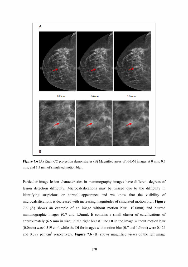
170
Figure 7.6 (A) Right CC projection demonstrates (B) Magnified areas of FFDM images at 0 mm, 0.7
mm, and 1.5 mm of simulated motion blur.
Particular image lesion characteristics in mammography images have different degrees of
lesion detection difficulty. Microcalcifications may be missed due to the difficulty in
identifying suspicious or normal appearance and we know that the visibility of
microcalcifications is decreased with increasing magnitudes of simulated motion blur. Figure
7.6 (A) shows an example of an image without motion blur (0.0mm) and blurred
mammographic images (0.7 and 1.5mm). It contains a small cluster of calcifications of
approximately (6.5 mm in size) in the right breast. The DI in the image without motion blur
(0.0mm) was 0.519 cm2, while the DI for images with motion blur (0.7 and 1.5mm) were 0.424
and 0.377 per cm2 respectively. Figure 7.6 (B) shows magnified views of the left image
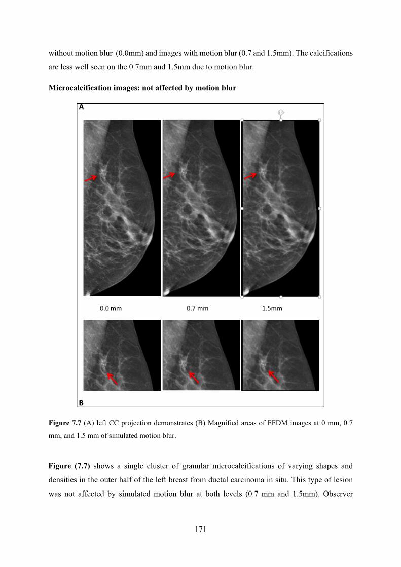
171
without motion blur (0.0mm) and images with motion blur (0.7 and 1.5mm). The calcifications
are less well seen on the 0.7mm and 1.5mm due to motion blur.
Microcalcification images: not affected by motion blur
Figure 7.7 (A) left CC projection demonstrates (B) Magnified areas of FFDM images at 0 mm, 0.7
mm, and 1.5 mm of simulated motion blur.
Figure (7.7) shows a single cluster of granular microcalcifications of varying shapes and
densities in the outer half of the left breast from ductal carcinoma in situ. This type of lesion
was not affected by simulated motion blur at both levels (0.7 mm and 1.5mm). Observer

172
detectability remained the same when simulated motion blur increased. Almost 100% of the
observers detected the lesion in all three comparisons (0.0-0.7mm, 0.0-1.5mm and 0.7-1.5mm).
The calcifications appear as focal clusters with an irregular outline. The microcalcifications of
similar shape, density and size of of individual calcifications within a focal cluster were not
affected by simulated motion blur. A cluster of about 2.0 cm2 was detected in the left breast.
The DI in the image without motion blur (0.0mm) was 1.798 per cm2 , while the DI for images
with motion blur (0.7 and 1.5mm) were 1.498 and 1.199 per cm2 respectively.
Figure 7.8 (A) Screening mammography image of right CC Projection. Magnified areas of a cluster of
microcalcifications.
Calcifications can appear as a focal cluster (Figure 7.8). In this example the microcalcifications
have similar shape, density and size of flecks. This type of calcification was not affected by
simulated motion blur for the three conditions (0.0-0.7 mm, 0.0-1.5 mm and 0.7-1.5mm) due
to the large size of the individual calcifications and also that the calcifications have high
contrast with their background tissues. Observer detectability remained the same when
simulated motion blur increased. A 100% of the observers detected the lesion in images without
motion blur (0.0 mm) and in both levels of blurred images (0.7 mm and 1.5 mm). The DI in
the image without motion blur (0.0 mm) was 0.863 per cm2, while the DI for images with
motion blur (0.7 and 1.5mm) were 0.648 and 0.504 per cm2, respectively. It is reasonable to

173
suggest that the impact of motion blur does not necessarily mean that the lesion has been
obscured completely by motion blur. The lesion may still appear, but it might not be determined
whether it is malignant or benign.
Figure 7.9 Screening mammography image of right cranio-caudal projection.
A cluster of microcalcifications that have a punctate shape is presented in Figure 7.9. For this
case, the BIRADS breast density is low dense (category B). This type of microcalcification is
considered difficult to see due to the small lesion size (less than 0.7 cm2) and low contrast in
relation to the background breast tissues. This type of lesion was affected by simulated motion
blur at 1.5 mm and its detectability decreased with increasing levels of motion blur. The
detectability at 0.0mm was 100%, while at 0.7 mm it decreased to 85%, but at a level of 1.5mm,
it became 42%. The DI in the image without motion blur (0.0 mm) was 0.863 per cm2, while
the DI for images with motion blur (0.7 and 1.5 mm) was 0.648 and 0.504 per cm2 respectively.
High-density breast tissue can make breast lesions difficult to see. Burrell et al., (2001)
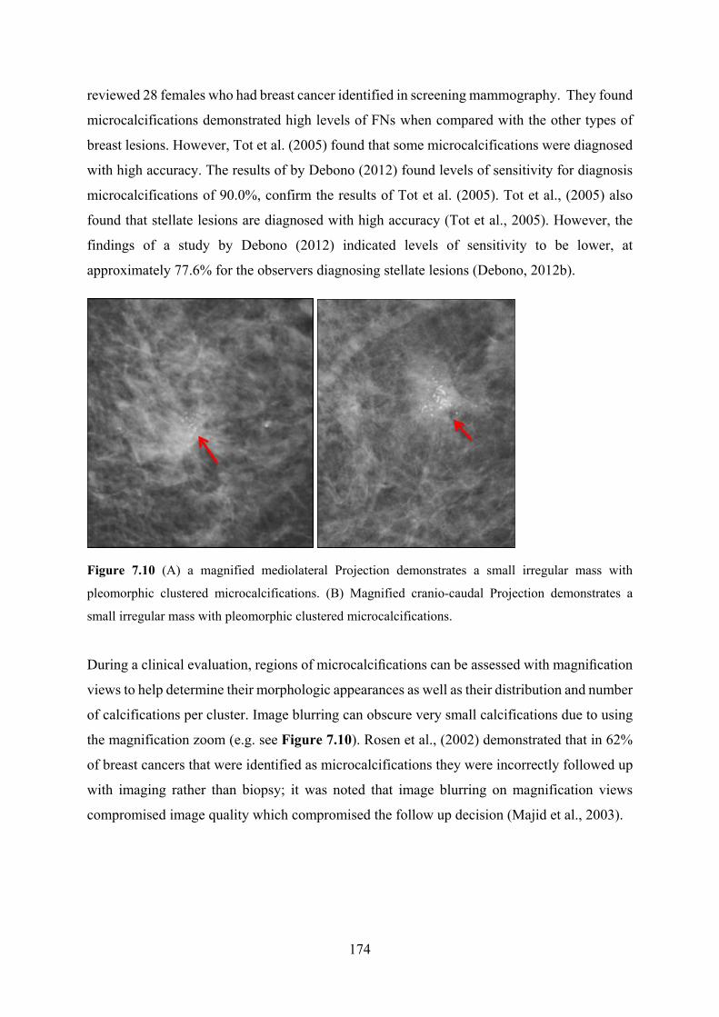
174
reviewed 28 females who had breast cancer identified in screening mammography. They found
microcalcifications demonstrated high levels of FNs when compared with the other types of
breast lesions. However, Tot et al. (2005) found that some microcalcifications were diagnosed
with high accuracy. The results of by Debono (2012) found levels of sensitivity for diagnosis
microcalcifications of 90.0%, confirm the results of Tot et al. (2005). Tot et al., (2005) also
found that stellate lesions are diagnosed with high accuracy (Tot et al., 2005). However, the
findings of a study by Debono (2012) indicated levels of sensitivity to be lower, at
approximately 77.6% for the observers diagnosing stellate lesions (Debono, 2012b).
Figure 7.10 (A) a magnified mediolateral Projection demonstrates a small irregular mass with
pleomorphic clustered microcalcifications. (B) Magnified cranio-caudal Projection demonstrates a
small irregular mass with pleomorphic clustered microcalcifications.
During a clinical evaluation, regions of microcalcifications can be assessed with magnification
views to help determine their morphologic appearances as well as their distribution and number
of calcifications per cluster. Image blurring can obscure very small calcifications due to using
the magnification zoom (e.g. see Figure 7.10). Rosen et al., (2002) demonstrated that in 62%
of breast cancers that were identified as microcalcifications they were incorrectly followed up
with imaging rather than biopsy; it was noted that image blurring on magnification views
compromised image quality which compromised the follow up decision (Majid et al., 2003).

175
7.6 The Impact of Motion Blur on Mammographic Image Features of
Breast Masses:
This part of the discussion focuses on the impact of motion blur on the image characteristics
of breast lesions. Tables 7.2 provides an overview of the findings from the FROC study,
generalising to different types of malignant mass present in this study. It is worth remembering
that the following ‘evaluation of image appearances’ in relation to cancer detection is based on
a limited number of cases. Consequently, caution should be exercised, as the evaluation would
need extending to a larger sample of each type of mass/lesion feature in order to have
confidence in the results. A larger sample size of different lesion types would be required to
make population based generalisations. Nevertheless, the following presents the first
discussion ever about lesion features in relation to cancer detection performance in blurred and
non-blurred mammographic images.
Table 7.2 Summary of the impact of motion blur on detection performance on each type of breast
masses. It is worth mentioning that this table was generated from cases in the current study and this
would need evaluating over a larger sample of each type of masses/lesion feature.
Types Mass Lesion density Size of mass
Motion blur effect
Spiculated Low contrast ratio with its background
Small size affected by motion blur
Irregular shape low or equal density Small size which vary in size
affected by motion blur
Obscured Low contrast ratio with its background
vary in size affected by motion blur
Oval or round/ Circumscribed
High contrast ratio with its background
Large size with regularly shaped
Not affected by motion blur
Microlobulated High contrast ratio with its background
Large size with irregularly shaped
Not affected by motion blur
Indistinct High contrast ratio with its background
small size with irregularly shaped
affected by motion blur

176
There are many factors related to the appearance of breast lesions within mammographic
images that could have an effect on lesion detection performance, such as lesion location within
the breast, lesion size, lesion shape and its contrast against background structures. Firstly,
lesion location within the breast, when the lesion is located within the fibro-glandular region
within an area of high breast density, or when the lesion has overlapping anatomical structures,
this makes lesion visibility more challenging. Secondly, lesion size, small types of breast
calcifications which have indefinite edges are considered the most difficult lesions to identify
due to their poor contrast and small size. Thirdly, lesion shape this can affect whether the
malignancy of a breast lesion is determined or not (Berlin, 2001; Fujihashi, 1994; Yankaskas
et al. 2001). Fourth, lesion contrast this can be calculated for both local and global background
areas (Rawashdeh et al., 2014; Mello-Thoms et al., 2005; Manning & Ethell, 2002); it
represents the ratio of the signal intensity of the lesion to its background. Figure (7.11) shows
examples of mammography images containing breast masses with different appearances due
to location, size and tissue background. The lesions have low contrast against background
tissues, thus making lesion visibility difficult, especially in the presence of simulate motion
blur. Some lesion locations within the breast present additional difficulties in the detection of
the lesion. For instance, when a breast lesion is located in the glandular area (appearing as
‘white’ in the image) this can be affected by motion blur. In contrast, a lesion located in the
fatty area (appearing as ‘dark’ in the image) will have high contrast in relation to the
background breast tissues, and this may not be greatly affected by motion blur. Generally,
cancers in some locations, such as in the inframammary fold or the axillary tail, are
predominantly perceived on only one mammographic image projection; this can lead to
difficulties in detection because an alternative image is not available. Such a difficulty extends
to when motion blur is present, as the diagnostic decision has to be made on a [potentially]
deficient image. A study by Bird et al., (1992) found a significant proportion of undetected
cancers in these difficult regions - approximately (25%) of cancers were in the retro-glandular
area of the breast and the sensitivity was between 85% and 90% (Bird et al., 1992). However,
Goergen et al., (1997) reported that no statistically significant differences exist between
regions, in terms of detection efficiency.

177
Figure 7.11 Demonstrates mammography images containing breast masses with different lesion
appearance due to location, size and tissue background.
A clear finding from this thesis is that motion blur has a high impact on low-density and
isodense masses. This thesis has assessed the combined influence of lesion density and motion
blur on detection performance and it has been generally demonstrated that better lesion
detection performance is associated with masses of higher density; this is in contrast to low-
density masses, which tend to have a poorer detection performance in the presence of simulated
motion blur. Previous studies have confirmed that mammographic density contributes to
challenges in screen reading accuracy (American College of Radiology, 2013; The Radiology
Assistant, 2013). It can be reasoned that small differences in contrast between the lesion density
and density of breast tissues (density of normal and abnormal tissue) could create difficulties
in the perception of important lesion characteristics, such as the edge angle of the lesion. The
assessment of lesion density is important in the differential diagnosis of breast masses. The
lesion density should be assessed in comparison with the surrounding parenchyma, or in
relation to the nipple in the case of fatty involution. The breast mass, in relation to the
surrounding parenchyma, is either low density radiopaque, high density radiopaque,
radiolucent, radiolucent and radiopaque combined. Figure (7.12) shows a group of malignant
breast masses, which were not affected by motion blur due to their having higher densities than
the background breast tissue. When the relevant lesion density is assessed, the choices of lesion
diagnosis will be restricted to the following probabilities; radiolucent circular/oval lesions such
as galactocele, lipoma and oil cyst. Low density radiopaque is considered equivalent to the

178
density of the surrounding parenchyma. In this thesis, low-density masses were affected by
motion blur, and they became more difficult to diagnose due to blurring. Figure (7.13) shows
a group of malignant breast masses. In these cases lesion detection performance was affected
by motion blur due to small differences in density between the lesions and background tissues.
Figure 7.12 Demonstrates a group of malignant of breast masses, which are not affected by motion
blur.
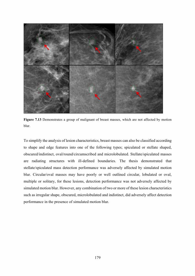
179
Figure 7.13 Demonstrates a group of malignant of breast masses, which are not affected by motion
blur.
To simplify the analysis of lesion characteristics, breast masses can also be classified according
to shape and edge features into one of the following types; spiculated or stellate shaped,
obscured/indistinct, oval/round/circumscribed and microlobulated. Stellate/spiculated masses
are radiating structures with ill-defined boundaries. The thesis demonstrated that
stellate/spiculated mass detection performance was adversely affected by simulated motion
blur. Circular/oval masses may have poorly or well outlined circular, lobulated or oval,
multiple or solitary, for these lesions, detection performance was not adversely affected by
simulated motion blur. However, any combination of two or more of these lesion characteristics
such as irregular shape, obscured, microlobulated and indistinct, did adversely affect detection
performance in the presence of simulated motion blur.

180
7.6.1 Examples of Masses Affected by Simulated Motion Blur
Figure 7.14 (A) mammography images with left MLO Projection, contains different magnitudes of
motion blur (0.7 & 1.5 mm) and image without motion blur (0.0mm). (B) Magnified views show small
malignant mass (signposted by red arrows).
Figure (7.14) demonstrates a small speculated malignant mass (measuring approximately 7.0
mm in diameter), indicated by the red arrow, in the upper half of the breast. This mass has an
irregular outline with fuzzy edges and it is pressing on the tissues around it. It is difficult to see
it. 29% of observers missed the mass even when no motion blur (0.0 mm) was present. The
detection performance relating to this malignant mass was worse in the presence of simulated
motion blur. Lesion detection performance decreased as the level of simulated motion blur
increased. 71% (5/7) of the observers detected the lesion in 0.0 mm level, whereas this
decreased to 43% (3/7) at 0.7mm and only 29% (2/7) at 1.5mm.

181
Figure 7.15 Left CC Projection, this mammography image shows a spiculated mass (arrow) that has an
irregular shape with indefinite edges.
Figure (7.15) is a cancerous mass which appears as partially round with irregular / spiked
outline (see arrows). Its BI-RADS breast density is category B. This mass is considered
difficult to see because the lesion size is very small (approximate lesion area <0.8 cm2) and it
has a low contrast, compared with the surrounding background tissues. Detection performance
was adversely affected by simulated motion blur and its detection performance decreased as
simulated motion blur increased. 100% (7/7) of the observers detected the lesion with no
motion blur (0.0 mm), whereas this decreased to 57% (4/7) at 0.7mm and only 29% (2/7) at
1.5mm of simulated motion blur.

182
Figure 7.16 Left Cranio-Caudal Projection mammography image contains a stellate mass (arrow) that
has an irregular outline (Lesion size 2.2 cm2).
Figure (7.16) shows a stellate mass (see arrow) with an irregular outline (approximate lesion
area 2.2 cm2); it has a BI-RADS breast density grade B. Although its density is higher than the
surrounding breast tissue and its size is fairly large, its detection performance was adversely
affected by simulated motion blur; detectability decreased as simulated motion blur increased.
71% (5/7) of the observers detected it with no motion blur (0.0mm); this decreased to 43%
(3/7) at 0.7mm and only 57% (4/7) detected the lesion at 1.5mm of simulated motion blur .
This thesis suggests that stellate masses are affected by simulated motion blur.

183
Figure 7.17 Mammography image left Medio-lateral oblique Projection shows indistinct breast mass
(arrow) that has an irregular outline.
Figure (7.17) demonstrates an indistinct partially round mass (arrow). It has an irregular
outline (approximate area of 1.7 cm2); it has a BI-RADS breast density grade B, and is located
in lower part of the breast (see red arrow). Its detection performance was adversely affected by
simulated motion blur, meaning its detectability decreased as simulated motion blur increased.
71% (5/7) of observers detected the lesion with no blur (0.0mm), and this decreased to 57% at
0.7mm and only 43% (3/7) at 1.5mm of simulated motion blur.

184
Figure 7.18 Mammography image with left Cranio-Caudal Projection demonstrates a stellate mass
(arrow) that has an irregular outline.
Figure (7.18) shows a large stellate mass (approximate area of 1.4 cm2) located in the middle
part of the breast (see arrow), it has a BI-RADS breast density C. It was adversely affected by
simulated motion blur. Its detectability decreased with increasing simulated motion blur.
Approximately 86% (6/7) of observers detected the lesion with no motion blur (0.0mm). This
decreased to 71% (5/7) at 0.7mm and only 57% (4/7) at 1.5mm of simulated motion blur.
Stellate masses may be difficult to diagnose due to the surrounding tissue obscuring its spicules.
Also, architectural distortion has subtle appearances and may present similarly to normal
overlapping breast tissue, causing it to be a typically undetected cancer and FN presentation.

185
Figure 7.19 Mammography image with left mediolateral oblique Projection contains breast mass
(arrow) that has an irregular outline (fuzzy edges).
Figure (7.19) shows a spiculated mass with a multi-pointed star-shaped outline. Its size is
approximately 1.4 cm2 and it is located in the upper part of the breast (see arrow). Its BI-RADS
grade is C. Lesion detection performance was adversely affected by motion blur. This
spiculated mass has a very small mass centre and a lace-like, fine reticular radiating structure
which causes parenchymal distortion and/or asymmetry. Detectability decreased with
increasing simulated motion blur. Approximately 86% (6/7) of the observers detected the lesion
with no motion blur (0.0 mm). This decreased to 57% (4/7) at 0.7mm and 57% (4/7) at 1.5mm
of simulated motion blur.
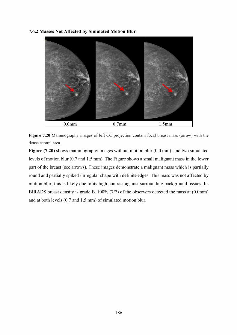
186
7.6.2 Masses Not Affected by Simulated Motion Blur
Figure 7.20 Mammography images of left CC projection contain focal breast mass (arrow) with the
dense central area.
Figure (7.20) shows mammography images without motion blur (0.0 mm), and two simulated
levels of motion blur (0.7 and 1.5 mm). The Figure shows a small malignant mass in the lower
part of the breast (see arrows). These images demonstrate a malignant mass which is partially
round and partially spiked / irregular shape with definite edges. This mass was not affected by
motion blur; this is likely due to its high contrast against surrounding background tissues. Its
BIRADS breast density is grade B. 100% (7/7) of the observers detected the mass at (0.0mm)
and at both levels (0.7 and 1.5 mm) of simulated motion blur.

187
Figure 7. 21 Screening mammography image of right Medio-lateral Oblique projection.
Figure (7.21) demonstrates a microlobulated mass which has an irregular shape with definite
edges. It is in the upper half of the breast (see arrow). Its density is higher than the surrounding
background breast tissues and its BIRADS density grade is C. Its detection performance was
not adversely affected by simulated motion blur. 100% (7/7) of the observers detected the mass
at (0.0mm) and at both levels (0.7 and 1.5 mm) of simulated motion blur.
Figure 7.22 Screening mammography image of left CC projection.

188
Figure (7.22) demonstrates a well circumscribed microlobulated mass with definite edges. It
has an approximate area of 12 mm2; it is depicted by (arrow) and is located in the lower half of
the breast. Its detection performance was not adversely affected by simulated motion blur.
100% (7/7) of the observers detected it with no blur (0.0mm) and at both levels of simulated
motion blur (0.7 and 1.5 mm).
Figure 7.23 Left MLO projection, mammography images show malignant breast mass, with an oval or
round shape and definite edges.
Figure (7.23) illustrates a large malignant mass (approximate area of 1.9 mm2) in the upper
half of the breast (see arrow). Its detection performance was not adversely affected by
simulated motion blur. 100% (7/7) of the observers detected it with no motion blur (0.0 mm)
and also at 0.7 and 1.5 mm levels of simulated motion blur.

189
7.7 Limitations of this Thesis:
While there is some promise in the results generated in this novel work, there are some
limitations to the results achieved. In clinical mammography, the image reader does not know
what magnitude of motion blur is present in an image, so it could be argued that it was
superfluous to investigate two different magnitudes of motion blur. However, it is known from
previous work (Ma et al., 2015) that motion blur is visible at around 0.7 mm of simulated
motion blur , so it is of interest to understand if this caused a reduction in observer performance;
if it didn’t, it was necessary to understand whether a higher magnitude of motion blur did cause
an effect. In this thesis the simulated motion blur had a global effect on the whole image and
in reality this is not always the case, as ‘real motion blur’ may affect only one region, several
regions or the whole mammographic image. Consequently, the results in this thesis are not able
to predict the impact of regional blurring on lesion detection performance.
Further limitations are related to the process of introducing simulated motion blur into the
image: It is possible that any image noise present in the original image may be blurred through
the mathematical simulation, while in real motion blur this would not occur. For the
mathematical simulation of blurring, as is the case in this thesis, the image would appear to be
slightly smoother than the non-blurred image. To overcome this potential smoothing effect, it
may be possible to adapt the mathematical simulation by adding noise back into the newly
created blurred image. Despite this, the current method gives us a certain level of control on
motion blur that could not be achieved with ‘real’ blurred images from a clinical setting.
The mathematical blurring process is enacted as a convolution mask that, in effect spreads each
pixel, redistributing its intensity into the neighbouring pixels based on a function and mask size
determined by the modelling of the pixel motion as a random vector path parameterised by the
characteristics of breast tissue (generalised) elastic coefficient, required duration and required
displacement. The latter two factors act as input to the simulation to determine the magnitude
of the blur effect. This creates a controllable blur mask for convolution that has a distribution
curve reflective of the intensity spread within a collimated light (energy) propagation system
reflective of the X-ray system used. Without modelling actual motion within the breast it is not
possible to determine the direction of motion at a specific locality within the breast, so this is
an approximation to the blur effect that is uniform for the entire image region. Localisation is
possible, but requires each source image to have a specific region of blur defined and in this

190
case motion is assumed to be radial, and the mask application adjusted accordingly on a per-
pixel basis, from the centre of the defined region, with maximum motion at the centre, reducing
to zero motion at the perimeter of the region. Given a large number of source images processed
for this study and the requirement for a consistent blur effect on all the generated image sets,
regional blurring was not used in this study. This is a limitation in that the blur effect is
indicative of the blur that would be present within a ‘real’ patient image in terms of magnitude
and effect, but does not replicate the directional nature of the blur that would occur for a ‘real’
image.
In respect of the power of the study, it should be noted that the prevalence of disease is much
higher than would be expected in a screening population, but this is difficult to overcome in
observer studies because the proportion of cancer cases to normal cases in clinical practice
cannot be represented exactly in a small sample as in observer studies. However, all
participants in observer studies have a heightened expectation of disease, since they are always
aware that their detection performance is being assessed. There are also many differences
between observer studies and clinical practice. For instance, in clinical practice, the observer
can review many images for each client (e.g. right and left for CC & MLO) as well as previous
screening mammograms. In addition, full patients’ information, risk factors and clinical
examination information is often available. With a free-response study of the type detailed in
this thesis, the observer can only see one image for each case and no information about the
client. Also they do not have available to them other clinical information which could help
inform their decision making.

191
7.8 Chapter Summary:
In summary, free-response data were analysed for the detection of malignant
microcalcifications and masses for three conditions; (i) no simulated motion blur (0.0 mm),
and for two magnitudes of simulated motion blur (0.7 and 1.5 mm). A statistically significant
difference was found for the detection of masses and microcalcifications. For both analyses, a
significant difference was observed between 0 mm and 0.7 mm, and between 0 mm and 1.5
mm of simulated motion blur , and also between (0.7and 1.5 mm) for microcalcifications. No
significant difference was detected between (0.7 and 1.5 mm) for masses. These trends were
similar, but not exactly the same as those observed in the combined two observers’ data
analysis. Comparison between single observer free-response data and combined two observers’
data demonstrates that the detection performance of microcalcifications improved, while there
was no improvement in detection performance for malignant masses. Regarding, the impact of
motion blur on physical characteristics, the results demonstrate that there were significant
differences in the physical measures of both masses and microcalcifications for all three
comparisons of simulated motion blur (0.0-0.7, 0.0-1.5 and 0.7-1.5 mm).

192
Chapter 8: Conclusion, Recommendations and Future work
This thesis used a novel mathematical algorithm to apply simulated motion blur to clinical
FFDM images which were either normal or had proven breast cancer present. Using this
blurring approach, this thesis represents the first study to investigate the impact of simulated
motion blur on cancer detection performance in FFDM using observer performance methods
and characterisation of lesion types.
For the single observer study, the results from this thesis are likely to have implications for
clinical practice. It could mean that when blur is observed in an image, a repeat image should
be considered as one would simply not know how much motion blur is present and what impact
it is having, in terms of cancer detection performance. In view of this, a key outcome of the
thesis is that caution should be exercised when making decisions about the acceptability of
images that appear to contain motion blur. This may also have implications for the type of
monitor used for the initial evaluation of technical quality of mammograms. For both masses
and microcalcifications, the findings indicate that simulated motion blur has a significant
detrimental effect on cancer detection performance.
When two observers’ data were combined to simulate double reporting, as occurs in
mammography screening, the key finding was that a combined read is likely to only have
beneficial outcomes. While there was no statistically significant benefit for breast masses, for
microcalcifications, there was a statistically significant difference between single and
combined free-response data. Given that image readers do not have a prior expectation of
masses or microcalcifications occurring in the image, the only recommendation can be that all
images have to receive double reporting.
For the physical measures of malignant masses, simulated motion blur had a negative impact
on edge angle and this appeared to have only a weak correlation with a reduction in detection
performance. It is reasonable to hypothesise that when the conspicuity of the mass increases it
does not necessarily mean that the detectability of mass would also increase. However,
conspicuity index did get statistically as the magnitude of simulate motion blur increased. The
edge angle was decreased with increasing the level of simulated motion blur. The change in
grey level was not statistically significant between the different magnitudes of simulated

193
motion blur. Image noise was statistically worse with an increasing level of simulated motion
blur.
For microcalcifications, the dispersion index was statistically worse with an increasing level of
simulated motion blur. This negative impact on the dispersion index was due to some small
calcifications/tight clusters becoming obscured. There are many factors related to the
appearance of breast lesions within mammographic images that could have an impact on lesion
detection performance, such as lesion location within the breast, lesion size, and lesion shape.
The calculation of missed lesions was used to identify the detectability of different lesion types.
The analysis of missed lesions should provide a less abstract concept which can be used to
evaluate lesion types. In summary, microcalcification clusters of small size or individual
calcifications are likely to be missed in the presence of simulated motion blur. For masses,
large lesions and those with high lesion-to-background contrast were not affected by simulated
motion blur. However, those with an irregular outline, with stellate shape, or those that have
fuzzy edges, have multi-pointed star-shaped are difficult to detect with simulated motion blur
present. Finally, high breast density was also a strong factor linked to poorer detection. Images
readers and technical staff need to be aware of the impact of motion blur on the detection of
cancer during the acquisition and reporting of FFDM images. For the benefit of clients, further
work is required to ensure that motion is recognised at the earliest possible opportunity.
8.2 Statement of Novelty
The main novel contributions of this PhD are summarised as follows:
1. Research problem: This is the first study to evaluate the impact of motion blur on
mammography lesion detection performance.
2. Novel method: This is the first study to use mathematical simulation for blur induction in
order to assess its impact on mammography breast cancer detection performance.
3. Novel method for physical measures: This is the first study to assess the impact of
simulated motion blur on the physical characteristics of microcalcification and masses in
mammography images. The impact of simulated motion blur on the physical characteristics of
malignant microcalcification images have been assessed using dispersion index, which is a
novel measure.
194
4. Novel analysis of data: This is the first study to use free-response data assess the impact of
mimic double reporting, using combined two observers’ data on blurred FFDM images.
5. New method: This is the first study to conduct a missed lesions analysis to establish reasons
why observers failed to detect lesions in the presence of simulated image blurring.
8.7 Recommendations and Future work
Future work
1. Evaluation of regional simulated motion blur
The simulated blur applied in this study was global in effect (i.e. the entire image). In clinical
mammography, motion blur may be global or regional. This study is not able to predict the
impact of regional blurring on lesion detection performance. In future work, it is important to
study the impact of regional blurring on lesion detection performance.
2. Evaluation of ‘real’ motion blur
Further studies are required to investigate the impact of real motion blur on lesion detection
performance. This will be a prospective study, collecting an appropriate number of real blurred
mammograms and their repeated images (containing no motion blur). A free-response study
will be used to measure detection performance.
3. Validation of Dispersion Index
The dispersion index was develeoped as a novel metric for this work since existing conspicuity
software could not be applied to microcalcifications due to their small individual size and wide
distribution pattern. No validation has been conducted on DI, but this could be a focus for post-
doctoral work.
195
Recommendations
There are significant consequences to motion blur in clinical practice and consequently this
thesis provides a number of recommendations to breast imaging professionals. Image readers
should be aware of the impact of motion blur on cancer detection and they should evaluate
images carefully for its presence prior to making an interpretation. In addition, staff should be
aware of motion blur during quality assessment of images in the mammography imaging room.
Within the UK, blurred images may need to be repeated, however due regard should be given
to NHSBSP quality assurance recommendations in which a repeat threshold of 3% has been
set. When motion blur is detected, this could lead to repeated images and increased recall rates,
both of which will increase radiation dose and represent a negative physical and psychological
experience for the client. If motion blur is not recognised, this could lead to misdiagnosis, late
detection and even symptomatic presentation as an interval cancer. On the other hand, motion
blur also has the potential to increase the number of lesion mimics (false positives), which may
lead to unnecessary biopsy, with the consequence of an unnecessary invasive procedure and
increased client anxiety.

196
Appendices:
Appendix A: Ethics Application HSCR 15-107

197
Appendix B: Ethics Application HSCR 15-110

198
Appendix C : Organisation Management Consent/ Agreement Letter

199

200
Appendix D: Participant Invitation Letter
Directorate of Radiograph, Centre of Health Sciences Research, University of Salford, Allerton Building, Salford, M6 6PU 31 May 2018 Dear Sir or Madam:
RE: Research Involvement: Image blurring and lesion detection in mammography
Research Governance and Ethics Committee Approval: RGEC
I am a PhD student under the supervision of Professor Peter Hogg, Dr John Thompson, Dr Claire Mercer, Mrs
Judith Kelly and Dr Rob Aspin at the University of Salford. I am currently investigating the impact of image
blurring caused by unwanted motion on an observers’ ability to detect clinically significant lesions in full field
digital mammography (FFDM) images. This research uses the latest and most advanced techniques in observer
performance, namely free-response receiver operating characteristics (FROC) method and a statistically powerful
jackknife alternative FROC (JAFROC) analysis. For this research I require expert observers to examine a series
of images that are either normal (no lesions) or contain lesions with varying degrees of simulated image blurring.
In this study an advanced computer algorithm developed at the University has been used to introduce the image
blurring.
I am approaching you as an experienced professional and potential volunteer to take part in the observer study. If
you are happy to take part in the research, please respond to the email address at the bottom of this letter and I
will be happy to give you more information. Your contribution will be appreciated, though no financial reward or
otherwise will be offered. It is expected that you will be required to make 3-4 visits to the University to complete
image evaluations using our 5 megapixel monitors. Each evaluation is expected to last up to 90 minutes. This
contract lays out the standards by which the observer group will adhere to and the conditions under which the
evaluations will be completed, thereby ensuring respect is afforded to all who are directly involved in this study.
If you have any further questions about the study that will help you decide whether to volunteer for this research,
or if you have any further queries, please get in touch via telephone or e-mail. Thank you for taking the time to
read this letter and I hope to hear from you in the near future.
Sincerely
Student name-------
Email ‐‐‐‐‐‐‐‐‐‐‐‐‐‐‐‐‐‐‐‐‐‐‐‐‐‐‐‐‐‐

201
Appendix E: Participant Information Sheet
Participant information sheet for observers participants in observation study (FROC study)
Study title: Determine the impact of image blurring on lesion
detection performance in full field digital mammography images (FFDM)
Chief investigator Telephone number
You will be given a copy of this information sheet to keep
We would like to invite you to take part in our research study. Before you decide we would like you to understand why the research is being done and what it would involve for you. Talk to others about the study if you wish and please ask if there is anything that is not clear. This is a Student project, required for successful completion of a Doctoral programme. I am currently investigating the impact of image blurring caused by unwanted motion on an observers’ ability to detect clinically significant lesions in full field digital mammography (FFDM) images.The aim of the study is to determine the impact of image blurring on lesion detection performance in full field digital mammography images (FFDM) using free-response receiver operating characteristics (FROC) method
Participant name:
Study Sponsor: University of Salford

202
1. What is the purpose of this study?
The purpose of this study to determine the impact of image blurring on lesion detection performance in full field digital mammography using the free-response receiver operating characteristics (FROC) method.
2. Why have I been invited?
This research uses the latest and most advanced techniques in observer performance, namely the Free-response Receiver Operating Characteristics (FROC) method and the statistically powerful jackknife alternative FROC (JAFROC) analysis. For this research I require expert observers to examine a series of full field digital mammographic (FFDM) images that are either normal (no lesions) or contain lesions with varying degrees of simulated image blurring. In this study an advanced computer algorithm developed at the University has been used to introduce image blurring to clinical images. You have been invited because you are considered an expert observer in mammography.
3. Do I have to take part?
Your decision to take part in this study is entirely voluntary. You may refuse to participate or you can withdraw from the study at any time.
4. What will happen to me if I take part?
It is expected that you will need to make 3-4 visits to the University of Salford to complete image evaluations using our 5 megapixel monitors. Each evaluation is expected to last up to 90 minutes. You will be asked to assess and localise lesions in mammographic images .The information you provide will be kept confidential and will be used only towards achieving the aim of the research.
5. Expenses and payments
Your contribution will be appreciated, though no financial reward or otherwise will be offered.
6. What are the possible disadvantages and risks of taking
This research does not pose any risk to its participants.
7. What are the possible benefits of taking part?
Your participation may help improve understanding of the impact of image blurring on cancer detection performance. Better awareness of the impact of image blurring may result in better breast cancer detection rates at the early stage and overall result in to the reduction of the mortality rate due to breast cancer. Alternatively, it may reduce the number of repeated images, if blurring is found to have no significant impact.

203
8. What if there is a problem or I want to complain?
If you wishes to complain in the first instance this can be discussed with researcher:
If you have any queries or questions please contact:
Principal investigator: ----------------------
Email ----------------------------
Phone number ------------------
University of Salford, School of Health Sciences
Or if preferred with researcher’s supervisor Professor -------------
Email ----------------------------
If you remain dissatisfied, please contact: Research Centres Manager Research and Enterprise G-08, Joule House, Acton Square, University of Salford, U.K, M5 4WT
9. Will my taking part in this study be kept confidential?
The information you give during FROC study will be kept in a locked cabinet within the University. The documents will be destroyed in five year after the end of the study.
10. What will happen to the results of the research study?
The results of the study will be included in a research thesis, would be discussed at research conferences and published in peer reviewed research journals.
11. Who is sponsoring the study?
The sponsor of the study has the duty to ensure that it runs properly and that it is insured. In this study, the sponsor is the University of Salford.
12. Who has reviewed this study?
This research was reviewed by the University of Salford Research and Ethics Committee, to protect your safety, rights, wellbeing and dignity. This Committee is

204
run by University of Salford but its members are not connected to the research they examine. This study has been reviewed and given a favourable opinion.
13. Further information and contact details
If you have any queries or questions please contact:
Principal investigator: ----------------------
Email ----------------------------
Phone number ------------------
University of Salford, School of Health Sciences
Alternatively, you can contact my supervisory team:

205
Appendix F: Poster to Invite the Participants
Experts of diagnostic mammography field are invited to participate in a PhD study, to
determine lesion detection performance FFDM images
Thisresearchusesthelatestandmostadvancedtechniquesinobserverperformancestudy,namelyFree‐response Receiver Operating Characteristics (FROC) method and a statistically powerfuljackknife alternative FROC (JAFROC) analysis. For this research I require expert observers toexamineaseriesofimagesthatareeithernormal(nolesions)orcontainlesions(malignantmassesandcalcifications)withvaryingdegreesof simulated imageblurring. In this studyanadvancedcomputeralgorithmdevelopedattheUniversityofSalfordhasbeenusedto introducethe imageblurring.Asaparticipant in this study, it is expected that youwillbe required tomake3‐4 visits to theUniversity to complete image evaluations using our 5megapixelmonitors. Each evaluation isexpectedtolastupto90minutes.Ifyoudecidethatyouwould liketo takepart in thestudyandfor further information,please
contacttheresearcher:
Mr.AhmedAbdullah,PhDstudent
E‐mail:([email protected] ).

206
Appendix G: Tables of the Collected Data
Table (G-1) Demonstrates the features of mammographic images (Projection of image, breast density,
and number of lesions per image). The characteristics of malignant breast masses with different shape
of margin, lesions’ BI-RADS and size of lesions are presented.
Image NO.
Projection of image & Side
Sharpness Type of lesion
Number of lesion per
image
Breast density
shape of margin
Lesion BI-RADS
Lesion size in mm
1 LCC
acceptable Malignant 1 C irregular
R5 16
2 RCC
acceptable Malignant 1 D irregular
R4 14
3 LCC
acceptable Malignant 1 C irregular
R5 10
4 RMLO
acceptable Malignant 1 B irregular
R5 16
5 RMLO
acceptable Malignant 1 B Spiculated
R5 14
6 LCC
acceptable Malignant 1 C irregular
R4 25
7 LMLO
acceptable Malignant 1 B irregular
R5 20
8 LCC
acceptable Malignant 1 C irregular
R4 25
9 LCC
acceptable Malignant 1 B irregular
R5 12.5
10 LMLO
acceptable Malignant 1 C irregular
R4 7
11 RMLO
acceptable Malignant 1 C Spiculated
R4 16
12 LCC
acceptable Malignant 1 C lobulated
R4 22.6
13 RMLO
acceptable Malignant 1 B Spiculated
R5 10
14 RCC
acceptable Malignant 1 C Irregular
R5 21
15 LCC
acceptable Malignant 1 B Spiculated
R5 9
16 LMLO
acceptable Malignant 1 C irregular
R5 8
17 LMLO
acceptable Malignant 1 B irregular
R5 15
18 LCC
acceptable Malignant 1 B irregular
R5 11
19 LMLO
acceptable Malignant 1 B irregular
R5 5
20 LCC
acceptable Malignant 1 C irregular
R4 8

207
Table (G-2) Demonstrates the features of mammographic images (Projection of image, breast density,
and number of lesions per image). The characteristics of malignant breast masses with different shape
of margin, lesions’ BI-RADS and size of lesions are presented.
Image NO.
Projection of image & Side
Sharpness Type of lesion
Number of lesion
per image
Breast density
the shape of margin
Lesion BI-
RADS
Lesion size in mm
21 RCC
acceptable Malignant 1 C Round
R3 9
22 RMLO
acceptable Malignant 1 B irregular
R4 14
23 RCC
acceptable Malignant 1 C irregular
R5 17
24 LMLO
acceptable Malignant 1 B lobulated
R4 23
25 LMLO
acceptable Malignant 1 B irregular
R5 25
26 LCC
acceptable Malignant 1 B irregular
R4 12
27 LCC
acceptable Malignant 1 B Spiculated
R5 10
28 RMLO
acceptable Malignant 1 B Spiculated
R4 12
29 LMLO
acceptable Malignant 1 C irregular
R4 16
30 LCC
acceptable Malignant 1 C Spiculated
R3 10
31 LCC
acceptable Malignant 1 B irregular
R4 14
32 RCC
acceptable Malignant 1 D irregular
R5 17
33 LMLO
acceptable Malignant 1 D irregular
R4 20
34 RMLO
acceptable Malignant 1 D irregular
R4 21
35 RCC
acceptable Malignant 1 B irregular
R4 9
36 LCC
acceptable Malignant 1 C Spiculated
R5 14
37 CC
acceptable Malignant 1 B irregular
R4 17
38 LCC
acceptable Malignant 1 C lobulated
R5 23
39 LCC
acceptable Malignant 1 B Spiculated
R4 14
40 LCC
acceptable Malignant 1 D Spiculated
R4 15

208
Table (G-3) Demonstrates the features of mammographic images (Projection of image, breast density,
and number of lesions per image). The characteristics of malignant breast masses with different shape
of margin, lesions’ BI-RADS and size of lesions are presented.
No. Projection of image
sharpness Type of lesion
lesions per image
Breast density
Shape of margin
Lesion BIRADS
LESION SIZE in
mm
41 LCC
acceptable Malignant 1 B Spiculated
R4 12
42 RCC
acceptable Malignant 1 B Spiculated
R4 8
43 RCC
acceptable Malignant 1 C Round
R4 7
44 RMLO
acceptable Malignant 1 C irregular
R5 15
45 RMLO
acceptable Malignant 1 C irregular
R5 20
46 LMLO
acceptable Malignant 1 C lobulated
R3 14
47 LCC
acceptable Malignant 1 B irregular
R4 10
48 LMLO acceptable Malignant 1 B irregular R4 8
49 LMLO acceptable Malignant 1 D irregular R5 18
50 LCC acceptable Malignant 1 C Spiculated R5 10
51 LCC acceptable Malignant 2 C irregular R3&R3 14&19
52 R acceptable Malignant 1 C irregular R5 15
53 RCC acceptable Malignant 1 B irregular R4 10
54 RMLO acceptable Malignant 1 C Spiculated R5 17
55 RMLO acceptable Malignant 1 B irregular R5 28
56 LMLO acceptable Malignant 1 C irregular R4 23
57 RCC acceptable Malignant 1 B irregular R4 11
58 LMLO acceptable Malignant 1 D distortion R4 27
59 LCC acceptable Malignant 1 B irregular R5 22
60 RCC acceptable Malignant 1 C Spiculated R4 13
61 RMLO acceptable Malignant 1 B Spiculated R4 8

209
Table (G-4) Demonstrates the features of mammographic images (Projection of image, breast density,
and number of lesions per image), and the characteristics of malignant breast masses with different
shape of margin, lesions’ BI-RADS and size of lesions are presented.
Image No.
Projection of image
sharpness Type of lesion
lesions per image
Breast density
Shape of margin
Lesion BIRADS
LESION SIZE in mm
62 LCC acceptable Malignant 1 B Spiculated R4 8
63 LCC acceptable Malignant 1 C Spiculated R4 5
64 LMLO acceptable Malignant 1 C irregular R4 13
65 RMLO acceptable Malignant 1 C irregular R4 14
66 LMLO acceptable Malignant 1 C irregular R4 17
67 RMLO acceptable Malignant 1 C irregular R5 22
68 RCC acceptable Malignant 1 A Spiculated R5 27
69 RCC acceptable Malignant 1 C Spiculated R4 15
70 RMLO acceptable Malignant 1 B Spiculated R4 6
71 LMLO acceptable Malignant 1 C irregular R4 15
72 LCC acceptable Malignant 1 D irregular R4 10
73 RCC acceptable Malignant 1 B irregular R4 10
74 RMLO acceptable Malignant 1 B irregular R5 17
75 LMLO acceptable Malignant 1 D irregular R5 13.5
76 LCC acceptable Malignant 1 C Spiculated R4 17
77 RMLO acceptable Malignant 1 B irregular R4 9
78 RCC acceptable Malignant 1 C irregular R5 16
79 LMLO acceptable Malignant 1 C Spiculated R5 12
80 LCC acceptable Malignant 1 A irregular R4 8
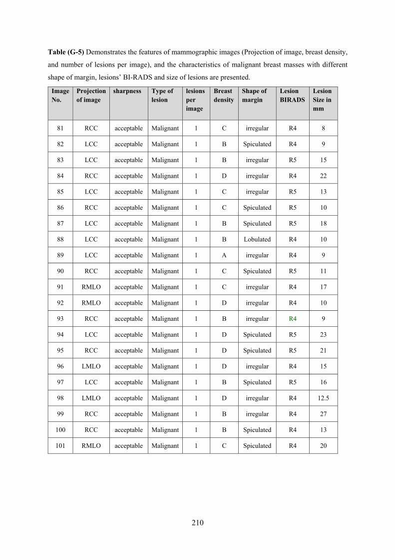
210
Table (G-5) Demonstrates the features of mammographic images (Projection of image, breast density,
and number of lesions per image), and the characteristics of malignant breast masses with different
shape of margin, lesions’ BI-RADS and size of lesions are presented.
Image No.
Projection of image
sharpness Type of lesion
lesions per image
Breast density
Shape of margin
Lesion BIRADS
Lesion Size in mm
81 RCC acceptable Malignant 1 C irregular R4 8
82 LCC acceptable Malignant 1 B Spiculated R4 9
83 LCC acceptable Malignant 1 B irregular R5 15
84 RCC acceptable Malignant 1 D irregular R4 22
85 LCC acceptable Malignant 1 C irregular R5 13
86 RCC acceptable Malignant 1 C Spiculated R5 10
87 LCC acceptable Malignant 1 B Spiculated R5 18
88 LCC acceptable Malignant 1 B Lobulated R4 10
89 LCC acceptable Malignant 1 A irregular R4 9
90 RCC acceptable Malignant 1 C Spiculated R5 11
91 RMLO acceptable Malignant 1 C irregular R4 17
92 RMLO acceptable Malignant 1 D irregular R4 10
93 RCC acceptable Malignant 1 B irregular R4 9
94 LCC acceptable Malignant 1 D Spiculated R5 23
95 RCC acceptable Malignant 1 D Spiculated R5 21
96 LMLO acceptable Malignant 1 D irregular R4 15
97 LCC acceptable Malignant 1 B Spiculated R5 16
98 LMLO acceptable Malignant 1 D irregular R4 12.5
99 RCC acceptable Malignant 1 B irregular R4 27
100 RCC acceptable Malignant 1 B Spiculated R4 13
101 RMLO acceptable Malignant 1 C Spiculated R4 20

211
Table (G-6) Demonstrates the features of mammographic images (Projection of image, breast density,
and number of lesions per image), and the characteristics of malignant breast microcalcifications with
different shape, distribution, lesions’ BI-RADS and size of lesions are presented.
Image No.
Projection of image
Sharpness Type of lesion
lesion per
image
Breast density
Calci. Distribution
Lesion BI-RADS
Lesion size in mm
1 LMLO acceptable Malignant 1 B Clustered R4 5
2 RCC acceptable Malignant 1 B Clustered R4 8
3 RCC acceptable Malignant 1 D Clustered R5 7
4 RCC acceptable Malignant 3 D Clustered R3
Whole group=9.6
5 LMLO acceptable Malignant 2 C Clustered R5 30&13
6 RCC acceptable Malignant 1 B Clustered R5 12
7 RCC acceptable Malignant 1 C Clustered R5 10
8 RCC acceptable Malignant 2 C Clustered R5 16&11
9 RMLO acceptable Malignant 1 B Clustered R3 10
10 RMLO acceptable Malignant 1 C Clustered R5 17.5
11 LCC acceptable Malignant 1 B Clustered R3 6
12 RCC acceptable Malignant 1 C Clustered R4 9
13 LCC acceptable Malignant 1 C Clustered R4 7.5
14 RCC acceptable Malignant 1 C Clustered R4 7
15 RCC acceptable Malignant 2 D Clustered R5 26&26
16 LMLO acceptable Malignant 2 D Clustered R5 27&9
17 LMLO acceptable Malignant 1 D Clustered R3 12.5
18 RCC acceptable Malignant 1 B Clustered R4 11.6
19 RCC acceptable Malignant 1 B Clustered R4 5.4
20 RMLO acceptable Malignant 1 B Clustered R4 10

212
Table (G-7) Demonstrates the features of mammographic images (Projection of image, breast density,
and number of lesions per image), and the characteristics of malignant breast microcalcifications with
different shape, distribution, lesions’ BI-RADS and size of lesions are presented.
Image No.
Projection of image
Sharpness Type of lesion
lesion per
image
Breast density
Calci. Distribution
Lesion BI-
RADS
Lesion size in mm
21 LMLO acceptable Malignant 1 C Clustered R5 22
22 LCC acceptable Malignant 1 C Clustered R4 13
23 RMLO acceptable Malignant 1 B Clustered R4 15
24 LMLO acceptable Malignant 1 B Clustered R5 9
25 RCC acceptable Malignant 1 B Clustered R4 13.7
26 RCC acceptable Malignant 3 C Clustered R4 10
27 LMLO acceptable Malignant 2 B Clustered R5 5
28 LMLO acceptable Malignant 1 B Clustered R4 12
29 LCC acceptable Malignant 1 B Clustered R4 15
30 RCC acceptable Malignant 1 C Clustered R4 6
31 RCC acceptable Malignant 1 B Clustered R3 8
32 RMLO acceptable Malignant 1 C Clustered R4 18
33 RCC acceptable Malignant 1 D Clustered R5 7
34 RCC acceptable Malignant 1 B Clustered R4 7
35 LMLO acceptable Malignant 2 C Clustered R3 12, 5
36 RCC acceptable Malignant 1 B Clustered R5 12
37 RMLO acceptable Malignant 1 C Clustered R4 15.6
38 RCC acceptable Malignant 1 B Clustered R3 6.5
39 LMLO acceptable Malignant 1 C Clustered R4 19
40 RCC acceptable Malignant 1 B Clustered R5 8

213
Table (G-8) Demonstrates the features of mammographic images (Projection of image, breast density,
and number of lesions per image), and the characteristics of malignant breast microcalcifications with
different shape, distribution, lesions’ BI-RADS and size of lesions are presented.
Image No.
Projection of image
Sharpness Type of lesion
lesion per image
Breast density
Calci. Distribution
Lesion BI-RADS
Lesion size in mm
41 LMLO acceptable Malignant 1 D Clustered R5 16
42 LCC acceptable Malignant 1 D Clustered R4 6
43 RCC acceptable Malignant 1 C Clustered R4 24
44 LCC acceptable Malignant 1 D Clustered R4 8
45 RCC acceptable Malignant 3 D Clustered R3,R3,R4 7.5,5.5,14
46 LCC acceptable Malignant 2 B Clustered R4,R5 10.5,25
47 RCC acceptable Malignant 1 C Clustered R5 20
48 RCC acceptable Malignant 2 C Clustered R5,R4 6, 6
49 RCC acceptable Malignant 1 D Clustered R3 6
50 LCC acceptable Malignant 1 B Clustered R4 11
51 RCC acceptable Malignant 1 B Clustered R5 14
52 LCC acceptable Malignant 1 C Clustered R3 5
53 RCC acceptable Malignant 1 D Clustered R4 14
54 LCC acceptable Malignant 1 C Clustered R3 6.4
55 RMLO acceptable Malignant 2 B Clustered R4 13
56 LCC acceptable Malignant 1 B Clustered R4 18
57 RCC acceptable Malignant 1 D Clustered R4 18
58 LMLO acceptable Malignant 1 B Clustered R4 12.5
59 LMLO acceptable Malignant 1 D Clustered R4 15
60 RCC acceptable Malignant 1 C Clustered R4 12
61 RCC acceptable Malignant 1 C Clustered R4 14
62 LCC acceptable Malignant 1 C Clustered R4 11

214
Appendix H: ROCView Instructions

215

216

217

218
Appendix I:
Table (I-1) The results of observation session for one observer represent true positive
cases (images contain malignant masses without image blurring).
Reader _ID
Modality _ID
Case _ID Lesion _ID TP _rating
2 0 1 1 5 2 0 2 1 10 2 0 4 1 9 2 0 5 1 10 2 0 6 1 8 2 0 7 1 7 2 0 8 1 10 2 0 9 1 5 2 0 10 1 9 2 0 11 1 3 2 0 12 1 9 2 0 13 1 9 2 0 14 1 9 2 0 15 1 9 2 0 16 1 10 2 0 17 1 3 2 0 18 1 5 2 0 19 1 9 2 0 20 1 7 2 0 21 1 9 2 0 22 1 7 2 0 23 1 7 2 0 24 1 10 2 0 25 1 9 2 0 26 1 4 2 0 27 1 4 2 0 28 1 4 2 0 30 1 7 2 0 31 1 9 2 0 32 1 9 2 0 33 1 10 2 0 34 1 5 2 0 35 1 10 2 0 36 1 4 2 0 37 1 8 2 0 38 1 8 2 0 39 1 5 2 0 41 1 7 2 0 42 1 10 2 0 43 1 9 2 0 44 1 6 2 0 45 1 6

219
2 0 46 1 4 2 0 47 1 9 2 0 48 1 2 2 0 49 1 4 2 0 51 1 9 2 0 52 1 9 2 0 53 1 9 2 0 54 1 6 2 0 55 1 9 2 0 56 1 7 2 0 57 1 7 2 0 58 1 6 2 0 59 1 6 2 0 60 1 2 2 0 61 1 9 2 0 62 1 4

220
Table (I-2) The results of observation session for one observer represent true positive
cases (images contain malignant masses with image blurring 0.7 mm).
Reader _ID Modality _ID Case _ID Lesion _ID TP _rating
2 0.7 1 1 5
2 0.7 2 1 4
2 0.7 4 1 6
2 0.7 5 1 6
2 0.7 6 1 7
2 0.7 7 1 7
2 0.7 8 1 4
2 0.7 9 1 3
2 0.7 12 1 8
2 0.7 13 1 7
2 0.7 14 1 2
2 0.7 15 1 8
2 0.7 16 1 8
2 0.7 17 1 4
2 0.7 18 1 4
2 0.7 19 1 8
2 0.7 20 1 7
2 0.7 21 1 6
2 0.7 22 1 4
2 0.7 23 1 7
2 0.7 24 1 9
2 0.7 25 1 6
2 0.7 26 1 5
2 0.7 27 1 4
2 0.7 30 1 1
2 0.7 31 1 6
2 0.7 32 1 9
2 0.7 33 1 6
2 0.7 35 1 8
2 0.7 36 1 6
2 0.7 37 1 5
2 0.7 38 1 3
2 0.7 39 1 6
2 0.7 41 1 5
2 0.7 42 1 6

221
2 0.7 43 1 6
2 0.7 45 1 3
2 0.7 46 1 4
2 0.7 47 1 6
2 0.7 48 1 2
2 0.7 49 1 6
2 0.7 50 1 3
2 0.7 51 1 5
2 0.7 52 1 6
2 0.7 53 1 6
2 0.7 54 1 2
2 0.7 55 1 5
2 0.7 56 1 5
2 0.7 57 1 6
2 0.7 58 1 2
2 0.7 59 1 3
2 0.7 60 1 4
2 0.7 61 1 6
2 0.7 62 1 4

222
Table (I-3) The results of observation session for one observer represent true positive cases
(images contain malignant masses with image blurring 1.5 mm).
Reader _ID Modality _ID
Case _ID
Lesion _ID
TP _rating
2 1.5 1 1 7
2 1.5 2 1 6
2 1.5 4 1 6
2 1.5 5 1 5
2 1.5 6 1 2
2 1.5 7 1 7
2 1.5 8 1 8
2 1.5 10 1 7
2 1.5 11 1 2
2 1.5 12 1 6
2 1.5 13 1 7
2 1.5 14 1 5
2 1.5 15 1 8
2 1.5 16 1 7
2 1.5 17 1 2
2 1.5 18 1 5
2 1.5 19 1 7
2 1.5 20 1 4
2 1.5 21 1 8
2 1.5 22 1 5
2 1.5 23 1 6
2 1.5 24 1 8
2 1.5 25 1 8
2 1.5 26 1 6
2 1.5 27 1 2
2 1.5 31 1 5
2 1.5 32 1 8
2 1.5 33 1 8
2 1.5 35 1 6
2 1.5 36 1 3
2 1.5 37 1 5
2 1.5 38 1 4
2 1.5 39 1 4
2 1.5 41 1 2
2 1.5 42 1 8
2 1.5 43 1 7
2 1.5 44 1 2
2 1.5 46 1 6
2 1.5 47 1 5
2 1.5 49 1 7
2 1.5 50 1 2
2 1.5 51 1 6

223
2 1.5 52 1 7
2 1.5 53 1 3
2 1.5 54 1 5
2 1.5 56 1 3
2 1.5 57 1 2
2 1.5 58 1 5
2 1.5 60 1 3
2 1.5 61 1 6
2 1.5 62 1 5
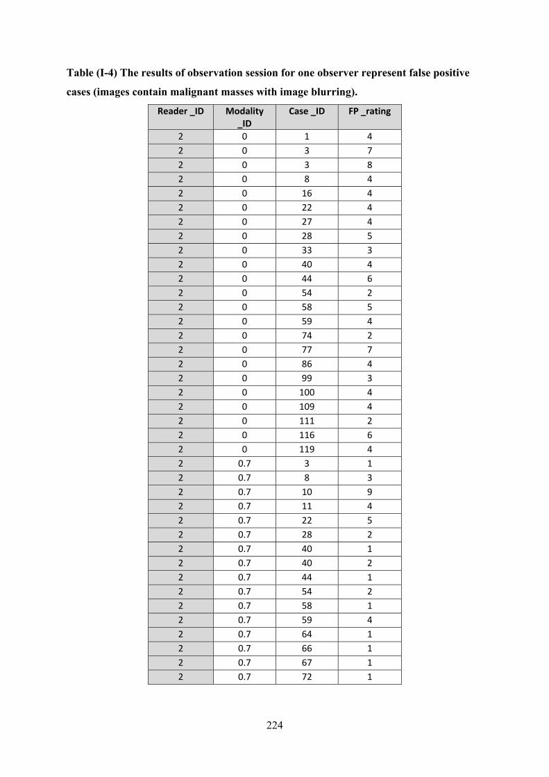
224
Table (I-4) The results of observation session for one observer represent false positive
cases (images contain malignant masses with image blurring).
Reader _ID Modality _ID
Case _ID FP _rating
2 0 1 4
2 0 3 7
2 0 3 8
2 0 8 4
2 0 16 4
2 0 22 4
2 0 27 4
2 0 28 5
2 0 33 3
2 0 40 4
2 0 44 6
2 0 54 2
2 0 58 5
2 0 59 4
2 0 74 2
2 0 77 7
2 0 86 4
2 0 99 3
2 0 100 4
2 0 109 4
2 0 111 2
2 0 116 6
2 0 119 4
2 0.7 3 1
2 0.7 8 3
2 0.7 10 9
2 0.7 11 4
2 0.7 22 5
2 0.7 28 2
2 0.7 40 1
2 0.7 40 2
2 0.7 44 1
2 0.7 54 2
2 0.7 58 1
2 0.7 59 4
2 0.7 64 1
2 0.7 66 1
2 0.7 67 1
2 0.7 72 1

225
2 0.7 74 1
2 0.7 77 5
2 0.7 79 1
2 0.7 80 1
2 0.7 82 2
2 0.7 86 3
2 0.7 88 1
2 0.7 89 1
2 0.7 94 1
2 0.7 94 2
2 0.7 99 4
2 0.7 100 3
2 0.7 102 2
2 0.7 104 2
2 0.7 106 1
2 0.7 106 1
2 0.7 110 1
2 0.7 111 4
2 0.7 116 5
2 0.7 119 5
2 0.7 121 1
2 1.5 8 2
2 1.5 22 2
2 1.5 27 4
2 1.5 28 2
2 1.5 40 4
2 1.5 58 2
2 1.5 59 5
2 1.5 74 2
2 1.5 86 3
2 1.5 89 2
2 1.5 97 4
2 1.5 100 3
2 1.5 104 3
2 1.5 108 3
2 1.5 111 3
2 1.5 116 4

226
Appendix J: The Results of Combined Two Observers Data
Table M-1 Demonstrates the FOMs of the 21 pairs of combining two observers’ data for three levels
of motion blur for microcalcification cases.
Observers pairs
FOMs for three levels motion blur
0.0 mm 0.7 mm 1.5 mm
1 0.944 0.860 0.853
2 0.923 0.850 0.796
3 0.908 0.860 0.781
4 0.936 0.884 0.811
5 0.947 0.898 0.8487
6 0.901 0.853 0.730
7 0.946 0.857 0.888
8 0.914 0.892 0.855
9 0.947 0.882 0.871
10 0.950 0.874 0.882
11 0.896 0.869 0.815
12 0.907 0.923 0.792
13 0.948 0.878 0.859
14 0.942 0.886 0.846
15 0.923 0.870 0.763
16 0.907 0.901 0.855
17 0.903 0.867 0.837
18 0.887 0.877 0.800
19 0.950 0.902 0.847
20 0.916 0.872 0.818
21 0.909 0.893 0.799
Average across
Observers
0.923 0.876 0.826

227
Table M-2 Demonstrates the FOMs of the 21 pairs of the observers for three levels of motion blur for
masses.
Observers pairs
FOMs for three levels of motion blur
0.0 mm 0.7 mm 1.5 mm
1 0.958 0.905 0.917
2 0.906 0.880 0.836
3 0.958 0.912 0.918
4 0.966 0.940 0.923
5 0.957 0.934 0.907
6 0.941 0.870 0.836
7 0.929 0.926 0.959
8 0.962 0.928 0.962
9 0.971 0.925 0.939
10 0.951 0.938 0.940
11 0.948 0.890 0.866
12 0.941 0.905 0.944
13 0.951 0.950 0.948
14 0.934 0.933 0.923
15 0.931 0.881 0.882
16 0.974 0.947 0.920
17 0.958 0.897 0.959
18 0.920 0.905 0.877
19 0.965 0.931 0.949
20 0.960 0.862 0.905
21 0.938 0.928 0.907
Average across
Observers
0.948 0.913 0.915

228
Appendix K: Conspicuity Index
Table: Measurement of conspicuity index of breast masses within mammographic images using conspicuity software. The physical parameters includes the maximum lesion diameter, the θ represents is the maximum slope angle to the edge of the lesion profile in degrees, σs = mean noise within the lesion, σn= mean background noise and SNR of lesions.
Blur Level mm
Conspicuity Index
d (max diameter)
θ (degrees)
ΔGL σ (l) σ (b) μ Lesion
μ Background
Case 1
0.0 51.631 24.450 63.765 88.903 42.734 69.744 192.939 104.036
0.7 66.389 18.589 61.030 93.344 21.061 40.134 194.894 101.550
1.5 74.993 17.133 59.797 93.600 16.109 31.417 194.417 100.817
Case 2
0.0 71.577 42.183 69.151 69.483 60.864 82.009 178.011 108.528
0.7 101.672 39.644 67.259 70.189 34.217 51.973 178.272 108.083
1.5 110.622 38.578 66.415 69.886 27.714 45.491 178.044 108.158
Case 3
0.0 45.003 24.917 66.945 76.644 51.102 80.162 184.039 107.394
0.7 55.621 18.911 64.153 79.006 22.724 47.957 185.694 106.689
1.5 58.383 16.928 62.927 79.353 15.307 40.332 185.950 106.597
Case 4
0.0 108.879 44.567 73.240 84.333 73.301 79.006 174.361 90.028
0.7 153.361 43.294 72.357 84.797 46.650 53.463 174.311 89.514
1.5 169.432 42.367 71.568 84.600 38.306 46.135 174.033 89.433
Case 5
0.0 66.273 48.606 70.833 66.464 96.237 91.397 166.844 100.381
0.7 78.105 45.194 67.952 67.706 67.191 62.960 167.272 99.567
1.5 81.129 43.583 66.377 68.269 58.253 54.862 167.417 99.147
Case 6
0.0 40.113 32.456 65.036 59.036 56.479 80.202 172.139 113.103
0.7 43.759 20.461 58.806 63.083 16.520 43.842 175.272 112.189
1.5 47.462 19.394 57.771 63.042 12.358 37.331 175.161 112.119

229
Blur Leve mm
Conspicuity Index
d (max diamete
r)
θ (degrees)
ΔGL σ (l) σ (b) μ Lesion
μ Background
Case 7
0.0 170.73 51.667 70.653 133.19 69.05 83.929 206.483 73.29
0.7 252.59 51.306 70.526 133.54 50.13 52.581 206.556 73.01
1.5 272.5 50.544 70.256 133.61 45.48 47.03 206.622 73.00
Case 8
0.0 140.63 40.339 72.605 96.358 54.27 62.947 161.567 65.20
0.7 222.31 38.761 71.959 96.797 28.2 39.953 161.783 64.98
1.5 238.35 37.289 71.290 96.836 23.71 35.017 161.806 64.96
Case 9
0.0 113.44 36.4 72.974 99.35 63.11 74.922 186.967 87.61
0.7 150.18 34.85 71.939 99.558 41.68 52.282 186.678 87.11
1.5 162.84 34.039 71.200 98.869 34.17 46.13 185.956 87.08
Case 10
0.0 124.98 66.322 71.213 108.73 84.55 136.28 188.722 79.9
0.7 169.81 64.222 70.483 109.86 43.24 102.26 189.556 79.69
1.5 181.56 63.439 70.149 109.91 36.41 94.026 189.6 79.69
Case 11
0.0 116.22 31.567 73.520 115.36 65.99 74.468 179.561 64.2
0.7 155.95 30.883 72.929 114.86 44.59 53.584 178.733 63.87
1.5 168.74 30.144 72.239 114.26 36.81 47.5 177.933 63.6
Case 12
0.0 82.89 24.728 69.508 107.98 57.51 58.192 155.578 47.60
0.7 117.32 23.311 68.925 108.1 29.77 43.803 155.344 47.24
1.5 127.94 22.811 68.526 107.41 24.9 39.023 154.589 47.18
Case 13
0.0 123.43 46.761 71.087 86.517 62.41 65.514 171.939 85.42
0.7 179.01 44.483 69.64 87.256 38.04 40.341 172.022 84.76
1.5 192.82 43.056 68.755 87.494 33.39 34.163 171.972 84.47
Case 14
0.0 127.07 47.378 69.536 127.66 58.45 106.01 202.578 74.916
0.7 166.60 45.644 69.144 128.66 34.55 80.8 203.35 74.69
1.5 178.28 44.361 68.758 128.76 27.53 73.348 203.506 74.74
Case 15
0 212.32 8.11 87.472 89.713 6.6268 55.20 252.00 162.29
0.7 229.83 7.055 86.018 87.172 5.8137 30.145 250.90 163.73
1.5 211.05 6.577 84.963 84.161 5.8231 24.110 247.86 163.7

230
Case 16
0 145.51 4.694 87.822 70.497 26.845 30.94 218.9 148.40
0.7 165.40 4.105 85.892 53.644 8.6917 12.09 205.17 151.52
1.5 116.77 3.711 83.104 40.697 4.7621 8.018 192.83 152.1
Case 17
0 239.96 4.1 88.336 133.43 17.60 45.73 239.56 106.13
0.7 221.32 2.85 87.149 113.26 8.718 19.83 222.47 109.20
1.5 198.75 2.838 86.088 90.783 6.846 13.44 200.50 109.72
Case 18
0 246.51 21.916 86.026 129.00 107.6 76.10 229.96 100.9
0.7 344.10 22.361 84.444 140.12 63.27 47.69 229.87 89.75
1.5 351.86 22.438 83.122 143.65 56.6 34.25 226.48 82.836
Case 19
0 542.70 9.383 88.400 133.98 29.39 41.71 242.04 108.06
0.7 553.27 8.533 87.386 128.25 17.49 25.98 237.85 109.6
1.5 451.24 7.205 86.277 121.58 12.44 19.93 231.17 109.58
Case 20
0 199.30 5.53 87.823 94 14.73 44.65 233.1 139.1
0.7 191.61 4.677 86.252 80.68 8.919 21.97 220.51 139.83
1.5 131.28 3.366 83.692 71.23 4.024 13.66 209.28 138.04
Case 21
0 124.32 5.1 87.425 90.563 32.9 49.50 217.84 127.28
0.7 128.06 3.35 85.811 84.266 10.14 22.09 213.58 129.316
1.5 116.57 3.233 84.238 70.694 6.947 15.00 200.4 129.70
Case 22
0 466.85 11.866 88.764 121.24 52.78 58.70 234.53 113.34
0.7 552.188 10.72 87.862 119.13 24.32 34.48 234.42 115.28
1.5 472.39 9.6 86.963 112.48 17.95 26.96 229.25 116.77
Case 23
0 192.33 4.255 88.092 112.89 15.30 46.7 222.43 109.53
0.7 162.39 3.35 86.562 89.40 9.191 21.91 200.35 110.9
1.5 91.292 3.616 82.005 68.65 8.410 14.98 180.15 111.5

231
Appendix M: Dispersion Index Tables
Table 7 The physical measures of the microcalcification in image without blurring
Area1 Mean1
StdDev1
Min1 Max1 Calc. NO.
D.I contrast
DI x Con
SNR Detect-ability
1 13.7 2610 62 2457 2933 11 0.801 0.890 0.713 41.94 1.00
2 23.5 2968 90 2702 3361 25 1.062 0.883 0.937 33.10 1.00
3 34.8 2965 93 2683 3361 29 0.832 0.882 0.734 31.98 1.00
4 40.4 2673 105 2381 3145 13 0.322 0.850 0.273 25.42 0.57
5 315.3 2889 170 2511 4095 61 0.193 0.705 0.274 16.99 1.00
5 58.7 2898 164 2520 3544 9 0.153 0.818 0.188 17.62 0.57
6 28.8 2704 101 2503 3298 24 0.834 0.820 0.684 26.73 1.00
7 13.9 2571 85 2361 2943 12 0.863 0.874 0.754 30.42 1.00
8 61.6 2520 111 2247 3017 15 0.243 0.835 0.291 22.64 0.86
8 79.2 2803 115 2335 3379 22 0.278 0.829 0.335 24.36 1.00
9 13.9 2571 85 2361 2943 9 0.648 0.874 0.566 30.42 1.00
10 66.7 2603 81 2368 3000 30 0.449 0.868 0.390 32.06 0.85
11 11.9 2787 108 2556 3236 9 0.755 0.861 0.651 25.83 1.00
12 18.2 2760 91 2572 3300 30 1.644 0.836 1.375 30.50 1.00
13 24.1 2765 140 2540 3385 25 1.039 0.817 0.849 19.74 1.00
14 3.9 2706 75 2549 3000 9 2.311 0.902 2.084 36.04 1.00
15 376.7 2809 161 2361 3722 27 0.072 0.755 0.095 17.48 0.57
16 159.3 2897 168 2278 3760 18 0.113 0.770 0.147 17.20 0.43
17 46.2 2720 143 2393 3342 9 0.195 0.814 0.158 19.09 1.00
18 21.2 2676 102 2453 3197 11 0.519 0.837 0.434 26.14 1.00
19 8.9 2906 109 2740 3433 10 1.123 0.847 0.951 26.72 0.72
20 15.2 2944 126 2732 3608 8 0.527 0.816 0.430 23.45 1.00
21 98.4 2613 136 2257 3528 60 0.610 0.741 0.452 19.16 1.00
22 15.2 2944 126 2732 3608 9 0.593 0.816 0.484 23.45 1.00
24 6.7 2624 87 2409 3085 10 1.498 0.851 1.274 30.09 1.00
25 32.5 2179 90 1911 2664 10 0.308 0.818 0.252 24.27 1.00
27 45.6 2393 81 2203 2740 23 0.504 0.873 0.441 29.44 1.00
28 7.6 2710 89 2515 3086 15 1.979 0.878 1.739 30.42 1.00
29 61.9 2670 91 2418 3037 13 0.210 0.879 0.185 29.41 1.00
30 11.1 2875 127 2595 3536 20 1.807 0.813 1.469 22.56 1.00
31 19.7 2663 63 2527 3008 8 0.407 0.885 0.360 42.16 1.00
32 63.9 2626 87 2397 3108 22 0.344 0.845 0.408 30.25 0.72
32 15.4 2654 67 2465 2915 5 0.325 0.910 0.357 39.52 1.00
33 13.9 2912 122 2646 3398 16 1.154 0.857 0.989 23.80 1.00
34 12.7 2857 66 2650 3113 8 0.629 0.918 0.578 43.32 1.00
35 23.8 2427 62 2256 2689 17 0.713 0.903 0.790 39.17 1.00
35 9.8 2539 68 2375 2835 9 0.914 0.896 1.021 37.35 0.72

232
36 37.1 2849 116 2411 3328 20 0.539 0.856 0.461 24.55 0.86
37 5.0 2744 96 2527 3128 8 1.596 0.877 1.401 28.57 1.00
38 14.1 2660 79 2490 3040 10 0.709 0.875 0.810 33.86 1.00
39 136.5 2276 143 1950 2881 42 0.308 0.790 0.390 15.87 0.86
40 29.5 2584 77 2408 2946 22 0.746 0.877 0.850 33.42 0.00
41 69.3 2579 121 2312 3314 40 0.577 0.778 0.449 21.30 1.00
42 12.4 2840 93 2659 3246 29 2.336 0.875 2.044 30.62 1.00
44 28.8 2719 90 2485 3200 20 0.695 0.850 0.591 30.13 1.00
45 22.2 2686 96 2465 3114 7 0.316 0.863 0.366 28.02 0.86
45 25.2 2738 73 2500 3099 9 0.357 0.883 0.404 37.72 0.72
46 92.1 2737 112 2447 3207 48 0.521 0.853 0.611 24.45 0.86
46 155.2 2545 116 2312 3104 35 0.225 0.820 0.275 21.93 0.72
47 201.2 2518 142 2194 3232 25 0.124 0.779 0.159 17.68 0.86
48 24.9 2728 85 2344 3223 35 1.404 0.847 1.659 32.14 1.00
48 9.2 2595 85 2425 3072 8 0.874 0.845 1.035 30.50 1.00
49 2.7 2612 61 2485 2799 8 3.002 0.933 2.801 42.56 1.00
50 19.2 2985 98 2719 3391 20 1.043 0.880 0.919 30.47 1.00
51 34.1 2889 109 2577 3340 13 0.382 0.865 0.330 26.42 0.57
52 9.5 2628 141 2369 3237 21 2.207 0.812 1.792 18.59 1.00
53 33.1 2349 117 2017 2770 18 0.544 0.848 0.462 20.02 0.86
54 13.6 2834 91 2596 3242 28 2.064 0.874 1.805 31.03 1.00
55 59.1 2472 65 2305 2914 15 0.254 0.848 0.215 38.22 1.00
56 83.9 2701 120 2431 3190 43 0.513 0.847 0.434 22.60 1.00
57 135.3 2637 211 2252 3686 54 0.399 0.715 0.286 12.50 0.00
58 55.1 2453 124 2267 3061 18 0.327 0.802 0.262 19.82 1.00
59 361.5 2319 172 1845 3269 60 0.166 0.709 0.118 13.46 0.72
60 20.5 2102 271 1775 3114 26 1.266 0.675 0.854 7.74 0.86
61 90.5 2532 119 2225 3154 32 0.354 0.803 0.284 21.33 1.00
62 115.7 2616 72 2366 2927 50 0.432 0.894 0.386 36.54 1.00

233
Table 7.7: The physical and clinical measures of the microcalcification cases in image with 0.7mm level of simulated blurring
Area1 Mean1 StdDev1 Min1 Max1 Calc.
NO. DI contrast DI
x Con
SNR Detect-ability
1 13.731 2607 39.558 2544 2774 11 0.80 0.94 0.75 65.90 1.00
2 23.55 2966 73.434 2766 3191 25 1.06 0.93 0.99 40.39 1.00
3 34.85 2964 77.104 2758 3191 29 0.83 0.93 0.77 38.44 0.86
4 40.41 2672 93.39 2420 2870 13 0.32 0.93 0.30 28.61 0.43
5 315.28 2888 156.028 2576 3928 61 0.19 0.74 0.26 18.51 1.00
5 58.66 2896 153.375 2589 3343 9 0.15 0.87 0.18 18.88 0.43
6 28.77 2702 73.459 2568 2996 24 0.83 0.90 0.75 36.78 1.00
7 13.90 2569 71.498 2405 2733 12 0.86 0.94 0.81 35.93 1.00
8 61.63 2519 102.512 2298 2887 15 0.24 0.87 0.28 24.58 0.57
8 79.18 2801 105.569 2375 3056 22 0.28 0.92 0.30 26.54 0.86
9 13.90 2569 71.498 2405 2733 9 0.65 0.94 0.61 35.93 0.85
10 66.74 2602 67.821 2419 2835 30 0.45 0.92 0.41 38.37 0.72
11 11.92 2781 77.574 2617 2999 9 0.76 0.93 0.70 35.85 0.57
12 18.25 2757 60.373 2657 3028 30 1.64 0.91 1.50 45.66 1.00
13 24.06 2760 105.626 2598 3152 25 1.04 0.88 0.91 26.13 0.57
14 3.90 2702 43.168 2600 2838 9 2.31 0.95 2.20 62.58 0.43
15 376.66 2808 154.694 2407 3304 27 0.07 0.85 0.08 18.15 0.14
16 159.29 2896 163.738 2317 3579 18 0.11 0.81 0.14 17.69 0.29
17 46.24 2718 133.598 2463 3078 9 0.19 0.88 0.17 20.35 0.43
18 21.21 2674 91.463 2497 2958 11 0.52 0.90 0.47 29.24 0.43
19 8.91 2892 66.389 2765 3136 10 1.12 0.92 1.04 43.56 0.43
20 15.18 2941 88.99 2775 3297 8 0.53 0.89 0.47 33.04 1.00
21 98.37 2612 119.705 2315 3180 60 0.61 0.82 0.50 21.82 1.00
22 15.18 2941 88.99 2775 3297 9 0.59 0.89 0.53 33.04 0.72
24 6.68 2620 60.679 2479 2818 10 1.50 0.93 1.39 43.18 1.00
25 32.46 2178 80.464 1971 2439 10 0.31 0.89 0.28 27.07 0.14
27 7.58 2705 51.628 2592 2862 15 1.98 0.95 1.87 52.39 1.00
28 45.60 2392 72.971 2244 2581 23 0.50 0.93 0.47 32.79 0.29
29 61.94 2669 80.685 2464 2894 13 0.21 0.92 0.19 33.08 0.86
30 11.07 2871 93.864 2669 3195 20 1.81 0.90 1.62 30.59 1.00
31 19.66 2661 45.362 2574 2885 8 0.41 0.92 0.38 58.66 0.72
32 15.37 2651 52.472 2517 2794 5 0.33 0.95 0.34 50.53 0.43
33 13.86 2907 87.203 2710 3185 16 1.15 0.91 1.05 33.34 1.00
34 12.71 2855 48.317 2736 2977 8 0.63 0.96 0.60 59.09 1.00
35 23.83 2426 48.466 2286 2566 17 0.71 0.95 0.75 50.05 0.43
35 9.85 2537 50.029 2420 2667 9 0.91 0.95 0.96 50.70 0.14
36 37.12 2847 103.645 2465 3176 20 0.54 0.90 0.48 27.47 1.00
37 5.01 2736 65.585 2565 2932 8 1.60 0.93 1.49 41.71 1.00
38 14.11 2660 60.335 2534 2884 10 0.71 0.92 0.77 44.09 1.00
39 136.47 2275 135.88 1999 2704 42 0.31 0.84 0.37 16.74 0.86
40 29.49 2583 56.726 2448 2805 22 0.75 0.92 0.81 45.53 0.00
41 69.29 2578 98.026 2346 3054 40 0.58 0.84 0.49 26.30 1.00
42 12.41 2837 57.486 2711 3011 29 2.34 0.94 2.20 49.35 1.00
44 28.76 2718 66.485 2539 3005 20 0.70 0.90 0.63 40.87 1.00
45 22.16 2686 81.269 2543 2904 7 0.32 0.92 0.34 33.05 0.57
45 25.21 2737 57.389 2576 2915 9 0.36 0.94 0.38 47.68 0.29
46 92.06 2736 100.833 2499 3059 48 0.52 0.89 0.58 27.13 0.72
46 155.22 2544 108.818 2362 2965 35 0.23 0.86 0.26 23.38 0.29

234
47 201.23 2517 134.244 2241 3023 25 0.12 0.83 0.15 18.75 1.00
48 24.92 2727 66.746 2388 2966 35 1.40 0.92 1.53 40.85 1.00
48 9.15 2593 59.546 2481 2827 8 0.87 0.92 0.95 43.54 0.86
49 2.67 2609 39.09 2543 2695 8 3.00 0.97 2.91 66.74 0.43
50 19.17 2982 82.713 2774 3226 20 1.04 0.92 0.96 36.05 0.86
51 34.07 2888 99.713 2614 3157 13 0.38 0.91 0.35 28.96 0.14
52 9.52 2621 93.8 2405 2918 21 2.21 0.90 1.98 27.94 0.86
53 33.07 2348 108.941 2060 2635 18 0.54 0.89 0.49 21.55 1.00
54 13.56 2772 410.758 2596 3057 28 2.06 0.91 1.87 6.75 0.86
55 59.05 2470 48.297 2360 2748 15 0.25 0.90 0.23 51.15 1.00
56 83.90 2699 106.534 2485 2996 43 0.51 0.90 0.46 25.34 1.00
57 135.26 2636 199.71 2305 3396 54 0.40 0.78 0.31 13.20 0.00
58 55.11 2452 114.308 2296 2970 18 0.33 0.83 0.27 21.45 1.00
59 361.54 2318 158.994 1916 2921 60 0.17 0.79 0.13 14.58 0.29
60 20.54 2072 319.739 1775 2823 26 1.27 0.73 0.93 6.48 0.72
61 90.48 2531 108.622 2276 2960 32 0.35 0.86 0.30 23.30 0.72
62 115.70 2614 59.432 2413 2814 50 0.43 0.93 0.40 43.99 0.72

235
Table The physical measures of the microcalcification in image with 1.5mm level of simulated blurring
Area1
Mean1 StdDev1
Min1 Max1
Calc. NO.
DI contrast DI x Con
SNR Detect-ability
1 13.7 2605 32 2555 2718 11 0.80 0.96 0.77 80.94 0.572
2 23.5 2966 70 2776 3137 25 1.06 0.95 1.00 42.61 0.850
3 34.8 2963 73 2769 3137 29 0.83 0.94 0.79 40.49 0.572
4 40.4 2672 88 2433 2838 13 0.32 0.94 0.30 30.24 0.000
5 315.3 2888 151 2590 3742 61 0.19 0.77 0.25 19.18 1.000
5 58.7 2896 148 2600 3260 9 0.15 0.89 0.17 19.51 0.143
6 28.8 2701 64 2585 2898 24 0.83 0.93 0.78 42.35 1.000
7 13.9 2568 69 2414 2697 12 0.86 0.95 0.82 37.32 1.000
8 61.6 2519 99 2316 2845 15 0.24 0.89 0.27 25.47 0.143
8 79.2 2801 103 2384 2990 22 0.28 0.94 0.30 27.24 0.430
9 13.9 2568 69 2414 2697 9 0.65 0.95 0.62 37.32 0.430
10 66.7 2602 64 2426 2777 30 0.45 0.94 0.42 40.66 0.430
11 11.9 2776 66 2634 2940 9 0.76 0.94 0.71 42.05 0.858
12 18.2 2754 52 2672 2946 30 1.64 0.93 1.54 52.84 1.000
13 24.1 2756 92 2605 3061 25 1.04 0.90 0.94 29.91 0.715
14 3.9 2698 35 2616 2803 9 2.31 0.96 2.22 76.60 0.286
15 376.7 2808 152 2430 3231 27 0.07 0.87 0.08 18.43 0.290
16 159.3 2895 162 2333 3475 18 0.11 0.83 0.14 17.86 0.000
17 46.2 2717 130 2474 2995 9 0.19 0.91 0.18 20.89 0.286
18 21.2 2673 90 2508 2901 11 0.52 0.92 0.48 29.86 0.572
19 8.9 2882 52 2771 3055 10 1.12 0.94 1.06 55.10 0.858
20 15.2 2938 73 2786 3199 8 0.53 0.92 0.48 40.38 1.000
21 98.4 2612 114 2323 3038 60 0.61 0.86 0.52 22.93 1.000
22 15.2 2938 73 2786 3199 9 0.59 0.92 0.54 40.38 0.286
24 6.7 2617 51 2498 2755 10 1.50 0.95 1.42 51.73 0.720
25 32.5 2177 77 1978 2395 10 0.31 0.91 0.28 28.23 0.430
27 7.6 2700 42 2601 2806 15 1.98 0.96 1.90 65.02 1.000
28 45.6 2392 70 2255 2555 23 0.50 0.94 0.47 34.21 0.000
29 61.9 2668 77 2474 2871 13 0.21 0.93 0.20 34.51 0.000
30 11.1 2869 83 2687 3079 20 1.81 0.93 1.68 34.51 0.715
31 19.7 2660 39 2590 2828 8 0.41 0.94 0.38 68.31 0.715
32 63.9 2625 71 2470 2814 22 0.34 0.93 0.37 36.83 0.290
32 15.4 2648 46 2530 2752 5 0.33 0.96 0.34 57.99 1.000
33 13.9 2902 72 2730 3085 16 1.15 0.94 1.09 40.41 1.000
34 12.7 2853 46 2744 2954 8 0.63 0.97 0.61 62.59 0.715
35 23.8 2425 44 2299 2530 17 0.71 0.96 0.74 55.12 0.143
35 9.8 2534 43 2431 2641 9 0.91 0.96 0.95 58.91 0.000

236
36 37.1 2845 99 2476 3123 20 0.54 0.91 0.49 28.69 0.715
37 5.0 2729 57 2564 2879 8 1.60 0.95 1.51 47.75 1.000
38 14.1 2661 55 2536 2815 10 0.71 0.95 0.75 48.15 0.860
39 136.5 2274 132 2017 2659 42 0.31 0.86 0.36 17.23 0.720
40 29.5 2582 49 2460 2745 22 0.75 0.94 0.79 53.15 0.000
41 69.3 2577 90 2355 2958 40 0.58 0.87 0.50 28.76 1.000
42 12.4 2834 48 2718 2954 29 2.34 0.96 2.24 59.00 1.000
44 28.8 2716 58 2557 2921 20 0.70 0.93 0.65 46.92 0.715
45 22.2 2685 77 2558 2869 7 0.32 0.94 0.34 34.80 0.143
45 25.2 2736 53 2594 2861 9 0.36 0.96 0.37 51.54 0.000
46 92.1 2736 97 2518 3018 48 0.52 0.91 0.58 28.19 0.720
46 155.2 2544 105 2374 2916 35 0.23 0.87 0.26 24.12 0.290
47 201.2 2517 131 2252 2939 25 0.12 0.86 0.15 19.20 0.860
48 24.9 2726 62 2398 2896 35 1.40 0.94 1.49 43.84 0.572
48 9.2 2591 51 2488 2762 8 0.87 0.94 0.93 50.34 0.290
49 2.7 2607 32 2555 2667 8 3.00 0.98 2.93 82.38 0.290
50 19.2 2979 79 2778 3175 20 1.04 0.94 0.98 37.85 0.585
52 9.5 2615 76 2424 2831 21 2.21 0.92 2.04 34.38 1.000
53 33.1 2347 107 2062 2601 18 0.54 0.90 0.49 21.84 0.572
54 13.6 2709 569 2596 2998 28 2.06 0.90 1.87 4.76 0.429
55 59.1 2469 42 2373 2669 15 0.25 0.93 0.24 58.31 1.000
56 83.9 2698 102 2498 2959 43 0.51 0.91 0.47 26.49 0.858
57 135.3 2636 196 2323 3280 54 0.40 0.80 0.32 13.46 0.000
58 55.1 2452 109 2301 2920 18 0.33 0.84 0.27 22.39 0.715
59 361.5 2318 155 1938 2763 60 0.17 0.84 0.14 14.99 0.286
60 20.5 1986 516 1775 2653 26 1.27 0.75 0.95 3.85 0.429
61 90.5 2531 104 2290 2878 32 0.35 0.88 0.31 24.23 1.000
62 115.7 2613 56 2425 2782 50 0.43 0.94 0.41 46.92 0.429

237
References
Akobeng, A. K. (2007) ‘Understanding diagnostic tests 1: sensitivity, specificity and predictive values.’, Acta paediatrica, 96(3), pp. 338–341. doi: 10.1111/j.1651-2227.2006.00180.x.
Al-osta, H. E. I. (2010) Detection of Breast Cancer Microcalcifications in Digitized Mammograms. University of Bradford. Available at: https://bradscholars.brad.ac.uk/bitstream/handle/20Al-Osta Thesis.pdf?
Al Mousa, D. S., Ryan, E. A., Mello-Thoms, C. and Brennan, P. C. (2014) ‘What effect does mammographic breast density have on lesion detection in digital mammography?’, Clinical Radiology. The Royal College of Radiologists, 69(4), pp. 333–341. doi: 10.1016/j.crad.2013.11.014.
Aldrich, B. and Desai, M. (1994) ‘Application of Spatial Grey Level Dependence Methods to Digitized Mammograms’.
Ali, R. M., England, A., McEntee, M. F. and Hogg, P. (2015) ‘A method for calculating effective lifetime risk of radiation-induced cancer from screening mammography’, Radiography. Elsevier Ltd, 21(4), pp. 298–303. doi: 10.1016/j.radi.2015.07.008.
Allec, N., Abbaszadeh, S., Scott, C. C., Lewin, J. M. and Karim, K. S. (2012) ‘Including the effect of motion artifacts in noise and performance analysis of dual-energy contrast-enhanced mammography’, Physics in Medicine and Biology, 57(24), pp. 8405–8425. doi: 10.1088/0031-9155/57/24/8405.
Alonzo-Proulx, O., Jong, R. A., & Yaffe, M. J. (2012). Volumetric breast density characteristics as determined from digital mammograms. Physics in medicine and biology, 57(1), 7443–7457. doi: 10.1088/0031-9155/57/22/7443
Alonzo-Proulx, O., Packard, N., Boone, J. M., Al-Mayah, A., Brock, K. K., Shen, S. Z., & Yaffe, M. J. (2010). Validation of a method for measuring the volumetric breast density from digital mammograms. Phys Med Biol, 55(11), 3027-3044. doi: 10.1088/0031-9155/55/11/003
American Cancer Society [ACS]. (2011a). Breast cancer facts & figures 2011-2012. Atlanta: American Cancer Society, Inc.
American Cancer Society [ACS]. (2013a). Breast cancer facts & figures 2013-2014. Atlanta.
American Cancer Society [ACS]. (2013b). Mammograms and other breast imaging tests. from http://www.cancer.org/healthy/findcancerearly/examandtestdescriptions/mammogramsandotherbreastimagingprocedures/mammograms-and-other-breast-imaging-procedures-toc
American Cancer Society [ACS]. (2015). Global cancer facts & figures (3rd. ed.). Atlanta.
AR Custom Medical Products. (2007). Custom Compression Paddles. Retrieved July 24, 2014, from http://www.arcustommedical.com/: http://www.arcustommedical.com/products.htm
American College of Radiology (2013) American College of Radiology BI-RADS® ATLAS — Mammography.
Apelt, D. and Peitgen, H. (2008) ‘Contrast Sensitivity in Mammographic Softcopy Reading – Determination with Psychophysical Procedures’, in Krupinski, E. (ed.) Digital

238
Mammography. USA: Springer Berlin Heidelberg, pp. 756–763.
Apelt, D., Strasburger, H., Klein, J. and Preim, B. (2010) ‘Impact of Adaptation Time on Contrast Sensitivity’, in Abbey, D. J. M. C. K. (ed.) Medical Imaging 2010: Image Perception, Observer Performance, and Technology Assessment. San Diego, California, USA. doi: 10.1117/12.845241.
Apelt, D., Strasburger, H., Rascher-Friesenhausen, R., Klein, J., Preim, B. and Peitgen, H.-O. (2009) ‘Contrast Senstivity in Mammographic Softcopy Reading’. Edited by B. Sahiner and D. J. Manning, 2(1), pp. 726318-726318–11. doi: 10.1117/12.810221.
Arden, G. B. (1978) ‘The importance of measuring contrast sensitivity in cases of visual disturbance.’, British Journal of Ophthalmology, 62(4), pp. 198–209. doi: 10.1136/bjo.62.4.198.
Aslund, M. (2007) ‘Digital Mammography with a Photon Counting Detector in a Scanned Multislit Geometry’. Available at: http://www.diva-portal.org/smash/record.jsf?pid=diva2:11798 (Accessed: 28 April 2015).
Ayyala Rama S.,MaryAnn Chorlton,Richard H. BehrmanPhyllis J. Kornguth, P. J. S. (2008) ‘Digital Mammographic Artifacts on Full-Field Systems : What Are They and How Do I Fix Them ?’, 2215.
Badano, A. (2003) ‘Optical blur and collection efficiency in columnar phosphors for X-ray imaging’, Nuclear Instruments and Methods in Physics Research Section A: Accelerators, Spectrometers, Detectors and Associated Equipment, 508(3), pp. 467–479. doi: 10.1016/S0168-9002(03)01651-6.
Baldelli, P., Phelan, N. and Egan, G. (2010) ‘Investigation of the effect of anode/filter materials on the dose and image quality of a digital mammography system based on an amorphous selenium flat panel detector’, British Journal of Radiology, 83(988), pp. 290–295. doi: 10.1259/bjr/60404532.
Bass, J. and Chiles, C. (1990) ‘Visual skill: Correlation with detection of solitary pulmonary nodules’, Invest Radiol., 25(9), p. 994–8. Investigative Radiology. 1990;25(9):994–997. doi: 10.1097/00004424-199009000-00006.
Bator, M. and Chmielewski, L. J. (2008) ‘Finding regions of interest for cancerous masses enhanced by elimination of linear structures and considerations on detection correctness measures in mammography’, Pattern Analysis and Applications, 12(4), pp. 377–390. doi: 10.1007/s10044-008-0134-x.
Berlin, L. (2001a) ‘Malpractice issues in radio: Defending the “missed” radiographic diagnosis’, American Journal of Roentgenology, 176(2), pp. 317–322. Available at: http://www.ajronline.org/doi/pdf/10.2214/ajr.176.2.1760317.
Berry-Smith, J. and Lonsdale, C. (2000) ‘Image blur: back to basics , Abstracts from Symposium Mammographicum 2000’. Available at: http://breast-cancer-research.com/supplements/2/S2 Abstracts.
Bick, U. (2010) ‘Mammographic Signs of Malignancy: Impact of Digital Mammography on Visibility and Appearance’, in Bick, U. and Diekmann, F. (eds) Digital Mammography. Springer Berlin Heidelberg, pp. 175–186.
Bick, U. and Diekmann, F. (2010) Digital Mammography, Journal of the Electrochemical Society.

239
Edited by U. Bick and F. Diekmann. Berlin, Heidelberg: Springer Berlin Heidelberg (Medical Radiology). doi: 10.1007/978-3-540-78450-0.
Broeders, M. J., Ten Voorde, M., Veldkamp, W. J., van Engen, R. E., van Landsveld – Verhoeven, C., ’t Jong – Gunneman, M. N., et al. (2015). Comparison of a flexible versus a rigid breast compression paddle: pain experience, projected breast area, radiation dose and technical image quality. European Radiology, 25(3), 821–829.
Bushberg, J. T., Seibert, J. A., Leidholdt, E. M., & Boone, J. M. (2012). The Essential Physics of Medical Imaging (Third ed.). Philadelphia, PA. USA: Lippincot (Wolters Kluwer Health).
Biltawi, M., Al-Najdawi, N. and Tedmori, S. (2012) ‘Mammogram enhancement and segmentation methods: classification, analysis, and evaluation’, The 13th international Arab …, (1), pp. 477–485. Available at: http://www.acit2k.org/ACIT/2012Proceedings/7103.pdf (Accessed: 28 April 2015).
Bird, R. E., Wallace, T. W. and Yankaskas, B. C. (1992) ‘Analysis of cancers missed at screening mammography.’, Radiology, 184(3), pp. 613–617. doi: 10.1148/radiology.184.3.1509041.
Birdwell, R. L., Ikeda, D. M., O’Shaughnessy, K. F. and Sickles, E. a (2001) ‘Mammographic characteristics of 115 missed cancers later detected with screening mammography and the potential utility of computer-aided detection.’, Radiology, 219(1), pp. 192–202. doi: 10.1148/radiology.219.1.r01ap16192.
Bisset, L. (2014) ‘Clinical audit of technical recall data for blur following the introduction of the breath hold technique in breast screening LE’, Breast Cancer Research, 15(Suppl 1), pp. 1–15. Available at: http://www.ncbi.nlm.nih.gov.scd-rproxy.u-strasbg.fr/pmc/articles/PMC4243136/pdf/bcr3701.pdf.
Blanch, J., Sala, M., Román, M., Ederra, M., Salas, D., Zubizarreta, R., Sanchez, M., Rué, M. and Castells, X. (2013) ‘Cumulative risk of cancer detection in breast cancer screening by protocol strategy’, Breast Cancer Research and Treatment, 138(3), pp. 869–877. doi: 10.1007/s10549-013-2458-5.
Blanks, R. G., Wallis, M. G. and Moss, S. M. (1998) ‘A comparison of cancer detection rates achieved by breast cancer screening programmes by number of readers , for one and two view mammography : results from the UK National Health Service breast screening programme’, pp. 195–201.
Boher, P. and Collomb-patton, V. (2012) ‘Full characterization of perceived motion-blur versus grey level transitions’, (August). Available at: https://www.researchgate.net/profile/Pierre_Boher/publication/251881716.
Boyle, E. R., Pak, D. and Williams, J. B. (1999) ‘Motion artifact seen on slot-scanning direct digital mammography’, American Journal of Roentgenology, 172(3), pp. 697–701. Available at: http://www.ajronline.org/doi/abs/10.2214/ajr.172.3.10063863 (Accessed: 28 April 2015).
Brook, O. R., Gourtsoyianni, S., Brook, A., Siewert, B., Kent, T. and Raptopoulos, V. (2013) ‘Split-bolus spectral multidetector CT of the pancreas: assessment of radiation dose and tumor conspicuity.’, Radiology, 269(1), pp. 139–48. doi: 10.1148/radiol.13121409.
Buissink, C., Thompson, J. D., Voet, M., Sanderud, a., Kamping, L. V., Savary, L., Mughal, M., Rocha, C. S., Hart, G. E., Parreiral, R., Martin, G. and Hogg, P. (2014) ‘The influence of

240
experience and training in a group of novice observers: A jackknife alternative free-response receiver operating characteristic analysis’, Radiography. Elsevier Ltd, 20(4), pp. 300–305. doi: 10.1016/j.radi.2014.06.016.
Burgess, A. E. (2011) ‘Visual perception studies and observer models in medical imaging.’, Seminars in nuclear medicine. Elsevier Inc., 41(6), pp. 419–36. doi: 10.1053/j.semnuclmed.2011.06.005.
Burgess, E. (1994) ‘Comparison of receiver operating characteristic and forced choice observer performance measurement methods’. Medical Physics, 22(5), pp.643–655. Available at: http://doi.wiley.com/10.1118/1.597576.
Byng, J., Boyd, N. and Fishell, E. (1994) ‘The quantitative analysis of mammographic densities.’, Physics in Medicine and Biology, 39, pp. 1629–1638. doi: 10.1088/0031-9155/39/10/008.
Cancer research UK (2016) Breast cancer mortality statistics. Available at: http://www.cancerresearchuk.org/health-professional/cancer-statistics/statistics-by-cancer-type/breast-cancer#heading-Two.
Cao, G., Zhao, Y. and Ni, R. (2010) ‘Edge-based Blur Metric for Tamper Detection’, Journal of Information Hiding and Multimedia Signal Processing, 1(1), pp. 20–27.
Carl J. D’Orsi, E. A. S. B. M. A. M. (2013) ‘Summary for Policymakers’, in Intergovernmental Panel on Climate Change (ed.) Climate Change 2013 - The Physical Science Basis. Cambridge: Cambridge University Press, pp. 1–30. doi: 10.1017/CBO9781107415324.004.
Carney, P. A., Miglioretti, D. L., Yankaskas, B. C., Kerlikowske, K., Rosenberg, R., Rutter, C. M., Geller, B. M., Abraham, L. A., Taplin, S. H., Dignan, M., Cutter, G. and Ballard-Barbash, R. (2003) ‘Individual and combined effects of age, breast density, and hormone replacement therapy use on the accuracy of screening mammography’, Annals of Internal Medicine, 138(3), pp. 168–175. doi: 200302040-00008 [pii].
Canadian Cancer Society. (2014). Mammography. Retrieved July 22, 2014, from http://www.cancer.ca: http://www.cancer.ca/en/cancer-information/diagnosis-and-treatment/tests-and-procedures/mammography
Chotas, H. G., Dobbins III, J. T., & Ravin, C. E. (1999). Principles of digital radiography with large-area, electronically readable detectors: a review of the basics. Radiology, 595-599.
Chakraborty, D. (2002) ‘Statistical power in observer-performance studies: comparison of the receiver operating characteristic and free-response methods in tasks involving localization’, Acad Radiol, 9(2), pp. 147–156. doi: 10.1016/S1076-6332(03)80164-2.
Chakraborty, D. P. (2010a) ‘A Status report on free-response analysis’, Radiation Protection Dosimetry, 139(1–3), pp. 20–25. doi: 10.1093/rpd/ncp305.
Chakraborty, D. P. (2010b) ‘Clinical relevance of the ROC and free-response paradigms for comparing imaging system efficacies’, Radiation Protection Dosimetry, 139(1–3), pp. 37–41. doi: 10.1093/rpd/ncq017.
Chakraborty, D. P. (2011) ‘New developments in observer performance methodology in medical imaging.’, Seminars in nuclear medicine. Elsevier Inc., 41(6), pp. 401–18. doi: 10.1053/j.semnuclmed.2011.07.001.

241
Chakraborty, D. P. and Berbaum, K. S. (2004) ‘Observer studies involving detection and localization: Modeling, analysis, and validation’, Medical Physics, 31(8), p. 2313. doi: 10.1118/1.1769352.
Chakraborty, D. P. and Yoon, H.-J. (2008) ‘Investigation of methods for analyzing location specific observer performance data’. Edited by B. Sahiner and D. J. Manning, 6917, p. 69170C–69170C–12. doi: 10.1117/12.770531.
Chakraborty, D. P. and Zhai, X. (2015) ‘Rjafroc’. Pittsburgh, PA. RJafroc software version 4.2; 2015. Available from: http://www.devchakra- borty.com/RJafroc.php32.
Chaloeykitti, L., Muttarak, M. and Ng, K. (2006) ‘Artifacts in mammography: ways to identify and overcome them.’, Singapore medical journal, 47(7)(66), p. 634. Available at: http://europepmc.org/abstract/med/16810441 (Accessed: 28 April 2015).
Chang, W., Lee, J. M., Lee, K., Yoon, J. H., Yu, M. H., Han, J. K. and Choi, B. I. (2013) ‘Assessment of a model-based, iterative reconstruction algorithm (MBIR) regarding image quality and dose reduction in liver computed tomography.’, Investigative radiology, 48(8), pp. 598–606. doi: 10.1097/RLI.0b013e3182899104.
Chesters, M. S. (1992) ‘Human visual perception and ROC methodology in medical imaging.’, Physics in medicine and biology, 37, pp. 1433–1476. doi: 10.1088/0031-9155/37/7/001.
Chevalier, M., Leyton, F., Tavares, M. N., Oliveira, M., Silva, T. A. and Peixoto, J. E. (2012) ‘Image Quality Requirements for Digital Mammography in Breast Cancer Screening’, Imaging of the Breast - Technical Aspects and Clinical Implication, (May 2014), pp. 115–132. doi: 10.5772/1230.
Chiu, S. Y. H., Duffy, S., Yen, A. M. F., Tab??r, L., Smith, R. A. and Chen, H. H. (2010) ‘Effect of baseline breast density on breast cancer incidence, stage, mortality, and screening parameters: 25-Year follow-up of a Swedish mammographic screening’, Cancer Epidemiology Biomarkers and Prevention, 19(5), pp. 1219–1228. doi: 10.1158/1055-9965.EPI-09-1028.
Choi, J. J., Kim, S. H., Kang, B. J., Choi, B. G., Song, B. and Jung, H. (2014) ‘Mammographic artifacts on full-field digital mammography.’, Journal of digital imaging, 27(2), pp. 231–6. doi: 10.1007/s10278-013-9641-4.
Cole, E., Pisano, E., Kistner, E. and Muller, K. (2003) ‘Diagnostic accuracy of digital mammography in patients with dense breasts who underwent problem-solving mammography: Effects of image processing and lesion’, Radiology, (2), pp. 153–160. Available at: http://pubs.rsna.org/doi/abs/10.1148/radiol.2261012024 (Accessed: 28 April 2015).
Colenbrander, A. (2001) ‘Measuring Vision and Vision Loss’, in Duane TD, Tasman W, E. A. (ed.) Duane’s Clinical Ophthalmology. Vol 5. pp. 1–42. Available at: http://www.ergoftalmologie.nl/presentaties/6_Kooijman_ref_Colenbrander.pdf.
Cook, A. J., Elmore, J. G., Miglioretti, D. L., Sickles, E. A., Aiello Bowles, E. J., Cutter, G. R. and Carney, P. A. (2010) ‘Decreased accuracy in interpretation of community-based screening mammography for women with multiple clinical risk factors’, Journal of Clinical Epidemiology. Elsevier Inc, 63(4), pp. 441–451. doi: 10.1016/j.jclinepi.2009.06.008.
Darlington, A. J. (2015) ‘Anatomy of the Breast’, in Digital Mammography. First. Cham: Springer

242
International Publishing, pp. 3–10. doi: 10.1007/978-3-319-04831-4_1.
Data, P., Shiel, S., Perry, N., Isabel, M. and Silva, S. (2009) ‘Full-Field Digital versus Screen- Film Mammography : Comparison within the UK Breast Screening Program and Systematic Review of Purpose : Methods : Results : Conclusion ’:, 251(2).
Danziger, K., & Simonsen, J. (2011). What Are the Different Types of Breast Cancer. Retrieved August 13, 2012, from http://www.genetichealth.com/brov_types_of_breast_cancer.shtml
Debono, J. (2012a) ‘Accuracy evaluation of radiographers screen reading mammograms’. Available at: http://hdl.handle.net/2123/10540.
Debono, J. C., Poulos, A. E., Houssami, N., Turner, R. M. and Boyages, J. (2015) ‘Evaluation of radiographers’ mammography screen-reading accuracy in Australia’, Journal of Medical Radiation Sciences, 62(1), pp. 15–22. doi: 10.1002/jmrs.59.
Delrue, L., Gosselin, R. and Ilsen, B. (2011) ‘Comparative Interpretation of CT and Standard Radiography of the Chest’, Comparative Interpretation of CT and Standard Radiography of the Chest, pp. 27–49. doi: 10.1007/978-3-540-79942-9.
Desai, N., Singh, A. and Valentino, D. J. (2010) ‘Practical evaluation of image quality in computed radiographic (CR) imaging systems’. Edited by E. Samei and N. J. Pelc, 1(c), p. 76224Q. doi: 10.1117/12.844640.
Dev Chakraborty Professor (no date) ‘Using JAFROC software to analyze data acquired according to the ROI paradigm Analyzing two breasts per case data’, (1), pp. 6–7.
Dewar, J. A. (2015) ‘Mammography Screening: Philosophy – Evidence for and against’, in Digital Mammography. Cham: Springer International Publishing, pp. 59–65. doi: 10.1007/978-3-319-04831-4_7.
Defreitas, K. F., Pellegrino, A., Farbizio, T. A., Janer, R., & Hitzke, G. (2008). Patent No. US 7319735 B2. US. Available at: http://www.scopus.com/inward/record.url?eid=2-s2.0-0242287170&partnerID=40&md5=c9745139d47a60bc4c190b9b0997acb8
Diekmann, F., Freyer, M., Diekmann, S., Fallenberg, E. M., Fischer, T., Bick, U. and Pöllinger, A. (2011) ‘Evaluation of contrast-enhanced digital mammography’, European Journal of Radiology. Elsevier Ireland Ltd, 78(1), pp. 112–121. doi: 10.1016/j.ejrad.2009.10.002.
Dinnes, J., Moss, S., Melia, J., Blanks, R., Song, F. and Kleijnen, J. (2001) ‘Effectiveness and cost-effectiveness of double reading of mammograms in breast cancer screening: findings of a systematic review’, The Breast, 10(6), pp. 455–463. doi: 10.1054/brst.2001.0350.
Drum, B., Calogero, D. and Rorer, E. (2007) ‘Assessment of visual performance in the evaluation of new medical products.’, Drug discovery today. Technologies, 4(2), pp. 55–61. doi: 10.1016/j.ddtec.2007.10.009.
Duijm, L. E. M., Louwman, M. W. J., Groenewoud, J. H., van de Poll-Franse, L. V, Fracheboud, J. and Coebergh, J. W. (2009) ‘Inter-observer variability in mammography screening and effect of type and number of readers on screening outcome.’, British journal of cancer, 100(6), pp. 901–907. doi: 10.1038/sj.bjc.6604954.
Dougherty, G., 2009. Digital image processing for medical applications CAMBRIDGE UNIVERSITY PRESS, ed., the United States of America by Cambridge University Press,

243
New York.
Donnelly, D. and JD Thompson (2017) ‘The impact of simulated respiratory motion on nodule detection in low-resolution Computed Tomography (CT) for attenuation correction (AC): a phantom stu’, in Poster Presentation, BNMS 2017, Birmingham, UK.
Duquenoy, P., George, C., & Solomonides, A. (2008). Considering something “ELSE”: ethical, legal and socio-economic factors in medical imaging and medical informatics. Computer Methods and Programs in Biomedicine, 92(3), 227–37. doi:10.1016/j.cmpb.2008.06.001
Eckstein, M. P. and Whiting, J. S. (1995) ‘Lesion detection in structured noise’, Academic Radiology, 2(3), pp. 249–253. doi: 10.1016/S1076-6332(05)80174-6.
Elder, J. H. and Zucker, S. W. (1998) ‘Local scale control for edge detection and blur estimation’, IEEE Transactions on Pattern Analysis and Machine Intelligence, 20(7), pp. 699–716. doi: 10.1109/34.689301.
Evans, A., Ellis, I., Pinder, S. and Wilson, R. (2002) Breast Calcification A Diagnostic Manual. first Publ. London: Greenwich Medical Media. Available at: http://mariorad.com/books/breast/015 Breast Calcification A Diagnostic Manual.
Evans, a. . and Blanks, R. . (2002) ‘Should Breast Screening Programmes Limit their Detection of Ductal Carcinoma In Situ?’, Clinical Radiology, 57(12), pp. 1086–1089. doi: 10.1053/crad.2002.1097.
Fallis, A. . (2013) Digital Image Processing for Medical Applications, Journal of Chemical Information and Modeling. Cambridge University Press. doi: 10.1017/CBO9781107415324.004.
Farshid, G., Sullivan, T., Downey, P., Gill, P. G. and Pieterse, S. (2011) ‘Independent predictors of breast malignancy in screen-detected microcalcifications : biopsy results in 2545 cases’, British Journal of Cancer. Nature Publishing Group, 105(11), pp. 1669–1675. doi: 10.1038/bjc.2011.466.
Field, A., Miles, J. and Field, Z. (2013) Discovering Statistics Using SPSS, Sage. doi: 10.1111/insr.12011_21.
Fujihashi, C. (1994) ‘Detection of decision error caused by the quantum noise in an optical signal system’, Journal of Lightwave Technology, 12(6), pp. 1057–1061. doi: 10.1109/50.296200.
Freitas, A. G., Kemp, C., Louveira, M. H., Fujiwara, S. M., & Campos, L. F. (2006). Digital mammography: current view and future applications. Radiologia Brasileira, 39.
Gao, X., Lu, W., Tao, D. and Li, X. (2010) ‘Image Quality Assessment and Human Visual System Xinbo’, IEEE transactions on medical imaging. Edited by P. Frossard, H. Li, F. Wu, B. Girod, S. Li, and G. Wei, 7744, p. 77440Z–77440Z–10. doi: 10.1117/12.862431.
Garnett, S. E. (2015) ‘Male Mammography’, in Digital Mammography. Cham: Springer International Publishing, pp. 239–240. doi: 10.1007/978-3-319-04831-4_29.
Gathani, T., Bull, D., Green, J., Reeves, G. and Beral, V. (2005) ‘Breast cancer histological classification: agreement between the Office for National Statistics and the National Health Service Breast Screening Programme.’, Breast cancer research : BCR, 7(6), pp. R1090-6. doi: 10.1186/bcr1352.

244
Gedraite, E. and Hadad, M. (2011) ‘Investigation on the effect of a Gaussian Blur in image filtering and segmentation’, ELMAR, 2011 Proceedings, (September), pp. 14–16. Available at: http://ieeexplore.ieee.org/xpls/abs_all.jsp?arnumber=6044249 (Accessed: 28 April 2015).
Geerligs, M., Peters, G. W. M., Ackermans, P. A. J., Oomens, C. W. J. and Baaijens, F. P. T. (2010) ‘Does subcutaneous adipose tissue behave as an (anti-)thixotropic material?’, Journal of Biomechanics. Elsevier, 43(6), pp. 1153–1159. doi: 10.1016/j.jbiomech.2009.11.037.
Geiser, W. R., Haygood, T. M., Santiago, L., Stephens, T., Thames, D. and Whitman, G. J. (2011) ‘Challenges in Mammography: Part 1, Artifacts in Digital Mammography’, American Journal of Roentgenology, 197(6), pp. W1023–W1030. doi: 10.2214/AJR.10.7246.
Gennaro, G., Toledano, A., Di Maggio, C., Baldan, E., Bezzon, E., La Grassa, M., Pescarini, L., Polico, I., Proietti, A., Toffoli, A. and Muzzio, P. C. (2010) ‘Digital breast tomosynthesis versus digital mammography: A clinical performance study’, European Radiology, 20(7), pp. 1545–1553. doi: 10.1007/s00330-009-1699-5.
Geller, B., Barlow, W., Ballard-Barbash, R., Ernster, V., Yankaskas, B., Sickles, E., et al. (2002). Use of the American College of Radiology BI-RADS to Report on the Mammographic Evaluation of Women with Signs and Symptoms of Breast Disease. Radiology, 536-542.
Goergen, S. K., Evans, J., Cohen, G. P. and MacMillan, J. H. (1997) ‘Characteristics of breast carcinomas missed by screening radiologists.’, Radiology, 204(1), pp. 131–135. doi: 10.1148/radiology.204.1.9205234.
Goossens, B., Luong, H., Platiša, L. and Philips, W. (2013) ‘Objectively measuring signal detectability, contrast, blur and noise in medical images using channelized joint observers’, 8673, p. 86730J. doi: 10.1117/12.2007915.
Gram, I. T., Funkhouser, E. and Tabár, L. (1997) ‘The Tabár classification of mammographic parenchymal patterns’, European Journal of Radiology, 24(2), pp. 131–136. doi: 10.1016/S0720-048X(96)01138-2.
Gur, D. (2007) ‘Objectively Measuring and Comparing Performance Levels of Diagnostic Imaging Systems and Practices’, Academic Radiology, 14(6), pp. 641–642. doi: 10.1016/j.acra.2007.04.007.
Hackney, L. (2015) ‘Aetiology and Epidemiology of Breast Cancer’, in Digital Mammography. Cham: Springer International Publishing, pp. 17–25. doi: 10.1007/978-3-319-04831-4_3.
Haimo Liu, I. K. (2012) Task Specific Evaluation Methology for Clinical Full Field Digital Mammomgraphy. University of Maryland. Available at: https://drum.lib.umd.edu/bitstream/handle/1903/13812/Liu_umd_0117E_13640.pdf?sequence=1&isAllowed=y.
Hambly, N. M., McNicholas, M. M., Phelan, N., Hargaden, G. C., O’Doherty, A. and Flanagan, F. L. (2009) ‘Comparison of digital mammography and screen-film mammography in breast cancer screening: A review in the Irish Breast Screening Program’, American Journal of Roentgenology, 193(October), pp. 1010–1018. doi: 10.2214/AJR.08.2157.
Haneuse, S., Buist, D. S. M., Miglioretti, D. L., Anderson, M. L., Carney, P. A., Onega, T., Geller, B. M., Kerlikowske, K., Rosenberg, R. D., Yankaskas, B. C., Elmore, J. G., Taplin, S. H., Smith, R. A. and Sickles, E. A. (2012) ‘Mammographic Interpretive Volume and Diagnostic

245
Mammogram Interpretation Performance in Community Practice’, 262(1), pp. 69–79. doi: 10.1148/radiol.11111026/-/DC1.
Harvey, S. C., Geller, B., Oppenheimer, R. G., Pinet, M., Riddell, L. and Garra, B. (2003) ‘Increase in cancer detection and recall rates with independent double interpretation of screening mammography’, American Journal of Roentgenology, 180(5), pp. 1461–1467. doi: 10.2214/ajr.180.5.1801461.
Haygood, T. M., Ryan, J., Brennan, P. C., Li, S., Marom, E. M., McEntee, M., Itani, M., Evanoff, M. and Chakraborty, D. (2012) ‘On the choice of acceptance radius in free-response observer performance studies’, The British journal of radiology, pp. 1–6. doi: 10.1259/bjr/42313554.
Heddson, B., Rönnow, K., Olsson, M. and Miller, D. (2007) ‘Digital versus screen-film mammography: a retrospective comparison in a population-based screening program.’, European journal of radiology, 64(3), pp. 419–25. doi: 10.1016/j.ejrad.2007.02.030.
Health Protection Agency. (2011). Risk of solid cancers following radiation Exposure: estimates for the UK population. Oxfordshire: Health Protection Agency.
Hendrick, R. E. (2010). Radiation doses and cancer risks from breast imaging studies. Radiology, 257(1), 246-253.
Hizukuri, A., Nakayama, R., Kashikura, Y., Takase, H., Kawanaka, H., Ogawa, T. and Tsuruoka, S. (2013) ‘Computerized determination scheme for histological classification of breast mass using objective features corresponding to clinicians’ subjective impressions on ultrasonographic images.’, Journal of digital imaging, 26(5), pp. 958–70. doi: 10.1007/s10278-013-9594-7.
Hofvind, S. S. H. and de Wolf, C. J. M. (2015) ‘Screening Programmes for Breast Cancer in Europe’, in Digital Mammography. Cham: Springer International Publishing, pp. 67–74. doi: 10.1007/978-3-319-04831-4_8.
Holladay, J. (2004) ‘Visual acuity measurements’, Journal of Cataract & Refractive Surgery, 3350(3). Available at: http://scholar.google.com/scholar?hl=en&btnG=Search&q=intitle:Visual+acuity+measurments#0 (Accessed: 8 May 2015).
Hogg p. Kelly J. and Mercer C. (2015) Digital Mammography. Edited by P. Hogg, J. Kelly, and C. Mercer. Cham: Springer International Publishing. doi: 10.1007/978-3-319-04831-4.
Husien, A. M. A. (1995) ‘The efficacy of double reading mammograms in breast screening’, Clinical Radiology, 50(1), p. 67. doi: 10.1016/S0009-9260(05)82972-1.
Huynh, P. T., Jarolimek, A. M. and Daye, S. (1998) ‘The false-negative mammogram’, Radiographics, 18(5), pp. 1137–1154. doi: 10.1148/radiographics.18.5.9747612.
Jackson, W. (1996) ‘X-ray image system design using a human visual model’ Available at: http://proceedings.spiedigitallibrary.org/proceeding.aspx?articleid=1016759 (Accessed: 28 April 2015).
Kaiser, P. (2009) ‘Prospective evaluation of visual acuity assessment: a comparison of Snellen versus ETDRS charts in clinical practice (An AOS Thesis)’, Transactions of the American Ophthalmological Society, (107), pp. 311–324. Available at: http://www.ncbi.nlm.nih.gov/pmc/articles/PMC2814576/ (Accessed: 28 April 2015).

246
Kallenberg, M. G. J. and Karssemeijer, N. (2012) ‘Compression paddle tilt correction in full-field digital mammograms.’, Physics in medicine and biology, 57(3), pp. 703–15. doi: 10.1088/0031-9155/57/3/703.
Kanal, K. M., Krupinski, E., Berns, E. a, Geiser, W. R., Karellas, A., Mainiero, M. B., Martin, M. C., Patel, S. B., Rubin, D. L., Shepard, J. D., Siegel, E. L., Wolfman, J. a, Mian, T. a and Mahoney, M. C. (2013) ‘ACR-AAPM-SIIM practice guideline for determinants of image quality in digital mammography.’, Journal of digital imaging, 26(1), pp. 10–25. doi: 10.1007/s10278-012-9521-3.
Kelly J, Hogg P, Millington S, Sanderud A, Willcock C, M. G. et al. (2012) ‘Paddle motion analysis – preliminary research’, in UK: University of Salford, 2011. In United Kingdom Radiological Congress (UKRC). Manchester, pp. 25–27. doi: 10.1111/j.1365-2990.2011.01241.x.
Kerlikowske, K., Grady, D., Barclay, J., Sickles, E. A. and Ernster, V. (1996) ‘Effect of age, breast density, and family history on the sensitivity of first screening mammography.’, JAMA : the journal of the American Medical Association, 276(1), pp. 33–38. doi: 10.1001/jama.276.1.33.
Klompenhouwer, E. G., Voogd, A. C., Den Heeten, G. J., Strobbe, L. J. A., De Haan, A. F. J., Wauters, C. A., Broeders, M. J. M. and Duijm, L. E. M. (2015) ‘Blinded double reading yields a higher programme sensitivity than non-blinded double reading at digital screening mammography: A prospected population based study in the south of the Netherlands’, European Journal of Cancer. Elsevier Ltd, 51(3), pp. 391–399. doi: 10.1016/j.ejca.2014.12.008.
Knox, M., O’Brien, A., Szabó, E., Smith, C. S., Fenlon, H. M., McNicholas, M. M. and Flanagan, F. L. (2015) ‘Impact of full field digital mammography on the classification and mammographic characteristics of interval breast cancers’, European Journal of Radiology. Elsevier Ireland Ltd, 84(6), pp. 1056–1061. doi: 10.1016/j.ejrad.2015.03.007.
Kolb, T. M., Lichy, J. and Newhouse, J. H. (2002) ‘Comparison of the performance of screening mammography, physical examination, and breast US and evaluation of factors that influence them: an analysis of 27,825 patient evaluations.’, Radiology, 225(1), pp. 165–75. doi: 10.1148/radiol.2251011667.
Kopans, D. B. (2007). Breast imaging (Third ed.). Philadelphia: Lippincott Williams & Wilkin.
Kriege, M., Brekelmans, C. T. M., Obdeijn, I. M., Boetes, C., Zonderland, H. M., Muller, S. H., Kok, T., Manoliu, R. A., Besnard, A. P. E., Tilanus-Linthorst, M. M. A., Seynaeve, C., Bartels, C. C. M., Kaas, R., Meijer, S., Oosterwijk, J. C., Hoogerbrugge, N., Tollenaar, R. A. E. M., Rutgers, E. J. T., De Koning, H. J. and Klijn, J. G. M. (2006) ‘Factors affecting sensitivity and specificity of screening mammography and MRI in women with an inherited risk for breast cancer’, Breast Cancer Research and Treatment, 100(1), pp. 109–119. doi: 10.1007/s10549-006-9230-z.
Krupinski, E. a (2011) ‘The role of perception in imaging: past and future.’, Seminars in nuclear medicine. Elsevier Inc., 41(6), pp. 392–400. doi: 10.1053/j.semnuclmed.2011.05.002.
Kulama, E. (2009) ‘Commissioning and Routine Testing of Full Field Digital Mammography Systems’, (April). Available at: https://assets.publishing.service.gov.uk/government/uploads/system/uploads/attachment_data/file/441857/nhsbsp-equipment-report-0604.pdf

247
Kundel, Harold and Revesz, G. (1976) ‘Lesion Conspicuity, Structured Noise , and Film Reader Error’, AJR. American journal of roentgenology, (126), pp. 1233–1238. Available at: http://www.ajronline.org/doi/abs/10.2214/ajr.126.6.1233.
Kundel, H. (1995) ‘Medical image perception’, Academic radiology. Cambridge. Available at: http://www.sciencedirect.com/science/article/pii/S1076633212800444 (Accessed: 28 April 2015).
Lança, C., Thompson, J. D. and Lança, L. (2015) ‘Visual Function Assessment in Medical Imaging Research’, 87(2), pp. 129–138.
Lanca, C., Thompson, J., Lanca, L. and Hogg, P. (2014) ‘A method to assess visual function prior to conducting medical imaging research using perceptual methodologies’, Radiologic Technology. Available at: http://usir.salford.ac.uk/34113/ (Accessed: 8 May 2015).
Lehman, W., Peacock, S., Drucker, M. J. and Urban, N. (1999) ‘Effect of age and breast density on screening mammograms with false-positive findings’, Cancer Research, (December), pp. 1651–1655.
Lewin, J. M., D’Orsi, C. J. and Hendrick, R. E. (2004) ‘Digital mammography’, Radiologic Clinics of North America, 42(5), pp. 871–884. doi: 10.1016/j.rcl.2004.06.004.
Legislation.gov.uk. (1998). Data Protection Act 1998. Retrieved from http://www.legislation.gov.uk/ukpga/1998/29/contents
Li, Y., Poulos, A., McLean, D. and Rickard, M. (2010) ‘A review of methods of clinical image quality evaluation in mammography.’, European journal of radiology. Elsevier Ireland Ltd, 74(3), pp. e122-31. doi: 10.1016/j.ejrad.2009.04.069.
Linder-Ganz, E., Shabshin, N., Itzchak, Y. and Gefen, A. (2007) ‘Assessment of mechanical conditions in sub-dermal tissues during sitting: A combined experimental-MRI and finite element approach’, Journal of Biomechanics, 40(7), pp. 1443–1454. doi: 10.1016/j.jbiomech.2006.06.020.
Lip, G., Zakharova, N., Duffy, S., Gillan, M. and Gilbert, F. (2010) ‘Breast density as a predictor of breast cancer risk’, 12(Suppl 3), p. P1. doi: 10.1186/bcr2654.
Liu, S. (1999) ‘The analysis of digital mammograms: spiculated tumor detection and normal mammogram characterization’, (May). Available at: ftp://ftp.ecn.purdue.edu/ace/delp/sheng-thesis/thesis.ps.Z.
Lu, W., Parikh, P. J., Hubenschmidt, J. P., Politte, D. G., Whiting, B. R., Bradley, J. D., Mutic, S. and Low, D. a. (2005) ‘Reduction of motion blurring artifacts using respiratory gated CT in sinogram space: A quantitative evaluation’, Medical Physics, 32(11), p. 3295. doi: 10.1118/1.2074187.
Ma, W., Hilton, B., Borgen, R., Kelly, J. and Hogg, P. (2016) ‘Comparative analysis of visual blurring detection in mammography images - clinical room monitor versus reporting grade monitor: initial results’, European Congress of Radiology, pp. 1–14. doi: 10.1594/ecr2016/C-0316.
Ma, W. K., Aspin, R., Kelly, J., Millington, S. and Hogg, P. (2015) ‘What is the minimum amount of simulated breast movement required for visual detection of blurring? An exploratory investigation’, The British Journal of Radiology, 88(1052), p. 20150126. doi: 10.1259/bjr.20150126.

248
Ma, W. K., Borgen, R., Kelly, J., Millington, S., Hilton, B., Aspin, R., Lança, C. and Hogg, P. (2017) ‘Blurred digital mammography images: an analysis of technical recall and observer detection performance’, The British Journal of Radiology, 90(1071), p. 20160271. doi: 10.1259/bjr.20160271.
Ma, W. K., Brettle, D., Howard, D., Kelly, J., Millington, S. and Hogg, P. (2014) ‘Extra patient movement during mammographic imaging: an experimental study.’, The British journal of radiology, 87(1044), p. 20140241. doi: 10.1259/bjr.20140241.
Ma, W. K., Hogg, P., Kelly, J. and Millington, S. (2014) ‘A method to investigate image blurring due to mammography machine compression paddle movement’, Radiography. Elsevier Ltd, pp. 4–9. doi: 10.1016/j.radi.2014.06.004.
Ma, W. Ke., McEntee, M. F., Mercer, C., Kelly, J., Millington, S. and Hogg, P. (2016) ‘Analysis of motion during the breast clamping phase of mammography’, The British Journal of Radiology, 89(1059), p. 20150715. doi: 10.1259/bjr.20150715.
Majid, A. S., de Paredes, E. S., Doherty, R. D., Sharma, N. R. and Salvador, X. (2003) ‘Missed Breast Carcinoma: Pitfalls and Pearls’, RadioGraphics, 23(4), pp. 881–895. doi: 10.1148/rg.234025083.
Manning, D. and Ethell, S. C. (2002) ‘Lesion conspicuity and AFROC performance in pulmonary nodule detection’, Radiography, (October), pp. 300–311. doi: 10.1117/12.462691.
Manning, D., Ethell, S., Donovan, T. and Crawford, T. (2006) ‘How do radiologists do it? The influence of experience and training on searching for chest nodules’, Radiography, 12(2), pp. 134–142. doi: 10.1016/j.radi.2005.02.003.
Manning, D. J. (1998) ‘Evaluation of diagnostic performance in radiography’, Radiography, 4(1), pp. 49–60. doi: 10.1016/S1078-8174(98)80030-8.
Manning, D. J., Ethell, S. C. and Donovan, T. (2004a) ‘Detection or decision errors? Missed lung cancer from the posteroanterior chest radiograph’, The British Journal of Radiology, 77(915), pp. 231–235. doi: 10.1259/bjr/28883951.
Marin, D., Choudhury, K. R., Gupta, R. T., Ho, L. M., Allen, B. C., Schindera, S. T., Colsher, J. G., Samei, E. and Nelson, R. C. (2013) ‘Clinical impact of an adaptive statistical iterative reconstruction algorithm for detection of hypervascular liver tumours using a low tube voltage, high tube current MDCT technique’, European Radiology, 23(12), pp. 3325–3335. doi: 10.1007/s00330-013-2964-1.
Masotti, M. (2005) Optimal image representations for mass detection in digital mammography. Available at: http://amsacta.unibo.it/1090/ (Accessed: 28 April 2015).
Massanes, F. and Brankov, J. G. (2011) ‘Motion perception in medical imaging’, SPIE Medical Imaging, 7966, pp. 1–10. doi: 10.1117/12.878417.
McDonald, D. M. (2015) ‘Breast Density and Influencing Factors’, in Digital Mammography. Cham: Springer International Publishing, pp. 11–16. doi: 10.1007/978-3-319-04831-4_2.
Medicine, A. A. of P. in (2005) ‘Assessment of display performance for medical imaging systems’, Med Phys, 4095. Available at: http://scholar.google.com/scholar?hl=en&btnG=Search&q=intitle:Assessment+of+Display (Accessed: 28 April 2015).

249
Mello-Thoms, C. (2006) ‘How does the perception of a lesion influence visual search strategy in mammogram reading?’, Academic radiology, 13(3), pp. 275–88. doi: 10.1016/j.acra.2005.11.034.
Mello-Thoms, C., Hardesty, L., Sumkin, J., Ganott, M., Hakim, C., Britton, C., Stalder, J. and Maitz, G. (2005) ‘Effects of lesion conspicuity on visual search in mammogram reading’, Academic Radiology, 12(9), pp. 830–840. doi: 10.1016/j.acra.2005.03.068.
Metz, C. E. (2008) ‘ROC analysis in medical imaging: a tutorial review of the literature’, Radiological physics and technology, 1(1), pp. 2–12. doi: 10.1007/s12194-007-0002-1.
Miglioretti, D. L., Smith-bindman, R., Abraham, L., Brenner, R. J., Patricia, A., Bowles, E. J. A., Buist, D. S. M. and Elmore, J. G. (2011) ‘Radiologist Characteristics Associated With Interpretive Performance of Diagnostic Mammography’, 99(24), pp. 1854–1863. doi: 10.1093/jnci/djm238.Radiologist.
Mucci, B., Lawson, S., Athey, G. and Scarisbrick, G. (1997) ‘Radiographers as readers in breast screening: Experience with a “red dot” method’, Breast, 6(4), pp. 183–185. doi: 10.1016/S0960-9776(97)90570-1.
Muller, S. (1999) ‘Full-field digital mammography designed as a complete system’, European journal of radiology, 31(1997), pp. 25–34. Available at: http://www.sciencedirect.com/science/article/pii/S0720048X99000662 (Accessed: 28 April 2015).
Murphy, F., Nightingale, J., Hogg, P., Robinson, L., Seddon, D. and Mackay, S. (2014) ‘Compression force behaviours: An exploration of the beliefs and values influencing the application of breast compression during screening mammography’, Radiography. Elsevier Ltd, pp. 1–6. doi: 10.1016/j.radi.2014.05.009.
Michaelson , J., Satija S., Moore, R. et al., “Estimates of the Sizes at Which Breast Cancers Become Detectable on Mammographic and Clinical Grounds,” Journal of Women's Imaging, 5(1), 3-10 (2003).
Nadenau, M., Winkler, S., Alleysson, D. and Kunt, M. (2000) ‘Human vision models for perceptually optimized image processing–a review’, Proceedings of the IEEE, pp. 1–15. Available at: ftp://ftp.c-tt.ru/Symmetricom/V-Factor/V-Factor-Support-Docs/HVS_Review_Final.pdf (Accessed: 28 April 2015).
NHSBSP Publication No 60 (2005) Consolidated Guidance on Standards For The NHS Breast screening Programme, NHS cancer Screening Programmes. Sheffield.
NHSBSP Publication No 63 (2006) Quality assurance guidelines for mammography including radiographic quality control, NHS cancer Screening Programmes. Available at: http://capitadiscovery.co.uk/bcu/items/1175568%5Cnhttp://www.cancerscreening.nhs.uk/breastscreen/publications/nhsbsp63.pdf.
Nicholson, B. T., LoRusso, A. P., Smolkin, M., Bovbjerg, V. E., Petroni, G. R. and Harvey, J. A. (2006) ‘Accuracy of Assigned BI-RADS Breast Density Category Definitions’, Academic Radiology, 13(9), pp. 1143–1149. doi: 10.1016/j.acra.2006.06.005.
Nodine, F. and Kundel, L. (1987) ‘Using eye movements to study visual search and to improve tumor detection’, (November), pp. 1241–1250.

250
Obuchowski, Nancy A., Michael L. Lieber, and K. A. P. (2000) ‘Data analysis for detection and localization of multiple abnormalities with application to mammography.’, Academic radiology, 7(7), pp. 516–525. doi: 10.1016/S1076-6332(00)80324-4.
Obuchowski, N. (2000) ‘Sample size tables for receiver operating characteristic studies’, American Journal of Roentgenology, (September), pp. 603–608. Available at: http://www.ajronline.org/doi/abs/10.2214/ajr.175.3.1750603 (Accessed: 24 August 2015).
Obuchowski, N. (2005) ‘Fundamentals of clinical research for radiologists’, Am. J. Roentgenol, (February), pp. 364–372. Available at: http://66.199.228.237/boundary/complex_decision_making_and_ethics/ROC_Analysis.pdf (Accessed: 28 April 2015).
Obuchowski, N. a, Beiden, S. V, Berbaum, K. S., Hillis, S. L., Ishwaran, H., Song, H. H. and Wagner, R. F. (2004) ‘Multireader, multicase receiver operating characteristic analysis: an empirical comparison of five methods.’, Academic radiology, 11(9), pp. 980–95. doi: 10.1016/j.acra.2004.04.014.
Ortiz-Perez, T. and Watson, A. B. (2015) ‘Mammography Techniques, Positioning, and Optimizing Image Quality’, in Breast Cancer Screening and Diagnosis. New York, NY: Springer New York, pp. 37–63. doi: 10.1007/978-1-4939-1267-4_3.
Osberger, W. (1999) Perceptual Vision Models for Picture Quality Assessmnet and Compression Applications. Available at: http://www.cis.rit.edu/people/faculty/pelz/lab/papers/eyetracking_methods/Osberger_thesis.pdf (Accessed: 28 April 2015).
Ossati, M. S. (2015) ‘Design , development and use of a deformable breast phantom to assess the relationship between thickness and lesion visibility in full field digital mammography Design , development and use of a deformable breast phantom to assess the relationship between’, (July).
Office for National Statistics[ONS]. (2012). Breast cancer: incidence, mortality and survival, 2010. Retrieved from www.ons.gov.uk.
Patel, P. N., Smith, C. K. and Patrick, C. W. (2005) ‘Rheological and recovery properties of poly(ethylene glycol) diacrylate hydrogels and human adipose tissue’, Journal of Biomedical Materials Research - Part A, 73(3), pp. 313–319. doi: 10.1002/jbm.a.30291.
Pathmanathan, P. (2006) Predicting Tumour Location by Simulating the Deformation of the Breast using Nonlinear Elasticity and the Finite Element Method. University of Oxford.
Perry, N., Broeders, M., de Wolf, C., Törnberg, S., Holland, R. and von Karsa, L. (2008) European guidelines for quality assurance in breast cancer screening and diagnosis., Annals of oncology : official journal of the European Society for Medical Oncology / ESMO. doi: 10.1093/annonc/mdm481.
Peters, C. O. and G. (2010) ‘Mechanical Behavior and Properties of Adipose Tissue’, in Biomaterials As Stem Cell Niche, pp. 153–171. doi: 10.1007/8415.
Pisano, E. D. and Yaffe, M. J. (2005) ‘Digital Mammography’, Radiology, Published (234), pp. 353–362.
Plöckinger, U. (2012) ‘Diagnosis and treatment of gastrinomas in multiple endocrine neoplasia type 1

251
(MEN-1)’, Cancers, 4(1), pp. 39–54. doi: 10.3390/cancers4010039.
Posso, M. C., Puig, T., Quintana, M. J., Sol??-Roca, J. and Bonfill, X. (2016) ‘Double versus single reading of mammograms in a breast cancer screening programme: a cost-consequence analysis’, European Radiology. European Radiology, 26(9), pp. 3262–3271. doi: 10.1007/s00330-015-4175-4.
Public Health England and NHS Screening Programme (2017) ‘NHS Breast Screening Programme: Consolidated standards’, (April), p. 28.
Polit, D. , & Beck, C. (2003). Nursing research: principles and methods (7 ed.): Lippincott Williams & Wilkins
Quinn B. Carroll, M.ED., R.T., (2011). Radiography in the Digital Age, physics, exposure, radiation biology, LTD.
Rafferty, E. a (2007) ‘Digital mammography: novel applications.’, Radiologic clinics of North America, 45(5), p. 831–43, vii. doi: 10.1016/j.rcl.2007.06.005.
Rawashdeh, M. A., Mello-thoms, C., Bourne, R. and Brennan, P. C. (2014) ‘Mammography : Radiologist and Image Characteristics That Determine the Accuracy of Breast Cancer Diagnosis’, pp. 731–736.
Ranger, N. T., Lo, J. Y., & Samei, E. (2010). A technique optimization protocol and the potential for dose reduction in digital mammography. Medical Physics, 37(3), 962–969.
Reed, W. (2005) ‘Mammography interpretation: factors influencing the assessment of accuracy and the perception of abnormality’, Journal of Medical Radiation Sciences, 52(2), pp. 23–25. doi: 10.1002/j.2051-3909.2005.tb00033.x.
Richard, S. and Siewerdsen, J. H. (2008) ‘Comparison of model and human observer performance for detection and discrimination tasks using dual-energy x-ray images.’, Medical physics, 35(11), pp. 5043–5053. doi: 10.1118/1.2988161.
Rourke, J. O., Mercer, C. E. and Starr, L. (2016) ‘Programme Evaluation : Technical recall and image blur within a breast screening service’, (January), pp. 3–4.
Ruschin, M., Timberg, P. and Båth, M. (2007b) ‘Dose dependence of mass and microcalcification detection in digital mammography: free response human observer studies’, Medical …, 34(2), pp. 400–407. Available at: http://scitation.aip.org/content/aapm/journal/medphys/34/2/10.1118/1.2405324 (Accessed: 21 May 2015).
Sabih, D.-E.-, Sabih, A., Sabih, Q. and Khan, A. N. (2011) ‘Image perception and interpretation of abnormalities; can we believe our eyes? Can we do something about it?’, Insights into imaging, 2(1), pp. 47–55. doi: 10.1007/s13244-010-0048-1.
Safdar, N. M., Siddiqui, K. M., Qureshi, F., Mirza, M. K., Knight, N., Nagy, P. and Siegel, E. (2009) ‘Vision and quality in the digital imaging environment: how much does the visual acuity of radiologists vary at an intermediate distance?’, AJR. American journal of roentgenology, 192(6), pp. W335-40. doi: 10.2214/AJR.07.3515.
Samani, A., Zubovits, J. and Plewes, D. (2007) ‘Elastic moduli of normal and pathological human breast tissues: an inversion-technique-based investigation of 169 samples’, Phys. Med. Biol,

252
52, pp. 1565–1576. doi: 10.1088/0031-9155/52/6/002.
Samei, E. (2003) ‘Performance of digital radiographic detectors: quantification and assessment methods’, Advances in digital radiography: RSNA, 27710, pp. 37–47. Available at: http://www.aapm.org/meetings/amos2/pdf/29-7979-41789-512.pdf (Accessed: 25 August 2015).
Samei, E., Flynn, M. J., Peterson, E. and Eyler, W. R. (2003) ‘Subtle lung nodules: influence of local anatomic variations on detection.’, Radiology, 228(1), pp. 76–84. doi: 10.1148/radiol.2273020509.
Saunders, R. S., Baker, J. a, Delong, D. M., Johnson, J. P. and Samei, E. (2007) ‘Does image quality matter? Impact of resolution and noise on mammographic task performance.’, Medical physics, 34(10), pp. 3971–3981. doi: 10.1118/1.2776253.
Saunders, R. S. and Samei, E. (2008) ‘The effect of breast compression on mass conspicuity in digital mammography.’, Medical physics, 35(10), pp. 4464–4473. doi: 10.1118/1.2977600.
Schindelin, J., Arganda-Carreras, I., Frise, E., Kaynig, V., Longair, M., Pietzsch, T., Preibisch, S., Rueden, C., Saalfeld, S., Schmid, B., Tinevez, J.-Y., White, D. J., Hartenstein, V., Eliceiri, K., Tomancak, P. and Cardona, A. (2012) ‘Fiji: an open-source platform for biological-image analysis’, Nature Methods, 9(7), pp. 676–682. doi: 10.1038/nmeth.2019.
Schueller, G., Riedl, C. C., Mallek, R., Eibenberger, K., Langenberger, H., Kaindl, E., Kulinna-Cosentini, C., Rudas, M. and Helbich, T. H. (2008) ‘Image quality, lesion detection, and diagnostic efficacy in digital mammography: full-field digital mammography versus computed radiography-based mammography using digital storage phosphor plates.’, European journal of radiology, 67(3), pp. 487–96. doi: 10.1016/j.ejrad.2007.08.016.
Schulz-Wendtland, R., Fuchsjäger, M., Wacker, T. and Hermann, K.-P. (2009) ‘Digital mammography: An update’, European Journal of Radiology, 72(2), pp. 258–265. doi: 10.1016/j.ejrad.2009.05.052.
Shannon, K. M. and Chittenden, A. (2015) ‘Breast Cancer Genetics and Risk Assessment’, in Breast Cancer Screening and Diagnosis. New York, NY: Springer New York, pp. 1–21. doi: 10.1007/978-1-4939-1267-4_1.
Shao, Y.-Z., Liu, L.-Z., Bie, M.-J., Li, C., Wu, Y., Xie, X. and Li, L. (2011) ‘Characterizing the clustered microcalcifications on mammograms to predict the pathological classification and grading: a mathematical modeling approach.’, Journal of digital imaging, 24(5), pp. 764–71. doi: 10.1007/s10278-011-9381-2.
Shetty, M. K. (2015a) Breast Cancer Screening and Diagnosis. Edited by M. K. Shetty. New York, NY: Springer New York. doi: 10.1007/978-1-4939-1267-4.
Shetty, M. K. (2015b) ‘Mammographic Signs of Breast Cancer’, in Breast Cancer Screening and Diagnosis. New York, NY: Springer New York, pp. 93–117. doi: 10.1007/978-1-4939-1267-4_5.
Sickles, E. A. (2010) ‘Screening-detected breast cancers: Discordant independent double reading in a population-based screening program’, Breast Diseases, 21(4), pp. 329–330. doi: 10.1016/j.breastdis.2010.10.023.
Souza, F. H., Wendland, E. M., Rosa, M. I. and Polanczyk, C. a (2013) ‘Is full-field digital

253
mammography more accurate than screen-film mammography in overall population screening? A systematic review and meta-analysis.’, Breast (Edinburgh, Scotland). Elsevier Ltd, 22(3), pp. 217–24. doi: 10.1016/j.breast.2013.02.013.
Spear, S. L., Bulan, E. J. and Venturi, M. L. (2009) Breast Augmentation, Plastic and Reconstructive Surgery. Edited by M. A. Shiffman. Berlin, Heidelberg: Springer Berlin Heidelberg. doi: 10.1007/978-3-540-78948-2.
Spuur, K., Hung, W. T., Poulos, A. and Rickard, M. (2011) ‘Mammography image quality: model for predicting compliance with posterior nipple line criterion.’, European journal of radiology. Elsevier Ireland Ltd, 80(3), pp. 713–8. doi: 10.1016/j.ejrad.2010.06.026.
Saha, G. B. (2013). Physics and Radiobiology of Nuclear Medicine. Springer.
Sprawls, P. (1995). http://www.sprawls.org. Retrieved from Mammography Physics and Technology for effective clinical imaging: http://www.sprawls.org/resources/MAMMO/module.htm#12
Sprawls, P. (1995). Image Noise. Retrieved 7 23, 2014, from http://www.sprawls.org: http://www.sprawls.org/ppmi2/NOISE/
Sprawls, P. (1995). Iodine and Barium Contrast Media. Retrieved September 22, 2014, from http://www.sprawls.org/: http://www.sprawls.org/ppmi2/XRAYCON/#Iodine and Barium Contrast Media
Svahn, T. and Tingberg, A. (2005) Optimisation of direct digital mammography with the Jackknife FROC method. Malmö University Hospital. Available at: http://lup.lub.lu.se/student-papers/record/.pdf.
Szczepura, K. & D. J. Manning (2016) ‘Validated novel software to measure the conspicuity index of lesions in DICOM images’, pp. 1–12. Available at: papers://7a3983cb-07ee-455d-beaa-365bbcdf065f/Paper/p969.
Säbel, M., & Aichinger, H. (1996). Recent development in breast imaging. Physics in medicine and biology, 41(3), 315–368.
Tanaka, R., Takamori, M., Uchiyama, Y., Nishikawa, R. M. and Shiraishi, J. (2015) ‘Using breast radiographers’ reports as a second opinion for radiologists’ readings of microcalcifications in digital mammography’, British Journal of Radiology, 88(1047). doi: 10.1259/bjr.20140565.
Taplin, S. H., Rutter, C. M., Elmore, J. G., Seger, D., White, D. and Brenner, R. J. (2000) ‘Accuracy of screening mammography using single versus independent double interpretation’, American Journal of Roentgenology, 174(5), pp. 1257–1262. doi: 10.2214/ajr.174.5.1741257.
Taplin, S. H., Rutter, C. M., Finder, C., Mandelson, M. T., Houn, F. and White, E. (2002) ‘Screening Mammography : Clinical Image Quality and the Risk of Interval’, (April), pp. 797–803.
The American College of Radiology (2014) ‘ACR – AAPM – SIIM Practice Parameter For Determinats of Image Quality in Digital Mammography’, Digital Mammography, 1076(Revised 2008), pp. 1–20.
The Radiology Assistant (2013) The Radiology Assistant _ BI-RADS for Mammography and Ultrasound 2013. Available at: http://www.radiologyassistant.nl/en/p4793bfde0ed53/breast-

254
calcifications-differential-diagnosis.html (Accessed: 13 May 2015).
Thompson, J. D., Lança, C., Lança, L. and Hogg, P. (2017) ‘A method to determine the impact of reduced visual function on nodule detection performance’, Radiography. Elsevier Ltd, 23(1), pp. 19–24. doi: 10.1016/j.radi.2016.07.002.
Thompson, J. D., Manning, D. J. and Hogg, P. (2013) ‘The value of observer performance studies in dose optimization: a focus on free-response receiver operating characteristic methods.’, Journal of nuclear medicine technology, 41(2), pp. 57–64. doi: 10.2967/jnmt.112.116566.
Thompson, J., Hogg, P., Thompson, S., Manning, D. and Szczepura, K. (2012) ‘ROCView: prototype software for data collection in jackknife alternative free-response receiver operating characteristic analysis.’, The British journal of radiology, 85(1017), pp. 1320–6. doi: 10.1259/bjr/99497945.
Tobergte, D. R. and Curtis, S. (2013) Digital Image Processing for Medical Applications, Journal of Chemical Information and Modeling. doi: 10.1017/CBO9781107415324.004.
Toennies, K. D. (2012) Guide to Medical Image Analysis. London: Springer London. doi: 10.1007/978-1-4471-2751-2.
Tot, T. (2005) ‘Correlating the ground truth of mammographic histology with the success or failure of imaging.’, Technology in cancer research & treatment, 4(1), pp. 23–28. Available at: http://ovidsp.ovid.com/ovidweb.cgi?T=JS&PAGE=reference&D=med4&NEWS=N&AN=15649084.
Uchiyama, Nachiko& Zanchetta, M. (2012) Mammography-Recent Advance. 1st edn. Edited by T. Smiljanic.
Varela, C., Karssemeijer, N., Hendriks, J. H. C. L. and Holland, R. (2005) ‘Use of prior mammograms in the classification of benign and malignant masses’, European Journal of Radiology, 56(2), pp. 248–255. doi: 10.1016/j.ejrad.2005.04.007.
Van Overveld, I. M. C. J. (1995) ‘Contrast, noise, and blur affect performance and appreciation of digital radiographs’, Journal of Digital Imaging, 8(4), pp. 168–179. doi: 10.1007/BF03168716.
Van den Biggelaar, F. J. H. M., Nelemans, P. J. and Flobbe, K. (2008) ‘Performance of radiographers in mammogram interpretation: A systematic review’, The Breast, 17(1), pp. 85–90. doi: 10.1016/j.breast.2007.07.035.
Van Ravesteijn, V. F., Boellaard, T. N., Van Der Paardt, M. P., Serlie, I. W. O., De Haan, M. C., Stoker, J., Van Vliet, L. J. and Vos, F. M. (2013) ‘Electronic cleansing for 24-H limited bowel preparation CT colonography using principal curvature flow’, IEEE Transactions on Biomedical Engineering, 60(11), pp. 3036–3045. doi: 10.1109/TBME.2013.2262046.
Veitch, D., Burford, K., Dench, P., Dean, N., & Griffin, P. (2012). Measurement of breast volume using body scan technology(computer-aided anthropometry). Work, 41 Suppl 1, 4038-4045. doi: 10.3233/WOR-2012-0068-4038
Waltz, F. and Miller, J. (1998) ‘An efficient algorithm for Gaussian blur using finite-state machines’, SPIE Conf. on Machine Vision…, (July), pp. 1–8. Available at: http://reviews.spiedigitallibrary.org/data/Conferences/SPIEP/47435/334_1.pdf (Accessed: 28 March 2015).

255
Wang Kei Ma, Rob Aspin, P. H. (2015) ‘What is the minimum amount of simulated breast movement required for visual detection of blurring: an exploratory investigation’.
Wang, F.-L., Chen, F., Yin, H., Xu, N., Wu, X., Ma, Lu, C. (2013). Effects of Age, Breast Density and Volume on Breast Cancer Diagnosis: A Retrospective Comparison of Sensitivity of Mammography and Ultrasonography in China's Rural Areas. Asian Pacific Journal of Cancer Prevention, 14(4), 2277-2282. doi: 10.7314/apjcp.2013.14.4.2277
Watson, A. and Null, C. (1997a) ‘Digital images and human vision’, A Bradford Book. Available at: http://ntrs.nasa.gov/search.jsp?R=20020041928 (Accessed: 28 April 2015).
Watson, A. and Null, C. (1997b) ‘Digital images and human vision’, MIT Press, 26, pp. 929–930. Available at: http://ntrs.nasa.gov/search.jsp?R=20020041928 (Accessed: 28 April 2015).
Wolfe, J. (1976) ‘Breast patterns as an index of risk for developing breast cancer’, American Journal of Roentgenology, 126(6), pp. 1130–1137. doi: 10.2214/ajr.126.6.1130.
Wee, C.-Y., Paramesran, R. and Mukundan, R. (2007) ‘Quality Assessment of Gaussian Blurred Images Using Symmetric Geometric Moments’, 14th International Conference on Image Analysis and Processing (ICIAP 2007). Ieee, pp. 807–812. doi: 10.1109/ICIAP.2007.4362875.
Wellman, P. S., Howe, R. D., Dalton, E. and Kern, K. a (1999) ‘Breast Tissue Stiffness in Compression is Correlated to Histological Diagnosis’, Technical Report. Harvard BioRobotics Laboratory, pp. 1–15.
Wellings, S. R., Jensen, H. M. and Marcum, R. G. (1975) ‘An Atlas of Subgross Pathology of the Human Breast With Special Reference to Possible Precancerous Lesions’, JNCI: Journal of the National Cancer Institute, 55(2), pp. 231–273. doi: 10.1093/jnci/55.2.231.
Whitman, G. J. and Haygood, T. M. (2012) Digital Mammography. Edited by G. J. Whitman and T. M. Haygood. Cambridge: Cambridge University Press. doi: 10.1017/CBO9781139049337.
Wilson, R., Liston, J., Thomas, K. G., Hopkins, C., Sellars, S. and Thompson, W. (2011) Quality assurance Guidelines for Breast cancer screening radioloyy Second edition editors, Radiology.
Wivell, G., Denton, E. R. E., Eve, C. B., Inglis, J. C. and Harvey, I. (2003) ‘Can radiographers read screening mammograms?’, Clinical Radiology, 58(1), pp. 63–67. doi: 10.1053/crad.2002.1087.
Winchester, D. P., & Winchester, D. J. (2006). Breast Cancer (Second ed.). Hamilton, Ontario: BC Decker.
Williams, P. L. (1995). Gray's Anatomy (38th ed.). New York: Churchill Livingston.
Wu, X., Gingold, E. L., Barnes, G. T., & Tucker, D. M. (1994). Normalized average glandular dose in molybdenum target-rhodium filter and rhodium target-rhodium filter mammography. Radiology, 193(1), 83-89.
Woudenberg, S. Van, Thijssen, M. and Young, K. (2001) ‘European protocol for the quality control of the physical and technical aspects of mammography screening’, European Communiti, pp. 57–166. Available at: http://scholar.google.com/scholar?hl=en&btnG=Search&q=intitle:European+protocol+for

256
(Accessed: 28 April 2015).
Weiner, I. B. and W. E. C. (2010) ‘The Corsini encyclopedia of psychology’. Available at: http://www.emeraldinsight.com/doi/10.1108/09504121011066941.
Yaffe, M. J. (2010) ‘Basic Physics of Digital Mammography’, in Bick, U. and Diekmann, F. (eds) Digital Mammography. Springer Berlin Heidelberg.
Yaffe, M. J. and Mainprize, J. G. (2011) ‘Risk of Radiation-induced Breast Cancer from Mammographic Screening’, Radiology, 258(1), pp. 98–105. doi: 10.1148/radiol.10100655.
Yaffe, M. J. (2010). Detectors for Digital Mammography. In U. Bick, & F. Diekmann, Digital Mammography. Springer
Yankaskas, B. C., Schell, M. J., Bird, R. E. and Desrochers, D. A. (2001) ‘Reassessment of Breast Cancers Missed During Routine Screening Mammography: A Community-Based Study’, (September), pp. 535–541.
Yap, M., Bister, M. and Ewe, H. (2003) ‘Gaussian Blurring-Deblurring for Improved Image Compression’, Digital Image Computing: …, pp. 10–12. Available at: http://books.google.com/books?hl=en&lr=&id=ozSinxlj08C&oi=fnd&pg (Accessed: 28 March 2015).
Young, S. Susan Ronald G. Driggers & Jacobs, E. L. (2008) Signal Processing and Performance Analysis for Imaging Systems.
Zanca, F., Hillis, S. L., Claus, F., Van Ongeval, C., Celis, V., Provoost, V., Yoon, H.-J. and Bosmans, H. (2012) ‘Correlation of free-response and receiver-operating-characteristic area-under-the-curve estimates: results from independently conducted FROC⁄ROC studies in mammography.’, Medical physics, 39(10), pp. 5917–29. doi: 10.1118/1.4747262.
Zanca, F., Van Ongeval, C., Claus, F., Jacobs, J., Oyen, R. and Bosmans, H. (2012) ‘Comparison of visual grading and free-response ROC analyses for assessment of image-processing algorithms in digital mammography.’, The British journal of radiology, 85(1020), pp. e1233-41. doi: 10.1259/bjr/22608279.
Zhang, D., Li, X. and Liu, B. (2012) ‘X-ray spectral measurements for tungsten-anode from 20 to 49 kVp on a digital breast tomosynthesis system’, Medical Physics, 39(6Part1), pp. 3493–3500. doi: 10.1118/1.4719958.
Zwiggelaar, R., Schumm, J. E. and Taylor, C. J. (1997) ‘The Detection of Abnormal Masses in Mammograms’, Medical Image Understanding Analysis, 7–8(Oxford 1979).
Zuley, M. L. (2010). Perceptual issues in reading mammograms. In E. K. Ehsan Samei, The Handbook of Medical Image Perception and Techniques (pp. 364-379). Cambridge: Cambridge University Press.
Zuley, M. L., Willison, K. M., Bonaccio, E., Miller, D. P., Leong, D. L., Seifert, P. J., et al. (2006). Full-Field Digital Mammography on LCD Versus CRT Monitors. American Journal of Roentgenology, 1492-1498.