School of Economics

L13500 Dissertation 2012/13

Title: The Effectiveness of Monetary Policy Measures and Macroprudential Regulation on the Housing Market: The Case of Malaysia

Student: Rachel Cho Suet Li

Student ID Number: 008116

Supervisor: Dr Teo Wing Leong

Word Count: 7448 words

This Dissertation is presented in part fulfilment of the requirement for the completion of an undergraduate degree in the School of Economics, University of Nottingham. The work isthe sole responsibility of the candidate.

1

I do give permission for my dissertation to be made available to students in future year if selected as an example of good practice.

Table of Contents

1) Introduction....................................................3

2) The Nature of the Malaysian Property Market.....................53) Literature Review...............................................6

4) Empirical Models................................................95) Data Sources...................................................11

6) Main Findings and Discussions..................................127) Concluding Remarks.............................................24

Abstract

By using a Vector Error Correction Model (VECM), this paper aims to test the impact of monetary policy and macroprudential regulation onthe Malaysian housing market. Monetary policy was found to have negative long run impacts on house prices, whereas in the short run,the policy rate reacts with a lag following a shock in house price. We attribute the slow response of the Central Bank to increasing house prices to the tranquil macroeconomic conditions Malaysia is currently undergoing. LTV limits were found to have very insignificant impacts on the price of houses, however, following its’ implementation, we observe a shift in demand from higher pricedproperties to lower priced properties. DTI restrictions, however, were found to have more significant impacts on house prices in

2

Malaysia. This may be due to the impact on loans approved in the real estate sector.

1) Introduction

Ever since the Asian Financial Crisis more than a decade ago, the

property markets have not received much attention, until the

occurrence of the recent Subprime Mortgage Crisis. Then, calls for

increased regulation in housing markets took centre stage in

policymaking decisions. In years preceding the crisis,

unfortunately, policy tools for dealing with real estate booms has

been one of ‘benign neglect’ (Bernanke, 2002). As booms and busts in

property markets frequently lead to macroeconomic instability, this

sector has to be regulated to prevent the recurrence of crises

associated with imbalances in the housing market.

Crowe et al (2012) provides 3 main reasons to regulate overheating

property markets. Firstly is the issue of over leveraging.

Activities in the property market involve borrowing from the

financial sector. As households/firms over leverage their borrowing

positions in the housing market, banks also tend to become over-

3

exposed to them. When property prices start to decline, borrowers

start defaulting on their loans, and banks will find themselves

dealing with an abnormal increase in NPLs (Non-Performing Loans).

This situation is detrimental to the balance sheets of the banks.

Secondly, the real estate market, as argued earlier, can be the

source of macroeconomic imbalance. This phenomenon can be explained

through the supply channel. Whenever there’s a major correction in

property prices, suppliers would also adjust their production

decisions accordingly (Igan et al, 2009). This would have an adverse

impact in the construction sector, leading to a decline in private

investment. Ultimately, if the rate of decline is prominent, poor

performance in the construction sector can have negative spill over

effects to the rest of the economy. Thirdly, swings in property

prices can have detrimental impacts on the health of the banking

sector, leading to a situation of credit crunch. Because real estate

assets are relatively illiquid, reselling properties in the

secondary market can be challenging, especially in situations of

excess supply. This is a characteristic of the previous Subprime

Crisis, when financial institutions withheld their lending

activities following a crash in property prices, due to lack of

capital. This situation of lack of credit availability caused the

crisis to spill over to the rest of the economic sectors, especially

the manufacturing sector, which is heavily dependent on credit to

continue their day-to-day operations.

Given the severity of crises associated with boom and bust cycles in

the property market, policymakers in Malaysia has been paying close

attention to the growth in this sector. As of late, real house

prices have increased rapidly. The next paragraph onwards would

explain the cause of this rapid increases, and if measures have been

taken to curb the increasing trend of house prices.

4

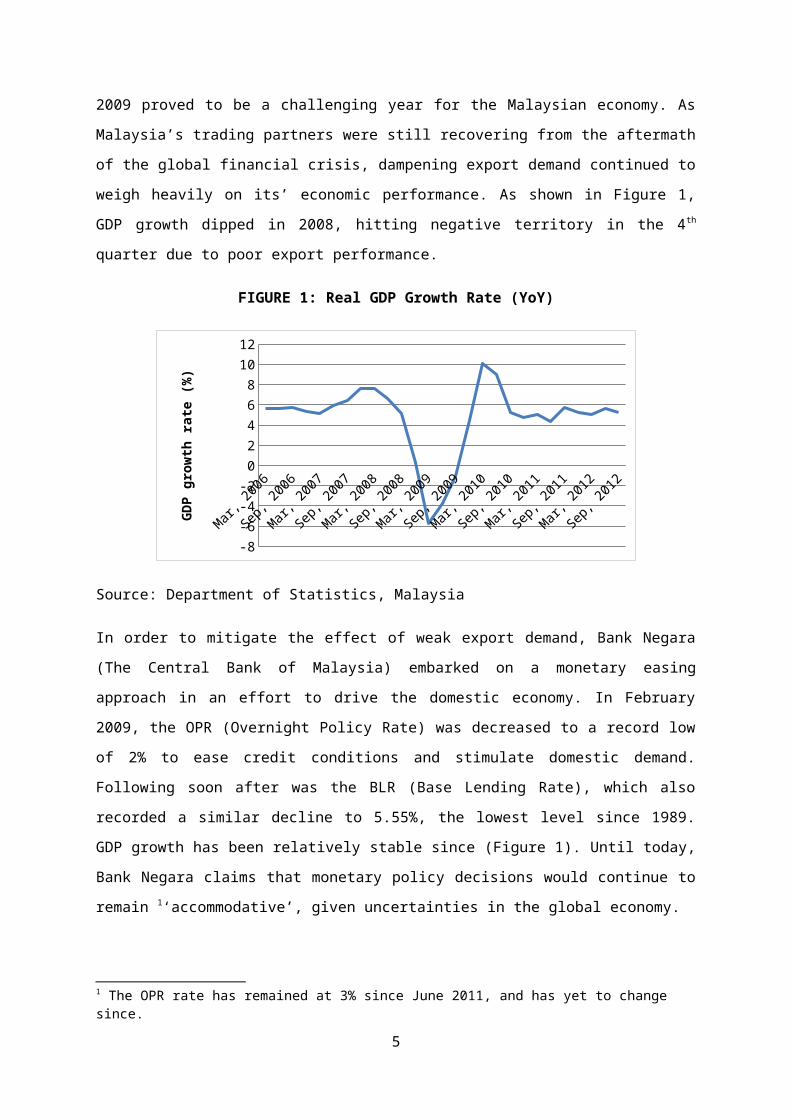
2009 proved to be a challenging year for the Malaysian economy. As

Malaysia’s trading partners were still recovering from the aftermath

of the global financial crisis, dampening export demand continued to

weigh heavily on its’ economic performance. As shown in Figure 1,

GDP growth dipped in 2008, hitting negative territory in the 4th

quarter due to poor export performance.

FIGURE 1: Real GDP Growth Rate (YoY)

Mar, 2006

Sep, 2006

Mar, 2007

Sep, 2007

Mar, 2008

Sep, 2008

Mar, 2009

Sep, 2009

Mar, 2010

Sep, 2010

Mar, 2011

Sep, 2011

Mar, 2012

Sep, 2012

-8-6-4-2024681012

GDP

grow

th r

ate

(%)

Source: Department of Statistics, Malaysia

In order to mitigate the effect of weak export demand, Bank Negara

(The Central Bank of Malaysia) embarked on a monetary easing

approach in an effort to drive the domestic economy. In February

2009, the OPR (Overnight Policy Rate) was decreased to a record low

of 2% to ease credit conditions and stimulate domestic demand.

Following soon after was the BLR (Base Lending Rate), which also

recorded a similar decline to 5.55%, the lowest level since 1989.

GDP growth has been relatively stable since (Figure 1). Until today,

Bank Negara claims that monetary policy decisions would continue to

remain 1‘accommodative’, given uncertainties in the global economy.

1 The OPR rate has remained at 3% since June 2011, and has yet to change since.

5

The reduction of borrowing costs seemed to have a positive impact on

the prices of property, which has continued on an upward trend since

monetary easing measures started in 2009 (Figure 1). As Figure 1

shows, since the OPR rate was lowered in 2009, house prices started

to accelerate at a faster rate compared to periods preceding 2009.

This trend has continued to the 2nd quarter of 2012. The real house

price index saw a slight decline in the 3rd quarter of 2012.

FIGURE 2: Real House Price (House Price Index/Consumer Price Index)

1

1.1

1.2

1.3

1.4

1.5

Real

Hou

se P

rice

Source: CEIC

As house prices continue to increase, housing affordability issues,

especially in the major cities of Kuala Lumpur, Selangor and Penang

started to receive ample attention from policymakers. As a result,

several measures have been taken by Bank Negara to cool the

6

overheating property market, namely the introduction of the Loan-to-

Value (LTV) limits in November 2010 and the Debt-to-Income (DTI)

restrictions, which recently took effect in January 2012. The main

aim of this research is to study the reactions of the Malaysian

property market to the decisions made by the Central Bank.

Section 2 of the paper would fist study the nature of the Malaysian

property market. This section would be discussing if activities in

the Malaysian property market have any impacts on the real economy.

Section 3 would be a literature review, analyzing the impact of

monetary policy and prudential policy measures for countries that

have adopted these measures. Section 4 and 5 would then discuss the

empirical model used to study the case of Malaysia. Section 6 would

mainly discuss the findings from the model. Section 7 will cover the

conclusion.

2) The Nature of the Malaysian Property Market

The Asian Financial Crisis and the Subprime Mortgage Crisis both

have something in common. In both scenarios, property markets in the

US and Asian economies suffered major corrections, leading to severe

economic downturns. These events would, by themselves provide strong

reasons to regulate overheating property markets. However, before

shifting our focus to evaluate the impact of the different

regulatory decisions made, it would only be fair to study if

property market developments can generate positive feedbacks to the

local economy.

Studies done by Ludwig and Slok (2004) and Case et al (2005) show

that increases in property prices in OECD countries do generate

positive feedbacks into domestic consumption. This goes the same for

the economy of Hong Kong, when Ho and Wong (2003) found positive

7

linkages between the prices of housing and domestic demand. However,

it would be too soon to generalise these results and apply it to the

Malaysian setting.

Hui (2009) examined the effects of property market developments on

both domestic consumption and private investment in Malaysia. Using

an Autoregressive Distributed Lag (ARDL) model, he evaluated both

the short and long run impacts of property prices on domestic

demand. Contrary to the results found from the OECD countries, Hui

(2009) found a negative long run relationship between property

prices and private consumption, implying that, in the long run,

Malaysian households are worse off from higher property prices. This

result can be attributed to many factors, the most notable being the

demographic nature of Malaysia. In 2006, 60% of Malaysia’s citizens

are in the working age group of 15-64 (Ng, 2006), and thus, are more

likely first time homebuyers. Thus, housing would be more likely

treated as a consumption good, rather than as an asset by the

Malaysian consumers. The nature of housing as a consumption good

causes the wealth effect on consumers to be negative in the event of

rising house prices, a unique feature of the Malaysian economy. On

the other hand, rising house prices has a positive effect on private

investment, both in the short and long run. This result can be

easily rationalised. If we treat housing as a tradable good in the

market for real estate, firms that sell it (property developers)

will typically increase supply in an event of rising prices.

Nonetheless, the decline in welfare suffered by Malaysian consumers

as a result of rising house prices provides us with a strong reason

to intervene in overheating property markets. The next section would

evaluate the impact of monetary policy decisions on the property

markets in both US and China.

8

3) Literature Review

The Property Market and the Stance of Monetary Policy: Evidence from

Countries

Prior to the subprime mortgage crisis in the US, real estate prices

have been increasing at rapid rates. Many have attributed this

increase to the low interest rate environment set by the Federal

Reserve, lowering borrowing costs and easing credit conditions.

Using a BVAR (Bayesian Vector Autoregression) model, Jarocinski and

Smets (2008) found evidence linking the occurrence of housing booms

in the US to low levels of short and long term interest rates. The

relationship between monetary easing and accelerating house prices

is not unique to the US economy. A research by Ahearne et al (2005)

show that, in periods preceding house price peaks in Japan, Sweden,

Australia and UK, monetary policy was eased. These findings provide

strong arguments that loose monetary policy may be one of the major

culprits for rapid growth in property prices.

Since monetary easing is positively correlated with property prices,

one would expect monetary tightening to have the opposite effect. We

will limit our study to the case of China. Xu and Chen’s (2012)

Pacific-Basin Financial Journal paper studied the impact of key

monetary policy variables on the growth of house prices in China. By

running a time series regression utilising quarterly data from 1998-

2009, they came up with a conclusion that an increase in interest

rates, coupled with slower money supply growth and tightening

mortgage downpayment policies play significant roles in moderating

the growth in house prices. A previous paper by Liang and Cao (2006)

confirmed the negative relationship between interest rates and

property prices, but limited their findings to long term interest

rates. On the contrary, they did not find significant results

9

linking money supply growth and short term interest rates to growth

in property prices. Given also the significance in the BC (bank

credit) variable, they drew a conclusion that tight credit policies

may be more effective in controlling the prices of property compared

to monetary policy tightening.

Although researchers would unanimously agree that monetary easing

usually precedes a housing boom, the effectiveness of monetary

tightening to contain the boom is usually treated with ambiguity.

Crowe et al (2011) labelled monetary policy as a ‘blunt’ instrument,

as an increase in interest rates is likely to adversely affect the

borrowing costs throughout the entire economy, not specific to the

real estate market. If the real estate boom coincided with general

macroeconomic overheating, then, increasing the policy rate would be

justified. However, if real estate booms occurred under 2tranquil

macroeconomic conditions, (Ariccia, 2012) increasing the policy rate

might only invite social and political opposition, making

policymaking decisions only harder for the Central Bank.

The paragraph above may well describe the current situation of the

Malaysian economy. Downside risks from abroad continue to weigh

heavily on its’ economic performance, limiting Bank Negara’s scope

to use the interest rate channel to contain property prices and

household debt. Given the limitations of monetary policy decisions,

we will now look into a more targeted approach to contain housing

booms, namely the LTV and DTI limits.

Effectiveness of LTV and DTI Limits: Evidence from Countries

Arricia et al (2012) indicated that monetary policy measures will be

more effective if complemented with macroprudential regulation. To

contain housing booms, a form of macroprudential regulation that 2 A case when a real estate boom does not coincide with general macroeconomic overheating/high inflation.

10

aims to improve borrowers’ eligibility criteria, namely the LTV and

DTI limits are used. In most economies, LTV and DTI limits are

reported simply as guidelines for mortgage issuance, therefore, it

is difficult to measure its’ effectiveness (Crowe et al, 2011).

Given the lack of data availability, most literature are directed

only to study the impact of LTV and DTI limits on 3 Asian economies

(Hong Kong, South Korea and to a lesser extent, Singapore), where

these measures are mandatory, and not mere guidelines.

Wong et al (2011) measured the impact of LTV regulations on mortgage

delinquency ratios using panel data analysis comprising 13

countries. Their aim was to measure the sensitivity of a change in

housing prices in economies that adopted a LTV regulation, compared

to those that didn’t. The results were obvious. For countries that

adopted the LTV policy, change in mortgage delinquency ratios were

less sensitive to swings in property prices. In addition, the

coefficient measuring the impact was statistically significant,

providing a strong argument that LTV limits do play an important

role in reducing household leverage.

In order to evaluate the impact of relaxing LTV limits on the Hong

Kong economy prior to the Asian Financial Crisis in 1997, Wong et al

(2011) ran a counterfactual simulation. The model found that, if LTV

limits were relaxed from 70% to 90% before 1997, a 40% change in

property prices (Property prices declined by 40% during the crisis)

would have caused an increase in the mortgage delinquency ratio from

0.6% to 1.71%. Thus, at least for Hong Kong, LTV limits do play a

part in mitigating the impacts of a financial crisis through the

household leverage channel.

So far, the study by Wong et al (2011) has only confirmed the impact

of LTV caps on mortgage delinquency ratios. Unfortunately, they did

not find a significant negative relationship between tightening LTV11

caps and property market activities across the 3 Asian countries

studied (Hong Kong, South Korea and Singapore). Only in the case of

Hong Kong, LTV limits had marginal impacts on property prices. Igan

and Kang (2011), however, found a significant negative relationship

for DTI tightening in the case of Korea. When DTI limits were

tightened, property transactions also declined in the metropolitan

states of Korea. Thus, the effect of dampening property prices

seemed to be more significant with tightening LTV caps in Hong Kong,

while property transactions seem to be affected more by a DTI

tightening in the Korean economy. Lower DTI limits also helped curb

speculation in the Korean property markets.

Both Hong Kong and Korea have revised their LTV and DTI regulations

since they were first implemented. In contrast, these measures are

relatively new to Malaysia. A 70% LTV limit on the 3rd house

purchased was first implemented in November 2010 to contain

speculative activities in the real estate market. Not long later,

DTI restrictions were introduced in January 2012 to contain the

alarmingly high household debt, where a borrower’s credit worthiness

would be evaluated based on their 3net income, instead of gross

income. Given the limited timeframe, there is currently no

literature studying the impact of these regulations for the case of

Malaysia.

4) Empirical Models

The models attempt to test the implication of central bank policies

and its’ impact on the market for real estate. This research is

particularly interested in analysing the impact of monetary policy

3 Gross income net of taxes and EPF (Employees Provident Fund) contributions

12

measures and macroprudential regulation on house prices. The 2

impacts are studied separately.

Modelling the Impact of Monetary Policy Measures on House Prices

We use the following model to determine the impact of monetary

policy measures:

HPt = β0 + β1IRt + β2GDPt + ut

Where:

HP = Real house price (House price index/CPI)

IR = Interbank rate (Proxy for monetary policy stance)

GDP = 4Seasonally adjusted real gross domestic product

Theoretically, a higher interbank rate implies higher borrowing

costs and hence, β1 is hypothesised to take a negative value. On the

other hand, higher GDP implies a higher level of economic activity.

Assuming positive spill over effects on the housing market due to

higher economic activity, β2 is hypothesised to take a positive

value.

In order to test for the presence of a cointegrating relationship

between the 3 variables, we first conduct some unit root tests.

Applying the Augmented Dickey-Fuller test, the null hypothesis that

HPt, IRt and GDPt each contain a unit root cannot be rejected at the

10% significance level. This implies the presence of non

stationarity in the model. We thus conclude that all 3 variables are

integrated of order 1(I(1)). The results table are presented below:

4 Since there is no seasonally adjusted real GDP data for Malaysia, we usedthe Eviews X12 function to seasonally adjust the data.

13

TABLE 1: Unit Root Tests

Variables HPt IRt GDPt

ADF Test level t-stat 3.155092 -2.521027 3.258040level p-

values

0.9952 0.1163 0.9996

Since the time series equation contains a unit root, we can proceed

to test for the presence of cointegration. Firstly, a lag length of

ρ=4 is chosen, as the data are recorded on a quarterly basis. We

then run a Vector Error Correction Model (VECM) of the form:

∆Yt = A1Yt-1 + A2∆Yt-2 + A3∆Yt-3 + A4∆Yt-4 + ɛt

Where:

Yt = [log (HPt), IRt, log (GDPt)]

Yt-1 = Error Correction Term (ECT)

In this model, log (HPt) is ordered first, followed by log (GDPt) and

then IRt.

Applying the ‘Intercept and No Trend’ structure, both the Johansen’s

trace and maximum eigenvalue tests reject the null hypothesis of no

cointegration and accepts the hypothesis of one cointegrating

relationship between the variables. This implies the existence of a

long run relationship between the 3 variables of interest.

Modelling the Impact of Macroprudential Regulation on House Prices

We test the impact of both LTV limits and DTI restrictions on house

prices.

Impact of LTV Limits and DTI Restrictions on House Prices

14

The method applied here is an extension of the previous model, the

only difference being the addition of 6 exogenous variables to

indicate the relationship between LTV limits and DTI restrictions on

real house prices:

∆Yt = A1Yt-1 + A2∆Yt-2 + A3∆Yt-3 + A4∆Yt-4 + β1DummyLTV_3months +

β2DummyLTV_6months + β3DummyLTV_3months + β4DummyDTI_3months +

β5DummyDTI_6months + β6DummyDTI_9months + ɛt

Where:

Yt = [log (HPt), IRt, log (GDPt)]

Yt-1 = Error Correction Term (ECT)

HP = Real house price (House price index/CPI)

GDP = 5Seasonally adjusted real gross domestic product

IR = Interbank rate (Proxy for monetary policy stance)

DummyLTV_3months = Dummy that takes the value of 1 in the 3 months

after implementation of the LTV limits

DummyLTV_6months = Dummy that takes the value of 1 in the 6 months

after implementation of the LTV limits

DummyLTV_9months = Dummy that takes the value of 1 in the 9 months

after implementation of the LTV limits

DummyDTI_3months = Dummy that takes the value of 1 in the 3 months

after implementation of the DTI restrictions

DummyDTI_6months = Dummy that takes the value of 1 in the 6 months

after implementation of the DTI restrictions

5 Since there is no seasonally adjusted real GDP data for Malaysia, we usedthe Eviews X12 function to seasonally adjust the data.

15

DummyDTI_9months = Dummy that takes the value of 1 in the 9 months

after implementation of the DTI restrictions

The method of including dummy variables to analyse the impact of LTV

limits and DTI restrictions is influenced by that of Igan and Kang

(2011).

We expect the sign of β1 , β2 and β3 to take on negative values, as

higher LTV limits are hypothesised to slow the growth of house

prices. Similarly, we expect the sign of β4 , β5 and β6 to be

negative, as more stringent rules on the approval of loans is

expected to have a negative impact on the real estate market.

5) Data Sources Data for all variables are taken straight from CEIC. All data are

recorded on a quarterly basis, with the exception of interbank rate,

which is recorded on a monthly basis. Data on interbank rates were

converted to quarterly data by averaging over 3 months. The

definition of the respective data are summarised in Table 2:

TABLE 2: Variables and Definitions

Variables Definition

HP House price index (2000=100)/Consumer Price Index

(2005=100)

GDP Real Gross Domestic Product at constant 2000

prices

IR

16

DummyLTV Dummy variable that takes the value of 1; for

2011Q1, 2011Q2 and 2011Q3 (3months, 6months and

9months after implementation of the LTV

regulations)

DummyDTI Dummy variable that takes the value of 1; for

2012Q1, 2012Q2 and 2012Q3 (3months, 6months and

9months after implementation of the DTI

regulations)

6) Main Findings and Discussions

The findings from the cointegration vector modelling the impact of monetary policy on house prices are first recorded:

Impact of Monetary Policy Measures on House Price

TABLE 3: Long run coefficients and error correction mechanism of the

monetary policy model

Long run CoefficientsVariables Coefficients

GDP 1.2749**

(0.7107)IR -1.4489***

(0.3829)Short-run dynamics (error correction mechanism)

Dependent Variable = ∆

HPt

Dependent Variable

= ∆ IRt

Dependent Variable = ∆

GDPt

6 The interbank rate is used instead of the Overnight Policy Rate (OPR) because OPR data is not available earlier than April 2004

17

Variable

s

Coefficients Variable

s

Coeffici

ents

Variables Coefficien

ts∆ HPt-1 0.17099

(0.1561)

∆ HPt-1 -0.9324

(-

0.6728)

∆ HPt-1 0.2142*

(0.1326)

∆ HPt-2 -0.0472

(0.1561)

∆ HPt-2 -0.8343

(1.3859)

∆ HPt-2 0.1131

(0.1470)∆ HPt-3 -0.1041

(-0.5839)

∆ HPt-3 0.3982

(1.5828)

∆ HPt-3 -0.0887

(0.1515)∆ HPt-4 0.4726

(0.1802)

∆ HPt-4 -1.5884

(1.5997)

∆ HPt-4 -0.0131

(0.1531)∆ GDPt-1 0.3359*

(0.2176)

∆ GDPt-1 7.3444**

*

(1.9318)

∆ GDPt-1 0.6449***

(0.1849)

∆ GDPt-2 0.02099

(0.2429)

∆ GDPt-2 2.6419

(2.1570)

∆ GDPt-2 0.1601

(0.2064)∆ GDPt-3 -0.3491**

(0.1992)

∆ GDPt-3 2.1516

(1.7689)

∆ GDPt-3 0.0305

(0.1693)∆ GDPt-4 0.2876*

(0.1724)

∆ GDPt-4 0.3471

(1.5306)

∆ GDPt-4 -0.0251

(0.1465)∆ IRt-1 -0.0341**

(0.0179)

∆ IRt-1 0.2860**

(0.1591)

∆ IRt-1 -0.0463***

(0.0152)∆ IRt-2 0.0308*

(0.0201)

∆ IRt-2 -0.1018

(0.1785)

∆ IRt-2 0.0154

(0.0171)∆ IRt-3 -0.0024

(0.0188)

∆ IRt-3 0.3563**

(0.1669)

∆ IRt-3 0.0005

(0.0159)∆ IRt-4 -0.0028

(0.0091)

∆ IRt-4 0.0339

(0.0805)

∆ IRt-4 0.0086

(0.0077)ECT -0.0022

(0.00386)

ECT -

0.1337**

*

ECT -0.0002

(0.00328)

18

(0.0343)Adjusted R squared =

0.031

Adjusted R squared

= 0.5373

Adjusted R squared =

0.1423Note: *,** and *** indicate 10%, 5% and 1% level of significance respectively. All

values in (.) are reported standard errors. The variables, GDP and HP are expressed

in logarithms.

Is there a long-run relationship?

The results of the Vector Error Correction Model are summarised in

Table 3. In the baseline model, the magnitude of the coefficient on

IR is negative, indicating that a 1% increase in interest rates

would lead to a 1.45% decrease in house prices in the long run. The

result found is consistent with the hypothesis that an increase in

the cost of borrowing would lead to a decrease in house prices. As

for GDP, the magnitude of the coefficient is positive, indicating

that a 1% increase in GDP would lead to an increase in house prices

by approximately 1.27%. Again, this is consistent with what was

hypothesised earlier. Both coefficients are statistically

significant, with GDP being significant at the 5% level, whereas IR

is significant at the 1% level.

The results obtained confirm the existence of a long run

relationship between monetary policy stance and the prices of

housing for the case of Malaysia. Assuming complete adjustment in

the long run, an increase in the policy rate implies an increase in

borrowing cost, thus, making the purchase of housing more costly. As

consumers hold back purchasing decisions, demand for housing falls.

Property developers would then face a situation of oversupply, and

would have to adjust their prices downward to clear the market.

19

In order to analyse the speed at which the market clears, we turn to

error correction model explaining the short run dynamics.

Short-run dynamics

Adjusted R-squared values

The adjusted R square value is 3.1% (with house prices as the

dependent variable), indicating that the model only explains 3.1% of

the variation in house prices (Reasons for the low R-square value

will be discussed in later sections). The R squared value when real

GDP is the dependent variable is also fairly low, at 14.23%, as only

14.23% of the variation in GDP can be explained by house prices and

policy rates. As real GDP is affected by many other factors other

than house prices and interest rates, this low R-squared value is

justified. On the other hand, when the dependent variable is IR, the

adjusted R square is very much higher, at 53.73%. This implies that

the variation in policy rates can be very much explained by

variations in both GDP growth rates and house prices.

Dependent Variable, ∆ HPt

The magnitude of the error correction term (ECT) is small,

signifying very slow adjustment towards its’ long run equilibrium.

However, the coefficient of the ECT is statistically insignificant,

thus, no conclusion can be drawn regarding the adjustment process of

house prices.

Dependent Variable, ∆ GDPt

Similarly, the magnitude of the ECT is very small and statistically

insignificant. Thus, nothing much can be said regarding the

magnitude of adjustment of GDP.

20

Dependent Variable, ∆ IRt

The ECT on interest rates, however, is very significant. This

indicates that within one period, 13.37% of the ‘error’ or

disequilibrium in interest rates is corrected. However, the sign of

adjustment is the opposite from what is hypothesised. Given that

house prices are increasing, one would expect policy rates to adjust

upward in the long run. However, this was not observed in the

results table, instead, a negative coefficient on the ECT was

obtained. This implies that policy rates decreases in response to

increases in house prices. This result sounds counter intuitive, as

it indicates the Central Bank’s failure to increase policy rates in

response to increasing house prices. However, given the current

economic outlook, this result doesn’t seem too unreasonable. As

discussed in the introduction, ever since the global financial

crisis struck in 2007, Malaysia’s growth has been weighed down by

weak external factors, dampening export demand. In these uncertain

times, it’s almost certain that growth concerns would supersede

other macroeconomic matters, such as rising asset prices. Even in

normal times, monetary policy decisions are usually governed by the7Taylor rule, with other concerns treated as secondary. In addition,

the rapid growth in house prices does not coincide with general

inflationary pressures or macroeconomic overheating, thus,

increasing the policy rate under such conditions can be difficult to

rationalize. As the Central Bank is accountable to both the public

and the federal government, policy decisions must best suit the

needs of the economy. Recently, the federal government has been

embarking on an expansionary fiscal policy program dubbed the

Economic Transformation Program (ETP) to drive the domestic economy

in the face of weak exports. This program involves extensive

7 The Taylor rule governs how nominal interest rates should be changed in response to fluctuations in output and inflation

21

investment in infrastructure, energy and the services industry.

Thus, it is important that borrowing costs are kept at low levels,

to encourage growth in private investment under this program.

However, this does not mean that the Central Bank is totally

oblivious about the growth in house prices. As shown by the impulse

response in Figure 3, it seems like the Central Bank does respond to

increases in house prices, however, only with a lag (Figure 3 in the

3rd row, 3rd column). To be exact, the Central Bank takes

approximately 2-3 quarters to respond to increases in house prices.

The slow response probably led to the stark increase in house prices

lately.

FIGURE 3: Impulse Response (Following Cholesky Ordering: Real GDP,

Interbank Rate, Real House Price)

Discussion

22

Although a long run negative relation can be established between

house prices and policy rates, a short run relationship between the

2 variables cannot be confirmed. In the short run, interest rates

respond to increases in house prices with a lag due to the reasons

discussed in the previous sub-section.

In conclusion, tightening monetary policy only has long run

implications on the Malaysian housing market, due to the above

mentioned reasons. The reluctance of the Central Bank to increase

policy rates in the midst of uncertainty in the global economy

probably caused monetary policy measures to be less effective in

curbing the prices of housing in the short run. The limitations of

monetary policy measures to control the growth of house prices led

the Central Bank to adopt alternative measures to cool the property

market. This led to the adoption of macroprudential measures in

November 2010 and January 2012, targeted especially to contain the

growth of house prices in the Malaysian housing market.

We now turn to analyse the impact of these measures on the Malaysian

property market.

Analysing the Impact of LTV limits and DTI restrictions on house

prices

This section aims to study the recently introduced LTV limits and

DTI restrictions on the prices of housing. For short run dynamics,

we only consider the case where ∆ HPt is the dependent variable, as

we’re only interested to analyse the change in house prices in

response to the introduction of macroprudential measures:

23

TABLE 4: Long run coefficients and error correction mechanism of

macroprudential regulation

Long run coefficientsVariables Coefficients

GDP 0.3905***

(0.0602)IR -0.1508***

(0.0298)Short-run dynamics (error correction mechanism); Dependent Variable

= ∆ HPt

Variables Coefficients∆ HPt-1 0.2095*

(0.1587)∆ HPt-2 -0.0699

(0.1708)∆ HPt-3 -0.1355

(-0.1805)∆ HPt-4 0.3586**

(0.1851)∆ GDPt-1 0.4082**

(0.2100)∆ GDPt-2 -0.1002

(0.2351)∆ GDPt-3 -0.1871

(0.2071)∆ GDPt-4 0.2916**

(0.1461)∆ IRt-1 -0.0346

(0.0166)∆ IRt-2 0.0433**

(0.0209)

24

∆ IRt-3 -0.0129

(0.0198)∆ IRt-4 0.0019

(0.2479)ECT -0.0655

(0.045)Exogenous Variables

DummyLTV_3months 0.0101

(0.0149)DummyLTV_6months -0.0158

(0.0165)DummyLTV_9months 0.0202

(0.0179)DummyDTI_3months 0.0269**

(0.0145)DummyDTI_6months 0.0021*

(0.0151)DummyDTI_9months -0.0209*

(0.0153)Adjusted R-squared = 0.2416Note: *,** and *** indicate 10%, 5% and 1% level of significance respectively. All

values in (.) are reported standard errors. The variables, GDP and HP are expressed

in logarithms. For short run relations, only the case where the dependent variable

is ∆ HPt is considered.

Discussion - Changes from the Previous Model

After the inclusion of the 6 exogenous dummy variables, the long run

coefficient on GDP became significant at the 1% level. The long run

coefficient on IR maintained its’ significance. However, with the

introduction of the 6 dummies, the magnitude of both coefficients

decreased quite significantly. In the long run, a 1% increase in GDP

would only increase house price by 0.39% (compared to 1.27%

25

previously) and a 1% increase in the policy rate would cause house

prices to decrease by only 0.15% (1.45% previously). The

introduction of the 6 dummy variables probably reduced the

explanatory power of both GDP and interest rates.

The adjusted R squared value increased from 3.1% to 24.16% (we are

only considering the case where ∆ HPt is the dependent variable),

implying that 21.06% of variation in house prices can be explained

by the 6 dummy variables introduced.

How effective are LTV Limits?

Surprisingly, the signs of the coefficients DummyLTV_3months and

DummyLTV_9months turn out to be the opposite from what was

hypothesised. Both coefficients turned out to be positive,

indicating that ever since the LTV limits were introduced, house

prices continued to accelerate. Only the coefficient on

DummyLTV_6months recorded a negative value. All 3 variables,

however, are statistically insignificant.

One argument to justify the insignificance of the 70% LTV limit

would be that the ruling is only enforced from the 3rd property

purchased onwards. Compared to Hong Kong and Korea where the ruling

was enforced from the 1st property purchased (Wong et al, 2011), one

can argue that Bank Negara’s measures may not be strict enough to

curb the growth in property prices.

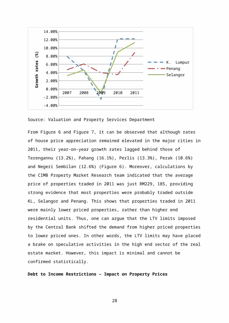
However, there is an interesting observation in the property markets

in 2011 (When the LTV ruling was implemented). If we shift our focus

to a breakdown by states, it seems that Terengganu, Pahang, Perlis,

Perak and Negeri Sembilan (NS) have been contributing to much of the

price increase in 2011, rather than the metropolitan states of KL,

26

Penang and Selangor. This can be illustrated from the diagrams

below:

FIGURE 4: Growth in House Prices (Terengannu, Pahang, Perlis, Perakand NS)

Source: Valuation and Property Services Department

FIGURE 5: Growth in House Prices (KL, Penang and Selangor)

27

2007 2008 2009 2010 2011

-5.00%

0.00%

5.00%

10.00%

15.00%

20.00%

TerengganuPerlisPahangPerakN. Sembilan

Grow

th rat

es (

%)

2007 2008 2009 2010 2011

-4.00%

-2.00%

0.00%

2.00%

4.00%

6.00%

8.00%

10.00%

12.00%

14.00%

K. LumpurPenangSelangor

Grow

th rat

es (

%)

Source: Valuation and Property Services Department

From Figure 6 and Figure 7, it can be observed that although rates

of house price appreciation remained elevated in the major cities in

2011, their year-on-year growth rates lagged behind those of

Terengannu (13.2%), Pahang (16.1%), Perlis (13.3%), Perak (10.6%)

and Negeri Sembilan (12.6%) (Figure 6). Moreover, calculations by

the CIMB Property Market Research team indicated that the average

price of properties traded in 2011 was just RM229, 185, providing

strong evidence that most properties were probably traded outside

KL, Selangor and Penang. This shows that properties traded in 2011

were mainly lower priced properties, rather than higher end

residential units. Thus, one can argue that the LTV limits imposed

by the Central Bank shifted the demand from higher priced properties

to lower priced ones. In other words, the LTV limits may have placed

a brake on speculative activities in the high end sector of the real

estate market. However, this impact is minimal and cannot be

confirmed statistically.

Debt to Income Restrictions – Impact on Property Prices

28

In contrast to LTV limits, the coefficients on DummyDTI_3months,

DummyDTI_6months and DummyDTI_9months show marginal significance,

with DummyDTI_3months being significant at the 5% level, whereas

DummyDTI_6months and DummyDTI_9months show significance at the 10%

level. However, the coefficients of DummyDTI_3months and

DummyDTI_6months still turn out to be positive, which is the

opposite from what was hypothesised. Only the magnitude of the

coefficient on DummyDTI_9months reports a negative value. The

coefficients are interpreted as follows:

3 months after implementation of the DTI ruling, house prices

were approximately 2.7% higher than the benchmark price level

in June 2000 (DummyDTI_3months = 0.027)

6 months after implementation of the DTI ruling, house prices

were approximately 0.2% higher than the benchmark price level

in June 2000 (DummyDTI_6months = 0.0021)

9 months after implementation of the DTI ruling, house prices

were approximately 2.1% lower than the benchmark price level

in June 2000 (DummyDTI_9months = -0.021)

While the LTV limits ruling was specifically directed at reducing

speculative activities in the property market, the DTI restrictions,

however, was implemented with the intention to reduce household

leverage. Over the years, the household debt-to-GDP ratio has been

steadily increasing, soaring to alarming levels in 2011 and 2012

(Figure 8). 8A large portion of household debt was directed towards

the purchase of residential properties (46.8% of total debt).

FIGURE 6: Household Debt to GDP Ratio (Annual)

8 Bank Negara Annual Report, 2012

29

2008 2009 2010 2011 20120.00%10.00%20.00%30.00%40.00%50.00%60.00%70.00%80.00%90.00%

60.40%71.70% 74.00% 75.80% 80.50%

Source: BNM Financial Stability and Payments System Report 2012

These measures, however, turned out to have indirect effects on the

market for real estate. As the Central Bank tightened borrowing

measures, the ease of obtaining loans for the purchase of real

estate also declines, leading to a slowdown in the real estate

market. This slowdown took effect in the 3rd quarter of 2012 where

loans approved saw a steady decline from the 2nd quarter to the 3rd

quarter of 2012 (Figure 9). At the same time, property prices also

fell, indicating that there is a negative spillover effect from

loans approved to property prices. Thus, we can safely claim that

probably, DTI restrictions impacted property prices through the loan

approved channel. However, since this measure was only implemented

very recently, it can be very difficult to gauge its’ full impact.

FIGURE 7: Loans Approved for Real Estate (MYR mn)

30

0500

10001500200025003000350040004500

MYR

mn

Source: CEIC

FIGURE 8: House Price Index (1Q11-3Q12)

135

145

155

165

175

Source: CEIC

Although house prices still recorded positive growth in the 1st

quarter and 2nd quarter of 2012 following the DTI ruling, the rate of

appreciation has been decreasing, with house prices being 2.7%

higher than the benchmark level in the 1st quarter and only 0.2%

higher in the 2nd quarter. Towards the 3rd quarter of 2012, house

31

prices started to decline, being 2.1% lower than the benchmark

level.

For the case of Malaysia, DTI tightening seems to be a better pre-

emptive tool to control the growth in house prices. This finding

contrasts with the results found in the Korean and Hong Kong

property market, where LTV limits were more effective in curbing the

growth in property prices, compared to DTI tightening (Igan and

Kang, 2011). DTI tightening was found to be more effective in

lowering property transactions in the Korean market. However, since

the way LTV limits and DTI tightening is implemented in Malaysia is

quite different from that in Hong Kong and Korea, it may not be fair

to do a direct comparison.

Surprisingly, both models have very low R-square values, indicating

that the independent variables explain very little of the variation

in house price. An important missing component might be the role of

expectations. As the real estate market is usually driven by

speculative activities, omitting expectations may create the problem

of endogeneity in the model. Because of the issue of data

availability, the expectations variable was left out. The next sub-

section will briefly explain the importance of expectations in the

housing market.

The Role of Expectations – The Missing Factor

The expectations of economic agents are usually important to explain

most of the variation in asset prices, particularly the stock market

and the housing market. For the US housing market, Case and Shiller

(2003) found that current house price appreciations can be explained

by past periods expectations of economic agents. Typically, if

households are optimistic about future house prices, their

expectations would be translated into purchasing decisions, leading

32

to higher prices in the future. In other words, expectations in the

real estate market can be self-fulfilling. Piazzesi and Schneider

(2009) confirmed the findings in their paper when they studied the

US housing market before the Subprime Crisis. Prior to the crisis,

economic agents’ beliefs of future house price increases caused a

housing bubble that eventually burst during the crisis.

A more recent paper studying the importance of expectations on

housing market dynamics would be that of Lambertini et al (2012).

Using data from the Michigan Survey of Consumers, they analysed the

importance of news and consumers’ beliefs on the prices of houses in

the US housing market and other macroeconomic fluctuations. Two of

the survey variables are employed, namely, ‘News on Business

Conditions’ is used as a proxy for news, while ‘Changes in

Expectations of Rising House Prices’ is used as a proxy for

consumers’ expectations of future house prices. A VAR model is then

applied to estimate the effect of news and expectations on the

changes in macroeconomic variables. The VAR analysis shows that a

positive innovation in the news variable leads to increases in house

prices, mortgage credit and residential investment. Similarly, a

positive innovation in the expectations variable leads to an

increase in house prices. During periods of housing booms, the role

of expectations is especially important to explain the variation in

house prices. In periods preceding the Subprime Crisis, expectations

account for over 40 to 50 percent of the forecast error variance of

housing market variables.

Given the importance of expectations to study housing market

dynamics, we have to distinguish whether the expectations formed by

economic agents are rational to begin with. Granziera and Kozicki

(2012) explain how housing bubbles are formed through expectations

that are not completely rational. Once they relaxed the assumption

33

of perfect rationality, their model became a good indicator to

explain the sharp appreciations in house prices during the US

housing boom and also, the major price correction that followed in

2007. Thus, this provides strong evidence that housing market

variables are driven mainly by irrational exuberance (irrational

behaviour), rather than by expectations that are perfectly rational.

Since property prices are usually driven by irrational exuberance

rather than perfectly rational assumptions, another question of

interest would be how much economic fundamentals explain the

variation in property prices. Quigley (1999) studied the case of the

US housing market from the period from 1986-1994. Although they

found that house prices in US do track fundamentals, regressing

house price variables on fundamentals alone leave a lot unexplained.

Such as, models including only economic fundamentals as their

benchmark variables can only explain between 10 to 40 percent of

variation in house prices (This is consistent with the adjusted R

squared results we found). This only goes to show that models

attempting to explain variation in house prices without including

expectations are likely to suffer from endogeneity issues.

This result does not apply specifically to the US housing market. In

the years preceding the Asian Financial Crisis, the supply of office

buildings were at all-time highs in the Klang Valley region, but

vacancy rates were also astonishingly high (Quigley, 1999),

indicating elements of speculative activity in the non-residential

sector in Malaysia. The same result was found in the Malaysian

condominium market. In mid-1990s, vacancy rates were already at

historical highs, yet, this number was expected to quadruple by

1997. This is a clear indication of speculative activities in the

high rise residential market prior to the Asian Financial Crisis.

34

As house prices continue on its’ upward trend in Malaysia, it is

everyone’s belief that speculative activities are quite prominent in

the housing market. As argued by existing literature, expectations

play a major role in explaining variation in housing market

variables. Thus, future pre-emptive measures implemented should also

be directed at curbing the expectations of economic agents regarding

future trends in property prices.

7) Concluding Remarks This paper examined the impact of monetary policy and

macroprudential regulation on house prices in Malaysia. While an

increase in the policy rate is found to negatively impact house

prices in the long run, the same argument cannot be applied to

discuss short run impacts, as empirical results cannot confirm the

existence of a short run relationship between interest rates and

changes in house prices. As for prudential policy measures, the

impact of tightening LTV limits on house prices cannot be

statistically confirmed, although state data shows a shift in demand

to lower price properties following the introduction of the ruling.

On the other hand, DTI restrictions seem to marginally impact house

prices. When DTI restrictions were introduced, house prices grew at

a slower rate in the 1st and 2nd quarters of 2012, before finally

turning negative in the 3rd quarter. However, the fact that dummy

variables are used to gauge the impact of these pre-emptive measures

means we cannot deny that the dummies may also capture other

impacts.

The LTV limit and DTI restrictions were implemented alongside 2

other fiscal measures announced in the Federal Budget plans, namely

the introduction of ‘My First Home Scheme’ program (Part of the 2011

Budget Plans) and an increase in the real property gains tax (RPGT).

35

While the 1st measure was implemented to ensure that first time

homebuyers can gain easy access to financing to purchase a

residential unit, the 2nd measure was aimed to decrease speculative

activities in the housing market. The 1st measure attempted to

address housing affordability issues by providing up to 100%

financing for the purchase of residential property to first time

homebuyers below the age of 35. This incentive only applies for

residential units not exceeding RM220,000 in value. The launch of

this project may have partially explained the spike in demand for

lower priced properties in 2011. On the other hand, the increase in

the RPGT from 5% to 10% (Part of the 2012 federal government’s

budget plans) may have also partially explained the slowdown in the

real estate sector in the 3rd quarter of 2012. Thus, given that

fiscal measures were implemented alongside prudential policy

measures, it can be quite difficult for us to gauge the ceteris

paribus impacts of both the LTV limits and DTI restrictions on the

property market. Possibly, the most we can do is to say both the

prudent lending guidelines and fiscal measures implemented jointly

impacted the market for real estate in 2011 and 2012.

Gopinath (2011) argued that neither macroprudential tools nor

monetary policy can work as stand-alone measures. Given their

limitations, they must be implemented in tandem to be effective.

While monetary policy measures have been said to be effective in

curtailing overheating markets, the risk of slowing down other

sectors through the increase in policy rate cannot be ignored.

Macroprudential tools, on the contrary, do not suffer from such

limitations. However, one cannot deny that rules-based approaches

are prone to circumvention. This fact is not meant to render

monetary policy nor macroprudential tools obsolete. Rather, it is

just a friendly reminder that as the financial sector develops,

36

financial innovation is unavoidable. Given this fact,

macroprudential and monetary policy tools should also be able to

catch up with the pace of innovation. This will be important to

ensure the resilience and soundness of the financial sector. As of

late, house prices have started to creep up again. It might be a

signal to revise our LTV limits and DTI restrictions, or even, to

start tightening monetary policy to tame the booming real estate

sector. (7,448 words)

References

1) Ahearne, A., Ammer, J., Doyle, B.M., Kole, L.S., and Martin, R.F., (2005) “House Prices and Monetary Policy: A Cross-Country Study”, International Finance Discussion Papers, Board of Governors of the Federal Reserve System. September 2005 (841)

2) Arricia, G.D., Igan, D., Laeven, L., Tong, H., Bakker, B., and Vandenbussche, J., (2012), “Policies for Macrofinancial Stability: How to deal with Credit Booms”, IMF Staff Discussion Note, No. 12/06

3) Bernanke, B. S., (2002) “Asset Price Bubbles and Monetary Policy,” Remarks before the New York Chapter of the National Association for Business Economics, New York, NY, Oct. 15 (Available at http://www.federalreserve.gov/boarddocs/speeches/2002/20021015/)

4) BNM (Bank Negara Malaysia) (2012), Annual Report 2012 (Malaysia: Kuala Lumpur)

5) BNM (Bank Negara Malaysia) (2012), Financial Stability and Payment Systems Report 2012 (Malaysia: Kuala Lumpur)

6) CIMB PMR (Property Market Research), “Hot Property”, Terrence Wong (CFA), 17 April 2012

7) Case, K.E and Shiller, R. (2003), “Is there a Bubble in the Housing Market?”, Cowles Foundation Paper (1089)

8) Case, K.E., Quigley, J.M and Shiller, R. (2005), “Comparing wealth effects: The Stock Market versus the Housing Market,” Advances in Macroeconomics, 5(1), pp.1-32

37

9) Crowe, C.W., Igan,D., Ariccia, G.D and Rabanal,P. (2011), “How toDeal with Real Estate Booms: Lessons from Country Experiences,” IMF Working Paper No. 11/91

10) Eickmeier, S and Hofmann, B (2010), “Monetary Policy, Housing Booms and Financial (Im)balances”, European Central Bank (ECB) Working Paper Series (1178)

11) Engle R.F. and Granger, C.W.J. (1987), “Cointegration and Error Correction Representation: Estimation and Testing”, Econometrica, 55(2), pp. 251-276

12) Lambertini, L., Mendicino, C and Punzi, M.T, (2012) “Expectations-Driven Cycles in the Housing Market: Evidence from Survey Data”, Premilinary draft, 23 September 2012

13) Gopinath, S. (2011), “Macroprudential Approach to Regulation—Scope and Issues”, ADBI Working Paper 286. Tokyo: Asian Development Bank Institute.(Available:http://www.adbi.org/workingpaper/2011/06/02/4558.macroprudential.regulation.scope.issues/)

14) Granziera, E and Kozicki, S (2012), “House Price Dynamics: Fundamentals and Expectations”, Bank of Canada Working Paper (April 2012)

15) Ho, L. and Wong, G. (2003), “The nexus between housing and the macroeconomy: Hong Kong as a case study”, paper presented at the Housing-Macroeconomy workshop at Chinese University of Hong Kong, August 24-25, Hong Kong

16) Hui, H.C., (2008) “Housing Price Misalignments from Fundamentalsbefore the 1997-1998 Financial Crisis: Evidence from Malaysia” Malaysia Pacific Rim Property Research Journal (Australian Business Dean’s Council Tier C). 14(2), 161-176

17) Hui, H.C. (2009) “The Impact of Property Market Developments on the Real Economy of Malaysia” International Research Journal of Finance and Economics (Australian Business Dean’s Council Tier C, SCOPUS cited). 30, 66-86

18) Igan, D., A. N. Kabundi, F. Nadal-De Simone, M. Pinheiro, and N.T. Tamirisa, (2009), “Three Cycles: Housing, Credit, and Real Activity”, IMF Working Paper No. 09/231

19) Igan, Deniz and Kang, Heedon (2011) “Do Loan-to-Value and Debt-to-Income Limits Work? Evidence from Korea” IMF Working Paper No. 11/297

38

20) Jarocinski, M. and Smets, F. (2008) “House Prices and the Stanceof Monetary Policy” Federal Reserve Bank of St. Louis Review. July/August 2008 (90(4)), pp 339-36

21) Liang.Q and Cao.H., (2006), “The impact of monetary policy on property prices: Evidence from China”, paper presented at the Nomura JAE Conference at Hitotsubashi University, September 15-16, Tokyo, Japan.

22) Ludwig A. and Slok T. (2004), “The relationship between stock prices, house prices and consumption in OECD countries”, Topics in Macroeconomics, 4(1), pp.1-26

23) Muelbauer, J and Murphy, A (1997), “Booms and busts in the UK Housing Market”, The Economic Journal (107), pp. 1701-1727

24) Ng, A. (2006), “Housing and Mortgage Markets in Malaysia”, in Kusamiarso B(Ed), Housing and the Mortgage Markets in SEACEN countries, SEACEN Publication, pp.123-188

25) Piazzesi, M., Schneider, M., (2009), “Momentum traders in the housing market: survey evidence and a search model”, American Economic Review (99), pp.406-411

26) Quigley, J.M (1999), “Real Estate Prices and Economic Cycles”, International Real Estate Review 2(1), pp.1-20

27) Toh, G.H and Endut, N (2008), “Household Debt in Malaysia”, Bank for International Settlements (BIS) Papers (46)

28) Wong, E.,T. Fong, K. Li and H.Choi (2011) “Loan-to-Value Ratio as a Macroprudential Tool: Hong Kong’s Experience and Cross-Country Evidence,” Hong Kong Monetary Authority Working Paper No. 01/2011

29) Xu, X.S., and Chen, T., (2012) “The effect of monetary policy onreal estate price growth in China”, Pacific Basin Finance Journal. (20) pp. 62-77

39