Allan G, Hanley N, McGregor PG, Swales JK & Turner K (2007)

The impact of increased efficiency in the industrial use of energy: A computable general equilibrium analysis for the United Kingdom, Energy Economics, 29 (4), pp. 779-798. This is the peer reviewed version of this article

NOTICE: this is the author’s version of a work that was accepted for publication in Energy Economics. Changes

resulting from the publishing process, such as peer review, editing, corrections, structural formatting, and

other quality control mechanisms may not be reflected in this document. Changes may have been made to this

work since it was submitted for publication. A definitive version was subsequently published in Energy

Economics, [VOL 29, ISSUE 4,(2007)] DOI: http://dx.doi.org/10.1016/j.eneco.2006.12.006

1

The Impact of Increased Efficiency in the Industrial

Use of Energy: A Computable General Equilibrium

Analysis for the United Kingdom

by

Grant Allana*, Nick Hanleyb, Peter McGregorac, Kim Swalesac and Karen Turnera

a Fraser of Allander Institute, Department of Economics, University of Strathclyde, Sir William Duncan

Building, 130 Rottenrow, Glasgow, Scotland, G4 0GE b Department of Economics, University of Stirling, Stirling, Scotland, FK9 4LA

c Centre for Public Policy for the Regions, Universities of Glasgow and Strathclyde

* Corresponding author: Tel: 00 44 141 548 3838, Fax: 00 44 141 548 5776

E-mail: grant.j.allan@strath.ac.uk

Postal address:

Fraser of Allander Institute,

Department of Economics,

University of Strathclyde,

Sir William Duncan Building,

130 Rottenrow,

Glasgow,

Scotland,

G4 0GE

The research reported here was funded by the UK Department for Environment Food

and Rural Affairs (DEFRA), though the paper also draws liberally on related research

which was funded by the EPSRC through the SuperGen Marine Energy Research

Consortium (Grant reference: GR/S26958/01). The authors are grateful to Tina

Dallman (DEFRA), Allistair Rennie (DEFRA) and Ewa Kmietowicz (DTI) for

discussion and comments.

2

Abstract

The conventional wisdom is that improving energy efficiency will lower

energy use. However, there is an extensive debate in the energy economics/policy

literature concerning “rebound” effects. These occur because an improvement in

energy efficiency produces a fall in the effective price of energy services. The

response of the economic system to this price fall at least partially offsets the expected

beneficial impact of the energy efficiency gain. In this paper we use of an economy-

energy-environment Computable General Equilibrium (CGE) model for the UK to

measure the impact of a 5% across the board improvement in the efficiency of energy

use in all production sectors. We identify rebound effects of the order of 30% - 50%,

but no backfire (no increase in energy use). However, these results are sensitive to the

assumed structure of the labour market, key production elasticities, the time-period

under consideration and the mechanism through which increased government

revenues are recycled back to the economy.

3

Section 1: Introduction

Governments and environmental pressure groups across the world are

advocating energy efficiency programs for either energy security or environmental

reasons (Cabinet Office, 2001; Carbon Trust, 2003; DEFRA, 2005; EEA, 1999;

Nordic Council of Ministers, 1999: Schutz and Welfens, 2000). Whilst the

conventional wisdom is that improving energy efficiency will lower energy use, there

is an extensive debate in the energy economics/policy literature on the actual impact

of such improvements. This debate focuses on the notion of “rebound” effects,

according to which the expected beneficial impacts on energy intensities are partially

offset as a consequence of the economic system’s responses to the fall in the effective

price of energy services that accompany the improvement in energy efficiency. The

“Khazoom-Brookes postulate” (Saunders, 1992) asserts an extreme form of this: that

improvements in energy efficiency can actually increase the demand for energy, a

phenomenon initially identified by Jevons (1865) and now known as “backfire”.

There is general agreement that some degree of rebound is to be expected, so

that if, for example, a 5% improvement in energy efficiency in a particular use will

generate energy savings of 3%, rebound would be 40%.1 Of course, the key question

is the pragmatic one: how big is this rebound effect likely to be? Empirical work has

concentrated on measuring rebound effects in consumer services (Dufournaud et al.,

1994; Greening et al, 2000; Small and Van Dender, 2005; Zein-Elabdin, 1997).

Moreover, existing studies generally focus on the “direct” rebound effects. This

restricts the analysis solely to the energy requirements to provide the consumer

services to which the efficiency improvement directly applies. Less frequently studied

are the “indirect” and “economy-wide” effects that are associated with the relative

price, output and income effects that will affect the consumption and production in

other energy using industries. This decomposition of rebound into direct, indirect and

economy-wide effects is first made by Greening et al (2000), who also point to a

shortage of empirical studies on the “non-direct” rebound effects.

1 We express rebound as a percentage, calculated as: (1 – (the actual percentage reduction in energy

use) / (the imposed percentage change in energy efficiency))x100. Therefore if, for example, there is no

change in energy use following an improvement in energy efficiency, so that the actual percentage

reduction in energy use is zero, rebound would be 100%. If energy use actually increases after the

improvement in efficiency, the reduction in energy use would be assigned a negative value and rebound

would be greater than 100%. Such a value indicates backfire.

4

A recent UK House of Lords (2005, p. 29) report sums up the present position

as follows:

Absolute reductions in energy consumption are thus possible at the

microeconomic level. However, this does not mean than an analogy can be made with macroeconomic effects. Apart from

anything else, the substitution effects observable at the macroeconomic level cannot be replicated by households, where demand for a range of goods is relatively inelastic… a business on

the other hand, could respond to cheaper energy by deliberately increasing consumption – using a more energy intensive process,

which would allow savings to be made elsewhere, for instance in manpower.

The House of Lords report seems to be making two points here. First, that energy

savings in production sectors are likely to have stronger indirect and economy-wide

impacts than energy saving in consumption activities. Second, that energy substitution

possibilities might be substantially greater in production than consumption.

In this paper we wish to tackle the question: how large are the rebound effects

likely to be for general improvements in energy efficiency in production activities in a

developed economy? Specifically, does an increase in the efficiency by which energy

is used in industrial production processes raise or lower the consumption of energy by

industry? Further, to what extent does this response differ across industries? The

method that we adopt is to undertake simulations with an economy-energy-

environment Computable General Equilibrium (CGE) model for the UK.

Using CGE modeling to analyse this problem has both strengths and

weaknesses. A key strength is that CGE models have a strong grounding in

conventional economic theory. They give an appropriate treatment of the supply side

changes resulting from supply side policies and allow the net impacts of energy policy

to be considered against a clear “counter-factual”. CGE models are also able to deal

numerically with the simultaneity prevalent where major economic changes occur and

to identify the orders of magnitude, not only the direction, of the resulting economic

effects. However, the approach does also have weaknesses. One is the data required to

operationalise the model: a set of multi-sectoral accounts is needed, together with a

5

large number of behavioural and technical parameters. Further, Sorrell et al, (2004)

argue that for the specific case of energy efficiency, the conventional neoclassical

relationships which CGE models typically use might fail to capture some of the

significant barriers to the penetration of new technologies. Finally, the particular

assumptions made about the CGE model closure make comparisons across models

difficult. For example, changing the assumption about the operation of the labour

market can generate significant variation in the energy use results.

Our key conclusion is that for our central case simulation, a general, across the

board, improvement in efficiency in energy use in UK production sectors has rebound

effect of the order of 55% in the short run and 30% in the long run, but no backfire

(no increase in energy use). Sensitivity analysis suggests that this central case result is

particularly sensitive to the imposed elasticities of substitution in the production

hierarchy. However, the results also vary significantly with the nature of the

assumptions made concerning the labour market, the way in which increased

government revenues are recycled back into the economy and the time period under

consideration.

In Section 2 we briefly summarise previous theoretical discussions and sketch

our own analysis of the likely system-wide ramifications of a stimulus to industrial

energy efficiency. We conclude, as have many others (e.g. Saunders, 2000b), that the

extent of rebound and backfire is an empirical issue. In Section 3 we describe our

energy-economy-environment computable general equilibrium (CGE) model of the

UK, UKENVI. In Section 4 we present the results of simulating an across the board

stimulus to energy efficiency in production sectors and in Section 5 we discuss the

results of our sensitivity analysis. Section 6 outlines the strengths and weaknesses of

this CGE modeling approach. Section 7 concludes and offers some recommendations

for future research.

6

Section 2: Analytical Background

It is instructive to provide a brief account of the literature on what has come to

be known as the macroeconomic rebound effect. This focuses on the Khazoom-

Brookes postulate, though both Khazoom (1980) and Brookes (1990) acknowledge

Jevons (1865) as being the originator of the basic idea that energy efficiency

improvement could lead to an increase in energy demand.

Jevons (1865) is concerned with the possible exhaustion of a finite natural

resource, namely coal. While largely an empirical study, a key passage examines the

argument that a more efficient use of coal would prolong its life. Jevons (1865, p.140)

argues, “it is wholly a confusion of ideas to suppose that the economical use of fuel is

equivalent to a diminished consumption.” Further, Jevons (1865, p.141-142) is clear

on the causes of this counter-intuitive result:

The number of tons used in any branch of industry is the product of the number of separate works, and the average number of tons

consumed in each. Now, if the quantity of coal used in a blast-furnace, for instance, be diminished in comparison with the yield,

the profits of the trade will increase, new capital will be attracted, the price of pig-iron will fall, but the demand for it increase; and eventually the greater number of furnaces will more than make up

for the diminished consumption of each.

While Jevons (1865) essentially argues for backfire, this is not the inevitable

outcome. However, modern theory has helped to identify the conditions that are likely

to generate significant rebound and even backfire effects. Khazzoom’s (1980) work is

partial equilibrium in nature, taking aggregate income and output as given. Brookes

(1990) began the development of the argument in a macroeconomic context, and

Saunders’ (1992, 2000a, 2000b) analyses extend this using a neoclassical growth

approach.

We examine the system-wide impact of improved resource productivity within

a general equilibrium framework. For simplicity, let us consider an “energy

augmenting” technical change that applies to all uses of energy. This means that if we

identify energy in natural units (this could be any physical measure of energy, e.g.

7

kWh, BTU or PJ) as E, energy in efficiency units as ε, and the rate of energy

augmenting technical progress as ρ, then:

(1) ε = 1+ Eρ

The subsequent price of energy, measured in efficiency units, pε, is given by:

(2) Eε E

pp = p

1 + ρ

where pE is the price of energy in natural units.

With constant energy prices in natural units, an improvement in energy

efficiency reduces the price of energy in efficiency units. Measured in natural units,

with energy prices constant, whether an improvement in energy efficiency reduces

energy use depends solely on the general equilibrium own-price elasticity of demand

for energy.2 Where this is greater than unity, the fall in the implicit price of energy

will generate an increase in expenditure on energy so that overall energy use would

rise: substitution, income and output effects would dominate efficiency effects. This

conceptual approach is ideal for a fuel that is imported, where the natural price is

exogenous, or only changes in line with the demand measured in natural units.

However, there are two problems presented by this procedure. The first is it is

difficult to identify the general equilibrium energy demand elasticity. A fall in energy

prices causes firms to adopt more energy intensive techniques. This is the substitution

effect. But a reduction in energy prices also increases output by reducing costs and

stimulating competitiveness, thereby stimulating energy use. This is the output effect.

This effect is likely to be especially important in very open economies that export

energy intensive goods, since international competitiveness improves. Additionally, in

a multi-sectoral world, a composition effect occurs whereby products which are

relatively energy-intensive in production fall in cost relative to those which are less-

2 By the general equilibrium demand curve for energy we mean the relationship between the price of

energy and the quantity demanded, allowing incomes, and the prices and outputs of all other goods to

8

energy intensive. This further stimulates energy demand. Finally a fall in energy

prices increases real incomes, the real wage and labour supply, generating an extra

impetus to aggregate output and energy use.

A second problem is that energy is typically a domestically produced product

which uses energy as one of its inputs. This means that the price of energy measured

in natural units will be endogenous in a general equilibrium system. In so far as an

across the board improvement in energy efficiency leads to a fall in the price of

energy measured in natural units, this will further encourage rebound effects.

We develop these arguments at greater length in Hanley et al, (2006) and

Allan et al, (2006). In this paper we simply point out that a large number of

parameters are potentially important for influencing the general equilibrium impact of

improvements in energy efficiency. Howarth (1997) and Saunders (1992, 2000a,

2000b) rightly stress the importance of the elasticity of substitution of energy (or

energy services) for other inputs in determining the size of rebound effects. However,

within a general equilibrium context, characteristics such as the openness of the

economy, the elasticity of supply of other inputs (capital and labour), the energy

intensity of individual production sectors and final demands, the elasticity of

substitution between commodities in consumption and the income elasticity of

demand for commodities are potentially important.

Undoubtedly the single most important conclusion of our analysis so far is that

the extent of rebound and backfire effects is always and everywhere an empirical

issue. It is simply not possible to determine the degree of rebound and backfire from

theoretical considerations alone, notwithstanding the claims of some contributors to

the debate. In particular, theoretical analysis cannot rule out backfire. Nor, strictly,

can theoretical considerations alone rule out the other limiting case, of zero rebound,

that a narrow engineering approach would imply. However, in an open economy such

as the UK it is virtually inconceivable that there would be no rebound effect

associated with energy efficiency improvements, since this would require zero

sensitivity to relative price changes throughout the entire system (not just Leontief

adjust. That is to say, if the price of energy could be fixed exogenously, this would be the

9

production technology). Even if it is conceded that neoclassical economic theory

tends to exaggerate the flexibility of the economic system by abstracting from some

real-world frictions, the zero rebound case seems extremely unlikely.

Section 3: The UKENVI model

CGE models are now extensively used in studies of the energy-economy-

environment nexus at the national (Beauséjour et al, 1995; Bergman, 1990; Conrad,

1999; Conrad and Schroder, 1993; Goulder, 1998; Lee and Roland-Holst, 1997) and

regional levels (Despotakis and Fisher, 1988; Li and Rose, 1995). The popularity of

CGEs in this context reflects their multi-sectoral nature combined with their fully

specified supply-side, facilitating the analysis of economic, energy and environmental

policies. Here we employ UKENVI, a CGE modelling framework parameterised on

UK data.

3.1 Structure

UKENVI has three transactor groups, namely households, corporations and

government; 25 commodities and activities, 5 of which are energy

commodities/supply and one exogenous external transactor (ROW).3 Throughout this

paper commodity markets are taken to be competitive. We do not explicitly model

financial flows.

The UKENVI framework allows a high degree of flexibility in the choice of

key parameter values and model closures. However, a crucial characteristic of the

model is that, no matter how it is configured, we impose cost minimisation in

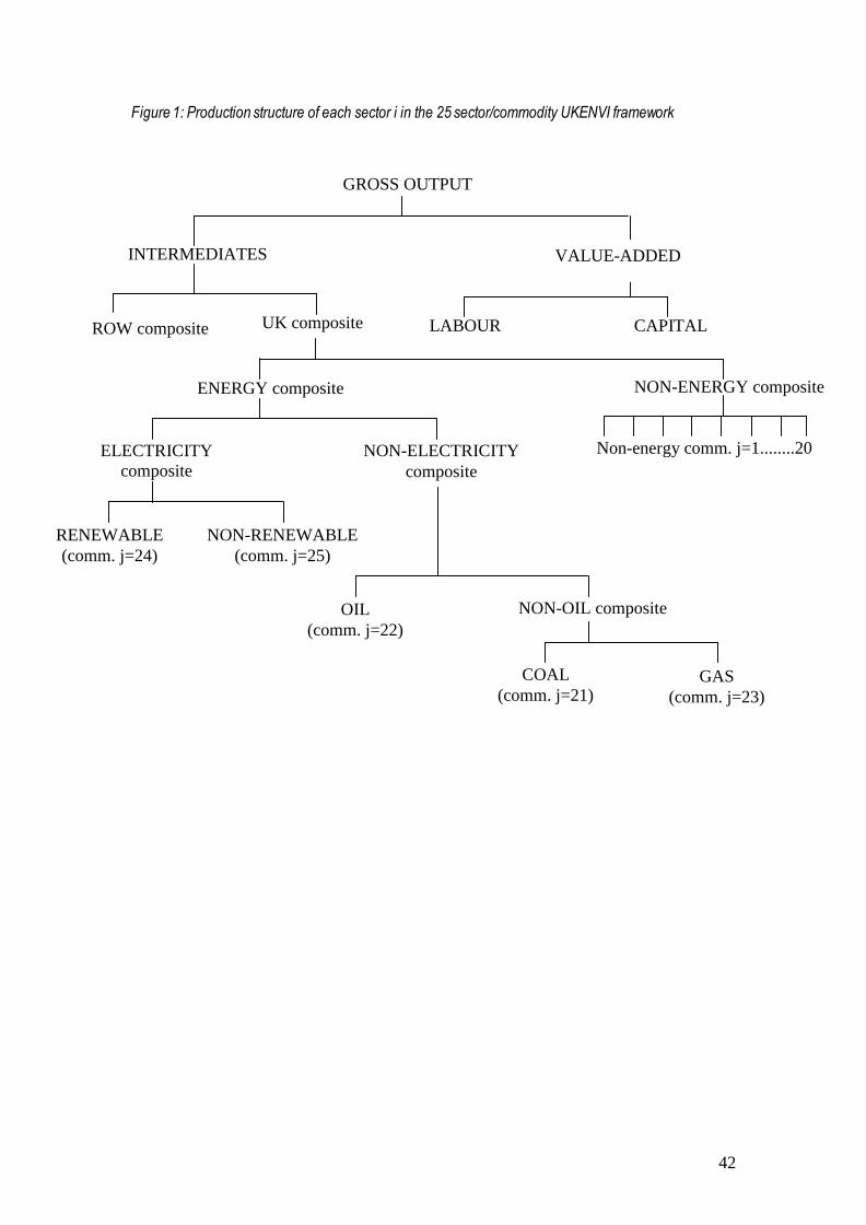
production with multi-level production functions (see Figure 1). There are four major

components of final demand: consumption, investment, government expenditure and

exports. Of these, in the central case scenario, real government expenditure is taken to

be exogenous. Consumption is a linear homogenous function of real disposable

income. Exports (and imports) are generally determined via an Armington link and

are therefore relative-price sensitive (Armington, 1969).

corresponding general equilibrium level of demand.

10

[Figure 1 here]

We parameterise the model to be in long-run equilibrium in the base-year

period. This implies that the capital stock in each industrial sector is initially fully

adjusted to its desired level. There are no vintage effects in the model and the only

technical change introduced in the simulations reported here concerns the step

improvement in energy efficiency. In this paper we give simulation results for two

alternate conceptual time periods: the short run and the long run. In the short run, the

capital stock is fixed, both in terms of its absolute size and in its distribution to

individual sectors, although labour can move freely between sectors in this time

interval. In the long run, capital stock in each sector readjusts to its new desired level,

given the new values for sectoral value added, the user cost of capital and the wage

rate. We assume that interest rates are fixed in international capital markets, so that

the user cost of capital varies with the price of capital goods.

The long run is a conceptual time period. However, where we run the model

in a period-by-period mode with the gradual updating of capital stocks, a close

adjustment to the long run values will often take over 25 years. If the model is run in

this mode, each sector's capital stock is updated between periods via a simple capital

stock adjustment procedure, according to which investment equals depreciation plus

some fraction of the gap between the desired and actual capital stock.4 This treatment

is wholly consistent with sectoral investment being determined by the relationship

between the capital rental rate and the user cost of capital. The capital rental rate is the

rental that would have to be paid in a competitive market for the (sector specific)

physical capital: the user cost is the total cost to the firm of employing a unit of

capital. Where the rental rate exceeds the user cost, desired capital stock is greater

than the actual capital stock and there is therefore an incentive to undertake net capital

investment. The resultant capital accumulation puts downward pressure on rental rates

and so tends to restore equilibrium. In the long run, the capital rental rate equals the

3 The sectoral breakdown is given in Appendix 1 and a condensed version of the UKENVI model is

given in Appendix 2. 4 This process of capital accumulation is compatible with a simple theory of optimal investment

behaviour given the assumption of quadratic adjustment costs.

11

user cost in each sector, and the risk-adjusted rate of return is equalised between

sectors.

We impose a single UK labour market characterised by perfect sectoral

mobility. In our central case scenario, wages are determined via a bargained real wage

function in which the real consumption wage is directly related to workers’ bargaining

power, and therefore inversely to the unemployment rate (Blanchflower and Oswald,

1994; Minford et al, 1994). Here, we parameterise the bargaining function from the

econometric work reported by Layard et al (1991):

(3) 10.068 0.40t tw u w

where: w and u are the natural logarithms of the UK real consumption wage and the

unemployment rate respectively, t is the time subscript and is a parameter which is

calibrated so as to replicate equilibrium in the base period.5

Two alternative treatments for the labour market are also considered. Firstly,

we include an exogenous labour supply closure, which, in effect, implies a completely

wage-inelastic aggregate labour supply function. This is quite a common labour

market closure in national CGE models, but is clearly a limiting case. In this closure,

the real wage adjusts continuously to ensure equality of aggregate labour demand and

the fixed aggregate labour supply. Nonetheless it is a useful benchmark. Secondly, as

an alternative limiting case, we incorporate a real wage resistance closure, in which

the real consumption wage is fixed and total employment changes to ensure labour

market equilibrium. In effect, labour supply is infinitely elastic (over the relevant

range) at the prevailing real wage rate. The impact of these two alternative treatments

of the labour market are detailed in Section 5 as part of sensitivity analysis around the

central case scenario.

3.2 Treatment of energy inputs to production in UKENVI

5 The calibrated parameter plays no part in determining the sensitivity of the endogenous variables to

exogenous disturbances, but the initial assumption of equilibrium is an important assumption.

12

Figure 1 summarises the production structure that is imposed in each sector of

UKENVI model. This separation of different types of energy and non-energy inputs in

the intermediates block is in line with the general ‘KLEM’ (capital-labour-energy-

materials) approach that is most commonly adopted in the literature. There is

currently no consensus on precisely where in the production structure energy should

be introduced, for example, within the primary inputs nest, most commonly

combining with capital (e.g. Bergman, 1988, Bergman, 1990), or within the

intermediates nest (e.g. Beauséjour et al, 1995). Given that energy is a produced

input, it seems most natural to position it with the other intermediates, and this is the

approach we adopt here. However, any particular placing of the energy input in a

nested production function restricts the nature of the substitution possibilities between

other inputs. The empirical importance of this choice is an issue that requires more

detailed research.

The multi-level production functions in Figure 1 are generally of constant

elasticity of substitution (CES) form, so there is input substitution in response to

relative price changes, but with Leontief and Cobb-Douglas (CD) available as special

cases. In the applications reported below, Leontief functions are specified at two

levels of the hierarchy in each sector – the production of the non-oil composite and

the non-energy composite – because of the presence of zeros in the base year data on

some inputs within these composites. CES functions are specified at all other levels.

We introduce the energy efficiency shock by increasing the productivity of the

energy composite in the production structure of all industries. This procedure operates

exactly as in equation (1). It is energy augmenting technical change. We do not

change the efficiency with which energy is used in the household or government

consumption, investment, tourism or export final demand sectors. When we vary the

elasticities of substitution in production in the sensitivity analysis, these are: the

elasticity of substitution between the energy composite and the non-energy composite

in the production of the UK composite; and also the elasticity of substitution between

the intermediates and value added in the production of gross output.

3.3 Database

13

The main database for UKENVI is a specially constructed Social Accounting

Matrix (SAM) for the UK economy for the year 2000. This required the initial

construction of an appropriate UK Input-Output (IO) table since an official UK

analytical table has not been published since 1995. A twenty-five sector SAM was

then developed for the UK using the IO table as a major input. The sectoral

aggregation is chosen to focus on energy sectors. The division of the electricity sector

between renewable and non-renewable generation used an experimental

disaggregation provided for Scotland. This was then adjusted to reflect the different

pattern in electricity generation between the UK and Scotland.

The information on income transfers that is necessary to expand the IO into a

SAM came from a set of Income-Expenditure accounts for the UK in 2000, developed

on the basis of single-entry bookkeeping, where any item of expenditure in one

account also appears as an item of income in another. Five sets of income-expenditure

accounts were constructed for households, corporations, government, capital and the

external sector (rest of the World). Full details on the construction of the UK IO table

and SAM are provided in Allan et al,( 2006).

The structural characteristics of the UKENVI model are parameterised on the

UK SAM for 2000. In all sectors, the elasticity of substitution at all points in the

multi-level production function takes the value of 0.3, apart from where Leontief

functions have been imposed. The Armington trade elasticities for imports and

exports are 5.0 for both renewable and non-renewable electricity, and 2.0 for all other

sectors.

Section 4: Results of the central case CGE simulations

The disturbance simulated using the UKENVI model is a 5 per cent

improvement in the efficiency by which energy inputs are used by all production

sectors. Recall that the five energy sectors in UKENVI are coal, oil, gas and

renewable and non-renewable electricity. This shock is a one-off permanent step

change in energy efficiency, as depicted in equation (1). It is introduced in the use of

the energy composite good (see Figure 1). This introduces a beneficial supply-side

14

disturbance, which would be expected to lower the price of energy, measured in

efficiency units, generally reduce the price of outputs and stimulate economic activity.

Our initial question remains: how will this affect the overall amount of energy

consumed by industrial sectors? And how will the change in total energy consumed

compare to the improvement in energy efficiency?

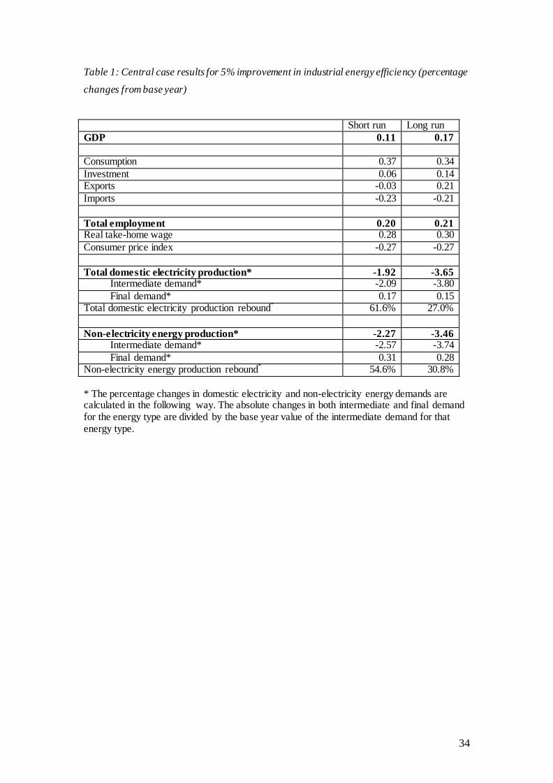
Table 1 reports the impacts on key aggregate variables for the central case

scenario. This is where the efficiency change is introduced costlessly and the default

model configuration and parameter values are used. The figures reported are

percentage changes from the base year values. Because the economy is taken to be in

full equilibrium prior to the energy efficiency improvement, the results are best

interpreted as being the proportionate changes over and above what would have

happened without the efficiency shock.

[Table 1 here]

Results are presented for two conceptual time periods: the short and long run.

Recall that in the short run, capital stocks are fixed at their base year values at the

level of individual sectors. In the long run, capital stocks adjust fully to their desired

sectoral values, given the efficiency shock and a fixed interest rate. With wage

determination characterised by a bargained wage curve, a beneficial supply-side

policy, such as an improvement in energy efficiency, increases employment, reduces

the unemployment rate and increase real wages. This has a positive impact on UK

economic activity that is greater in the long run than in the short run. In the long run

there is an increase of 0.17% in GDP and 0.21% in employment and exports. The

expansion is lower in the short run, where GDP increases by 0.11%, where there is a

larger increase in consumption but actually a fall in exports.

The energy efficiency improvement primarily increases the competitiveness of

energy intensive sectors through a reduction in their relative price. In the long run,

two mechanisms drive this change in competitiveness. First, the increase in energy

efficiency raises the production efficiency of energy intensive sectors by the greatest

amount. Second, the production techniques used in energy sectors themselves are

typically energy intensive, so that the price of energy tends to fall. For both these

15

reasons, energy-intensive sectors experience relatively large reductions in unit costs in

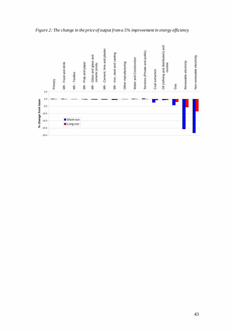
the long run, which are passed through to lower prices. However, as we shall see, in

the short-run, capacity issues also affect prices, sometimes in a dramatic way. The

changes in the short-run and long-run output prices are reported in Figure 2.

[Figure 2 here]

In the long run, although real and nominal wages rise, the increase in energy

efficiency, together with fixed interest rates, is large enough to generate price

reductions in all production sectors. However, there are clear sectoral differences that

generally reflect the energy intensity of the sector. In the long run, prices in the

manufacturing and service sectors show a small decrease, reflecting their relatively

low energy use. Within the manufacturing sectors, energy use as a proportion of the

total value of output ranges from 0.79 % for electrical and electronics to 4.70 % for

iron, steel and casting activities. An even lower energy incidence is found in service

sectors (both public and private) where energy inputs range from 0.47 % for health

and social work to 1.48 % for distribution and transport.

The largest impact on the price of output comes in the energy sectors

themselves, though across these sectors there is clearly a non-uniform response. The

largest reductions in price occur in electricity production, with the price in the non-

renewable electricity sector falling by more than the price in the renewable electricity

sector. This reflects the heavier reliance of the non-renewable electricity production

sector on energy inputs. In the UK SAM for 2000, the renewable and non-renewable

electricity sectors purchase 41 and 52 per cent of their inputs respectively from the

combined five energy sectors (sectors 21-25 in UKENVI).6

In the short run, fixed capital stocks mean that in each sector the marginal cost

of the production of value added increases with output. An increase in the demand for

a sector’s value added in this time interval therefore leads, ceteris paribus, to an

increase in the price of value added, with a corresponding rise in the sector’s capital

6 The high value for energy purchases in the renewable energy sector reflects the fact that for both the

renewable and non-renewable electricity sectors, generation and distribution are combined. Therefore,

there are large purchases of electricity by the electricity sectors.

16

rental rate. On the other hand, where the demand for a sector’s value added falls, the

value added price will fall, as will the capital rental rate.

One interesting short-run result is that the output price actually increases in

most of the non-energy sectors. These are the primary sector, the food and drink

sector, and all the service and utility sectors. These price increases can be traced to a

high ratio of value added to gross output in these sectors and the fact that in all these

sectors there is a slight increase in both the nominal wage, as reported in Table 1, and

the capital rental rate. Therefore, in these cases the increases in factor costs are greater

than the reduction in intermediate costs brought about by the improvement in energy

efficiency. This again partly reflects the very low proportionate energy purchases in

these sectors.

On the other hand, the price adjustments in the energy production sectors are

quite different. First, both in the short and long run, energy prices fall. Second, the

price reduction in the short run is greater than in the long run. Third, these price

changes are particularly marked for the electricity generating sectors.

The long-run reduction in energy prices reflects the fact that these sectors have

relatively energy intensive production processes, so that increased energy efficiency

has a relatively powerful negative impact on their price. Also in the short run,

reductions in output demand in these sectors lead to falls in the capital rental rates,

such that the price reductions over this time interval are greater than those in the long

run. For example, there are significant falls in output price in the renewable and non-

renewable electricity generating sectors (down over 20%) in the short run, where the

capital rental rates fall by 23.76% and 26.18% respectively.

The short- and long-run changes in the output of each sector are shown in

Figure 3. As would be expected, the increased efficiency of energy inputs has

expanded the output of all non-energy sectors, with the increase almost always being

greater in the long than in the short run. Outputs increase most in those non-energy

sectors that have greater energy intensities, notably “iron, steel and casting” and “pulp

and paper” where output increases in the long run by 0.67% and 0.46% respectively.

On the other hand, the output of the five energy sectors falls in both the short and long

17

run, and in this case the long-run reduction is greater than the short-run. The large

reductions in price in the short run go some way to offsetting the demand fall that

occurs in this time period.

[Figure 3 here]

Because the exogenous energy efficiency improvement applies only to the use

of energy as an intermediate input, in calculating rebound effects we compare the

change in production in energy sectors against the initial intermediate domestic

demand for that energy type. The results are presented in Table 1. They are broken

down into changes in intermediate demand and changes in final demand and the

energy sectors have been separated into electricity and non-electricity energy

production.

For total energy demand, rebound is 62% and 54% respectively in the

electricity and non-electricity energy sectors in the short-run. These rebound effects

are mainly determined through demand for energy as an intermediate input. In all

cases the overall expansion of the economy generates additional final demand energy

use, but this is relatively small. It is largest in non-electricity energy production in the

short run, but even here it only adds an additional 6% to the intermediate rebound

effect (increasing it from 48% to 54%). Rebound is much reduced in the long run: the

corresponding long-run total rebound figures for electricity and non-electricity energy

production are 27% and 31%.

Section 5: Sensitivity Analysis

Our central case results presented in Table 1 are dependent upon the structural

data embedded in the base year values of the UK SAM. However, they will also be

sensitive to the choice of key parameters values in the UKENVI model, the recycling

of additional government revenues, additional costs that might accompany energy

efficiency improvements and the nature of the labour market. In the next four

subsections we outline the effects of varying these assumptions.

18

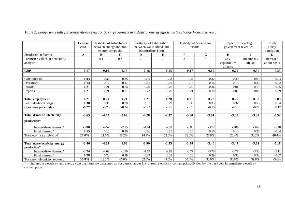
5.1 Results of varying key elasticities

We begin by varying some key parameter values used to derive the central

case results. The parameters that are expected to affect the results most strongly are

the elasticity of substitution between energy and non-energy intermediate composites

and between value-added and intermediate inputs in the production of gross output. In

the central results, both these parameters have an elasticity of 0.3. For sensitivity, we

vary these parameters (independently) to 0.1 and 0.7. Another potentially important

parameter is the elasticity of export demand. In the central results, this parameter was

set at 2 for the non-energy and the non-electricity energy sectors and 5 for the

electricity sectors. For sensitivity, we produce one simulation where the export

demand parameter is set at 2 for all sectors and a second simulation where it is given

the value 5 for all sectors.

[Table 2 here]

Column A in Table 2 gives the long-run results for the central case scenario.

This column replicates the figures given in column 2 of Table 1. Columns B and C

show the long-run results produced by varying the elasticity of substitution between

energy and non-energy intermediate inputs. As expected, increasing this elasticity -

reflecting a greater degree of substitutability between energy and non-energy inputs -

results in a higher GDP impact, although this effect is rather small. The GDP results

vary from 0.16% in the low elasticity case to 0.18% when the elasticity of substitution

is higher. There are similarly small impacts on other aggregate variables. However,

changing this parameter has a major impact on energy use and the extent of rebound.

Consider first intermediate demand. For non-electricity energy production, the

fall in intermediate demand, expressed as a proportion of initial intermediate demand,

is –4.62% where the elasticity of substitution between energy and non-energy

intermediate composites is 0.1. The figure is –1.96% where the elasticity takes the

value 0.7. This translates to a rebound of 7% with the lower, as against a value of over

60% with the higher, elasticity value. Although the variation for electricity is a little

lower it is still substantial. Also, as we would expect given the limited impact on

19

aggregate economic activity, the positive energy final demand changes are left almost

unchanged by variations in this parameter.

It is useful to look at the empirical evidence concerning the substitutability of

energy inputs. Howarth (1997) refers to research that concludes that the elasticity of

substitution between energy and non-energy inputs is less than unity. This included a

reference to the work of Manne and Richels (1992) who estimated an elasticity of

substitution of 0.4 between energy and value-added. The Greening et al (2000)

extensive survey of US work reports some studies that have found an elasticity of

substitution greater than one (Chang, 1994; Hazilla and Kop, 1986), but the vast

majority of estimates are less than unity. The range of substitution elasticities found in

the empirical literature is therefore broadly consistent with the range over which we

simulate here.

Columns D and E in Table 2 show the long-run results when the elasticity of

substitution between value added and intermediate inputs in the production of gross

output is varied. This is the point at the very top level of the production hierarchy

shown in Figure 1. In this case, increasing the ease of substitution towards the now

cheaper intermediate inputs slightly lowers the impact on GDP (from 0.17% in the

central case to 0.15%), and produces a smaller overall effect on employment (down

from 0.21% in the central case to 0.20%). However, increasing this elasticity of

substitution does reduce the fall in energy use and therefore increase rebound. These

changes are not trivial but are not as strongly as from changing the elasticity of

substitution between the energy and non-energy composites discussed earlier.

Columns F and G in Table 2 show the sensitivity of the long-run results to

varying the export demand elasticities. In the low elasticity case, the export demand

elasticity for all sectors is set equal to 2; in the high elasticity case it is set equal to 5.

Increasing the elasticity of demand for exports will stimulate output where sectoral

prices fall. However, in this case, these variations have very small impacts on

aggregate activity or energy use. The increase in competitiveness is too slight in

export intensive industries. This outcome contrasts with the results reported in Hanley

et al (2006) for the simulated impact of energy efficiency improvements in the

Scottish economy. Here direct exports of energy were stimulated by the fall in prices

20

in the energy sectors (especially electricity). In the Scottish case, this expansion is

large enough to generate backfire.

5.2 Results of enforcing government budget constraint

Another potentially important feature of the central case simulation is the

treatment of the government sector. In the central case and all sensitivity simulations

performed up to now, the improvement in energy efficiency stimulates aggregate

economic output and employment. Given fixed average tax rates, there will be an

increase in the tax revenues of the UK government and a reduction in social security

spending. In our central case, the government saves all of this improvement to its

budgetary position. This increased government revenue can however be recycled back

to the economy through enforcing an active government budget constraint, which we

model as maintaining the base year ratio of government savings to GDP.

In the UKENVI model this government budget constraint can be imposed in

two ways that have quite different economic impacts. First, additional revenue can be

used to expand general government expenditure, distributed across sectors using the

base-year weights. Second, extra revenues received can be recycled back to

households through reduced income tax. The long run impacts of these two scenarios

are shown in Columns H and J of Table 2.

When the additional tax revenues are recycled as extra government

expenditure, this acts as an exogenous demand injection and stimulates GDP and

employment. The sectoral changes in output are focused on government sectors, as

would be expected. However, when increased revenues are recycled in the form of a

decreased income tax rate, there are significantly larger impacts. This form of revenue

recycling has both supply- and demand-side effects.

On the demand side, lowering the tax rate raises take home wages and thus

stimulates household consumption demand. However, under a bargained wage curve

labour market closure, there is also a supply-side impact. A fall in the income tax rate

means that a lower nominal wage is needed to maintain a given real take-home wage.

At any given level of unemployment, nominal wages will fall. This makes substitution

21

towards labour more attractive, which boosts employment. The level of employment

increases significantly with the recycling of revenue. In the central case employment

increases by 0.21%, as against 0.26% when government expenditure adjust and 0.38%

higher when income tax rates adjusts. There is also a significant increase in the impact

on GDP in both cases, but again this is especially strong when income tax rates adjust.

The energy impacts are also rather different under these two scenarios. When

government expenditure adjusts, total electricity consumption actually falls by more

than under the central scenario. This reflects the switch towards less energy intensive

government demands, and increased employment in public sectors crowding out more

energy intensive activity. When income tax rates adjust, however, the electricity use

falls by less and rebound increases. For example, for the non-electricity energy

production, rebound increases from 31% in the central case simulation to 40% where

increased revenues are recycled through lower taxes.

5.3 Results of implementing a costly energy efficiency policy

Our assumption up to this point has been that energy efficiency improvements

are like “manna from heaven” – a costless benefit. In this section we report simulation

results where we assume that gains in energy efficiency will be accompanied by other

costs borne by production sectors. Such costs can be introduced in a number of ways.

In the present set up of the UKENVI model this is most straightforwardly done

through an increase in labour costs generated through reduced labour efficiency,

although other alternatives are available. The size of the labour efficiency loss that we

introduce in each sector is just enough to counter the impact of the increase in energy

efficiency on overall production costs. This reduction in labour efficiency can be

thought of as representing additional labour required to implement the improvement

in energy efficiency.7

The size of the negative shock in each sector has been calibrated such that

with no change in product or factor prices, the increase in costs implied by the

7 For instance, this could take the form of employing somebody to enforce the energy efficient

technology. However, in principle the same sort of effect can be introduced by reducing the capital

efficiency parameter, thereby imposing increased capital costs.

22

reduced labour efficiency just equals the reduction in cost implied by the 5%

improvement in energy efficiency. The reduction in labour efficiency in sector i (λ i) is

therefore estimated as:

(4) 0.05 ii

i

E

L

where Ei and Li are the base year expenditures on energy and labour in sector i.

The aggregate results from simultaneously introducing both the positive

energy efficiency improvement and the negative shock to the productivity of labour

inputs, are shown in the final column (Column K) of Table 2. This simulation results

in a very small increase in total employment over the base year value and a fall in

GDP. We consider the results reported in Column K to be the most extreme example

of a “costly” energy efficiency improvement, in that the net impact is broadly cost

neutral to individual industries. We would expect actual energy efficiency

improvements to lie somewhere between this simulation and the “costless” simulation

represented by the central case results.

The costly energy efficiency simulation generates changes in energy use that

are very different to those in the other simulations carried out thus far. In the long

run, energy consumption falls by slightly more than the 5% energy efficiency

improvement. Introducing fully-offsetting labour costs related to energy efficiency

improvements neutralises the overall cost reduction and thus prevents a significant

demand switch towards the output of more energy intensive sectors, thereby

preventing rebound. However, where fully-offsetting other costs accompany energy

savings, we are robbed of the increases in output and employment that otherwise go

with such efficiency improvements.

5.4 Results from different labour market closures

Assumptions concerning labour market behaviour can have a major impact on

the macroeconomic effects of any exogenous economic disturbance. In the

simulations reported up to now we have assumed that the supply side of the labour

23

market can be characterised by a bargained real wage function in which the real

consumption wage is directly related to workers’ bargaining power, and therefore

inversely related to the unemployment rate. In this sensitivity analysis two alternative

specifications of the labour market are considered. In one, we impose an exogenous

labour supply function, in which there is a completely wage inelastic aggregate labour

supply function, so that aggregate employment is effectively fixed. This is quite a

common assumption in national CGE models, but seems unduly restrictive. In the

other, we impose a real wage resistance closure, in which the real wage is set

exogenously at the prevailing real wage, and employment adjusts to ensure

equilibrium. This simulation could also be thought to capture an economy with perfect

flow migration (McGregor et al, 1996).8 These closures can be considered as limiting

cases capturing zero and infinite elasticity of labour supply with respect to the real

consumption wage.

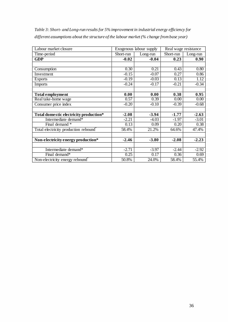
[Table 3 here]

Table 3 shows the aggregate results in the short and long run from introducing

a 5% energy efficiency improvement in production under these two labour market

closures. In the exogenous labour supply scenario there is, as would be anticipated, a

significant increase in the real take-home wages, but also a small decrease in GDP in

each time interval. The GDP change is the result of compositional effects. In the real

wage resistance case, GDP rises in both the short (0.23%) and long run (0.90%),

accompanied by a substantial increase in overall employment, over 4 times greater

than that in the central scenario. In the exogenous labour supply closure, the fall in

energy use is greater than in the central case. Rebound is reduced. However, in the

real wage resistance closure, there is a bigger energy rebound than under the central

case. For electricity use, for example, the short- and long-run total rebound figures of

62% and 27% are increased to 65% and 47% respectively. Similar adjustments occur

with non-electrical energy use.

8 In the central case simulations we assume population is fixed.

24

Section 6: The strengths and weaknesses of the CGE modelling approach

What are the major strengths and weaknesses of this form of analysis for this

type of problem? First, from a conceptual point of view, a major strength of CGE

analysis is that it is grounded in standard economic theory, but can deal with

circumstances that are too complex for tractable analytical solutions. As such, CGE

analysis is a numerical aid to analytical thought. For example, in the energy efficiency

we know there are a whole range of substitution, income, output and sectoral

composition effects that will operate simultaneously. A CGE analysis can deal with

this simultaneity.

A second advantage is that theory can often indicate the direction in which a

variable will move after the introduction of an exogenous disturbance, but is less good

at quantifying the size of the change. For example, we can say from a fairly informal

theoretical analysis that we would expect an energy efficiency improvement to be

accompanied by rebound effects. However, there is a crucial difference, for the

viability of policy, between a 5% rebound and 150% rebound. CGE analysis is

parameterised to reflect the structural and behavioural characteristics of the economy

under analysis. Whilst the CGE simulation would not claim pinpoint accuracy, an

appropriate order of magnitude is achievable. Furthermore, it is straightforward to

undertake sensitivity analysis with this type of model.

Third, from a modelling perspective, CGE analysis has a very well developed

supply side. Many policy issues, of which energy efficiency is one, are essentially

supply side problems. However, it is common to see analysts attempting to tackle

supply side problems with demand driven models.

Fourth, from a purely practical point of view, CGE modelling makes it simpler

to evaluate the net impacts of energy policy change since it makes very clear what the

“counter-factual” is. This counter-factual is the base-line run of the model without the

change in energy efficiency. All changes in output, employment and energy use that

are observed from the technology shock are then measured relative to this baseline.

This makes the marginal effects of technology change clear. However, evaluating the

25

same policy using time series or cross-sectional statistical data requires us to be able

to identify the counter-factual by appropriate statistical control. This may be much

harder, and risks confusing the actual drivers of changes in energy use.

To turn to the weaknesses of this approach, the first is that a CGE model is

information intensive in that it requires an initial set of multi-sectoral accounts (in the

form of a SAM), a set of formally specified behavioural relationships and a large

number of parameter values. Many of these behavioural relationships and their

associated parameters will not be estimated econometrically, or at least not for the

economy under consideration of for that time period. For example, Saunders (2006)

draws attention to the possible problems of specifying particular forms of the

production function, and the substitution possibilities that this imposes. Moreover,

CGE simulation models are rarely tested against their predictive power. It is therefore

very easy to invest the model results with misplaced concreteness.

Second, some would see the theoretical supply-side rigour of the model as a

weakness. For example, CGE models typically take it as axiomatic that firms

maximize profits, which implies that they minimise costs. However in the specific

case of energy efficiency, there is a significant and growing literature that focuses on

barriers to the adoption of the most efficient energy technologies (Sorrell et al, 2004).

This literature argues that conventional neoclassical behavioural functions of the type

assumed here fail to capture some of the significant barriers to the penetration of new

technologies. Such barriers include, for example, imperfect information and

significant transactions costs that are neglected in the optimisation processes that

underlies the functions. Although adjustment costs can be incorporated into CGE

models, such models might still privilege market forces as against behavioural ones.

Third, there is variation between CGE models so that care needs to taken when

comparing results across models. In particular, there are a number of issues about

closing the model where different assumptions can be made. These are likely to apply

to the way in which the labour and capital markets are assumed to operate. We have

seen in this paper how changing the assumptions concerning the labour market

closure, for example, can generate very different simulated outcomes. Sometimes

26

model results can be driven by assumptions that are not apparent to an uninformed

reader.

Where one is dealing with economic issues - such as the impact of energy

efficiency improvements - which have complex, system-wide impacts, CGE analysis

should be one of the methods adopted as an aid to analysis and as a tool to assess

broad orders of magnitude for different effects. However, such models should be used

in a transparent manner. Their strong theoretical basis means that unlike many

econometric models, they are not black boxes, but should produce results that are both

clear and comprehensible.

Section 7: Conclusion

The simulations reported in this paper suggest that for the UK, we expect a

general, across the board, improvement in efficiency in energy use in production to

have significant rebound effects but no backfire. Short-run rebound effects are above

50%, whilst the long-run values are around 30%. Increases in energy efficiency will

reduce energy use, but not by the full proportionate amount. Moreover these impacts

will vary across energy types. Most of the rebound effect is captured within the

demand for energy as an intermediate input. There are increases in the demand for

energy driven by the accompanying expansion in final demand. However, in this

particular case these increases are small.

We test these results to see how sensitive they are to changes in key parameter

values and model closure rules. This analysis backs up the generally held view that

the energy use results are heavily dependent on the substitution possibilities in

production in general, and the value taken by the elasticity of substitution between the

energy and non-energy inputs in particular. However, note that we found these results

are also sensitive to assumptions made about the nature of the labour market, the

conceptual time period under consideration and the recycling of government revenue

saving.

Our analysis shows that it is quantitatively important how we treat any

changes in government revenues that result from changes in economic activity and

27

employment that accompany improvements in energy efficiency. We have enforced a

government budget constraint in which the additional government revenue is recycled

through two alternative channels. Recycling this revenue through raising government

expenditure delivers a significantly smaller economic impact than recycling it through

reducing the average rate of income tax. With the income tax adjustment, the demand

side is affected by increased household consumption, while the supply-side is

simultaneously stimulated via a lower nominal wage being required to generate any

given real take-home wage. This makes substitution towards labour more attractive,

and production more competitive, boosting employment, GDP and increasing rebound

to 40%.

This work could usefully be extended in a number of ways. First, we have

dealt here solely with improvements in energy efficiency across production sectors,

and have excluded efficiency gains in household energy use, where a significant

portion of energy policy is directed. Second, analysis could be focused on specific

energy efficiency improvements in individual sectors, rather than general, across the

board improvements to applying to all production sectors.

28

References

Allan GJ, Hanley ND, McGregor PG, Swales JK, Turner KR. The macroeconomic

rebound effect and the UK economy. Final report to DEFRA, May 2006. Online at

http://www.defra.gov.uk/science/project_data/DocumentLibrary/EE01015/EE01015_

3553_FRP.pdf

Armington P. A theory of demand for products distinguished by place of production.

IMF Staff Papers 1969; 16; 157-178

Beauséjour L, Lenjosek G, Smart M. A CGE approach to modelling carbon dioxide

emissions control in Canada and the United States. The World Economy 1995; 18;

457-489

Bergman L. Energy policy modelling: a survey of general equilibrium approaches.

Journal of Policy Modelling 1988; 10(3); 377-399

Bergman L. Energy and environmental constraints on growth: a CGE modelling

approach. Journal of Policy Modelling 1990; 12; 671-691

Blanchflower DG, Oswald AJ. The wage curve. M.I.T. Press: Cambridge,

Massachusetts; 1994

Brookes L. The greenhouse effect: the fallacies in the energy efficiency solution.

Energy Policy 1990; March; 199-201

29

Cabinet Office. Resource productivity: making more with less. HMSO: London; 2001

Carbon Trust. The future for UK energy? New report on renewables highlights key

areas for investment for the UK. Press Release. 29th October 2003. available online at

http://www.carbontrust.co.uk/NR/rdonlyres/21887EFA-869F-4D85-95DC-

F5324DD82DA4/0/PressRelease_29_10_03.pdf

Chang KP. Capital-energy substitution and the multi-level CES production function.

Energy Economics 1994; 16; 22-26

Conrad K 1999. Computable general equilibrium models for environmental

economics and policy analysis. In: van den Bergh JCJM (Ed), Handbook of

environmental and resource economics. Edward Elgar Publishing Ltd: Cheltenham;

1999.

Conrad K, Schröder M. Choosing environmental policy instruments using general

equilibrium models. Journal of Policy Modelling 1993; 15; 521-543

Department of Environment Food and Rural Affairs. One future - different paths: The

UK’s shared framework for sustainable development. HMSO: London; 2005.

Despotakis KA, Fisher AC. Energy in a regional economy: a computable general

equilibrium model for California. Journal of Environmental Economics and

Management 1988; 15; 313-330

30

Dufournaud CM, Quinn JT, Harrington JJ. An applied general equilibrium (AGE)

analysis of a policy designed to reduce the household consumption of wood in the

Sudan. Resource and Energy Economics 1994; 16; 69-90

European Environment Agency. Making sustainability accountable: Eco-efficiency,

resource productivity and innovation. Topic report No. 11/1999: Copenhagen,

Denmark; 1999.

Goulder LH. Effects of carbon taxes in an economy with prior tax distortions: an

intertemporal general equilibrium analysis. Journal of Environmental Economics and

Management 1998; 29; 271-297

Greening LA, Greene DL, Difiglio C. Energy efficiency and consumption – the

rebound effect – a survey. Energy Policy 2000; 28; 389-401

Hanley ND, McGregor PG, Swales JK, Turner KR. The impact of a stimulus to

energy efficiency on the economy and the environment: A regional computable

general equilibrium analysis. Renewable Energy 2006; 31; 161-171

Hazilla M, Kop RJ. Testing for separable function structure using temporary

equilibrium models. Journal of Econometrics 1986; 33; 119-141

House of Lords. Energy efficiency, science and technology committee, 2nd report of

session 2005-06, Volume 1 report. The Stationary Office: London; 2005.

31

Howarth RB. Energy efficiency and economic growth. Contemporary Economic

Policy 1997; 15; 1-9

Jevons WS. The coal question, An inquiry concerning the progress of the nation, and

the probably exhaustion of our coal mines. Macmillan: London; 1865.

Khazzoom DJ. Economic implications of mandated efficiency in standards for

household appliances. Energy Journal 1980; 1(4); 21-39

Layard R, Nickell S, Jackman R. Unemployment: macroeconomic performance and

the labour market. Oxford University Press: Oxford; 1991.

Lee H, Roland-Holst DW 1997. Trade and the environment. In Francois JF, Reihert

KA (Eds), Applied methods for trade analysis: a handbook. Cambridge University

Press: Cambridge, 1997.

Li P, Rose A. Global warming policy and the Pennsylvania economy: a computable

general equilibrium analysis. Economic Systems Research 1995; 7; 151-171

McGregor PG, Swales JK, Yin YP. A long-run interpretation of regional input-output

analyses. Journal of Regional Science 1996; 36; 479-501

Manne AS, Richels RG. Buying greenhouse insurance: the economics of CO2

emissions limits. MIT Press: Cambridge, Massachusetts; 1992.

32

Minford P, Stoney P, Riley J, Webb B. An econometric model of Merseyside:

validation and policy simulations. Regional Studies 1994; 28; 563-575

Nordic Council of Ministers. Factors 4 and 10 in the Nordic countries. TemaNord

1999:528: Copenhagen, Denmark; 1999

Saunders HD. The Khazzoom-Brookes postulate and neoclassical growth. The Energy

Journal 1992; 13(4); 131-148

Saunders HD. A view from the macro side: rebound, backfire and Khazzoom-

Brookes. Energy Policy 2000a; 28; 439-449

Saunders HD. Does predicted rebound depend upon distinguishing between energy

and energy services? Energy Policy 2000b; 28; 497-500

Saunders HD. Fuel conserving (and using) production functions. Unpublished

working paper 2006

Schutz H, Welfens MJ. Sustainable development by dematerialisation in production

and consumption – strategy for the new environmental policy in Poland. Wuppertal

Papers 2000, No. 103

Small K., Van Dender K. The effect of improved fuel economy on vehicle miles

traveled: estimating the rebound effect using U.S. state data, 1966-2001. UCI

Economics Working Paper 05-06-03 2005; also available as UCEI, Energy Policy and

33

Economics Working Paper 014

Sorrell S, O’Malley E, Schleich J, Scott S. The economics of energy efficiency:

barriers to cost-effective investment. Edward Elgar: Cheltenham; 2004.

Zein-Elabdin EO. Improved stoves in Sub-Saharan Africa: the case of the Sudan.

energy economics 1997; 19; 465-475

34

Table 1: Central case results for 5% improvement in industrial energy efficiency (percentage

changes from base year)

Short run Long run

GDP 0.11 0.17

Consumption 0.37 0.34

Investment 0.06 0.14 Exports -0.03 0.21

Imports -0.23 -0.21

Total employment 0.20 0.21 Real take-home wage 0.28 0.30

Consumer price index -0.27 -0.27

Total domestic electricity production* -1.92 -3.65 Intermediate demand* -2.09 -3.80

Final demand* 0.17 0.15 Total domestic electricity production rebound

* 61.6% 27.0%

Non-electricity energy production* -2.27 -3.46 Intermediate demand* -2.57 -3.74

Final demand* 0.31 0.28 Non-electricity energy production rebound

* 54.6% 30.8%

* The percentage changes in domestic electricity and non-electricity energy demands are calculated in the following way. The absolute changes in both intermediate and final demand for the energy type are divided by the base year value of the intermediate demand for that energy type.

35

Table 2: Long-run results for sensitivity analysis for 5% improvement in industrial energy efficiency (% change from base year)

Central

case

Elasticity of substitution

between energy and non-

energy composite

Elasticity of substitution

between value added and

intermediate input

Elasticity of demand for

exports

Impact of recycling

government revenues

Costly

policy

simulation

Simulation reference A B C D E F G H J K

Parameter values in sensitivity

analysis

0.1 0.7 0.1 0.7 2 5 Gov.

expenditure

adjusts

Income tax

adjusts

Increased

labour costs

GDP 0.17 0.16 0.18 0.18 0.15 0.17 0.19 0.20 0.34 -0.33

Consumption 0.34 0.34 0.35 0.35 0.33 0.34 0.37 0.40 0.69 -0.04

Investment 0.14 0.12 0.17 0.15 0.10 0.13 0.16 0.13 0.33 -0.32

Exports 0.21 0.21 0.24 0.20 0.26 0.22 0.34 0.01 0.19 -0.25

Imports -0.21 -0.21 -0.21 -0.22 -0.20 -0.21 -0.10 -0.02 0.03 -0.09

Total employment 0.21 0.21 0.21 0.21 0.20 0.21 0.23 0.26 0.38 0.03

Real take-home wage 0.30 0.30 0.30 0.31 0.29 0.30 0.33 0.37 0.55 0.04

Consumer price index -0.27 -0.23 -0.24 -0.22 -0.25 -0.23 -0.19 -0.13 -0.22 0.17

Total domestic electricity

production*

-3.65 -4.42 -2.09 -4.28 -2.37 -3.60 -3.61 -3.68 -3.34 -5.52

Intermediate demand* -3.80 -4.57 -2.25 -4.44 -2.52 -3.85 -3.77 -3.84 -3.62 -5.48

Final demand* 0.15 0.15 0.16 0.16 0.15 0.15 0.16 0.16 0.28 -0.04

Total electricity rebound* 27.0% 11.6% 58.2% 14.4% 52.6% 28.0% 27.8% 26.4% 33.2% -10.4%

Total non-electricity energy

production*

-3.46 -4.34 -1.66 -3.90 -2.55 -3.48 -3.40 -3.47 -3.01 -5.18

Intermediate demand* -3.74 -4.62 -1.96 -4.19 -2.83 -3.77 -3.70 -3.77 -3.53 -5.11

Final demand* 0.28 0.28 0.29 0.29 0.28 0.28 0.29 0.30 0.52 -0.07

Total non-electricity rebound* 30.8% 13.2% 66.8% 22.0% 49.0% 30.4% 32.0% 30.6% 39.8% -3.6%

* = changes in electricity and energy consumptions are calculated as absolute changes in e.g. total electricity consumption, divided by the base year intermediate electricity

consumption

36

Table 3: Short- and Long-run results for 5% improvement in industrial energy efficiency for

different assumptions about the structure of the labour market (% change from base year)

Labour market closure Exogenous labour supply Real wage resistance

Time-period Short-run Long-run Short-run Long-run

GDP -0.02 -0.04 0.23 0.90

Consumption 0.30 0.21 0.43 0.80

Investment -0.15 -0.07 0.27 0.86 Exports -0.19 -0.03 0.13 1.12

Imports -0.24 -0.17 -0.21 -0.34

Total employment 0.00 0.00 0.38 0.95 Real take-home wage 0.57 0.39 0.00 0.00

Consumer price index -0.20 -0.10 -0.39 -0.68

Total domestic electricity production* -2.08 -3.94 -1.77 -2.63

Intermediate demand* -2.21 -4.03 -1.97 -3.01 Final demand * 0.13 0.09 0.20 0.38

Total electricity production rebound* 58.4% 21.2% 64.6% 47.4%

Non-electricity energy production* -2.46 -3.80 -2.08 -2.23

Intermediate demand* -2.71 -3.97 -2.44 -2.92 Final demand* 0.25 0.17 0.36 0.69

Non-electricity energy rebound* 50.8% 24.0% 58.4% 55.4%

37

Appendix 1: Sectoral aggregation used in UKENVI

Sector SIC (92)

Agriculture, forestry and fishing 1, 2, 5

Other mining and quarrying, including oil and gas

extraction 11 to 14

Food and drink 15.1 to 16

Textiles 17.1 to 19.3

Pulp, paper and articles of paper and board 21.1 to 21.2

Glass and glass products, ceramic goods and clay products 26.1 to 26.4

Cement, lime plaster and articles in concrete, plaster and

cement and other non-metallic products 26.5 to 26.8

Iron, steel first processing, and casting 27.1 to 27.5

Other metal products 28.1 to 28.7

Other machinery 29.1 to 29.7

Electrical and electronics 30 to 33

Other manufacturing 20, 22, 24.11 to 25.2, 34 to 37

Water 41

Construction 45

Distribution and transport 50 to 63

Communications, finance and business 64.1 to 72 and 74.11 to 74.8

Research and development 73

Public admin and education 75+80

Health and social work 85.1-85.3

Other services 90-95

Coal (Extraction) 10

Oil processing and nuclear refining 23

Gas 40.2 to 40.3

Electricity – renewable 40.1

Electricity - non-renewable 40.1

38

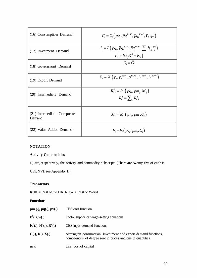
Appendix 2. A condensed version of UKENVI

(1) Gross Output Price

( , )i i i ipq pq pv pm

(2) Value Added Price

,( , )i i n k ipv pv w w

(3) Intermediate Composite Price

( )i ipm pm pq

(4) Wage setting

, ,n n n

Nw w cpi t

L

(5) Labour force

L L

(6) Consumer price index RUK RUK ROW ROW

i i i i i ii i i

cpi pq pq pq

(7) Short-run capital supply

s s

i iK K

(8) Long-run capital rental

, ( )k iw uck kpi

(9) Capital price index RUK RUK ROW ROW

i i i i i ii i i

kpi pq pq pq

(10) Labour demand

,( , , )d d

i i i n k iN N V w w

(11) Capital demand

,( , , )d d

i i i n k iK K V w w

(12) Labour market clearing

s d

iiN N N

(13) Capital market clearing

s d

i iK K

(14) Household income

_

,(1 ) (1 )n n n k k i kiY Nw t w t T

(15) Commodity demand

i i i i i iQ C I G X R

39

(16) Consumption Demand

, , , , RUK ROW

i i i i iC C pq pq pq Y cpi

(17) Investment Demand

,, , , RUK ROW d

i i i i i i j jiI I pq pq pq b I

d d

j j j jI h K K

(18) Government Demand

i iG G

(19) Export Demand

, , , ,RUK ROW RUK ROW

i i i i iX X p p p D D

(20) Intermediate Demand , , ,d d

i j i i j jR R pq pm M

,d d

i i jjR R

(21) Intermediate Composite Demand

, ,i i i i iM M pv pm Q

(22) Value Added Demand

, ,i i i i iV V pv pm Q

NOTATION

Activity-Commodities

i, j are, respectively, the activity and commodity subscripts (There are twenty-five of each in

UKENVI: see Appendix 1.)

Transactors

RUK = Rest of the UK, ROW = Rest of World

Functions

pm (.), pq(.), pv(.) CES cost function k

S(.), w(.) Factor supply or wage-setting equations

K

d(.), N

d(.), R

d(.) CES input demand functions

C(.), I(.), X(.) Armington consumption, investment and export demand functions, homogenous of degree zero in prices and one in quantities uck User cost of capital

40

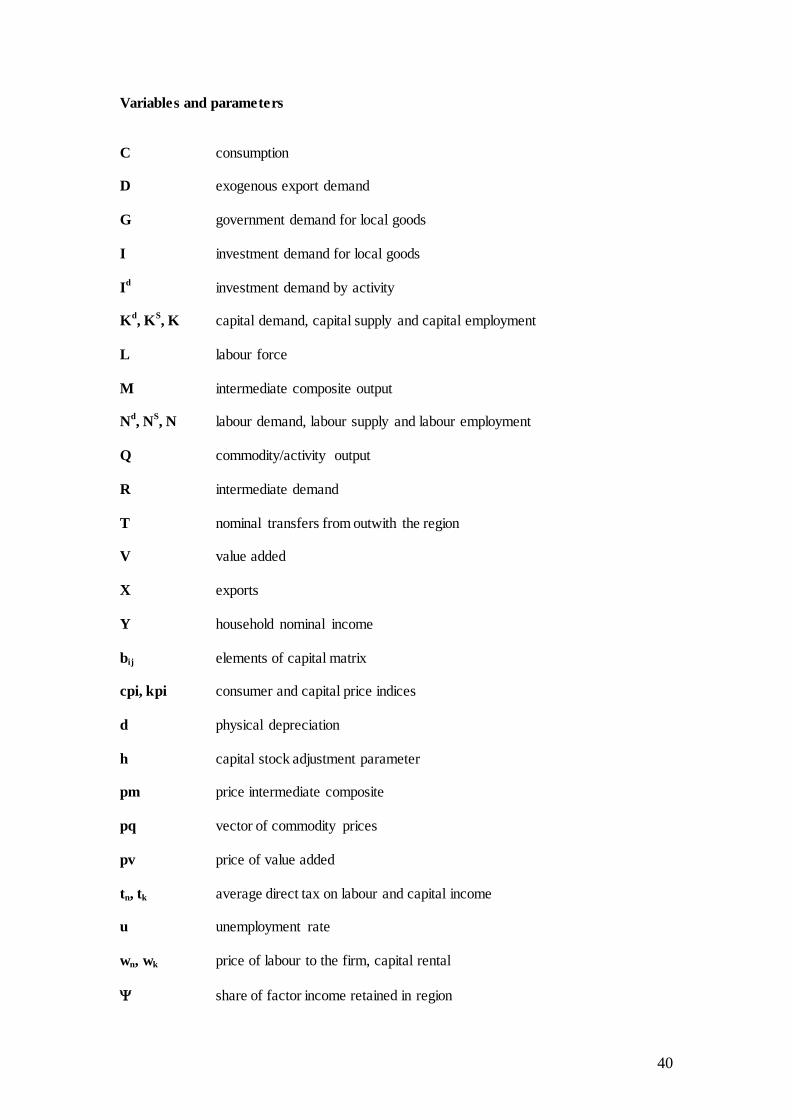
Variables and parameters

C consumption D exogenous export demand

G government demand for local goods

I investment demand for local goods

I

d investment demand by activity

K

d, K

S, K capital demand, capital supply and capital employment

L labour force

M intermediate composite output

N

d, N

S, N labour demand, labour supply and labour employment

Q commodity/activity output

R intermediate demand

T nominal transfers from outwith the region V value added

X exports

Y household nominal income

bij elements of capital matrix cpi, kpi consumer and capital price indices

d physical depreciation

h capital stock adjustment parameter pm price intermediate composite pq vector of commodity prices pv price of value added

tn, tk average direct tax on labour and capital income

u unemployment rate

wn, wk price of labour to the firm, capital rental

share of factor income retained in region

41

consumption weights

capital weights

42

Figure 1: Production structure of each sector i in the 25 sector/commodity UKENVI framework

GAS

(comm. j=23)

COAL

(comm. j=21)

NON-OIL composite OIL

(comm. j=22)

NON-RENEWABLE

(comm. j=25)

RENEWABLE

(comm. j=24)

NON-ELECTRICITY

composite

ELECTRICITY

composite

Non-energy comm. j=1........20

NON-ENERGY composite ENERGY composite

CAPITAL LABOUR UK composite

INTERMEDIATES

GROSS OUTPUT

VALUE-ADDED

ROW composite

43

Figure 2: The change in the price of output from a 5% improvement in energy efficiency

-25.0

-20.0

-15.0

-10.0

-5.0

0.0

5.0

Pri

mary

Mfr

- F

ood

an

d d

rin

k

Mfr

- T

extile

s

Mfr

- P

ulp

and

pa

pe

r

Mfr

- G

lass a

nd g

lass a

nd

cera

mic

pro

du

Mfr

- C

em

en

t, lim

e a

nd p

laste

r

Mfr

- Iro

n, ste

el an

d c

asting

Oth

er

manu

factu

ring

Wa

ter

an

d C

onstr

uction

Serv

ices (

Pri

vate

an

d p

ublic

)

Coa

l extr

action

Oil

(refinin

g a

nd d

istr

ibution)

an

d

nu

cle

ar

Gas

Ren

ew

ab

le e

lectr

icity

Non

-ren

ew

ab

le e

lectr

icity

% c

han

ge f

rom

base

Short-run

Long-run

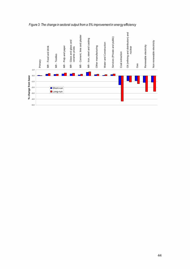
44

Figure 3: The change in sectoral output from a 5% improvement in energy efficiency

-5.0

-4.0

-3.0

-2.0

-1.0

0.0

1.0

Pri

ma

ry

Mfr

- F

oo

d a

nd

dri

nk

Mfr

- T

extile

s

Mfr

- P

ulp

an

d p

ap

er

Mfr

- G

lass a

nd

gla

ss a

nd

ce

ram

ic p

rod

u

Mfr

- C

em

en

t, lim

e a

nd

pla

ste

r

Mfr

- Iro

n, ste

el a

nd

ca

stin

g

Oth

er

ma

nu

factu

rin

g

Wa

ter

an

d C

on

str

uctio

n

Se

rvic

es (

Pri

va

te a

nd

pu

blic

)

Co

al e

xtr

actio

n

Oil

(re

fin

ing

an

d d

istr

ibu

tio

n)

an

d

nu

cle

ar

Ga

s

Re

ne

wa

ble

ele

ctr

icity

No

n-r

en

ew

ab

le e

lectr

icity

% c

ha

ng

e f

rom

ba

se

Short-run

Long-run