The Impact of ICT on Vegetable Farmers in Honduras - EconStor
87
econstor Make Your Publications Visible. A Service of zbw Leibniz-Informationszentrum Wirtschaft Leibniz Information Centre for Economics Pineda, Allan; Aguero, Marco; Espinoza, Sandra Working Paper The Impact of ICT on Vegetable Farmers in Honduras IDB Working Paper Series, No. IDB-WP-243 Provided in Cooperation with: Inter-American Development Bank (IDB), Washington, DC Suggested Citation: Pineda, Allan; Aguero, Marco; Espinoza, Sandra (2011) : The Impact of ICT on Vegetable Farmers in Honduras, IDB Working Paper Series, No. IDB-WP-243, Inter- American Development Bank (IDB), Washington, DC This Version is available at: http://hdl.handle.net/10419/89017 Standard-Nutzungsbedingungen: Die Dokumente auf EconStor dürfen zu eigenen wissenschaftlichen Zwecken und zum Privatgebrauch gespeichert und kopiert werden. Sie dürfen die Dokumente nicht für öffentliche oder kommerzielle Zwecke vervielfältigen, öffentlich ausstellen, öffentlich zugänglich machen, vertreiben oder anderweitig nutzen. Sofern die Verfasser die Dokumente unter Open-Content-Lizenzen (insbesondere CC-Lizenzen) zur Verfügung gestellt haben sollten, gelten abweichend von diesen Nutzungsbedingungen die in der dort genannten Lizenz gewährten Nutzungsrechte. Terms of use: Documents in EconStor may be saved and copied for your personal and scholarly purposes. You are not to copy documents for public or commercial purposes, to exhibit the documents publicly, to make them publicly available on the internet, or to distribute or otherwise use the documents in public. If the documents have been made available under an Open Content Licence (especially Creative Commons Licences), you may exercise further usage rights as specified in the indicated licence. www.econstor.eu
-
Upload
khangminh22 -
Category
Documents
-
view
3 -
download
0
Transcript of The Impact of ICT on Vegetable Farmers in Honduras - EconStor
econstorMake Your Publications Visible.
A Service of
zbwLeibniz-InformationszentrumWirtschaftLeibniz Information Centrefor Economics
Pineda, Allan; Aguero, Marco; Espinoza, Sandra
Working Paper
The Impact of ICT on Vegetable Farmers inHonduras
IDB Working Paper Series, No. IDB-WP-243
Provided in Cooperation with:Inter-American Development Bank (IDB), Washington, DC
Suggested Citation: Pineda, Allan; Aguero, Marco; Espinoza, Sandra (2011) : The Impact ofICT on Vegetable Farmers in Honduras, IDB Working Paper Series, No. IDB-WP-243, Inter-American Development Bank (IDB), Washington, DC
This Version is available at:http://hdl.handle.net/10419/89017
Standard-Nutzungsbedingungen:
Die Dokumente auf EconStor dürfen zu eigenen wissenschaftlichenZwecken und zum Privatgebrauch gespeichert und kopiert werden.
Sie dürfen die Dokumente nicht für öffentliche oder kommerzielleZwecke vervielfältigen, öffentlich ausstellen, öffentlich zugänglichmachen, vertreiben oder anderweitig nutzen.
Sofern die Verfasser die Dokumente unter Open-Content-Lizenzen(insbesondere CC-Lizenzen) zur Verfügung gestellt haben sollten,gelten abweichend von diesen Nutzungsbedingungen die in der dortgenannten Lizenz gewährten Nutzungsrechte.
Terms of use:
Documents in EconStor may be saved and copied for yourpersonal and scholarly purposes.
You are not to copy documents for public or commercialpurposes, to exhibit the documents publicly, to make thempublicly available on the internet, or to distribute or otherwiseuse the documents in public.
If the documents have been made available under an OpenContent Licence (especially Creative Commons Licences), youmay exercise further usage rights as specified in the indicatedlicence.
www.econstor.eu
The Impact of ICT on Vegetable Farmers in Honduras
Allan Edgardo Pineda Burgos Marco Antonio Agüero Rodríguez Sandra Karina Espinoza
Department of Research and Chief Economist
IDB-WP-243IDB WORKING PAPER SERIES No.
Inter-American Development Bank
March 2011
The Impact of ICT on Vegetable Farmers
in Honduras
Allan Edgardo Pineda Burgos Marco Antonio Agüero Rodríguez
Sandra Karina Espinoza
Alimentos Preferidos, S.A.
2011
Inter-American Development Bank
http://www.iadb.org Documents published in the IDB working paper series are of the highest academic and editorial quality. All have been peer reviewed by recognized experts in their field and professionally edited. The information and opinions presented in these publications are entirely those of the author(s), and no endorsement by the Inter-American Development Bank, its Board of Executive Directors, or the countries they represent is expressed or implied. This paper may be freely reproduced.
Cataloging-in-Publication data provided by the Inter-American Development Bank Felipe Herrera Library Pineda Burgos, Allan Eduardo. The impact of ICT on vegetable farmers in Honduras / Allan Edgardo Pineda Burgos, Marco Antonio Agüero Rodríguez, Sandra Karina Espinoza. p. cm. (IDB working paper series ; 243) Includes bibliographical references. 1. Agriculture—Honduras—Information services—Case studies. 2. Agriculture—Information technology—Honduras—Case studies. I. Agüero Rodríguez, Marco Antonio. II. Espinoza, Sandra Karina. III. Inter-American Development Bank. Research Dept. IV. Title. V. Series.
Abstract* Honduran farmers are at a disadvantage when dealing with intermediaries because they lack timely information about market prices. This paper first analyzes which information and communications technology (ICT) would be most suitable for sending price information to producers scattered throughout the country at a reasonable cost and in a sustainable way. Negotiations by two groups of farmers were compared: one to which market prices were not sent (control) and one to which prices were sent (treatment). A simple uninterrupted time series research design was used, followed by linear regression analysis and univariant analyses to determine the cases in which the treatment had an impact on farmers’ negotiations. Findings are reported, as well as recommendations and lessons learned.
JEL Classification: D24, O33, Q12, Q13 Keywords: Information and communications technology; Agriculture; Cell phones; SMS, Communication for development; Honduras; Central America
*This paper was undertaken in conjunction with the preparation of the Inter-American Development Bank’s 2011 Development in the Americas Report on Information and Communications Technology in Latin America and the Caribbean. The authors wish to thank the EDA Project, which provided the database of the vegetable farmers that were the subject of the study and allowed us to conduct all the surveys of those farmers who receive its technical assistance. They also contributed the market prices that are gathered by their Marketing Department. The authors are grateful to Gabriela Tábora and Melissa Pineda, who collaborated on the surveys and tabulations, Rebecca Westbrook, who contributed to the initial proposal, and all the farmers who gave their time to answer the surveys.
1
1. Introduction Honduras is a country with a vocation for agriculture and forestry. Agriculture accounts for
12.24 percent of GDP, and agriculture, forestry, fishing, and hunting account for 34.55
percent of the economically active population (Honduras in Figures, 2008).
The dynamics of the agriculture sector depend on the balance between supply and
demand, which can change from week to week, as seen in the prices published weekly by
the Information System for Agricultural Markets and Products of Honduras (SIMPAH) and
the weekly price reports from EDA (Farmer Training and Development of the Millennium
Challenge Account-MCA). The weekly prices for August through December 2009 are
graphed in Annex 4.
There is high demand for agricultural products because they are staples of the
Honduran diet. However, in recent years, the infrastructure for agricultural production has
been gradually declining due to factors such as inadequate public policy, significant
restrictions on financing for agriculture, adverse climate, the lack of technical assistance
and training, and the lack of timely market information (Hernández, 2003).
The lack of capacity for market management by farmers is an advantage for
wholesalers, marketplaces, and the agro-industrial sector, which normally have the logistics
and technology necessary for obtaining timely information about price movements for
agricultural products in local, regional, national, and international markets.
1.1 Analysis of Information and Communication Technologies as Government Policy
The World Bank study “Information and Communication for Development 2009” measures
(on a scale of 1 to 10 with 10 being the highest) the use of information and communication
technologies (ICTs) using three indicators: a) access to ICT services; b) availability of
payment for ICT services; and c) adoption of ICTs for public and private sector use.
According to these criteria, Honduras is in third place in Central America, with scores of 4,
4, and 6, respectively. It is ranked higher than Nicaragua, which has scores of 4, 3, and 5,
respectively, but below Guatemala and El Salvador, whose scores are 5, 7, and 7,
respectively. The leading countries in the world for these indicators are Canada,
Switzerland, and Denmark, with a perfect score of 10 for each of the three criteria.
2
1.2 Analysis of the Horticulture Sector
Honduras has great potential for producing fresh vegetables for the domestic market and for
export. The country has a geographic advantage because of its location in relation to other
countries and to the world’s largest market, the United States. It also has a variety of
settings and climates for producing a wide variety of crops.
In 2002, imports of vegetables such as chopped tomatoes, cabbages, onions, carrots,
potatoes, yucca (cassava), lettuce, and cauliflower increased sharply, representing 27.66
percent of the total value of agricultural imports (US$271.3 million), much higher than in
2000, when it was 6 percent. This increase was mainly due to the extraordinary importation
of 18,119,000 kg of chopped tomatoes, for an estimated value of US$28,583,465 (Mesa
Agrícola Hondureña, 2002).
Vegetables are cultivated on less than 5 percent of farms, on a total area of 24,000
hectares. Except for cantaloupe and watermelon (which contribute 5 percent of GDP), these
crops are produced on a very small scale. The typical vegetable farmer cultivates less than 1
hectare (10,000 m2) and needs to improve his technology, although lately the companies
that produce tomatoes, cucurbits, and East Asian vegetables have promoted the adoption of
new technologies for medium-scale farmers (2 to 5 hectares) who are now using drip
irrigation, plug transplanting, and hybrid seeds.
The horticulture sector is vital to the economy of several agricultural regions
because of the participation of some 15,000 small production units that were important
sources of employment and income during the year (Honduran Agricultural Forum, 2002).
The majority are national vegetable farmers whose production is sold in the domestic
market. They almost always farm without technical assistance, they have no access to credit
services, they work individually, and generally they are not affiliated with any formal
organization. In general, small and medium vegetable growers are the first link in the
production chain, they pay the highest prices for inputs, and they are the first in the
commercialization chain in which intermediaries obtain the highest profits in the shortest
time.
According to the Honduran Agricultural Forum (Mesa Agrícola Hondureña) in
2002, the small scale of production was due to the fact that Honduras had no specific plan
to develop its horticultural potential. Moreover, it does not have a strategy to develop small
3

farms dedicated to horticulture in general or to resolve the contradictions and deficiencies
in the system for marketing vegetables. There are no agreements, market orders, or other
instruments that would facilitate the ongoing provision of vegetables to national consumers
and Central American markets. Commercialization margins should be adjusted to
acceptable levels so that all stakeholders in the marketing chain receive fair compensation
for their participation.
Consequently, the typical vegetable farmer faces the following limitations: low
utilization of capital; lack of access to modern irrigation technologies (micro-aspersion,
pressurized irrigation); uncertainty about price movements; little participation in first- and
second-tier business organizations; low availability of technical assistance services
specializing in the productive and commercial management of vegetables; and, no influence
in the development of sectoral policies.
1.3 Analysis of Information and Communication Technologies in Honduran
Agriculture
The Millennium Development Goals for the rural sector of developing countries do not
necessarily correspond to unified criteria or a shared vision (Unwin, 2009). This
observation is important for the application of ICTs in developing countries and, above all,
in those with a largely rural and dispersed population like Honduras.
Most political analysts and government decision-makers do not include the use of
ICTs as an integral part of their strategies or initiatives. Unwin found that the use of ICTs
in combination with better management skills can play a fundamental role in creating,
disseminating, and implementing a shared vision of rural development and in contributing
to, among other things, a non-formal educational process that could place the rural producer
virtually closer to the business centers or the most important local, regional, and national
markets through the provision of information.
Among the most important efforts to reduce the gap between the producer and
market information is the Information System for Agricultural Products Markets in
Honduras (SIMPAH), which gathers, systematizes, and publicizes the prices of the main
agricultural products in the national and international market (FHIA, 2009).
4
Experiences with market price information that began with a government initiative
were found in other countries. In Honduras in 2008, the MCA and EDA—both funded with
a donation from the United States government—began to publicize prices over the two
radio stations with the greatest coverage in the country and continued to do so successfully
for several months.
As noted by Monge and John (2004), there was major progress with the publicizing
of prices in Costa Rica. “Along these lines, the central government, with support from
international cooperation, has undertaken a number of projects and programs to strengthen
market management capacity and promote access to information about the prices for the
main agricultural products using information technologies, including Internet access, radio,
television, and mobile telephones.”
1.4 Statement of the Problem
Historically, most Honduran farmers have lacked formal technical training. This has kept
them at a disadvantage, with low yields and considerable post-harvest losses. The
wholesale intermediaries continue to be the real beneficiaries of agricultural production, as
they do not make the effort or take the risks that the farmers assume in the process. For
years, technical assistance from private institutions has improved the techniques used in the
countryside. This has had a positive impact on vegetable production in the country, leading
to increased yields and improved quality. Nevertheless, so far very few (or in some cases
none) have invested in reducing the gap between market information and the farmer,
providing them with access to market price information, enabling them to improve their
position for negotiating fairer prices from the wholesalers and thereby increasing their
earnings as a reward for their efforts and the risks they take. (Dutch Development Service,
2005)
1.5 Justification
In recent years, ICTs have evolved rapidly, which has increased their presence in business,
education, and labor and made important contributions to the efforts of developing
countries to reduce social exclusion and poverty (Lanza, 2002). Increasingly, public and
private institutions devoted to development have begun different applications of ICTs in
5
their formation/training, services, and production processes. Formation/training programs
are oriented towards ICTs with a broad presence of micro-electronic means (radio, TV,
videos) and communications and information processing technologies (networks,
computers).
Distance learning and distance information have made excellent use of ICTs. There
has been an evolution beginning with the use of media such as written correspondence,
radio, and television to make the contents of learning accessible to populations in distant
places and those who, because of their work, do not have time to be physically present at an
information center. One example of a medium for formation/learning is Channel 10 of
Honduran national television, which has educational programming. Several programs are
now broadcast on how to operate and maintain ICT-based equipment using media such as
satellite television and the Internet. With the advent of ICTs, unprecedented possibilities
have arisen for reaching faraway populations and for making the conditions for access to
new markets more flexible.
According to Allen L. Hammond: “Nothing has contributed so much as information
and communication technology to giving an impetus to economic growth and the
integration of markets during the last ten years all over the world. Much of the economic
benefit stemming from ICTs and the rapid increase in Internet access has been seen so far
in the developed world, where e-commerce is already transforming many industries and in
which email, the mobile telephone, and instant messaging are omnipresent.” C. K. Prahalad
notes that poor communities are beginning to use digital technologies to create sustainable
solutions to the problems they face (Lanza, 2002).
This study used one of the ICTs—selecting the most appropriate one—to help close
the gap between the small, rural vegetable grower and up-to-date information on market
prices for vegetables. A number of inputs were used to conduct the study. These included
the experience of agencies working in Honduras such as Farmer Training and Development
(EDA) with the support of the Millennium Challenge Account, field research, the
knowledge and experience of the staff comprising the team and of outside advisors, and the
results of different instruments, such as surveys and polls answered by stakeholders in the
Honduran vegetable sector that use ICTs.
6
The study measured the capacity of short message service (SMS) to provide
periodic information to farmers on market prices for nine vegetables and how farmers used
this information to negotiate better terms and thereby increase their earnings. The results
will assist public and private institutions in taking advantage of ICTs in order to provide
information more efficiently to this population.
Around the world, one of the main problems with many attempts to use ICTs for
development has been the tendency to concentrate first on the technology and later on
analyzing the potential that ICTs can offer poor and marginal communities, generally the
most excluded. Many initiatives that have been implemented in that context have tended to
focus on supply rather than demand. As a result, the information that has been delivered has
been insufficient. Delivery of ICTs has also been unsustainable once the initial funding and
external support has ended (Unwin, 2009).
This study overcame these deficiencies of the preliminary work done. It first
assessed the needs of rural vegetable growers. Subsequently, work was done to determine
which ICTs could provide a solution to that situation. Beyond that, the study has also
proposed a sustainable solution to the problem.
1.6 Limitations of the Research
The main approach for solving the problem of the lack of market price information for
vegetable growers was technological. First, an analysis was done to determine which ICT
had the most advantages to be used to send price information to producers. Dissemination
through radio, the Internet, and SMS was analyzed. Then, once the SMS was chosen, the
mobile service companies were analyzed to determine which one to use. The study
determined whether sending text messages through CELTEL with its TIGO brand covered
a large number of producers and whether the information empowered them to negotiate
better prices for their produce.
SMS, or Short Message Service, is a mobile data source that allows for
alphanumeric messaging between mobile phones and other equipment, such as systems for
voice messaging and email. SMS is a system for storage and sending. The messages are
sent to a short messaging service center (SMSC) for different types of equipment, such as
mobile telephones or email. The SMSC interacts with the mobile network to determine the
7
user’s availability and location to receive a text message. Since SMS uses a control channel
rather than a voice channel, one characteristic of SMS is that the user can receive a text
message even if they are making a call. The telephone only needs to be on. If the telephone
is off, the SMSC will wait until it is on in order to send the message. A “message received”
is sent to the SMSC from the MSC when the mobile telephone message is delivered,
allowing the SMSC to provide confirmation of receipt to the person sending it (La Voz al
Mundo, 2008).
According to La Voz al Mundo 2008 (Voice of the World), the SMS Web has
become a powerful tool for marketing and publicity. It enables companies to be in direct
contact with their clients through the mobile phone. What professional does not at least
have one mobile telephone?
The spread of cell phones has been accompanied by the spread of cell phone
applications. Around 500 billion SMS were sent worldwide in 2004 (Unwin, 2009).
According to the International Web as published in La Voz al Mundo, “The SMS Web is a
perfect medium for sending messages, because it can both promote a product and be useful
to the client. For example, we announce that we launched a new service in the company
that can be of interest to him/her. Therefore, it is an excellent way to achieve customer
loyalty and an effective way to get repeat sales.”
8
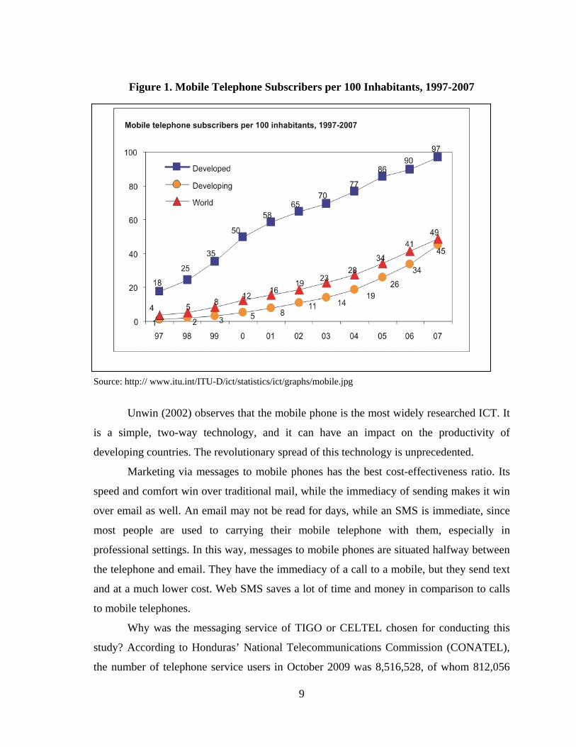
Figure 1. Mobile Telephone Subscribers per 100 Inhabitants, 1997-2007
Source: http:// www.itu.int/ITU-D/ict/statistics/ict/graphs/mobile.jpg
Unwin (2002) observes that the mobile phone is the most widely researched ICT. It
is a simple, two-way technology, and it can have an impact on the productivity of
developing countries. The revolutionary spread of this technology is unprecedented.
Marketing via messages to mobile phones has the best cost-effectiveness ratio. Its
speed and comfort win over traditional mail, while the immediacy of sending makes it win
over email as well. An email may not be read for days, while an SMS is immediate, since
most people are used to carrying their mobile telephone with them, especially in
professional settings. In this way, messages to mobile phones are situated halfway between
the telephone and email. They have the immediacy of a call to a mobile, but they send text
and at a much lower cost. Web SMS saves a lot of time and money in comparison to calls
to mobile telephones.
Why was the messaging service of TIGO or CELTEL chosen for conducting this
study? According to Honduras’ National Telecommunications Commission (CONATEL),
the number of telephone service users in October 2009 was 8,516,528, of whom 812,056
9
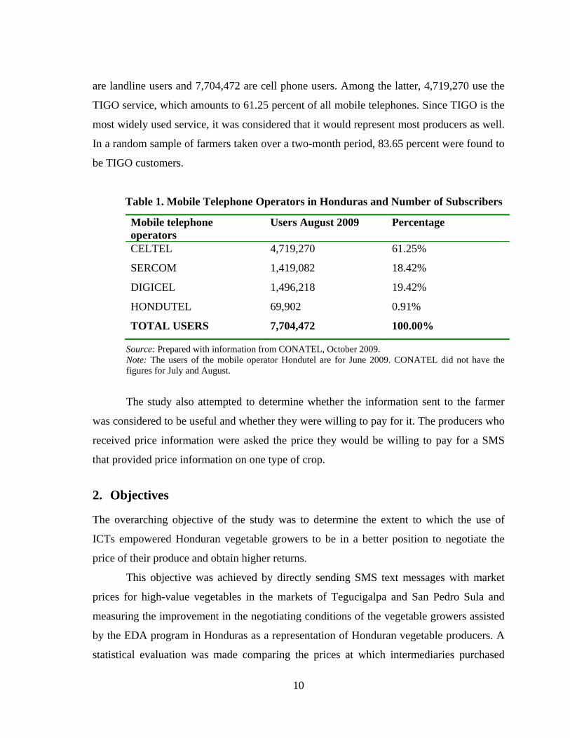
are landline users and 7,704,472 are cell phone users. Among the latter, 4,719,270 use the
TIGO service, which amounts to 61.25 percent of all mobile telephones. Since TIGO is the
most widely used service, it was considered that it would represent most producers as well.
In a random sample of farmers taken over a two-month period, 83.65 percent were found to
be TIGO customers.
Table 1. Mobile Telephone Operators in Honduras and Number of Subscribers
Mobile telephone operators
Users August 2009 Percentage
CELTEL 4,719,270 61.25%
SERCOM 1,419,082 18.42%
DIGICEL 1,496,218 19.42%
HONDUTEL 69,902 0.91%
TOTAL USERS 7,704,472 100.00%
Source: Prepared with information from CONATEL, October 2009. Note: The users of the mobile operator Hondutel are for June 2009. CONATEL did not have the figures for July and August.
The study also attempted to determine whether the information sent to the farmer
was considered to be useful and whether they were willing to pay for it. The producers who
received price information were asked the price they would be willing to pay for a SMS
that provided price information on one type of crop.
2. Objectives The overarching objective of the study was to determine the extent to which the use of
ICTs empowered Honduran vegetable growers to be in a better position to negotiate the
price of their produce and obtain higher returns.
This objective was achieved by directly sending SMS text messages with market
prices for high-value vegetables in the markets of Tegucigalpa and San Pedro Sula and
measuring the improvement in the negotiating conditions of the vegetable growers assisted
by the EDA program in Honduras as a representation of Honduran vegetable producers. A
statistical evaluation was made comparing the prices at which intermediaries purchased
10
from farmers who had access to the price information with those paid by intermediaries to
others who did not have access to this information.
2.1. Specific Objectives
The specific objectives of the study were the following:
1. Assess the effectiveness of SMS text messaging for disseminating
information about vegetable prices in Honduras, specifically for the
horticulture sector.
2. Ascertain the popularity of mobile phones among vegetable producers in
Honduras.
3. Make a socioeconomic assessment of a sub-sample of the horticulture
producers studied.
4. Provide information to investors so that they can determine if collecting
and disseminating market price information can be a profitable and
sustainable activity that, at a reasonable cost, helps vegetable growers
negotiate better prices for their produce.
3. Sources of Information For this study, different sources were used to substantiate and validate the proposal for
solution. Books, Internet consultations, and interviews with experts were used and are
reflected throughout the document, along with surveys of producers.
3.1 Primary
The primary information was collected from interviews with the main actors. Market data
were collected from the Marketing Department of the EDA Program, which has staff in the
northern and central parts of the country. Information was also gathered on the results of
sales of horticulture produce by the team in charge of the study, through cell phone calls
and personal interviews with a selected sample of producers.
11
3.2 Secondary
Secondary sources were consulted on the following issues:
• ICTs and their impact on development projects
• ICTs and development
• ICTs as an instrument for development in Honduras
• Design of experiments
• Design of quasi-experimental investigations
• Statistics for investigation
• Statistics with SPSS
• Previous studies about disseminating market prices using ICTs in
Honduras
• The use of cell telephones in Honduras
3.3 Techniques for Gathering Information
Various techniques were used to obtain in-depth knowledge about the factors affecting the
appropriate management of information technologies. These were personal communication,
telephone calls, and surveys of producers.
3.4 Information-Gathering Process
At the outset, the research team received a list of producers from the EDA Program that had
harvested or were harvesting for four months in a row during the year. The list included
telephone numbers and addresses of the farmers, the planting date and estimated harvest
date, the crop planted, and the size of the parcel of land.
It was possible to communicate with most of the producers who had CELTEL cell
phones. The subscribers were selected for economic reasons (sending text messages
represents a fixed cost for the use of the platform of each cell phone company with a
variable cost for each message sent) and because this company has a greater percentage of
producers who are subscribers. Using this procedure, the information provided by EDA
was verified: the cell phone number provided by them was in effect that of the producer,
and they would harvest at least one of the vegetables of interest on the estimated dates.
12
The market prices gathered from August 2009 to the week of October 4-10, 2009
were also received from EDA. Calls were made to the farmers harvesting between August
15 and October 14, who did not have the market prices when they were harvesting, in order
to conduct the survey in Annex 1.
The EDA Marketing Department provided information weekly on the prices paid on
these dates to farmers by Dandy market in San Pedro Sula and Zonal Belén in Tegucigalpa.
The prices continued to be received weekly until December 15. The prices were for the nine
vegetables considered to be the most profitable for the farmers, according to EDA. These
were yellow onions, sweet peppers, carrots, cabbage, salad tomatoes and processing
tomatoes, potatoes, cucumbers, plantain, and yucca/cassava.
A text message was sent with that information twice a week to the farmers over a
period of two months. The SMS included the prices by size of the vegetable (large,
medium, and small) since this information is very relevant to the buyer. This information
came from the Dandy and Zonal Belén markets since they are the most important ones for
wholesalers in San Pedro Sula and Tegucigalpa, respectively (Edgardo Varela of EDA).
Each producer who had been surveyed by telephone was called when their harvest was
over.
In order to consolidate the research and delve further into the use of ICTs, the
research team analyzed the socioeconomic conditions of the farmers. A survey was
designed to gather information about the availability of basic utilities, sources of income,
participation of family members in the production process, and others. From the list of
producers, 50 were randomly selected for an on-site socioeconomic assessment. The survey
was tabulated and the results enabled some preliminary conclusions to be drawn about the
relationship between the socioeconomic status of the farmer and the use of at least one ICT.
Figure 2 depicts a flow chart of the processes used in this study (not including the
socioeconomic analysis), including the procedure used and the interactions with those
involved.
13
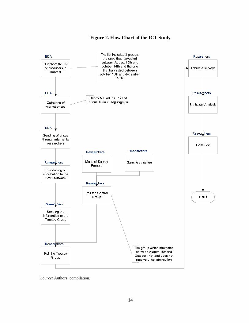
Figure 2. Flow Chart of the ICT Study
Source: Authors’ compilation.
14
15
4. Methodology
In order to find a solution to the problem of lack of real and timely price information, the
current situation was analyzed using the Ishikawa diagram, which enables an in-depth
examination of the primary and secondary causes of the problem.
4.1 Cause-Effect Analysis
The cause-effect analysis, or diagram, shown in Figure 3, presents the factors contributing
to the identified problem. One of the virtues of this diagram is that it promotes teamwork
by having different groups affected by the problem participate, which increases the
possibility that the causes of the problem will be identified and understood. The diagram
contains all of the variables influencing the lack of real and timely vegetable market price
information for vegetable growers.
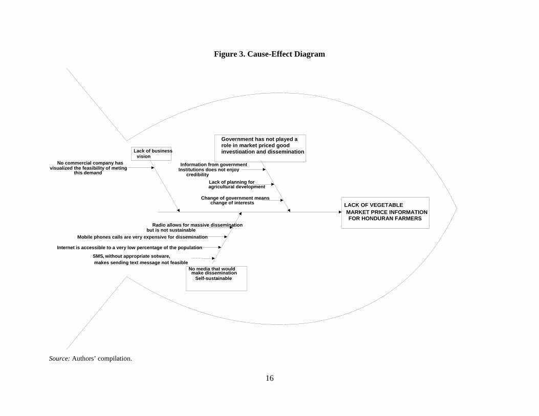
Figure 3. Cause-Effect Diagram
LACK OF VEGETABLE
MARKET PRICE INFORMATION FOR HONDURAN FARMERS
Lack of business vision
No media that would make dissemination
Self-sustainable
Government has not played a role in market priced good investigation and dissemination
Information from government Institutions does not enjoy
credibility
No commercial company has visualized the feasibilit of meting y
this demand
Internet is accessible to a very low percentage of the population
SMS , without appropriate so are, t wmakes sending text message not feasible
Mobile phones calls are very expensive for dissemination
Radio allows for massive dissemination but is not sustainable
Change of government means change of interests
Lack of planning foragricultural development
Source: Authors’ compilation.
16
The central government has lacked the capacity to create a system to publicize
market prices for agricultural products massively and in a sustainable way. The most
noteworthy effort was the creation of the SIMPAH, which was transferred to the FHIA to
be managed. Unfortunately, since dissemination of market prices is done by email, it has
had scant impact, as it does not reach farmers in isolated areas.
Radio broadcasts do not allow for sustainable provision of information, even though
they have the advantage of being inexpensive. It was not until the advent of the Internet,
together with dissemination via cell phone, that it has been possible to send messages en
masse through SMS.
Despite the fact that this technology has been in operation in Honduras for about a
decade, no private sector initiative had taken advantage of this business opportunity to meet
the demand for price information at a reasonable cost while at the same time generating
income from the service provided.
Once the SMS option was selected, using the methodology described above, the
study looked at whether in effect the transmission of weekly prices via SMS would enable
vegetable growers to negotiate a higher sales price of their produce with wholesalers.
4.2 Rationale for the Option Selected
Because SMS technology is a low-cost alternative for the recipient (i.e., the vegetable
grower), it was considered together with the radio as a possible ICT for dissemination. In
comparing the two low-cost alternatives, EDA determined that sustainability in the use of
SMS was the most important factor. Radio broadcasting could have been used to
demonstrate whether in effect there is a difference in income for vegetable farmers if they
receive price information, comparing the sales price for the two groups: one that does not
receive prices over a two-month period and the other that receives price information over
the radio for two months. However, this would not have met objective 3 of this study,
which is that the information generated induces a company or investor to take on the
activity as a profitable venture that also meets the need of Honduran vegetable farmers for
information.
17
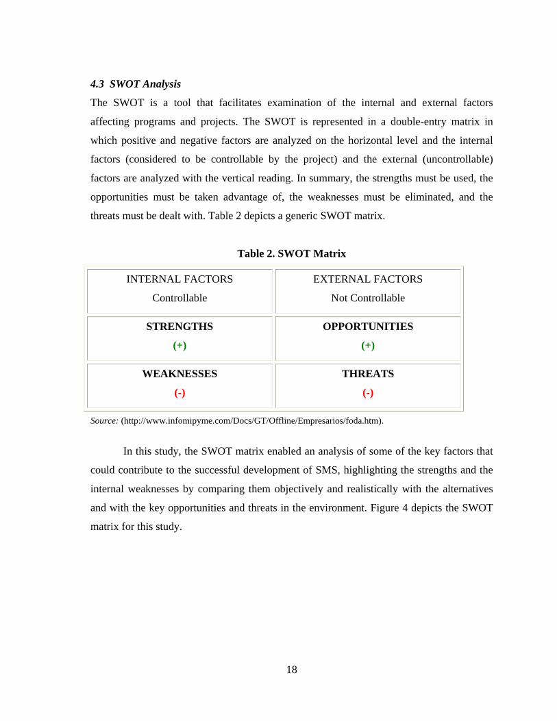
4.3 SWOT Analysis
The SWOT is a tool that facilitates examination of the internal and external factors
affecting programs and projects. The SWOT is represented in a double-entry matrix in
which positive and negative factors are analyzed on the horizontal level and the internal
factors (considered to be controllable by the project) and the external (uncontrollable)
factors are analyzed with the vertical reading. In summary, the strengths must be used, the
opportunities must be taken advantage of, the weaknesses must be eliminated, and the
threats must be dealt with. Table 2 depicts a generic SWOT matrix.
Table 2. SWOT Matrix
INTERNAL FACTORS
Controllable
EXTERNAL FACTORS
Not Controllable
STRENGTHS
(+)
OPPORTUNITIES
(+)
WEAKNESSES
(-)
THREATS
(-)
Source: (http://www.infomipyme.com/Docs/GT/Offline/Empresarios/foda.htm).
In this study, the SWOT matrix enabled an analysis of some of the key factors that
could contribute to the successful development of SMS, highlighting the strengths and the
internal weaknesses by comparing them objectively and realistically with the alternatives
and with the key opportunities and threats in the environment. Figure 4 depicts the SWOT
matrix for this study.
18
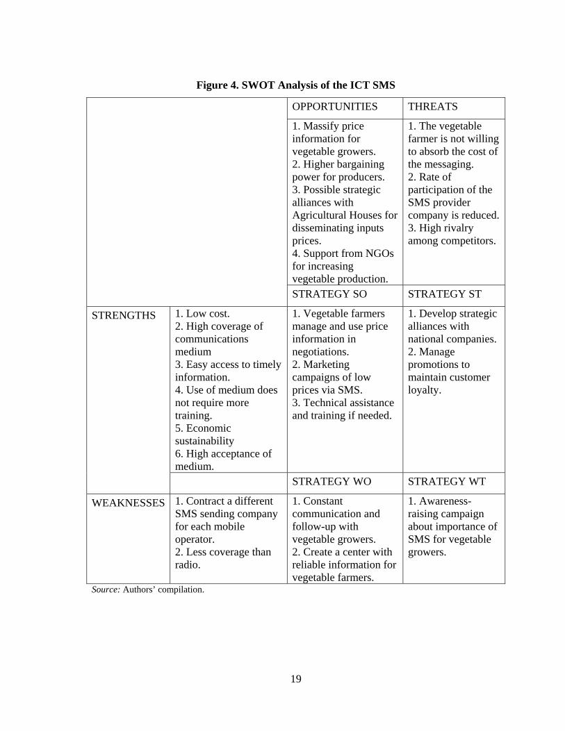
Figure 4. SWOT Analysis of the ICT SMS
OPPORTUNITIES THREATS
1. Massify price information for vegetable growers. 2. Higher bargaining power for producers. 3. Possible strategic alliances with Agricultural Houses for disseminating inputs prices. 4. Support from NGOs for increasing vegetable production.
1. The vegetable farmer is not willing to absorb the cost of the messaging. 2. Rate of participation of the SMS provider company is reduced. 3. High rivalry among competitors.
STRATEGY SO STRATEGY ST
STRENGTHS 1. Low cost. 2. High coverage of communications medium 3. Easy access to timely information. 4. Use of medium does not require more training. 5. Economic sustainability 6. High acceptance of medium.
1. Vegetable farmers manage and use price information in negotiations. 2. Marketing campaigns of low prices via SMS. 3. Technical assistance and training if needed.
1. Develop strategic alliances with national companies. 2. Manage promotions to maintain customer loyalty.
STRATEGY WO STRATEGY WT
WEAKNESSES 1. Contract a different SMS sending company for each mobile operator. 2. Less coverage than radio.
1. Constant communication and follow-up with vegetable growers. 2. Create a center with reliable information for vegetable farmers.
1. Awareness-raising campaign about importance of SMS for vegetable growers.
Source: Authors’ compilation.
19
4.4 Analysis of the Options
The factors taken into consideration when evaluating the various options for disseminating
prices through ICT were the following:
• Geographic coverage: greater coverage for a greater number of farmers
can be achieved.
• Massification of use: the more vegetable growers who use the ICT, the
more receivers of the price messages there will be.
• Unit cost for sending per recipient.
• Sustainability: even when a dissemination program can begin with
financing from the government or some non-governmental entity, having
the income from the activity cover the costs and generate a profit in the
medium term must be considered.
• Efficacy of receipt of the message: the message must reach the farmer in
a timely fashion. If the message is sent but not received by the recipient,
it will not be useful.
Ways of disseminating market prices efficiently, effectively, and sustainably were
analyzed. The first option analyzed was sending price information over the Internet. The
second option was dissemination of market prices over the radio, using the radio stations
with the greatest coverage in the country. The third option analyzed was disseminating
prices by SMS text messages to a specific group of vegetable farmers.
The options for communication technologies that most Honduran producers have
are radio and cellular telephones. The cost of radio dissemination per farmer receiving the
price can be low. A 30-second radio spot broadcast twice a day for a month on one of the
two radio stations with the greatest coverage in Honduras (Radio América or HRN) can
cost $1,000 (Varela, E., personal communication, April 2009). The cost of sending a text
message is $0.05 per recipient plus a fixed cost of $200 a month for use of the platform of a
company that provides this service (Padilla, L., personal communication, October 2009).
Radio is the cheapest medium for dissemination because of the number of people
listening to it, which makes it more efficient. However, if we consider effectiveness and
20
sustainability, SMS is more advantageous. When the message is broadcast, if the farmer is
not there to hear it or one of his family members is not there to tell him later, the message is
lost. The SMS, however, is stored in the mobile telephone even when there is no cell phone
signal at the farmer’s location during the day, and it will be received when the phone is in
an area reached by the signal. This enables the farmer to read the SMS at any time of day
and to save it after it is received.
In terms of sustainability, the radio spots could be funded by an entity such as the
government of Honduras through the Secretariat for Agriculture and Ranching or through a
non-governmental entity. Once funding is no longer available, dissemination ends. SMS is
versatile since only those who receive the information pay for it. This payment not only
sustains the sending of the information by this medium, but also represents a savings to the
farmers, who can thus avoid having to go to the important purchasing centers or markets to
check the sales price for their produce. This study concluded that the solution was to
disseminate market prices for the most profitable or most widely consumed vegetables via
SMS or text messages when the subscriber (vegetable grower) asks for it.
Table 3. Summary of Advantages and Disadvantages of the Options
Alternative for solution
Advantages Disadvantages
Internet - Low cost per recipient - Little access in rural areas - Low number of users
Radio
- Massive dissemination in a large percentage of the national territory
- Very low cost per recipient
- Cost of dissemination must be covered by some institution.
- System can be unsustainable because of not finding donor institutions or sponsors.
- If recipient is not present at time of broadcast, the message is lost.
SMS - Widespread dissemination throughout the country.
- Low cost per recipient. - Recipient of message pays for the
information. - Can be incorporated into a
publicity system in order to increase profitability.
- The message is received when there is cell signal and is recorded in the cell phone.
- Less coverage than radio. - A different company must be
contracted for sending SMS for each mobile operator with which one wants to work.
Source: Authors’ compilation.
21
4.5 Hypothesis
The increase in income from their production for the farmers assisted by the EDA program
has a statistically significant relationship to the empowerment that results from having
access to up-to-date and reliable market prices for vegetables disseminated by information
and communication technologies.
4.6 Research Design
According to Bernal (2006), a quasi-experimental design is one in which the researcher
controls only one variable in two groups being compared. By definition, this design does
not use random selection. This kind of design is frequently used in the social sciences in
general when random selection is not always possible, and it is very useful when a control
group cannot be identified. In this study, two groups selected at two given periods of time
were compared: one which received market price information for vegetables and another
that did not (so the only variable controlled is price information given to the treated group).
Among quasi-experimental designs are Interrupted Time Series Designs. An
Interrupted Time Series Design is one of the most effective and powerful quasi-
experimental designs, especially when complemented by other elements. An Interrupted
Time Series Design refers to a long series of observations made of the same variable
consecutively over time. The observations can be made of the same units or study subjects,
as in studies of medical or psychiatric symptoms in an individual observed repeatedly. The
observations can also be of different units or subjects for study (with common
characteristics), as in the case of traffic deaths in a department or state of a country over
many years, during which the population is constantly changing (Shadish, 2002).
A Simple Interrupted Time Series Design requires a treatment of one of the groups
being compared and many observations (preferably more than 100, according to Shadish,
2002) before and after the treatment. A design with 10 observations can be diagrammed as
follows:
O1 O2 O3 O4 O5 X O6 O7 O8 O9 O10
22
In this study, it was the observation of farmers that grow nine types of vegetables (similar
in this characteristic), but in two distinct groups: those who do not receive market prices
and those who do.
As can be seen from the surveys in Annexes 1 and 2, other variables were studied
that could have an influence on the price received: type of intermediary or final customer to
which they sell (the number of probable final intermediaries is measured), the crop, the
market to which they sell (local or main cities, with which the payment capacity of their
market is measured), size of the parcel of land they have (to measure whether there is
bargaining power because of volume), years of experience with the crop, and time of
receiving technical assistance, among others. By measuring these variables, the effect of
each factor on the farmer’s bargaining power, and therefore the price received, was
measured if there was any effect at all.
In designing the survey for systematizing it later, the book Statistics for Research,
with a Guide to SPSS (Argyrous, 2005) was consulted. This reference also provides
guidelines on how to enter the information from the survey into the SPSS program Version
15.
4.7 Description of the Variables Department where production is located. The department of Honduras where the
production occurred. The farmers of the EDA project are located in 16 of the 18
departments of the country, but the random sample only included 14 of them. A political
map of Honduras is shown on Annex 6.
Years of technical assistance. The goal of technical assistance is to improve the quantity
and quality of production using better production techniques. The technical assistance from
the EDA project also includes seeking new markets for the farmers. The main goal of the
marketing component is to establish more formal commercial relationships, according to
Edgardo Varela.
Years of experience with the crop. This varies greatly in the sample, from one crop cycle
(months) to several decades of experience.
23

Crop. There are nine crops (dividing tomatoes into salad and processing). There are no
onion growers in the sample, though it is one of the crops for which prices were sent. Each
crop has a different behavior. The price varies according to the crop itself (supply and
demand) and the price can be very different from week to week with respect to the other
crops.
Month of harvest. Since the investigation design is Interrupted Time Series, each group
was divided into three months: August, September, and October (partial) for those treated
and October (partial), November, and December for those not treated.
Area planted. The unit of measure is the manzana (mz), which is widely used in
Honduras. One manzana has 7400 m2. There is a broad range of areas (from 0.13 to more
than 9 manzanas). A normal question for this variable is whether having a larger area of
land gives farmers more bargaining power.
Total production. The unit of measure is the pound. Each crop has a different yield per
area planted because of its particular biological characteristics. Like the previous variable,
there is the question of whether there is more negotiating power with greater production.
There are six ranges of production in multiples of 10,000 pounds to more than 50,000
pounds.
Market. Although the prices used in the study are from two main markets in the two main
cities, there were 16 markets, among them the two main ones, but there is a considerable
number of farmers who sold locally or to nearby small cities.
Type of client. This is type of client to which the farmer sells their produce. There are
eight categories, among them supermarkets, intermediaries, market retailers, and industry.
Quality by category. Because of the different price ranges paid for different quality, this
variable was added. Some vegetables have no range of categories and some have three.
Percentage difference of price. By having various crops, the principal dependent variable
must be made uniform since the prices for each of the vegetables are different among
24
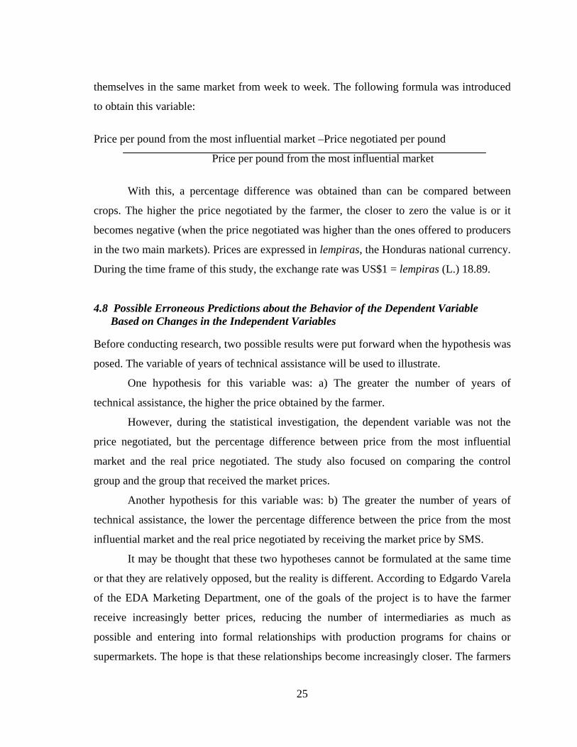
themselves in the same market from week to week. The following formula was introduced
to obtain this variable:
Price per pound from the most influential market –Price negotiated per pound
Price per pound from the most influential market
With this, a percentage difference was obtained than can be compared between
crops. The higher the price negotiated by the farmer, the closer to zero the value is or it
becomes negative (when the price negotiated was higher than the ones offered to producers
in the two main markets). Prices are expressed in lempiras, the Honduras national currency.
During the time frame of this study, the exchange rate was US$1 = lempiras (L.) 18.89.
4.8 Possible Erroneous Predictions about the Behavior of the Dependent Variable Based on Changes in the Independent Variables Before conducting research, two possible results were put forward when the hypothesis was
posed. The variable of years of technical assistance will be used to illustrate.
One hypothesis for this variable was: a) The greater the number of years of
technical assistance, the higher the price obtained by the farmer.
However, during the statistical investigation, the dependent variable was not the
price negotiated, but the percentage difference between price from the most influential
market and the real price negotiated. The study also focused on comparing the control
group and the group that received the market prices.
Another hypothesis for this variable was: b) The greater the number of years of
technical assistance, the lower the percentage difference between the price from the most
influential market and the real price negotiated by receiving the market price by SMS.
It may be thought that these two hypotheses cannot be formulated at the same time
or that they are relatively opposed, but the reality is different. According to Edgardo Varela
of the EDA Marketing Department, one of the goals of the project is to have the farmer
receive increasingly better prices, reducing the number of intermediaries as much as
possible and entering into formal relationships with production programs for chains or
supermarkets. The hope is that these relationships become increasingly closer. The farmers
25
who recently entered the program do not necessarily have close relationships with their
buyers, because it takes time to build them. In the group of producers that received limited
technical assistance, like one crop cycle or a few months, those who receive the market
price information can reduce this differential by obtaining better prices. However, this same
trend may not happen among the two groups of producers with more time of technical
assistance, since their close relationships, which can even include pre-negotiations, are not
affected by the farmers having market prices.
4.9 Statistical Analysis
With the information from the survey, a Univariant Analysis of Variance (ANOVA) was
carried out, testing for the interaction of each variable with the treatment (sending of
prices). For these analyses, all the variables in 4.4 were used, with the percentage difference
of price as the dependent variable and the treatment as the independent variable, which
interacted with the other independent variables. Bryman and Cramer (2005) suggest that the
steps for the Univariant ANOVA include the Levene test of homogeneity of variants in
order to determine the method for comparison of means to use.
A Linear Regression Analysis was used that included all the variables. Argyrous
(2005) indicated that the variable Enter method is generally favored because it means that
before the statistical analysis, we must think about what our hypothesis suggests about the
nature of the relationships of interest to us. This method was used, including all the
variables of interest which were forecasted to have an influence on the dependent variable.
As part of the analysis of the information, a specific study was made of the surveys
of the treated group, in which the frequencies of the farmers saying they had benefited from
price information and those who did not was measured. To corroborate the information, a
calculation was made of the frequency of those who would be willing to pay for the
information and the reasons stated for why they would or would not pay. There was also a
calculation of the difference in price for which the treated producers sold versus what they
think they would have sold for if they did not have the price information.
26

4.10 Socioeconomic Assessment
The socioeconomic assessment was made using the Poverty Score Card for Honduras
developed and provided by the researcher Mark Schreiner. Visits were made to the homes
of 46 of 50 randomly selected producers from the total sample of producers surveyed
(control group and those treated). The tables from the National Poverty Line and the
USAID Extreme Poverty Line were used to determine the probability that the producer’s
income was below the poverty line.
Aside from the valuable information provided by the survey used for the
assessment, the following issues were found:
• The isolation of various agricultural production regions in the country.
• The difficulty in transporting harvests because of the condition of the
country’s secondary and tertiary roads.
• Difficulty of recharging cell phones daily due to the lack of electricity.
Farmers cannot therefore leave them on all day, limiting communication.
• The value of technical assistance in the most isolated zones of the
country where no government entity has regular access to provide it.
5. Results The following tables depict the statistical results from the surveys on price information with
the control group and the treated group.
Table 4. Linear Regression Analysis: Variables Entered/Removed (b)
Model Variables Entered Variables Removed Method
1 Quality category, Treatment, Nearest main city price, Years technical assistance, Market, Years experience (a)
. Enter
a All variables listed included b Dependent: Price Percentage Difference
27

Table 5. Model Summary
Model R
R Squar
e
Adjusted R
Square
Std. Error of
the Estimate
Change Statistics R Square Change
F Change df1 df2
Sig. F Change
1 0.452(a) 0.205 0.196 0.73455 0.205 23.282 6 543 0.000
a Predictors: (Constant), Quality category, Treatment, Nearest main city price, Years of technical assistance, Market, Years of experience
The model shows a low regression coefficient between the combination of
independent variables included and the dependent variable. The level of significance of the
coefficient is high. Despite the model explaining a low portion of the behavior of the
independent variable, the probability that it happened by chance is very low.
Table 6. ANOVA(b)
Model
Sum of
Squares df Mean Square F Sig.
1 Regression 75.372 6 12.562 23.282 .000(a)
Residual 292.984 543 .540
Total 368.355 549
a Predictors: (Constant), Quality category, Treatment, Nearest main city price, Years of technical assistance, Market, Years of experience b Dependent: Price Percentage difference
28
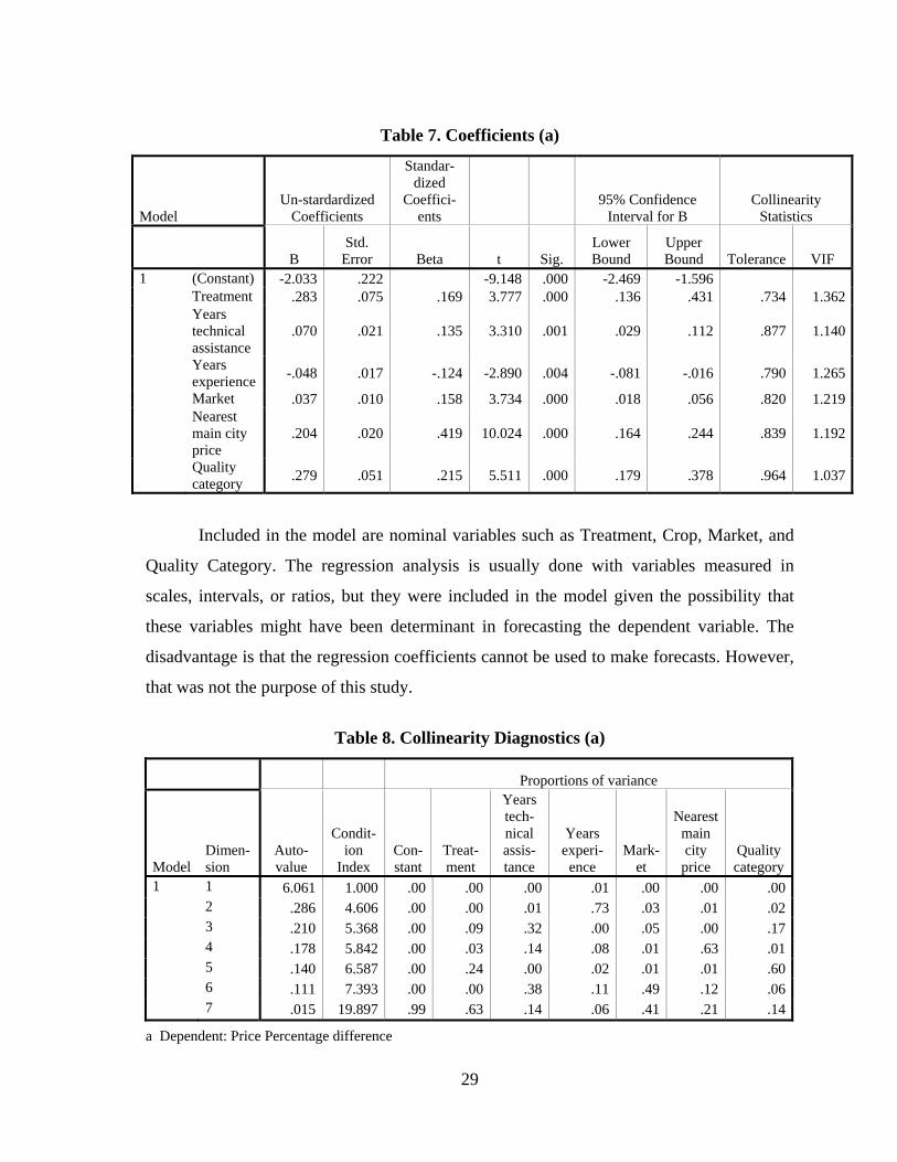
Table 7. Coefficients (a)
Model Un-stardardized
Coefficients
Standar-dized
Coeffici-ents
95% Confidence Interval for B
Collinearity Statistics
B Std.
Error Beta t Sig. Lower Bound
Upper Bound Tolerance VIF
1 (Constant) -2.033 .222 -9.148 .000 -2.469 -1.596 Treatment .283 .075 .169 3.777 .000 .136 .431 .734 1.362 Years
technical assistance
.070 .021 .135 3.310 .001 .029 .112 .877 1.140
Years experience -.048 .017 -.124 -2.890 .004 -.081 -.016 .790 1.265
Market .037 .010 .158 3.734 .000 .018 .056 .820 1.219 Nearest
main city price
.204 .020 .419 10.024 .000 .164 .244 .839 1.192
Quality category .279 .051 .215 5.511 .000 .179 .378 .964 1.037
Included in the model are nominal variables such as Treatment, Crop, Market, and
Quality Category. The regression analysis is usually done with variables measured in
scales, intervals, or ratios, but they were included in the model given the possibility that
these variables might have been determinant in forecasting the dependent variable. The
disadvantage is that the regression coefficients cannot be used to make forecasts. However,
that was not the purpose of this study.
Table 8. Collinearity Diagnostics (a)
Proportions of variance
Model
Dimen-sion
Auto-value
Condit-ion
Index Con-stant
Treat-ment
Years tech-nical assis-tance
Years experi-ence
Mark-et
Nearest main city
price Quality category
1 1 6.061 1.000 .00 .00 .00 .01 .00 .00 .00 2 .286 4.606 .00 .00 .01 .73 .03 .01 .02 3 .210 5.368 .00 .09 .32 .00 .05 .00 .17 4 .178 5.842 .00 .03 .14 .08 .01 .63 .01 5 .140 6.587 .00 .24 .00 .02 .01 .01 .60 6 .111 7.393 .00 .00 .38 .11 .49 .12 .06 7 .015 19.897 .99 .63 .14 .06 .41 .21 .14
a Dependent: Price Percentage difference
29
Leaving aside the independent term, we see that multi-collinearity affects the
variable Treatment more than other independent variables, which is what has a greater
proportion of variance associated with the index of condition. Variables like Area Planted
and Client Type, which were not significant in preliminary tests, were not included in the
model.
5.1 One-Way ANOVA Treatment by Crop
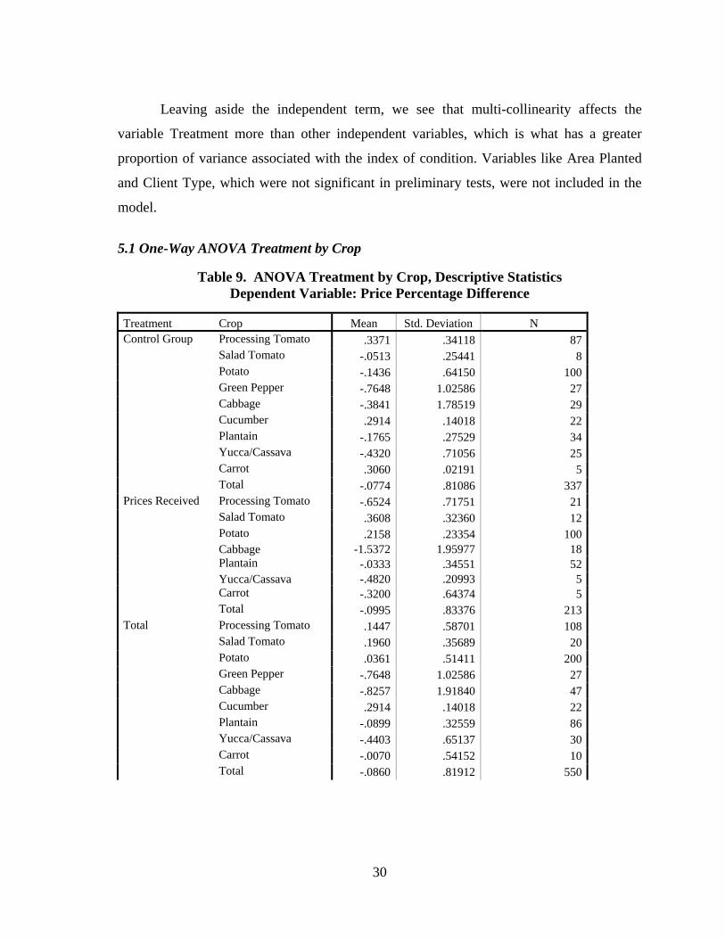
Table 9. ANOVA Treatment by Crop, Descriptive Statistics Dependent Variable: Price Percentage Difference
Treatment Crop Mean Std. Deviation N Control Group Processing Tomato .3371 .34118 87 Salad Tomato -.0513 .25441 8 Potato -.1436 .64150 100 Green Pepper -.7648 1.02586 27 Cabbage -.3841 1.78519 29 Cucumber .2914 .14018 22 Plantain -.1765 .27529 34 Yucca/Cassava -.4320 .71056 25 Carrot .3060 .02191 5 Total -.0774 .81086 337 Prices Received Processing Tomato -.6524 .71751 21 Salad Tomato .3608 .32360 12 Potato .2158 .23354 100 Cabbage -1.5372 1.95977 18 Plantain -.0333 .34551 52 Yucca/Cassava -.4820 .20993 5 Carrot -.3200 .64374 5 Total -.0995 .83376 213 Total Processing Tomato .1447 .58701 108 Salad Tomato .1960 .35689 20 Potato .0361 .51411 200 Green Pepper -.7648 1.02586 27 Cabbage -.8257 1.91840 47 Cucumber .2914 .14018 22 Plantain -.0899 .32559 86 Yucca/Cassava -.4403 .65137 30 Carrot -.0070 .54152 10 Total -.0860 .81912 550
30

Table 10. Levene’s Test of Equality of Error Variances (a) Dependent Variable: Price Percentage Difference
F df1 df2 Sig 18.399 15 534 .000
Tests the null hypothesis that the error variance of the dependent variable is equal across groups. a Design: Intercept + Treatment + Crop + Treatment * Crop
The Levine Test of Homogeneity showed that there are significant differences
between the variances of the groups. Because of this, the Tamhane Post Hoc Comparison of
Measures Test suggested by Bryman (2005) was conducted. It was not possible to reduce
the grossly unequal variances neither through transforming the data by taking the log or
square root of the dependent variable.
Table 11. Test of Between-Subjects Effects
Dependent Variable: Price Percentage Difference
Source
Type III Sum of Squares df
Mean Square F Sig.
Corrected Model 95.461(a) 15 6.364 12.453 .000
Intercept 12.084 1 12.084 23.645 .000 Treatment 3.400 1 3.400 6.653 .010 Crop 55.124 8 6.891 13.483 .000 Treatment * Crop 39.370 6 6.562 12.840 .000
Error 272.894 534 .511 Total 372.421 550 Total corrected 368.355 549
a R squared = .259 (Adjusted R Squared = .238)
The results indicate there is a significant effect for the treatment factor (p<0.010)
and a highly significant interaction effect for Treatment and Crop (p<0.0001) as well as for
the Crop factor (p<0.0001).
31
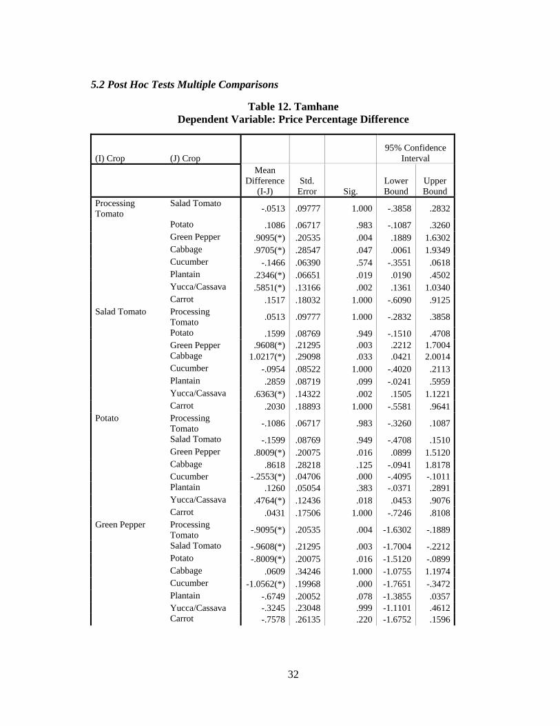
5.2 Post Hoc Tests Multiple Comparisons
Table 12. Tamhane Dependent Variable: Price Percentage Difference
(I) Crop (J) Crop 95% Confidence
Interval
Mean Difference
(I-J) Std.
Error Sig. Lower Bound
Upper Bound
Processing Tomato
Salad Tomato -.0513 .09777 1.000 -.3858 .2832
Potato .1086 .06717 .983 -.1087 .3260 Green Pepper .9095(*) .20535 .004 .1889 1.6302 Cabbage .9705(*) .28547 .047 .0061 1.9349 Cucumber -.1466 .06390 .574 -.3551 .0618 Plantain .2346(*) .06651 .019 .0190 .4502 Yucca/Cassava .5851(*) .13166 .002 .1361 1.0340 Carrot .1517 .18032 1.000 -.6090 .9125 Salad Tomato Processing
Tomato .0513 .09777 1.000 -.2832 .3858
Potato .1599 .08769 .949 -.1510 .4708 Green Pepper .9608(*) .21295 .003 .2212 1.7004 Cabbage 1.0217(*) .29098 .033 .0421 2.0014 Cucumber -.0954 .08522 1.000 -.4020 .2113 Plantain .2859 .08719 .099 -.0241 .5959 Yucca/Cassava .6363(*) .14322 .002 .1505 1.1221 Carrot .2030 .18893 1.000 -.5581 .9641 Potato Processing
Tomato -.1086 .06717 .983 -.3260 .1087
Salad Tomato -.1599 .08769 .949 -.4708 .1510 Green Pepper .8009(*) .20075 .016 .0899 1.5120 Cabbage .8618 .28218 .125 -.0941 1.8178 Cucumber -.2553(*) .04706 .000 -.4095 -.1011 Plantain .1260 .05054 .383 -.0371 .2891 Yucca/Cassava .4764(*) .12436 .018 .0453 .9076 Carrot .0431 .17506 1.000 -.7246 .8108 Green Pepper Processing
Tomato -.9095(*) .20535 .004 -1.6302 -.1889
Salad Tomato -.9608(*) .21295 .003 -1.7004 -.2212 Potato -.8009(*) .20075 .016 -1.5120 -.0899 Cabbage .0609 .34246 1.000 -1.0755 1.1974 Cucumber -1.0562(*) .19968 .000 -1.7651 -.3472 Plantain -.6749 .20052 .078 -1.3855 .0357 Yucca/Cassava -.3245 .23048 .999 -1.1101 .4612 Carrot -.7578 .26135 .220 -1.6752 .1596
32
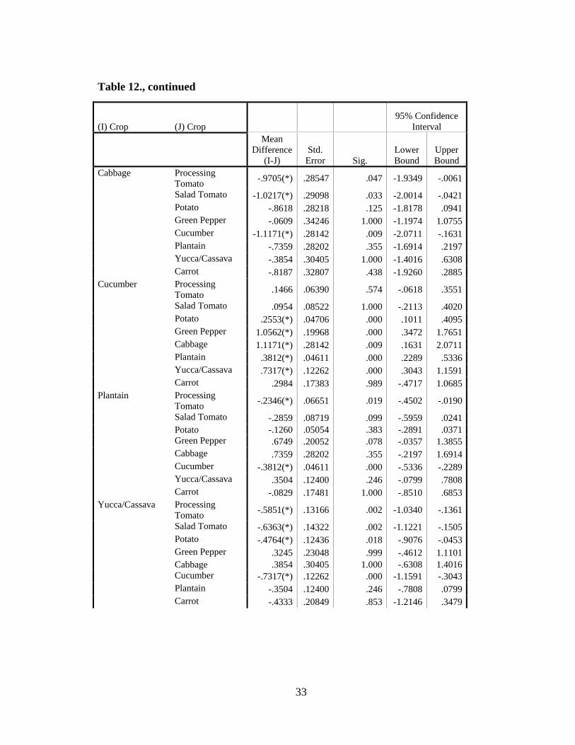
Table 12., continued
(I) Crop (J) Crop 95% Confidence
Interval
Mean Difference
(I-J) Std.
Error Sig. Lower Bound
Upper Bound
Cabbage Processing Tomato -.9705(*) .28547 .047 -1.9349 -.0061
Salad Tomato -1.0217(*) .29098 .033 -2.0014 -.0421 Potato -.8618 .28218 .125 -1.8178 .0941 Green Pepper -.0609 .34246 1.000 -1.1974 1.0755 Cucumber -1.1171(*) .28142 .009 -2.0711 -.1631 Plantain -.7359 .28202 .355 -1.6914 .2197 Yucca/Cassava -.3854 .30405 1.000 -1.4016 .6308 Carrot -.8187 .32807 .438 -1.9260 .2885 Cucumber Processing
Tomato .1466 .06390 .574 -.0618 .3551
Salad Tomato .0954 .08522 1.000 -.2113 .4020 Potato .2553(*) .04706 .000 .1011 .4095 Green Pepper 1.0562(*) .19968 .000 .3472 1.7651 Cabbage 1.1171(*) .28142 .009 .1631 2.0711 Plantain .3812(*) .04611 .000 .2289 .5336 Yucca/Cassava .7317(*) .12262 .000 .3043 1.1591 Carrot .2984 .17383 .989 -.4717 1.0685 Plantain Processing
Tomato -.2346(*) .06651 .019 -.4502 -.0190
Salad Tomato -.2859 .08719 .099 -.5959 .0241 Potato -.1260 .05054 .383 -.2891 .0371 Green Pepper .6749 .20052 .078 -.0357 1.3855 Cabbage .7359 .28202 .355 -.2197 1.6914 Cucumber -.3812(*) .04611 .000 -.5336 -.2289 Yucca/Cassava .3504 .12400 .246 -.0799 .7808 Carrot -.0829 .17481 1.000 -.8510 .6853 Yucca/Cassava Processing
Tomato -.5851(*) .13166 .002 -1.0340 -.1361
Salad Tomato -.6363(*) .14322 .002 -1.1221 -.1505 Potato -.4764(*) .12436 .018 -.9076 -.0453 Green Pepper .3245 .23048 .999 -.4612 1.1101 Cabbage .3854 .30405 1.000 -.6308 1.4016 Cucumber -.7317(*) .12262 .000 -1.1591 -.3043 Plantain -.3504 .12400 .246 -.7808 .0799 Carrot -.4333 .20849 .853 -1.2146 .3479
33
34
Table 12., continued
(I) Crop (J) Crop 95% Confidence
Interval
Mean Difference
(I-J) Std.
Error Sig. Lower Bound
Upper Bound
Carrot Processing Tomato -.1517 .18032 1.000 -.9125 .6090
Salad Tomato -.2030 .18893 1.000 -.9641 .5581 Potato -.0431 .17506 1.000 -.8108 .7246 Green Pepper .7578 .26135 .220 -.1596 1.6752 Cabbage .8187 .32807 .438 -.2885 1.9260 Cucumber -.2984 .17383 .989 -1.0685 .4717 Plantain .0829 .17481 1.000 -.6853 .8510 Yucca/Cassava .4333 .20849 .853 -.3479 1.2146
Based on the means observed. * The mean difference is significant at .05 level.
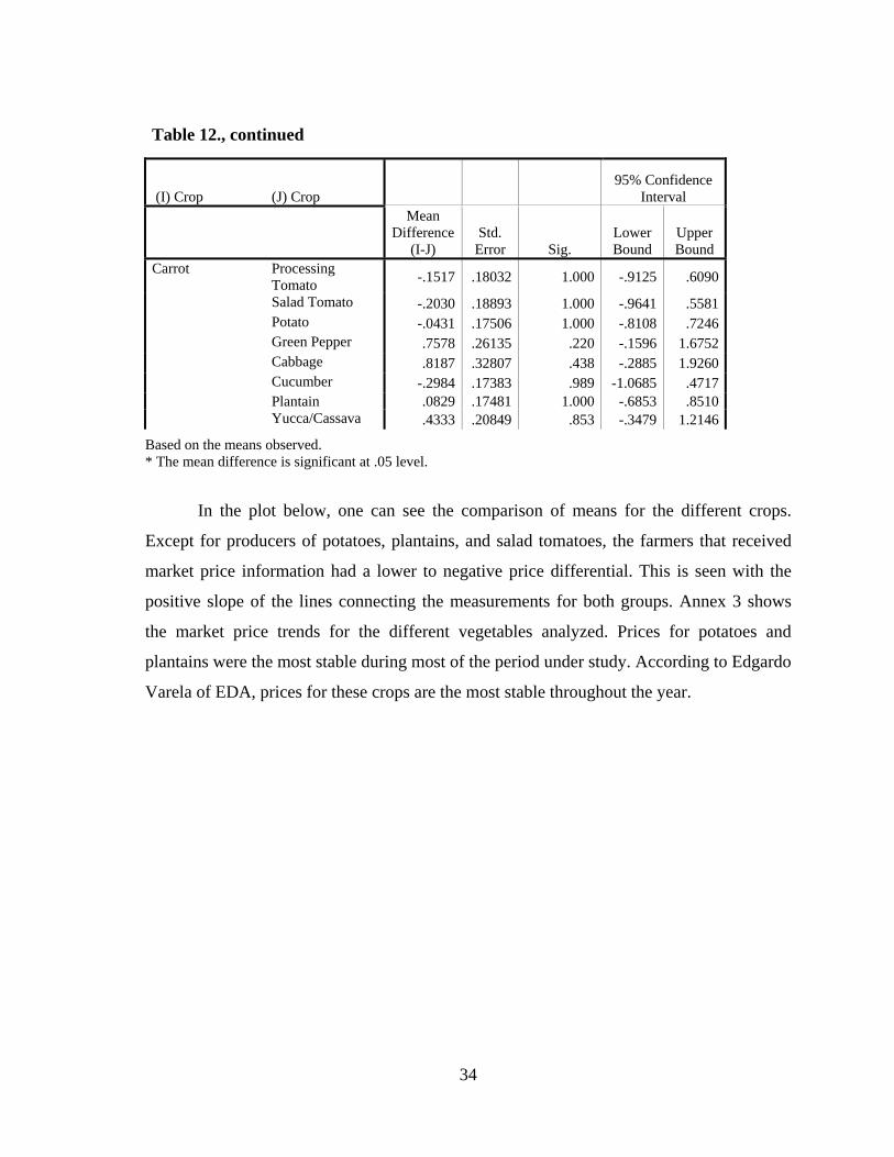
In the plot below, one can see the comparison of means for the different crops.
Except for producers of potatoes, plantains, and salad tomatoes, the farmers that received
market price information had a lower to negative price differential. This is seen with the
positive slope of the lines connecting the measurements for both groups. Annex 3 shows
the market price trends for the different vegetables analyzed. Prices for potatoes and
plantains were the most stable during most of the period under study. According to Edgardo
Varela of EDA, prices for these crops are the most stable throughout the year.
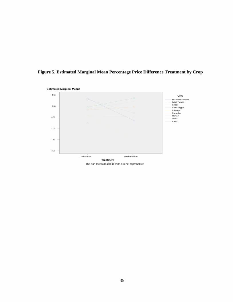
Figure 5. Estimated Marginal Mean Percentage Price Difference Treatment by Crop
The non measureable means are not represented
Crop
YuccaPlantain Cucumber Cabbage Green Pepper Potato Salad Tomato Processing Tomato
Carrot
-2.00
-1.50
-1.00
-0.50
0.00
0.50
Estimated Marginal Means
TreatmentReceived PricesControl Grup
35

5.3 One-Way ANOVA Treatment by Years of Technical Assistance Table 13. ANOVA Treatment by Years of Technical Assistance,-Descriptive Statistics
Dependent variable: Price Percentage Difference
Treatment
Years of Technical Assistance Mean
Standard Deviation N
Control Group <0.5 years .1989 .40789 37 0.6-1.0 years -.5494 .93975 67 1.1-1.5 years .1355 .39466 33 1.6-2.0 years .0164 .96085 132 2.1-2.5 .2500 .00000 2 >2.5 years -.0573 .39345 66 Total -.0774 .81086 337 Prices Received
<0.5 years -.1788 1.21595 40
0.6-1.0 years -.1959 1.03758 46 1.1-1.5 years -.1234 .64743 87 1.6-2.0 years .6700 . 1 2.1-2.5 .1017 .28151 18 >2.5 years .1524 .15636 21 Total -.0995 .83376 213 Total <0.5 years .0027 .93467 77 0.6-1.0 years -.4055 .99166 113 1.1-1.5 years -.0523 .59857 120 1.6-2.0 years .0214 .95888 133 2.1-2.5 .1165 .27017 20 >2.5 years -.0067 .36171 87 Total -.0860 .81912 550
Table 14. Levene Test of Equality of Error Variances (a) Dependent Variable: Price Percentage Difference
F gl1 gl2 Significance 3.794 11 538 .000
Tests the null hypothesis that the error variance of the dependent variable is equal across groups. a Design: Intersection + Treatment + Years technical assistance + Treatment * Years technical assistance
36
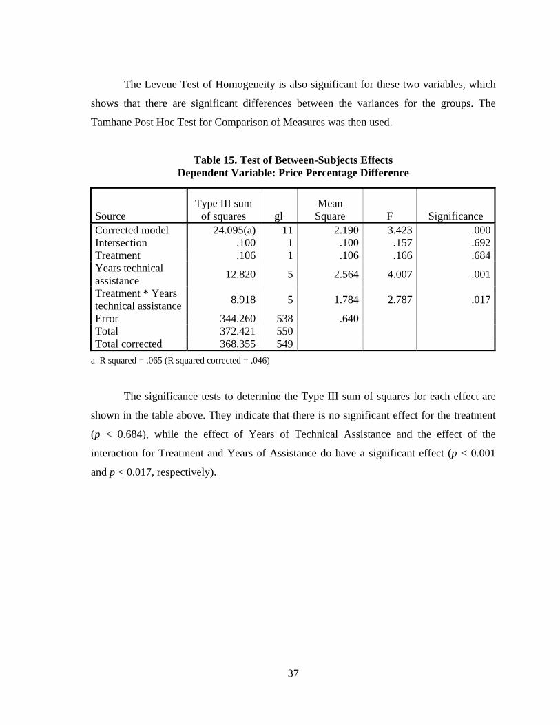
The Levene Test of Homogeneity is also significant for these two variables, which
shows that there are significant differences between the variances for the groups. The
Tamhane Post Hoc Test for Comparison of Measures was then used.
Table 15. Test of Between-Subjects Effects Dependent Variable: Price Percentage Difference
Source Type III sum
of squares gl Mean Square F Significance
Corrected model 24.095(a) 11 2.190 3.423 .000Intersection .100 1 .100 .157 .692Treatment .106 1 .106 .166 .684Years technical assistance 12.820 5 2.564 4.007 .001
Treatment * Years technical assistance 8.918 5 1.784 2.787 .017
Error 344.260 538 .640 Total 372.421 550 Total corrected 368.355 549
a R squared = .065 (R squared corrected = .046)
The significance tests to determine the Type III sum of squares for each effect are
shown in the table above. They indicate that there is no significant effect for the treatment
(p < 0.684), while the effect of Years of Technical Assistance and the effect of the
interaction for Treatment and Years of Assistance do have a significant effect (p < 0.001
and p < 0.017, respectively).
37
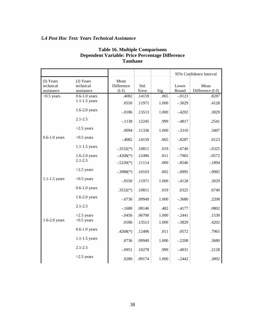
5.4 Post Hoc Test: Years Technical Assistance
Table 16. Multiple Comparisons Dependent Variable: Price Percentage Difference
Tamhane
95% Confidence Interval
(I) Years technical assistance
(J) Years technical assistance
Mean Difference
(I-J) Std.
Error Sig. Lower Bound
Mean Difference (I-J)
<0.5 years 0.6-1.0 years .4082 .14159 .065 -.0123 .8287 1.1-1.5 years .0550 .11971 1.000 -.3029 .4128
1.6-2.0 years -.0186 .13513 1.000 -.4202 .3829
2.1-2.5 -.1138 .12245 .999 -.4817 .2541
>2.5 years .0094 .11336 1.000 -.3310 .3497
0.6-1.0 years <0.5 years -.4082 .14159 .065 -.8287 .0123
1.1-1.5 years -.3532(*) .10811 .019 -.6740 -.0325
1.6-2.0 years -.4268(*) .12496 .011 -.7965 -.0572 2.1-2.5 -.5220(*) .11114 .000 -.8546 -.1894
>2.5 years -.3988(*) .10103 .002 -.6995 -.0982
1.1-1.5 years <0.5 years -.0550 .11971 1.000 -.4128 .3029
0.6-1.0 years .3532(*) .10811 .019 .0325 .6740
1.6-2.0 years -.0736 .09949 1.000 -.3680 .2208
2.1-2.5 -.1688 .08146 .482 -.4177 .0802
>2.5 years -.0456 .06700 1.000 -.2441 .15301.6-2.0 years <0.5 years .0186 .13513 1.000 -.3829 .4202
0.6-1.0 years .4268(*) .12496 .011 .0572 .7965
1.1-1.5 years .0736 .09949 1.000 -.2208 .3680
2.1-2.5 -.0951 .10278 .999 -.4031 .2128
>2.5 years .0280 .09174 1.000 -.2442 .3002
38
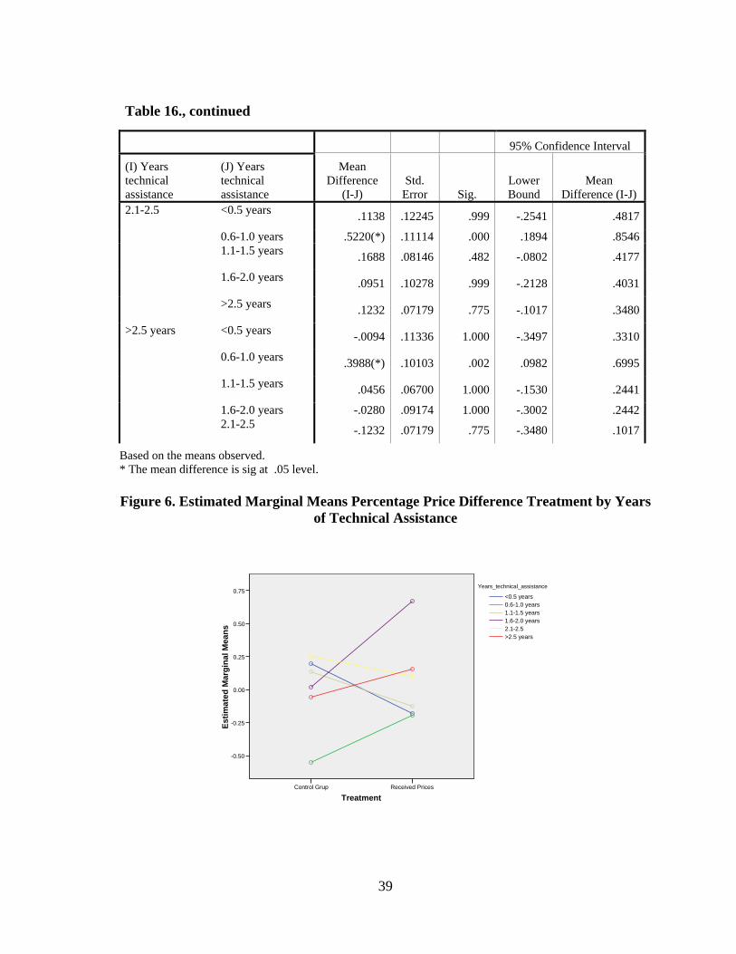
Table 16., continued
95% Confidence Interval
(I) Years technical assistance
(J) Years technical assistance
Mean Difference
(I-J) Std.
Error Sig. Lower Bound
Mean Difference (I-J)
2.1-2.5 <0.5 years .1138 .12245 .999 -.2541 .4817
0.6-1.0 years .5220(*) .11114 .000 .1894 .8546 1.1-1.5 years .1688 .08146 .482 -.0802 .4177
1.6-2.0 years .0951 .10278 .999 -.2128 .4031
>2.5 years .1232 .07179 .775 -.1017 .3480
>2.5 years <0.5 years -.0094 .11336 1.000 -.3497 .3310
0.6-1.0 years .3988(*) .10103 .002 .0982 .6995
1.1-1.5 years .0456 .06700 1.000 -.1530 .2441
1.6-2.0 years -.0280 .09174 1.000 -.3002 .2442 2.1-2.5 -.1232 .07179 .775 -.3480 .1017
Based on the means observed. * The mean difference is sig at .05 level. Figure 6. Estimated Marginal Means Percentage Price Difference Treatment by Years
of Technical Assistance
TreatmentReceived PricesControl Grup
Estim
ated
Mar
gina
l Mea
ns
0.75
0.50
0.25
0.00
-0.25
-0.50
>2.5 years2.1-2.51.6-2.0 years1.1-1.5 years0.6-1.0 years<0.5 years
Years_technical_assistance
39

By graphing the interaction, we see that farmers with only one production cycle that
received market price information had a favorable differential price percentage. Those who
received technical assistance for 1-1.5 years and 2-2.5 years also negotiated better.
Producers with fewer years of technical assistance seem to negotiate better, empowered by
price information. Most likely, producers who have received more technical assistance have
developed stronger relationships with their buyers, and thus did not see a significant change
in the price received by them once they received price information. During the study, some
producers indicated that they had pre-negotiated the price of their production before the
harvest.
5.5 One-Way ANOVA Treatment by Area Planted
Table 17. ANOVA Treatment by Area Planted -Descriptive Statistics Dependent Variables: Price Percentage Difference
Treatment Area planted Mean Std. Deviation N
Control Group <= 0.25 mz .2429 .49141 73 0.26-0.5 mz .1877 .42372 52 0.51-0.75 mz -.6418 1.16043 17 0.76-1.0 mz -.0456 1.06802 93 1.1-1.25 mz .3060 .02191 5 > 1.26-1.5 mz -.6840 .85974 25 > 1.5 -.3175 .52284 72 Total -.0774 .81086 337 Prices Received
<= 0.25 mz -.3666 1.09055 62
0.26-0.5 mz .0816 .21085 43 0.51-0.75 mz -.2124 1.51604 21 0.76-1.0 mz .0741 .65065 29 > 1.26-1.5 mz .1486 .32147 29 > 1.5 -.1372 .35063 29 Total -.0995 .83376 213 Total <= 0.25 mz -.0370 .87413 135 0.26-0.5 mz .1397 .34654 95 0.51-0.75 mz -.4045 1.36802 38 0.76-1.0 mz -.0171 .98380 122 1.1-1.25 mz .3060 .02191 5 > 1.26-1.5 mz -.2369 .75161 54 > 1.5 -.2657 .48501 101 Total -.0860 .81912 550
40
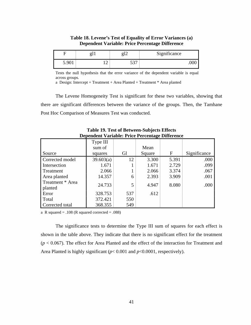
Table 18. Levene’s Test of Equality of Error Variances (a) Dependent Variable: Price Percentage Difference
F gl1 gl2 Significance
5.901 12 537 .000
Tests the null hypothesis that the error variance of the dependent variable is equal across groups. a Design: Intercept + Treatment + Area Planted + Treatment * Area planted
The Levene Homogeneity Test is significant for these two variables, showing that
there are significant differences between the variance of the groups. Then, the Tamhane
Post Hoc Comparison of Measures Test was conducted.
Table 19. Test of Between-Subjects Effects Dependent Variable: Price Percentage Difference
Source
Type III sum of squares Gl
Mean Square F Significance
Corrected model 39.603(a) 12 3.300 5.391 .000Intersection 1.671 1 1.671 2.729 .099Treatment 2.066 1 2.066 3.374 .067Area planted 14.357 6 2.393 3.909 .001Treatment * Area planted 24.733 5 4.947 8.080 .000
Error 328.753 537 .612 Total 372.421 550 Corrected total 368.355 549
a R squared = .108 (R squared corrected = .088)
The significance tests to determine the Type III sum of squares for each effect is
shown in the table above. They indicate that there is no significant effect for the treatment
(p < 0.067). The effect for Area Planted and the effect of the interaction for Treatment and
Area Planted is highly significant (p< 0.001 and p<0.0001, respectively).
41
5.6 Post hoc Tests: Area Planted
Table 20. Multiple Comparisons Dependent Variable: Price Percentage Difference
Tamhane
95% Confidence Interval
(I) Area planted
(J) Area planted
Mean Difference (I-
J) Std.
Error Sig. Lower Bound
Mean Difference (I-
J) <= 0.25 mz 0.26-0.5 mz -.1767 .08321 .527 -.4324 .0789 0.51-0.75
mz .3674 .23433 .938 -.3843 1.1192
0.76-1.0 mz -.0199 .11659 1.000 -.3770 .3372 1.1-1.25 mz -.3430(*) .07587 .000 -.5773 -.1088 > 1.26-1.5
mz .1998 .12697 .929 -.1939 .5935
> 1.5 .2287 .08938 .210 -.0454 .50280.26-0.5 mz <= 0.25 mz .1767 .08321 .527 -.0789 .4324 0.51-0.75
mz .5442 .22475 .349 -.1844 1.2727
0.76-1.0 mz .1568 .09590 .900 -.1386 .4522 1.1-1.25 mz -.1663(*) .03688 .000 -.2811 -.0515 > 1.26-1.5
mz .3765(*) .10829 .019 .0352 .7178
> 1.5 .4054(*) .05994 .000 .2212 .58970.51-0.75 mz <= 0.25 mz -.3674 .23433 .938 -1.1192 .3843 0.26-0.5 mz -.5442 .22475 .349 -1.2727 .1844 0.76-1.0 mz -.3873 .23913 .917 -1.1512 .3765 1.1-1.25 mz -.7105 .22214 .058 -1.4329 .0120 > 1.26-1.5
mz -.1676 .24436 1.000 -.9456 .6104
> 1.5 -.1387 .22711 1.000 -.8729 .59540.76-1.0 mz <= 0.25 mz .0199 .11659 1.000 -.3372 .3770 0.26-0.5 mz -.1568 .09590 .900 -.4522 .1386 0.51-0.75
mz .3873 .23913 .917 -.3765 1.1512
1.1-1.25 mz -.3231(*) .08961 .009 -.6004 -.0458 > 1.26-1.5
mz .2197 .13563 .909 -.1995 .6389
> 1.5 .2486 .10130 .273 -.0627 .56001.1-1.25 mz <= 0.25 mz .3430(*) .07587 .000 .1088 .5773 0.26-0.5 mz .1663(*) .03688 .000 .0515 .2811 0.51-0.75
mz .7105 .22214 .058 -.0120 1.4329
0.76-1.0 mz .3231(*) .08961 .009 .0458 .6004 > 1.26-1.5
mz .5429(*) .10275 .000 .2161 .8696
> 1.5 .5717(*) .04924 .000 .4188 .7247
42
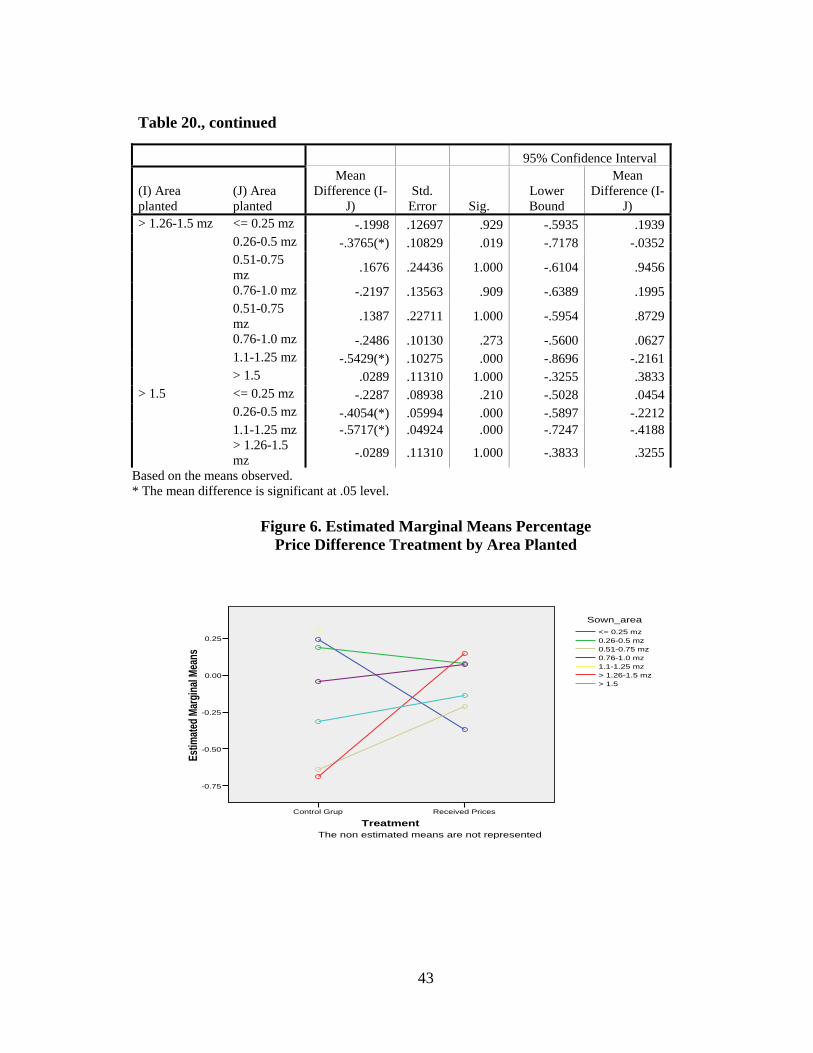
Table 20., continued
95% Confidence Interval
(I) Area planted
(J) Area planted
Mean Difference (I-
J) Std.
Error Sig. Lower Bound
Mean Difference (I-
J) > 1.26-1.5 mz <= 0.25 mz -.1998 .12697 .929 -.5935 .1939 0.26-0.5 mz -.3765(*) .10829 .019 -.7178 -.0352 0.51-0.75
mz .1676 .24436 1.000 -.6104 .9456
0.76-1.0 mz -.2197 .13563 .909 -.6389 .1995 0.51-0.75
mz .1387 .22711 1.000 -.5954 .8729
0.76-1.0 mz -.2486 .10130 .273 -.5600 .0627 1.1-1.25 mz -.5429(*) .10275 .000 -.8696 -.2161 > 1.5 .0289 .11310 1.000 -.3255 .3833> 1.5 <= 0.25 mz -.2287 .08938 .210 -.5028 .0454 0.26-0.5 mz -.4054(*) .05994 .000 -.5897 -.2212 1.1-1.25 mz -.5717(*) .04924 .000 -.7247 -.4188 > 1.26-1.5
mz -.0289 .11310 1.000 -.3833 .3255
Based on the means observed. * The mean difference is significant at .05 level.
Figure 6. Estimated Marginal Means Percentage Price Difference Treatment by Area Planted
TreatmentReceived PricesControl Grup
Estim
ated M
argin
al Me
ans
0.25
0.00
-0.25
-0.50
-0.75
> 1.5> 1.26-1.5 mz1.1-1.25 mz0.76-1.0 mz0.51-0.75 mz0.26-0.5 mz<= 0.25 mz
Sown_area
The non estimated means are not represented
43

By plotting the interaction, we can see that farmers with areas planted of <0.25 mz
and those with 0.26-0.50 mz who received market prices via SMS obtained a lower price
differential (the negotiated price was closer to or above the market price) than those who
did not receive prices using this technology. We can conclude that the producers who have
less negotiating power (in this case because they have a smaller area planted) and received
price information were empowered and received better prices (considering the weekly price
in which they harvested) than those who did not have price information.
5.7 One-Way ANOVA Treatment per Market
Table 21. ANOVA Treatment by Market, Descriptive Statistics Dependent variables: Price Percentage Difference
Treatment Market Mean Std. Deviation N
Control Group La Ceiba -2.2840 .66673 5 Comayagua .2900 .00000 7 Copán .1350 .20207 4 Lempira .1500 .03464 3 La Paz .4825 .21559 8 Ocotepeque .1405 .15375 19 Olanchito -.3640 .08488 10 Santa Bárbara .0229 .40406 14 San Pedro
Sula -.5871 1.48270 56
Tegucigalpa .0776 .47126 199 Yoro -.4200 .10914 10 Intibucá .3650 .43134 2 Total -.0774 .81086 337 Received prices
La Ceiba -.6700 .00000 3
Copán -4.6250 .88388 2 Lempira -.1047 .85471 92 La Paz -3.0000 . 1 El Paraíso .1550 .05196 4 Olanchito .1375 .07300 12 San Pedro
Sula .0446 .40677 68
Tegucigalpa .2169 .26807 16 Intibucá -.7222 1.11377 9 Choluteca .0700 .00000 6 Total -.0995 .83376 213
44
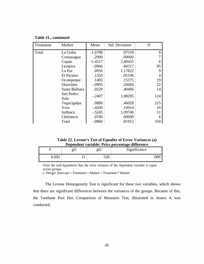
Table 21., continued
Treatment Market Mean Std. Deviation N
Total La Ceiba -1.6788 .97559 8 Comayagua .2900 .00000 7 Copán -1.4517 2.49455 6 Lempira -.0966 .84217 95 La Paz .0956 1.17822 9 El Paraíso .1550 .05196 4 Ocotepeque .1405 .15375 19 Olanchito -.0905 .26684 22 Santa Bárbara .0229 .40406 14 San Pedro
Sula -.2407 1.08295 124
Tegucigalpa .0880 .46028 215 Yoro -.4200 .10914 10 Intibucá -.5245 1.09746 11 Choluteca .0700 .00000 6 Total -.0860 .81912 550
Table 22. Levene’s Test of Equality of Error Variances (a) Dependent variable: Price percentage difference
F gl1 gl2 Significance
6.092 21 528 .000
Tests the null hypothesis that the error variance of the dependent variable is equal across groups. a Design: Intercept + Treatment + Market + Treatment * Market
The Levene Homogeneity Test is significant for these two variables, which shows
that there are significant differences between the variances of the groups. Because of this,
the Tamhane Post Hoc Comparison of Measures Test, illustrated in Annex 4, was
conducted.
45
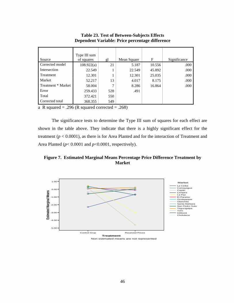
Table 23. Test of Between-Subjects Effects Dependent Variable: Price percentage difference
Source Type III sum
of squares gl Mean Square F Significance Corrected model 108.922(a) 21 5.187 10.556 .000Intersection 22.549 1 22.549 45.892 .000Treatment 12.301 1 12.301 25.035 .000Market 52.217 13 4.017 8.175 .000Treatment * Market 58.004 7 8.286 16.864 .000Error 259.433 528 .491 Total 372.421 550 Corrected total 368.355 549
a R squared = .296 (R squared corrected = .268)
The significance tests to determine the Type III sum of squares for each effect are
shown in the table above. They indicate that there is a highly significant effect for the
treatment (p < 0.0001), as there is for Area Planted and for the interaction of Treatment and
Area Planted (p< 0.0001 and p<0.0001, respectively).
Figure 7. Estimated Marginal Means Percentage Price Difference Treatment by
Market
TreatmentReceived PricesControl Grup
Estim
ated M
argina
l Mean
s
1.00
0.00
-1.00
-2.00
-3.00
-4.00
-5.00
CholutecaIntibucáYoroTegucigalpaSan Pedro SulaSanta BárbaraOlanchitoOcotepequeEl ParaísoLa PazLempiraCopánComayaguaLa Ceiba
Market
Non estimated means are not represented
46
The harvest is sold in many markets. The most interesting trends are found in the
largest markets of Tegucigalpa, San Pedro Sula, and La Ceiba. In these three markets, the
farmers who received price information obtained a larger price differential. It can also be
observed in the graph depicting the other interactions that in various situations, the farmers
who received price information had a larger price differential than those in the control
group.
Does this mean that those who had the price information were poorer negotiators?
To answer this question, other factors had to be studied in depth, such as the price trends
for each vegetable during the period studied. Annex 4 contains graphs of price trends for
each crop. Nearly all the crop prices showed a downward trend during the period studied.
Only cabbage had a recovery peak at the end of the period under study.
This downward price trend causes a mathematical situation that can hide the
empowerment effect on the producers who received market price information. An
explanation will be given before proceeding to a mathematical explanation.
The research team interviewed informal agricultural intermediaries in several
regions of Honduras, one of them in the department of Intibucá, to learn about the margins
that the intermediaries look for when negotiating. According to this intermediary, the
intermediaries set fixed margins on prices, not percentage margins. In the example that he
put forward, he used a margin of L.1.50 per pound when the prices are “fair to good” and
L.1.00 as a minimum when market prices are low. The example he used was broccoli. He
explained that the one who “sacrifices” or is affected when prices are low is the farmer,
because the intermediary “has to have a minimum L.1.00 margin of contribution.”
A hypothetical situation was presented with salad tomatoes, the price of which fell
from L.7.00 per pound in September to L.4.00 per pound in November in the Tegucigalpa
market. We assumed a farmer in the Control Group that receives L.5.50 per pound in
September, assuming a margin of L.1.50 established by the intermediary interviewed
(L.7.00 – L.1.50 = L.5.50).
If the Price Percentage Differential formula is applied, the following result is
obtained:
47
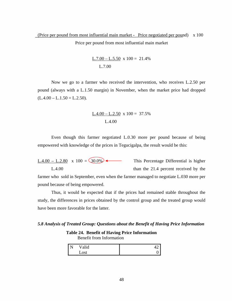
(Price per pound from most influential main market - Price negotiated per pound) x 100
Price per pound from most influential main market
L.7.00 – L.5.50 x 100 = 21.4%
L.7.00
Now we go to a farmer who received the intervention, who receives L.2.50 per
pound (always with a L.1.50 margin) in November, when the market price had dropped
(L.4.00 – L.1.50 = L.2.50).
L.4.00 – L.2.50 x 100 = 37.5%
L.4.00
Even though this farmer negotiated L.0.30 more per pound because of being
empowered with knowledge of the prices in Tegucigalpa, the result would be this:
L.4.00 – L.2.80 x 100 = 30.0% This Percentage Differential is higher
L.4.00 than the 21.4 percent received by the
farmer who sold in September, even when the farmer managed to negotiate L.030 more per
pound because of being empowered.
Thus, it would be expected that if the prices had remained stable throughout the
study, the differences in prices obtained by the control group and the treated group would
have been more favorable for the latter.
5.8 Analysis of Treated Group: Questions about the Benefit of Having Price Information Table 24. Benefit of Having Price Information Benefit from Information
N Valid 42 Lost 0
48
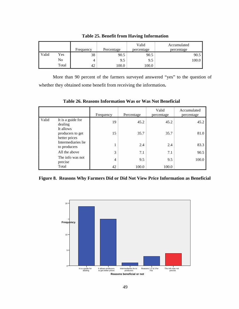
Table 25. Benefit from Having Information
Frequency Percentage Valid
percentage Accumulated
percentage Valid Yes 38 90.5 90.5 90.5 No 4 9.5 9.5 100.0 Total 42 100.0 100.0
More than 90 percent of the farmers surveyed answered “yes” to the question of
whether they obtained some benefit from receiving the information.
Table 26. Reasons Information Was or Was Not Beneficial
Frequency Percentage Valid
percentage Accumulated percentage
Valid It is a guide for dealing 19 45.2 45.2 45.2
It allows producers to get better prices
15 35.7 35.7 81.0
Intermediaries lie to producers 1 2.4 2.4 83.3
All the above 3 7.1 7.1 90.5 The info was not
precise 4 9.5 9.5 100.0
Total 42 100.0 100.0 Figure 8. Reasons Why Farmers Did or Did Not View Price Information as Beneficial
The info was not precise
Reasons 1,2 & 3 for Yes
Intermediaries lie to producers
It allows producers to get better prices
It is a guide f r odealing
Frequency
20
10
5
0
Reasons beneficial or not
49
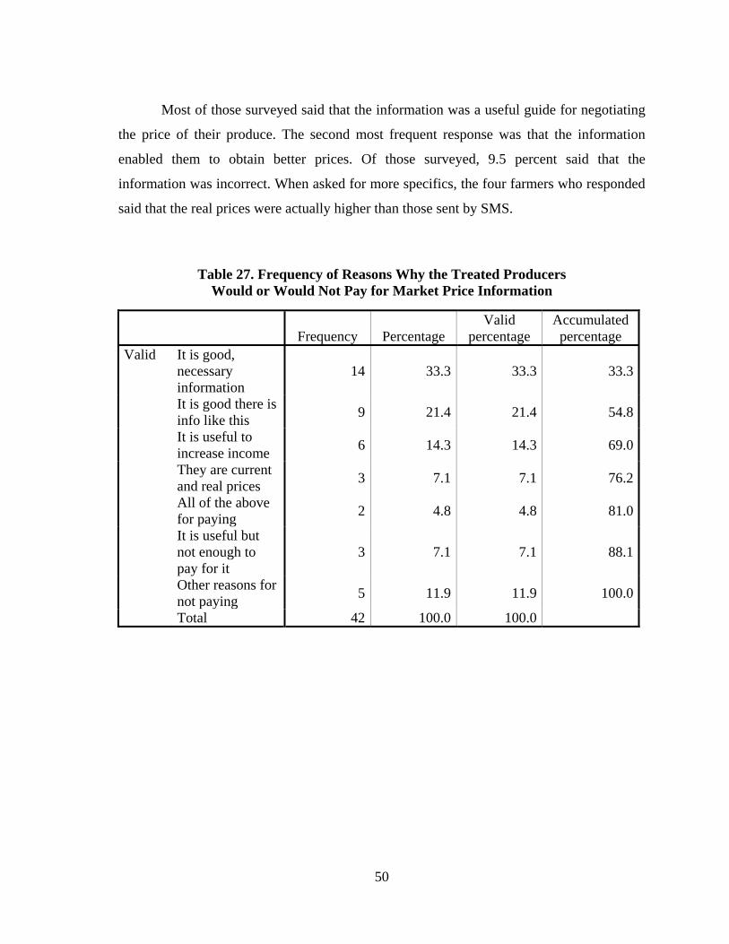
Most of those surveyed said that the information was a useful guide for negotiating
the price of their produce. The second most frequent response was that the information
enabled them to obtain better prices. Of those surveyed, 9.5 percent said that the
information was incorrect. When asked for more specifics, the four farmers who responded
said that the real prices were actually higher than those sent by SMS.
Table 27. Frequency of Reasons Why the Treated Producers
Would or Would Not Pay for Market Price Information
Frequency Percentage Valid
percentage Accumulated percentage
Valid It is good, necessary information
14 33.3 33.3 33.3
It is good there is info like this 9 21.4 21.4 54.8
It is useful to increase income 6 14.3 14.3 69.0
They are current and real prices 3 7.1 7.1 76.2
All of the above for paying 2 4.8 4.8 81.0
It is useful but not enough to pay for it
3 7.1 7.1 88.1
Other reasons for not paying 5 11.9 11.9 100.0
Total 42 100.0 100.0
50
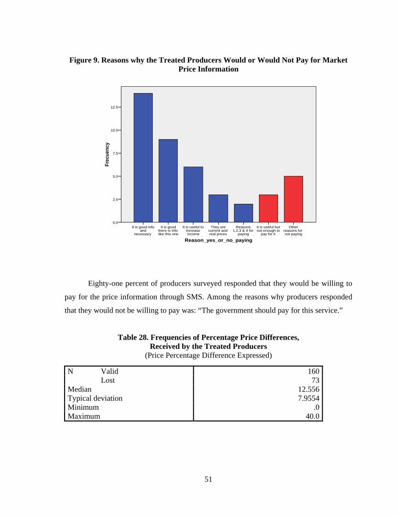
Figure 9. Reasons why the Treated Producers Would or Would Not Pay for Market Price Information
Reason_yes_or_no_paying
Other reasons for not paying
It is useful but not enough to
pay for it
Reasons 1,2,3 & 4 for
paying
They are current and real prices
It is useful to increase income
It is good there is info like this one
It is good info and
necessary
Frec
uenc
y12.5
10.0
7.5
5.0
2.5
0.0
Eighty-one percent of producers surveyed responded that they would be willing to
pay for the price information through SMS. Among the reasons why producers responded
that they would not be willing to pay was: “The government should pay for this service.”
Table 28. Frequencies of Percentage Price Differences, Received by the Treated Producers
(Price Percentage Difference Expressed)
N Valid 160 Lost 73 Median 12.556 Typical deviation 7.9554 Minimum .0 Maximum 40.0
51
52
Table 29. Price Percentage Differences
Frequency Percentage Valid
percentage Accumulated percentage
Valid 0.00% 20 8.6 12.5 12.5 0.01-5.00% 4 1.7 2.5 15.0 5.01-
10.00% 43 18.5 26.9 41.9
10.01-15.00% 39 16.7 24.4 66.3
15.01-20.00% 44 18.9 27.5 93.8
>20.00% 10 4.3 6.3 100.0 Total 160 68.7 100.0 Lost 99.00 73 31.3 Total 233 100.0
Although a high percentage of farmers consulted answered that they did not know
what price they would have obtained if they had not had the prices sent by SMS (result in
73 of 233 weekly negotiations), of those who did respond (representing 160 negotiations),
87.5 percent reported obtaining a positive price differential. The median result was a 12.5
percent higher price negotiated. This price differential makes it possible to pay for the
information during the harvest period if we considered a price for the SMS of L.18.00
suggested by Luis Padilla, owner of SOTEICA, a company whose business is sending SMS
for marketing and related purposes.
5.9 Results of the Socioeconomic Assessment Below are graphs showing the results from randomly selected producers for each of the 10
questions on the Poverty Score Card for Honduras.
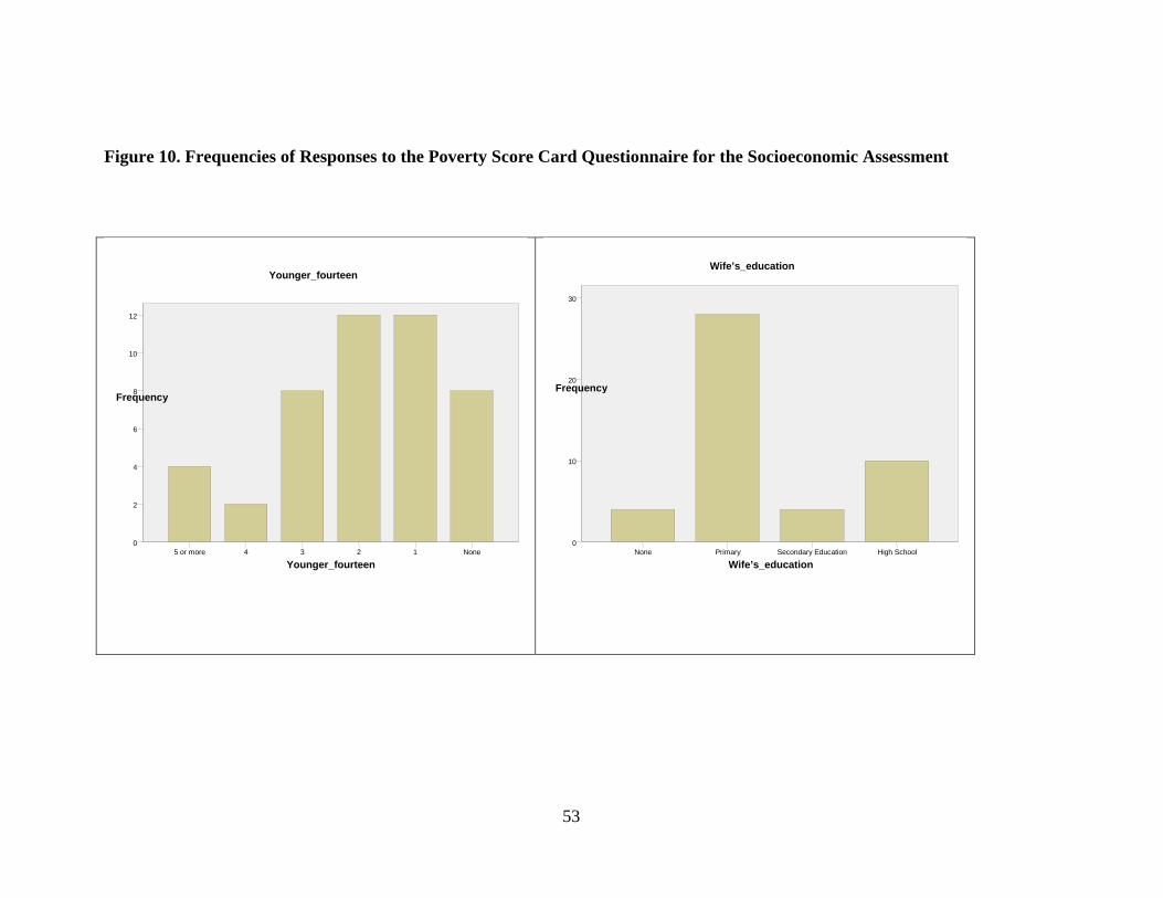
Figure 10. Frequencies of Responses to the Poverty Score Card Questionnaire for the Socioeconomic Assessment
Wife’s_educationYounger_fourteen
30
Wife’s_educationHigh SchoolSecondary EducationPrimaryNone
Frequency20
10
0
Younger3
_fourteenNone12 45 or more
Frequency
12
10
8
6
4
2
0
53
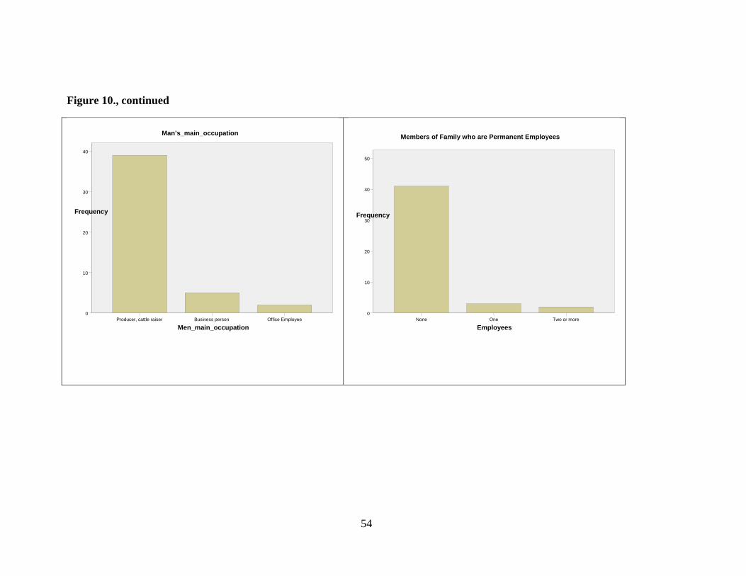
Figure 10., continued
Man’s_main_occupation Members of Family who are Permanent Employees
EmployeesTwo or moreOneNone
Frequency
50
40
30
20
10
0
Me onn_main_occupatiBusiness person Office EmployeeProducer, cattle raiser
Frequency
40
30
20
10
0
54

Figure 10., continued
House’s floor construction materialBedrooms in the house
Construction materialGraniteCement BrickClay Brick, cementDirt
Frequency
20
15
10
5
0
Number Four or moreThreeTwoOne
Frequency
20
15
10
5
0
55
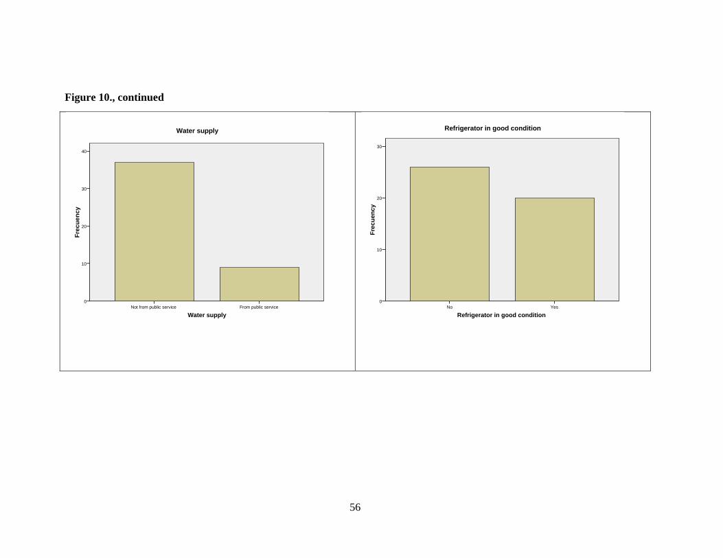
Figure 10., continued
Water supplyFrom public serviceNot from public service
Frec
uenc
y
40
30
20
10
0
Water supply
Refrigerator in good conditionYesNo
Frec
uenc
y
30
20
10
0
Refrigerator in good condition
56
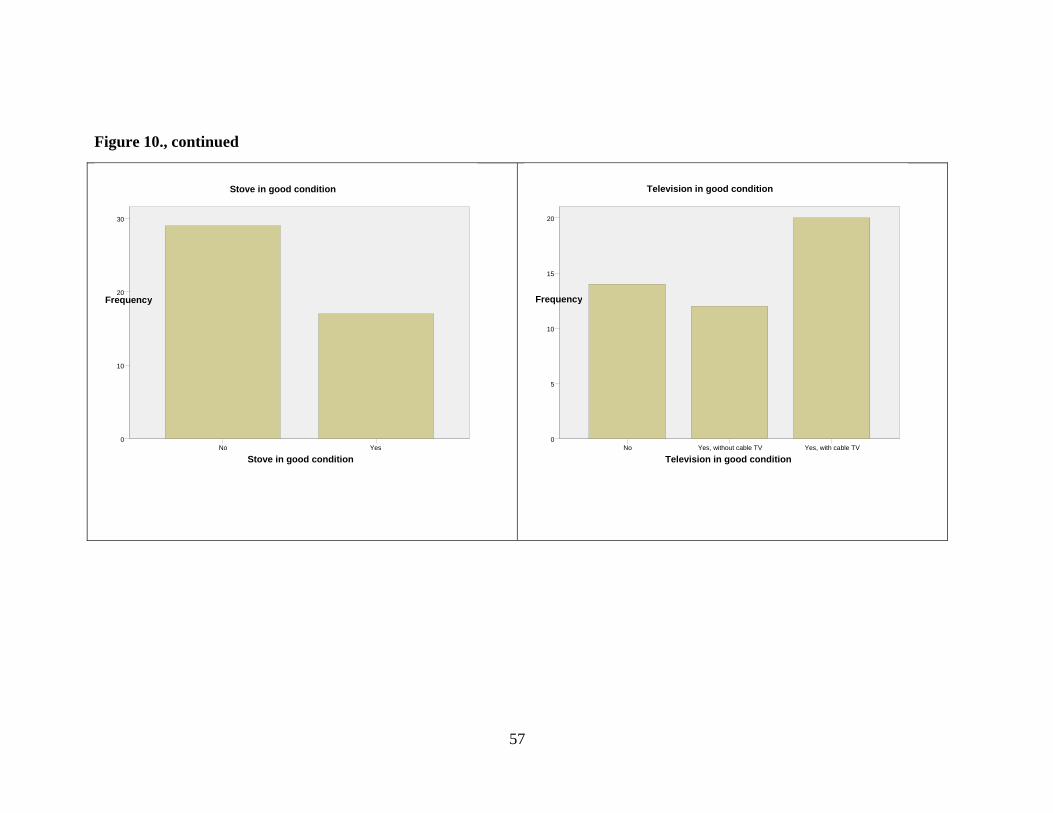
57
Figure 10., continued
Television in good conditionYes, with cable TVYes, without cable TVNo
Frequency
Television in good condition
5
0
20
15
10
Stove in good conditionYesNo
Frequency
30
Stove in good condition
0
20
10
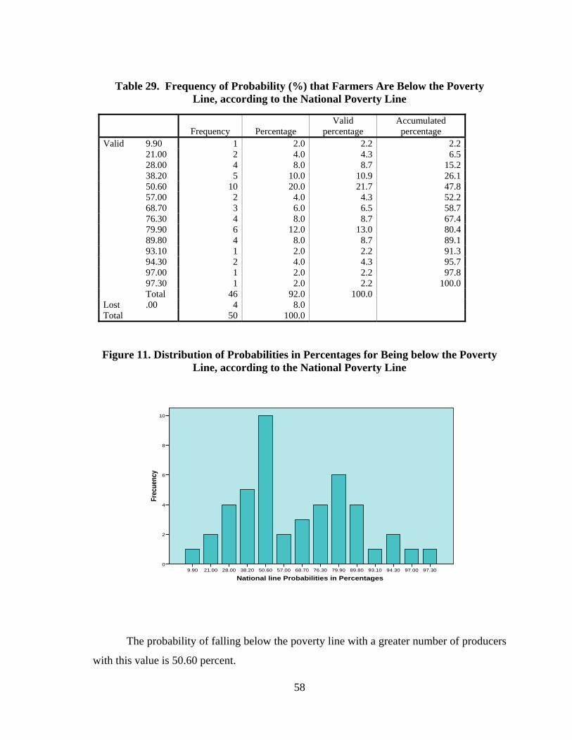
Table 29. Frequency of Probability (%) that Farmers Are Below the Poverty Line, according to the National Poverty Line
Frequency Percentage Valid
percentage Accumulated
percentage Valid 9.90 1 2.0 2.2 2.2 21.00 2 4.0 4.3 6.5 28.00 4 8.0 8.7 15.2 38.20 5 10.0 10.9 26.1 50.60 10 20.0 21.7 47.8 57.00 2 4.0 4.3 52.2 68.70 3 6.0 6.5 58.7 76.30 4 8.0 8.7 67.4 79.90 6 12.0 13.0 80.4 89.80 4 8.0 8.7 89.1 93.10 1 2.0 2.2 91.3 94.30 2 4.0 4.3 95.7 97.00 1 2.0 2.2 97.8 97.30 1 2.0 2.2 100.0 Total 46 92.0 100.0 Lost .00 4 8.0 Total 50 100.0
Figure 11. Distribution of Probabilities in Percentages for Being below the Poverty Line, according to the National Poverty Line
National line Probabilities in Percentages97.3097.0094.3093.1089.8079.9076.3068.7057.0050.6038.2028.0021.009.90
Frec
uenc
y
10
8
6
4
2
0
The probability of falling below the poverty line with a greater number of producers
with this value is 50.60 percent.
58
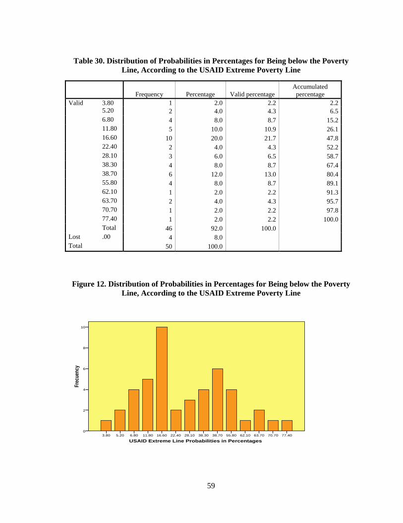
Table 30. Distribution of Probabilities in Percentages for Being below the Poverty Line, According to the USAID Extreme Poverty Line
Frequency Percentage Valid percentage Accumulated
percentage Valid 3.80 1 2.0 2.2 2.2 5.20 2 4.0 4.3 6.5 6.80 4 8.0 8.7 15.2 11.80 5 10.0 10.9 26.1 16.60 10 20.0 21.7 47.8 22.40 2 4.0 4.3 52.2 28.10 3 6.0 6.5 58.7 38.30 4 8.0 8.7 67.4 38.70 6 12.0 13.0 80.4 55.80 4 8.0 8.7 89.1 62.10 1 2.0 2.2 91.3 63.70 2 4.0 4.3 95.7 70.70 1 2.0 2.2 97.8 77.40 1 2.0 2.2 100.0 Total 46 92.0 100.0 Lost .00 4 8.0 Total 50 100.0
Figure 12. Distribution of Probabilities in Percentages for Being below the Poverty Line, According to the USAID Extreme Poverty Line
USAID Extreme Line Probabilities in Percentages77.4070.7063.7062.1055.8038.7038.3028.1022.4016.6011.806.805.203.80
Frec
uenc
y
10
8
6
4
2
0
59
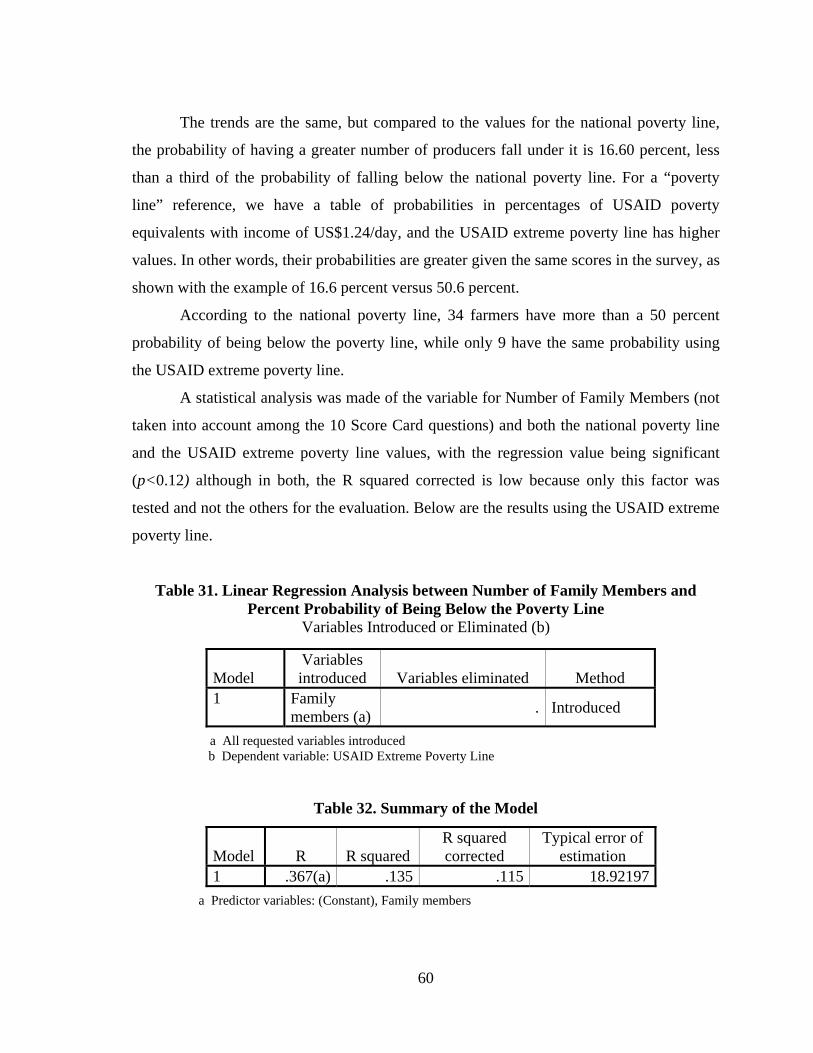
The trends are the same, but compared to the values for the national poverty line,
the probability of having a greater number of producers fall under it is 16.60 percent, less
than a third of the probability of falling below the national poverty line. For a “poverty
line” reference, we have a table of probabilities in percentages of USAID poverty
equivalents with income of US$1.24/day, and the USAID extreme poverty line has higher
values. In other words, their probabilities are greater given the same scores in the survey, as
shown with the example of 16.6 percent versus 50.6 percent.
According to the national poverty line, 34 farmers have more than a 50 percent
probability of being below the poverty line, while only 9 have the same probability using
the USAID extreme poverty line.
A statistical analysis was made of the variable for Number of Family Members (not
taken into account among the 10 Score Card questions) and both the national poverty line
and the USAID extreme poverty line values, with the regression value being significant
(p<0.12) although in both, the R squared corrected is low because only this factor was
tested and not the others for the evaluation. Below are the results using the USAID extreme
poverty line.
Table 31. Linear Regression Analysis between Number of Family Members and Percent Probability of Being Below the Poverty Line
Variables Introduced or Eliminated (b)
Model Variables introduced Variables eliminated Method
1 Family members (a) . Introduced
a All requested variables introduced b Dependent variable: USAID Extreme Poverty Line
Table 32. Summary of the Model
Model R R squared R squared corrected
Typical error of estimation
1 .367(a) .135 .115 18.92197 a Predictor variables: (Constant), Family members
60
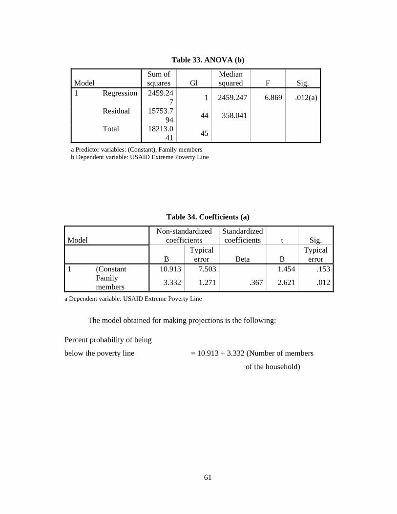
Table 33. ANOVA (b)
Model Sum of squares Gl
Median squared F Sig.
1 Regression 2459.247 1 2459.247 6.869 .012(a)
Residual 15753.794 44 358.041
Total 18213.041 45
a Predictor variables: (Constant), Family members b Dependent variable: USAID Extreme Poverty Line
Table 34. Coefficients (a)
Model Non-standardized
coefficients Standardized coefficients t Sig.
B Typical
error Beta B Typical
error 1 (Constant 10.913 7.503 1.454 .153 Family
members 3.332 1.271 .367 2.621 .012
a Dependent variable: USAID Extreme Poverty Line
The model obtained for making projections is the following: Percent probability of being
below the poverty line = 10.913 + 3.332 (Number of members
of the household)
61
6. Conclusions
1. The SMS or text message is a low-cost mechanism for disseminating
price information that can reach a significant portion of the Honduran
population (50 municipalities out of 298 are represented by 208 farmers
with cellular telephone coverage). This represents a little more than 15
percent coverage of the national territory.
2. Dissemination of prices over the radio meets the requirements for being
a medium for mass dissemination, with broad coverage of the entire
country at a low cost. However, an evaluation of the way the
information is received shows that its efficiency depends on whether the
person receiving the message is present during the broadcast; otherwise,
the message is lost.
3. Of the ICTs evaluated, the SMS is the one with the versatility to be
sustainable for commercial firms that could provide the service, thereby
meeting the demand for market prices from Honduran vegetable
farmers. The one using the service would be willing to pay a reasonable
amount for accessing the sales prices from the country’s main markets.
4. As of October 2009, the month when the information was received from
CONATEL, CELTEL was the company with the most subscribers.
61.25 percent of all mobile telephone users in Honduras have CELTEL
service, while in a selected sub-sample of 208 vegetable growers, 83.65
percent had service from that company.
5. The linear regression analysis shows that the variables of Treatment,
Quality Category, Price from the Closest City, Years of Technical
Assistance, Market, and Years of Experience with the Crop are
significant for explaining the dependent variable Percentage Difference
between Market Price and Negotiated Price. The R2 adjusted is low at
0.196, but the model is highly significant at <0.0001.
6. The ANOVA univariant analysis used to measure the interactions
between Treatment by Area Planted and Treatment by Years of
62
7. Of the nine vegetable crops assisted by the EDA Program, with the
exception of plantain, potatoes, and salad tomatoes, the ICTs became a
tool that provided timely reference prices that were used by the farmer
to maximize profits and minimize the profit margin of the intermediary.
In other words, it can be generally concluded that the technology
reduced the gap between the farmer and their participation in a free and
diverse market.
8. As stated by 91 percent of the farmers surveyed that received market
prices, the price information was useful to them. Of these farmers, when
asked what the price would have been if they had not received this
information, 87 percent said that they obtained a higher price, averaging
12.5 percent more.
9. According to the socioeconomic assessment made with a sub-sample of
the vegetable farmers studied and the USAID extreme poverty line, 9 of
the 46 farmers visited and surveyed had a more than 50 percent
probability of falling below the poverty line. According to the national
poverty line, another way to assess poverty according to the results of
the Poverty Score Card for Honduras, 34 of the 46 farmers have more
than a 50 percent probability of falling below the poverty line.
10. In analyzing the socioeconomic conditions of the farmers surveyed in
this study, the sample indicates a certain homogeneity in terms of living
conditions: a subsistence production family unit that normally does not
have the capacity to efficiently negotiate the sale of its harvest because
of isolation or exclusion from various elements that interact in a market,
chief among them “reference price information.”
63
11. The socioeconomic analysis revealed the real reason why more farmers
did not respond to the first attempts to communicate with them and why
some could not be contacted at all. At the start of the study, this was
attributed to errors in the database of farmers used or to problems with
the mobile telephone signal. A large number of farmers do not have
access to electricity, cannot recharge their cell phones, and can only turn
them on when they need them. Thus, communication did not occur.
7. Recommendations
1. The study centered on the dissemination of market prices from the main
markets in Tegucigalpa and San Pedro Sula because of limits in the
budget and staff devoted to collecting prices. However, if dissemination
is to be undertaken for commercial purposes, it is necessary to consider
disseminating prices from markets like Santa Rosa de Copán and San
Salvador (El Salvador), which are very important markets for vegetable
farmers in the west, from markets in La Ceiba, which is the most
important market on the Atlantic seaboard, and others that have
considerable commercial importance.
2. The veracity of the price information is extremely important for
dissemination in a commercial form. Information should always be
obtained from reliable sources by staff who are keenly aware of its
importance.
8. Lessons Learned
1. One of the main reasons for the lack of price information is not the
absence of information itself but the government’s inability to provide
electricity to an important part of the population. This makes it difficult
to watch television, listen to the radio, or recharge mobile phones. Even
when a producer has bought a mobile phone and has access to a mobile
phone company signal, communication can be limited because of the
difficulty of recharging mobile devices.
64
2. During the period under study, several companies showed interest in
starting price information delivery through a mobile service, according
to Edgardo Varela from EDA Project. However, not one company had
solid information about the demand for this service. It was only a
preconceived notion that it might be both useful to producers and a
profitable activity.
3. Small producers responded positively to their participation in the
activity of “prices through text messages” However, later in the study,
when asked about their willingness to pay for the information, the
response was not so positive. This confirms the general perception that
the normal behavior of Honduran small and medium farmers is as
producers and not as entrepreneurs. For years, development projects
implemented by private companies or NGOs have been working to
change that limited vision, but there is still a long way to go.
65
References Argyrous, G. 2005. Statistics for Research: With a Guide to SPSS. London, United
Kingdom: SAGE Publications Ltd.
Banco Central de Honduras. 2007. “Producto Interno Bruto y Gasto Nacional.” Honduras
en Cifras 2004-2008, 70.
Bernal, C. 2006. Metodología de la Investigación. Mexico: Pearson Prentice Hall.
Bryman, A. and D. Cramer. 2005. Quantitative Data Analysis with SPSS 12 and 13. New
York, NY: Psychology Press.
Caja de Herramientas. 2001. FODA. Recovered on December 6, 2009. Available at
http://www.infomipyme.com/Docs/GT/Offline/Empresarios/foda.htm
Dutch Development Service. 2005. Informe Final de Diagnóstico de actores socio
productivos, potencialidades y oportunidades para el desarrollo económico local
en el territorio de la Mancomunidad de Municipios Lencas de la Sierra de La Paz,
Marcala y Nahuaterique en el marco del Programa de Desarrollo Binacional en la
zona fronteriza terrestre de Honduras.
FHIA. 2009. Informe de Evaluación de SIMPAH Honduras.
http://www.mioa-oima.org/espanol/doc/OIMA_Executive Summary Honduras.pdf.
Hernández, R. 2003. Competitividad de las MIPYME en Centroamérica: Políticas de
fomento y "mejores prácticas". Economic Commission for Latin America and the
Caribbean (ECLAC) and German Cooperation Agency (GTZ).
International Telecommunications Union. 2009. Available at
http:// www.itu.int/ITU-D/ict/statistics/ict/graphs/mobile.jpg
Lanza, M. 2002. Information and Communication Technologies as an Instrument for
Development. Tegucigalpa, Honduras: United Nations Development Program, 27
Mesa Agrícola Hondureña, Horticultura.
http://www.google.hn/search?hl=es&source=hp&q=falta+de+pol%C3%ADticas+ag
r%C3%ADcolas+en+honduras&lr=&rlz=1R2GGLL_es&aq=f&oq=
Monge, R. and J. Hewitt. 2004. Tecnologías de la Información y las Comunicaciones
(TICs) y el futuro desarrollo de Costa Rica: el desafío de la exclusión. Serie Digital
#3. San Jose, Costa Rica: Fundación CAATEC.
66
National Telecommunications Commission. June 2009. Written report presented at the
request of the researchers.
Schreiner, M. 2010. Un Índice de Calificación de Pobreza para Honduras. Recovered in
February, 2010 available at: www.microfinance.com/#Honduras.
Shadish, W., T. Cook, and D. Campbell. 2002. Experimental and Quasi-Experimental
Designs. Boston, MA: Houghton Mifflin Company.
Unwin, T. 2009. ICT4D: Information and Communication Technology for Development.
Cambridge: Cambridge University Press.
Voz al Mundo. El SMS Web: Todo ventajas. http://www.vozalmundo.com/index.php?id=5347
World Bank. 2009. Information and Communications for Development: Extending Reach
and Increasing Impact. Washington, DC: The International Bank for Reconstruction
and Development.
67
Annex 1. Survey of Farmers to Whom Prices Were Not Sent
Encuesta para productores EDA posterior a cosechaNo tratados
1.1 Nombre del productor:
1.2 Comunidad:
1.3 Municipio:
1.4 Departamento:
1.5 Año en que inicio a recibir asistencia técnica de parte de EDA‐MCA:
Saludo: Buenas tardes Sr(a)_______, le estamos hablando del proyecto EDA, para corroborar algunos datos
¿Nos permite realizarle una corta encuesta?
2.1 ¿En que mes(es) cosechó su producto?
Jul Sem 1 AgoSem 1 Sep Sem 1 Oct Sem 1 Nov Sem 1Jul Sem 2 Ago Sem 2 Sep Sem 2 Oct Sem 2 Nov Sem 2Jul Sem 3 Ago Sem 3 Sep Sem 3 Oct Sem 3 Nov Sem 3Jul Sem 4 Ago Sem 4 Sep} Sem 4 Oct Sem 4 Nov Sem 4
3.1 ¿Cuáles son los productos que cultivó, área cosechada y producción obtenida? *Cultivos estudiados
Producto Área Sembrada Producción* Tomate Pera Papa
Tomate Manzano Pepino
Chile Dulce Plátano
Repollo Yuca
Cebolla amarilla
*Libras , ki logramos , gavetas , ca jas , sacos , cargas , quinta les
Si es una unidad que no especi fique peso(ej. Saco) consulte a l productor
a cuántas l ibras equivale
3.2 ¿Cuántos años de experiencia tiene en este cultivo?Cultivo Años
4.1 ¿Cuál es el Mercado de destino de su producto?Producto Mercado Destino ej. San Pedro Sula, Tegucigalpa, Ceiba, etc…
4.2 ¿A quién vendió su producto?Producto Comprador ej. Intermediario, Industria, Puesto en el mercado
Supermercado, autoconsumo para procesamiento, autoconsumo para venta al detalle
4.3 ¿A qué precio por unidad negoció su producto?Cosecha (1era, 2nda, 3era, 4ta) Precio Cosecha (1era, 2nda, 3era, 4ta) Precio
Cultivo 1 Culti 3
Cultivo 2
4.6 ¿Cuál es la distancia hacia el mercado al que vende su producto?En kilómetros u horas y minutos en carro o en bestia.
4.7 ¿En qué medio de transporte traslada su producto? 4.8 ¿Cómo transporta su producción?Medio FormaCamión En cestaCarro pickup En sacoCarro refrigerado En binesBestia A granelOtro
Despedida: Gracias Sr(a) por el tiempo proporcionado.
I. Datos Generales
II. Informacion de Precios
IV. Mercado
III. Producción
vo
68
Annex 2. Survey of Farmers to Whom Prices Were Sent
2.4 ¿Obtuvo beneficios al recibir la información de precios del Programa EDA a través de mensajitos?Si ¿Porque? Orienta para negociar
Permite obtener mejor precioLos interemediarios le mienten al productorOtros*
* Expl icar
No ¿Porque? Se obtuvo lo que el intermediario ofrecióAún con la información no se puede negociar mejorLa información no fue precisaSe tiene negociado un precio fijo con compradorConsume su propio producto para procesoConsume su propio producto para venta al detalle
*Si la respuesta es afirmativa pasar a l a pregunta 2.5, s i es negativa pasar a l a 2.9.
2.5 ¿Cuando el proyecto EDA haya terminado usted estaría dispuesto a pagar para obtener lainformación de precios?
Si ¿Por que? La información:Es buena, valiosa y necesaria.Es excelente que haya una información de este orden.La información es buena, sirve para mejorar nuestros ingresos en las ventas.Interesa porque son los precios oficiales, actuales y reales.Cubre todos los productos y mercados más influyentes.La difusión es muy buena, nos llega a tiempo.Otro*
*Expl icar
No ¿Por qué? La información:Debería ser enviada por el estadoNo sirve tantoSirve, pero no para pagar por ellaOtro*
*Expl icar
2.6 ¿Cuánto estaría dispuesto a pagar por un mensajito del precio del día?*Dejar que el productor contes te abiertamente, s i no lo hace, proponer l as s iguientes al ternativas :
Rango de precioL.10.00‐L12.00L.12.01‐L14.00L.14.01‐L16.00
>L.16.00
2.7 ¿A qué precio por unidad negoció su producto?Cosecha (1era, 2nda, 3era, 4ta) Precio
Cultivo 1
Cultivo 2
2.8 ¿Qué precio hubiera obtenido si no hubiera conocido los preciosde mercado?
Diferencia en centavos /Cosecha (1era, 2nda, 3era, 4ta) Precio (L.) Unidad*
Cultivo 1 * A calcular posterior a la encuesta
Cultivo 2
69
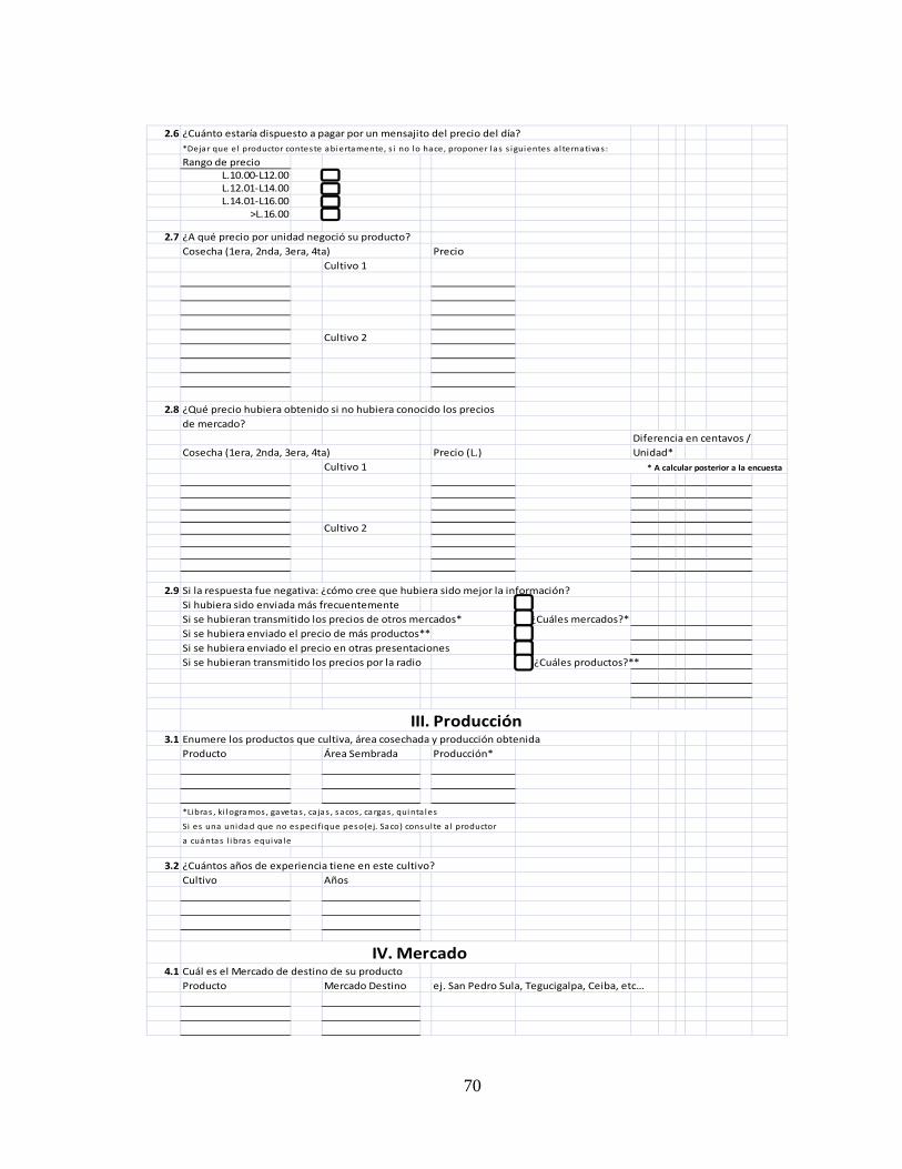
2.6 ¿Cuánto estaría dispuesto a pagar por un mensajito del precio del día?*Dejar que el productor conteste abiertamente, s i no lo hace, proponer l as s iguientes alternativas :
Rango de precioL.10.00‐L12.00L.12.01‐L14.00L.14.01‐L16.00
>L.16.00
2.7 ¿A qué precio por unidad negoció su producto?Cosecha (1era, 2nda, 3era, 4ta) Precio
Cultivo 1
Cultivo 2
2.8 ¿Qué precio hubiera obtenido si no hubiera conocido los preciosde mercado?
Diferencia en centavos /Cosecha (1era, 2nda, 3era, 4ta) Precio (L.) Unidad*
Cultivo 1 * A calcular posterior a la encuesta
Cultivo 2
2.9 Si la respuesta fue negativa: ¿cómo cree que hubiera sido mejor la información?Si hubiera sido enviada más frecuentementeSi se hubieran transmitido los precios de otros mercados* ¿Cuáles mercados?*Si se hubiera enviado el precio de más productos**Si se hubiera enviado el precio en otras presentacionesSi se hubieran transmitido los precios por la radio
3.1 Enumere los productos que cultiva, área cosechada y producción obtenidaProducto Área Sembrada Producción*
*Libras , ki logramos, gavetas , cajas , sacos , cargas , quinta les
Si es una unidad que no especi fique peso(ej. Saco) consulte al productor
a cuántas l ibras equiva le
3.2 ¿Cuántos años de experiencia tiene en este cultivo?Cultivo Años
4.1 Cuál es el Mercado de destino de su productoProducto Mercado Destino ej. San Pedro Sula, Tegucigalpa, Ceiba, etc…
IV. Mercado
III. Producción
¿Cuáles productos?**
70
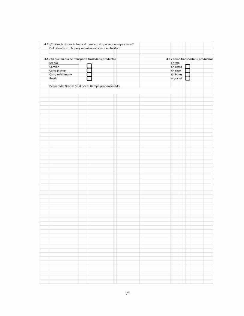
4.3 ¿Cuál es la distancia hacia el mercado al que vende su producto?
En kilómetros u horas y minutos en carro o en bestia.
4.4 ¿En qué medio de transporte traslada su producto? 4.5 ¿Cómo transporta su producciónMedio FormaCamión En cestaCarro pickup En sacoCarro refrigerado En binesBestia A granel
Despedida: Gracias Sr(a) por el tiempo proporcionado.
71
Annex 3
Guide to Interpretation of Scorecard Indicators
The following information comes from the Honduran National Institute of Statistics,
Manual de Encuestador, XXXV Encuesta Permanente de Hogares de Propósitos Múltiples,
Tegucigalpa, 2007.
1. How many household members are 14 years old or younger?
According to page 13 of the manual, “household members are those who have eaten and
slept in the residence for the past six months; eaten and slept in the residence for less than
six months, but who currently live in the residence and plan to continue; and those who,
because of work, only spend weekends at the residence.”
2. What is the highest educational level that the female head/spouse has reached?
According to page 18 of the manual, the response options are defined as follows:
None: The person has never gone to school or attended a literacy program
Literacy program: Programs to help adults learn basic reading and writing
Preschool: Pre-primary school, also known as pre-kindergarten and kindergarten. The
classes teach children social habits and psycho-motor skills
Primary: The first six grades of formal schooling. It includes “basic education”
educational institutions that offer nine grades
Common cycle: A three-year course of studies called the “basic plan” or the “common
cycle of general culture”. The prerequisite is having passed sixth grade
Diversified: A four-year course of studies whose prerequisite is having passed the
common cycle or ninth grade. It includes the specialties of salesperson, public
accountant, primary teacher, artist, secretary, computer technician, business
administration, etc.
Higher than diversified includes the following:
Technical school: Two-year college programs for mid-level professionals. The
prerequisite is having passed diversified. Majors include sales, education, etc.
Non-college post-secondary: This covers students and graduates of the National
72
Agricultural School in Catacamas, the National School of Forestry Science in
Siguatepeque, the Panamerican Agricultural College (Zamorano), military and
police academies, Our Lady of Suyapa Seminary, the Center of Construction and
Architectural Design, etc. It also includes graduates of the former Francisco
Morazán College.
College: Public and private universities that train professionals
Graduate school: Courses of study completed after having obtained an initial college
degree. The courses of study last from one to five years.
3. What is the main occupation of the male head/ spouse?
According to page 33 in the manual, an occupation “is the type of work that the person
does . . . the main occupation is the one that the respondent considers to be the main
one.” Specific definitions follow the third revision of the CIUO.
4. How many household members receive a salary in their main occupation?
According to pages 33–34 of the manual, this includes “blue- or white-collar public
employees, blue- or white-collar private employees, and domestic servants”
A blue- or white-collar public employee is “someone who works for the government and
whose salary is paid by the State, including people in the armed forces”
A blue- or white-collar private employee is “someone who works in a privately owned
business”
A domestic servant “does housework for monthly remuneration. Examples are maids,
cooks, washerpeople, nannies, gardeners, and chauffeurs”.
5. How many rooms does the household use as bedrooms?
According to pages 10–11 of the manual, this includes “all rooms used for sleeping,
regardless of whether they are used for some other purpose during the day.”
A room is a “space demarcated by walls that reach from the floor to the roof. Folding
screens or thin partitions do not count as walls.”
73
6. What is the main construction material of the floors of the residence?
According to page 6 of the manual, “If the residence has different types of floors, record the
main type.”
7. What is the household’s source of water?
According to page 7 in the manual, the relevant source is that which “provides the
majority of water used by the household.” Public network covers water supplied by
“SANAA and the municipal governments”.
Not public network covers piped water provided privately, bucket-drawn wells, pump
wells, rivers, creeks, springs, water-tank trucks, pickups with barrels/drums of water,
public/community spigots, or others (including getting water from a neighbor).
8. Does any household member have a working refrigerator?
The manual does not provide any additional information about this indicator.
9. Does any household member have a working stove with four burners?
The manual does not provide any additional information about this indicator.
10. Does any household member have a working television with or without cable?
The manual does not provide any additional information about this indicator.
74
Annex 4.
Price Trends of Nine Crops Studied
Red lines represent Tegucigalpa’s prices
Blue lines represent San Pedro Sula’s prices
0.00
2.00
4.00
6.00
8.00
10.00
Price pe
r lb
Price Tendency Processing Tomatoe
Series1
Series2
0.00
2.00
4.00
6.00
8.00
10.00
12.00
Price
per lb
Price Tendency Salad Tomatoe
Series1
Series2
0.00
1.00
2.00
3.00
4.00
5.00
6.00
01/08/2009 01/09/2009 01/10/2009 01/11/2009 01/12/2009
Price per lb
Price Tendency Potatoe
Series1
Series2
0.00
0.50
1.00
1.50
2.00
2.50
3.00
3.50
08/08/2009 08/09/2009 08/10/2009 08/11/2009
Price per lb
Price Tendency Green Pepper
Series1
Series2
0.00
0.50
1.00
1.50
2.00
2.50
3.00
3.50
01/08/2009 01/09/2009 01/10/2009 01/11/2009 01/12/2009
Price per lb
Price Tendency Cabbage
Series1
Series2
0.00
0.50
1.00
1.50
2.00
2.50
3.00
Price per lb
Price Tendency Cucumber
Series1
Series2
0.00
0.50
1.00
1.50
2.00
2.50
3.00
3.50
08/08/2009 08/09/2009 08/10/2009 08/11/2009
Price per lb
Price Tendency Plantain
Series1
Series2
0.000.501.001.502.002.503.003.504.00
Price per lb
Price Tendency Yucca
Series1
Series2
75
0.000.501.001.502.002.503.003.504.00
Price per lb
Price Tendency Carrot
Series1
Series2
76
Annex 5. Post Hoc Tests
Market
Multiple Comparisons
Dependent Variable: Price Percentage difference
Tamhane
(I) Market (J) Market 95% Confidence
Interval
Mean Difference
(I-J) Std.
Error Sig. Lower Bound
Mean Difference (I-
J) La Ceiba Comayagua -1.9688 .34492 .064 -4.0250 .0875 Copán -.2271 1.0752
2 1.000 -7.2292 6.7750
Lempira -1.5821 .35558 .182 -3.5561 .3919 La Paz -1.7743 .52270 .307 -4.0539 .5053 El Paraíso -1.8338 .34590 .094 -3.8814 .2139 Ocotepeque -1.8193 .34672 .096 -3.8597 .2211 Olanchito -1.5883 .34958 .190 -3.6053 .4287 Santa Bárbara -1.7016 .36143 .115 -3.6456 .2423 San Pedro
Sula -1.4380 .35837 .288 -3.3947 .5186
Tegucigalpa -1.7668 .34635 .114 -3.8103 .2768 Yoro -1.2588 .34665 .523 -3.2998 .7823 Intibucá -1.1542 .47798 .924 -3.1982 .8897 Choluteca -1.7488 .34492 .123 -3.8050 .3075Comayagua La Ceiba 1.9688 .34492 .064 -.0875 4.0250 Copán 1.7417 1.0184
0 1.000 -6.1758 9.6591
Lempira .3866(*) .08640 .002 .0781 .6951 La Paz .1944 .39274 1.000 -1.9716 2.3605 El Paraíso .1350 .02598 .719 -.2724 .5424 Ocotepeque .1495(*) .03527 .044 .0021 .2969 Olanchito .3805(*) .05689 .000 .1495 .6114 Santa Bárbara .2671 .10799 .924 -.2223 .7565 San Pedro
Sula .5307(*) .09725 .000 .1863 .8751
Tegucigalpa .2020(*) .03139 .000 .0921 .3119 Yoro .7100(*) .03451 .000 .5305 .8895 Intibucá .8145 .33090 .955 -.8293 2.4584 Choluteca .2200 .00000 . .2200 .2200
77
(I) Market (J) Market 95% Confidence
Interval
Mean Difference
(I-J) Std.
Error Sig. Lower Bound
Mean Difference (I-
J) Copán La Ceiba .2271 1.0752
2 1.000 -6.7750 7.2292
Comayagua -1.7417 1.01840 1.000 -9.6591 6.1758
Lempira -1.3550 1.02205 1.000 -9.1920 6.4820
La Paz -1.5472 1.09150 1.000 -8.3763 5.2818
El Paraíso -1.6067 1.01873 1.000 -9.5167 6.3034
Ocotepeque -1.5922 1.01901 1.000 -9.4960 6.3116
Olanchito -1.3612 1.01998 1.000 -9.2434 6.5210
Santa Bárbara -1.4745 1.02411 1.000 -9.2681 6.3191
San Pedro Sula -1.2109 1.0230
3 1.000 -9.0271 6.6052
Tegucigalpa -1.5397 1.01888 1.000 -9.4463 6.3670
Yoro -1.0317 1.01898 1.000 -8.9361 6.8727
Intibucá -.9271 1.07080 1.000 -7.9671 6.1128
Choluteca -1.5217 1.01840 1.000 -9.4391 6.3958
Lempira La Ceiba 1.5821 .35558 .182 -.3919 3.5561 Comayagua -.3866(*) .08640 .002 -.6951 -.0781 Copán 1.3550 1.0220
5 1.000 -6.4820 9.1920
La Paz -.1922 .40213 1.000 -2.3068 1.9224 El Paraíso -.2516 .09023 .446 -.5744 .0712 Ocotepeque -.2372 .09333 .679 -.5685 .0942 Olanchito -.0062 .10345 1.000 -.3742 .3619 Santa Bárbara -.1195 .13830 1.000 -.6473 .4083 San Pedro
Sula .1441 .13009 1.000 -.3113 .5995
Tegucigalpa -.1846 .09193 .987 -.5104 .1412 Yoro .3234 .09304 .067 -.0082 .6549 Intibucá .4279 .34199 1.000 -1.1889 2.0447 Choluteca -.1666 .08640 .995 -.4751 .1419
78
(I) Market (J) Market 95% Confidence
Interval
Mean Difference
(I-J) Std.
Error Sig. Lower Bound
Mean Difference (I-
J) La Paz La Ceiba 1.7743 .52270 .307 -.5053 4.0539 Comayagua -.1944 .39274 1.000 -2.3605 1.9716 Copán 1.5472 1.0915
0 1.000 -5.2818 8.3763
Lempira .1922 .40213 1.000 -1.9224 2.3068 El Paraíso -.0594 .39360 1.000 -2.2202 2.1013 Ocotepeque -.0450 .39432 1.000 -2.2013 2.1114 Olanchito .1860 .39684 1.000 -1.9559 2.3279 Santa Bárbara .0727 .40732 1.000 -2.0221 2.1675 San Pedro
Sula .3363 .40460 1.000 -1.7670 2.4395
Tegucigalpa .0076 .39399 1.000 -2.1508 2.1659 Yoro .5156 .39425 1.000 -1.6412 2.6724 Intibucá .6201 .51355 1.000 -1.5619 2.8021 Choluteca .0256 .39274 1.000 -2.1405 2.1916El Paraíso La Ceiba 1.8338 .34590 .094 -.2139 3.8814 Comayagua -.1350 .02598 .719 -.5424 .2724 Copán 1.6067 1.0187
3 1.000 -6.3034 9.5167
Lempira .2516 .09023 .446 -.0712 .5744 La Paz .0594 .39360 1.000 -2.1013 2.2202 Ocotepeque .0145 .04381 1.000 -.1749 .2038 Olanchito .2455 .06254 .058 -.0038 .4947 Santa Bárbara .1321 .11107 1.000 -.3575 .6218 San Pedro
Sula .3957(*) .10066 .013 .0388 .7527
Tegucigalpa .0670 .04075 1.000 -.1040 .2380 Yoro .5750(*) .04320 .000 .3698 .7802 Intibucá .6795 .33192 .998 -.9612 2.3203 Choluteca .0850 .02598 .987 -.3224 .4924Ocotepeque La Ceiba 1.8193 .34672 .096 -.2211 3.8597 Comayagua -.1495(*) .03527 .044 -.2969 -.0021 Copán 1.5922 1.0190
1 1.000 -6.3116 9.4960
Lempira .2372 .09333 .679 -.0942 .5685 La Paz .0450 .39432 1.000 -2.1114 2.2013 El Paraíso -.0145 .04381 1.000 -.2038 .1749 Olanchito .2310 .06694 .128 -.0235 .4855 Santa Bárbara .1177 .11361 1.000 -.3711 .6064 San Pedro
Sula .3813(*) .10345 .029 .0162 .7463
Tegucigalpa .0525 .04722 1.000 -.1204 .2254
79
(I) Market (J) Market 95% Confidence
Interval
Mean Difference
(I-J) Std.
Error Sig. Lower Bound
Mean Difference (I-
J) Ocoteque Yoro .5605(*) .04935 .000 .3649 .7562 (continued) Intibucá .6651 .33277 .999 -.9732 2.3033 Choluteca .0705 .03527 .997 -.0769 .2179Olanchito La Ceiba 1.5883 .34958 .190 -.4287 3.6053 Comayagua -.3805(*) .05689 .000 -.6114 -.1495 Copán 1.3612 1.0199
8 1.000 -6.5210 9.2434
Lempira .0062 .10345 1.000 -.3619 .3742 La Paz -.1860 .39684 1.000 -2.3279 1.9559 El Paraíso -.2455 .06254 .058 -.4947 .0038 Ocotepeque -.2310 .06694 .128 -.4855 .0235 Santa Bárbara -.1133 .12206 1.000 -.6120 .3854 San Pedro
Sula .1503 .11267 1.000 -.2480 .5486
Tegucigalpa -.1785 .06498 .577 -.4247 .0678 Yoro .3295(*) .06654 .002 .0727 .5864 Intibucá .4341 .33575 1.000 -1.1963 2.0645 Choluteca -.1605 .05689 .608 -.3914 .0705Santa Bárbara La Ceiba 1.7016 .36143 .115 -.2423 3.6456 Comayagua -.2671 .10799 .924 -.7565 .2223 Copán 1.4745 1.0241
1 1.000 -6.3191 9.2681
Lempira .1195 .13830 1.000 -.4083 .6473 La Paz -.0727 .40732 1.000 -2.1675 2.0221 El Paraíso -.1321 .11107 1.000 -.6218 .3575 Ocotepeque -.1177 .11361 1.000 -.6064 .3711 Olanchito .1133 .12206 1.000 -.3854 .6120 San Pedro
Sula .2636 .14533 .999 -.2812 .8084
Tegucigalpa -.0651 .11246 1.000 -.5528 .4226 Yoro .4429 .11337 .113 -.0467 .9324 Intibucá .5474 .34807 1.000 -1.0640 2.1588 Choluteca -.0471 .10799 1.000 -.5365 .4423San Pedro Sula La Ceiba 1.4380 .35837 .288 -.5186 3.3947 Comayagua -.5307(*) .09725 .000 -.8751 -.1863 Copán 1.2109 1.0230
3 1.000 -6.6052 9.0271
Lempira -.1441 .13009 1.000 -.5995 .3113 La Paz -.3363 .40460 1.000 -2.4395 1.7670 El Paraíso -.3957(*) .10066 .013 -.7527 -.0388 Ocotepeque -.3813(*) .10345 .029 -.7463 -.0162 Olanchito -.1503 .11267 1.000 -.5486 .2480
80
(I) Market (J) Market 95% Confidence
Interval
Mean Difference
(I-J) Std.
Error Sig. Lower Bound
Mean Difference (I-
J) San Pedro Sula Santa Bárbara -.2636 .14533 .999 -.8084 .2812 (continued) Tegucigalpa -.3287 .10219 .135 -.6889 .0315 Yoro .1793 .10319 1.000 -.1858 .5443 Intibucá .2838 .34489 1.000 -1.3280 1.8957 Choluteca -.3107 .09725 .149 -.6551 .0337Tegucigalpa La Ceiba 1.7668 .34635 .114 -.2768 3.8103 Comayagua -.2020(*) .03139 .000 -.3119 -.0921 Copán 1.5397 1.0188
8 1.000 -6.3670 9.4463
Lempira .1846 .09193 .987 -.1412 .5104 La Paz -.0076 .39399 1.000 -2.1659 2.1508 El Paraíso -.0670 .04075 1.000 -.2380 .1040 Ocotepeque -.0525 .04722 1.000 -.2254 .1204 Olanchito .1785 .06498 .577 -.0678 .4247 Santa Bárbara .0651 .11246 1.000 -.4226 .5528 San Pedro
Sula .3287 .10219 .135 -.0315 .6889
Yoro .5080(*) .04665 .000 .3274 .6886 Intibucá .6125 .33238 1.000 -1.0268 2.2519 Choluteca .0180 .03139 1.000 -.0919 .1279Yoro La Ceiba 1.2588 .34665 .523 -.7823 3.2998 Comayagua -.7100(*) .03451 .000 -.8895 -.5305 Copán 1.0317 1.0189
8 1.000 -6.8727 8.9361
Lempira -.3234 .09304 .067 -.6549 .0082 La Paz -.5156 .39425 1.000 -2.6724 1.6412 El Paraíso -.5750(*) .04320 .000 -.7802 -.3698 Ocotepeque -.5605(*) .04935 .000 -.7562 -.3649 Olanchito -.3295(*) .06654 .002 -.5864 -.0727 Santa Bárbara -.4429 .11337 .113 -.9324 .0467 San Pedro
Sula -.1793 .10319 1.000 -.5443 .1858
Tegucigalpa -.5080(*) .04665 .000 -.6886 -.3274 Intibucá .1045 .33269 1.000 -1.5340 1.7430 Choluteca -.4900(*) .03451 .000 -.6695 -.3105
81
82
(I) Market (J) Market 95% Confidence
Interval
Mean Difference
(I-J) Std.
Error Sig. Lower Bound
Mean Difference (I-
J) Intibucá La Ceiba 1.1542 .47798 .924 -.8897 3.1982 Comayagua -.8145 .33090 .955 -2.4584 .8293 Copán .9271 1.0708
0 1.000 -6.1128 7.9671
Lempira -.4279 .34199 1.000 -2.0447 1.1889 La Paz -.6201 .51355 1.000 -2.8021 1.5619 El Paraíso -.6795 .33192 .998 -2.3203 .9612 Ocotepeque -.6651 .33277 .999 -2.3033 .9732 Olanchito -.4341 .33575 1.000 -2.0645 1.1963 Santa Bárbara -.5474 .34807 1.000 -2.1588 1.0640 San Pedro
Sula -.2838 .34489 1.000 -1.8957 1.3280
Tegucigalpa -.6125 .33238 1.000 -2.2519 1.0268 Yoro -.1045 .33269 1.000 -1.7430 1.5340 Choluteca -.5945 .33090 1.000 -2.2384 1.0493Choluteca La Ceiba 1.7488 .34492 .123 -.3075 3.8050 Comayagua -.2200 .00000 . -.2200 -.2200 Copán 1.5217 1.0184
0 1.000 -6.3958 9.4391
Lempira .1666 .08640 .995 -.1419 .4751 La Paz -.0256 .39274 1.000 -2.1916 2.1405 El Paraíso -.0850 .02598 .987 -.4924 .3224 Ocotepeque -.0705 .03527 .997 -.2179 .0769 Olanchito .1605 .05689 .608 -.0705 .3914 Santa Bárbara .0471 .10799 1.000 -.4423 .5365 San Pedro
Sula .3107 .09725 .149 -.0337 .6551
Tegucigalpa -.0180 .03139 1.000 -.1279 .0919 Yoro .4900(*) .03451 .000 .3105 .6695 Intibucá .5945 .33090 1.000 -1.0493 2.2384
Based on the means observed. * The mean difference is sig. at 0.05 level.
Annex 6. Political Map of Honduras
83