Computer Networks 53 (2009) 382–399

Contents lists available at ScienceDirect

Computer Networks

journal homepage: www.elsevier .com/locate /comnet

The impact of a realistic packet traffic model on the performanceof surveillance wireless sensor networks

Ilker Demirkol a, Cem Ersoy a,*, Fatih Alagöz a, Hakan Deliç b

a Computer Networks Research Laboratory, Department of Computer Engineering, Bog�aziçi University, Bebek 34342 Istanbul, Turkeyb Wireless Communications Laboratory, Department of Electrical and Electronics Engineering, Bog�aziçi University, Bebek 34342 Istanbul, Turkey

a r t i c l e i n f o

Article history:Received 4 May 2008Received in revised form 18 October 2008Accepted 26 October 2008Available online 7 November 2008

Responsible Editor: H.S. Hassanein

Keywords:Packet traffic modelWireless sensor networksSurveillance sensor networksIntrusion detection applications

1389-1286/$ - see front matter � 2008 Elsevier B.Vdoi:10.1016/j.comnet.2008.10.021

* Corresponding author. Tel.: +90 2123596861; faE-mail addresses: ilker@boun.edu.tr (I. Demirko

(C. Ersoy), alagoz@boun.edu.tr (F. Alagöz), delic@bo

a b s t r a c t

It is quite common to see that classical periodic or Poisson packet traffic models are usedfor evaluating the performance of wireless sensor networks (WSNs). However, these mod-els may not be appropriate for modeling the data traffic resulting from a particular appli-cation. Furthermore, they may be overestimating the performance of a WSN. In this paper,we show the significance of using a realistic and application-specific packet traffic modelby comparing the performance of a well-known WSN protocol under the SurveillanceWSN packet traffic model (SPTM), as well as under periodic and binomial traffic models.A packet traffic framework specific to surveillance applications is proposed which is thenused for deriving SPTM analytically. In order to be adaptable and flexible, SPTM incorpo-rates a probabilistic and parametric sensor detection model. Simulation results show thatto employ an application-specific packet traffic model has significant impact on the perfor-mance evaluation of the WSN and ordinary traffic models may overestimate the capacity ofthe WSN.

� 2008 Elsevier B.V. All rights reserved.

1. Introduction

Potential application areas of wireless sensor networks(WSNs) show contrasting properties which prevent thedevelopment of universal algorithms serving all purposes.Military applications may require very fast response time,whereas in agriculture, delay sensitivity may be tradedwith energy conservation. Likewise, a communication pro-tocol may perform in a very energy-efficient manner whenused for one application, and it may perform quite poorlyin another. One application-dependent characteristic of aWSN is the type of data traffic generated by the nodes.The model that represents the aggregate packet traffic inthe network or a cluster of the network can be used todetermine the maximum stable throughput, expected de-lay and the packet loss characteristics. Furthermore, the ef-fects of parameters such as node density and target

. All rights reserved.

x: +90 2122872461.l), ersoy@boun.edu.trun.edu.tr (H. Deliç).

velocity can be investigated in depth once an appropriatedata traffic model is available.

When communication protocols are developed withouttaking into account the properties of the data traffic, theymay behave inefficiently. In the WSN literature, the perfor-mance evaluation of the protocols are generally carried outwith periodic data traffic as in [1–3], or using common datatraffic models such as Poisson point processes [4–6]. How-ever, event-driven applications such as target detectionand tracking produce bursty traffic which cannot be mod-eled as either periodic or Poisson [7]. Although there arepacket traffic models available for legacy communicationnetworks, the unique features and requirements of WSNscall for the design and development of dedicated models.For instance, the limited battery capacity necessitates theuse of sleep-listen periods and sensing intervals to extendthe lifetime of the network.

In this paper, we investigate the importance of using arealistic packet traffic model by deriving a specific surveil-lance WSN packet traffic model (SPTM) and comparing theperformance of a WSN medium access control (MAC)

List of symbols

Symbol DefinitionuðdÞ probability of detection of a target at distance da Elfes detection parameterb Elfes detection parameterh angular coordinate of the sensor when the pole

is set to the target locationc probability of detection for any one sensor

within the du-distance of the targetqmax maximum stable throughputf probability of packet collision in a contention

periodW random variable of the index of the first occu-

pied slotn probability that a slot assignment results in a

collisionless transmissiona Gauss–Markov mobility model randomness

parameterCi location of target at instance ici coverage degree at point Ci

cx;y coverage degree at point x,y, i.e. the number ofsensor nodes that have positive detection prob-ability for a target at x,y

Di disk whose center is at Ci and whose radius isdu, i.e. the coverage area of a the sensor at loca-tion Ci

du sensing rangedc certain detection rangeE direction of the mobile in Gauss–Markov mobil-

ity modelF random variable that represents the index of

first occupied slot given that it is selected byonly one node

Ki random variable that represents the detectiondegree of the event point Ci

ki detection degree at point Ci

kx;y detection degree at point x,y, i.e. the number ofsensor nodes that detects the target at x,y

L border lengthM number of contending nodesN number of sensorsp probability that a deployed node is within the

du-distance of the target pointr radial coordinate of the sensor when the pole is

set to the target locationS speed of the mobile in Gauss–Markov mobility

modeltcoll time spent for the collided packets’ transmis-

sionstCW time spent for waiting the first occupied con-

tention slottlisten listen period in secondstX time needed for the transmission of a packet

type X where X is RTS, CTS, DATA or ACK.ts sensing intervaltslot one slot durationtstx time required for a successful packet transmis-

sionvT target velocityW border widthXi number of sensor nodes that have non-zero

detection probability, i.e. the sensor nodes thatresides within the du-distance of the eventpoint Ci

Yi number of nodes that reside in Ai

Z number of contention slots in a contention win-dow

z number of successive collisions

I. Demirkol et al. / Computer Networks 53 (2009) 382–399 383

protocol under different packet traffic models. We showthat the underlying packet traffic model can result in dis-similar performance results for the same average packettraffic loads. This observation is significant because the im-proper packet traffic models may result in underestimatedor overestimated performance results and lead to ineffi-cient protocol design and implementation.

In the WSN literature, the application-specific packettraffic models are not studied extensively. In [8], the trafficgenerated by a single WSN node connected to a body tem-perature or an electrocardiogram sensor is investigated formedical applications. The traffic traces of an intrusiondetection scenario are studied in [9], where numericalfunction fitting is carried out for the total number of pack-ets generated at any instance. However, no generalizedanalytical model is derived. An analytical packet trafficmodel for intrusion detecting WSN is investigated in [7]in which binary sensor detection is assumed. However,binary detection is an idealized model in which the detec-tion probability is defined with only a single parameter. Toachieve a more configurable and potentially more realistic

packet traffic, a probabilistic detection model is employedin this work which includes a set of parameters to definethe range-based detection probabilities. These detectionparameters can be set according to the physical propertiesof the sensors deployed and of the potential targets. Basedon this probabilistic detection model, we introduce aframework for the SPTM and derive the analytical formulafor its components. The derived SPTM model is used to cor-roborate how a realistic packet traffic modeling makes adifference.

In Section 2, we describe the packet traffic frameworkthat is used for the SPTM and present an analytical modelfor the proposed framework. Then, in Section 3, we verifythe introduced analytical model with simulations. In Sec-tion 4, packet traffic generation algorithms are presentedbased on the proposed analytical packet traffic model.The performance evaluation results of the well-known S-MAC protocol [10] are compared for SPTM, as well as theperiodic and the binomial packet traffic models in Section5. Finally, Section 6 includes the analytical derivations ofthe maximum stable throughput to verify the simulation

Fig. 1. Illustration of the dependency between subsequent number ofdetections where ts is the sensor sampling period.

384 I. Demirkol et al. / Computer Networks 53 (2009) 382–399

results. A list of symbols used in the mathematical equa-tions are given at the end of the text.

2. Surveillance wireless sensor networks packet trafficmodel

Surveillance wireless sensor networks (SWSN) repre-sent the WSN applications in which the deployed sensornodes monitor an area such as border for potential intruderentrance. When an intrusion is detected, the detecting sen-sors send data packets to the sink so that the necessary ac-tions can be taken. Such a network can be employed forsecurity applications, habitat monitoring, or disaster man-agement applications. Because of the distinctive propertiesof these applications, the generated data are bursty and re-quire a specific packet traffic model.

2.1. SWSN packet traffic model (SPTM) framework

Packet traffic models can be represented by a Markovprocess where the state ~s corresponds to the event that sdata packets are generated by the sensing nodes at a givendata generation instant which are mainly the sensor sam-pling instances for surveillance networks. The state transi-tion probability from state ~a to state ~b indicates theprobability of generating b data packets with the knowl-edge of a data packets generated at the previous samplinginstant. The dependency between the number of packetsgenerated at the successive sampling instances determinesthe order of the Markov process. The order is zero formemoryless packet traffic models such as Poisson andperiodic data traffic, i.e. the probability of a transition tostate ~b is independent from the current state. For SPTM,the order is a positive value depending on the propertiesof the intruder movements and sensor node attributeswhich is formulated in [7]. The dependency in subsequentnumber of detections is represented in Fig. 1. The crossshaded sensors in Fig. 1 detect the target in the two con-secutive sampling instances, and hence, generate datapackets in both sampling instances. The subsequent setof detecting sensors is determined by the target velocityand the sensing interval of the sensors, ts.

Since radio communication and sensing are two sepa-rate power consuming operations for sensors,1 each hasits own duty cycle. The duty cycles can be static or can beincreased dynamically in case of event presence. For eithercase, assume that the sensing duty cycle interval is ts inthe presence of a target, which means that each node sensesthe environment once in ts seconds. Hence, after the target isdetected by a sensor at location ðx; yÞ at time t, it will possi-bly be detected by the same node again at location ðx0; y0Þ attime t þ ts, where the Euclidian distance between ðx; yÞ andðx0; y0Þ is vT ts, with vT being the velocity of the target withinthe ðt; t þ tsÞ period as illustrated in Fig. 1. When one datapacket is created at each target detection, assuming thatthe sensing offset of all sensors are the same, the number

1 As a numerical example, Crossbow motes require 5 mA for the sensorboard operations whereas 8 mA and 12 mA are required by the radio boardfor reception and transmission, respectively. However, when both boardsare in sleep mode, they require only a few lA’s [11].

of data packets generated at point ðx; yÞ is equal to the detec-tion degree of that location, kx;y, which is defined as the num-ber of sensor nodes that actually detect the event.2 Hence, arealistic packet traffic model for an SWSN application shouldprovide the probability mass function (PMF) of the detectiondegree given the previous detection degree.

The assumption of sensing offset synchronization isacceptable since for successful communication of thesleeping neighboring nodes, time synchronization betweenthem is always necessary. Time division multiple access(TDMA) based protocols require strict synchronization,however carrier sense multiple access (CSMA) based proto-cols, such as S-MAC, require looser synchronization. Hence,the sensing duty cycle can be synchronized using the com-munication cycle. Moreover, even if the communicationand the sensing duty cycles are different, the correspond-ing detection packets will be transmitted at the beginningof the next communication duty cycle.

Different sensor detection models are proposed for sen-sor nodes [12]. The detection probability of an event by asensor node is in general a function of the sensor-to-eventdistance. According to the binary detection model, an eventoccurring within a specific range (sensor range) of a sensornode is detected by that node with probability 1, and it isnot detected, otherwise. In other words, for the binarydetection model, the probability of the target detectionby a sensor is

uðdÞ1 if d 6 dc;

0 if dc < d;

�ð1Þ

where d is the distance between the target and the sensornode and dc is the threshold distance for detection, whichis also called the sensing range.

Zou et al. [13] proposed a more general, probabilisticsensor detection model based on the Elfes’ work [14]. Here,the dependency is parametric enabling the representationof different sensor types. Specifically, in the Elfes sensordetection model, the probability that a sensor detects anevent at distance d is

2 Since intrusion detection is investigated as the event-driven application,the terms target detection and event are used interchangeably.

Coverage Degreeat time t

Coverage Degreeat time t+ts

Detection Degreeat time t

Detection Degreeat time t+ts

... ...

Packet Traffic

2

1 1

......

Fig. 2. SWSN packet traffic model (SPTM) framework.

I. Demirkol et al. / Computer Networks 53 (2009) 382–399 385

uðdÞ ¼1 if d 6 dc;

e�aðd�dcÞb if dc < d < du;

0 if du 6 d;

8><>: ð2Þ

where dc; du define the certainty and uncertainty bound-aries in detection, respectively. To clarify the term sensingrange, dc can be called the certain detection range and du

can be called sensing range, for the Elfes case. Hence, thetarget is detected with probability 1, if the target is withinthe certain detection range and it is detected with an expo-nential probability, if it is outside of the certain detectionrange but still within the sensing range. No detection oc-curs by the sensors that are further than the sensing range.The parameters a and b, as well as du; dc , reflect the phys-ical properties of the sensors. In particular, a and b deter-mine the rate and region of decay in uðdÞ. An alternativedetection model that incorporates false alarm rate andadditive white Gaussian noise is Neyman–Pearson detector[15]. However, the Elfes model can accommodate theNeyman–Pearson detector through proper parametermatching as indicated in [16].

Calculation of the total number of detecting sensornodes, dx;y, requires the knowledge of the number of sensornodes that have positive detection probability, which iscalled the coverage degree and represented as cx;y for thedetection point ðx; yÞ. For an event location, a subset ofthe nodes with positive detection probability will detectthe event. Therefore, the coverage degree of a location is al-ways greater than or equal to its detection degree. For theElfes model, the sensor nodes that have positive detectionprobability are those within du distance of the event point,and for the binary detection model, they are the nodeswithin dc distance. In addition, with the Elfes model, thelocations of the sensor nodes determine the probabilitiesof the number of detections, since the detection probabilityis a function of the target distance for each sensor. Hence,

(1) The number of detecting sensor nodes (detectiondegree) is always less than or equal to the numberof sensor nodes that have a positive detection prob-ability (coverage degree), i.e. kx;y 6 cx;y.

(2) For the binary detection model, the detection degreeis always equal to the coverage degree, i.e. kx;y ¼ cx;y.

(3) The Elfes model reduces to the binary detectionmodel, if du ¼ dc , and as a result, it enables moregeneral and flexible sensor detection modeling.

The framework for SPTM is shown schematically inFig. 2 and described as follows. As the target crosses theborder, it can be detected by the sensor nodes deployedto the border which sample the environment periodically,i.e. once in ts seconds. Hence, to find the number of datapackets generated because of the target detections at thelocation ðx; yÞ, we first need to know the number of nodesthat can detect the target at ðx; yÞwhich is the coverage de-gree of that location, cx;y. Once we have the coverage de-gree, we then need to calculate the detection degree, kx;y,based on cx;y. Hence, for consecutive number of detections,we have to know the dependency between the coveragedegrees of the target locations at consecutive samplingtimes. The main components of the framework are (i) the

coverage degree, (ii) the detection degree, (iii) relation be-tween the detection degree and the coverage degree (ar-row 1), and (iv) the dependency of successive coveragedegrees (arrow 2). The analytical derivations of these com-ponents are given in Section 2.2.

2.2. Analytical model of the SPTM framework

In the WSN literature, two types of deployment are as-sumed in general: random deployment (e.g. [17,18]) andgrid deployment (e.g. [19,20]). In grid deployment, nodesare placed deterministically along grid points, while in ran-dom deployment they are placed randomly in the applica-tion area. In this paper, we assume uniformly randomdeployment. However, we use the probabilities of thenumber of sensor nodes deployed within a specific area in-stead of setting the individual locations randomly. That en-ables the calculation of the coverage degree of the eventlocations without generating the whole deployment map.

Since cx;y is defined as the number of sensor nodes thathas a positive probability to detect the target at ðx; yÞ, thePMF of cx;y is determined by the probability of the totalnumber of sensors within the distance du of ðx; yÞ. How-ever, as the surveillance area and the total number of sen-sors deployed within its borders are known, for eachsensor node deployment, the event that the deployed nodeis within the du-distance of the target point is a Bernoullitrial with the probability of success p ¼ pd2

u=LW , whereðL;WÞ is the length and width of the borders of the surveil-lance area. Hence, the total number of sensor nodes withindistance du of a point forms a Binomial distribution. More-over, for large number of retrials and small success proba-bility, Binomial distribution can be approximated by aPoisson distribution. This is generally the case for intrusiondetection applications, since the number of deployed sen-sors, N, gives the number of retrials and the probabilitythat a deployed node resides within the du-distance ofthe target point, p, is small because of the large deploy-ment area. The mean of the equivalent Poisson distributionis

k ¼ Np ¼ Npd2u

LW: ð3Þ

The coverage degree probabilities of area points, hence,form a Poisson PMF. However, as illustrated in Fig. 1, be-cause the number of sensor nodes within the sensing

Fig. 3. Geometric representation of successive target detection locations.

386 I. Demirkol et al. / Computer Networks 53 (2009) 382–399

ranges are similar, the coverage degree probabilities of twonearby surveillance area points are not independent ofeach other. If we are given the coverage degree of the tar-get location at time t, we cannot use the Poisson distribu-tion with the mean value given in (3) to estimate thecoverage degree of the target location at time t þ ts, whichwill be the next detection point.3

Fig. 3 shows the reason for the degree-dependency be-tween the successive points. Let C1 and C2 denote loca-tions of the target at times t and t þ ts, respectively. If thetarget velocity at time t is vT , then the distance betweenC1 and C2 is equal to vT ts. In addition, the coverage degreeof point C1 ðC2Þ equals to the number of sensor nodesresiding on D1ðD2Þ, where Di is the disk whose center isat Ci and whose radius is du. The dependency of the cover-age degrees of points C1 and C2 is represented by the inter-section of the two disks.

To investigate the dependency of the coverage degrees,we have to first look into the deployment probabilities ofthe crescent areas A1 and A2, and the intersection areaA3 which are defined as:

A3 ¼ D1 \D2; Ai ¼ Di �A3; i ¼ 1;2:

Let the random variable Yi denote the number of nodesthat reside in Ai. Then,

PðYi þY3 ¼ nÞ ¼ PðXi ¼ nÞ; i ¼ 1;2; ð4Þ

where the random variable Xi denotes the number of sen-sor nodes that have non-zero detection probability, i.e. thesensor nodes that resides within the du-distance of theevent point Ci.

Given that point C1 has coverage degree c1, the proba-bility that point C2 has coverage degree c2 is found as fol-lows. Define cmin ¼minðc1; c2Þ. Then,

PðX2 ¼ c2jX1 ¼ c1Þ

¼Xcmin

i¼0

PðX2 ¼ c2jY3 ¼ iÞPðY3 ¼ ijX1 ¼ c1Þ: ð5Þ

3 The locations that the target resides at sampling times will be nameddetection point or event point, even if the detection degree is zero for thesake of readability.

If it is known that there exist c1 sensors on the first disk,then the probability of having i of them inside A3 pos-sesses a Binomial distribution, where the probability ofsuccess is A3=pd2

u. Hence,

PðY3 ¼ ijX1 ¼ c1Þ ¼c1

i

� �A3

pd2u

!i

1� A3

pd2u

!c1�i

: ð6Þ

The probability of having c2 � i sensors within A2 againpossesses the Binomial distribution. However, c1 sensorsare known to be out of that area. Hence, we are left withN � c1 sensors to be deployed in the entire surveillancearea minus D1. As a result,

PðX2 ¼ c2jY3 ¼ iÞ

¼ PðY2 ¼ c2 � iÞ ¼N � c1

c2 � i

� �

� A2

LW � pd2u

!c2�i

1� A2

LW � pd2u

!N�c1�ðc2�iÞ

: ð7Þ

Therefore, given c1, the probability of having a coveragedegree of c2 in the next detection point can be calculatedby using (5)–(7). However, according to (2), even if the cov-erage degree of a detection point is known, the number oftarget detections, and hence, the number of data packetsgenerated are probabilistic. To calculate the detection de-gree of an event point, we first have to find the probabilityof event detection, uðdÞ, per sensor node within the sens-ing range du. Then, a PMF for the number of detectingnodes can be generated which is a function of coverage de-gree cx;y. For that, we utilize the circle area element defini-tion which is illustrated in Fig. 4. The circle area elementis defined as

dA ¼ rdrdh:

Assume that a sensor node resides within the sensingrange of the event location. Then, the probability of detec-tion, c, is equal to the probability that the sensor resides inany specific circle area element and detects the target fromthat distance. For any sensor within du distance of thetarget,

Fig. 4. Circle area element at distance r and with angle h.

Table 1Parameters for the reference scenario.

Parameter Notation Value

Border length L 10,000 mBorder width W 1000 mNumber of sensors N 10,000Sensing range du 20 mCertain detection range dc 0 mSensing parameter a 0.1Sensing parameter b 1Target velocity vT 10 m/sSensing interval ts 1 s

4 As will be described in Section 4, any target trajectory with varyingdirection and speed can be used as an input to generate successive coverageand detection degrees, analytically.

I. Demirkol et al. / Computer Networks 53 (2009) 382–399 387

c ¼Z 2p

0

Z du

0

dA

pd2u

uðrÞ ¼Z 2p

0

Z du

0

rdrdh

pd2u

uðrÞ: ð8Þ

However, uðrÞ is a piecewise function and therefore theintegral in (8) can be divided into appropriate intervals asin

c ¼Z 2p

0

Z du

dc

rdrdh

pd2u

e�aðr�dcÞb þZ 2p

0

Z dc

0

rdrdh

pd2u

: ð9Þ

Eq. (9) can be integrated according to the Elfes parame-ter values used. For b ¼ 1, the probability of detection isfound to be

c ¼ d2c

d2u

þ 2

a2d2u

½1þ adc � eaðdc�duÞð1þ aduÞ�: ð10Þ

When all sensors are identical, which implies the samec, and because sensor nodes are distributed uniformly, thePMF of the detection degree of the event point is Binomialwith the probability of success, c.

If we define Ki to be the random variable that repre-sents the detection degree of the event point Ci, then

PðKi ¼ kijXi ¼ ciÞ ¼ci

ki

� �cki ð1� cÞci�ki : ð11Þ

The probabilities of possible detection degrees of apoint can be calculated if the coverage degree of that pointis known. However, as (5) indicates, the coverage degreesof successive detection points are not i.i.d., which meansthat the numbers of successive data packet generationsare dependent. Given that Cj is the subsequent point ofdetection point that comes right after Ci, and kj is thedetection degree of the detection point Cj, this dependencycan be formulated as

PðKj ¼ kjjXi ¼ ciÞ

¼XN�ci

cj¼0

PðKj ¼ kjjXj ¼ cjÞPðXj ¼ cjjXi ¼ ciÞ:ð12Þ

The accuracy of the analytical formulation derived forthe components of SPTM framework is verified in Section3. Moreover, the packet traffic generation using these for-mula is presented in Section 4.

3. Validation of SWSN packet traffic model (SPTM)framework

As a reference scenario, we set the system parametervalues as specified in Table 1, and investigate the coverageand the detection degrees of the area points under uni-formly distributed random deployment. The value for theparameter Number of Sensors is selected so that if regulargrid deployment is employed, that many nodes are re-quired for a minimum coverage of 99% of the surveillancearea.

For evaluating the case with the Elfes detection model,10,000 simulation runs are performed. At each run, N sen-sors are randomly deployed to a rectangle surveillancearea that has length L and width W with uniform distribu-tion. Then, one target crosses the area with the velocity vT .While the target crosses the area, at each ts seconds, thecoverage degree of the target location and the number oftarget detections generated are logged with the corre-sponding time values to be able to extract the dependencyof successive target locations. Detection of the target bythe surrounding sensor nodes are determined probabilisti-cally based on the sensor-target distance. The target usesthe shortest crossing path.4 As a result, at each simulationrun, bW=vT tsc ¼ 100 samples are taken in which the targetis possibly detected. At each sampling, the coverage anddetection degree values of the target locations are logged.After all simulations are completed, the probability massfunctions are constructed based on the following histogramsof the logged data:

� Histogram of the detection degrees observed, ki, for thetarget detection points with coverage degree ci, which isdenoted as HistðkijXi ¼ ciÞ,

� Histogram of the coverage degrees of the successor tar-get detection points for the locations with coveragedegree ci, which is denoted as Histðciþ1jXi ¼ ciÞ.

0 1 2 3 4 50

0.1

0.2

0.3

0.4

0.5

0.6

0.7

0.8

0.9

1

Detection Degree

Prob

abilit

y

Elfes Detector − Simulation (Xi = 5)Elfes Detector − Analysis (Xi = 5)Binary Detector (Xi = 5)

Fig. 5. The detection degree PMF for points with coverage degree of 5.

0 1 2 3 4 50

0.05

0.1

0.15

0.2

0.25

0.3

0.35

0.4

0.45

Detection Degree

Prob

abilit

y

Analysis (Xi = 4)Simulation (Xi = 4)Analysis (Xi = 4 | Xi−1 = 0)Analysis (Xi = 4 | Xi−1 = 1)Analysis (Xi = 4 | Xi−1 = 2)Analysis (Xi = 4 | Xi−1 = 3)Analysis (Xi = 4 | Xi−1 = 4)Analysis (Xi = 4 | Xi−1 = 5)

Fig. 6. The detection degree PMF for points with coverage degree of 4.

01

23

45

0

5

10

15

200

0.2

0.4

0.6

0.8

1

Detection Degree

Detection Range (dc)

Prob

abilit

y

Binary Detection

Fig. 7. The effect of the certain detection range parameter, dc , on thedetection degree probabilities for coverage degree of 5.

01

23

45 0

0.02

0.04

0.06

0.08

0.1

0

0.2

0.4

0.6

0.8

1

α

Detection Degree

Prob

abilit

y

Binary Detection

Fig. 8. The effect of the detection parameter a on the detection degreeprobabilities for coverage degree of 5.

388 I. Demirkol et al. / Computer Networks 53 (2009) 382–399

Fig. 5 depicts PðKi ¼ kjXi ¼ 5Þ, which is the detectiondegree PMF for the points with coverage degree of 5. Asseen in the figure, the simulation results verify the analyt-ical work presented for the probabilities of the number ofsensors detecting an event, given the number of sensorswithin the sensing range. If the binary sensor detectionmodel was used instead, the resulting PMF would givethe probabilities of

PðKi ¼ kjXi ¼ 5Þ ¼1 if k ¼ 5;0 otherwise;

�ð13Þ

which have very diverse values since the number of sensornodes within the sensing range of the target directly givesthe number of sensors detecting this target, i.e. if a sensoris within the sensing range of the target, it detects thetarget with probability 1. To show that the detection de-gree PMF of an event point is determined by its coveragedegree regardless of the history of coverage degree values,PðKi ¼ kjXi ¼ 4Þ is compared to PðKi ¼ kjðXi ¼ 4ÞðXi�1 ¼ jÞÞ in Fig. 6. As Figs. 5 and 6 show, the packet trafficmodel presented in Section 2 provides a mathematicalframework for the packet traffic incurred by the SWSN.

To achieve accurate packet traffic model, Elfes parame-ters should be set according to the detection characteris-tics of the sensors deployed. Fig. 7 depicts the effect ofdifferent certain detection ranges on the number of detec-tions for a point with coverage degree of 5 where thesensing range of the sensors is 20 m. The figure showsthe crucial effect of the sensing properties of the sensorson the detection degree probabilities. Note that the binarydetection model is achieved for the special case where thecertain detection range parameter, dc is equal to the sens-ing range parameter, du. As seen in Fig. 7, the packet traf-fic based on the parametric detection model will be verydifferent from the one based on the idealized binarydetection model.

The significance of setting the Elfes parameters accu-rately is also seen in Fig. 8 where the detection degrees

I. Demirkol et al. / Computer Networks 53 (2009) 382–399 389

for different values of the Elfes detection parameter a isshown. As the figure depicts, given a point with a specificcoverage degree value, the detection degree probabilitiesvaries considerably depending on the detection parametervalue used. Hence, in addition to the use of a parametricdetection model, the use of sensor-specific parameter val-ues is also very crucial. Note that, setting the a parameterto zero yields the binary detection model which results insubstantially different detection degree probabilities for agiven coverage degree value.

4. Packet traffic generation using analytical SPTMmodel

Based on the presented analytical work for the coverageand the detection degree models, synthetic packet trafficfor an intrusion detection scenario can be generated asfollows.

4.1. SPTM packet traffic generation algorithm

Packet traffic starts with the entrance of the target tothe surveillance area. Since there is no coverage degree his-tory at that time, the initial coverage degree is generatedaccording to the Poisson distribution with mean given in(3). Based on the detection degree PMF for the generatedcoverage degree value, a detection degree value is pro-duced. Then, with the dependencies described in Section2, subsequent coverage degrees and the correspondingdetection degree values are generated. Algorithm 1 pre-sents the steps to create sample packet traffic streams con-sidering the Elfes detection model for b ¼ 1 case.

Algorithm 1.

Packet traffic generation algorithm for the Elfes model

1:

Set c0 to be a random value chosen from the Poissondistribution with mean given in (3) {entrance point cov.deg.}

2:

Calculate As based on the vT , ts and du. 3: Calculate k0 based on the probabilities found in (10)

and (11) {entrance point detection deg.}j k

4: for t ¼ 1 to W

vT tsassuming a shortest crossing path do

5:

Choose a value for ct randomly, based on theprobabilities found in (5)–(7).

6:

Calculate kt based on the probabilities found in (10)and (11).

7:

end for

Although Algorithm 1 assumes a shortest crossing pathfor the target, any path with constant target speed can beevaluated by changing the second term in Step 4 withb‘=vT tsc, where ‘ represents the length of the target cross-ing path. That is because all analytical work presented isstill applicable by dividing the path into piecewise linearpaths. In addition, if a target with varying speed and/orvarying direction is to be simulated, the target trajectorycan be used to generate the corresponding packet trafficas follows: Assume that the target trajectory is given as

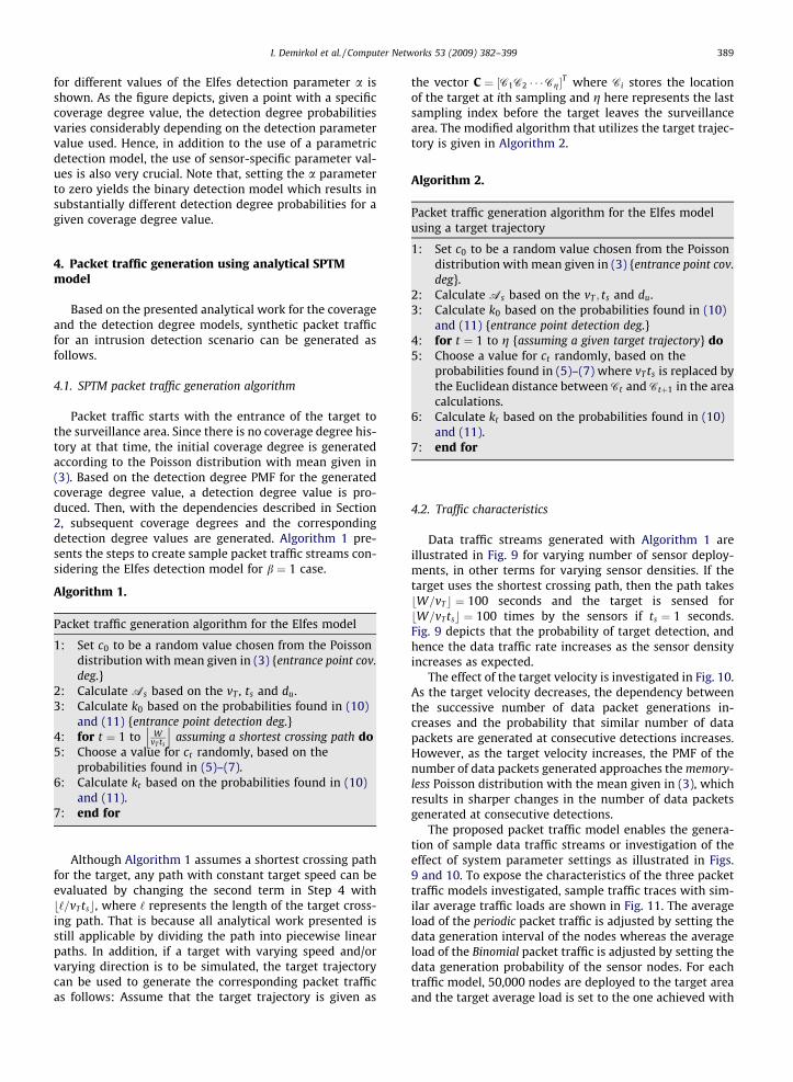
the vector C ¼ ½C1C2 � � �Cg�T where Ci stores the locationof the target at ith sampling and g here represents the lastsampling index before the target leaves the surveillancearea. The modified algorithm that utilizes the target trajec-tory is given in Algorithm 2.

Algorithm 2.

Packet traffic generation algorithm for the Elfes modelusing a target trajectory

1:

Set c0 to be a random value chosen from the Poissondistribution with mean given in (3) {entrance point cov.deg}.

2:

Calculate As based on the vT ; ts and du. 3: Calculate k0 based on the probabilities found in (10)

and (11) {entrance point detection deg.}

4: for t ¼ 1 to g {assuming a given target trajectory} do 5: Choose a value for ct randomly, based on the

probabilities found in (5)–(7) where vT ts is replaced bythe Euclidean distance between Ct and Ctþ1 in the areacalculations.

6:

Calculate kt based on the probabilities found in (10)and (11).

7:

end for

4.2. Traffic characteristics

Data traffic streams generated with Algorithm 1 areillustrated in Fig. 9 for varying number of sensor deploy-ments, in other terms for varying sensor densities. If thetarget uses the shortest crossing path, then the path takesbW=vTc ¼ 100 seconds and the target is sensed forbW=vT tsc ¼ 100 times by the sensors if ts ¼ 1 seconds.Fig. 9 depicts that the probability of target detection, andhence the data traffic rate increases as the sensor densityincreases as expected.

The effect of the target velocity is investigated in Fig. 10.As the target velocity decreases, the dependency betweenthe successive number of data packet generations in-creases and the probability that similar number of datapackets are generated at consecutive detections increases.However, as the target velocity increases, the PMF of thenumber of data packets generated approaches the memory-less Poisson distribution with the mean given in (3), whichresults in sharper changes in the number of data packetsgenerated at consecutive detections.

The proposed packet traffic model enables the genera-tion of sample data traffic streams or investigation of theeffect of system parameter settings as illustrated in Figs.9 and 10. To expose the characteristics of the three packettraffic models investigated, sample traffic traces with sim-ilar average traffic loads are shown in Fig. 11. The averageload of the periodic packet traffic is adjusted by setting thedata generation interval of the nodes whereas the averageload of the Binomial packet traffic is adjusted by setting thedata generation probability of the sensor nodes. For eachtraffic model, 50,000 nodes are deployed to the target areaand the target average load is set to the one achieved with

0 20 40 60 80 100 1200

0.5

1

1.5

2

2.5

3

Time (sec.)

Tota

l Num

ber o

f Dat

a Pa

cket

s G

ener

ated

per

Sec

ond

0 20 40 60 80 100 1200

0.5

1

1.5

2

2.5

3

3.5

4

Time (sec.)

Tota

l Num

ber o

f Dat

a Pa

cket

s G

ener

ated

per

Sec

ond

0 20 40 60 80 100 1202

3

4

5

6

7

8

9

Time (sec.)

Tota

l Num

ber o

f Dat

a Pa

cket

s G

ener

ated

per

Sec

ond

Fig. 9. Effect of node density on data traffic.

390 I. Demirkol et al. / Computer Networks 53 (2009) 382–399

the SPTM traffic for the target speed of 1 m/s and the sens-ing range of 20 m. As seen in Fig. 11, the number of consec-utive SPTM packet generations are correlated. That is whythe interval of the total number of packets generated per sec-ond is larger in the periodic and Binomial packet traffictraces.

Although Figs. 9 and 10 show the traffic generated forshortest crossing paths, different target mobility modelscan be used in SPTM with Algorithm 2. The Gauss–Markovmobility model [21] is widely utilized in ad hoc networkswhere the speed and the direction of mobile node is as-sumed to be correlated over time and modeled as aGauss–Markov stochastic process using the equations

Stþ1 ¼ aSt þ ð1� aÞSþffiffiffiffiffiffiffiffiffiffiffiffiffiffiffiffiffið1� a2Þ

qSXt ; ð14Þ

Etþ1 ¼ aEt þ ð1� aÞEþffiffiffiffiffiffiffiffiffiffiffiffiffiffiffiffiffið1� a2Þ

qEXt ; ð15Þ

where St and Et are the new speed and direction of thetarget at time interval t; �S and E are constants represent-ing the mean value of speed and direction as t !1, and

SXt and EXt are zero-mean Gaussian distributed randomvariables. The degree of randomness is adjusted by the aparameter. As a increases, the current velocity is morelikely to be influenced by the previous velocity, whereassetting a to zero yields the well-known Random Walkmodel. Fig. 12a shows a sample target trajectory for bordercrossing with mean speed of 10 m/s, mean direction of 90�(to represent the aim of crossing the border perpendicu-larly), the memory level parameter a ¼ 0:8 and settingthe Gaussian random variable variances to the one quarterof the mean speed and direction, respectively.

The packet traffic trace for the target trajectory shownin Fig. 12a is given in Fig. 12b. As seen in the figure, theconsecutive packet traffic is correlated. This is an expectedbehavior since, for any target mobility model, the consecu-tive target detection locations will have similar coveragedegrees. Gauss–Markov mobility model results in varyingspeeds, however when vT ts < 2du, the consecutive cover-age degrees will be correlated. For du ¼ 20 m and ts ¼ 1 s,the speeds below 40 m/s will result in a dependency,

0 50 100 150 200 2500

0.5

1

1.5

2

2.5

3

3.5

4

4.5

5

Time (sec.)

Tota

l Num

ber o

f Dat

a Pa

cket

s G

ener

ated

per

Sec

ond

0 20 40 60 80 100 1200

0.5

1

1.5

2

2.5

3

3.5

4

Time (sec.)

Tota

l Num

ber o

f Dat

a Pa

cket

s G

ener

ated

per

Sec

ond

0 10 20 30 40 50 600

1

2

3

4

5

6

Time (sec.)

Tota

l Num

ber o

f Dat

a Pa

cket

s G

ener

ated

per

Sec

ond

Fig. 10. Effect of target velocity on data traffic.

I. Demirkol et al. / Computer Networks 53 (2009) 382–399 391

which actually corresponds to 144 km/h whereas the real-istic target speeds are expected to be lower. For the rarecases where the target goes faster than 144 km/h, for thepacket traffic creation, the Poisson distribution can be usedto generate the coverage degrees and (8)–(11) can be usedto generate the detection degrees based on these coveragedegrees.

5. Impact of a realistic packet traffic model

To investigate the effect of the underlying packet trafficmodel, we conduct various simulations with three differenttypes of packet traffic generation: (i) periodic data genera-tion (ii) binomial data generation achieved by Bernoulli tri-als of the individual nodes, (iii) data generation by SPTMwhich corresponds to the realistic packet traffic for SWSN.We study the impact by examining the performance resultsfor the Sensor-MAC (S-MAC) protocol [10]. S-MAC is aCSMA/CA-based MAC protocol that divides the network into

virtual clusters, where the cluster members have the samesleep-listen schedules and the members at the intersectionof different clusters also wake up at listen periods’ of theirneighboring clusters. Although there are a number ofimprovements on S-MAC such as Time-out-MAC (T-MAC)[22] and Dynamic Sensor-MAC (DSMAC) [23], because ourgoal is to show that using a realistic traffic model makes adifference, we will focus on the basic S-MAC protocol.

The performance of S-MAC is evaluated with the threedifferent packet traffic models based on two performancecriteria. The first one is the average packet delay as usedin [24,25] which is a crucial performance metric for time-critical applications such as disaster monitoring and targettracking. For MAC protocols, packet delay is defined as thetime passed from the data packet’s reception by the sen-der’s MAC layer to its arrival to the destination node’sMAC layer which includes the queueing delay, collision de-lays and the transmission delay. Selecting the averagepacket delay as a performance metric also enables the

0 100 200 300 400 500 600 700 800 900 10000

2

4

6

8

10

12

14

16

Time (sec.)

Tota

l Num

ber o

f Dat

a Pa

cket

s G

ener

ated

per

Sec

ond

0 100 200 300 400 500 600 700 800 900 10000

2

4

6

8

10

12

14

16

Time (sec.)

Tota

l Num

ber o

f Dat

a Pa

cket

s G

ener

ated

per

Sec

ond

0 100 200 300 400 500 600 700 800 900 10000

2

4

6

8

10

12

14

16

Time (sec.)

Tota

l Num

ber o

f Dat

a Pa

cket

s G

ener

ated

per

Sec

ond

Fig. 11. Packet traffic traces of different traffic models with similar mean packet loads.

392 I. Demirkol et al. / Computer Networks 53 (2009) 382–399

investigation of the maximum stable throughput of a sys-tem by inspecting the traffic load that results in infiniteaverage delay.

The second performance criterion inspected is the pack-et drop rate as in [26,27], which is described as the rate ofthe packets dropped due to the limited buffer, or someother system or environment effect such as protocoltime-outs. The packet drop rate is critical if the redundancyof the information sent is low, in other words if the infor-mation within each data packet is crucial for theapplication.

We consider one of the virtual clusters formed in thenetwork separately to investigate the performance of theS-MAC protocol without the influence of the overlayingprotocols such as the routing protocol. Within a virtualcluster, all members that have a data packet to send con-tend for the medium. S-MAC allocates contention slotsfor election of the node that will be given access to themedium. At the beginning of the contention slot period,all pending nodes pick a slot randomly. If a node did not re-ceive start of any transmission before its slot’s time arrives,

it starts to transmit a ready-to-send (RTS) packet. Once thetransmitted packet arrives at the destination node success-fully, the destination node replies with a clear-to-send(CTS) packet. On the other hand, if the first occupied slotis actually selected by two or more nodes, then these nodesstart transmitting their RTS packets at the same time,which results in a collision. These sender nodes realizethe collision when no CTS packet is returned by the desti-nation node within a specified time. Once the CTS packet istransmitted or the CTS time-out triggers, the contentionslot procedure is started again. S-MAC simulation parame-ters and their values are listed in Table 2. Section 5.1 de-scribes the three packet traffic patterns used in thesimulations. Then, Section 5.2 presents the results of thecomparison.

5.1. Packet traffic patterns

To evaluate the impact of the SPTM traffic pattern, twoother data traffic patterns with different data traffic loadsare used for comparison. The traffic load is defined as the

Table 3Parameters of the packet traffic patterns.

Traffic type Parameter Value range

2000 2100 2200 2300 2400 25000

100

200

300

400

500

600

700

800

900

1000

0 10 20 30 40 50 60 70 80 90 1000

2

4

6

8

10

12

14

16

Time (sec.)

Tota

l Num

ber o

f Dat

a Pa

cket

s G

ener

ated

per

Sec

ond

Fig. 12. SPTM traffic generation algorithm is used with Gauss–Markovmobility model.

Table 2Scenario parameters.

Parameter Value

Number of contending sensors 20Bandwidth 20 KbpsData packet size 128 bitRTS/CTS/ACK packet size 26 bitListen period 0.1 sSYNC + Sleep period 0.9 s

I. Demirkol et al. / Computer Networks 53 (2009) 382–399 393

number of new packet arrivals to a system, i.e. the totalnumber of data packets created per unit time for WSNapplications.5 The periodic data traffic is achieved wheneach sensor node generates data with a specific time inter-

5 Two types of traffic loads are defined in the literature, namely, theoffered traffic load and the carried traffic load. In this work, we study thechanges in the system performance according to the number of datapackets generated. Hence, we use the term traffic load to represent theoffered traffic load.

val. A common interval is used by all sensors; however, theyare allowed to choose a random offset. As a result, a period-ically repeating packet traffic occurs. In this traffic model,average packet traffic load can be varied by changing thedata generation interval defined in the system. To have asimplistic and non-periodic packet traffic, probabilistic datageneration is used where the sensor nodes generate datapacket at each unit time based on a specific probability. Con-sequently, the individual data traffic is a Bernoulli processand the aggregate data traffic becomes a Binomial traffic.Here, the traffic load is determined by the probability valueassigned to all sensor nodes for data generation. Both peri-odic data traffic and Binomial packet traffic have the com-mon property of being independent of external eventssuch as target detection. Moreover, in both types of traffic,individual sensor data generation times are independent ofthe other sensors’ data generations.

The SPTM traffic is composed of data packets generatedby the sensor nodes at target detections. Hence, there is adependency between data generations of the neighboringsensors which results in a bursty packet traffic. SPTM pack-et traffic scenario is generated as follows. Within the clus-ter area in which sensor nodes are deployed uniformlyrandom, one target is assumed to move according to therandom waypoint mobility model, which is commonlyadopted in ad hoc networking research community[28,29]. In this model, the mobile is assigned a destinationpoint (‘‘waypoint”) within the rectangular area defined,and a speed uniformly in a given interval. When it reachesthe destination, it remains static for a predefined pausetime and then starts moving again according to the samerule. With SPTM, different packet traffic loads are achievedby altering the value of the sensing range parameter of thedetection degree model. The crucial parameters of thepacket traffic scenarios and their value ranges used forthe simulations are listed in Table 3.

Since we investigate the performance of the S-MAC andtry to isolate it from the other communication layers, in-stead of simulating the whole border, we simulate justone part of it in which all nodes are one-hop away andare able to contend for the medium. Thus, we set a squareshaped area in which all nodes can hear each other.

5.2. Packet traffic model simulation results

S-MAC is implemented in OPNET Modeler simulator[30] based on its ns-2 implementation [31]. Results pre-sented in this section include the average delay and thepacket drop rate of the S-MAC protocol for the three differ-

Periodic Data generation interval 2.25–20 sBinomial Data generation probability 0.05–0.4SPTM Sensing range 15–40 mSPTM Target speed 1 m/sSPTM Pause time 0 sSPTM Area length 100 mSPTM Area width 100 m

394 I. Demirkol et al. / Computer Networks 53 (2009) 382–399

ent packet traffic patterns under various average trafficloads. Each simulation run with a different seed generateda slightly different average aggregate load. Therefore, eachsimulation run is presented as a separate data point in thefigures. The simulated network execution durations arelimited to 12 h, which is sufficient for the convergence ofthe performance values and to have realistic performanceresults. For instance, within that duration, each sensornode generates approximately 2000 packets when periodicdata traffic is selected with the packet interval parameterequal to 20 s.

5.2.1. Unlimited buffer caseThe S-MAC performance results of one-hop delay aver-

ages are shown in Fig. 13 for different packet traffic pat-terns. As seen in the figure, except for very low dataloads where no contention occurs and for very high dataloads where the system is saturated, SPTM results in muchhigher delays than the binomial and periodic data traffic.The reason is that although the amount of data packetsgenerated are close, the packet traffic generated by SPTMis bursty, which results in more contention compared tothe other traffic types. Note that these delays are onlyone-hop link delays, and they must be accumulated untilthe data packet reaches the sink node for the calculationof the end-to-end delay. Hence, other traffic models over-estimate the performance results of the S-MAC protocolfor the SWSN applications, which may result in an ineffi-cient system design.

The effect of the number of contending nodes on theperformance results are investigated by comparing thethree packet traffic types for 10, 20 and 30 nodes. Fig. 14depicts the comparison where for all three cases SPTMpacket traffic yields different performance results thanthe other two models. As the number of contending nodesincreases, the average delays observed for a given load in-crease. The reason is that more contending nodes result inhigher probability of collisions and hence, higher success-ful medium access delays.

0 1 2 3 4 5 6 7 8 910−1

100

101

102

103

104

Average Packet Traffic Load (pkts/sec)

Aver

age

Del

ay (s

ec)

BinomialPeriodicSPTM

Fig. 13. Average delay vs. average load for the S-MAC protocol underdifferent packet traffic patterns (log graph).

In addition to the average packet delays, we also ex-plore the variance of the packet delays which can beimportant for the overlaying WSN application. We choosesample runs from each type of packet traffic pattern thathas similar average traffic loads. Fig. 15 shows the delayhistogram for the sample runs with the average data traf-fic load around 5 packets/s. The system is found to be sta-ble in all of the traffic patterns under this average load.However, as seen in Fig. 15, for similar average trafficloads, the packets arrive with larger delays when SPTMpattern is used.

The SPTM scenario parameter settings also shape theMAC performance as shown in Fig. 16, where the averagedelay results for two different target velocities are shown.Hence, to have a realistic model, appropriate values of thesystem parameters should also be determined.

5.2.2. Limited buffer caseAn important limitation in sensor nodes that should be

considered is the limited memory capacity. That is why, inthe real life scenarios, certain protocol limits are definedfor the number of data packets to be buffered. In addition,if the delay of the packets in the queue reaches to a certainlevel, packet content can be useless for an application inwhich case the packet should be dropped. If a new datapacket arrives from the application layer when the databuffer is full, either this packet can be merged to the previ-ous packets by data aggregation, or one of the old packetsor the new packet may be dropped. Since the packet droprate is an important indicator for the MAC protocol perfor-mance, we study the limited buffer systems for this crite-rion, setting the data packet buffer limit to be 10 or 50packets.

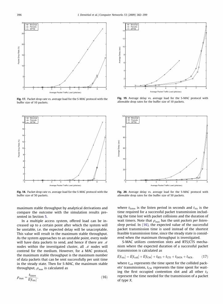
The packet drop percentages for different packet trafficpatterns are shown in Figs. 17 and 18 for the buffer size of10 and 50 packets, respectively. The SPTM resulted inmuch higher packet drop rates for the traffic loads higherthan 3 and 5 packets/s, respectively. This is also an indica-tion of burstiness of the packet traffic generated by theSPTM, since similar traffic loads always result in morepacket drops for SPTM. Moreover, for the range of 3–7packets/s, although there is no packet drops in the othertraffic types, SPTM packet traffic results in non-negligiblepacket drop rates.

We investigate the average delay results for the threepacket traffic patterns for the case where the newly cre-ated packets are dropped when the buffer is full. Assigninga packet drop rate threshold of 10%, Figs. 19 and 20 showthe average packet delays encountered for the buffer sizeof 10 and 50 packets, respectively. The SPTM packet trafficstill creates much higher average delays compared to thetwo other packet traffic patterns.

6. Analytical verification of the maximum throughputfound by the SPTM packet traffic

The figures presented in Section 5 includes the perfor-mance results of the S-MAC communication protocolachieved by simulation for the three different packet trafficmodels. To verify these results in part, we investigate the

0 1 2 3 4 5 6 7 8 9 1010−2

10−1

100

101

102

103

104

Average Packet Traffic Load (pkts/sec)

Aver

age

Del

ay (s

ec)

BinomialPeriodicSPTM

0 1 2 3 4 5 6 7 8 910−1

100

101

102

103

104

Average Packet Traffic Load (pkts/sec)

Aver

age

Del

ay (s

ec)

BinomialPeriodicSPTM

0 2 4 6 8 10 12 1410−1

100

101

102

103

104

Average Packet Traffic Load (pkts/sec)

Aver

age

Del

ay (s

ec)

BinomialPeriodicSPTM

Fig. 14. Average delay vs. average load for the S-MAC protocol for different number of contending nodes (log graph).

0 10 20 30 40 50 60 70 80100

101

102

103

104

105

106

Delay (sec)

Num

ber o

f Occ

uren

ce

BinomialPeriodicSPTM

Fig. 15. Delay histogram of sample runs with similar average traffic loads.

1 1.5 2 2.5 3 3.5 4 4.5 5 5.5 60

5

10

15

20

25

30

35

Average Packet Traffic Load (pkts/sec)

Aver

age

Del

ay (s

ec)

SPTM (vT=10 m/s)SPTM (vT=1 m/s)

Fig. 16. Average delay vs. average load for the S-MAC protocol withdifferent system parameter values.

I. Demirkol et al. / Computer Networks 53 (2009) 382–399 395

0 1 2 3 4 5 6 7 8 90

5

10

15

20

25

30

Average Packet Traffic Load (pkts/sec)

Pack

et D

rop

Rat

e (%

)

BinomialPeriodicSPTM

Fig. 17. Packet drop rate vs. average load for the S-MAC protocol with thebuffer size of 10 packets.

0 1 2 3 4 5 6 7 8 90

2

4

6

8

10

12

14

16

18

20

Average Packet Traffic Load (pkts/sec)

Pack

et D

rop

Rat

e (%

)

BinomialPeriodicSPTM

Fig. 18. Packet drop rate vs. average load for the S-MAC protocol with thebuffer size of 50 packets.

0 1 2 3 4 5 6 7 80

2

4

6

8

10

12

14

16

Average Packet Traffic Load (pkts/sec)

Aver

age

Del

ay (s

ec)

BinomialPeriodicSPTM

Fig. 19. Average delay vs. average load for the S-MAC protocol withallowable drop rates for the buffer size of 10 packets.

0 1 2 3 4 5 6 7 80

20

40

60

80

100

120

Average Packet Traffic Load (pkts/sec)

Aver

age

Del

ay (s

ec)

BinomialPeriodicSPTM

Fig. 20. Average delay vs. average load for the S-MAC protocol withallowable drop rates for the buffer size of 50 packets.

396 I. Demirkol et al. / Computer Networks 53 (2009) 382–399

maximum stable throughput by analytical derivations andcompare the outcome with the simulation results pre-sented in Section 5.

In a multiple access system, offered load can be in-creased up to a certain point after which the system willbe unstable, i.e. the expected delay will be unacceptable.This value will result in the maximum stable throughput.As the system approaches to an unstable point, every nodewill have data packets to send, and hence if there are M

nodes within the investigated cluster, all M nodes willcontend for the medium. However, for a MAC protocol,the maximum stable throughput is the maximum numberof data packets that can be sent successfully per unit timein the steady state. Then for S-MAC, the maximum stablethroughput, qmax is calculated as

qmax ¼tlisten

E½tstx�; ð16Þ

where tlisten is the listen period in seconds and tstx is thetime required for a successful packet transmission includ-ing the time lost with packet collisions and the duration ofwait timers. Note that qmax has the unit packets per listen-sleep period. In (16), the expected value of the successfulpacket transmission time is used instead of the shortestfeasible transmission time, since the steady state is consid-ered when the maximum throughput is investigated.

S-MAC utilizes contention slots and RTS/CTS mecha-nism where the expected duration of a successful packettransmission is calculated as

E½tstx� ¼ E½tcoll� þ E½tCW� þ tRTS þ tCTS þ tDATA þ tACK; ð17Þ

where tcoll represents the time spent for the collided pack-ets’ transmissions, tCW represents the time spent for wait-ing the first occupied contention slot and all other tX

represent the time needed for the transmission of a packetof type X.

Table 4Simulation parameters used in analytical formula.

Parameter Value

Number of contention slots 63Number of contending nodes 20Slot time 0.001 sSleep period 0.9 sListen period 0.1 sBandwidth 20 KbpsData packet size 128 bitRTS/CTS/ACK packet size 26 bit

Table 5Numerical results found by analysis.

Parameter Calculated value

n 0.8492f 0.1508E½tCW� 0.0025 sE½tcoll� 0.0011 sE½tstx� 0.0139 s

I. Demirkol et al. / Computer Networks 53 (2009) 382–399 397

Since S-MAC is 1-persistent CSMA and collision isunderstood by the CTS time-out triggered when no CTSpacket is received after tCTS, the expected time spent forcollisions is calculated as

E½tcoll� ¼X1z¼0

zðE½tCW� þ tRTS þ tCTSÞfz; ð18Þ

where z is the number of successive collisions and f is theprobability of packet collision in a contention period. How-ever, in a protocol with contention slots, a collision occurswhen the first occupied slot is selected by two or morenodes. Therefore, the probability that a slot assignment re-sults in a collisionless transmission is

n ¼ ð1� fÞ ¼XZ�1

f¼1

PðF ¼ f jZ;MÞ; ð19Þ

where PðF ¼ f jZ;MÞ represents the probability that f isthe first occupied slot and it is selected by only one nodegiven that the contention window consists of Z contentionslots and there are M contending nodes. Thus,

PðF ¼ f jZ;MÞ ¼MðZ� f ÞM�1

ZM; ð20Þ

because there are ZM different slot assignment possibili-ties among which the following assignments results in col-lisionless transmission: f is chosen by any of M nodes andthe slots f þ 1 to Z, i.e. Z� f slots, are chosen randomly byM� 1 nodes. Incorporating (20) into (21) yields

n ¼XZ�1

f¼1

PðF ¼ f jZ;MÞ

¼Mð2M�1 þ � � � þ ðZ� 1ÞM�1Þ

ZM: ð21Þ

The expected waiting time till the first occupied contentionslot is

E½tCW� ¼XZw¼1

ðw� 1ÞPðW ¼ wÞtslot; ð22Þ

where tslot is one slot duration and W represents the ran-dom variable of the index of the first occupied slot. There-fore, PðW ¼ wÞ gives the probability that the wth slot is thefirst occupied slot which can be defined as

PðW ¼ wÞ ¼ Pððsi P w; 8i ¼ 1::MÞ ^ ðsi ¼ w; 9i ¼ 1::MÞÞ;

where si represents the slot chosen by node i.Consequently,

PðW ¼ wÞ ¼ Z� wþ 1Z

� �M

� Z� wZ

� �M

: ð23Þ

The maximum stable throughput of S-MAC under SPTMpacket traffic can be calculated analytically once the sys-tem parameter values are given. To compare the maximumstable throughput achieved at simulation results with theanalytically found throughput, the simulation parametersvalues given in Table 4 are applied to (16)–(23), and themaximum stable throughput formula components are cal-culated to be as tabulated in Table 5. According to these

values, the maximum stable throughput is found to be7.195 packets/s. The traffic load that results in instabilityin Fig. 13 matches the analytical maximum stable through-put result. Although the simulation results match the ana-lytical results at the maximum stable throughput, theintermediate throughput-delay value calculations remainas an open issue.

Note that these calculations require the exact averagedelay derivations for the given average traffic loads whichmust consider the randomly deployed node locations, ran-domly moving target’s trajectory, MAC collision probabili-ties that depend on the number of data packets of thenodes and individual packet delays that depend on thepacket queue size of the sensor nodes.

7. Conclusions

In this paper, a new packet traffic model framework isdevised for intrusion detection applications using theElfes sensor detection model. The system design parame-ters considered in this framework are the number of sen-sors deployed, the area size of the border, the detectiondistance thresholds, the target velocity, the samplinginterval and the Elfes detection model parameters. Simu-lation results support the analytical work presented forthe packet traffic model under this probabilistic detectionmodel.

To show the importance of using a realistic packet traf-fic model for evaluating WSN communication protocols,we investigate the performance of S-MAC for differentpacket traffic models. Simulation results indicate that eval-uating S-MAC with a packet traffic model other than theone proposed may give misleading results for the intrusiondetection applications. The reason is revealed to be thebursty nature of the SPTM packet traffic which is provenanalytically. Although, the effect of using a realistic packettraffic model is demonstrated for a MAC protocol, it canalso be emphasized for other layers such as routing proto-

398 I. Demirkol et al. / Computer Networks 53 (2009) 382–399

cols. Moreover, the proposed model can be a baseline tohave separate analytical studies for event-based WSN.

As a future work, the presented packet traffic model canbe extended to include multiple target trajectories. In addi-tion, the analytical traffic model can be updated by consid-ering the relayed packets as part of the routing activity.The impact of using a realistic packet traffic model can alsobe investigated for the energy consumption metric. Usingthe proposed packet traffic model, the performance of var-ious kinds of applications can easily be investigated such asthe one in which the detecting nodes send their packetswith a certain probability.

Acknowledgement

This work is supported by the Scientific and Technolog-ical Council of Turkey (TUBITAK) under the Grant Number106E082.

References

[1] B. Gedik, L. Liu, P.S. Yu, ASAP: an adaptive sampling approach to datacollection in sensor networks, IEEE Trans. Parallel Distrib. Syst. 18(12) (2007) 1766–1783.

[2] S. Kashihara, N. Wakamiya, M. Murata, Implementation andevaluation of a synchronization-based data gathering scheme forsensor networks, in: Proc. IEEE ICC, vol. 5, Korea, 2005, pp. 3037–3043.

[3] S. Gandham, M. Dawande, R. Prakash, An integral flow-based energy-efficient routing algorithm for wireless sensor networks, in: Proc.IEEE WCNC, vol. 4, Atlanta, USA, 2004, pp. 2341–2346.

[4] Y. Ma, J.H. Aylor, System lifetime optimization for heterogeneoussensor networks with a hub-spoke topology, IEEE Trans. MobileComput. 3 (3) (2004) 286–294.

[5] X. Shi, G. Stromberg, SyncWUF: An ultra low-power MAC protocol forwireless sensor networks, IEEE Trans. Mobile Comput. 6 (1) (2007)115–125.

[6] S.D. Muruganathan, A.O. Fapojuwo, A hybrid routing protocol forwireless sensor networks based on a two-level clustering hierarchywith enhanced energy efficiency, in: Wireless Communications andNetworking Conference, 2008, WCNC 2008, IEEE, 2008, pp. 2051–2056.

[7] I. Demirkol, F. Alagöz, H. Deliç, C. Ersoy, Wireless sensor networks forintrusion detection: packet traffic modeling, IEEE Commun. Lett. 10(1) (2006) 22–24.

[8] G.G. Messier, I.G. Finvers, Traffic models for medical wireless sensornetworks, IEEE Commun. Lett. 11 (2007) 13–15.

[9] Y. Wong, W. Seah, L. Ngoh, W. Wong, Sensor traffic patterns in targettracking networks, in: Wireless Communications and NetworkingConference, 2007, WCNC 2007, IEEE, 2007, pp. 4123–4126.

[10] W. Ye, J. Heidemann, D. Estrin, Medium access control withcoordinated adaptive sleeping for wireless sensor networks, IEEE/ACM Trans. Netw. 12 (3) (2004) 493–506.

[11] Crossbow Technology Inc., MPR-MIB Users Manual, June 2006.[12] Y. Zou, K. Chakrabarty, Sensor deployment and target localization

based on virtual forces, in: Proc. IEEE INFOCOM’03, vol. 2, SanFrancisco, USA, 2003, pp. 1293–1303.

[13] Y. Zou, K. Chakrabarty, Uncertainty-aware and coverage-orienteddeployment for sensor networks, J. Parallel Distrib. Comput. 64 (7)(2004) 788–798.

[14] A. Elfes, Occupancy grids: a stochastic spatial representation foractive robot perception, in: S.S. Iyengar, A. Elfes (Eds.), AutonomousMobile Robots: Perception, Mapping and Navigation, vol. 1, IEEEComputer Society Press, 1991, pp. 60–70.

[15] E. Onur, C. Ersoy, H. Deliç, How many sensors for an acceptablebreach detection probability?, Comput Commun. 29 (2006) 173–182.

[16] E. Onur, C. Ersoy, H. Deliç, L. Akarun, Surveillance wireless sensornetworks: deployment quality analysis, IEEE Netw. 21 (6) (2007)48–53. November–December.

[17] W. Peng-Jun, Y. Chih-Wei, Coverage by randomly deployed wirelesssensor networks, IEEE Trans. Inf. Theory 52 (6) (2006) 2658–2669.

[18] S. Ren, Q. Li, H. Wang, X. Chen, X. Zhang, Design and analysis ofsensing scheduling algorithms under partial coverage for objectdetection in sensor networks, IEEE Trans. Parallel Distrib. Syst. 18 (3)(2007) 334–350.

[19] G. Wang, G. Cao, T.L. Porta, W. Zhang, Sensor relocation in mobilesensor networks, in: Proc. IEEE INFOCOM, vol. 4, Miami, USA, 2005,pp. 2302–2312.

[20] C. Pandana, K.J.R. Liu, Maximum connectivity and maximum lifetimeenergy-aware routing for wireless sensor networks, in: Proc. IEEEGLOBECOM’05, vol. 2, St. Louis, USA, 2005, pp. 1034–1038.

[21] B. Liang, Z.J. Haas, Predictive distance-based mobility managementfor PCS networks, in: INFOCOM (3), 1999, pp. 1377–1384.

[22] T.V. Dam, K. Langendoen, An adaptive energy-efficient MAC protocolfor wireless sensor networks, in: Proc. ACM SenSys, Los Angeles,USA, 2003, pp. 171–180.

[23] P. Lin, C. Qiao, X. Wang, Medium access control with a dynamic dutycycle for sensor networks, in: Proc. IEEE WCNC, vol. 3, Atlanta, USA,2004, pp. 1534–1539.

[24] J. Zhu, S. Papavassiliou, J. Yang, Adaptive localized QoS-constraineddata aggregation and processing in distributed sensor networks,IEEE Trans. Parallel Distrib. Syst. 17 (9) (2006) 923–933.

[25] S.C. Ergen, P. Varaiya, PEDAMACS: power efficient and delay awaremedium access protocol for sensor networks, IEEE Trans. MobileComput. 5 (7) (2006) 920–930.

[26] A.K. Karmokar, D.V. Djonin, V.K. Bhargava, Optimal and suboptimalpacket scheduling over correlated time varying flat fading channels,IEEE Trans. Wireless Commun. 5 (2) (2006) 446–456.

[27] F. Zhenghua, L. Haiyun, P. Zerfos, S. Lu, L. Zhang, M. Gerla, The impactof multihop wireless channel on TCP performance, IEEE/ACM Trans.Netw. 4 (2) (2006) 209–221.

[28] C. Bettstetter, G. Resta, P. Santi, The node distribution of the randomwaypoint mobility model for wireless ad hoc networks, IEEE Trans.Mobile Comput. 2 (3) (2003) 257–269.

[29] L. Hu, D. Evans, Localization for mobile sensor networks, in: Proc.ACM MobiCom, Philadelphia, USA, 2004, pp. 45–57.

[30] Opnet Modeler, URL <http://www.opnet.com/products/modeler/home.html>, 2006.

[31] The Network Simulator-ns-2, URL <http://www.isi.edu/nsnam/ns/>,2006.

Ilker Demirkol received the B.Sc. (with hon-ors), M.Sc. and Ph.D. degrees in computerengineering from Bogazici University, Istan-bul, Turkey, in 1998, 2002, and 2008 respec-tively. Currently, he is a post-doctoralresearcher in University of Rochester, NY. Heworked as a database, system and networkengineer from 1997 to 2004. He was researchand teaching assistant in Bogazici University,Computer Engineering department from 2004to 2008. His research interests include theareas of wireless communications, wireless ad

hoc and sensor networks, and optimization of communication networks.

Cem Ersoy received his BS and MS degrees inelectrical engineering from Bogazici Univer-sity, Istanbul, in 1984 and 1986, respectively.He worked as an R&D engineer in NETAS A.S.between 1984 and 1986. He received his Ph.D.in electrical engineering from PolytechnicUniversity, Brooklyn, New York in 1992. Cur-rently, he is a professor in the ComputerEngineering Department of Bogazici Univer-sity. His research interests include perfor-mance evaluation and topological design ofcommunication networks, wireless commu-

nications and mobile applications. He is a Senior Member of IEEE.

I. Demirkol et al. / Computer Networks 53 (2009) 382–399 399

Fatih Alagöz is currently an associate pro-fessor in the Department of Computer Engi-neering, Bogazici University, Turkey. He waswith the Department of Electrical Engineer-ing, Harran University, Turkey. During 2001–2003, he was with the Department of Elec-trical and Computer Engineering, UAE Uni-versity, UAE. He obtained his D.Sc. degree inelectrical engineering in 2000, from GeorgeWashington University, USA. His currentresearch areas include terrestrial and satellitemobile networks, sensor networks, UWB

communications. He has edited two books, and published more than fiftyscholarly papers in selected journals and conferences.

Hakan Deliç received the B.S. degree (withhonors) in electrical and electronics engi-neering from Bogazici University, Istanbul,Turkey, in 1988, and the M.S. and the Ph.D.degrees in electrical engineering from theUniversity of Virginia, Charlottesville, in 1990and 1992, respectively. He was a ResearchAssociate with the University of VirginiaHealth Sciences Center from 1992 to 1994. InSeptember 1994, he joined the University ofLouisiana at Lafayette, where he was on theFaculty of the Department of Electrical and

Computer Engineering until February 1996. He was a Visiting AssociateProfessor in the Department of Electrical and Computer Engineering,

University of Minnesota, Minneapolis, during the 2001–2002 academicyear. He is currently a professor of electrical and electronics engineeringat Bogazici University, and a visiting professor with the Faculty of Elec-trical Engineering, Mathematics and Computer Science, Delft Universityof Technology, Netherlands. His research interests lie in the areas ofcommunications and signal processing with current focus on wirelessmultiple access, ultra-wideband communications, OFDM, robust systems,and sensor networks.