ES struktūrinių fondų poveikio bendrajam vidaus

produktui vertinimas

1 p r i e d a s . L i e t u v o s e k o n o m i k o s H E R L I T m o d e l i s : a p r a š y m a s i r i n s t r u k c i j a

Užsakovas: LR Finansų ministerija

Paslaugų teik÷jas: UAB „BGI Consulting“

2009, rugpjūtis

2

The HERLIT model of the Lithuanian economy:

Description and User Guide

prepared by

John Bradley

UAB “BGI Consulting”

2009

Contact for communications

EMDS - Economic Modelling and Development Strategies Dr. John Bradley 14 Bloomfield Avenue, Dublin 8, Ireland Phone: +353-1-454 5138 Mobile : +353-86-829 8799 Skype : bradleysjandm Fax: +353-1-497 0001 Mail: john.bradley@iol.ie

UAB “BGI Consulting” – Business Government Innovation Consulting Jonas Jatkauskas, Public policy department Address: Užupio Str. 11-8, Vilnius, Lithuania Phone: (+370 5) 215 4075, 215 3969 Fax: (+370 5) 215 4837 E-mail: info@bgiconsulting.lt Website: www.bgiconsulting.lt

3

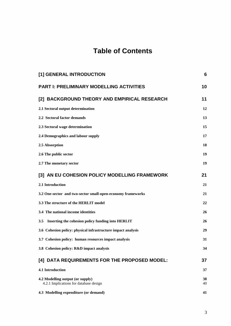
Table of Contents

[1] GENERAL INTRODUCTION 6

PART I: PRELIMINARY MODELLING ACTIVITIES 10

[2] BACKGROUND THEORY AND EMPIRICAL RESEARCH 11

2.1 Sectoral output determination 12

2.2 Sectoral factor demands 13

2.3 Sectoral wage determination 15

2.4 Demographics and labour supply 17

2.5 Absorption 18

2.6 The public sector 19

2.7 The monetary sector 19

[3] AN EU COHESION POLICY MODELLING FRAMEWORK 21

2.1 Introduction 21

3.2 One-sector and two-sector small-open-economy frameworks 21

3.3 The structure of the HERLIT model 22

3.4 The national income identities 26

3.5 Inserting the cohesion policy funding into HERLIT 26

3.6 Cohesion policy: physical infrastructure impact analysis 29

3.7 Cohesion policy: human resources impact analysis 31

3.8 Cohesion policy: R&D impact analysis 34

[4] DATA REQUIREMENTS FOR THE PROPOSED MODEL: 37

4.1 Introduction 37

4.2 Modelling output (or supply) 38 4.2.1 Implications for database design 40

4.3 Modelling expenditure (or demand) 41

4

4.3.1 Implications for database design 42

4.4 Modelling income 42 4.4.1 Implications for database design 42

PART II: MODEL CONSTRUCTION AND TESTING 43

[5] CREATION OF A DATABASE FOR HERLIT 44

5.1 Introduction 44

5.2: The international data used in HERLIT 44

5.3: Lithuanian national accounts and related data 45

5.4: A miscellaneous set of data 46

5.5: The generation of the complete HERLIT database. 46

[6] EMPIRICAL ECONOMETRIC RESEARCH FOR HERLIT 49

6.1 Introductory remarks 49

6.2 The model equation listing 51

6.3: Calibrating the joint factor demand systems 52

6.4 : Calibration of the remaining behavioural equations 52

6.5 Calibration results for behavioural equations 53 The Manufacturing sector 53 The Market Services sector 56 The Building and Construction sector 57 The Agricultural sector 58 Demographics and labour supply 59 Expenditure 60 Expenditure deflators 60 Concluding remarks on calibration 61

[7] CONSTRUCTION AND TESTING OF THE HERLIT MODEL 62

7.1 Introduction 62

7.2 Checking the model structure 62

7.3 Shocking the model 63 7.3.1 A shock to world output (OWM) 64 7.3.2 A public employment shock (LG) 65 7.3.3 A shock to government investment (IGV) 65 7.3.4 A shock to all exogenous price levels 66 7.3.5 Conclusions on responses to shocks 67

[8] CONCLUDING REMARKS 68

8.1 Possible weaknesses in the HERLIT-based analysis 68

5

8.2 A future work programme for HERLIT 69

REFERENCES 70

ANNEX 1: THE HERLIT MODEL EQUATION LISTING 72

ANNEX 2: GENERATING THE HERLITDB DATABASE 104

ANNEX 3: IMPLEMENTING, TESTING AND RUNNING HERLIT 1 34

ANNEX 4: A HERLIT-BASED PROJECTION METHODOLOGY 137

ANNEX 5: MASTER DICTIONARY OF HERLIT MODEL VARIABLE S 142

6

[1] General introduction The new HERLIT model of the Lithuanian economy is described in this report, as a background to the application of the model to examine the likely impacts of the SPD 2004-2006 on the macro economy. The actual SPD impact analysis will be presented in a separate report. Taken together, the two reports constitute the final stage of our contractual work on the macroeconomic side of the ex-post SPD analysis. Of necessity, this report is rather technical, since the issues involved in model design and construction are in themselves very technical. But some knowledge of how the HERLIT model functions is useful, if not essential, in order to understand and interpret the SPD policy impact results. Since the reform of the European Union’s policy for economic and social cohesion in the late 1980s, both the Commission and the national governments of member states who receive investment aid have been faced with two separate but inter-related tasks. The first task involves the design of integrated programmes of public investment that implement the EU cohesion policy and which are part financed by Structural Funds and Cohesion Funds, and co-financed out of domestic resources. In our work we have to take the design of the SPD as given, but we can examine some counterfactual variations as part of the impact evaluation. The second task involves the evaluation of the impact of the investment programmes that implement cohesion policy, before (ex ante), during (mid-term) and after (ex post) their implementation.1 In our work, we are required to carry out an ex-post impact evaluation, and this is carried out with the aid of the new HERLIT model, and documented in a separate report. Since the late 1980s, the task of impact evaluation has been implemented in two different ways. The first – micro evaluation – examines likely impacts at a highly disaggregated level of individual projects, measures and groups of measures. The second – macro evaluation – takes place at a more aggregated level of Operational Programmes and/or at the level of the entire set of investment programmes such as those that make up the Lithuanian SPD 2004-2006 and the Cohesion Fund. For the macro stage of evaluation, with which we are concerned, disaggregation of the SPD and Cohesion Fund investment programmes takes the form of three economic categories: physical infrastructure, human resources and direct aid to firms. In the HERLIT model to be described in this report, we incorporate mechanisms that can analyse the SPD and Cohesion Fund programme impacts in terms of these three economic categories. If a higher degree of disaggregation were desired (such as further disaggregation into different types of physical infrastructure), then the design of the HERLIT model would have to be modified accordingly. This would be possible in future work.2 In order to be able to analyse the impacts of policies that are as complex as those that make up the SPD and the Cohesion Fund, one needs to have a fairly sophisticated economic model. Some of the features of the model that will be required for the analysis include the following: 1 See “Ex-ante evaluation of the Lithuanian Objective 1 programme: Final Report”, CSES,

October 2003, for the ex-ante evaluation of the Lithuanian SPD 2004-2006. 2 The three-way split of the SPD into physical infrastructure, human resources and direct aid to

firms is also the one that is used by the European Commission in its own in-house evaluations.

7

a) The model must have a well specified production, expenditure and income side, permitting the quantification of SPD and Cohesion Fund policy impacts on the performance of a range of production sectors (e.g., manufacturing, building and construction, agriculture, market and non-market services), on all the standard elements of expenditure (private and public consumption, investment, trade), and on elements of income (such as wage rates and profits).

b) The model must handle public sector revenue and expenditure, in order to permit

analysis of shifts in public sector balances due to the absorption and disbursement of EU funds and domestic co-finance.

c) The model must handle the labour market, distinguishing labour demand (at level

of each production sector), labour supply, population growth and migration. d) Where necessary, the model should have monetary mechanisms in order to permit

analysis of the impact of SPD and Cohesion Fund policies on monetary variables (e.g., interest rates and exchange rates).

e) It must be possible to analyse the trade flows between Lithuania and the rest of the

world in order to examine net trade impacts of SPD and Cohesion Fund policies. f) The model should be structural, in the sense of being based, where appropriate on

micro-foundations. Within that structure, the supply-side of the model must be designed in such a way as to permit incorporation of the main mechanisms through which EU cohesion policy initiatives impact on the productive potential of the recipient economy.3

The HERLIT model described in this report addresses these desired features in the case of the Lithuanian economy. However, it should be emphasized that the kind of sophisticated econometric modelling that is more common in the advanced, developed economies of the EU is not equally feasible for an economy like Lithuania. In most of the new EU member states that joined in 2004, time series of data prior to about the year 1995 tend to be unreliable for modelling and rapid structural development has been taking place since 1995. Both factors place severe limits on the kinds of econometric (or “calibration”) techniques that can be used during model construction in an economy like Lithuania. This first version of the HERLIT model was constructed using annual national accounting and other data time series covering the period 1995-2007, i.e., thirteen observations. This is inadequate to support rigorous econometric testing. So, simplified model calibration techniques have to be used, as will be described later in the report. The HERLIT model is an instrument designed to analyse the macroeconomic and macro-sectoral impacts of the Lithuanian SPD and Cohesion Fund policy actions and is an adaptation of the HERMIN modelling framework that is widely used by the Commission and by many national Governments (see Bradley et al, 2004 for a survey). HERLIT is intended for use in the ex-post evaluation of SPD 2004-2006 and of the Cohesion Funds for the same period.4 Since EU cohesion policy is implemented over an extended period of years, and has longer-term impacts even after implementation is complete, HERLIT must be capable of quantifying the short-term (implementation) impacts as well as the longer-term (supply-side) impacts that become important in the post-implementation

3 The requirement to have appropriate micro-foundations is to ensure that the application of SPD

policies does not change the structure of the model in unpredictable ways, thereby invalidating use of the model for ex-ante or ex-post impact analysis.

4 Henceforth, we will use the term “EU cohesion policy” to include the SPD and the Cohesion Funds.

8

period. Furthermore, HERLIT needs to be flexible enough to permit a range of “no-cohesion-policy” counterfactuals, e.g., zero EC intervention, or any other desired counterfactual. It must also be capable of distinguishing between point-impacts (i.e., impacts for any given year) and cumulative impacts (i.e., impacts that are accumulated from any base year (e.g., 2004) to any subsequent year (e.g., out as far as the selected terminal date, 2020).5 In designing HERLIT we also need to direct attention to the issue of policy crowding out, i.e., where EU cohesion policy expenditure might result in negative feedback on private sector activity through higher tax rates, higher interest rates and labour market tightening. However, the initial experience in previous analysis of cohesion policy impacts has been that these crowding-out effects are unlikely to be very large in the “new” EU member states, particularly since the EU interventions relate to the provision of public goods necessary to modernize the economy (see Bradley and Untiedt, 2008). We also have to take account of the fact that the Lithuanian cohesion policies were implemented during a period of very high growth and low unemployment, prior to the present global recession. To a degree, this background performance of the Lithuanian economy was related to the impacts of cohesion policy. However, most of the growth was driven by a consumer spending and a building and construction boom. Nevertheless, the fact that cohesion policy was partially implemented during a period of high growth needs to be taken into account in the ex-post impact analysis. In contract, the current SPD 2007-2013 is being implemented in a period of deep recession and negative growth. To implement as many of the above features as possible, HERLIT seeks an appropriate balance between simplicity and complexity. In addition, we pay attention to the need both to quantify policy impacts as well as to highlight and explain the underlying policy mechanisms. So HERLIT should be regarded both as a tool for carrying out quantitative impact analysis as well as a tool to assist the more qualitative explanation of the results. The rest of the report is divided into two main phases: Part I: Description of the preliminary activities to the construction of HERLIT Part II: Description of the construction and testing of HERLIT. Within Part I there are three Sections. Section 2 sets the applied theoretical background to the model, drawing of the macroeconomic literature on modelling. Section 3 discusses how we approach the task of modelling the impact of the EU cohesion policy instruments on the macro economy. Section 4 discusses the data needs of a model like HERLIT in general terms. Within Part II there are four Sectionss. Section 5 describes in detail how we constructed the database for HERLIT, drawing on EUROSTAT and national sources. The detail is provided so that any interested user will be in the position to update the database as new data become available. Section 6 describes the calibration of the behavioural equations in HERLIT, i.e., those equations that are derived from theory (in Section 2), but which contain parameters that must be assigned values on the basis of actual data. Section 7

5 The implementation phase of cohesion policy expenditures for the 2004-2006 programming

period effectively ended in December, 2008. In order to examine the post-implementation impacts, we need to run the analysis out beyond 2008. We select the year 2020 as a terminal date, since it is sufficiently far into the future to analysis long-tailed consequences of the cohesion policy investment programmes.

9

describes how the model functions as a system, and shows how it can be “tested” by exposing it to a series of standardised policy and other shocks. We also describe how HERLIT can be used to produce a baseline “forecast” (more properly, a baseline “projection”) that will be needed when we study the impacts of the SPD. Section 8 concludes, and suggests ways in which HERLIT might be improved in the future.

10

Part I: Preliminary Modelling Activities

11

[2] Background theory and empirical research Any economic model that is intended for use in the analysis of the impacts of EU cohesion policy investment programmes needs to have a structure that is appropriate to the aims of the analysis. We set out below some areas of the economy where specific mechanisms must be modelled, since they are very relevant to the way in which cohesion policy is likely to impact on the economy. We start with output determination, since the implementation and the post-implementation impacts of EU cohesion policy are designed to stimulate output and productivity (supply), with secondary impacts on expenditure (demand). A specific range of sectors must be examined, since the aim is to improve primarily the performance of manufacturing and market services, while the big infrastructural programmes are implemented through the building and construction sector. The agricultural sector is only affected by EU cohesion policy to a very minor extent, but it is useful to detach that sector from the non-agricultural side of the economy.6 Finally, some elements of EU cohesion policy programmes are implemented through the government (or non-market) sector, so that sector must also be studied. In previous economic policy modelling it has often been the case that output and factor inputs (such as labour and capital) are studied in isolation from each other. However, when one needs to analyse how EU cohesion policy is likely to affect output, employment and factor productivity, one must handle these aspects in an integrated way. We describe how a production function approach is necessary, and how it can be used empirically to assist in the analysis and interpretation of policy impacts. In a small, open economy like Lithuania, with a fixed exchange rate relative to the euro, most prices are heavily influenced by external price movements. However, the domestic wage rate is determined to some extent by domestic forces, and wage bargaining must be analysed carefully. We review briefly a structural way of doing this (the so called “Scandinavian” model of Lindbeck, 1979). In view of the very long-tailed effects of EU cohesion policies, it is important to study how movements in demographics and labour supply affect the outcome, and are in turn affected by the cohesion policy. We review some of the issues. Although EU cohesion policy investment programmes have impacts on consumption and trade, these are not the primary focus of the programmes. Nevertheless, we need to examine how demand-side (or Keynesian) impacts affect an economy. We review the consumption function, and discuss how trade impacts can be studied. The EU cohesion policy programmes are implemented mainly through public sector policy instruments (such as investment in physical infrastructure, training programmes and direct transfers made to private firms. We review the economic analysis of the public sector, revenue and expenditure aspects. We also review monetary issues. However, in the case of Lithuania the fixed exchange rate against the euro greatly simplifies the analysis.

6 It is the Common Agriculture Policy (or CAP) that has the biggest impacts on the performance of

the agriculture sector. However, our focus is on EU cohesion policy.

12

2.1 Sectoral output determination The theory underlying the study of a small open economy like Lithuania requires that the equation for output in a mainly internationally traded sector like manufacturing reflects both purely supply side factors (such as the real unit labour costs and international price competitiveness), as well as the extent of dependence of output on a general level of world demand, for example through operations of multinational enterprises, as described by Bradley and FitzGerald (1988). By contrast, domestic demand should play only a limited role in manufacturing, mostly in terms of its impact on the rate of capacity utilisation. However, manufacturing, in any but very extreme cases, will always include a large number of partially sheltered sub-sectors producing items that are partially non-traded. Hence, we would expect domestic demand to play some role in manufacturing, possibly also influencing capacity output decisions of firms. A common approach is to use a hybrid supply-demand equation of the form:

(2.1) log( ) log( ) log( / )OT a a OW a ULCT POT= + +1 2 3 + + +a FDOT a POT PWORLD a t4 5 6log( ) log( / ) where OW represents the important external (or world) demand and FDOT represents the possible influence of domestic absorption. We further expect OT to be negatively influenced by real unit labour costs (ULCT/POT) and by the relative price of domestic versus world goods (POT/PWORLD). Fairly simple forms of the market service sector output equation (OM) and the building and construction output equation (OB) are usually quite adequate: (2.2) log(OM) = a1 + a2 log(FDOM) + a3 log(OW) + a4 log(ULCM/POM) + a4 t (2.3) log(OB) = b1 + b2 log(IBCTOT) + b3 log(ULCB/POB) + b4 t where FDOM is a measure of domestic demand and OW is a measure of “world” demand (in the OM equation) and IBCTOT is total investment in building and construction by all the other four sectors. The inclusion of the world output term (OW) in the market services OM equation can take account of countries that have large tourism, international transport services that are internationally traded, or large transit trade (as in the Baltic States). The variables ULCM and ULCB are unit labour costs in market services and building and construction, respectively, and are deflated using the sectoral GDP deflators (POM and POB).

Output in agriculture can be studied in great sub-sectoral detail. However, in the first version of HERLIT we take the view that progress in reforming and modernising agriculture will depend on very specific conditions in Lithuania. Basically, we summarise these complex processes in terms of the rate of productivity growth and the associated process of labour release from the sector. But for eventual use in a macroeconomic policy model, agricultural output (OA) is usually derived from inverting a time-trended labour productivity equation, (2.4) log(OA/LA) = a0 + a1 t Output in the public sector (OGV) is determined mainly by public sector employment (LG), which is a policy instrument (i.e., set by government decision, subject to a public finance constraint). The identity reads as follows:

13

(2.4) OGV = LG*WG + OGNWV where OGV is non-market services output (in current prices), LG is employment numbers, WG is average annual earnings and OGNWV is non wage output.

2.2 Sectoral factor demands

We assume a production function of the general form:

(2.5) Q f K L= ( , ) where Q represents output, K capital stock and L employment. However, output is not necessarily determined by this relationship.7 We have seen above that manufacturing output is determined by a mixture of world and domestic demand, together with price and cost competitiveness terms. Having determined output in this way, the role of the production function is to constrain the determination of factor demands in the process of cost minimisation that is assumed. This is in contrast to the case of profit maximisation, where output and factor demands are all determined simultaneously, constrained by the production function.

Hence, given Q (determined as in equations (2.1), (2.2) and (2.3) in a hybrid supply-demand relationship), and given (exogenous) relative factor prices, the factor inputs, L and K, are determined via optimisation behaviour of firms by the production function constraint. Hence, the production function operates in the model as a technology constraint and is only indirectly involved in the determination of output. It is partially through these interrelated factor demands that the longer run efficiency enhancing effects of policy and other shocks like the EU Single Market and cohesion policy are believed to operate.8

Ideally, policy analysis should allow for a production function with a fairly flexible functional form that permits a variable elasticity of substitution. As the experience of several small open economies suggests, this issue is important (Bradley and Fitz Gerald, 1988). When an economy opens to international trade and becomes progressively more influenced by activities of foreign-owned multinational companies, the traditional substitution of capital for labour following an increase in the relative price of labour need no longer happen to the same extent. The internationally mobile capital may choose to move to a different location than seek to replace costly domestic labour. In terms of the neoclassical theory of firm, the isoquants get more curved as the technology moves away from a Cobb-Douglas towards a Leontief type.9

Since the Cobb-Douglas production function is very restrictive (with its assumed unit elasticity of substitution), we use the more general CES form of the added value production function and impose it on the factor demand systems of the manufacturing (T), market services (M) and building and construction (B) sectors. Thus, in the case of manufacturing;

7 In some models (such as the QUEST model of DG-ECFIN), capacity output is determined by the production function, with actual output determined in Keynesian fashion by demand. The ratio of actual to capacity output is usually taken as a measure of capacity utilization. 8 Bradley and Fitz Gerald (1988) set out a more rigorous theoretical statement of the determination of output and factor demands. 9 Most models use the simple Cobb-Douglas production function, which is more tractable analytically. However, the imposition of a unit elasticity of substitution may seriously exaggerate the possibilities of factor substitution as relative factor prices change.

14

(2.6) ( ) { } ( ){ }[ ] ρρρ δδλ1

1exp−−− −+= KTLTtAOT ,

In this equation, OT, LT and KT are added value, employment and the capital stock, respectively, A is a scale parameter, ρ is related to the constant elasticity of substitution, δ is a factor intensity parameter, and λ is the rate of Hicks neutral technical progress.

In both the manufacturing and market service sectors, factor demands are derived on the basis of cost minimisation subject to given output, yielding a joint factor demand equation system (i.e., the demand for capital and labour) of the schematic form:

(2.7a)

=w

rQgK ,1

(2.7b)

=w

rQgL ,2

where w and r are the cost of labour and capital, respectively.10

Although the central factor demand systems in the manufacturing (T), market services (M) and building and construction (B) sectors are functionally identical, they will have different estimated parameter values and two further crucial differences.

(a) First, output in the manufacturing sector (OT) is driven by world demand (OW)

and domestic demand (FDOT), and is influenced by international price competitiveness (PCOMPT) and real unit labour costs (RULCT). In the sheltered sectors, on the other hand, we tend to find that output in market services and building & construction (OM and OB) is driven mainly by domestic demand (FDOMS and IBCTOT, respectively), with only a very limited possible role for world demand (OW) in driving OM. This captures the essential difference between the neoclassical-like tradable manufacturing sector and the more two more sheltered Keynesian non-traded sector.11

(b) Second, the output price in manufacturing (T) is mainly externally determined by

the world price. In the market services and building sectors (M and B), the producer prices are a mark-up on costs.12 This puts another difference between the partially price taking tradable sector and the price making non-tradable sector.

The modelling of factor demands in the agriculture sector is normally treated very simply, but can always be extended in satellite models, where the institutional aspects of agriculture are fully included. We saw above that GDP in agriculture can be modelled simply as an inverted productivity relationship. Labour input into agriculture is modelled as a (declining) time trend, and not as part of a neo-classical optimising system, as in manufacturing, market services and building and construction. Labour is assumed to be

10 The above treatment of the capital input to production in HERMIN is influenced by the earlier work of d’Alcantara and Italianer, 1982 on the vintage production functions in the HERMES model. The implementation of a full vintage model was impossible, even for the original four EU cohesion countries. A hybrid putty-clay model is adopted in HERMIN (Bradley, Modesto and Sosvilla-Rivero, 1995). 11 When we refer to a sector as being “non-traded”, we mean that its output is only sold locally and is not exported, nor is it subject to direct competition from imported substitutes. Many service sector activities fall into this category. 12 In the case of the M sector output price, one would have to examine for a possible role of world prices, particularly in economies with significantly traded sectors.

15

gradually “released” out of the sector int non-agricultural sectors. The capital stock in agriculture is modelled as a trended capital/output ratio.13

Finally, in the non-market service sector the factor demands (i.e., numbers employed and fixed capital formation) are exogenous instruments and are effectively under the control of policy makers, subject to fiscal solvency and other policy criteria.

2.3 Sectoral wage determination

Study of the determination of wages and prices in a small open economy like Lithuania can be approached in many different ways. One might design equations that are specific to each sector, and influenced by sectoral characteristics (e.g., the degree of exposure to world competitiveness pressures, the degree of unionisation, required levels of human capital, etc.). However interesting and insightful this approach might be, it runs the risk of permitting wide divergences to emerge in the evolution of sectoral wage inflation. However, such divergences in wage inflation rates tend not to be observed in practice, at least over a medium-term horizon. Of course significant differences in the level of sectoral wages are observed, and these can persist over long periods.

For Lithuania, we adopt a simpler approach, influenced by the so-called “Scandinavian” model as it applies to most small open economies (Lindbeck, 1979). Based on this approach, the behaviour of the internationally exposed manufacturing sector (T) is assumed to play a dominant role in relation to wage determination in the other sectors of the economy. More specifically, the wage inflation determined in the manufacturing sector tends to be passed through to the down-stream, more “sheltered sectors, e.g., building and construction, market services, agriculture and non-market services, in equations of the form:

(2.8a) WMDOT = WTDOT + ε

(2.8b) WBDOT = WTDOT + ε

(2.8c) WADOT = WTDOT + ε

(2.8d) WGDOT = WTDOT + ε

where WTDOT, WMDOT, WBDOT, WADOT and WGDOT are the wage inflation rates in manufacturing, market services, building and construction, agriculture and non-market services, respectively, and ε is a random error term.14

In the crucial case of manufacturing, wage rates are assumed to be determined as the outcome of a bargaining process that takes place between organised trades unions and employers, with the possible intervention of the government. Formalised theory of wage bargaining points to four paramount explanatory variables (Layard, Nickell and Jackman, 1990):

13 We emphasise that the simple trended relationships that we use in agriculture can always be replaced by more sophisticated models. Agriculture is “different”, and standard neoclassical optimising paradigms are not appropriate in the new EU member states. At this stage we merely aim to disaggregate it from the private non-agriculture sectors (T, B and M). 14 Equations 2.8(a)-(d) are actually behavioural, in the sense that they state a statistically testable hypothesis. Examination of Lithuanian data series for the period 1995-2007 suggests that they do capture trend behaviour (i.e., differences are fairly random, and a unit coefficient on WTDOT is plausible.

16

a) Output prices: The price that the producer can obtain for output clearly influences the price at which factor inputs, particularly labour, can be purchased profitably.

b) Consumer prices: This is the main concern of workers, and it can often deviate from producer prices.

c) The tax wedge: This wedge is driven by total taxation between the wage denominated in output prices and the take home consumption wage actually enjoyed by workers. Research suggests that it has at most a transitory impact.

d) The rate of unemployment: The unemployment or structural “Phillips curve” effect in the equation is a proxy for bargaining power. For example, unemployment is usually inversely related to the bargaining power of trades unions (i.e., the higher the rate of unemployment, the weaker is the bargaining power of trade unions). The converse applies to employers.

e) Labour productivity: The productivity effect comes from workers’ efforts to maintain their share of added value, i.e. to enjoy some of the gains from higher productivity or output per worker.

A general log-linear formulation of the Layard-Nickell-Jackman type wage equation can take the following form:

(2.9) Log(WT) = a1 +a2 log(POT) + a3 log(PCONS) + a4 log(WEDGE)

+ a5 log(LPRT) + a6 UR

where WT represents the wage rate, POT the price of manufactured goods, PCONS the consumption deflator, WEDGE the tax “wedge”, LPRT labour productivity and UR the rate of unemployment.

This is a very important equation in HERLIT when analysing fiscal shocks, or, more generally, EU cohesion policy shocks, for reasons such as the following:

i. Any public policy that serves to boost the economy is likely to increase employment

and reduce unemployment. Depending on whether the labour supply is endogenous (say, through migration) or exogenous (a closed labour market), the increase in numbers employed will not necessarily be equal to the reduction in numbers unemployed. Since the expected calibrated value of the coefficient on UR is negative (i.e., higher unemployment is assumed to dampen wage bargaining), any reduction in the rate of unemployment will serve to push up wage rates. This effect will be higher in the case of a closed labour market than in the case of an open labour market.

ii. EU cohesion policy is specifically designed to raise the level of labour productivity, as will be explained in the next section. The knock-on impact on wage rates will depend on the magnitude and sign of the coefficient of LPRT (labour productivity in manufacturing). In practice, this coefficient is positive, but can range between zero and unity. Any value higher than unity is unsustainable in the longer term. Any value less than zero would imply that the work force was willing to work harder for less wages. In countries with strong trades unions, values near unity can be observed. But in countries like Ireland and Lithuania, and other small states where inward investment is important, one usually finds values in the range from about 0.3 to 0.8. In those cases, the wage-push effects of EU cohesion-type policies will be smaller than in cases where the productivity elasticity is near unity, since some of the benefits of higher productivity go to profits rather than wages.

17

iii. The third mechanism through which wage inflationary impacts of cohesion-type policies can operate is through their impacts on prices. In the cases of either fixed or partially fixed exchange rates, the deflator of manufacturing output is usually anchored partially to world prices, and is less affected by domestic inflationary pressures. But wages can also be partially linked to consumer prices, and any cost push effects of cohesion policy will work mainly through this channel.

iv. The above points focus only on policy effects that may cause wage inflation in manufacturing. But once inflationary pressures come on wage rates in manufacturing, they are transmitted onwards to all the other sectors, via the transmission mechanisms on the so-called Scandinavian model (see equations 2.8(a)-(d) above).

v. The mechanisms through which wage pressures transmits to other areas of the economy (e.g., to sectoral output) are complicated. For example, manufacturing output is sensitive to international price competitiveness and to movements in unit labour costs (see equation 2.2 above). One can say that a rise in real unit labour costs (ULCT/POT) will reduce manufacturing output (OT), when other things are equal. But one would have to actually simulate the model with a specific kind of EU cohesion policy shock in order to see how real unit labour costs would be affected.

2.4 Demographics and labour supply In any medium-term policy analysis, population growth can be modelled through a “natural” growth rate, corrected for net additions or subtractions due to migration. Net migration flows can then be modelled using a standard Harris-Todaro approach that drives migration by the relative attractiveness of the local (or national) and international labour markets, where the latter can be proxied by an appropriate destination of migrants, e.g., the UK, Germany, Sweden, Ireland, etc. in the case of Lithuania (Harris and Todaro, 1970).15 Attractiveness can be measured in terms of the relative expected wage, i.e., the product of the probability of being employed by the average wage in each region.

The evolution of population tends to be fairly stable, in the absence of large migration flows or other demographic disasters. In that case, it would be simpler to treat population as exogenous, and project it using external information. However, the presence of migration flows complicates matters since population movements and shifts in the labour force can take place.

In policy analysis, it is useful to treat population in terms of three age cohorts: pre-working age (NJUV); working age (NWORK); and post-working age (NELD). In all three cases one can specify a natural growth mechanism (where the rate of growth/decline is obtained from data). However, we link net out-migration (NM) only to the working age group, based on the fact that most migrants are of working age). The three equations are as follows:

(2.10a) ∆NJUV = a1 NJUV-1 + ε

(2.10a) ∆NWORK = b1 NWORK-1 + b2 NM + ε

(2.10a) ∆NELD = c1 NELD-1 + ε

15 The Irish-UK migration relationship is long established, and can be explored econometrically. In the case of Lithuania, the short time span and the relatively poor quality of migration data makes it very difficult to test the Harris-Todaro framework, and to calibrate the parameters.

18

where ε is a stochastic error term. Note that if net outward migration (NM) is measured as a positive number, the sign of the coefficient b2 will be expected to be negative.16 The calibrated parameters a1 ,b1 and c1 are the “natural” growth rates of the respective population cohorts.

Finally, the labour force participation rate (i.e., LFPR, the fraction of the working-age population (NWORK) that participates in the labour force (LF)), is treated as a single aggregate.17 The aggregate labour force participation rate (LFPR) can be modelled as a function of the unemployment rate (UR) and a time trend that is designed to capture slowly changing socio-economic and demographic conditions, together with the possibility of an encouraged/discouraged worker effect, proxied by the unemployment rate (UR).

(2.11) LFPR = a1 + a2 UR + a3 t

2.5 Absorption

Household consumption represents by far the largest component of aggregate demand in most developed economies. The properties of the consumption function play an important role in transmitting the effects of changes in fiscal policy to aggregate demand via the Keynesian multiplier. The determination of household consumption is usually kept simple in models of the new EU member states, and private consumption (CONS) is determined partially by real personal disposable income (YRPERD), with the possibility of capturing a wealth effect (WNH). In other words, we assume that consumers are only partially liquidity constrained.

(2.12) CONS = a1 + a2 YRPERD + a3 WNH-1 If the coefficient a3 is identically zero, households become completely liquidity constrained, i.e., they can only consume out of their current income and have no access to savings or credit in order to smooth their consumption. More sophisticated approaches could be adopted.18 However, such versions are unlikely to be capable of being calibrated in most of the new member states, due to unavailability of data time series sufficiently long to facilitate econometric estimation and the rapid development of banking facilities operating in the household sector of the economy.

As for the remaining elements of absorption, public consumption is determined primarily by public employment, which is (effectively) a constrained policy instrument. Private investment is determined within production sectors as the investment part of the sectoral factor demand systems (see above). Public investment is a constrained policy instrument. Inventory changes (DS) are modelled using the standard stock-adjustment approach. Finally, in keeping with the guiding spirit of the two-sector small-open-economy model, exports and imports are not modelled explicitly (see below). Instead, the net trade surplus can be residually determined from the balance between GDP on an

16 In equations 2.10a-c, we assume for simplicity that all migrants are of working age. 17 Future versions of the HERLIT model might disaggregate employment by gender, in which case a similar disaggregation of the labour force would be required. For the present, we do not implement this disaggregation. 18 For example, in the Irish HERMIN model, experiments were carried out with hybrid liquidity constrained and permanent income models of consumption. It was found that the long-run properties of the model were relatively invariant to the choice between a hybrid and a pure liquidity constrained function. However, if a forward looking model of wage income is used, the adjustment properties of the model change radically (Bradley and Whelan, 1997).

19

output basis (GDPFC) and domestic absorption (GDA). Hence, to the extent that a policy shock drives up domestic absorption more than output, the net trade surplus deteriorates. The sectoral output equations take on many of the properties of export equations (i.e., they can be influenced by world demand, competitiveness, etc.

2.6 The public sector Any model that will be used for public policy impact analysis needs to include a high degree of institutional detail in the public sector. Within the category of total public expenditure, we distinguish public consumption (mainly wages of public sector employees), transfers (social welfare, subsidies, debt interest payments), and capital expenditure (public housing, infrastructure, investment grants to industry). Within public sector debt interest, we would ideally like to distinguish interest payments to domestic residents from interest payments to foreigners, the latter representing a leakage out of GDP through the balance of payments.

One often needs a method of altering public policy instruments within a policy model in reaction to the economic consequences of any given policy shock. If all the policy instruments are exogenous, this is not possible, although instruments can be changed on the basis of off-model calculations. A possible solution of the problem is by incorporating an “intertemporal fiscal closure rule”, whose task is to ensure that some policy instrument (such as the direct tax rate) is manipulated in such a way as to keep the debt/GNP ratio close to an exogenous notional target debt/GNP ratio. A policy feed back rule might take the following form:

(2.13)

−−−

−

−

=∆ −−

GNPV

GNDTGNDTGNDTGNDT

GNPV

GNDTGNDTRGTYP

)()()( *11

**

βα

where RGTYP is the personal tax rate, GNDT is the total national debt, GNDT* is the target value of GNDT, GNPV is nominal GNP, and the values of the parameters α and β are selected in the light of model simulations. Of course, the performance of the rule can be quite sensitive to the choice of the numerical values of α, β.

2.7 The monetary sector The above modelling framework captures the direct pass-through of changes in the nominal exchange rate into prices and wages, and also the indirect effects operating through competitiveness impacts of real exchange rate (relative price of tradable goods) and real unit labour costs on output. In addition, the framework captures the effects of changes in real interest rates on output and inflation through capital formation and labour/investment decisions of firms. Both nominal exchange rate and real interest rate are therefore important exogenous policy variables of the original model framework, though disjoint. The real interest rate could be endogenised by introducing market nominal interest rates that will move according to: i) the laws of international arbitrage in response to movements in the world interest

rates and exogenous country risk premium, and

20

ii) the extent of the sterilization policies/reserve accumulations that the country authorities decide to undertake. In this framework, international reserve targets can also be implemented as a target policy variable, if relevant for a particular country.

In addition, the block of monetary aggregates could be linked to other variables (notably, consumption, output and interest rates), building on well established concepts. However, such a sophisticated approach would very likely distract from the core function of a medium-term model like HERLIT that is designed for the analysis of EU cohesion policy impacts, without necessarily adding much by way of robust analysis that could not be included in off-model adjustment of the (exogenous) interest and exchange rates. A simpler approach is probably more desirable.

21

[3] An EU cohesion policy modelling framework 2.1 Introduction

The Keynesian, demand-driven view of the world that dominated macro modelling prior to the mid-1970s was found to be inadequate when the economies of the OECD were hit by the supply-side shocks of the crises of the 1970s. From the mid-1970s onwards, attention came to be focused on issues of productivity and cost competitiveness as important ingredients in output determination, at least in highly open economies. More generally, analysis of the importance of the manner in which expectation formation was handled by modellers could no longer be ignored, and the reformulation of empirical macro models took place against the background of a radical renewal of macroeconomic theory in general.

The original HERMIN modelling framework drew on many aspects of the above revision and renewal of macro economic modelling. The origins of the HERMIN model can be found in the complex multi-sectoral HERMES model that was developed by the European Commission in the early 1980s (d’Alcantara and Italianer, 1982). HERMIN was initially designed to be a small-scale version of the HERMES model framework in order to take account of the very limited data availability in the poorer, less-developed EU member states and regions on the Western and Southern periphery (i.e., Ireland, Portugal, Spain and Greece). A consequence of the lack of detailed macro-sectoral data, and of sufficiently long time-series that had no structural breaks, was that the HERMIN modelling framework needed to be based on a fairly simple theoretical framework that permitted analysis of a reasonably robust kind. Also, inter-country and inter-region comparisons were highly desirable, since they facilitated the selection of key behavioural parameters in situations where sophisticated econometric analysis was difficult, if not impossible.

An example of a simple but useful theoretical modelling framework is one that treats goods as being of two types: internationally tradable (T) and non-tradable (N) (see Lindbeck, 1979). Drawing on this literature, relatively simple versions of the model can be used to structure debates that take place over macroeconomic issues in small open economies. The HERMIN model shows how an empirical model can be constructed that incorporates and builds on many of these relatively robust theoretical insights.

3.2 One-sector and two-sector small-open-economy frameworks In the simplest one-sector model, all goods are assumed to be internationally tradable, and all firms in the small open economy are assumed to be perfect competitors. This has two strong implications;

a) Goods produced domestically are perfect substitutes for goods produced

elsewhere, so that prices (mediated through the exchange rate) cannot deviate from world levels;

b) Firms are able to sell as much as they desire to produce at going world prices. It

rules out Keynesian phenomena right from the start.

22

The ‘law of one price’, operating through goods and services arbitrage, therefore ensures that the domestic price is determined as follows:

(3.1) p ep

t t= *

where pt is the domestic price, e is the price of foreign currency (or the exchange rate), and pt

* is the world price. Under a fixed exchange rate this means that in the simple stylised model, domestic inflation is determined entirely abroad by the inflation rate of pt*. The second implication of perfect competition is that the small open economy faces an infinitely elastic world demand function for its output, and an infinitely elastic world supply function for whatever it wishes to purchase.

A major weakness of the one-sector model as a description of economic reality, even for an economy as extremely open as Lithuania, is that the assumption (implied by perfect competition) that domestic firms can sell all they desire to produce at going world prices is clearly unrealistic. For example, to take account of the phenomenon that world demand exerted an impact on Irish output independent of its impact on price, Bradley and FitzGerald, 1988 proposed a model in which a significant proportion of tradable-sector production in the small, open economy is assumed to be carried out by internationally mobile multi-national corporations (MNCs), whose price-setting decisions are independent of the local (or host) factor costs. When world output expands, MNCs expand production at all their production locations. However, the proportion of MNC investment located in any individual host economy depends on its relative competitiveness. This allows the host country’s output to be determined both by domestic factor costs and by world demand. However, since the internal demand is often very small relative to world demand, it plays no role in the MNC's output decisions.

Another weakness of the one-sector small open economy model is that, as already implied, government spending is precluded from having any impacts on output. However, research suggests otherwise. Most studies of Irish employment and unemployment conclude that the debt-financed fiscal expansion of the late-1970s did indeed boost employment and reduce unemployment, albeit temporarily, and at the expense of requiring very contractionary policies over the course of the whole 1980s (Barry and Bradley (1991)).

To address these criticisms, one can add an extra sector, the non-tradable (N) sector, to the above one sector model. Output and employment in the (internationally) tradable sector (T) continues to be determined as before, while the non-internationally tradable (N) sector operates more like a closed economy model. The interactions between the two sectors prove interesting, however. For example, the price of non-tradables is determined by the interaction of supply and demand for these goods. This extension to two sectors (tradable and non-tradable) motivated the decision to identify the real world approximation of these sectors in the specification of the HERMIN model. We approximate the tradable sector mainly with manufacturing, and the non-tradable sector with market services. However, in reality, some proportion of manufacturing is likely to be non-traded, and elements of market services (such as tourism, financial and professional services) are likely to be internationally traded. Consequently, the sectoral identification is only approximate.

3.3 The structure of the HERLIT model We now discuss some practical and empirical implications that need to be taken into account when designing an empirical model of a typical European small open economy like Lithuania, building on the stylised insights of the two-sector theoretical model. Since the model is being constructed in order to analyse medium and long-term impacts of EU

23

cohesion policies, there are three general and systemic requirements which it should satisfy:

(i) The model must be disaggregated into a small number of crucial production

sectors which allows one identify and model the key sectoral shifts in the economy over the years of development.

(ii) The model must specify the mechanisms through which a “cohesion-type”

economy is connected to the external world. The external (or world) economy is a very important direct and indirect factor influencing the economic growth and convergence of the lagging EU economies, through trade of goods and services, inflation transmission, population emigration and inward foreign direct investment.

(iii) The construction of the model must recognise that a possible conflict may exist

between actual situation in the country, as captured in a HERLIT model calibrated with the use of historical data, and the changed structure towards which the cohesion economy is evolving in an economic environment dominated by EMU, the Single European Market and wider forces of globalisation. In other words, design and calibration purely on the basis of econometrics using past data (even where feasible) are likely to be inappropriate.

The framework design of the HERLIT model focuses on key structural features of a cohesion-type economy, of which the following are important:

a) The degree of economic openness, exposure to world trade, and response to external and internal shocks;

b) The relative sizes and features of the internat6ionally traded and non-traded sectors and their development, production technology and structural change;

c) The mechanisms of wage and price determination;

d) The functioning and flexibility of labour markets with the possible role of international and inter-regional labour migration;

e) The role of the public sector and the possible consequences of public debt accumulation, as well as the interactions between the public and private sector trade-offs in public policies.

f) Monetary mechanisms that may affect development in medium and long-term time horizons.

In order to satisfy these requirements, the initial HERMIN framework originally had four sectors: manufacturing (a mainly (internationally) traded sector), market services (a mainly non-traded sector, that included building and construction), agriculture, and government (or non-market) services: see Bradley, Herce and Modesto, 1995. In the present Lithuanian model, HERLIT, we further disaggregate the older aggregate market services sector (N) into two separate sub-sectors: building and construction (B) and the rest of market services (M).19 Given the severe data restrictions that face modellers in cohesion and transition economies, this is as close to an empirical representation of the traded/non-traded disaggregation as we are likely to be able to implement in practice. Although agriculture also has internationally traded elements, its underlying characteristics (e.g., traditional structure, price support and other aspects of the Common Agriculture Policy (CAP) require separate treatment. Similarly, the government (or non-market) sector is non-traded, but is best formulated in a way that recognises that it is 19 The separate treatment of building and construction (B) is desirable since a large proportion of the SPD and Cohesion Funds involve investment in physical infrastructure.

24

mainly driven by policy instruments that are available – to some extent, at least – to policy makers.20 The internal structure of the HERLIT modelling framework is composed of three main blocks:

i. A supply block,

ii. An absorption block, and

iii. An income distribution block.

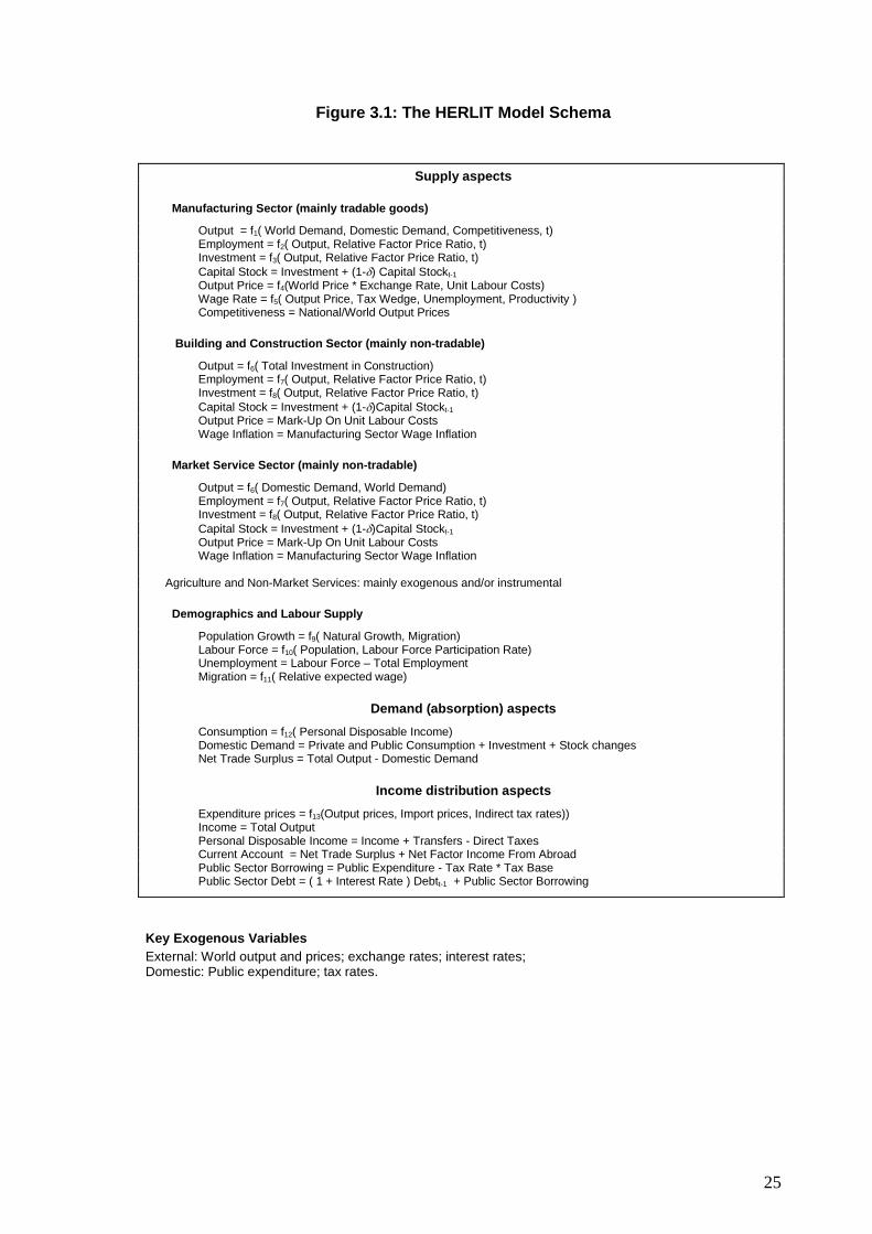
Obviously, the HERLIT model functions as an integrated system of equations, with interrelationships between all their sub-components. However, for expositional purposes we describe the framework in terms of the above three sub-components, which are schematically illustrated in Figure 3.1.

Conventional Keynesian mechanisms are included in the short-term behaviour of the HERLIT model. This statement should not be misunderstood as implying that HERLIT is a simple Keynesian model. Nevertheless, when subject to a demand shock, expenditure and income distribution sub-components generate fairly standard income-expenditure mechanisms. For example, the implementational phase of EU cohesion policy has a demand component, as public expenditure is increased, but longer-term supply side benefits have yet to appear.

But the HERLIT model also has many neoclassical features in the longer term. Thus, output in manufacturing is not simply driven by demand. It is also influenced by price and cost competitiveness, where firms seek out minimum cost locations for production (Bradley and FitzGerald, 1988). In addition, factor demands in manufacturing and market services are derived on the assumption of cost minimization, using a CES production function constraint, where the capital/labour ratio is sensitive to relative factor prices. The incorporation of a structural Phillips curve mechanism in the wage bargaining mechanism introduces further relative price effects. Most importantly, we will show later that the cohesion policy mechanisms operate through the supply side of the model, at least in the medium to long term.

HERLIT handles the three complementary ways of measuring GDP in the national accounts, on the basis of output, expenditure and income. On the output basis, HERLIT disaggregates five sectors: manufacturing (OT), building and construction (OB), market services (OM), agriculture (OA) and the public (or non-market) sector (OG). On the expenditure side, HERLIT disaggregates GDP into the conventional five components: private consumption (CONS), public consumption (G), investment (I), stock changes (DS), and the net trade balance (NTS).21 National income is determined on the output side, and disaggregated into private and public sector elements of wages and profits.

20 Elements of public policy are endogenous, but we prefer to handle these in terms of policy feed-back rules rather than behaviourally (see previous section). 21 The traded/non-traded disaggregation implies that only a net trade balance is logically consistent. Separate equations for exports and imports could be appended to the model, but would function merely as conveniently calculated “memo” items that were not an essential part of the model’s behavioural logic.

25

Figure 3.1: The HERLIT Model Schema

Supply aspects

Manufacturing Sector (mainly tradable goods)

Output = f1( World Demand, Domestic Demand, Competitiveness, t) Employment = f2( Output, Relative Factor Price Ratio, t) Investment = f3( Output, Relative Factor Price Ratio, t) Capital Stock = Investment + (1-δ) Capital Stockt-1 Output Price = f4(World Price * Exchange Rate, Unit Labour Costs) Wage Rate = f5( Output Price, Tax Wedge, Unemployment, Productivity ) Competitiveness = National/World Output Prices

Building and Construction Sector (mainly non-tradable)

Output = f6( Total Investment in Construction) Employment = f7( Output, Relative Factor Price Ratio, t) Investment = f8( Output, Relative Factor Price Ratio, t) Capital Stock = Investment + (1-δ)Capital Stockt-1 Output Price = Mark-Up On Unit Labour Costs Wage Inflation = Manufacturing Sector Wage Inflation

Market Service Sector (mainly non-tradable)

Output = f6( Domestic Demand, World Demand) Employment = f7( Output, Relative Factor Price Ratio, t) Investment = f8( Output, Relative Factor Price Ratio, t) Capital Stock = Investment + (1-δ)Capital Stockt-1 Output Price = Mark-Up On Unit Labour Costs Wage Inflation = Manufacturing Sector Wage Inflation Agriculture and Non-Market Services: mainly exogenous and/or instrumental

Demographics and Labour Supply

Population Growth = f9( Natural Growth, Migration) Labour Force = f10( Population, Labour Force Participation Rate) Unemployment = Labour Force – Total Employment Migration = f11( Relative expected wage)

Demand (absorption) aspects

Consumption = f12( Personal Disposable Income) Domestic Demand = Private and Public Consumption + Investment + Stock changes Net Trade Surplus = Total Output - Domestic Demand

Income distribution aspects

Expenditure prices = f13(Output prices, Import prices, Indirect tax rates)) Income = Total Output Personal Disposable Income = Income + Transfers - Direct Taxes Current Account = Net Trade Surplus + Net Factor Income From Abroad Public Sector Borrowing = Public Expenditure - Tax Rate * Tax Base Public Sector Debt = ( 1 + Interest Rate ) Debtt-1 + Public Sector Borrowing

Key Exogenous Variables External: World output and prices; exchange rates; interest rates; Domestic: Public expenditure; tax rates.

26

3.4 The national income identities

The income-output identity is used in HERLIT to derive corporate profits. In the actual model, there are various data refinements, but the identity is essentially of the form:

(3.2) YC = GDPFCV - YW where YC is profits, GDPFCV is GDP at factor cost, and YW is the wage bill for the entire economy. Income of the private sector (YP) is determined in a relationship of form:

(3.3) YP = GDPFCV + GTR where GTR is total public sector transfers to the private sector. Income of the household (or personal) sector (YPER) is defined essentially as:

(3.4) YPER = YP – YCU where YCU is that element of total profits (YC) that is retained within the corporate sector for reinvestment, as distinct from being distributed to households as dividends. Finally, personal disposable income (YPERD) is defined as

(3.5) YPERD = YPER - GTY where GTY represents total direct taxes (income and employee social contributions) paid by the household sector. It is the constant price version of YPERD (i.e., YRPERD=YPERD/PCONS) which drives private consumption in the consumption function:

(3.6) CONS = a1 + a2 YRPERD + a3 WNH-1

3.5 Inserting the cohesion policy funding into HERLIT In its most simple form, the EU cohesion policy data, as negotiated by the recipient country with the EC, consists of time series for the total Community (EC) funding allocation to each recipient state, usually expressed in millions of current euro. The HERLIT notation for these basic data is GECSFEC_E, and they are given for the years 2004-2008 inclusive.

As part of the negotiations with the European Commission, a domestic co-finance ratio is agreed. This percentage is designated as RDCOFIN in the formulae below. The total EC and domestic public (EC+DP) expenditure is then split between three main economic categories using the national shares implicit in the detailed sectoral and regional Operational Programmes contained in the national cohesion policy document. These economic categories are physical infrastructure, human resources, and direct aid to the productive sectors. The further allocation of the direct aid to productive sectors is carried out using assumed shares (as between manufacturing, market services and agriculture).

The EC total expenditure contribution for each of the years 2004 to 2008 in current euro is considered as a datum in the analysis (GECSFEC_E). This is converted to national

27

currency (GECSFEC) using exchange rate for a selected base period, and is denoted by LTEUR. Consequently,

GECSFEC = GECSFEC_E * LTEUR

The implied domestic public (DP) co-finance contribution (GECSFDP), is derived using an assumed domestic co-finance ratio (RDCOFIN, the per cent of the total of EC and domestic public finance that is the domestic co-finance). RDCOFIN is defined by us as follows. If GECSFEC is the EU funding contribution, and GECSFDP is the domestic public co-finance contribution, then:

RDPCOFIN=100*GECSFDP/(GECSFEC+GECSFDP)

In HERLIT we take the domestic public co-finance ratio (RDPCOFIN) as a datum and transform the above definition to define the level of domestic co-funding, given a specified level of EU funding, i.e., we solve the above equation for GECSFDP:

GECSFDP = (RDPCOFIN/(100-RDPCOFIN)) * GECSFEC The implied domestic private (PR) co-finance contribution (GECSFPR), is similarly derived using an assumed domestic co-finance ratio (RPRCOFIN percent), defined as follows. Total EC plus DP finance is taken as the base for calculating the domestic private co-finance ratio.

RPRCOFIN=100*GECSFPR/(GECSFEC+GECSFDP)

In HERLIT we solve the above equation for the level of domestic private co-finance (GECSFPR):

GECSFPR = (RPRCOFIN/100) * (GECSFEC+GECSFDP)

Total (EC+DP+PR) expenditure (GECSF) is defined as:

GECSF = GECSFEC + GECSFDP + GECSFPR

This total (GECSF) is then disaggregated into three main economic categories.

(a) Physical infrastructure (IGVCSFXX)

(b) Human Resources (GTRSFXX), and

(c) Direct Aid to the Productive Sector (TRIXX),

where XX=EC (Community), DP (Domestic Public) and PR (Domestic Private) contribution. The percentage share going to physical infrastructure is RIGVCSF; the share going to human resources is RGTRSF. The residual goes to direct aid to the productive sector.

28

Physical infrastructure (PI):

The amounts being spent to fund investment in physical infrastructure are as follows:

IGVCSFEC = (RIGVCSFE/100) * GECSFEC IGVCSFDP = (RIGVCSFD/100) * GECSFDP IGVCSFPR = (RIGVCSFP/100) * GECSFPR

where the EC, DP and PR notation is as explained above. These equations allocate portions of total cohesion policy expenditure (GECSFXX) to investment expenditures on physical infrastructure. In HERLIT we further permit RIGVCSFE, RIGVCSFD and RIGVCSFP to vary according to whether it is associated with an EC (E), domestic public (D) or domestic private (P) finance. In practice, these ratios are often invariant (i.e., RIGVCSFE=RIGVCSFD=RIGVCSFP). Human resources (HR): The amounts being spent to fund investment in human resource activities are as follows:

GTRSFEC = (RGTRSFE/100) * GECSFEC GTRSFDP = (RGTRSFD/100) * GECSFDP GTRSFPR = (RGTRSFP/100) * GECSFPR

where the EC, DP and PR notation is as explained above. These equations allocate portions of total cohesion policy expenditure (GECSFXX) to investment expenditures on human resources. In HERLIT we further permit RGTRSFE, RGTRSFD and RGTRSFP to vary according to whether it is associated with an EC (E), domestic public (D) or domestic private (P) finance. In practice, these ratios are often invariant (i.e., RGTRSFE=RGTRSFD=RGTRSFP). Direct aid to the productive sectors (APS, residual): The amounts being spent on activities to aid the productive sectors are determined residually as follows:

TRIEC = GECSFEC - (IGVCSFEC+GTRSFEC) TRIDP = GECSFDP - (IGVCSFDP+GTRSFDP) TRIPR = GECSFPR - (IGVCSFPR+GTRSFPR)

where the EC, DP and PR notation is as explained above. Direct aid to the productive sectors (TRIXX) is disaggregated into its three main sectoral allocations (manufacturing (T), Market Services (M) and (residually, Agriculture (A) ). The allocation of sectoral shares (as between T, M and A sectors) is usually independent of the source of the funding (i.e., between EC, DP and PR) Manufacturing (Percentage share = RTRIT):

TRITEC = (RTRITE/100) * TRIEC TRITDP = (RTRITD/100) * TRIDP TRITPR = (RTRITP/100) * TRIPR

These equations in the model allocate portions of cohesion policy expenditure on aid to the productive sectors (TRIXX) to aid expenditures on manufacturing. HERLIT further

29

permits RTRITE, RTRITD and RTRITP to vary according to whether it is associated with an EC (E), domestic public (D) or domestic private (P) finance. In practice, these ratios are usually invariant (i.e., RTRITE=RTRITD=RTRITP). Market Services (Percentage share = RTRIM):

TRIMEC = (RTRIME/100) * TRIEC TRIMDP = (RTRIMD/100) * TRIDP TRIMPR = (RTRIMP/100) * TRIPR

What these equations in the model do is allocate portions of cohesion policy expenditure on aid to the productive sectors (TRIXX) to aid expenditures on market services. In the HERLIT model we further permit RTRIME, RTRIMD and RTRIMP to vary according to whether it is associated with an EC (E), domestic public (D) or domestic private (P) finance. In practice, these ratios are invariant (i.e., RTRIME=RTRIMD=RTRIMP). Agriculture (residual):

TRIAEC = TRIEC – (TRITEC+TRIMEC) TRIADP = TRIDP – (TRIMEC+TRIMDP) TRIAPR = TRIPR – (TRIMPR+TRIMPR)

We further disaggregate total aid to the productive sectors (APS) into two main economic categories; R&D and other direct aid. The percentage share of total APS funding (TRI) (=TRIEC+TRIDP+TRIPR) going to R&D is defined as RRDTCSF, defined as:

RRDTCSF = 100*(TRIRD/TRI) The above equation is used in HERLIT to determine TRIRD, given values for RRDTCSF and TRI:

TRIRD = (RRDTCSF/100) * TRI; The accumulation of the constant price version of these funds directed at R&D activities (TRIRD) can be used in the model to derive a measure of a "stock" of R&D (KRTRIRD), and is explained below.

3.6 Cohesion policy: physical infrastructure impact analysis

HERLIT assumes that any cohesion policy expenditure on physical infrastructure that is directly financed by EC aid subvention (IGVCSFEC) is matched by a domestically financed public expenditure (IGVCSFDP) and a domestic privately financed component (IGVCSFPR).22 Hence, the total public and private cohesion policy infrastructure expenditure (IGVCSF) is defined in the model as follows (in current prices):

IGVCSF = IGVCSFEC + IGVCSFDP + IGVCSFPR

22 The notation used in HERLIT originated in earlier years, when the NDP, as implemented, was referred to as the Community Support Framework (or CSF). So, the letters “CSF” in variables like IGVCSF, are no longer appropriate. But in what follows we have left the notation unchanged, but, of course, the appropriate concepts are being used.

30

Inside the HERLIT model, these cohesion policy-related expenditures are converted to real terms (by deflating the nominal expenditures by the investment price) and are then added to any existing (non-cohesion policy) real public infrastructure investment, determining total real investment in infrastructure (IGINF). Using the perpetual inventory approach, these investments are accumulated into a notional ‘stock’ of infrastructure (KGINF):

KGINF = IGINF + (1-0.02) * KGINF(-1)

where a 2 per cent rate of stock depreciation is assumed. This accumulated stock is divided by the (exogenous) baseline non-cohesion policy stock (KGINF0) to give the cohesion policy-related relative improvement in the stock of infrastructure (KGINFR):

KGINFR = KGINF / KGINF0

This ratio enters into the calculation of any spillovers (or externalities) associated with improved infrastructure.

As regards the public finance implications of cohesion policy, the total cost of the increased public expenditure on infrastructure (IGVCSF - IGVCSFPR) is added to the domestic public sector capital expenditure (GK) in the model. Any increase in the domestic public sector deficit (GBOR) is limited by the extent of EC cohesion policy-related aid subventions (IGVCSFEC), since such investment expenditures are provided by the EC and are not a charge on the Lithuanian exchequer. Whether or not the post-cohesion policy public sector deficit rises or falls relative to the no-cohesion policy baseline will depend both on the magnitude of domestic co-financing and the stimulus imparted to the economy by the cohesion policy shock. In practice, with a low rate of domestic public co-finance, the budgetary position usually improves, as will be seen when the model is used to simulate examples of EU cohesion policy programmes.

In the absence of any externality (or spillover) mechanisms, the HERLIT model initially determines the demand (or Keynesian) effects of the cohesion policy infrastructure programmes, the supply effects being only included to the extent that they are captured by any induced shifts in relative prices or by any tightening of the labour market. This transitory effect will depend on the size of the policy multipliers, which will be known from the testing results for HERLIT and to be reported later.

We can now switch in various spillover (or externality) effects to augment the conventional demand-side impacts of the EU cohesion policy infrastructure programmes in order to capture likely additional supply-side benefits. In each case, the strength of the spillover effect is defined as a fraction of the improvement of the stock of infrastructure over and above the baseline (no-cohesion policy) projected level (KGINFR), i.e.,

Externality effect = KGINFRη

where η is the spillover elasticity. The spillover elasticity can be approximately calibrated numerically, drawing on the empirical growth theory research literature (see Bradley and Untiedt, 2008). In any model-based simulations, the externality effects can be phased in over an extended period, reflecting the implementation stages of the cohesion policy programmes and the fact that benefits from improved infrastructure may only be exploited with a lag by the private sector in terms of increased activity.23

23 For example, if a motorway is being constructed between city A and city B, and no parts are opened until it is complete, then there will be no spillover benefits until after completion. In such a case, the “phase-in” process would only start operating after completion, and would be zero during the implementation phase.

31

Externality effects associated with improved infrastructure are introduced into the following areas of HERLIT:

i. A direct influence on manufacturing output (OT) and market services output (OM)

of improved infrastructure (KGINF), i.e. any rise in the stock of infrastructure relative to the no-cohesion policy baseline (KGINFR) will be reflected in a direct induced rise in output, by an amount that will depend on the size assumed for the spillover elasticity.

ii. Total factor productivity (TFP) in manufacturing (T) as well as in market services

(M) is increased, once again by an amount that will depend on the size assumed for the spillover elasticity.

The first type of externality is an unqualified benefit to the economy, and directly enhances its performance in terms of increased manufacturing and market services output for given inputs. However, the second type is likely to have a negative down-side since labour is shed as total factor productivity improves unless output can be increased to offset this loss. Inevitably production will become less labour intensive in a way that may differ from the experience of more developed economies in the EU core.

3.7 Cohesion policy: human resources impact analysis

HERLIT assumes that any cohesion policy expenditure on human resources directly financed through the European Social Fund (ESF) by the EU (GTRSFEC) is matched by a domestically financed public and private expenditure (GTRSFDP and GTRSFPR). Hence, the total expenditure on human resources (GTRSF) is defined in the model as follows (in current prices):

GTRSF = GTRSFEC + GTRSFDP + GTRSFPR

As regards the public finance implications, the total cost of the increased expenditure on human resources (GTRSFEC+GTRSFDP) is added to public expenditure on income transfers (GTR). However, the increase in the domestic public sector deficit (GBOR) is limited by the extent of cohesion policy aid subventions (GTRSFEC).

Since the complex institutional detail of the many ESF human resource (HR) training and education programmes cannot be handled in a stylised macroeconomic model like HERLIT, one needs to simplify drastically if these mechanisms are to be included in the model. For example, we assume that each trainee or participant in a training course is paid an average annual income (WTRAIN), taken to be some fraction of the average industrial wage (WT). Each instructor is assumed to be paid the average annual wage appropriate to the aggregate market service sector (WM). We assume an overhead on total wage costs to take account of buildings, equipment, materials, etc (OVERHD), and a trainee-instructor ratio (TRATIO).24 Hence, total HR expenditure (GTRSF) can be written as follows (in nominal terms):

24 Standard parameter values of OVERHD=0.30, TMUP=0.30 and TRATIO=15 are initially assumed, but these can be modified as more detailed information becomes available. In other words, a building/equipment overhead of 30%, an income support payment to trainees of 30% of the average industrial wage, and a trainee-instructor ratio of 15:1. Obviously, these can be varied, to reflect specific country Social Fund preferences.

32

GTRSF = (1+OVERHD) * (SFTRAIN*WTRAIN + LINS*WN)

where SFTRAIN is the number of trainees being supported and LINS is the number of instructors, defined as SFTRAIN/TRATIO.25 In other words, the wage bill for trainers and trainees, plus the mark up to cover building, machinery and equipment, exhausts the funding. This formula is then inverted in the HERLIT model and used to estimate the approximate number of extra trainees per year that can be funded from cohesion policy for a given total expenditure GTRSF on human resources, i.e.,

SFTRAIN = (GTRSF/(1+OVERHD)) / (WTRAIN + WN/TRATIO) The wage bill of the HR programme (SFWAG) is as follows:

SFWAG = SFTRAIN*WTRAIN + LINS*WN

The number of cohesion policy-funded trainees (measured in trainee-years) is accumulated into a 'stock' (KSFTRAIN) by means of a perpetual inventory-like formula, with a ‘depreciation’ rate of 5 per cent:26

KSFTRAIN = SFTRAIN + (1-0.05) * KSFTRAIN(-1)

In order to quantify the increase in the stock of human capital (measured in trainee years), we need to define the initial pre-cohesion policy stock of human capital, KTRAIN0. This is a conceptually difficult challenge, and we are again forced to simplify drastically. We base our measure of human capital on the average number of years of formal education and training that the labour force has achieved prior to the implementation of cohesion policy. We can cut through the complex details of the education system and simplify it as follows:

KTRAIN0 = YPLS*FPLS*DPLS + YHS*FHS*DHS + YNUT*FNUT*DNUT + YUT*FUT*DUT

where the notation is as follows:

YPLS = standardised number of years in primary and lower secondary cycle FPLS = fraction of population with primary and lower secondary cycle education DPLS = “discount” factor for years of primary and lower secondary cycle27

25 Even if we were able to obtain full details of the inputs and outputs of the ESF training schemes, the HERLIT simplification would still be of use since it “endogenises” the ESF schemes in the macro impact simulations in a way that would be very difficult to do with the ex-post ESF data. 26 If the HR programmes are badly designed and ineffective, obviously the raw stock proxy, KSFTRAIN will be a poor guide to future benefits. However, that can be handled by imposing low, or zero spillover benefits. 27 The reason for including a “discount” factor is as follows. Although many studies assume that a single year of primary cycle education adds as much to human capital (and is as valuable a contribution as an input to productive working activity), as one year of university education, this is very unlikely to be true in practice. Adding up the years of education without weighting them is likely to bias the level of human capital upwards. For example, since primary and lower secondary level education are becoming the norm throughout the EU, we might discount these years relative to years of higher secondary, tertiary non-university and tertiary university education. If one sets the discount factor to zero, this is equivalent to assuming that primary and lower secondary education is a prerequisite for acquiring human capital, and not a part of productivity-enhancing human capital. However, this is a rather extreme assumption.

33

YHS = standardised number of years higher secondary cycle FHS = fraction of population with higher secondary education DHS = “discount” factor for years of higher secondary cycle

YNUT = standardised number of years in non-university tertiary cycle FNUT = fraction of population with non-university tertiary education DNUT = “discount” factor for years of non-university tertiary cycle

YUT = standardised number of years in university tertiary cycle FUT = fraction of population with university tertiary cycle DUT = “discount” factor for years university tertiary cycle

The accumulated stock of trainees (KSFTRAIN) is added to the exogenous baseline stock of trained workers (KTRAIN0) and is divided by the baseline stock to give the relative improvement in the proportion of trained workers associated with the cohesion policy-funded HR programmes:

KTRNR = (KTRAIN0+KSFTRAIN) / KTRAIN0

and it is this ratio (KTRNR) that enters into the calculation of spillovers (or externalities) associated with improved human resources.

In the absence of any externality mechanisms, HERLIT calculates the income-expenditure effects of the cohesion policy human resource programmes. These effects are limited in magnitude. In addition, a sizeable fraction of the HR policy payments to trainees may simply replace existing unemployment transfers. The ‘overhead’ element of these programmes (equal to OVERHD*SFWAG) is assumed to boost non-wage public consumption directly.

HERLIT introduces spillover (or externality) effects to augment the demand-side impacts of the cohesion policy human resource programmes. In each case, the strength of the spillover effect is defined as a fraction of the improvement of the stock of ‘trained’ workers over and above the baseline (no-cohesion policy) projected level, i.e.,

Externality effect = KTRNR η

here η is the spillover (or externality) elasticity. The spillover elasticity can be approximately calibrated numerically, drawing on the empirical growth theory research literature (see Bradley and Untiedt, 2008). In the model-based simulations, the externality effects can be phased in over an extended period, reflecting the implementation stages of the cohesion policy programmes and the fact that benefits from improved human resources may only be exploited with a lag by the private sector in terms of increased activity.

Two types of spillover effects associated with human capital are introduced into HERLIT:28

28 It is well known that untrained and/or unskilled workers compete in the labour market in a very ineffective way, and when demand is low, are much more likely to end up as long-term unemployed than are skilled/trained workers (Layard, Nickell and Jackman, 1991). We assume that all HR/ESF trainees are in the unskilled or semi-skilled category, and that their temporary removal from the labour force for the duration of their training scheme has almost no effect on wage bargaining behaviour through the Phillips curve ‘pressure’ effect in the HERLIT wage equation.

34

i. The direct influence on manufacturing and market services output (OT and OM)

of improved human capital, i.e. any rise in the “stock” of human capital relative to the no-cohesion policy baseline (proxied by KTRNR) will be reflected in an induced rise in output.

ii. Labour embodied technical change in manufacturing (T) and in market services

(M) is increased, where a given output can now be produced by less workers or where any increased level of sectoral output can become more skill intensive but less employment intensive.

3.8 Cohesion policy: R&D impact analysis

Using data on R&D expenditures published by EUROSTAT, we can construct a pre-EU cohesion policy stock of R&D (KRTRIRD). We generate a total stock of pre-cohesion policy R&D by accumulating real expenditures on R&D (i.e., deflated nominal expenditures), using the perpetual inventory formula. The value of real R&D (RRandD) in 1995 is assumed to be 0.5 per cent of GDP in 1995. To initialise the stock KRTRIRD for 1995, we set it at 10 years accumulated RRandD (1995). Given the somewhat ephemeral nature of R&D, we assume an 8% rate of depreciation. The data generation is carried out in the computer package, TSP, and is shown below:

SMPL 1995 1995; KRTRIRD=10.0*(0.5/100)*GDPFC; SMPL 1996 2007; GENR KRTRIRD=RRandD+(1-0.08)*KRTRIRD(-1);

HERLIT assumes that any cohesion policy-based expenditure on R&D that is directly financed by EC aid subvention is matched both by a domestically financed public expenditure and an (often significantly large) domestic privately financed component. The APS (direct aid to productive sectors) injection of EU funding (TRIEC) is accompanied by a national public counterpart (TRIDP) and a private sector counterpart (TRIPR). Only part of total APS (i.e., TRI) consists of R&D expenditures (i.e., TRIRD). Hence, the total public and private cohesion policy R&D expenditure (TRIRD) is defined in the model as follows (in current prices):

TRIRD = (RRDTCSF/100) * (TRIEC+TRIDP+TRIPR)

Inside HERLIT, these cohesion policy-related expenditures are converted to real terms (by deflating the nominal expenditures by an appropriate price) and are then added to any existing (non-cohesion policy) real R&D investment, determining total real investment in R&D (RTRIRD). We accumulate the real TRIRD expenditures (RTRIRD) to obtain a real stock of R&D (KRTRIRD).29 However, when it comes to the public sector accounts, we exclude private transfers TRIPR from public SPD capital expenditure (GEKCSF).

We define total "real" R&D investment expenditures as the sum of real non-cohesion policy R&D investments (RRANDD) and additional APS R&D investments (TRIRD/PCONS, where the deflator used in the consumption price)

29 If the R&D programmes are badly designed and ineffective, obviously the raw stock proxy, KRTRIRD will be a poor guide to future benefits. However, that can be handled by imposing low, or zero spillover benefits.

35

RTRIRD = RRANDD+TRIRD/PCONS

R&D investment is accumulated into a notional stock (KRTRIRD) by a perpetual inventory formula, assuming an 8% depreciation rate.

KRTRIRD = RTRIRD + (1-0.08)*KRTRIRD-1

The new (augmented) stock of R&D (KRTRIRD) is related to a baseline ex-ante stock (KRTRIRD00). Spillovers are associated with increases in this ratio (KRTRIRDR).

KRTRIRDR=KRTRIRD / KRTRIRD0

This ratio enters into the calculation of any externalities (spillovers) associated with an improved stock of R&D, as described above. The remainder of aid to productive sectors (APS), i.e., the element that is not devoted to R&D activities, is assumed to have only transitory Keynesian impacts, and no long-term spillover impacts.

As regards the public finance implications of the APS expenditure, the total cost of the increased public expenditure on R&D is added to the domestic public sector capital expenditure (GK). Any increase in the domestic public sector deficit (GBOR) is limited by the extent of EC APS-related aid subventions. Whether or not the post-cohesion policy public sector deficit rises or falls relative to the no-cohesion policy baseline will depend both on the magnitude of domestic co-financing and the stimulus imparted to the economy by the cohesion policy shock.

In the complete absence of any externality (or spillover) mechanisms, HERLIT calculates the demand (or Keynesian) effects of the APS-funded R&D programmes, the supply effects being only included to the extent that they are captured by any induced shifts in relative prices. This transitory effect will depend on the size of the policy multipliers, which will be known from the testing results for the HERLIT model, to be reported later in Section 7.

We can now switch in various spillover (or externality) effects to augment the conventional demand-side impacts of the APS-funded R&D programmes in order to capture likely additional supply-side benefits. In each case, the strength of the spillover effect is defined as a fraction of the improvement of the stock of R&D over and above the baseline (no-cohesion policy) projected level (KRTRIRDR), i.e.,

Externality effect = KRTRIRDR η

where η is the spillover elasticity. The spillover elasticity can be approximately calibrated numerically, drawing on the empirical growth theory research literature (see Bradley and Untiedt, 2008). In any model-based simulations, the spillover effects can be phased in over an extended period, reflecting the implementation stages of the APS-funded R&D programmes and the fact that benefits from improved R&D may only be exploited with a lag by the private sector in terms of increased activity.

Spillover effects associated with improved R&D are introduced into the following areas of HERLIT:

i. The direct influence on manufacturing and market services output (OT and OM)

of improved R&D (KRTRIRD), i.e. any rise in the stock of R&D relative to the no-cohesion policy baseline (KRTRIRDR) will be reflected in an induced rise in output.

36

ii. Total factor productivity (TFP) in manufacturing (T) as well as in market services

(M) is increased As in the case of the other spillovers (from enhanced stocks of physical infrastructure and human capital), the first type of spillover above is an unqualified benefit to the economy, and directly enhances its performance in terms of increased manufacturing sub-sector output for given inputs. However, the second type is likely to have a negative down-side, in that labour is shed as total factor productivity improves, unless output can be increased to offset this loss. Inevitably production will become less labour intensive in a way that may differ from the experience of more developed economies in the EU core.

37

[4] Data requirements for the proposed model: 4.1 Introduction Most macro models that are constructed for use in forecasting and policy analysis focus on the disaggregated treatment of the expenditure side of the economy, with the generation of output usually treated as a single aggregate measure of GDP. In addition, there is often only a rudimentary treatment of the income side of the economy. Such models normally incorporate equations for all the main expenditure aggregates, such as equations for household consumption, total investment, inventory changes, exports and imports. Even in economies where data are in short supply, the national accounts usually provide enough data, and for a sufficiently long period, to develop the above equations, together with the price and wage equations that serve to complete orthodox, Keynesian-type, income-expenditure models. In Keynesian-type, income-expenditure models, a fairly standard way to model the output side of the national accounts is to determine total GDP in an output-expenditure identity, (i.e., output is determined by demand), and to determine potential GDP using an aggregate production or cost function in terms of full-employment and the actual capital stock. A rate of capacity utilization (CUP) can then be defined as:

CUP = GDP/GDPPOT where GDPPOT is potential (or capacity) GDP. The measure of capacity utilization can then be fed back into price and wage equations, and serves to drive any inflationary or deflationary pressures being experienced in the economy. Such models are reasonably easy to develop, and are usually applied to short-term forecasting and demand-side policy analysis. But they are of less use when the focus is on the medium or long term (i.e., a time horizon of from three to ten or more years), since over such a time period the aggregate (and often rudimentary) method of modelling output can give rise to problems. For medium to long-term modelling, attention needs to switch away from demand to the determination of supply. The possibly heterogeneous nature of the productive sectors of the economy also becomes an important issue, and this calls for much greater disaggregation of GDP on the output side, and on its determinants. The demand-side, of course, continues to play a role, but the processes of production of GDP in the different sectors being modelled become more important than the process of distributing aggregate GDP across the different expenditure categories. In Table 4.1 below, we illustrate the basic types of disaggregation that are of interest in macro-sectoral modelling, on the output, expenditure and income sides of the national accounts.

38

Table 4.1: Basic forms of model disaggregation

Production sectors

Expenditure categories

Income types

Agriculture Household consumption Wage income Manufacturing Public consumption Company profits Building and construction Investment Market services Stock changes Public services Exports Imports

We now briefly examine how the main elements of the three different classifications of GDP can be modelled. 4.2 Modelling output (or supply) If it is desired to understand how the supply side of the economy operates, then the model cannot just treat output as a single aggregate measure of GDP. It must also examine how output is produced in different sectors, and needs to consider the following issues: (i) How many sectors have to be disaggregated in order for the constituent sub-

sectors to be regarded as being reasonably homogeneous in their behaviour? (ii) What kind of balance exists between the supply processes and the demand

processes that result in the determination of output? (iii) What kind of “technology” links the factor inputs (e.g., capital, labour, energy,

other materials, etc.) to the production of output, and how is the use of these inputs optimised, i.e., how can GDP be produced if profits are maximised or costs minimised?

(iv) How does the “technology” constraint (either in the form of a production function

or a cost function) influence factor inputs, and should factor demands be estimated independently or as a joint, constrained factor demand system?

(v) How are output prices determined? (vi) How are the prices of factor inputs determined, e.g., the cost of capital, the wage

rate, energy prices, etc.? (vii) What associated identities are need in order to “close” the system of equations? These questions have strong implications for the way in which the supply-side modelling is carried out. Concerning issue (i), treating GDP as a single aggregate has obvious advantages in terms of analytic and computational simplicity. But once one disaggregates the production side of a model into sub-sectors, the complexity of the overall model rapidly escalates. There is often a temptation to believe that insight increases in direct proportion to the number of sub-sectors treated. However, this is not always the case, and sectoral disaggregation is often accompanied by theoretical incoherence. The decision on sectoral disaggregation needs to be taken carefully, in light of data availability and quality, the known stylised properties of the different production sectors, and the ability to maintain an adequate degree of theoretical control over the structure of the model.

39

Issue (ii) – the determination of output – requires decisions on whether gross output or added-value is the concept that should be modelled. In the absence of data constraints, one should model gross output, and determine added-value residually by subtracting material inputs (separately modelled) from gross output. But this is seldom possible, since national accounting data are almost always published in value-added terms, and it is not always possible to obtain gross output measures that are consistent with the value added data contained in the national accounting statistics. Decisions on the forces that drive output will always be very sector specific. For example, agricultural output will often be supply determined, i.e., the maximum feasible output is produced, using the given technology and constrained by factor and other inputs, and any surpluses are exported, and any food deficits are supplied by imports. Manufacturing output, on the other hand, will usually be driven by a mixture of supply and demand factors. If at least some of a manufacturing sub-sector output is exported, world demand will have an influence on production. If most output is produced for the local market, domestic demand will be dominant, but will have to compete against imports. Relative prices and costs will also play a role. If foreign multi-national firms are active in a sector, this must also taken into account in modelling output (see Bradley and Fitz Gerald,988) Turning to issues (iii) and (iv) – technology and factor demands – it is common for employment and investment equations to be specified independently of each other. But in the medium-term it is essential to model factor inputs (e.g., capital and labour) as being derived from an optimising assumption such as profit maximisation or cost minimisation, subject to a production or cost function constraint. In such an approach, one is seldom able to obtain the close fit that econometric work on eclectic employment and investment equations often gives. Structurally constrained joint factor demand systems often produce a poor fit to the historical data, but what one looses in terms of fit, one gains in terms of the theoretical consistency of the model, and this can be useful in addressing the so-called Lucas critique of policy modelling.30 Issues that become relevant in the case of (v) – output price determination – include the degree of exposure of the sector to international trade (openness) and whether price setting is market based or subject to regulation. Hence, traded manufactured products will have their price determined on international markets. But an essentially non-traded service like retail distribution will have its price determined mainly as a mark-up on local domestic costs. In the case of the cost of labour – item (vi) – it becomes necessary to understand how wage bargaining – or the wider operation of the labour market – influences the determination of the wage rate. Since much of labour in agriculture is self-employed, the issue of wage determination is mainly relevant in manufacturing, market services and the public sector. At a macro level, possible influences would include the cost of living (measured by consumer prices), productivity and the degree of shortage or excess supply of labour. At the micro level, issues of education, training and wider human capital become relevant, but these factors are seldom treated in macro models. In the case of the cost of capital – also item (vi) – this is a “derived” measure that arises from the neoclassical optimising model assumed for the sector being modelled. Its determinants include the price of capital goods, interest rates, depreciation rates, corporate tax rates and any relevant subsidies. In economies with well developed capital 30 In essence, the Lucas critique states that since policy alters economic structure, models built on past data

cannot be used to analyse future policy shocks (Lucas, 1976). Models that consist of reduced form specifications and complex empirical lag structures are particularly vulnerable to the Lucas critique. Models with reasonably coherent micro underpinnings, where structural change is explicitly modelled, are less vulnerable.

40

markets, the concept of “cost of capital” is very important. But where capital markets are under-developed, and interest rates do not always truly reflect the cost of money, then the concept is less relevant. Finally, item (vii) addresses the manner in which any specific sub-sector model functions as an integrated system of equations rather than a set of independent equations. In certain situations, key variables are determined by identities rather than by behavioural equations, but of course the behavioural equations and identities are closely interrelated. The simplest type of identities are “adding up” equations, used, say, to define GDP on an output basis as the sum of all the individual output components (e.g., agriculture, manufacturing, market services, etc.). In another “definitional” types, if one models real manufacturing GDP (denoted by OT) and employment in manufacturing (denoted by LT), then labour productivity in manufacturing (denoted by LPRT) is defined by the identify:

LPRT = OT / LT In another example of , if one models real manufacturing GDP (OT), the deflator of GDP (POT), employment (LT) and the wage rate in manufacturing (WT), then corporate profits (or the gross operating surplus in manufacturing, YCT) will be determined residually by an identity:

YCT = POT*OT – LT*WT

4.2.1 Implications for database design In what follows, we designate a typical sub-sector using the identifier “Z”. In the model HERLIT, “Z” will take a range of five sectoral indicators: “A” for agriculture; “T” for manufacturing; “M” for market services; “B” for building and construction; “G” for the public sector. In order to model the production side of sub-sector “Z”, at the very least we require data on GDP arising in that sector (designated by the letter O), in current (OZV) and constant base year prices (OZ). If constant price data are not available, we could use an appropriate price deflator (say, POZ), and generate the missing constant price variable (OZ) in an identity (OZ=OZV/POZ). Next, we require data on the factor inputs to production in sector “Z”. In the simple case of added value GDP (OZ), we require employment numbers (LZ), and either the capital stock (KZ) or sectoral investment flows (IZV and IZ).31 Capital stock data are very difficult to obtain, and in any case the use of capital stock measures is fraught with conceptual and measurement difficulties.32 If we have sectoral investment flows, we can accumulate real investment into a proxy capital stock. The final element of sectoral data that is required is the wage rate (WZ) (i.e., the “price” of labour). Since we wish to model the income side of GDP in a way that is consistent with the output and expenditure sides, what we really need is the national accounting definition of the sectoral annual wage bill (YWZ), and dividing YWZ by total sectoral employment (LZ) generates average annual earnings per worker (WZ). This is the correct national accounting definition of the “wage rate”.33

31 In the absence of sectoral real investment flows, we can deflate the nominal variables (IZV)

with any appropriate aggregate investment or other price index (PIZ). 32 In a macro model system, there is no point in using an endogenous variable (say, the capital

stock) unless it can be modelled, i.e., defined inside the model by either a behavioural equation or an identity.

33 In the HERLIT model we will distinguish further between employees (in receipt of wage income) and employers and the self-employed (in receipt of income from distributed profits).

41

As will be described in Section 5, a wide range of other useful and relevant variables can be generated from the above set of “basic” data. In summary, the following “raw” data are needed to model supply-side processes in any sector Z (where Z stands for T, M, B, A or G):

Notation Definition OZV GDP arising in sector Z (current prices) OZ GDP arising in sector Z (constant base

year prices) IZV Investment by sector Z (current prices) IZ Investment by sector Z (constant base

year prices) LZ Numbers employed in sector Z

(thousands) YWZ Wage bill in sector Z (current prices)

4.3 Modelling expenditure (or demand) The early Keynesian macro models focused almost entirely on modelling the expenditure side of the national accounts as measures of demand. Where output (or supply) was explicitly modelled, it was usually set equal to demand, and supply-side issues were generally down played, with the assumption that supply would always adjust automatically to demand. Supply-side mechanisms were considered only in the wage equation (if a Philips curve was included) and in capacity utilization effects on prices. Indeed, it is surprising how this general approach, with modest modifications, has endured in standard empirical policy models, even in the face of the critique of Keynesian macroeconomics mounted by the new classical school, the rational expectations school (Lucas, 1976), and the neo-Keynesian school (Blanchard and Fischer, 1999). There are many reasons why many macro models continue to be dominated by demand-side modelling of the main components of expenditure. First, such models are often used for short-term forecasting and short-term budgetary analysis, where production capacity tends to be assumed to be fixed and where demand fluctuations are important. Even in a major public investment programme (e.g., in physical infrastructure), the short-term impacts that arise while the infrastructure is being built will be largely on the demand (or expenditure) side, with supply-side impacts confined to any “over heating” impacts through wage, price and interest rate reactions. Second, good data are usually available for the expenditure side of the national accounts, and this encourages researchers to concentrate on using these data, to the neglect of other areas of the economy where data are often less plentiful. Finally, the required theoretical frameworks are fairly simple, and widely known (e.g., consumer theory, investment functions, trade equations, etc.

42

4.3.1 Implications for database design The basic data requirements are for time series of the main expenditure aggregates in both current and constant prices. The ability to model expenditure in terms of disaggregated elements will be driven by data availability, and by whether there is anything to be gained by looking at how aggregate and disaggregate mechanisms may differ, and possibly yield different insights. Although the expenditure data are usually available, it is also necessary to gather data of other aspects of the economy in order to specify and estimate the different equations. For example, in the case of the consumption function, one needs a measure of real household disposable income, and this will originate from the output side and the income side of the model. 4.4 Modelling income In the income side of the national accounts there are basically two main kinds of income: wage income and profits. Although the situation is more complicated in the complete version of the national accounts, in simplified form, one has an identity of the following schematic form:

Y = YW + YC where Y denotes GDP on an income basis, YW denotes the total economy-wide wage bill, and YC denotes company profits (or gross operating surplus). Although this identity is at the centre of the income side of GDP, it should be noted that its main element, i.e., wage income, has already been determined in the output side of the national accounts in terms of the wage rate, employment and the derived wage bill. In general, one does not model profits (or gross operating surplus) directly, but determines YC residually as the difference between GDP and the wage bill. It is usual to include the income re-distribution activities of the government within this aspect of a model structure. For example, the determination of household disposable income (the driver of household consumption in the expenditure side of the model) will be determined mainly by wage income, but will also be influenced by direct taxation (which reduces disposable income) and income transfers (which increase disposable income). But most of the government revenue raising and expenditure activities can be best described in terms of identities or “quasi-identities”, rather than by behavioural equations. We will show how these identities can be formulated when we describe the complete model structure. 4.4.1 Implications for database design The central elements of the income side of the national accounts have either been determined already (e.g., wage income in the output side), or in terms if residuals (e.g., company profits as the difference between GDP (output) and the total wage bill(income)). The task of assembling the data on public sector expenditure and revenue is usually tedious, but seldom gives rise to gaps in data.

43

Part II: Model Construction and Testing

44

[5] Creation of a database for HERLIT 5.1 Introduction The objective in this section is to describe in detail how the HERLIT model database is set up. The database includes at least all the variables required to set up the HERLIT model. But in addition, many useful extra variables are generated to assist in the exploration of the patterns of behaviour in the economy while the model system is being designed, calibrated and improved. For example, sectoral employment data are needed within HERLIT for five production sectors: manufacturing (LT), market services (LM), building and construction (LB), agriculture (LA) and the public (or non-market) sector (LG). In order to check the validity, stability and accuracy of these five series, we also calculate the sectoral employment shares. Thus, if L represents total employment numbers, and LA is employment in agriculture, then we calculate LASHR as 100*(LA/L), i.e., the percentage share of employment in agriculture. Similarly, we calculate the other four sectoral employment shares. These “share” variables, together with a range of other variables, are not needed inside HERLIT, but are very useful when examining the raw data and describing evolving trends in the economy.

However, at the stage where the data are transferred from the TSP econometric software database (which consists of a data binary file called HERLITDB.TLB), to the HERLIT model database in the simulation software (WINSOLVE) (a binary file called HERLIT.SDF), we select only the necessary and sufficient data for the model, i.e., the exact number of variables needed in the model, which is a subset of the entire country database HERLITDB.TLB.

Three main stages are gone through in generating the HERLIT database.

5.2: The international data used in HERLIT The data for the first step are generated using a TSP batch file called DataGen_International_HERLIT.TSP. In any file, the extension “TSP“ always denotes a TSP batch file, i.e., a sequence of TSP calculations that are carried out automatically when the batch file (or program) is executed. This TSP batch file reads in the necessary international data needed for HERLIT. This consists of data downloaded from the database system AMECO, that is maintained by the European Commission (DG-ECFIN) and available to the public. AMECO provides the following data for use in HERLIT:

i. Industrial output in a wide range of actual and potential trading partners;

ii. Total imports of a wide range of actual and potential trading partners

iii. The rate of unemployment in the EU15, as a proxy for an “alternative“ labour market

iv. A range of national exchange rates against the euro, plus the euro rate for the LTL.

The input data are in the form of an Excel file called AMECO_International_HERLIT.XLS, which can be easily generated using AMECO. This TSP batch file simply processes these input data and writes them out to a TSP binary database file called AMECO_International_HERLIT.TLB. The process is illustrated below:

45

Reads AMECO_International_HERLIT.XLS

DataGen_International_HERLIT.TSP

Generates AMECO_International_HERLIT.TLB

5.3: Lithuanian national accounts and related data

The second TSP batch file is called DataGen_OTHER_HERLIT.TSP, and its task is to input a range of national accounting and other related data for Lithuania. Once again, the data come mainly from the AMECO database, suitably transformed and modified.34 In this stage, there are four data input files, in the form of four Excel input spreadsheets.

AMECO_Part01_HERLIT.XLS: Standard national accounting data from AMECO

AMECO_Part02_HERLIT.XLS: Public sector revenue and expenditure data from AMECO

AMECO_Part03_HERLIT.XLS: NACE 17 branch data from AMECO

Export_Shares_HERLIT.XLS: Export share data from EUROSTAT for Lithuania

A series of data transformations are sometimes carried out within the TSP batch file DataGen_OTHER_HERLIT.TSP, which generate a range of other variables. For example, AMECO gives data in billions of currency units, and this has to be transformed to the units of millions used in HERLIT. The sequence of calculations is illustrated in the diagram below, showing the TSP batch file, the four data input Excel files, and the generated TSP binary database file, BASIC_OTHER_HERLIT.TLB

AMECO_Part01_HERLIT.XLS AMECO_Part02_HERLIT.XLS AMECO_Part03_HERLIT.XLS Export_Shares_HERLIT.XLS

DataGen_OTHER_HERLIT.TSP

BASIC_OTHER_HERLIT.TLB

34 Of course, the Lithuanian national accounting data are also available locally from the

Lithuanian Statistics Office, Statistics Lithuania. The AMECO data are derived from the EUROSTAT version of the local data, and equivalent to them. Using the EUROSTAT/AMECO versions makes it easier to have standardised international data.

reads

generates

46

5.4: A miscellaneous set of data

Although AMECO/EUROSTAT sources provide a wide range of data that can be used in setting up the HERLIT database, nevertheless, not all data required are available directly from either of these two sources. Three simple examples will illustrate this point. In the first example, AMECO provides data on total revenue from direct taxation (GTY, in HERLIT notation). But the HERLIT model needs to have total direct tax revenue further disaggregated into income tax paid directly by households (GTYPER) and corporation tax revenue that is paid by firms (GTYC). The split of GTY into GTYP and GTYC is required in order to construct a measure of household disposable income in the model. GTYC is paid by the company sector, but GTYP is paid by the household sector and affects household disposable income directly.

In a second example, HERLIT also needs to distinguish data on social insurance contributions paid by workers from contributions paid by employers. In both cases, the required split permits a more accurate definition of household disposable income and we need data from outside AMECO/EUROSTAT in order to make the required split. These are usually obtained from national sources, or – in the absence of local data – we make an approximation of the split.

In a third example, HERLIT needs data on gross fixed capital formation by the five user branches in the model: manufacturing, market services, building and construction, agriculture, and non-market services). These data are complete absent from AMECO/EUROSTAT, and are taken directly from the Statistics Lithuania web site.

The data generation process is shown in the diagram below. The TSP batch file, DataGen_MISCEL_HERLIT.TSP reads in the data file BASIC_MISCEL_HERLIT.XLS, which contains any miscellaneous data inputs that are required. The resulting transformed and augmented data are then written out to a TSP binary database file called BASIC_MISCEL_HERLIT.TLB, as illustrated below.

BASIC_MISCEL_HERLIT.XLS

BASIC_MISCEL_HERLIT.TSP

BASIC_ MISCEL _HERLIT.TLB

5.5: The generation of the complete HERLIT database. In the fourth and final stage, the three TSP binary database files generated in Stages 1-3 above are read into, and processed by the TSP program batch file, DataGen_HERDATA_HERLIT.TSP. This is the main data generation task and carries out very extensive processing. The data generation process is illustrated below. The three binary database input files are called AMECO_International_HERLIT.TLB (international data, common to all country models); BASIC_OTHER_HERLIT.TLB (national accounting and other related data for Lithuania), and the third file BASIC_MISCEL_HERLIT.TLB (containing a small set of miscellaneous data that are not directly available from AMECO/Eurostat).

reads

generates

47

AMECO_International_HERLIT.TLB BASIC_MISCEL_HERLIT.TLB BASIC_OTHER_HERLIT.TLB

DataGen_HERDATA_HERLIT.TSP

HERLITDB.TLB

The final TSP binary database file that is generated – namely, HERLITDB.TLB - is a comprehensive set of annual time series for Lithuania, which is the main input database for the HERLIT model database. The TSP binary database file, HERLITDB.TLB, is the basic input to all subsequent stages of the installation of the HERLIT model. It is used in the calibration of the HERLIT behavioural equations, as a source of historical data for input to the model simulation software (WINSOLVE), and more generally as a source of systematic data for a wide range of analysis of the Lithuanian economy.

The “raw” data that are gathered and input directly in the first three stages described above form only a small part of the total database, and the remainder of the data are generated from the “raw” data as well as from previously generated data. The full details of these operations are presented in Annex 2 (in the annotated listing of the DataGen_HERDATA_HERLIT.TSP batch TSP file), which consists of statements of the following general form:

Left hand side variable = f(“basic” data, “generated” data) A special case of this is the statement of form:

“basic” data variable = “basic” data variable (e.g., CONSV = CONSV) A command of the above form has the effect of simply storing the “basic” data variable (e.g., CONSV) in the TSP binary database HERLITDB.TLB. More generally, the commands in the TSP batch file DataGen_HERDATA_HERLIT.TSP are designed to be executed in sequence. In other words, any “generated” data that occurs on the right hand side of an equation must have appeared on the left hand side of an earlier statement. So, great care must be exercised if any changes or extensions are made to the original TSP batch file. In what follows we provide a short description of the structure of the DataGen_HERDATA_HERLIT.TSP batch file. The TSP file is listed in Annex 2, annotated clearly with explanatory comments, so that it can be examined directly by the interested reader. At the start of the file, the three TLB data files containing “basic” data are read in and the output file (HERLITDB.TLB) is defined. This latter “binary” data file is designed to contain the complete set of data needed to set up the HERLIT model. After some introductory definitions (mainly of time trend variables), the file then processes the international output and price data, and defines a measure of the level of activity in the world economy that reflects the importance of the countries as Lithuanian trading partners (i.e., the aggregate world output (OWIP) variable, aggregate world imports (OWM) and the aggregate world price variable (PWORLD). The program then works systematically through the five sectors of the HERLIT model, in the following order: Manufacturing (T); Market services (M); Building and construction

reads

generates

48

(B); Agriculture (A); and Non-market (or Government) services (G). In every case, the limited number of “basic” data variables are read in and stored, and a series of complex data generations take place. The demographic and labour force data are then processed, and various measures of unemployment derived. The basic measure of the unemployment rate (UR) used in HERLIT is that given by the ILO/LFS approach, although we also include two other administrative or “entitlements-based” definitions. The next section of the TSP file generates all the necessary data on GDP on an expenditure basis. A full treatment of expenditure is available in HERLIT, including private consumption (CONS), public consumption (G), investment (I), stock changes (DS), exports (X) and imports (M). It should be noted that total investment is further disaggregated on the supply-side of the model into investment activities carried out by the five production sectors used in HERLIT (see above). The next section of the TSP file deals with government revenue and expenditure activities, and derives the public sector borrowing requirement and accumulates the national debt. The final section of the TSP file deals with the income side of the Lithuanian national accounts, and derives the measure of real household disposable income (YRPERD) that is used to drive household consumption (CONS). A complete dictionary of the variables used in the HERLIT model can be provided on request. In order to update and modify HERLIT, this information would be essential. However, when the model is used for SPD impact analysis, only a small sub-set of variables is usually needed, and these will be explained carefully at a later stage.

49

[6] Empirical econometric research for HERLIT

6.1 Introductory remarks The HERLIT model consists of a system of linear and non-linear equations, where the number of equations is equal to the number of endogenous variables in the model. The equations are of two types: behavioural and identity. The behavioural equations are derived from theory. The identities are adding-up or definitional relations that simply reflect the structure of the national accounts. Only the behavioural equations contain numerical parameters, whose values are not pre-determined by theory. The usual way to obtain estimates of these parameters is to use econometric techniques, applied to time series data for all the variables (endogenous and exogenous) that are contained in any given equation. For small models, it is sometimes possible to apply econometrics to the model as a whole (i.e., a full “systems” calibration). Realistically, even when plenty of data points are available, for large-scale models one must use single-equation econometric techniques and try to control for the various types of statistical bias that this generates. Having outlined all the relevant behavioural equations previously in Section 2, we now present the calibration results. In view of the extremely constrained data sets available for use in Lithuania (mainly for the period 1995-2007, inclusive, i.e., only thirteen annual observations), and the fact that the early part of the sample is still affected to some extent by post-liberalisation transitional structural change, we are forced to use very simple calibration techniques. Before proceeding with the analysis of the individual equations, a few qualifying remarks concerning our approach to calibration are appropriate. The small number of observations available prevented us from undertaking the sophisticated econometric estimation and hypothesis testing techniques commonly used to calibrate macro models.35 Three different approaches to model calibration (or estimation) have been used in the literature of modelling in the economies of the new EU member states. The first tries to extend the database backwards into the pre-liberalisation (i.e., pre-1990) period, an example of which is provided for Poland by Welfe, Welfe, Florczak and Sabanty, 2002. The second constructs a “panel” of cross-country data, and imposes constraints on the parameters across countries. An example is provided by Barrell and Holland, 2002, in the case of the new member state models of the UK National Institute NiGEM model. Neither of these approaches is satisfactory, the first because the pre-liberalisation period data are unsafe to use since prices are not determined by market interactions; the second, because it is not satisfactory to impose cross-country constraints for economies of very different characteristics (e.g., Lithuania versus Poland). We have chosen to use a simple curve-fitting approach, based on the post-1995 Lithuanian data. The limitation of about thirteen annual observations excludes any sophisticated econometrics, in the sense of formalised and robust hypothesis testing. By keeping the behavioural equations very simple, and ignoring lags, the number of behavioural parameters can be kept to a minimum. Using ordinary least squares, a form of “curve-fitting” is carried out, where the derived parameters are examined and related

35 For example, hypothesis testing techniques permit one to use the data to select which of a

range of different possible behavioural equations would best fit the data is any specific case. However, the power of such tests becomes so weak as to be useless when the data sample is short.

50

to other knowledge of the economy in question (such as degree of openness, stage of development, etc.) and to a range of estimates from other EU models, where longer data sets are usually available. In its extreme form, this reduces to the way in which computable general equilibrium (CGE) models are calibrated, i.e., by imposing all important parameters, and using one year’s data to force congruence with the data for that year. Advantages of this approach include the tight theoretical control imposed on the model, the use of the most recent and consequently, most relevant data sample, and the use of judgement to ensure the relevance of the parameters. Disadvantages are numerous, including a complete lack of ability to carry out formal hypothesis testing. The curve-fitting approach to calibrating the HERLIT model relies on judgement, aided by single equation estimation using “ordinary least squares” (OLS). There is really no way out of this dilemma, since waiting for the next twenty years for more, and better, data to arrive in not a practical option! We look to the OLS output to give us some usable curve-fitting information on the values of model parameters that appear to make the behavioural equation roughly congruent with the data for the entire sample of eleven years. However, we can modify these calibrated parameters in the light of the underlying theoretical implications for the range of values as well as the empirical experience from others modelling exercises in the EU cohesion countries (such as Greece, Ireland and Portugal), where longer time series are usually available (typically, AMECO often includes the period 1980-2007). Sometimes we impose a particular parameter value for which we have some prior (extra-model) knowledge in order to be able to calibrate the remainder of the parameters. On almost all occasions we have therefore run several regressions with modified structure, from which we picked up the one fitting best the underlying assumptions. In a few equations, we are simply unable to calibrate the parameters using OLS, and in those cases we impose values that are plausible in the light of the known characteristics of a specific economy. This is not a very satisfactory situation, but is somewhat better than the technique used in computable general equilibrium (CGE) models of calibration using a single observation. The OLS-based calibration (or curve fitting) technique is only feasible if the number of parameters in each behavioural equation is kept to an absolute minimum. Hence, all HERLIT behavioural equations are kept as simple as possible, often at the price of poor within-sample tracking. We avoid the use of any dummy variables. In particular, structures such as the CES production function are imposed to make calibration easier. There is an obvious loss in the within sample tracking performance and in capturing dynamics of adjustment and behaviour, but there is little or nothing that one can do about these problems. There are twenty behavioural equations in HERLIT that have to be calibrated, as follows:36 • GDP arising in manufacturing (OT) • Factor demands in manufacturing (employment (LT) and investment (IT) • The GDP deflator for manufacturing (POT) • Average annual earnings in manufacturing (WT) • GDP arising in marketed services (OM) • Factor demands in marketed services(employment (LM) and investment (IM)

36 The wage inflation equations for market services (WMDOT), building and construction (WBDOT), agriculture (WADOT) and non-market services (WGDOT), are actually “behavioural”, but we impose a unit coefficient (see Section 1 above).

51

• The GDP deflator for market services (POM) • GDP arising in building & construction (OB) • Factor demands in building & construction (employment (LB) and investment (IB) • The GDP deflator for building and construction (POB) • GDP arising in agriculture, forestry and fishing (OA) • Labour input in agriculture, forestry and fishing (LA) • Fixed capital stock in agriculture, forestry and fishing (KA) • Pre-working age population (NJUV) • Working age population (NWORK) • Post working age population (NELD) • Labour force participation rate (LFPR) • Household consumption (CONS) • Deflator of total investment (PI) • Deflator of private consumption (PCONS)) The above set of behavioural equations is embedded within a much larger set of identities, which are of vital importance to the performance and properties of the model, but do not contain numerical parameters that need to be calibrated. Together, the behavioural equations and the identities form an integrated system, and should not be considered in isolation from each other. We now present the calibration process for each behavioural equation and technical details on the chosen specification.

6.2 The model equation listing An overview of the behavioural and identity equations can be obtained from the listing of the model equations contained in the file HERLIT.TXT, a copy of which is contained in Annex 1. This is an annotated version of the Lithuanian model file, where the meaning of all the equations (identities as well as behavioural equations) is explained in detail, and which includes the final values selected for all the calibrated behavioural equation parameters. We illustrate this by extracting the consumption function from the complete model listing, as follows: @ A "Permanent Income Hypothesis" (PIH) consumption function is specified. @ Consumers can be partially or totally liquidity c onstrained, as determined @ in the equation calibration. *P ACONS1 = 1007.42 ; *P ACONS2 = 0.887555 ; {SR impact MPC} *P ACONS3 = 0.0 ; {MPC out of wealth} *A CONS = ACONS1+ACONS2*YRPERD+ACONS3*WNH(-1) ;

Any line starting with the symbol “@” is simply an explanatory comment, designed to assist the reader in understanding the meaning of the equation. The lines starting with

52

“*P” give numerical values of behavioural parameters. These are inserted manually from the values derived in the TSP calibration output files to be described below. The line starting with “*A” (or “M”) designates that a behavioural equations will immediately follow. In the illustrative case of the consumption function, this is formulated in terms of a partial liquidity constraint. In the case of Lithuania, a wealth effect was included (i.e., ACONS3) but was set at zero in calibration. The crucial parameter ACONS2 is the so-called impact “marginal propensity to consume”, and was found to take the value 0.887. All the other behavioural equations in the model listing HERLIT.TXT are described in a similar fashion. We now describe the three TSP batch files that were used to calibrate the complete HERLIT model.

6.3: Calibrating the joint factor demand systems The “joint factor demand” system is an integrated set of two equations that determine labour and capital inputs, subject to a CES production function constraint. The theoretical derivations have been given previously in Section 2. The TSP batch file CALIB_JFDPC_HERLIT.TSP is used to calibrate the joint factor demand system for the three sectors manufacturing (T), market services (M) and ), building and construction (B). This is illustrated below:

HERLITDB.TLB (input data)

CALIB_JFDPC_HERLIT.TSP

CALIB_JFDPC_HERLIT.OUT (calibration)

In other words, the TSP batch file CALIB_JFDPC_HERLIT.TSP accesses the HERLIT database (HERLITDB.TLB) and produces an output file called CALIB_JFDPC_HERLIT.OUT. This output file shows a series of calibrations, based on free estimation (i.e., no imposed parameter constraints) and for a series of three imposed values of the elasticity of substitution (σ) in the CES production function. The range of values includes σ=0.2 (quasi Leontief), σ=0.5 (mid way between Leontief and Cobb-Douglas), and σ=0.8 (quasi Cobb-Douglas). In the case of the HERLIT factor demand systems, we used the unconstrained estimation of σ.

6.4 : Calibration of the remaining behavioural equations We have previously noted that one of the difficulties in relying on econometric calibration techniques for new EU member states is that there are usually not enough data observations available with which to carry out formal hypothesis testing and structural stability analysis. A second difficulty is that many of these economies are undergoing rapid structural change, rendering unreliable any calibration performed, even using a run of thirteen years data.

reads

outputs

53

Rather than use parameter values that may vary randomly over a wide spectrum due to data “noise”, we carry out a series of what we call “standardised” calibrations for the HERLIT model. By this we mean a set of very simple behavioural equation formulations, where no use is made of “dummy” variables. We try to ensure that the resulting properties of the calibrated HERLIT equations are both reasonable (within the specific country model) and are also reasonable (across a series of economies that might reasonably be expected to share similar structural characteristics with Lithuania). This task is performed by the TSP batch file HERLIT_Standardised_Calibration.TSP, as illustrated below;

HERLITDB.TLB (data input)

HERLIT_Standardised_Calibration.TSP

HERLIT_Standardised_Calibration.OUT (calibration)

Once again, the TSP batch file accesses the HERLIT country database, HERLITDB.TLB, and produces an output file, HERLIT_Standardised_Calibration.OUT, from which the values of the calibrated parameters can be extracted for insertion into the model file, HERLIT.TXT.

6.5 Calibration results for behavioural equations The Manufacturing sector The equation that determines manufacturing output (6.1 below, reproduced from Section 1) is very difficult to calibrate, since one is trying to obtain values for up to six parameters, using only a maximum of about thirteen observations. A series of parameter impositions needed to be made. In the first of these, we imposed values of -0.2 for the two competitiveness elasticities (a4 and a5). From the literature, we know that these elasticities tend to be low in aggregate equation specifications, and only take higher values when manufacturing output is disaggregated into NACE two and three digit level (Carling, et al, 2001).

(6.1) log( ) log( ) log( / )OT a a OW a ULCT POT= + +1 2 3 + + +a FDOT a POT PWORLD a t4 5 6log( ) log( / ) Next, we imposed the elasticity with respect to domestic demand as zero. For Lithuania this is probably a very reasonable assumption, since it has a very high ratios of exports and imports to GDP, and tends to import a wide range of industrial goods and other inputs that are not produced locally. It also is consistent with the low Keynesian multipliers that one typically finds in small open economies. We also imposed the elasticity with respect to world demand at unity. The problem here is that the variable OW (trade-weighted world imports) and the time tend to be highly correlated, and the resulting multi-colinearity make the parameter estimates very

inputs

outputs

54

imprecise.37 It is probably reasonable to assume that Lithuanian manufacturing will react strongly to changes in world demand, and a unit elasticity is a useful initial approximation. We also constrain the elasticity with respect to domestic demand (FDOT) to be zero. The presence of the final demand term, FDOT, provides a Keynesian flavour to the sector that may not be appropriate in the case of small, open economies like Lithuania that produce a restricted range of manufactured goods. However, it should be stressed that this does not interfere with the operation of cohesion policy mechanisms, insofar as they operate through boosting sectoral output, sectoral factor productivity. Reference to the material in Section 3, sub-sections 3.5-3.8 contains complete information on how the mechanisms of cohesion policy operate in HERLIT. The results are presented below in Table 6.1. Since the calibration is so constrained, the only points to note are the small negative time trend. We expect the trend to be positive in all of the new member states, as they integrate into the EU Single Market. It should be noted that we can adjust the time trend in out-of-sample projections, and use it to proxy any expected changes due to progressive integration into the EU single market.

Table 6.1

Log(OT) = a 1 + a2*Log(OWM) + a 3*Log(FDOT) + a 4*Log(RULCT) + a 5*Log(PCOMPT) + a 6*T

Country a 2 a3 a4 a5 a6

LT 1 0 -0.2 -0.2 0.019

In Table 6.2 we present the calibration of the joint factor demand system for manufacturing. Since we impose a CES production function (equation 6.2 below), we are essentially trying to recover the underlying CES parameters.

(6.2) ( ) { } ( ){ }[ ] ρρρ δδλ1

1exp−−− −+= KTLTtAOT ,

Calibration yielded a plausible value of 0.795 for the elasticity of substitution (SIGT), which places it nearer the Cobb-Douglas value of unity than the Leontief value of zero. The remaining three parameters were calibrated from the data (using a highly non-linear approach implemented with TSP batch files described above. The most interesting, and economically significant, parameters is LAMT, the rate of Hicks-neutral technical progress. The calibrated value was 0.082 (or 8.2 per cent per year). The high values for many of the new member states may be capturing both the continued modernisation of existing manufacturing plants, as well as the inflow of foreign direct investment (i.e., the addition of new, high-technology, plants). Results are shown only for the CES parameters SIGT and LAMT. The other two parameters, AT and DELT have a scaling rather than an economic role.

37 We cannot make use of other econometric techniques to deal with multi-colinearity and unit roots, since the techniques that handle these problems require very large data samples. We have only thirteen observations.

55

Table 6.2

CES Production function parameters - T-sector

Country SIGT LAMT LT 0.795 0.082

The simple specification of the equation determining the deflator of manufacturing GDP (POT) seeks the balance between price taking behaviour (PWORLD) and a mark-up on unit labour costs (ULCT). Once again, free calibration gave unreasonable results, due to extreme multi-co-linearity between PWORLD and ULCT. Given the high degree of openness of the Lithuanian economy, we imposed a parameter of 0.8 as the elasticity of POT with respect to PWORLD.

Table 6.3

Log(POT) = a1 + a2*Log(PWORLD) + (1-a2)*Log(ULCT)

Country a2

LT 0.8

The fourth behavioural equation in the manufacturing sector determines the wage rate (or, more accurately, average annual earnings, WT). The theoretical derivation was explained in Section 2 above, and the equation takes the form:

(6.3) Log(WT) = a1 +a2 log(POT) + a3 log(PCONS) + a4 log(WEDGE)

+ a5 log(LPRT) + a6 UR

Early experimentation suggested that it was the manufacturing GDP deflator, POT rather than the consumption deflator, PCONS, that was the main price determinant of earnings. The elasticity of WT with respect to POT was 0.96. Since HERLIT is a medium-term model, we imposed full pass-through of prices (i.e., full indexation of wages to prices). This implies that the elasticity of WT with respect to PCONS is 0.04 (i.e., 1.00-0.96).

Table 6.4

Log(WT) = a1 + a2*Log(POT) + (1-a2)*Log(PCONS) + a3 *Log(LPRT) + a4*URBAR

Country a2 a3 a4 **

LT 0.957 0.850 -0.015

Experimentation also suggested that the rate of unemployment (URBAR, a two-year moving average of UR) was not very influential in wage bargaining, although negative effects were usually found. Rather than introduce spurious heterogeneity into the wage equation, we imposed a moderate Philips curve coefficient of -0.015, and will keep the size of the parameter under observation. The problem here is that there are almost no formal, econometric-based studies of the structural Phillips curve in any of the new member states.38 Consequently, one has no established research literature from which

38 The LITMOD model of Moller-Andersen et al, 2005 contained an excessively high Philips curve parameter

that disrupted the model simulations.

56

to draw guidance on modelling wage bargaining. Nevertheless, it would be unwise to assume that “tension” in the labour market – as proxied by the rate of unemployment – had no impact on wage bargaining in Lithuania. Because of large-scale outmigration from Lithuania after the year 2004, the labour market tightened, and wage bargaining is likely to have become more sensitive to unemployment than it was in the past. The absorption of cohesion funds almost certainly serves to tighten the labour market further. But in view of the poor state of empirical research in many of the new EU member states, we do not have any firm guidelines.

The most interesting parameter is the elasticity of wages to productivity (a3). In terms of its consequences for productivity-driven wage inflation push, low values produce less inflation push. Calibrated values could range from highs of unity (i.e., full pass-through of productivity to wages), to values close to zero. The calibrated value was 0.85, which suggest that most of productivity gains end up in higher wage rates.

The Market Services sector Only three behavioural equations need to be calibrated in this sector, since wage behaviour is determined by pass-through of inflationary trends from manufacturing (as discussed in Section 1 on the so-called Scandinavian model). The equation specification for output (OM) is as follows:

(6.4) log(OM) = a1 + a2 log(FDOM) + a3 log(OW) + a4 log(ULCM/POM) + a4 t

Although this is a predominantly non-traded sector (since only certain services are normally exported), nevertheless there could be some impacts of world demand (OW), due to transit trade from Russia.

The strongest effect is from domestic demand, and the size of the coefficient a2 plays a major role in determining the magnitude of the Keynesian multiplier. The calibrated value was found to be 0.53. A positive time trend was also found, at the rate of 3.1 per cent per year.

Table 6.5

Log(OM) = a1 + a2*Log(FDOM) + a3*Log(OWM) + a4*Log( RULCM) + a5*T

Country a2 a3 a4 a5

LT 0.526 0.0 0 0.031

The CES production function was also used in the market services sector to derive the joint factor demand system for employment (LM) and investment (IM). In the M sector we also were able to calibrate the elasticity of substitution freely, and the value was almost 0.9, i.e. the production function is almost of Cobb-Douglas type. The most interesting finding is lower rate of Hicks–neutral technical progress, as compared to the case of manufacturing. The calibrated value was 0.044 (i.e., 4.4 per cent annually), compared to the value of 8.2 per cent in manufacturing.

57

Table 6.6

CES Production function parameters - M-sector

Country SIGM LAMM LT 0.872 0.044

The last behavioural equation in market services determines the output deflator (POM) as a mark-up on unit labour costs, with the possibility of direct influences of world prices (PWORLD). After calibration tests, we concluded that both effects play a role, and found a short-run elasticities of 0.43 (with respect to unit labour costs) and long-run elasticities of 0.78. Imposing price homogeneity, this yielded an elasticity of 0.22 with respect to world prices.

Table 6.7

Log(POM) = a 1 + a2*Log(ULCM) + (1-a 2-a3)*Log(ULCM(-1)+a 3*Log(PWORLD)

Country a 2 a3 LT 0.428 0.216

The Building and Construction sector Although we describe the output equation determining OB as “behavioural”, it is, in effect, a quasi identity, related to an underlying input-output relationship. We link total investment in building and construction activities (IBCTOT, determined within the model as investment by type of good) to output (OB), with the possibility of a cost effect and a time trend (TOB).

(6.5) log(OB) = b1 + b2 log(IBCTOT) + b3 log(ULCB/POB) + b4 t

We noticed that in many of the new member states that the ratio of OB to IBCTOT declined steadily over time, and this was also the case in Lithuania. The explanation is difficult to find, but the pattern of behaviour seems to be fairly robust. However, when we come to use the models to project out-of-sample, we will consider changes to the time trend.

Table 6.8

Log(OB) = a 1 + a2*Log(IBCTOT) + a 3*log(ULCB/POB) + a 4*TOB

Country a2 a3 a4 LT 1.0 0 -0.043

The CES production function form was also used in the building and construction sector. We found a value of 0.77 for the elasticity of substitution, which makes the technology nearly Cobb-Douglas. An interesting finding was that the rate of Hicks–neutral technical progress was quite low, at 2.1 per cent annually, i.e., lower than manufacturing and market services. However, it would be unwise to assume that this value will serve to characterise the future behaviour of the sector, and it can be modified in projections.

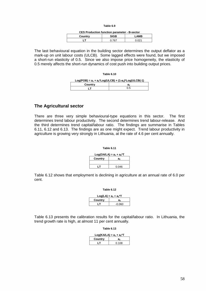
58

Table 6.9

CES Production function parameter - B-sector

Country SIGB LAMB LT 0.767 0.021

The last behavioural equation in the building sector determines the output deflator as a mark-up on unit labour costs (ULCB). Some lagged effects were found, but we imposed a short-run elasticity of 0.5. Since we also impose price homogeneity, the elasticity of 0.5 merely affects the short-run dynamics of cost push into building output prices.

Table 6.10

Log(POB) = a 1 + a2*Log(ULCB) + (1-a 2)*Log(ULCB(-1)

Country a 2 LT 0.5

The Agricultural sector There are three very simple behavioural-type equations in this sector. The first determines trend labour productivity. The second determines trend labour-release. And the third determines trend capital/labour ratio. The findings are summarise in Tables 6.11, 6.12 and 6.13. The findings are as one might expect. Trend labour productivity in agriculture is growing very strongly in Lithuania, at the rate of 4.6 per cent annually.

Table 6.11

Log(OA/LA) = a 1 + a2*T

Country a 2

LT 0.046

Table 6.12 shows that employment is declining in agriculture at an annual rate of 6.0 per cent.

Table 6.12

Log(LA) = a 1 + a2*T

Country a 2 LT -0.060

Table 6.13 presents the calibration results for the capital/labour ratio. In Lithuania, the trend growth rate is high, at almost 11 per cent annually.

Table 6.13

Log(KA/LA) = a 1 + a2*T

Country a 2 LT 0.108

59

Demographics and labour supply This part of the HERLIT model contains four behavioural equations that determine population changes (for three ages cohorts) and the labour force participation rate. We had intended to have a fifth behavioural equation to determine net migration outflows, but it proved impossible to find enough reliable data on these flows. Until such data are made available in published sources, we will be forced to continue to exclude a behavioural equation for migration. However, exogenous assumptions can be made “off model” for projections.

Consequently, unless one invokes the migration mechanism, the population equations play a rather minor role in the model, merely projecting existing natural rates of growth and decline. The results are summarised in Tables 6.14, 6.15 and 6.16. They demonstrate the well-known finding that birth rates are falling in Lithuania, and as a result, the pre-working age numbers (NJUV) are in decline, at an annual rate of about 3 per cent. The results for working age population suggest that while there is still some modest growth in the working age population, the high outward migration has reduced numbers dramatically since 2003. Finally, the post-working age population is increasing at a rate of 1.3 per cent annually.

Table 6.14

∆(NJUV) = a1*NJUV(-1) Country a 1

LT -0.030

Table 6.15

∆ (NWORK) = a1*NWORK(-1) Country a 1

LT 0.0051

Table 6.16

∆ (NELD) = a1*NELD(-1) Country a 1

LT 0.0126

In Table 6.17 we show the results of calibrating the labour force participation rate (LFPR). The empirical results presented something of a calibration paradox. We found quite high effects of unemployment (the encouraged/discouraged worker effect). But these effects tended not to be observable in the historical data. In other words, large variations in unemployment rates did not seem to shift the participation rates much. In practice, LFPR was usually trended, with only very minor fluctuations. Consequently, we set the coefficient on unemployment at zero (a2), and included only the time trend. This situation will have to be monitored in the future, in a search for a more comprehensive model of labour supply.

The results are shown in Table 6.17, and we see that the participation rate is declining at a slowly rate of 0.14 percentage points per year.

60

Table 6.17

LFPR = a1 + a2*URBAR(-1) + a 3*T

Country a 2 a3 LT 0 -0.139

Expenditure The calibration results for the consumption function are shown in Table 6.18. The specification is a hybrid of the liquidity constrained “Keynesian” function (the first term) and a permanent income effect (the last term).

The most important parameter insofar as the Keynesian multiplier is concerned is the so-called “marginal propensity to consume” (or MPC). It lies at the upper end of the plausible range (taking a value of 0.89), and the MPC out of wealth is set at zero.

Table 5.18

CONS = a1 + a2*YRPERD + a3*WNH(-1)

Country a2 a3 LT 0.887 0.0

Expenditure deflators The final two behavioural equations determine the price deflators for total investment (PI) and private consumption (PCONS). In both cases these are functions of the prices of inputs to expenditure, namely the GDP deflator (PGDPFC) and the import price (PM). In the case of the consumption deflator, we add an indirect tax term, TINC, and assume that all indirect tax changes appear as price changes, i.e., tax changes are passed on to consumption prices.

If input-output tables were used, these equations would become identities, and would be determined in terms of transformations of I-O coefficients. Our specification is based on an approximation to the more detailed use of I-O tables. Due to the high degree of multi-colinearity between PGDPFC and PM, it proved difficult to obtain stable and plausible coefficients. In the case of the investment deflator (PI), the elasticity of PI with respect to PGDPFC (the domestic GDP deflator) was found to be quite low, at 0.23. Consequently, the import price (PM) is the main determinant of investment prices. In the case of the consumption deflator, we found an elasticity of 0.69 on PGDPFC, reflecting the role of locally produced services in the consumption bundle.

Table 6.19

Log(PI) = a 1 + a2*Log(PGDPFC) + (1-a 2)*Log(PM),

(apply to: PIT, PIM, PIB, PIA, PIG)

Country a 2 LT 0.229

61

Table 6.20

Log(PCONS) = a 1 + a2*Log(PGDPFC) + (1-a 2)*Log(PM) +a3*TINC

Country a 2 a3 LT 0.687 1

Concluding remarks on calibration In an ideal world, we would have long and stable data series for use in calibrating the HERLIT behavioural equations, and could use these data series to carry out more formalised econometric calibration and hypothesis testing. The unfortunate reality is that we have at most thirteen annual observations, and less in many cases (due to lags and/or truncated time series). Furthermore, the quality of the data is sometimes poor, and the underlying structure of the economy was changing rapidly in the run-up to EC accession in 2004 and in the immediate post-accession period. What this means is that any attempt to use simple curve-fitting, based on OLS regressions is likely to produce erratic results in terms of parameter values. These values could, in turn, induce strange behaviour in the HERLIT models. After extensive testing of the first versions of the databases and models, we concluded that it may be better to impose parameter values where these can be inferred from theoretical considerations or from other sources. The responses of the model is now not dependent on fluctuating parameter values, and this is probably preferable to a situation of unstable responses. However, as new and better data become available over the coming years, we will need to keep the situation under review.

62

[7] Construction and testing of the HERLIT model 7.1 Introduction In Section 6 we described the first stage of model testing, namely the calibration of the behavioural equations of the HERLIT model. We now move to further testing, starting with the simulations that were designed to check the within-sample tracking performance. It should be stressed that HERLIT is not a model designed for short-term forecasting. It includes none of the special fixes and dummy variables that are commonly used to ensure good within-sample performance in many short-term forecasting models.39 But it needs to be emphasised that good within-sample tracking is usually achieved at the expense of dispensing with a sound theoretical structure and coherent medium-term performance. In this section we describe how HERLIT can be subjected to a battery of further tests with the object of examining the performance of the system of equations as a whole. We first describe briefly the process of checking the model structure by forcing the model’s behavioural equations to track the within-sample data exactly (i.e., “fixing” of intercept adjustments or “add-factors” for the behavioural equations of the model). Then we describe how the model is subjected to a series of standard exogenous and policy shocks in order to explore the pattern of its responses. HERLIT can also be used to prepare a baseline medium-term forecast or projection, based on assumptions about the future values of the so-called exogenous and policy variable sin the model. This will be an important element of the use of HERLIT to evaluate the impacts of the SPD policies. But because such a forecast will change as new data become available, we will present it in our second report on the SPD impacts, and not in this model USER Guide. Nevertheless, the forecasting methodology is described in Annex 4 of this report. 7.2 Checking the model structure Even though HERLIT is primarily designed for policy oriented experiments of a complex kind, we do not completely neglect its within sample tracking performance. Not only is a reasonable within sample tracking a necessary condition for the model to be realistic, but it would also point out the weak parts of the model, i.e. the behavioural equations whose calibration neglected some important factors, or identities that were mis-specified. Therefore checking of the model’s within sample properties provides valuable information on the quality of the calibration process and is used in the design stage of model construction, when modellers often have to return back to the calibration stage if such checks produce unsatisfactory results. The control of the within sample performance is initially carried out by a means of a so-called “residual check” simulation. Once the individual behavioural equations have been calibrated, and the model as a parameterised system of equations is set up, we run a static simulation which uses the historical values of the endogenous and exogenous variables on the right hand side of every equation of the model to compute the endogenous (behavioural or identity) variable that is designated as being determined by this equation. The resulting values of the endogenous variables for every simulated year

39 For example, the LITMOD model of Moller-Andersen et al, 2005 contained many dummy variables, and

produced close tracking of historical data as a consequence.

63

of the sample is then compared to their actual historical values. More specifically, we are interested in the percentage difference of the simulated from actual values. There is no obvious benchmark as to what percentage difference constitutes a reasonable fit of an equation. Rather, it varies from a case to case, but overall we aim at between 5 and 10 per cent difference for all of the more important behavioural variables. Of course, variables computed as identities must, by definition, fit exactly if simulated in this “single-equation” way, up to a numerical rounding error. In addition, we also want these differences for each behavioural variable to change signs over time, suggesting a random error. If this residual check produces unsatisfactory results, we can revert back to calibration of the most troublesome equations and carry out a review the equation specification. In the case of HERLIT, we finished with most behavioural variables showing less than 5 per cent difference from the historical values in every year. The main exceptions were investment variables, which are very difficult to track with a model of the highly constrained type that we specify.40 On balance, the within sample tracking results boosted our confidence in the ability of the model to reflect reality reasonably well. However, it falls far short of the rigorous testing normally carried out on econometric models, where long and stable time series of data are available and support rigorous econometric analysis. Having performed the residual check procedure described above, we can then carry out the usual kind of within-sample static and dynamic system simulations. In static system simulations, the model is re-started every time period, and the historical data used for lags. In dynamic simulations, on the other hand, the model is started at some point in time, and the solution values are used for lags in subsequent periods. The dynamic simulation is a more searching test of model performance than the static simulation. We obviously want to use the information on the magnitude of error that the individual equations display during the within sample check, in the out of the sample projections and simulations. In order to do so, we carry out a static, within sample simulation as before, but this time we solve each equation independently and not as part of the simultaneous system (i.e., a “residual checking” simulation). We then compute absolute differences between the simulated and true values. These absolute differences are used to create the so called constant adjustment (or CA) factors each year for each behavioural variable. These adjustment factors act, effectively, as corrections to our estimates of behavioural intercepts in each behavioural equation, with the property that they make the computed “behavioural” variable exactly fit the within sample data. Therefore, if we add these constant adjustment factors back to each behavioural equation we will obtain a perfect fit of the whole model, within sample. What is more important, though, is that we can use this information on the error in our behavioural intercepts in the out of the sample projections and simulations, as is described in Annex 4, when we describe how baseline projections can be prepared using HERLIT.

7.3 Shocking the model We can examine the properties of HERLIT using a series of simulated shocks to exogenous variables. In order to examine the full medium-term properties of the model, we need to simulate the model over a long period. To do this, we use a baseline projection for the period 2007 to 2020, since the year 2007 is the last one for which

40 The highly constrained specification of the factor demand systems in manufacturing, building and market

services is an essential requirement if the model is to be useful in the analysis of the long-term impacts of cohesion policies. Refer to Task 1 for full details of the CES production function and factor demand specifications.

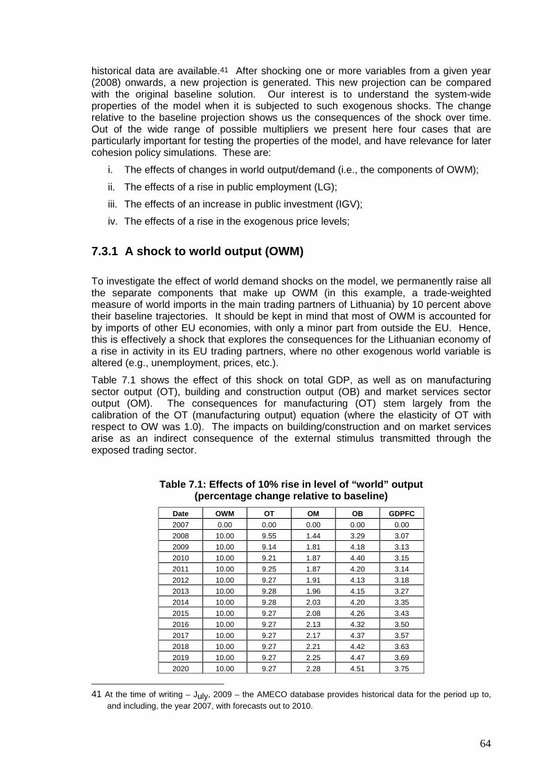
64

historical data are available.41 After shocking one or more variables from a given year (2008) onwards, a new projection is generated. This new projection can be compared with the original baseline solution. Our interest is to understand the system-wide properties of the model when it is subjected to such exogenous shocks. The change relative to the baseline projection shows us the consequences of the shock over time. Out of the wide range of possible multipliers we present here four cases that are particularly important for testing the properties of the model, and have relevance for later cohesion policy simulations. These are:

i. The effects of changes in world output/demand (i.e., the components of OWM);

ii. The effects of a rise in public employment (LG);

iii. The effects of an increase in public investment (IGV);

iv. The effects of a rise in the exogenous price levels;

7.3.1 A shock to world output (OWM)

To investigate the effect of world demand shocks on the model, we permanently raise all the separate components that make up OWM (in this example, a trade-weighted measure of world imports in the main trading partners of Lithuania) by 10 percent above their baseline trajectories. It should be kept in mind that most of OWM is accounted for by imports of other EU economies, with only a minor part from outside the EU. Hence, this is effectively a shock that explores the consequences for the Lithuanian economy of a rise in activity in its EU trading partners, where no other exogenous world variable is altered (e.g., unemployment, prices, etc.).

Table 7.1 shows the effect of this shock on total GDP, as well as on manufacturing sector output (OT), building and construction output (OB) and market services sector output (OM). The consequences for manufacturing (OT) stem largely from the calibration of the OT (manufacturing output) equation (where the elasticity of OT with respect to OW was 1.0). The impacts on building/construction and on market services arise as an indirect consequence of the external stimulus transmitted through the exposed trading sector.

Table 7.1: Effects of 10% rise in level of “world” output (percentage change relative to baseline)

Date OWM OT OM OB GDPFC

2007 0.00 0.00 0.00 0.00 0.00

2008 10.00 9.55 1.44 3.29 3.07

2009 10.00 9.14 1.81 4.18 3.13

2010 10.00 9.21 1.87 4.40 3.15

2011 10.00 9.25 1.87 4.20 3.14

2012 10.00 9.27 1.91 4.13 3.18

2013 10.00 9.28 1.96 4.15 3.27

2014 10.00 9.28 2.03 4.20 3.35

2015 10.00 9.27 2.08 4.26 3.43

2016 10.00 9.27 2.13 4.32 3.50

2017 10.00 9.27 2.17 4.37 3.57

2018 10.00 9.27 2.21 4.42 3.63

2019 10.00 9.27 2.25 4.47 3.69

2020 10.00 9.27 2.28 4.51 3.75

41 At the time of writing – July, 2009 – the AMECO database provides historical data for the period up to,

and including, the year 2007, with forecasts out to 2010.

65

OW: “world” output; GDPM: real GDP at market prices; OT: GDP in manufacturing; OB: GDP in building & construction; OM: GDP in market services

7.3.2 A public employment shock (LG)

Table 7.2 presents the model’s response to a sustained 10 percent increase in the number of employees in the public sector (LG). In terms of levels, this amounts to an increase of about 40,000 new jobs in the sector. The increase in expenditure on public sector wages is financed by running a larger deficit (if necessary) and not by increasing tax rates or cutting public expenditure elsewhere.

As can be seen from Table 7.2, total employment increases initially by only 44,000 as a result of the Keynesian demand mechanism (i.e., when the extra public sector employees spend their wages). In other words, the impact multiplier is 1.10. This slightly increases to about 51,600 at the end of the simulation period, indicating a long-run Keynesian employment multiplier of 1.29. We emphasise again that this simulation was run under the assumption that tax rates are exogenous and there is no additional fiscal crowding-out effect. The imposition of a “balanced budget” constraint would serve to reduce the size of the Keynesian multiplier.

Table 7.2: Effects of 10% increase in public sector employment (Change relative to baseline, thousands)

Date LG L Multiplier

2007 0.00 0.00 0.00

2008 39.97 43.86 1.10

2009 39.97 46.94 1.17

2010 39.97 48.37 1.21

2011 39.97 48.70 1.22

2012 39.97 49.17 1.23

2013 39.97 49.59 1.24

2014 39.97 50.00 1.25

2015 39.97 50.38 1.26

2016 39.97 50.72 1.27

2017 39.97 51.03 1.28

2018 39.97 51.32 1.28

2019 39.97 51.59 1.29

LG = employment in non-market services; L = total employment

In fact, given the strong revenue buoyancy, this shock is almost self-financing and the borrowing requirement (expressed as a share of GDP) does not change much relative to the “no shock” baseline. But it should be remembered that the size of the public sector has increased relative to the size of the private sector, and this may be considered undesirable for other reasons.

7.3.3 A shock to government investment (IGV)

The next shock we describe relates to an increase in public investment in infrastructure. Table 7.3 shows the effect of a permanent 10 percent increase in nominal public investment. As can be seen from Table 7.3, there is a initially modest Keynesian

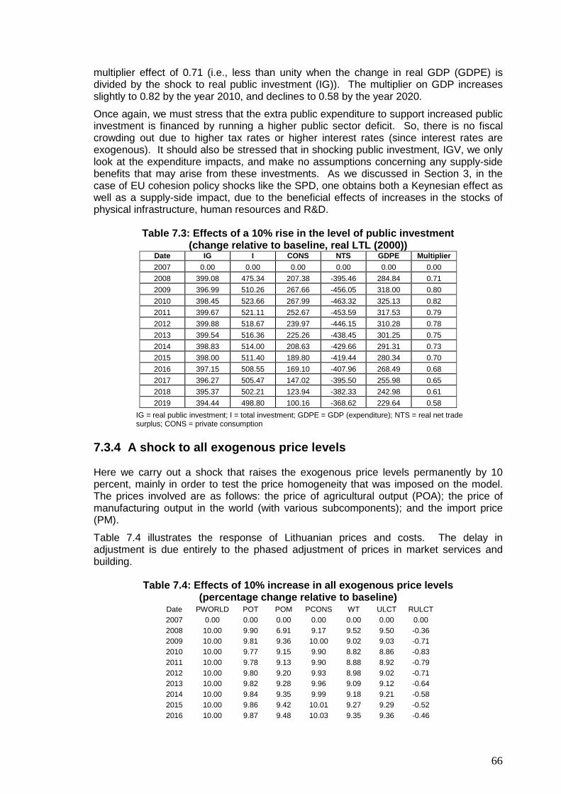
66

multiplier effect of 0.71 (i.e., less than unity when the change in real GDP (GDPE) is divided by the shock to real public investment (IG)). The multiplier on GDP increases slightly to 0.82 by the year 2010, and declines to 0.58 by the year 2020.

Once again, we must stress that the extra public expenditure to support increased public investment is financed by running a higher public sector deficit. So, there is no fiscal crowding out due to higher tax rates or higher interest rates (since interest rates are exogenous). It should also be stressed that in shocking public investment, IGV, we only look at the expenditure impacts, and make no assumptions concerning any supply-side benefits that may arise from these investments. As we discussed in Section 3, in the case of EU cohesion policy shocks like the SPD, one obtains both a Keynesian effect as well as a supply-side impact, due to the beneficial effects of increases in the stocks of physical infrastructure, human resources and R&D.

Table 7.3: Effects of a 10% rise in the level of pu blic investment (change relative to baseline, real LTL (2000))

Date IG I CONS NTS GDPE Multiplier

2007 0.00 0.00 0.00 0.00 0.00 0.00

2008 399.08 475.34 207.38 -395.46 284.84 0.71

2009 396.99 510.26 267.66 -456.05 318.00 0.80

2010 398.45 523.66 267.99 -463.32 325.13 0.82

2011 399.67 521.11 252.67 -453.59 317.53 0.79

2012 399.88 518.67 239.97 -446.15 310.28 0.78

2013 399.54 516.36 225.26 -438.45 301.25 0.75

2014 398.83 514.00 208.63 -429.66 291.31 0.73

2015 398.00 511.40 189.80 -419.44 280.34 0.70

2016 397.15 508.55 169.10 -407.96 268.49 0.68

2017 396.27 505.47 147.02 -395.50 255.98 0.65

2018 395.37 502.21 123.94 -382.33 242.98 0.61

2019 394.44 498.80 100.16 -368.62 229.64 0.58

IG = real public investment; I = total investment; GDPE = GDP (expenditure); NTS = real net trade surplus; CONS = private consumption

7.3.4 A shock to all exogenous price levels Here we carry out a shock that raises the exogenous price levels permanently by 10 percent, mainly in order to test the price homogeneity that was imposed on the model. The prices involved are as follows: the price of agricultural output (POA); the price of manufacturing output in the world (with various subcomponents); and the import price (PM).

Table 7.4 illustrates the response of Lithuanian prices and costs. The delay in adjustment is due entirely to the phased adjustment of prices in market services and building.

Table 7.4: Effects of 10% increase in all exogenous price levels (percentage change relative to baseline)

Date PWORLD POT POM PCONS WT ULCT RULCT 2007 0.00 0.00 0.00 0.00 0.00 0.00 0.00 2008 10.00 9.90 6.91 9.17 9.52 9.50 -0.36 2009 10.00 9.81 9.36 10.00 9.02 9.03 -0.71 2010 10.00 9.77 9.15 9.90 8.82 8.86 -0.83 2011 10.00 9.78 9.13 9.90 8.88 8.92 -0.79 2012 10.00 9.80 9.20 9.93 8.98 9.02 -0.71 2013 10.00 9.82 9.28 9.96 9.09 9.12 -0.64 2014 10.00 9.84 9.35 9.99 9.18 9.21 -0.58 2015 10.00 9.86 9.42 10.01 9.27 9.29 -0.52 2016 10.00 9.87 9.48 10.03 9.35 9.36 -0.46

67

2017 10.00 9.89 9.53 10.05 9.41 9.43 -0.42 2018 10.00 9.90 9.58 10.06 9.47 9.49 -0.37 2019 10.00 9.91 9.62 10.07 9.53 9.54 -0.34

PWORLD = World price; POT = manufacturing output deflator; POM = market services output deflator; PCONS = Consumption deflator; WT = Average annual earnings in manufacturing; ULCT = unit labour costs, manufacturing; RULCT: Real unit labour costs, manufacturing

7.3.5 Conclusions on responses to shocks

The shocks illustrate some of the properties of the HERLIT model. For example, world market conditions feed into the economy of Lithuania mainly through the internationally exposed manufacturing sector but also indirectly through the market services sector. External price shocks pass quickly into domestic prices, under the assumption of a fixed exchange rate. Public employment and investment shocks have relatively modest Keynesian impacts on the economy. However, it must be recognised that the public employment (LG) and public investment (IGV) shocks impact mainly on the demand side of the economy. In Section 3 we showed how these demand-side (or Keynesian) impacts can be augmented through supply-side productivity-enhancing effects that are associated with EU cohesion policy initiatives implemented in the SPD.

The above set of tests serve to alert us to the importance of the market services and building and construction sectors (i.e., the mainly non-traded sectors). The latter is destined to play a major role in the implementation of the physical infrastructure investment programmes of the cohesion policies, which will absorb a high proportion of the funding. They also demonstrate the rather different properties of the manufacturing sector, due to its direct exposure to the global economy, its more limited exposure to the domestic economy, and the role played by international competitiveness.

68

[8] Concluding remarks

8.1 Possible weaknesses in the HERLIT-based analysis Previous attempts to quantify the likely impacts of EU cohesion policy programme impacts have come in for severe criticism.42 Some of these criticisms are justified, particularly insofar as they refer to the relatively poor quality of EU cohesion policy expenditure data. For example, in current analysis of cohesion policy impacts, we are obliged to use the CP financial allocation data as equivalent to actual investment data. Clearly these two kinds of data are closely related to each other, but the absence of actual data for actual investments, with the correct timing of implementation, forces us to use the financial planning data. In an ex-ante study, there is probably no way out of the dilemma. But for mid-term and ex-post studies, of the kind to be described in the second report, the errors in timing as between the actual financial allocations and the actual investment activity could be significant, at least during the implementation phase. When it comes to questions concerning the reliability of the HERLIT (or any other) economic model, other issues arise. For example, how appropriate is the structure of the model as a tool for investigating the medium- to long-term impacts of cohesion policy on growth and development, as distinct from the short-term (Keynesian) impacts that arise during implementation? Even within an acceptable model structure, how reliable is the calibration of the behavioural equations? Here we are captives of the quality of the available data, and there are serious deficiencies with respect to availability and reliability. But even if one accepts the HERMIN-type neo-Keynesian macro-econometric model structure, and the data are reliable, what about the manner in which the cohesion policy mechanisms are incorporated into the models, and the manner in which the “spillover” mechanisms are handled? In the cases of countries that have previously implemented EU cohesion policy programmes, only in the cases of Spain, and Ireland to a lesser extent, is there any body of micro-economic and cost-benefit analysis research upon which the macro-spillover mechanisms can be calibrated. In the case of Lithuania, we have been as yet unable to find any concrete micro or project-level evaluations. In the absence of such research, one is forced to draw on international research from large developed economies, and regions of such economies, and to use these findings as substitutes for the missing results for the new member states. The implication of the above is that one should look upon the HERLIT model as a way of exploring the consequences of different assumptions concerning supply-side spillovers, rather than as a tool that inputs “correct” spillover parameters and produces a unique “correct” impact evaluation. A more serious consideration concerns the fact that different model systems produce different cohesion policy impact evaluations. In Bradley and Untiedt, 2007 this is explored for the cases of HERMIN, the QUEST model operated by the European Commission, DG-ECFIN, and to a lesser extent, the ECOMOD model of Brussels University. Few, if any, of these differences can be resolved by appeal to solid econometric research, since the data deficiencies in the new member states have already been described. What this suggests is that the comparison of different models

42 A recent report by the Court of Auditors was particularly critical of the use of previous HERMIN models in the ex-post evaluation of CSF 1994-99.

69

ought to be carried out in a way that forces the modellers to confront the actual challenges of the assisted countries, and the likely behaviour of the policy makers and other economic agents. The norms of behaviour, and the institutional capacities of the new member states differ from each other, differ from the assisted “old” member states, and differ from the advanced “donor” states.

8.2 A future work programme for HERLIT We have described the May 2009 revised implementation of the HERLIT model. Future work might focus on the following kinds of tasks:

i. Implementation of the HERLIT system on the computer systems of the Ministry of Finance, and familiarisation by Ministry staff

ii. Monitoring the implications of revisions as new and revised data become available,

and highlighting any major implications for policy analysis carried out using earlier versions;

iii. Improving the technical implementation of the HERLIT model system, so that it can

be made more “user friendly”; iv. Comparison of the EU cohesion policy impacts derived using the HERLIT model

with results derived using other models, such as QUEST. v. Continual monitoring of the remaining data problems that were identified from our

use of the AMECO/EUROSTAT data systems; vi. Regular annual updating of the HERLIT database when a new version of the

AMECO database is issued.

70

References Barrell, R. and D. Holland, 2002. “The NIGEM approach to modelling EU accession”, paper

presented at Macromodels 2002, Cedzyna, Poland, December 4-7.

Barry, F. and J. Bradley (1991). "On the Causes of Ireland's Unemployment", Economic & Social Review, Vol. 22, No. 4, pp. 253-286.

Barry, F. and J. Bradley (1997). “FDI and Trade: the Irish Host-Country Experience”, Economic Journal, 107(445), pp. 1798-1811, November.

Barry, F., Bradley, J., Kejak, M., Vavra, D. 2003. “The Czech economic transition: exploring options using a macrosectoral model”, The Economics of Transition, 11(3), 539-67.

Bradley, J. and J. Fitz Gerald (1988). "Industrial output and factor input determination in an econometric model of a small open economy", European Economic Review, Vol. 32, pp. 1227-1241.

Bradley, J., Fitz Gerald, J., Kearney, I. 1992. “The Role of the Structural Funds: Analysis of Consequences for Ireland in the Context of 1992”, Policy Research Series No. 13, The Economic & Social Research Institute, Dublin.

Bradley, J., Herce, J.A., Modesto L. 1995. “Modelling in the EU Periphery. The Hermin Project”, Economic Modelling 12, special issue, 219-220.

Bradley, J., K. Whelan and J. Wright (1995). "HERMIN Ireland", Economic Modelling, Vol. 12, No. 3, pp. 219-220.

Bradley, J., L. Modesto and S. Sosvilla-Rivero (1995). "Similarity and diversity in the EU periphery: A HERMIN-based investigation", Economic Modelling, Vol. 12, No. 3, pp. 219-220.

Bradley, J., Whelan, K. 1997. “The Irish expansionary fiscal contraction: A tale from open small European economy”, Economic Modelling 14, 175-201.

Bradley, J., Petrakos, G., Traistaru, I. (eds.) 2004. Integration, Growth and Cohesion in an Enlarged European Union, New York: Springer.

Bradley, J., Gacs, J., Kangur, A., Lubenets, N. 2004 “HERMIN: A macro model framework for the study of cohesion and transition”, in J. Bradley, G. Petrakos and I. Traistaru (eds.), Integration, Growth and Cohesion in an Enlarged European Union, Springer, New York.

Bradley, J., Untiedt, G. (2008): „Do economic models tell us anything useful about Cohesion Policy impacts? A comparison of HERMIN, QUEST and ECOMOD“, in: Stierle-von Schütz, U., M.H. Stierle, F.B. Jennings Jr., A. Kuah (eds), Regional Economic Policy in Europe – New Challenges for Theory, Empirics and Normative Interventions, Edwardr Elgar, Cheltenham UK, pp. 159-180.

Carlin, W., Glynn, A., Van Reenen, J. 2001. “Export market performance of OECD countries: an empirical examination of the role of cost competitiveness”, The Economic Journal, vol. 111 (January), 128-162.

D’Alcantara, G., Italianer, A. 1982. A European project for a multinational macrosectoral model, Document MS 11, DG XII, Brussels: Commission of the European Communities.

Harris, J., Todaro, M. 1970. “Migration, Unemployment and Development: A Two Sector Analysis”, American Economic Review, Vol. 60, 126-142.

Jakaitiene, A. and V. Klyviene (2007). “Assessing the impact of the EU funds on Lithuanian economic development”, Monetary Studies, Volume XI No. 2 December

Karpavicius, S. (2009). The Effects Of Fiscal Instruments On The Economy Of Lithuania, Working Paper Series, No. 4, Economic Research Division, Bank of Lithuania.

Layard, R., Nickell, S, Jackman, R., 1991. Unemployment, macroeconomic performance and the labour market. Oxford University Press, Oxford, Great Britain.

71

Lindbeck, A. 1979. “Imported and structural inflation and aggregated demand: The Scandinavian model reconstructed”, in: Lindbeck, A. (ed.), Inflation and Employment in Open Economies. North-Holland, Amsterdam.

Møller Andersen, F., D. Celovb, D. Grindersleva and A. Kazlauskasc (2005). “A macro-econometric model of Lithuania LITMOD”, Economic Modelling, Volume 22, Issue 4, July 2005, Pages 707-719

Pierse, R. 1998. WINSOLVE Version 3: An Introductory Guide, Department of Economics, University of Surrey, June.

Vetlov, I. (2004). The Lithuanian block of the ECSB multi-country model, Discussion paper No. 13, Bank of Finland, Institute of Economies in Transition,

Welfe, W., Welfe, A., Florczak, W., Sabanty, L. 2002. “The W8-2000 medium-term macroeconometric model of the Czech Republic economy”, paper presented at the International Conference MACROMODELS 2002, Cedzyna, The Czech Republic, December4-7.

72

Annex 1: The HERLIT Model Equation Listing @ ================================================= ============================ @ @ @ HERMIN (HERLIT) @ @ A FIVE-SECTOR MODEL OF THE ECONOMY OF LITHUANIA @ @ Version 2009/2: May 21, 200 9 @ @ @ This listing contains the HERLIT HERMIN model equ ations as used by the WINSOLVE @ software. The code describes exactly how the SPD impact evaluation system is @ implemented. Explanations of the underlying just ification for the HERLIT @ model is provided in textbooks of modern macroeco nomic theory and empirical @ economics at the level of Mankiw (2005), and in C arlin and Soskice (2005), and @ in the accompanying user documentation. @ @ ------------------------------------------------- ---------------------------- @ @ Definition of sectoral notation for disaggreg ation of production bloc @ of the HERLIT model of the Lithuanian economy @ @ (T) = Manufacturing (including mining and quar rying) @ (NACE CODES: Section C + D + E) @ @ (B) = Building and construction @ (NACE CODES: Section F) @ @ (M) = Market services (includes trade & repair , hotels & restaurants, @ transport, storage & communication, fina ncial intermediation, @ real estate, renting & business activiti es, other community, social @ & personal services) @ (NACE CODES: Section G + H + I + J + K + O + P ) @ @ (A) = Agriculture (includes forestry, hunting & fishing) @ (NACE CODES: Section A + B) @ @ (G) = Non-market Services (public administrati on and defence, health @ and social work, and education) @ (NACE CODES: Section L + M + N + Q) @ @ ------------------------------------------------- ---------------------------- @ -- @ The following spillover parameters are imposed (with values based on -- @ international literature)Numerical values are entered as exogenous -- @ variables in the relevant WINSOLVE simulation batch LOG files -- -- @ -- @ ------------------------------------------------- ---------------------------- @ @ "ETA" denotes a spillover elasticity, with the fo llowing qualifiers, where @ default values of the elasticities are shown in brackets @ @ Manufacturing output @ -------------------- @ @ ETATQI = Output spillover - infrastructure (0.20) @ ETATQH = Output spillover - human capital (0.20) @ ETATQR = Output spillover - R&D (0.05) @ @ Manufacturing productivity @ -------------------------- @

73

@ ETATPI = Labour productivity spillover - infrastr ucture (0.10) @ ETATPH = Labour productivity spillover - to human capital (0.10) @ ETATPR = Labour productivity spillover - R&D (0.0 5) @ @ Market services output @ -------------------- @ @ ETAMQI = Output spillover - infrastructure (0.05) @ ETAMQH = Output spillover - human capital (0.05) @ ETAMQR = Output spillover - R&D (0.01) @ @ Market services productivity @ ---------------------------- @ @ ETAMPI = Labour productivity spillover - infrastr ucture (0.05) @ ETAMPH = Labour productivity spillover - human ca pital (0.05) @ ETAMPR = Labour productivity spillover - R&D (0.0 25) @ @ Set other key SF parameters, as exogenous variabl es @ ------------------------------------------------- -- @ @ OVERHD = ESF training overhead (default set at 30 % of wage expenditure) @ @ TMUP = Fraction of manufacturing wage paid to E SF trainees (30%) @ @ TRATIO = ESF trainee/instructor ratio (default se t at 15:1) @ @ ------------------------------------------------- ---------------------------- @ @ Allocation of Structural and Cohesion Fund inv estment expenditure. @ @ ------------------------------------------------- ---------------------------- @ @ Starting with the annual total allocation of EC a id (GECSFEC_E) in millions @ of current euro, there is a sequence of eight ste ps to handle the source of @ funding and to allocate it to the various economi c categories of investment: @ Step 1: EC funding data input @ ------ @ Enter EC annual expenditure contribution for the statutory period (e.g., @ 2004-20068 in the case of SPD 2004-2006), in curr ent euro as data (GECSFEC_E). @ If the "n+2" rule is invoked, then enter data for the extended period (e.g., @ 2004-2008 in the case of SPD 2004-2006) @ Step 2: Currency conversion @ ------ @ Convert GECSFEC_E to Lithuanian litas (GECSFEC), using an appropriate euro @ exchange rate (LTEUR, units of litas per euro). GECSFEC = LTEUR * GECSFEC_E ; @ Step 3: Domestic public co-finance @ ------ @ Derive the implied domestic public (DP) co-financ e contribution (GECSFDP), @ using an assumed domestic public co-finance ratio (RDPCOFIN percent), where @ this is defined as follows: @ RDPCOFIN=100*GECSFDP/(GECSFEC+GECSF DP) GECSFDP = (RDPCOFIN/(100-RDPCOFIN)) * GECSFEC; @ Step 4: Private co-finance @ ------ @ Derive the implied domestic private (PR) co-finan ce contribution (GECSFPR),

74

@ using an assumed domestic private co-finance rati o (RPRCOFIN percent), where @ this is defined as follows: @ RPRCOFIN=100*GECSFPR/(GECSFEC+GECSF DP) @ Note that total EC plus DP finance is taken as th e base for calculating the @ domestic private co-finance ratio. GECSFPR = (RPRCOFIN/100) * (GECSFEC+GECSFDP); @ Step 5: Total (EC+DP+PR) finance @ ------ @ Define total (EC+DP+PR) expenditure in local curr ency (GECSF). If one wishes @ to ignore private co-finance, set RPRCOFIN (above ) to zero. GECSF = GECSFEC + GECSFDP + GECSFPR; @ Step 6: @ ------ @ Disaggregate finance into the three main SF econo mic categories using @ NSRF, NDP or OPs, where @ XX=EC (Community), DP (Domestic Public) and PR (D omestic Private). @ Physical infrastructure ------------ (IGVCSFXX ) @ Human Resources -------------------- (GTRSFXX) @ Direct Aid to the Productive Sector --- (TRIXX), @ The percentage shares going to Physical Infrastru cture (PI) are RIGVCSFX, @ where X=E (Community), D (Domestic Public) and P (Domestic Private). Usually @ these shares are identical across E, D and P. IGVCSFEC = (RIGVCSFE/100) * GECSFEC ; IGVCSFDP = (RIGVCSFD/100) * GECSFDP ; IGVCSFPR = (RIGVCSFP/100) * GECSFPR ; @ Total expenditure on physical infrastructure (IGV CSF) IGVCSF=IGVCSFEC+IGVCSFDP+IGVCSFPR; @ The percentage shares going to Human Resources (H R) are RGTRSFX. Usually @ these shares are identical across E, D and P. GTRSFEC = (RGTRSFE/100) * GECSFEC ; GTRSFDP = (RGTRSFD/100) * GECSFDP ; GTRSFPR = (RGTRSFP/100) * GECSFPR ; @ Total expenditure on human resources (GTRSF) GTRSF=GTRSFEC+GTRSFDP+GTRSFPR; @ Residual expenditure is allocated to Direct Aid t o the Productive Sector (APS). TRIEC = GECSFEC - (IGVCSFEC+GTRSFEC) ; TRIDP = GECSFDP - (IGVCSFDP+GTRSFDP) ; TRIPR = GECSFPR - (IGVCSFPR+GTRSFPR) ; @ Total expenditure on aid to productive sectors (T RI) TRI=TRIEC+TRIDP+TRIPR; @ Step 7: @ ------ @ Disaggregate Direct Aid to the Productive Sector (APS) into its sectoral

75

@ allocations to Manufacturing (T). Market Services (M) and Ahriculture (A). @ APS to Manufacturing (Percentage shares = RTRITX) . Usually these shares are @ identical across E, D and P. TRITEC = (RTRITE/100) * TRIEC ; TRITDP = (RTRITD/100) * TRIDP ; TRITPR = (RTRITP/100) * TRIPR ; @ Total APS to manufacturing (TRIT) TRIT = TRITEC+TRITDP+TRITPR; @ APS to Market services (Percentage shares = RTRIM X). Usually these shares are @ identical across E, D and P. TRIMEC = (RTRIME/100) * TRIEC ; TRIMDP = (RTRIMD/100) * TRIDP ; TRIMPR = (RTRIMP/100) * TRIPR ; @ Total APS to market services (TRIM) TRIM = TRIMEC+TRIMDP+TRIMPR; @ APS to Agriculture sector (defined as the residua l: may be zero): TRIAEC = TRIEC - TRITEC - TRIMEC ; TRIADP = TRIDP - TRITDP - TRIMDP ; TRIAPR = TRIPR - TRITPR - TRIMPR ; @ Total APS to Agriculture (TRIA) TRIA = TRIAEC+TRIADP+TRIAPR; @ Step 8: @ ------ @ Disaggregate total APS into two main economic cat egories; R&D and other @ direct aid. The percentage share of TRI (=TRIEC+T RIDP+TRIPR) going to R&D @ is assumed to be RRDTCSF. RRDTCSF is used to cal culate total expenditure @ from APS going to fund R&D (TRIRD). The accumula tion of the constant @ price version of TRIRD (i.e., RTRIRD) is used lat er to derive a measure @ of a "stock" of R&D (KRTRIRD) TRIRD = (RRDTCSF/100) * TRI; @ ------------------------------------------------- ------------------------ @ ------------------------------------------------- ------------------------ @ -------------- ---------------- @ -------------- [I] Production: the supply side of HERLIT ---------------- @ -------------- ---------------- @ ------------------------------------------------- ------------------------ @ ------------------------------------------------- ------------------------ @ ----------------------------------- ---- @ ----- MANUFACTURING SECTOR (T) - ---- @ ----------------------------------- ---- @ OWXX is a trade-weighted measure of world activit y in the model. There @ are two such measures: OWIP and OWM). OWIP is a trade-weighted measure of @ industrial output. OWM is a trade-weighted measu re of imports. @ An AMECO-based set of trading partners is adopted for each model. @ The weight is given by (XWO1-XWO9), the industria l production by @ IPCTP1-IPCTP9, and imports by MCTP1-MCTP9.

76

@ The nine main Lithuanian trading partners are as follows (with 2007 export @ shares in brackets), whose share makes up about 7 0 per cent of total @ Lithuanian exports. @ [1] Russia (13.86) @ [2] Latvia (12.03) @ [3] Germany (9.36) @ [4] Estonia (7.04) @ [5] Poland (6.60) @ [6] The Netherlands (5.27) @ [7] The United Kingdom (4.79) @ [8] Sweden (4.90) @ [9] The United States (4.70) @ Trade-weighted industrial output measure: OWIP (n ine trading partners). OWIP = exp( XWO1*log(IPCTP1) + XWO2*log(IPCTP2) + X WO3*log(IPCTP3) + XWO4*log(IPCTP4) + XWO5*log(IPCTP5) + X WO6*log(IPCTP6) + XWO7*log(IPCTP7) + XWO8*log(IPCTP8) + X WO9*log(IPCTP9) ); @ Trade-weighted imports measure: OWM (nine trading partners) OWM = exp( XWO1*log(MCTP1) + XWO2*log(MCTP2) + XWO 3*log(MCTP3) + XWO4*log(MCTP4) + XWO5*log(MCTP5) + XWO 6*log(MCTP6) + XWO7*log(MCTP7) + XWO8*log(MCTP8) + XWO 9*log(MCTP9) ); @ Weighted domestic demand (FDOT) reflects the manu facturing output content of @ a unit change in any of the four components of do mestic demand. The @ components used include the following four items: @ CONS = Private (household) consumption @ RGENW = Non-wage public consumption @ IBCTOT = Housing and other construction inves tment @ IMETOT = Investment in machinery and equipmen t @ Exports are not included in FDOT (i.e., it is not weighted "final" demand). @ World output (OWXX) is directly incorporated into the output (OT) equation @ (see below). The weights (AIOT*) are derived from country input/output @ tables. *P AIOTC = 0.3; *P AIOTG = 0.1; *P AIOTB = 0.2; *P AIOTM = 0.2; FDOT=AIOTC*CONS + AIOTG*RGENW + AIOTB*(IBCTOT)+AIOT M*IMETOT ; @ GDP produced in the manufacturing sector (OT) is determined by a hybrid @ supply-demand equation. The influence of externa l factors incorporates the @ role of foreign direct investment and portfolio i nvestment. The domestic @ demand factors represent the conventional Keynesi an mechanism. @ The driving variables are as follows: @ OWZZ : World demand (proxied by world outpu t (OWIP) or imports (OWM) @ ULCT/POT : The real unit cost of labour @ FDOT : Sectoral weighted domestic demand @ POT/PWORLD : Relative domestic-to-world prices @ TOT : A time trend, to capture other shift s in the drivers of OT @ Infrastructure, human capital and R&D spillovers are included as options in @ the modification of OT. Note that in the baselin e NSRF simulation, the ratios @ KGINFR, KTRNR and KRTRIRDR are set to unity. @ KGINFR = Increase in stock of physical infrastr ucture (relative to baseline) @ KTRNR = Increase in stock of trained labour (r elative to baseline) @ KRTRIRDR = Increase in stock of R&D (relative to baseline)

77

*P AOT1 = 8.68418; *P AOT2 = 1.0; {Elasticity of OT wrt OWM} *P AOT3 = 0.0; {Elasticity of OT wrt FDOT} *P AOT4 = -0.2; {Elasticity of OT wrt RULCT } *P AOT5 = -0.2; {Elasticity of OT wrt PCOMP T} *P AOT6 = 0.019072; {Autonomous time trend} *M log(OT)= ( AOT1 + (DETATQI*ETATQI)*log(KGINFR) + (DETATQH*ETATQH)*log(KTRNR) + (DETATQR*ETATQR)*log(KRTRIRDR) +AOT2*log(OWM) +AOT3*log(FDOT) +AOT4*log(RULCT) +AOT5*log(PCOMPT) +AOT6*TOT); @ Investment demand (IT) and labour demand (LT) are derived by cost @ minimization, using a semi putty-clay CES product ion function @ with constant returns to scale. ERFPT is the exp ected relative factor @ price ratio and T represents time. Technical prog ress is assumed to be @ Hicks-neutral. @ CES production function parameters (AT, SIGT, LAM T and DELT) *P AT = 13.24408 ; {Scale parameter} *P SIGT = 0.79478 ; {Elasticity of substitut ion: 0 < SIGT < 1} *P LAMT = 0.081993 ; {Rate of Hicks-neutral t echnical progress} *P DELT = 0.81011 ; {Weight for capital inpu t} @ Infrastructure and R&D have a total factor produc tivity externality effect @ in the production function. Human capital is emb odied in labour and the @ returns to increases in human capital are interna lised. @ Scale parameter, augmented by spillover mechanism s (ATX) ATX=AT * (KGINFR)^(DETATPI*ETATPI) * (KRTRIRDR)^(DETATPR*ETATPR); @ (IT) Investment demand is the first part of the j oint factor demand system. *A IT=OT*exp(-log(ATX) - LAMT*TT + SIGT/(1-SIGT)*log(1-DELT) + SIGT/(1-SIGT) * log ( (DELT/(1-DELT))^(SIGT)*ERFPT^(1-SIGT) + 1. 0)) + TRITRL; @ TRITRL (real) is the Keynesian (implementation) i mpact of aid to the @ productive sector provided to boost T-sector inve stment. It is treated @ as an exogenous addition to investment. TRITRL=TRIT/PIT ; @ The manufacturing capital stock (KT) is accumulat ed using the perpetual @ inventory formula, assuming a DEPTRAT per cent ra te of depreciation @ ( 0 < DEPTRAT < 1) and using the investment serie s (IT) derived from the @ factor demand system. KT=IT+(1-DEPTRAT)*KT(-1); @ Note two ways to determine KT0. The second equat ion included in the model @ permits the definition of a baseline (no-NSRF) KT 0 equal to the actual KT. @ This baseline can be exogenised in with-SF simula tions, using the first @ equation option. KT0=KT0; KT0=KT;

78

@ KTR is the ratio of the post-NSRF to the pre-NSRF capital stock @ in the T sector. It is only different from unity in with-NSRF simulations. KTR=(KT/KT0) ; @ (LT) Labour demand is the second part of the join t factor demand system. @ The effective input of labour is LT * KTRNR^(DET ATPH*ETATPH), where @ KTRNR is a training stock ratio dependent on NSRF training expenditures @ This is equivalent to augmenting the labour-embod ied technical progress @ term, LAMLT *A LT=OT*exp(-(DETATPH*ETATPH)*log(KTRNR)-log(ATX)-LAM T*TT + SIGT/(1-SIGT)*log(DELT) + SIGT/(1-SIGT) * log( (DELT/(1-DELT))^(-SIGT)*ERFPT^ (SIGT-1) + 1.0 )); @ Split total employment between self-employed (LTS EMP) and employees (LTEMP) LTSEMP=SETRAT*LT; LTEMP=LT-LTSEMP; @ The local currency world price (PWORLD) and impor t price (PM) are related to @ a selection of prices in trading partners (in loc al currency) and the @ corresponding bilateral exchange rates. There ar e two categories: euro-zone @ countries and non euro-zone countries @ Euro-zone wholesale prices @ (Germany, Italy, France, Spain, the Netherlands, Belgium) @ ------------------------------------------------- -------------------------- @ The price index in EURO (PDE, PITA, etc.) is conv erted to the currency of @ the country being modelled by multiplying by a na tional currency per EURO @ index. Note the switch in notation for Italy (PI TA in place of PIT), since @ PIT is used elsewhere. PDE = (DEP/DEEUR)*(LTEUR/369.52); PITA= (ITP/ITEUR)*(LTEUR/369.52); PFR = (FRP/FREUR)*(LTEUR/369.52); PES = (ESP/ESEUR)*(LTEUR/369.52); PNL = (NLP/NLEUR)*(LTEUR/369.52); PBE = (BEP/BEEUR)*(LTEUR/369.52); @ Non-euro-zone wholesale prices @ (UK, Sweden, USA) @ -------------------------------------- @ The price index in sterling, Swedish Kroner and U S dollars (UKP, SEP and USP) @ is converted to the currency of the country being modelled by multiplying by @ a national currency/foreign currency index. PUK = (UKP/UKEUR)*(LTEUR/606.28729); PSE = (SEP/SEEUR)*(LTEUR/43.75503); PUS = (USP/USEUR)*(LTEUR/400.08661); @ "World" manufacturing price (PWORLD) and national import price (PM) @ ------------------------------------------------- ------------------

79

@ The "world" manufacturing price for the country b eing modelled is an @ export-weighted set of wholesale price indices, i n the local currency. @ The nine export weights (XW1 - XW9) are re-normal ised versions of the @ full set of export weights (XWYY in OWXX above) PWORLD=exp( XWP1*log(PDE)+XWP2*log(PITA)+XWP3*log(P FR)+XWP4*log(PNL) +XWP5*log(PUK)+XWP6*log(PUS) ); @ The import deflator is linked to import-weighted world prices, in local @ currency. This is only an approximation, so ther e are residuals. *M log(PM) = (MWP1*log(PDE)+MWP2*log(PITA)+MWP3*log(PF R)+MWP4*log(PNL) +MWP5*log(PUK)+MWP6*log(PUS) ); @ The deflator of manufacturing added-value in the local currency (POT) @ is determined by the "world" price in the local c urrency (PWORLD) and @ by a mark-up on unit labour costs (ULCT). Price homogeneity is imposed. *P APOT1 = 0.151584 ; *P APOT2 = 0.8 ; {Elasticity of POT wrt PW ORLD} *M log(POT) = ( APOT1+APOT2*log(PWORLD)+(1-APOT2)*log( ULCT) ); POTDOT = 100*(POT/POT(-1)-1); @ Manufacturing productivity (LPRT) is defined as G DP produced per unit of @ labour (LT). LPRT=OT/LT; LPRTDOT=100*(LPRT/LPRT(-1)-1); @ Average annual earnings in manufacturing (WT) are determined in a bargaining @ model by output prices (POT), consumption prices (PCONS), a tax wedge @ (WEDGE), a two-year average of the unemployment r ate (URBAR) and productivity @ (LPRT). Full indexation to prices is imposed. For theoretical background to @ wage bargaining, see: (Layard, Nickell and Jackma n, "Unemployment", 1991, @ pp. 173-214). *P AWT1 = 0.042384 ; *P AWT2 = 0.956609 ; {Elasticity of WT wrt POT} *P AWT3 = 0.850290 ; {Elasticity of WT wrt LPRT} *P AWT4 = -0.015 ; {Semi-elasticity of WT wrt U RBAR} *M log(WT) = (AWT1+(AWT2*log(POT)+(1-AWT2)*log(PCONS)) +AWT3*log(LPRT)+AWT4*URBAR); @ WTDOT is the rate of wage inflation WTDOT=100*(WT/WT(-1)-1); @ The cost of capital in manufacturing (PKT) is det ermined by the investment @ price (PIT) and a "real" rate of interest (RRSA). Check that RRSA is @ always positive. If RRSA goes negative, replace b y a positive lower bound. @ This simple formulation of the cost of capital is used as a starting point. @ Capital grants and corporate tax rates could also be included if necessary. RRSA = 10.0; PKT=PIT*(DEPTRAT+RRSA/100); @ RFPT is the relative factor price (labour (WT) re lative to capital (PKT)). RFPT=WT/PKT;

80

@ Expectations for the relative factor price are as sumed to be autoregressive. ERFPT = (RFPT+0.75*RFPT(-1))/(1+0.75); @ The unit labour cost in manufacturing (ULCT) is d efined as the manufacturing @ wage bill (YWT) per unit of real added-value in m anufacturing (OT). ULCT=YWT/OT; @ Real unit labour costs (RULCT) are defined by def lating nominal unit labour @ costs (ULCT) by the output deflator (POT). It is equivalent to labour's @ share of added-value (LSHRT) RULCT = ULCT/POT; @ International price competitiveness (PCOMPT) is d efined as the ratio of @ manufacturing prices (POT) to world prices (PWORL D), both denominated in @ the local currency. PCOMPT = POT/PWORLD; @ The value of T-sector GDP (OTV) is calculated fro m the price (POT) and the @ volume (OT). OTV=POT*OT; @ The manufacturing wage bill (YWT) is the product of numbers employed (LT) @ and the wage rate (WT). YWT=LTEMP*WT; @ Labour share of added-value in manufacturing (LSH RT) is the wage bill (YWT) @ divided by the value of output (OTV). LSHRT= 100*(YWT/OTV); @ Profits in the T-sector (YCT) are derived residua lly by subtracting the @ wage bill (YWT) from added-value in the T-sector (OTV). Note that profits @ are assumed to be retained in the domestic econom y and not repatriated. YCT=OTV-YWT; @ Profits repatriated by foreign firms (YCTREP) are assumed to be a constant @ fraction (KYCTREP) of total profits in manufactur ing (YCT) YCTREP = KYCTREP * YCT ; @ --------------------------------------- --------- @ ------- MARKET SERVICES SECTOR (M) ------- @ --------------------------------------- --------- @ The weighted domestic demand measure (FDOM) refle cts the M-sector output @ content of a unit change in any of the components of domestic demand. @ The components used are the same as for manufactu ring (T) above, i.e., @ private consumption (CONS), non-wage public consu mption (RGENW), housing @ and other construction investment (IBC), and inve stment in machinery and @ equipment (IME). The weights (AIOM*) are derived from input/output tables. *P AIOMC = 0.6; *P AIOMG = 0.6; *P AIOMB = 0.5; *P AIOMM = 0.5; FDOM=AIOMC*CONS + AIOMG*RGENW + AIOMB*(IBCTOT)+AIOMM*IMETOT;

81

@ GDP arising in the MS-sector (OM) is determined b y weighted domestic demand @ (FDOM), world demand (proxied by OWZZ), cost pres sures (real unit labour @ costs) and a time trend to capture residual facto rs (TOM). @ Infrastructure, human capital and R&D spillovers are included as options in @ the modification of OM. Note that in the baselin e NSRF simulation the ratios @ KGINFR, KTRNR and KRTRIRDR are set to unity. Spil lovers in the M-sector are @ more problematic than in the T-sector, and the de fault elasticities in OM @ are always assumed to be lower than in OT, based on the international literature. @ KGINFR = Increase in stock of physical infrastru cture (relative to baseline) @ KTRNR = Increase in stock of trained labour (re lative to baseline) @ KRTRIRDR= Increase in stock of R&D (relative to b aseline) *P AOM1 = 4.38315 ; *P AOM2 = 0.525863 ; {Elasticity of OM wrt FDO M} *P AOM3 = 0.0 ; {Elasticity of OM wrt OWM } *P AOM4 = 0.0 ; {Elasticity of OM wrt RUL CM} *P AOM5 = 0.030931 ; {Autonomous time trend} *M log(OM) = ( AOM1 + (DETAMQI*ETAMQI)*log(KGINFR) + (DETAMQH*ETAMQH)*log(KTRNR) + (DETAMQR*ETAMQR)*log(KRTRIRDR) + AOM2*log(FDOM) + AOM3*log(OWM) + AOM4*log(RULCM) + AOM5*TOM ); @ Investment (IM) and labour demand (LM) are derive d using cost minimization, @ using a semi putty-clay CES production function w ith constant returns to @ scale. ERFPM is the expected relative factor pri ce ratio and TM is time. @ Technical progress is assumed to be Hicks-neutral . @ CES production function parameters (AM, SIGM, LAM M and DELM) *P AM = 27.01650 ; {Scale parameter} *P SIGM = 0.87218 ; {Elasticity of substituti on: 0 < SIGM < 1} *P LAMM = 0.044159 ; {Rate of Hicks-neutral te chnical progress} *P DELM = 0.87109 ; {Weight for capital input } @ There is a total factor productivity externality, due to infrastructure @ and R&D, as in the T-sector (see above). @ Scale parameter, augmented by spillover mechanism s (AMX) AMX = AM * (KGINFR)^(DETAMPI*ETAMPI) * (KRTRIRDR)^(DETAMPR*ETAMPR) ; @ Investment demand (IM) is the first part of the j oint factor demand system. *A IM=OM*exp(-log(AMX) - LAMM*TM + SIGM/(1-SIGM)*log(1-DELM) + SIGM/(1-SIGM) * log( (DELM/(1-DELM))^SIGM*ERFPM^( 1-SIGM)+ 1.0)) + TRIMRL ; @ TRIMRL (real) is the Keynesian (implementation) i mpact of Aid to the @ Productive sector provided to boost M-sector inve stment. TRIMRL=TRIM/PIM ; @ The capital stock (KM) is accumulated from invest ment flows (IM) using the @ perpetual inventory formula, with a depreciation rate of DEPMRAT per cent @ ( 0 < DEPMRAT < 1).

82

KM=IM+(1-DEPMRAT)*KM(-1); @ Note two ways to determine KM0. The second equat ion included in the model @ permits the definition of a baseline (no-NSRF) KM 0 equal to the actual KM. @ This baseline can be exogenised in with-SF simula tions, using the first @ equation option. KM0=KM0; KM0=KM; @ KMR defines the increase in the M-sector capital stock (KM) relative to an @ ex-ante baseline (KM0) KMR=(KM/KM0) ; @ Labour demand (LM) is the second part of the join t factor demand system. @ The effective input of labour is LM * KTRNR^(DET AMPH*ETAMPH). This is @ equivalent to changing the labour-embodied techni cal progress term, LAMM *A LM=OM*exp(-(DETAMPH*ETAMPH)*log(KTRNR)-log(AMX)- LA MM*TM + SIGM/(1-SIGM)*log(DELM) + SIGM/(1-SIGM) * log( (DELM/(1-DELM))^(-SIGM)*ERFPM ^(SIGM-1) + 1.0 )) ; @ Split total employment between self-employed (LMS EMP) and employees (LMEMP) LMSEMP=SEMRAT*LM; LMEMP=LM-LMSEMP; @ The M-sector output price deflator (POM) is deter mined as a mark-up on @ unit labour costs (ULCM), with the possibility of a degree of external @ price taking (PWORLD). Note the one-year lag in cost mark-up and the @ imposition of price homogeneity. *P APOM1 = 0.875712 ; *P APOM2 = 0.428143 ; {SR elasticity of PO M wrt ULCM} *P APOM3 = 0.215502 ; {Elasticity of POM w rt PWORLD} *M log(POM) = ( APOM1+APOM2*log(ULCM)+(1-APOM2-APOM3)* LOG(ULCM(-1))+APOM3*log(PWORLD) ); POMDOT = 100*(POM/POM(-1)-1); @ Labour productivity (LRPM) is defined as the rati o of output (OM) to @ employment (LM). LPRM=OM/LM; LPRMDOT=100*(LPRM/LPRM(-1)-1); @ The "Scandinavian" model assumption of homogeneou s labour markets is @ invoked to equate G-sector wage inflation (WM/WM( -1)) to wage inflation in @ manufacturing (WT/WT(-1)). This is imposed as an identity, but must be @ checked to ensure that it is consistent with obse rved data. See note on @ WT above for background research. The medium-term orientation of the model @ focuses on the competitiveness constraint on WT. WM may destabilise wage @ bargaining in the short term, but the exposed sec tor is very likely to @ constrain M-sector wage setting in the longer ter m. @ For background research on the Scandinavian model , see Lindbeck (ed.), @ Inflation and Employment in Open Economies, 1979. *A WM = WM(-1)* (WT/WT(-1)) ;

83

@ The annual inflation rate (WMDOT) is defined. WMDOT=100*(WM/WM(-1)-1); @ The cost of capital (PKM) is determined by the in vestment price (PIM) and @ an average "real" interest rate (RRSA) (see remar ks above on PKT). It is @ assumed that all sectors face a common, positive real interest rate (RRSA). PKM=PIM*(DEPMRAT+RRSA/100); @ RFPM is the relative factor price ratio (labour ( WM) to capital (PKM)) RFPM=WM/PKM; @ Expectations of relative factor prices (ERFPM) ar e formed by a simple one- @ period autoregressive moving average. ERFPM = (RFPM+0.75*RFPM(-1))/(1+0.75); @ Unit labour cost (ULCM) is derived from the wage bill (YWM) divided @ by real output (OM) ULCM=YWM/OM; @ Real unit labour costs (RULCM) are defined by def lating nominal unit labour @ costs (ULCM) by the output deflator (POM). It is equivalent to labour's @ share of added-value (LSHRM) RULCM = ULCM/POM; @ The value of M-sector GDP (OMV) is determined as the product of the @ price (POM) and real output (OM). OMV=POM*OM; @ The M-sector wage bill (YWM) is the product of em ployment (LM) and the @ wage rate (WM). YWM=LMEMP*WM; @ Labour's share of added value in the M-sector (LS HRM) is calculated @ from the wage bill (YWM) and the value of output (OMV). LSHRM=100*YWM/OMV; @ Profits in the M-sector (YCM) are derived by subt racting the wage bill @ (YWM) from the value of M-sector GDP (OMV). Unli ke manufacturing, it @ is assumed that all services profits are retained domestically. YCM=OMV-YWM; @ ------------------------------------------ --------------- @ ----- The building & construction secto r (B) ------ @ ------------------------------------------ --------------- @ GDP in the B-sector (OB) is determined by total B &C-type investment @ (IBCTOT), real unit labour costs (ULCB/PCONS) and a time trend (TOB). @ No NSRF-related spillover mechanisms are assumed for this sector. *P AOB1 = -0.321594; *P AOB2 = 1.0 ; {Fixed elasticity of OB wrt IBCTOT} *P AOB3 = 0.0 ; {Time varying elasticity of OB wrt RULCB} *P AOB4 = -0.043453 ; {Autonomous time trend}

84

*M log(OB) = ( AOB1+(AOB2+AOB3*TOB)*log(IBCTOT)+AOB4*T OB ); @ Investment (IB) and labour demand (LB) are derive d using cost @ minimization, using a semi putty-clay CES product ion function @ with constant returns to scale, as in the T-secto r (see above). @ ERFPB is the expected relative factor price ratio and TB is time. @ CES production function parameters (AB, SIGB, LAM B and DELB) *P AB = 26.08184 ; {Scale parameter} *P SIGB = 0.76713 ; {Elasticity of substitut ion: 0 < SIGB < 1} *P LAMB = 0.020602 ; {Rate of Hicks-neutral t echnical progress} *P DELB = 0.94937 ; {Weight for capital inpu t} @ Investment demand (IB) is the first part of the j oint factor demand system. *A IB=OB*exp(-log(AB) - LAMB*TB + SIGB/(1-SIGB)*log(1-DELB) + SIGB/(1-SIGB) * log( (DELB/(1-DELB))^SIGB*ERFPB ^(1-SIGB)+ 1.0)) ; @ The capital stock (KB) is accumulated from invest ment flows (IB) using the @ perpetual inventory formula, with a depreciation rate of DEPBRAT per cent. KB=IB+(1-DEPBRAT)*KB(-1); @ Labour demand (LB) is the second part of the join t factor demand system. *A LB=OB*exp(-log(AB)- LAMB*TB + SIGB/(1-SIGB)*log(DELB) + SIGB/(1-SIGB) * log( (DELB/(1-DELB))^(-SIGB)*ERFP B^(SIGB-1) + 1.0 )) ; @ Split LB into employees (LBEMP) and self-employed (LBSEMP) LBSEMP = SEBRAT*LB; LBEMP = LB - LBSEMP; @ The B-sector output price deflator (POB) is deter mined as a pure @ mark-up on unit labour costs (ULCB). In other wo rds, the B&C sector is @ assumed to produce non-traded output. Note the o ne-year lag @ and the imposition of price homogeneity. *P APOB1 = 0.682612 ; *P APOB2 = 0.5 ; {SR elasticity of POB wrt UL CB} *M log(POB) = ( APOB1+APOB2*log(ULCB)+(1-APOB2)*log(UL CB(-1)) ); POBDOT = 100*(POB/POB(-1)-1); @ Labour productivity (LRPB) is defined as the rati o of output (OB) to @ employment (LB). LPRB=OB/LB; LPRBDOT=100*(LPRB/LPRB(-1)-1); @ The "Scandinavian" model assumption of homogeneou s labour markets is @ invoked to equate G-sector wage inflation (WB/WB( -1)) to wage inflation in @ manufacturing (WT/WT(-1)). This is imposed as an identity, but must be @ checked to ensure that it is consistent with obse rved data. See note on @ WT above for background research. The medium-term orientation of the model @ focuses on the competitiveness constraint on WT. WB may destabilise wage

85

@ bargaining in the short term, but the exposed sec tor is very likely to @ constrain B-sector wage setting in the longer te rm. *A WB = WB(-1) * (WT/WT(-1)) ; @ The annual inflation rate (WBDOT) is defined. WBDOT=100*(WB/WB(-1)-1); @ The cost of capital (PKB) is determined by the in vestment price (PIB) and @ an average "real" interest rate (RRSA). See rema rks above on PKT and PKM. PKB=PIB*(DEPBRAT + RRSA/100); @ RFPB is the relative factor price (labour (WB) to the cost of capital (PKB). RFPB=WB/PKB; @ Expectations of relative factor prices (ERFPB) ar e formed by a simple @ one-period autoregressive moving average. ERFPB = (RFPB+0.75*RFPB(-1))/(1+0.75); @ Unit labour cost (ULCB) is derived from the wage bill (YWB) divided @ by real output (OB) ULCB=YWB/OB; @ Real unit labour costs (RULCB) are defined by def lating nominal unit labour @ costs (ULCB) by the output deflator (POB). It is equivalent to labour's @ share of added-value (LSHRB) RULCB = ULCB/POB; @ The value of B-sector GDP (OBV) is determined as the product of the @ price (POB) and real output (OB). OBV=POB*OB ; @ The B-sector wage bill (YWB) is the product of nu mbers of employees @ (LBEMP) and the wage rate (WB). YWB=LBEMP*WB; @ Labour's share of added value in the B-sector (LS HRB) is calculated @ from the wage bill (YWB) and the value of output (OBV). LSHRB=100*(YWB/OBV); @ Profits in the B-sector (YCB) are derived by subt racting the wage bill @ (YWB) from the value of B-sector GDP (OBV) YCB=OBV-YWB; @ ------------------------------------- ------ @ -------- AGRICULTURE SECTOR (A) - ------ @ ------------------------------------- ------ @ The HERMIN HERLIT behavioural model of the agricu lture sector is simple and @ robust. We separate out the key components of ag riculture from the rest of @ the private non-agriculture sector (i.e., manufac turing and market services). @ A series of simple time trends is used to endogen ise these components. If @ necessary, A-sector model could be deepened at a later stage.

86

@ Agricultural GDP (OA) is determined from a time-t rended labour productivity @ relationship (TOA). Unlike the cases of T and M, no production function is @ imposed. The view is taken that low productivity in the A-sector is @ partially caused by under-employment. As investm ent and mechanisation @ grows, labour is "released" for work in the non-a griculture sectors, and @ productivity increases. *P AOA1 = 2.19854 ; *P AOA2 = 0.046078 ; {Trend "increase" in agric ultural productivity} *M log(OA) = log(LA) + ( AOA1+AOA2*TOA ); @ Numbers engaged in agriculture (employees and sel f employed) (LA) are @ modelled as an exponential time trend (TLA). Thi s captures the post- @ liberalisation phase of the new EU member states. But when projecting @ out to the future, care should be taken if the em ployment share is @ stabilizing. *P ALA1 = 5.90060 ; *P ALA2 = -0.060358 ; {Trend "decline" in agricu ltural employment} *M log(LA) = ( ALA1+ALA2*TLA ); @ Split LA into employees (LAEMP) and self-employed (LASEMP) LASEMP = SEARAT*LA; LAEMP = LA - LASEMP; @ The capital intensity of agricultural output (KA/ OA) is modelled as @ an exponential time trend (TKA). Take care when p rojecting out-of-sample. *P AKA1 = -0.077832 ; *P AKA2 = 0.107817 ; {Trend "increase" in capit al intensity in agriculture} *M log(KA) = log(OA) + ( AKA1+AKA2*TKA ); @ TRIARL (real) is the Keynesian (implementation) i mpact of Aid to @ Productive Sector provided to boost A-sector inve stment. TRIARL=TRIA/PIA ; @ Agricultural investment (IA) is recovered by inve rting the perpetual @ inventory formula used to define the capital stoc k (KA), where DEPARAT @ is the assumed depreciation rate. IA =KA-(1-DEPARAT)*KA(-1) + TRIARL ; @ Labour productivity (LRPA) is defined as the rati o of output (OA) to @ employment (LA). LPRA=OA/LA; LPRADOT=100*(LPRA/LPRA(-1)-1); @ The "Scandinavian" model assumption of homogeneou s labour markets is @ invoked to equate A-sector wage inflation (WA/WA( -1)) to wage inflation in @ manufacturing (WT/WT(-1)). This is imposed as an identity, but must be @ checked to ensure that it is consistent with obse rved data. See note on @ WT above for background research. *A WA = WA(-1) * (WT/WT(-1)) ; WADOT = 100*(WA/WA(-1)-1);

87

@ Wage income in the A-sector (YWA) is the product of LA and WA. YWA = LAEMP*WA; @ The value of GDP arising in the A-sector (OAV) is calculated as the product @ of the deflator (POA) and the volume (OA). OAV=POA*OA; @ Labour's share of added value in the A-sector (LS HRA) is calculated @ from the wage bill (YWA) and the value of output (OAV). LSHRA=100*(YWA/OAV); @ Profits in the A-sector (YCA) are derived by subt racting the wage bill @ (YWA) from the value of A-sector GDP (OAV) YCA=OAV-YWA; @ -------------------------------------- ---------- @ ----- NON-MARKET SERVICES SECTOR (G ) ----- @ -------------------------------------- ---------- @ The value of GDP arising in the G-sector (OGV) is measured mainly by wage @ inputs (YWG) but also includes a non-wage element (OGNWV). OGV = YWG + OGNWV; @ The value of the non-wage element of G-sector out put (OGNWV) is indexed to @ the deflator of output (POG) and (exogenous) real non-wage consumption (OGNW). @ For convenience, OGNW is treated as a policy inst rument. Note that "overhead" @ costs of running the ESF training programmes are included as an element of @ non-wage public consumption (but defaults to zero in the absence of ESF @ programme expenditure). OGNWV=POG*OGNW + OVERHD*SFWAG ; @ Real G-sector GDP (OG) is calculated by deflating nominal GDP (OGV) @ by the sectoral output price (POG). OG = OGV/POG; @ The "Scandinavian" model assumption of homogeneou s labour markets is @ invoked to equate G-sector wage inflation (WG/WG( -1)) to wage inflation in @ manufacturing (WT/WT(-1)). This is imposed as an identity, but must be @ checked to ensure that it is consistent with obse rved data. See note on @ WT above for background research. The medium-term orientation of the model @ focuses on the competitiveness constraint on WT. WG may destabilise wage @ bargaining in the short term, but the exposed sec tor is very likely to @ constrain G-sector wage setting in the longer te rm. *A WG = WG(-1) * (WT/WT(-1)) ; WGDOT = 100*(WG/WG(-1)-1); @ The inflation rate of the deflator of G-sector ou tput (POG/POG(-1)) @ is equated to G-sector wage inflation (WG/WG(-1)) , since they are @ essentially the same entity. *A POG = POG(-1) * (WG/WG(-1)); @ The G-sector wage bill (YWG) is the product of em ployment (LG) and the

88

@ wage rate (WG). ESF instructors are assumed to be in the YWG wage bill, @ and are paid at the rate WM. In the absence of ES F programme expenditure, @ this term defaults to zero. YWG=LG*WG + LINS*WM ; @ ---------------------------------------- ---- @ --- Demographics and labour supply --- @ ---------------------------------------- ---- @ Youth population (NJUV), is modelled as an expone ntial growth process, *P ANJUV1 = -0.029958 ; {"Natural" growth rate of NJUV: zero if NJUVDUM=0} *A NJUV = NJUV(-1) + (ANJUV1*NJUVDUM)*NJUV(-1); @ "Working" age population (NWORK), is modelled as an exponential growth @ process, corrected for international (working-age ) net out-migration (NM). *P ANWORK1 = 0.00508400 ; {"Natural" growth rate of NWORK: zero if NWORKDUM=0} *A NWORK = NWORK(-1) + (ANWORK1*NWORKDUM)*NWORK(-1) - NM; @ Post-working age population (NELD), is modelled a s an exponential growth @ process. *P ANELD1 = 0.012585 ; {"Natural" growth rate of NELD: zero if NELDDUM=0} *A NELD = NELD(-1) + (ANELD1*NELDDUM)*NELD(-1); @ Definition of total population (N). N = NJUV+NWORK+NELD; @ The dependent population (NDEP) is defined as the sum of the youth @ population (NJUV) and the post-working age popula tion (NELD) NDEP=NJUV+NELD; @ Net international migration is modelled in Harris -Todaro fashion as a @ function of the unemployment rate differential wi th an alternative labour @ market (UR-UR_ALT). The alternative labour marke t will vary from country @ to country. Note that for net out-migration, NM > 0. NMRAT = NMRATH + NMRATM*( ((UR-UR_ALT) + (UR(-1)-UR _ALT(-1)))/2 ); @ Calculation of net migration (NM) from the migrat ion ratio (NMRAT) NM = (NMRAT/100)*LF(-1); @ Ratio of national <-> alternative employment rate s (RE) RE = (100-UR)/(100-UR_ALT); @ The labour force participation rate (LFPR) can be determined by the @ unemployment rate (URBAR(-1)) - the discouraged w orker effect - and a @ time trend (TLFPR). *P ALFPR1 = 71.1284 ; *P ALFPR2 = 0.0 ; {Marginal impact of URBAR (-1) on LFPR} *P ALFPR3 = -0.138732 ; {Trend in LFPR}

89

*A LFPR = ALFPR1 + ALFPR2*URBAR(-1) + ALFPR3*TLFPR; @ The labour force (LF) is obtained in an identity from the participation @ rate (LFPR) and the population of working age (NW ORK). There is a @ correction for ESF-scheme trainees, a fraction (T FRACT) of whom can be @ taken out of the active labour force (LF) LF = (LFPR/100)*NWORK - TFRACT*SFTRAIN ; @ Total non-agricultural employment (LNA) is the su mmation of numbers employed @ in the T, B, M and G sectors. LNA = LT+LB+LM+(LG+LINS); @ Total employment (L) is the summation of numbers employed in the five sectors @ T, B, M, A and G. L = LNA + LA ; @ Unemployment is defined according to the ILO stan dard. The numbers @ unemployed (U) are residually determined as the d ifference between @ labour supply (LF) and labour demand (L). U=LF-L; @ The (percentage) unemployment rate (UR) is define d as the ratio of numbers @ unemployed (U) to the labour force (LF). UR=100*(U/LF); @ URP is a modified measure of the unemployment rat e, designed to permit @ a distinction to be made between the actual rate of unemployment (UR) @ and the manner in which NSRF-induced changes in u nemployment influence @ wage bargaining. If TFRACT is zero, all the new t rainees are assumed to @ have been long-term unemployed and have minimal i mpact on wage @ bargaining. In this case there is little or no m ovement in URP. If @ TFRACT is unity, all are assumed to be short-term unemployed and the @ increase in SF trainees is fully reflected in URP . URP=100*(LFPR/100*NWORK-TFRACT*SFTRAIN-L)/(LFPR/100 *NWORK-TFRACT*SFTRAIN); @ URBAR defines a moving average unemployment rate for use in the wage @ equation (WT) in manufacturing. Its role is to " dampen" responses of @ wage bargaining and labour force participation to changes in the @ unemployment rate. URBAR = (URP+URP(-1))/2; @ The real after-tax average annual earnings in man ufacturing (RATWT) @ is defined as the nominal wage (WT) corrected for direct taxation (RGTYP), @ and social insurance contributions paid by employ ees, and is deflated by @ the consumption price (PCONS). RATWT=WT*(1-RGTYP-RGTYSOCW)/PCONS; @ ------------------------------------------------- -------------------------- @ ------------------------------------------------- -------------------------- @ -------- [II] Absorption and the demand side o f HERLIT ------------ @ ------------------------------------------------- -------------------------- @ ------------------------------------------------- -------------------------- @ --- Determination of domestic absorption @ Household consumption (CONS)

90

@ ---------------------------- @ Financial wealth (WNH) is accumulated using a rea l interest rate RIRLT, @ where S is real household-sector savings @ Real long-term interest rate (RNLRE) RNLRE=RNL-PCONSDOT; WNH=(1+RNLRE/100)*WNH(-1)+S ; @ Real personal savings (S) are derived from real p ersonal disposable income @ (YRPERD) and personal consumption (CONS) S=YRPERD-CONS ; @ A "Permanent Income Hypothesis" (PIH) consumption function is specified. @ Consumers can be partially or totally liquidity c onstrained, as determined @ in the equation calibration. *P ACONS1 = 1007.42 ; *P ACONS2 = 0.887555 ; {SR impact MPC} *P ACONS3 = 0.0 ; {MPC out of wealth} *A CONS = ACONS1+ACONS2*YRPERD+ACONS3*WNH(-1) ; @ The value of household consumption (CONSV) is der ived as the product of @ the consumption deflator (PCONS) and the volume o f consumption (CONS). CONSV=PCONS*CONS; @ Nominal savings (SAV) are defined as nominal disp osable income (YPERD) less @ the value of household consumption (CONSV). SAV = YPERD - CONSV; @ The personal savings ratio (SAVRAT) is defined as the ratio of savings @ (SAV) to personal disposable income (YPERD). SAVRAT = 100*SAV/YPERD; @ Public consumption (G) @ ---------------------- @ The value of public consumption (GV) is determine d by the wage bill (YWG) @ plus a (small) non-wage nominal element (GENW). GV=YWG+GENW; @ The volume of total public consumption (G) is obt ained by deflating GV by PG G=GV/PG; @ Real public non-wage public consumption is treate d as a policy instrument @ (RGENW). The overhead element in the ESF program me (OVERHD*SFWAG) is counted @ as part of GENW (see OGNWV earlier) GENW=PG*RGENW + OVERHD*SFWAG; @ Investment (IV, I) @ ------------------ @ Real public sector investment (IG) is obtained by deflating the

91

@ (exogenous) nominal investment instrument (IGV) b y the deflator (PIG). @ Total public sector investment includes NSRF and non-NSRF elements IG = (IGV+IGVCSF) / PIG; @ The value of investment in manufacturing (ITV) is the product of the @ T-sector investment deflator (PIT) and real T-sec tor investment (IT). ITV = PIT * IT; @ The value of investment in building and construct ion (IBCV) is the product of @ the BC-sector investment deflator (PIBC) and real BC-sector investment (IBC). IBV = PIB * IB; @ The value of investment in market services (IMV) is the product of the @ M-sector investment deflator (PIM) and real M-sec tor investment (IM). IMV = PIM * IM; @ The value of investment in agriculture (IAV) is t he product of the @ A-sector investment deflator (PIA) and real A-sec tor investment (IA). @ The value of investment in agriculture (IAV). IAV = PIA * IA; @ Total real investment (I) is the sum of sectoral investment in the @ T, B, M, A and G sectors. I = (IT+IB+IM+IA+IG) ; @ Both public and private sector fixed investment ( IGINF and IOTH), @ which add to I, are disaggregated into building a nd construction (B&C) @ and machinery and equipment (M&E). This breakdow n is essential for the @ appropriate modelling of weighted domestic demand measures such as FDOT @ and FDOM (see equations for OT and OM above). @ The B&C element of investment has a much greater domestic output content @ than for M&E, which usually has a high import con tent. An exogenous fraction @ WIGM of public investment (IGINF) is assumed to b e M&E (i.e., IGINFM). Note @ IGINF is defined later in the expenditure side of the public sector accounts. @ The M&E element of public investment (IGINFM) is assumed to be a constant @ fraction (WIGM) of total public investment (IGINF ). IGINFM = WIGM * IGINF; @ Public investment in B&C (IGINFB) is then residua lly calculated. IGINFB = IGINF - IGINFM; @ Private investment (IOTH) is residually calculate d from total @ investment (I) and public investment (IGINF). IOTH = I - IGINF; @ The M&E element of private investment (IOTHM) is assumed to be a constant @ fraction (WIOM) of total private investment (IOTH ). IOTHM = WIOM * IOTH; @ Private non-housing investment in B&C (IOTHB) is residually calculated. IOTHB = IOTH - IOTHM; @ The objective of the above calculations is to end up with a two-way split of

92

@ total non-housing investment (INH) into two compo nents: B&C (IBCTOT) and M&E @ (IMETOT). These can then be used in the weighted domestic demand variables @ FDOT and FDOM in the manufacturing and market ser vice sector output @ determination. IBCTOT = IGINFB + IOTHB; IMETOT = IGINFM + IOTHM; @ The value of total investment (IV) is the sum of sectoral investments in the @ T, BC, N, A and G sectors. IV=(ITV+IBV+IMV+IAV)+(IGV+IGVCSF) ; @ The deflator of total investment (PI) is calculat ed as the ratio of @ the value (IV) to volume (I) of total investment. PI=IV/I; @ Inventory changes (DSV, DS) @ --------------------------- @ Stock changes (DS) can be modelled as a partial a djustment @ process to a target stock/output ratio (ST/OT). *P ADS1 = 0.078905 ; *P ADS2 = 0.037096 ; *A DS=ADS1*OT+ADS2*ST(-1); @ The stock of inventories (ST) is defined as the a ccumulation of inventory @ changes (DS). ST=DS+ST(-1); @ The value of stock changes is derived from the ap propriate deflator @ (PDS) and real stock changes (DS). DSV=PDS*DS; @ Net trade balance (NTSV, NTS) @ ----------------------------- @ The net trade balance in real terms (NTS) is resi dually determined from @ GDP on an output basis (GDPM, to be defined later ), less consumption @ (CONS + G), investment (I) and stock changes (DS) , and includes a @ statistical discrepancy (STATDIS) from the Nation al Accounts, where @ GDPE = GDPM + STATDIS NTS = GDPM-(CONS+I+G+DS) + STATDIS; @ The net trade surplus in value terms (NTSV). NTSV = GDPMV-(CONSV+IV+GV+DSV) + STATDISV; @ ------------------------------------------------- - @ --- National expenditure and demand identities -- - @ ------------------------------------------------- - @ GDP on an expenditure basis (GDPEV) is the sum of personal consumption @ (CONSV), total investment (IV), public consumptio n (GV), stock changes @ (DSV) and the net trade surplus (NTSV).

93

GDPEV=(CONSV+IV+GV+DSV)+NTSV; @ Note two variants of equation for GDPEV0. The se cond permits the @ definition of a baseline GDPEV0 equal to the actu al GDPEV. The first @ permits one to exogenise GDPEV0 in NSRF-type simu lations. GDPEV0=GDPEV0; GDPEV0=GDPEV; @ GDP on an expenditure basis, in real terms. GDPE=(CONS+I+G+DS)+NTS ; @ The deflator of GDP on an expenditure basis (PGDP E). PGDPE=GDPEV/GDPE; @ ------------------------------------------------- --------- @ ------------- Absorption price determination ---- --------- @ ------------------------------------------------- --------- @ All domestic absorption prices are determined in terms of the deflators of @ their two main components: GDP at factor cost (PG DPFC) and imports (PM). @ The deflator of GDP at factor cost (PGDPFC) is de fined later. @ Deflator of investment in manufacturing (PIT) *P APIT1 = 0.044585 ; *P APIT2 = 0.228878 ; {Elasticity of PIT wrt PGD PFC} *A PIT = exp( APIT1+APIT2*log(PGDPFC)+(1-APIT2)*log(PM ) ); @ Deflator of investment in building & construction (PIB) *P APIB1 = 0.044585 ; *P APIB2 = 0.228878 ; {Elasticity of PIB wrt PGD PFC} *A PIB = exp( APIB1+APIB2*log(PGDPFC)+(1-APIB2)*log(PM ) ); @ Deflator of investment in market services (PIM) *P APIM1 = 0.044585 ; *P APIM2 = 0.228878 ; {Elasticity of PIM wrt PGDP FC} *A PIM = exp( APIM1+APIM2*log(PGDPFC)+(1-APIM2)*log(P M) ); @ Deflator of investment in agriculture (PIA) *P APIA1 = 0.044585 ; *P APIA2 = 0.228878 ; {Elasticity of PIA wrt PGDP FC} *A PIA = exp( APIA1+APIA2*log(PGDPFC)+(1-APIA2)*log(PM ) ); @ The deflator of public investment (PIG) @ TSP results: *P APIG1 = 0.044585 ; *P APIG2 = 0.228878 ; {Elasticity of PIG wrt PGD PFC} *A PIG = exp( APIG1+APIG2*log(PGDPFC)+(1-APIG2)*log(PM ) ); @ The deflator of personal consumption (PCONS). Not e that all net

94

@ indirect taxes (TINC) are assumed to bear on cons umption prices. @ TINC is defined later in the tax revenue part of the model. *P APCONS1 = -0.179371 ; *P APCONS2 = 0.687114 ; {Elasticity of PCONS wr t PGDPFC} *P APCONS3 = 1.0 ; {Semi-elasticity of PCO NS wrt TINC} *A PCONS = exp( APCONS1+APCONS2*log(PGDPFC)+(1-APCONS2 )*log(PM) +APCONS3*TINC ); PCONSDOT=100*(PCONS/PCONS(-1)-1); @ The inflation rate of the deflator of government consumption (PG) is taken @ to be the same as for the deflator of public sect or GDP (POG). *A PG = PG(-1) * (POG/POG(-1)) ; @ The deflator of non-agricultural stock changes (P DST). *P APDS1 = -0.164244 ; *P APDS2 = 0.50 ; {Elasticity of PDS wrt P GDPFC} *A PDS = exp( APDS1+APDS2*log(PGDPFC)+(1-APDS2)*log(PM ) ); @ The deflator of net factor income (PYFN) is linke d to the OM deflator (POM). *A PYFN = PYFN(-1) * (POM/POM(-1)); @ ------------------------------------------------- ------------------------- @ ------------------------------------------------- ------------------------- @ ------------- [III] Income distribution in HER LIT ----------------- @ ------------------------------------------------- ------------------------- @ ------------------------------------------------- ------------------------- @ ------------------------------------------------- ---- @ ----- Public sector (revenue and expenditure) -- ---- @ ------------------------------------------------- ---- @ ---------- Revenue -------------------- @ Revenue from indirect taxes (GTE) @ --------------------------------- GTE=RGTE*CONSV; @ Derive GFS version of GTE, using (exogenous) rati o R_GTE GTE_GFS=(R_GTE)*GTE; @ Revenue from direct taxes (GTYP) @ -------------------------------- GTYP=RGTYP*YW; @ The implicit rate (RGTYP) can be endogenised thro ugh a policy feed-back rule. @ It is currently set as an exogenous policy instru ment (RGTYPEX). RGTYP = RGTYPEX ; @ Corporate tax revenue (GTYC)

95

@ ---------------------------- GTYC=RGTYC*YC(-1); @ Total income tax revenue (GTY) GTY=GTYP+GTYC; @ Social insurance contributions (GTYSOC) @ --------------------------------------- @ Social insurance contributions: employees (GTYSOC W) GTYSOCW=RGTYSOCW*YW; @ Social insurance contributions: employers (GTYSOC E) GTYSOCE=RGTYSOCE*YW; @ Total social insurance contributions (GTYSOC) GTYSOC=GTYSOCW+GTYSOCE; @ Other (non-tax) current revenue (GREVCO) @ ---------------------------------------- GREVCO=RGREVCO*GDPFCV; @ Total current revenue (GREVC) @ ----------------------------- GREVC=(GTE_GFS)+(GTY)+GTYSOC+GREVCO; @ Non-SF capital revenue (GREVK) is exogenous @ ------------------------------------------------- ----------------------------- @ Accounting for EC Structural Fund transfe rs (CSFTRAN) @ ------------------------------------------------- ----------------------------- @ The variable CSFTRAN represents the total EU inje ction of Structural fund-type @ aid (training, infrastructural and other). CSFTRAN=(GTRSFEC+IGVCSFEC+TRITEC+TRIMEC+TRIAEC); @ The variable CSFTRANR represents the total EC str uctural fund type aid as a @ percentage of GDPEV. CSFTRANR=100*(CSFTRAN/GDPEV); @ The EC structural fund aid is represented as a ca pital inflow from abroad @ (CSFTRAN) and feeds into total revenue (GREV). @ Total revenue (current and capital) @ ----------------------------------- GREV=GREVC+GREVK+CSFTRAN; @ ----------------------------------------- @ ---------- Public expenditure ----------- @ ----------------------------------------- @ Public consumption (GV) @ ----------------------- @ Public consumption (GV_GFS) is derived from the n ational accounts value of

96

@ GV, using the exogenous ratio (R_GV) GV_GFS=(R_GV)*GV; @ Other current expenditure (GEXPCO) @ ---------------------------------- GEXPCO=RGEXPCO*GV_GFS; @ Public subsidies (GSUB) @ ----------------------- @ Subsidies (GSUB) are assumed to be made on a GDP base. Need to be careful @ with this if it is desired to run down GSUB as a share of GDP GSUB=RGSUB*GDPFCV; @ Derive GFS version of GSUB, using exogenous ratio (R_GSUB) GSUB_GFS=(R_GSUB)*GSUB; @ Public transfer payments (GTR) @ ------------------------------ @ Domestic social transfer payments (GTRSOC) are as sumed to be based @ on total population (N), and are indexed to consu mer prices (PCONS). GTRSOC = RGTRSOC*(PCONS*N); @ Interest on national debt (GTRND) is related to a n implicit interest rate @ (RGND) and the stock of debt (GND). GTRND = (RGND/100) * GND ; @ ------------------------------------------------- ------------------------- @ ------------- Incorporate Structural Funds: Hum an Capital ------------- @ ------------------------------------------------- ------------------------- @ Total (EU+Domestic) CSF expenditure on training ( GTRSF) is used to derive @ the number of implied new trainees (SFTRAIN), ass uming a trainee/instructor @ ratio (TRATIO), an "overhead" cost ratio (OVERHD) , and average annual @ payment rates to trainees (WTRAIN) and instructor s (WM). Hence, @ @ GTRSF = (SFTRAIN*WTRAIN+LINS*WM)*(1+OVERHD ) @ @ and this identity is solved for SFTRAIN below. SFTRAIN = (GTRSF/(1.0+OVERHD)) / (WTRAIN+WM/TRATIO) ; @ The wage element of the EU training expenditures is defined as SFWAG. SFWAG=SFTRAIN*WTRAIN+LINS*WM; @ The number of instructors to be employed is relat ed to the number of new @ trainees (SFTRAIN), assuming a trainee/instructor ratio of TRATIO. LINS = SFTRAIN/TRATIO; @ The average annual payment to a trainee is assume d to be a fraction of the @ average annual earnings in the T-sector. WTRAIN=TMUP*WT; @ KTRAIN (the stock of trained workers in the priva te sector of the economy), @ is only used in the baseline pre-simulation to de termine the initial human @ capital stock. In later simulations, this initia l stock appears as the @ exogenous variable KTRAIN0. The education notati on in the formulae below @ is defined in ESRI (2002), Appendix 1.

97

*P YPLS = 9 ; *P YHS = 4 ; *P YNUT = 2 ; *P YUT = 4 ; *P FPLS = 0.54 ; *P FHS = 0.31 ; *P FNUT = 0.03 ; *P FUT = 0.12 ; *P DPLS = 0.0 ; *P DHS = 1.0 ; *P DNUT = 1.0 ; *P DUT = 1.0 ; KTRAIN=(YPLS*FPLS*DPLS+YHS*FHS*DHS+YNUT*FNUT*DNUT+YUT*FUT*DUT)*LF; KTRAIN0=KTRAIN0; KTRAIN0=KTRAIN; @ Trainees are accumulated with a notional "depreci ation" rate of 5 per cent. KSFTRAIN=SFTRAIN+(1-0.05)*KSFTRAIN(-1); @ The equation for KTRNR calculates the new (increa sed) ratio of trained @ workers (relative to the baseline) that arises as a result of the EU- @ funded training schemes. Positive externalities are associated with @ increases in this ratio relative to an ex-ante ba seline (KTRAINO). KTRNR=(KTRAIN0+KSFTRAIN)/KTRAIN0; @ ------------------------------------ @ ----- End of human capital section @ ------------------------------------ @ Total transfer payments (GTR) @ ----------------------------- GTR = GTRSOC + GTRND + GTRABR + SFTRAIN*WTRAIN ; @ Total current expenditure (GEC) @ ------------------------------- GEC=GV+GSUB+GTR+GEXPCO; GEC_GFS=GV_GFS+GSUB_GFS+GTR+GEXPCO; @ Capital expenditure (GEK) @ ------------------------- @ Non-NSRF public investment (IGV_GFS) is determine d using the exogenous @ ratio R_GFS applied to the exogenous IGV (nat acc ts) IGV_GFS=(R_IGV)*IGV; @ ------------------------------------------------- ---------------------------- @ ------------- Incorporate Structural Funds: Inf rastructure --------------- @ ------------------------------------------------- ---------------------------- @ Total public infrastructural investment (IGINFV) includes domestic non-EU @ (IGV) and the purely EU expenditures (IGVCSF). IGINFV=IGV+IGVCSF; IGINF = IGINFV/PIG;

98

@ Infrastructural investment is accumulated into a notional stock (KGINF) by a @ perpetual inventory formula, assuming a DEPGRAT p er cent depreciation rate. *P DEPGRAT = 0.02; KGINF = IGINF + (1-DEPGRAT)*KGINF(-1); KGINF0=KGINF0; KGINF0=KGINF; @ The new (augmented) stock of infrastructure (KGIN F) is related to a baseline @ ex-ante stock (KGINF0). Externalities are associa ted with increases in this @ ratio. KGINFR=(KGINF/KGINF0); @ Public capital expenditure includes both domestic and EU-financed elements @ of the EU infrastructural projects and capital tr ansfers to private sector @ as production/investment aids. It also includes capital transfers (GTRK). @ Total expenditure on the EU projects (EC, DP and PR) is GECSFT @ ------------------------------------------------- ------------- GECSFT=IGVCSF+GTRSF+(TRIT+TRIM+TRIA) ; @ Public expenditure on the EU projects (EC, DP) is GECSFP @ ------------------------------------------------- ------- GECSFP=IGVCSFEC+IGVCSFDP+GTRSFEC+GTRSFDP+(TRITEC+TRITDP+TRIMEC+TRIMDP +TRIAEC+T RIADP) ; @ EC-financed expenditure on the EU projects (EC) i s GECSFE @ ------------------------------------------------- -------- GECSFE=IGVCSFEC+GTRSFEC+(TRITEC+TRIMEC+TRIAEC) ; @ An approximate "real" version of GECSFT is GECSFT R @ ------------------------------------------------- - GECSFTR=GECSFT/PIG; @ GECSFRAT is the ratio of total expenditure on str uctural funds (EC, @ DP and PR) relative to ex-post GDPEV. GECSFRAT=100*(GECSFT/GDPEV); @ GECSFRAP is the ratio of public expenditure on st ructural funds (EC, DP) @ relative to ex-post GDPEV. GECSFRAP=100*(GECSFP/GDPEV); @ GECSFRAE is the ratio of EU expenditure on struct ural funds (EC) relative to @ ex-post GDPEV. GECSFRAE=100*(GECSFE/GDPEV); @ GECSFRA0 is the ratio of total structural fund ex penditure relative to @ ex-ante GDPEV (i.e., GDPEV0). GECSFRA0=100*(GECSFT/GDPEV0); @ --------------------------------------------- @ ---------- End of infrastructure section @ --------------------------------------------- @ ------------------------------------------------- ----------------------------

99

@ -------- Incorporate Structural Funds: Aid to P roductive Sectors ---------- @ ------------------------------------------------- ---------------------------- @ The APS (direct aid to productive sectors) inject ion of EU funding (TRIEC) is @ accompanied by a national public counterpart (TRI DP) and a private sector @ counterpart (TRIPR). Only part of total TRI cons ists of R&D expenditures @ (i.e., TRIRD). We accumulate the real TRIRD expe nditures (RTRIRD) deflating @ by the consumption price) to obtain a stock of R& D (KRTRIRD). However, we @ exclude TRIPR from public SF capital expenditure (GEKCSF) below. @ Define total "real" R&D investment expenditures a s the sum of real non-ROP @ R&D investments (RRANDD) and additional ROP R&D i nvestments (TRIRD/PCONS) RTRIRD = RRANDD+TRIRD/PCONS; @ R&D investment is accumulated into a notional sto ck (KRTRIRD) by a perpetual @ inventory formula, assuming an 8% depreciation ra te. Check sensitivity to @ higher rates of "depreciation" KRTRIRD = RTRIRD + (1-0.08)*KRTRIRD(-1); KRTRIRD0= KRTRIRD0; KRTRIRD0= KRTRIRD; @ The new (augmented) stock of R&D (KRTRIRD) is rel ated to a baseline ex-ante @ stock (KRTRIRD0). Spillovers are associated with increases in this ratio @ (KRTRIRDR). KRTRIRDR=(KRTRIRD/KRTRIRD0); @ ------------------------------------------------- @ ------ End of Aid to productive sector section @ ------------------------------------------------- @ Total public capital expenditure (GEK, GEK_GFS) @ ----------------------------------------------- GEK = (IGV) +(IGVCSF-IGVCSFPR) +(TRIT-TRITPR)+(TRIM-TRIMPR)+(TRIA-TRIAP R) +GTRK+GKO ; GEK_GFS = (IGV_GFS) +(IGVCSF-IGVCSFPR) +(TRIT-TRITPR)+(TRIM-TRIMPR)+(TR IA-TRIAPR) +GTRK+GKO ; @ Total public expenditure, current and capital (GE XP) @ ------------------------------------------------- --- GEXP = GEC + GEK; GEXP_GFS = GEC_GFS + GEK_GFS; @ Public sector total borrowing requirement (GBOR) @ ------------------------------------------------ GBORC = GEC_GFS - GREVC ; GBOR = GEXP_GFS - GREV; @ Public sector borrowing requirement as percentage of GDPEV (GBORR) @ ------------------------------------------------- ----------------- GBORR = 100*GBOR/GDPEV; @ National debt accumulation (GND)

100

@ --------------------------------- @ A simple process of national debt accumulation is modelled. There is @ an exogenous and endogenous option, depending on the value of DUMGND: @ DUMGND = 1 implies that GND is exogenous @ DUMGND = 0 implies that GND is endogenous GND = DUMGND*GNDEX + (1-DUMGND) *( GND(-1)+GBOR ) ; @ The debt/GDP ratio (RDEBT) is a memo item, but ca n be used to influence the @ intertemporal fiscal closure rule RDEBT=100*GND/GDPEV; TINC = RGTE - RGSUB ; WEDGE = (1+RGTYP)*(1+RGTE); @ ------------------------------------------------- ---------- @ -------- Private and personal income determinatio n -------- @ ------------------------------------------------- ---------- @ The definition of gross domestic product at facto r cost (GDPFCV) @ aggregates the five sectoral added-value measures . Note that it @ is the definition of GDP on the output side (i.e. , GDPFCV) that @ is used to drive the income side of the model. GDPFCV= (OTV+OBV+OMV+OAV+OGV); @ Definition of GDP at factor cost in real terms. GDPFC=(OT+OB+OM+OA+OG); @ Definition of the deflator of GDP at factor cost (PGDPFC). PGDPFC=GDPFCV/GDPFC; @ The net indirect tax adjustment (GTE-GSUB) to GDP at factor cost (GDPFCV) @ is made to define GDP at market prices (GDPMV). GDPMV=GDPFCV+(GTE-GSUB); @ A "real" net indirect tax adjustment (GTRE-GSRUB) to real GDP at factor @ cost is made to define real GDP at market prices (GDPM). GDPM=GDPFC+(GTRE-GSRUB); @ Real indirect taxation and subsidies are linked t o notional volume bases. @ The National Accounting conventions are complex, and this is a simplification @ of how the deflation is actually handled. @ Indirect taxes (GTE) are assumed to be levied ent irely on personal @ consumption (CONS). The ratio is estimated from the sample data. GTRE=RGTRE*CONS; @ Subsidies (GSUB) are assumed to apply to GDPFC. GSRUB=RGSRUB*GDPFC; @ The deflator of GDP at market prices (PGDPM) is r ecovered from an identity. PGDPM=GDPMV/GDPM; @ The net factor income from abroad (YNF) adjustmen t is made to GDP

101

@ to define GNP. For countries with high FDI and/or foreign debt, @ (e.g., Luxembourg, Ireland), this is a very large correction, due to @ foreign debt interest and profit repatriation by foreign multinationals. @ It may be less relevant to the CEE economies, whe re GDP and GNP are @ likely to be very similar in size. @ Calculation of nominal GNPV. GNPV=GDPMV+YFN; @ Calculation of real GNP GNP=GDPM+YRFN; @ The annual growth rate of GNP (GNPDOT) is a usefu l memo item. GNPDOT = 100*(GNP/GNP(-1) - 1.0); @ Per capita GNP is defined (GNPPC). GNPPC = GNP/N; @ Real net factor income from abroad (YRFN) is defl ated using POT. @ The exogenous variable KYFNX ensures no discrepan cy with the National @ Accounts, where a different convention is used. YRFN=YFN/PYFN; @ The deflator of GNP is defined (PGNP). PGNP=GNPV/GNP; @ Total depreciation (DEPV) is linked to the value of the total capital stock DEPV = DEPRAT*(PI*(KT+KM+KB+KA+KGINF)); @ ------------------------------------------------- -------------------------- @ The following series of National Accounting ident ities lead to a definition @ of personal disposable income (YPERD) and taxable income (YPERT) @ ------------------------------------------------- -------------------------- @ Net (of depreciation) domestic product at factor cost (NDPFCV). NDPFCV=GDPMV-DEPV-(GTE-GSUB); @ Net (of depreciation) national product at factor cost (NNPFCV). NNPFCV=NDPFCV+YFN+YASA; @ Private sector income (YP) adds in transfers (GTR ) and private sector @ income transfers through the balance of payments, current account (BPTPR) @ BPTPR is linked to total current transfers with R OW (NCTROW) BPTPR=BPTPRAT*NCTROW; YP=NNPFCV+GTR+(SFTRAIN*WTRAIN)+BPTPR; @ Corporate profits (YC) are derived residually. YC=NDPFCV-YWA-YWNA+YASA; @ Undistributed (or retained) profits (YCU) are det ermined as a fraction @ (YCURAT) of total profits (YC), but may be sensit ive to the business cycle @ (GNPDOT). YCU=YCURAT*YC;

102

@ Personal income (YPER) is obtained from private i ncome (YP) less @ retained profits (YCU). YPER=YP-YCU; @ Personal disposable income (YPERD) nets off direc t tax revenue (GTYP+GTYSOCW) @ from personal income (YPER). YPERD=YPER-(GTYP+GTYSOCW); @ Real personal disposable income (YRPERD) deflates YPERD using the consumption @ deflator (PCONS). YRPERD=YPERD/PCONS; @ Real personal disposable income per capita (YRPER DPC). YRPERDPC = YRPERD/N; @ Non-agricultural wage bill (YWNA) sums the wage b ills in the T, B, M and @ G-sectors. YWNA=YWT+YWB+YWM+YWG; @ Total (economy-wide) wage bill (YW) sums the wage bills in the @ non-agriculture (YWNA) and agriculture (YWA) sect ors YW=YWNA+YWA; @ Average annual earnings in the non-agriculture se ctor (WNA). WNA=YWNA/(LTEMP+LBEMP+LMEMP+LG); @ Annual inflation rate of WNA (WNADOT). WNADOT=100*(WNA/WNA(-1)-1); @ Total economy-wide productivity (LPROD) LPROD = GDPFC/L ; LPRODDOT=100*(LPROD/LPROD(-1)-1); @ ------------------------------------------------- ------ @ --- Balance of payments and net factor income flo ws --- @ ------------------------------------------------- ------ @ Private net income flows through the current acco unt of the balance of @ payments (YFNPO) are driven by the rate of return (RYFNPO) on assets held @ abroad (NFLP). At present it is exogenous. @ Balance of trade (NTSV) as a percentage of GNP (N TSVR). NTSVR=100*NTSV/GDPEV; @ Balance of payments on current account (BP) consi sts of the balance @ of trade (NTSV), net factor payments from abroad (YFN) and a residual @ item (BPRES). BOPC = NTSV + YFN + NCTROW; NKTROW=NKTROWO+GECSFX; BOPT = BOPC + NKTROW; @ Balance of payments (current account) as a percen tage of GDPEV (BOPCR).

103

BOPCR = 100*BOPC/GDPEV; @ Balance of payments (capital account) as a percen tage of GDPEV (BOPTR). BOPTR = 100*BOPT/GDPEV;

104

Annex 2: Generating the HERLITDB database ? ------------------------------------------------- ----------------- ? ------------------------------------------------- ----------------- ? ? HERDATA_HERLIT.TSP ? Generates HERLIT database ? ? LAST CHANGED: JUNE 9, 2009 ? ? ------------------------------------------------- ----------------- ? ------------------------------------------------- ----------------- ? ? Basic data series are read in from three TSP bina ry databases: ? [1] AMECO_International_HERLIT.TLB ? [2] Basic_OTHER_HERLIT.TLB ? [3] Basic_MISCEL_HERLIT.TLB ? All the rest of the data are either generated usi ng formulae, or ? are initialised. ? HERDATA_HERLIT.TSP generates all the required dat a for the HERLIT ? model and creates the TSP binary database HERLITD B.TLB ? ? ------------------------------------------------- --------------- ? -------------------------------------------- ? Frequency, observation period and data file ? -------------------------------------------- OPTIONS LIMERR=10 LIMWARN=1 LIMWNUMC=1; ? Access the basic data for model HERLIT FREQ A; SMPL 1995 2010; IN AMECO_International_HERLIT, Basic_MISCEL_HERLIT, Basic_OTHER_HERLIT; ? Set an encompassing data sample period and create the ? output database HERLITDB.TLB SMPL 1995 2008; OUT HERLITDB; ? --------------------------- ? Define time trend index (T) ? --------------------------- ? Set time index (T), 1995 = 1 READ T; 1 2 3 4 5 6 7 8 9 10 11 12 13 14; T=T ; print t; ? ------------------------------------------------- --------- ? Input and process data for global trading part ners ? ------------------------------------------------- --------- ? EXTRACT: Index of industrial output - derive rate of change

105

ATIP=ATIP; normal ATIP,2000,1; ATIPDOT=100*(ATIP/ATIP(-1)-1); BEIP=BEIP; normal BEIP,2000,1; BEIPDOT=100*(BEIP/BEIP(-1)-1); CZIP=CZIP; normal CZIP,2000,1; CZIPDOT=100*(CZIP/CZIP(-1)-1); DEIP=DEIP; normal DEIP,2000,1; DEIPDOT=100*(DEIP/DEIP(-1)-1); DKIP=DKIP; normal DKIP,2000,1; DKIPDOT=100*(DKIP/DKIP(-1)-1); EEIP=EEIP; normal EEIP,2000,1; EEIPDOT=100*(EEIP/EEIP(-1)-1); ELIP=ELIP; normal ELIP,2000,1; ELIPDOT=100*(ELIP/ELIP(-1)-1); ESIP=ESIP; normal ESIP,2000,1; ESIPDOT=100*(ESIP/ESIP(-1)-1); FIIP=FIIP; normal FIIP,2000,1; FIIPDOT=100*(FIIP/FIIP(-1)-1); FRIP=FRIP; normal FRIP,2000,1; FRIPDOT=100*(FRIP/FRIP(-1)-1); IEIP=IEIP; normal IEIP,2000,1; IEIPDOT=100*(IEIP/IEIP(-1)-1); ITIP=ITIP; normal ITIP,2000,1; ITIPDOT=100*(ITIP/ITIP(-1)-1); JPIP=JPIP; normal JPIP,2000,1; JPIPDOT=100*(JPIP/JPIP(-1)-1); LTIP=LTIP; normal LTIP,2000,1; LTIPDOT=100*(LTIP/LTIP(-1)-1); LVIP=LVIP; normal LVIP,2000,1; LVIPDOT=100*(LVIP/LVIP(-1)-1); NLIP=NLIP; normal NLIP,2000,1; NLIPDOT=100*(NLIP/NLIP(-1)-1); NOIP=NOIP; normal NOIP,2000,1; NOIPDOT=100*(NOIP/NOIP(-1)-1);

106

PLIP=PLIP; normal PLIP,2000,1; PLIPDOT=100*(PLIP/PLIP(-1)-1); PTIP=PTIP; normal PTIP,2000,1; PTIPDOT=100*(PTIP/PTIP(-1)-1); SEIP=SEIP; normal SEIP,2000,1; SEIPDOT=100*(SEIP/SEIP(-1)-1); UKIP=UKIP; normal UKIP,2000,1; UKIPDOT=100*(UKIP/UKIP(-1)-1); USIP=USIP; normal USIP,2000,1; USIPDOT=100*(USIP/USIP(-1)-1); RUIP=RUIP; normal RUIP,2000,1; RUIPDOT=100*(RUIP/RUIP(-1)-1); ? EXTRACT: Total country imports, normalise and der ive rate of change normal ATM,2000,1; ATMDOT=100*(ATM/ATM(-1)-1); normal BEM,2000,1; BEMDOT=100*(BEM/BEM(-1)-1); normal BGM,2000,1; BGMDOT=100*(BGM/BGM(-1)-1); normal CHM,2000,1; CHMDOT=100*(CHM/CHM(-1)-1); normal CYM,2000,1; CYMDOT=100*(CYM/CYM(-1)-1); normal CZM,2000,1; CZMDOT=100*(CZM/CZM(-1)-1); normal DEM,2000,1; DEMDOT=100*(DEM/DEM(-1)-1); normal DKM,2000,1; DKMDOT=100*(DKM/DKM(-1)-1); normal EEM,2000,1; EEMDOT=100*(EEM/EEM(-1)-1); normal ELM,2000,1; ELMDOT=100*(ELM/ELM(-1)-1); normal ESM,2000,1; ESMDOT=100*(ESM/ESM(-1)-1); normal FIM,2000,1; FIMDOT=100*(FIM/FIM(-1)-1); normal FRM,2000,1; FRMDOT=100*(FRM/FRM(-1)-1); normal HUM,2000,1; HUMDOT=100*(HUM/HUM(-1)-1);

107

normal IEM,2000,1; IEMDOT=100*(IEM/IEM(-1)-1); normal ITM,2000,1; ITMDOT=100*(ITM/ITM(-1)-1); normal JPM,2000,1; JPMDOT=100*(JPM/JPM(-1)-1); normal LTM,2000,1; LTMDOT=100*(LTM/LTM(-1)-1); normal LVM,2000,1; LVMDOT=100*(LVM/LVM(-1)-1); normal MTM,2000,1; MTMDOT=100*(MTM/MTM(-1)-1); normal NLM,2000,1; NLMDOT=100*(NLM/NLM(-1)-1); normal NOM,2000,1; NOMDOT=100*(NOM/NOM(-1)-1); normal PLM,2000,1; PLMDOT=100*(PLM/PLM(-1)-1); normal PTM,2000,1; PTMDOT=100*(PTM/PTM(-1)-1); normal ROM,2000,1; ROMDOT=100*(ROM/ROM(-1)-1); normal RUM,2000,1; RUMDOT=100*(RUM/RUM(-1)-1); normal SEM,2000,1; SEMDOT=100*(SEM/SEM(-1)-1); normal SIM,2000,1; SIMDOT=100*(SIM/SIM(-1)-1); normal SKM,2000,1; SKMDOT=100*(SKM/SKM(-1)-1); normal TRM,2000,1; TRMDOT=100*(TRM/TRM(-1)-1); normal UKM,2000,1; UKMDOT=100*(UKM/UKM(-1)-1); normal USM,2000,1; USMDOT=100*(USM/USM(-1)-1); ? EXTRACT: Industrial prices, and derive rate of ch ange BEP=BEP; BEPDOT=100*(BEP/BEP(-1)-1); DEP=DEP; DEPDOT=100*(DEP/DEP(-1)-1); ESP=ESP; ESPDOT=100*(ESP/ESP(-1)-1); FRP=FRP; FRPDOT=100*(FRP/FRP(-1)-1);

108

ITP=ITP; ITPDOT=100*(ITP/ITP(-1)-1); NLP=NLP; NLPDOT=100*(NLP/NLP(-1)-1); SEP=SEP; SEPDOT=100*(SEP/SEP(-1)-1); UKP=UKP; UKPDOT=100*(UKP/UKP(-1)-1); USP=USP; USPDOT=100*(USP/USP(-1)-1); ? EXTRACT: Unemployment rate (alternative labour ma rket-UK) UR_ALT=UKUR; ? EXTRACT: Exchange rates against the euro BEEUR=BEEUR; BEEURDOT=100*(BEEUR/BEEUR(-1)-1); CZEUR=CZEUR; CZEURDOT=100*(CZEUR/CZEUR(-1)-1); DEEUR=DEEUR; DEEURDOT=100*(DEEUR/DEEUR(-1)-1); EEEUR=EEEUR; EEEURDOT=100*(EEEUR/EEEUR(-1)-1); ELEUR=ELEUR; ELEURDOT=100*(ELEUR/ELEUR(-1)-1); ESEUR=ESEUR; ESEURDOT=100*(ESEUR/ESEUR(-1)-1); FREUR=FREUR; FREURDOT=100*(FREUR/FREUR(-1)-1); IEEUR=IEEUR; IEEURDOT=100*(IEEUR/IEEUR(-1)-1); ITEUR=ITEUR; ITEURDOT=100*(ITEUR/ITEUR(-1)-1); CYEUR=CYEUR; CYEURDOT=100*(CYEUR/CYEUR(-1)-1); LVEUR=LVEUR; LVEURDOT=100*(LVEUR/LVEUR(-1)-1); LTEUR=LTEUR; LTEURDOT=100*(LTEUR/LTEUR(-1)-1); HUEUR=HUEUR; HUEURDOT=100*(HUEUR/HUEUR(-1)-1); MTEUR=MTEUR; MTEURDOT=100*(MTEUR/MTEUR(-1)-1); NLEUR=NLEUR; NLEURDOT=100*(NLEUR/NLEUR(-1)-1); PLEUR=PLEUR;

109

PLEURDOT=100*(PLEUR/PLEUR(-1)-1); PTEUR=PTEUR; PTEURDOT=100*(PTEUR/PTEUR(-1)-1); SIEUR=SIEUR; SIEURDOT=100*(SIEUR/SIEUR(-1)-1); SKEUR=SKEUR; SKEURDOT=100*(SKEUR/SKEUR(-1)-1); SEEUR=SEEUR; SEEURDOT=100*(SEEUR/SEEUR(-1)-1); UKEUR=UKEUR; UKEURDOT=100*(UKEUR/UKEUR(-1)-1); BGEUR=BGEUR; BGEURDOT=100*(BGEUR/BGEUR(-1)-1); ROEUR=ROEUR; ROEURDOT=100*(ROEUR/ROEUR(-1)-1); USEUR=USEUR; USEURDOT=100*(USEUR/USEUR(-1)-1); ? ------------------------------------------------- ---- ? xxxxxxxxxxxxxxxxxxxxxxxxxxxxxxxxxxxxxxxxxxxxxxxxx xxxx ? ------------------------------------------------- ---- ? COUNTRY-SPECIFIC: Renormalise export weights for HERLIT ? ------------------------------------------------- ---- ? xxxxxxxxxxxxxxxxxxxxxxxxxxxxxxxxxxxxxxxxxxxxxxxxx xxxx ? ------------------------------------------------- ---- ? Set exchange rate for country being modelled ZZEUR=LTEUR; ? Select 9 largest trading partners TOTXWSHR=(XWEE+XWDE+XWRU+XWSE+XWNL+XWPL+XWLV+XWUK+XWUS); XWO1=XWEE/TOTXWSHR; XWO2=XWDE/TOTXWSHR; XWO3=XWRU/TOTXWSHR; XWO4=XWSE/TOTXWSHR; XWO5=XWNL/TOTXWSHR; XWO6=XWPL/TOTXWSHR; XWO7=XWLV/TOTXWSHR; XWO8=XWUK/TOTXWSHR; XWO9=XWUS/TOTXWSHR; IPCTP1=EEIP; IPCTP2=DEIP; IPCTP3=RUIP; IPCTP4=SEIP; IPCTP5=NLIP; IPCTP6=PLIP; IPCTP7=LVIP; IPCTP8=UKIP; IPCTP9=USIP; MCTP1=EEM; MCTP2=DEM; MCTP3=RUM; MCTP4=SEM; MCTP5=NLM; MCTP6=PLM;

110

MCTP7=LVM; MCTP8=UKM; MCTP9=USM; print XWO1, XWO2, XWO3, XWO4, XWO5, XWO6, XWO7, XWO 8, XWO9; print IPCTP1,IPCTP2,IPCTP3,IPCTP4,IPCTP5,IPCTP6,IPC TP7,IPCTP8,IPCTP9; print MCTP1, MCTP2, MCTP3, MCTP4, MCTP5, MCTP6, MCT P7, MCTP8, MCTP9; ? --------------------------------------- ? END OF COUNTRY-SPECIFIC SECTION ? --------------------------------------- ? Construct OWIP as export-weighted average of the industrial output OWIP = XWO1*log(IPCTP1) + XWO2*log(IPCTP2) + XWO3* log(IPCTP3) + XWO4*log(IPCTP4) + XWO5*log(IPCTP5) + X WO6*log(IPCTP6) + XWO7*log(IPCTP7) + XWO8*log(IPCTP8) + X WO9*log(IPCTP9) ; OWIP = exp(OWIP); OWIPDOT=100*(OWIP/OWIP(-1)-1); print OWIP, OWIPDOT; ? Construct OWM as export-weighted average of the i mports OWM = XWO1*log(MCTP1) + XWO2*log(MCTP2) + XWO3*lo g(MCTP3) + XWO4*log(MCTP4) + XWO5*log(MCTP5) + XWO 6*log(MCTP6) + XWO7*log(MCTP7) + XWO8*log(MCTP8) + XWO 9*log(MCTP9) ; OWM = exp(OWM); OWMDOT=100*(OWM/OWM(-1)-1); print OWM, OWMDOT; ? ------------------------------------------------- ------------------- ? Convert foreign prices to local currency; index 2 000=1 ? The price index in EURO (PDE, PITA, etc.) is conv erted to the currency of ? the country being modelled by multiplying by a na tional currency per EURO ? index. Note the switch in notation for Italy (PI TA in place of PIT), since ? PIT is used elsewhere. PDE= (DEP/DEEUR) * (LTEUR/369.52); print PDE; normal PDE,2000,1; print PDE, DEP, DEEUR, LTEUR; PITA=(ITP/ITEUR) * (LTEUR/369.52); print PITA; normal PITA,2000,1; print PITA, ITP, ITEUR, LTEUR; PFR= (FRP/FREUR) * (LTEUR/369.52); print PFR; normal PFR,2000,1; print PFR, FRP, FREUR, LTEUR; PES= (ESP/ESEUR) * (LTEUR/369.52); print PES; normal PES,2000,1; print PES, ESP, ESEUR, LTEUR; PNL= (NLP/NLEUR) * (LTEUR/369.52); print PNL; normal PNL,2000,1; print PNL, NLP, NLEUR, LTEUR; PBE= (BEP/BEEUR) * (LTEUR/369.52); print PBE;

111

normal PBE,2000,1; print PBE, BEP, BEEUR, LTEUR; ? Non-euro-zone wholesale prices (UK, Sweden, USA) ? The price index in sterling, Swedisk Kroner and U S dollars (UKP, SEP and USP) ? is converted to the currency of the country being modelled by multiplying by ? a national currency/foreign currency index. PUK= (UKP/UKEUR) * (LTEUR/606.28729); print PUK; normal PUK,2000,1; print PUK, UKP, UKEUR, LTEUR; PSE= (SEP/SEEUR) * (LTEUR/43.75503); print PSE; normal PSE,2000,1; print PSE, SEP, SEEUR, LTEUR; PUS= (USP/USEUR) * (LTEUR/400.08661); print PUS; normal PUS,2000,1; print PUS, USP, USEUR, LTEUR; ? "World" manufacturing price (PWORLD) and national import price (PM) ? The "world" manufacturing price for the country b eing modelled is an ? export-weighted set of wholesale price indices, i n the local currency. ? The export weights (XWP1 - XWP6) are re-normalise d versions of the ? full set of export weights (XWYY) print XWDE, XWIT, XWFR, XWNL, XWUK, XWUS; print PDE, PITA, PFR, PNL, PUK, PUS; XWP1=XWDE/(XWDE+XWIT+XWFR+XWNL+XWUK+XWUS); XWP2=XWIT/(XWDE+XWIT+XWFR+XWNL+XWUK+XWUS); XWP3=XWFR/(XWDE+XWIT+XWFR+XWNL+XWUK+XWUS); XWP4=XWNL/(XWDE+XWIT+XWFR+XWNL+XWUK+XWUS); XWP5=XWUK/(XWDE+XWIT+XWFR+XWNL+XWUK+XWUS); XWP6=XWUS/(XWDE+XWIT+XWFR+XWNL+XWUK+XWUS); TEMPSUM=XWP1+XWP2+XWP3+XWP4+XWP5+XWP6; print XWP1, XWP2, XWP3, XWP4, XWP5, XWP6 TEMPSUM; PWORLD = XWP1*log(PDE)+XWP2*log(PITA)+XWP3*log(PFR) +XWP4*log(PNL) + XWP5*log(PUK)+XWP6*log(PUS); PWORLD=exp(PWORLD); PWORLDOT=100*(PWORLD/PWORLD(-1)-1); print PWORLD, PWORLDOT; ? Use export weights (XWP*) for endogenising PM as well (MWP*) MWP1=XWP1; MWP2=XWP2; MWP3=XWP3; MWP4=XWP4; MWP5=XWP5; MWP6=XWP6; ? EXTRACT: Alternative unemployment rate, taken as the UK UR_ALT=UKUR; ? ------------------------------------------------- ---------- ? End on input and processing of international data ? ------------------------------------------------- ----------

112

? EXTRACT: Long-term interest rate (RNL) RNL=RNL; print RNL; ? ------------------------------------------------- ---------- ? EXTRACT: Total Investment Data (IV and I) ? ? EXTRACT: Sectoral investment data do not always s um exactly ? to total investment. This is dealt with by using sectoral ? weights to derive sectoral investment from overal l total. ? ------------------------------------------------- ---------- IV=IV; I=I; PI=IV/I; print IV, I, PI; ? We assume that there are no sectoral investment d eflators, so we ? use a single aggregate investment deflator (PI) ? EXTRACT: Input sectoral investment shares for T, M, B, A and G ITVSHR=ITVSHR; IMVSHR=IMVSHR; IBVSHR=IBVSHR; IAVSHR=IAVSHR; IGVSHR=IGVSHR; TOTSHR=ITVSHR+IMVSHR+IBVSHR+IAVSHR+IGVSHR; print ITVSHR, IMVSHR, IBVSHR, IAVSHR, IGVSHR, TOTSH R; ? ------------------------------------------------- ? ------------------------------------------------- ? Manufacturing sector (T) ? Input data: OTV, OT, LT, LTEMP, YWT ? ------------------------------------------------- ? ------------------------------------------------- ? EXTRACT: OTV, OT OTV=OTV; OT=OT; POT=OTV/OT; POTDOT=100*(POT/POT(-1)-1); OTDOT=100*(OT/OT(-1)-1); print POT, POTDOT, OTDOT; ? Total fixed investment ITV=ITVSHR*IV; IT=ITV/PI; PIT=ITV/IT; PITDOT=100*(PIT/PIT(-1)-1); ITRAT=100*IT/OT; print ITRAT, PITDOT; ? Generate capital stock in T-sector (Note: 1995 KT /IT ratio = 10) ? assuming a 8% rate of depreciation DEPTRAT=0.08; print IT; SMPL 1995 1995; KT=IT*10; SMPL 1996 2008; GENR KT=IT+(1-DEPTRAT)*KT(-1);

113

smpl 1995 2008; ? EXTRACT LT, LTEMP: Number of gainfully occupied p ersons and employees LT=LT; LTEMP=LTEMP; ? Calculate the number of self-employed LTSEMP=LT-LTEMP; ? Define the SE to total employment ratio for use i n the model SETRAT=LTSEMP/LT; ? Labour productivity and growth rate LPRT=OT/LT; LPRTDOT=100*(LPRT/LPRT(-1)-1); print LPRTDOT; ? EXTRACT YWT : Wage Bill YWT=YWT; ? Calculate the average annual earning per employee (WT) WT=YWT/LTEMP; WTDOT=(WT/WT(-1)-1)*100; print WT, WTDOT; ? Real rate of return: A 10% rate of return can be assumed (RRSA) RRSA1=10; RRSA2=RNL-POTDOT; print RRSA1, RRSA2, RNL, POTDOT; RRSA=RRSA1; ? Cost of capital PKT=PIT*(0.08+RRSA/100); RFPT=WT/PKT; RFPTDOT=100*(RFPT/RFPT(-1)-1); ERFPT=(RFPT+0.75*RFPT(-1))/(1.0+0.75); print RFPT, RFPTDOT; ? Unit labour cost and growth rate of unit labour c ost ULCT=YWT/OT; ULCTDOT=100*(ULCT/ULCT(-1)-1); print ULCT, ULCTDOT; ? Real unit labour cost and growth rate of real uni t labour cost RULCT=ULCT/POT; RULCTDOT=100*(RULCT/RULCT(-1)-1); print RULCT, RULCTDOT; ? Competition measure (in national currency terms) PCOMPT=POT/PWORLD; print PCOMPT; ? Labour share of added-value LSHRT=100*(YWT/OTV); print LSHRT;

114

? Corporate profits (notional) YCT=OTV-YWT; YCTRAT=100*YCT/OTV; print YCTRAT; ? Input profit repatriation (YCTREP) YCTREP=YCTREP; KYCTREP=YCTREP/YCT; print YCT, YCTREP, KYCTREP; ? ---------------------------------------------- ? ---------------------------------------------- ? Market services sector (M) ? Input data: OMV, OM, LM, LMEMP, YWM ? ---------------------------------------------- ? ---------------------------------------------- ? EXTRACT OMV, OM OMV=OMV; OM=OM; POM=OMV/OM; POMDOT=100*(POM/POM(-1)-1); OMDOT=100*(OM/OM(-1)-1); print POM, POMDOT, OMDOT; ? Total investment in market services IMV=IMVSHR*IV; IM=IMV/PI; PIM=IMV/IM; PIMDOT=100*(PIM/PIM(-1)-1); IMRAT=100*IM/OM; print IMRAT; ? Generate capital stock in M-sector (Note: 1995 KM /IM ratio is 10) ? assuming a 5% rate of depreciation DEPMRAT=0.05; print IM; SMPL 1995 1995; KM=IM*10; SMPL 1996 2008; GENR KM=IM+(1-DEPMRAT)*KM(-1); smpl 1995 2008; ? EXTRACT LM and LMEMP: Number of gainfully occupie d persons LM=LM; LMEMP=LMEMP; ? Calculate the number of self-employed LMSEMP=LM-LMEMP; ? Define the SE to total employment ratio for use i n the model SEMRAT=LMSEMP/LM; ? Labour productivity and growth rate LPRM=OM/LM;

115

LPRMDOT=100*(LPRM/LPRM(-1)-1); print LPRMDOT; ? EXTRACT YWM: Wage bill YWM=YWM; ? Calculate average annual earnings per employee (W M) WM=YWM/LMEMP; WMDOT=(WM/WM(-1)-1)*100; print WM, WMDOT; ? Cost of Capital PKM=PIM*(0.05+RRSA/100); RFPM=WM/PKM; ERFPM=(RFPM+0.75*RFPM(-1))/(1.0+0.75); ? Unit labour cost (nominal) and growth rate ULCM=YWM/OM; ULCMDOT=100*(ULCM/ULCM(-1)-1); print ULCM, ULCMDOT; ? Real unit labour cost and labour share RULCM=ULCM/POM; RULCMDOT=100*(RULCM/RULCM(-1)-1); print RULCM, RULCMDOT; LSHRM=100*YWM/OMV; print LSHRM; ? Corporate profits, (notional) YCM=OMV-YWM; YCMRAT=100*YCM/OMV; print YCMRAT; ? ---------------------------------------------- ? ---------------------------------------------- ? Building & Construction sector (B) ? Input data: OBV, OB, LB, LBEMP, YWB ? ---------------------------------------------- ? ---------------------------------------------- ? EXTRACT OBV, OB OBV=OBV; OB=OB; POB=OBV/OB; POBDOT=100*(POB/POB(-1)-1); OBDOT=100*(OB/OB(-1)-1); print POB, POBDOT, OBDOT; ? Total investment in building & construction IBV=IBVSHR*IV; IB=IBV/PI; PIB=IBV/IB; PIBDOT=100*(PIB/PIB(-1)-1); IBRAT=100*IB/OB; print IBRAT;

116

? Generate capital stock in B-sector (Note: 1995 KB /IB ratio is 10) ? assuming a 5% rate of depreciation DEPBRAT=0.05; print IB; SMPL 1995 1995; KB=IB*10; SMPL 1996 2008; GENR KB=IB+(1-DEPBRAT)*KB(-1); smpl 1995 2008; ? EXTRACT LB and LBEMP: Number of gainfully occupie d persons LB=LB; LBEMP=LBEMP; ? Calculate the number of self-employed LBSEMP=LB-LBEMP; ? Define the SE to total employment ratio for use i n the model SEBRAT=LBSEMP/LB; ? Labour productivity and growth rate LPRB=OB/LB; LPRBDOT=100*(LPRB/LPRB(-1)-1); print LPRBDOT; ? EXTRACT YWB: Wage bill YWB=YWB; ? Calculate average annual earnings per employee (W B) WB=YWB/LBEMP; WBDOT=(WB/WB(-1)-1)*100; print WB, WBDOT; ? Cost of Capital PKB=PIB*(0.05+RRSA/100); RFPB=WB/PKB; ERFPB=(RFPB+0.75*RFPB(-1))/(1.0+0.75); ? Unit labour cost (nominal) and growth rate ULCB=YWB/OB; ULCBDOT=100*(ULCB/ULCB(-1)-1); print ULCB, ULCBDOT; ? Real unit labour cost and labour share RULCB=ULCB/POB; RULCBDOT=100*(RULCB/RULCB(-1)-1); print RULCB, RULCBDOT; LSHRB=100*YWB/OBV; print LSHRB; ? Corporate profits, (notional) YCB=OBV-YWB; YCBRAT=100*YCB/OBV; print YCBRAT;

117

? ------------------------------------------ ? ------------------------------------------ ? Agriculture sector (A) ? Input data: OAV, OA, LA, LAEMP, YWA ? ------------------------------------------ ? ------------------------------------------ ? EXTRACT OAV, OA OAV=OAV; OA=OA; OADOT=100*(OA/OA(-1)-1); POA=OAV/OA; POADOT=100*(POA/POA(-1)-1); print OADOT, POADOT; ? EXTRACT LA and LAEMP: Number of gainfully occupie d persons LA=LA; LAEMP=LAEMP; LASEMP=LA-LAEMP; ? Define the SE to total employment ratio for use i n the model SEARAT=LASEMP/LA; LPRA=OA/LA; LPRADOT=100*(LPRA/LPRA(-1)-1); print LPRADOT; ? Total investment in agriculture IAV=IAVSHR*IV; IA=IAV/PI; PIA=IAV/IA; IARAT=100*IA/OA; print IARAT; ? Generate capital stock in A-sector (1995 KA/IA ra tio = 10) ? assuming a 2.5% rate of depreciation DEPARAT=0.03; print IA; SMPL 1995 1995; KA=10*IA; smpl 1996 2008; GENR KA=IA+(1-DEPARAT)*KA(-1); smpl 1995 2008; ? EXTRACT YWA: YWA=YWA; ? Calculate average annual earnings per employee (W A) WA=YWA/LAEMP; WADOT=(WA/WA(-1)-1)*100; print WA, WADOT; ? Non-wage (profit) income in agriculture (YCA) YCA=OAV-YWA; YCARAT=100*YCA/OAV; print YCARAT;

118

? Wage share of added value in agriculture (LSHRA) LSHRA=100*YWA/OAV; print LSHRA; ? ------------------------------------------- ? ------------------------------------------- ? Government sector (G) ? Input data: OGV, OG, LG, YWG ? ------------------------------------------- ? ------------------------------------------- ? EXTRACT: OGV OG OGV=OGV; OG=OG; POG=OGV/OG; POGDOT=100*(POG/POG(-1)-1); print POGDOT; ? EXTRACT LG LG=LG; LPRG=OG/LG; ? EXTRACT YWG: Wage bill for the employed YWG=YWG; ? Average annual earnings per employee (WG) WG=YWG/LG; WGDOT=(WG/WG(-1)-1)*100; print WG, WGDOT; ? Investment IGV=IGVSHR*IV; IG=IGV/PI; PIG=IGV/IG; PIGDOT=100*(PIG/PIG(-1)-1); print PIGDOT; ? Real public investment (mainly infrastructure) IG=IGV/PIG; ? Generate (notional) capital stock (mainly infrast ructure) in G-sector ? Take 1995 KG/IG ratio = 20 and assume a 2% rate o f depreciation print IG; SMPL 1995 1995; KG=20*IG; SMPL 1996 2008; GENR KG=IG+(1-0.02)*KG(-1); smpl 1995 2008; ? Investment rate in G sector IGRAT=100*IG/OG; print IGRAT; ? Non-wage government output (OGNWV) OGNWV=OGV-YWG;

119

OGNWVRAT=100*OGNWV/OGV; OGNW=OGNWV/POG; print OGNWV, OGNW, OGNWVRAT; ? ------------------------------------------------- - ? ------------------------------------------------- - ? Demographic and labour supply data ? Input data: N, NJUV, NELD, NM, LF, UOFF, UB ? ------------------------------------------------- - ? ------------------------------------------------- - ? Population is defined as follows: ? N: total population ? NJUV: population less than working age ? NWORK: population of working age ? NELD: population over working age ? EXTRACT: NJUV, NELD, N NJUV=NJUV; NELD=NELD; N=N; NWORK = N -(NJUV+NELD); ? The "dependent" population (for use as social wel fare payments base) NDEP = NJUV+NELD; ? EXTRACT NM: Net migration (negative is out-migrat ion) NM=NM; ? EXTRACT LF: Labour Force LF=LF; ? Generate numbers unemployed (ILO measure) U=LF-(LT+LM+LB+LA+LG); ? Migration rate, as fraction of labour force (NMRA T) NMRAT=100*(NM/LF(-1)); NMRATH=NMRAT; NMRATM=0.0; print NMRAT, NMRATH, NMRATM; ? Labour force participation rate (percent) LFPR=100*LF/NWORK; print LFPR; ? Gainfully occupied persons (total, private non-ag , private and non-ag) L=LT+LM+LB+LA+LG; LPNA=LT+LM+LB; LP=LPNA+LA; LNA=LT+LM++LB+LG; ? Total self-employed LSEMP LSEMP=LASEMP+LTSEMP+LMSEMP+LBSEMP; ? Total employees LEMP LEMP=L-LSEMP;

120

? Numbers employed in non-agricultural sector ? Employees LNAEMP and self-employed LNASEMP LNAEMP=LTEMP+LMEMP+LBEMP+LG; LNASEMP=LNA-LNAEMP; ? Numbers employed in private non-agricultural sect or ? Employees LPNAEMP and self-employed LPNASEMP LPNAEMP=LTEMP+LMEMP+LBEMP; LPNASEMP=LPNA-LPNAEMP; ? Define ILO unemployment rate UR=100*(U/(LF)); URP=UR; print UR; ? Moving average unemployment rate over two periods URBAR=(UR+UR(-1))/2.0; ? Employment rate relative to alternative labour ma rket RE=(100-UR)/(100-UR_ALT); ? ------------------------------------------------- ----------- ? ------------------------------------------------- ----------- ? Expenditure data ? Input data: CONSV, CONS, GV, G, DSV, DS, XV, X, M V, M ? ------------------------------------------------- ----------- ? ------------------------------------------------- ----------- ? Construction of GDP (at market prices) on an expe nditure basis (GDPE) ? EXTRACT: CONSV, CONS CONSV=CONSV; CONS=CONS; CONSDOT=100*(CONS/CONS(-1)-1); PCONS=CONSV/CONS; PCONSDOT=100*(PCONS/PCONS(-1)-1); print CONSDOT, PCONSDOT; ? Government consumption GV ? EXTRACT: GV, G: GV=GV; G=G; GDOT=100*(G/G(-1)-1); PG=GV/G; PGDOT=100*(PG/PG(-1)-1); GENW=GV-YWG; print GDOT, PGDOT; ? Private & public housing investment (set to zero initially) IHPV=0; PIH=1.0; IHGV = 0; IHG=0; IHV = IHPV + IHGV;

121

IHP=IHPV/PIH; IH = IHP + IHG; ? Total real investment I=IT+IM+IB+IA+IG+IH; IP=IT+IM+IB+IA; INH=I-IH; ? EXTRACT: Fraction of public sector investment tha t consists of ? machinery and equipment (ME) WIGM=WIGM; ? EXTRACT: Fraction of private sector investment th at consists of ? machinery and equipment (ME) WIOM=WIOM; print WIGM, WIOM; ? Re-label IGV as investment in public infrastructu re (IGINFV) IGINFV=IGV; IGINF=IGINFV/PIG; ? Generate total stock of infrastructure (from IG) ? Initial 1995 KGINF/IG ratio was set at 20 (see KG above) ? Assume a 2% rate of depreciation print IGINF; SMPL 1995 1995; KGINF=20*(IG); SMPL 1996 2008; GENR KGINF=IGINF+(1-0.02)*KGINF(-1); smpl 1995 2008; IGINFM=WIGM*IGINF; IGINFB=IGINF-IGINFM; IOTH=INH-IGINF; IOTHM=WIOM*IOTH; IOTHB=IOTH-IOTHM; ? Total investment, disaggregated into B&C and M&E goods IBCTOT=IGINFB+IOTHB; IMETOT=IGINFM+IOTHM; ? IHV added IV=ITV+IMV+IBV+IAV+IGV+IHV; IPV=ITV+IMV+IBV+IAV; PI=IV/I; PIDOT=100*(PI/PI(-1)-1); print PI, PIDOT; ? Private sector capital stock KP=KT+KM+KB+KA; ? EXTRACT: DSV, DS: DSV=DSV; DS=DS; PDS=DSV/DS;

122

? Generate stock level of inventories (ST) ? Assume initial stock/output ratio is 25% print OT; SMPL 1995 1995; ST=0.25*OT; SMPL 1996 2008; GENR ST=DS+ST(-1); smpl 1995 2008; ? EXTRACT: XV, X : exports XV=XV; X=X; PX=XV/X; PXDOT=100*(PX/PX(-1)-1); ? EXTRACT: MV, M : imports MV=MV; M=M; print M, MV; PM=MV/M; PMDOT=100*(PM/PM(-1)-1); print PM, PX, PMDOT, PXDOT; ? Construction of NTS (Net Trade Surplus) NTSV = XV-MV; NTS = X-M; ? Construction of gross domestic absorption GDAV = CONSV + IV + GV + DSV; GDA = CONS + I + G + DS; PGDA = GDAV/GDA; PGDADOT = 100*(PGDA/PGDA(-1)-1); GDPEV = GDAV + NTSV; GDPEV0=GDPEV; GDPE = GDA + NTS; PGDPE = GDPEV/GDPE; PGDPEDOT = 100*(PGDPE/PGDPE(-1)-1); print PGDPE, PGDPEDOT; ? Definition of GDP at factor costs ? EXTRACT: YAFS, YRAFS (adjustment for financial s ervices) YAFS=YAFS; YRAFS=YRAFS; PYAFS= 1; print YAFS, YRAFS, PYAFS; ? Construction of GDP at factor costs ? Note that the sectoral GDP data is not usually gi ven at ? factor cost! Rather, it is often given in "basic" prices. ? What we refer to as "GDP" is actually "GVA". GDPFCV=OTV+OMV+OBV+OAV+OGV-YAFS; GDPFC=OT+OM+OB+OA+OG-YRAFS;

123

? GDP per head (GDPFCPC) GDPFCPC=GDPFC/N; GDPFCDOT=100*(GDPFC/GDPFC(-1)-1); PGDPFC=GDPFCV/GDPFC; PGDPFCDT=100*(PGDPFC/PGDPFC(-1)-1); print GDPFCDOT,PGDPFC, PGDPFCDT; ? ------------------------------------------------- ----------- ? I/O weights for definition of weighted final dema nd measures ? Initially, these are estimates based on other sou rces and ? use I/O data, where available ? ------------------------------------------------- ----------- PARAM AIOTC 0.3; PARAM AIOTG 0.1; PARAM AIOTB 0.2; PARAM AIOTM 0.2; PARAM AIOMC 0.6; PARAM AIOMG 0.6; PARAM AIOMB 0.5; PARAM AIOMM 0.5; GEW=YWG; RGENW=GENW/PG; ? Define the weighted final demand measures (FDOT, FDOM) FDOT=AIOTC*CONS+AIOTG*RGENW+AIOTB*(IBCTOT+IH)+AIOTM*IMETOT; FDOM=AIOMC*CONS+AIOMG*RGENW+AIOMB*(IBCTOT+IH)+AIOMM*IMETOT; ? ------------------------------------------------- --- ? ------------------------------------------------- --- ? Public expenditure data categories ? ------------------------------------------------- --- ? ------------------------------------------------- --- ? EXTRACT: Subsidies on products (GSUB, GSUB_GFS) ? Note: GSUB: Nat Accts version; GSUB_GFS: GFS vers ion ? Convert all AMECO units of Mrd to Millions GSUB=GSUB; GSUB_GFS=GSUB_GFS; ? Define ratio of GSUB_GFS to GSUB (R_GSUB). Note t hat ? we will determine GSUB in the model, and derive ? GSUB_GFS using the ratio R_GSUB. R_GSUB=GSUB_GFS/GSUB; print R_GSUB; ? Derive subsidy rate (for the Nat Accts version of GSUB) RGSUB=GSUB/GDPFCV; print GSUB, RGSUB; ? Construction of total transfer payments ? EXTRACT: GTRSOC (AMECO): Current transfers to soc ial benefits GTRSOC=GTRSOC;

124

? Derive the "rate" of social welfare transfers (RG TRSOC) RGTRSOC=GTRSOC/(PCONS*N); print RGTRSOC; ? EXTRACT: AMECO - National Debt Interest Payments GTRND=GTRND; ? EXTRACT: Transfers abroad (GTRABR) (BOP data) GTRABR=GTRABR; ? Total transfers (GTR) GTR= GTRSOC + GTRND + GTRABR; ? EXTRACT: AMECO - Total public consumption (GV_GFS ) GV_GFS=GV_GFS; ? Define the ratio of GV_GFS to GV. Note that ? we will determine GV in the model, and derive ? GVB_GFS using the ratio R_GV. R_GV=GV_GFS/GV; print R_GV; ? EXTRACT: AMECO - Residual current expenditure (GE XPCO) GEXPCO=GEXPCO; ? Define a rate for GEXPCO (RGEXPCO). This rate ? will be used to determine GEXPCO in the model. RGEXPCO=GEXPCO/GV_GFS; print RGEXPCO; ? Generate total current expenditure (GEC_GFS) GEC_GFS = GV_GFS+GSUB_GFS+GTR+GEXPCO; ? Define total current expenditure (Nacct Accts) (G EC) GEC=GV+GSUB+GTR+GEXPCO; ? EXTRACT: AMECO - Government Capital Transfers GTRK=GTRK; ? EXTRACT: AMECO - Public investment/GFCF (IGV_GFS) IGV_GFS=IGV_GFS; ? EXTRACT: AMECO - Government total expenditure (GE XP_GFS) GEXP_GFS=GEXP_GFS; ? Derive GKO residually GKO=GEXP_GFS-(GEC_GFS+IGV_GFS+GTRK); ? Define total capital expenditure (Nat Accts). Not e that ? IGV (nat. accts def) was defined earlier in the g overnment ? sector data. GEK = IGV + GTRK + GKO ;

125

R_IGV=IGV_GFS/IGV; print R_IGV; ? Define total capital expenditure (GEK_GFS) GEK_GFS = IGV_GFS+GTRK+GKO; ? Define total public expenditure (GEXP) GEXP=GEC+GEK; ? ------------------------------------------------- ----- ? ------------------------------------------------- ----- ? Tax and other government revenue data ? ------------------------------------------------- ----- ? ------------------------------------------------- ----- ? Define the total wage bill (for use as tax base) YWNA=YWT+YWM+YWB+YWG; YW=YWNA+YWA; ? EXTRACT: AMECO - Indirect taxes (GTE and GTE_GFS) GTE=GTE; GTE_GFS=GTE_GFS; ? Define ratio of GTE_GFS to GTE (R_GTE). Note tha t ? this ratio will be used to determine GTE_GFS in ? the model R_GTE = GTE_GFS/GTE; print R_GTE; ? Define the indirect tax rate (RGTE) (Nat Accts) RGTE=GTE/CONSV; print RGTE; ? EXTRACT: AMECO - Total direct taxes (GTY) GTY=GTY; ? EXTRACT: Corporate and private income/profits tax (GTYC, GTYP) GTYC=GTYC; GTYP=GTYP; print GTYC, GTYP, GTY; ? Derive share of GTYC in total (GTYC+GTYP) GTYCSHR=GTYC/(GTYC+GTYP); print GTYCSHR; ? Recalculate GTYC (based on AMECO GTY total) GTYC=(GTYCSHR)*GTY; ? Define personal income tax (GTYP) GTYP=GTY-GTYC; print GTY, GTYP, GTYC; ? EXTRACT: AMECO - Total social security contributi ons (GTYSOC) GTYSOC=GTYSOC;

126

? EXTRACT: Social insurance contributions paid by e mployers and ? employees (GTYSOCE & GTYSOCW) GTYSOCE=GTYSOCE; GTYSOCW=GTYSOCW; print GTYSOCE, GTYSOCW, GTYSOC; ? Derive share of GTYSOCE in total (GTYSOCE+GTYSOCW ) GTYSOCES=GTYSOCE/(GTYSOCE+GTYSOCW); print GTYSOCES; ? Recalculate GTYSOCE (based on AMECO total GTYSOC) GTYSOCE=(GTYSOCES)*GTYSOC; ? Define employees social insurance contributions ( GTYSOCW) GTYSOCW=GTYSOC-GTYSOCE; print GTYSOC, GTYSOCE, GTYSOCW; ? EXTRACT: AMECO - Other revenue GREVCO=GREVCO; ? EXTRACT: Revenue from abroad (GREVABR)(BOP) GREVABR=GREVABR; GREVDOM=GREVCO-GREVABR; print GREVCO, GREVDOM, GREVABR; RGREVCO=GREVCO/GDPFCV; print RGREVCO; ? Define total current revenue (GREVC) (GFS definit ion) GREVC = (GTE_GFS)+GTY+GTYSOC+GREVCO; ? EXTRACT: AMECO - Total Revenue (GREV_GFS) GREV_GFS=GREV_GFS; ? Derive capital revenue residually (GREVK) GREVK=GREV_GFS-GREVC; ? The gross wage bill (YW) is the income tax base. Define the ? implicit rate of personal income tax (RGTYP) and social insurance ? contributions (RGTYSOC, RGTYSOCE, RGTYSOCW). ? Note that we define the implicit rate of corporat ion tax later, ? after YC (corporate profits) are defined RGTYP=GTYP/YW; RGTYPEX=RGTYP; RGTYSOC=GTYSOC/YW; RGTYSOCW=GTYSOCW/YW; RGTYSOCE=GTYSOCE/YW; print RGTYP, RGTYSOC, RGTYSOCW, RGTYSOCE; ? Define total revenue (current & capital) (GREV) GREV = GREVC + GREVK; print GREVC GREV ; ? ------------------------------------------------- --

127

? Define the public sector borrowing requirement ? Current (GBORC) and total (GBOR) (GFS measures) ? ------------------------------------------------- -- GBORC = GEC_GFS - GREVC; GBOR = GEXP_GFS - GREV; ? Set exogenous version of national debt (GNDTG) ? for use in policy feed-back rule ? EXTRACT: Public debt stock (GND) GND=GND; GNDEX=GND; GNDTG=GND; print GND, GNDEX; DUMGND=1; RGND=100*GTRND/GND; print RGND, RNL; ? --------------------------------------- ? Construction of GDP at market prices ? Input data: GTRE, YFN, DEP, GTTI ? --------------------------------------- ? EXTRACT: Constant price indirect taxes (GTRE). GTRE = GTRE; RGTRE=GTRE/CONS; PGTE=GTE/GTRE; print RGTRE, PGTE; ? EXTRACT: Constant price subsidies (GSRUB). GSRUB=GSRUB; RGSRUB=GSRUB/GDPFC; PGSUB=GSUB/GSRUB; print RGSRUB, PGSUB; ? Definition of GDPMV/GDPM (market prices) GDPMV = GDPFCV+(GTE-GSUB); GDPM = GDPFC+(GTRE-GSRUB); ? Check GDPE and GDPM differences DIFGDPEV=GDPEV-GDPMV; DIFGDPE=GDPE-GDPM; PDIFnom=100*DIFGDPEV/GDPEV; PDIFreal=100*DIFGDPE/GDPE; print DIFGDPEV, DIFGDPE, PDIFnom, PDIFreal; GDPMDOT = 100*(GDPM/GDPM(-1)-1); PGDPM = GDPMV/GDPM; PGDPMDOT = 100*(PGDPM/PGDPM(-1)-1); print GDPMDOT,PGDPMDOT; ? Define overall public expenditure and tax ratios (nat accts) GEXPRAT=100*GEXP/GDPMV; GREVRAT=100*GREV/GDPMV;

128

print GEXPRAT, GREVRAT; ? Investment ratios IRGDP = 100*IV/GDPEV; print IRGDP; IGVRAT=IGV/GDPEV; print IGVRAT; GDPEDOT = 100*(GDPE/GDPE(-1)-1); PGDPE = GDPEV/GDPE; PGDPEDOT = 100*(PGDPE/PGDPE(-1)-1); print GDPEDOT, PGDPE, PGDPEDOT; STATDISV=GDPEV-GDPMV; STATDIS=GDPE-GDPM; RGDPEV=GDPEV/GDPMV; RGDPE=GDPE/GDPM; print STATDIS, STATDISV, RGDPEV, RGDPE; RSDIS=100*STATDIS/GDPE; RSDISV=100*STATDISV/GDPEV; print RSDIS, RSDISV; ? EXTRACT: Balance of payments items (YFN, NCTROW, NKTROW and GECSFECX) YFN=YFN; NCTROW=NCTROW; NKTROW=NKTROW; GECSFECX=GECSFECX; ? Convert GECSFECX to local currency GECSFX=LTEUR*GECSFECX; print GECSFX, GECSFECX, LTEUR; print YFN, NCTROW, NKTROW, GECSFX; YFNRAT=100*YFN/GDPMV; print YFNRAT; PYFN=PGDPE; YRFN=YFN/PYFN; GNPV=GDPMV+YFN; GNP=GDPM+YRFN; GNPDOT=100*(GNP/GNP(-1)-1); GNPPC=GNP/N; KYFNX=YRFN/(YFN/POT); PGNP=GNPV/GNP; ? EXTRACT: Total depreciation (DEPV) DEPV=DEPV; DEPRAT=DEPV/(PI*(KT+KM+KB+KA+KGINF)); RDEP=100*DEPV/GDPFCV; print DEPRAT RDEP; print GDPMV, DEPV, GTE, GSUB; NDPFCV = GDPMV-DEPV-(GTE-GSUB); print NDPFCV; ? EXTRACT: Adjustment for stock appreciation (YASA) YASA=YASA;

129

? Net national product, at factor cost (NNPFCV) NNPFCV=NDPFCV+YFN+YASA; print NNPFCV; ? EXTRACT: Ratio of private to total NCTROW (BPTPRA T) BPTPRAT=BPTPRAT; ? Relate private BOP flows (BPTPR) to NCTROW BPTPR=BPTPRAT*NCTROW; ? Private income YP=NNPFCV+GTR+BPTPR; print YP; ? Corporate profits (YC) YC=NDPFCV-YW+YASA+YAFS; YCRAT=100*YC/GDPFCV; print YCRAT; ? Define implicit rate of corporation tax (RGTYC) RGTYC=GTYC/YC(-1); print RGTYP, RGTYSOC, RGTYC; ? Undistributed profits ? In absence of data, assume 20% profits undistribu ted YCURAT=0.20; YCU=YCURAT*YC; YPER=YP-YCU; print YPER; ? Define personal disposable income by netting off personal ? direct tax paid (GTYP) and social insurance contr ibutions ? paid by workers (GTYSOCW). YPERD=YPER-(GTYP+GTYSOCW); print YPERD; YRPERD=YPERD/PCONS; YRPERDPC=YRPERD/N; SAV=YPERD-CONSV; SAVRAT=100*SAV/YPERD; print SAVRAT; ? Derive household (non-housing) wealth variable (W NH) smpl 1995 2008; S=YRPERD-CONS; RNLRE = RNL-PCONSDOT; print YRPERD, CONS, S, RNL, PCONSDOT, RNLRE; ? Define financial wealth variable WNH print YRPERD, CONS, S; SMPL 1995 1995; WNH=5*S; SMPL 1996 2008; GENR WNH=(1+RNLRE/100)*WNH(-1)+S; print WNH S RNLRE; smpl 1995 2008;

130

WNA=YWNA/(LTEMP+LMEMP+LBEMP+LG); WNADOT=100*(WNA/WNA(-1)-1); LPROD=GDPFC/L; LPRODDOT=100*(LPROD/LPROD(-1)-1); ONA=OT+OM+OB+OG; OPNA=OT+OM+OB; POPNA=(OTV+OMV+OBV)/(OT+OM+OB); POPNADOT=100*(POPNA/POPNA(-1)-1); YWPNA=YWT+YWM+YWB; WPNA=(YWT+YWM+YWB)/(LTEMP+LMEMP+LBEMP); RWPNA=WPNA/PCONS; RWPNADOT=100*(RWPNA/RWPNA(-1)-1); LPRPNA=(OT+OM+OB)/(LT+LM+LB); ULCPNA=(YWT+YWM+YWB)/(OT+OM+OB); TINC=RGTE-RGSUB; ? Definition of the tax wedge and the real wage aft er tax and ? social security payments in the T-sector WEDGE=(1+RGTYP)*(1+RGTE); RATWT=WT*(1-RGTYP-RGTYSOCW)/PCONS; print TINC, WEDGE; ? Derive balance of payments identities ? Balance of payments on current account (BOPC) con sists of the ? balance of trade (NTSV), net factor payments from abroad (YFN) ? and net current transfers from the ROW (NCTROW). BOPC = NTSV + YFN + NCTROW; ? Total balance of payments (BOPT) adds net capital transactions ? with the ROW (NKTROW) NKTROWO=NKTROW-GECSFX; print NKTROWO, NKTROW, GECSFX; BOPT = BOPC + (NKTROWO+GECSFX); ? Balance of payments (current acct) as a percentag e of GDPEV (BOPCR). BOPCR = 100*BOPC/GDPEV; ? Balance of payments (capial acct) as a percentage of GDPEV (BOPTR). BOPTR = 100*BOPT/GDPEV; NTSVR=100*(NTSV/GDPEV); GBORR=100*(GBOR/GDPEV); print BOPC, BOPT, NTSV, GBOR, GDPEV; print BOPCR, BOPTR, NTSVR, GBORR; RDEBT=100*GND/GDPEV; print RDEBT; ? ------------------------------------------------- ---------- ? ------- Initialisation of NSRF and other variabl es ------ ? ------------------------------------------------- ---------- ? Data are specific to Lithuania for the year 2006 KTRAIN=(10*0.3201*0.0 + 2*0.2862*1.0 + 3*0.2315*1.0 + 4*0.1622*1.0)*LF;

131

KTRAIN0=KTRAIN; KTRNR=KTRAIN/KTRAIN0; KT0=KT; KTR=KT/KT0; KM0=KM; KMR=KM/KM0; TMUP=0.3; WTRAIN=TMUP*WT; print WT, TMUP, WTRAIN; KGINF0=KGINF; KGINFR=KGINF/KGINF0; ? ------------------------------------------------- ? YELLOW: Variables to be generated and initialised ? ------------------------------------------------- ? Endogenous variables (see dictionary list) CSFTRAN=0; CSFTRANR=0; GECSF=0; GECSFDP=0; GECSFE=0; GECSFEC=0; GECSFP=0; GECSFPR=0; GECSFRA0=0; GECSFRAE=0; GECSFRAP=0; GECSFRAT=0; GECSFT=0; GECSFTR=0; GTRSF=0; GTRSFDP=0; GTRSFEC=0; GTRSFPR=0; IGVCSF=0; IGVCSFDP=0; IGVCSFEC=0; IGVCSFPR=0; KIHP=0; KSFTRAIN=0; LINS=0; SFTRAIN=0; SFWAG=0; TRI=0; TRIA=0; TRIADP=0; TRIAEC=0; TRIAPR=0; TRIARL=0; TRIDP=0; TRIEC=0; TRIM=0; TRIMDP=0; TRIMEC=0; TRIMPR=0; TRIMRL=0; TRIPR=0; TRIRD=0; TRIT=0;

132

TRITDP=0; TRITEC=0; TRITPR=0; TRITRL=0; ? Exogenous variables (see dictionary list) DETAMPH=0; DETAMPI=0; DETAMPR=0; DETAMQH=0; DETAMQI=0; DETAMQR=0; DETATPH=0; DETATPI=0; DETATPR=0; DETATQH=0; DETATQI=0; DETATQR=0; DUMGND=1; ETAMPH=0; ETAMPI=0; ETAMPR=0; ETAMQH=0; ETAMQI=0; ETAMQR=0; ETATPH=0; ETATPI=0; ETATPR=0; ETATQH=0; ETATQI=0; ETATQR=0; GECSFEC_E=0; NELDDUM=0; NJUVDUM=0; NWORKDUM=0; OVERHD=0; RDPCOFIN=0; RGTRSFD=0; RGTRSFE=0; RGTRSFP=0; RIGVCSFD=0; RIGVCSFE=0; RIGVCSFP=0; RPRCOFIN=0; RRANDD=0; RRDTCSF=0; RTRIMD=0; RTRIME=0; RTRIMP=0; RTRITD=0; RTRITE=0; RTRITP=0; TB=T; TKA=T; TLA=T; TLFPR=T; TM=T; TOA=T; TOB=T; TOM=T; TOT=T; TRATIO=T;

133

TT=T; TYAFS=T; TFRACT=0; ? Define pre-NSRF real R&D expenditures RRandD=RandD/PCONS; RTRIRD=RRandD; print RandD, RRandD, RTRIRD;; ? Define the stock of "real" (pre-NSRF) R&D (KRTRIR D) ? Generate total stock of pre-NSRF R&D by accumulat ing pre-NSRF RRandD ? The value of RRandD/GDPFC in 1995 is assumed to b e 0.005 (i.e., ? 0.5 per cent. To initialise KRTRIRD for 1995, we set it at 10 years ? accumulated RRandD (1995). Given the ephemeral n ature of R&D, we assume ? an 8% rate of depreciation SMPL 1995 2008; print GDPFC; SMPL 1995 1995; KRTRIRD=10.0*(0.5/100)*GDPFC; SMPL 1996 2008; GENR KRTRIRD=RRandD+(1-0.08)*KRTRIRD(-1); smpl 1995 2008; print KRTRIRD; ? Initialise KRTRIRD0 and the ratio KRTRIRDR KRTRIRD0=KRTRIRD; KRTRIRDR=KRTRIRD/KRTRIRD0; ? Reset calibrated values of CES scale parameters AMX = 27.01650; ATX = 13.24408; END;

134

Annex 3: Implementing, testing and running HERLIT The WINSOLVE program is a sophisticated tool, specifically designed to facilitate the management and use of large-scale macro models. It can be used in two modes: interactive and batch. However, it is seldom advisable to use the interactive mode when the model being implemented is complex and large. All routine use of the HERLIT model is carried out though the medium of carefully designed and pre-written WINSOLVE batch simulation files. These are standard ASCII or text files that must always have the file extension LOG, e.g., the file HERLIT_LG.LOG is a WINSOLVE batch simulation file that makes a shock to the exogenous variable LG (public employment). There is a sequence of four sets of WINSOLVE operations and related batch files needed to get to the final stage of executing an SPD impact analysis. These files are as follows: Stage 1: Preparing the historical data for reading into WINSOLVE The first operation is carried out using the TSP batch file DataDump_WINSOLVE_HERLIT.TSP, and is used to dump all the data needed for the model HERLIT out to three XLS files for subsequent input to WINSOLVE, as illustrated below:

HERLITDB.TLB (data input)

DataDump_WINSOLVE_HERLIT.TSP

HERLIT_EXOG.XLS HERLIT_ENDOG1.XLS HERLIT_ENDOG2.XLS

The database binary file, HERLITDB.TLB is accessed, and the necessary and sufficient set of HERLIT model data is extracted and written out to the three generated XLS files. Note that WINSOLVE expects there to be a perfect, one-to-one match between the list of variables actually used in any specific country model and the set of data series input. If any variables needed by the model are missing, an error message will be generated. In there are any “surplus” variables in the set of XLS input files, an error message will also be generated. Three XLS data files are generated by running DataDump_WINSOLVE_HERLIT.TSP: HERLIT_EXOG.XLS, HERLIT_ENDOG1.XLS and HERLIT_ENDOG2.XLS. The explanation for the need for these three files (rather than one) is as follows. First, it is useful to distinguish between exogenous and endogenous variables, particularly when we come later to carry out an out-of-sample projections. Second, Microsoft Excel imposes a restriction of 256 columns in any spreadsheet, and there are more than 256 endogenous variables. Consequently, we need to split them into two parts, making three files in total.43 Note that some special requirements attach to these files. First, they need to be stored as Microsoft Excel, version 4.0, in order to be able to read them into WINSOLVE. Second, all references to “missing” data (#N/A in the initial Excel files) must be removed

43 The restriction to 256 columns has been removed in Office 2007. However, many users may still only have access to Office 2003.

inputs

outputs

135

and replaced by some other cell entry (usually selected as zero). Third, the column that contains the identifiers for the year must be generated manually, taking account of the specific range of data. Stage 2: Inserting historical data into WINSOLVE Every time a new set of historical data is prepared (usually about once every year), these data must be input to WINSOLVE, using the three XLS files described in Stage 1. This is best carried out interactively, using the following sequence of steps. Step1: Execute WINSOLVE Step2: Load model file, HERLIT.TXT Step3: Create a blank data set over 1995-202044 Step4: Read each of the 3 XLS files generated from Step 2 above Step5: Save data in a file named HERLIT.SDF Step 1 is performed simply by double clicking on the WINSOLVE icon located on the desktop. Step 2 is performed by clicking on the “open model” icon on the WINSOLVE menu. Step 3 is performed by using the “data” menu, and clicking on “create new data”. Use the subsequent menu to define an annual set of data, from 1995-2020. Do not initialise the data (as in the displayed menu). Step 4 is performed also by using the “data” menu, using the “open data” command. Use this to load each of the three XLS files HERLIT_EXOG.XLS, HERLIT_ENDOG1.XLS and HERLIT_ENDOG2.XLS, with the new data overwriting the old (null) data. In step 5 the complete set of historical data can be stored permanently in a wide variety of formats. The generic WINSOLVE format (SDF) is preferable. Having saved the data in this format, as HERLIT.SDF, one can simply read it in all subsequent simulations, until such times as it needs updating. Stage 3: Model simulations: Testing Phase Any newly constructed model should always be subjected to a wide range of diagnostic testing before it is ever used for “real” policy analysis simulations. The results of these tests have already been described previously, in Section 7 above. Here we simply list the sequence of pre-prepared WINSOLVE batch simulation files that can be used to test the model very simply. a) HERLIT_RESIDUAL_CHECK.LOG: Carries out single equations residual check b) HERLIT_PROJX.LOG: Projects exogenous variables for 2008-2020 c) HERLIT_PROJN.LOG: Carries out model simulations out to 2020

(baseline) (HERLIT_BASELINE.XLS) d) HERLIT_OWM.LOG Shock to world demand e) HERLIT_LG.LOG Shock to public employment f) HERLIT_IGV.LOG Shock to public employment g) HERLIT_PRICE.LOG Shock to all exogenous price variables h) HERLIT_DEVALUATION.LOG Devaluation against Euro

44 We use the year 2020 as the terminal year for simulations. This permits simulations to continue for a

further seven years beyond 2013, the end of the current Structural Fund programme period. Of course only the data from the start of the sample to the end of the historical data period are actually available. Data beyond the historical sample4 is set automatically to zero.

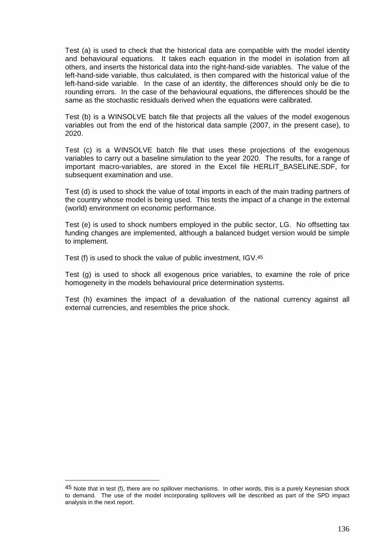
136

Test (a) is used to check that the historical data are compatible with the model identity and behavioural equations. It takes each equation in the model in isolation from all others, and inserts the historical data into the right-hand-side variables. The value of the left-hand-side variable, thus calculated, is then compared with the historical value of the left-hand-side variable. In the case of an identity, the differences should only be die to rounding errors. In the case of the behavioural equations, the differences should be the same as the stochastic residuals derived when the equations were calibrated. Test (b) is a WINSOLVE batch file that projects all the values of the model exogenous variables out from the end of the historical data sample (2007, in the present case), to 2020. Test (c) is a WINSOLVE batch file that uses these projections of the exogenous variables to carry out a baseline simulation to the year 2020. The results, for a range of important macro-variables, are stored in the Excel file HERLIT_BASELINE.SDF, for subsequent examination and use. Test (d) is used to shock the value of total imports in each of the main trading partners of the country whose model is being used. This tests the impact of a change in the external (world) environment on economic performance. Test (e) is used to shock numbers employed in the public sector, LG. No offsetting tax funding changes are implemented, although a balanced budget version would be simple to implement. Test (f) is used to shock the value of public investment, IGV.45 Test (g) is used to shock all exogenous price variables, to examine the role of price homogeneity in the models behavioural price determination systems. Test (h) examines the impact of a devaluation of the national currency against all external currencies, and resembles the price shock.

45 Note that in test (f), there are no spillover mechanisms. In other words, this is a purely Keynesian shock to demand. The use of the model incorporating spillovers will be described as part of the SPD impact analysis in the next report.

137

Annex 4: A HERLIT-based projection methodology The reason why we need a baseline scenario is that we will require a baseline projection of the economy into the future against which we can evaluate the impacts of cohesion policy actions. In the case of evaluating the impacts of cohesion policy, we need a baseline scenario that extends very far into the future, in order to quantify the long-tailed consequences of the policies. The main supply-side benefits of cohesion policy will only occur after the SPD 2004-2006 funding ceases at end 2008. This is because the improved stocks of physical infrastructure, human capital and R&D will generate long-term benefits that endure after the policies have terminated. At this stage it is important to be clear about the distinctions between “forecasts” and “projections”. Definition 1: Projection: A “baseline” projection is a simulation generated by HERLIT when any set of projections of all the exogenous variables is fed into the model, and results are generated for all the endogenous variables Definition 2: Forecast: A “baseline” projection (according to Definition 1 above) takes on the characteristics of a “forecast” when the assumptions for the exogenous variables are prepared carefully to be in line with informed analysis by national and international forecasting experts, and where the initial model projections are adjusted in light of off-model information by these experts as well as by the model operators. If we were only interested in the EU cohesion policy impacts, then any reasonable baseline projection could be used. Policy impacts (evaluated as deviations from a baseline) tend not to be very sensitive to the exact nature of the baseline.46 One could derive the baselines in a very simple way, and not pay very much attention to the “realism” of the assumptions or the fine detail of the projection. But there is usually a very particular interest in the baseline projection itself, as well as in the “levels” of the “with-cohesion-policy” simulation. Unrealistic baseline projections attract negative attention and criticism. This means that every effort should be made to choose realistic values for the out-of-sample exogenous variables and policy instruments. In that way we can move to a more realistic medium/long-tern forecast, and be in a position to stand over the quality and realism of the baseline. The preparation of a baseline projection is the first stage in the preparation of a realistic medium-term forecast. For the purposes of out-of-sample projection, the external and policy variables in HERLIT can be grouped into five different types, as follows: [1] External (or world) variables There are about 20 variables in this important category in HERLIT.

(a) World economic growth: The rate of growth of manufacturing output and total

imports in Lithuania’s main trading partners (i.e., the main export destinations that include Estonia, Germany, Russia, Sweden, the Netherlands, Poland, Latvia, the United Kingdom, the United States, etc.). We make an assumption concerning the likely future growth in these trading partner economies for the period 2008-

46 More technically, for a linear model, the policy multipliers are invariant with respect to the nature of the baseline. A model like HERLIT is nonlinear, so the magnitude of the policy multipliers may become somewhat sensitive to the baseline, within a very wide range of outcomes.

138

2020. These assumptions are made in light of whatever forecasts of the international economy are available. Of course, beyond 2009 the assumptions are somewhat speculative.

(b) External prices: These include the price of imports (PM), agricultural prices

(POA), as well as the output prices of manufactured goods in a series of the recipient economy’s main trading partners.47 We make the initial assumption of a common inflation rate of 3 per cent per year for the period 2009-2020. More realistic assumptions are then prepared, in light of developments in the global economy.

(c) EU27 unemployment rate: This is available for use should one wish to

endogenise migration flows. But in the HERLIT model, migration flows can be left exogenous.

[2] Internal (or policy) variables These are mainly public expenditure instruments (including public sector employment) and tax rates, and there are over twenty variables in this category.

(a) Public employment (LG): Employment numbers can be frozen at their end-of-

sample (2007) value, when there are no data more recent than 2007. This is equivalent to maintaining public consumption expenditure fixed in real terms. Alternatively, any available indicators can be used.

(b) Other elements of real public consumption (RGENW, OGNW): These can also

usually frozen at their end-of-sample (2007) values, when there are no data more recent than 2007. Alternatively, any available indicators can be used.

(c) Other elements of public expenditure (e.g., IGV): These are usually projected to

grow in nominal terms at the same rate as world prices (i.e., 3 per cent per year). Thus, they are assumed to be maintained approximately fixed in real terms, ex ante. Of course, it the domestic rate of inflation rises above the (assumed) world rate of 3 per cent, then this assumption would need to be revisited. It should be stressed that the assumption with respect to IGV concerns public sector investment expenditure that are not part of the domestic co-financed element of cohesion policy. If all such IGV expenditures are regarded as part of domestic public co-finance, then IGV would be projected as zero, and the cohesion policy variables would be used instead. In practice there is usually some elements of IGV that are unrelated to cohesion policy rules.48

(d) Tax rates: These are usually fixed at their end-of-sample (2007) values.

Alternatively, any available indicators can be used. Consequently, revenues (in nominal prices) will grow at the same rate as the relevant tax base (e.g., CONSV in the case of RGTE, the rate of indirect taxes). When the consequences for future revenue generation are known from initial simulations, then these assumptions will need to be revisited.

47 In HERMIN models of EU countries, the partial exogeneity of agricultural prices follows from the Common Agriculture Policy (or CAP). 48 Note that all of the private investment categories (by sector, as in IT, IM, IB, IA; and by type of

good, as in IOTHM and IOTHB) are endogenous, and are determined by simulating the model.

139

(e) The exchange rate of the LTL against the currencies of its main trading partners: These are initially projected to end 2008 using Central Bank data, and further projected beyond 2008 as being fixed at their end-2008 values.

(f) Interest rates: These are initially projected to end 2008 using Central Bank data,

and further projected beyond 2008 as being fixed at their end-2008 values. [3] Other exogenous variables There are two main categories: trade weights and a miscellaneous category.

(a) Trade weights: These are used in the model to weight the components of world

import growth. In the projection, it is assumed that they are fixed at their end-of-sample (2007) values.

(b) Miscellaneous: Most remaining exogenous variables are projected as being fixed

in real terms, ex ante. [4] Modifications of out-of-sample time trends A range of time trends have been used in the model, and values were calibrated using the within-sample data from 1995-2007. However, it would be unwise to project these trend rates of growth unchanged into the medium term without some reflection on their characteristics. The following are the main kinds of assumptions made about the future path of the key time trends in the HERLIT model:

(a) Hicks neutral technical progress: The calibrated values within-sample for

manufacturing, building and construction, and market services, are used initially. Out of sample, these can be modified. For example, if the calibrated rates are very high, it would be unwise to assume that technical progress would necessarily continue at this rate.

(b) Agricultural productivity growth: The within-sample growth rate can be used.

When these are very high, they can be tapered off over time, in line with the behaviour of more advanced member states.

(c) Agricultural employment: Projecting high rates of decline in employment in

agriculture would mean (essentially) that the sector would become insignificant in time. Projected rates are derived in light of each country’s particular circumstances.

(d) The capital/output ratio in agriculture: As for (b) and (c) above.

(e) Labour force participation rate: The within-sample annual changes (declines or

increases) are usually set to zero out of sample. Hence, the participation rate can be frozen at its end-of-sample (2007) level, or forced to track any desired path in the future.

(f) Trend sectoral output growth: Where there are significant time trends in any

sectoral output equations (positive or negative), these have to be projected with care.

[5] Behavioural intercept adjustments

140

We usually make the simple assumption that the value of the end-of-sample (2007) error for the behavioural equations is projected forward to 2020 unchanged. However, where a behavioural equation defines a rate of change or a flow (e.g., wage inflation in the M-sector (WMDOT), etc.), then we project the error as zero. These are fairly standard assumptions made when models are used to project future trends of the economy.

Concluding remarks on forecasting Economic models are used in two different but related situations: forecasting and policy analysis. If one requires simply to forecast aggregate GNP and its components forward a few years, a simple approach based on extrapolating recent past trends, adjusted by a study of likely future world trends, and applied with a common sense will probably out-guess any large structural economic model! However, if a series of detailed sectoral forecasts, based on a range of different world scenarios and domestic policy stances, is required, the simple isolated time-series approach becomes less relevant. But in such situations, macro-models may have some problems. The so-called "Lucas critique" asserts that model-based policy analysis is invalid since the model's structural parameters (the numbers obtained from statistical analysis of past data) cannot be assumed to remain unchanged in the face of future policy regime shifts. However, the force of the Lucas critique is greatest in the case of "reduced form" models, i.e., small-scale models whose equations represent a mixture of behavioural, policy reaction and ad hoc dynamic elements.49 The HERLIT model is more “structural”, and structural change is actually modelled explicitly. However, care must still be exercised to ensure that one does not stray into configurations of the economy which are very different to those which characterised the years used for model calibration. Most conventional models use adaptive or extrapolative expectations mechanisms: i.e., future performance of a particular variable is affected only by present and past factors. "Rational" or “model consistent” expectations mechanisms assume that people form views about the future by taking account of all available information, including available economic model forecasts. For example, if the Lithuanian government announced a major fiscal restructuring, involving public expenditure cut-backs, the effects of such an announcement would be immediate if the policy was “credible”.50 However, if the policy lacked credibility, nothing would happen. Models can be used to develop medium-term forecasts, conditional on judgemental assumptions concerning the world economy and domestic policy. Such forecasts are never used in "pure" form, and are altered post hoc in the light of judgement and experience. A model provides an essential accounting and economic framework within which to formulate and evaluate forecasts. The absence of such a framework makes realistic medium-term forecasting difficult, if not impossible, to carry out. But its presence is still no absolute guarantee of the validity of the forecast. Policy and scenario analysis can be carried out using the HERLIT model. Ideally, such scenarios should not differ too much from the historical pattern of behaviour. In practice one sometimes pushes the model to its limits and beyond (i.e., in terms of very large

49 For example, the VAR model of Čuvak, would be vulnerable to the Lucas critique, if used for

policy analysis rather than forecasting. 50 For an example of an application of a HERMIN model that contains forward-looking expectation mechanisms, see the study of the 1987-98 fiscal restructuring in Ireland (Bradley and Whelan, 1997).

141

policy shocks), and so one must be careful to adjust ones evaluation of the validity of the results accordingly. Models are also useful for the analysis of the macroeconomic consequences of wider policy initiatives, in such areas as industrial and business policy, labour market initiatives, social policy, tax reform, etc. In particular, the HERLIT model is designed for analysis of the impact of EU cohesion policy.

142

Annex 5: Master dictionary of HERLIT model variable s Exogenous variables in HERLIT model

[B] Basic input - AMECO [B] Basic input - other source [GZ or GI] Generate & initialise [G] Generate

Name Type Description Comment

Basic

Generated ATIP B Austria: Industrial production (index) AMECO ATM B Austria: Total imports (index) AMECO AUIP B Australia: Industrial production (index) AMECO AUM B Australia: Total imports (index) AMECO BEIP B Belgium: Industrial production (index) AMECO BEM B Belgium: Total imports (index) AMECO BEP B Belgium: Wholesale prices (index) AMECO BGIP B Bulgaria: Industrial production (index) AMECO BGM B Bulgaria: Total imports (index) AMECO BPRES B BOP item: residual BPTPRNE B BOP item: private sector transfers BRIP B Brazil: Industrial production (index) AMECO BRM B Brazil: Total imports (index) AMECO CAIP B Canada: Industrial production (index) AMECO CAM B Canada: Total imports (index) AMECO CHIP B Switzerland: Industrial production (index) AMECO CHM B Switzerland: Total imports (index) AMECO CNIP B China: Industrial production (index) AMECO CNM B China: Total imports (index) AMECO CYIP B Cyprus: Industrial production (index) AMECO

143

CYM B Cyprus: Total imports (index) AMECO CZIP B Czech Republic: Industrial production (index) AMECO CZM B Czech Republic: Total imports (index) AMECO DEIP B Germany: Industrial production (index) AMECO DEM B Germany: Total imports (index) AMECO DEP B Germany: Wholesale prices (index) AMECO DEPARAT GI Depreciation rate: agriculture Set to 0.025 DEPBRAT GI Depreciation rate: building & construction Set to 0.05 DEPMRAT GI Depreciation rate: market services Set to 0.05

DEPRAT G Depreciation rate: whole economy (implicit) DEPV = DEPRAT*(PI*(KT+KM+KB+KA+KGINF)) DEPTRAT GI Depreciation rate: manufacturing Set to 0.08 DETAMPH GZ Spillover phase-in: Sector M / Type PH Set to zero DETAMPI GZ Spillover phase-in: Sector M / Type PI Set to zero DETAMPR GZ Spillover phase-in: Sector M / Type PR Set to zero DETAMQH GZ Spillover phase-in: Sector M / Type QH Set to zero DETAMQI GZ Spillover phase-in: Sector M / Type QI Set to zero DETAMQR GZ Spillover phase-in: Sector M / Type QR Set to zero DETATPH GZ Spillover phase-in: Sector T / Type PH Set to zero DETATPI GZ Spillover phase-in: Sector T / Type PI Set to zero DETATPR GZ Spillover phase-in: Sector T / Type PR Set to zero DETATQH GZ Spillover phase-in: Sector T / Type QH Set to zero DETATQI GZ Spillover phase-in: Sector T / Type QI Set to zero DETATQR GZ Spillover phase-in: Sector T / Type QR Set to zero DKIP B Denmark: Industrial production (index) AMECO DKM B Denmark: Total imports (index) AMECO DUMGND GI Dummy variable for GND (exogenous/endogenous) Set to unity (default) EEIP B Estonia: Industrial production (index) AMECO EEM B Estonia: Total imports (index) AMECO ELIP B Greece: Industrial production (index) AMECO ELM B Greece: Total imports (index) AMECO ESIP B Spain: Industrial production (index) AMECO ESM B Spain: Total imports (index) AMECO ESP B Spain: Wholesale prices (index) AMECO ETAMPH GZ Spillover elasticity: Sector M / Type PH Set to zero ETAMPI GZ Spillover elasticity: Sector M / Type PI Set to zero ETAMPR GZ Spillover elasticity: Sector M / Type PR Set to zero

144

ETAMQH GZ Spillover elasticity: Sector M / Type QH Set to zero ETAMQI GZ Spillover elasticity: Sector M / Type QI Set to zero ETAMQR GZ Spillover elasticity: Sector M / Type QR Set to zero ETATPH GZ Spillover elasticity: Sector T / Type PH Set to zero ETATPI GZ Spillover elasticity: Sector T / Type PI Set to zero ETATPR GZ Spillover elasticity: Sector T / Type PR Set to zero ETATQH GZ Spillover elasticity: Sector T / Type QH Set to zero ETATQI GZ Spillover elasticity: Sector T / Type QI Set to zero ETATQR GZ Spillover elasticity: Sector T / Type QR Set to zero FIIP B Finland: Industrial production (index) AMECO FIM B Finland: Total imports (index) AMECO FRIP B France: Industrial production (index) AMECO FRM B France: Total imports (index) AMECO FRP B France: Wholesale prices (index) AMECO GECSFEC_E GZ Total annual EC funding for NSRF (in current euro) Set to zero GKO B Residual category of public capital expenditure GNDEX G Exogenous variant of GND, for use in policy feedback rule Set to GND GREVK B Non-NSRF capital revenue GTRABR B Government transfers abroad GTRK B Government capital transfers GTTI B Government trading and investment income HKIP B Hong Kong: Industrial production (index) AMECO HKM B Hong Kong: Total imports (index) AMECO HRIP B Croatia: Industrial production (index) AMECO HRM B Croatia: Total imports (index) AMECO HUIP B Hungary: Industrial production (index) AMECO HUM B Hungary: Total imports (index) AMECO IEIP B Ireland: Industrial production (index) AMECO IEM B Ireland: Total imports (index) AMECO IGV B Government investment: current prices IHGV B Public housing investment: current prices INIP B India: Industrial production (index) AMECO INM B India: Total imports (index) AMECO ISIP B Iceland: Industrial production (index) AMECO

145

ISM B Iceland: Total imports (index) AMECO ITIP B Italy: Industrial production (index) AMECO ITM B Italy: Total imports (index) AMECO ITP B Italy: Wholesale prices (index) AMECO JPIP B Japan: Industrial production (index) AMECO JPM B Japan: Total imports (index) AMECO KIHP G Private housing investment (share of GDPE) KRIP B Korea: Industrial production (index) AMECO KRM B Korea: Total imports (index) AMECO

KYCTREP G Repatriated manufacturing profits (YCTREP as a fraction of YCT) LG B Total employment in G-sector (thousands) LTIP B Lithuania: Industrial production (index) AMECO LTM B Lithuania: Total imports (index) AMECO LUIP B Luxembourg: Industrial production (index) AMECO LUM B Luxembourg: Total imports (index) AMECO LVIP B Latvia: Industrial production (index) AMECO LVM B Latvia: Total imports (index) AMECO MKIP B Macedonia: Industrial production (index) AMECO MKM B Macedonia: Total imports (index) AMECO MTIP B Malta: Industrial production (index) AMECO MTM G Malta: Total imports (index) AMECO MW1 G Import fraction from DE (used in definition of PM) Use export weights MW2 G Import fraction from IT (used in definition of PM) Use export weights MW3 G Import fraction from FR (used in definition of PM) Use export weights MW4 G Import fraction from ES (used in definition of PM) Use export weights MW5 G Import fraction from NL (used in definition of PM) Use export weights MW6 G Import fraction from BE (used in definition of PM) Use export weights MW7 G Import fraction from UK (used in definition of PM) Use export weights MW8 G Import fraction from SE (used in definition of PM) Use export weights MW9 G Import fraction from US (used in definition of PM) Use export weights MXIP B Mexico: Industrial production (index) AMECO MXM B Mexico: Total imports (index) AMECO NELDDUM GI Dummy variable: exogenises NELD Set to unity NJUVDUM GI Dummy variable: exogenises NJUV Set to unity NLIP B Netherlands: Industrial production (index) AMECO NLM B Netherlands: Total imports (index) AMECO

146

NLP B Netherlands: Wholesale prices (index) AMECO NOIP B Norway: Industrial production (index) AMECO NOM B Norway: Total imports (index) AMECO NWORKDUM GI Dummy variable: exogenises NWORK Set to unity NZIP B New Zealand: Industrial production (index) AMECO NZM B New Zealand: Total imports (index) AMECO OGNW G Non-wage element of OG OGNWV=POG*OGNW OVERHD GZ Overhead in ESF training schemes (fraction of wage bill) Set to zero PLIP B Poland: Industrial production (index) AMECO PLM B Poland: Total imports (index) AMECO POA G GDP deflator for agriculture (index) PTIP B Portugal: Industrial production (index) AMECO PTM B Portugal: Total imports (index) AMECO R_GSUB G GFS -> NA conversion of GSUB GSUB_GFS=(R_GSUB)*GSUB R_GTE G GFS -> NA conversion of GTE GTE_GFS=(R_GTE)*GTE R_GV G GFS -> NA conversion of GV GV_GFS=(R_GV)*GV R_IGV G GFS -> NA conversion of IGV IGV_GFS=(R_IGV)*IGV

RDPCOFIN GZ Domestic public co-finance ratio [ 100*GECSFDP/(GECSFEC+GECSFDP) ] Set to zero RGENW G Non-wage public consumption (constant prices) GENW=PG*RGENW RGEXPCO G Expenditure rate (used to derive GEXPCO from GV_GFS) GEXPCO=RGEXPCO*GV_GFS RGND G Implicit interest rate on national debt (per cent) GTRND = (RGND/100) * GND RGREVCO G Implicit tax rate (used to derive GREVCO from GDPFCV) GREVCO=RGREVCO*GDPFCV

RGSRUB G Implicit expenditure rate (used to derive GSRUB from GDPPC) GSRUB=RGSRUB*GDPFC

RGSUB G Implicit expenditure rate (used to derive GSUB from GDPPCV) GSUB=RGSUB*GDPFCV RGTRE G Implicit tax rate (used to derive GTRE from CONS) GTRE=RGTRE*CONS RGTRSFD GZ Share of NSRF (D) funding going to human resources (ESF) Set to zero RGTRSFE GZ Share of NSRF (E) funding going to human resources (ESF) Set to zero RGTRSFP GZ Share of NSRF (P) funding going to human resources (ESF) Set to zero RGTRSOC G Implicit rate of social welfare payments (links GTRSOC to N) GTRSOC = RGTRSOC*(PCONS*N) RGTW G Implicit rate of wealth tax (on proxy base GDPEV) GTW=RGTW*GDPEV RGTYC G Implicit rat eof corporation tax (on base YC(-1)) GTYC=RGTYC*YC(-1)

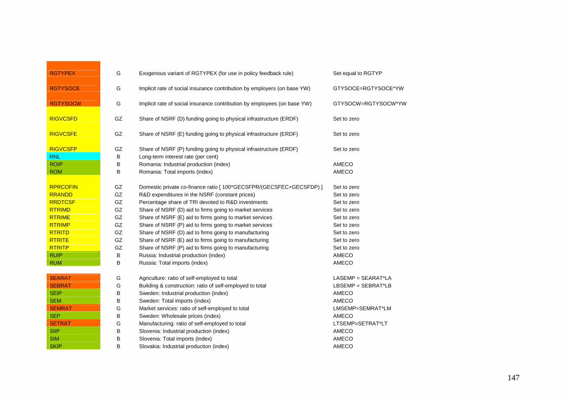
147

RGTYPEX G Exogenous variant of RGTYPEX (for use in policy feedback rule) Set equal to RGTYP

RGTYSOCE G Implicit rate of social insurance contribution by employers (on base YW) GTYSOCE=RGTYSOCE*YW

RGTYSOCW G Implicit rate of social insurance contribution by employees (on base YW) GTYSOCW=RGTYSOCW*YW

RIGVCSFD GZ Share of NSRF (D) funding going to physical infrastructure (ERDF) Set to zero

RIGVCSFE GZ Share of NSRF (E) funding going to physical infrastructure (ERDF) Set to zero

RIGVCSFP GZ Share of NSRF (P) funding going to physical infrastructure (ERDF) Set to zero RNL B Long-term interest rate (per cent) ROIP B Romania: Industrial production (index) AMECO ROM B Romania: Total imports (index) AMECO

RPRCOFIN GZ Domestic private co-finance ratio [ 100*GECSFPR/(GECSFEC+GECSFDP) ] Set to zero RRANDD GZ R&D expenditures in the NSRF (constant prices) Set to zero RRDTCSF GZ Percentage share of TRI devoted to R&D investments Set to zero RTRIMD GZ Share of NSRF (D) aid to firms going to market services Set to zero RTRIME GZ Share of NSRF (E) aid to firms going to market services Set to zero RTRIMP GZ Share of NSRF (P) aid to firms going to market services Set to zero RTRITD GZ Share of NSRF (D) aid to firms going to manufacturing Set to zero RTRITE GZ Share of NSRF (E) aid to firms going to manufacturing Set to zero RTRITP GZ Share of NSRF (P) aid to firms going to manufacturing Set to zero RUIP B Russia: Industrial production (index) AMECO RUM B Russia: Total imports (index) AMECO SEARAT G Agriculture: ratio of self-employed to total LASEMP = SEARAT*LA SEBRAT G Building & construction: ratio of self-employed to total LBSEMP = SEBRAT*LB SEIP B Sweden: Industrial production (index) AMECO SEM B Sweden: Total imports (index) AMECO SEMRAT G Market services: ratio of self-employed to total LMSEMP=SEMRAT*LM SEP B Sweden: Wholesale prices (index) AMECO SETRAT G Manufacturing: ratio of self-employed to total LTSEMP=SETRAT*LT SIIP B Slovenia: Industrial production (index) AMECO SIM B Slovenia: Total imports (index) AMECO SKIP B Slovakia: Industrial production (index) AMECO

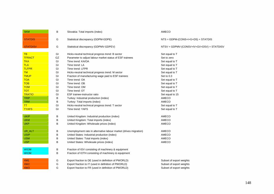
148

SKM B Slovakia: Total imports (index) AMECO

STATDIS G Statistical discrepancy (GDPM-GDPE) NTS = GDPM-(CONS+I+G+DS) + STATDIS

STATDISV G Statistical discrepancy (GDPMV-GDPEV) NTSV = GDPMV-(CONSV+IV+GV+DSV) + STATDISV TB GI Hicks-neutral technical progress trend: B sector Set equal to T TFRACT GZ Parameter to adjust labour market status of ESF trainees Set to zero TKA GI Time trend: KA/OA Set equal to T TLA GI Time trend: LA Set equal to T TLFPR GI Time trend: LFPR Set equal to T TM GI Hicks-neutral technical progress trend: M sector Set equal to T TMUP GI Fraction of manufacturing wage paid to ESF trainees Set to 0.3 TOA GI Time trend: OA Set equal to T TOB GI Time trend: OB Set equal to T TOM GI Time trend: OM Set equal to T TOT GI Time trend: OT Set equal to T TRATIO GI ESF trainee-instructor ratio Set equal to 15 TRIP B Turkey: Industrial production (index) AMECO TRM B Turkey: Total imports (index) AMECO TT GI Hicks-neutral technical progress trend: T sector Set equal to T TYAFS GI Time trend: YAFS Set equal to T UKIP B United Kingdom: Industrial production (index) AMECO UKM B United Kingdom: Total imports (index) AMECO UKP B United Kingdom: Wholesale prices (index) AMECO

UR_ALT B Unemployment rate in alternative labour market (drives migration) AMECO USIP B United States: Industrial production (index) AMECO USM B United States: Total imports (index) AMECO USP B United States: Wholesale prices (index) AMECO WIGM B Fraction of IGV consisting of machinery & equipment WIOM B Fraction of IOTH consisting of machinery & equipment XM1 G Export fraction to DE (used in definition of PWORLD) Subset of export weights XW2 G Export fraction to IT (used in definition of PWORLD) Subset of export weights XW3 G Export fraction to FR (used in definition of PWORLD) Subset of export weights

149

XW4 G Export fraction to ES (used in definition of PWORLD) Subset of export weights XW5 G Export fraction to NL (used in definition of PWORLD) Subset of export weights XW6 G Export fraction to BE (used in definition of PWORLD) Subset of export weights XW7 G Export fraction to UK (used in definition of PWORLD) Subset of export weights XW8 G Export fraction to SE (used in definition of PWORLD) Subset of export weights XW9 G Export fraction to US (used in definition of PWORLD) Subset of export weights

XWAT B Export fraction to Austria (used in definition of OWIP and OWM)

XWAU B Export fraction to Australia (used in definition of OWIP and OWM)

XWBE B Export fraction to Belgium (used in definition of OWIP and OWM)

XWBG B Export fraction to Bulgaria (used in definition of OWIP and OWM)

XWBR B Export fraction to Brazil (used in definition of OWIP and OWM)

XWCA B Export fraction to Canada (used in definition of OWIP and OWM)

XWCH B Export fraction to Switzerland (used in definition of OWIP and OWM)

XWCN B Export fraction to China (used in definition of OWIP and OWM)

XWCY B Export fraction to Cyprus (used in definition of OWIP and OWM)

XWCZ B Export fraction to Czech Republic (used in definition of OWIP and OWM)

XWDE B Export fraction to Germany (used in definition of OWIP and OWM)

XWDK B Export fraction to Denmark (used in definition of OWIP and OWM)

XWEE B Export fraction to Estonia (used in definition of OWIP and OWM)

XWEL B Export fraction to Greece (used in definition of OWIP and OWM)

XWES B Export fraction to Spain (used in definition of OWIP and OWM)

150

XWFI B Export fraction to Finland (used in definition of OWIP and OWM)

XWFR B Export fraction to France (used in definition of OWIP and OWM)

XWHK B Export fraction to Hong Kong (used in definition of OWIP and OWM)

XWHR B Export fraction to Croatia (used in definition of OWIP and OWM)

XWHU B Export fraction to Hungary (used in definition of OWIP and OWM)

XWIE B Export fraction to Ireland (used in definition of OWIP and OWM)

XWIN B Export fraction to India (used in definition of OWIP and OWM)

XWIS B Export fraction to Island (used in definition of OWIP and OWM)

XWIT B Export fraction to Italy (used in definition of OWIP and OWM)

XWJP B Export fraction to Japan (used in definition of OWIP and OWM)

XWKR B Export fraction to Korea (used in definition of OWIP and OWM)

XWLT B Export fraction to Lithuania (used in definition of OWIP and OWM)

XWLU B Export fraction to Luxembugh (used in definition of OWIP and OWM)

XWLV B Export fraction to Latvia (used in definition of OWIP and OWM)

XWMK B Export fraction to Macedonia (used in definition of OWIP and OWM)

XWMT B Export fraction to Malta (used in definition of OWIP and OWM)

XWMX B Export fraction to Mexico (used in definition of OWIP and OWM)

XWNL B Export fraction to the Netherlands (used in definition of OWIP and OWM)

XWNO B Export fraction to Norway (used in definition of OWIP and OWM)

151

XWNZ B Export fraction to New Zealand (used in definition of OWIP and OWM)

XWPL B Export fraction to Poland (used in definition of OWIP and OWM)

XWPT B Export fraction to Portugal (used in definition of OWIP and OWM)

XWRO B Export fraction to Romania (used in definition of OWIP and OWM)

XWRU B Export fraction to Russia (used in definition of OWIP and OWM)

XWSE B Export fraction to Sweden (used in definition of OWIP and OWM)

XWSI B Export fraction to Slovenia (used in definition of OWIP and OWM)

XWSK B Export fraction to Slovakia (used in definition of OWIP and OWM)

XWTR B Export fraction to Turkey (used in definition of OWIP and OWM)

XWUK B Export fraction to United Kingdom (used in definition of OWIP and OWM)

XWUS B Export fraction to United States (used in definition of OWIP and OWM) YASA B Adjustment for stock appreciation (current prices) YCURAT G Fraction of total profits retained in firm (YCU/YC) YCU=YCURAT*YC YFN B BOP item: net factor income from abroad

ZZEUR B Exchange rate: units of national currency to euro (ZZ=BG, CZ etc.) AMECO

ZZGBP B Exchange rate: units of national currency to sterling (ZZ=BG, CZ etc.) AMECO

ZZSEK B Exchange rate: units of national currency to Swedish crown (ZZ=BG, CZ etc.) AMECO

ZZUSD B Exchange rate: units of national currency to US dollar (ZZ=BG, CZ etc.) AMECO

152

Endogenous variables in HERLIT model

Basic input - AMECO Basic input - other source Generate & initialise Generate

Name Type Description Comment

Basic

Generated

AMX GZ Adjusted M-sector CES efficiency parameter (incorporating spillovers) Zero before calibration

ATX GZ Adjusted T-sector CES efficiency parameter (incorporating spillovers) Zero before calibration

BP G Balance of payments (curent account) BPR G BP, expressed as percentage of GDPEV CONS B Household consumption (constant prices) CONSV B Household consumption (cuurent prices) CSFTRAN GZ Total EC funding injection (equals GECSFEC) Set to zero CSFTRANR GZ CSFTRAN expressed as a percentage of GDPEV Set to zero DEPV Total (economy-wide) depreciation DS B Inventory stock changes DSV B Inventory stock changes ERFPB G Moving average of RFPB (expected relative factor price ratio) ERFPM G Moving average of RFPM (expected relative factor price ratio) ERFPT G Moving average of RFPT (expected relative factor price ratio) FDOM G Weighted measure of domestic demand (used in OM) FDOT G Weighted measure of domestic demand (used in OT)

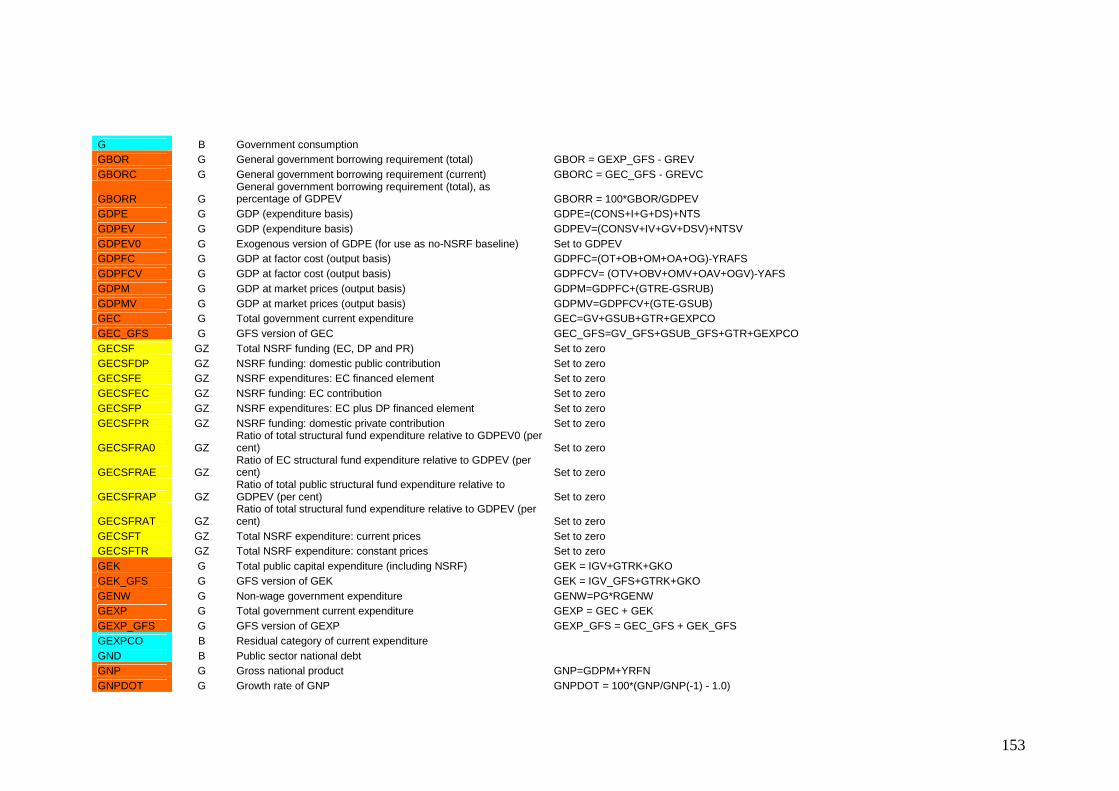
153

G B Government consumption GBOR G General government borrowing requirement (total) GBOR = GEXP_GFS - GREV GBORC G General government borrowing requirement (current) GBORC = GEC_GFS - GREVC

GBORR G General government borrowing requirement (total), as percentage of GDPEV GBORR = 100*GBOR/GDPEV

GDPE G GDP (expenditure basis) GDPE=(CONS+I+G+DS)+NTS GDPEV G GDP (expenditure basis) GDPEV=(CONSV+IV+GV+DSV)+NTSV GDPEV0 G Exogenous version of GDPE (for use as no-NSRF baseline) Set to GDPEV GDPFC G GDP at factor cost (output basis) GDPFC=(OT+OB+OM+OA+OG)-YRAFS GDPFCV G GDP at factor cost (output basis) GDPFCV= (OTV+OBV+OMV+OAV+OGV)-YAFS GDPM G GDP at market prices (output basis) GDPM=GDPFC+(GTRE-GSRUB) GDPMV G GDP at market prices (output basis) GDPMV=GDPFCV+(GTE-GSUB) GEC G Total government current expenditure GEC=GV+GSUB+GTR+GEXPCO GEC_GFS G GFS version of GEC GEC_GFS=GV_GFS+GSUB_GFS+GTR+GEXPCO GECSF GZ Total NSRF funding (EC, DP and PR) Set to zero GECSFDP GZ NSRF funding: domestic public contribution Set to zero GECSFE GZ NSRF expenditures: EC financed element Set to zero GECSFEC GZ NSRF funding: EC contribution Set to zero GECSFP GZ NSRF expenditures: EC plus DP financed element Set to zero GECSFPR GZ NSRF funding: domestic private contribution Set to zero

GECSFRA0 GZ Ratio of total structural fund expenditure relative to GDPEV0 (per cent) Set to zero

GECSFRAE GZ Ratio of EC structural fund expenditure relative to GDPEV (per cent) Set to zero

GECSFRAP GZ Ratio of total public structural fund expenditure relative to GDPEV (per cent) Set to zero

GECSFRAT GZ Ratio of total structural fund expenditure relative to GDPEV (per cent) Set to zero

GECSFT GZ Total NSRF expenditure: current prices Set to zero GECSFTR GZ Total NSRF expenditure: constant prices Set to zero GEK G Total public capital expenditure (including NSRF) GEK = IGV+GTRK+GKO GEK_GFS G GFS version of GEK GEK = IGV_GFS+GTRK+GKO GENW G Non-wage government expenditure GENW=PG*RGENW GEXP G Total government current expenditure GEXP = GEC + GEK GEXP_GFS G GFS version of GEXP GEXP_GFS = GEC_GFS + GEK_GFS GEXPCO B Residual category of current expenditure GND B Public sector national debt GNP G Gross national product GNP=GDPM+YRFN GNPDOT G Growth rate of GNP GNPDOT = 100*(GNP/GNP(-1) - 1.0)

154

GNPPC G GNP per head: constant prices GNPPC = GNP/N GNPV G Gross national product GNPV=GDPMV+YFN GREV G Total government revenue GREV=GREVC+GREVK

GREVC G Total current revenue GREVC=(GTE_GFS)+(GTY+GTW)+GTYSOC+GTTI+GREVCO GREVCO B Other (non-tax) current revenue GSRUB G Subsidies: constant prices GSUB B Subsidies: current prices GSUB_GFS B GFS version of GSUB GTE B Revenue from indirect taxes: current prices GTE_GFS B GFS version of GTE GTR G Total government transfers GTR=GTRSOC+GTRND+GTRABR GTRE G Revenue from indirect taxes: constant prices GTRE=RGTRE*CONS GTRND B Interest payments on the national debt GTRSF GZ Total NSRF ESF expenditures Set to zero GTRSFDP GZ NSRF ESF expenditures: DP element Set to zero GTRSFEC GZ NSRF ESF expenditures: EC element Set to zero GTRSFPR GZ NSRF ESF expenditures: PR element Set to zero GTRSOC G Social transfer payments (income support, etc.) GTW B Revenue from wealth taxes GTY G Total revenue from taxes on income GTY=GTYP+GTYC GTYC B Revenue from corporation taxes GTYP B Revenue from taxes on personal incomes GTYSOC G Revenue from total social insurance contributions GTYSOC=GTYSOCW+GTYSOCE GTYSOCE B Revenue from total social insurance contributions by employers GTYSOCW B Revenue from total social insurance contributions by employees GV B Government consumption GV_GFS B GFS version of government consumption I G Total fixed capital formation IA B Fixed capital formation: agriculture IAV B Fixed capital formation: agriculture IB B Fixed capital formation: building & construction IBCTOT G Fixed capital formation by type of good: building & construction IBCTOT = IGINFB + IOTHB IBV B Fixed capital formation: building & construction IG B Fixed capital formation: government (non-NSRF)

IGINF G Total fixed public capital formation: physical infrastructure: constant prices IGINF = IGINFV/PIG

155

IGINFB G Building & construction element of IGINF IGINFB = IGINF - IGINFM IGINFM G Machinery & equipment element of IGINF IGINFM = WIGM * IGINF

IGINFV G Total fixed public capital formation: physical infrastructure: current prices IGINFV=IGV

IGV_GFS B GFS version of IGV IGVCSF GZ NSRF-related investment expenditures on infrastructure Set to zero

IGVCSFDP GZ NSRF-related investment expenditures on infrastructure: DP element Set to zero

IGVCSFEC GZ NSRF-related investment expenditures on infrastructure: EC element Set to zero

IGVCSFPR GZ NSRF-related investment expenditures on infrastructure: PR element Set to zero

IH G Total investment in housing IH=IHG+IHP IHG G Investment in public housing IHG=IHGV/PIH IHP G Investment in private housing IHP = KIHP*GDPE IHV G Total investment in housing IHV = PIH * IH IM B Fixed capital formation: market services IMETOT G Fixed capital formation by type of good: machinery & equipment IMETOT = IGINFM + IOTHM IMV B Fixed capital formation: market services INH G Total fixed capital formation, excluding housing INH = I - IH IOTH G Fixed capital formation: private non-housing IOTH = INH - IGINF

IOTHB G Fixed capital formation: private non-housing (building & construction) IOTHB = IOTH - IOTHM

IOTHM G Fixed capital formation: private non-housing (machinery & equipment) IOTHM = WIOM * IOTH

IT B Fixed capital formation: manufacturing ITV B Fixed capital formation: manufacturing IV G Total fixed capital formation KA G Capital stock: agriculture KB G Capital stock:building & construction KGINF G Capital stock: infrastructure KGINF0 G Capital stock: infrastructure (for use as no-NSRF baseline) Set equal to KGINF KGINFR G Ratio of KGINF to KGINF0 KM G Capital stock: market services KM0 G Capital stock: market services (for use of no-NSRF baseline) Set equal to KM KMR G Ratio of KM to KM0 KRTRIRD G Accumulated "stock" of R&D KRTRIRD = RTRIRD + (1-0.08)*KRTRIRD(-1) KRTRIRD0 G Accumulated "stock" of R&D (for use of no-NSRF baseline) Set equal to KRTRIRD KRTRIRDR G Ratio of KRTRIRD to KRTRIRD0 KRTRIRDR=(KRTRIRD/KRTRIRD0)

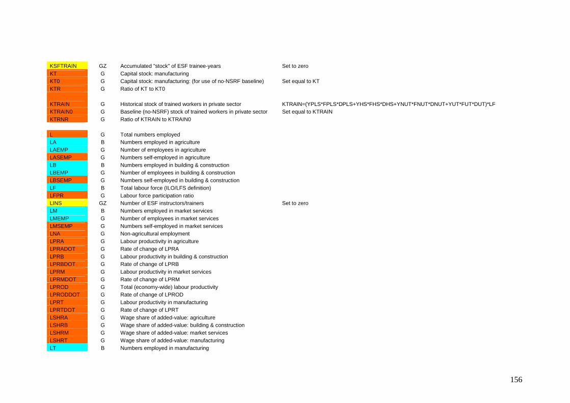
156

KSFTRAIN GZ Accumulated "stock" of ESF trainee-years Set to zero KT G Capital stock: manufacturing KT0 G Capital stock: manufacturing: (for use of no-NSRF baseline) Set equal to KT KTR G Ratio of KT to KT0

KTRAIN G Historical stock of trained workers in private sector KTRAIN=(YPLS*FPLS*DPLS+YHS*FHS*DHS+YNUT*FNUT*DNUT+YUT*FUT*DUT)*LF KTRAIN0 G Baseline (no-NSRF) stock of trained workers in private sector Set equal to KTRAIN KTRNR G Ratio of KTRAIN to KTRAIN0 L G Total numbers employed LA B Numbers employed in agriculture LAEMP G Number of employees in agriculture LASEMP G Numbers self-employed in agriculture LB B Numbers employed in building & construction LBEMP G Number of employees in building & construction LBSEMP G Numbers self-employed in building & construction LF B Total labour force (ILO/LFS definition) LFPR G Labour force participation ratio LINS GZ Number of ESF instructors/trainers Set to zero LM B Numbers employed in market services LMEMP G Number of employees in market services LMSEMP G Numbers self-employed in market services LNA G Non-agricultural employment LPRA G Labour productivity in agriculture LPRADOT G Rate of change of LPRA LPRB G Labour productivity in building & construction LPRBDOT G Rate of change of LPRB LPRM G Labour productivity in market services LPRMDOT G Rate of change of LPRM LPROD G Total (economy-wide) labour productivity LPRODDOT G Rate of change of LPROD LPRT G Labour productivity in manufacturing LPRTDOT G Rate of change of LPRT LSHRA G Wage share of added-value: agriculture LSHRB G Wage share of added-value: building & construction LSHRM G Wage share of added-value: market services LSHRT G Wage share of added-value: manufacturing LT B Numbers employed in manufacturing

157

LTEMP G Number of employees in manufacturing LTSEMP G Numbers self-employed in manufacturing N G Total population NDEP G Dependant population (NJUV+NELD) NDPFCV G Net domestic product at factor cost NELD B Population above working age NJUV B Population below working age NM B Net migration abroad (positive if net out-migration) NMRAT G NM expressed as a percentage of LF(-1) NMRAT = 100*(NM/LF(-1)) NNPFCV G Net national product at factor cost NNPFCV=NDPFCV+YFN+YASA NTS G Net trade balance (exports less imports) NTS = GDPM-(CONS+I+G+DS) + STATDIS

NTSV G Net trade balance (exports less imports) NTSV = GDPMV-(CONSV+IV+GV+DSV) + STATDISV NTSVR G NTSV, expressed as a percentage of GDPEV NTSVR=100*NTSV/GDPEV NWORK B Working age population NWORK=N-(NJUV+NELD) OA B GDP at factor cost: agriculture OAV B GDP at factor cost: agriculture OB B GDP at factor cost: building & construction OBV B GDP at factor cost: building & construction OG B GDP at factor cost: government OGNWV Non-wage GDP at factor cost: government OGV B GDP at factor cost: government OM B GDP at factor cost: market services OMV B GDP at factor cost: market services OT B GDP at factor cost: manufacturing OTV B GDP at factor cost: manufacturing OWIP G World industrial output: index See definition in model listing OWM G World imports: index See definition in model listing PBE G Wholesale prices: Belgium (index) PCOMPT G International competitiveness (POT/PWORLD) PCONS G Household consumption: deflator (index) PCONSDOT G Annual rate of change of PCONS PDE G Wholesale prices: Germany (index) PDS G Stock changes: deflator (index) PES G Wholesale prices: Spain (index)

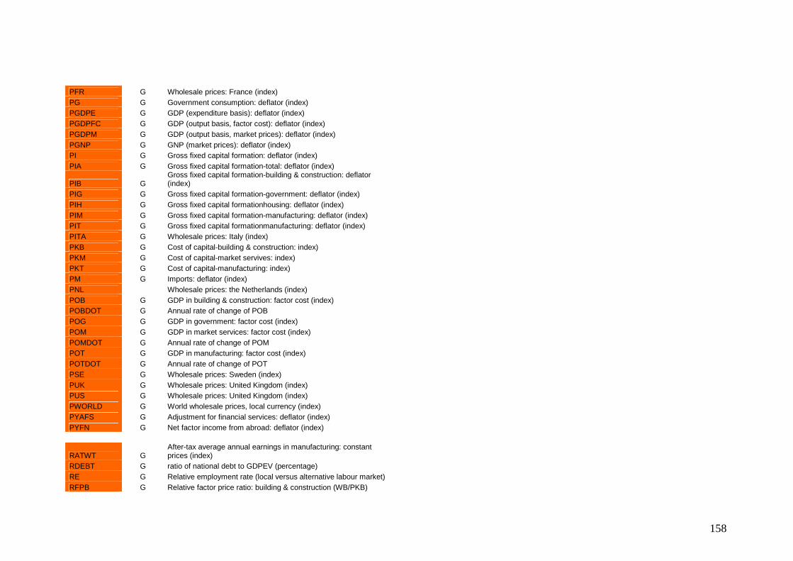
158

PFR G Wholesale prices: France (index) PG G Government consumption: deflator (index) PGDPE G GDP (expenditure basis): deflator (index) PGDPFC G GDP (output basis, factor cost): deflator (index) PGDPM G GDP (output basis, market prices): deflator (index) PGNP G GNP (market prices): deflator (index) PI G Gross fixed capital formation: deflator (index) PIA G Gross fixed capital formation-total: deflator (index)

PIB G Gross fixed capital formation-building & construction: deflator (index)

PIG G Gross fixed capital formation-government: deflator (index) PIH G Gross fixed capital formationhousing: deflator (index) PIM G Gross fixed capital formation-manufacturing: deflator (index) PIT G Gross fixed capital formationmanufacturing: deflator (index) PITA G Wholesale prices: Italy (index) PKB G Cost of capital-building & construction: index) PKM G Cost of capital-market servives: index) PKT G Cost of capital-manufacturing: index) PM G Imports: deflator (index) PNL Wholesale prices: the Netherlands (index) POB G GDP in building & construction: factor cost (index) POBDOT G Annual rate of change of POB POG G GDP in government: factor cost (index) POM G GDP in market services: factor cost (index) POMDOT G Annual rate of change of POM POT G GDP in manufacturing: factor cost (index) POTDOT G Annual rate of change of POT PSE G Wholesale prices: Sweden (index) PUK G Wholesale prices: United Kingdom (index) PUS G Wholesale prices: United Kingdom (index) PWORLD G World wholesale prices, local currency (index) PYAFS G Adjustment for financial services: deflator (index) PYFN G Net factor income from abroad: deflator (index)

RATWT G After-tax average annual earnings in manufacturing: constant prices (index)

RDEBT G ratio of national debt to GDPEV (percentage) RE G Relative employment rate (local versus alternative labour market) RFPB G Relative factor price ratio: building & construction (WB/PKB)

159

RFPM G Relative factor price ratio: market services (WM/PKM) RFPT G Relative factor price ratio: manufacturing (WT/PKT) RGTYP G Implicit rate of direct personal income tax RIRLT G Real long-term rate of interest: per cent) RRSA G Real rate of return on investments (index) RTRIRD GZ Percentage of NSRF TRI devoted to R&D Set to zero RULCB G Unit labour costs: building & construction (index) RULCM G Unit labour costs: market services (index) RULCT G Unit labour costs: manufacturing (index) S G Personal savings: constant prices SAV G Personal savings: current prices SAVRAT G Personal savings ratio SFTRAIN GZ ESF trainees supported: thousands Set to zero SFWAG GZ Wage bill element of ESF scheme Set to zero ST G Stock of inventories: constant prices TINC G Net indirect tax rate (used in PCONS) TINC = RGTE - RGSUB TRI GZ Total NSRF expenditure on direct aid to firms Set to zero TRIA GZ Total NSRF expenditure on direct aid to agricultural production Set to zero TRIADP GZ NSRF expenditure on direct aid to agricultural production: DP Set to zero TRIAEC GZ NSRF expenditure on direct aid to agricultural production: EC Set to zero TRIAPR GZ NSRF expenditure on direct aid to agricultural production: PR Set to zero

TRIARL GZ NSRF expenditure on direct aid to agricultural production: constant price Set to zero

TRIDP GZ Total NSRF expenditure on direct aid to firms: DP Set to zero TRIEC GZ Total NSRF expenditure on direct aid to firms: EC Set to zero TRIM GZ NSRF expenditure on direct aid to firms in market services: DP Set to zero TRIMDP GZ NSRF expenditure on direct aid to firms in market services: DP Set to zero TRIMEC GZ NSRF expenditure on direct aid to firms in market services: EC Set to zero TRIMPR GZ NSRF expenditure on direct aid to firms in market services: PR Set to zero

TRIMRL GZ NSRF expenditure on direct aid to firms in market services: constant price Set to zero

TRIPR GZ Total NSRF expenditure on direct aid to firms: PR Set to zero TRIRD GZ Total NSRF expenditure on direct aid to firms: R&D Set to zero TRIT GZ NSRF expenditure on direct aid to firms in manufacturing: DP Set to zero TRITDP GZ NSRF expenditure on direct aid to firms in manufacturing: EC Set to zero TRITEC GZ NSRF expenditure on direct aid to firms in manufacturing: PR Set to zero TRITPR GZ NSRF expenditure on direct aid to firms in manufacturing: Set to zero

160

constant price

TRITRL GZ NSRF expenditure on direct aid to firms in manufacturing: constant price Set to zero

U G Numbers unemployed ULCB G Unit labour costs: building & construction ULCM G Unit labour costs: market services ULCT G Unit labour costs: manufacturing UR G Unemployment rate (percentage) URBAR G Two-year moving average of UR

URP G Unemployment rate, adjusted for ESF schemes (used in WT equation) Set equal to UR

WA G Average annual earnings, agriculture WADOT G Annual percentage change in WA WB G Average annual earnings, building & construction WBDOT G Annual percentage change in WB WEDGE G Tax wedge (used in WT equation) WG G Average annual earnings, government WGDOT G Annual percentage change in WG WM G Average annual earnings, market services WMDOT G Annual percentage change in WM WNA G Average annual earnings, non-agriculture sector WNADOT G Annual percentage change in WNA WNH G Wealth (measured as accumulated savings) WT G Average annual earnings, manufacturing WTDOT G Annual percentage change in WT WTRAIN G Average annual earnings of ESF trainees WTRAIN=TMUP*WT YAFS G Adjustment for financial services YC G Corporate profits YC=NDPFCV-YWA-YWNA+YASA+YAFS YCA G Profits in agriculture (value added less wage bill) YCA=OAV-YWA YCB G Profits in building & construction (value added less wage bill) YCB=OBV-YWB YCM G Profits in market services (value added less wage bill) YCM=OMV-YWM YCT G Profits in manufacturing (value added less wage bill) YCT=OTV-YWT YCTREP B Repatriated profits YCU G Undistributed profits (i.e., retained in firms) YP G Private sector income YPER G Personal income

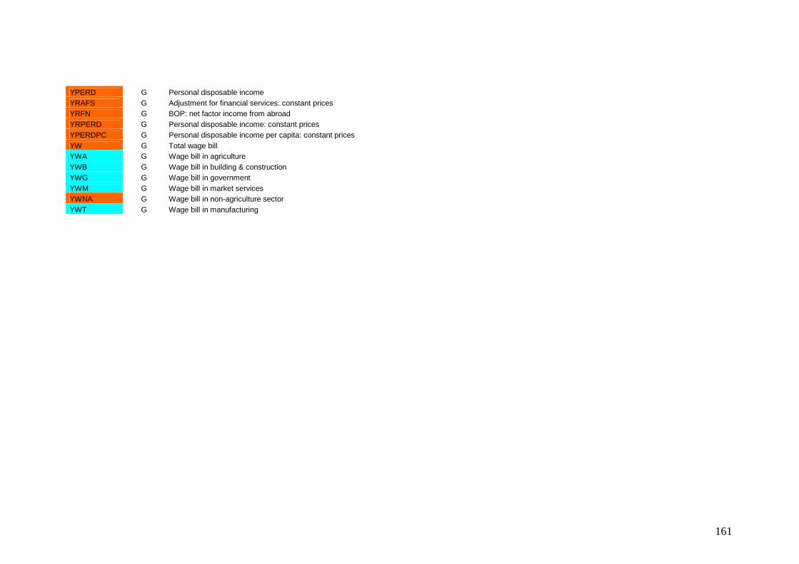
161

YPERD G Personal disposable income YRAFS G Adjustment for financial services: constant prices YRFN G BOP: net factor income from abroad YRPERD G Personal disposable income: constant prices YPERDPC G Personal disposable income per capita: constant prices YW G Total wage bill YWA G Wage bill in agriculture YWB G Wage bill in building & construction YWG G Wage bill in government YWM G Wage bill in market services YWNA G Wage bill in non-agriculture sector YWT G Wage bill in manufacturing

162