1

The Habit Persistence Hypothesis: Empirical Evidence from Jamaica1

Oluwafemi O. Bamikole

May, 2013

Abstract

This paper seeks to empirically verify if the habit persistence phenomenon holds in the Jamaican

economy. The results of the GMM time series estimation show the existence of habit formation

by Jamaican consumers. Past consumption habits affect the growth rate of consumption,

consequently in order to build the confidence of consumers in the Jamaican economy, the

inflation rate, foreign and domestic interest rates have to be moderately adjusted to encourage

good consumption habits.

JEL Classification Codes: D12, E21, C01

Keywords: Habit persistence, GMM, consumption growth, Jamaica

1 The author is grateful to Dr. P.N. Whitely at the University of the West Indies who positively shaped this paper

with useful comments. All errors are mine.

2

1. Introduction

The literature on consumption theory and hypotheses has grown over the years. From

Keynes’ pioneer work on the Absolute Income Hypothesis, Hall’s Permanent Income Hypothesis

treatise to several variants of these models in the 21st century. T.M. Brown’s 1952 Econometrica

article provides a sound theoretical background for consequent articles on the habit persistence

hypothesis; he develops a consumption function which lends itself to empirical verification by

estimating short-run and long-run multipliers of consumption that are derived from the lagged

values of consumption. This paper, however, uses the methodology of Kiley. Kiley shows, using

a consumption function that is separable in consumption and leisure that the growth rate of

consumption depends not only on the past levels of consumption but also on total labour supply,

the substitution between consumption and leisure and real interest rate.

However, Kiley’s model is modified somewhat, real foreign interest rate and some other

control variables are incorporated to drive home the crucial conclusion that habit formation is

necessarily an inextricable aspect of the consumption function. An interesting fact that emerges

from Kiley’s work is that habit persistence is not a feature that fundamentally drives the

consumption growth dynamics. This has largely motivated the need for this research at this

crucial time when consumers’ confidence in the Jamaican economy has been at a low ebb due to

unstable inflation rates, a huge debt burden that refuses to disappear and the just concluded

negotiations with IMF officials with implications for upward tax changes and wage cuts.

In this paper, the lagged value of consumption was initially regressed on its present value,

however it is more instructive to do this by using the growth rate of consumption, the results of

this regression provide profound results for the trend of consumption and the influence of past

3

consumption levels on this trend. In addition, unit root tests2 are carried out initially to determine

if the series employed exhibit a random walk or a random walk with drift. After removing the

unit root and dealing with the problem of spurious regression, a GMM estimation procedure is

then carried out. The GMM results reveal that past values of consumption negatively impact the

growth rate of consumption; this is not alarming as the real purchasing power, especially for the

average Jamaican household, has been long truncated by high domestic prices and a volatile

exchange rate.

The paper is divided into five sections. Section 1 looks at the introduction of the study,

section 2 deals with literature review. Section 3 focuses on the methodology of the study, data

sources and description, econometric specification of the model and the time-series model

assumptions. Section 4 outlines the empirical results and economic implications of the stylized

facts and section 5 closes the study with the summary, conclusion and recommendations.

Section 2: Literature Review

T.M. Brown’s 1952 experimentation with various alternative hypotheses leads to the

development of a habit “hysteresis” or habit persistence theory of a casual bias with a lag. Brown

then selects the theory and fits it to the observed Canadian data by first building around it a small

macro-model of the economy followed by simultaneous estimation of the parameters. Overall,

his results show the existence of habit persistence in the consumption function. Diaz, et al (2002)

assert, using a general equilibrium framework, that habit formation brings a hefty increase in

precautionary savings and mild fluctuation in the coefficient of variation and the Gini index of

wealth; the authors further assert that households in habits economies dislike consumption

2 A formal description of unit root tests is shown in the appendix

4

fluctuations when compared to their counterparts in a world of time separable preferences. This

should, according to the authors, increase the amount of their precautionary savings.

Ferson and Constantinides (1991) examine the impacts of habit persistence and durability

of consumption on the Euler equation and they find out that the coefficient of lagged

consumption expenditures enters the Euler equation negatively and dominates the effect of

durability. Habit persistence implies that the coefficient of lagged consumption expenditures is

negative, while durability implies positive coefficient for the variable. The Euler equation is

specified as follows:

])1[(1

0

1

A

t

ttCAE

where 110 tt CC ------ (1)

In equation 1, Ct represents consumption expenditures at time, t. A is the concavity parameter, β

is the rate of time discount and β1 is the parameter representing habit persistence which is

expected to be less than zero if there is evidence of habit formation and greater than zero if the

effect of durability dominates. In a time separable model β1 is set to zero. If, according to these

authors, both effects are present, the sign of the coefficients indicates which of the two effects

dominates. Also, Winder and Palm (1989) estimate a linearized form of the Euler equation and

find support for habit persistence in Netherlands.

Moreover, Eichenbaum, Hansen and Singleton (1988), Dum & Singleton (1986), using

monthly data, confirm that the coefficient of lagged consumption expenditures enters the Euler

equation positively using the same estimation framework that Diatz, et al employ. Hall (1978)

also states, using a random walk model, that consumption growth is clearly unpredictable based

on the information known to the consumer when the consumption choice was made. Kiley’s

5

(2007) model is adopted because it favours an estimation of a variant of the Euler equation,

Kiley examines the three hypotheses of consumption which are rule-of-thumb behaviour, habit-

persistence and permanent income and he shows that his data appear most consistent with non-

separable preferences over consumption and leisure in the United States. The variables Kiley

uses in his article are the growth rate of consumption, the lagged value of consumption measured

by nondurable and service expenditures c(t), real interest rate r(t), labour and transfer income per

capita y(t) . His model is stated as follows:

Δln(C(t)) = const.+ sr(t) + hΔln(C(t −1)) + lΔln(L(t)) + bΔln(Y(t)) + e(t) --------- (2)

Singh and Ullah (1976) are quick to point out that economists often treat HPH (Habit

Persistence Hypothesis) and PIH (Permanent Income Hypothesis) as one; they refer to this as a

wrong modeling approach and clearly distinguish between these two distinct hypotheses. The

slowness in the reaction of consumer demand to the changes in income is caused by inertia, “the

habits, customs, standards and the levels associated with real consumption previously enjoyed

are likely to impact on the human physiological and psychological system”. Moreover, HPH

affirms that when income falls, consumption will fall by less than proportionately to the fall in

income owing to hysteresis in consumer habits. However, PIH asserts that households’ current

consumption level depends not on their transitory income but the discounted value of their future

earnings.

Fuhrer (2002) inquires if the habit formation process has implications for monetary

policy formulation. His empirical results, using both VAR analysis and GMM estimation

technique, depict that the hypothesis of no habit formation is rejected. The inclusion of a habit

formation in consumer’s utility function improves the short-run dynamic behaviour of the model.

Habit formation allows the model to match the response of real spending to monetary shocks. A

6

habit formation parameter of 0.9 is obtained from the GMM estimation results and this

corroborates the author’s point that a jump in consumption spending can cause a corresponding

increase in inflation. Rossi (n.d.) affirms, using an Italian consumption data and GMM

methodology to estimate an Euler equation, that ignoring habit persistence can lead to misleading

outcomes in determining the factors that contribute to consumers’ spending. The author

estimates the habit persistence coefficient to be -0.283.

Section 3: Description of Data

The data employed in this study are derived from the Edward Seaga Database, Bank of

Jamaica website and Index Mundi. The data span from 1980-2011. The variables in the study are

private final consumption (measured in millions of JS$), GDP at current market prices (measured

in millions of JS$; this is a proxy for income), domestic interest rate, foreign interest rate,

domestic inflation rate and nominal exchange rate (JS$ to US$).

Table 1: Descriptive Statistics of Data

Variable Mean Median Standard

Deviation

Maximum

Value

Minimum

Value

FINR 5.029 5.375 2.110 8.680 0.50

DINR 6.3880 6.7150 8.010 20.290 -12.790

INCOME 313.855 224.500 341.358 1080 4.78

INF 17.6750 12.6150 14.901 77.30 5.950

EXC 35.5320 29.200 29.650 87.89 1.450

CONSUMPTION 258912.900 155310.90 309955.60 942107.60 3146.80

7

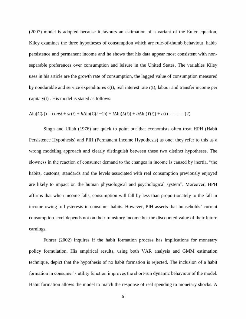
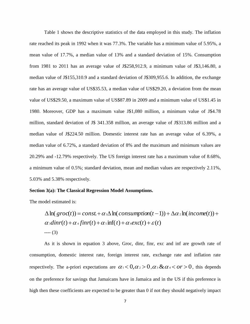
Table 1 shows the descriptive statistics of the data employed in this study. The inflation

rate reached its peak in 1992 when it was 77.3%. The variable has a minimum value of 5.95%, a

mean value of 17.7%, a median value of 13% and a standard deviation of 15%. Consumption

from 1981 to 2011 has an average value of J$258,912.9, a minimum value of J$3,146.80, a

median value of J$155,310.9 and a standard deviation of J$309,955.6. In addition, the exchange

rate has an average value of US$35.53, a median value of US$29.20, a deviation from the mean

value of US$29.50, a maximum value of US$87.89 in 2009 and a minimum value of US$1.45 in

1980. Moreover, GDP has a maximum value J$1,080 million, a minimum value of J$4.78

million, standard deviation of J$ 341.358 million, an average value of J$313.86 million and a

median value of J$224.50 million. Domestic interest rate has an average value of 6.39%, a

median value of 6.72%, a standard deviation of 8% and the maximum and minimum values are

20.29% and -12.79% respectively. The US foreign interest rate has a maximum value of 8.68%,

a minimum value of 0.5%; standard deviation, mean and median values are respectively 2.11%,

5.03% and 5.38% respectively.

Section 3(a): The Classical Regression Model Assumptions.

The model estimated is:

)()()inf()()(

))(ln())1(ln(.))(ln(

6543

21

ttexcttfinrtdinr

tincometnconsumptioconsttgroc

---- (3)

As it is shown in equation 3 above, Groc, dinr, finr, exc and inf are growth rate of

consumption, domestic interest rate, foreign interest rate, exchange rate and inflation rate

respectively. The a-priori expectations are 0,0 21 , 0& 43 or , this depends

on the preference for savings that Jamaicans have in Jamaica and in the US if this preference is

high then these coefficients are expected to be greater than 0 if not they should negatively impact

8

the consumption growth rate function and 0& 65 . There is no correlation between the

variables (both dependent and independent) and the error term E (U/x1, x2…….x1i) = 0 , thus the

strict exogeneity assumption holds. The residuals are extracted and regressed against the

variables, all the parameters of this regression are insignificant and the coefficient of

determination is 0.0078. Also, there is no lagged dependent variable in the model. Instrumental

variables are used in the model because they correlate with the independent variables but do not

have any relationship with the error term; the GMM orthogonality test shows a p-value of 0.521.

The Sargan’s test statistic p-value of 0.73 supports the validity of the instruments employed.

There are no exact relationships between the independent variables, if this assumption is

violated, it will become impossible to estimate the coefficients of the model. In order to test for

multicollinearity, a correlation matrix as shown in table 5 in the appendix is done. The matrix

depicts that none of the correlation coefficients are high. In addition to the correlation matrix

shown, the tolerance and the variance inflation factor (VIF) tests depict values that are less than

0.2 or 0.10 and 5 or 10 respectively. The consistency property is preserved because of the use of

large data set spanning from 1980 to 2011.

The variance is constant in any time period given any of the independent variables Var

(U/x1, x2…….x1i) = 0.; this is shown by the variance of the GMM regression which has a value

of 0.2235, thus the model does have a constant variance. To further support the fact that the

variance is constant, the White-Heteroskedasticity Test is done and the χ2 value from the table is

18.307, this exceeds the test statistic of 3.57; this implies that there is a failure to reject the null

hypothesis of constant variance. The Durbin Watson statistic takes on a value of 2 so there is no

evidence of serial autocorrelation. The errors are independent of the regressors and are

independently and identically distributed (i.i.d.). The Histogram-Normality test shows that

9

errors are normally distributed, the Jarque-Bera statistic has a value of 1.2178 which is lesser

than 5.99 ( Chi-Square with two degrees of freedom at the 5% level).

Section 3 (b): Methodology of the Study.

This study makes use of a Hansen’s 1982 GMM modeling framework, however for the

purpose of this research, a linear form of Kiley’s Euler’s equation is estimated. This framework

has been employed consistently by macroeconomists such as Hall (1978), Ferson and

Constantinides (1991), Kiley (2007), Eichenbaum, Hansen and Singleton (1988) and others to

estimate consumption and asset-pricing models and other macro-models that have micro

foundations because of its built-in assumptions and the efficiency with which parameters are

estimated. The Augmented Dickey-Fuller and the Phillips-Perron tests3 are used to determine if

the variables are not stationary and to ascertain how many times they have to be differenced to

remove unit root. After this is done, a GMM model is estimated.

This estimation technique is employed because of; one, its ability to handle estimation of

Euler equations. Consumption may not be exogenous in the model so there is a need to use

instrumental variables that are correlated with it to control for endogeneity. Two, the asymptotic

properties of the model ensure that standard errors are robust and the coefficients estimated are

consistent, unbiased and efficient. That is, the estimators possess the BUE (Best Unbiased

Estimators) properties.

Section 3(c): The Assumptions of the GMM model

If exy where x is a k x 1 vector of explanatory variables and some are

endogenous. Hansen (1982) assumes that there exist sets of variables z (instrumental variables)

of size l ≥ k that satisfy the 2SLS assumptions which are called the GMM assumptions. l is the

3 The details of the tests are shown in the appendix

10

number of instruments. The instruments are considered orthogonal to the errors, 0)( ezE ,

this assumption holds in the estimated model shown in table 4.

In addition, the rank of the expected value of the transposed matrix of the instrumental

variables and k x1 vector of the independent variables must be exactly equal to the number of

parameters in the model, kxzErank ))(( where l= k, the IV estimator is the solution of the

sample counterpart of the moment equation 0))(( IVbezE . However, if l > k this defines a

set of l equations to determine k parameters. Thus, the system has no solution (over-

identification). This assumption holds because the instruments used are more than the variables

and as such the system is over-identified. The simultaneous weighting matrix, W which has a

l * l matrix of weights is used in the model, it is non-random, symmetric and a positive semi-

definite matrix. Pre-whitening, heteroskedasticity and autocorrelation consistent standard errors

(HAC) are used in the GMM regression output shown in table 3. The asymptotic properties of

the GMM are presented in the appendix.

11

Section 4 (a): Presentation of Results

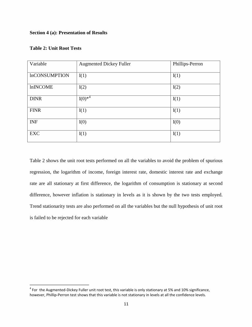
Table 2: Unit Root Tests

Variable Augmented Dickey Fuller Phillips-Perron

lnCONSUMPTION I(1) I(1)

lnINCOME I(2) I(2)

DINR I(0)*4 I(1)

FINR I(1) I(1)

INF I(0) I(0)

EXC I(1) I(1)

Table 2 shows the unit root tests performed on all the variables to avoid the problem of spurious

regression, the logarithm of income, foreign interest rate, domestic interest rate and exchange

rate are all stationary at first difference, the logarithm of consumption is stationary at second

difference, however inflation is stationary in levels as it is shown by the two tests employed.

Trend stationarity tests are also performed on all the variables but the null hypothesis of unit root

is failed to be rejected for each variable

4 For the Augmented-Dickey Fuller unit root test, this variable is only stationary at 5% and 10% significance,

however, Phillip-Perron test shows that this variable is not stationary in levels at all the confidence levels.

12

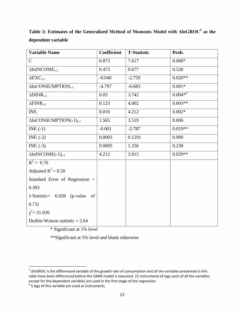
Table 3: Estimates of the Generalized Method of Moments Model with ΔlnGROC5 as the

dependent variable

Variable Name Coefficient T-Statistic Prob.

C 0.873 7.617 0.000*

ΔlnINCOMEt-1 0.473 0.677 0.520

ΔEXCt-1 -0.040 -2.759 0.020**

ΔlnCONSUMPTIONt-1 -4.797 -6.683 0.001*

ΔDINRt-1 0.03 3.742 0.004*6

ΔFINRt-1 0.123 4.002 0.003**

INFt 0.016 4.212 0.002*

ΔlnCONSUMPTION(-1)t-1 1.565 3.519 0.006

INFt (-1) -0.001 -2.787 0.019**

INFt (-2) 0.0003 0.1291 0.900

INFt (-3) 0.0005 1.256 0.238

ΔlnINCOME(-1)t-1 4.212 3.915 0.029**

R2 = 0.76

Adjusted R2

= 0.50

Standard Error of Regression =

0.393

J-Statistic= 6.928 (p-value of

0.73)

χ2= 21.026

Durbin-Watson statistic = 2.64

* Significant at 1% level

**Significant at 5% level and blank otherwise

5 ΔlnGROC is the differenced variable of the growth rate of consumption and all the variables presented in this

table have been differenced before the GMM model is executed. 22 instruments (4 lags each of all the variables except for the dependent variable) are used in the first stage of the regression. 6 5 lags of this variable are used as instruments.

13

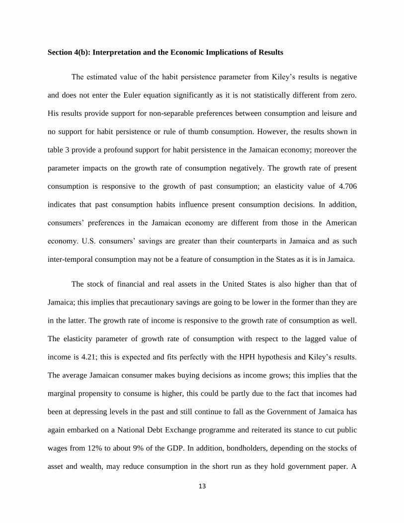
Section 4(b): Interpretation and the Economic Implications of Results

The estimated value of the habit persistence parameter from Kiley’s results is negative

and does not enter the Euler equation significantly as it is not statistically different from zero.

His results provide support for non-separable preferences between consumption and leisure and

no support for habit persistence or rule of thumb consumption. However, the results shown in

table 3 provide a profound support for habit persistence in the Jamaican economy; moreover the

parameter impacts on the growth rate of consumption negatively. The growth rate of present

consumption is responsive to the growth of past consumption; an elasticity value of 4.706

indicates that past consumption habits influence present consumption decisions. In addition,

consumers’ preferences in the Jamaican economy are different from those in the American

economy. U.S. consumers’ savings are greater than their counterparts in Jamaica and as such

inter-temporal consumption may not be a feature of consumption in the States as it is in Jamaica.

The stock of financial and real assets in the United States is also higher than that of

Jamaica; this implies that precautionary savings are going to be lower in the former than they are

in the latter. The growth rate of income is responsive to the growth rate of consumption as well.

The elasticity parameter of growth rate of consumption with respect to the lagged value of

income is 4.21; this is expected and fits perfectly with the HPH hypothesis and Kiley’s results.

The average Jamaican consumer makes buying decisions as income grows; this implies that the

marginal propensity to consume is higher, this could be partly due to the fact that incomes had

been at depressing levels in the past and still continue to fall as the Government of Jamaica has

again embarked on a National Debt Exchange programme and reiterated its stance to cut public

wages from 12% to about 9% of the GDP. In addition, bondholders, depending on the stocks of

asset and wealth, may reduce consumption in the short run as they hold government paper. A

14

unit change in the growth rate of the exchange rate reduces the growth rate of consumption by

4%. This shows that Jamaicans have a high preference for foreign goods especially automobiles,

industrial tools and other luxuries and given the fact that Jamaica is highly dependent on capital

goods from abroad and does little export of value-added goods, an appreciation of the US dollar

is a good thing for those who have substantial amount of dollar to purchase goods in the States,

however this hurts the local economy through high prices of production inputs.

Domestic interest rate also favours the growth rate of consumption in the short run as it is

expected. Commercial banks, have since the early 2000s, been lending at fairly low rates to

accommodate producers and other investors who are in dire need of funds. The greater the access

to funds by the business class, the higher the velocity of circulation in the economy as production

activities gain momentum consequently improving consumers’ outlook. Foreign interest rate also

enters the Euler equation positively as expected. Ben Bernanke, the Federal Reserve Chairman,

in the States has promised to keep interest rate low until unemployment rate falls to a little bit

over 6%; this is expected to boost consumption activities in the States directly.

Also, Jamaican consumers who live in the States benefit directly from the low interest

rate regime because they pay less for mortgage, hire purchases and loans and all these point to an

increase in consumption both in the short run and long run. Jamaicans residing in the local

economy also benefit both directly and indirectly. Indirectly, remittance inflows increase and

consumers who earn less or whose consumption is autonomous still buy more. Directly, cost of

doing business in the States is lower. Upstream and downstream firms can easily source for

essential inputs into the production process and consumption is thereby enhanced in the long run.

15

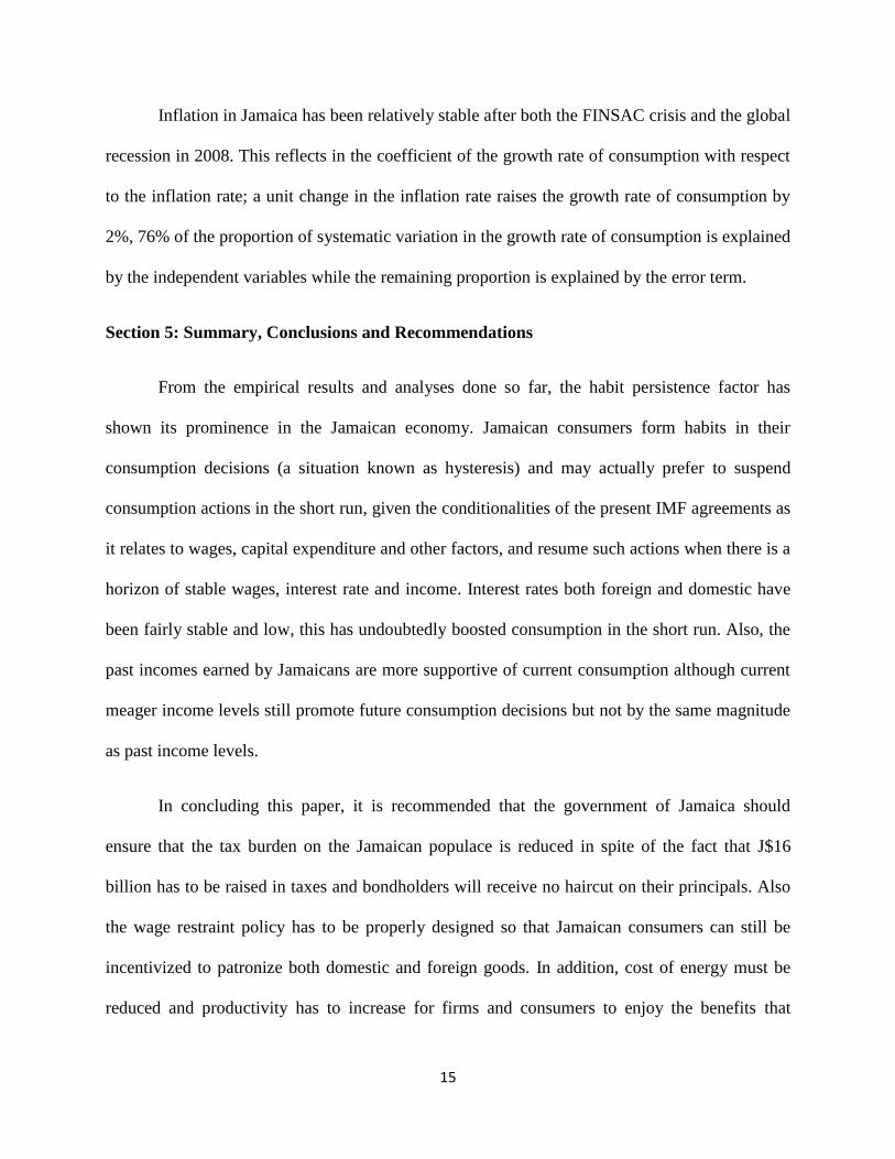
Inflation in Jamaica has been relatively stable after both the FINSAC crisis and the global

recession in 2008. This reflects in the coefficient of the growth rate of consumption with respect

to the inflation rate; a unit change in the inflation rate raises the growth rate of consumption by

2%, 76% of the proportion of systematic variation in the growth rate of consumption is explained

by the independent variables while the remaining proportion is explained by the error term.

Section 5: Summary, Conclusions and Recommendations

From the empirical results and analyses done so far, the habit persistence factor has

shown its prominence in the Jamaican economy. Jamaican consumers form habits in their

consumption decisions (a situation known as hysteresis) and may actually prefer to suspend

consumption actions in the short run, given the conditionalities of the present IMF agreements as

it relates to wages, capital expenditure and other factors, and resume such actions when there is a

horizon of stable wages, interest rate and income. Interest rates both foreign and domestic have

been fairly stable and low, this has undoubtedly boosted consumption in the short run. Also, the

past incomes earned by Jamaicans are more supportive of current consumption although current

meager income levels still promote future consumption decisions but not by the same magnitude

as past income levels.

In concluding this paper, it is recommended that the government of Jamaica should

ensure that the tax burden on the Jamaican populace is reduced in spite of the fact that J$16

billion has to be raised in taxes and bondholders will receive no haircut on their principals. Also

the wage restraint policy has to be properly designed so that Jamaican consumers can still be

incentivized to patronize both domestic and foreign goods. In addition, cost of energy must be

reduced and productivity has to increase for firms and consumers to enjoy the benefits that

16

production processes have to offer. For future studies, it will be quite instructive to investigate

how the tax rate will affect consumption dynamics both in the short and long run especially as it

relates to evidence of hysteresis in consumption decisions.

17

References

Brown, T.M. (1952). “Habit Persistence and Lags in Consumer Behaviour”, Econometrica,

Vol.20, No.3.

Dias, M. (2008). Microeconometrics Lecture Notes Spring Notes. UCL- Department of

Economics. Retrieved from http://www.homepages.ucl.ac.uk/

Dickey, D.A. & Fuller, W.A. (1979). “Distribution of Estimators for Autoregressive Time Series

with a Unit Root”, Journal of American Statistical Association, 74, p. 427-431

Eichenbaum, M.S., Hansen, L.P., & Singleton, K.J. (1988) “A Time-Series Analysis of

Representative Agent Models of Consumption and Leisure Choices under Certainty”.

Quarterly Journal of Economics 103, 51-78.

Ferson, W.E., & Constantinides, G.M. (1991). Habit persistence and Durability in Aggregate

Consumption. National Bureau of Economic Research Working Paper No. 3631

Fuhrer, J.C. (2002) “Habit Formation in Consumption and its Implications for Monetary Policy

Models”. American Economic Review.

18

Hansen, L.P. (1982). “Large Sample Properties of Generalized Method of Moments Estimators,

Econometrica, Vol.50, No.4, 1029-1054.

Kiley, M.T. (2007) Habit Persistence, Non-Separability between Consumption and Leisure, or

Rule-of-Thumb Consumers; Which accounts for the Predictability of Consumption

Growth? Finance and Economics Discussions Series, Divisions of Research & Statistics

and Monetary Affairs. Federal Reserve Board, Washington, D.,C.

Pijon-Mas, D., et al (2002). Precautionary Savings and Wealth Distribution under Habit

Formation. Retrieved from http://www.econ.umn.edu/~vroj/papers/jmehabits2.pdf.

Singh, B. & Ullah, A. (1976) “The Permanent Income versus Habit Persistence Hypothesis”.

Review of Economics and Statistics, Vol. 58, No.1. pp.96-103.

Soderlind,P.(2002). Lecture Notes for Econometrics. Gallen: University of St. Gallen

Rossi, M. (nd). Household’s Consumption Under Habit Formation Hypothesis. Evidence from

Italian Households using the Survey of Household and Wealth. Retrieved from

http://www. sx.ac.uk/economics/discussion-papers/papers-text/dp595.pdf

Winder, C.A., & Palm, F.C. (1990). Stochastic Implications of the Life-Cycle Consumption

Model under Rational Habit Formation. Working paper. University of Limburg

19

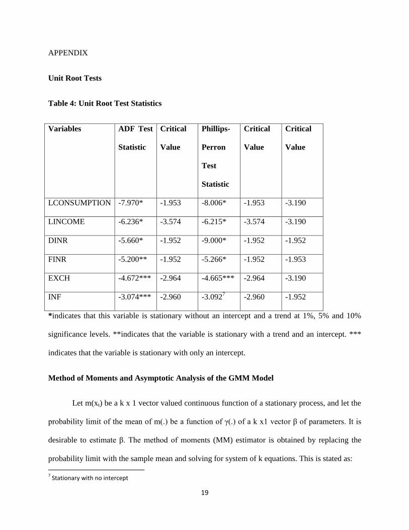
APPENDIX

Unit Root Tests

Table 4: Unit Root Test Statistics

Variables ADF Test

Statistic

Critical

Value

Phillips-

Perron

Test

Statistic

Critical

Value

Critical

Value

LCONSUMPTION -7.970* -1.953 -8.006* -1.953 -3.190

LINCOME -6.236* -3.574 -6.215* -3.574 -3.190

DINR -5.660* -1.952 -9.000* -1.952 -1.952

FINR -5.200** -1.952 -5.266* -1.952 -1.953

EXCH -4.672*** -2.964 -4.665*** -2.964 -3.190

INF -3.074*** -2.960 -3.0927 -2.960 -1.952

*indicates that this variable is stationary without an intercept and a trend at 1%, 5% and 10%

significance levels. **indicates that the variable is stationary with a trend and an intercept. ***

indicates that the variable is stationary with only an intercept.

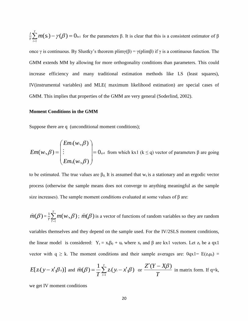
Method of Moments and Asymptotic Analysis of the GMM Model

Let m(xt) be a k x 1 vector valued continuous function of a stationary process, and let the

probability limit of the mean of m(.) be a function of γ(.) of a k x1 vector β of parameters. It is

desirable to estimate β. The method of moments (MM) estimator is obtained by replacing the

probability limit with the sample mean and solving for system of k equations. This is stated as:

7 Stationary with no intercept

20

1

1

0)()( kx

T

t

tsm

for the parameters β. It is clear that this is a consistent estimator of β

once γ is continuous. By Slustky’s theorem plimγ(β) = γ(plimβ) if γ is a continuous function. The

GMM extends MM by allowing for more orthogonality conditions than parameters. This could

increase efficiency and many traditional estimation methods like LS (least squares),

IV(instrumental variables) and MLE( maximum likelihood estimation) are special cases of

GMM. This implies that properties of the GMM are very general (Soderlind, 2002).

Moment Conditions in the GMM

Suppose there are q (unconditional moment conditions);

1

1

0

),(

),(

),( qx

tq

t

t

wEm

wEm

wEm

from which kx1 (k ≤ q) vector of parameters β are going

to be estimated. The true values are β0. It is assumed that wt is a stationary and an ergodic vector

process (otherwise the sample means does not converge to anything meaningful as the sample

size increases). The sample moment conditions evaluated at some values of β are:

)(m

=

T

T

twm1

),( ; )(m

is a vector of functions of random variables so they are random

variables themselves and they depend on the sample used. For the IV/2SLS moment conditions,

the linear model is considered: Yt = xtβ0 + ut where xt and β are kx1 vectors. Let zt be a qx1

vector with q ≥ k. The moment conditions and their sample averages are: 0qx1= E(ztμt) =

)]([ 0tt xyzE and

T

t

ttt xyzT

m1

)(1

)(

or T

XYZ )( in matrix form. If q=k,

we get IV moment conditions

21

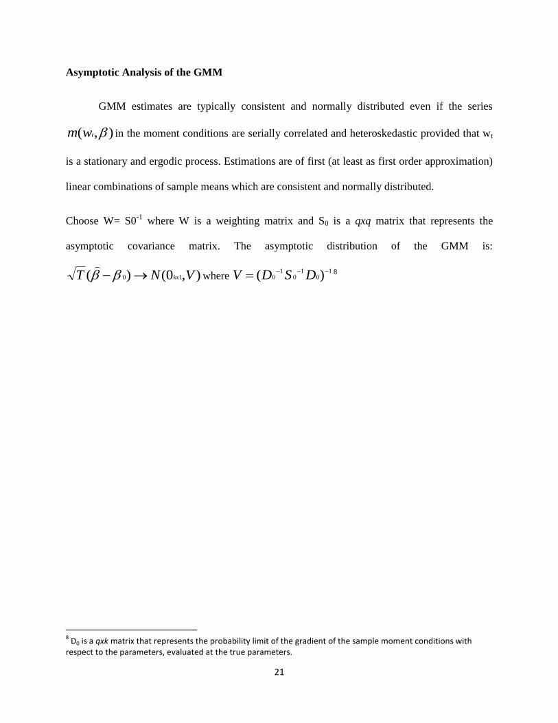
Asymptotic Analysis of the GMM

GMM estimates are typically consistent and normally distributed even if the series

),( twm in the moment conditions are serially correlated and heteroskedastic provided that wt

is a stationary and ergodic process. Estimations are of first (at least as first order approximation)

linear combinations of sample means which are consistent and normally distributed.

Choose W= S0-1

where W is a weighting matrix and S0 is a qxq matrix that represents the

asymptotic covariance matrix. The asymptotic distribution of the GMM is:

),0()( 10 VNT kx

where 1

01

01

0 )( DSDV 8

8 D0 is a qxk matrix that represents the probability limit of the gradient of the sample moment conditions with

respect to the parameters, evaluated at the true parameters.

22

Figure 1: Line Graph of the variables

Figure 1 shows the depiction of the trend of the variables. The variables do not have any

relationship with the time trend.

-20

0

20

40

60

80

1980 1985 1990 1995 2000 2005 2010

DLOGGROCTIMEDLOGCONSUMPTIONDLOGINCOME

DEXCINFDDINRDFINR

23

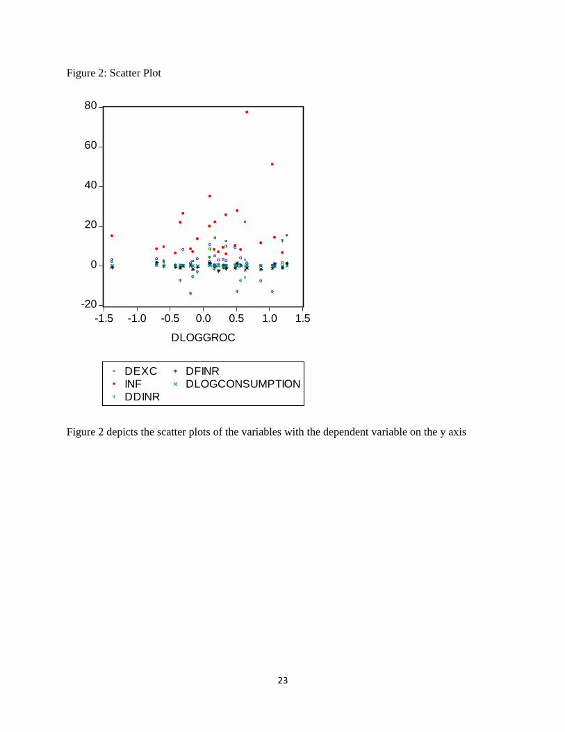
Figure 2: Scatter Plot

Figure 2 depicts the scatter plots of the variables with the dependent variable on the y axis

-20

0

20

40

60

80

-1.5 -1.0 -0.5 0.0 0.5 1.0 1.5

DLOGGROC

DEXCINFDDINR

DFINRDLOGCONSUMPTION

24

Table 5: Correlation Matrix

Variable DLOGGROC DLOGCONS DLOGINCOME DFINR DDINR INF

DLOGGROC 1.0000 -0.3256 0.5027 -0.0750 -0.0441 0.2031

DLOGCONS -0.3256 1.0000 0.008829 0.1775 0.2692 0.5751

DLOGINCOME 0.5027 0.0883 1.0000 -0.2205 -0.4043 0.4845

DFINR -0.0750 0.1775 -0.2205 1.0000 0.0095 -0.0510

DDINR -0.0441 0.2692 -0.4043 0.0095 1.0000 -0.1186

INF 0.2031 0.5751 0.4845 -0.0598 0.1186 1.0000

Table 5 shows the correlation matrix of the dependent and independent variables. The correlation

coefficients between the independent variables are low, however those between the dependent

and independent variables are moderate; this implies that the model does not have

multicollinearity problem.