arX

iv:a

stro

-ph/

0009

466v

1 2

8 Se

p 20

00

The GZK Feature in our Neighborhood of the

Universe

Michael Blanton a, Pasquale Blasi a Angela V. Olinto b,1,

aFermi National Accelerator Laboratory, Batavia, IL 60510-0500bDepartment of Astronomy & Astrophysics, & Enrico Fermi Institute,

The University of Chicago, Chicago, IL 60637

Abstract

We calculate numerically the spectrum of ultra-high energy cosmic rays on Earthassuming that their sources are distributed in space like the observed galaxies. Weuse the CfA2 and the PSCz galaxy redshift surveys to model the local galaxy distri-bution, properly taking into account the galaxy selection functions for each survey.When the survey selection effects are included, we find that the local overdensity isonly a factor of two, an order of magnitude less than used in some earlier studies. Anoverdensity of two is not enough to bridge the gap between the predicted numberof events above 1020 eV and the measured flux at these highest energies. This con-clusion is particularly strong for soft injection spectra (∝ E−3) where the observednumber of events is 6 σ higher than the expected one. However, if the injectionspectrum is hard (∝ E−2), the small local overdensity helps bring the present datawithin 2σ of the low number of events predicted above 1020 eV. In this case, theGreisen-Zatzepin-Kuzmin cutoff is not a cutoff but rather a feature in the cosmicray spectrum.

Key words: Cosmic Rays, Ultra-high energy, Propagation, AccelerationPACS: 96.40.- zv, 95.85.Ry, 13.85.Tp

1 Introduction

The unexpected detection of cosmic rays with energies above 1020 eV hastriggered considerable interest in the possible origin and nature of these par-ticles [1]. These highest energy events are surprising for the following reasons.If these particles are protons, they likely originate in extragalactic sources,

1 Corresponding author. E-mail: olinto@oddjob.uchicago.edu

Preprint submitted to Elsevier Preprint 1 February 2008

since at these high energies the Galactic magnetic field cannot confine pro-tons in the Galaxy. However, extragalactic protons with energies above a fewtimes 1019 eV can produce pions through interactions with the cosmic mi-crowave background (CMB) and consequently lose significant amounts of en-ergy as they traverse intergalactic distances [2]. Therefore, in addition to theextraordinary energy requirements for astrophysical sources to accelerate pro-tons to >∼1020 eV, the photopion threshold reaction suppresses the observableflux above ∼ 1020 eV. These conditions were expected to cause a naturalhigh-energy limit to the cosmic ray spectrum known as the Greisen-Zatsepin-Kuzmin (GZK) cutoff [2].

As clearly shown by the most recent compilation of the AGASA collaborationdata [3], the spectrum of cosmic rays does not end at the expected GZK cutoff.The significant flux observed above 1020 eV together with a nearly isotropicdistribution of event arrival directions has challenged astrophysically basedscenarios (see e.g., [4] and references therein) and has inspired a number ofalternatives (see, e.g., [5] and references therein). However, the GZK cutoffis not an absolute end to the cosmic ray spectrum but it generates a feature

around 5 × 1019 eV. The spectrum recovers at energies above this feature [6]and the local distribution of sources can significantly affect the agreementbetween predicted and observed spectra. In particular, a local overdensity ofsources can decrease the gap between observed and detected events above theGZK cutoff [7–9]. This effect can easily be understood: photopion energy losseslimit the maximum distance at which sources can contribute at the highestenergies to a few tens of Mpc, while cosmic rays below the pion productionthreshold come from much larger volumes. A local overdensity will increasethe observed flux at the highest energies relative to the lower energy flux. Herewe show that the observed local overdensity is not high enough to explain thedata unless, perhaps, the sources have a hard injection spectrum.

In the following, we simulate the propagation of ultra-high energy cosmic rays(UHECRs) from extragalactic sources to Earth. Our numerical propagationcode includes pair production, photopion production, and adiabatic losses dueto the universe’s expansion. For a uniform distribution of sources, our numer-ical results agree well with previous results and analytical calculations. Westudy the effect of a local overdensity by assuming that the number density ofsources is proportional to the number density of galaxies. To keep this studyindependent of specific hypothetical sources, we use different injection spec-tra and consider a possible source evolution with redshift. However, since weassume that UHECRs are protons, our results are mostly relevant for extra-galactic astrophysical acceleration scenarios.

Rather than adopting analytic models of the galaxy distribution, as do [9,10],we extract the distribution of galaxies from observations of large scale struc-ture using the CfA2 and the PSCz galaxy catalogs. We assume that the den-

2

sity field derived from these studies has the same shape as the density fieldof UHECR sources, although a priori UHECR sources may cluster differentlyfrom luminous matter. We show that the local density is only about a factorof two above the mean, in contrast with much higher estimates previouslypublished [8]. This large discrepancy was caused by neglecting the necessarygalaxy selection functions which account for the fact that nearby galaxies arefar easier to detect than far away galaxies. Once we include the selection func-tions, we find that the real overdensity is not high enough to bridge the gapbetween predicted and observed spectra for soft sources (J(E) ∝ E−γ, withγ = 3). However, sources with a hard injection spectrum (γ<∼2.1) can fit thepresent data within 2σ, at energies above a few 1019 eV. Sources of UHECRsdistributed as ordinary galaxies are marginally consistent with present dataand, for hard injection spectra, the GZK cutoff is not really a cutoff but afeature in the high-energy cosmic ray spectrum.

The plan of this paper is as follows. In §2, we discuss the proper way to model adistribution of sources associated with galaxies. We derive the galaxy densityfield in our neighborhood of the universe using the CfA2 and PSCz galaxyredshift surveys with their respective selection function. In §3, we describe ourUHECR propagation code. In §4, we display the results for different injectionspectra and a realistic spatial distribution of sources. We also contrast ourresults with previous work and analytical estimates. We conclude in §5.

2 The Galaxy Density Field

Although galaxies are not homogeneously distributed in the local universe,the GZK cutoff is usually calculated assuming a homogeneous distributionof sources throughout space. If the sources are distributed like the luminousmatter around us, the effects of an inhomogeneous galaxy distribution needsto be taken into account when predicting the spectrum of UHECRs. In orderto include the effects of the spatial inhomogeneity in the UHECR spectrum,we must consider the estimated galaxy density field in our neighborhood ofthe universe. The density field is usually measured by selecting galaxies froman imaging survey of the sky and taking their redshifts. Almost invariably, thegalaxies are selected to be brighter than some limiting flux in some band, flim,expressed as an “apparent magnitude,” mlim = −2.5 log10(flim/f0), where f0 isan arbitrary zero-point. For all (or for some random subsample) of the galaxiesbrighter than this, one takes their spectra and determines their redshifts z.According to the Hubble law, the redshifts are related to their distances d =H0cz, where c is the speed of light and H0 ≡ 100h Mpc/ km/s, with h ≈ 0.5–0.8 (e.g., [11]).

However, a flux-limited survey is not a volume-limited survey. In a flux-limited

3

survey, the raw distribution of redshifts cannot be used without regard tothe way galaxies were selected. Here we describe the proper way to derivedensity fields from galaxy redshift surveys. We limit ourselves to measuringthe density in redshift space and do not include the small effects of deviationsfrom the Hubble law due to galaxy peculiar velocities. We base our approachon methods dating back to [12] (see, e.g., [13] for a recent review).

We will use two surveys for our analysis. To compare directly with [8], weconsider the Center for Astrophysics Redshift Survey (CfA2; [14]). Althoughthis survey comprises about 10,000 galaxy redshifts (selected to be brighterthan m = 15.5, a B-band magnitude), it covers only about 17% of the wholesky. In order to better evaluate the effects of the density field of galaxies onthe cosmic ray spectrum, we should use surveys which probe the density fieldover nearly the whole sky. The best sample of galaxies to use for this purposeis the IRAS PSCz Survey [15], which consists of about 15,000 galaxies withinfrared fluxes > 0.6 Jy and covers about 84% of the sky.

A consequence of the flux limits in any survey is that at different redshifts, adifferent set of galaxy luminosities L is observed, determined by the faintestluminosity observable at that redshift Lmin(z). For an Euclidean metric, thisluminosity is related to the flux limit by:

Lmin(z) = 4π(H0cz)2flim. (1)

At cosmological distances (generally only appropriate when z > 0.1) morecomplicated relations apply, which in general depend on the cosmologicalmodel [16] (see [17] for a useful compilation of results). If the distributionof galaxy luminosities is described by the galaxy luminosity function Φ(L),then the fraction of all galaxies that are observable at any redshift is given by:

φ(z) =

∫

∞

Lmin(z) dL Φ(L)∫

∞

0 dL Φ(L). (2)

The quantity φ(z) is usually referred to in the literature as the “selection func-tion” [18]. The most common methods used to determine the galaxy luminosityfunction from the survey itself are those of [19] and [20]. These methods as-sume that the luminosity function is universal (i.e., independent of redshift)and use nearby galaxies to determine the shape of the faint end and far awaygalaxies for the shape of the bright end.

Consider, for example, Figure 1, which shows in the top panel the distributionof galaxies and redshifts in CfA2. Here we express galaxy luminosity in termsof the “absolute magnitude,” M = −2.5 log10 L+ const; thus, in the figure, thefaintest galaxies are at the top. The thick solid line shows the flux limit of the

4

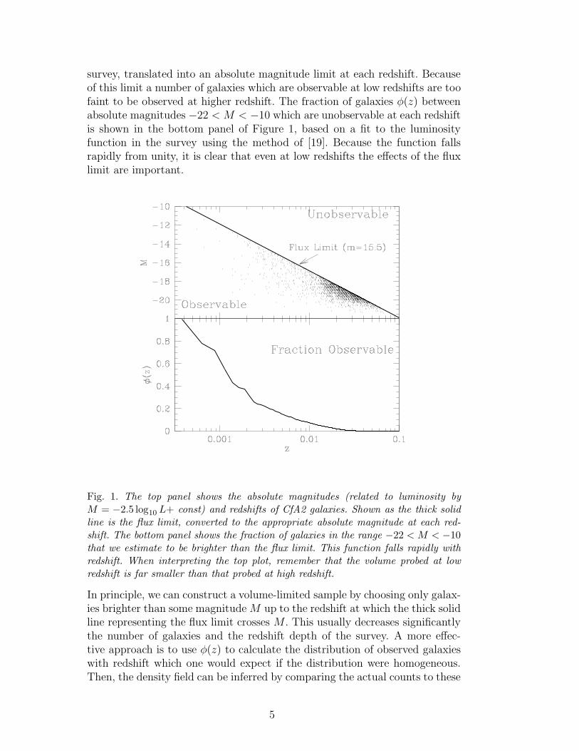
survey, translated into an absolute magnitude limit at each redshift. Becauseof this limit a number of galaxies which are observable at low redshifts are toofaint to be observed at higher redshift. The fraction of galaxies φ(z) betweenabsolute magnitudes −22 < M < −10 which are unobservable at each redshiftis shown in the bottom panel of Figure 1, based on a fit to the luminosityfunction in the survey using the method of [19]. Because the function fallsrapidly from unity, it is clear that even at low redshifts the effects of the fluxlimit are important.

Fig. 1. The top panel shows the absolute magnitudes (related to luminosity byM = −2.5 log10 L+ const) and redshifts of CfA2 galaxies. Shown as the thick solidline is the flux limit, converted to the appropriate absolute magnitude at each red-shift. The bottom panel shows the fraction of galaxies in the range −22 < M < −10that we estimate to be brighter than the flux limit. This function falls rapidly withredshift. When interpreting the top plot, remember that the volume probed at lowredshift is far smaller than that probed at high redshift.

In principle, we can construct a volume-limited sample by choosing only galax-ies brighter than some magnitude M up to the redshift at which the thick solidline representing the flux limit crosses M . This usually decreases significantlythe number of galaxies and the redshift depth of the survey. A more effec-tive approach is to use φ(z) to calculate the distribution of observed galaxieswith redshift which one would expect if the distribution were homogeneous.Then, the density field can be inferred by comparing the actual counts to these

5

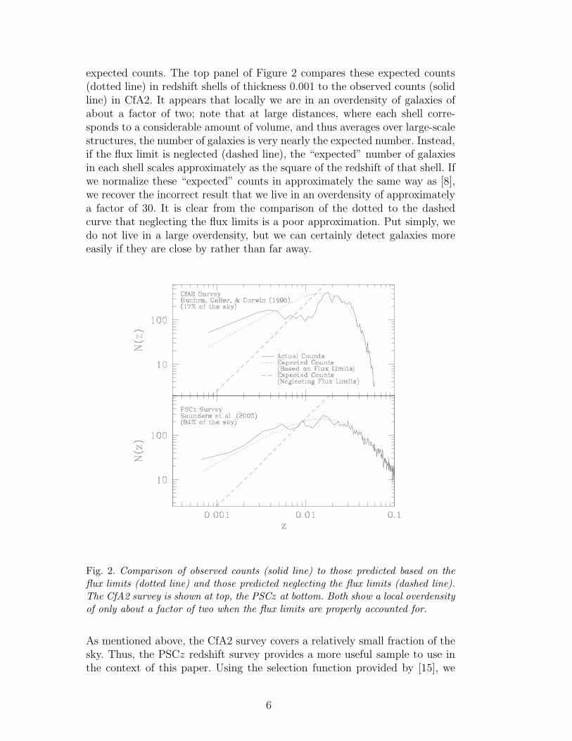
expected counts. The top panel of Figure 2 compares these expected counts(dotted line) in redshift shells of thickness 0.001 to the observed counts (solidline) in CfA2. It appears that locally we are in an overdensity of galaxies ofabout a factor of two; note that at large distances, where each shell corre-sponds to a considerable amount of volume, and thus averages over large-scalestructures, the number of galaxies is very nearly the expected number. Instead,if the flux limit is neglected (dashed line), the “expected” number of galaxiesin each shell scales approximately as the square of the redshift of that shell. Ifwe normalize these “expected” counts in approximately the same way as [8],we recover the incorrect result that we live in an overdensity of approximatelya factor of 30. It is clear from the comparison of the dotted to the dashedcurve that neglecting the flux limits is a poor approximation. Put simply, wedo not live in a large overdensity, but we can certainly detect galaxies moreeasily if they are close by rather than far away.

Fig. 2. Comparison of observed counts (solid line) to those predicted based on theflux limits (dotted line) and those predicted neglecting the flux limits (dashed line).The CfA2 survey is shown at top, the PSCz at bottom. Both show a local overdensityof only about a factor of two when the flux limits are properly accounted for.

As mentioned above, the CfA2 survey covers a relatively small fraction of thesky. Thus, the PSCz redshift survey provides a more useful sample to use inthe context of this paper. Using the selection function provided by [15], we

6

again show the expected versus the observed counts for the PSCz survey inthe bottom panel of Figure 2. This survey also shows we are living in a slightoverdensity, and furthermore reveals the general homogeneity of the nearbyuniverse. (The actual counts and their dependence on redshift are differentfrom CfA2, because the galaxies are selected in different ways).

3 The Propagation Code for UHECRs

Armed with a more realistic model of the local universe, we can calculatethe spectrum of UHECRs that would be observed on Earth for extragalacticsources with different injection spectra. Our numerical propagation code in-cludes pair production and photopion production as energy losses, as well asadiabatic losses due to the expansion of the universe. We compare our numeri-cal results with analytical calculations which we carry out as in [6]. In order toisolate the effect of density inhomogeneities we neglect the effect of magneticfields in this paper.

We compare the results of the simulations with the observed spectrum byrequiring that the total number of simulated events with energy above a nor-malizing energy, Enorm, be the same as what is observed. In general we chooseEnorm ≃ 1019 eV since at lower energies the flux of cosmic rays is likely tohave a galactic origin and at higher energies the observed number of eventsis very small. For a given source spectral index, we generate many realiza-tions of the spectrum on Earth. Each realization has the same total numberof observed particles above Enorm calculated as follows. The flux of UHE-CRs contributed from a shell of thickness ∆z at redshift z is proportionalto p(z) ∝ (1 + z)m−5/2f(z), where the redshift dependence of the density ofsources and the flux suppression due to distance are included explicitly [21]. Inthis formula, we allow for source luminosity evolution through the parameterm. The function f(z) describes possible deviations from a homogeneous spatialdistribution of sources. For a homogeneous distribution f(z) = 1, otherwisef(z) represents the local overdensity of sources at redshift z as, for example,those derived from the catalogs introduced in §2. We assign the redshift of oneevent by extracting a random number according to the distribution p(z) givenabove. The energy of the particle at the source is extracted from a distributionrepresenting the spectrum of the source assumed to have the form of a powerlaw E−γ . The particle is then propagated from the source to the detector.

The photopion energy losses are simulated following [22]. In each spatial stepof the simulation of size ∆s (∼ 200 kpc), the average number of photons thatcan induce the production of pions in the scattering with a proton of energy

7

E at time t is

〈Nph(E, ∆s)〉 =∆s

Kp(E)l(E). (3)

Here, l(E) = c [(1/E)(dE/dt)]−1 is taken from [6] and Kp(E) is an effectiveinelasticity at energy E, which can be approximated by

Kp(E) ≃ 0.2(

Eth + 2.5E

Eth + E

)

, (4)

with Eth = 3 × 1011 GeV [22]. Once the average number of pion producingphotons has been determined over the path ∆s, the actual number of photonswith which the proton interacts is extracted from a Poisson distribution withmean 〈Nph(E, ∆s)〉. For sufficiently small ∆s, the number of photons in eachstep is usually either zero or one. The energy of each photon is extracted from aPlanck distribution at temperature TCMB = 2.728 K (with a minimum energycorresponding to the threshold for pion production). Since the CMB photonsare isotropically distributed in space, we extract the interaction angle from aflat distribution in cos(θ). The final energy of the proton after each scatteringwith a CMB photon is calculated from the kinematics of the scattering. Sincethe inelasticity for pair production is very low, we treat it as a continuousenergy loss process.

We compare our numerical results with analytic results for the modificationfactor from single sources and from a distribution of sources as in [6]. Theagreement is excellent and the effect of the fluctuations at energies larger than∼ (3−4)×1019 eV is evident in Figures 5–8 as we discuss below. The averageof the simulated flux is slightly larger than the analytic one, as expected forthe stochastic process of photopion production (on small distances there is anappreciable chance that some protons do not interact at all).

4 Results

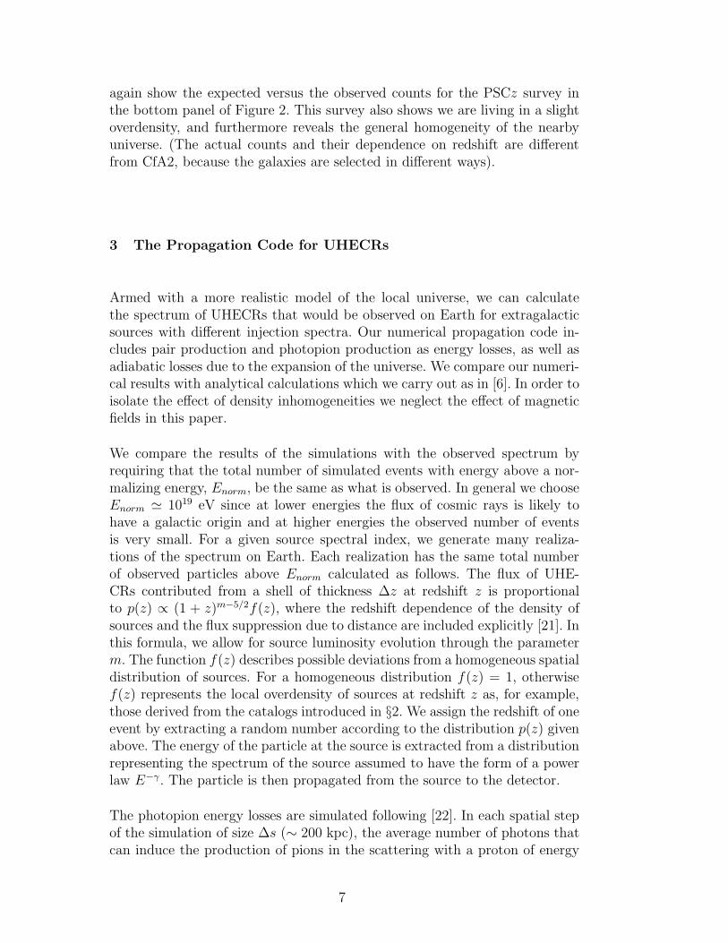
As we stressed above, a local overdensity increases the observed flux aboveGZK energies with respect to the flux at lower energies. To show this effectclearly, we estimated the change in the spectrum due to a simple top-hatmodel before considering more realistic models of the galaxy density field. InFigure 3, we display the results of our analytical calculation for three choicesof the overdensity, ρ/ρ = 1, 10, 30 (solid, dashed, and dash-dotted linesrespectively), all in a volume of radius ∼ 20 Mpc around the Earth and withsource spectral index γ = 3. From this figure, it is clear that the overdensity

8

increases the flux at the highest energies versus the flux at and below the GZKfeature, as mentioned above.

Fig. 3. The effect of a local overdensity within 20 Mpc on the fluxes of UHE-CRs, according to our analytical calculation for three choices of the overdensity,ρ/ρ = 1, 10, 30 (solid, dashed and dash-dotted lines respectively), all in a volumeof radius ∼ 20 Mpc around the Earth and with source spectral index γ = 3.

The galaxy surveys discussed in §2 provide a more realistic model of the localdensity field. Among the different surveys, the PSCz catalog covers a lot moresolid angle and reaches further (up to a redshift zmax = 0.1) when comparedto the CfA2 survey. Thus, we use the PSCz to study the effect of differentsource spectra below. But first we compare the results of the two catalogs fora fixed spectral index (γ = 3) with the homogeneous distribution in Figure4. This choice of γ allows a direct comparison of our results with those of[8]. In this figure, we normalize the spectrum by requiring that the number ofevents with energy above 1019 eV equal the AGASA number of 728 [23,24].The error bars in the simulation are obtained by generating 100 realizationsand calculating the mean and variance of the set. Figure 4 shows that the twocatalogs give very similar results.

In Figure 5, we compare the case of a homogeneous distribution and the PSCzcatalog versus the AGASA data also for γ = 3. The total number of eventswith E > 1020 eV is 1.2 ± 1.0 for the homogeneous case and 1.5 ± 1.0 for thePSCz catalog of galaxies. Both numbers are consistent with 1, while AGASAhas detected 8 events with E > 1020 eV. The data is more than 6 σ away fromthe observations. None of our realizations have the observed number of eventsfor this soft spectrum. In the figure, the solid and dashed lines represent theresult of the analytical calculations for the same value of the parameters andfor the homogeneous and PSCz cases respectively. The dash-dotted and dash-

9

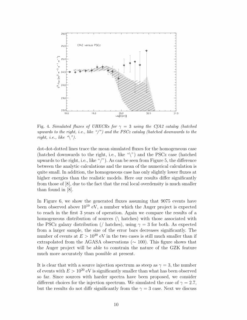
Fig. 4. Simulated fluxes of UHECRs for γ = 3 using the CfA2 catalog (hatchedupwards to the right, i.e., like “/”) and the PSCz catalog (hatched downwards to theright, i.e., like “\”).

dot-dot-dotted lines trace the mean simulated fluxes for the homogeneous case(hatched downwards to the right, i.e., like “\”) and the PSCz case (hatchedupwards to the right, i.e., like “/”). As can be seen from Figure 5, the differencebetween the analytic calculations and the mean of the numerical calculation isquite small. In addition, the homogeneous case has only slightly lower fluxes athigher energies than the realistic models. Here our results differ significantlyfrom those of [8], due to the fact that the real local overdensity is much smallerthan found in [8].

In Figure 6, we show the generated fluxes assuming that 9075 events havebeen observed above 1019 eV, a number which the Auger project is expectedto reach in the first 3 years of operation. Again we compare the results of ahomogeneous distribution of sources (\ hatches) with those associated withthe PSCz galaxy distribution (/ hatches), using γ = 3 for both. As expectedfrom a larger sample, the size of the error bars decreases significantly. Thenumber of events at E > 1020 eV in the two cases is still much smaller than ifextrapolated from the AGASA observations (∼ 100). This figure shows thatthe Auger project will be able to constrain the nature of the GZK featuremuch more accurately than possible at present.

It is clear that with a source injection spectrum as steep as γ = 3, the numberof events with E > 1020 eV is significantly smaller than what has been observedso far. Since sources with harder spectra have been proposed, we considerdifferent choices for the injection spectrum. We simulated the case of γ = 2.7,but the results do not diffr significantly from the γ = 3 case. Next we discuss

10

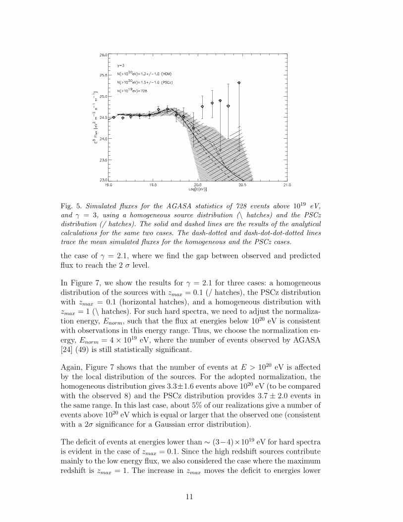
Fig. 5. Simulated fluxes for the AGASA statistics of 728 events above 1019 eV,and γ = 3, using a homogeneous source distribution (\ hatches) and the PSCzdistribution (/ hatches). The solid and dashed lines are the results of the analyticalcalculations for the same two cases. The dash-dotted and dash-dot-dot-dotted linestrace the mean simulated fluxes for the homogeneous and the PSCz cases.

the case of γ = 2.1, where we find the gap between observed and predictedflux to reach the 2 σ level.

In Figure 7, we show the results for γ = 2.1 for three cases: a homogeneousdistribution of the sources with zmax = 0.1 (/ hatches), the PSCz distributionwith zmax = 0.1 (horizontal hatches), and a homogeneous distribution withzmax = 1 (\ hatches). For such hard spectra, we need to adjust the normaliza-tion energy, Enorm, such that the flux at energies below 1020 eV is consistentwith observations in this energy range. Thus, we choose the normalization en-ergy, Enorm = 4 × 1019 eV, where the number of events observed by AGASA[24] (49) is still statistically significant.

Again, Figure 7 shows that the number of events at E > 1020 eV is affectedby the local distribution of the sources. For the adopted normalization, thehomogeneous distribution gives 3.3±1.6 events above 1020 eV (to be comparedwith the observed 8) and the PSCz distribution provides 3.7 ± 2.0 events inthe same range. In this last case, about 5% of our realizations give a number ofevents above 1020 eV which is equal or larger that the observed one (consistentwith a 2σ significance for a Gaussian error distribution).

The deficit of events at energies lower than ∼ (3−4)×1019 eV for hard spectrais evident in the case of zmax = 0.1. Since the high redshift sources contributemainly to the low energy flux, we also considered the case where the maximumredshift is zmax = 1. The increase in zmax moves the deficit to energies lower

11

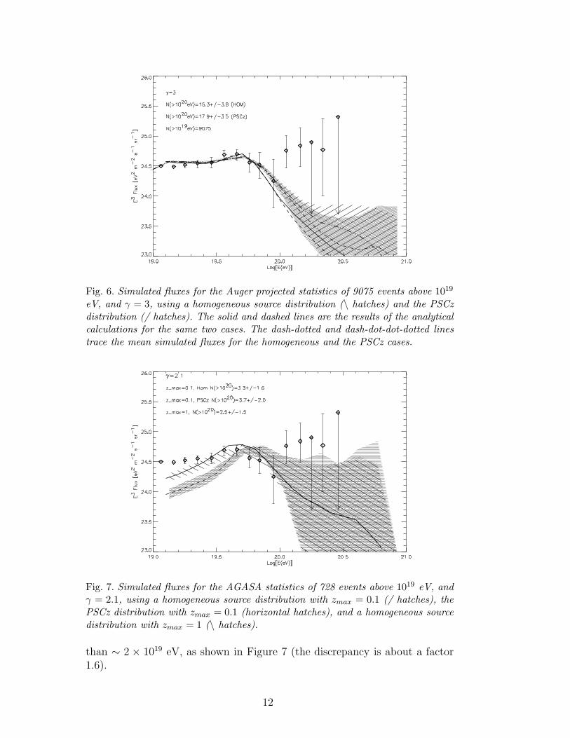
Fig. 6. Simulated fluxes for the Auger projected statistics of 9075 events above 1019

eV, and γ = 3, using a homogeneous source distribution (\ hatches) and the PSCzdistribution (/ hatches). The solid and dashed lines are the results of the analyticalcalculations for the same two cases. The dash-dotted and dash-dot-dot-dotted linestrace the mean simulated fluxes for the homogeneous and the PSCz cases.

Fig. 7. Simulated fluxes for the AGASA statistics of 728 events above 1019 eV, andγ = 2.1, using a homogeneous source distribution with zmax = 0.1 (/ hatches), thePSCz distribution with zmax = 0.1 (horizontal hatches), and a homogeneous sourcedistribution with zmax = 1 (\ hatches).

than ∼ 2 × 1019 eV, as shown in Figure 7 (the discrepancy is about a factor1.6).

12

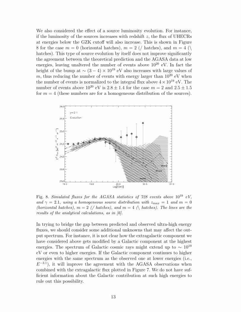
We also considered the effect of a source luminosity evolution. For instance,if the luminosity of the sources increases with redshift z, the flux of UHECRsat energies below the GZK cutoff will also increase. This is shown in Figure8 for the case m = 0 (horizontal hatches), m = 2 (/ hatches), and m = 4 (\hatches). This type of source evolution by itself does not improve significantlythe agreement between the theoretical prediction and the AGASA data at lowenergies, leaving unaltered the number of events above 1020 eV. In fact theheight of the bump at ∼ (3 − 4) × 1019 eV also increases with large values ofm, thus reducing the number of events with energy larger than 1020 eV whenthe number of events is normalized to the integral flux above 4×1019 eV. Thenumber of events above 1020 eV is 2.8 ± 1.4 for the case m = 2 and 2.5 ± 1.5for m = 4 (these numbers are for a homogeneous distribution of the sources).

Fig. 8. Simulated fluxes for the AGASA statistics of 728 events above 1019 eV,and γ = 2.1, using a homogeneous source distribution with zmax = 1 and m = 0(horizontal hatches), m = 2 (/ hatches), and m = 4 (\ hatches). The lines are theresults of the analytical calculations, as in [6].

In trying to bridge the gap between predicted and observed ultra-high energyfluxes, we should consider some additional unknowns that may affect the out-put spectrum. For instance, it is not clear how the extragalactic component wehave considered above gets modified by a Galactic component at the highestenergies. The spectrum of Galactic cosmic rays might extend up to ∼ 1019

eV or even to higher energies. If the Galactic component continues to higherenergies with the same spectrum as the observed one at lower energies (i.e.,E−3.1), it will improve the agreement with the AGASA observations whencombined with the extragalactic flux plotted in Figure 7. We do not have suf-ficient information about the Galactic contribution at such high energies torule out this possibility.

13

Another aspect of this problem that should be considered is the effect ofextragalactic magnetic fields. As shown in [25,26], a large scale magnetic fieldwith strength ∼ 10−7 – 10−9 G can steepen the spectrum of the observedcosmic ray particles significantly. This effect would improve the agreementwith the AGASA data. But as the diffusive limit is reached, the effect might goin the opposite direction: for instance, if the effective diffusion coefficient is toosmall, then the propagation time may be larger than the age of the universe forlow energy particles generated beyond some distance, considerably reducingthe cosmic ray horizon [27]. In other words a smaller portion of the universewould contribute to the observed flux, thus reducing it. The highest energycomponent of the spectrum should not be affected appreciably by diffusivepropagation, since most of the particles with E > 1020 eV originate in the localuniverse, where propagation is likely to be non-diffusive. A complete answerto this question awaits a full propagation code that includes the effects of arealistic model of extragalactic magnetic fields.

5 Conclusion

We have studied the effects on the spectrum of ultra-high energy cosmic rays ofsources associated with a realistic model for the galaxy distribution providedby the PSCz and CfA2 catalogs. We considered different injection spectraand the possibility of luminosity evolution of UHECR sources with redshift.We showed that when the galaxy selection functions are properly accountedfor, the local overdensity is not as large as found by [8]. Thus, the AGASAobservations are inconsistent with the predicted flux above 1020 eV for softinjection spectra (γ ≃ 3).

We confirm that a local overdensity helps bridge the agreement between theoryand observations but only (and only slightly) for hard injection spectra (γ ≃2). In this case, the observations are within 2σ of the predicted number ofevents, in agreement with the findings of [9]. Sources of UHECRs having adensity field following that of galaxies are therefore consistent with presentdata only for hard injection spectra and, in this case, the GZK cutoff is notreally a cutoff but a feature in the overall cosmic ray spectrum.

As future experiments such as the Pierre Auger Project [28], the High Reso-lution Fly’s Eye [29], the Telescope Array [30], and the EUSO [31] and OWL[32] satellite experiments increase the number of events observed above 1020

eV, a better determination of the shape of the GZK feature will be obtained.The GZK feature will contain information both on the injection spectrum (i.e.,γ) as well as the clustering properties of the sources. Given γ, the clusteringproperties, and the angular distribution of arrival directions, a population ofsources might be identifiable. If associated with active galaxies or some other

14

specific class of astrophysical objects, the shape of the GZK feature can befurther used to constrain intergalactic magnetic fields [33] as well as moreexotic pieces of physics, such as violations of Lorentz invariance [34].

Alternatively, the gap between observed and predicted flux may widen as moredata accumulates. This would indicate that astrophysical proton acceleratorsare unlikely sources of UHECRs. The added difficulty in reaching the extremeenergies in astrophysical sources further justifies the search for alternative ex-planations. Future experiments will play a crucial role in settling this longstanding mystery, through the determination of the cosmic ray flux, and ar-rival direction distribution, and the great discriminator: the composition atextremely high energies.

Acknowledgment

This work was supported by NSF through grant AST-0071235 and DOE grantDE-FG0291 ER40606 at the University of Chicago and at Fermilab by DOEand NASA grant NAG 5-7092.

References

[1] M. Takeda et al., Phys. Rev. Lett. 81 (1998) 1163; M. Takeda et al. preprint astro-ph/9902239 (submitted to Astrophys. J.); N. Hayashida et al. Phys. Rev. Lett.73 (1994) 3491; D. J. Bird et al. Astrophys J. 441 (1995) 144; Phys. Rev. Lett. 71(1993) 3401; Astrophys. J. 424 (1994) 491; M. A. Lawrence, R. J. O. Reid and A.A. Watson, J. Phys. G. Nucl. Part. Phys. 17 (1991) 773; N. N. Efimov et al., Ref.Proc. International Symposium on Astrophysical Aspects of the Most EnergeticCosmic Rays, eds. M. Nagano and F. Takahara (World Scientific, Singapore,1991), p. 20; D. Kieda et al., HiRes Collaboration, Proceeds. 26th ICRC SaltLake (1999); J. Linsley, Phys. Rev. Lett. 10 (1963) 146.

[2] K. Greisen, Phys. Rev. Lett. 16 (1966) 748; G. T. Zatsepin and V. A. Kuzmin,Sov. Phys. JETP Lett. 4 (1966) 78.

[3] N. Hayashida et al. (2000)

[4] A. Olinto, Phys.Rept. 333-334 (2000) 329.

[5] P. Bhattacharjee and G. Sigl, Phys. Rept. 327 (2000) 109.

[6] V. Berezinsky and S. Grigorieva, Astron. Astroph. 199 (1988) 1.

[7] Berezinsky, V. S., and Grigorieva, S. I., Proc. 16th. Int. Cosmic Ray Conf., Kyoto2 (1979) 81.

15

[8] G. A. Medina-Tanco, Proceedings of 26th ICRC, Salt Lake City, Utah, vol 4, 346(1999); Medina Tanco, G. A., Astrophys. J. 510 (1999) 91.

[9] J. N. Bahcall and E. Waxman, hep-ph/9912326v2 (2000).

[10] V.S. Ptuskin, S.I. Rogovaya, & V.N. Zirakashvili, Proceedings of 26th ICRC,Salt Lake City, Utah, vol 4, 271 (1999).

[11] Branch, D. 1998, ARA&A, 36, 17

[12] Davis, M., & Huchra, J. 1982, ApJ, 254, 437

[13] Strauss, M. A., & Willick, J.A. 1995, Phys. Rep., 261, 271

[14] Huchra, J. P., Geller, M. J., & Corwin, Jr., H. G. 1995, ApJ, 70, 687

[15] Saunders, W., Sutherland, W. J., Maddox, S. J., Keeble, O., Oliver, S. J.,Rowan-Robinson, M., McMahon, R. G., Efstathiou, G., Tadros, H., White,S. D. M., Frenk, C. S., Carraminana, A., Hawkins, M. R. S. 2000, submittedto MNRAS, preprint (astro-ph/0001117)

[16] Peebles, P. J. E. 1993, Principles of Physical Cosmology (Princeton, NJ:Princeton University Press)

[17] Hogg, D. W. 1999, astro-ph/9905116

[18] Peebles, P. J. E. 1980, The Large-Scale Structure of the Universe (Princeton,NJ: Princeton University Press)

[19] Efstathiou, G., Ellis, R. S., & Peterson, B. S. 1988, MNRAS, 232, 431

[20] Sandage, A., Tammann, G. A., & Yahil, A. 1979, ApJ, 232, 352

[21] V. S. Berezinsky, S.V. Bulanov, V. A. Dogiel, V. L. Ginzburg, and V. S. Ptuskin,Astrophysics of Cosmic Rays, (Amsterdam: North Holland, 1990).

[22] Achterberg et al. 1998 A. Achterberg, Y. A. Gallant, C. A. Norman, D. B.Melrose, astro-ph/9907060

[23] Takeda, M., et al., Phys. Rev. Lett. 81, 1163 (1998).

[24] Hayashida, N., et al., Appendix to Astrophys. J. 522, 225 (1999) (preprintastro-ph/0008102).

[25] P. Blasi and A. V. Olinto, 1999, Phys. Rev. D 59, 023001.

[26] G. Sigl, M. Lemoine, and P. Biermann, Astropart. Phys. 10 (1999) 141.

[27] T. Stanev, R. Engel, A. Muecke, R. J. Protheroe, J. P. Rachen, astro-ph/0003484.

[28] J. W. Cronin, Nucl. Phys. B. (Proc. Suppl.) 28B (1992) 213.

[29] S. C. Corbato et al., Nucl. Phys. B (Proc. Suppl.) 28B (1992) 36.

[30] M. Teshima et al., Nucl. Phys. B (Proc. Suppl.) 28B (1992) 169.

16

[31] see http://www.ifcai.pa.cnr.it/Ifcai/euso.html

[32] R. E. Streitmatter, Proc. of Workshop on Observing Giant Cosmic Ray AirShowers from > 1020 eV Particles from Space, eds. J. F. Krizmanic, J. F. Ormes,and R. E. Streitmatter (AIP Conference Proceedings 433, 1997).

[33] E. Waxman and J. Miralda-Escude, Astrophys. J. 472 (1996) L89; G. A. MedinaTanco, E. M. de Gouveia Dal Pino, and J. E. Horvath, Astropart. Phys. 6 (1997)337; G. Sigl, M. Lemoine, and A. V. Olinto, Phys. Rev. 56 (1997) 4470; M.Lemoine, G. Sigl, A. V. Olinto, and D. Schramm, Astropart. Phys. 486 (1997)L115; G. Sigl, M. Lemoine, and P. Biermann, Astropart. Phys. 10 (1999) 141; D.Ryu, H. Kang and P. L. Bierman, Astron. Astrophys. 335 (1998) 19.

[34] L. Gonzalez-Mestres, Nucl. Phys. B (Proc. Suppl.) 48 (1996) 131; S. Colemanand S. L. Glashow, Phys. Rev. D 59 (1999) 116008; H. Sato and T. Tati,Prog. Theor. Phys. 47 (1972) 1788; D. A. Kirzhnits and V. A. Chechin, Sov. J.Nucl. Phys. 15 (1972) 585; R. Aloisio, P. Blasi, P Ghia, and A. Grillo, preprintINFN/AE-99/24.

17