Univers

ity of

Cap

e Tow

n

The external validity of treatment effects: An investigation of educational production

Sean M. Muller

Thesis Presented for the Degree of DOCTOR OF PHILOSOPHY

in the Department of Economics UNIVERSITY OF CAPE TOWN

22nd February 2014

Univers

ity of

Cap

e Tow

n

The copyright of this thesis vests in the author. No quotation from it or information derived from it is to be published without full acknowledgement of the source. The thesis is to be used for private study or non-commercial research purposes only.

Published by the University of Cape Town (UCT) in terms of the non-exclusive license granted to UCT by the author.

Univers

ity of

Cap

e Tow

n

Until I found myself writing, unsupervised, a full draft of my Honours disser­tation over a summer holiday in 2002 I had never considered an academic career or completing a PhD. Among the important academic influences since then have been the 'bullshit detector' philosophy of my first serious econometrics instructor - also the supervisor of this and a previous dissertation - Martin Wittenberg. This perhaps more than anything else led to my interests in choice theory being succes­sively hibernated in favour of topics in applied microeconometrics. In addition, the Views on Institutional and Behavioural Economics (VIBE) course convened by Justine Burns and Malcolm Keswell introduced me to a range of extremely interesting literatures within economics, including one - intergenerational mobil­ity - that was the basis for my first Master's dissertation and subsequent journal publications. Nicoli Nattrass introduced me to the idea of academic activism in economics, showed admirable tolerance of public criticism from an undergradu­ate upstart and encouraged my application (and successful re-application) for the Rhodes scholarship. Don Ross introduced me to the work of Ken Binmore and, indirectly, the literature on the philosophy of economics, in which I now have an active research interest. My studies at Oxford deepened my technical understand­ing and, at times, understanding of the academic discipline of economics.

I would like to thank the many friends and colleagues who have, in their own ways and sometimes over both Masters and PhD dissertations, made these years tolerable or occasionally even pleasant. Some deserve special mention, in no par­ticular order: Konstantin Sofianos, Amy and Simon Halliday, Oscar Masinyana, Diaa Noureldin, Donald Powers, Salih Solomon, Andy Kerr, Cath Kannemeyer, Matt Penfold and Valentina Gosetti. Thanks also to my parents and sister for their support, encouragement as my career trajectory changed, along with consistent determination to keep me level-headed. My grandfather lived to see the start of this PhD but not its completion; his encouraging invocations live on, as does the principled example set by the activities of his youth. Perhaps most importantly, I thank my wife Sara for her support as well as tolerance of, or company in, the long hours of work and the vicissitudes of the PhD process and academia in general. I feel obliged to apologise for the fact that for almost the entire time since we met I have been working on academic dissertations. From now on I will try to restrict myself to journal articles ...

Chapters 1 and 3 benefited from seminar comments at the Economic Society of South Africa's Biennial Conference (Stellenbosch, 2011), Stellenbosch Univer­sity, the Evidence and Causality in the Sciences (ECitS) conference (Kent, 2011) and the CEMAPRE Workshop on the Economics and Econometrics of Education (Lisbon, 2013).

Univers

ity of

Cap

e Tow

n

Abstract Author: Title:

Date:

Sean Mfundza Muller The external validity of treatment effects: An investigation of educational production 17th February 2014

The thesis begins, in chapter 1, with an overview of recent debates concerning the merits of randomised programme evaluations and a detailed review of the lit­erature on the extrapolation of treatment effects ('external validity'). Building on the insights of Cook and Campbell ( 1979) and a result by Hotz, Imbens, and Mor­timer (2005), I then argue that the fundamental challenge to external validity may be interactive relationships between the treatment variable and other covariates.

The empirical relevance of this claim is developed through two contributions to the economics of education literature, using data from the Tennessee class size experiment known as 'Project STAR'. Chapter 2 contributes to the literature on teacher quality, describing and implementing a novel method for constructing a value-added quality measure that uses a single cross-section of data in which stu­dents and teachers are randomly assigned to different-sized classes. The core insight is that constructing the value-added measure within treatment categories creates a plausible measure of quality that is simultaneously independent of treat­ment. The analysis of chapter 3 concerns the literature on class size effects. I argue that the effect of class size on educational achievement may be dependent on other class-level factors and that this should be considered when estimating educational production functions. Using the variable constructed in chapter 2, I estimate interaction effects between class size and teacher quality and find a number of statistically and economically significant effects. Specifically, higher quality teachers are associated with more beneficial effects of smaller classes.

Those results suggest a possible unification of the class size and teacher quality literatures, with the policy problem being one of finding an optimal combination of these two factors . The broader contribution, further to the analysis of chapter 1, is to illustrate an obstacle to external validity: class size effects are unlikely to be the same across contexts where the teacher quality distribution differs. The experimental estimation of class size effects therefore serves as an empirical case study of the challenges to external validity that arise from interaction.

ii

Univers

ity of

Cap

e Tow

n

Contents

Summary viii

1 Randomised trials for policy: a review of the external validity of treat-ment effects 1 1.1 The credibility controversy: randomised evaluations for policy-

making . . . . . . . . . . . . . . . . . . . . . . . . . . . . . . . 2 1.1.1 Randomised evaluations . . . . . . . . . . . . . . . . . . 5 1.1.2 Estimating average treatment effects conditional on co-

variates . . . . . . . . . . . . . . . . . . . . . . . . . . . 7 1.1.3 Randornised evaluations: specific criticisms and defences . 9

1.2 External validity of treatment effects: A review of the literature . 13 1.2.1 The medical literature on external validity . . 14 1.2.2 Philosophers on external validity . . . . . . . . . . . . . 17 1.2.3 External validity in experimental economics . . . . . . . 19 1.2.4 The programme evaluation and treatment effect literature . 20 1.2.5 The structural approach to programme evaluation . . . . . 25 1.2.6 Decision-theoretic approaches to treatment effects and wel-

fare . . . . . . . . . . 31 1.2.7 Forecasting for policy? . . . . . . . . . . . . . . . . 33 1.2.8 Summary . . . . . . . . . . . . . . . . . . . . . . . 36

1.3 Interacting factors, context dependence and external validity 38 1.3.1 Interactive functional forms and external validity 39 1.3.2 Heterogeneity of treatment effects . . . . 44 1.3.3 Selection, sampling and matching . . . . 47 1.3.4 Implications for replication and repetition 50

1.4 Conclusions and implications for empirical work 52

Class size and teacher quality: a case of implausible external validity 56

iii

Univers

ity of

Cap

e Tow

n

2 Constructing a teacher quality measure from cross-sectional, experi-mental data 59 2.1 The literature on valued-added teacher quality measures . 62 2.2 Models of educational production . . 67 2.3 Quality measure construction . . . . . 71

2.3.1 Score changes or score levels . 71 2.3.2 Isolating teacher quality . . . 74 2.3.3 Discussion . . . . . . . . . . 76 2.3.4 Quality a Ia Chetty, Friedman, Hilger, Saez, Schanzen-

bach, and Yagan (2011) . . . . . . . 78 2.4 Implementation with Project STAR data . . . 80

2.4.1 Correlations among quality measures 81 2.4.2 Quality across school location . . . 85 2.4.3 Quality and teacher characteristics . 88 2.4.4 Support from subjective measures 94 2.4.5 Class size versus class type . 102

2.5 Comparisons of explanatory power . 104 2.6 Conclusion . . . . . . . . . . . . . 111

Appendix A Class size and variance of quality measures 112 A.1 Small denominators . . . . . . . . . 113 A.2 Possible selection or attrition effects . . . . . 120

Appendix B Kernel densities for demeaned scores 126

Appendix C Figures and tables not shown in text 131 C.1 Scatter plots comparing rankings . . . . . . . . . . . . . . . . 131 C.2 Quality measures across school types based on reading scores 133 C.3 STAR 'effective teachers' relative to quality measure rankings 136 C.4 Residualising on actual class size . . . . . . . . . . . . . . . . 142

3 The external validity of class size effects: teacher quality in Project snR 1« 3.1 Educational production functions and class size effects 147

3.1.1 Why class size?. . . . . . . . . . . . . . . . . 148 3.2 A model of class size in educational production . . . . 150 3.3 Project STAR: 'the Barbary steed' of the class size literature 153

3.3.1 Data overview . . . . . . . . . . . . . . . . . . 154 3.3.2 Separating class size and quality . . . . . . . . . 156

3.4 Empirical analysis: quality matters for class size effects . 158 3.4.1 Main results . . . . . . . . . . . . . . . . . . . . 160

lV

Univers

ity of

Cap

e Tow

n

3.4.2 Importance of the dependent variable . . . . . . . . . 173 3.4.3 Using treatment assignment instead of actual class size 181

3.5 Further econometric complications . . . . . . . . . . . . . . . 185 3.5.1 Own-score bias, attenuation bias and the 'reflection effect' 185 3.5.2 Standard errors ....................... 186 3.5.3 Implications of interaction for the quality variable ..... 188 3.5.4 Robustness of interaction terms to different functional forms 196

3.6 Better modest than LATE? . . . . . . . . . . . . . . . . . . . . . 198

Appendix D Figures not shown in text 0.1 Marginal effects of class size on reading scores 0.2 Marginal effects of quality on reading scores .

Conclusion

Bibliography

v

202 202 206

210

215

Univers

ity of

Cap

e Tow

n

List of Tables

1.1 1.2

2.1 2.2 2.3 2.4 2.5 2.6 2.7 2.8 2.9 2.10 2.11

Criticisms of randomised or quasi-random evaluations . . . . . . Minimum empirical requirements for external validity (assuming an ideal experiment, with no specification of functional form)

Kolmogorov-Smimov test of equality of distributions Correlations between quality measures: Mathematics Correlations between quality measures: Reading Correlations between maths & reading teacher quality measures Variation explained by teacher characteristics Variation explained by teacher characteristics Variation explained by teacher characteristics Variation in quality explained by experience Variation in quality explained by experience . Variation in quality explained by experience . Descriptive statistics for STAR 'effective' and 'less effective' teach-

10

42

81 82 83 84 89 90 91 92 93 93

ers . . . . . . . . . . . . . . . . . . . . . . . . . . . . . . . . . . 96 2.12 Comparing descriptive statistics for STAR 'effective teacher' sam-

ples . . . . . . . . . . . . . . . . . . . . . . . . . . . . . . . . 98

A.1 Relationship betwen number of observations and teacher quality 120

C.l Spearman rank correlations for qA 142 C.2 Spearman rank correlations for qD 143

3.1 Marginal effects of quality and size on score changes: Mathemat-ics . . . . . . . . . . . . . . . . . . . . . . . . . . . . . . . . 162

3.2 Marginal effects of quality and size on score changes: Reading 163 3.3 Different specifications: Grade I mathematics I74 3.4 Different specifications: Grade I reading I75 3.5 Different specifications: Grade 2 mathematics I76 3.6 Different specifications: Grade 2 reading 177 3.7 Different specifications: Grade 3 mathematics 178

VI

Univers

ity of

Cap

e Tow

n

3.8 Different specifications: Grade 3 reading . . . . . . 179 3.9 Robustness of regression results: Mathematics scores 183 3.10 Robustness of regression results: Reading scores . . 184 3.11 Explanatory power of school fixed effects for qD: Mathematics 192 3.12 Explanatory power of school fixed effects for qD: Reading . . 192 3.13 Explanatory power of school fixed effects for qA: Mathematics 193 3.14 Explanatory power of school fixed effects for qA: Reading 193 3.15 Effect of interaction on constructed quality differences . . . . 195

vii

Univers

ity of

Cap

e Tow

n

Summary

The basic concern of this thesis is with the use of treatment effects estimated from randomised evaluations to address policy questions or inform policy decisions. The primary focus of the analysis is on the challenge of extrapolating experi­mental estimates to contexts or populations besides those in which the original experiments were conducted ('external validity'). Chapter 1 of the dissertation presents an original review of the literature on external validity. The first compo­nent discusses contributions in medicine and philosophy, as well as four different sub-disciplines of economics: experimental economics, structural econometrics, time-series forecasting and the experiment-focused programme evaluation litera­ture itself. The second component of the review argues that the problem of exter­nal validity can be usefully seen - as suggested by Cook and Campbell ( 1979) - as a problem of interacting causal relationships. That analysis, building on key con­tributions to the evaluation literature, such as Hotz et al. (2005), shows that the set of assumptions required to guarantee external validity is, in statistical terms at least, equivalent to the set of assumptions that would allow non-experimental identification of causal effects; belief in the prospect of obtaining unconfounded non-experimental effects may therefore be no less plausible than belief in the sim­ple external validity of experimentally-identified effects. I argue, in addition, that this change of perspective leads to a focus on the causes of interaction, as opposed to the 'treatment heterogeneity' literature which focuses on the consequences of such underlying relationships. That in tum draws attention to the fact that the ma­jor empirical obstacles to external validity may be researchers' lack of knowledge of these relationships, the incomparability of interacting factors across contexts, and the likelihood that many such factors may not be observable.

Chapters 2 and 3 attempt to provide empirical substance to the abstract argu­ments of Chapter 1 by examining the extensively studied case of interventions to reduce school class sizes and their effects on test scores. The starting point is the insight that the effect of class size on educational outcomes may not be indepen­dent of factors that determine the quality of students' classroom experience. Most notably, there are reasons to expect that the effect of class size, as well as a re-

viii

Univers

ity of

Cap

e Tow

n

duction in that variable, will depend to some extent on teacher quality. To obtain empirical evidence on this question I utilise the well-known, publicly available, Tennessee Project STAR dataset. A major challenge is that there does not appear to be any dataset in the literature that contains information on an experimental class size intervention and direct information on teacher quality. In an attempt to circumvent this problem, Chapter 2 proposes a novel version of a value-added teacher quality measure, the construction of which is made possible by exploit­ing the random assignment of students and teachers to classes - as was the case in Project STAR. The measure differs from the standard value-added measures in that it uses a single cross-section of teacher information rather than a series of observations over time, but compensates for this by virtue of random matching of students and teachers within schools. In that chapter, I construct the measure using the STAR data, provide results on the veracity of some of the underlying assumptions required and compare the resultant variable to two alternative mea­sures of class quality- including that used by Chetty et al. (2011) in their analysis of STAR.

Chapter 3 expands on the motivation for examining the case of class size inter­ventions through a discussion of the broader literature on educational production. It discusses alternative specifications of the production function that explicitly account for the role of class size if indeed this variable does interact with class­level factors. That serves as a basis for the subsequent empirical analysis. I then estimate - using a least-squares regression based on the preceding model of the education production function - the marginal effects of class size at different quar­tiles of the teacher quality distribution and the marginal effects of one standard deviation change in quality at different class sizes. These estimates are obtained for Grades 1 to 3, for mathematics as well as reading scores. Some statistically and economically significant results are obtained, suggesting the possibility that there may be meaningful interaction between teacher quality and class size. To examine the possible sensitivity of the results to different specifications, various alternatives are estimated and compared. While robust to some changes, the main sensitivity is in relation to the dependent variable used - test score changes, which is our preferred variable, or test score levels (often used in the literature on STAR). As an additional check, alternative specifications of the treatment variable are ex­plored, using a treatment dummy instead of actual class size and instrumenting for class size using treatment assignment. The results are found to be robust to these different approaches. The chapter discusses some additional technical issues that are important for the results, such as choice of standard errors, the implications of an interactive production function for the proposed quality variable, reflection effects and the possible sensitivity of interaction estimates to functional form as-

ix

Univers

ity of

Cap

e Tow

n

sumptions. There are a number of caveats to the empirical findings and these can­not be seen as definitive, but rather a first attempt at examining the issue of class size-teacher quality interactions - an issue that has not been previously explored in the economics of education literature.

In conclusion, I argue - in agreement with other authors - that the usefulness of estimates from randomised evaluations for policy remains an open question if we employ the same econometric standards that are used to advocate for the priority of experimental methods in identifying causal effects. Given this, it would seem appropriate that researchers explicitly recognise the limitations of existing results for policy, as well as the prospective usefulness of future experimental studies. The present study is a contribution, therefore, both to the economics of education literature and a small, but growing, literature on the external validity of treatment effects and the policy relevance of econometric work.

X

Univers

ity of

Cap

e Tow

n

Chapter 1

Randomised trials for policy: a review of the external validity of treatment effects

In the last decade some researchers in economics have taken the view that ran­domised trials are the 'gold standard' for evaluating policy interventions and iden­tifying causal effects. This has led to controversy and a series of exchanges, in­cluding not only econometricians but philosophers, statisticians and policy ana­lysts, regarding the uses and limitations of different econometric methods. Much of this debate concerns reasons why randomised evaluations may not, in practice, identify the causal effect of interest or, alternatively, may not identify a causal effect that is of relevance to policy. These concerns are broadly of three types: whether many questions of interest can be even notionally addressed via exper­imentation; reasons why identification of the causal effect in the experimental sample ('internal validity') may fail; and, limitations of the extent to which such an effect is informative outside of that sample population ('external validity').

While the literature on experimental and quasi-experimental methods deals ex­tensively with threats to internal validity, and despite the popularisation of ran­domised evaluations due to their apparent usefulness for policy, the literature on external validity is remarkably undeveloped. 1 Work on the subject has increased in recent years but there remains little guidance - and no consensus - on how es­timated treatment effects can be used to estimate the likely effects of a policy in

1The term 'quasi-experimental' is not uniformly used in the literature. For our purposes here we use it to refer to methods that are not structural, but rather claim to use or identify variation that is exogenous without in fact using data from deliberate, randomised experiments. Examples are: analysis based on 'natural experiments'; interrupted time series design; regression discontinuity design; and various forms of instrumental variable analysis.

1

Univers

ity of

Cap

e Tow

n

a different, or larger, population. The vast majority of empirical studies, includ­ing in top journals, contain no formal analysis of external validity. The concern of this chapter is to provide a survey - the first of its kind to our knowledge - of the literature on external validity, including contributions from other disciplines. This provides a motivation for, and direction to, the contributions of subsequent chapters.

Section 1.1 details the broader debate about randomised trials in economics, provides formal notation and an outline of some key results, and lists specific criticisms of experimental methods. Section 1.2 reviews the existing literature on external validity, including some contributions from outside the programme evaluation literature. It draws out a number of common themes across these liter­atures, focusing in particular on the basic intuition that external validity depends on similarity of the population(s) of interest to the experimental sample. The fi­nal contribution, in section 1.3, develops a perspective on external validity based on the role of variables that interact with the cause of interest to determine indi­viduals' final outcomes. This, we suggest, provides a framework within which to examine the question of population similarity in a way that allows for some formal statements - already developed by other researchers - of the requirements for external validity. These, in tum, have close resemblance to requirements for internal validity, which provides some basis for comparing and contrasting these two issues for empirical analysis. The chapter concludes by arguing that it is not coherent to insist on formal methods for obtaining internal validity, while bas­ing assessments of external validity on qualitative and subjective guesses about similarity between experimental samples and the population(s) of policy inter­est. Insisting on the same standards of rigour for external validity as for obtaining identification of causal effects would imply that much of the existing applied liter­ature is inadequate for policy purposes. The obstacles to econometric analysis that underlie this conclusion are not limited to randomised evaluations and therefore consideration of external validity suggests more modesty, in general, in claiming policy relevance for experimental and non-experimental methods. This conclu­sion, along with our linkage of interactive functional forms and external validity, provides a foundation for the empirical analysis of subsequent chapters.

1.1 The credibility controversy: randomised evalu­ations for policymaking

The possibility of using econometric methods to identify causal relationships that are relevant to policy decisions has been the subject of controversy since

2

Univers

ity of

Cap

e Tow

n

the early and mid-20th century. The famous Keynes-Tinbergen debate (Keynes, 1939) partly revolved around the prospect of successfully inferring causal rela­tionships using econometric methods, and causal terminology is regularly used in Haavelmo's (1944) foundational contribution to econometrics. Heckman (2000, 2008) provides detailed and valuable surveys of that history. Randomised exper­iments began to be used in systematic fashion in agricultural studies (by Ney­man (1923)), psychology and education, though haphazard use had been made of similar methods in areas such as the study of telepathy.2 Although some studies involving deliberate randomisation were conducted in, or in areas closely relat­ing to, economics the method never took hold and economists increasingly relied on non-experimental data sources: either cross-sectional datasets with many vari­ables ('large N, small T') but limited time periods, or time series datasets with small numbers of variables over longer time periods ('small N, large T'). The for­mer tended to be used by microeconometricians while the latter was favoured by macroeconometricians and this distinction largely continues to the present day. Our concern in this study is the use of microeconometric methods to inform pol­icy decisions and thus, although an integration of these literatures is theoretically possible, we will focus on data sources characterised by limited time periods.

For much of that era econometricians relied on two broad approaches to obtain­ing estimates of causal effects: structural modelling and non-structural attempts to include all possibly relevant covariates to prevent confounding/bias of estimated coefficients. The latter relied on obtaining statistically significant coefficients in regressions that were robust to inclusion of ('conditioning on') plausibly relevant covariates, where the case for inclusion of particular variables and robustness to unobserved factors was made qualitatively (albeit sometimes drawing on contri­butions to economic theory). The structural approach involves deriving full eco­nomic models of the phenomena of interest by making assumptions about the set of relevant variables, the structure of the relationship between them and the behaviour of economic agents. The rapid adoption of approaches based on ran­dom or quasi-random variation stems in part from dissatisfaction with both these preceding methods. Structural methods appear to be constrained by the need to make simplifying assumptions that are compatible with analytically producing an estimable model, but that may appear implausible, or at the least are not inde­pendently verified. On the other hand, non-structural regression methods seem unlikely to produce estimates of causal effects given the many possible relations between the variables of interest and many other, observed and unobserved, fac-

2Herberich, Levitt, and List (2009) provide an overview of randomised experiments in agri­cultural research and Hacking ( 1988) provides an entertaining account of experiments relating to telepathy.

3

Univers

ity of

Cap

e Tow

n

tors. This seeming inability to identify causal effects under plausible restrictions led to a period in which many econometricians and applied economists abandoned reference to causal statements - a point emphasised in particular by Pearl (2009), but see also Heckman (2000, 2008).

In this context, the further development and wider understanding of economet­ric methods for analysis using experimental, or quasi-experimental (Angrist and Krueger, 2001), data presented the promise of reviving causal analysis without needing to resort to seemingly implausible structural models. Randomisation, or variation from it, potentially severs the connection between the causal variable of interest and confounding factors. Many expositions of experimental methods cite LaLonde's (1986) paper showing the superiority of experimental estimates to ones based on various quasi-structural assumptions in the case of job market training programmes.3 As a result, Banerjee (2007) has described randomised trials as the "gold standard" in evidence and Angrist and Pischke (2010) state that the adoption of experimental methods has led to a "credibility revolution" in economics. Such methodological claims have, however, been the subject of a great deal of criticism. Within economics, Heckman and Smith (1995), Heckman and Vytlacil (2007a), Heckman and Urzua (2010), Keane (2005, 2010a,b), Deaton (2008, 2009, 2010), Ravallion (2008, 2009), Leamer (2010) and Bardhan (2013), among others, have argued that the case for experimental methods has been overstated and that conse­quently other methods- particularly structural approaches (Rust, 2010)- are being displaced by what amounts to a fad. See also the contributions in Banerjee and Kanbur (2005). The more extreme proponents of these methods have sometimes been referred to as 'randomistas' (Deaton (2008), Ravallion (2009)).

Some of the concerns raised by Deaton are based on detailed work in the philos­ophy of science by Cartwright (2007, 201 0). There also exists an active literature in philosophy on the so-called 'evidence hierarchies' developed in medicine; the notion that some forms of evidence are inherently superior to others. In standard versions of such hierarchies randomised evaluations occupy the top position. This is primarily due to the belief that estimates from randomised evaluations are less likely to be biased (Hadom, Baker, Hodges, and Hicks, 1996) or provide better es­timates of 'effectiveness' (Evans, 2003). Nevertheless, a number of contributions have critically addressed the implicit assumption that the idea of a 'gold standard' - a form of evidence unconditionally superior to all others - is coherent. Concato, Shah, and Horwitz (2000), for example, question whether this view of evidence

3We refer to these as 'quasi-structural' since in most cases they are not based on full structural models but rather specific assumptions on underlying structural relationships that, theoretically, enable identification using observational data.

4

Univers

ity of

Cap

e Tow

n

is conceptually sound and whether it is confirmed empirically. Most of these ref­erences come from the medical literature in which randomised trials have been a preferred method for causal inference long before their adoption in economics. The generic problem of integrating different forms of evidence has not yet been tackled in any systematic fashion in economics, though studies delineating what relationships/effects various methodological approaches are identifying (Angrist (2004), Heckman and Vytlacil (2005, 2007b), Heckman and Urzua (2010)) may provide one theoretical basis for doing so. Nevertheless, some advocates of these methods continue to argue strongly that, "Randomized experiments do occupy a special place in the hierarchy of evidence, namely at the very top" (lmbens, 2010: 10).

1.1.1 Randomised evaluations

The great advantage of randomised evaluations is that they offer the prospect of simple estimation of causal effects by removing the risk of bias from confounding factors that plagues analysis using observational data. Introducing some formal notation, Yi is the outcome variable for individual i, which becomes Yi(1) = Y1i

denoting the outcome state associated with receiving treatment (Ti = 1) and Yi(O) = Yoi denoting the outcome state associated with not receiving treatment (7i = 0). The effect of treatment for any individual is b.i = Yli - Y0i.4 This formulation can be seen to be based on a framework - the more complete version of which is known as the Neyman-Rubin model after Neyman (1923) and Rubin (1974) -of counterfactuals, since in practice the same individual cannot simul­taneously be observed in treated and non-treated states. Holland (1986) is a key early review of this framework.

Assume we are interested in the average effect of treatment (E[Y1i - Yoi]).5

To empirically estimate this, one might consider simply subtracting the average outcomes for those receiving treatment and the untreated. One can rewrite this difference as:

E[YiiTi = 1]- E[Yil7i =OJ ={E[Ylil7i = 1]- E[Yoil7i = 1]} + {E[YoiiTi = 1]- E[Yoil7i = 0]}

4In subsequent analysis, following a notational convention in some of the literature, 6. is used to signify a treatment effect and is subscripted accordingly if that is anything other than Y1 i - Yoi.

5Note that in some approaches - see for instance Imbens (2004) - the 'i' subscript is used to denote sample treatment effects as opposed to those for the population. This distinction is not im­portant for the above discussion but in later analysis we, instead, distinguish between populations using appropriately defined dummy variables.

5

Univers

ity of

Cap

e Tow

n

The second term, representing the difference between potential outcomes of treatment recipients and non-recipients in the non-treated state represents 'selec­tion bias', the extent to which treatment receipt is associated with other factors that affect the outcome of interest. An ideal experiment in which individuals are randomly allocated into treatment and control groups, with no effects of the exper­iment itself beyond this, ensures that on aggregate individuals' potential outcomes are the same regardless of treatment receipt so E[YoiiT = 1] = E[YoiiT =OJ. A randomised evaluation can therefore estimate an unbiased effect of treatment on those who were treated, which is the first term above, not because it removes selection bias but because it balances it across the treatment and control groups (Heckman and Smith, 1995). Therefore, provided that the treatment of one in­dividual does not affect others, randomisation enables estimation of the average treatment effect. As various authors have pointed out, this result need not hold for other properties of the treatment effect distribution, such as the median, unless one makes further assumptions. For instance, if one assumes that the causal effect of treatment is the same for all individuals (6i = 6j, Vi and j), then the me­dian treatment effect can also be estimated in the above fashion. That assumption, however, appears excessively strong and allowing for the possibility that treatment effect varies across individuals raises a host of other - arguably more fundamental - concerns, which we discuss in somewhat more detail below.

Nevertheless, the average effect is often of interest. To connect the above to one popular estimation method, least squares regression, one can begin by writing the outcome as a function of potential outcomes and treatment receipt:

Yi = (1 - T)Yoi + TYli

= Yoi + T(Yli - Yoi)

Writing the potential outcomes as:

Yoi a:+ uoi

yli 0: + T + Uli

where uoi = Yoi - E[Yoi], and similarly for uli• and T is then the average treatment effect (.6.). We can then write the previous equation as:

6

Univers

ity of

Cap

e Tow

n

Y = o: + TT + [T(u1 - uo) + uo]

Taking expectations:

E[YIT] = o: + TT + E[T(u1- uo)] + E[uo]

We have E[u0] = 0 by definition and randomisation ensures that the second last

term is zero, so:

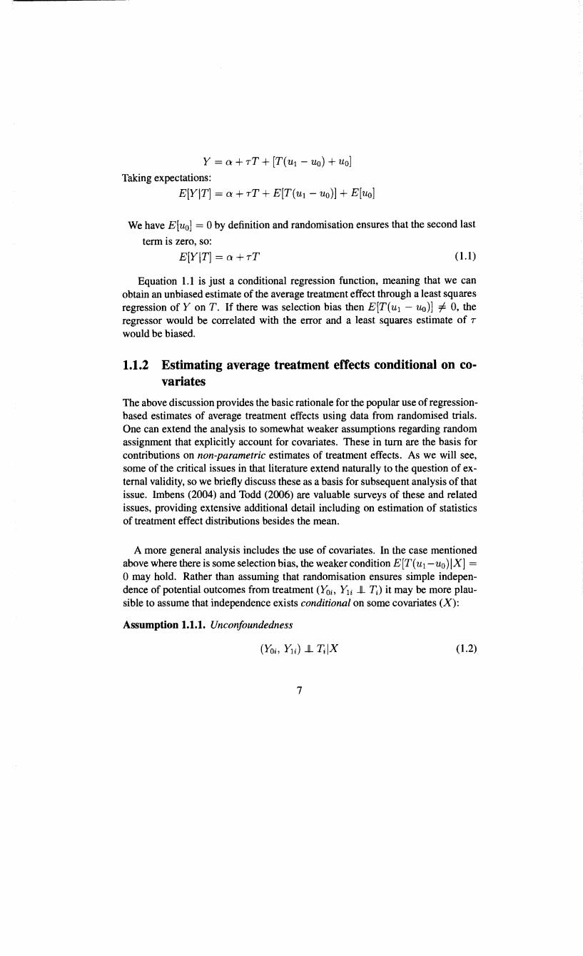
E[YIT] = 0: + TT (1.1)

Equation 1.1 is just a conditional regression function, meaning that we can obtain an unbiased estimate of the average treatment effect through a least squares regression of Yon T. If there was selection bias then E[T(u1 - uo)] =f. 0, the regressor would be correlated with the error and a least squares estimate of T

would be biased.

1.1.2 Estimating average treatment effects conditional on co­variates

The above discussion provides the basic rationale for the popular use of regression­based estimates of average treatment effects using data from randomised trials. One can extend the analysis to somewhat weaker assumptions regarding random assignment that explicitly account for covariates. These in tum are the basis for contributions on non-parametric estimates of treatment effects. As we will see, some of the critical issues in that literature extend naturally to the question of ex­ternal validity, so we briefly discuss these as a basis for subsequent analysis of that issue. lmbens (2004) and Todd (2006) are valuable surveys of these and related issues, providing extensive additional detail including on estimation of statistics of treatment effect distributions besides the mean.

A more general analysis includes the use of covariates. In the case mentioned above where there is some selection bias, the weaker condition E[T( u1 -u0 ) IX] = 0 may hold. Rather than assuming that randomisation ensures simple indepen­dence of potential outcomes from treatment (Yoi, Yii JL 7i) it may be more plau­sible to assume that independence exists conditional on some covariates (X):

Assumption 1.1.1. Unconfoundedness

(1.2)

7

Univers

ity of

Cap

e Tow

n

Unconfoundedness ensures that we can write the average treatment effect in terms of expectations of observable variables (rather than unobservable potential outcomes) conditional on a vector of covariates.6 The probability of receiving treatment given the covariates (X) is known as 'the propensity score', written: e(x) = Pr(T = 1/X = x). Where treatment is dichotomous: e(x) = E[T/X = x]. For a number of purposes it is useful to know a result by Rosenbaum and Ru­bin ( 1983) that unconfoundedness - as defined above conditional on X - implies unconfoundedness conditional on the propensity score. This has the advantage of reducing the 'dimensionality' of the estimation problem by summarising a pos­sibly large number of relevant covariates into a single variable (lmbens, 2004 ), albeit by assuming a parametric form for the propensity score.?

In order to then obtain the preceding, desirable results under this weaker as­sumption, one also requires sufficient overlap between the distributions of covari­ates in the treated and non-treated populations:

Assumption 1.1.2. Overlapping support

0 < Pr(T = 1/X) < 1 (1.3)

This condition states that no covariate value, or combination of covariate values where X is a vector, perfectly predicts treatment receipt.

Three points about the above approach are particularly important for our later discussion of external validity. First, to implement it in practice a researcher must be able to accurately estimate the conditional average treatment effect for every realisation of X and T (denoted x and t), which in tum requires that these be represented in both treatment and control populations (the 'overlapping support' assumption) and with large enough sample size to enable accurate estimation.8

Second, the unconditional average treatment effect is estimated by averaging over the distribution of x but that is often unknown and therefore requires further as­sumptions to make the approach empirically feasible. Finally, it is possible that

6Heckman, Ichimura, and Todd ( 1997) show that a weaker assumption can be used if the interest is in the effect of treatment on the treated, though Imbens (2004) argues that it is hard to see how this weaker form can be justified without also justifying the stronger unconfoundedness assumption - see also the discussion in Todd (2006).

7In other words, the dimensionality problem is 'shifted' to estimation of the propensity score where various arguments are deployed to justify particular functional forms.

8 As various authors (lmbens (2004), Heckman and Vytlacil (2007a), Todd (2006)) have noted, where there is inadequate overlap in the support, identification can be obtained conditional on limiting the sample to the relevant part of the support. The substantive rationale for this is that it allows identification of some effect, but with the caveat that the restriction is otherwise ad hoc.

8

Univers

ity of

Cap

e Tow

n

both the above assumptions could be satisfied subject to knowledge of, and data on, the relevant conditioning variables even without experimental variation. In that case, which as a result is also often referred to as 'selection on observables', observational data is enough to secure identification of the average treatment ef­fect. The experimental literature proceeds from the assumption that unconfound­edness, conditional or not, is - at the very least - more likely to hold in experimen­tal data, a position which has some support from the empirical literature but is also contested. For instance, the previously mentioned paper by LaLonde (1986) is often cited to support this claim. In contrast, Smith and Todd (2005a,b) argue that the issue is not the uniform superiority of experimental or non-experimental methods, but rather the appropriateness of particular non-experimental methods given the quality of the data available.

1.1.3 Randomised evaluations: specific criticisms and defences

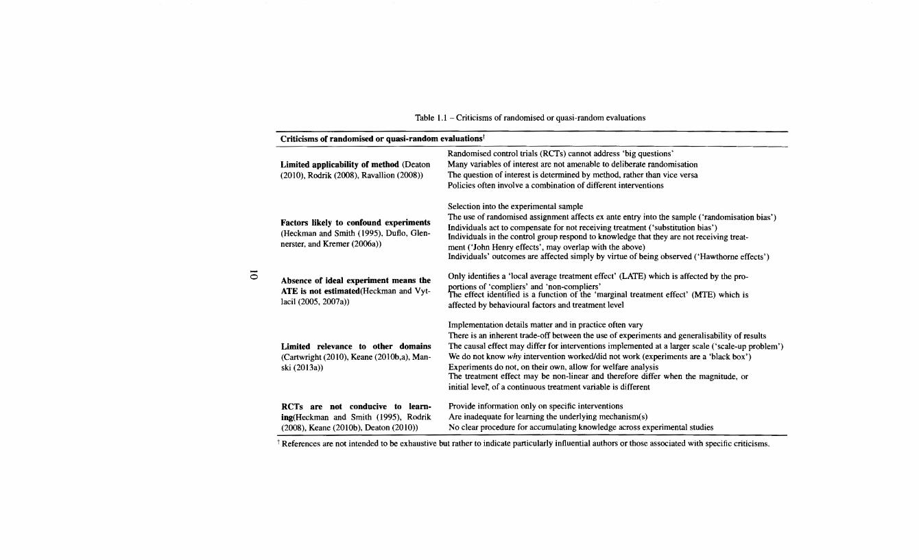
In its conditional formulation the formal case for experimental methods appears somewhat more nuanced, with experimental assignment increasing the likelihood of an unconfoundedness condition being satisfied. That in tum depends on anum­ber of implicit assumptions about successful design and implementation of exper­iments as well as the broader applicability of such methods. Unsurprisingly, these are the issues on which many criticisms have focused. Table 1.1 summarises limi­tations to randomised evaluations that have been identified by critics and, in some cases, acknowledged by proponents of these methods.

9

Univers

ity of

Cap

e Tow

n

-0

Table 1.1 -Criticisms of randomised or quasi-random evaluations

Criticisms of randomised or quasi-random evaluations t

Limited applicability of method (Deaton (2010), Rodrik (2008), Ravallion (2008))

Factors likely to confound experiments (Heckman and Smith (1995), Dufto, Glen­nerster, and Kremer (2006a))

Absence of ideal experiment means the ATE is not estimated(Heckman and Vyt­lacil (2005, 2007a))

Limited relevance to other domains (Cartwright (2010), Keane (2010b,a), Man­ski (2013a))

RCTs are not conducive to learn­ing(Heckman and Smith (1995), Rodrik (2008), Keane (20l0b), Deaton (2010))

Randomised control trials (RCTs) cannot address 'big questions' Many variables of interest are not amenable to deliberate randomisation The question of interest is determined by method, rather than vice versa Policies often involve a combination of different interventions

Selection into the experimental sample The use ofrandomised assignment affects ex ante entry into the sample ('randomisation bias') Individuals act to compensate for not receiving treatment ('substitution bias') Individuals in the control group respond to knowledge that they are not receiving treat-ment ('John Henry effects', may overlap with the above) Individuals' outcomes are affected simply by virtue of being observed ('Hawthorne effects')

Only identifies a 'local average treatment effect' (LATE) which is affected by the pro­portions of 'compliers' and 'non-compliers' The effect identified is a function of the 'marginal treatment effect' (MTE) which is affected by behavioural factors and treatment level

Implementation details matter and in practice often vary There is an inherent trade-off between the use of experiments and generalisability of results The causal effect may differ for interventions implemented at a larger scale ('scale-up problem') We do not know why intervention worked/did not work (experiments are a 'black box') Experiments do not, on their own, allow for welfare analysis The treatment effect may be non-linear and therefore differ when the magnitude, or initial lever, of a continuous treatment variable is different

Provide information only on specific interventions Are inadequate for learning the underlying mechanism(s) No clear procedure for accumulating knowledge across experimental studies

t References are not intended to be exhaustive but rather to indicate particularly influential authors or those associated with specific criticisms.

Univers

ity of

Cap

e Tow

n

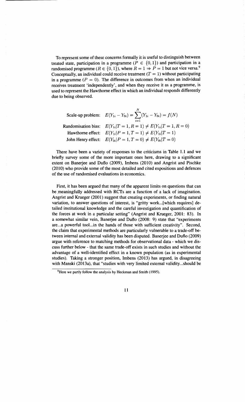
To represent some of these concerns formally it is useful to distinguish between treated state, participation in a programme (P E {0, 1}) and participation in a randomised programme (R E {0, 1} ), where R = 1 :::} P = 1 but not vice versa.9

Conceptually, an individual could receive treatment (T = 1) without participating in a programme (P = 0). The difference in outcomes from when an individual receives treatment 'independently', and when they receive it as a programme, is used to represent the Hawthorne effect in which an individual responds differently due to being observed.

N

Scale-up problem: E(Yli- Yoi) = L(Yli- Yoi) = f(N) i=l

Randomisation bias: E(Y1iiT = 1, R = 1) =!= E(YliiT = 1, R = 0)

Hawthorne effect: E(YliiP = 1, T = 1) =!= E(YliiT = 1)

John Henry effect: E(YoiiP = 1, T = 0) =!= E(YoiiT = 0)

There have been a variety of responses to the criticisms in Table 1.1 and we briefly survey some of the more important ones here, drawing to a significant extent on Banerjee and Duflo (2009), lmbens (2010) and Angrist and Pischke (201 0) who provide some of the most detailed and cited expositions and defences of the use of randomised evaluations in economics.

First, it has been argued that many of the apparent limits on questions that can be _meaningfully addressed with RCTs are a function of a lack of imagination. An grist and Krueger (200 1) suggest that creating experiments, or finding natural variation, to answer questions of interest, is "gritty work ... [which requires] de­tailed institutional knowledge and the careful investigation and quantification of the forces at work in a particular setting" (Angrist and Krueger, 2001: 83). In a somewhat similar vein, Banerjee and Dufto (2008: 9) state that "experiments are ... a powerful tool.. .in the hands of those with sufficient creativity". Second, the claim that experimental methods are particularly vulnerable to a trade-off be­tween internal and external validity has been disputed. Banerjee and Duflo (2009) argue with reference to matching methods for observational data - which we dis­cuss further below - that the same trade-off exists in such studies and without the advantage of a well-identified effect in a known population (as in experimental studies). Taking a stronger position, Imbens (2013) has argued, in disagreeing with Manski (2013a), that "studies with very limited external validity ... should be

9Here we partly follow the analysis by Heckman and Smith ( 1995).

11

Univers

ity of

Cap

e Tow

n

[taken seriously in policy discussions]" (lmbens, 2013: 405). A partly comple­mentary position has been to emphasise the existence of a continuum of evaluation methods (Roe and Just, 2009).

A popular position among RCT practitioners is that many concerns can be em­pirically assuaged by conducting more experimental and quasi-experimental eval­uations in different contexts. Angrist and Pischke (2010), for instance, argue that "A constructive response to the specificity of a given research design is to look for more evidence, so that a more general picture begins to emerge" (Angrist and Pischke, 2010: 23). The idea being that if results are relatively consistent across analyses then, for instance, this would suggest that the various concerns implying confounding or limited prospects for extrapolation are not of sufficient magnitude to be empirically important. This counterargument is particularly relevant for is­sues relating to external validity and we give it more detailed consideration in section 1.3.

Another response has been to note that a number of the challenges to experi­mental work also affect non-experimental approaches. The effects of observation on outcomes - such as John Henry and Hawthorne effects - may equally arise in the collection of survey data.

A final point, made by critics and advocates, is that the use of randomised evaluations and formulation and estimation of structural models need not be mu­tually exclusive. The relevance of theory for randomised evaluations was sub­ject of the contributions to Banerjee and Kanbur (2005). More recently, Card, Della Vigna, and Malmendier (2011) classify experiments- evaluations ('field ex­periments') and lab-based experiments- into four categories based on the extent to which they are informed by theory: descriptive (estimating the programme ef­fect); single model (interpreting results through a single model); competing model (examining results through multiple competing models); and, parameter estima­tion (specifying a particular model and using randomisation to estimate a param­eter/parameters of interest). They argue that there is no particular reason why experiments need be 'descriptive' and therefore subject to criticisms (Heckman and Smith (1995), Deaton (2010)) that they do little to improve substantive under­standing. Those authors do, however, show that in practice a large proportion of the increase in experiment-based articles in top-ranked economics journals is due to descriptive studies. Ludwig, Kling, and Mullainathan (2011) make a related argument, that more attention should be directed to instances where economists feel confident in their prior knowledge of the structure of causal relationships so

12

Univers

ity of

Cap

e Tow

n

that randomised evaluations can be used to estimate parameters of interest. 10

Many of the above criticisms of randomised trials can, in fact, be delineated by the two broad categories of internal and external validity. The former affect researchers' ability to identify the causal effect in the experimental sample and the latter the prospects of using estimated treatment effects to infer likely policy effects in other populations. While internal validity is the main concern of the experimental programme evaluation literature, in economics and elsewhere, the issue of external validity is largely neglected. And yet by definition the useful­ness of any estimate for policy necessarily depends on its relevance outside of the experiment. This concern is the focus of the present chapter and the next sec­tion reviews the cross-disciplinary literature on the external validity of estimated treatment effects from randomised evaluations.

1.2 External validity of treatment effects: A review of the literature

The applied and theoretical econometric literatures that deal explicitly with exter­nal validity of treatment effects are still in the early stages of development. Here we provide an overview of the concept of external validity and contributions from different literatures. As noted above, there are currently two broad approaches to the evaluation problem in econometrics, albeit with increasing overlap between them. In what follows, in this and subsequent chapters, our focus will be on critically engaging with the literature that builds on the Neyman (1923)-Rubin (1974) framework of counterfactuals and advocates the use of experimental or quasi-experimental methods in economics; Angrist and Pischke (2009) provide an accessible overview of this framework as applied to econometric questions, while Morgan and Winship (2007) use it for a broader discussion of causal inference in social science particularly in relation to the causal graph methods advocated by Pearl (2009). The alternative to this approach would be the framework of struc­tural econometrics, but a correspondingly detailed assessment of that literature would go well beyond the scope of the present work. We will, however, note relevant insights from that literature in the analysis that follows.

10It is worth noting that while usefully expanding on the ways in which experiments can be em­ployed, neither of these two analyses acknowledges the historical limitations of structural methods, "the empirical track record [of which] is, at best, mixed" (Heckman, 2000: 49). In short, while the claims made for descriptive randomised evaluations may be excessive, relating these more closely to theory simply reintroduces the concerns with structural work that partly motivated the rise in popularity of such methods.

13

Univers

ity of

Cap

e Tow

n

Perhaps the earliest and best-known discussions of external validity in social science are in the work of Campbell and Stanley ( 1966) and Cook and Campbell ( 1979) on experimental and quasi-experimental analysis and design. Although not formally defined, the basic conception of external validity those authors utilise is that the treatment effect estimated in one population is the same as the effect that would occur under an identical intervention in another population. An alternative, though not mutually exclusive, conception of external validity concerns the extent to which the effect of one policy or intervention can be used to infer the (possibly different) effect of a related policy or intervention in the same population or a different one. In reviewing the extant literature we will note contributions that have made preliminary efforts to address the question of predicting the effects of new policies. However, the problem of extrapolating the effect of the same programme from one context to another is of widespread interest and informative enough to merit exclusive consideration, so that will be the focus of the analysis.

Operating within this conception of external validity, we now provide the first of a number of formal definitions of this concept. Adding to our previous notation, let D be a dummy equal to one for the population of policy interest and zero for the experimental population. In what follows the focus is confined to the average treatment effect, which has been the focus of most contributions to the experimental literature, though the issues raised also apply to other properties of the treatment effect distribution. Given this we have:

Definition Simple external validity

E[Yi(l)- Yi(O)jDi = 1] = E[Yi(l)- Yi(O)IDi =OJ (1.4)

The requirement of identical treatment effects, albeit in the aggregate, across contexts in equation ( 1.4) is strong and arguably unnecessarily so for many cases of interest. In subsections below we consider alternate approaches to, and for­mulations of, this concept. Three formal alternatives are suggested by different econometric literatures: external validity as a question of forecast accuracy; exter­nal validity as stability in policy decisions across contexts; and, external validity conditional on a vector of covariates. This last definition emerges from recent theoretical and empirical contributions on this subject in the experimental pro­gramme evaluation literature. That, in tum, will form a reference point for much of the remaining analysis in this thesis.

1.2.1 The medical literature on external validity

One way of framing the debates on randomised evaluations discussed in section 1.1 is as a problem of assigning precedence to certain forms of evidence relative

14

Univers

ity of

Cap

e Tow

n

to others. A related problem is integrating different kinds of evidence. Both issues have been recognised in the medical literature for some time. 11 Evans (2003) notes that the so-called 'evidence hierarchy' in medicine, with randomised controls tri­als at the top, goes back to Canadian guidelines developed in 1979. It is from this literature that the, now controversial, term 'gold standard' emerged. Authors dif­fer on the interpretation of the hierarchy, with some suggesting that it is indicative of a (non-trivial) weighting of different sources of evidence while others see it as guiding a lexicographic process in which evidence only from the method highest on the hierarchy is considered. Given this, and that medical analogies are popular in methodological debates on RCTs in economics, it is somewhat instructive to consider developments in the medical literature.

Mirroring some of the methodological debates in economics, two contributions to the medical literature by McKee, Britton, Black, McPherson, Sanderson, and Bain ( 1999) and Benson and Hartz (2000) caused controversy for suggesting that estimates from observational studies were not markedly different from experimen­tal evaluations. This, in tum, prompted an editorial asserting that "the best RCT still trumps the best observational study" (Barton, 2000), while recognising that there ought to be some flexibility in relation to different kinds of evidence. Within these contributions, however, the reasons for the similarity across the different methods could only be the subject of speculation: the observational studies may have been successful in controlling for confounding factors, the randomised tri­als may have been poorly conducted or the problems studied may not have had the sources of bias that randomisation is traditionally used to avoid. This reflects a broader problem that has perhaps been addressed more systematically in the econometrics literature: understanding conceptually what parameter a given ran­domised trial is estimating and why, therefore, it may differ from a parameter estimated in an observational study.

Parallel to such studies, in recent decades medical scientists and practitioners have increasingly expressed concerns about the external validity of randomised experiments. One particular area of interest has been selection of participants into the experimental sample. Unlike many of the experiments considered in the economics literature medical RCTs often have strong, explicit exclusion and in­clusion criteria. Falagasa, Vouloumanoua, Sgourosa, Athanasioud, Peppasa, and Siemposa (2010), for instance, review thirty RCTs relating to infectious diseases and argue, based on the authors' expertise, that many of these experiments ex­elude a significant proportion of patients that are treated by clinicians. That is

11 I am grateful to JP Vandenbroucke for drawing some of the references and arguments in this literature to my attention.

15

Univers

ity of

Cap

e Tow

n

problematic because such studies typically say little about external validity and it is left to clinicians to make a qualitative judgement as to whether and how the published results may be relevant for a given patient whose characteristics are not well-represented in the experimental sample. In statistics and econometrics this issue of 'adequate representation' of characteristics is dealt with formally via as­sumptions on the 'support' of relevant variables - an issue we address in the next section.

In addition to explicit criteria, a number of studies have examined other reasons why patients and clinicians are hard to recruit into experimental samples. Ross, Grant, Counsell, Gillespie, Russell, and Prescott ( 1999) provide a survey of those contributions, noting that reasons for non-participation relate to decision-making by both the clinician and the patient. The decisions of both clinician and patient are affected by, among other factors: attitudes to risk; the possible costs (time, travel, etc) imposed by the trial; preferences over treatment; perceived probability of success of the proposed intervention; and, experiment characteristics such as information provided and even the personality of the researcher or recruiter. The authors advocate gathering more information on reasons for non-participation. As Heckman and Smith (1995) note, such concerns go at least as far back as Kramer and Shapiro ( 1984 ), who noted markedly lower participation rates for randomised as opposed to non-randomised trials.

Besides selection problems, there are a variety of other factors that have been identified as likely to affect external validity of medical trials. Rothwell (2005a,b, 2006) has provided a number of influential discussions of the broader challenge where external validity is defined as, "whether the results [from randomised trials or systematic reviews] can be reasonably applied to a definable group of patients in a particular clinical setting in routine practice" (Rothwell, 2005a: 82). He notes that published results, rules and guidelines for designing and conducting clinical trials, treatment and medicine approval processes all largely neglect external va­lidity, which is remarkable since ultimately it is external validity - here by defini­tion- that determines the usefulness of any given finding (at least for clinicians). Besides the selection problem, he notes the following additional issues: the set­ting of the trial (healthcare system, country and type of care centre); variation of the effect by patient characteristics, including some that are inadequately captured and reported; differences between trial protocols and clinical practice; reporting of outcomes on particular scales, non-reporting of some welfare-relevant outcomes (including adverse treatment effects) and reporting of results only from short-term follow-ups. In relation to the debate regarding the merits of RCTs, Rothwell is strongly in favour of these over observational studies because of the likelihood of

16

Univers

ity of

Cap

e Tow

n

bias (failed internal validity) with the latter approach. Rather his view is that a failure to adequately address external validity issues is limiting the relevance and uptake of results from experimental trials.

Dekkers, von Elm, Algra, Romijn, and Vandenbroucke (2010) take a somewhat different approach. Those authors make a number of key claims and distinctions:

• Internal validity is necessary for external validity;

• External validity (the same result for different patients in the same treatment setting) should be distinguished from applicability (same result in a differ­ent treatment setting);

• "The only formal way to establish the external validity would be to repeat the study in the specific target population" (Dekkers et al., 2010: 91).

The authors note three main reasons why external validity may fail: the of­ficial eligibility criteria may not reflect the actual trial population; there may be differences between the 'target population' and experimental population that af­fect treatment effects; treatment effects for those in the study population are not a good guide for patients outside the eligibility criteria. They conclude that external validity, unlike internal validity, is too complex to formalise and requires a range of knowledge to be brought to bear on the question of whether the results of a given trial are informative for a specific population.

In summary, the medical literature is increasingly moving away from rigid ev­idence hierarchies in which randomised trials always take precedence. Many studies are raising challenging questions about external validity, driven by the question asked by those actually treating patients: "to whom do these results ap­ply?" (Rothwell, 2005a). Medicine, therefore, can no longer be used to justify a decision-making process that is fixated on internal validity and the effects derived from randomised trials without regard to the generalisability of these results.

1.2.2 Philosophers on external validity

The discussion in section 1.1 noted the contribution by philosopher Nancy Cartwright to the debate in economics on the merits of RCTs. Nevertheless, Guala (2003) notes that, "Philosophers of science have paid relatively little attention to the internaUexternal validity distinction." (Guala, 2003: 1198). This can partly be explained by the fact that many formulations of causality in philosophy do not lend themselves to making clean distinctions between these two concepts.

17

Univers

ity of

Cap

e Tow

n

Cartwright, for example, advocates a view of causality that, in economics, bears closest relation to the approaches of structural econometricians Cartwright ( 1979, 1989, 2007). Structural approaches are more concerned with correct specifica­tion and identification of mechanisms rather than effects, whereas the literature developed from the Neyman-Rubin framework orients itself toward 'the effects of causes rather than the causes of effects' Holland (1986). Cartwright (2011a,b) makes explicit the rejection of the internal-external validity distinction, arguing that "'external validity' is generally a dead end: it seldom obtains and .. .it de­pends so delicately on things being the same in just the right ways" (Cartwright, 2011 b: 14 ). She also differentiates between the external validity of effect size and external validity of effect direction, arguing that both "require a great deal of background knowledge before we are warranted in assuming that they hold" (Cartwright, 2011a). Broadly speaking, Cartwright is sceptical of there being any systematic method for obtaining external validity and is critical of research programmes that fail to acknowledge the limitations and uncertainties of existing methods.

Nevertheless, not all philosophers take quite so pessimistic a view. Guala (2003), with reference to experimental economics which we discuss next, argues for the importance and usefulness of analogical reasoning, whereby populations of interest are deemed to be 'similar enough' to the experimental sample. Another notable exception is Steel's (2008) examination of extrapolation in biology and so­cial science. Steel's analysis is perhaps closer to Cartwright's in emphasising the role of mechanisms in obtaining external validity. Specifically, Steel advocates what he calls 'mechanism-based extrapolation'. In particular, he endorses (Steel, 2008: 89) a procedure of comparative process tracing: learn the mechanism (e.g. by experimentation); compare aspects of the mechanism where we expect the two populations to be most likely to differ; if the populations are adequately similar then we may have some confidence about the prospect of successful extrapolation.

The above proposals are not formalised in any way that would render them directly useful in econometrics. In relation to Steel's proposals one might note - following Heckman's (2000) review of 20th century econometrics - that there has not been a great deal of success in identifying economic mechanisms. Nev­ertheless, as in the case of medicine we will see that the themes of similarity and analogies have formal counterparts in the econometric literature. Much of Guala's analysis of the validity issue has referred specifically to the case of experimental economics and it is to that literature that we now tum.

18

Univers

ity of

Cap

e Tow

n

1.2.3 External validity in experimental economics

While the concern of this dissertation is 'experimental programme evaluation' and its role in informing policy, a related area of economics in which the issue of ex­ternal validity has been explored in more detail is experimental economics. The majority of studies in that sub-discipline to date have been concerned with testing various hypotheses concerning agent behaviour, either of the choice theoretic or game theoretic variety. The motivation may be the testing of a specific prediction of a formal model of behaviour, but could also involve searching for empirical reg­ularities premised on a simple hypothesis (Roth, 1988). The majority of these ex­periments have been conducted in what one might call laboratory settings, where recruited participants play games, or complete choice problems, that are intended to test hypotheses or theories about behaviour and "the economic environment is very fully under the control of the experimenter" (Roth, 1988: 974). One famous example is the paper by Kahneman and Tversky (1979) in which experimental results revealed behaviour that violated various axioms or predictions of expected utility theory.

The main criticism of such results, typically from economic theorists, has been that the laboratory environment and the experiments designed for it may not be an adequate representation of the actual context in which individuals make economic decisions (Loewenstein (1999), Sugden (2005), Schram (2005), Levitt and List (2007)). One aspect of this emphasised by some authors (Binmore (1999)) is that behaviour in economic contexts contains important dynamic elements, including learning, depending on history and repetition. 'One-shot' experiments may, there­fore, not be identifying behaviour that is meaningful on its own. Another is that subjects may not be adequately incentivised to apply themselves to the task, a crit­icism that has particularly been made of hypothetical choice tasks. Furthermore, participants have traditionally been recruited from among university students and even when drawn from the broader population are rarely representative.

Given our preceding definition of external validity it should come as no surprise that many of the above criticisms have been framed, or interpreted, as statements about the limited external validity of laboratory experiments. Loewenstein ( 1999: 25), arguing from the perspective of behavioural economics, suggests that this is "the dimension on which [experimental economists'] experiments are particularly vulnerable" and raises some of the above reasons to substantiate this view. By contrast, Guala and Mittone (2005) argue that the failure of external validity as a generic requirement is 'inevitable'. Instead, they argue that experiments should be seen as contributing to a 'library of phenomena' from which experts will draw in order to determine on a case-by-case basis what is likely to hold in a new

19

Univers

ity of

Cap

e Tow

n

environment. A somewhat different position is taken by Samuelson (2005) who emphasises the role that theory can/should play in determining how and to what contexts experimental results can be extended.

One response to the previous criticisms - and therefore indirectly concerns about external validity - has been to advocate greater use of 'field experiments' (Harrison and List (2004), Levitt and List (2009), List (2011)), the argument be­ing that the contexts in which these take place are less artificial and the popula­tions more representative. Depending on the research question and scale of the experiment, some such studies begin to overlap with the experimental programme evaluation literature. Another, related, response is to advocate replication. As Samuelson (2005: 85) puts it, an "obvious observation is that more experiments are always helpful". The argument here is that conducting experiments across multiple, varying contexts will either reveal robustness of the result or provide variation that may assist in better understanding how and why the effect differs. Something like this position underpins the systematic review/meta analysis liter­ature, particularly popular in medicine, in which the results from different studies of (approximately) the same phenomenon are aggregated to provide some overar­ching finding. 12

The nature of the external validity challenge is different for experimental eco­nomics because while researchers appear to have control over a broader range of relevant factors, manipulation/control of these can potentially lead to to the creation of contexts that are too artificial and therefore the relevance of results obtained become questionable. Perhaps the most relevant point for our purposes is that no systematic or formal resolution to the external validity challenge has yet been presented in the experimental economics literature.

1.2.4 The programme evaluation and treatment effect litera­ture

Although there are a number of alternative formulations within economics that are effectively equivalent to the notion of external validity, the issue - as formulated in the broader statistical literature - has arisen primarily in relation to experimental work. Remarkably, despite Campbell and Stanley ( 1966) and Cook and Camp­bell's (1979) work, which itself was reviewed in one of the earliest and most cited

12Note that this form of 'meta analysis' is different to analyses in economics that examine the outcomes of studies of a similar issue, or outcome variable, but arguably distinct parameters. An example of that approach is Card, Kluve, and Weber's (2010) study of active labour market programmes.

20

Univers

ity of

Cap

e Tow

n

overviews of experimental methods in programme evaluation by Meyer ( 1995), the external validity challenge has not been dealt with in the experimental evalu­ation literature in any detail. 13 As Rodrik (2008: 20) notes, "considerable effort is devoted to convincing [readers] of the internal validity of the study. By con­trast, the typical study based on a randomised field experiment says very little about external validity." More specifically, the lack of formal and rigorous analy­sis of external validity contrasts markedly with the vast theoretical and empirical literatures on experimental or quasi-experimental methods for obtaining internal validity. This disjunct continues to be the basis for disagreements between con­tributors to the field; see for instance the recent exchange between lmbens (2013) and Manski (2013b).

From the perspective of practitioners, and guides for practitioners, Banerjee and Duflo (2009) and Duflo, Glennerster, and Kremer (2006b) address the issue of external validity informally. 14 As above, the authors discuss issues such as compliance, imperfect randomisation and the like, which are recognised as affect­ing external validity because they affect internal validity. In addition, the authors note concerns regarding general equilibrium/scale-up effects (though not the pos­sible non-linearity of effects in response to different levels of treatment intensity). Banerjee and Duflo (2009) deal with the basic external validity issue under the heading of 'environmental dependence', which can be separated into two issues: "impact of differences in the environment where the program is evaluated on the effectiveness of the program"; and, "implementer effects" (Banerjee and Duflo, 2009: 159-160).

Some empirical evidence on the latter has recently been provided by Allcott and Mullainathan (2012) and Bold, Kimenyi, Mwabu, Nganga, and Sandefur (2013). Allcott and Mullainathan (2012) examine how the effect of an energy conserva­tion intervention by a large energy company (OPower) - emailing users reports of consumption along with encouragement to conserve electricity - varied with the providers across 14 different locations. The first finding is that "there is statis­tically and economically signicant heterogeneity in treatment effects across sites, and this heterogeneity is not explained by individually-varying observable charac­teristics"(Allcott and Mullainathan, 2012: 22). Exploring this further, the authors find that the sites selected for participation in the programme were a non-random

13For a more recent take on the external validity question from one of these authors, see Cook (2014).

14Angrist and Pischke (2009) provide a guide to obtaining internally valid estimates and com­plications that arise in doing so and Morgan and Winship (2007) similarly focus on questions of identification using the framework of causal graphs, but with no substantive discussion of the generalisability of results.

21

Univers

ity of

Cap

e Tow

n

selection from OPower's full set of sites based on observable characteristics. In addition, the characteristics increasing the probability of participation were (neg­atively) correlated with the estimated average treatment effect. They conclude, however, that significant heterogeneity from unobserved factors remains and that therefore it is not possible to predict the effect of scaling-up the intervention with any confidence.

Bold et al. (2013) provide results on an intervention in Kenya that involved the hiring of additional contract teachers. An experiment embedded in a larger gov­ernment programme randomised 192 schools into three different groups: those receiving a contract teacher via the government programme; those receiving the teacher via an NGO; and, the control group. They find that while the NGO­managed intervention had a positive effect on test scores, the same basic inter­vention when implemented by government had no significant effect. Using the geographical distribution of schools from a national sampling frame, Bold et al. (2013) also examine the impacts across location. They find no significant varia­tion across space and therefore conclude that "we find no reason to question the external validity of earlier studies on the basis of their geographic scope"(Bold et al., 2013: 5). By contrast, both papers attribute differences in impacts to im­plementing parties and obviously that constitutes evidence of a failure of external validity broadly defined.

General equilibrium, 'spillover' and 'scale-up' effects are another threat to ex­ternal validity if they are not accounted for. Despite the well-known analysis by Miguel and Kremer (2004) of positive externalities from a randomized deworming intervention, such effects have only recently begun to be considered in systematic fashion in the programme evaluation literature - see, for instance, the work of Baird, Bohren, Mcintosh, and Ozier (20 14) on designing experiments to estimate spillover effects.

In this review our interest lies, more narrowly, with the external validity ques­tion abstracting from issues that compromise internal validity or similarity of the intervention across populations. 15 In this regard, Banerjee and Duflo (2009) cor­rectly note that the basic problem arises from the fact that variation/heterogeneity in the treatment effect across individuals means that it may well vary by covari­ates, which in turn may vary across contexts. How to address this? Those authors argue, in essence, for two approaches. First, researchers could use their expertise, theory or ex ante knowledge of populations to determine whether the population

15Allcott and Mullainathan (2012) argue that compliance was not likely to be empirically im­portant in the data they consider.

22

Univers

ity of

Cap

e Tow

n

of policy interest is similar enough for the original experimental result(s) to carry­over to this new context. Conceptually this bears a close resemblance to the 'ana­logical reasoning' approach advocated in philosophy by Guala (2005). As they acknowledge, however, this is - by economists' standards at least - 'very loose and highly subjective'. The second, more objective, approach is to replicate stud­ies across different contexts. The authors argue that this indicates whether results generalise and allows knowledge to accumulate on specific kinds of interventions. Duflo et al. (2006b) make a similar argument, but in addition recognise that "as we cannot test every single permutation and combination of contexts, we must also rely on theories of behavior that can help us decide whether if the program worked in context A and Bit is likely to work inC" (Duflo et al., 2006b).

The relevance of covariates to external validity concerns further reinforces the sense that, as has already been noted, the definition of simple external validity in (1.4) is too strong to be useful. A more subtle statistical definition has been developed in the programme evaluation literature. This states that an estimate has external validity if it can be used to predict the average treatment effect, which may be different, in another population given a set of observable covariates. In econometrics this definition has been formalised by Hotz et al. (2005), who refer to it as conditional external validity. Define the relevant covariate as W and as shorthand let Tli indicate receipt of treatment and Toi non-receipt. Then:

Definition Conditional external validity

E[Yi(1) - Yi(O)IDi = 1] = Ew[E[YiiTli, Di = 0, Wi]- E[YiiToi, Di = 0, Wi]IDi = 1] (1.5)

In words, this second definition states that: the average treatment effect in the population of policy interest (on the left -hand side) can be expressed in terms of an expectation of the covariate-varying treatment effect in the experimental sample (Di = 0) taken across the covariate (W) distribution in the population of interest (Di = 1).

Hotz et al. (2005) show that given independence of treatment assignment and outcomes in the experimental sample (Ti JL (Yi(O), Yi(1))1Di = 0), two further conditions are sufficient for (1.5) to hold. First, independence of 'location' from outcomes conditional on a set' of covariates:

Assumption 1.2.1. Location independence

(1.6)

23

Univers

ity of

Cap

e Tow

n

Second, overlapping support of the relevant controls/covariates:

Assumption 1.2.2. Overlapping support

For all w, 6 < Pr(Di = lJWi = w) < 1-6,

for some 6 > 0 and for all wE W

(1.7)

Location independence states that potential outcomes (under treatment or con­trol) do not vary across locations except as a result of differences between indi­viduals in values of the covariates in W. Assumption 1.2.2 states that there is a non-zero probability of being in either location for any realised values of the covariates (Wi = w). Within these two conditions are a number of implicit as­sumptions, discussed by Hotz et al. (2005), such as the assumption of identical treatment across context and no macro effects (existence of important factors that have little or no variance within the populations).

While ( 1.5) is simply a formal result, Hotz et al. (2005) make it clear that the intention is to show how a researcher might go about estimating the likely effect of treatment in a population of interest based on estimated treatment effects in an experimental sample. From this perspective, the expression implies that to proceed non-parametrically one would estimate the treatment effect across the distribution of the covariate (W) in the experimental sample and reweight this to account for the distribution of W in the population of interest. In the next section we expand on this point and suggest that such an approach provides a set of very clear formal requirements for obtaining external validity, comparable to the well­known sets of alternative assumptions that must be satisfied to obtain internal validity.

A related contribution to the literature is the analysis by Angrist and Fernandez­Vlli (2010, 2013), which examines the extrapolation/external validity problem when estimating a local average treatment effect (LATE). What separates that analysis from Hotz et al. (2005) is, following the LATE-ATE distinction- that ob­served covariates are assumed to capture the characteristics that determine com­pliance.

While Hotz et al. (2005) and Angrist and Fernandez-Val (2013) describe some ways in which an empirical analysis can be based on systematic comparisons across populations, no detailed analysis is provided of the implications of the above criteria for empirical practice in general. The next section expands on that question.

24

Univers

ity of

Cap

e Tow

n

1.2.5 The structural approach to programme evaluation

While Samuelson (2005) advocates the use of theoretical models to guide extrap­olation of results in experimental economics, within the programme evaluation literature there already exists a well-developed body of work with a similar moti­vation. This builds on the earlier structural econometrics literature discussed pre­viously. Heckman and Vytlacil (2007a,b) and Heckman and Abbring (2007) pro­vide an unparalleled overview and development of this body of work and therefore we refer primarily to those surveys, which contain extensive references to specific contributions. 16 In doing this it is important to clearly distinguish between using experiments to test theories, as is often the case in experimental economics, as opposed to using theories to inform the estimation and extrapolation of parame­ters.17

Heckman and Vytlacil (2007a) make a number of pointed distinctions. The first is between econometric and 'statistical' approaches to causal inference. They characterise the former as the specification and estimation of structural models, while the latter is described as being oriented towards experimental identification of causal relationships. The authors criticise the experimental literature for: con­fusing the econometric problems of identification and estimation; not systemati­cally addressing selection into, or compliance with, experiments; largely ignoring the welfare effects of policies; neglecting, or being unable to address, the problem of forecasting policy effects; and, promoting an analytical framework in which knowledge cannot accumulate.

The primary difference between the structural approach and the one based on randomised experiments is that structural econometric models, "do not start with the experiment as an ideal but start with well-posed, clearly articulated models for outcomes and treatment choice where the unobservables that underlie the se­lection and evaluation problem are made explicit" (Heckman and Vytlacil, 2007a: 4835). It is precisely for this reason that - as alluded to in discussion of philo­sophical contributions - the conceptual distinction between internal and external validity is not as valuable in the case of structural modelling; if we are prepared to assume the correctness of a full structural model then identifying the parameter(s)

16Heckman and Vytlacil (2005) in fact contrast the approach they develop- discussed further below - with the experimental and structural literatures. It is fairly clear, however, that their approach is essentially an extension of the structural literature and therefore this distinction largely disappears in the later survey papers Heckman and Vytlacil (2007a,b).

17Duflo et al. (2006b: 70-75), as one example, conflate these two issues, so that a discussion which is ostensibly about using theory to extrapolate estimated effects deals primarily with using experiments to test theoretical predictions.

25

Univers

ity of

Cap

e Tow

n

of interest necessarily implies the ability to forecast the effect in other populations given data on the relevant variables. This applies also to causal analysis using directed graphs, as described by Pearl (2009).

There are close conceptual similarities between the view of econometrics ad­vocated in Heckman and Vytlacil (2007a,b) and Cartwright's (1989) philosoph­ical theory of causal inference. Heckman and Vytlacil (2007a) state, following Marschak (1953 ), that "The goal of explicitly formulated econometric models is to identify policy-invariant or intervention-invariant parameters that can be used to answer classes of policy evaluation questions" (Heckman and Vytlacil, 2007a: 4789). Cartwright's theory, going back to Cartwright (1979), is based on a notion of stable 'capacities', the identification of which is required for reliable causal prediction. Unsurprisingly, then, there is an appreciable amount of conceptual overlap between criticisms of the randomista approach to causal inference in the philosophy and structural econometrics literatures. Arguably the key difference is that the structural literature almost uniformly proceeds on the assumption that time-, policy- and intervention-invariant parameters exist for questions of interest, whereas this is left as an open question in the philosophy literature.

It is important to note that while the basic rationale for the structural approach is premised on use of full economic models of the phenomena of interest, such models rarely exist and when they do are not - in the form in which theorists specify them - estimable. Structural econometrics therefore typically uses pared­down models of economic relationships and optimising behaviours, which in turn are adapted in such a way as to make them relevant to estimation. The struc­tural econometric approach begins with the specification of an explicit economet­ric model of individual choice, often referred to as a latent index model - often called 'the Roy model' (Roy, 1951). Heckman and Robb (1985) is an impor­tant early discussion of this model in the context of programme evaluation. In its full specification that allows, in fact requires, the specification of individual constraints (broadly defined), utility function and characteristics affecting the out­come of interest. This in turn allows, theoretically, analysis of ex ante versus ex post outcomes of an intervention, selection effects, welfare analysis and behav­ioral responses to interventions.

The general latent index model extends the standard treatment effect framework by simply modelling the participation decision explicitly. 18 Note that we now

18There are various ways of presenting this, with minor notational differences and differing levels of generality, but here we follow the presentation of Heckman and Vytlacil (2005).

26

Univers

ity of

Cap

e Tow

n

introduce a set of variables Z, such that X ~ Z. 19 First, assume there exists some cost of receiving treatment: C = J-tc(Z) + Uc. An individual's gain from treatment is then: Y1 - Y0 - C. They will then select into treatment if this is positive. We can rewrite the potential outcomes as: 20

Yi = 11,1 (X) + u1

Yo = J-to(X) + Uo

One can write the generic index model of participation as:

if J-tr(Z) - Ur ~ 0 otherwise

where for the preceding version of the 'Roy model': J-Lr( Z) J-Lo(Z)- J-Lc(Z)); and, Ur = (U1- Uo- Uc).

(1.8)

(J-tl (Z) -

This extension has two significant implications. First, if we allow for the possi­bility of selection into treatment and control groups, or selective compliance with assignment, then the latent index model provides a basis - in economic theory -for analysing the implications of different kinds of selection for various estima­tors of treatment effects. Second, explicitly recognising the relationship between individual choice and treatment may lead to a reconsideration of what it is that researchers wish to estimate. As discussed in Heckman and Abbring (2007), such models can - theoretically at least - be extended further to account for social in­teraction and general equilibrium effects. In contrast, most analysis conducted within the treatment effect framework requires that individual treatment effects are not influenced by the treatment receipt of others (known - following Rubin -as the 'stable unit treatment value assumption' (SUTVA)).

The second point emerges most clearly from the work of Heckman and Vyt­lacil (2005), described also in Heckman and Vytlacil (2007a,b) and summarised in Todd (2006). Within the latent index framework it is possible to derive rep­resentations of the treatment effects estimated through the experimental or quasi­experimental approach that locate these in relation to theoretical representations of individual choice and selection processes.21 Specifically, Heckman and Vytlacil

19In this literature Z is sometimes referred to as a set, or vector, containing the variables in X and at least one additional variable, while at the same time Z is used to denote the additional vari­able(s) in question without any change in font or notation. We follow this, occasionally confusing, convention.

20More general representations write these in nonseparable form. 21 Heckman and Vytlacil (2007a,b) argue that since randomisation is in fact an instrument of

a particular sort, from a structural perspective the distinction between random and quasi-random variation is largely unnecessary.

27

Univers

ity of

Cap

e Tow

n

(2005) propose a new concept they call the 'marginal treatment effect' (MTE):

Heckman and Vytlacil (2005) provide a useful way of thinking about this as representing the mean gain (Y1 - Yo) from treatment for individuals with charac­teristics X who would be indifferent about treatment receipt if they were exoge­nously assigned a value z for some (instrumental) variable such that u(z) = u. The average treatment effect can then be written as:

The average effect of treatment on the treated, as well as the local average treat­ment effect, can similarly by written as functions of the MTE. The dependence on unobservable factors ( u) affects the interpretation of these effects. The authors argue that this approach unifies the treatment effect and structural econometric lit­eratures, but with the advantage of using somewhat weaker assumptions than the latter. There are notable connections with the assumptions used in the treatment effect literature. The framework developed in Heckman and Vytlacil (2005) also invokes an unconfoundedness assumption - phrased more generically in terms of instrumental variables (of which randomised assignment can be seen as a special case) - and an assumption of overlapping support, mirroring those in (1.2) and (1.3).

As noted by Heckman and Vytlacil (2005), where individuals comply with ex­perimental assignment, either because they do not differ on unobservable factors or because these do not- for whatever reason- affect individuals' behaviour in re­lation to treatment, all the different treatment effects (ATE, MTE, ATT and LATE) are equal. Since our analysis is interested in external validity absent imperfect compliance, this simply confirms that the MTE - as with the broader literature based on latent index models - is not directly relevant to our concerns here; our interest is in external validity under perfect compliance.

This is not to say that the MTE is irrelevant to the external validity problem in general. To the contrary, it provides the basis for a much more ambitious agenda. Heckman and Vytlacil (2007a) classify the policy evaluation problem into three types:

1. Evaluating interventions that have already taken place;

28

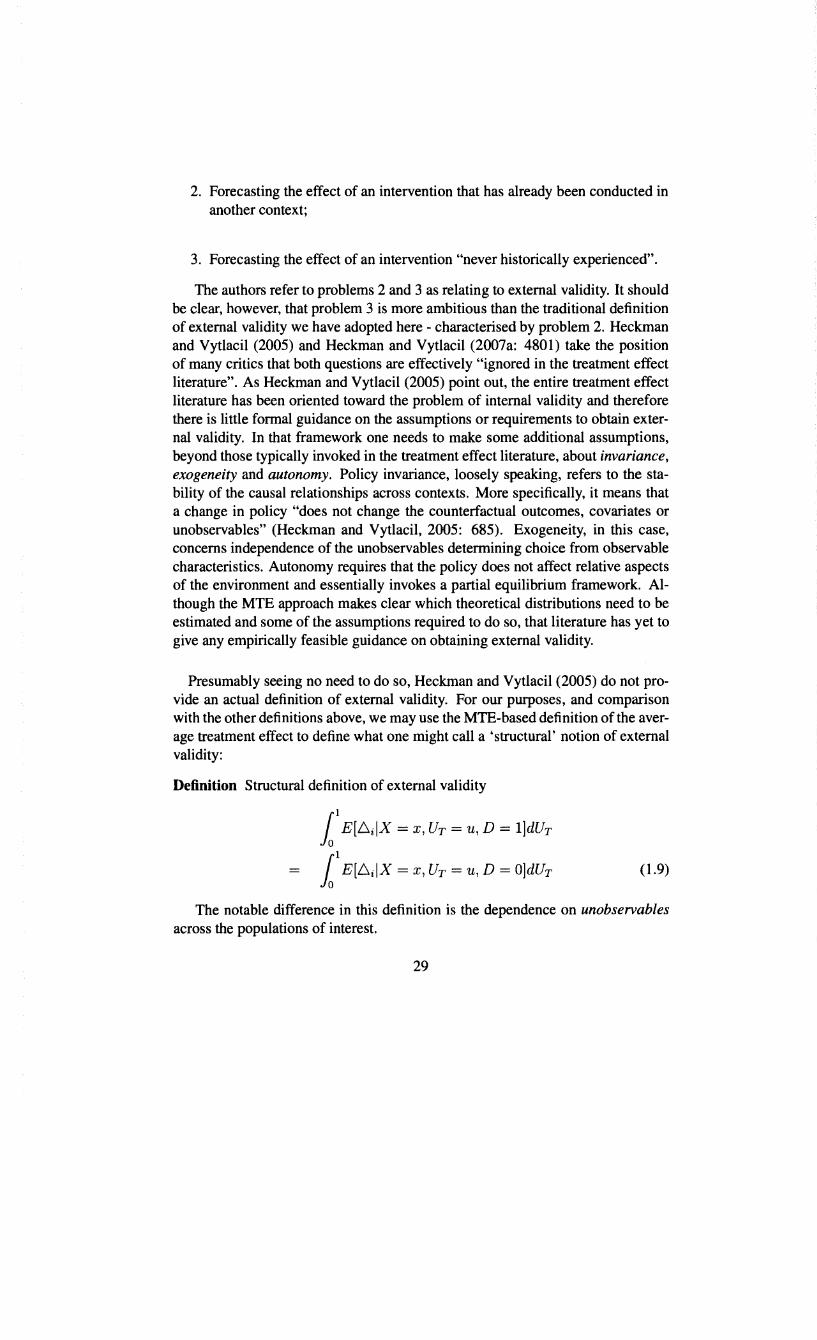
Univers

ity of

Cap

e Tow

n

2. Forecasting the effect of an intervention that has already been conducted in another context;

3. Forecasting the effect of an intervention "never historically experienced".

The authors refer to problems 2 and 3 as relating to external validity. It should be clear, however, that problem 3 is more ambitious than the traditional definition of external validity we have adopted here - characterised by problem 2. Heckman and Vytlacil (2005) and Heckman and Vytlacil (2007a: 4801) take the position of many critics that both questions are effectively "ignored in the treatment effect literature". As Heckman and Vytlacil (2005) point out, the entire treatment effect literature has been oriented toward the problem of internal validity and therefore there is little formal guidance on the assumptions or requirements to obtain exter­nal validity. In that framework one needs to make some additional assumptions, beyond those typically invoked in the treatment effect literature, about invariance, exogeneity and autonomy. Policy invariance, loosely speaking, refers to the sta­bility of the causal relationships across contexts. More specifically, it means that a change in policy "does not change the counterfactual outcomes, covariates or unobservables" (Heckman and Vytlacil, 2005: 685). Exogeneity, in this case, concerns independence of the unobservables determining choice from observable characteristics. Autonomy requires that the policy does not affect relative aspects of the environment and essentially invokes a partial equilibrium framework. Al­though the MTE approach makes clear which theoretical distributions need to be estimated and some of the assumptions required to do so, that literature has yet to give any empirically feasible guidance on obtaining external validity.

Presumably seeing no need to do so, Heckman and Vytlacil (2005) do not pro­vide an actual definition of external validity. For our purposes, and comparison with the other definitions above, we may use the MTE-based definition of the aver­age treatment effect to define what one might call a 'structural' notion of external validity:

Definition Structural definition of external validity

11

E[6iiX = x, Ur = u, D = l]dUr

11

E[6iiX = x, Ur = u, D = O]dUr (1.9)

The notable difference in this definition is the dependence on unobservables across the populations of interest.

29

Univers

ity of

Cap

e Tow

n

Given the above one may wonder why economists, or indeed any researchers, wanting to conduct programme evaluations would adopt anything other than a structural econometrics approach. While possibly the most theoretically compre­hensive framework for evaluation, structural econometrics is not without prob­lems. Two in particular stand out. The first is theoretical: formulating a structural model requires extensive theoretical assumptions many of which are not, or cannot be, empirically verified. Manski (2000) notes, in relation to the earlier literature, that latent index models have not been uncontroversial and that "some researchers have regarded these models as ill-motivated imputation rules whose functional form and distributional assumptions lack foundation" (Manski, 2000: 431 ). The second reason, already noted, is empirical: the information required in order to estimate structural models is often unavailable. Heckman and Vytlacil (2007a: 481 0) note four types of data required: private preferences; social preferences; ex ante distributions of outcomes in alternative states; and, ex post information regarding the relevant outcomes. Although the authors note that there exist litera­tures on the first two, there is little convincing evidence that satisfactory empirical derivation of preferences at any level has been achieved. It therefore remains an open question whether it is feasible to obtain data on all the relevant dimensions since this in itself rests on contested theoretical assumptions. For example, there are now a wide range of competing models of choice in the theoretical microeco­nomics literature and as yet no consensus on which of these ought to be employed to infer well-ordered preferences (or even whether well-ordered preferences exist for all individuals).

Both issues explain, to some extent, why despite its own limitations the 'design­based' approach to programme evaluation has gained so much popularity in eco­nomics in recent decades. The unquestionably valuable contributions of the struc­tural literature are to locate the effects estimated using experiments within a more general model of mechanisms and economic behaviour, as well as revealing the strong implicit assumptions required for treatment effects from randomisation to inform a decision-making process as framed by economic theory. In the anal­ysis of the next section we will essentially ignore the complications that arise from considering choice-based compliance with treatment assignment, not be­cause these are unimportant in general but because our objective is to isolate what are arguably even more basic challenges for external validity.

30

Univers

ity of

Cap

e Tow

n

1.2.6 Decision-theoretic approaches to treatment effects and welfare

A strand of the theoretical literature (Heckman, Smith, and Clements ( 1997), Heckman and Smith (1998), Manski (2000), Dehejia (2005)) related to structural contributions on treatment effect estimation considers the implications of treat­ment effect heterogeneity for optimal policy decisions, where a "planner wants to choose a treatment rule that maximizes the population mean outcome" (Manski, 2000: 417). Following Manski (2000: 423-424), an individual j in population J has a treatment response function Yj ( ·) : T -+ Y. The policymaker needs to specify a treatment rule for each j but only has at their disposal a set of ob­servable characteristics for each individual, x j E X. 22 There is then a set of functions/treatment rules, b E B where B : X -+ T, mapping characteristics to treatment assignment. Given the emphasis on the mean outcome, the problem of interest is:

max E{y[b(x)]} b(-)EB

An optimal treatment rule, b*, is one that maximises expected outcomes con­ditional on individual characteristics:

b*(x) = argmaxE[y(t)lx], x EX (1.10) tET

There are perhaps two key considerations in this literature. The first is the na­ture of the decision maker's welfare function as defined over the full distribution of treatment effects. The above formulation is most compatible with a utilitarian so­cial welfare function, but others - such as the Rawlsian welfare function in which the well-being of the worst off individual is maximised - will be associated with different optimal treatment rules. Particularly challenging is that some welfare functions depend on the full distribution of outcomes. The second critical issue is the information available to the decision maker from econometric analysis. In this regard, an important consideration - emphasised in particular by Manski (2000) -is the relevance of uncertainty and ambiguity in relation to estimated effects that arises from making, often unverifiable, estimating assumptions. In a construc­tive vein Manski (2011, 2013a) argues for greater recognition of the salience of identifying assumptions by, where possible, reporting appropriate bounds on es­timated effects rather than simple point estimates. In many instances only strong assumptions produce informative bounds.

22For an alternative approach, see Berger, Black, and Smith (200 1) on the use of 'statistical profiling' to allocate individuals to government programmes.

31

Univers

ity of

Cap

e Tow

n

It is interesting, given our preceding discussion of the medical literature, that Manski (2000) gives as a practical example of the generic decision problem, the case of a medical practitioner in possession of reported results from a randomised trial who is considering whether to allocate treatment to specific patients. Dehejia (2005) similarly considers a case in which there is a caseworker with individual­specific information and a policymaker who decides whether to have a uniform treatment rule (all or no individuals given treatment), or to allow the caseworker discretion to decide. Such formulations raise interesting questions about the ben­efits of decentralisation versus central planning. Another notable aspect of the decision problem is that while the physician in Manski's example "has extensive covariate information ... for the patients", the "medical journal articles that report the findings of clinical trials, however, do not usually report extensive covariate in­formation for the subjects of the experiment" (Manski, 2000: 433). Allocation of treatment is most simple when there is no variation in the treatment effect across covariates, but when that is not the case an optimal decision requires covariate­specific information. 23 One complication emphasised by Manski is that in the presence of uncertainty regarding individual response functions - in other words, variation in response exists even among individuals with the same observed co­variate values- more covariate information is always weakly beneficial; additional information never leads to a less optimal choice of treatment rule. Where there is ambiguity about responses this need not be true.

As with the literature surveyed in the previous subsection, there is much to rec­ommend the logic and theoretical insights of such contributions, even if they are often practically hard to implement or produce bounds on estimated effects that are very wide. In the analysis of the next section it suffices to show how external validity may fail without actually formalising the policymaker's decision process in this manner. If certain factors imply that a given programme simply does not work in the population of interest, then the form of the social welfare function is obviously of secondary concern. This is not in any way to caricature what are thorough and subtle studies: both cited authors have also addressed external va­lidity concerns as distinct from the decision making problem, as is made clear in Manski (2013a), as well as the contributions in Manski (2011, 2013b) and Dehejia (2013).

Where these contributions do have some relevance for our analysis is in framing the idea of external validity. The basic definition provided in 1.4 can be thought

23Relatedly, while exclusion and inclusion criteria can be a downside of medical trials, they can also be (as also noted by Ravallion (2009)) desirable in as much as in some cases they reflect a tailoring of an experiment to the likely recipients.

32

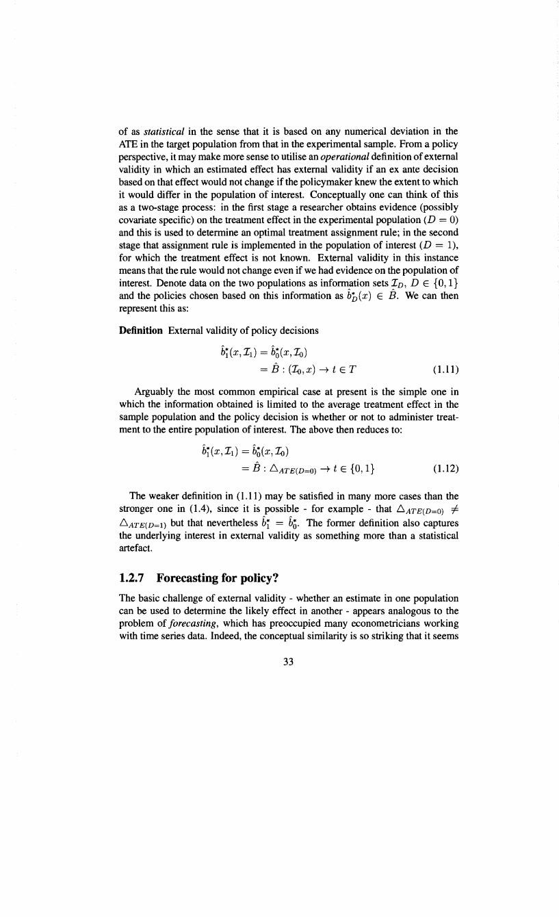
Univers

ity of

Cap

e Tow

n

of as statistical in the sense that it is based on any numerical deviation in the ATE in the target population from that in the experimental sample. From a policy perspective, it may make more sense to utilise an operational definition of external validity in which an estimated effect has external validity if an ex ante decision based on that effect would not change if the policymaker knew the extent to which it would differ in the population of interest. Conceptually one can think of this as a two-stage process: in the first stage a researcher obtains evidence (possibly covariate specific) on the treatment effect in the experimental population (D = 0) and this is used to determine an optimal treatment assignment rule; in the second stage that assignment rule is implemented in the population of interest (D = 1), for which the treatment effect is not known. External validity in this instance means that the rule would not change even if we had evidence on the population of interest. Denote data on the two populations as information sets Iv, D E {0, 1} and the policies chosen based on this information as h'D ( x) E B. We can then represent this as:

Definition External validity of policy decisions

b~ (x, Il) = b~(x, Io)

= B : (Io, X) --+ t E T (1.11)

Arguably the most common empirical case at present is the simple one in which the information obtained is limited to the average treatment effect in the sample population and the policy decision is whether or not to administer treat­ment to the entire population of interest. The above then reduces to:

b~(x, Il) = b~(x, Io)

= B: 6.ATE(D=O)--+ t E {0, 1} (1.12)

The weaker definition in ( 1.11) may be satisfied in many more cases than the stronger one in (1.4), since it is possible - for example - that 6.ATE(D=O) =!= 6.ATE(D=l) but that nevertheless hi = h0. The former definition also captures the underlying interest in external validity as something more than a statistical artefact.

1.2. 7 Forecasting for policy?

The basic challenge of external validity - whether an estimate in one population can be used to determine the likely effect in another - appears analogous to the problem of forecasting, which has preoccupied many econometricians working with time series data. Indeed, the conceptual similarity is so striking that it seems

33

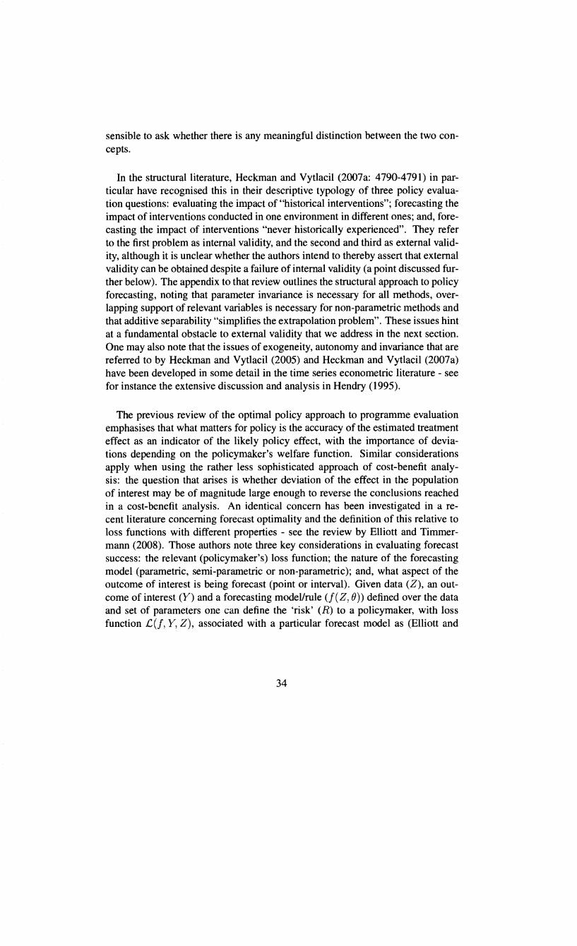
Univers

ity of

Cap

e Tow

n

sensible to ask whether there is any meaningful distinction between the two con­cepts.

In the structural literature, Heckman and Vytlacil (2007a: 4790-4791) in par­ticular have recognised this in their descriptive typology of three policy evalua­tion questions: evaluating the impact of "historical interventions"; forecasting the impact of interventions conducted in one environment in different ones; and, fore­casting the impact of interventions "never historically experienced". They refer to the first problem as internal validity, and the second and third as external valid­ity, although it is unclear whether the authors intend to thereby assert that external validity can be obtained despite a failure of internal validity (a point discussed fur­ther below). The appendix to that review outlines the structural approach to policy forecasting, noting that parameter invariance is necessary for all methods, over­lapping support of relevant variables is necessary for non-parametric methods and that additive separability "simplifies the extrapolation problem". These issues hint at a fundamental obstacle to external validity that we address in the next section. One may also note that the issues of exogeneity, autonomy and invariance that are referred to by Heckman and Vytlacil (2005) and Heckman and Vytlacil (2007a) have been developed in some detail in the time series econometric literature - see for instance the extensive discussion and analysis in Hendry (1995).

The previous review of the optimal policy approach to programme evaluation emphasises that what matters for policy is the accuracy of the estimated treatment effect as an indicator of the likely policy effect, with the importance of devia­tions depending on the policymaker's welfare function. Similar considerations apply when using the rather less sophisticated approach of cost-benefit analy­sis: the question that arises is whether deviation of the effect in the population of interest may be of magnitude large enough to reverse the conclusions reached in a cost-benefit analysis. An identical concern has been investigated in a re­cent literature concerning forecast optimality and the definition of this relative to loss functions with different properties - see the review by Elliott and Timmer­mann (2008). Those authors note three key considerations in evaluating forecast success: the relevant (policymaker's) loss function; the nature of the forecasting model (parametric, semi-parametric or non-parametric); and, what aspect of the outcome of interest is being forecast (point or interval). Given data (Z), an out­come of interest (Y) and a forecasting model/rule (f(Z, 0)) defined over the data and set of parameters one can define the 'risk' (R) to a policymaker, with loss function £(!, Y, Z), associated with a particular forecast model as (Elliott and

34

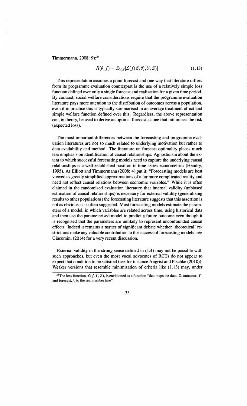
Univers

ity of

Cap

e Tow

n

Timmermann, 2008: 9):24

R(O, f)= Ey,z[.C(J(Z, 0), Y, Z)] (1.13)

This representation assumes a point forecast and one way that literature differs from its programme evaluation counterpart is the use of a relatively simple loss function defined over only a single forecast and realisation for a given time period. By contrast, social welfare considerations require that the programme evaluation literature pays more attention to the distribution of outcomes across a population, even if in practice this is typically summarised in an average treatment effect and simple welfare function defined over this. Regardless, the above representation can, in theory, be used to derive an optimal forecast as one that minimises the risk (expected loss).

The most important differences between the forecasting and programme eval­uation literatures are not so much related to underlying motivation but rather to data availability and method. The literature on forecast optimality places much less emphasis on identification of causal relationships. Agnosticism about the ex­tent to which successful forecasting models need to capture the underlying causal relationships is a well-established position in time series econometrics (Hendry, 1995). As Elliott and Timmermann (2008: 4) put it: "Forecasting models are best viewed as greatly simplified approximations of a far more complicated reality and need not reflect causal relations between economic variables." While it is often claimed in the randomised evaluation literature that internal validity (unbiased estimation of causal relationships) is necessary for external validity (generalising results to other populations) the forecasting literature suggests that this assertion is not as obvious as is often suggested. Most forecasting models estimate the param­eters of a model, in which variables are related across time, using historical data and then use the parameterised model to predict a future outcome even though it is recognised that the parameters are unlikely to represent unconfounded causal effects. Indeed it remains a matter of significant debate whether 'theoretical' re­strictions make any valuable contribution to the success of forecasting models; see Giacomini (20 14) for a very recent discussion.

External validity in the strong sense defined in ( 1.4) may not be possible with such approaches, but even the most vocal advocates of RCTs do not appear to expect that condition to be satisfied (see for instance Angrist and Pischke (2010)). Weaker versions that resemble minimisation of criteria like ( 1.13) may, under

24The loss function, C(f, Y, Z), is envisioned as a function "that maps the data, Z, outcome, Y, and forecast,f, to the real number line".

35

Univers

ity of

Cap

e Tow

n

certain circumstances, allow studies that lack internal validity to outperform those that do in forecasting outcomes in new populations.

As should be evident from the discussion in section 1.1, approaches that ne­glect the relationship between estimated models and the data generating process ('true structural equation') are considered untenable in microeconometrics. This is quite understandable given that the concern of much of the applied microe­conometrics literature has been in identifying the relationships between specific variables, net of confounding by others. That need not, however, provide the best methodological basis for addressing the challenge of predicting the effects of policy interventions and some researchers outside economics (Pearl, 2009) have argued forcefully that a different paradigm is required. However, the contrast with the time series forecasting literature indicates also that the limited time peri­ods available in most microeconometric datasets constrain prospects for a similar approach to developing forecasts; there is too little data available over too widely­spaced intervals to calibrate models based on forecasts. As a partly related issue, one may note that the question of parameter stability has been directly addressed -albeit not resolved - in the forecasting literature, whereas even the most advanced theoretical literatures in microeconometrics have yet to tackle this problem in any substantive way.

This comparison suggests that from a policy perspective there is no meaning­ful conceptual difference between external validity and forecast accuracy. The academic distinction arises from data availability, the definition of the welfare function over a population rather than a single outcome and the established focus of microeconometrics on identifying causal relationships.

1.2.8 Summary

The approaches to the basic external validity question in the areas surveyed each have their own favoured emphasis and, particularly within economics, formal frameworks for addressing the problem of transporting estimated effects from one population to another. In some instances these differences in emphasis draw at­tention to different possible definitions of the concept. Nevertheless, a number of common themes are discernible. First, that the vast majority of contributions con­sider it highly unlikely that simple external validity will hold for most questions and populations of interest. Second, that similarity between populations is funda­mental to the extrapolation problem. Such similarities might be determined qual­itatively, as in the method of 'analogical reasoning' advocated by some philoso­phers. What the issue of similarity brings to the fore in formal frameworks is the

36

Univers

ity of

Cap

e Tow

n

relevance of covariates, or characteristics of individuals. The issue can then be associated with assumptions/requirements for overlapping supports of variables across populations. This is particularly interesting because similar assumptions are required for obtaining internal validity, but where the populations are the 're­cipients' and 'non-recipients' of the treatment of interest. A final theme is the importance of structure for extrapolation, whether in the form of fully developed models or, at least, more detailed information on the nature of causal relations besides only estimated mean effects.

In the next section we present a simple framework in which to further consider these issues and attempt to draw some implications for making policy claims using estimates derived within the experimental tradition. By assuming perfect compli­ance with treatment assignment we remove the many complications introduced in the instrumental variables literature, including new developments there relating to selection and marginal treatment effects, and yet still find substantial barriers to extrapolation. Our analysis builds on Hotz et al. (2005), as do Allcott and Mul­lainathan (2012) who reach some similar conclusions albeit with a rather more optimistic emphasis.

37

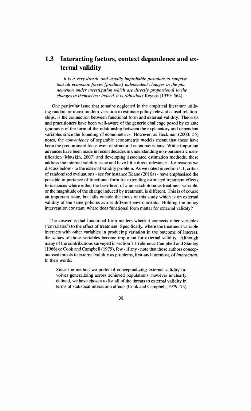
Univers

ity of

Cap

e Tow

n

1.3 Interacting factors, context dependence and ex­ternal validity

it is a very drastic and usually improbable postulate to suppose that all economic forces [produce] independent changes in the phe­nomenon under investigation which are directly proportional to the changes in themselves; indeed, it is ridiculous Keynes (1939: 564)

One particular issue that remains neglected in the empirical literature utilis­ing random or quasi-random variation to estimate policy-relevant causal relation­ships, is the connection between functional form and external validity. Theorists and practitioners have been well-aware of the generic challenge posed by ex ante ignorance of the form of the relationship between the explanatory and dependent variables since the founding of econometrics. However, as Heckman (2000: 55) notes, the convenience of separable econometric models meant that these have been the predominant focus even of structural econometricians. While important advances have been made in recent decades in understanding non-parametric iden­tification (Matzkin, 2007) and developing associated estimation methods, these address the internal validity issue and have little direct relevance - for reasons we discuss below - to the external validity problem. As we noted in section 1.1, critics ofrandomised evaluations- see for instance Keane (2010a)- have emphasised the possible importance of functional form for extending estimated treatment effects to instances where either the base level of a non-dichotomous treatment variable, or the magnitude of the change induced by treatment, is different. This is of course an important issue, but falls outside the focus of this study which is on external validity of the same policies across different environments. Holding the policy intervention constant, where does functional form matter for external validity?

The answer is that functional form matters where it connects other variables ('covariates') to the effect oftreatment. Specifically, where the treatment variable interacts with other variables in producing variation in the outcome of interest, the values of those variables become important for external validity. Although many of the contributions surveyed in section 1.1 reference Campbell and Stanley ( 1966) or Cook and Campbell ( 1979), few - if any - note that those authors concep­tualised threats to external validity as problems, first-and-foremost, of interaction. In their words:

Since the method we prefer of conceptualizing external validity in­volves generalizing across achieved populations, however unclearly defined, we have chosen to list all of the threats to external validity in terms of statistical interaction effects (Cook and Campbell, 1979: 73)

38

Univers

ity of

Cap

e Tow

n

The authors identify three different forms of interaction. The first, which they refer to as 'interaction of selection and treatment', concerns the possibility that the characteristics of those in an experimental sample are affected by the demands of participation. This to some extent captures the intuition of the choice-based latent variable approach discussed above in relation to structural econometric models. The second is 'interaction of setting and treatment', by which the authors seem to mean in particular the institutional environment (contrasting a bureaucracy with a university campus or military camp). The third possibility they consider is that historical context may interact with treatment to affect the outcome. In some sense, each of these 'threats' reflects a different mechanism by which an exper­imental sample may become unrepresentative along dimensions that have some bearing on the effect of treatment. This is most clear from the fact that the solu­tions Cook and Campbell (1979) propose to avoid, or remedy, failures of external validity primarily concern sampling methods - an issue we address further in sec­tion 1.3.3.

The remainder of this review utilises the idea of interaction between the treat­ment variable and other factors as a basis for structuring what we believe to be the basic challenges for external validity and providing an alternative perspective on other analyses that have identified those challenges.

1.3.1 Interactive functional forms and external validity

To represent the above concerns in econometric form we might simply extend the standard representation of potential outcomes provided in section 1.1 as follows. A dichotomous treatment variable, T E {0, 1 }, is associated with average effects To and T1 that are independent of covariates.25 Consider two sets of covariates, X and W, which we assume for simplicity are independent of treatment assign­ment.26 Furthermore, the effect of covariates (W) on potential outcomes is itself dependent on treatment.

Yo = To + X /3 + W "( + uo

y1 = T1 + X /3 + w ( 6 + "() + U1

Then we can write the average treatment effect as:

E[Y1- Yo]= (T1- To)+ E[WJT = 1]6 (1.14)

25It is fairly straightforward to extend the analysis to the case where the treatment variable is not dichotomous, taking on values To in the 'control group' and T1 in the 'treatment group'.

26Note that this is not the same as the unconfoundedness conditions mentioned previously, which assume that assignment is independent of potential outcomes conditional on covariates.

39

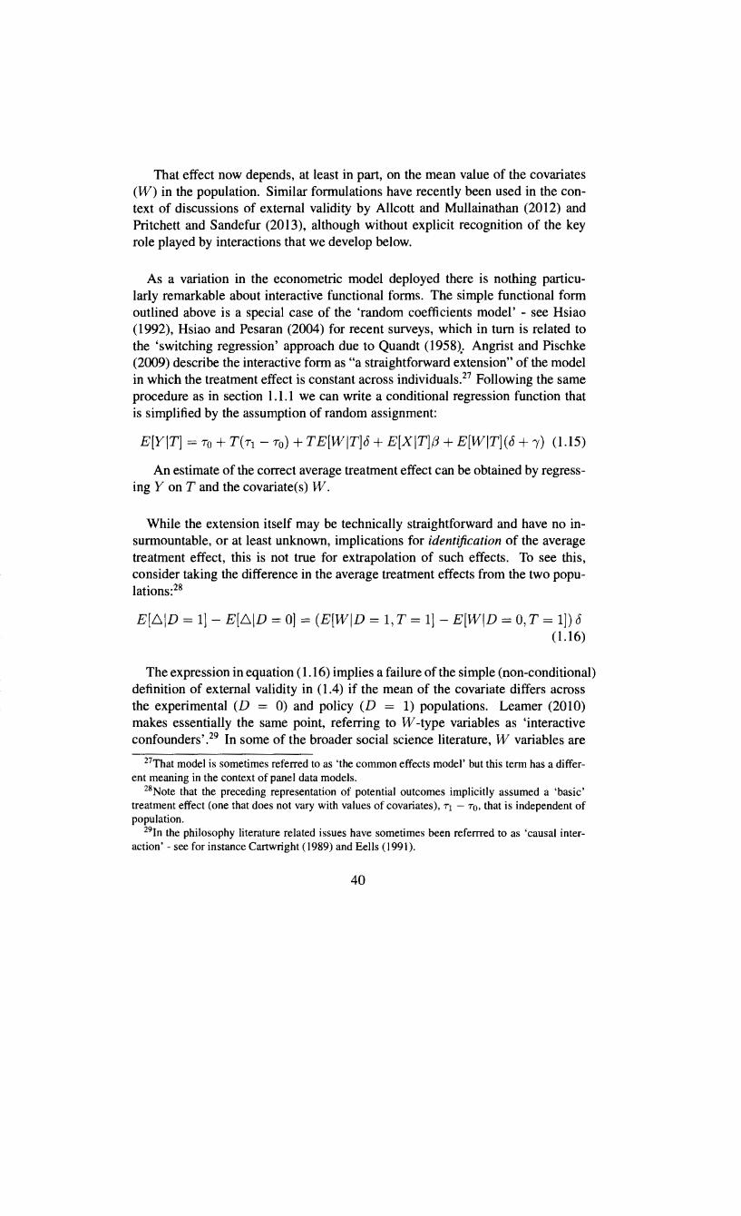
Univers

ity of

Cap

e Tow

n

That effect now depends, at least in part, on the mean value of the covariates (W) in the population. Similar formulations have recently been used in the con­text of discussions of external validity by Allcott and Mullainathan (2012) and Pritchett and Sandefur (2013), although without explicit recognition of the key role played by interactions that we develop below.

As a variation in the econometric model deployed there is nothing particu­larly remarkable about interactive functional forms. The simple functional form outlined above is a special case of the 'random coefficients model' - see Hsiao (1992), Hsiao and Pesaran (2004) for recent surveys, which in tum is related to the 'switching regression' approach due to Quandt (1958),. Angrist and Pischke (2009) describe the interactive form as "a straightforward extension" of the model in which the treatment effect is constant across individuals.27 Following the same procedure as in section 1.1.1 we can write a conditional regression function that is simplified by the assumption of random assignment:

E[Y\T] =To+ T(Tl- To)+ TE[W\T]£5 + E[X\T],B + E[W\T](£5 + r) (1.15)

An estimate of the correct average treatment effect can be obtained by regress­ing Yon T and the covariate(s) W.

While the extension itself may be technically straightforward and have no in­surmountable, or at least unknown, implications for identification of the average treatment effect, this is not true for extrapolation of such effects. To see this, consider taking the difference in the average treatment effects from the two popu­lations:28

E[6\D = 1]- E[6\D =OJ = (E[W\D = 1, T = 1] - E[W\D = 0, T = 1]) 6 (1.16)

The expression in equation ( 1.16) implies a failure of the simple (non-conditional) definition of external validity in (1.4) if the mean of the covariate differs across the experimental (D = 0) and policy (D = 1) populations. Leamer (2010) makes essentially the same point, referring to W -type variables as 'interactive confounders'. 29 In some of the broader social science literature, W variables are

27That model is sometimes referred to as 'the common effects model' but this term has a differ­ent meaning in the context of panel data models.

28Note that the preceding representation of potential outcomes implicitly assumed a 'basic' treatment effect (one that does not vary with values of covariates), T1 -To, that is independent of population.

29In the philosophy literature related issues have sometimes been referrred to as 'causal inter­action' -see for instance Cartwright (1989) and Eells (1991).

40

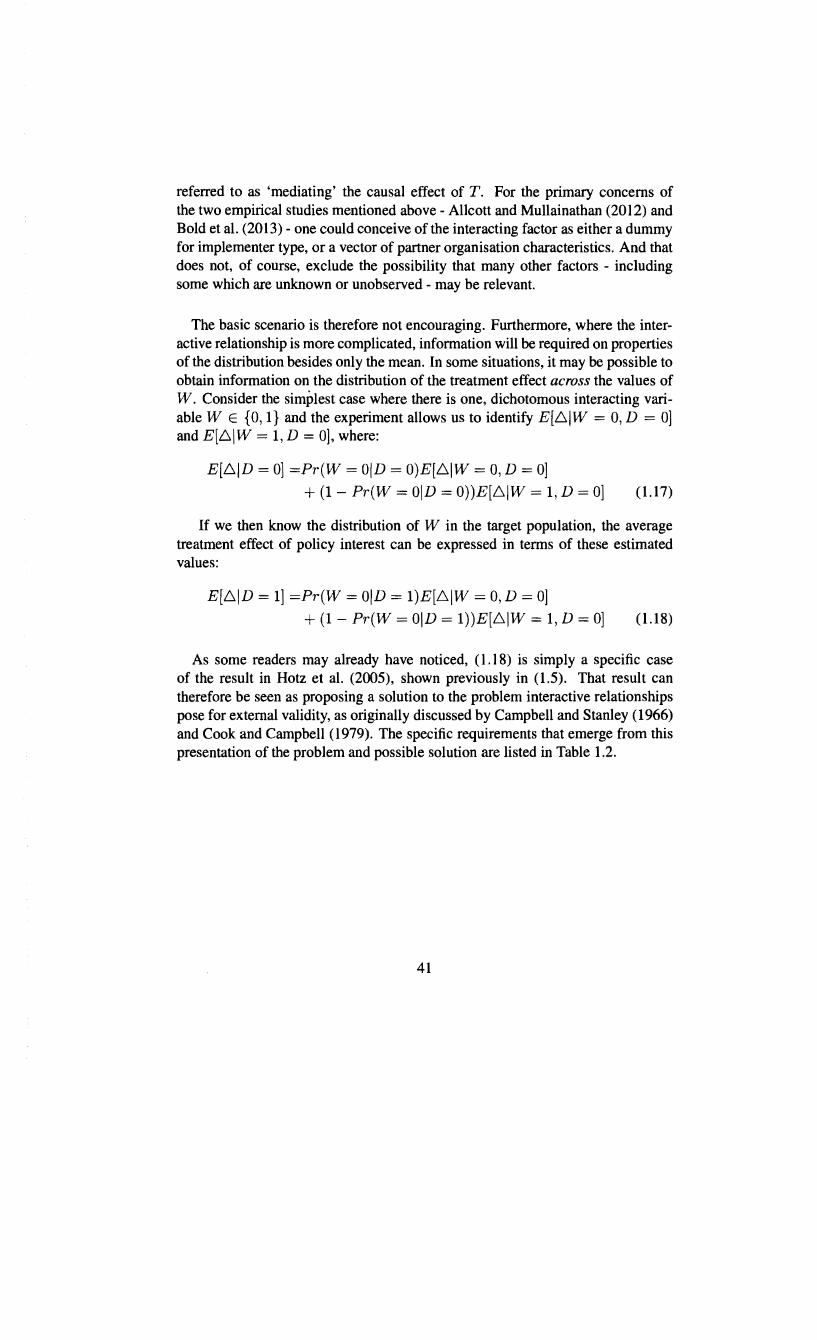
Univers

ity of

Cap

e Tow

n

referred to as 'mediating' the causal effect ofT. For the primary concerns of the two empirical studies mentioned above- Allcott and Mullainathan (2012) and Bold et al. (2013)- one could conceive of the interacting factor as either a dummy for implementer type, or a vector of partner organisation characteristics. And that does not, of course, exclude the possibility that many other factors - including some which are unknown or unobserved - may be relevant.

The basic scenario is therefore not encouraging. Furthermore, where the inter­active relationship is more complicated, information will be required on properties of the distribution besides only the mean. In some situations, it may be possible to obtain information on the distribution of the treatment effect across the values of W. Consider the simplest case where there is one, dichotomous interacting vari­able W E {0, 1} and the experiment allows us to identify E[6IW = 0, D =OJ and E[6IW = 1, D =OJ, where:

E[6ID =OJ =Pr(W =OlD= O)E[6IW = 0, D =OJ

+ (1- Pr(W =OlD= O))E[6IW = 1, D =OJ (1.17)

If we then know the distribution of W in the target population, the average treatment effect of policy interest can be expressed in terms of these estimated values:

E[6ID = 1J =Pr(W =OlD= 1)E[6IW = 0, D =OJ

+ (1- Pr(W =OlD= 1))E[6IW = 1, D =OJ (1.18)

As some readers may already have noticed, ( 1.18) is simply a specific case of the result in Hotz et al. (2005), shown previously in (1.5). That result can therefore be seen as proposing a solution to the problem interactive relationships pose for external validity, as originally discussed by Campbell and Stanley (1966) and Cook and Campbell (1979). The specific requirements that emerge from this presentation of the problem and possible solution are listed in Table 1.2.

41

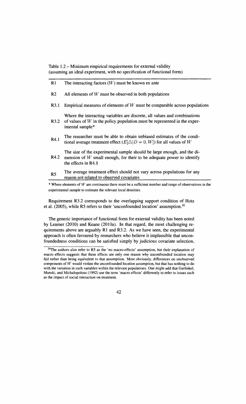
Univers

ity of

Cap

e Tow

n

Table 1.2 - Minimum empirical requirements for external validity (assuming an ideal experiment, with no specification of functional form)

R1

R2

R3.1

R3.2

R4.1

R4.2

R5

The interacting factors (W) must be known ex ante

All elements of W must be observed in both populations

Empirical measures of elements of W must be comparable across populations

Where the interacting variables are discrete, all values and combinations of values of W in the policy population must be represented in the exper­imental sample*

The researcher must be able to obtain unbiased estimates of the condi­tional average treatment effect (E[L.ID = 0, W]) for all values of W

The size of the experimental sample should be large enough, and the di­mension of W small enough, for their to be adequate power to identify the effects in R4.1

The average treatment effect should not vary across populations for any reason not related to observed covariates

* Where elements of W are continuous there must be a sufficient number and range of observations in the

experimental sample to estimate the relevant local densities.

Requirement R3.2 corresponds to the overlapping support condition of Hotz et al. (2005), while R5 refers to their 'unconfounded location' assumption.30

The generic importance of functional form for external validity has been noted by Leamer (2010) and Keane (2010a). In that regard, the most challenging re­quirements above are arguably R1 and R3.2. As we have seen, the experimental approach is often favoured by researchers who believe it implausible that uncon­foundedness conditions can be satisfied simply by judicious covariate selection,

30The authors also refer to RS as the 'no macro-effects' assumption, but their explanation of macro effects suggests that these effects are only one reason why unconfounded location may fail rather than being equivalent to that assumption. Most obviously, differences on unobserved components of W would violate the unconfounded location assumption, but that has nothing to do with the variation in such variables within the relevant populations. One might add that Garfinkel, Manski, and Michalopolous (1992) use the term 'macro effects' differently to refer to issues such as the impact of social interaction on treatment.

42

Univers

ity of

Cap

e Tow

n

or clever structural modelling. However, to know in advance what the interacting factors are must require some reliable theoretical knowledge. Worse, it is widely recognised that there is often no persuasive theoretical reason to choose one func­tional form over another. This has spurred the literature on non-parametric estima­tion but, as should be clear from the above framework, non-parametric estimation of the average treatment effect is insufficient for extrapolation. As (Heckman and Vytlacil, 2007a: 4855) put it, "To extend some function ... to a new support requires functional structure: It cannot be extended outside of sample support by a purely nonparametric procedure". This point, more than any other, is underemphasised or unacknowledged in contributions to the experimental literature. Relatedly, we must have good reasons to believe that measured variables are comparable across populations. For example, how does one compare racial categories across pop­ulations of different countries for the purposes of reweighting treatment effects? There may be theoretical concerns that 'race' is a notion with different meaning in different societies and that therefore there is no common variable across such populations. More obviously, different categorisations may be used in different populations so that the available variables are not comparable.

The availability of information on the treatment effect across the support of interacting variables also has important implications for decision making. Manski summarises the problem as follows:

The physician may have extensive covariate information for his own patients but the journal report of the clinical trial may only report out­comes within broad risk-factor groups ... However the available exper­imental evidence, lacking covariate data, only reveals mean outcomes in the population as a whole, not mean outcomes conditional on co­variates. Hence the planner faces a problem of treatment choice under ambiguity.Manski (2000: 419)

Interaction in itself is not an obstacle to estimating the average treatment ef­fect in the experimental sample. In the context of estimating the ATE using a regression, even if the nature of the interactions are unknown a regression on the treatment variable that only conditions on the relevant covariates - but omits inter­action terms - will produce an unbiased estimate. This follows from the general result- see for instance Wooldridge (2002: 21) - that E[YjX, W, f(X, W)] = E[YjX, W], provided E[YjX, W] is linear in the parameters. However, predict­ing the average treatment effect in another population using the estimated param­eters would require the original functional form to have been correctly specified.

43

Univers

ity of

Cap

e Tow

n

The bottom line is that unless researchers have accurate ex ante beliefs about the factors that interact with the treatment variable and are able to collect data on these, forecasting effects of treatment in new populations will be a matter of luck. The framework based on interactive functional forms suggests that this can take three forms: that the causal effect happens to be approximately the same across individuals; that the causal effect does not actually depend on the values of other variables (additive separability); or, that there is little variation in the mean values of the interacting variables across contexts.

1.3.2 Heterogeneity of treatment effects

Given the above one might expect guides for empirical practice to address the is­sue in some detail, but discussion of interaction terms is absent from some of the main 'manuals' for conducting analysis based on randomised evaluations (Angrist and Pischke (2009), Duflo et al. (2006b)) - an omission also noted by Gelman (2000). To the extent that these issues have received any widespread attention in the treatment effect literature it has primarily been in relation to studies that ex­amine 'treatment effect heterogeneity' within experimental populations, in other words the extent to which an estimated treatment effect varies across subgroups. In that vein, while Allcott and Mullainathan (2012) and, more recently, Pritch­ett and Sandefur (2013) both utilise representations of potential outcomes similar to the ones deployed above, those authors place little emphasis on the role of functional form per se, rather simply proceeding from the assumption that- for whatever reason - treatment effects vary with covariate values. We now briefly examine this heterogeneity-premised approach.

If the treatment effect were constant for all individuals in the entire population then external validity would, necessarily, hold. Variation in the treatment effect is sometimes referred to in the literature as 'treatment heterogeneity', but this term is not used consistently. Specifically, it is important for our purposes to distinguish between three conceptions of treatment heterogeneity. The first, and arguably more common use of the term to date, focuses on heterogeneity relating to the presence of compliers and non-compliers in instrumental variable estimation of local average treatment effects - see for instance Angrist (2004) and the discussion in Angrist and Pischke (2009). The second refers to some fundamental level of randomness that produces 'intrinsic' variation in the effect across individuals with identical characteristics. The third concerns the existence of empirical variation in the average treatment effect itself across values of covariates. These obviously need not be mutually exclusive, since if the characteristics of compliers and non­compliers differ then that would manifest as heterogeneity across the covariates

44

Univers

ity of

Cap

e Tow

n

representing these characteristics. Contributions on external validity have mir­rored this distinction: Angrist and Fernandez-Val (2010, 2013) present an anal­ysis of the extrapolation/external validity problem focused on compliance in the case of estimating LATEs, whereas Hotz et al. (2005), Crump, Hotz, Imbens, and Mitnik (2008) and Crump, Hotz, Imbens, and Mitnik (2009) provide definitions of external validity based only on variation in the treatment effect across covariate values. In part contrast to these, structural approaches distinguish themselves in examining variation in behavioural responses to treatment across different popu­lations- see for instance Heckman and Vytlacil (2005).

Having assumed perfect compliance, assumed-away selection based on choice and having no particular interest in intrinsic heterogeneity, what is relevant to the present review is variation across covariates. The way in which that has been addressed in the literature is largely unsatisfactory. Authors typically conduct het­erogeneity analyses across subgroups that are defined after the experiment has been completed, based on covariate data that was collected to establish success of random assignment or to justify a conditional unconfoundedness assumption. "At best, researchers have estimated average effects for subpopulations defined by categorical individual characteristics" Crump et al. (2008: 398), but this is typically ad hoc (see also Deaton, 2008, 2010). In some instances it could quite plausibly be argued that this constitutes specification searching without compen­sating adjustments for the statistical significance of results. Rothwell (2005b) makes similar points in relation to the medical literature; Schochet (2008) pro­vides a set of guidelines for education evaluations; and, Fink, McConnell, and Vollmer (20 13) provide an overview of such practices in development economics along with some, standard, suggestions regarding correction for multiple hypothe­sis testing. Abadie, Chingos, and West (2013) address a related problem in which researchers examine heterogeneity across subgroups defined by the outcome vari­able- what those authors refer to as 'endogenous stratification'.

Some more systematic methods have been proposed. Hotz et al. (2005) pro­pose a method for testing the unconfoundedness assumption across two experi­mental populations by comparing the actual mean outcomes for controls to those predicted using data from the other population. Perhaps most notable is the con­tribution of Crump et al. (2008) who develop two non-parametric tests: the first is of the null hypothesis of zero average treatment effect conditional on a set of observable covariates in subpopulations (as defined by the covariates); the second is for the null hypothesis that the conditional average treatment effect is the same across subpopulations, in other words a test of treatment heterogeneity across the variable(s) defining the subgroups. Djebbari and Smith (2008) utilise a number

45

Univers

ity of

Cap

e Tow

n

of other methods to test for heterogeneity in data on the PROGRESA conditional cash transfer program implemented in Mexico. The authors make some effort to account for multiple tests and consider various non-parametric bounds of the vari­ance of treatment effects. Allcott and Mullainathan (2012) also suggest a particu­lar F-test of whether treatment effects vary within sub-groups of the experimental population as defined by covariate values. It is essentially a test for joint signifi­cance of the parameters on the interaction terms between sub-group dummies and the treatment variable. This would appear to be a version of the more general case proposed by Crumpet al. (2008).31 The authors discuss potential empirical obsta­cles to this approach, such as a possible lack of power caused by small samples and the fact that in-and-of itself the test provides no basis for extrapolating to a new population. As they note, the greatest value of such tests is likely to be where the null hypothesis of no sub-group variation is rejected.

In their comment on external validity, Pritchett and Sandefur (20 13) examine variation in estimates of the effect of five different kinds of interventions and con­clude that this is large enough to call into question the likelihood of external va­lidity of such effects. In addition, they take an approach to heterogeneity that is similar to the previously-cited study by Concato et al. (2000), by comparing the mean squared error in non-experimental and experimental estimates. Their con­clusion is that "policymakers interested in minimizing the error of their parameter estimates would do well to prioritize careful thinking about local evidence over rigorously-estimated causal effects from the wrong context" (Pritchett and Sande­fur, 2013: 25). Concato et al. (2000) come to a complementary finding, that "summary results of randomized, controlled trials and observational studies were remarkably similar for each clinical topic we examined ... Viewed individually, the observational studies had less variability in point estimates (i.e., less heterogeneity of results) than randomized, controlled trials on the same topic".

Under the assumption of unconfoundedness the heterogeneity of treatment ef­fects across covariates is the consequence of a true causal relationship in which the treatment variable interacts with covariates to produce values of the outcome of interest. As we have seen, such interaction is the major challenge for obtain­ing external validity of results from ideal experiments. While ex post, data-driven assessment of heterogeneity may be informative about possible threats to extrapo­lation, the result has been that the experimental literature has largely neglected the question of why interactions would exist and whether incidentally-gathered data is adequate for a rigorous assessment.

31 Allcott and Mullainathan (2012) appear to be unaware of the work by Crumpet al. (2008).

46

Univers

ity of

Cap

e Tow

n

1.3.3 Selection, sampling and matching

Another way to frame the external validity problem is as a case of sample selection bias: the population being experimented on has come about through some kind of selection process and is therefore importantly different from the population we are interested in.32 That suggests, in tum, two other issues that are relevant to solving, or better understanding, the external validity problem.

Sampling

The first of these concerns the use of deliberate sampling of experimental popu­lations. In their analysis, Allcott and Mullainathan (2012) note the possible ad­vantages, at the experimental design stage, of "RCTs with representative samples of the Target population of interest" (Allcott and Mullainathan, 2012: 32), and replicating experiments in locations where the support of the covariates overlaps with a portion of the support in the target population that does not exist in pre­ceding experiments. Similar views are expressed by Falagasa et al. (2010: 11) that researchers should endeavour to "[match] the population to be included in the RCT to the respective population that is expected to be encountered in general practice".

In fact, all these ideas can be found in Cook and Campbell (1979) who, much as they identify external validity as a problem of interaction, consider solutions as be­ing fundamentally dependent on sampling. Those authors discuss three possible, sampling-based solutions: 'random sampling for representativeness'; 'deliber­ate sampling for heterogeneity'; and, 'impressionistic modal instance modelling' (Cook and Campbell, 1979: 74-80). The first two solutions are self-explanatory in the context of preceding discussions and correspond exactly to the two sugges­tions by Allcott and Mullainathan (2012). The third appears to refer to a process somewhat similar to that used when conducting case studies: look for instances that most closely resemble the situation of interest and conduct experiments on these. This bears some similarity to the idea of 'analogical reasoning' proposed in philosophy by Guala (2003) and is suggested by Cook and Campbell only for situations where relatively low generalisability is required.

In as much as representative sampling of the population of interest yields exper­imental estimates across the support of the relevant covariates in that population, it appears the most likely of the three approaches to lead to external validity. Rep­resentative sampling, however, assumes that a target population is known ex ante.

32This draws attention to the fact that an 'ideal experiment', which we have assumed in the preceding analysis, is defined relative to factors within the experimental sample.

47

Univers

ity of

Cap

e Tow

n

Some empirical studies appear to have the more ambitious objective of estimating effects that are valid across multiple contexts, including populations that are dis­joint from the original experimental sample. In that instance, deliberate sampling for heterogeneity will be required to obtain a large enough coverage of the support to be able to reweight conditional average treatment effects in the way envisaged by Hotz et al. (2005) in (1.5). A similar issue has been discussed in a recent paper by Solon, Haider, and Wooldridge (2013), albeit with an emphasis on the uses of weighting in empirical work rather than external validity per se.

Approached from what one might call (a la Keane (2010b)) the 'atheoretic' perspective of treatment heterogeneity, the suggestion that researchers sample for heterogeneity seems unobjectionable. However, from the perspective of inter­active functional forms this injunction appears to beg the question. Besides the requirement that it be coherent to compare these variables across contexts, a con­cern noted in Table 1.2, sampling for heterogeneity requires that researchers know in advance which variables play a role in determining the effect of the treatment variable. And yet, as we now briefly discuss, a similar assumption would suffice to justify the use of non-experimental methods to obtain identification of causal effects (internal validity).

Matching

A prominent method for estimating causal effects using non­experimental data are matching estimators; Imbens (2004 ), Todd (2006) and Mor­gan and Winship (2007) all provide overviews of the relevant literature. As Rubin (1973) notes, the early matching literature was concerned with improving preci­sion of estimates, whereas his interest - and much of the interest in the literature since Rubin's contributions- has been concerned with using matching to remove, or mitigate, bias. The basic process is intuitive: to ensure unconfoundedness -as in (1.2)- without experimental assignment, the researcher matches individuals from the 'treatment' and 'no treatment' groups based on a set of observable co­variates. 33 If these are co variates that would otherwise confound estimation then it is possible to obtain an unbiased estimate of the average causal effect of interest by summing-up effects across matched individuals (or sub-groups). This is essen­tially a non-parametric approach which means that matching estimators "do not require specifying the functional form of the outcome equation and are therefore not susceptible to bias due to misspecification along that dimension" (Todd, 2006: 3861).

33These terms are in quotes to indicate that there need not have been experimental assignment. Matching methods are sometimes employed, as per their original use, even with experimental data in order to improve precision- see lmbens's (2004) discussion.

48

Univers

ity of

Cap

e Tow

n

The two issues that have preoccupied the theoretical literature are: how to ob­tain the best matches between individuals or groups; and, how best to weight these individual- or group-specific effects. The criteria by which optimality is assessed are bias reduction and asymptotic efficiency. Empirically a number of other prob­lems arise. The most obvious is how to choose the set of covariates upon which matches are constructed. Todd (2006: 3869) notes that "unfortunately there is no theoretical basis for choosing a particular set". 34 A second problem is that in some datasets there may not exist any matches for some subsets of the pop­ulation. Strictly speaking this means the effect of interest cannot be estimated. However, some authors have proposed redefining the effect of interest based on the more limited support of the covariates that is used. 35 A final problem is that the dimension of the covariate vector might be large, making accurate estimation with most datasets infeasible. One solution to this problem has been to employ a version of the previously mentioned theorem by Rosenbaum and Rubin (1983) that conditioning on the propensity score is equivalent to conditioning on the co­variates directly. Matching is then conducted on the basis of propensity scores. As noted previously, while this resolves the dimensionality of the immediate es­timation problem, it does so by shifting this challenge to the estimation of the propensity score.

Our interest in matching is not as an alternative per se to experimental meth­ods, or indeed structural ones. Instead we are interested in how the assumptions required for matching estimators to be unbiased compare to the assumptions re­quired for (conditional) external validity to hold. The key assumption required for cross-sectional matching estimators is that the set of covariates satisfies the unconfoundedness assumption in (1.2). An additional assumption is required to ensure that there exist matches for all individuals in the population (or treatment population of the researcher is estimating the ATT), which corresponds to the as­sumption of overlapping support in (1.3). Comparing these assumptions to those required for conditional external validity (Hotz et al., 2005) - assumption 1.2.1 and 1.2.2 - indicates that the requirements are identical, with the dummy for treat­ment receipt/population replaced by a dummy for presence in the experimental or policy population. Absent any other considerations, it would seem that if we

34Some authors in the broader causal inference literature - Spirtes, Glymour, and Scheines ( 1993) and Pearl (2009) - have developed algorithmic methods for identification of causal relation­ships and may disagree with this claim. The likely success of those methods remains contested, however, and detailed consideration of them would take us beyond the focus of the present review.

35This appears to be one reason why many matching studies prefer to estimate the effect of treatment on the treated, which produces an asymmetry in the conditions that must be satisfied; most notably, the key concern becomes finding matches for individuals in the 'treated' population, preferably from a 'large reservoir of controls'- see Imbens (2004: 14).

49

Univers

ity of

Cap

e Tow

n

are to believe in atheoretic external validity we should also be willing to believe in the unbiasedness of non-experimental estimators of treatment effects. That ba­sic idea has been recognised by a number of authors, such as Deaton (2008: 44) who notes the relationship between qualitative arguments for similarities across contexts used by advocates of experimental methods to claim some level of gen­eralisability of their experimental results, with the logic of matching estimators for deriving causal effects from non-experimental data.

The preceding discussion suggests one important caveat to the above conclu­sion. In comparing the problems of matching and external validity it is useful to distinguish between two kinds of variables that are relevant for matching using non-experimental data: variables that might confound the estimated treatment ef­fect, by being correlated with the causal variable and the outcome variable; and, variables that could be independent of the causal variable of interest, but interact with it and therefore mediate its effect on the outcome. Because matching does not require specification of functional form this distinction is not directly relevant for that theory - though one might expect that it should inform decisions about which variables to use or obtain data on - but it is relevant for external validity from an ideal experiment since that need only be concerned with interacting vari­ables. Given this distinction one could argue that in scenarios where experimental assignment and compliance approximate the ideal, the set of variables required to satisfy unconfounded location is a subset of those required to satisfy unconfound­edness in non-experimental data. Another caveat is that the process by which individuals select, or are selected, into an experimental sample is likely to differ from the process whereby some come to receive a non-experimental intervention and others do not. Such differences, however, would require some level of theo­retical modelling to distinguish.

1.3.4 Implications for replication and repetition

As we have seen, a popular position among proponents of randomised evaluations is that the problem of external validity is fundamentally empirical rather than con­ceptual: to assess if an effect holds across other populations or interventions that are somewhat different we must experimentally test that hypothesis. Duflo et al. (2006b: 71) suggest that "it is a combination of replications and theory that can help generalize the lessons from a particular program". And (An grist and Pis­chke, 2010: 23) state that: "a constructive response to the specificity of a given research design is to look for more evidence, so that a more general picture begins to emerge ... The cumulative force of ... studies has some claim to external validity". The implication here is that to simply point out the limitations of experimental

50

Univers

ity of

Cap

e Tow

n

results is 'non-constructive' and therefore ought to be disregarded. Even schol­ars such as Manski (2013a) appear to temper criticism in the face of this dictum. By contrast, Deaton (20 10: 30) argues that "repeated successful replications of a [typical randomised evaluation experiment] is both unlikely and unlikely to be persuasive" and Rodrik (2008: 21) states that ,"Repetition would surely help. But it is not clear that it is a magic bullet."

As we have already noted, the emphasis on replication emerges from Cook and Campbell's (1979) suggestion of 'sampling for heterogeneity'. Those authors advocate an identical position to modem experimentalists, arguing that: "in the last analysis, external validity .. .is a matter of replication [and] ... a strong case can be made that external validity is enhanced more by many heterogeneous small experiments than by one or two large experiments" (Cook and Campbell, 1979: 80). What is striking about the analysis of Dufto et al. (2006b) and Angrist and Pischke (2010) is that the authors provide no systematic framework for determin­ing whether evidence across contexts is 'similar' or 'similar enough', nor how we ought to cumulate knowledge over multiple experiments in different contexts. This is in marked contrast to the detailed and careful development of arguments illustrating why randomised variation suffices to identify causal effects within a given sample. Indeed, with both proponents and critics of randomised evaluations, little specific justification is given for claims regarding replication.

By contrast, the obstacles to external validity identified in our preceding analy­sis of functional form and interaction provide a clear indication of the challenges to using replication, as a form of 'sampling for heterogeneity', to resolve the ex­trapolation problem. 36 To aid extrapolation replication should: take place in do­mains that differ according to the interacting variables, the values of these vari­ables must be observed and, for the final policy prediction, the functional form of the relationship should be known or it ought to be possible to obtain non­parametric estimates. The puzzle, however, is that in the empirically simpler case where the functional form and relevant interacting factors are known ex ante then replication may not be necessary. As per Hotz et al. 's (2005) definition of con­ditional external validity in 1.5, we need only observe the relevant factors in the experimental and policy populations and reweight accordingly. The only role of replication, in that instance, would be to observe the value of the treatment ef­fect across parts of the support of the vector of interacting variables that is in the

36As per Cook and Campbell's (1979) sampling-based solutions to the external validity prob­lem, an alternative would be to use replication as a way of obtaining a random sample from the population of interest. This is not, however, the standard justification for replication in the litera­ture.

51

Univers

ity of

Cap

e Tow

n

policy population, but not in previous experimental populations. This is a more subtle point than addressed in the literature and again says nothing about how re­searchers will come to know which factors mediate the causal effect and which do not. In the absence of knowing what causes heterogeneity one cannot deliberately sample for it.

The closest to an explicit method for using replication to aid prediction is dis­cussed by Imbens (2010, 2013). The former advocates the use of repeated ex­periments to semi-parametrically estimate the functional relationship between a causal variable and the outcome of interest without estimating causal parameters. That, in tum, relies on the existence of 'detailed information' on the characteris­tics of the relevant populations. It should be clear that this is a direct extension of Hotz et al. (2005), with the exception of assuming that some parameteric struc­ture can be imposed on the relationship.37 The problems implicit in the latter approach therefore carry-over to the replication case. Most obviously, researchers must somehow know and be able to observe all relevant interacting factors in all populations. In addition it must be possible for practically feasible levels of repli­cation to obtain information on the support (joint distribution) of all such interact­ing factors present in the target/policy population. This, unfortunately, somewhat undermines one of the primary motivations for emphasising randomised evalua­tions - discussed in section 1.1 - that researchers need not know the underlying model or observe other causal factors in order to identify a causal effect of inter­est. One may note that there exist no studies in the literature that can claim, or have claimed, to satisfy these requirements. Imbens (2013: 406) makes the more modest proposal of using the differences in average value of covariates to assess the possible difference in average treatment effects across two populations. This, too, relies on the assumption that the relevant variables are observable and says nothing about how to identify these.

1.4 Conclusions and implications for empirical work

Randomised trials have now been utilised in research areas as diverse as physics, biology, medicine, sociology, politics and economics, and as a consequence have become somewhat synonymous with scientific practice. Where they are able to satisfy, or closely approximate, the ideal experiment randomised evaluations al­low researchers to estimate the causal effect of the intervention in the experimental population. It is important to recognise that the prospects for success with such

37Imbens (20 I 0: 25) specifically refers to "fitting a flexible functional form" to the relevant conditional expectation.

52

Univers

ity of

Cap

e Tow

n

methods is likely to vary by discipline. Specifically, the nature of problems in ar­eas such as physics and, to a lesser extent, human biology are such that it is easier to control and manipulate factors than in economics, and the identified causal rela­tionships are more likely to be stable over time and space. That may partly reflect stability in mechanisms, but also the stability of relevant interactive factors over contexts, something which is relatively implausible for many questions of interest in economics. For example, Ludwig et al. (2011: 33) cite the discovery that statins reduce the risk of heart disease, even though the process by which they do so is not yet understood, to justify the use of evidence from 'black box' evaluations to make policy decisions. Similarly, Angrist and Pischke (2010) "inconclusive or incomplete evidence on mechanisms does not void empirical evidence of pre­dictive value. This point has long been understood in medicine, where clinical evidence of therapeutic effectiveness has for centuries run ahead of the theoretical understanding of disease". However, there are few - if any - economic processes that appear likely to possess the stability across contexts that basic human biol­ogy does and therefore such comparisons seem unlikely to be informative about external validity in economics.38

Our analysis of interaction, which builds upon the much-referenced but other­wise, in economics, largely neglected insights of Campbell and Stanley ( 1966) and Cook and Campbell (1979), examines a logically distinct problem: when causes interact with other factors, extrapolation to new contexts requires data on these factors in both contexts and, for most sample sizes, knowledge of the functional form of the underlying mechanism. In the absence of these, the researcher or policymaker relies implicitly or explicitly on the optimistic assumption that - if the expectation of the treatment effect is of interest - the means of any mediating factors are approximately the same across the experimental and policy popula­tions. If that assumption is false then even where the average treatment effect of a given experimental evaluation is accurately estimated it will not generalise to other environments. In this regard, it is our view that the work of Hotz et al. (2005)in particular and, in the realm of instrumental variable estimation, Angrist and Fernandez-Val (2013) provide the first indications of what a systematic, for­mal approach to external validity might look like. In both cases variation of treat­ment effects across the distribution of covariates is fundamental. Therefore where there is full overlap in the supports of the relevant variables across the populations of interest and these are observed in the experiment, researchers can get some

38This point is acknowledged by lmbens (2010). In philosophy the influential work of Nancy Cartwright (1979, 1989, 2007) has emphasised the importance of what she refers to as 'stable capacities' in order to predict the causal effects of interventions. And as Cartwright notes, differing opinions on the likely existence of similarly stable properties in domains of economic interest were one consideration in early debates on the merits of econometric analysis.

53

Univers

ity of

Cap

e Tow

n

sense of external validity problems from an analysis of 'treatment heterogeneity' - which we have defined in the narrow sense to exclude issues of compliance that are nevertheless partly addressed in Angrist and Fernandez-Val (2013). Tests of heterogeneity, while briefly popular in the experimental evaluation literature, have typically been conducted ex post on data that happens to be available - with the concomitant risk of falsely significant results due to either multiple hypothesis testing or a failure to deal with dependence across variables. Tools for more sys­tematic approaches have recently been proposed by Crumpet al. (2008). Regard­less, only a very small minority of contributions to the applied literature make any attempt to extend empirical analysis of treatment heterogeneity to forecast­ing/extrapolation of results in new contexts and there is currently no consensus on appropriate methods for doing so.

The above review is based on a deliberately simplified version of the extrapo­lation problem, assuming-away many real world obstacles to obtaining an 'ideal experiment'. This includes ignoring the consequences of individual optimising behaviour, which is the starting point for the entire structural literature. Even in that pared-down scenario we identified - in Table 1.2 - five major obstacles to obtaining external validity in practice. The absence, to date, of any search­based method for obtaining knowledge of the relevant interacting variables some­what undermines the oft-stated rationale for experimental methods of obtaining meaningful causal effects without committing to implausible structural assump­tions. Such knowledge, in tum, is required to gather the data necessary to conduct such analyses in practice. It is also possible that for some important variables -such as the history of institutions in different countries - there is no meaningful overlap in support, rendering extrapolation in this formal framework impossible. What is perhaps most striking is that the requirements for external validity to be achieved parallel those required to obtain identification ('internal validity') from non-experimental data. This, we suggest, confirms the view expressed by authors such as Manski (2013a,b) that the external validity question deserves at least as much attention as internal validity. Perhaps this problem can be solved, as sug­gested by Cook and Campbell (1979) and much more recently by Allcott and Mullainathan (2012), through constructing the experimental population via ran­dom sampling of the population of interest, much as the treatment populations are constructed by random assignment. Some studies, however, appear to aspire to much greater generalisability even without such representative sampling, which is problematic.

From the perspective of using econometric programme evaluations to inform policy making this raises two questions. First, what should the null hypothesis

54

Univers

ity of

Cap

e Tow

n

of researchers be, that causal relationships are interactive or additively separa­ble? As things stand the majority of contributions to the experimental programme evaluation literature that seek to make any claims of relevance beyond the ex­perimental sample implicitly assume additive separability. Prudence suggests the opposite approach when informing policy: assuming interactive functional forms unless there is evidence to suggest otherwise. The second issue is how important such interaction effects are empirically. Where are interactive relationships im­portant? And to what extent does unrecognised functional form and variation in the means of mediating variables across contexts affect external validity from a policymaker's perspective?

The next two chapters attempt to provide some direct evidence on these ques­tions, using as a specific example studies of the effect of class size reductions on student test scores. The results provide some suggestive evidence against the im­plicit hypothesis of additive separability. Perhaps more importantly, the analysis illustrates the extent of the challenge in adequately addressing the likely depen­dence of causal effects on other factors and therefore their external validity, even in the absence of the many complications emphasised in the structural literature.

55

Univers

ity of

Cap

e Tow

n

Class size and teacher quality: a case of implausible external validity?

The preceding chapter examined the implications of interactive functional forms for the extrapolation of treatment effects to new contexts. Whether and when in­teractions of this kind exist is a separate question on which there is currently little evidence, partly because of the emphasis on ex post analyses of heterogeneity. In the next two chapters I will make the case that interactions of this kind do plau­sibly exist, and are empirically salient, in the effect of class size on educational outcomes. The large literature on class size effects contains many high-quality randomised evaluations and has not typically considered the possibility of inter­action, making it a particularly suitable example of the potential empirical impor­tance of the issues raised in Chapter 1. Besides noting the neglect of the interaction problem, the analysis also illustrates the empirical challenges to addressing this satisfactorily.

Specifically, I examine the literature on experimental and quasi-experimental estimates of the effect of school class size on students' test score outcomes. Be­sides the large number of high quality studies on this topic, it is also an inter­vention that has featured in discussions of external validity. Angrist and Pischke (2010), for instance, argue that there is some evidence to suggest a stable effect on test scores from a ten-student reduction in class size. Very few papers in the experimental literature postulate any specific mechanism by which class size has this causal effect or give any consideration to how class size would enter into a 'production function' of educational outcomes. I suggest that the effect of class size may partly, or even primarily, be due to its moderating effect on other vari­ables at the class level - a proposal which appears to be original in this literature. The most obvious of the variables mediated by class size, which is also the subject of an entire sub-literature of its own, is teacher quality.

If the effect of class size depends on teacher quality this implies an interactive functional form for the production function, which in tum implies that simple ex-

56

Univers

ity of

Cap

e Tow

n

ternal validity will fail where mean teacher quality in the population of interest differs from that in the experimental sample. This is true even if the experiment in question approximated the ideal of random assignment with full compliance. To our knowledge no experimental intervention has collected data on teacher quality as well as class size. Therefore data to directly adjudicate this question does not currently exist, suggesting that claims of generalisability may be premature if in­teraction between these variables is important. In a novel attempt to circumvent this problem, Chapter 2 proposes a way of constructing a value-added measure of teacher quality within treatment categories of a class size experiment if teachers and students have been randomly assigned to classes. This criterion is satisfied by the Tennessee Studentffeacher Achievement Ratio experiment, more commonly known as Project STAR, which has been used for a number of studies in the eco­nomics literature. Chapter 2 reviews the rapidly-growing literature on value-added quality measures and discusses how our proposed measure differs from the more typical approach. We then construct the teacher quality measure using the STAR data, demonstrate that some of the underlying assumptions of the procedure are satisfied and compare the resultant measure to alternative measures of teacher or class quality. The measure is subject to a number of caveats, which are noted and discussed.

Chapter 3 presents a detailed discussion of the literatures on educational pro­duction and class size, building on the simple representation of class size in the education production function that was used in Chapter 2 to explicate the construc­tion of the teacher quality measure. The chapter also provides an overview of the STAR data. That data is then used to estimate various regressions of changes in standardised student test scores in, separately, reading and mathematics, on: class size, teacher quality and an interaction ofthese two variables, across Grades 1 to 3. The results are mixed but include some statistically and economically significant interaction effects. These appear to be broadly robust to different specifications, though with some caveats which we discuss at length. These findings give some preliminary support to the assessment of the programme evaluation literature pro­vided in Chapter 1. This is true in two respects. First, the results show that a literature containing many high quality experimental or quasi-experimental stud­ies that have been used to inform or influence policy, have neglected a key threat to external validity. Furthermore, it is not clear that measures exist which would allow meaningful comparison of teacher quality distributions across populations. Second, our analysis itself is subject to many caveats, thereby demonstrating that even when possible mediating relationships are recognised empirical analysis is extremely difficult, especially when conducted ex post. Our positive contribution is to suggest that class size and teacher quality interventions need not be thought

57

Univers

ity of

Cap

e Tow

n

of as competing or mutually exclusive, but that the policy problem may instead be to find the optimal combination of these two factors.

58

Univers

ity of

Cap

e Tow

n

Chapter 2

Constructing a teacher quality measure from cross-sectional, experimental data

Abstract

The literature on value-added teacher quality measures primarily uses longitudinal, non-experimental datasets and is therefore concerned with pre­venting bias from non-random matching of students and teachers. This chapter examines prospects for constructing such a measure using a single cohort of students from experimental data where teachers and students are randomly matched within schools. A novel approach is proposed and con­structed using data from the Project STAR class size experiment conducted in Tennessee in the 1980s. Two alternative methods are implemented, along with a measure proposed by Chetty et al. (20 11 ), and the results from the three rankings compared. In addition, the explanatory power of these dif­ferent quality measures is compared and related to findings in the broader teacher quality literature. Our preferred measure has the advantage of ex­cluding the effects of class size and obtains indirect support from subjective measures of quality in a sub-sample of the STAR teachers. It can therefore be used in the chapter 3, for estimating quality-size interactions.

Following from the demonstrated challenges of interactive relationships for external validity, the focus of the present chapter is on constructing a measure of teacher quality that can be used to examine the interaction between this variable and class size. As we discuss below, to date economists have rarely attempted to measure teacher quality directly, while at the same time observable teacher characteristics do not appear to have a substantial, or consistent, effect on student outcomes. The primary literature in economics of education on this subject con­cerns the construction of so-called 'value-added' teacher quality measures. These

59

Univers

ity of

Cap

e Tow

n

are typically constructed using longitudinal, administrative datasets in which the same teacher can be observed with multiple cohorts of students over different time periods. The primary objective of such methods is to overcome biases caused by non-random matching of teachers and students, within and (depending on the in­tended purpose of the measure) across schools. Our interest is in examining the importance of teacher quality for class size effects, requiring both variables to be unconfounded by other factors. The present chapter provides a foundation for that analysis by proposing and implementing a novel measure of teacher quality using a single year of data on the performance of students under a particular teacher. This exploits random matching of students and teachers in some experimental evaluations, as opposed to other contributions which utilise multiple observations on teachers over time.

Whether unconfounded measures of teacher quality can be constructed using non-experimental data is a subject of active debate in the literature. There appears to be some consensus, however, that identifying the effect of class size requires experimental, or at least quasi-experimental, data. To circumvent the problem of needing unbiased measures of both variables we propose constructing a teacher quality measure by exploiting the random matching of students and teachers that takes place within, at least some, class size experiments. Such matching took place in the Tennessee Project STAR study, which is considered one of the high­est quality experiments in the class size literature; hence we use that data to con­struct the proposed measure and, in the next chapter, utilise this to examine our primary question of interest regarding interaction between the quality of the class­room experience and size. The standard experimental scenario is that students and teachers are matched within schools, so that is the level at which subsequent anal­ysis is conducted. So econometric analyses of class size effects in Project STAR control for school fixed effects, thereby using within-school variation to identify the treatment effect of interest. Other measures that have been constructed using similar data, such as Chetty et al.'s (2011) 'omnibus measure' of class quality -which we discuss further below - are not constructed to be independent of class size and therefore are inadequate for our purposes.

Instead we propose a different approach, the intuition for which may be aided by a numerical example. Consider some teacher, teacher A, in school S teaching Grade I who is randomly assigned to the 'small class' treatment with 15 students in a class. Teacher B, also in Grade I of school S, is randomly assigned to the 'regular class' treatment (effectively the control group) with a class of 25 students. All the students are also randomly assigned to these classes. Students write a standardised mathematics test at the end of Grade I. For each student we calculate

60

Univers

ity of

Cap

e Tow

n

the change in score from an equivalent mathematics test in Grade 0 and average these over the class. The same is done for all the classes in all other schools in the experiment. Our approach then ranks Teacher Ns class aggregate score change within all other teachers assigned to small classes. Teacher A ranks 35th, i.e. has the 35th-highest aggregate score change, out of 100 teachers of small classes. Conducting a similar process, Teacher B ranks 60th out of 100 teachers assigned to regular size classes. Our assertion is that this shows Teacher A to be of relatively higher quality than Teacher B, at least as judged by effect on student scores. The difference in rank provides a quantitative measure of that difference, which is independent of the effect of class size. Notice that because A and B are in the same schoolS their students' scores will be affected by the same school-level factors, while random assignment of students to their classes from the same pool of students should ensure approximately equal student ability.

As with the value-added literature we use student test scores, specifically single­year changes in test scores from assessments carried out at the end of each year. Averaging these score changes over students within a class for a particular grade, one can construct a ranking of teachers across schools, but within class size as­signment, that is therefore independent of class size. The ranking is of course not independent of other determinants of student outcomes that vary across schools. Our key insight is that random assignment of teachers across treatment categories leads - in the limit - to distributions of standardised average score changes that are the same across these categories. By standardising class-level scores within each category one can therefore compare teacher quality across treatment assignment categories but within schools. In other words, for the purposes of within-school analysis the quality measure is unconfounded by other factors and is independent of class size, precisely what is needed for our subsequent analysis of interaction effects. One caveat is that this measure may incorporate the effect of other factors, besides teacher quality, that contribute to class quality. For the purposes of esti­mating interaction effects this is not problematic since our thesis is that class size interacts with class quality, of which we simply expect teacher quality to be the most important component. This issue could be of concern if the measure were to be used for incentive or reward purposes, which we do not advocate, but even then only if such factors varied across classes within schools.

The remainder of the present chapter provides technical and empirical sub­stance to this approach. Section 2.1 briefly reviews the literature on value-added quality measures and explains how our work differs from the typical contribu­tion on this topic. Section 2.2 outlines the main existing models of educational production in the literature. Section 2.3 makes explicit the model typically as-

61

Univers

ity of

Cap

e Tow

n

sumed in the empirical class size literature, representing class size as separate from other classroom characteristics within a structure in which classroom ef­fects are also separated from school-level factors. Utilising this model we then demonstrate, analytically, how a kind of value-added teacher quality measure can be constructed from data in which there is random matching of teachers and stu­dents within schools. The use of this method to construct such a measure using the STAR data is the subject of section 2.4. Besides examination of the resultant output, we conduct various robustness checks along with tests of some of the ana­lytical assumptions. The chapter concludes with a comparison of the explanatory power of the different quality measures for student achievement, both contempo­raneously and for future time periods.

2.1 The literature on valued-added teacher quality measures

The main concern of the economics of education literature is determining the ex­tent to which different factors contribute to student achievement. This can be rep­resented formally (Bowles ( 1970), Hanushek (1979)) as an educational production function for student outcomes, though in practice the majority of empirical studies do not explicitly link estimation strategies to assumptions on the production func­tion (Todd and Wolpin (2003)); the next chapter discusses such issues in more detail. Within this broader interest one can distinguish between factors that oper­ate at three levels: the student, the classroom and the school. The present chapter concerns the effect of teachers on achievement, a classroom-level relationship. Other examples of factors operating at this level are class size and peer effects.

The problems with measuring teacher quality, sometimes referred to more pur­posefully as 'measuring teacher effectiveness', are well-known in the economics of education literature. The basic challenge has been to find objective measures or characteristics of teachers that have significant explanatory power when it comes to student outcomes. However, as is noted in many studies and surveys, little robust association has been found between teacher characteristics captured in surveys - such as teacher age, gender, race, experience and tertiary education -and student outcomes such as test scores. This has also been the case with the STAR data from the very first analyses by Word, Johnston, Bain, Fulton, Zaharias, Achilles, Lintz, Folger, and Breda ( 1990), with the exception that Krueger ( 1999) found small experience effects- also found by Chetty et al. (2011) (and seemingly larger in magnitude) for outcomes later in life.

62

Univers

ity of

Cap

e Tow

n

An alternative to using descriptive characteristics is to use information obtained from observations of teachers in the actual process of teaching. So-called 'sub­jective assessments' of this kind are a staple of academic work on education in other disciplines, where it is not uncommon to construct measures of teacher abil­ity based on classroom observations. Furthermore, classroom observations are a key component of some countries' formal teacher assessment systems - see for instance the discussion in Rosenthal (2004) on the UK's Office for Standards in Education (OFSTED) inspections. Yet, reflecting the general historical suspicion of measures based explicitly on individuals' judgements- in this case of teaching ability, style or success - direct subjective measures of teacher quality are rarely used in the economics literature. 1 Recently, preliminary research by Goldhaber and Anthony (2007) and Rockoff and Speroni (2010, 2011) has provided encour­aging evidence of the accuracy of subjective measures, but for the moment these studies remain the exception rather than the norm in the extant literature. In our discussion in section 2.4.4 we note some evidence of this kind that is available from STAR and which seems to have been omitted from other studies.

Instead of subjective measures, different methods have been developed to use student outcomes as an indirect measure of teacher quality. These 'value-added' measures (YAMs) vary according to the nature of the available data and the asso­ciated solutions provided to the identification problem. The surveys by Hanushek and Rivkin (2012) and Hanushek and Rivkin (2006) provide a detailed overview of the literature, from which we select a few recent, notable works. Rockoff (2004) utilises a New Jersey panel dataset with multiple observations on both students and teachers to estimate the variation in teacher quality by looking at teacher fixed effects. Rivkin, Hanushek, and Kain (2005) also use a longitudinal dataset, from Texas, to examine the impact of teacher fixed effects relative to other factors such as class size and observable teacher characteristics. However, since students can­not be matched to teachers, the authors instead focus on variation in aggregated outcomes at grade level, using across-cohort, within-school variation in outcomes along with teacher turnover - assumed to be exogenous - to identify the parame­ters of interest. Hanushek and Rivkin (20 1 0) give an overview of these and other results in the literature on the 'effect' of a standard deviation in teacher quality on student outcomes. By contrast, Rothstein's (2010) analysis is a thorough ex­amination and critique of the value-added approach. Two factors of concern are: how long teacher effects last; and, whether students are assigned to classes inde­pendent of past performance. Rothstein's empirical contribution is to show that the exclusion restrictions required by various value-added measures in relation to

1 See Manski (2004) for a critical assessment of the, analogous, attitude in economics to elici­tation of subjective beliefs or probabilities.

63

Univers

ity of

Cap

e Tow

n

these two limitations are not supported in the observational dataset he uses from North Carolina. Specifically, sorting takes place based on students' lagged scores. The thrust of Rothstein's conclusions is, in tum, disputed by Chetty, Friedman, and Rockoff (2011) who find similar sorting based on scores but show that this does not appear to correspond to sorting on variables - such as parental household income- that are typically unobserved in most educational datasets.

Such considerations are potentially important for our purposes since it is de­sirable that the teacher quality measure we use to estimate interactions be un­confounded by factors that could lead to spurious results - either in terms of the statistical significance of interaction effects or their magnitude. Our innovation is to utilise the random assignment of students and teachers that sometimes takes place in randomized programme evaluations to construct such a measure. While there is an extensive literature - going back at least to Hanushek ( 1971) - on using observational data to estimate the contribution of teachers to variance in student achievement, few contributions to the YAM literature have utilised data from ran­domised experiments, instead relying either on extensive background data (on students and teachers) or strong identifying assumptions.

The work by Rivkin et al. (2005) is a sophisticated recent representative of the traditional approach to ascertaining the extent to which teachers contribute to the variation in student scores and their method for attempting to identify 'teacher effects' has also been used by Chetty et al. (2011). The key differences in our ap­proach from that one are two-fold: First, our interest is in constructing a measure of quality that can be used directly in regressions - a somewhat different concern to a decomposition of variance; second, our focus is on data based on random assignment of teachers and students within schools whereas the literature on vari­ance decomposition has typically used observational data and Rivkin et al. (2005) use what is at best quasi-experimental data. As the authors note, "the central es­timation problem results from the processes that match students with teachers, and schools" (Rivkin et al., 2005: 424). Consequently, in the absence of matched teacher-student data, the authors require plausibly exogenous variation in teacher quality at the grade level and utilise variation in teacher turnover. Two obvious concerns arise in relation to this approach. First, it requires an assumption that variation in teacher turnover is not associated with other factors affecting grade­level outcomes. Because the focus is on within-school, rather than across-school, variation this assumption is perhaps plausible. However, the second problem is that the estimated variation cannot be separated from any effects on outcomes specifically related to a teacher entering a new school. For instance, if entering teachers are less effective as they adapt to the new institutional environment then

64

Univers

ity of

Cap

e Tow

n

the estimated variance in latent quality - and hence magnitude of the 'teacher effect' - may be exaggerated. It is well-known that the measured value-added of teachers is lower in the first few years of their career - see the discussion by Staiger and Rockoff (201 0) - but the effect of entering a new school appears to be unexplored in the literature.

Nye, Konstantopoulos, and Hedges (2004) appear to have been the first to ex­ploit the opportunity presented by data from a randomised trial to resolve some of the limitations faced by the traditional variance decomposition literature. They used the randomisation process in Project STAR to examine teacher effects of this kind, thereby addressing our second insight above. However, as with the rest of the variance decomposition literature, their focus is on comparison of aggregate outcomes across classes of the same size within the same school. Rather than the regression-based methods favoured in the applied econometrics literature, these authors utilise hierarchical linear models - more common in the education liter­ature to which they contribute - to construct estimates of the variance in teacher effects but the emphasis of the analysis is the same. Very recently Nye et al. 's (2004) insights have been taken-up in the economics literature by Chetty et al. (2011) who use an ANOVA analysis to estimate the effects of classroom quality on test scores and later adult earnings.

In contrast to our interest, however, neither group of authors gives any sub­stantive consideration to the possibility or importance of interacting the treatment (class type) with the classroom effect or the specific implications of this for their empirical methods. Nye et al. (2004) briefly attempt, as a robustness check, an analysis of the link between teacher effects and class size by repeating their esti­mation within a sample of only regular-sized classes and reported that since the results are fairly similar the issue may not be important. Chetty et al. (2011) re­peat that method and in addition attempt to control for the relationship between these variables in regressions in which they control for class size, but as we dis­cuss in the next chapter these approaches are insufficiently thorough. At the very least they fail to make explicit the assumptions required for their analyses and the conditions under which these may fail. This is also true of Konstantopolous and Sun (2011); those authors set-out with the same basic interest as ours - namely to investigate whether 'teacher effectiveness' and class size interact - but do not engage with the relevant economics literature on value-added measures, nor do they make explicit their assumptions regarding the true functional form.

To summarise, YAMs occupy an important place in the literature for three rea­sons. First, one would intuitively expect that student outcomes are significantly

65

Univers

ity of

Cap

e Tow

n

affected, at the margin, by their teacher. Related to this, resource allocation to education in all educational systems to date has been primarily for personnel, of which the greatest component is teacher salaries. Finally, few studies have found a robust association between descriptive teacher characteristics such as age, qual­ifications, gender, experience and the like, and student outcomes. This latter issue has led to an emphasis on defining teacher quality by student outcomes. That in tum has not been without controversy, most particularly when coupled with pro­posals that such measures should be incorporated into policy mechanisms dealing with the employment of, or incentives for, teachers. Besides the possibility that such an approach may reorient education toward the tests used to construct YAMs, there is also the concern that YAMs may be biased by factors not specific to the teacher (Rothstein, 2010). For the current thesis it suffices to note that our quality measure is not intended to be used for incentive or reward systems.

As with Nye et al. (2004) and Chetty et al. (2011) our approach departs from the traditional teacher value-added literature by using data from a randomised experiment, thereby addressing selection problems in allocation within schools through the randomisation of students and teachers to classrooms within schools. Such randomisation does not account for selection of students and teachers across schools but one can address such selection by controlling for school fixed effects. However, our approach differs from Nye et al. (2004) and Chetty et al. (20 11) in constructing a measure of class quality that we argue can be used to rank teachers across schools for the purpose of within-school analyses, rather than looking to decompose variance in outcomes into a 'teacher effect'. In chapter 3 this enables us to go beyond the existing class size literature and estimate interaction effects between class size and teacher/class quality. Our prior is that teacher quality is likely the most important component of the effect, and consequently - following Rothstein (2010) and Chetty et al. (2011)- we use the terms interchangeably. As we will see, while there is no way of testing this prior with the data available, iso­lating the components of the interaction is not necessary for the present analysis.

66

Univers

ity of

Cap

e Tow

n

2.2 Models of educational production

To consider how we might use educational outcomes to measure the quality or importance of teachers it is valuable to first outline a model of the factors that contribute to these outcomes. Such models are referred to in the literature as education production functions- Bowles (1970) and Hanushek (1971, 1979) are three important early efforts at specifying such models. Below we outline the standard approach and briefly mention some issues identified by Todd and Wolpin (2003) and Rothstein (2010).

The standard approach begins with an equation like (2.1) linking sets of factors to students' educational achievement.

Achievement= F(Indiv, Hhd, Teacher, School, Community)+ error (2.1)

For almost all empirical work it is assumed, often implicitly, that this takes an additively separable form.2 Equation (2.2) provides such a specification, where the achievement (A) of student i in class j in grade g and school k is a function of an individual's intrinsic, or independent, ability (a0i 9 ), household characteristics (Higk), classroom factors such as teacher quality (q;i), classroom resources (R9i) and average peer ability (aoijg), along with school-level factors (G9k) and random shocks (Eigjk). The theoretical literature on educational production functions tends not to represent class size explicitly, which we will do here. By contrast, the em­pirical literature, in specification of regression functions, assumes that class size (091 ) enters independently of other classroom factors and the prevailing hypothe­sis is that 8 < 0.

Aigjk = aoig + 0:1 Higk + (3 f ( q;1 , R9 j, aoigj) + 8C9 j

+ o:2Ggk + Eigjk (2.2)

Note that we define the class size variable for child i to exclude i so it can be equal to zero. Under this formulation, an one-student increase in class size leads to a uniform change (expected to be a decrease) in achievement, represented by 8, independent of other variables.

In the theoretical literature the most comprehensive parametric forms of F( ·) take into account the effect of past inputs as well as current ones, and do so in a

2The same observation is made by Hanushek and Rivkin (2012: 134).

67

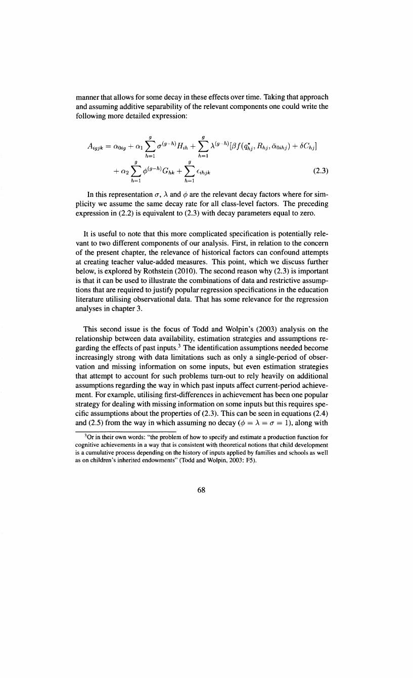
Univers

ity of

Cap

e Tow

n

manner that allows for some decay in these effects over time. Taking that approach and assuming additive separability of the relevant components one could write the following more detailed expression:

9 9

Ai9 jk = aoi9 + 0:1 L a(9 -h) Hih + L >.(9 -h)[f3f(q'hj, Rhj, iioihj) + 6Chj] h=l h=l

9 9

+ 0'2 L ¢;(9 -h)Ghk + L Eihjk (2.3) h=l h=l

In this representation a, ).. and <P are the relevant decay factors where for sim­plicity we assume the same decay rate for all class-level factors. The preceding expression in (2.2) is equivalent to (2.3) with decay parameters equal to zero.

It is useful to note that this more complicated specification is potentially rele­vant to two different components of our analysis. First, in relation to the concern of the present chapter, the relevance of historical factors can confound attempts at creating teacher value-added measures. This point, which we discuss further below, is explored by Rothstein (2010). The second reason why (2.3) is important is that it can be used to illustrate the combinations of data and restrictive assump­tions that are required to justify popular regression specifications in the education literature utilising observational data. That has some relevance for the regression analyses in chapter 3.

This second issue is the focus of Todd and Wolpin's (2003) analysis on the relationship between data availability, estimation strategies and assumptions re­garding the effects of past inputs. 3 The identification assumptions needed become increasingly strong with data limitations such as only a single-period of obser­vation and missing information on some inputs, but even estimation strategies that attempt to account for such problems tum-out to rely heavily on additional assumptions regarding the way in which past inputs affect current-period achieve­ment. For example, utilising first-differences in achievement has been one popular strategy for dealing with missing information on some inputs but this requires spe­cific assumptions about the properties of (2.3). This can be seen in equations (2.4) and (2.5) from the way in which assuming no decay (</J =)..=a= 1), along with

30r in their own words: "the problem of how to specify and estimate a production function for cognitive achievements in a way that is consistent with theoretical notions that child development is a cumulative process depending on the history of inputs applied by families and schools as well as on children's inherited endowments" (Todd and Wolpin, 2003: FS).

68

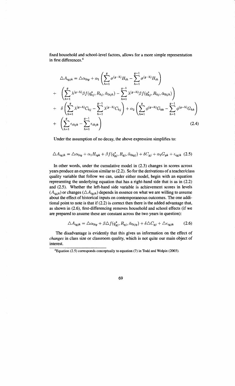
Univers

ity of

Cap

e Tow

n

fixed household and school-level factors, allows for a more simple representation in first differences.4

6Agjk = 6aoig + a1 (t a(g~h) Hih - I: a(g~h) Hih)

h=l h=l

+ (t _A(g~h) f3f(qhj• Rhj, O:oijh) -I: _A(g~h) f3f(qhj• Rhi• O:oijh)) h=l h=l

+ 8 (t, AI•-•> c.; -~ AI•-•> c.;) + "' (t, .p<•-•>c.,-~ .p<n-•>c.,)

+ (t Eihjk - I: Eihjk) h=l h=l

(2.4)

Under the assumption of no decay, the above expression simplifies to:

In other words, under the cumulative model in (2.3) changes in scores across years produce an expression similar to (2.2). So for the derivations of a teacher/class quality variable that follow we can, under either model, begin with an equation representing the underlying equation that has a right-hand side that is as in (2.2) and (2.5). Whether the left-hand side variable is achievement scores in levels (Agjk) or changes (6Agjk) depends in essence on what we are willing to assume about the effect of historical inputs on contemporaneous outcomes. The one addi­tional point to note is that if (2.2) is correct then there is the added advantage that, as shown in (2.6), first-differencing removes household and school effects (if we are prepared to assume these are constant across the two years in question):

The disadvantage is evidently that this gives us information on the effect of changes in class size or classroom quality, which is not quite our main object of interest.

4Equation (2.5) corresponds conceptually to equation (7) in Todd and Wolpin (2003).

69

Univers

ity of

Cap

e Tow

n

Rothstein (2010) has developed this insight from Todd and Wolpin (2003) in a different direction, considering what such specifications might imply for teacher value-added measures based on observational data. Specifically, if such measures are to be used as personnel management tools then - as in the variance decom­position literature - we need to be concerned about sorting of students across classrooms. However, the issue in this case cannot be resolved by the quasi­experimental approach of Hanushek and Rivkin (2010) because, even if we are willing to accept the underlying assumptions, the method only identifies the vari­ance contribution of teachers, not the value added by individual teachers. Roth­stein exploits the fact that a genuine measure of teacher value-added should not be a statistically significant predictor of student scores in periods prior to the stu­dent being in the relevant teacher's class. Using this basic insight he constructs various falsification tests for common ('simple') value-added measures and shows that these are indeed violated empirically in his North Carolina sample, thereby calling into question the use of such measures for personnel and indeed other pur­poses. While a cumulative model is not necessary for this kind of outcome - serial correlation in a student's intrinsic ability would suffice - if it does characterise the true relationship then such problems are likely to be more serious. Furthermore, a cumulative model implies that in terms of social return the concept of 'teacher value added' should not be confined to a single year. Rothstein shows that us­ing a richer set of observed controls than in simple YAMs mitigates, but does not remove, the problem.

While some authors have recently questioned whether those findings are in fact as problematic for the use of V AMs as Rothstein suggests, there is no consensus as yet on these issues. Chetty et al. (2011) have argued that while they can reproduce similar results to Rothstein in a different American dataset, controlling for a full set of observables reduces the problem to a degree where it is materially irrelevant. Furthermore, by matching their educational data to tax records they are able to check whether there is student sorting on some factors that are unobservable in education datasets; they find that this does not appear to be the case. Either way, for our purposes the key point is that Rothstein's concerns relate primarily to the process of teacher-student matching and this is not a concern in an experiment where students and teachers were randomly matched, as was the case in Project STAR.

For the work that follows here both the above considerations are important: in order to construct a defensible measure of teacher quality we need to make as­sumptions about the underlying data generating process; and, to specify regression equations by which we can estimate meaningful interaction effects it is necessary

70

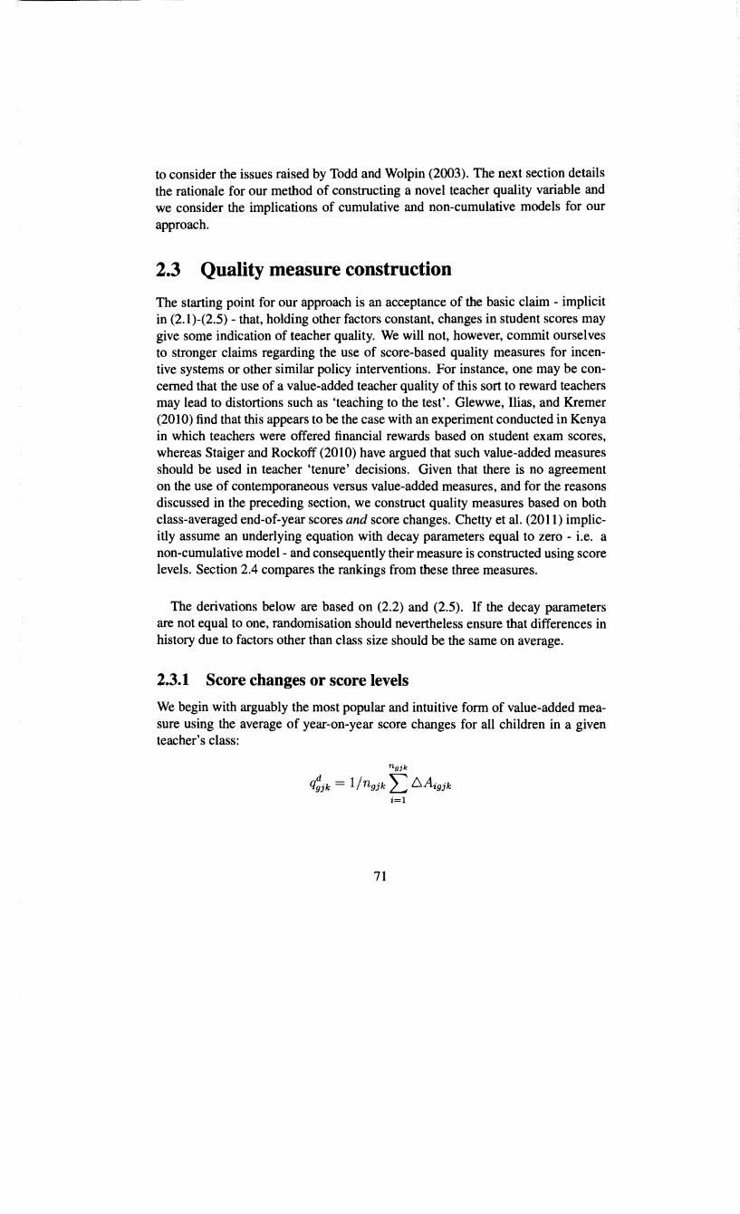
Univers

ity of

Cap

e Tow

n

to consider the issues raised by Todd and Wolpin (2003). The next section details the rationale for our method of constructing a novel teacher quality variable and we consider the implications of cumulative and non-cumulative models for our approach.

2.3 Quality measure construction

The starting point for our approach is an acceptance of the basic claim - implicit in (2.1 )-(2.5) - that, holding other factors constant, changes in student scores may give some indication of teacher quality. We will not, however, commit ourselves to stronger claims regarding the use of score-based quality measures for incen­tive systems or other similar policy interventions. For instance, one may be con­cerned that the use of a value-added teacher quality of this sort to reward teachers may lead to distortions such as 'teaching to the test'. Glewwe, Ilias, and Kremer (2010) find that this appears to be the case with an experiment conducted in Kenya in which teachers were offered financial rewards based on student exam scores, whereas Staiger and Rockoff (2010) have argued that such value-added measures should be used in teacher 'tenure' decisions. Given that there is no agreement on the use of contemporaneous versus value-added measures, and for the reasons discussed in the preceding section, we construct quality measures based on both class-averaged end-of-year scores and score changes. Chetty et al. (2011) implic­itly assume an underlying equation with decay parameters equal to zero - i.e. a non-cumulative model- and consequently their measure is constructed using score levels. Section 2.4 compares the rankings from these three measures.

The derivations below are based on (2.2) and (2.5). If the decay parameters are not equal to one, randomisation should nevertheless ensure that differences in history due to factors other than class size should be the same on average.

2.3.1 Score changes or score levels

We begin with arguably the most popular and intuitive form of value-added mea­sure using the average of year-on-year score changes for all children in a given teacher's class:

ngjk

q;jk = 1/n9jk ~::::>~~Aigjk i=l

71

Univers

ity of

Cap

e Tow

n

If we assume that the underlying relationship is as simple as in (2.2) then dif­ferencing removes constant factors as shown in (2.6). By contrast, we know that if historical inputs matter- as in (2.3) - with no decay then differencing gives us (2.5). If we utilise the latter result (from (2.5)) then:

ngjk

q:jk = L ~Aigjk i=l

= ~·gJkaOig + a1H.9 + f3f. 9Jk(q;Jk' Rgjk, ao.gjk) + c5Cgjk

+a2Ggk + ~·gjkEigjk (2.7)

Note that the omitted subscript denotes the mean of variables across the rele­vant subpopulation (in this case, students within each class).5

In words, then, equation (2.7) states that the teacher value-added measure for the teacher of classroom j in grade g and school k is equal to the average of score differences for all nJ children in the teacher's class between grades g and g- 1, which is a function of class-level means of: changes in the factors outlined in Section 2.2 that vary across students; and, the levels of factors that are constant over students such as class-level and school effects. (Note that n9 j = C9J but we use n for the sake of convention).

An alternative is to use aggregate year-end scores. If we are prepared to assume a non-cumulative production function as in (2.2) then we can obtain an analogous expression to the above:

ngj

q;jk = L Aigjk i=l

= a 0.9 j + a 1H.9 j + {3j.9 jk(q;j, R 9J, ao.9J) + c5C9 j + a2Ggk + E.9 jk (2.8)

There are possible limitations to using such measures of teacher value-added with observational data, even given the convenient simplifying assumptions be­hind (2.2). For example, there is the possibility that the formation of classes takes

5To keep subsequent notation legible, we express means as follows:

E[xiJk] = X-Jk

E[f(xiJk)] = fJk(x;Jk)

E[l'>f(x;Jk)] = 6-Jkf(x;Jk)

72

Univers

ity of

Cap

e Tow

n

into account student and teacher ability, leading to cov( q;jk' aoigjk) =/= 0. If, for instance, weaker students - with below-average aoigjk and b.aoigjk - are assigned to stronger teachers then: cov(q;jk' b.aoigjk) < 0. In this case, qgjk and q~jk would understate the value of better teachers and overstate the value of worse ones. That would also lead to an underestimate of the variation in student outcomes that is due to teachers. Hence the concern with student-teacher matching in the burgeon­ing literature on value-added measures, discussed in the preceding section.6

.

This problem can be tackled in one of two ways. First, one could utilise longi­tudinal data to control for observed teacher and student characteristics in previous years. If these factors are the ones used in the actual assignment process then util­ising them as conditioning variables may be enough to avoid bias. Two examples of this approach are Rockoff (2004) and Chetty et al. (2011). A second approach is to use experimental data in which students and teachers are randomly matched. The ideal situation would be one in which this random matching takes place across the whole sample, that is: every student-teacher pairing is equally probable. To our knowledge no such data exists, primarily because the random allocation of children to schools is difficult and very likely undesirable.7 However, some stud­ies - such as Project STAR - have randomly matched teachers and students within schools and it is this characteristic that we exploit in the derivations that follow. Successful randomisation of this form implies that, within a given school, student achievement in grade g - 1 is independent of the quality of the assigned teacher in grade g.

The representations in (2.5) and (2.6) also imply the existence of another po­tentially confounding factor, namely class size - or, in the latter case, the change in class size. Therefore even where teacher assignment to classes is independent of their characteristics, a class size effect could be misleadingly represented in the quality measure if we simply take the first difference from observational data.

There are a few characteristics of the Project STAR design that in principle make this insight particularly relevant for that data. There were three different possible assignments in STAR for a given year: small class (13 - 17 students); regular class (22- 25 students); and, a regular class with teaching aide. Children

6In addition to the previous references Rockoff (2004) and Hanushek and Rivkin (2006) also provide useful discussions of this issue

7Even in studies that involve random allocation of an additional teacher as the treatment -in Duflo, Dupas, and Kremer (20 ll) to reduce class size - there is no indication that the actual matching of teachers and schools is itself random. In charter school experiments students' suc­cess in applying to a specific school or schools may be randomised but does not lead to random assignment across schools in general since the applicant pool is self-selected.

73

Univers

ity of

Cap

e Tow

n

enter the Project in various grades, from kindergarten to Grade 3, and once en­tered the intention is that they are retained in the same class size assignment. (In practice, as we discuss later, matters were somewhat more complicated). Thus !::,Cgjk may vary within classes and across years. For example, a student entering the Project in Grade 1 from a 'regular' size class in another school and randomly assigned to a small class will experience a decrease in class size (!::,C

9Jk < 0) for

Grade 1, whereas a student who entered STAR in kindergarten and stayed in the same size class will have !::,CgJk = 0. This issue is therefore somewhat related to our preceding discussion regarding the assumption that household, school and community effects are constant. In the case of class size, the fact that there are no baseline scores means that in practical terms !::,C9Jk is not observable for new entrants, which removes the problem although admittedly only by obliging us to omit those students from the class aggregate changes.In 2.4 we discuss the extent to which this affects the proportion of children whose scores are included in the class average.

If we were concerned about having to omit such students we might want to in­stead use a quality measure based on an end-of-year average - as shown in (2.8) -rather than score changes. Here we instead consider such a measure as a robust­ness check of sorts on our preferred measure, which uses aggregate score changes. The details are provided in the empirical work of the next section.

2.3.2 Isolating teacher quality

Our aim is to construct variable that gives a meaningful ranking of teachers (class­rooms). Adopting similar logic to the above, Nye et al. (2004) analyse variation in value-added teacher quality in the STAR data by focusing on a sub-sample of schools containing at least two classes of the same type; the authors use differ­ences between these classes to estimate the variance in teacher quality, pooling the within-school results across schools to give a final estimate based on a large enough sample. In a similar analysis, Chetty et al. (20 11) exploit random match­ing to identify the effect of class assignment on future earnings. Unlike these contributions, however, our interest is in construction of an actual quality measure that ideally has values for all teachers in the sample and so a different approach is required.

The key insight of our approach is that we will construct this ranking within class type but across schools. In addition to the preceding assumptions that inform our preferred specification in (2.5), we state five further assumptions that enable us to obtain direct information on true teacher quality.

74

Univers

ity of

Cap

e Tow

n

The first two assumptions are premised on the success of the experimental de­sign described above. First, that class size is independent of teacher quality.

Assumption 2.3.1. Random assignment

cjk JL qjk

The second assumption is that by virtue of random assignment within schools, one obtains identical teacher quality distributions (<p(q*)) within each treatment category and across schools.

Assumption 2.3.2. Equal quality distributions

The next set of assumptions concern the term f(qj0k, Rj0 k, i'iojok), which repre­

sents the 'classroom effect' of class j in school k. Given random assignment it seems plausible to assume that classroom resources are the same within schools, even where class size is different. Let j 0 and j 1 represent two teachers from the set of teachers Jk in school k.

Assumption 2.3.3. Equal classroom resources

R9jki(C = C0) = Rgiki(C = C 1

)

R9jk(jo) = R9jk(jl), Vjo, J1 E Jk

Randomisation of students across classes (including class types) within schools also means we can plausibly assume that within a given school, k, average peer quality is approximately the same across classes of different sizes. Note, however, that this implicitly assumes-away Lazear (2001)'s emphasis on the fact that the probability of a disruptive peer increases with class size.

Assumption 2.3.4. Equality of peer effects

Finally, we assume that f ( ·) is linear and additively separable so that we replace (3 f ( q}ok, Rjok, iiojok) with an expression that allows us to consider teacher quality separately from classroom resources and peer effects.

Assumption 2.3.5. Additive separability of class-level variables

75

Univers

ity of

Cap

e Tow

n

Under these assumptions and the additive models of class size in (2.2) and (2.3), one could construct a quality measure based on ranking teachers within class types using, respectively, either year-end score averages, or average score changes.

One advantage of rankings - as opposed to numerical scores - is that they allow comparison of the consequences of different quality measures, a fact we make use of in the next section. However, a ranking does discard valuable information, exaggerates differences between teachers with similar scores and may be inconve­nient if the numbers of teachers in the class size categories differ. An alternative is to create a standardised numerical measure by standardising qjk9 (given (2.2)) or qfkg (given (2.5)) within class types, which yields a quality measure that is independent of class size but informative within schools. Subject to the above as­sumptions being satisfied, one standard deviation in this quality measure can be given the same interpretation across class types.

For some class size or type Cr and score-based quality measure qv:

(2.9)

Demeaning qv within class type removes, under our functional form assump­tions, the effect of class size. While the quality measure and ranking across schools is likely to be affected by community- and school-level factors, these will - again, under the above assumptions - affect teachers in the same school identically. Therefore their relative ranks within the treatment categories are in­formative about quality. Intuitively, if a teacher of a small class in school k is at the 60th percentile for small classes, while a teacher of a regular class in the same school (k) is at the 20th percentile of all regular classes, we would conclude that the small class teacher is of higher quality in terms of test score achievement.

2.3.3 Discussion

The above analysis effectively identifies two sets of assumptions that are required for our proposed method. The first set, discussed in section 2.2, concern the basic form of the education production function. Our preferred specification - a vari­ant of (2.3) - assumes the production function: is additively separable across sets of factors at the levels of the individual (including their household), school and classroom; contains cumulative effects; and, these effects do not decay. Of these, the assumption of cumulative effects is perhaps the most plausible. Whether these sets of factors are additively separable is unknown at present. In the spirit of chapter 1 we would not be comfortable making policy recommendations based on

76

Univers

ity of

Cap

e Tow

n

models that assume-away interactions of that kind. Nevertheless, this assumption is commonly invoked in the literature - in analyses such as Chetty et al. (20 11 ), discussed below - and in that sense, at least, is not controversial. The assumption that may be most problematic is that of no decay in the effects of variable val­ues from preceding periods. This is the subject of current research and there is currently little direct evidence or consensus on the question. The final section of this chapter provides estimates of changes in the effect of a given year's quality over time. If the assumption is false then - as can be seen from (2.4) - the quality measure will in fact be a measure of the aggregate change in quality experienced by children in each class. In the presence of random assignment it is unlikely that this will bias the measure since qigjk JL qi(g-l)Jk• but it will introduce some noise.

With the exception of the assumption of additive classroom effects (assump­tion 2.3.5), the second set of assumptions listed in the previous section rest on the success of experimental randomisation (assumption 2.3.1) and the asymptotic benefits of this. In small samples, equality of resources and, in particular, average peer effects may be violated. Appendix A provides some additional analysis of the latter issue, but note that provided random assignment holds, differences in peers will only add noise to a teacher quality measure and not compromise the alterna­tive interpretation of the variable as a measure of class quality. Unequal classroom resources could also lead to noise in the quality measure, if random, or bias if for some reason resources and quality are correlated. We are unaware of any evidence in the literature, on STAR or otherwise, to suggest compensating behaviour of this kind. Finally, the equality of the quality distributions in the treatment categories - assumption 2.3.2- is assured asymptotically by random assignment. However, in finite samples the strict equality will not hold and for empirical purposes the issue is how much noise is introduced into the relative locations of teachers from the same school within the different categories.

Assumption 2.3.5 assumes additive separability of class-level factors (teacher quality, resources and peer effects), extending the assumption introduced in 2.2 that class size can be separated from these factors. If random assignment holds and peer effects and resources are approximately the same across classes in the same school, then failure of assumption 2.3.5 will not affect the measure in a material way. If there are small-sample differences in these factors then interaction effects will further confound direct measurement of teacher quality. In that circumstance, the variable will still be a valid measure of class quality - something that is less problematic for the broader purpose of the thesis and analysis of chapter 3.

77

Univers

ity of

Cap

e Tow

n

The key point is that the above analysis shows how a measure of teacher qual­ity can be created that, within schools, is unconfounded by other factors and is independent of class size by construction. Our view is that in many empirical sce­narios, provided random assignment holds, the most likely negative outcome due to the failure of the preceding assumptions is a noisy measure of class quality.

2.3.4 Quality a Ia Chetty et al. (2011)

In that regard, it is informative to contrast our proposed approach with Chetty et al.'s (2011) method of using "end-of-class peer test scores [as] an omnibus measure of class quality" (Chetty et al., 2011: 1596). It bears noting that in many respects the methods employed by these authors are similar to those utilised in Nye et al. (2004). By virtue of being framed in econometric terms, the Chetty et al. (2011) measure is more easily comparable to ours and hence we provide a brief discussion of their quality measure.

The first notable aspect of that approach is that the authors assume - as we do above - an additive role for class size. Second, the paper hinges on a measure of 'class quality' for each student i in class j and school k, which is constructed by averaging the end-of-year scores for an individual's peers and subtracting from this the average scores for all peers in the same grade of that school. In a slight variation of our notation above, we represent the total number of classes in grade g of school k as Jgk. so that j E {1, ... , Jgk}. Using this we can represent the Chetty et al. (2011) quality measure as:8

(2.10)

Building on the preceding analysis of the assumptions required to justify our approach, it is interesting to consider what the different models of educational pro­duction in (2.1) and (2.3) imply for Chetty et al. 's (2011) approach to constructing the quality measure. It is fairly straightforward to show how that measure - de­noted as above by qgk -is affected by the relevant specification of the education

8In fact, the final version of the measure used by Chetty et al. (2011) omits individual's own scores- we address the issue of 'leave-out means' of this kind in the next chapter when we deal with regression analysis of class size effects. Besides the analysis in the final section, for our present purposes it suffices to focus on a single, class-level measure of quality and henceforth we will treat all measures as such unless stated otherwise.

78

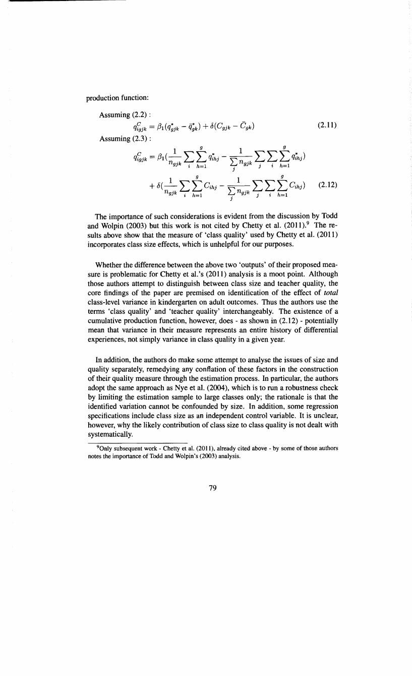
Univers

ity of

Cap

e Tow

n

production function:

Assuming (2.2) :

q~jk = f3I(q;jk- ij;k) + 8(Cgjk- Cgk)

Assuming (2.3):

(2.11)

(2.12)

The importance of such considerations is evident from the discussion by Todd and Wolpin (2003) but this work is not cited by Chetty et al. (2011).9 The re­sults above show that the measure of 'class quality' used by Chetty et al. (2011) incorporates class size effects, which is unhelpful for our purposes.

Whether the difference between the above two 'outputs' of their proposed mea­sure is problematic for Chetty et al.'s (2011) analysis is a moot point. Although those authors attempt to distinguish between class size and teacher quality, the core findings of the paper are premised on identification of the effect of total class-level variance in kindergarten on adult outcomes. Thus the authors use the terms 'class quality' and 'teacher quality' interchangeably. The existence of a cumulative production function, however, does - as shown in (2.12) - potentially mean that variance in their measure represents an entire history of differential experiences, not simply variance in class quality in a given year.

In addition, the authors do make some attempt to analyse the issues of size and quality separately, remedying any conflation of these factors in the construction of their quality measure through the estimation process. In particular, the authors adopt the same approach as Nye et al. (2004), which is to run a robustness check by limiting the estimation sample to large classes only; the rationale is that the identified variation cannot be confounded by size. In addition, some regression specifications include class size as an independent control variable. It is unclear, however, why the likely contribution of class size to class quality is not dealt with systematically.

90nly subsequent work - Chetty et al. (20 II), already cited above - by some of those authors notes the importance of Todd and Wolpin's (2003) analysis.

79

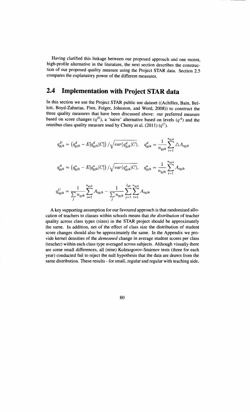
Univers

ity of

Cap

e Tow

n

Having clarified this linkage between our proposed approach and one recent, high-profile alternative in the literature, the next section describes the construc­tion of our proposed quality measure using the Project STAR data. Section 2.5 compares the explanatory power of the different measures.

2.4 Implementation with Project STAR data

In this section we use the Project STAR public use dataset ((Achilles, Bain, Bel­lott, Boyd-Zaharias, Finn, Folger, Johnston, and Word, 2008)) to construct the three quality measures that have been discussed above: our preferred measure based on score changes (qD), a 'naive' alternative based on levels (qA) and the omnibus class quality measure used by Chetty et al. (2011) (qc).

1 ngjk

1 J9 k ngjk

q~jk = 2:: """'Agjk - 2:: """'"""' Agjk n ·k~ n ·k~~ . 9J i=l . 9J j=l i=l

J J

A key supporting assumption for our favoured approach is that randomised allo­cation of teachers to classes within schools means that the distribution of teacher quality across class types (sizes) in the STAR project should be approximately the same. In addition, net of the effect of class size the distribution of student score changes should also be approximately the same. In the Appendix we pro­vide kernel densities of the demeaned change in average student scores per class (teacher) within each class type averaged across subjects. Although visually there are some small differences, all (nine) Kolmogorov-Smirnov tests (three for each year) conducted fail to reject the null hypothesis that the data are drawn from the same distribution. These results - for small, regular and regular with teaching aide,

80

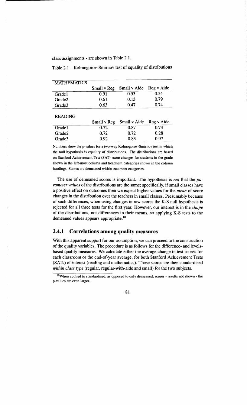
Univers

ity of

Cap

e Tow

n

class assignments - are shown in Table 2.1.

Table 2.1 - Kolmogorov-Smimov test of equality of distributions

MATHEMATICS Small v Reg Small v Aide Reg v Aide

Gradel 0.91 0.53 0.54 Grade2 0.61 0.13 0.79 Grade3 0.63 0.47 0.74

READING Small v Reg Small v Aide Reg v Aide

Gradel 0.72 0.87 0.74 Grade2 0.72 0.72 0.28 Grade3 0.92 0.83 0.97

Numbers show the p-values for a two-way Kolmogorov-Smimov test in which

the null hypothesis is equality of distributions. The distributions are based

on Stanford Achievement Test (SAT) score changes for students in the grade

shown in the left-most column and treatment categories shown in the column

headings. Scores are demeaned within treatment categories.

The use of demeaned scores is important. The hypothesis is not that the pa­rameter values of the distributions are the same; specifically, if small classes have a positive effect on outcomes then we expect higher values for the mean of score changes in the distribution over the teachers in small classes. Presumably because of such differences, when using changes in raw scores the K-S null hypothesis is rejected for all three tests for the first year. However, our interest is in the shape of the distributions, not differences in their means, so applying K-S tests to the demeaned values appears appropriate. 10

2.4.1 Correlations among quality measures

With this apparent support for our assumption, we can proceed to the construction of the quality variables. The procedure is as follows for the difference- and levels­based quality measures. We calculate either the average change in test scores for each classroom or the end-of-year average, for both Stanford Achievement Tests (SATs) of interest (reading and mathematics). These scores are then standardised within class type (regular, regular-with-aide and small) for the two subjects.

10When applied to standardised, as opposed to only demeaned, scores - results not shown - the p-values are even larger.

81

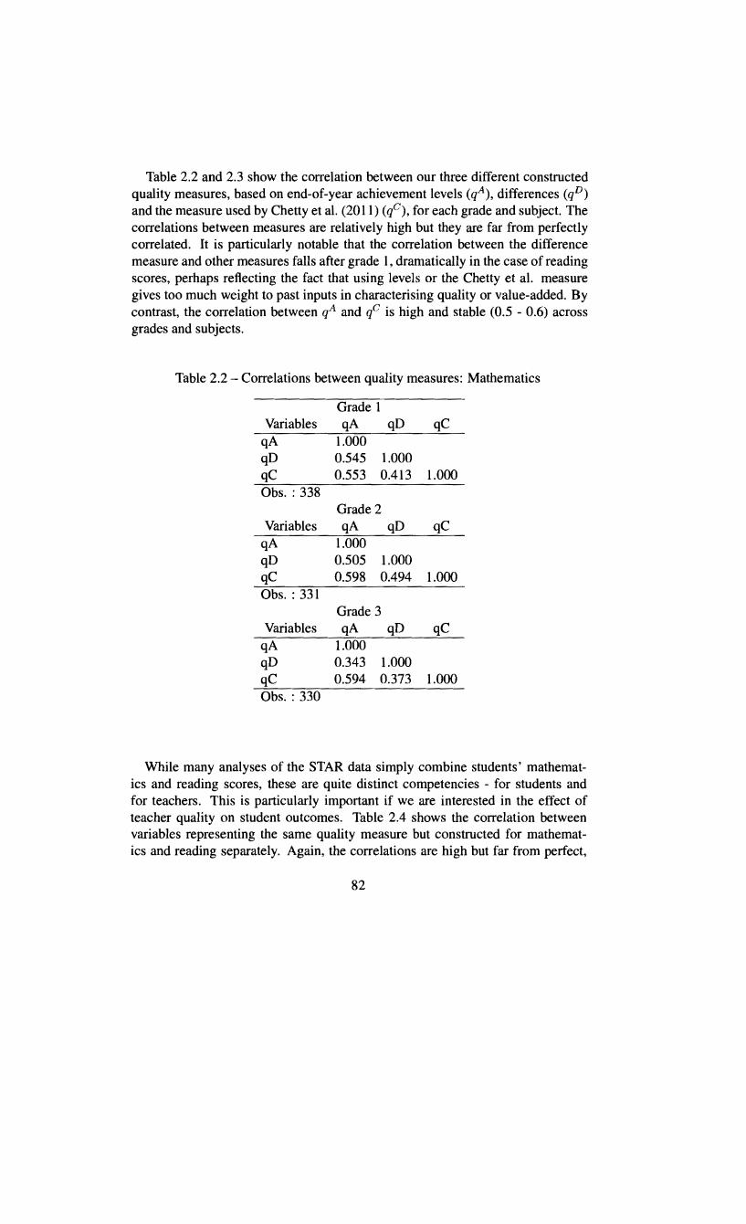
Univers

ity of

Cap

e Tow

n

Table 2.2 and 2.3 show the correlation between our three different constructed quality measures, based on end-of-year achievement levels (qA), differences (qD)

and the measure used by Chetty et al. (2011) (q0 ), for each grade and subject. The correlations between measures are relatively high but they are far from perfectly correlated. It is particularly notable that the correlation between the difference measure and other measures falls after grade I, dramatically in the case of reading scores, perhaps reflecting the fact that using levels or the Chetty et al. measure gives too much weight to past inputs in characterising quality or value-added. By contrast, the correlation between qA and q0 is high and stable (0.5 - 0.6) across grades and subjects.

Table 2.2 - Correlations between quality measures: Mathematics

Grade 1 Variables qA qD qC

qA 1.000 qD 0.545 1.000 qC 0.553 0.413 1.000 Obs.: 338

Grade 2 Variables qA qD qC

qA 1.000 qD 0.505 1.000 qC 0.598 0.494 1.000 Obs. : 331

Grade 3 Variables qA qD qC

qA 1.000 qD 0.343 1.000 qC 0.594 0.373 1.000 Obs.: 330

While many analyses of the STAR data simply combine students' mathemat­ics and reading scores, these are quite distinct competencies - for students and for teachers. This is particularly important if we are interested in the effect of teacher quality on student outcomes. Table 2.4 shows the correlation between variables representing the same quality measure but constructed for mathemat­ics and reading separately. Again, the correlations are high but far from perfect,

82

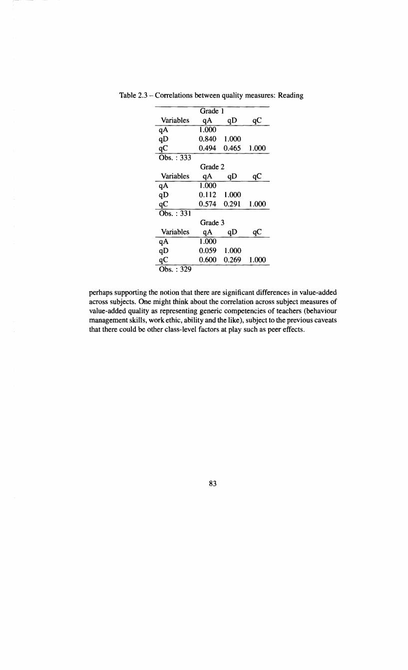
Univers

ity of

Cap

e Tow

n

Table 2.3- Correlations between quality measures: Reading

Grade 1 Variables qA qD qC

qA 1.000 qD 0.840 1.000 qC 0.494 0.465 1.000 Obs.: 333

Grade 2 Variables qA qD qC

qA 1.000 qD 0.112 1.000 qC 0.574 0.291 1.000 Obs. : 331

Grade 3 Variables qA qD qC

qA 1.000 qD 0.059 1.000 qC 0.600 0.269 1.000 Obs.: 329

perhaps supporting the notion that there are significant differences in value-added across subjects. One might think about the correlation across subject measures of value-added quality as representing generic competencies of teachers (behaviour management skills, work ethic, ability and the like), subject to the previous caveats that there could be other class-level factors at play such as peer effects.

83

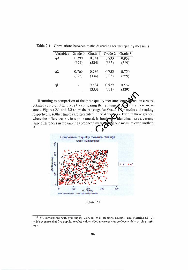
Univers

ity of

Cap

e Tow

n

Table 2.4 - Correlations between maths & reading teacher quality measures

Variables Grade 0 Grade 1 Grade 2 Grade 3 qA 0.799 0.841 0.833 0.857

(325) (334) (335) (329)

qC 0.763 0.736 0.755 0.770 (325) (334) (335) (329)

qD 0.634 0.529 0.567 (333) (331) (329)

Returning to comparison of the three quality measures one can obtain a more detailed sense of differences by comparing the rankings produced by these mea­sures. Figures 2.1 and 2.2 show the rankings for Grade 1 for maths and reading respectively. (Other figures are presented in the Appendix). Even in these grades, where the differences are less pronounced, it should be evident that there are many large differences in the rankings produced by favouring one measure over another. II

0

Comparison of quality measure rankings Grade 1 Mathematics

100 200 300 400 qD ranking

Note: Low ranklngs axrespond to high quality.

Figure 2.1

11 This corresponds with preliminary work by Wei, Hembry, Murphy, and McBride (2012) which suggests that five popular teacher value-added measures can produce widely varying rank­ings.

84

Univers

ity of

Cap

e Tow

n

Comparison of quality measure rankings Grade 1 Reading

0 100 200 qD ranking

300 400

Not.: Low rantings axrupond to high quality.

Figure 2.2

2.4.2 Quality across school location

One issue of interest is whether and how measured classroom quality varies across school locations. In the STAR sample schools were drawn from locations classi­fied as 'rural', 'suburban', 'urban' and 'inner city'. If the differences between schools in terms of contribution to student outcomes, as well as selection of stu­dents into schools, is fixed over time, then using score differences may provide some useful information. Such considerations, however, guarantee us that we can conclude very little from comparing the levels-based quality measure across school types. Figure 2.3-2.5 show variation over school types and grades even for our difference-based measure (qD) constructed using mathematics scores. The analogous figures for reading are shown in the Appendix.

Although we have no particular prior in this regard, the patterns in these fig­ures are worth remarking on. In particular, the levels-based measures (qA and qc ) show a fairly consistent pattern across school locations in contrast with the change-based measure (qD) . However, the pattern is in the opposite direction across the levels-based measures: inner city schools have uniformly lower quality levels when based on simple averages of score levels (qA) , but uniformly higher quality levels when using the measure proposed by Chetty et al. (2011) (qc ). The former result is precisely as expected, since we expect inner city schools to draw students with lower socio-economic status (SES) and we know from the mod-

85

Univers

ity of

Cap

e Tow

n

Comparison of quality measures over school types Quality measure qD: Mathematics

Inner city Suburban

Grade 1 Grade 3

Rural

- Grade21

Figure 2.3

Urban

Comparison of quality measures over school types Quality measure qA: Mathematics

Inner city Suburban Rural Urban

- GradeO - Grade1 - Grade2 - Grade3

Figure 2.4

86

Univers

ity of

Cap

e Tow

n

..... 0 &:: .,.., "' . ~

0

Comparison of quality measures over school types Quality measure qC: Mathematics

Inner city Suburban Rural Urban ~~~--------------~

- Grade 0 - Grade 1 - Grade 2 - Grade 3

Figure 2.5

els and derivations in section 2.2 and 2.3 that this contaminates that measure. Whether these schools also receive weaker teachers is less clear but there is little reason to believe they would attract uniformly better teachers.

Given this, the pattern created across schools by qc might seem strange, except that on further inspection these tum-out not to be statistically significant. 12 On re­flection this is also as we would expect: values of qc are determined by deviations of individual classes from within-school means.

By contrast, the differences between inner city qD scores and those for rural and urban scores are significant across all grades (at the 10% level) but the direction changes. As illustrated in Figure 2.3, in Grade 1 mean quality is lower at inner city schools but this is reversed in Grade 3. The magnitude of the differences in Grade 3 are much smaller- approximately a third to a quarter of the size. This does not indicate that the difference-based quality measure is invalid. Rather, it follows from the fact that demeaning average score changes within class types does not remove the effects of factors that vary within types: in this case, school location. Where the quality measure is used for within-school comparisons we need not be concerned since such factors are common to all classes in a given school.

12We run a series of simple regressions with the relevant quality variable on the left hand side and dummies for the school types (locations) on the right. All dummies are statistically significant for the qA regressions whereas none are significant in the q0 regressions.

87

Univers

ity of

Cap

e Tow

n

2.4.3 Quality and teacher characteristics

As noted at the beginning of this chapter, most studies in the literature on teacher value-added find that descriptive teacher characteristics such as age, experience, formal qualifications and gender explain little of the variation in student outcomes or value-added measures of quality. Is the same true for the measure we propose and the others with which we compare it?

The results in Tables 2.5- 2.7 are intended to address this question. These show coefficients from regressions of each quality measure on the available teacher characteristics from the STAR dataset for the relevant grade. The variables used are a continuous measure of years of teacher experience and dummies - with the base category listed first- for: race (white, black, Asian); gender (female, male); education (Bachelors, Masters, specialist qualification, doctorate); and, position on the 'career ladder' (not on the ladder, apprentice, probation, Level 1, Level 2 and Level 3).

In the absence of any priors there is nothing to suggest that any of the factors are systematically significant in explaining quality and the R2 values for our pre­ferred measure (qD) as well as Chetty et al.'s (2011) measure (qc) are very low. The primary exception is teacher's race in explaining qA; by this measure, black teachers appear to be associated with lower-than-average quality. This is mislead­ing, however, since the race of teachers is likely to be correlated with the SES of students and the resources available to schools. For example, in Grade 1 the per­cent of students in a class receiving a free lunch is 78% if the teacher is black but only 45% if a teacher is white. In fact, a paper by Dee (2004) has shown a posi­tive role model effect in relation to teacher and student race. The significance of race coefficients in the regressions in Table 2.6 then simply emphasises the point that simple end-of-year averages of scores are not a very good measure of teacher quality since they are affected by many other factors.

A related issue concerns a recent paper by Mueller (2013), which examines interactions between teacher experience and class size. As a preliminary in­vestigation into the extent to which that analysis addresses our broader interest, namely interaction between quality and class size, we run univariate regressions of the three quality measures on teacher experience. 13 The next chapter discusses

13Mueller (2013) actually uses a 'rookie' dummy variable but this discards information and the cut-off used to determine who is a rookie is defined based on the estimates that are produced rather

88

Univers

ity of

Cap

e Tow

n

Table 2.5 - Variation explained by teacher characteristics

Variation in quality explained by characteristics Grade I Grade 2 Grade 3

qD Reading Maths Reading Maths Reading Maths

Experience -0.004 -0.016** 0.010 0.003 0.003 0.005 (0.007) (0.007) (0.007) (0.007) (0.007) (0.007)

Male 0.622 0.159 -0.434 0.180 -0.202 -0.511 * (0.676) (0.701) (0.574) (0.576) (0.309) (0.308)

Black -0.552*** -0.293* 0.169 -0.136 0.570*** 0.226* (0.148) (0.153) (0.140) (0.140) (0.137) (0.137)

Masters 0.008 0.146 -0.025 -0.060 0.058 0.195 (0.115) (0.118) (0.119) (0.119) (0.119) (0.119)

Specialist 0.698 -0.737 -0.733 -0.222 0.151 -0.320 (0.678) (0.703) (0.582) (0.584) (0.578) (0.577)

Doctorate 0.659 0.150 0.600 0.751 (0.954) (0.989) (0. 717) (0.719)

Apprentice -0.386 0.017 -0.163 0.192 0.158 -0.046 (0.271) (0.281) (0.274) (0.275) (0.334) (0.334)

Probation -0.451 0.228 -0.392 0.075 -0.121 0.113 (0.277) (0.286) (0.294) (0.295) (0.301) (0.300)

Levell -0.002 0.217 0.089 0.362** -0.014 0.197 (0.209) (0.217) (0.180) (0.180) (0.215) (0.215)

Level2 -0.082 0.616 0.580 0.212 -0.011 -0.166 (0.474) (0.491) (0.440) (0.441) (0.305) (0.304)

Level3 0.703** 0.368 0.501 0.546 0.154 0.536* (0.322) (0.327) (0.369) (0.371) (0.288) (0.287)

Asian -0.752 0.347 (1.009) (1.007)

R2 0.12 0.05 0.06 0.03 0.07 0.06 N 332 336 325 325 326 327

* p < 0.1; ** p < 0.05; *** p < 0.01

89

Univers

ity of

Cap

e Tow

n

Table 2.6 - Variation explained by teacher characteristics

Variation in quality explained by characteristics Grade 0 Grade I Grade 2 Grade 3

qA Reading Maths Reading Maths Reading Maths Reading Maths

Experience 0.015** 0.015** 0.001 -0.006 0.010 0.006 0.006 0.004 (0.006) (0.007) (0.007) (0.007) (0.007) (0.007) (0.007) (0.007)

Black -0.080 -0.041 -0.732*** -0.516*** -0.733*** -0.663*** -0.910*** -0.875*** (0.092) (0.096) (0.143) (0.150) (0.134) (0.134) (0.129) (0.128)

Masters -0.079 -0.083 -0.030 0.066 -0.050 -0.037 0.176 0.290*** (0.071) (0.074) (0.112) (0.117) (0.113) (0.114) (0.112) (0.111)

Masters+ -0.076 -0.089 (0.199) (0.207)

Specialist 0.146 0.371 0.515 -0.007 0.386 0.700 0.454 0.176 (0.327) (0.340) (0.662) (0.694) (0.561) (0.563) (0.544) (0.4 77)

Apprentice -0.076 -0.175 -0.395 -0.146 0.187 0.445* 0.128 0.186 (0.404) (0.419) (0.261) (0.274) (0.263) (0.264) (0.314) (0.308)

Probation 0.059 -0.021 -0.486* -0.272 -0.327 -0.162 0.347 0.521 * (D.410) (0.426) (0.267) (0.278) (0.283) (0.284) (0.283) (0.281)

Levell 0.060 -0.082 -0.107 0.047 0.184 0.155 0.365* 0.437** (0.389) (0.404) (0.201) (0.211) (0.173) (0.174) (0.203) (0.201)

Level2 0.433 0.080 -0.198 0.058 0.029 -0.146 0.114 0.023 (0.452) (0.469) (0.461) (0.484) (0.423) (0.425) (0.286) (0.284)

Level3 0.682 0.298 0.707** 0.431 0.143 -0.102 0.053 0.139 (0.502) (0.522) (0.313) (0.321) (0.355) (0.357) (0.271) (0.269)

Male 0.776 0.352 -0.160 0.237 -0.387 -0.508* (0.660) (0.692) (0.553) (0.555) (0.290) (0.289)

Doctorate 0.954 0.041 0.746 0.516 (0.932) (0.977) (0.690) (0.693)

Asian 0.357 0.697 (0.949) (0.944)

R2 0.07 0.04 0.15 0.07 0.12 0.10 0.16 0.17 N 294 294 333 337 328 328 326 331

* p < 0.1; •• p < 0.05; ••• p < 0.01

90

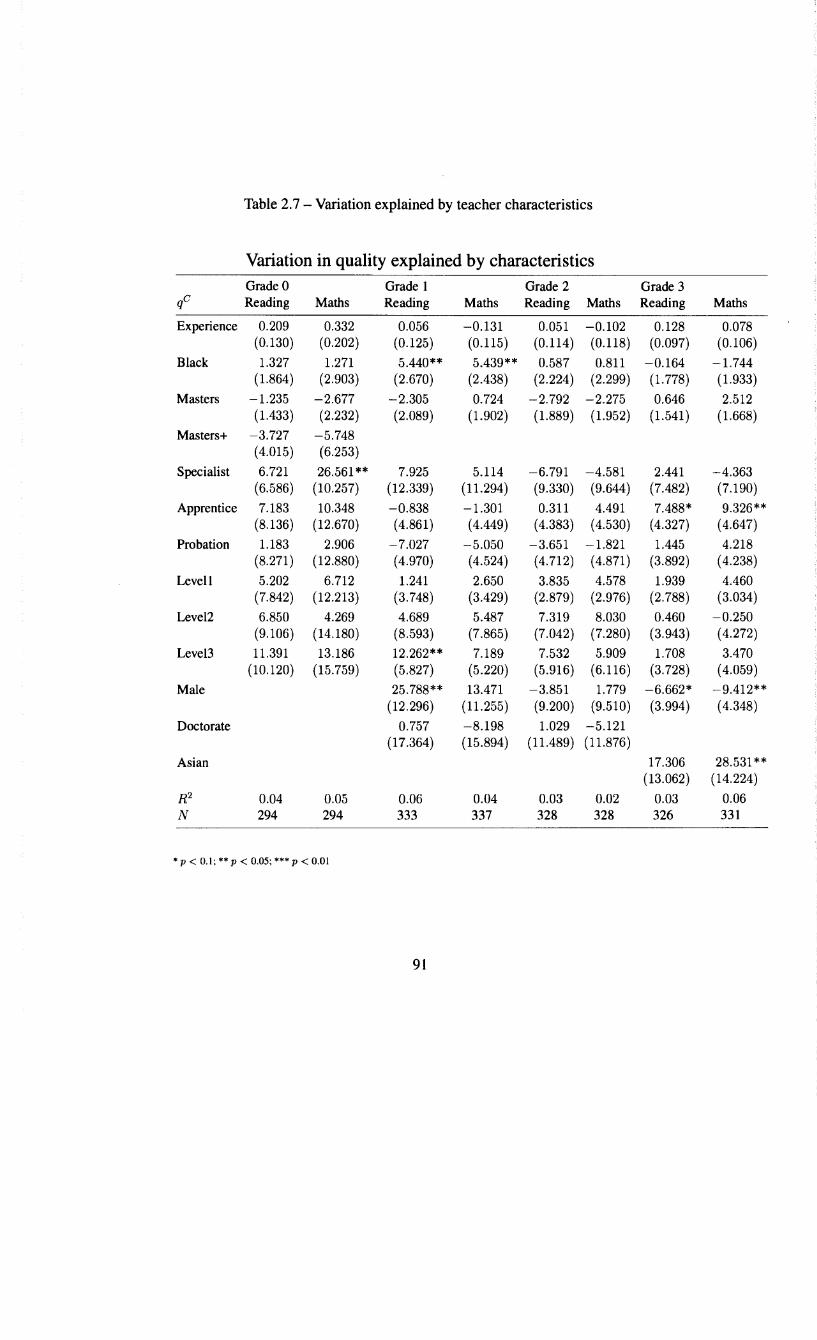
Univers

ity of

Cap

e Tow

n

Table 2. 7 - Variation explained by teacher characteristics

Variation in quality explained by characteristics Grade 0 Grade 1 Grade 2 Grade 3

qc Reading Maths Reading Maths Reading Maths Reading Maths

Experience 0.209 0.332 0.056 -0.131 0.051 -0.102 0.128 0.078 (0.130) (0.202) (0.125) (0.115) (0.114) (0.118) (0.097) (0.106)

Black 1.327 1.271 5.440** 5.439** 0.587 0.811 -0.164 -1.744 (1.864) (2.903) (2.670) (2.438) (2.224) (2.299) (1. 778) ( 1.933)

Masters -1.235 -2.677 -2.305 0.724 -2.792 -2.275 0.646 2.512 (1.433) (2.232) (2.089) (1.902) (1.889) (1.952) (1.541) ( 1.668)

Masters+ -3.727 -5.748 ( 4.015) (6.253)

Specialist 6.721 26.561 ** 7.925 5.114 -6.791 -4.581 2.441 -4.363 (6.586) (10.257) (12.339) (11.294) (9.330) (9.644) (7.482) (7.190)

Apprentice 7.183 10.348 -0.838 -1.301 0.311 4.491 7.488* 9.326** (8.136) (12.670) (4.861) (4.449) (4.383) (4.530) (4.327) ( 4.647)

Probation 1.183 2.906 -7.027 -5.050 -3.651 -1.821 1.445 4.218 (8.271) (12.880) (4.970) (4.524) (4.712) (4.871) (3.892) ( 4.238)

Levell 5.202 6.712 1.241 2.650 3.835 4.578 1.939 4.460 (7.842) (12.213) (3.748) (3.429) (2.879) (2.976) (2.788) (3.034)

Level2 6.850 4.269 4.689 5.487 7.319 8.030 0.460 -0.250 (9.106) (14.180) (8.593) (7.865) (7.042) (7.280) (3.943) (4.272)

Level3 11.391 13.186 12.262** 7.189 7.532 5.909 1.708 3.470 (10.120) (15.759) (5.827) (5.220) (5.916) (6.116) (3.728) (4.059)

Male 25.788** 13.471 -3.851 1.779 -6.662* -9.412** (12.296) (11.255) (9.200) (9.510) (3.994) (4.348)

Doctorate 0.757 -8.198 1.029 -5.121 (17.364) (15.894) (11.489) (11.876)

Asian 17.306 28.531 ** (13.062) (14.224)

R2 0.04 0.05 0.06 0.04 0.03 0.02 0.03 0.06 N 294 294 333 337 328 328 326 331

• p < 0.1; •• p < 0.05; *** p < 0.01

91

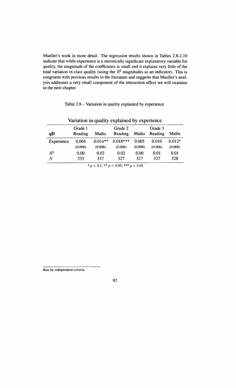
Univers

ity of

Cap

e Tow

n

Mueller's work in more detail. The regression results shown in Tables 2.8-2.10 indicate that while experience is a statistically significant explanatory variable for quality, the magnitude of the coefficients is small and it explains very little of the total variation in class quality (using the R2 magnitudes as an indicator). This is congruent with previous results in the literature and suggests that Mueller's anal­ysis addresses a very small component of the interaction effect we will examine in the next chapter.

Table 2.8 - Variation in quality explained by experience

Variation in quality explained by experience

Grade 1 Grade 2 Grade 3 qD Reading Maths Reading Maths Reading Maths

Experience 0.004 -0.014** 0.018*** 0.005 0.010 0.012* (0.006) (0.006) (0.006) (0.006) (0.006) (0.006)

R2 0.00 0.02 0.02 0.00 0.01 0.01 N 333 337 327 327 327 328

* p < 0.1; ** p < 0.05; *** p < 0.01

than by independent criteria.

92

Univers

ity of

Cap

e Tow

n

Table 2.9- Variation in quality explained by experience

Variation in quality explained by experience

Grade 0 Grade 1 Grade 2 Grade 3 qA Reading Maths Reading Maths Reading Maths Reading Maths

Experience 0.018*** 0.017*** 0.008 -0.001 0.009 0.001 -0.001 -0.002 (0.005) (0.005) (0.006) (0.006) (0.006) (0.006) (0.006) (0.006)

R2 0.03 0.03 0.00 0.00 0.01 0.00 0.00 0.00 N 324 324 334 338 330 330 327 332

* p < 0.1; ** p < 0.05; *** p < 0.01

Table 2.10- Variation in quality explained by experience

Variation in quality explained by experience

Grade 0 Grade 1 Grade 2 Grade 3 qC Reading Maths Reading Maths Reading Maths Reading Maths

Experience 0.170 0.290* 0.203* 0.031 0.133 -0.055 0.103 0.053 (0.108) (0.164) (0.108) (0.097) (0.099) (0.103) (0.081) (0.089)

R2 0.01 0.01 0.01 0.00 0.01 0.00 0.01 0.00 N 324 324 334 338 330 330 327 332

* p < 0.1; ** p < 0.05; *** p < 0.01

93

Univers

ity of

Cap

e Tow

n

2.4.4 Support from subjective measures

Earlier we mentioned the role of subjective assessments of teacher quality. While largely (and deliberately) neglected in the empirical literature in economics, there is some evidence of this kind from Project STAR. Due to the way it was obtained this data can be used to see if changes in average student scores are associated with the factors measured in such observational assessments. Essentially our interest is in whether the subjective evidence collected on teacher quality corresponds to our favoured measure of that variable. As we show below, because the sampling of teachers for the classroom observations was based on class-average score changes we can draw a direct correspondence between the subjective results and our pre­ferred quality measure. The fact that the STAR sub-study shows that teachers with higher class-average score changes were also of higher subjective quality supports our preferred measure and indeed the broader literature utilising student score changes.

As part of Project STAR two follow-up studies - Bain, Lintz, and Word ( 1989) and Appendix D of Word et al. (1990) - were done with samples of teachers se­lected on the basis of student performance. Bain et al. (1989) ranked teachers by increases in aggregate scores of their students in mathematics and reading from kindergarten to Grade 1. The top 15% were chosen for the follow-up analysis. Us­ing a similar approach, Word et al. (1990: 259-284) rank Grade 2 and 3 teachers by 'class scaled average score gains', selecting 65 teachers from the top 10% of the resultant distribution and 65 from the bottom 50%. Both follow-up studies utilised a teacher questionnaire to obtain further information on teacher background and characteristics, as well as elicit beliefs about teaching practices. Furthermore, and most interesting for our purposes, both included a checklist to be completed by an external assessor during observation of classroom practice.

Unfortunately there are some limitations to the information from the above­mentioned reports. First, the raw data itself is not publicly available, making an ideal analysis - where we match teachers within our quality distribution to the subjective measures of their individual performance - impossible. 14 Furthermore, there are problems in how the sampling procedure was designed and implemented. Word et al. ( 1990) do not provide a full description of how the sample was cho­sen- for instance, how were the 65 'less effective' teachers selected from the 340 teachers in the bottom 50% of the distribution? Also, the final analysis shows a sample of only 60 'less effective' teachers, without specifying why 5 were ex-

14 Attempts to contact Project STAR founder Helen Bain for further information were unsuc­cessful.

94

Univers

ity of

Cap

e Tow

n

eluded. By contrast, Bain et al. ( 1989) do provide an exhaustive description of the sample selection process, but they do not select a comparison group, meaning that the results of that study are of limited usefulness for within-sample comparisons.

Despite these limitations it is possible to extract some useful information from the study reported in Word et al. (1990). Since that sample was selected based on positioning within the distribution of class-average score changes this may pro­vide some indirect corroboration that the distribution of those changes - i.e. a value-added measure - is a useful proxy for teacher quality. In other words, the question we are interested in is: are higher (lower) class-average changes in test scores associated with better (worse) performance in observational assessments of teacher performance or ability? As already noted, a number of recent con­tributions to the literature - such as Rockoff and Speroni (2010) - have showed strong associations between these different kinds of measures. Since assessors in the STAR follow-up were not informed of teachers' position in the distribution of class averaged score changes, the subjective quality assessments can be assumed to be independent of that information.

Word et al. 's (1990) analysis examined differences between teachers, cate­gorised as described above, on two dimensions: descriptive characteristics and observational recording of teachers' actual classroom practice. The descriptive characteristics comprise those already available in the core STAR dataset: high­est degree achieved, certification, teaching experience, level on the state 'career ladder' and personal characteristics such as race and gender. The only additional descriptive variable that appears to have been captured is teacher age. The second dimension is therefore the one of greater interest for our purposes. Teachers were assessed on twelve different criteria; a table with those and the associated results is reproduced from Word et al. ( 1990) as Table 2.11.

95

Univers

ity of

Cap

e Tow

n

\0 0'1

Table 2.11- Descriptive statistics for STAR 'effective' and 'less effective' teachers

Effective teachers' ratings Less effective teachers' ratings

Criterion (1,2,3) (4) (1,2,3) (4)

Instruction is guided by a preplanned curriculum 17% 83%* 38% 62%

There are high expectations for student learning 33% 67% 41% 59%

Students are carefully oriented to lessons 23% 77%** 53% 48%

Instruction is clear and focused 19% 81 %*** 59% 41% Learning progress is monitored closely 19% 81% 51% 49% When students don't understand they are retaught 22% 78%* 45% 55%

Class time is used for learning 13% 87%*** 48% 52% There are smooth, efficient classroom routines 11% 89%*** 45% 55%

Instructional groups formed in the classroom fit instructional needs 19% 81%* 38% 62%

Standards for classroom behaviour are explicit 14% 86%*** 44% 56%

Personal interactions between teacher and students are positive 13% 88%*** 44% 56%

Incentives and rewards for students are used to promote excellence 18% 82%* 37% 63%

Notes: I. Source: Word eta!. (Table D-17, 1990: 261).

2. "The performance category is from one to four; 1 equals poor and 4 equals excellent" (from observation instrument in Word eta!., 1990: 264).

3. In the survey instrument each performance criterion is accompanied by a 'practices checklist' requiring a 'Yes/No' response from the observer, but this data is not reported.

4. * p<0.05, ** p<0.01, *** p<0.001

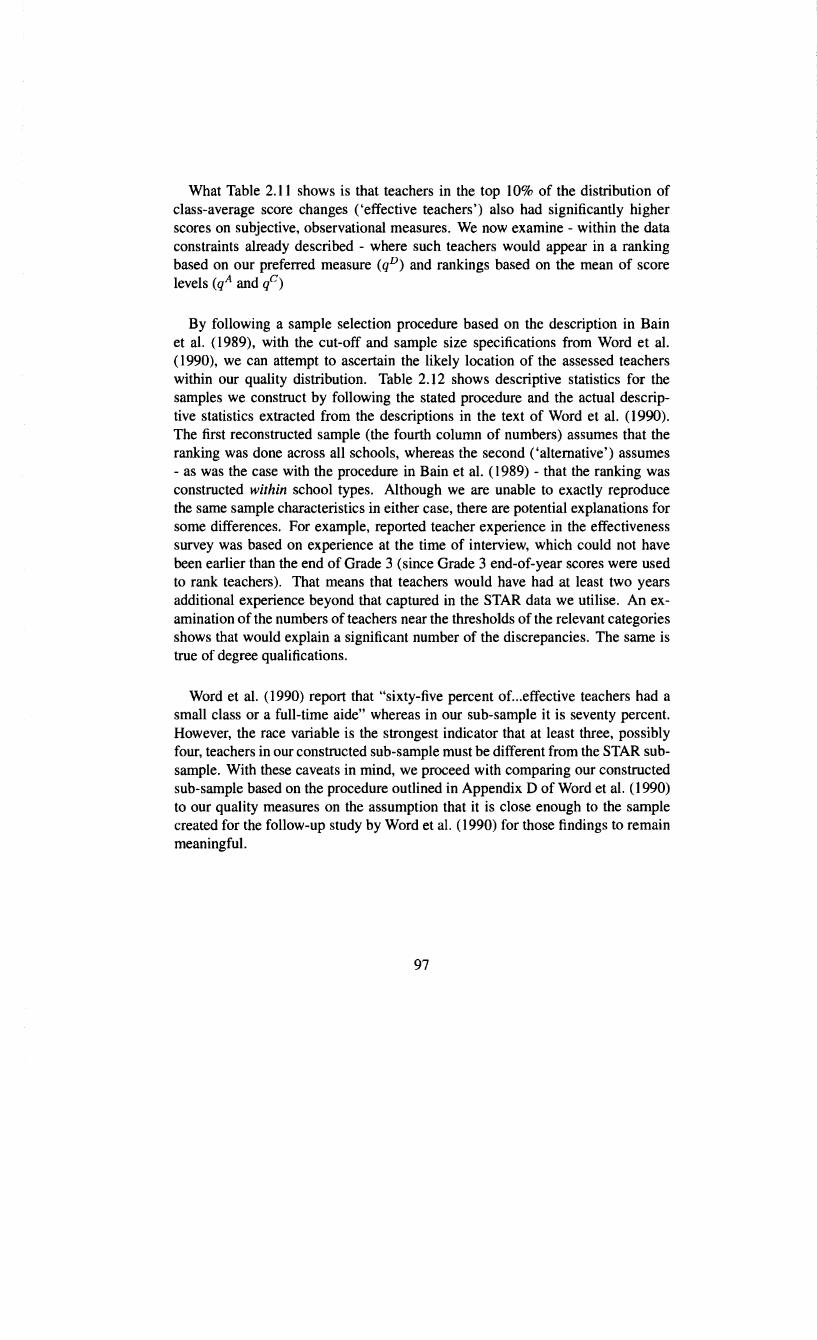
Univers

ity of

Cap

e Tow

n

What Table 2.11 shows is that teachers in the top 10% of the distribution of class-average score changes ('effective teachers') also had significantly higher scores on subjective, observational measures. We now examine - within the data constraints already described - where such teachers would appear in a ranking based on our preferred measure (qD) and rankings based on the mean of score levels (qA and qc)

By following a sample selection procedure based on the description in Bain et al. ( 1989), with the cut-off and sample size specifications from Word et al. ( 1990), we can attempt to ascertain the likely location of the assessed teachers within our quality distribution. Table 2.12 shows descriptive statistics for the samples we construct by following the stated procedure and the actual descrip­tive statistics extracted from the descriptions in the text of Word et al. ( 1990). The first reconstructed sample (the fourth column of numbers) assumes that the ranking was done across all schools, whereas the second ('alternative') assumes - as was the case with the procedure in Bain et al. ( 1989) - that the ranking was constructed within school types. Although we are unable to exactly reproduce the same sample characteristics in either case, there are potential explanations for some differences. For example, reported teacher experience in the effectiveness survey was based on experience at the time of interview, which could not have been earlier than the end of Grade 3 (since Grade 3 end-of-year scores were used to rank teachers). That means that teachers would have had at least two years additional experience beyond that captured in the STAR data we utilise. An ex­amination of the numbers of teachers near the thresholds of the relevant categories shows that would explain a significant number of the discrepancies. The same is true of degree qualifications.

Word et al. (1990) report that "sixty-five percent of...effective teachers had a small class or a full-time aide" whereas in our sub-sample it is seventy percent. However, the race variable is the strongest indicator that at least three, possibly four, teachers in our constructed sub-sample must be different from the STAR sub­sample. With these caveats in mind, we proceed with comparing our constructed sub-sample based on the procedure outlined in Appendix D of Word et al. ( 1990) to our quality measures on the assumption that it is close enough to the sample created for the follow-up study by Word et al. ( 1990) for those findings to remain meaningful.

97

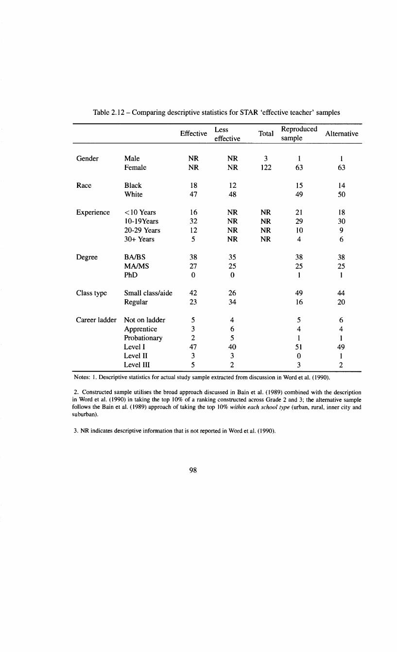
Univers

ity of

Cap

e Tow

n

Table 2.12- Comparing descriptive statistics for STAR 'effective teacher' samples

Effective Less Total

Reproduced Alternative

effective sample

Gender Male NR NR 3 1 1 Female NR NR 122 63 63

Race Black 18 12 15 14 White 47 48 49 50

Experience <10 Years 16 NR NR 21 18 10-19Years 32 NR NR 29 30 20-29 Years 12 NR NR 10 9 30+ Years 5 NR NR 4 6

Degree BA/BS 38 35 38 38 MAIMS 27 25 25 25 PhD 0 0

Class type Small class/aide 42 26 49 44 Regular 23 34 16 20

Career ladder Not on ladder 5 4 5 6 Apprentice 3 6 4 4 Probationary 2 5 1 Level I 47 40 51 49 Level II 3 3 0 1 Level III 5 2 3 2

Notes: I. Descriptive statistics for actual study sample extracted from discussion in Word eta!. (1990).

2. Constructed sample utilises the broad approach discussed in Bain et a!. (1989) combined with the description in Word eta!. (1990) in taking the top 10% of a ranking constructed across Grade 2 and 3; the alternative sample follows the Bain et a!. ( 1989) approach of taking the top I 0% within each school type (urban, rural, inner city and suburban).

3. NR indicates descriptive information that is not reported in Word eta!. (1990).

98

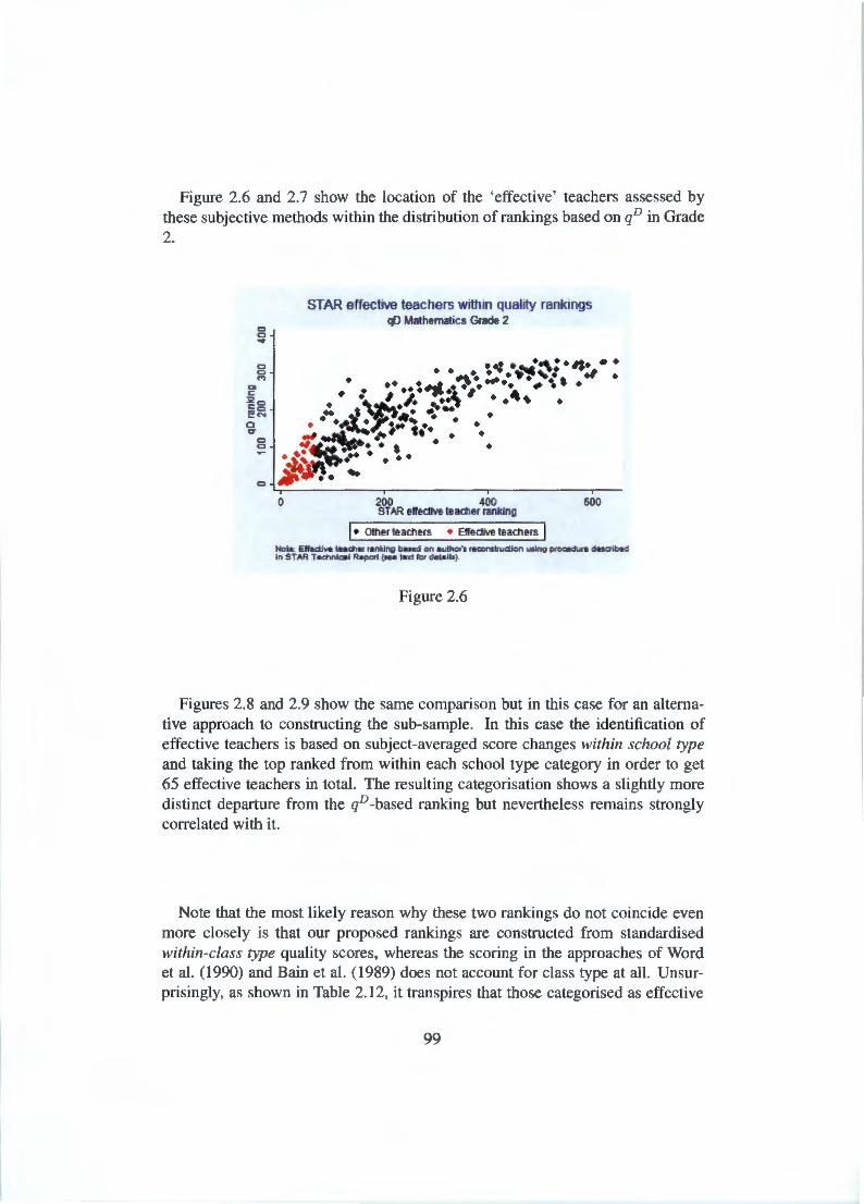
Univers

ity of

Cap

e Tow

n

Figure 2.6 and 2.7 show the location of the 'effective' teachers assessed by these subjective methods within the distribution of rankings based on qD in Grade 2.

0 .,.

C) C)

•

C) C)

STAR effective teachers within quality rankings qD Mathematics Grade 2

• • • ~ •: • .:..&!.\! •I$• ~ •• -· .... ,. - . . .. . ~ .-.. ...... .. \' . • • ~~. , .. ~::~\ , •• t\ ~ • .. I ~ ....... ...,• • .... •

• • •t~t.V •7•~ .. • • • • -~~ ... ~ , .. . . ti#~ • • • • . . ' •Jl ••• • ••

C) 1* •• ~ 0 200 400 600

STAR etreclive teacher ranking

I• Other teachers • Etredive teachers I Note: Ellll<tlve t .. dl• rantiog baHd or> aulhof's racol'tllrvciion usiog procad,.a dasaibed In STAR h dlnlc. l R~ ~ lui lor d•llllll).

Figure 2.6

Figures 2.8 and 2.9 show the same comparison but in this case for an alterna­tive approach to constructing the sub-sample. In this case the identification of effective teachers is based on subject-averaged score changes within school type and taking the top ranked from within each school type category in order to get 65 effective teachers in total. The resulting categorisation shows a slightly more distinct departure from the qD -based ranking but nevertheless remains strongly correlated with it.

Note that the most likely reason why these two rankings do not coincide even more closely is that our proposed rankings are constructed from standardised within-class type quality scores, whereas the scoring in the approaches of Word et al. ( 1990) and Bain et al. (1989) does not account for class type at all. Unsur­prisingly, as shown in Table 2.12, it transpires that those categorised as effective

99

Univers

ity of

Cap

e Tow

n

C) C) ....

C) C) ..,

ct c: :i<o c:o ~N Cl cr

C) C) -C)

0

STAR effective teachers within quality rankings qD Reading Grade 2

. ............ ~ . ......... ,~.._,, . .. ~ , ·~ .. • # • ' t\• \ •t.• • •: I • • •

• I ~~. •••' ·~ • • • ,. v ..... ~ ta• • • . . .. .~.·.~ ...... , ..... .. ..... .., .. ._,.... . • .: .. " ·~ • ~ ~ •• •# • • .. -.,._._:-;$ .,.. • • . ~ .. •• ~, ..

200 400 600 STAR effective teacher ranking

I• Other teachers • Elfedive teachers I Nota: Ell•d iv• t .. ch .. r• nking 1>..-d on auttlcn r.a.nslrudion using proc.ctLK• desaibtd in STAR T•chniao l R• porl ( .. • lui for d•lails).

Figure 2.7

teachers based on student scores were more likely to have small classes than those classified as less effective.

Another point to note is that the way in which the ranking was constructed re­sulted in the vast majority of teachers in this category being in Grade 2 rather than Grade 3 - graphs of the latter are provided in Figures C.8 and C.9 in Appendix C.2. As Figure C.18 shows, the distribution of score changes in Grade 3 is closer to the origin - i.e. the nature of the tests was such that smaller absolute score im­provements occur in Grade 3 relative to Grade 2 - and this is why hardly any of the teachers designated as 'effective' are from Grade 3. Although a flaw in the sam­ple selection procedure, this is likely to lead to an understating of the differences between high- and low-ranked teachers according to score change measures. The reason is that if the 65 (eventually 60) less effective teachers chosen from there­mainder of Grade 2 and 3 teachers were chosen randomly, there are likely to be some in Grade 3 who in fact are effective teachers once the lower gains in that grade are taken into account.

As mentioned, the project documentation does not actually explain how the 'less effective' teachers were chosen from the remainder of the sample so we cannot locate these individuals in the graphs. Nevertheless, it should be evident that the criteria coincide very closely with the basis for our favoured quality mea­sure (qv) . The subjective findings based on classroom observations therefore add

100

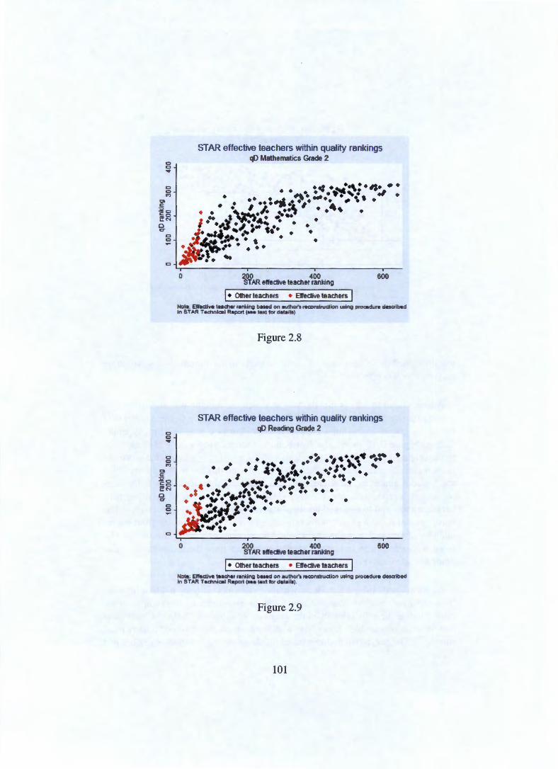
Univers

ity of

Cap

e Tow

n

0 0 ...

0 0

STAR effective teachers within quality rankings q0 Mathematics Grade 2

• • • ~ ·: •.:-&!\! •I$•.- • . -· ....... ,... - . •• •....1 .-••••• •\•. • • •• ·~~·.&. I .... • • .... ..!... ~. .. ··-~ • • ... ~ • .. '_..,.~· . .... . . ·~l·~·., .. . : .. J• _,.s - ... # ,_ • • -.t.L.-""'J.•· • ' • • . ~ ~··· ....

0 ~ ·). ~

0 0 ... 0 0 (')

0 c: :i< o <:o ~ .... a cr

0 0

0

0 200 400 600 STAR elfedive teacher ranking

I• Other teachers • Elfec:tive teachers I Nota: Ellac:tiva laacher rankil\ll baH<! on authon ramnstruclion usi 1111 pro<aaura d .. a it>ad In STAR Tachnlc:. l R~ ( ... tax! for datails)

0

Figure 2.8

STAR effective teachers within quality rankings qD Reading Grade 2

• • :, • • •• 41.., .. ~ • • • •• , • ; •• •I ~~ ' •

• # • ' 4•\ •t.• .. ·:I·· •• • I .AI-~• •••• ·~ • • ¥~ ~ • • • ... .... ' ,.~· .... , ... .s ...... .. ..,......... • •• . "·· .,~ ..... . . ... -:•fiJ .... . .

••• • . ..,., .. 200 400 600 STAR elfedive teacher ranking

I• Other teachers • Elfec:tive teachers I Nota: Ellaclive teacher ra illll buad on author's ramnstruclion usii\Q procedure a .. aibaa in STAR Tachnic:. l Report ( ... tax! lor datai ls).

Figure 2.9

101

Univers

ity of

Cap

e Tow

n

some support to the use of this quality measure. By contrast, as shown in Figures C.10-C.17 in the Appendix, this sub-sample does not coincide at all closely with the upper range of the other quality measures and therefore provides no useful corroboration of those.

Even leaving aside the aforementioned data limitations, such as not being able to create a one-to-one link between these assessments and the rest of the data, some final caveats are required. For example, if a teacher's performance under assessment is affected by characteristics of students in the class that also affect achievement, then the subjective assessment may be correlated with a value-added measure of teacher quality for a reason besides these constructs measuring the same latent teacher quality variable. For example, larger positive changes in stu­dent scores may be associated with less disruptive students- as per Lazear (2001) - while at the same time giving a better impression of the teacher in subjective assessments. 15 These issues of confounding are, however, not addressed in the existing literature.

2.4.5 Class size versus class type

One complicating factor in Project STAR is that assignment is not to a unique class size but, as described previously, rather to ranges of class sizes ( 13-17 and 22-25). As often happens in experiments, some subjects ended-up in classes whose sizes were outside the prescribed ranges. These are a non-insignificant proportion of cases, ranging from 19.5% - 33.4% in a given grade. A possibly larger concern for simple estimation of class size effects is that the final class size may be affected by other factors. Some schools may have, for instance, made efforts to have classes at the bottom of each range. An examination of the data, along with the detailed guide for determining sizes in the STAR technical report - see Word et al. ( 1990) - suggests no reason to believe that this was a concern in practice.

15 A further, more vexing, caveat to the entire 'teacher quality' literature is that it may not make sense to separate teacher ability and class characteristics. For example, we might assume that teacher competence is captured by two measures: subject knowledge and behavioural control. A teacher with strong behaviour control skills may perform much better than a teacher with good subject knowledge in an unruly class, while the reverse would be true in a well-behaved class. If observed teacher performance depends on the combination of multi-dimensional quality and classroom characteristics then score changes and subjective assessments are as much a proxy for the suitability of teacher-class pairings as teacher ability. To our knowledge this issue has received little attention in the economics literature and, while a worthy subject for future research, would take us too far afield from the focus of this thesis, but we note it here for the sake of completeness.

102

Univers

ity of

Cap

e Tow

n

For our purposes, however, there is an additional issue: our derivations in sec­tion 2.3 require demeaning within class type, but if class type differs from size then this could lead to a contamination of the quality measure, with teachers in smaller classes within the range having higher scores (assuming a positive class size effect). As a robustness check we create a measure in which we residualise, within class type, class average scores or score changes on actual class size before standardising. We denote these modified quality measures as q~ and qf. Table C.l and C.2 in Appendix C.4 show the Spearman rank correlations between the residualised and non-residualised measures. For the levels-based measure (qA) the smallest correlation is 0.992 and for our preferred change-based measure (qD) the smallest is 0.995 and all are highly significant. This suggests that the measures constructed within class types are not significantly confounded by within-type variation, which is reassuring for our basic approach.

103

Univers

ity of

Cap

e Tow

n

2.5 Comparisons of explanatory power

Among the main interests of the literature on value-added measures of teacher quality is the magnitude of the effect of quality on achievement and the extent to which that effect deteriorates over time - see for instance the discussions in Hanushek and Rivkin (2006, 2012). As already noted, the vast majority of these contributions utilise longitudinal, administrative data and aim to identify teacher quality as the persistent component in the score changes of different cohorts of students taught by the same teacher. Our data and approach is rather different, so in order to directly compare the 'performance' of our constructed measures (qA

and qD), we do so against the measure (q0 ) used by Chetty et al. (2011) on the STAR data.

A few minor difficulties should be noted. In the majority of their analysis Chetty et al. (20 11) use a dependent variable based on score percentile ranks, whereas in our analysis we favour the use of standardised scores in order to compare esti­mates to the broader literature. However, in one instance those authors do note the equivalent of their estimate in standard deviations, which enables us to make an adequate comparison below of our estimates with theirs. Second, while we distinguish between mathematics and reading scores, Chetty et al. (20 11) follow Krueger ( 1999) in averaging these scores for individual students and using that as the dependent variable. Chetty et al. (2011) also use this combined average as the input into construction of their quality measure. A final issue is that their paper focuses on the effects of variation in kindergarten teacher (class) quality, whereas our difference-based measure can only be calculated for Grade 1 onwards. In re­sults not shown we produce estimates similar to Chetty et al. (20 11) using our reconstruction of their quality measure and the STAR public use dataset (Achilles et al., 2008) for kindergarten. Furthermore, as we will see, the magnitude of the results for Grade 1 using their quality measure (q0 ) appear very similar to the kindergarten results.

Our first approach is to estimate a very simple regression specification, in which score levels from grade 1 to grade 8 are regressed on the relevant quality measure from grade 1, along with school and entry year fixed effects. The results for math­ematics achievement are shown in figure 2.1 0. The more naive measure, qA, has the largest coefficient for the contemporaneous effect of quality on achievement as well as for subsequent years. Recall that our motivation for favouring qD was partly on the basis that it would go some way to eliminating historical factors from the quality calculation, but by virtue of that is likely to explain a smaller propor­tion of the variation in achievement. This preferred measure is associated with

104

Univers

ity of

Cap

e Tow

n

an effect on achievement that is statistically indistinguishable in magnitude from the measure used by Chetty et al. (2011): 0.358 for qD versus 0.373 for qc. By comparison, Chetty et al. (2011: 1638) report an effect of 0.32 standard deviations in kindergarten scores. 16

Where the two measures differ is in their estimated effect in later years. Chetty et al. (20 11) report that the effect of qc from kindergarten on Grade 8 scores is negligible and we replicate that result using qc for Grade 1. However, our results suggest that the entire effect of qc disappears after one year, which is unexpected and somewhat in contrast with other literature which finds a more gradual decline (Hanushek and Rivkin, 2006). Our alternative measures are more consistent with that broader literature. Though also showing a marked decline in effect, from Grade 2 onward that remains fairly stable for both (qA and qc) measures: one standard deviation change in teacher quality is associated with a corresponding 0.1 standard deviation in student test scores. The results for reading - shown in figure 2.11 - are largely the same for our two measures, while for qc they indicate a marginally more gradual decay of reading effects that are also larger in magnitude for later years.

160ur replicated estimates, not shown, of the kindergarten effect of q0 are 0.339 for mathemat­ics and 0.328 for reading.

105

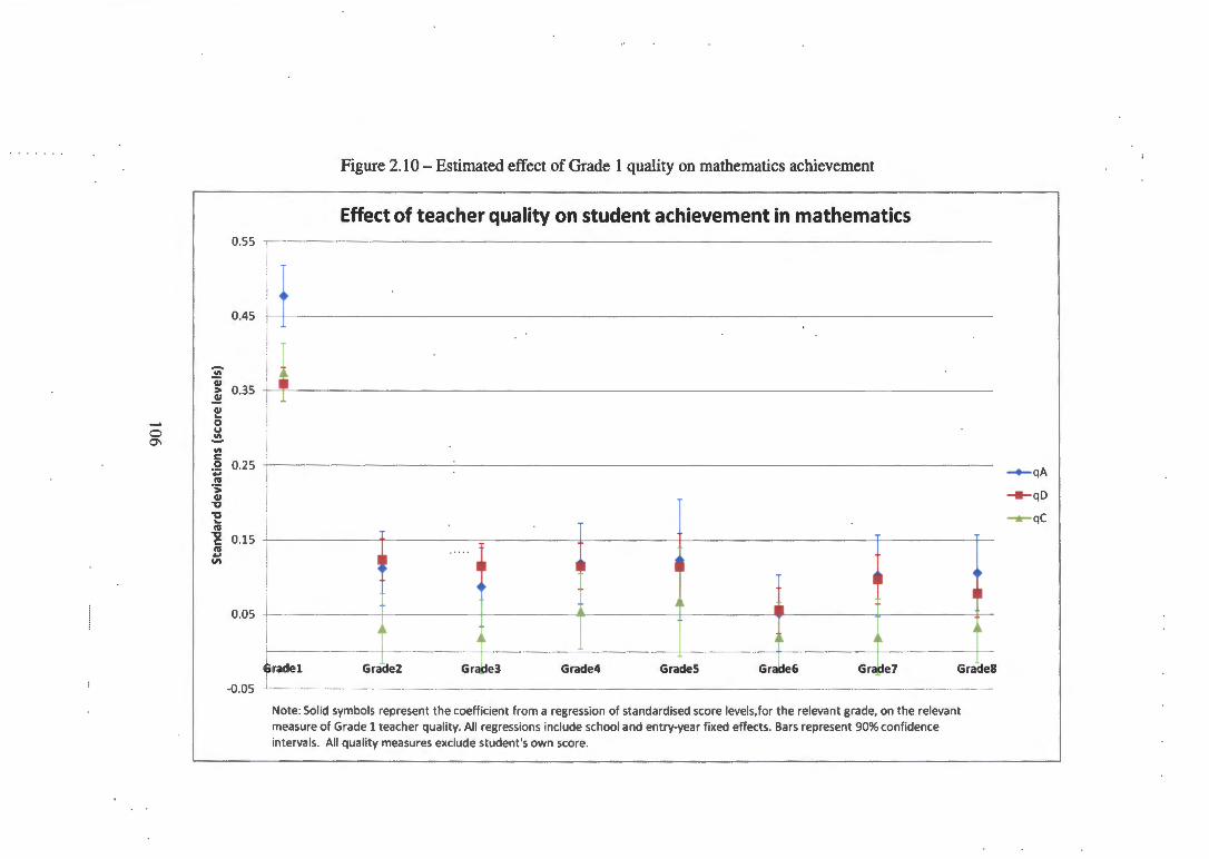
Univers

ity of

Cap

e Tow

n...... I 0 0'1

Figure 2.10 - Estimated effect of Grade 1 quality on mathematics achievement

Effect of teacher quality on student achievement in mathematics 0.55 ,-------------------------------------------------------------------------------------

0.45 ~ I

T

1 0.35 ~ CIJ .._ 0 u Ill -Ill c: .Q 0.25 .. IV ·:; CIJ ., ., .._ IV

-g 0.15 IV

i .. VI I

~

r 0.05 t

~ ~ - a

• II

I • ... 1 Gradel GraCie2 GraJte3 Grade4 GradeS Gr.Jie6 Gr~e7 GradeS

-0 .05

Note: Solid symbols represent the coefficient from a regression of standardised score levels, for the relevant grade, on the relevant measure of Grade 1 teacher quality. All regressions include school and entry-year fixed effects. Bars represent 90% confidence intervals. All quality measures exclude student's own score.

-+-qA

~qD

-r-qC

Univers

ity of

Cap

e Tow

nI

..... 0 -.)

Figure 2.11 - Estimated effect of Grade 1 quality on reading achievement

Effect of teacher quality on student achievement in reading 0.55 .-------------------------------------------------------------------------------------

0.45 + I

~ 0.35 + .!! • Ql ... 0 u ~

"' c .2 0.25 I ... IV

T 1 ·:;;

I Ql , , ... IV

"g 0.15 I IV

' ~

' • • T

• • ...

Ill

• l I o.o5 I

1 Gradel Grade2 Grade3 Gr~e4 G ra~es Grade6 Grade7 GradeS

-0.05 I I

Note: Solid symbols represent the coefficient from a regression of standardised reading score levels, for the relevant grade, on the relevant measure of Grade 1 teacher quality. All regressions include school and entry-year fixed effects. Bars represent 90% confidence intervals. All quali ty measures exclude student's own score.

-+-qA

-tl-qD

-r-qC

Univers

ity of

Cap

e Tow

n

Another advantage of the qD and qA measures is that they are constructed so as to be independent of class size. The next chapter reports estimates of class size and quality effects from various specifications of the educational production function using these variables. Here we examine any implications of this for the magnitude of the quality coefficient. Since q0 is strongly correlated with class size, while qA and qD are not, one may expect that the results shown in Figures 2.10 and 2.11 would change when class assignment is included as a regression covariate. In fact, using that regression specification produces similar results (not shown) for all measures, using mathematics and reading scores.

Chetty et al. (20 11) suggest a different approach to estimating the effect of teacher (class) quality net of class size effects: they limit the sample used to stu­dents that were in regular-sized classes (i.e. assigned to 'regular' or 'regular with aide' treatment groups). Figures 2.12 and 2.13 show the estimates from this sub­sample of students. The contemporaneous effect on mathematics scores remains the same, but the contemporaneous effect on reading scores decreases from 0.36 to 0.18. For Grades 2 to 4 the point estimates for all quality measures decrease, meaning that for q0 some of these become negative. However, the smaller sample sizes lead to wider confidence intervals and weakened ability to assert differences between point estimates.

108

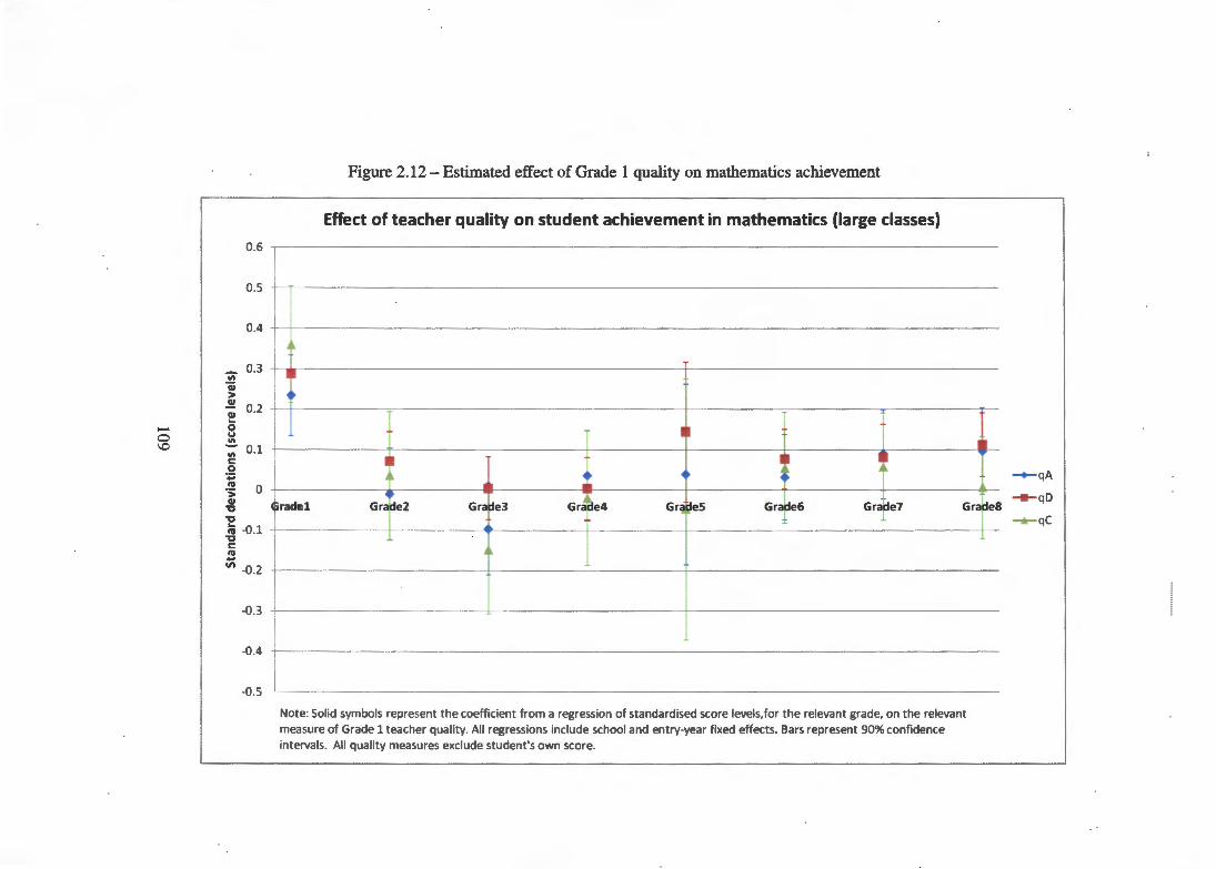
Univers

ity of

Cap

e Tow

n-0 \0

Figure 2.12- Estimated effect of Grade 1 quality on mathematics achievement

Effect of teacher quality on student achievement in mathematics (large classes)

0.6 .-------------------------------------------------------------------------------------

0.5 +-~----------------------------------------------------------------------------------

0.4

0.3 "' "ii >

.!! 0.2 cu .... Q u

~ 0.1 ~ Q

~ 0 cu

"C "C ; -0.1 -g Ill

~ -0.2

-0.3

-0 .4

-0.5

~

·~ ~

.. II

II II ~~ _..

Gradel Gril de2 Gra ~e3 Gr~ ~e4 Gr~ ~es Grat e6 Grf e7 Gra

-+-qA

8 ~qD

...,._qC del

I

I I

I

Note: Sol id symbols represent the coefficient from a regression of standardised score levels, for the relevant grade, on the relevant measure of Grade 1 teacher quality. All regressions include school and entry-year fiKed effects. Bars represent 90% confidence intervals. All quality measures exclude student's own score.

Univers

ity of

Cap

e Tow

n

Figure 2.13 - Estimated effect of Grade 1 quality on reading achievement

Effect of teacher quality on student achievement in reading (large classes)

0.5 ,-------------------------------------------------------------------------------------

0.4

0.3

-;;; a:; ~ 0.2 Ql

- I 0 - u 0 ~ 0.1 "' c 0 ... IV

-~ 0 "C "C ... IV

-g -0 .1 IV ... Ill

-0.2

-0.3

-0 .4

0 ~ I

T

I II I li •• 1 -~

~~

•• 4

Gradel Gra de2 Gra lte3 Gra ~e4 Gra ~es Gra de6 Gralte7 Gradel 8

1 ~------------

Note: Sol id symbols represent the coefficient from a regression of standardised reading score levels,for the relevant grade, on the relevant measure of Grade 1 teacher quality. All regressions include school and entry-year fixed effects. Bars represent 90% confidence intervals. All qua li ty measures exclude student's own score.

-+-qA

---qD

...._qc

Univers

ity of

Cap

e Tow

n

Appendix A

Class size and variance of quality measures

As mentioned in the main text, one disadvantage of using a quality measure based on score changes is that it reduces the number of students that can be used to calculate the relevant average. Possible concerns about the effect of this on our difference-based quality measure (qD) may fall along two dimensions. First, we may be concerned about the inaccuracy (high variance) of the measure when cal­culated using very small numbers of students. Second, we may be concerned that turnover is correlated with factors that are also associated with student outcomes. For example, a lower quality school may have higher student turnover leading to less accurate teacher quality measures in these schools. Alternatively, exit and en­try of students may be associated with characteristics of students, including their past scores, which might then lead to a bias in the value of the quality measure calculated.

Some analyses side-step this problem by, as is the case with Chetty et al. (2011), using end-of-year averages. However, we show in the main text that this approach suffers from a variety of other problems and limitations both in relation to the the­oretical concerns raised by Todd and Wolpin (2003) and properties of the STAR data itself. Ding and Lehrer (2011 b) provide an analysis ofthe dynamics of STAR students as they move through the programme but their interest is not in teacher quality or class average achievement. Below we examine the difference-based quality measure we construct (qD) for sensitivity to the two above-mentioned con­cerns.

112

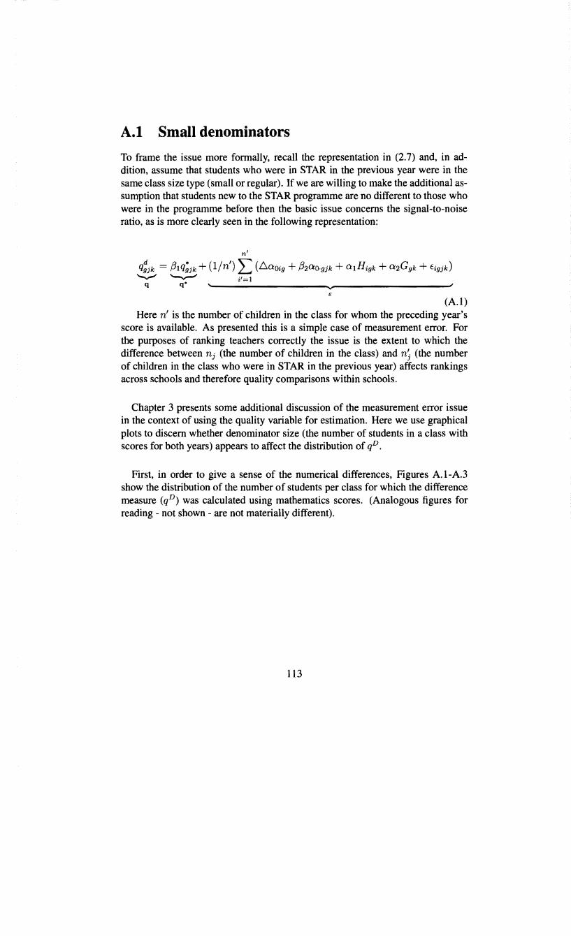
Univers

ity of

Cap

e Tow

n

A.l Small denominators

To frame the issue more formally, recall the representation in (2.7) and, in ad­dition, assume that students who were in STAR in the previous year were in the same class size type (small or regular). If we are willing to make the additional as­sumption that students new to the STAR programme are no different to those who were in the programme before then the basic issue concerns the signal-to-noise ratio, as is more clearly seen in the following representation:

n'

q~jk = f3Iq;jk + (1/n') I: (6aoi9 + f32ao.gjk + a1Higk + a2Ggk + Eigjk) ...__..,. ..__,_, i' = 1

q q• '-------------------~------------------~ (A.l)

Here n' is the number of children in the class for whom the preceding year's score is available. As presented this is a simple case of measurement error. For the purposes of ranking teachers correctly the issue is the extent to which the difference between n1 (the number of children in the class) and nj (the number of children in the class who were in STAR in the previous year) affects rankings across schools and therefore quality comparisons within schools.

Chapter 3 presents some additional discussion of the measurement error issue in the context of using the quality variable for estimation. Here we use graphical plots to discern whether denominator size (the number of students in a class with scores for both years) appears to affect the distribution of qD.

First, in order to give a sense of the numerical differences, Figures A.l-A.3 show the distribution of the number of students per class for which the difference measure (qD) was calculated using mathematics scores. (Analogous figures for reading - not shown - are not materially different).

113

Univers

ity of

Cap

e Tow

n

c: Gl

e Gl a.

c

""

ceo Gl e Gl a. ~

N

c

0

0

Denominator of average score changes Grade 1 Mathematics

5 10 15 20 Number of students

Figure A. l

Denominator of average score changes Grade 2 Mathematics

5 10 15 20 Number of students

Figure A.2

114

25

25

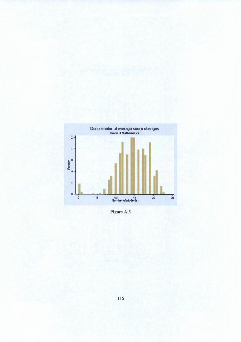
Univers

ity of

Cap

e Tow

nC>

0>

-co c ~ a; II.. ....

N

C>

0

Denominator of average score changes Grade 3 Mathematics

5 10 15 20 Number of students

Figure A.3

115

25

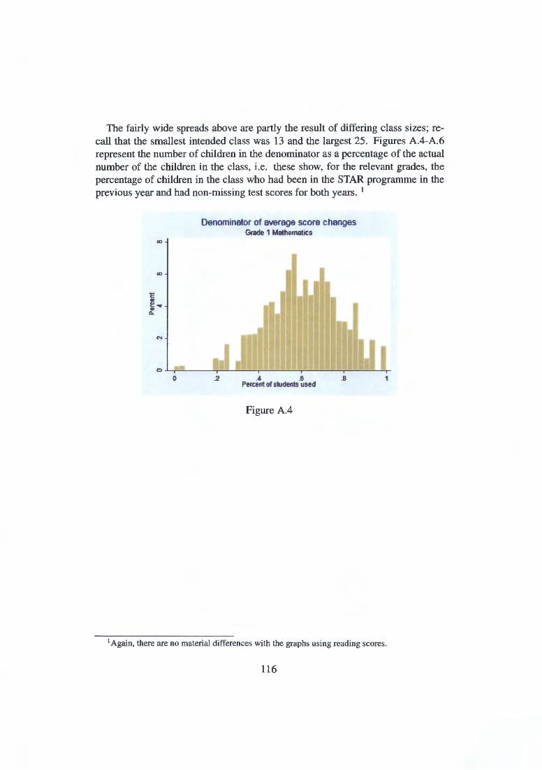
Univers

ity of

Cap

e Tow

n

The fairly wide spreads above are partly the result of differing class sizes; re­call that the smallest intended class was 13 and the largest 25. Figures A.4-A.6 represent the number of children in the denominator as a percentage of the actual number of the children in the class, i.e. these show, for the relevant grades, the percentage of children in the class who had been in the STAR programme in the previous year and had non-missing test scores for both years. 1

CD

c "' ~ ... ., a..

0

Denominator of average score changes Grade 1 Mathematics

.2 .4 .6 .8 Percent of students used

Figure A.4

1 Again, there are no material differences with the graphs using reading scores.

116

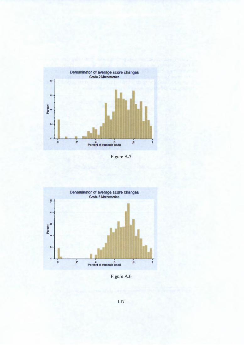
Univers

ity of

Cap

e Tow

n"E ., ~ ... ., a..

0

co

- <0 c: ., ~ ., ll.. ...

"'

0

0

0

Denominator of average score changes Grade 2 Mathematics

.2 .4 .6 .8 Percent of students used

Figure A.5

Denominator of average score changes Grade 3 Mathematics

2 .4 .6 .8 Percent of students used

Figure A.6

117

Univers

ity of

Cap

e Tow

n

The percentage of students in a class that can be used for a difference calcula­tion is primarily a function of turnover in the STAR sample - there is relatively little missing data on test scores for students who were in the programme. The more students entering and leaving the sample the smaller the proportion that, in a given year, were in the sample in the preceding year.

As a final graphical assessment, the figures below show scatter plots of qD by the number of students used to calculate the average score change. There does not appear to be any systematic pattern, such as wider dispersion of scores for small denominators or lower dispersion for larger denominators.2

...

00 c:r •

Variance in qO by denominator Grade 1 Mathematics

• • • •

• • • • • • • • •

• •

•

5 6 7 8 9 101112 131415 16 1718 1920 21 23 Number of students

Figure A.7

2Theoretically we would expect the variance to decrease with sample size, but this need not be the case for any given empirical 'draw' from the distribution of the sample variance.

118

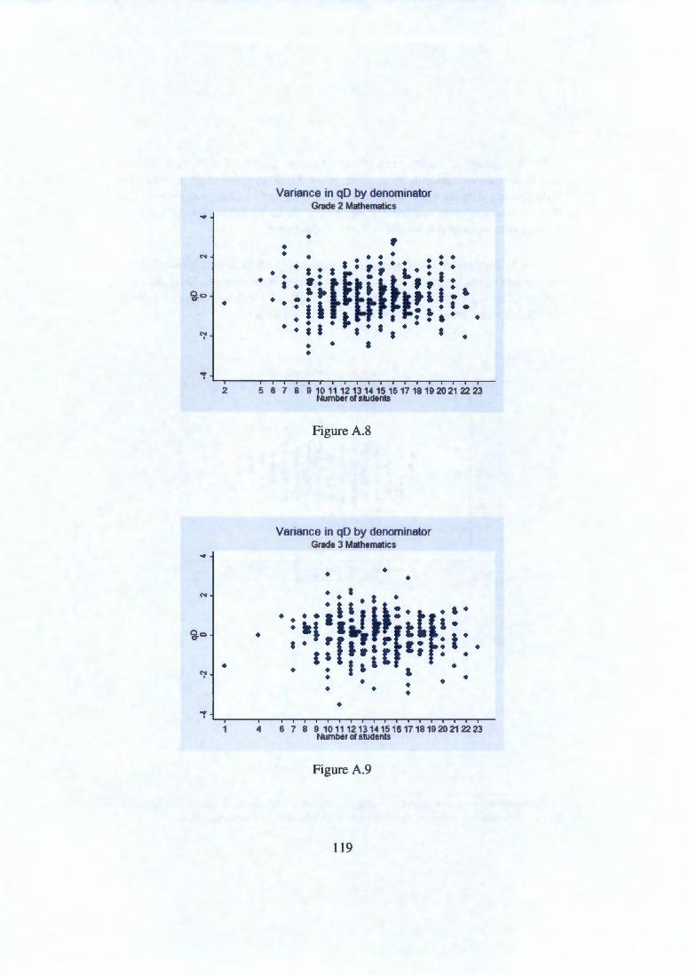
Univers

ity of

Cap

e Tow

n

N

go

~

• • • •

Variance in qO by denominator Grade 2 Mathematics

• • • • • •

• , • • • • • • • • • • • • • • •.• . ,, s.·: .

: niEU~i· ~r:: . . I l l: t.. ! • . . . ~ . . . ~ • • I • • a a • •

• • • • •

•

2 5 6 7 8 9 10 1112 131415 16 17 18 19 20 21 22 23

•

•

Number of students

Figure A.8

Variance in qO by denominator Grade 3 Mathematics

• • •

• 4 6 7 8 91011121314151617181920212223

Number of students

Figure A.9

119

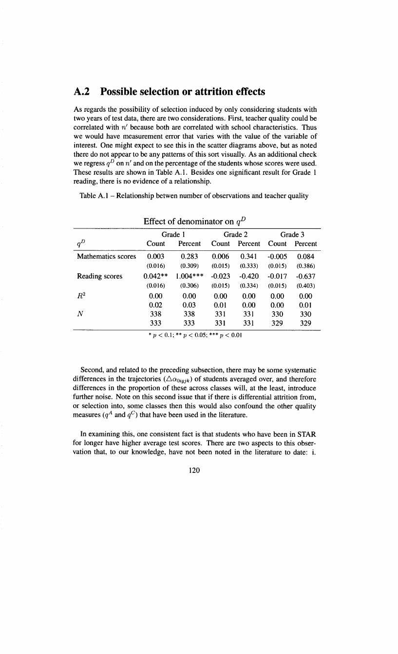
Univers

ity of

Cap

e Tow

n

A.2 Possible selection or attrition effects

As regards the possibility of selection induced by only considering students with two years of test data, there are two considerations. First, teacher quality could be correlated with n' because both are correlated with school characteristics. Thus we would have measurement error that varies with the value of the variable of interest. One might expect to see this in the scatter diagrams above, but as noted there do not appear to be any patterns of this sort visually. As an additional check we regress qD on n' and on the percentage of the students whose scores were used. These results are shown in Table A.l. Besides one significant result for Grade 1 reading, there is no evidence of a relationship.

Table A.l - Relationship betwen number of observations and teacher quality

Effect of denominator on qD

Grade 1 Grade 2 Grade 3 qD Count Percent Count Percent Count Percent

Mathematics scores 0.003 0.283 0.006 0.341 -0.005 0.084 (0.016) (0.309) (0.015) (0.333) (0.015) (0.386)

Reading scores 0.042** 1.004*** -0.023 -0.420 -0.017 -0.637 (0.016) (0.306) (0.015) (0.334) (0.015) (0.403)

R2 0.00 0.00 0.00 0.00 0.00 0.00 0.02 0.03 0.01 0.00 0.00 0.01

N 338 338 331 331 330 330 333 333 331 331 329 329

* p < 0.1; ** p < 0.05; *** p < 0.01

Second, and related to the preceding subsection, there may be some systematic differences in the trajectories (6aoigjk) of students averaged over, and therefore differences in the proportion of these across classes will, at the least, introduce further noise. Note on this second issue that if there is differential attrition from, or selection into, some classes then this would also confound the other quality measures (qA and qc) that have been used in the literature.

In examining this, one consistent fact is that students who have been in STAR for longer have higher average test scores. There are two aspects to this obser­vation that, to our knowledge, have not been noted in the literature to date: i.

120

Univers

ity of

Cap

e Tow

n

Even students who have not been in small classes have scores that are increasing with the years spent in STAR; ii. Scores are higher for students who were in the STAR programme for longer, even in kindergarten. In other words, scores are (unconditional) predictors of continuation in STAR.

Score distribution by years in STAR and classtype Grade 0, Mathematics

• • • • • • • • • • c c • Ul • • • • • • • • -- •

• • • • • • • • • - - -• • • • • • • • -- -.,

f t ~c

Sc U>'l'>

~ .., ., 'iiic <.>Q oo .... • a a •

• • • • • • • • • • c

c .., • s R RA s R RA s R RA s R RA

1 year 2years 3years 4 years

Figure A.10

121

Univers

ity of

Cap

e Tow

n

Score distribution by years in STAR and classtype Grade 2 Mathematics

• • • • • • - • • 0 0 • • • • • • • -• -,._

• • • • • • • • - - • 0 s a a ' 'L') • .,<O s & f a a 0 • I s r_ ~ l;:o • a .. • 1-0 • <"' & I & a • (/)

"Co .!!'L') a a • • "''L') .., f r a a- .. • (/)

0 f ,. t r ~ .-0 s ' f & I a It) • a f a ' • s • s • • • 0 • It)

• • s R RA s R RA s R RA s R RA

1 year 2years 3 years 4 years

Figure A.l 2

122

Univers

ity of

Cap

e Tow

n

Score distribution by years in STAR and classtype Grade 3 Mathematics

0 0 CD

• • • • • • • • • • • • • •

• • • • • -• • Q> O ~o o,._

I I • • • • ' I I & I • <>

"' 1-<( (/) .., .!! o (UO ~(I)

• • 0 I • • 0

"' • s R RA s R RA s R RA s R RA

1 year 2 years 3 years 4 years

Figure A.13

Note, however, that because the direction and approximate magnitude of the differences are broadly the same for all class types, these should therefore not affect estimates of the gains from being in a small class. So while the results are interesting, and possibly merit some separate work, they do not indicate a problem for our current analysis. Similar patterns can be seen for reading scores as shown in Figures A.14-A.17.

123

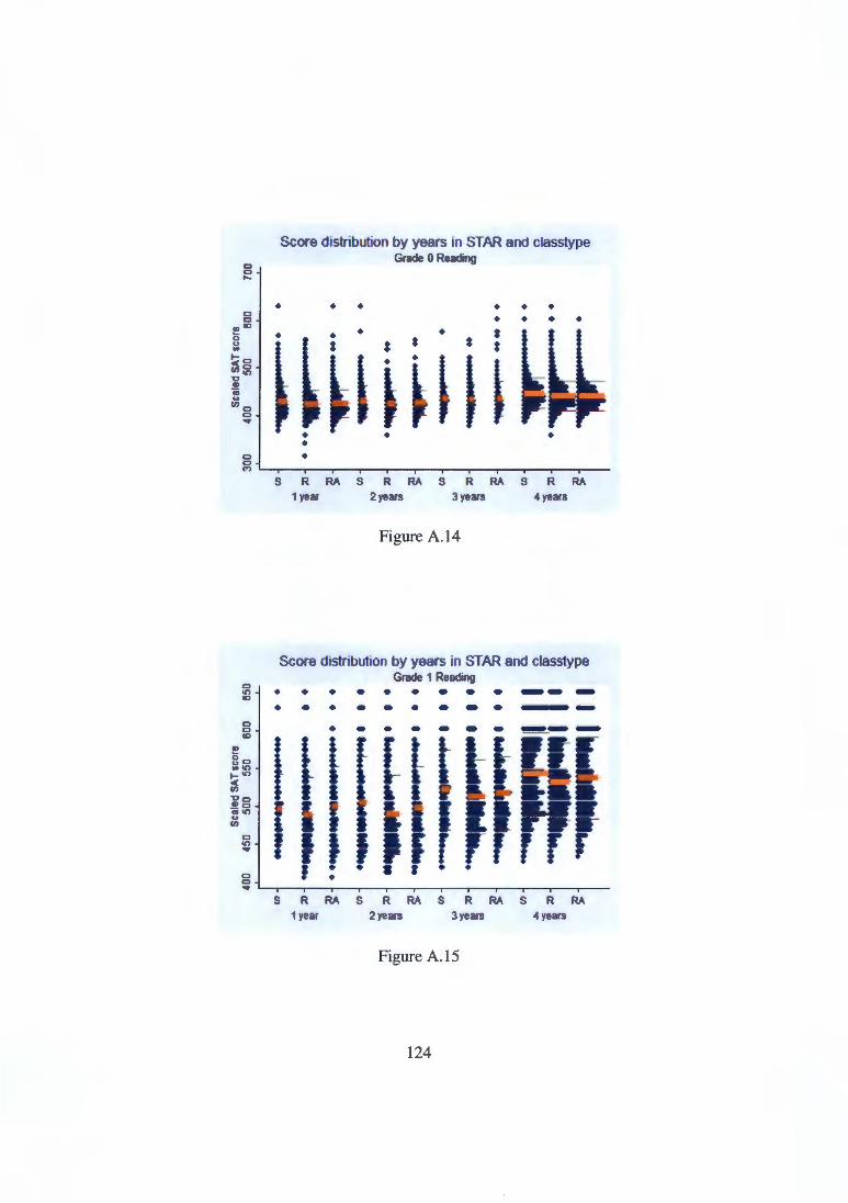
Univers

ity of

Cap

e Tow

n

Score distnbution by years in STAR and classtype

C) Grade 0 Reading

C) .....

• • • • • • C) C) • • • • .,.., • • a 0 • • a a u l l * "'

~g • •

l ' (/)"' "0

"' ;;:; u (I) C)

C) ~

• • • • C) • C) ..,

s R RA s R RA s R RA s R RA 1 year 2 years 3 years 4 years

Figure A.14

Score distnbution by years in STAR and classtype Grade 1 Reading

C)

"' • • • • • • • • • ---"' • • • • • • -- • -C) • • • • - - - !!!!!!!!!!!t.--C)

"'

I l l f ~l l ll "' 8o "'"' 1-"' < (I) I I I l I "De .!!!c

"'"' u

l I I (I)

C) I a I I • "' ~ I r r r r f • • • C) • C)

~

s R RA s R RA s R RA s R RA 1 year 2years 3years 4 years

Figure A. 15

124

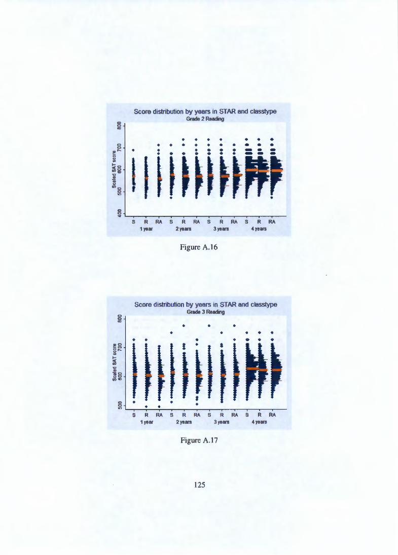
Univers

ity of

Cap

e Tow

n

Score distribution by years in STAR and classtype

0 Grade 2 Reading

0 CD

• • • • • • • 0 • • • • • • • • • • 0 • • • • ., .... • • - • -0 • • • • • • • ---...

I I "' ~ g (/)"' "D ., c;; ... (/)0 f 0

ll')

• 0 0 ...

s R RA s R RA s R RA s R RA 1 year 2years 3 years 4years

Figure A.16

Score distribution by years in STAR and classtype

0 Grade 3 Reading

0 CD

• • • • • • • •

• • • • • • • Cl) 0 I • a ~o 8,.._ "' 1-..: (/)

"D ., ~g (/)CD

• • ' 0 • 0 • • ll')

s R RA s R RA s R RA s R RA 1 year 2years 3years 4 years

Figure A.17

125

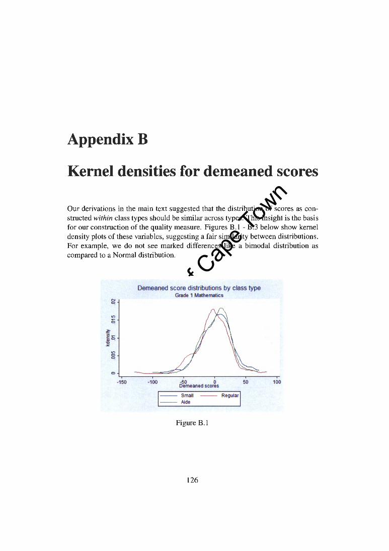
Univers

ity of

Cap

e Tow

n

Appendix B

Kernel densities for demeaned scores

Our derivations in the main text suggested that the distribution of scores as con­structed within class types should be similar across types. This insight is the basis for our construction of the quality measure. Figures B.l - B.3 below show kernel density plots of these variables, suggesting a fair similarity between distributions. For example, we do not see marked differences like a bimodal distribution as compared to a Normal distribution.

-150

Demeaned score distributions by class type Grade 1 Mathemat ics

-100 -50 0 Demeaned scores

1

-- Small -- Regular I .-- Aide .

Figure B.l

126

50 100

Univers

ity of

Cap

e Tow

n0

-50

-100

Demeaned score distributions by class type Grade 2 Mathematics

0 50

I== Demeaned scores

Small Aide

Figure B.2

Regular I

Demeaned score distributions by class type Grade 3 Mathematics

-50

I== 0

Demeaned scores

Small Aide

Figure B.3

127

50

Regular I

100

100

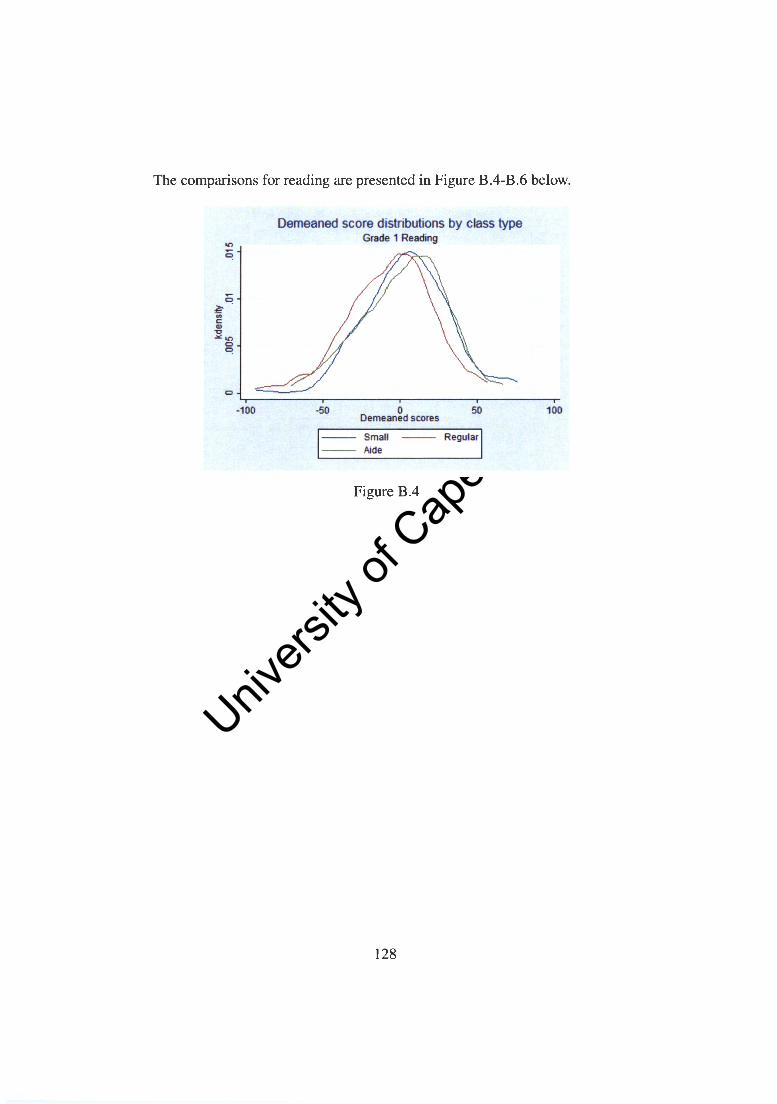
Univers

ity of

Cap

e Tow

n

The comparisons for reading are presented in Figure B.4-B.6 below.

-100

Demeaned score distributions by class type Grade 1 Reading

-50 0 Demeaned scores

50

1

-- Small -- Regular I _-- Aide .

Figure B.4

128

100

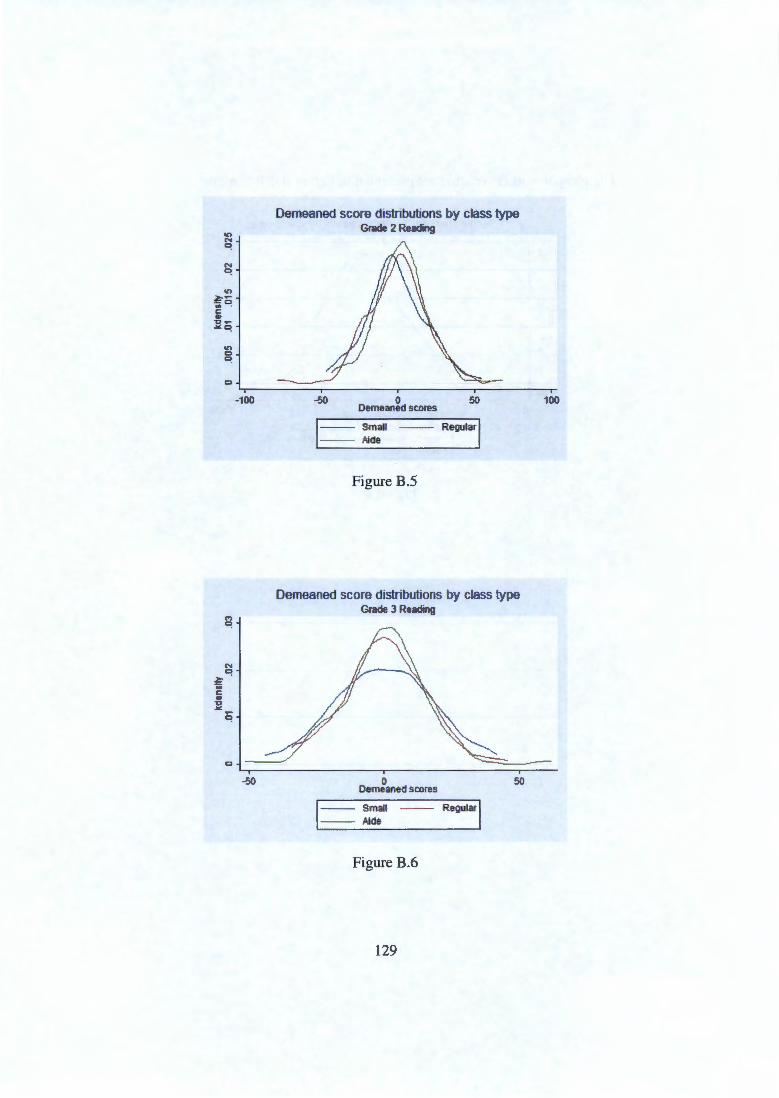
Univers

ity of

Cap

e Tow

n

N 0

~t ' ... c:: Ill .., ...

Ci

-100

-50

Demeaned score distributions by class type Grade 2 Reading

-50

I== 0

Demeaned scores

Small Aide

Figure B.5

50

Regular I

Demeaned score distributions by class type Grade 3 Reading

I== 0

Demeaned scores

Small Aide

Figure B.6

129

50

Regular I

100

Univers

ity of

Cap

e Tow

n

Visual comparisons have their limits, so we also run Kolmogorov-Smimov tests for equality of two distributions. The null hypothesis is that the distributions are the same and the p-values for these tests are reported in Table 2.1 in the main text. None of those values suggests that the null can be rejected at the 10% level.

130

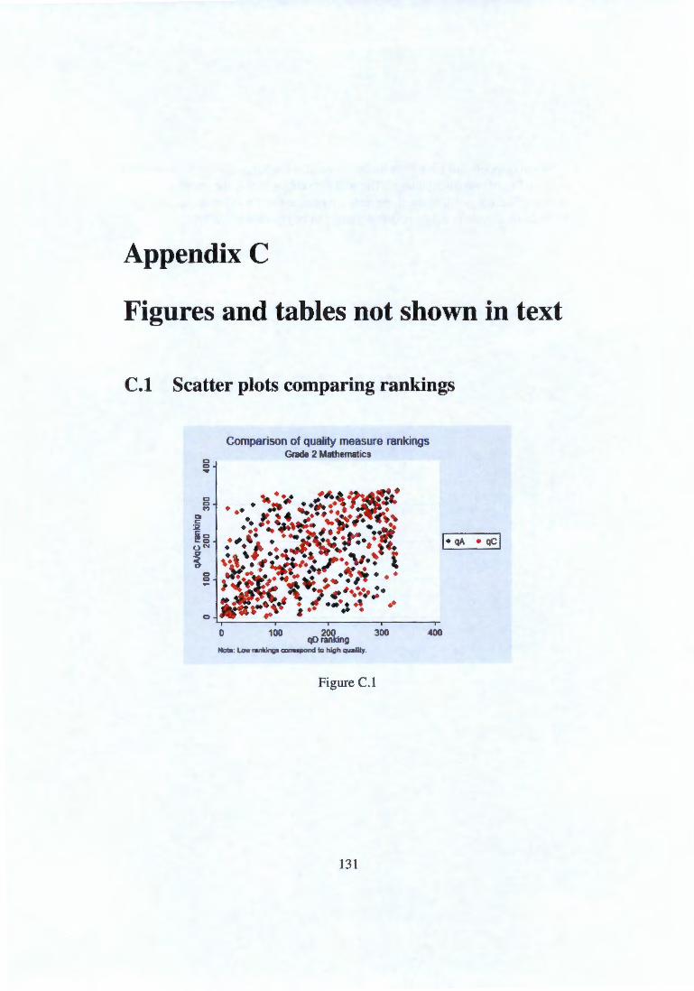
Univers

ity of

Cap

e Tow

n

Appendix C

Figures and tables not shown in text

C.l Scatter plots comparing rankings

Cl c

C) C) ...

C) C) M

:i1 CCI !!!c o"'

~ C) C)

0

Comparison of quality measure rankings Grade 2 Mathematics

100 200 qD ranking

300 400

Nota: L.ow ranldngs CDirRipC>f\d to high quolity.

Figure C. I

13 1

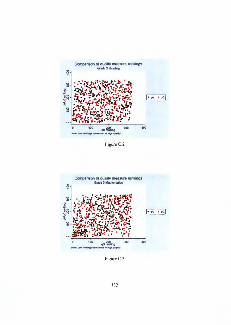
Univers

ity of

Cap

e Tow

n

C) C) M

0 c: :;;c c:C)

~C) u "' <T

~ C) C)

0

0

Comparison of quality measure rankings Grade 2 Reading

100 200 QD ranking

300 400

Note. Low ranldngs a>nespond to high quality.

0

Figure C.2

Comparison of quality measure rankings Grade 3 Mathematics

•

100 200 QD ranking

300 400

Nota: Low rantings axrupond to high quality.

Figure C.3

132

Univers

ity of

Cap

e Tow

n

C.2

0 c: :;;:

0 0 ...

0 0 M

c:o ~0 u"'

~ 0 0

0

Comparison of quality measure rankings Grade 3 Reading

100 200 qD ranking

300 400

Nota: Low ranllngo axrospond to high quality.

Figure C.4

Quality measures across school types based on reading scores

133

Univers

ity of

Cap

e Tow

n

Q)

~ "' ~C) :?I Cii "' .,. ._ o..., :i .. Q)

::1

Comparison of quality measures over school types Quality measure qA: Reading

Inner city Suburban Rural Urban

- GradeD - Grade1 - Grade2 - Grade3

Figure C.5

Comparison of quality measures over school types Quality measure qD: Reading

Inner city Suburban

Grade 1 Grade 3

Rural

- Grade21

Figure C.6

134

Urban

Univers

ity of

Cap

e Tow

nComparison of quality measures over school types

Quality measure qC: Reading

lnnerdty Suburban Rural Urban

- GradeO - Grade1 - Grade2 - Grade3

Figure C.7

135

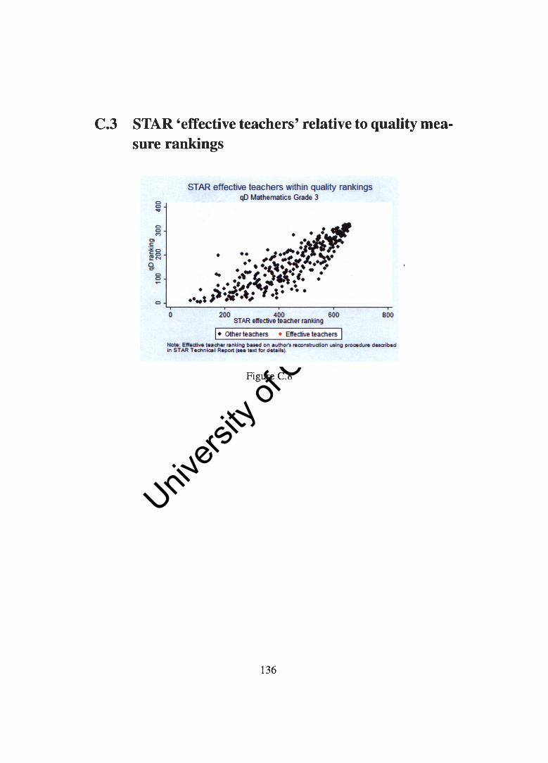
Univers

ity of

Cap

e Tow

n

C.3 STAR 'effective teachers' relative to quality mea­sure rankings

0 0 • 0 0 ...,

co c: :i<o c:o !!!N 0 .,.

0 0

0

0

STAR effective teachers within quality rankings qO Mathematics Grade 3

. . ~if .. ·;.,..1fi..-• ..• :'S'-.-:~ .. '1. •• ,.. . . ··~· ... .. .,•t.. ·~ .. , . . \ -... . . ', ~ .. • ~!..J.41'-... '·' • ••• .... ,I ...... , •

200 400 600 STAR e!feclive teacher ranking

I• Other teachers • E!fective teachers I 800

Note: Effective t .. c:n., ranting bued on author'o rotcorulruc:tion using pn>Citdure ducribed in STAR Tec:hni<» l Repod { ... tu:t lor details).

Figure C.8

136

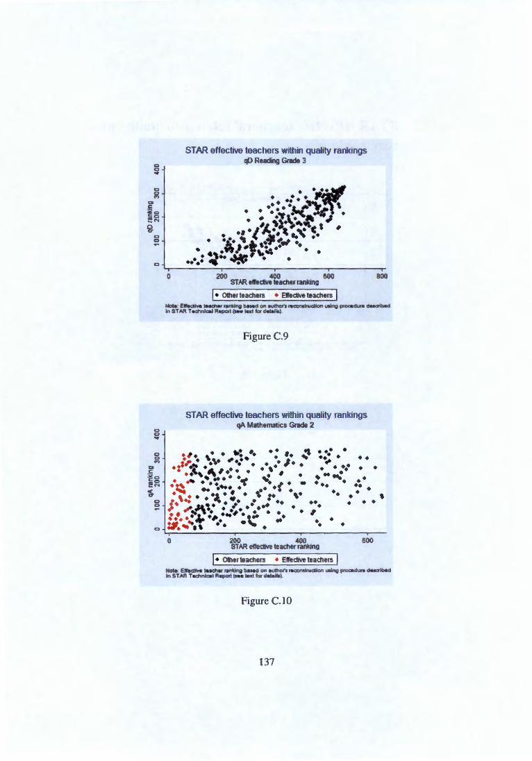
Univers

ity of

Cap

e Tow

n

C) C) .. C) C) ..,

Cl c: :li!o <=o ~ .... 0 .,.

C) C)

C)

C) C) .. C) C) ..,

C) C)

0

STAR effective teachers within quality rankings qD Reading Grade 3

· .. ::· ·~· ........... ~ ..... ' • • • ~ ·~:- :llf • •• ~·~· ~ .I • ~'' • J; .. ~. c ' • • •• ~ ~v•' .. , •• . .,. .. 't .. ..,. ......

I # •• •• • . . . \.~ .. .... : ..:·· ~ . . 200 400 600

STAR effective teacher ranking

I• Other teachers • Effective teachers I BOO

Not•: EIIK:Iive t .. c:her ranting baM<! on alllho<'l reconslruciion using pn>ced..,. d .. cribed In STAR hchniaol R..,ac! ( ... tut lor d.tall>).

Figure C.9

STAR effective teachers within quality rankings qA Mathematics Grade 2

.,. . . •: .. . : ..

.•. • '\• ,... • •I• ...... . . . . . . •• ··'' 4\'·· •.. ~ # • • ... • .... ·-r "'· • .. , -· ~... . .. •:

•

• •• • • •• ., . ..... ...... • •• •

•• •

•• • •• ~· .

•

. ~, ... ·~ . : . \ :• . .. . . . . .. \• ..ta.~• • I .• ••• •• • . , • • • . ...., . .,. . . .. .. t _· .... ... .... •

• .... . ..... '- ... C) :~., ., • • • • • •••

0 200 400 600 STAR elfeclive teacher ranking

I• Other teachers • Elfeclive teachers I Nola: EIIK:Iiva taach .. ranting bllH<I on autl>ex's rRCOnslruciion using pn>ced..,. d .. cribad in STAR Tac:hniaol R•pcxt (Kalaxl for dalai l>).

Figure C. lO

137

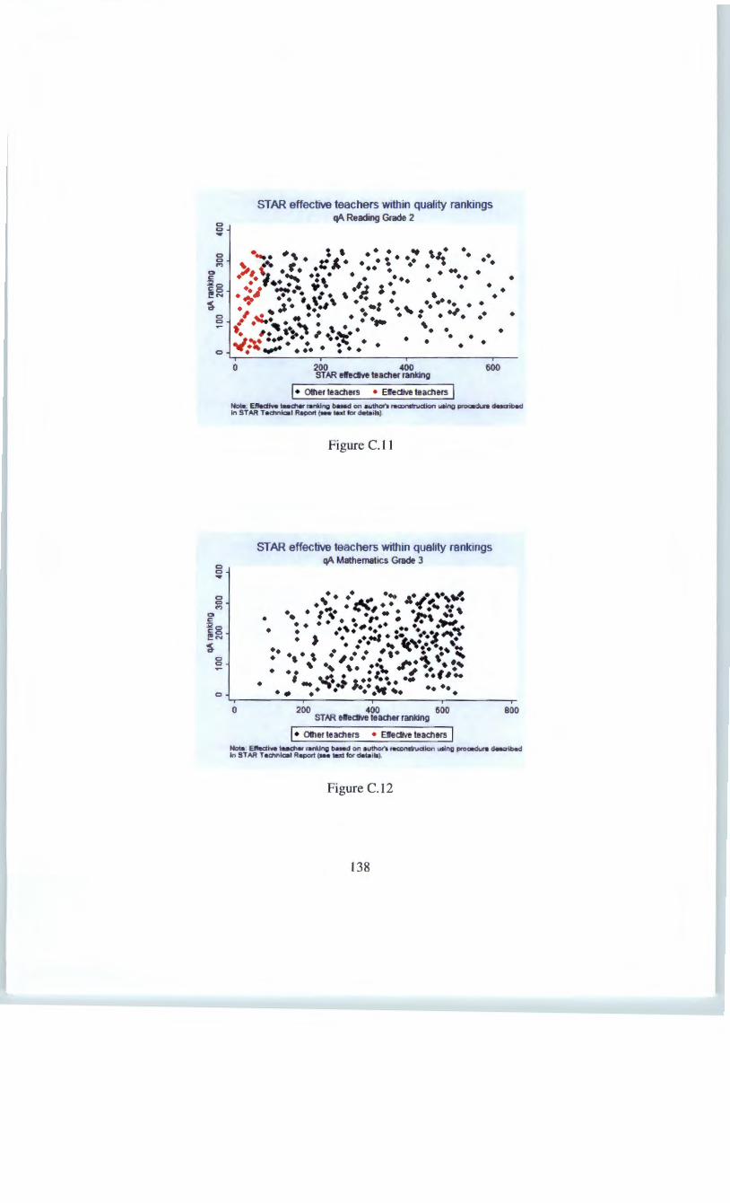
Univers

ity of

Cap

e Tow

n

0 0 • 0 0 ..,

STAR effective teachers within quality rankings qA Reading Grade 2

• • ... \ ' • • • .. \t• •• • ' ••• ; •• • ::I.. • .: ~. ••• • \ •• i''· ,_. ., •• • • • •• • • .... • • .: .~·;.: .•. •: ·'.: : ·. . . .. . ~~~ ........ \. ~ .. . . . ~ . .. .. ,. . : . . .... . . , . .~ ...... ·~·· ... · .. 0 • .. • • • • • • •

0 •• • • • ... • • .... ' •

•• ,.~ , ••• l •• ·'~·. • •• • • _ _~._. ..• . . ·~.. . . . 0 ~: .. ~· .: • • :.. • •

•

0 0 • 0 0 ..,

0 r::: :i<o r:::o ~ .... ~

0 0

0

0 200 400 600 STAR effective teacher ranking

I• other teachers • Effective teachers I Nola: Eflec:tlve teacher ranking basad on authon rtmnsltuction Uling procadL.WR duaibed In STAR Tac:hnlao l Rape<! ( ... lutlordelail•).

0

Figure C.ll

STAR effective teachers within quality rankings

•

qA Mathematics Grade 3

. .. · ..... ~.·~· ,.,~~ • \l • z!t(. • • "' ...... . . ~~· ·'- . ·-·, •\ ~ . . ..... ,. . ,.- ~ . . . ., .#. .. .. .. ·--· . . • . • . ..# ....

• .. • .·~. ·~ .. 4 :·'- • , . . . .. ,~ ..... ~ .. .. . . . •. . .. ,. . .. ' . ' . ,. . . .'\' . . ' .. ~· ··~ .,., ....• ·; .~ . ::.. . ... , ... ... -.·.~ ~:. -·:. .. . . . . . ..... ... . . 200 400 600

STAR eiTedive teacher ranking

I• Other teachers • Effective teachers I BOO

Nola: Ellec:tr.al,..c:her ranting buad o n authon reconstruction using procadura dasaibad in STAR Tac:hniaol Rape<! ( ... lutlor dalailo).

Figure C.l2

138

Univers

ity of

Cap

e Tow

n

0 0 ..

0 0

0

0 0 ..

STAR effective teachers within quality rankings qA Reading Grade 3

•

. ... ·-~.t· e~~~•• .. •.: . . .. . ·~ . ,; ~ .. . . .. . . ., .. ... . . ' .... ~. ... .. . . . .,. .. .. .. ~..._~, ~ .. . . . ' . . . . . ,· .... ·-. ""' ..... • •• : ., •• #( • • ', ; -. ... \. . ... , .... •i ... .z •••••••• , • ~ ~ . .. ~ ~ . . .;.. ...• . . '···.,.,.It .• ~~ ....... ~ ... ., . . .. .

~---------r---------r---------.---------. 0 200 400 600 BOO

STAR effective teacher ranking

I• Other teachers • Efrec:tive teachers I Note: EIIRdlve teacner ,.nllng bued on aLI!hor'l reconstruction using proe»dure d esaibed in STAR Tecnnical Report ( ... text lcr detail>)

Figure C. 13

STAR effective teachers within quality rankings qC Mathematics Grade 2

. . . . .. .. .,. '· · .. · : ·. ··,. . . . ... . .. . . . . •. • •• • .... I ... • t ••• • .• • ... .. .,.. . . . ,. .. . ... ... . •.. ....... . . .. . . . . .. . .. , .

• 4' ... ~ tt ·' •••••••• • : ,r.. ·,~.~··· , . . . . .. . .. '_. . ' .. .. .. . . /.. . ., .... ._. .. ···.~ . . . .. ~ .. '. , • •

• • ,

• •• h. • • ••

• •

,.,.__ .. ·: ' . .. . 0 ,.. •• ·., ... • • • •• • •

0 200 400 600 STAR effective teacher ranking

I• Other teachers • Elfec:tive teachers I Note: Effective teacner ranting bued on aull>ac's reconstruction using proe»dura desailad in STAR Tecnnical Reporl (lee text lcr details).

Figure C. 14

139

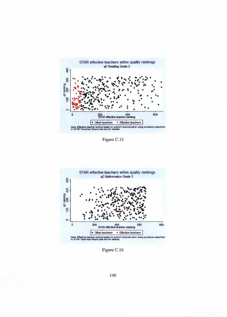
Univers

ity of

Cap

e Tow

n

0 0:::

0 0 ....

0 0 ..,

0 0

0

0 0 ....

0 0 ..,

:i<o <=o ~N u .,.

0 0

0

STAR effective teachers within quality rankings qC Reading Grade 2

. . . . .. ' . .. ..... •• • ...·~· ··~· #. .. ........ , ... • <. •• ~ ~ ...... ,, ••

• • ... • • • • • -,• I• ... .. . ·~~~. . .. . . . . ......... ,.. . . . • • • • ..

• .., •• ~.. • • #. • • . ,. ; . . . . ; . .... ~·- # :·:· • .. • '·' •

• • • • w.. : • • &.. • • •• • ~-,. ~, ... ~. .. . . ~.... ... . .... , .. . . . ~ ... ,.-.. .... .. . . • •

• • • 0 200 400 600

STAR effective teacher ranking

I• Other teachers • Effective teachers I

• •

Nota: Ell..:tive teac:Mf ranting baHd on aulhon <aa>nslruc:tion using pn>CR<Iure dosaibed In STAR Tecnnlao l Rep«i {Helul lo<d•t.ils).

0

Figure C.15

STAR effective teachers within quality rankings qC Mathematics Grade 3

• •

. . . .. ~ ~~··~ ... ,. . . ........ ' . . . rlt . ~"·.,#.A .... . • •• •• • ..._. I . . ........ -. ·~, .,

•I• :. • •t,llt•!•11......••• .. • ... , .. • •• •v.• T • I# • •;=' •• : •• ,. • .., ' .:t! • ~ ' • • • • •t .. ~. • • • 1•. ,.

... • • • .\ • • • ••• \ ~ ~ i'. . . .. .,. . ..~ ... ... ·· .. .. •: . .. .. ·~ . .. . . . 200 400 600

STAR elledive teacher ranking

I• Other teachers • Effective teachers I 800

Nota: Ell..:tive tead>M <anting baHd on authOf's Jaconslruc:tion uoing ptOCRdUJe dHctibed in STAR Tecnnical R._t ( ... text Ia< d•t.ils).

Figure C.l6

140

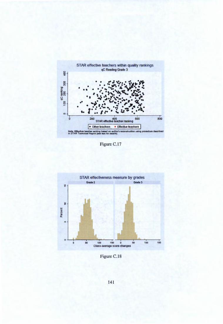
Univers

ity of

Cap

e Tow

n

0 0 ... 0 0

"' "' <: :i<o <=o ~ ..... u CT

0 0

0

0

STAR effective teachers within quality rankings qC Reading Grade 3

•

• • .. J ··~·· • ·~ .... ·~~ .............. ~~ .... ~. • • • • .... 4 •\_.,. ••••• • • • • ... ... r .. ~ ... " . ·:,.~ .. ~··· , . . "'· . ~ ,. ... \ . . . . ·' ....... . . --.: ~·· ~ .. ~ ... · .... •• •• • "-··· r •:( ... , . .. . ,. . -..· . . ......... : . ~·.ft ... . .. . . . . , .. •• ~ 1 ...... _.., ••• . .. . - .

200 400 600 STAR e1fedive teacher ranking

I• Other teachers • E1fedive teachers I BOO

Not• : Ell.ctiv• lu cn• ,.nldng b..-d on • ulhon r•conslrudion Llling pr<><»dure d .. oribtil in STAR T..:hnic:. l RllpDfl (aelut for d.U.ils)

Figure C.17

STAR effectiveness measure by grades Grade 2 Grade 3

0 100 1!50 0 !50 100

Class-average score changes

Figure C.18

141

Univers

ity of

Cap

e Tow

n

C.4 Residualising on actual class size

In the main text we noted that in the actual Project STAR experiment there was variation in class size within treatment assignment (class type) categories. Our quality measure, however, was constructed only within these categories and did not explicitly account for variation within them. To check whether this makes a significant difference we residualised class average scores (or score changes) on actual class size before constructing the ranking. Table C.l and C.2 show the Spearmank rank correlations between the residualised and non-residualised measures. For the levels-based measure (qA) the smallest correlation is 0.992 and for our preferred change-based measure (qD) the smallest is 0.995 and all are highly significant. From this we conclude that the class-type based measures are not significantly confounded by within-type variation.

Table C.l - Spearman rank correlations for qA

GradeO Gradel Grade2 Grade3 MATHEMATICS Correlation 0.997 0.993 0.995 0.993 p-value 0.000 0.000 0.000 0.000 N 325 339 335 333 READING Correlation 0.995 0.993 0.995 0.992 p-value 0.000 0.000 0.000 0.000 N 325 334 335 328

Note: The correlation coefficients show the Spearman rank correlation be­

tween the relevant quality variable and the same variable residualised on actual

class size.

142

Univers

ity of

Cap

e Tow

n

Table C.2 - Spearman rank correlations for qD

Gradel Grade2 Grade3 MATHEMATICS Correlation 0.997 1.000 1.000 p-value 0.000 0.000 0.000 N 338 331 329 READING Correlation 0.995 1.000 1.000 p-value 0.000 0.000 0.000 N 333 331 328

Note: The correlation coefficients show the Spearman rank correlation be­

tween the relevant quality variable and the same variable residualised on actual

class size.

143

Univers

ity of

Cap

e Tow

n

Chapter 3

The external validity of class size effects: teacher quality in Project STAR

Abstract

As discussed in Chapter 1, the external validity of treatment effects is of fundamental importance for policy and interaction effects are critical deter­minants of external validity. This chapter provides an empirical exploration of the significance of this relationship in the context of experimental evalua­tions of class size effects on student outcomes. While the existing literature assumes an additively separable educational production function, the way in which class size is hypothesised to affect outcomes more plausibly implies an alternative specification in which the marginal effect of size depends on teacher (class) quality. To investigate this possibility the novel measure of quality constructed in Chapter 2 is used to estimate possible interaction ef­fects between teacher quality and class size in the Tennessee Project STAR dataset. Results are mixed across grades and subjects, but include statisti­cally and economically significant effects that suggest dependence between the class size effect and class quality. Given the analysis in Chapter I, this implies that even the results from an ideal class size experiment cannot be extrapolated to a different context without information on the distribution of teacher (class) quality; the external validity of class size effects will depend on the teacher quality distribution in the populations of interest. In addition, our analysis contributes to the economics of education literature by consid­ering the relationship between teacher quality and class size. In the presence of an interactive production function the policy problem may be to find an optimal combination of size and quality, in contrast to much of the existing literature which treats such interventions as mutually exclusive.

144

Univers

ity of

Cap

e Tow

n

The use of randomised interventions to estimate causal relationships brings with it the promise of greater credibility of policy prescriptions based on econo­metric analysis. Many studies have been in the area of education, tackling ques­tions such as the effects of class size, textbook allocation, grade-based tracking and teacher incentives. This approach, when successfully implemented, provides internal validity - achieving identification of the causal effect. It need not, how­ever, provide external validity: identification of a causal effect that would occur in the implementation of the same intervention in other contexts. While the im­portance of both forms of validity has been known for some time in the broader social science literature, there have been only a handful of contributions dealing with external validity in the recent econometrics literature.

Chapter 1 shows in detail that if the (possibly reduced form) linear structural equation contains an interaction term involving the treatment variable, the average treatment effect will vary with the mean of the interacting variable. The analysis of the present chapter is premised on the claim that the relationship between class size and student outcomes may be a good example of such a relationship: class size may have an effect partly because it moderates the causal effect of other variables. Perhaps the most important of these is the effect of the teacher, which one strand of the literature argues is the most important school-based component of the education production function. Until recently, however, the literature could to a large extent be characterised by two types of contributions: those emphasising the role of teacher quality (or teacher effects more broadly) and those emphasising the importance of material factors, in which category class size analyses have been placed. In the present paper, by contrast, our interest is in how these two types of factors interact with each other. Given the 'production function' terminology we would argue that this kind of interdependence between inputs should be the default assumption. Within the literature on firms additively separable production functions are considered highly implausible and there is little reason to believe that the production of education is likely to be less complex than the production of goods.

Chapter 2 showed how, in a randomised evaluation satisfying certain condi­tions, a value-added teacher quality measure can be constructed so that it is or­thogonal to class size. This is important because direct measures of teacher qual­ity rarely exist and where they do it is not in association with experimental data on class size. That analysis therefore presents the possibility of estimating un­confounded interaction effects between size and, broadly defined, teacher quality using the same data. Our empirical analysis uses the Tennessee Studentffeacher Achievement Ratio project ('Project STAR') conducted in the late 1980s, which

145

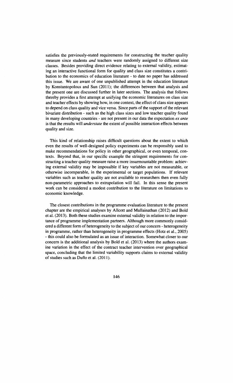
Univers

ity of

Cap

e Tow

n

satisfies the previously-stated requirements for constructing the teacher quality measure since students and teachers were randomly assigned to different size classes. Besides providing direct evidence relating to external validity, estimat­ing an interactive functional form for quality and class size constitutes a contri­bution to the economics of education literature - to date no paper has addressed this issue. We are aware of one unpublished attempt in the education literature by Konstantopolous and Sun (2011); the differences between that analysis and the present one are discussed further in later sections. The analysis that follows thereby provides a first attempt at unifying the economic literatures on class size and teacher effects by showing how, in one context, the. effect of class size appears to depend on class quality and vice versa. Since parts of the support of the relevant bivariate distribution - such as the high class sizes and low teacher quality found in many developing countries - are not present in our data the expectation ex ante is that the results will understate the extent of possible interaction effects between quality and size.

This kind of relationship raises difficult questions about the extent to which even the results of well-designed policy experiments can be responsibly used to make recommendations for policy in other geographical, or even temporal, con­texts. Beyond that, in our specific example the stringent requirements for con­structing a teacher quality measure raise a more insurmountable problem: achiev­ing external validity may be impossible if key variables are not measurable, or otherwise incomparable, in the experimental or target populations. If relevant variables such as teacher quality are not available to researchers then even fully non-parametric approaches to extrapolation will fail. In this sense the present work can be considered a modest contribution to the literature on limitations to economic knowledge.

The closest contributions in the programme evaluation literature to the present chapter are the empirical analyses by Allcott and Mullainathan (2012) and Bold et al. (2013). Both these studies examine external validity in relation to the impor­tance of programme implementation partners. Although more commonly consid­ered a different form of heterogeneity to the subject of our concern - heterogeneity in programme, rather than heterogeneity in programme effects (Hotz et al., 2005) - this could also be formulated as an issue of interaction. Somewhat closer to our concern is the additional analysis by Bold et al. (2013) where the authors exam­ine variation in the effect of the contract teacher intervention over geographical space, concluding that the limited variability supports claims to external validity of studies such as Dufto et al. (20 II).

146

Univers

ity of

Cap

e Tow

n

The remainder of the chapter is structured as follows. Section 3.1 summarises the literature on educational production functions with a particular emphasis on experimental or quasi-experimental analyses of class size effects, demonstrating why these constitute a valuable empirical case study for the external validity prob­lem.1 Section 3.3 gives a more detailed overview of the STAR data than was provided in the previous chapter and discusses how the strengths of that experi­mental design enable our analysis of interactions. With this background, Section 3.4 presents the empirical analysis and considers robustness of these to alternative specifications and assumptions made regarding other aspects of the production function. There are some important additional technical issues - specification con­cerns when estimating interaction effects, choice of standard errors, the relevance of interaction for our quality measure and reflection effects - mentioned briefly in that section which require further consideration and these are addressed more fully in section 3.5. Section 3.6 locates our findings within the existing empirical literature and discusses the implications for external validity of class size effect estimates in general.

3.1 Educational production functions and class size effects

The issues of causal interaction discussed in Chapter 1 are entirely generic in the sense that they concern causal inference in general rather than any particular area of study. To demonstrate the empirical relevance of such issues requires, however, that we narrow our focus to a particular causal relationship of interest. This sec­tion explains three reasons for choosing the example of class size effects. First, these have been the subject of numerous high-quality studies based on either ran­dom or quasi-random variation across different contexts. Second, the apparent stability of these effects has been cited to substantiate the view that external va­lidity of average treatment effects may often hold for questions of policy interest. Finally, we argue that although this point has been neglected in the literature on educational production functions, class size exemplifies the interaction problem because its primary causal effect may be through the moderation of the effects of other variables operating at the classroom level.

1There is some overlap between our discussion here and that in 2.2, but this is necessary for completeness and the emphasis of the discussions is different.

147

Univers

ity of

Cap

e Tow

n

3.1.1 Why class size?

The usefulness of randomised evaluations for informing policy has been the sub­ject of a series of important recent debates. Most critical contributions rely either on theoretical or conceptual criticisms, or specific empirical illustrations of how policy questions may not be adequately addressed through a randomised evalua­tion. This is partly because there are very few areas in which enough experiments have been conducted to engage with a diversity of evidence. A notable exception is the case of educational interventions where there now exists a sufficient num­ber of studies to justify thorough meta-analyses of the kind performed by Kremer and Holla (2009), Glewwe, Hanushek, Humpage, and Ravina (2011) and McE­wan (2013). In this context experiments to test the effects of class size reductions have been specifically cited as a possible example of simple external validity, with Angrist and Pischke (2010: 24) noting that in the four studies they consider: "a ten-student reduction in class size produces about a 0.2 to 0.3 standard deviation increase in individual test scores". This provides one motivation for our study of class size using the Project STAR experiment.2

The second motivation is that, it will be argued, class size is a prime candidate for a variable whose effect is dependent on the value of other variables, imply­ing an interactive functional form for the underlying data generating process. For instance, if a teacher is very bad it is plausible that greater exposure (lower class size) to that teacher has little, if any, positive effect whereas the opposite may be true for a high quality teacher. The only paper in the economics literature to have tackled this issue directly is Lazear (2001), who develops a theoretical model of the classroom as a public good that suffers from 'congestion' as pupil numbers increase. This model has been consistently overlooked by subsequent empirical studies, perhaps because of implausibly strong modelling assumptions regarding maximising behaviour of teachers and schools - a commonly-raised concern with structural approaches to econometrics in general (Heckman (2000), Imbens (2010, 2013)). As Krueger (2003) notes, however, the structural approach does have the advantage that it "yields a specific functional form for the education production function" (Krueger, 2003: 54) and Keane (2010a,b) has noted the implications of that for randomised programme evaluations. So while structural interaction is implied by examining variation in treatment effects across other variables, most studies have neglected explicit consideration of appropriate functional form rep­resentations of class size. Even structural approaches such as Todd and Wolpin

2Related concerns about external validity are raised in a very recent article by Pritchett and Sandefur (2013), focusing empirically on returns to education and class size effects. The empha­sis there, however, is more on cross-country comparisons of estimated parameters and possible selection into experimental samples.

148

Univers

ity of

Cap

e Tow

n

(2003) begin methodological discussion with fully non-parametric models, but base empirical estimation on linear models with the simplest of additive forms. Some prescient discussion on this issue can be found in Hanushek (1979) and Ehrenberg, Brewer, Gamoran, and Willms (2001). The result is that some anal­yses - for instance Bandiera, Larcinese, and Rasul's (2010) quasi-experimental analysis of university class size effects - argue that results are 'generalisable' be­cause of similarity in a few incidentally observed variables across contexts.

Some particularly relevant contributions to the class size literature are Krueger (1999), Krueger and Whitmore (2001), Nye et al. (2004) and Chetty et al. (2011) using the STAR data.3 Konstantopolous (2011), Konstantopolous and Sun (2011) and Jackson and Page (2013) follow Krueger (1999) in examining variation in the class size effect across other variables. Ding and Lehrer (2011a) and Chetty et al. (20 11) show, however, that some of these relationships are no longer statistically significant when all covariates are considered simultaneously. Taking different perspectives on the external validity problem, Ding and Lehrer (2010a) examine possible Hawthorne effects in Project STAR and Rivkin and Jepsen (2009) con­sider limitations to extrapolation due to scale-up effects on the quality of available teachers by examining an actual class-size reduction programme in California. While Konstantopolous and Sun (2011) is most similar to the present paper by virtue of its interest in how teacher effects may depend on class sizes in Project STAR, the substance of that paper is otherwise very different and, as discussed in a later section, less convincing.

3By the 1990s there had been many hundreds of studies of the effect of class size on educational outcomes using non-experimental data (Hanushek, 1999, 2003). Subsequently many studies have used random or quasi-random variation; early examples in economics are An grist and Lavy ( 1999), Krueger (1999), Hoxby (2000) and Krueger and Whitmore (2001). Krueger (2003) and Hanushek (2003) survey these and other studies but disagree on whether systematically large and positive class size effects have been identified. There are now too many recent contributions to detail here: Urquiola (2006), Browning and Heinesen (2007) and Bandiera et al. (2010) are more recent contributions but using similar approaches to estimation and identification to previous studies; Chingos (2012) and Choa, Glewwe, and Whitler (2012) provide evidence from new US states that implemented class size reduction policies; Urquiola and Verhoogen (2009) and Heinesen (2010) use regression-discontinuity strategies with class-size caps; and, Koenker and Ma (2006) implement quantile estimation extending earlier work by Levin (2001). Ding and Lehrer (2010a,b, 20llb) use the STAR data to examine treatment effect dynamics with similar results regarding effect decay found by Jacob, Lefgren, and Sims (2010) using non-experimental data from North Carolina.

149

Univers

ity of

Cap

e Tow

n

3.2 A model of class size in educational production

To formalise these concerns and develop a basis for the subsequent empirical anal­ysis, we propose a simple model of educational production in which class size is represented explicitly rather than as part of a generic vector of inputs. Based on that we outline an empirical strategy that utilises the randomisation in Project STAR to estimate interaction effects between class quality and class size.

As we saw in the preceding chapter, a general specification of educational pro­duction might look as follows:

Student achievement= F(Indiv, Hhd, Class, School)+ error

The majority of empirical contributions to the economics literature assume that all components ofF() can be represented as additively separable.4 There are var­ious problems with this from the perspective of class size studies. The most basic concern is the absence of justification for conceiving of class size as a factor that has a direct causal effect of its own. Arguments in favour of smaller classes in the education literature have often emphasised the effect on teachers' opportunity to interact with, and give greater attention to, individual students. Hattie (2005) pro­vides a critical survey, while Blatchford and Mortimer ( 1994) discuss mechanisms and Blatchford, Goldstein, and Mortimore ( 1998) explicitly consider factors that may mediate the class size effect. Given this, one would expect that the effect on student outcomes partly depends on teacher competence, effort and ability, which together will be referred to as 'teacher quality'. That hypothesis is also implied by the more generic notion that larger classes 'dilute' the educational experience: the effect on educational achievement may depend on what the quality of the undi­luted experience is.

In the economics literature, Lazear's (2001) 'disruption' model is the only rep­resentation that, to our knowledge, allows for the specific possibility that class size interacts with other class-level factors. The broad idea is the same, as Lazear puts it: "the cost of adding additional students can be thought of as a congestion effect" (Lazear, 2001: 779). That paper takes the insight in a different direction, however, as Lazear attempts to provide an explanation for why there is little consensus in the empirical literature on whether class size matters. In particular, the argument he makes is that class size is typically a choice variable for profit-maximising schools that has different optimal values in different situations. The key variable

4Two exceptions are Figlio (1999) and Harris (2007), but the issues discussed in those papers are largely unrelated to our primary concerns - class size effects and external validity.

150

Univers

ity of

Cap

e Tow

n

in that optimisation process is assumed to be student behaviour, as represented by a 'disruption' parameter representing the proportion of time a given student is behaving in class. The probability of disruption in a given class can be determined based on the distribution of this parameter within the class.

The assumptions required to derive the Lazear model are arguably inappropri­ate for empirical analysis concerning public schools, for which resource and class size decisions are often imposed externally. Instead, our analysis adopts a more agnostic approach, using a marginally more complicated form of the production function than traditionally used in the literature and thereby allowing class size to interact with other factors. Recent theoretical specifications of parametric forms ofF(·) take into account the effect of past inputs as well as current ones, and do so in a manner that allows for some 'decay' in these effects over time (Todd and Wolpin (2003), Rothstein (2010)). As in Chapter 2 we build on that approach, assuming additive separability of individual- and school-level components. Now, however, we do not assume that teacher quality and class size are additively sepa­rable. One can then write the following more specific expression for the achieve­ment of student i in classroom j in grade g and school k, in which the role of class size is represented explicitly:

g g

Ajgk = aoig +alL (Jg-h Hih + f3 L v-h(l - 8Chj)f(q~j' Rhj, ao-jh)

h=l h=l g g

+ a2 L </J9 -hGhk + L Eihjk (3.1) h=l h=l

The individual-level ability parameter aoig represents what the student would achieve even absent other factors; Hi9 represents the contribution of household factors that could include variables such as parental education and household in­come; G9k represents school-level factors which could include school manage­ment and school-level resources; and, Eigjk is an individual-specific error term. The remaining term captures our approach to class size, where C91 is total class size and C91 ( = C91 - 1) is used to represent class size excluding the pupil in ques­tion. The variable R91 represents classroom resources, q;1 is true teacher quality and a0.19 is the mean ability of student i's classmates.5 These inputs are converted into a 'classroom effect' by a production technology represented by f(-). In the case of one-on-one tuition (i.e. a personal tutor), a 0-19 = 0 and C91 = 0 so i gets

5In this case the subscript is best thought of as representing a sample mean: no-jg = nj

1/ni 2.:: noijg· i=l

151

Univers

ity of

Cap

e Tow

n

the full benefit of the classroom effect and there is no (positive or negative) peer effect. Every additional student reduces this effect by a factor of 8. The param­eters ¢, .X and fJ represent the rate of decay of prior ( h < g) realisations of the associated variables.

Assuming that child i is in the same class type up to the current grade (g), the average treatment effect under successful randomisation for two fixed class sizes C 1 (under treatment) and Co (the control) is:

E[AijgkiC9 j = C1] - E[Aj9kiC9 j =Co] g

= f38(C1 -Co) L E[.Xg-h f(q'hi' Rhj, ao.jh)] (3.2) h=l

In other words, the representation of the educational production technology in (3 .1) implies the type of context-dependent treatment effect discussed in Chapter 1.

Our approach in (3.1) differs from Lazear in a few respects. First, it explicitly relates the class size effect to the classroom effect. This is critical for consideration of the issues raised regarding interaction and external validity. Second, we do not develop a model of class size optimisation. Whether the model Lazear constructs is informative for empirical purposes is a moot point, but since our empirical application randomly allocates students to class types the issue of class size choice is arguably less of a concern.6 Finally, our model does not allow the marginal effect of additional students (8) to vary with the characteristics of students. Such a relationship could imply 8 = p( Hig) - propensity to misbehave is associated with household factors- meaning that the expression in (3.2) may understate problems of external validity.

Our analysis differs from Todd and Wolpin (2003) in similar ways. That paper focuses on choice-based reasons why educational intervention effects identified in randomised trials may not address the policy question of interest, while class size

60f course, as the discussion in Chapter I makes clear, a structural approach would insist on modelling choice-based compliance with assignment along with issues such as substitution effects. Besides our consideration of interaction, the objective of our analysis is to follow as closely as possible the standard approach in the experimental programme evaluation literature. We therefore do not adopt the structural approach, using index models or otherwise; the merits of that method require dedicated work that is beyond the scope of the present thesis.

152

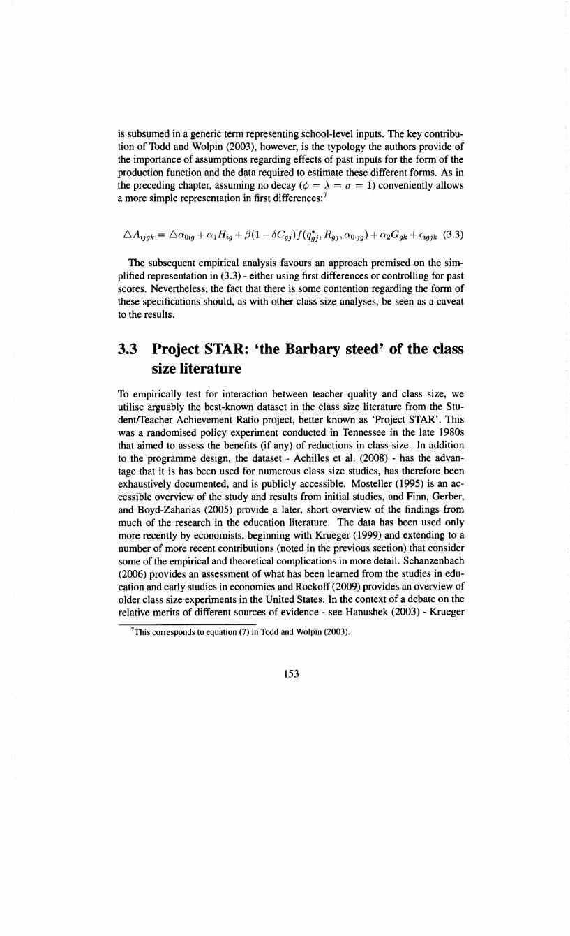
Univers

ity of

Cap

e Tow

n

is subsumed in a generic term representing school-level inputs. The key contribu­tion of Todd and Wolpin (2003), however, is the typology the authors provide of the importance of assumptions regarding effects of past inputs for the form of the production function and the data required to estimate these different forms. As in the preceding chapter, assuming no decay(¢ = A = O" = 1) conveniently allows a more simple representation in first differences:7

The subsequent empirical analysis favours an approach premised on the sim­plified representation in (3.3) -either using first differences or controlling for past scores. Nevertheless, the fact that there is some contention regarding the form of these specifications should, as with other class size analyses, be seen as a caveat to the results.

3.3 Project STAR: 'the Barbary steed' of the class size literature

To empirically test for interaction between teacher quality and class size, we utilise arguably the best-known dataset in the class size literature from the Stu­dent!feacher Achievement Ratio project, better known as 'Project STAR'. This was a randomised policy experiment conducted in Tennessee in the late 1980s that aimed to assess the benefits (if any) of reductions in class size. In addition to the programme design, the dataset - Achilles et al. (2008) - has the advan­tage that it is has been used for numerous class size studies, has therefore been exhaustively documented, and is publicly accessible. Mosteller (1995) is an ac­cessible overview of the study and results from initial studies, and Finn, Gerber, and Boyd-Zaharias (2005) provide a later, short overview of the findings from much of the research in the education literature. The data has been used only more recently by economists, beginning with Krueger (1999) and extending to a number of more recent contributions (noted in the previous section) that consider some of the empirical and theoretical complications in more detail. Schanzenbach (2006) provides an assessment of what has been learned from the studies in edu­cation and early studies in economics and Rockoff (2009) provides an overview of older class size experiments in the United States. In the context of a debate on the relative merits of different sources of evidence - see Hanushek (2003) - Krueger

7This corresponds to equation (7) in Todd and Wolpin (2003).

153

Univers

ity of

Cap

e Tow

n

(2003) attests to the value of this data in referring to it as "the single Barbary steed of the class size literature" (Krueger, 2003: 36).

3.3.1 Data overview

Project STAR was conducted over four years from 1985 to 1989 in the state of Tennessee in the United States, involving 11,600 students, 79 schools and 1,341 teachers (classes). The intervention began in kindergarten and finished in Grade 3.8 School participation was on an opt-in basis, which - along with enrolment requirements and deliberate over-sampling of schools with higher proportion of students receiving free lunches - means that the programme population of schools is not a random sample of Tennessee schools. Krueger ( 1999) suggests, however, that beyond enrolment there is little evidence of systematic differences from state averages on other variables. There were three types of classes in the study: 'small' ( 13-17 students), 'regular' (22-25 students) and 'regular with an aide' (also 22-25 students but with a full-time teaching aide). Both students and teachers were ran­domly assigned to class types. Concern has been expressed in the literature that regular classes had part-time (as opposed to full-time in the aide treatment) teach­ing aides after kindergarten (Krueger, 2003: 500-501), which would confound identification of an aide effect. Furthermore, after preliminary analysis appeared to show no effect of aides in kindergarten, children in regular classes were ran­domly reassigned in Grade 1 across classes with and without aides.9

Children in the programme completed various tests of academic performance at the end of each year, but an important limitation is that no baseline information is available on achievement either prior to entering the programme or at the moment of entry. If a child was assigned to a small or regular class, the intention of the experimental design was that they should remain in that class type throughout the programme. Therefore the group with the longest 'exposure' to treatment were those who entered a programme school in kindergarten and remained in that school until the end of Grade 3. Any child who entered a programme school after kindergarten (which was not legally mandatory) and before the end of the programme was randomly assigned to one of the class types. Students leaving schools exited the programme, although measures of post-programme outcomes may be available for some of these children. As the experiment involved only one cohort across different grades, each teacher was observed only once. The

8The majority of schools - 80% - had four grades or less, so it would not have been possible to continue the programme beyond Grade 3 in most of the original programme schools.

9Krueger (2003: 499) suggests that this was to mollify some parents whose children ended-up in regular classes without aides.

154

Univers

ity of

Cap

e Tow

n

study captured basic characteristics of teachers - such as experience, gender, race and level of education - but there was no attempt in the primary experiment at measuring teacher quality directly. 10

Due to differing grade-level enrolments at different schools, and the nature of the design, there is variation within treatment groups in class size. Schools were only accepted into the programme if they had sufficient numbers of children for at least one class of each type (i.e. 57 students in the grade). Beyond this threshold, larger numbers could be accommodated by increasing class sizes to the permitted maximum (for grades with up to 67 students) and then adding additional classes. For example, a 70 student grade could be accommodated by assigning an addi­tional small class. 11 Besides grade size there does not appear to be any relation between this variation and other factors. That is relevant for the objectives of this paper, since the interactive model of education production suggests that using ac­tual class size is preferable to using the binary treatment variable and that is the approach that will be taken in the empirical analysis.

The achievement measures we focus on, following other studies and the models in (3.1) and (3.3), are outcomes in Stanford Achievement Tests (SATs) in reading and mathematics. Krueger ( 1999) reports similar results across the SATs and the Tennessee-specific Basic Skills First tests that were administered from Grade 1. 12

An important point is that we use the SAT scaled scores as provided. This al­lows us to estimate value-added specifications since scores are comparable across gradesP

10There was one ex post attempt at measuring quality using subjective assessments for a sub­sample of teachers, which found that teachers with higher student score gains also scored more highly on subjective assessments. Reconstructing the likely sub-sample, chapter 2 showed a good match between that and the ranking based on our class size-independent quality measure. Unfor­tunately, as noted there, we have not been able to obtain teacher-specific data for the subjective quality measures.

11 The exhaustive class allocation plan is provided in the official Project STAR technical report by Word et al. (1990).

12Table 2 in Finn et al. (2005) gives an overview of the various measures available, including some non-achievement measures. Among the achievement measures are also two less-often used SAT measures: 'listening scale' and word recognition tests.

13By contrast, Mosteller (1995) norms to national performance while Krueger (1999) normal­izes within the regular class types and then assigns a percentile to students in small classes based on that distribution. Besides giving an interpretation to coefficients in terms of score percentiles, this may also be motivated by concerns of comparability. However, the information we have been able to find suggests that while scaled scores from the (9th) edition of the SATs that was used cannot be compared across subjects, they can be compared across grades within subject (see for instance Finn and Achilles, 1990: 562).

155

Univers

ity of

Cap

e Tow

n

Some recent studies, such as Krueger and Whitmore (200 1) and Chetty et al. (2011), have extended the basic STAR dataset to include data on the post-programme outcomes of participants such as their earnings and whether they wrote a col­lege entrance examination. While it would be interesting to apply a similarly­motivated analysis to that data, the core dataset - Achilles et al. (2008) - is most suited to our primary interest. 14

In any experimental evaluation the actual success of random assignment is al­ways a key concern in establishing whether internal validity has been achieved. To our knowledge, all studies of STAR have found that the initial assignment pro­cess was successful - see for instance Krueger ( 1999) and Hanushek ( 1999) - and we will not repeat the detail of those findings here. With an experiment that has a longitudinal component, however, there is the additional concern that attrition may act as a confounding factor. Although outward attrition was sizeable - various authors have noted that less than one-half of students participated in the full pro­gramme- the conclusion of studies such as Krueger's (1999) has been that there is no systematic selection that would bias estimated coefficients. This has, however, been disputed by Hanushek ( 1999). The main purpose of the present paper, being concerned with the importance of interactive specifications relative to past fully linear specifications, is such that we need not delve any further into these internal validity analyses. Where an additional contribution is required is in relation to a classroom effect measure that separates class/teacher quality and class size.

3.3.2 Separating class size and quality

In testing for interaction effects between a treatment variable and other variables one important concern, although often not given due attention in most empirical work examining 'treatment heterogeneity' of this kind, is that a covariate that has not been randomly assigned may introduce an endogeneity problem. This chal­lenge is, for example, neglected by Mueller's (2013) recent paper on interaction effects between teacher experience and class size in STAR, meaning that paper does not in fact identify a causal effect of experience per se. The ideal situation, therefore, is where both variables hypothesised to interact have been randomised. In most instances that occurs where this is an explicit component of multiple-arm experimental designs (Cox and Reid, 2000). In our model in (3.1) the two interact­ing variables are class size and classroom effect/teacher quality. In Project STAR

14See Finn, Zaharias, Fish, and Gerber (2007) for a basic user guide to the core data and some of its extensions. Note that various measures of achievement are also available from Grade 4 onward, but participation rates vary substantially across these measures which implies the possibility of confounding selection.

156

Univers

ity of

Cap

e Tow

n

random assignment was explicitly associated with class type: students and teach­ers were randomly assigned to either small or regular classes, and within regular classes to those with or without a teaching aide. This means that within schools the quality of the teacher a given student received was effectively randomly as­signed from the quality distribution of teachers in that school and grade.

Chapter 2 laid out our contribution in this regard, following other authors - most notably Chetty et al. (2011) - that have constructed class quality measures using the STAR data. The key difference is that those measures are not independent of class size and therefore cannot be used to estimate interaction effects. Chetty et al. (2011) construct an 'omnibus' measure of class quality in STAR but, as the name implies, not in a way that allows separate consideration of class size. Nye et al. (2004) propose limiting the analysis to schools with at least two classes of each type in order to allow comparisons of teachers in the same class type in the same school but this does not quite address our interest. Konstantopolous and Sun (20 11) ostensibly aim to isolate teacher effect residuals in a hierarchical linear model in order to examine interactions with class size but do not, in fact, provide any description of this process or empirical results from it. Instead the authors report quantile regressions on teacher effects within each class type and without meaningful comparisons across these. Our insight in Chapter 2 was to utilise the fact that the distribution of teacher quality across schools ought, by virtue of random assignment within schools, to be approximately the same across class types. If we then create a quality measure, or ranking, using all teachers in the experimental sample for a particular grade within each class type, this would allow comparisons of relative teacher quality within schools.

To illustrate again, consider two kindergarten teachers in a single school se­lected for the STAR experiment, one (R) randomly assigned to a regular class the other (S) to a small class. For every kindergarten teacher in the sample we calculate the mean student test score gain on common, standardised tests for the students in their class. The method ranks teacher R relative to all other teachers in the experiment that were assigned to regular classes and teacher S relative to all others in small classes, based on the mean score gain. Assume R ranks at the 20th percentile of regular class teachers. The same process ranks S at the 40th per­centile among teachers in small classes. From this we conclude that the quality of teacher R is higher than that of teacher S since all school effects are shared and random assignment of students to classes should ensure that mean student abil­ity is approximately the same. The difference between their percentile positions provides a quantitative measure of differences in quality. By first defining quality within class type we eliminate the effect of class size from this variable thereby

157

Univers

ity of

Cap

e Tow

n

enabling estimation of plausibly unconfounded interaction effects. 15

We now proceed to our primary empirical contribution: investigation of the existence of class size-teacher quality interaction effects in the STAR data.

3.4 Empirical analysis: quality matters for class size effects

In estimating interaction effects our choice of regression specifications aims to stay as close to the extant literature as possible, specifically Krueger's (1999) ap­proach to estimating treatment effects from the STAR data. However, our choice of teacher value-added measure draws attention to the fact that what is of interest in a given grade is the change in a student's score, not the actual score level since­under our assumptions - the latter is more likely to be confounded by cumulative, unmeasured factors.

In this section we report results from tests of the size-quality interaction hy­potheses using the Project STAR data. Using our quality variable we estimate our primary regression equations for Grades 1-3 in the STAR experiment. Recall that omission of kindergarten follows from the fact that there were no baseline test scores and tests were written at the end of the academic year. This is not ideal, since as discussed below, some authors have argued that the largest effects in STAR are observed in the kindergarten year. 16 However, those studies focus on levels-based dependent variables that are unsatisfactory for our purposes. As we will see from the empirical results, however, this choice is not inconsequential.

The change in test score on a particular subject - either maths or reading - of child i is regressed on a vector of explanatory variables from the current period: teacher quality measure, class size, a quality-size interaction term, individual­specific characteristics (race, gender and whether the child is receiving a free

15In practice, in the STAR experiment class sizes varied within class type and therefore for the purposes of the analysis that follows we took the additional precaution of residualising mean score changes on class size within class type assignment. That issue is discussed in section 2.4.5 and appendix C.4.

16In theory one may also be concerned about the selective attrition that is a focus of Hanushek's (1999) criticisms, but in practice this is less of a problem- if a problem at all- for our analysis: our interest is deliberately not in extrapolating from these estimates to policy recommendations; and, demonstrating interaction effects for retained students is no less of an advance on the existing literature.

158

Univers

ity of

Cap

e Tow

n

lunch), school location (urban, rural, suburban or inner city) and school and entry­year fixed effects. The regression equation can be expressed as:

One seeming oddity of the above expression is that school fixed effects are in­cluded even though the dependent variable is differenced. Note, however, that this follows directly from the expression in (3.3), which implies that under a cu­mulative specification of the production function school effects may be relevant predictors of student achievement changes or trajectories. These fixed effects are included primarily because our quality measure is only valid for within-school comparisons. This, in tum, follows from the fact that randomization of teachers and students took place within schools (Krueger, 1999: 523).

The variable qD is our teacher/class quality measure based on score differences. As with authors such as Chetty et al. (2011), Nye et al. (2004) and Konstan­topolous and Sun (2011) we do not commit ourselves to an interpretation of the coefficient on this classroom effect (,82); the underlying causal channels could consist of a variety of factors whether the outcome variable is test scores (as in our case) or adult earnings. Furthermore, for our purposes the overriding interest is in two issues:

I. Whether interaction between quality and class size is statistically signifi­cant: ,83 = 0?

2. The relative magnitude of interaction: how does ~3qfl compare to ~1 for

various values of qD; and, how does ~3Cj compare to ~2 for different class sizes?

One important caveat is necessary regarding the intuition for the quality mea­sure discussed in the previous section. In Chapter 2 the rationale for our quality measure is illustrated using an educational production function in which class size and teacher quality enter additively. Thus the formal justification for the quality measure is premised on a model that assumes the null hypothesis (non-interaction) to be true. This allows us to test the null hypothesis that the interaction effect is zero, but if the effect is significantly different from zero the magnitude of the estimated coefficient must be treated with caution. 17

17The direction of the bias is an empirical rather than analytical question, since it depends on the extent to which the interaction with class size may affect an individual teacher's YAM score

159

Univers

ity of

Cap

e Tow

n

One last point to note is that the quality variable utilised in our regressions, as in section 2.4.5, omits the individual's own test score in calculating the class average score change. This is to avoid a direct form of bias in the quality variable that could possibly lead to bias in the coefficient of the interaction effect. In practice, therefore, the quality measure used (qD) is calculated using class-average score changes ( qd, for individual i experimentally assigned Cr ). The subscript '_i' indicates that individual i's value is excluded.

q§gk = (q~jgk- E[q~jgk(Cr)])/aq~

A similar 'leave-out mean' approach is taken by Chetty et al. (20 II) in con­structing their quality measure (qc), which can then be written as:

1 (ngjk-1) 1 ( Jgk (ngjk-1) )

q~k = (n .k _ 1) L A_igjk- L:(n .k _ 1) L L Agjk- Aigjk 9J _t=1 . 9J J=l t=l

J

3.4.1 Main results

The results are presented by subject and grade, where the quality variable has been constructed using score changes for that subject, on the assumption that teacher 'quality' may vary by subject. The dependent variable is standardised Stanford Achievement Test scores. Following a somewhat similar method to Krueger (1999) we standardise these dependent variable scores by the mean and standard deviation of scores from regular classes only. Krueger's approach is to construct percentiles using all regular and aide classes and locate scores from small classes within that distribution. Our intention is instead to express coeffi­cients as the effect on the dependent variable in terms of standard deviations of test scores in regular-sized classes. 18

As noted by Cox and Reid (2000): "the significance (or otherwise) of main ef­fects is virtually always irrelevant in the presence of appreciable interaction" (Cox and Reid, 2000: I 07). Hence we report estimates of the marginal effects of the

across schools. This in tum depends on relative magnitudes of other variables in the production function such as community- and school-level factors. Section 3.5.3 of Chapter 2 provides further detail.

18To confirm that this works, define Z as the variable of interest and Y as the standardised equivalent: Y = z ~ Ji, where 11 and a are the mean and standard deviation of some sub-group of Z. Furthermore, we have the average treatment effect as: o: = E[YIC1] - E[YIC0]. Rewriting in terms of Z: o: = (1/a)(E[ZICI]- J.l)- (1/a)(E[ZICo]- J.l). Hence we have: ATE(Z) =a ATE(Y). So our estimated coefficient will be in terms of the standard deviations of the sub-group.

I60

Univers

ity of

Cap

e Tow

n

two variables of interest taken at fixed values of the other. 19 (The corresponding regression results, which we discuss further in the next subsection, can be found in column (4) of Tables 3.3-3.8). In addition we report the marginal effect of being in a class with a teaching aide, which in the absence of a more complicated spec­ification is simply the regression coefficient on the dummy variable. What is of interest here in relation to the interaction effects is not so much the significance of a given marginal effect, but rather the differences in marginal effects as estimated across the distribution of the interacting variable.

Table 3.1 and 3.2 summarise the results of the marginal effects from our pre­ferred specification, using mathematics and reading scores respectively. The de­pendent variable is score changes and we control for individual-level characteris­tics (receiving a free lunch, gender and race) as well as school and entry year fixed effects. As discussed above, while one oft-invoked advantage of difference-based specifications is that they remove time-invariant fixed effects, there are plausi­ble cumulative formulations of the education production function in which school fixed effects are not removed by score differencing. Given the heavy reliance of the entire analysis on within-school random assignment we therefore follow Krueger (1999) in controlling for fixed effects even in specifications using first differences. 20 We use actual class size as an explanatory variable and hence to construct the interaction variable with class quality. This corresponds to speci­fication (4) in the regression results reported in Section 3.4.3, which shows that alternatives - class assignment dummy or use of this as an instrument - do not affect the statistical significance or magnitude of our main results.

19This makes use of the margins and marginsplot commands in recent versions of the Stata package.

20In separate analysis, not shown, we find that excluding these fixed effects does not materially change our conclusions or markedly affect precision of the estimates.

161

Univers

ity of

Cap

e Tow

n

Table 3.1 -Marginal effects of quality and size on score changes: Mathematics

Score changes (6A)

Grade 1 Grade 2 Grade 3

dA/dQ C=13 0.552*** 0.619*** 0.612*** (0.036) (0.031) (0.030)

C=17 0.517*** 0.576*** 0.580*** (0.024) (0.020) (0.021)

C=22 0.474*** 0.522*** 0.540*** (0.024) (0.018) (0.017)

C=25 0.447*** 0.490*** 0.516*** (0.033) (0.024) (0.022)

dA/dC Q=p25 -0.011 ** 0.008* 0.013*** (0.005) (0.004) (0.004)

Q=p50 -0.017*** 0.001 0.008** (0.004) (0.004) (0.004)

Q=p75 -0.021 *** -0.006 0.003 (0.005) (0.004) (0.004)

Aide 0.079** 0.094*** 0.004 (0.035) (0.030) (0.030)

0.31 0.36 0.35 3,579 4,210 4,372

Columns show, for Grades 1 to 3, the marginal effects of class quality, size and teaching

aide in Project STAR from our preferred specification in which mathematics end-of-year

score changes are regressed on quality, class size, a quality-size interaction variable, aide

dummy and a vector of controls for individual student's race, gender and free lunch receipt.

Additional variables control for school location, school fixed effects and entry year effects.

Asterisks represent p-values as follows: * p < 0.1; ** p < 0.05; *** p < 0.0 I . Marginal

effects are evaluated at the upper and lower limits of the class size categories ( 13 and 17

for 'small', 22 and 25 for 'regular') and the 25th, 50th and 75th percentiles of the quality

distribution.

162

Univers

ity of

Cap

e Tow

n

Table 3.2- Marginal effects of quality and size on score changes: Reading

Score changes ([}.A)

Grade 1 Grade 2 Grade 3

dA/dQ C=13 0.452*** 0.391 *** 0.505*** (0.036) (0.036) (0.034)

C=17 0.436*** 0.390*** 0.461 *** (0.026) (0.024) (0.023)

C=22 0.415*** 0.390*** 0.406*** (0.026) (0.021) (0.020)

C=25 0.403*** 0.389*** 0.373*** (0.034) (0.028) (0.026)

dA/dC Q=p25 -0.028*** 0.006 0.006 (0.005) (0.005) (0.005)

Q=p50 -0.031 *** 0.006 -0.000 (0.005) (0.004) (0.004)

Q=p75 -0.033*** 0.006 -0.007 (0.005) (0.005) (0.005)

Aide 0.191*** 0.041 -0.020 (0.036) (0.034) (0.033)

0.34 0.22 0.23 3,609 4,174 4,374

Columns show, for Grades I to 3, the marginal effects of class quality, size and teaching

aide in Project STAR from our preferred specification in which mathematics end-of-year

score changes are regressed on quality, class size, a quality-size interaction variable, aide

dummy and a vector of controls for individual student's race, gender and free lunch receipt.

Additional variables control for school location, school fixed effects and entry year effects.

Asterisks represent p-values as follows: * p < 0.1; ** p < 0.05; *** p < 0.01 . Marginal

effects are evaluated at the upper and lower limits of the class size categories ( 13 and 17

for 'small', 22 and 25 for 'regular') and the 25th, 50th and 75th percentiles of the quality

distribution.

163

Univers

ity of

Cap

e Tow

n

Looking at the point estimates, the qualitative nature of the results is broadly the same across grades and subjects. First, the positive effect of quality decreases with class size. Second, where the marginal effect of class size is significant, it becomes more negative with higher quality. As with some other studies using the STAR data the strongest results are found for earlier grades. While Chetty et al. (2011) focus on kindergarten, because we are using score changes and no baseline tests were conducted the earliest grade we can utilise is Grade 1 and this gives the strongest results in terms of statistical significance of marginal effects and interaction. As measured by the R2 , the proportion of the variance in scores explained by the independent variables is substantially lower for reading scores in Grade 2 and 3.

Note that contrary to other authors our primary interest is not in the marginal effect of class size (ala Krueger (1999)) or class quality (as per Chetty et al. (2011)) but rather how each effect varies across the other variable. The largest such differences are in the results for Grade 1 mathematics. At the largest assigned class size (25) a one standard deviation increase in quality increases achievement change by 0.45 of a standard deviation, but at the smallest assigned size (13) increases by 0.55 of a standard deviation: an increase of 23.5% from the large class effect. Similarly, at low quality levels (the 25th percentile of this particular population) a one-student increase in class size decreases achievement change by 0.1 of a standard deviation, but at higher quality levels (the 75th percentile) it decreases achievement change by 0.2 of a standard deviation: a doubling of the class size effect. These differences are smaller for Grade 1 reading, being 12% and 18% respectively.

The insignificance, or possible positive effect, of class size in later grades may appear to contradict the findings of Krueger (1999: Table V, 112) who reports similar estimates across all four grades. The difference, we suggest, is due to the choice of the dependent variable. Krueger regresses score levels on class size and controls. If the educational production function is cumulative with low de­cay then a large effect in kindergarten followed by small or no effects in higher grades may still produce large and significant coefficients in regressions using score levels from the higher grades; by virtue of high correlation between as­signment from year-to-year one cannot distinguish when the effect took place.21

21 And note that with the exception of the distinction between regular classes with and without aides, over which students were re-randomised from kindergarten to Grade I, the experimental de­sign intends for there to be perfect correlation across years in assignment. Anything less than this indicates some level of non-compliance, which as we noted in the previous section is - fortunately - fairly small.

164

Univers

ity of

Cap

e Tow

n

Although Krueger (1999), and Krueger and Whitmore (2001), preceded publica­tion of Todd and Wolpin's (2003) valuable typology, Krueger (1999) does attempt to estimate the cumulative effect of assignment by estimating the coefficient on a variable representing cumulative years in small classes using pooled data. Do­ing so he concludes that the largest effect comes from initial assignment, but that the effect of subsequent years is still positive and significant. As a consequence, Krueger dismisses the value-added specification (Krueger, 1999: 523) of the kind we favour here, because it fails to capture the large initial effect of assignment. This is less of a problem for our primary purpose in the present paper, namely the estimation of interaction effects. If anything it may indicate that the magnitude of our results is understated. Suffice to say that our findings are not irreconcilable with Krueger's.

A somewhat surprising result is that besides being largely insignificant for Grade 2 and 3 achievement changes in reading scores, class size appears to have a positive effect on changes in mathematics achievement in low quality classes in these grades. In other words, for class quality at the 25th percentile larger classes have a positive effect. One needs to be somewhat cautious in interpreting this result. Comparing the class size coefficient in columns (1) and (9) of Table 3.6 and 3.8 shows that the positive coefficient arises from using score changes as the dependent variable rather than score levels, meaning that the positive effect has nothing to do with our inclusion of a quality measure or interaction effect. This suggests one particular explanation: the positive coefficient in Grades 2 and 3 may reflect a catch-up effect on the part of students in larger classes, given an initial advantage that accrued to students who were in small classes in kindergarten or Grade 1. In this respect note that - consistent with the preceding literature, such as Krueger ( 1999) - the net effect of class size remains negative: the benefit of a smaller class in earlier years is larger than the apparently low or negative effect in later years. That can be seen in columns (5)-(9) of Tables 3.3-3.8, which report the coefficient on class size for a specification using score levels as the dependent variable. Taking this into account, one can see that the direction of the interaction effect is consistent across grades and subjects, with higher teacher quality being associated with a more beneficial effect of smaller classes.

A second, perhaps more unexpected, result is the significance of having a teach­ing aide in a regular-sized classroom. The effect size ranges from 0.08 and 0.094 of a standard deviation for Grade 1 and 2 mathematics, to 0.191 of a standard de­viation for Grade I reading. The extant literature using the STAR data reports no significant effect of an aide and as a result many authors collapse the 'regular' and 'regular with aide' categories into one. The possible explanation for this result

165

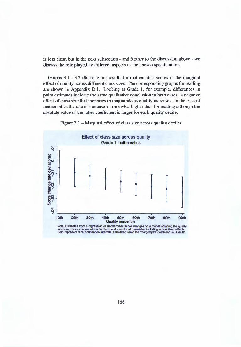
Univers

ity of

Cap

e Tow

n

is less clear, but in the next subsection - and further to the discussion above - we discuss the role played by different aspects of the chosen specifications.

Graphs 3.1 - 3.3 illustrate our results for mathematics scores of the marginal effect of quality across different class sizes. The corresponding graphs for reading are shown in Appendix D .1. Looking at Grade 1, for example, differences in point estimates indicate the same qualitative conclusion in both cases: a negative effect of class size that increases in magnitude as quality increases. In the case of mathematics the rate of increase is somewhat higher than for reading although the absolute value of the latter coefficient is larger for each quality decile.

~ 0 ,·

Figure 3.1 -Marginal effect of class size across quality deciles

10th 20th

Effect of class size across quality Grade 1 mathematics

30th 40th 50th 60th 70th Quality percentile

80th 90th

Note: Estimates from a regression of standardised score changes on a model including the quality measure, class size, an interaction term and a vector of covariates including school fiXed effects. Bars represent 90% confidence intervals , calculated using the 'marginsplot' command in State12.

166

Univers

ity of

Cap

e Tow

nN 0

~· 0 ~0 '5 . Q) 'C

-co ~ Q)

~ 1! ,· u

~~ 0 . Uo

C/)

(") 0 ,·

Figure 3.2- Marginal effect of class size across quality deciles

10th 20th

Effect of class size across quality Grade 2 mathematics

30th 40th 50th 60th 70th Quality percentile

80th 90th

Note: Estimates from a regression or standardised score changes on a model including the qualily measure, class size, an interaction tenn and a vector or c0118riates including school fiXed effects. Bars represent 90% confidence intervals, calculated using the 'marginsplof command in Stata12.

167

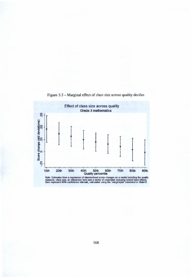
Univers

ity of

Cap

e Tow

n

.... 0 ,·

Figure 3.3 -Marginal effect of class size across quality deciles

10th 20th

Effect of class size across quality Grade 3 mathematics

30th 40th 50th 60th 70th Quality percentile

80th 90th

Note: Estimates from a regression of standardised score changes on a model including the quality measure, class size, an interaction tenn and a vector of ccwariates including school fiXed effects. Bars represent 90% confidence intervals, calculated using the ·marginsplot' command in Stata12.

168

Univers

ity of

Cap

e Tow

n

The results, again using mathematics scores, showing the marginal effect of class across different quintiles of the quality distribution are in graphs 3.4 - 3.6. The corresponding graphs for reading are in appendix 0.2.

In all our regressions, precision of estimates is a serious constraint even for estimating simple interactive models, as can be seen from the relatively wide con­fidence intervals in these graphs. There are some interesting characteristics of the standard errors in these regressions but we follow the applied econometrics literature in, conservatively, using the largest standard errors. In this case the largest variances are from the 'conventional' standard errors (calculated under the assumption of homoscedasticity and no clustering), not those that account for clustering. The broader implication of this lack of precision, arising in no small part due to our exploiting within-school variation, is that it limits our ability to test more complicated forms of the education production function. 22 We discuss both these points in more detail in the next section, but suffice to say that there are good reasons to believe that our basic findings ought not to be compromised by either issue.

22McEwan's (20 13) survey of programme evaluations in education provides a fairly detailed discussion of power limitations of this sort.

169

Univers

ity of

Cap

e Tow

nFigure 3.4- Marginal effect of quality across class sizes

Effect of quality across class sizes Grade 1 mathematics

13 14 15 16 17 18 19 20 21 22 23 24 25 Class size

Note: Estimates from a regression of standardised score changes on a model including the quality measure, class size, an interaction term and a vector of CCM!riates including school fiXed effects. Bars represent 90% confidence intervals, calculated using the 'marginsplof command in Stata12.

170

Univers

ity of

Cap

e Tow

n10 ~ c: .Q i;j ·s:co Q) • -,:, -,:, (ij ....... 10 Q)IO Cl • c: Ill

.J::. u QliO ... 0

0 u

Cl)

10 ~

Figure 3.5 -Marginal effect of quality across class sizes

Effect of quality across class sizes Grade 2 mathematics

I I l [ l l I l [ I I 13 14 15 16 17 18 19 20 21 22 23 24 25

Class size Note: Estimates from a regression of standardised score changes on a model including the quality maasure, class size, an interaction term and a vector of covariates including school flXSd effects. Bars represent 90% confidence intervals, calculated using the 'marginsplof command in State12.

171

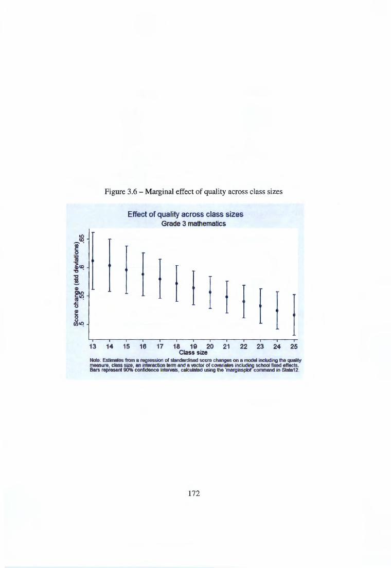
Univers

ity of

Cap

e Tow

nFigure 3.6 - Marginal effect of quality across class sizes

Effect of quality across class sizes Grade 3 mathematics

13 14 15 16 17 18 19 20 21 22 23 24 25 Class size

Note: Estimates from a regression of standardised score changes on a model including the quality measure, class size, en interaction term end a vector of c01111rietes including school fixed effects. Bars represent 90% confidence intervals, calculated using the ·marginsplot' command in Stata12.

172

Univers

ity of

Cap

e Tow

n

3.4.2 Importance of the dependent variable

The regression model estimated in Tables 3.1 and 3.2 follows directly from our conceptualisation of the education production function in earlier sections. Nev­ertheless, it is important to note the sensitivity of results to other specifications. Tables 3.3 - 3.8 examine in more detail the effect of including certain controls and not others, on score changes and levels. An obvious specification check when utilising a differenced dependent variable is to estimate a specification with the current year's value as dependent variable and the preceding year's observation as an additional explanatory variable, thereby relaxing the implicit constraint that the latter coefficient be equal to one. As shown in column (5) of Tables 3.3 -3.8, though the results do sometimes differ relative to our preferred specification, significant interaction effects are found with both specifications so this does not materially affect our overall findings.

173

Univers

ity of

Cap

e Tow

n

-.) ~

Table 3.3 -Different specifications: Grade 1 mathematics

qD Score changes (6A1) Score levels( A 1)

(1) (2) (3) (4) (5) (6) (7) (8) (9) Class size -0.009*** -0.011 *** -0.016*** -0.016*** -0.027*** -0.042*** -0.042*** -0.034*** -0.032***

(0.004) (0.004) (0.004) (0.004) (0.004) (0.005) (0.005) (0.004) (0.004)

qD Maths 0.666*** 0.666*** 0.666*** 0.561*** 0.435*** 0.403*** (0.091) (0.090) (0.091) (0.076) (0.098) (0.023)

Interaction -0.009** -0.009* -0.009* -0.006 -0.002 (0.005) (0.005) (0.005) (0.004) (0.005)

Aide 0.077** 0.079** 0.079*** 0.080** 0.080** 0.032 (0.034) (0.035) (0.029) (0.037) (0.037) (0.036)

Scoret-1 0.013*** (0.000)

R2 0.25 0.30 0.30 0.31 0.62 0.36 0.36 0.29 0.29 N 4,163 3,655 3,655 3,579 3,579 3,579 3,579 4,074 4,074

Each column shows coefficient estimates from various specifications of an education production function, using the Project STAR public use dataset.

Column (4) is our preferred specification - used to calculate marginal effects in Tables 3.1 and 3.2 - in which score changes are regressed on a

value-added quality variable (qD) constructed using scores for the same subject as the dependent variable, class size, a size-quality interaction term,

aide dummy and a vector of covariates that are not shown. These are: individual student's race, gender and free lunch receipt as well as school

location, school fixed effects and entry year effects. All specifications except columns (1)-(3) use these controls. Columns (1 )-(4) have score changes

as the dependent variable whereas score levels are used in columns (5)-(9). Asterisks represent p-values as follows: * p < 0.1; ** p < 0.05; *** p < 0.01.

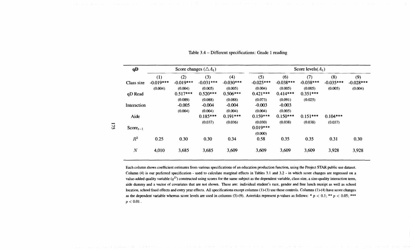
Univers

ity of

Cap

e Tow

n--....1 VI

Table 3.4- Different specifications: Grade 1 reading

qD Score changes (~A1 ) Score levels( A 1)

(1) (2) (3) (4) (5) (6) (7) (8) (9) Class size -0.019*** -0.019*** -0.031 *** -0.030*** -0.025*** -0.038*** -0.038*** -0.035*** -0.028***

(0.004) (0.004) (0.005) (0.005) (0.004) (0.005) (0.005) (0.005) (0.004)

qD Read 0.517*** 0.520*** 0.506*** 0.421 *** 0.414*** 0.351 *** (0.089) (0.088) (0.088) (0.073) (0.091) (0.025)

Interaction -0.005 -0.004 -0.004 -0.003 -0.003 (0.004) (0.004) (0.004) (0.004) (0.005)

Aide 0.185*** 0.191 *** 0.159*** 0.150*** 0.151 *** 0.104*** (0.037) (0.036) (0.030) (0.038) (0.038) (0.037)

Scoret-1 0.019*** (0.000)

R2 0.25 0.30 0.30 0.34 0.58 0.35 0.35 0.31 0.30

N 4,010 3,685 3,685 3,609 3,609 3,609 3,609 3,928 3,928

Each column shows coefficient estimates from various specifications of an education production function, using the Project STAR public use dataset.

Column (4) is our preferred specification- used to calculate marginal effects in Tables 3.1 and 3.2 - in which score changes are regressed on a

value-added quality variable (qD) constructed using scores for the same subject as the dependent variable, class size, a size-quality interaction term,

aide dummy and a vector of covariates that are not shown. These are: individual student's race, gender and free lunch receipt as well as school

location, school fixed effects and entry year effects. All specifications except columns ( 1 )-(3) use these controls. Columns (I)-( 4) have score changes

as the dependent variable whereas score levels are used in columns (5)-(9). Asterisks represent p-values as follows: * p < 0.1; ** p < 0.05; *** p < 0.01.

Univers

ity of

Cap

e Tow

n

Table 3.5- Different specifications: Grade 2 mathematics

qD Score changes (6A2) Score levels(A2 )

(1) (2) (3) (4) (5) (6) (7) (8) (9)

Class size 0.006* 0.005* -0.001 0.000 -0.004 -0.020*** -0.020*** -0.018*** -0.017*** (0.003) (0.003) (0.004) (0.004) (0.003) (0.004) (0.004) (0.004) (0.003)

qDMaths 0.773*** 0.758*** 0.759*** 0.532*** 0.309*** 0.238*** (0.074) (0.074) (0.076) (0.057) (0.082) (0.018)

Interaction -0.011 *** -0.011 *** -0.011 *** -0.007*** -0.004 (0.004) (0.004) (0.004) (0.003) (0.004)

Aide 0.096*** 0.094*** 0.068*** 0.045 0.046 0.020 - (0.029) (0.030) (0.022) (0.032) (0.032) (0.033) -...l 0'\

Scoret-l 0.018*** (0.000)

Rz 0.17 0.35 0.35 0.36 0.67 0.32 0.32 0.29 0.29 N 4,656 4,403 4,403 4,210 4,210 4,210 4,210 4,459 4,459

Each column shows coefficient estimates from various specifications of an education production function, using the Project STAR public use dataset.

Column (4) is our preferred specification - used to calculate marginal effects in Tables 3.1 and 3.2 - in which score changes are regressed on a

value-added quality variable (qD) constructed using scores for the same subject as the dependent variable, class size, a size-quality interaction term,

aide dummy and a vector of covariates that are not shown. These are: individual student's race, gender and free lunch receipt as well as school

location, school fixed effects and entry year effects. All specifications except columns (1)-(3) use these controls. Columns (1)-(4) have score changes

as the dependent variable whereas score levels are used in columns (5)-(9). Asterisks represent p-values as follows: * p < 0.1; ** p < 0.05; *** p < 0.01.

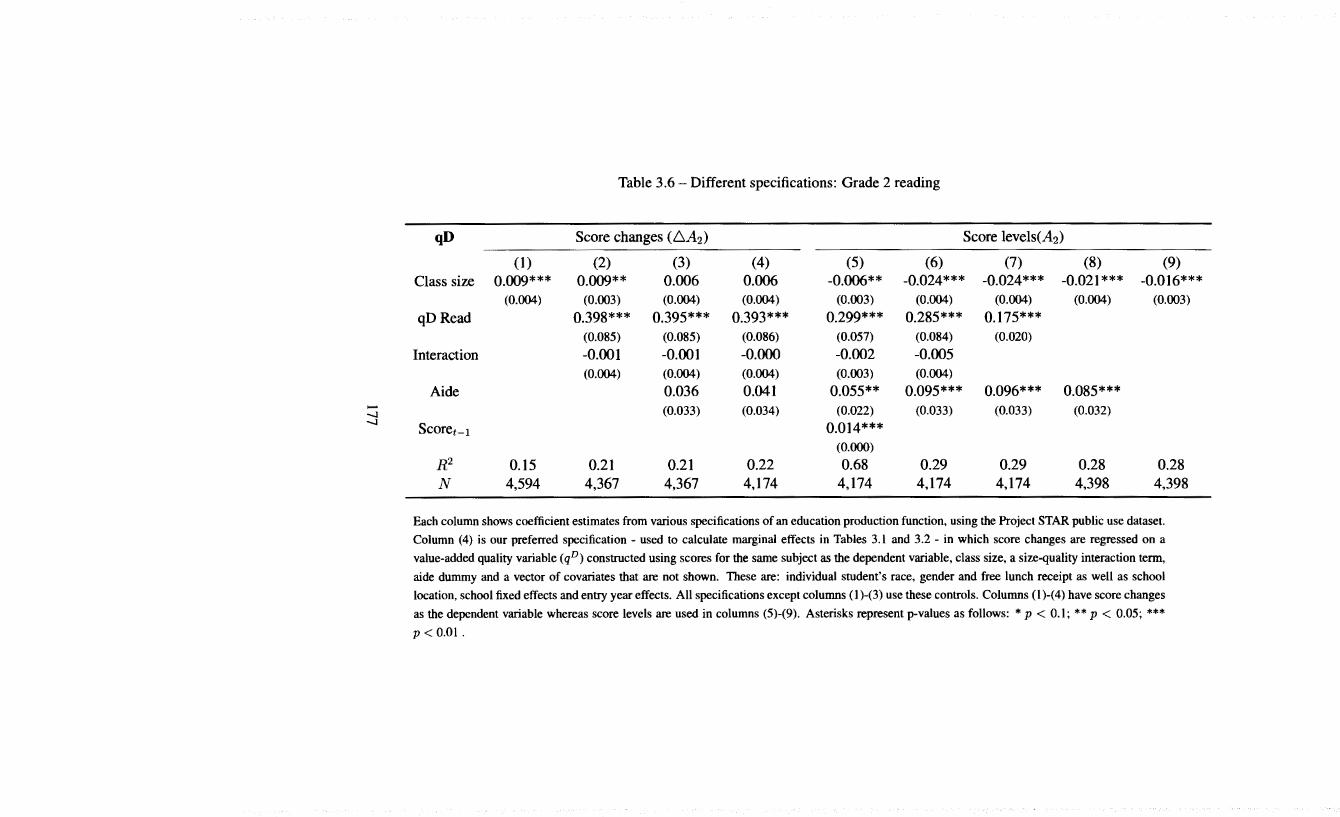
Univers

ity of

Cap

e Tow

n-......:1 ......:1

Table 3.6- Different specifications: Grade 2 reading

qD Score changes (6A2) Score levels(A2)

(1) (2) (3) (4) (5) (6) (7) (8) (9) Class size 0.009*** 0.009** 0.006 0.006 -0.006** -0.024*** -0.024*** -0.021 *** -0.016***

(0.004) (0.003) (0.004) (0.004) (0.003) (0.004) (0.004) (0.004) (0.003)

qD Read 0.398*** 0.395*** 0.393*** 0.299*** 0.285*** 0.175*** (0.085) (0.085) (0.086) (0.057) (0.084) (0.020)

Interaction -0.001 -0.001 -0.000 -0.002 -0.005 (0.004) (0.004) (0.004) (0.003) (0.004)

Aide 0.036 0.041 0.055** 0.095*** 0.096*** 0.085*** (0.033) (0.034) (0.022) (0.033) (0.033) (0.032)

Scoret-1 0.014*** (0.000)

R2 0.15 0.21 0.21 0.22 0.68 0.29 0.29 0.28 0.28 N 4,594 4,367 4,367 4,174 4,174 4,174 4,174 4,398 4,398

Each column shows coefficient estimates from various specifications of an education production function, using the Project STAR public use dataset.

Column (4) is our preferred specification- used to calculate marginal effects in Tables 3.1 and 3.2- in which score changes are regressed on a

value-added quality variable (qD) constructed using scores for the same subject as the dependent variable, class size, a size-quality interaction term,

aide dummy and a vector of covariates that are not shown. These are: individual student's race, gender and free lunch receipt as well as school

location, school fixed effects and entry year effects. All specifications except columns (1)-(3) use these controls. Columns (1)-(4) have score changes

as the dependent variable whereas score levels are used in columns (5)-(9). Asterisks represent p-values as follows: * p < 0.1; ** p < 0.05; *** p < 0.01.

Univers

ity of

Cap

e Tow

n

...... -J 00

Table 3.7- Different specifications: Grade 3 mathematics

qD Score changes (6A3 ) Score levels(A3)

(1) (2) (3) (4) (5) (6) (7) (8) (9) Class size 0.007** 0.008*** 0.008** 0.008** 0.002 -0.011 *** -0.011 *** -0.012*** -0.013***

(0.003) (0.003) (0.004) (0.004) (0.003) (0.004) (0.004) (0.004) (0.003)

qD Maths 0.705*** 0.705*** 0.714*** 0.475*** 0.237*** 0.220*** (0.070) (0.070) (0.070) (0.051) (0.077) (0.019)

Interaction -0.007** -0.007** -0.008** -0.005** -0.001 (0.003) (0.003) (0.003) (0.002) (0.004)

Aide 0.001 0.004 0.001 -0.004 -0.004 -0.004 (0.030) (0.030) (0.022) (0.033) (0.033) (0.034)

Scoret-l 0.018*** (0.000)

R2 0.19 0.34 0.34 0.35 0.69 0.28 0.28 0.25 0.25 N 4,684 4,499 4,499 4,372 4,372 4,372 4,372 4,557 4,557

Each column shows coefficient estimates from various specifications of an education production function, using the Project STAR public use dataset.

Column (4) is our preferred specification - used to calculate marginal effects in Tables 3.1 and 3.2 - in which score changes are regressed on a

value-added quality variable (qD) constructed using scores for the same subject as the dependent variable, class size, a size-quality interaction term,

aide dummy and a vector of covariates that are not shown. These are: individual student's race, gender and free lunch receipt as well as school

location, school fixed effects and entry year effects. All specifications except columns (1)-(3) use these controls. Columns (1)-(4) have score changes

as the dependent variable whereas score levels are used in columns (5)-(9). Asterisks represent p-values as follows: * p < 0.1; ** p < 0.05; *** p < 0.01.

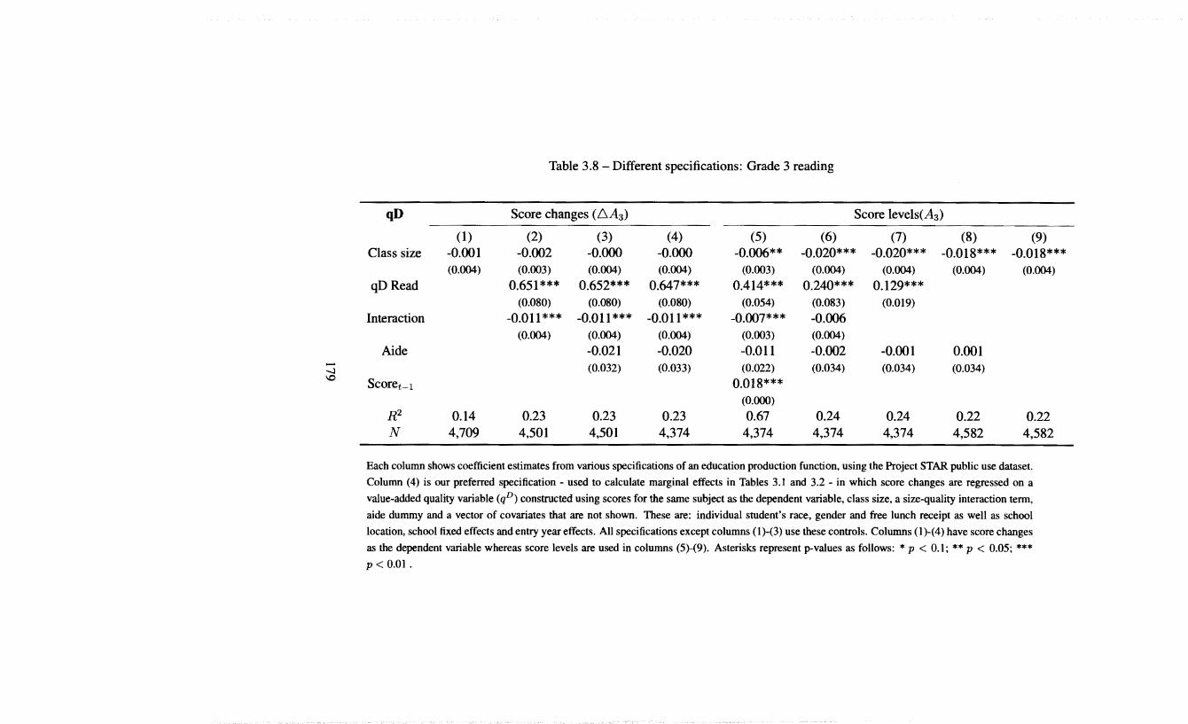
Univers

ity of

Cap

e Tow

n..... -.....] \0

Table 3.8- Different specifications: Grade 3 reading

qD Score changes (.6A3 ) Score levels(A3 )

(1) (2) (3) (4) (5) (6) (7) (8) (9) Class size -0.001 -0.002 -0.000 -0.000 -0.006** -0.020*** -0.020*** -0.018*** -0.018***

(0.004) (0.003) (0.004) (0.004) (0.003) (0.004) (0.004) (0.004) (0.004)

qDRead 0.651*** 0.652*** 0.647*** 0.414*** 0.240*** 0.129*** (0.080) (0.080) (0.080) (0.054) (0.083) (0.019)

Interaction -0.011 *** -0.011 *** -0.011 *** -0.007*** -0.006 (0.004) (0.004) (0.004) (0.003) (0.004)

Aide -0.021 -0.020 -0.011 -0.002 -0.001 0.001 (0.032) (0.033) (0.022) (0.034) (0.034) (0.034)

Scoret-1 0.018*** (0.000)

R2 0.14 0.23 0.23 0.23 0.67 0.24 0.24 0.22 0.22 N 4,709 4,501 4,501 4,374 4,374 4,374 4,374 4,582 4,582

Each column shows coefficient estimates from various specifications of an education production function, using the Project STAR public use dataset.

Column (4) is our preferred specification -used to calculate marginal effects in Tables 3.1 and 3.2 - in which score changes are regressed on a

value-added quality variable (qD) constructed using scores for the same subject as the dependent variable, class size, a size-quality interaction term,

aide dummy and a vector of covariates that are not shown. These are: individual student's race, gender and free lunch receipt as well as school

location, school fixed effects and entry year effects. All specifications except columns ( 1 )-(3) use these controls. Columns (1 )-( 4) have score changes

as the dependent variable whereas score levels are used in columns (5)-(9). Asterisks represent p-values as follows: * p < 0.1; ** p < 0.05; *** p < 0.01.

Univers

ity of

Cap

e Tow

n

Another issue is how the inclusion of our constructed quality variable, without the interaction, affects the coefficient on class size. Given that the quality measure is constructed to be (unconditionally) independent of class size we would expect that its inclusion does not have a statistically significant effect on that coefficient. In most cases this is what we find, though as can be seen from columns (7) and (8) in Tables 3.3-3.8 there does seem to be a partial correlation between the variables that affects the coefficient - increasing it in magnitude - when using score levels as the dependent variable. Fortunately this does not appear to be material when using achievement changes.

The same cannot be said when using the current year's test score in levels as the dependent variable and not including the previous year on the right-hand side. As the above tables show, using this specification renders most of the interaction ef­fects insignificant and in some cases has a similar effect on the significance of the aide variable - reproducing the results of the literature in that regard. As already noted, it comes as something of a surprise that the aide dummy is significant in some levels specifications - Grade l and Grade 2 reading - since most previous papers have simply collapsed aide and regular classes together on the basis that they do not appear to be materially different. This could be because most studies combine mathematics and reading scores, but is an interesting result that perhaps suggests the role of aides in the study ought to be revisited.

There are a few points to be made in relation to the choice of specification and sensitivity to this. First, and most simply, it is important for the consistency of our account that the estimated model corresponds to the implications of our ear­lier assumptions - for the purpose of constructing the quality measure - regarding the underlying relationship. This requires utilising score changes as the dependent variable or, at least, using the preceding year's score as an explanatory variable- to control for confounding historical factors - when using score levels as the depen­dent variable. When that is done the estimated interaction effect is significant in most cases. The second issue is whether the literature provides a particular reason to adopt one or other of these specifications. While such issues are discussed at length by Todd and Wolpin (2003), that paper post-dates Krueger (1999) (and in­deed Krueger and Whitmore (2001)) and is not referenced by Chetty et al. (2011). As a consequence, these key contributions do not substantiate their choice of a levels-based specification over one that considers score changes. In fact, since - as we have seen - changes in scores are the basis for value-added models of teacher quality, there appears to be a stronger case for focusing on these. As we noted above in comparing our results to the existing literature, Krueger ( 1999) rejected the value-added specification because the largest results in levels were

180

Univers

ity of

Cap

e Tow

n

for kindergarten and these would not be captured by a specification using score changes. That is an ex post data-driven decision, whereas here we have committed ex ante to a particular formulation of the educational production function.

The last question to address, then, is why we might observe this sensitivity of the results to the dependent variable used. Our motivation for differencing achievement was the existence of a cumulative production function (Todd and Wolpin, 2003). That creates two problems for estimation. First, the presence of unobserved present and historical inputs leads to an increase in unexplained vari­ation and possibly a decrease in the precision of estimates. Second, and more concerning, is that correlations between unobserved or omitted explanatory vari­ables from preceding periods may lead to biases in the estimates. If we compare columns (5) and (6) in Tables 3.3 - 3.8 we see a possible combination of these two factors: failing to control for the previous year's test score, when the dependent variable is current year's scores in levels, is associated with a smaller coefficient on the interaction term and a larger standard error. Omitting previous year's score is consistently associated with a smaller coefficient on quality and an increase in the coefficient on class size. As noted in our earlier discussion regarding Krueger's ( 1999) results, this is as we would expect: with past scores excluded, the coeffi­cient on the class size variable will be picking-up the cumulative effects of initial assignment not only the effect of the particular year under consideration. 23

3.4.3 Using treatment assignment instead of actual class size

Another specification issue to consider is that by using actual class size rather than a dummy for assignment we may be picking-up a complex form of endogeneity. Recall that the reason for using class size itself is that it potentially gives us more useful information on the underlying production function than a somewhat arbi­trary assigned change in size. There is no evidence, to our knowledge, that class sizes within assignment categories are endogenous. Nevertheless, we address this concern by estimating two obvious alternative specifications: utilising a dummy variable indicating assignment to a regular class; and, instrumenting for class size using assignment.24 In both cases the interaction effect is adapted accordingly. The estimates of the relevant coefficients from these alternative approaches - or­dinary least squares with the continuous class size variable ('OLS'), a categorical treatment variable ('Dummy') and instrumental variables ('IV') are shown in Ta­ble 3.9 and 3.10 below. Note that in all cases the instruments for class size and

23 Note that, as indicated in the notes to the tables, we have restricted the sample to those students with scores in both years in order to ensure that the differences in results are due to the specification change rather than changes in sample composition.

24 Krueger ( 1999) runs through the same process for his results.

181

Univers

ity of

Cap

e Tow

n

the interaction term are, as we might expect, highly significant predictors in the first-stage regressions.

182

Univers

ity of

Cap

e Tow

n

Table 3.9- Robustness of regression results: Mathematics scores

qD Grade 1 Grade 2 Grade 3

OLS Dummy IV OLS Dummy IV OLS Dummy IV qD Maths 0.666*** 0.456*** 0.712*** 0.759*** 0.506*** 0.780*** 0.714*** 0.527*** 0.736***

(0.091) (0.027) (0.098) (0.076) (0.020) (0.081) (0.070) (0.019) (0.077)

Class size -0.016*** -0.017*** 0.000 0.002 0.008** 0.010** (0.004) (0.005) (0.004) (0.004) (0.004) (0.004)

Interaction -0.009* 0.078** -0.011 ** -0.011 *** 0.092*** -0.012*** -0.008** 0.068** -0.009** (0.005) (0.034) (0.005) (0.004) (0.031) (0.004) (0.003) (0.029) (0.004)

Aide 0.079** 0.074** 0.084** 0.094*** 0.091 *** 0.086*** 0.004 -0.003 -0.003

- (0.035) (0.034) (0.035) (0.030) (0.030) (0.030) (0.030) (0.030) (0.030) 00 Small 0.119*** -0.016 -0.079** w

(0.033) (0.031) (0.032) R2 0.31 0.31 0.31 0.36 0.36 0.36 0.35 0.35 0.35 N 3,579 3,579 3,579 4,210 4,210 4,210 4,372 4,372 4,372

All columns show coefficients from our preferred specification of the education production function estimated using the Project STAR public use

dataset. In this specification score changes are regressed on a value-added quality variable (qD) constructed using scores for the same subject as

the dependent variable, class size, a size-quality interaction term, aide dummy and a vector of covariates that are not shown. These are: individual

student's race, gender and free lunch receipt as well as school location, school fixed effects and entry year effects. All specifications include these

covariates. For each grade: the left-hand column reports coefficients from a regression using actual class size; the central column utilises instead a

dummy for treatment assignment; and, the right-hand column uses treatment assignment to instrument for class size and the interaction term. The

instrument employed for the latter is simply a variable created by interacting the treatment dummy with the quality variable. Asterisks represent

p-values as follows: * p < 0.1; ** p < 0.05; *** p < 0.01 .

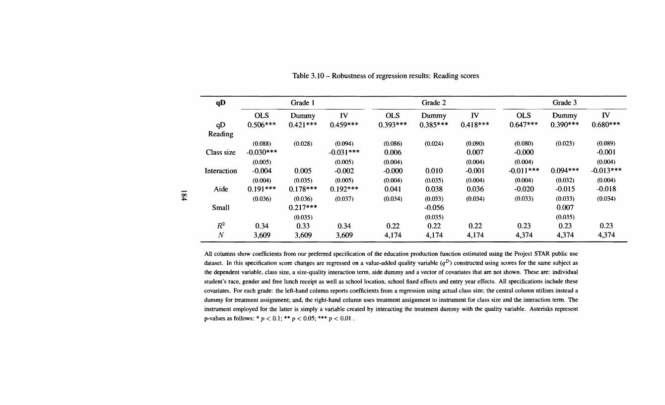
Univers

ity of

Cap

e Tow

n

Table 3.10 - Robustness of regression results: Reading scores

qD Grade 1 Grade 2 Grade 3 --

OLS Dummy IV OLS Dummy IV OLS Dummy IV qD 0.506*** 0.421 *** 0.459*** 0.393*** 0.385*** 0.418*** 0.647*** 0.390*** 0.680***

Reading (0.088) (0.028) (0.094) (0.086) (0.024) (0.090) (0.080) (0.023) (0.089)

Class size -0.030*** -0.031 *** 0.006 0.007 -0.000 -0.001 (0.005) (0.005) (0.004) (0.004) (0.004) (0.004)

Interaction -0.004 0.005 -0.002 -0.000 0.010 -0.001 -0.011 *** 0.094*** -0.013*** (0.004) (0.035) (0.005) (0.004) (0.035) (0.004) (0.004) (0.032) (0.004)

- Aide 0.191 *** 0.178*** 0.192*** 0.041 0.038 0.036 -0.020 -0.015 -0.018 00

(0.036) (0.036) (0.037) (0.034) (0.033) (0.034) (0.033) (0.033) (0.034) ~

Small 0.217*** -0.056 0.007 (0.035) (0.035) (0.035)

R2 0.34 0.33 0.34 0.22 0.22 0.22 0.23 0.23 0.23 N 3,609 3,609 3,609 4,174 4,174 4,174 4,374 4,374 4,374

All columns show coefficients from our preferred specification of the education production function estimated using the Project STAR public use

dataset. In this specification score changes are regressed on a value-added quality variable (qD) constructed using scores for the same subject as

the dependent variable, class size, a size-quality interaction term, aide dummy and a vector of covariates that are not shown. These are: individual

student's race, gender and free lunch receipt as well as school location, school fixed effects and entry year effects. All specifications include these

covariates. For each grade: the left-hand column reports coefficients from a regression using actual class size; the central column utilises instead a

dummy for treatment assignment; and, the right-hand column uses treatment assignment to instrument for class size and the interaction term. The

instrument employed for the latter is simply a variable created by interacting the treatment dummy with the quality variable. Asterisks represent

p-values as follows: * p < 0.1; ** p < 0.05; *** p < 0.01.

Univers

ity of

Cap

e Tow

n

The results show that using a dummy for assignment, or utilising that variable as an instrument for actual class size, does not affect the sign or significance of the coefficients. Note that assignment to a small class led to average small class sizes of seven to eight students less than in regular/large classes, so it is necessary to divide the coefficient by that number for comparison purposes. Doing this reveals that the magnitude of the coefficient on the dummy variable is consistent with that on actual class size. Comparing the magnitude of the coefficients from the OLS and IV regressions we see that instrumenting for class size produces coefficients that have a larger absolute value.

3.5 Further econometric complications

There are a number of additional econometric issues raised by the preceding anal­ysis that deserve some separate consideration. A first set of issues noted by Chetty et al. (2011) are that the coefficient on a value-added quality measure, even using a leave-out mean, may be upward biased by a reflection effect (Manski, 1993) of a student's own ability on the scores of others. It may also be attenuated as a result of student-specific variation in achievement that has nothing to do with teacher quality. Second, the use of data based on clusters (schools and classes) necessitates consideration of the appropriate standard errors for the estimated co­efficients. A third issue is what an interactive functional form might imply for the novel approach in Chapter 2 to constructing a teacher quality measure. Finally, a known problem with estimating interaction effects is that they may be biased by a failure to correctly characterise the functional form of one of the variables.25

3.5.1 Own-score bias, attenuation bias and the 'reflection ef­fect'

The basic justification of our quality measure - as explained in section 3.3 and chapter 2 - was based on averages (of score changes or levels) across all students in a given class for whom information was available. While this is adequate for the purposes of constructing a quality measure or ranking on its own, if we intend to utilise such a variable in a regression where an individual student's score is the dependent variable, then that score should be excluded from the average used to construct the quality measure. In practice this means constructing a quality measure for every individual student, which is tedious but straightforward, and that is the variable used in the preceding regressions. This was also the approach taken by Chetty et al. (2011).

251 am grateful to Gideon du Rand for emphasising this concern.

185

Univers

ity of

Cap

e Tow

n

A more difficult issue relates to the so-called 'reflection effect' described by Manski (1993). In our case, the potential problem is that if student i's ability or achievement affects the achievement of her classmates - as we assume in our production function (3.3) - then the coefficient on the quality variable will be biased even with the modification mentioned above. Chetty et al. (20 11) note that with the data available one cannot resolve the problem; at best one can attempt to bound the extent of the bias. The reflection problem is particularly an issue for studies like Chetty et al. (2011), because the magnitude of the coefficient on the quality measure is of primary interest. In the (online) appendix to their paper Chetty et al. (2011) derive- subject to a number of simplifying assumptions- an expression for the reflection effect and estimate the relevant components in order to provide a bound on the likely bias. The bias is an inverse function of class size and therefore is substantially reduced since the latter is above 13 and up to 25 in the experiment. In fact, those authors conclude that the magnitude of the upward bias is approximately of the same order as the downward attenuation bias due to end-of-year score averages being a somewhat noisy measure of class quality.

Formally characterising the attenuation and reflection effects is significantly more challenging when the interest is in the marginal effect in the presence of an interactive functional form. This is particularly true if one wishes to utilise a fully specified production function to simultaneously characterise these two biases - as seems appropriate. By contrast, Chetty et al. (2011) characterise the two effects separately. While one may therefore be encouraged by those authors' conclusion that the two effects offset each other, this must remain a caveat to interpretation of the magnitude of our estimated marginal effects of quality. To what extent might these concerns affect estimates of the marginal effects? That the reflection effect is inversely proportional to class size may lead to an understatement- in the results shown in Table 3.1 and 3.2 - of the extent to which the marginal effect of quality declines with class size. Furthermore, attenuation bias due to noise in the measure of teacher/class quality is likely, leading to results with understated significance by virtue of attenuated coefficients.

3.5.2 Standard errors

In general it is desirable to report standard errors for estimates that are robust to possible rnisspecification or account for clustering. The fact that sample clustering can lead to downward-biased standard errors when assuming random sampling at the level of individuals is well-known. See for instance Moulton (1986, 1990), Pepper (2002) and Wooldridge (2003). The reason for this is primarily the exis­tence of positive within-cluster correlations, so that in effect the extent of infor-

186

Univers

ity of

Cap

e Tow

n

mation provided by this variation is overstated. Less emphasised is the fact that, in principle, adjusting for clustering could lead to a decrease in the magnitude of the estimated standard errors.

The issue of clustering is of obvious relevance in the present case, where ob­servations represent individual students, but in reality these are grouped in classes and schools. TWo different approaches have been taken to clustering when using the STAR data and these choices reflect some differences in specification. We focus on Krueger (1999) and Chetty et al. (2011). Krueger, who implements a fairly straightforward estimation of treatment effects, clusters by class. Krueger (1999: 511) reports that these "robust standard errors are about two-thirds larger than the OLS standard error". Chetty et al. (2011) take a different approach, clus­tering on school rather than class on the basis that "clustering by school provides a conservative estimate of standard errors" (Chetty et al., 2011: 1619) and show in an appendix that for their specifications clustering by school does give, almost uniformly, larger standard errors than clustering by class.

For our purposes the question is which of these two approaches to adopt. We began by implementing both approaches and examining the effect on the standard errors relative to simply using the least squares standard errors. It transpires that using standard errors clustered at the class level leads to sizeable reductions rel­ative to OLS in all specifications where the quality variable is included. A close reading of Chetty et al. (20 11 ), for instance Chetty et al. (footnote 30 2011: 1640), reveals that those authors observed a similar effect. As they note, reductions in the magnitude of standard errors as a result of clustering may occur "when the intra-class correlation coefficient is small". More specifically, the literature notes that this may occur when the intra-cluster correlation is negative. This is not a full explanation, since it is not immediately clear why this is the case and from Krueger's (1999) results it is evident that the problem does not exist across all specifications of interest.

In this respect it is valuable to revisit the quality measure described in section 3.3. This measure was constructed at a class level, with the consequence that a significant proportion of what would be the shared error within classes will be cap­tured by that variable. It is perhaps unsurprising, then, that clustering at the class level has a very different effect in specifications including quality measures. As a consequence, we follow Chetty et al.'s (2011) approach in using school- rather than class-level clustering as a robustness check on the significance of results. In the presence of controls for school fixed effects we do not expect this to greatly reduce the significance of our results and indeed it does not.In fact, even at the

187

Univers

ity of

Cap

e Tow

n

school level clustered errors are smaller than the simple OLS ones but the effect is less marked than when clustering on class. Hence our results in this regard are compatible with Chetty et al. (2011), who note that "[errors clustered by school] are in nearly all cases larger than those from clustering on only classroom" (Chetty etal.,2011: 1619).

What those authors do not explicitly note is that in a minority of cases the for­mer are still smaller than the usual OLS standard errors. For our specifications this was true for the majority of cases. Besides the effects of clustering, heteroscedas­ticity robust standard errors were also somewhat larger than the unadjusted OLS standard errors, though the magnitude of the difference was marginal. Although we cannot be sure of the reason for these somewhat unexpected results, Angrist and Pischke (2009: 307) note that robust standard errors can have poor finite sam­ple properties which can lead to clustered standard errors that are smaller than 'conventional' ones. Whatever the underlying reason, the conclusion is that using robust or clustered standard errors - by class or school - increases the apparent significance of our results. In keeping with the spirit of the empirical literature we report the more conservative results, which in this case are associated with the usual OLS standard errors.

3.5.3 Implications of interaction for the quality variable

There is a tension between the analysis and discussion in the present chapter, which focuses on interaction of class size and teacher quality, and the preceding chapter in which our approach to constructing the quality measure followed the economics of education literature in assuming additive separability of the educa­tion production function. This apparent tension raises two key questions:

I. What implications would an interaction between teacher quality and class size have for the validity of our proposed quality measure?

2. Given the above, how might this affect estimation of interaction effects us­ing qD?

The second question can in part be addressed as a purely logical issue. The crucial point is that a test for interaction using the constructed measure produces an acceptable test of the null hypothesis, since if biasing of the quality measure by interaction leads us to reject the null then we need not be concerned that this is a Type I error (since any bias arises because the null is false). Relatedly, in the absence of any reason to believe that interaction would lead to a quality measure

188

Univers

ity of

Cap

e Tow

n

that would induce false acceptance of the null (Type II error), we can conclude that rejection of the null of additive separability given our quality measure is, ceteris paribus, a reliable indicator that the true functional form is interactive. Therefore the constructed measure remains useful to our broader interest and, in addition, the analysis of interactions in this chapter provides information on one of the assumptions made in constructing the measure. It is theoretically possible that if the quality measure is biased in some way we might accept the null even though it is false. In this sense at least any tests of the null of additive separability can be thought of as conservative.

Besides the correctness of acceptance or rejection of the null an additional issue of interest is the extent of bias, if any, in the magnitude of the estimated parameter on the interaction term. This is not an issue that can resolved logically and there­fore the effect of an interactive functional form on our quality measure is likely to matter most if we want to examine the quantitative aspects of the relationship (i.e. magnitude) as opposed to only the qualitative aspect (is there interaction or not).

We now examine whether and how the interactive form has implications for our approach to constructing the quality measure, using the basic model in (3.5). It should be noted that in the construction of quality measures, the possible impor­tance of functional form is not explicitly addressed by Chetty et al. (2011), Nye et al. (2004) or Konstantopolous and Sun (2011)- the studies most similar to this one.

Aigjk = o:oig + o:1Higk + ,B(l- >.C9j)J(q;j, R9j, o:o.9 j) + 6C9j

+ o:2G gk + Eigjk (3.5)

For simplicity of exposition we work with this functional form rather than its cumulative equivalent. Regarding the parameters we assume: ,B > 0, >. 2:: 0 and 6 < 0. Note that the parameter >., representing the reduction in the effect of class quality on scores due to class size, is constrained by the requirement that >.Cgjk ::; 1. If we were to assume (3.5), and follow the procedure detailed in sections 2.3 and 2.4 of the preceding chapter for creating the qA measure, this would give us:

189

Univers

ity of

Cap

e Tow

n

Averaging within-class scores:

q9Jk = ao.9 + a1H.gk + ,8(1 - >.C9J)f(q;J, R9 j, ao-39 ) + 6C9j + a2Ggk + f..gjk (3.5.1)

Assuming f (.)is additively separable:

= ao.9 + a1H.gk + ,81(1- >.Cgj)q;j + ,82(1- >.C9 j)Rgj + ,83(1- >.C9 j)ao.jg

+ 6C9j + a2Ggk + E.gJk (3.5.2)

Demeaning within class type:

ijgjk = ao.g + alil.g + ,Blii;j + ,B2Rgj + ,835:0-jg + a2Ggk + E.gjk

- >.Cgj[,Blii;j + ,B2Rgj + ,B3ao-j9 ] (3.5.3)

We can use (3.5.3) to demonstrate the problems that arise because of inter­action.26 First, note that class size now determines the extent to which teacher (classroom) quality affects our constructed quality measure relative to other fac­tors at the school and household level. What this means is that a good teacher in a poor community is more likely to be ranked lower than a bad teacher in a wealthy community if they are also in a larger class size category. While non-class fac­tors affected rankings even when assuming a non-interactive functional form, the effects were the same across class size categories so we were able to construct a quality measure that was meaningful for within-school comparisons.

This leads to a prediction: if teacher quality interacts with class size then school fixed effects should explain a greater portion of the variation in quality for regular­sized classes than small classes. To test this we regress our difference-based qual­ity measure on dummies for all schools separately by class type and grade. The results are shown in Table 3.11 and 3.12 for qD. The Grade 1 and 2 mathematics R2 and adjusted R2 are substantially higher for regular-size classes, while these statistics are approximately the same in Grade 3. The pattern for reading in Grade 1 is the same but in Grades 2 and 3 is mixed. This could indicate, as observed for instance in the differing correlations between quality measures, something different about the production function for reading relative to mathematics. For example, if non-classroom factors are more important for reading outcomes - i.e.

26Recall that qA is just ij divided by the within-type standard deviation of averaged scores. This is of no importance for the derivations here.

190

Univers

ity of

Cap

e Tow

n

the coefficients on the relevant variables in the production function are larger -then the effect of the interactive terms may be relatively less important.

191

Univers

ity of

Cap

e Tow

n

Table 3.11 -Explanatory power of school fixed effects for qD: Mathematics

Grade 1 Grade 2 Grade 3 Small Reg Aide Small Reg Aide Small Reg Aide

R2 0.73 0.92 0.88 0.65 0.79 0.82 0.72 0.87 0.80 R2 adj 0.30 0.76 0.57 0.19 0.24 0.39 0.40 0.38 0.33 F-stat 1.72 5.83 2.84 1.40 1.44 1.89 2.23 1.77 1.71 N 124 114 100 130 99 102 138 86 106

Table 3. I 2 - Explanatory power of school fixed effects for qD: Reading

Small Reg Aide Small Reg Aide Small Reg Aide \0 R2 0.79 0.90 0.93 0.73 0.79 0.86 0.71 0.82 0.87 N

R2 adj 0.47 0.70 0.75 0.37 0.22 0.52 0.38 0.17 0.57 F-stat 2.42 4.47 5.19 2.04 1.39 2.57 2.13 1.25 2.92 N 122 113 98 130 99 102 138 86 105

Univers

ity of

Cap

e Tow

n

Table 3.13 - Explanatory power of school fixed effects for qA: Mathematics

Grade 0 Grade 1 Grade 2 Grade 3 Small Reg Aide Small Reg Aide Small Reg Aide Small Reg Aide

R2 0.77 0.90 0.93 0.78 0.83 0.94 0.82 0.88 0.91 0.76 0.88 0.87 R2 adj 0.41 0.54 0.63 0.44 0.50 0.80 0.58 0.55 0.68 0.48 0.41 0.57 F-stat 2.11 2.52 3.16 2.29 2.49 6.47 3.48 2.69 4.05 2.77 1.90 2.92 N 127 99 99 124 115 100 131 99 105 140 87 107

Table 3.14- Explanatory power of school fixed effects for qA: Reading

Grade 0 Grade 1 Grade 2 Grade 3 - Small Reg Aide Small Reg Aide Small Reg Aide Small Reg Aide \.0 w R2 0.75 0.91 0.90 0.82 0.86 0.96 0.77 0.89 0.91 0.70 0.89 0.91 R2 adj 0.34 0.56 0.53 0.53 0.58 0.84 0.47 0.61 0.68 0.37 0.49 0.70 F-stat 1.83 2.61 2.41 2.85 3.13 8.21 2.60 3.17 4.07 2.08 2.22 4.37 N 127 99 99 122 114 98 131 99 105 138 86 105

Univers

ity of

Cap

e Tow

n

As shown in Table 3.13 and 3.14, a similar pattern is observed for the qA mea­sure and indeed that is more consistent across mathematics and reading.

The problem arises not so much in the school or household effects or scaling factors - the betas - but rather in the effect of the relative class sizes ( C0 and C1). The specific implications are shown in Table 3.15. Under our various as­sumptions, interaction between quality and class size leads our quality measure to exaggerate differences in relative quality where the higher quality teacher is in the smaller class. Furthermore, if the class size difference is large relative to the quality difference, it is possible that the measure even gives an incorrect ordering within the same school but across different class size assignments. By contrast, where the better teacher is in a larger class the quality difference is understated. 27

Unfortunately there are no simple or obvious solutions to the problems outlined. Along with the possibility that interaction may lead to greater noise in our quality measure, we cannot rule-out the possibility that it may lead to a bias - in either direction - in the magnitude of coefficients estimated using the quality measure; this therefore remains an important caveat to our quantitative results.

27In results not shown we construct within-school rankings of teachers based on their position in the cumulative distribution of score changes within their class type. We then subtract the percentile of the lower ranked teachers from those of higher-ranked ones across class types. The scenarios in Table 3.15 suggest that the difference should be bigger when the higher-ranked teacher is in a small class as opposed to a regular-sized one. Our results appear to support this prediction, with the difference being in the order of 3 percentiles in the context of mean percentile differences of 25-30.

194

Univers

ity of

Cap

e Tow

n

Table 3.15 -Effect of interaction on constructed quality differences

Effect on ( iiokt - ii1kt) f3I (..\Coiio - ..\C1iii) f32R9i(..\Co- ..\C1) f33iio. 9j(..\Co- ..\C1) -\0 VI

.- Co> C1 decrease decrease decrease qo > qi

Co< C1 indeterminate increase increase

Univers

ity of

Cap

e Tow

n

3.5.4 Robustness of interaction terms to different functional forms

A final set of concerns specific to our interest here relate to the importance of functional form when estimating interaction effects. In particular, as various au­thors have noted, interaction terms may be spuriously significant if the functional form of a regression model is misspecified. For instance, if the true model (data generating process) contains quadratics of the basic variables and these terms are omitted in the regression model then an included interaction term will most likely be significant even though it is absent from the true model. This is particularly relevant since our model in (3.4) is proposed as an improvement to existing spec­ifications rather than a fully developed structural model.28

This is an important concern in general, but in addition there is no consensus in the class size literature as yet as to whether effects are linear or not. However, note that in constructing our quality variable the objective was that it should be orthogonal to class size. Estimates of the correlations and partial correlations (not shown) confirm that this is the case. If the two variables on which one estimates an interaction effect are orthogonal to each other then the form of confounding described is less likely to occur (Ozer-Balli and Sorensen, 2013). For this reason we do not believe that misspecification of the functional form of either the class or quality variables would have led to spuriously significant interaction effects.

Nevertheless, to examine the robustness of our results to this concern we em­ploy two different approaches. First, Ozer-Balli and Sorensen (2013) suggest run­ning regressions in which the explanatory variables of interest have been resid­ualised on all other variables, including each other but excluding the interaction effect. These two residualised variables are then used to construct the interaction variable and the regression is estimated on these three variables along with the vector of covariates used in our previous specifications. This approach is inspired by the Frisch-Waugh-Lovell theorem (Frisch and Waugh (1933), Lovell (1963, 2008)). Re-estimating the coefficients on the class-quality interaction term leads to only one case - Grade 3 mathematics - where an originally significant coeffi­cient becomes insignificant.

280ne might add that the problem of functional fonn is not convincingly addressed by many structural models. While complex functional fonns may arise from the core assumptions behind the model, those themselves may be represented using simplistic functional forms for the sake of producing neat analytical results.

196

Univers

ity of

Cap

e Tow

n

The second robustness check is to use an algorithm proposed by Royston and Sauerbrei (2008) and developed into a Stata command as described in Royston and Sauerbrei (2009). The basic idea of this approach is to utilise a subset of all possible functional forms - the class of polynomial functions known as 'fractional polynomials' - and conduct a series of tests for the significance of interaction in the presence of these fairly flexible functional forms. This method is new and not all its formal properties have been characterised, so the results should be seen as merely a suggestive robustness check.

Our results (not shown) from running the algorithm produce p-values for the four variations in the tests discussed by Royston and Sauerbrei (2009), which sug­gest that there is statistically significant interaction between class size and class quality for Grade 1 and 2 in all variations of the test, and for Grade 3 when us­ing the most flexible functional form. This is a reassuring result. Note that the interaction effects in our regressions for Grade 3 -reported in tables 3.7 and 3.8 - are significant in those regressions. Three versions of the Royston-Sauerbrei algorithm indicate that the significance of these effects may be due to incorrect specification of the functional form, but the most flexible of the four forms of the test finds the opposite conclusion.

Putting these robustness checks together we conclude that statistically signifi­cant interaction terms in the first two grades are not due to misspecification. The results for Grade 3 are more variable, but together the tests are inconclusive. The problem of functional form is one that bedevils all empirical work except the few successful implementations of fully non-parametric methods. In the samples produced by randomised evaluations one faces the additional problem of inade­quate power (McEwan, 2013) to identify anything beyond fairly simple functional forms. While there is good reason to believe that the manner in which teacher quality and class size enter the educational production function is not simply lin­ear- as is often assumed- the (constructed) orthogonality of these two variables in our data should ensure that this does not confound our estimates of the interaction effect.

197

Univers

ity of

Cap

e Tow

n

3.6 Better modest than LATE?

Our empirical analysis finds statistically significant interaction effects between class size and class quality in Project STAR. These results in some sense encom­pass Mueller's (2013) study of interaction between teacher experience and class size, since experience effects are one component of teacher quality in general. 29

The magnitude of some of the estimated interaction effects is of a size relevant for policy purposes, with the most notable result for Grade 1 mathematics suggest­ing that the negative effect of class size is twice as large for teachers/classes at the 75th percentile of the quality distribution against those at the 25th percentile. Such interactions are of interest for obtaining a deeper understanding of the nature of class size effects and may provide a basis for integrating the class size and teacher quality literatures. To date many authors have considered class size and teacher quality interventions as conflicting options, whereas our analysis suggests that the policy problem may be best framed as seeking to obtain the optimal combination of these two factors in an educational production function.

While making a contribution to a positive theory of class size effects, within the broader theme of this thesis the analysis of the present chapter also serves to illustrate the extent of the challenges faced in extrapolating experimental results to other contexts. The prospect of class size-teacher quality interaction also com­pounds concerns (Schrag (2006), Rivkin and Jepsen (2009)) relating to the effect of large-scale class size reduction policies on teacher quality. The efficacy of class size reductions may depend crucially on other, observed and unobserved, factors in the educational production function and - as chapter 1 showed - this implies that it may not be possible to generalise such results across contexts with any confidence.

Constructing our novel teacher value-added measure -justified in extensive de­tail in the preceding chapter- is key to the empirical analysis. Yet as with other such measures constructed using experimental (Chetty et al. (2011)) and longi­tudinal (Rothstein (2010), Sass, Semykina, and Harris (2013)) data, this has its own limitations and requires certain assumptions about the underlying functional form which could be incorrect. Similarly, while significant interaction effects are found with our preferred regression specification, using score changes or at least controlling for past scores, this is generally not the case when excluding past achievement. In both respects the present work is an advance on the existing lit­erature but only a small step toward a more sophisticated analysis of the way in

29Regression results shown in Table 2.8 in the preceding chapter indicated that experience mea­sures explain a negligible proportion of variance in our value-added teacher quality measure.

198

Univers

ity of

Cap

e Tow

n

which class size enters into educational production functions.

If anything, however, the challenges in conducting an analysis of interaction effects, along with its limitations, provides an even more sobering perspective on prospects for the use of estimated class size effects to inform policy decisions. While large-scale administrative datasets could be used to examine the issue fur­ther, such efforts are constrained by non-random matching of students and teach­ers, while the vast majority of randomised class size evaluations conducted to date cannot- given their design- account for the relationship with teacher qual­ity at all. The ideal basis for such analysis would be data from an experiment in which teachers and students are randomly assigned to classes of different sizes, assessments of teacher quality are made based on classroom observations and lon­gitudinal information exists on the performance of students and teachers.

An additional challenge is that the literature does not imply any particular re­lationship between class size and teacher quality, partly because there are many dimensions to quality. A teacher skilled at handling behavioral problems may be able to mitigate the effect of class size increases, while a teacher of weaker 'quality' in this respect will not. This would produce a positive interaction effect where the negative effect of class size is smaller for higher quality teachers. On the other hand, a highly competent teacher in relation to their subject matter but without good behavior management may make impressive achievements in small classes, but might perform worse than a less competent teacher in large classes. This would result in a negative interaction effect. A value-added measure based on score changes - as employed in the preceding empirical analysis - does not dis­tinguish between these different dimensions of teacher quality, or indeed between this and other class-level factors, and is therefore likely to be a noisy measure of the variation of interest.

Beyond identifying specific dimensions of quality, we do not know where the Tennessee data falls within the theoretical distribution of teacher quality or the empirical distribution across countries. As Rockoff (2004) notes in his use of data from one New Jersey county, "salaries, geographic amenities, and other factors that affect districts' abilities to attract teachers vary to a much greater degree at the state or national level" (Rockoff, 2004: 250). For this reason the empirical, structural literature on matching has emphasised (Todd, 2006) the importance of matching individuals within the same labour market. 30 It seems reasonable to as­sume that these and other factors will exacerbate problems of external validity to

30It is in this sense that the challenges of 'overlapping support' and 'macro effects' -discussed in chapter 1 - are related.

199

Univers

ity of

Cap

e Tow

n

an even greater extent when such estimates are used to inform policy decisions in other countries. For instance, within the United States it is likely that there are quality controls in place that are absent, or less well enforced, in develop­ing countries. In which case the support of the teacher quality distribution in the STAR sample will not overlap with the lower ranges of quality distributions in these other locations. Yet the interactive model is most intuitively appealing when considering endpoints of the theoretical distribution of quality; a terrible teacher could make class size a negligible factor, while an excellent teacher could use small classes to dramatic effect or mitigate the negative effects of large classes. If that intuition is correct, simple external validity will fail most dramatically where the sample population does not approximate the distribution of quality at these ex­tremes in the population of interest. So while our analysis uses developed country data, such interactions have the potential to call into question a number of conclu­sions and perspectives in the literature on educational interventions in developing countries.

In the absence of convincing representations of the educational production func­tion, the simple external validity of class size effects depends at present on good fortune that: either class size is an additive causal factor the effect of which does not depend on the distributions of other variables; or, that differences across con­texts somehow cancel each other out or are implicitly captured by intelligent choice of the dependent variable. Our analysis suggests that both these scenar­ios are implausible, though a definitive conclusion will require further research. A final hope might be that reliable extrapolation can be obtained without knowl­edge of the form of the production function by using a non-parametric method to achieve Hotz et al.'s (2005) definition of conditional external validity. How­ever, besides the well-known sample size challenges presented by non-parametric methods, the greater dilemma is arguably that for this method to work researchers must know ex ante which are the most quantitatively important variables in the production function and be able to observe these.

Whether these requirements can be satisfied in the future is an open question but it is evident that they are not addressed in the majority of contributions to date. In the domain of academic economics it may sometimes be true that 'LATE is better than nothing' Imbens (20 1 0). However, within the broad scope of the posi­tion advocated by Manski (20 13a) we suggest that for policy purposes researchers acknowledge the extent of the uncertainty posed by such limitations to extrapola­tion. Given the limits to external validity we have detailed above even for a large, well-designed experiment, when it comes to informing policy that could affect the welfare of whole societies it is surely better that researchers not overstate the

200

Univers

ity of

Cap

e Tow

n

generalizability of their results. In short, it may be better to be modest rather than late.

201

Univers

ity of

Cap

e Tow

n

AppendixD

Figures not shown in text

D.l Marginal effects of class size on reading scores

202

Univers

ity of

Cap

e Tow

nFigure D.l - Marginal effect of class size across quality deciles

10th 20th

Effect of class size across quality Grade 1 reading

30th 40th 50th 60th 70th Quality percentile

80th 90th

Note: Estimates from a regression of standardised score changes on a model including the quality measure, class size, an interaction term and a vector of coveriates including school fiXed effects. Bars represent 90% confidence intervals, calculated using the 'marginsplof command in Stata12.

203

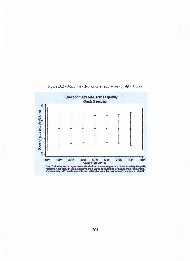
Univers

ity of

Cap

e Tow

nFigure D.2- Marginal effect of class size across quality deciles

10th 20th

Effect of class size across quality Grade 2 reading

30th 40th 50th 60th 70th Quality percentile

80th 90th

Note: Estimates from a regression of standardised score changes on a model including the quality measure, class size, an interaction term and a vector of cOVBriates including school fiXed effects. Bars represent 90% confidence intervals, calculated using the ·marginsplot' command in Stata12.

204

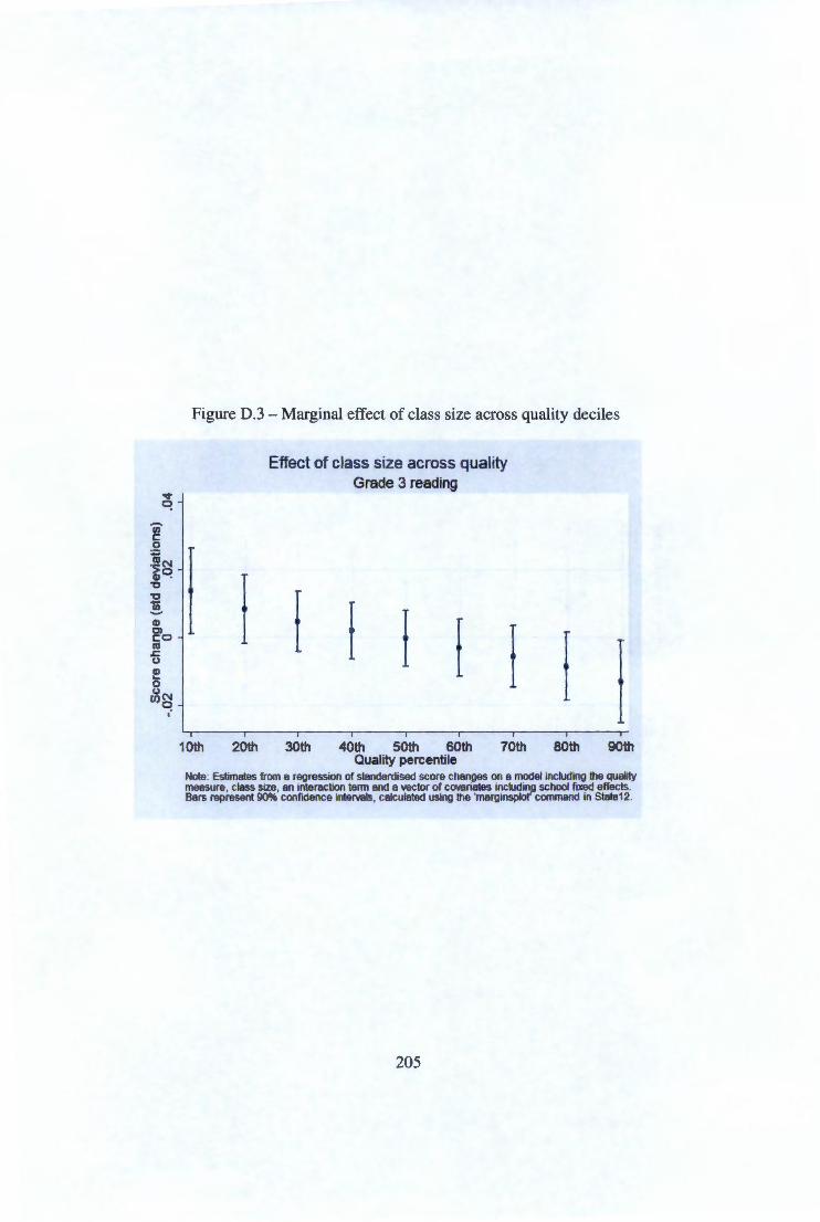
Univers

ity of

Cap

e Tow

nFigure D.3 - Marginal effect of class size across quality deciles

10th 20th

Effect of class size across quality Grade 3 reading

30th 40th 50th 60th 70th Quality percentile

80th 90th

Note: Estimates from a regression of standardised score changes on a model including the quality measure, class size, an interaction term and a vector of COIIBriates including school fiXed effects. Bars represent!IO% confidence intervals, calculated using the ·marginsplof command in Stata12.

205

Univers

ity of

Cap

e Tow

n

D.2 Marginal effects of quality on reading scores

206

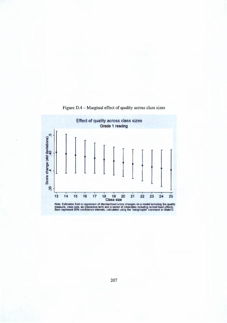
Univers

ity of

Cap

e Tow

nFigure D.4 - Marginal effect of quality across class sizes

Effect of quality across class sizes Grade 1 reading

13 14 15 16 17 18 19 20 21 22 23 24 25 Class size

Note: Estimates from a regression of standardised score changes on a model including the quality measure, class size, an interaction term and a vector of c01111riates including school fiXed effects. Bars represent 90% confidence intervals, calculated using the 'marginsplor command in Stata12.

207

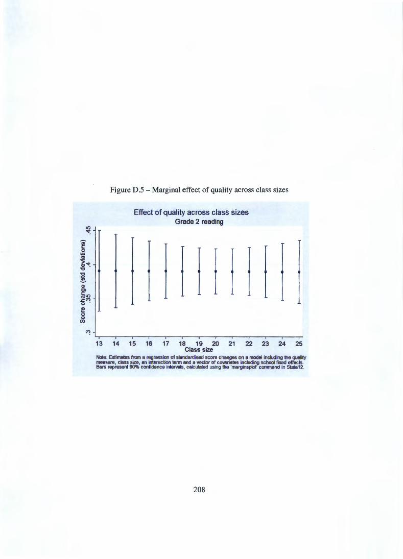
Univers

ity of

Cap

e Tow

nFigure D.5- Marginal effect of quality across class sizes

Effect of quality across class sizes Grade 2 reading

13 14 15 16 17 18 19 20 21 22 23 24 25 Class size

Note: Estimates from a regression of standardised score changes on a model including the quality measure, class size, an interaction term and a vector of coveriates including school fiXed effects. Bars represent 90% confidence intervals, calculated using the ·marginsplof command in Stata12.

208

Univers

ity of

Cap

e Tow

nFigure 0.6- Marginal effect of quality across class sizes

Effect of quality across class sizes Grade 3 reading

13 14 15 16 17 18 19 20 21 22 23 24 25 Class size

Note: Estimates from a regression of standardised score changes on a model including the quality measure, class size, an interaction term and a Yector of cOY!Iriates including school fiXed effects. Bars represent 90% confidence interYels, calculated using the 'marginsplof command in Stata12.

209

Univers

ity of

Cap

e Tow

n

Conclusion

If researchers wish to use their results to make policy recommendations - as 1m­hens (2010) suggests is the primary goal of much of the experimental literature - then it is critical that empirical, theoretical or methodological limitations to the policy relevance of results are clearly and comprehensively acknowledged. The relevance of experimentally identified causal effects typically depends on the ap­plicability of those estimates to a population that is different from the one in which the original experiment was conducted. The correct identification of causal effects ('internal validity') is therefore an insufficient criterion for evidence to be policy relevant. Instead what ultimately matters is the ability to use such results to fore­cast, in whatever way, the likely consequences of a policy ('external validity') in the population of interest.

The overarching concern of this thesis has been with the implications of in­teractions in causal relationships. Chapter 1 argued - following the basic insight of Campbell and Stanley (1966) and Cook and Campbell (1979)- that this is the most fundamental challenge to external validity in as much as it exists even in the presence of an ideal experiment. As with the broader problem of external valid­ity, this issue has largely been neglected in the empirical programme evaluation literature to date. Our analysis, building on Hotz et al. (2005), showed how in­teraction between variables in the 'production function' for causal effects implies that average treatment effects will differ across populations where the mean of the interacting covariates are different- a failure of 'simple external validity'. Leamer (2010) has referred to such variables as 'interactive confounders'.

This provides a useful framework within which the assumptions required for external validity can be more clearly appreciated. It implies that for estimated av­erage treatment effects to carry over identically to other populations it must be true that the means of all interacting variables are the same across these populations. While Hotz et al. (2005) propose a more sophisticated formulation of external validity in which covariate-specific treatment effects are weighted by the distribu­tion of covariates in the population of interest, the assumptions required for this

210

Univers

ity of

Cap

e Tow

n

to be achieved are analogous to the assumptions required by econometric match­ing estimators for the identification of average treatment effects. This reveals a clear tension: for experimental methods to be preferable to non-experimental alternatives it must be true that the assumptions required for matching estima­tors are implausible within the sample population, yet similar assumptions are required for experimental estimates to be informative outside the sample popu­lation. Thus if we reject the possibility of obtaining credible identification from non-experimental estimators we should, accordingly, be wary of any claims that experimental estimates can be extrapolated to other populations. Furthermore, in practice these assumptions require that researchers know, ex ante, what the rele­vant interacting variables are and can obtain data on the distributions in both the experimental and policy populations. That does not appear to be the case in most policy-related experiments conducted to date.

Whether interactions of this kind are in fact important is, to some extent, an empirical question. In order to provide some evidence on this, and other issues concerning the use of randomised evaluations, the remainder of the thesis focused on topics in the economics of education. Chapter 3 discussed experimental evalua­tions of class size effects. Specifically, we argued that it is implausible to presume, ex ante, that the effect of class size is independent of other variables in the produc­tion function of educational achievement. In particular, it seems plausible - and in accord with contributions to the education literature - that the importance of class size depends on the quality of the teacher and classroom environment. To date the economics of education literature has dealt with class size and teacher quality as independent considerations and often - as in the exchange between Krueger (2003) and Hanushek (2003) - competing policy priorities. Instead we suggest the possibility that teacher quality and class size interact, and therefore are com­plementary, in their effect on educational achievement. From a policy perspective that suggests the problem is to find the optimal combination of teacher quality and class size in the presence of resource constraints, rather than simply choosing one intervention over the other.

To assess this assertion outside of a full, plausible structural model requires that both the measures of teacher quality and class size are unconfounded by other factors. Using the Project STAR class size experiment, Chapter 2 showed how a value-added teacher quality variable can be constructed using a single cross­section of teacher observations when students and teachers are randomly assigned to classes. Specifically, that method exploits the fact that - in the limit - the dis­tribution of teacher quality across treatment categories should be the same. The ranking implied by that measure obtains indirect support from a study that con-

211

Univers

ity of

Cap

e Tow

n

ducted classroom observations on a subset of class teachers. Furthermore, in terms of explanatory power in relation to student achievement the measure produces re­sults compatible with other contributions to the quality literature.

Using this new measure, the regression results in Chapter 3 provided evidence of statistically and economically significant interaction effects between size and quality on student test score changes. On its own that is a contribution to the eco­nomics of education literature. However, in the context of the analysis in Chapter l what such interactions imply is that experimental estimates of the average ef­fect of class size reductions will, even if the researcher succeeded in identifying the confounded average treatment effect in the sample, not carry-over to other populations where the mean of the teacher quality distribution is different.

Together the above analyses suggest, at the least, that the question of exter­nal validity remains inadequately interrogated both theoretically and empirically. These issues are not yet dealt with in any systematic fashion in the vast majority of contributions to the experimental evaluation literature. How researchers inter­pret the limitations that interaction implies for simple extrapolation of estimated effects depends on how prevalent such relationships are believed to be. At base this is a question about the very nature of causal relationships in the domains in which economists conduct research. An appropriate prior may be to assume that, much as additively separable firm production functions are considered implausi­ble, interactive relationships are the norm unless proved otherwise. The present literature, however, implicitly assumes either additive separability or the ability of researchers to qualitatively determine which contexts are 'similar enough' for extrapolation. The problem with the latter strategy is that, as noted above, if re­searchers are able to determine similarity between sample and policy populations in this way, there is no obvious reason why they cannot equivalently determine whether recipients and non-recipients of non-experimental interventions are sim­ilar enough to satisfy a selection-on-observables assumption. In which case the experimental method is unnecessary.

In this context, the view that the only credible evidence for policy analysis is experimental (or, at worst, quasi-experimental) appears premature, as does the fo­cus on micro-level issues that are amenable to analysis by experimental variation. While many critics have noted that experimental methods may lead to neglect of 'big questions', there has been less discussion of the possibility that even the results of small-scale interventions may be misleading if systemic issues are not addressed. For example, another important set of experimental contributions to the economics of education literature concern teacher absenteeism. Yet if ab-

212

Univers

ity of

Cap

e Tow

n

senteeism is primarily an outcome of under-equipped teachers and poor working conditions then interventions at the micro-level that focus on teacher incentives may lead to an inefficient allocation of resources. The South African education system, for example, is recognised as achieving close to universal access but very poor performance on educational outcomes. Many studies have noted connections between poor outcomes with inefficiency, low teacher quality and inadequate pro­fessionalism. In this context randomised evaluations may assist in identifying effective interventions. However, there are also reasons - such as high teacher workloads, large class sizes, inadequate infrastructure and schooling resources -to believe that some of the observed causes of poor performance may also be the consequences of inadequate resources for the system as a whole. In that case the kind of micro-level interventions most suited to randomised evaluation may be irrelevant, or even suggest unsuitable policies, when macro-level institutional constraints have not been adequately studied.

As with all empirical work, the core analysis of chapters 2-3 is subject to a number of caveats. In chapter 2 we invoked a number of assumptions on the edu­cational production function along with the success of random assignment and its implications. If these hold then the method proposed and implemented for con­ducting a value-added quality measure would produce a variable which adequately represents teachers' relative quality. Similarly, the regression analysis in chapter 3 proceeded from the imposition of certain restrictions on the form of the cumula­tive production function. These turned-out to be non-trivial since while significant interaction effects were found for our favoured specification using score changes as the basis for the dependent variables, these were absent or less systematic when using score levels and not controlling for previous year's achievement. Relatedly, while random assignment resolves some of the key identification problems in the YAM and class size literatures, the results could be affected by measurement error in the teacher quality variable (leading to downward bias) as well as the possibility of reflection effects (upward bias). Finally, if interaction does exist then this com­plicates the construction of the quality measure, meaning at the least that it will be a more noisy measure, but potentially also that the magnitude of estimates could be upward or downward biased. In these respects our analysis is no less vulner­able to such assumptions than the existing literature; Chetty et al. (2011) suggest bounds on measurement error and reflection effects in their analysis, but do so using simple, additive decompositions and do not consider issues related to cu­mulative functional forms raised by Todd and Wolpin (2003). Within the broader theme of the thesis - limits to the external validity of estimates using experimen­tal data - the caveats to our empirical findings arguably emphasise the extent of the challenge posed by interactive relationships even with the highest quality of

213

Univers

ity of

Cap

e Tow

n

~--

experimental studies such as Project STAR.

Given the above it is clear that procedures for using experimental results to pre­dict the effects of policies in new environments remain largely undeveloped and the consequences similarly unrecognised. In our chosen example, the fact that most studies of class size effects have not even collected data on teacher quality implies that we may never be able to extend these results in a satisfactory way to other contexts. Whether future research design could be improved to address and anticipate such challenges remains an open question. And while advocates of al­ternative methods may endorse those instead, the problem of functional form is no less problematic for structural modelling where there is often little basis to choose one functional form over another and, as acknowledged by Heckman and Vytlacil (2007a: 4855), non-parametric methods for identification do not assist in resolv­ing the problem of extrapolation. The basic interaction problem may be removed, or ameliorated, by representative sampling of the population of interest or - more ambitiously - sampling for representation of the full support of the joint distri­bution of interacting covariates. Since such procedures are not currently utilised in the vast majority of reported studies, and it remains unclear whether they are feasible, our analysis implies that more caution should be exercised in claiming policy relevance for experimental estimates of programme effects.

214

Univers

ity of

Cap

e Tow

n

experimental studies such as Project STAR.

Given the above it is clear that procedures for using experimental results to pre­dict the effects of policies in new environments remain largely undeveloped and the consequences similarly unrecognised. In our chosen example, the fact that most studies of class size effects have not even collected data on teacher quality implies that we may never be able to extend these results in a satisfactory way to other contexts. Whether future research design could be improved to address and anticipate such challenges remains an open question. And while advocates of al­ternative methods may endorse those instead, the problem of functional form is no less problematic for structural modelling where there is often little basis to choose one functional form over another and, as acknowledged by Heckman and Vytlacil (2007a: 4855), non-parametric methods for identification do not assist in resolv­ing the problem of extrapolation. The basic interaction problem may be removed, or ameliorated, by representative sampling of the population of interest or - more ambitiously - sampling for representation of the full support of the joint distri­bution of interacting covariates. Since such procedures are not currently utilised in the vast majority of reported studies, and it remains unclear whether they are feasible, our analysis implies that more caution should be exercised in claiming policy relevance for experimental estimates of programme effects.

214

Univers

ity of

Cap

e Tow

n

Bibliography

Abadie, A., M. M. Chingos, and M. R. West (2013). Endogenous stratification in randomized experiments. NBER working paper (19742).

Achilles, C., H. P. Bain, F. Bellott, J. Boyd-Zaharias, J. Finn, J. Folger, J. John­ston, and E. Word (2008). Tennessee's Student Teacher Achievement Ratio (STAR) project. http: I /hdl. handle. net /1902. 1/107 66. Distribu­tor: HEROS, Inc., Helen Pate Bain and Carolyn Cox (Co-Chairs), Jayne Boyd­Zaharias; Version V 1.

Allcott, H. and S. Mullainathan (2012). External validity and partner selection bias. NBER Working Paper (18373).

Angrist, J. (2004). Treatment effect heterogeneity in theory and practice. Eco­nomic Journal 114, C52-C83.

An grist, J. and I. Fernandez-Val (20 1 0). ExtrapoLATE-ing: external validity and overidentification in the LATE framework. NBER Working Paper ( 16566).

Angrist, J. and I. Fernandez-Val (20 13 ). ExtrapoLATE-ing: external validity and overidentification in the LATE framework. In D. Acemoglu, M. Arellano, and E. Dekel (Eds.), Advances in Economics and Econometrics: Theory and Ap­plications, Econometric Society Monographs, Tenth World Congress (Vol.l/1). Cambridge University Press.

Angrist, J. D. and A. B. Krueger (2001). Instrumental variables and the search for identification: from supply and demand to natural experiments. Journal of Economic Perspectives 15(4), 69-85.

Angrist, J. D. and V. Lavy (1999). Using Maimonides' rule to estimate the effect of class size on scholastic achievement. Quarterly Journal of Eco­nomics 1 14(2), 533-575.

Angrist, J.D. and J.-S. Pischke (2009). Mostly harmless econometrics. Princeton: Princeton University Press.

215

Univers

ity of

Cap

e Tow

n

Angrist, J. D. and J.-S. Pischke (2010). The credibility revolution in empirical economics: how better research design is taking the con out of econometrics. Journal of Economic Perspectives 24(2), 3-30.

Bain, H. P., M. N. Lintz, and E. Word (1989). A study of fifty effective teachers whose class average gain scores ranked in the top 15% of each of four school types in Project STAR. Unpublished paper (ED321877).

Baird, S., A. Bohren, C. Mcintosh, and B. Ozier (2014). Designing experi­ments to measure spillover effects. World Bank Policy Research Working Pa­per (6824).

Bandiera, 0., V. Larcinese, and I. Rasul (2010). Heterogenous class size effects: new evidence from a panel of university students. Economic Journal120(549), 1365-1398.

Banerjee, A. V. (2007). Making aid work. Cambridge(MA): MIT Press.

Banerjee, A. V. and E. Duflo (2008). The experimental approach to development economics. NBER Working Paper 14467.

Banerjee, A. V. and E. Duflo (2009). The experimental approach to development economics. Annual Review of Economics 1, 151-178.

Banerjee, A. V. and S. M. R. Kanbur (2005). New Directions in Development Economics: Theory Or Empirics? : a Symposium in Economic and Political Weekly. Working paper (New York State College of Agriculture and Life Sci­ences. Dept. of Applied Economics and Management). Cornell University.

Bardhan, P. (2013, 20 May). Little, big: two ideas about fighting global poverty. Boston Review.

Barton, S. (2000). Which clinical studies provide the best evidence? the best ret still trumps the best observational study. British Medical Journal321, 255-256.

Benson, K. and A. J. Hartz (2000). A comparison of observational studies and ran­domized, controlled trials. New England Journal of Medicine 342(25), 1878-1886.

Berger, M., D. Black, and J. Smith (200 1 ). Evaluating profiling as a means of allo­cating government services. In M. Lechner and F. Ffeiffer (Eds.), Econometric Evaluation of Labour Market Policies, Volume 13 of ZEW Economic Studies, pp. 59-84. Physica-Verlag HD.

216

Univers

ity of

Cap

e Tow

n

Binmore, K. (1999). Why experiment in economics? Economic Journal 109, 16-24.

Blatchford, P., H. Goldstein, and P. Mortimore (1998). Research on class size effects: a critique of methods and a way forward. International Journal of Educational Research 29(8), 691-710.

Blatchford, P. and P. Mortimer ( 1994 ). The issue of class size for young children in schools: what can we learn from research? Oxford Review of Education 20(4), 411-428.

Bold, T., M. Kimenyi, G. Mwabu, A. Nganga, and J. Sandefur (2013). Scaling up what works: experimental evidence on external validity in Kenyan education. Center for Global Development Working Paper (321).

Bowles, S. (1970). Towards an educational production function. In W. L. Hansen (Ed.), Education, income and human capital, pp. 9-70. National Bureau of Economic Research.

Browning, M. and E. Heinesen (2007). Class size, teacher hours and educational attainment. Scandinavian Journal of Economics 109(2), 415-438.

Campbell, D. T. and J. C. Stanley (1966). Experimental and Quasi-experimental Designs for Research. Chicago: Rand McNally College Publishing.

Card, D., S. Della Vigna, and U. Malmendier (2011). The role of theory in field experiments. Journal of Economic Perspectives 25(3), 39-62.

Card, D., J. Kluve, and A. Weber (2010). Active labour market policy evaluations: A meta-analysis. The Economic Journal 120(548), F452-F477.

Cartwright, N. (1979). Causal laws and effective strategies. Nous 13, 419-437.

Cartwright, N. (1989). Nature's Capacities and their Measurement. Oxford: Oxford University Press.

Cartwright, N. (2007). Hunting causes and using them: approaches in philosophy and economics. Cambridge: Cambridge University Press.

Cartwright, N. (2010). What are randomised controlled trials good for? Philo­sophical studies 147, 59-70.

Cartwright, N. (2011a). Evidence, external validity, and explanatory relevance. In G. J. Morgan (Ed.), Philosophy of Science Matters: The Philosophy of Peter Achinstein, pp. 15-28. New York: Oxford University Press.

217

Univers

ity of

Cap

e Tow

n

Cartwright, N. (2011b). Predicting 'it will work for us': (way) beyond statistics. In P. I. McKay, F. Russo, and J. Williamson (Eds.), Causality in the sciences. Oxford (UK): Oxford University Press.

Chetty, R., J. N. Friedman, N. Hilger, E. Saez, D. W. Schanzenbach, and D. Yagan (2011). How does your kindergarten classroom affect your earnings? evidence from Project STAR. Quarterly Journal of Economics 126(4), 1593-1659.

Chetty, R., J. N. Friedman, and J. E. Rockoff (2011). The long-term impacts of teachers: teacher value-added and student outcomes in adulthood. NBER Working Paper (17699).

Chingos, M. M. (2012). The impact of a universal class-size reduction policy: evidence from Floridas statewide mandate. Economics of Education Review 31, 543-562.

Choa, H., P. Glewwe, and M. Whitler (2012). Do reductions in class size raise stu­dents test scores? evidence from population variation in Minnesotas elementary schools. Economics of Education Review 2012, 77-95.

Concato, J., N. Shah, and R. Horwitz (2000). Randomized controlled trials, obser­vational studies, and the hierarchy of research designs. New England Journal of Medicine 342(25), 1887-1892.

Cook, T. D. (2014). Generalizing causal knowledge in the policy sciences: Ex­ternal validity as a task of both multiattribute representation and multiattribute extrapolation. Journal of Policy Analysis and Management 33(2), 527-536.

Cook, T. D. and D. T. Campbell (1979). Quasi-Experimentation: design and Analysis Issues for Field Settings. Wadsworth.

Cox, D. R. and N. Reid (2000). The theory of the design of experiments. Chapman and Hall. Monographs on statistics and applied probability 86.

Crump, R. K., V. J. Hotz, G. W. Imbens, and 0. A. Mitnik (2008). Nonparamet­ric tests for treatment effect heterogeneity. Review of Economics and Statis­tics 90(3), 389-405.

Crump, R. K., V. J. Hotz, G. W. Imbens, and 0. A. Mitnik (2009). Dealing with limited overlap in estimation of average treatment effects. Biometrika 96( 1 ), 187-199.

Deaton, A. (2008, October 9th). Instruments of development: Randomization in the tropics, and the search for the elusive keys to economic development. Keynes Lecture, British Academy.

218

Univers

ity of

Cap

e Tow

n

Deaton, A. (2009). Instruments of development: randomization in the tropics, and the search for the elusive keys to economic development. NBER working paper (w14690).

Deaton, A. (2010). Instruments, randomization, and learning about development. Journal of Economic Literature 48(2), 424-455.

Dee, T. S. (2004). Teachers, race, and student achievement in a randomized ex­periment. Review of Economics and Statistics 86( 1 ), 195-210.

Dehejia, R. H. (2005). Program evaluation as a decision problem. Journal of Econometrics 125, 141-173.

Dehejia, R. H. (2013). The porous dialectic: experimental and non-experimental methods in development economics. WIDER Working Paper (No. 2013/11).

Dekkers, 0. M., E. von Elm, A. Algra, J. A. Romijn, and J. P. Vandenbroucke (2010). How to assess the external validity of therapeutic trials: a conceptual approach. International Journal of Epidemiology 39, 89-94.

Ding, W. and S. F. Lehrer (2010a). Estimating context-independent treatment effects in education experiments. Unpublished working paper.

Ding, W. and S. F. Lehrer (2010b). Estimating treatment effects from contam­inated multiperiod education experiments: the dynamic impacts of class size reductions. Review of Economics and Statistics 92(1), 31-42.

Ding, W. and S. F. Lehrer (2011a). Experimental estimates of the impacts of class size on test scores: robustness and heterogeneity. Education Economics 19(3), 229-252.

Ding, W. and S. F. Lehrer (2011b). Understanding the role of time-varying unob­served ability heterogeneity in education production. forthcoming.

Djebbari, H. and J. Smith (2008). Heterogeneous impacts in PROGRESA. Jour­nal of Econometrics 145, 64-80.

Duflo, E., P. Dupas, and M. Kremer (2011). Peer effects, teacher incentives, and the impact of tracking: evidence from a randomized evaluation in Kenya. American Economic Review 101(5).

Duflo, E., R. Glennerster, and M. Kremer (2006a). Chapter 61: Using randomiza­tion in development economics research: a toolkit. In Handook of Development Economics Volume 4. Amsterdam: Elsevier.

219

Univers

ity of

Cap

e Tow

n

Dufto, E., R. Glennerster, and M. Kremer (2006b). Using randomization in de­velopment economics research: a toolkit. Accessed 24th January 2011 from http://www.povertyactionlab.org/sites/default/files/documents/Using

Eells, E. (1991 ). Probabilistic causality. Cambridge: Cambridge University Press.

Ehrenberg, R. G., D. J. Brewer, A. Gamoran, and J.D. Willms (2001). Class size and student achievement. Psychological Science in the Public Interest 2(1 ), 1-30.

Elliott, G. and A. Timmermann (2008). Economic forecasting. Journal of Eco­nomic Literature 46(1), 3-56.

Evans, D. (2003). Hierarchy of evidence: a framework for ranking evidence eval­uating healthcare interventions. Journal of Clinical Nursing I2(1), 77-84.

Falagasa, M. E., E. K. Vouloumanoua, K. Sgourosa, S. Athanasioud, G. Peppasa, and I. I. Siemposa (2010). Patients included in randomised controlled trials do not represent those seen in clinical practice: focus on antimicrobial agents. International Journal of Antimicrobial Agents 36, 1-13.

Figlio, D. N. (1999). Functional form and the estimated effect of school resources. Economics of Education Review 18(2), 241-252.

Fink, G., M. McConnell, and S. Vollmer (2013). Testing for heterogeneous treat­ment effects in experimental data: false discovery risks and correction pro­cedures. Journal of Development Effectiveness. Published online at http : //dx.doi.org/10.1080/19439342.2013.875054.

Finn, J. D. and C. M. Achilles (1990). Answers and questions about class size: a statewide experiment. American Educational Research Journal 27(3), 557-577.

Finn, J.D., S. B. Gerber, and J. Boyd-Zaharias (2005). Small classes in the early grades, academic achievement and graduating from high school. Journal of Educational Psychology 97(2), 214-223.

Finn, J.D., J.-B. Zaharias, R. M. Fish, and S. B. Gerber (2007, January). Project STAR and beyond: database user's guide. Available online at www.heros­inc.org/starUsersGuide.pdf.

Frisch, R. and F. V. Waugh (1933). Partial time regressions as compared with individual trends. Econometrica I(4), 387-401.

220

Univers

ity of

Cap

e Tow

n

Garfinkel, 1., C. F. Manski, and C. Michalopolous (1992). Micro experiments and macro effects. In Evaluating welfare and training programs, pp. 253-276. Cambridge (MA).

Gelman, A. (2000). A statistician's perspective on Mostly Harmless Economet­rics: An Empiricist's Companion, by Joshua D. Angrist and J orn-Steffen Pis­chke. Stata Journal9(2), 315-320.

Giacomini, R. (2014). Economic theory and forecasting: lessons from the litera­ture. CEMMAP working paper (CWP41114).

Glewwe, P., N. Ilias, and M. Kremer (2010). Teacher incentives. American Eco­nomic Journal: Applied Economics 2(3), 205-227.

Glewwe, P. W., E. A. Hanushek, S.D. Humpage, and R. Ravina (2011). School resources and educational outcomes in developing countries: a review of the literature from 1990 to 2010. NBER 17554.

Goldhaber, D. and E. Anthony (2007). Can teacher quality be effectively as­sessed? National board certification as a signal of effective teaching. Review of Economics and Statistics 89(1), 134-150.

Guala, F. (2003). Experimental localism and external validity. Philosophy of Science 70(5), 1195-1205.

Guala, F. (2005). Economics in the lab: completeness vs. testability. Journal of Economic Methodology 12(2), 185-196.

Guala, F. and L. Mittone (2005). Experiments in economics: external validity and the robustness of phenomena. Journal of Economic Methodology 12(4), 495-515.

Haavelmo, T. (1944 ). The probability approach in econometrics. Economet­rica 12, iii-iv,1-115.

Hacking, I. (1988). Telepathy: origins of randomization in experimental design. Isis 79(3), 427-451.

Hadorn, D. C., D. Baker, J. S. Hodges, and N. Hicks (1996). Rating the quality of evidence for clinical practice guidelines. Journal of Clinical Epidemiol­ogy 49(7).

Hanushek, E. A. (1971 ). Teacher characteristics and gains in student achieve­ment: estimation using micro data. American Economic Review: Papers & Proceedings 61(2), 280-288.

221

Univers

ity of

Cap

e Tow

n

Hanushek, E. A. (1979). Conceptual and empirical issues in the estimation of educational production functions. Journal of Human Resources 14(3), 351-388.

Hanushek, E. A. (1999). Some findings from an independent investigation of the Tennessee STAR experiment and from other investigations of class size effects. Educational evaluation and policy analysis 21(2), 143-163.

Hanushek, E. A. (2003). The failure of input-based schooling policies. Economic Journal 113(485), 64-98.

Hanushek, E. A. and S. G. Rivkin (2006). Teacher quality. In E. A. Hanushek and F. Welch (Eds.), Handbook of the Economics of Education, Volume 2, pp. 1051-1078. Elsevier.

Hanushek, E. A. and S. G. Rivkin (2010). Generalizations about using value­added measures of teacher quality. American Economic Review 100(2), 267-271.

Hanushek, E. A. and S. G. Rivkin (20 12). The distribution of teacher quality and implications for policy. Annual Review of Economics 4, 131-157.

Harris, D. N. (2007). Diminishing marginal returns and the production of educa­tion: an international analysis. Education Economics 1 5(1 ), 31-53.

Harrison, G. W. and J. A. List (2004). Field experiments. Journal of Economic Literature 42(4), 1009-1055.

Hattie, J. (2005). The paradox of reducing class size and improving learning outcomes. International Journal of Educational Research 43(6), 387-425.

Heckman, J. and J. H. Abbring (2007). Econometric evaluation of social pro­grams, part iii: Distributional treatment effects, dynamic treatment effects, dy­namic discrete choice, and general equilibrium policy evaluation. In J. Heck­man and E. Leamer (Eds.), Handbook of Econometrics (Volume 6B), Vol­ume 6B, Chapter 72, pp. 5145-5303. Amsterdam: Elsevier.

Heckman, J. and R. Robb (1985). Alternative methods for evaluating the impact of interventions: An overview. Journal of Econometrics 30, 239-267.

Heckman, J., J. Smith, and N. Clements (1997). Making the most out of pro­gramme evaluations and social experiments: accounting for heterogeneity in programme impacts. Review of Economic Studies 64(4), 487-535.

222

Univers

ity of

Cap

e Tow

n

Heckman, J. and E. Vytlacil (2007a). Econometric evaluation of social programs, part i: Causal models, structural models and econometric policy evaluation. In J. Heckman and E. Leamer (Eds.), Handbook of Econometrics (Volume 6B), Volume 6B, Chapter 70, pp. 4779-4874. Amsterdam: Elsevier.

Heckman, J. and E. Vytlacil (2007b). Econometric evaluation of social programs, part ii: Using the marginal treatment effect to organize alternative econometric estimators to evaluate social programs, and to forecast their effects in new en­vironments. In J. Heckman and E. Leamer (Eds.), Handbook of Econometrics (Volume 6B), Volume 6B, Chapter 71, pp. 4875-5143. Amsterdam: Elsevier.

Heckman, J. J. (2000). Causal parameters and policy analysis in economics: a twentieth century retrospective. Quarterly Journal of Economics 115, 45-97.

Heckman, J. J. (2008). Econometric causality. International Statistical Review 76, 1-27.

Heckman, J. J., H. lchimura, and P. Todd (1997). Matching as an econometric evaluation estimator: evidence from evaluating a job training programme. Re­view of Economic Studies 64( 4 ), 605--654.

Heckman, J. J. and J. Smith (1998). Evaluating the welfare state. In Economet­rics and Economic Theory in the 20th Century: The Ragnar Frisch Centennial Symposium, pp. 241-318. Cambridge University Press.

Heckman, J. J. and J. A. Smith ( 1995). Assessing the case for social experiments. Journal of Economic Perspectives 9(2), 85-110.

Heckman, J. J. and S. Urzua (2010). Comparing IV with structural models: What simple IV can and cannot identify. Journal of Econometrics 1 56( 1 ), 27-37.

Heckman, J. J. and E. Vytlacil (2005). Structural equations, treatment effects and econometric policy evaluation. Econometrica 73(3), 669-738.

Heinesen, E. (2010). Estimating class-size effects using within-school variation in subject-specific classes. Economic Journal 120, 737-760.

Hendry, D. F. (1995). Dynamic Econometrics. Oxford: OUP.

Herberich, D. H., S.D. Levitt, and J. A. List (2009). Can field experiments return agricultural economics to the glory days? American Journal of Agricultural Economics 91(5), 1259-1265.

Holland, P. W. (1986). Statistics and causal inference. Journal of American Sta­tistical Association 81 (396), 945-960.

223

Univers

ity of

Cap

e Tow

n

Hotz, V. J., G. W. Imbens, and J. H. Mortimer (2005). Predicting the efficacy of future training programs using past experiences at other locations. Journal of Econometrics 125, 241-270.

Hoxby, C. M. (2000). The effects of class size on student achievement: new evidence from population variation. Quarterly Journal of Economics 115( 4 ), 1239-1285.

Hsiao, C. (1992). Random coefficient models. In L. Matyas and P. Sevestre (Eds.), The Econometrics of Panel Data: Handbook of theory and applications, pp. 72-94. Springer.

Hsiao, C. and M. H. Pesaran (2004). Random coefficient panel data models. IZA Discussion Paper 1236.

Imbens, G. (2004). Nonparametric estimation of average treatment effects under exogeneity: a review. Review of Economics and Statistics 86(1), 4-29.

Imbens, G. W. (2010). Better LATE than nothing: Some comments on Deaton(2009) and Heckman and Urzua(2009). Journal of Economic Litera­ture 48(2), 399-423.

Imbens, G. W. (2013). Book review feature: Public Policy in an Uncertain World. Economic Journal123, F401-F411.

Jackson, E. and M. E. Page (2013). Estimating the distributional effects of edu­cation reforms: a look at Project STAR. Economics of Education Review 32, 92-103.

Jacob, B. A., L. Lefgren, and D. P. Sims (2010). The persistence of teacher­induced learning. Journal of Human Resources 45(4), 915-943.

Kahneman, D. and A. Tversky (1979). Prospect theory: an analysis of decision under risk. Econometrica 47(2), 263-292.

Keane, M. (2005, 17-19 September). Structural vs. atheoretic approaches to econometrics. Keynote Address at the Duke Conference on Structural Mod­els in Labor, Aging and Health.

Keane, M. P. (2010a). A structural perspective on the experimentalist school. Journal of Economic Perspectives 24(2), 47-58.

Keane, M.P. (2010b). Structural vs. atheoretic approaches to econometrics. Jour­nal of Econometrics 156( 1 ), 3-20.

224

Univers

ity of

Cap

e Tow

n

Keynes, J. (1939). Professor Tinbergen's method. Economic Journal 49(195), 558-577.

Koenker, R. and L. Ma (2006). Quantile regression methods for recursive struc­tural equation models. Journal of Econometrics 134, 4 71-506.

Konstantopolous, S. (2011). How consistent are class size effects? Evaluation Review 35(1 ), 71-92.

Konstantopolous, S. and M. Sun (2011). Are teacher effects larger in small classes? Unpublished working paper.

Kramer, M. and S. Shapiro (1984). Scientific challenges in the application of randomized trials. Journal of the American Medical Association 252, 2739-2745.

Kremer, M. and A. Holla (2009). Improving education in the developing world: what have we learned from randomized evaluations? Annual Review of Eco­nomics 1, 513-542.

Krueger, A. B. (1999). Experimental estimates of education production functions. Quarterly Journal of Economics 114(2), 497-532.

Krueger, A. B. (2003). Economic considerations and class size. Economic Jour­naZI 13(485), 34-63.

Krueger, A. B. and D. Whitmore (2001). The effect of attending a small class in the early grades on college-test taking and middle school test results: evidence from Project STAR. Economic Journal111(468), 1-28.

LaLonde, R. J. (1986). Evaluating the econometric evaluations of training pro­grams with experimental data. American Economic Review 96(4), 604-619.

Lazear, E. P. (2001). Educational production. Quarterly Journal of Eco­nomics 116(3), 777-803.

Leamer, E. (201 0). Tantalus on the road to asymptopia. Journal of Economic Perspectives 24(2), 31-46.

Levin, J. (2001). For whom the reductions count: a quantile regression analysis of class size and peer effects on scholastic achievement. Empirical Economics 26, 221-246.

Levitt, S. D. and J. A. List (2007). Viewpoint: On the generalizability of lab behaviour to the field. Canadian Journal of Economics 40(2), 347-370.

225

Univers

ity of

Cap

e Tow

n

Levitt, S.D. and J. A. List (2009). Field experiments in economics: the past, the present and the future. European Economic Review 53, 1-18.

List, J. A. (2011). Why economists should conduct field experiments and 14 tips for pulling one off. Journal of Economic Perspectives 25(3 ), 3-16.

Loewenstein, G. (1999). Experimental economics from the vantage point of be­havioural economics. Economic Journal109, 25-34.

Lovell, M. (1963). Seasonal adjustment of economic time series and multiple regression analysis. Journal of American Statistical Association 58(304), 993-1010.

Lovell, M. (2008). A simple proof of the FWL theorem. Journal of Economic Education 39( 1 ), 88-91.

Ludwig, J., J. R. Kling, and S. Mullainathan (2011). Mechanism experiments and policy evaluations. Journal of Economic Perspectives 25(3), 17-38.

Manski, C. (1993). Identification of endogenous social effects: the reflection problem. Review of Economic Studies 60, 531-542.

Manski, C. (2000). Identification and decisions under ambiguity: empirical analy­sis of treatment response and normative analysis of treatment choice. JoE 95(2), 415-442.

Manski, C. (2004 ). Measuring expectations. Econometrica 72(5), 1329-1376.

Manski, C. (2011). Policy analysis with incredible certitude. Economic Jour­nal121(554), F261-F289.

Manski, C. F. (2013a). Public policy in an uncertain world: analysis and deci­sions. Cambridge (MA): Harvard University Press.

Manski, C. F. (2013b). Response to the review of 'public policy in an uncertain world'. Economic Journal123, F412-F415.

Marschak, J. (1953). Economic measurements for policy and prediction. In W. Hood and T. Koopmans (Eds.), Studies in Econometric Method, pp. 1-26. Wiley.

Matzkin, R. L. (2007). Nonparametric identification. In J. Heckman and E. Leamer (Eds.), Handbook of Econometrics (Volume 6B), Volume 6B, Chap­ter 73, pp. 5307-5368. Amsterdam: Elsevier.

226

Univers

ity of

Cap

e Tow

n

McEwan, P. J. (2013). Improving learning in primary schools of developing coun­tries: a meta-analysis of randomized experiments. Unpublished working paper.

McKee, M., A. Britton, N. Black, K. McPherson, C. Sanderson, and C. Bain ( 1999). Interpreting the evidence: choosing between randomised and nonran­domised studies. British Medical Journal319, 312-315.

Meyer, B. D. (1995). Natural and quasi-experiments in economics. Journal of Business and Economic Statistics 13(2), 151-161.

Miguel, E. and M. Kremer (2004 ). Worms: identifying impacts on education and health in the presence of treatment externalities. Econometrica 72( 1 ), 159-217.

Morgan, S. L. and C. Winship (2007). Counterfactuals and causal inference. Cambridge: Cambridge University Press.

Mosteller, F. ( 1995). The Tennessee study of class size in the early school grades. The Future of Children: Critical Issues for Children and Youths 5(2), 113-127.

Moulton, B. R. (1986). Random group effects and the precision of regression estimates. Journal of Econometrics 32, 385-397.

Moulton, B. R. (1990). An illustration of a pitfall in estimating the effects of aggregate variables on micro units. Review of Economics and Statistics 72(2), 334-338.

Mueller, S. (2013). Teacher experience and the class size effect - experimental evidence. Journal of Public Economics 98, 44-52.

Neyman, J. (1923). Statistical problems in agricultural experiments. Journal of the Royal Statistical Society II Suppl.(2), 107-180.

Nye, B., S. Konstantopoulos, and L. V. Hedges (2004). How large are teacher effects? Educational evaluation and policy analysis 26(3), 237-257.

Ozer-Balli, H. and B. E. Sorensen (2013). Interaction effects in econometrics. Empirical Economics 45(1).

Pearl, J. (2000 (2009)). Causality: Models,reasoning and inference. Cambridge: Cambridge University Press.

Pepper, J. V. (2002). Robust inferences from random clustered samples: an ap­plication using data from the panel study of income dynamics. Economics Let­ters 75, 341-345.

227

Univers

ity of

Cap

e Tow

n

Pritchett, L. and J. Sandefur (2013). Context matters for size. Center for Global Development Working Paper 336.

Quandt, R. E. (1958). The estimation of the parameters of a linear regression system obeying two separate regimes. Journal of American Statistical Associ­ation 53(284 ), 873-880.

Ravallion, M. (2008, March). Evaluation in the practice of development. World Bank Policy Research Working Paper 454 7.

Ravallion, M. (2009, February). Should the Randomistas rule? Economists' Voice.

Rivkin, S. G., E. A. Hanushek, and J. F. Kain (2005). Teachers, schools and academic achievement. Econometrica 73(2), 417-458.

Rivkin, S. G. and C. Jepsen (2009). Class size reduction and student achievement: the potential tradeoff between teacher quality and class size. Journal of Human Resources 44( 1 ), 223-250.

Rockoff, J. (2009). Field experiments in class size from the early twentieth cen­tury. Journal of Economic Perspectives 23( 4 ), 211-230.

Rockoff, J. E. (2004 ). The impact of individual teachers on student achievement: evidence from panel data. American Economic Review: Papers & Proceed­ings) 94(2), 247-252.

Rockoff, J. E. and C. Speroni (20 10). Subjective and objective evaluations of teacher effectiveness. American Economic Review: Papers & Proceed­ings 100(2), 261-266.

Rockoff, J. E. and C. Speroni (2011). Subjective and objective evaluations of teacher effectiveness: evidence from New York City. Labor Economics 18(5), 687-696.

Rodrik, D. (2008, October). The new development economics: we shall ex­periment, but how shall we learn? Harvard Kennedy School Working Pa­per RWPOB-055.

Roe, B. E. and D. R. Just (2009). Internal and external validity in economics re­search: tradeoffs between experiments, field experiments, natural experiments, and field data. American Journal of Agricultural Economics 91(5), 1266-1271.

Rosenbaum and D. Rubin (1983). The central role of the propensity score in observational studies for causal effects. Biometrika 70, 41-55.

228

Univers

ity of

Cap

e Tow

n

Rosenthal, L. (2004 ). Do school inspections improve school quality? Ofsted inspections and school examination results in the UK. Economics of Education Review 23(2), 143-151.

Ross, S., A. Grant, C. Counsell, W. Gillespie, I. Russell, and R. Prescott (1999). Barriers to participation in randomised controlled trials: a systematic review. Journal of Clinical Epidemiology 52(12), 1143-1156.

Roth, A. E. (1988). Laboratory experimentation in economics: a methodological overview. Economic Journal98, 974-1031.

Rothstein, J. (2010). Teacher quality in educational production: tracking, decay, and student achievement. Quarterly Journal of Economics 125(1), 175-214.

Rothwell, P. M. (2005a). External validity of randomised controlled trials: "to whom do the results of this trial apply?". Lancet 365, 82-93.

Rothwell, P.M. (2005b). Subgroup analysis in randomised controlled trials: im­portance, indications, and interpretation. Lancet 365, 17 6-186.

Rothwell, P. M. (2006). Factors that can affect the external validity of randomised controlled trials. PLoS CLinical Trials 1(1), 1-5.

Roy, A. (1951). Some thoughts on the distribution of earnings. Oxford Economic Papers 3, 135-146.

Royston and Sauerbrei (2009). Two techniques for investigating interactions be­tween treatment and continuous covariates in clinical trials. Stata Journal9(2), 230-251.

Royston, P. and W. Sauerbrei (2008). Multivariable Model-building: a Pragmatic Approach to Regression Analysis Based on Fractional Polynomials for Mod­elling Continuous Variables. Chichester, UK: Wiley.

Rubin, D. (1973). Matching to remove bias in observational studies. Journal of Educational Psychology 29(1), 159-183.

Rubin, D. (1974). Estimating causal effects oftreatments in randomized and non­randomized studies. Journal of Educational Psychology 66, 688-701.

Rust, J. (2010). Comments on: "Structural vs. atheoretic approaches to econo­metrics" by Michael Keane. Journal of Econometrics 156, 21-24.

Samuelson, L. (2005). Economic theory and experimental economics. Journal of Economic Literature 43(1), 65-107.

229

Univers

ity of

Cap

e Tow

n

Sass, T. R., A. Semykina, and D. N. Harris (2013). Value-added models and the measurement of teacher productivity. Economics of Education Review http : //dx.doi.org/10.1016/j.econedurev.2013.10.003.

Schanzenbach, D. W. (2006). What have researchers learned from Project STAR. Brookings Papers on Education Policy 9, 205-228.

Schochet, P. Z. (2008). Technical methods report: Guidelines for multiple testing in impact evaluations. Washington, DC: National Center for Education Evalua­tion and Regional Assistance, Institute of Education Sciences, U.S. Department of Education.

Schrag, P. (2006). Policy from the hip: class-size reduction in California. Brook­ings Papers on Education Policy 9, 229-243.

Schram, A. (2005). Artificiality: The tension between internal and external valid­ity in economic experiments. Journal of Economic Methodology 12(2), 225-237.

Smith, J. and P. Todd (2005a). Does matching overcome LaLonde's critique of nonexperimental estimators? Journal of econometrics 125( 1), 305-353.

Smith, J. and P. Todd (2005b). Rejoinder. Journal of Econometrics 125(12), 365-375.

Solon, G., S. J. Haider, and J. Wooldridge (2013). What are we weighting for? NBER Working Paper ( 18859).

Spirtes, P., C. N. Glymour, and R. Scheines (2000 (1993)). Causation, prediction and search. Cambridge(MA): MIT Press.

Staiger, D. 0. and J. E. Rockoff (2010). Searching for effective teachers with imperfect information. Journal of Economic Perspectives 24(3), 97-118.

Steel, D. (2008). Across the boundaries: extrapolation in biology and social science. Oxford: Oxford University Press.

Sugden, R. (2005). Journal of Economic Methodology 12(2), 177-184.

Todd, P. E. (2006). Chapter 60: Evaluating social programs with endogenous program placement and selection of the treated. In Handook of Development Economics Volume 4. Amsterdam: Elsevier.

Todd, P. E. and K. I. Wolpin (2003). On the specification and estimation of the production function for cognitive achievement. Economic Journal 113( 485), 3-33.

230

Univers

ity of

Cap

e Tow

n

Urquiola, M. (2006). Identifying class size effects in developing countries: evi­dence from rural Bolivia. Review of Economics and Statistics 88( 1 ), 171-177.

Urquiola, M. and E. Verhoogen (2009). Class-size caps, sorting and the regression-discontinuity design. American Economic Review 99(1), 179-215.

Wei, H., T. Hembry, D. L. Murphy, andY. McBride (2012, May). Value-Added Models in the Evaluation of Teacher Effectiveness: a Comparison of Models and Outcomes. Pearson Research Report.

Wooldridge, J. M. (2002). Econometric analysis of cross section and panel data. Cambridge(MA): MIT Press.

Wooldridge, J. M. (2003). Cluster-sample methods in applied econometrics. American Economic Review (Papers&Proceedings) 93(2), 133-138.

Word, E., J. Johnston, H. P. Bain, B. D. Fulton, J. B. Zaharias, C. M. Achilles, M. N. Lintz, J. Folger, and C. Breda (1990). The state of Tennessee's Stu­dent!feacher Achievement Ratio (star) project: Technical report 1985-1990. Tennessee State Department of Education. Available at http : I I www . education-consumers. comlprojectstar .php (Last accessed 7th April 2012).

231