OECD DEVELOPMENT CENTRE

Working Paper No. 46(Formerly Technical Paper No. 46)

THE EXTERNAL FINANCINGOF BRAZILIAN IMPORTS

(SPECIAL SERIES ON MIXED CREDITS,IN COLLABORATION WITH ICEPS)

by

Enrico Colombatto, with Elisa Luciano, Luca Gargiulo,Pietro Garibaldi and Giuseppe Russo

Research programme on:Financial Policies for the Global Dissemination of Economic Growth

October 1991OCDE/GD(91)180

TABLE OF CONTENTS

PREFACE . . . . . . . . . . . . . . . . . . . . . . . . . . . . . . . . . . . . . . . . . . . . . . . . . . . . . . 9

SUMMARY . . . . . . . . . . . . . . . . . . . . . . . . . . . . . . . . . . . . . . . . . . . . . . . . . . . . . 10

FOREWORD . . . . . . . . . . . . . . . . . . . . . . . . . . . . . . . . . . . . . . . . . . . . . . . . . . . 13

1. INTRODUCTION . . . . . . . . . . . . . . . . . . . . . . . . . . . . . . . . . . . . . . . . . . . 15

2. EXPORT CREDITS: THE DATA . . . . . . . . . . . . . . . . . . . . . . . . . . . . . . . 19

3. METHODOLOGICAL ISSUES: THE GENERAL CASE . . . . . . . . . . . . . . . 233.1 Some special cases: the grace period . . . . . . . . . . . . . . . . . . . . . . . . . . . 243.2 Uncertainty . . . . . . . . . . . . . . . . . . . . . . . . . . . . . . . . . . . . . . . . . . . . . . 273.3 Loans obtained and paid back in the same currency . . . . . . . . . . . . . . . . . 273.4 Loans obtained and paid back in different currencies . . . . . . . . . . . . . . . . 293.5 Uncertainty and special cases for the country subsidy . . . . . . . . . . . . . . . 303.6 Decomposition of the subsidy’s present value into

addenda for each period (under certainty) . . . . . . . . . . . . . . . . . . . . . . . . 313.7 A comparison with previous OECD studies . . . . . . . . . . . . . . . . . . . . . . . . 34

4. THE ESTIMATES . . . . . . . . . . . . . . . . . . . . . . . . . . . . . . . . . . . . . . . . . . 374.1 The data . . . . . . . . . . . . . . . . . . . . . . . . . . . . . . . . . . . . . . . . . . . . . . . . . 374.2 The results . . . . . . . . . . . . . . . . . . . . . . . . . . . . . . . . . . . . . . . . . . . . . . . 38

5. FINAL COMMENTS . . . . . . . . . . . . . . . . . . . . . . . . . . . . . . . . . . . . . . . . 535.1 Summary of the main findings . . . . . . . . . . . . . . . . . . . . . . . . . . . . . . . . . 535.2 The methodology . . . . . . . . . . . . . . . . . . . . . . . . . . . . . . . . . . . . . . . . . . 535.3 The results . . . . . . . . . . . . . . . . . . . . . . . . . . . . . . . . . . . . . . . . . . . . . . . 54

REFERENCES . . . . . . . . . . . . . . . . . . . . . . . . . . . . . . . . . . . . . . . . . . . . . . . . . . 58

APPENDIX . . . . . . . . . . . . . . . . . . . . . . . . . . . . . . . . . . . . . . . . . . . . . . . . . . . . . 59

7

PREFACE

The OECD Development Centre and the Institute for International EconomicCooperation and Development (ICEPS), with financial support from the Italian Government,have carried out a series of country studies on "mixed credits", following a methodologydeveloped and tested by Professor André Raynauld.

Some Member countries of the Development Assistance Committee (DAC), andItaly in particular, were of the opinion that it was only through detailed analytical work thatsome of the misgivings about the use of mixed credits in development assistance couldbe clarified.

Following the completion of the pilot study on Tunisia (published by theDevelopment Centre in 1988) a methodological seminar was organized by ICEPS in Romein November 1988, where it was decided to undertake four additional country studies onTurkey, Indonesia, Thailand and Brazil. Each of these studies was carried out in closecollaboration between the three partners: ICEPS, a national research institute in thecountry concerned, and the OECD Development Centre.

In the Brazilian case, this paper shows that the impact of export-credit operationson the economy as a whole has been slight, representing less than three per cent of totalimports over the years 1985 to 1989. Attention is therefore given to analysis of themethodology used to measure the extent of the subsidy implied by supportive financinggiven to Brazilian imports by the exporting countries. Of particular importance is theweight given to the application of repayment grace periods in the calculation of real costsor benefits accruing to Brazil as a beneficiary of import subsidies. Such considerations,naturally, are also relevant to analysis of such subsidies in other countries. In this sense,this study differs from its companions in the Mixed Credits series (on Tunisia, Turkey,Indonesia and Thailand) and widens the discussion to the methodological issues centralto the series as a whole. It is therefore a complement to the other papers and helps toplace the series as a whole in its scientific context.

After directing this series of country studies, Professor André Raynauld hasundertaken a comparative analysis of the results in a synthesis study with a view todrawing more general conclusions and offering policy recommendations for the future.

Jean Bonvin Giuseppe Bonanno di LinguaglossaDirector of Co-ordination Secretary-GeneralOECD Development Centre ICEPS

9

RÉSUMÉ

D’une manière générale les opérations de crédits à l’exportation (OCE) ont eu unrôle modeste dans l’économie brésilienne. Au cours de la période 1985-1989 ils neconcernaient que 2.57 pour cent du total des importations du Brésil, importationslargement concentrées dans "l’équipement" (incluant les services de l’administrationpublique mais non les transports), "les céréales" et "le charbon" en provenance des Etats-Unis, du Canada et de la France (ces trois secteurs représentant environ 88.5 pour centdu total des importations).

En principe, la subvention équivaut à la valeur de la différence entre lesremboursements aux conditions du marché et aux conditions libérales, c’est-à-dire ladifférence entre les paiements d’intérêts avec et sans conditions libérales. Cependant lesproblèmes apparaissent car, i) les prêts assortis de conditions libérales ne sont pastoujours disponibles dès la signature de l’accord, ii) de tels prêts bénéficient généralementd’un différé d’amortissement, iii) le taux d’intérêt sur le prêt et le facteur d’actualisationpeuvent évoluer dans le temps et surtout, iv) les évaluations de bénéfices ex-ante sontdifficiles à définir si l’on se réfère aux données ex-post.

Finalement l’importance de la subvention varie selon la durée prise enconsidération par le bénéficiaire. Trois cas, au moins, sont envisageables : le receveurpeut décider de procéder à un ajustement économique, i) si l’accord sur le prêt assorti deconditions libérales a été ratifié, ii) si le versement est intervenu, iii) progressivement, avecle remboursement du prêt, la subvention apparaît comme un gain annuel concrétisé aumoment du paiement des intérêts.

Les implications des questions sus-mentionnées ont été examinées en détail etcomparées à la méthodologie classique qui est en fait un cas particulier du critère plusgénéral proposé dans ce document.

Les 581 OCE décrites dans notre base de données ont été analysées enconséquence. Si l’on utilise la méthodologie classique, les résultats montrent qu’au Brésille taux des subventions accordées dans le cadre des OCE a toujours été positif (lamoyenne étant de 5.3 pour cent) mais très irrégulier (frôlant le zéro en 1989).

Des écarts avec les résultats obtenus par la méthode classique se produisent, i)si le différé d’amortissement est pris en compte, ce qui provoque une hausse du tauxmoyen de subvention (jusqu’à 6.9 pour cent) ; ii) lorsque l’on procède à une évaluationplus serrée du taux d’intérêt semi-annuel, ce qui augmente ensuite le taux de subvention(jusqu’à 7.4 pour cent) ; iii) lorsque l’on établit une distinction entre le différéd’amortissement nominal et réel, ce qui réduit le taux de subvention de 5.3 à 4.7 pourcent ; iv) si l’on rejette l’hypothèse d’un taux d’intérêt constant qui fait monter le taux desubvention à 7.4 pour cent (avec différé d’amortissement) et, v) avec une distinction entrele taux d’intérêt du marché et le taux d’actualisation qui peut fort bien entraîner unenouvelle hausse du taux estimé de subvention (les dernières estimations étantdépendantes du choix du nouveau taux d’actualisation). Finalement la méthode des ratios

10

de valeur actualisée a été utilisée afin de calculer au prorata la subvention pendant toutela durée du prêt.

Considérée dans son ensemble, l’analyse donne lieu à deux observations d’ordregénéral. D’une part, malgré la dimension modeste de l’OCE dans les importationsbrésiliennes au cours de la seconde moitié des années 80, le rôle de la subvention a étésignificatif, parfois très important (comme en 1988) dans certains secteurs industrielscomme l’équipement, mais aussi très irrégulier dans le temps et selon les industries. Cecipeut signifier que ces transactions n’ont pas suivi les "règles du jeu" mais ont nécessitéune approche au cas par cas. D’autre part, les questions de méthodologie qui doivent êtreenvisagées au moment de l’évaluation du taux de subvention sont très importantes.Comme le montre ce document, les estimations de taux peuvent varier considérablemententre les différents critères allant (dans le cas du Brésil) de moins de 5 pour cent à plusde 10 pour cent. Ceci explique que pendant la période 1985-1989, la subvention totaleaccordée au Brésil aurait aussi bien pu être inférieure à 100 millions de dollars quesupérieure à 250 millions de dollars.

SUMMARY

On average, the role of export-credit operations (ECOs) in the Brazilian economyhas been modest: during the 1985-89 period they involved only 2.57 per cent of totalBrazilian imports, highly concentrated in "equipment" (excluding transport, but includinggovernment services), "cereals" and "coal", with the United States, Canada and Francebeing the most important partners (covering on average 88.5 per cent of the total).

The subsidy, in principle, corresponds to the value of the difference betweenrepayments according to market and "soft" conditions, that is, the difference betweeninterest payments without and with soft terms.

However, problems arise because (i) soft loans are not always made available assoon as they are agreed upon, (ii) such loans usually benefit from a grace period, (iii) theinterest rate on the loan and the discount factor can change over time, and, last but notleast, (iv) ex-ante evaluations of the benefit are hard to capture by looking at ex-post data.

Finally, the importance of the subsidy varies with the time it is taken into accountby the beneficiary. At least three cases are possible: the recipient may decide to adjusthis economic behaviour (i) when the soft loan has been agreed upon, (ii) when it has beendisbursed, (iii) gradually, as the loan is paid back, that is, the subsidy is perceived as ayearly benefit which materializes as interest is paid back.

The implications of the issues mentioned above have been explored in detail andcompared with the standard methodology which is actually a particular case of the moregeneral criteria proposed in the paper.

11

The 581 ECOs described in our data base have been analysed accordingly. Theresults show that with the standard methodology the rate of subsidy implied in BrazilianECOs has always been positive (the simple average being 5.3 per cent) but highly variable(and very close to zero in 1989).

Departures from the standard estimate occur (i) when the grace period is takeninto account, which leads to an increase of the average rate of subsidy to 6.9 per cent;(ii) with a more precise calculation of the semi-annual interest rate, which further raises therate of subsidy to 7.4 per cent; (iii) when there is a distinction between nominal and actualgrace periods, which reduces the subsidy from 5.3 per cent to 4.7 per cent; (iv) with theremoval of the constant-interest-rate hypothesis, which raises the subsidy to 7.4 per cent(with a grace period) and 9.5 per cent (without a grace period); and (v) with a distinctionbetween the market interest rate and the discount rate, which may well provoke a furtherrise in the estimated rate of subsidy (the new estimates depending on the choice of thenew discount rates). Finally the present-value-shares method has been applied in orderto prorate the subsidy throughout the duration of the loan.

As a whole, the analysis suggests two rather general comments. On the onehand, in spite of the modest weight of ECOs in the Brazilian import bill, the element ofsubsidy they have implied in the second half of the 1980s has been significant, very highin certain years (1988) and industries (equipment), but also highly variable over time andbetween industries. This could mean that these transactions did not follow standardized"rules of the game" and require a case-by-case approach. On the other hand, themethodological issues to be considered when evaluating the rate of subsidy are indeedcrucial. As has been demonstrated in this paper, estimates of the rates can vary greatlybetween the different criteria, ranging (in the Brazilian example) from less than 5 per centto above 10 per cent. This means that during the 1985-89 period Brazil’s total subsidycould have been less than $100 million or as much as $250 million.

12

FOREWORD

The original aim of this work was twofold. First, we wanted to understand the roleof export-credit operations (ECOs) in the Brazilian case: the value of these transactions,the measurement of the subsidy they imply, and the distribution of the benefits over timeand among industries. The second objective was to determine the impact of ECOs on theeconomy, both from a sectoral and a general point of view, with their microeconomic andmacroeconomic implications.

However, in spite of early hopes and repeated efforts, the data set provided by theBrazilian authorities was not adequate for our purposes. In particular, they covered onlyfive years (1985-89) and a limited number of (very large) industries — not enough to carryout any serious econometric work. Furthermore, during that period financial flows to theBrazilian economy at market conditions were virtually nil, so that ECOs were no longer afinancial opportunity for the authorities, but indeed one of the very few possibilitiesavailable.

As such, the benefit Brazil derived from these operations was linked not only totheir amounts and conditions, but also to the very fact that they were offered. As a matterof fact, the value of ECOs during these years was too low to have any significant impacton the economy as a whole.

Given these crucial shortcomings, the focus of the study has been shifted fromanalysing the economic impact of ECOs in the Brazilian case to examining themethodological issues raised by the measurement of the subsidy implied by ECOs. Eachmeasure — and the choice among them is not as obvious as it may seem — has led todifferent estimates; and these differences have then been illustrated by means of theBrazilian data.

This work — a more complete version of which is available upon request — hasbeen carried out thanks to the efforts of many people. The OECD Development Centre(Paris) and ICEPS (Rome) have financed the study and provided all sorts of helpthroughout the project. Mr. Motta Veiga of FUNCEX has made it possible for us to havethe official data necessary for the empirical work. As for my co-authors, Dr. E. Luciano(University of Torino) has helped me through Section 3 (which is the core of the paper)and parts of Section 4, Mr. P. Garibaldi (URCC Piemonte) through Section 1 and parts ofSection 4, Mr. Giuseppe Russo (Centro Einaudi, Torino) through Section 5 and manyefforts (not reported here for the reason mentioned above) to estimate the micro- andmacro-effects of the operations examined, and Mr. L. Gargiulo (URCC Piemonte) analysedthe raw data in Section 2 and wrote computer programs.

Enrico ColombattoUniversity of Turin and ICER

July 1991

13

I. INTRODUCTION

Since the late 1960s Brazil’s gross foreign debt has increased from less than$4 billion (1968) to some $114 billion (1988), rising sharply as a proportion of both exportsand GDP.

Several causes are at the origin of this rise. By and large, prior to the first oilshock gross debt increased mainly because of the desire to accumulate reserves. In themid-1970s, however, net growth of debt gained momentum as a consequence of the firstoil shock — which led to a fall in the terms of trade as well as in foreign demand forBrazilian exports — and because of the reluctance to cut imports and GDP growth. Thesituation deteriorated sharply in the 1980s, due to the second oil shock1 and the rise inworld interest rates2; as a consequence, the country’s indebtedness rapidly becameunsustainable3.

In recent years, debt strategies have been replaced by policies aimed at restoringthe external balance and reducing inflation regardless of the effects on GDP growth. Asa matter of fact, the debt issue now plays a secondary role, for there is not much that canbe done about it: the trade surplus is not enough to service the outstanding debt, so thata moratorium on debt servicing cannot be avoided. At the same time, however, thefinancial problem remains: new resources are still badly needed in order to obtain thefixed capital to be invested in the most competitive industries, but new funds are verydifficult to attract, given the country’s poor standing as a debtor.

Within this framework the role of export-credit operations (ECOs)4 may changein various respects. On the one hand, ECOs are one of the very few channels whichenable the country to maintain its imports when no cash is available to pay for them. Onthe other hand, low credibility may affect the propensity of the exporter to engage in ECOsand, in turn, both the volume and the conditions which characterise such transactions.

For reasons which will be clearer shortly, this study is not concerned with howECOs have evolved in the Brazilian case. It focuses on their main features during thesecond half of the 1980s: in particular, after a short comment on the data available(Section 2), Section 3 explains how the subsidy element included in ECOs can bemeasured, which is then computed in Section 4. The main conclusions and comments arethen the subject of Section 5.

15

NOTES

1. Brazil’s terms of trade fell by 40 per cent between 1978 and 1982.

2. It is worth recalling that at the time the share of variable interest rate debt was wellover 60 per cent, mainly denominated in US dollars; it is hardly surprising that therise in LIBOR (from 10.3 per cent in 1978 to 18.9 per cent in 1981) hit Brazilparticularly hard.

3. At the beginning of the 1980s debt servicing was already absorbing over 60 percent of export earnings.

4. ECOs refer to non-cash transactions in which exports to Brazil (mainly from theOECD countries) are associated with particularly favourable financial conditions(with respect to the current market terms).

16

Brazilian Foreign Debt, 1965-1991(million $)

Year Gross debt1 Internationalreserves

Net debt

1965 3 644 483 3 161

1966 3 666 421 3 245

1967 3 281 786 2 495

1968 3 780 257 3 523

1969 4 403 656 3 747

1970 5 128 1 190 3 938

1971 6 628 1 754 4 874

1972 10 165 4 219 5 946

1973 12 939 6 509 6 430

1974 19 416 5 463 13 953

1975 23 737 4 167 19 570

1976 29 031 6 667 22 364

1977 41 397 7 442 33 955

1978 53 614 12 190 41 424

1979 60 419 9 839 50 580

1980 70 957 6 875 64 082

1981 79 946 7 507 72 439

1982 92 812 3 997 88 815

1983 98 095 4 562 93 533

1984 105 015 11 961 93 054

1985 105 526 11 618 93 908

1986 113 043 6 754 106 289

1987 123 560 7 864 115 696

1988 115 646 1 118 114 258

1989 111 290

1990 115 3422

1991 114 7962

1. Medium- and long-term debt outstanding at the end of the year (including private non-guaranteed external debt).

2. Estimates.

Source: World Bank, World Debt Tables, various years.

17

Total Debt Stock(million $)

1970 1975 1980 1985 1990

Long-term debt 5 128 23 737 57 431 91 638 94 882

Public1 3 421 14 144 40 826 74 461 86 304

Private 1 706 9 593 16 605 17 177 8 578

1. Plus publicly guaranteed.

Source: World Bank, World Debt Tables, various years.

Main variables and debt indicators

1980 1985 1987 1988 1989

Gross debt/Exports (%) 305 360 430 317 302

Gross debt/GNP (%) 31 49 42 34 36

Interest/Exports (%) 34 31 26 36 15

Debt Service/Exports(%)

63 39 42 49 31

Interest rate (%) 12.5 9.1 7.8 9.4 8.5

Maturity (years) 10.3 11.8 13.1 11.4 12.8

Grace period (years) 3.9 3.2 3.1 3.9 3.2

Source: World Bank, World Debt Tables, various years.

18

II EXPORT CREDITS: THE DATA

As in many debt-troubled countries, ECOs may have some interesting features inthe Brazilian situation. In particular, such transactions may be the only way for Brazil toimport high-priority commodities without immediate disbursement of hard currency.

Of course these transactions are not immune from drawbacks. On the one hand,the soft-credit element which characterises them may be offset by higher prices of thecommodities involved. On the other hand, these subsidies may induce the importer to buygoods which would not have been purchased under market conditions. That does notmean that such imports are useless, but it is likely that they generate inefficiencies,especially from the microeconomic standpoint.

The data set which has been made available to us by the Central Bank of Brazilthrough the "Fundaçao de Estudios do Commercio Exterior" is not rich enough to allow anin-depth analysis of these possibilities. However, it is satisfactory for estimating thesubsidy element included in ECOs concerning Brazil and making some observations abouttheir possible impact.

Such data include ECOs for 14 industries in the 1985-1989 period5; and accordingto our source, they include all operations which have taken place in that time span. Ascan be seen in the tables, the limited total of ECOs has been concentrated in cereals,machinery and coal6, without corresponding to their relative weights in total imports. Asa consequence, if the data actually covered the totality, the conclusions would bestraightforward: ECOs are almost irrelevant in the Brazilian context. On the other hand,if the data are just a sample, one should concentrate on its quality, relative to the totality— a task which goes beyond the aim of this work7.

The main ECO sources for Brazil have been the USA, Canada and France (onaverage they represent 88.5 per cent of ECOs with Brazil).

19

NOTES

5. Those classified as "Federal Government Services" have been included in "OtherEquipment and Machinery", the underlying hypothesis being that such operationsconcern fixed-capital imports for infrastructure.

6. Except in 1988.

7. In order to assess the peculiarity of the sample, some weighted estimates for thesectoral rates of subsidy have been put forward, the weights being 1985 imports:

Σj wj Σi subsi

______________

Σj wj Σ i loani

with i = 1, ..., Ij

j = 1, ..., J

Ij : number of observations relative to the jth industryJ : number of industries examinedwj : (imports of industry j)/(total imports)

20

ECOs and Imports - Brazil(million $)

1985 1986 1987 1988 1989 Average

ECOs (value) 820 308 226 438 207

Imports (cif) 14 332 15 557 16 581 16 055 20 022

ECOs/Imports 5.72% 1.98% 1.36% 2.73% 1.04% 2.57%

Subsidized Exports to Brazil, from 1985 to 1989

Industry (a) (b) (c) (d) (e) (f)

Food 18 3.10 14.5 0.72 803 156

Textiles/clothing 64 11.02 79.3 3.97 1 239 324

Other consumergoods

17 2.93 27.6 1.38 1 622 183

Cereals 244 42.00 750.9 37.56 3 078 47

Chemicals 10 1.72 2.7 0.14 273 59

Paper/cellulose 5 0.86 7.5 0.37 1 492 92

Plastics/rubber 1 0.17 0.3 0.02 350 0

Iron/non-ferrousmetals

33 5.68 38.3 1.92 1 161 139

Other rawmaterials

2 0.34 1.6 0.08 789 61

Coal 17 2.93 248.3 12.42 14 603 97

Oil 10 1.72 59.4 2.97 5 939 81

Transportequipment

15 2.58 10.2 0.51 678 152

Otherequipment1

145 24.96 758.9 37.95 5 234 391

(a) Number of ECOs.(b) Number, as percentage of total ECOs for Brazil.(c) Value, in million dollars.(d) Value, as percentage of total ECOs for Brazil.(e) Average value of ECOs.(f) Coefficient of variation for the ECO average value.

(1) Including "Federal Government Services", as pointed out in the text.

Source: Banco Central do Brazil, 1990.

21

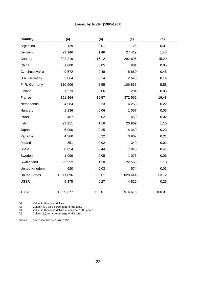
Loans, by lender (1985-1989)

Country (a) (b) (c) (d)

Argentina 129 0.01 126 0.01

Belgium 29 146 1.46 27 419 1.43

Canada 302 219 15.12 292 696 15.29

China 1 000 0.05 981 0.05

Czechoslovakia 9 572 0.48 8 880 0.46

D.R. Germany 2 864 0.14 2 643 0.14

F. R. Germany 110 906 5.55 106 865 5.58

Finland 1 273 0.06 1 204 0.06

France 391 364 19.57 372 962 19.48

Netherlands 4 584 0.23 4 258 0.22

Hungary 1 136 0.06 1 067 0.06

Israel 467 0.02 459 0.02

Italy 23 211 1.16 20 969 1.10

Japan 5 000 0.25 4 340 0.23

Panama 4 360 0.22 3 967 0.21

Poland 351 0.02 349 0.02

Spain 8 854 0.44 7 940 0.41

Sweden 1 096 0.05 1 076 0.06

Switzerland 23 952 1.20 22 569 1.18

United Kingdom 620 0.03 574 0.03

United States 1 071 896 53.61 1 028 444 53.72

USSR 5 375 0.27 4 826 0.25

TOTAL 1 999 377 100.0 1 914 616 100.0

(a) Value, in thousand dollars.(b) Column (a), as a percentage of the total.(c) Value, in thousand dollars at constant 1985 prices.(d) Column (c), as a percentage of the total.

Source: Banco Central do Brazil, 1990.

22

III METHODOLOGICAL ISSUES: THE GENERAL CASE

Within the framework of concessionary financing, the subsidy implied in a singleoperation is usually measured as the value of the difference between repaymentsaccording to market and soft8 conditions. On aggregate, the subsidy for the borrowingcountry at a fixed date is then the sum of the subsidies for all the loans extended oroutstanding at that date.

According to the above definition, given that principal repayments are assumed tobe the same under subsidised and non-subsidised conditions, the subsidy can bemeasured as the difference between interest payments without and with soft conditions.

If it is assumed that no uncertainty exists and the loan is made available as soonas it is agreed upon, disbursement takes place at time 0 and interest payments are madeat the end of each time period, from 1 on. Assume that (i) the loan under scrutiny lastsT periods, (ii) the market interest rate for period (t-1, t) is it , (iii) the soft rate — in thesame currency9 as that for it — is rt . In addition, let Dt be the residual debt at t, measuredin the same currency as that used for it and rt .

Hence, the subsidy in terms of present value at time 0 is

[1]

where Φ(t,0) is the discount factor from t to 0.

If the rate of interest which applies to alternative investments and borrowingbetween t-1 and t is it*, the present value of the subsidy becomes

[2]

Of course, it* can be different from it , since the former refers to investment andloans in general, while the latter is more appropriate to the kind of operations consideredhere. In addition, the measure defined by formula [2] depends on the principal repaymentschedule because of the residual debt Dt-1, which is, however, supposed to be the samefor both soft and market loans.

23

1 Some special cases: the grace period

In the real world, (i) soft loans are not always made available as soon as they areagreed upon, and (ii) they usually benefit from a grace period, during which the principalis not paid back and after which it is paid at a constant rate.

Concerning the first point, in principle, the time of disbursement or of signature areequally acceptable as the initial period. If disbursement is preferred it means that thesubsidy is perceived when the loan is made available, so that its economic effectsmaterialise only when the authorities "see" that they are getting resources at softconditions. On the other hand, by referring to the time of signature one assumes that theauthorities (or economic actors in general) behave according to the perceived presentvalue of the future stream of benefits; and it is obvious that this perception occurs at themoment of signature, that is, before disbursement. In short, the borrower may adjust hisbehaviour when the financial flow is actually made available or he may also anticipate aflow, as long as he believes it will be available.

In what follows the second hypothesis has been accepted as more plausible: time0 is therefore the time of signature10.

Of course, another way to proceed is to analyse the subsidy as a benefit whichbelongs to each period in which it occurs, as the difference between what should havebeen repaid by the borrower according to market conditions, and what is repaid accordingto ECO conditions. As will be shown in Section 3.6, the present value of the subsidy asa whole does not change; but it may be of some interest to compare the subsidy both asan anticipated stream of benefits, and as it matures through the duration of the loan.

As for the second point, if τ is the number of periods covered by the grace period,so that the first principal repayment is at (τ+1), principal installments are equal to L/(T-τ),where L is the amount of the loan. Residual debt is:

[3]

When the interest rate on alternative investments and borrowing is the same, [2]becomes

[4]

This is the most general expression for the present value of the subsidy whenresidual debt behaviour is described by [3] and the interest rate on investment is the sameas that on borrowing.

24

Furthermore, if it is assumed that

i) the interest rate on alternative loans is the same as the interest rate oninvestments;

ii) such interest rate, denoted by , is equal to the market interest rate for the loan

under scrutiny (it);iii) the actual (subsidised) interest rate (rt) is constant over time (rt = r); andiv) the market interest rate (it) is constant too (it = i), so that the same happens to

discount factors.

Under conditions (i)-(iv), [4] simplifies into

[5]

and, as a percentage of the loan,

[6]

which is the basic formula used in the subsidy evaluation for a single loan by Raynauld(1988)11, Önis-Özmucur (1989) and, in continuous time, by Horvarth (1975, 1976) andPhaup (1981).

In particular, if the nominal grace period has length τ, G is the actual grace period,and d is the time it takes to make the money available after the signature (so that d ≡ τ-G)12, the formulas [5] and [6] above are acceptable only when d = 0, so that τ = G.

Let us now formalize Raynauld’s case, where G = 0 ≠ τ. This assumption calls fortwo caveats. For if the loan is disbursed at the end of its grace period, its actual life is T-d.As a consequence, not only the actual grace period has to be taken into account properlywhen carrying out the estimates, but the duration of the loan is d periods shorter, and thewhole loan is to shifted d periods forward. As a matter of fact, other recent studies haveneither cut, nor shifted the loans, thereby estimating the subsidy as

whereas it would have been more appropriate to use

25

which becomes

[7]

[8]

when G = 0 (and τ = d).

The use of Raynauld’s formula raises three further problems: the choice of themarket interest rate i, the switching from one kind of time subdivision to another, and itsmeaning under uncertainty.

According to Raynauld, the rate i is approximated by the rate of return on medium-and long-term government bonds in the lender country, which estimates the costs of fundsto the lender, plus a spread. This choice is justified by the assumption that loans would nothave been offered at a lower rate than this.

Secondly, when estimates are carried out by setting each period equal to one k-thof a year, the periodic interest rate becomes

As a consequence, if the duration of the loan is T years with a grace period of tyears, the adoption of the correct periodic interest rate leads to a subsidy equal to13

If rk is approximated by r/k — or if r is a nominal annual rate — the subsidybecomes14

26

2 Uncertainty

The formulas in the previous sections usually apply to ex-post data. However, ifthe simplifying hypothesis of certainty is abandoned, the use of ex-post data forpresent-value formulas deprives such data of part of their meaning. Furthermore, ex-postestimates of ex-ante evaluations are not a satisfactory measure of the subsidy or ofexpectations about the subsidy.

As a matter of fact, a better ex-post evaluation should be stated in terms of futurevalue15. As for ex-ante expectations, when computing the present value of the subsidyreferring to a single loan one should consider future principal repayments, interest ratesand exchange rates.

The first are usually fixed on a contractual basis.

On the other hand, interest rates can be either fixed (by contract16) or floating. Inthe latter case no certain prediction about their future value can be made. Likewise, futureexchange rates cannot be predicted.

As a consequence, the subsidy as present value can be treated as a fixed quantityonly under the hypothesis of perfect foresight. In particular, Raynauld’s version — whichis that used by the OECD — requires one of the following sets of assumptions:

A) a fixed contractual interest rate both actual and market — plus (i) and (iv) above,or

B) r contractually fixed plus (i), (ii) and (iv) above, or

C) stationary expectations plus (i) and (iv) above, or

D) perfect foresight in addition to the hypotheses (i) to (iv) above.

If a compound-amount or future-value approach is used, the problem of variablequantities does not arise, since an ex-post evaluation requires true values by definition.

3 Loans obtained and paid back in the same currency

Returning to the present-value approach, assume that loans are made availableas soon as they are committed. If all loans are obtained and repaid in the same currency,the country subsidy is the sum of the subsidies on the loans outstanding at 0 as well ason those to be extended in the future17.

As concerns the loans outstanding at 0, there are two possible interpretations,each of which leads to a different definition of the country subsidy.

In a restrictive sense, loans outstanding at 0 are those extended at 0. In a broadersense, they are both those signed in the past and not completely reimbursed at 0, andthose signed at 0.

27

The subsidy corresponding to the strict interpretation is an entirely forwardmeasure, which assigns at time 0 the value of the subsidies foreseen at 0, due tocontracts dated at or after 0. The corresponding measure in the broad interpretation, onthe contrary, assigns at 0 both the subsidies foreseen at 0 on loans still to be extended,and those on loans granted now or in the past.

Formally, the subsidies for the country at 0 are defined respectively as

[9]

where S0(n) is the current value of the subsidies due to the loans signed at n, with nvarying from the beginning of our period (0) to the horizon N, and

[10]

where S0(n) is the same as above if n ≥ 0, and is only part of the subsidy due to theperiodic payments dated 0 or after 0 for loans granted previously.

Despite this difference, starting from the general definition of the subsidy for asingle loan S0

g, if only one loan is authorised in each time period, the aggregate subsidycan be formalized as

[11]

with

[12]

where T(n) is the duration of the loan signed at n, it(n) and rt(n) are the market and thesubsidised interest rates due in the period (t-1, t) on the loan received at n.

In the formula above Dt(n) is the residual debt at t of the loan obtained at n. Whenn ≥ 0, Dt(n) is the initial amount of the loan; when n < 0, Dt(n) is null for t < 0. As amatter of fact, with the definition [12] for loans signed before 0 only the part of the subsidydue to installments paid at or after 0 is considered.

Obviously, if a maximum of M loans with different contractual agreements (interestrates, currencies or periodicity) are received in each time period, the subsidy becomes:

28

with

[13]

[14]

where T(n,m) is the duration of the m-th loan authorised at n, it(n,m) and rt(n,m) are itsmarket and subsidised interest rates for the period (t-1,t), and Dt(n,m) is its residual debtat t.

4 Loans obtained and paid back in different currencies

If loans are obtained and repaid in different currencies, the procedure suggestedin Raynauld (1988) applies and the subsidy can be computed as a percentage of the loanitself before summing up over different lines of credit. The country subsidy is thus theweighted average of these percentages, the weights being the amounts of the loansexpressed in a single currency at a given exchange rate.

As a consequence, if a maximum of M loans are extended at n, the amount ofwhich is L(n,m), the subsidy becomes (with n ≥ 0)

[15]

where en(m) is the exchange rate at n between the currency of the m-th loan, cn(m), anda reference currency, denoted with c, so that en(m) ≡ c/cn(m).

If n takes both positive and negative values the formula is then

[16]

29

with

[17]

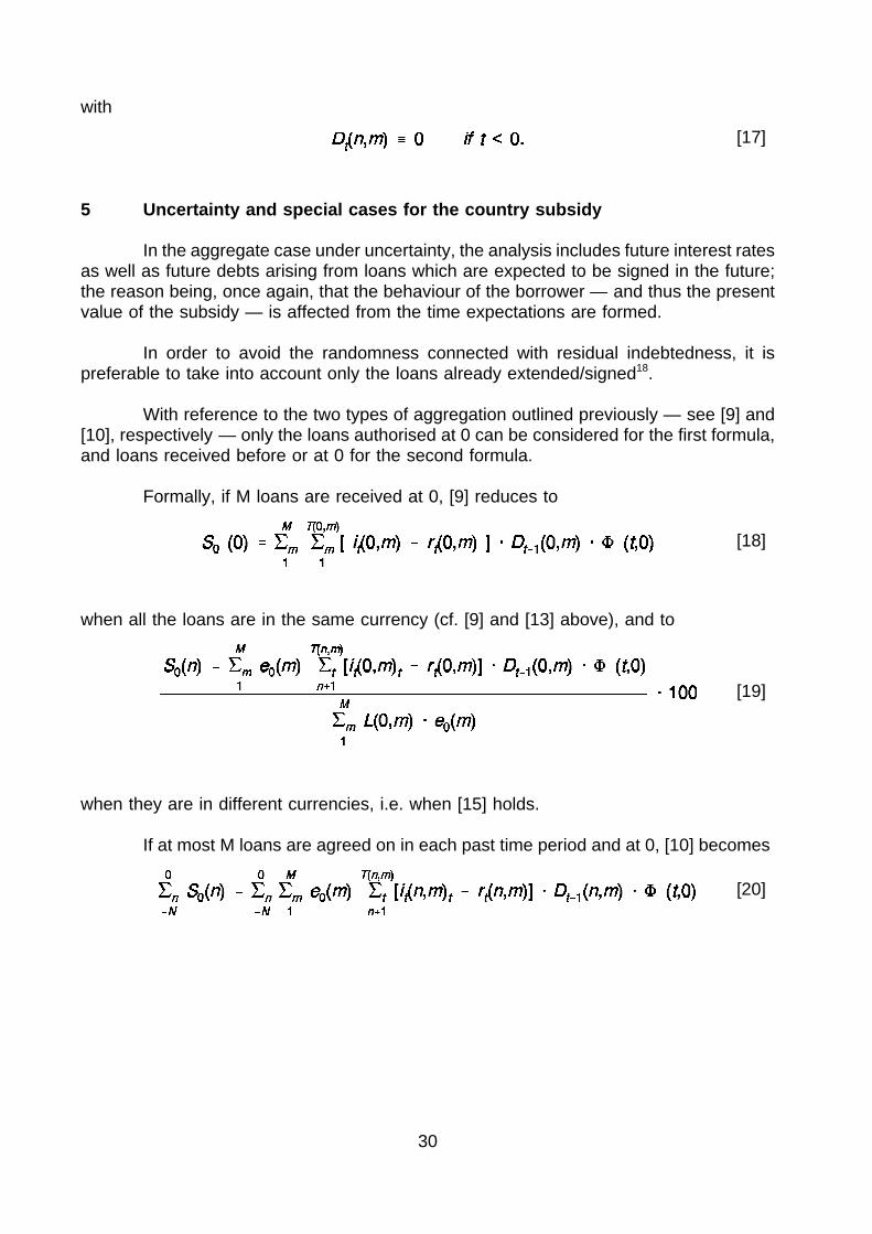
5 Uncertainty and special cases for the country subsidy

In the aggregate case under uncertainty, the analysis includes future interest ratesas well as future debts arising from loans which are expected to be signed in the future;the reason being, once again, that the behaviour of the borrower — and thus the presentvalue of the subsidy — is affected from the time expectations are formed.

In order to avoid the randomness connected with residual indebtedness, it ispreferable to take into account only the loans already extended/signed18.

With reference to the two types of aggregation outlined previously — see [9] and[10], respectively — only the loans authorised at 0 can be considered for the first formula,and loans received before or at 0 for the second formula.

Formally, if M loans are received at 0, [9] reduces to

[18]

when all the loans are in the same currency (cf. [9] and [13] above), and to

[19]

when they are in different currencies, i.e. when [15] holds.

If at most M loans are agreed on in each past time period and at 0, [10] becomes

[20]

30

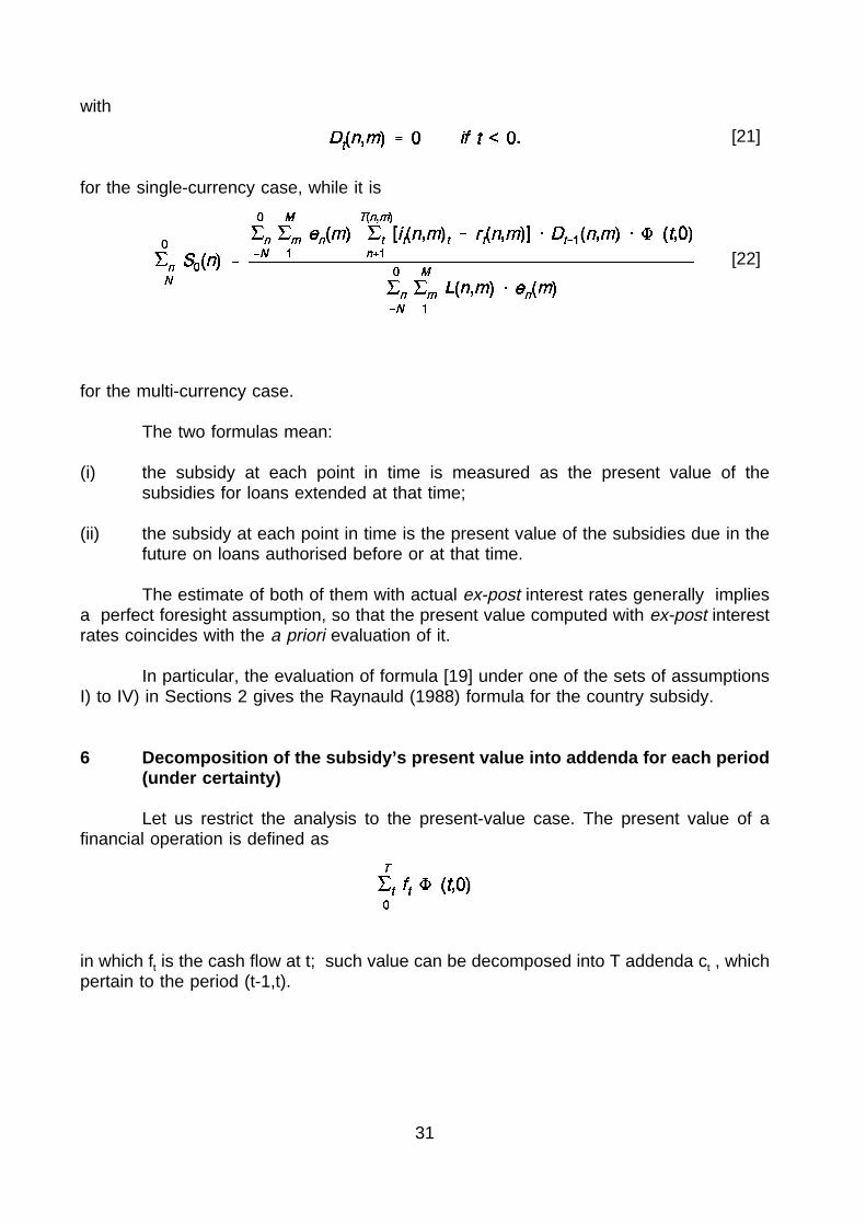
with

for the single-currency case, while it is

[21]

[22]

for the multi-currency case.

The two formulas mean:

(i) the subsidy at each point in time is measured as the present value of thesubsidies for loans extended at that time;

(ii) the subsidy at each point in time is the present value of the subsidies due in thefuture on loans authorised before or at that time.

The estimate of both of them with actual ex-post interest rates generally impliesa perfect foresight assumption, so that the present value computed with ex-post interestrates coincides with the a priori evaluation of it.

In particular, the evaluation of formula [19] under one of the sets of assumptionsI) to IV) in Sections 2 gives the Raynauld (1988) formula for the country subsidy.

6 Decomposition of the subsidy’s present value into addenda for each period(under certainty)

Let us restrict the analysis to the present-value case. The present value of afinancial operation is defined as

in which ft is the cash flow at t; such value can be decomposed into T addenda ct , whichpertain to the period (t-1,t).

31

This can be done by means of the financial notion of outstanding. If the financialoperation under scrutiny has an internal rate of return R, its outstanding is defined as thepresent value, computed at rate R, of the cash flows which will be paid or received in thefuture

[23a]

or, equivalently, as the final value at t of the cash flows already paid or received

[23b]

The notion of outstanding allows us to state that the addendum of the presentvalue for the period (t-1,t) is:

(i) the outstanding at t-1, considered as an outflow;(ii) the outstanding and the cash flow at t, considered as inflows.

Since both of them must be discounted, the share is:

Note (see [23b]) that ws follows the recurrence relation

Substituting for ft and reminding the recurrence relation for discount factors thefollowing shares are obtained:

The addenda ct have the property that their sum equates the present value of thefinancial operation:

[24]

32

The period quota for the single-loan present value of the subsidy, , can be

defined as the difference between the ct for the concessional credit and the ct for the non-concessional loan. Formally, if variables referring to hard credit are denoted with boldtypes, the shares of the subsidy are:

In particular, for a single hard loan the cash flows are:

while for soft loans the same cash flows hold, with rt instead of it.

As a consequence, the outstandings are:

[25a]

and

[25b]

These streams of payments do have an internal rate of return19, so that the ct ofa single loan can easily be computed, according to [24].

In the particular case of constant interest rates, the internal rate of return on theloan coincides with the interest rate paid on it, and the outstanding coincides with theresidual debt with opposite sign. It follows that if both the market and soft interest rates areconstant, or are supposed to be constant, as in Raynauld (1988), both the "market" andthe "subsidised" outstandings are equal to the opposite of the residual debt. The latter,in turn, is always assumed to be the same under hard and soft conditions, so that thefollowing equalities hold:

[26]

33

and the formula for ct becomes

[27]

In the case described by Raynauld (1988) it and rt are assumed to be constant;in addition, it * is also assumed to be constant and equal to i, so that the expression forct turns trivially into

[27]

In this particular case the share of the present value corresponding to the period(t-1,t) is simply the difference between the interest which would have been paid undermarket conditions (iDt-1) and that actually paid (rDt-1)

20,21.

7 A comparison with previous OECD studies

As for each single loan, the subsidy estimate accepted in Raynauld (1988) andÖnis-Özmucur (1989) can be obtained as a special case of the subsidy understood aspresent value of the interest gains associated to a soft-credit operation.

Under certainty both the actual and the market interest rate are supposed to beconstant over the loan life; the cost of alternative sources and the profitability ofalternative uses of funds is thus the same and it is equal to the market interest rate on theloan.

Under uncertainty, Raynauld’s estimate requires either stationary expectations orperfect foresight, plus the hypotheses above: more precisely, it requires one of thehypothesis sets A to D of Section 3.2.

As concerns the aggregate subsidy, it can be computed at each point in time bysumming over the loans committed at that time.

In the future, however, the country will benefit not only from these subsidies, butalso from subsidies on

a) future loans; and

b) loans already extended, but with interest payments due in the future.

These should be taken into account when computing an aggregate subsidy. Inparticular, it seems reasonable that a given year’s subsidy should include at least the loanscommitted in that year, even if they were made available afterwards.

Their actual grace period should also be taken into account, without overlookingthe fact that a loan does not produce a subsidy between commitment and disbursement.

34

35

NOTES

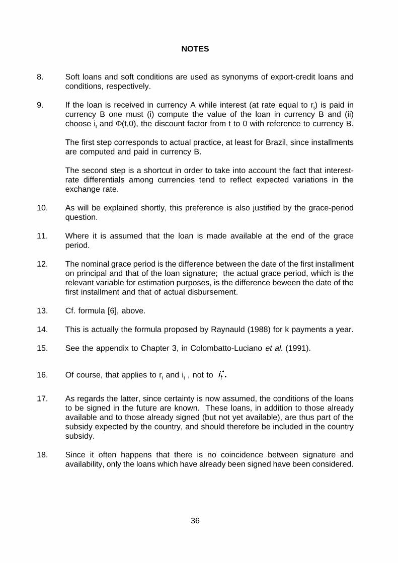
8. Soft loans and soft conditions are used as synonyms of export-credit loans andconditions, respectively.

9. If the loan is received in currency A while interest (at rate equal to rt) is paid incurrency B one must (i) compute the value of the loan in currency B and (ii)choose it and Φ(t,0), the discount factor from t to 0 with reference to currency B.

The first step corresponds to actual practice, at least for Brazil, since installmentsare computed and paid in currency B.

The second step is a shortcut in order to take into account the fact that interest-rate differentials among currencies tend to reflect expected variations in theexchange rate.

10. As will be explained shortly, this preference is also justified by the grace-periodquestion.

11. Where it is assumed that the loan is made available at the end of the graceperiod.

12. The nominal grace period is the difference between the date of the first installmenton principal and that of the loan signature; the actual grace period, which is therelevant variable for estimation purposes, is the difference beween the date of thefirst installment and that of actual disbursement.

13. Cf. formula [6], above.

14. This is actually the formula proposed by Raynauld (1988) for k payments a year.

15. See the appendix to Chapter 3, in Colombatto-Luciano et al. (1991).

16. Of course, that applies to rt and it , not to

17. As regards the latter, since certainty is now assumed, the conditions of the loansto be signed in the future are known. These loans, in addition to those alreadyavailable and to those already signed (but not yet available), are thus part of thesubsidy expected by the country, and should therefore be included in the countrysubsidy.

18. Since it often happens that there is no coincidence between signature andavailability, only the loans which have already been signed have been considered.

36

19. Such rates can be derived by solving the following:

[26a]

and

[26b]

20. It can be demonstrated that a proper aggregation of these shares makes itpossible to shift from Raynauld’s (1988) measure to the other criterion widely usedin the literature [cf. Fleisig-Hill (1984) and also Colombatto-Luciano et al. (1991),Chapter 2, Section 6.2].

21. Cf. also Peccati (1990) for a presentation of the idea of a present-value splittingup under certainty and Luciano-Peccati (1990) for a similar analysis underuncertainty.

37

IV THE ESTIMATES

1 The data

The data set which has been made available for this work reports transactions withsemi-annual payments: as a consequence, subsidies and present-value shares have beencomputed with reference to half-year periods.

In order to group loans according to their beneficiaries, the following industrieshave been singled out22:

- food- textiles and clothing- other consumer goods- cereals- chemical products- paper and cellulose- plastics and rubber- iron, steel and non-ferrous metals- other raw materials- coal- oil- transport equipment- other equipment and machinery

As already explained, services (with no further specification) were included in thelast-named industry, on the assumption that the corresponding loans were linked toimports of fixed capital.

The year in which the loan was agreed was known, but not the date ofdisbursement. Hence, it was assumed that the financial resources were actually madeavailable at the middle of the year of agreement. In some estimates, however, it has alsobeen assumed that disbursement took place half way between the middle of the year ofagreement (signature) and the end of the grace period. The caveats mentioned inSections 3 and 3.7 have nevertheless been respected.

The emphasis has been laid upon sectoral subsidies; the subsidy for Brazil as awhole plays a secondary role and has been computed in two different ways. A firstversion weights the rate of subsidy for each sector according to the weight of each sectorin ECOs; a second version weights the subsidy rates according to the weight of eachsector in total 1985 Brazilian imports23.

The market interest rate i(m) was defined as the government-bond yield24 of thecountry issuing the currency in which interest is paid, plus a spread.

The spread entering our estimates differs from the actual spreads applying toBrazil in 1985-89, for the data on non-subsidised loans, and hence on spreads, are

38

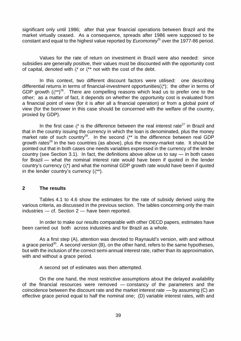
significant only until 1986; after that year financial operations between Brazil and themarket virtually ceased. As a consequence, spreads after 1986 were supposed to beconstant and equal to the highest value reported by Euromoney25 over the 1977-86 period.

Values for the rate of return on investment in Brazil were also needed: sincesubsidies are generally positive, their values must be discounted with the opportunity costof capital, denoted with it* or it** not with the cost of the debt.

In this context, two different discount factors were utilised: one describingdifferential returns in terms of financial-investment opportunities(it*); the other in terms ofGDP growth (it**)

26. There are compelling reasons which lead us to prefer one to theother; as a matter of fact, it depends on whether the opportunity cost is evaluated froma financial point of view (for it is after all a financial operation) or from a global point ofview (for the borrower in this case should be concerned with the welfare of the country,proxied by GDP).

In the first case it* is the difference between the real interest rate27 in Brazil andthat in the country issuing the currency in which the loan is denominated, plus the moneymarket rate of such country28. In the second it** is the difference between real GDPgrowth rates29 in the two countries (as above), plus the money-market rate. It should bepointed out that in both cases one needs variables expressed in the currency of the lendercountry (see Section 3.1). In fact, the definitions above allow us to say — in both casesfor Brazil — what the nominal interest rate would have been if quoted in the lendercountry’s currency (it*) and what the nominal GDP growth rate would have been if quotedin the lender country’s currency (it**).

2 The results

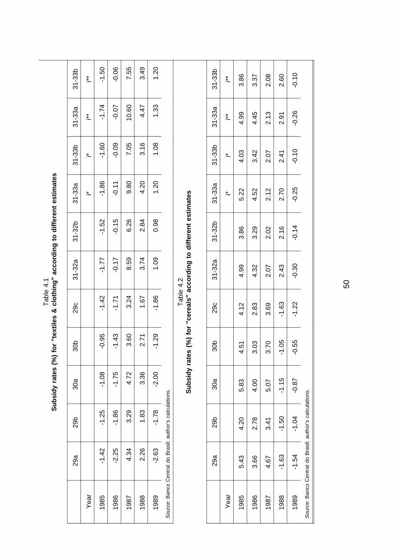
Tables 4.1 to 4.6 show the estimates for the rate of subsidy derived using thevarious criteria, as discussed in the previous section. The tables concerning only the mainindustries — cf. Section 2 — have been reported.

In order to make our results comparable with other OECD papers, estimates havebeen carried out both across industries and for Brazil as a whole.

As a first step (A), attention was devoted to Raynauld’s version, with and withouta grace period30. A second version (B), on the other hand, refers to the same hypotheses,but with the inclusion of the correct semi-annual interest rate, rather than its approximation,with and without a grace period.

A second set of estimates was then attempted.

On the one hand, the most restrictive assumptions about the delayed availabilityof the financial resources were removed — constancy of the parameters and thecoincidence between the discount rate and the market interest rate — by assuming (C) aneffective grace period equal to half the nominal one; (D) variable interest rates, with and

39

without a grace period; (E) a rate of return on Brazilian investment different from themarket cost of the single loan, with and without a grace period.

On the other hand, the idea of future-value shares was implemented by estimating(F) the shares due to each single period when the interest rate is held constant, the graceperiod is null and the nominal semi-annual soft subsidised rate is used (in accordance withRaynauld’s hypotheses); (G) the corresponding shares with the nominal grace period andthe actual interest rate. These shares were finally aggregated over the existing andfuture loans, as if the latter had been perfectly foreseen in 1985 (time 0).

*******

Estimates for each sector under (A) were carried out according to the followingformulas31:

[29a]

where

with a grace period32, and

[29b]

without a grace period (which is Raynauld’s case, stricto sensu).

The results for Brazil as a whole are summarised in Table 4.533: in particular, thesubsidy turns out to be positive over the 1985-1989 period, with a peak of 20.78 per centin 198834.

At an industry level, it is important to recall that the presence of a negative rateof subsidy (e.g. iron, steel etc. in 1986) is caused by the sign of the difference betweenthe market interest rate and the interest rate agreed upon between Brazil and theexporter35.

40

It may also be emphasised that the inclusion of the grace period (see 29a) causesa rise in the estimated rate of subsidy (see columns 29a and 29b compared). Thisincrease depends on the relation between the following quantities:

in [29a]

in [29b]

As a matter of fact, both the denominator and the numerator in [29b] are greaterthan in [29a]. However, since in our case the subsidy in [29b] is lower than in [29a], thefall in the denominator, going from [29a] to [29b], must overcompensate the fall in thenumerator. It is worth stressing that this result applies to the absolute value of the subsidy;for the sign of the subsidy in [29b] does not depend on the content of the square brackets,but on the difference between the market and the actual interest rate, which show up inthe same way in [29a] and [29b].

The correct semi-annual interest rate is

for the j-th industry.

The inclusion of this rate (estimates B) leads to a subsidy computed as follows:

[30a]

with a grace period, and

[30b]

without a grace period.

41

The results indicate that estimates B generate a larger subsidy than estimates A36.

This can be explained by pointing out that r/2 overestimates the true, agreed-uponinterest rate, so that the difference between the market and the actual interest rate turnsout to be lower than what it really is. Thus the simplified version underestimates theeffective subsidy. Of course, the greater the value of r, the lower the bias37.

It is worth pointing out that the subsidy according to [30a] is not only greater thanthat generated by [29a], but also than that by [29b]. The first difference is due to theswitching from the nominal to the actual semi-annual cost of the debt. The second meansthat the introduction of the nominal grace period provokes a fall in the estimate of thesubsidy, which is not enough to compensate for the increase due to the aforementionedswitching.

*******

As is known, loans are usually made available only some time after the signature.Accordingly, the set of estimates (C) has been run by setting the actual grace period Gequal to half the nominal one τ. The semi-annual interest payment is its crude version(following [7] in Section 3.1), so that Raynauld’s version of the subsidy (corresponding to[29b] above) becomes

[29c]

with

The results can be examined in their aggregate form in column 29c38. If comparedwith the standard version (i.e. Raynauld’s, described in [29b]), the delayed availability ofthe financial resources leads to a fall in the absolute value of the subsidy. As a matter offact, this variation reflects the content of the square brackets in [29b] and [29c]. Since thenew addendum of [29c] is lower than one, the rate of subsidy following [29b] is greaterthan that computed after [29c].

*******

As mentioned above, estimates D remove the constant rate hypothesis, andinclude formula [5] in Section 3.1 with [4] (in the same section) as a reference for eachloan.

42

Semi-annual interest rates have been computed exactly, so that according to D,in general terms, the subsidy for the j-th sector is

In the case with a grace period one has

[31]

[32a]

In the case without a grace period one has

[32b]

The results obtained by applying this criterion are presented in columns 31-32aand 32b, with and without a grace period, respectively39. No general conclusion can bederived by analysing the subsidy in its formal version. The data show, however, that whenthe interest rate tends to increase over a given time period, the adoption of a variable-ratehypothesis, instead of a constant-rate hypothesis (compare [30a] with [32a]), generatestwo kinds of effects. There is an interest-rate effect (of ambiguous sign); and a discount-rate effect, which determines a smaller (higher) subsidy with increasing (decreasing) rates.For instance, the 1989 results, which show a higher subsidy in the variable-rate case,imply that the interest-rate effect has been positive and stronger than the (negative)discount-rate effect.

*******

The distinction between the market interest rate and the rate used in discountfactors (which reflects the cost of the debt or the profitability of investment in the Brazilianeconomy40, and still depends on m because of the currency) for each loan, forms theobject of the E set of estimates. In particular the present value formalized in [4] has beenadopted, with it*(m) ≠ it(m), as well as the correct semi-annual interest rate.

43

Hence, the j-th sector subsidy is the now the same as in [31], with Ω redefined as

[32a]

with a grace period, and

[33b]

without a grace period.

The results are displayed in the last columns of each table. In this case subsidiesappear to be always larger, in absolute value, than those calculated by assuming equalitybetween the two rates41 (compare columns 31-32a with 31-32ai*)42.

Since i > i* and i > i** (in general), and since the two rates are the cost ofindebtedness (i) and the rates of returns on investment (i* or i**), respectively, the usualmethodology underestimates the discount factor, and, in turn, leads to a further reductionof the subsidy present value.

Of course, the results obtained with i* differ from those with i** because of thedifference between financial and real investment opportunities. For instance, if the subsidyratio computed through i** is greater than that computed through i* (see columns 31-33a-i*

and 31-33a-i**), it follows that the rate on real investment (i**) must necessarily be lowerthan that on financial opportunities (i*).

*******

As for the i-th sector, the present-value shares due to the first period (semester)of the loan follow (estimates F):

[34a]

44

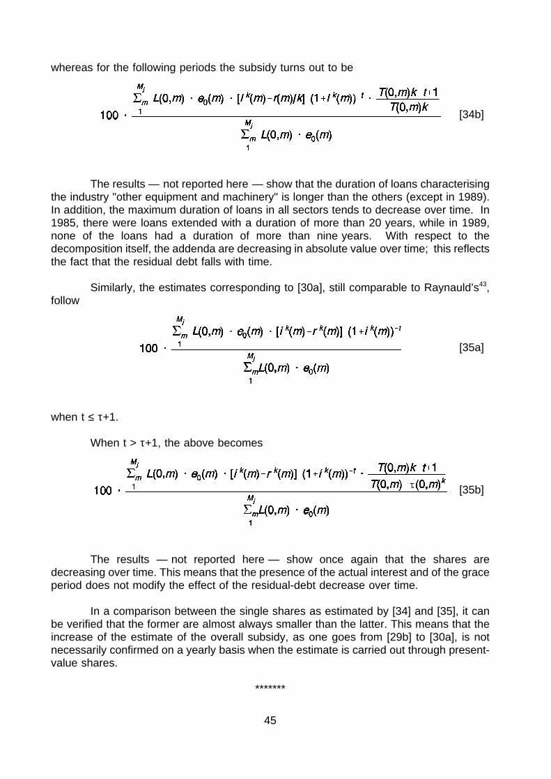
whereas for the following periods the subsidy turns out to be

[34b]

The results — not reported here — show that the duration of loans characterisingthe industry "other equipment and machinery" is longer than the others (except in 1989).In addition, the maximum duration of loans in all sectors tends to decrease over time. In1985, there were loans extended with a duration of more than 20 years, while in 1989,none of the loans had a duration of more than nine years. With respect to thedecomposition itself, the addenda are decreasing in absolute value over time; this reflectsthe fact that the residual debt falls with time.

Similarly, the estimates corresponding to [30a], still comparable to Raynauld’s43,follow

[35a]

when t ≤ τ+1.

When t > τ+1, the above becomes

[35b]

The results — not reported here — show once again that the shares aredecreasing over time. This means that the presence of the actual interest and of the graceperiod does not modify the effect of the residual-debt decrease over time.

In a comparison between the single shares as estimated by [34] and [35], it canbe verified that the former are almost always smaller than the latter. This means that theincrease of the estimate of the overall subsidy, as one goes from [29b] to [30a], is notnecessarily confirmed on a yearly basis when the estimate is carried out through present-value shares.

*******

45

The final set of estimates considers period shares on aggregate, so as to obtainfor each year the sum of shares of the loans outstanding in that period. If present valuesare computed with respect to 1985, [29b] becomes44

[36]

where the residual debt at t-1 is given by

and t = 0 in 1985, beginning of the second half year.

The results are reported in the appendix, Table 12.

On the other hand, in correspondence with [30a], the estimate of the subsidyfollows

[37]

with

The results are reported in the appendix, Table 13.

The most evident outcome of the estimates based on [36] and [37], apart from thelonger loan life in "other equipment and machinery", can be noticed by comparingTables (12) and (13). On aggregate, the estimate based on the hypothesis [30a] againbecomes greater than that based on [29b]. The use of the actual semi-annual cost of thedebt and of the grace period repeats in each yearly share the increases which it generateson the whole present value of the subsidy. Thus the effect mentioned when comparing

46

[34] and [35], concerning the increase in the estimated subsidy as one goes from [29b] to[30a], no longer applies in this framework.

The sectoral distribution of the subsidy across industries is very irregular since itis concentrated in "cereals" and "other equipment and machinery". For that reason andconsiderations put forward in Section 2, the subsidies to Brazil have also been computedby weighting the sectoral rate of subsidy with the weight of each sector in Brazilian totalimports in 1985. The difference between the standard estimate (Table 4.5) and theweighted estimates (Table 4.6) shows that the structure of subsidised imports differsgreatly from that of total imports45.

47

NOTES

22. The original data set is actually organised according to a different groupingcriterion; the one put forward here, on the other hand, follows the balance-of-payments classification suggested in the publications by the Banco do Brazil.

23. See Section 2.

24. Cf. also IMF, International Financial Statistics, various years, row 61.

25. Transactions only in dollars were considered, since spreads seemed to beindependent of currencies, at least up to 1986.

26. The need for a nominal rate comparable with that of the loan currency can besatisfied by considering the opportunity cost of capital in the borrowing country.Such cost differs from the money-market rate in the currency-issuing country foran amount which is supposed to be equal to the difference between the Brazilianreal interest rate (real GDP growth rate) and that of the country issuing thecurrency. Thus, the opportunity cost has been computed as the sum of suchdifference and the money-market rate.

27. Cf. IMF, International Financial Statistics, various years, rows 60c and 99b.p x.

28. Cf. also IMF, International Financial Statistics, various years, row 60c.

29. Cf. IMF, International Financial Statistics, various years, row 99b.p x.

30. The term "without a grace period" is to be understood in Raynauld’s way.Actually, Raynauld’s work is not directly comparable with our estimates "with agrace period".

31. Cf. the previous sections for the notation; the dependence of the interest rate ontime 0 has been dropped.

32. T and τ are measured in years.

33. Cf. also the appendix: Table 1 (with a grace period) and Table 2 (without a graceperiod).

34. As a matter of fact, such a peak is due to the behaviour of the "other equipment& machinery" sector, where the rate of subsidy is 23.71 per cent. This sector’sresults are heavily subsidised and highly representative (83 per cent of the loansextended in 1988, according to our data set).

35. Cf. the content of the square brackets in (29b), which is greater than zero.

48

36. Cf. also the appendix: Table 3 (with a grace period) and Table 4 (without a graceperiod).

37. It can be shown that the deviation of the true semi-annual interest-rate differentialfrom the simplified differential falls as r increases.

38. Cf. also the appendix, Table 5. It should be pointed out that in this case theint(grace) function has been used, since the original data describe the graceperiod in half years, not years.

39. Cf. also the appendix: Table 6 in the case with a grace period, Table 7 withouta grace period.

40. Indeed, the appropriate formula involves two interest rates for discountingpurposes: the cost of the debt and the profit on investment. However, it wouldhave been necessary to adopt a future-value methodology; instead, for the sakeof comparability with the values described in the formulas [29] to [32] above, aunique discount factor has been used, which has been computed with referenceto the profitability of investment in Brazil, rather than to the cost of the debt.

41. It may be worth recalling that this is actually the criterion adopted in Raynauld(1988).

42. Cf. also the appendix: Table 8 for it* and Table 10 for it**, both with a graceperiod; Table 9 for it* and Table 11 for it**, without a grace period.

43. The market and the discount rates are kept equal and the parameters are heldconstant.

44. The formula is obtained by referring [28] to semi-annual payments, and using theaggregation methodology [27b].

45. It should be emphasized, however, that our data do not allow any comment onsuch a structure.

49

Tab

le4.

1S

ubsi

dyra

tes

(%)

for

"tex

tiles

&cl

othi

ng"

acco

rdin

gto

diffe

rent

estim

ates

29a

29b

30a

30b

29c

31-3

2a31

-32b

31-3

3a31

-33b

31-3

3a31

-33b

Yea

ri*

i*i*

*i*

*

1985

-1.4

2-1

.25

-1.0

8-0

.95

-1.4

2-1

.77

-1.5

2-1

.86

-1.6

0-1

.74

-1.5

0

1986

-2.2

5-1

.86

-1.7

5-1

.43

-1.7

1-0

.17

-0.1

5-0

.11

-0.0

9-0

.07

-0.0

6

1987

4.34

3.29

4.72

3.60

3.24

8.59

6.26

9.80

7.05

10.6

07.

55

1988

2.26

1.83

3.36

2.71

1.67

3.74

2.84

4.20

3.16

4.47

3.49

1989

-2.6

3-1

.78

-2.0

0-1

.29

-1.8

61.

090.

981.

201.

081.

331.

20

Sou

rce:

Ban

coC

entr

aldo

Bra

sil;

auth

or’s

calc

ulat

ions

.

Tab

le4.

2S

ubsi

dyra

tes

(%)

for

"cer

eals

"ac

cord

ing

todi

ffere

ntes

timat

es

29a

29b

30a

30b

29c

31-3

2a31

-32b

31-3

3a31

-33b

31-3

3a31

-33b

Yea

ri*

i*i*

*i*

*

1985

5.43

4.20

5.83

4.51

4.12

4.99

3.86

5.22

4.03

4.99

3.86

1986

3.66

2.78

4.00

3.03

2.83

4.32

3.29

4.52

3.42

4.45

3.37

1987

4.67

3.41

5.07

3.70

3.69

2.07

2.02

2.12

2.07

2.13

2.08

1988

-1.6

3-1

.50

-1.1

5-1

.05

-1.6

32.

432.

162.

702.

412.

912.

60

1989

-1.5

4-1

.04

-0.8

7-0

.55

-1.2

2-0

.30

-0.1

4-0

.25

-0.1

0-0

.26

-0.1

0

Sou

rce:

Ban

coC

entr

aldo

Bra

sil;

auth

or’s

calc

ulat

ions

.

50

Tab

le4.

3S

ubsi

dyra

tes

(%)

for

"coa

l"ac

cord

ing

todi

ffere

ntes

timat

es

29a

29b

30a

30b

29c

31-3

2a31

-32b

31-3

3a31

-33b

31-3

3a31

-33b

Yea

ri*

i*i*

*i*

*

1985

11.4

09.

4611

.82

9.83

9.01

14.0

311

.50

16.8

613

.75

16.9

513

.80

1986

-8.0

7-7

.63

-7.2

7-6

.89

-8.0

7-4

.72

-4.5

2-5

.05

-4.8

4-4

.91

-4.7

1

1987

0.90

1.46

1.65

2.00

2.00

5.92

3.80

6.93

4.30

7.85

4.69

1988

-9.1

5-8

.60

-8.2

2-7

.72

-9.1

5-2

.81

-2.7

0-2

.90

-2.7

8-2

.94

-2.8

2

1989

-0.4

7-0

.33

0.49

0.40

-0.2

94.

073.

034.

533.

335.

053.

67

Sou

rce:

Ban

coC

entr

aldo

Bra

sil;

auth

or’s

calc

ulat

ions

.

Tab

le4.

4S

ubsi

dyra

tes

(%)

for

"oth

ereq

uipm

ent"

acco

rdin

gto

diffe

rent

estim

ates

29a

29b

30a

30b

29c

31-3

2a31

-32b

31-3

3a31

-33b

31-3

3a31

-33b

Yea

ri*

i*i*

*i*

*

1985

3.48

2.69

4.54

3.61

1.64

2.51

1.89

3.39

2.58

4.03

3.11

1986

0.24

5.62

6.31

5.87

5.86

7.13

6.65

8.11

7.57

8.47

7.90

1987

18.8

615

.93

19.1

016

.14

14.6

324

.06

20.1

129

.19

24.1

035

.03

28.4

7

1988

23.7

118

.04

24.1

418

.41

14.8

931

.45

24.1

337

.64

28.4

445

.66

33.8

6

1989

2.30

2.00

2.80

2.43

2.10

370.

004.

305.

434.

595.

764.

86

Sou

rce:

Ban

coC

entr

aldo

Bra

sil;

auth

or’s

calc

ulat

ions

.

51

Tab

le4.

5S

ubsi

dyra

tes

(%)

for

"Bra

zil"

acco

rdin

gto

diffe

rent

estim

ates

29a

29b

30a

30b

29c

31-3

2a31

-32b

31-3

3a31

-33b

31-3

3a31

-33b

Yea

ri*

i*i*

*i*

*

1985

5.29

4.17

5.92

0.01

3.73

4.97

3.90

5.67

4.44

5.76

4.53

1986

2.20

1.67

2.67

2.05

1.59

4.10

3.23

4.66

3.66

4.95

3.89

1987

5.78

4.72

6.23

5.06

4.76

7.04

5.71

0.04

6.55

9.37

7.36

1988

20.7

815

.80

21.2

716

.22

13.0

527

.91

21.4

333

.36

25.2

340

.39

29.3

9

1989

0.33

0.39

1.06

0.96

0.36

3.49

2.82

3.84

3.08

4.20

3.35

Sou

rce:

Ban

coC

entr

aldo

Bra

sil;

auth

or’s

calc

ulat

ions

.

Tab

le4.

6S

ubsi

dyra

tes

(%)

for

"Bra

zil(

wei

ghte

dav

erag

e)"

acco

rdin

gto

diffe

rent

estim

ates

29a

29b

30a

30b

29c

31-3

2a31

-32b

31-3

3a31

-33b

31-3

3a31

-33b

Yea

ri*

i*i*

*i*

*

1985

4.39

3.46

5.13

4.09

2.92

3.76

2.94

4.37

3.41

4.58

3.59

1986

7.07

5.77

7.48

6.10

5.39

9.84

7.95

11.6

59.

3512

.71

10.1

3

1987

9.05

7.42

9.42

7.71

7.17

10.0

08.

4111

.87

9.86

13.9

511

.39

1988

23.2

10.

0423

.64

18.0

814

.68

30.8

223

.70

36.8

327

.89

44.6

133

.16

1989

0.54

0.57

1.20

1.10

0.56

3.29

2.73

3.59

2.96

3.88

3.18

Sou

rce:

Ban

coC

entr

aldo

Bra

sil;

auth

or’s

calc

ulat

ions

.

52

V FINAL COMMENTS

1 Summary of the main findings

This study has two key aspects. It adopts significant methodological improvementsfor evaluating and estimating the subsidy implicit in export-credit transactions.Furthermore, the results obtained, although highly dependent on the quality of the sampleavailable, shed some light on the characteristics of the Brazilian approach to export-creditfacilities.

2 The methodology

The standard method of estimating the implicit subsidy in a financial transaction,(typically, a multiperiod loan, with grace period) is based on an extended set of conditions.In particular,

i) the discount rate used in computing present values, which is equivalent to thatapplicable to alternative borrowing opportunities, is equal to the market rate for theloan under scrutiny; this rate, however, usually refers to the cost of funds, not therate of return on alternative investments;

ii) the rate mentioned above is considered constant over time; as a consequence,stationary expectations are involved in the calculation of the subsidy;

iii) discrepancies between the nominal (contractual) grace period and the actual graceperiod tend to be overlooked.

At various stages and levels of this study these restrictions were removed andreplaced by more realistic assumptions. For example, a complete set of estimates hasbeen obtained by adopting:

i) an alternative interest rate (i*) reflecting the alternative conditions for investmentsin financial markets;

ii) an alternative interest rate (i**) reflecting the alternative conditions for investmentsin the real sector;

iii) both constant and variable interest rates;

iv) both the null-grace period hypothesis and a more realistic positive-grace periodhypothesis.

All these improvements are additive and do not replace the standard methodology;thus, the results which follow may still be compared with those obtained in the literature.

53

Finally, two other issues have been analysed in depth: the decomposition of thepresent subsidy value into single addenda — one for each period of the loan’s duration —and uncertainty. The former provide the estimates reported in Tables 12-13. The latterhas been discussed in Section 2.

3 The results

The data set provided by the Banco Central do Brazil included 581 export-creditoperations in the 1985-1989 period.

Brazil in the ECO context is significant for it is the world’s second greatest recipientof export credits. In 1987, a highly critical year for Brazil’s external debt, ECOs amountedto $11.8 billion, that is 9.5 per cent of total indebtedness.

Nevertheless, according to our data, for the whole five-year period soft transactionstotalled about $2 billion compared to total imports in the same period of about $150 billion,i.e. only 1.3 per cent of Brazilian imports.

As a matter of fact, the period covered by our sample does raise some problems.To start with, the most indebted developing countries faced severe difficulties in obtainingfinancial resources from abroad in the second half of the 1980s46. Furthermore, exportcredits were hit particularly hard by the financial drought of the period, given the highdependence of ECOs on private agencies.

In addition, the Brazilian situation was particularly worrying, as the country’sforeign-debt crisis reached a peak. After the interest moratorium all official and non-official(private) agencies ceased to consider soft financing for Brazil. The situation easedsomewhat in the second half of 1988 (when an agreement with the IMF was reached), butmany restrictions were then imposed, such as

i) exposure ceilings and transaction limits;

ii) case-by-case review of the projects to be financed;

iii) short-term financing only.

As for the rate of subsidy, the Brazilian case is characterised by very largevariations during the 1985-1989 period. The unweighted aggregate reaches a maximumof of 33.4 per cent in 1988 and a minimum of 3.8 per cent in the following year. The sameapplies to import-weighted estimates.

In general, the rate of subsidy turns out to be high, but the amount of the subsidiesremains low (as long as the data set is actually the totality), about 0.8 per cent of totalBrazilian imports of goods and services. The impact on the economy as a whole cannothave been great.

Furthermore, it should be recalled that the borrowing country does not usually reapthe full potential benefit of the ECO subsidy. On the one hand, subsidised export flows

54

may be overpriced (so as to compensate for part of the subsidy); on the other, such flowsmay generate a substitution effect, in which an importer is induced to buy (and to produceat home) a sub-optimal set of commodities.

Both situations are hard to assess in the Brazilian case. Serious microeconomicdistortions (the substitution effect) are likely to arise only if a given industry is offered along-enough and large-enough stream of ECOs. But if the economy turns out to beaffected by significant substitution effects even when such restrictions are not met, themicroeconomic distortions may be even more harmful. Our statistical evidence is verypoor in this respect and thus no clear-cut conclusion can be drawn47.

Moreover, it is known that the possibility of facing overpriced imports depends,among other things, on the import elasticity of the borrower. No reliable estimate has beenobtained for the Brazilian economy in the second half of the 1980s.

Subsidy rates (percent) for 13 sectors[formulas (31-33a), i*]

1985 1986 1987 1988 1989

Food 0.0 3.6 5.6 18.9 6.6

Textiles and clothing -1.9 -0.1 9.8 4.2 1.2

Other consumer goods 2.4 3.4 5.5 9.3 6.1

Cereals 5.2 4.5 2.1 2.7 -0.2

Chemical products 3.5 4.7 5.2 5.8 0.0

Paper and cellulose 0.0 8.1 8.3 0.0 4.4

Plastics and rubber 0.0 5.5 0.0 0.0 0.0

Iron/steel/non-ferrous metals 1.8 -20.2 4.3 16.2 7.2

Other raw materials 0.0 0.0 6.4 0.0 0.0

Coal 16.9 -5.1 6.9 -2.9 4.5

Oil 2.1 21.7 0 24.2 0

Transport equipment -12.2 5.1 8.3 6.6 7.8

Other equipment & machinery(*) 3.4 8.1 29.2 37.6 5.4

BRAZIL (unweighted) 5.7 4.6 8.2 33.3 3.8

BRAZIL (weighted) 4.4 11.7 11.9 36.8 3.6

(*) services included.

55

It is quite likely, however, that Brazil benefited from subsidised imports not onlythrough ECOs, but also by means of other, more relevant, channels (such as officiallysupported export credits, ODA loans, etc.).

Of course, these may also have altered the trade and production structure of theBrazilian economy. A piece of non-conclusive evidence in this respect is the growingdegree of anomaly shown by the Brazilian import structure:

World/Brazilian import geographical structures (Rank-correlation coefficients)

1966 0.934

1971 0.964

1975 0.944

1985 0.747

1987 0.838

Source: author’s calculation from OECD data.

The rank-correlation coefficient between the geographical import structures ofBrazil and the rest of the world declines over time. Further work on the dynamics of thecompetitive structure of the Brazilian economy thus seems justified.

It would have been important to assess Brazilian import prices relative to the restof the world; the lack of data on import unit values from the United States, the mostimportant exporter to Brazil, has made this unfeasible.

However, on the whole it is likely that subsidised imports did not have a seriousimpact on relative international prices, given the small weight of Brazil’s trade in total worldtrade.

56

NOTES

46. The total net inflow of external funds to developing countries fell from $66.5 billionin 1980 to $33.5 billion in 1985 and $25.6 billion in 1989.

47. A possible exception is the case of "cereals", an industry characterised by anunusually large share of ECOs (42 per cent of total transactions, 37.6 per cent oftotal value). It is likely that some exporters have tried to get rid of their excesssupply by subsidising exports, so that the relative price of wheat has fallen, at theexpense of Brazilian agriculture.

57

REFERENCES

Banco Central do Brazil, Boletim Especial: Series Historicas do Setor Externo 1971-85,1988.

Banco Central do Brazil, Creditos Oficiais e Multilaterais, 1990.

Fleisig, H. and, C. Hill, "The Benefits and Costs of Official Export Credit Programs ofIndustrial Countries: an Analysis", World Bank Staff Working Papers, 59, The World Bank,Washington, D.C., 1984.

Horvarth, J., "Are Eximbank Credits Subsidized? Toward an Empirical Analysis", in P.Marer (ed.), US Financing of East-West Trade, International Development Center,Bloomington, Indiana, 1975.

Horvarth, J., "The Scope of the International Grant Economy: the Case of Eximbank", inM. Pfaff (ed.), Frontiers of Social Thought, North Holland, Amsterdam, 1976.

Luciano, E. and, L. Peccati, "A Decomposition for Random Discounted Cash Flows",Working Paper, FUR Conference, 1990.

Peccati, L., "Multiperiod Analysis of a Levered Portfolio", Revista AMASES (Proceedingsof the Eighth Meeting of the Euro Working Group), 1, 1990.

Phaup, D., "Export Credit Competition", Working Paper, Union College, Schenectady, NewYork, 1981.

Raynauld, A., The External Financing of Tunisia’s Imports, OECD Development Centre,Paris, 1988.

Önis, Z and , S. Özmucur, Capital Flows and External Financing of Turkey’s Imports,OECD, Paris, 1991.

58

APPENDIX

59

Table 1. Formula (29a)

Hp: a) constant interest rates,b) semi-annual interest rate = r/2,c) semi-annual alternative interest rate = √(1+i)-1,d) with grace period.

Ratio (*)

Sector 1985 1986 1987 1988 1989

FoodTextiles & clothingOther consumer goodsCerealsChemical productsPaper and cellulosePlastics & rubberIron, steel and non-ferrous metals

Other raw materialsCoalOilTransport equipmentOther equipment andmachinery (**)

BRAZILBRAZIL (weightedaverage)

0.000-1.4242.2355.4322.9400.0000.000

2.1640.000

11.3992.809

-9.254

3.4785.285

4.385

2.927-2.2482.8793.6623.6425.4285.745

-27.6680.000

-8.06512.703

2.807

6.0252.203

7.078

6.9584.3432.4164.6680.345

-9.0860.000

0.5446.9970.8980.0003.376

18.8635.780

9.049

11.7902.2625.311

-1.6281.9350.0000.000

7.9980.000

-9.15419.366

0.623

23.71020.780

23.208

3.206-2.6272.177

-1.5440.0001.7870.000

3.6970.000

-0.4700.0005.734

2.2980.326

0.536

(*) 100 ≠ Subsidy / Principal.

(**) services included.

Source: ‘Banco Central do Brasil’ (1988, 1990); author’s calculations.

60

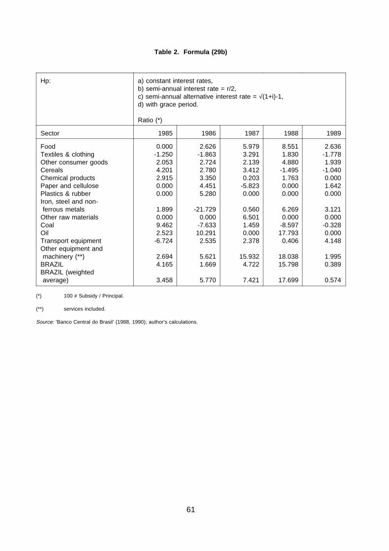
Table 2. Formula (29b)

Hp: a) constant interest rates,b) semi-annual interest rate = r/2,c) semi-annual alternative interest rate = √(1+i)-1,d) with grace period.

Ratio (*)

Sector 1985 1986 1987 1988 1989

FoodTextiles & clothingOther consumer goodsCerealsChemical productsPaper and cellulosePlastics & rubberIron, steel and non-ferrous metals

Other raw materialsCoalOilTransport equipmentOther equipment andmachinery (**)

BRAZILBRAZIL (weightedaverage)

0.000-1.2502.0534.2012.9150.0000.000

1.8990.0009.4622.523

-6.724

2.6944.165

3.458

2.626-1.8632.7242.7803.3504.4515.280

-21.7290.000

-7.63310.291

2.535

5.6211.669

5.770

5.9793.2912.1393.4120.203

-5.8230.000

0.5606.5011.4590.0002.378

15.9324.722

7.421

8.5511.8304.880

-1.4951.7630.0000.000

6.2690.000

-8.59717.793

0.406

18.03815.798

17.699

2.636-1.7781.939

-1.0400.0001.6420.000

3.1210.000

-0.3280.0004.148

1.9950.389

0.574

(*) 100 ≠ Subsidy / Principal.

(**) services included.

Source: ‘Banco Central do Brasil’ (1988, 1990); author’s calculations.

61

Table 3. Formula (30a)

Hp: a) constant interest rates,b) semi-annual interest rate = r/2,c) semi-annual alternative interest rate = √(1+i)-1,d) with grace period.

Ratio (*)

Sector 1985 1986 1987 1988 1989

FoodTextiles & clothingOther consumer goodsCerealsChemical productsPaper and cellulosePlastics & rubberIron, steel and non-ferrous metals

Other raw materialsCoalOilTransport equipmentOther equipment andmachinery (**)

BRAZILBRAZIL (weightedaverage)

0.000-1.0762.6045.8303.3290.0000.000

2.3760.000

11.8193.507

-7.501

4.5435.916

5.134

3.448-1.7523.2344.0043.8955.7126.018

-25.5960.000

-7.27213.172

3.078

6.3072.669

7.483

7.5974.7222.7375.0660.835

-7.5900.000

0.9657.3931.6510.0003.774

19.0956.225

9.421

12.0463.3605.524

-1.1472.2480.0000.000

8.3540.000

-8.21619.369

1.110

24.14021.268

23.636

3.697-1.9962.833

-0.8730.0002.2820.000

4.1790.0000.4870.0005.851

2.8041.061

1.203

(*) 100 ≠ Subsidy / Principal.

(**) services included.

Source: ‘Banco Central do Brasil’ (1988, 1990); author’s calculations.

62

Table 4. Formula (30b)

Hp: a) constant interest rates,b) semi-annual interest rate = r/2,c) semi-annual alternative interest rate = √(1+i)-1,d) with grace period.

Ratio (*)

Sector 1985 1986 1987 1988 1989

FoodTextiles & clothingOther consumer goodsCerealsChemical productsPaper and cellulosePlastics & rubberIron, steel and non-ferrous metals

Other raw materialsCoalOilTransport equipmentOther equipment andmachinery (**)

BRAZILBRAZIL (weightedaverage)

0.000-0.9452.3934.5053.2210.0000.000

2.0860.0009.8333.159

-5.424

3.6114.689

4.093

3.020-1.4283.0323.0313.5804.6855.531

-20.0890.000

-6.89110.650

2.778

5.8702.048

6.098

6.5283.6022.4313.7010.605

-4.8650.000

0.9456.8691.9950.0002.658

16.1355.059

7.705

8.7522.7095.073

-1.0542.0490.0000.000

6.5440.000

-7.71617.795

0.884

18.41416.221

18.075

3.039-1.2912.521

-0.5490.0002.0980.000

3.5370.0000.3960.0004.232

2.4300.962

1.099

(*) 100 ≠ Subsidy / Principal.

(**) services included.

Source: ‘Banco Central do Brasil’ (1988, 1990); author’s calculations.

63

Table 5. Formula (29c)

Hp: a) constant interest rates,b) semi-annual interest rate = r/2,c) semi-annual alternative interest rate = √(1+i)-1,d) with grace period.

Ratio (*)

Sector 1985 1986 1987 1988 1989

FoodTextiles & clothingOther consumer goodsCerealsChemical productsPaper and cellulosePlastics & rubberIron, steel and non-ferrous metals

Other raw materialsCoalOilTransport equipmentOther equipment andmachinery (**)

BRAZILBRAZIL (weightedaverage)

0.000-1.4242.2354.1213.2910.0000.000

2.1640.0009.0112.566

-5.536

1.6393.732

2.923

2.828-1.7113.0072.8283.6424.2475.745

-20.7230.000

-8.0659.2372.768

5.8591.592

5.391

6.0503.2362.1823.6900.128

-4.4680.000

0.5566.9972.0010.0002.427

14.6344.757

7.174

7.8321.6705.311

-1.6281.9350.0000.000

6.0890.000

-9.15419.366

0.484

14.89013.048

14.683

2.725-1.8551.877

-1.2160.0001.7870.000

3.0530.000

-0.2890.0004.001

2.0960.363

0.559

(*) 100 ≠ Subsidy / Principal.

(**) services included.

Source: ‘Banco Central do Brasil’ (1988, 1990); author’s calculations.

64

Table 6. Formula (31; 32a)

Hp: a) constant interest rates,b) semi-annual interest rate = r/2,c) semi-annual alternative interest rate = √(1+i)-1,d) with grace period.

Ratio (*)

Sector 1985 1986 1987 1988 1989

FoodTextiles & clothingOther consumer goodsCerealsChemical productsPaper and cellulosePlastics & rubberIron, steel and non-ferrous metals

Other raw materialsCoalOilTransport equipmentOther equipment andmachinery (**)

BRAZILBRAZIL (weightedaverage)

0.000-1.7702.2314.9903.1670.0000.000

1.6980.000

14.0342.037

-10.990

2.5054.966

3.756

3.301-0.1693.2014.3184.3427.3475.254

-17.8920.000

-4.71917.833

4.599

7.1274.102

9.842

5.1898.5944.9812.0734.5596.1670.000

3.7126.0075.9180.0007.452

24.0567.039

9.995

16.7193.7408.5782.4265.3310.0000.000

14.5480.000

-2.81322.515

5.909

31.44927.910

30.815

6.1361.0925.668

-0.2970.0004.1790.000

6.5790.0004.0680.0007.482

5.0743.485

3.286

(*) 100 ≠ Subsidy / Principal.

(**) services included.

Source: ‘Banco Central do Brasil’ (1988, 1990); author’s calculations.

65

Table 7. Formula (31; 32b)

Hp: a) constant interest rates,b) semi-annual interest rate = r/2,c) semi-annual alternative interest rate = √(1+i)-1,d) with grace period.

Ratio (*)

Sector 1985 1986 1987 1988 1989

FoodTextiles & clothingOther consumer goodsCerealsChemical productsPaper and cellulosePlastics & rubberIron, steel and non-ferrous metals

Other raw materialsCoalOilTransport equipmentOther equipment andmachinery (**)

BRAZILBRAZIL (weightedaverage)

0.000-1.5222.0563.8632.8390.0000.000

1.5210.000

11.4991.854

-7.698

1.8893.901

2.939

2.833-0.1452.9423.2883.9776.0994.842

-14.6420.000

-4.52314.216

4.060

6.6463.227

7.954

4.5536.2584.4032.0163.2242.6150.000

3.4425.5923.8040.0004.615

20.1145.707

8.413

12.0342.8357.8032.1624.7980.0000.000

10.9540.000

-2.69920.627

5.496

24.12621.429

23.699

4.9360.9794.972

-0.1390.0003.8050.000

5.5180.0003.0250.0005.208

4.3032.823

2.727

(*) 100 ≠ Subsidy / Principal.

(**) services included.

Source: ‘Banco Central do Brasil’ (1988, 1990); author’s calculations.

66

Table 8. Formula (31; 33a)

Hp: a) constant interest rates,b) semi-annual interest rate = r/2,c) semi-annual alternative interest rate = √(1+i)-1,d) with grace period.

Ratio (*)

Sector 1985 1986 1987 1988 1989

FoodTextiles & clothingOther consumer goodsCerealsChemical productsPaper and cellulosePlastics & rubberIron, steel and non-ferrous metals

Other raw materialsCoalOilTransport equipmentOther equipment andmachinery (**)

BRAZILBRAZIL (weightedaverage)

0.000-1.8552.3895.2223.4630.0000.000

1.7710.000

16.8622.144

-12.232

3.3915.669

4.366

3.569-0.1063.3604.5154.6778.0875.543

-20.1790.000

-5.05121.679

5.051

8.1114.662

11.652

5.6459.7975.5042.1215.2328.3070.000

4.2696.4346.9290.0008.279

29.1908.202

11.874

18.8684.1969.2562.6975.7570.0000.000

16.1950.000

-2.90424.173

6.574

37.64233.358

36.832

6.5911.2036.146

-0.2470.0004.4370.000

7.1650.0004.5290.0007.784

5.4253.835

3.587

(*) 100 ≠ Subsidy / Principal.

(**) services included.

Source: ‘Banco Central do Brasil’ (1988, 1990); author’s calculations.

67

Table 9. Formula (31; 33b)

Hp: a) constant interest rates,b) semi-annual interest rate = r/2,c) semi-annual alternative interest rate = √(1+i)-1,d) with grace period.

Ratio (*)

Sector 1985 1986 1987 1988 1989

FoodTextiles & clothingOther consumer goodsCerealsChemical productsPaper and cellulosePlastics & rubberIron, steel and non-ferrous metals

Other raw materialsCoalOilTransport equipmentOther equipment andmachinery (**)

BRAZILBRAZIL (weightedaverage)

0.000-1.5962.1994.0263.0800.0000.000

1.5840.000

13.7461.948

-8.456

2.5834.444

3.412

3.030-0.0923.0873.4234.2786.6885.104

-16.3290.000

-4.83517.120

4.443

7.5663.663

9.349

4.9347.0544.8602.0663.6803.5380.000

3.9585.9834.2980.0005.078

24.1006.549

9.855

13.3433.1648.4152.4065.1690.0000.000

12.0860.000

-2.78422.126

6.115

28.43725.225

27.894

5.2851.0835.384

-0.1020.0004.0370.000

5.9930.0003.3330.0005.391

4.5903.082

2.957

(*) 100 ≠ Subsidy / Principal.

(**) services included.

Source: ‘Banco Central do Brasil’ (1988, 1990); author’s calculations.

68

Table 10. Formula (31; 33a)

Hp: a) constant interest rates,b) semi-annual interest rate = r/2,c) semi-annual alternative interest rate = √(1+i)-1,d) with grace period.

Ratio (*)

Sector 1985 1986 1987 1988 1989

FoodTextiles & clothingOther consumer goodsCerealsChemical productsPaper and cellulosePlastics & rubberIron, steel and non-ferrous metals

Other raw materialsCoalOilTransport equipmentOther equipment andmachinery (**)

BRAZILBRAZIL (weightedaverage)

0.000-1.7412.2384.9893.2700.0000.000

1.6750.000

16.9492.088

-11.980

4.0345.762

4.577

3.579-0.0663.3324.4454.6088.0135.481

-20.6160.000

-4.91424.138

4.993

8.4674.951

12.712

5.96710.597

5.7432.1345.655

10.8170.000

4.6346.6767.8530.0008.664

35.0329.365

13.949

21.0734.6479.7382.9086.0470.0000.000

17.6980.000

-2.93825.329

7.160

45.66340.389

44.606

7.0471.3306.618

-0.2570.0004.6640.000

7.8260.0005.0490.0007.999

5.7604.197

3.881

(*) 100 ≠ Subsidy / Principal.

(**) services included.

Source: ‘Banco Central do Brasil’ (1988, 1990); author’s calculations.

69

Table 11. Formula (31; 33a)

Hp: a) constant interest rates,b) semi-annual interest rate = r/2,c) semi-annual alternative interest rate = √(1+i)-1,d) with grace period.

Ratio (*)

Sector 1985 1986 1987 1988 1989

FoodTextiles & clothingOther consumer goodsCerealsChemical productsPaper and cellulosePlastics & rubberIron, steel and non-ferrous metals

Other raw materialsCoalOilTransport equipmentOther equipment andmachinery (**)

BRAZILBRAZIL (weightedaverage)

0.000-1.4982.0633.8592.9020.0000.000

1.5000.000

13.7961.899

-8.197

3.1054.531

3.591

3.017-0.0603.0613.3664.2156.6145.046

-16.5530.000

-4.70518.905

4.383

7.9043.887

10.134

5.1997.5475.0662.0843.9544.5260.000

4.2956.2034.6940.0005.279

28.4747.357

11.389

14.5823.4878.8502.5955.4270.0000.000

13.0790.000

-2.81823.172

6.664

33.86429.986

33.158

5.6301.2025.790

-0.1020.0004.2410.000

6.5250.0003.6710.0005.502

4.8593.346

3.178

(*) 100 ≠ Subsidy / Principal.

(**) services included.

Source: ‘Banco Central do Brasil’ (1988, 1990); author’s calculations.

70

Table 12 is not available due to technical reasons

71

Table 13. Formula (37)Decomposition of the present subsidy value into addenda due to each period.

(loans extended from 1985 to 1989; 1985 values)

a b c d e f g

1985 II s. 0 0 0.021 0.835 0.091 0 0

1986 I s. 0 0 0.020 0.787 0.087 0 0

1986 II s. 0.129 -0.029 0.067 0.913 0.428 0.147 1.045

1987 I s. 0.124 -0.028 0.062 0.724 0.401 0.142 1.000

1987 II s. 0.466 0.171 0.137 0.642 0.358 -0.100 0.851

1988 I s. 0.430 0.166 0.122 0.420 0.300 -0.108 0.712

1988 II s. 0.592 0.270 0.161 0.182 0.275 -0.116 0.584

1989 I s. 0.550 0.254 0.139 0.131 0.224 -0.122 0.466

1989 II s. 0.549 0.232 0.279 0.051 0.174 -0.050 0.357

1990 I s. 0.483 0.217 0.248 0.021 0.128 -0.060 0.256

1990 II s. 0.421 0.203 0.219 -0.006 0.085 -0.076 0.163

1991 I s. 0.363 0.191 0.182 -0.008 0.051 -0.094 0.078

1991 II s. 0.303 0.169 0.148 -0.005 0.020 -0.111 0

1992 I s. 0.253 0.146 0.120 -0.003 0.016 -0.126 0

1992 II s. 0.207 0.120 0.093 0 0.011 -0.130 0

1993 I s. 0.174 0.100 0.072 0 0.007 -0.134 0

1993 II s. 0.145 0.081 0.056 0 0.005 -0.135 0

1994 I s. 0.120 0.064 0.045 0 0.003 -0.136 0

1994 II s. 0.091 0.047 0.034 0 0.002 -0.136 0

1995 I s. 0.063 0.033 0.025 0 0 -0.131 0

1995 II s. 0.039 0.019 0.018 0 0 -0.126 0

1996 I s. 0.031 0.015 0.011 0 0 -0.121 0

1996 II s. 0.024 0.012 0.005 0 0 -0.116 0

a. food b. textiles and clothingc. other consumer goods d. cerealse. chemical products f. paper and celluloseg. plastics & rubber h. iron, steel and non-ferrous metalsi. other raw materials j. coalk. oil l. transport equipmentm. other equipment and machinery (**)s = semester(**) Government services included

72

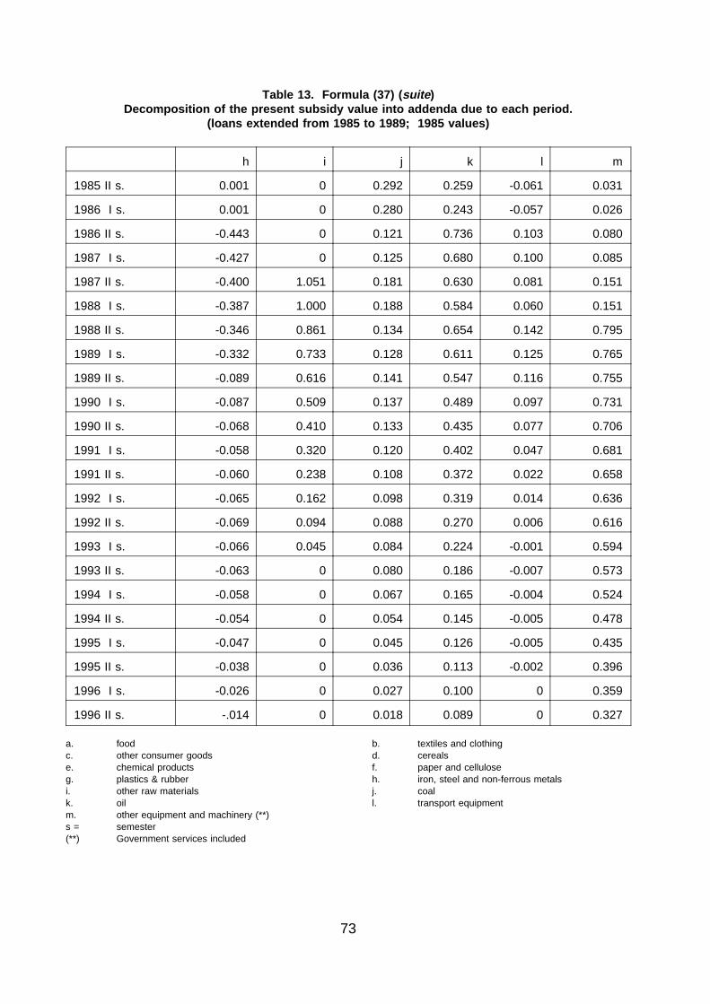
Table 13. Formula (37) ( suite )Decomposition of the present subsidy value into addenda due to each period.

(loans extended from 1985 to 1989; 1985 values)

h i j k l m

1985 II s. 0.001 0 0.292 0.259 -0.061 0.031

1986 I s. 0.001 0 0.280 0.243 -0.057 0.026

1986 II s. -0.443 0 0.121 0.736 0.103 0.080

1987 I s. -0.427 0 0.125 0.680 0.100 0.085

1987 II s. -0.400 1.051 0.181 0.630 0.081 0.151

1988 I s. -0.387 1.000 0.188 0.584 0.060 0.151

1988 II s. -0.346 0.861 0.134 0.654 0.142 0.795

1989 I s. -0.332 0.733 0.128 0.611 0.125 0.765

1989 II s. -0.089 0.616 0.141 0.547 0.116 0.755

1990 I s. -0.087 0.509 0.137 0.489 0.097 0.731

1990 II s. -0.068 0.410 0.133 0.435 0.077 0.706

1991 I s. -0.058 0.320 0.120 0.402 0.047 0.681

1991 II s. -0.060 0.238 0.108 0.372 0.022 0.658

1992 I s. -0.065 0.162 0.098 0.319 0.014 0.636

1992 II s. -0.069 0.094 0.088 0.270 0.006 0.616

1993 I s. -0.066 0.045 0.084 0.224 -0.001 0.594

1993 II s. -0.063 0 0.080 0.186 -0.007 0.573

1994 I s. -0.058 0 0.067 0.165 -0.004 0.524

1994 II s. -0.054 0 0.054 0.145 -0.005 0.478

1995 I s. -0.047 0 0.045 0.126 -0.005 0.435

1995 II s. -0.038 0 0.036 0.113 -0.002 0.396

1996 I s. -0.026 0 0.027 0.100 0 0.359

1996 II s. -.014 0 0.018 0.089 0 0.327

a. food b. textiles and clothingc. other consumer goods d. cerealse. chemical products f. paper and celluloseg. plastics & rubber h. iron, steel and non-ferrous metalsi. other raw materials j. coalk. oil l. transport equipmentm. other equipment and machinery (**)s = semester(**) Government services included

73

Table 13. Formula (37)( suite )Decomposition of the present subsidy value into addenda due to each period.

(loans extended from 1985 to 1989; 1985 values)

a b c d e f g

1997 I s. 0.017 0.008 0 0 0 -0.112 0

1997 II s. 0.011 0.005 0 0 0 -0.090 0

1998 I s. 0.005 0.002 0 0 0 -0.069 0

1998 II s. 0 0 0 0 0 -0.050 0

1999 I s. 0 0 0 0 0 -0.032 0

1999 II s. 0 0 0 0 0 -0.015 0

2000 I s. 0 0 0 0 0 0 0

2000 II s. 0 0 0 0 0 0 0

2001 I s. 0 0 0 0 0 0 0

2001 II s. 0 0 0 0 0 0 0

2002 I s. 0 0 0 0 0 0 0

2002 II s. 0 0 0 0 0 0 0

2003 I s. 0 0 0 0 0 0 0

2003 II s. 0 0 0 0 0 0 0

2004 I s. 0 0 0 0 0 0 0

2004 II s. 0 0 0 0 0 0 0

2005 I s. 0 0 0 0 0 0 0

2005 II s. 0 0 0 0 0 0 0

2006 I s. 0 0 0 0 0 0 0

2006 II s. 0 0 0 0 0 0 0

TOTAL 5.590 2.468 2.284 4.684 2.666 -2.207 5.512

a. food b. textiles and clothingc. other consumer goods d. cerealse. chemical products f. paper and celluloseg. plastics & rubber h. iron, steel and non-ferrous metalsi. other raw materials j. coalk. oil l. transport equipmentm. other equipment and machinery (**)s = semester(**) Government services included

74

Table 13. Formula (37)( suite )Decomposition of the present subsidy value into addenda due to each period.

(loans extended from 1985 to 1989; 1985 values)

h i j k l m

1997 I s. -0.003 0 0.010 0.078 0 0.289

1997 II s. 0.008 0 0.001 0.067 0 0.255

1998 I s. 0.005 0 0 0.058 0 0.222

1998 II s. 0.002 0 0 0.049 0 0.192

1999 I s. 0 0 0 0.040 0 0.164

1999 II s. 0 0 0 0.032 0 0.138

2000 I s. 0 0 0 0.025 0 0.114

2000 II s. 0 0 0 0.018 0 0.092

2001 I s. 0 0 0 0.012 0 0.072

2001 II s. 0 0 0 0.006 0 0.054

2002 I s. 0 0 0 0 0 0.038

2002 II s. 0 0 0 0 0 0.022

2003 I s. 0 0 0 0 0 0.008

2003 II s. 0 0 0 0 0 0.007

2004 I s. 0 0 0 0 0 0.006

2004 II s. 0 0 0 0 0 0.004

2005 I s. 0 0 0 0 0 0.003

2005 II s. 0 0 0 0 0 0.002

2006 I s. 0 0 0 0 0 0.001

2006 II s. 0 0 0 0 0 0

TOTAL -3.183 6.039 2.696 8.764 0.848 12.236

a. food b. textiles and clothingc. other consumer goods d. cerealse. chemical products f. paper and celluloseg. plastics & rubber h. iron, steel and non-ferrous metalsi. other raw materials j. coalk. oil l. transport equipmentm. other equipment and machinery (**)s = semester(**) Government services included

75