Article

The Exergy Cost Theory Revisited

César Torres * and Antonio Valero *

�����������������

Citation: Torres, C.; Valero, A. The

Exergy Cost Theory Revisited.

Energies 2021, 14, 1594. https://

doi.org/10.3390/en14061594

Academic Editor: Noam Lior

Received: 11 February 2021

Accepted: 8 March 2021

Published: 13 March 2021

Publisher’s Note: MDPI stays neutral

with regard to jurisdictional claims in

published maps and institutional affil-

iations.

Copyright: © 2021 by the authors.

Licensee MDPI, Basel, Switzerland.

This article is an open access article

distributed under the terms and

conditions of the Creative Commons

Attribution (CC BY) license (https://

creativecommons.org/licenses/by/

4.0/).

CIRCE Institute, Universidad de Zaragoza, 50018 Zaragoza, Spain* Correspondence: ctorresc@unizar.es (C.T.); valero@unizar.es (A.V.)

Abstract: This paper reviews the fundamentals of the Exergy Cost Theory, an energy cost accountingmethodology to evaluate the physical costs of products of energy systems and their associated waste.Besides, a mathematical and computationally approach is presented, which will allow the practitionerto carry out studies on production systems regardless of their structural complexity. The exergycost theory was proposed in 1986 by Valero et al. in their “General theory of exergy savings”. It hasbeen recognized as a powerful tool in the analysis of energy systems and has been applied to theevaluation of energy saving alternatives, local optimisation, thermoeconomic diagnosis, or industrialsymbiosis. The waste cost formation process is presented from a thermodynamic perspective ratherthan the economist’s approach. It is proposed to consider waste as external irreversibilities occurringin plant processes. A new concept, called irreversibility carrier, is introduced, which will allow theidentification of the origin, transfer, partial recovery, and disposal of waste.

Keywords: thermoeconomics; exergy cost theory; waste costing assessment; lineal productive models

1. Introduction

According to management theory, the cost is defined as the amount of resourcesrequired to produce something or deliver a service. In addition to a managerial techniquefor measuring energy resources consumption, energy cost accounting must provide arational method for assessing the production costs and their impact on the environment.There is a broad international agreement that exergy is the most suitable thermodynamicproperty for cost assessment, at least for energy-intensive systems.

The cost of a product is formed by adding up the resources that have been necessaryfor its production. Nevertheless, these resources have been products of a previous process,so boundaries must be set that precisely limit its objectivity. There are no cost meters, noris it a measurable physical property. It is an emergent property that needs an analyst toevaluate it. However, it quantifies how many resources have been necessary to producesomething. As nothing is produced in isolation from its waste and co-products and thereis always a multiplicity of resources used, cost evaluation is not a trivial activity. Costinglooks for the origin of the production process and quantifies it.

The problem of exergy costs allocation was formulated in 1986 by Valero et al. [1]:“Given a system whose limits have been defined and a disaggregation level that specifies the sub-systems that constitute it, how do we obtain the costs (average costs) of all the flows that becomeinterrelated in this structure?”. The Exergy Cost Theory [2] (ECT) answers the question usingthe following rules:

Resources rule: In the absence of external assessment, the exergy cost of the flowsentering the plant equals their exergy.

Cost Conservation Rule: All cost generated by the production process must be includedin the final product’s cost. In the absence of an external assessment, we have to assigna zero value for the cost of the losses of the plant.

Energies 2021, 14, 1594. https://doi.org/10.3390/en14061594 https://www.mdpi.com/journal/energies

Energies 2021, 14, 1594 2 of 42

Unspent Fuel rule: If an output flow of a process is a part of the unspent fuel of thisprocess, the unit exergy cost is the same as that of the input flow from which theoutput flow comes (also known as F rule).

Co-products rule: If a process has a product composed of several flows, with the samethermodynamic quality, then the same unit exergy cost will be assigned to all of them(also known as P rule).

The Fuel–Product terminology used in thermoeconomics is due to G. Tsatsaronis [3].This idea was a major breakthrough for the detailed cost analysis of industrialenergy systems.

The methods based on the direct application of the ECT are well established andwidely accepted to account for the exergy costs. One can find examples in [4]. However,the method has some significant drawbacks:

The original ECT has some shortcomings from a mathematical viewpoint and haslimitations and accuracy problems from a software implementation perspective. However,the most notable problem is the allocation of waste costs, which is not dealt with in arigorous and general way.

Waste is inseparable from production and has always been considered an annoyingand hidden part of it. The usual thermoeconomic methods, such as ECT, average costtheory [5], or the specific cost method of exergy calculation (SPECO) [6], do not soundlyaddress the problem of waste cost allocation. Other methodologies, such as thermoeco-nomic functional analysis [7] or cumulative exergy consumption [8], provide differentwaste analysis approaches, but none of them give a general solution to the problem.

Waste thermoeconomic cost accounting has gained importance in the last fifteen yearsbecause it allows the discipline to be used as an accounting tool to help assess and designsustainable energy systems [9–11].

Torres et al. [12] highlight the importance of identifying the waste cost formationprocess to make a correct cost allocation. In this paper, a new rule for cost allocation ofwaste was proposed:

Waste rule: The exergy cost of a waste stream leaving the system’s boundaries isallocated null (waste cost internalization). Its exergy cost, formed by adding the fuelrequired to produce it plus the fuel used to carry and dispose of it, is allocated to theprocesses, which have generated it.

This paper has two main objectives: First, it makes an in-depth reflection on theformation process of waste costs. A new concept, called irreversibility carrier, is introducedto identify the origin, transfer, partial recovery, and disposal of waste and to permit itsmanagement as an external irreversibility. It means that waste or external losses shouldbe considered not as flows that leave the system through a dissipative process but asirreversibilities, which originate before, during the production process, but manifest them-selves externally.

Second, it introduces a new methodology for calculating exergy costs, which combinesgraph theory [13] and productive linear models [14] with the Exergy Cost Theory, providinga rigorous mathematical approach, a more robust software implementation, and integratingwaste cost allocation into the model.

2. Waste from a Thermodynamic Viewpoint

Waste is an unwanted material or energy flow that is generated when something isdiscarded or produced. It may be characterized by thermal, mechanical, chemical, or otherintensive properties, such as radioactive ones. A waste will cease to be a waste whenit reaches thermodynamic equilibrium with its surrounding environment. If it does notencounter constraints that prevent it from doing so, it will evolve spontaneously. Thus,if it is hotter or colder, at higher or lower pressure, more concentrated or dilute, or if ithas more chemical reactivity than its surroundings, it will dampen its exergy to zero. In

Energies 2021, 14, 1594 3 of 42

general terms, this environment would be Thanatia [15], a—not so imaginary—state ofthe completely degraded planet Earth. That is, it might be taken as a general reference ofzero exergy.

In other words, first, every residue has exergy with respect to a dead reference environ-ment associated with the biosphere, which we call Thanatia. Second, every residue evolvesspontaneously, losing its exergy until it cancels out. That is, its pressure, temperature, andchemical potential are equalized to those of its environment. Although thermodynamicsalone cannot estimate its rate, it can predict its final state. This degradation process is notharmless to life on earth, and we call the residue a pollutant as long as it damages thenatural environment, i.e., as long as its intensive properties are different from those of theenvironment.

As examples, we observe that gases coming out of a stack have a different concentra-tion from that of the atmosphere and are diluted in it. They are hotter and cool down, andas they are at higher pressure, they expand to atmospheric pressure. Moreover, wastewateris diluted in rivers, which in turn are diluted in the sea, which acts as a universal dumpingground. Moreover, the lack of lubrication produces noise, which is nothing more than apressure wave transmitted to the surrounding air from the rubbing materials. Of course,as solid waste is less movable, it is more difficult for it to react, i.e., to be metabolizedby the environment, but a landfill is expected to act as a large digester that dampens itschemical reactivity.

As summary, any manufacture of material goods requires exergy resources that areconverted into products and waste, both with their exergy. The difference between theexergy of the resources used minus that of the products is called internal irreversibility.When waste crosses the boundaries of the productive system it still has exergy that willirreversibly degrade when it is released into the environment. It is deferred more or lessin time, and can potentially damage the biosphere. We call this spontaneous processesexternal irreversibility. Moreover, at its end-of-life, even products behave as waste, if theydo not become recycled.

That is to say, the production of goods and services always generates internal andexternal irreversibilities both, not only of one type. The first law of thermodynamics appliedto the analysis of production systems focuses on the flows that cross the system boundaries.That is, only waste can be counted but does not give clues to locate its origin. In contrast, aconventional view of the second law on the same system focuses on internal exergy lossesas an analysis element to improve its efficiency. In other words, attention is focused oninternal irreversibilities that allow seeking the causes of internal costs. An integral vision ofthermodynamics applied to production systems must consider both internal and externalirreversibilities. Therefore, the cost of production should reflect both losses.

The Irreversibility Carrier Concept

As mentioned above, cost quantifies the resource losses incurred to produce some-thing. Therefore, an essential question for cost assessment is how internal and externalirreversibilities manifest in a plant and determine its layout. Due to a useless loss ofpressure, temperature, or chemical potential, internal irreversibility can be located in anycomponent of a plant, but its effects can appear anywhere as useless heat. It is the casewhen the location of a cause does not match the location of its effects.

Suppose a Rankine cycle power plant. We know that for each unit and for the plantin general: Fu − Pu = Iu + Lu, where Fu is the exergy of the resources required to producePu units of exergy in process u; Iu are its internal irreversibilities; and Lu are the locallosses, such as waste heat, noise, or leakage. These losses are usually minor and difficult tomeasure. Conventionally, the engineer puts insulation in the equipment to minimize them.From a thermoeconomic point of view, these losses are ignored and considered internalirreversibilities, Iu. Therefore, the above expression can be taken as

Fu − Pu = Iu = T0Sg,u > 0 (1)

Energies 2021, 14, 1594 4 of 42

Nevertheless, F and P have energy content, HF and HP. Then, the first law also statesfor each and every unit as well as the overall plant, that HF,u − HP,u = Qu.

Obviously, the processes are designed to have good thermal and acoustic insulation.Therefore, Qu is not significant in terms of the overall heat released at the overall plant,ΣQu. In fact, it is observed that for each unit, ΣQu is released, and an irreversibility Iu isgenerated, but they are not related one by one, except at the level of the entire plant.

It is worth asking now, where does the heat released caused by each and every oneof the units appear? Remarkably, the heat released is detectable, while irreversibility is aconceptual construct with no local manifestation. Therefore, where does such a heat releaseoriginate from a second law point of view? What is the best way to understand this fact?How can the the first and the second laws be reconciled? The answer is obvious: at thelevel of the complete plant, it is true that

Sg,tot = ∑ Qu/T0

As it is well known, most of the heat released in a power plant is rejected in the boilerand condenser-cooling tower subsystem, or in other words, FT − PT = ∑ Qu = ∑ Iu. Notethat at the whole power plant, HF nearly coincide with its exergy F and HP equals P.

This is an important idea, even though it seems evident. Fu and Pu are located ineach and every component. However, released heats appear anywhere on the plant. Inother words, Fu, Pu, and Iu are located in each component, while each and every Qu arenot. This is a strong argument for using exergy in thermoeconomics. Using the second lawallows locating the true causes of degradation in the units where they appear. Therefore,the casualization of inefficiencies is better located.

One cannot pinpoint the causes of inefficiencies simply by looking at the different heatreleases and noise that ends as heat to the environment, even if local irreversibilities areeventually dispersed as heat fluxes to the environment. Besides that, it is not an easy way toidentify the origin of each degraded heat among the different units in a plant. In any case,these unwanted heats must be eliminated, and they need additional dissipative equipmentto achieve it. This is the case of a condenser in a power plant. In other words, internalirreversibilities, sooner or later, generate waste. However, they need a mass medium tomanifest. Let us call this medium an irreversibility carrier.

A waste stream has exergy, whether thermal, mechanical, or chemical. In addition, ithas its cost of formation, transference, partial recovery, and disposal that must be identified.In parallel with the product cost formation process, there is a waste cost formation process.The irreversibility carrier concept allows us to identify the origin, itinerary, and disposalof any residual stream of the plant regardless it is a mass stream or not. These flows stillhave exergy that the system does not recover. Instead, one needs to spend additionalresources to partially dispose of them in dissipative units. It is the case of the stack and itsauxiliary systems for combustion gases. These units avoid a more significant impact on theenvironment and constitute a technological response to the necessary internalization of thecosts of waste produced by industrial processes.

By contrast with internal irreversibilities, in the production of mass waste, waste isitself its carrier. Waste production is easy to find its origin and also easy to follow suchstream to the dissipative unit. In terms of mass, the industry produces more waste thancommodities and, worse, more types of residual streams than products. For example, in achemical reaction such as combustion, one is interested in the heat released rather than thereaction’s products. Even in the case of reactors in industrial chemistry, metallurgy and allmanufacturing processes in which a reaction product is obtained, the types of unwantedwaste are always present. With these basic ideas, we can see how thermoeconomics canassess the costs of waste associated with internal and external irreversibilities. This processis found by following its irreversibility carrier, which identifies its origin, transfer, partialrecovery, and disposal. The irreversibility carrier is the generalization of the negentropyconcept introduced by C. Frangopoulus [7]. It now extends not only to steam carrying

Energies 2021, 14, 1594 5 of 42

entropy to be condensed in a Rankine cycle, but to any mass or energy flow that carries awaste to be disposed of in the environment.

Sometimes waste flows are caused by technological limitations imposed by the equip-ment and processes of the plant. However, it is, unfortunately, typical to overlook theexternal effects of waste. This practice is called cost outsourcing or cost externalization,that is, letting society or the environment assume the impact of the plant’s waste. This isthe case of greenhouse gases produced by combustion processes. Therefore, the techniquesof waste allocation or costs internalization will increasingly become a common practice inthe near future. Waste flows still have exergy to be recovered or to dispose of them. In anycase, one needs to spend additional resources, thus increasing the system’s irreversibility.In accounting terms, as already said, if waste streams cross the system’s boundaries, theycan be considered as external irreversibilities. However, appropriate allocation needs tolocate which internal process causes them.

For instance, the stack of a combined cycle does not cause the exiting gases. This wastestream has at least three types of waste: rejected heat, CO2, and NOx (plus water, oxygen,nitrogen, and other components of the incoming air, not considered waste). Carbon dioxideand water are produced by the combustion of carbonated fuel, while NOx and excess heatare produced in the combustion chamber. One can compare this combustion chamber toan ideal fuel cell. In such a case, only CO2 and water would be produced. The remainingwaste, CO2, and NOx are material streams that need additional dissipative units to getrid of them. Carbon dioxide requires carbon capture and storage techniques, while NOxrequires special combustion chambers to prevent its formation. These abatement processesrequire further fuel and investment whose costs must be added to the plant product(s).

Therefore, the cost of disposing such gases is always associated with the type ofequipment and/or fuel used. In general, all the productive components involved inthe formation of waste contribute to the cost of the waste. In short, non-material wastestreams, like noise, destabilized (or unbalanced) forces that cause vibrations, or excesstemperature that turns into rejected heat are internal irreversibilities that eventually turninto waste heat. They need material carriers. However, these carriers easily blur theircausal origin. The local entropy generation is the measure of the additional carrying loadof the irreversibility carrier.

They are real streams of waste that have an origin, itinerary, and end. Therefore,it is easy to identify their cost formation process as well as its logical disaggregation.Along this way, they add costs: First, of its formation exergy in the chemical reaction, thenthat of conduction and eventual separation, and finally their abatement costs. Alike thedefinition of fuel and product, that of waste also depends on the analyst and ultimately onsociety. In fact, nature does not produce waste because it recycles everything in the shortor long term. As long as waste has exergy, it can be recovered. That is, a material streamcan be recovered as much as it differs from its reference environment. The distinctionbetween internal and external irreversibilities will also depend on the analyst. However,the cost of any malfunction in the plant must have a single value, independent of theirreversibilities classification.

Therefore, for a proper allocation of the costs of wastes, we must follow their formationprocess and assess the cost of their formation and disposal to the processes in which theyare produced, according to the ideas of irreversibility carrier and polluter pays’ principle. Inparallel to the cost formation process of the products, there is a cost formation processof wastes.

From these reflections, one can draw some conclusions. First, as long as waste hasexergy, it can be used before going out of the production process. This is achieved withequipment that we call recovery units. Second, if waste cannot be recovered, it is necessaryto reduce its exergy. We will do it in dissipative units. Note that the latter units consumeexergy in order to dissipate it. In general, they exchange one type of residual exergy foranother. Third, complete abatement or total exergy recovery is too costly. Because theyfollow the law of diminishing returns, in other words, the behavior of this equipment is

Energies 2021, 14, 1594 6 of 42

governed by an entropic behavior. For example, in the separation of a component in amixture, it is easier to separate a given amount of the minority component if its compositionis at 10% than at 1%, which will be less expensive to separate it at a concentration of 0.1%,and so on. This makes total decontamination technically and economically unfeasibleand achieving total purity extremely costly. It is an application of the Third Law ofThermodynamics applied to separation processes. As a practical application, a designerof these types of equipment must take into account that there are entropic limits (pinchpoints) that are neither technically nor economically achievable.

3. The Productive Structure Graph

Throughout this paper, a simplified model of a gas turbine cycle with co-generation(hereafter referred to as TGAS) is used as a case study, see Figure 1.

1

2 3

4

5

COMB

COMP GTUR

HRSG

STCK

0

2

34

5

1

6 7

88a

9

Figure 1. Flowsheet of TGAS plant.

The TGAS plant uses natural gas (flow #5) to produces 10 MW of electric power(flow #6) and 7.6 kg/s of saturated steam at 20 bar of pressure (flow #8) from freshwater(flow #8a), partially recovering the residual heat of gases (flow #4). Finally, the wastecombustion gases are expelled through a stack (flow #9). The combustor has 2% of heatlosses, and the isentropic efficiency of the turbine and compressor is 87%. This flowsheetalso indicates the system boundaries and the aggregation level. The thermodynamicproperties of the plant are shown in Table 1. To simplify the model, flows #0 and #8aare removed from further analysis because their exergy values equal to zero. We are notconsidered the pump required to increase the water pressure from 1 to 20 bar because theexergy value of the work flow is negligible (1.8 kW).

From a theoretical viewpoint, an energy system is defined beforehand as a set of sub-systems or thermodynamic processes linked to each other and the environment by anotherset of mass, heat, and work flows, quantified by its exergies. In essence, it constitutes aflow sheet, as it is shown in Figure 1.

Industrial installations have a productive purpose. Their objective is to obtain oneor several products by processing external resources. For each process of the system, itis necessary to identify the flows that constitute their product and the flows required toobtain them called fuel. Energy flows (e.g., heat or work) appear at the process inlet asfuel stream or the process outlet as the product stream. When working with mass streams,it is appropriate to operate with exergy differences associated with each energy transferbetween the inlets and the outlets. The output flows that are not part of the productionprocess are considered as unspent or recoverable fuel.

Energies 2021, 14, 1594 7 of 42

Table 1. Thermodynamic properties of TGAS case study.

Flow m (kg/s) T (◦C) p (bar) h (kJ/kg) s (kJ/kg K) B (kW)

0 37.53 20 1.013 0 0 01 0.7324 20 50,000 0 36,6202 37.53 291.4 8 272.4 0.0648 95123 38.26 1050 7.84 1205 1.170 32,9904 38.26 598.2 1.05 676.5 1.264 11,7075 38.26 137.4 1.013 137.3 0.394 835.36 10,2257 10,000

8a 7.6 20 1.013 83.9 0.296 08 7.6 212.4 20 2799 6.340 71689 38.26 137.4 1.013 137.3 0.394 835.3

A fuel stream group will consist of

• one or several inflows that provide exergy to the process and• input and output flows enter into the process and leave it, after some exergy transfer

to the process.

A product stream group will consist of

• one or several outflows produced by the process and• output and input flows enter into the process and leave it, after some exergy increase.

The exergetic efficiency of a process u is defined as the ratio between the exergyobtained or product Pu and the exergy supplied or fuel Fu. It measures how reversible aprocess is. Its inverse value is the exergy unit consumption ku, i.e., the amount of resourcesrequired per unit of the product obtained:

ku =Fu

Pu= 1 +

Iu

Pu≥ 1, Pu > 0 (2)

Table 2 shows the definition of the fuel and product streams of each process in thecase of TGAS plant.

Table 2. Processes description and efficiency definition of TGAS plant.

Nr Key Process Fuel Product

1 COMB Combustor B1 B3 − B22 COMP Compressor B6 B2 − B03 GTUR Turbine B3 − B4 B6 + B74 HRSG HRSG B4 − B5 B8 − B8a5 STCK Stack B5 B9

3.1. The Production Layer

Let V = {u0, u1, . . . , un} be the set of the n components or processes that constitute thesystem, for some defined boundaries and aggregation level. The component u0 representsthe environment. Let define B = {b1, . . . , bm} as the set of the m flows that interchangeexergy between the processes. Finally, let L = {`1, . . . , `nr} be the set of all the productive(fuel and products) groups of the system. Each component of the system has one or morefuel and product streams, let Fu and Pu be the sets of fuel and product streams of theprocess u, respectively. On the other hand, each stream ` ∈ L could have several inputs andoutput flows. Let us denote El and Sl as the sets of input and output streams, respectively,of the productive group `. A fuel stream must have at least one input flow, and a productstream must have at least one output flow.

Energies 2021, 14, 1594 8 of 42

Defining system boundaries is essential to determine the system costs. For thispurpose, the environment is defined as an additional process complementary to the globalplant. The system outputs are the fuel of the environment F0, and the system resourcesare the product of the environment P0. A productive group must be defined for each finalproduct and each external resource to ensure the information about them.

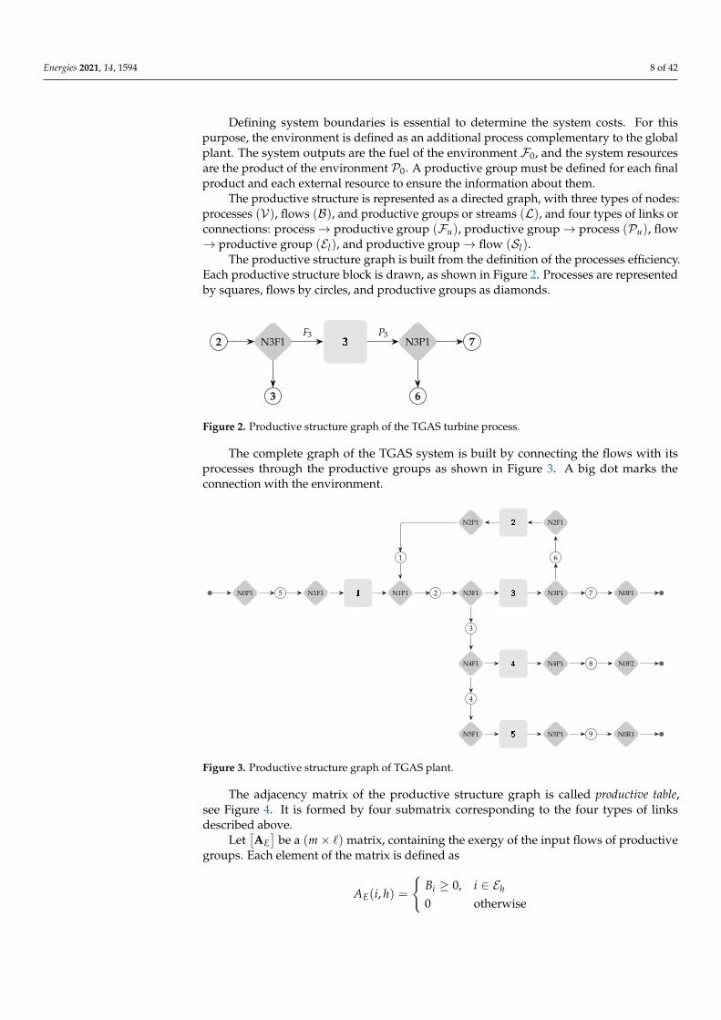
The productive structure is represented as a directed graph, with three types of nodes:processes (V), flows (B), and productive groups or streams (L), and four types of links orconnections: process→ productive group (Fu), productive group→ process (Pu), flow→ productive group (El), and productive group→ flow (Sl).

The productive structure graph is built from the definition of the processes efficiency.Each productive structure block is drawn, as shown in Figure 2. Processes are representedby squares, flows by circles, and productive groups as diamonds.

2 N3F1 3

3

N3P1

6

7F3 P3

Figure 2. Productive structure graph of the TGAS turbine process.

The complete graph of the TGAS system is built by connecting the flows with itsprocesses through the productive groups as shown in Figure 3. A big dot marks theconnection with the environment.

N0P1 5 N1F1 1 N1P1 2 N3F1 3 N3P1 7

2 N2F1

6

N2P1

1

4N4F1

3

N4P1 8

5N5F1

4

N5P1 9

N0F1

N0F2

N0R1

Figure 3. Productive structure graph of TGAS plant.

The adjacency matrix of the productive structure graph is called productive table,see Figure 4. It is formed by four submatrix corresponding to the four types of linksdescribed above.

Let[AE]

be a (m× `) matrix, containing the exergy of the input flows of productivegroups. Each element of the matrix is defined as

AE(i, h) =

{Bi ≥ 0, i ∈ Eh

0 otherwise

Energies 2021, 14, 1594 9 of 42

Let[AS]

be a (`×m) matrix, containing the exergy of the output flows of productivegroups. Each element of the matrix is defined as

AS(l, j) =

{Bj ≥ 0, j ∈ Sl

0 otherwise

Let[AF]

be a (` × n) matrix, containing the exergy values of fuels streams of theprocesses, defined as

AF(l, u) =

Fl,u = ∑i∈El

Bi − ∑j∈Sl

Bj ≥ 0, l ∈ Fu

0 otherwise

Let[AP]

to be a (n× `) matrix, which contains the exergy values of product streamsof the processes, defined as

AP(u, h) =

Ph,u = ∑j∈Sh

Bj − ∑i∈Eh

Bi ≥ 0, h ∈ Pu

0 otherwise

Vector ν0 (1× `) contains the exergy values of the external resources, and vectorω0 (`× 1) contains the exergy values of the system outputs:

ν0,i =

{Bi ≥ 0, i ∈ Sh, h ∈ P0

0 otherwiseω0,i =

{Bi ≥ 0, i ∈ Eh, h ∈ F0

0 otherwise

Let F and P be (n × 1) vectors, whose elements are the exergy values of fuel andproduct of the system’s components, and B a (m × 1) vector, whose elements are theflows exergy.

The submatrices of the productive table verify the following properties:

F = t[AF]

ul

P =[AP]

ul

B =[AE]

ul =t[AS

]ul

E = ω0 +[AF]

un +[AS]

um = ν0 +t[AP

]un +

t[AE]

um

(3)

where E is a (`× 1) vector whose elements represent the total exergy processed by eachproductive group, defined as

Eh =

∑

i∈Eh

Bi = Fu,h + ∑j∈Sh

Bj ≥ 0, h ∈ Fu

∑j∈Sh

Bj = Pu,h + ∑i∈Eh

Bi ≥ 0, h ∈ Pu

The exergy balance in a productive group is conservative, and the exergy of the inputstreams equals the exergy of the output streams because productive groups are logical orfictitious units. The exergy of a productive group depends on the type of productive group.If the productive group is a fuel stream, its exergy is the sum of the exergy of their inputflows and the sum of the exergy of their output flows if it is a product stream group. Theexergy balance in a unit process is given by Equation (1), and it is written in the vectorialform as

F− P = I (4)

Energies 2021, 14, 1594 10 of 42

where I is a (1×m) vector whose elements are the internal irreversibility values Iu of eachsystem’s component.

outputs

n m `

0 0 ν0in

puts

n 0 0 0[AP]

P

m 0 0 0[AE]

B

` ω0[AF] [

AS]

0 E

F B E

Figure 4. Productive table of an energy system.

Note that to obtain coherent values for processes efficiency, the exergy values of theflows Bi must be non-negative, as well as the exergy values of the fuel and product groups.This condition is evident in nearly all real cases, but if we work with the flow exergyB = H − H0 − T0 (S − S0) near environment temperature and low pressures, it couldtake negative values, in this case, the environmental conditions must be revised. Otherconditions must be satisfied at process level are Fi − Pi ≥ 0 and Fi, Pi > 0. Obviously,if both are equal to zero, there is no effective process (consider that sometimes bypassand redundant processes are used in complex plants). If Fi > 0 and Pi = 0 it should beconsidered as a dissipative unit.

The submatrices that defining the productive structure table for TGAS system, usingthe Coordinate Sparse Matrix (row, col, value) format, are as follows:

[AE](9× 14) =

1 2 6 3 4 5 7 8 91 2 3 5 7 9 12 13 14

36,620 9512 10,225 32,990 11,707 2173 10,000 7168 835.3

[AS](14× 9) =

11 4 2 5 7 6 6 8 101 2 3 4 5 6 7 8 9

36,620 9512 32,990 11,707 835.3 10,225 10,000 7168 835.3

[AF](14× 5) =

1 3 5 7 91 2 3 4 5

36,620 10,225 21,283 10,872 835.3

[AP](5× 14) =

1 2 3 4 52 4 6 8 10

23,478 9512 20,225 7168 835.3

Coordinate Sparse Matrix format is commonly used when the number of non-zero

elements represents less than 10% of the total matrix elements. Each column of thesematrices determines an element of the matrix in the form (row, col, value), see Table 3 toknow the index of each productive group.

Energies 2021, 14, 1594 11 of 42

3.2. The Waste Layer

From the viewpoint of processes, we must distinguish among productive components,whose purpose is to make useful products, and dissipative components that not gener-ate any final product but are responsible for disposing of the waste created during theproduction. Let us denote VP ⊂ V as the subset of productive units and VR ⊂ V as thesubset of dissipative units. For convenience, each waste flow is defined as the product ofa dissipative unit, so the waste cost reallocation could be made from dissipative units toproductive components.

Figure 5 shows the cost allocation scheme for dissipative processes and waste flowsstreams in the productive structure. Flows to be disposed enter as fuel of the dissipativeunit (DIS) together with the resources required to eliminate them; the product of thedissipative unit is the removed exergy, flow (r), that connects with a waste stream to theenvironment (ENV), which redistributes the cost among the productive units (u) and (v)that produce it. Meanwhile, the flow cost leaving the system (entering the environment) iszero. In other words, waste streams are treated as external irreversibilities of the productiveunits that generated them. This fact will be formally studied here.

DIS

F1

F2

PP r R ENV

u

v

Figure 5. Waste allocation scheme in the productive structure of a system.

In the case of TGAS example, flow #4 enters on the fuel group F1, and F2 group is notused in this case, but it could represent the work and electricity flows of the equipmentrequired to extract the gases (forced or induced draft fans). The product of the dissipativeunit is the eliminates exergy of output gases B9. The productive group R, corresponds toindex #14. It is a logical node whose function is to redistribute the cost of gases B∗9 amongthe processes having contributed to generate the waste flows, in this case, the combustionprocess #1. Therefore, the cost of waste going outside the plant (entering the environment)is zero, and the remaining exergy will be considered as external irreversibility.

From a conceptual viewpoint, the definition of efficiency in dissipative units would bethe same as in a productive unit: the amount of exergy produced divided by the providedexergy resources. However, from an engineering viewpoint, the meaning is different: in adissipative unit, its production purpose is to eliminate a waste stream (thermal, chemical,or physical), so its product is the exergy we need to dissipate it. As Figure 5 shows, thefuel has two components. One (F1) is the waste stream we want to dispose of, and theother is the additional resources needed to do so, such as labor, electricity, water, coolingair, or chemicals, referred to as F2. Therefore, the unit consumption in a dissipative unitcould be defined as k = 1 + F2/F1. This means that if no additional resources are required,its unit consumption is 1, and the dissipative unit is a simple pipeline. However, in thereal world, it always needs additional resources, which increase its unit consumption. Thehigher the consumption of additional resources for waste disposal, the lower the efficiencyof a dissipation unit is.

Waste flows are identified as all the unwanted and unavoidable flows crossing thesystem boundaries. Let us denote R as the subset of output system flows F0 formed bythe system’s waste flows. Therefore, the system outputs could be split into two parts:ω0 = ωT + ωR.

Energies 2021, 14, 1594 12 of 42

Let ωR be a (`× 1) vector containing the exergy of the waste flows and ωT as a (`× 1)vector containing the exergy of the final products:

ωR,h =

{Eh h ∈ R0 otherwise

ωT,i =

{Ei i ∈ F0 ∩ R0 otherwise

(5)

Let[AR]

be a (`× n) matrix, called waste-process table, whose elements Rhu representthe exergy of waste stream h generated by the process u. According to the Figure 5, theexergy balance is written as

Br = ωR,h = ∑u∈VP

Rhu, r ∈ Eh, h ∈ R

The matrix[AR]

verifies the following properties:

ωR =[AR]

un (6)

R ≡ t[AR]

ul (7)

where R is a (n× 1) vector whose elements contain the exergy of the waste generated byeach process. Note that, meanwhile, Equation (6) is an equality based on the definition ofthe waste process table and Equation (7) is a definition; the values of R do not correspondto physical flows, but they are identified as external irreversibilities of the processes, asit will be shown in Equation (32). The waste process table describes the cost formationprocess of waste, and it is integrated as an additional layer of the productive structure inparallel to the fuel structure.

In the case of the TGAS plant, where only thermal wastes are considered, the wasteprocess table will be

[AR](14× 5) =

141

835.3

There are not always single criteria to determine the

[AR]

values. In general, theanalyst requires a detailed thermodynamic analysis of processes to identify where thewaste is formed, see Section 10.

Figure 6 describes the waste internalization of a generic component. The value Rurepresents the additional fuel that must be spent to remove waste. It becomes externalirreversibilities IR

u of the component u.

u

Ru

Fu Pu

IRu

Iu

Fu − Pu = Iu

Ru = IRu

Fu + Ru − Pu = Iu + IRu

Figure 6. Fuel–Product–Waste schema for a generic productive component.

The exergy balance of the global system is written as

FT − PS =n

∑j=1

Ij = IT , (8)

Energies 2021, 14, 1594 13 of 42

where FT is the sum of the exergy of external resources ν0,i; PS is the sum of the exergy ofthe flows ω0,i crossing the system’s boundaries, including both final production and waste;and IT is the sum of the internal irreversibilities.

However, when one introduces a productive purpose, part of the outputs of the systemcan become waste, so the overall exergy balance is rewritten as

FT − PT = ∑i∈V

Ii + ∑i∈R

ω0,i = IT + IR,

the second term of the right side of equation represents the total external irreversibilities IR.

IR = ∑u∈V

IRu = ∑

u∈VRu = ∑

r∈Rω0,r

On the other hand, if one considers that the costs of the waste leaving the system arezero, because they have no value in the production system, the exergy cost balance on thewaste stream will be

B∗r = ∑u∈VP

κ∗h Rhu, h ∈ R,

where κ∗h = k∗r is the unit exergy cost of the waste stream Br, and the cost of the wastegenerated by each productive component will be

R∗u = ∑h∈R

κ∗h Rhu, u ∈ VP

The costs of the waste are internalized and assessed to the productive components thatgenerated them. Therefore, according to Figure 6, the cost of irreversibilities (internal andexternal) is zero, and the cost balance for each productive component of the system becomes

P∗u = F∗u + R∗u, u ∈ VP

It means that the production exergy cost of a process P∗u is equal to the cost of theresources required F∗u plus the cost of disposed waste R∗u that generates.

In conclusion, waste always has a cost, but as it cannot be sold, its cost must beallocated to the final products, or better, to the processes that have produced them. In thesame way that there is a cost of formation of products, there is also a cost of formation ofwaste, which is identified with matrix

[AR]. Waste is obviously a problem for productive

systems, but it also represents an opportunity for energy saving by recovering them to beused in other processes.

4. The Fuel–Product–Waste Cost Allocation Rules

The exergy cost of a flow is an emergent property, that is, one cannot measure itindependently of the formation process of a flow stream. Cost is always linked to theproduction process. Furthermore, this process links a set of internal and external flows.Therefore, a complete set of interrelated cost flows must be determined, not an individualcost. There is not only interesting to find the costs of final products, but it is also valuableto have them for internal products. Then, the cost build-up for each final product couldbe traced through the energy system. The Fuel–Product (FP) rules offer a procedure fordetermining the exergy cost of the m flows of an energy plant, building a system of m linearequations with m unknowns, based on the productive structure definition, as it will beshown in this section.

As explained beforehand, given an energy system whose productive structure hasbeen specified, the exergy cost of a flow of that system is defined as the amount of exergyrequired to produce this flow.

Energies 2021, 14, 1594 14 of 42

Let us denote B∗i as the exergy cost of the system flow i and k∗i asthe correspondingexergy cost per unit of product exergy. The cost of the exergy processed on a productivestream h is defined as

E∗h =

∑

i∈Eh

B∗i , h ∈ Fu

∑j∈Sh

B∗j , h ∈ Pu

Let us denote E∗h as the cost of exergy processed in a stream, and κ∗h its cost per unitof exergy. Therefore, the cost of each fuel and product stream of a generic process u isdefined as

F∗u,h = E∗h − ∑j∈Sl

B∗j h ∈ Fu

P∗u,h = E∗h − ∑j∈El

B∗i h ∈ Pu

Finally, the exergy cost of fuel and product of the process u is defined as the sum ofthe fuel or product streams of the process:

F∗u = ∑h∈Fu

F∗u,h P∗u = ∑h∈Pu

P∗u,h

The FP rules that define the exergy cost of the system flow could be written using thenotation of the productive structure model, as follows:

Resources rule: The exergy cost is relative to the system boundaries. In the absenceof external assessment, the exergy costs of the flows entering the system equaltheir exergy.

B∗i = Bi, i ∈ Sh, h ∈ P0 (9)

Cost Conservation rule: The exergy cost is a conservative property.

P∗u = F∗u + R∗u, u ∈ V (10)

This rule implies all the cost associated to a process, both the spent resources cost F∗uand cost of waste generated R∗u, must be assessed as a production cost.

Unspent fuel rule: All the outputs of a fuel group have the same unit cost equal to theunit cost of the input fuel streams:

k∗j = κ∗h =F∗u,h

Fu,h, j ∈ Sh, h ∈ Fu (11)

This rule implies that the process irreversibilities will be added to the cost of theoutput product streams.

Co-production rule: All products of the same quality at the output of a system’s com-ponent have the same unit exergy cost.

• All the product groups of a process have the same unit exergy cost:

P∗uPu

=P∗u,l

Pu,l, ` ∈ Pu (12)

• All the outputs streams of a product group have the same unit exergy cost:

k∗j = κ∗h , j ∈ Sh, h ∈ Pu (13)

Energies 2021, 14, 1594 15 of 42

The idea of products of the same quality needs a detailed aggregation level ofthe system.

Waste rule: The exergy cost of waste exiting the analyzed system must be charged tothe product of the components that generate them.

ω∗0,h = 0, h ∈ RR∗u = ∑

h∈Rκ∗h Rhu, u ∈ VP. (14)

This rule implies that the cost of waste flows, leaving the system boundaries, is zero,and then the cost of the non-recoverable exergy of these flows is assessed to the finalproducts by means of the waste internalization.

Let us also define the bifurcation ratio yj as

yj ≡Bj

El=

B∗jE∗l

, j ∈ E` ` ∈ Lu

these ratios distribute the cost proportionally to the exergy content. In the case of a fuelgroup, they define the recoverable fuel rule and, in the case of product groups, they definethe co-production rule. Therefore, the unit cost of internal flows equals the unit cost of theproductive group the flow comes from.

k∗j = κ∗` j ∈ S` ` ∈ Lu (15)

The Exergy Cost theory provides a set of rational rules based on thermodynamiccriteria and the productive purpose. Now, we will prove that the FP rules are necessary andsufficient conditions to unequivocally determine the exergy cost of all flows of a definedenergy system.

4.1. Fuel–Product–Waste Rules Matrix Representation

Let F∗ and P∗ be (n × 1) vectors, whose elements are the exergy cost of fuel andproduct of the processes related, and B∗ a (m× 1) vector, whose elements are the exergycost of the flows, finally E∗ is a (`× 1) vector, whose elements contains the total exergycost of the productive streams. Let k∗P, k∗, and k∗E be the corresponding vectors containingthe unit costs.

If one applies the Input-Output cost model [16] to the productive table, one obtainsthe following equations:

E∗ = ν0 +t[AE

]k∗ + t[AP

]k∗P (16)

B∗ = t[AS]

k∗E (17)

P∗ = t[AF]

k∗E + t[AR]

k∗E (18)

Now, let us prove that the above equations verify the ECT rules of cost allocation:Equation (16) defines the cost of productive groups, as a linear function of its inputs:

E∗h = ν0,h + k∗P,u Pu,h + ∑i∈Eh

k∗i Bi

If h ∈ P0, i.e., it is a resource stream, by rule FP1: E∗h = ν0,hIf h is a product stream, i.e., h ∈ Pu, we need to verify

E∗h = k∗P,u Pu,h + ∑i∈Eh

k∗i Bi

Energies 2021, 14, 1594 16 of 42

by rule FP4P, k∗P,u = κ∗h , and

k∗P,u Pu,h + ∑i∈Eh

k∗i Bi = P∗u,h + ∑i∈Eh

k∗i Bi = E∗h .

Finally, if h is a fuel stream, i.e., h ∈ Fh, by the stream cost definition, Equation (16)is verified:

E∗h = ∑i∈Eh

k∗i Bi

Equation (17) relates the cost of flows and productive streams. Now, we need to verifyfor all the flows that B∗j = κ∗h Bj, j ∈ Sh, but by Equation (15) it is satisfied. It means thatthe unit costs of a flow equals cost of productive groups the flow comes from.

Equation (18) defines the cost balances of processes as a linear function of the cost ofproductive stream groups. By cost balance, rule FP2: P∗u = F∗u + R∗u.

By rule FP5R, the second addend of equation is satisfied.On the other hand, from the first addend, it must satisfy

F∗u = ∑h∈Fu

κ∗h Fu,h,

by definition of fuel stream, and rule FP3, it leads to

F∗u,h = E∗h − ∑i∈Eh

k∗i Bi = κ∗h(Eh − ∑

i∈Eh

Bi)= κ∗h Fu,h

therefore, Equation (18) is satisfied.The cost balance Equation (18) could be also written as

F∗ = t[AF]

k∗ER∗ = t[AR

]k∗E

P∗ = F∗ + R∗(19)

This result proves that the FP rules could be expressed using the algebraic relation-ships (16)–(18), which provide a set of n + m + ` equations with n + m + ` unknowns thatpermit to determine the exergy costs of flows and productive streams.

4.2. Exergy Cost Computation

This section explains a new algorithm for calculating the exergy cost of system andprocess product flows, based on the matrix representation of the ECT rules. First, itcalculates the cost of productive groups, then the cost of internal flows Equation (15), andthe processes costs by Equation (19).

Let αE be a (m × `) matrix so that[AE]= B αE, αS be a (` × m) matrix so that[

AE]= E αS. Let αF be a (` × n) matrix so that

[AF]= E αF, and similarly, Let αR be

a (` × n) matrix so that[AR]= E αR. Finally, let αP to be a (n × m) matrix, so that[

AP]= P αP.

These matrices are obtained by scaling the rows of the productive table by the corre-sponding exergy streams, then Equation (3) is rewritten as

F = tαF E (20)

B = tαS E (21)

E = tν0 +tαP P + tαEB (22)

Energies 2021, 14, 1594 17 of 42

Let a0 be a (`× 1) vector, whose elements indicate if a stream is a system output:

a0,l =

{1 if l ∈ F0

0 otherwise(23)

Equation (5) shows that the system outputs could be separated into final productionand waste. Let us define the corresponding adjacency vectors (aT and (aR (×1) indicatingwhether the production flows are final products or waste:

aT,l =

{1 if l ∈ F0 ∩ R0 otherwise

aR,l =

{1 if l ∈ R0 otherwise

(24)

The following relationships are verified:

αP ul = un

αR un = aR

αF un + αS αE ul + a0 = ul

a0 = aT + aR

(25)

Substituting these matrices into Equations (16) to (18), it leads to the followingrelationships:

tE∗ = ν0 +tE∗ αS αE + tP∗ αP (26)

tP∗ = tE∗(αF + αR

)(27)

and substituting Equation (27) into Equation (26), the following system of ` equations with` unknowns, to determine the exergy cost of the productive streams E∗, is obtained:

t(U` − 〈A〉)E∗ = ν0 (28)

where 〈A〉 = αSαE + (αF + αR) αP is called cost characteristic matrix.To demonstrate that Equation (28) has a unique solution, we will prove that 〈A〉 is a

productive matrix, see Appendix A, or equivalently that 〈A〉ul ≤ ulFrom Equation (25), we get (αS αE + αF αP + αR αP )ul = ul − aT ≤ ul . Therefore,

as an energy system has final products, i.e., aT > 0, the exergy costs of the flows can beunequivocally determined by

E∗ = t⟨E∗∣∣ν0 where⟨E∗∣∣ ≡ (Ul − 〈A〉)−1 (29)

Once the cost of productive groups are determined, the cost of flows could be obtainedby applying Equation (15), and the production cost of processes by Equation (27).

Moreover, matrix⟨E∗∣∣ is definite positive, see Appendix A, i.e., all its elements are

non-negative. Therefore, the exergy costs are always non-negative because the exergy ofexternal resources is a non-negative magnitude.

Applying the exergy balance, (4), (20) lead to P = t(αF + αR)E− I−R, and substitut-ing into Equation (22):

ν0 = t(Ul − 〈A〉)E + tαP

(I + R

), (30)

then, right multiplying both sides of Equation (30) by⟨E∗∣∣, we get the exergy cost of pro-

ductive streams as a function of the irreversibilities and waste generated by the processes:

tE∗ = tE + t(I + R)

αP ·⟨E∗∣∣ (31)

Energies 2021, 14, 1594 18 of 42

Applying Equation (27), a similar expression for exergy cost of flows is found:

tB∗ = tB + t(I + R)

αP ·⟨E∗∣∣ αS (32)

Equation (31) is essential to understand the process of cost formation. It shows theexergy cost of a flow equals its exergy plus the sum of all exergy destroyed (internal andexternal irreversibilities) during the production process of that flow. The above equationαP (I + R) represents the local exergy losses assessed to each productive group, and thenthe cost operator 〈E∗| distributes these values to the remaining processes of the system asadditional resources consumption. As it is shown in Equation (31), waste is consideredan irreversibility.

As the last term in Equation (32) is positive, the exergy cost of a flow is always greatestor equal to its exergy: B∗i ≥ Bi for each i. The equality is satisfied only if there is noirreversibility in the production of such flow. It is the case of the external resources, whosecost is equal to its exergy. Therefore, irreversibility reduction implies production costdecrease and resources saving.

Let us calculate the exergy costs of flows and productive streams of the TGAS plantaccording to the method exposed above.

The submatrices that define the productive structure table for the TGAS plant, usingthe sparse coordinate (row, col, value) format, are

αE (9× 14) =

1 2 6 3 4 5 7 8 91 2 3 5 7 9 12 13 141 1 1 1 1 1 1 1 1

αS (9× 14) =

11 4 2 5 7 6 6 8 101 2 3 4 5 6 7 8 91 1 y3 y4 1 y6 y7 1 1

αF + αR (14× 5) =

1 3 5 7 9 141 2 3 4 5 11 1 1− y3 1− y4 1 1

αP (5× 14) =

1 2 3 4 52 4 6 8 101 1 1 1 1

where the bifurcation ratios are

y3 ≡B4

B3=

B∗4B∗3

y6 ≡B6

B6 + B7=

B∗6B∗6 + B∗7

y4 ≡B5

B4=

B∗5B∗4

y7 ≡B7

B6 + B7=

B∗7B∗6 + B∗7

In general, the α matrices are determined as follows:

αP(u, l) = Pu,l/Pu l ∈ PuαF(l, u) = 1−∑j∈Sl

yj l ∈ FuαR(l, u) = Ru,l/El l ∈ R, u ∈ VPαE(i, l) = 1 i ∈ El , l ∈ LuαS(l, j) = yj j ∈ Sl , l ∈ Lu

Then, the cost characteristic matrix compute the exergy cost, by means of Equation (29),is given by

〈A〉(`× `) =

11 1 4 6 3 2 5 5 7 7 9 6 8 101 2 2 3 4 5 6 7 8 9 10 12 13 141 1 1 y6 1 1 1− y3 y3 1− y4 y4 1 y7 1 1

Energies 2021, 14, 1594 19 of 42

Note that the cost matrix depends only on the bifurcation ratios. The sum of each rowof the internal productive groups is 1, meanwhile if the rows of the system output groupssum to zero, then 〈A〉matrix is productive.

Tables 3–5 show the exergy and exergy cost values for the TGAS plant for productivegroups, physical flows, and processes, calculated using Equation (29). Each productivestream has an assigned key code that indicates the node to which it belongs and the streamtype. Each flow is also defined as the pair of connected productive groups. The globalefficiency of the plant is 46.8%, and the unit exergy costs of electricity and heat are 1.8 and2.59, respectively. Note that the waste stream cost (N5P1) is 1429.7 kW. This means that 4%of natural gas is dissipated to the environment as exhaust gases. This cost is charged tothe combustion chamber product and redistributed to the final products of the system. Inthe next sections, we will explain in detail which part is due to the internal irreversibilitiesof the processes and which part is due to waste allocation. Observe that the cost balancefor the overall system is satisfied E∗14 = E∗11 + E∗12, as well as flows cost overall balance:B∗1 = B∗7 + B∗8 .

Table 3. Productive streams exergy costs for TGAS example.

Id Key E (kW) E∗ (kW) k∗E (J/J)

1 N1F1 36,620 36,620.0 1.00002 N1P1 32,990 56,465.7 1.71163 N2F1 10,225 18,417.3 1.80124 N2P1 9512 18,417.1 1.93625 N3F1 32,990 56,465.7 1.71166 N3P1 20,225 36,429.3 1.80127 N4F1 11,707 20,037.7 1.71168 N4P1 7168 18,608.1 2.59609 N5F1 835.3 1429.7 1.7116

10 N5P1 835.3 1429.7 1.711611 N0P1 36,620 36,620.0 1.000012 N0F1 10,000 18,012.0 1.801213 N0F2 7168 18,608.1 2.596014 N0R1 835.3 1429.7 1.7116

Table 4. Exergy balances and unit cost of TGAS processes.

Id Process F (kW) P (kW) I (kW) k (J/J) k∗P (J/J)

1 COMB 36,620 23,478 13,142 1.5598 1.62072 COMP 10,225 9512 713 1.0750 1.93623 GTRB 21,283 20,225 1058 1.0523 1.80124 HRSG 10,871.7 7168 3703.7 1.5167 2.59605 STCK 835.3 835.3 0.0 1.0000 1.7116

Total 36,620 17,168 19,452 2.1330 2.1330

Energies 2021, 14, 1594 20 of 42

Table 5. Exergy cost of flows for TGAS example.

Id From To B (kW) B∗ (kW) k∗ (J/J)

1 N0P1 N1F1 36,620 36,620.0 1.00002 N2P1 N1P1 9512 18,417.1 1.93623 N1P1 N3F1 32,990 56,465.7 1.71164 N3F1 N4F1 11,707 20,037.7 1.71165 N4F1 N5F1 835.3 1429.7 1.71166 N3P1 N2F1 10,225 18,417.3 1.80127 N3P1 N0F1 10,000 18,012.0 1.80128 N4P1 N0F2 7168 18,608.1 2.59609 N5P1 N0R1 835.3 1429.7 1.7116

5. The Generalized Exergy Cost

As mentioned above, the exergy cost is relative to the system boundaries. Therefore,we will distinguish between the thermodynamic system that constitutes the installationand its environment. Exergy cost, also called direct exergy cost, only takes the processesirreversibility (both internal and external) inside the boundaries of the system into account.

From a natural resource management point of view, the system boundaries should beset at the extraction level of non-renewable resources from nature [17]. The exergy cost ofthe natural gas processed in a gas turbine will be higher than its exergy due to the extraction,storage, and transportation processes necessary to use it. Moreover, direct exergy cost doesnot consider the fact that the units that form an installation are functional products, andthey have their own exergy cost because to keep them in operation, additional, exergy willbe required.

On the other hand, when considering the economic aspects, the perspective is extendedwith the introduction of two additional factors: the market prices of the fuels c0 (e/MWh)which are not linked to the exergy of the resources processed, and the cost of depreciation,maintenance, and operation of the plant required for the production process Z (e/h).

For these reasons, the generalized exergy cost concept is introduced as a broader view ofdirect exergy cost, where the costs of the system flows consider the interactions with thephysical and/or economic environment. Therefore, the Resources rules should be adapted toconsider the external valuation of resources C0 = c0 E, which could be measured in energyor monetary units per unit of time. If costs consider Z expenditures, either measured inenergy or in monetary units and levelized per time unit, the Balance Cost Rule must beincluded this factor and rewritten as follows:

CP,i = CF,i + CR,i + Zi

where CP, CF, and CR are the generalized exergy cost of the products, fuels, and waste ofeach system process, respectively.

According to these ideas, the exergy cost Equations (16) and (17) could be rewrittenfor generalized exergy cost as

CE = C0 +tαE C + tαP CP

C = tαS CE

CP = t(αF + αR)

CE + Z

where CE and cE(`× 1) are vectors whose elements contain the generalized exergy cost andunit exergy cost of the productive streams, respectively, and C and c are (m× 1) vectorswhose elements contain the generalized exergy cost and unit exergy cost of flows. CP andcP(n× 1) are vectors, whose elements contain the generalized exergy cost and the unitexergy cost of the process production.

C0 is a (`× 1) vector whose elements represent the cost of external resources, and Z isa (n× 1) vector whose elements represent the costs directly allocated to the processes.

Energies 2021, 14, 1594 21 of 42

Therefore, the generalized exergy cost of flows could be determined as

tC =( tC0 +

tZ αP)〈E∗| αS

Note that as the values of the matrix 〈E∗| are dimensionless, the measured magnitudesof generalized exergy costs are the same to that of external resources.

Some examples of generalized exergy cost are thermoecological cost [8], defined as“The cumulative consumption of non-renewable exergy connected with the fabrication of a particularproduct, increased by the additional consumption required to compensate for environmental lossescaused by the rejection of harmful substances to the environment”, or the exergoeconomic cost [3],which evaluates the monetary cost of internal flows and products of complex plants. Theeffects of the environment relations on the generalized exergy cost can be introduced bymodifying an external assessment c0 and Z, meanwhile, the way to distribute costs, basedon exergy, remains unaltered.

6. Process Thermoeconomics

Process Thermoeconomics [18,19] (formerly Symbolic Thermoeconomics) is a method-ology based on the Exergy Cost theory for the analysis of the productive structure and thenatural resources consumption process in energy systems. It was introduced in 1988 [20]as a technique to obtain general equations that relate the overall efficiency of an energy sys-tem and other thermoeconomic variables, such as fuel, product, and exergy cost, with theefficiency and irreversibility of each component which forms it. By using these equations,it is possible to analyze the influence of the individual components on the whole system.

6.1. The Fuel–Product Table

The first stage to identify the cost formation process consists of building a productivescheme, which shows the relationships among the system processes. The problem ofproductive structure identification at the process level is closely related to the productivestructure table previously introduced in this paper.

The Fuel-Product table, also called FP Table, represents the production structure of anenergy system at the process level (see Table 6) and describes how the production processesare related; that is, which processes produce the resources for each process and where eachprocess’s resources come from.

Table 6. Fuel–Product Table.

Final ProductProcess Resources

1 · · · j · · · n Total

External E01 · · · E0j · · · E0n P0Resources

ProcessProducts

1 E10 E11 · · · E1j · · · E1n P1...

......

......

...i Ei0 Ei1 · · · Eij · · · Ein Pi...

......

......

...n En0 En1 · · · Enj · · · Enn Pn

Total F0 F1 · · · Fj · · · Fn

According to this model, the production of one component is used as fuel of anothercomponent or as part of the total output of the plant:

Pi = Ei0 +n

∑j=1

Eij i = 0, 1, . . ., n

Energies 2021, 14, 1594 22 of 42

where Eij is the production portion of the i-th component that fuels the j-th component.In the above expression, we consider component 0 as the system environment, then Ei0represents the production portion of the component i which leads to the final product,coming from the environment to the component i.

On the other hand, the resources entering each component could be expressed as

Fi = E0i +n

∑j=1

Eji i = 0, 1, . . ., n

where E0i represents the external resources entering the plant, which go into the i-thcomponent. Moreover, the second law states that the process resources Fi are alwaysgreater or equal to the production of such process Pi. Finally, the total fuel and product ofthe system can be expressed as

FT ≡ P0 =n

∑j=1

E0j

PS ≡ F0 =n

∑j=1

Ej0

Table 6 could be expressed in matrix form as follows:0 Fe

Ps [E]

These submatrices satisfy Equations (33)–(36):

P = Ps +[E]

un (33)tF = Fe +

tun[E]

(34)

FT = Fe un (35)

PS = tun Ps (36)

where Ps = t(E10, . . . , En0

)is a (n × 1) vector which contains the exergy values of the

system outputs for each component, and Fe =(E01, . . . , E0n

)is a (1× n) vector which

contains the exergy values of the system inputs for each component.[E]

is a (n × n)matrix containing the internal exergy interchange between processes. Its elements Eij ≥ 0represent the production portion of the i-th component that fuels the j-th component.

The FP table could be done graphically in the case of an aggregated system with a fewprocesses under analysis, but in general, this method is not feasible for complex structuresand must be derived from the productive structure table described in Section 3.

From Equations (20)–(22) of the productive table, it leads to

tE(Ul − αV

)= tν0 +

tun[AP]

It could be proved, from Equation (25), that the matrix Ul − αV is productive and itsinverse L ≡

(Ul − αV

)−1 is non-negative; therefore, Equation (22) could be rewritten as

tE =( tν0 +

tu[AP])

L, (37)

then, replacing Equation (37) into Equation (20) leads to

tF =( tν0 +

tu[AP])

L αF,

Energies 2021, 14, 1594 23 of 42

therefore, let define the elements of the FP table as[E]≡[AP]L αF (38)

tFe ≡ tν0L αF (39)

Ps ≡[AP]L a0 (40)

By construction, all their elements are non-negatives and satisfy Equation (34). Toprove that they define the FP table, we need to check that Equations (38) to (40) also satisfiesEquation (33). Indeed, applying Equation (25) leads to L

(a0 + αFFun

)= ul , and one has

Ps +[E]un =

[AP]L(a0 + αFun

)=[AP]ul = P

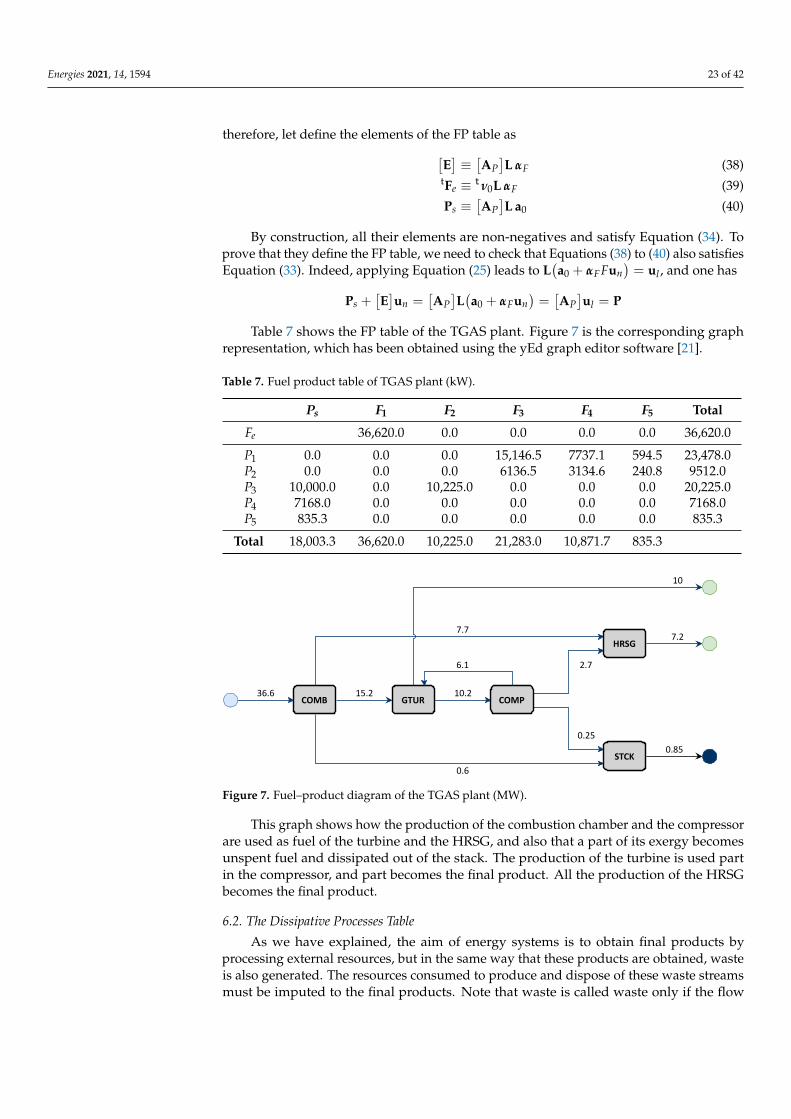
Table 7 shows the FP table of the TGAS plant. Figure 7 is the corresponding graphrepresentation, which has been obtained using the yEd graph editor software [21].

Table 7. Fuel product table of TGAS plant (kW).

Ps F1 F2 F3 F4 F5 Total

Fe 36,620.0 0.0 0.0 0.0 0.0 36,620.0

P1 0.0 0.0 0.0 15,146.5 7737.1 594.5 23,478.0P2 0.0 0.0 0.0 6136.5 3134.6 240.8 9512.0P3 10,000.0 0.0 10,225.0 0.0 0.0 0.0 20,225.0P4 7168.0 0.0 0.0 0.0 0.0 0.0 7168.0P5 835.3 0.0 0.0 0.0 0.0 0.0 835.3

Total 18,003.3 36,620.0 10,225.0 21,283.0 10,871.7 835.3

COMB GTUR COMP

HRSG

STCK

15.2

10

7.2

0.85

0.6

0.25

6.1

7.7

2.7

36.6 10.2

Figure 7. Fuel–product diagram of the TGAS plant (MW).

This graph shows how the production of the combustion chamber and the compressorare used as fuel of the turbine and the HRSG, and also that a part of its exergy becomesunspent fuel and dissipated out of the stack. The production of the turbine is used partin the compressor, and part becomes the final product. All the production of the HRSGbecomes the final product.

6.2. The Dissipative Processes Table

As we have explained, the aim of energy systems is to obtain final products byprocessing external resources, but in the same way that these products are obtained, wasteis also generated. The resources consumed to produce and dispose of these waste streamsmust be imputed to the final products. Note that waste is called waste only if the flow

Energies 2021, 14, 1594 24 of 42

crosses the system boundaries. Therefore, the system outputs split in two parts Ps = Pt +Pr,final products Pt, and the waste Pr, so that

Pt =[AP]

L aT (41)

Pr =[AP]

L aR (42)

where aT and aR are (`× 1) vectors, whose elements indicate if the streams group is a finalproduct or a waste, such that aT + aR = a0.

Just as there is a productive table for the processes, there is also a table for their waste.Let

[D]

be a (n× n) matrix, called a dissipative process table, where its elements dij representthe exergy dissipated by the i process, which has been produced by component j. Thismatrix verifies

Pr =[D]un (43)

tR = tun[D]

(44)

The dissipative table performs the same function as the waste table, described inprevious sections, at the process level, and could be obtained as[

D]≡[AP]

L αR =[AP]

αR (45)

The dissipative table[D]

represents the waste formation process of the system. Thisprocess follows the opposite direction to the production process and identifies where wastehas been produced. In the case of the TGAS example, we made the assumption that gaseswere generated in the combustion chamber, then the table has only one non-zero element:d5,1 = B9.

6.3. The Cost Equations for the Process Model

The Fuel–Product–Waste tables help to identify the cost formation process. Now, weneed to determine the production cost of processes. Let us consider the generalized costequations of the productive table

tCE = tC0 +tC αE + tCpαP (46)

tC = tC αS (47)tCF = tC αF (48)tCR = tC αR (49)

and the cost balance equation for the processes

CP = CF + CR + Z (50)

The generalized cost of the productive groups CE can be calculated as a function ofthe production cost of processes as

tCE =( tC0 +

tcP[AP])

L (51)

then, replacing Equation (51) into Equations Equations (48) and (49), and applying thedefinition of the FP table (38) leads to

tCF = tC0 LαF +tcP[E]

(52)tCR = tcP

[D]

(53)

substituting these equations into the cost balance Equation (50) leads to

tCP = tCe +tcP([

E]+[D])

(54)

Energies 2021, 14, 1594 25 of 42

where tCe =tC0 LαF +

tZ is a (n× 1) vector whose elements contain the cost of externalresources used in each process.

The above equation allows one to determine the production costs of processes CP.Once the production cost are obtained, applying Equation (51) the costs of the system flowscan be determined by means of

tC =( tC0 +

tCP αP)L αS (55)

Let be[C]

a (n + 1× n + 1) matrix whose elements Cij represents the cost of flowproduced by process i used as fuel to process j, including the environment process 0. Thismatrix is called cost table, and it is defined as

Cij =

Ce,j i = 0; j = 1, . . . , ncP,i(Eij + Dij) i = 1, . . . , n; j = 1, . . . , ncP,i Ei0 i = 1, . . . , n; j = 0

(56)

In the next sections, we develop a general methodology to obtain analytical formulaefor the production costs that relate the global efficiency and the production costs with itsindividual components’ efficiency.

7. The Resource-Driven Model

The objective of the resource-driven model is to represent the thermoeconomic vari-ables of a system as a function of the external resources and the efficiency of the individualprocesses. Let us define the distribution coefficient yij ≡ Eij/Pi as the portion of theproduction of the j-th component used as resource in the i-th component.

Let 〈FP〉 be a (n× n) matrix whose elements are the distribution coefiecients, defined as

〈FP〉 ≡ P−1 [E], (57)

replacing Equation (57) into Equation (34) leads to

F = Fe +t〈FP〉P (58)

It shows how the fuel of each component is a linear function of the products that form it.Let 〈RP〉 (n× n) to be the matrix of waste distribution ratios ψij = Dij/Pi, defined as

〈RP〉 ≡ P−1 [D] (59)

replacing into the waste table definition Equation (44) leads to

R = t〈RP〉P (60)

7.1. Cost Equations in the Resource-Driven Model

In order to compute the production exergy cost, one can replace Equations (57) and (59)into cost balance Equations (52) to (54), leading to

tCF = tCe +tCP 〈FP〉 (61)

tCR = tCP 〈RP〉 (62)tCP = tCe +

tCP 〈FP〉+ tCP 〈RP〉 (63)

Therefore the production exergy cost could be computed as

tCP = tCe⟨P∗∣∣ where

⟨P∗∣∣ ≡ (Un − 〈FP〉 − 〈RP〉)−1, (64)

Energies 2021, 14, 1594 26 of 42

Note that the matrix operator⟨P∗∣∣ includes both information of production cost dis-

tribution 〈FP〉 and waste allocation 〈RP〉. Besides, the equation of direct exergy cost isgiven by

tP∗ = tFe⟨P∗∣∣ (65)

Once the exergy costs are calculated, the Fuel–Product cost table can be obtained fromEquation (56). Table 8 shows this table for the TGAS plant example. Note that the sum ofrows equals the sum of columns. The first row and column represent the environment. Thetotal resources entering the system, 36,620 kW, are distributed to the cost of final products:electricity: 18,011.7 kW; heat: 18,608.3 kW. The cost of electricity is 1.8 times the cost ofnatural gas, and the cost of heat is 2.59 times. The cost of waste gases F∗5 = 1429.7 kW ischarged to the combustor and redistributed to rest of processes. The cost of the stack gasesleaving the system is zero.

Table 8. Direct Exergy Cost fuel–product table for TGAS example.

F∗0 F∗

1 F∗2 F∗

3 F∗4 F∗

5 Total

P∗0 36,620.0 0.0 0.0 0.0 0.0 36,620.0

P∗1 0.0 0.0 0.0 24,547.2 12,539.1 963.4 38,049.7P∗2 0.0 0.0 0.0 11,881.4 6069.2 466.3 18,416.9P∗3 18,011.7 0.0 18,416.9 0.0 0.0 0.0 36,428.6P∗4 18,608.3 0.0 0.0 0.0 0.0 0.0 18,608.3P∗5 0 1429.7 0 0 0 0 1429.7

Total 36,620.0 38,049.7 18,416.9 36,428.6 18,608.3 1429.7

7.2. Production Cost Decomposition

The production cost of the processes can be calculated using Ëcrefeq:cprd, explainedin the previous section. It requires the fuel–product and waste allocation tables. To get abetter understanding of the cost formation process, it is necessary to break down the costinto the contributions of internal irreversibilities vmCe

P, and waste vmCrP.

Let 〈P∗| ≡ (Un − 〈FP〉)−1 be the base production cost operator, without consideringwaste allocation.

The matrix of waste distribution ratios can be written as 〈RP〉 = δ ·ψR, where ψ is a(r× n) whose elements are the waste distribution ratios ψij corresponding to the dissipativeunits (or the active rows of the 〈RP〉 matrix) and δR =

(ui1 , . . . , uir

)is a (n× r) matrix,

whose columns are the unit vector ui = (0, . . . , 1, . . . , 0) corresponding to the dissipativecomponent index i.

Therefore, applying the Woodbury formula, see Appendix B, we can obtain theproduction cost operator

⟨P∗∣∣, from the base production cost operator 〈P∗|, as follows:⟨

P∗∣∣ = 〈P∗|(Un +

⟨R∗∣∣)

where S ≡ (UD −ψ 〈P∗| δR)−1 is a (r × r) matrix, and

⟨R∗∣∣ ≡ δR · S ψ 〈P∗| is the waste

cost operator. Therefore, substitution into Equation Equation (64) leads to

CP = CeP + Cr

P (66)

where:

tCeP = tCe 〈P∗| (67)

tCrP = tCe

P⟨R∗∣∣ (68)

Energies 2021, 14, 1594 27 of 42

Equations (66) to (68) allows one to determine the production cost as the sum of thecontribution of process irreversibilities and waste allocation. First, we compute the baseproduction cost operator to determine the production cost due to internal irreversibilitiesCe

P. Once it is determined, the production cost due to waste is computed employing thewaste cost operator Equation (68).

This expression can also be written as

tCP =( tCe +

tCR)〈P∗|

and

tCR = tCe δR S ψ

where CR represents both the cost of waste allocated to each process and the equivalentresources required to abate the waste generated by each process. Therefore, the productioncost due to waste could be computed as

tCrP = tCR 〈P∗|

The cost decomposition values for TGAS example are shown in Table 9.

Table 9. Production direct exergy cost for TGAS example.

Process F∗ (kW) R∗ (kW) P∗ (kW) k∗P (kW/kW) k∗

P,e (kW/kW) k∗P,r (kW/kW)

COMB 36,620.0 1429.7 38,049.7 1.6207 1.5598 0.0609COMP 18,416.9 0.0 18,416.9 1.9362 1.8634 0.0728GTRB 36,428.6 0.0 36,428.6 1.8012 1.7335 0.0677HRSG 18,608.3 0.0 18,608.3 2.5960 2.4985 0.0975STCK 1429.7 0.0 1429.7 1.7116 1.6473 0.0643

8. The Demand-Driven Model

In the previous section, we studied the representation of the system’s thermoeconomicvariables as a function of its components’ efficiency, the distribution coefficients, and theexternal resources. The optimization and diagnosis analysis of a thermal system requiresstudying the productive structure’s behavior as a function of the total production ordemand objectives. This section presents an alternative representation that relates thethermoeconomic variables of the system with the total plant production, the efficiency ofits components, and a new type of parameter called junction ratio.

We define, in a analogous way to distribution coefficients, the junction coefficients qijas the portion of the resources of the j-th component coming from the i-th product.

qij =Eij

Fj

n

∑i=0

qij = 1

Let 〈PF〉 be a (n × n) matrix, so that[E]= 〈PF〉 F and qe is a (n × 1) vector, so

that Fe = F qe. Their elements qij = Eij/Fj, called junction ratios, represent the ratio ofproduction of process j used as fuel on process i. They verify

qe +t〈PF〉un = un (69)

Similarly, let 〈KP〉 be a (n× n) matrix, so that[E]= 〈KP〉 P and considering that κe

is a (1× n) vector, so one obtains that Fe = κe P. Their elements κij = Eij/Pj, are dubbed

Energies 2021, 14, 1594 28 of 42

technical coefficients or unit consumption ratios, and represent the amount of resourcesprovided by process j needed to obtain one unit of the process product i. They verify

〈KP〉 = 〈PF〉KD

ke = k qe

k = ke +t〈KP〉u

where k = diag(k1, . . . , kn), which verifies F = k P. Note that the unit consumption of theprocess i equals to the sum of its technical coefficients. Therefore, 〈KP〉 and ke contain theinformation about the efficiency of local components.

Replacing these matrices into Equation (33) leads to

P = Ps + 〈KP〉P (70)

and therefore: (Un − 〈KP〉

)P = Pt

By construction, 〈KP〉 is a productive matrix, therefore it has inverse |P〉 ≥ Un, andit verifies that

P = |P〉Ps where |P〉 =(Un − 〈KP〉

)−1

F = |F〉Ps where |F〉 = KD|P〉I = |I〉Ps where |I〉 = (KD −Un)|P〉

These formulas allow the fuel, product, and internal irreversibility of the system com-ponents to be related in terms of unit exergy consumption and system outputs, includingboth final products and waste.

On the other hand, let 〈KR〉 be a (n× n) matrix, so that[D]= 〈KR〉 P, whose elements

ρij = dij/Pj represent the waste streams generated by a process per unit produced. Bydefinition of the waste table, Equation (42) it leads Pr = 〈KR〉P, therefore

Ps = Pt + Pr = Pt + 〈KR〉P

and replacing into Equation (70), we get:

P = Pt + 〈KP〉P + 〈KR〉P

Therefore, we can relate the fuel, product, and irreversibility of the system componentsas a function of the final demand:

P =∣∣P⟩Pt where

∣∣P⟩ = (Un − 〈KP〉 − 〈KR〉)−1

F =∣∣F⟩Pt where

∣∣F⟩ = KD∣∣P⟩

I =∣∣I⟩Pt where

∣∣I⟩ = (KD −Un)∣∣P⟩

Note that production operators do not only depend on local unit consumption, butalso on waste generation ratios.

The total system resources can also be expressed, according to the definition of thetechnical coefficients, as follows:

FT =n

∑i=1

κ0i Pi

or in matrix notation:FT = κe P = κe |P〉Ps = κe

∣∣P⟩Pt (71)

depending on whether waste is considered or not.

Energies 2021, 14, 1594 29 of 42

For example, the total fuel of the TGAS system could be written in terms of their unitlocal consumptions, and the system outputs

FT =κ01(κ13 B7 + κ14 B8)

1− κ23 κ32 − κ15 ρ51

The effect of waste on total fuel consumption is given by the term κ15 ρ51.Finally, the external irreversibilities of the system Pr, could be also related to its final

demand, by means of the relationship

Pr =∣∣R⟩Pt where

∣∣R⟩ = 〈KR〉∣∣P⟩

In the previous section, we can obtain the production operator∣∣P⟩ from the base

production operator |P〉. In a similar way, the waste generation ratios matrix could bedecomposed in the form 〈KR〉 = δR · ρ, where ρ is a (r× n) corresponding to the non nullrows of 〈KR〉matrix. Applying the Woodbury formula, see Appendix B, leads to∣∣P⟩ = |P〉(Un + δRSρ|P〉) (72)

where S ≡ (Ur − ρ|P〉δR)−1 is a (r× r) matrix, and the waste operator is computed as∣∣R⟩ = δR S ρ|P〉 (73)

Cost Equations in the Demand-Driven Model

Dividing both sides of the cost balance (64) by P, it could be written in terms of thedemand-driven model as

tcP = tCeP−1 + tcP(〈KP〉+ 〈KR〉

)therefore, the unit exergy cost of product can be obtained as

cP = tce∣∣F⟩ (74)

where ce = F−1 Ce is a n× 1 vector, whose elements are the external resources costs perunit of fuel consumed in the process. The direct unit exergy cost is calculated as

k∗P = t∣∣F⟩qe =

t∣∣P⟩κe

Applying Equations (72) and (73) to (74) leads to

cP = tce |F〉(Un +

∣∣R⟩) (75)

In the same way as the resource-driven model, the unit production cost could bedecomposed into the amount due exclusively to ce

P irreversibilities plus the amount due towaste cr

P .

ceP = ce |F〉

crP = ce

P∣∣R⟩

The cost balance of the system could be written from Equation (71) as

FT = k∗P,e Ps = k∗P Pt

Table 9 shows the production cost of the processes of the TGAS plant. As can be seen,the production cost due to waste allocation represents near 4% of the total production costof the system.

The values of k∗P,r show the impact of waste on the final production cost. However,waste could also be partially used in other processes, i.e., recycled. The limit of these costs

Energies 2021, 14, 1594 30 of 42

is given by k∗P,e. Exergy cost theory could be applied to Industrial Ecology [22], which canhelp to solve several significant problems such as the identification of integration, efficiencyimprovement, quantification of benefits obtained by integration, or determination of pricesbased on physical roots [23].

We have explained two different ways of evaluating the production cost—the resource-driven and the demand-driven model—as functions of the components’ efficiencies, theexternal resources, and the distribution or junction coefficients. The demand-driven modelis used in local optimization and diagnosis. Meanwhile, the resource-driven model is usedin processes integration and waste cost allocation.

The information in the resource-driven model representation has the direction of theproduction process. If the external resources are known, the remaining thermoeconomicproperties can be evaluated. The demand-driven model representation uses an equivalentlogical structure, but the information has the opposite direction. If we know the demand orthe final products of a plant, it is possible to determine the resources needed to obtain anyinternal product and their unit costs. Both representations are complementary and figureout the complete picture of the production process and cost formation. The operators ofboth models could be related by using the relationships[

E]= P 〈FP〉 = 〈KP〉 P[

R]= P 〈RP〉 = 〈KR〉 P

then, production operators are similar matrices, with the same values in the diagonal, andthey are related by

〈P∗| = P−1 |P〉 P (76)

This formulation has been widely applied in different thermoeconomic fields like costaccounting [24–27], local optimization [28,29], and diagnosis of energy systems [30–32].

9. The Irreversibility Cost Formula

As explained above, the exergy cost depends on the cost of external resources. If noexternal evaluation is considered, the exergy cost of the flows entering the system is equal totheir exergies. This indicates that, once the system boundaries are defined, the productioncosts only take into account the internal and external irreversibilities of the system. Thedirect exergy cost does not take into account physical or economic interactions with othersystems and only depends on the efficiency of the local components, and thus on the localirreversibilities.

In a previous section, we have obtained the relationship (32) between the cost of flowsand the irreversibilities of processes. As irreversibility is a property of processes, it isinteresting to relate it to the cost of production.

Consider the direct exergy cost Equation (65) of the resources-driven model:

P∗ = t〈P∗| Fe,

On the other side, from Equation (58), the exergy of resources could be expressed as

Fe = P + I− t〈FP〉P,

using the relation R = t〈RP〉P, and replacing into Equation (65), leads to

P =(P− t〈FP〉P− t〈RP〉P + R + I

) t⟨P∗∣∣,therefore, by definition of operator

⟨P∗∣∣, we get

P∗ = P + t⟨P∗∣∣(I + R)

(77)

Energies 2021, 14, 1594 31 of 42

It means that the cost of exergy production is equal to its exergy plus all the internalirreversibilities and waste generated by each process generated to obtain this product. Thematrix operator

⟨P∗∣∣ is the footprint of the exergy destruction of the energy systems I + R.

One can prove that⟨P∗∣∣ ≥ Un, therefore Equation (77) could be expressed as

P∗ = F + R + t(⟨P∗∣∣−Un)(

I + R)

therefore P∗ ≥ F + R, and it follows that the unit production cost of a process is alwaysgreatest or equal to the unit local consumption:

k∗P,u ≥ ku + ρu = 1 +Iu + IR

uPu

.

A similar expression from unit direct exergy can be obtained by applying Equation (76)to the irreversibility cost formula Equation (77):

tkP = tu(Un +

∣∣I⟩+ ∣∣R⟩) (78)

This equation is an alternative to computing the unit exergy production cost of pro-cesses, decomposed by the contribution of irreversibilities and waste. The irreversibilityoperator could be computed from the base operator as∣∣I⟩ = |I〉(Un +

∣∣R⟩) = |I〉+ |I〉 δR · S ρ|P〉

where |I〉 δR (n× r) are the columns of the irreversibility operator corresponding to thedissipative units and S ρ|P〉 (r× n) are the active rows of the waste operator

∣∣R⟩.The irreversibility cost formula makes it possible to explain the process of product cost

formation of an energy system and trace the destruction of exergy from external resourcesto final products. By construction, this formula is only valid for the direct cost of exergy.Next, an extension of this formula is presented, taking into account physical and economicinteractions, and not only the exergy of external resources.

Equation (78) can be extended to include the cost of external resources by introducingthe irreversibility cost factor vector c∗e (1× n) such as

cP = c∗e(Un +

∣∣I⟩+ ∣∣R⟩) (79)

In order to determine the irreversibility cost factor independently of the exergy cost,we take the following relationship:

Un +∣∣I⟩+ ∣∣R⟩ = (Un − 〈KP〉 − 〈KR〉+ KD −Un + 〈KR〉)

∣∣P⟩ = (Un − 〈PF〉)∣∣F⟩,

combining with Equations (74) and (79), we get the following system of linear equations:

tce =tc∗e(Un − 〈PF〉

), (80)

Equation (80) allows one to determine the irreversibility cost factor from the internalproductive structure 〈PF〉 and the cost of external resources. Note that, in the case of directexergy cost, ce = qe, and by definition of exergy junction ratios, the irreversibility cost ratioc∗e = tu, corresponds to the expression of Equation (78).

The irreversibility cost factor c∗e obtained from Equation (80) can be interpreted asthe minimum costs for a given value of external resources, obtained when one makes thehypothesis that the system has no internal and external irreversibilities, i.e., Kn = Un and〈KR〉 = 0.

If we want to distinguish the exergy cost due to internal irreversibilities from the costdue to waste allocation, the former can be obtained directly from Equation (79), taking〈KR〉 equal to zero.

tceP = tc∗e

(Un + |I〉

)

Energies 2021, 14, 1594 32 of 42

The generalized irreversibility cost formula allows for a breakdown of the contributionof external resources to exergy destruction. The irreversibility cost factor plays two rolesin the formula: First, it is the cost of the inputs to the system used in each process, i.e., itaccounts for irreversibilities outside the system boundaries, and second, it is the cost ofexergy destruction of the processes within the boundaries.

To illustrate the application of this formula, we will calculate the thermo-ecologicalcost footprint for the TGAS plant. The system boundaries have been extended to considerthe extraction, processing, and transport to the plant of natural gas, as well as the reductionin CO2.

The following assumptions are made to calculate the TEC of external resources [17]:a value of 1.082 kW/kW NG (domestic Natural Gas including CO2 emissions) for the unitcost of NG, and a value of 0.238 kW/kW NG for the cost of CO2 abatement. Finally, wealso include the depreciation, maintenance, and operating costs of the plant’s processesZ. They have been calculated from the work in [33] and converted to energy units using anatural gas price of 20 MWh as the conversion factor. In this example, the costs of reducingCO2 are considered as an external cost that is allocated to the stack process. These valuesare summarized in Table 10.

Table 11 and Figure 8 show the TEC costs of the TGAS plant using the external resourcecost values from the Table. One can see the importance of CO2 emissions.

In the case of direct exergy cost, the unit resource cost is one. Meanwhile, in the caseof thermo-ecological costs, the unit resource cost is greater than one. Rows I represent thecontribution of the irreversibility of the i-th process to the unit cost, and row R represents thecontribution of the external irreversibility of both hot gases and CO2 emissions. The exergycost of the flue gas is 12.8 times the exergy of the dissipated gases. This cost is redistributedto the final products of the plant and accounts for about 20% of the total cost.

Table 10. Estimation of external resources costs (kW) for TGAS Plant.

COMB COMP GTURB HRSG STCK

Z 141.92 1216.38 1662.40 1076.51 8715.56Ce 39623 0 0 0 0

Table 11. Thermoecological production cost decomposition on TGAS Plant (kW/kW).

COMB COMP GTURB HRSG STCK

c∗e 1.0859 1.3628 1.2438 1.2647 11.5998

I1 0.6078 0.7262 0.6755 0.9736 0.6419I2 0.0000 0.1516 0.0460 0.0663 0.0437I3 0.0000 0.1038 0.0966 0.0454 0.0299I4 0.0000 0.0000 0.0000 0.6535 0.0000R 0.4553 0.5439 0.5060 0.7293 0.4808

Total 2.1490 2.8883 2.5679 3.7328 12.7961

Energies 2021, 14, 1594 33 of 42

1.0

1.5

2.0

2.5

3.0

3.5

4.0

COMB COMP GTRB HRSG

Uni

t Cos

t (kW

/kW

)

ENV COMB COMP GTRB HRSG STCK

Figure 8. Generalized irreversibility–cost decomposition graphics for TGAS plant.

10. Methods for Cost Allocation of Waste

As we have seen, there is not a general criterion to allocate the cost of the systemwaste. It depends on the type and the nature of the waste flows. For example, in thecase of the heat dissipated in the condenser of a Rankine cycle, we can distribute the costproportionally to the entropy generated by each process. Meanwhile, the combustiongases eliminated by the combined cycle stack are allocated to the combustion process.The allocation of waste costs should be based on the following criteria [34]:

(a) The cost of waste must be charged to the productive units that have generated it. Here,it is essential to establish a conceptual difference between the exergy of waste and itscost. Costs also encompass exergy consumption to be involved in the elimination ofthe system waste. Therefore, it is the cost, not its exergy, that is of actual interest. Thisraises a need that is expressed in the second premise.

(b) It is needed to identify the process of cost formation of waste. This process is parallel tothe process of production cost formation because waste is eliminated in the dissipativecomponents, but formed along with the productive processes.

(c) The responsibility of a productive component for waste generation lies in its contribu-tion to the formation cost of waste.

To identify waste flows at the process level, it is necessary to relate each waste flowwith the physical and chemical processes taken place in dissipative units. We must defineas many dissipative units as waste flows. Dissipative units are defined in such a waythat the output product stream is a waste flow, and input fuel streams are these flowsthat one wants to be eliminated and the resources required to do that. The irreversibilitycarriers allow one to identify the origin, path, and end of waste streams and then build thedissipative table

[D].

The FP table helps to explain the cost formation process of system products and waste.In this section, we will propose four methods to obtain the values of the elements ψri ofmatrix 〈RP〉, based on the productive structure information at the processes level:

Method A (Exergy distribution): It is directly based on the information provided by theFP table [12]. Then, we consider the values of the table

[D]

as the exergy provided bythe component j that is disposed in the dissipative unit r:

ψrj =Eir

Fr − E0r, r ∈ VD, j ∈ VP (81)

This method looks for the immediate cause and distributes the waste’s costs to thecomponents that have produced it directly and in proportion to their exergy.

Energies 2021, 14, 1594 34 of 42

The next methods are based on the contribution of the productive units to the directexergy cost of waste. As the unit production cost has not been determined yet, wewill consider the value of the unit cost due to irreversibilities ce

P,i and the values of theproduction cost operator |P〉 instead. In all cases, direct exergy cost is considered.

Method B (Exergy cost distribution): This allocation method is similar to the previousone, but it distributes the cost in proportion to their exergy cost instead of exergy.Note that in many cases, the exergy of waste is not relevant but their cost. Accordingto (52), if r ∈ VD is a dissipative unit,

CeF,r = C0r +

n

∑j=1

ceP,j Ejr

Equation (52) means that the production cost is equal to the sum of the cost of exergystreams eliminated in this dissipative unit, and the waste cost must be allocated to theprocesses have produced them.

ψrj =cP,jEjr

CeF,r − C0r

, r ∈ VR, j ∈ VP (82)

Method C (Irreversibility–cost distribution): A more complex method considers the com-plete chain of production cost [34]. It is based on Equation (77):

CeP,r = Pr + ∑

j∈VP

Ijπ∗jr

where π∗jr is the corresponding element in matrix 〈P∗|. Decomposing the exergy ofwaste by its individual contributions, we get

CeP,r = C0r + ∑

j∈VP

Ejr + Ijπ∗jr

therefore, the waste cost distribution parameters could be defined as

ψrj =Ejr + Ijπ

∗jr

CeP,r − C0r

, r ∈ VD, j ∈ VP (83)

This method combines the first one with the irreversibility cost formula, to distributethe cost according to the irreversibility carriers of waste streams. This method takesinto account the full path of the waste cost formation.

Method D (Resources distribution): The last proposed method is based on the idea ofcost definition, i.e., the cost of waste is the amount of external resources spent to pro-duce it, and then allocate the cost of waste proportionally to the resources consumed:

CeP,r =

n

∑j=1

E0j π∗jr

and the waste distribution parameters are defined as

ψrj =E0j π∗jr

CeP,r

, r ∈ VR, j ∈ VP (84)

This method allocates the waste cost to the overall system according to the proportionof each external resource used to produce the waste. This method is used in the TGASexample. It is equivalent to increasing the cost of natural gas by a factor of 1.0609 (6%),

Energies 2021, 14, 1594 35 of 42

determined by calculation of CR, and therefore the cost of all streams is increased bythe same factor.

Table 12 shows the values of waste costs allocated to each process CR and the unitproduction cost of each component due to waste for each of the proposed methods. The totalcost of waste and the unit production cost of final products are the same for methods one,two, and four, and the method based on irreversibility carrier allocation is slightly different.

Table 12. Waste allocation cost using process thermoeconomics methods.

Method A Method B Method C Method DProcess CR cr

P CR crP CR cr

P CR crP

COMB 1017.5 0.0433 951.3 0.0405 1130.4 0.0481 1429.7 0.0609COMP 412.2 0.1161 478.4 0.1231 278.0 0.1025 0.0 0.0728GTUR 0.0 0.0677 0.0 0.0677 20.9 0.0682 0.0 0.0677HRSG 0.0 0.0975 0.0 0.0975 0.0 0.0968 0.0 0.0975STCK 0.0 0.0643 0.0 0.0643 0.0 0.0638 0.0 0.0643

As discussed throughout this paper, the formation of the cost of waste is parallel to theproduction cost. The process model can help provide methods for the first approximationto the allocation of the waste cost, but in general, the construction of waste tables is usuallyexternal to calculating production costs. In this line, several researchers have proposeddifferent waste cost allocation methods in recent years [35–38].

11. Recycling Saving Accounting

As long as these residual streams have exergy, they can be retrieved in recovery units;it is the case of the heat recovery steam generator (HRSG) in the TGAS example. Theserecovery units are integrated into the plant and constitute productive units that, insteadof expending exergy to dispose of waste, their exergy is recovered to produce some otherby-product. In the case of the TGAS plant, the recovery unit produces saturated steam.

The potential savings from waste recycling can be estimated if one knows the produc-tion costs due to external irreversibilities. The production cost due to waste Cr

P indicatesthe maximum amount of resources that could be saved if waste were recycled.

It is well known that not all waste could be saved for technical and economic reasons,but through the process integration and Industrial Symbiosis [39], it is possible that othersystems convert this waste into resources. The exergy cost theory allows evaluating the costof waste, accounting for the resources savings and providing fair prices to waste becomingby-products.

Let σi to be the percentage of waste i that could be reused or recycling ratio, in theseconditions Ps,r = σr Pr,i. Therefore, the waste allocation matrix can be recalculated as

βσR = (Ur − σ)βR

where σ is a (r × r) diagonal matrix whose elements contain the recycling ratios of thesystem. By introducing this matrix, it is possible to recalculate the waste operators, as

Sσ =(Ur − βσ

R〈P∗|δR)−1⟨

R∗∣∣σ= Sσ βσ

R〈P∗|

and the production cost as a function of the recycling ratios is given by

CP = CeP(Un +

⟨R∗∣∣σ

)(85)

The waste rule in a recovery unit is the with Cost Conservation rule. The exergy cost offinal waste plus that of the obtained by-product is the cost of entering waste plus the spent

Energies 2021, 14, 1594 36 of 42

fuel to abate them. This reduces the cost of final waste, then at the end of the analysis, onlythese final waste costs add to the final costs of the plant product(s). Clearly, recovering theexergy of waste saves exergy and reduces the cost of products.

Consider the TGAS plant again, and suppose there is not an HRSG to recover partof the escape gases of the turbine. In this situation, the cost of electricity will be 3.662 kWof natural gas for one kW of electricity produced. Moreover, we have lost 11.7 MW in hotgases leaving the gas turbine.

The cost of electricity and flue gas as a function of recycling rates can be obtainedusing the formulation introduced in this section, as shown in Figure 9. The unit cost ofelectricity is 3.662 if turbine escape gases are not recovered. It is near two times more thanthe turbine with heat recover steam generator, that recover 92.86% of escape gases.

The unit cost of electricity as function of the recycling ratio σ is

k∗P,3(σ) =κ01 κ13

1− κ23 κ32 − σ κ15 ρ51

This function is not linear, and its slope is decreasing, which means that the exergysaving decreases when the recirculation ratio increases. If we want to recover more than90% of the energy from the exhaust gases, the decrease in the unit cost of electricity is notrelevant, and possibly the investment cost to do so is much higher than the natural gassavings obtained.

As shown in this simple example, the use of recycling or recovering units as productiveprocesses is a key practice for energy saving. The work in [40] shows another example ofProcess Thermoeconomics applying to recycling saving by system integration.

1

1.5

2

2.5

3

3.5

4

0 10 20 30 40 50 60 70 80 90 100

Uni

t Cos

t (kW

/kW

)

Recycling Ratio (%)

Electricity Gases

Figure 9. Recycling saving graph for the TGAS plant.

12. Conclusions

This paper reviews the fundamentals of the Exergy Cost Theory, an energy costaccounting methodology for assessing physical costs that incorporates both the productionof products and their associated waste. Besides, a mathematically and computationallyuseful formulation is presented, which will allow the practitioner to carry out studies onproductive systems regardless of their structural complexity.

The process of waste cost formation is presented from a thermodynamic perspectivethat contrasts with the conventional economists’ approach. It is proposed to consider wasteas external irreversibilities whose origin is in plant processes.

We propose to generalize the idea of waste, and consequently we have created a theoryto evaluate its cost in any production process. Waste is an unwanted effluent of matter orenergy, which leaves the plant and will sooner or later dissipate into the environment. It isclear that waste has exergy, as its temperature, pressure, concentration, or composition

Energies 2021, 14, 1594 37 of 42

differs from the same properties of the environment. Therefore, waste can be utilizedbefore going outside through the use of recovery units. However, if this waste cannotbe recovered, it is necessary to reduce their exergy using dissipation units. Logically, awaste will cease to be waste when it reaches complete thermodynamic equilibrium withits environment.

The conventional classification [41] of waste as solid waste and emissions as gaseouswaste, wastewater, particulate matter, noise, and emissions of different wavelengths(i.e., pollutants) does not make sense from the point of view of thermodynamics. Theyare all outflows that give rise to external irreversibilities. Moreover, they are inherent toproduction. All production has its associated waste. Waste is generally more voluminousand entropically complex than the manufactured products.

The current perception of the effects of waste on climate change, water pollution,the constant growth of landfills, and the consequent depletion of raw materials has led toscientific attention being paid to its minimization and abatement and the internalization ofits costs. Thus, prices should reflect the resources consumed and the external impact ofwaste generation.

This mindset change leads to a revision of the current theories of optimization anddiagnosis of industrial processes. For example, the definition of process efficiency mustreflect both internal and external irreversibilities.

ku =Fu + Ru

Pu= 1 +

Iu + IRu

Pu

The objective function to be minimized is the production cost plus the combinedminimization of waste and its associated abatement costs, both inside and outside theproduction plant’s boundaries. Optimization of production processes should not use costexternalization. Unfortunately, cost externalization is, and has been, a common practice in theeconomies of developed countries and, in general, it is an economic practice that transfersthe costs of external impacts to society, to developing countries or future generations.

The main contribution of the new model presented in this article is the integrationof the different methodologies derived from ECT with the productive linear models ofInput–Output analysis. The cost equations of ECT, the characteristic equations of StructuralTheory, and the formulation of Symbolic Exergoeconomics can be obtained from theproduction structure table.

Furthermore, it allows proving the existence, uniqueness, and positiveness of thesolution to the exergy cost allocation problem in a mathematically rigorous way. It providesa set of numerical procedures and general formulae, valid for any state of the system, whichsolely depends on the productive structure and its interaction with the environment. Theyserve as a guideline to develop software for thermoeconomic analysis of energy systems.The TGAS plant results illustrating the methodology of this paper have been obtainedusing TAESS (Thermoeconomic Analysis of Energy System Software). It is freely availableon the web site [42].

As a summary, the following algorithms and formulae are introduced:

• The Fuel–Product table Equations (38)–(40).• Internal and external cost decomposition. Both direct or generalized exergy cost

Equations (66)–(68)• The Fuel–Product cost table Equation (56)• Irreversibility-cost formula, both for direct and generalized costs Equations (79)

and (80).• Cost of physical flows. The same tables that in the case of processes can be obtained

Equation (55).

All thermoeconomic or exergoeconomic theories should take this new formulationinto account because they use a partial view of the Second Law by concentrating theirdiscussions on internal irreversibilities and their impact on the other components that canbe located within the production structure. Parallel to the product cost formation process,

Energies 2021, 14, 1594 38 of 42

there is a waste cost formation process. For this purpose, the concept of irreversibility carrierhas been defined, which identifies the origin, transfer, recovery, abatement, and disposal ofa waste output stream. As the physical waste leaves the plant, the waste cost is added backto the final production cost of the plant. This process is called cost internalization.

Another concept that has been outlined and should be developed is the pinch point ofwaste recoverability. It is essential to know that as the generalized force gradients relativeto the temperature, pressure or chemical potentials of a waste stream approach thoseof the environment, the exergy transfer kinetics, and thus the exergy recoverability ofwaste, decrease to zero. If one looks at Figure 9, every time a percentage of the waste isrecycled, the total system’s efficiency improves further. However, when the proportionof waste recycling increases, efficiency does not increase linearly. The production cost ofthe gas turbine as a function of recycling gases is convex, i.e., the exergy savings at thebeginning of the recycling process are quite remarkable. However, as one approaches itstheoretical limit—the reference environment, the exergy saving nullifies. This means thateach additional increase in recycling corresponds to a smaller efficiency gain. Similarly,complete waste abatement or full exergy recovery is too costly and yields low results.

In fact, this is the law of diminishing returns governed by entropic behavior. Froma global point of view, our economic system will never wholly reduce all its pollution.Pollutants can be minimized and diluted but not avoided. Therefore, neither the toxicity tolife nor the degradability of the environment will disappear. However, low doses lengthenthe deterioration time. The theory developed here allows explaining mathematically andphysically this type of reflection.

Author Contributions: Conceptualization, A.V. and C.T.; methodology, C.T. and A.V.; validation, A.V.and C.T.; writing—original draft preparation, C.T.; writing—review and editing, C.T.; supervision,A.V. All authors have read and agreed to the published version of the manuscript.

Funding: This research received no external funding.

Institutional Review Board Statement: Not applicable.

Informed Consent Statement: Not applicable.

Conflicts of Interest: The authors declare no conflict of interest.

NomenclatureScalars

n Number of system processesm Number of system flows` Number of productive groupsr Number of dissipative processesB Exergy of a flow (kW)C Generalized exergy costc Unit generalized exergy costE Exergy of a productive group (kW)F Exergy of a fuel stream (kW)I Internal irreversibilities of a process (kW)IR External irreversibilities of a process (kW)k Unit consumption (kW/kW)L Exergy of local Loses (kW)P Exergy of a product stream (kW)q Bifurcation ratioR Exergy of waste allocated to a process (kW)Sg Generated Entropy (kW/K)

Energies 2021, 14, 1594 39 of 42

y Bifurcation ratioZ Cost associated to a processψ waste allocation ratioρ waste generation ratioσ Recycling ratio of waste

Vectors and Matrices

a0 Adjacency matrix of system outputs (`× 1)[AE]

Adjacency matrix of input flows of productive groups (m× `)[AF]

Adjacency matrix of fuel streams of processes (`× n)[AP]

Adjacency matrix of product streams of processes (n× `)[AR]

Adjacency matrix of waste streams of processes (`× n)[AS]

Adjacency matrix of output flows of productive groups (`×m)[D]

Dissipative process table[E]

Fuel–Product table〈A〉 Productive matrix of the system (`× `)

〈FP〉 Matrix of bifurcation ratios (n× n)〈KP〉 Matrix of unit consumptions (n× n)〈KR〉 Matrix of waste generation ratios (n× n)〈PF〉 Matrix of junction ratios (n× n)〈RP〉 Matrix of waste allocation ratios (n× n)〈X∗| Generic base operator cost matrix for resources–driven model (n× n)⟨

X∗∣∣∣ Generic operator cost matrix for resources–driven model (n× n)

|X〉 Generic base operator matrix for demand–driven model (n× n)∣∣X⟩ Generic operator matrix for demand–driven model (n× n)un Unitary vector (n× 1)Un Identity matrix (n×m)

ν0 Vector of exergy of external resources (`× 1)ω0 Vector of exergy of system outputs (`× 1)

Sets

B Set of system flowsL Set of system productive groupsR Set of system waste streamsV Set of system processesEl Set of input flows of the productive group lSl Set of output flows of the productive group lFu Set of fuel streams of process uPu Set of product streams of process u

Subscripts, superscripts and accents

t Transpose matrix or vectorˆ Diagonal matrix* Related to exergy costs0 Related to environmente Related to inputF Related to fuelP Related to product

Energies 2021, 14, 1594 40 of 42

R Related to wasteS Related to system outputT Related to total or final production

Appendix A. Productive Matrices

Very often, problems in the biological, physical, and social sciences can be reduced toproblems involving matrices which, due to certain constraints, have some special structure.One of the most common situations is where a square matrix has non-positive off-diagonaland positive diagonal entries [43]. Such matrices appear in economic input–output produc-tion models [16].

A square matrix M is said to be diagonal dominant if for every row of the matrix,the magnitude of the diagonal entry in a row is larger or equal than the sum of the off-diagonal entries

|aii| ≥ ∑i 6=j

∣∣aij∣∣ 1 ≤ i ≤ n

and it is called strictly diagonal dominant if it at least exists a row i0 such as

∑j

∣∣ai0 j∣∣ > 0

A positive square matrix A is said to be productive if there exist a non-negative vectorx such that x ≥ A · x.

In a linear production model, the elements aij of matrix A represent the amount ofproduction of activity j required to produce one unit of the production of activity i.

The key property of a linear production model is the fact that if such a model isproductive then it is capable of producing any positive output vector y, that is, if amatrix A is productive then for any y ≥ 0, the equation (U−A) x = y has a uniquenon-negative solution.

Let A to be a positive square matrix, then the following conditions are equivalent:

(a) A is productive.(b) There exists a positive diagonal matrix D, such that D−1(U−A)D is strictly diagonal

dominant.

(c) limk→∞

Ak = 0, and (U−A)−1 = U +∞

∑k=1

Ak

(d) U−A is inverse positive. That is, L = (U−A)−1 exists, and L > U.(e) The maximum of the moduli of the eigenvalues of A, ρ(A) ≤ 1

A matrix M = U−A satisfying these conditions is called M-Matrix.

Appendix B. The Woodbury Formula

Given a regular matrix A and its inverse, L ≡ A−1, assume that several elements of Aare changed, i.e., aij = aij − ∆aij, producing A = A− ∆A, therefore the new inverse matrixA−1 can be found by adjusting the known matrix A−1, by means of

L ≡ (A− ∆A)−1 = L(UD − ∆A L)−1 (A1)

Suppose now, like in the previous example, that changes in matrix A involve only afew rows (or columns) i1, . . . , ir. Let α = {ui1 , . . . , uir} a (n× r) matrix, whose columns arethe unit vector ui correspond to changed rows, and let β a (r× n) matrix whose rows arethe changing rows of A and ∆A = α · β.

Energies 2021, 14, 1594 41 of 42

Therefore, supposing αβL and βLα are productive matrices, then applying the seriesproperty to Equation (A1), we get

(Un − αβL)−1 = Un + α

[Ur +

∞

∑k=1

βLα

]βL = Un + α · SβL

where S = (Ur − βLα)−1 is a (r× r) matrix; therefore,

L = L(U + α · SβL) = (U + Lα · Sβ)L = L + Lα · SβL (A2)

This expression is known as the Woodbury formula [44]. Note that Lα is a (n× r) matrixwhich columns are the i1, . . . , ir columns of matrix L, and SβL is a (r × n) matrix. Theproduct of these two matrices is the update of the inverse matrix L.

If r << n, this formula is an important improvement for the computation of (A− ∆A)−1.Instead, to calculate again the inverse of a (n× n) matrix, you only need to compute S, theinverse of a (r× r) matrix, and some additional matrix multiplications.

References1. Valero, A.; Lozano, M.; Muñoz, M. A general theory of exergy saving. Part I: On the exergetic cost. Comput. Aided Eng. Energy

Syst. Second Law Anal. Model. 1986, 3, 1–8.2. Lozano, M.; Valero, A. Theory of the exergetic cost. Energy 1993, 18, 939–960. [CrossRef]3. Tsatsaronis, G.; Winhold, M. Exergoeconomic analysis and evaluation of energy-conversion plants-I. A new general methodology.

Energy 1985, 10, 69–80. [CrossRef]4. Keshavarzian, S.; Rocco, M.V.; Gardumi, F.; Colombo, E. Practical approaches for applying thermoeconomic analysis to energy

conversion systems: Benchmarking and comparative application. Energy Convers. Manag. 2017, 150, 532–544. [CrossRef]5. Moran, M., Fundamentals of Exergy Analysis and Exergy-Aided Thermal Systems Design. In Thermodynamic Optimization of

Complex Energy Systems; Bejan, A., Mamuth, E., Eds.; Kluwer Academic Publishers: Dordrecht, The Netherlands, 1999; pp. 73–92.6. Lazzaretto, A.; Tsatsaronis, G. SPECO: A systematic and general methodology for calculating efficiencies and costs in thermal

systems. Energy 2006, 31, 1257–1289. [CrossRef]7. Frangopoulos, C. Thermo-economic functional analysis and optimization. Energy 1987, 12, 563–571. [CrossRef]8. Szargut, J. Exergy Method: Technical and Ecological Applications; WIT Press: Southampton, UK, 2005.9. Sciubba, E. Extended exergy accounting applied to energy recovery from waste: The concept of total recycling. Energy 2003,

28, 1315–1334. [CrossRef]10. Gonzalez, A.; Sala, J.; Flores, I.; Lopez, L. Application of thermoeconomics to the allocation of environmental loads in the life

cycle assessment of cogeneration plants. Energy 2003, 28, 557–574. [CrossRef]11. Cecchin, A.; Salomone, R.; Deutz, P.; Raggi, A.; Cutaia, L. Relating Industrial Symbiosis and Circular Economy to the Sustainable

Development Debate. In Industrial Symbiosis for the Circular Economy: Operational Experiences, Best Practices and Obstacles to aCollaborative Business Approach; Salomone, R., Cecchin, A., Deutz, P., Raggi, A., Cutaia, L., Eds.; Springer International Publishing:Cham, Switzerland, 2020; pp. 1–25. [CrossRef]

12. Torres, C.; Valero, A.; Rangel, V.; Zaleta, A. On the cost formation process of the residues. Energy 2008, 33, 144–152. [CrossRef]13. Diestel, R. Graph Theory; Springer: Berlin, Germany, 2017; [CrossRef]14. Gale, D. The Theory of Linear Economic Models; The University of Chicago Press: Chicago, IL, USA, 1960.15. Valero, A.; Valero-Delgado, A. Thanatia: The Destiny of the Earth’s Mineral Resources;World Scientific: London, UK, 2014. [CrossRef]16. Miller, R.E.; D.Blair, P. Input-Output Analisis. Foundations and Extensions, 2nd ed.; Cambridge University Press: Cambridge,

UK, 2009.17. Usón, S.; Kostowski, W.J.; Stanek, W.; Gazda, W. Thermoecological cost of electricity, heat and cold generated in a trigeneration

module fuelled with selected fossil and renewable fuels. Energy 2015, 92, 308–319.18. Torres, C. Symbolic Thermoeconomic Analysis of Energy Systems. In Exergy, Energy System Analysis and Optimization;

Frangopoulos, C., Ed.; Eolss Publishers: Oxford, UK, 2009; Volume 2, pp. 61–81.19. Valero, A.; Usón, S.; Torres, C.; Stanek, W. Theory of exergy cost and thermo-ecological cost. In Thermodynamics for Sustainable

Management of Natural Resources; Stanek, W., Ed.; Springer: Cham, Switzerland, 2017; Chapter 7. [CrossRef]20. Valero, A.; Torres, C. Algebraic Thermodynamic Analysis of Energy Systems; American Society of Mechanical Engineers, Advanced

Energy Systems Division (Publication) AES: New York, USA, 1988; Volume 7, pp. 13–23.21. yWorks. yEd Graph Editor. Available online: https://www.yworks.com/products/yed (accessed on 18 February 2021).22. Ayres, R.; Ayres, L. Industrial Ecology: Towards Closing the Material Cycle; Edward Elgar Publishing: Northampton, MA, USA, 1996.23. Valero, A.; Usón, S.; Torres, C.; Valero, A. Application of thermoeconomics to industrial ecology. Entropy 2010, 12, 591–612.

[CrossRef]

Energies 2021, 14, 1594 42 of 42

24. Keshavarzian, S.; Gardumi, F.; Rocco, M.V.; Colombo, E. Off-Design Modeling of Natural Gas Combined Cycle Power Plants:An Order Reduction by Means of Thermoeconomic Input–Output Analysis. Entropy 2016, 18, 71. [CrossRef]

25. Picallo, A.; Escudero, C.; Flores, I.; Sala, J.M. Symbolic thermoeconomics in building energy supply systems. Energy Build. 2016,127, 561–570. [CrossRef]

26. Leiva-Illanes, R.; Escobar, R.; Cardemil, J.M.; Alarcón-Padilla, D.C.; Uche, J.; Martínez, A. Exergy cost assessment of CSP drivenmulti-generation schemes: Integrating seawater desalination, refrigeration, and process heat plants. Energy Convers. Manag. 2019,179, 249–269. [CrossRef]

27. Usón, S.; Uche, J.; Martínez, A.; del Amo, A.; Acevedo, L.; Bayod, A. Exergy assessment and exergy cost analysis of arenewable-based and hybrid trigeneration scheme for domestic water and energy supply. Energy 2019, 168, 662–683. [CrossRef]

28. Lozano, M.; Valero, A.; Serra, L. Local Optimization of Energy Systems; American Society of Mechanical Engineers, AdvancedEnergy Systems Division (Publication) AES: New York, NY, USA, 1996; Volume 36, pp. 241–250.

29. Uche, J.; Serra, L.; Valero, A. Thermoeconomic optimization of a dual-purpose power and desalination plant. Desalination 2001,136, 147–158. [CrossRef]

30. Torres, C.; Valero, A.; Serra, L.; Royo, J. Structural theory and thermoeconomic diagnosis: Part I. On malfunction and dysfunctionanalysis. Energy Convers. Manag. 2002, 43, 1503–1518. [CrossRef]

31. Lazzaretto, A.; Toffolo, A.; Reini, M.; Taccani, R.; Zaleta-Aguilar, A.; Rangel-Hernandez, V.; Verda, V. Four approaches comparedon the TADEUS (thermoeconomic approach to the diagnosis of energy utility systems) test case. Energy 2006, 31, 1586–1613.ECOS 2003. [CrossRef]

32. Keshavarzian, S.; Rocco, M.V.; Colombo, E. Thermoeconomic diagnosis and malfunction decomposition: Methodology improve-ment of the Thermoeconomic Input-Output Analysis (TIOA). Energy Convers. Manag. 2018, 157, 644–655. [CrossRef]

33. Valero, A.; Lozano, M.A.; Serra, L.; Tsatsaronis, G.; Pisa, J.; Frangopoulos, C.; von Spakovsky, M.R. CGAM problem: Definitionand conventional solution. Energy 1994, 19, 279–286. [CrossRef]

34. Agudelo, A.; Valero, A.; Torres, C. Allocation of waste cost in thermoeconomic analysis. Energy 2012, 45, 634–643. [CrossRef]35. Santos, J.; Nascimento, M.; Lora, E.; Reyes, A.M. On the negentropy application in thermoeconomics: A fictitious or an exergy

component flow? Int. J. Thermodyn. 2009, 12, 163–176.36. Seyyedi, S.M.; Ajam, H.; Farahat, S. A new criterion for the allocation of residues cost in exergoeconomic analysis of energy

systems. Energy 2010, 35, 3474–3482. [CrossRef]37. Da Silva, J.A.M.; Santos, J.J.; Carvalho, M.; De Oliveira, S. On the thermoeconomic and LCA methods for waste and fuel allocation

in multiproduct systems. Energy 2017, 127, 775–785. [CrossRef]38. Denise, L.M.H.; Vicente, T.G.E.; Sergio, C.H.; Martín, S.P.; Teresa, L.A.; Raúl, L.L. An Irreversibility-Based Criterion to Determine

the Cost Formation of Residues in a Three-Pressure-Level Combined Cycle. Entropy 2020, 22, 299. [CrossRef] [PubMed]39. Valero, A.; Uson, S.; Torres, C.; Valero, A.; Agudelo, A.; Costa, J. Thermoeconomic tools for the analysis of eco-industrial parks.

Energy 2013, 62, 62–72. [CrossRef]40. Rangel-Hernandez, V.H.; Torres, C.; Zaleta-Aguilar, A.; Gomez-Martinez, M.A. The exergy costs of electrical Power, Cooling,

and Waste Heat from a Hybrid System Based on a Solid Oxide Fuel Cell and an Absorption Refrigeration System. Energies 2019,12, 3476. [CrossRef]

41. Nakamura, S.; Kondo, Y. Waste Input-Output Analysis: Concepts and Application to Industrial Ecology; Springer: Tokyo, Japan, 2009.42. The Exergoecology Portal. Available online: https://www.exergoecology.com/ (accessed on 1 March 2021).43. Plemmons, R. M-Matrix Characterizations. 1—Nonsingular M-Matrices. Linear Algebra Its Appl. 1977, 3, 175–188. [CrossRef]44. Hager, W. Updating the Inverse of a Matrix. SIAM Rev. 1977, 31, 221–239. [CrossRef]