The exchange rate regime in Asia: From crisis to crisis

The exchange rate regime in Asia: From Crisisto Crisis

Ila Patnaik, Ajay Shah, Anmol Sethy, Vimal Balasubramaniam

Working Paper 2010-69

May 2010

National Institute of Public Finance and PolicyNew Delhi

http://www.nipfp.org.in

The exchange rate regime in Asia:From Crisis to Crisis

Ila Patnaik∗ Ajay Shah Anmol Sethy Vimal Balasubramaniam

May 19, 2010

Abstract

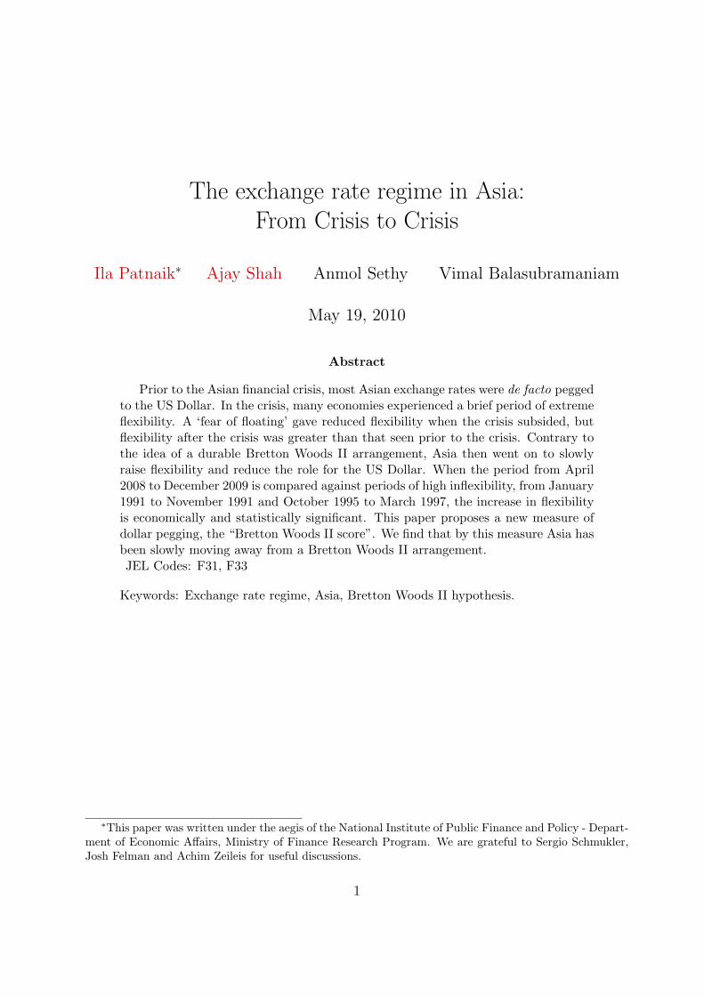
Prior to the Asian financial crisis, most Asian exchange rates were de facto peggedto the US Dollar. In the crisis, many economies experienced a brief period of extremeflexibility. A ‘fear of floating’ gave reduced flexibility when the crisis subsided, butflexibility after the crisis was greater than that seen prior to the crisis. Contrary tothe idea of a durable Bretton Woods II arrangement, Asia then went on to slowlyraise flexibility and reduce the role for the US Dollar. When the period from April2008 to December 2009 is compared against periods of high inflexibility, from January1991 to November 1991 and October 1995 to March 1997, the increase in flexibilityis economically and statistically significant. This paper proposes a new measure ofdollar pegging, the “Bretton Woods II score”. We find that by this measure Asia hasbeen slowly moving away from a Bretton Woods II arrangement.JEL Codes: F31, F33

Keywords: Exchange rate regime, Asia, Bretton Woods II hypothesis.

∗This paper was written under the aegis of the National Institute of Public Finance and Policy - Depart-ment of Economic Affairs, Ministry of Finance Research Program. We are grateful to Sergio Schmukler,Josh Felman and Achim Zeileis for useful discussions.

1

http://openlib.org/home/ila

http://www.mayin.org/ajayshah

Contents

1 The exchange rate regime in Asia 3

2 Methodology 4

3 Results 73.1 An example: Korea . . . . . . . . . . . . . . . . . . . . . . . . . . . . . . . 73.2 The exchange rate regime in Asia . . . . . . . . . . . . . . . . . . . . . . . 93.3 Sensitivity analyses . . . . . . . . . . . . . . . . . . . . . . . . . . . . . . . 13

4 Conclusion 15

A Appendix 18A.1 Vietnam . . . . . . . . . . . . . . . . . . . . . . . . . . . . . . . . . . . . . 18A.2 China . . . . . . . . . . . . . . . . . . . . . . . . . . . . . . . . . . . . . . 19A.3 Malaysia . . . . . . . . . . . . . . . . . . . . . . . . . . . . . . . . . . . . . 20A.4 India . . . . . . . . . . . . . . . . . . . . . . . . . . . . . . . . . . . . . . . 21A.5 Hong Kong . . . . . . . . . . . . . . . . . . . . . . . . . . . . . . . . . . . 22A.6 Indonesia . . . . . . . . . . . . . . . . . . . . . . . . . . . . . . . . . . . . 23A.7 Philippines . . . . . . . . . . . . . . . . . . . . . . . . . . . . . . . . . . . . 24A.8 Singapore . . . . . . . . . . . . . . . . . . . . . . . . . . . . . . . . . . . . 25A.9 Thailand . . . . . . . . . . . . . . . . . . . . . . . . . . . . . . . . . . . . . 26A.10 Taiwan . . . . . . . . . . . . . . . . . . . . . . . . . . . . . . . . . . . . . . 27

2

1 The exchange rate regime in Asia

Questions connected with the exchange rate regime have been an important part of under-standing macroeconomic policies and outcomes in Asia. In the period leading up to theAsian crisis of 1997, many Asian economies had highly inflexible exchange rates. In theaftermath of the Asian crisis, while many economies announced reforms of the exchangerate regime, Calvo and Reinhart (2002) pointed out that there was a substantial differencebetween the de jure and de facto exchange rate regime, and that many economies had goneback to a high degree of exchange rate inflexibility after the crisis.

A substantial research effort tried to understand the sources of this ‘fear of floating’. Somehypotheses which have been offered include the desire to reduce the currency risk facedby corporations with currency mismatches and incomplete financial markets, and the de-sire to stabilise domestic inflation in a small open economy with substantial exchange ratepassthrough.1 Dooley, Folkerts-Landau, and Garber (2003) have hypothesised the emer-gence of an Asian-led ‘Bretton Woods II’ regime motivated by exchange rate mercantilism.Some economists have argued that central bank actions aimed at exchange rate underval-uation should be an integral part of the optimal growth strategy in developing economies(Rodrik, 2008). Other researchers have argued that there is little evidence about a causalimpact of exchange rate undervaluation on growth in the long run(Woodford, 2009).

The macroeconomic policy framework in some Asian countries has involved a certain in-terlocking set of features: exchange rate inflexibility, large current account surpluses, andthe accumulation of large foreign exchange reserves. This has led to concerns about globalimbalances. The resolution of these imbalances may be critically linked to modifying theexchange rate regime in some Asian economies (Lane and Milesi-Ferretti, 2004).

In parallel, there has been interest in questions about the role of the US dollar (usd) inAsian exchange rate arrangements as opposed to the Euro (eur), the Yen (jpy) and theBritish Pound (gbp). To the extent that Asian economies have moved away from the usd,how important have these other major international currencies become?

In this setting, the following four questions are of interest:

1. In the period immediately after the Asian crisis, did Asian economies go back to pre-crisislevels of exchange rate flexibility?

2. Did Asian economies then evolve into a durable ‘Bretton-Woods II’ arrangement, featuringexchange rate inflexibility and pegging to the usd?

3. To what extent have Asian exchange rate regimes shifted focus from the usd to the eur,the jpy and the gbp?

1These hypotheses have been documented in Eichengreen and Hausman (1999); Hausmann, Gavin,Pages-Serra, and Stein (1999); Patnaik and Shah (2010 (forthcoming).

3

4. To what extent did exchange rate regimes encounter abrupt change in the global financialcrisis of 2008, when compared with the experience of 1997?

In this paper, we offer new evidence on these questions. The role of the dollar as apredominant international currency to which Asian countries peg is explicitly explored.We propose a ‘Bretton Woods II Score’. Prior to the Asian crisis, the average bw-II Scorewas high. The score dropped sharply during the crisis and rose again after it. However,after 2006 the score declined. This suggests that Asia has slowly moved away from thetight dollar pegging.

The remainder of this paper is organised as follows. Section 2 explains the methodologyused to measure the fine structure of exchange rate regimes in Asia, and obtain dates ofstructural change of the exchange rate regime. Section 3 analyses the results obtainedby measurement and dating of the de facto currency regime in each economy, in order toaddress the four questions enumerated above. Detailed results for each of the 11 economieshave been placed in an appendix, and Section 4 concludes.

2 Methodology

The importance of measuring the de facto exchange rate regime has motivated researchon data-driven methods for the classification of exchange rate regimes. This literaturehas attempted to create datasets identifying the exchange rate regime in operation forall economies in recent decades, using a variety of alternative heuristic procedures.(Levy-Yeyati and Sturzenegger, 2005; Reinhart and Rogoff, 2004; Calvo and Reinhart, 2002)

For instance, Reinhart and Rogoff (2004) use a variety of descriptive statistics to classifythe exchange rate regime. They classify the exchange rate regime as a crawling peg whenthe probability that the monthly nominal exchange rate (typically to the usd) is within±1% over a rolling five year period is above 80%. Reinhart and Rogoff (2004) also createa classification with seven types of exchange rate regimes.2 In similar fashion, Levy-Yeyatiand Sturzenegger (2005) classify countries into three regimes – float, intermediate and fixed– by examining the volatility of exchange rates.

In terms of the range of dates covered, Calvo and Reinhart (2002); Reinhart and Rogoff(2004); Levy-Yeyati and Sturzenegger (2005) analyse exchange rate regimes till 2002, 2003and 2004 respectively.3 In order to examine more recent events, the imf de facto clas-sification of exchange rate regimes and monetary policy frameworks is useful in that itis regularly updated. While it is available from 1998 onwards, a revised system for the

2The categories are: peg, band, crawling peg, crawling band, moving band, managed float and free float.This is similar to the International Monetary Fund’s (imf) areaer classification. The fine classificationwithin these coarse categories is also available on their website.

3Ilzetski, Reinhart and Rogoff have extended the database using the method in Reinhart and Rogoff(2004) till December 2007.

4

http://www.economics.harvard.edu/faculty/rogoff/files/ERA_Background_Material.htm

classification has been adopted (Habermeier, Kokenyne, Veyrune, and Anderson, 2009),which hinders comparisons with the previous years.

The estimation strategy used in this paper (Zeileis, Shah, and Patnaik, 2010 (forthcoming)builds on this literature in three respects. Exchange rate flexibility is measured as a realnumber from 0 (very high flexibility) to 1 (hard peg). Structural change in the exchangerate regime is addressed using a sound inferential strategy which yields estimates of breakdates to the resolution of the week. Finally, the econometric computations are easilyredone using current data, allowing for easy updation of the de facto exchange rate regimedatabase, thus permitting the analysis of current questions.

The point of departure for this strategy is a linear regression model based on cross-currencyexchange rates (with respect to a suitable numeraire). Used at least since Haldane and Hall(1991), this model was popularized by Frankel and Wei (1994) (and is hence also calledthe Frankel-Wei model). Recent applications of this estimation strategy include Benassy-Quere, Coeure, and Mignon (2006), Shah, Zeileis, and Patnaik (2005) and Frankel and Wei(2007). An independent currency, such as the Swiss Franc (chf), is chosen as an arbitrary‘numeraire’. If estimation involving the Indian rupee (inr) is desired, the model estimatedis:

d log(

INR

CHF

)= β1 + β2 d log

(USD

CHF

)+ β3 d log

(GBP

CHF

)+ β4 d log

(JPY

CHF

)+ β5 d log

(EUR

CHF

)+ ε

This regression picks up the extent to which the inr/chf rate fluctuates in response tofluctuations in the usd/chf rate. If there is pegging to the usd, then fluctuations in thegbp, jpy and eur will be irrelevant, and we will observe β3 = β4 = β5 = 0 while β2 = 1.The R2 of this regression is also of interest; values near 1 suggest reduced exchange rateflexibility.4

The choice of currencies in the regression analysis reflects the core international currenciesin the global financial system. The Composition of Foreign Exchange Reserves (cofer)database maintained by the imf suggests that more than 83% of the world’s reserves havealways been held in usd, eur (formerly dem), gbp and jpy. Maintained since 1995,the cofer database has 140 economies reporting composition of reserves. Since 2000,an average of 97.8% of world reserves reported to the imf have been held in these fourcurrencies.

To understand the de facto exchange rate regime in a given economy for a given timeperiod, this ols regression can be utilised. In order to address change in the exchange

4The Deutsche Mark is used as a proxy for the Euro in the older data. Hence, the term ‘dur’ is usedinstead of ‘eur’, to convey the concatenation of the time-series of dem/chf rates followed by the eur/chfrates.

5

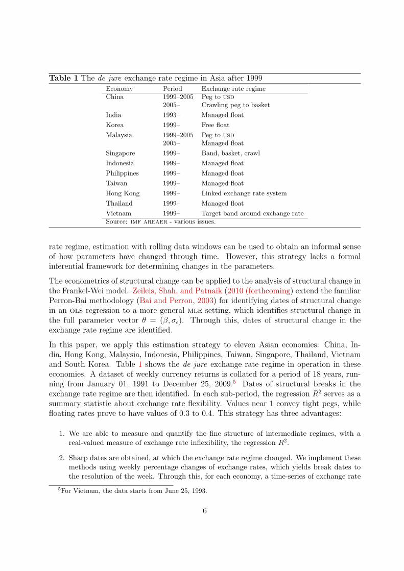
Table 1 The de jure exchange rate regime in Asia after 1999

Economy Period Exchange rate regimeChina 1999–2005 Peg to usd

2005– Crawling peg to basketIndia 1993– Managed floatKorea 1999– Free floatMalaysia 1999–2005 Peg to usd

2005– Managed floatSingapore 1999– Band, basket, crawlIndonesia 1999– Managed floatPhilippines 1999– Managed floatTaiwan 1999– Managed floatHong Kong 1999– Linked exchange rate systemThailand 1999– Managed floatVietnam 1999– Target band around exchange rateSource: imf areaer - various issues.

rate regime, estimation with rolling data windows can be used to obtain an informal senseof how parameters have changed through time. However, this strategy lacks a formalinferential framework for determining changes in the parameters.

The econometrics of structural change can be applied to the analysis of structural change inthe Frankel-Wei model. Zeileis, Shah, and Patnaik (2010 (forthcoming) extend the familiarPerron-Bai methodology (Bai and Perron, 2003) for identifying dates of structural changein an ols regression to a more general mle setting, which identifies structural change inthe full parameter vector θ = (β, σε). Through this, dates of structural change in theexchange rate regime are identified.

In this paper, we apply this estimation strategy to eleven Asian economies: China, In-dia, Hong Kong, Malaysia, Indonesia, Philippines, Taiwan, Singapore, Thailand, Vietnamand South Korea. Table 1 shows the de jure exchange rate regime in operation in theseeconomies. A dataset of weekly currency returns is collated for a period of 18 years, run-ning from January 01, 1991 to December 25, 2009.5 Dates of structural breaks in theexchange rate regime are then identified. In each sub-period, the regression R2 serves as asummary statistic about exchange rate flexibility. Values near 1 convey tight pegs, whilefloating rates prove to have values of 0.3 to 0.4. This strategy has three advantages:

1. We are able to measure and quantify the fine structure of intermediate regimes, with areal-valued measure of exchange rate inflexibility, the regression R2.

2. Sharp dates are obtained, at which the exchange rate regime changed. We implement thesemethods using weekly percentage changes of exchange rates, which yields break dates tothe resolution of the week. Through this, for each economy, a time-series of exchange rate

5For Vietnam, the data starts from June 25, 1993.

6

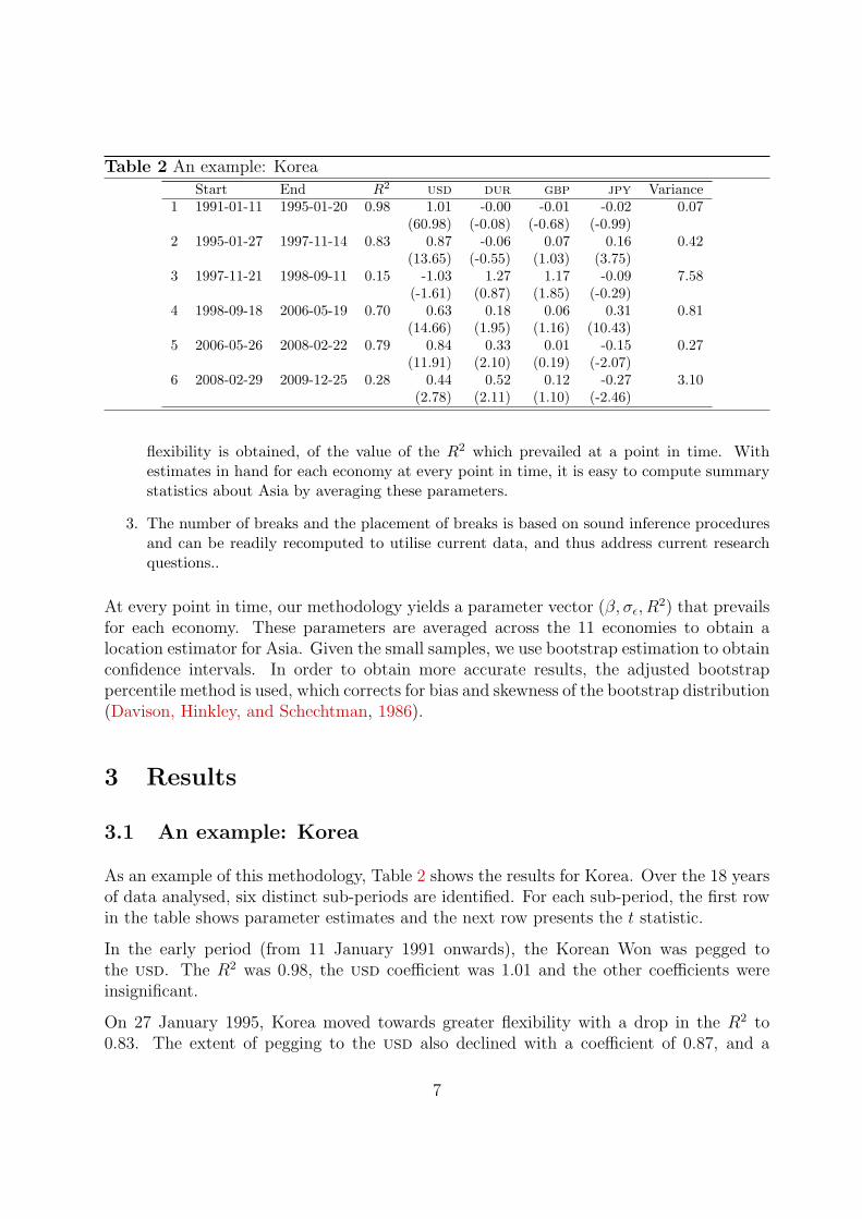
Table 2 An example: Korea

Start End R2 usd dur gbp jpy Variance1 1991-01-11 1995-01-20 0.98 1.01 -0.00 -0.01 -0.02 0.07

(60.98) (-0.08) (-0.68) (-0.99)2 1995-01-27 1997-11-14 0.83 0.87 -0.06 0.07 0.16 0.42

(13.65) (-0.55) (1.03) (3.75)3 1997-11-21 1998-09-11 0.15 -1.03 1.27 1.17 -0.09 7.58

(-1.61) (0.87) (1.85) (-0.29)4 1998-09-18 2006-05-19 0.70 0.63 0.18 0.06 0.31 0.81

(14.66) (1.95) (1.16) (10.43)5 2006-05-26 2008-02-22 0.79 0.84 0.33 0.01 -0.15 0.27

(11.91) (2.10) (0.19) (-2.07)6 2008-02-29 2009-12-25 0.28 0.44 0.52 0.12 -0.27 3.10

(2.78) (2.11) (1.10) (-2.46)

flexibility is obtained, of the value of the R2 which prevailed at a point in time. Withestimates in hand for each economy at every point in time, it is easy to compute summarystatistics about Asia by averaging these parameters.

3. The number of breaks and the placement of breaks is based on sound inference proceduresand can be readily recomputed to utilise current data, and thus address current researchquestions..

At every point in time, our methodology yields a parameter vector (β, σε, R2) that prevails

for each economy. These parameters are averaged across the 11 economies to obtain alocation estimator for Asia. Given the small samples, we use bootstrap estimation to obtainconfidence intervals. In order to obtain more accurate results, the adjusted bootstrappercentile method is used, which corrects for bias and skewness of the bootstrap distribution(Davison, Hinkley, and Schechtman, 1986).

3 Results

3.1 An example: Korea

As an example of this methodology, Table 2 shows the results for Korea. Over the 18 yearsof data analysed, six distinct sub-periods are identified. For each sub-period, the first rowin the table shows parameter estimates and the next row presents the t statistic.

In the early period (from 11 January 1991 onwards), the Korean Won was pegged tothe usd. The R2 was 0.98, the usd coefficient was 1.01 and the other coefficients wereinsignificant.

On 27 January 1995, Korea moved towards greater flexibility with a drop in the R2 to0.83. The extent of pegging to the usd also declined with a coefficient of 0.87, and a

7

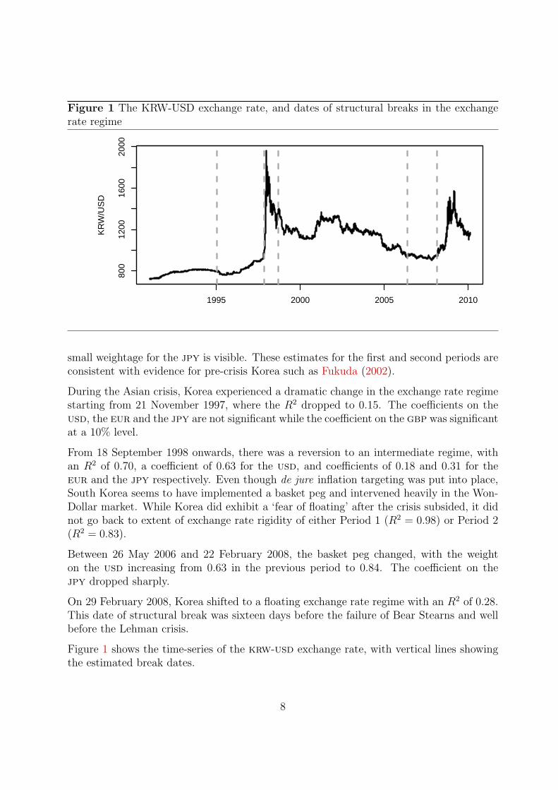
Figure 1 The KRW-USD exchange rate, and dates of structural breaks in the exchangerate regime

800

1200

1600

2000

KR

W/U

SD

1995 2000 2005 2010

small weightage for the jpy is visible. These estimates for the first and second periods areconsistent with evidence for pre-crisis Korea such as Fukuda (2002).

During the Asian crisis, Korea experienced a dramatic change in the exchange rate regimestarting from 21 November 1997, where the R2 dropped to 0.15. The coefficients on theusd, the eur and the jpy are not significant while the coefficient on the gbp was significantat a 10% level.

From 18 September 1998 onwards, there was a reversion to an intermediate regime, withan R2 of 0.70, a coefficient of 0.63 for the usd, and coefficients of 0.18 and 0.31 for theeur and the jpy respectively. Even though de jure inflation targeting was put into place,South Korea seems to have implemented a basket peg and intervened heavily in the Won-Dollar market. While Korea did exhibit a ‘fear of floating’ after the crisis subsided, it didnot go back to extent of exchange rate rigidity of either Period 1 (R2 = 0.98) or Period 2(R2 = 0.83).

Between 26 May 2006 and 22 February 2008, the basket peg changed, with the weighton the usd increasing from 0.63 in the previous period to 0.84. The coefficient on thejpy dropped sharply.

On 29 February 2008, Korea shifted to a floating exchange rate regime with an R2 of 0.28.This date of structural break was sixteen days before the failure of Bear Stearns and wellbefore the Lehman crisis.

Figure 1 shows the time-series of the krw-usd exchange rate, with vertical lines showingthe estimated break dates.

8

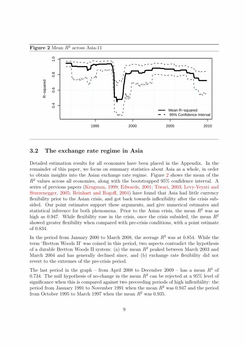
Figure 2 Mean R2 across Asia-110.

40.

60.

81.

0

R−

squa

red

1995 2000 2005 2010

Mean R−squared 95% Confidence Interval

3.2 The exchange rate regime in Asia

Detailed estimation results for all economies have been placed in the Appendix. In theremainder of this paper, we focus on summary statistics about Asia as a whole, in orderto obtain insights into the Asian exchange rate regime. Figure 2 shows the mean of theR2 values across all economies, along with the bootstrapped 95% confidence interval. Aseries of previous papers (Krugman, 1999; Edwards, 2001; Tiwari, 2003; Levy-Yeyati andSturzenegger, 2005; Reinhart and Rogoff, 2004) have found that Asia had little currencyflexibility prior to the Asian crisis, and got back towards inflexibility after the crisis sub-sided. Our point estimates support these arguments, and give numerical estimates andstatistical inference for both phenomena. Prior to the Asian crisis, the mean R2 was ashigh as 0.947. While flexibility rose in the crisis, once the crisis subsided, the mean R2

showed greater flexibility when compared with pre-crisis conditions, with a point estimateof 0.834.

In the period from January 2000 to March 2008, the average R2 was at 0.854. While theterm ‘Bretton Woods II’ was coined in this period, two aspects contradict the hypothesisof a durable Bretton Woods II system: (a) the mean R2 peaked between March 2003 andMarch 2004 and has generally declined since, and (b) exchange rate flexibility did notrevert to the extremes of the pre-crisis period.

The last period in the graph – from April 2008 to December 2009 – has a mean R2 of0.734. The null hypothesis of no-change in the mean R2 can be rejected at a 95% level ofsignificance when this is compared against two preceeding periods of high inflexibility: theperiod from January 1991 to November 1991 when the mean R2 was 0.947 and the periodfrom October 1995 to March 1997 when the mean R2 was 0.935.

9

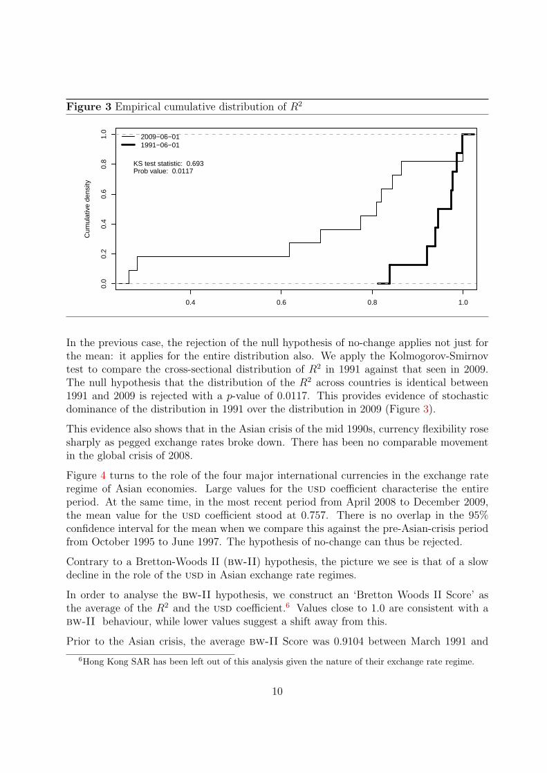
Figure 3 Empirical cumulative distribution of R2

0.4 0.6 0.8 1.0

0.0

0.2

0.4

0.6

0.8

1.0

Cum

ulat

ive

dens

ity

2009−06−011991−06−01

KS test statistic: 0.693Prob value: 0.0117

In the previous case, the rejection of the null hypothesis of no-change applies not just forthe mean: it applies for the entire distribution also. We apply the Kolmogorov-Smirnovtest to compare the cross-sectional distribution of R2 in 1991 against that seen in 2009.The null hypothesis that the distribution of the R2 across countries is identical between1991 and 2009 is rejected with a p-value of 0.0117. This provides evidence of stochasticdominance of the distribution in 1991 over the distribution in 2009 (Figure 3).

This evidence also shows that in the Asian crisis of the mid 1990s, currency flexibility rosesharply as pegged exchange rates broke down. There has been no comparable movementin the global crisis of 2008.

Figure 4 turns to the role of the four major international currencies in the exchange rateregime of Asian economies. Large values for the usd coefficient characterise the entireperiod. At the same time, in the most recent period from April 2008 to December 2009,the mean value for the usd coefficient stood at 0.757. There is no overlap in the 95%confidence interval for the mean when we compare this against the pre-Asian-crisis periodfrom October 1995 to June 1997. The hypothesis of no-change can thus be rejected.

Contrary to a Bretton-Woods II (bw-II) hypothesis, the picture we see is that of a slowdecline in the role of the usd in Asian exchange rate regimes.

In order to analyse the bw-II hypothesis, we construct an ‘Bretton Woods II Score’ asthe average of the R2 and the usd coefficient.6 Values close to 1.0 are consistent with abw-II behaviour, while lower values suggest a shift away from this.

Prior to the Asian crisis, the average bw-II Score was 0.9104 between March 1991 and

6Hong Kong SAR has been left out of this analysis given the nature of their exchange rate regime.

10

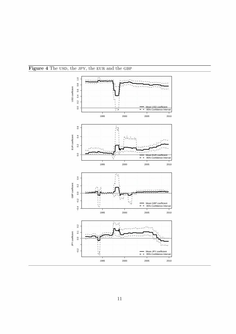
Figure 4 The usd, the jpy, the eur and the gbp

0.0

0.2

0.4

0.6

0.8

1.0

US

D c

oeffi

cien

t

1995 2000 2005 2010

Mean USD coefficient 95% Confidence Interval

0.0

0.2

0.4

0.6

EU

R c

oeffi

cien

t

1995 2000 2005 2010

Mean EUR coefficient 95% Confidence Interval

−0.

4−

0.2

0.0

0.2

0.4

GB

P c

oeffi

cien

t

1995 2000 2005 2010

Mean GBP coefficient 95% Confidence Interval

−0.

20.

00.

10.

2

JPY

coe

ffici

ent

1995 2000 2005 2010

Mean JPY coefficient 95% Confidence Interval

11

Figure 5 The ‘Bretton Woods II’ score for Asia

0.2

0.4

0.6

0.8

1.0

Ave

rage

Bre

tton

Woo

ds II

Sco

re

1995 2000 2005 2010

Table 3 Ranking economies based on bw-II score

1991 to 1997 1997 to 1999 1999 to 2007 2007 to 2009China 1 1 2 1

Vietnam 3 2 3 2Taiwan 6 5 6 3

Philippines 10 4 5 4Malaysia 7 6 1 5

India 8 3 4 6Singapore 9 7 7 7Thailand 5 10 8 8Indonesia 2 8 10 9

Korea 4 9 9 10

March 1997; the score dropped dramatically during the crisis and returned to an averageof 0.8347 between July 1999 and December 2006. The score in the last period, January2007 to December 2009, stood at 0.7535. The decline in the bw-II Score is statisticallysignificant with no overlap in confidence intervals between the first and the last period.This suggests that Asia has slowly moved away from the bw-II arrangement (Figure 5).

Countries can be ranked, in any period, by the values seen for the average bw-II score.Table 3 shows these ranks. Big increases in these rank through the entire period arevisible for Thailand, Indonesia and Korea. In the last period, the top four countries withbw-II behaviour were China, Vietnam, Taiwan and the Philippines.

Alongside this shift away from the bw-II arrangement, there has been an important rise ofthe eur in Asia’s exchange rate regimes. From December 1997 onwards, the lower boundof the 95% confidence interval for the mean value of the eur coefficient has exceeded 0.05.In the latest period from April 2008 onwards, the 95% confidence interval runs from 0.133to 0.336 with a point estimate for the mean of 0.220.

In the case of the gbp, until December 2001, H0 : β3 = 0 could not be rejected. Fromthat date onwards, a small coefficient with a point estimate of 0.029 has emerged, where

12

H0 can be rejected at a 95% level of significance.

There was a period from April 1994 till August 2005 where with the jpy, H0 : β4 = 0could be rejected. The point estimate for the jpy was as high as 0.159 in October 1997.In this period, the jpy had achieved a certain role as an international currency. But thepoint estimate has declined through time, and in the recent period from August 2005 toDecember 2009, H0 : β4 = 0 cannot be rejected.

To summarise, our findings confirm the incidence of tight usd pegging before the Asiancrisis. After the Asian crisis, Asia returned to a regime of high inflexibility (fear of floating).But this was not as inflexible as that prevailing before the crisis. In the following years,there is some evidence of the inflexibility and dollar pegging that has been made prominentby Dooley, Folkerts-Landau, and Garber (2003). However, there is early evidence of Asiamoving towards greater flexibility, and a certain shift away from the usd towards thegbp and strongly towards the eur, though not towards the jpy. The evidence suggests abrief period in which the jpy played an important role in Asian currency arrangements,but after that the role of the jpy has subsided.

3.3 Sensitivity analyses

We perform three robustness checks on the main results:

1. GDP weights instead of equal weights when averaging across economies.

2. An alternative location estimator – the trimmed mean – to avoid the undue influence ofextreme values on the sample mean.

3. Addition of other floating currencies in the Frankel-Wei regression

Does the use of equal weights for all economies make our results biased in favour of smalleconomies? To answer this question, we weight economies by gdp. Figure 6 superposesthe mean R2 value using equal weights with one that uses gdp weights. gdp weighted R2

data suggests greater inflexibility because of the presence of China which has a large gdpand an inflexible exchange rate. However, the difference between the two series is small,particularly in recent years.

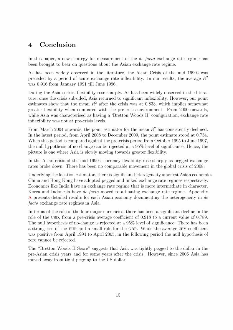
Figure 7 plots the trimmed mean alongside the ordinary mean. There is a small differencebetween the two in the recent past. Our results are hence not an artifact of extreme values.

Does the addition of other floating currencies in the Frankel-Wei regression change theresults? Regression analysis with Australian dollar and the Canadian dollar, only withthe Australian dollar, and only with the Canadian dollar does not alter the measure offlexibility (R2) or the break-dates. However, it does alter the coefficient on each currencydue to the correlation structure between the independent variables.

13

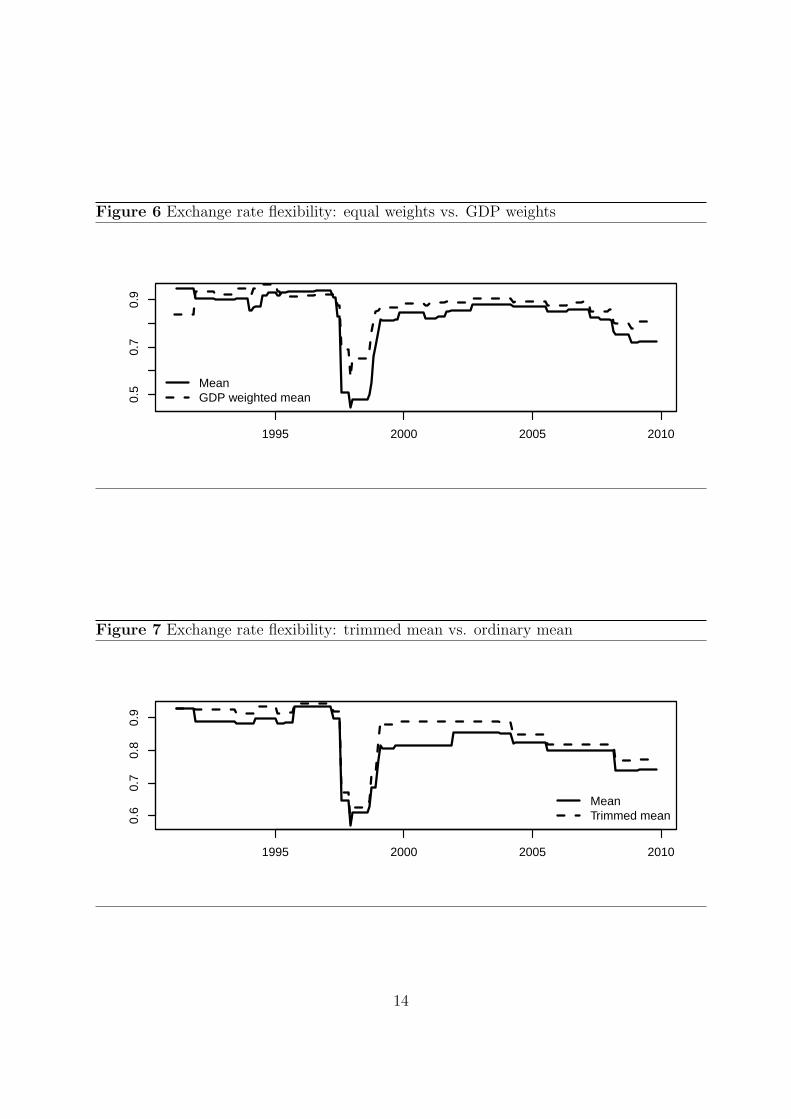
Figure 6 Exchange rate flexibility: equal weights vs. GDP weights

0.5

0.7

0.9

1995 2000 2005 2010

MeanGDP weighted mean

Figure 7 Exchange rate flexibility: trimmed mean vs. ordinary mean

0.6

0.7

0.8

0.9

1995 2000 2005 2010

MeanTrimmed mean

14

4 Conclusion

In this paper, a new strategy for measurement of the de facto exchange rate regime hasbeen brought to bear on questions about the Asian exchange rate regime.

As has been widely observed in the literature, the Asian Crisis of the mid 1990s waspreceded by a period of acute exchange rate inflexibility. In our results, the average R2

was 0.916 from January 1991 till June 1996.

During the Asian crisis, flexibility rose sharply. As has been widely observed in the litera-ture, once the crisis subsided, Asia returned to significant inflexibility. However, our pointestimates show that the mean R2 after the crisis was at 0.833, which implies somewhatgreater flexibility when compared with the pre-crisis environment. From 2000 onwards,while Asia was characterised as having a ‘Bretton Woods II’ configuration, exchange rateinflexibility was not at pre-crisis levels.

From March 2004 onwards, the point estimator for the mean R2 has consistently declined.In the latest period, from April 2008 to December 2009, the point estimate stood at 0.734.When this period is compared against the pre-crisis period from October 1995 to June 1997,the null hypothesis of no change can be rejected at a 95% level of significance. Hence, thepicture is one where Asia is slowly moving towards greater flexibility.

In the Asian crisis of the mid 1990s, currency flexibility rose sharply as pegged exchangerates broke down. There has been no comparable movement in the global crisis of 2008.

Underlying the location estimators there is significant heterogeneity amongst Asian economies.China and Hong Kong have adopted pegged and linked exchange rate regimes respectively.Economies like India have an exchange rate regime that is more intermediate in character.Korea and Indonesia have de facto moved to a floating exchange rate regime. AppendixA presents detailed results for each Asian economy documenting the heterogeneity in defacto exchange rate regimes in Asia.

In terms of the role of the four major currencies, there has been a significant decline in therole of the usd, from a pre-crisis average coefficient of 0.918 to a current value of 0.789.The null hypothesis of no-change is rejected at a 95% level of significance. There has beena strong rise of the eur and a small role for the gbp. While the average jpy coefficientwas positive from April 1994 to April 2005, in the following period the null hypothesis ofzero cannot be rejected.

The “Bretton Woods II Score” suggests that Asia was tightly pegged to the dollar in thepre-Asian crisis years and for some years after the crisis. However, since 2006 Asia hasmoved away from tight pegging to the US dollar.

15

References

Bai, J., and P. Perron (2003): “Computation and Analysis of Multiple Structural ChangeModels,” Journal of Applied Econometrics, 18, 1–22.

Benassy-Quere, A., B. Coeure, and V. Mignon (2006): “On the Identification of De FactoCurrency Pegs,” Journal of the Japanese and International Economies, 20(1), 112–127.

Calvo, G. A., and C. M. Reinhart (2002): “Fear of floating,” Quarterly Journal of Eco-nomics, CXVII(2), 379–408.

Davison, A. C., D. V. Hinkley, and E. Schechtman (1986): “Efficient bootstrap simula-tion,” Biometrika, 73(3), 555–566.

Dooley, M. P., D. Folkerts-Landau, and P. Garber (2003): “An essay on the revivedBretton Woods system,” Discussion Paper w9971, NBER.

Edwards, S. (2001): “Exchange rate regimes, capital flows and crisis prevention,” Discussionpaper, NBER Working Paper No 8529.

Eichengreen, B., and R. Hausman (1999): “Exchange Rates and Financial Fragility,” .

Frankel, J., and S.-J. Wei (1994): “Yen bloc or dollar bloc? Exchange rate policies of theEast Asian countries,” in Macroeconomic linkage: Savings, exchange rates and capital flows,ed. by T. Ito, and A. Krueger. University of Chicago Press.

Frankel, J. A., and S.-J. Wei (2007): “Assessing China’s Exchange Rate Regime,” Discussionpaper, NBER Working Paper 13100.

Fukuda, S. (2002): “Post-crisis exchange rate regimes in east Asia,” CIRJE Discussion Paper,CIRJE-F-181, University of Tokyo, November.

Habermeier, K., A. Kokenyne, R. Veyrune, and H. Anderson (2009): “Revised Systemfor the Classification of Exchange Rate Arrangements,” IMF Working Papers, WP/09/211.

Haldane, A. G., and S. G. Hall (1991): “Sterling’s relationship with the dollar and thedeutschemark: 1976-89,” The Economic Journal, 101, 436–443.

Hausmann, R., M. Gavin, C. Pages-Serra, and E. Stein (1999): “Financial turmoil andthe choice of exchange rate regime,” Inter-American Development Bank.

Krugman, P. (1999): “What happened to Asia?,” Global competition and integration, p. 315.

Lane, P., and G. Milesi-Ferretti (2004): Financial globalization and exchange rates. Centrefor Economic Policy Research.

Levy-Yeyati, E., and F. Sturzenegger (2005): “Classifying Exchange Rate Regimes: Deedsvs. Words,” European Economic Review, 49, 1603–1635.

Patnaik, I., and A. Shah (2010 (forthcoming)): “Does the currency regime shape unhedgedcurrency exposure?,” Journal of International Money and Finance.

16

Reinhart, C. M., and K. S. Rogoff (2004): “The Modern History of Exchange Rate Ar-rangements: A Reinterpretation,” The Quarterly Journal of Economics, 119(1), 1–48.

Rodrik, D. (2008): “The real exchange rate and economic growth,” Brookings Papers on Eco-nomic Activity, 2, 365–412.

Shah, A., A. Zeileis, and I. Patnaik (2005): “What is the new Chinese currency regime?,”Discussion paper, Wirtschaftsuniversitat Wien.

Tiwari, R. (2003): “Post-crisis Exchange Rate Regimes in Southeast Asia: An empirical surveyof de-facto policies,” University of Hamburg Seminar Paper.

Woodford, M. (2009): “Is an Undervalued Currency the Key to Economic Growth?,” ColumbiaUniversity Discussion Papers.

Zeileis, A., A. Shah, and I. Patnaik (2010 (forthcoming)): “Testing, Monitoring, and DatingStructural Changes in Exchange Rate Regimes,” Computational Statistics & Data Analysis.

17

A Appendix

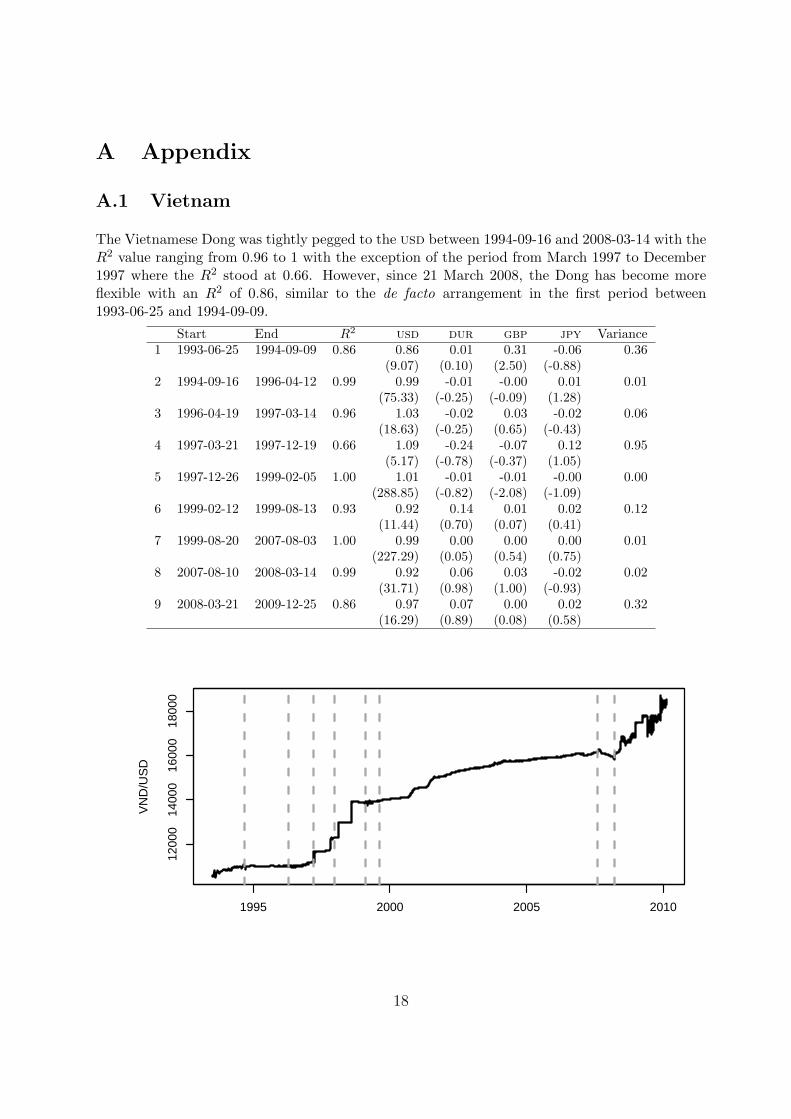
A.1 Vietnam

The Vietnamese Dong was tightly pegged to the usd between 1994-09-16 and 2008-03-14 with theR2 value ranging from 0.96 to 1 with the exception of the period from March 1997 to December1997 where the R2 stood at 0.66. However, since 21 March 2008, the Dong has become moreflexible with an R2 of 0.86, similar to the de facto arrangement in the first period between1993-06-25 and 1994-09-09.

Start End R2 usd dur gbp jpy Variance1 1993-06-25 1994-09-09 0.86 0.86 0.01 0.31 -0.06 0.36

(9.07) (0.10) (2.50) (-0.88)2 1994-09-16 1996-04-12 0.99 0.99 -0.01 -0.00 0.01 0.01

(75.33) (-0.25) (-0.09) (1.28)3 1996-04-19 1997-03-14 0.96 1.03 -0.02 0.03 -0.02 0.06

(18.63) (-0.25) (0.65) (-0.43)4 1997-03-21 1997-12-19 0.66 1.09 -0.24 -0.07 0.12 0.95

(5.17) (-0.78) (-0.37) (1.05)5 1997-12-26 1999-02-05 1.00 1.01 -0.01 -0.01 -0.00 0.00

(288.85) (-0.82) (-2.08) (-1.09)6 1999-02-12 1999-08-13 0.93 0.92 0.14 0.01 0.02 0.12

(11.44) (0.70) (0.07) (0.41)7 1999-08-20 2007-08-03 1.00 0.99 0.00 0.00 0.00 0.01

(227.29) (0.05) (0.54) (0.75)8 2007-08-10 2008-03-14 0.99 0.92 0.06 0.03 -0.02 0.02

(31.71) (0.98) (1.00) (-0.93)9 2008-03-21 2009-12-25 0.86 0.97 0.07 0.00 0.02 0.32

(16.29) (0.89) (0.08) (0.58)

1200

014

000

1600

018

000

VN

D/U

SD

1995 2000 2005 2010

18

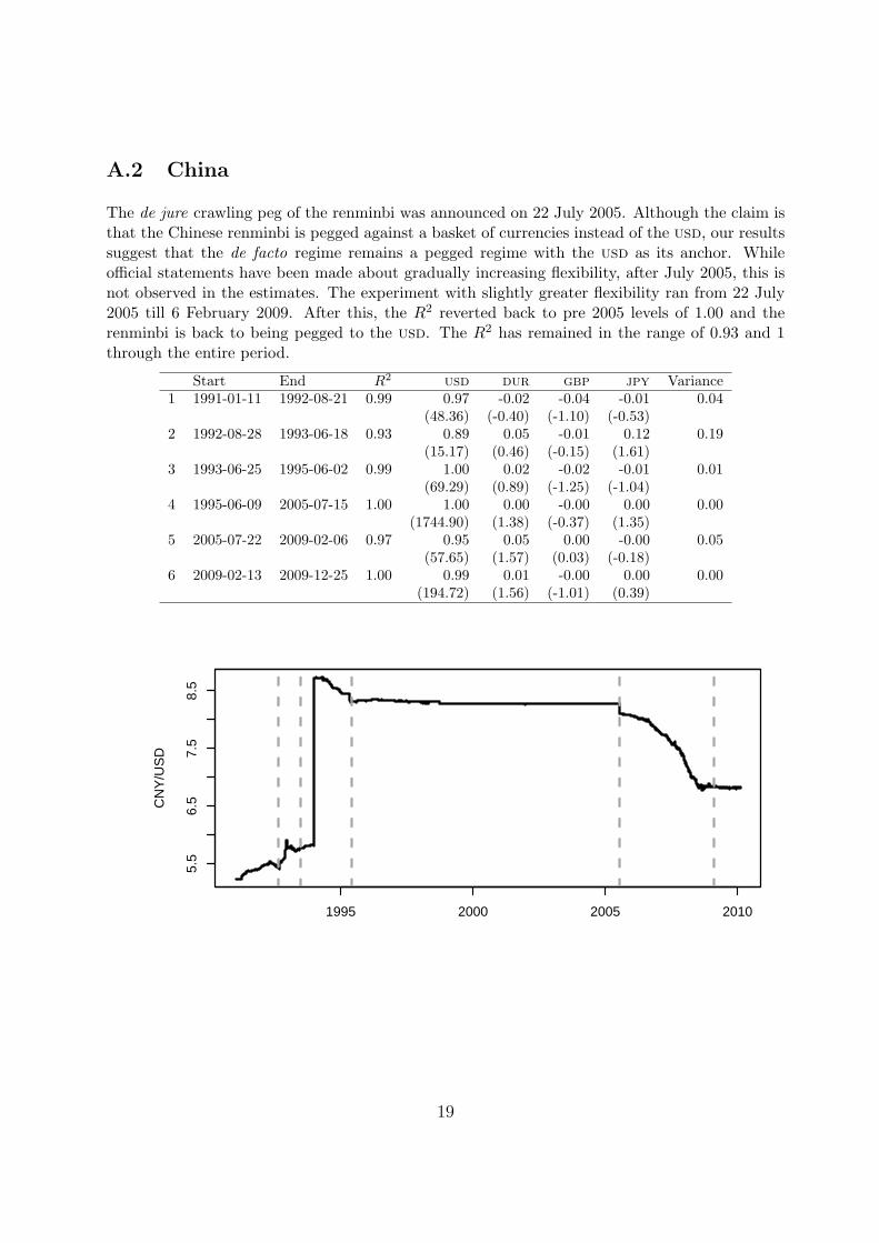
A.2 China

The de jure crawling peg of the renminbi was announced on 22 July 2005. Although the claim isthat the Chinese renminbi is pegged against a basket of currencies instead of the usd, our resultssuggest that the de facto regime remains a pegged regime with the usd as its anchor. Whileofficial statements have been made about gradually increasing flexibility, after July 2005, this isnot observed in the estimates. The experiment with slightly greater flexibility ran from 22 July2005 till 6 February 2009. After this, the R2 reverted back to pre 2005 levels of 1.00 and therenminbi is back to being pegged to the usd. The R2 has remained in the range of 0.93 and 1through the entire period.

Start End R2 usd dur gbp jpy Variance1 1991-01-11 1992-08-21 0.99 0.97 -0.02 -0.04 -0.01 0.04

(48.36) (-0.40) (-1.10) (-0.53)2 1992-08-28 1993-06-18 0.93 0.89 0.05 -0.01 0.12 0.19

(15.17) (0.46) (-0.15) (1.61)3 1993-06-25 1995-06-02 0.99 1.00 0.02 -0.02 -0.01 0.01

(69.29) (0.89) (-1.25) (-1.04)4 1995-06-09 2005-07-15 1.00 1.00 0.00 -0.00 0.00 0.00

(1744.90) (1.38) (-0.37) (1.35)5 2005-07-22 2009-02-06 0.97 0.95 0.05 0.00 -0.00 0.05

(57.65) (1.57) (0.03) (-0.18)6 2009-02-13 2009-12-25 1.00 0.99 0.01 -0.00 0.00 0.00

(194.72) (1.56) (-1.01) (0.39)

5.5

6.5

7.5

8.5

CN

Y/U

SD

1995 2000 2005 2010

19

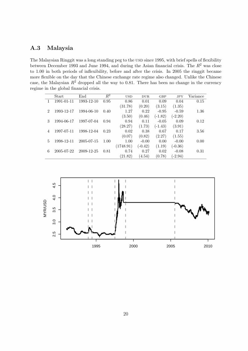
A.3 Malaysia

The Malaysian Ringgit was a long standing peg to the usd since 1995, with brief spells of flexibilitybetween December 1993 and June 1994, and during the Asian financial crisis. The R2 was closeto 1.00 in both periods of inflexibility, before and after the crisis. In 2005 the ringgit becamemore flexible on the day that the Chinese exchange rate regime also changed. Unlike the Chinesecase, the Malaysian R2 dropped all the way to 0.81. There has been no change in the currencyregime in the global financial crisis.

Start End R2 usd dur gbp jpy Variance1 1991-01-11 1993-12-10 0.95 0.86 0.01 0.09 0.04 0.15

(31.78) (0.20) (3.15) (1.35)2 1993-12-17 1994-06-10 0.40 1.27 0.22 -0.95 -0.59 1.36

(3.50) (0.46) (-1.82) (-2.20)3 1994-06-17 1997-07-04 0.94 0.94 0.11 -0.05 0.09 0.12

(28.27) (1.73) (-1.43) (3.91)4 1997-07-11 1998-12-04 0.23 0.02 0.38 0.67 0.17 3.56

(0.07) (0.82) (2.27) (1.55)5 1998-12-11 2005-07-15 1.00 1.00 -0.00 0.00 -0.00 0.00

(1748.91) (-0.42) (1.19) (-0.36)6 2005-07-22 2009-12-25 0.81 0.74 0.27 0.02 -0.08 0.31

(21.82) (4.54) (0.78) (-2.94)

2.5

3.0

3.5

4.0

4.5

MY

R/U

SD

1995 2000 2005 2010

20

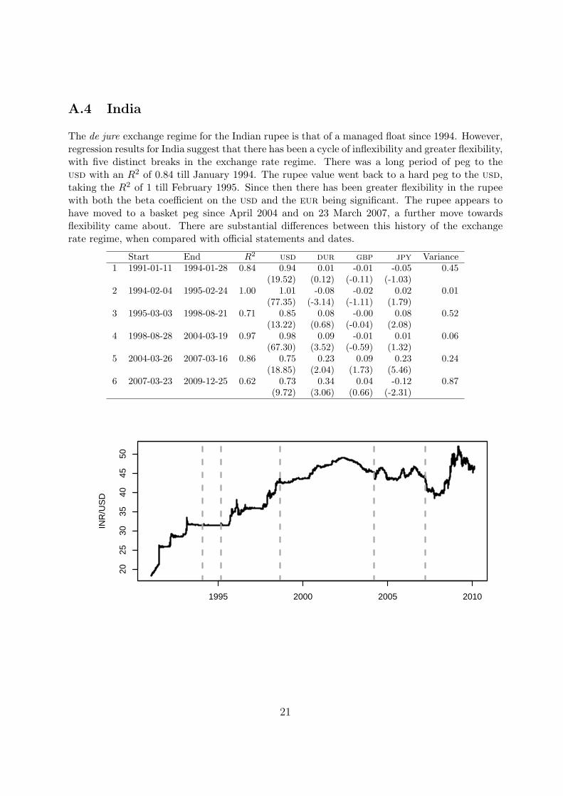
A.4 India

The de jure exchange regime for the Indian rupee is that of a managed float since 1994. However,regression results for India suggest that there has been a cycle of inflexibility and greater flexibility,with five distinct breaks in the exchange rate regime. There was a long period of peg to theusd with an R2 of 0.84 till January 1994. The rupee value went back to a hard peg to the usd,taking the R2 of 1 till February 1995. Since then there has been greater flexibility in the rupeewith both the beta coefficient on the usd and the eur being significant. The rupee appears tohave moved to a basket peg since April 2004 and on 23 March 2007, a further move towardsflexibility came about. There are substantial differences between this history of the exchangerate regime, when compared with official statements and dates.

Start End R2 usd dur gbp jpy Variance1 1991-01-11 1994-01-28 0.84 0.94 0.01 -0.01 -0.05 0.45

(19.52) (0.12) (-0.11) (-1.03)2 1994-02-04 1995-02-24 1.00 1.01 -0.08 -0.02 0.02 0.01

(77.35) (-3.14) (-1.11) (1.79)3 1995-03-03 1998-08-21 0.71 0.85 0.08 -0.00 0.08 0.52

(13.22) (0.68) (-0.04) (2.08)4 1998-08-28 2004-03-19 0.97 0.98 0.09 -0.01 0.01 0.06

(67.30) (3.52) (-0.59) (1.32)5 2004-03-26 2007-03-16 0.86 0.75 0.23 0.09 0.23 0.24

(18.85) (2.04) (1.73) (5.46)6 2007-03-23 2009-12-25 0.62 0.73 0.34 0.04 -0.12 0.87

(9.72) (3.06) (0.66) (-2.31)

2025

3035

4045

50

INR

/US

D

1995 2000 2005 2010

21

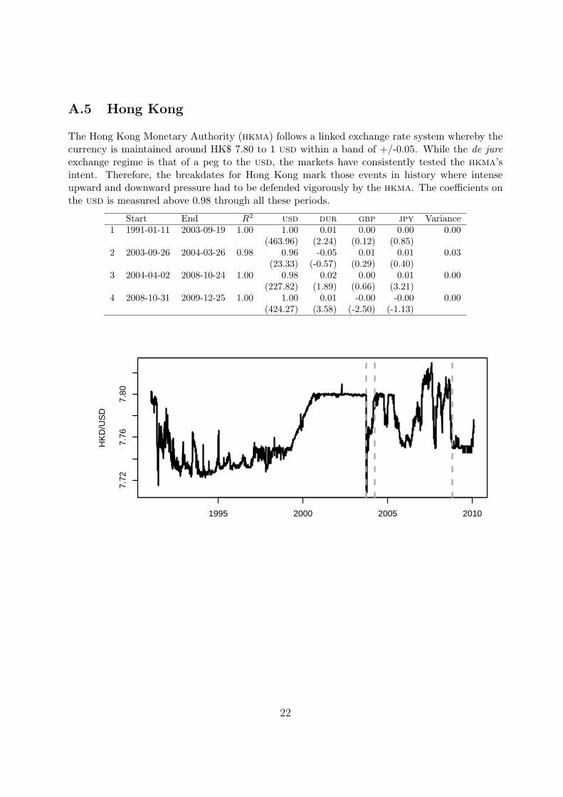
A.5 Hong Kong

The Hong Kong Monetary Authority (hkma) follows a linked exchange rate system whereby thecurrency is maintained around HK$ 7.80 to 1 usd within a band of +/-0.05. While the de jureexchange regime is that of a peg to the usd, the markets have consistently tested the hkma’sintent. Therefore, the breakdates for Hong Kong mark those events in history where intenseupward and downward pressure had to be defended vigorously by the hkma. The coefficients onthe usd is measured above 0.98 through all these periods.


(463.96) (2.24) (0.12) (0.85)2 2003-09-26 2004-03-26 0.98 0.96 -0.05 0.01 0.01 0.03

(23.33) (-0.57) (0.29) (0.40)3 2004-04-02 2008-10-24 1.00 0.98 0.02 0.00 0.01 0.00

(227.82) (1.89) (0.66) (3.21)4 2008-10-31 2009-12-25 1.00 1.00 0.01 -0.00 -0.00 0.00

(424.27) (3.58) (-2.50) (-1.13)

7.72

7.76

7.80

HK

D/U

SD

1995 2000 2005 2010

22

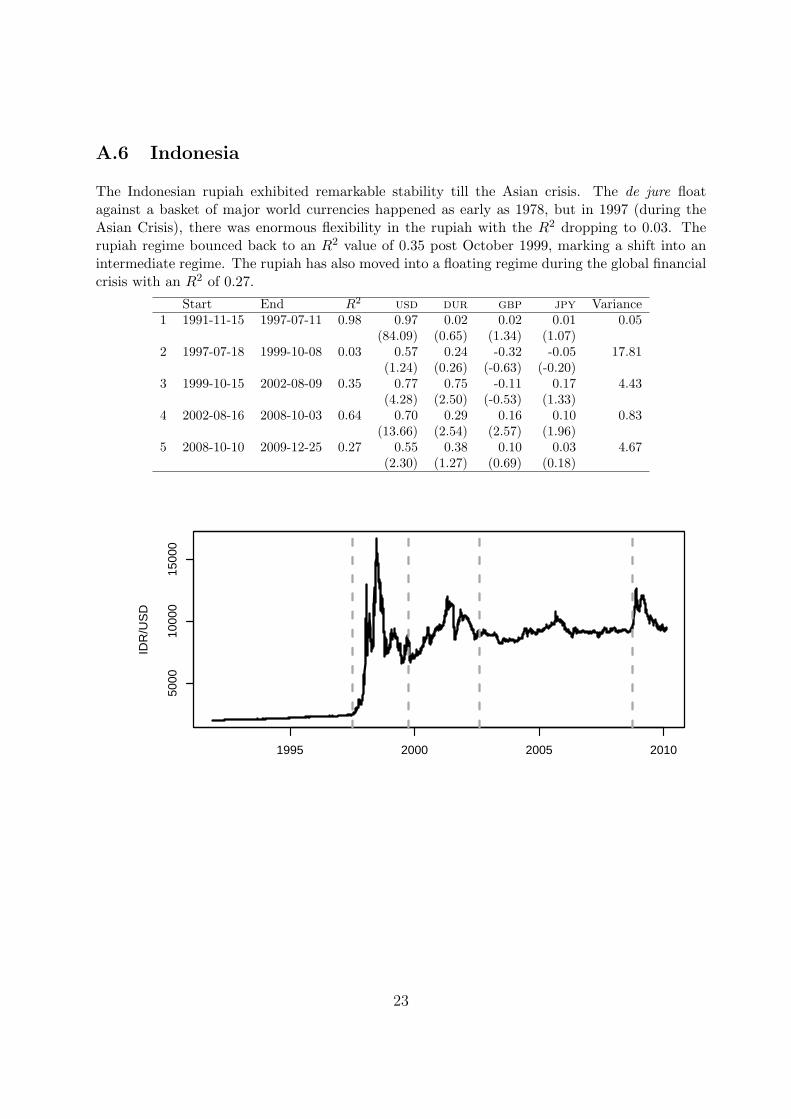
A.6 Indonesia

The Indonesian rupiah exhibited remarkable stability till the Asian crisis. The de jure floatagainst a basket of major world currencies happened as early as 1978, but in 1997 (during theAsian Crisis), there was enormous flexibility in the rupiah with the R2 dropping to 0.03. Therupiah regime bounced back to an R2 value of 0.35 post October 1999, marking a shift into anintermediate regime. The rupiah has also moved into a floating regime during the global financialcrisis with an R2 of 0.27.


(84.09) (0.65) (1.34) (1.07)2 1997-07-18 1999-10-08 0.03 0.57 0.24 -0.32 -0.05 17.81

(1.24) (0.26) (-0.63) (-0.20)3 1999-10-15 2002-08-09 0.35 0.77 0.75 -0.11 0.17 4.43

(4.28) (2.50) (-0.53) (1.33)4 2002-08-16 2008-10-03 0.64 0.70 0.29 0.16 0.10 0.83

(13.66) (2.54) (2.57) (1.96)5 2008-10-10 2009-12-25 0.27 0.55 0.38 0.10 0.03 4.67

(2.30) (1.27) (0.69) (0.18)

5000

1000

015

000

IDR

/US

D

1995 2000 2005 2010

23

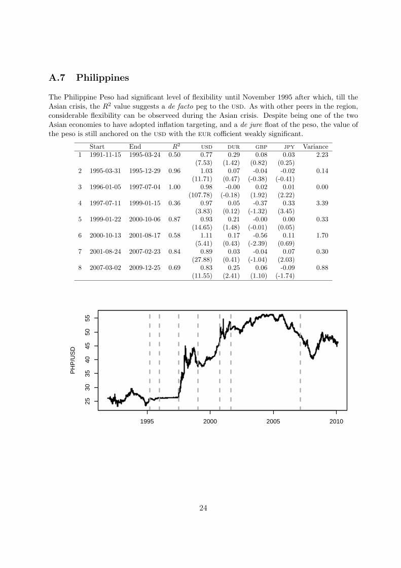
A.7 Philippines

The Philippine Peso had significant level of flexibility until November 1995 after which, till theAsian crisis, the R2 value suggests a de facto peg to the usd. As with other peers in the region,considerable flexibility can be observeed during the Asian crisis. Despite being one of the twoAsian economies to have adopted inflation targeting, and a de jure float of the peso, the value ofthe peso is still anchored on the usd with the eur cofficient weakly significant.


(7.53) (1.42) (0.82) (0.25)2 1995-03-31 1995-12-29 0.96 1.03 0.07 -0.04 -0.02 0.14

(11.71) (0.47) (-0.38) (-0.41)3 1996-01-05 1997-07-04 1.00 0.98 -0.00 0.02 0.01 0.00

(107.78) (-0.18) (1.92) (2.22)4 1997-07-11 1999-01-15 0.36 0.97 0.05 -0.37 0.33 3.39

(3.83) (0.12) (-1.32) (3.45)5 1999-01-22 2000-10-06 0.87 0.93 0.21 -0.00 0.00 0.33

(14.65) (1.48) (-0.01) (0.05)6 2000-10-13 2001-08-17 0.58 1.11 0.17 -0.56 0.11 1.70

(5.41) (0.43) (-2.39) (0.69)7 2001-08-24 2007-02-23 0.84 0.89 0.03 -0.04 0.07 0.30

(27.88) (0.41) (-1.04) (2.03)8 2007-03-02 2009-12-25 0.69 0.83 0.25 0.06 -0.09 0.88

(11.55) (2.41) (1.10) (-1.74)

2530

3540

4550

55

PH

P/U

SD

1995 2000 2005 2010

24

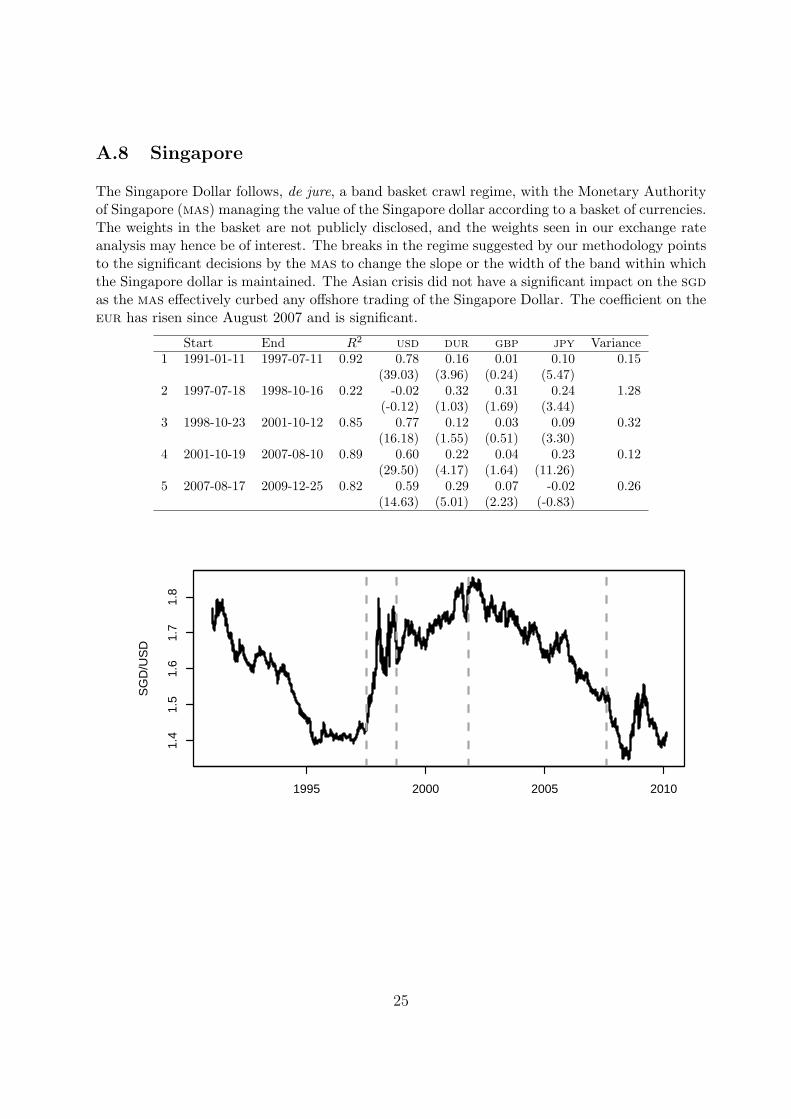
A.8 Singapore

The Singapore Dollar follows, de jure, a band basket crawl regime, with the Monetary Authorityof Singapore (mas) managing the value of the Singapore dollar according to a basket of currencies.The weights in the basket are not publicly disclosed, and the weights seen in our exchange rateanalysis may hence be of interest. The breaks in the regime suggested by our methodology pointsto the significant decisions by the mas to change the slope or the width of the band within whichthe Singapore dollar is maintained. The Asian crisis did not have a significant impact on the sgdas the mas effectively curbed any offshore trading of the Singapore Dollar. The coefficient on theeur has risen since August 2007 and is significant.


(39.03) (3.96) (0.24) (5.47)2 1997-07-18 1998-10-16 0.22 -0.02 0.32 0.31 0.24 1.28

(-0.12) (1.03) (1.69) (3.44)3 1998-10-23 2001-10-12 0.85 0.77 0.12 0.03 0.09 0.32

(16.18) (1.55) (0.51) (3.30)4 2001-10-19 2007-08-10 0.89 0.60 0.22 0.04 0.23 0.12

(29.50) (4.17) (1.64) (11.26)5 2007-08-17 2009-12-25 0.82 0.59 0.29 0.07 -0.02 0.26

(14.63) (5.01) (2.23) (-0.83)

1.4

1.5

1.6

1.7

1.8

SG

D/U

SD

1995 2000 2005 2010

25

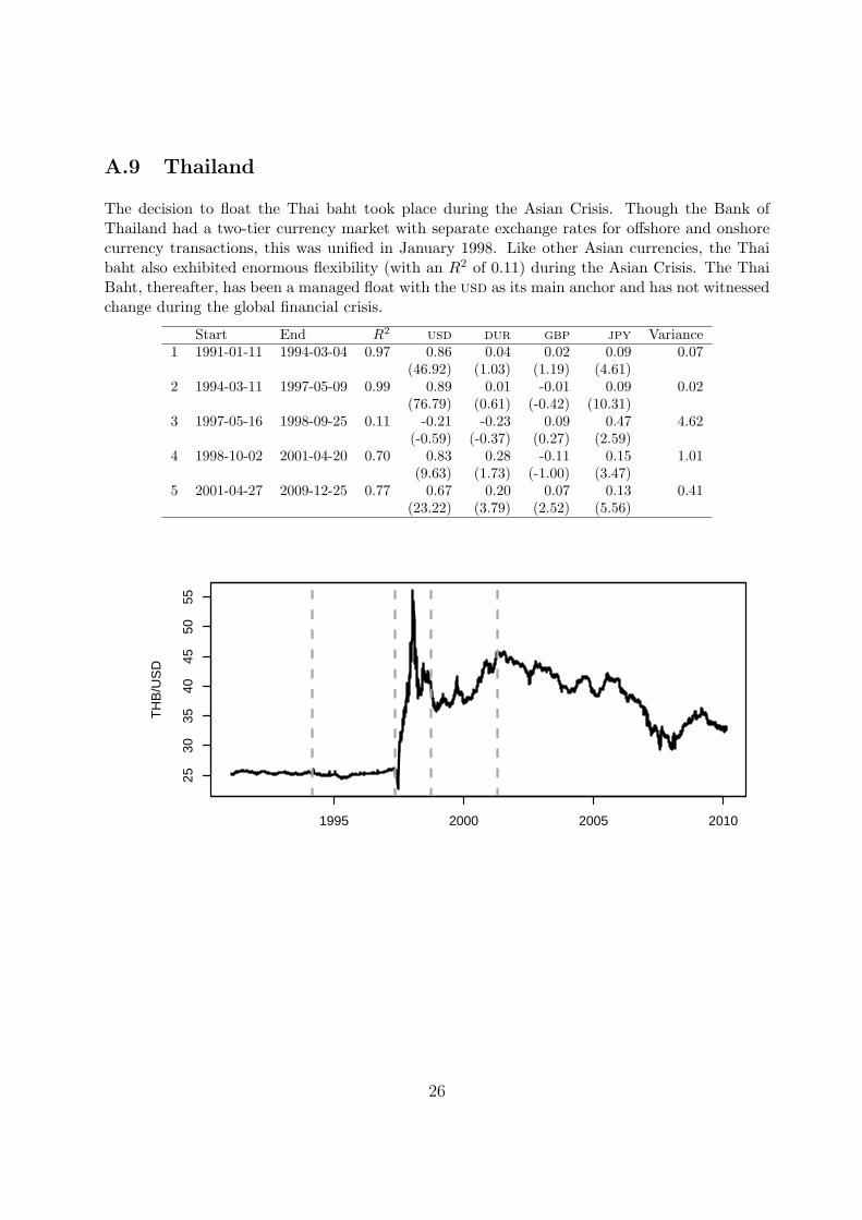
A.9 Thailand

The decision to float the Thai baht took place during the Asian Crisis. Though the Bank ofThailand had a two-tier currency market with separate exchange rates for offshore and onshorecurrency transactions, this was unified in January 1998. Like other Asian currencies, the Thaibaht also exhibited enormous flexibility (with an R2 of 0.11) during the Asian Crisis. The ThaiBaht, thereafter, has been a managed float with the usd as its main anchor and has not witnessedchange during the global financial crisis.


(46.92) (1.03) (1.19) (4.61)2 1994-03-11 1997-05-09 0.99 0.89 0.01 -0.01 0.09 0.02

(76.79) (0.61) (-0.42) (10.31)3 1997-05-16 1998-09-25 0.11 -0.21 -0.23 0.09 0.47 4.62

(-0.59) (-0.37) (0.27) (2.59)4 1998-10-02 2001-04-20 0.70 0.83 0.28 -0.11 0.15 1.01

(9.63) (1.73) (-1.00) (3.47)5 2001-04-27 2009-12-25 0.77 0.67 0.20 0.07 0.13 0.41

(23.22) (3.79) (2.52) (5.56)

2530

3540

4550

55

TH

B/U

SD

1995 2000 2005 2010

26

A.10 Taiwan

The de jure flexible exchange rate system was adopted in 1979, with an added clause that whenthe market is disrupted by seasonal or irregular factors, the Central Bank of the Republic of China(Taiwan) (CBC) will step in. In essence, our methodology captures the nuanced statement fromthe cbc with a peg on the usd before the Asian crisis, and a peg with greater flexibility after theAsian Crisis. Since the global crisis, the coefficient on the eur has risen from 0.13 in the previousperiod to 0.19 tilting the balance within the basket to the usd and eur.


(42.43) (0.04) (1.50) (4.22)2 1996-07-05 1997-07-25 0.98 0.97 0.05 0.03 0.01 0.02

(31.65) (1.08) (0.93) (0.56)3 1997-08-01 1998-10-30 0.44 0.52 0.18 0.16 0.23 0.99

(3.47) (0.66) (1.14) (4.12)4 1998-11-06 2008-01-25 0.88 0.78 0.13 0.05 0.11 0.20

(37.47) (2.96) (2.00) (6.79)5 2008-02-01 2009-12-25 0.84 0.80 0.19 0.00 -0.10 0.34

(16.12) (2.66) (0.10) (-2.82)

2628

3032

34

TW

D/U

SD

1995 2000 2005 2010

27

The exchange rate regime in Asia: From crisis to crisis

Documents

Transcript of The exchange rate regime in Asia: From crisis to crisis