The entropy of lies: playing twenty questions with a liar

Yuval Dagan∗ Yuval Filmus† Daniel Kane‡ Shay Moran§∗

November 2, 2018

Abstract

“Twenty questions” is a guessing game played by two players: Bob thinks of an integerbetween 1 and n, and Alice’s goal is to recover it using a minimal number of Yes/No questions.Shannon’s entropy has a natural interpretation in this context. It characterizes the averagenumber of questions used by an optimal strategy in the distributional variant of the game: let µbe a distribution over [n], then the average number of questions used by an optimal strategythat recovers x ∼ µ is between H(µ) and H(µ) + 1.

We consider an extension of this game where at most k questions can be answered falsely.We extend the classical result by showing that an optimal strategy uses roughly H(µ)+ kH2(µ)questions, where H2(µ) =

∑

xµ(x) log log 1

µ(x) . This also generalizes a result by Rivest et

al. (1980) for the uniform distribution.Moreover, we design near optimal strategies that only use comparison queries of the form “x ≤

c?” for c ∈ [n]. The usage of comparison queries lends itself naturally to the context of sorting,where we derive sorting algorithms in the presence of adversarial noise.

1 Introduction

The “twenty questions” game is a cooperative game between two players: Bob thinks of an integerbetween 1 and n, and Alice’s goal is to recover it using the minimal number of Yes/No questions.An optimal strategy for Alice is to perform binary search, using log n queries in the worst case.

The game becomes more interesting when Bob chooses his number according to a distribution µknown to both players, and Alice attempts to minimize the expected number of questions. In thiscase, the optimal strategy is to use a Huffman code for µ, at an expected cost of roughly H(µ).

What happens when Bob is allowed to lie (either out of spite, or due to difficulties in thecommunication channel)? Renyi [19] and Ulam [24] suggested a variant of the (non-distributional)“twenty questions” game, in which Bob is allowed to lie k times. Rivest et al. [20], using ideasof Berlekamp [4], showed that the optimal number of questions in this setting is roughly log n +k log log n. There are many other ways of allowing Bob to lie, some of which are described by Spencerand Winkler [23] in their charming work, and many others by Pelc [18] in his comprehensive surveyon the topic.

∗Department of Electrical Engineering and Computer Science, Massachusetts Institute of Technology.†Computer Science Department, Technion. Taub Fellow — supported by the Taub Foundations. The research

was funded by ISF grant 1337/16.‡Department of Computer Science and Engineering and Department of Mathematics, University of California at

San Diego.§Department of Computer Science, Princeton University.

1

Distributional “twenty questions” with lies. This work addresses the distributional “twentyquestions” game in the presence of lies. In this setting, Bob draws an element x according to adistribution µ, and Alice’s goal is to recover the element using as few Yes/No questions as possibleon average. The twist is that Bob, who knows Alice’s strategy, is allowed to lie up to k times. BothAlice and Bob are allowed to use randomized strategies, and the average is measured according toboth µ and the randomness of both parties.

Our main result shows that the expected number of questions in this case is

H(µ) + kH2(µ), where H2(µ) =∑

x

µ(x) log log1

µ(x),

up to an additive factor of O(k log k + kH3(µ)), where H3(µ) =∑

x µ(x) log log log(1/µ(x))) (hereµ(x) is the probability of x under µ.) See Section 3 for a complete statement of this result.

When µ is the uniform distribution, the expected number of queries that our algorithm makesis roughly log n+ k log log n, matching the performance of the algorithm of Rivest et al. However,the approach by Rivest et al. is tailored to their setting, and the distributional setting requires newideas.

As in the work of Rivest et al., our algorithms use only comparison queries, which are queriesof the form “x ≺ c?” (for some fixed value c). Moreover, our algoritms are efficient, requiringO(n) preprocessing time and O(log n) time per question. Our lower bounds, in contrast, apply toarbitrary Yes/No queries.

Noisy sorting. One can apply binary search algorithms to implement insertion sort. Whilesorting an array typically requires Θ(n log n) sorting queries of the form “xi ≺ xj?”, there aresituations where one has some prior knowledge about the correct ordering. This may happen, forexample, when maintaining a sorted array: one has to perform consecutive sorts, where each sort isnot expected to considerably change the locations of the elements. Assuming a distribution Π overthe n! possible permutations, Moran and Yehudayoff [16] showed that sorting a Π-distributed arrayrequires H(Π) + O(n) sorting queries on average. We extend this result to the case in which theanswerer is allowed to lie k times, giving an algorithm which uses the following expected numberof queries:1

H(Π) +O(nk).

This result is tight, and matches the optimal algorithms for the uniform distribution due toBagchi [3] and Long [15], which use n log n+O(nk) queries.

Table 1 summarizes the query complexities of resilient and non-resilient searching and sortingalgorithms, in both the deterministic and the distributional settings. To the best of our knowledge,we present the first resilient algorithms in the distributional setting.

On randomness. All algorithms presented in the paper are randomized. Since they only employpublic randomness which is known for both players, there exists a fixing of the randomness whichyields a deterministic algorithm with the same (or possibly smaller) expected number of queries.However, this comes at the cost of possibly increasing the running time of the algorithm (since weneed to find a good fixing of the randomness); it would be interesting to derive an explicit efficientdeterministic algorithm with a similar running time.

1Strictly speaking, this bound holds only under the mild condition that k is at most exponential in n.

2

Setting Searching Sorting

No lies; deterministic log n [classical] n log n [classical]No lies; distributional H(µ) [classical] H(Π) +O(n) [16]k lies; deterministic log n+ k log log n [20] n log n+Θ(nk) [3, 15, 14]k lies; distributional H(µ) + kH2(µ) [this paper] H(Π) + Θ(nk) [this paper]

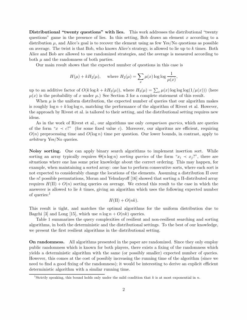
Table 1: Query complexities of searching and sorting in different settings, ignoring lower-orderterms. All terms are exact upper and lower bounds except for those inside the O(·) and Θ(·)notations.

. . .

µ(x1) µ(xn)

0 1x1 xn

Figure 1: Representing items as centers of segments partitioning the interval [0, 1].

1.1 Main ideas

Upper bound. Before presenting the ideas behind our algorithms, we explore several other ideaswhich give suboptimal results. The first approach that comes to mind is simulating the optimalnon-resilient strategy, asking each question 2k+1 times and taking the majority vote, which resultsin an algorithm using Θ(kH(µ)) queries on average.

A better approach is using tree codes, suggested by Schulman [21] as an approach for makinginteractive communication resilient to errors [10, 21, 13]. Tree codes are designed for a differenterror model, in which we are bounding the fraction of lies rather than their absolute number; for anε-fraction of lies, the best known constructions suffer a multiplicative overhead of 1 +O(

√ε) [12].

In contrast, we are aiming at an additive overhead of kH2(µ).Using a packing bound, one can prove that there exists a (non-interactive) code of expected

length roughly H(µ) + 2kH2(µ), coming much closer to the bound that we are able to get (but offby a factor of 2 from our target H(µ) + kH2(µ)). The idea, which is similar to the proof of theGilbert–Varshamov bound, is to construct a prefix code w1, . . . , wn in which the prefixes of wi, wj oflength min(|wi|, |wj |) are at distance at least 2k+1 (whence the factor 2k in the resulting bound);this can be done greedily. Apart from the inferior bound, two other disadvantages of this approachis that it is not efficient and uses arbitrary queries.

In contrast to these prior techniques, which do not achieve the optimal complexity, might askarbitrary questions, and could result in strategies which cannot be implemented efficiently, in thispaper we design an efficient and nearly optimal strategy, relying on comparison queries only, andutilizing simple observations on the behavior of binary search trees under the presence of lies.

Following the footsteps of Rivest et al. [20], our upper bound is based on a binary searchalgorithm on the unit interval [0, 1], first suggested in this context by Gilbert and Moore [11]:given x ∈ [0, 1], the algorithm locates x by first asking “x < 1/2?”; depending on the answer,asking “x < 1/4?” or “x < 3/4?”; and so on. If x ∈ [0, 1] is chosen uniformly at random then theanswers behave like an infinite sequence of random and uniform coin tosses.

In order to apply this kind of binary search to the problem of identifying an unknown ele-ment (assuming truthful answers), we partition the unit interval [0, 1] into segments of lengthsµ(x1), . . . , µ(xn), and label the center of each segment with the corresponding item (see Figure 1).

3

<

<

>

... ...

> lie

<

<

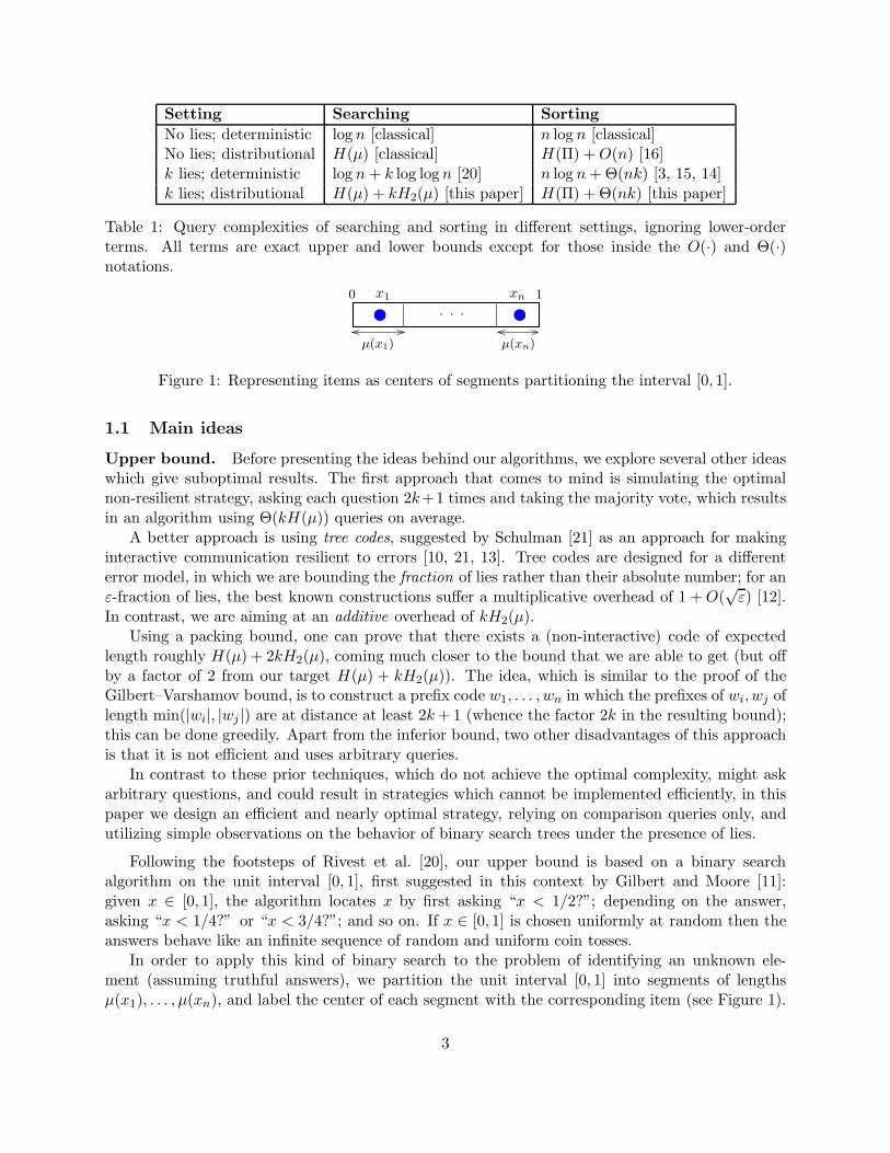
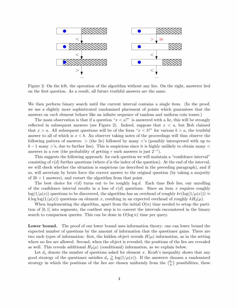
Figure 2: On the left, the operation of the algorithm without any lies. On the right, answerer liedon the first question. As a result, all future truthful answers are the same.

We then perform binary search until the current interval contains a single item. (In the proof,we use a slightly more sophisticated randomized placement of points which guarantees that theanswers on each element behave like an infinite sequence of random and uniform coin tosses.)

The main observation is that if a question “x < a?” is answered with a lie, this will be stronglyreflected in subsequent answers (see Figure 2). Indeed, suppose that x < a, but Bob claimedthat x > a. All subsequent questions will be of the form “x < b?” for various b > a, the truthfulanswer to all of which is x < b. An observer taking notes of the proceedings will thus observe thefollowing pattern of answers: > (the lie) followed by many <’s (possibly interspersed with up tok− 1 many >’s, due to further lies). This is suspicious since it is highly unlikely to obtain many <answers in a row (the probability of getting r such answers is just 2−r).

This suggests the following approach: for each question we will maintain a “confidence interval”consisting of r(d) further questions (where d is the index of the question). At the end of the interval,we will check whether the situation is suspicious (as described in the preceding paragraph), and ifso, will ascertain by brute force the correct answer to the original question (by taking a majorityof 2k + 1 answers), and restart the algorithm from that point.

The best choice for r(d) turns out to be roughly log d. Each time Bob lies, our unrollingof the confidence interval results in a loss of r(d) questions. Since an item x requires roughlylog(1/µ(x)) questions to be discovered, the algorithm has an overhead of roughly kr(log(1/µ(x))) ≈k log log(1/µ(x)) questions on element x, resulting in an expected overhead of roughly kH2(µ).

When implementing the algorithm, apart from the initial O(n) time needed to setup the parti-tion of [0, 1] into segments, the costliest step is to convert the intervals encountered in the binarysearch to comparison queries. This can be done in O(log n) time per query.

Lower bound. The proof of our lower bound uses information theory: one can lower bound theexpected number of questions by the amount of information that the questioner gains. There aretwo such types of information: first, the hidden object reveals H(µ) information, as in the settingwhere no lies are allowed. Second, when the object is revealed, the positions of the lies are revealedas well. This reveals additional H2(µ) (conditional) information, as we explain below.

Let dx denote the number of questions asked for element x. Kraft’s inequality shows that anygood strategy of the questioner satisfies dx ' log(1/µ(x)). If the answerer chooses a randomizedstrategy in which the positions of the lies are chosen uniformly from the

(dxk

)

possibilities, these

4

positions reveal log(dxk

)

≈ k log dx ' k log log(1/µ(x)) information given x. Taking expectationover x, the positions of the lies reveal at least kH2(µ) information beyond the identity of x.

1.2 Related work

Most of the literature on error-resilient search procedures has concentrated on the non-distributionalsetting, in which the goal is to give a worse case guarantee on the number of questions asked, undervarious error models. The most common error models are as follows:2

• Fixed number of errors. This is the error model we consider, and it is also the one suggestedby Ulam [24]. This model was first studied by Berlekamp [4], who used an argument similarto the sphere-packing bound to give a lower bound on the number of questions. Rivest etal. [20] used this lower bound as a guiding principle in their almost matching upper boundusing comparison queries.

• At most a fixed fraction p of the answers can be lies. This model is similar to the oneconsidered in error-correcting codes. Pelc [17] and Spencer and Winkler [23] (independently)gave a non-adaptive strategy for revealing the hidden element when p ≤ 1/4, and showedthat the task is not possible (non-adaptively) when p > 1/4. Furthermore, when p < 1/4there is an algorithm using O(log n) questions, and when p = 1/4 there is an algorithm usingO(n) questions, which are both optimal (up to constant factors). Spencer and Winkler alsoshowed that if questions are allowed to be adaptive, then the hidden element can be revealedif and only if p < 1/3, again using O(log n) questions.

• At most a fixed fraction p of any prefix of the answers can be lies. Pelc [17] showed thatthe hidden element can be revealed if and only if p < 1/2, and gave an O(log n) strategywhen p < 1/4. Aslam and Dhagat [2] and Spencer and Winkler gave an O(log n) strategy forall p < 1/2.

• Every question is answered erroneously with probability p, an error model common in in-formation theory. Renyi [19] showed that the number of questions required to discover thehidden element with constant success probability is (1 + o(1)) log n/(1− h(p)).

The distributional version of the “twenty questions” game (without lies) was first considered byShannon [22] in his seminal paper introducing information theory, where its solution was attributedto Fano (who published it later as [8]). The Shannon–Fano code uses at most H(µ)+1 questions onaverage, but the questions can be arbitrary. The Shannon–Fano–Elias code (also due to Gilbert andMoore [11]), which uses only comparison queries, asks at most H(µ)+2 questions on average. Daganet al. [7] give a strategy, using only comparison and equality queries, which asks at most H(µ) + 1questions on average.

Sorting The non-distributional version of sorting has also been considered in some of the settingsconsidered above:

• At most k errors: Lakshmanan et al. [14] gave a lower bound of Ω(n log n+kn) on the numberof questions, and an almost matching upper bound of O(n log n + kn + k2) questions. An

2This section is heavily based on Pelc’s excellent and comprehensive survey [18]

5

optimal algorithm, using n log n + O(kn) questions, was given independently by Bagchi [3]and Long [15].

• At most a p fraction of errors in every prefix: Aigner [1] showed that sorting is possible if andonly if p < 1/2. Borgstrom and Kosaraju [5] had showed earlier that even verifying that anarray is sorted requires p < 1/2.

• Every answer is correct with probability p: Feige et al. [9] showed in an influential paper thatΘ(n log(n/ǫ)) queries are needed, where ǫ is the probability of error.

• Braverman and Mossel [6] considered a different setting, in which an algorithm is givenaccess to noisy answers to all possible

(n2

)

comparisons, and the goal is to find the most likelypermutation. They gave a polynomial time algorithm which succeeds with high probability.

The distributional version of sorting (without lies) was considered by Moran and Yehudayoff [16],who gave a strategy using at most H(µ) + 2n queries on average, based on the Gilbert–Moorealgorithm.

Paper organization. After a few preliminaries in Section 2, we describe our results in full inSection 3. We prove our lower bound on the number of questions in Section 4. We present ourmain upper bound in Section 5, and an improved version in Section 6. We close the paper with adiscussion of sorting in Section 7.

2 Definitions

We use the notation( n≤k

)

=∑k

ℓ=0

(nℓ

)

. Unless stated otherwise, all logarithms are base 2. We

define log(x) = log(x + C) and ln(x) = ln(x + C) for a fixed sufficiently large constant C > 0satisfying log log logC > 0.

Information theory. Given a probability distribution µ with countable support, the entropyof µ is given by the formula

H(µ) =∑

x∈suppµ

µ(x) log1

µ(x).

Twenty questions game. We start with an intuitive definition of the game, played by a ques-tioner (Alice) and an answerer (Bob). Let U be a finite set of elements, and let µ be a distributionover U , known to both parties. The game proceeds as follows: first, an element x ∼ µ is drawn andrevealed to the answerer but not to the questioner. The element x is called the hidden element. Thequestioner asks binary queries of the form “x ∈ Q?” for subsets Q ⊆ U . The answerer is allowedto lie a fixed number of times, and the goal of the questioner is to recover the hidden element x,asking the minimal number of questions on expectation.

Decision trees. Let U be a finite set of elements. A decision tree T for U is a binary treeformalizing the question asking strategy in the twenty questions game. Each internal node of vof T is labeled by a query (or question) — a subset of U , denoted by Q(v); and each leaf is labeledby the output of the decision tree, which is an element of U . The semantics of the tree are as

6

follows: on input x ∈ U , traverse the tree by starting at the root, and whenever at an internal nodev, go to the left child if x ∈ Q(v) and to the right child if x /∈ Q(v).

Comparison tree. Given an ordered set of elements x1 ≺ x2 ≺ · · · ≺ xn, comparison questionsare questions of the form Q = x1, . . . , xi−1, for some i = 1, . . . , n+1. In other words, the questionsare “x ≺ xi?” for some i = 1, . . . , n + 1. An answer to a comparison question is one of ≺,. Acomparison tree is a decision tree all of whose nodes are labeled by comparison questions.

Adversaries. Let k ≥ 0 be a bound on the number of lies. An intuitive way to formalize thepossibility of lying is via an adversary. The adversary knows the hidden element x and receivesthe queries from the questioner as the tree is being traversed. The adversary is allowed to lie atmost k times, where each lie is a violation of the above stated rule. Formally, an adversary is amapping that receives as input an element x ∈ X, a sequence of the previous queries and theiranswers, and an additional query Q ⊆ U , which represents the current query. The output of theadversary is a boolean answer to the current query; this answer is a lie if it differs from the truthvalue of “x ∈ Q”.

We also allow the adversary and the tree to use randomness: a randomized decision tree is adistribution over decision trees and a randomized adversary is a distribution over adversaries.

Computation and complexity. The responses of the adversary induce a unique root-to-leafpath in the decision tree, which results in the output of the tree. A decision tree is k-valid if itoutputs the correct element against any adversary that lies at most k times.

Given a k-valid decision tree T and a distribution µ on U , the cost of T with respect to µ,denoted c(T, µ), is the maximum, over all possible adversaries that lie at most k times, of theexpected3 length of the induced root-to-leaf path in T . Finally, the k-cost of µ, denoted ck(µ), isthe minimum of c(T, µ) over all k-valid decision trees T .

Basic facts. We will refer to the following well-known formula as Kraft’s identity :

Fact 2.1 (Kraft’s identity). Fix a binary tree T , let L be its set of leaves and let d(ℓ) be the depthof leaf ℓ. The following applies:

∑

ℓ∈L(T )

2−d(ℓ) ≤ 1.

We will use the following basic lower bound on the expected depth by the entropy:

Fact 2.2. Let T be a binary tree and let µ be a distribution over its leaves. Then

H(µ) ≤ Eℓ∼µ

[

d(ℓ)]

.

In other words, for any distribution µ, c0(µ) ≥ H(µ). In fact, it is also known that c0(µ) ≤H(µ) + 1.

3The expectation is also taken with respect to the randomness of the adversary and the tree when they arerandomized.

7

3 Main results

This section is organized as follows: The lower bound is presented in Section 3.1. Then, the twosearching algorithms are presented in Section 3.2, and finally the application to sorting is presentedin Section 3.3.

3.1 Lower bound

In this section we present the following lower bound on ck(µ), namely, on the expected number ofquestions asked by any k-valid tree (not necessarily a comparison trees).

Theorem 3.1. For every non-constant distribution µ and every k ≥ 0,

ck(µ) ≥(

Ex∼µ

log1

µ(x)

)

+ k(

Ex∼µ

log log1

µ(x)

)

− (k log k + k + 1).

The proof of this lower bound appears in Section 4.

Proof overview. Consider a k-valid tree; we wish to lower bound the expected number of ques-tions for x ∼ µ. Let dx denote the number of questions asked when the secret element is x.Then, by the entropy lower bound when the number of mistakes is k = 0, it follows that typ-ically, dx & log(1/µ(x)). Moreover, the transcript of the game (i.e. the list of questions andanswers) determines both x and the positions of the k lies. This requires

dx + k log(dx) & log(1/µ(x)) + k log log(1/µ(x))

bits of information. Taking expectation over x ∼ µ then yields the stated bound.Our proof formalizes this intuition using standard and basic tools from information theory. One

part that requires a subtler argument is showing that indeed one may assume that dx & log(1/µ(x))for all x. This is done by showing that any k-valid tree can be modified to satisfy this constraintwithout increasing the expected number of questions by too much. The crux of this argument,which relies on Kraft’s identity (Fact 2.1), appears in Lemma 4.1.

3.2 Upper bounds

We introduce two algorithms. The first algorithm, presented in Section 3.2.1, is simpler, however,the second algorithm has a better query complexity. The expected number of questions asked bythe first algorithm is at most

H(µ) + (k + 1)H2(µ) +O(k2H3(µ) + k2 log k), where H3(µ) =∑

x

µ(x) log log log1

µ(x).

The second algorithm, presented in Section 3.2.2, removes the quadratic dependence on k, and hasan expected complexity of:

H(µ) + kH2(µ) +O(kH3(µ) + k log k).

In Section 3.2.3 we robustify the guarantees of these algorithms and consider scenarios where theexact distribution µ is not known but only some prior η ≈ µ, or where the actual number of lies isless than the bound k (whence the algorithm achieves better performance).

8

3.2.1 First algorithm

Suppose that we are given a probability distribution µ whose support is the linearly ordered setx1 ≺ · · · ≺ xn. In this section we overview the proof of the following theorem (the complete proofappears in Section 5):

Theorem 3.2. There is a k-valid comparison tree T with

c(T, µ) ≤ H(µ) + (k + 1)

n∑

i=1

µi log log1

µi+O

(

k2n∑

i=1

µi log log log1

µi+ k2 log k

)

,

where µi = µ(xi).

The question-asking strategy simulates a binary search to recover the hidden element. If, atsome point, the answer to some question q is suspected as a lie then q is asked 2k+1 times to verifyits answer. When is the answer to q suspected? The binary search tree is constructed in a mannerthat if no lies are told then roughly half of the questions are answered ≺, and half . However,if, for example, the lie “x x50” is told when in fact x = x10, then all consecutive questions willbe of the form “x ≺ xi?” for i > 50, and the correct answer would always be ≺. Since no morethan k lies can be told, almost all consecutive questions will be answered ≺, and the algorithm willsuspect that some earlier question is a lie.

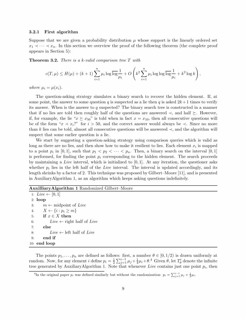
We start by suggesting a question-asking strategy using comparison queries which is valid aslong as there are no lies, and then show how to make it resilient to lies. Each element xi is mappedto a point pi in [0, 1], such that p1 < p2 < · · · < pn. Then, a binary search on the interval [0, 1]is performed, for finding the point pi corresponding to the hidden element. The search proceedsby maintaining a Live interval, which is initialized to [0, 1]. At any iteration, the questioner askswhether pi lies in the left half of the Live interval. The interval is updated accordingly, and itslength shrinks by a factor of 2. This technique was proposed by Gilbert–Moore [11], and is presentedin AuxiliaryAlgorithm 1, as an algorithm which keeps asking questions indefinitely.

AuxilliaryAlgorithm 1 Randomized Gilbert–Moore

1: Live ← [0, 1]2: loop

3: m← midpoint of Live4: X ← i : pi ≥ m5: if x ∈ X then

6: Live ← right half of Live7: else

8: Live ← left half of Live9: end if

10: end loop

The points p1, . . . , pn are defined as follows: first, a number θ ∈ [0, 1/2) is drawn uniformly atrandom. Now, for any element i define pi =

12

∑i−1j=1 µj+

14µi+θ.4 Given θ, let T ′

θ denote the infinitetree generated by AuxiliaryAlgorithm 1. Note that whenever Live contains just one point pi, then

4In the original paper pi was defined similarly but without the randomization: pi =∑i−1

j=1µj +

1

2µi.

9

(as there are no lies) the hidden element must be xi. Denote by Tθ the finite tree corresponding tothe algorithm which stops whenever that happens. We present two claims about these trees whichare proved in Section 5.1.

First, conditioned on any hidden element xi, the answers to all questions (except, perhaps, forthe first answer) are distributed uniformly and independently, where the distribution is over therandom choice of θ. This follows from the fact that all bits of pi except for the most significant bitare i.i.d. unbiased coin flips.

Claim 3.3. For any element xi, let (At) be the random sequence of answers to the questionsin AuxiliaryAlgorithm 1, containing all answers except for the first answer, assuming there are nolies. The distribution of the sequence (At) is the same as that of an infinite sequence of independentunbiased coin tosses, where the randomness stems from the random choice of pi.

Second, since min(pi − pi−1, pi+1 − pi) ≥ µi/4, one can bound the time it takes to isolate xi asfollows.

Claim 3.4. For any element xi and any θ, the leaf in Tθ labeled by xi is of depth at most log(1/µi)+3. Hence, if x is drawn from a distribution µ, the expected depth of the leaf labeled x is at most∑

i µi log(1/µi) + 3 = H(µ) + 3.

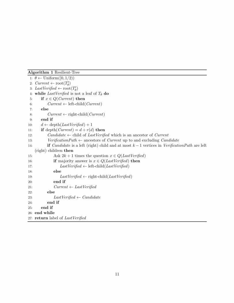
We now describe the k-resilient algorithm: Algorithm 1 (the pseudocode appears as well). Atthe beginning, a number θ is randomly drawn. Then, two concurrent simulations over T ′

θ areperformed, and two pointers to nodes in this tree are maintained (recall that T ′

θ is the infinitebinary search tree). The first pointer, Current , simulates the question-asking strategy accordingto T ′

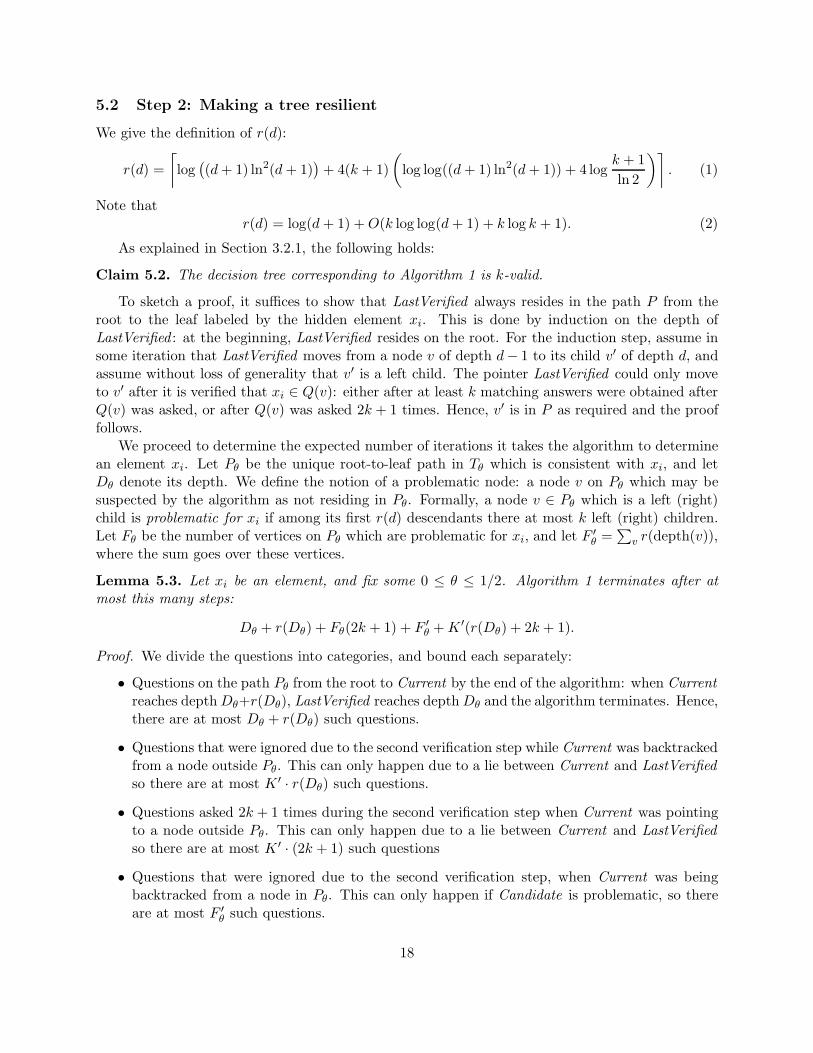
θ, ignoring the possibility of lies. In particular, it may point on an incorrect node in the tree(reached as a result of a lie). Since Current ignores the possibility of lies, there is a different pointer,LastVerified , which verifies the answers to the questions asked in the simulation of Current . Allanswers in the path from the root to LastVerified are verified as correct, and LastVerified willalways be an ancestor of Current . See Figure 3 for the basic setup.

The algorithm proceeds in iterations. In every iteration the question Q(Current) is askedand Current is advanced to the corresponding child accordingly. In some of the iterations alsoLastVerified is advanced. Concretely, this happens when the depth of Current in T ′

θ equals d+r(d),where d is the depth of LastVerified and r(d) ≈ log d+ k log log d.5 In these iterations, the answergiven to Q(LastVerified ) is being verified, as detailed next.

The verification process. Next, we examine the verification process when LastVerified is ad-vanced. There are two possibilities: first, when the answer to the question Q(LastVerified ), whichwas given when Current traversed it, is verified to be correct. In that case, LastVerified moves toits child which lies on the path towards Current . In the complementing case, when the the answerto the question Q(LastVerified) is detected as a lie, then LastVerified moves to the other child. Inthat case, Current is no longer a descendant of LastVerified , hence Current is moved up the treeand is set to LastVerified .

We now explain how the answer to Q(LastVerified ) is verified. There are two verification steps:the first step uses no additional questions and the second step uses 2k + 1 additional questions.Usually, only the first step will be used and no additional questions will be spent during verification.In the first verification step one checks whether the following condition holds:

5The exact definition of r(d) is in Equation (1).

10

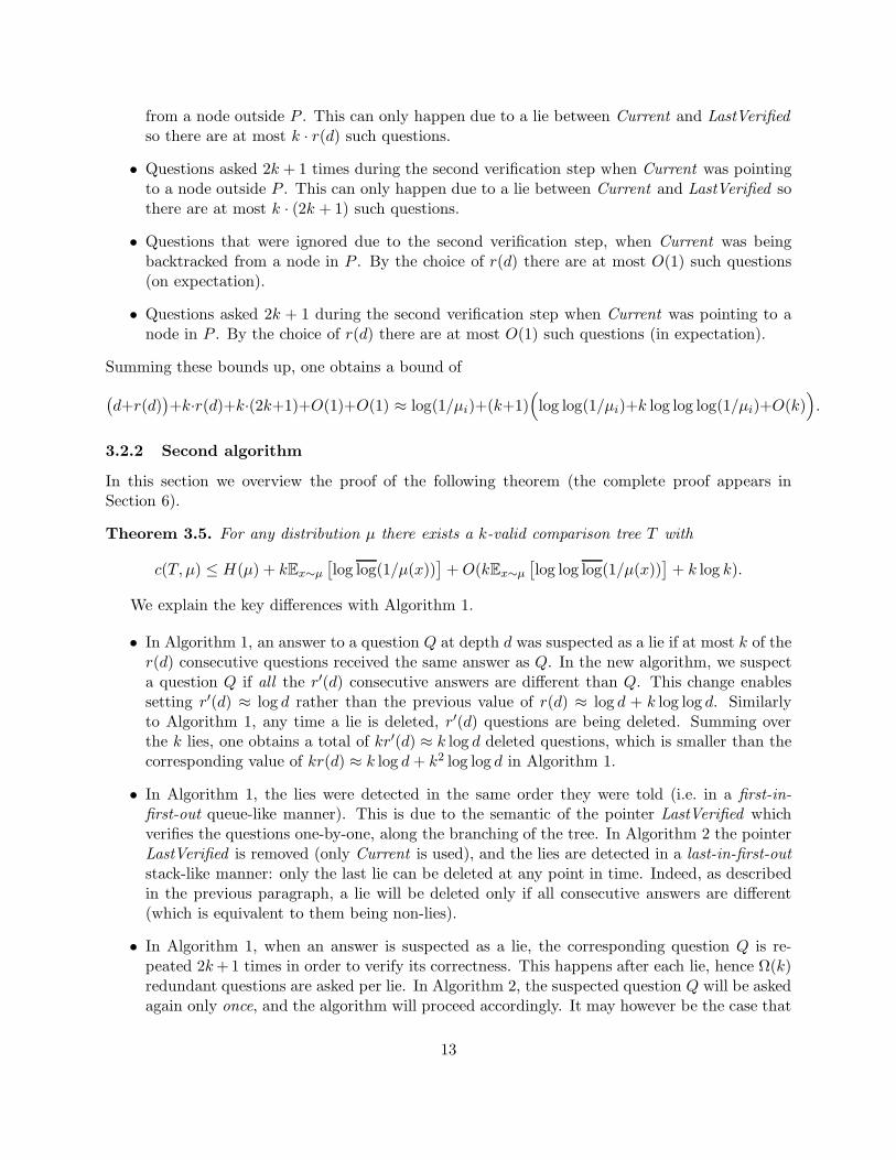
Algorithm 1 Resilient-Tree

1: θ ← Uniform([0, 1/2))2: Current ← root(T ′

θ)3: LastVerified ← root(T ′

θ)4: while LastVerified is not a leaf of Tθ do

5: if x ∈ Q(Current) then6: Current ← left-child(Current)7: else

8: Current ← right-child(Current)9: end if

10: d← depth(LastVerified) + 111: if depth(Current) = d+ r(d) then12: Candidate ← child of LastVerified which is an ancestor of Current13: VerificationPath ← ancestors of Current up to and excluding Candidate14: if Candidate is a left (right) child and at most k− 1 vertices in VerificationPath are left

(right) children then

15: Ask 2k + 1 times the question x ∈ Q(LastVerified)16: if majority answer is x ∈ Q(LastVerified) then17: LastVerified ← left-child(LastVerified)18: else

19: LastVerified ← right-child(LastVerified)20: end if

21: Current ← LastVerified22: else

23: LastVerified ← Candidate24: end if

25: end if

26: end while

27: return label of LastVerified

11

Root

LastVerified

<

>

< >

>

>

>

Candidate

Current

Lie!

d

r(d)

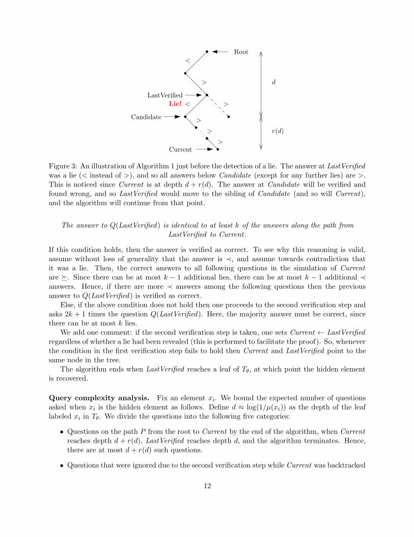
Figure 3: An illustration of Algorithm 1 just before the detection of a lie. The answer at LastVerifiedwas a lie (< instead of >), and so all answers below Candidate (except for any further lies) are >.This is noticed since Current is at depth d + r(d). The answer at Candidate will be verified andfound wrong, and so LastVerified would move to the sibling of Candidate (and so will Current),and the algorithm will continue from that point.

The answer to Q(LastVerified) is identical to at least k of the answers along the path fromLastVerified to Current .

If this condition holds, then the answer is verified as correct. To see why this reasoning is valid,assume without loss of generality that the answer is ≺, and assume towards contradiction thatit was a lie. Then, the correct answers to all following questions in the simulation of Currentare . Since there can be at most k − 1 additional lies, there can be at most k − 1 additional ≺answers. Hence, if there are more ≺ answers among the following questions then the previousanswer to Q(LastVerified ) is verified as correct.

Else, if the above condition does not hold then one proceeds to the second verification step andasks 2k + 1 times the question Q(LastVerified). Here, the majority answer must be correct, sincethere can be at most k lies.

We add one comment: if the second verification step is taken, one sets Current ← LastVerifiedregardless of whether a lie had been revealed (this is performed to facilitate the proof). So, wheneverthe condition in the first verification step fails to hold then Current and LastVerified point to thesame node in the tree.

The algorithm ends when LastVerified reaches a leaf of Tθ, at which point the hidden elementis recovered.

Query complexity analysis. Fix an element xi. We bound the expected number of questionsasked when xi is the hidden element as follows. Define d ≈ log(1/µ(xi)) as the depth of the leaflabeled xi in Tθ. We divide the questions into the following five categories:

• Questions on the path P from the root to Current by the end of the algorithm, when Currentreaches depth d + r(d), LastVerified reaches depth d, and the algorithm terminates. Hence,there are at most d+ r(d) such questions.

• Questions that were ignored due to the second verification step while Current was backtracked

12

from a node outside P . This can only happen due to a lie between Current and LastVerifiedso there are at most k · r(d) such questions.

• Questions asked 2k + 1 times during the second verification step when Current was pointingto a node outside P . This can only happen due to a lie between Current and LastVerified sothere are at most k · (2k + 1) such questions.

• Questions that were ignored due to the second verification step, when Current was beingbacktracked from a node in P . By the choice of r(d) there are at most O(1) such questions(on expectation).

• Questions asked 2k + 1 during the second verification step when Current was pointing to anode in P . By the choice of r(d) there are at most O(1) such questions (in expectation).

Summing these bounds up, one obtains a bound of

(

d+r(d))

+k·r(d)+k·(2k+1)+O(1)+O(1) ≈ log(1/µi)+(k+1)(

log log(1/µi)+k log log log(1/µi)+O(k))

.

3.2.2 Second algorithm

In this section we overview the proof of the following theorem (the complete proof appears inSection 6).

Theorem 3.5. For any distribution µ there exists a k-valid comparison tree T with

c(T, µ) ≤ H(µ) + kEx∼µ

[

log log(1/µ(x))]

+O(kEx∼µ

[

log log log(1/µ(x))]

+ k log k).

We explain the key differences with Algorithm 1.

• In Algorithm 1, an answer to a question Q at depth d was suspected as a lie if at most k of ther(d) consecutive questions received the same answer as Q. In the new algorithm, we suspecta question Q if all the r′(d) consecutive answers are different than Q. This change enablessetting r′(d) ≈ log d rather than the previous value of r(d) ≈ log d + k log log d. Similarlyto Algorithm 1, any time a lie is deleted, r′(d) questions are being deleted. Summing overthe k lies, one obtains a total of kr′(d) ≈ k log d deleted questions, which is smaller than thecorresponding value of kr(d) ≈ k log d+ k2 log log d in Algorithm 1.

• In Algorithm 1, the lies were detected in the same order they were told (i.e. in a first-in-first-out queue-like manner). This is due to the semantic of the pointer LastVerified whichverifies the questions one-by-one, along the branching of the tree. In Algorithm 2 the pointerLastVerified is removed (only Current is used), and the lies are detected in a last-in-first-outstack-like manner: only the last lie can be deleted at any point in time. Indeed, as describedin the previous paragraph, a lie will be deleted only if all consecutive answers are different(which is equivalent to them being non-lies).

• In Algorithm 1, when an answer is suspected as a lie, the corresponding question Q is re-peated 2k+1 times in order to verify its correctness. This happens after each lie, hence Ω(k)redundant questions are asked per lie. In Algorithm 2, the suspected question Q will be askedagain only once, and the algorithm will proceed accordingly. It may however be the case that

13

this process will repeat itself and also the second answer to this question will be suspected asa lie and Q will be asked once again and so on. In order to avoid an infinite loop we add thecondition that if the same answer is told k + 1 times then it is guaranteed to be correct andwill not be suspected any more.

• The removal of LastVerified forces finding a different method of verifying the correctness ofan element x upon arriving at a leaf of Tθ. One option is to ask the question “element = x?”2k + 1 times and take the majority vote, where each = question is implemented using one and one . This will, however, lead to asking Ω(k) redundant questions each time x is notthe correct element. Instead, one asks “element = x?” multiple times, stopping either whenthe answer = is obtained k + 1 times, or by the first the answer 6= has obtained more thanthe answer =. The total redundancy imposed by these verification questions throughout thewhole search is O(k).

To put the algorithm together, we exploit some simple combinatorial properties of paths containingmultiple lies.

3.2.3 A fine-grained analysis of the guarantees

In this section, we present a stronger statement for the guarantees of our algorithms. First, thealgorithms do not have to know exactly the distribution µ from which the hidden element is drawn:an approximation suffices for getting a similar bound. Recall that the algorithm gets as an inputsome probability distribution η. This distribution might differ from the true distribution µ. Thecost of using η rather than µ is related to D(µ‖η), the Kullback–Leibler divergence between thedistributions.

Secondly, the algorithm has stronger guarantees when the actual number of lies is less than k.This is an improvement comparing to the algorithm of Rivest et al. [20] mentioned in the intro-duction. It will be utilized in the application of sorting, where the searching algorithm is invokedmultiple times with a bound on the total number of lies (rather the number of lies per iteration). Wepresent the general statement with respect to Algorithm 2. The statement and the correspondingbound on Algorithm 1 appears in Lemma 5.1 in Section 5.

Theorem 3.6. Assume that Algorithm 2 is invoked with the distribution (η1, . . . , ηn). Then, forany element xi, the expected number of questions asked when xi is the secret is at most

log (1/ηi) + E[K ′] log log1

ηi+O

(

E[K ′] log log log1

ηi+ E[K ′]logk + k

)

,

where K ′ is the expected number of lies. (The expectation is taken over the randomness of bothparties.)

As a corollary, one obtains Theorem 3.5 and the following corollary, which corresponds to usinga distribution different from the actual distribution.

Corollary 3.7. Assume that Algorithm 2 is invoked with (η1, . . . , ηn) while (µ1, . . . , µn) is the truedistribution. Then, for a random hidden element drawn from µ, the expected number of questionsasked is at most

H(µ) + kEx∼µ

[

log log(1/µ(x))]

+O(k Eµ

[

log log log(1/µ(x))]

+ klogk)

+D(µ‖η) +O(k logD(µ‖η)),

14

where D(µ‖η) =∑

x∈suppµ µ(x) logµ(x)η(x) is the Kullback–Leibler divergence between µ and η.

Corollary 3.7 follows from Theorem 3.6 by bounding K ′ ≤ k, taking expectation over xi ∼ µ,noting that

∑

i µi log(1/ηi) = H(µ) +D(µ‖η) and applying Jensen’s inequality with the functionx 7→ log x.

3.3 Sorting

One can apply Algorithm 2 to implement a stable version of the insertion sort using comparisonqueries. Let Π be a distribution over the set of permutations on n elements. Complementing withprior algorithms achieving a complexity of H(Π)+O(n) in the randomized setting with no lies [16],and n log n + O(nk + n) in the deterministic setting with k lies [3, 15], we present an algorithmwith a complexity of H(Π) + O(nk + n+ k log k) in the distributed setting with k lies. Note thatk log k = O(nk) unless unless the unlikely case that k = ew(n), hence the k log k term can beignored. Therefore, the guarantee of our algorithm matches the guarantees of the prior algorithmssubstituting either k = 0 or Π = Uniform.

Theorem 3.8. Assume a distribution Π over the set of all permutations on n elements. There existsa sorting algorithm which is resistant to k lies and sorts the elements using H(Π)+O(nk+n+k log k)comparisons on expectation.

(The proof appears in Section 7.) The randomized algorithms benefit from prior knowledge,namely, when one has information about the correct ordering. This is especially useful for main-taining a sorted list of elements, a procedure common in many sequential algorithms. In thesesettings, the values of the elements can change in time, hence, the elements have to be re-sortedregularly, however, their locations are not expected to change drastically.

The suggested sorting algorithm performs n iterations of insertion sort. By the end of eachiteration i, x1, . . . , xi are successfully sorted. Then, on iteration i+1, one performs a binary searchto find the location where xi+1 should be inserted, using conditional probabilities.

The guarantee of the algorithm is asymptotically tight: a lower bound of H(Π) follows frominformation theoretic reasons, and a lower bound of Ω(nk) follows as well: the bound of Lakshmananet al. [14] can be adjusted to the randomized setting.

4 Lower bound

In this section, we prove Theorem 3.1.Let µ be a distribution over U and let T be a (possibly randomized) k-valid decision tree with

respect to µ. First we assume that with probability 1, the number of questions asked on anyx ∈ suppµ is at least α(x) = ⌈log(1/µ(x))/2⌉. This assumption will later be removed.

Consider a randomized adversary that, after seeing the secret element x ∼ µ, picks uniformlyat random a subset of at most k questions to lie on from the first α(x) questions.

Let Q denote the random variable of the transcript of the game (i.e. the sequence of queriesand the answers provided by the adversary), and leet |Q| denote its length (i.e. the number ofquery/answer pairs). Let X denote the random variable of the secret element, and let L denotethe random variable describing the positions of the lies (so, L is a subset of size at most k of

15

1, . . . , α(x)). Note that Q determines both X and L (since T is k-valid). Therefore,

E[|Q|] ≥ H(Q) ≥ H(X,L) = H(X) +H(L|X) = Ex∼µ

log1

µ(x)+H(L|X),

where the first inequality is due to Fact 2.2. Now,

H(L|X) =∑

x

µ(x) log

(

α(x)

≤ k

)

≥∑

x

µ(x) log(

(α(x)/k)k)

≥ k Ex∈µ

log log1

µ(x)− (k log k + k),

where the first inequality is due to the well-known formula(

n≤m

)

≥ (n/m)m. This finishes the proofunder the assumption that the number of questions is at least α(x) for every x ∈ suppµ.

We next show that this assumption can be removed: we will show that any k-valid tree T , can betransformed to a k-valid tree T ′ that satisfies this assumption and c(T ′, µ) ≤ c(T, µ)+ 1. It sufficesto show this for a deterministic k-valid tree T , since a randomized k-valid tree is a distribution overdeterministic k-valid trees. The lower bound on c(T , µ) then follows from the lower bound on T ′

plus the additive factor of 1 due to the transformation of T to T ′.Fix a deterministic k-valid tree T and let V be the set of elements for which there exists an

x-labeled leaf with depth less than α(x). We will show that∑

x∈V µ(x)α(x) ≤ 1. This impliesthat increasing the number of questions asked on x to be at least α(x) for all x ∈ V increases theexpected number of questions by at most

∑

x∈V µ(x)α(x) ≤ 1.

Lemma 4.1.∑

x∈V

µ(x)α(x) ≤ 1.

Proof. For any x ∈ V , let dx < α(x) denote the minimum depth of an x-labeled leaf in T . ByFact 2.1:

1 ≥∑

x∈V

2−dx ≥∑

x∈V

2− log(1/µ(x))/2 =∑

x∈V

√

µ(x).

Therefore,

∑

x∈V

µ(x)α(x) ≤∑

x∈V

µ(x) log(1/µ(x))/2

=∑

x∈V

√

µ(x) ·(

√

µ(x) · log(1/√

µ(x)))

≤∑

x∈V

√

µ(x) (√t log

(

1/√t)

≤ H(Ber(√t)) ≤ 1 for all t ∈ [0, 1])

≤ 1. (∑

x∈V

√

µ(x) ≤ 1)

16

Remark. We could slightly improve the lower bound in Theorem 3.1 to

ck(µ) ≥ H(µ) + k Ex∈µ

log log1

µ(x)−(

k log k +Θ(√k))

,

by setting ǫ = 1/√k, α(x) = ⌈(1− ǫ) log(1/µ(x))⌉, and following a similar argument.

5 First algorithm

In this section, we prove Theorem 3.2. It follows immediately from the following lemma:

Lemma 5.1. Fix a set of elements x1 ≺ x2 ≺ · · · ≺ xn, and fix a probability distribution vector(µ1, . . . , µn). There is a k-valid comparison tree that for any element xi asks on expectation at most

log(1/µi) + E[K ′ + 1] log log1

µi+ E[K ′ + 1]O

(

k log log log1

µi+ klogk

)

,

questions, where K ′ is the number of lies told, and the expectation is over the randomness of boththe questioner and the answerer, conditioned on xi being the hidden element.

We rely on the definition of the algorithm from Section 3.2.1. Since we are proving a boundon a specific algorithm, one can assume that the actions of the adversary are deterministic giventhe hidden element and the history of questions and answers. The proof of the theorem is in threesteps. In the first step, we analyze the randomized nonresistant decision trees Tθ and T ′

θ defined inSection 3.2.1. In the second step, we analyze the k-valid tree. In the final step, we make calculationswhich bound the expected number of asked questions and conclude the proof.

5.1 Step 1: Analyzing the nonresistant decision tree

In this section, we prove the two claims from Section 3.2.1.

Proof of Claim 3.3. Note that pi is uniform in[

12

∑i−1j=1 µj +

14µi,

12

∑i−1j=1 µj +

14µi + 1/2

)

. Define

p 7→ p mod 1/2: [0, 1)→ [0, 1/2) in the obvious way:

p mod 1/2 =

p if 0 ≤ p < 1/2,

p− 1/2 if 1/2 ≤ p < 1.

Note that pi mod 1/2 is distributed uniformly in [0, 1/2) and that the binary representation of piequals the binary representation of pi mod 1/2, except, perhaps, for the bit which corresponds to2−1 (the bit b1 in the binary representation pi = 0.b1b2 · · · ). Hence, the bits of pi (except for thefirst bit) are distributed as an infinite sequence of independent unbiased coin tosses.

Note that the answer to question no. t in AuxiliaryAlgorithm 1 equals bit t of the binary repre-sentation of pi. In particular, the answers (except for the first one) are distributed as independentunbiased coin tosses.

Proof of Claim 3.4. Let di = min (pi − pi−1, pi+1 − pi) ≥ µi/4 be the minimal distance of pi fromits neighboring points (assuming p0 = 0 and pn+1 = 1, for completeness). After t steps of thealgorithm, Live is an interval of width 2−t containing xi. Therefore if 2−t ≤ di then xi is the onlypoint contained in Live. This shows that the depth of the leaf labeled xi is at most ⌈log(1/di)⌉ ≤⌈log(4/µi)⌉ ≤ log(1/µi) + 3.

17

5.2 Step 2: Making a tree resilient

We give the definition of r(d):

r(d) =

⌈

log(

(d+ 1) ln2(d+ 1))

+ 4(k + 1)

(

log log((d+ 1) ln2(d+ 1)) + 4 logk + 1

ln 2

)⌉

. (1)

Note thatr(d) = log(d+ 1) +O(k log log(d+ 1) + k log k + 1). (2)

As explained in Section 3.2.1, the following holds:

Claim 5.2. The decision tree corresponding to Algorithm 1 is k-valid.

To sketch a proof, it suffices to show that LastVerified always resides in the path P from theroot to the leaf labeled by the hidden element xi. This is done by induction on the depth ofLastVerified : at the beginning, LastVerified resides on the root. For the induction step, assume insome iteration that LastVerified moves from a node v of depth d− 1 to its child v′ of depth d, andassume without loss of generality that v′ is a left child. The pointer LastVerified could only moveto v′ after it is verified that xi ∈ Q(v): either after at least k matching answers were obtained afterQ(v) was asked, or after Q(v) was asked 2k + 1 times. Hence, v′ is in P as required and the prooffollows.

We proceed to determine the expected number of iterations it takes the algorithm to determinean element xi. Let Pθ be the unique root-to-leaf path in Tθ which is consistent with xi, and letDθ denote its depth. We define the notion of a problematic node: a node v on Pθ which may besuspected by the algorithm as not residing in Pθ. Formally, a node v ∈ Pθ which is a left (right)child is problematic for xi if among its first r(d) descendants there at most k left (right) children.Let Fθ be the number of vertices on Pθ which are problematic for xi, and let F ′

θ =∑

v r(depth(v)),where the sum goes over these vertices.

Lemma 5.3. Let xi be an element, and fix some 0 ≤ θ ≤ 1/2. Algorithm 1 terminates after atmost this many steps:

Dθ + r(Dθ) + Fθ(2k + 1) + F ′θ +K ′(r(Dθ) + 2k + 1).

Proof. We divide the questions into categories, and bound each separately:

• Questions on the path Pθ from the root to Current by the end of the algorithm: when Currentreaches depthDθ+r(Dθ), LastVerified reaches depthDθ and the algorithm terminates. Hence,there are at most Dθ + r(Dθ) such questions.

• Questions that were ignored due to the second verification step while Current was backtrackedfrom a node outside Pθ. This can only happen due to a lie between Current and LastVerifiedso there are at most K ′ · r(Dθ) such questions.

• Questions asked 2k + 1 times during the second verification step when Current was pointingto a node outside Pθ. This can only happen due to a lie between Current and LastVerifiedso there are at most K ′ · (2k + 1) such questions

• Questions that were ignored due to the second verification step, when Current was beingbacktracked from a node in Pθ. This can only happen if Candidate is problematic, so thereare at most F ′

θ such questions.

18

• Questions asked 2k + 1 during the second verification step when Current was pointing toa node in P . This can only happen if Candidate is problematic, hence there are at mostFθ(2k + 1) such questions.

5.3 Step 3: Culmination of the proof

In this section we perform calculations to bound the expected number of questions, using Lemma 5.3.

Lemma 5.4. The expected questions asked on xi is at most

log(1/µi) + 3 + E[K ′ + 1]r(log(1/µi) + 3) +

∞∑

d=1

(

r(d)

≤ k

)

2−r(d)(r(d) + 2k + 1) + O(k EK ′).

Proof. We will use the notation of Lemma 5.3. Claim 3.4 shows that Dθ ≤ log(1/µi) + 3. Sincer(d) is monotone nondecreasing, also r(Dθ) ≤ r(log(1/µi) + 3). Let Zd be the indicator of whetherthe node of depth d in Pθ is problematic for xi, for 1 ≤ d ≤ log(1/µi) + 3. Claim 3.3 shows that

E[Zd] = Pr[Zd = 1] ≤(

r(d)

≤ k

)

2−r(d).

Hence,

Eθ[Fθ] = E

θ

⌊log(1/µi)+3⌋∑

d=1

Zd

≤∞∑

d=1

(

r(d)

≤ k

)

2−r(d),

Eθ[F ′

θ] = Eθ

⌊log(1/µi)+3⌋∑

d=1

Zdr(d)

≤∞∑

d=1

(

r(d)

≤ k

)

r(d)2−r(d).

This completes the proof.

In what follows, we will show that∑∞

d=1

(r(d)≤k

)

r(d)2−r(d) is at most some absolute constant. As

r(d) = Ω(2k +1), this will imply that∑∞

d=1

(r(d)≤k

)

(2k + 1)2−r(d) = O(1). Applying Lemma 5.4 and(2) concludes the proof follows. We begin with three auxiliary lemmas.

Lemma 5.5. For any n, k ≥ 1,(

n≤k

)

≤ enk.

Proof. For ℓ ≤ k we have(nℓ

)

/nk ≤ (nℓ/ℓ!)/nk ≤ 1/ℓ!. Hence( n≤k

)

/nk ≤∑k

ℓ=0 1/ℓ! < e.

Lemma 5.6. For any a, b ≥ 1, log(a + b) ≤ log a + log b + 1. As a consequence, ln(a + b) ≤ln a+ ln b+ 1.

Proof. log(a+ b) ≤ log(2max(a, b)) ≤ 1 + log a+ log b.

Lemma 5.7. For all a, b ≥ e and all x ≥ b+ 4a(ln a+ ln b), it holds that x ≥ a lnx+ b.

19

Proof. Denote c = 4. Note that for all x ≥ a, the function x−a lnx− b is monotone nondecreasingin x (since its derivative is 1 − a/x ≥ 0). Hence, it is sufficient to prove that x ≥ a lnx + b forx = b + ca(ln a + ln b), a value which exceeds a. Assume, indeed, that x = b + ca(ln a + ln b).Applying Lemma 5.6 twice and using the fact that c = 4,

a lnx = a ln (b+ ca(ln a+ ln b)) ≤ a ln b+ a ln(ca(ln a+ ln b)) + 1

= a ln b+ a ln ca+ a ln(ln a+ ln b) + 1

≤ a ln b+ a ln a+ a ln c+ a ln ln a+ a ln ln b+ 2

≤ 2a ln b+ 2a ln a+ a ln c+ 2a ≤ ca(ln a+ ln b) = x− b.

As stated above, we would like to show that∑∞

d=1

(r(d)≤k

)

r(d)2−r(d) = O(1). In particular, since(r(d)≤k

)

≤ er(d)k, it is sufficient to show that∑∞

d=1 r(d)k+12−r(d) = O(1). Since

∑∞d=2

(

d ln2 d)−1

is a convergent series, it is sufficient to show that r(d)k+12−r(d) ≤(

(d+ 1) ln2(d+ 1))−1

. This isequivalent to

r(d) ≥ log((d+ 1) ln2(d+ 1)) + (k + 1) ln(r(d))/ ln 2. (3)

Applying Lemma 5.7 (for k ≥ 2 and large enough d) with a = (k+1)/ ln 2 and b = log(

(d+ 1) ln2(d+ 1))

,implies that the current definition of r(d) satisfies (3). (We leave the case k = 1 to the reader.)

6 Second algorithm

We prove Theorem 3.6, from which Theorem 3.5 follows. We start by explaining the main differencesbetween Algorithm 1 and Algorithm 2. The pointer Current will be defined as before: it simulatesa search on the tree, asking one question in every iteration. In this algorithm, Current simulatesTθ, the finite tree, rather the infinite T ′

θ. The pointer LastVerified is removed. Still, it will bepossible to correct lies and Current will move up the tree whenever a lie is revealed, deleting therecent answers. We proceed by giving some definitions:

Definition 6.1. Two non-root nodes in Tθ are matching children if they are either both rightchildren or both left children. Two non-root nodes are opposing children if they are not matchingchildren.

Definition 6.2. A node v in the tree Tθ is a lie with respect to an element x, if either v is a leftchild and x /∈ Q(parent(v)) or v is a right child and x ∈ Q(parent(v)).

In particular, v is a lie if the answer to Q(parent(v)) which causes Current to move fromparent(v) to v is a lie.

Differently from the first algorithm, a node v will be suspected as a lie only if all the descendantsin the path to Current are opposing to v (rather than at most k of them are matching v). In anyiteration, we set Suspicious to be the deepest node in the path from the root to Current which is anopposing child to Current . All descendants of Suspicious along this path are opposing children toSuspicious . An action will be taken only if there are r′(depth(Suspicious)) opposing descendants,where r′ : N → N is a monotonic nondecreasing function to be defined later. In other words, anaction will be taken only if depth(Current) = depth(Suspicious) + r′(depth(Suspicious)). If thatcondition holds, Suspicious is suspected as a lie, and one sets Current ← parent(Suspicious). Inthe next iteration, the question Q(parent(Suspicious)) will be asked again. We call this action

20

of moving Current up the tree a jump back, or, more specifically, a jump-back atop Suspicious .We add a note: at some iterations to be elaborated later, there will be no Suspicious node. Thedefinition of r′(j) is as follows:

r′(j) =⌈

log(

2k(j + 1) ln2(j + 1))

+ e+ 4e(

1 + ln(

log(

2k(j + 1) ln2(j + 1) + e)))⌉

. (4)

Note thatr′(j) ≤ log j + C(logk + log logj) (5)

for some constant C > 0.We proceed with a few more definitions. To avoid ambiguity, for any distinct nodes v 6= v′, we

refer to Q(v) and Q(v′) as distinct questions, even if the sets they represent are identical.

Definition 6.3. Fix a node v and assume that Q(parent(v)) is asked. We say that v is given asan answer if either v is a left child and the given answer was “x ∈ Q(parent(v))”, or v is a rightchild and “x /∈ Q(parent(v))” was given.

In particular, v is given as an answer if an answer to Q(parent(v)) makes Current move fromparent(v) to v. Note that if a node is given as an answer k + 1 times, it is not a lie.

Definition 6.4. Given a certain point at the execution of the algorithm, we say that a node in Tθ

is verified if it was given as an answer at least k + 1 times before.

The following claim is obvious.

Claim 6.5. If v is verified then v is not a lie.

We proceed by explaining another difference from Algorithm 1: if a node is Suspicious andtriggers a jump-back, the corresponding question is asked again just once, rather than 2k + 1times. There is no guarantee that the new answer is correct. The simulation of Current continuesaccording to the new answer. It might happen that the same node will be suspected again andCurrent will jump-back again to the same location. Then, the same question will be asked thethird time. Note that an answer can be incorrectly suspected, even if no lies are told. This maylead to an infinite loop, where Current jumps back atop the same node indefinitely. To avoid sucha situation, one sets Suspicious ← None if the node which is supposed to be suspicious is verified.

We give a full definition of how Suspicious is defined: first, if all nodes in the path to Current (ex-cept for the root) are matching children, then Suspicious ← None. Otherwise, SuspiciousCandidateis set as the deepest node in the path from the root to Current which is an opposing child toCurrent . If SuspiciousCandidate is verified then Suspicious ← None, otherwise Suspicious ←SuspiciousCandidate . The pseudocode for setting Suspicious appears in the function setSuspi-

cious in Algorithm 2.Before proceeding, we present the following claim, which follows from the discussion on Algo-

rithm 1.

Claim 6.6. If v is a lie, then any descendant of v which is a matching child to v is a lie.

We add the following definition:

Definition 6.7. Let v be a node in Tθ. We say that a jump-back deletes v if v was in the pathfrom the root to Current just before the jump-back, and v is not in the path to Current right afterthe jump-back.

21

We explain how the algorithm behaves when multiple lies are told. Assume that a lie v wasgiven as an answer, and let d = depth(v). If no other lies are told, all descendants of v in the pathto Current will be opposing children to v. The lie v will be deleted once depth(Current) = d+r′(d).However, it may be the case that more lies are told. These are necessarily opposing to v, and afterthey are told, Suspicious does not equal v and v cannot be deleted. However, Suspicious will pointat the last lie which will be deleted. Then, the other lies will be deleted one after the other. Atsome point, once all lies which are descendants of v are deleted, v will be pointed by Suspiciousagain, and it will finally be deleted once depth(Current) = d+ r′(d).

Lastly, we explain how the algorithm is terminated and the hidden element is found. In the pre-vious algorithm, this was done once LastVerified reached a leaf of Tθ. In the absence of LastVerified ,we devise a different and more efficient way to verify the correctness of an element. Once Currentreaches a leaf of Tθ, one checks whether the label e of that leaf is indeed the hidden element.The verification process consists of asking multiple times whether the correct element is e. Eachquestion of the form “element = e?” can be implemented using two comparison questions, asking“ e?” and “ e?”. For simplicity, assume that the algorithm asksverification questions of theform “= e?” and that the answers are = and 6=. The questioner will ask this equality questionmultiple times until it either gets k+1 =-answers or until it gets more 6=-answers than =-answers.If k+1 =-answers are obtained then the hidden element is e and the search terminates. If more 6=-answers than =-answers are obtained, the element e is suspected as not being the hidden element.Then, one performs a jump back atop Suspicious if Suspicious 6= None and otherwise one jumpsatop Current , setting Current ← parent(Current). From that point, the next iteration proceeds.The pseudocode of this verification process appears in the function verifyObject, which appearsin Algorithm 2. We will prove in Lemma 6.14 that the total number of verification questions askedduring the whole search is O(k). In Lemma 6.9, we will show that if e is not the hidden elementthen a lie will be deleted upon a return from verifyObject(e).

The pseudocode of the complete algorithm is presented as Algorithm 2. First, an initializationis performed, where Current ← root(Tθ). Then multiple iterations are performed until the elementis found. Any iteration consists of the following structure: first, Q(Current) is asked and Currentis advanced accordingly from parent to child. Then, one checks whether Current is a leaf of Tθ.If so, the verification process proceeds, and as a result either the algorithm terminates or a jumpback is taken. If Current does not point to a leaf, one checks whether a jump-back atop Suspiciousshould be taken and proceeds accordingly.

6.1 Proof

Fix a hidden element xi, and let P be the path from the root to the leaf labeled xi in Tθ. A nodev ∈ P of depth d is problematic for xi if all the r′(d) closest descendants of v in P are opposingchildren with v (in particular, v cannot be problematic if there are less than r′(d) descendants of vin P ). Note the significance of a problematic node: if v is problematic, then even if no lies are told,v will be Suspicious and will initiate a jump-back. The following lemmas categorize the differentjump-backs taken throughout the algorithm.

Lemma 6.8. Fix some iteration of the algorithm where Current does not reside in P . Then, eitherSuspicious is a lie or Current is a lie. In particular, if Suspicious = None then Current is a lie.

Proof. Assume there is a lie, and divide into different cases according to SuspiciousCandidate :

22

Algorithm 2 Resilient-Tree

1: θ ← Uniform([0, 1/2))2: Current ← root(Tθ)3: while true do

4: if x ∈ Q(Current) then ⊲ Q(Current) is asked5: Current ← left-child(Current)6: else

7: Current ← right-child(Current)8: end if

9: Suspicious ← setSuspicious(Current)10: if Current is a leaf of Tθ then ⊲ Checking termination condition11: e← the label of Current12: if verifyObject(e) then13: return e14: else if Suspicious 6= None then

15: Current ← parent(Suspicious)16: else

17: Current ← parent(Current)18: end if

19: else if Suspicious 6= None and depth(Current) = depth(Suspicious) +r′(depth(Suspicious)) then

20: Current ← parent(Suspicious) ⊲ Jumping-back atop Suspicious21: end if

22: end while

23: return label of LastVerified24:

25: function verifyObject(e)26: Ask the question “= e?” repeatedly, until either:27: (1) k + 1 =-answers are obtained. In that case: return true28: (2) More 6=-answers than =-answers are obtained. In that case: return false29: end function

30:

31: function setSuspicious(Current)32: if All nodes in the path from the root (excluding) to Current (including) are matching

children then

33: return None34: else

35: SuspiciousCandidate ← the deepest node in the path from the root to Current which isan opposing child with Current

36: if SuspiciousCandidate is verified then

37: return None38: else

39: return SuspiciousCandidate40: end if

41: end if

42: end function

23

• SuspiciousCandidate is undefined: in that case, all nodes in the path from the root (excluding)to Current (including) are matching children. As assumed, there exists a lie v in the pathto Current . Since Current is a matching child and a descendant of v, Claim 6.6 implies thatCurrent is a lie.

• SuspiciousCandidate is not a lie. As assumed, there is a different lie v in the path to Current .We will show that v is an opposing child with SuspiciousCandidate : if v is an ancestor ofSuspiciousCandidate , then these nodes are opposing children, from Claim 6.6. If v is a descen-dant of SuspiciousCandidate it is an opposing child to v by definition of SuspiciousCandidate .Hence, these two nodes are opposing children. Since SuspiciousCandidate is an opposing childto Current , the nodes v and Current are matching children, hence, Claim 6.6 implies thatCurrent is a lie as well.

• If SuspiciousCandidate is a lie, then Suspicious = SuspiciousCandidate and Suspicious is alie.

We categorize jump-backs following a return from verifyObject.

Lemma 6.9. Assume that verifyObject(e) is called and returns false, resulting in a jump-back.Then, one of the following applies:

1. The hidden element is e and a lie was told in verifyObject.

2. The hidden element is not e and the jump-back deletes a lie.

Proof. If e is the hidden element, a lie has to be told for the call to return false. Assume that e isnot the hidden element. After the call returns, a jump-back is either taken atop Suspicious (if itis defined), or atop Current , if Suspicious = None. In both cases, Lemma 6.8 implies that a lie isdeleted.

We categorize jump-backs taken when depth(Current) = depth(Suspicious)+r′(depth(Suspicious)).

Lemma 6.10. Assume a jump-back was taken as a result of depth(Current) = depth(Suspicious)+r′(depth(Suspicious)). Then one of the following applies:

1. The jump-back deletes a lie.

2. The jump-back is atop a problematic node.

Proof. Divide into cases, according to whether Current resides in P :

• If Current does not reside in P , Lemma 6.8 implies that either Suspicious or Current is a lie.Since both are going to be deleted, a lie is going to be deleted.

• If Current resides in P , the definition of a problematic node implies that Suspicious is prob-lematic and Item 2 applies.

Next, we prove that there can be at most k jump-backs atop the same Suspicious node.

24

Lemma 6.11. Assume in some point of the algorithm that k jump-backs atop v were taken before.Then, v cannot be labeled as Suspicious.

Proof. Assume for contradiction that v is labeled as Suspicious . This implies that v was given as ananswer at least k + 1 times: once before each jump-back and once after the last jump-back, whichimplies that v is verified and contradicts the fact that v is labeled as Suspicious (since Suspiciouscannot be verified by definition).

We finalize the categorization of jump-backs with an immediate corollary of Lemma 6.9, Lemma 6.10and Lemma 6.11.

Corollary 6.12. Each jump back can be categorizes as one the following:

• A jump-back that either deletes a lie or that is taken as a result of a lie being told in veri-

fyObject. There are at most K ′ such jump-backs.

• A jump-back atop a problematic node v labeled Suspicious. There can be at most k suchjump-backs for each node v.

After categorizing the jump-backs, we categorize the different questions asked by the algorithm.Let M be the largest depth of Current throughout the algorithm. Let depth(xi) be the depth ofthe leaf of Tθ labeled xi. Let L be the number of nodes problematic for xi and let D1, . . . ,DL bethe depths of these nodes. Let V be the number of verification questions asked by the algorithm(namely, “= e?” questions asked in verifyObject).

Lemma 6.13. The number of questions asked by the algorithm on element xi is at most

2V + depth(xi) +K ′(r′(M) + 1) + kL∑

j=1

(r′(Dj) + 1).

Proof. We say that an answer is deleted by a jump-back if the node which corresponds to thisanswer is deleted (the node where Current moves right after the answer is told). Note that thesame question can be asked and deleted multiple times, each counted separately. We will count theanswers rather than the questions, dividing them into multiple categories:

• Answers to verification questions, amounting to 2V answers, since each verification questionis implemented using two ≺ questions.

• Answers not deleted: these correspond to questions in the path from the root to the leaflabeled xi, amounting to depth(xi) questions.

• Answers deleted as a result of a jump-back categorized as Item 6.12 in Corollary 6.12. Thereare at most K ′ such jump-backs, each deleting at most r′(M) + 1 answers, to a total ofK ′(r′(M) + 1) deleted answers.

• Answers deleted as a result of a jump back categorized as Item 6.12 in Corollary 6.12. Therecan be at most k such jump-backs for each problematic node, and a total of k

∑Lj=1(r

′(dj)+1)questions.

25

To complete the proof, we bound the different terms in Lemma 6.13. We start by bounding thefirst term.

Lemma 6.14. V ≤ 3k + 1.

Proof. Let K ′1 be the total number of lies in the verification questions, and let K ′

2 be the number oftimes that the function verifyObject was invoked with a request to verify an incorrect element.Divide the jump-backs into different categories:

• Number of questions asked over invocations of verifyObject which ended in a success:note that verifyObject ends with success only once. In that case, k + 1 =-answers areobtained and K ′

1,1 6=-answers are obtained, for some K ′1,1 ∈ 0, 1, . . . , k. The total number

of questions asked is k + 1 +K ′1,1.

• The number of questions asked over invocations of verifyObject which ended in failure,when the object tested was the correct object. In such cases, m+ 1 6=-answers are obtainedand m =-answers are obtained, for some m ∈ 0, 1, . . . , k − 1. The number of lies is m + 1and the number of questions asked is 2m + 1 ≤ 2(m + 1). The total number of questionsasked over all such invocations is at most 2K ′

1,2, where K ′1,2 is the total number of lies over

such invocations.

• The number of quesions asked when the answer should be 6=: in such cases, m+1 6=-answersare obtained and m =-answers are obtained, for some m ∈ 0, 1, . . . , k. Note that 2m + 1questions are told where m is the number of lies. Summing over all such invocations, oneobtains a bound of K ′

2 + 2K ′1,3 where K ′

1,3 is the number of lies told in such invocations.

Summing the over the different categories and noting that K ′1,1 +K ′

1,2 +K ′1,3 = K ′

1, one concludesthat the number of verification questions asked is at most k + 1+ 2K ′

1 +K ′2. By Lemma 6.9, each

time that the function was invoked in a request to verify an incorrect object was followed by a jumpback which caused a lie to be deleted. Hence, K ′

1 +K ′2 ≤ k. This concludes the proof.

The second term in Lemma 6.13 is bounded by log(1/µi) + 3 using Claim 3.4. We proceed bybounding the third term. To bound M , we start with the following auxiliary lemma:

Lemma 6.15. Let q0, a ≥ 1. Define qi = qi−1 + a log qi−1 + a, for all i > 0. Then, it holds thatqi ≤ q0 + Cai(log q0 + log a+ log i+ 1), for the constant C = 8.

Proof. We bound qi by induction on i. For i = 0 and i = 1 the statement is trivial. For theinduction step, fix some i ≥ 1. Using the induction hypothesis, Lemma 5.6, and the inequalitylog x ≤ x, it holds that

qi+1 − qia

− 1 = log qi ≤ log (q0 + Cai(log q0 + log a+ log i+ 1))

≤ log q0 + log(Cai(log q0 + log a+ log i+ 1)) + 1

= log q0 + logC + log a+ log i+ log(log q0 + log a+ log i+ 1) + 1

≤ log q0 + logC + log a+ log i+ log q0 + log a+ log i+ 1 + 1

= 2 log q0 + logC + 2 log a+ 2 log i+ 2.

The result follows by substituting C = 8 and applying the induction hypothesis.

26

The next lemma bounds M :

Lemma 6.16. It always holds that M ≤ log(1/µi)Cklogk(logk + log log(1/µi)).

Proof. Define C ′ ≥ 1 to be a sufficiently large constant such that for all j ≥ 1: r′(j) ≥ a log j + afor a = C ′logk. It follows from Eq. (5) that such a value of C ′ exists. Define the infinite sequenceq0, q1, q2, . . . as follows: q0 = log(1/µ(x)) + 3 and qj+1 = qj + a log qj + a for the value of a definedabove.

Claim 3.4 implies that q0 bounds form above the maximal depth of Current when there are nolies. Additionally, note that by induction, qj+1 ≥ qj + r′(qj) bounds from above the maximal depthof Current when there are at most j lies. Applying Lemma 6.15, one obtains the desired result.

As a corollary, we bound r′(M), which corresponds to the third term in Lemma 6.13.

Corollary 6.17.

r′(M) ≤ log log(1/µi) +O(log log log(1/µi) + logk).

Proof. This follows immediately from Lemma 6.16 and Eq. (5).

Lastly, we bound the last term in Lemma 6.13.

Lemma 6.18.

E

k

L∑

j=1

(r′(Dj) + 1)

≤ C

for some universal constant C > 0, where the expectation is over the random choice of 0 ≤ θ < 1/2.

Proof. For m ∈ N, let Zm be the indicator of whether the node at depth m in P is problematicfor xi (in particular, Zm = 0 if depth(xi) < m). From Lemma 3.3, it holds that E[Zm] = Pr[Zm =1] ≤ 2−r′(m). In particular,

E

L∑

j=1

k(r′(Dj) + 1)

= E

[

∞∑

m=1

Zmk(r′(m) + 1)

]

≤∞∑

m=1

2−r′(m)k(r′(m) + 1). (6)

For simplicity, we will bound∑∞

m=1 2−r′(m)kr′(m) which is within a constant factor of the right hand

side of (6). Since∑∞

m=2 m−1 log−2(m) is a convergent series, it is sufficient that 2−r′(m)r′(m) ≤

(

2k(m+ 1) ln2(m+ 1))−1

. This is equivalent to r′(m) ≥ log r′(m) + log(

2k(m+ 1) ln2(m+ 1))

,hence it is sufficient to require r′(m) ≥ e ln r′(m) + log

(

2k(m+ 1) ln2(m+ 1))

+ e. Lemma 5.7implies that this inequality holds for r′(m) (defined in (4)) as required.

The proof follows from Lemma 6.13, Lemma 6.14, Claim 3.4, Corollary 6.17 and Lemma 6.17.

7 Sorting

We present the proof of Theorem 3.8.

27

Proof of Theorem 3.8. Let Π: [k] → [k] be random variable defining the correct ordering over theelements, namely, xΠ−1(1) < xΠ−1(2) < · · · < xΠ−1(n), and let Πℓ : [ℓ] → [ℓ] be the permutationdefining the correct ordering between x1, . . . , xℓ, namely, xΠ−1

ℓ(1) < xΠ−1

ℓ(2) < · · · < xΠ−1

ℓ(ℓ). In

other words, for all 1 ≤ i, j ≤ ℓ, xi < xj if and only if Πℓ(i) < Πℓ(j).Our sorting procedure proceeds in iterations, finding the correct ordering between x1, . . . , xℓ by

the end the ℓ’th iteration, for ℓ = 1, . . . , n. In other words, it finds Πℓ on iteration ℓ. Given Πℓ−1,one only has to find Πℓ(ℓ). This can be implemented using comparison questions: the question“Πℓ(i) ≤ r?” is equivalent to “xi < Π−1

ℓ−1(r)?”.The resulting algorithm is simple: in each iteration ℓ = 1, . . . , n, find Πℓ(ℓ) by invoking Algo-

rithm 2 with the distribution Πℓ(ℓ) | Πℓ−1.We will bound the expected number of questions asked by this algorithm. Fix some permutation

π, set pπ = Pr[Π = π], and set pπ,ℓ as the probability that Πℓ agress with π conditioned on Πℓ−1

agreeing with π. Define k′ℓ as the expected number of lies on round ℓ. It follows from Theorem 3.5that the expected number of questions asked in iteration ℓ is at most

log1

pπ,ℓ+O

(

k′ℓ log log1

pπ,ℓ+ k′ℓ log k + k

)

.

Summing over ℓ = 1, . . . , n, one obtains:

log1

∏nℓ=1 pπ,ℓ

+O

(

n∑

ℓ=1

(

k′ℓ log log1

pπ+ k′ℓ log k + k

)

)

≤ log1

pπ+O

(

k log log1

pπ+ k log k + kn

)

.

Taking expectation over π ∼ Π and applying Jensen’s inequality with x 7→ log x, one obtains abound of

H(Π) +O(k logH(π) + k log k + kn) ≤ H(Π) +O(k log k + kn).

References

[1] Martin Aigner. Finding the maximum and minimum. Discrete Applied Mathematics, 74:1–12,1997.

[2] Javed A. Aslam and Aditi Dhagat. Searching in the presence of linearly bounded errors. InProceedings of the 23rd annual Symposium on Theory of Computing (STOC’91), pages 486–493, 1991.

[3] A. Bagchi. On sorting in the presence of erroneous information. Information Processing Letters,43:213–215, 1992.

[4] Elwyn R. Berlekamp. Block coding for the binary symmetric channel with noiseless, delaylessfeedback, pages 61–85. Wiley, New York, 1968.

[5] R. Sean Borgstrom and S. Rao Kosaraju. Comparison based search in the presence of errors.In Proceedings of the 25th annual symposium on theory of computing (STOC’93), year = 1993,pages = 130–136.

28

[6] Mark Braverman and Elchanan Mossel. Noisy sorting without resampling. In SODA, pages268–276, 2008.

[7] Yuval Dagan, Yuval Filmus, Ariel Gabizon, and Shay Moran. Twenty (simple) questions. In49th ACM Symposium on Theory of Computing (STOC 2017), 2017.

[8] Robert Mario Fano. The transmission of information. Technical Report 65, Research Labora-tory of Electronics at MIT, Cambridge (Mass.), USA, 1949.

[9] Uriel Feige, David Peleg, Prabhakar Raghavan, and Eli Upfal. Computing with noisy infor-mation. SIAM Journal on Computing, 23:1001–1018, 1994.

[10] Ran Gelles et al. Coding for interactive communication: A survey. Foundations and Trends R©in Theoretical Computer Science, 13(1–2):1–157, 2017.

[11] E. N. Gilbert and E. F. Moore. Variable-length binary encodings. Bell System TechnicalJournal, 38:933–967, 1959.

[12] Bernhard Haeupler. Interactive channel capacity revisited. In Foundations of Computer Sci-ence (FOCS), 2014 IEEE 55th Annual Symposium on, pages 226–235. IEEE, 2014.

[13] Gillat Kol and Ran Raz. Interactive channel capacity. In Proceedings of the forty-fifth annualACM symposium on Theory of computing, pages 715–724. ACM, 2013.

[14] K.B. Lakshmanan, B. Ravikumar, and K. Ganesan. Coping with erroneous information whilesorting. IEEE Transactions on Computers, 40:1081–1084, 1991.

[15] Philip M. Long. Sorting and searching with a faulty comparison oracle. Technical ReportUCSC–CRL–92–15, University of California at Santa Cruz, November 1992.

[16] Shay Moran and Amir Yehudayoff. A note on average-case sorting. Order, 33(1):23–28, 2016.

[17] Andrzej Pelc. Coding with bounded error fraction. Ars Combinatorica, 42:17–22, 1987.

[18] Andrzej Pelc. Searching games with errors—fifty years of coping with liars. Theoretical Com-puter Science, 270:71–109, 2002.

[19] Alfred Renyi. On a problem of information theory. MTA Mat. Kut. Int. Kozl., 6B:505–516,1961.

[20] Ronald L. Rivest, Albert R. Meyer, Daniel J. Kleitman, and Karl Winklmann. Coping witherrors in binary search procedures. Journal of Computer and System Sciences, 20:396–404,1980.

[21] Leonard J Schulman. Coding for interactive communication. IEEE transactions on informationtheory, 42(6):1745–1756, 1996.

[22] Claude Elwood Shannon. A mathematical theory of communication. Bell System TechnicalJournal, 27:379–423, 1948.

[23] Joel Spencer and Peter Winkler. Three thresholds for a liar. Combin. Probab. Comput.,1(1):81–93, 1992.

[24] Stanislav M. Ulam. Adventures of a mathematician. Scribner’s, New York, 1976.

29