
THE EFFECTS OF THE REAL EXCHANGE RATE ON THE TRADE BALANCE: IS THERE A J-CURVE FOR VIETNAM? A VAR...
15
. 1020 THE EFFECTS OF THE REAL EXCHANGE RATE ON THE TRADE BALANCE: IS THERE A J-CURVE FOR VIETNAM? A VAR APPROACH Khieu Van HOANG 1 ABSTRACT This study employs a reduced-form VAR model to estimate trade balance’s responses to a positive shock to the real VND/USD exchange rate. For this purpose, we apply identification restrictions based on the conclusion by Krugman, Obstfeld and Melitz (2012), and on the theory of the AA-DD model to estimate the impulse response functions of the trade balance. We use a monthly data set of four endogenous variables and two exogenous variables from January 1995 to December 2012. Since the data of two endogenous variables is unavailable in monthly basis, we interpolate those series using Chow and Lin’s (1971) annualized approach from their annual series. Overall, we find that there exists a J-curve for Vietnam, and its effect lasts for 11 months. Particularly, the worsening effect on the trade balance becomes most severe in the third and the fourth months. Keywords: Trade balance, Real exchange rate, VAR INTRODUCTION Depreciation of a currency has great impacts on the trade balance, but the impact may vary across countries, probably due to different levels of economic development. The Marshall-Lerner condition states that real depreciation of the domestic currency improves the trade balance in the long run if the sum of the absolute values of elasticity of import and export demand is greater than one (Krugman et al., 2012). Real depreciation causes the trade balance to improve in two different ways. First, such real depreciation makes exported goods cheaper in terms of foreign currency and therefore more competitive. Consequently, this leads to an increase in the quantity of exports. Second, real depreciation causes the prices of imported goods to increase in terms of the domestic currency. Thus, the quantity of import demanded decreases in the long run. However, there is also a so-called J-curve effect on the trade balance in the short run, which states that the trade balance is immediately worsened due to real depreciation of the domestic currency, and that the J-curve usually lasts for several months. This is because the quantity effect is dominated by the price effect 1 The National Graduate Institute for Policy Studies, Tokyo, Japan.Lecturer in Monetary Economics at the Banking Academy, Hanoi, Vietnam. Email: [email protected] Asian Journal of Empirical Research journal homepage: http://aessweb.com/journal-detail.php?id=5004
Transcript of THE EFFECTS OF THE REAL EXCHANGE RATE ON THE TRADE BALANCE: IS THERE A J-CURVE FOR VIETNAM? A VAR...
.
1020
THE EFFECTS OF THE REAL EXCHANGE RATE ON THE TRADE BALANCE:
IS THERE A J-CURVE FOR VIETNAM? A VAR APPROACH
Khieu Van HOANG 1
ABSTRACT
This study employs a reduced-form VAR model to estimate trade balance’s responses to a positive
shock to the real VND/USD exchange rate. For this purpose, we apply identification restrictions
based on the conclusion by Krugman, Obstfeld and Melitz (2012), and on the theory of the AA-DD
model to estimate the impulse response functions of the trade balance. We use a monthly data set of
four endogenous variables and two exogenous variables from January 1995 to December 2012.
Since the data of two endogenous variables is unavailable in monthly basis, we interpolate those
series using Chow and Lin’s (1971) annualized approach from their annual series. Overall, we find
that there exists a J-curve for Vietnam, and its effect lasts for 11 months. Particularly, the
worsening effect on the trade balance becomes most severe in the third and the fourth months.
Keywords: Trade balance, Real exchange rate, VAR
INTRODUCTION
Depreciation of a currency has great impacts on the trade balance, but the impact may vary across
countries, probably due to different levels of economic development. The Marshall-Lerner
condition states that real depreciation of the domestic currency improves the trade balance in the
long run if the sum of the absolute values of elasticity of import and export demand is greater than
one (Krugman et al., 2012). Real depreciation causes the trade balance to improve in two different
ways. First, such real depreciation makes exported goods cheaper in terms of foreign currency and
therefore more competitive. Consequently, this leads to an increase in the quantity of exports.
Second, real depreciation causes the prices of imported goods to increase in terms of the domestic
currency. Thus, the quantity of import demanded decreases in the long run. However, there is also a
so-called J-curve effect on the trade balance in the short run, which states that the trade balance is
immediately worsened due to real depreciation of the domestic currency, and that the J-curve
usually lasts for several months. This is because the quantity effect is dominated by the price effect
1 The National Graduate Institute for Policy Studies, Tokyo, Japan.Lecturer in Monetary Economics at the Banking
Academy, Hanoi, Vietnam. Email: [email protected]
Asian Journal of Empirical Research
journal homepage: http://aessweb.com/journal-detail.php?id=5004
Asian Journal of Empirical Research, 3(8)2013: 1020-1034
1021
in the short run. In other words, since the prices of imports go up in terms of the domestic currency
due to real depreciation, whereas the quantity of imports and exports cannot quickly adjust, the
trade balance deteriorates. Statistical data from the International Financial Statistics (IFS) shows
that the Vietnamese dong (VND) has been depreciating in nominal term against the US dollar
(USD). However, since Vietnam inflation is much higher than US inflation, the VND has actually
appreciated in real term. In addition, data reported by the General Statistics Office of Vietnam
(GSO) reveals that the trade balance of Vietnam has been persistently in deficit for many years
(except 1992 and 2012). Thus, one may question on the linkage between the real VND/USD
exchange rate and the Vietnam’s trade balance. This study therefore tries to address the research
questions: How might real depreciation of the VND affect the trade balance in the short run? Is
there a J-curve for Vietnam? Since our objective is to estimate the responses of the trade balance to
a positive shock to the real VND/USD exchange rate in the short run, and to examine whether a J-
curve exists, this paper does not test the Marshall-Lerner condition, and assumes that it holds for
Vietnam.
There have been many empirical studies on the existence of J-curve for many countries. The
results, however, differ across countries. Stučka (2004) used a reduced-form model approach to
estimate the trade balance’s response to permanent domestic currency depreciation, and found that
the J-curve exists in Croatia. Petrović and Gligorić (2009) applied autoregressive distributed lag
approach to estimate the impact of the real exchange rate on the trade balance of Serbia, and found
the existence of J-curve. Ahmad and Yang (2004) examined the hypothesis of J-curve on China’s
bilateral trade with the G-7 countries by utilizing the cointegration and causality tests and found no
indication of a negative short-run response which characterizes J-curve. Yuen-Ling et al. (2008)
employed the Vector Error Correction Model (VECM), and impulse response analyses to identify
the relationship between the real exchange rate and the trade balance in Malaysia from 1955 to
2006. The study found no evidence of the existence of J-curve for the Malaysia case.
Overview on vietnam’s trade
Since the Reformation in 1986, Vietnam has adopted market-oriented policies including trade
policies. In the early 1990s, Vietnam gradually opened its economy and traded with many countries
in the world. However, because of the starting point at a poor country which heavily depended on
agriculture, the volume of trade in the early 1990s was fairly limited. Yet, Vietnam’s trade volume
has increased significantly since 1995 (13.6 billion US dollars)2, when the Vietnamese
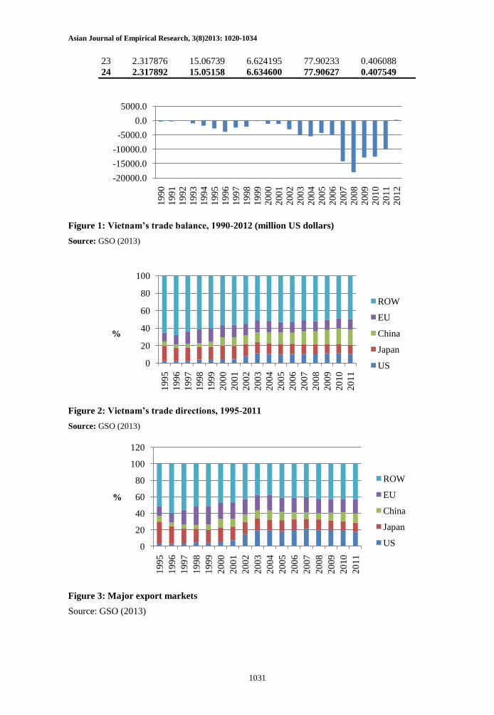
government’s development policies came into effect. It is notable that Vietnam’s trade balance has
been persistently in deficit since 1990, except 1992 and 2012 with small surpluses. Especially,
2008 was the year which exhibited the largest deficit, more than 18 billion US dollars3 (Figure 1,
2 According to GSO
3 GSO
Asian Journal of Empirical Research, 3(8)2013: 1020-1034
1022
see Appendix). In terms of trade partners, Vietnam has traded with almost all countries in the world
since 1995, and the trade volume has therefore increased considerably since then. Japan and
European Union (EU) have been major trade partners of Vietnam since the early 1990s. Before
2000, the trade volume (the sum of export and import) between Vietnam and the US, and China
was smaller compared to that between Vietnam and Japan, and EU. Nevertheless, since the early
2000s, the US and China have also become major trade partners of Vietnam, who accounted for
approximately 11.5% and 17.5%, respectively of Vietnam’s total trade volume in 2012 (Figure 2,
see Appendix). Regarding the export markets, the US has played a role as the biggest export market
of Vietnam since 2003. EU, Japan and China are the second, the third and the fourth biggest
markets, respectively (Figure 3, see Appendix).
Variables and data descriptions
Our VAR model uses four endogenous variables and two exogenous variables, which are adequate
in explaining the trade policy framework of a small open economy like Vietnam. We choose
endogenous variables based on the variables used by Yuen-Ling et al. (2008). In their model, they
used the real exchange rate expressed by Ringgit Malaysia (RM) against United States Dollar
(USD), Malaysia’s gross domestic product, gross domestic product (GDP) of the US, and the ratio
of exports to imports. In our VAR model, we use the real exchange rate denominated by units of
Vietnamese dong (VND) per one unit US dollar (USD), Vietnam’s real GDP, the ratio of exports to
imports, and the money supply (M1) as four endogenous variables. We include the money supply
in the VAR model as a policy variable because the money supply has been used by the State Bank
of Vietnam as a main instrument of the monetary policy as well as the exchange rate policy. In
addition, we use the world oil price as a proxy for expected inflation, and the US real GDP as a
proxy for foreign income. The reason we use the US real GDP as a proxy for foreign income is that
the US is the biggest export market of Vietnam. Additionally, the US economy is large enough to
affect other economies. Therefore, when the US GDP changes, it is likely that GDP of other trade
partners of Vietnam also changes. We treat the world oil price and the US real GDP as exogenous
variables in our VAR model. In order to estimate the VAR model, we tried to acquire a monthly
data set from January 1995 to December 2012 including 216 observations, but Vietnam’s real
GDP, exports and imports are unavailable in monthly basis. Thus, to obtain monthly data of those
variables, we interpolate those series using Chow and Lin’s (1971) annualized approach from their
annual series. Once having monthly data of exports and imports, the ratio of export to import is
computed. The real VND/USD exchange rate is calculated as follow:
q =E×Pus
P (1)
where q represents the real VND/USD exchange rate; E represents the VND/USD nominal
exchange rate; Pus
represents the US price level, and P represents the domestic price level.
Asian Journal of Empirical Research, 3(8)2013: 1020-1034
1023
According to relative purchasing power parity (PPP), the percent change of the real exchange rate
is given by:
%∆q = %∆E + πus − π
where πus
denotes US inflation, and π represents domestic inflation. The data set used to estimate
our VAR model is obtained from several various sources. The data of the nominal exchange rate,
Vietnam’s consumer price index, Vietnam’s real GDP and the money supply is obtained from the
International Financial Statistics (IFS). The data of exports and imports is acquired from the
General Statistics Office of Vietnam. The data of US real GDP and US consumer price index is
obtained from the US Bureau of Economic Analysis (BEA). Finally, the data of world oil price is
collected from the World Bank. All the variables in our model are expressed in the form of
annualized growth rates except the ratio of export to import. Since the data was already seasonally
adjusted by the statistics agencies, we do not apply the seasonal adjustment to the series. The
definitions of variables used in our model and their data sources are summarized in Table 2 (see
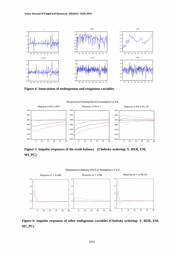
Appendix). Also, Figure 4 (see Appendix) shows their movements over time.
Model specification
Our VAR model is in the following form:
𝐹𝑡 = 𝐴0 + 𝐴1𝐹𝑡−1 + 𝐴2𝐹𝑡−2 +⋯+ 𝐴𝑝𝐹𝑡−𝑝 + 𝐵0𝑋𝑡 + 𝐵1𝑋𝑡−1 +⋯+ 𝐵𝑝𝑋𝑡−𝑝 + 𝑒𝑡 (2)
where Ft={Y, RER, EM, M1_PC}' is a 4x1 vector of endogenous variables; A0 is a 4x1 vector of
intercept terms; A1, …, Ap are 4x4 matrices of coefficients; Xt={Y_US, WOP}' is a 2x1 vector of
exogenous variables; B0, …, Bp are 4x2 matrices of coefficients; and et is a 4x1 vector of error
terms.
Identification strategy
The error term et is the so-called reduced-form (or observed) residuals in the reduced-form VAR,
which are usually correlated. Let’s denote ut as the unobserved structural innovations, which are
uncorrelated. It is insightful to express et in terms of ut as et=Cut
where E(etet')=Σ, E(utut')=I, and C is a 4x4 matrix. Thus,Σ=CC'
By imposing restrictions on the matrix C, we could identify the model.According to Krugman et al.
(2012), when the domestic currency depreciates in real term, the trade balance is immediately
affected. Thus, it is reasonable to impose a restriction such that the real exchange rate has a
contemporaneous impact on the trade balance. In addition, consistent with the AA-DD model, an
increase in the real income will increase the real money demand, which in turn causes the interest
rate to rise. In an open economy, such an increase in the real interest rate appreciates the domestic
Asian Journal of Empirical Research, 3(8)2013: 1020-1034
1024
currency in the short run. Hence, real GDP is supposed to contemporaneously affect the real
exchange rate. Ultimately, since the money supply has been used as a main instrument of the
monetary policy of the State Bank of Vietnam, it is feasible to assume that the money supply is
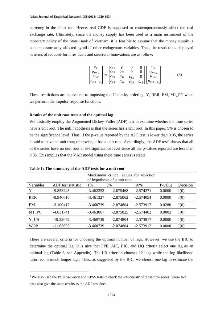
contemporaneously affected by all of other endogenous variables. Thus, the restrictions displayed
in terms of reduced-form residuals and structural innovations are as follow:
𝑒𝑌𝑒𝑅𝐸𝑅𝑒𝐸𝑀
𝑒𝑀1_𝑃𝐶
=
𝑐11𝑐21𝑐31𝑐41
0𝑐22𝑐32𝑐42
00𝑐33𝑐43
000𝑐44
𝑢𝑌
𝑢𝑅𝐸𝑅𝑢𝐸𝑀
𝑢𝑀1_𝑃𝐶
(3)
These restrictions are equivalent to imposing the Cholesky ordering: Y, RER, EM, M1_PC when
we perform the impulse response functions.
Results of the unit root tests and the optimal lag
We basically employ the Augmented Dickey-Fuller (ADF) test to examine whether the time series
have a unit root. The null hypothesis is that the series has a unit root. In this paper, 5% is chosen to
be the significance level. Thus, if the p-value reported by the ADF test is lower than 0.05, the series
is said to have no unit root; otherwise, it has a unit root. Accordingly, the ADF test4 shows that all
of the series have no unit root at 5% significance level since all the p-values reported are less than
0.05. This implies that the VAR model using these time series is stable.
Table 1: The summary of the ADF tests for a unit root
Mackinnon critical values for rejection
of hypothesis of a unit root
Variables ADF test statistic 1% 5% 10% P-value Decision
Y -9.853245 -3.462253 -2.875468 -2.574271 0.0000 I(0)
RER -8.940610 -3.461327 -2.875062 -2.574054 0.0000 I(0)
EM -3.100417 -3.460739 -2.874804 -2.573917 0.0280 I(0)
M1_PC -4.631741 -3.463067 -2.875825 -2.574462 0.0002 I(0)
Y_US -19.32672 -3.460739 -2.874804 -2.573917 0.0000 I(0)
WOP -11.63695 -3.460739 -2.874804 -2.573917 0.0000 I(0)
There are several criteria for choosing the optimal number of lags. However, we use the BIC to
determine the optimal lag. It is nice that FPE, AIC, BIC, and HQ criteria select one lag as an
optimal lag (Table 3, see Appendix). The LR criterion chooses 12 lags while the log likelihood
ratio recommends longer lags. Thus, as suggested by the BIC, we choose one lag to estimate the
4 We also used the Phillips-Perron and KPSS tests to check the stationarity of those time series. These two
tests also give the same results as the ADF test does.
Asian Journal of Empirical Research, 3(8)2013: 1020-1034
1025
VAR. To double check the optimal lag and stability of the VAR, we test for autocorrelation among
the residuals, and examine the roots of characteristic polynomial. The autocorrelation LM test
shows that there is no autocorrelation among residuals (Table 4, see Appendix). In addition, all the
roots of characteristic polynomial are less than 1, which implies that the VAR satisfies the stability
condition (Table 5, see Appendix). Thus, we are confident to estimate the VAR model with one
lag. In the following parts, using the identification restrictions, we will discuss the impulse
response functions of the ratio of export to import with respect to positive shocks of other
endogenous variables, specially focusing on a positive shock of the real exchange rate to find
whether there are J-curve effects on the trade balance of Vietnam.
Responses of the trade balance to a positive real exchange rate shock
Since the real exchange rate is denominated in terms of units of VND per USD, an increase in the
real exchange rate means real depreciation of the domestic currency. Figure 5 (see Appendix)
indicates that real depreciation of the domestic currency has negative impacts on the trade balance
in a certain period of time. Specifically, the trade balance deteriorates significantly after 2 months.
The negative effect of real depreciation on the trade balance becomes worst in the 3rd
and the 4th
months, and decreases since then. Such a negative effect on the trade balance is statistically
significant until the 11th
month, which implies that a positive shock to the real exchange rate
worsens the trade balance for 11 months, at 5% significance level. Even though Vietnam is a
developing country, this finding is highly consistent with the conclusion by Krugman et al. (2012),
which stated that for most industrial countries a J-curve lasts more than six months but less than a
year. In addition, this result, together with Stučka’s (2004) and Petrović and Gligorić’s (2009),
positively contribute to literature in the sense that J-curve effects do exist in emerging countries
where exchange rate policies are considered to be immature. Our result, however, is in contrast to
Yuen-Ling, Wai-Mun, and Geoi-Mei’s (2008), which revealed that there is no evidence of a J-
curve for Malaysia. One possible reason this difference is that impulse response functions
generated from the VECM are not robust since there are issues with standard errors.
Our finding, however, implies that the J-curve effect on the trade balance of Vietnam is quite long.
It takes at least 11 months for the trade balance to recover after real depreciation of the domestic
currency. This implies that the price effect is dominant over the quantity effect, and it could be
explained by two main reasons. First, the export capacity of Vietnam is quite limited because of
limited capital stock. Furthermore, the majority of exported goods is agricultural products, or is
processed from agricultural products, which heavily depends on crops and climate changes. Thus,
exporting firms cannot quickly adjust to take advantage of real depreciation of the domestic
currency. Second, the demand for imports of the Vietnamese economy is quite high and persistent.
Vietnam is a developing country, and has been in the phase of industrializing the economy whereas
its domestic manufacturing is immature and unable to fulfill the demand for high-tech products that
are essential for the industrialization. Therefore, real depreciation of the domestic currency, which
Asian Journal of Empirical Research, 3(8)2013: 1020-1034
1026
makes the prices of imported goods in terms of domestic currency increase, necessarily causes the
total value of import to rise.
Responses of the trade balance to a positive real income shock
An increase in real income is expected to increase the demand for imported goods, thereby
worsening the trade balance. Figure 5 (see Appendix) shows that a positive shock to real income
immediately worsens the trade balance. The negative effect on the trade balance becomes less
severe and gradually declines since the second month. The worsening effect of a positive shock to
real income on the trade balance is statistically significant at 5% significance level until the 20th
month, which implies that an increase in real income negatively affects the trade balance for 20
months. This persistent effect could be explained through the development policies of the
Vietnamese government. As discussed earlier, Vietnam has been in the stage of modernizing the
economy. Thus, a rise in real income in current period will stimulate the demand for import of
modern machinery and equipment in the future periods. Moreover, many Vietnamese people are
“foreign-goods-loving”. Hence, when their income goes up, they tend to demand more imported
goods, which are believed to have higher quality than domestically produced goods.
Responses of the trade balance to a positive money supply shock
Theoretically, how an increase in the money supply affects the trade balance depends on where the
funds are used. If the funds are used to encourage the export sector, then the trade balance is
improved. In contrast, if the funds are utilized to support import, then the trade balance deteriorates.
Usually, central banks expand the money supply to stimulate exports, thereby improving the trade
balance. Figure 5 (see Appendix) suggests that a positive shock to the money supply may have a
positive effect on the trade balance. Accordingly, the effect might be strongest in the third month
since the occurrence of the shock. However, such impacts are statistically insignificant at 5%
significance level.
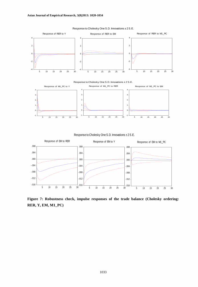
Impulse response functions of other endogenous variables
This section summarizes the impulse responses of other endogenous variables to structural shocks
since this is not the main objective of this paper. Figure 6 (see Appendix) shows that real
depreciation of the domestic currency has a positive effect on real GDP from the second to the
fourth month. However, a positive shock to the money supply is unlikely to affect the real GDP
growth rate since the effect is not statistically significant. Likewise, a positive shock to the trade
balance is unlikely to have any effect on real GDP. The real exchange rate increases in the first
month and then declines from the second to the fifth months due to a positive shock to real income.
A rise in the money supply causes the real exchange rate to fall from the second to the fourth month
while the impact of a positive shock to the trade balance on the real exchange rate is statistically
insignificant. In terms of the monetary policy, a positive shock to the real exchange rate leads to a
rise in the money supply for 5 months. A positive shock to real GDP immediately increases the
Asian Journal of Empirical Research, 3(8)2013: 1020-1034
1027
money supply but the effect becomes statistically insignificant afterwards. The effect of a positive
shock to the trade balance on the money supply is also statistically insignificant.
Variance decomposition of the trade balance
In this part, we only discuss the variance decomposition of the trade balance to determine how the
variations in the trade balance depend on variations of other endogenous variables. The variance
decomposition of other endogenous variables is not discussed since it is beyond the research
territory of this paper5.
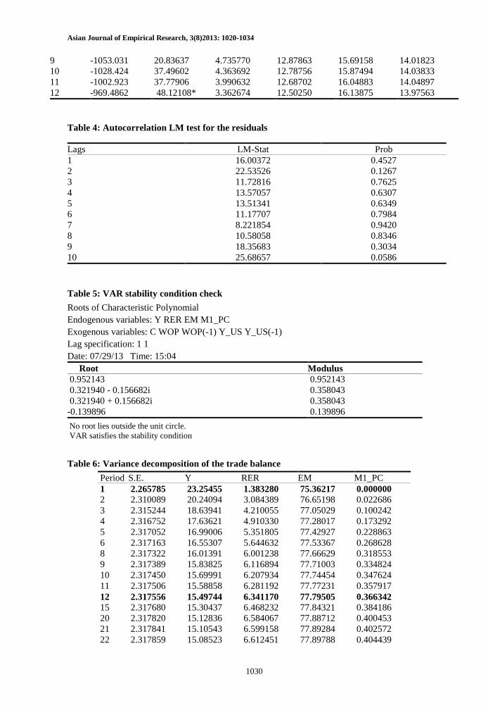
Table 6 (see Appendix) presents the variance decomposition of the trade balance due to its own
shocks, and variations of other endogenous variables. Accordingly, the variation in the trade
balance in the 1st horizon is mainly explained by its own innovations (approximately 75.4%). Apart
from its own shocks, real income also plays an important role in explaining the variations of the
trade balance. It accounts for about 23.3% in the 1st horizon. The real exchange rate only comprises
around 1.4% of the variations of the trade balance in the first horizon. The money supply is
assumed to have no impact on the trade balance in the 1st horizon. The importance of real income in
explaining the variations of the trade balance is decreasing over time while the proportions of the
real exchange rate, the money supply and its own shocks become increasing. In the 24th
horizon,
77.9% of the variations of the trade balance are explained by its own innovations while real income
accounts for 15.1%. The real exchange rate and the money supply comprise 6.6% and 0.4%,
respectively, of the variations in the trade balance. Overall, apart from its own shocks, the
variations in the trade balance are mainly explained by variations of real income and the real
exchange rate. The importance of the money supply in explaining the variations of the trade
balance is trivial.
Robustness of the results
In order to ensure the robustness of the estimation of impulse response functions, we use various
identification restrictions. First, we impose a restriction such that real income is contemporaneously
affected by the real exchange rate, and the trade balance is contemporaneously influenced by real
income. This means that we use the Cholesky ordering: RER, Y, EM, M1_PC. We express this
restriction in terms of the reduced-form residuals and structural innovations as follow:
𝑒𝑌𝑒𝑅𝐸𝑅𝑒𝐸𝑀
𝑒𝑀1_𝑃𝐶
=
𝑐110𝑐31𝑐41
𝑐12𝑐22𝑐32𝑐42
00𝑐33𝑐43
000𝑐44
𝑢𝑌
𝑢𝑅𝐸𝑅𝑢𝐸𝑀
𝑢𝑀1_𝑃𝐶
(4)
This identification restriction produces results (Figure 7, see Appendix) almost similar to our
findings based on the identification restriction earlier. A slight difference is that J-curve effect in
5 The variance decomposition of other endogenous variables could be provided upon request.
Asian Journal of Empirical Research, 3(8)2013: 1020-1034
1028
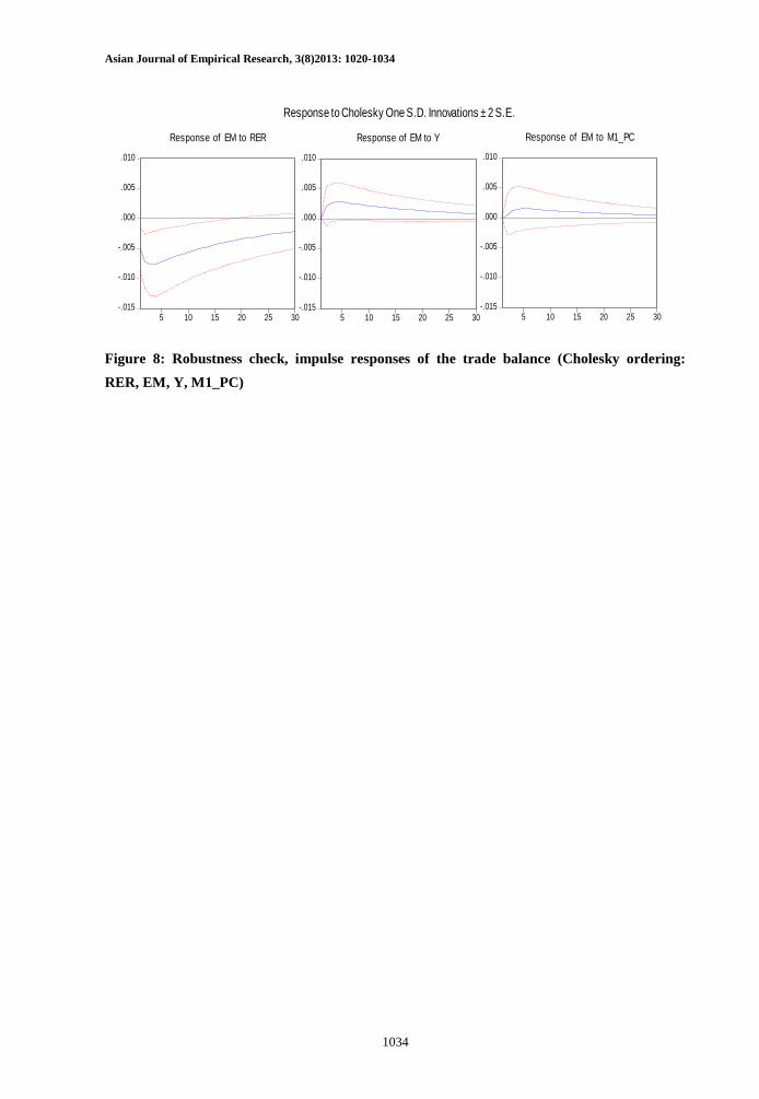
this case lasts a bit longer. It lasts for 15 months instead of 11 months.Second, we impose a
restriction such that real income is contemporaneously affected by the real exchange rate and the
trade balance. This is equivalent to using the Cholesky ordering: RER, EM, Y, M1_PC. This
restriction is exhibited in terms of the reduced-form residuals and structural innovations as follow:
𝑒𝑌𝑒𝑅𝐸𝑅𝑒𝐸𝑀
𝑒𝑀1_𝑃𝐶
=
𝑐1100𝑐41
𝑐12𝑐22𝑐32𝑐42
𝑐130𝑐33𝑐43
000𝑐44
𝑢𝑌
𝑢𝑅𝐸𝑅𝑢𝐸𝑀
𝑢𝑀1_𝑃𝐶
(5)
This identification restriction also generatesalmost similar results (Figure 8, see Appendix) to our
major findings earlier. A minor difference is that the J-curve effect in this restriction lasts a bit
longer (14 months). Another difference is that the effect of a positive shock to real income on the
trade balance now becomes statistically insignificant. Nevertheless, this is unworthy to be worried
since our finding on J-curve is still consistent under various identification restrictions.
CONCLUDING REMARKS
In this study, we employed a VAR framework to examine how the trade balance is affected by
selected economic variables. Particularly, we investigated how real depreciation of the domestic
currency (VND) influences the trade balance over time. Various identification restrictions were
imposed to check the robustness of the results. To sum up, our estimation results affirm that there
exists a J-curve for Vietnam. The worsening effect on the trade balance due to a positive shock to
the real exchange rate is strongest in the 3rd
and the 4th
months. More importantly, J-curve effect
lasts about 11 months, which implies that the trade balance needs at least 11 months to improve
after real depreciation of the domestic currency. In the context of a changeable world nowadays,
this finding suggests that the export sector needs to improve capacity, and be able to actively
manage the production so as to quickly adjust to take advantage of real depreciation of the
domestic currency.
This study, however, may have limitations. Although the US is the biggest export market as well as
a major trade partner of Vietnam, and almost all the trade transactions are made in USD, it might
be more adequate to use the real effective exchange rate instead of the real VND/USD exchange
rate. This is because the real effective exchange rate also takes account of other strong currencies.
Yet, this requires a lot of effort to acquire enough data, and needs appropriate calculation method.
Thus, this could be a suggestion for further research. In spite of that, our findings in this study are
significant and robust to some certain extent.
Asian Journal of Empirical Research, 3(8)2013: 1020-1034
1029
REFERENCES
Ahmad, J. & Yang, J. (2004). Estimation of the J-curve in China. Economics Series East West
Center Working Papers.
Chow, G. C. & Lin, A. (1971). Best Linear Unbiased Interpolation, Distribution, and Extrapolation
of Time Series by Related Series. The Review of Economics and Statistics, Vol. 53, No. 4, p.
372-375.
Krugman, P. R., Obstfeld, M. & Melitz, M. J. (2012). International Economics: Theory and Policy,
Ninth Edition, p. 428-437 & p. 447-449. Addison-Wesley.
Petrović, P. & Gligorić, M. (2012). Exchange Rate and Trade Balance: J-curve Effect.
PANOECONOMICUS, Vol. 1, p. 23-41.
Stučka, T. (2004). The Effects of Exchange Rate Change on the Trade Balance in Croatia. IMF
Working Paper, WP/04/65.
Yuen-Ling, N., Wai-Mun, H. & Geoi-Mei, T. (2008). Real Exchange Rate and Trade Balance
Relationship: An Empirical Study on Malaysia. International Journal of Business and
Management, Vol. 3, No. 8, p. 130-137.
Appendix
Table 2: Definitions of variables and their data sources
Variable Abbreviation Source
Endogenous
variables
Growth rate of the real
VND/USD exchange rate RER
Computed by using available
data from IFS and BEA.
Real domestic GDP
growth rate Y IFS
Money supply growth rate M1_PC IFS
The ratio of export to
import EM
Computed by using data from
GSO
Exogenous
variables
Growth rate of US real
GDP Y_US BEA
Growth rate of the world
oil price WOP World Bank
Table 3: Lag length criteria
Lag LogL LR FPE AIC SC HQ
0 -1421.484 NA 49.51843 15.25380 15.59685 15.39278
1 -1121.897 570.6428 2.463686* 12.25288* 12.87035* 12.50303*
2 -1110.224 21.74078 2.580609 12.29866 13.19057 12.66000
3 -1097.567 23.03653 2.676431 12.33404 13.50039 12.80656
4 -1092.641 8.756615 3.014424 12.45123 13.89201 13.03492
5 -1084.454 14.20844 3.282601 12.53391 14.24912 13.22878
6 -1078.064 10.81897 3.646852 12.63560 14.62524 13.44165
7 -1071.738 10.44411 4.058913 12.73796 15.00204 13.65520
8 -1066.335 8.689430 4.568022 12.85011 15.38862 13.87852
Asian Journal of Empirical Research, 3(8)2013: 1020-1034
1030
9 -1053.031 20.83637 4.735770 12.87863 15.69158 14.01823
10 -1028.424 37.49602 4.363692 12.78756 15.87494 14.03833
11 -1002.923 37.77906 3.990632 12.68702 16.04883 14.04897
12 -969.4862 48.12108* 3.362674 12.50250 16.13875 13.97563
Table 4: Autocorrelation LM test for the residuals
Lags LM-Stat Prob
1 16.00372 0.4527
2 22.53526 0.1267
3 11.72816 0.7625
4 13.57057 0.6307
5 13.51341 0.6349
6 11.17707 0.7984
7 8.221854 0.9420
8 10.58058 0.8346
9 18.35683 0.3034
10 25.68657 0.0586
Table 5: VAR stability condition check
Roots of Characteristic Polynomial
Endogenous variables: Y RER EM M1_PC
Exogenous variables: C WOP WOP(-1) Y_US Y_US(-1)
Lag specification: 1 1
Date: 07/29/13 Time: 15:04
Root Modulus
0.952143 0.952143
0.321940 - 0.156682i 0.358043
0.321940 + 0.156682i 0.358043
-0.139896 0.139896
No root lies outside the unit circle.
VAR satisfies the stability condition
Table 6: Variance decomposition of the trade balance
Period S.E. Y RER EM M1_PC
1 2.265785 23.25455 1.383280 75.36217 0.000000
2 2.310089 20.24094 3.084389 76.65198 0.022686
3 2.315244 18.63941 4.210055 77.05029 0.100242
4 2.316752 17.63621 4.910330 77.28017 0.173292
5 2.317052 16.99006 5.351805 77.42927 0.228863
6 2.317163 16.55307 5.644632 77.53367 0.268628
8 2.317322 16.01391 6.001238 77.66629 0.318553
9 2.317389 15.83825 6.116894 77.71003 0.334824
10 2.317450 15.69991 6.207934 77.74454 0.347624
11 2.317506 15.58858 6.281192 77.77231 0.357917
12 2.317556 15.49744 6.341170 77.79505 0.366342
15 2.317680 15.30437 6.468232 77.84321 0.384186
20 2.317820 15.12836 6.584067 77.88712 0.400453
21 2.317841 15.10543 6.599158 77.89284 0.402572
22 2.317859 15.08523 6.612451 77.89788 0.404439
Asian Journal of Empirical Research, 3(8)2013: 1020-1034
1031
23 2.317876 15.06739 6.624195 77.90233 0.406088
24 2.317892 15.05158 6.634600 77.90627 0.407549
Figure 1: Vietnam’s trade balance, 1990-2012 (million US dollars)
Source: GSO (2013)
Figure 2: Vietnam’s trade directions, 1995-2011
Source: GSO (2013)
Figure 3: Major export markets
Source: GSO (2013)
-20000.0
-15000.0
-10000.0
-5000.0
0.0
5000.0
19
90
19
91
19
92
19
93
19
94
19
95
19
96
19
97
19
98
19
99
20
00
20
01
20
02
20
03
20
04
20
05
20
06
20
07
20
08
20
09
20
10
20
11
20
12
0
20
40
60
80
100
19
95
19
96
19
97
19
98
19
99
20
00
20
01
20
02
20
03
20
04
20
05
20
06
20
07
20
08
20
09
20
10
20
11
%
ROW
EU
China
Japan
US
0
20
40
60
80
100
120
19
95
19
96
19
97
19
98
19
99
20
00
20
01
20
02
20
03
20
04
20
05
20
06
20
07
20
08
20
09
20
10
20
11
%
ROW
EU
China
Japan
US
Asian Journal of Empirical Research, 3(8)2013: 1020-1034
1032
Figure 4: Innovations of endoegenous and exogenous variables
Figure 5: Impulse responses of the trade balance (Cholesky ordering: Y, RER, EM,
M1_PC)
Figure 6: Impulse responses of other endogenous variables (Cholesky ordering: Y, RER, EM,
M1_PC)
-10
-5
0
5
10
15
96 98 00 02 04 06 08 10 12
Y
-50
-40
-30
-20
-10
0
10
20
96 98 00 02 04 06 08 10 12
RER
0.5
0.6
0.7
0.8
0.9
1.0
1.1
96 98 00 02 04 06 08 10 12
EM
-20
-10
0
10
20
30
96 98 00 02 04 06 08 10 12
M1_PC
-30
-20
-10
0
10
20
30
96 98 00 02 04 06 08 10 12
WOP
-30
-20
-10
0
10
20
30
96 98 00 02 04 06 08 10 12
Y_US
-.020
-.015
-.010
-.005
.000
.005
.010
5 10 15 20 25 30
Response of EM to RER
-.020
-.015
-.010
-.005
.000
.005
.010
5 10 15 20 25 30
Response of EM to Y
-.020
-.015
-.010
-.005
.000
.005
.010
5 10 15 20 25 30
Response of EM to M1_PC
Response to Cholesky One S.D. Innovations ± 2 S.E.
-.2
.0
.2
.4
.6
5 10 15 20 25 30
Response of Y to RER
-.2
.0
.2
.4
.6
5 10 15 20 25 30
Response of Y to EM
-.2
.0
.2
.4
.6
5 10 15 20 25 30
Response of Y to M1_PC
Response to Cholesky One S.D. Innovations ± 2 S.E.
Asian Journal of Empirical Research, 3(8)2013: 1020-1034
1033
Figure 7: Robustness check, impulse responses of the trade balance (Cholesky ordering:
RER, Y, EM, M1_PC)
-4
-2
0
2
4
5 10 15 20 25 30
Response of RER to Y
-4
-2
0
2
4
5 10 15 20 25 30
Response of RER to EM
-4
-2
0
2
4
5 10 15 20 25 30
Response of RER to M1_PC
Response to Cholesky One S.D. Innovations ± 2 S.E.
-1
0
1
2
3
4
5 10 15 20 25 30
Response of M1_PC to Y
-1
0
1
2
3
4
5 10 15 20 25 30
Response of M1_PC to RER
-1
0
1
2
3
4
5 10 15 20 25 30
Response of M1_PC to EM
Response to Cholesky One S.D. Innovations ± 2 S.E.
-.016
-.012
-.008
-.004
.000
.004
.008
5 10 15 20 25 30
Response of EM to RER
-.016
-.012
-.008
-.004
.000
.004
.008
5 10 15 20 25 30
Response of EM to Y
-.016
-.012
-.008
-.004
.000
.004
.008
5 10 15 20 25 30
Response of EM to M1_PC
Response to Cholesky One S.D. Innovations ± 2 S.E.
Asian Journal of Empirical Research, 3(8)2013: 1020-1034
1034
Figure 8: Robustness check, impulse responses of the trade balance (Cholesky ordering:
RER, EM, Y, M1_PC)
-.015
-.010
-.005
.000
.005
.010
5 10 15 20 25 30
Response of EM to RER
-.015
-.010
-.005
.000
.005
.010
5 10 15 20 25 30
Response of EM to Y
-.015
-.010
-.005
.000
.005
.010
5 10 15 20 25 30
Response of EM to M1_PC
Response to Cholesky One S.D. Innovations ± 2 S.E.