the effects of heat treatment on microstructure, hardness

THE EFFECTS OF HEAT TREATMENT ON MICROSTRUCTURE, HARDNESS

AND FATIGUE BEHAVIOR OF (AMS5659) 15-5 PRECIPITATION

HARDENABLE STAINLESS STEEL

A THESIS SUBMITTED TO

THE GRADUATE SCHOOL OF NATURAL AND APPLIED SCIENCES

OF

MIDDLE EAST TECHNICAL UNIVERSITY

BY

ŞAHİN GÖREN

IN PARTIAL FULFILLMENT OF THE REQUIREMENTS

FOR

THE DEGREE OF MASTER OF SCIENCE

IN

METALLURGICAL AND MATERIALS ENGINEERING

OCTOBER 2018

Approval of the thesis:

THE EFFECTS OF HEAT TREATMENT ON MICROSTRUCTURE,

HARDNESS AND FATIGUE BEHAVIOR OF (AMS5659) 15-5

PRECIPITATION HARDENABLE STAINLESS STEEL submitted by ŞAHİN GÖREN in partial fulfillment of the requirements for the degree of Master of Science in Metallurgical and Materials Engineering Department, Middle East Technical University by,

Prof. Dr. Halil Kalıpçılar Dean, Graduate School of Natural and Applied Sciences Prof. Dr. C. Hakan Gür Head of Department, Metallurgical and Materials Eng. Prof. Dr. Rıza Gürbüz Supervisor, Metallurgical and Materials Eng. Dept., METU

Examining Committee Members:

Prof. Dr. Bilgehan Ögel Metallurgical and Materials Engineering Dept., METU Prof. Dr. Rıza Gürbüz Metallurgical and Materials Engineering Dept., METU Prof. Dr. C. Hakan Gür Metallurgical and Materials Engineering Dept., METU Assist. Prof. Dr. Mert Efe Metallurgical and Materials Engineering Dept., METU Assist. Prof. Dr. Kazım Tur Metallurgical and Materials Engineering Dept., Atılım Uni.

Date: 09.10.2018

iv

I hereby declare that all information in this document has been obtained and presented in accordance with academic rules and ethical conduct. I also declare that, as required by these rules and conduct, I have fully cited and referenced all material and results that are not original to this work.

Name, Last name: Şahin Gören

Signature :

v

ABSTRACT

THE EFFECTS OF HEAT TREATMENT ON MICROSTRUCTURE,

HARDNESS AND FATIGUE BEHAVIOR OF (AMS5659) 15-5

PRECIPITATION HARDENABLE STAINLESS STEEL

Gören, Şahin

M.Sc., Department of Metallurgical and Materials Engineering

Supervisor: Prof. Dr. Rıza Gürbüz

October 2018, 123 pages

In this study, effects of heat treatment parameters on microstructure, hardness and

fatigue behavior of 15-5 precipitation hardenable stainless steels have been

examined. Heat treatments have been conducted in three different steps

homogenization, solutionizing and aging treatment at different temperatures and

times. Microstructural analysis in terms of grain size and chemical composition

analysis have been performed by optical and scanning electron microscope (SEM).

Then, hardness measurements were applied for all heat treated specimens. Fatigue

tests have been conducted at negative stress ratio (R) equal to -1 under constant

amplitude cyclic loading for selected group of heat treated specimens. Fatigue test

results have been evaluated according to AGARD-AG-292 and ISO 12107 standards

in order to see the effect of heat treatment parameters on fatigue limit of the 15-5

precipitation hardenable stainless steels. Fatigue limit was determined as stress level

at 107

cycles on stress vs. cycle (S-N) curve. It was also calculated by using staircase

method in order to verify the fatigue limit that was found as stress level at 107

cycles

on S-N curve. Higher hardness and fatigue limit were achieved for aging treatment at

4800C for 1h and 400

0C for 70h compared to aging treatment at 550

0C for 4h. The

measurements and test results show that by changing heat treatment parameters,

vi

hardness and fatigue limit of 15-5 precipitation hardenable stainless steel can be

increased.

Keywords: Precipitation Hardenable (PH) Stainless Steels, Heat Treatment,

Hardness, Microstructure, Fatigue, S-N Curves.

vii

ÖZ

ISIL İŞLEMİN (AMS5659) 15-5 ÇÖKELİMLİ SERTLEŞEBİLİR

PASLANMAZ ÇELIK ALAŞIMININ MİKROYAPI, SERTLİK VE

YORULMA DAVRANIŞI ÜZERİNDEKİ ETKİSİNİN İNCELENMESİ

Gören, Şahin

Yüksek Lisans, Metalurji ve Malzeme Mühendisliği Bölümü

Tez Yöneticisi: Prof. Dr. Rıza Gürbüz

Ekim 2018, 123 sayfa

Bu çalışmada, ısıl işlem parametrelerinin 15-5 çökelimli sertleştirilebilir paslanmaz

çelik alışımının mikroyapı, sertlik ve yorulma davranışı üzerindeki etkileri

incelenmiştir. Isıl işlem homojenleştirme, çözündürme ve yaşlandırma olarak üç faklı

aşamada farklı sıcaklık değerlerinde ve farklı sürelerde uygulanmıştır. Mikroyapı

analizi, tane boyutu ve kimyasal bileşim, optik ve taramalı elektron mikroskobu

kullanılarak gerçekleştirildi. Sonrasında, ısıl işlem görmüş tüm numuneler için sertlik

ölçümü alındı. Yorulma testleri sabit genlikli çevrimsel yük altında, negatif gerilme

oranı R=-1’de ısıl işlem görmüş numunelerden seçilen grup için uygulandı. Yorulma

testi sonuçları, ısıl işlem parametrelerinin 15-5 çökelimli sertleştirilebilir paslanmaz

çelik alaşımının yorulma limiti üzerindeki etkisini görmek için AGARD-AG-292 ve

ISO 12107 standartlarına göre değerlendirilmiştir. Yorulma limiti değeri gerilme-

çevrim (S-N) eğrisi üzerindeki 107 çevrim değerine karşılık gelen gerilme olarak

belirlenmiştir. Yorulma limiti değeri, gerilme-çevrim (S-N) eğrisi üzerinde buluanan

gerilme değerini doğrulamak amacıyla merdiven yöntemi kullanılarak da

hesaplanmıştır. 4800C’de 1 saat ve 400

0C’de 70 saat olarak uygulanan yaşlandırma

işlemlerinde 5500C’de 4 saat uygulanan yaşlandırma işlemine kıyasla daha yüksek

sertlik ve yorulma mukavemetine ulaşıldı. Ölçümler ve test sonuçları, ısıl işlem

viii

parametreleri değiştirilerek, 15-5 çökelimli sertleştirilebilir paslanmaz çeliklerin

sertlik ve yorulma davranışlarının arttırılabildiğini göstermektedir.

Anahtar Kelimeler: Çökelimli sertleşebilir paslanmaz çelikler, Isıl işlem,

Mikroyapı, Sertlik, Yorulma, Gerilme- Çevrim Eğrisi.

ix

To My Precious Parents

x

ACKNOWLEDGEMENTS

I wish to express my sincere thanks to my advisor Prof. Dr. Rıza Gürbüz for his great

support, encouragement and guidance throughout the whole time on this study.

I am deeply thankful to deliver thankfulness to Turkish Aerospace Industry (TAI) for

great support and permission to perform tests in its premises and equipment.

I am deeply thankful to heat treatment laboratory technician Yusuf Yıldırım for his

infinite support and patience.

I wish to express my sincere thanks to Alp Aykut Kibar for his great support and

patience for Scanning Electron Microscope (SEM) analyses.

My special thanks reserve to Mr. Ömer Duman, Mr. Mustafa Yavuz and Mr. Mesut

Talha Güven for their great support on specimen manufacturing.

Finally, I would like to express my indebtedness to my parents to present me

exceptional life and unrequited love.

xi

TABLE OF CONTENTS

ABSTRACT ………………………………………………………………………….v

ÖZ…………………...................................................................................................vii

ACKNOWLEDGEMENTS .. ...................................................................................... x

TABLE OF CONTENTS ............................................................................................ xi

LIST OF TABLES ..................................................................................................... xv

LIST OF FIGURES ................................................................................................. xvii

CHAPTERS

1. INTRODUCTION .................................................................................................. 1

1.1. MOTIVATION ............................................................................................... 2

1.2. AIM OF THE WORK AND MAIN CONTRIBUTION ................................. 4

2. THEORETICAL BACKGROUND ........................................................................ 5

2.1. PRECIPITATION HARDENABLE STAINLESS STEELS ………………..5

2.2.1. CLASSIFICATION OF PH STAINLESS STEELS ............................... 6

2.2.1.1. AUSTENITIC PH STAINLESS STEELS....................................... 7

2.2.1.2. SEMI-AUSTENITIC PH STAINLESS STEELS ............................ 7

2.2.1.3. MARTENSITIC PH STAINLESS STEELS ................................... 8

2.2. HEAT TREATMENT OF PH STAINLESS STEELS.................................... 9

2.3.1. HEAT TREATMENT OF (AMS5659) 15-5PH STAINLESS STEEL 12

2.3.1.1. SOLUTION TREATMENT OF 15-5 PH STAINLESS STEEL ....... 12

2.3.1.2. COOLING AND TRANSFORMATION FOR 15-5 PH STAINLESS

STEEL ......................................................................................... 13

2.3.1.3. PRECIPITATION HARDENING OF 15-5PH STAINLESS STEEL 13

2.3. MANUFACTURING METHOD .................................................................. 14

2.4. MICROSTRUCTURE OF 15- 5 PH STAINLESS STEEL .......................... 15

2.5. HARDNESS VALUES OF 15-5 PH STAINLESS STEEL ......................... 20

2.6. TENSILE PROPERTIES OF 15-5 PH STAINLESS STEEL ....................... 24

xii

2.7. FATIGUE PROPERTIES ............................................................................. 27

2.7.1. DEFINITIONS AND TERMS FOR FATIGUE .................................... 28

2.7.2. NUCLEATION AND GROWTH OF FATIGUE CRACK .................. 31

2.7.2.1. CRACK INITIATION PERIOD .................................................... 31

2.7.2.2. CRACK GROWTH PERIOD…………………………………….33

2.7.3. STRESS- LIFE DIAGRAMS (S-N CURVES) ..................................... 34

2.7.4. FATIGUE BEHAVIOR AND STRESS- LIFE DIAGRAMS FOR 15-5

PH STAINLESS STEEL. ............................................................ 36

2.8. STATISTICAL ANALYSIS OF FATIGUE TEST DATA .......................... 38

2.8.1. AGARD-AG-292 FOUR (4) PARAMETER BEST FITTING

TECHNIQUE .............................................................................. 39

2.8.2. STAIRCASE METHOD FOR FATIGUE LIMIT CALCULATION ... 42

2.8.3. NORMAL PROBABILITY PLOT FOR OUTLIERS

DETERMINATION .................................................................... 44

2.9. FRACTURE SURFACE ANALYSIS OF 15-5 PH STAINLESS STEELS . 46

3. EXPERIMENTAL PROCEDURE ....................................................................... 51

3.1. MATERIAL .................................................................................................. 51

3.2. SPECIMEN GEOMETRY ............................................................................ 51

3.3. HEAT TREATMENT PARAMETERS ........................................................ 53

3.3.1. GROUP-1 SPECIMENS........................................................................ 54

3.3.2. GROUP-2 SPECIMENS........................................................................ 55

3.3.3. GROUP-3 SPECIMENS........................................................................ 55

3.3.4. GROUP-4 SPECIMENS........................................................................ 55

3.3.5. GROUP-5 SPECIMENS........................................................................ 56

3.3.6. GROUP-6 SPECIMENS........................................................................ 56

3.4. METALLOGRAPHY .................................................................................... 57

3.4.1. SPECIMEN PREPARATION ............................................................... 57

3.4.2. SPECIMEN ETCHING ......................................................................... 57

3.5. GRAIN SIZE MEASUREMENT .................................................................. 57

3.6. HARDNESS TEST ....................................................................................... 58

3.7. ROUGHNESS MEASUREMENT ................................................................ 58

3.8. STATIC AND FATIGUE TESTS ................................................................. 59

xiii

3.8.1. TENSILE TEST..................................................................................... 59

3.8.2. FATIGUE TEST .................................................................................... 59

4. RESULTS AND DISCUSSIONS ......................................................................... 63

4.1. MICROSTRUCTURE OF THE SAMPLE ................................................... 63

4.1.1. GRAIN SIZE MEASUREMENT RESULTS ....................................... 66

4.2. HARDNESS TEST RESULTS ..................................................................... 70

4.3. TENSILE TEST RESULTS .......................................................................... 73

4.4. SURFACE ROUGHNESS MEASUREMENT RESULTS .......................... 76

4.4.1. SURFACE ROUGHNESS RESULTS FOR GROUP-1 SPECIMEN... 77



4.5. FATIGUE TEST RESULTS ......................................................................... 79

4.5.1. FATIGUE TEST RESULTS FOR GROUP-1 SPECIMENS ................ 80

4.5.1.1. FATIGUE LIMIT CALCULATION BY STAIRCASE METHOD

FOR GROUP-1 SPECIMENS ................................................ 81







4.5.4. COMPARISON OF S-N CURVES ....................................................... 88

4.6. FRACTURE SURFACE ANALYSIS RESULTS ........................................ 91

4.6.1. FRACTURE SURFACE ANALYSIS RESULTS FOR TENSILE TEST

SPECIMENS ............................................................................... 91

4.6.1.1. FRACTURE SURFACE ANALYSIS RESULTS FOR GROUP-1

SPECIMENS .......................................................................... 91


SPECIMENS .......................................................................... 95


SPECIMENS .......................................................................... 97

xiv

4.7.1. FRACTURE SURFACE ANALYSIS RESULTS FOR FATIGUE TEST

SPECIMENS ............................................................................... 99


SPECIMENS ........................................................................ 100


SPECIMENS ........................................................................ 105


SPECIMENS ........................................................................ 108

5. CONCLUSION ................................................................................................... 117

REFERENCES ......................................................................................................... 119

xv

LIST OF TABLES

TABLES

Table 1 Precipitation hardenable stainless steels. [1] .................................................... 7

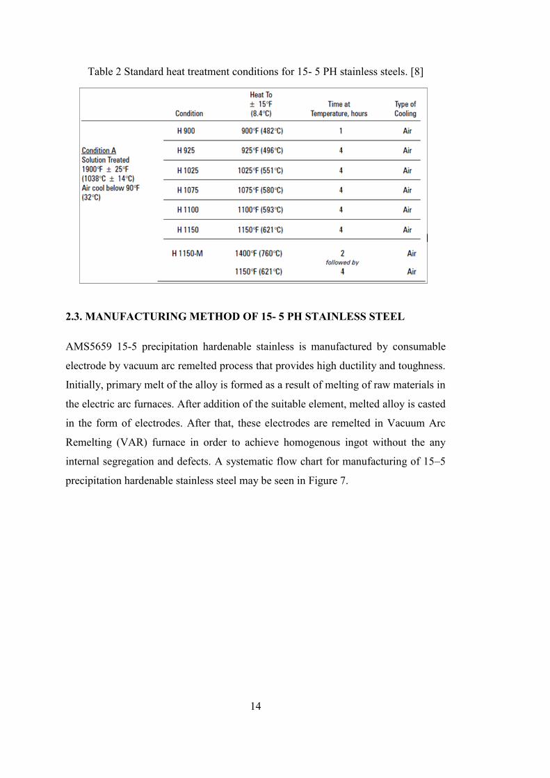
Table 2 Standard heat treatment conditions for 15- 5 PH stainless steels. [8] .......... 14

Table 3 Hardness values for different aging condition. [12] ...................................... 21

Table 4 Mechanical properties of 15-5 PH stainless steel different aging condition.

[8] ................................................................................................................................ 26

Table 5 Fatigue test results for 15-5 PH stainless steels for H-900 and H-1050

conditions. [22] ........................................................................................................... 36

Table 6 High cycle fatigue behavior of 15–5 PH martensitic stainless steel. [4] ....... 37

Table 7 Conditions for parameters SI, H, A, B and C in fitting equation ................... 42

Table 8 Chemical Composition for 15-5 PH Stainless Steels. .................................... 51

Table 9 Applied heat treatment for group-1 specimens. ............................................. 54

Table 10 Applied heat treatment for group-2 specimens. ........................................... 55





Table 15 Calculation of total counts for grain size measurement analysis. ................ 68

Table 16 Grain size measurement results.................................................................... 69

Table 17 Hardness test results ..................................................................................... 71

Table 18 Hardness, types and number of specimens for static and fatigue tests ........ 74

Table 19 Tensile test and hardness results. ................................................................. 75

Table 20 Actual and approximated UTS values ......................................................... 76

Table 21 Fatigue test results for group-1 specimens (15-5 PH Stainless Steels

exposed to Hom.@11500C /1h + Sol.@1040

0C /0.5h + Aged 550

0C /4h) ................. 80



0C /0.5h + Aged 480

0C /1h) ................. 83

xvi



0C /0.5h + Aged 400

0C /70h) .............. 86

Table 24 Quantitative elemental analysis results for point-1(intermetallic) .............. 94

Table 25 Quantitative elemental analysis results for point-2 (matrix phase). ............ 95

Table 26 Selected fatigue test specimen for fracture surface analysis. .................... 100

Table 27 Quantitative elemental analysis results for point-1. .................................. 104

Table 31 Quantitative elemental analysis results for point-1. .................................. 112

xvii

LIST OF FIGURES

FIGURES

Figure 1 Queen Liliuokalani, Aloha Airlines’ Boeing 737-297 N73711, at Kahalui

Airport (OGG), Maui, Hawaii, following the accident on April 28, 1988.[2] .................. 2

Figure 2 Components with AMS5659 15-5 PH stainless steels 1: out fit rib; 2: engine

front suspension; 3: rib; 4: engine back suspension; 5: plain ribs; 6: lower spar.[3] ......... 3

Figure 3 Actuator system components for an Indian aircraft.[4] ....................................... 4

Figure 4 Position of PH steels in the Schaeffler-Delong's diagram. [5] ............................ 6

Figure 5 Effect of alloy contents on transformation temperatures of precipitation

hardenable stainless steels. [1] ......................................................................................... 10

Figure 6 Precipitation hardening sequence. [6] ............................................................... 11

Figure 7 Manufacturing process flow of 15–5 PH martensitic stainless steels. [4] ......... 15

Figure 8 Bright field TEM micrograph of the aged material showing the distribution

of the Cu precipitates (in white) in one martensite lath (in black). [10] .......................... 16

Figure 9 TEM and HRTEM micrographs of Cu precipitates and reversed austenite

obtained from specimen aged at 5800C for 4 h (a-b) aged at 620

0C for 4 h (c-d). [11] ... 17

Figure 10 Concentration of Ni on a cross section of a copper precipitate in an APT

volume obtained on the aged material. [10] ..................................................................... 18

Figure 11 Bright field TEM micrographs showing spherical niobium carbides

(arrows). Right hand side figure shows a larger magnification image of carbide. [10] ... 18

Figure 12 Optical micrographs of 15-5 PH aged at various temperatures for 4h. [11].... 19

Figure 13 Optical micrographs of the material in different metallurgical conditions:

(a) solution annealed, (b) aged at 5800C for 0.25h, (c) aged at 580

0C for 4h. [9] ........... 20

Figure 14 Variation of hardness & impact energy as a function of homogenizing heat

treatment time. [26] .......................................................................................................... 22

Figure 15 Temperature and time effect on the hardening behavior at different aging

condition for 17-4 PH stainless steel. [14] ....................................................................... 22

Figure 16 Required time to achieve peak hardness according to aging temperature for

15-5 PH stainless steels. [11] ........................................................................................... 23

xviii

Figure 17 Effect of aging time on the hardness of the solution-treated specimens.

[31] ................................................................................................................................... 24

Figure 18 Deviation of the yield, tensile strength and elongation according to

homogenization time. [26] ............................................................................................... 25

Figure 19 Effect of ageing time at 5800C on the tensile behavior of 17-4 PH at room

temperature. [9] ................................................................................................................ 26

Figure 20 Typical tensile behavior for various heat treatment conditions for 15-5 PH

stainless steel bar, at room temperature condition. [16] ................................................... 27

Figure 21 Schematic exhibition of loading types. [17] .................................................... 29

Figure 22 Schematic exhibition of basic terms on sinusoidal fatigue loading. [18] ........ 30

Figure 23 Different phases of the fatigue life. [19] .......................................................... 31

Figure 24 Effect of the cycle slip on the crack nucleation. [19] ..................................... 32

Figure 25 Cross section of microcrack. [19] .................................................................... 33

Figure 26 Effect of the grain boundary on crack growth period for an Al-alloy. [19] .... 33

Figure 27 Evolution of the fatigue crack front. [20] ....................................................... 34

Figure 28 Typical S-N curves. [21] .................................................................................. 35

Figure 29 Idealized S-N curve. [21] ................................................................................. 35

Figure 30 Stress vs. Life curve of 15-5 PH stainless steels for H900 and H1150

conditions. [22] ................................................................................................................. 37

Figure 31 Schematic P-S-N diagram for three probabilities of failure and log normal

distributions of lives. [23] ................................................................................................ 39

Figure 32 Extrapolation of data for statistical analysis. [24] ........................................... 40

Figure 33 Least Square Fitting Concept for non-linear analysis of test data. [24] .......... 42

Figure 34 Example of staircase test data. [25] ................................................................. 43

Figure 35 Schematically calculation of the fatigue limit according to staircase

method. ............................................................................................................................. 44

Figure 36 Normal probability plot for hypothetical fatigue test data. .............................. 46

Figure 37 Fractographs of aged samples a (solution treated) b (H900) condition. [26] .. 47

Figure 38 Observation of fatigue failure from internal inclusion after fatigue testing.

[27] ................................................................................................................................... 48

Figure 39 SEM and optical micrographs of a fish-eye fracture with ODA around a

non-metallic inclusion. [28] ............................................................................................. 49

xix

Figure 40 The size of dark areas (Optically Dark Area, ODA) in the vicinity of an

inclusion at a fracture origin increases with increase in fatigue life. [29] ....................... 49

Figure 41 Round Bar 15-5 PH (a) and heat treatment specimen geometry (b)................ 52

Figure 42 Fatigue test specimens after machining. .......................................................... 52

Figure 43 Technical drawing of static and fatigue test specimens. .................................. 53

Figure 44 Heat treated specimens during air cooling...................................................... 54

Figure 45 Etchants with chemical compositions. ............................................................. 57

Figure 46 Optical microscope image for indented surface. ............................................. 58

Figure 47 General view of INSTRON 5985 machine grips with tensile test specimen. . 59

Figure 48 General view for RUMUL magnetic resonant testing machine grips. [37] ..... 60

Figure 49 Optical microscope image for specimen As-received+ Homogenization at

11500C for 1 hour as a result of Marble’s Etching with time a (20 seconds), b (40

seconds), c (60 seconds), d (80 seconds). ........................................................................ 64


11500C for 1 hour as a result of Kalling’s Etching with time a (20 seconds), b (40

seconds), c (60 seconds), d (80 seconds) ......................................................................... 65

Figure 51 Optical microscope image for specimen (a) Sol. at 10400C/0.5h (b) Hom.

at 11500C/1h (c) Hom. at 1150

0C/1h+ Sol. at 1040

0C/0.5h +Aged at 400

0C/70h (d)

Hom. at 11500C/1h+ Sol. at 1040


0C/4h ........................................ 66

Figure 52 Optical microscope image for specimen which is solutionized at

10400C/0.5h +Aged at 400

0C/70h with arbitrary test lines with specific length ............. 67

Figure 53 Stress vs. strain curve for group-5 tensile test specimens. .............................. 74

Figure 54 Surface roughness reduction factor γ for high strength steels as a function

of Ra (average surface roughness) and the tensile strength. [19] .................................... 79

Figure 55 Normal probability plot for group-1 specimens (15-5 PH Stainless Steels


0C /0.5h + Aged 550

0C /4h) ...................... 81

Figure 56 Fatigue limit calculation by staircase method for group-1 specimens (15-5

PH Stainless Steels exposed to Hom.@11500C /1h + Sol.@1040

0C /0.5h + Aged

5500C /4h) ........................................................................................................................ 82

Figure 57 Staircase sequence for group-1 specimens (15-5 PH Stainless Steels


0C /0.5h + Aged 550

0C /4h) ...................... 82

xx



0C /0.5h + Aged 480

0C /1h) ...................... 84



0C /0.5h + Aged

4800C /1h) ........................................................................................................................ 85



0C /0.5h + Aged 550

0C /4h) ...................... 85



0C /0.5h + Aged 400

0C /70h) .................... 87


PH Stainless Steels exposed to Hom.@11500C /1h +Sol.@1040

0C /0.5h +Aged

4000C /70h) ...................................................................................................................... 88



0C /0.5h + Aged 400

0C /70h) .................... 88

Figure 64 Stress versus life (S-N) curves for three groups of group-5 specimens. .......... 89

Figure 65 Relation between surface condition and ultimate tensile strength (UTS) on

fatigue limit for high strength steels. [40] ........................................................................ 90

Figure 66 Cup-and-cone type fracture surface for tensile tested specimen (SP-21) ........ 91

Figure 67 SEM micrograph showing (a) general view of fracture surface (b)

equiaxed dimples on fracture surface of tensile tested specimen (SP-21) ....................... 92

Figure 68 SEM micrograph showing equiaxed dimples with some intermetallic

inside for tensile tested specimen (SP-21) ....................................................................... 93

Figure 69 SEM image with in-lens detector for tensile tested specimen (SP-21) ............ 93

Figure 70 EDX analysis results for point-1(intermetallic) ............................................... 94

Figure 71 EDX analysis results for point- 2 (matrix phase). ........................................... 95

Figure 72 Brittle fracture surface for tensile tested specimen (SP-3) .............................. 96

Figure 73 SEM f micrograph showing general view of brittle fracture surface of

tensile tested specimen (SP-3) .......................................................................................... 96

Figure 74 SEM micrograph showing dimple/voids and cleavages/facets view of

fracture surface of group-2 tensile test specimen. (SP-3) ................................................ 97

Figure 75 Brittle fracture surface for tensile tested specimen (SP-13) ............................ 97

xxi

Figure 76 SEM micrograph showing general view of brittle fracture surface of tensile

tested specimen. (SP-13) .................................................................................................. 98

Figure 77 SEM micrograph showing dimple/voids and cleavages/facets (dominant)

view of fracture surface of group-3 tensile test specimen. (SP-13) ................................. 98

Figure 78 SEM fractograph showing general view of crack initiation site for (SP-1) .. 100

Figure 79 SEM fractograph showing crack initiation point for (SP-1) .......................... 101



Figure 82 SEM fractograph showing general view of crack initiation site for (SP-13) 102

Figure 83 SEM fractograph showing crack initiation point for (SP-13) ........................ 103

Figure 84 EDX analysis results for point- 1 in Figure 83. ............................................. 103

Figure 85 SEM micrograph showing fatigue striations and crack growth direction

group-1 cyclic loaded specimen (SP-1) ......................................................................... 104






Figure 91 SEM fractograph showing crack initiation in detail for (SP-9). .................... 107









Figure 99 EDX analysis results for crack initiation point of (SP-7) .............................. 111



Figure 101 Optical image for fracture surface of group -1 failed specimens. ............... 113

Figure 102 Optical image for fracture surface of group -2 failed specimens. ............... 114

xxii

Figure 103 Optical image for fracture surface of group -3 failed specimens ................ 114

Figure 104 The inclusion at the center of the fish eye. [29] ........................................... 115

1

CHAPTER 1

INTRODUCTION

Steels are important structural materials that are widely used in areas such as

automotive, construction, transportation, energy, defense and many other for long

years. Thanks to its wide usage areas, many researchers have been focused on steel

structures. In the previous, classical types of steels that is not carrying significant

load in structural applications are manufactured. In the succeeding years, many

contemporary structures of steels are manufactured that bring out high mechanical

properties and long-life usage with low cost requirements for steel manufacturing

industries. As a result; the steel improvement studies take substantial part of

materials science and engineering. Mechanical properties of steels are basically

modified by change in composition and heat treatments steps during or after

manufacturing. Today, there exist a wide range of steels which allows safety and

improved mechanical properties for various application and design.

During World War II, the need for high strength, corrosion resistant steels with

reasonable production cost, that would provide significant mechanical properties

especially fatigue strength at moderately elevated temperatures lead to development

of precipitation hardenable stainless steels. These alloys were firstly introduced in

1946. [1] In the following twenty years, a number of stainless steels, which are

hardened by precipitation reaction, have been used in manufacturing of high

performance aircrafts, missiles and other military structures. Since the mechanical

2

properties of precipitation hardenable stainless steels are affected by heat treatment

during manufacturing, determination of heat treatment parameters according to

desired mechanical properties has been important issue and research areas. When the

usage areas of precipitation hardenable stainless steels are considered, failure of

these steels has been becoming another important research topic. Since the failure of

critical components of aircrafts and some other military structures may cause

catastrophic damages, thus life time prediction becomes quite important both in

terms of users and system.

The fatigue life determination of a component is quite critical, in 1988 the Aloha

B737 and in 2006 the Los Angeles B767 accidents are some memorable disasters

caused by fatigue failure of a components. Over the last few decades, many scientists

and companies focus on steel and fatigue studies in order to eliminate these

disastrous failures.

Figure 1 Queen Liliuokalani, Aloha Airlines’ Boeing 737-297 N73711, at Kahalui

Airport (OGG), Maui, Hawaii, following the accident on April 28, 1988.[2]

1.1. MOTIVATION

Selection of suitable materials for aircraft structure is quite critical due to mechanical

property requirements. Since most of the aircraft component is subjected to cyclic

loading case, fatigue performance of aircraft material are becomes one of the

3

important requirements for aircraft industry. Fatigue failures often occur suddenly

that may cause disastrous results for a system. Fatigue failures show brittle failure

characteristics even in ductile materials. Therefore, there is almost never plastic

deformation occurs prior to fracture. Fatigue failures comprise the initiation of some

microcracks and propagation of these cracks up to final fracture.

AMS5659 15-5 precipitation hardenable stainless steel is one of the important

structural materials for aircraft structure. The fatigue properties of these steels can be

improved by the changing of heat treatment cycle during manufacturing. By

changing heat treatment parameters mechanical properties of the steels may be

improved as a result of some changes in microstructure. It is used in aircraft parts

such as landing gear, some engine fitting parts and actuator parts for modern fighter

aircrafts.

Figure 2 Components with AMS5659 15-5 PH stainless steels 1: out fit rib; 2: engine

front suspension; 3: rib; 4: engine back suspension; 5: plain ribs; 6: lower spar.[3]

4

Figure 3 Actuator system components for an Indian aircraft.[4]

The aircraft industry requests determination and improving of the fatigue behavior of

AMS5659 15-5 precipitation hardenable stainless steels by the application of

different heat treatment cycles.

1.2. AIM OF THE WORK AND MAIN CONTRIBUTION

The scope of this study is to investigate the mechanical properties of the AMS5659

15-5 precipitation hardenable stainless steels and analyze the effect of heat treatment

parameters on microstructure, hardness, tensile and fatigue strength. In order to

achieve this, AMS5659 15-5 steel specimens were heat treated with different

temperature and time periods during heat treatment cycles. Hardness tests were

conducted by hardness testing machine. Tensile tests were carried out by using

universal electro-mechanic tensile test machine. In addition, fatigue tests were

conducted by servo-hydraulic and resonant fatigue testing machine in order to see

effects of heat treatment parameters on these properties.

Changing heat treatments parameters, the hardness, tensile strength and fatigue

strength of AMS5659 15-5 precipitation hardenable stainless steels can be increased

positively. Thus, life of aircraft components can be improved under static and fatigue

loading in service conditions.

5

CHAPTER 2

THEORETICAL BACKGROUND

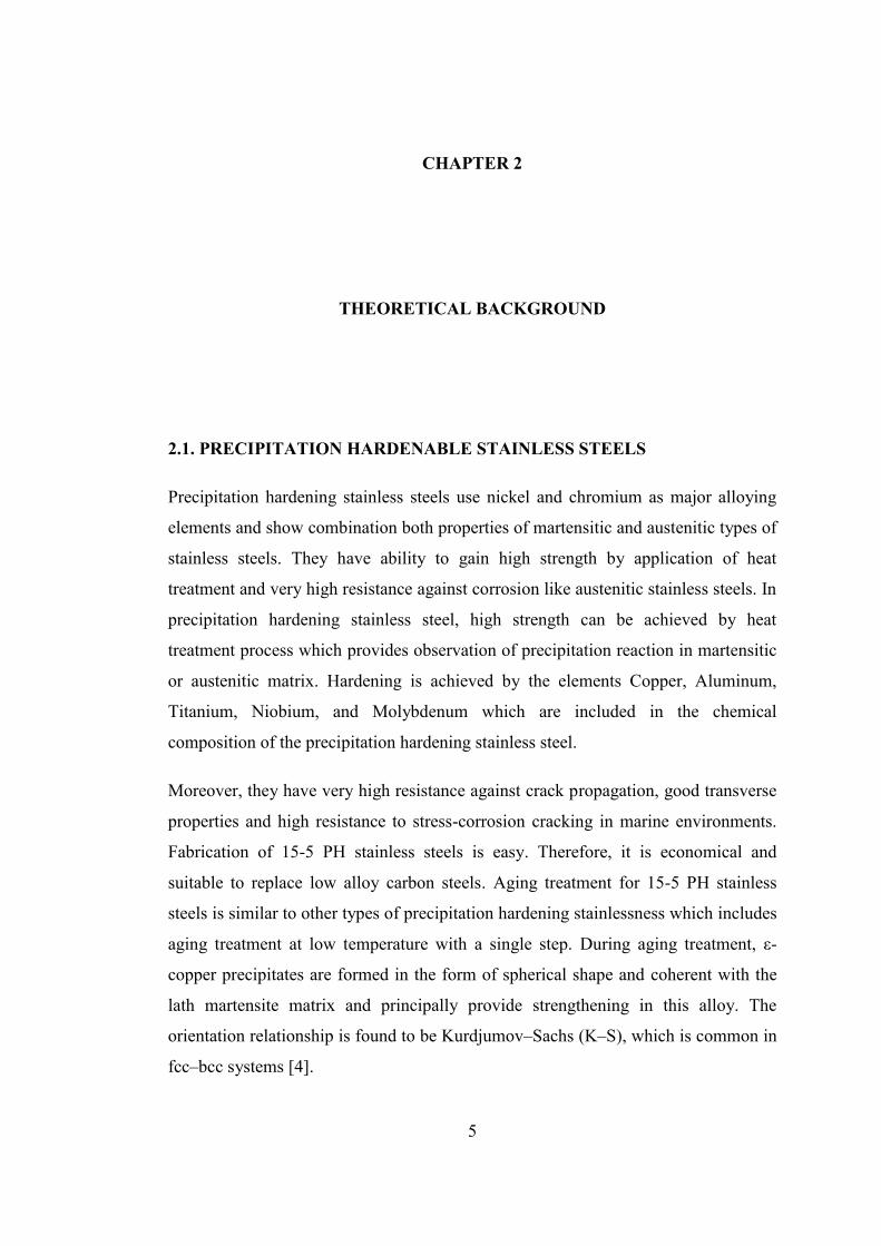
2.1. PRECIPITATION HARDENABLE STAINLESS STEELS

Precipitation hardening stainless steels use nickel and chromium as major alloying

elements and show combination both properties of martensitic and austenitic types of

stainless steels. They have ability to gain high strength by application of heat

treatment and very high resistance against corrosion like austenitic stainless steels. In

precipitation hardening stainless steel, high strength can be achieved by heat

treatment process which provides observation of precipitation reaction in martensitic

or austenitic matrix. Hardening is achieved by the elements Copper, Aluminum,

Titanium, Niobium, and Molybdenum which are included in the chemical

composition of the precipitation hardening stainless steel.

Moreover, they have very high resistance against crack propagation, good transverse

properties and high resistance to stress-corrosion cracking in marine environments.

Fabrication of 15-5 PH stainless steels is easy. Therefore, it is economical and

suitable to replace low alloy carbon steels. Aging treatment for 15-5 PH stainless

steels is similar to other types of precipitation hardening stainlessness which includes

aging treatment at low temperature with a single step. During aging treatment, ε-

copper precipitates are formed in the form of spherical shape and coherent with the

lath martensite matrix and principally provide strengthening in this alloy. The

orientation relationship is found to be Kurdjumov–Sachs (K–S), which is common in

fcc–bcc systems [4].

6

The advantage of precipitation hardening steels is that they can be supplied in

solution treated condition, which is ready for aging treatment. Strength of these steels

can be increased by the application of a single aging treatment at low temperature.

This is known as aging treatment or age-hardening. In addition, there is not occurring

any size distortion for these steels during aging treatment that makes application of

the heat treatment easy.

Figure 4 Position of PH steels in the Schaeffler-Delong's diagram. [5]

2.1.1. CLASSIFICATION OF PH STAINLESS STEELS

A wide range of engineering properties can be achieved by variations of heat

treatment parameters during manufacturing of precipitation hardenable stainless

steels. Presently, there exist three types of precipitation hardenable stainless steels.

All types of these steels are essentially austenitic at their normal annealing

temperatures. Precipitation hardenable stainless steels are grouped as austenitic,

semi-austenitic and martensitic types. The currently available precipitation

hardenable stainless steels with chemical compositions are listed in Table 1.

7

Table 1 Precipitation hardenable stainless steels. [1]

2.1.1.1. AUSTENITIC PH STAINLESS STEELS

Austenitic precipitation hardening steels keep their austenitic structure after

annealing and hardening as a result of aging treatment. Precipitation hardening phase

is soluble at the annealing temperature of 1095 to 1120°C. It remains in solution

during rapid cooling. When the steels are reheated to 650 to 760°C, precipitation

reaction occurs in the matrix phase. Thus, hardness and strength of the material may

be increased.

As it is shown in table 1, the alloy A-286 is a typical example of austenitic

precipitation hardenable stainless steels. These alloys show lower mechanical

properties in room-temperature conditions, Moreover; their yield strength is around

690 MPa and retains a large proportion of this yield strength up to temperature as

high as 700°C.

2.1.1.2. SEMI-AUSTENITIC PH STAINLESS STEELS

Unlike martensitic types of precipitation hardening stainless steels, annealed semi-

austenitic precipitation hardening steels are soft enough to be cold worked. Semi-

austenitic steels retain their austenitic structure at room temperature. These steels can

form martensitic structure at very low temperatures.

8

During solution treatment, alloy is heated to a high enough temperature in order to

remove carbon atoms from solid solution and provide formation of precipitates as

chromium carbide (Cr23C6) for semi-austenitic alloys. These reaction causes decrease

in chromium content in austenite matrix. Therefore, austenite matrix becomes

unstable and during cooling it transforms to martensite phase. If the solutionizing is

done at higher temperature (955oC) few types of carbide may be precipitated. Final

stage is precipitation hardening, which is carried out in the range of 480 to 650oC.

During this step, aluminum in the martensite combines with the some of the nickel in

the matrix phase to form intermetallic precipitates of NiAl and Ni3Al.

As it is shown in table 1, the semi-austenitic precipitation hardenable stainless steels

are 17-7 PH, PH 15-7 Mo, PH 14-8 Mo, AM 350 and AM 355. These alloys are

manufactured primarily as sheet since the austenitic structure obtained during

annealing provides superior formability. The transformation to martensite prior to

precipitation hardening may be accomplished by some mechanical or thermal

processes. Yield strength for these steels is over 1380 MPa. These steels keep their

mechanical properties up to temperature 480°C.

2.1.1.3. MARTENSITIC PH STAINLESS STEELS

Martensitic precipitation hardening stainless steels have a predominantly austenitic

structure at annealing temperatures around 1040 to 1065°C. Upon cooling to room

temperature, microstructure changes from the austenite to lath type of martensite

phase. As it is shown in Table 1, the martensitic precipitation hardenable stainless

steels are 17-4 PH, 15-5 PH, PH 13-8 Mo, AM 362, AM 363, AFC- 77 and Custom

455. These materials are used as bar or forged condition, although some types of

these PH stainless steels are available as castings or sheet and plate form. Hardening

is achieved by a single low aging treatment. This treatment provides yield strength

from 1170 to 1370 MPa. These steels can be used up to temperature as high as 480°C

without losing mechanical properties.

These steels are generally used in the aircraft industry. The basic usage areas for

these steels are blading, bolts, nozzles, pins, landing assemblies, and ribs and

9

stringers which are manufactured from the martensitic precipitation hardenable

stainless steels.

15-5 PH stainless steel is the one of the important martensitic precipitation

hardenable stainless steel containing approximately 3-4 wt % pct Copper (Cu) and

that provide main strengthening as a result of precipitation reaction in the martensite

matrix. After solution heat-treatment, this alloy is generally hardened by seven

standard heat treatment cycles.

2.2. HEAT TREATMENT OF PH STAINLESS STEELS

In this section general ınformation about heat treatment of PH stainless steels are

given. Following section includes the information for heat treating process of the

(AMS5659) 15-5 PH stainless steels, which is studied in this thesis, in detail.

Basic composition of the stainless steels is composed of elements iron, carbon and

chromium. Precipitation hardenable stainless steels include significant amount of

other elements in chemical composition, in order to reach a wide range of

mechanical properties and formability. Each of these elements in stainless steels have

two important functions, one at high temperature and the other one is during cooling

from high temperature which are determining microstructures and phases.

There exist two crystallographic arrangements for stainless steels at elevated

temperatures that are ferrite, a body- centered cubic (BCC) crystal structure, and

austenite, a face- centered cubic (FCC) crystal structure. Each of the elements in

chemical compositions helps the formation of one or other of these crystal structures.

The elements chromium (Cr), molybdenum (Mo), silicon (Si), aluminum (Al),

titanium (Ti), vanadium (V) and phosphorous (P) provide formation of ferrite with

BCC structure. The elements, which provide austenite with FCC structure, are iron

(Fe), carbon (C), nickel (Ni), manganese (Mn) copper (Cu) and cobalt (Co). The

relative proportion of these elements in the composition determines crystal structure

of the stainless steels at elevated temperature. In general, steels with ferritic structure

at elevated temperature retain its crystal structure during cooling and non-heat

treatable. However, austenitic steels at high temperature may keep its crystal

10

structure or may transform to martensitic, a body centered tetragonal (BCT) structure

that have higher strength during cooling.

There exist two symbols, MS and MF, used to indicate temperatures at which

transformation from austenite to martensite takes place. In austenitic steels, all of the

elements other than aluminum and cobalt tend to lower MS and MF temperatures. The

solubility of the alloying element in the austenite increases by increasing

temperature. This makes possible to control the MS and MF temperatures for stainless

steels for intermediate alloying elements content. The effect of the alloying element

content on the MS and MF transformation temperatures can be seen in Figure 5.

Figure 5 Effect of alloy contents on transformation temperatures of precipitation

hardenable stainless steels. [1]

There exist three important steps for heat treatment cycle of precipitation hardenable

stainless steels. The first step is solution treatment. In this step, steels are exposed to

high temperature in order to dissolve all alloying elements to reach supersaturated

solid solution at high temperature. Temperature and time values for this step may be

determined according to chemical composition of steels and desired mechanical

properties. The second step of heat treating cycle is formation of a supersaturated

solid solution as a result of very rapid cooling or quenching. Since solubility of most

elements at room temperature is lower than at elevated temperature, supersaturated

solid solution is formed at room temperature.

11

The last and the most important step to reach desired mechanical properties is

precipitation hardening or aging treatment. The primary requirement of an alloy for

precipitation hardening is that the solubility of an element B in the phase A decreases

with decreasing temperature. At room temperature precipitation reaction does not

take place since rate of diffusion is almost zero. However, elevated temperature

provides easy atomic immigration thus some intermetallics and precipitates are

formed by alloying elements.

Figure 6 Precipitation hardening sequence. [6]

Initially, formed sub-microscopic precipitates are observed along the crystallographic

planes of the matrix phase. Due to difference in lattice dimension between the matrix

phase and precipitates, some straining is created in the matrix. Strengthening of

precipitation hardenable stainless steels is defined development of this straining in

the matrix phase as a result of precipitation reaction.

Size and distribution of these precipitates can be controlled by changing the aging

temperature and time periods. Most effective strengthening can be reached by small

and uniformly distributed precipitates. When temperatures is increased to

intermediate range, the precipitate particles become larger and are not so effective so

12

maximum hardening is usually achieved in shorter time. At high temperature in

precipitation range, precipitates may also grow to even larger size that cause shearing

between precipitates and matrix phase. This condition cause reliving of the strain in

the matrix phase and called overaged.

2.2.1. HEAT TREATMENT OF (AMS5659) 15-5 PH STAINLESS STEEL

Mechanical properties of (AMS5659) 15-5 PH stainless steels are reached basically

by two mechanisms during heat treatment. The first one is transformation of

austenite to martensite phase by cooling from solution treatment (annealing)

temperature. The second one is precipitation of the hardening elements during aging

treatment. At annealing temperature, 15-5 PH stainless steels have composed of

mainly austenitic structure with some dissolved alloying elements in chemical

composition.

There exist three most critical factors in thermal processing of 15-5 PH stainless

steels which are solution treatment temperature, cooling conditions and temperature

for precipitation hardening reactions.

2.2.1.1. SOLUTION TREATMENT OF 15-5 PH STAINLESS STEEL

The solution treatment temperature is selected to reach the optimum combination of

austenite composition for martensitic transformation and solubility of hardening

elements. Higher or lower annealing temperature may affect the mechanical

properties and microstructure of the 15-5 PH stainless steels. Lower annealing

temperature may cause decrease in both yield and ultimate tensile strength for 15-5

PH stainless steels when the material is aged. The reason for decrease in strength can

be explained by lesser amount of hardening elements that goes into solution thus;

softer martensite is formed. Higher annealing temperature causes increase in ultimate

strength but decrease in yield strength for 15-5 PH stainless steels. At higher solution

treatment temperature, amount of alloying elements in solution will be more that

causes less transformation during cooling. As a result of this, there may be more

retained austenite which decreases the yield strength. When the yield strength is

13

exceeded by deformation process, austenite phase may transform to stronger

martensitic phase that provides higher ultimate tensile strength.

2.2.1.2. COOLING AND TRANSFORMATION FOR 15-5 PH STAINLESS

STEEL

15-5 PH stainless steels are cooled continuously from their solution treatment

temperature to room temperature. This cooling provides formation of supersaturated

solid solution since solubility of alloying elements becomes less at room temperature

condition. Moreover, transformation of austenite to martensite phase may cause

increase in volume, so cooling rate should be controlled in order to prevent cracking

phenomena due to mechanical strains which is caused by expansion. It is also

important that martensite finish (Mf) temperature is reached during cooling to ensure

complete martensitic transformation.

2.2.1.3. PRECIPITATION HARDENING OF 15-5 PH STAINLESS STEEL

After cooling, the structure of martensitic phase is supersaturated by alloying

elements. The final heating step for 15-5 PH stainless steels includes reheating of

material for a temperature range between 450 to 6200C. This operation improves the

both ultimate and yield strength as a results of precipitation reaction and formation of

intermetallic compounds.

Size and distribution of the precipitates may be controlled by changing the time and

temperature during aging treatment that provide wide range of desired mechanical

properties. Highest strength is obtained by uniformly distributed small precipitates by

keeping at low temperature in aging treatment range for a long times. Higher aging

temperature causes larger and fewer precipitates. Moreover, higher aging

temperature may cause reformation of austenite phase which cause decrease on

hardness and strength of 15-5 PH stainless steel.

There exist seven (7) standard heat treatments process that are H 900, H 925, H

1025, H 1075, H 1100, H 1150, H 1150-M, Application of this heat treatment

processes may be referred to MIL-H-6875 handbook [7].

14

Table 2 Standard heat treatment conditions for 15- 5 PH stainless steels. [8]

2.3. MANUFACTURING METHOD OF 15- 5 PH STAINLESS STEEL

AMS5659 15-5 precipitation hardenable stainless is manufactured by consumable

electrode by vacuum arc remelted process that provides high ductility and toughness.

Initially, primary melt of the alloy is formed as a result of melting of raw materials in

the electric arc furnaces. After addition of the suitable element, melted alloy is casted

in the form of electrodes. After that, these electrodes are remelted in Vacuum Arc

Remelting (VAR) furnace in order to achieve homogenous ingot without the any

internal segregation and defects. A systematic flow chart for manufacturing of 15–5

precipitation hardenable stainless steel may be seen in Figure 7.

15

Figure 7 Manufacturing process flow of 15–5 PH martensitic stainless steels. [4]

2.4. MICROSTRUCTURE OF 15- 5 PH STAINLESS STEEL

As it mentioned before, 15-5 precipitation hardenable stainless steels include

chromium and nickel as the major alloying elements. They also comprise copper that

plays significant role in precipitation reaction during aging treatment. There may

exist some other elements such as niobium and molybdenum which may cause

formation of some carbide during heat treatment.

Precipitation hardened stainless steels have complex microstructure that is developed

during a sequence of solution treatment. The resulting microstructure of 15-5 PH

stainless steels includes lath martensite, Cu precipitates, retained austenite depending

aging time and temperatures. When the material is heated to annealing temperature,

all alloying elements in chemical compositions are dissolved and austenite phase is

16

formed. After air cooling supersaturated solid solution is formed with lath martensite

matrix which includes high density of dislocations in the microstructure.

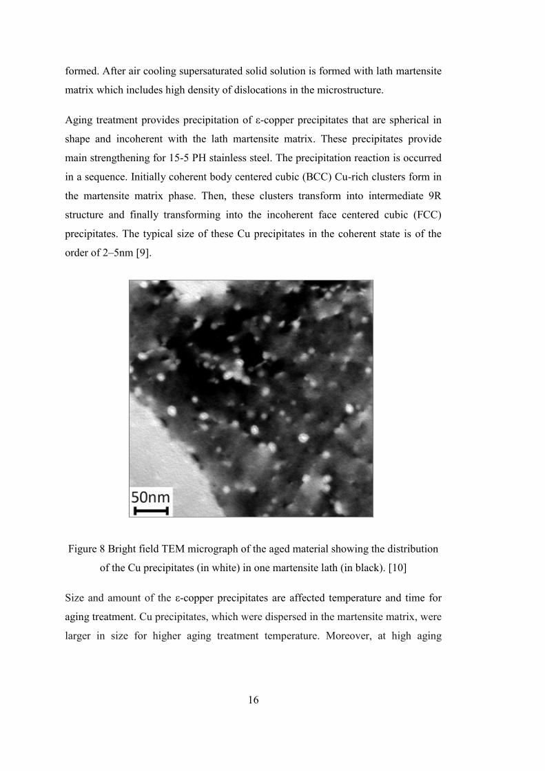
Aging treatment provides precipitation of ε-copper precipitates that are spherical in

shape and incoherent with the lath martensite matrix. These precipitates provide

main strengthening for 15-5 PH stainless steel. The precipitation reaction is occurred

in a sequence. Initially coherent body centered cubic (BCC) Cu-rich clusters form in

the martensite matrix phase. Then, these clusters transform into intermediate 9R

structure and finally transforming into the incoherent face centered cubic (FCC)

precipitates. The typical size of these Cu precipitates in the coherent state is of the

order of 2–5nm [9].

Figure 8 Bright field TEM micrograph of the aged material showing the distribution

of the Cu precipitates (in white) in one martensite lath (in black). [10]

Size and amount of the ε-copper precipitates are affected temperature and time for

aging treatment. Cu precipitates, which were dispersed in the martensite matrix, were

larger in size for higher aging treatment temperature. Moreover, at high aging

17

temperature, shape of the Cu precipitates transformed from spherical to elliptical

with a diagonal axis about 15 nm that can be seen in Figure 9. [11]

Figure 9 TEM and HRTEM micrographs of Cu precipitates and reversed austenite

obtained from specimen aged at 5800C for 4 h (a-b) aged at 620

0C for 4 h (c-d). [11]

In addition to this, for the same aging time, increase in aging temperature cause

reformation of austenite phase in the microstructure. Since both copper and austenite

have the same FCC structure with the similar lattice parameter, copper particles

behave favorable nucleation sites for reversed austenite phase. After precipitation of

Cu, Ni and C atoms start to segregate around copper precipitate from lath martensite

matrix which is shown in Figure 10. The reversed austenite formation reaction is also

affected by this phenomenon. Since the segregation of Ni and C reduce the austenite

stabilizing temperature, reversed austenite formation may become possible around

the Cu precipitates.

18

Figure 10 Concentration of Ni on a cross section of a copper precipitate in an APT

volume obtained on the aged material. [10]

In 15- 5 PH stainless steels, niobium is also included in the chemical composition in

order to decrease amount of carbon into carbides. Therefore, it is also possible to

observe some niobium carbide particles in the microstructure. Size of these particles

is around 300 nm in diameter that is shown in Figure 11. However, observation of

precipitates, carbides and reversed austenite are not possible under optical

microscope

Figure 11 Bright field TEM micrographs showing spherical niobium carbides

(arrows). Right hand side figure shows a larger magnification image of carbide. [10]

19

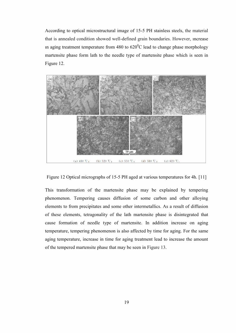
According to optical microstructural image of 15-5 PH stainless steels, the material

that is annealed condition showed well-defined grain boundaries. However, ıncrease

ın aging treatment temperature from 480 to 6200C lead to change phase morphology

martensite phase form lath to the needle type of martensite phase which is seen in

Figure 12.

Figure 12 Optical micrographs of 15-5 PH aged at various temperatures for 4h. [11]

This transformation of the martensite phase may be explained by tempering

phenomenon. Tempering causes diffusion of some carbon and other alloying

elements to from precipitates and some other intermetallics. As a result of diffusion

of these elements, tetragonality of the lath martensite phase is disintegrated that

cause formation of needle type of martensite. In addition increase on aging

temperature, tempering phenomenon is also affected by time for aging. For the same

aging temperature, increase in time for aging treatment lead to increase the amount

of the tempered martensite phase that may be seen in Figure 13.

20

Figure 13 Optical micrographs of the material in different metallurgical conditions:

(a) solution annealed, (b) aged at 5800C for 0.25h, (c) aged at 580

0C for 4h. [9]

2.5. HARDNESS VALUES OF 15-5 PH STAINLESS STEEL

Hardness is an important mechanical property of the materials which is defined a

measure of material resistance against localized plastic deformation or resistance to a

wear. Hardness of 15-5 PH stainless steel that is affected by heat treatment process.

As it mentioned before there exist seven (7) standard heat treatments process that are

H 900, H 925, H 1025, H 1075, H 1150, H 1100, H 1150-M for these steels.

According to different aging temperature and time period, different hardness values

can be achieved that is shown in Table 3.

21

Table 3 Hardness values for different aging condition. [12]

Heat Treatment Condition Hardness in HRC

Solution annealed 36 HRC

H900 Condition 38 HRC






As it mentioned before, heat treatment was conducted in three steps that were

homogenization, solutionizing and aging treatment for 15-5 PH stainless steels in this

study. Hardness of the 15-5 PH stainless steels is affected by temperature and time

period of each heat treatment steps. The effect of homogenization time on hardness

of the 15-5 PH stainless is examined by Yoo et al. (2006). Increasing in time for

homogenization from 1 to 5 hours, initially leads to decrease on hardness. However,

after two hours, increase in time for homogenization causes increase on the hardness

of the 15-5 PH stainless steels. This increase on hardness is explained according to

composition of the supersaturation solid solution. As the time for homogenization

increases, solubility of the alloying element in the austenite matrix increases at high

temperature. During cooling, driving force become much higher to form some

intermetallic and other second phase particles which cause increase on hardness.

Variation of the hardness of 15-5 PH stainless steels with homogenization time is

presented in Figure 14.

22

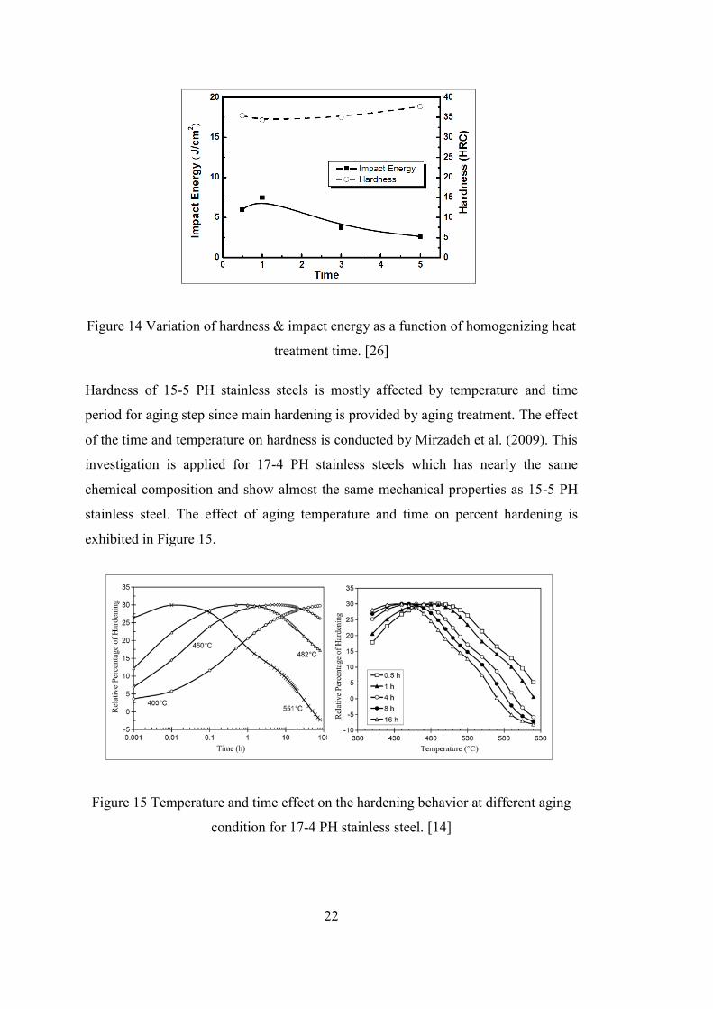
Figure 14 Variation of hardness & impact energy as a function of homogenizing heat

treatment time. [26]

Hardness of 15-5 PH stainless steels is mostly affected by temperature and time

period for aging step since main hardening is provided by aging treatment. The effect

of the time and temperature on hardness is conducted by Mirzadeh et al. (2009). This

investigation is applied for 17-4 PH stainless steels which has nearly the same

chemical composition and show almost the same mechanical properties as 15-5 PH

stainless steel. The effect of aging temperature and time on percent hardening is

exhibited in Figure 15.

Figure 15 Temperature and time effect on the hardening behavior at different aging

condition for 17-4 PH stainless steel. [14]

23

As it mentioned before, main hardening is provided by precipitation of the copper

element as a ε- copper precipitates, which prevent motion of dislocations in the

martensite matrix. Change in temperature and time period of aging treatment affects

size and distribution of these precipitates. At lower aging temperatures, hardness

value increases slowly compared to higher aging temperature which increases

rapidly. It can be also said that at lower aging temperature, time needed to achieve

peak hardness is generally high while for higher aging temperature, it is low that may

be seen in Figure 16.

Figure 16 Required time to achieve peak hardness according to aging temperature for

15-5 PH stainless steels. [11]

Increase on aging temperature leads to decrease relative percent of hardening. This

decrease is explained by coarsening of the ε- copper precipitates, recovery and re-

transformation of the martensite to austenite phase. When the size of precipitates

increases, probability of inhibiting the motion of the dislocation decreases that

causes decrease on hardness of the 15-5 PH stainless steels.

In addition, it is difficult to keep peak hardness value at higher aging temperature,

since after reaching peak value hardness becomes very sensitive against time. Hsiao

et al. (2002) studied development of microstructure and aging reaction for 17-4 PH

stainless steels. Accordingly, the steel reached peak hardness value at aging

temperature 4800C after 1 h, however by keeping the material for a prolonged time

24

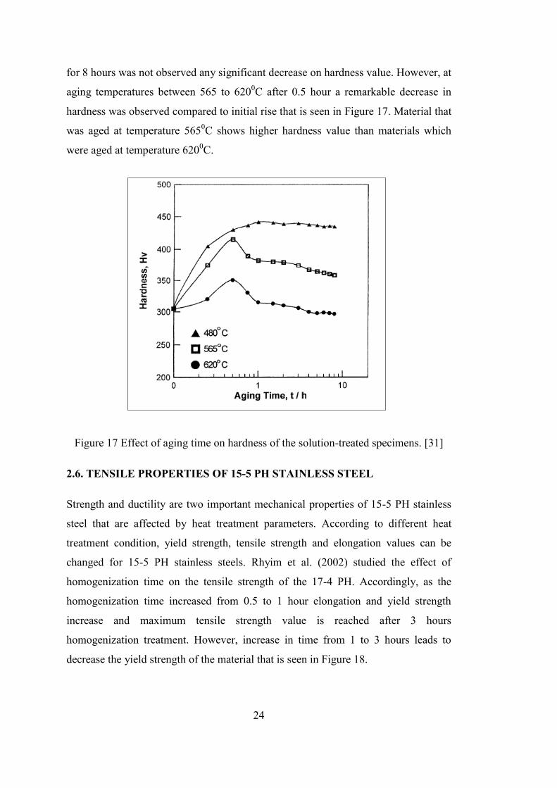
for 8 hours was not observed any significant decrease on hardness value. However, at

aging temperatures between 565 to 6200C after 0.5 hour a remarkable decrease in

hardness was observed compared to initial rise that is seen in Figure 17. Material that

was aged at temperature 5650C shows higher hardness value than materials which

were aged at temperature 6200C.

Figure 17 Effect of aging time on hardness of the solution-treated specimens. [31]

2.6. TENSILE PROPERTIES OF 15-5 PH STAINLESS STEEL

Strength and ductility are two important mechanical properties of 15-5 PH stainless

steel that are affected by heat treatment parameters. According to different heat

treatment condition, yield strength, tensile strength and elongation values can be

changed for 15-5 PH stainless steels. Rhyim et al. (2002) studied the effect of

homogenization time on the tensile strength of the 17-4 PH. Accordingly, as the

homogenization time increased from 0.5 to 1 hour elongation and yield strength

increase and maximum tensile strength value is reached after 3 hours

homogenization treatment. However, increase in time from 1 to 3 hours leads to

decrease the yield strength of the material that is seen in Figure 18.

25

Figure 18 Deviation of the yield, tensile strength and elongation according to

homogenization time. [26]

Aging temperature also has important effect on yield and tensile strength of the 15-5

PH stainless steels. Bhambroo et al. (2013) studied effects of solution annealing and

aging treatment on mechanical properties of the 15-5 PH stainless steels. Tensile

properties of the materials were evaluated for different aging and solution annealed

conditions at room temperature at a strain rate of 1x10-4

/s. Consequently, aging at

5800C cause a sharp increase in the yield and tensile strength of the material in the

initial stage while on prolong time for aging, the yield and tensile strength of the

material reduced and fixed around 1020 MPa that is seen in Figure 19.

26

Figure 19 Effect of ageing time at 5800C on the tensile behavior of 17-4 PH at room

temperature. [9]

As it mentioned before, there exist seven standard heat treatment processes for 15-5

PH stainless steels which provide different mechanical properties. Tensile and

elongation properties of the 15-5 PH stainless steel may be seen in Table 4. H900

heat treatment condition provides highest tensile and yield strength for 15-5 PH

stainless steel while values for H1150-M condition is lowest. This decrease may also

be explained the coarsening of the ε-copper precipitates and re-formation of the

austenite phase at high aging temperature.

Table 4 Mechanical properties of 15-5 PH stainless steel. [8].

27

In most design case, stress versus strain curves were used in handling of the tensile

behavior of 15-5 PH stainless steels that is presented in Figure 20.

Figure 20 Typical tensile behavior for various heat treatment conditions for 15-5 PH

stainless steel bar, at room temperature condition. [16]

2.7. FATIGUE PROPERTIES

Fatigue is a form of the failure that is observed in structures and components when

subjected to dynamic and fluctuating stresses that may be shown on bridges, aircraft,

railways and some machine components. Fatigue failures in metallic structures may

cause significant problems. Several serious fatigue failures were studied and reported

by August Wöhler in the 19th century. He recognized that, when a material is

exposed to a single static load far below the static strength of the materials, no

damage observed on the structures and components. However, ıf the same load is

exposed in many times it may cause failure of the components. Therefore, the term

fatigue is explained by the type of failure that occurs after a long period of applied

cyclic stress or strains.

28

Fatigue failure is observed in brittle nature even in ductile metals, but there may be

very little plastic deformation during failure. Repeated cyclic load in fatigue

mechanism causes initiation of small microcracks that are followed by growth up to

complete failure. In addition, fracture surface of the fatigue failure is directly

perpendicular to direction of applied tensile stress.

There exist three basic factors which are necessary for fatigue failures:

There should be a maximum tensile stress with a sufficiently high value.

There should be an enough variation and fluctuation on applied load.

Applied load should expose sufficiently large number of cycles.

2.7.1. DEFINITIONS AND TERMS FOR FATIGUE

The applied cyclic load may be in the form of axial (tension-compression), bending,

or torsional (twisting). In fatigue concept, there exist three different cyclic stress vs.

time diagrams. The first one is where the maximum and minimum applied stress

(load) levels are equal that is called fully reversed stress vs. time diagram. The

second type is where applied stress (load) are asymmetrical that is known as repeated

stress vs. time diagram. Stresses (loads) may be in the form of compression-

compression, tension- tension and tension- compression. The final stress vs. cycle

diagram is where stress (load) level varies randomly in frequency and amplitude.

That is named as irregular stress vs. cycle diagram.

29

Figure 21 Schematic exhibition of loading types. [17]

There exist several parameters that are cyclic stress (load) range, cyclic stress (load)

amplitude, mean stress (load) and stress (load) ratio used to fluctuating stress (load)

vs. cycle diagrams.

30

Stress (load) range is the algebraic difference between the consecutive peak forces

and valley in fatigue loading:

𝜎𝑟 = 𝜎𝑚𝑎𝑥 − 𝜎𝑚𝑖𝑛 (2.1)

Stress (load) amplitude is the one half of the range of cycle:

𝜎𝑎 = (𝜎𝑟

2 ) =

𝜎𝑚𝑎𝑥− 𝜎𝑚𝑖𝑛

2 (2.2)

Mean stress (load) is the algebraic average of the maximum and minimum stresses in

constant amplitude fatigue loading:

𝜎𝑚 = 𝜎𝑚𝑎𝑥− 𝜎𝑚𝑖𝑛

2 (2.3)

Stress (force) ratio is the ratio of minimum stress (load) over maximum stress (load):

𝑅 = 𝜎𝑚𝑖𝑛

𝜎𝑚𝑎𝑥 (2.4)

Figure 22 Schematic exhibition of basic terms on sinusoidal fatigue loading. [18]

31

2.7.2. NUCLEATION AND GROWTH OF FATIGUE CRACK

According to some microscopic investigation in the initial period of the 20th century,

nucleation of fatigue crack starts as invisible microcracks in slip bands. Nucleation of

these microcracks generally takes place very early period in the fatigue life when a

cyclic stress just above the fatigue limit is applied. In addition, these microcracks

generally remain invisible during significant part of the total fatigue life. Therefore,

it can be said that when these cracks become visible, there will be small percentage

of total fatigue life for a laboratory specimen. On the other hand for real structure,

the remaining percentage of the total fatigue life will be much larger even if cracks

become visible.

When a microcrack has been reached, crack exhibit a low growth rate due to some

microstructural effects such as grain boundary. However, crack away from the

nucleation site show more regular growth rate. This situation can be named as a real

crack growth period. Therefore, until the failure, fatigue life is consisted by two

periods which are crack initiation period and crack growth period.

Figure 23 Different phases of the fatigue life. [19]

2.7.2.1. CRACK INITIATION PERIOD

Cyclic slips are enabled by cyclic shear stress. In the microscopic point of view,

these shear stresses are not distributed homogenously on the material. This

inhomogeneity is affected by shape and size of the grains, crystallographic

orientation of the grains and anisotropy of the materials which cause variation of the

shear stress from one grain to another. Some surface grains for the materials are

usually more favorable for cyclic slip mechanism than others. When a cyclic slip

32

occurs, a slip step is formed at the surface of the material. When load is increased,

some strain hardening is formed on these slip bands. During unloading, this

hardening causes formation of the shear stress in the same slip but in reversed

direction that causes formation of a reversed slip band in parallel. Cyclic loading

provides back and forth movement for the slip bands that leads to the formation of

intrusions and extrusions on the surface of the materials. These intrusions and

extrusions provide formation of a microcrack on the surface of the materials. These

cracks are initially propagated in parallel with slip bands with a very small growth

rate like 1 nm in each cycle. When crack reached sufficient length, becomes

dominant to overcome the stress field at the tip of the slip bands. Thus, crack growth

plane changes to perpendicular direction to the principal stress.

Figure 24 Effect of the cycle slip on the crack nucleation. [19]

2.7.2.2. CRACK GROWTH PERİOD

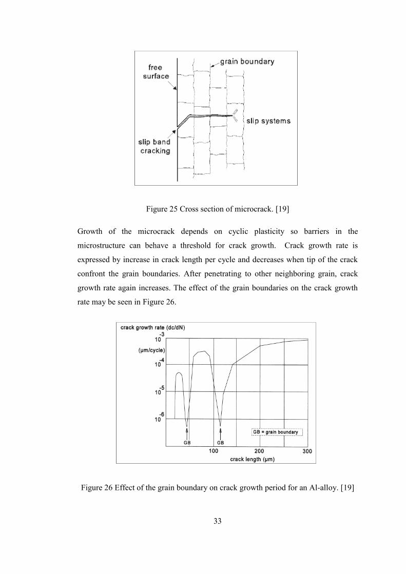
If a microcrack grows through adjacent grains, restrain on the cyclic slip mechanism

increases due to effect of the neighboring grains. Therefore, it may become difficult

to continue the cyclic slip only by one slip plane that provides observation of the

more slip planes. As a result, the growth direction of the microcracks deviates from

slip band orientation. There exists usually a tendency to grow perpendicular direction

normal to applied stress that is shown in Figure 25.

33

Figure 25 Cross section of microcrack. [19]

Growth of the microcrack depends on cyclic plasticity so barriers in the

microstructure can behave a threshold for crack growth. Crack growth rate is

expressed by increase in crack length per cycle and decreases when tip of the crack

confront the grain boundaries. After penetrating to other neighboring grain, crack

growth rate again increases. The effect of the grain boundaries on the crack growth

rate may be seen in Figure 26.

Figure 26 Effect of the grain boundary on crack growth period for an Al-alloy. [19]

34

During the crack growth period, there is not large gradients in the crack growth since

crack cannot grow in the random direction through the grains. Therefore, crack front

generally remains coherent which may be seen in Figure 277.

Figure 27 Evolution of the fatigue crack front. [20]

2.7.3. STRESS- LIFE DIAGRAMS (S-N CURVES)

Similar to other mechanical properties, fatigue characteristics of the materials can

also be derived by laboratory tests. Test apparatus provide service conditions with

respect to stress level, time and frequency. In general, two different fatigue testing

systems are used with different loading condition. These systems are axial and

rotating bending fatigue testing systems.

A range of tests may be performed by subjecting specimens to cycling stress at

different stress levels and the number of cycles up to failure is recorded. Results of

the fatigue tests are plotted as stress versus number of cycles to failure for all tested

specimens. This plot is called S-N curves that provide information for fatigue

behaviors of materials. The bases of the stress-life diagrams are known as Wohler S-

N diagrams which can be seen in Figure 28. S-N diagrams represent the mean of the

data from several fatigue tests.

35

Figure 28 Typical S-N curves. [21]

Stress versus number of cycles to failure data (S-N) may also be plotted on a log-log

plots that is seen in Figure 29. These diagrams are generally called as idealized S-N

curve.

Figure 29 Idealized S-N curve. [21]

S–N curves for some ferrous materials (iron base) and some titanium alloys become

horizontal at large number of cycles, or it can be said there exist a limiting stress

level. This stress level is called by fatigue limit or sometimes endurance limit and

below this stress level, fatigue failure will not occur. In other words, fatigue limit

36

represents the maximum stress level that will not cause failure for an infinite number

of cycles. For many high strength steels, fatigue limits are generally ranged between

30% and 60% of the ultimate tensile strength. Typical trend of S-N curve for those

types of materials can be shown curve A in Figure 28.

Most of nonferrous alloys such as aluminum, copper, magnesium do not show

endurance limit. S-N diagrams for these alloys shows a downward trend through

relatively large number of cycles. For these types of materials, fatigue behavior is

specified as fatigue strength that is defined as stress levels at which failure will occur

for some determined number of cycles. Typical trend of S-N curve for those types of

materials can be shown curve B in Figure 28.

2.7.4. FATIGUE BEHAVIOR AND STRESS- LIFE DIAGRAMS FOR 15-5 PH

STAINLESS STEEL.

15-5 PH stainless steels are preferred in aerospace and defense industries thanks to

its high fatigue performance. Fatigue performance of the 15-5 PH stainless steel is

much affected by heat treatment condition. Increase in aging temperature from 4800C

to 5500C causes decrease on fatigue limit of the 15-5 PH stainless steel of 5 to 10

percent [22]. Fatigue test results (R=0.1) for two different heat treatment conditions

may be seen in Table 5.

Table 5 Fatigue test results for 15-5 PH stainless steels for H-900 and H-1050

conditions. [22]

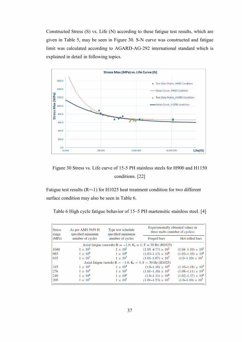
37

Constructed Stress (S) vs. Life (N) according to these fatigue test results, which are

given in Table 5, may be seen in Figure 30. S-N curve was constructed and fatigue

limit was calculated according to AGARD-AG-292 international standard which is

explained in detail in following topics.

Figure 30 Stress vs. Life curve of 15-5 PH stainless steels for H900 and H1150

conditions. [22]

Fatigue test results (R=-1) for H1025 heat treatment condition for two different

surface condition may also be seen in Table 6.

Table 6 High cycle fatigue behavior of 15–5 PH martensitic stainless steel. [4]

38

2.8. STATISTICAL ANALYSIS OF FATIGUE TEST DATA

By its nature, fatigue test results for a material is a random process, so there is

always scatter in test results, although controlling of fatigue testing conditions

carefully. This scatter in fatigue data causes analysis of fatigue test results and

application of these to real problems much difficult. Therefore, some statistical

methods are needed to handle these scatter in fatigue test results. Statistical methods

generally provide information on the limited number of tested specimens and finding

a specified degree of confidence level on test results. The construction of S-N can be

basically described to the individual data points. The one of the common function

that provides an adequate fitting for certain data is known as normal distribution

(Gaussian distribution) and defined with equation 2.5.

𝑝 (𝑆) = (1

𝜎√2𝜋 ) 𝑒𝑥𝑝 (

−𝑆2

2𝑆𝜎2) (2.5)

A normal distribution p(S) shows variation with variable (S), mean (µ) and variance

(σ2) of these all values of S. The function p(S) is also known as probability density

function. This shows a measure of a width of the scatter band. In most cases, normal

distribution gives a good approximation for distribution of fatigue lives of metallic

specimens in logarithmic scale.

Parameters related to population can only be estimated from tested sample.

Otherwise, ın order to obtain exact values of parameters for the population, whole

population should be tested. The estimates of behavior of the population from a

tested sample, and the confidence level are the essence of the statistical analysis of

metal fatigue data of specimens.

39

Figure 31 Schematic P-S-N diagram for three probabilities of failure and log normal

distributions of lives. [23]

In general, specimens are tested at different stress levels so different probabilities of

failures may exist for S-N curves. In the conventional S-N curves, fifty percent

(50%) probability corresponds to median is preferred. These curves are referred to as

P-S-N curves and scatter in endurance increases through the fatigue limit that can be

seen in Figure 3131. According to this statistical concepts, construction of S- N

curves and calculation of fatigue limit were carried according to AGARD-AG-292

HELICOPTER FATIGUE DESIGN GUIDE [24] that is explained in following

section in detail.

2.8.1. AGARD-AG-292 FOUR (4) PARAMETER BEST FITTING

TECHNIQUE

As it mentioned before, ın order to get representative results from fatigue tests, a

large number specimens are needed for construction of S-N curves. However, for

most of the cases, the number of fatigue test specimens is usually limited in practice

due to cost and time consuming. Therefore, in order to get accurate results for the

design, the mean fatigue strength concept is used. The mean fatigue strength can be

reached by a relatively small number of specimens by using some fitting technique to

40

establish S-N curves. The curve shape for fatigue test results can be constructed by

some regression analysis as is shown in below.

The result of a fatigue test consists of a pair of values, one of which is related to the

applied load and the other is the number of cycle. The trend of test data can be

interpreted by the relationship S = f (N) with S = maximum stress and N = number of

cycles to failure. The type of the equation f (N) can be established by a numerical

analysis of test data. For this kind of curve, the Weibull four parameters equation

may be commonly used.

Determination of curve shape for S-N curves is carried out according to equation

(2.6);

S

Si = H + A ∗ (N + C)B (2.6)

Where, S is the applied maximum stress level, Si is the stress level at infinity, N is

the number of cycles for a given stress level and H, A, C and B are the variables for

construction of best fit for test data points. S-N curve shape can be derived from test

data and exhibits % 50 probabilities.

In order to derive mean S-N curve, fatigue test data are projected to a given number

of cycles through which is shown in Figure 32.

Figure 32 Extrapolation of data for statistical analysis. [24]

41

The extrapolation for test data is usually carried according to design criteria. In

general, for ferrous materials extrapolation is carried out to 10 million cycles and 50

million cycles for nonferrous materials like aluminum alloys. Mean and standard

deviations for extrapolated fatigue test data are calculated according to log normal

probability distribution function by using following equations.

𝑙𝑜𝑔 𝑆 =∑(𝑙𝑜𝑔𝑆𝑖)

𝑛 (2.7)

𝜎 = √∑(𝑙𝑜𝑔𝑆𝑖− 𝑙𝑜𝑔 𝑆)2

𝑛−1 (2.8)

where:

S= Mean fatigue strength for fatigue test data at extrapolated number of cycles

Si= Fatigue strength of individual specimen at extrapolated number of cycles

n= Number of specimens

𝜎= standard deviation

Best estimates of the unknown constants SI, H, A, B and C are obtained in fitting the

equation 2.6 by applying the method of least squares to fatigue life that can be seen

in Figure 33. Due to the fact that the S-N curve is practically horizontal for small and

large values of N, the regression of stress on life is performed, i.e. the sum of squared

deviations in the vertical direction between test data points and the best fitting curve

is minimized.

42

Figure 33 Least Square Fitting Concept for non-linear analysis of test data. [24]

Since equation 2.6 is nonlinear, a nonlinear regression algorithm is used according to

equation 2.6 and the minimization is done according to some conditions for variables

SI, H, A, B and C for those are shown in Table 7. In most of the cases H is taken as

one (1) since it has less effect on curve shape.

Table 7 Conditions for parameters SI, H, A, B and C in fitting equation

Conditions for Variables

A≥0 B≤0 C≥0 H≥0 Si≥0

2.8.2. STAIRCASE METHOD FOR FATIGUE LIMIT CALCULATION

Alternatively, fatigue limit of a materials can also be estimated according to staircase

method that is given in ISO 12107 International Standard (Metallic materials —

Fatigue testing — Statistical planning and analysis of data) [25]. Staircase method

provides to get rough estimates for the fatigue strength for the materials to be tested.

There exist two important points in staircase method. The first one is determination

of the stress level for the first specimen. The second one is the determination of the

increment value between stress levels. Stress level for fist specimen can be

determined according to expected average fatigue strength. On the other hand,

increment value may be determined standard deviation of the stress at 107 million

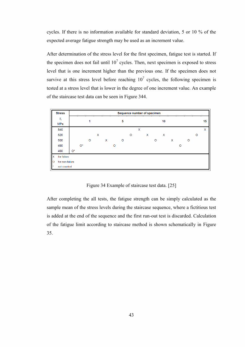
43

cycles. If there is no information available for standard deviation, 5 or 10 % of the

expected average fatigue strength may be used as an increment value.

After determination of the stress level for the first specimen, fatigue test is started. If

the specimen does not fail until 107 cycles. Then, next specimen is exposed to stress

level that is one increment higher than the previous one. If the specimen does not

survive at this stress level before reaching 107 cycles, the following specimen is

tested at a stress level that is lower in the degree of one increment value. An example

of the staircase test data can be seen in Figure 344.

Figure 34 Example of staircase test data. [25]

After completing the all tests, the fatigue strength can be simply calculated as the

sample mean of the stress levels during the staircase sequence, where a fictitious test

is added at the end of the sequence and the first run-out test is discarded. Calculation

of the fatigue limit according to staircase method is shown schematically in Figure

35.

44

Figure 35 Schematically calculation of the fatigue limit according to staircase

method.

2.8.3. NORMAL PROBABILITY PLOT FOR OUTLIERS DETERMINATION

As it mentioned before, fatigue test results for material is a random process, so there

is always scatter in the test results by its nature. Therefore, in order to determine

correct shape for S-N curve. Outliers should be determined according to standard

deviation of fatigue test data and not be included in S-N curve construction.

The use of normal probability plot is quite common in order to see if a given physical

phenomenon follows a certain kind of statistical distribution and to obtain

graphically the characteristic values of the distribution. Scatter bands for outliers are

determined at endurance limit by using projected fatigue test data.

First of all, all projected test data points (stress values at logarithmic scale) are sorted

in ascending order from smallest to largest. Integer numbers are also sorted in

ascending order like (1, 2, 3, etc.). Then cumulative probability function P(i) shall be

calculated by using both data according to equation 2.13.

𝑃(𝑖) =𝑖

𝑛+1 (2.9)

45

where:

𝑛= Number of all xi elements of the sample

i= Integer number corresponding to the order of xi

In order to find theoretical normal distribution according to fatigue test data, inverse

cumulative distribution (ICDF) function is used by using cumulative probability

function. (e.g. “NORM.S.INV” function can be used for excel). Then, theoretical

stress values for projected data are calculated by using equation 2.14.

𝑆(𝑥) = 𝑋 + ICDF ∗ σ (2.10)

where:

S(x)= Projected theoretical stress on logarithmic scale

X= Mean stress on logaritmic scale for projected data

σ=Standard deviation for projected stress values on logarithmic scale

After plotting theoretical value of stress and the inverse of the standard normal

cumulative distribution, outliers’ criteria can be determined according to value of

standard deviation for projected stress values on logarithmic scale. The normal

probability plot for hypothetical fatigue test data can be seen in Figure 36.

46

Figure 36 Normal probability plot for hypothetical fatigue test data.

2.9. FRACTURE SURFACE ANALYSIS OF 15-5 PH STAINLESS STEELS

Failure of materials may lead to huge costs so it is important to understand fracture

mode and mechanism of the materials in design. Causes of failures may be improper

material selection or processing, the improper component design and improper usage

areas. Fracture of the metals is a form of failure where materials separate into small

pieces due to some stresses at a temperature below the melting point. The applied

stress on the materials may be tensile, compressive, shear or torsional. Depending of

the degree of material plasticity and elongation, fracture is named as ductile or brittle

fracture for engineering materials. Ductile materials usually show high amount of

plastic deformation which means high energy absorption before failure. On the other

hand, for brittle materials there exists little or no plastic deformation before failure

due to low energy absorption. Any types of fracture take place in two steps that are

crack formation and crack propagation. It can also be said that fracture mode for the

materials highly dependent on crack propagation mechanism.

47

As it mentioned before, there exist seven standard heat treatment conditions for 15-5

PH stainless steels. These treatments provide different types of fracture modes for

tensile tested specimens. Palanisamy et al. (2015) investigated the effect of aging on

the fracture mode of the tensile test specimen by comparing the specimens which

were exposed to solution treated (Hardness HV= 352, UTS= 1048) and H900

(Hardness HV= 486, UTS= 1466) condition. The fracture surface of the tensile tested

specimens is shown in Figure 37.

Figure 37 Fractographs of aged samples a (solution treated) b (H900) condition. [26]

The fracture surface of the specimen that is exposed to solution treated condition,

shows ductile fracture mode. In addition, small equiaxed dimples are uniformly

distributed on fracture surface. However, fracture surface of the specimen, which is

exposed to H900 condition, is composed both cleavages/facets and dimple/voids on

the fracture surface. This type of fracture mode is known as mixed mode of fracture

or quasi-cleavage fracture.

High strength metallic materials are very sensitive to small defects in the

microstructure which causes formation of stress concentration locally. Therefore,

under cyclic loading, flaws or some none metallic inclusions with a size of a few

microns may cause initiation of some micro-cracks. In 15-5 PH stainless steels,

there exist ε- copper precipitates and some other non-metallic oxide inclusion in the

microstructure. Although size of these particles is mostly controlled during

manufacturing, it may cause initiation of cracks during cyclic loading.

48

Schönbaueret al. (2015) investigated the cause of crack initiation for 17-4 PH

stainless steels after high cycle fatigue failure. The fatigue failure is initiated from a

non-metallic inclusion in the interior part of the specimen. For these specimens, there

is no any sign for the surface cracks so fatigue crack is grown in inside of the

specimen until final failure. The size of the non-metallic inclusion may be seen in

Figure 38.

Figure 38 Observation of fatigue failure from internal inclusion [27].

There exists optically dark area (ODA) around the non-metallic inclusion that causes

initiation of the fatigue failure. It is also very difficult to measure the size of this

ODA area and this type of failure mode is known as fish-eye. SEM and optical

micrographs for these ODA may be seen in Figure 39.

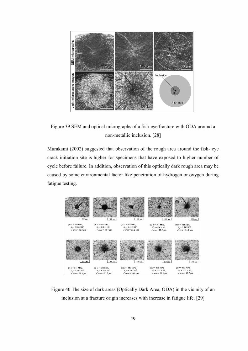
49

Figure 39 SEM and optical micrographs of a fish-eye fracture with ODA around a

non-metallic inclusion. [28]

Murakami (2002) suggested that observation of the rough area around the fish- eye

crack initiation site is higher for specimens that have exposed to higher number of

cycle before failure. In addition, observation of this optically dark rough area may be

caused by some environmental factor like penetration of hydrogen or oxygen during

fatigue testing.

Figure 40 The size of dark areas (Optically Dark Area, ODA) in the vicinity of an

inclusion at a fracture origin increases with increase in fatigue life. [29]

51

CHAPTER 3

EXPERIMENTAL PROCEDURE

3.1. MATERIAL

AMS5669 15-5 precipitation hardenable stainless steel was selected for the

experiments. The chemical composition of the material was determined by using X-

ray fluorescent (XRF) analyzers gun and presented in table 7.

Table 8 Chemical Composition for 15-5 PH Stainless Steels.

Chemical Composition Percent % (XRF Results)

Iron 75.25

Chromium 15.37

Nickel 3.28

Copper 3.82

Manganese 0.85

Molybdenum 0.11

Niobium 0.34

3.2. SPECIMEN GEOMETRY

The material was in the form of a round bar which was manufactured by forging with

a diameter of 25.4 mm. Thirty (30) disc shaped specimens with a thickness of 12 mm

were cut from round bar 15-5 PH material for heat treatment experiments.

52

Figure 41 Round Bar 15-5 PH (a) and heat treatment specimen geometry (b).

In addition, forty six (46) specimens were manufactured for static and fatigue tests.

Geometry for these specimens were determined according to ASTM E466 [30]

standard that provide some design criteria for the specimen geometry to ensure

observation of failure in the reduced (gage) section. Geometry for these specimens is

presented in Figure 43.

Figure 42 Fatigue test specimens after machining.

53

Figure 43 Technical drawing of static and fatigue test specimens.

3.3. HEAT TREATMENT PARAMETERS

Thirty (30) specimens were heat treated for determination of the parameters for

homogenization, solutionizing and aging treatment steps. Heat treatment steps were

consisted of homogenization, solutionizing and aging treatment that provides

precipitation reaction. As it mentioned before, heat treatment was applied in six

groups in order to see effect heat treatment parameters on microstructure, hardness

and fatigue behavior of the 15- 5 PH stainless steel better. In brief, homogenization

treatment was applied at 11500C for three different times 0.5, 1 and 3h. Solutionizing

was applied at 10400C for time period 0.5h. Finally, aging treatment was applied at

three different temperatures 4000C, 480

0C and 550

0C with three different times 1, 4

and 70 hours. All heat treatments were performed at laboratory type of heat treating

furnaces with max temperature capacity 12000C. After completing heat treatment all

specimens were air cooled which is seen in Figure 44.

54

Figure 44 Heat treated specimens during air cooling.

Inıtially, specimens were separated six (6) groups before heat treatments ın order to

compare results in terms of the heat treatment parameters on microstructure and

hardness better. All disc shaped specimens were designated as SP-1 to SP-30

respectively before heat treatment.

3.3.1. GROUP-1 SPECIMENS

Five (5) specimens were heat treated in order to see the effects of the solutionizing

and homogenization separately compared to as- received state.

Table 9 Applied heat treatment for group-1 specimens.

Specimens As- received Homogenization Treatment Solution Treatment

SP-1 X - -

SP-2 - - 10400C / 0.5h

SP-3 - - 10400C / 2 h

SP-4 - 11500C / 0.5 h -

SP-5 - 11500C / 1 h -

SP-6 - 11500C / 3 h -

55


Three (3) specimens were heat treated at different homogenization time under the

same solutionizing condition in order to see the effect of heat treatment time for

homogenization.


Specimens Homogenization Solution Treatment Aging Treatment

SP-7 11500C / 0.5 h 1040

0C / 0.5 h -

SP-8 11500C / 1 h 1040

0C / 0.5 h -

SP-9 11500C / 3 h 1040

0C / 0.5 h -


Three (3) specimens were heat treated at different aging time under the same

solutionizing condition without homogenization. These heat treatment conditions

were applied to observe effect of different aging treatments for the same

solutionizing condition.


Specimens Homogenizaiton Solution Treatment Aging

Treatment

SP-10 - 10400C / 0.5 h 480

0C / 1 h

SP-11 - 10400C / 0.5 h 550

0C / 4 h

SP-12 - 10400C / 0.5 h 400

0C / 70 h


Three (3) specimens were heat treated at the same solutionizing and homogenization

time under different aging condition. This heat treatment group was determined in

order to examine the effect of different aging treatments for the same solutionizing

and homogenization condition.

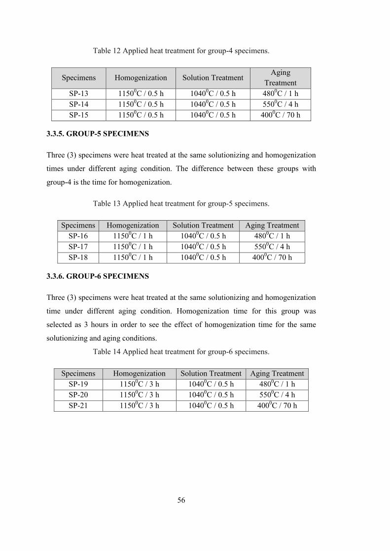
56


Specimens Homogenization Solution Treatment Aging

Treatment

SP-13 11500C / 0.5 h 1040

0C / 0.5 h 480

0C / 1 h

SP-14 11500C / 0.5 h 1040

0C / 0.5 h 550

0C / 4 h

SP-15 11500C / 0.5 h 1040

0C / 0.5 h 400

0C / 70 h



times under different aging condition. The difference between these groups with

group-4 is the time for homogenization.



SP-16 11500C / 1 h 1040

0C / 0.5 h 480

0C / 1 h

SP-17 11500C / 1 h 1040

0C / 0.5 h 550

0C / 4 h

SP-18 11500C / 1 h 1040

0C / 0.5 h 400

0C / 70 h



time under different aging condition. Homogenization time for this group was

selected as 3 hours in order to see the effect of homogenization time for the same

solutionizing and aging conditions.



SP-19 11500C / 3 h 1040

0C / 0.5 h 480

0C / 1 h

SP-20 11500C / 3 h 1040

0C / 0.5 h 550

0C / 4 h

SP-21 11500C / 3 h 1040

0C / 0.5 h 400

0C / 70 h

57

3.4. METALLOGRAPHY

3.4.1. SPECIMEN PREPARATION

Specimens’ surfaces were oxidized during heat treatments since there was no inert

atmosphere for heating furnace. Specimens were ground by finer grits of emery

paper (up to 2000grit) and then polished using a diamond paste of 3 µm particle size

on a lapping wheel. Oxide layer that is formed during heat treatment was removed

completely by grinding and polishing. Buehler trade grinding and polishing machine

and emery papers were used during preparation of the metallographic specimens.

3.4.2. SPECIMEN ETCHING

Specimens were etched by using two different etchants which were Marble’s and

Kalling’s with a composition given in ASTM E407 – 07 [31] standard in order to

determine the more suitable etchant for examination of the microstructure and to

reveal grain boundaries better.

Figure 45 Etchants with chemical compositions.

3.5. GRAIN SIZE MEASUREMENT

Grain size analysis was performed according to ASTM E 112 [32] standard by using

horizontal line approach for all heat treated specimens. Initially, grain size

measurements were conducted automatically by the Lieca optical microstructure

analysis tool. However, microstructures were so complex for too in order to identify

grain boundaries correctly. Therefore, all measurements were done manually.

58

3.6. HARDNESS TEST

In order to determine the hardness, disc shaped specimens were used after

microstructural analysis. Wizhard trade HR-521 (L) Series 810-Rockwell Type

Hardness Testing Machines [33] was used and measurement carried out according to

ASTM E18 – (16) [34] standard. 150 kgf load was applied through spheroconical

diamond indenter at four different points on the specimen surface for 15 sec.

Average of four measurements was taken as hardness value of specimens. Indenter

surface was also examined under optical microscope in order to find diameter of

spheroconical diamond indenter. According to Figure 46, it can be said that diameter

was almost 600 µm.

Figure 46 Optical microscope image for indented surface.

3.7. ROUGHNESS MEASUREMENT

Roughness is the important parameters that affect the fatigue test results of high

strength steels. Before testing, surface roughness of the all fatigue test specimens

were measured by Marsurf PS 10 mobile roughness measuring instrument [35].

Surface roughness values were measured by needle on the head of the movable part.

This needle scans the surface of the specimen ± 5 mm on the specimen surface.

Roughness measurement was done in Ra scale at three times and average of three

measurements was taken as roughness value of specimens.

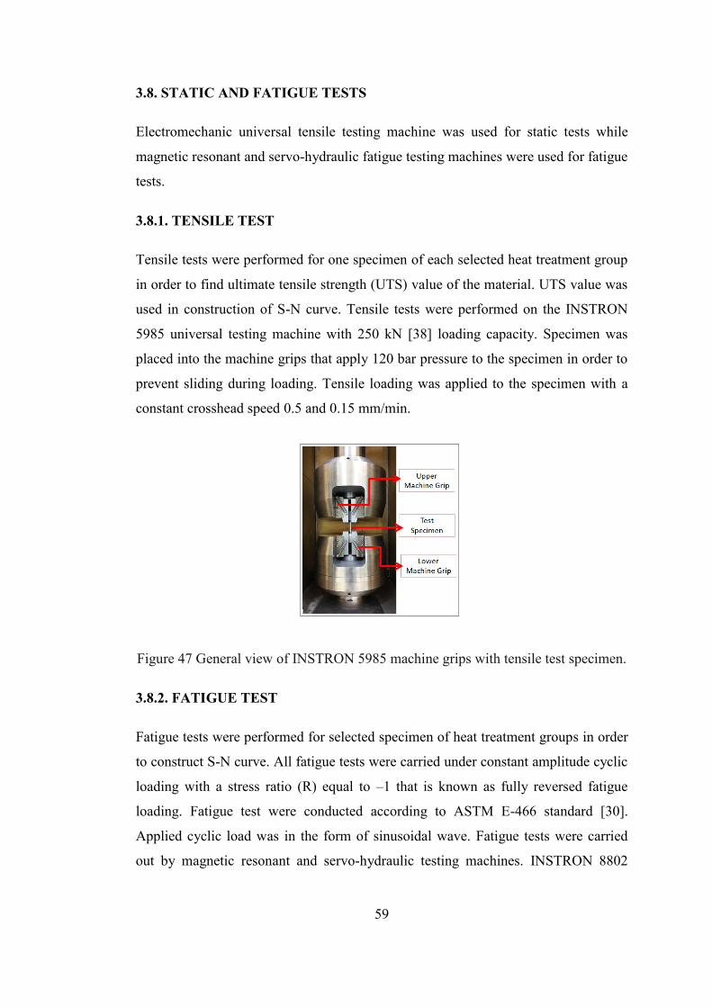
59

3.8. STATIC AND FATIGUE TESTS

Electromechanic universal tensile testing machine was used for static tests while

magnetic resonant and servo-hydraulic fatigue testing machines were used for fatigue

tests.

3.8.1. TENSILE TEST

Tensile tests were performed for one specimen of each selected heat treatment group

in order to find ultimate tensile strength (UTS) value of the material. UTS value was

used in construction of S-N curve. Tensile tests were performed on the INSTRON

5985 universal testing machine with 250 kN [38] loading capacity. Specimen was

placed into the machine grips that apply 120 bar pressure to the specimen in order to

prevent sliding during loading. Tensile loading was applied to the specimen with a

constant crosshead speed 0.5 and 0.15 mm/min.

Figure 47 General view of INSTRON 5985 machine grips with tensile test specimen.

3.8.2. FATIGUE TEST

Fatigue tests were performed for selected specimen of heat treatment groups in order

to construct S-N curve. All fatigue tests were carried under constant amplitude cyclic

loading with a stress ratio (R) equal to –1 that is known as fully reversed fatigue

loading. Fatigue test were conducted according to ASTM E-466 standard [30].

Applied cyclic load was in the form of sinusoidal wave. Fatigue tests were carried

out by magnetic resonant and servo-hydraulic testing machines. INSTRON 8802

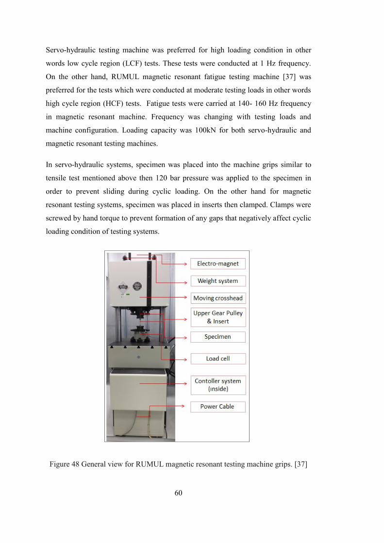
60

Servo-hydraulic testing machine was preferred for high loading condition in other

words low cycle region (LCF) tests. These tests were conducted at 1 Hz frequency.

On the other hand, RUMUL magnetic resonant fatigue testing machine [37] was

preferred for the tests which were conducted at moderate testing loads in other words

high cycle region (HCF) tests. Fatigue tests were carried at 140- 160 Hz frequency

in magnetic resonant machine. Frequency was changing with testing loads and

machine configuration. Loading capacity was 100kN for both servo-hydraulic and

magnetic resonant testing machines.

In servo-hydraulic systems, specimen was placed into the machine grips similar to

tensile test mentioned above then 120 bar pressure was applied to the specimen in

order to prevent sliding during cyclic loading. On the other hand for magnetic

resonant testing systems, specimen was placed in inserts then clamped. Clamps were

screwed by hand torque to prevent formation of any gaps that negatively affect cyclic

loading condition of testing systems.

Figure 48 General view for RUMUL magnetic resonant testing machine grips. [37]

61

Magnetic resonant fatigue testing machine works at material natural resonant

condition. Before, application of cyclic loading static mean load was applied by a

spindle system that is actuated by a servo gearmotor then force is coupled by springs

to the system. Dynamic loading of the specimens is done by a mechanical oscillating

system. Oscillating system can be described by activated masses, elasticities and test

specimen. There exists an electromagnet that activates the oscillating system. Test

frequency can be changed by activating and deactivating masses in the system.

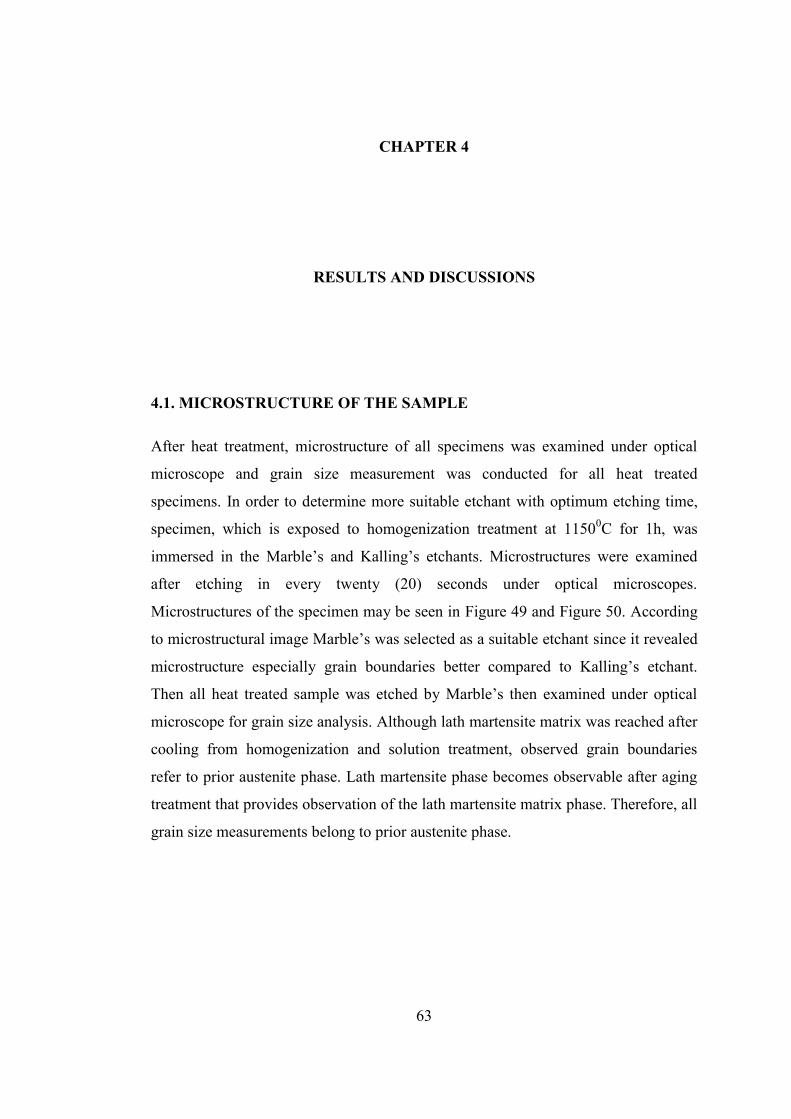
63

CHAPTER 4

RESULTS AND DISCUSSIONS

4.1. MICROSTRUCTURE OF THE SAMPLE

After heat treatment, microstructure of all specimens was examined under optical

microscope and grain size measurement was conducted for all heat treated

specimens. In order to determine more suitable etchant with optimum etching time,

specimen, which is exposed to homogenization treatment at 11500C for 1h, was

immersed in the Marble’s and Kalling’s etchants. Microstructures were examined

after etching in every twenty (20) seconds under optical microscopes.

Microstructures of the specimen may be seen in Figure 49 and Figure 50. According

to microstructural image Marble’s was selected as a suitable etchant since it revealed

microstructure especially grain boundaries better compared to Kalling’s etchant.

Then all heat treated sample was etched by Marble’s then examined under optical

microscope for grain size analysis. Although lath martensite matrix was reached after

cooling from homogenization and solution treatment, observed grain boundaries

refer to prior austenite phase. Lath martensite phase becomes observable after aging

treatment that provides observation of the lath martensite matrix phase. Therefore, all

grain size measurements belong to prior austenite phase.

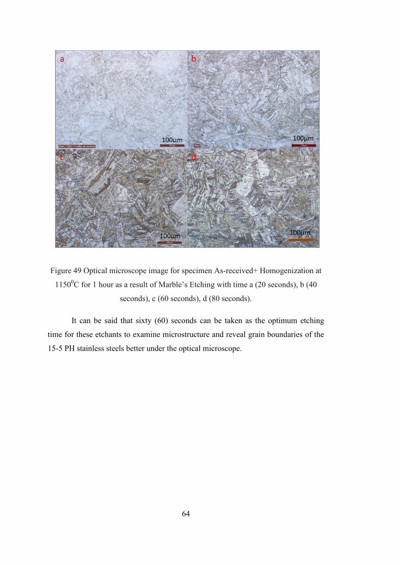
64


11500C for 1 hour as a result of Marble’s Etching with time a (20 seconds), b (40

seconds), c (60 seconds), d (80 seconds).

It can be said that sixty (60) seconds can be taken as the optimum etching

time for these etchants to examine microstructure and reveal grain boundaries of the

15-5 PH stainless steels better under the optical microscope.

100µm 100µm

65


11500C for 1 hour as a result of Kalling’s Etching with time a (20 seconds), b (40

seconds), c (60 seconds), d (80 seconds)

Microstructure of 15-5 PH stainless steel was consisted lath martensite phase after

homogenization and solution treatment followed by air cooling. However, after aging

treatment microstructure was transformed to needle type of martensite which can be

seen in Figure 51. This transformation can be explained by tempering of the lath

martensite matrix during aging treatment. Increase of aging time leads to enhance

fineness of the needle type of martensite structure. This transformation is explained

by continuous rejection of carbon and other alloying elements from the martensite

matrix that causes reduction of the tetragonality of the crystal structure as a result of

tempering.

66

Figure 51 Optical microscope image for specimen (a) Sol. at 10400C/0.5h (b) Hom.

at 11500C/1h (c) Hom. at 1150

0C/1h+ Sol. at 1040


0C/70h (d)

Hom. at 11500C/1h+ Sol. at 1040


0C/4h

4.1.1. GRAIN SIZE MEASUREMENT RESULTS

After etching of the specimens, all heat treated samples were examined under optical

microscope to measure the grain size. Grain size measurement was done in order to

examine the relation between heat treatment parameters and grain size. All grain size

measurements were performed by Lieca optical microstructure analysis tool

according to ASTM E112 [32]. As it mentioned before identification of grain

boundaries correctly was so difficult for optical microscope analysis tool. Therefore,

all measurements were done manually according to procedure given below.

Average grain size measurement was conducted according to following steps [38];

67

Step-1: Several arbitrary test lines with specific length were drawn on the

micrograph

Step-2: If grains were fully included on the line, it is counted as 1. If not, it is

counted as 0.5.

Step-3: This counting process was conducted for eleven lines.

Step-4: Then, all counted data were summed and divided into number of test lines in

order to determine average count for one test line.

Step-5: Test lines with specific length were divided number of average counts per

line.

Step-6: Calculated length for one count was firstly converted to meter then divided

by magnification of the micrograph in order to determine average grain size.

Figure 52 Optical microscope image for specimen which is solutionized at

10400C/0.5h +Aged at 400

0C/70h with arbitrary test lines with specific length

1

2 3

4 5

9

8

6

7

11

10

68

Step-1: Eleven lines were drawn with a 10 cm length.

Step-2& 3: Number of counts per line was calculated and shown in table Table 15.

Table 15 Calculation of total counts for grain size measurement analysis.

Number of

Lines Counts

1 0.5+1+1+1+1+1+1+1+1+0.5=10

2 0.5+1+1+1+1+1+1+1+1+1+0.5=11

3 0.5+1+1+1+1+1+1+1+1+1+1=11.5

4 0.5+1+1+1+1+1+1+1+1+1+0.5=11

5 0.5+1+1+1+1+1+1+1+1+1+0.5=11

6 0.5+1+1+1+1+1+1+1+1+1+0.5=11

7 0.5+1+1+1+1+1+1+1+0.5=9

8 0.5+1+1+1+1+1+1+1+1+1=10.5

9 0.5+1+1+1+1+1+1+1+0.5=9

10 0.5+1+1+1+1+1+1+1+1+1+0.5=11

11 0.5+1+1+1+1+1+1+1+1+0.5=10

Total Counts 115 counts in eleven (11) lines

Step-4: Number of average counts for one test line was calculated.

Average Counts =115

11= 10.45 (4.1)

Step-5: Length of test line was divided number of average counts per line.

10𝑐𝑚

10.45= 0.96𝑐𝑚 (4.2)

Step-6: 0.96 cm was converted to meter 0.96*10-2

m. Then, it was divided to

magnification.

0.96∗10^(−2) m

500= 19.2 ∗ 10−6m = 19µm (4.3)

These calculations were conducted for all heat treated specimens and results were

presented in table 16.

69

Table 16 Grain size measurement results.

As it mentioned before, measured grain size values belong to prior austenite grains

that was formed during homogenization and solution treatment. There was no

significant difference between the grain size values for different heat treatment

conditions. All heat treatment steps which were homogenization, solutionizing and

aging treatments provide nearly the same grain size value for 15-5 PH stainless

steels. Grain size values changes between 20 to 35 µm for 15-5 PH stainless steels.

These values are consistent with the values given in the literature that is presented in

chapter 2.

Heat

Treatment

Groups

Homogenizatio

n Treatment

Solution

Treatment

Aging

Treatment

Average

Grain Size

(µm)

Gro

up-1

SP-1 As-Received Condition 26

SP-2 10400C / 0.5h 23

SP-3 10400C / 2h 19

SP-4 11500C / 0.5h - - 28

SP-5 11500C / 1h - - 36

SP-6 11500C / 3h - - 30

Gro

up

-2 SP-1 1150

0C / 0.5h 1040

0C / 0.5h - 26

SP-2 11500C / 1h 1040

0C / 0.5h - 29

SP-3 11500C / 3h 1040

0C / 0.5h - 28

Gro

up-3

SP-1 - 10400C / 0.5h 480

0C / 1h 24

SP-2 - 10400C / 0.5h 550

0C / 4h 22

SP-3 - 10400C / 0.5h 400

0C / 70h 19

Gro

up-4

SP-1 11500C / 0.5h 1040

0C / 0.5h 480

0C / 1h 25

SP-2 11500C / 0.5h 1040

0C / 0.5h 550

0C / 4h 24

SP-3 11500C / 0.5h 1040

0C / 0.5h 400

0C / 70h 28

Gro

up-5

SP-1 11500C / 1h 1040

0C / 0.5h 480

0C / 1h 26

SP-2 11500C / 1h 1040

0C / 0.5h 550

0C / 4h 29

SP-3 11500C / 1h 1040

0C / 0.5h 400

0C / 70h 28

Gro

up-6

SP-1 11500C / 3h 1040

0C / 0.5h 480

0C / 1h 32

SP-2 11500C / 3h 1040

0C / 0.5h 550

0C / 4h 24

SP-3 11500C / 3h 1040

0C / 0.5h 400

0C / 70h 23

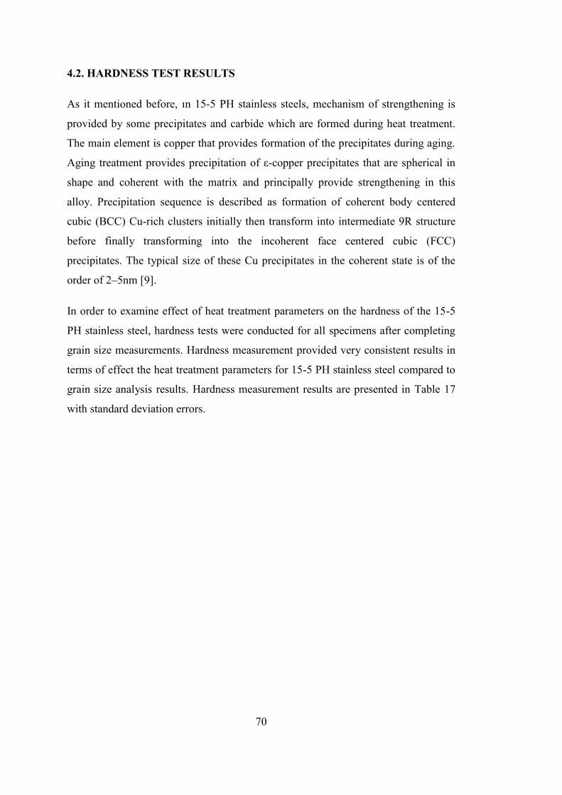
70

4.2. HARDNESS TEST RESULTS

As it mentioned before, ın 15-5 PH stainless steels, mechanism of strengthening is

provided by some precipitates and carbide which are formed during heat treatment.

The main element is copper that provides formation of the precipitates during aging.

Aging treatment provides precipitation of ε-copper precipitates that are spherical in

shape and coherent with the matrix and principally provide strengthening in this

alloy. Precipitation sequence is described as formation of coherent body centered

cubic (BCC) Cu-rich clusters initially then transform into intermediate 9R structure

before finally transforming into the incoherent face centered cubic (FCC)

precipitates. The typical size of these Cu precipitates in the coherent state is of the

order of 2–5nm [9].

In order to examine effect of heat treatment parameters on the hardness of the 15-5

PH stainless steel, hardness tests were conducted for all specimens after completing

grain size measurements. Hardness measurement provided very consistent results in

terms of effect the heat treatment parameters for 15-5 PH stainless steel compared to

grain size analysis results. Hardness measurement results are presented in Table 17

with standard deviation errors.

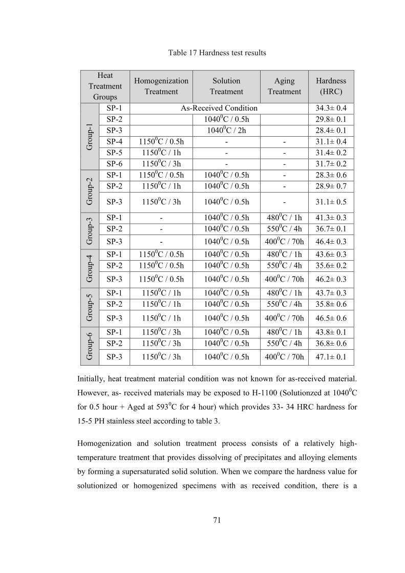
71

Table 17 Hardness test results

Heat

Treatment

Groups

Homogenization

Treatment

Solution

Treatment

Aging

Treatment

Hardness

(HRC) G

roup-1

SP-1 As-Received Condition 34.3± 0.4

SP-2 10400C / 0.5h 29.8± 0.1

SP-3 10400C / 2h 28.4± 0.1

SP-4 11500C / 0.5h - - 31.1± 0.4

SP-5 11500C / 1h - - 31.4± 0.2

SP-6 11500C / 3h - - 31.7± 0.2

Gro

up-2

SP-1 11500C / 0.5h 1040

0C / 0.5h - 28.3± 0.6

SP-2 11500C / 1h 1040

0C / 0.5h - 28.9± 0.7

SP-3 11500C / 3h 1040

0C / 0.5h - 31.1± 0.5

Gro

up-3

SP-1 - 10400C / 0.5h 480

0C / 1h 41.3± 0.3

SP-2 - 10400C / 0.5h 550

0C / 4h 36.7± 0.1

SP-3 - 10400C / 0.5h 400

0C / 70h 46.4± 0.3

Gro

up-4

SP-1 11500C / 0.5h 1040

0C / 0.5h 480

0C / 1h 43.6± 0.3

SP-2 11500C / 0.5h 1040

0C / 0.5h 550

0C / 4h 35.6± 0.2

SP-3 11500C / 0.5h 1040

0C / 0.5h 400

0C / 70h 46.2± 0.3

Gro

up

-5 SP-1 1150

0C / 1h 1040

0C / 0.5h 480

0C / 1h 43.7± 0.3

SP-2 11500C / 1h 1040

0C / 0.5h 550

0C / 4h 35.8± 0.6

SP-3 11500C / 1h 1040

0C / 0.5h 400

0C / 70h 46.5± 0.6

Gro

up-6

SP-1 11500C / 3h 1040

0C / 0.5h 480

0C / 1h 43.8± 0.1

SP-2 11500C / 3h 1040

0C / 0.5h 550

0C / 4h 36.8± 0.6

SP-3 11500C / 3h 1040

0C / 0.5h 400

0C / 70h 47.1± 0.1

Initially, heat treatment material condition was not known for as-received material.

However, as- received materials may be exposed to H-1100 (Solutionzed at 10400C

for 0.5 hour + Aged at 5930C for 4 hour) which provides 33- 34 HRC hardness for

15-5 PH stainless steel according to table 3.

Homogenization and solution treatment process consists of a relatively high-

temperature treatment that provides dissolving of precipitates and alloying elements

by forming a supersaturated solid solution. When we compare the hardness value for

solutionized or homogenized specimens with as received condition, there is a

72

decrease in the hardness value. As it mentioned before, hardening phenomena for

precipitation hardenable stainless steels directly related to strain field around ε-Cu

precipitations that obstruct the motion of the dislocations. At high temperature, all

precipitates and other intermetallic dissolve in the solid solution. Then, lath

martensitic microstructure is formed after homogenization and solutionizing

followed by air cooling. Although there exist very high density of the dislocations in

the lath martensitic microstructure, hardness value is generally low since after

homogenization or solutionizing, there are no strengthening phase in the matrix.

It can be also said that increase in time for homogenization and solution treatment for

the same temperature does not lead to significant change on hardness of the 15-5 PH

stainless steel. However, it may be expected that increase in time keeping for these

treatment, more precipitates and other hardening elements dissolve so hardness may

decrease more. According to hardness test results of group-2, it can be said that

application of the homogenization before solution treatments does not have more

effects on hardness. 15-5 PH stainless steels may include some -delta ferrite phase

that has detrimental effect on mechanical properties. Increase in time for

homogenization decreases the volume fraction of the delta ferrite phase and change

of the phase morphology from elongated to spherical [13]. Therefore, three different

time period for homogenization treatment was applied during heat treatment

condition.

According to hardness test results it can be said that, main hardening for 15-5 PH

stainless steels was provided by aging treatment. When aging treatment is applied,

supersaturated solid solution allows formation of the ε-copper precipitates. When we

compared to aging treatment at 4800C with 550

0C for 4h, there is very high number

of ε-copper precipitates with smaller size. At lower aging temperature and time

period, there is not enough driving force solute atoms for diffusion and to form

precipitates. This phenomenon causes formation of high number of precipitates with

smaller size. Therefore, motion of the dislocation becomes much difficult due to

more strain field formed around the precipitate in lath martensite matrix. Thus,

hardness increase more compared to aging treatment 5500C for 4h.

73

The decrease of hardness may be explained by growth of ε-copper precipitates and

reformation of the austenite in the microstructures. Growth of size of precipitates

cause decrease on the probability of the pinning of dislocations that leads to decrease

on hardness. On the other hand, areas around copper precipitates may contain some

austenite forming elements like Ni and Fe. Segregation of these elements on the

surround of ε-copper precipitates provides formation of austenite stable region.

These regions behave nucleation sites for austenite phases since they have the same

fcc structure with the similar lattice parameter. It is s also known that solubility of

the Cu in austenite is higher than lath martensite matrix so increase in temperature

drive solubility of the precipitates on the reformed austenite region thus hardness of

15-5 PH stainless steels decreases more.

According to hardness test results, aging treatment at 4000C for 70h provide peak

hardness value for 15-5 PH stainless steels. As it mentioned before, it may be formed

some delta ferrite phase in the microstructure that is formed during manufacturing.

Aging treatment at 4000C for 70h provides another precipitation reaction which takes

place on the -delta ferrite phase thus provide more increase on hardness of the 15-5

PH stainless steels.

4.3. TENSILE TEST RESULTS

In order to see the effect of heat treatment parameters on tensile and fatigue strength,

group-5 specimens were selected. As it mentioned before, forty six (46) specimens

were manufactured for three different groups of group-5 specimens. Detail number

of specimens for static and fatigue test can be seen in Table 18.

After heat treatment, tensile tests were applied ın order to see the effect of heat

treatment parameters on ultimate tensile strength. The main reason for performing

tensile test was determination of UTS that was used for stress value at fırst cycle in

S-N curve construction step for 15-5 PH stainless steel. Locating of the UTS value

on S-N curve provides more accurate curve shape especially at low cycle region.

74

Table 18 Hardness, types and number of specimens for static and fatigue tests

Specimen

Group Heat Treatment Conditions

# of Static

Specimen

# of

Fatigue

Specimen

Hardness

(HRC)

Group-1

Hom. at 11500C for 1hr +

Sol. at 10400C for 0.5hr +

Aged at 5500C for 4hr

1 20 35.8±

0.6

Group-2

Hom. at 11500C for 1hr +

Sol. at 10400C for 0.5hr +

Aged at 4800C for 1hr

1 11 43.7±

0.3

Group-3

Hom. at 11500C for 1hr + Sol.

at 10400C for 0.5hr + Aged

at 4000C for 70hr

1 12 46.5±

0.6

Tensile tests were conducted for one specimen of each group. Stress versus strain

curves is exhibited in Figure 53.

Figure 53 Stress vs. strain curve for group-5 tensile test specimens.

During tensile tests, crosshead speed for specimen which was exposed to aging

treatment at temperature 5500C for one hour was 0.15 mm/min while for others

tensile loading was applied with a constant crosshead speed 0.50 mm/min. Therefore,

0

200

400

600

800

1000

1200

1400

1600

0 0,05 0,1 0,15 0,2 0,25 0,3 0,35

Stre

ss (

MP

a)

Strain (mm/mm)

Stress vs. Strain Curves

Aged@480C_1h Aged@550C_4h Aged@400C_70h

75

there exists difference in curve shape of stress vs. strain curves. As it mentioned

before, the main purpose of tensile test application was finding ultimate tensile

strength value of the 15-5 stainless steels after different heat treatment condition.

Ultimate tensile strength values were used in S-N curve construction.

Table 19 Tensile test and hardness results.

Specimen

Group

Hardness

(HRC)

Max

Load

(kN)

UTS (MPa)

Strain at

Max Load

(mm/mm)

Strain at

Failure

(mm/mm)

Group-1 35.8± 0.6 55.8 1110 0.149 0.278

Group-2 43.7± 0.3 69.4 1381 0.199 0.303

Group-3 46.5± 0.6 76.3 1517 0.183 0.276

Moreover, increase in UTS causes decrease on the extension value according to

comparison of results of group-2 and group-3. Tensile test results for specimens

which are exposed to aging treatment at 5500C for 4h and 480

0C for 1h are almost

the same with the results given literature in chapter 2. Therefore, it can be said that,

suitable heat treatment conditions were applied in terms of temperature and time

period. In addition, tensile test result for specimen that is exposed to aging treatment

at 4000C for 1h is highest compared to other. This value can be explained by

precipitation reaction in the delta ferrite phase which provides more strengthening for

15-5 PH stainless steels. According to tensile test results, it can be also said that there

exist direct relation between hardness and ultimate tensile strength of the material.

Therefore, the effect of heat treatment parameters on tensile strength of the 15-5 PH

stainless steels is almost the same with effect on hardness in terms of time and

temperature period for homogenization, solutionizing and aging treatment.

There exist also an approximate relationship between the hardness and the tensile

strength of the high strength steels that were given in below equation (4.4). The

relation between hardness and ultimate tensile strength for the specimens can also be

corrected by the equation below.

UTS(MPa) = (3.38 ∗ HB, ⟨HB > 175⟩) [39] (4.4)

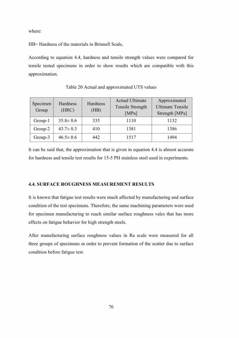
76

where:

HB= Hardness of the materials in Brinnell Scale,

According to equation 4.4, hardness and tensile strength values were compared for

tensile tested specimens in order to show results which are compatible with this

approximation.

Table 20 Actual and approximated UTS values

Specimen

Group

Hardness

(HRC)

Hardness

(HB)

Actual Ultimate

Tensile Strength

[MPa]

Approximated

Ultimate Tensile

Strength [MPa]

Group-1 35.8± 0.6 335 1110 1132

Group-2 43.7± 0.3 410 1381 1386

Group-3 46.5± 0.6 442 1517 1494

It can be said that, the approximation that is given in equation 4.4 is almost accurate

for hardness and tensile test results for 15-5 PH stainless steel used in experiments.

4.4. SURFACE ROUGHNESS MEASUREMENT RESULTS

It is known that fatigue test results were much affected by manufacturing and surface

condition of the test specimens. Therefore, the same machining parameters were used

for specimen manufacturing to reach similar surface roughness vales that has more

effects on fatigue behavior for high strength steels.

After manufacturing surface roughness values in Ra scale were measured for all

three groups of specimens ın order to prevent formation of the scatter due to surface

condition before fatigue test.

77

4.4.1. SURFACE ROUGHNESS RESULTS FOR GROUP-1 SPECIMEN

Surface roughness value was changing between 0.132 to 0.381 µm for group-1

specimens.



specimens.

0

0,05

0,1

0,15

0,2

0,25

0,3

0,35

0,4

1 2 3 4 5 6 7 8 9 10 11 12 13 14 15 16 17 18 19

Surf

ace

Ro

ugh

nes

s (R

a-µ

m)

Specimen Number

Roughness vs. Specimen Number

Ra (Mean)=0.205 µm

0

0,05

0,1

0,15

0,2

0,25

0,3

0,35

0,4

1 2 3 4 5 6 7 8 9 10 11Surf

ace

Ro

ugh

nes

s (R

a-µ

m)

Specimen Number

Surface Roughness vs. Specimen Number

Ra (Mean)= 0.189 µm

78



specimens.

When the average values for surface roughness are compared, there is not much

difference between surface roughness values that cause formation of the scatter on

fatigue test results. The effect of the surface roughness on fatigue strength of high

strength steels as a reduction factor may be shown in Figure 54. According to Figure

54, if the surface roughness value is lower than 0.25 micron there is no reduction on

fatigue strength of high strength steels. According to our surface roughness

measurement results, it can be said that there is no effect of surface roughness on

fatigue behavior of 15-5 PH stainless steels for this study. However, there exist some

deviations in surface roughness of specimens in the same group. This may cause

formation of some scatter in fatigue test results.

0

0,05

0,1

0,15

0,2

0,25

0,3

0,35

0,4

1 2 3 4 5 6 7 8 9 10 11 12

Surf

ace

Ro

ugh

ne

ss (

Ra-

µm

)

Specimen Number

Surface Roughness vs. Specimen Number

Ra (Mean)= 0.183 µm

79

Figure 54 Surface roughness reduction factor γ for high strength steels as a function

of Ra (average surface roughness) and the tensile strength. [19]

4.5. FATIGUE TEST RESULTS

Fatigue behavior for 15-5 PH stainless steels was examined for three different groups

of group-5 specimens that were presented in table 18. Fatigue behavior for these

three groups is considered according to S-N curve construction by calculating fatigue

limits.

All the specimens were executed with the same procedure constant amplitude cyclic

loading according to ASTM E466 – 15 testing standard [30]. The run-out criteria was

chosen as 1.0 E+07 cycles. In addition, test was terminated according to observation

of the visible cracks on specimen surface or 1.0 E+07 cycles for run-out specimens.

As it mentioned before S-N curve was constructed according to AGARD-AG-292

HELICOPTER FATIGUE DESIGN GUIDE [24]. In addition fatigue limit was also

calculated according to staircase method that is given in ISO 12107 International

Standard (Metallic materials — Fatigue testing — Statistical planning and analysis of

data) [25].

80

4.5.1. FATIGUE TEST RESULTS FOR GROUP-1 SPECIMENS

Twenty (20) specimens were tested in order to construct S-N curves according to

procedure that was defined in section 2.8.1.



0C /0.5h + Aged 550

0C /4h)

Specime

n

No

Stress

[Mpa]

Life

[cycle]

Frequency

[Hz]

log (Std.

Dev. At)

1.0x107

Stress

at

1.0x107

[Mpa]

R2

SP-1 760 13.251 156

0.034

441 0.954

SP-2 760 12.192 155

SP-3 710 46.276 158

SP-4 710 57.783 158

SP-5 610 120.019 157

SP-6 510 135.921 159

SP-7 510 713.442 158

SP-8 460 867.472 159

SP-9 440 11.000.000 159

SP-10 440 11.000.000 159

SP-11 460 135921 159

Std.

Dev. of

Stress

@1.0x107

SP-12 440 11.000.000 158

33

SP-13 460 10.000.065 159

SP-14 440 11.000.000 145

SP-15 840 18.458 1

SP-16 840 10.049 1

SP-17 940 6.347 1

SP-18 940 7.161 1

SP-19 610 181.943 159

SP-20 440 11.000.000 159

SP-21

(Static) 1110 1 -

According to fatigue test results, fatigue limit (1.0x107) was determined as 441MPa

for the specimens that were exposed to heat treatment (Hom.@11500C /1h +

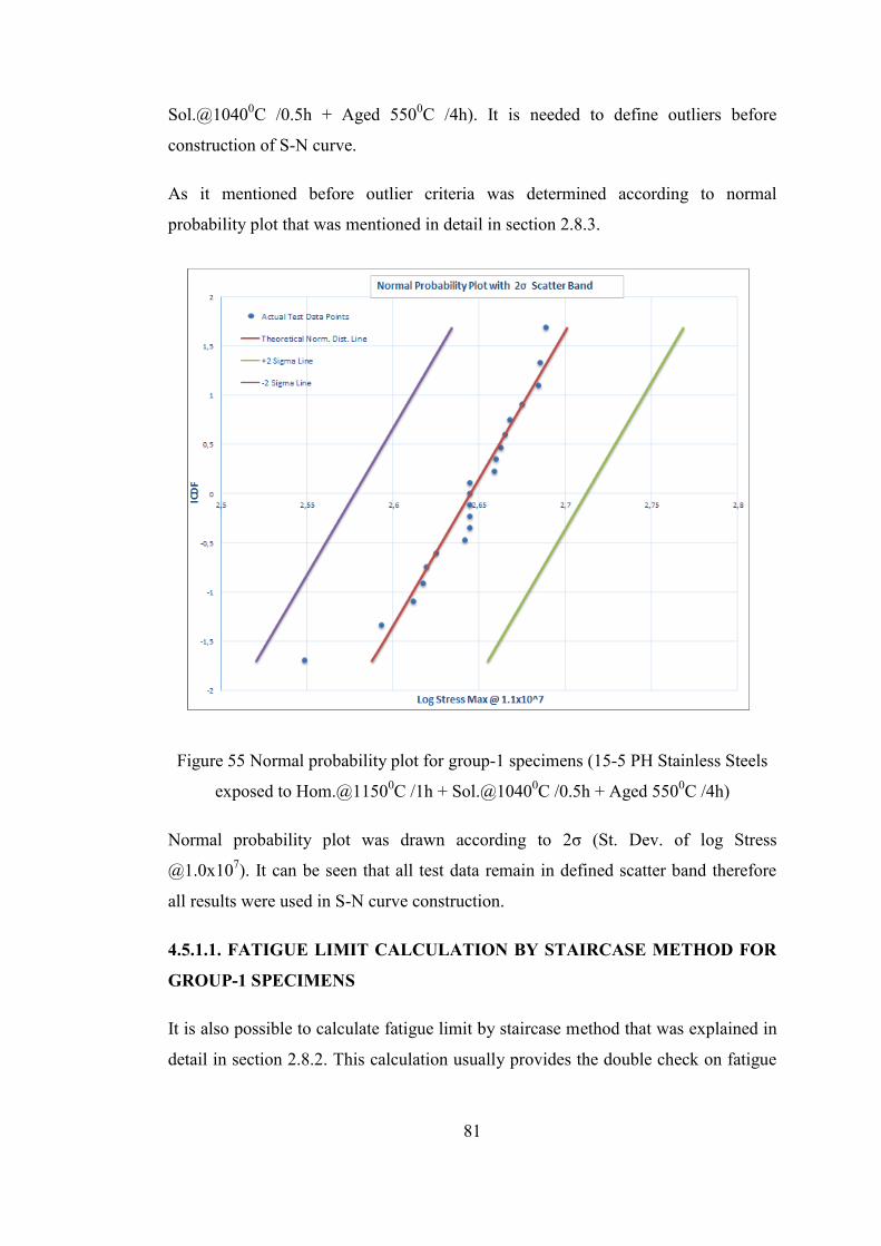
81

Sol.@10400C /0.5h + Aged 550

0C /4h). It is needed to define outliers before

construction of S-N curve.

As it mentioned before outlier criteria was determined according to normal

probability plot that was mentioned in detail in section 2.8.3.



0C /0.5h + Aged 550

0C /4h)

Normal probability plot was drawn according to 2σ (St. Dev. of log Stress

@1.0x107). It can be seen that all test data remain in defined scatter band therefore

all results were used in S-N curve construction.

4.5.1.1. FATIGUE LIMIT CALCULATION BY STAIRCASE METHOD FOR

GROUP-1 SPECIMENS

It is also possible to calculate fatigue limit by staircase method that was explained in

detail in section 2.8.2. This calculation usually provides the double check on fatigue

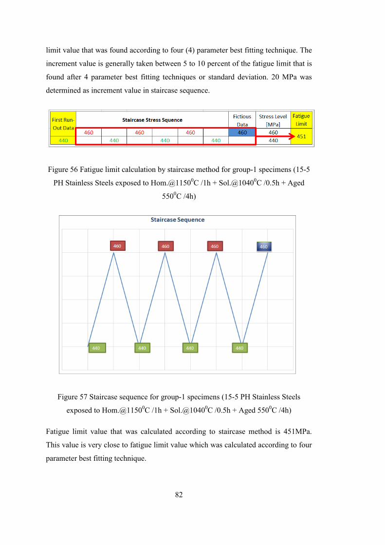
82

limit value that was found according to four (4) parameter best fitting technique. The

increment value is generally taken between 5 to 10 percent of the fatigue limit that is

found after 4 parameter best fitting techniques or standard deviation. 20 MPa was

determined as increment value in staircase sequence.



0C /0.5h + Aged

5500C /4h)



0C /0.5h + Aged 550

0C /4h)

Fatigue limit value that was calculated according to staircase method is 451MPa.

This value is very close to fatigue limit value which was calculated according to four

parameter best fitting technique.

83


Eleven (11) specimens were tested in order to construct S-N curves according to

procedure that was defined in section 2.7.



0C /0.5h + Aged 480

0C /1h)

Specimen

No

Stress

[Mpa]

Life

[cycle]

Frequency

[Hz]

Std. Dev.

of log

Stress

@1.0x107

Stress

@1.0x107

[Mpa]

R2

SP-1 710 280.082 161

0.057

519 0.903

SP-2 1160 3.397 1

SP-3

(Static) 1381 1 -

SP-4 610 1.729.986 161

SP-5 560 10.087.227 161

SP-6 860 12.561 159

Std. Dev.

of Stress

@107

SP-7 760 183.800 161

61

SP-8 560 99.152 161

SP-9 510 4.604.306 161

SP-10 460 11000000 162

SP-11 510 437761 161

SP-12 860 40534 160

According to fatigue test results, fatigue limit (1.0x107) was determined as 519MPa


Sol.@10400C /0.5h + Aged 480


construction of S-N curve the same procedure was applied for group-2 specimens.

84



0C /0.5h + Aged 480

0C /1h)

It can be seen that all test data remain in defined scatter band therefore all results

were used in S-N curve construction.

4.5.2.1. FATIGUE LIMIT CALCULATION BY STAIRCASE METHOD FOR

GROUP-2 SPECIMENS

Fifty (50) MPa was determined as increment value in staircase sequence according to

fatigue limit that was found according to four parameter best fitting technique.

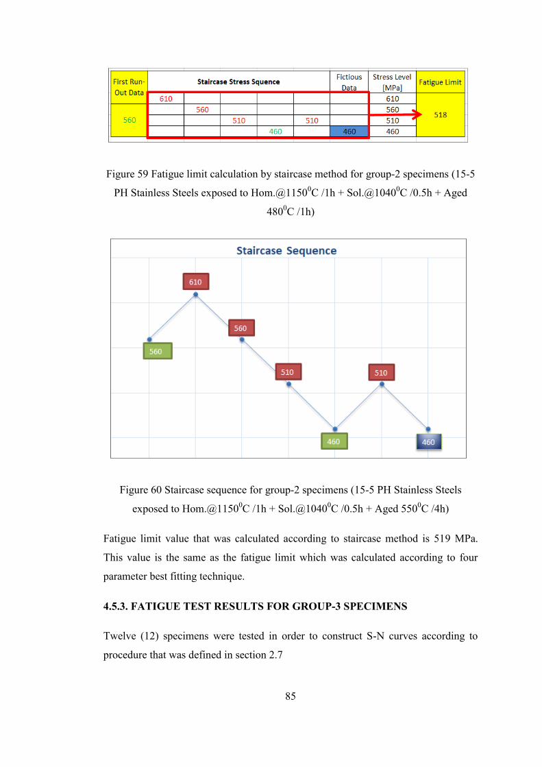
85



0C /0.5h + Aged

4800C /1h)



0C /0.5h + Aged 550

0C /4h)

Fatigue limit value that was calculated according to staircase method is 519 MPa.

This value is the same as the fatigue limit which was calculated according to four



Twelve (12) specimens were tested in order to construct S-N curves according to

procedure that was defined in section 2.7

86



0C /0.5h + Aged 400

0C /70h)

Specimen

No

Stress

[Mpa]

Life

[cycle]

Frequency

[Hz]

Std. Dev.

of log

Stress

@1.0x107

Stress

@1.0x107

[Mpa]

R2

SP-1 860 51.206 156

0.054

493 0.958

SP-2 760 113.644 161

SP-3 610 1.759.600 159

SP-4 560 7.433.969 162

SP-5 510 113.197 162

SP-6 460 11.000.000 160

SP-7 510 1.009.078 161

Std. Dev.

of Stress

@107

SP-8 460 11.000.000 160

54

SP-9 460 11.000.000 162

SP-10 510 11.000.000 161

SP-11 1360 1032 1

SP-12 1160 3976 1

SP-13

(static) 1517 1 -

According to fatigue test results, fatigue limit (1.0x107) was determined as 493 MPa


Sol.@10400C /0.5h + Aged 400


construction of S-N curve the same procedure was applied for group-3 specimens.

87



0C /0.5h + Aged 400

0C /70h)

It can be seen that all test data remain in defined 2σ (St. Dev. of log Stress

@1.0x107) scatter band therefore all results were used in S-N curve construction.

4.5.3.1 FATIGUE LIMIT CALCULATION BY STAIRCASE METHOD FOR

GROUP-3 SPECIMENS

Fifty (50) MPa was determined as increment value in staircase sequence according to

fatigue limit.

88


PH Stainless Steels exposed to Hom.@11500C /1h +Sol.@1040

0C /0.5h +Aged

4000C /70h)



0C /0.5h + Aged 400

0C /70h)

Fatigue limit value that was calculated according to staircase method is 503 MPa.

This value is very close to fatigue limit value which was calculated according to four


4.5.4. COMPARISON OF S-N CURVES

Stress versus life (S-N) curves were constructed according to the same procedure that

was given is section 2.8.1.

89

Figure 64 Stress versus life (S-N) curves for three groups of group-5 specimens.

According to fatigue test results of three groups of group-5 specimens, heat treatment

parameters have significant effects on fatigue behavior of 15-5 precipitation

hardenable stainless steels. Fatigue limit value for aging treatment at temperature

4800C for 1h has higher fatigue limit compared to aging treatment at 550

0C for 4h.

This difference on the fatigue limit can be explained by precipitation of copper. As it

mentioned before, at lower aging temperature (4800C) with lower time (1h), there

exist high number ε-cupper precipitates with smaller size. In addition, it can be also

said that there exist a direct relation between hardness and fatigue limit of 15-5 PH

stainless steels that are exposed to aging treatment at 4800C for 1h and at 550

0C for

4h. According to fatigue limit calculations, changing aging treatment parameters

from 5500C for 4h to 480

0C for 1h, fatigue limit of 15-5 PH stainless steel may be

increased by 15% (15 percent). In addition, if aging treatment parameters are

changed to 4000C for 70h, fatigue limit may be increased by 11% (11 percent).

In addition, hardness does not always show direct relation with fatigue strength for

15-5 PH stainless steels. Specimens, which were exposed aging treatment at

temperature 4000C for 1h, have higher hardness value compared to specimens that

were exposed to aging treatment at temperature 4800C for 1h. However, fatigue limit

for these specimens is lower. This inverse relation may be explained by susceptibility

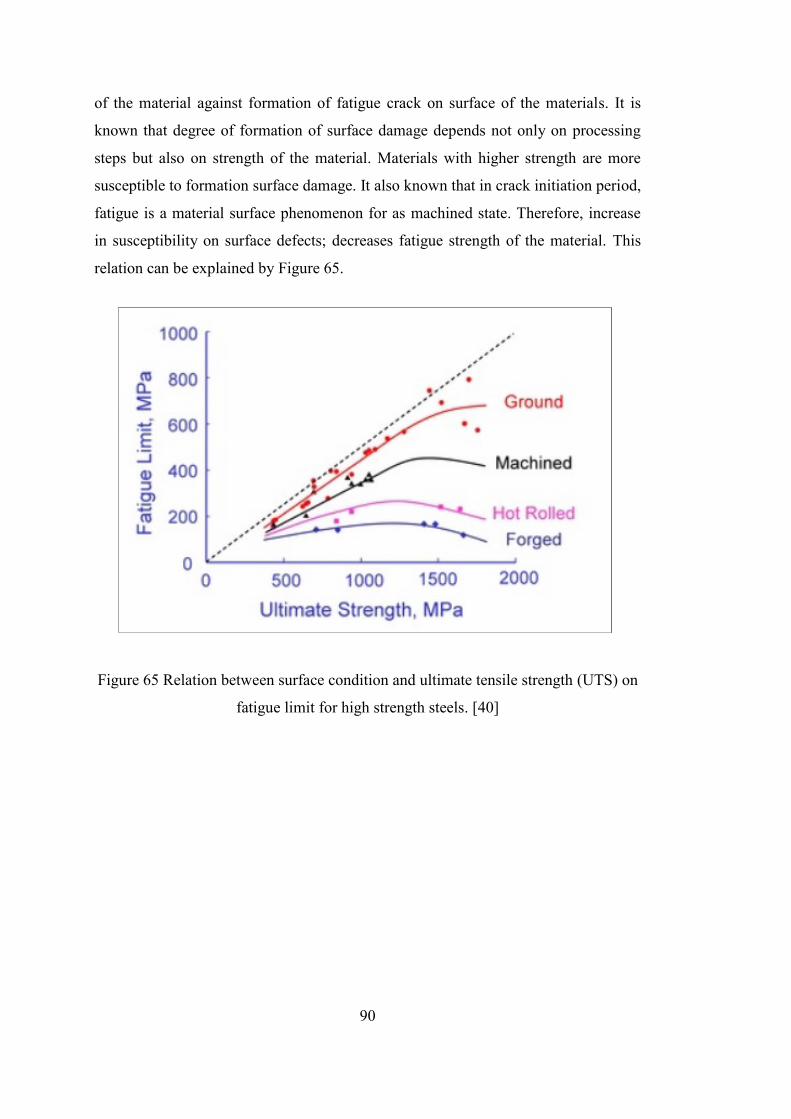
90

of the material against formation of fatigue crack on surface of the materials. It is

known that degree of formation of surface damage depends not only on processing

steps but also on strength of the material. Materials with higher strength are more

susceptible to formation surface damage. It also known that in crack initiation period,

fatigue is a material surface phenomenon for as machined state. Therefore, increase

in susceptibility on surface defects; decreases fatigue strength of the material. This

relation can be explained by Figure 65.

Figure 65 Relation between surface condition and ultimate tensile strength (UTS) on

fatigue limit for high strength steels. [40]

91

4.6. FRACTURE SURFACE ANALYSIS RESULTS

Fracture surface analysis is important in order to interpret static and fatigue test

results better. Therefore, fracture analysis was conducted for tensile test specimens in

order to classify fracture modes and determination of crack initiation site for several

fatigue tested specimens. Scanning Electron Microscopy (SEM) and Energy

Dispersive X-Ray analysis (EDX) was used in order to determine the cause of

failure in the microstructure.

4.6.1. FRACTURE SURFACE ANALYSIS RESULTS FOR TENSILE TEST

SPECIMENS

Fracture surface analysis was conducted by scanning electron microscopy (SEM) and

energy dispersive x-ray analysis (EDX).


SPECIMENS

Ductile fracture (cup and cone) type fracture mode was observed for the specimen

which is exposed to aging treatment at 5500C for 4h. SEM analysis was also

conducted for detail analysis.

Figure 66 Cup-and-cone type fracture surface for tensile tested specimen (SP-21)

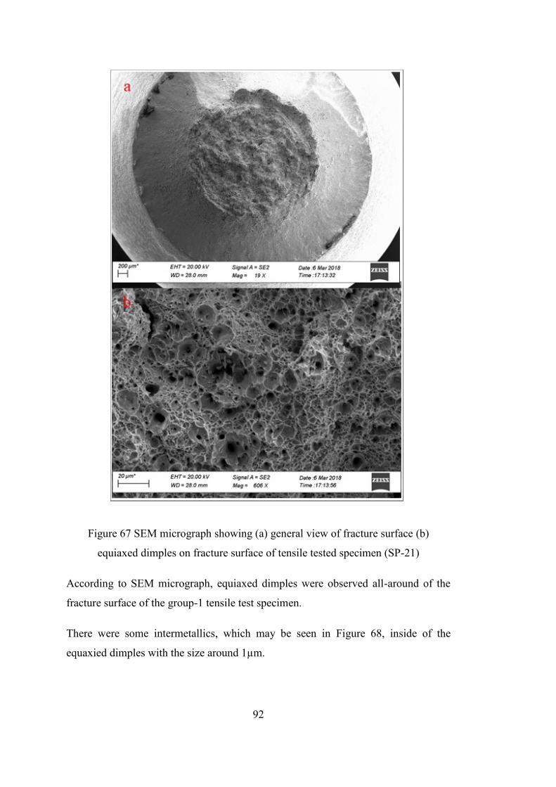
http://www.intertek.com/analysis/microscopy/edx/



92

Figure 67 SEM micrograph showing (a) general view of fracture surface (b)

equiaxed dimples on fracture surface of tensile tested specimen (SP-21)

According to SEM micrograph, equiaxed dimples were observed all-around of the

fracture surface of the group-1 tensile test specimen.

There were some intermetallics, which may be seen in Figure 68, inside of the

equaxied dimples with the size around 1µm.

93

Figure 68 SEM micrograph showing equiaxed dimples with some intermetallic

inside for tensile tested specimen (SP-21)

Figure 69 SEM image with in-lens detector for tensile tested specimen (SP-21)

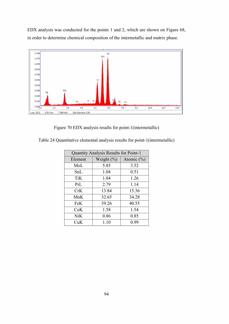
94

EDX analysis was conducted for the points 1 and 2, which are shown on Figure 68,

in order to determine chemical composition of the intermetallic and matrix phase.

Figure 70 EDX analysis results for point-1(intermetallic)

Table 24 Quantitative elemental analysis results for point-1(intermetallic)

Quantity Analysis Results for Point-1

Element Weight (%) Atomic (%)

MoL 5.85 3.52

SnL 1.04 0.51

TiK 1.04 1.26

PrL 2.79 1.14

CrK 13.84 15.36

MnK 32.65 34.28

FeK 39.26 40.55

CoK 1.58 1.54

NiK 0.86 0.85

CuK 1.10 0.99

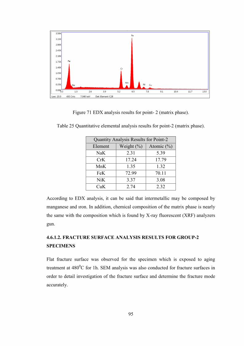
95

Figure 71 EDX analysis results for point- 2 (matrix phase).

Table 25 Quantitative elemental analysis results for point-2 (matrix phase).



NaK 2.31 5.39

CrK 17.24 17.79

MnK 1.35 1.32

FeK 72.99 70.11

NiK 3.37 3.08

CuK 2.74 2.32

According to EDX analysis, it can be said that intermetallic may be composed by

manganese and ıron. In addition, chemical composition of the matrix phase is nearly

the same with the composition which is found by X-ray fluorescent (XRF) analyzers

gun.


SPECIMENS

Flat fracture surface was observed for the specimen which is exposed to aging

treatment at 4800C for 1h. SEM analysis was also conducted for fracture surfaces in

order to detail investigation of the fracture surface and determine the fracture mode

accurately.

96

Figure 72 Brittle fracture surface for tensile tested specimen (SP-3)

Figure 73 SEM f micrograph showing general view of brittle fracture surface of

tensile tested specimen (SP-3)

Closer investigation was conducted for center and edge of the fracture surface to

determine fracture mode of the specimen. According to SEM micrograph that is

shown in Figure 74, both small dimples and cleavages were observed on the fracture

surface. Mixed mode of fracture or quasi-cleavage fracture was observed for the

specimen that is exposed to aging treatment at 4800C for 1h.

97

Figure 74 SEM micrograph showing dimple/voids and cleavages/facets view of

fracture surface of group-2 tensile test specimen. (SP-3)


SPECIMENS

Flat fracture surface was also observed for the specimen which is exposed to aging

treatment at 4000C for 70h. SEM analysis was also conducted for fracture surfaces in

order to investigate fracture surface in detail and determine the fracture mode

accurately.

Figure 75 Brittle fracture surface for tensile tested specimen (SP-13)

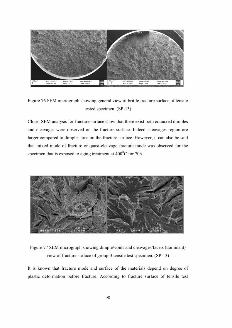
98

Figure 76 SEM micrograph showing general view of brittle fracture surface of tensile

tested specimen. (SP-13)

Closer SEM analysis for fracture surface show that there exist both equiaxed dimples

and cleavages were observed on the fracture surface. Indeed, cleavages region are

larger compared to dimples area on the fracture surface. However, it can also be said

that mixed mode of fracture or quasi-cleavage fracture mode was observed for the

specimen that is exposed to aging treatment at 4000C for 70h.

Figure 77 SEM micrograph showing dimple/voids and cleavages/facets (dominant)

view of fracture surface of group-3 tensile test specimen. (SP-13)

It is known that fracture mode and surface of the materials depend on degree of

plastic deformation before fracture. According to fracture surface of tensile test

99

results, specimen that was exposed to aging treatment at temperature 5500C show

cup and cone type fracture mode with equiaxed dimples on the surface was observed.

Moreover, some intermetallics were also observed inside of the dimples. Size of

these intermetallics was around 1µm. Cup and cone type fracture mode is observed

as a result of microvoids coalescence that form dimples just before failure. These

intermetallics cause formation of cracks due to high stress concentration around

themselves which initiate cracks. After reaching critical size, grow in maximum

shear stress direction.

On the other hand, specimens which were exposed to aging treatment at temperature

4000C and 480

0C show mixed mode of fracture or quasi-cleavage fracture mode.

Small dimples and cleavages were observed on the fracture surface of these

specimens. However, cleavages area is larger for the specimen aged at temperature

4000C for 1h. This difference between the fracture modes is caused by hardness of

the specimens. Increase in hardness causes decrease in ductility of the specimens and

amount of plastic deformation before failure. Therefore, fracture mode changes from

cup and cone to quasi-cleavage fracture mode.

4.7.1. FRACTURE SURFACE ANALYSIS RESULTS FOR FATIGUE TEST

SPECIMENS

Fracture surface analysis for fatigue test specimens was conducted in order to define

crack initiation sites. Specimens were selected according to different stress level and

different number of cycles before failure. Details of selected specimens are given in

table 26.

100

Table 26 Selected fatigue test specimen for fracture surface analysis.

Specimen

Groups

Heat Treatment

Parameters Selected Specimen

Group-1

Hom. at 11500C/1hr

+ Sol. at

10400C/0.5hr +

Aged at 5500C/4hr

SP-1 (Smax=

760Mpa-

N=13251)

SP-5 (Smax=

610Mpa-

N=120019)

SP-13

(Smax=

460Mpa-

N=10000065)

Group-2

Hom. at 11500C/1hr

+ Sol. at

10400C/0.5hr +

Aged at 4800C/1hr

SP-1 (Smax=

710Mpa-

N=280082)

SP-5 (Smax=

560Mpa-

N=10087227)

SP-9 (Smax=

510Mpa-

N=4604306)

Group-3

Hom. at 11500C/1hr

+ Sol. at

10400C/0.5hr +

Aged at 4000C/70hr

SP-1 (Smax=

860Mpa-

N=51206)

SP-4 (Smax=

560Mpa-

N=7433969)

SP-7 (Smax=

510Mpa-

N=1009078)


SPECIMENS

Crack is initiated at the center of the specimen. In order to determine cause of

initiation, closer examination was conducted at crack initiation point.

Figure 78 SEM fractograph showing general view of crack initiation site for (SP-1)

101

It is observed that crack is initiated from an inclusion at the center of the specimen.

Size of the inclusion is around 20 to 30 µm.

Figure 79 SEM fractograph showing crack initiation point for (SP-1)

SEM micrograph that is shown in Figure 80 show that crack initiation may also be

observed at surface of the specimen.


102


Crack is also initiated at the center of the specimen. Closer SEM analyses show that

there exists an inclusion with a size of 20 µm leads to crack initiation.


103


In order to determine chemical composition of the inclusion, which cause initiation

of cracks, EDX analysis was conducted on the surface of the inclusion that may be

seen as point 1 in Figure 83.

Figure 84 EDX analysis results for point- 1 in Figure 83.

104

Table 27 Quantitative elemental analysis results for point-1.



O K 41.47 54.28

MgK 14.59 12.57

AlK 41.12 31.92

CaK 1.13 0.59

MnK 0.91 0.35

FeK 0.78 0.29

EDX analysis result shows that, inclusion is composed by oxygen. Therefore, it may

be said that oxide inclusion with a size of 20 to 30 µm leads to initiation of cracks

for 15-5 PH stainless steel under cyclic loading.

In order to determine crack growth direction, direction of striations was also

examined. Crack growth direction may be seen in Figure 85.


group-1 cyclic loaded specimen (SP-1)

105


SPECIMENS

Crack initiation sites were also examined for group-2 fatigue test specimens ın order

to see the effect of heat treatment crack initiation sites. Crack is initiated at the

surface for specimen-1.



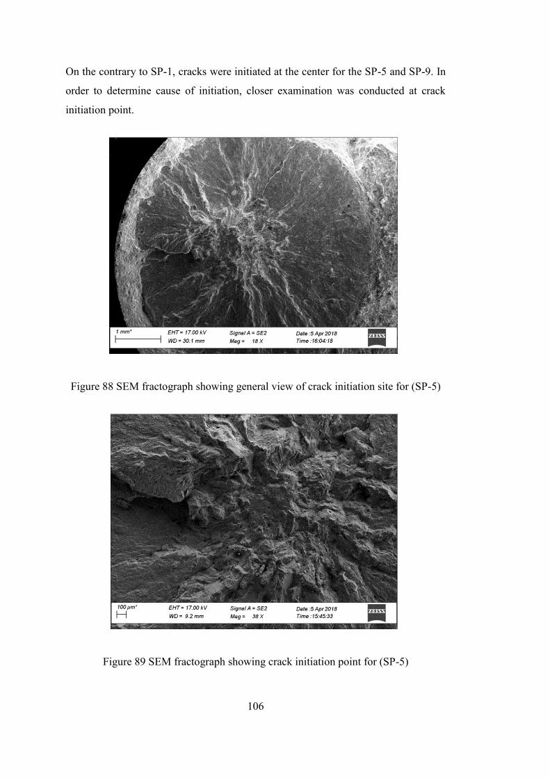
106

On the contrary to SP-1, cracks were initiated at the center for the SP-5 and SP-9. In

order to determine cause of initiation, closer examination was conducted at crack

initiation point.



107

Closer SEM micrograph shows that inclusions with 20 to 30 µm cause initiation of

the cracks at the center of the specimens.


Figure 91 SEM fractograph showing crack initiation in detail for (SP-9).

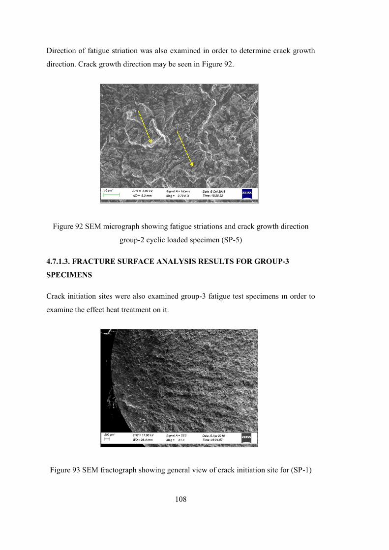
108

Direction of fatigue striation was also examined in order to determine crack growth

direction. Crack growth direction may be seen in Figure 92.




SPECIMENS

Crack initiation sites were also examined group-3 fatigue test specimens ın order to

examine the effect heat treatment on it.


109


Crack was initiated at the surface for the SP-1. However, cracks were initiated for

SP-4 and SP-7. In order to find cause of crack initiation closer SEM analysis was

conducted.


110


SEM analysis show that inclusion with a size of 20-30 µm leads to initiation of

cracks at inside of the specimen that may be seen in Figure 98.


111


EDX analysis was conducted for crack initiation point and show that the inclusion is

composed by oxide that is shown in Figure 98.

Figure 99 EDX analysis results for crack initiation point of (SP-7)

112

Table 28 Quantitative elemental analysis results for point-1.



O K 33.13 63.94

AlK 7.19 8.23

SiK 8.21 9.03

CaK 4.99 3.84

PmL 31.77 6.77

MnK 7.62 4.28

FeK 7.08 3.91

Fatigue striations and crack growth direction was also examined for specimen-7.



According to scanning electron microscopy (SEM) analysis results, it is observed

that crack initiation sites can be both on surface and inside for 15-5 PH stainless

steels specimens after fatigue failure. There is not significant difference on crack

initiation sites for different heat treatment parameters of three groups of group-5

specimens. Instead heat treatment parameters, crack initiation sites are mostly

affected by applied cyclic stress.

In general, crack initiation sites were observed in the inside of the specimens which

were exposed maximum stress below 560 MPa. Stress level higher than 600 MPa

113

causes observation of crack initiation at the surface of the specimens. Therefore, it

can be said that surface defects that cause crack initiation are more sensitive at high

stress level compared to interior defects.

In addition, cracks were initiated by an inclusion with a size of 20 to 30 in the inside

of the specimens. In order to determine chemical composition of these inclusions,

EDX analysis was performed. EDX analysis showed that these defects are composed

by oxide particles according to chemical compositions. EDX analysis show that these

inclusions are mostly in the form of oxide inclusions. EDX analysis was also done

for matrix phase on the fracture surface for fatigue tested specimens. Results showed

very similar chemical composition for 15-5 PH stainless steels that was found by

XRF gun.

In order to reach general comments for crack initiation sites, fracture surface of all

failed specimens were examined optically in order to see effect of heat treatment

parameters and fatigue stress level on the crack initiation sites.

Figure 101 Optical image for fracture surface of group -1 failed specimens.

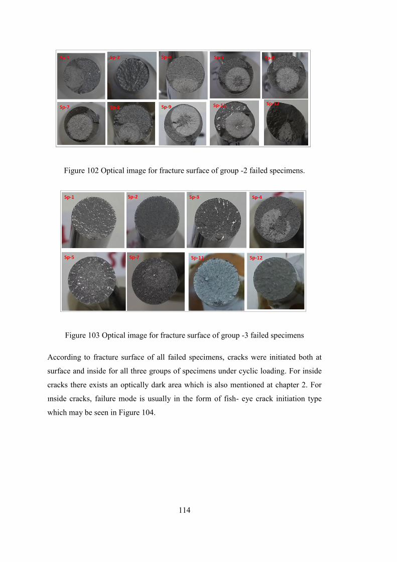
114

Figure 102 Optical image for fracture surface of group -2 failed specimens.

Figure 103 Optical image for fracture surface of group -3 failed specimens

According to fracture surface of all failed specimens, cracks were initiated both at

surface and inside for all three groups of specimens under cyclic loading. For inside

cracks there exists an optically dark area which is also mentioned at chapter 2. For

ınside cracks, failure mode is usually in the form of fish- eye crack initiation type

which may be seen in Figure 104.

115

Figure 104 The inclusion at the center of the fish eye. [29]

Observation of this optically dark rough area may be caused by some environmental

factor like penetration of hydrogen or oxygen during fatigue testing.

117

CHAPTER 5

CONCLUSION

The aim of this study is to investigate effect of the heat treatment parameters on the

microstructure and mechanical properties especially hardness and fatigue strength of

the AMS5659 15-5 precipitation hardenable stainless steel. In order to achieve this,

heat treatment processes were applied by three different steps which were

homogenization, solutionizing and aging treatment. Heat treatments were applied at

different temperature and time periods. After completing the heat treatment,

microstructure of the specimens was analyzed in terms of grain size. Then, hardness

test was performed for all heat treated disc shaped specimens in HRC scale in order

to see the effect of heat treatment parameters on hardness of the 15-5 PH stainless

steels. Then, tensile and fatigue tests were conducted for selected heat treated group.

Fatigue tests were conducted by servo-hydraulic and resonant fatigue testing

machines at different frequency for low and high cycle region. Fatigue test results

were used to construct S-N curve for three different specimen groups of group-5

specimens that were exposed to different heat treatment condition. After completing

static and fatigue tests, fracture surface analysis was applied by scanning electron

microscopy (SEM) and Energy Dispersive X-Ray analysis (EDX) in order to

determine fracture mode for tensile test specimen and to see crack initiation sites for

fatigue test specimens. Following conclusions can be drawn from this particular

study:


118

1. Fatigue limit of the 15-5 PH stainless steel has been increased 15% (15

percent) by changing heat treatment parameter from 5500C for 4h to 480

0C

for 1h. In addition, aging treatment at 4000C for 70h provides 11% (11

percent) increase on fatigue limit compared to aging condition at 5500C for

4h. Increase in fatigue limit may be explained by increase in strength of

material.

2. Both surface and inside cracks were observed for fatigue test specimens.

Moreover, ınside cracks may be initiated from an oxide inclusion with a size

of 20-30 µm for 15-5 PH stainless steel under cyclic loading.

3. Changing aging treatment from 5500C for 4h to 480

0C for 1h, hardness of 15-

5 PH stainless steel was increased by 18% (18 percent). In addition, if aging

treatment parameters are changed to 4000C for 70h, hardness has been

increased by 23% (23 percent). Increase in hardness is provided by

precipitation reaction during aging treatment.

4. Tensile strength of 15-5 PH stainless steel was increased 20% (20 percent) by

changing heat treatment parameter from 5500C for 4h to 480

0C for 1h.

Indeed; it is also increased 27% (27 percent) by application of aging

treatment at 4000C for 70h.

119

REFERENCES

[1] Slunder, C. J., Hoenie, A. F., & Hall, A. M. (January 1967). Thermal and

Mechanical Treatment for Precipitation- Hardening Stainless Steels. 1-192.

Retrieved March 25, 2018, from http://adsbit.harvard.edu//full/1967NASSP5089

[2] History Hour: Aloha Airlines Flight 243 incident. (2017, April 28). Retrieved

April 07, 2018, from https://www.aerotime.aero/en/did-you-know/18542-history-

hour-aloha-airlines-flight-243-incident

[3] Herny, E. (2009). Mechanical characterization and investigation of thermal and

thermomechanical aging mechanisms of martensitic stainless steel 15-

5PH. International Heat Treatment and Surface Engineering,3(1-2), 65-69.

doi:10.1179/174951509x466957

[4] KUMAR, A., & PRASAD, E. (2013). Indian Academy of Sciences. Indigenous

development and airworthiness certification of 15–5 PH precipitation hardenable

stainless steel for aircraft applications,38, 3-23. Retrieved Oct. & nov., 2016.

[5] Fakić, B., & Cubela, D. (2013). Review of The development oF Research in the

Design of Semi Austenitic Stainless Steel 17-7PH. Journal of Trends in the

Development of Machinery and Associated Technology,17(1), 57-60. Retrieved

March 16, 2018.

[6] Research may precipitate hard results. (2006). Metal Powder Report, 61(7), 24-

31. doi:10.1016/s0026-0657(06)70691-9. Retrieved March 6, 2018.

[7] Rep. No. MIL-H-6875H at 1-29 (1989). Military Specification Heat Treatment of

Steel.

http://adsbit.harvard.edu/full/1967NASSP5089.....S/0000015.000.html

https://www.aerotime.aero/en/did-you-know/18542-history-hour-aloha-airlines-flight-243-incident

https://www.aerotime.aero/en/did-you-know/18542-history-hour-aloha-airlines-flight-243-incident

120

[8] 15- 5 PH Stainless Steel Product Data Sheet. (n.d.). Retrieved October 4, 2016,

from https://www.spacematdb.com/spacemat/manudatasheets/15-

5_PH_Data_Sheet.pdf.

[9] Bhambroo, R., Roychowdhury, S., & Kain, V. (2013). Effect of reverted austenite

on mechanical properties of precipitation hardenable 17-4 stainles ssteel. Materials

Science& Engineering A,568, 127-133. Retrieved May 6, 2017.

[10] Couturier, L., Geuser, F. D., Descoins, M., & Deschamps, A. (2016). Evolution

of the microstructure of a 15-5PH martensitic stainless steel during precipitation

hardening heat treatment. Materials & Design,107, 416-425.

doi:10.1016/j.matdes.2016.06.068

[11] PENG, X. Y., ZHOU, X. L., & HUA, X. Z. (2015). Journal of Iron and Steel

Research, International. Ffect of Aging on Hardening Behavior of 15-5 PH Stainless

Steel,22(7), 607-614. Retrieved May 5, 2017.

[12] Devi, R. S., & Nath, J. S. (2013). Effect of Precipitation Hardening on

Microstructural Characteristics of 15-5 Ph Steel. International Journal of Engineering

Research and Development,9(1), 22-26. Retrieved March 14, 2017, from

http://www.ijerd.com/paper/vol9-issue1/F09012226.pdf

[13] (Yooa, W. D., & Leeb, J. H. (2006). Solid State Phenomena. Study on the

Microstructure and Mechanical Properties of 17-4 PH Stainless Steel depending on

Heat Treatment and Aging Time,118, 15-20. Retrieved December 3, 2016.)

[14] (Mirzadeh, H., & Najafizadeh, A. (2009). Materials Chemistry and Physics.

Aging kinetics of 17-4 PH stainless steel, 116, 119-124. Retrieved November 2,

2016.)

[15] (Hsiaoa, C. N. (2002). Materials Chemistry and Physics. Aging reactions in a

17-4 PH stainless steel, 74, 134-142. Retrieved November 2, 2016.)

[16] United States. Federal Aviation Administration. (2005). Metallic Materials

Properties Development and Standardization (MMPDS): CHAPTER 2 - STEEL

https://www.spacematdb.com/spacemat/manudatasheets/15-5_PH_Data_Sheet.pdf

https://www.spacematdb.com/spacemat/manudatasheets/15-5_PH_Data_Sheet.pdf

http://www.ijerd.com/paper/vol9-issue1/F09012226.pdf

121

ALLOYS. Retrieved October 20, 2017, from

https://www.sae.org/publications/books/content/b-983/.

[17] Callister, W. D. (2007). Materials science and engineering: An introduction (7th

ed.).NewYork: John Wiley & Sons.

https://abmpk.files.wordpress.com/2014/02/book_maretial-science-callister.pdf

[18] Fathemi, A. (2014, June 2). Training and Seminars. Retrieved from

https://www.efatigue.com/training/Chapter_4.pdf

[19] Schijve, J. (2009). Fatigue of structures and materials(2nd ed.). Berlin: Springer.

[20] Farahani, A. V. (2005). Advances in fatigue, fracture and damage assessment of

materials(Vol. 1). Billerica, MA: WIT Press. doi:10.2495/1-85312-836-8/02

[21] Stress-life Diagram (s-n Diagram). (n.d.). Retrieved May 30, 2018, from

https://www.semanticscholar.org/paper/Stress-life-Diagram-(s-n-Diagram)/ =abstract

[22] BOEING. (1968). Fatigue Properties of 17-4 PH and 15-5 PH Steel in the H-900

and H-1050 Condition. Retrieved April 20, 2017, from

http://www.dtic.mil/dtic/tr/fulltext/u2/691794.pdf

[23] Pook, L. (2009). Metal fatigue: What it is, why it matters(Vol. 145, Ser. 1525).

Dordrecht: Springer.

[24] Liard, F. (1983). Helicopter fatique design guide. Neuilly-sur-Seine: AGARD.

[25] ISO 12107: Metallic materials - fatigue testing - Statistical planning and

analysis of data. (2003). Ginebra: ISO.

[26] Palanisamy, D., Senthil, P., & Senthilkumar, V. (2016). The effect of aging on

machinability of 15Cr–5Ni precipitation hardened stainless steel. Archives of Civil

and Mechanical Engineering,16(1), 53-63. doi:10.1016/j.acme.2015.09.004

[27] Schönbauer, B. M., Yanase, K., & Endo, M. (2017). The influence of various

types of small defects on the fatigue limit of precipitation-hardened 17-4PH stainless

https://abmpk.files.wordpress.com/2014/02/book_maretial-science-callister.pdf

https://www.efatigue.com/training/Chapter_4.pdf

https://www.semanticscholar.org/paper/Stress-life-Diagram-(s-n-Diagram)/

122

steel. Theoretical and Applied Fracture Mechanics,87, 35-49.

doi:10.1016/j.tafmec.2016.10.003

[28] Schönbauer, B. M., Yanase, K., & Endo, M. (2016). VHCF properties and

fatigue limit prediction of precipitation hardened 17-4PH stainless steel. International

Journal of Fatigue,88, 205-216. doi:10.1016/j.ijfatigue.2016.03.034

[29] Murakami, Y. (2002). Effects of Nonmetallic Inclusions on Fatigue

Strength. Metal Fatigue,75-127. doi:10.1016/b978-008044064-4/50006-2

[30] ASTM E466 – 15. Standard Practice for Conducting Force Controlled Constant

Amplitude Axial Fatigue Tests of Metallic Materials. Retrieved October 14, 2017.

[31] ASTM E407 − 07 (Reapproved 2015) Standard Practice for Microetching

Metals and Alloys. Retrieved July 2, 2017.

[32] ASTM E112 – 13. Standard Test Methods for Determining Average Grain Size.

Retrieved June 25, 2017.

[33] HR-521 (L) /523 (L) Series 810-Rockwell Type Hardness Testing Machines.

(n.d.). Retrieved July 11, 2018, from https://ecatalog.mitutoyo.com/HR-521-L-523-

L-Series-810-Rockwell-Type-Hardness-Testing-Machines-C1334.aspx

[34] ASTM E18 – (16).Standard Test Methods for Rockwell Hardness of Metallic

Materials. Retrieved October 25, 2017.

[35] GmbH, M. (n.d.). MarSurf PS 10 - Mobile roughness measuring instrument -

Mahr Metrology. Retrieved July 11, 2018.

[36] 5980 Serisi Çift Kolonlu Zemin Tipi Test Sistemleri (Yüksek Kapasite). (n.d.).

Retrieved July 11, 2018, from http://www.instron.com.tr/tr-tr/products/testing-

systems/universal-testing-systems/electromechanical/5900/5980-floor-model

[37] (2018, July 11). Retrieved from http://www.rumul.ch/220_products.php

https://ecatalog.mitutoyo.com/HR-521-L-523-L-Series-810-Rockwell-Type-Hardness-Testing-Machines-C1334.aspx

https://ecatalog.mitutoyo.com/HR-521-L-523-L-Series-810-Rockwell-Type-Hardness-Testing-Machines-C1334.aspx

http://www.instron.com.tr/tr-tr/products/testing-systems/universal-testing-systems/electromechanical/5900/5980-floor-model

http://www.instron.com.tr/tr-tr/products/testing-systems/universal-testing-systems/electromechanical/5900/5980-floor-model

http://www.rumul.ch/220_products.php

123

[38] Dericioğlu, F. A. (2018, October 17). Metallography Lecture Notes. Lecture

presented at Quantitative Metallography.

[39] Inc. (n.d.). EFunda: Convert Hardness: Tensile Strength (Approx.). Retrieved

July 12, 2018.

[40] Finite Element Model Stress-Life Technical Background. (n.d.). Retrieved from

https://www.efatigue.com/fem/background/stresslife.html

https://www.efatigue.com/fem/background/stresslife.html

the effects of heat treatment on microstructure, hardness

Documents

Transcript of the effects of heat treatment on microstructure, hardness