The effective-field study of a mixed spin-1 and spin-5/2 Ising ferrimagnetic system

This article has been downloaded from IOPscience. Please scroll down to see the full text article.

2009 Phys. Scr. 79 065006

(http://iopscience.iop.org/1402-4896/79/6/065006)

Download details:

IP Address: 95.183.152.38

The article was downloaded on 16/03/2011 at 11:30

Please note that terms and conditions apply.

View the table of contents for this issue, or go to the journal homepage for more

Home Search Collections Journals About Contact us My IOPscience

IOP PUBLISHING PHYSICA SCRIPTA

Phys. Scr. 79 (2009) 065006 (11pp) doi:10.1088/0031-8949/79/06/065006

The effective-field study of a mixed spin-1and spin-5/2 Ising ferrimagnetic systemBayram Deviren1,2, Mehmet Batı1,3 and Mustafa Keskin4

1 Institute of Science, Erciyes University, 38039 Kayseri, Turkey2 Department of Physics, Nevsehir University, 50300 Nevsehir, Turkey3 Department of Physics, Rize University, 53100 Rize, Turkey4 Department of Physics, Erciyes University, 38039 Kayseri, Turkey

E-mail: keskin@erciyes.edu.tr

Received 14 November 2008Accepted for publication 6 April 2009Published 22 May 2009Online at stacks.iop.org/PhysScr/79/065006

AbstractAn effective-field theory with correlations is developed for a mixed spin-1 and spin-5/2 Isingferrimagnetic system on the honeycomb (δ = 3) and square (δ = 4) lattices in the absence andpresence of a longitudinal magnetic field. The ground-state phase diagram of the model isobtained in the longitudinal magnetic field (h) and a single-ion potential or crystal-fieldinteraction (1) plane. We also investigate the thermal variations of the sublatticemagnetizations, and present the phase diagrams in the (1/|J |, kBT/|J |) plane. Thesusceptibility, internal energy and specific heat of the system are numerically examined, andsome interesting phenomena in these quantities are found due to the absence and presence ofthe applied longitudinal magnetic field. Moreover, the system undergoes second- andfirst-order phase transition; hence, the system gives a tricritical point. The system also exhibitsreentrant behavior.

PACS numbers: 05.50.+q, 05.70.Fh, 75.10.Hk, 75.30.Kz, 75.50.Gg

1. Introduction

During the past several decades, much effort has beendevoted to determine the critical behavior and other statisticalproperties of the various Ising systems, which would enablea deeper understanding of order–disorder phenomena instatistical physics and condensed matter physics. The Isingsystems consisting of mixed spins of different magnitudes,the so-called mixed-spin Ising models, are among the mostinteresting extensions of the standard spin-1/2 Ising system.Mixed spin Ising systems provide good models to investigateferrimagnetic materials that are currently of great interestdue to their possible useful properties for technologicalapplications, as well as academic research. The well-knownmixed spin Ising systems are spins (1/2, 1), spins (1/2, 3/2)and spins (1, 3/2) Ising systems. These systems have beenstudied extensively by using the methods of equilibriumstatistical physics such as the mean-field approximation(MFA), effective-field theory (EFT), cluster variationmethod (CVM), renormalization group (RG) techniquesand Monte-Carlo (MC) simulations (see [1–5] for spins(1, 1/2), [6–10] for spins (1/2, 3/2) and [11–15] for spins(1, 3/2) Ising systems, and references therein). Moreover,

the exact solutions of the spins (1/2, 1) were studiedon a honeycomb lattice [16], a bathroom tile [17], dicedlattices [18], a Bethe lattice [19], a two-fold Cayley tree [20],several decorated planar lattices [21] and a bilayer Bethelattice [22]. Dynamics of the mixed spin-1/2 and spin-1Ising system [23, 24] has also been investigated by usingthe Glauber-type stochastic dynamics [25], the dynamicalpair approximation [26], the dynamic MC simulations andfinite-size scaling arguments [27], the MC simulations andthe dynamical pair approximation [28, 29] and the pairapproximation with point distribution [30]. The exact solutionof spins (1/2, 3/2) Ising system has also been studiedon the Bethe lattice [31] and a two-fold Cayley tree [32]by using the exact recursion relations, on the honeycomblattice within the framework of exact star–triangle mappingtransformations [33], on the extended Kagomé lattice [34]and Union Jack (centered square) lattice [35] by establishinga mapping correspondence with the eight-vertex model.On the other hand, the exact formulation of the mixed spin(1, 3/2) Ising ferrimagnetic system on the Bethe lattice hasbeen examined by using the exact recursion relations [36].Moreover, recently, the dynamic phase transitions in thekinetic mixed spins (1/2, 3/2) [37] and spins (1, 3/2) [38]

0031-8949/09/065006+11$30.00 1 © 2009 The Royal Swedish Academy of Sciences Printed in the UK

Phys. Scr. 79 (2009) 065006 B Deviren et al

ferrimagnetic systems under a time-dependent magneticfield have been studied by using the Glauber-type stochasticdynamics. The mixed spins (1/2, 5/2) [39–41], spins (3/2,5/2) [42–44], spins (1, 2) [45–47] and spins (2, 5/2) [48–50]have received less attention. But, up to now, as far as weknow, nobody has studied the spin-1 and spin-5/2 Isingsystem.

Therefore, the aim of this paper is to study themagnetic properties of the mixed spin-1 and spin-5/2 Isingferrimagnetic system in the absence and presence of alongitudinal magnetic field on the honeycomb and squarelattices by using the EFT with correlations in detail. Theground state phase diagram of the model is obtained in thelongitudinal magnetic field (h) and a single-ion potential orcrystal-field interaction (1) plane. We also investigate thethermal variations of the sublattice magnetizations and presentthe phase diagrams in the (1/|J |, kBT/|J |) plane for h = 0.Moreover, the susceptibility, internal energy and specificheat of the system are numerically examined, and someinteresting phenomena in these quantities are found due tothe applied longitudinal magnetic field. This method, namelyEFT with correlation, was first introduced by Honmura andKaneyoshi [51] and Kaneyoshi et al [52], which is a moreadvanced method dealing with Ising systems than the MFA,because it considers more correlations. Then, the methodhas been widely developed and applied to various magneticsystems [53], including thin films, superlattices [54–56] andmixed spin Ising systems [57–59].

The rest of the paper is organized as follows. In section 2,we introduce briefly the basic framework of the EFT withcorrelations and give the formulation for the mixed spin-1 andspin-5/2 Ising model on the honeycomb and square lattices.In section 3, the numerical results for the magnetizations,phase diagrams and thermodynamic quantities, such assusceptibility, internal energy and specific heat of the model,are studied in detail. The paper ends with a brief summary andconclusion of the work in section 4.

2. Formulation

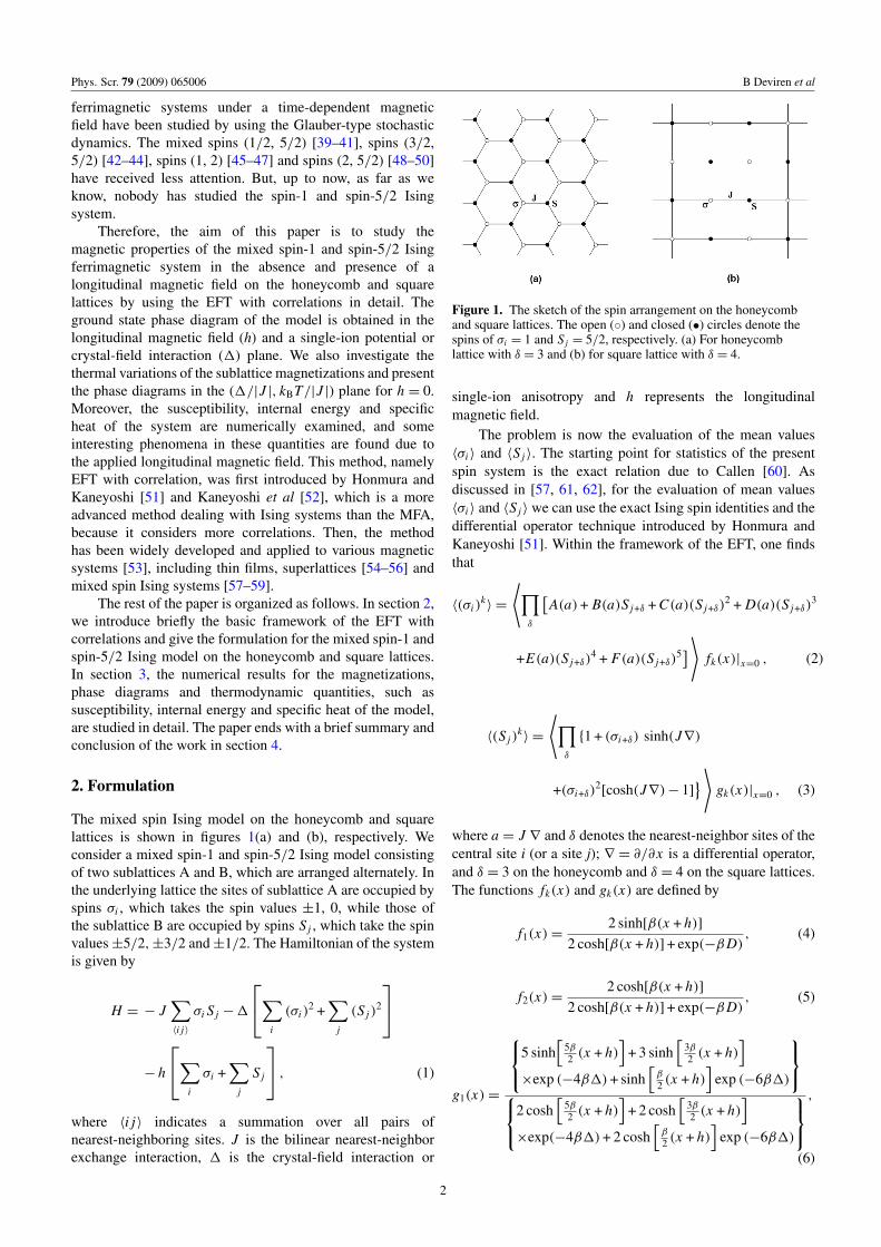
The mixed spin Ising model on the honeycomb and squarelattices is shown in figures 1(a) and (b), respectively. Weconsider a mixed spin-1 and spin-5/2 Ising model consistingof two sublattices A and B, which are arranged alternately. Inthe underlying lattice the sites of sublattice A are occupied byspins σi , which takes the spin values ±1, 0, while those ofthe sublattice B are occupied by spins S j , which take the spinvalues ±5/2, ±3/2 and ±1/2. The Hamiltonian of the systemis given by

H = − J∑〈i j〉

σi S j − 1

∑i

(σi )2 +

∑j

(S j )2

− h

∑i

σi +∑

j

S j

, (1)

where 〈i j〉 indicates a summation over all pairs ofnearest-neighboring sites. J is the bilinear nearest-neighborexchange interaction, 1 is the crystal-field interaction or

Figure 1. The sketch of the spin arrangement on the honeycomband square lattices. The open (◦) and closed (•) circles denote thespins of σi = 1 and S j = 5/2, respectively. (a) For honeycomblattice with δ = 3 and (b) for square lattice with δ = 4.

single-ion anisotropy and h represents the longitudinalmagnetic field.

The problem is now the evaluation of the mean values〈σi 〉 and 〈S j 〉. The starting point for statistics of the presentspin system is the exact relation due to Callen [60]. Asdiscussed in [57, 61, 62], for the evaluation of mean values〈σi 〉 and 〈S j 〉 we can use the exact Ising spin identities and thedifferential operator technique introduced by Honmura andKaneyoshi [51]. Within the framework of the EFT, one findsthat

〈(σi )k〉 =

⟨∏δ

[A(a) + B(a)S j+δ + C(a)(S j+δ)

2 + D(a)(S j+δ)3

+E(a)(S j+δ)4 + F(a)(S j+δ)

5] ⟩

fk(x)|x=0 , (2)

〈(S j )k〉 =

⟨∏δ

{1 + (σi+δ) sinh(J∇)

+(σi+δ)2[cosh(J∇) − 1]

} ⟩gk(x)|x=0 , (3)

where a = J ∇ and δ denotes the nearest-neighbor sites of thecentral site i (or a site j); ∇ = ∂/∂x is a differential operator,and δ = 3 on the honeycomb and δ = 4 on the square lattices.The functions fk(x) and gk(x) are defined by

f1(x) =2 sinh[β(x + h)]

2 cosh[β(x + h)] + exp(−β D), (4)

f2(x) =2 cosh[β(x + h)]

2 cosh[β(x + h)] + exp(−β D), (5)

g1(x) =

5 sinh[

5β

2 (x + h)]

+ 3 sinh[

3β

2 (x + h)]

×exp (−4β1) + sinh[

β

2 (x + h)]

exp (−6β1)

2 cosh[

5β

2 (x + h)]

+ 2 cosh[

3β

2 (x + h)]

×exp(−4β1) + 2 cosh[

β

2 (x + h)]

exp (−6β1)

,

(6)

2

Phys. Scr. 79 (2009) 065006 B Deviren et al

g2(x) =

25 cosh[

5β

2 (x + h)]

+ 9 cosh[

3β

2 (x + h)]

× exp(−4β1) + cosh[

β

2 (x + h)]

exp(−6β1)

4 cosh[

5β

2 (x + h)]

+ 4 cosh[

3β

2 (x + h)]

× exp(−4β1) + 4 cosh[

β

2 (x + h)]

exp(−6β1)

,

(7)

g3(x) =

125 sinh[

5β

2 (x + h)]

+ 27 cosh[

3β

2 (x + h)]

× exp(−4β1) + cosh[

β

2 (x + h)]

exp(−6β1)

8 cosh[

5β

2 (x + h)]

+ 8 cosh[

3β

2 (x + h)]

× exp(−4β1) + 8 cosh[

β

2 (x + h)]

exp(−6β1)

,

(8)

g4(x) =

625 cosh[

5β

2 (x + h)]

+ 81 cosh[

3β

2 (x + h)]

× exp(−4β1) + cosh[

β

2 (x + h)]

exp(−6β1)

16 cosh[

5β

2 (x + h)]

+ 16 cosh[

3β

2 (x + h)]

×exp(−4β1) + 16 cosh[β

2 (x + h)]exp(−6β1)

,

(9)

g5(x) =

3125 sinh[

5β

2 (x + h)]

+ 243 cosh[

3β

2 (x + h)]

× exp(−4β1) + cosh[

β

2 (x + h)]

exp(−6β1)

32 cosh[

5β

2 (x + h)]

+ 32 cosh[

3β

2 (x + h)]

× exp(−4β1) + 32 cosh[β

2 (x + h)]

exp(−6β1)

,

(10)where β = 1/kBT , kB is the Boltzmann constant and T is theabsolute temperature. The coefficients A(a), B(a), C(a), D(a),E(a) and F(a) in equation (2) are obtained by using the exactvan der Waerden identity

A(a)=1

128

[3 cosh

(5a

2

)− 25 cosh

(3a

2

)+ 150 cosh

(a

2

)],

B(a) =1

960

[9 sinh

(5a

2

)−125 sinh

(3a

2

)+ 2250 sinh

(a

2

)],

C(a) =1

48

[−5 cosh

(5a

2

)+ 39 cosh

(3a

2

)− 34 cosh

(a

2

)],

D(a) =1

24

[− sinh

(5a

2

)+ 13 sinh

(3a

2

)− 34 sinh

(a

2

)],

E(a) =1

24

[cosh

(5a

2

)− 3 cosh

(3a

2

)+ 2 cosh

(a

2

)],

F(a) =1

60

[sinh

(5a

2

)− 5 sinh

(3a

2

)+ 10 sinh

(a

2

)]. (11)

Equations (2) and (3) are also exact and are valid for anylattice. If we try to exactly treat all the spin–spin correlationsfor that set of equations, the problem quickly becomesintractable. A first obvious attempt to deal with it is to ignorecorrelations; the decoupling approximation:⟨

σi (σi ′)2 . . . σin

⟩∼= 〈σi 〉

⟨(σi ′)2

⟩· · · 〈σin 〉,⟨

S j (S j ′)2 . . . (S jn )5⟩∼= 〈S j 〉

⟨(S j ′)2

⟩· · · 〈(S jn )5

〉,

(12)

with i 6= i ′6= · · · 6= in and j 6= j ′

6= · · · 6= jn have beenintroduced within the EFT with correlations [51, 53, 63].In fact, the approximation corresponds essentially to theZernike approximation [64] in the bulk problem, and hasbeen successfully applied to a great number of magneticsystems including the surface problems [51, 53, 63, 65]. Onthe other hand, in the mean-field theory, all the correlations,including the self-correlations, are neglected. Based on theseapproximations, equations (2) and (3) reduce to

mA =[A(a) + B(a)〈S j 〉 + C(a)

⟨(S j )

2⟩+ D(a)

⟨(S j )

3⟩

+E(a)⟨(S j )

4⟩+ F(a)

⟨(S j )

5⟩]δ

f1(x)|x=0, (13)

qA =[A(a) + B(a)〈S j 〉 + C(a)

⟨(S j )

2⟩+ D(a)

⟨(S j )

3⟩

+E(a)⟨(S j )

4⟩+ F(a)

⟨(S j )

5⟩]δ

f2(x)|x=0, (14)

mB = [1 + 〈σi 〉 sinh(J∇)

+⟨(σi )

2⟩{cosh(J∇) − 1}

]δg1(x)|x=0, (15)

qB = [1 + 〈σi 〉 sinh(J∇)

+⟨(σi )

2⟩{cosh(J∇) − 1}

]δg2(x)|x=0, (16)

rB = [1 + 〈σi 〉 sinh(J∇)

+⟨(σi )

2⟩{cosh(J∇) − 1}

]δg3(x)|x=0, (17)

υB = [1 + 〈σi 〉 sinh(J∇)

+⟨(σi )

2⟩{cosh(J∇) − 1}

]δg4(x)|x=0, (18)

wB = [1 + 〈σi 〉 sinh(J∇)

+⟨(σi )

2⟩{cosh(J∇) − 1} ]δg5(x)|x=0, (19)

So far we have discussed the basic formulation of the mixedspin-1 and spin-5/2 Ising model with a crystal-field in alongitudinal magnetic field with a coordination number δ;hence equations (13)–(19) can be used to investigate thethermal variations of the sublattice magnetizations and thenphase diagrams can be calculated. As one can see, in ourtreatment new order parameters qA, qB, rB, vB and wB

naturally appear, which one is able to evaluate. This isnot the case with the standard MFA where all correlationsare neglected. This is one of the reasons why the presentframework provides better results than the standard MFA.

2.1. Application to the honeycomb lattice (δ = 3)

We are now interested in studying the transition temperature(or the phase diagrams) of the system. Certain features of

3

Phys. Scr. 79 (2009) 065006 B Deviren et al

the phase diagram can be determined analytically througha Landau free energy expansion in the order parameters.For simplicity, we will discuss in detail the honeycomblattice with δ = 3 seen in figure 1(a). Putting δ = 3 intoequations (13)–(19), and expanding the right-hand sides ofthese equations, one can obtain the following set of coupledequations:

mA = A0 + A1mB + A2m2B + A3m3

B A4m4B + A5m5

B

+ A6m6B + A7m7

B + A8m8B + A9m9

B + A10m10B

+ A11m11B + A12m12

B + A13m13B + A14m14

B + A15m15B ,

(20)

mB=B0+B1mA+B2m2A+B3m3

A+B4m4A+B5m5

A+ B6m6A, (21)

where the coefficients Ai (i = 0, 1, . . . , 15) andB j ( j = 0, 1, 2, . . . , 6) can be easily calculated by applyingmathematical relations exp(α∇) f (x) = f (x + α) andexp(α∇) g(x) = g(x + α) as given in the appendix A. Thedefinitions of the sublattice magnetizations for the honeycomblattice are mA = 〈σi 〉 and mB = 〈S j 〉. Solving the coupledequations (20) and (21), we can obtain the magnetizationcurves for the honeycomb lattice. We will perform thiscalculation in the next section.

2.2. Application to the square lattice (δ = 4)

In this subsection, we shall obtain the set of coupledequations on the square lattice with δ = 4. For constructingthese coupled equations, we need to consider not three- butfour-site blocks as seen in figure 1(b). To obtain the set ofcoupled equations, one can put δ = 4 into equations (13)–(19)and expand the right-hand sides of these equations. Theapplication of equations (13)–(19) to square lattice with δ = 4leads then to the following set of mutually coupled equations

mA = C0 + C1mB + C2m2B + C3m3

B + C4m4B + C5m5

B

+ C6m6B + C7m7

B + C8m8B + C9m9

B + C10m10B

+ C11m11B + C12m12

B + C13m13B + C14m14

B + C15m15B

+ C16m16B + C17m17

B + C18m18B + C19m19

B + C20m20B , (22)

mB = D0 + D1mA + D2m2A + D3m3

A + D4m4A

+ D5m5A + D6m6

A + D7m7A + D8m8

A, (23)

where the coefficients Ck (k = 0, 1, . . . , 20) andDl (l = 0, 1, . . . , 8) can be easily calculated by applyingmathematical relations exp(α∇) f (x) = f (x + α) andexp(α∇) g(x) = g(x + α) as given in appendix B. Thedefinitions of the sublattice magnetizations for the squarelattice are mA = 〈σi 〉 and mB = 〈S j 〉. Solving the coupledequations (22) and (23), we can obtain the magnetizationcurves for the square lattice.

2.3. Thermodynamical properties

Now, we illustrate how to calculate the thermodynamicalquantities (the susceptibility χα , internal energy U and

specific heat C) for the system with a crystal-field in alongitudinal magnetic field. The susceptibility for the systemcan be determined easily from the following equation:

χα = limh→0

∂mα

∂h, (24)

where α (α = A, B) are the values of the sublatticemagnetizations. Hence, the total longitudinal susceptibility[66] is given by

χT = χA + χB =∂mA

∂h

∣∣∣∣h=0

+∂mB

∂h

∣∣∣∣h=0

. (25)

The internal energy per site of the system can be obtainedfrom the thermodynamic average of the Hamiltonian. Inthe traditional method [67], the internal energy U of themixed-spin system is given by

U

N= −

1

2〈σi Ei 〉 −

1

2〈S j E j 〉 −1

(⟨(σi )

2⟩

+⟨(S j )

2⟩)

− h(〈σi 〉 + 〈S j 〉

), (26)

with Ei = −J∑

δ S j+δ and E j = −J∑

δ σi+δ , wherethe summations are over the nearest neighbors of a site i (or asite j). 〈σi Ei 〉 and 〈S j E j 〉 can be written as

〈σi Ei 〉 = z J[A(a) + B(a)〈S j 〉 + C(a)

⟨(S j )

2⟩

+D(a)⟨(S j )

3⟩+ E(a)

⟨(S j )

4⟩+ F(a)

⟨(S j )

5⟩]δ−1

×∂

∂∇

[A(a) + B(a)〈S j 〉 + C(a)

⟨(S j )

2⟩

+D(a)⟨(S j )

3⟩+ E(a)

⟨(S j )

4⟩+ F(a)

⟨(S j )

5⟩]

× f1(x)|x=0, (27)

〈S j E j 〉 = z J[1 + 〈σi 〉 sinh(J∇) +

⟨(σi )

2⟩(cosh(J∇) − 1)

]δ−1

×∂

∂∇

[1 + 〈σi 〉 sinh(J∇) +

⟨(σi )

2⟩(cosh(J∇) − 1)

]g1(x)|x=0.

(28)

It is clear that for the evaluation of internal energy U , we mustknow equations (26)−(28), and also the parameters mA, mB,qA, qB, rB, vB and wB. Then, these quantities can be easilyobtained by solving equations (13)–(19) numerically.

Finally, the specific heat C of the system can bedetermined from the relation

C =∂U

∂T. (29)

3. Numerical results and discussions

In this section, we examine some interesting and typicalresults for the mixed spin-1 and spin-5/2 Ising model witha crystal-field in a longitudinal magnetic field. Numericalresults and discussions are given only for a honeycomb latticefor the reason that these results are similar for a square lattice,except that the critical temperature occurs at high values.

4

Phys. Scr. 79 (2009) 065006 B Deviren et al

Table 1. All possible spin configurations of the model, their respective energies and the conditions for the existence of the configurations.

Two-site blocks Energy Condition

〈−1 − 5/2〉 −52 J + 7

2 h −294 1 5J − 2h > 0, J − h + 41 < 0 and 5J − 2h + 21 > 0

〈−1 − 3/2〉 −32 J + 5

2 h −134 1 J − 21 > 0, J − h + 21 > 0 and J − h + 41 < 0

〈−1 − 1/2〉 −J2 + 3

2 h −54 1 J − 21 > 0, J − 2h + 21 > 0 and J − h + 21 < 0

〈−1 + 3/2〉32 J −

12 h −

134 1 h > 0, J − 21 < 0 and J − h − 41 > 0

〈−1 + 5/2〉52 J −

32 h −

294 1 h > 0, J − 21 < 0, J − h − 41 < 05J + 2h < 0 and 5J + 2h − 21 < 0

〈+1 − 5/2〉52 J + 3

2 h −294 1 h < 0, J − 21 < 0, J + h − 41 < 05J − 2h < 0 and 5J − 2h − 21 < 0

〈+1 − 3/2〉32 J + 1

2 h −134 1 h < 0, J + h − 41 > 0 and J − 21 < 0

〈+1 + 1/2〉 −J2 −

32 h −

54 1 J − 21 > 0, J + 2h + 21 < 0 and J + h + 21 < 0

〈+1 + 3/2〉 −32 J −

52 h −

134 1 J + h + 41 < 0, J + h + 21 > 0 and J − 21 > 0

〈+1 + 5/2〉 −52 J −

72 h −

294 1 J + h + 41 > 0, 5J + 2h + 21 > 0 and 5J + 2h > 0

〈0 + 5/2〉 −52 h −

254 1 J − 21 < 0, 5J + 2h − 21 > 0 and 5J + 2h + 21 < 0

〈0 + 1/2〉 −h2 −

1

4 J + 2h + 21 < 0, J − 21 > 0 and h > 0

〈0 − 1/2〉h2 −

1

4 J − 2h + 21 < 0, J − 21 > 0 and h < 0

〈0 − 5/2〉52 h −

254 1 J − 21 < 0, 5J − 2h − 21 > 0 and 5J − 2h + 21 < 0

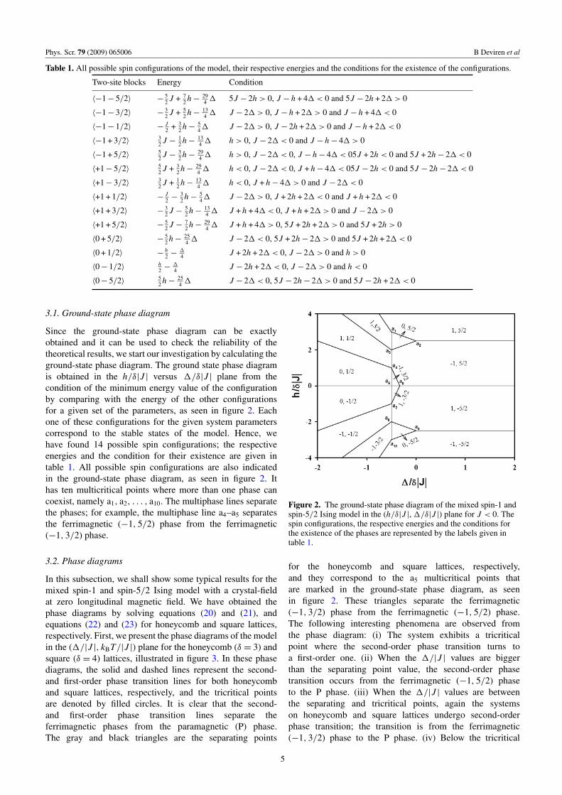
3.1. Ground-state phase diagram

Since the ground-state phase diagram can be exactlyobtained and it can be used to check the reliability of thetheoretical results, we start our investigation by calculating theground-state phase diagram. The ground state phase diagramis obtained in the h/δ|J | versus 1/δ|J | plane from thecondition of the minimum energy value of the configurationby comparing with the energy of the other configurationsfor a given set of the parameters, as seen in figure 2. Eachone of these configurations for the given system parameterscorrespond to the stable states of the model. Hence, wehave found 14 possible spin configurations; the respectiveenergies and the condition for their existence are given intable 1. All possible spin configurations are also indicatedin the ground-state phase diagram, as seen in figure 2. Ithas ten multicritical points where more than one phase cancoexist, namely a1, a2, . . . , a10. The multiphase lines separatethe phases; for example, the multiphase line a4–a5 separatesthe ferrimagnetic (−1, 5/2) phase from the ferrimagnetic(−1, 3/2) phase.

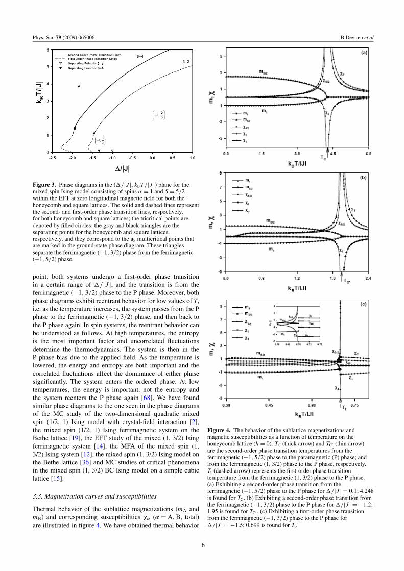
3.2. Phase diagrams

In this subsection, we shall show some typical results for themixed spin-1 and spin-5/2 Ising model with a crystal-fieldat zero longitudinal magnetic field. We have obtained thephase diagrams by solving equations (20) and (21), andequations (22) and (23) for honeycomb and square lattices,respectively. First, we present the phase diagrams of the modelin the (1/|J |, kBT/|J |) plane for the honeycomb (δ = 3) andsquare (δ = 4) lattices, illustrated in figure 3. In these phasediagrams, the solid and dashed lines represent the second-and first-order phase transition lines for both honeycomband square lattices, respectively, and the tricritical pointsare denoted by filled circles. It is clear that the second-and first-order phase transition lines separate theferrimagnetic phases from the paramagnetic (P) phase.The gray and black triangles are the separating points

Figure 2. The ground-state phase diagram of the mixed spin-1 andspin-5/2 Ising model in the (h/δ|J |, 1/δ|J |) plane for J < 0. Thespin configurations, the respective energies and the conditions forthe existence of the phases are represented by the labels given intable 1.

for the honeycomb and square lattices, respectively,and they correspond to the a5 multicritical points thatare marked in the ground-state phase diagram, as seenin figure 2. These triangles separate the ferrimagnetic(−1, 3/2) phase from the ferrimagnetic (−1, 5/2) phase.The following interesting phenomena are observed fromthe phase diagram: (i) The system exhibits a tricriticalpoint where the second-order phase transition turns toa first-order one. (ii) When the 1/|J | values are biggerthan the separating point value, the second-order phasetransition occurs from the ferrimagnetic (−1, 5/2) phaseto the P phase. (iii) When the 1/|J | values are betweenthe separating and tricritical points, again the systemson honeycomb and square lattices undergo second-orderphase transition; the transition is from the ferrimagnetic(−1, 3/2) phase to the P phase. (iv) Below the tricritical

5

Phys. Scr. 79 (2009) 065006 B Deviren et al

Figure 3. Phase diagrams in the (1/|J |, kBT/|J |) plane for themixed spin Ising model consisting of spins σ = 1 and S = 5/2within the EFT at zero longitudinal magnetic field for both thehoneycomb and square lattices. The solid and dashed lines representthe second- and first-order phase transition lines, respectively,for both honeycomb and square lattices; the tricritical points aredenoted by filled circles; the gray and black triangles are theseparating points for the honeycomb and square lattices,respectively, and they correspond to the a5 multicritical points thatare marked in the ground-state phase diagram. These trianglesseparate the ferrimagnetic (−1, 3/2) phase from the ferrimagnetic(−1, 5/2) phase.

point, both systems undergo a first-order phase transitionin a certain range of 1/|J |, and the transition is from theferrimagnetic (−1, 3/2) phase to the P phase. Moreover, bothphase diagrams exhibit reentrant behavior for low values of T,i.e. as the temperature increases, the system passes from the Pphase to the ferrimagnetic (−1, 3/2) phase, and then back tothe P phase again. In spin systems, the reentrant behavior canbe understood as follows. At high temperatures, the entropyis the most important factor and uncorrelated fluctuationsdetermine the thermodynamics. The system is then in theP phase bias due to the applied field. As the temperature islowered, the energy and entropy are both important and thecorrelated fluctuations affect the dominance of either phasesignificantly. The system enters the ordered phase. At lowtemperatures, the energy is important, not the entropy andthe system reenters the P phase again [68]. We have foundsimilar phase diagrams to the one seen in the phase diagramsof the MC study of the two-dimensional quadratic mixedspin (1/2, 1) Ising model with crystal-field interaction [2],the mixed spin (1/2, 1) Ising ferrimagnetic system on theBethe lattice [19], the EFT study of the mixed (1, 3/2) Isingferrimagnetic system [14], the MFA of the mixed spin (1,3/2) Ising system [12], the mixed spin (1, 3/2) Ising model onthe Bethe lattice [36] and MC studies of critical phenomenain the mixed spin (1, 3/2) BC Ising model on a simple cubiclattice [15].

3.3. Magnetization curves and susceptibilities

Thermal behavior of the sublattice magnetizations (mA andmB) and corresponding susceptibilities χα (α = A, B, total)are illustrated in figure 4. We have obtained thermal behavior

Figure 4. The behavior of the sublattice magnetizations andmagnetic susceptibilities as a function of temperature on thehoneycomb lattice (h = 0). TC (thick arrow) and TC′ (thin arrow)are the second-order phase transition temperatures from theferrimagnetic (−1, 5/2) phase to the paramagnetic (P) phase; andfrom the ferrimagnetic (1, 3/2) phase to the P phase, respectively.Tt (dashed arrow) represents the first-order phase transitiontemperature from the ferrimagnetic (1, 3/2) phase to the P phase.(a) Exhibiting a second-order phase transition from theferrimagnetic (−1, 5/2) phase to the P phase for 1/|J | = 0.1; 4.248is found for TC. (b) Exhibiting a second-order phase transition fromthe ferrimagnetic (−1, 3/2) phase to the P phase for 1/|J | = −1.2;1.95 is found for TC′ . (c) Exhibiting a first-order phase transitionfrom the ferrimagnetic (−1, 3/2) phase to the P phase for1/|J | = −1.5; 0.699 is found for Tt.

6

Phys. Scr. 79 (2009) 065006 B Deviren et al

of sublatice magnetizations and corresponding susceptibilitiesby solving equations (20) and (21), and equations (20),(21) and (25), respectively. We present a few representativegraphs to display their behavior for only a honeycomblattice, seen in figures 4(a)–(c). The results are depictedin figures 4(a)–(c) for the system with zero longitudinalmagnetic field (h = 0), when the values of 1/|J | are 0.1,−1.2 and −1.5, respectively. In these figures, TC (thick arrow)and TC′ (thin arrow) are the second-order phase transitiontemperatures from the ferrimagnetic (−1, 5/2) phase to theP phase and from the ferrimagnetic (−1, 3/2) phase tothe P phase, respectively. Tt (dashed arrow) represents thefirst-order phase transition temperature from the ferrimagnetic(−1, 3/2) phase to the P phase. It is seen from figure 4(a)for 1/|J | = 0.1 that the system undergoes a second-orderphase transition from the ferrimagnetic (−1, 5/2) phase tothe P phase, because sublattice magnetizations go to zerocontinuously as the temperature increases and a second-orderphase transition occurs at TC = 4.248. When the temperatureapproaches TC, the sublattice susceptibility χ5/2 increasesvery rapidly and goes to positive infinity at TC = 4.248. Onthe other hand, the other sublattice susceptibility χ1 decreasesvery rapidly and goes to negative infinity at TC = 4.248.The total susceptibility χT exhibits the usual temperaturebehavior in the vicinity of TC, χT → +∞ as T → TC. Thishas also been tested by our sublattice magnetizations andsusceptibilities calculations, because we found exactly thesame TC for both calculations. Figure 4(b) illustrates thethermal variations of m1, m5/2 and χα for 1/|J | = −1.2, andthe behavior of figure 4(b) is similar to figure 4(a), except thatthe system undergoes a second-order phase transition from theferrimagnetic (−1, 3/2) phase to the P phase at TC′ = 1.95.Figure 4(c) is calculated for 1/|J | = −1.5 and shows m1,m5/2 go to zero discontinuously as the temperature increases;hence a first-order phase transition occurs at Tt = 0.699.Moreover, in the vicinity of Tt the sublattice susceptibilityχ5/2 rapidly increases for T < Tt and suddenly decreases forT > Tt. On the other hand, χ1 decreases very rapidly forT < Tt and suddenly increases for T > Tt. If one comparesthe behavior of sublattice magnetizations and susceptibilities,one can see that Tt is found to be exactly the same for bothcalculations.

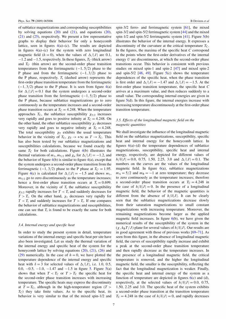
3.4. Internal energy and specific heat

In order to study the present system in detail, temperaturevariations of the internal energy and specific heat per site havealso been investigated. Let us study the thermal variation ofthe internal energy and specific heat of the system for thehoneycomb lattice by solving equations (20), (21), (26) and(29) numerically. In the case of h = 0, we have plotted thetemperature dependence of the internal energy and specificheat with δ = 3 for selected values of 1/|J |, i.e. 1.0, 0.5,0.0, −0.5, −1.0, −1.47 and −1.5 in figure 5. Figure 5(a)shows that when T < TC or T > TC the specific heat forthe second-order phase transition increases with increasingtemperature. The specific heats may express the discontinuityat T = TC, although in the high-temperature region (T >

TC) they take finite values. As to the specific heat, itsbehavior is very similar to that of the mixed spin-1/2 and

spin-3/2 ferro- and ferrimagnetic system [61], the mixedspin-3/2 and spin-5/2 ferrimagnetic system [44] and the mixedspin-1/2 and spin-5/2 ferrimagnetic system [41]. Figure 5(b)illustrates the behavior of the internal energy. It expresses adiscontinuity of the curvature at the critical temperature TC.In the figures, the maxima of the specific heat C correspondto the points where the first-order derivatives of the internalenergy U are discontinuous, at which the second-order phasetransitions occur. This behavior is consistent with previousstudies on mixed spin-1 and spin-2 [47] and mixed spin-2and spin-5/2 [48, 49]. Figure 5(c) shows the temperaturedependences of the specific heat, when the phase transitionis first order and 1/|J | = −1.47 and 1/|J | = −1.5. At thefirst-order phase transition temperature, the specific heat Carrives at a maximum value, and then reduces suddenly to asmall value. The corresponding internal energies are given infigure 5(d). In this figure, the internal energies increase withincreasing temperature discontinuously at the first-order phasetransition temperature.

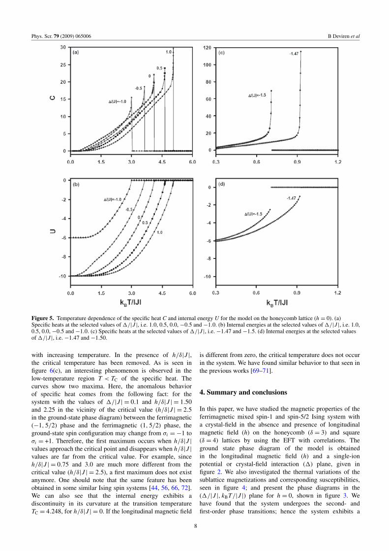
3.5. Effects of the longitudinal magnetic field on themagnetic quantities

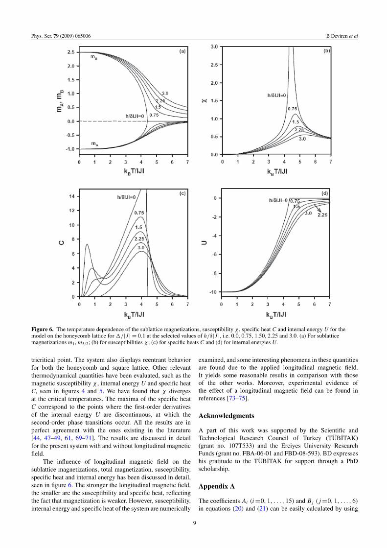
We shall investigate the influence of the longitudinal magneticfield on the sublattice magnetizations, susceptibility, specificheat and internal energy for the honeycomb lattice. Infigures 6(a)–(d) the temperature dependences of sublatticemagnetizations, susceptibility, specific heat and internalenergy, respectively, are depicted for different values ofh/δ|J | = 0.0, 0.75, 1.50, 2.25, 3.0 and 1/|J | = 0.1. Thenumbers on the curves are the values of the longitudinalmagnetic field. In figure 6(a), sublattice magnetizationsmA = 5/2 and mB = −1 at zero temperature; they decreaseto zero continuously as the temperature increases; thereforea second-order phase transition occurs at TC = 4.248 inthe case of h/δ|J | = 0. In the presence of a longitudinalmagnetic field, the behavior of the magnetic quantities isdifferent from the absence of h/δ|J |. It can be clearlyseen that the sublattice magnetizations decrease slowlyfrom their saturation magnetizations to small constantmagnetizations with increasing temperature. Moreover, theremaining magnetizations become larger as the appliedmagnetic field increases. In figure 6(b), we have given thenumerical results of the susceptibility of the system in the(χ, kBT/J ) plane for several values of h/δ|J |. Our results arein good agreement with those of previous works [69–71]. Asseen from this figure, in the absence of longitudinal magneticfield, the curves of susceptibility rapidly increase and exhibita peak at the second-order phase transition temperatureand then rapidly decrease as the temperature increases. Inthe presence of a longitudinal magnetic field, the criticaltemperature is removed, and the higher the longitudinalmagnetic field, the smaller is the susceptibility, reflecting thefact that the longitudinal magnetization is weaker. Finally,the specific heat and internal energy of the system as afunction of temperature are depicted in figures 6(c) and (d),respectively, at the selected values of h/δ|J | = 0.0, 0.75,1.50, 2.25 and 3.0. The specific heat of the system exhibitsa second-order phase transition at the transition temperatureTC = 4.248 in the case of h/δ|J | = 0, and rapidly decreases

7

Phys. Scr. 79 (2009) 065006 B Deviren et al

Figure 5. Temperature dependence of the specific heat C and internal energy U for the model on the honeycomb lattice (h = 0). (a)Specific heats at the selected values of 1/|J |, i.e. 1.0, 0.5, 0.0, −0.5 and −1.0. (b) Internal energies at the selected values of 1/|J |, i.e. 1.0,0.5, 0.0, −0.5 and −1.0. (c) Specific heats at the selected values of 1/|J |, i.e. −1.47 and −1.5. (d) Internal energies at the selected valuesof 1/|J |, i.e. −1.47 and −1.50.

with increasing temperature. In the presence of h/δ|J |,the critical temperature has been removed. As is seen infigure 6(c), an interesting phenomenon is observed in thelow-temperature region T < TC of the specific heat. Thecurves show two maxima. Here, the anomalous behaviorof specific heat comes from the following fact: for thesystem with the values of 1/|J | = 0.1 and h/δ|J | = 1.50and 2.25 in the vicinity of the critical value (h/δ|J | = 2.5in the ground-state phase diagram) between the ferrimagnetic(−1, 5/2) phase and the ferrimagnetic (1, 5/2) phase, theground-state spin configuration may change from σi = −1 toσi = +1. Therefore, the first maximum occurs when h/δ|J |

values approach the critical point and disappears when h/δ|J |

values are far from the critical value. For example, sinceh/δ|J | = 0.75 and 3.0 are much more different from thecritical value (h/δ|J | = 2.5), a first maximum does not existanymore. One should note that the same feature has beenobtained in some similar Ising spin systems [44, 56, 66, 72].We can also see that the internal energy exhibits adiscontinuity in its curvature at the transition temperatureTC = 4.248, for h/δ|J | = 0. If the longitudinal magnetic field

is different from zero, the critical temperature does not occurin the system. We have found similar behavior to that seen inthe previous works [69–71].

4. Summary and conclusions

In this paper, we have studied the magnetic properties of theferrimagnetic mixed spin-1 and spin-5/2 Ising system witha crystal-field in the absence and presence of longitudinalmagnetic field (h) on the honeycomb (δ = 3) and square(δ = 4) lattices by using the EFT with correlations. Theground state phase diagram of the model is obtainedin the longitudinal magnetic field (h) and a single-ionpotential or crystal-field interaction (1) plane, given infigure 2. We also investigated the thermal variations of thesublattice magnetizations and corresponding susceptibilities,seen in figure 4; and present the phase diagrams in the(1/|J |, kBT/|J |) plane for h = 0, shown in figure 3. Wehave found that the system undergoes the second- andfirst-order phase transitions; hence the system exhibits a

8

Phys. Scr. 79 (2009) 065006 B Deviren et al

Figure 6. The temperature dependence of the sublattice magnetizations, susceptibility χ , specific heat C and internal energy U for themodel on the honeycomb lattice for 1/|J | = 0.1 at the selected values of h/δ|J |, i.e. 0.0, 0.75, 1.50, 2.25 and 3.0. (a) For sublatticemagnetizations m1, m5/2; (b) for susceptibilities χ ; (c) for specific heats C and (d) for internal energies U.

tricritical point. The system also displays reentrant behaviorfor both the honeycomb and square lattice. Other relevantthermodynamical quantities have been evaluated, such as themagnetic susceptibility χ , internal energy U and specific heatC, seen in figures 4 and 5. We have found that χ divergesat the critical temperatures. The maxima of the specific heatC correspond to the points where the first-order derivativesof the internal energy U are discontinuous, at which thesecond-order phase transitions occur. All the results are inperfect agreement with the ones existing in the literature[44, 47–49, 61, 69–71]. The results are discussed in detailfor the present system with and without longitudinal magneticfield.

The influence of longitudinal magnetic field on thesublattice magnetizations, total magnetization, susceptibility,specific heat and internal energy has been discussed in detail,seen in figure 6. The stronger the longitudinal magnetic field,the smaller are the susceptibility and specific heat, reflectingthe fact that magnetization is weaker. However, susceptibility,internal energy and specific heat of the system are numerically

examined, and some interesting phenomena in these quantitiesare found due to the applied longitudinal magnetic field.It yields some reasonable results in comparison with thoseof the other works. Moreover, experimental evidence ofthe effect of a longitudinal magnetic field can be found inreferences [73–75].

Acknowledgments

A part of this work was supported by the Scientific andTechnological Research Council of Turkey (TÜBITAK)(grant no. 107T533) and the Erciyes University ResearchFunds (grant no. FBA-06-01 and FBD-08-593). BD expresseshis gratitude to the TÜBITAK for support through a PhDscholarship.

Appendix A

The coefficients Ai (i =0, 1, . . . , 15) and B j ( j =0, 1, . . . , 6)

in equations (20) and (21) can be easily calculated by using

9

Phys. Scr. 79 (2009) 065006 B Deviren et al

the mathematical relations exp(α∇) f (x) = f (x + α) andexp(α∇)g(x) = g(x + α), where ∇ = ∂/∂x is a differentialoperator. These coefficients Ai (i = 0, 1, . . . , 15) andB j ( j = 0, 1, 2, . . . 6) are obtained as follows:

A0 =1

16 777 216 [27 f1(−15J/2) − 675 f1(−13J/2)

+ 9675 f1(−11J/2) − 79 075 f1(−9J/2)

+ 415 575 f1(−7J/2) − 989 919 f1(−5J/2)

+ 86 775 f1(−3J/2) + 8946 225 f1(−J/2)

+ 8946 225 f1(J/2) + 86 775 f1(3J/2)

− 989 919 f1(5J/2) + 415 575 f1(7J/2)

− 79 075 f1(9J/2) + 9675 f1(11J/2)

− 675 f1(13J/2) + 27 f1(15J/2)],

A15 =1

1728 000 [− f1(−15J/2) + 15 f1(−13J/2)

− 105 f1(−11J/2) + 455 f1(−9J/2) − 1365 f1(−7J/2)

+ 3003 f1(−5J/2) − 5005 f1(−3J/2) + 6345 f1(−J/2)

− 6345 f1(J/2) + 5005 f1(3J/2) − 3003 f1(5J/2)

+ 1365 f1(7J/2) − 455 f1(9J/2) + 105 f1(11J/2)

− 15 f1(13J/2) + f1(15J/2)],

B0 = g1(0),

B1 =32 [−g1(−J ) + g1(J )] ,

B2 =34 [−6g1(0) + g1(−2J ) + 2g1(−J ) + 2g1(J ) + g1(2J )],

B3 =18 [−g1(−3J ) − 12g1(−2J ) + 27g1(−J ) − 27g1(J )

+ 12g1(2J ) + g1(3J )],

B4 =38 [16g1(0) + g1(−3J ) − 9g1(−J ) − 9g1(J ) + g1(3J )],

B5 =38 [−g1(−3J ) + 4g1(−2J ) − 5g1(−J ) + 5g1(J )

− 4g1(2J ) + g1(3J )],

B6 =18 [−20g1(0) + g1(−3J ) − 6g1(−2J ) + 15g1(−J )

+ 15g1(J ) − 6g1(2J ) + g1(3J )].

Appendix B

The coefficients Ck (k = 0, 1, . . . , 20) and Dl (l =

0, 1, . . . , 8) in equations (22) and (23) can be easilycalculated by the same way. These coefficients are obtainedas follows:

C0 =1

4294 967 296 [81 f1(−10J ) − 2700 f1(−9J )

+ 49 950 f1(−8J ) − 576 300 f1(−7J ) + 4572 925 f1(−6J )

− 23 752 176 f1(−5J ) + 75 239 400 f1(−4J )

− 59 476 400 f1(−3J ) − 342 915 150 f1(−2J )

+ 1157 549 400 f1(−J ) + 2673 589 236 f1(0)

+ 1157 549 400 f1(J ) − 342 915 150 f1(2J )

− 59 476 400 f1(3J ) + 75 239 400 f1(4J )

− 23 752 176 f1(5J ) + 4572 925 f1(6J ) − 576 300 f1(7J )

+ 49 950 f1(8J ) − 2700 f1(9J ) + 81 f1(10J )],

C20 =1

207 360 000 [ f1(−10J ) − 20 f1(−9J ) + 190 f1(−8J )

− 1140 f1(−7J ) + 4845 f1(−6J ) − 15 504 f1(−5J )

+ 38 760 f1(−4J ) − 77 520 f1(−3J ) + 125 970 f1(−2J )

− 167 960 f1(−J ) + 184 756 f1(0) − 167 960 f1(J )

+ 125 970 f1(2J ) − 77 520 f1(3J ) + 38 760 f1(4J )

− 15 504 f1(5J ) + 4845 f1(6J ) − 1140 f1(7J )

+ 190 f1(8J ) − 20 f1(9J ) + f1(10J )],

D0 = [g1(0)],

D1 = 2[−g1(−J ) + g1(J )],

D2 =12 [−14g1(0)+3g1(−2J )+4g1(−J )+4g1(J )+3g1(2J )],

D3 =12 [−g1(−3J ) − 6g1(−2J ) + 15g1(−J ) − 15g1(J )

+ 6g1(2J ) + g1(3J )],

D4 =116 [246g1(0) + g1(−4J ) + 24g1(−3J )

− 8g1(−2J ) − 120g1(−J ) − 120g1(J )

− 28g1(2J ) + 24g1(3J ) + g1(4J )],

D5 =14 [−g1(−4J ) − 4g1(−3J ) + 26g1(−2J ) − 36g1(−J )

+ 36g1(J ) − 26g1(2J ) + 4g1(3J ) + g1(4J )],

D6 =18 [−110g1(0) + 3g1(−4J ) − 8g1(−3J ) − 12g1(−2J )

+ 72g1(−J )+72g1(J )−12g1(2J )−8g1(3J )+3g14J )],

D7 =14 [−g1(−4J ) + 6g1(−3J ) − 14g1(−2J ) + 14g1(−J )

− 14g1(J ) + 14g1(2J ) − 6g1(3J ) + g1(4J )],

D8 =116 [70g1(0) + g1(−4J ) − 8g1(−3J ) + 28g1(−2J )

− 56g1(−J )−56g1(J )+28g1(2J )−8g1(3J )+g1(4J )].

References

[1] Iwashita T and Uryu N 1984 Phys. Status Solidi b 125 551[2] Zhang G M and Yang Ch Z 1993 Phys. Rev. B 48 9452[3] Kaneyoshi T 1999 Physica A 272 545[4] Kasama T, Muraoka Y and Idogaki T 2006 Phys. Rev. B 73

214411[5] Belmamoun Y and Kerouad M 2008 Phys. Scr. 77 025706[6] Benayad N, Dakhama A, Klumper A and Zittartz J 1996

Z. Phys. B 101 623[7] Bobak A and Jurcisin M 1996 J. Magn. Magn. Mater. 163 292[8] Buendía G M and Cardona R 1999 Phys. Rev. B 59 6784[9] Albayrak E and Akkaya S 2007 Phys. Scr. 76 354

[10] Essaoudi I, Barner K and Ainane A 2007 Physica A 385 208[11] Bobák A and Jurcisin M 1997 Physica B 233 187[12] Abubrig O F, Horvath D, Bobak A and Jascur M 2001

Physica A 296 437[13] Tucker J W 2001 J. Magn. Magn. Mater. 237 215[14] Bobak A, Abubrig O F and Horvath D 2002 J. Magn. Magn.

Mater. 246 177[15] Wei G Z, Zhang Q and Gu Y W 2006 J. Magn. Magn. Mater.

301 245.

10

Phys. Scr. 79 (2009) 065006 B Deviren et al

[16] Goncalves L L 1985 Phys. Scr. 32 248Goncalves L L 1986 Phys. Scr. 33 192

[17] Strecka J 2006 Physica A 360 379[18] Jascur M and Strecka J 2005 Condensed Matter Phys. 8 869[19] da Silva N R and Salinas S R 1991 Phys. Rev. B 44 852

Albayrak E and Keskin M 2003 J. Magn. Magn. Mater. 261196

[20] Ekiz C 2005 J. Magn. Magn. Mater. 293 759[21] Oitmaa J 2005 Phys. Rev. B 72 224404[22] Albayrak E and Yilmaz S 2008 Physica A 387 1173

Ekiz C 2008 Physica A 387 1185[23] Buendía G M and Machado E 1998 Phys. Rev. E 58 1260[24] Keskin M, Canko O and Polat Y 2008 J. Korean Phys. Soc. 53

497[25] Glauber R J 1963 J. Math. Phys. 4 294[26] Godoy M and Figueiredo W 2000 Phys. Rev. E 61 218[27] Godoy M and Figueiredo W 2002 Phys. Rev. E 65 026111[28] Godoy M and Figueiredo W 2002 Phys. Rev. E 66 036131[29] Godoy M and Figueiredo W 2004 Braz. J. Phys. 34 422

Godoy M and Figueiredo W 2004 Physica A 339 392[30] Ekiz C and Keskin M 2003 Physica A 317 517[31] Albayrak E and Alçi A 2005 Physica A 345 48

Ekiz C 2005 J. Magn. Magn. Mater. 293 913[32] Zhang X and Kong X M 2006 Physica A 369 589[33] Jascur M and Strecka J 2005 Physica A 358 393[34] Strecka J and Canová L 2006 Condensed Matter Phys. 9 179[35] Strecka J 2006 Phys. Status Solidi b 243 708[36] Albayrak E 2003 Int. J. Mod. Phys. B 17 1087

Ekiz C 2006 J Magn. Magn. Mater. 307 139[37] Deviren B, Keskin M and Canko O 2009 J. Magn. Magn.

Mater. 321 458[38] Keskin M, Kantar E and Canko O 2008 Phys. Rev. E 77

051130[39] Ekiz C 2005 Physica A 353 286[40] Matasovská S and Jascur M 2007 Physica A 383 339[41] Deviren B, Keskin M and Canko O 2009 Physica A 388 1835[42] Albayrak E and Yigit A 2007 Phys. Status Solidi b 244 748[43] Albayrak E and Yigit A 2006 Phys. Lett. A 353 121[44] Zhang Q, Wei G and Gu Y 2005 Phys. Status Solidi b 242 924[45] Keskin M, Ertas M and Canko O 2009 Phys. Scr. 79 025501[46] Wei G Z, Gu Y W and Liu J 2006 Phys. Rev. B 74 024422

Zhang Q, Wei G, Win Z and Lang Y 2004 J. Magn. Magn.Mater. 280 14

[47] Albayrak E and Yigit A 2005 Physica A 349 471[48] Kaneyoshi T, Nakamura Y and Shin S 1998 J. Phys.: Condens.

Matter 10 7025Nakamura Y 2000 Phys. Rev. B 62 11742

[49] Wei G Z, Zhang Q and Xin Z H 2004 J. Magn. Magn. Mater.277 1

[50] Albayrak E and Yigit A 2007 Physica A 375 174[51] Honmura R and Kaneyoshi T 1979 J. Phys. C: Solid State

Phys. 12 3979[52] Kaneyoshi T, Fittipaldi I P, Honmura R and Manabe T 1981

Phys. Rev. B 24 481

[53] Balcerzak T 1991 J. Magn. Magn. Mater. 97 152[54] Kaneyoshi T and Beyer H 1980 J. Phys. Soc. Japan 49 1306[55] Hai T and Li Z Y 1989 Phys. Status Solidi b 156 641

Hai T, Li Z Y, Lin G L and George T F 1991 J. Magn. Magn.Mater. 97 227

[56] Jascur M and Kaneyoshi T 1993 J. Phys.: Condens. Matter 56313

[57] Kaneyoshi T 1987 J. Phys. Soc. Japan 56 2675Kaneyoshi T 1988 Physica A 153 556Li Z Y and Kaneyoshi T 1988 Phys. Rev. B 37 7785Kaneyoshi T 1989 Solid State Commun. 70 975Kaneyoshi T 1990 J. Magn. Magn. Mater. 92 59Kaneyoshi T 1994 Physica A 205 677

[58] Benayad N, Klumper A, Zittartz J and Benyoussef A 1989Z. Phys. B 77 339

[59] Bobák A and Jurcisin M 1997 Physica A 240 647[60] Callen H B 1963 Phys. Lett. 4 161[61] Kaneyoshi T, Jascur M and Tomczak P 1992 J. Phys.:

Condens. Matter 4 L653Kaneyoshi T, Tucker J W and Jascur M 1992 Physica A 186

677[62] Kaneyoshi T and Jascur M 1993 Phys. Status Solidi b

175 225[63] Kaneyoshi T, Honmura R, Tamura I and Sarmento E F 1984

Phys. Rev. B 29 5121[64] Zernike F 1940 Physica A 7 565[65] Kaneyoshi T, Tamura I and Sarmento E F 1983 Phys. Rev. B

28 6491Kaneyoshi T 1986 Phys. Rev. B 33 7688

[66] Kaneyoshi T, Jascur M and Tomczak P 1993 J. Phys.:Condens. Matter 5 5331

[67] Kaneyoshi T, Jascur M and Fittipaldi I P 1993Phys. Rev. B 48 250

[68] Hui K 1988 Phys. Rev. B 38 802Keskin M, Pınar M A, Erdinç A and Canko O 2006

Physica A 364 263[69] Wei G Z, Liang Y Q, Zhang Q and Xin Z H 2004 J. Magn.

Magn. Mater. 271 246[70] Jiang W and Bai B D 2006 Phys. Status Solidi b 243 2892[71] Balcerzak T 2003 Physica A 317 213

Jiang W, Bai B D and Wei G Z 2005 Physica A 354 301Jiang W, Bai B D, Lo V C and Liu W 2005 J. Appl. Phys. 97

10B307Mancini F and Naddeo A 2006 Phys. Rev. E 74 061108Canpolat Y, Torgursul A and Polat H 2007 Phys. Scr. 76 597

[72] Kaneyoshi T and Jascur M 1992 Phys. Rev. B 46 3374Jiang W, Wie G Z and Xin Z H 2001 Phys. Status

Solidi b 225 215Kaneyoshi T 2004 Physica A 339 403

[73] Doerr M, Kramp S and Loewenhaupt M 2001Physica B 294 164

[74] Koyama K and Fujii H 2001 Physica B 294 168[75] Albertini F, Bolzoni F and Paoluzi A 2001 Physica B

294 172

11