Kinetics of domain growth in finite Ising strips

Physica A 183 (1992) 130-147 North-Holland ~ [ ~

Kinetics of domain growth in finite Ising strips

E.V. Albano 1, K. Binder, D.W. H e e r m a n n 2, and W. Paul lnstitut fiir Physik, Johannes Gutenberg Universitiit Mainz, Staudinger Weg 7, W-6500 Mainz, Germany

Received 28 November 1991

Monte Carlo simulations are presented for the kinetics of ordering of the two-dimensional nearest-neighbor Ising models in an L × M geometry with two free boundaries of length M >> L. This geometry models a "terrace" of width L on regularly stepped surfaces, adatoms adsorbed on neighboring terraces being assumed to be noninteracting. Starting out with an initially random configuration of the atoms in the lattice gas at coverage 0 = 1/2 in the square lattice, quenching experiments to temperatures in the range 0.85 ~< T/T c ~< 1 are considered, assuming a dynamics of the Glauber model type (no conservation laws being operative). At T~ the ordering behavior can be described in terms of a time-dependent correlation length ~:(t), which grows with the time t after the quench as ~(t) - t ~/~ with the dynamic exponent z ~ 2.1, until the correlation length settles down at its equilibrium value 2L/~ (for correlations in the direction of the steps). Below T c a two-stage growth is observed: in the first stage, the scattering intensity (rh2(t)) grows linearly with time, as in the standard kinetic Ising model, until the domain size is of the same size as the terrace width. The further growth of (ritz(t)) in the second stage is consistent with a logarithmic law.

1. Introduction and overview

The kinetics of the formation of ordered domains at surfaces has found widespread theoretical interest (for some reviews see refs. [1-9]) and also some experiments to test these ideas have been performed [9-16]. Clearly, an understanding of such processes is a prerequisite for a microscopic understanding of the dynamics of more complex processes in materials science involving surfaces, such as catalysis, corrosion, etc.

So far most of the theoretical work has considered adsorption on perfectly fiat ideal substrate surfaces of infinite extent. Such substrates rarely occur in nature. Thus occasionally substrates containing quenched [17-20[ or annealed

Alexander von Humboldt fellow. Present and permanent address: INIFTA, Universidad de La Plata, C.C. 16, Suc. 4, (1900) La Plata, Argentina.

2 Present address: Institut f/it Theoretische Physik, Universit~it Heidelberg, Philosophenweg 19, W-6900 Heidelberg, Germany.

0378-4371/92/$05.00 © 1992- Elsevier Science Publishers B.V. All rights reserved

E.V. Albano et al. / Domain growth in finite Ising strips 131

(mobile) impurities [21] have been considered. While on ideal substrates the domain size l(t) grows with time t (after the adatoms have been adsorbed on the surface in a completely random configuration) according to a power law, l(t) ~ t x, where the growth exponent x = 1/2 for a non-conserved order parameter [1-9], point defects are found to slow down the growth dramatically at late stages, leading e.g. to logarithmic growth laws ( l ( t ) ~ In t), since the domain walls get pinned [17-20].

In the present paper we consider another deviation from substrate surface ideality, which very frequently occurs in nature, namely the occurrence of surface steps. We consider a highly idealized situation only, assuming a perfectly regularly stepped surface (which in a "thought experiment" one produces by cutting a cubic crystal under a small angle relative to a (100) surface, see fig. 1). In previous work, we have shown that even this simplified model exhibits a wealth of ordering phenomena already in thermal equilibrium [22-25], even within the framework of the nearest-neighbor lattice gas model. Assuming a square lattice of preferred adsorption sites (fig. 1), the ordering

y ~ Z ,X

V L "1

T U I x )

0 . . . . . . r T r , ° T S. 1 I~ {L

x

Fig. 1. (a) Schematic view of a regularly s tepped surface, where steps at a distance L apart in x direction run parallel to each other over a distance M in y direction, to form a "staircase" of L x M terraces, on which adsorpt ion can take place.

(b) Cross section through one terrace of width L. Open circles represent substrate atoms, full circle represents an absorbate atom.

(c) Corrugat ion potential corresponding to the geometry of case (b). We assume that the substrate creates a lattice of preferred sites, at which ada toms can be bound to the surface with an energy e, In the rows adjacent to the terrace boundaries , however, in general different binding energies el, E L should be assumed. The energy barrier AU separates neighboring preferred sites.

132 E.V. Albano et al. / Domain growth in finite lsing strips

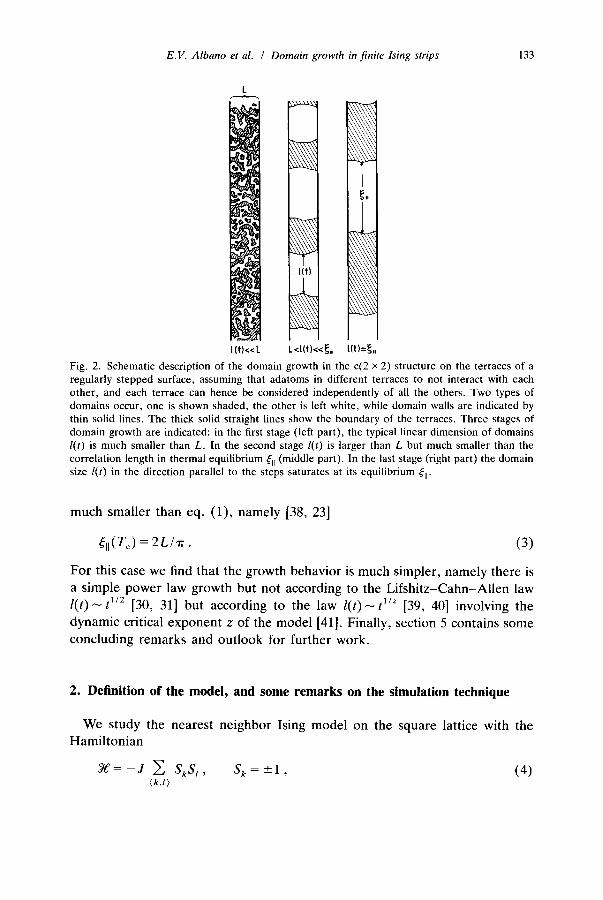
that would occur on an infinitely large flat terrace is the c(2 x 2) structure, see e.g. refs. [22, 26, 27]. In the finite terrace geometry L x M considered in fig. 1, no true long range order can occur even in the limit M--->~: since such a system is quasi one-dimensional, its ordering is unstable against the sponta- neous formation of domain walls, see fig. 2, which are typically spaced at a

distance ~:11 given by [28, 29]

~11 ~ L1/2 e x p ( f i n t L / k B T ) , (1)

where fint is the interfacial tension between coexisting domains with opposite orientation of the order parameter.

In the present paper, we consider domain growth for the case of this simple c(2 × 2) structure on L x M terraces with M>> L where the equilibrium structure is described by eq. (1) as long as M >> £11, while the system is ordered as a monodomain when ~11 ~> M [23]. We find that the standard curvature- driven [30-33] growth law l ( t ) - t 1/2 holds during very early stages only, requiring l ( t ) ~ L (fig. 2). Then a cross over sets in to a second stage with a much slower growth, possibly a logarithmic law

l ( t ) ~ in t . (2)

The slowness of the growth in this regime in fact is understood from the fact that as the domain walls in this regime on the average run straight over the terrace (fig. 2, middle part) , the average curvature which would act as a driving force vanishes. Due to the smoothness of the interfacial profile, there is a weak driving force leading to further coarsening of the structure, namely an interaction between walls decaying exponentially with the distance between them. By such a mechanism, there will be fewer and fewer walls left as time passes, and a growth law such as eq. (2) should result [34, 35]. This mechanism is reminiscent of a model suggested by Kawasaki and coworkers [34, 35], who considered the dynamics of an ensemble of interacting "kinks" and "antikinks". Basically the same law, eq. (2), also results for the dynamics of the formation of wetting layers at surfaces, where one also has to consider the random motion of an interface [36, 37]. However , if the average positions of the domain walls fluctuate, they may undergo a slow diffusive motion along the terrace and then the l ( t ) ~ In t law might cross over to l ( t ) ~ t I/2 again.

In section 2, we briefly describe the model and the simulation technique. Section 3 then describes the results obtained for quenches to temperatures below T c. Section 4 describes data on quenches right at the critical point T c. There in equilibrium the correlation function in the direction along the terrace for M--> o0 is predicted to show an exponential decay with a length ~II which is


L

t (t)<< L

t ( t ) I

L<t(t)<<~. I(t)=[,, Fig. 2. Schematic description of the domain growth in the c(2 x 2) structure on the terraces of a regularly stepped surface, assuming that adatoms in different terraces to not interact with each other, and each terrace can hence be considered independently of all the others. Two types of domains occur, one is shown shaded, the other is left white, while domain walls are indicated by thin solid lines. The thick solid straight lines show the boundary of the terraces. Three stages of domain growth are indicated: in the first stage (left part), the typical linear dimension of domains l(t) is much smaller than L. In the second stage l(t) is larger than L but much smaller than the correlation length in thermal equilibrium ~¢11 (middle part). In the last stage (right part) the domain size l(t) in the direction parallel to the steps saturates at its equilibrium ~11"

m u c h smal ler than eq. (1), name ly [38, 23]

¢ft(Tc) : 2 L / , n . (3)

For this case we find that the growth behav ior is much simpler , namely there is

a s imple power law growth but not according to the L i f s h i t z - C a h n - A l l e n law

l ( t ) ~ t 1/2 [30, 31] bu t according to the law l ( t ) - t l/z [39, 40] involving the

dynamic critical e x p o n e n t z of the model [41]. Final ly , section 5 conta ins some

conc lud ing remarks and ou t look for fur ther work.

2. Definition of the model, and some remarks on the simulation technique

We study the neares t ne ighbor Ising mode l on the square lattice with the H a m i l t o n i a n

= - J ~ S k S I , S k = - - + l , (4) (k,l>

1 3 4 E.V. Albano et al. / Domain growth in finite lsing strips

with ferromagnetic exchange interaction J restricted between nearest neighbors. The symbol (k , l) indicates that over pairs of nearest neighbors is summed once. We choose a L x M geometry (fig. 1) with two free boundaries of length M and periodic boundary conditions in the other direction. In contrast to refs. [22-25] neither fields at the boundaries nor in the bulk are applied. In the framework of the lattice gas model alluded to in fig. 1, this corresponds to a choice of binding energies e I = •L = • + 2J and a choice of the

chemical potential /z = - e + 8J. In view of the nonuniformity of the physical properties across the terrace

(fig. 1) created by the free boundary conditions, it is of interest to distinguish correlation functions parallel and perpendicular to the free ends of the terrace, and to consider the order parameter profile across the terrace. Denoting S k = S(i, j, t), where the index i labels the x coordinate of lattice site k (the direction across the terrace, see fig. 1) and t is the observation time in the simulation, and j the y coordinate, the local order parameter of interest is the

row magnetization m(i , t), M

m(i , t) = ( l / M ) ~ S(i, j, t ) . (5) j=l

Our initial condition at time t = 0 always is a random spin configuration, and the system evolves in time according to the standard single spin flip Monte Carlo method as described in ref. [42], using transition probabilities like in the work of Metropolis et al. [43]. Time t is then measured in the unit of at tempted Monte Carlo steps per site (MCS), spins being considered for flipping in a sequential order. The deterministic choice of the next spin to be updated, that is, the next at tempted configuration in phase space enhances the mobility of the interfaces but will not change the time laws of the growth processes we want to study. Of course, in this type of nonequilibrium Monte Carlo simulation it is crucial to average over a large number of statistically independent runs [40]. We used samples of at least 288 up to 1000 runs. These calculations were carried out at the multitransputer facility of the Condensed Matter Theory Group at Mainz (see refs. [23, 44] for a description of this facility), using a random number generator described in ref. [45]. The sample averaging in the following will be denoted by the symbol ( . . . ) .

Of course, in the absence of magnetic fields the symmetry of the Hamilto- nian eq. (4) against spin reversal implies (re(i , t)) -~ 0, and this property is in fact satisfied by the simulation to a very good accuracy. Hence the quantity which is actually recorded is the average of the absolute value, ([m(i, t)[), of the profile, as well as the total magnetization and its square

L

(Ir~(/)[) = ( l /L) ~ (Im(i, t)[), (6) i = 1

E.V. Albano et al. / Domain growth infinite lsing strips 135

(( )) (rh2(t)) = ( l / L ) ~] m(i, t) . (7) i = 1

In addition, we study the correlation functions parallel and perpendicular to the terrace,

L

gll(Y, t) --- ( l / L ) ~] (S(i , j, t) S(i, j + y, t)) , (8) i = 1

M

g l ( x , t) = ( l / M ) ~ (S(1, j , t) S(1 + x, j, t ) ) . (9) j = l

Note that all distances are measured in units of the lattice spacing, and in eq. (8) the index j also is averaged over, as is appropriate due to the translational invariance in the y direction. Of course, due to the free boundary conditions the correlation gll(x = i, y, t) = (S(i , j, t) S(i, j + y, t)) depends on the x coordinate explicitly. This dependence is not considered here, only a correlation averaged across the terrace is considered, in order to gain statistics. Similarly, correlations (S( i , j, t) S(i + x, j, t)) are expected to depend on both i and x: only the special case where one site (i) is at the free boundary is actually considered here.

3. Quenching "experiments" to temperatures T < T c

Fig. 3 gives typical data for the time evolution of the magnetization profile across the terrace. It is seen that already after a short time ( t - 2 0 0 MCS) the profile has reached the shape which is also characteristic for the equilibrium shape [22], while its absolute magnitude is still significantly too small. It is also seen that at short times (t = 10 to 40MCS) the range over which the free boundary reduces the profile is only 2 to 3 lattice spacings, while at later times this range is significantly larger, particularly at the temperature T = 0.95T c. This gradual build-up of correlations across the terrace is also obvious from the behavior of the correlation function g±(x, t), see fig. 4. It is seen that this correlation function at late times is rather flat in the center of the terrace and then decreases strongly at the other side of the terrace (figs. 4a,b). This behavior reflects the fact that fluctuations of the order parameters are large near the two free boundaries, and for temperatures such that the correlation length ~: is distinctly smaller than L these fluctuations near the two boundaries are not much correlated. In contrast, at T c (fig. 4c) correlations extend throughout the terrace from one boundary to the other, and then such an effect is absent. Fig. 5 shows the time dependence of the absolute value of the total magnetization and its square. While the law (rh 2(t))~ t holds initially (for times t ~< 40), a crossover to a slower growth is clearly recognized at the later

136 E.V. Albano et al. / Domain growth in finite 1sing strips

^

E v

.45

.'40

.35

• 30

.25

.20

.15

.10

.85

O.

,~0 t. 10 ..-z,O x 9 0 ~ 180

5 I0 15 20 25

i

A__

g

. 4 5

. 4 0

. 3 5

. 3 0

.25

. 2 0

. 1 5

. l O

. 0 5

O.

mO ~ I0 +40 xgO ~180

5 10 15 20 2 5

i

.'55

.43

.35

30

.25

:~ .20 E T .15

.10

.35

@.

~0 ~I0 +40 ×90 ~180

~ l [ k ~ l I d { ~ t l l h l I I I I I I I { I l d l l l I I I ] 1 I d { ~ l ~ h ' 1 '

5 19 15 20 25

i

Fig. 3. Time evolution of the order parameter profile (Im(i, t)]) for T/T~ = 0.85 (a), 0.90 (b) and 0.95 (c), using L = 24, M --= 288 and 325 (a), 533 (b) and 190 (c) samples. Different symbols indicate various times t, as shown in the figure.


1.0

. 9

.8

: .7

X . 6 -4

.4

.3

.2

.1

O.

o O ~ 0 +t.O x 9 0 ~,180 a

0 5 i0 15 20 x

x

.9

.8

.7

.6

.5

.4

.3

.2

.i

3.

I,-, oO ~, 10 4- t.O x 90 • 180 u

i , . . . . . .

0 5 10 15 20 ×

. 8

7

5

5

4-

3

2

1

O.

C eO AIO ,,/,0 x90 ,~ 180

0 5 I 0 15 20 x

Fig. 4. Time evolution of the transverse correlation function g±(x, t) for T / T c = 0.85 (a), 0.95 (b) and 1.0 (c), using L = 24 and M = 288 throughout. 288 samples were used in case (c). Different symbols indicate various times t, as shown in the figure.


,25

A

_= .:o lie

.15

.1@

A

A-" .05 IE V

09

(9

0 (9

/e,

J

50 i00 150

i

^ O @

LE V

. 15

. i 0 A

~ . 0 5 V

¢,

0 ¢,

0

O 0

o / / " ~ ~ ~ ~ ~ ~, ~

50 100 150

t

Fig. 5. Time evolution of (Irh(t)l) (octagons) and (rh2(t)) (triangles) for T / T c = 0.85 (a) and 0.95 (b). Straight lines indicate the initial (tfi2(t)) ~ t law.

times. It must be emphasized that the data in fig. 5 are still far from equilibrium at all times shown: e.g. , at T / T c = 0 . 8 5 , the equilibrium value of (In]I) is ( I r h ( t ~ o g l ) = ( I r h l ) T ~ 0 . 8 7 [231, and at T / T ~ = 0 . 9 5 , ([rh(t~ogl) ~ 0 . 3 6 . For L = 12 and M = 144 very long runs have been performed (up to t = 9500 MCS), averaging over 302 samples at T/T¢ = 0.95. In this case, equilibrium was reached at a time of about t ~ 300 steps. We expect that for the larger systems the equilibration times where I(t) settles down at ~11 (fig. 2) are much larger. Since the approach of (In~(t)[) and {rh2(t)) to the respective thermal equilibrium values ( In] ] ) T and (rh 2) r is very gradual, the associated relaxation time is rather hard to measure precisely from (noisy!) Monte Carlo data, and thus we have not attempted to do this.

Fig. 6 shows that at intermediate times the growth law is indeed consistent with the expected logarithmic law, eq. (2). The intercept of the apparent straight line in the law (rh2(t)) oc (In t - In t . . . . . ) with the abscissa can be taken as a definition of the effective crossover time from the initial law, (rh2(t)) oc t,


0.12

0.10 i ! i i

~i b°' 008

7E o.oo

0.O4

0.02 ~ ~ 0 * * 8 m v" f , a ,

2 5 10 20 50 I00 200

t

Fig. 6. Plot of (rn2(/)) VS. In t for the system with L = 24, M = 288 and four temperatures as indicated.

to the logarithmic law. It is clear that f rom such a definition crossover times in

the range t .. . . . ~- 10 to t .. . . . ~ 20 result, in the range of temperatures studied. In fact, defining a crossover t ime t .. . . . by equating l(t) and L one finds [40]

L -~ l(t) ~ (1 - T/Tc)"(z-2)t 1/2 ~ t . . . . . o c L2(1 - T/Tc) -2~(z-2~ '

T---~ T c , (10)

where u is the correlation length exponent and z the dynamic exponent (v = 1 and z ~ 2.13 [46] in the Ising model) . However , the data in fig. 6 seem to imply a somewhat stronger tempera ture dependence of t . . . . . rather than what would follow from eq. (10), but this may be due to the fact that eq. (10) holds only very close to the critical point.

If one would assume that (rh 2(0 ) follows a crossover scaling of the form

{th2(t)) ~ (1 - T/To) 2È(z 2)tf(t/t . . . . . ) , (11)

where the scaling function f ( x ) must have the propert ies f(x--->0)----~l, f ( x - - -~ ) - - ->( lnx ) / x , one would predict that the prefactor of the logarithm depends on L only but not on temperature ,

( rh2(t)) 0c LZ(ln t - In t c . . . . ) . (12)

This would imply that the straight lines in fig. 6 (for T less than Tc) should all be parallel to each other. While this holds for T = 0.85T c and T = 0 .90T c, it


seems to be violated for T = 0 .95T c. We cannot rule out, however , that the data for T = 0 .95T c are imprecise due to an insufficient sample averaging or due to a too small value of M.

It also is of great interest to study the approach of the correlation function gLl(Y, t) (eq. (8)) towards equilibrium (fig. 7). In equilibrium, one ultimately

A

~°t~Ooo 0.5 l a * * X X x O o a * * xx~oOO

* + x x Oo o

+ x o o . Xx x oo °

÷ x x oo * x °o

0.2 ~ *÷ x x ± +

+ ±

0.1 ÷

0 . 0 5 ±

TIT c =0.85 a +

L=26 M=288 t=10

°ooo

K °o o x x t=180

x x

x

t= 90

0.02

(a) 0.01

0

÷ t=40

10 20 30

Y / t = 10 ~ f S / t = 40lope

1.5 5.0

2.0 ~ +'++'/,, ~" ~ . , , * j o t = 18o

-~ , ++/~

~ . . . ~ , ~ L(t)

0 . 2 ~ slope=O 5

0.11 (b ) 1 2 5 10 20 50

Y Fig. 7. (a) Semilog plot of the longitudinal correlation function gll(Y) as function of the distance y along the y axis of the terraces (fig. 1), for L = 24, M = 288, T = 0.85T~ and four t imes t after the quench as indicated.

(b) Same as (a) but log- log plot of In gll(Y, t) vs. In y. Arrows indicate l(t) for t = 4, 9 and 18 ( f rom left to right, respectively).

E.V. Albano et al. / Domain growth in finite lsing strips 141

expects the behavior glt(Y, t )~ exp(-y/~:ll ), for y of the order of ~11 (eq. (1)). Thus it is interesting to test whether the behavior at intermediate times can simply be described by an exponential decay with a time-dependent length, gll(Y, t )~exp[ -y / l ( t ) ] , which is the picture implicitly suggested by fig. 2. If such a relation were true, one simply would expect straight line behavior on the semilog plot, fig. 7a. However, this simple law does not seem to be a correct description for the range of times and distances displayed in fig. 7a, as is obvious from the pronounced curvature for the semilog plot. In order to check for other possible decay laws fig. 7b replots the same data as shown in fig. 7a in the form of a log-log plot of In gPr(Y, t) vs. y; a Gaussian decay or a stretched exponential behavior would show up as a straight line. It is seen that after a short transient period (t~>50MCS) the correlation function settles down according to a behavior where two distinct regions can be recognized: in a region where y is less than the characteristic length l(t) we have - l n g ( y , t ) ~ y ~/2, while the decay for y > l ( t ) seems to be stronger than exponential (an exponential decay should show up as a slope one in fig. 7, but the effective slope for y > l(t) in fig. 7b seems to be close to 1.5). One must bear in mind, of course, that the regime of y shown in fig. 7 is y ~< L = 24; and it is possible that only for l(t)>> L does one find the decay gll(Y, t) exp[-y/ l ( t )] . In fig. 7b, the estimates for l(t) were extracted from the data in fig. 6 via the formula [40]

12(t) = L M ( r h Z ( t ) ) / ( r n Z ) r . (13)

Clearly, it would be interesting to study gll(Y, t) also in the regime of very late times where l(t) >> L. This would require much more statistical effort than was available for the present study, and hence is left to a future investigation. Also an understanding for the behavior - I n g(y, t)o:y 1/2 for y < l ( t ) would be desirable.

4. Quenching "experiments" to the critical temperature

Some of our data for the choice T = T c were already included in figs. 4 and 6. These data have already indicated that some features of the behavior of the growth of correlations are distinctly different here. Of course, we may expect that the behavior is somewhat simpler for T = T~ than for T < To: in the latter case, we have very different static lengths controlling thermal equilibrium: the correlation length ~:l, which measures the extent over which boundary effects are felt in profiles of the order parameter (fig. 3) or the correlation function


g l ( x , t), fig. 4; the terrace width L; and the correlation length ~11 (eq. (1), fig. 2). At the critical point, however, all three lengths are of the same order (cf. eq. (3), for instance).

This behavior is also apparent from the time evolution of the profile (Im(i, t)l) of the absolute value of the magnetization across the film (due to our choice of M finite this quantity stays nonzero for T t> To, of course). Fig. 8 shows that (Ira(i, t)l) is flat in the central part of the film only for very early times, where the characteristic length l ( t ) ~ L ; at later times where l ( t )

saturates at a value of order L the profile is nonuniform throughout the film. A strikingly simple behavior now also results for the behavior of the

longitudinal correlation function gll(Y, t): apart from very small y, the data are now consistent with a simple exponential decay, even at very early times (fig. 9). The resulting time-dependent correlation length ~(t) is consistent with the expected power law [39, 40]

~( t ) ~ t ' /z (14)

with z ~ 2.13 [46], see fig. 10, until ~(t) saturates at the equilibrium value, as given by eq. (3).

At this point, we comment on the apparent logarithmic growth law seen also for T = T c in fig. 6. Since all characteristic time-dependent lengths should first grow proportional to ~(t) as given by eq. (14), as long as ~(t) ~ L, and in the late stages settle down at constant values of order L (as shown by eq. (3), for example), it is not clear if at T c a meaningfully large range of times, where ( th 2(t)) ~ In t holds, exists. Although in fig. 6 the data are consistent with such a law for about a decade in time, (th 2(0) increases only by about a factor of two in this regime, and thus the good fit to a law ( t h e ( t ) ) ~ l n t may be a numerical coincidence of any function showing a slow saturation at an equilibrium value. In fact, the saturation value of (th2(t)) is nearly reached at t = 2 0 0 MCS: this is seen from the finite size scaling result for such terrace geometries [47],

(th2) T. c "/M, (is)

where ~7 = 1/4 for the d = 2 Ising model. Neglecting the prefactor of order unity in eq. (15), one would obtain ( th2)rc=0.0377. From the data of refs. [22, 23] one obtains (th 2)Tc (L = 24, M = 288) ~ 0.036, which coincides with the saturation value reached in the present simulation. Again, extensive additional simulations studying the precise functional form of the approach towards equilibrium and the associate relaxation time would be very desirable.


A

~2 e v

35

30

25

20

15

I0

05

O.

• 0 ~ 10 * 40 × 90 ~, 180

5 IC 15 20 25

i

Fig. 8. T ime evolution of the order parameter profile (Ira(i, t)l ) for T = To, L = 24, and M = 288. Da ta are obtained from averaging 288 samples. Different symbols indicate various t imes t,

1.0

0.50

0.20

o.lo

0.05

0.02

0.01

\ .

k i ~ . ~ . ~ ~ 1t}:12"93

\ . \ t=90 I~1t1=11.73

' ~ ~,~-~(t I = 7.75 T = T c

L=2/, M=288 \ ~\ t=lO t=40

i i i

10 20 30

Y

Fig. 9. Semilog plot of the longitudinal correlation function gri(Y, t) as function of the distance y for T = To, L = 24 and M = 288. Straight lines indicate a behavior gll (Y, t)o: exp[-y/~(t)], and the value of ~(t) is indicated for all four t imes t shown.

144 E.V. Albano et al. / Domain growth in finite Ising strips

2 0 ~ . .~-'- . . . . . . . . . . . .

10 - o ~ ( T c ) : 2 L / ~

t.7

5

t Fig. 10. Log-log plot of the time-dependent correlation length ¢(t), as extracted from fig. 9, versus time. Dashed horizontal asymptote indicates the equilibrium length given by eq. (3).

5. Conclusions

In this paper some Monte Carlo studies simulating the growth of ordered domains out of initially disordered configurations on terraces of width L at stepped surfaces were presented. Also the growth of correlations out of initially disordered systems right at the critical temperature was considered. In the latter case, the behavior is relatively simple: the (longitudinal) correlation function along the terrace is a simple exponential (fig. 9), and the time- dependent correlation length ¢(t) grows according to power law (¢(t)oc t l /z

with z-~ 2.13) until it saturates at the characteristic length occurring in thermal equilibrium, ¢(Tc)= 2L/~r (fig. 10). Both in the order parameter profile (fig. 8) and in the (transverse) correlation function across the terrace (fig. 4c) there is spatial structure on a single length scale, of order L.

For T < Tc, however, many more length scales are simultaneously relevant in this problem, and thus the behavior is much more intricate: both in the order parameter profiles across the terrace (figs. 3a-c) and the transverse correlation function (figs. 4a,b) the finite thermal correlation length ~T ~ 11 - T~ Tel ~ provides additional structure; in the direction parallel to the steps, the large length El I ~ L I/2 exp ( f~n tL /kBT) >> L allows for a second regime of slow domain growth (probably logarithmic), in addition to the standard growth law for the domain size, l ( t ) ~ t 1/2, valid for l ( t ) ~ L. As is obvious from figs. 5a,b, deviations from this standard growth law occur soon, and the crossover to the (logarithmic?) law (fig. 6) is not sharp. Thus if one has only a limited time range for analysis at ones disposal, as it always happens in experiment, one may easily take a step-induced crossover as observed here as


an effective growth exponent a in a power law l ( t ) ~ t a with a distinctly smaller

value than a = 1/2. In real systems, the situation will be further complicated due to some distribution of terrace widths and also irregularities along the steps, which are not ideally straight as supposed in figs. 1 and 2 but may have kinks and other defects.

F rom this discussion it is clear that the present model is a crude simplifica- tion of reality. Nevertheless, even for this simple model the present study is only a first exploratory step and many conclusions remain tentative specula- tions: we have restricted ourselves to a single choice of L, and also only a modest range of times was investigated. For certain aspects, studies with distinctly larger values of M (to simulate the limiting behavior for M - - - ~ ) would be very desirable. All these studies are very involved and time- consuming, however, since extensive sample averaging over many equivalent Monte Carlo runs is necessary. For the present work we have used only of the order of 150 hours CPU time on a multitransputer facility; after this exploratory study we plan a more extensive investigation in future, which will need

about a factor 100 more effort. Finally, we point out that the present problem may also be relevant for

technologically relevant processes such as grain growth in two-phase materials containing randomly placed parallel fibers or whiskers [48].

Acknowledgements

One of us (E.V.A.) was supported by the Alexander von Humbold t -

foundat ion during his stay in Mainz. Also partial support f rom the Materialwis- senschaftliches Forschungszentrum ( M W F Z ) and the Bundesministerium f/Jr Forschung und Technologie (BMFT) , Bonn, and the B A Y E R A G , Lever- kusen, under grant no. 03M4028 is acknowledged. We thank G.S. Grest for

useful comments .

References

[1] J.D. Gunton, M. San Miguel and P.S. Sahni, in: Phase Transitions and Critical Phenomena, vol. VIII, C. Domb and J.L. Lebowitz, eds. (Academic Press, New York, 1983) p. 267.

[2] H. Furukawa, Adv. Phys. 34 (1985) 703. [3] K. Binder and D.W. Heermann, in: Scaling Phenomena in Disordered Systems, R. Pynn and

T. Skjeltorp, eds. (Plenum, New York, 1985) p. 207. [4] K. Binder, Ber. Bunsenges. Phys. Chem. 90 (1986) 257. [5] K. Binder, D.W. Heermann, A. Milchev and A. Sadiq, in: Heidelberg Colloquium on Glassy

Dynamics, I. Morgenstern and L. van Hemmen, eds., Lecture Notes in Physics, vol. 275 (Springer, Berlin, 1987) p. 154.


[6] O.G. Mouritsen, in: Kinetics of Ordering and Growth at Surfaces, M.G. Lagatly, ed. (Plenum, New York, 1990) p. 1.

[7] K. Binder, in: Kinetics of Ordering and Growth at Surfaces, M.G. Lagally, ed. (Plenum, New York, 1990) p. 31.

[8] K. Binder, in: Phase Transformations in Materials, P. Haasen, ed., Materials Science and Technology, vol. 5 (VCH Verlagsgesellschaft, Weinheim, 1991) p. 405.

[9] S. Komura and H. Furukawa, eds., Dynamics of Ordering Processes in Condensed Matter (Plenum, New York, 1988).

[10] M.G. Lagally, ed., Kinetics of Ordering and Growth at Surfaces (Plenum, New York, 1990). [11] G.C. Wang and T.M. Lu, Phys. Rev. Lett. 50 (1983) 2014. [12] P.K. Wu, J.H. Perepezko, J.T. McKinney and M.G. Lagally, Phys. Rev. Lett. 51 (1983)

1577. [13] M.C. Tringides, P.K. Wu, W. Moritz and M.G. Lagally, Bet. Bunsenges. Phys. Chem. 90

(1986) 277. [14] M.C. Tringides, P.K. Wu and M.G. Lagally, Phys. Rev. Lett. 59 (1987) 315. [15] P.K. Wu, M.C. Tringides and M.G. Lagally, Phys. Rev. B 39 (1989) 7595. [16] M. Henzler and H. Busch, Phys. Rev. B 41 (1990) 4891. [17] J. Villain, Phys. Rev. Lett. 52 (1984) 1543. [18] G. Grinstein and J.F. Fernandez, Phys. Rev. B 29 (1984) 389. [19] G.S. Grest and D.J. Srolovitz, Phys. Rev. B 32 (1985) 3014.

D.J. Srolovitz and G.S. Grest, Phys. Rev. B 32 (1985) 3021. [20] E. Pytte and J.F. Fernandez, Phys. Rev. B 31 (1985) 616.

E.T. Gawlinski, S. Kumar, M. Grant, J.D. Gunton and K. Kaski, Phys. Rev. B 32 (1985) 1575.

[21] O.G. Mouristen and P.J. Shah, Phys. Rev. B 40 (1989) 11445; 41 (1990) 7003. [22] E.V. Albano, K. Binder, D.W. Heermann and W. Paul, Surf. Sci. 223 (1989) 151. [23] E.V. Albano, K. Binder, D.W. Heermann and W. Paul, Z. Phys. B 77 (1989) 445. [24] E.V. Albano, K. Binder, D.W. Heermann and W. Paul, J. Chem. Phys. 91 (1989) 3700. [25] E.V. Albano, K. Binder, D.W. Heermann and W. Paul, J. Star. Phys. 61 (1990) 161. [26] K. Binder and D.P. Landau, Surf. Sci. 108 (1981) 503. [27] K. Binder and D.P. Landau, in: Molecule-Surface Interaction, K. Lawley, ed. (Wiley, New

York, 1989) p. 91. [28] M.E. Fisher, J. Phys. Soc. Jpn. Suppl. 26 (1969) 87. [29] M.E. Fisher and V. Privman, J. Stat. Phys. 33 (1983) 385. [30] S.M. Allen and J.W. Cahn, Acta Metall. 27 (1979) 1085. [31] I.M. Lifshitz, Soy. Phys. JETP 15 (1962) 939. [32] T. Ohta, D. Jasnow and E. Kawasaki, Phys. Rev. Lett. 49 (1982) 1223. [33] G.F. Mazenko, Phys. Rev. B 42 (1990) 4487; Phys. Rev. Lett. 63 (1989) 1605. [34] K. Kawasaki and T. Nagai, Physica A 121 (1983) 175.

T. Nagai and K. Kawasaki, Physica A 120 (1983) 587; 134 (1986) 483. [35] K. Kawasaki and T. Nagai, J. Phys. C 19 (1986) L551.

K. Kawasaki, A. Ogawa and T. Nagai, Physica B 149 (1988) 97. [36] R. Lipowsky, J. Phys. A 18 (1985) L585. [37] K.K. Mon, K. Binder and D.P. Landau, Phys. Rev. B 35 (1987) 3683. [38] J.L. Cardy, J. Phys. A 17 (1984) L385. [39] A. Sadiq and K. Binder, J. Stat. Phys. 35 (1984) 517. [40] A. Milchev, K. Binder and D.W. Heermann, Z. Phys. B 63 (1986) 521. [41] P.C. Hohenberg and B.I. Halperin, Rev. Mod. Phys. 49 (1977) 435. [42] K. Binder and D.W. Heermann, Monte Carlo Simulation in Statistical Physics. An Intro-

duction (Springer, Berlin, Heidelberg, New York, 1988). [43] N. Metropolis, A.W. Rosenblnth, M.N. Rosenbluth, A.H. Teller and E. Teller, J. Chem.

Phys. 21 (1953) 1087. [44] R.C. Desai and D.W. Heermann, Comput. Phys. Commun. 50 (1988) 297.


[45] W. Paul, D.W. Heermann and R.C. Desai, J. Comput. Phys. 82 (1989) 489. [46] S. Wansleben and D.P. Landau, J. Appl. Phys. 61 (1987) 3968. [47] K. Binder and J.S. Wang, J. Stat. Phys. 55 (1989) 87. [48] E.A. Holm, G.N. Hassold and D.J. Srolovitz, in: Simulation and Theory of Evolving

Microstructures, M.P. Anderson and A.D. Rollett, eds. (The Minerals, Metals & Materials Society, Warrendale, PA, 1990) p. 57.

Kinetics of domain growth in finite Ising strips

Documents

Transcript of Kinetics of domain growth in finite Ising strips