1

WORKING PAPERS IN ECONOMICS

No 382

The effect of risk, ambiguity, and coordination on farmers’ adaptation to climate change: A framed field experiment

Francisco Alpizar Fredrik Carlsson,

Maria Naranjo

September 2009

ISSN 1403-2473 (print) ISSN 1403-2465 (online)

SCHOOL OF BUSINESS, ECONOMICS AND LAW, UNIVERSITY OF GOTHENBURG Department of Economics Visiting adress Vasagatan 1, Postal adress P.O.Box 640, SE 405 30 Göteborg, Sweden Phone + 46 (0)31 786 0000

2

The effect of risk, ambiguity, and coordination on farmers’

adaptation to climate change: A framed field experiment

Francisco Alpizara

Fredrik Carlsson

b

Maria Naranjo

c

Abstract The risk of loses of income and productive means due to adverse weather associated to climate change can significantly differ

between farmers sharing a productive landscape. It is important to learn more about how farmers react to different levels of risk,

under measurable and unmeasurable uncertainty. Moreover, the costs associated to investments in reduced vulnerability to

climatic events are likely to exhibit economies of scope. We explore these issues using a framed field experiment that captures

realistically the main characteristics of production, and the likely weather related loses of premium coffee farmers in Tarrazu,

Costa Rica. Given that the region recently was severely hit by an extreme, albeit very infrequent, climatic event, we expected to

observe, and found high levels of risk aversion, but we do observe farmers making trade offs under different risk levels. Although

hard to disentangle at first sight given the high level of risk aversion, we find that farmer’s opt more frequently for safe options in

a setting characterized by unknown risk. Finally, we find that farmers to a large extent are able to coordinate their decisions in

order to achieve a lower cost of adaptation, and that communication among farmers strongly facilitates coordination.

JEL codes: C93, D81, H41, Q16, Q54

Keywords: Risk aversion, ambiguity aversion, technology adoption, climate change, field

experiment.

Acknowledgments: We have received valuable comments from Olof Johansson-Stenman and Maria Claudia Lopez. Financial support from Sida to the Environmental Economics Unit at Göteborg University and to the Environment for Development Center at CATIE is gratefully acknowledged. a Environment for Development Center, Tropical Agricultural and Higher Education Center (CATIE), 7170, Turrialba, Costa Rica. Tel: + 506 2558 2215, e-mail: falpizar@catie.ac.cr b Department of Economics, Göteborg University, Box 640, SE-40530 Göteborg, Sweden. Tel: + 46 31 7864174, e-mail: Fredrik.Carlsson@economics.gu.se c Environment for Development Center, Tropical Agricultural and Higher Education Center (CATIE), 7170, Turrialba, Costa Rica. Tel: + 506 2558 2379, e-mail: mnaranjo@catie.ac.cr

3

1. Introduction

There is an extensive literature on the effects of climate change on agriculture (see e.g. Adams,

1989; Mendelsohn et al., 1994; Schlenker et al., 2005). The early literature predicted very large

costs, but these estimates were criticized for ignoring the possibility of adaptation. The IPCC

(2007) defines adaptation as “the adjustment in natural or human systems in response to actual

or expected climatic stimuli or their effects, which moderates harm or exploits beneficial

opportunities.” From a farmers perspective climate change can be seen as a technology shock,

whose potentially negative effects can be moderated by adapting its production function in

anticipation to the new reality. There is an extensive literature on agricultural technology

adoption in developing countries. A lot of attention has been put on explaining why the adoption

rates have been so low in these countries; see Feder et al. (1985) for a survey. A number of

explanations have been put forward including credit constraints, social networks, and tenure

insecurity.

In this paper, we are interested in three aspects of adaptation to climate change. First, we

want to investigate the effect of the level of the risk of income losses due to climate change on

farmers’ willingness to adapt. Second, we want to explore if farmers are ambiguity averse and if

that can explain adaptation behavior. Third, we want to know if and to what extent farmers are

able to coordinate their adaptation efforts, if there are economies of scope in costs.

Risk and risk aversion are likely to be important factors for the farmer’s choice of

production technology and inputs. In the case of climate change, the major change in risk is the

increased climatic variability and the increased risk of large losses due to extreme weather and

flooding. In order to investigate the role of risk and risk aversion on the farmer’s likelihood of

adapting to climate change we use a framed field experiment (Harrison and List, 2004),

conducted with small-scale coffee farmers in Costa Rica. In the experiment, farmers are asked to

act as if the decisions reflect their actual behavior, and the experiment involved real monetary

pay-offs. The experiment is similar to a standard risk experiment such as in Holt and Laury

(2002). Previous risk experiments with farmers in developing countries include, for example

Binswanger (1980), Binswanger and Sillers (1983), and Wik et al. (2004). In our case the

experiment is framed and the values are chosen to make it a decision whether to adapt to climate

change or not. We want to test the effect of the risk of income losses on adaptation behavior.

4

There are several reasons for using a framed field experiment instead of using actual

production data (see e.g. Antle, 1987, 1989; Pope and Just, 1991; Chavas and Holt, 1996). First,

with actual production data it is difficult to disentangle adaptation due to changes in risk and risk

perception from other reasons such as changes in soil fertility, or new market opportunities.

Second, it is not clear whether farmers actually are aware of changes in climate over time due to

global warming, as opposed to the usual climatic variability. Thirdly, climate change might bring

about production conditions, particularly for extreme events, that have no historical parallel.

In addition to risk aversion, some authors argue that ambiguity aversion is a key factor

hindering the adoption of new technology. In economics, the interest in unmeasurable

uncertainty1 or ambiguity was spurred by the Ellsberg paradox (Ellsberg, 1961). A number of

experimental studies have shown that people are ambiguity averse; see e.g. Fox and Tversky

(1995), Moore and Eckel (2006), Slovic and Tversky (1974). For development of theories of

ambiguity aversion see for example Gajdos et al. (2008) and Klibanoff et al. (2005). With

ambiguity aversion we mean that there is a preference for known over unknown risks.2

In the context of climate change and technology adoption, both the status quo (no

adaptation) and the new state (adaptation) could be characterized by both risk and ambiguity.

Climate change is a complex phenomenon, and the estimates of for example future increases in

temperature or the likelihood of extreme events are very uncertain. The risks associated with not

adapting to climate change could therefore be described as unknown or unmeasurable. If farmers

are ambiguity averse, they would then be more likely to adapt to climate change when the risk of

a disaster is unknown to them compared to a similar situation with a known risk. In the

experiment, we will test the effect of unknown risk on adaptation behavior.

In the

case of technology adoption, the status quo is perceived as one where the level of uncertainty is

known to the agent given her experience with the old technology. On the other hand, the benefits

of the new technology in good or bad scenarios are ambiguous, leading agents to reject it in favor

of the old one. In simple terms, the status quo is perceived as a safe, known bet. A recent paper

that uses this setting is Engle-Warnick et al. (2007) that conduct a field experiment on coffee

farmers in Peru.

1 Knight (1921) distinguished between measurable and unmeasurable uncertainty. 2 Klibanoff et al (2005) defines ambiguity aversion as a preference for situations that exhibit less uncertainty about the underlying probabilities: “[…]an aversion to mean preserving spreads in the induced distribution of expected utilities […].” (p. 1852).

5

There is one other aspect that we investigate: the capacity and willingness of farmers to

coordinate in pursuit of lower adaptation costs. The cost of technology adoption is potentially a

function of the behavior of others. One important reason is learning from others (Bandeira and

Rasul, 2006; Besley and Case, 1993). Another reason is that the costs and benefit of a technology

might actually depend on how many farmers buy and use the technology due to economies of

scope. This makes the adaptation decision a public good, since the value depends on how many

people that adopt (Dybvig and Spatt, 1983). This opens the door for government intervention; for

example, Dybvig and Spatt (1983) suggest insuring early adopters against the possibility that

others do not adopt. In our experiment, we design a situation where the cost of technology

adoption is lower if everybody in the group adopts. However, players will face different risks,

and ultimately have different utility functions. This means that the decision can be viewed as a

coordination game, where there could be multiple equilibrium (see for example Ochs, 1995;

Cooper et al., 1999).

Depending on a number of factors, including the physical and social distance between

farmers, and the quality of the institutions, farmers will be more or less able to communicate with

each other in pursuit of reduced costs as described above. It is then important to differentiate

between situations were coordination is possible with and without communication. Experimental

evidence points consistently to the fact that communication leads to increased cooperation and

hence higher payoffs in common pool resource and public good settings (Cardenas et al., 2004;

Ledyard, 1995; Sally 1995). Moreover, studies also show that the link is not unequivocal, as

players might react negatively if they identify non-cooperating behavior in the course of group

discussions. Some explanations for the effect of communication on group decisions include

persuasion, verbal promises in a trusting environment, creation of a group identity that favors

cooperation, and improved understanding of the game; see for example Buchan et al. (2006),

Bochet et al. (2006), and Bochet and Putterman (2008). Ostrom et al (1994) stress the latter

motive, which is likely to play a larger role when the context of the experiment is increasingly

complicated due to group size, task at hand, level of education, and field experimental conditions.

In the experiment we investigate the extent at which farmers adapt a new technology when there

are economies of scope in the adaptation cost. This is done with and without communication

between the players. We also investigate conduct treatments with and without communication

when there are no strategic reasons for communication, in order to isolate any learning effect.

6

The rest of the paper is organized as follows: Section 2 provides background information

on our sample and on the study area where the experiment was conducted. Section 3 introduces

the experimental design and procedure. Section 4 presents the results, and Section 5 concludes

the paper.

2. Description of sample and study area

The experiment was conducted with coffee producers in the high altitude mountains and valleys

of the Tarrazu region of Costa Rica. All coffee producers are organized in a cooperative, which

provided our sampling frame. This organizational setting is quite common in the country, since

membership to a cooperative allows them to share the costs of coffee milling, and gain better

access to commercialization chains. Still, individual farmers are completely free to make

decisions on their land. The Tarrazu region is well known for its premium quality gourmet coffee,

which results from the mix of high altitude, cold weather, and lots of sun. According to a census

of coffee producers (ICAFE-INEC, 2007), there are 672 coffee farmers in Tarrazu; notably these

make 75% of all farms in the region. Average farm size is 9.8 ha, but 56% of all the farms are

smaller than 5 ha. Almost all of the farmers own their land, and in 2006 only 16% had

outstanding loans on their land. This gives a picture of a prosperous region that has an equal

distribution of income, but at the same time is highly vulnerable to changes in the profits of their

land -- since farms are small, profits generally are just enough to cover the household’s day-to-

day expenses. The possibility of finding work outside the farm is limited, given that 84% of the

farmers have only basic or no education.

In early 2008, the tropical storm Alma hit the region with full force. The occurrence of

extreme events in this region is very rare, given that it faces the Pacific Ocean. Based on

historical records starting in 1949, there have been only five extreme events coming near to the

Pacific coast of Costa Rica, and Alma was the one that came nearest to the country and furthest

south (IMN, 2008). Only in two occasions, extreme climatic events originating in the Pacific

Ocean have seriously affected the Central American region, one in 2005 and Alma in 2008. The

Tarrazu regions was one of the most heavily affected, with approximately 12% of all coffee

plants being lost.

In total, 211 farmers participated in our experiment. Table 1 provides descriptive statistics

for the Tarrazu region based on the coffee census and for our sample.

7

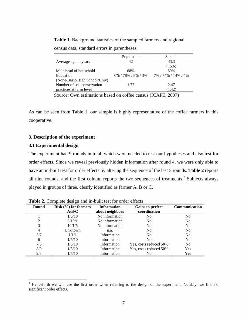
Table 1. Background statistics of the sampled farmers and regional

census data, standard errors in parentheses.

Population Sample Average age in years 42 43.3

(15.6) Male head of household 68% 69% Education (None/Basic/High School/Univ)

6% / 78% / 8% / 3% 7% / 74% / 14% / 4%

Number of soil conservation practices at farm level

1.77

2.47 (1.42)

Source: Own estimations based on coffee census (ICAFE, 2007)

As can be seen from Table 1, our sample is highly representative of the coffee farmers in this

cooperative.

3. Description of the experiment

3.1 Experimental design

The experiment had 9 rounds in total, which were needed to test our hypotheses and also test for

order effects. Since we reveal previously hidden information after round 4, we were only able to

have an in-built test for order effects by altering the sequence of the last 5 rounds. Table 2 reports

all nine rounds, and the first column reports the two sequences of treatments.3

Subjects always

played in groups of three, clearly identified as farmer A, B or C.

Table 2. Complete design and in-built test for order effects Round Risk (%) for farmers

A/B/C Information

about neighbors Gains to perfect

coordination Communication

1 1/5/10 No information No No 2 5/10/1 No information No No 3 10/1/5 No information No No 4 Unknown n.a. No No

5/7 1/1/1 Information No No 6 1/5/10 Information No No

7/5 1/5/10 Information Yes, costs reduced 50% No 8/9 1/5/10 Information Yes, costs reduced 50% Yes 9/8 1/5/10 Information No Yes

3 Henceforth we will use the first order when referring to the design of the experiment. Notably, we find no significant order effects.

8

Risk and ambiguity aversion

Rounds 1 to 3 are essentially a standard risk experiments. Risk levels (1, 5 and 10%) were chosen

to be realistic based on expert advice, and then validated with pilot studies. In our context where

decisions are made annually, a 1% risk level means that farmers might face an extreme event

once every hundred years. Historical data show the occurrence of extreme events in this region is

indeed extremely rare. We explicitly told them to consider their group members as neighbors, but

at this stage asked for no interaction between the three players. We did not give them any

information about the risk level of the other group members. Farmers were also told that their

annual profits in the case of no extreme event were 500,000 colones (approximately US$10004

),

and in the case of an extreme event affecting his land, profits would be 50,000 colones per year.

The annual cost of investing in adaptation practices was 200,000 colones. We actually made a

point of making sure that all these numbers correspond to the reality of coffee farming in the

Tarrazu Region, using a representative hectare of land. It is important to stress that the Tarrazu

Region uses a high productivity, conventional production technology, and the soil conservation

practices required to adapt to climate change are not part of this technological package. Farmers

normally would not spend their capital and labor in these practices.

Round 4 was identical to the previous except that now we introduced uncertainty about the risk

level. We told all group members that “you do not know your own risk or the risk of the others.

The only thing you know is that your risk could be 1, 5 or 10 out of 100. We do not know your

level of risk either.” We then proceeded to explain that at the end we would randomly determine

which level of risk would apply for payment. Strictly, the risk is not unknown here, so this is

sometimes called a situation of weak ambiguity. The main reason why we opted for this approach

was to avoid subjects believing that the experiment was rigged by the researchers. Thus, it was

clear to the participants that we did not have more information about the risk than what they had.

The payoff of a farmer facing the weakly ambiguous situation in our experiment is then

determined by two known probabilities. The first one relates to the risk level that each farmer will

ultimately face. In our case, the risk could take any of three values with equal probability. The

second one refers to the probabilities of an extreme event, which in our case are 1, 5 and 10%.

Hence, the expected risk is 5.3%. We therefore compare the share of subjects adapting when the

4 At the time of the experiment 1 USD = 500 colones.

9

risk is known and equal to 5% with the share of subject adapting when the risk is unknown but

the expected value is 5.3%. Strictly we should have used other probabilities since the expected

value is not exactly 5%. However, we wanted to keep the probabilities as simple as possible.

Table 3 summarizes the design of the first four rounds.

Table 3. Risk and ambiguity treatments.

Risk levels5 Adapt (safe option)

Not adapt (risky option) Degree of risk aversion if indifferent

Bad outcome Good outcome 1% 300,000 50,000 500,000 3.4 5% 300,000 50,000 500,000 2.25

10% 300,000 50,000 500,000 1.75 Unknown (between

1 and 10%) 300.000 50,000 500,000 If indifferent between unknown and

risk of 5%, then ambiguity neutral

In Round 5, all farmers faced a risk level of 1%. This round was designed as a first introduction

to information about the risk of the other farmers in the group We then tested for differences

between this treatment in order 1 (round 5) and order 2 (round 7) and found no significant

differences in the distribution of the responses using a Chi-square test (p-value = 0.828).

Gains to coordination and communication

Finally, Rounds 6 to 9 were designed to test the effect of potential gains of adaptation

coordination and the role of communication in increasing the likelihood of coordination. In all

these four rounds, Farmers A, B and C faced a risk level of 1, 5 and 10%, respectively, and this

information was known to all players. We did this in order to reduce the informational

differences between treatments with and without communication. In Round 7, after stressing that

they all had different risk levels, and that extreme events could affect one farmer and not the

others, we told them “if the three of you decide to adapt, the cost of adaptation is 100,000

colones. If less than three of you decide to adapt, then the cost of adaptation is the same as

before, that is 200,000 colones.” Do note that at this stage we are still not allowing any

interaction between the players, so that Rounds 6 and 7 differ only in the potentially reduced

adaptation costs. Round 8 is identical to Round 7 but now we finally allowed for interaction

between the three group members, which allows us to test for the role of communication when

5 Farmers faced all risk levels in one round or the other of the first 3 rounds

10

there are gains to coordination.. Finally in, rounds 6 and 9 there are no gains to coordination and

hence no strategic reason for changing behavior in round 9 as a result of communication. Hence

our two-by-two design allows us to isolate the use of communication as a way of gaining a better

understanding of the experiment (in round 9) from using communication as a tool for

coordination.

3.2 Experimental procedure

The cooperative in Tarrazu organizes yearly meetings with all its members, grouped in 11

villages. We used those meetings to invite farmers to our experiments (called workshops). The

invitation was done jointly with the cooperative, and included information about the date, time

and place of our workshops in each of the communities. We also mentioned that we were hoping

to learn from their experience of a changing climate, and that they would have the opportunity to

participate in a set of activities in which they could earn some money, depending on their

decisions as farmers. A detachable slip was to be returned to us, where name, telephone number,

and location were filled by the farmer. We followed up this invitation with phone calls

confirming their interest in participating. This strategy is not different from the one used by the

cooperative to call for their own meetings. In total, we handed out 434 invitations and received

397 expressions of interest, i.e. slips with contact details.

A team of three highly trained field experimenters conducted all the work. Farmers were let

into the room when they arrived and were randomly assigned as farmers A, B or C in chairs

arranged in groups of three. We made sure that people coming together did not form part of the

same group. After a prudent lapse of time, we closed the chairs available to subjects, and late

comers were allowed only as observers at the back of the room.

After welcoming the subjects and telling them about the purpose of the workshop, we

explained that the experiment was going to last two hours, and reassured them about the

confidentially of their individual responses. At this time we allowed people to leave if they chose

to do so, but extremely few took this option and only due to lack of time. We also requested that

there should be no interaction between subjects until we specifically allowed them to

communicate.

We then explained the main aspects of the experiment. We introduced the notion of climate

change and most importantly described the different possibilities available to farmers as

11

adaptation to climate change strategies. At all times we kept a neutral perspective concerning the

need to invest in adaptation. We did mention that a change in precipitation and temperature, as

well as in the frequency of extreme events, could negatively affect their profitability due to

increased erosion, reduced soil fertility, and in the worst case, extreme losses like the ones

experience during the tropical storm Alma. Obviously, this was nothing new to the farmers.

One of the main aspects at this stage was to explain risk to the farmers. We used visual aids

depicting combinations of hundred red and white dots equivalent to 0, 1, 5 and 10%. These visual

representations of risk were available at all times. A tombola with 100 red and white balls was

also used, mainly to relate the risk charts with the number of balls in the tombola and eventually

to our payment strategy. Throughout this presentation we stressed that risk could differ between

neighbors and that the occurrence of an event was independent for all subjects. Several trials

were done until all questions were evacuated.

The actual experiment started with an explanation of the setting. We told them that we

wanted to learn about their decisions as farmers in nine subsequent rounds, and that at the end of

the experiment we would pay them according to their decisions. We stressed that they should

regard their group members as neighbors. At this stage subjects were asked to open a booklet

containing an example sheet, nine decision sheets, i.e. one for each round, and an exit survey.

The pages were stapled such that they could not browse forward in the booklet. The example

sheet included in Annex 1 was used to explain the basics of the 9 rounds. At this stage, we

introduced the payoffs and walked each farmer neutrally through the decision whether to invest

or not. Again we used the tombola to show them how their payment was going to be determined

according to their risk.

Finally we proceeded to explain the payment method, which is quite standard for this type

of experiments. First of all, we told them that one of the nine rounds was going to be randomly

selected for a real payment.6

6 Later in the experiment, we explained that, for Round 4 with ambiguous risk, a further random selection of risk was needed.

Also, given our budget limitations, we explained that an exchange

rate of one in thousand was going to be used, but asked them to focus on the per hectare payoffs

that corresponded with their reality as coffee producers. Notably, even our converted payment

exceeded a one day worth of salary in a coffee farm, clearly enough to achieve saliency. Before

starting the experiment we conducted several example payments to show both how we were

12

going to pay but also to make it very clear that they were playing for real money. Note that all the

realizations of the risks and the outcomes were make after all nine rounds had been played.

The following is the actual translated script read for Round 1. The actual decision sheets

were similar to the example sheet provided in Annex 1, so the script served to guide subjects

through the details of the round. Small variations in this script were needed in the rest of the

rounds.

Figure 1. Translated script for round 1 CASE 1: In this case the question is whether you choose to invest or not in adaptation, given the level of risk shown in your sheet. As visual help, you can see in this slide the possible risk levels you can face. [PUT SLIDE WITH 3 RISK LEVELS]

- If you choose to invest in adaptation, your profit is [₡300.000] independently of the level of risk. - If you choose not to invest in adaptation, your profit will depend on the risk of a natural disaster, as

described in your sheet You do not know the level of risk of other farmers. This risk could be higher or lower than yours. The other farmers do not know your risk either. Also please remember that what happens to you will not necessarily happen to the others. In practice this means that each one of you separately will draw a ball from the tombola to determine what happens to your farm. As mentioned before, the number of red balls in the tombola depends on your own risk. In some cases, there will be 5 red balls, others might have just 1 and for some there will be 10 red balls in the tombola. Please check carefully your level of risk. Will you choose to adapt or not, given that level of risk. Do not forget that you do not know the risk of the other farmers, and that each case is a new situation that has no relation to the previous. Please do not talk to each other. Do you have nay question? [WAIT] Please mark your decision in the corresponding box.

4. Results

A total of 211 observations were gathered in the 11 workshops. The following results explore our

two main research questions: (i) risk and ambiguity aversion, and (ii) to what extent farmers can

coordinate their adaptation decision to reduce costs, and the importance of communication. For

the first issue, we conduct our analysis based on individual observations, and for the second issue

the relevant unit of observation is group decisions.

4.1 Risk and ambiguity aversion

We begin by looking at how farmers behave at various levels of risk of having their crops

destroyed by extreme weather associated to climate change. At this stage of the experiment, the

farmers did not know the level of risk of the other participants. Each farmer made the decision to

adapt or not for three risk levels. A number of farmers were inconsistent in the sense that they

adapt at a low, but not at a high, level of risk. In total, 17% of the farmers were inconsistent. At

13

this stage of the analysis, we remove inconsistent farmers, and are left with 175 observations. In

Table 4 the number and share of farmers adapting and not adapting at the three different levels of

risks are presented.

Table 4. Number of farmers not adapting and adapting under various levels of risk

Risk of crops

destroyed

Degree of relative risk

aversion if indifferent

Not adapt Adapt

1% 3.4 120 (69%) 55 (31%)

5% 2.25 40 (23%) 135 (77%)

10% 1.75 9 (5%) 166 (95%)

P-value of chi-square test of difference in distribution between risk levels = 0.000

As expected, the share of farmers adapting increases as the level of risk increases, and the

differences in shares are significant using a Chi-square test. The degree of relative risk aversion,

assuming a constant relative risk aversion utility function which is only a function of the pay-off,

is higher than 3.4 for 31% of he subjects, and the median degree of risk aversion is between 2.25

and 3.4. Consequently, the farmers are very likely to adapt to climate change, even at relatively

low levels of risks. Still, given that our experiment took place a few weeks after the occurrence of

an extreme event as dramatic as Alma we think it is noteworthy that 69% of all farmers did not

adapt at a risk of 1%. When the risk level increased to 10%, only 5% of the subjects do not adapt.

We next investigate if farmers are ambiguity averse. This is done by comparing the shares

of subject adapting when the risk is known and when the risk is unknown. The results for the

aggregate data are presented in Table 5.

Table 5. Number of farmers not adapting and adapting when the risk known and 5%, and when

the risk is unknown

Risk of crops destroyed Not adapt Adapt

Known risk, 5% 40 (23%) 135 (77%)

Unknown risk (between 1 and 10%) 38 (26%) 137 (74%)

P-value, chi-square test of difference in distribution between known and unknown risk = 0.797

14

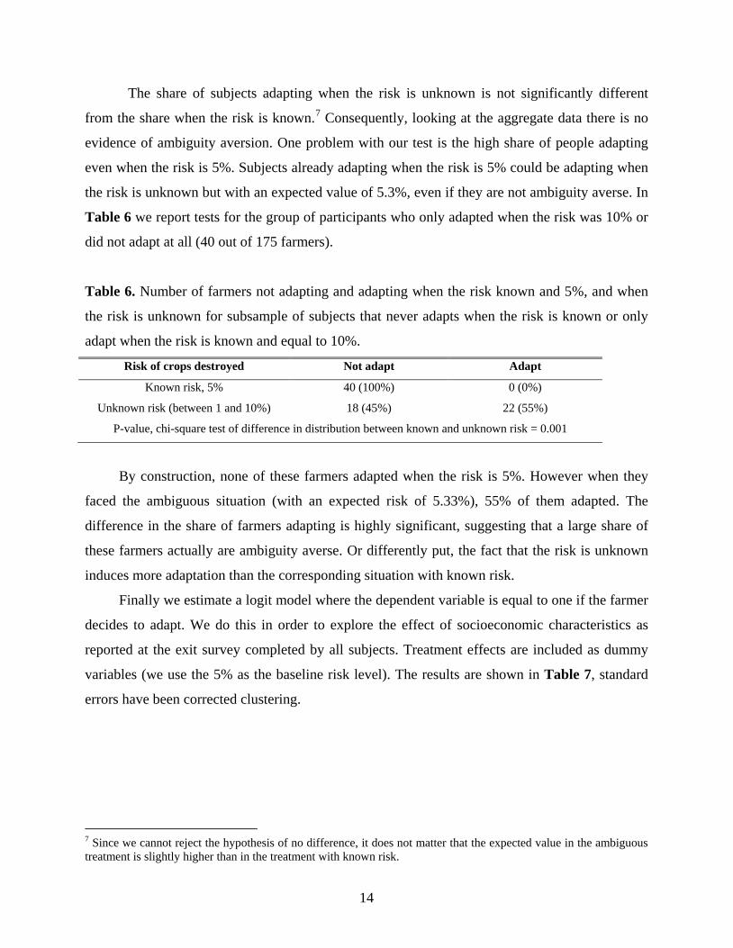
The share of subjects adapting when the risk is unknown is not significantly different

from the share when the risk is known.7

Consequently, looking at the aggregate data there is no

evidence of ambiguity aversion. One problem with our test is the high share of people adapting

even when the risk is 5%. Subjects already adapting when the risk is 5% could be adapting when

the risk is unknown but with an expected value of 5.3%, even if they are not ambiguity averse. In

Table 6 we report tests for the group of participants who only adapted when the risk was 10% or

did not adapt at all (40 out of 175 farmers).

Table 6. Number of farmers not adapting and adapting when the risk known and 5%, and when

the risk is unknown for subsample of subjects that never adapts when the risk is known or only

adapt when the risk is known and equal to 10%.

Risk of crops destroyed Not adapt Adapt

Known risk, 5% 40 (100%) 0 (0%)

Unknown risk (between 1 and 10%) 18 (45%) 22 (55%)

P-value, chi-square test of difference in distribution between known and unknown risk = 0.001

By construction, none of these farmers adapted when the risk is 5%. However when they

faced the ambiguous situation (with an expected risk of 5.33%), 55% of them adapted. The

difference in the share of farmers adapting is highly significant, suggesting that a large share of

these farmers actually are ambiguity averse. Or differently put, the fact that the risk is unknown

induces more adaptation than the corresponding situation with known risk.

Finally we estimate a logit model where the dependent variable is equal to one if the farmer

decides to adapt. We do this in order to explore the effect of socioeconomic characteristics as

reported at the exit survey completed by all subjects. Treatment effects are included as dummy

variables (we use the 5% as the baseline risk level). The results are shown in Table 7, standard

errors have been corrected clustering.

7 Since we cannot reject the hypothesis of no difference, it does not matter that the expected value in the ambiguous treatment is slightly higher than in the treatment with known risk.

15

Table 7. Logit results using the 5% risk level as baseline, dependent variable is equal to one if

farmer adapts

Description (Mean) Marginal effect P-value

Treatment characteristics

Low risk (1%) = 1 if low risk (0.25) -0.441 0.000

High risk (10%) = 1 if low risk (0.25) 0.242 0.000

Ambiguity treatment = 1 if ambiguity treatment (0.25) 0.012 0.757

Subject characteristics

Male = 1 if subject is male (0.71) 0.138 0.026

Age Age in years (43.33) 0.001 0.371

Big coffee farm = 1 if number of hectares > 5 (0.27) -0.129 0.032

Previous investment in soil conservation Number of soil conservation

measures they have taken (2.46)

0.032 0.073

Losses due to Alma = 0 if no losses, 2 if losses larger than

250 000 colones per hectare, 1

otherwise (1.81)

-0.023 0.485

Number of subjects / observations 171 / 700

Pseudo-R2 0.252

Both treatment dummy variables for known risk have the expected sign and are highly

significant. The ambiguity treatment has no significant effect, as expected from the aggregate

tests conducted in Table 6. From the subject characteristics, we find that males have a

significantly higher probability of adapting, whereas age and education have no significant effect

on the behavior in the experiment. Subjects with a big coffee farm are less likely to adapt, which

could be a reflection of the fact that they have more resources to overcome adverse effects

without compromising their livelihood. Finally farmers who already invest in soil conservation

are more likely to invest in additional practices to reduce the effect of climate change on their

land.

4.2 The role of communication and cost saving coordination

In the last part four rounds of the experiment, subjects always knew their own risk and the risk of

the two other group members. The first difference between the rounds is whether subjects are

allowed to communicate or not. The second difference is whether there is an incentive to

coordinate on adaptation or not. As explained in Section 3.1, farmers were told that if all group

16

members decide to adapt, adaptation costs would be reduced by 50%. This is indeed a realistic

situation, since there are economies of scope in the provision of technical assistance and purchase

of equipment and materials needed for the adoption of soil conservation practices. We now focus

on the decision at the group level, and not the individual farmer. For that reason, we remove

groups with less than 3 farmers, resulting in a total of 68 groups. Table 8 summarizes the

outcomes in the groups for the four treatments.

Table 8. Number of groups with different number of subjects adapting in each treatment8

Treatment 6 Treatment 7 Treatment 8 Treatment 9 Number of subjects adapting

No gains to coordinate & no communication

Gains to coordinate & no communication

Gains to coordinate &

communication

No gains to coordinate &

communication 0 3 (4%) 0 (0%) 1 (1%) 3 (4%) 1 11 (16%) 9 (13%) 6 (9%) 11 (16%) 2 32 (47%) 26 (38%) 14 (21%) 28 (41%) 3 22 (33%) 33 (49%) 47 (69%) 26 (39%)

There are two interesting comparison that can be made. First we can test if the whole

distribution of the number of subject adapting in a group is different for two treatments (Chi-

square test). Secondly we can test if the share of groups actually achieving full coordination in

adaptation and hence a possible cost reduction (i.e. were all three players adapt) is different for

the alternative treatments (proportion test).

To begin with, let us look at treatment 6 and 7. In both cases subjects were not allowed to

communicate, but in round 7 the adaptation costs were reduced if all adapted. There is a

significant increase (proportion test p-value = 0.055) in the share of groups where all adapt, and

hence get reduced adaptation cost, but there is no significant difference in the overall distribution.

(Chi square test p-value = 0.111). So farmers are able to coordinate only to a limited extent if

they cannot communicate with each other, and the pattern of “failed” coordination efforts is not

different in both cases. The question is what happens if we allow for communication, as in

treatment 8 (compared to 7). Communication in the pursuit of reduced adaptation costs achieves a

significant change in the distribution of responses (Chi-square test p-value = 0.053) and in 69%

of the groups all subjects adapts, thereby reaping the benefits of coordination. This share is

significantly different from the share in treatment 7 (proportion test p-value = 0.015). This result

is further strengthened if we compare treatments 8 and 9. In round 8 communications is allowed 8 Treatments 6-9, were played in different orders to test for order effects, but since we found no significant order effects aggregate results are reported in the table.

17

and if coordination is successful, will lead to reduced costs. In round 9, communication is also

allowed, but is inconsequential in terms of costs. The increase in number of groups where

everybody adapts is high and significant when cost reductions are at stake compared with no

gains to coordination (proportion test p-value = 0.001). The difference in distributions is also

significant using a chi-square test (p-value = 0.004). In order to test the effect of communication

alone, we can compare treatments 6 and 9, which are not significantly different in terms of the

distribution of responses (p-value = 0.896) or the share of groups coordinating (p-value = 0.473).

Hence communication has no effect on farmer’s decisions in the absence of further gains from

coordination. In our experimental setting, communication is thus not important in the sense of

learning and understanding the experiment, but it is important for strategic coordination reasons.

5. Discussion

Our experiment was conducted with coffee farmers in the Tarrazu region of Costa Rica, which

was heavily affected by hurricane Alma in early 2008. This type of extreme events is new to the

region, and many farmers were taken by surprise. We purposely conducted our experiment in the

region a few months after Alma. In particular, it is hard to explain to farmers that climate change

could imply a change in the pattern of extreme events when farmers have lots of prior experience

with these types of events, and it is too likely that they will disregard key experimental features.

Given that farmers in Tarrazu were well aware of the dangers of an extreme event, but at the

same time have little or no priors with respect to the likelihood of future events, we believe this

was a good setting to run risk experiments and most importantly, to test farmer’s behavior in

response to a changing climate.

As expected, we observe high levels of risk aversion, but we do observe farmers making

trade offs, and 69% do not adapt if the risk of large income losses is 1%. Hence some farmers

still do not adapt, even in the presence of the close memories of an extreme event. Furthermore,

we find evidence of a strong effect on adaptation of ambiguity aversion for the group of farmers

who did not adapt at low risk levels.

The implications for policy making of this ambiguity aversion are not straightforward, and

there is a lot of discussion particularly with respect to environmental risks, which are frequently

associated with unmeasurable uncertainty (see for example Treich 2009; Viscusi, 1998; Viscusi

and Hamilton, 1999). In the case of climate change, it is actually realistic to assume that farmers,

18

climate experts, and the government do not know the risk associated to changes in climate..

Viscusi (1998) and Viscuis and Hamilton (1999) argue against “conservatism bias”. Treich 2009

discusses two implications of acting on ambiguity aversion. On the one hand, from a purely

accounting view, putting concerns for ambiguity aversion on top of risk aversion at the

government level might lead to too much protection and too much investment in avoiding certain,

unmeasurable, risks. On the other hand, peoples’ preferences could favor governmental policies

that are attentive of their aversion to ambiguous situations. Our results contribute to this

discussion by identifying that both risk and ambiguity aversion seems to be important motives

behind adaptation to climate change decisions. We found that around 50% of those who choose

not to adapt to a 5% risk when the risk was know, do adapt if the risk is ambiguous but

comparable in expected level. Consequently, ambiguity aversion is an important factor for

technology adoption decisions.

What if the government actually knows the true distribution of probabilities of different

levels of risk, and farmers exhibit ambiguity aversion? This resembles a situation where people

have biased risk perceptions: see for example Olof Johansson-Stenman (2008) for a discussion

about perceived and objective risk. From a social efficiency perspective, this might lead, in

retrospect, to too much adaptation. In that situation, it could be optimal for the government to

provide costly information to reduce the degree of ambiguity among the individuals, insurance

programs against worse case scenarios, and improved safety networks, just to mention a few

strategies to deal with the extreme negative scenario.

Finally, we also explored the role of communication and monetary incentives (in the form

of cost reducing economies of scope arising from full coordination) on the decision to adapt or

not to climate change. Monetary incentives for coordination significantly increase the degree of

adaptation, but if communication is allowed, farmers are able to coordinate more frequently in

pursuit of the reduced adaptation costs. Notably, if no financial incentives are allowed,

communication is irrelevant for the farmer’s private decision. Do note that this are experienced

farmers who make similar decisions every day, and hence are less likely to be influenced by peers

when it comes to how they run their own land.

19

References

Adams, R. (1989) Global climate change and agriculture: An economic perspective, American

Journal of Agricultural Economics 71, 1272-1279.

Antle, J. (1987) Econometric estimation of producers’ risk attitudes, American Journal of

Agricultural Economics 69, 509-522.

Antle, J. (1989) Nonstructural risk attitude estimation, American Journal of Agricultural

Economics 71, 774-784.

Bandeira, O. and I. Rasul (2006) Social networks and technology adoption in northern

Mozambique, Economic Journal 116, 869-902.

Besley, T. and A. Case (1993) Modeling technology adoption in developing countries, American

Economic Review, Papers and proceedings 83, 396-402.

Binswanger, H. (1980) Attitudes towards risk: Experimental measurement in rural India,

American Journal of Agricultural Economics 62, 395-407.

Binswanger, H. and D. Sillers (1983) Risk aversion and credit constraints in farmers’ decision-

making: A reinterpretation, Journal of Development Studies 20, 5-21.

Bochet, O., T. Page, and L. Putterman (2006) Communication and Punishment in Voluntary

Contribution Experiments, Journal of Economic Behavior and Organization 60, 11-26.

Bochet, O. and L. Putterman (2008) Not Just Babble: Opening the Black Box of Communication

in a Voluntary Contribution Experiment. European Economic Review

53, 309-326.

Buchan, N., E.J. Johnson and R.T.A. Croson (2006) Let’s get personal: An international

examination of the influence of communication, culture and social distance on other

regarding preferences. Journal of Economic Behavior and Organization 60, 373-398.

Cardenas, J.C., T.K. Ahn and E. Ostrom (2004). Communication and cooperation in a common-

pool resource dilemma: A field experiment. Working Paper, Workshop in Political Theory

and Policy Analysis, Indiana University.

Chavas, J. and M. Holt (1996) Economic behavior under uncertainty: A joint analysis of risk

preferences and technology, Review of Economics and Statistics 78, 329-335.

Cooper, R., D. DeJong, R. Forsythe, T. Ross. (1990) Selection Criteria in Coordination Games:

Some Experimental Results, American Economic Review 80, 218-233.

20

Dybvig, P. and C. Spatt (1983) Adoption externalities as public goods, Journal of Public

Economics 231-247.

Ellsberg, D. (1961) Risk, ambiguity, and the Savage axioms, Quarterly Journal of Economics 75,

643-669.

Engle-Warnick, J., J. Escobal and S. Laszlo (2007) Ambiguity aversion as a predictor of

technology choice: Experimental evidence from Peru, Working Paper 2007-1, CIRANO,

Montreal Quebec.

Feder, G., R. Just and D. Zilberman (1985) Adoption of agricultural innovations in developing

countries: A survey, Economic Development and Cultural Change 33, 255-298.

Fox, C. and A. Tversky (1995) Ambiguity aversion and comparative ignorance, Quarterly

Journal of Economics 110, 585-603.

Gajdos, T., H. Takashi, J.-M. Tallon, J.-C. Vergnaud (2008) Attitude toward imprecise

information, Journal of Economic Theory 140, 23-56.

Harrison, G.W. and J.A. List (2004) Field Experiments. Journal of Economic Literature, 42,

1009–1055.

Holt, C. A., Laury, S. K. (2002), Risk aversion and incentive effects. American Economic Review

92, 1644-1655.

ICAFE-INEC (2007) Censo Cafetalero-Principales Resultados. ICAFE, San Jose, Costa Rica.

IMN (2008) Special Meteorological Report on Tropical Storm Alma, San Jose, Costa Rica.

IPCC (2007) Climate Change 2007: Impacts, Adaptation and Vulnerability. Contribution of

Working Group II to the Fourth Assessment Report of the Intergovernmental Panel on

Climate Change. Cambridge University Press, Cambridge, UK.

Johansson-Stenman, O. (2008) Mad cows, terrorism and junk food: Should public policy reflect

perceived or objective risks?, Journal of Health Economics 27, 234-248.

Klibanoff, P., M. Marinacci, S. Mukerji (2005) A smooth model of decision making under

ambiguity, Econometrica 73, 1849-1892.

Knight, F. (1921) Risk, Uncertainty, and Profit, Boston: Houghton Mifflin.

Ledyard, J.O. (1995) Public Goods: A survey of experimental research. In The Handbook of

Experimental Economics, ed. John Kagel and Alvin Roth, 111-194. Princeton, N.J:

Princeton University Press.

21

Mendelsohn, R., W. Nordhaus and D. Shaw (1994) The impact of global warming: A Ricardian

analysis, American Economic Review 84, 753-771.

Moore, E. and C. Eckel (2006) Measuring ambiguity aversion, Working paper, University of

Texas at Dallas.

Ochs, J. (1995) Coordination Problems, in Kagel, H. and A. Roth (Eds) Handbook of

Experimental Economics, pp. 195-251. Princeton: Princeton University Press.

Ostrom, E., R. Gardner and J. Walker, eds. (1994). Rules, Games and Common-Pool Resources.

Ann Arbor: University of Michigan Press.

Pope, R. and R. Just (1991) On testing the structure of risk preferences in agricultural supply

analysis, American Journal of Agricultural Economics 73, 743-748.

Sally, D. (1995) Conversation and cooperation in social dilemmas: A Meta-analysis of

experiments from 1958-1992. Rationality and Society 7, 58-92

Schlenker, W., M. Hanemann and A. Fisher (2005) Will U.S. agriculture really benefit from

global warming? Accounting for irrigation in the hedonic approach, American Economic

Review 95, 395-406.

Slovic, P. and A. Tversky (1974) Who accepts Savage’s axiom?, Behavior Science 19, 368-373.

Treich, N. (2009) The value of statistical life under ambiguity aversion, Journal of Environmental

Economics and Management, forthcoming.

Viscusi, W.K. (1998). Rational Risk Policies. Oxford University Press.

Viscusi, W.K., and J.T. Hamilton (1999). Are risk regulators rational? Evidence from hazardous

waste cleanup decisions, American Economic Review 89, 1010-1027.

Wik, M., T. Kebede, O. Bergland and S. Holden (2004) On the measurement of risk aversion

from experimental data, Applied Economics 36, 2443-2451.

22

Annex 1. Example sheet for farmer A used to explain the experiment