DISCUSSION PAPER SERIES

DP15710 (v. 2)

The Economic Case for GlobalVaccinations: An Epidemiological Modelwith International Production Networks

Sebnem Kalemli-Ozcan, Selva Demiralp, SevcanYesiltas, Muhammed Yildirim and Cem Cakmakli

INTERNATIONAL MACROECONOMICS AND FINANCE

MACROECONOMICS AND GROWTH

ISSN 0265-8003

The Economic Case for Global Vaccinations: AnEpidemiological Model with International Production

NetworksSebnem Kalemli-Ozcan, Selva Demiralp, Sevcan Yesiltas, Muhammed Yildirim and Cem

Cakmakli

Discussion Paper DP15710 First Published 24 January 2021 This Revision 24 January 2021

Centre for Economic Policy Research 33 Great Sutton Street, London EC1V 0DX, UK

Tel: +44 (0)20 7183 8801 www.cepr.org

This Discussion Paper is issued under the auspices of the Centre’s research programmes:

International Macroeconomics and FinanceMacroeconomics and Growth

Any opinions expressed here are those of the author(s) and not those of the Centre for EconomicPolicy Research. Research disseminated by CEPR may include views on policy, but the Centreitself takes no institutional policy positions.

The Centre for Economic Policy Research was established in 1983 as an educational charity, topromote independent analysis and public discussion of open economies and the relations amongthem. It is pluralist and non-partisan, bringing economic research to bear on the analysis ofmedium- and long-run policy questions.

These Discussion Papers often represent preliminary or incomplete work, circulated to encouragediscussion and comment. Citation and use of such a paper should take account of its provisionalcharacter.

Copyright: Sebnem Kalemli-Ozcan, Selva Demiralp, Sevcan Yesiltas, Muhammed Yildirim andCem Cakmakli

The Economic Case for Global Vaccinations: AnEpidemiological Model with International Production

Networks

Abstract

COVID-19 pandemic had a devastating effect on both lives and livelihoods in 2020. The ar-rival ofeffective vaccines can be a major game changer. However, vaccines are in short supply as ofearly 2021 and most of them are reserved for the advanced economies. We show that the globalGDP loss of not inoculating all the countries, relative to a counterfactual of global vaccinations, ishigher than the cost of manufacturing and distributing vaccines globally. We use an economic-epidemiological model of international production and trade networks and calibrate the model to 65countries. Our estimates suggest that up to 49 percent of the global economic costs of the pan-demic in 2021 are borne by the advanced economies even if they achieve universal vaccination intheir own countries.

JEL Classification: N/A

Keywords: N/A

Sebnem Kalemli-Ozcan - kalemli@econ.umd.eduUniversity of Maryland and CEPR

Selva Demiralp - sdemiralp@ku.edu.trKoc University

Sevcan Yesiltas - syesiltas@ku.edu.trKoc University

Muhammed Yildirim - mayildirim@ku.edu.trKoc University

Cem Cakmakli - ccakmakli@ku.edu.trKoc University

Powered by TCPDF (www.tcpdf.org)

The Economic Case for Global Vaccinations:

An Epidemiological Model with International ProductionNetworks*

Cem Cakmaklı† Selva Demiralp‡ Sebnem Kalemli-Ozcan§ Sevcan Yesiltas¶

Muhammed A. Yıldırım||

January, 2021

Abstract

COVID-19 pandemic had a devastating effect on both lives and livelihoods in 2020. The ar-rival of effective vaccines can be a major game changer. However, vaccines are in short supplyas of early 2021 and most of them are reserved for the advanced economies. We show that theglobal GDP loss of not inoculating all the countries, relative to a counterfactual of global vacci-nations, is higher than the cost of manufacturing and distributing vaccines globally. We use aneconomic-epidemiological framework that combines a SIR model with international productionand trade networks. Based on this framework, we estimate the costs for 65 countries and 35 sec-tors. Our estimates suggest that up to 49 percent of the global economic costs of the pandemicin 2021 are borne by the advanced economies even if they achieve universal vaccination in theirown countries.

Keywords: COVID-19; Sectoral Infection Dynamics; Globalization; International I-O LinkagesJEL Codes: E61, F00, C51

*We thank Yasin Simsek for excellent research assistance. We acknowledge the support from ICC Research Foundation.†Koc University.‡Koc University.§University of Maryland, NBER and CEPR.¶Koc University.

||Koc University & Growth Lab, Center for International Development at Harvard University.

1

No Man is an Island“No man is an island entire of itself; every man is a piece of the continent, a part of themain; if a clod be washed away by the sea, Europe is the less, as well as if a promontorywere, as well as any manner of thy friends or of thine own were; any man’s deathdiminishes me, because I am involved in mankind. And therefore never send to know forwhom the bell tolls; it tolls for thee. .”

– John Donne

1 Introduction

The COVID-19 shock was unexpected and severe. The global output is expected to contract 4.4

percent in 2020, as a result.1 The world was caught unprepared as countries hastily put together

policies to curb the spread of the virus, contain the financial panic, and offset the economic contrac-

tion all at the same time. The entire year was spent with lockdown policies that went on and off,

as the countries learned from each others’ experiences. Renewed upticks in countries through cross

border travelling highlighted the limitations of country specific lockdowns in a global pandemic. In

retrospect, it became evident that a globally coordinated lockdown in Spring and Summer of 2020

could have contained the pandemic. This would have earned time for the policy makers to invest in

testing and contact tracing procedures.

Approximately one year after the outbreak, the policymakers are at the crossroads of a critical

decision again, this time with respect to global coordination of manufacturing and distributing the

vaccines worldwide. In this paper, we demonstrate the importance of making the vaccine globally

available, not from a moral standpoint but from an economic one, by illustrating the large economic

costs in the absence of global vaccinations. Ironically, a significant portion of these costs will be

borne by the advanced countries, despite the fact that they might vaccinate most of their citizens

by the summer of 2021. This is because advanced economies (AEs) are tightly connected to un-

vaccinated trading partners which consist of a large number of emerging markets and developing

economies (EMDEs). Thus, the devastating economic conditions in these countries under the ongo-

ing pandemic can cause a non-negligible drag on the AEs as well. Even though AEs relative costs are

less than that of EMDEs as a percentage of their GDPs, their larger sizes imply that they bear a large

1IMF World Economic Outlook, October estimate: https://www.imf.org/en/Publications/WEO/Issues/2020/09/30/world-economic-outlook-october-2020.

2

fraction of the total global costs. Within the group of AEs, the relative costs increase proportional to

their exposure to unvaccinated trade partners. Regarding the pandemic, World Health Organization

(WHO) Director Dr. Tedros Ghebreyesus and the President of the European Commission Dr. Ursula

von der Leyen noted that “None of us will be safe until everyone is safe.” Our findings extend

this argument to the economies by showing that no economy fully recovers until every economy

recovers.

In order to estimate the economic costs of COVID-19 that are solely due to international linkages,

we develop a framework that combines an epidemiological Susceptible-Infected-Recovered (SIR)

model with international trade and production network.2 In this framework, external demand for

each country’s sectoral output changes with its trade partners’ specific infection rates. This approach

captures how the “global fear factor” can reduce the domestic output as a result of changes in for-

eign consumption due to voluntary social distancing abroad. The pandemic also acts as a negative

shock to supply because the production patterns in all countries are affected from sick workers and

lockdowns. We link the production in each country to other countries’ infection dynamics through

international production networks. We take a granular approach and consider demand and sup-

ply shocks at the two-digit sectoral level. Given the extensive evidence on the disproportionate

intensity of the COVID-19 shock on certain sectors, our approach allows us to combine the sectoral

heterogeneity in infection dynamics with sectoral heterogeneity in global trade networks.3

We introduce the vaccine as an immediate treatment of the virus, which improves the sectoral

demand and supply conditions in a vaccinated country. Consequently, the economic costs of the

pandemic that arise due to negative domestic sectoral demand and supply shocks disappear in a

given country, where the vaccine becomes available. However, the costs due to the international

factors remain as long as foreign countries are not vaccinated. We show that even if a given country

has access to the vaccine, it experiences a sombre recovery with a drag on its GDP when its trading

partners do not have access to vaccines. The reasons for this sub-par performance of a country with

full inoculation are twofold: First, this country’s exports cannot fully recover as long as there is weak

external demand from the countries that are still suffering from the pandemic. Second, this country’s

2See Cakmaklı et al. (2020) for a similar framework focusing on the domestic costs and the importance of financing ofthese costs through capital flows, highlighting the interplay between external finance and fiscal space in EMDEs. In thatwork, we focus on the role of foreign demand shocks as a function of infection dynamics.

3See Gourinchas et al. (2020) who uses heterogenetiy in sectoral shocks to identify business failures.

3

imports of final and/or intermediate goods are also affected when the supplier countries are not

fully recovered from the pandemic, which in turn decreases the country’s production capacity.

We estimate COVID losses for 65 countries and 35 sectors. Figures 1 and 2 show the importance

of incorporating international and inter-sectoral trade linkages in the calculation of the economic

costs of the pandemic. Figure 1 shows the trade networks. Each node represents a country. The

larger the country’s GDP, the bigger the node size. The darker blue nodes are more open countries

measured by the ratio of imports and exports to GDP. In our calibration, we assume AEs have access

to vaccination. These countries are marked with a black border around their nodes. Out of 65

countries, 41 countries are classified as AEs who have access to vaccination. Some countries in the

AE group are essentially emerging markets. We still classify these countries, including China and

Russia, among AEs, because they have access to vaccines. The remaining 25 countries (including a

residual entity called the ”Rest of the World”) belong to the set of EMDEs who are assumed to be

unvaccinated. The thicker is the line between any two countries, the higher is the intensity of trade

between those countries.

These international linkages are comprised of sectoral links. Industries use inputs from a variety

of other industries. These inputs can be supplied either domestically or internationally. In Figure 2

we show a glimpse of the global inter-industry production network. In this network, each node rep-

resents an industry. The node size indicates the total intermediate input usage of the industry. The

node color shows the share of imported inputs in the industry such that the industries with darker

shades of red use more international inputs. Looking at the figure, one can argue that an industry

with a relatively larger node size and a darker color (such as ”Coke an Refined Petroleum” as op-

posed to ”Real Estate”) will be more exposed to the drag from the pandemic if its’ imported inputs

are obtained from unvaccinated trade partners and if the production of these inputs require more

in-person contacts, increasing the fraction of sick workers. The lines between the nodes show the

supply relationships, where the thicker lines represent stronger relations. The directed line points

from the supplier to the target industry. According to OECD (2020), the total value of world trade

was 18 trillion USD. Within this total, intermediate products constituted 10.6 trillion USD, corre-

sponding to 59 percent of world trade in 2015. Such a high prevalence of intermediate products

reflects increasing prominence of global value chains (The World Bank, 2020).

4

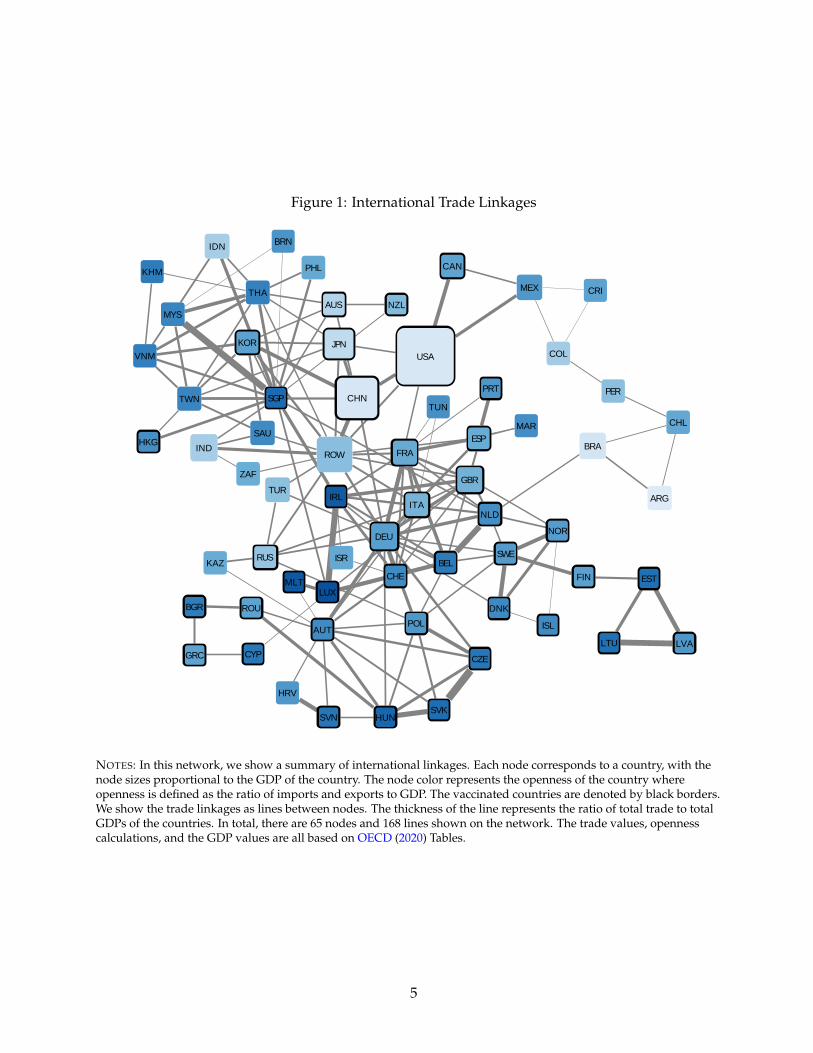
Figure 1: International Trade Linkages

CAN

MYS

MEX

KHM

USA

IND

CHL

ZAF

ARG

IDN

BRAHKG

AUS

PER

PHL

KOR

DNK

NZL

ISL

CHN

NOR

SGP

EST

THA

FIN

AUT

LVA

CZE

LTU

DEU

PRT

HUN

ESP

ITA

MAR

POL

TUN

SVK

ROW

SVN

TUR

CHE

RUS

HRV

GRC

KAZ

BGR

MLT

CYP

ROU

ISR BEL

JPN

FRA

TWN

IRL

SAU

LUX

VNM

NLD

COL

SWE

CRI

GBR

BRN

NOTES: In this network, we show a summary of international linkages. Each node corresponds to a country, with thenode sizes proportional to the GDP of the country. The node color represents the openness of the country whereopenness is defined as the ratio of imports and exports to GDP. The vaccinated countries are denoted by black borders.We show the trade linkages as lines between nodes. The thickness of the line represents the ratio of total trade to totalGDPs of the countries. In total, there are 65 nodes and 168 lines shown on the network. The trade values, opennesscalculations, and the GDP values are all based on OECD (2020) Tables.

5

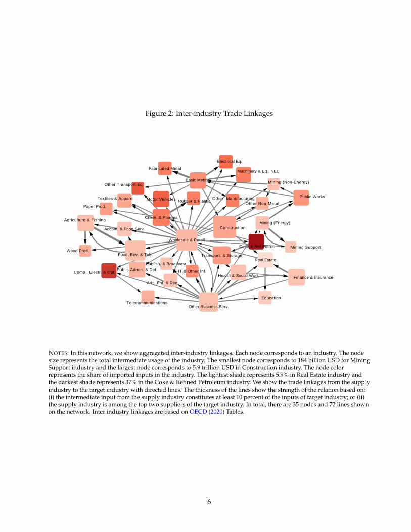
Figure 2: Inter-industry Trade Linkages

Other Transport Eq.

Motor Vehicles

Machinery & Eq., NEC

Electrical Eq.

Comp., Electr. & Opt.

Fabricated Metal

Basic Metals

Other Non-MetalRubber & Plastic

Coke & Ref Petrol.

Paper Prod.

Wood Prod.

Textiles & Apparel

Chem. & Pharma

Mining (Non-Energy)

Public Works

Other Business Serv.

Mining (Energy)

Mining Support

Arts, Ent. & Rec.

Wholesale & Retail

Education

Agriculture & Fishing

Public Admin. & Def.

Food, Bev. & Tob.

Health & Social Work Finance & Insurance

IT & Other Inf.

Telecommunications

Publish. & Broadcast.

Accom. & Food Serv.

Transport. & StorageReal Estate

Construction

Other Manufacturing

NOTES: In this network, we show aggregated inter-industry linkages. Each node corresponds to an industry. The nodesize represents the total intermediate usage of the industry. The smallest node corresponds to 184 billion USD for MiningSupport industry and the largest node corresponds to 5.9 trillion USD in Construction industry. The node colorrepresents the share of imported inputs in the industry. The lightest shade represents 5.9% in Real Estate industry andthe darkest shade represents 37% in the Coke & Refined Petroleum industry. We show the trade linkages from the supplyindustry to the target industry with directed lines. The thickness of the lines show the strength of the relation based on:(i) the intermediate input from the supply industry constitutes at least 10 percent of the inputs of target industry; or (ii)the supply industry is among the top two suppliers of the target industry. In total, there are 35 nodes and 72 lines shownon the network. Inter industry linkages are based on OECD (2020) Tables.

6

Our approach is data-driven. We do not allow firms to optimize and change their positions in

global value chains in response to changes in prices, wages, or shocks to labor because we focus on

the very short-run. As argued by Shih (2020); Carvalho et al. (forthcoming), the time needed to re-

build these networks is longer than the average duration of price stickiness. Our analysis is meant to

capture the first-round effects of an unequal vaccine distribution throughout 2021. In this sense, our

approach can be viewed as a special case of the sticky price closed economy network model of

Baqaee and Farhi (2020a,b). We assume strong complementarities between intermediate inputs and

do not allow labor adjustments within or across sectors. Such re-allocations are clearly important

in the medium run and will likely reduce the estimated costs presented in this paper. Nevertheless,

we opt for a data-centric approach because we want to focus on the immediate economic costs. We

estimate the economic costs borne by the advanced economies in the absence of equitible distribu-

tion of vacccination in the rest of the world. Such costs arise due to the existing global trade and

production networks. Thus, we use the inter-country inter-industry linkages in the data at the start

of the COVID shock and calculate the costs in a baseline scenario where the vaccines are available in

AEs but not in EMDEs, relative to a counterfactual of global vaccinations. Our approach amplifies

the role of the production network since shortages of labor and intermediate inputs will have an

immediate economic effect on the production.

We show that even if AEs eliminate the domestic costs of the pandemic thanks to the vaccines,

the costs they bear due to their international linkages would be in the range of 0.2 trillion USD and

2.6 trillion USD, depending on the strength of trade and production linkages. Overall, AEs can

bear up to 49 percent of the global costs in 2021. These numbers are far larger than the 27.2 billion

USD cost of manufacturing and distributing vaccines globally.4 The trade related costs that we have

calculated are an order of magnitude larger than those estimated by other studies that are in the

range of 119 to 466 billion.5 The reason for this discrepancy is twofold. Our estimates are based on

an economic-epidemiological framework that incorporates the effects of infection dynamics through

sectoral heterogeneity in exports and imports. Second, our calibration is based on a much larger set

of countries and sectors. In contrast, the other studies’ estimates only focus on the export part of

4See Access to COVID-19 Tools (ACT) Accelerator Partnership.5https://www.reuters.com/article/us-health-coronavirus-vaccine-gdp-trfn-idUSKBN28D217

https://www.who.int/docs/default-source/coronaviruse/act-accelerator/2020-summary-analysis-of-ten-donor-countries-11 26 2020-v2.pdf

7

trade by considering the loss in export revenue in main AEs from low-income countries (LICs) for

few selected sectors. These studies lack epidemiological content and hence do not allow exports to

evolve endogenously with the country-specific infection rates. As a result, our costs are larger.6, 7

We use OECD’s multi-industry multi-national input-output tables with 65 countries and 35 in-

dustries. In order to show the key channels of our model, namely exports and imports, we consider

three specifications. In the first specification, we solely focus on the foreign demand shocks that

affect exports. That is, if country A is fully vaccinated and wants to export to country B, which is

not fully vaccinated, the exports of country A will be lower compared to the counterfactual where

country B was also inoculated.

In the second specification, we introduce the effects of interruptions in imported inputs at the

country level in addition to weak external demand affecting exports. That is, we assume that to-

tal inputs are imported at the country level, regardless of where they came from, and distributed

among the domestic sectors.8 Continuing with our example from specification 1, suppose country B

lowers its production due to sick workers, lockdowns, or due to interruptions to its own imports of

intermediate goods from yet another unvaccinated country C. In turn, this will reduce total imports

to country A coming both from countries B and C, relative to the counterfactual that both of these

countries are also vaccinated.

In the third specification, we employ fully integrated inter-country inter-industry input-output

matrices. Under this specification, inputs from different country-sectors cannot be distributed across

the sectors of country A. Hence, it delivers the highest economic costs for country A. For example,

suppose the construction industry in country A imports steel from unvaccinated country B, and

the manufacturing industry in country A imports steel from another vaccinated country such as D.

Then, when imports from B goes down, construction industry cannot borrow steel from the manu-

6We should highlight that the costs that we calculate are not the overall costs of the pandemic in 2021 but the costs thatstem from unequal global vaccine distribution in 2021. IMF projects a cumulative global cost of 11 trillion USD during2020-2021 period due to the pandemic (See https://blogs.imf.org/2020/10/13/a-long-uneven-and-uncertain-ascent/.)

7The costs that we estimate do not include the costs on human health either. In contrast, Cutler and Summers (2020)focus entirely on health related costs and calculate the economic costs for the US due to COVID-19 related prematuredeath, long-term health impairment, and mental health.

8This treatment is analogous to building a country level input-output table, similar to the Bureau of Economic Anal-ysis’ practice of building the well-established US I-O matrices. For example, the steel imports of the United States fromGermany and China constitute the total imports of steel that is distributed across US’ sectors based on each industry’sshare of the input. We construct these input-output tables for each of the 65 countries separately.

8

facturing industry.

We consider these specifications under three vaccination and lockdown scenarios. In our first

and second scenarios, AEs are inoculated immediately, but the EMDEs are not. Hence the dynamics

of the pandemic in the unvaccinated EMDEs feed back into the economic recovery of the AEs. In

the second scenario we add endogeneous lockdowns in EMDEs, different from the first scenario.

The lockdown decisions depend on the ICU bed capacities of countries. This is motivated by the

observation that COVID-19 overwhelmed health systems through sharp increases in ICU bed oc-

cupancies (Mendoza et al. (2020)). In the third scenario, we allow for a gradual distribution of the

vaccines in both AEs and EMDEs, keeping the endogenous lockdowns. In this more realistic sce-

nario, we still assume that only 50 percent of the population in EMDEs are vaccinated at the end of

2021. In contrast, there is universal vaccination in AEs, completed early in 2021.

In the first scenario, we find that the global aggregate GDP losses range from 2.9 to 4.3 trillion

USD, depending on the three specifications based on the configuration of export and import shocks

that we have described above. Out of these aggregate costs, a range of 0.5 to 1.6 trillion dollars

are suffered by the AEs. Once we incorporate endogenous lockdowns in the second scenario, the

supply of inputs produced by EMDEs will decline further while their export demand from AEs will

strengthen as the lockdowns reduce the number of infections in EMDEs. Hence, even though the

costs that stem from the export channel decline (specification 1), the costs that stem from the import

channels (specifications 2 and 3) will increase. In this scenario, the overall losses range from 1.5 to

6.1 trillion USD, with 0.2 to 2.6 trillion USD of the costs borne by the AEs. In our final scenario, the

vaccination is completed within four months in the AEs, whereas the full distribution of vaccines is

still not completed by the end of 2021 in EMDEs. The losses are mitigated for all three specifications

as the vaccines are also available in EMDEs. The aggregate losses in this scenario are 1.84 to 3.8 tril-

lion USD, of which 0.4 to 1.9 trillion USD of the losses are borne by the AEs. Overall, AEs may bear

somewhere from 13 percent to 49 percent of the global losses arising from an unequal distribution

of vaccines in 2021. This range corresponds to 0.3 to 3.7 percent of their 2019 GDPs, depending on

different scenarios.

The remainder of this paper is organized as follows: In Section 2, we provide an overview of the

literature. In Section 3, we present the model. In Section 4, we describe vaccine development and

9

availability. Our quantitative findings are summarized in Section 5. Section 6 concludes.

2 Literature

There is a rapidly growing literature that aims to capture the economic impact of COVID-19 crisis.

Many papers utilize SIR models or its extensions to incorporate the infection dynamics into their

analysis. However, most of this literature focuses on closed economies, excluding the international

production and trade linkages that we consider. Papers such as Stock (2020), Alvarez et al. (2020),

and Acemoglu et al. (2020) consider the trade-off between the lives and the livelihoods. They reach

the conclusion that full lockdowns during the early stages of the pandemic is the optimal policy for

advanced closed economies. Alon et al. (2020) and Alfaro et al. (2020) take a developing country

perspective, focusing on the informal sector and small firms. They reach the opposite conclusion in

terms of lockdowns, arguing that lockdowns harm the livelihoods at a greater scale in these coun-

tries.

A separate group of papers focus on the endogenous response of demand or supply to the in-

fection rates. Papers such as Farboodi et al. (2020), Eichenbaum et al. (2020), Krueger et al. (2020),

and Eichenbaum et al. (2020) model the endogenous response of consumption or employment to the

pandemic, that is missing from the SIR models. These papers aim to capture the interplay between

infection dynamics and the determinants of demand or supply in closed economies. However, none

of these papers model both supply and demand dynamics simultaneously.

The recent empirical evidence shows the importance of both supply and demand shocks at the

sectoral level, where the size of the demand shock is more pronounced. Using granular data for

the US, Chetty et al. (2020) document a decline of 39% in consumer spending in the top-quartile of

income distribution and 13% in the bottom quartile during the first month of the pandemic. The de-

cline is heterogenous across sectors with more significant drops in industries that require in-person

contacts. The authors emphasize that the fear of contacting the disease is the main source of the

decline in spending at the initial stages of the pandemic. Similarly, using cell phone data to track

movements of individuals, Goolsbee and Syverson (2020) show that even though the consumer traf-

fic fell by 60%, only 7% could be explained by the shutdown restrictions. The authors suggest that

10

the changes in consumer behavior are most likely driven by the fear of infection.

To be consistent with this evidence, we model both sectoral demand and supply shocks for an

open economy, which is missing in the above cited literature. Hence, our main contribution to the

literature is to develop and open economy model with both sectoral demand and supply shocks that

are endogenous to the infection rates. Furthermore, these shocks are linked to the other countries

through trade and production networks. We model the epidemiological part similar to the closed

economy literature as in Acemoglu et al. (2020), Alvarez et al. (2020), Farboodi et al. (2020), and

Eichenbaum et al. (2020).9 10

3 Conceptual Framework

We model a reduced form partial equilibrium multi-sector multi-country model. Our modeling

choices are driven by the data as we calibrate our model to 65 country-35 sector international trade

and production network. We incorporate both supply and demand shocks to the model through

the epidemiological part. An important deviation of our work from the literature is the fact that we

assume static global value chains, where producers and suppliers do not optimize as a response to

the pandemic shock. We opt for this approach because we want to calculate the first-round effects

of the shocks. These shocks are propagated through the existing global value chains as we observe

them in the data as of 2020.11 On the demand side, the empirical evidence illustrates that the con-

sumers altered their consumption behavior in a sector-specific manner due to the the ”fear factor”

(Goolsbee and Syverson, 2020; Chetty et al., 2020). To capture this behavior, we model a reduced

form consumption function and calibrate it to real-time spending data.

Ability to work from home, physical proximity requirements and lockdowns are all domestic

factors that pin down the sectoral supply shock in a closed economy epidemiological model.12 The

9There is also a closed economy literature with rich input-output and network dynamics, similar to us, but this litera-ture omits the epidemiology part. See Barrot et al. (2020), Bonadio et al. (2020), and Baqaee et al. (2020), Baqaee and Farhi(2020a,b) and Guerrieri et al. (2020).

10The only other study that we are aware of which considers both demand and supply shocks at the sectoral level isby del Rio-Chanona et al. (2020).

11For full optimization, see Baqaee and Farhi (2020a,b) and Bonadio et al. (2020), where the latter considers the responseof the network to the supply shock and the former has a flexible model that can incorporate the responses to both supplyand demand shocks.

12Most infection dynamics models, including Acemoglu et al. (2020), Alvarez et al. (2020), Farboodi et al. (2020), and

11

novelty of our model is to introduce yet another factor that affects sectoral supply though inter-

national linkages. For instance, the car industry requires steel, plastics, textiles, electronics, and

numerous other inputs to make its final product. Critically, many of these inputs are provided in-

ternationally. Depending on the infection rates of the country that they are imported from, they

constitute a further supply shock for our small open economy. Similarly, demand shocks move with

the infection rates. Once infections reach a certain threshold, demand stalls and remains rather slug-

gish. In our model, even if the domestic infection rates are reduced, countries still suffer from weak

external demand if other countries’ infection rates are not improved simultaneously.

We calibrate our model to analyse the consequences of a hypothetical distribution of vaccination.

We assume that when AEs have access to the vaccine, local demand and supply shocks in AEs

due to high infection rates disappear. Nevertheless, AEs still suffer from the economic costs of the

pandemic as they are still affected from the foreign demand and supply shocks transmitted from

EMDEs. Specifically:

i Exports of final goods: In EMDEs where the pandemic is still ongoing, aggregate demand will

not fully recover. Hence, the exports of AEs would not return to pre-pandemic levels.

ii Exports of intermediate goods: Intermediate inputs produced by the AEs would not be de-

manded as much because of weaker overall growth in EMDEs.

iii Imports of intermediate goods: Intermediate inputs produced by EMDEs for industries in AEs

would fall short of meeting total demand in AEs as the supply in EMDEs is subject to domestic

and international supply shocks due to the pandemic.

iv Imports of final goods: The goods and services produced and sold by EMDEs to AEs would

decline as well.

3.1 The Economic Framework

Figure 3 summarizes our theoretical framework. We ponder the figure for a given industry in a

country that is exposed to COVID-19 shock. The bottom half of the figure describes the supply

Eichenbaum et al. (2020), do not use the sectoral heterogeneity in disease dynamics. To the best of our knowledge, Baqaeeet al. (2020) is the only paper with a similar sectoral heterogeneity to us.

12

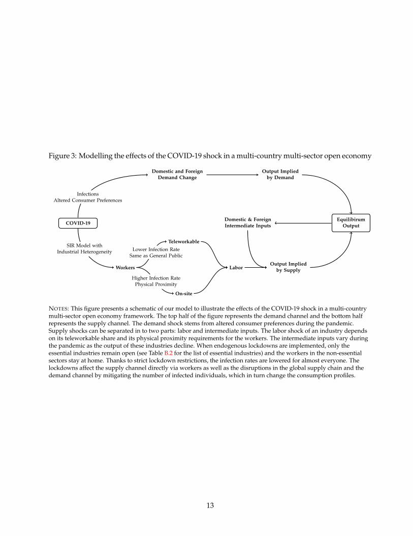
Figure 3: Modelling the effects of the COVID-19 shock in a multi-country multi-sector open economy

COVID-19

Domestic and ForeignDemand Change

Output Impliedby Demand

Workers

Teleworkable

On-site

Labor

Domestic & ForeignIntermediate Inputs

Output Impliedby Supply

EquilibirumOutput

SIR Model withIndustrial Heterogeneity

InfectionsAltered Consumer Preferences

Lower Infection RateSame as General Public

Higher Infection RatePhysical Proximity

NOTES: This figure presents a schematic of our model to illustrate the effects of the COVID-19 shock in a multi-countrymulti-sector open economy framework. The top half of the figure represents the demand channel and the bottom halfrepresents the supply channel. The demand shock stems from altered consumer preferences during the pandemic.Supply shocks can be separated in to two parts: labor and intermediate inputs. The labor shock of an industry dependson its teleworkable share and its physical proximity requirements for the workers. The intermediate inputs vary duringthe pandemic as the output of these industries decline. When endogenous lockdowns are implemented, only theessential industries remain open (see Table B.2 for the list of essential industries) and the workers in the non-essentialsectors stay at home. Thanks to strict lockdown restrictions, the infection rates are lowered for almost everyone. Thelockdowns affect the supply channel directly via workers as well as the disruptions in the global supply chain and thedemand channel by mitigating the number of infected individuals, which in turn change the consumption profiles.

13

side and the upper half depicts the demand side. On the supply side, the transmission dynamics

of the virus would differ depending on whether the workers are on-site or at a remote location like

home. We describe this in the next section in detail when we introduce the SIR model. Among

the professions that need to be carried out on the work site, we assume that the viral transmission

depends on the physical proximity between the workers or between the workers and the customers.

An on-site worker could be exposed to infection either at work or outside work. Intermediate inputs,

including the imported ones, directly affect supply. These imports are function of the pandemic in

the other countries. The viral transmission dynamics are also affected from the implementation of

different lockdown policies and vaccines in our country as well as in other countries. Moreover, the

output of an industry becomes intermediate inputs for other industries, albeit with a delay.

The economics profession unanimously agrees that the prerequisite for economic recovery is the

elimination of the virus so that demand normalizes.13 As shown in the upper part of the figure,

infection rate affects both domestic and foreign demand, feeding into the equilibrium output in a

given sector in our country. We model demand as a reduced form function where demand deviates

from its normal pattern as a function of the number of infected people. Hence, the demand profile

changes depending on the infection levels in the population, which, in turn, is mitigated by the

lockdown decisions and vaccines.

3.2 The Epidemiological SIR Model

We use the main workhorse framework in many epidemiological studies, namely the Susceptible-

Infected-Recovered (SIR) model.14 Let’s take a population of size N. At any given time, we can split

the population into three classes of people: Susceptible (St), Infected (It) and Recovered (Rt) as of

time t. The susceptible group does not yet have immunity to disease, and the individuals in this

group have the possibility of getting infected. The recovered group, on the other hand, consists of

individuals who are immune to the disease. Immunity can be developed either because the individ-

13See IMF World Economic Outlook, April 2020. Also contributions in Baldwin and di Mauro (2020). FormerFederal Reserve Chairman Bernanke noted in March 2020 that ”Nothing will work if health issues aren’t resolved,”sending a clear message to governments. See the transcript of Bernanke’s interview on March 25 is available atthis link: https://www.cnbc.com/2020/03/25/cnbc-transcript-former-fed-chairman-ben-bernanke-speaks-with-cnbcs-andrew-ross-sorkin-on-squawk-box-today.html

14See for example Allen (2017) among others.

14

ual goes through the infection or because she gets vaccinated. The SIR model builds on the simple

principle that a fraction of the infected individuals in the population, It−1N , can transmit the disease to

susceptible ones St−1 with an (structural) infection rate of β. Therefore, the number of newly infected

individuals in the current period is βSt−1It−1N . The newly infected individuals should be deducted

from the pool of susceptible individuals in the current period. Meanwhile, in each period, a fraction

γ of the infected people recovers from the disease, which in turn reduces the number of actively

infected individuals.15 To track any changes in the number of individuals in the above-mentioned

three groups, the following set of difference equations is used:

∆St = −βSt−1It−1

N(1)

∆Rt = γIt−1 (2)

∆It = βSt−1It−1

N− γIt−1 (3)

The law of motion for the number of infected individuals shows the trajectory of the pandemic at

the aggregate level. Note that, ∆St + ∆Rt + ∆It = 0 holds at any given time, assuming that the size

of the population remains constant.

We modify the canonical SIR model to allow for sectoral heterogeneity in terms of the size and

working conditions that can lead to distinct infection trajectories in each sector. The transmission

of the virus accelerates with close physical proximity. Hence, employees working in the industries

with higher physical proximity are infected with a higher probability. We assume that the economy

is composed of K sectors. We denote the industries by subscript i = 1, . . . , K. Each industry has Li

workers and there is also the non-working population which we denote by NNW . Each industry has

two types of workers: (i) employees who can perform their jobs remotely (i.e., teleworkable) and (ii)

employees who need to be on-site to fulfill their tasks. In each industry, we denote the number of

employees in the first group with TWi and the second group with Ni. Hence:

Li = TWi + Ni. (4)

15See also Atkeson (2020), Bendavid and Bhattacharya (2020), Dewatripont et al. (2020), Fauci et al. (2020), Li et al.(2020), Linton et al. (2020), and Vogel (2020) on different mortality estimates.

15

For the disease propagation, we lump the non-working population and the employees in the tele-

workable jobs together, and call them the “at-home” group. We denote the at-home group with

index i = 0. The total number of individuals in this group is, therefore,:

N0 = NNW +K

∑i=1

TWi. (5)

Suppose that the infection rate in the at-home group is β0. In order to account for heterogeneous

physical proximities across industries, we compute the rate of infection for each industry i, denoted

by βi, as:

βi = β0Proxi for i = 1, . . . , K (6)

where Proxi is the proximity index for industry i that we obtain from O*NET database.16 It is plau-

sible to think that the decline in demand during COVID-19 in a particular industry would lead to a

decline in proximity (see Eichenbaum et al. (2020)). Nevertheless, we do not incorporate this in our

model and take the proximity rates as exogenous.

Here, Si,t, Ii,t and Ri,t denote the number of susceptible, infected and recovered individuals,

respectively, and Ni = Si,t + Ii,t + Ri,t denotes the total number of on-site individuals in industry i

and the at-home group (i = 0). Susceptible individuals in the at-home group can get infected from

the infected individuals in the entire society:

∆S0,t = −β0S0,t−1It−1

N(7)

where It = ∑Ki=1 Ii,t + I0,t captures the total number of infected individuals. An on-site worker in

sector i, however, could be exposed to infection either at work, at the rate of βiSi,t−1Ii,t−1

Ni, or outside

work, that involves all the remaining activities –including family life, shopping and commuting–

at the rate β0Si,t−1It−1N . Hence, the number of susceptible individuals among the on-site workers in

industry i changes as:

∆Si,t = −βiSi,t−1Ii,t−1

Ni− β0Si,t−1

It−1

N(8)

16https://www.onetcenter.org/database.html. See Section 4.1 for the details on this measure.

16

The recovery rate is the same for all types of infected individuals:

∆Ri,t = γIi,t−1 (9)

The number of infected individuals changes as the susceptible individuals get infected and some

infected individuals recover from the disease:

∆Ii,t = −(∆Ri,t + ∆Si,t

)(10)

With industrial heterogeneity, we match the employment size weighted average βi’s of the in-

fected individuals to observed overall β in a country. For an on-site worker in industry i, the implied

β parameter can be approximated by (β0 + βi). 17 For a non-working individual, this parameter is

only β0. Using Equation (6), we impose:

β0N0

N+

K

∑i=1

(β0 + βi)Ni

N= β0 + β0

K

∑i=1

ProxiNi

N= β (11)

Hence, we solve for β0 in terms of β, industry size, and the proximity levels as:

β0 = β

1 +K

∑i=1

ProxiNi

N

−1

. (12)

Once the parameters are computed the evolution of infections in the extended multi-sector SIR

model can be written as

∆It = FIt−1 − νIt−1 (13)

where It = (I0,t, I1,t, . . . , Ii,t, . . . , IK,t)′ together with

17A report by DISK labor union in Turkey claims a three-fold increase in infection rates among workers: http://disk.org.tr/2020/04/rate-of-covid-19-cases-among-workers-at-least-3-times-higher-than-average/. Here, we take amoderate stance and set the rate to be 2 times higher on average for the workers.

17

F =

β0S0,t−1

N β0S0,t−1

N . . . . . . β0S0,t−1

N β0S0,t−1

N

β0S1,t−1

N β0S1,t−1

N + β1S1,t−1

N1β0

S1,t−1N . . . . . . β0

S1,t−1N

β0S2,t−1

N β0S2,t−1

N β0S1,t−1

N + β1S1,t−1

N2β0

S2,t−1N . . . β0

S2,t−1N

......

. . ....

......

. . ....

β0SK,t−1

N β0SK,t−1

N . . . . . . β0SK,t−1

N + βKSK,t−1

NK

, ν =

γ 0 . . . . . . 0 0

0 γ 0 . . ....

...... 0 γ 0

......

...... 0

. . . 0...

0 . . . . . . 0 γ 0

0 . . . . . . . . . 0 γ

Using these system matrices, R0 can be computed using the largest eigenvalue of the matrix F−1ν.

Given the initial size of the groups based on employment numbers, the eigenvalue would approxi-

mately correspond to the normalization present in Equation 12.

3.3 Production Side

As shown in the lower half of Figure 3, the pandemic affects production through labor supply and

inputs. First, the labor supply is decreased from the workers who get infected or put under lock-

down by the governments. Second, decreased labor force in a country’s trade partners result in

reduced availability of intermediate inputs, albeit with a delay. The combined impact of the labor

supply and intermediate inputs result in a decline in production through the supply side in the short

run.

In the short run, firms have little time to adjust for the shocks. We assume a Leontief production

function to capture these short run dynamics. In this framework, countries need to combine inputs

in fixed ratios to produce a single unit of output. These ratios are determined by the present tech-

nology and the combination of inputs available in the country. All these inputs, including labor, are

assumed to be complementary to each other. For instance, to produce a single unit of an automobile,

after setting up its factory for a specific type of production process, a car company requires inputs

in certain ratios such as 4 workers, 100 kilograms of steel, 4 tires, 4 seats, a microprocessor, a car

battery, etc. (These numbers are for illustrative purposes). In general, we can write the unit output

requirement in industry i in country c in terms of its inputs as:

yc,i =

{lc,i, zi1

c,i, . . . , zinic,i

}(14)

18

where lc,i denotes the unit labor requirement of industry i in country c and zijc,i denotes the amount

of intermediate inputs that should be used in industry i from industry ij to produce a single unit

of i. Going back to our automobile example, with 400 workers, 10 tons of steel, 400 tires, 400 seats,

100 microprocessors and 100 batteries, a car company would be able to produce 100 automobiles.

Increasing the number of tires to 500, or number of workers to 1000 would not change the number

of automobiles produced. However, in the long run, given an increase in wages, the car company

may want to readjust its manufacturing technology to require less workers. We focus on the short-

run effects and assume that firms take the COVID-19 shock as temporary and hence do not adjust

their production and position in the global value chain. As a result, we use the Leontief production

function to combine labor and intermediate inputs.

Formally, with these assumptions, we can write the output in industry i in country c as:

Yc,i = min

Lc,i

lc,i,

Zi1c,i

zi1c,i

, . . . ,Z

inic,i

zinic,i

(15)

where Lc,i captures the amount of labor allocated by country c to industry i and Zijc,i denotes the

amount of output of industry ij used in industry i of country c. The ij could capture an industry

from another country as well a domestic industry. In our car company example, one of ijs would

correspond to tires, that can either be supplied domestically or internationally. It is important to note

that this production function also captures the network effects. In particular, taking the minimum

in Equation 15 requires considering all inputs to the industry.

During the pandemic, the inputs are affected differently. On the labor side, we have two groups

of workers, at-home and on-site. These workers have different infection dynamics as shown in the

previous section. The total number of available workers at time t is:

Lc,i,t = (Nc,i − Ic,i,t) + TWi

(1− Ic,0,t

Nc,0

)(16)

where Nc,i is the number of on-site workers in industry i in country c, Ic,i,t is the number of in-

fected workers among on-site workers, and TWi is the number of at-home workers (i.e., those who

can work remotely) in industry i. The ratio Ic,0,t/Nc,0 captures the fraction of individuals who are

19

infected in the at-home group, which includes the non-working population as well as all at-home

workers (i.e., teleworkers) in the economy.18

When there are no international supply shocks, changes in the local labor supply are the only

factors that lower aggregate supply during to the pandemic. When there are supply shocks to im-

ported inputs, the output in country c in industry i would decline by a multiplicative factor dc,i. This

multiplicative factor is implicitly a function of the global pandemic. Following the supply shock,

the output level changes to:

Yc,i = dc,iYc,i. (17)

We assume that the intermediate inputs from this industry will also decline with same ratio.

The shocks propagate through input-output linkages. In our model, we assume that the produc-

tion is being done daily. We assume that the propagation of a foreign input shock is not simulta-

neous, assuming that it would take some time for the disrupted input to arrive at the production

location. To capture the travel time, we use the intermediate inputs produced two weeks prior to

the production of a good. From a practical point of view, incorporation of this two-week delay elim-

inates the estimation of a rather complicated system of 65 countries with simultaneous trade flows.

Instead, we take the supply shock in a particular country as given and analyze its impact on the

other countries rather than a simultaneous feedback between the countries.

In order to determine the level of final output imposed by the supply constraints during the

pandemic, we combine the changes in the domestic labor force with the changes in the availability

of imported intermediate inputs. Hence, the output in industry i in country c coming from the

domestic and international supply channel during the pandemic is equal to:

YSc,i = Yc,i min

Lc,i

Lc,i,

Zi1c,i

Zi1c,i

, . . . ,Z

inic,i

Zinic,i

. (18)

where Zijc,i is the level of industry ij during the pandemic. Using the car company example above,

let’s assume that the car company produces 100 automobiles a day. Let’s further assume that out of

400 workers, 50 of them got infected and cannot report to work. Moreover, the tire company who

18To declutter the notation, we will skip the time index below.

20

supplies for this car company was also affected by the pandemic and could only produce 300 tires

fourteen days ago for the car company to use in today’s production. Suppose all the other inputs

remain at their normal levels. In this example, the automobile production decreases to 75 that day

because the binding constraint is the available tires for production.

Utilizing this framework, we introduce different specifications involving the availability of inter-

mediate inputs in our simulations below. In equilibrium, we take the minimum level of the output

implied by supply vs. the output implied by demand to find the level of output for the economy

during the pandemic.

3.4 The Demand Side

During the pandemic period, consumer priorities and preferences change dramatically due to many

reasons. First, there is the fear of infection which leads to voluntary social distancing. The fear of

infection is related to the number of infected individuals in the society. In order to minimize the risks

of getting infected, individuals alter their behavior and change their consumption patterns, such as

refraining from public events, restaurants or malls. These pandemic-related changes in demand

patterns affect the sectors that require closer proximity more than the others. There is also the fear

of transmitting the disease to others. Individuals may choose to minimize their social interactions

with a precautionary motive, in order to avoid infecting others inadvertently. In addition to the fear

factor, there is uncertainty about the duration of the pandemic and the related economic outlook

which affects aggregate demand. Aggregate expenditure typically declines during times of elevated

uncertainty.

In order to capture the change in demand patterns during the pandemic, we consider two de-

mand profiles for each industry, one corresponding to normal times and the other one corresponding

to the brunt of the pandemic. We determine the demand for each industry during normal times from

the consumption data in national accounts. As for the COVID-19 period, we estimate changes in the

expenditure levels during the pandemic using credit card spending data. For the sectors where we

do not have the credit card data, we use industry reports and expert opinions.19 The progression

19Expected final demand changes and the resources we use in this estimation are presented in Table B.1 of the Ap-pendix.

21

of the pandemic and the normalization of demand as the pandemic fades is a gradual process. In

order to capture this steady adjustment, we assume that the individuals move between these two

profiles smoothly, as a function of the number of infected individuals in the country. The demand

structure we employ here is similar to Cakmaklı et al. (2020). We express the utility function of a

representative agent who maximizes her utility by optimally allocating her income on the expendi-

ture of different goods from each industry. Following the literature on input-output analysis (see,

for example Acemoglu et al. (2012), among others), we assume that the representative agent has a

Cobb-Douglass utility function:

U(e1, . . . , en) =n

∏i=1

eαii , (19)

with ei denoting the level of expenditure in industry i, and αi representing the share of industry i

in total expenditure with ∑ni=1 αi = 1 and 0 < αi < 1 for all i = 1, . . . , n. The utility function in

Equation 19 incorporates a budget restriction which implies that the total income (w) equals total

expenditure, i.e., w = ∑ni=1 ei. With the Cobb-Douglass utility function, αi determines the share of

industry i in the expenditure so that ei = αiw for i = 1, . . . , n.

During times of the pandemic, demand patterns change. For the sake of simplicity, we assume

that changes in demand come from two channels. First, the pandemic changes preferences and pri-

orities, which implies an adjustment in sectoral weights. Second, sectoral demand also changes due

to the income effect, which is a function of aggregate output (demand). Consequently, these two

effects lead to a change in the expenditure structure. To capture this change, we construct a ratio,

δi(I), that is directly linked to the number of active infections. This shows the expenditure in indus-

try i when the infection level is I, relative to the expenditure during normal times (See Cakmaklı et

al. (2020) for details). During the pandemic, the expenditure shares as a function infections can be

written as:

ei = δi(I)ei

As the demand ratio approaches 1, it signals that the number of infections decline and demand

normalizes. As the demand ratio approaches 0, it reflects that the number of infections increase and

demand shrinks due to the pandemic. Using this ratio, we write the limiting cases for δi(I). For small

I (i.e., I ≤ 0.1 I), δi(I) = 1. Thus, for a small number of infections, demand remains intact such that

22

the ratio of demand during normal times equals demand during the pandemic. For large I, which

corresponds to the peak of the pandemic, limI→∞

δi(I) ≡ δi. If the demand for an industry i completely

collapses during the pandemic (e.g., the airline industry), then δi = 0. If there is no change in

demand during the pandemic (e.g., food industry), then, δi = 1. We assume that δi is the utmost

demand change in a particular sector that is globally valid under a fully developing pandemic. In

this framework, we assume that the ratio of demand, δi(I) , smoothly fluctuates between 1 when

nobody is infected and δi when a very large number individuals get infected using the functional

form as:

δi(I) =

1 if I ≤ 0.1 I

δi1+(I/ I−0.1)δi+(I/ I−0.1) if I > 0.1 I

(20)

It is important to note that the overwhelming uncertainty about the course of the virus may suppress

economic confidence for a longer period of time. To the extent that the actual normalization is slower

than what is implied by Equation (20), we err on the conservative side by assuming a faster recovery.

In our simulations, we let the pandemic take its course separately in each country and use the

number of infected patients in each country as the determinant of demand change in a particular

industry. Given the smooth transition function, we model the changes in the final demand levels

using δ values. Let’s illustrate the final demand of country c in industry i with Fc,i. Accordingly, the

new level of final demand in industry i in country c during the pandemic becomes:

Fc,i(I) = Fc,iδi(Ic) (21)

where Fc,i(I) represents the revised demand during the pandemic when the number of infections is

Ic in country c.

In order to account for the total demand of each sector, we need to consider not only domestic

but also foreign demand. We utilize OECD Inter-Country Input-Output (ICIO) Tables,20 which pro-

vides us with input demand of industry i in country c from any industry in any country. The final

demand vector has 2340 entries indexed by (c, i), corresponding to each country-industry combina-

20https://www.oecd.org/sti/ind/inter-country-input-output-tables.htm

23

tion. By dividing the rows of ICIO matrix with the total output of industry (c, i), we obtain the direct

requirements matrix A. This matrix summarizes the usage of each intermediate input to generate

$1 worth of output. Output of each industry is either used as an intermediate input or consumed

as final demand. Using matrix notation, we decompose the total output into intermediate and final

usage as:

Y = AY + F (22)

Here, Y denotes the output vector and F denotes the final demand vector whose entries are Yc,i and

Fc,i respectively.21 Therefore, we can solve for the output to satisfy the final demand as:

Y = (I−A)−1F (23)

From this equation, we write the total output of country c as:

Yc =n

∑i=1

Yc,i (24)

Using the demand change from Equation 21 during the infection, the demand channel changes

the output as:

YDt = (I−A)−1F(It). (25)

where YDt represents the output and F(It) represents the vector of demand at time t as a function of

the number of infections, It. Therefore, the output also changes with the dynamics of the pandemic.

3.5 Equilibrium

In equilibrium, production declines by the largest magnitude that is implied by either supply or

demand side. In other words, during the pandemic, we expect the output vector to be:

YEQt = min(YS

t , YDt ) (26)

where min represents element by element minimum function for two vectors, namely YSt and YD

t .

21With a slight abuse of the notation, we drop the subscript to refer to vectors or matrices of the variables.

24

The value-added of the output in industry i in country c is calculated from the shares of value

added in each industry during normal times as:

VAEQc,i,t = YEQ

c,i,tVAc,i

Yc,i(27)

Therefore, GDP of the country c at time t can be obtained through:

GDPEQc,t =

n

∑i=1

VAEQc,i,t (28)

4 Data and Calibration

4.1 Data

We use OECD ICIO Tables. As the industrial classification, OECD uses an aggregation of 2-digit ISIC

Rev 4 codes to 36 sectors. The last sector, ”Private households with employed persons,” does not

have any linkages with other industries. We drop that sector from our analysis when we measure

international inter-industry linkages. This leaves us with 35 sectors. Throughout our analysis, we

will make use of this classification labeled as OECD ISIC Codes.

To calculate the industry level teleworkable share and the physical proximity measures shown

in the lower part of Figure 3, we use the occupational composition of the industries. We use the list

provided by Dingel and Neiman (2020) for the occupations which can fulfill their tasks remotely.

Dingel and Neiman (2020) use several measures from O*NET to identify which occupations are tele-

workable. For the workers that continue to perform their jobs on-site, we assume that the infection

rate depends on the physical proximity that is required in their workplace. To calculate the proxim-

ity requirements for the occupations, we use the self-reported Physical Proximity values available

in the Work Context section of the O*NET database. O*NET collects the physical proximity infor-

mation through surveys with following categories: (1) I don’t work near other people (beyond 100

ft.); (2) I work with others but not closely (e.g., private office); (3) Slightly close (e.g., shared office);

(4) Moderately close (at arm’s length); (5) Very close (near touching). We divide the category values

by 3 to make category (3) our benchmark. Specifically, a proximity value larger than 1 indicates a

25

closer proximity than the ‘shared office’ level and a value smaller than 1 corresponds to less-dense

working conditions. We create a single physical proximity value for each occupation by comput-

ing a weighted average of the normalized category values. We calculate the proximity values at

the industry level after removing the teleworkable portion from the employees. We create a single

proximity value for each occupation by weighting the normalized score with the percentage of the

answers in each category.

To obtain industry-level teleworkable share and proximity values, we calculate the weighted

average of the values corresponding to the occupations in each industry using the Occupational

Employment Statistics (OES) provided by the U.S. Bureau of Labor Statistics (BLS). OES data follows

four-digit NAICS codes to classify industries. In order to convert proximity data to OECD ISIC

codes, we make use of the correspondence table between 2017 NAICS and ISIC Revision 4 Industry

Codes, provided by the U.S. Census Bureau. We provide the teleworkable share and the proximity

index for the industries in Table B.1 of the Appendix.

We obtain employment by sector data from OECD’s Trade in employment (TiM) database Horvat

et al. (2020). For 14 countries that have missing data in TiM, we obtained the total employment from

the World Development Indicators database of the World Bank. We use the value added per em-

ployer information from the closest geographical aggregation and use this information to distribute

the employment to industries for these 14 countries.

4.2 SIR Parameters

The countries in our sample have distinct experiences regarding the course of the pandemic. Con-

sidering the SIR model, the two fundamental structural parameters, the resolution, and the infection

rates, define the pandemic’s trajectory. The resolution rate is a disease-specific structural parameter

that does not vary much across the countries. According to the report by the WHO 22, the median

recovery time for the mild cases is reported to be approximately two weeks. The mean recovery time

could be longer when we include severe cases. In this paper, we err on the optimistic side and set

γ = 1/14 ≈ 0.07 to establish a mean recovery time of 14 days. However, the infection rate is closely

related to the measures taken by the countries to contain the pandemic. The infection rate might

22https://www.who.int/docs/default-source/coronaviruse/who-china-joint-mission-on-covid-19-final-report.pdf

26

vary across countries and across time, depending on the timing of such measures. Accordingly, for

the calibration of β, we make use of publicly available datasets.23 For each country, we estimate a

generic SIR model described in (1)-(3) using official data on the pandemic. We employ the methodol-

ogy proposed in Cakmakli and Simsek (2020) to capture the changes in the rate of infection over time

for the countries in our sample. Briefly, this involves estimating a SIR model with time-varying pa-

rameters in a statistically coherent way to accommodate various non-pharmaceutical interventions.

These factors include lockdowns or other changes such as the virus’s mutations and advancements

in the treatment of the disease. For each country, the data spans the period from the day the number

of active infections exceeds 1000 until the end of November 2020. Consequently, we use the param-

eter values estimated as of the end of November 2020 to simulate the pandemic’s evolution over the

next year in each country. Except for Australia, New Zealand and China, which have been relatively

successful in suppressing the infections, we imposed an R0 between 1.1 and 1.3 for all countries.

These values are reported in Table B.3 of the Appendix.

Under full lockdown, only a few industries are active. We construct the list of industries that are

closed during lockdowns based on international examples of government decrees. The list of these

sectors is given in Table B.2 of the Appendix. From these industries and using the employment data

at 4 digits, we calculated the share of each OECD ISIC industry that would remain active during the

lockdown. Finally, we calculated the share of public employees that are not affected by the lockdown

using the publicly available information.

4.3 Demand Changes

Turning to the demand side that is depicted in the upper half of Figure 3, we use publicly available

credit card spending data to calculate the estimated demand changes during the pandemic in each

industry. To that end, we use data from Turkey, which is a representative EMDE. We particularly

choose an EMDE to capture the demand changes during the pandemic because the demand effect is

particularly pronounced for the unvaccinated countries. The demand effect essentially disappears in

AEs once the vaccine becomes available. Nevertheless, as a robustness check, a comparison with the

23The data is obtained from GitHub, COVID-19 Data Repository by the Center for Systems Science and Engineering(CSSE), at Johns Hopkins University.

27

US credit card data reflects that the changes in demand patterns are rather similar between EMDEs

and AEs.24 Armed with this evidence, we assume that the changes in demand arising from the “fear

factor” can be generalized around the globe.

The list of OECD ISIC industries, and the expected changes are listed in Table B.1 of the Ap-

pendix along with explanations. The data on credit card spending is not available for the full set of

sectors. In this case, we use projections based on sectoral reports, experiences of other countries and

historical data on the specific sector as well as the whole manufacturing sector. While the aggregate

demand shock is computed as 23% when we focus only on the sectors with credit card spending

data, it is 16% when we consider the full set of sectors. Therefore, our sensitivity analysis indicate

little or no change in our qualitative findings.

Demand is a function of the number of infections and this relationship is governed by the I

parameter of Equation 20 that determines the speed at which the public approaches the maxi-

mum decline in demand. We select this parameter to be country specific. In particular, we set

I = population/2000 to capture a relevant range for the number of infections (see below for our

simulations). This limit implies that the utility function returns to normal times if the number of in-

fections remain below population/20000. This approach is consistent with the levels observed dur-

ing the summer of 2020, when the number of infections decreased and the consumption rebounded

back to relatively normal levels as observed from the credit-card spending data in Turkey and the

US.24Considering Turkey and the US as representative EMDE and AE countries respectively, we compare their credit card

spending data, focusing on two industry groups, namely “Accommodation,” and “Gasoline Stations.”We obtained theunderlying data from the Central Bank of the Republic of Turkey and the Bureau of Economic Analysis that group weeklycredit card transactions into various expenditure categories. To avoid a misleading comparison between Turkey and theUS, we consider these two expenditure categories that are defined in the same manner by these agencies. To illustrate,two weeks after Turkey and the US were hit by COVID-19 pandemic, the weekly estimates of percentage differencesfrom the typical spending suggest rather similar demand patterns in these countries: The corresponding declines in theaccommodation sector for the week of March 25 are 40.1% for Turkey and 43.6% for the US. In the gasoline industry, thenumbers are 81.1% decline in Turkey and 85.6% decline in the US. Thee corresponding estimates for the week of April 1are -41.5% in Turkey and -46.8% in the US for Accommodation; -82.2% in Turkey and -85.2% in the US for the gasolineindustry respectively.

28

4.4 Supply Shock Specifications

Recall from Equation 18 that the supply is affected from the inputs during the pandemic with the

following relationship:

YSc,i = Yc,i min

Lc,i

Lc,i,

Zi1c,i

Zi1c,i

, . . . ,Z

inic,i

Zinic,i

.

where “˜” sign denotes the levels of the inputs and the output during the course of pandemic. Dur-

ing the pandemic, we assume that the output of country c in industry i changes to:

Yc,i = dc,iYc,i

where d captures the proportional decline in the production of that industry. We refrain from the

time index but we solve for this equation daily. When we incorporate the intermediate inputs into

our calculations, we assume that these inputs are produced fourteen days earlier, in order to accom-

modate the transportation time.

In the first specification, we ignore potential interruptions in the delivery of intermediate inputs.

Our goal is to solely focus on the decline in the final demand of EMDEs. The export demand in

EMDEs can decline either through labor supply shocks due to infections and lockdowns or through

final demand changes. Hence, labor is the only limiting factor on the supply side. This gives us the

following relationship for the output implied by supply under the first specification:

Yc,iS = Yc,iLc,i

Lc,i. (29)

Starting with the second specification, we incorporate the drag coming from the intermediate

inputs channel into our calculations. In specification 2, we assume that the inputs are aggregated at

the country level, wherever they come from, and then distributed to the specific industries within

the country. This is akin to building national input-output matrices, such as the U.S. input-output

matrices build by the Bureau of Economic Analysis (BEA). For instance, suppose the particular input

is steel and the country in question is Germany. We assume that the total imported steel in Germany

is distributed proportionately among the different industries in Germany, such as automotive and

29

appliance, in accordance with demand conditions. Essentially, we impose that the firms within a

country can adjust to an outside shock more easily and redistribute the inputs among themselves.

With this assumption, a fixed proportion of industry ij present in country c is allocated to industry

i. We can write the fixed proportion term as:

rijc,i ≡

∑x Yc,ix,ij

∑x ∑i Yc,ix,ij

(30)

where Yc,ix,ij

denotes the output of industry ij produced in country x and exported to country c to be

used in industry i. Therefore,

Zijc,i = r

ijc,i ∑

x∑

iYc,i

x,ij(31)

During the pandemic, the available intermediate input from industry ij in country c to be used in

industry j changes to:

Zijc,i = r

ijc,i ∑

x∑

idx,ijY

c,ix,ij

. (32)

Hence, the output implied in the second specification becomes:

Yi,Sm = Yi

m min

Lim

Lim

,∑x ∑i dx,i1Yc,i

x,i1

∑x ∑i Yc,ix,i1

, . . . ,∑x ∑i dx,ini

Yc,ix,ini

∑x ∑i Yc,ix,ini

. (33)

In effect, with this specification we keep track of the changes in the level of an industry within a

country.

In the third specification, we utilize the inter-country inter-industry matrix. Here, we assume

that supply shocks can also be specific to the importing sector. Going back to the example of German

automotive industry and appliance industry, in this specification we assume that the steel inputs

used in the automotive industry cannot be transferred to the appliance industry. Furthermore, if the

imported steel for these two industries are coming from different countries, then the heterogeneity in

the infection rates of those countries will come into picture. This specification is our most stringent

case. Specifically, a particular input imported by industry ij can be put into use only by industry

i. Therefore, we can combine all the inputs that come from different countries, indexed by x, to be

30

used in industry i to obtain:

Zijc,i = ∑

xYc,i

x,ij. (34)

When supply shocks to intermediate inputs are industry specific, pandemic driven decline in im-

ported inputs in each industry is:

Zijc,i = ∑

xdx,ijY

c,ix,ij

(35)

Therefore, the output in this specification can be written as:

YSc,i = Yc,i min

Lc,i

Lc,i,

∑x dx,i1Yc,ix,i1

∑x Yc,ix,i1

, . . . ,∑x dx,ini

Yc,ix,ini

∑x Yc,ix,ini

. (36)

In specifications 2 and 3, we use the minimum function, which is sensitive to outliers. To be on the

conservative side and prevent these outliers from driving our results, we focus on sizable inputs.

Therefore, when we calculate the minimum, we impose the following two filters: (i) Filter small

values: We do not consider an input industry in the supply side if the value of that input is less

than 10 thousand USD, daily. (ii) Filter small industries: For a given industry, we only consider

input industries that constitute at least (1/35)th of the total inputs of that industry. We choose this

threshold because we have 35 industries that are used as inputs.

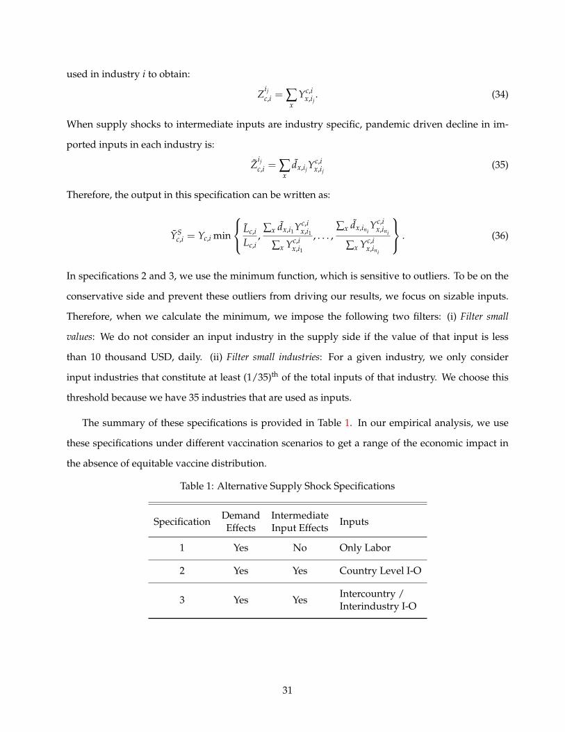
The summary of these specifications is provided in Table 1. In our empirical analysis, we use

these specifications under different vaccination scenarios to get a range of the economic impact in

the absence of equitable vaccine distribution.

Table 1: Alternative Supply Shock Specifications

SpecificationDemand Intermediate

InputsEffects Input Effects

1 Yes No Only Labor

2 Yes Yes Country Level I-O

3 Yes YesIntercountry /Interindustry I-O

31

5 Results

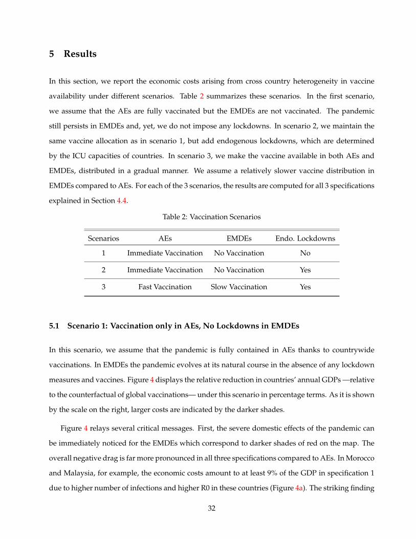
In this section, we report the economic costs arising from cross country heterogeneity in vaccine

availability under different scenarios. Table 2 summarizes these scenarios. In the first scenario,

we assume that the AEs are fully vaccinated but the EMDEs are not vaccinated. The pandemic

still persists in EMDEs and, yet, we do not impose any lockdowns. In scenario 2, we maintain the

same vaccine allocation as in scenario 1, but add endogenous lockdowns, which are determined

by the ICU capacities of countries. In scenario 3, we make the vaccine available in both AEs and

EMDEs, distributed in a gradual manner. We assume a relatively slower vaccine distribution in

EMDEs compared to AEs. For each of the 3 scenarios, the results are computed for all 3 specifications

explained in Section 4.4.

Table 2: Vaccination Scenarios

Scenarios AEs EMDEs Endo. Lockdowns

1 Immediate Vaccination No Vaccination No

2 Immediate Vaccination No Vaccination Yes

3 Fast Vaccination Slow Vaccination Yes

5.1 Scenario 1: Vaccination only in AEs, No Lockdowns in EMDEs

In this scenario, we assume that the pandemic is fully contained in AEs thanks to countrywide

vaccinations. In EMDEs the pandemic evolves at its natural course in the absence of any lockdown

measures and vaccines. Figure 4 displays the relative reduction in countries’ annual GDPs —relative

to the counterfactual of global vaccinations— under this scenario in percentage terms. As it is shown

by the scale on the right, larger costs are indicated by the darker shades.

Figure 4 relays several critical messages. First, the severe domestic effects of the pandemic can

be immediately noticed for the EMDEs which correspond to darker shades of red on the map. The

overall negative drag is far more pronounced in all three specifications compared to AEs. In Morocco

and Malaysia, for example, the economic costs amount to at least 9% of the GDP in specification 1

due to higher number of infections and higher R0 in these countries (Figure 4a). The striking finding

32

Figure 4: Relative Decline in GDPs under Scenario 1: No Lockdowns (%)

(a) Specification 1 – Only Demand

$9 B

$8 B

$34 B

$13 B

$21 B

$20 B

$17 B$31 B$22 B

$2 B

$111 B

25 - 3120 - 2517 - 2014 - 1712 - 1410 - 129 - 108 - 97 - 86 - 75 - 64.5 - 54 - 4.53.5 - 43 - 3.52.5 - 32 - 2.51.5 - 21 - 1.5.5 - 10 - .5

(b) Specification 2 – Country Level Intermediate Inputs

$19 B

$24 B

$73 B

$27 B

$49 B

$46 B

$39 B$85 B$36 B

$3 B

$297 B

25 - 3120 - 2517 - 2014 - 1712 - 1410 - 129 - 108 - 97 - 86 - 75 - 64.5 - 54 - 4.53.5 - 43 - 3.52.5 - 32 - 2.51.5 - 21 - 1.5.5 - 10 - .5

(c) Specification 3 – Country-Industry Level Intermediate Inputs

$26 B

$36 B

$94 B

$37 B

$66 B

$65 B

$51 B$125 B$46 B

$4 B

$438 B

25 - 3120 - 2517 - 2014 - 1712 - 1410 - 129 - 108 - 97 - 86 - 75 - 64.5 - 54 - 4.53.5 - 43 - 3.52.5 - 32 - 2.51.5 - 21 - 1.5.5 - 10 - .5

NOTES: This figure shows the relative reductions in GDP under Scenario 1, where the unvaccinated countries do notimpose lockdowns. Vaccinated countries are highlighted with light gray borders. Shades of yellow correspond torelatively lower costs while shades of red correspond to higher relative losses. GDP loss values are shown on the map fora few selected countries.

33

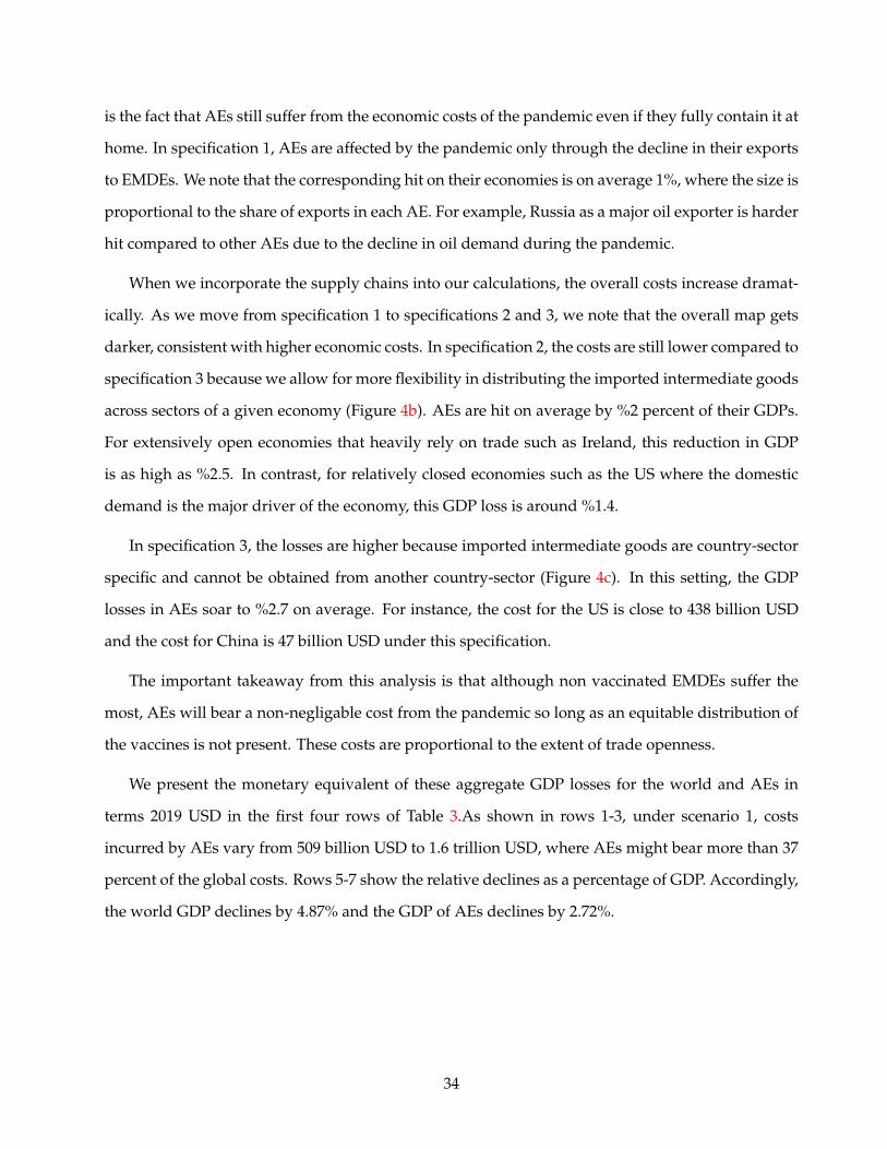
is the fact that AEs still suffer from the economic costs of the pandemic even if they fully contain it at

home. In specification 1, AEs are affected by the pandemic only through the decline in their exports

to EMDEs. We note that the corresponding hit on their economies is on average 1%, where the size is

proportional to the share of exports in each AE. For example, Russia as a major oil exporter is harder

hit compared to other AEs due to the decline in oil demand during the pandemic.

When we incorporate the supply chains into our calculations, the overall costs increase dramat-

ically. As we move from specification 1 to specifications 2 and 3, we note that the overall map gets

darker, consistent with higher economic costs. In specification 2, the costs are still lower compared to

specification 3 because we allow for more flexibility in distributing the imported intermediate goods

across sectors of a given economy (Figure 4b). AEs are hit on average by %2 percent of their GDPs.

For extensively open economies that heavily rely on trade such as Ireland, this reduction in GDP

is as high as %2.5. In contrast, for relatively closed economies such as the US where the domestic

demand is the major driver of the economy, this GDP loss is around %1.4.

In specification 3, the losses are higher because imported intermediate goods are country-sector

specific and cannot be obtained from another country-sector (Figure 4c). In this setting, the GDP

losses in AEs soar to %2.7 on average. For instance, the cost for the US is close to 438 billion USD

and the cost for China is 47 billion USD under this specification.

The important takeaway from this analysis is that although non vaccinated EMDEs suffer the

most, AEs will bear a non-negligable cost from the pandemic so long as an equitable distribution of

the vaccines is not present. These costs are proportional to the extent of trade openness.

We present the monetary equivalent of these aggregate GDP losses for the world and AEs in

terms 2019 USD in the first four rows of Table 3.As shown in rows 1-3, under scenario 1, costs

incurred by AEs vary from 509 billion USD to 1.6 trillion USD, where AEs might bear more than 37

percent of the global costs. Rows 5-7 show the relative declines as a percentage of GDP. Accordingly,

the world GDP declines by 4.87% and the GDP of AEs declines by 2.72%.

34

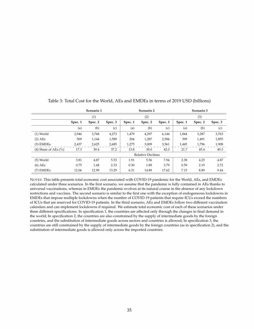
Table 3: Total Cost for the World, AEs and EMDEs in terms of 2019 USD (billions)

Scenario 1 Scenario 2 Scenario 3

(1) (2) (3)

Spec. 1 Spec. 2 Spec. 3 Spec. 1 Spec. 2 Spec. 3 Spec. 1 Spec. 2 Spec. 3

(a) (b) (c) (a) (b) (c) (a) (b) (c)

(1) World 2,946 3,768 4,273 1,479 4,297 6,144 1,844 3,287 3,763(2) AEs 509 1,144 1,589 204 1,287 2,584 399 1,491 1,855(3) EMDEs 2,437 2,625 2,685 1,275 3,009 3,561 1,445 1,796 1,908

(4) Share of AEs (%) 17.3 30.4 37.2 13.8 30.0 42.0 21.7 45.4 49.3

Relative Declines

(5) World 3.81 4.87 5.53 1.91 5.56 7.94 2.38 4.25 4.87(6) AEs 0.75 1.68 2.33 0.30 1.89 3.79 0.59 2.19 2.72(7) EMDEs 12.06 12.99 13.29 6.31 14.89 17.62 7.15 8.89 9.44

NOTES: This table presents total economic cost associated with COVID-19 pandemic for the World, AEs, and EMDEscalculated under three scenarios. In the first scenario, we assume that the pandemic is fully contained in AEs thanks touniversal vaccinations, whereas in EMDEs the pandemic evolves at its natural course in the absence of any lockdownrestrictions and vaccines. The second scenario is similar to the first one with the exception of endogeneous lockdowns inEMDEs that impose multiple lockdowns when the number of COVID-19 patients that require ICUs exceed the numbersof ICUs that are reserved for COVID-19 patients. In the third scenario, AEs and EMDEs follow two different vaccinationcalendars and can implement lockdowns if required. We estimate total economic cost of each of these scenarios underthree different specifications: In specification 1, the countries are affected only through the changes in final demand inthe world; In specification 2, the countries are also constrained by the supply of intermediate goods by the foreigncountries, and the substitution of intermediate goods across sectors and countries is allowed; In specification 3, thecountries are still constrained by the supply of intermediate goods by the foreign countries (as in specification 2), and thesubstitution of intermediate goods is allowed only across the imported countries.

35

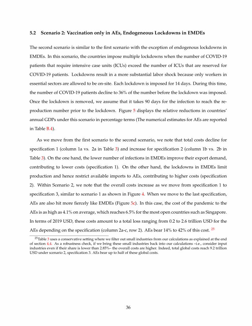
5.2 Scenario 2: Vaccination only in AEs, Endogeneous Lockdowns in EMDEs

The second scenario is similar to the first scenario with the exception of endogenous lockdowns in

EMDEs. In this scenario, the countries impose multiple lockdowns when the number of COVID-19

patients that require intensive case units (ICUs) exceed the number of ICUs that are reserved for

COVID-19 patients. Lockdowns result in a more substantial labor shock because only workers in

essential sectors are allowed to be on-site. Each lockdown is imposed for 14 days. During this time,

the number of COVID-19 patients decline to 36% of the number before the lockdown was imposed.

Once the lockdown is removed, we assume that it takes 90 days for the infection to reach the re-

production number prior to the lockdown. Figure 5 displays the relative reductions in countries’

annual GDPs under this scenario in percentage terms (The numerical estimates for AEs are reported

in Table B.4).

As we move from the first scenario to the second scenario, we note that total costs decline for

specification 1 (column 1a vs. 2a in Table 3) and increase for specification 2 (column 1b vs. 2b in

Table 3). On the one hand, the lower number of infections in EMDEs improve their export demand,

contributing to lower costs (specification 1). On the other hand, the lockdowns in EMDEs limit

production and hence restrict available imports to AEs, contributing to higher costs (specification

2). Within Scenario 2, we note that the overall costs increase as we move from specification 1 to

specification 3, similar to scenario 1 as shown in Figure 4. When we move to the last specification,

AEs are also hit more fiercely like EMDEs (Figure 5c). In this case, the cost of the pandemic to the

AEs is as high as 4.1% on average, which reaches 6.5% for the most open countries such as Singapore.

In terms of 2019 USD, these costs amount to a total loss ranging from 0.2 to 2.6 trillion USD for the

AEs depending on the specification (column 2a-c, row 2). AEs bear 14% to 42% of this cost. 25

25Table 3 uses a conservative setting where we filter out small industries from our calculations as explained at the endof section 4.4. As a robustness check, if we bring these small industries back into our calculations –i.e., consider inputindustries even if their share is lower than 2.85%– the overall costs are higher. Indeed, total global costs reach 9.2 trillionUSD under scenario 2, specification 3. AEs bear up to half of these global costs.

36

Figure 5: Relative Decline in GDPs under Scenario 2: Endogeneous Lockdowns (%)

(a) Specification 1 – Only Demand

$4 B

$3 B

$14 B

$5 B

$8 B

$8 B

$7 B$11 B$9 B

$1 B

$45 B

25 - 3120 - 2517 - 2014 - 1712 - 1410 - 129 - 108 - 97 - 86 - 75 - 64.5 - 54 - 4.53.5 - 43 - 3.52.5 - 32 - 2.51.5 - 21 - 1.5.5 - 10 - .5

(b) Specification 2 – Country Level Intermediate Inputs

$19 B

$26 B

$79 B

$30 B

$54 B

$50 B

$43 B$91 B$39 B

$3 B

$342 B

25 - 3120 - 2517 - 2014 - 1712 - 1410 - 129 - 108 - 97 - 86 - 75 - 64.5 - 54 - 4.53.5 - 43 - 3.52.5 - 32 - 2.51.5 - 21 - 1.5.5 - 10 - .5

(c) Specification 3 – Country-Industry Level Intermediate Inputs

$37 B

$61 B

$137 B

$60 B

$100 B

$98 B

$78 B$197 B$67 B

$6 B

$744 B

25 - 3120 - 2517 - 2014 - 1712 - 1410 - 129 - 108 - 97 - 86 - 75 - 64.5 - 54 - 4.53.5 - 43 - 3.52.5 - 32 - 2.51.5 - 21 - 1.5.5 - 10 - .5

NOTES: This figure shows the reductions in relative GDP under Scenario 2, where we model endogenous lockdowns inunvaccinated countries. Shades of yellow correspond to relatively lower ratios and shades of red correspond to higherrelative losses. Vaccinated countries are highlighted with light gray borders. GDP loss values are shown on the map for afew selected countries.

37

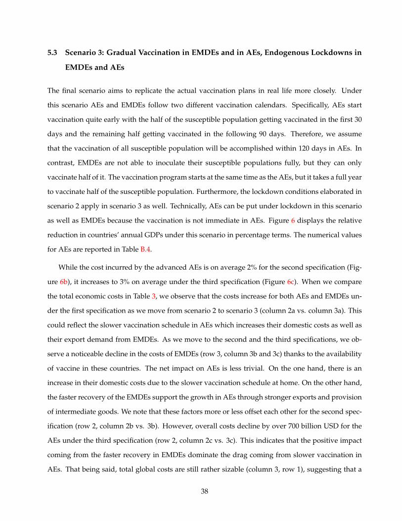
5.3 Scenario 3: Gradual Vaccination in EMDEs and in AEs, Endogenous Lockdowns in

EMDEs and AEs

The final scenario aims to replicate the actual vaccination plans in real life more closely. Under

this scenario AEs and EMDEs follow two different vaccination calendars. Specifically, AEs start

vaccination quite early with the half of the susceptible population getting vaccinated in the first 30

days and the remaining half getting vaccinated in the following 90 days. Therefore, we assume

that the vaccination of all susceptible population will be accomplished within 120 days in AEs. In

contrast, EMDEs are not able to inoculate their susceptible populations fully, but they can only

vaccinate half of it. The vaccination program starts at the same time as the AEs, but it takes a full year

to vaccinate half of the susceptible population. Furthermore, the lockdown conditions elaborated in

scenario 2 apply in scenario 3 as well. Technically, AEs can be put under lockdown in this scenario

as well as EMDEs because the vaccination is not immediate in AEs. Figure 6 displays the relative

reduction in countries’ annual GDPs under this scenario in percentage terms. The numerical values

for AEs are reported in Table B.4.

While the cost incurred by the advanced AEs is on average 2% for the second specification (Fig-

ure 6b), it increases to 3% on average under the third specification (Figure 6c). When we compare

the total economic costs in Table 3, we observe that the costs increase for both AEs and EMDEs un-

der the first specification as we move from scenario 2 to scenario 3 (column 2a vs. column 3a). This

could reflect the slower vaccination schedule in AEs which increases their domestic costs as well as

their export demand from EMDEs. As we move to the second and the third specifications, we ob-

serve a noticeable decline in the costs of EMDEs (row 3, column 3b and 3c) thanks to the availability

of vaccine in these countries. The net impact on AEs is less trivial. On the one hand, there is an

increase in their domestic costs due to the slower vaccination schedule at home. On the other hand,

the faster recovery of the EMDEs support the growth in AEs through stronger exports and provision

of intermediate goods. We note that these factors more or less offset each other for the second spec-

ification (row 2, column 2b vs. 3b). However, overall costs decline by over 700 billion USD for the

AEs under the third specification (row 2, column 2c vs. 3c). This indicates that the positive impact

coming from the faster recovery in EMDEs dominate the drag coming from slower vaccination in

AEs. That being said, total global costs are still rather sizable (column 3, row 1), suggesting that a

38

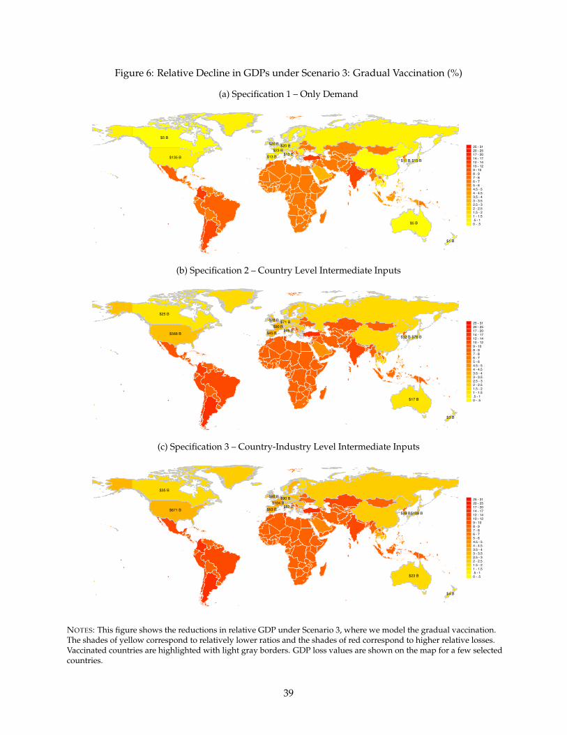
Figure 6: Relative Decline in GDPs under Scenario 3: Gradual Vaccination (%)

(a) Specification 1 – Only Demand

$5 B

$5 B

$20 B

$13 B

$23 B

$20 B

$13 B$15 B$11 B

$1 B

$135 B

25 - 3120 - 2517 - 2014 - 1712 - 1410 - 129 - 108 - 97 - 86 - 75 - 64.5 - 54 - 4.53.5 - 43 - 3.52.5 - 32 - 2.51.5 - 21 - 1.5.5 - 10 - .5

(b) Specification 2 – Country Level Intermediate Inputs

$17 B

$25 B

$71 B

$45 B

$90 B

$78 B

$46 B$76 B$32 B

$3 B

$568 B

25 - 3120 - 2517 - 2014 - 1712 - 1410 - 129 - 108 - 97 - 86 - 75 - 64.5 - 54 - 4.53.5 - 43 - 3.52.5 - 32 - 2.51.5 - 21 - 1.5.5 - 10 - .5

(c) Specification 3 – Country-Industry Level Intermediate Inputs

$23 B

$35 B

$90 B

$53 B

$104 B

$92 B

$57 B$109 B$39 B

$4 B

$671 B

25 - 3120 - 2517 - 2014 - 1712 - 1410 - 129 - 108 - 97 - 86 - 75 - 64.5 - 54 - 4.53.5 - 43 - 3.52.5 - 32 - 2.51.5 - 21 - 1.5.5 - 10 - .5

NOTES: This figure shows the reductions in relative GDP under Scenario 3, where we model the gradual vaccination.The shades of yellow correspond to relatively lower ratios and the shades of red correspond to higher relative losses.Vaccinated countries are highlighted with light gray borders. GDP loss values are shown on the map for a few selectedcountries.

39

slow inoculation calendar such as the one depicted in scenario 3 is ”too little, too late.” Under this

relatively more realistic scenario, the total cost for the world varies between 1.8 and 3.8 trillion USD

depending on the availability of the intermediate goods. Strikingly, for the third specification, the

absolute costs for the AEs is almost as high as the costs for EMDEs (column 3c, row 2 vs. row 3).

Under all three scenarios and all three specifications, the GDP costs dwarf the 27.2 billion USD cost

reported by Access to COVID-19 Tools (ACT) Accelerator partnership to manufacture and distribute

the vaccine globally.

We consider the framework that is depicted in Figure 6c as the most realistic case that mimics the

actual developments during the pandemic more closely. As of this writing in January 2021, there are

delays in the implementation of the vaccine in AEs while such delays are far more noticeable for the

EMDEs. Consequently, lockdowns and vaccinations are simultaneously observed both in AEs and

EMDEs at the same time. Thus, the assumptions that are valid for this scheme seem to match the

real world the best. Figure 7 filters out the costs that arise from international costs and only focuses

on the domestic costs for this baseline specification. To that end, for a given country, we assume

that the course of pandemic follows the same pattern as specification 3 of scenario 3 within the

country. Meanwhile, the rest of the world is devoid of the pandemic, and, hence, is back to normal.

We run this simulation separately for 65 countries. As expected, compared to Figure 6c, the losses

are subdued. The costs borne by the EMDEs are not significantly different from those observed in

Figure 6c because the bulk of the costs incurred by the EMDEs are domestically driven. For the

AEs, however, we observe that the domestic costs are far less important compared to those that

arise from international linkages. For the US, for example, while the domestic costs of the pandemic

are 92 billion USD, when we add the costs due to trade linkages the toll rises to 744 billion USD.

Countries like China, Australia, and New Zealand, which have the pandemic under control, have

negligible domestic costs where most of their costs shown in Figure 6c are driven by international

linkages. This figure corroborates the importance of international linkages in the disease toll.

5.4 Sectoral Heterogeneity

Recall from Figure 3 and our eloborate discussion of the model that the economic costs that we

estimate for each country are calculated at the sectoral level. Sectoral aggregates yield the country-

40

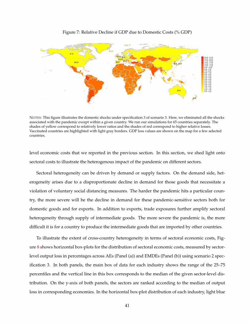
Figure 7: Relative Decline if GDP due to Domestic Costs (% GDP)

$0 B

$1 B

$3 B

$8 B$15 B

$12 B

$6 B$1 B$0 B

$0 B

$92 B

25.00 - 31.0020.00 - 25.0017.00 - 20.0014.00 - 17.0012.00 - 14.0010.00 - 12.009.00 - 10.008.00 - 9.007.00 - 8.006.00 - 7.005.00 - 6.004.50 - 5.004.00 - 4.503.50 - 4.003.00 - 3.502.50 - 3.002.00 - 2.501.50 - 2.001.00 - 1.500.50 - 1.000.00 - 0.50

NOTES: This figure illustrates the domestic shocks under specification 3 of scenario 3. Here, we eliminated all the shocksassociated with the pandemic except within a given country. We run our simulations for 65 countries separately. Theshades of yellow correspond to relatively lower ratios and the shades of red correspond to higher relative losses.Vaccinated countries are highlighted with light gray borders. GDP loss values are shown on the map for a few selectedcountries.

level economic costs that we reported in the previous section. In this section, we shed light onto

sectoral costs to illustrate the heterogenous impact of the pandemic on different sectors.

Sectoral heterogeneity can be driven by demand or supply factors. On the demand side, het-

erogeneity arises due to a disproportionate decline in demand for those goods that necessitate a

violation of voluntary social distancing measures. The harder the pandemic hits a particular coun-

try, the more severe will be the decline in demand for these pandemic-sensitive sectors both for

domestic goods and for exports. In addition to exports, trade exposures further amplify sectoral

heterogeneity through supply of intermediate goods. The more severe the pandemic is, the more

difficult it is for a country to produce the intermediate goods that are imported by other countries.

To illustrate the extent of cross-country heterogeneity in terms of sectoral economic costs, Fig-

ure 8 shows horizontal box-plots for the distribution of sectoral economic costs, measured by sector-

level output loss in percentages across AEs (Panel (a)) and EMDEs (Panel (b)) using scenario 2 spec-

ification 3. In both panels, the main box of data for each industry shows the range of the 25–75

percentiles and the vertical line in this box corresponds to the median of the given sector-level dis-

tribution. On the y-axis of both panels, the sectors are ranked according to the median of output

loss in corresponding economies. In the horizontal box-plot distribution of each industry, light blue

41

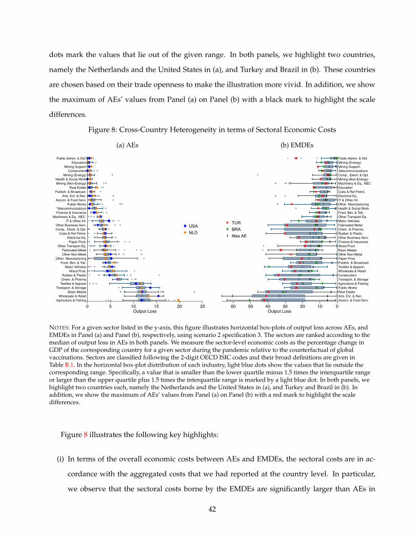
dots mark the values that lie out of the given range. In both panels, we highlight two countries,

namely the Netherlands and the United States in (a), and Turkey and Brazil in (b). These countries

are chosen based on their trade openness to make the illustration more vivid. In addition, we show

the maximum of AEs’ values from Panel (a) on Panel (b) with a black mark to highlight the scale

differences.

Figure 8: Cross-Country Heterogeneity in terms of Sectoral Economic Costs

(a) AEs

Agriculture & FishingWholesale & Retail

Basic MetalsTransport. & Storage

Textiles & ApparelChem. & PharmaRubber & Plastic

Wood Prod.Motor Vehicles

Food, Bev. & Tob.Other Manufacturing

Other Non-MetalFabricated Metal

Other Transport Eq.Paper Prod.

Electrical Eq.Coke & Ref Petrol.

Comp., Electr. & Opt.Other Business Serv.

IT & Other Inf.Machinery & Eq., NEC

Finance & InsuranceTelecommunications

Public WorksAccom. & Food Serv.

Arts, Ent. & Rec.Publish. & Broadcast.

Real EstateMining (Non-Energy)Health & Social Work

Mining (Energy)Construction

Mining SupportEducation

Public Admin. & Def.

0 5 10 15 20 25Output Loss

USANLD

(b) EMDEs

Accom. & Food Serv.Arts, Ent. & Rec.Real EstatePublic WorksAgriculture & FishingTransport. & StorageConstructionWholesale & RetailTextiles & ApparelPublish. & Broadcast.Paper Prod.Other Non-MetalBasic MetalsWood Prod.Finance & InsuranceOther Business Serv.Rubber & PlasticChem. & PharmaFabricated MetalMotor VehiclesOther Transport Eq.Food, Bev. & Tob.Health & Social WorkOther ManufacturingIT & Other Inf.Electrical Eq.Coke & Ref Petrol.EducationMachinery & Eq., NEC Mining (Non-Energy)Comp., Electr. & Opt.TelecommunicationsMining SupportMining (Energy)Public Admin. & Def.

0102030405060Output Loss

TURBRAMax AE

NOTES: For a given sector listed in the y-axis, this figure illustrates horizontal box-plots of output loss across AEs, andEMDEs in Panel (a) and Panel (b), respectively, using scenario 2 specification 3. The sectors are ranked according to themedian of output loss in AEs in both panels. We measure the sector-level economic costs as the percentage change inGDP of the corresponding country for a given sector during the pandemic relative to the counterfactual of globalvaccinations. Sectors are classified following the 2-digit OECD ISIC codes and their broad definitions are given inTable B.1. In the horizontal box-plot distribution of each industry, light blue dots show the values that lie outside thecorresponding range. Specifically, a value that is smaller than the lower quartile minus 1.5 times the interquartile rangeor larger than the upper quartile plus 1.5 times the interquartile range is marked by a light blue dot. In both panels, wehighlight two countries each, namely the Netherlands and the United States in (a), and Turkey and Brazil in (b). Inaddition, we show the maximum of AEs’ values from Panel (a) on Panel (b) with a red mark to highlight the scaledifferences.

Figure 8 illustrates the following key highlights:

(i) In terms of the overall economic costs between AEs and EMDEs, the sectoral costs are in ac-

cordance with the aggregated costs that we had reported at the country level. In particular,

we observe that the sectoral costs borne by the EMDEs are significantly larger than AEs in

42

each sector. The black mark in panel (b), which shows the maximum sectoral cost in AEs, is

typically lower than the average sectoral costs borne by the EMDEs.

(ii) There is substantial sectoral heterogeneity within both AEs and EMDEs.

(iii) The sectoral costs for the EMDEs are the highest for those sectors that are more severely af-

fected from the domestic pandemic conditions such as accommodation and food services, arts

and entertainment, or real estate (Panel (b)). The economic costs in these sectors primarily

reflect the decline in demand due to the fear factor in these countries where the pandemic is

not contained.

(iv) When we turn to AEs that are vaccinated at a faster pace, we observe a different sectoral break-

down. Because the domestic drag from the pandemic is eliminated in these countries, the

sectors that bear the highest economic costs are those that are more exposed to trade with un-

vaccinated countries such as textiles and apparel, basic metals, or food, beverage, and tobacco

industries. Recall from Figure 2 that all of these sectors are either sizable importers of inputs

(shown by the node color) or they are connected to other industries that are major importers of

inputs, such as the thick edge connecting the mining sector (which is mostly based in EMDEs)

to basic metal sector. Thus, our findings are strongly supportive of our predictions from the

discussion of Figure 2.

(v) In order to give a glance about the sectoral costs with respect to trade exposure, we plot a

couple of countries with different levels of trade openness. The idea is to visually illustrate

whether those countries that are more open to trade suffer larger sectoral costs. Recall that

the node color in Figure 1 illustrated trade openness. We observe that the countries that are

represented by darker nodes in Figure 1 bear higher economic costs. More specifically, within

two AEs such as the Netherlands and the US, we observe that the sectoral costs are generally

higher in Netherlands compared to US, consistent with more trade exposure. A similar picture

emerges when we compare the sectoral costs for two EMDE countries. Turkey is more open

to trade relative to Brazil. Consequently, sectoral costs borne by Turkey, are generally higher

than those of Brazil.

43

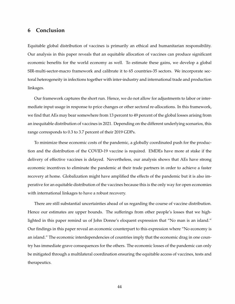
6 Conclusion

Equitable global distribution of vaccines is primarily an ethical and humanitarian responsibility.

Our analysis in this paper reveals that an equitable allocation of vaccines can produce significant

economic benefits for the world economy as well. To estimate these gains, we develop a global

SIR-multi-sector-macro framework and calibrate it to 65 countries-35 sectors. We incorporate sec-

toral heterogeneity in infections together with inter-industry and international trade and production

linkages.

Our framework captures the short run. Hence, we do not allow for adjustments to labor or inter-

mediate input usage in response to price changes or other sectoral re-allocations. In this framework,

we find that AEs may bear somewhere from 13 percent to 49 percent of the global losses arising from

an inequitable distribution of vaccines in 2021. Depending on the different underlying scenarios, this

range corresponds to 0.3 to 3.7 percent of their 2019 GDPs.

To minimize these economic costs of the pandemic, a globally coordinated push for the produc-

tion and the distribution of the COVID-19 vaccine is required. EMDEs have more at stake if the

delivery of effective vaccines is delayed. Nevertheless, our analysis shows that AEs have strong

economic incentives to eliminate the pandemic at their trade partners in order to achieve a faster

recovery at home. Globalization might have amplified the effects of the pandemic but it is also im-

perative for an equitable distribution of the vaccines because this is the only way for open economies

with international linkages to have a robust recovery.

There are still substantial uncertainties ahead of us regarding the course of vaccine distribution.

Hence our estimates are upper bounds. The sufferings from other people’s losses that we high-

lighted in this paper remind us of John Donne’s eloquent expression that “No man is an island.”

Our findings in this paper reveal an economic counterpart to this expression where “No economy is

an island.” The economic interdependencies of countries imply that the economic drag in one coun-

try has immediate grave consequences for the others. The economic losses of the pandemic can only

be mitigated through a multilateral coordination ensuring the equitable access of vaccines, tests and

therapeutics.

44

References

Acemoglu, Daron, Vasco M Carvalho, Asuman Ozdaglar, and Alireza Tahbaz-Salehi, “The net-work origins of aggregate fluctuations,” Econometrica, 2012, 80 (5), 1977–2016.

, Victor Chernozhukov, Ivan Werning, and Michael D Whinston, “A Multi-Risk SIR Model withOptimally Targeted Lockdown,” Working Paper 27102, National Bureau of Economic ResearchMay 2020.

Alfaro, Laura, Oscar Becerra, and Marcela Eslava, “EMEs and COVID-19 Shutting Down in a Worldof Informal and Tiny Firms,” Working Paper 27360, National Bureau of Economic Research June2020.

Allen, Linda JS, “A primer on stochastic epidemic models: Formulation, numerical simulation, andanalysis,” Infectious Disease Modelling, 2017, 2 (2), 128–142.

Alon, Titan M, Minki Kim, David Lagakos, and Mitchell VanVuren, “How Should Policy Re-sponses to the COVID-19 Pandemic Differ in the Developing World?,” Working Paper 27273, Na-tional Bureau of Economic Research 2020.

Alvarez, Fernando E, David Argente, and Francesco Lippi, “A simple planning problem forCOVID-19 lockdown,” Working Paper 26981, National Bureau of Economic Research 2020.

Atkeson, Andrew, “How Deadly is COVID-19? Understanding the Difficulties with Estimation ofits Fatality Rate,” Working Paper 26965, National Bureau of Economic Research 2020.

Baldwin, Richard and B Weder di Mauro, Economics in the Time of COVID-19, Vol. 26, Centre forEconomic Policy Research, London, 2020. A VoxEU. org Book.

Baqaee, David and Emmanuel Farhi, “Nonlinear Production Networks with an Application to theCOVID-19 crisis,” Working Paper 27281, National Bureau of Economic Research 2020.

and , “Supply and Demand in Disaggregated Keynesian Economies with an Application to theCOVID-19 crisis,” Working Paper 27152, National Bureau of Economic Research 2020.

, , Michael J. Mina, and James H. Stock, “Reopening Scenarios,” Working Paper 27244, Na-tional Bureau of Economic Research 2020.

Barrot, Jean-Noel, Basile Grassi, and Julien Sauvagnat, “Sectoral effects of social distancing,” 2020.Available at SSRN.

Bendavid, Eran and Jay Bhattacharya, “Is Coronavirus as Deadly as They Say?,” Wall Street Journal,2020, 24.

Bonadio, Barthelemy, Zhen Huo, Andrei A Levchenko, and Nitya Pandalai-Nayar, “Global SupplyChains in the Pandemic,” Working Paper 27224, National Bureau of Economic Research 2020.

Cakmakli, Cem and Yasin Simsek, “Bridging the COVID-19 Data and the Epidemiological Modelusing Time Varying Parameter SIRD Model,” Working Paper series 20-23, Rimini Centre for Eco-nomic Analysis July 2020.

45

Cakmaklı, Cem, Selva Demiralp, Sebnem Kalemli-Ozcan, Sevcan Yesiltas, and Muhammed AliYıldırım, “COVID-19 and Emerging Markets: An Epidemiological Multi-Sector Model for a SmallOpen Economy with an Application to Turkey,” Working Paper 27191, National Bureau of Eco-nomic Research 2020.

Carvalho, Vasco M, Makoto Nirei, Yukiko Saito, and Alireza Tahbaz-Salehi, “Supply Chain Dis-ruptions: Evidence from the Great East Japan Earthquake,” The Quarterly Journal of Economics,forthcoming.

Chetty, Raj, John N Friedman, Nathaniel Hendren, Michael Stepner, and The Opportunity In-sights Team, “How Did COVID-19 and Stabilization Policies Affect Spending and Employment?A New Real-Time Economic Tracker Based on Private Sector Data,” Working Paper 27431, Na-tional Bureau of Economic Research 2020.

Cutler, David M and Lawrence H Summers, “The COVID-19 pandemic and the $16 trillion virus,”Jama, 2020, 324 (15), 1495–1496.

del Rio-Chanona, R Maria, Penny Mealy, Anton Pichler, Francois Lafond, and J Doyne Farmer,“Supply and demand shocks in the COVID-19 pandemic: an industry and occupation perspec-tive,” Oxford Review of Economic Policy, 2020, 36 (Supplement 1), S94–S137.

Dewatripont, Mathias, Michel Goldman, Eric Muraille, and Jean-Philippe Platteau, “Rapidlyidentifying workers who are immune to COVID-19 and virus-free is a priority for restarting theeconomy,” Working Paper, VOX CEPR Policy Portal 2020.

Dingel, Jonathan I and Brent Neiman, “How many jobs can be done at home?,” Working Paper26948, National Bureau of Economic Research 2020.

Eichenbaum, Martin S, Sergio Rebelo, and Mathias Trabandt, “The macroeconomics of epi-demics,” Working Paper 26882, National Bureau of Economic Research 2020.

Farboodi, Maryam, Gregor Jarosch, and Robert Shimer, “Internal and external effects of socialdistancing in a pandemic,” Working Paper 27059, National Bureau of Economic Research 2020.

Fauci, AS, HC Lane, and RR Redfield, “COVID-19-Navigating the Uncharted.,” The New EnglandJournal of Medicine, 2020, 382 (13), 1268–1269.

Goolsbee, Austan and Chad Syverson, “Fear, Lockdown, and Diversion: Comparing Drivers ofPandemic Economic Decline 2020,” Working Paper 27432, National Bureau of Economic Research2020.

Gourinchas, Pierre-Olivier, Sebnem Kalemli-Ozcan, Veronika Penciakova, and Nicholas Sander,“COVID-19 and SME failures,” Working Paper 27877, National Bureau of Economic Research2020.

Guerrieri, Veronica, Guido Lorenzoni, Ludwig Straub, and Ivan Werning, “Macroeconomic Impli-cations of COVID-19: Can Negative Supply Shocks Cause Demand Shortages?,” Working Paper26918, National Bureau of Economic Research 2020.

Horvat, Peter, Colin Webb, and Norihiko Yamano, “Measuring employment in global valuechains,” 2020. https://www.oecd-ilibrary.org/content/paper/00f7d7db-en.

46

Krueger, Dirk, Harald Uhlig, and Taojun Xie, “Macroeconomic dynamics and reallocation in anepidemic,” CEPR COVID Economics, 2020, 1 (5), 21–55.

Li, Ruiyun, Sen Pei, Bin Chen, Yimeng Song, Tao Zhang, Wan Yang, and Jeffrey Shaman, “Sub-stantial undocumented infection facilitates the rapid dissemination of novel coronavirus (SARS-CoV2),” Science, 2020.

Linton, Natalie M, Tetsuro Kobayashi, Yichi Yang, Katsuma Hayashi, Andrei R Akhmetzhanov,Sung mok Jung, Baoyin Yuan, Ryo Kinoshita, and Hiroshi Nishiura, “Incubation period andother epidemiological characteristics of 2019 novel coronavirus infections with right truncation: astatistical analysis of publicly available case data,” Journal of Clinical Medicine, 2020, 9 (2), 538.

Mendoza, Enrique G, Eugenio I Rojas, Linda L Tesar, and Jing Zhang, “A Macroeconomic Modelof Healthcare Saturation, Inequality and the Output-Pandemia Tradeoff,” Technical Report, Na-tional Bureau of Economic Research 2020.

OECD, “OECD Inter-Country Input-Output (ICIO) Tables,” 2020. https://www.oecd.org/sti/ind/inter-country-input-output-tables.htm.

Shih, Willy C., “Global Supply Chains in a Post-Pandemic World: Companies Need to Make TheirNetworks More Resilient. Here’s How.,” Harvard Business Review, 2020, 98 (5), 82–89.

Stock, James H, “Data gaps and the policy response to the novel coronavirus,” Working Paper 26902,National Bureau of Economic Research 2020.

The World Bank, “World Development Report 2020: Trading for Development in the Age of GlobalValue Chains,” 2020. https://www.worldbank.org/en/publication/wdr2020.

Vogel, Gretchen, “New blood tests for antibodies could show true scale of coronavirus pandemic,”Science, March 19 2020.

47

APPENDIX

A Vaccine Development and Availability

The competition to produce a safe and effective COVID-19 vaccine heated up in the second half of

2020 with the unstoppable global march of the virus. Vaccine safety trials in humans started as early

as March 2020, and thirteen of them reached the final stages of testing by year-end 2020. 26

The development cycle of an effective vaccine from the lab to clinic requires years of intense re-

search and testing until it finally reaches people’s arms. In this section, we go over the development

and accessibility of all the coronavirus vaccines that have reached publicly disclosed deals across

the globe, along with a brief discussion of the vaccine testing process.

A.1 Vaccines Classified by Developmental Phases

A.1.1 Preclinical Phase

Scientists typically kick off the development of a new vaccine with a preclinical phase. During this

phase, an experimental vaccine goes through a set of screenings and evaluations to determine which

antigen should be used to trigger an immune response. Before tested on humans, it is first tested on

cells and then on animals such as mice or monkeys to evaluate its safety and potential to prevent the

disease. As of December 2020, the WHO confirmed 87 preclinical vaccines in active development.

Among all, in September 2020, Saint-Herblain-based company Valneva announced that they signed

a vaccine partnership with the UK government for its inactivated COVID-19 vaccine, VLA2001. Un-

der the agreement, if vaccine development is successful, Valneva will provide the UK government

with 60 million doses in the second half of 2021. UK Government then has options over 40 million

doses in 2022 and a further 30 million to 90 million doses, in aggregate, across 2023 to 2025. UK

government is also investing upfront in the scale up and development of the vaccine.

26For timely updates on the COVID-19 vaccination, see the following websites: https://www.bloomberg.com/graphics/covid-vaccine-tracker-global-distribution/ and https://www.nytimes.com/interactive/2020/science/coronavirus-vaccine-tracker.html

48

A.1.2 Phase 1

If the vaccine successfully stimulates the immune system, scientists proceed with the testing of the

vaccine in human clinical trials in three phases. In Phase 1, the vaccine is given to a small number of

volunteers to assess its safety, confirm that it triggers an immune response, and determine the accu-

rate dosage. Generally during this phase vaccines are tested in young, healthy adult volunteers. As

of December 2020, the WHO confirmed that there are 41 vaccines testing safety and dosage in active

Phase 1. Among all, a protein-based vaccine developed by the University of Queensland confirmed

its potential to protect hamsters from the virus. The university then launched Phase 1 trials in July

2020, supplementing the proteins with an adjuvant made by CSL to trigger the immune system. In

September 2020, the vaccine developers signed an agreement with the Australian government to

deliver 51 million doses if the trials deliver positive results. They expected their first supply of the

vaccines to be ready in mid-2021.

A.1.3 Phase 2

In Phase 2, the vaccine is given to hundreds of volunteers to further assess its safety and ability

to invoke an immune response. This phase consists of multiple trials in which various age groups

and different formulations of the vaccine are investigated. Besides the inoculated group, a placebo

group is included to determine whether the changes in the vaccinated group are due to the vaccine,

or whether they took place as a coincidence. As of December 2020, the WHO confirmed that there

are 17 vaccines in expanded safety trials of Phase 2. Among all, Sanofi/GlaxoSmithKline (GSK),

CureVac, and UBI Group are those that negotiated several deals to supply the vaccine.

Paris-based company Sanofi and Brentford-based company GSK announced that they collabo-

ratively launched Phase 1 and 2 clinical trials in September. During the preclinical phase, Sanofi

developed a protein-based vaccine, supplementing the viral proteins with adjuvants made by GSK

to trigger the immune system. Before kicking off their clinical trials, Sanofi negotiated several ma-

jor deals to supply the vaccine, including agreements with the United States, European Union, and

Canada to provide 100 million doses, 300 million doses, and up to 72 million doses, respectively.

Sanofi also reached an agreement with COVAX– an international collaboration to deliver the vac-

49

cine equitably across the world and led by the World Health Organization, Global Vaccine Alliance

Gavi, and the Coalition for Epidemic Preparedness–to provide 200 million doses. They have plans

to extend their supply of the vaccine to one billion doses in 2021.

After observing a promising response in the immune systems of their vaccinated volunteers in a

Phase 1 clinical trial, Tubingen-based company CureVac launched the next Phase 2 trial in September

2020 to further assess the safety and ability to generate an immune response of its mRNA based-

genetic vaccine. They expect to make the preliminary data of their Phase 3 study public in the first

quarter of 2021.

In November 2020, CureVac negotiated a deal to provide the European Union with up to 225

million doses of their vaccine. They have plans to extend their supply of the vaccine to 300 million

doses in 2021 and up to 600 million doses the following year.

Colorado-based company UBI Group launched its Phase 2 study to vaccinate hundreds of vol-

unteers to evaluate the ability of its protein-based vaccine to stimulate their immune systems. UBI

group negotiated a few deals with Covax and Other Jurisdictions to provide 200 million doses and

2 million doses, respectively.

A.1.4 Phase 3

In Phase 3, the vaccine is given to thousands of volunteers to see how many get infected, compared

to those who received a placebo. This phase consists of multiple trials that help scientists to assess

whether the vaccine is effective against the coronavirus. It further confirms its safety in a much larger

group of people. As of December 2020, the WHO confirmed that there are 13 vaccines in large-scale

efficacy tests. Among all, 9 companies have entered deals with several countries to supply their

vaccine needs.

A.1.5 Authorization for use

In early November 2020, New York-based Pfizer and the German company BioNTech made their

first evidence public that their mRNA-based genetic coronavirus vaccine was 95 percent effective,

which was a milestone in the development of an effective coronavirus vaccine. Afterwards, the

50

companies applied to the U.S. Food and Drug Administration (FDA) for an emergency use autho-

rization. On December 2, the UK gave emergency authorization to their vaccine. Following the

go-ahead given by the FDA, Pfizer and BioNTech is expected to manufacture over 1.3 billion doses

of their vaccine worldwide by the end of 2021.

In a partnership with US National Institutes of Health, Boston-based company Moderna launched

its Phase 3 study and announced that its mRNA-based genetic coronavirus vaccine’s efficacy rate is

estimated as 94.1 percent by late November 2020. Following Pfizer & BioNTech, Moderna made the

second application to FDA to get approval. In the meantime, the company negotiated with several

countries including Canada, Japan, and Qatar and EU members to supply the vaccine after approval.

In August 2020, the US government awarded the company an additional $1.5 billion in exchange for

100 million doses if the vaccine proves safe and effective.

The British-Swedish company AstraZeneca and the University of Oxford created a coronavirus

vaccine using the viral vector technology based on chimpanzee adenovirus. Based on their recent

scientific trials, the efficacy rate is announced to be 70 percent. Meanwhile AstraZeneca signed a

series of deals to supply their vaccine if its safety and efficacy is approved. The US government

awarded the project $1.2 billion in support for 300 million doses. The company declared that they

expect to manufacture two billion doses of their vaccine if approved.

The Gamaleya Research Institute, part of Russia’s Ministry of Health, has created a coronavirus

vaccine–renamed Sputnik V–that is developed by viral vector technology based on two adenoviruses

Ad5 & Ad26. According to the preliminary results of Phase 3 trials announced in November 2020,

the efficacy rate is estimated to be 91 percent. Russia negotiated a set of agreements to supply

the vaccine to several countries including Brazil, India, Mexico, Venezuela, Uzbekistan, Egypt, and

Nepal.

In addition to the above-mentioned biotech companies, Novavax, Johnson & Johnson, Sinovac

Biotech, CanSino Biologics, Sinopharm, Medicago/GSK are those that have launched their Phase 3

trials to assess the efficacy and safety of their vaccines. Tables A.1–A.2 provide further details on the

coronavirus vaccines, the companies that developed them as well as the supply of the vaccines to

the countries with which they have negotiated.

51

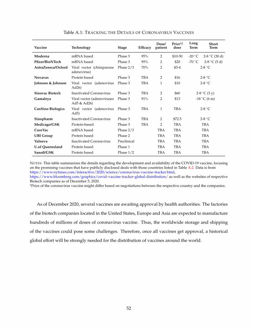
Table A.1: TRACKING THE DETAILS OF CORONAVIRUS VACCINES

Vaccine Technology Stage EfficacyDose/

patientPrice*/dose

LongTerm

ShortTerm

Moderna mRNA based Phase 3 95% 2 $10-50 -20 ◦C 2-8 ◦C (30 d)

Pfizer/BioNTech mRNA based Phase 3 95% 2 $20 -70 ◦C 2-8 ◦C (5 d)

AstraZeneca/Oxford Viral vector (chimpanzeeadenovirus)

Phase 2/3 70% 2 $3-4 2-8 ◦C

Novavax Protein based Phase 3 TBA 2 $16 2-8 ◦C

Johnson & Johnson Viral vector (adenovirusAd26)

Phase 3 TBA 1 $10 2-8 ◦C

Sinovac Biotech Inactivated Coronavirus Phase 3 TBA 2 $60 2-8 ◦C (3 y)

Gamaleya Viral vector (adenovirusesAd5 & Ad26)

Phase 3 91% 2 $13 -18 ◦C (6 m)

CanSino Biologics Viral vector (adenovirusAd5)

Phase 3 TBA 1 TBA 2-8 ◦C

Sinopharm Inactivated Coronavirus Phase 3 TBA 2 $72.5 2-8 ◦C

Medicago/GSK Protein-based Phase 3 TBA 2 TBA TBA

CureVac mRNA based Phase 2/3 TBA TBA TBA

UBI Group Protein based Phase 2 TBA TBA TBA

Valneva Inactivated Coronavirus Preclinical TBA TBA TBA

U.of Queensland Protein based Phase 1 TBA TBA TBA

Sanofi/GSK Protein based Phase 1/2 TBA TBA TBA

NOTES: This table summarizes the details regarding the development and availability of the COVID-19 vaccine, focusingon the promising vaccines that have publicly disclosed deals with those countries listed in Table A.2. Data is fromhttps://www.nytimes.com/interactive/2020/science/coronavirus-vaccine-tracker.html,https://www.bloomberg.com/graphics/covid-vaccine-tracker-global-distribution/ as well as the websites of respectiveBiotech companies as of December 5, 2020.*Price of the coronavirus vaccine might differ based on negotiations between the respective country and the companies.

As of December 2020, several vaccines are awaiting approval by health authorities. The factories

of the biotech companies located in the United States, Europe and Asia are expected to manufacture

hundreds of millions of doses of coronavirus vaccine. Thus, the worldwide storage and shipping

of the vaccines could pose some challenges. Therefore, once all vaccines get approval, a historical

global effort will be strongly needed for the distribution of vaccines around the world.

52

Table A.2: CORONAVIRUS VACCINE ORDERS

Vaccine / Country Mod

erna

Pfize

r/B

ioN

Tech

Ast

raZ

enec

a/O

xfor

d

Nov

avax

John

son

&Jo

hnso

n

Sino

vac

Bio

tech

Gam

aley

a

Can

Sino

Bio

logi

cs

Sino

phar

m

Med

icag

o/G

SK

Cur

eVac

UB

IG

roup

Val

neva

U.o

fQ

ueen

slan

d

Sano

fi/G

SK

India 100 100 200U.S. 100 100 300 110 100 100EU 80 200 400 200 225 300Canada 20 20 20 76 38 76 72Japan 50 120 120U.K. 7 40 100 60 30 60 60Brazil 100 46 100Indonesia 100 50 15 60Mexico 34 77 64 35China 200Russia 160Australia 10 34 40 51Pakistan 88Uzbekistan 70Egypt 50Nepal 50Latin America Bloc 160Turkey 50Middle East Bloc 75Covax 300 200 200Other 5 45 63 20 4 2

NOTES: This table summarizes the COVID-19 vaccine orders (in millions) given by countries. We use informationavailable in various resources includinghttps://www.nytimes.com/interactive/2020/science/coronavirus-vaccine-tracker.html,https://www.bloomberg.com/graphics/covid-vaccine-tracker-global-distribution/ as well as the websites of respectiveBiotech companies as of December 5, 2020. The Latin America bloc covers all countries in the region except Brazil. TheEuropean Union bloc represents the 27 countries of the European Union. The Covax agreement extends to mostcountries in the world, including many in Africa that wouldn’t otherwise be covered. The countries included in “Other”without a population figure, such as Somalia and Syria, have been omitted. The Middle East bloc covers United ArabEmirates, Egypt, Bahrain and Jordan.

53

B Additional Figures and Tables

List of Figures and Tables:

• Figure B.1: The Structure of OECD Inter-Country Input-Output (ICIO) Table

• Table B.1: Proximity Index, Teleworkable Share and Demand Changes Across Industries

• Table B.2: List of Essential Sectors during Lockdowns

• Table B.3: Country Settings for Various Scenarios

• Table B.4: Relative reduction in GDP of Advanced Economies (AEs) under Scenarios 2 and 3(%).

• Table B.5: ICU Bed Capacities

54

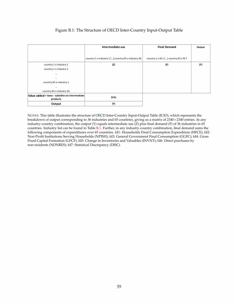
Figure B.1: The Structure of OECD Inter-Country Input-Output Table

Intermediate use Final Demand Output

country 1 x industry 1 […] country 65 x industry 36 country 1 x fd 1 […] country 65 x fd 7

country 1 x industry 1 (Z) (F) (Y)

country 1 x industry 2

…

…

country 65 x industry 1

…

country 65 x industry 36

Value added + taxes - subsidies on intermediate products

(VA)

Output (Y)

NOTES: This table illustrates the structure of OECD Inter-Country Input-Output Table (ICIO), which represents thebreakdown of output corresponding to 36 industries and 65 countries, giving us a matrix of 2340×2340 entries. In anyindustry-country combination, the output (Y) equals intermediate use (Z) plus final demand (F) of 36 industries in 65countries. Industry list can be found in Table B.1. Further, in any industry-country combination, final demand sums thefollowing components of expenditures over 65 countries. fd1: Households Final Consumption Expenditure (HFCE); fd2:Non-Profit Institutions Serving Households (NPISH); fd3: General Government Final Consumption (GGFC); fd4: GrossFixed Capital Formation (GFCF); fd5: Change in Inventories and Valuables (INVNT); fd6: Direct purchases bynon-residents (NONRES); fd7: Statistical Discrepancy (DISC).

55

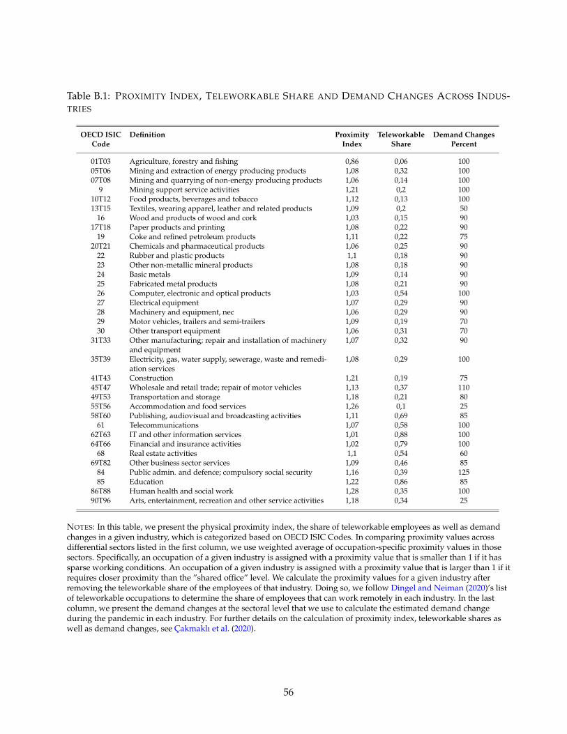
Table B.1: PROXIMITY INDEX, TELEWORKABLE SHARE AND DEMAND CHANGES ACROSS INDUS-TRIES

OECD ISIC Definition Proximity Teleworkable Demand ChangesCode Index Share Percent

01T03 Agriculture, forestry and fishing 0,86 0,06 10005T06 Mining and extraction of energy producing products 1,08 0,32 10007T08 Mining and quarrying of non-energy producing products 1,06 0,14 100

9 Mining support service activities 1,21 0,2 10010T12 Food products, beverages and tobacco 1,12 0,13 10013T15 Textiles, wearing apparel, leather and related products 1,09 0,2 50

16 Wood and products of wood and cork 1,03 0,15 9017T18 Paper products and printing 1,08 0,22 90

19 Coke and refined petroleum products 1,11 0,22 7520T21 Chemicals and pharmaceutical products 1,06 0,25 90

22 Rubber and plastic products 1,1 0,18 9023 Other non-metallic mineral products 1,08 0,18 9024 Basic metals 1,09 0,14 9025 Fabricated metal products 1,08 0,21 9026 Computer, electronic and optical products 1,03 0,54 10027 Electrical equipment 1,07 0,29 9028 Machinery and equipment, nec 1,06 0,29 9029 Motor vehicles, trailers and semi-trailers 1,09 0,19 7030 Other transport equipment 1,06 0,31 70

31T33 Other manufacturing; repair and installation of machineryand equipment

1,07 0,32 90

35T39 Electricity, gas, water supply, sewerage, waste and remedi-ation services

1,08 0,29 100

41T43 Construction 1,21 0,19 7545T47 Wholesale and retail trade; repair of motor vehicles 1,13 0,37 11049T53 Transportation and storage 1,18 0,21 8055T56 Accommodation and food services 1,26 0,1 2558T60 Publishing, audiovisual and broadcasting activities 1,11 0,69 85

61 Telecommunications 1,07 0,58 10062T63 IT and other information services 1,01 0,88 10064T66 Financial and insurance activities 1,02 0,79 100

68 Real estate activities 1,1 0,54 6069T82 Other business sector services 1,09 0,46 85

84 Public admin. and defence; compulsory social security 1,16 0,39 12585 Education 1,22 0,86 85

86T88 Human health and social work 1,28 0,35 10090T96 Arts, entertainment, recreation and other service activities 1,18 0,34 25

NOTES: In this table, we present the physical proximity index, the share of teleworkable employees as well as demandchanges in a given industry, which is categorized based on OECD ISIC Codes. In comparing proximity values acrossdifferential sectors listed in the first column, we use weighted average of occupation-specific proximity values in thosesectors. Specifically, an occupation of a given industry is assigned with a proximity value that is smaller than 1 if it hassparse working conditions. An occupation of a given industry is assigned with a proximity value that is larger than 1 if itrequires closer proximity than the ”shared office” level. We calculate the proximity values for a given industry afterremoving the teleworkable share of the employees of that industry. Doing so, we follow Dingel and Neiman (2020)’s listof teleworkable occupations to determine the share of employees that can work remotely in each industry. In the lastcolumn, we present the demand changes at the sectoral level that we use to calculate the estimated demand changeduring the pandemic in each industry. For further details on the calculation of proximity index, teleworkable shares aswell as demand changes, see Cakmaklı et al. (2020).

56

Table B.2: LIST OF ESSENTIAL SECTORS DURING LOCKDOWNS

NACE Rev. 2 Definition

01 Crop and animal production, hunting and related service activities10 Manufacture of food products

1722 Manufacture of household and sanitary goods and of toilet requisites1811 Printing of newspapers1920 Manufacture of refined petroleum products21 Manufacture of basic pharmaceutical products and pharmaceutical preparations35 Electricity, gas, steam and air conditioning supply36 Water collection, treatment and supply463 Wholesale of food, beverages and tobacco4646 Wholesale of pharmaceutical goods4711 Retail sale in non-specialised stores with food, beverages or tobacco predominating472 Retail sale of food, beverages and tobacco in specialised stores4730 Retail sale of automotive fuel in specialised stores4773 Dispensing chemist in specialised stores4774 Retail sale of medical and orthopaedic goods in specialised stores4781 Retail sale via stalls and markets of food, beverages and tobacco products4920 Freight rail transport4941 Freight transport by road5224 Cargo handling53 Postal and courier activities60 Programming and broadcasting activities61 Telecommunications639 Other information service activities75 Veterinary activities86 Human health activities87 Residential care activities

NOTES: This table provides the list of the essential sectors that we consider for the implementation of lockdowns underScenario 2 & Scenario 3. The table is based on Cakmaklı et al. (2020) where authors use government decrees to identifythese sectors.

57

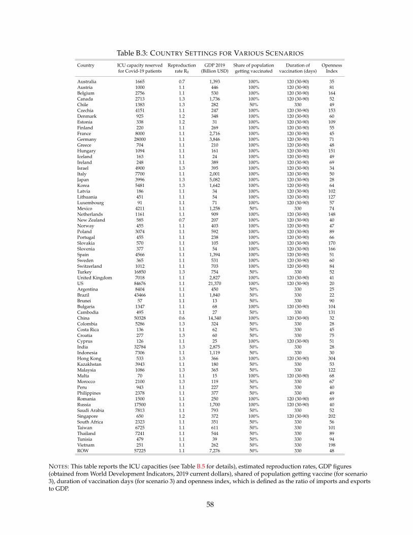
Table B.3: COUNTRY SETTINGS FOR VARIOUS SCENARIOS

Country ICU capacity reserved Reproduction GDP 2019 Share of population Duration of Opennessfor Covid-19 patients rate R0 (Billion USD) getting vaccinated vaccination (days) Index

Australia 1665 0.7 1,393 100% 120 (30-90) 35Austria 1000 1.1 446 100% 120 (30-90) 81Belgium 2756 1.1 530 100% 120 (30-90) 164Canada 2713 1.3 1,736 100% 120 (30-90) 52Chile 1383 1.3 282 50% 330 49Czechia 4151 1.1 247 100% 120 (30-90) 153Denmark 925 1.2 348 100% 120 (30-90) 60Estonia 338 1.2 31 100% 120 (30-90) 109Finland 220 1.1 269 100% 120 (30-90) 55France 8000 1.1 2,716 100% 120 (30-90) 45Germany 28000 1.1 3,846 100% 120 (30-90) 71Greece 704 1.1 210 100% 120 (30-90) 48Hungary 1094 1.1 161 100% 120 (30-90) 151Iceland 163 1.1 24 100% 120 (30-90) 49Ireland 248 1.1 389 100% 120 (30-90) 69Israel 4900 1.3 395 100% 120 (30-90) 34Italy 7700 1.1 2,001 100% 120 (30-90) 50Japan 3996 1.3 5,082 100% 120 (30-90) 28Korea 5481 1.3 1,642 100% 120 (30-90) 64Latvia 186 1.1 34 100% 120 (30-90) 102Lithuania 451 1.1 54 100% 120 (30-90) 127Luxembourg 91 1.1 71 100% 120 (30-90) 57Mexico 4211 1.1 1,258 50% 330 74Netherlands 1161 1.1 909 100% 120 (30-90) 148New Zealand 585 0.7 207 100% 120 (30-90) 40Norway 455 1.1 403 100% 120 (30-90) 47Poland 3074 1.1 592 100% 120 (30-90) 89Portugal 455 1.1 238 100% 120 (30-90) 66Slovakia 570 1.1 105 100% 120 (30-90) 170Slovenia 377 1.1 54 100% 120 (30-90) 166Spain 4566 1.1 1,394 100% 120 (30-90) 51Sweden 365 1.1 531 100% 120 (30-90) 60Switzerland 1012 1.1 703 100% 120 (30-90) 84Turkey 16850 1.3 754 50% 330 52United Kingdom 7018 1.1 2,827 100% 120 (30-90) 41US 84676 1.1 21,370 100% 120 (30-90) 20Argentina 8404 1.1 450 50% 330 25Brazil 43466 1.1 1,840 50% 330 22Brunei 57 1.1 13 50% 330 90Bulgaria 1347 1.1 68 100% 120 (30-90) 104Cambodia 495 1.1 27 50% 330 131China 50328 0.6 14,340 100% 120 (30-90) 32Colombia 5286 1.3 324 50% 330 28Costa Rica 136 1.1 62 50% 330 45Croatia 277 1.3 60 50% 330 75Cyprus 126 1.1 25 100% 120 (30-90) 51India 32784 1.3 2,875 50% 330 28Indonesia 7306 1.1 1,119 50% 330 30Hong Kong 533 1.3 366 100% 120 (30-90) 304Kazakhstan 3943 1.1 180 50% 330 53Malaysia 1086 1.3 365 50% 330 122Malta 70 1.1 15 100% 120 (30-90) 68Morocco 2100 1.3 119 50% 330 67Peru 943 1.1 227 50% 330 40Philippines 2378 1.1 377 50% 330 49Romania 1500 1.1 250 100% 120 (30-90) 69Russia 17500 1.1 1,700 100% 120 (30-90) 40Saudi Arabia 7813 1.1 793 50% 330 52Singapore 650 1.2 372 100% 120 (30-90) 202South Africa 2323 1.1 351 50% 330 56Taiwan 6725 1.1 611 50% 330 101Thailand 7241 1.1 544 50% 330 89Tunisia 479 1.1 39 50% 330 94Vietnam 251 1.1 262 50% 330 198ROW 57225 1.1 7,276 50% 330 48

NOTES: This table reports the ICU capacities (see Table B.5 for details), estimated reproduction rates, GDP figures(obtained from World Development Indicators, 2019 current dollars), shared of population getting vaccine (for scenario3), duration of vaccination days (for scenario 3) and openness index, which is defined as the ratio of imports and exportsto GDP.

58

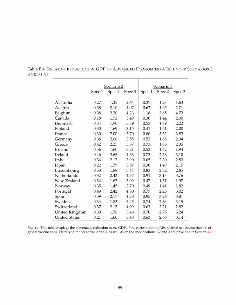
Table B.4: RELATIVE REDUCTION IN GDP OF ADVANCED ECONOMIES (AES) UNDER SCENARIOS 2AND 3 (%)

Scenario 2 Scenario 3Spec 1 Spec 2 Spec 3 Spec 1 Spec 2 Spec 3

Australia 0.27 1.35 2.64 0.37 1.23 1.63Austria 0.38 2.10 4.07 0.62 1.95 2.71Belgium 0.38 2.20 4.23 1.18 3.85 4.73Canada 0.18 1.52 3.49 0.30 1.44 2.00Denmark 0.34 1.90 3.59 0.53 1.69 2.22Finland 0.30 1.69 3.15 0.41 1.51 2.00France 0.30 2.00 3.70 0.86 3.32 3.83Germany 0.36 2.06 3.55 0.53 1.85 2.34Greece 0.42 2.25 3.87 0.73 1.85 2.35Iceland 0.56 1.60 3.21 0.53 1.42 1.94Ireland 0.46 2.65 4.53 0.73 2.56 3.10Italy 0.34 2.17 3.90 0.65 2.30 2.83Japan 0.22 1.79 3.87 0.30 1.49 2.15Luxembourg 0.53 1.88 3.44 0.83 2.32 2.85Netherlands 0.52 2.42 4.57 0.91 3.13 3.76New Zealand 0.34 1.67 3.09 0.47 1.51 1.97Norway 0.35 1.45 2.70 0.49 1.41 1.82Portugal 0.49 2.42 4.80 0.77 2.25 3.02Spain 0.39 2.17 4.28 0.95 3.26 3.81Sweden 0.34 1.83 3.45 0.74 2.63 3.15Switzerland 0.37 2.15 4.09 0.63 2.21 2.82United Kingdom 0.30 1.76 3.48 0.70 2.75 3.24United States 0.21 1.60 3.48 0.63 2.66 3.14

NOTES: This table displays the percentage reduction in the GDP of the corresponding AEs relative to a counterfactual ofglobal vaccinations. Details on the scenarios 2 and 3, as well as on the specifications 1,2 and 3 are provided in Section 4.4.

59

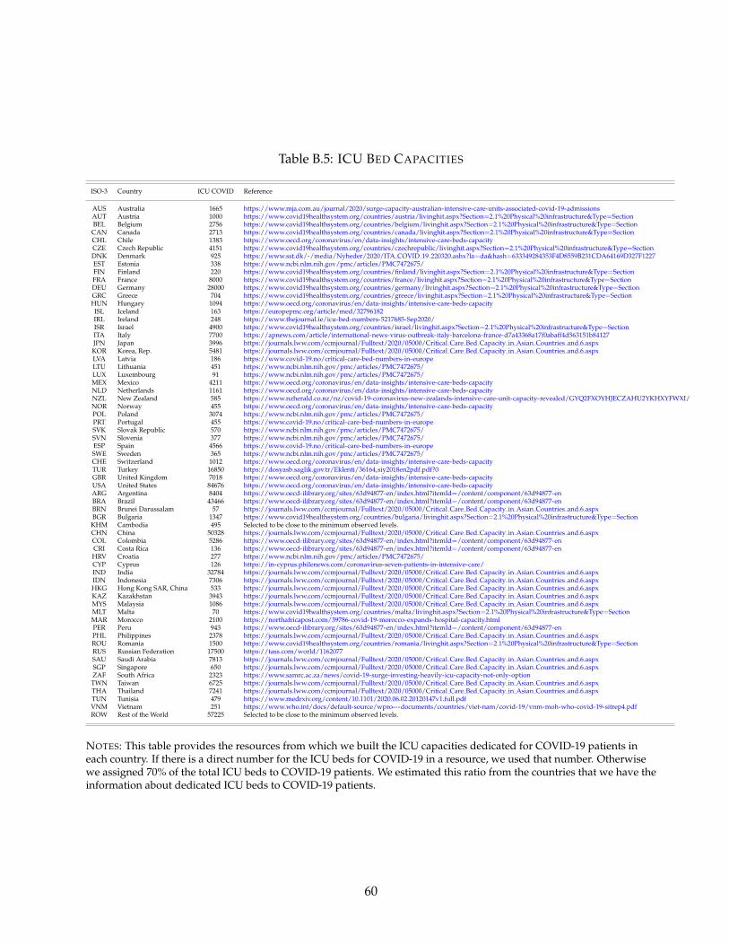
Table B.5: ICU BED CAPACITIES

ISO-3 Country ICU COVID Reference

AUS Australia 1665 https://www.mja.com.au/journal/2020/surge-capacity-australian-intensive-care-units-associated-covid-19-admissionsAUT Austria 1000 https://www.covid19healthsystem.org/countries/austria/livinghit.aspx?Section=2.1%20Physical%20infrastructure&Type=SectionBEL Belgium 2756 https://www.covid19healthsystem.org/countries/belgium/livinghit.aspx?Section=2.1%20Physical%20infrastructure&Type=SectionCAN Canada 2713 https://www.covid19healthsystem.org/countries/canada/livinghit.aspx?Section=2.1%20Physical%20infrastructure&Type=SectionCHL Chile 1383 https://www.oecd.org/coronavirus/en/data-insights/intensive-care-beds-capacityCZE Czech Republic 4151 https://www.covid19healthsystem.org/countries/czechrepublic/livinghit.aspx?Section=2.1%20Physical%20infrastructure&Type=SectionDNK Denmark 925 https://www.sst.dk/-/media/Nyheder/2020/ITA COVID 19 220320.ashx?la=da&hash=633349284353F4D8559B231CDA64169D327F1227EST Estonia 338 https://www.ncbi.nlm.nih.gov/pmc/articles/PMC7472675/FIN Finland 220 https://www.covid19healthsystem.org/countries/finland/livinghit.aspx?Section=2.1%20Physical%20infrastructure&Type=SectionFRA France 8000 https://www.covid19healthsystem.org/countries/france/livinghit.aspx?Section=2.1%20Physical%20infrastructure&Type=SectionDEU Germany 28000 https://www.covid19healthsystem.org/countries/germany/livinghit.aspx?Section=2.1%20Physical%20infrastructure&Type=SectionGRC Greece 704 https://www.covid19healthsystem.org/countries/greece/livinghit.aspx?Section=2.1%20Physical%20infrastructure&Type=SectionHUN Hungary 1094 https://www.oecd.org/coronavirus/en/data-insights/intensive-care-beds-capacityISL Iceland 163 https://europepmc.org/article/med/32796182IRL Ireland 248 https://www.thejournal.ie/icu-bed-numbers-5217685-Sep2020/ISR Israel 4900 https://www.covid19healthsystem.org/countries/israel/livinghit.aspx?Section=2.1%20Physical%20infrastructure&Type=SectionITA Italy 7700 https://apnews.com/article/international-news-virus-outbreak-italy-barcelona-france-d7a43368a17f0abaff4d563151b84127JPN Japan 3996 https://journals.lww.com/ccmjournal/Fulltext/2020/05000/Critical Care Bed Capacity in Asian Countries and.6.aspxKOR Korea, Rep. 5481 https://journals.lww.com/ccmjournal/Fulltext/2020/05000/Critical Care Bed Capacity in Asian Countries and.6.aspxLVA Latvia 186 https://www.covid-19.no/critical-care-bed-numbers-in-europeLTU Lithuania 451 https://www.ncbi.nlm.nih.gov/pmc/articles/PMC7472675/LUX Luxembourg 91 https://www.ncbi.nlm.nih.gov/pmc/articles/PMC7472675/MEX Mexico 4211 https://www.oecd.org/coronavirus/en/data-insights/intensive-care-beds-capacityNLD Netherlands 1161 https://www.oecd.org/coronavirus/en/data-insights/intensive-care-beds-capacityNZL New Zealand 585 https://www.nzherald.co.nz/nz/covid-19-coronavirus-new-zealands-intensive-care-unit-capacity-revealed/GYQ2FXOYHJECZAHU2YKHXYFWXI/NOR Norway 455 https://www.oecd.org/coronavirus/en/data-insights/intensive-care-beds-capacityPOL Poland 3074 https://www.ncbi.nlm.nih.gov/pmc/articles/PMC7472675/PRT Portugal 455 https://www.covid-19.no/critical-care-bed-numbers-in-europeSVK Slovak Republic 570 https://www.ncbi.nlm.nih.gov/pmc/articles/PMC7472675/SVN Slovenia 377 https://www.ncbi.nlm.nih.gov/pmc/articles/PMC7472675/ESP Spain 4566 https://www.covid-19.no/critical-care-bed-numbers-in-europeSWE Sweden 365 https://www.ncbi.nlm.nih.gov/pmc/articles/PMC7472675/CHE Switzerland 1012 https://www.oecd.org/coronavirus/en/data-insights/intensive-care-beds-capacityTUR Turkey 16850 https://dosyasb.saglik.gov.tr/Eklenti/36164,siy2018en2pdf.pdf?0GBR United Kingdom 7018 https://www.oecd.org/coronavirus/en/data-insights/intensive-care-beds-capacityUSA United States 84676 https://www.oecd.org/coronavirus/en/data-insights/intensive-care-beds-capacityARG Argentina 8404 https://www.oecd-ilibrary.org/sites/63d94877-en/index.html?itemId=/content/component/63d94877-enBRA Brazil 43466 https://www.oecd-ilibrary.org/sites/63d94877-en/index.html?itemId=/content/component/63d94877-enBRN Brunei Darussalam 57 https://journals.lww.com/ccmjournal/Fulltext/2020/05000/Critical Care Bed Capacity in Asian Countries and.6.aspxBGR Bulgaria 1347 https://www.covid19healthsystem.org/countries/bulgaria/livinghit.aspx?Section=2.1%20Physical%20infrastructure&Type=SectionKHM Cambodia 495 Selected to be close to the minimum observed levels.CHN China 50328 https://journals.lww.com/ccmjournal/Fulltext/2020/05000/Critical Care Bed Capacity in Asian Countries and.6.aspxCOL Colombia 5286 https://www.oecd-ilibrary.org/sites/63d94877-en/index.html?itemId=/content/component/63d94877-enCRI Costa Rica 136 https://www.oecd-ilibrary.org/sites/63d94877-en/index.html?itemId=/content/component/63d94877-enHRV Croatia 277 https://www.ncbi.nlm.nih.gov/pmc/articles/PMC7472675/CYP Cyprus 126 https://in-cyprus.philenews.com/coronavirus-seven-patients-in-intensive-care/IND India 32784 https://journals.lww.com/ccmjournal/Fulltext/2020/05000/Critical Care Bed Capacity in Asian Countries and.6.aspxIDN Indonesia 7306 https://journals.lww.com/ccmjournal/Fulltext/2020/05000/Critical Care Bed Capacity in Asian Countries and.6.aspxHKG Hong Kong SAR, China 533 https://journals.lww.com/ccmjournal/Fulltext/2020/05000/Critical Care Bed Capacity in Asian Countries and.6.aspxKAZ Kazakhstan 3943 https://journals.lww.com/ccmjournal/Fulltext/2020/05000/Critical Care Bed Capacity in Asian Countries and.6.aspxMYS Malaysia 1086 https://journals.lww.com/ccmjournal/Fulltext/2020/05000/Critical Care Bed Capacity in Asian Countries and.6.aspxMLT Malta 70 https://www.covid19healthsystem.org/countries/malta/livinghit.aspx?Section=2.1%20Physical%20infrastructure&Type=SectionMAR Morocco 2100 https://northafricapost.com/39786-covid-19-morocco-expands-hospital-capacity.htmlPER Peru 943 https://www.oecd-ilibrary.org/sites/63d94877-en/index.html?itemId=/content/component/63d94877-enPHL Philippines 2378 https://journals.lww.com/ccmjournal/Fulltext/2020/05000/Critical Care Bed Capacity in Asian Countries and.6.aspxROU Romania 1500 https://www.covid19healthsystem.org/countries/romania/livinghit.aspx?Section=2.1%20Physical%20infrastructure&Type=SectionRUS Russian Federation 17500 https://tass.com/world/1162077SAU Saudi Arabia 7813 https://journals.lww.com/ccmjournal/Fulltext/2020/05000/Critical Care Bed Capacity in Asian Countries and.6.aspxSGP Singapore 650 https://journals.lww.com/ccmjournal/Fulltext/2020/05000/Critical Care Bed Capacity in Asian Countries and.6.aspxZAF South Africa 2323 https://www.samrc.ac.za/news/covid-19-surge-investing-heavily-icu-capacity-not-only-optionTWN Taiwan 6725 https://journals.lww.com/ccmjournal/Fulltext/2020/05000/Critical Care Bed Capacity in Asian Countries and.6.aspxTHA Thailand 7241 https://journals.lww.com/ccmjournal/Fulltext/2020/05000/Critical Care Bed Capacity in Asian Countries and.6.aspxTUN Tunisia 479 https://www.medrxiv.org/content/10.1101/2020.06.02.20120147v1.full.pdfVNM Vietnam 251 https://www.who.int/docs/default-source/wpro---documents/countries/viet-nam/covid-19/vnm-moh-who-covid-19-sitrep4.pdfROW Rest of the World 57225 Selected to be close to the minimum observed levels.

NOTES: This table provides the resources from which we built the ICU capacities dedicated for COVID-19 patients ineach country. If there is a direct number for the ICU beds for COVID-19 in a resource, we used that number. Otherwisewe assigned 70% of the total ICU beds to COVID-19 patients. We estimated this ratio from the countries that we have theinformation about dedicated ICU beds to COVID-19 patients.

60