Discussion Papers

Is There Still a Case for Merchant Interconnectors? Insights from an Analysis of Welfare and Distributional Aspects of Options for Network Expansion in the Baltic Sea Region

Clemens Gerbaulet and Alexander Weber

1404

Deutsches Institut für Wirtschaftsforschung 2014

Opinions expressed in this paper are those of the author(s) and do not necessarily reflect views of the institute. IMPRESSUM © DIW Berlin, 2014 DIW Berlin German Institute for Economic Research Mohrenstr. 58 10117 Berlin Tel. +49 (30) 897 89-0 Fax +49 (30) 897 89-200 http://www.diw.de ISSN electronic edition 1619-4535 Papers can be downloaded free of charge from the DIW Berlin website: http://www.diw.de/discussionpapers Discussion Papers of DIW Berlin are indexed in RePEc and SSRN: http://ideas.repec.org/s/diw/diwwpp.html http://www.ssrn.com/link/DIW-Berlin-German-Inst-Econ-Res.html

Is there still a Case for MerchantInterconnectors? Insights from an Analysisof Welfare and Distributional Aspects ofOptions for Network Expansion in the

Baltic Sea RegionClemens Gerbaulet∗†, Alexander Weber∗

August 2014

Despite the ongoing appetite of financial investors for merchant investmentsinto the European electricity network, the EC is reluctant to approve suchundertakings, thus implicitly favoring regulated investments. Based on atwo-level model, we analyze the impact of profit-maximizing merchant trans-mission investment as compared to welfare-maximizing regulated transmissioninvestment. We apply the model to the Baltic Sea region, which has in the pastbeen subject to rapid interconnector development and still would benefit fromincreased interconnection. We obtain stable results indicating that merchantinvestment may well contribute to overall welfare, but at the same time, “themerchant takes it all”, i.e. in many cases merchant profits are close to theoverall efficiency gain, and sometimes even higher. These results underline thatthat distributional aspects, besides mere welfare arguments should be takeninto account when analyzing the impact of merchant transmission investment.

JEL Codes: L51, L94, D30, D60Keywords: Merchant, Regulated, Transmission Expansion, MPEC

∗Berlin University of Technology, Workgroup for Infrastructure Policy (WIP), Straße des 17. Juni 135,10623 Berlin. {cfg,aw}@wip.tu-berlin.de.

†German Institute for Economic Research (DIW Berlin), Department of Energy, Transportation, Envi-ronment, Mohrenstraße 58, 10117 Berlin.

1

Contents1. Introduction 3

2. Model 52.1. The Regulator’s Optimization Problem . . . . . . . . . . . . . . . . . . . . 52.2. The Merchant’s Optimization Problem . . . . . . . . . . . . . . . . . . . . 72.3. Further Assumptions . . . . . . . . . . . . . . . . . . . . . . . . . . . . . . 82.4. Model Implementation . . . . . . . . . . . . . . . . . . . . . . . . . . . . . 8

3. Model Application to the Baltic Sea Region 93.1. Data . . . . . . . . . . . . . . . . . . . . . . . . . . . . . . . . . . . . . . . 9

3.1.1. Generation . . . . . . . . . . . . . . . . . . . . . . . . . . . . . . . 93.1.2. Network . . . . . . . . . . . . . . . . . . . . . . . . . . . . . . . . . 113.1.3. Load . . . . . . . . . . . . . . . . . . . . . . . . . . . . . . . . . . . 113.1.4. Investment Cost . . . . . . . . . . . . . . . . . . . . . . . . . . . . 123.1.5. Reference Hours . . . . . . . . . . . . . . . . . . . . . . . . . . . . 13

3.2. Scenarios . . . . . . . . . . . . . . . . . . . . . . . . . . . . . . . . . . . . 133.3. The Merchant’s Investment Choices . . . . . . . . . . . . . . . . . . . . . 13

4. Results and Discussion 144.1. The Stackelberg Case . . . . . . . . . . . . . . . . . . . . . . . . . . . . . . 144.2. Relaxing the Stackelberg Assumption . . . . . . . . . . . . . . . . . . . . . 15

5. Conclusion 20

A. Nomenclature 26

B. Background on Merchant Interconnectors in Europe 27

C. Flow limits due to Network Topology 28

D. Identification of Reference Hours 30

E. Tables 31

2

1. IntroductionCurrent European electricity policy, driven by market integration and decarbonisationtargets, sets a strong impetus for expanding transmission networks: European transmissioncompanies identified in their 2012 plans (ENTSO-E, 2012a, p. 70) investment needs ofroughly e100 bn by 2022. Although most of the investment can be expected to beregulated, merchant transmission investments1 are possible within the current legal andinstitutional framework, but need to be approved on a case-by-case basis by the EuropeanCommission. In light of the large investment needs some see an increasing importance ofthis option (Cuomo and Glachant, 2012; Mann, 2013). What, however, remains unclearis the role merchant transmission investment can or should play in this context: While atfirst glance the difference between profit-maximizing “merchant” transmission investmentand (supposed-to-be) welfare-maximizing investment seems to be easy to analyze, this isnot so much the case once further aspects are taken into account.Although, in theory, merchant transmission lines might be an option, Joskow and

Tirole (2005) find (by extending theoretical models) that in practice problems of assetspecificity, lumpiness and market power pose serious problems to the desirability ofmerchant interconnectors. In a similar line of reasoning, Kuijlaars and Zwart (2003) andKnops and De Jong (2005) underline the problems of underinvestment (as compared tothe welfare optimal solution). As a remedy to the under-investment problem, Brunekreeft(2005) suggests (regulatory) “capacity checks.” From a modeling perspective, e.g. Egereret al. (2013); Doorman and Frøystad (2013) find, for cases of the North and Baltic Seas,that those transmission expansion alternatives leading to the highest welfare contributioncannot be financed by earnings from arbitrage (on which merchant transmission projectswould rely) and thus substantiate the theoretical considerations of under-investment andsimultaneously call for putting “capacity checks” into context. Further, Joskow (2005)and Turvey (2006) highlight that market driven interconnector investment may overlookreliability aspects while focusing on wholesale-driven economic aspects.

The above findings, which seem to deliver strong arguments against merchant transmis-sion expansion, need to be qualified: Regulated arrangements may not always be possible.One reason for this is that if technology is (new and) risky, the regulator may not be ableto credibly commit to not expropriate the upside and would thus prevent the investment.Gans and King (2004) argue that in such a case, temporary “access holidays” (i.e. anexemption from TPA rules) and thus an exemption from monopoly regulation may helpto overcome the investment barrier as the commitment to partially cease regulation couldbe given more credibly. In addition to enabling investments, they also highlight thatsuch “access holidays” may also be used to set incentives for a quicker delivery of theinvestment. Beyond the risk-argument literature (Brunekreeft, 2004; Kristiansen andRosellón, 2010; Teusch et al., 2012) suggests two more relevant reasons: first, regulators ofthe affected jurisdictions might not want to agree on the project as redistributive effects

1Merchant lines must be financed from the earnings of arbitrage between electricity prices in the twointerconnected jurisdictions, while regulated lines are financed by fees raised via grid tariffs overseenby a regulator.

3

could be unwanted and, second, vertically integrated transmission companies could behindered by the group’s management as the project could interfere with the utilities’generation/retail positions.

The former, inter-jurisdictional coordination aspect is highlighted by e.g. Gately (1974);Nylund (2012); Tangerås (2012); Buijs and Belmans (2012); Egerer et al. (2013) usingboth analytic and simulation models: They confirm that coordination of transmissioninvestment can be highly complex. Concerning the latter argument, de Hauteclocque andRious (2011) emphasize that in addition to TSO subsidiary companies, which historicallytook on the role, generator companies could also play an important role as merchantinvestors in Europe.Further, Littlechild (2012) generally argues in favor of merchant interconnectors on

the basis of case evidence – in those he finds that merchant investment was superior towhat regulators attempted to do.

In the EU, however, merchant interconnectors have not yet played a big role, as ofAugust 2014, only three such projects have been realized and Cuomo and Glachant (2012)find that the European Commission has, over time, become more and more reluctant togrant exemptions from regulation. An outline of the history of merchant interconnectorinvestment is presented in Annex B. Yet, there are still numerous2 proponents of merchantinvestments and hence, the issue cannot be considered “dead”.Therefore, the objective of this paper is to understand the impact, both in terms

of welfare and distribution, of “market”-driven transmission investment as comparedto both socially optimal (regulated) transmission investment and the absence of suchinvestment in the European context. We study the problem in the example of the BalticSea region, where systems of different energy planning paradigms provide a case forincreased interconnection. Our contribution is in both the modeling and the results:

• For the modeling, we use a bi-level set up to take into account the interdepen-dence between the strategic capacity choices of merchant investors and the welfare-maximizing choices left to the regulated part of the sector. We use a full repre-sentation of the extra high voltage (EHV) grid of the region studied, allowing forendogenous, line-sharp transmission expansion while taking into account direct-current load flow (DCLF) principles, bidding-zone-based unit-commitment andprice formation. We do further use a k-means approach to select reference hoursto keep the problem computationally tractable. To our knowledge, such a level ofdetail has not previously been used to study the impact of merchant investments.

• We find that, somehow contrary to the more stylized analyses cited above, welfarecontribution of merchant investment is roughly between 80 and 90% of the maximumimprovement possible, but that this welfare increase does mainly accrue to themerchant investor as a rent. In some cases, redistribution is so severe that themerchant’s rent is higher than his welfare contribution. Therefore, the argumentthat merchant investment may be an option if regulated transmission investment isnot possible seems to be weakened: From a perspective of distributional aspects,

2cf. Mann (2013)

4

policy-makers might not want to pursue a solution which does not bring any benefitto established actors or even reduces their welfare.

The remainder of this paper is structured as follows: Next, section 2 outlines therespective optimization problems of merchants and regulators and the model applicationsused in this paper. Section 3 describes the application and relevant input parameters.The results of the application are discussed in section 4. Section 5 concludes.

2. ModelThe regulator in our model seeks to minimize overall cost of the electricity system bycontrolling power plant dispatch and deciding on AC transmission expansion. Powerplant dispatch follows a zonal approach, as currently implemented in Europe; however,if cheaper than transmission expansion, deviations from the zonal merit order list areallowed.Merchants that plan and build cross-border lines have a different objective. Their

goal is to maximize profit (i.e. their congestion rent), which is the congestion revenueminus the line investment cost. Congestion revenue accrues when prices between twoconnected zones differ and further trade between these zones is limited due to upstreamgrid congestion or full utilization of the cross-border line. The price difference on themerchant’s line multiplied by the amount of energy transmitted is the congestion revenue.As (operational) withholding of capacity is not an option within the EU legislation, wedo not consider this alternative.3We model the interaction between the two parties as a two-stage game where the

merchant’s optimization problem is solved taking into account the reaction of the regulatorand assume that there is only one merchant investor. This implies that the merchant isfirst-mover in this game, i.e. the Stackelberg leader. Although this set-up seems to bevery preconditioning, it yields interesting results, which remain stable when we relax theStackelberg assumption later on.

2.1. The Regulator’s Optimization ProblemThe regulator’s objective is to minimize system cost, by coordinating both dispatch andnetwork expansion. Although the regulator has a global view, he may not be able conducttransmission investment between all systems which limits his powers and thus mimicsthe inability to coordinate cross-border investment.

Power plant dispatch is conducted on the basis of bidding zones, i.e. transmission is notpriced within zones. Transmission is modeled following DCLF principles (Schweppe et al.,1988; Stigler and Todem, 2005; Leuthold et al., 2012). As transmission expansion problemsin electricity networks are typically non-convex, we apply a linear relaxation provided byTaylor and Hover (2011). There, the flow in the existing network strictly follows DCLF

3Yet, Brunekreeft and Newbery (2006) argue that allowing capacity withholding during operation inthe exemption period could reduce problems of under-investment.

5

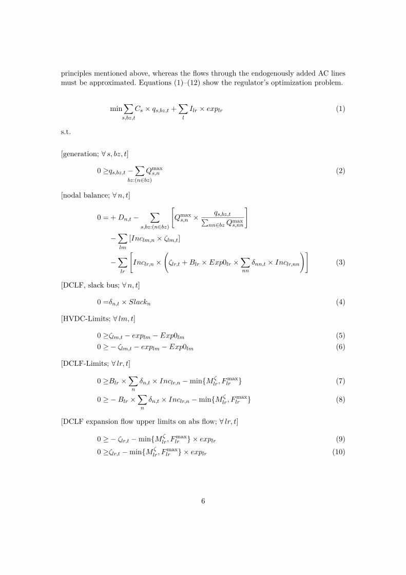
principles mentioned above, whereas the flows through the endogenously added AC linesmust be approximated. Equations (1)–(12) show the regulator’s optimization problem.

min∑s,bz,t

Cs × qs,bz,t +∑l

Ilr × explr (1)

s.t.

[generation; ∀ s, bz, t]

0 ≥qs,bz,t −∑

bz:(n∈bz)Qmaxs,n (2)

[nodal balance; ∀n, t]

0 = +Dn,t −∑

s,bz:(n∈bz)

[Qmaxs,n ×

qs,bz,t∑nn∈bz Q

maxs,nn

]

−∑lm

[Inclm,n × ζlm,t]

−∑lr

[Inclr,n ×

(ζlr,t +Blr × Exp0lr ×

∑nn

δnn,t × Inclr,nn

)](3)

[DCLF, slack bus; ∀n, t]

0 =δn,t × Slackn (4)

[HVDC-Limits; ∀ lm, t]

0 ≥ζlm,t − explm − Exp0lm (5)0 ≥− ζlm,t − explm − Exp0lm (6)

[DCLF-Limits; ∀ lr, t]

0 ≥Blr ×∑n

δn,t × Inclr,n −min{M ζlr, F

maxlr } (7)

0 ≥−Blr ×∑n

δn,t × Inclr,n −min{M ζlr, F

maxlr } (8)

[DCLF expansion flow upper limits on abs flow; ∀ lr, t]

0 ≥− ζlr,t −min{M ζlr, F

maxlr } × explr (9)

0 ≥ζlr,t −min{M ζlr, F

maxlr } × explr (10)

6

[DCLF expansion flow lower limits on abs flow; ∀ lr, t]

0 ≥Blr ×∑n

Inclr,n × δn,t × Explr − ζlr,t

−min{M ζlr, F

maxlr } × [Explr − explr] (11)

0 ≥−Blr ×∑n

Inclr,n × δn,t × Explr + ζlr,t

−min{M ζlr, F

maxlr } × [Explr − explr] (12)

The overall cost is determined in the argument of the minimization in (1). It consists ofthe generation cost as well as the grid expansion cost. (2) constrains maximum electricitygeneration qs,bz,t per technology and bidding zone. The network is represented by anincidence matrix Incl,n, assigning line end points to nodes n. Lines l are divided intoregulated AC lines lr ∈ l and merchant DC lines lm ∈ l. Voltage angles are expressedby δn,t, relative line susceptance is denoted as Bl. Nodal balance is enforced by (3),where nodal generation, demand, flows of existing AC lines (angle difference times Bl),including expansion (ζlr,t), and DC line flows ζlm,t are taken into account. For eachsynchronous area, a slack node is defined through (4) to ensure a unique solution duringthe optimization. For controllable flows on merchant lines, conditions (5, 6) impose therespective flow limits: Exp0lm denotes existing capacity in MW, explm is the endogenouslydetermined capacity expansion. For the AC lines, (7, 8) impose the relevant thermallimits onto the phase angle differences. Here, Fmax

lr denotes the thermal limit of existingline lr, whereas M ζ

lr shows the lower bound given by parallel paths. M ζl is determined

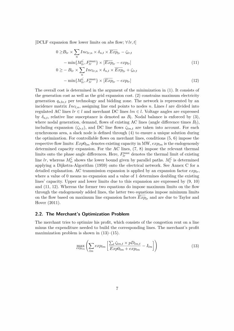
applying a Dijkstra-Algorithm (1959) onto the electrical network. See Annex C for adetailed explanation. AC transmission expansion is applied by an expansion factor explr,where a value of 0 means no expansion and a value of 1 determines doubling the existinglines’ capacity. Upper and lower limits due to this expansion are expressed by (9, 10)and (11, 12). Whereas the former two equations do impose maximum limits on the flowthrough the endogenously added lines, the latter two equations impose minimum limitson the flow based on maximum line expansion factors Explr and are due to Taylor andHover (2011).

2.2. The Merchant’s Optimization ProblemThe merchant tries to optimize his profit, which consists of the congestion rent on a lineminus the expenditure needed to build the corresponding lines. The merchant’s profitmaximization problem is shown in (13)–(15).

maxexplm

(∑lm

explm

[∑t ζlm,t × pDlm,t

Exp0lm + explm− Ilm

])(13)

7

s.t.pDlm,t =

∑∀n,nn:

Inclm,n=1,Inclm,nn=−1

(pn,t − pnn,t) ∀lm, t (14)

explm ≥0 ∀lm (15)

The profit of the merchant is determined in (13), where the flow is multiplied by the pricedifference and subtracted by the investment cost of lines. In case the merchant expandspreviously existing lines, he is only eligible to receive the share of the congestion rentsattributable to his capacity addition. Both the flow on regulated and merchant lines is setby the regulator. The price pn,t and the price difference between nodes pDlm,t in (14) area result of the regulator’s optimization. The price can be defined in two ways: It can eitherbe the dual variable of the zonal balance or the marginal cost of the most expensive powerplant dispatched in the respective bidding zone. In the former case, the price would bethe zonal average of the duals of the nodal balance in (3), giving the cost of an additionalMWh to be delivered in that area. This price would include the cost of regulated networkexpansion, which would be attributed to the importing zone. As opposed to this, justtaking the marginal cost of the most expensive power plant dispatched in the biddingarea, would neglect long-run costs of network expansion and any marginal flow effects. Inthe following we will call the different approaches to be reflecting long-run marginal cost(LRMC) and short-run marginal cost (SRMC), respectively.

2.3. Further AssumptionsInvestments in specific lines are restricted to a single actor. The regulator can invest inAC lines while the merchant can invest in DC cross-border lines only, i.e.

lm ∩ lr = ∅.

2.4. Model ImplementationThe two-stage model set-up translates into an MPEC (mathematical problem with equi-librium constraints). For sufficiently small problems, MPECs can be solved by expressingthe follower’s problem(s) in their Karush-Kuhn-Tucker (KKT) form. The computationaldifficulty lies then in quickly solving the complementarity problem (Gabriel and Leuthold,2010), but often this can be done efficiently with help of disjunctive constraints, suchthat the MPEC can be solved as a mixed integer problem (MIP), using a large range ofsolvers available (Leuthold et al., 2012).As the MPEC of this paper (when applied to the real system of the Baltic Sea

Region) is too complex for the traditional, integrated approach, the solution space for themerchant’s investment decision is discretized and each element is evaluated by solvingthe corresponding lower-level linear problem (LP). Then, the profit maximizing choice isselected in a consecutive step by evaluating all lower-level outcomes. Although it couldbe argued that this is not precise, because slightly different figures would result if the

8

discretization would not be applied, real HVDC projects actually come in steps, withsome minor exceptions for smaller projects. Further, this approach also eliminates thedifficulties that the bi-linearity in (13) would pose to integrated solution approaches.

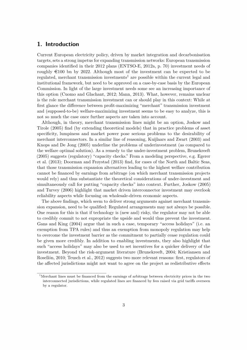
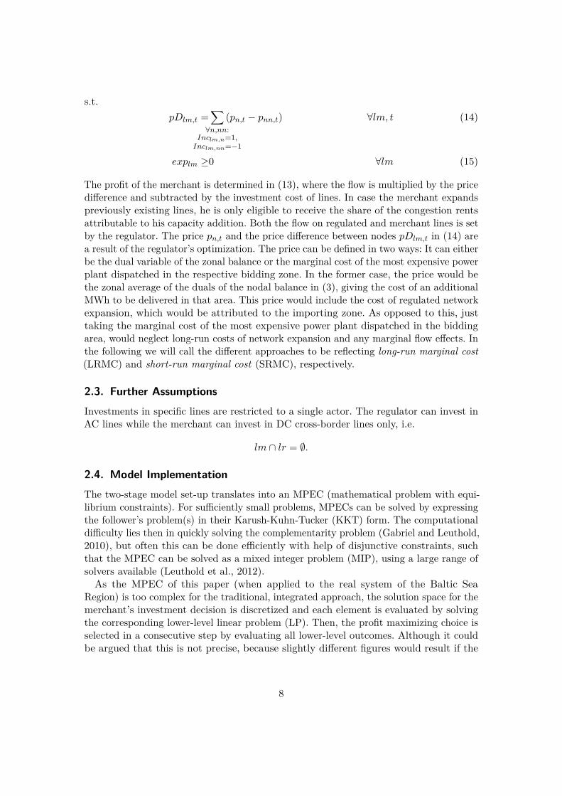
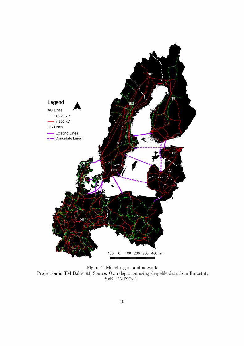
3. Model Application to the Baltic Sea RegionWe apply the model to the electrical System of the Baltic Sea Neighboring countries(Denmark, Estonia, Finland, Germany, Latvia, Lithuania, Poland, and Sweden), takinginto account bidding zones in Sweden (SvK, 2011), and publicly available plans for bothgeneration and network through 2020. An overview of the network and bidding zones isgiven in Figure 1.We essentially apply information from ENTSO-E’s (2012a) 10-Year Network Devel-

opment Plan (“TYNDP”, including the “Scenario Outlook and Adequacy Forecast”,SOAF, ENTSO-E, 2012c), assuming Scenario “B” 2020, the “Baltic Energy MarketInterconnection Plan” (BEMIP, EC, 2009a, 2012; CESI, 2009). Further, we use diversesources on generation, load and networks as set out in section 3.1.

In addition to that, we need to choose a set of both distinct reference hours consideredby the model and the possible investment choices of the merchant in order to keep themodel computationally feasible. These adjustments are tackled in sections 3.1.5 and 3.3,respectively.To conduct our analysis, we compare the merchant solution against two extreme

scenarios in terms of costs and rents accruing to the different parties (generators, regulatedtransmission, consumers, merchant investors). The two additional scenarios are (i) theFully Planned case, where we assume a cost-minimizing, central regulator who conductsplant dispatch and network expansion, both for AC and DC lines, and (ii) the AC Onlycase, where no DC expansion is possible, but plant dispatch and AC investment is donein a cost-minimizing way. The overall three different scenarios compared against eachother are introduced in section 3.2.

3.1. Data3.1.1. Generation

Generation technologies considered are both dispatchable and non-dispatchable (i.e.variable renewable energy sources; VRE) types. For dispatchable generation, power plantdata from PLATTS (2011) is used as a basis for the spatial distribution of technologieswithin the electricity grid. For VRE generation, locations and distribution of installationsare determined using NUTS-2 potential maps from ESPON (2010, pp. 226), except forGermany, where detailed data on installation sites is available from the TSOs. Theresulting distribution of generation capacities is, subsequently, scaled according to SOAF-data using a brown-field approach. For dispatchable generation, fuel and carbon priceswere taken, where applicable, from the “Current Policies Scenario” of IEA’s World EnergyOutlook (International Energy Agency and Organisation for Economic Co-operationand Development, 2011, pp. 64, 66), in line with the assumptions of the Baltic Regional

9

AC Lines

≤ 220 kV≥ 300 kV

DC Lines

Existing LinesCandidate Lines

Legend

100 0 100 200 300 400 km

Figure 1: Model region and networkProjection in TM Baltic 93, Source: Own depiction using shapefile data from Eurostat,

SvK, ENTSO-E.

10

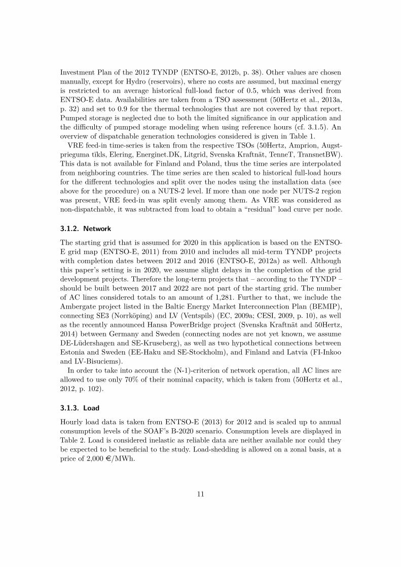
Investment Plan of the 2012 TYNDP (ENTSO-E, 2012b, p. 38). Other values are chosenmanually, except for Hydro (reservoirs), where no costs are assumed, but maximal energyis restricted to an average historical full-load factor of 0.5, which was derived fromENTSO-E data. Availabilities are taken from a TSO assessment (50Hertz et al., 2013a,p. 32) and set to 0.9 for the thermal technologies that are not covered by that report.Pumped storage is neglected due to both the limited significance in our application andthe difficulty of pumped storage modeling when using reference hours (cf. 3.1.5). Anoverview of dispatchable generation technologies considered is given in Table 1.

VRE feed-in time-series is taken from the respective TSOs (50Hertz, Amprion, Augst-prieguma t̄ıkls, Elering, Energinet.DK, Litgrid, Svenska Kraftnät, TenneT, TransnetBW).This data is not available for Finland and Poland, thus the time series are interpolatedfrom neighboring countries. The time series are then scaled to historical full-load hoursfor the different technologies and split over the nodes using the installation data (seeabove for the procedure) on a NUTS-2 level. If more than one node per NUTS-2 regionwas present, VRE feed-in was split evenly among them. As VRE was considered asnon-dispatchable, it was subtracted from load to obtain a “residual” load curve per node.

3.1.2. Network

The starting grid that is assumed for 2020 in this application is based on the ENTSO-E grid map (ENTSO-E, 2011) from 2010 and includes all mid-term TYNDP projectswith completion dates between 2012 and 2016 (ENTSO-E, 2012a) as well. Althoughthis paper’s setting is in 2020, we assume slight delays in the completion of the griddevelopment projects. Therefore the long-term projects that – according to the TYNDP –should be built between 2017 and 2022 are not part of the starting grid. The numberof AC lines considered totals to an amount of 1,281. Further to that, we include theAmbergate project listed in the Baltic Energy Market Interconnection Plan (BEMIP),connecting SE3 (Norrköping) and LV (Ventspils) (EC, 2009a; CESI, 2009, p. 10), as wellas the recently announced Hansa PowerBridge project (Svenska Kraftnät and 50Hertz,2014) between Germany and Sweden (connecting nodes are not yet known, we assumeDE-Lüdershagen and SE-Kruseberg), as well as two hypothetical connections betweenEstonia and Sweden (EE-Haku and SE-Stockholm), and Finland and Latvia (FI-Inkooand LV-Bisuciems).

In order to take into account the (N-1)-criterion of network operation, all AC lines areallowed to use only 70% of their nominal capacity, which is taken from (50Hertz et al.,2012, p. 102).

3.1.3. Load

Hourly load data is taken from ENTSO-E (2013) for 2012 and is scaled up to annualconsumption levels of the SOAF’s B-2020 scenario. Consumption levels are displayed inTable 2. Load is considered inelastic as reliable data are neither available nor could theybe expected to be beneficial to the study. Load-shedding is allowed on a zonal basis, at aprice of 2,000 e/MWh.

11

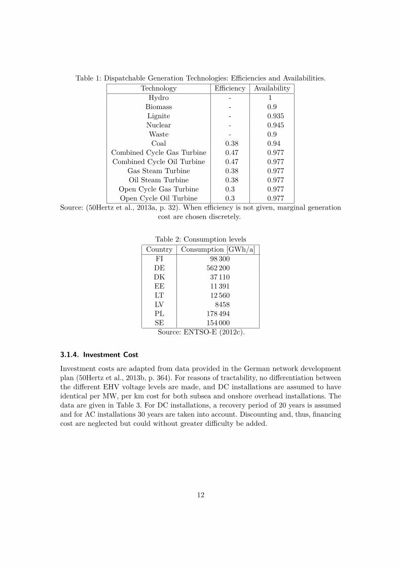
Table 1: Dispatchable Generation Technologies: Efficiencies and Availabilities.Technology Efficiency Availability

Hydro - 1Biomass - 0.9Lignite - 0.935Nuclear - 0.945Waste - 0.9Coal 0.38 0.94

Combined Cycle Gas Turbine 0.47 0.977Combined Cycle Oil Turbine 0.47 0.977

Gas Steam Turbine 0.38 0.977Oil Steam Turbine 0.38 0.977

Open Cycle Gas Turbine 0.3 0.977Open Cycle Oil Turbine 0.3 0.977

Source: (50Hertz et al., 2013a, p. 32). When efficiency is not given, marginal generationcost are chosen discretely.

Table 2: Consumption levelsCountry Consumption [GWh/a]

FI 98 300DE 562 200DK 37 110EE 11 391LT 12 560LV 8458PL 178 494SE 154 000Source: ENTSO-E (2012c).

3.1.4. Investment Cost

Investment costs are adapted from data provided in the German network developmentplan (50Hertz et al., 2013b, p. 364). For reasons of tractability, no differentiation betweenthe different EHV voltage levels are made, and DC installations are assumed to haveidentical per MW, per km cost for both subsea and onshore overhead installations. Thedata are given in Table 3. For DC installations, a recovery period of 20 years is assumedand for AC installations 30 years are taken into account. Discounting and, thus, financingcost are neglected but could without greater difficulty be added.

12

Table 3: Grid investment cost. Source: (50Hertz et al., 2013b, p. 364)Grid Technology Cost Unit

AC overhead line (2 systems) 1.4 Me/kmDC line 700 e/(MW×km)

DC converter station 130 e/kW

3.1.5. Reference Hours

Due to the computational complexity, we restrict our analysis to 8 reference hours. Toselect those, we apply a k-Means clustering approach in order to identify hours that bestrepresent typical situations of load and VRE-infeed. See Annex D for details. We alsoaccount for the size of the respective clusters by introducing a weight factor that correctsfor the “duration” of the reference hour.

3.2. ScenariosWe compare three scenarios to show the effect of different grid expansion approaches:

1. AC Only: No new HVDC lines are allowed; only a fully coordinated regulator mayexpand AC-lines between adjacent countries,

2. Stackelberg: The Stackelberg-game is modeled; Merchant is first-mover for HVDClines; regulator is follower for AC connections and dispatch,

3. Fully Planned: All lines are expanded on a cost-minimizing basis by the regulator.

The rationale behind this set-up is to identify how well the second best solution ofallowing merchants to build HVDC lines performs, both in terms of total cost andallocation of rents to producers, consumers, and merchants. For the calculation of rents,it is necessary to make assumptions for both the consumer’s willingness-to-pay (WTP)and the pricing mechanism. For the former, we assume a WTP of 180 e/MWh, makingsure this limit is never hit. For the pricing mechanism, we evaluate pricing based both onthe long-run and the short-run marginal cost (LRMC/SRMC) as defined in 2.2.

3.3. The Merchant’s Investment ChoicesAs noted in 2.4, we discretize the merchant’s action space in order to overcome thecomputational difficulties of bi-linearity and of the integrated solution of the MPEC, i.e.reformulating the lower level into its KKT form. We choose the following approach toselect the investment choices available to the merchant investor:

1. First, we select the non-zero HVDC expansion decisions of the fully planned casethat are equal or greater than 250 MW. These are the candidate lines that themerchant investor is entitled to invest in.

13

2. For the candidate lines, we allow the merchant to invest in steps of 250 MW, from0 to four 250 MW steps beyond the fully planned extension level, and including theexact value of the fully planned level.

The discretization results in 62 208 investment alternatives. The overall MPEC was solvedon a computing cluster, using GUROBI and each of the LPs consumed about 43 secondsof CPU time.

4. Results and DiscussionIn this section, we present and discuss our results. First (section 4.1), we present theoutcomes of the Stackelberg game, where the merchant investor is the leader of thetwo-stage game. Second, in section 4.2, we relax the Stackelberg assumption by takinga look at the larger set of investment options, most still profitable from a merchantperspective, but less extreme than the Stackelberg optimum.

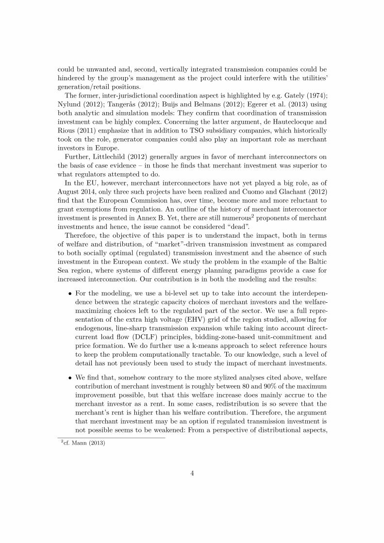
4.1. The Stackelberg CaseWe compare outcomes of the Stackelberg scenarios against the AC Only and Fully Plannedscenarios. The DC transmission investment decisions in the Stackelberg cases (both underLRMC and SRMC pricing) and in the Fully Planned scenario are presented in Table 4.The AC Only scenario is left out since no investment into additional DC transmissioncapacity takes place here.Interestingly, while under LRMC pricing, a significant underinvestment – just about

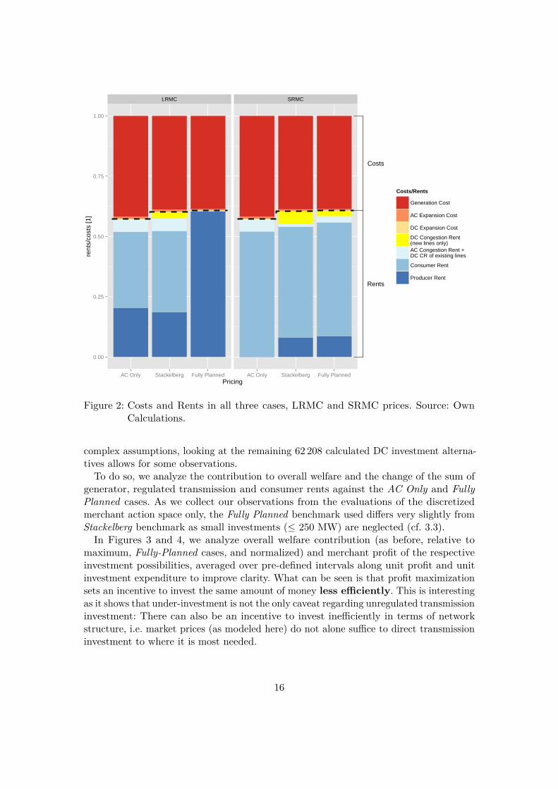
36 % of the DC transmission expenditure in the ’optimal’ case – is observable, themerchant invests even more than in the Fully Planned case when SRMC pricing isapplied. This latter observation is somewhat counterintuitive to the underinvestmentcritique brought forward against merchant investments in the literature. In course of thissection, we will discuss this observation in more detail. The economic implications of themerchant’s choices, under both pricing schemes, are presented in Figure 2:4 rents andcosts for each actor are stacked group-wise, illustrating changes in welfare, distributionand efficiency. The costs for the different cases are given in 6.The analysis of rents & costs yields some interesting insights:

• While we see that under LRMC pricing the merchant’s investment expenditure isrelatively low, and nearly 3 times higher under SRMC pricing, the welfare gainsare in both cases fairly equal: These amount to roughly 80–90% of what could havebeen gained under the Fully Planned solution.

• Still, despite this not-so-small welfare gain, in the LRMC case, it nearly fully accruesto the merchant investor as a rent, while under SRMC pricing the merchant profit is

4To improve the presentation, consumer and producer rents are reduced by their respective minima,and generation cost by half of their minimum so that absolute changes remain observable. Further, itis important to note that the congestion rents of AC lines and existing DC lines are combined (lightblue) and congestion rents accruing to new DC transmission investments are separate (yellow).

14

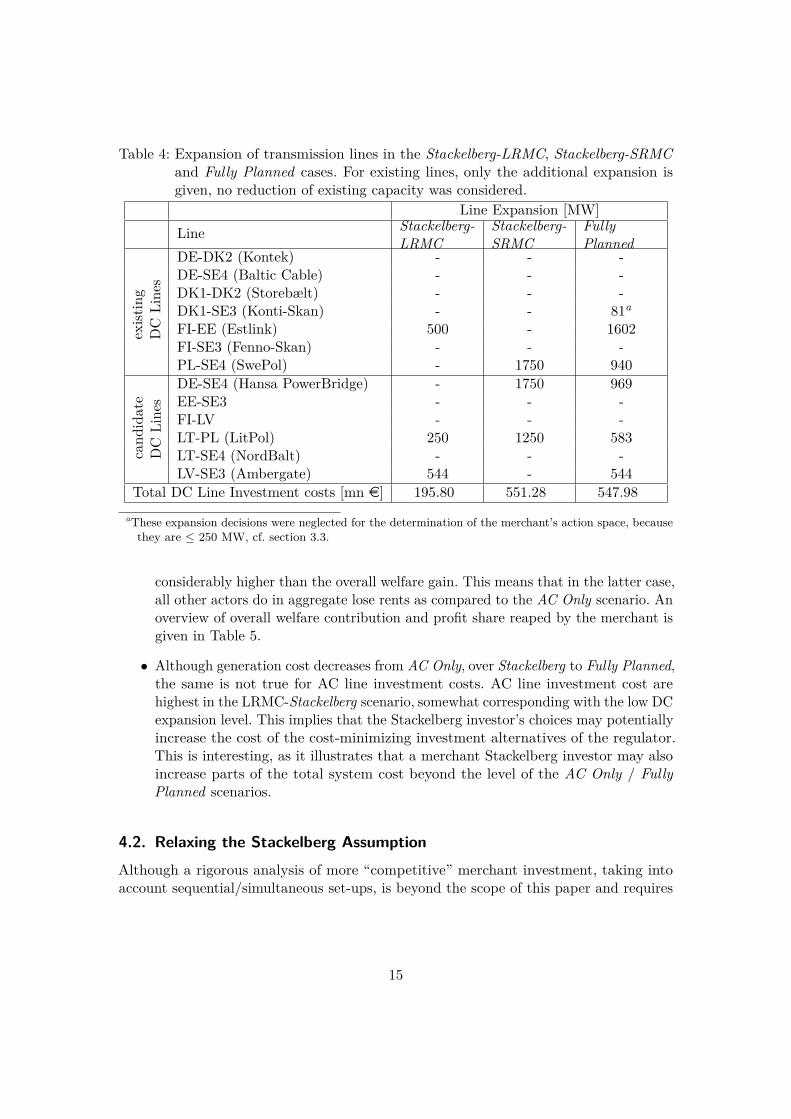
Table 4: Expansion of transmission lines in the Stackelberg-LRMC, Stackelberg-SRMCand Fully Planned cases. For existing lines, only the additional expansion isgiven, no reduction of existing capacity was considered.

Line Expansion [MW]Line Stackelberg-

LRMCStackelberg-SRMC

FullyPlanned

exist

ing

DC

Lines

DE-DK2 (Kontek) - - -DE-SE4 (Baltic Cable) - - -DK1-DK2 (Storebælt) - - -DK1-SE3 (Konti-Skan) - - 81a

FI-EE (Estlink) 500 - 1602FI-SE3 (Fenno-Skan) - - -PL-SE4 (SwePol) - 1750 940

cand

idate

DC

Lines

DE-SE4 (Hansa PowerBridge) - 1750 969EE-SE3 - - -FI-LV - - -LT-PL (LitPol) 250 1250 583LT-SE4 (NordBalt) - - -LV-SE3 (Ambergate) 544 - 544

Total DC Line Investment costs [mn e] 195.80 551.28 547.98aThese expansion decisions were neglected for the determination of the merchant’s action space, becausethey are ≤ 250 MW, cf. section 3.3.

considerably higher than the overall welfare gain. This means that in the latter case,all other actors do in aggregate lose rents as compared to the AC Only scenario. Anoverview of overall welfare contribution and profit share reaped by the merchant isgiven in Table 5.

• Although generation cost decreases from AC Only, over Stackelberg to Fully Planned,the same is not true for AC line investment costs. AC line investment cost arehighest in the LRMC-Stackelberg scenario, somewhat corresponding with the low DCexpansion level. This implies that the Stackelberg investor’s choices may potentiallyincrease the cost of the cost-minimizing investment alternatives of the regulator.This is interesting, as it illustrates that a merchant Stackelberg investor may alsoincrease parts of the total system cost beyond the level of the AC Only / FullyPlanned scenarios.

4.2. Relaxing the Stackelberg AssumptionAlthough a rigorous analysis of more “competitive” merchant investment, taking intoaccount sequential/simultaneous set-ups, is beyond the scope of this paper and requires

15

Rents

Costs

LRMC SRMC

0.00

0.25

0.50

0.75

1.00

AC Only Stackelberg Fully Planned AC Only Stackelberg Fully PlannedPricing

rent

s/co

sts

[1]

Costs/Rents

Generation Cost

AC Expansion Cost

DC Expansion Cost

DC Congestion Rent(new lines only)AC Congestion Rent +DC CR of existing lines

Consumer Rent

Producer Rent

Figure 2: Costs and Rents in all three cases, LRMC and SRMC prices. Source: OwnCalculations.

complex assumptions, looking at the remaining 62 208 calculated DC investment alterna-tives allows for some observations.

To do so, we analyze the contribution to overall welfare and the change of the sum ofgenerator, regulated transmission and consumer rents against the AC Only and FullyPlanned cases. As we collect our observations from the evaluations of the discretizedmerchant action space only, the Fully Planned benchmark used differs very slightly fromStackelberg benchmark as small investments (≤ 250 MW) are neglected (cf. 3.3).

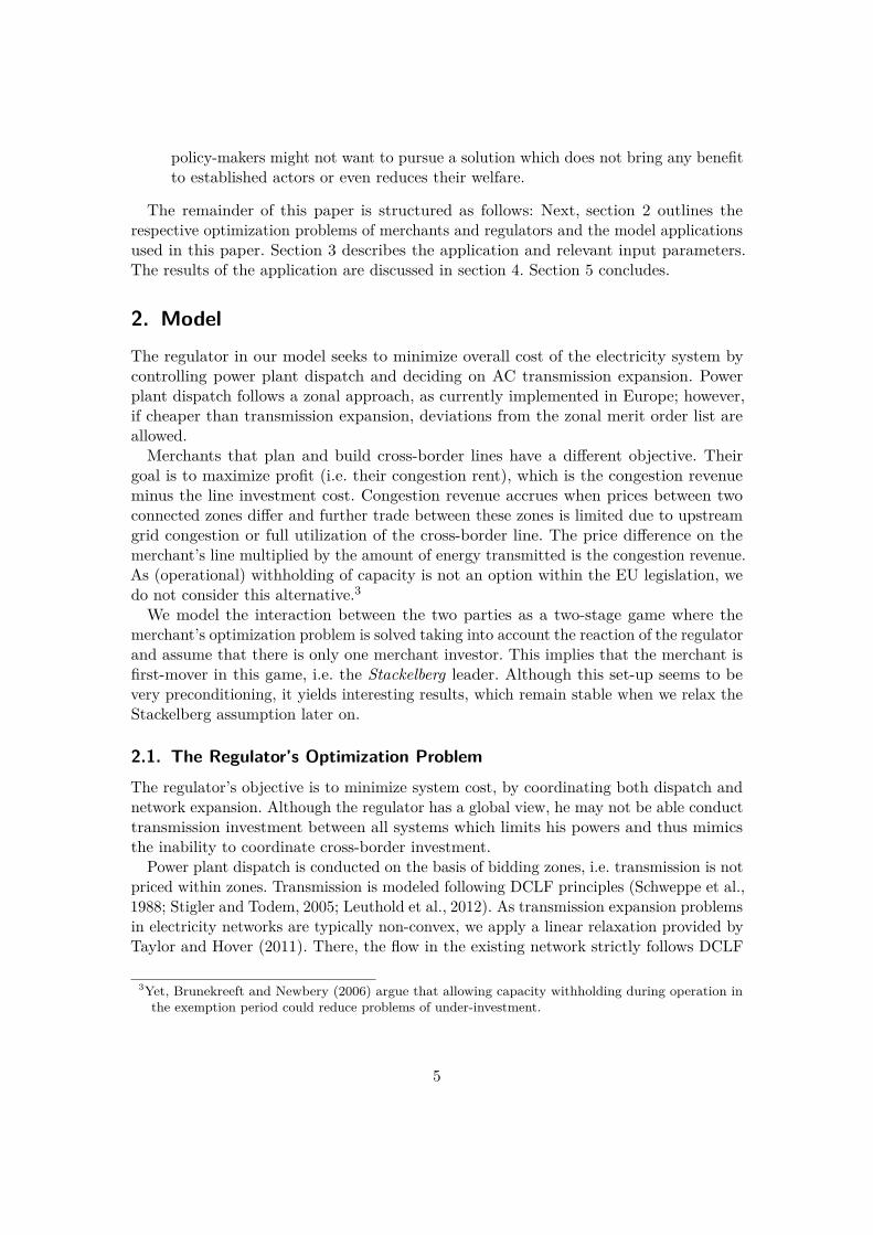
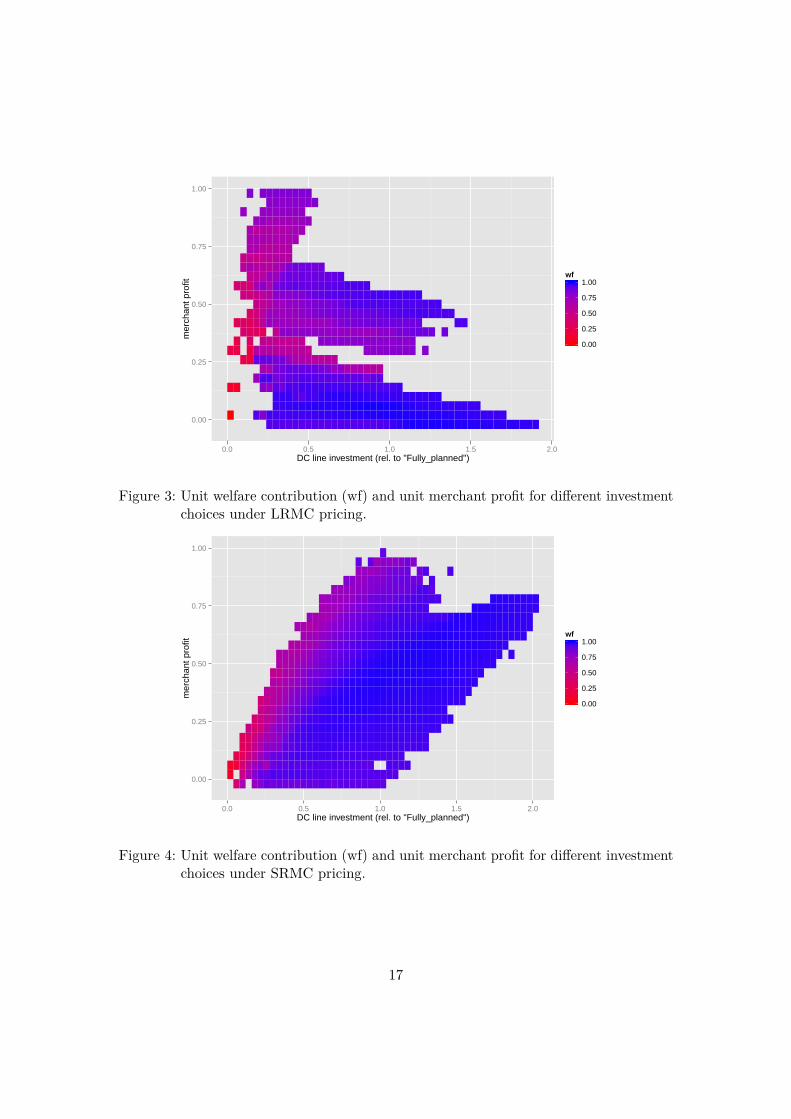
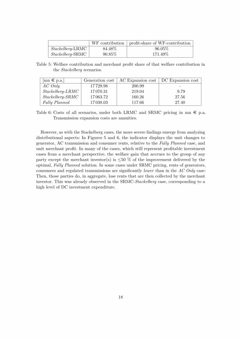
In Figures 3 and 4, we analyze overall welfare contribution (as before, relative tomaximum, Fully-Planned cases, and normalized) and merchant profit of the respectiveinvestment possibilities, averaged over pre-defined intervals along unit profit and unitinvestment expenditure to improve clarity. What can be seen is that profit maximizationsets an incentive to invest the same amount of money less efficiently. This is interestingas it shows that under-investment is not the only caveat regarding unregulated transmissioninvestment: There can also be an incentive to invest inefficiently in terms of networkstructure, i.e. market prices (as modeled here) do not alone suffice to direct transmissioninvestment to where it is most needed.

16

0.00

0.25

0.50

0.75

1.00

0.0 0.5 1.0 1.5 2.0DC line investment (rel. to "Fully_planned")

mer

chan

t pro

fit

0.00

0.25

0.50

0.75

1.00wf

Figure 3: Unit welfare contribution (wf) and unit merchant profit for different investmentchoices under LRMC pricing.

0.00

0.25

0.50

0.75

1.00

0.0 0.5 1.0 1.5 2.0DC line investment (rel. to "Fully_planned")

mer

chan

t pro

fit

0.00

0.25

0.50

0.75

1.00wf

Figure 4: Unit welfare contribution (wf) and unit merchant profit for different investmentchoices under SRMC pricing.

17

WF contribution profit-share of WF-contributionStackelberg-LRMC 84.48% 96.05%Stackelberg-SRMC 90.85% 171.49%

Table 5: Welfare contribution and merchant profit share of that welfare contribution inthe Stackelberg scenarios.

[mn e p.a.] Generation cost AC Expansion cost DC Expansion costAC Only 17 729.98 200.99 -Stackelberg-LRMC 17 070.31 219.04 9.79Stackelberg-SRMC 17 063.72 160.26 27.56Fully Planned 17 038.03 117.66 27.40

Table 6: Costs of all scenarios, under both LRMC and SRMC pricing in mn e p.a.Transmission expansion costs are annuities.

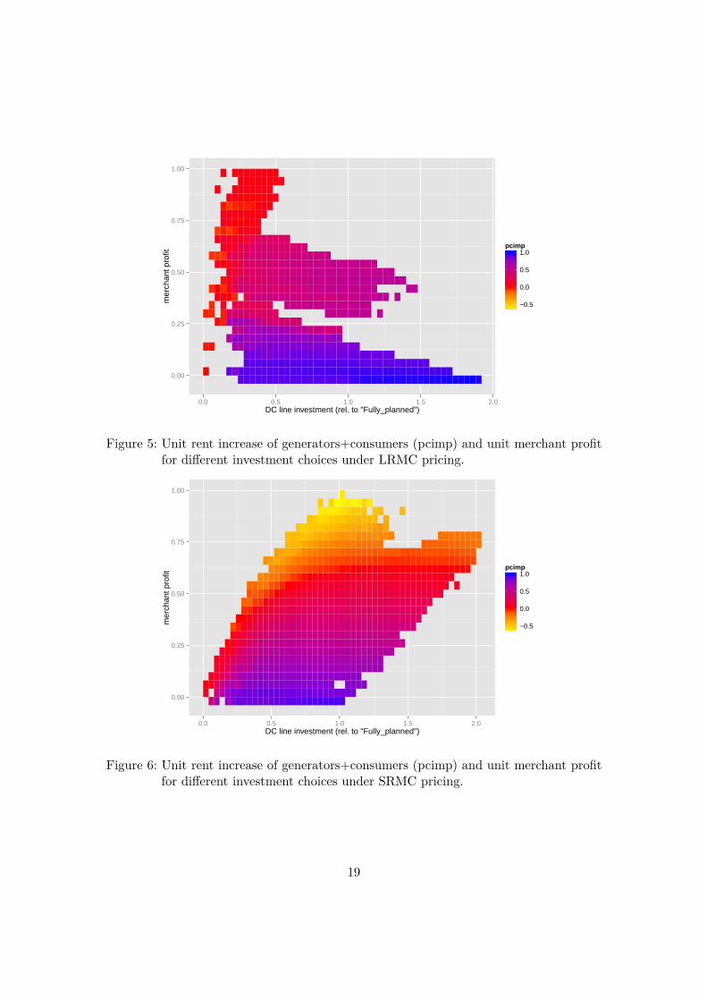
However, as with the Stackelberg cases, the more severe findings emerge from analyzingdistributional aspects: In Figures 5 and 6, the indicator displays the unit changes togenerator, AC transmission and consumer rents, relative to the Fully Planned case, andunit merchant profit. In many of the cases, which still represent profitable investmentcases from a merchant perspective, the welfare gain that accrues to the group of anyparty except the merchant investor(s) is ≤50 % of the improvement delivered by theoptimal, Fully Planned solution. In some cases under SRMC pricing, rents of generators,consumers and regulated transmissions are significantly lower than in the AC Only case:Then, those parties do, in aggregate, lose rents that are then collected by the merchantinvestor. This was already observed in the SRMC-Stackelberg case, corresponding to ahigh level of DC investment expenditure.

18

0.00

0.25

0.50

0.75

1.00

0.0 0.5 1.0 1.5 2.0DC line investment (rel. to "Fully_planned")

mer

chan

t pro

fit

−0.5

0.0

0.5

1.0pcimp

Figure 5: Unit rent increase of generators+consumers (pcimp) and unit merchant profitfor different investment choices under LRMC pricing.

0.00

0.25

0.50

0.75

1.00

0.0 0.5 1.0 1.5 2.0DC line investment (rel. to "Fully_planned")

mer

chan

t pro

fit

−0.5

0.0

0.5

1.0pcimp

Figure 6: Unit rent increase of generators+consumers (pcimp) and unit merchant profitfor different investment choices under SRMC pricing.

19

5. ConclusionIn our analysis, merchant investment can, from an overall welfare perspective, lead tosurprisingly fair results: We obtain ∼ 80–90% welfare gain as compared to the ideal,Fully Planned case. This seems to hold also for cases where we relax the Stackelbergassumption. However, we find evidence that the welfare losses implied by the merchantinvestment decisions not only relate to the investment volume, but also the merchant’snetwork structure.What may matter more is that the distributional effects of merchant transmission

investment are quite severe: “The merchant takes it all” may, for some situations, bethe correct diagnosis; “all” meaning the overall welfare contribution generated by themerchant’s investment choices. Further to that, there are situations where rents accruedby the merchant investor are even higher than the welfare gain induced by the merchantinvestment. This case is surely one that would make it hard to justify merchant activity,even if regulated (and carefully planned) alternatives are not at hand. Further, theseobservations illustrate that the idea that (especially short-term) zonal prices could leadto stimulation of sensible infrastructure investment is a fallacy.

Relating those findings to the arguments used in favor of allowing merchant investment,such as high technological risk and difficulties of different jurisdictions/actors to coordinate,implies that even if those arguments apply, merchant investment should be consideredwith extreme care, as the distributional consequences may be worse than doing nothingat all.More specifically, relating those findings to the recent developments of technology,

governance and realized cross-border interconnector projects in Europe, it seems that littlespace is left for allowing merchant interconnectors to play any serious role: Technology(HVDC connections, often subsea) is more mature than it was in the 1990s, and it seemsto be sufficiently well understood by both regulators and network companies. Additionally,the numerous DC-interconnector projects realized since the nineties, especially in theBaltic Sea region, are encouraging the belief that coordination problems between differentjurisdictions can be overcome and are, thusly, not a valid problem. This is consistentwith the increasing reluctance of the EC to approve merchant interconnector projects, asobserved by Cuomo and Glachant (2012).Concerning the potentially severe distributional effect of interconnector investment,

the existence of inter-regulatory agreements, which do presumably also cover rent-sharingissues, gives some hope that regulators are able to cope with these aspects and that gainsfrom trade can be distributed in accordance with political objectives.

AcknowledgmentThe authors thank Christian von Hirschhausen and Daniel Huppmann for valuablecomments and support.

20

References50Hertz, Amprion, TenneT, and TransnetBW (2012): Netzentwicklungsplan Strom2012, 2. überarbeiteter Entwurf der Übertragungsnetzbetreiber, URL: http://www.netzentwicklungsplan.de/content/netzentwicklungsplan-2012-2-entwurf.

50Hertz, Amprion, TenneT, and TransnetBW (2013a): Bericht der deutschenÜbertragungsnetzbetreiber zur Leistungsbilanz 2013 nach EnWG §12 Abs.4 und 5, 50Hertz and Amprion and TenneT and TransnetBW, URL:http://www.bmwi.de/BMWi/Redaktion/PDF/J-L/leistungsbilanzbericht-2013,property=pdf,bereich=bmwi2012,sprache=de,rwb=true.pdf.

50Hertz, Amprion, TenneT, and TransnetBW (2013b): Netzentwicklungsplan Strom 2013,2. Entwurf der Übertragungsnetzbetreiber, URL: http://www.netzentwicklungsplan.de/content/netzentwicklungsplan-2013-erster-entwurf.

Askheim, L. O. (2012): Developers’ objectives and NRA decisions: NorGer HVDC,URL: http://www.eui.eu/Projects/FSR/Documents/Presentations/Energy/2012/120127Exemptions/120127AskheimLarsOlav.pdf.

BNetzA (2010): Bundesnetzagentur gives green light to the first direct currentinterconnector to Norway, URL: http://www.bundesnetzagentur.de/SharedDocs/Pressemitteilungen/EN/2010/101125DirectCurrentInterconnectorNorway.html?nn=193356.

Brunekreeft, G. (2004): Market-based investment in electricity transmission networks:controllable flow, Utilities Policy 12(4):269–281.

Brunekreeft, G. (2005): Regulatory issues in merchant transmission investment, ElectricityTransmission Electricity Transmission 13(2):175–186.

Brunekreeft, G. and Newbery, D. (2006): Should merchant transmission investment besubject to a must-offer provision?, Journal of Regulatory Economics 30(3):233–260.

Buijs, P. and Belmans, R. (2012): Transmission Investments in a Multilateral Context,Power Systems, IEEE Transactions on 27(1):475–483.

CESI (2009): Working Group "Electricity interconnections". Phase II: method-ology for the assessment of new infrastructures and application to the assess-ment of the interconnection projects already identified in the Baltic area.,CESI, URL: http://ec.europa.eu/energy/infrastructure/doc/2009_bemip_a9017216-interconnections-phase_ii-final-june_2009.pdf.

Cuomo, M. and Glachant, J.-M. (2012): EU Electricity Interconnector Policy:Shedding Some Light on the European Commission’s Approach to Exemptions,URL: http://www.florence-school.eu/portal/page/portal/FSR_HOME/ENERGY/Publications/Policy_Briefs/PB_2012.06_digital.pdf.

21

Dijkstra, E. (1959): A note on two problems in connexion with graphs, NumerischeMathematik 1(1):269–271.

Doorman, G. L. and Frøystad, D. M. (2013): The economic impacts of a submarineHVDC interconnection between Norway and Great Britain, Energy Policy 60:334–344.

EC (2005): EXEMPTION DECISION NO. E/2005/001, ESTLINK PROJECT,URL: http://ec.europa.eu/energy/infrastructure/exemptions/doc/doc/electricity/2005_estlink_decision_en.pdf.

EC (2007): Exemption decision on the BritNed interconnector, URL: http://ec.europa.eu/energy/infrastructure/exemptions/doc/doc/electricity/2007_britned_decision_en.pdf.

EC (2008): Exemption decision on the East-West Cable project, URL: http://ec.europa.eu/energy/infrastructure/exemptions/doc/doc/electricity/2008_east_west_cable_decision_uk_en.pdf.

EC (2009a): Baltic Energy Market Interconnection Plan (BEMIP), URL: http://ec.europa.eu/energy/infrastructure/bemip_en.htm.

EC (2009b): Commission staff working document on Article 22 of Directive 2003/55/ECconcerning common rules for the internal market in natural gas and Article 7 ofRegulation (EC) No 1228/2003 on conditions for access to the network for cross-border exchanges in electricity, EC, Brussels, URL: http://ec.europa.eu/energy/infrastructure/infrastructure/gas/doc/sec_2009-642.pdf.

EC (2009c): Regulation (EC) No 714/2009 of the European Parliament and of the Councilof 13 July 2009 on conditions for access to the network for cross-border exchangesin electricity and repealing Regulation (EC) No 1228/2003, URL: http://eur-lex.europa.eu/LexUriServ/LexUriServ.do?uri=CELEX:32009R0714:EN:NOT.

EC (2010): Ausnahmegenehmigung der Energie-Control Kommission gemäßArtikel 7 der Verordnung (EG) Nr. 1228/2003 für Eneco Valcanale S.r.l.,URL: http://ec.europa.eu/energy/infrastructure/exemptions/doc/doc/electricity/2010_arnoldstein_travisio_decision_de.pdf.

EC (2012): Baltic Energy Market Interconnection Plan 4th progress report,URL: http://ec.europa.eu/energy/infrastructure/doc/20121016_4rd_bemip_progress_report_final.pdf.

Egerer, J., Kunz, F., and Hirschhausen, C. v. (2013): Development scenarios for the Northand Baltic Seas Grid – A welfare economic analysis, Utilities Policy 27(0):123–134.

ENTSO-E (2011): ENTSO-E Grid Map, ENTSO-E, Brussels, URL: https://www.entsoe.eu/resources/grid-map/.

22

ENTSO-E (2012a): 10-Year Network Development Plan 2012, ENTSO-E, Brüssel, URL:https://www.entsoe.eu/system-development/tyndp/tyndp-2012/.

ENTSO-E (2012b): Regional Investment Plan Baltic Sea, ENTSO-E, Brussels, URL:https://www.entsoe.eu/system-development/tyndp/tyndp-2012/.

ENTSO-E (2012c): Scenario Outlook & Adequacy Forecast 2012-2030,ENTSO-E, Brussels, URL: https://www.entsoe.eu/system-development/system-adequacy-and-market-modeling/soaf-2012-2030/.

ENTSO-E (2013): Consumption Data, URL: https://www.entsoe.eu/data/data-portal/consumption/.

ESPON (2010): ReRisk - Regions at Risk of Energy Poverty, ESPON, Luxembourg, PVund Wind Potential: S. 226 ff., URL: http://www.espon.eu/export/sites/default/Documents/Projects/AppliedResearch/ReRISK/ReRiskfinalreport.pdf.

Gabriel, S. A. and Leuthold, F. U. (2010): Solving discretely-constrained MPEC problemswith applications in electric power markets, Energy Economics 32(1):3–14.

Gans, J. S. and King, S. P. (2004): Access Holidays and the Timing of InfrastructureInvestment, Economic Record 80(248):89–100.

Gately, D. (1974): Sharing the Gains from Regional Cooperation: A Game TheoreticApplication to Planning Investment in Electric Power, International Economic Review15(1):195–208.

Green, R., Staffell, I., and Vasilakos, N. (2011): Divide and conquer? Assessing k-meansclustering of demand data in simulations of the British electricity system., URL:http://www.upo.es/eps/troncoso/Citas/IDEAL07/CitaIDEAL07-3.pdf.

Hansen, D. F.-P. (2012): TPA and Unbundling Exemptions, Bundesnetzagen-tur, Fiesole, URL: http://www.energy-regulators.eu/portal/page/portal/FSR_HOME/ENERGY/Policy_Events/Workshops/2012/TPA%20and%20Unbundling%20Exemptions/120127_Hansen.pdf.

de Hauteclocque, A. and Rious, V. (2011): Reconsidering the European regulation ofmerchant transmission investment in light of the third energy package: The role ofdominant generators, Energy Policy 39(11):7068–7077.

International Energy Agency and Organisation for Economic Co-operation and Develop-ment (2011): World energy outlook 2011, IEA, International Energy Agency : OECD,Paris.

Joskow, P. and Tirole, J. (2005): Merchant Transmission Investment, Journal of IndustrialEconomics 53(2):233–264.

23

Joskow, P. (2005): Patterns of Transmission Investment, Faculty of Economics, Universityof Cambridge, URL: http://www.econ.cam.ac.uk/electricity/publications/wp/ep78.pdf.

Knops, H. and De Jong, H. (2005): Merchant interconnectors in the European electricitysystem, Journal of Network Industries 6:261–292.

Kristiansen, T. and Rosellón, J. (2010): Merchant electricity transmission expansion: AEuropean case study, Energy 35(10):4107–4115.

Kuijlaars, K.-J. and Zwart, G. (2003): Regulatory Issues Surrounding Merchant Intercon-nection, In: Conference on Methods to Regulate Unbundled Transmission and Distribu-tion Business on Electricity Markets, Stockholm, URL: http://www.marketdesign.se/images/uploads/2003/cp_061603_2_zwart_kuijlaars.pdf.

Leuthold, F., Weigt, H., and von Hirschhausen, C. (2012): A Large-Scale Spatial Opti-mization Model of the European Electricity Market, Networks and Spatial Economics12(1):75–107.

Littlechild, S. (2012): Merchant and regulated transmission: theory, evidence and policy,Journal of Regulatory Economics 42(3):308–335.

Mann, J. (2013): Financing transmission – a third way?, URL: http://www.eprg.group.cam.ac.uk/wp-content/uploads/2013/05/Mann.pdf.

Nylund, H. (2012): Regional cost sharing in expansions of electricity transmission grids,working Paper.

PLATTS (2011): World Electric Power Plants Database, URL: http://www.platts.com/Products/worldelectricpowerplantsdatabase.

R Core Team (2013): R: A Language and Environment for Statistical Computing, URL:http://www.R-project.org/.

Schweppe, F. C., Caramanis, R. D., Tabors, M. C., and Bohn, R. E. (1988): Spot Pricingof Electricity, Kluwer, Boston.

Stigler, H. and Todem, C. (2005): Optimization of the Austrian Electricity Sector (ControlZone of VERBUND APG) by Nodal Pricing, Central European Journal of OperationsResearch 13(2):105–125.

Svenska Kraftnät and 50Hertz (2014): Press Release: Swedish-German cooperation onelectricity connection: Hansa PowerBrigde, URL: http://www.50hertz.com/de/file/140328_Press_Release_Hansa_PowerBridge.pdf.

SvK (2011): Idag införs elområden - Svenska Kraftnät, URL: http://svk.se/Press/Nyheter/Nyheter-pressmeddelanden/Allmant/Idag-infors-elomraden/.

24

Tangerås, T. P. (2012): Optimal transmission regulation of an integrated energy market,Energy Economics 34(5):1644–1655.

Taylor, J. and Hover, F. (2011): Linear Relaxations for Transmission System Planning,Power Systems, IEEE Transactions on 26(4):2533–2538.

Teusch, J., Behrens, A., and Egenhofer, C. (2012): The Benefits of Investing in ElectricityTransmission: Lessons from Northern Europe, CEPS - The Centre for European PolicyStudies, URL: http://www.ceps.eu/ceps/dld/6542/pdf.

Turvey, R. (2006): Interconnector economics, Energy Policy 34(13):1457–1472.

25

A. NomenclatureSetsbz Bidding zonel Lines in the electric gridlm Subset of l, merchant lineslr Subset of l, regulated linesn Nodes Power plant technologyt Hour

ParametersBl Line susceptanceCs Marginal production cost of plant type sDn,t Demand at node n in tExp0l Initial line expansion levelExpl Maximum expansion level of line lFmaxl Thermal limit of existing line lIl Investment cost per MW on line lIncl,n Incidence matrixM ζl Upper bound on zeta-flows

Qmaxs,n Maximum generation of plant s at node n

Slackn Slack bus

Variablesδn,t Phase angleζlr,t Flows through endogenously added AC linesζlm,t Flows through DC linesexpl Expansion on line lpn,t price at node n in tpDlm,t Price difference on merchant lines in tqs,bz,t Generation of plant s in bidding zone bz in t

26

B. Background on Merchant Interconnectors in EuropeInvestments in electricity grid infrastructure, as well as increased competition, are animportant element in the development of the internal energy market that the EuropeanCommission (EC) seeks to promote. EC regulation 714/2009 (EC, 2009c) allows ex-emptions from certain aspects of the regulation for investments in cross-border lines inorder to stimulate investments that would not occur due to excessively high risk wereexemptions not in place. When building electricity grids, costs are generally sunk andnot recoverable. The risks potential investors face may include a change in the costand revenue structure, as described in (EC, 2009b). This might be caused by regulatoryuncertainty, especially when more than one regulator is involved or when technologicalrisk is high. Therefore a potential investor may be allowed an exemption from parts ofexisting regulation.

A full exemption frees the interconnector from the obligation to third party access andenables the owner to set fees and tariffs that are used to earn revenues through congestionrents. Equivalently, the owner might be able to withhold capacity in order to increasethe congestion rents.

These exemptions may be granted by the National Regulatory Authorities (NRAs) fora limited time and are reviewed by the European Commission if more than one MemberState is involved in granting the exemption following amongst other things these rules:

• the investment needs to increase competition;

• the risk involved necessitates the exemption; and

• the exemption must not hinder the functioning of the internal market and theregulated system.

An analysis of the four exemption decisions by the EC since 2005 is conducted by Cuomoand Glachant (2012). The authors observe a recent tightening of the exemption regimeby not granting full exemptions and imposing additional requirements on cross-borderinterconnector development. The EC has made decisions for the following cases:

• Estlink, a 350 MW HVDC cable between Estonia and Finland, commissioned in2006;

• BritNed, a 1 GW HVDC cable connecting the British and Dutch grids, commissioned2011;

• East–West Cable One, a 350 MW HVDC cable connecting Great Britain andIreland, delayed; and

• Arnoldstein/Tarvisio, a 132 kV, 160 MW AC line between Austria and Italy, com-missioned 2012.

The decision by the NRAs allowing EstLink an exemption from tariff regulationand third party access was confirmed by the EC in 2005 (EC, 2005). For BritNed, the

27

exemption was approved in 2007, but due to concerns regarding a possible undersizing ofthe interconnector’s capacity, the obligation to present a financial report 10 years into theinterconnector’s operation was added. If the revenues were to exceed the expectations, theNRA could introduce a profit cap or require BritNed to increase capacity (which wouldnot be covered by the exemption) in order to reduce congestion rents EC (2007). Theexemption for the East-West Cable was confirmed by the EC in 2009 as the risk involvedin the project was deemed sufficient due to the planned competing regulated 500 MWinterconnector EirGrid (EC, 2008). The approval was linked to the commissioning ofEirGrid and also included conditions regarding congestion management and trading.The project is currently delayed. The EC decided in 2010 that the exemption for theAC overhead interconnector Arnoldstein-Tarvisio would be granted, but no exemptionfrom third party access would be given. Furthermore all increases in capacity had to beapproved by the EC (EC, 2010).Furthermore NorGer KS, the company in charge of the development of the NorGer

cable between Norway and Germany, applied in March 2010 for an exemption for 25 yearsand full capacity of the planned cable (1,400 MW). The project fulfilled the requirementsof being a new interconnector between states (Norway being on a par with MemberStates (Hansen, 2012)), expected enhancement of competition, investment risk and noharmful effects to the market according to the German regulatory authority BNetzA.The exemption was granted by BNetzA in 2010 (BNetzA, 2010). Because the EC’s riskassessment showed that the interconnector might still be built without exemption andNorway’s preference for a regulated interconnector, NorGer KS withdrew the applicationin April 2011 (Askheim, 2012).

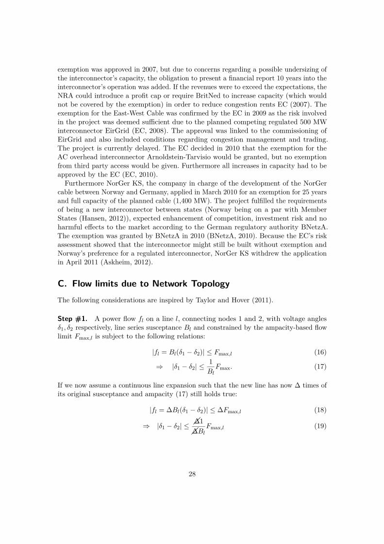
C. Flow limits due to Network TopologyThe following considerations are inspired by Taylor and Hover (2011).

Step #1. A power flow fl on a line l, connecting nodes 1 and 2, with voltage anglesδ1, δ2 respectively, line series susceptance Bl and constrained by the ampacity-based flowlimit Fmax,l is subject to the following relations:

|fl = Bl(δ1 − δ2)| ≤ Fmax,l (16)

⇒ |δ1 − δ2| ≤1BlFmax. (17)

If we now assume a continuous line expansion such that the new line has now ∆ times ofits original susceptance and ampacity (17) still holds true:

|fl = ∆Bl(δ1 − δ2)| ≤ ∆Fmax,l (18)

⇒ |δ1 − δ2| ≤ ��∆1��∆Bl

Fmax,l (19)

28

Thus, (16)=(19) and we have a limit on angle-differences along lines that is independentof the expansion factor ∆ of the line, but only depends on its physical characteristics.

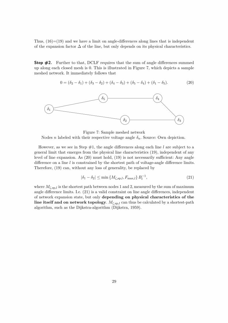
Step #2. Further to that, DCLF requires that the sum of angle differences summedup along each closed mesh is 0. This is illustrated in Figure 7, which depicts a samplemeshed network. It immediately follows that

0 = (δ2 − δ1) + (δ3 − δ2) + (δ4 − δ3) + (δ5 − δ4) + (δ1 − δ5). (20)

δ1

δ5 δ4

δ2 δ3

Figure 7: Sample meshed networkNodes n labeled with their respective voltage angle δn. Source: Own depiction.

However, as we see in Step #1, the angle differences along each line l are subject to ageneral limit that emerges from the physical line characteristics (19), independent of anylevel of line expansion. As (20) must hold, (19) is not necessarily sufficient: Any angledifference on a line l is constrained by the shortest path of voltage-angle difference limits.Therefore, (19) can, without any loss of generality, be replaced by

|δ1 − δ2| ≤ min {Mζ,sp,l, Fmax,l}B−1l , (21)

whereMζ,sp,l is the shortest path between nodes 1 and 2, measured by the sum of maximumangle difference limits. I.e. (21) is a valid constraint on line angle differences, independentof network expansion state, but only depending on physical characteristics of theline itself and on network topology.Mζ,sp,l can thus be calculated by a shortest-pathalgorithm, such as the Dijkstra-algorithm (Dijkstra, 1959).

29

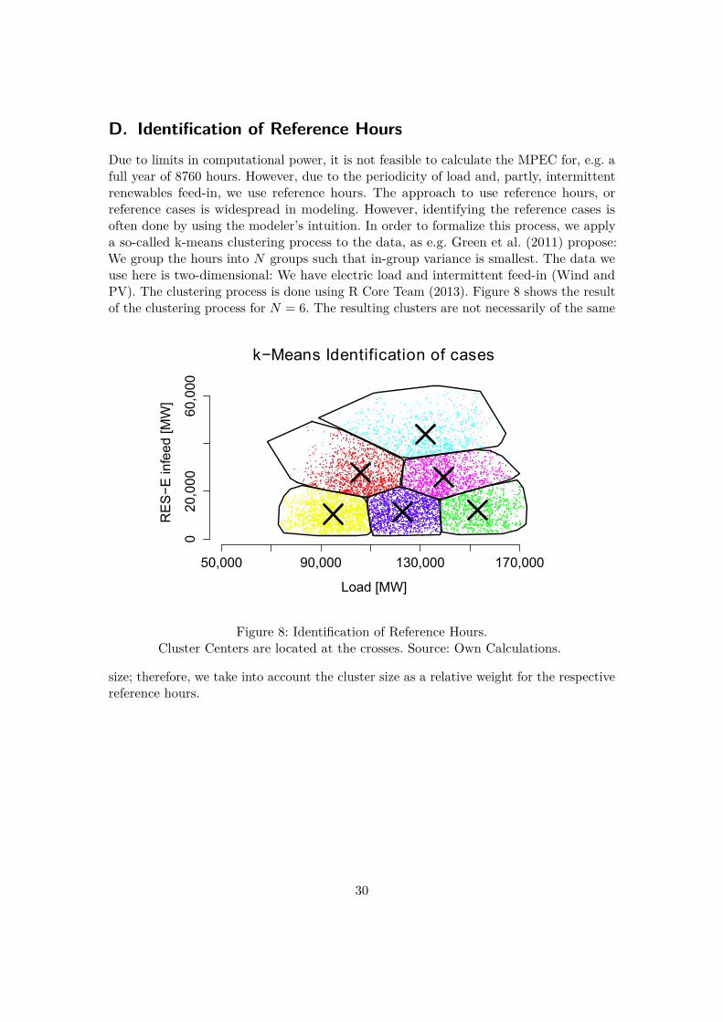
D. Identification of Reference HoursDue to limits in computational power, it is not feasible to calculate the MPEC for, e.g. afull year of 8760 hours. However, due to the periodicity of load and, partly, intermittentrenewables feed-in, we use reference hours. The approach to use reference hours, orreference cases is widespread in modeling. However, identifying the reference cases isoften done by using the modeler’s intuition. In order to formalize this process, we applya so-called k-means clustering process to the data, as e.g. Green et al. (2011) propose:We group the hours into N groups such that in-group variance is smallest. The data weuse here is two-dimensional: We have electric load and intermittent feed-in (Wind andPV). The clustering process is done using R Core Team (2013). Figure 8 shows the resultof the clustering process for N = 6. The resulting clusters are not necessarily of the same

Load [MW]

RE

S−

E in

feed

[MW

]

50,000 90,000 130,000 170,000

020

,000

60,0

00

k−Means Identification of cases

Figure 8: Identification of Reference Hours.Cluster Centers are located at the crosses. Source: Own Calculations.

size; therefore, we take into account the cluster size as a relative weight for the respectivereference hours.

30

E. Tables

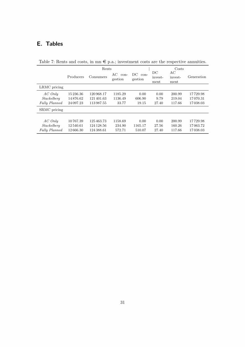
Table 7: Rents and costs, in mn e p.a.; investment costs are the respective annuities.Rents | Costs

Producers Consumers AC con-gestion

DC con-gestion

DCinvest-ment

ACinvest-ment

Generation

LRMC pricing

AC Only 15 236.36 120 968.17 1185.29 0.00 0.00 200.99 17 729.98Stackelberg 14 876.62 121 401.63 1136.49 606.90 9.79 219.04 17 070.31

Fully Planned 24 097.23 113 987.55 33.77 19.15 27.40 117.66 17 038.03

SRMC pricing

AC Only 10 767.39 125 463.73 1158.69 0.00 0.00 200.99 17 729.98Stackelberg 12 540.61 124 128.56 234.90 1165.17 27.56 160.26 17 063.72

Fully Planned 12 666.30 124 388.61 572.71 510.07 27.40 117.66 17 038.03

31