THE DIFFERENCES BETWEEN A STANDARD COSTING ...

THE DIFFERENCES BETWEEN A STANDARD COSTING AND NORMAL COSTING METHOD OF MANUFACTURING OPERATING

INCOME CALCULATION CAUSED BY THE IMPLEMENTATION OF A NEW INTEGRATED INFORMATION SYSTEM

Kamila Fałat, MScWroclaw University of Economics and BusinessFaculty of Economics and FinanceDepartment of FinanceKomandorska 118/120, 53-345 Wroclaw, Polande-mail: [email protected]: 0000-0003-0417-8730

Received 4 December 2019, Accepted 7 October 2020

Abstract

Research background: When a company changes a few separated information systems into one integrated information system there can appear the obligation of costing method change. It happens especially when the company is a part of an international manufacturing corporation.Purpose: The main goal of the paper is to compare two methods of manufacturing operating income calculation and data presentation when a company changes a costing method from normal costing to standard costing.Research methodology: In the paper for this research comparative analysis was used between two methods of manufacturing operating income calculation. In the first method manufacturing operating income is the difference between revenues from manufacturing operations and the costs of goods manufactured. In the second one manufacturing operating income is calculated as a sum of production variances, purchase price variances, currency variances and inventory adjustments. Pearson’s correlation coefficients for pairs of variables were calculated in both of the costing methods. A comparative analysis was done on the basis of a case study executed in a big international wholesaler. The company is a member of an international manufacturing corporation.Results: The same manufacturing operating incomes were obtained in both methods. The absolute values of Pearson’s correlation coefficients were similar in normal and standard costing, but they differ in directions.Novelty: In standard costing manufacturing operating income is calculated as a sum of various types of variances. They are calculated as deviations from standard costs. It enables the easier identification of impacting a company’s results factors.

Folia Oeconomica StetinensiaVolume 20 (2020) Issue 2

DOI: 10.2478/foli-2020-0038

#0##0#

Kamila Fałat96

Introduction

Manufacturing operating income is an important indicator for manufacturing companies, especially when they are part of an international manufacturing corporation. It allows to compare their results in the whole corporation excluding specific local law regulations e.g. tax regulations. Manufacturing operating income measures companies’ performance.

Manufacturing operating income is the difference between revenues from manufacturing operations and the costs of goods that are manufactured (Horngren, 2009). The costs of goods manufactured are costs of materials used for production and operating expenses. Material costs are divided into two groups: direct material costs and indirect material costs. A finished product consists of direct materials, they are included in the bill of material which serves as a reference for product data and contains a list of the parts or components that are required to manufacture a product. The bill of material is a multi-level document that provides build data for multiple sub-processes. Managing a production process is equivalent to managing the bill of material, in order to track product changes and maintain an accurate list of required components at a certain phase in the production process (Griffioen, Christiaanse, Hulstijn, 2017). Indirect materials are not part of the product, they are not in the bill of material, they are needed for a production process. Operating expenses are divided into three groups: direct costs, indirect costs and fixed costs. Indirect costs are costs of external services, supplies, utilities and salaries from non-production departments. Fixed costs consist mainly of machines depreciation.

How manufacturing income is calculated and presented depends on the costing method which a company uses. Traditionally manufacturing operating income is calculated as the difference between revenues from manufacturing operations and the costs of goods manufactured. It is usually used in normal costing and in actual costing. In actual costing the company bases on actual usages for a direct and an indirect costs calculation, whereas in normal costing actual usages are used for a direct costs calculation and planned usages for an indirect costs calculation. In standard costing the company bases on planned usages for a direct and

Keywords: manufacturing operating income calculation, integrated information system implementation, variance analysis

JEL classification: M41, O16

The Differences Between a Standard Costing and Normal Costing Method... 97

indirect costs calculation (Świderska, 2010). In the standard costing method manufacturing operating income is calculated as a variance between actual costs and standard costs.

Standard costing is a traditional cost accounting method. The primary purpose of applying standard costing is cost control. Other objectives of standard costing are the performance evaluation of a company, preparing budgets, pricing products, costing inventories and facilitation making decisions by management. Standard costing is used in manufacturing and service industries. Williamson (1996) indicates petroleum refinery, pharmaceuticals and chemistry industries, automotive, canned vegetable and fruit, and fast food restaurant industries. Hilton (2001) pointed out many service industries and non-profit organizations.

Due to the fact that standard costing is the idea which was for the first time described in 1889 by British accountant George P. Norton in “Textile Manufacturers’ Bookkeeping” (Solomons, 1994) some academicians suggest that standard costing is no longer suitable in today’s global and competitive environment. Richard Fleischman and Thomas Tyson (1998) stated that standard costing cannot provide adequate assistance in the areas of construction strategy and operational management. Hilton (2001) noticed that the highly competitive environment and improved production technologies cause the decreasing role of labor in the production process and shortened product life cycle which decrease the importance of standard costing. Drury (2009) stated that the usefulness of standard costing in a modern business environment has been questioned because of the changing cost structure, inconsistency with modern management approaches. He underlined the importance of direct labor and delay in feedback reporting. At the extreme, Lucas (1997) claimed that standard costing has become obsolete.

In response to these statements, several studies have been undertaken in various countries by several authors to find out whether standard costing is becoming obsolete or is still a useful tool in the hand of management. Table 1 shows the research.

Table 1. Research concerning the validity of standard costing

Author Year Research Sample Result

1 2 3 4

David Lyall and Carol Graham 1993 231 companies in the United King-dom

More than 90% of the surveyed companies apply standard costing for cost control purposes and 63% of the managers using the technique reported being satisfied in terms of decision-making supports

Kamila Fałat98

1 2 3 4

Maliah Sulaman, Nik Nazli, Nik Ahmad and Norhayati Mohd Alwi

2005 local firms in Malaysia, 21 Japanese firms

70% of local firms in Malaysia and 76% of 21 Japanese firms use standard costing

Marie, Cheffi, Louis and Rao 2010 100 companies doing business in Dubai (UAE): 57 companies from the industrial sector and 43 from the service and trading sector

77% of companies in the industrial sector and 39% of companies in the service sector use standard costing

Badem, Ergin and Drury 2013 13 primary and 300 supplier com-panies in the automotive industry in Turkey

On average 77% of the companies use standard costing

Md. Mamunur Rashid 2016 28 listed pharmaceuticals and chemical companies in Bangladesh

75% (21out of 28) of the companies use standard costing

Source: own elaboration based on revised articles.

The above research shows that standard costing is still used in economic reality. It is an important tool in the hand of management. Companies use standard costing in manufacturing and service industries throughout the world. They apply standard costing to cost control, performance evaluation, costing inventories, computing product costs, decision making and budgeting. Standard costing is one of the most widespread systems for accounting orientated towards planning and is technologically well-equipped with data processing systems like that of SAP (Heupel, 2006). Standard costing allows management to conduct a more in-depth variance analysis for each product cost (Farkas, Kersting, Stephens, 2016).

Heupel (2006) pointed out seven steps of standard costing implementation and their advantages which are presented in Table 2.

Table 2. Steps of standard costing implementation and their advantages

Step Step description Advantage

1 process analysis more detailed analysis of processes and procedures

2 determining planning specifications and cost drivers systematic detection of the potential for improvement

3 determining the standard level of activity for all cost centers systematic detection of the potential for improvement

4 determining usage volumes and periods for each cost category of a cost center in reference to the standard level of activity

systematic detection of the potential for improvement

5 valuation of planned usage volumes and periods with fixed prices systematic detection of the potential for improvement

6 analysis within cost centers for establishing basic best practice and optimal costs

systematic detection of the potential for improvement

7 variance analysis decentralized acceptance of responsibility for costs

Source: own elaboration on the basis of Heupel (2006).


In manufacturing operating income calculation in the standard costing method there are four types of variances taken into consideration: production variances, purchase price variances, currency variances and inventory adjustments.

Production variance measures a company’s production process performance therefore the company is the most interested in its value. Production variance consists mainly of two types of variances: input price variance and input quantity variance. Input price variance appears in two situations. Firstly, when there is a difference between the planned prices and actual prices of raw materials consumed in a production process. The second situation is when there are differences between planned activity rates and actual activity rates (Ocneanu, Cojocaru, 2013). The labor tariff is calculated as a quotient of labor costs and labor hours. The machine tariff is a quotient of machine costs and machine hours. Actual labor and machine tariffs are different from planned labor and machine tariffs usually when actual volume is lower or higher than volume used for a standard costs setting. Volume is the main driver of labor and machine hours spent to produce finished goods. Cost savings or overspending can be also the reason for variance in labor and machine tariffs. Input quantity variance is caused by differences between the planned and actual consumption of materials (Nowak, 2011). For example, waste in the production process is higher than planned. Input quantity variance also appears when actual labor or machine efficiency is different from the efficiency set in the standard cost of semi-finished or finished goods, so there is different time of labor or machine spent on manufacturing a production order. Input quantity variance can be caused by different units of measure of materials, which are consumed for production, so then there appear errors in the bill of materials and in the conversion factors of raw materials.

Purchase price variance is the difference between the actual purchased raw material price and the standard raw material price. Standard price is usually set as the last purchased price from the period before changes of system settings or a price which includes a price increase or decrease declared by a supplier (Nowak, 2015). The main reason of purchase price variance is price increase or decrease which happened after changes of the system settings. When price from an invoice is higher than the standard price the variance is negative. When there was an invoiced price decrease purchase price variance is positive.

Currency variance is the difference between current currency rate and fixed currency rate which is valid for the accounting year. It is usually Bloomberg’s rate from September of the year before.

Inventory adjustment comes from stock revaluation. It usually happens when there are semi-finished and finished goods prices changes. Inventory adjustment includes also the physical

Kamila Fałat100

waste of poor quality materials and non-working inventories. Poor quality raw materials appear when the expiration date is exceeded, or when a supplier sent poor quality raw materials and he/she rejected a complaint. Non-working inventories are raw materials which were not used for production due to the lack of demand of the finished goods.

The main goal of the article is to compare two methods of manufacturing operating income calculation and data presentation in the situation when a company changes a costing method from normal costing to standard costing. In an analyzed company in the article the reason of the change is a new integrated system implementation in a manufacturing corporation. The author wants to check if the value of manufacturing operating income calculated in these two methods gives the same results. The company changes the method of manufacturing operating income calculation due to a decision made by the corporate board of directors. The biggest advantage of standard costing is the control of production processes. At the beginning assumptions are made, revenues and costs are estimated and planned usually during an operating plan preparation. They are then compared with actual data reported in production processes. It enables identifying ineffective operations in production processes. Each variance between standard costs and actual costs is analyzed. It allows implementing improvements and thus avoids unfavorable variances in the future.

Each company wants to maximize profit and minimize loss. In reaching the goal of an organization compete many control systems like production control, quality control and stocks control. The cost information system is important because it monitors the results of all functions in the company. The detailed analysis of costs, the calculation of production cost, the loss quantification and the estimation of work efficiency provide a solid basis for financial control (Lepădatu, 2010). Standard costing helps the company to maximize profit and minimize loss and enables its detailed costs control.

The research hypothesis states that the method of manufacturing operating income calculation does not have an impact on its value, but it provides different additional information.

The remainder of the article is organized as follows. The next section is the methodology section which describes the calculation formulas used for a comparative analysis between normal costing and standard costing. The research results section presents the results of the analysis for nine quarters after a new integrated system implementation in a big international wholesaler. Conclusions of the research are included in the summary.


1. Research Methodology

In order to show the consequences of changing the methodology of costing from normal costing to standard costing the author analyzes two methods of manufacturing operating income calculation and data presentation. The change of methodology was caused by the replacement of a few systems with one integrated information system called SAP in a company which is part of an international manufacturing corporation. The system implementation was executed in 2018. The main reason of the change was a decision made by the corporate board of directors. For this research a comparative analysis between two methods of manufacturing operating income calculation was used. A comparative analysis was done on the basis of a case study executed in a big international wholesaler.

In the first method manufacturing operating income (calculating formula (1)) is calculated as a difference between revenues from manufacturing operations and costs of goods manufactured (calculating formula (2)). It is used in normal costing.

MOI = RV – COGM (1)where:

MOI – manufacturing operating income,RV – revenues,COGM – costs of goods manufactured.

COGM = MC + OPEX (2)where:

COGM – costs of goods manufactured,MC – material costs,OPEX – operating costs.

Data provided in the first method enabled calculating revenues and costs indicators: revenues/operating costs (RV/OPEX), material costs/revenues (MC/RV) and revenues/costs of goods manufactured (RV/COGM).

In the second method manufacturing operating income (calculating formula (3)) is calculated as a sum of production variances, purchase price variances, currency variances and inventory adjustments. It is used in standard costing.

MOI = PV + PPV + CV + IA (3)

Kamila Fałat102

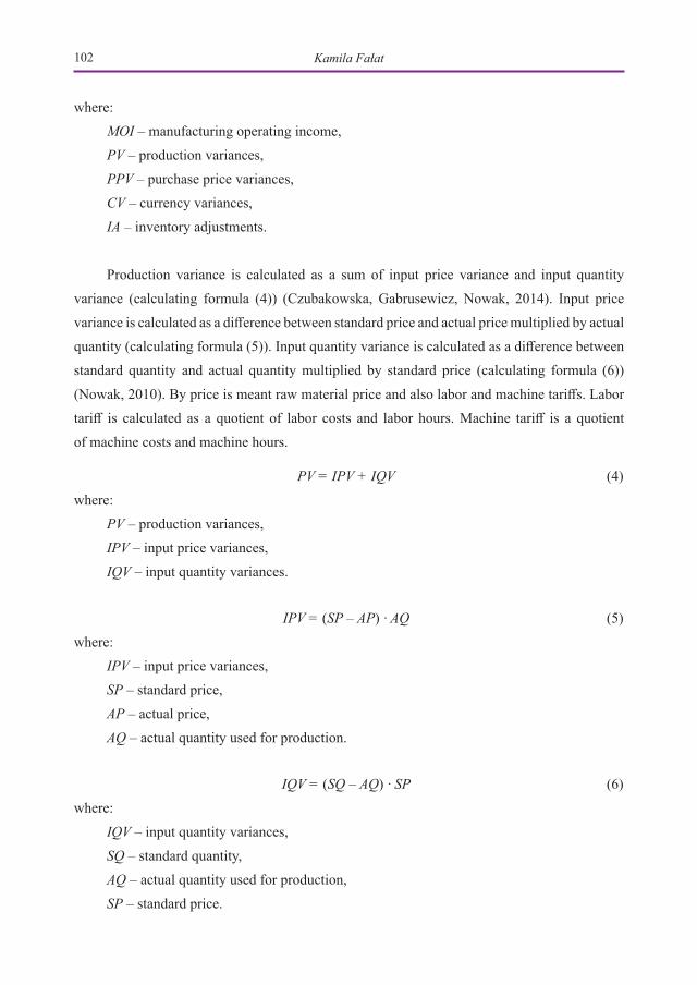
where: MOI – manufacturing operating income, PV – production variances,PPV – purchase price variances,CV – currency variances,IA – inventory adjustments.

Production variance is calculated as a sum of input price variance and input quantity variance (calculating formula (4)) (Czubakowska, Gabrusewicz, Nowak, 2014). Input price variance is calculated as a difference between standard price and actual price multiplied by actual quantity (calculating formula (5)). Input quantity variance is calculated as a difference between standard quantity and actual quantity multiplied by standard price (calculating formula (6)) (Nowak, 2010). By price is meant raw material price and also labor and machine tariffs. Labor tariff is calculated as a quotient of labor costs and labor hours. Machine tariff is a quotient of machine costs and machine hours.

PV = IPV + IQV (4)where:

PV – production variances,IPV – input price variances,IQV – input quantity variances.

IPV = (SP – AP) · AQ (5)where:

IPV – input price variances,SP – standard price,AP – actual price, AQ – actual quantity used for production.

IQV = (SQ – AQ) · SP (6)where:

IQV – input quantity variances,SQ – standard quantity,AQ – actual quantity used for production, SP – standard price.


Purchase price variance is the difference between the standard price of an item and the actual price paid to buy the item, multiplied by the actual quantity of units purchased. Actual price is the price from an invoice (calculating formula (7)).

PPV = (SP – AP) · AQ (7)where:

PPV – purchase price variance,SP – standard price,AP – actual price from an invoice, AQ – actual quantity of purchased units.

Currency variances are differences between fixed currency rates and actual currency rates (calculating formula (8)).

CV = (FCR – ACR) · IV (8)where:

CV – currency variance,FCR – fixed currency rate,ACR – actual currency rate, IV – invoice value in foreign currency.

Inventory adjustments are a sum of the waste of raw material and stock revaluation (calculating formula (9)).

IA = WRM + SR (9)where:

IA – inventory adjustments,WRM – waste of raw material,SR – stock revaluation.

Manufacturing operating incomes were calculated by using both methods in an Excel file. A comparative analysis between the results achieved in these two methods was done. In the first method manufacturing operating income was calculated manually, whereas in the second method variances were calculated by an integrated information system called SAP. The research sample consists of revenues and costs of goods manufactured reported in nine quarters after SAP implementation. The sample is small and not representative, but only these data are available.

Kamila Fałat104

In the standard costing method the quarterly standards of revenues and costs of goods manufactured were established. In this method of costing standard revenues equal the standard costs of goods manufactured, so manufacturing operating income equals 0. It means that revenues cover costs. Variances between: actual and standard revenues, standard and the actual costs of goods manufactured, standard and actual manufacturing operating income were calculated (calculating formula (10)) (Nowak, 2010).

actual vs. standard value = AV – SV (10)where:

AV – actual value,SV – standard value.

After that Pearson’s correlation coefficients were calculated to show whether and how strongly pairs of variables were related. In standard costing a correlation between three variables: variances between actual and standard revenues, variances between standard and actual costs of goods manufactured, variances between standard and actual manufacturing operating income was calculated. In normal costing a correlation was calculated also between three variables: actual revenues, actual costs of goods manufactured and actual manufacturing operating income. It was done in Excel by using the PEARSON formula. As a result of this a correlation matrix was created. A correlation matrix is a table which presents correlation coefficients between variables (Ostasiewicz, Rusnak, 2011). Each cell in the table shows the correlation between two variables. Afterwards correlation coefficients in standard and normal costing were compared to check the direction and strength between variables in both methods of costing.

2. Results and discussion

The analyzed time period amounts to nine quarters after SAP implementation. The research was carried out in a manufacturing company. The firm is a big international wholesaler. It sells its products all around the whole world. The company’s portfolio has 185 finished goods and 97 semi-finished goods. The production process is complex, and it has three production levels. The research sample consists of revenues and costs of goods manufactured which were reported in the first nine quarters after the implementation of SAP. The data are presented in thousands of dollars (kUSD).

Table 3 shows manufacturing operating income which is calculated in the normal costing method. It is calculated as a difference between revenues and costs of goods manufactured. Only


in the sixth and last quarters does the company make a profit. In first quarter revenues are the lowest and in the last quarter revenues are the highest. In the analyzed period material costs are proportional to revenues, the higher revenues the higher material costs. Operating expenses are also higher from quarter to quarter.

Table 3. Manufacturing operating income calculated in the normal costing method

Category/period 1 2 3 4 5 6 7 8 9

Revenues 727.60 1,156.50 1,257.67 1,294.02 1,384.62 1,496.00 1,362.66 1,760.45 1,810.61

Material costs 417.65 861.22 734.64 768.47 860.22 835.63 816.90 1,101.06 1,165.32Total operating expenses: 624.40 570.95 569.86 666.96 586.17 612.10 665.55 661.60 620.79

Direct costs 291.52 266.57 266.06 311.40 273.68 285.78 310.74 308.89 289.84

Indirect costs 176.96 161.82 161.51 189.03 166.13 173.48 188.63 187.51 175.94

Fixed costs 155.91 142.56 142.29 166.54 146.36 152.84 166.19 165.20 155.01Costs of goods manufactured 1,042.05 1,432.17 1,304.50 1,435.43 1,446.39 1,447.72 1,482.45 1,762.66 1,786.12

Manufacturing operating income –314.46 –275.67 –46.83 –141.42 –61.76 48.27 –119.79 –2.21 24.49

Source: own elaboration.

Furthermore, the first method allows calculating revenues and costs indicators RV/OPEX, MC/RV and RV/COGM. Table 4 shows them, they are calculated on the basis of the data given in Table 3. The data are available directly. In the analyzed period indicator RV/OPEX increases. It means that from 1 USD of operating expenses more revenues are generated. MC/RV informs which part of the revenues are material costs. In the second quarter MC/RV was the highest and amounts to 74%. It was caused by physical waste of poor quality raw materials. RV/COGM is increasing in the analyzed period. It means that from 1 USD of costs of goods manufactured more revenues were generated.

Table 4. Revenues and costs indicators

Indicator/period 1 2 3 4 5 6 7 8 9

RV/OPEX 1.17 2.03 2.21 1.94 2.36 2.44 2.05 2.66 2.92

MC/RV (%) 57.00 74.00 58.00 59.00 62.00 56.00 60.00 63.00 64.00

RV/COGM 0.70 0.81 0.96 0.90 0.96 1.03 0.92 1.00 1.01


Kamila Fałat106

Table 5 shows manufacturing operating income which is calculated in the standard costing method. It is calculated as a sum of production variances, purchase price variances, currency variances and inventory adjustments. Variances were calculated by the SAP system accordingly to its settings. The worst production variance is in the first quarter and it amounts to 263 kUSD. In the sixth, eighth and ninth quarters production variances are positive. It means that volume is very good and better than it was assumed in the standards. Purchase price variance is the worst in the first quarter. It means that there was price increase and the standard price was corrected since the second quarter. Since the eighth quarter there was another price increase. According to currency variance, the biggest impact on it came from the United States dollar due to the fact that the biggest part of raw materials is bought in the United States dollar. Each exchange rate change has a direct impact on currency variance. In the analyzed period inventory adjustments show that there was the highest raw material disposal in the second quarter. It was caused by the exceeded expiration date of one of the raw materials.

Table 5. Manufacturing operating income calculated in the standard costing method

Category/period 1 2 3 4 5 6 7 8 9

Production variances –263.11 –194.66 –60.74 –113.07 –48.48 32.90 –92.37 48.77 54.90Purchase price variances –19.39 –4.73 11.13 1.26 1.52 –1.14 4.43 –10.00 –7.08

Currency variances –6.37 –3.26 –16.80 –3.86 –10.79 –8.47 –22.93 –29.71 –2.63

Inventory adjustments –25.59 –73.03 19.58 –25.75 –4.02 24.99 –8.91 –11.26 –20.70Manufacturing operating income –314.46 –275.67 –46.83 –141.42 –61.76 48.27 –119.79 –2.21 24.49


Comparing manufacturing operating income calculated by using a normal costing (Table 3) to manufacturing operating income calculated by using standard costing (Table 5), it can be said that the results are equal. It means that each calculation method gives the same value of manufacturing operating income. Both methods need different data for calculation and provide additional data that can be obtained from the calculation. In normal costing we can see revenues, operating expenses and material costs. In standard costing we do not have this information directly. On the other hand, in standard costing from manufacturing operating income calculation we can receive other information such as production variances, purchase prices variances, waste of raw materials and currency variances. We can see if there were raw material price increases or decreases. Standard costing gives more information about manufacturing operating income drivers. From the management perspective it is very good to


know why the result is so good or so bad. The most important is the fact that manufacturing operating income is the same in both calculation methods.

Pearson’s correlation coefficients were calculated in order to compare both methods of costing. Table 6 presents quarterly standard revenues, costs of goods manufactured and manufacturing operating income. They were set during the operating plans preparation. The highest standards of revenues and costs of goods manufactured were observed in the third year after the implementation of SAP. Quarterly standard manufacturing operating incomes amount to 0 in each quarter.

Table 6. Quarterly standard revenues, costs of goods manufactured and manufacturing operating income

Category/year 1 2 3

Quarterly standard revenues 1,300 1,460 1,534

Quarterly standard costs of goods manufactured 1,300 1,460 1,534

Quarterly standard manufacturing operating income 0 0 0


Table 7. Actual vs. standard revenues, costs of goods manufactured and manufacturing operating income

Category/period 1 2 3 4 5 6 7 8 9 Total

Actual vs. Standard revenues –572.40 –143.50 –42.33 –5.98 –75.38 36.00 –97.34 300.45 350.61 –249.88

Standard vs. Actual costs of goods manufactured

257.95 –132.17 –4.50 –135.43 13.61 12.28 –22.45 –302.66 –326.12 –639.49

Standard vs. Actual manufacturing operating income

–314.46 –275.67 –46.83 –141.42 –61.76 48.27 –119.79 –2.21 24.49 –889.37


Variances between: actual and standard revenues, standard and actual costs of goods manufactured, standard and actual manufacturing operating income were calculated and are presented in Table 7. The table shows that variances between standard and actual manufacturing operating income amount to actual manufacturing operating income. It can be said that actual manufacturing operating income is a sum of variance between actual vs. standard revenues and variance between standard vs. actual costs of goods manufactured. In the analysed period the company made a loss of 889.37 kUSD. The result was mainly caused by 639.40 kUSD negative

Kamila Fałat108

variance between standard vs. actual costs of goods manufactured. The rest of the negative impact, 249.88 kUSD came from variance between actual vs. standard revenues. It means that the company spent more costs than assumed and achieved lower revenues than planned. The costs of goods manufactured were the main driver of manufacturing operating income.

In normal costing and standard costing Pearson’s correlation coefficients were calculated to present the strength and direction of linear relationships between pairs of variables. In normal costing Pearson’s correlation coefficients were calculated between revenues and costs of goods manufactured, revenues and manufacturing operating income, costs of goods manufactured and manufacturing operating income. These three variables: actual revenues, actual costs of manufactured goods and actual manufacturing operating income are dependent. As a result of the correlation calculations a correlation matrix was created. It is presented in Table 8. Correlation between revenues and costs of goods manufactured amounts to 0.96 which means that there is a very high positive linear relationship. A positive relationship means that increase of revenues causes an increase of the costs of goods manufactured, so these variables move in the same direction. It is typical for a manufacturing company when increase of volume and revenues causes an increase of variable costs. The correlation between revenues and manufacturing operating income amounts to 0.86 which means that there is a highly positive linear relationship. The correlation between costs of goods manufactured and manufacturing operating income amounts to 0.68 which means that there is a moderate positive linear relationship. In this company in the analyzed period when costs of goods manufactured increase manufacturing operating income also increases. It can be mainly caused by the fact that material costs determine on average 62% of revenues.

Table 8. Correlation matrix in normal costing for revenues, costs of goods manufactured and manufacturing operating income

Correlation Revenues Costs of goods manufactured

Manufacturing operating income

Revenues 1.00 0.96 0.86

Costs of goods manufactured 0.96 1.00 0.68

Manufacturing operating income 0.86 0.68 1.00


In standard costing Pearson’s correlation coefficients in the analyzed period were also calculated. For the calculation three variables are used: variances between actual and standard revenues, variances between standard and actual costs of goods manufactured, variances between


standard and actual manufacturing operating income. The variables are dependent. Pearson’s correlation coefficients were calculated for three pairs of data:

– variances actual vs. standard revenues and variances standard vs. actual costs of goods manufactured,

– variances actual vs. standard revenues and variances standard vs. actual manufacturing operating income,

– variances standard vs. actual costs of goods manufactured and variances standard vs. actual manufacturing operating income.

As a result of these calculations a correlation matrix was created. Table 9 presents it. The correlation between variances actual vs. standard revenues and variances standard vs. actual costs of goods manufactured amounts to –0.91 which means that there is a very high negative linear relationship. Negative relationship means that the increase of variances actual vs. standard revenues causes a decrease of variances standard vs. actual costs of goods manufactured, so these variables move in different directions. The correlation between variances actual vs. standard revenues and variances standard vs. actual manufacturing operating income amounts to 0.82 which means that there is a highly positive linear relationship. The correlation between variances standard vs. actual costs of goods manufactured and variances standard vs. actual manufacturing operating income amounts to –0.51 which means that there is a moderate negative linear relationship. It means that when variance between standard vs. actual costs of goods manufactured decreases, variance between standard vs. actual manufacturing operating income increases.

Table 9. Correlation matrix in standard costing for variances between actual and standard revenues, costs of goods manufactured, manufacturing operating income

Correlation Actual vs. Standard revenues

Standard vs. Actual costs of goods manufactured

Standard vs. Actual manufacturing operating

incomeActual vs. Standard revenues 1.00 –0.91 0.82Standard vs. Actual costs of goods manufactured –0.91 1.00 –0.51

Standard vs. Actual manufacturing operating income 0.82 –0.51 1.00


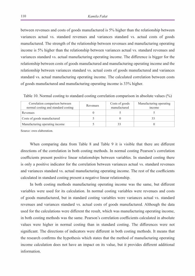
Table 10 presents normal costing to standard costing correlation comparison for absolute values. It shows that Pearson’s correlation coefficients calculated in absolute values were higher in normal costing than in standard costing. The table shows that the strength of the relationship

Kamila Fałat110

between revenues and costs of goods manufactured is 5% higher than the relationship between variances actual vs. standard revenues and variances standard vs. actual costs of goods manufactured. The strength of the relationship between revenues and manufacturing operating income is 5% higher than the relationship between variances actual vs. standard revenues and variances standard vs. actual manufacturing operating income. The difference is bigger for the relationship between costs of goods manufactured and manufacturing operating income and the relationship between variances standard vs. actual costs of goods manufactured and variances standard vs. actual manufacturing operating income. The calculated correlation between costs of goods manufactured and manufacturing operating income is 33% higher.

Table 10. Normal costing to standard costing correlation comparison in absolute values (%)

Correlation comparison between normal costing and standard costing Revenues Costs of goods

manufacturedManufacturing operating

incomeRevenues 0 5 5

Costs of goods manufactured 5 0 33

Manufacturing operating income 5 33 0


When comparing data from Table 8 and Table 9 it is visible that there are different directions of the correlation in both costing methods. In normal costing Pearson’s correlation coefficients present positive linear relationships between variables. In standard costing there is only a positive indicator for the correlation between variances actual vs. standard revenues and variances standard vs. actual manufacturing operating income. The rest of the coefficients calculated in standard costing present a negative linear relationship.

In both costing methods manufacturing operating income was the same, but different variables were used for its calculation. In normal costing variables were revenues and costs of goods manufactured, but in standard costing variables were variances actual vs. standard revenues and variances standard vs. actual costs of goods manufactured. Although the data used for the calculations were different the result, which was manufacturing operating income, in both costing methods was the same. Pearson’s correlation coefficients calculated in absolute values were higher in normal costing than in standard costing. The differences were not significant. The directions of indicators were different in both costing methods. It means that the research confirms the hypothesis which states that the method of manufacturing operating income calculation does not have an impact on its value, but it provides different additional information.


The most important limitation of the study is the research sample which consists of revenues and costs of goods manufactured reported in nine quarters after the implementation of SAP. From the statistical point of view the data are not representative. The sample is small. Because of this the author wants to perform research in the future with a bigger research sample. The next limitation concerns the fact that only one manufacturing company was studied. This was caused by data availability. Furthermore, the implementation of a new integrated information system is not a common situation in economic reality.

Conclusions

Changing the costing method from normal costing to standard costing is a difficult process. In the analyzed company the change was driven by the replacement of a few information systems by a new integrated information system. It was a corporate decision because the company is a member of a manufacturing corporation. The management wanted to unify the costing method and results reporting in the whole corporation. The cost information system plays an important role in every organization within decision making; the costs are a fundamental factor of the decision. Very important is the efficiency of the cost information system. It should be useful for decision support. An important task of management is to ensure the control over operations, processes, activity sectors, and not ultimately on costs (Lepădatu, 2010).

In the paper manufacturing operating income was calculated by using two costing methods. The results were compared and analyzed. From the case study it is known that manufacturing operating income is the same in normal costing and standard costing methods. Input data needed for calculations are different, but the output data are equal. In a normal costing method the difference between revenues and costs of goods manufactured is used for manufacturing operating income calculation. Whereas in the standard costing method the sum of production variances, purchase price variances, currency variances and inventory adjustments is needed for calculating manufacturing operating income. SAP provides these variances. Standard costing allows management to conduct a more in-depth variance analysis for each product cost (Farkas, Kersting, Stephens, 2016).

To compare both methods of costing Pearson’s correlation coefficients were calculated to present the strength and direction of the linear relationship between pairs of variables. In each method different variables were used for calculations. In normal costing variables were revenues and costs of goods manufactured, but in standard costing variables were variances actual vs. standard revenues and variances standard vs. actual costs of goods manufactured. Pearson’s

Kamila Fałat112

correlation coefficients calculated in absolute values were higher in normal costing than in standard costing. The differences were not significant. Indicators calculated in both methods of costing differ in their directions.

To sum up, the costing method does not have an impact on manufacturing operating income value. The results are the same. The management has to decide which information they need in order to know reasons of manufacturing operating income value. The most important question is not “How much is manufacturing operating income?”, but “Why do we have such manufacturing operating income?”. It has to give knowledge for next periods to avoid some errors, mistakes or wrong decisions in the future.

References

Badem, A.C., Ergin, E., Drury, C. (2013). Is Standard Costing Still Used? Evidence from Turk-ish Automotive Industry. International Business Research, 6 (7), 81–88. DOI: 10.5539/ibr.v6n7p79.

Czubakowska, K., Gabrusewicz, W., Nowak, E. (2014). Rachunkowość zarządcza. Metody i zastosowania. Warszawa: PWE.

Drury, C. (2009). Management Accounting for Business (4th ed.). Cengage Learning. U.K. Learn-ing Notes.

Farkas, M., Kersting, L., Stephens, W. (2016). Modern Watch Company: An instructional re-source for presenting and learning actual, normal, and standard costing systems, and vari-able and fixed overhead variance analysis. Journal of Accounting Education, 56–68. DOI: 10.1016/j.jaccedu.2016.02.001.

Fleischman, R.K., Tyson, T.N. (1998). The Evolution of Standard Costing in the U.K. and U.S.: From Decision Making to Control. ABACUS, 34 (1). DOI: 10.1111/1467-6281.00024.

Griffioen, P., Christiaanse, R., Hulstijn, J. (2017). Controlling Production Variances in Complex Business Processes. Software Engineering and Formal Methods, 72–85.

Heupel, T. (2006). Implementing standard costing with an aim to guiding behavior in sustain-ability oriented organisations. Sustainability Accounting and Reporting, 153–180. DOI: 10.1007/978-1-4020-4974-3_7.

Hilton, R.W. (2001). Managerial Accounting: Creating Value in a Dynamic Business Environ-ment (5th ed.). New York, NY: McGraw-Hill Irwin.

Horngren, Ch.T. (2009). Cost accounting a managerial emphasis. Pearson International Edi-tion.


Lepădatu, G. (2010). The importance of the cost information in making decisions. Romanian Economic and Business Review, 6 (1), 52–66.

Lyall, D., Graham, C. (1993). Managers’ Attitudes to Cost Information. Management Decision, 3 1(8), 41–45.

Lucas, M. (1997). Standard costing and its role in today’s manufacturing environment. Manage-ment Accounting, 75 (4), 32–34.

Marie, A., Cheffi, W., Louis, R.J., Rao A. (2010). Is Standard Costing Still Relevant? Evidence from Dubai. Management accounting quarterly, 11 (2), 1–10.

Nowak, E. (2015). Metody ilościowe w rachunku kosztów przedsiębiorstwa. Zarządzanie i Fi-nanse. Journal of Management and Finance, 13 (4/2).

Nowak, E. (2011). Rachunek kosztów w jednostkach gospodarczych. Wrocław: Ekspert wydawnictwo i doradztwo.

Nowak, E., Wierzbiński, M. (2010). Rachunek kosztów. Modele i zastosowania. Warszawa: PWE.

Ocneanu, L., Cojocaru, C. (2013). Improving Managerial Accounting and Calculation of Labor Costs in the Context of Using Standard Cost. Economy Transdisciplinarity Cognition, 16 (1).

Ostasiewicz, S., Rusnak, Z. (2011). Statystyka. Elementy teorii i zadania. Wrocław: Wydawnic-two Uniwersytetu Ekonomicznego.

Solomons, D. (1994). Costing Pioneers: Some Links with the Past. The Accounting Historians Journal, 21 (2), 136.

Sulaiman, M., Nazli, N., Ahmad, N., Norhayati, M.A. (2005). Is standard costing obsolete? Empirical evidence from Malaysia. Managerial Auditing Journal, 20, 109–124. DOI: 10.1108/02686900510574539.

Rashid, M.M. (2016). Standard costing practices in Listed Pharmaceuticals and Chemical In-dustries in Bangladesh. The Cost and Management, 44 (6), 44–50.

Świderska, G.K. (2010). Controlling kosztów i rachunkowość zarządcza. Warszawa: Diffin.

Williamson, D. (1996). Cost and Management Accounting. UK: Prentice Hall.

THE DIFFERENCES BETWEEN A STANDARD COSTING ...

Documents

Transcript of THE DIFFERENCES BETWEEN A STANDARD COSTING ...